
IRRIGATION USER MANUAL | Agri Limpopo
587
IRRIGATION USER MANUAL WRC report no. TT 819/2/20 ISBN 978-0-6392-0146-7 May 2020
-
Upload
khangminh22 -
Category
Documents
-
view
1 -
download
0
Transcript of IRRIGATION USER MANUAL | Agri Limpopo

IRRIGATION USER MANUAL
WRC report no. TT 819/2/20 ISBN 978-0-6392-0146-7
May 2020

Obtainable from Water Research Commission Private Bag X03 GEZINA, 0031 [email protected] or download from www.wrc.org.za
DISCLAIMER This report has been reviewed by the Water Research Commission (WRC) and approved for
publication. Approval does not signify that the contents necessarily reflect the views and policies of the WRC, nor does mention of trade names or commercial products constitute endorsement or
recommendation for use.

CHAPTER 1
Introduction
1

Table of Contents
1 Purpose of the manual ................................................................................................................................................................................................................... 1.1 2 Background on irrigation in the RSA .......................................................................................................................................................................... 1.1 3 Rainfall and evaporation patterns .................................................................................................................................................................................... 1.2 4 Water as a resource........................................................................................................................................................................................................................... 1.3 5 Importance of irrigated agriculture ................................................................................................................................................................................ 1.5 6 Sectoral water consumption ................................................................................................................................................................................................... 1.6 7 Scope and potential of irrigation in South Africa ......................................................................................................................................... 1.7 8 Water legislation ...............................................................................................................................................................................................................................1.10 9 References ................................................................................................................................................................................................................................................1.10
All rights reserved Copyright 2019 ARC-Agricultural Engineering (ARC-AE)
2

1 Purpose of the manual The purpose of the manual is to serve as a reference guide for producers for the planning, choice installation, management and maintenance of an irrigation system. In most cases, the chapters contain an introductory portion from the existing Irrigation Design Manual. This basic information is of importance for both the irrigation consultant who has to design and plan the system, as well as for the producer who has to operate the system. It should help with multi-disciplinary cooperation when a system is planned. In most cases, the chapters contain a portion, which informs on the basic practical aspects regarding installation, management and maintenance of an irrigation system. If specific specialist information is required, it is recommended that a professional in the specific area of expertise be consulted. 2 Background on irrigation in the Republic of South Africa Large areas of the Republic of South Africa are subject to hot and dry climatic conditions, high evaporation and a low and intermittent rainfall, where optimal crop production is not possible without the addition of plant-available water by means of irrigation. The predominant hot and sunny climate is, however, advantageous for plant growth and a large variety of crops are successfully cultivated under irrigation in areas where suitable soils and sufficient water sources occur. Irrigation therefore contributes substantially to agricultural production for the local as well as for the export market. Irrigation has been applied in the Cape Province as far back as 1797. The first large irrigation scheme was however only established near Clanwilliam in 1912 and up until the 1930s, various schemes were developed with state aid by irrigation boards. During the depression of the thirties and forties, the state developed various large irrigation schemes for socio-economic reasons. Since the 1950s, the emphasis fell on the economic development of disadvantaged areas in the former homelands and the state also developed various irrigation schemes in those areas. A large number of state water schemes were erected countrywide at the same time ‒ for the storage and/or transfer of water between catchment areas, in order to ensure water supplies to irrigators and other users. Private irrigation development, however, took place parallel to the development of state and irrigation board schemes. Approximately 44% of the land currently under irrigation was developed by private enterprise, against 26% on state water schemes, which includes 4% small-scale farmer schemes and 30% on irrigation board schemes. Up to the1930s, flood irrigation, with gravitational flow of water, was primarily applied. Since the 1940s, irrigation under pressure was started and the use of sprinkler irrigation was on the increase. The use of micro systems in the RSA became established in the 1970s and the use of self-driven kinetic systems became popular later during the same decade.
3

1.2 Irrigation User Manual
3 Rainfall and evaporation patterns The average annual rainfall and evaporation in the RSA is shown in Figures 1.1(a) and 1.1(b) (DWAF, 1986).
Figure 1.1(a): Average annual rainfall (Source: South Africa Tours and Travel, 2019)
Figure 1.1(b): Average annual evaporation (Source: Frederick et al., 2010) Less than 20% of the surface of the RSA of 1,05 million square kilometre has a semi-humid climate with an average rainfall of more than 750 mm/annum and an average evaporation of less than 1 400 mm/annum. Forestry is applied generally in these mainly mountainous regions, although, to a lesser extent, irrigation and dryland cultivation of crops apply. Regions with a rainfall of more than 500 mm/annum and an evaporation of less than 1 800 mm/annum include the central highveld, eastern coastal region and the winter rainfall region. Irrigation of a large variety of crops, as well as dryland cultivation of mainly maize, sugar cane and wheat generally apply in these regions. The rest of the country largely has a warm and semi-dry to dry climate, with an average rainfall, which provides in less than 50% of the evapo-transpiration needs of crops for optimal growth and production. Irrigation is therefore essential for crop cultivation in these regions.
4

Introduction 1.3
4 Water as a resource South Africa is classified as water scarce country (Reinders, 2010) with an estimated average annual rainfall of 495 mm (Annandale et al., 2011). An estimated 21% of South Africa is considered arid, receiving less than 200 mm/year rainfall, while 44% is regarded as semi-arid as it receives between 200 and 500 mm/year. According to Aquastat statistics (FAO, 2016)), 65% of South Africa does not receive enough rainfall to support dryland agriculture. In addition, most (approx. 80%) rainfall occurs within a five-month rainfall season (Reinders, 2010). Therefore, only a fraction the surface area of South Africa has access to rainfall hence suitable for crop production. An estimated 13% (approx.. 14 million hectares) worth of soils are fertile and can support dryland crop production (Annandale et al., 2011; World Wide for Nature, 2018). However, most of this area is considered marginal. Only 3% of the land surface of South Africa is considered moderate to high-potential land for irrigated agriculture (World Wide for Nature, 2018). According to FAO (2016), the estimated area in South Africa with irrigation potential in 1992 was 1.5 million ha. This is similar to the 1996 NDA estimation of potential irrigable land of 1.58 million ha (Backeberg, 2003).
A number of assessments since 1990 documented either the actual area under irrigated crops or the registered area under irrigation, using various approaches to derive the estimates. According to these estimates, the area under irrigation ranged between 1.21 and 1.58 million ha and the area registered for irrigation use between 1.44 and 1.68 million ha.
Given the uncertainty about the area currently irrigated, the estimated amount of water used by irrigated agriculture is also unclear. It is estimated that irrigated agriculture uses between 51% (Backeberg et al., 1996) and 63% (Water Accounts for South Africa 2000, in Reinders (2010)) of SA's water resources. According to Statistics South Africa (2010), 62% of water is being used by irrigation, 23% for meeting urban requirements and the remaining 15% is shared by other users (rural users, mining and bulk industrial, power generation and afforestation).
Table 1.1 Water use by irrigated agriculture, expressed nationally and per province for the 2014/15 study period
Province Total Area (ha)
Cultivated Area (ha) a
Irrigated Area (ha) c
Irrigated Area (% of Total Area)
Irrigated Area (% of Cultivated
Area)
ET (Mil m3/yr)
ET/ha (m3/ha)
ET (% of tot.
Use) Eastern Cape 16 896 600 1 355 239 152 866 0.90 11.3 1070 7000 10.5
Free State 12 982 520 3 796 784 129 077 0.99 3.4 832 6446 8.1 Gauteng 1 817 831 405 056 20 115 1.11 5.0 154 7656 1.5 KwaZulu-
Natal 9 436 132
1 428 847 177 341 1.88 12.4 1518 8560 14.9
Mpumalanga 7 649 469 1 306 403 125 595 1.64 9.6 1245 9913 12.2 Northern Cape 37 288 940
272 079 144 579 0.39 53.1 1135 7850 11.1
Limpopo 12 575 390 1 251 682 218 302 1.74 17.4 1930 8841 18.9 North West 10 488 170 2 183 704 97 211 0.93 4.5 752 7736 7.4
Western Cape 12 946 220 1 947 345 269 476 2.08 13.8 1583 5874 15.5 Total / Mean* 122 081 272 13 947 139 1 334 562 1.30* 14.5* 10 221 7753* 100.0
(Source: Van Niekerk et al., 2018)
5

1.4 Irrigation User Manual
Table 1.2 Water use by crop type, for the 2014/15 study period
Crop type Rainfall season Group # samples /
pixels Max ET (mm/yr)
Median ET (mm/yr)
Mean ET (mm/yr)
Standard deviation (mm/yr)
Area (ha)
Maize Summer All 72 969 1 385 615 618 113 1 771 083
Irrigated 3 689 1 385 737 764 187 76 246 Rainfed 69 280 1 378 611 610 102 1 694 837
Wheat Summer All 1 558 1 088 600 591 109 40 907
Irrigated 217 1 088 658 655 136 4 038 Rainfed 1 341 1 069 597 581 100 36 870
Other small grains Summer
All 3 335 1 290 590 590 93 50 934 Irrigated 184 1 129 660 663 189 4 050 Rainfed 3 151 1 290 589 586 82 46 884
Vegetables Summer
All 30 085 1 380 637 646 100 545 822 Irrigated 1 445 1 380 771 789 180 18 843 Rainfed 28 640 1 354 634 639 89 526 979
Grapes – Table Winter
All 5 726 1 368 782 788 261 12 381 Irrigated 5 638 1 368 786 791 260 12 192
Grapes – Wine Winter
All 41 315 1 399 571 595 190 106 022 Irrigated 39 937 1 399 574 598 190 103 010 Rainfed 1 378 1 126 500 528 172 3 012
Grapes – Other Summer Irrigated 145 1 315 793 754 254 403 Fruit – Citrus
Winter Irrigated 5 708 1 400 678 696 221 11 731
Summer Irrigated 164 1 396 911 925 206 403 Fruit – Stone Winter Irrigated 11 145 1 399 632 655 256 21 918 Fruit – Pome Winter Irrigated 15 702 1 398 833 828 237 31 322 Fruit – Other Winter Irrigated 1 425 1 331 553 572 210 3 002
Oil seeds Summer All 11 656 1 386 508 510 102 290 047
Irrigated 589 1 386 619 628 173 8 257 Rainfed 11 067 941 504 504 93 281 790
Lucerne Summer Irrigated 1 001 1 396 825 831 251 17 875 Other pastures
& forages Summer All 199 861 1 397 539 537 123 2 157 027
Irrigated 7 213 1 394 612 630 175 42 749 Rainfed 192 648 1 397 536 534 119 2 114 279
Sugarcane Summer All 208 095 1 400 756 744 155 279 414
Irrigated 13 031 1 400 906 914 196 55 929 Rainfed 195 064 1 399 750 732 145 223 485
Irrigation therefore contributes substantially to agricultural production for the local as well as for the export market.
6

Introduction 1.5
5 Importance of irrigated agriculture
Despite the fact that irrigated agriculture uses a large proportion of the available water resources, the importance of this sector for the economy and food security is undisputed. Irrigation supports approximately 25 to 30% of national agricultural production; it is estimated that up to 90% of irrigated areas are planted with high-value crops (e.g. potatoes, vegetables, grapes and other fruit and tobacco), of which 25 to 40% are industrial crops such as sugarcane and cotton (Backeberg, 2005).
According to Greyling (2015), there has been a clear shift from low value basic food crops to high-value export crops since 2008. This resulted in SA becoming a net importer of food in terms of volume. Although negative in terms of national food security (national production meeting demands), it generates foreign revenue. The United States Department of Agriculture (USDA) estimated that the area under irrigated maize production in SA has more than doubled over the past 12 years (2000 to 2013) – from 100 000 ha in 2000/01 to 240 500 ha in 2011/12 (G-Feed, 2013). A record maize yield was expected for the 2013/14 production season, with the USDAFAS-Washington estimating that the maize produced under irrigation would be nearly 2.5 million tons, or 20% of the total maize production in SA (estimated at 12.5 million tons) (G-Feed, 2013).
Overall, the direct contribution of agriculture to SA’s GDP is relatively low, estimated to be between 4 and 5.3% (Backeberg et al., 1996; NDA, 1996). A more recent estimate for 2008 indicates a contribution of 2.5% (WWF for Nature, 2018). However, it is estimated that the indirect contribution of agriculture to the GDP is much higher at between 14% (WWF for Nature, 2018) and 30% (Backeberg, 2005).
The irrigation systems currently in general use in the RSA, are differentiated as follows: • Static systems which are permanent after installation and not normally moved. This
includes micro, drip and permanent sprinkler systems. • Portable systems which are moved mechanically or manually from one position to
another, in order to irrigate the entire farm land surface. This includes quick-couple, drag-line, hop-along, big gun, side-roll and irrigating boom systems.
• Moving systems which move over the field under its own power while it irrigates. This includes centre pivot, linear, moving gun and moving irrigating boom systems.
• Flood irrigation systems by which water flows under gravitation is applied to the fields. This includes basin, border, furrow, short furrow and contour irrigation.
The utilisation tendencies of the different irrigation methods are shown graphically in Figure 1.2.
7

1.6 Irrigation User Manual
Figure 1.2: Projection of utilisation tendencies of different irrigation methods (Felix, 2019) 6 Sectoral water consumption The projected sectoral water consumption and requirements from 2020 until 2040 and the estimated water requirements until 2010 are given in Table 1.3. Table 1.3: Projected future sectoral water consumption and requirements in the RSA (DWS, 2018)
Consumer sector 2020 2025 2030 2040
(million m³/y) (%) (million
m³/y) % (million m³/y) % (million
m³/y) %
Municipal (industries, commerce, urban and rural domestic)
4 900 30,0 5 400 31,8 5 800 33,0 6 600 35,5
Agriculture (irrigation and livestock watering)
9 500 58,2 9 600 56,5 9 700 55,2 9 800 52,7
Mining and bulk industrial 921 5,7 968 5,8 1 017 5,8 1 124 6,0
Strategic/Power generation 390 2,4 410 2,4 430 2,4 450 2,4
International obligations 178 1,1 178 1,0 178 1,0 178 1,1
Afforestation 432 2,6 433 2,5 434 2,6 434 2,3 TOTAL 16 321 100,0 16 989 100,0 17 559 100,0 18 586 100,0
Irrigation is however by far the largest single water user. It is estimated that water resources in the RSA have already been developed to close to their full potential and that further development of those sources will be extremely expensive.
8

Introduction 1.7
7 Scope and potential of irrigation in South Africa The calculated surface areas of irrigated farmland in the RSA, as well as calculations of lands with irrigation potential and the availability of water for further irrigation development, is shown in Table 1.2 per province. Table 1.4: Potential area for expansion per province (Irrigation Strategy, 2015) Province Scheme/Area Potential
Expansion (ha) Comments
Eastern Cape Upper Orange River Catchment Umzimvubu Dam Foxwood Dam
4 000 2354 1 250
Orange River re-Planning Study (ORRS) by DWS (DWS, 2014) According to Mzimvubu and Foxwood Water Projects Feasibility Studies
Free State Upper Orange River Catchment
3 000 Orange River re-Planning Study (ORRS) by DWS (DWS, 1990)
Gauteng No possible expansion KwaZulu-Natal Makhathini
Irrigation Scheme
10 000 Makhathini Master Plan
Limpopo Over allocation of water resources (DWSA reports)
Mpumalanga 3 000 Information supplied by official from Department of Agriculture in Mpumalanga.
Northern Cape Upper Orange River Catchment
5 000 (Indications are that most of these have already been allocated)
Orange River Planning Study (ORRS) by DWS (DWS, 1990)
North West Taung Irrigation Scheme
1 259 Budget Planning Report by Endecon Ubuntu (Pty) Ltd, 2011
Western Cape 5000 Availability of the hectares will depend on the increased capacity with the raising of Clan William Dam wall.
Total 34 863
9

1.8 Irrigation User Manual
The calculated contribution of irrigation to commercial agricultural production in the RSA is shown in Table 1.5. Besides products that are marketed formally, crop cultivation under irrigation in remote regions, contributes substantially to food security in such areas. Table 1.5: Calculated contribution of irrigation to commercial crop production in the RSA (Food Statistics, 1990)
Crop
Area under irrigation
Production
x 1 000 ha
% total area cultivated
X 1 000 ha
% of national production
Maize Wheat Other small grain Potatoes Vegetables Grapes Citrus Other fruit Oil seeds Sugar cane Cotton Tobacco Lucerne Other grazing crops
110 170 52 39
108 103 35 95 54 60 18 12
203 104
3
12 3
70 66 90 85 80 10 15 17 85 70 15
660 740 200 1200 1330 1300 1100 1200 108 4000 17 20
1600 800
10 30 6
80 90 90 90 90 15 25 42 90 80 25
Crops which are mainly cultivated under irrigation, include potatoes, sugar cane, vegetables, grapes, citrus, deciduous fruit, tobacco and lucerne, of which deciduous fruit, citrus and table grapes are the main export products. Irrigation also contributes substantially to the production of wheat, sugar cane, cotton and other grazing crops. The contribution of irrigation to production for local as well as export markets also gives an indication of the economic importance of irrigation. An example of annual water requirements by Water Management Area (WMA) and sector in 2000 is shown in Table 1.4. The water requirements in 2000 were estimated to be spread as follows between the major uses at a standardized 98% assurance of water supply: irrigation 62%, domestic 27%, mining, industrial and power 8%, afforestation 3% (Backeberg, 2010).
10

Introduction 1.9
Table 1.6: Total water requirements per Water Management Area and sector Water management area
Irrigation Urban Rural Mining and bulk industrial
Power generation
Affore-station
Total require-ments
Limpopo
238 34 28 14 7 1 322
Luvuvhu/Letaba
248 10 31 1 0 43 333
Crocodile West and Marico
445 547 37 127 28 0 1 184
Olifants
557 88 44 94 181 3 967
Inkomati
593 63 26 24 0 138 844
Usutu to Mhlatuze
432 50 40 91 0 104 717
Thukela
204 52 31 46 1 0 334
Upper Vaal
114 635 43 173 80 0 1 045
Middel Vaal
159 93 32 85 0 0 369
Lower Vaal
525 68 44 6 0 0 643
Mvoti to Umzimkulu
207 408 44 74 0 65 798
Mzimvubu to Keiskamma
109 99 39 0 0 46 374
Upper Orange
780 126 60 2 0 0 968
Lower Orange
977 25 17 9 0 0 1 028
Fish to Tsitsikamma
763 112 16 0 0 7 898
Gouritz
254 52 11 6 0 14 337
Olifants/Doring
356 7 6 3 0 1 373
Breede
577 39 11 0 0 6 633
Berg
301 389 14 0 0 0 702
TOTAL FOR COUNTRY
7 920 62%
2 897 23%
574 4%
755 6%
297 2%
428 3%
12 871
Source: Overview of the SA Water Sector
11

1.10 Irrigation User Manual
8 Water legislation The apportioning and use of water is controlled by legislation. The National Water Act (Act no. 36 of 1998) is currently being implemented and the content thereof is based on, amongst others, the following principles: • All water, wherever it may occur in the water cycle, is a communal source, which should be subject
to national control and should enjoy equal status before the law. • Ownership of water should not exist, but only the right to usage. • The occurrence of a water source relative to soil must not by itself establish priorities for the
preferential use thereof. • The development, apportioning and management of water sources must take into consideration
public interest, sustainability, equality and efficient use and done in such a way that it reflects the value of water for the community. Provision must also be made for basic domestic requirements and the needs of the environment and international obligations.
• The National Water Act makes provision for the establishment of catchment area control bodies (CMAs – Catchment Management Agencies) and Water User’s Associations (WUAs) to manage water sources. The CMAs will act as organizations that manage, develop and protect water within their individual water management regions. For an example, organization that was formerly an Irrigation Board, will under the Water Act be known as a Water User’s Association. Changes to the structure and operation of the Department of Water Affairs and Forestry will also have to be made to make provision for the new role that CMAs will play.
12
Introduction 1.11
9 References 1. Backeberg, G.R. 2005. Water institutional reforms in South Africa. Water Policy 7: 107 - 123 2. Backeberg, G.R., Bembridge, T.J., Bennie, A.T.P., Groenewald, J.A., Hammes, P.S., Pullen, R.A.
& Thompson, H. 1996. Policy proposal for irrigated agriculture in South Africa. Water Research Commission.
3. Committee on Food and Feeding Strategy. 1990. The nature and potential of the Natural
Resources of the RSA and the Determining Influence thereof on Future Agricultural Development, Department of Agricultural Development, Pretoria, RSA.
4. Department of Agriculture, Forestry and Fisheries. 2018. Irrigation Strategy for South Africa, 2015 5. Department of Water Affairs and Forestry. 1986. Management of the Water Sources of South
Africa, Pretoria, RSA.
6. Department of Water and Sanitation. 2018. Water Security and Water Governance in South Africa; in National Water and Sanitation Master Plan, 2018
7. Governing Board Induction Manual. Overview of the SA Water Sector. 8. Food statistics 1990. Contribution of irrigation to commercial crop production in the RSA 9. Greyling, J. 2005. A look at the contribution of the agricultural sector to the South African
economy (online). https://www.grainsa.co.za/a-look-at-the-contribution-of-the-agricultural-sector-to-the-south-african-economy
10. NDA. 1996. Report on the role of agriculture in the South African economy. National Department
of Agriculture 11. Uys, W.J., Burger, J.H., Heyns, P.J., Kleinhans, E.P.J., Koegelenberg, F.H., Lategan, M.T.,
Mulder, D.J., Smal, H.S., Stimie, C.M., van der Merwe, F.P.J. and Viljoen, P.D. 1996. Irrigation Design Manual. ARC-Institute for Agricultural Engineering
12. Van der Watt, H.v.H. and Theo H. van Rooyen. 1990. A Glossary of Soil Science. The Soil Science
Association of South Africa. 13. Van Niekerk, A., Jarmain, C., Goudriaan, R., Muller, S.J., Ferreira, F., Munch, Z., Pauw, T.,
Stephenson, G., Gibson, L., 2018. An Earth Observation Approach Towards MAPPING Irrigated Area and Quantifying Water Use By Irrigated Crops in South Africa. Water Research Commission Report, Report No. TT 745/17
14. World Wide Fund for Natur. 2018. Agriculture: Facts and Trends, South Africa (online):
http://awsassets.wwf.org.za/downloads/facts_brochure_mockup_04_b.pdf
13

IRRIGATION USER MANUAL
CHAPTER 2
Water
14

Table of Contents
1 Introduction ...................................................................................................................................... 2.1 2 The Irrigation Farmer and the Water Act .......................................................................................... 2.1
2.1 The objective of the National Water Act ................................................................................. 2.1 2.2 Water management strategies .................................................................................................. 2.1
2.2.1 Catchment area management strategy ........................................................................... 2.2 2.2.2 Water User’s associations .............................................................................................. 2.2
2.3 Considerations for the issuing of permits ................................................................................ 2.2 2.4 Environmental impact studies .................................................................................................. 2.3 2.5 Dam safety legislation ............................................................................................................. 2.3
2.5.1 Background .................................................................................................................... 2.3 2.5.2 Definitions and requirements ......................................................................................... 2.3 2.5.3 Dam classification ......................................................................................................... 2.4
3 Different water sources ..................................................................................................................... 2.4
3.1 Earth dams ............................................................................................................................... 2.4 3.1.1 Construction................................................................................................................... 2.4 3.1.2 Capacity ......................................................................................................................... 2.5 3.1.3 Dam operational rules .................................................................................................... 2.6 3.1.4 Maintenance................................................................................................................... 2.6
3.2 Underground water sources ..................................................................................................... 2.8 3.2.1 Boreholes ....................................................................................................................... 2.8
3.2.1.1 Locating boreholes ........................................................................................... 2.8 3.2.1.2 Terminology ..................................................................................................... 2.9 3.2.1.3 Testing of boreholes ....................................................................................... 2.10 3.2.1.4 Management of boreholes .............................................................................. 2.11
3.2.2 Sand points .................................................................................................................. 2.11 3.3 Rivers ..................................................................................................................................... 2.12
4 Supply systems ............................................................................................................................. 2.12 4.1 Pipes ....................................................................................................................................... 2.12 4.2 Channels ................................................................................................................................ 2.12
4.2.1 Structure in channels .................................................................................................... 2.13 4.2.2 Lining of channels ........................................................................................................ 2.13
4.2.2.1 Earth channels ................................................................................................. 2.14 4.2.2.2 Concrete channels ............................................................................................ 2.14
4.3 Trouble shooting tables .......................................................................................................... 2.15
5 Water measuring ............................................................................................................................. 2.15 5.1 Units ....................................................................................................................................... 2.15 5.2 Weirs .................................................................................................................................... 2.16
5.2.1 Terminology pertaining to weirs ................................................................................ 2.16 5.2.1.1 Approach velocity at weirs ............................................................................ 2.16 5.2.1.2 End contractions ............................................................................................ 2.17 5.2.1.3 Submerged weirs ........................................................................................... 2.17
5.2.2 Choice of weir ............................................................................................................. 2.18 5.2.3 Setting up of weirs ...................................................................................................... 2.18 5.2.4 Tables .......................................................................................................................... 2.19
5.3 Volumetric and gravimetric methods ..................................................................................... 2.25 5.3.1 Volumetric flow measurement ..................................................................................... 2.26 5.3.2 Gravimetric flow measurement .................................................................................... 2.26
5.4 Maintenance of weirs and flumes ........................................................................................... 2.26
6 Water quality ................................................................................................................................. 2.26 6.1 Physical water properties ........................................................................................................ 2.27 6.2 Chemical water properties ...................................................................................................... 2.27
15

Water 2.3
6.3 Organic properties ................................................................................................................... 2.27 6.4 Water analyses for irrigation ................................................................................................... 2.27 6.4.1 Sampling procedure ...................................................................................................... 2.29 6.4.2 Sampling frequency ...................................................................................................... 2.30 6.5 Water quality parameters for irrigation ................................................................................... 2.30 6.5.1 Salinity .......................................................................................................................... 2.30 6.5.2 Sodicity ......................................................................................................................... 2.30 6.5.3 Chloride......................................................................................................................... 2.31 6.5.4 Iron and manganese ...................................................................................................... 2.31 6.5.5 Miscellaneous problems ................................................................................................ 2.31 6.5.5.1 Nitrogen ............................................................................................................ 2.31 6.5.5.2 Deposits on crops .............................................................................................. 2.32 6.5.5.3 pH ...................................................................................................................... 2.32 6.6 Effect of water quality on irrigation equipment ...................................................................... 2.32 6.6.1 Corrosion or scaling of irrigation equipment ................................................................. 2.32 6.6.2 Clogging of drippers ...................................................................................................... 2.34 6.7 Pre-filtering and treatment of irrigation water ........................................................................ 2.35 6.7.1 Sedimentation and aeration ............................................................................................ 2.35 6.7.2 Acid treatment ................................................................................................................ 2.36 6.7.3 Oxidizing agent’s treatment ........................................................................................... 2.36 6.7.4 Ultraviolet (VT) ............................................................................................................. 2.37 6.7.5 Copper ionization ........................................................................................................... 2.37 6.7.6 Heat treatment ................................................................................................................ 2.37 6.8 South African classification systems for water ....................................................................... 2.37 7 References ..................................................................................................................................... 2.38
All rights reserved Copyright 2019 ARC-Agricultural Engineering (ARC-AE)
16

17

Water 2.1
1 Introduction The increasing demand on the available water sources and increasing costs have placed pressure on the water consumers to use water more effectively. To make the effective use of water possible, make sure of the following: • Effective management of the irrigation water; • Measuring to determine the amount of available water for irrigation; • Maintenance of especially the infrastructure; • Ensure that available water reaches the fields. This chapter aims to explain information regarding the National Water Act, available water sources, supply systems, water measuring and water quality to the producer. It also contains practical information regarding the maintenance of canals and water measuring apparatus, as well as fault detection tables for supply systems. The information mentioned originates mainly from the Irrigation Design Manual of the ARC-Institute for Agricultural Engineering
2 The Irrigation Farmer and the National Water Act The allocation of water and the use thereof by individual users from the different sectors, is regulated by legislation. The act currently in force, is the National Water Act (Act 36 of 1998), which determines that the government is the official protector or supervisor of the country’s water. This act, which was promulgated on 1 October 1998, meant the beginning of a new era in water allocation and management, because of the drastic changes made to the previous act. One of the most important changes is that ownership of water lapses, as water is now seen as a communal resource, of which the government is the protector, and that access to the use thereof is based on obtaining permission in the form of a permit. This approach is meant to contribute to the implementing of an integrated catchment area management system, wherein the available water as resource is divided between the users of different sectors in the catchment areas of the country. The principles on which the current act is based, as well as a number of practical implications thereof, are discussed briefly. 2.1 The objectives of the National Water Act The National Water Act aims at ensuring that the country’s water resources are protected, used, developed, managed and controlled in a sustainable and fair manner to the benefit of all the inhabitants of South Africa.
This objective will be reached by means of, among others, the following separate objectives: • Provision of water for basic human use and ecological needs as the first priority (collectively called the
reserve) • Promotion of the effective, sustainable and beneficial use of water in public interest • Facilitation of social and economical development for the improvement of living standards and the welfare
of the community • Making provision for increasing water requirements, especially for the urban and industrial sectors • Prevention of pollution and decline of water sources, by monitoring of the quality of water • Planning of directives for the management of floods and droughts. 2.2 Water management strategies
The act provides for the establishment of organisational structures to manage water with the National Water Resources Strategy (NWRS).
18

2.2 Irrigation User Manual At national level, the Department of Water Affairs and Forestry has made provision for the establishment of a Catchment Management Agency (CMA) for each of the 18 water management areas as identified. Within each CMA, the water users will be represented by Water User Associations (WUA’s), which are organisations with a legal status. In the irrigation sector, it means that the organisations previously known as Irrigation Boards, are now changed to WUA’s. The National Water Act expects from the irrigation farmer to register his water use with the Department of Water Affairs and Forestry as an individual, if he is not a member of the WUA, or by the WUA if he is a member.
2.2.1 Catchment area management strategy
Each CMA must progressively develop a catchment area management strategy to indicate how water will be managed within its area. In the process of developing this strategy, the CMA must obtain the co-operation and concurrence of all water related matters with the different role players in its area. The strategy will have to be revised from time to time and must include a water allocation plan which indicates how water will be divided between the current and future users. The CMA is also responsible for the issuing of licences or permits for water use within its area.
2.2.2 Water User Associations
Water User Associations function on a lower level than the CMA’s and their actions are subject to the regulations as stipulated by the CMA. The Minister of Water Affairs and Forestry has authority for the establishment of WUA’s and may initiate such an establishment by itself or in reaction to a request from a group of water users. The specific functions of the WUA will be determined by its constitution, as approved by the Minister.
If an irrigation farmer is a member of a WUA, he will have to confine himself to the regulations as laid down by the constitution and he will have to inform the designer if it may implicate limitations for the irrigation system which is being provided. Two examples of the application thereof, are the following:
• The extraction rate of water from the water distribution system of the WUA may be limited according to
the constitution. • The National Water Act also requires that water use is monitored and measured as far as possible and
therefore it can be required that a specific water meter is installed as part of the irrigation system.
2.3 Considerations for the issuing of permits
When a decision is made on the allocation of water, the CMA can request that the permission or permit is subject to certain requirements:
• Relating to the protection of:
o the relevant water source o the stream flow conditions o other existing and potential users
• Relating to water management by:
o specifying the management practices and other requirements such as water conserving measures; o demanding the monitoring, analysis and reporting from all users, by specifying the measuring
equipment and manner of measuring; o demanding the compilation and implementation of a water management plan; o demanding payment for water use; o demanding, in the permit, the provision of water by the permit holder to a third party; o institute the registration of water use as a prerequisite for the use thereof, in the case of a general
authorisation; • Relating to back-flow and waste water by:
o specifying the water source or other site for discharging; o specifying the permissible levels of certain or all chemical or physical elements; o specifying the treatment of the water before discharging; and
19

Water 2.3
• In the case of extraction or storage of water: o require the permit holder to become a member of a WUA before he may use water.
2.4 Environmental impact studies
Sections 21, 22 and 26 of the Environmental Conservation Act of 1989 aim at ensuring that the effect of all activities on the environment must be considered before continuing with any works.
The act identifies activities which could possibly have a detrimental effect on the environment and for which approval must be obtained from the Department of Environmental Affairs and Tourism. The activities regarding irrigation are the following:
• Construction of canals, water furrows and pipelines used for diverting or extracting water from a river,
including the transfer of water from a catchment area or storage dam. • Construction of water and weir structures which influence the flow of water in a river. • Schemes for the extraction or use of groundwater or surface water for bulk water provision. • Changing of land use from pastures to other agricultural use (e.g. irrigation).
If the irrigation planning includes any of the above activities, approval must be obtained beforehand. An environmental impact study done by an independent consultant, may be required. Under such circumstances, the designer must inform the client, so that the necessary professionals can be consulted. The Department of Environmental Affairs and Tourism can be contacted, or information may be obtained from their web-site: http://www.environment.gov.za.
2.5 Dam safety legislation
Dam safety legislation attempts to set certain safety standards and, in so doing, limit potential loss of life and infrastructural damage.
2.5.1 Background In 1984, Article 9C, which deals with “Safety of dams”, was included in the Water Act. It is also known as the Water Amendment Act, 1984: Act no 96 of 1984, which was published in Government Gazette no 9339. Regulations arising from this act were implemented in 1986 and comprised the conditions and requirements which had to be met regarding the classification, design, construction, registration, commissioning, operation, maintenance and abandonment of a dam with a safety risk. A number of conditions and requirements are set according to different dam sizes and threat potential. 2.5.2 Definitions and requirements The following three definitions are listed as part of the regulations: • A dam may be defined as any structure within which water may be stored. • A “dam with a safety risk” may be defined as a dam which has a storage capacity in excess of 50 cubic
metres and a vertical wall height, measured on the downstream side, in excess of five metres. Furthermore, any dam not fitting the above description may be declared a dam with a safety risk if, in the Minister’s judgement, the structure is such that it poses a threat to human lives or public safety.
• An “approved professional engineer” may be defined as a professional engineer who has been approved
by the Minister in consultation with the Engineering Council of South Africa (ECSA), for the purposes of this article.
Requirements arising out of the act are the following: • An owner of a dam which was built before the implementation of the act must register the dam within 120
days of that date. 20

2.4 Irrigation User Manual • An owner of a dam which was completed after the implementation of the act must register it within 120
days of the date at which it is ready to store or release water. • An owner of a dam must comply with all the regulations, as specified by the act, regarding the design,
construction, commissioning, modification, enlargement or use thereof. 2.5.3 Dam classification Every dam with a safety risk must be classified by the Director General as a category I, II, or III dam in terms of the size (maximum wall height) and the potential threat thereof. For this purpose, the threat potential may be defined as the indication of the potential loss of life (PLL) and the potential economic loss (PEL) that the collapse of the dam could result in. The separate consideration of the PLL and PEL is accepted as the highest resultant value. Table 2.1 summarises the categories of dams with safety risks. Table 2.1: Dam safety risk classifications
Size classes (h = max. wall-height in metre)
Threat potential
Minor (PLL = 0 and PEL: minimal)
Considerable (0 < PLL ≤ 10 or
PEL: considerable)
High (PLL > 10 or PEL: high)
Small (5 < h < 12) Category 1 Category II Category II Medium (12 ≤ h < 30) Category II Category II Category II
Big (h ≥ 30) Category III Category III Category III Before work starts on the construction of a new dam, or on modifications to an existing dam, the local Water Affairs office must be contacted for the necessary application forms and permits. The maximum wall height (h) is the height measured from the surface of the river or stream up to the top of the wall. This measurement is done on the downstream side of the wall. 3 Different water sources Different water sources, e.g. rivers, canals, dams, boreholes and sand points are used by producers as water sources. 3.1 Earth dams
Earth dams are used by producers as storage dams in most cases and are discussed in this manual.
3.1.1 Construction
The following method is recommended:
• Remove topsoil and vegetation from the wall area and go in 300 mm deep in impenetrable material at the
core area. • The cut-off furrow must be at least 800 mm in impenetrable material. • Build wall by placing and sealing of layers not thicker than 150 mm. • Water must be added by means of sprinklers, if necessary, until a thick homogenic compactness is
obtained. • Compact with wheel scoops, sheep foot rollers, or wheel tractors (caterpillar compacting is not
acceptable). • Compacting of impenetrable material between cut-off walls must be done with a manual compactor or
vibrator compactor. • Crest must be 20 mm per metre higher than heights indicated.
21

Water 2.5
• Impenetrable material must contain at least 30% clay with sand and gravel. • Pipe through a dam wall must be insulated or closed off. The pipe must have a series of collars to
eliminate leakages. Drainage pipes to remove drainage water are necessary.
3.1.2 Capacity
The capacity of the dam is determined by the prevailing rainfall patterns of the area. Provision must also be made in planning the capacity of the dam for the deposition of silt over the expected lifespan of the dam. Figure 2.1 provides a method for the determination of the approximate volume of storage dams. Dams with a small surface-area to depth ratio are the most suitable for storage, as there will be lower water losses due to evaporation than would be the case with large, shallow dams with the same volume of water.
1 2 3 4
V = 0,27 V = 0,35 V = 0,42 V = 0,49
5 6
V = 0,100 L × D × F V = 0,417 L × D × F
Legend: V = VOLUME [m³] L = LENGTH [m] D = DEPTH [m] F = FETCH [m]
22

2.6 Irrigation User Manual
7 8
V = 0,167 L × D × F V = 0,367 L × D × F
Legend: V = VOLUME [m³] L = LENGTH [m] D = DEPTH [m] F = FETCH [m]
9 10
V = 0,233 L × D × F V = 0,300 L × D × F
Figure 2.1: Approximate capacity of dam basins
3.1.3 Dam operating rules
With operational rules, especially with larger schemes, it can be ensured that water is transferred to future seasons by means of water restrictions when a certain dam volume percentage is reached. With permanent crops, the use of operational rules is a strong recommendation. It serves as an important managerial aid for the relevant irrigation farmers. At a 50% dam stand, a quota of 30% can be set, i.e. 30% of the amount of water allocation is supplied during the period that the dam volume is less than 50% of the full capacity volume. Similar measures can be arranged at farm level, by monitoring the dam volume by installing a water level rod in the dam basin.
3.1.4 Maintenance
With earth dams, the farmer should establish and follow a well-planned program that indicates what should be expected, when and how often such inspection must be done. All relevant information must be on a dam plan or checklist to simplify inspection work. Quarterly inspections should be sufficient. Under unusual circumstances, i.e. when a dam is being filled for the first time or when problems are experienced, more regular inspection could be necessary. In accordance with dam safety legislation, inspections must be performed at 5-year intervals or longer, over and above the routine inspections. The owner or a registered professional engineer, or a professional team of engineers, depending on the classification of the dam, must perform these inspections (see Section 2.5.3). The following aspects must get attention during an inspection of earth dams:
23

Water 2.7
• Differential subsidence on the crest, against slopes and surroundings sections: Slight subsidence of even 1% of the wall height is acceptable, but it must be monitored. Any excessive subsidence, which is more than the provision made in the design specifications, will increase the danger of flooding of the non-overflow crest, since the freeboard is then in effect smaller. Excessive subsidence must be investigated and filled where necessary. Differential subsidence and cracks in the longitudinal direction, which coincides with bulging against the bottom part of the slope, can be the forerunner of a slip, especially where wet patches or seepage occur in the vicinity. If unsure, consult a professional. Monitor the spot where subsidence occurs, by recording the position and the position of the subsidence regarding the longitudinal centre line of the crest, on the plan.
• Slope erosion: Erosion caused by storm water or excessive irrigation must be repaired by backfilling,
planting grass and ensuring that the rip-rap is repaired regularly. All storm water must also be drained away. • Bulging against the slope: Bulging is usually a sign of an impending slip. If bulging occurs, inspect for
longitudinal or diagonal cracks near the bulge. Consult a professional because it is not a simple task to combat a slip. This is a serious problem and can lead to dam collapse.
• Leaching along the water line: Where breaker actions loosen fine particles against the water line or from
under the slope protection, which can lead to subsidence against the slope, the condition must be rectified by providing sufficient slope protection.
• Cracks on the crest or against slopes: The position of the crack will determine what action should be taken to
rectify the problem. Cracks on the crest or against the slope can be attributed to differential subsidence. This occurs when the different types of material that was used in the different zones of the earth wall or foundation did not all subside equally. The type of material in a certain zone of the wall or foundation may subside more than the adjacent material and can cause cracks longitudinal or diagonal to the wall. In the case of a homogeneous material dam wall, as well as a wall with zones, such cracks can indicate an impending slip. Diagonal cracks need immediate attention since the seepage of water to the inside of the dam wall must be prevented.
• Holes or tunnels made by burrowing animals: Burrowing animals such as mongoose and African Ant-bear
can cause problems and must be continually taken care of in some way or other to prevent them from burrowing holes in the wall.
• Ant and termite activity on the crest or against the slopes: It has occurred that termites and ants have caused
subsidence of small dams. It is especially termites that cause problems, since it is very difficult to eradicate them permanently with insecticides. The damage they cause is usually subsurface where they cause internal pipe forming. It is extremely difficult to identify the problem in time.
• Vegetation: Trees can cause problems, since the root system can invade the wall and thus form waterways
along which water seepage can occur. This happens often when a tree dies and its roots rot or when the tree is uprooted by strong wind. Not all vegetation is harmful. Grass is often planted against slopes to prevent soil erosion.
• Seepage, wet patches and springs against the downstream slope and in the flow zone. Seepage occurs in all
earth dams. If the seepage is not excessive and the seepage water is clear and without sediment, it can be accepted as normal. If sediment is present, the origin of the sediment and the source of the seepage must be found. If the flow increases and/or if sediment is present, large-scale maintenance work may be necessary to preventing possible dam subsidence.
• Drainage system: It is good practice to inspect the toe drain system regularly, since the functioning of the
system can then be inspected at the same time. Such inspections contribute an important contribution to the safety of the dam wall. Regular inspections and monitoring of the toe drain will enable you to determine the origin of unexplained flow increase and whether sediment is present in the water. Muddy water indicates that fine particles are being removed or flushed out from the wall or foundation. It creates hollows or cause pipe forming in the wall or foundation. With earth dam there is always some measure of seepage through the wall and foundation. Some form of drainage system is necessary to collect the seepage water and control the
24

2.8 Irrigation User Manual
seepage. With small dams, the toe drain may be the only drainage system provided for this purpose. If an internal drainage or filter system is built into the earth wall, the toe drain must be connected to it, so that seepage water can also flow out via the system.
3.2 Underground water
Underground water originates from rain, and also forms part of the hydrological cycle. Underground water is supplemented by water which slowly seeps down through the upper layer until it reaches an impermeable layer. Here, it may form a dam, or flow through a fissure into the next area. In areas where there are no fissures, the water may rise to a level underground, known as the water table.
The exploitation of underground water is usually achieved via the use of boreholes, sand extraction points and springs. The availability and volume of underground water is very dependent on the volume of rain, the geology of the environment and the abstraction of water from the underground in surrounding areas.
3.2.1 Boreholes
The use of borehole water for irrigation should be approached with care, as the stability of the supply from the source over an extended period is unknown. It is not within the scope of this document to provide a detailed exposition of all the possible techniques (especially those involving geophysics) and their application in the exploration for groundwater resources. It is essential, however, that observational techniques be fully used. Field mapping and geological observation often holds the key to any successful water borehole drilling project. For example, are the existing boreholes in an area drilled on visible targets or on satellite images and air photo identified lineaments? The location and assessment of "dry" (unsuccessful) borehole positions also can provide invaluable information when siting new holes. Observational Techniques: These include: a study and interpretation of published geological and hydrogeological maps; a study and interpretation of available remotely-sensed information (aerial photographs and satellite images); the interrogation of existing data bases such as the National Groundwater Data Base and: geological observation in the field. Geophysical Techniques: The geohydrologist should identify potential targets with geophysics serving as a backup to identify optimal positions and/or to move drilling positions to more accessible or favourable places. No geophysics should be done until targets are identified. Specific targets should be identified from existing geological maps, satellite images, air photos and field mapping as required. Where good outcrop occurs, geophysics should be used as a backup to field mapping which is the primary "tool". Generally, more geophysics is required as the extent of outcrop becomes less.
3.2.1.1 Locating boreholes
There are various methods which are used for locating a site for a future borehole. These include guessing, divining and scientific methods.
Scientific indication, using electrical resistance, electromagnetism, seismic refraction and the magnetic and gravimetric methods are commonly used. The latter methods are also known as the geophysical methods.
The abstraction rates of other boreholes in the areas nearby the intended drilling site may give a good indication of what might be expected.
For the indication of possible borehole sites, consultants registered with the SA Council of Natural Sciences may be used. A list of recommended consultants may be obtained from the Directorate of Geohydrology of the Department of Water Affairs and Forestry.
25

Water 2.9
3.2.1.2 Terminology
• Static or rest level This is the level to which the water will rise in the borehole before pumping is started. • Dynamic or pump water-level This term denotes the level to which the water will drop while the pump is operating. The rate of
abstraction would thus indicate that it is equal to the rate of supplementation of water from the environment.
• Borehole depth This indicates the total depth of the hole, i.e. the distance from the surface of the ground to the bottom, or
lowest point of the hole. • Hydraulic gradient This is an imaginary line linking all the major pressure points next to a pipeline or aquifer. The water may
be static or flowing. • The radius of influence
The borehole can only draw water from an area within a certain distance of the centre of the borehole. In other words, this is the distance from the borehole at which water will no longer flow towards the borehole.
• Drawdown This is the difference between the static water-level and the dynamic water-level. • Supplementation rate This gives an indication of the rate at which water will flow through a vertical section, one metre wide,
over the entire depth of the aquifer. It may give an indication of the borehole’s ability to supply water. Thus, for example, a borehole with a supplementation rate of 70 litres per day is only suitable for household use. Aquifers may have supplementation rates of as high as 70 000 litres per day per metre.
• Borehole development This is a process used on both new and existing boreholes to remove drilling residue and silty deposits,
for example. • Aquifer stimulation This process is executed in order to increase the effective yield of the borehole by extending the radius of
influence. Fault formation is usually done with explosives.
26

2.10 Irrigation User Manual
Figure 2.2: Section through a borehole
3.2.1.3 Testing of boreholes
Before the pump is chosen and the associated abstraction rate of a borehole is determined, the borehole must first be tested. It is recommended that the testing of the borehole yield should be handled by experts.
For the best indication of how much water there is in an aquifer, test holes are drilled at certain distances from the hole being tested and the water level in these holes is monitored. However, this test is expensive and is normally only used on boreholes for municipal use.
The Borehole Water Association of South Africa recommends that step and constant supply tests should be conducted on boreholes.
The step withdrawal test is conducted by drawing water for one hour at a rate lower than the drilling contractor’s blow test. This is followed by three similar hourly tests at increased rates. During the tests, the supply, the drop in water level and the elapsed time are noted. These readings are plotted on a log-linear scale. This graph gives an idea of the abstraction rate of the water from the borehole, as well as the accompanying drop in water level.
Table 2.2 gives an indication of the constant abstraction tests for certain times (running time) for which water is pumped for use. During these tests, the water is drawn for the times indicated in the table. The water levels are noted continuously and, after switching off the pump, the time is measured for the water to rise to 90% of the level at the start.
27

Water 2.11
Table 2.2: Recommended times for testing of boreholes
Service time [h/day] Testing time [h]
0-2 4
2-4 6
5-11 24
12-17 48
17-24 168 3.2.1.4 Management
It is the duty of every borehole owner to keep record of: • Geological description of borehole samples • Date of drilling and installation • Borehole specifications, such as depth, supply, section/profile, type of pump, lining specifications and
length of pipes • Surplus water height at the end of the drilling process • Blow test supply during the drilling process • Results of pump test To help ensure a constant supply over a long period, the following measurements should also be taken: • Water level readings • Daily rainfall records • Volume of water pumped over time • Position of other boreholes in nearby areas By keeping records, graphs may be compiled which could, for example, give a timeous indication of the danger of falling water levels. This information may serve as a good data source for the creation of models on the aquifer supply for future boreholes. These models are used by geohydrologists to determine the groundwater potential for an area. The Borehole Water Association of South Africa recommends that borehole pumps should only draw water at 40% to 60% of the tested supply so as not to exceed the borehole’s yield and, in doing so, to apply long-term resource conservation. Boreholes can be risky, especially during a drought when pumping is done continuously for 30 days, because the delivery test is only done for a day or two. 3.2.2 Sand points
Rivers that flow through Granite Mountains where the worn materials of the mountains are quarzitic, the coarse sand originating from the mountains will collect. This coarse sand will accumulate in pits of up to 4 km long, 4 m to 7 m deep and will stretch over the entire breadth of the river. The pit will be headed off by a solid layer of rock downstream similar to a weir. The fine sand, silt and clay that also flows down the river will be swept down to the sea by the river water. Examples of this are the Crocodile River in Northwest, the Limpopo River on the northern border of the RSA and the Olifants River in Natal. This pit of coarse sand, where the sand particles are 2 mm to 6 mm in size, will look like a dry riverbed but is in reality a water-bearing sand bed. To determine whether a dry river carries water, a 6 mm to 8 mm high-tension steel rod or equally thick galvanised wire can be pushed into the sand. If the rod enters the sand easily, the sand is water-bearing. The rod may be blocked by a rock or a clay-bank.
28

2.12 Irrigation User Manual The potential water source can be determined as follows: • Measure the length, breadth and depth of the sand. The total volume is calculated herewith • Determine the water to sand relation by placing a 2 sample of dry sand in a container and weigh the
sand. Now slowly fill the container with water only until the sand is saturated. Now weigh the sand + water. Subtract the weight of the sand from the sand/water mixture and calculate the relation.
• With the weight of the sand deducted from the weight of the sand + water, the potential of the water in the sand bed can be determined.
The installation of pipe network for the sand points is done as follows: A trench is dug in the sand across the rover up to water level. A pipe of uPVC, asbestos cement or steel, with drag links that can withstand suction power without leaking, are laid against a slope of approximately 1:200 uphill to the pump position against the wall. The suction pipe must be laid accurately to prevent air collection in the pipe. The size of the suction pipe must be such that the water velocity does not exceed 1 m/s. A sand point will be able to deliver 3 to 4 m³/h on a grid of 4 × 4 m. The flow rate in the suction pipe therefor increases by 3-4 m³/h every 2 m because the sand points are distributed on both sides of the pipeline. Nozzles are affixed to the pipe onto which 40 mm LDPE class 6 pipe can be connected (Eckard, 1998)
The sand points, which are manufactured from 40 mm LDPE, are grooved with a hacksaw and the grooves are 2.5 mm to 3 mm long. Ten to fifteen such grooves are cut 20 mm apart for the extraction of water from the sand bed. The end of the sand point is sealed.
The sand points can be installed as follows: Place a 100 mm steel pipe in the vertical position where the sand point must be. Place a sand point with grooves in the steel pipe and pump water through it. The water will displace the sand between the sand point and the steel pipe and the steel pipe with the sand point will settle into the sand. Persist until the sand point is at the required depth (4-7 m). Remove the steel pipe and leave the sand point in position. Repeat process for other sand points. When all the sand points have been installed, bend the sand point so that it runs gradually uphill and connect it airtight with the nozzles on the main suction pipe (Eckard, 1998). 3.3 Rivers Rivers serve as water sources for irrigation in many cases. The most important considerations before deciding on a specific river as water source, is to determine whether the river is perennial during the irrigation season, the choice of the position suitable for the extraction of water and the most suitable pump installation for the conditions. The constancy of the river can be obtained from long-term records of the river-measuring stations from the Department of Water Affairs and Forestry. The choice of the extraction point must be such that sand deposit is limited to a minimum to prevent possible damage to the pump impellers and to create a stable extraction point. The most suitable pump for use is discussed in Chapter 6: Pumps and Drive systems.
4 Supply systems
4.1 Pipes
The different types of pipes used as supply systems for irrigation are dealt with in Chapter 8: Irrigation pipes, fittings and valves.
4.2 Canals
Canals are used as water sources by producers who receive water from the older water schemes and irrigation boards. Three types of canals are normally used: non-erosional canals lined with concrete or stone masonry, erodible canals of earth and grass-lined canals. To minimize the cost of non-erodible canals, it is important to keep the cost of the excavation and material for the lining as low as possible. In general, canals are designed as such that, for the chosen canal profile, the excavation and the filling must cancel out. The part of the canal that transports the water must be in the excavation part. If earth canals are used, it is important that the proposed side slopes should always be maintained as well as ensuring that the maximum proposed flow rates are never exceeded. This will prevent erosion.
29

Water 2.13
The side slopes of these canals are mainly dependent on the type and erodibility of the material. Table 2.3 shows suitable side slopes for different materials.
Table 2.3: Safe side slopes
Material Side slopes (vertical : horizontal)
Hard rock Vertical Worn, cracked or soft rock Vertical Clay and hard gravel 1:0.5 Clay loam and gravel loam 1:1 Sandy loam 1:1.5 Sandy soil 1:2
Table 2.4 gives maximum average flow rates that are safe against erosion used during the design process. Table 2.4: Maximum average flow rates that are safe against erosion
Material Average flow rate [m/s]
Very light, flowing sand 0.2-0.3 Very light, loose sand 0.3-0.4 Coarse sand or light sandy soil 0.4-0.6 Ordinary sandy soil 0.6-0.7 Sandy loamy soil 0.7-0.8 Loam, alluvial soil 0.8-1.0 Firm loam, clay loam 1.0-1.2 Stiff clayey soil and gravelly soil 1.2-1.5 Coarse gravel and stony gravel 2.0-2.5 Conglomerate, soft shale, soft rock formations 2.0-2.5 Hard rock 3.0-4.5 Although grass in canals will stabilise the canal and prevent erosion. The presence of grass can lead to energy losses and flow delay. The type and condition of the grass determines the resistance to flow. Grass canals can easily wash away if the stand of grass is at its weakest.
4.2.1 Structures in canals
It is recommended that a professional be consulted for the design and construction of structures in canals. The structures normally used for flood irrigation are described in Chapter 11: Flood irrigation.
4.2.2 Lining of canals
There is a wide variety of lining and sealing materials available on the market. Each type of material has its own benefits and disadvantages depending on the shape of the canal surface material, access flow rates in the canal, climate, soil and water condition availability of labour and the design lifespan of the canal.
30

2.14 Irrigation User Manual Four basic types of lining and sealing materials are used (Wambach, 2001):
• Sealers that are painted on: Liquid materials used to seal cracks or are used as a sealing coat over the
existing concrete lining or geotextile lining. These agents consist of polyurethane. bitumen and cement mixtures.
• Re-lining with concrete only: Replace parts of canal where concrete has eroded by spraying concrete over these parts.
• Exposed geomembranes: Reline canal with geomembranes by placing it in the canal by means of various fastening methods.
• Geomembrane with a protective concrete layer: The canal is lined with geomembrane and a protective layer of concrete of at least 60mm is sprayed over the membrane.
4.2.2.1 Earth canals
• A geotextile layer with bitumen The earth canal is first compacted. Usually with a roller compaction. A layer of geotextile is then placed
in the canal. A trench must be dug on both sides of the canal walls. So that the geotextile can be anchored in these trenches. The trenches are covered with soil to ensure that the geotextile remains in place. The geotextile is then painted with bitumen. The exact application methods may differ from product to product. It is therefore recommended that the specific product application methods be followed exactly. In areas with a high soil water content. Drainage systems must be used on the bottom of the canal to prevent negative hydrostatic pressure.
• Geomembrane The canal is first compacted but where it very coarse. Geotextile can be used to protect the geomembrane.
Provision for the drainage of ground water must also be made where necessary. A soil cover can be used on the bottom of the canal over the lining material to protect it against mechanical damage during maintenance and ultraviolet rays. The soil cover is seldom less than 300mm.
4.2.2.2 Concrete canals
• Bitumen If only cracks and movement seams have to be sealed. Polyurethane or bitumen sealers can be used. It is
however very important that the surface is prepared correctly before the sealer is applied. The crack or seam must be cleaned with steel brushes to remove all loose materials. It is recommended that the surface should also be sandblasted before the sealer is applied. Each product has specific preparation methods to be followed for optimal bonding and sealing.
If the concrete is already badly worn away. Follow the procedures below: Paint a coat of bitumen on the concrete. While the coat is still wet. Paste a layer of geotextile on the
bitumen and smooth out all creases. The geotextile must be placed as such that the open side of the joint overlapping points downstream. Allow the layer with geotextile to dry before applying another two coats of bitumen.
• Geomembrane It is very important that damaged canal sections should be prepared. Cleaned and repaired thoroughly
before relining. The geomembrane is available in different thicknesses that vary from 0.4 mm to 2.5 mm. The geomembrane can be obtained in widths of over 6 m and up to 250 m in length.
The same method as mentioned with earth canals where the geomembrane ends are anchored on top of
the canal ridge are used more generally. With larger canals the membrane ends are cast solidly in concrete. The membrane can also be glued to the canal wall by means of heat melting.
It is however important that the geomembrane be installed and joined according to specifications. All
joints and seams must be inspected and tested before use. Where the geomembrane gets a protective layer over it. It is recommended that a layer of geotextile be placed underneath the geomembrane. The geomembrane can be covered with concrete, packed, sprayed concrete blocks or paving stones. Where
31

Water 2.15
concrete is used the layer must be at least 60 mm thick. A protective layer is used where regular maintenance is necessary and the membrane has a greater chance of being damaged.
4.3 Trouble shooting tables
Table 2.5: Trouble shooting table for supply systems
Problem Possible causes Solution
Capacity of canal reduces
Canal is silted up Clean canal
Leakages occur as result of damaged canal Repair
Outflow sieve blocks Clean sieve
Damage to outflow structure Repair
Flow rate of pipeline reduces
Burst pipeline Repair
Blockage as result of bacterial growth/ lime deposit/iron sediment Chlorinate/apply acid
Air collection Check operation of air valve or install air valve if absent
Build-up of sand in low-lying areas Replace flush valve or flush the valve
Pump problems See Irrigation Evaluation Manual
Negative pressure in the pipeline Replace and install air valve/s
5 Water measuring Water measuring is extremely important for control over the effective use of water. There are many methods of measuring the flow rates of water. Some methods require accurate intricate and expensive equipment while there are other easier methods to be used. The best method will depend on the flow rate that is measured he conditions under which measuring is done and the accuracy required. Measuring weir notches as well as volumetric and gravimetric methods are discussed in this chapter. All methods of water measuring such as the Parshall flume. Crump measuring structure, the float and small opening methods are discussed in the Irrigation Design Manual of the ARC-Institute for Agricultural Engineering. The use of water meters is dealt with in Chapter 8: Irrigation pipes, fittings and valves. 5.1 Units
When measuring the size of the stream of water (flow rate of water) the unit litre per second (/s) is mainly used. If the stream (flow rate) becomes greater than 1000 /s. the unit becomes clumsy. It is then better to use the unit correctly as (m³/s). Another unit which is sometimes used especially by suppliers and users of pumps, m³/h. During water measuring it is mostly necessary to use other quantities such as surface, volume, mass and rate. Table 2.6 shows the conversion factor for flow rate.
32

2.16 Irrigation User Manual Table 2.6: Conversion table for flow rate
Conversion from Factors for conversion to
Cusec (ft³/s)
Gallon (USA)/ min
Gallon (UK) / min /s m³/s m³/h
Cusec (ft³/s) 1.0 448.8 373.7 28.32 0.028 32 101.94
Gallon(USA)/min 0.002 23 1.0 0.833 0.063 1 0.000 063 1 0.227
Gallon(UK)/min 0.002 67 1.2 1.0 0.075 8 0.000 075 8 0.273
/s 0.035 3 15.85 13.199 1.0 0.001 3.6
m³/s 35.31 15 850 13 199 1 000 1.0 3 600
m³/h 0.009 8 4.403 3.666 0.278 0.000 278 1.0
5.2 Weirs
The weir is one of the oldest, cheapest, most straightforward and reliable structures for the determination of flow in channels where sufficient water depth is available.
A simple weir consists of a structure in wood, metal or concrete placed perpendicular to the flow in a channel. The structure has a sharp-edged opening or notch of specific shape and dimension through which the water can flow. Weirs are identified by shape as indicated below.
Rectangular Cipolletti V-shaped
Figure 2.3: Typical weir shapes 5.2.1 Terminology pertaining to weirs
Figure 2.4: Weir terminology
33

Water 2.17
5.2.1.1 Approach velocity at weirs
The approach velocity of the water in the pool formed upstream of a weir should preferably be lower than 0.1 m/s. Therefore the cross-sectional area of the pool should be relatively large compared to the cross-sectional area of the stream flowing through the weir. Where it is not practically possible to keep the approach velocity within acceptable limits. Relevant improvements to the specific flow equations should be made.
Figure 2.5: Approach velocity at weirs 5.2.1.2 End contractions
When the channel feeding the water to the weir is wider than the weir crest. The sides of the stream will narrow where it crosses the weir. The width of the stream flowing over the weir will be slightly narrower than crest width. The phenomenon is known as end contraction.
Figure 2.6: End contraction at weirs
5.2.1.3 Submerged weirs
Free overflow occurs when the flow after the weir is not backed up. With flood run-off the water level on the downstream side of the weir may rise above the weir crest height. This reduces the overflow capacity and is known as a submerged condition.
34

2.18 Irrigation User Manual
Figure 2.7: Submerged weirs 5.2.2 Choice of weir
Each type of weir has certain advantages under specific conditions. Generally for accurate readings a standard V-notch or a rectangular suppressed (parallel sides with no side contractions) weir should be used. The Cipolletti and rectangular weirs with full end contractions are especially suited for water division.
Normally the observer has a reasonable idea of the quantities to be measured and taking the following into account. A choice can be made of the suitable weir for particular circumstances:
• The maximum expected water height above the weir must be at least 60 mm to prevent the nappe
from adhering to the weir crest. Furthermore it is difficult to take accurate readings on the measuring scale if (h) is too low.
• The length of the rectangular and Cipolletti weirs must be at least equal to three times the water
height above the weir crest. • The V-notch is the most suitable for measurements smaller than 100 m³/h. • The V-notch is as accurate as the other weir types for flows between 100 and 1000 m³/h provided that
submergence does not occur. • The weir crest must be as high above the channel floor as possible so that free overflow (of the
nappe) will take place. • The flow depth over the weir should not exceed 600 mm.
5.2.3 Setting up of weirs
35

Water 2.19
Figure 2.8: Setting up of weirs • The structure must be sturdy and placed as close to perpendicular to the flow direction as possible in
a straight section of the channel. • The inner face of the structure must be smooth and set up vertically to the water surface. • The crest must be level in the case of rectangular and Cipolletti weirs. The sides of the V-notch must
be equidistant from an imaginary vertical line drawn through the lower point of the V. • The weir crest should be at least 2 mm thick (not sharp). • The weir crest must preferably be higher than 2h and in any case never lower than 300 mm above the
channel floor (see Figure 2.8). • The distance between the sides of the notch and the channel sides must not be less than 2h and never
less than 300 mm. • The nappe should only touch the sharp crest of the notch and not the thicker part of the structure. • Air should be able to circulate freely around the nappe. • The measuring scale must be fixed at a distance 4h from the structure in a position where it can be
easily read. • If the cross-sectional area of the water flowing through the weir is A and the maximum expected
height above the weir is h. the cross-sectional area of the water pool above the restriction must not be less than 8A for a distance of 20h from the structure.
• If the water pool above the structure is smaller than prescribed the approach velocity may be too high
and the measuring scale readings accordingly too low. The approach velocity will then have to be taken into account when determining Q.
• The measuring scale must be calibrated to accommodate the maximum expected water level above
the weir. • The structure must not let any water pass through the floor or sides. • The channel section downstream of the structure must be sufficiently large to prevent high backing
up of water. • The accuracy of weirs decreases with a high percentage of silt in the water.
36

2.20 Irrigation User Manual 5.2.4 Tables for the calculation of stream flow through measuring weir notch
Tables 2.7-2.10 shows the stream flow (m³/h) through measuring weir notches for a specific flow depth (m). The following example illustrates the use of these tables:
Example 2.1:
A farmer receives 1 cusec scheduled water and leads the water in an earth furrow to his fields. He wants to calculate how much water is lost in the earth furrow and he decides to measure the flow rate at the end of the furrow. How must he measure the flow rate?
Solution:
Install a V-notch to measure the flow rate. The flow depth is 160 mm. Look under the columns “flow depth” until you find 160 mm and the flow rate opposite this figure is 51 m³/h. Therefore the flow rate = 51 m³/h at the end of the furrow. From Table 2.6 it follows that 1 cusec = 28.32 /s. = 101.95 m3/h. The water that is lost is 101.95 – 51 = 50.95 m3/h Table 2.7: Stream flow through a 1.0 m rectangular measuring weir notch with end contractions (m³/h)
Flow depth
(m) 0 1 2 3 4 5 6 7 8 9
0.06 96 98 101 103 106 108 111 113 116 118
0.07 121 123 126 129 131 134 137 139 142 145
0.08 147 150 153 156 158 161 164 167 170 173
0.09 175 178 181 184 187 190 193 196 199 202
0.10 205 208 211 214 217 220 224 227 230 233
0.11 236 239 243 246 249 252 255 259 262 265
0.12 269 272 275 278 282 285 289 292 295 299
0.13 302 306 309 312 316 319 323 326 330 333
0.14 337 341 344 348 351 355 358 362 366 369
0.15 373 377 380 384 388 391 395 399 403 406
0.16 410 414 418 421 425 429 433 437 440 444
0.17 448 452 456 460 464 468 471 475 479 483
0.18 487 491 495 499 503 507 511 515 519 523
0.19 527 531 535 540 544 548 552 556 560 564
0.20 568 572 577 581 585 589 593 598 602 606
0.21 610 614 619 623 627 631 636 640 644 649
0.22 653 657 662 666 670 675 679 683 688 692
0.23 696 701 705 710 714 719 723 727 732 736
0.24 741 745 750 754 759 763 768 772 777 781
0.25 786 790 795 800 804 809 813 818 823 827
0.26 832 836 841 846 850 855 860 864 869 874
0.27 878 883 888 893 897 902 907 911 916 921
0.28 926 930 935 940 945 950 954 959 964 969
37

Water 2.21
Flow depth (m) 0 1 2 3 4 5 6 7 8 9
0.29 974 978 983 988 993 998 1003 1006 1012 1017
0.30 1022 1027 1032 1037 1042 1047 1052 1057 1062 1067
0.31 1072 1076 1081 1086 1091 1096 1101 1106 1111 1116
0.32 1121 1126 1131 1136 1142 1147 1152 1157 1162 1167
0.33 1172 1177 1182 1187 1192 1197 1202 1208 1213 1218
0.34 1223 1228 1233 1238 1243 1249 1254 1259 1264 1269
0.35 1274 1280 1285 1290 1295 1301 1306 1311 1316 1321
0.36 1327 1332 1337 1342 1348 1353 1358 1363 1369 1374
0.37 1379 1385 1390 1395 1401 1406 1411 1417 1422 1427
0.38 1433 1438 1443 1449 1454 1459 1465 1470 1475 1481
0.39 1486 1492 1497 1502 1508 1513 1519 1524 1530 1535
0.40 1540 1546 1551 1557 1562 1568 1573 1579 1584 1590
0.41 1595 1601 1606 1612 1617 1623 1628 1634 1639 1645
0.42 1650 1656 1661 1667 1672 1678 1683 1689 1695 1700
0.43 1706 1711 1717 1722 1728 1734 1739 1745 1750 1756
0.44 1762 1767 1773 1779 1784 1790 1795 1801 1809 1812
0.45 1818 1824 1829 1835 1841 1846 1852 1858 1864 1869
0.46 1875 1881 1886 1892 1898 1903 1909 1915 1921 1926
0.47 1932 1938 1944 1949 1955 1961 1967 1972 1978 1984
0.48 1990 1995 2001 2007 2013 2019 2024 2030 2036 2042
0.49 2048 2053 2059 2065 2071 2077 2083 2088 2094 2100
0.50 2106 2112 2118 2124 2129 2135 2141 2147 2153 2159
Table 2.8: Rectangular measuring weir notch without end contractions (m³/h)
Flow depth
(m) 0 1 2 3 4 5 6 7 8 9
0.06 97 100 102 105 107 110 112 115 117 120
0.07 123 125 128 131 133 136 139 142 144 147
0.08 150 153 156 158 161 164 167 170 173 176
0.09 179 182 185 188 191 194 197 200 203 206
0.10 209 213 216 219 222 225 229 232 235 238
0.11 242 245 248 252 255 258 262 265 268 272
0.12 275 279 282 286 289 293 296 300 303 307
0.13 310 314 318 321 325 329 332 336 340 343
0.14 347 351 354 358 362 366 370 373 377 381
0.15 385 389 393 396 400 404 408 412 416 420
0.16 424 428 432 436 440 444 448 452 456 460
0.17 464 468 473 477 481 485 489 493 497 502
38
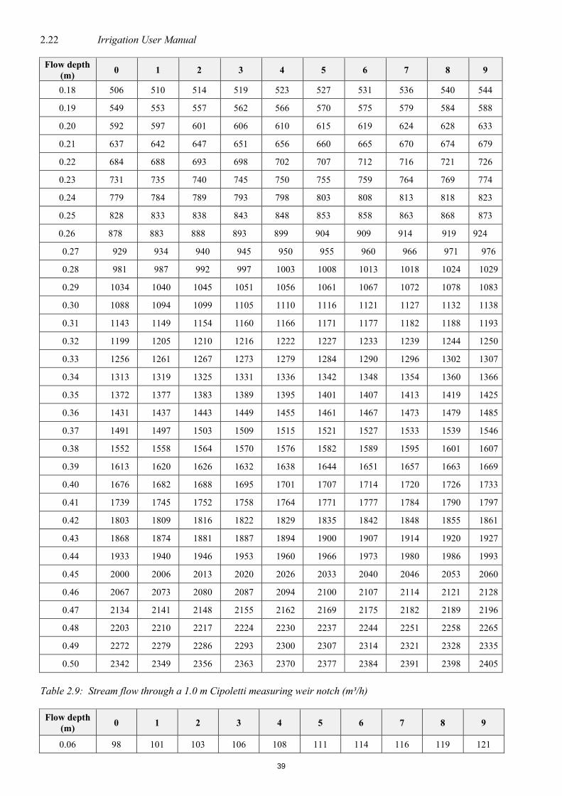
2.22 Irrigation User Manual Flow depth
(m) 0 1 2 3 4 5 6 7 8 9
0.18 506 510 514 519 523 527 531 536 540 544
0.19 549 553 557 562 566 570 575 579 584 588
0.20 592 597 601 606 610 615 619 624 628 633
0.21 637 642 647 651 656 660 665 670 674 679
0.22 684 688 693 698 702 707 712 716 721 726
0.23 731 735 740 745 750 755 759 764 769 774
0.24 779 784 789 793 798 803 808 813 818 823
0.25 828 833 838 843 848 853 858 863 868 873
0.26 878 883 888 893 899 904 909 914 919 924
0.27 929 934 940 945 950 955 960 966 971 976
0.28 981 987 992 997 1003 1008 1013 1018 1024 1029
0.29 1034 1040 1045 1051 1056 1061 1067 1072 1078 1083
0.30 1088 1094 1099 1105 1110 1116 1121 1127 1132 1138
0.31 1143 1149 1154 1160 1166 1171 1177 1182 1188 1193
0.32 1199 1205 1210 1216 1222 1227 1233 1239 1244 1250
0.33 1256 1261 1267 1273 1279 1284 1290 1296 1302 1307
0.34 1313 1319 1325 1331 1336 1342 1348 1354 1360 1366
0.35 1372 1377 1383 1389 1395 1401 1407 1413 1419 1425
0.36 1431 1437 1443 1449 1455 1461 1467 1473 1479 1485
0.37 1491 1497 1503 1509 1515 1521 1527 1533 1539 1546
0.38 1552 1558 1564 1570 1576 1582 1589 1595 1601 1607
0.39 1613 1620 1626 1632 1638 1644 1651 1657 1663 1669
0.40 1676 1682 1688 1695 1701 1707 1714 1720 1726 1733
0.41 1739 1745 1752 1758 1764 1771 1777 1784 1790 1797
0.42 1803 1809 1816 1822 1829 1835 1842 1848 1855 1861
0.43 1868 1874 1881 1887 1894 1900 1907 1914 1920 1927
0.44 1933 1940 1946 1953 1960 1966 1973 1980 1986 1993
0.45 2000 2006 2013 2020 2026 2033 2040 2046 2053 2060
0.46 2067 2073 2080 2087 2094 2100 2107 2114 2121 2128
0.47 2134 2141 2148 2155 2162 2169 2175 2182 2189 2196
0.48 2203 2210 2217 2224 2230 2237 2244 2251 2258 2265
0.49 2272 2279 2286 2293 2300 2307 2314 2321 2328 2335
0.50 2342 2349 2356 2363 2370 2377 2384 2391 2398 2405
Table 2.9: Stream flow through a 1.0 m Cipoletti measuring weir notch (m³/h)
Flow depth (m) 0 1 2 3 4 5 6 7 8 9
0.06 98 101 103 106 108 111 114 116 119 121
39

Water 2.23
Flow depth (m) 0 1 2 3 4 5 6 7 8 9
0.07 124 127 129 132 135 138 140 143 146 149
0.08 152 154 157 160 163 166 169 172 175 178
0.09 181 184 187 190 193 196 199 202 205 209
0.10 212 215 218 221 225 228 231 234 238 241
0.11 244 248 251 254 258 261 265 268 271 275
0.12 278 282 285 289 292 296 299 303 307 310
0.13 314 317 321 325 328 332 336 340 343 347
0.14 351 355 358 362 366 370 374 377 381 385
0.15 389 393 397 401 405 409 413 417 421 425
0.16 429 433 437 441 445 449 453 457 461 465
0.17 469 473 478 482 486 490 494 499 503 507
0.18 511 516 520 524 528 533 537 541 546 550
0.19 555 559 563 568 572 577 581 585 590 594
0.20 599 603 608 612 617 622 626 631 635 640
0.21 644 649 654 658 663 668 672 677 682 686
0.22 691 696 700 705 710 715 719 724 729 734
0.23 739 743 748 753 758 763 768 773 777 782
0.24 787 792 797 802 807 812 817 822 827 832
0.25 837 842 847 852 857 862 867 872 877 883
0.26 888 893 898 903 908 913 919 924 929 934
0.27 939 945 950 955 960 966 971 976 981 987
0.28 992 997 1003 1008 1013 1019 1024 1030 1035 1040
0.29 1046 1051 1057 1062 1067 1073 1078 1084 1089 1095
0.30 1100 1106 1111 1117 1122 1128 1133 1139 1145 1150
0.31 1156 1161 1167 1173 1178 1184 1189 1195 1201 1206
0.32 1212 1218 1223 1229 1235 1241 1246 1252 1258 1264
0.33 1269 1275 1281 1287 1293 1298 1304 1310 1316 1322
0.34 1327 1333 1339 1345 1351 1357 1363 1369 1375 1381
0.35 1386 1392 1398 1404 1410 1416 1422 1428 1434 1440
0.36 1446 1452 1458 1464 1471 1477 1483 1489 1495 1501
0.37 1507 1513 1519 1525 1532 1538 1544 1550 1556 1562
0.38 1569 1575 1581 1587 1593 1600 1606 1612 1618 1625
0.39 1631 1637 1643 1650 1656 1662 1669 1675 1681 1688
0.40 1694 1700 1707 1713 1719 1726 1732 1739 1745 1751
0.41 1758 1764 1771 1777 1784 1790 1797 1803 1810 1816
0.42 1823 1829 1836 1842 1849 1855 1862 1868 1875 1881
0.43 1888 1895 1901 1908 1914 1921 1928 1934 1941 1948
40

2.24 Irrigation User Manual
Flow depth (m) 0 1 2 3 4 5 6 7 8 9
0.44 1954 1961 1968 1974 1981 1988 1994 2001 2008 2015
0.45 2021 2028 2035 2042 2048 2055 2062 2069 2075 2082
0.46 2089 2096 2103 2110 2116 2123 2130 2137 2144 2151
0.47 2158 2164 2171 2178 2185 2192 2199 2206 2213 2220
0.48 2227 2234 2241 2248 2255 2262 2269 2276 2283 2290
0.49 2297 2304 2311 2318 2325 2332 2339 2346 2353 2360
0.50 2367 2374 2382 2389 2396 2403 2410 2417 2424 2432
41

Water 2.25
Table 2.10: Stream flow through a V-notch (m³/h)
Flow depth (m) 0 1 2 3 4 5 6 7 8 9
0.06 4 5 5 5 5 5 6 6 6 6
0.07 6 7 7 7 7 8 8 8 8 9
0.08 9 9 10 10 10 10 11 11 11 12
0.09 12 12 13 13 13 14 14 15 15 15
0.10 16 16 17 17 17 18 18 19 19 19
0.11 20 20 21 21 22 22 23 23 24 24
0.12 25 25 26 26 27 27 28 29 29 30
0.13 30 31 31 32 33 33 34 35 35 36
0.14 36 37 38 38 39 40 40 41 42 43
0.15 43 44 45 45 46 47 48 49 49 50
0.16 51 52 52 53 54 55 56 57 57 58
0.17 59 60 61 62 63 64 65 65 66 67
0.18 68 69 70 71 72 73 74 75 76 77
0.19 78 79 80 81 82 83 84 86 87 88
0.20 89 90 91 92 93 95 96 97 98 99
0.21 100 102 103 104 105 106 108 109 110 112
0.22 113 114 115 117 118 119 121 122 123 125
0.23 126 127 129 130 132 133 134 136 137 139
0.24 140 142 143 145 146 148 149 151 152 154
0.25 155 157 158 160 162 163 165 166 168 170
0.26 171 173 175 176 178 180 181 183 185 186
0.27 188 190 192 193 195 197 199 201 202 204
0.28 206 208 210 212 214 215 217 219 221 223
0.29 225 227 229 231 233 235 237 239 241 243
0.30 245 247 249 251 253 255 257 259 262 264
0.31 266 268 270 272 274 277 279 281 283 286
0.32 288 290 292 295 297 299 301 304 306 308
0.33 311 313 316 318 320 323 325 328 330 332
0.34 335 337 340 342 345 347 350 352 355 357
0.35 360 363 365 368 370 373 376 378 381 384
0.36 386 389 392 394 397 400 403 405 408 411
0.37 414 417 419 422 425 428 431 434 436 439
0.38 442 445 448 451 454 457 460 463 466 469
0.39 472 475 478 481 484 487 490 493 496 500
0.40 503 506 509 512 515 519 522 525 528 531
0.41 535 538 541 545 548 551 555 558 561 565
42

2.26 Irrigation User Manual
Flow depth (m) 0 1 2 3 4 5 6 7 8 9
0.42 568 571 575 578 582 585 588 592 595 599
0.43 602 606 609 613 616 620 624 627 631 634
0.44 638 642 645 649 653 656 660 664 667 671
0.45 675 679 682 686 690 694 698 701 705 709
0.46 713 717 721 725 729 733 736 740 744 748
0.47 752 756 760 764 768 773 777 781 785 789
0.48 793 797 801 805 810 814 818 822 826 831
0.49 835 839 844 848 852 856 861 865 869 874
0.50 878 883 887 891 896 900 905 909 914 918
5.3 Volumetric and Gravimetric methods
5.3.1 Volumetric flow measurement
Volumetric measurement is one of the most straightforward and accurate methods of flow measurement. With this method the full flow is discharged into a container of known volume and the time taken to fill the container recorded. This method is often used to calibrate other measuring devices.
For flow measurement a stopwatch must measure to ± 0.1 second accuracy therefore for an accuracy of ± 1%. It must be possible to fill the container in 20 seconds.
Theoretically a flow of approximately 5 /s can be determined with a normal 20 bucket. In practice however, a maximum flow of 3 /s may be determined. A maximum flow of 30 /s can be determined with a 200 litre oil barrel.
tVQ = (2.1)
where Q = flow rate [/s]
V = container volume [] T = time to fill container [s]
Example 2.2: Determine the flow [/h] for the following case: Container diameter = 100 mm Container depth = 200 mm Average filling time = 20 s (five readings) Solution:
2
2
2
DContainer volume = h4
0.1= 0.24
= 0.0016m
π
π × ×
43

Water 2.27
From equation 2.1:
3 3
VQ = t0.0016=
20= 0.08 10 m /s= 288 /h
−×
5.3.2 Gravimetric flow measurement
One litre of water weighs one kilogram. If the container volume is unknown. a quantity of water is discharged into a container while the time is recorded. The mass of water is derived by determining the mass of the full as well as the empty container.
5.4 Maintenance of weirs and flumes
Regular maintenance of water measuring devices is required to ensure long, accurate performance and reduce or avoid costly repairs. The following aspects are important:
Weirs: • Keep the ponding area free of sediments and plant growth • Ensure that there is no leakage through or around the device • Regularly check the position of the weir plate relative to the crest • Maintain the condition of the crest finish in good order • Remove rust from steel sections by wire brush and coat with a bituminous paint Flumes: • Remove sediments and accretions especially in approach and venturi sections • If manufactured from steel, remove rust by wire brush and coat with a bituminous paint • Avoid erosion immediately downstream of the device • Recast the floor if the existing one is no longer level • Regularly check the measuring scale position relative to the crest
6 Water quality Irrigated agriculture is dependent on an adequate water supply of usable quality. Water quality concerns have often been neglected because good quality water supplies have been plentiful and readily available. This situation is now changing in many areas. Intensive use of nearly all good quality supplies means that new irrigation projects and old projects seeking new or supplemental supplies must rely on lower quality and less desirable sources. To avoid problems when using these poor quality water supplies. There must be sound planning to ensure that the quality of water available is put to the best use (Ayers & Westcot, 1994). Irrigation water users may experience a range of impacts as a result of changes in water quality. These may be categorised as follows: • reduced crop yield (as a result of increased salinity or the presence of constituents that are toxic to plants); • impaired crop quality (this may result in inferior products or pose a health risk to consumers); • impairment of soil suitability (as a result of the degradation of soil properties and accumulation of
undesirable constituents or toxic constituents); • damage to irrigation equipment (corrosion or encrustation).
44

2.28 Irrigation User Manual The measurement and interpretation of the quality of the water to be used for irrigation of crops is one of the first steps to be taken in the planning of an irrigation project. While a few aspects of irrigation water quality have a direct impact on plants and irrigation equipment. The primary goal of water analysis is to judge the effect of the water on the soil and ultimately on the plants grown on the soil. As such much of the interpretation of the water analysis is based on a prediction of the consequences for the soil. The interpretation of the test results is in many cases dependent on the intended use of the water. Some plant species and production systems may have much different requirements or tolerances. The most important aspect concerning water problems is to adapt the planning of the cultivation of crops to suit the water and not the changing of the soil and water to suit the crop. The analyses and properties of the soil, water and cultivar should be seen as an entity in order to determine the best recommendations and practices. 6.1 Physical water properties Physical impurities are those particles which occur in the water and which can be “measured”. Sediment, for example, has a diameter of higher than 0.001 mm. while turbidity has a diameter of less than 0.001 mm. Sediment may be removed by the use of sediment dams, sand filters, disc filters or cyclonic separators. Turbidity is removed using flocculants followed by settlement or filtration 6.2 Chemical water properties The chemical quality of water reflects the composition and concentration of the dissolved matter within it. This matter includes cations such as calcium, magnesium and sodium as well as anions such as bicarbonate, sulphate and chloride. Boron, fluorides and nitrates occur in lower, but significant concentrations. Chemical elements and/or compounds which separately, or in combination with each other, give rise to problems in plants, soils and irrigation equipment. There is an increasing demand for the determination of not only salts, but also for the presence of heavy metals, such as mercury, lead and manganese – which are found as a result of increasing industrial pollution – and/or micro-elements in irrigation water analyses.
6.3 Organic properties Organic chemicals are made up of carbon (C), hydrogen (H), as well as nitrogen (N) and oxygen (O). Organic compounds are derived from living organism as well as industrial sources. Organic impurities in water may be sub-divided into organic colloids, algae and bacterial growths. Excessive plant nutrient levels, can increase biological clogging problems. Bacterial growth or other biological activity should be monitored and prevented if possible. Biological corrosion is best prevented by commencing with a clean, sediment-free system that is maintained as such. The organic content of the water, and especially the Assimilable Organic Carbon (AOC) content should be kept as low as possible in order to deprive micro-organisms of nutrition. Most organic compounds dissolved in water do not dissociate into ions, consequently they do not affect the salt content of the water. 6.4 Water analyses for irrigation Farm water comes from a number of different sources and so its quality varies. Water from various sources may be of an unsuitable quality for its intended use for irrigation, stock, household or other farm activities. Far too often, an irrigation water test is used as a diagnostic tool after plants are exhibiting some type of stress. However, irrigation water tests should be done before the irrigation system is installed and with some frequency, dependent on the outcome of the initial test, location and the potential for fluctuations in water source quality. Irrigation water samples should be tested for at least the analyses listed in Table 2.11. For irrigation planning and rehabilitation electrical conductivity (EC), sodium adsorption ratio (SAR), pH (and pHs if the Langelier Saturation Index is not calculated) and Langelier Saturation Index are critical. Analysing for iron (Fe) and manganese (Mn) concentration may also be beneficial if the water has a low salt content and negative Langelier Index. Consider the
45

Water 2.29
water source when determining what analyses should be performed. One way to evaluate analysis quality is to compare the sum of the cations (+) with the sum of the anions (-) in units of me/l. These two sums should differ by no more than 20 percent when a water analysis is done correctly. A complete record must be kept of samples handed in for analysis. It is preferable to use as SANAS or Agrilasa accredited approved laboratory. Table 2.11: Water analyses for irrigation
Conversions 100 mS/m = 1dS/m = 100 mmhos/m = 1 mmhos/cm = 1000 μmhos/cm 1 mg/ = 1 ppm equivalent weight = atomic weight / charge of ion me/ = mg/ / equivalent weight mmol/ = me/ / charge of ion
46

2.30 Irrigation User Manual Table 2.12: Some water quality indicators for risk Degree of suitability for crop production Low Moderate Medium High Very high Extreme
Expected yield decrease due to salts (%)
Salinity risk (mS/m) <25 25-75 75-225 225-400 400-600 >600
Sodium build-up if value + (RSC) <1,25 1.25-2.5 >2.5
Chloride (me/l) <4 4-10 >10
Toxicity (SAR) <3 3-5 5-7 7-9 >9
Degree of emitter clogging risks Low Moderate Medium High Very high Extreme
HCO3/CO3 precipitation (‘ZiCa) <8.6 8.6 >8.6
Iron <0.3 0.3 >0.3
Manganese <0.3 0.3 >0.3
pHc <8.4precipitate lime 8.4 >8.4 precipitate lime
Scaling vs corrosion Scale Medium Scale Balance Medium
Corrosion Corrosion
LANGELIER INDEX (LI) +2 0.5 0.0 -0.5 -2
Ryznar Stability Index (RSI) 4.5-5.0 5.6-6.0 6.0-7.0 7.0-7.5 7.5-9.0
BICARBONATE (White wash) “White wash” > 90 ppm (1.5 meq/l) CO3/HCO3
EATON – GYPSUM REQUIREMENTS +Na build-up -Ca precipitation
Permeability problems due to sodium (SARa) <6 6-9 >9
CORROSION INDEX <0.1 No corrosion >0.1 Aggressive water
PERMANENT HARDNESS + Value = permanent hardness (SO4 + salts + Cl)
6.4.1 Sampling procedure Sampling irrigation water starts with a clean container. Label the container with sample identification, contact information, sample date, location, type of crop to be irrigated water source (e.g. dam, river or borehole), and type of irrigation system used (e.g. sprinkler. flood. micro. or moving systems). Use an empty plastic or glass bottle, preferably plastic, to prevent breakage during transport. Rinse the bottle well three to four times with the water to be used for the sample. Rinse the container at least three times with the water to be tested and fill it all the way to the top. Wastewater containing high concentrations of suspended organic materials requires special handling. Ask the laboratory about its requirements. Water samples taken from a dam, river or stream face the mouth of the bottle upstream. plunge the neck downwards about 30 cm below the water surface. tilt the neck slightly upwards to let it fill completely. where there is no current. push the bottle forward horizontally until it is filled. River water must be sampled in the flow of the river. Stagnant water can have a higher salt concentration. Water samples taken from a borehole continuously operate the pump for at least 10 minutes. let the water flush the fittings and pipes. collect a sample of water by allowing the water from the pump to flow directly into the sample bottle. When water from an irrigation system is analysed, the laterals must be flushed sufficiently to ensure that a representative sample is taken.
47

Water 2.31
6.4.2 Sampling frequency Testing frequency is based on water use and source. Surface waters are subject to seasonal weather and flow patterns and may need frequent monitoring. The chemical composition of groundwater changes slowly and usually needs to be tested only annually or biannually. Wastewater sampling frequency, such as for effluent, should be based on the farm’s circumstances. Sampling may be dictated by a permit from a regulatory agency. 6.5 Water quality parameters for irrigation Water used for irrigation can vary greatly in quality depending upon type and quantity of dissolved salts. Salts are present in irrigation water in relatively small but significant amounts. They originate from dissolution or weathering of the rocks and soil. including dissolution of lime. gypsum and other slowly dissolved soil minerals. These salts are carried with the water to wherever it is used. In the case of irrigation. the salts are applied with the water and remain behind in the soil as water evaporates or is used by the crop.
The suitability of a water for irrigation is determined not only by the total amount of salt present but also by the kind of salt. Various soil and cropping problems develop as the total salt content increases. and special management practices may be required to maintain acceptable crop yields. Water quality or suitability for use is judged on the potential severity of problems that can be expected to develop during long-term use (Ayers & Westcot, 1994).
6.5.1 Salinity (electrical conductivity) Electrical conductivity (EC) is a measure of the ability of water to conduct an electrical current. This ability is a result of the presence of ions in water such as carbonate, bicarbonate, chloride, sulphate, nitrate, sodium, potassium, calcium and magnesium, all of which carry an electrical charge. Most organic compounds dissolved in water do not dissociate into ions, consequently they do not affect the EC. Irrigation with water containing salt induces salt into the soil profile. When no or little leaching of salt takes place from the soil profile, salt accumulates and a saline soil is formed. Crops are sensitive to soil salinity; yield is reduced if grown on salt-affected soils. The presence of dissolved salts in soil water reduces the physiological availability of water to plants (Chapter 3 Soil: paragraph 3.3.2.1). When the salt content reaches a concentration where the plant is no longer able to extract sufficient water for its requirements, salinity-induced water stress develops, the growth rate starts to decline and. if it continues for a significant period of time, crop yield starts to decline. The soil salinity at which plant growth starts to decline is defined as the threshold salinity. It is usually expressed as the EC of the saturated-soil extract, which is the reference water content for the measurement of soil salinity. Crop yield has been found to decrease approximately linearly with salinity increases above the threshold salinity. Both the threshold salinity and the slope of yield decline above this point are specific to a particular crop or cultivar (Chapter 3 Soil: Tables 3.5 and Table 3.6). The symptoms plants display when affected by salinity are similar in appearance to those of drought, namely, stunted growth, wilting (even though the soil may not be dry), a darker, bluish-green colour and in some cases thicker, waxier leaves. Symptoms vary with the growth stage. Usually symptoms are more obvious when plants are affected during early growth stages. Mild salinity effects may go unnoticed because the effect may be uniform over a field, with no basis for comparison (DWAF, 1996). 6.5.2 Sodicity (sodium) The sodium adsorption ratio (SAR) is an index of the potential of a given irrigation water to induce sodic soil conditions. It is calculated from the concentrations of sodium, calcium and magnesium in water.
48

2.32 Irrigation User Manual
NaSAR = Ca Mg
2+
where Na = sodium concentration [me/] Ca = calcium concentration [me/] Mg = Magnesium concentration [me/] By irrigation with sodium-rich water, soil sodicity is induced. Negative effects associated with sodium affected soils, include • reduced crop yield and quality as a result of sodium uptake through the roots of sodium sensitive plants • crop quality is affected by sodium-induced leaf injury in plants of which leaves are the marketed product.
or where fruit size and appearance are affected by sodium-induced yield decreases; • impaired soil physical conditions. as manifested by reduced soil permeability (infiltration rate and
hydraulic conductivity) and an increased tendency for hard setting; and • reduced crop yield and quality Overhead sprinkling of sensitive crops can cause toxicities not encountered when irrigating by surface methods. The toxicity occurs due to excess quantities of sodium and chloride from the irrigation water being absorbed through leaves wet by the sprinklers. Extreme cases have resulted in severe leaf burn and defoliation. Absorption and toxicity occur mostly during periods of high temperature and low humidity (<30%). frequently aggravated by windy conditions. Rotating sprinkler heads present the greatest risk. Between rotations water evaporates and the salts become more concentrated in the shrinking volume of water. Slowly rotating sprinklers (less than 1 revolution per minute) cause alternate wetting and drying cycles; the slower the speed of rotation, the greater the absorption. High frequency (near daily) spray irrigation has also created problems in some cases (DWAF, 1993 and 1996). Sodium toxicity is often modified or reduced if sufficient calcium is available in the soil. 6.5.3 Chloride Chloride is not adsorbed or held back by soils, therefore it moves readily with the soil-water, is taken up by the crop, moves in the transpiration stream, and accumulates in the leaves. If the chloride concentration in the leaves exceeds the tolerance of the crop, injury symptoms develop such as leaf burn or drying of leaf tissue. Normally, plant injury occurs first at the leaf tips (which is common for chloride toxicity), and progresses from the tip back along the edges as severity increases. Excessive necrosis (dead tissue) is often accompanied by early leaf drop or defoliation. Crop quality is affected by chloride-induced leaf injury in plants whose leaves are the marketed product, or where fruit size and appearance are affected by chloride-induced yield decreases. 6.5.4 Iron and Manganese Problems with iron and manganese blockages occur where iron ions (Fe2+) and manganese ions (Mn2+) are found in water. These ion forms occur in solution in water. Oxidation (Fe2+ to Fe3+ and Mn2+ to Mn4+) causes sedimentation. The sediment is usually Fe (OH)3 and/or MnO2 which may cause blockage of drip and micro-irrigation systems. However, water containing more than 0.4 mg/ of iron should not be chlorinated, as it forms insoluble iron compounds which accelerate blocking. This irrigation water should be exposed to air as much as possible in order to promote flocculation and sedimentation. 6.5.5 Miscellaneous problems 6.5.5.1 Nitrogen Nitrogen occurs predominantly as nitrate in irrigation water. The ammonium form is usually a result of contamination with waste water. Nitrogen is one of the essential macro plant nutrients and its presence in irrigation water is mostly viewed as beneficial.
49

Water 2.33
Nitrogen in irrigation water is primarily of concern because of: • its stimulatory effect on plant growth when applied in excess of plant requirements. • its potential to leach and contaminate ground water sources. and • its stimulatory effect on nuisance growth of algae and aquatic plants in irrigation structures (canals.
storage. dams. etc.). that can interfere with the efficient distribution of irrigation water (diminished carrying or storage capacity of irrigation structures and clogging of sprinklers and micro-irrigation openings)
Nitrogen in irrigation water (N) is largely a fertility issue, and nitrate-nitrogen (NO3-N) can be a significant N source in South Africa. The nitrate ion often occurs at higher concentrations than ammonium in irrigation water. Waters high in N can cause quality problems in many crops and excessive vegetative growth in some vegetables. However, these problems can usually be overcome by good fertilizer and irrigation management. Regardless of the crop, nitrate should be credited toward the fertilizer rate especially when the concentration exceeds 10 ppm NO3-N (45 ppm NO-3).
6.5.5.2 Deposits on crops A scaling water mostly presents a problem of white scale formation on leaves and fruit when sprinklers are used. These deposits often build up on leaves, fruit and flowers and negatively affect the marketability of these products. No numerical criteria are provided for these effects. The presence of oxidised iron as a result of corrosion can give rise to a red discolouration of the water and impact negatively on the aesthetic quality of irrigated fruits. 6.5.5.3 pH The solubility and bio-availability of many plant nutrients and potentially toxic constituents are highly dependent on pH. For example, most micro-nutrients and heavy metals are unavailable for plant uptake at high pH and available (often at toxic concentrations) at lower pH levels. Soil microbial populations are also markedly affected by soil and water pH levels. The effect of pH on crop production is thus mostly indirect. Since soil is more strongly buffered against changes in pH than water, irrigation water will cause soil pH to change slowly and is seldom a problem in itself. Direct contact with crop foliage by either high or low pH waters causes foliar damage, which can, depending on the severity and timing of the damage, result in a decreased yield or damage to fruit or other marketable products. Extreme pH values are associated with corrosion and encrustation of irrigation equipment. Common on-farm management practices to mitigate against the effects that irrigation water pH may have on soil sustainability, are to: • apply agricultural lime to maintain soil pH in the desired range when irrigating with low pH water; and/or • apply soil acidifiers (e.g. sulphur. reduced nitrogenous fertilizers. etc.) to maintain soil pH in the desired
range when irrigating with high pH water. 6.6 Effect of water quality on irrigation equipment The impact irrigation water quality constituents have on irrigation equipment that distribute and apply water, is for all practical purposes not site specific and the direct result of the interaction between water quality constituents and components of irrigation equipment. This interaction is determined primarily by the material irrigation equipment is made of, or the type of equipment used. However, there are also site-specific factors such as material used, temperature, bacteria and external electric currents. 6.6.1 Corrosion or scaling of irrigation equipment Metal, concrete and plastics can all deteriorate over time due to contact with irrigation water. The conversion from pure metal to metal oxides or sulphides is spontaneous. Metal corrosion is influenced by the presence of electrical fields, the conjunction of dissimilar metals, bacteriological activity and physical processes. Organic contaminants in groundwater are primarily responsible for the degradation of synthetic materials like plastics and PVC. Concrete is eroded by water that is under-saturated with regard to calcium carbonate (Du Plessis et al., 2017).
50

2.34 Irrigation User Manual Although minor scaling which forms a protective layer against corrosion inside pipes are normally considered beneficial, excessive scaling reduce flow rates and damage water systems, necessitating repair or replacement. The most common cause of scaling is the precipitation of calcium carbonate when saturation is exceeded. Although less frequent, gypsum precipitation also occurs in irrigation equipment when water high in calcium and sulphate is used. There are several indices with which corrosion and scaling can be predicted. The most commonly used is the Langelier Saturation Index (LI), which was developed by Wilfred Langelier in 1936. The LI is an approximate measure of the degree of saturation of calcium carbonate in water. It is widely used to indicate the likelihood of corrosion and scaling, and is calculated as the difference between actual measured pH of water (pHa) and the hypothetical saturation pH of the water (pHs). pHs is the calculated theoretical pH at which water with a given bicarbonate and calcium ion concentration and total dissolved solids content at a given temperature, would be in equilibrium with solid calcium carbonate
LI = pHa - pHs A positive LI indicates that water is over-saturated and scaling is likely, while a negative LI indicates a water that is under-saturated with respect to calcium carbonate, and potentially corrosive.
Fitness-for-Use Langelier Index
Corrosion Scaling
Ideal > -0.5 <+0.5
Acceptable -0.5 to -1.0 +0.5 to +1.0
Problematic -1.0 to -2.0 +1.0 to +2.0
Unacceptable < -2.0 >+2.0 The tendency of a water to form a scaling film or be aggressive can be reduced by manipulation of the chemical composition of the water. Mitigating measures are mostly preferred (Du Plessis et al., 2017). • Scaling is commonly reduced by removal of alkalinity and calcium hardness from the water until it becomes
slightly under saturated with respect to the calcium carbonate concentration, and consequently slightly aggressive. (Alkalinity can be reduced by adding a weak acid solution. while calcium hardness can be reduced by Base Exchange softening. which is seldom practical for irrigation applications).
• Conversely, an aggressive water, which tends to attack unprotected structures, can be stabilised by increasing the alkalinity and calcium content. Poorly-controlled additions may result in a scaling water.
• A water which is corrosive to metal fittings can usually be rendered less corrosive by increasing its alkalinity and reducing the sulphate and chloride content. Alkalinity addition is the more simple procedure since removal of sulphate and chloride would necessitate using desalination techniques.
• The modifications necessary to achieve acceptably stable water may be very complex and require a high level of treatment skills and sophisticated analytical facilities. The amount of chemicals to be added can be determined by graphical methods, using manual calculations, or with computer software, such as Stasoft III.
Solving chemical corrosion problems (Du Plessis et al., 2017): • Chemical corrosion can be eliminated or alleviated by using corrosion-resistant coatings or materials (e.g.
PVC pipes) for all elements of the water distribution system which come into direct contact with the water. • Cathodic protection may be required in some instances, for example where pipelines run close to electrical
cables, or close to electric railway lines. • The resistance of concrete to corrosion as a result of dissolution of lime by low salinity soft water can be
greatly increased by the use of good quality concrete compared to poor quality porous concrete. • Corrosion can be avoided by preventing different metals from having contact with one another in the water
distribution system. • Chemical corrosion can be reduced by limiting sulphate and chloride concentrations in the water
51

Water 2.35
Solving biological corrosion problems • Biological corrosion is best prevented by commencing with a clean, sediment-free system that is
maintained as such. Bacterial growth or other biological activity should be monitored and prevented if possible.
• The organic content of the water, and especially the Assimilable Organic Carbon (AOC) content should be kept as low as possible in order to deprive micro-organisms of nutrition. This in turn will limit the amount of post-disinfection required. However, post-disinfection using chlorination or chloramination is imperative at high AOC concentrations and/or in distribution systems having long retention times. Rechlorination in multiple steps may be required to ensure the presence of adequate chlorine residual in all parts of the distribution system.
6.6.2 Clogging of drippers (Du Plessis et al., 2017) The low flow rates in drip emitters are conducive to clogging problems. While it is relatively easy to spot blocked openings, it is very difficult to distinguish one that is partially blocked. Both alter the hydraulics of the entire system, result in a decrease in the uniformity of application and give rise to reduced yields. Ayers and Westcot (1994) cover the topic of clogging in drip irrigation systems in quite some detail while Nakayama and Bucks (1991) provide an overview of the body of research that deals with the contribution water quality makes to emitter clogging as well as the treatment options that are available address its causes.
Potential Clogging of drippers by irrigation water constituents (after Nakayama and Bucks (1991))
Water Quality Constituent Fitness for Use Category
Ideal Acceptable Tolerable Unacceptable
Suspended Solids (mg/L) <50 50-75 75-100 >100
pH <7.0 7.0-7.5 7.5-8.0 >8.0
Manganese (mg/L) <0.1 0.1-0.5 0.5-1.5 >1.5
Total Iron (mg/L) <0.2 0.2-0.5 0.5-1.5 >1.5
E.coli (counts x 106 /100 mL) <1.0 1.0-2.0 2.0-5.0 >5.0 Often clogging of drippers is not a result of the irrigation water composition per se. but as a result of fertigation (phosphorous fertilizers precipitate at relatively low calcium concentrations and anhydrous or liquid ammonia cause increase in pH which can cause precipitation of calcium carbonate) or biological growths inside dripper lines. Chemical precipitation of substances such as lime, iron, manganese and phosphates can also cause clogging. Lime precipitation is usually predicted with the Langelier Index, but in general, problems can be expected if pH exceeds 8. Iron in the soluble ferrous form can be oxidised into the insoluble ferric Fe3+ form. Iron also may contribute to biologically mediated clogging, as it is often found in iron bacterial slime. Ayers and Westcot (1994) recommend a threshold of 2 mg/l Fe, and as low as 0.5 mg/l if tannin like compounds that are often found in acid waters are present.
52

2.36 Irrigation User Manual Table 2.13: Physical, chemical and biological factors involved in emitter clogging (Nakayama and Bucks, 1991) Physical Chemical Biological
Inorganic materials Alkaline earth cations Algae
Sand (50-250 µm) Calcium
Silt (2-50 µm) Magnesium Bacteria
Clay (<2 µm) Heavy metal cations Filament
Iron Slime
Organic materials Manganese
Anions Microbial activities
Aquatic plants Carbonate Iron
Phytoplankton Hydroxide Manganese
Algae Silicate Sulphur
Sulphide
Aquatic animals
Zooplankton Fertiliser sources
Snails Aqueous ammonia
Iron
Bacteria (0.4-2 µm) Copper
Zinc
Plastic cutting Manganese
Phosporous
Lubricant residue
6.7 Pre-filtering and treatment of irrigation water In certain cases, the chemical, biological and physical condition of irrigation water necessitates pre-treatment and pre-filtration before the water is filtered to the desired quality. 6.7.1 Sedimentation and aeration In cases where the irrigation water contains solid particles in suspension in excess of 200 parts per million, it is advisable to have a sedimentation dam where the particles can be sedimented before the water is filtered. This will prevent an overload on the filters as well as excessive backwashing of them. The following points are important for the use of a sedimentation dam: • The outlet of the dam should be as far as possible from its inlet. • The back-wash water from the filters should be dumped as far as possible from the inlet (preferably not
back into the dam). • It must be possible to clean the dam with the minimum effort. • Water for filtration should be drawn from the upper layer of the dam (suction pipe mounted on float). A
long, narrow sedimentation dam is more effective than a square one.
53

Water 2.37
Sedimentation time is that time which is needed by certain material particle sizes to sediment under gravity.
v1ts = (2.2)
where ts = sedimentation time [min]
l = total distance [m] v = sedimentation rate [m/min]
Example 2.3 Calculate the sedimentation time for particles with a diameter of 0.002 mm over a depth of 1.8 m. Solution: From Table 2.14 the sedimentation rate is 0.015 m/min According to equation 2.1
1.8Sedimentation time is = = 120 minutes0.015
This implies that the water should stay in the dam for at least two hours before being fed into the irrigation system. The minimum volume water stored should thus be twice the hourly flow rate of the irrigation system. Where there is iron in the water, it is necessary to aerate the water so that the iron may oxidise. The iron oxide will then sediment in the dam and the water may be drawn off the surface for irrigation. Table 2.14: Approximate sedimentation rates for different soil texture classes.
Soil texture Particle size [mm] Sedimentation rate [m/min]
Coarse sand > 0.5 38 Medium sand 0.25-0.5 22
Fine sand 0.1-0.25 5 Very fine sand 0.05-0.1 0.9
Silt 0.002-0.05 0.015 Clay < 0.002 0.0006
6.7.2 Acid treatment Acid treatment is done when magnesium, calcium and carbonate salts pose a threat of blocking to the drippers. A water sample should first be analysed in the laboratory before recommendations are made. Acid should not be added at the same point as chlorine. Acid treatment may increase the effectiveness of chlorine if the pH is reduced to between 4.5 and 5.
6.7.3 Oxidizing agent’s treatment Oxidizing agents (most well-known chlorination) react with chemical groups on organic matter, changing the chemical structure of this material. Organic matter includes peat, algae, bacteria, plant debris, and pathogens. Pathogens are killed after exposure to the oxidizing agent if it is present at a certain concentration and duration. The oxidizing agent. However, can be depleted by organic matter in the water. That is why water should be pre-filtered before it is treated with oxidizing agents. Oxidizing agents also react with iron and other metals. Oxidizing agents include bromine, chlorine gas, sodium hypochlorite, calcium hypochlorite, chlorine dioxide. Ozone, and activated peroxygen.
54

2.38 Irrigation User Manual 6.7.4 Ultraviolet (UV) Ultraviolet radiation involves exposure of the water in tubular chambers to UV light, which kills living cells (including pathogens) by disrupting their DNA. Particulates in the water disperse the light, reducing the effectiveness of UV radiation. Prefiltration of the water is necessary. 6.7.5 Copper ionization Copper ionization is the release of copper ions into the water resulting from an electrical charge passed between copper plates. Copper ions are toxic to most pathogens and plants, but the levels used to treat water are well below those which cause phytotoxicity. Copper is also sometimes delivered as a dissolved salt, such as copper sulphate. 6.7.6 Heat treatment Heat treatment is another method of disinfesting water, but it is energy intensive and therefore too costly for treating large volumes. A temperature of 95°C for 30 seconds is sufficient to kill most plant pathogens. 6.8 South African classification systems for water The Department of Water Affairs and Forestry developed the South African water quality directives to provide water quality information to water users. Volume 4 (DWAF, 1993 and 1996) of the directives specifically deals with irrigation water and contains criteria for the evaluation of water by indicating the acceptable levels for specific elements and other parameters in four classes. The document is available from the Department. A summary of the directives is included in Table 2.4. Table 2.15: Various limits for specific problems with irrigation water
Water quality constituent Fitness for use for irrigation water
Good (Class 1)
Fair (Class 2)
Marginal (Class 3
Unacceptable (Class 4)
Salinity and sodicity
Electrical conductivity (EC. mS/m) 0-40 40-90 90-270 270-540
Sodium adsorption ratio (SAR. mmol/0.5) 0-1.5 1.5-3.0 3.0-5.0 5.0-10.0
Potentially toxic ions
Boron (B. mg/) 0-0.2 0.2-0.9 0.9-1.5 1.5-3.0
Chloride (Cl. mg/) 0-105 105-140 140-350 >350
(mmol/) 0-3 3-4 4-10 >10
Sodium 0-3 3-5 5-7 7-9
(SAR.( mmol/)0.5) 0-3 mmol/ Na (0-70 mg/ Na)
Trace elements (mg/)
Aluminium (Al) 0-5.0 0-5.0 5.0-10.0 10.0-20.0
Arsenic (As) 0-0.1 0-0.1 0.1-1.0 1.0-2.0
Beryllium (Be) 0-1.0 0-0.1 0.1-0.25 0.25-0.5
Cadmium (Cd) 0-0.01 0-0.01 0.01-0.025 0.025-0.05
Chromium (Cr) 0-0.1 0-0.1 0.1-0.5 0.5-1.0
Cobalt (Co) 0-0.05 0-0.05 0.05-2.5 2.5-5.0
Copper (Cu) 0-0.2 0-0.2 0.2-2.5 2.5-5.0
55

Water 2.39
Fluoride (F) 0-2.0 0-2.0 2.0-7.5 7.5-15.0
Iron (Fe) 0-5.0 0-5.0 5.0-10.0 10.0-0.0
Lead (Pb) 0-0.2 0-0.2 0.2-1.0 1.0-2.0
Lithium (Li) 0-2.5 0-2.5 – –
Manganese (Mn) 0-0.2 0-0.2 0.2-5.0 5.0-10.0
Molybdenum(Mo) 0-0.01 0-0.01 0.01-0.025 0.025-0.05
Nickel (Ni) 0-0.2 0-0.2 0.2-1.0 1.0-2.0
Selenium (Se) 0-0.02 0-0.02 0.02-0.025 0.025-0.05
Uranium (U) 0-0.1 0-0.01 0.01-0.05 0.05-0.1
Vanadium (V) 0-0.1 0-0.1 0.1-0.5 0.05-0.1
Zinc (Zn) 0-1.0 0-1.0 1.0-2.5 2.5-5.0
Warning: The values shown should only be taken as an indication. Experts should be consulted if any doubt exists.
7 References 1. AYERS, R.S. & WESTCOTT, D.W. 1994. Water quality for agriculture. FAO Irrigation and Drainage
Paper No. 29 (Rev.1). FAO. Rome. 2. ECKARD, J.H. 1998. Personal communication. RSA. 3. DEPARTMENT OF WATER AFFAIRS AND FORESTRY, 1993. South African Water Quality
Guidelines. Volume 4: Agricultural Use. 4. DEPARTMENT OF WATER AFFAIRS AND FORESTRY, 1996. South African Water Quality
Guidelines (second edition). Volume 4: Agricultural Use: Irrigation. 5. DU PLESSIS, M., ANNANDALE, J., BENADE, N., VAN DER LAAN, M., JOOSTE, S., DU PREEZ,
C., BARNARD, J., RODDA, N., DABROWSKI, J., GENTHE, B. & NELL, P. 2017. Risk based.site-specfic. irrigation water qualty guidelines (Vol 1) Description of decision support system. Water Research Commision (TT000/17 In Press).
6. NAKAYAMA, F.S. & BUCKS, D.A. 1991. Water quality in drip/trickle irrigation: A review. Irrigation
science. vol 12. no 4:187-192. 7. National Water Act (1998). RSA Government Gazette No. 36 of 1998: 26 August 1998. No. 19182. Cape
Town. RSA. 8. PROTOPAPAS, C.N. 2002. Personal communication. Department of Agriculture. Western Cape. RSA. 9. WAMBACH, L. 2001. Ondersoek na materiale vir kanaalbelyning. ARC-Institute for Agricultural
Engineering. RSA.
56

IRRIGATION USER MANUAL
CHAPTER 3
Soil
57

58

Table of Contents
3.1 Introduction .................................................................................................................................... 3.1 3.2 Soil science ...................................................................................................................................... 3.1
3.2.1 Soil formation ........................................................................................................................ 3.1 3.2.2 Soil classification ................................................................................................................... 3.1
3.2.3 Soil mapping .......................................................................................................................... 3.1 3.3 Physical properties of soil ............................................................................................................... 3.2 3.3.1 Partical density ...................................................................................................................... 3.2 3.3.2 Particle size and soil texture classes ...................................................................................... 3.2 3.3.3 Surfaces area ......................................................................................................................... 3.5 3.3.4 Nature and behaviour of clay ................................................................................................ 3.6 3.3.5 Soil depth and effective soil depth ........................................................................................ 3.6 3.3.6 Bulk density .......................................................................................................................... 3.6 3.3.7 Particle density ...................................................................................................................... 3.7 3.3.8 Porosity ................................................................................................................................. 3.7 3.4 Soil structure .................................................................................................................................. 3.8
3.4.1 Types and characterization of soil structure ........................................................................ 3.10 3.4.2 Aggregate stability .............................................................................................................. 3.10 3.5 Chemical properties of soil ........................................................................................................... 3.10 3.5.1 Chemical composition of soils ............................................................................................ 3.10
3.5.2 Salinity ................................................................................................................................. 3.10 3.5.2.1 Salinity effects on crops ........................................................................................... 3.11 3.5.2.2 Management of salinity problems ............................................................................ 3.11
3.5.2.2.1 Drainage .................................................................................................... 3.11 3.5.2.2.2 Leaching ................................................................................................... 3.11
3.5.2.2.3 Crop tolerance ........................................................................................... 3.14 3.5.2.2.4 Cultural practices ...................................................................................... 3.14 3.5.3 Sodicity ................................................................................................................................ 3.15 3.5.3.1 Dispersion ............................................................................................................... 3.15 3.5.3.2 Application of ameliorants ....................................................................................... 3.15 3.5.4 Specific ion effects ............................................................................................................... 3.15
3.5.5 Alkalinity and acidity .......................................................................................................... 3.15 3.5.6 Cation adsorption and the cation exchange capacity (CEC) of soils .................................... 3.15 3.6 Water holding characteristics of soil ............................................................................................. 3.16 3.6.1 Soil water potential .............................................................................................................. 3.17 3.6.2 Soil water characteristics ..................................................................................................... 3.17 3.6.3 Application of soil water content information .................................................................... 3.18 3.6.3.1 Field capacity (FC) .................................................................................................. 3.18 3.6.3.2 Permanent wilting point (PWP) .............................................................................. 3.19 3.6.3.3 Available water capacity or available water content (AWC) .................................. 3.19
3.6.3.4 Total available water (TAW) ................................................................................. 3.19 3.6.4 Methods for characterizing soil water content .................................................................... 3.20 3.6.5 Water holding capacity ......................................................................................................... 3.21 3.7 Water movement in soil ............................................................................................................... 3.21
3.7.1 Infiltration ............................................................................................................................ 3.21 3.7.2 Infiltrability ......................................................................................................................... 3.23 3.7.3 Permeability and hydraulic conductivity .............................................................................. 3.23 3.7.4 Saturated and unsaturated hydraulic conductivity ................................................................ 3.23 3.7.5 Permeability and Hydraulic conductivity ............................................................................. 3.30 3.7.6 Saturated and unsaturated hydraulic conductivity ................................................................ 3.30
59

Soil 3.1
3.8 Irrigation potential of land............................................................................................................. 3.24 3.8.1 Irrigation potential classes ................................................................................................... 3.24 3.8.2 Soil and water specifications for irrigation planning .......................................................... 3.25 3.9 Soil samples and analysis for irrigation ........................................................................................ 3.31 3.10 References ................................................................................................................................... 3.32
All rights reserved Copyright 2019 ARC-Agricultural Engineering (ARC-AE)
60

3.0 Irrigation User Manual 1 Introduction Soil is the thin loose outer layer of the earth’s crust, consisting of weathered mineral material that has been changed under the influence of the genetic and environmental factors of the parent material, climate, topography and living organisms. Thus, soil is not just simply weathered geological material. Soil survey information is useful in planning, designing, and implementing an irrigation system for a farm. Information regarding the kind of soil(s) and associated characteristics helps in determining the length of run, water application rate, soil amendment needs, leaching requirements, general drainage requirements, and field practices for maintaining optimum soil conditions for plant growth. The evaluation of soil for irrigation purposes requires the co-operation of a number of specialists in their own fields, and the execution of a number of specialized investigations. A thorough knowledge of soil types in a potential irrigation project is essential for both economic and technical reasons. Risk analysis, advantages regarding the planned irrigation development and the layout of the planned irrigation scheme, per se, are all-dependent on a thorough knowledge of the site and the nature of the soils in the proposed irrigation scheme. An irrigation scheme must be adapted to the soil and the general agricultural system, and not vice versa. When incorrect irrigation practices are applied to certain soils, it can have adverse financial implications. This also applies to cases where soil, which is unsuitable for irrigation, is irrigated. Such practices can also result in the deterioration of soil – a limited resource. Therefore, the container size (an ocean or a pipe) is irrelevant – the water column (90 m high) determines the amount and therefore the mass of water supported by a unit of area. 3.2 Soil science Soil science is that spectrum of earth science that deals with soils as very slowly renewable natural resources on the earth’s surface. It involves the study of soil formation, classification and mapping, the physical, chemical, biological and mineralogical properties of soil, as well as the processes and behaviour of soil systems and their use and management (Sumner, 2000). 3.2.1 Soil formation The concept of soil-forming factors is one of earliest and most important of soil science. It defines soil as a component of ecosystems that must be characterized in terms of both geological substrate and biological input (Jenny, 1941). Soils develop as a result of the interplay of the five factors; parent material, climate, organisms, topography and time (FitzPatrick, 1983). 3.2.2 Soil classification Soil survey is a systematic study of the soil of an area including classification and mapping of the properties and the distribution of various soil units. The practical purpose of soil survey is to enable more numerous, more accurate and more useful predictions to be make for specific purposes than could have been made otherwise. To achieve this purpose, it is necessary to determine the pattern of the soil cover. 3.2.3 Soil mapping Soil mapping is the process of delineating natural bodies of soils, classifying and grouping the delineated soils into map units, and capturing soil property information for interpreting and depicting soil spatial distribution on a map. Soil mapping is to divide soil patterns into relatively homogeneous units; map the distribution of these units, so enabling the soil properties over any area to be predicted; and characterize the mapped units in such a way
61

Soil 3.1
that useful statements can be made about their land use and irrigation potential and response to changes in management. 3.3 Physical properties of soil The physical properties of soils influence soil water availability and movement through the profile, compactability, salt and nutrient transport and accumulation. 3.3.1 Particle density One can define particle density as the mass of soil particles divided by the volume occupied by the solids (i.e. excluding voids and water). Typical values for solids range from 2 500 and 2 800 kg/m3, with average particle density of 2 650 kg/m3 (particle density of quarts) being representative of many soils. Particle density value enters into calculations of porosity and particle size distribution (Skopp, 2000). 3.3.2 Particle size and soil texture classes Particle size distribution is the most fundamental physical property of a soil, defines soil texture, and provides the basis for a classification system. The different particles, which occur in soil, are described in general terms as sand, silt and clay. Soil texture refers to the weight proportion of the separates for particles less than 2 mm in diameter as determined from a laboratory particle-size distribution. Field estimates of soil texture class are based on qualitative criteria, such as how the soil feels (gritty, smooth, sticky) and how it responds to rubbing between the fingers to form a ribbon. Sand particles feel gritty and can be seen individually with the naked eye. Silt particles have a smooth feel to the fingers when dry or wet and cannot be seen individually without magnification. Clay soils are sticky in some areas and not sticky in others. The size classification used in South Africa is set out in Table 3.1. It is important to note that the term “soil” (sometimes referred to as fine soil) only refers to particles smaller than 2.0 mm. Many soils, however, also contain fragments larger than 2.0 mm. Depending on the size thereof, it is referred to as stones, gravel or cobble stones. Thirteen texture classes are currently used in South Africa. A diagrammatical exposition of the classes and their confines, are shown in Figure 3.1. This figure, which is known as a texture triangle, is used to determine the texture class of soil, of which the particle size compound is known. With the exception of loam, the class name indicates the size fraction (or fractions) which are dominant. In this way, it can be deduced that in the “sandy clay” texture class, sand and clay are the two dominant size fractions. In the texture class “loam”, there is more or less an equal amount of sand, silt and clay present in the soil. These types of soils are also accepted to have favourable soil physical characteristics in almost all respects, such as being readily tillable, good air and water permeability and reasonably high water-holding abilities. Although the coarse fragments are not considered to be soil, it is important to determine the amount of coarse fragments in a soil – especially on a volume basis – when it is evaluated for irrigation purposes. The presence of coarse fragments reduces the amount of actual soil, and thus reduces the capacity of the soil to store water and plant nutrients.
62

3.2 Irrigation User Manual Table 3.1: Size confinements of soil particles according to the SA-system (Van der Walt & Van Rooyen, 1995).
Size class Diameter (mm) Pebbles > 250,0 Stones 250,0-75,00 Gravel 75,00-2,00
Very coarse sand 2,00-1,00 Coarse sand 1,00-0,50
Medium sand 0,50-0,25 Fine sand 0,25-0,10
Very fine sand 0,10-0,05 *Silt 0,05-0,002 Clay < 0,002
Figure 3.1: Soil texture chart (Van der Walt & Van Rooyen, 1995)
Some of the physical characteristics, which are distinctive of the different size classes, are illustrated in Table 3.2. Two further terms used generally in practice are “light” and “heavy”. When the sand fraction is dominant in the soil, we speak of a light soil, which then indicates that it is readily tillable. On the other hand, there are soils with a fine texture where silt and/or clay is the dominant fraction. Such soils are known as heavy soils, because it is plastic and tough when wet and hard and difficult to break when dry, it is therefore difficult to till. The words light and heavy refers to arability of soil as determined by the texture class thereof.
63

Soil 3.3
Table 3.2: Physical characteristics of different size classes
Characteristics Texture class Coarse sand Fine sand Silt Clay
Water holding capacity Very low Low Moderately low Very high Internal drainage Excessive Good Fair Poor Infiltration rate Very fast Fast Slow Extremely slow Runoff potential Low Low-medium Medium-high High Heat transfer Fast Moderately fast Slow Very slow Aeration/gas exchange Very good Good Moderately good Very poor Cation adsorption ability Limited Extremely low Low Very high Other properties Susceptible to wind erosion. In high
rainfall areas: usually acidic and poor in nutrients
Most favourable for production purposes
Easily water-logged and drain slowly
Figure 3.2: Schematic texture size.
Where laboratory results are not available, the sausage test can be used to estimate soil clay content and thereby textural classification (Figure 3.3). This is done as follows: Take a handful of soil, add a bit of water if it is dry. Knead the soil and roll it between the palms of the hands as evenly as possible to form a sausage about 90 mm long and 7 mm thick. The objective is to bend the sausage without breaking it. Stop bending it the moment it starts to crack.
64

3.4 Irrigation User Manual
Sand Moistened ball cracks when compressed: falls apart (10%)
Loamy sand Cracks and does not allow a sausage to be rolled (15-20%)
Sandy clay loam Can be rolled out thinly but cracks when bent (20-35%)
Clay loam Cracks under attempts to form a “O” (25-40%)
Sandy clay “O” can be formed with some cracking (35-55%)
Clay “O” can be formed without cracking (> 55%)
Figure 3.3: Hand-feel method whereby texture class of soil can be determined
3.3.3 Surfaces area The surface area of the individual particles is important factor in water and nutrient adsorption, soil transport properties and soil strength. Surface area also acquires coatings which imparts colour to the soil. Surface area increases as texture class gets finer (Fig. 3.4), and is especially high in fine clay soils, which makes them most reactive texture class (Scaetzl & Anderson, 2010).
Figure 3.4: Surface area of different textures (Scaetzl & Anderson, 2010)
65

Soil 3.5
Clay is the fraction in the soil, with the most influence on soil behaviour. In saturated flow, water moves rapidly through coarse-textured soils such as sands, because they have larger pores and little surface area to attract the water with matric (suction) forces. In clays, pore space is small and usually not well interconnected, leading to low permeability’s. The high surface area of clayey soils (Fig. 3.4), however, means that much water can be retained, although much is held so lightly that plants cannot extract it from the surfaces of the clays (Scaetzl & Anderson, 2010). 3.3.4 Nature and behaviour of clay Clay minerals are usually classified into two main groups, structured and amorphous. Structured clays sub classified into two types: 1:1 and 2:1 minerals. The most common mineral of the 1:1 type is kaolinite with a low specific area. At the opposite end is montmorillonite, a 2:1 mineral of the expanding type. As the montmorillonite crystals expand, their internal as well as external surfaces come into play, thus increasing the effective specific surface several fold. 3.3.5 Soil depth and effective soil depth The depth to which crop roots are able to explore the soil is very important as this will influence the amount of water and nutrients crops have access to. Under most circumstances is the effective soil depth is much shallower than the actual depth of a soil. The depth of soil up to a limiting layer is one of the most important properties of a soil in determining its irrigability and its effective root growth. The ideal is a well-drained soil with a soil depth of 1 200 mm or more. With above average irrigation management, good harvests may be obtained in shallow soil with an effective soil depth of 450 mm. Soil depth determine the reservoir or storage volume in which water and nutrients are stored in the soil. A deep soil can therefore store more water than a shallow soil. The definition for effective depth is: The depth to a layer that differs sufficiently from the overlying material in physical or chemical properties to prevent or seriously retard the growth of roots and water movement. The effective depth can be restricted by unfavourable physical conditions such as differences in texture and structure between the topsoil and subsoil, compacted subsurface layers and unfavourable chemical conditions such as salinity, sodicity, acidity or element toxicity. Healthy root growth is a very good indicator of effective soil depth. 3.3.6 Bulk density The bulk density is the mass of the dry soil per unit of total volume. The total volume is determined before the sample is dried. Values vary roughly between 1 000 and 1 800 kg/m3, although higher values may be found in compacted soil. In contrast with the particle density, the bulk density is highly labile. It is affected by the structure of the soil, that is, its looseness or degree of compaction, as well as by its swelling and shrinkage characteristics. The latter depend both on clay content and water content (Hillel,1989). Bulk density is use in the conversion of gravimetric quantity to a volumetric basis. Methods, which are generally used to determine bulk density, are the clot and wax, and cylinder methods. The bulk density (ρb) of soil can be determined with the aid of the following equation:
(ρb) =Mass dry soil
Volume dry soil… … … … … … … … . (3.1)
66

3.6 Irrigation User Manual
Table 3.3: Bulk density of different texture classes (Stevens & Laker, 2012)
Texture of Soil Bulk density (kg.m-3) Fine textured 1000-1600 Fine textured 1000-1600 Sand Loamy sand Sandy loam
1200-1800
Fine sand Very high (>1800) Bulk density is, however, not the best indicator of the degree of inhibition of root growth by a compacted subsurface soil layer. It has been found that so-called “soil strength”, i.e. the mechanical resistance of the soil to root penetration, is the best measure of it. Soil strength is measured by means of instruments called penetrometers. They work on the principle that a probe, connected to either a proving ring or spring, is pushed into the soil. The pressure at which the probe enters (breaks into) the soil is recorded. Penetrometers vary from sophisticated constant rate electronic digital ones to simple pocket penetrometers. 3.3.7 Particle density Particle density is the mean mass per volume of solids. In most mineral soils, the value is about 2600 to 2700 kg.m-3. This is close to the density of quartz (2650 kg.m-3), which is generally the most prevalent mineral in the coarsest fraction of the soil, and is therefore the value use in most calculations (Hillel, 1998). 3.3.8 Porosity Porosity is an index of the relative pore space in a soil or porosity is the percentage of the total volume of soil, which is not filled by solid particles and in which the water for plant absorption is stored. It is therefore the “tank” in which water is stored in the soil. Its value generally ranges from 0.3 to 0.6 (30 to 60%). Or porosity (pore space) of a soil is the open spaces between the soil particles. These spaces are filled by air and water. The porosity of a soil is determined by the arrangement of the soil particles. If the particles are packed close together, for example in sandy soils or compact sub soils, the total porosity of the soil is low. Well-structured medium-textured to clay soils, especially those with porous aggregates and high organic matter levels, have high total porosit. The Coarse-textured soils tend to be less porous than fine-textured soils, though the mean size of individual pores is greater in the former. In clayey soils, the porosity is highly variable as the soil alternately swells, shrinks, disperse, compacts and cracks (Warrick, 2000). The porosity can be determined with the aid of the following equation: Porosity (ф) = (1 - ρb / ρd) × 100… … … … … … … … . (3.2) Where ρb = bulk density and ρd = the average particle density of the soil. (Particle density of quarts is 2650 kg/m-3) Soil pores are classified into two types, viz. (i) macropores and (ii) micropores. Macropores Sandy soils have high macroporosity. Clayey soils have low macroporosity, especially if they (i) are not well-structured and/or (ii) contain swelling type clay minerals. Macropores have three main functions in soils: a. Downward movement of water through the soil under the force of gravity takes place only in macropores. Thus soils with inadequate macroporosity have slow and inadequate movement of water into subsoils, which is an important storage place of plant-available water. Soils with inadequate macroporosity in the deeper layers are poorly drained. This can cause serious problems under irrigation. Despite the fact that they have high total porosity, clayey soils thus have low hydraulic conductivities and are often poorly drained, because
67

Soil 3.7
of their low macroporosity. In contrast sandy soils have, despite their low total porosities, high hydraulic conductivities and are often excessively drained if there are no limiting layers within the bottom of the profile. b. Soil aeration takes place in macropores. Soils with inadequate macroporosity, such as poorly structured clay soils and swelling clays are poorly aerated. c. Root growth takes place in macropores. Plant roots cannot function properly without enough oxygen. The same is true for favourable soil organisms. Micropores Medium-textured and clayey soils have high microporosity. Sandy soils have low microporosity. Downward movement of water under the force of gravity, soil aeration and root growth, do not take place in micropores. The function of micropores is to retain water in the soil against the force of gravity. Thus the microporosity of a soil determines its plant-available water storage capacity. This is why medium-textured and clayey soils have high water storage capacities, while sandy soils have low water storage capacities.
3.4 Soil structure The arrangement or organization of the particles in the soil is called soil structure, or structure refers to the arrangement of primary soil particles e.g. sand, silt and clay into natural aggregates called peds. Aggregates formed by tillage or other human-induced practices are called clods (Schaetzl & Anderson, 2010). Because soil particles differ in shape, size, and orientation, the mass of them can form complex and irregular patterns that are difficult to characterize in exact geometric terms (Hillel, 1998). The term tilth is often used to describe the quality of soil structure for plant growth. A soil considered to possess good tilth is one that readily fractures whether the stress arises from tillage, emerging seedlings or growing roots and provides an optimal environment for growth of plants (Kay & Angers, 2000). The physical structure of a soil can be altered by various management practices such as tillage, control of wheel traffic, organic matter and gypsum additions and the quality of irrigation water applied. Soils with good structure will have moderate organic matter contents, lightly textured, and calcium as the dominant cation.
68

3.8 Irrigation User Manual
Table 3.4: Different structural units in a soil. (Van Antwepen et al., 2013)
69

Soil 3.9
3.4.1 Types and characterization of soil structure Morphological descriptions of soil structure include reference to the extent of development and shape of peds and aggregates (Kay & Angers, 2000). It can be described as follows: • Platy: Horizontally layered, thin, and flat resembling wafers
• Prismatic or columnar: Vertically orientated pillars, often six-sided. Such structures are common in B-horizons of clayey soils
• Blocky: Cube-like blocks of soil, sometimes angular with well-defined planar faces
• Massive: High clay content with no recognizable structural units
3.4.2 Aggregate stability The concept of aggregate stability is applied to the destructive action of water. Repeating the wetting of aggregates, (irrigation) may cause their collapse, as the bonding substances dissolve or weaken. Aggregates are more vulnerable to sudden than to gradual wetting, owing to the air occlusion effect. Irrigation and raindrops provides the energy to detach particles and transport them away (Hillel, 1998).
3.5 Chemical properties of soil Soil chemistry concerns the chemical reactions that occur at the interface between soil particles and the soil solution (water) surrounding these particles. These reactions have a profound influence on nutrient availability to growing plants and, furthermore, influence soil biological and physical properties, such as infiltration and hydraulic conductivity. 3.5.1 Chemical composition of soils Variations in the chemical composition of soils result mainly from variability of the mineral and organic matter content in soils and from variability of the types of compounds comprising the mineral fraction. Some of the most important fluxes of elements in soils that affect their chemical composition are the loss of cations by leaching (irrigation and rainfall), or accumulation of cations in arid environments. It is useful to classify elements as either major elements or trace elements in soils. The major elements are characterized by being present in sufficient concentrations that they form discrete phases whose properties affect the properties of the soil, which they comprise. Trace elements are often found at such low concentrations that they do not contribute to the bulk properties of the soil. Only the eight elements O, Si, Al, Fe, Ca, Mg, Na and K occur at concentrations exceeding 1% in the earth’s crust, and they are classified as major elements (Helmke 2000). 3.5.2 Salinity Salinity is a measure of the concentration of all soluble salts in soil or water as electrical conductivity (EC). The salinity (EC) is mostly measured in South Africa as milli-Siemens per meter (mS/m), but the standard international (SI) unit is deci-Siemens per meter (dS m-1). The traditional division between saline and non-saline soils in Soil Science has been standardised on at a saturated electrical conductivity (EC) of 400 mS m-1. Bresler et al. (1982), recommended that this limit be decreased to 200 mS m-1, because of the large number of crops and ornamentals, which can be injured by salinity even in the saturated paste EC range of 200 to 400 mS m-1. This recommendation was not accepted and South Africa and most other countries are still using the 400 mS m-1 value (SSSA, 2007).
70

3.10 Irrigation User Manual Table 3.5: Crop tolerance and yield potential of selected crops as influenced by irrigation water salinity (ECw) and soil salinity (ECe). (FAO, 1995).
Yield Potential 100% 90% 50% Field Crops ECe ECw ECe ECw ECe ECw Cotton (Horeum vulgare) 800 530 1000 670 1800 1200 Wheat (Triticum vulgaris) 600 400 740 490 1300 870 Sugarcane (Saccharum officnarum) 170 110 340 230 1000 680 Maize (Zea mays) 170 110 250 170 590 390 Vegetable Crops Beetroot (Beta vulgaris) 400 270 510 340 960 640 Tomato (Lycopersicon esculentum) 250 170 350 230 760 500 Potato (Solanum tuberosum) 170 110 250 170 590 390 Lettuce (Lactuca sativa) 130 90 210 140 510 340 Onion (Allium cepa) 120 80 180 120 430 290 Carrot (Daucus carota) 100 70 170 110 460 300 Forage Crops Barley (Hordeum vulgare) 600 400 740 490 1300 870 Ryegrass (Lolium perenne) 560 370 690 460 1200 810 Lucerne (Medicago sativa) 200 130 340 220 880 590 Clover (Trifolium pratense) 150 100 320 220 1000 680 Fruit Crops Date Palm (Phoenix dactylifera) 400 270 680 450 1800 1200 Orange (Citrus sinensis) 170 110 230 160 480 320 Grape (Vitus sp.) 150 100 250 170 670 450 Strawberry (Fragaria sp.) 100 70 130 90 250 170
3.5.2.1 Salinity effects on crops The general effect of soil salinity on plants is mostly an osmotic effect. This means that salts increase the energy with which water is held in the soil. In other words, the soil must be kept wetter to supply the same amount of plant-available water as would be present without the salts. Plants then must increase the energy they expend to obtain water from the soil. The plant must use energy to get water that would otherwise be used for growth, flowering, or fruiting. When soil salinity exceeds a plant’s threshold tolerance, growth reductions occur. As salt concentration increases, water becomes increasingly difficult for the plant to absorb. A plant can actually die from water stress or drought in a moist soil if the salt concentration becomes high enough. Crop tolerance and yield potential of selected crops as influenced by irrigation water salinity and soil salinity by the FAO (1985) are provided in Table 3.5 (EC values in mS m-1). 3.5.2.2 Management of salinity problems Saline soils cannot really be reclaimed by any chemical amendment, conditioner or fertilizer. Only leaching can remove salts from the plant root zone. The amount of water necessary is related to the initial salt level in the soil, the final salt level desired and the quality of the irrigation water. In many cases, salt-affected soils are the result of applications of salt in irrigation water. All waters carry dissolved salts and some leaching is required to maintain desirable soil conditions. Good land management methods prevent salt build-up. Adequate drainage prevents salts leached from the surface by irrigation from returning to the plant root zone by upward capillary action. Regular efficient irrigation and drainage provide successful reclamation of saline soils.
71

Soil 3.11
3.5.2.2.1 Drainage Soils that do not have drainage problems under dry-land conditions may get waterlogged if irrigated. This may be as a result of over-irrigation, shallow soils or low quality water and/or salts. If economically justifiable, artificial drainage may be considered, or irrigation should be withdrawn from the specific field. Before a soil is drained, it is essential that all possible factors causing the waterlogging is improved or removed. In this regard, leaking earth dams, blocked natural drainage channels or watercourses, dense soil layers (resulting from tilling) with low infiltration rates as well as over-irrigating, plays a considerable role. The cause of the waterlogging and free water can be determined by means of a detailed soil survey and a decision on the most suitable type of drainage system can then be made. Salinity problems encountered in irrigated agriculture are very frequently associated with an uncontrolled water table within one to two metres of the ground surface. In most soils with a shallow water table, water rises into the active root zone by capillarity and, if the water table contains salts, it becomes a continual source of salts to the root zone as water is used by the crop or evaporates at the soil surface. Salinization from this source can be rapid in irrigated areas in hot climates where portions of the land remain fallow for extended periods. The rate of soil salinity accumulation from an uncontrolled shallow water table will depend upon irrigation management, salt concentration and depth of the groundwater, soil type, and climatic conditions (FAO, 1995). In arid and semi-arid climates, a salinity problem caused or complicated by poor drainage cannot be adequately controlled until the water table is stabilized and maintained at a safe depth – usually at least two metres. This requires open drainage to remove a part of the salty subsurface water. When drainage is adequate, salinity related directly to water quality and irrigation management becomes a problem only if the salts applied with the irrigation water are allowed to accumulate to a concentration which reduces yield. Effective salinity control, therefore, must include adequate drainage to control and stabilize the water table and leaching as needed to reduced the accumulated salts. A net downward flux of surface applied water to achieve the required leaching will then control the salinity. 3.5.2.2.2 Leaching It takes time to accumulate salts in the root zone to a concentration that reduces yield. Most irrigation water is of such good quality that, without leaching, two or more years of irrigation will be required before salinity accumulates sufficiently to affect yield. Further, the later in the growing season the salts reach damaging concentrations, the less will be their effect. This suggests that if salts are low enough at the start of the irrigation season, efficiency of water use during the growing season can be 100 percent (no leaching) without loss of yield due to salinity. For the next season, rainfall, dormant season and pre-plant irrigations, singly or in combination, can be used to replenish deep soil moisture and leach soils free enough of accumulated salts to allow efficient water use again during the next growing season. It is often difficult to supply both essential crop water and leaching water during the hot summer season. The key factor to remember is that leaching is not needed until accumulating salinity is expected to exceed crop tolerance and reduce yield (FAO, 1995). The timing of leaching does not appear to be critical provided crop tolerance is not exceeded for extended or critical periods of time. The leaching requirement must be satisfied to prevent excessive salt accumulation. Leaching can be done seasonally or at even longer intervals, as necessary to keep salinity below the threshold above which yields may be unacceptably reduced. In many instances, the usual inefficiencies of water application satisfy the leaching requirement and additional leaching is wasteful of water. Where low leaching fractions (<0.10) are needed, as with good quality water, inefficiencies in irrigation water application will almost always apply sufficient extra water to accomplish leaching. In other instances, particularly with higher salinity water, meeting the leaching requirement is difficult and requires large amounts of water, possibly adding to a drainage problem. It can be assumed that an appreciable portion of the total deep percolation losses from normal irrigation practices is useful in controlling salinity (FAO), 1995. Irrigation with poor quality water not only has a negative effect on yields, but may also lead to the general deterioration of good irrigable land. To prevent this, special management techniques, such as leaching, should be used. The leaching requirement is the minimum amount of irrigation water that is needed to pass through
72

3.12 Irrigation User Manual the root zone to control the salts within the tolerances of that particular cultivar, taking into consideration the quality of the water used. The leaching requirement may be determined with the aid of equation 3.5.
LR = EC𝑖𝑖
5(EC𝑒𝑒) - EC𝑖𝑖 ………………………. (3.3)
Where LR = leaching requirement [fraction] ECi = electric conductivity of irrigation water [mS/m] ECe = concentration limits for salinity sensitivity of particular crops without yield losses [mS/m]
NIR𝐿𝐿 =ET
1 − LR … … … … … … … … … … … … (3.4)
Where NIRL = nett irrigation requirement with leaching added [mm] ET = evapotranspiration [mm] LR = leaching requirement [fraction] Table 3.6: Percentage crop loss per 1 mS/m increase in electrical conductivity for certain crops (FAO, 1995).
If the EC-value of a soil is higher than the limit value of the crop to be cultivated on it, a soil scientist can be consulted on how to rehabilitate the soil, e.g., if the soil has an EC-value higher than the limit value for the relevant crop, it can only be cultivated if it can be leached to reduce the EC-value. By using a gypsum treatment and leaching calculated and prescribed by a soil scientist, the soil can be rehabilitated.
Crop Electrical conductivity
[mS/m]
Percentage crop loss per 1 mS/m increase in conductivity of saturation extract exceeding limit values
[%] Apricot Beetroot Bermuda grass Brussels sprouts Cabbage Cotton Cucumber Dates Grapes Green beans Lettuce Lucerne Maize (grain) Maize (feed) Onions Oranges Peaches Peanuts Pomelos Potatoes Prunes Radishes Spinach Strawberries Sudan grass Sugar cane Sugar beet Sweet potato Sweetcorn Tomatoes Wheat
160 400 690 280 180 770 250 400 150 100 130 150 170 180 120 170 170 320 180 170 150 120 200 100 280 170 700 150 170 250 600
0,24 0,09 0,64
0,092 0,097 0,52 0,13
0,036 0,096 0,19 0,13 0,12 0,12
0,074 0,16 0,16 0,21 0,29 0,16 0,12 0,18 0,13
0,076 0,33
0,043 0,059 0,059 0,11 0,12
0,099 0,071
73

Soil 3.13
3.5.2.2.3 Crop tolerance All plants do not respond to salinity in a similar manner; some crops can produce acceptable yields at much greater soil salinity than others (Tables 3.5 and 3.6). This is because some are better able to make the needed osmotic adjustments enabling them to extract more water from a saline soil. The ability of the crop to adjust to salinity is extremely useful. In areas where a build-up of soil salinity cannot be controlled at an acceptable concentration for the crop being grown, an alternative crop can be selected that is both more tolerant of the expected soil salinity and can produce economical yields. There is an 8 to 10-fold range in salt tolerance of agricultural crops. This wide range in tolerance allows for a much greater use of moderately saline water much of which was previously thought to be unusable. It also greatly expands the acceptable range of water salinity (ECw) considered suitable for irrigation (FAO, 1995). 3.5.2.2.4 Cultural practices The primary management options to control salinity is: adequate drainage, leaching to control salinity within the tolerance of the crop or, if this cannot be done, change to a more salt tolerant crop that requires less leaching for adequate salt control. These management practices are the ones most appropriate for long-term salinity control but there are separate cultural practices that can have a profound effect upon germination, early seedling growth and ultimately on yield of crop. Low yields are often the result of obtaining poor crop stands during the germination or early seedling stage of growth. These short-term cultural practices that aid in salinity control become more important as the irrigation water salinity increases, and are often done on an annual or continual basis. They include ridging and land smoothing for better water distribution, timing of irrigations to prevent crusting and water stress, placement of seed to avoid areas likely to be salinized, and care in selection of materials, rate and placement of fertilizers (FAO, 1995). 3.5.3 Sodicity Sodicity refers to soil exchange capacity and the degree to which sites are occupied by sodium ions, as compared to the more preferred calcium ion. The sodicity is measured in Exchangeable Sodium Percentage (ESP) or as the sodium adsorption ratio (SAR) of the saturation soil extract and is calculated from the sodium, calcium and magnesium concentration in the saturated extract. The historical criterion to distinguish between sodic and non-sodic conditions has been an exchangeable sodium percentage (ESP) equal to 15% or more of the soil cation exchange capacity (CEC). 3.5.3.1 Dispersion Sodic soils contain excessive concentrations of sodium and are a concern because this causes clay dispersion (breaking up of soil aggregates), followed by clay particles moving into soil pores and creating blockages that impede the infiltration of water and air into the soil. 3.5.3.2 Application of ameliorants The purpose of an amendment to sodic soils is to provide soluble calcium to replace exchangeable sodium adsorbed on clay surfaces. Two main types of amendments; those that add calcium directly to the soil and those dissolve calcium from calcium carbonate (CaCO3) already present in the soil. Calcium amendments include gypsum and calcium chloride. Gypsum is moderately soluble in water. An irrigation of 1 000 mm of water can dissolve between 10 and 30 tons of gypsum per hectare. Calcium chloride is highly water soluble and fast-acting, but it generally is too expensive to use. Similarly iron and aluminium sulphates are usually too costly and have not been used for any large-scale improvement of sodic soils in the past. Calcium carbonate must be present in the soil when acid or acid-forming amendments are added. Acid-forming or acidic amendments include sulphuric acid, elemental sulphur and calcium carbonate – sulphur. Sulphuric acid reacts immediately with the soil calcium carbonate to release soluble calcium for exchange
74

3.14 Irrigation User Manual with sodium. Elemental sulphur must be oxidized by soil bacteria and react with water to form sulphuric acid. It does require special handling and application equipment. Organic matter decomposition and plant root action also help dissolve the calcium compounds found in most soils, thus promoting reclamation but this is relatively a slow process. 3.5.4 Specific ion effects A toxicity problem is different from a salinity problem in that it occurs within the plant itself and is not caused by a water short-age. Toxicity normally results when certain ions are taken up with the soil-water and accumulate in the leaves during water transpiration to an extent that results in damage to the plant. The degree of damage depends upon time, concentration, crop sensitivity and crop water use, and if damage is severe enough, crop yield is reduced. The usual toxic ions in irrigation water are chloride, sodium and boron. Each can cause damage, individually or in combination (FAO, 1995). 3.5.5 Alkalinity and acidity The degree of acidity or alkalinity of a soil is normally expressed as a pH value. Soil pH is generally regarded as very important since it tends to correlate with other properties such as degree of base saturation. The pH tends to be related to rainfall. As rainfall increases the pH falls as a result of the depletion of the basic cations. The reaction of the soil normally ranges from pH 3 to pH 9.(FitzParick, 1983). A pH of 7 is neutral, less than 7 is acidic and higher than 7 is alkaline. Most crops prefer a slight to moderate acidic soil (pH between 5,5 and 7). The pH of the soil is only an indicator of the soil reaction and is not normally taken as a criterion when evaluating soils for irrigation. pH extremes are an indication that problems might occur under irrigation. pH spectrum of different soils is given in Fig 3.6
Soil pH (Water) range Class name
<4.5 Extremely acid
4.5-5.0 Very strongly acid
5.1-5.5 Strongly acid
5.6-6.0 Medium acid
6.1-6.5 Slightly acid
6.6-7.3 Neutral
7.3-7.8 Mildly alkaline
7.9-8.4 Moderately alkaline
8.5-9.0 Strongly alkaline
>9.0 Very strongly alkaline
Figure 3.5: Classification of soil pHwater (Van der Walt & Van Rooyen, 1995)
3.5.6 Cation adsorption and the cation exchange capacity (CEC) of soils Soil colloids (clay minerals and humus) have negative charges. These negative charges attract cations, which are then attached to the surface of the colloid by the negative charges. This process is called cation adsorption (Note the “d”) This process is fortunate, in that the adsorbed cations are available for absorption (uptake) by plants, but are also protected against leaching from the soil. Adsorbed cations can be replaced by other cations. This process is called cation exchange. The number of negative charges in a soil or on a soil colloid is called the cation exchange capacity (CEC) of the soil or colloid. It is expressed on a mass basis, usually per kilogram soil or colloid (clay or organic matter). Soil organic matter has a very high CEC (Table 3.7). Humus is specifically relevant here. Undecomposed organic matter makes very little, if any, contribution. Different types of clay mineral have widely different CECs.
75

Soil 3.15
Table 3.7: Cation exchange capacities (CEC) of soil colloids (Stevens &Laker, 2012) Colloid CEC (cmol/kg)
Humus (Organic matter) 100-300 Humus (Organic matter) 100-300 Montmorillonite clay 60-100 Montmorillonite clay 60-100 Illite clay 20-40 Illite clay 20-40 Kaolinite clay 3-15 Kaolinite clay 3-15
3.6 Water holding characteristics of soil Roots remove water from soil pores by the creation of suction. Plants use water from large soil pores first because the energy required is less than to remove water held by small pores. Some plants have the ability to extract water from drier soil more easily than others. The efficient irrigator should aim to minimize the time soil is in a saturated or dry state, and maximize the time that water is readily available to the plant. Soil water was originally, arbitrarily classified, into different forms such as gravitational water, capillary water, hygroscopic water, etc. these early groupings have been replaced by a fundamental concept referred to as soil water potential. 3.6.1 Soil water potential Soil water does not vary in form, within the range of our interest, but it does vary in energy with which it is retained in the soil. The work required to move an incremental volume of water from some reference state to the soil water is known as the total soil water potential, Ψ. The usual reference state, arbitrary defined as having zero potential, is pure water with a flat air-water interface at some specified elevation, temperature and air pressure (Jensen, 1981). The total soil water potential may be expressed as the sum of four component potentials (Jensen, 1981).: Ψ = Ψg + Ψp + Ψo + Ψn ............................................................... (3.5) Where Ψ = total soil water potential Ψg = gravitational potential Ψp = matric or pressure potential Ψo = osmotic potentialand Ψn = pneumatic potential 3.6.2 Soil water characteristics As water is moved from a soil, the matric or pressure potential of the water remaining is decreased (a larger negative number). A curve showing the functional relationship between matric potential and soil water content is known as the water characteristics. Water is retained in the soil by a combination of the attraction of particle surfaces for water and the capillary action of water in the soil pores. The matric potential is related to the curvatures of the air-water interfaces, which in turn are affected by the soil pore geometry as well as the wetness.at high matric potentials (near zero), most of the soil pores are filled with water and the total porosity and pore size distribution ((Jensen 1981). Indication of the different water retention curves for different textures is given in Fig.3.6.
76

3.16 Irrigation User Manual
Figure 3.6: Water retention curve (HYDROGOLD, 2019)
3.6.3 Application of Soil water content information A primary use of soil water content information is for evaluation of the hydrologic water balance described by: P + I = ET + D + R – ΔW.................................................................(3.6) Where P = precipitation, I = irrigation, ET = evapotranspiration (Evaporative water loss from the soil and from plants), D = drainage or deep percolation, R = runoff, and ΔW = the change in water storage within the profile (soil water depletion). The convention used here is that inputs to the soil profile are taken as positive, and outputs negative. The concept is based on conservation of mass (water), and is similar to the familiar exercise of balancing inputs and outlays from a checking account (Or & Wraith, 2000). Some soil water content parameters important to farmers and irrigation designers is given in Fig. 3.7.
77

Soil 3.17
Figure 3.7: Parameters of soil water content and the relationship between them (Annandale et al., 2005)
3.6.3.1 Field capacity (FC) Observations of water content changes in the soil profile following wetting by irrigation or rainfall show that the rate of change decreases in time. In some cases, water content attains a nearly constant value within 2-3 days after wetting, following soil water redistribution in response to internal drainage. Field Capacity (θfc) is defined as the amount of water that the soil can retain after it has been saturated and allowed to drain to a stage where the drainage rate has become very small. Field capacity is seen as the maximum amount of water a soil can retain against the earth’s gravity. When FC is reached, most of the ground water in the macro pores have drained and only a portion of the meso and micro pores are filled with water. The practical implications of field capacity is that, if the soil is wetted to above its FC, seen from an irrigation point of view, it amounts to wastage and loss of water, because the water is no longer available for the plant roots. The matric potential, is mostly between 0.005 and 0.015 Mpa when FC is reached. 3.6.3.2 Permanent wilting point (PWP) Permanent wilting point (θpwp) is the water content at which plants can no longer extract soil water, and thus irreversibly wilt and die. This water content is primarily dependent on the soil’s ability to transmit water, but also to some degree on the plant’s ability to withstand or mitigate drought. Though commonly taken as PWP at -1.5Mpa(-15bars) matric potential, there is substantial variation among plant species in their abilities to resist soil drought, with some plants surviving to well below this standard wilting point (Or & Wraith, 2000). The permanent wilting point should not be confused with the phenomenon of transient wilting, which is commonly observed during the afternoon when evaporative demand is greatest. In this case, plants are able to rehydrate to some extent at night.
78

3.18 Irrigation User Manual 3.6.3.3 Available water capacity or available water content (AWC) Plant available water capacity (θa) is the amount of water contained in the soil between field capacity (θfc) and permanent wilting point (θpwp) and represent the amount of soil water available for crop uptake (Veihmeyer & Henderson, 1927; van Antwerpen et al., 2013)
θa ≡ θfc − θpwp……………………………………….........…..(3.7) Available water content is a rather simplify terminology, because more energy must be exerted to extract water as the soil dries, in accord with the potential theory of water movement. Many farmers irrigate when the available water has been depleted a certain amount, depending upon the crop. For high-water-requiring crops such as potatoes, irrigation may be scheduled at 15 to 25% depletion (85 to 75% available water remaining in the soil), for other crops, the depletion may go to 50 to 75% before irrigation (Jensen, 1981). This bank account type of irrigation ignores any relation between depletion and water potential. As with field capacity, available water is a useful concept, providing that one recognizes its limitations and that it varies with soil depth, climatic factors that influence evapotranspiration, and the soil profile characteristics.
3.6.3.4 Total available water (TAW) As soils differ in depth and therefore their ability to store water, effective rooting depth is taken into account to convert available water capacity to total available water. TAW is the amount of water that a crop can extract from its root zone, and its magnitude depends on the type of soil and the rooting depth. As the water content above field capacity cannot be held against the forces of gravity, will drain, and as the water content below wilting point cannot be extracted by plant roots, the TAW in the root zone is the difference between the water content at field capacity and wilting point (FAO, 1998): TAW = 1000 × (θfc - θpwp) × Zr .......................................................................(3.8) Where,
TAW = Total Available Water in the root zone [mm], θfc = the water content at field capacity [m3 m-3], θpwp = the water content at wilting point [m3 m-3], Zr = the rooting depth [m].
79

Soil 3.19
Figure 3.8: Available water for plant growth (HYDROGOLD, 2019)
3.6.4 Methods for characterizing soil water content Some of the most common methods used to characterize and determine soil water content, on a mass or volume basis, in the laboratory or in situ: Soil Water content on Mass Basis (Gravimetric water) Mass of gravimetric soil water content is expressed relatively to the mass of oven dry soil according to:
Pw or Ɵm(𝑀𝑀𝑀𝑀𝑀𝑀𝑀𝑀𝑀𝑀𝑒𝑒𝑀𝑀𝑀𝑀𝑀𝑀𝑖𝑖𝑀𝑀–𝑀𝑀𝑀𝑀𝑀𝑀𝑀𝑀𝑀𝑀𝑀𝑀𝑒𝑒𝑀𝑀𝑀𝑀𝑀𝑀𝑀𝑀𝑀𝑀𝑀𝑀𝑖𝑖𝑀𝑀)
𝑀𝑀𝑀𝑀𝑀𝑀𝑀𝑀𝑀𝑀𝑀𝑀𝑒𝑒𝑀𝑀𝑀𝑀𝑀𝑀𝑀𝑀𝑀𝑀𝑀𝑀𝑖𝑖𝑀𝑀 X 100 ….........................…… (3.9)
and has units of g g-1 or kg kg-1 or other consistent mass units Soil Water on Volume Basis (Volumetric water) The volumetric water content (Ɵv) is defined as the volume of water per bulk volume of soil: Volumetric water content (𝜃𝜃𝑀𝑀) = �𝛲𝛲𝑤𝑤
100 × 𝜌𝜌𝑏𝑏
𝜌𝜌𝑤𝑤�…….................…… (3.10)
Where: Pw = gravimetric water content of soil pb = bulk density of soil pw = density of water (equal to 1 000 kg/m3 or = 1g/cm3
Please note: Units of both pb and pw in the term 𝜌𝜌𝜌𝜌𝑤𝑤
must be the same, namely: in kg/m3 or g/cm3 The measurement of soil water content in the field is done by: neutron scattering, tensiometers, time domain reflectometry, electric and dielectric methods, and capacitance methods. Several new sensors and
80

3.20 Irrigation User Manual measurement methods are based on combinations of capacitive, reflective and frequency-shift principles, all of which are governed by the soil dielectric properties (Or & Wraith, 2000). 3.6.5 Water holding capacity The water holding capacity refers to the maximum amount of water that soil can hold under natural conditions. Water holding capacity is also called the ‘saturation water content’. The amount of water that a specific soil is able to hold, defined as the ratio of the mass of water to the dry mass of the soil, when that soil is completely saturated with water. According to van Antwerpen (2013) water holding capacity is the maximum amount of water a particular soil can hold within a specified depth (usually 1 metre). Water is held in the pores between soil particles. The forces of attraction between soil particles and water molecules keep the water from being lost through drainage. The strength of this force declines rapidly as distance from the soil particle increases. Water is therefore held less tightly at the centre of the pore than on the surface of the soil particle. As a result, the first water to be taken up by the plant comes from the centre of large pores. Water in small pores and closer to soil particles requires more energy for removal and is the last to be utilised by the plant. Pore size and the related water holding capacity of a soil are determined largely by clay content and the bulk density of the soil. To a lesser extent, the organic matter content also influences how much water a soil can hold. 3.7 Water movement in soil Water movement in soils occurs under both saturated and unsaturated conditions. Saturated conditions occur mostly below the water table where water movement is predominantly horizontal, with lesser components of flow in the vertical direction. While unsaturated conditions generally predominate above the water table, localized zones of saturation can excist especially following precipitation or irrigation. As a general rule, water movement in the unsaturated zone is vertical (Radcliffe & Rasmussen, 2000). 3.7.1 Infiltration Infiltration is the process of water entry into the soil, generally through the soil surface and vertically downward. If a dry soil is wetted, the infiltration rate is initially high, but it decreases rapidly as the soil is wetted. (Fig. 3.10). In the region of field capacity, (see Section 3.6.3.1) the infiltration rate stabilises, and it is this infiltration rate that is important. Factors such as structure, texture, exchangeable sodium percentage, drop size, density and soil moisture content of the soils will influence the infiltration rate. Field observations indicated that crust formation is a determining factor. This crust is formed mainly due to the external energy of rain and irrigation droplets which break down the soil particles and rearrange them during wetting. This plays an important role in choosing a suitable irrigation system. Soils with initial infiltration rates of higher than 125 mm/h, or basic infiltration rates of less than 3 mm/h, are regarded as unsuitable for irrigation. The values obtained on the same soils with different methods, differ widely. Double ring, single ring, furrow and infiltrometer are the best known methods for measuring infiltration.
81

Soil 3.21
Figure 3.9: Infiltration curves (HYDROGOLD, 2019)
With pressurised irrigation systems the rate at which you apply water must not exceed the soils’ infiltration rate. With surface irrigation systems the application at any point in time must be long enough to allow enough water to enter the soil profile.. Exceeding the infiltration rate can depending on a specific situation result in soil damage and run-off. It can also cause erosion, loss of fertilisers and excessive water logging of the root zone in low-lying areas.
Gravel Fine Sand Loam
Rapid Moderate Moderate
Fractured granite Fractured limestone Heavy clay
Slow to moderate Slow to moderate Slow
Figure 3.10: Different textures infiltration rate (HYDROGOLD, 2019).
82

3.22 Irrigation User Manual
Table 3.8: Average infiltration rates for various soil types (Stevens & Buys, 2012) Texture group Suggested application rate (mm/h) Infiltration rate range
(mm/h) Average soil structure
Well structured soil
Sand 50 100 20-250 Sandy loam 20 45 10-80 Loam 20 45 1-20 Clay loam 2 40 2-5 Light Clay 2 5 0-3.5 Medium clay 0.5 5 0.1-8
3.7.2 Infiltrability This is the maximum flux of water that a soil can take in through its surface. Thus, it is the maximum infiltration rate (im), which can be achieved in a soil. This is a key factor in irrigation system selection and design. When the water supply rate is higher than im (maximum infiltrability of the soil), then water cannot infiltrate and causes ponding and/or runoff. The infiltrability of a soil decreases with time during an infiltration process until a constant rate, called the steady state infiltrability or final infiltration rate (FIR), is reached. Irrigation water application rate should not exceed FIR. FIR is dependent on the following soil factors: • Texture, especially the amount and type of clay. In general FIR decreases with increasing clay
content. • Structure, especially stability of the structure of the topsoil. • Crusting. This is related to soil properties and irrigation water quality, as discussed earlier. In most
irrigated soils in South Africa this is probably the most dominating factor affecting FIR. • The uniformity (or conversely, degree of layering) of the soil profile. 3.7.3 Permeability and Hydraulic conductivity Permeability may be defined as the ease with which the gasses, water and plant roots can penetrate a horizon or layer and move through it. In terms of irrigation, there are no minimum values according to which soils may be evaluated. However, it is important where leaching or over-irrigation is deemed necessary and the excess water must be drained off. Permeability is dependent on soil characteristics such as porosity, structure, texture, and the state of the soil water level. When referring to permeability of water, the term hydraulic conductivity is used. The hydraulic conductivity (Kw), describes the capability of the soil at a certain soil water content to conduct water through the pores. 3.7.4 Saturated and unsaturated hydraulic conductivity A general rule is that water is conducted faster through a saturated soil, i.e. the wetter the soil, the higher is the hydraulic conductivity thereof. In an unsaturated pore, Kw is always lower than in a saturated pore. The reason for the first-mentioned is that the water must follow a longer flow distance through an unsaturated pore than through a saturated pore. The longer the flow distance, the larger becomes the effect of the friction resistance that the water molecules experience and the slower the water will be conducted through the pore. In an unsaturated condition, it can occur that a micro pore (completely saturated with water) will conduct water faster than a macro pore (which is only partly saturated with water). The opposite applies when both pores are saturated with water.
83

Soil 3.23
3.8 Irrigation potential of land Successful irrigation schemes are based on, among other things, a sound knowledge of the soils concerned. Theoretically, any type of soil is irrigable if enough capital and management skills are available. These ideal conditions are however seldom, if ever, complied with. The land suitability must be for sustainable use, that is, permanently productive under the anticipated irrigation regime. 3.8.1 Irrigation potential classes Irrigation Planning Staff (1980), Hensley & Laker (1980), Bester & Liengme (1989), Dohse et al. (1991) and Nell (1991) have reviewed procedures for the assessment of land for irrigation development in South Africa. Irrigation Classes: • Class 1 – Highly suitable for irrigation with few or no limitations or preconditions. Topography is
flat, soils are well drained, of moderate permeability and are deep, medium textured with good available water holding capacity.
• Class 2 – Suitable for irrigation with slight limitations such as undulating topography, moderately well drained soils, moderately slow or moderately rapid permeability or moderate depth of soil.
• Class 3 – Low suitability with moderately severe limitations such as significantly rolling topography, imperfect or somewhat excessively drained soils, slow or rapid permeability, or shallow soils.
• Class 4 – Not suitable for irrigation under most conditions with severe limitations. • Class 5 – Soils with severe limitations, not recommended at all, such as soils in natural waterways,
soils in the river floodplain, soils presently eroded or soils showing the presence of any permanent or potential water table.
Soil depth provides the volume of soil material for root development, water storage and nutrient uptake. Effective soil depth can be considered as the depth freely permeable to plant roots and water. The derived Irrigation Potential Classes used in terms of soil depth are: • Class 1 – 900 to 1500 mm • Class 2 – 600 to 900 mm • Class 3 – 300 to 600 mm • Class 4 – 150 to 300 mm • Class 5 – 0 to 150 mm Soil wetness is a reflection of the rate at which water is removed from the soil by both runoff and percolation. Position, slope, infiltration rate, surface runoff, permeability, and redoximorphic features are significant factors influencing the soil wetness class. Profile morphology is used to determine the depth of water saturation and the maximum height of signs of hydromorphy is used as depth limit. • Class 1: Not wet above 1500 cm • Class 2: Wet in some part between 1000 and 1500 cm • Class 3: Wet in some part between 500 and 1000 cm • Class 4: Wet in some part between 250 and 500 cm • Class 5: Wet in some part above a depth of 250 cm Soils with more than 10% and less than 35% clay and without significant different textural layers are considered irrigable (Irrigation Class 1). Soils with distinct different textural layers, less than 10% clay and more than 35% clay were classified as Irrigation Class 3 or worse. Irrigation Classes 1 and 2 can be recommended for irrigation. Irrigation Class 3 is normally not recommended for large-scale irrigation development under average conditions, but small areas may be considered if they adjoin or are enclosed by areas of Irrigation Classes 1 and 2.
84

3.24 Irrigation User Manual 3.8.2 Soil and water specifications for irrigation planning Minimum soil survey observation density:
o Detailed profile observation on a grid of 100 m x 100 m or 150 m x 150 m depending on terrain, done by auguring or by profile pits if the area is very sandy or stony.
o At least one profile pit sampled for analyses per 50 ha surveyed.
Minimum site properties to be recorded at each observation site: o Topography, terrain unit and slope
o Micro relief, rockiness, erosion degree and type, flooding hazard, compaction, etc.
o Parent Material
Minimum soil properties to be recorded per profile o Soil form/family
o Presence and depth of any water table
o Evidence of surface crusting
o Evidence of root and water impeding layers
For each horizon, the following should be recorded o Texture: Field estimate of clay percentage and dominant sand grade
o Soil structure
o Soil colour
o Extent and colour of mottling
o Presence of lime and gypsum
o Mechanical limitations
Minimum soil chemical analysis per sample and calculations for assessment of salinity, sodicity, and alkalinity.
o Electrical conductivity of the saturation extract (salinity hazard and determination of threshold values for salt sensitive crops)
o Soluble cations (minimum: Na, Ca, and Mg) of the saturation extract to calculate sodium adsorption ration (SAR)
o Soluble anions (minimum: Cl, SO4) of the saturation extract
o pH Water
o Exchangeable cations (minimum: Na, Ca, Mg, and K)
o Cation exchange capacity to calculate exchangeable sodium percentage (ESP)
Soil chemical analysis for fertility assessment o Phosphate status
o Potassium status
o Acidity/Alkalinity
o Lime/Gypsum requirement
o Additional special crop specific requirements
85

Soil 3.25
Minimum soil physical analysis per sample
o Particle size distribution, minimum clay, silt and sand (3-fraxtion), but preferably 7-fraxtion analyses
Minimum soil physical properties per map unit o Available water capacity
o Soil infiltration rate
Water quality assessment o Electrical conductivity
o Cations: Sodium, Calcium, Magnesium (to calculate SAR), Potassium, and Boron
o Anions: Chloride, Sulphate, Nitrate, Nitrite, and Phosphate
o pH and pHs to calculate the Langelier Index to determine if the water has corrosive or scaling-dissolving tendency on irrigation equipment
o Water class rating and the effect thereof on soils, crops, and irrigation equipment
Soil reports and maps o The following should be included in the report (but not limited to)
Summary including major findings and recommendation and a table showing the area (in ha) for each soil and land class.
A statement of objectives for the survey
A location map
Description of the survey procedure
Brief description of the geology, climate and vegetation
A description of each soil or land class map unit
Tabulated properties of soil analysis
Summary of irrigation water quality
Soil and land class irrigation assessment and recommendations
Referencing of source material and a reference list
Appendix: Detailed soil description and accompanying detailed soil analyses tables.
o The following maps are to be produced. Maps are to be produced on a GIS system.
Soil map (Fig3.11)
Irrigation potential map (Fig3.12)
Effective soil depth map (Fig3.14
Clay content (A and B horizon)(Fig3.15
86

3.26 Irrigation User Manual
Figure 3.11: Soil map (Nell & Stenekamp, 2006).
87

Soil 3.27
Figure 3.12: Irrigation potential map (Nell & Stenekamp, 2006).
88

3.28 Irrigation User Manual
Figure 3.13: Clay content map (Nell & Dreyer, 2007).
89

Soil 3.29
Figure 3.14: Effective depth map (Nell & Dreyer, 2007).
90

3.30 Irrigation User Manual 3.9 Soil samples and analyses for irrigation Soil samples are necessary so that the physical and chemical nature of the soil may be determined. Without the analysis of a soil sample, no reliable irrigation recommendations may be made. Furthermore, if the soil sampling is not done accurately, the laboratory analysis will be worthless. The following method should be followed to obtain a sample: • If a variety of soil types exists, then the different soils should be individually sampled. • Samples may be taken using a spade or a soil auger. However, a profile hole is preferred, as a better
idea of root distribution and the limiting layer may be obtained. • Soils samples should preferably not be taken in areas that were fertilised recently. After the profile
pits have been excavated, the different layers should be identified and sampled separately. • If the various layers cannot be clearly distinguished, a soil sample should be taken every 300 mm • Profile pits should be properly backfilled after sampling for safety reasons. • Stones form part of the profile and should form part of the sample. In stone less ground, 2 kg of soil
is needed and, in the case of stony ground, 3 kg or more is necessary for analysis. • The samples should be placed in a suitable container and marked clearly. • For irrigation, planning the topsoil and the subsoil must be sampled. • Soil samples must be analyse according to methods described by the Non-Affiliated Soil Analysis
Work Committee (1991). • Chemical assessment: Samples must be analyse for pH(water);cation exchange capacity (CEC
calculation for gypsum requirement); Electrical Conductivity (EC) of the saturation extract (salinity hazard); soluble cations and ions of the saturation extract (SAR, Cl, SO4, Na, Ca, Mg); exchangeable (not extractable) cations (ESP calculation – sodicity hazard)
• Physical assessment: Particle size distribution, available water capacity, infiltration and hydraulic conductivity and pressure plate analyses.
91

Soil 3.31
3.10 References 1. ANNANDALE, J.G., STEYN, M, BENADÉ, N, JOVANOVIC, N.Z. & SOUND, P. 2005. Irrigation
Management Multimedia software. In: Technology Transfer of the Soil Water Balance (SWB) Model as a User Friendly Irrigation Scheduling Tool. WRC REPORT NO. TT 251/05.
2. BESTER, H.C. & LIEGME, D.P. 1989. The evaluation of land for irrigation: A literature review. SIRI, Report No. GB/A/90/03, ISCW, Pretoria.
3. BRESLER, E., MCNEAL, B.L. & CARTER, D.L. 1982. Saline and sodic soils. Springer-Verlag, New York. 4. DOHSE, T.E., SCHOEMAN, J.L., TURNER, D.P. 1991. Changing aspects to the assessment of land suitability
for irrigation planning. Proceedings Southern African Irrigation Symposium, Durban, June 1991, SABI, Pretoria.
5. FAO. 1985. Water quality for agriculture. R.S. Ayers and D.W. Westcot. FAO Irrigation and Drainage Paper 29, Rev. 1. FAO, Rome.
6. FAO. 1998. Crop evapotranspiration – Guidelines for computing crop water requirements – FAO Irrigation and drainage paper 56. FAO – Food and Agriculture Organization of the United Nations Rome.
7. FITZPATRICK, E.A. 1983. Soils. Their formation, classification and distribution. Longman London. 8. HELMKE, P.A., 2000. The chemical composition of soils. In: M.E.Sumner (Eds) Soil Science. Handbook.
CRC Press LLC. 9. HILLEL, D. 1998. Environmental soil physics. Academic Press, San Diego. 10. HENSLEY, M. & LAKER, M.C. 1980. A proposed integrated procedure for the identification, delineation,
evaluation and planning of irrigable land. Proc. 9th. National Congress, Soil Sci. Soc. S.A., Durban, Tech. Comm. No. 174, Dept. Agriculture and Fisheries, Pretoria.
11. HYDROGOLD, 2019. HYDROGOLD.org – Free Educational Resources. http://hydrogold.org/education.soil_moisture_concepts.html
12. IRRIGATION PLANNING STAFF. 1980. A method of evaluating land for irrigation development. Proc. 9th National Congress, Soil, Sci.Soc. S.A., Durban, Tech. Comm. No. 174.
13. JENSEN, M.E. 1981. Design and operation of farm irrigation systems. An ASAE Monograph No. 3, American Society of Agricultural Engineers, Michigan.
14. KAY, B.D. & ANGERS, D.A. 2000. Soil structure. In: M.E.Sumner (Eds) Soil Science. Handbook. CRC Press LLC.
15. NELL, J.P. 1991. Besproeibaarheid van gestruktuurde gronde. M.Sc. Agric. Universiteit van die Oranje Vrystaat, Bloemfontein.
16. NELL, J.P. 2010. The primary salinity, sodicity and alkalinity of South African soils. Ph.D. in Soil Science. University of the Free State, Bloemfontein.
17. NELL, J.P. & STENEKAMP, P.I. 2006. Resis Project: Soil survey for New Forest Irrigation Scheme. Report No GW/A/2006/70, ARC – Institute for Soil, Climate and Water, Pretoria.
18. NELL, J.P. & DREYER, J.G. 2007. Resis Project: Soil survey for Adriaansdraai Irrigation Scheme. Report No GW/A/2007/161, ARC – Institute for Soil, Climate and Water, Pretoria.
19. NON-AFFILIATED SOIL ANALYSIS WORKING COMMITTEE. 1991. Methods of soil analysis. SSSSA, Pretoria
20. OR, D. & WRAITH, J.M. 2000. Soil water content and water potential relationships. In: M.E.Sumner (Eds) Soil Science. Handbook. CRC Press LLC.
21. RADCLIFFE, D.E. & RASMUSSEN, T.C. 2000. Soil water movement. In: M.E.Sumner (Eds) Soil Science. Handbook. CRC Press LLC.
22. STEVENS, J.B. & LAKER, M.C. 2012. Training material for extension advisors in irrigation water management. Volume 2: Technical Learner Guide. Part 2: Assessing of Soil Resources. WRC Report TT540/2/12.
23. SZABOLCS, I. 1989. Salt-affected soils. CRC Press, INC. Florida. 24. SCHAETZL, R.J. & ANDERSON, S. 2010. Soils; genesis and geomorphology. Cambridge University Press,
Cambridge. 25. SKOPP, J.M. 2000. Physical properties of primary particles. In: M.E.Sumner (Eds) Soil Science. Handbook.
CRC Press LLC. 26. SSSA. 2007. Glossary of Soil Science Terms. Soil Science Society of America. 27. SUMNER, M. E. 2000. Soil Science. Handbook. CRC Press LLC.
92

3.32 Irrigation User Manual 28. VAN ANTWERPEN, R., WETTERGREEN, T., VAN DER LAAN, M., MILES, N., RHODES, R. &
WEIGEL, A. 2013. Understanding & Managing soils in the South African sugar industry. South African Sugarcane Research Institute, Mount Edgecombe.
29. VAN DER WALT, H.v.H. & VAN ROOYEN, T.H. 1995. A glossary of Soil Science (Sec. Edition). The Soil Science Society of South Africa, Pretoria.
30. VEIHMEYER, F.J. & HENDRICKSON, A.H. 1927. The relation of soil moisture to cultivation and plant growth. Proc. 1st Intern. Congr. Soil Sci. 3: 498-513.
31. WARRICK, A.W. 2000. Soil physics. In: M.E.Sumner (Eds) Soil Science. Handbook. CRC Press LLC.
93

IRRIGATION USER MANUAL
CHAPTER 4 Crop water requirements
94

Table of Contents 1 Introduction ........................................................................................................................................................................................................................................ 4.1 2 Climate ..................................................................................................................................................................................................................................................... 4.2
2.1 Evaporation ............................................................................................................................................................................................................................ 4.2 2.2 Radiation ................................................................................................................................................................................................................................... 4.2 2.3 Temperature .......................................................................................................................................................................................................................... 4.3 2.4 Water vapour ........................................................................................................................................................................................................................ 4.4 2.5 Wind ................................................................................................................................................................................................................................................. 4.5 2.6 Rainfall ........................................................................................................................................................................................................................................ 4.5
2.6.1 Rainfall parameters ....................................................................................................................................................................................... 4.6 2.6.2 Effective rainfall .............................................................................................................................................................................................. 4.6
2.7 Automatic weather stations ................................................................................................................................................................................. 4.9 .3 Crops ....................................................................................................................................................................................................................................................... 4.10
3.1 The role played by water in plants ........................................................................................................................................................... 4.10 3.2 Plant roots ............................................................................................................................................................................................................................. 4.11
3.2.1 Root systems ................................................................................................................................................................................................... 4.11 3.2.2 Factors influencing root development ............................................................................................................................... 4.12
3.3 Plant water withdrawal patterns.................................................................................................................................................................... 4.13 4 Evapotranspiration .................................................................................................................................................................................................................... 4.13
4.1 General ..................................................................................................................................................................................................................................... 4.14 4.2 The Penman-Monteith equation ................................................................................................................................................................... 4.14 4.3 Daily and seasonal evapotranspiration ................................................................................................................................................ 4.15 4.4 Peak periods of evapotranspiration .......................................................................................................................................................... 4.15 4.5 Factors influencing evapotranspiration ............................................................................................................................................... 4.15 4.6 Effect of soil water levels on crop growth and harvests .................................................................................................. 4.16 4.7 Critical periods ................................................................................................................................................................................................................ 4.16 4.8 Determination of evapotranspiration ..................................................................................................................................................... 4.16
4.9 Calculation of the nett irrigation requirement ............................................................................................................................. 4.19
5 References .......................................................................................................................................................................................................................................... 4.21 6 Appendix A ......................................................................................................................................................................................................................................... 4.22 7 Appendix B ......................................................................................................................................................................................................................................... 4.43
All rights reserved Copyright 2019 ARC-Agricultural Engineering (ARC-AE)
95

Crop water requirements 4.1 1 Introduction The main purpose of irrigation is to supplement the soil water reserve in order to enable optimal crop production in regions where it would not otherwise be possible because of insufficient rain. However, to apply irrigation efficiently, it is essential to understand the water requirements of the crop and apply the correct volume of water in the correct place and at the correct time. This organised way on which water is supplemented, is called irrigation scheduling. This chapter contains information regarding crop water requirement determination from “Class notes and Water management course” of the University of Stellenbosch, as edited by Dr. J.E. Hoffman as well as the “Irrigation Management CD” as compiled by J.G. Annandale, N.Z. Jovanovic, J.M. Steyn and G.R. Backeberg. A plant absorbs water from the soil reservoir via its roots by reacting to soil-water tension or a water surplus and is usually able to adapt to its soil-water environment within reason. The water that is absorbed is released as vapour to the atmosphere through stomata, via the transpiration process. Water uptake is not an active plant process, but in reality, the atmosphere draws water out of the plant leaf chambers via vapour pressure. The atmosphere therefore provides the energy needed for water movement through the soil-plant system. As shown in Figure 4.1, by virtue of water exiting the leaves due to the atmospheric evaporative demand, a water potential gradient draws the water into the leaves, which in turn draws the water column up the stem and from the soil into the roots. Less than 1% of the water reaching the leaves of plants are used for photosynthesis and plant growth. It is mainly lost to the atmosphere through transpiration. Transpiration is also regarded as the “vehicle” for water and mineral transport to the upper parts of the plant from the roots while cooling the leaves due to the evaporative process. The relatively wetter soil causes a higher potential energy compared to the drier atmosphere with a lower potential energy (Annandale et al., 2011; Goohoora et al., 2011). When the sun rises, stomatas open and water evaporates from the sub-stomatal cavities of the leaves. Overall, water is transported in the plant through the combined efforts of individual cells and the conductive tissues of the vascular system (Goohoora, et al., 2011). The potential gradient causes the water to move from the stems to the leaves. This lowers the potential in the stems and water moves from the root system to the stems, in turn lowering root water potential. Soil water potential is now higher than root water potential and so water moves from the soil into the roots. This gradient in water potential is the driving force for water uptake. The lowest water potential of the system is in the atmosphere (water vapour pressure). (Annandale et al., 2011; Goohoora et al., 2011). The plant is not completely like a straw or wick, as it has some control over the resistance to water movement. If evaporative demand is too high, the plant can dehydrate. Under these conditions, stomata’s close to prevent excessive water loss. When the plant cannot take up water fast enough to replenish losses, it wilts. The plant can survive temporary wilting, common in the middle of the day under dry-land cropping, but the closed stomata reduce photosynthesis, and production will be lost. Irrigation aims to replace the water lost to the atmosphere. However, because it is difficult to separate the fraction of water lost from transpiration through leaves and evaporation from the soil surface, the crop water requirement is taken as the combination of evaporation and transpiration, and is referred to as Evapotranspiration (ET). ET rates are normally high during dry, warm and windy conditions, and low during cool and moist conditions. ET, however, is not only determined by prevailing weather conditions. The crop type, stage of growth and health of the plant also play an important role. Factors such as varying leaf area index can result in different water requirements for different crop types, and in different crop growth stages for the same crop type. In addition, crop yield can be more sensitive to water shortages in some growth stages, making the crop water requirements during these sensitive stages more important. From an irrigation perspective, it is important to know that as the soil wetness decreases around the roots, the soil-water suction (tension at which the water is held by the soil) increases, thereby making it necessary for the plant-water suction also to increase for water to be absorbed by the root system. The primary goal of the irrigator is to ensure that the water within the root zone is maintained at a suction lower than that of the water within the root system. This ensures that the plant is able to extract water from the soil at a rate needed to maintain its normal physiological activity (Annandale et al., 2011; Goohoora et al., 2011).
96

4.2 Irrigation User Manual
Source: https://www.usgs.gov; http://agritech.tnau.ac.in
Figure 4.1: Movement of water through the roots, stems, leaves, stomata of plants into the atmosphere while climatic, crop and soil water factors affect the rate of transpiration. Because the climate is the driving force for evaporative demand a reliable knowledge of the environmental factors that causes transpiration and evaporation, can help the irrigator to make sound management decisions about the best time, how much and how often water should be applied for optimal plant growth. The total loss of water via transpiration (T) and evaporation (E) from surrounding soil surfaces is referred to as evapotranspiration (ET). 2 Climate An understanding of the following climatic factors is necessary for the determination of crop water requirement: 2.1 Evaporation Water evaporation rate depends on humidity, temperature, radiation, air movement and attitude above sea level. Evaporation (E) can be determined by exposing free water to the atmosphere with a Class-A evaporation pan or using data from a nearby weather station and the Penman-Monteith equation for determining reference short grass evapotranspiration (ET0).
Therefore, evaporation is not really a weather parameter but may be seen as a combination of different influences. Recently, commercial automatic weather stations have become more available, affordable and easier to manage and have become the main method used to determine evaporation. It is important that when using an automatic weather stations to determine ET0, that the installation must be according to international standards and the calibration of the sensors must be done regularly as indicated by the manufacturer. An uncalibrated sensor can cause mistakes in the measurement and subsequent calculations. Because of the increase in availability automatic weather stations, the American Class A Evaporation pan is rarely still used for the determination of evaporation. More information on the American Class A Evaporation pan can be found in Appendix B at the end of the chapter.
2.2 Radiation All daily, seasonal and cyclic climate changes can be traced back to the energy that reaches the earth in the form of electromagnetic radiation from the sun.
Radiation intensity is expressed in terms of watt per square metre [W/m2]. The intensity relates to the rate at which energy is received. At times it may be necessary to indicate a quantity of energy. The unit of energy is the joule [J]. An intensity of 1 W/m2 is equal to 1 J/s per m2. The intensity of full summer sunlight is in the order of 1 000 W/m2.
It is often referred to as light intensity when radiation relates to photosynthesis. Light is the radiation to which the
97

Crop water requirements 4.3 human eye is sensitive. Plants, however, do not react to radiation in the same way as the human eye. It is therefore incorrect to compare light, as observed by eye, to the use by plant for photosynthesis. The unit of light intensity is the lux [l×] (1 W/m2 ≈ 680 lx).
Radiation measurement is usually done by measuring the temperature relationship which occurs when the sun shines on a blackened surface and most automatic weather stations includes a silicon cell pyranometer (Figure 4.2). The pyranometer must be installed level and according to the manufacturer’s prescriptions and must be calibrated to give reliable readings.
Another important factor is sunshine duration. This is the period between which the sun just begins to appear above the horizon until it just disappears below the horizon. Weather experts consider sunshine duration as the period of "full" sunshine. With manual weather stations, sunshine duration was measured with the Campbell-Stokes sunshine meter using the fact that it was when the sun could burn a visible mark on special paper through a glass sphere of specific dimensions. With the increased use of automatic weather stations, data from pyranometer is used for sunshine duration determination.
Source: www.campbellsci.co.za
Figure 4.2: Silicon cell pyranometer used for measuring radiation on an AWS (www.campbellsci.co.za)
2.3 Temperature In South Africa air temperature is indicated in degrees Celsius [ºC]. In measuring temperature, special care must be taken to eliminate the effect of radiation of the sun or radiation from the earth's surface.
Temperature can be measured with suitable thermometers in a Stevenson shield. The Stevenson shield is used to house measuring instruments and is designed to shield as many of the sun's rays and reflections from the earth's surface as possible from the instruments, while allowing unrestricted air-flow over them. The purpose is to measure air temperature without the influence of radiation. The Stevenson shield is erected on a metal frame so that the instruments therein are 1,2 m above the ground. The shield must open southwards so that the sun does not shine on the instruments when readings are taken. A Stevenson shield usually contains a maximum, minimum and standard or dry bulb thermometer. The maximum and minimum thermometers are mostly only read twice per day and indicate the highest and lowest temperatures since the previous readings, respectively. The standard thermometer indicates the temperature at the time of reading. At times a continuous record of the temperatures is required, which can be measured with a thermograph. Thermograph readings must always be corrected by comparing them to the maximum and minimum thermometers.
When an automatic weather station is used, temperature is measured with calibrated temperature sensors installed in a Radiation shield/Gill screen (Figure 4.3). The Radiation shield has the same shielding and ventilated effect from radiation as the Stevenson shield. The advantage of using an automatic weather station is that the minimum, maximum, and average temperatures can be obtained for a specific period as well as for the whole season. This data can be downloaded and stored for future reference.
Both extremely high and low temperatures can have an adverse effect on a crop. Cooling as well as frost combating can be executed by application of water during critical periods and it will have an influence on the total water requirement of the crop. It may also be necessary to install an additional irrigation system to meet these requirements. Provision for the additional required water must therefore be made during planning, as well as for as the costs it may
98

4.4 Irrigation User Manual implicate. (See Chapter 5: Guidelines for irrigation system selection and planning) Sensors that measure the canopy temperatures of temperature sensitive crops can also be connected to automatic weather stations with alarms set to send a message to a mobile phone or an irrigation control system.
Source: www.rototronic.com
Figure 4.3: Radiation shield/ Gill screen for ventilation and shielding of temperature and humidity sensors on an AWS
2.4 Water vapour The relationship between the different gases comprising the atmosphere is exceptionally constant, the only exception being water vapour, which can change from one minute to the next. The atmosphere is saturated when the maximum water vapour is present. When saturated air is cooled, excess water vapour will condense in the form of clouds, mist, dew or frost. Alternatively, the air will become unsaturated with an increase in temperature. Such air can become very "dry" without losing any water vapour, depending on the temperature increase.
Relative humidity used to be measured with a hygrograph placed in a Stevenson sun shield, the measuring element being human hair, which stretches as it becomes moist. Water vapour can also be measured with two thermometers, the bulb of one being covered with a moist cloth. The dryer it becomes, the quicker water evaporates from the moist cloth, cooling the bulb down (like a canvas water bag). The relative moisture can be obtained from tables (see Table 4.7, Appendix A) by making use of the temperature difference between the dry and wet bulb thermometers. The cloth on the wet bulb thermometer should ideally be moistened with distilled water. A measure of the actual amount of moisture present in the air is the dew point. The dew point is the temperature at which air will be saturated with water vapour if it is cooled down at a constant pressure. Dew point is not dependant on temperature like relative humidity and it is also measured in K or ºC. Vapour-pressure deficit (VPD) is the difference (deficit) between the amount of moisture in the air and how much moisture the air can hold when it is saturated. Once air becomes saturated, water will condense out to form clouds, dew or films of water over leaves. When using an automatic weather station (AWS), the measurement of the humidity is automated with humidity sensors, and data for minimum, maximum and average humidity and vapour pressure deficit can be downloaded and stored for later reference (Figure 4.4).
Source: https://www.campbellsci.co.za
Figure 4.4: Humidity and temperature sensor that will be installed inside the Radiation shield/ Gill screen
99

Crop water requirements 4.5 2.5 Wind Wind originates due to differences in air pressure. Air moves from an area of high pressure to one of low pressure. These pressure differences may occur locally or could originate in pressure systems spanning thousands of kilometres.
Wind measurement consists of two components, namely direction and speed. At most weather stations speed and direction is measured by means of an anemometer, which has three circular cups mounted on a vertical axis, with a directional measuring wind vane (Figure 4.5, image on the left). The speed with which the cups rotate is proportional to the wind speed. The axis about which the cups rotate is connected to a mechanical counter, which is read at a fixed time (always 08:00). The "distance" that the wind has moved during a period of time is measured by determining the difference between two consecutive readings. The "distance" usually describes the wind run and may be interpreted as the average wind speed for the particular period. For most purposes, the average wind speed, over a long period as measured with ordinary anemometers, is of little value. The average speed and direction is usually required for a shorter period, like an hour. In many cases, instant peak values are also important. There are various types of wind meters using different techniques to continually measure and register wind speed and velocity.
Wind direction is given as the compass direction that the wind is blowing from. Wind direction is recorded with a wind vane. Modern data loggers are capable of giving detailed statistical summaries of wind direction. Units are in degrees clockwise from north. Wind meters are erected so that air movement at a height of 2 m or 10 m is measured. It is important to keep the area of exposure free from obstructions as wind measurement is strongly influenced by local conditions. The recognised unit for wind speed is metres per second [m/s], although it is often indicated in km/hour (1 m/s = 3,6 km/hour). Seafarers use knots, one knot being equal to 0,514 m/s. Sonic anemometers are also available that uses the calculation of the movement of a sound wave from the axis. The benefit of a sonic anemometer is mainly the fact that is doesn’t have any moving parts that can break easily (Figure 4.5, image on the right).
Source: https://www.campbellsci.co.za Figure 4.5: Cup and sonic anemometer used for measuring wind speed on an AWS
2.6 Rainfall Rainfall is the depth of rain measured in a correctly set up rain gauge for a specific period. The primary source of water for agricultural production for most of the world is rainfall. The main characteristics of rainfall that are important is its amount, frequency and intensity. This varies from place to place, day to day, month to month and also year to year. Precise knowledge of these characteristics is essential for planning its full utilisation. Information of the amount, intensity and distribution of monthly or annual rainfall for the most important places in the world is generally available. Long-term records of daily rainfall have been compiled for years; norms and standard deviations have been worked out; floods and droughts have been defined and climatic zones of potential evapotranspiration less precipitation have been mapped from rainfall patterns and crop studies. Investigations using computers are continuously in progress and efforts are being made to predict future trends in order to refine planning.
100

4.6 Irrigation User Manual In its simplest sense, effective rainfall means useful or utilizable rainfall. Rainfall is not necessarily useful or desirable at the time, rate or amount in which it is received. Some of it may be unavoidably wasted while some may even be destructive. Just as total rainfall varies, so does the amount of effective rainfall (Doorenbos and Pruitt, 1977).
It is important to determine the water requirements of crops during the growing season as well as during different periods of growth and development to be able to know how far these needs are met by rainfall. Also, provisions for disposing of excess rain water and reducing waste by changing management practices must be planned and budgeted for. Without the necessary information on these basic points, no irrigation project can be planned or productively and economically executed. (www.fao.org; Irrigation water needs Chapter 1).
Rainfall measurement can be automated with a tipping bucket rain gauge (Figure 4.6) connected to a data logger. The rain gauge measuring mechanism consists of a pair of tipping buckets and an electronic reed switch. Rainwater is funneled into one of the buckets, which tips the water out when full. During the tipping process, the other bucket is placed in a position below the funnel to, in turn, be filled and tip. Each tip moves a small magnet past a reed switch. This pulse is registered by a data logger, enabling rainfall amount and intensity to be recorded. Rainfall intensity can be important in determining surface runoff and erosion.
Source: www.davisinstruments.com
Figure 4.6: Tipping bucket rain gauge
2.6.1 Rainfall parameters The rainfall for an area is often characterised by the average of the total annual rainfall measured over a long period. Usually the results of at least 30 years are used to determine an acceptable average. The greater the precision of long-term data on rainfall patterns and care taken in interpreting them, the higher the efficiency of the use of the rainfall available. (www.fao.org; Irrigation water needs, Chapter 1)
As extreme values strongly influence the average, a tendency to express rainfall for an area in terms of a median value has arisen. The median is the middle value obtained when yearly values are arranged in ascending order.
The average annual rainfall is used in the planning of dam capacities and also in irrigation water balance calculations. The shorter the period for which averages are determined, the less reliable the results are. 2.6.2 Effective rainfall All rain that falls is not available to plant roots because of interception, evaporation, run-off and seepage. In the context of irrigation water requirements, effective rainfall is the portion that infiltrates in the soil, is retained in the root zone and most important is used to offset transpiration requirements of the vegetation that reduces the need for irrigation (Allen et al., 2011). In other words, the effective rainfall is the total rainfall minus runoff, minus evaporation and minus deep percolation. Only the water retained in the root zone can be used by the plants, and represents what is called the effective part of the rainwater. The term effective rainfall is used to define this fraction of the total amount of rainwater useful for meeting the water need of the crops. Rainfall figures are often used as if all rainfall reaches the soil root zone. This is not the case as dense foliage needs more water to wet the leaf cover to such an extent that water will move between the leaves to wet the soil. The part of rainfall which remains on branches and
101

Crop water requirements 4.7 leaves of plants is known as intercepted water, which is considered only as water being lost by evaporation and not water which may eventually trickle down the stalk. When showers are light the entire rainfall may be intercepted by the plants. Some rain water might also stagnate on the soil surface. This water can infiltrate in the soil over time or be lost due to evaporation. It can either be useful for meeting the water needs of the plants but may also be harmful and create drainage problems.
A relatively large quantity of water is therefore subtracted from the measured rainfall as evaporation losses and depends mainly on the following: • Density of foliage: Trees and shrubs intercept more water for the same area than strawberries or onions. • Leaf area: Leafy crops intercept more water than stalky crops, e.g. potatoes as opposed to wheat. • Rainfall duration: A short shower will have a higher percentage of interception than a long shower of the same
intensity. • Rainfall intensity: High intensity showers have a lower percentage of interception and vice versa, for the same
time. Statistics obtained from South African weather experts indicate that interception by plants makes up no more than 10-15% of annual rainfall. With forests, however, the loss may be as high as 25% of total annual rainfall. There are varied opinions on the hydrological significance of interception, but not in a plant physiological sense. Regarding plant physiology, intercepted rain is not a loss, as the water on the leaves help to cool the plant, thereby saving an equal amount of soil water. From a production point of view, the annual or seasonal effective rainfall as far as the water requirement of crops is concerned, should be interpreted as that portion of total annual or seasonal rainfall which is useful directly and/or indirectly for crop production at the site where it falls without pumping. It therefore includes water intercepted by plants, the part that is lost by evaporation from the soil surface, the precipitation lost by evapotranspiration during growth as well as the fraction which contributes to leaching and percolation. In view hereof, interception losses should be seen as an alternative and not as additional to transpiration.
Table 4.1. Factors influencing effective rainfall through infiltration, surface run-off and evapotranspiration
Factor Relevant characteristics
Rainfall Amount, intensity, frequency, distribution over area as well as time
Other meteorological parameters Temperature, radiation, relative humidity, wind velocity
Land Topography, slope, type of use
Soil Depth, texture, structure, bulk density, salt and organic matter content
Soil water Head, suspended matter, turbidity due to clay or colloids, viscosity, temperature, nature of dissolved salts (Na+, N03-)
Soil water Depth from surface, quality
Management Type of tillage, degree of levelling, type of layout (bunding, terracing, ridging), use of soil conditioners
Channel Size, slope, shape, roughness and back water effect
Crops Nature of crops, depth of root system, degree of ground cover, stage of growth, crop rotations
Different methods exist to estimate the effective rainfall. Monthly effective rainfall can either be calculated by using equation 4.1 or by using the tables below (Table 4.2 and 4.3) as compiled by Dastane (1978) and Doorenbosch & Pruit (1977). In any determination of effective rainfall, the long-term monthly rainfall average must be used, if available. It is normally for 30 years or longer, and will take any seasonal changes and droughts into account. If enough data is available, the scientific approach as reflected in equation 4.2 can be used to determine daily Re. If only monthly data is available, equation 4.1 can be used to give an indication of monthly Re.
102

4.8 Irrigation User Manual
( )avere
R 20R 4.1
2−
=
where Re = effective rainfall [mm/month]
Raver = long-term average monthly rainfall [mm/month] In all instances effective rainfall is zero if a negative value is obtained. Daily effective rainfall can also be determined by using a value for daily evaporation by using the following equation: (4.2) E1,5 - R = R oe
where Re = effective rainfall [mm/day] R = rainfall [mm/day] Eo = Evaporation [mm/day]
As an alternative, a rough estimate of the effective rainfall can be obtained by using Table 4.2. (Dastane, 1978; Doorenbosch & Pruit, 1977).
Table 4.2: Rainfall (R) and Effective Rainfall (Re) in mm/month
R (mm/month) Re (mm/month) R (mm/month) Re (mm/month)
0 0 130 79
10 0 140 87
20 2 150 95
30 8 160 103
40 14 170 111
50 20 180 119
60 26 190 127
70 32 200 135
80 39 210 143
90 47 220 151
100 55 230 159
110 63 240 167
120 71 250 175 According to Savva and Frenken (2002) one of the most commonly used methods is the USDA Soil Conservation Service Method, presented in Table 4.3. The relationship between the average monthly effective rainfall and the mean monthly rainfall is shown for different average monthly crop evapotranspiration (ETc). At the time of irrigation, the net depth of irrigation water that can be stored effectively over the root zone is assumed to be equal to 75 mm. Correction factors are presented for different depths that can be effectively stored. Data in Table 4.3 do not account for the infiltration rate of the soil or rainfall intensity. In the cases where infiltration is low and rainfall intensities are high, considerable water may be lost by runoff, which is not accounted for in this method (FAO, 1984). It might therefore overestimate Re, which is not recommended (Allen et al. 2011). Verification of the values might also be necessary.
103

Crop water requirements 4.9 Table 4.3: Average monthly effective rainfall, as related to average monthly ETc and mean monthly rainfall by using the USDA method (FAO, 1984) Monthly mean rainfall (mm)
13 25 38 50 63 75 88 100 113 125 138 150 163 175 188 200
Average monthly effective rainfall (mm)*
Average monthly ETc (mm)
25 8 16 24
50 8 17 25 32 39 46
75 9 18 27 34 41 48 56 62 69
100 9 19 28 35 43 52 59 66 73 80 87 94 100
125 10 20 30 37 46 54 62 70 76 85 92 98 107 116 120
150 10 21 31 39 49 57 66 74 81 89 97 104 112 119 127 133
175 11 22 32 42 52 61 69 78 86 95 103 111 118 126 134 141
200 11 23 33 44 54 64 73 82 91 100 109 117 125 134 142 150
225 12 24 35 47 57 68 78 87 96 106 115 124 132 141 150 159
250 13 25 38 50 61 72 84 92 102 112 121 132 140 150 158 167
* Where net depth of water that can be stored in the soil at time of irrigation is greater or smaller than 75 mm, the correction factor to be used is:
Effective storage (mm) 20 25 38 50 63 75 100 125 150 175 200
Storage factor 0.73 0.77 0.86 0.93 0.97 1.00 1.02 1.04 1.06 1.07 1.08
SAPWAT 4 may also be consulted for determination of effective rainfall where the effective rainfall is subtracted from evapotranspiration to give a derived monthly irrigation requirement. As an aid to judgement, the monthly 20th percentile, median and 80th percentile evapotranspiration, effective rainfall and irrigation requirements is calculated. A similar calculation is done for the full season. This gives an indication of the situation of a favourable, normal and severe season (Van Heerden & Walker, 2016). The method chosen to determine effective rainfall is a personal choice and it is recommended that it be verified or calibrated by measuring changes in soil water content over time for each situation as surface run-off and evaporation of rainfall from the wet soil surface is not included in the above-mentioned methods (Dastane, 1978). When the Re value is used for irrigation system planning purposes, the empirical methods as described in equation 4.1 and 4.2 might be sufficient but needs verification when applied in all conditions. 2.7 Automatic weather stations The Weather Bureau and the ARC Institute for Soil, Climate and Water is in a continuous process of automation and increasing its weather station network, the advantage being that the information is more readily available than with manual stations. For example, it will be possible to obtain information from certain stations on the day of measurement and it will also simplify the obtaining of hourly readings. Commercial weather stations are freely available and affordable for site-specific installations (Figure 4.7). As an alternative, short- and long-term weather data can be obtained from the South African Weather Service (www.weathersa.co.za), or other websites of service providers linked to either weather station suppliers or specific industry representative organisations. A few examples of these are:
- http://www.droughtsa.org.za/about-the-drought/rainfall-data.html - http://www.weatherphotos.co.za/ - https://iri.columbia.edu/our-expertise/climate/forecasts/seasonal-climate-forecasts/ - https://www.yr.no/place/South_Africa/ - https://www.windguru.cz/ - https://www.accuweather.com/en/za/south-africa-weather - www.vitalweather.co.za
104

4.10 Irrigation User Manual As evaporation and evapotranspiration cannot be measured directly by commercially available automatic weather stations, it can be pre-programmed with on-board calculations to give a reliable answer with equations like the Penman-Monteith equation whereby the reference evapotranspiration (ET0) can be determined accurately.
Source: www.campbellsci.com
Figure 4.7: Automatic weather station indicating all sensors (www.campbellsci.com) 3 Crops Crop water requirements depend on the relationship between water absorption and transpiration. In order to achieve the optimum water application and utilization by the crops, the irrigator needs to have an understanding of the basic factors influencing water uptake by the plant. (Goohoora et al., 2011). 3.1 The role played by water in plants Water is by far the largest plant component. It constitutes 80-90% of the fresh weight of most herbaceous plant parts and more than 50% of the fresh weight of woody plants (Goohoora et al., 2011). Water influences the metabolism, physiological activity and growth of plants, and also functions as a solvent in plants in which gases, minerals and organic solutions are transported from one part to another. (Goohoora et al., 2011). Water plays an important role within the plant, with photosynthesis and many hydrological processes as well as maintaining turgor which is imperative to cell enlargement and produces plant growth.
More than 90% of the water absorbed by a plant's roots is released in the atmosphere as water vapour. The process is known as transpiration and is defined as the loss in water to the atmosphere from a growing plant, which is regulated by physical and physiological processes in the plant. Why do plants lose such large quantities of water through transpiration? The answer lies in the composition of a leaf. The main function of a leaf is photosynthesis, which manufactures food for the entire plant, the required energy being obtained from sunlight. The plant must therefore expose the largest possible transpiration area to sunlight. Sunlight is, however, only one of the requirements for photosynthesis, as the chlorophyll also requires carbon dioxide. Carbon dioxide is normally readily available in the air surrounding the plant, but before it can reach the plant cells by diffusion, it must be dissolved. Carbon dioxide in the air must come into contact with a moist cell surface because the cell walls cannot readily absorb it in a gaseous form. Evaporation occurs wherever water is exposed to air. The
105

Crop water requirements 4.11 evaporation of water from the leaf surface has a two-fold function, namely the absorption of carbon dioxide as described above and plant cooling. Plants have developed a number of special methods to limit evaporation which in turn limits carbon dioxide absorption. This is also referred to as carbon dioxide fixation. Photosynthesis and loss of water through transpiration are therefore firmly bound in the life of green plants. The age, size, root development, health and canopy cover of plants have a big influence on the evapotranspiration of the plant (Olivier, 2017). 3.2 Plant roots Plant activity is normally proportional to soil water availability and therefore also the rate of water absorption by the root system. While small quantities of water may be absorbed by external plant components under certain conditions, the root system is usually the organ of absorption for virtually all the water required by upper plant sections. Therefore, the depth of the root system for each crop determines the soil water reservoir size or the total available water in normal and deep soils. The water withdrawal pattern is then determined by the lateral distribution and specific properties of the roots. Absorption of water and nutrients takes place through the root hairs. Older root sections suberise and transmit less water and dissolve nutrients. Plant roots make contact with water in two ways: • capillary movement of water to the roots and/or • root growth from dry to moist areas. Osmosis is the process by which root hairs absorb water ‒ it is the movement of water through a selectively permeable membrane from a higher water potential to a lower water potential. When roots absorb water, the soil water content reduces at that point, causing an increase in the soil water tension, binding the remaining water. The soil water tension will be at its highest when the soil moisture content has dropped close to wilting point, in other words, the attracting or suction force of the water in the soil is at its highest. However, rapid root growth during active growth periods maintains sufficient water contact even though the soil water profile is decreasing as a whole and no capillary addition occurs. In any case, root growth is more rapid than capillary water movement during active root growth. It may eventually happen that the roots are unable to supply water to the plant fast enough ‒ this is called temporary wilting and if it continues too long, the plant may wilt permanently. 3.2.1 Root systems The nature of the root system which a plant can develop under optimal soil and climatic conditions is predetermined by its genetic code (see Table 4.4 and Figure 4.8). Therefore, each plant species has its own characteristic, natural root growth pattern. Some plants have a tap root which tends to penetrate rapidly, deep into the subsurface layers while others have slowly growing roots which develop a shallow, primary system with many lateral, secondary and tertiary roots.
Table 4.4: Natural root depth Crop Natural root depth [mm]
Alfalfa (Lucerne) 900+ Almonds 900+ Apricots 500+
Avocados 900 Bananas 500 Beans 600
Brassicas 500 Citrus 900+
106

4.12 Irrigation User Manual
Crop Natural root depth [mm]
Clover 300 Grapes 900
Green peas 450 Macadamia 900
Mangos 600+ Mealies 600+ Olives 900
Onions (transplanted) 450 Onions (seed) 600
Pecan nuts 900 Pineapple 450 Potatoes 350
Sugar cane 900+ Tomatoes 600
Wheat 900+
Source: www.researchgate Figure 4.8: Natural root depth and distribution
3.2.2 Factors influencing root development Root penetration is seriously deterred by dense subsurface ground layers and the root depth in many South African soils is limited to the upper 250 mm of the profile by a plough sole. More information on soil can be found in Chapter 3: Soil. Roots cannot penetrate a hard layer unless cracks occur and find it difficult or impossible to grow from one to another soil layer where the texture differs drastically. A factor limiting root growth may also be a shortage of nutrients or an underground chemical imbalance. Root growth is limited by a high water profile.
107

Crop water requirements 4.13
Figure 4.9: Root development due to physical and chemical soil limitations Most roots will occur in the wetted area when soil is only partially irrigated, e.g. with drip irrigation. Root depths will also be influenced by irrigation practices, e.g. with a too short cycle length and standing time, most plants will tend to develop a shallow root system to adapt to the shallow wetted depth. 3.3 Plant water withdrawal patterns
Figure 4.10: Typical plant water withdrawal pattern With most plants the active roots are mainly concentrated in the upper part of the root zone (Fig. 4.10). Therefore, the most rapid water withdrawal occurs in the area of highest root concentration under favourable temperature and aerating conditions. The reduction of soil water also takes place more rapidly in the upper soil layer as soil water evaporates directly from it. With the reduction in available water in that part of the root zone, the soil water tension binding the remaining water increases. Plants then withdraw water at a deeper level where it is bound with less energy. Plants with deeper rooting systems have a better ability to make use of the full soil profile and tend to be more resilient when facing dry periods.
108

4.14 Irrigation User Manual 4 Evapotranspiration The combined loss of water from a given surface during a specific time by evaporation from the soil surface and through plant transpiration is known as evapotranspiration. 4.1 General Only a small part of the water which a plant absorbs from the soil is taken up by the plant cells. By far the largest part of the water is released through the stoma to the atmosphere by transpiration. A plant's water consumption varies during the season and also increases to a point with an increase in crop size or leaf area. Plant water absorption is also higher with a high soil water level.
𝐸𝐸𝐸𝐸 = 𝐸𝐸 + 𝐸𝐸 (4.3)
where ET = evapotranspiration [mm/period] E = evaporation from soil surface [mm/period] T = transpiration of growing plant [mm/period] The estimated evapotranspiration values are very important regarding the following: • Determination of amount of irrigation water required for optimal plant growth • Planning of irrigation schemes • Design of drainage systems • Development planning of river systems • Determination of dam capacities • General catchment area management 4.2 The Penman-Monteith equation
The energy balance of a reference grass surface can be calculated and used as an estimate of evaporative demand. This is commonly known as the Penman-Monteith equation and can be calculated from measured solar radiation, air temperature, wind speed and humidity. Radiation supplies the energy for evaporation, the humidity or vapour pressure and temperature influences the driving force (vapour pressure gradient), and wind influences the resistance to this vapour loss. A typical value for grass reference evaporation on a warm summer day will be around 8 mm d-1. The availability of affordable and reliable automatic weather stations has made this sort of calculation routine. The short grass ET0 is used as a reference point for calculating ETc for other crops (more details are provided in Section 4.4.8). There has been an international effort to use a standardized form of the Penman-Monteith equation. This has resulted in the publication of the FAO 56 version of the equation, which assumes a hypothetical crop with a height of 12 cm, a canopy resistance of 70 s m-1 and a reflectivity or albedo of 0.23 and wind measured 2 m above the soil surface (Allen et al., 1998). The equation uses the following parameters as measured by an automatic weather station to give a value for reference evapotranspiration ETo (mm. d-1):
Rn = Net radiation (MJ m-2 d-1) G = Soil heat flux (MJ m-2 d-1) Tavg = Daily average air temperature (oC) U2 = Daily average wind speed measured at 2 m height (m s-1) VPD = Vapour pressure deficit (kPa)
More detail on how to calculate the terms in this equation can be found on the FAO website (www.fao.org). The calculations are also described in detail in Allen et al. (1998).
In addition, if weather data are missing, estimates of their values can be made, thereby enabling one to still use the Penman-Monteith equation. In fact, it is far better to estimate missing weather data and then use a mechanistic estimate of evaporation, than to use a seemingly simpler empirical equation, of which there are many, that appears
109

Crop water requirements 4.15 not to need certain variables to estimate evaporation. Solar radiation, temperature, vapour pressure and wind speed all affect evaporation, so errors will be made by simply ignoring one or more of these variables. Estimating weather data can be done using the recommended FAO procedures (Allen et al., 1998). 4.3 Daily and seasonal evapotranspiration Evapotranspiration is at its highest during the middle of the day and lowest during the night. The typical pattern of seasonal evapotranspiration for an annual crop is illustrated in Figure 4.10. Seasonal evapotranspiration is used to determine the amount of water required for irrigation during one season.
Figure 4.11: Typical seasonal evapotranspiration 4.4 Peak periods of evapotranspiration The peak period is aligned with the plant's growth stage with the highest average evapotranspiration. An irrigation system must be designed to supply sufficient water during the plants' peak period of evapotranspiration. This peak consumption period usually occurs when plants start to become productive. 4.5 Factors influencing evapotranspiration The rate of soil-water withdrawal by the evapotranspiration process is mainly determined by: • climate • soil water storage • irrigation practice • soil texture • tilling practice • type of crop being cultivated • salinity of soil or irrigation water Of the above, climate is the factor which has the highest influence on evapotranspiration. The use of mulch also has an effect on evapotranspiration. The mulch may consist of organic material (such as hay) or a permanent green crop (such as clover). In the case of dry material, the mulch can aid in limiting evaporation from the soil and thereby reduce the evapotranspiration. The irrigation requirement is therefore reduced. There is however a danger that the organic material may prevent the crop from absorbing the chemicals applied to the surface.
110

4.16 Irrigation User Manual In the case of green mulch, the evapotranspiration will increase as a result of the water utilised by the mulch crop. Provision must therefore be made for the additional irrigation water required during system planning (see Chapter 5: Guidelines for irrigation system selection and planning). 4.6 Effect of soil water levels on crop growth and harvests Most plants absorb water easily at a high minimum water level (low soil water depletion level) provided that sufficient air is present in the soil. As the soil water level reduces, the plant must use more energy to withdraw water from the soil. Crop damage may occur if the soil water level drops too low and plants may wilt temporarily or even permanently if the condition continues too long. 4.7 Critical periods Most plants have a critical period during the growth season when sufficient soil water must be maintained for optimal production. If enough water is available for germination as well as the development of a sufficient growth density with yearly crops, the critical period will generally occur during the latter part of the growing season. This is during the period of flowering to fruit ripening.
Table 4.5: The critical periods of crops
Crop Critical period
Almonds Blossoming, shoot growth, cell division, fruit growth Avocados Flowering, cell division, fruit growth Bananas Flowering, cell division, fruit growth Beans Blossoming until fruit growth Brassicas Remaining 50 days before harvesting Citrus Blossoming, cell division, fruit growth Clover Continually Deciduous fruit Blossoming, shoot growth, cell division, fruit growth Grapes Budding, flowering, cell division, fruit growth Macadamia Flowering, cell division, fruit growth Mangos Flowering, cell division, fruit growth Mealies Plum forming until beard forming Olives Blossoming, cell division, fruit growth Onions Bulb formation until harvesting Peas, green Blossoming until fruit growth Pecan nuts Flowering, cell division, fruit growth Pineapple Vegetative growth stage Potatoes Blossoming until harvesting Tomatoes Flowering until harvesting Wheat Ear appearance until ear completion
4.8 Determination of crop-evapotranspiration Determination of crop-evapotranspiration (ETc) is the first step in project planning and the design of irrigation systems. For crops the ETc is assumed to be the evapotranspiration of a crop with no reduction in transpiration due
111

Crop water requirements 4.17 to a water shortage. As mentioned in section 4.4.2. the method most used is to start with the reference short grass ET0. (Allen et al., 2011 and Doorenbos and Pruitt, 1977). ET0 is then adapted to determine the ETc of other crops by multiplying it with a specific crop coefficient (Figure 4.12).
The equation for crop-evapotranspiration is the following:
𝐸𝐸𝐸𝐸𝑐𝑐 = 𝑘𝑘𝑐𝑐 × 𝐸𝐸𝐸𝐸𝑜𝑜 (4.4)
where ETc = crop-evapotranspiration [mm/period] kc = crop coefficient [fraction] ETo = reference short grass evapotranspiration [mm/period]
Source: https://www.skyeinstruments.com
Figure 4.12: The calculation of crop-evapotranspiration with the aid of a weather station Most changes in the crop coefficient (kc) are the results of variations in leaf area, stomatal control by the plants and aerodynamic resistance, which depend on the canopy height, roughness and wind speed. Therefore, kc values are consistent from one location to another unless the new location has an undulating terrain or climate with definite effects on stomatal function (Allen et al., 2011). This is the reason why kc values can be used more universally where water and salinity stress don’t have an influence on transpiration. By using reference evapotranspiration (ET0) from a short grass, it takes seasonal phases of the crop as well as climatic conditions into consideration. The crop coefficient also differs from crop to crop and also varies during the growing season. There are two approaches for determination of kc. The first method is where the effects of soil evaporation are averaged into the kc value. This single or mean kc value represents the average evaporation rates from the soil and the plant surfaces on a specific day. The second approach is where the kc is divided into a basal crop coefficient (kcb) and a separate component (ke) that represents the evaporation from the soil surface. The basal crop coefficient (kcb) represents ET conditions where the soil surface is dry, but sufficient moisture is available at the roots to support
ETc = ET0 x kc
112

4.18 Irrigation User Manual transpiration. Generally, calculation of a daily time step is required when applying the dual kc method, while the mean kc can be applied on daily, weekly or monthly time steps. The mean kc method is generally used in irrigation system planning and design, while the dual kc method is used for irrigation scheduling, soil water balance calculations and studies specific to the effects of day-to-day variation in soil surface wetness and the resulting impact on daily ETc (Allen et al., 2011). A crop coefficient curve is used to illustrate the changes of kc over the growing season, depending on the change in vegetation cover and plant physiology. The curve is divided into an initial growth stage, a crop development stage, a mid-season stage and a late season stage as illustrated in Figure 4.13.
Source: http://www.fao.org/nr/water/cropinfo_tomato.html Figure 4.13: Mean crop coefficient (kc) curve indicating the four different growth stages
Source: (http://www.fao.org, Chapter 5) Figure 4.14: Dual crop coefficient curves indicating the four different growth stages showing the basal Kcb (thick line), soil evaporation Ke (thin line) and the corresponding single Kc = Kcb + Ke curve (dashed line) (http://www.fao.org, Chapter 5) The computer program or model, SAPWAT4, uses crop dual coefficients for the estimation of crop-evapotranspiration for all crops irrigated in South Africa. A list of crop coefficients, as well as reference evapotranspiration for weather stations over the entire country is shown in Appendix A (Tables 4.6 to 4.8). The climatic data forms part of SAPWAT4. The program is available from the Water Research Commission (WRC) and can be used to examine different irrigation approaches. Training is, however, essential. More information on the
113

Crop water requirements 4.19 mechanism of the calculations used in SAPWAT4 can be found in Van Heerden and Walker (2016). Other crop coefficients are normally available from crop scientists researching the water requirements of specific crops.
The reference evapotranspiration is shown in SAPWAT4 as average daily values per month for the different weather stations and is determined by internationally accepted standards as published by the FAO. By using reference evapotranspiration from a short grass, it takes seasonal phases of the crop as well as climatic conditions into consideration. With this self-compensating reference values as basis, the crop coefficient (kc) can be used more universally. The crop coefficient also differs from crop to crop and also for the part of the growing season.
Example 4.1: Calculate the expected crop-evapotranspiration for table grapes in Kakamas in December with Penman-Monteith methods. From equation 4.4:
ETc = kc × ETo kc = 0,67 (from Table 4.12) ETo = 9,4 × 31 (from Table 4.14) = 291.4 mm/month ∴ETc = 0,67 × 291,4 = 195,2 mm/month.
4.9 Calculation of the nett irrigation requirement
The nett irrigation requirement (NIR) is the amount of water required by the crop to comply with the crop evapotranspiration in a specific growth phase and during a specific period. It can be calculated as follows:
𝑁𝑁𝑁𝑁𝑁𝑁 = (𝐸𝐸𝐸𝐸𝑜𝑜 × 𝑘𝑘𝑐𝑐) − 𝑁𝑁𝑒𝑒 (4.5)
where NIR = Nett Irrigation Requirement [mm/period] kc = Crop coefficient ETo = Reference evapotranspiration [mm/period] Re = Effective rainfall [mm]
Example 4.2: Calculate the Nett Irrigation requirement (NIR) for a productive stand of avocado’s growing in the Tzaneen area using equations 4.1 for effective rain (Re) and 4.5. for NIR with the weather data below:
Month Length kc ETo ETo Average
Rain (Rave) No days (n)
mm/day mm/month mm
Sept 30 0.58 3.5 105 8
Oct 31 0.68 3.8 117.8 66
Nov 30 0.88 4 120 111
Dec 31 0.98 4.1 127.1 135
Jan 31 0.98 4.2 130.2 204
Feb 28 0.88 3.9 109.2 188
114

4.20 Irrigation User Manual The solution of the stated problem will be as follows:
Month Length Average rainfall (Rave)
Effective rainfall (Re) (must be ≥0)
ETo kc NIR per day
(NIRd) Days (n) mm/month mm/month mm/month mm/day
Sept 30 8 0 105 0.58 2,0
Oct 31 66 23 117.8 0.68 1,8
Nov 30 111 46 120 0.88 2,0
Dec 31 135 58 127.1 0.98 2,2
Jan 31 204 92 130.2 0.98 1,1
Feb 28 188 84 109.2 0.88 0,4
115

Crop water requirements 4.21
5 References
1. Allen, R.G., Howell, T.A. and Snyder, R.I. 2011. Chapter 5. Irrigation water requirements. Irrigation, Sixth edition. Irrigation Association, Fairfax, Virginia, USA
2. Allen, R.G., Pereira, L.S., Rae, D. and Smith, M. 1998. Crop Evapotranspiration. Guidelines for
Computing Crop Water Requirements. FAO Irrigation and Drainage Paper No. 56, Rome, Italy.
3. Annandale, J.G., Jovanovic, N.Z., Benadé, N. and Allen, R.G. 2002. User-friendly software for estimation and missing data error analysis of the FAO 56-standardized Penman-Monteith daily reference crop evaporation. Irrigation Science 21, 57-67.
4. Annandale, J.G., Stirzaker, R.J., Singels, A., Van der Laan, M. and Laker M.C. 2011. Irrigation scheduling research: South African experiences and future prospects. Water SA Vol. 37 No. 5 WRC 40-Year Celebration Special Edition 2011.
5. Dastane, N.G. 1978. FAO. Irrigation and Drainage Paper 25. Effective rainfall in irrigated agriculture. Rome.
6. Doorenbos, J. and Kassam, A.H. 1979. FAO. Irrigation and Drainage Paper 33. Yield response to water.
Rome.
7. Doorenbos, J. and Pruitt, W.O. 1977. FAO. Irrigation and Drainage Paper 24. Guidelines for predicting crop water requirements. Rome.
8. Goohoora, D., Sharma, F.C., Adhikari, D.D. and Benes, S.E. 2011. Chapter 3: Soil-Water-Plant Relations., Irrigation, Sixth edition. Irrigation Association, Fairfax, Virginia, USA
9. Olivier, F. 2017. Basics of Irrigation scheduling. SASRI Information Sheet. https://sasri.org.za/publications/
10. Piaget, J. and Lategan, M.T. 1986. Inleiding tot Besproeiing Deel I. Stellenbosch.
11. Smith, M. 1992. CROPWAT, a Computer Program for Irrigation and Management. FAO Irrigation and
Drainage Paper No 46. United Nations Food and Agricultural Organisation. Rome. Italy
12. Soil and Irrigation Research Institute. 1985. Beraamde Besproeiingsbehoeftes van Gewasse in Suid-Afrika.
13. Van Heerden, P.S. and Walker, S. 2016. Upgrading of SAPWAT 3 as a management tool to estimate the irrigation water use of crops. Revised edition SAPWAT 4. WRC Report No. TT662/16
116

4.22 Irrigation User Manual 4.6 Appendix A Table 4.6: Penman-Monteith Crop Coefficients: Perennials Assumptions: 1. Weekly irrigations
2. Cover: Mature orchards/vineyards = 75% Young orchards/vineyards = 40% Other crops = 100% 3. Wetted area: Orchards/vineyards = 50% Other crops = 100%
Crop Crop options Climatic region kc
Jan Feb Mar Apr May Jun Jul Aug Sep Oct Nov Dec
Almonds Mature/middle season All areas 0.90 0.87 0.64 0.37 0.24 0.24 0.24 0.24 0.56 0.90 0.90 0.90
Almonds Young/middle season All areas 0.53 0.51 0.41 0.29 0.23 0.23 0.23 0.23 0.37 0.53 0.53 0.53
Apples Mature/middle season All areas 0.98 0.93 0.69 0.42 0.28 0.28 0.28 0.28 0.28 0.50 0.95 0.98
Apples Young/middle season All areas 0.57 0.55 0.43 0.30 0.23 0.23 0.23 0.23 0.23 0.34 0.55 0.57
Apricots Mature/middle season All areas 0.71 0.59 0.47 0.35 0.28 0.28 0.28 0.28 0.56 0.89 0.90 0.83
Apricots Young/middle season All areas 0.44 0.39 0.33 0.25 0.24 0.24 0.24 0.24 0.37 0.53 0.54 0.50
Asparagus All areas 0.96 0.89 0.56 0.38 0.38 0.38 0.38 0.38 0.38 0.66 0.96 0.96
Avocado Mature Lowveld 0.98 0.88 0.68 0.58 0.58 0.58 0.58 0.58 0.58 0.68 0.88 0.98
Avocado Young Lowveld 0.57 0.51 0.37 0.31 0.31 0.31 0.31 0.31 0.31 0.37 0.50 0.57
Bananas Ratoon Lowveld 0.90 0.90 0.84 0.70 0.56 0.49 0.49 0.49 0.49 0.49 0.69 0.90
Brambles Winter rain/Highveld 1.11 1.03 0.86 0.69 0.61 0.61 0.61 0.61 0.79 1.08 1.11 1.11
Cherries Mature/middle season Highveld 0.74 0.60 0.46 0.32 0.25 0.25 0.25 0.25 0.32 0.73 0.90 0.87
Cherries Young/middle season Highveld 0.46 0.40 0.34 0.28 0.24 0.24 0.24 0.24 0.27 0.46 0.53 0.52
Citrus Mature/average production All areas 0.63 0.63 0.63 0.62 0.61 0.61 0.61 0.62 0.63 0.63 0.63 0.63
Citrus Young/average production All areas 0.38 0.38 0.38 0.39 0.39 0.39 0.39 0.38 0.38 0.38 0.38 0.38
Coffee Mature Lowveld 0.98 0.88 0.68 0.58 0.58 0.58 0.58 0.58 0.58 0.68 0.88 0.98
Coffee Young Lowveld 0.57 0.51 0.37 0.31 0.31 0.31 0.31 0.31 0.31 0.37 0.50 0.57
Cut flowers All areas 1.15 1.15 1.15 0.90 0.62 0.62 0.62 0.62 0.88 1.15 1.15 1.15
Date palm Mature Karoo/North Cape 0.98 0.98 0.98 0.98 0.79 0.59 0.59 0.68 0.88 0.98 0.98 0.98
117

Crop water requirements 4.23
Table 4.6: (continue)
Crop Crop options Climatic region kc
Jan Feb Mar Apr May Jun Jul Aug Sep Oct Nov Dec
Date palm Young Karoo/North Cape 0.57 0.57 0.57 0.57 0.45 0.32 0.32 0.38 0.51 0.57 0.57 0.57
Fescue pasture All areas 0.80 0.80 0.80 0.80 0.76 0.72 0.72 0.74 0.78 0.80 0.80 0.80
Grapes Table/middle season All areas 0.66 0.57 0.45 0.37 0.26 0.26 0.26 0.26 0.34 0.63 0.67 0.67
Grapes Wine/middle season All areas 0.55 0.55 0.49 0.34 0.26 0.26 0.26 0.26 0.29 0.50 0.55 0.55
Guavas Mature Winter rainfall 0.90 0.90 0.90 0.65 0.38 0.38 0.38 0.38 0.38 0.41 0.67 0.87
Guavas Young Winter rainfall 0.53 0.53 0.53 0.40 0.25 0.25 0.25 0.25 0.25 0.27 0.39 0.51
Litchi Mature Lowveld 0.83 0.78 0.73 0.68 0.65 0.72 0.84 0.91 0.91 0.91 0.91 0.88
Litchi Young Lowveld 0.50 0.47 0.44 0.42 0.40 0.44 0.50 0.54 0.54 0.54 0.54 0.52
Lucerne Semi-dormant Areas with frost 0.86 0.86 0.78 0.62 0.47 0.38 0.38 0.46 0.62 0.78 0.86 0.86
Lucerne Semi-dormant Areas without frost 0.86 0.86 0.86 0.77 0.61 0.52 0.52 0.57 0.69 0.80 0.86 0.86
Macadamia Mature All areas 0.90 0.79 0.57 0.35 0.24 0.24 0.24 0.24 0.56 0.90 0.90 0.90
Macadamia Young All areas 0.53 0.48 0.38 0.28 0.23 0.23 0.23 0.23 0.37 0.53 0.53 0.53
Mangoes Mature Lowveld 0.72 0.67 0.62 0.56 0.51 0.53 0.53 0.78 0.83 0.83 0.82 0.78
Mangoes Young Lowveld 0.45 0.43 0.41 0.39 0.37 0.37 0.37 0.48 0.50 0.50 0.50 0.48
Pastures Summer & Winter All areas 0.85 0.85 0.85 0.85 0.85 0.85 0.86 0.86 0.86 0.86 0.86 0.85
Pastures Summer/perennial All areas 0.81 0.81 0.76 0.66 0.55 0.50 0.50 0.50 0.55 0.65 0.76 0.81
Pawpaws Mature Lowveld 0.94 0.94 0.94 0.67 0.39 0.39 0.39 0.48 0.66 0.85 0.94 0.94
Pawpaws Young Lowveld 0.55 0.55 0.55 0.41 0.26 0.26 0.26 0.31 0.40 0.50 0.55 0.55
Peaches Mature/middle season All areas 0.80 0.66 0.51 0.36 0.29 0.29 0.29 0.31 0.69 0.94 0.94 0.93
Peaches Young/middle season All areas 0.49 0.42 0.35 0.28 0.24 0.24 0.24 0.26 0.43 0.55 0.55 0.54
Pears Mature/middle season All areas 0.97 0.82 0.60 0.39 0.28 0.28 0.28 0.28 0.31 0.62 0.94 0.98
118

4.24 Irrigation User Manual Table 4.6: (continue)
Crop Crop options Climatic region kc
Jan Feb Mar Apr May Jun Jul Aug Sep Oct Nov Dec
Pears Young/middle season All areas 0.56 0.49 0.39 0.29 0.23 0.23 0.23 0.23 0.25 0.40 0.55 0.57
Pecan nuts Mature All areas 0.82 0.66 0.50 0.34 0.25 0.25 0.25 0.33 0.82 0.90 0.90 0.90
Pecan nuts Young All areas 0.50 0.43 0.36 0.29 0.25 0.25 0.25 0.28 0.49 0.53 0.53 0.53
Pistachio Mature All areas 0.82 0.80 0.61 0.39 0.28 0.28 0.28 0.28 0.54 0.82 0.82 0.82
Pistachio Young All areas 0.49 0.48 0.39 0.29 0.24 0.24 0.24 0.24 0.36 0.49 0.49 0.49
Plums Mature/middle season All areas 0.89 0.72 0.55 0.38 0.29 0.29 0.29 0.29 0.37 0.80 0.94 0.94
Plums Young/middle season All areas 0.53 0.45 0.37 0.29 0.24 0.24 0.24 0.24 0.28 0.48 0.55 0.55
Salt bush All areas 0.31 0.31 0.31 0.31 0.29 0.26 0.26 0.26 0.29 0.31 0.31 0.31
Strawberries All areas 0.75 0.51 0.38 0.38 0.38 0.38 0.38 0.38 0.50 0.74 0.86 0.86
Sugar Winter harvest KwaZulu-Natal/Lowveld 1.15 1.15 1.15 1.15 1.12 0.68 0.39 0.51 0.77 1.02 1.15 1.15
Sugar Spring harvest KwaZulu-Natal/Lowveld 1.15 1.15 1.15 1.15 1.15 1.15 1.15 1.15 1.12 0.67 0.44 0.88
Tea Lowveld 0.68 0.68 0.68 0.70 0.72 0.75 0.76 0.76 0.76 0.75 0.72 0.70
Walnuts Mature All areas 0.90 0.90 0.58 0.23 0.23 0.23 0.23 0.23 0.23 0.56 0.90 0.90
Walnuts Young All areas 0.53 0.53 0.38 0.23 0.23 0.23 0.23 0.23 0.23 0.37 0.53 0.53
119

Crop water requirements 4.25
Table 4.7: Penman-Monteith Crop Coefficients: Annuals Assumptions: 1. Weekly irrigations
2. Wetted area = 100%
Crop Plant / Crop option Days Climatic region
kc Months from plant
Mnth 1
Mnth 2
Mnth 3
Mnth 4
Mnth 5
Mnth 6
Mnth 7
Mnth 8
Mnth 9 Remarks
Babala Spring/Summer 140 All areas 0.38 0.65 1.05 1.02 0.59
Barley Winter 140 All areas 0.64 0.82 1.12 1.11 0.66
Beans Dry Spring 100 All areas 0.45 1.02 1.14 0.87
Beans Green Spring/Summer 90 All areas 0.45 0.91 1.03
Beetroot 90 All areas 0.46 0.94 0.98
Brinjals Spring 140 All areas 0.39 0.66 1.11 1.10 0.65
Broccoli 80 All areas 0.63 0.86 0.98
Brussels sprouts Autumn 120 All areas 0.64 0.87 1.07 1.01
Butternut 110 All areas 0.52 0.89 0.98 0.82
Cabbage Early Spring 75 All areas 0.58 0.93 0.99
Canola Spring 120 All areas 0.39 0.66 1.10 0.90
Carrots Spring/Summer 100 All areas 0.44 0.67 0.94 0.98
Carrots Autumn/Winter 107 All areas 0.48 0.67 0.92 1.00
Cauliflower Main Spring 100 All areas 0.55 0.82 0.99 0.99
Cauliflower Main Summer 90 All areas 0.53 0.84 0.99 0.99
Cauliflower Main Autumn 120 All areas 0.59 0.80 0.98 1.00
Cauliflower Main Winter 100 All areas 0.73 0.89 0.99 0.99
Cereals Grazing Autumn 190 All areas 0.48 0.60 0.88 0.90 0.90 0.80 0.50
120
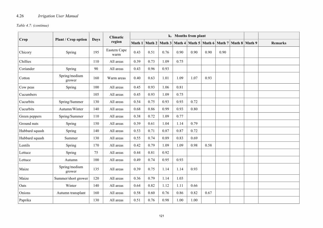
4.26 Irrigation User Manual Table 4.7: (continue)
Crop Plant / Crop option Days Climatic region
kc Months from plant
Mnth 1 Mnth 2 Mnth 3 Mnth 4 Mnth 5 Mnth 6 Mnth 7 Mnth 8 Mnth 9 Remarks
Chicory Spring 195 Eastern Cape warm 0.43 0.51 0.76 0.90 0.90 0.90 0.90
Chillies 110 All areas 0.39 0.73 1.09 0.75
Coriander Spring 90 All areas 0.43 0.96 0.93
Cotton Spring/medium grower 160 Warm areas 0.40 0.63 1.01 1.09 1.07 0.93
Cow peas Spring 100 All areas 0.45 0.93 1.06 0.81
Cucumbers 105 All areas 0.45 0.93 1.09 0.75
Cucurbits Spring/Summer 130 All areas 0.54 0.75 0.93 0.93 0.72
Cucurbits Autumn/Winter 140 All areas 0.68 0.86 0.99 0.93 0.80
Green peppers Spring/Summer 110 All areas 0.38 0.72 1.09 0.77
Ground nuts Spring 150 All areas 0.39 0.61 1.04 1.14 0.79
Hubbard squash Spring 140 All areas 0.53 0.71 0.87 0.87 0.72
Hubbard squash Summer 130 All areas 0.55 0.74 0.89 0.83 0.69
Lentils Spring 170 All areas 0.42 0.79 1.09 1.09 0.98 0.58
Lettuce Spring 75 All areas 0.44 0.81 0.92
Lettuce Autumn 100 All areas 0.49 0.74 0.95 0.93
Maize Spring/medium grower 135 All areas 0.39 0.75 1.14 1.14 0.93
Maize Summer/short grower 120 All areas 0.36 0.79 1.14 1.03
Oats Winter 140 All areas 0.64 0.82 1.12 1.11 0.66
Onions Autumn transplant 160 All areas 0.58 0.60 0.76 0.86 0.82 0.67
Paprika 130 All areas 0.51 0.76 0.98 1.00 1.00
121

Crop water requirements 4.27
Table 4.7 (continue)
Crop Plant / Crop option Days Climatic region
kc Months from plant
Mnth 1 Mnth 2 Mnth 3 Mnth 4 Mnth 5 Mnth 6 Mnth 7 Mnth 8 Mnth 9 Remarks
Parsley Spring 270 All areas 0.49 1.13 1.15 1.15 1.15 1.15 1.15 1.15 0.73 Actually a bi-annual plant
Pastures Autumn 170 All areas 0.45 0.77 0.80 0.80 0.80 0.69
Peas Autumn/Winter 110 All areas 0.49 0.82 1.09 1.07
Potatoes Spring/Summer 120 All areas 0.29 0.89 1.09 1.01
Pumpkin Spring/Summer 125 All areas 0.38 0.67 0.88 0.79 0.59
Pumpkin Autumn/Winter 150 All areas 0.39 0.63 0.86 0.87 0.70
Radishes Spring/Summer 45 All areas 0.72 0.86
Ryegrass Autumn 250 All areas 0.61 0.97 1.00 1.00 1.00 1.00 1.00 1.00 0.74
Sorghum Spring 170 All areas 0.45 0.77 0.80 0.80 0.80 0.69
Soybeans Spring/short grower 120 All areas 0.43 1.04 1.14 1.04
Soybeans Spring/medium grower 130 All areas 0.44 0.97 1.14 1.14 0.83
Soybeans Spring/long grower 140 All areas 0.43 0.87 1.14 1.14 0.99
Sweet melon Spring/Summer 105 All areas 0.64 0.95 0.96 0.83
Sweet melon Autumn/Winter 120 All areas 0.66 0.91 1.00 0.90
Spinach Autumn 190 All areas 0.39 0.51 0.77 0.98 0.99 0.98 0.95
Squash Spring 105 All areas 0.53 0.79 0.89 0.82
Sugarbeet Spring 240 All areas 0.42 0.60 0.96 1.15 1.15 1.15 1.15 1.15
Sunflower Spring/Summer 100 All areas 0.40 0.92 1.14 0.86
Sweet potatoes Spring 150 All areas 0.42 0.82 1.09 1.09 1.03
Sweetcorn Spring/Summer 90 All areas 0.53 0.82 0.99
122
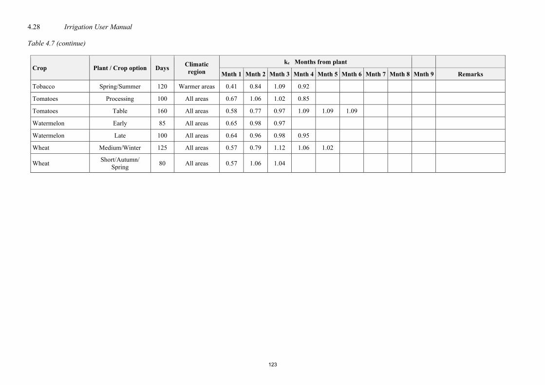
4.28 Irrigation User Manual Table 4.7 (continue)
Crop Plant / Crop option Days Climatic region
kc Months from plant
Mnth 1 Mnth 2 Mnth 3 Mnth 4 Mnth 5 Mnth 6 Mnth 7 Mnth 8 Mnth 9 Remarks
Tobacco Spring/Summer 120 Warmer areas 0.41 0.84 1.09 0.92
Tomatoes Processing 100 All areas 0.67 1.06 1.02 0.85
Tomatoes Table 160 All areas 0.58 0.77 0.97 1.09 1.09 1.09
Watermelon Early 85 All areas 0.65 0.98 0.97
Watermelon Late 100 All areas 0.64 0.96 0.98 0.95
Wheat Medium/Winter 125 All areas 0.57 0.79 1.12 1.06 1.02
Wheat Short/Autumn/ Spring 80 All areas 0.57 1.06 1.04
123

Crop water requirements 4.29
Table 4.8: Average daily reference evapotranspiration and yearly rainfall data (Source: SAPWAT)
Station Longitude (º)
Latitude (º)
Elevation (m)
MAP (mm)
Average daily ET0 (mm/day)
Jan Feb Mrch April May June July Aug Sept Oct Nov Dec
Addo Olifantpark 25.75 -33.45 152 406 5.7 5.1 4.2 3.2 2.5 2.2 2.3 2.9 3.7 4.5 5.2 5.7
Addo Sitrus Ns 25.7 -33.57 85 360 5.8 5.2 4.2 3.3 2.6 2.2 2.3 2.9 3.8 4.4 5.1 5.7
Adelaide Pp, 26.28 -32.67 600 460 6.2 5.7 4.6 3.7 3.2 2.9 3.2 3.7 4.5 4.9 5.6 6.1
Alexander Bay 16.32 -28.34 21 39 4.5 4.2 3.6 2.9 2.2 2.4 2.3 2.7 3.3 3.8 4.4 4.4
Alice 26.85 -32.78 520 570 5.1 4.6 3.7 2.9 2.4 2.1 2.4 2.9 3.7 4.2 4.7 5.1
Alto 18.85 -34.02 225 777 5.7 5.5 4.0 2.9 2.1 1.6 1.7 2.1 2.8 3.7 4.3 5.1
Amalienstein 21.47 -33.48 474 294 6.4 5.9 4.5 3.1 2.2 1.9 2.1 2.7 3.7 4.6 5.6 6.2
Amatikulu 31.52 -20.03 45 1026 4.7 4.5 4.1 3.4 2.7 2.3 2.5 3.0 3.5 4.0 4.3 4.6
Athole – Agr 30.58 -26.6 1620 937 4.2 3.9 3.4 2.6 1.9 1.5 1.7 2.2 3.0 3.5 3.8 4.1
Aws 27.85 -28.87 1640 706 4.7 4.2 3.4 2.5 1.8 1.3 1.5 2.2 3.1 3.8 4.5 4.8
Badplaas Vygeboom 30.62 -25.87 1100 788 5.1 4.8 4.1 3.5 2.9 2.5 2.8 3.6 4.6 4.8 4.8 5.0
Bamboesspruit, Otto 25.97 -26.95 1460 546 6.3 5.7 4.8 4.0 3.0 2.7 2.9 3.9 5.6 6.2 6.6 7.0
Barberton Koffieko 30.97 -25.75 777 811 4.7 4.7 4.1 3.3 2.9 2.6 2.9 3.6 4.3 4.4 4.6 4.7
Barberton Senteeko 30.75 -25.63 1300 1151 4.1 4.0 3.4 2.9 2.6 2.4 2.4 2.9 3.5 3.7 3.9 4.0
Barkly Oos 27.6 -30.97 1799 675 6.0 5.4 4.3 3.2 2.5 2.1 2.3 3.2 4.4 4.9 5.5 6.3
Bathurst Ns. 26,82 -33,52 259 683 5,1 4,7 4,0 3,4 3,1 2,9 3,1 3,3 3,8 4,1 4,6 5,0
Baviaanskloof I 24,07 -33,57 450 287 7,1 6,3 5,1 3,7 2,8 2,3 2,5 3,1 4,3 5,1 6,2 6,8
Baynesfield Estate 30,33 -29,75 914 852 3,9 3,7 3,2 2,6 2,0 1,7 2,0 2,7 3,2 3,4 3,7 3,9
Beaufort-West 22,35 -32,21 857 222 7,1 6,4 5,0 3,8 3,1 2,7 2,8 3,5 4,4 5,4 6,4 7,1
Beestekraal:Vaalko 27,6 -25,18 1096 544 4,8 4,5 3,8 2,9 2,2 1,7 1,9 2,5 3,5 4,2 4,6 4,6
Bergkwagga Park 25,47 -32,22 1204 412 5,7 5,1 4,0 2,9 2,0 1,6 1,8 2,6 3,7 4,4 5,2 5,7
Bethal 29.28 -26.27 1640 754 4.9 4.5 3.9 3.2 2.5 2.3 2.4 3.2 4.2 4.7 4.9 5.1
Bethal: Wildebeesfo 29.52 -26.17 1635 721 5.1 5.0 4.3 3.6 2.8 2.4 2.6 3.6 4.8 5.2 5.4 5.2
Bethlehem 18.97 -33.92 376 1572 5.0 4.9 3.7 2.6 1.7 1.3 1.5 1.8 2.6 3.7 4.5 4.9
124

4.30 Irrigation User Manual Table 4.8: (continue)
Station Longitude (º)
Latitude (º)
Elevation (m)
MAP (mm)
Average daily ET0 (mm/day)
Jan Feb Mrch April May June July Aug Sept Oct Nov Dec
Bethlehem; Loch Lam 28.3 -28.17 1631 739 4.9 4.4 3.6 2.7 1.9 1.5 1.6 2.3 3.2 3.9 4.5 4.9
Bien Donne (Nivv) 18.98 -33.83 138 822 6.9 6.5 5.2 3.3 2.0 1.6 1.7 2.4 3.3 4.9 6.0 6.4
Bien Donne Pp 18.98 -33.85 138 646 6.3 5.9 4.8 3.1 1.7 1.3 1.4 2.2 2.8 4.2 5.2 5.7
Bloemendal.Bishops 30.47 -29.53 838 887 4.5 4.3 3.7 2.9 2.1 1.8 2.1 2.9 3.6 4.1 4.3 4.7
Bloemfontein 26.11 -29.07 1422 552 6.3 5.6 4.3 3.3 2.6 2.3 2.5 3.4 4.4 5.3 6.2 6.6
Bloodriver: Rehling 30.53 -27.85 1234 803 4.7 4.3 3.8 3.1 2.5 2.4 2.6 3.3 4.3 4.4 4.7 4.9
Blouputs 20.15 -28.5 442 115 7.4 6.8 5.0 4.3 3.1 2.7 2.6 3.8 4.8 5.7 7.1 8.1
Bolo Reserve 27.63 -32.38 880 724 5.1 4.5 4.1 3.4 3.1 3.0 3.2 3.8 4.4 4.5 4.7 5.0
Bonfoi 18.78 -33.93 153 923 5.6 5.6 4.3 3.2 2.2 1.8 2.0 2.5 3.3 4.3 4.8 5.3
Boontjieskraal 19.35 -34.2 128 426 5.9 5.4 4.3 2.9 2.0 1.6 1.6 2.0 2.9 4.1 5.1 5.8
Brakspruit Agr. 26.98 -26.75 1402 654 6.4 5.8 4.8 4.1 3.3 2.8 3.1 4.2 5.8 6.2 6.5 6.7
Bucklands 26.72 -33.1 366 452 5.6 5.1 4.1 3.3 2.7 2.4 2.6 3.1 4.0 4.5 5.0 5.5
Buffelsfontein 26.7 -31.37 1783 634 6.0 5.1 4.1 3.1 2.5 2.1 2.3 3.2 4.2 4.8 5.4 6.0
Buffelskloof 21.22 -33.48 518 323 5.7 5.2 3.9 2.8 2.0 2.0 2.1 2.4 3.2 4.1 5.0 5.5
Buffelspoort II Ag 27.48 -25.75 1230 596 5.4 5.0 4.3 3.6 2.9 2.5 2.7 3.6 4.6 5.2 5.5 5.5
Buland 28.6 -24.42 1000 700 4.5 4.3 3.4 3.2 2.4 2.2 2.0 2.4 3.8 4.9 4.9 5.2
Bultfontein; Arbeid 26.07 -28.18 1371 506 6.8 5.8 4.7 3.6 2.5 2.0 2.3 3.3 4.6 5.7 6.4 6.9
Burgersfort Marone 30.33 -24.75 915 551 5.0 4.8 4.3 3.5 2.8 2.4 2.6 3.4 4.5 5.1 5.3 5.1
Calvinia 19.46 -31.28 981 209 7.1 6.6 5.3 3.9 3.0 2.6 2.6 3.1 3.9 5.2 6.0 6.8
Calvinia ‒ Tnk 19.77 -31.47 980 206 6.0 5.6 4.4 3.3 2.6 2.1 2.2 2.7 3.6 4.7 5.4 5.9
Calvinia Wk. 19.77 -31.48 974 208 8.9 8.0 6.8 5.0 4.0 3.1 3.2 4.1 5.2 6.4 8.0 8.6
Cape Padrone 26.45 -33.75 168 762 4.8 4.5 3.8 3.3 2.9 2.7 2.8 3.1 3.4 3.8 4.2 4.7
125

Crop water requirements 4.31
Table 4.8: (continue)
Station Longitude (º)
Latitude (º)
Elevation (m)
MAP (mm)
Average daily ET0 (mm/day)
Jan Feb Mrch April May June July Aug Sept Oct Nov Dec
Cape St. Lucia 32.24 -28.3 111 1292 4.6 4.3 3.8 3.0 2.5 2.1 2.3 2.8 3.3 3.7 4.2 4.5
Cape Town 18.32 -33.54 17 506 6.1 5.7 4.3 3.0 2.1 1.7 1.8 2.4 3.1 4.1 4.9 5.7
Carnarvon Ps. 22 -30.97 1280 215 9.4 8.0 6.3 4.6 3.4 2.6 3.0 4.1 5.3 6.9 8.2 8.8
Cedara – Agr 30.28 -29.53 1076 853 4.3 4.1 3.5 3.0 2.4 2.0 2.2 3.0 3.4 3.7 4.1 4.3
Chiltern Damwal 19.15 -34.05 309 879 5.2 4.8 3.7 2.5 1.8 1.5 1.6 2.0 2.7 3.5 4.5 5.0
Citrusdal (Nivv) 18.98 -32.57 198 437 7.0 6.3 4.9 3.1 1.8 1.3 1.4 2.2 3.1 4.6 5.9 6.6
Citrusdal Pp 18.98 -32.55 198 281 7.2 6.3 5.0 3.5 2.3 1.2 1.7 2.1 3.0 4.4 5.3 6.3
Clocolan 27.55 -28.9 1600 686 5.0 4.5 3.6 2.7 1.9 1.4 1.6 2.3 3.3 4.1 4.8 5.3
Cobham – Bos 29.42 -29.68 1675 1240 4.2 3.9 3.3 2.8 2.3 2.0 2.3 3.0 3.7 3.8 4.2 4.3
Colesberg 25.1 -30.7 1328 385 6.7 5.8 4.5 3.2 2.2 1.7 1.9 2.9 4.2 5.1 6.0 6.7
Concordia 19.85 -33.68 937 565 5.5 5.1 4.0 2.9 2.2 1.8 1.9 2.3 3.0 3.9 4.8 5.3
Cradock Pp, 25.68 -32.22 846 341 7.1 6.2 5.0 3.6 2.8 2.3 2.5 3.4 4.6 5.4 6.3 7.0
Darling 18.38 -33.38 110 594 6.7 6.4 5.1 3.5 2.0 1.4 1.5 2.2 3.2 4.7 6.0 6.4
Darnal 31.38 -29.27 85 1084 4.7 4.4 3.8 3.0 2.3 2.0 2.1 2.7 3.2 3.7 4.2 4.6
De Aar 24.01 -30.39 1243 288 7.1 6.4 4.9 3.5 2.8 2.4 2.6 3.3 4.3 5.4 6.3 7.0
De Aar 24.02 -30.65 1243 320 8.0 6.6 5.2 3.6 2.6 2.1 2.3 3.4 4.7 5.9 7.1 8.1
De Doorns (Niww) 19.67 -33.47 457 352 5.8 5.3 4.1 2.8 2.0 1.6 1.9 2.4 3.4 4.4 5.2 5.7
De Keur 19.3 -32.98 945 782 6.2 5.5 4.4 3.1 2.1 1.3 1.4 1.9 2.6 3.4 4.7 5.6
De Keur (Old) 19.3 -32.97 945 685 6.2 5.8 4.6 3.1 2.2 1.7 1.8 2.4 3.2 4.2 5.1 5.8
De Rust 19.12 -34.17 330 797 5.0 4.8 3.8 2.8 1.8 1.5 1.3 1.7 2.3 3.4 4.2 4.9
De Tuin 20.1 -29.87 970 135 9.7 8.7 6.8 5.0 3.6 2.9 3.1 4.2 5.5 7.1 8.5 9.4
De Tuin 18.98 -33.13 80 546 6.5 6.1 4.6 3.1 1.8 1.3 1.4 2.0 3.0 3.9 5.0 6.4
De Vlei 19.68 -33.43 490 150 5.7 4.8 3.9 2.7 1.9 1.8 1.8 2.2 3.1 4.0 4.8 5.5
Deelville 19.33 -33.35 480 582 6.2 5.9 4.6 2.9 1.8 1.4 1.4 2.0 3.0 4.2 5.2 6.0
126

4.32 Irrigation User Manual Table 4.8: (continue)
Station Longitude (º)
Latitude (º)
Elevation (m)
MAP (mm)
Average daily ET0 (mm/day)
Jan Feb Mrch April May June July Aug Sept Oct Nov Dec
Dennehoek 23.85 -33.87 640 1052 5.0 4.7 3.9 3.1 2.4 2.1 2.3 2.7 3.4 3.9 4.5 4.9
Die Krans 21.68 -33.55 229 232 6.0 5.4 4.2 2.8 2.1 1.9 2.2 2.6 3.6 4.6 5.4 6.0
Dohne ‒ Agr 27.47 -32.52 899 747 5.2 5.0 4.4 4.0 3.8 3.6 3.5 4.1 4.5 4.7 4.8 5.4
Dohne Ns Ii 27.47 -32.52 899 743 4.7 4.4 3.9 3.5 3.1 3.0 3.2 3.5 3.9 4.1 4.5 4.8
Dohne Ns. 27.47 -32.52 899 740 5.1 4.9 4.2 3.7 3.5 3.4 3.5 4.0 4.6 4.5 4.9 5.2
Douglas; Tronk. 23.75 -29.07 1030 344 7.3 6.0 4.9 3.5 2.6 2.1 2.3 3.3 4.5 5.7 6.7 7.1
Driefontein 20.4 -34.38 91 471 5.5 5.0 4.1 3.1 2.2 1.8 1.8 2.3 3.2 4.1 4.8 5.4
Drieplotte ‒ Agr 24.63 -29.05 1120 433 6.2 5.0 4.9 3.2 2.7 2.2 2.3 3.6 4.3 4.4 6.0 6.1
Duiwelskloof: Westf 30.12 -23.73 750 1049 4.2 3.9 3.4 2.9 2.4 2.1 2.3 2.8 3.5 3.8 4.0 4.1
Dundee: Res.Station 30.32 -28.17 1219 757 5.3 4.9 4.3 3.5 2.9 2.7 3.0 3.8 4.8 5.0 5.3 5.5
Dunghye Park 19.52 -34.32 122 521 5.8 5.5 4.4 3.1 2.2 1.7 1.8 2.2 3.1 4.1 5.1 5.8
Durban 30.57 -29.58 8 1003 4.3 4.3 3.6 3.0 2.5 2.1 2.2 2.8 3.2 3.8 4.2 4.1
East London 27.52 -33.02 125 860 4.5 4.4 3.7 3.1 3.1 2.8 3.1 3.3 3.4 3.6 4.3 4.6
Elandsheights 28.18 -30.85 1830 1120 3.3 3.4 3.2 4.5 2.8 4.1 3.0 2.8 2.4 3.7 3.0 2.9
Elgin 19.03 -34.13 305 1215 4.8 4.5 3.6 2.4 1.8 1.4 1.6 2.0 2.6 3.8 4.2 4.2
Elgin (NIVV) 19.03 -34.13 305 1116 4.8 4.4 3.4 2.3 1.8 1.5 1.7 2.0 2.7 3.4 4.2 4.6
Elliot Voorligting 27.85 -31.35 1463 744 4.9 4.4 3.8 3.1 2.8 2.5 2.7 3.3 4.0 4.2 4.7 5.1
Elsenburg 18.83 -33.85 177 653 6.2 5.9 4.6 3.2 2.1 1.7 1.8 2.3 3.0 4.2 5.4 5.9
Elsenburg 18.83 -33.85 177 596 6.1 5.7 4.7 3.5 2.2 1.7 2.1 2.4 2.9 4.2 4.8 5.6
Endeavour 26.37 -33.47 366 573 4.6 4.3 3.5 2.7 2.4 2.3 2.4 2.7 3.2 3.7 4.3 4.8
Estcourt 29.52 -29.01 1180 738 4.8 4.4 3.7 3.1 2.3 1.8 2.3 2.8 3.9 4.4 4.9 4.9
Estcrt: Tabamhlope 29.65 -29.03 1450 930 4.6 4.3 3.6 3.0 2.5 2.0 2.3 3.0 3.9 4.4 4.5 4.9
Excelsior 19.45 -32.95 953 443 6.5 6.1 4.6 3.1 2.1 1.7 1.8 2.3 3.3 4.6 5.7 6.2
127

Crop water requirements 4.33
Table 4.8: (continue)
Station Longitude (º)
Latitude (º)
Elevation (m)
MAP (mm)
Average daily ET0 (mm/day)
Jan Feb Mrch April May June July Aug Sept Oct Nov Dec
Fenfield 27 -32.53 1425 708 4.4 4.1 3.3 2.6 2.1 2.0 2.2 2.7 3.4 3.6 4.2 4.4
Ficksburg; Kersiepr 27.85 -28.87 1640 710 5.0 4.5 3.7 2.8 2.0 1.6 1.7 2.5 3.6 4.2 4.7 5.1
Fleurbaix 18.83 -33.95 85 716 5.4 4.9 3.8 2.6 1.7 1.4 1.4 1.9 2.7 3.8 4.5 5.1
Genl J.C.Steyn Gev 25.33 -33.4 200 368 6.8 6.2 5.0 4.0 3.4 3.0 3.3 3.8 4.6 5.2 5.9 6.7
George 22.25 -33.58 221 776 4.2 3.7 3.1 2.4 2.0 1.9 2.0 2.3 2.6 3.2 3.8 4.1
Germiston 28.09 -26.15 1665 708 4.9 4.5 3.9 3.2 2.7 2.5 2.6 3.4 4.6 5.0 5.3 5.3
Goedehoop 18.77 -33.92 235 606 5.3 5.2 4.3 3.4 2.4 1.8 2.0 2.4 2.9 4.0 4.4 5.1
Graafwater Ko-Op 18.6 -32.17 177 288 5.8 5.3 4.2 3.0 2.1 1.7 1.8 2.3 3.2 4.3 5.1 5.5
Grasrug 18.83 -33.47 213 426 6.7 6.5 5.2 3.6 2.4 1.7 1.7 2.2 3.1 4.6 5.9 6.5
Groot Constantia 18.42 -34.03 107 1085 5.1 4.6 3.7 2.5 1.8 1.7 1.8 2.2 2.9 3.8 4.6 5.0
Groot Vlakte 19.62 -33.32 1155 548 5.0 4.7 3.7 2.4 1.6 1.1 1.2 1.8 2.6 3.5 4.3 5.0
Grootfontein 25.02 -31.29 1263 377 5.9 5.3 4.1 3.1 2.4 2.3 2.2 3.0 3.7 4.6 5.2 5.9
Grootfontein XI, 25.02 -31.48 1270 383 7.2 6.1 4.9 3.9 3.3 2.6 3.0 3.8 4.9 5.6 6.5 7.1
Grootvlakte 19.62 -33.33 1160 718 5.9 5.3 4.1 2.8 2.1 1.5 1.2 2.0 2.3 3.2 4.2 4.7
Gullemberg 28.97 -23.83 1100 561 5.3 4.9 4.4 4.0 3.0 2.9 3.1 4.1 5.3 5.7 5.9 5.8
H.L.S. Augsburg 18.9 -32.17 500 223 7.0 6.2 4.9 3.3 2.0 1.6 1.6 2.3 3.4 4.8 5.9 6.5
Hazyview Burgersha 31.08 -25.12 722 967 4.1 4.0 3.4 2.8 2.2 1.8 1.9 2.4 3.1 3.5 3.8 3.9
Hazyview, Kranskop 30.87 -28.97 1120 849 4.3 4.1 3.6 3.2 2.9 2.7 3.0 3.5 4.1 4.0 4.3 4.3
Hazyview; Sabie San 31.13 -25.03 530 881 4.4 4.2 3.7 2.9 2.4 2.0 2.2 2.7 3.4 3.8 4.1 4.2
Hectrsprt; Laughing 31.58 -25.6 350 844 5.1 4.8 4.2 3.5 2.9 2.7 3.0 4.0 4.9 4.9 5.1 5.0
Heidedal 19.07 -32.93 725 1179 4.5 4.2 3.3 2.1 1.4 1.0 1.1 1.6 2.3 3.4 3.8 4.3
Helderfontein (NIV 18.88 -33.92 179 791 5.8 5.7 4.4 2.8 1.9 1.6 1.8 2.3 3.1 4.5 5.1 5.5
Heldervue 18.72 -32.82 755 811 5.5 5.1 4.0 2.8 2.0 1.7 1.8 2.2 2.9 4.0 4.7 5.3
Hertzogville; Karee 25.3 -28.2 1326 502 7.1 6.1 4.9 3.8 2.9 2.3 2.6 3.7 5.2 6.1 6.9 7.4
128

4.34 Irrigation User Manual Table 4.8: (continue)
Station Longitude (º)
Latitude (º)
Elevation (m)
MAP (mm)
Average daily ET0 (mm/day)
Jan Feb Mrch April May June July Aug Sept Oct Nov Dec
Hillcrest: Sensako 30.75 -29.8 732 817 4.1 4.1 3.5 2.9 2.4 2.1 2.5 3.0 3.5 3.6 4.1 4.2
Hobhouse 27.13 -29.52 1448 609 5.0 4.3 3.4 2.5 1.7 1.2 1.4 2.0 3.0 3.7 4.6 5.0
Hoedsprt Jongmansp 30.8 -24.38 610 514 5.0 4.9 4.2 3.4 2.6 2.3 2.4 3.2 4.2 4.6 4.8 4.7
Hopetown; Alfalfa 24.18 -29.65 1143 311 5.3 4.9 3.9 2.8 1.8 1.3 1.5 2.2 3.2 4.2 5.0 5.6
Ideal Hill 18.88 -32.8 152 286 7.8 7.1 5.6 3.7 2.3 1.6 1.5 2.2 3.4 5.1 6.5 7.4
Jaagbaan 30.68 -29.35 1018 809 3.9 3.7 3.2 2.6 2.0 1.7 2.0 2.6 3.1 3.4 3.8 4.1
Jamestown 26.78 -31.07 1650 574 6.6 5.5 4.5 3.4 2.6 2.2 2.4 3.3 4.5 5.2 5.9 6.7
Jan Kempdorp; Vaalh 24.83 -27.95 1175 448 6.3 5.5 4.5 3.4 2.4 1.9 2.1 3.1 4.4 5.4 6.2 6.4
Jansenville Pp 24.7 -32.93 414 290 7.1 6.3 4.9 3.6 2.9 2.4 2.7 3.3 4.2 5.0 6.2 6.9
JC Steyngev-Landbo 25.35 -33.4 96 359 5.7 5.2 4.3 3.2 2.6 2.3 2.5 2.8 3.9 4.5 5.4 5.8
Johannesburg 28.03 -26.12 1753 718 5.1 4.8 4.0 3.3 2.7 2.5 2.5 3.4 4.5 5.1 5.3 5.3
Jolette 19.55 -33.5 370 123 5.6 5.0 4.6 3.3 1.9 1.7 1.6 2.7 3.6 4.7 5.1 5.5
Jonaskraal 19.9 -34.4 103 388 6.1 5.7 4.6 3.3 2.3 1.8 1.8 2.3 3.2 4.5 5.4 6.0
Joubertina 23.87 -33.82 549 504 5.4 4.9 4.0 2.9 2.2 1.8 2.0 2.5 3.3 3.9 4.6 5.2
Kakamas 20.62 -28.77 720 106 9.5 8.3 6.7 5.0 3.6 2.8 3.2 4.2 5.5 7.1 8.5 9.4
Karringmelksrivier 20.77 -34.13 192 429 5.8 5.4 4.3 3.2 2.6 2.1 2.1 2.4 3.2 4.1 5.2 5.9
Kei Mouth 28.15 -32.67 258 774 4.8 4.5 3.8 3.3 3.1 2.8 3.1 3.6 4.0 4.1 4.5 4.7
Keimoes 20.97 -28.7 762 119 7.6 6.4 5.1 3.8 2.8 2.3 2.7 3.4 4.7 6.1 7.2 7.8
Keimoes. 21 -28.73 748 161 7.3 6.6 5.2 4.0 2.8 2.3 2.6 3.6 4.6 5.7 6.6 7.4
Kestell 28.7 -28.32 1707 709 5.3 4.9 4.1 3.2 2.8 2.6 2.7 3.3 4.4 4.9 5.3 5.5
Kimberley 24.46 -28.48 1204 415 7.0 6.2 4.8 3.7 3.0 2.6 2.9 4.0 4.9 5.9 6.8 7.2
129

Crop water requirements 4.35
Table 4.8: (continue)
Station Longitude (º)
Latitude (º)
Elevation (m)
MAP (mm)
Average daily ET0 (mm/day)
Jan Feb Mrch April May June July Aug Sept Oct Nov Dec
Klaver 18.37 -31.47 42 174 6.9 6.6 5.6 4.1 3.2 2.7 2.7 3.3 4.1 5.1 6.1 6.8
Klawer Wynkelder 18.63 -31.78 68 216 7.0 6.8 5.7 4.2 3.0 2.2 2.4 3.2 4.3 5.8 6.5 6.8
Klein Bottelary 18.73 -33.9 110 682 6.1 5.6 4.6 3.4 2.3 1.7 1.7 2.2 3.1 4.2 4.8 5.6
Klein Waterval 19.02 -33.88 186 1134 6.9 7.2 5.4 3.8 2.4 1.8 2.0 2.4 3.4 4.6 4.2 5.7
Klipfontein 25.73 -32.6 735 411 6.3 5.8 4.6 3.9 3.2 2.7 2.9 3.5 4.4 4.8 5.6 6.3
Klippan: Koster 26.95 -26.05 1561 608 5.5 5.3 4.3 3.7 2.8 2.5 2.7 3.6 5.1 5.8 6.0 6.1
Kokstad 29.25 -30.32 1305 728 4.5 4.0 3.3 2.8 2.1 1.8 2.1 2.6 3.5 3.8 4.4 4.6
Kokstad ‒ Agr 29.42 -30.52 1372 832 4.4 4.1 3.4 2.7 2.2 1.8 2.0 2.7 3.4 3.8 4.2 4.5
Komatiprt; Tenbosch 31.97 -25.4 189 564 5.3 5.1 4.3 3.5 2.8 2.4 2.8 3.7 4.6 5.1 5.3 5.2
Koster Kooperasie 26.92 -25.83 1585 620 5.9 5.4 4.5 3.7 3.1 2.6 3.0 4.0 5.2 5.9 6.5 6.3
Kroonstad 27.14 -27.4 1348 606 5.8 5.3 4.3 3.4 2.8 2.6 2.6 3.5 4.7 5.5 5.9 6.1
Kuruman 23.43 -27.47 1312 356 5.6 5.0 4.1 3.0 2.3 1.8 1.9 2.6 3.6 4.5 5.3 4.8
Kuruman 23.26 -27.28 1300 420 6.4 5.8 4.5 3.4 2.4 2.0 2.3 3.1 4.2 5.2 6.3 6.5
L.Trichard: Levubu (S 30.28 -23.08 610 842 4.9 4.6 4.0 3.4 2.9 2.6 2.6 3.3 4.2 4.5 4.7 4.8
La Motte 19.08 -33.88 206 852 5.9 5.6 4.3 2.9 1.8 1.5 1.7 2.2 3.0 4.2 5.0 5.6
La Plaisante 19.2 -33.45 260 633 6.5 6.1 4.7 3.1 2.0 1.7 1.8 2.3 3.2 4.5 5.6 6.2
Landau 18.97 -33.6 122 517 6.7 6.2 4.8 3.1 1.9 1.4 1.5 2.1 3.1 4.6 5.7 6.1
Langgewens (WRS) 18.7 -33.28 177 415 7.1 7.1 5.8 4.2 2.8 2.1 2.0 2.5 3.5 5.1 6.2 6.9
Langkloof 23.58 -33.78 722 605 4.5 4.1 3.5 2.7 2.3 1.7 1.9 2.4 2.8 3.9 4.0 4.5
Langkloof (NIVV) 23.58 -33.78 722 632 5.3 4.9 4.0 3.2 2.7 2.4 2.5 2.8 3.4 3.9 4.6 5.1
Le Bonheur 18.87 -33.83 260 841 6.2 6.1 4.8 3.5 2.2 1.5 1.7 2.1 3.1 4.3 4.8 5.6
Letaba Letsitele 30.32 -23.87 623 714 4.3 4.1 3.6 2.9 2.3 1.9 2.0 2.5 3.2 3.8 4.0 4.2
Letsitele: Eiland 30.67 -23.67 457 551 4.7 4.4 3.8 3.0 2.3 2.0 2.1 2.7 3.6 4.2 4.5 4.6
Lidney 26 -33.67 200 551 5.2 4.9 4.0 3.5 3.2 2.9 3.0 3.3 3.8 4.3 4.6 5.1
130

4.36 Irrigation User Manual Table 4.8: (continue)
Station Longitude (º)
Latitude (º)
Elevation (m)
MAP (mm)
Average daily ET0 (mm/day)
Jan Feb Mrch April May June July Aug Sept Oct Nov Dec
Little Harmony, Ri 30.32 -29.93 869 893 3.9 3.8 3.2 2.6 1.9 1.5 1.7 2.3 2.8 3.2 3.5 3.8
Longdown 19.17 -34.05 300 687 5.4 5.0 4.0 2.8 2.0 1.7 1.8 2.2 2.9 3.7 4.6 5.1
Longdown 19.17 -34.05 340 819 4.7 4.9 3.7 2.7 2.1 1.4 1.5 1.7 2.5 3.4 3.8 4.5
Lorraine 19.05 -32.05 320 251 7.0 6.6 5.3 3.7 2.4 1.8 1.9 2.7 3.8 5.2 6.2 6.8
Loskop ‒ Proefstas 29.4 -25.17 945 631 5.3 5.1 4.3 3.5 2.7 2.3 2.5 3.3 4.5 5.0 5.2 5.3
Lutzville (Niww) 18.43 -31.6 31 144 6.4 6.1 5.0 3.8 2.8 2.3 2.4 3.0 4.1 5.0 5.8 6.2
Lydenburg Longtom 30.62 -25.13 2118 898 4.0 3.7 3.2 2.6 2.0 1.6 1.7 2.3 3.1 3.4 3.7 3.8
Lydenburg Rosenkra 30.62 -24.9 1525 614 4.3 4.1 3.4 2.8 2.1 1.7 1.8 2.4 3.2 3.8 4.0 4.2
Lydenburg; Doornhoe 24.88 -25.68 1644 649 4.7 4.6 3.9 3.4 2.6 2.3 2.5 3.2 4.2 4.7 4.6 4.5
Macuville ‒ Agr 29.9 -22.27 522 310 5.8 5.5 5.0 3.9 3.0 2.5 2.7 3.5 4.5 5.4 5.7 5.9
Malelane Proefpla 31.55 -25.45 380 569 5.3 5.1 4.5 3.9 3.4 3.3 3.4 4.1 4.7 5.0 5.2 4.9
Malelane Vergelege 31.5 -25.5 369 578 4.7 4.5 3.9 3.1 2.4 2.2 2.4 3.0 3.8 4.2 4.5 4.7
Malelane; Hoechst.L 31.63 -25.63 272 781 5.4 5.1 4.4 3.6 2.9 2.6 2.8 3.8 4.8 5.1 5.2 5.3
Malelane; Kaalrugt 31.57 -25.62 390 845 5.1 4.9 4.2 3.4 2.7 2.5 2.8 3.7 4.5 4.8 5.0 5.1
Mara – Agr 29.57 -23.15 894 432 4.9 4.6 4.1 3.3 2.6 2.1 2.3 3.0 4.0 4.4 4.7 4.9
Marble Hall: Moosri 29.42 -25.02 1065 515 4.9 4.6 3.9 3.0 2.2 1.8 1.9 2.6 3.5 4.1 4.5 4.7
Marquard; Saaiplaas 27.35 -28.68 1510 636 5.4 4.7 3.8 2.8 2.0 1.5 1.6 2.3 3.6 4.1 4.8 5.3
Marquard; Wildebees 27.33 -28.5 1450 600 6.6 5.8 4.8 3.6 2.7 2.2 2.4 3.3 4.7 5.5 6.1 6.8
Mayfield, Stanger 31.15 -29.2 610 1276 4.2 3.9 3.4 2.8 2.1 1.9 2.1 2.7 3.3 3.7 4.0 4.2
Meerlust 18.75 -34.02 33 609 5.9 6.0 4.3 3.1 2.1 1.8 1.9 2.3 3.0 4.0 4.5 5.4
Melmoth 31.24 -28.35 770 806 4.8 4.5 3.8 3.2 2.6 2.2 2.4 3.3 4.0 4.3 4.7 4.9
Merle I 18.93 -33.87 180 688 5.4 5.1 3.9 2.6 1.6 1.2 1.3 1.7 2.4 3.6 4.1 5.0
Messina 30.03 -22.2 549 340 5.9 5.8 4.9 4.3 3.7 3.3 3.4 4.1 4.9 5.8 6.3 6.1
131

Crop water requirements 4.37
Table 4.8: (continue)
Station Longitude (º)
Latitude (º)
Elevation (m)
MAP (mm)
Average daily ET0 (mm/day)
Jan Feb Mrch April May June July Aug Sept Oct Nov Dec
Messina Proefplaas 29.92 -22.23 700 319 4.8 4.5 4.2 3.3 2.5 2.0 2.2 2.8 3.6 4.1 4.6 4.8
Mhlati 31.53 -25.47 309 578 5.0 4.8 3.9 3.1 2.4 2.0 2.2 2.9 3.7 4.2 4.6 4.9
Mhlume 31.8 -26.03 280 778 5.0 4.7 3.9 3.2 2.4 2.0 2.2 3.1 4.0 4.4 4.6 4.9
Middleton 25.83 -32.98 549 353 6.1 5.5 4.4 3.4 2.7 2.3 2.7 3.2 4.1 4.8 5.5 6.0
Montagu 20.07 -33.47 223 312 6.6 6.1 4.7 3.5 2.9 2.4 2.5 2.9 3.5 4.6 5.6 6.4
Montagu Polisie 20.13 -33.8 225 316 6.5 5.9 4.6 3.1 2.1 1.6 1.7 2.4 3.5 4.5 5.7 6.4
Moorreesburg Ko-Op 18.68 -33.15 158 421 7.0 6.7 5.2 3.6 2.3 1.7 1.7 2.3 3.3 5.0 6.1 6.7
Morewag 18.93 -33.68 240 395 6.0 5.6 4.0 3.3 1.9 1.5 1.4 1.9 2.2 3.8 4.2 5.8
Morgenstond 20.02 -33.93 140 301 5.9 5.2 4.2 3.1 2.1 1.8 1.6 2.2 3.0 4.2 5.3 5.8
Mortimer I 25.67 -32.38 840 318 6.7 6.1 5.0 3.8 2.9 2.6 3.0 3.7 4.7 5.5 6.3 6.8
Mountain Vineyards 18.95 -33.88 362 1320 6.0 5.8 4.6 3.3 2.2 1.8 2.0 2.5 3.3 4.6 5.4 5.7
Mt. Edgecombe 31.03 -29.7 96 1017 4.4 4.2 3.6 2.8 2.1 1.8 2.0 2.5 3.0 3.6 4.0 4.3
Natal Est., Thornv 30.4 -29.75 860 819 4.3 4.2 3.6 3.0 2.3 1.9 2.2 3.0 3.7 4.0 4.3 4.4
Nchosa, Muden 30.37 -28.97 793 666 5.0 4.6 3.8 3.1 2.4 2.0 2.3 3.1 3.9 4.3 4.7 5.0
Nelsprt Friedenhei 30.98 -25.43 671 754 5.0 4.8 4.2 3.6 3.1 2.8 2.9 3.5 4.3 4.5 4.5 4.7
Nelspruit 30.58 -25.27 665 805 4.8 4.7 4.0 3.5 3.0 2.9 3.0 3.6 4.6 4.8 5.0 4.8
Nelspruit: NISSV 30.97 -25.45 660 782 4.9 4.7 4.0 3.3 2.9 2.5 2.6 3.3 4.1 4.3 4.5 4.7
Newcastle 29.56 -27.45 1199 917 5.3 4.8 4.2 3.5 2.9 2.7 2.8 3.6 4.7 5.3 5.5 5.6
Ngome: Sapekoe Est. 31.45 -27.85 1010 1424 4.6 4.4 3.9 3.4 2.9 2.6 2.9 3.5 3.7 3.9 4.2 4.4
Nietvoorbij 18.87 -33.9 146 689 6.2 6.2 4.5 3.3 2.1 1.7 1.9 2.1 3.0 4.2 5.0 5.6
Nietvoorbij (NIWW) 18.87 -33.9 146 768 6.1 5.9 4.5 3.0 1.9 1.6 1.7 2.3 3.2 4.5 5.4 5.8
Nivv 18.85 -33.92 160 685 5.2 4.9 3.6 2.3 1.4 1.2 1.3 1.7 2.4 3.7 4.6 5.1
Nkwalini 31.53 -28.72 154 740 4.8 4.6 3.9 3.2 2.4 2.0 2.2 2.9 3.7 4.2 4.4 4.7
Nooitgedacht 18.85 -34.03 343 876 5.3 4.9 3.9 2.7 2.0 1.9 2.0 2.2 2.9 3.9 4.8 5.0
132

4.38 Irrigation User Manual Table 4.8: (continue)
Station Longitude (º)
Latitude (º)
Elevation (m)
MAP (mm)
Average daily ET0 (mm/day)
Jan Feb Mrch April May June July Aug Sept Oct Nov Dec
Nooitgedacht ‒ Cer 19.33 -33.22 1040 845 5.5 5.1 3.9 2.7 1.8 1.5 1.5 2.0 2.7 3.7 4.5 5.1
Nw Koop Madibogo 25.2 -26.42 1311 427 6.3 5.7 4.9 3.8 3.0 2.5 2.8 3.8 5.2 5.9 6.5 6.6
Okiep 17.52 -28.36 927 152 6.5 6.1 5.1 3.4 2.4 1.9 2.1 2.7 3.7 4.7 5.9 6.5
Onseepkans. 19.28 -28.78 305 85 5.6 5.3 4.3 3.0 2.0 1.5 1.6 2.3 3.4 4.5 5.2 5.7
Oos Londen ‒ Wk 27.83 -33.03 125 768 5.0 4.7 3.9 3.6 3.3 3.0 3.2 3.3 3.5 3.8 4.3 4.7
Opwag 21.95 -28.88 884 190 8.5 7.4 6.0 4.5 3.3 2.6 2.9 4.1 5.3 6.7 7.8 8.4
Orania:Beker Loop- 24.6 -29.88 1140 324 7.6 5.9 4.9 3.6 2.6 2.0 2.3 3.4 4.3 5.4 6.7 7.6
Oudtshoorn 22.12 -33.35 335 254 6.1 5.6 4.4 3.0 2.3 2.1 2.1 2.6 3.2 4.3 5.3 5.9
Outeniqua (WRS) 22.42 -33.92 204 768 4.1 3.9 3.2 2.6 2.3 2.1 2.1 2.3 2.8 3.3 3.8 4.1
Paddock 30.22 -30.78 503 1151 3.9 3.6 3.1 2.7 2.3 2.0 2.2 2.8 3.1 3.1 3.6 3.8
Patensie, 24.83 -33.78 150 445 5.5 4.9 3.9 3.1 2.4 2.1 2.3 2.7 3.5 4.2 4.8 5.4
Philadelphia Polis 18.58 -33.67 76 467 6.0 5.6 4.4 2.9 1.7 1.2 1.3 1.8 2.7 4.1 5.2 5.8
Pietersburg 29.27 -23.52 1230 476 5.0 4.8 4.2 3.5 2.9 2.6 2.7 3.3 4.1 5.2 5.4 5.2
Pietrsbrg: Univ.V/D 29.67 -23.85 1250 456 5.4 5.2 4.4 3.7 3.0 2.6 2.8 3.7 4.8 5.5 5.4 5.3
Pioneer Seed, Grey 30.62 -29.03 1110 826 4.6 4.2 3.6 3.0 2.3 2.0 2.3 3.1 4.0 4.3 4.7 4.8
Pk Le Rouxdam; Oukr 24.68 -29.93 1143 364 6.0 5.3 4.2 3.0 2.0 1.6 1.8 2.5 3.6 4.6 5.5 6.2
Plaatkop: Alwal Nrt 26.88 -30.8 1349 496 6.2 5.7 4.3 3.0 2.1 1.8 2.0 2.8 4.3 5.1 5.7 6.5
Plooysburg; S.A.P. 24.23 -29.02 1082 377 6.1 5.2 4.2 3.0 2.1 1.6 1.8 2.5 3.7 4.6 5.6 6.0
Pmburg: Ukulinga Res. 30.4 -29.67 775 719 4.6 4.4 3.8 3.1 2.6 2.3 2.5 3.0 3.6 3.9 4.4 4.6
Pofadder ‒ Pol 19.38 -29.13 989 93 6.1 5.2 4.1 2.9 2.0 1.5 1.7 2.4 3.4 4.5 5.4 6.2
Poffader 19.23 -29.08 994 98 7.0 6.3 5.1 3.5 2.5 1.9 2.2 2.9 4.1 5.1 6.3 7.0
Pongola 31.58 -27.4 308 671 4.9 4.6 3.9 3.0 2.3 1.9 2.1 2.8 3.5 4.1 4.4 4.8
Port Elizabeth 25.36 -33.59 58 632 4.6 4.1 3.3 2.9 2.3 1.9 2.0 2.5 2.9 3.5 4.1 4.7
Porterville Ko-Op 19.02 -33.02 145 522 6.1 5.7 4.4 2.9 1.8 1.4 1.5 2.0 2.9 4.2 5.2 6.0
133

Crop water requirements 4.39
Table 4.8: (continue)
Station Longitude (º)
Latitude (º)
Elevation (m)
MAP (mm)
Average daily ET0 (mm/day)
Jan Feb Mrch April May June July Aug Sept Oct Nov Dec
Postmasburg 23 -28.18 1324 325 6.8 6.2 4.8 3.6 2.8 2.3 2.6 3.5 4.5 5.6 6.5 7.1
Potchefstroom Agr; 27.08 -26.73 1345 602 6.0 5.4 4.6 3.7 3.0 2.6 2.9 4.0 5.5 6.1 6.5 6.5
Potchefstroom; Noyo 27 -26.78 1370 578 6.1 5.6 4.7 3.9 3.2 2.7 3.0 4.1 5.5 6.1 6.2 6.4
Powers Court 30.63 -29.97 631 1018 3.7 3.5 3.1 2.7 2.2 2.0 2.2 2.7 2.9 3.2 3.5 3.7
Preston Park 25.93 -33.5 330 452 5.9 5.4 4.5 3.7 2.9 2.6 2.8 3.2 3.9 4.6 5.1 5.7
Pretoria: N.I.Plant 28.33 -25.73 1299 703 5.6 5.2 4.5 3.6 2.9 2.4 2.7 3.6 4.8 5.3 5.5 5.5
Prieska 22.45 -29.4 933 232 6.9 6.4 5.1 3.5 2.5 1.9 2.2 3.0 4.2 5.2 6.5 7.2
Prinskraal 20.12 -34.63 15 424 5.2 4.8 4.0 2.9 2.0 1.6 1.6 2.1 3.0 4.0 4.7 5.2
Protem 20.08 -34.27 259 463 6.0 5.5 4.4 3.2 2.3 1.9 1.9 2.3 3.1 4.2 5.1 5.7
Punda Milia 31.01 -22.41 462 590 5.7 5.1 4.4 4.0 3.3 2.9 3.1 3.9 4.6 5.6 5.7 5.9
Queenstown 26.87 -31.9 1099 527 6.0 5.4 4.3 3.5 3.0 2.7 2.9 3.7 4.6 5.0 5.6 6.1
Reitz Ko-Op, 28.43 -27.8 1615 723 5.9 5.4 4.5 3.5 2.8 2.3 2.5 3.4 4.7 5.3 5.6 6.0
Rhebokrant 24.63 -34.1 160 842 5.3 4.9 4.1 3.7 3.2 2.8 2.9 3.1 3.4 3.9 4.4 5.0
Richmond: Sapekoe E 30.15 -29.93 1200 1182 3.8 3.9 3.5 2.9 2.5 2.6 3.0 3.5 3.9 3.5 4.0 3.9
Richtersveld 16.9 -28.13 42 58 6.8 6.4 5.3 4.3 3.0 2.1 2.4 3.1 4.1 5.3 6.1 6.7
Riebeek-Wes 18.87 -33.35 168 546 6.7 6.4 5.0 3.3 2.0 1.6 1.6 2.3 3.2 4.7 5.8 6.3
Rietbron 23.07 -32.93 820 222 7.3 6.4 5.2 3.7 2.6 2.3 2.6 3.2 4.3 5.3 6.4 7.0
Rietbron ‒ Mun 23.15 -32.9 762 210 6.4 5.5 4.3 3.0 2.0 1.6 1.7 2.5 3.4 4.7 5.7 6.4
Rietrivier, Sandper 24.62 -29.07 1140 362 6.8 5.9 4.7 3.4 2.5 1.9 2.1 3.0 4.3 5.2 6.3 6.7
Riversdal Ko-Op 21.27 -34.08 122 455 5.3 4.9 3.9 2.8 2.1 1.8 1.8 2.3 3.1 4.0 4.7 5.2
Robertson (Nivv) 19.9 -33.83 156 294 5.9 5.3 4.1 2.9 2.1 1.8 2.0 2.5 3.5 4.3 5.3 5.8
Robertson Pp 19.88 -33.83 156 360 5.3 5.1 3.7 2.7 1.7 1.8 1.6 2.2 2.6 3.5 4.5 4.7
Roedtan 29.08 -24.57 973 554 6.2 6.0 5.0 4.0 3.1 2.6 2.9 4.0 5.5 6.4 6.5 6.4
134

4.40 Irrigation User Manual Table 4.8: (continue)
Station Longitude (º)
Latitude (º)
Elevation (m)
MAP (mm)
Average daily ET0 (mm/day)
Jan Feb Mrch April May June July Aug Sept Oct Nov Dec
Roodeheuwel (Wrs) 22.25 -33.63 301 249 6.2 5.8 4.5 3.0 2.0 1.6 1.7 2.4 3.4 4.5 5.5 6.0
Roodeplaat ‒ Agr 28.35 -25.58 1164 645 5.8 5.4 4.6 3.8 3.1 2.6 2.9 3.8 5.0 5.7 5.9 5.9
Rustenburg ‒ Agr 27.3 -25.72 1157 614 4.9 4.6 3.9 3.0 2.4 1.9 2.0 2.7 3.7 4.3 4.7 4.9
Rustenhof 18.78 -34.05 56 696 5.7 5.6 4.1 3.1 2.1 1.7 1.7 2.1 3.0 4.0 4.4 5.3
Schweizer Reneke 25.43 -27.18 1280 499 7.0 5.7 4.9 4.0 3.0 2.3 2.6 3.8 5.3 5.9 6.7 7.1
Scottburg:Crocworl 30.77 -30.28 100 911 4.3 4.1 3.6 3.0 2.6 2.3 2.4 2.9 2.9 3.4 3.8 4.0
Serjeantsrivier 19.52 -34.13 366 557 5.8 5.4 4.3 2.9 1.9 1.5 1.5 2.0 2.8 3.9 4.9 5.5
Settlers:Landbousk 28.55 -24.95 1050 639 5.2 5.0 4.0 3.2 2.4 1.9 2.2 3.0 4.2 4.7 5.1 5.1
Sevontein, Elandsk 30.13 -29.75 1375 930 4.4 4.1 3.6 2.9 2.3 1.9 2.1 3.0 3.6 3.9 4.2 4.4
Sitrusbeurs Gvb. 25.32 -33.77 110 492 5.5 4.9 4.0 3.3 2.6 2.3 2.4 2.9 3.7 4.3 4.9 5.4
Somerset Oos ‒ Hos 25.58 -32.73 717 506 6.1 5.5 4.4 3.5 2.9 2.5 2.9 3.5 4.2 4.6 5.3 6.0
Spekboom 25.87 -33.45 259 424 5.9 5.4 4.4 3.5 2.7 2.3 2.6 3.0 3.9 4.5 5.1 5.9
Spitskop,Prieska 22.85 -29.6 939 236 8.4 7.0 5.5 3.9 2.8 2.1 2.3 3.5 4.9 6.1 7.5 8.3
Stellenboschvlei 23.42 -32.25 970 216 8.9 8.2 6.5 5.1 4.1 3.6 3.8 4.4 5.8 6.6 7.7 8.8
Sterkstroom 26.52 -31.65 1297 478 6.4 5.4 4.3 3.2 2.4 2.1 2.3 3.1 4.1 4.7 5.6 6.4
Sugar Mill, Sezela 30.58 -30.33 160 1024 4.2 4.2 3.7 3.2 2.8 2.4 2.6 3.1 3.5 3.9 4.2 4.2
Sutherland 20.4 -32.23 1456 229 6.2 5.7 4.5 3.3 2.5 2.0 2.0 2.6 3.3 4.3 5.4 6.1
Taung 24.73 -27.55 1097 442 7.0 5.9 4.9 3.9 3.0 2.6 2.8 3.8 5.1 5.9 7.0 7.4
Tenbosch 31.9 -25.33 179 607 5.1 4.7 3.9 3.1 2.4 1.9 2.1 2.8 3.7 4.3 4.6 5.0
Thabazimbi 27.24 -24.37 1028 671 6.3 6.0 4.9 4.0 3.3 3.0 3.2 4.1 5.2 6.3 6.6 6.7
The Grange, Umzimk 29.97 -30.25 762 800 3.8 3.8 3.2 2.5 1.7 1.3 1.5 2.0 2.7 3.2 3.6 3.8
Tongaat 31.13 -29.57 72 1026 4.3 4.2 3.5 2.7 1.9 1.5 1.6 2.2 2.8 3.5 3.9 4.3
Tot-U-Diens 19.85 -33.68 915 534 5.5 5.0 4.0 2.9 2.2 1.8 1.9 2.3 3.0 3.9 4.7 5.3
Towoomba 28.33 -24.9 1143 635 5.1 4.9 4.2 3.3 2.6 2.2 2.5 3.2 4.3 5.0 5.2 5.3
135

Crop water requirements 4.41
Table 4.8: (continue)
Station Longitude (º)
Latitude (º)
Elevation (m)
MAP (mm)
Average daily ET0 (mm/day)
Jan Feb Mrch April May June July Aug Sept Oct Nov Dec
Tweespruit; 27.07 -29.2 1585 637 6.1 5.2 4.1 3.0 2.2 1.6 1.8 2.8 4.0 4.8 5.6 6.2
Tygerhoek (WRS) 19.9 -34.13 168 498 5.8 5.4 4.3 3.0 2.1 1.6 1.7 2.2 3.2 4.2 5.1 5.7
Ugie 28.27 -31.22 1280 927 4.6 4.1 3.6 3.0 2.4 2.0 2.1 3.1 3.8 4.1 4.3 5.0
Ukulinga Res Stn 30.4 -29.67 775 678 3.5 3.8 3.2 2.6 2.3 2.3 2.0 3.0 3.6 3.6 3.8 0.0
Umtata 28.47 -31.35 696 654 4.7 4.1 3.6 3.0 2.2 1.8 2.3 2.7 3.4 4.0 4.5 4.5
Umzimkulu 30.43 -30.68 180 1143 4.0 3.8 3.3 2.5 1.9 1.6 1.7 2.1 2.7 3.2 3.7 4.0
Underchurch 27.37 -32.32 850 496 5.4 4.9 4.1 3.4 2.9 2.7 2.8 3.6 4.4 4.6 5.1 5.4
Upington Ns. 21.25 -28.45 793 158 6.9 6.0 4.7 3.4 2.3 1.8 2.0 2.9 4.0 5.1 6.3 6.9
Vaalkrantz 26.05 -33.37 380 452 5.2 4.7 3.9 3.1 2.6 2.4 2.6 2.9 3.6 4.1 4.7 5.2
Vaalwater: Elandskl 28.05 -24.28 1215 614 4.8 4.5 3.9 3.2 2.5 2.2 2.4 3.2 4.3 4.9 5.1 4.9
Van Wyksvlei 21.82 -30.35 962 172 8.4 7.4 5.7 4.1 2.8 2.1 2.4 3.4 4.6 6.2 7.5 8.2
Veldreserwe 19.45 -33.65 275 271 7.0 6.3 4.8 3.3 2.3 1.9 2.0 2.5 3.5 4.7 5.9 6.7
Venda: Lwamondo 30.37 -23.05 885 897 5.0 4.7 4.2 3.5 3.1 2.8 2.7 3.5 4.5 4.9 5.1 5.0
Venda: Rabali 30.12 -22.87 1 371 6.4 5.9 5.2 4.4 3.5 3.0 3.2 4.2 5.5 6.2 6.4 6.2
Venda: Sigonde. 30.77 -22.42 405 363 4.8 4.7 4.0 3.3 2.5 2.1 2.2 2.8 3.7 4.2 4.6 4.9
Venda: Tshiombo 30.5 -22.8 650 824 5.2 4.9 4.3 3.6 2.9 2.7 2.8 3.5 4.6 4.9 5.2 5.3
Ventersdorp: Sterks 26.72 -26.47 1375 564 6.1 5.5 4.7 3.8 3.0 2.6 2.9 4.0 5.4 6.2 6.6 6.6
Vereeniging; Rusoord. 28.32 -26.83 1450 562 5.2 4.9 4.1 3.2 2.4 1.9 2.1 3.0 4.5 5.1 5.6 5.4
Vergelegendruif 18.92 -34.1 260 790 5.2 5.1 3.7 2.6 1.8 1.4 1.3 2.2 2.7 3.6 3.7 4.7
Vergelegenvrug 18.9 -34.08 80 740 5.3 5.1 3.8 2.6 1.7 1.6 1.6 2.1 2.7 3.5 4.0 5.0
Viljoenskroon; Riet 26.92 -27.17 1321 596 5.5 4.9 4.1 3.2 2.3 1.9 2.1 3.0 4.3 5.3 5.7 6.1
Viljoenslaagte: Kop 27.45 -27.23 1401 621 6.2 5.7 4.7 3.8 2.8 2.3 2.6 3.7 5.0 5.8 6.1 6.4
Villiers Ko-Op. 28.62 -27.03 1493 638 5.1 4.7 4.0 3.1 2.3 1.9 2.1 2.9 4.0 4.6 5.0 5.3
Villiersdorp 19.3 -33.98 366 697 6.0 5.5 4.4 3.1 2.3 2.0 2.3 2.5 3.4 4.3 5.2 5.8
136

4.42 Irrigation User Manual Table 4.8: (continue)
Station Longitude (º)
Latitude (º)
Elevation (m)
MAP (mm)
Average daily ET0 (mm/day)
Jan Feb Mrch April May June July Aug Sept Oct Nov Dec
Vrede En Lust 18.95 -33.85 160 881 6.4 5.9 4.9 3.6 2.3 1.6 1.8 2.1 3.3 4.6 5.0 5.6
Vredenburg Ko-Op 18 -32.9 128 326 5.8 5.6 4.7 3.7 2.7 2.2 2.2 2.6 3.5 4.6 5.3 5.7
Vryburg; Armoedsvlakt 24.63 -26.95 1234 437 6.6 5.4 4.6 3.6 2.5 2.0 2.2 3.2 4.6 5.5 6.3 6.6
Vryburg; Vergelegen 24.2 -25.78 1065 372 6.1 5.3 4.6 4.2 2.7 2.2 2.5 3.6 4.6 5.4 6.1 5.9
Walkers Hoek, Ladys 29.67 -28.47 1200 785 4.6 4.2 3.5 2.6 2.0 1.6 1.8 2.5 3.3 3.8 4.3 4.6
Waterfall, Utrecht 30.25 -27.8 1180 704 5.2 4.8 4.0 3.2 2.6 2.3 2.6 3.5 4.4 4.8 5.1 5.4
Welgevallen II 18.85 -33.93 116 698 5.6 5.3 4.1 2.8 1.9 1.6 1.6 2.1 2.9 4.3 5.0 5.3
Welkom; Sandvet. 26.68 -28.13 1295 519 5.1 4.6 3.7 2.8 1.9 1.4 1.6 2.2 3.2 4.0 4.7 5.1
Weltevrede 20.62 -33.93 405 362 5.4 5.0 3.8 2.5 1.7 1.2 1.3 1.9 2.8 3.8 4.8 5.3
Welverdiend An. 26.72 -30.72 1348 582 7.9 6.1 5.0 3.5 2.6 1.9 2.3 3.3 4.6 5.7 6.8 7.8
Wepener 27.03 -29.73 1438 615 5.4 4.4 3.7 2.7 1.9 1.5 1.7 2.4 3.3 4.3 5.0 5.5
Wepener 27.02 -29.44 1440 626 6.3 5.4 4.0 3.2 2.5 2.2 2.4 3.4 4.2 5.2 5.8 6.2
Wesselsbron; Cornel 26.45 -27.7 1325 521 6.5 5.7 4.6 3.5 2.6 2.0 2.3 3.5 4.7 5.7 6.3 6.7
Weston College, Mo 30.03 -29.22 1390 800 4.1 4.0 3.3 2.7 2.1 1.8 2.0 2.6 3.4 3.8 3.9 4.1
Whyte Bank, Adelaid 26.23 -32.42 950 599 5.6 5.2 4.4 3.8 3.4 3.4 3.6 3.9 4.5 4.7 5.2 5.4
Willowmore. 23.5 -33.28 840 267 6.9 6.1 4.8 3.4 2.4 2.1 2.2 3.0 3.9 4.9 6.1 6.7
Winterberg LS. 26.63 -32.78 456 445 6.5 6.0 4.8 4.1 3.4 2.9 3.2 3.8 4.6 4.9 5.6 6.4
Wistaria 25.05 -33.68 348 514 5.0 4.5 3.5 2.7 2.0 1.8 2.0 2.3 3.0 3.6 4.4 4.8
Witrivier; Malekutu 31.2 -25.2 676 756 4.8 4.7 3.9 3.4 2.6 2.4 2.4 3.3 4.3 4.8 4.9 4.8
Witteklip 21.83 -34.2 150 449 5.0 4.5 3.7 3.0 2.5 2.1 2.2 2.5 3.1 3.8 4.4 4.9
Zebediela 29.27 -24.3 1250 577 4.5 4.9 4.4 3.8 3.1 2.7 2.9 3.4 4.9 5.4 5.3 4.9
Zeerust 26.05 -25.33 1207 590 5.7 5.3 4.4 3.7 3.1 3.0 3.1 4.0 5.2 6.0 6.2 6.1
137

Crop water requirements 4.43
4.7 Appendix B 1 Evaporation measurement with an A-pan Evaporation can be measured by exposing free water to the atmosphere and then determining the loss through evaporation. Therefore, evaporation is not really a weather parameter but may be seen as a combination of different influences. The South African Weather Bureau and the Department of Agriculture used to make use of the American Class A evaporation pan to measure evaporation. The pan is circular, 1,22 m in diameter and 250 mm deep. The water surface height is read from a scale located diagonally in the water. As with a rain gauge the evaporation pan must be placed away from obstructions and in such a way that sun and wind can move around it freely. Only direct rain must fall in the pan but it must also not be screened off. The pan must never be in the shadow. The Symonds pan is not recommended for measuring evaporation for irrigation. 1.1 Erection of a class A evaporation pan The evaporation pan rests on a framework approximately 200 mm high, which is placed level on the ground. The openings between the lower beams of the framework may be filled up but those between the upper beams must be kept clean to promote ventilation and ease leak detection. Grass and weeds around the pan must be kept short.
Figure 4.15: Erection of class A evaporation pan 1.2 Calibrating the scale A stilling basin which is connected to the main pan by a hole, is provided around the scale. When water is added to the pan, it takes about a minute for the water in the stilling basin to reach the same level, therefore wait a few minutes before taking a reading.
Figure 4.16: The class A evaporation pan scale
138

4.44 Irrigation User Manual The scale is calibrated as follows: Once the pan has been positioned on the framework, it is filled with water until the metal pointer at H (see Figure 4.16) is just submerged. The right hand side of the scale is then adjusted with the nuts at B until the water surface at G gives a scale reading of 138, and locked in position. Then the pan is filled until the scale reading is approximately 50, this reading being recorded in column 4 (see Table 4.9). This process is repeated whenever the pan is cleaned or moved. Evaporation pan readings may be recorded on a form (see Table 4.9) which makes provision for the date (column 1), rainfall (column 2), water level before regulation (column 3), water level after regulation (column 4) and evaporation (column 5). 1.3 Reading the scale As with all weather readings, the evaporation is measured at 08:00. The position where the scale cuts the water surface is wetted by finger before reading the scale. The reading at the contact point is then taken. Note that the white lines on the scale indicate EVEN values (e.g. 70, 72, 74, 76, 78) while the blue lines indicate UNEVEN values (e.g. 71, 73, 75, 77, 79). The value to be recorded from the enlarged part of Figure 4.16 is 73. Regularly make sure that the connecting hole between the pan and stilling basis is not blocked. The evaporation for a specific day is determined by subtracting the reading for that day from the value in column 4 from the previous day, dividing the difference by two and adding it to the rainfall for the day. The unit is millimetres. Evaporation pan readings are divided by two to allow for the enlarged scale used in the class A evaporation pan. NB: When the water level is higher than 50 mm due to rain, water is removed until approximately the 50 level and the value recorded in column 4. When the water level is lower than 100 due to evaporation, water is added up to approximately 50 and the value recorded in column 4.
Example 4.3: (See Table 4.9) Reading procedure for class A evaporation pan • Day 1: Start with a reading of 50 and record it in column 4. • Day 2: Read the water level, record the value, e.g. 72 in column 3 as well as column 4, determine the A-pan
evaporation for day 1 as indicated and record it in column 5. • Day 3: The same as for day 2. • Day 4: Read the water level, record the value, e.g. 112 in column 3 and regulate to ± 50 by adding water.
Water level after regulating: In this case it is 48 which is recorded in column 4, the A-pan evaporation is determined as indicated and recorded in column 5.
• Day 5: The same as for day 2 and 3. • Day 6: Record the rainfall for day 5 in column 2. Record the water level reading in column 3 and 4,
determine the evaporation as indicated and record in column 5.
Table 4.9: An example of recording A-pan evaporation reading
1 2 3 4 5
Calculations Date Rainfall
[mm]
Water level before regulating
[mm]
Water level after regulating
[mm]
Evaporation [mm]
1 50
2 72 72 11 72 50 11
2−
=
3 97 97 12,5 97 72 12.5
2−
=
4 112 48* 7,5 112 97 7.5
2−
=
139

Crop water requirements 4.45
5 72 72 12 72 48 12
2−
=
6 12 62 62 7 62 72 12 7
2−
+ =
* Water added to A-pan 1.4 Maintenance It is imperative that the pan regularly be cleaned once per month. The following procedure is followed: • Record the scale reading. • Invert the pan and remove all accretions, silt, duckweed, etc. Ensure that the connecting hole between the pan
and stilling basin is open. Rinse the whole pan thoroughly. • Inspect the pan, especially the base and seams for possible leakages and rust spots. When rusting becomes
severe, the A-pan must be painted with aluminium bituminous paint. • Always clean the openings between the upper beams to ensure good ventilation • Re-erect the pan level as close as possible to the previous position on the frame. Fill with water and calibrate
the scale as indicted in 1.2. • Fill the pan to the starting reading prior to cleaning. 1.5 Calculation of A-pan evaporation with crop factors This method assumes that, for a given period, crop-evapotranspiration (ETc) is directly proportional to the A-pan evaporation (Eo). This method is based on the average monthly A-pan evaporation and crop factors. The place and vicinity where the A-pan is erected is important in obtaining a true reflection of the evaporation. Different crops have different crop factors which vary during the growth season and should be adapted to suit the area as shown in Tables 4.10 to 4.15. This method is only used where the A-pan is still used. One of the biggest limitations of this method is that the crop factors are site-specific. Evaporation from a free water level in an A-evaporation pan does not have the same characteristics as transpiration from a living plant. It has an inherent fault when the A-pan evaporation is used for determining crop-evapotranspiration, except if the crop factor (f) is adapted accordingly for the local conditions.
Figure 4.17: Direct determination of crop-evapotranspiration by using A-pan evaporation
and crop factors
The equation to determine crop-evapotranspiration (ETc) directly from A-pan evaporation is as follows:
𝐸𝐸𝐸𝐸𝑐𝑐 = 𝑓𝑓 ×E𝑜𝑜 (4.6)
140

4.46 Irrigation User Manual
where ETc = crop-evapotranspiration [mm/period] f = crop factor for direct use with A-pan evaporation [fraction] Eo = A-pan evaporation [mm/period]
The crop factor may be determined by the following equation:
𝑓𝑓 = 𝑘𝑘𝑝𝑝 × 𝑘𝑘𝑐𝑐 (4.7)
where f = crop factor for direct use with A-pan evaporation [fraction] kp = pan coefficient [fraction] kc = crop coefficient [fraction]
The crop factors (Tables 4.10 to 4.16) for use with A-pan evaporation was adapted to make provision for different climatic zones.
141

Crop water requirements 4.47
Table 4.10: Estimated design crop factors for perennial crops in the summer rainfall areas for use with an A-pan – June 1996
Perennial crops Description Months of the year
Jan Feb Mar Apr May Jun Jul Aug Sept Oct Nov Dec
Citrus
0.55 0.60 0.65 0.70 0.65 0.60 0.45 0.45 0.45 0.45 0.45 0.50
Table grapes
0.50 0.60 0.60 0.40 0.20 0.20 0.12 0.12 0.12 0.20 0.30 0.40
Deciduous fruit Late 0.50 0.60 0.50 0.20 0.20 0.20 0.20 0.20 0.20 0.25 0.30 0.40
Medium 0.60 0.60 0.40 0.20 0.20 0.20 0.20 0.20 0.25 0.30 0.30 0.40
Early 0.60 0.60 0.20 0.20 0.20 0.20 0.20 0.25 0.30 0.30 0.40 0.50
Wine grapes Sub-intensive 0.25 0.25 0.20 0.20 0.20 0.20 0.20 0.20 0.20 0.25 0.25 0.25
Intensive 0.50 0.50 0.30 0.20 0.20 0.20 0.20 0.20 0.20 0.30 0.40 0.50
Pastures Rye grass - 0.50 0.70 0.70 0.60 0.50 0.50 1.00 0.70 0.70 0.70 -
Pastures Kikuyu 0.70 0.70 0.70 0.70 - - - - 0.30 0.60 0.70 0.70
Alfalfa Frost areas 0.70 0.70 0.70 0.50 0.40 0.30 0.30 0.40 0.50 0.70 0.80 0.70
Avocado
0.65 0.65 0.65 0.65 0.65 0.65 0.65 0.65 0.65 0.65 0.65 0.65
Coffee 0.65 0.65 0.65 0.65 0.65 0.65 0.65 0.65 0.65 0.65 0.65 0.65
Litchi 0.75 0.75 0.75 0.75 0.75 0.75 0.75 0.75 0.75 0.75 0.75 0.75
Macadamia 0.65 0.65 0.65 0.65 0.65 0.65 0.65 0.65 0.65 0.65 0.65 0.65
Pecan nuts 0.65 0.65 0.65 0.65 0.35 0.35 0.35 0.65 0.65 0.65 0.65 0.65
Bananas 0.80 0.80 0.80 0.80 0.80 0.80 0.80 0.80 0.80 0.80 0.80 0.80
Tea 0.70 0.70 0.70 0.70 0.70 0.70 0.70 0.70 0.70 0.70 0.70 0.70
Mangos 0.65 0.65 0.65 0.65 0.65 0.65 0.65 0.65 0.65 0.65 0.65 0.65
142

4.58 Irrigation Design Manual Table 4.11: Estimated design crop factors for agronomic crops in the summer rainfall areas for use with an A-pan – June 1996
Agronomic crops Planting date End of growth season
Months of the year
Jan Feb Mar Apr May Jun Jul Aug Sept Oct Nov Dec
Mealies 1 Oct 15 Feb 0.75 0.60 0.40 0.60 0.75
Mealies 15 Dec 15 Apr 0.75 0.75 0.60 0.50 0.40
Wheat 15 May 15 Sept 0.30 0.60 0.70 0.80 0.50
Wheat 15 Jun 30 Nov 0.30 0.50 0.80 0.80 0.70 0.40
Soya beans 1 Dec 15 Apr 0.60 0.70 0.70 0.50 0.30
Potatoes 1 Jan 30 Apr 0.30 0.50 0.80 0.80
Potatoes 1 Mar 15 Jul 0.30 0.50 0.70 0.80 0.80
Potatoes 1 Jun 15 Oct 0.30 0.50 0.70 0.80 0.80
Potatoes 1 Nov 15 Mar 0.70 0.80 0.80 0.30 0.50
Tobacco 15 Oct 15 Feb 0.70 0.40 0.30 0.60 0.75
Ground-nuts 1 Oct 31 Jan 0.50 0.30 0.70 0.60
Cotton
Area A 1 Oct 30 Apr 0.85 0.60 0.50 0.30 0.30 0.60 0.85
Area B 1 Nov 30 Apr 0.80 0.80 0.60 0.40 0.30 0.50
Area C 1 Nov 15 Apr 0.70 0.80 0.60 0.50 0.20 0.35 Area A: Limpopo, Eastern Transvaal, Lowveld and Northern Natal Area B: Loskop, Rust-De Winter and Barberton Area C: Vaalharts, Karoo, Eastern Cape and Transvaal middle veld
143

Crop water requirements 4.59
Table 4.12: Estimated design crop factors for vegetables in the summer rainfall areas for use with an A-pan – June 1996
Vegetable crops Portion of growing season [%]
0-20 20-40 40-60 60-80 80-100 Beans 0.30 0.40 0.60 0.60 0.70 Brassicas 0.40 0.60 0.70 0.70 0.70 Cucurbits 0.30 0.40 0.60 0.70 0.70 Peas 0.30 0.30 0.40 0.70 0.60 Onions 0.30 0.40 0.70 0.70 0.70 Tomatoes 0.30 0.40 0.70 0.70 0.70
144

4.58 Irrigation Design Manual Table 4.13: Estimated design crop factors for perennial crops in the winter rainfall area for use with an A-pan – June 1990
Perennial crops Description Months of the year
Jan Feb Mar Apr May Jun Jul Aug Sept Oct Nov Dec
Citrus
0.40 0.40 0.50 0.50 0.40 0.40 0.30 0.30 0.40 0.40 0.40 0.40
Table grapes 0.50 0.60 0.60 0.30 0.20 0.20 0.20 0.20 0.20 0.30 0.40 0.50
Deciduous fruit Late 0.55 0.55 0.55 0.35 0.20 0.20 0.20 0.25 0.30 0.40 0.45 0.50
Medium 0.55 0.40 0.35 0.30 0.20 0.20 0.20 0.25 0.30 0.40 0.45 0.50
Early 0.40 0.35 0.35 0.30 0.20 0.20 0.20 0.25 0.30 0.40 0.45 0.50
Wine grapes
Sub-intensive 0.25 0.25 0.20 0.20 0.20 0.20 0.20 0.20 0.20 0.20 0.25 0.25
Intensive Late 0.50 0.50 0.50 0.30 0.20 0.20 0.20 0.20 0.20 0.30 0.40 0.50
Early 0.50 0.50 0.30 0.20 0.20 0.20 0.20 0.20 0.20 0.30 0.40 0.50
Pasture Mixed 0.55 0.55 0.55 0.55 0.55 0.55 0.55 0.55 0.55 0.55 0.55 0.55
Pasture Kikuyu 0.55 0.55 0.55 0.55 0.55 0.55 0.55 0.55 0.55 0.55 0.55 0.55
Alfalfa Frost areas 0.55 0.55 0.55 0.55 0.55 0.55 0.55 0.55 0.55 0.55 0.55 0.55
Guavas Prune Aug 0.40 0.50 0.40 0.40 0.30 0.30 0.30 0.20 0.20 0.20 0.30 0.40
145

Crop water requirements 4.59
Table 4.14: Estimated design crop factors for agronomic crops in the winter rainfall area for use with an A-pan – June 1990
Agronomic crops Planting date End of growing season
Months of the year
Jan Feb Mar Apr May Jun Jul Aug Sept Oct Nov Dec
Mealies 1 Oct 15 Feb 0.55 0.40 0.30 0.50 0.55
Wheat 15 May 15 Sept 0.25 0.30 0.50 0.65 0.40
Soya beans 1 Dec 15 Apr 0.60 0.70 0.55 0.55 0.30
Potatoes 1 Jan 31 Mar 0.40 0.70 0.60
Potatoes 1 Jun 31 Sept 0.40 0.70 0.70 0.55
Potatoes 1 Aug 30 Nov 0.40 0.70 0.70 0.55
Potatoes 1 Nov 31 Jan 0.60 0.40 0.70
Table 4.15: Estimated design crop factors for vegetables in the winter rainfall area for use with an A-pan – June 1990
Vegetable crops Portion of growing season[%]
0-20 20-40 40-60 60-80 80-100
Beans 0.25 0.30 0.50 0.50 0.55
Brassicas 0.30 0.50 0.50 0.55 0.55
Cucurbits 0.25 0.30 0.40 0.40 0.40
Peas 0.25 0.30 0.30 0.55 0.50
Onions 0.25 0.30 0.50 0.50 0.50
Tomatoes 0.25 0.30 0.50 0.55 0.55
146

4.58 Irrigation Design Manual Table 4.16: Percentage relative humidity, only applicable for heights from the sea level to 450 m above sea level and wind speeds < 1.5 m/s.
Dry bulb [ºC]
Difference between wet and dry bulb thermometer readings [ºC] 1 2 3 4 5 6 7 8 9 10 11 12 13 14 15 16 17 18
50 95 89 84 80 75 71 66 62 58 54 51 47 44 41 37 34 32 29 49 95 89 84 79 75 70 66 62 58 54 50 47 43 40 37 34 31 28 48 94 89 84 79 74 70 66 61 57 53 50 46 43 39 36 33 30 27 47 94 89 84 79 74 70 65 61 57 53 49 45 42 39 35 32 29 26 46 94 89 83 79 74 69 65 60 56 52 48 45 41 38 35 31 28 26 45 94 89 83 78 73 69 64 60 56 52 48 44 41 37 34 31 28 25 44 94 89 83 78 73 68 64 59 55 51 47 43 40 36 33 30 27 24 43 94 88 83 78 73 68 63 59 55 51 47 43 39 36 32 29 26 23 42 94 88 83 78 72 68 63 58 54 50 46 42 38 35 31 28 25 22 41 94 88 83 77 72 67 62 58 53 49 45 41 37 34 30 27 24 21 40 94 88 82 77 72 67 62 57 53 48 44 40 37 33 29 26 23 20 39 94 88 82 77 71 66 61 57 52 48 44 40 36 32 28 25 22 18 38 94 88 82 76 71 66 61 56 51 47 43 39 35 31 27 24 20 17 37 94 87 82 76 70 65 60 55 51 46 42 38 34 30 26 23 19 16 36 94 87 81 76 70 65 60 55 50 45 41 37 33 29 25 21 18 15 35 93 87 81 75 70 64 59 54 49 44 40 36 32 28 24 20 17 13 34 93 87 81 75 69 64 58 53 48 44 39 35 30 26 23 19 15 12 33 93 87 80 74 69 63 58 52 47 43 38 34 29 25 21 17 14 10 32 93 86 80 74 68 62 57 52 46 42 37 32 28 24 20 16 12 8 31 93 86 80 73 67 62 56 51 45 41 36 31 27 22 18 14 10 7 30 93 86 79 73 67 61 55 50 44 39 34 30 25 21 17 13 9 5 29 93 86 79 72 66 60 54 49 43 38 33 28 24 19 15 11 7 3 28 93 85 79 72 65 59 53 48 42 37 32 27 22 18 13 9 5 1 27 92 85 78 71 65 59 52 47 41 36 30 25 21 16 11 7 3 - 26 92 85 78 71 64 58 51 46 40 34 29 24 19 14 9 5 - - 25 92 84 77 70 63 57 50 44 38 33 27 22 17 12 7 3 - -
147

Crop water requirements 4.59
Table 4.16: (continued)
Dry bulb [ºC]
Difference between wet and dry bulb thermometer readings [ºC] 1 2 3 4 5 6 7 8 9 10 11 12 13 14 15 16 17 18
24 92 84 77 69 62 56 49 43 37 31 26 21 15 10 5 - - - 23 92 84 76 69 62 55 48 42 36 30 24 18 13 8 3 - - - 22 92 83 76 68 61 54 47 40 34 28 22 16 11 5 - - - - 21 91 83 75 67 60 52 46 39 32 26 20 14 8 3 - - - - 20 91 83 74 66 59 51 44 37 30 24 18 12 6 - - - - - 19 91 82 74 65 58 50 43 35 29 22 15 9 3 - - - - - 18 91 82 73 65 56 49 41 34 27 20 13 7 - - - - - - 17 90 81 72 64 55 47 39 32 24 17 10 4 - - - - - - 16 90 81 71 62 54 46 37 30 22 15 8 1 - - - - - - 15 90 80 71 61 52 44 36 27 20 12 5 - - - - - - - 14 90 79 70 60 51 42 33 25 17 9 2 - - - - - - - 13 89 79 69 59 49 40 31 23 14 6 - - - - - - - - 12 89 78 68 57 48 38 29 20 11 3 - - - - - - - - 11 18 77 66 56 46 36 26 17 8 - - - - - - - - - 10 88 77 65 54 44 34 24 14 5 -
9 88 76 64 53 42 31 21 11 1
8 87 75 63 51 40 29 18 7 - 7 87 74 61 49 37 26 14 - - 6 86 73 60 47 35 23 - - - 5 86 72 58 45 32 - - - - 4 85 70 56 42 - - - - - 3 84 69 54 - - - - - - 2 84 68 - - - - - - - 1 83 - - - - - - - -
148

IRRIGATION USER MANUAL
CHAPTER 5
Guidelines for irrigation system selection and planning
149

Guidelines for irrigation system selection and planning 5.1
Table of Contents 1 Introduction .................................................................................................................................... 5.1 2 Factors that influence the choice of irrigation system ................................................................... 5.2 3 Classification of systems ................................................................................................................ 5.4
3.1 Flood irrigation systems ....................................................................................................... 5.5 3.1.1 Border irrigation.......................................................................................................... 5.5 3.1.2 Furrow irrigation ......................................................................................................... 5.5 3.1.3 Basin irrigation............................................................................................................ 5.6 3.1.4 Short-furrow irrigation ................................................................................................ 5.7
3.2 Moving systems ................................................................................................................... 5.7 3.2.1 Centre pivot ................................................................................................................. 5.7 3.2.2 Linear system .............................................................................................................. 5.7 3.2.3 Travelling gun ............................................................................................................ 5.8
3.3 Static systems ....................................................................................................................... 5.8 3.3.1 Sprinkler systems ........................................................................................................ 5.8 3.3.2 Micro-irrigation systems ............................................................................................5.13
4 Comparison between the various systems ................................................................................... 5.14 5 Automation .................................................................................................................................. 5.18 6 The irrigation design .................................................................................................................... 5.18
6.1 Information required for the planning of an irrigation system ............................................5.19 6.2 Evaluation of the design report ...........................................................................................5.20
6.2.1 Information that must be provided by the irrigation consultant to the producer ........5.21 6.2.2 Interpretation of the design report ..............................................................................5.21
7 Installation and commissioning ................................................................................................... 5.23 8 References .................................................................................................................................... 5.25 APPENDIX A: TYPICAL PEAK DESIGN FORMS ......................................................................... 5.26
All rights reserved Copyright 2019 ARC-Agricultural Engineering (ARC-AE)
150

151

Guidelines for irrigation system selection and planning 5.1
1 Introduction The National Water Act for South Africa (1998) has placed increasing pressure on the effective utilisation of the available water, especially by the agricultural sector as largest water consumer in the country. It often occurs that a producer makes an uninformed decision in the purchase of an irrigation system and is then burdened with an irrigation system that does not comply with the requirements for efficient irrigation. These practices cannot be economically justified. In general, it is because the producer, as client, is not aware of what his/her role in the design of a system should be and is also not aware of the high level of professionalism he/she should expect and demand from the designer. The criteria that determine the success or failure of an irrigation project are the yield and quality of the product. To ensure optimum yield of quality products, all aspects regarding the cultivation of the crop must get close attention. It is of no use installing the best irrigation system if e.g., the soil preparation is neglected. To ensure that all aspects regarding an irrigated field gets sufficient attention, information must be gathered in time, in order to do the soil preparation at the correct time, to order and obtain the correct and best planting material and to ensure that the system is correctly installed according to the specifications. Only then can the producer be ensured of obtaining optimum production of quality crops and that economically viable farming units can be of benefit to the country. This manual has been compiled to assist producers to effectively implement and manage irrigation at the farm level. The different stages of an irrigation system’s life cycle are shown in Figure 5.1 The producer should have a good working knowledge of irrigation engineering in order to assist the designer during the planning (feasibility) stage of the system, to evaluate the design, to install the system and equipment, and to maintain and manage it. Management includes regular monitoring of the system, starting immediately after installation to set a benchmark of the system’s performance for the rest of its lifetime. Monitoring should point out when evaluation is necessary which will indicate whether adjustments are needed regarding the design, installation, operation or maintenance to optimise system performance. The importance of multi-disciplinary cooperation, especially during the selection of a suitable system and during the planning stage, cannot be emphasised enough. Producers should also realise that more than 80% of the life cycle costs of an irrigation system is the operational costs – investment costs are typically less than 15%, yet more attention is given to the initial cost and the operational costs (electricity consumption, maintenance requirements, etc.) is often overlooked.
Figure 5.1: Irrigation system life cycle
152

5.2 Irrigation User Manual The purpose of this chapter is to provide the producer with information needed for the planning of an effective irrigation system and how the proposed design can be evaluated. This chapter should enable the producer to make a choice between the different systems, by considering the benefits and disadvantages of systems. The expected life spans, maintenance requirements, energy and labour costs of different systems are also discussed. 2 Factors that influence the choice of irrigation system The choice in selecting an irrigation system for a specific requirement is not easy, since the different systems have a wide range of application. Various factors play a role in the choice of a system and are mentioned in Table 5.1 below:
153

Guidelines for irrigation system selection and planning 5.3
Table 5.1: Factors to be considered when a choice between different irrigation systems has to be made (Solomon, 1998)
Physical Economical Institutional
1. Crops: crops to be cultivated, crop rotation, height
of crop, tilling practices, pest control requirements, water requirements and climate control requirements.
2. Water supply: source, amount available, quality (physical, chemical, biological), reliability and application (schedule, frequency, tempo and duration).
3. Land: Shape and size (ha), obstructions / land boundaries and topography / slope, flood danger, access route and appearance of water table
4. Soil: Texture, uniformity, depth, infiltration rate, soil water capacity and bearing strength.
5. Climate: rainfall, temperature, frost, humidity, wind and evaporation.
6. Energy sources: type, availability, reliability of parts and service.
1. Capital investment period 2. Credit availability and interest rates 3. Life span of equipment 4. Cost and inflation: energy,
management and maintenance costs, labour / supervision costs, equipment costs
5. Cash flow 6. Tax
1. Availability and reliability of labour 2. Level of competency and literacy of
labourers 3. Authority’s expectation of the development
(if applicable) 4. Level of irrigation control required 5. Potential for theft and vandalism 6. Health matters 7. Water rights and water regulations 8. Incentives from authorities 9. Availability of equipment and support
services 10. Maintenance, management and installation
requirements of systems 11. Protection of ecology
154

5.4 Irrigation User Manual Although each type of system has its ideal field of application, the final choice is with the user of the system, the producer. Each producer has his/her own reasons why he/she undertakes the irrigation development. The purpose of the development can be influenced by economic, social or environmental factors. Economic objectives strive for maximum yields on the investment (highest cost-benefit ratio) or maximum net benefit on the development. Social objectives may include benefits such as lower risk of theft, ease of operation and management, etc., resulting in less stress in the life of a farmer, or the use of locally manufactured equipment that supports economic development. Environmental objectives may include the responsible use of resources such as soil and water. 3 Classification of systems The following diagram illustrates the classification of irrigation systems.
Border
Furrow
Basin
Short-furrow
Centre pivot
Linear move
Traveling gun
Flood
Moving
Sprinkler
Micro
Static
Irrigation systems
Permanent
Portable
Drip
Micro sprayers
Mini sprinklers
Quick coupling
Dragline
Hop-along
Boom
Side-roll
Big gun
Figure 5.2: Irrigation system classification
155
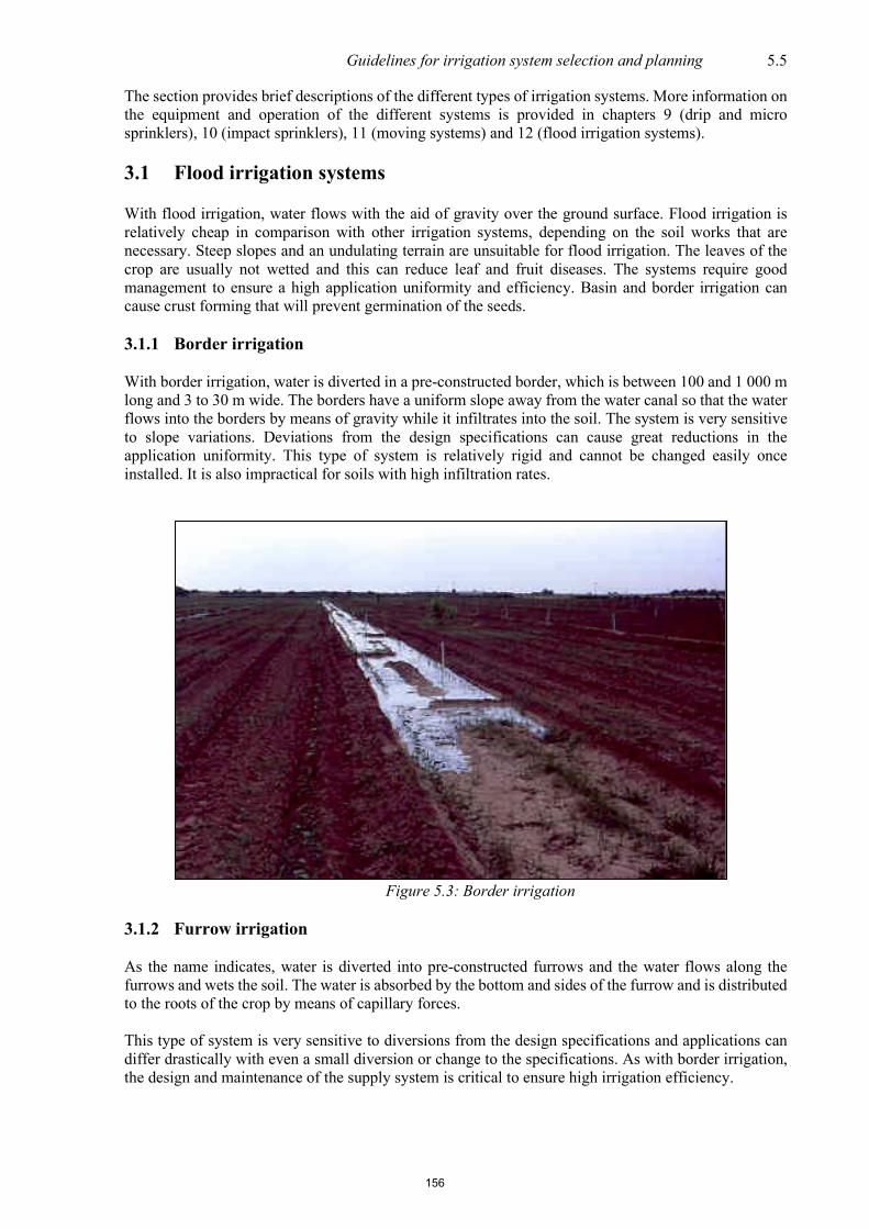
Guidelines for irrigation system selection and planning 5.5
The section provides brief descriptions of the different types of irrigation systems. More information on the equipment and operation of the different systems is provided in chapters 9 (drip and micro sprinklers), 10 (impact sprinklers), 11 (moving systems) and 12 (flood irrigation systems). 3.1 Flood irrigation systems
With flood irrigation, water flows with the aid of gravity over the ground surface. Flood irrigation is relatively cheap in comparison with other irrigation systems, depending on the soil works that are necessary. Steep slopes and an undulating terrain are unsuitable for flood irrigation. The leaves of the crop are usually not wetted and this can reduce leaf and fruit diseases. The systems require good management to ensure a high application uniformity and efficiency. Basin and border irrigation can cause crust forming that will prevent germination of the seeds.
3.1.1 Border irrigation
With border irrigation, water is diverted in a pre-constructed border, which is between 100 and 1 000 m long and 3 to 30 m wide. The borders have a uniform slope away from the water canal so that the water flows into the borders by means of gravity while it infiltrates into the soil. The system is very sensitive to slope variations. Deviations from the design specifications can cause great reductions in the application uniformity. This type of system is relatively rigid and cannot be changed easily once installed. It is also impractical for soils with high infiltration rates.
Figure 5.3: Border irrigation
3.1.2 Furrow irrigation
As the name indicates, water is diverted into pre-constructed furrows and the water flows along the furrows and wets the soil. The water is absorbed by the bottom and sides of the furrow and is distributed to the roots of the crop by means of capillary forces.
This type of system is very sensitive to diversions from the design specifications and applications can differ drastically with even a small diversion or change to the specifications. As with border irrigation, the design and maintenance of the supply system is critical to ensure high irrigation efficiency.
156

5.6 Irrigation User Manual
Figure 5.4: Furrow irrigation
3.1.3 Basin irrigation
Basin irrigation is the diversion of a certain amount of water into a pre-constructed basin with an even ground surface. The water is then cut off and the water in the basin is allowed to infiltrate the soil. The basins vary in size and are dependent on the available stream size, topography and soil factors. As an example, basins for planting grain are one hectare in size and basins for fruit trees are approximately 1 m². Basin irrigation is especially suitable for even soils with uniform texture or where a large stream relative to the basin size is available. Soils with a very high or very low infiltration rate can be irrigated. With larger basins, the cost of the type of system will depend especially on the amount of ground works to make the bottom even.
Figure 5.5: Basin irrigation
157

Guidelines for irrigation system selection and planning 5.7
3.1.4 Short-furrow irrigation
Short-furrow irrigation is a combination of basin and furrow irrigation and consists of short furrows with little or no longitudinal slopes, in which a certain amount of water is let in, in a relatively short time and the water is allowed to infiltrate the soil. The system is more labour-intensive than furrow irrigation and mechanical tilling is difficult after construction, but greater variation in application is possible than with other flood systems.
3.2 Moving systems
Moving systems are all systems that move while applying water to the field surface.
3.2.1 Centre pivot
A centre pivot consists of a metal frame and pipes, supported at approximately 50 m intervals by wheels with an A-frame and rotates around a fixed centre. Emitters are mounted on the pipes and wet the soil while the construction rotates around the centre. Because of the circled wetting pattern, there are always odd field lots that are never irrigated (corner systems reduce this problem). This type of system is relatively expensive; therefore, the aim must be to plant and irrigate two harvests per year under the system. The high application rate at the end of the centre pivot can result in run-off water. A centre pivot’s operation has the lowest labour requirement and also the least problems from a managerial point of view.
Figure 5.6: Centre pivot
3.2.2 Linear system
This system’s metal frame structure looks exactly the same as that of a centre pivot. The only difference between this system and the centre pivot is that the linear system moves laterally over the field and not in a circle. The system is kept on a straight path by means of a cable followed by guide sensors. A flexible drag hose connected to a hydrant usually provides the water supply. Various hydrants are spaced equally across the field. The initial cost is high, but labour requirements are low. This system is especially suited for rectangular fields.
158

5.8 Irrigation User Manual 3.2.3 Travelling gun
This system consists of a high-volume, high-pressure sprinkler mounted on a trolley with wheels and moves over the field by means of a cable or pipe drum method while it irrigates. Although this system has a low labour requirement, the energy requirement is high. The system is also wind sensitive and can have a high maintenance requirement. The travelling gun is very suitable for high-growing crops and also where fields are unevenly shaped.
Figure 5.7: Travelling gun
3.3 Static systems
All systems that stand still while irrigating are called static systems.
3.3.1 Sprinkler systems All systems that irrigate by means of sprinklers or sprayers under pressure above the ground and wet the soil this way are known as sprinkler systems.
159

Guidelines for irrigation system selection and planning 5.9
3.3.1.1 Permanent systems Permanent systems consist of laterals and emitters at fixed positions. Pipes and emitters therefore do not have to be moved at all during the lifetime of the system. The system has a low labour requirement, but the initial capital cost is high. The system is not as sensitive to wind as movable systems because the entire area is irrigated at once. Better control over water application is possible, especially where the system is fully automated. Crops are not exposed to mechanically damage by the moving of pipes and sprinklers but tilling of the fields is difficult because the permanent emitters protrude, above the soil.
Figure 5.8: Typical lay-out of a permanent system
3.3.1.2 Portable systems Portable systems are all systems that have to be moved from one position to another after each standing time to wet the entire surface. These systems have an initial low capital cost but are relatively labour intensive.
• Quick-coupling system
A quick coupling system consists of surface quick couple pipes of lightweight steel, aluminium, polyethylene or uPVC with sprinklers mounted on them. The pipes and sprinklers are set up at a certain position and the pump is switched on. The pump is switched off after a certain time and the pipes with sprinklers are moved to the next position. Crops, which are sensitive to mechanical damage such as tobacco, must rather not be irrigated by means of this system. Crop leaves are at risk to leaf diseases since the leaves are wetted. Irrigation time per day is reduced as a result of the time it takes to move the pipes. Good management is essential to ensure that equal and sufficient water is applied over the entire field. Energy requirements of these systems are higher than that of flood irrigation.
160

5.10 Irrigation User Manual
Figure 5.9: Typical layout of a quick coupling system
• Dragline system
With a dragline system sprinkler are connected to the laterals system by means of high quality hoses of rubber or plastic. The laterals therefore only have to be moved (if moveable) after 5 to 7 standing times and not after each standing time as with quick coupling systems. It is not necessary to switch off the pump when the sprinklers are moved.
Figure 5.10: Typical layout of a dragline system.
161

Guidelines for irrigation system selection and planning 5.11
• Hop-along system
This type of system has permanent laterals, as with the permanent system, but only the sprinklers are moved. Each sprinkler position has an automatic stop valve that closes off the water when the sprinkler is moved to the next position. Although the system is cheaper than a permanent system it is more labour intensive.
Figure 5.11: Typical layout of a hop-along system
• Big gun
This type of system is a very large sprinkler that works at high pressure to wet a relatively large area. The system is less labour intensive than other portable sprinkler systems. The high pressure and high flow rate result in a high-energy requirement. The large drops can also damage small plants and can promote crust-forming.
• Boom irrigator
The boom irrigator consists of a rotating boom of 20 to 100 m in length on which sprinklers are mounted. The boom is mounted on a central base-frame, which is either self-driven or can be pulled by a tractor. Labour requirement is therefore low. With the correct design, this system is able to give good application uniformity. High-pressure models are extremely sensitive to wind and have a high energy requirement. Special roads must be built to move this system.
162

5.12 Irrigation User Manual
Figure 5.12: Boom irrigator
• Side-roll system
The side-roll system consists of lengths of lateral pipes connected by means of a torsion coupling to form a moving axle for metal wheels of approximately 2 to 3 m in diameter. The wheels are usually 12 m apart and the full length of the system can be 400 m. Side-roll systems stand still during irrigation and water is obtained from hydrants. In the centre of the lateral pipe is an internal combustion engine mounted on a base-frame with four wheels. It drives the system from one standing position to another. On most of the systems, the sprinklers are mounted on balanced rollers so that the sprinklers always stand vertical. Because the lateral pipe is only 1,0 to 1,5 m above ground level, this type of system is not suitable for maize, sunflower or tobacco. Lush vegetation can become entangled in the wheels and makes moving difficult. Moving is extremely difficult against steep slopes and the system must preferable be anchored to protect it from wind damage.
Figure 5.13: Side-roll
163

Guidelines for irrigation system selection and planning 5.13
3.3.2 Micro-irrigation systems Micro-irrigation is the slow application of water on a regular basis on a limited portion of the surface of the field. Because of the great number of laterals required for micro-irrigation it is a relatively expensive system. This system can be fully computerised. Irrigation can take place 24 hours a day (no move is necessary). The system has a low labour and energy requirement, but initial capital costs are high.
3.3.2.1 Drip systems
Drip irrigation consists of polyethylene (PE) pipes fitted with drippers at fixed intervals. A dripper lets water out through a small opening at low pressure and a low flow rate. The pipes are laid parallel to each other over the field. Drippers spaced at fixed distances on the pipes spread the water over the field. The water that drips on the soil is distributed horizontally with the aid of capillary action and vertically by means of gravity. The system is therefore recommended for soils with a coarse structure. Almost no evaporation of water from the soil surface takes place and the water application is not influenced by the wind. Crops are not wetted and this reduces the occurrence of leaf and fruit diseases.
Soils with poor water distribution ability should be managed carefully when irrigated by this system. Root diseases occur more often if irrigation scheduling is insufficient. Drippers get blocked easily (physically, chemically and biologically) if effective filtration and maintenance is not present. Annual crops are difficult to irrigate by means of this system because the surface pipes have to be removed during harvesting. Subsurface drip irrigation is recommended in these cases. Subsurface drip irrigation is the application of water with a subsurface drip system near the plant’s root system. Thin-walled dripper pipe (0,1 to 0,5 mm wall thickness) is normally used for subsurface drip irrigation.
Figure 5.14: Drip irrigation
3.3.2.2 Micro-sprinkler systems Micro-sprinklers are small sprayers that distribute the water mainly on the soil below the crop. The sprayers are connected by means of short elastic or rigid pipes or directly on the polyethylene laterals and are provided with water this way. Micro-sprinklers are mostly used in greenhouses and orchards where the rows of trees are spaced wide apart.
Micro-sprinklers are used for strip wetting (this is where the entire soil surface is not wetted, but only those strips in the field where crops are present). The exception on the rule is in greenhouses where micro sprayers are used as an overhead system to wet the entire area. A variety of sprayers are available, depending on the distribution pattern required. A larger area of wetting is obtained than with drip irrigation and it is therefore suitable for a wider variety of soils, e.g. soils with a coarse texture. As with drip systems, filtration is also essential, but not in the same measure, because blockage does not occur as easily as with drippers. This type of system is influenced by wind, but not as much as sprinkler or moving systems.
164

5.14 Irrigation User Manual
Figure 5.15: Micro-sprinklers
4 Comparison between the various systems Tables 5.2 and 5.3 were drawn up arising from the above information to assist the producer in the choice between different systems. The following symbols are used in Table 5.2 to describe the factors that have an influence on the choice:
+ is an indication of a good reason for choosing a specific system
0 is an indication that the specific factor has no influence on the choice
- is an indication that the specific factor will negatively impact on the choice of the
system.
165

Guidelines for irrigation system selection and planning 5.15
Table 5.2: Comparison between different irrigation systems (adapted NEH 652, 1997)
Factor
Flood Sprinkler Moving Micro
Border / Basin Furrow Side-roll Drag-line /
Hop-along Big gun Permanent Centre pivot Linear Travelling
gun Drip Thin wall drip
Micro-jet
1 Crop
Standing crop + - + - 0 0 + + + - - -
Row crops 0 + + + + + + + + + + 0
Vegetables + - 0 0 0 0 0 0 0 - - -
Orchards, vineyards + + - + - + - - - + 0 +
Potatoes 0 + + 0 0 0 + + 0 + + 0
2 Land and soil
Low soil water
capacity - - - - - + + + - + + +
Low infiltration rate + + 0 0 - + 0 + 0 0 0 +
High salt content 0 0 - - - - - - - 0 0 0
Highly erodible - - 0 0 - + - 0 - + + +
166

5.16 Irrigation User’s Manual
Factor
Flood Sprinkler Moving Micro Border /
Basin Furrow Side-roll Dragline /
Hop-along Big gun Permanent Centre
pivot Linear Travelling
gun Drip Thin
wall drip
Micro-jet
Undulating terrain - - - + - + 0 - 0 + + + Fields with unusual
shape + + - + 0 + - - 0 + + +
3. Water supply
Low continuous flow
rate - + + - + + + + + + + +
High periodic flow rate + + - - - - - - - - - -
Delivery schedule
- Continuous - + + + + + + + + + + +
- Rotational 0 0 - - - - - - - - - -
4. Climate
Windy + + - - - - - - - + + 0 High temperature + + - - - 0 0 0 - + + + 5. Social /Institutional
Management inputs 0 + - - - + + + - + + + Automation potential 0 0 0 0 0 + + + 0 - + +
167

Guidelines for irrigation system selection and planning 5.17
The estimated costs, application efficiency and labour requirements of various irrigation systems are given in Table 5.3. Table 5.3 Summary of systems
Irrigation group Irrigation system
Estimated capital costs
[R/ha] (x 103) 2019
System efficiency
[%]
Life expectancy [years]
Labour requirements [ha/labour]
Annual maintenance
costs [% of capital
costs]
Flood
Furrow N/A* 86-95 10 15 5
Border N/A* 86-95 15 10 5
Basin N/A* 86-95 20 12 5
Static
Sprinkler
Permanent 25-27 90 15 50 1
Dragline 12-14 75 10 25 4
Quick-coupling 11-13 83 12 20 3
Hop-along (semi-permanent) 13-15 75 12 25 2
Big gun 10-12 75 10 20 4
Micro
Permanent drip 16-24 95 5-15 30 2
Seasonal drip 12-14 95 2 20 30**
Subsurface drip 21-26 98 10 25 3
Micro sprinkler 15-22 85 10 30 3
Micro sprayer 23-25 85 15 30 3
Mobile
Travelling gun 10-12 78 10 25 6
Travelling boom 11-13 75 12 30 6
Centre pivot 19-22 90 15 100+ 5
Linear move 16-19 90 15 100+ 6
Note: The estimated capital costs exclude the costs of the pump station, supply system, distribution system and installation of the equipment. Drip and micro system costs were calculated for vineyards, orchards and vegetables. Subsurface drip costs were calculated for lucerne and sugarcane. *N/A – costs not available at this stage **In the case of thin walled pipe installed above ground, the maintenance cost is estimated as 30% of
the capital cost.
168

5.18 Irrigation User’s Manual
The graph in Figure 5.16 shows the estimated energy requirements in kWh per mm gross irrigation requirement per hectare for various system efficiencies associated with the different irrigation systems. The energy costs (in R) can be calculated by multiplying this value by the electricity tariff. The graph was developed for a pump efficiency of 80% and a motor efficiency of 95%.
Figure 5.16: Energy requirements for different dynamic heads at varying levels of system efficiency 5 Automation In section 5 of chapter 9, automation in drip and micro-sprinkler irrigation systems is discussed. This section summarises the advantages and disadvantages of mechanical/hydraulic, electric/hydraulic and computerised systems with its requirements and design approach. Almost any irrigation system can be automated by incorporating either mechanical appliances, timers or sensors and computers in the operation of the system. With automation, manual intervention in the operation of the system is reduced or eliminated. Automation saves time and improves irrigation efficiency. This allows for other farming activities or tasks to also be prioritised and completed. However, automating an irrigation system can be quite expensive and complex, and requires skillful design, installation, management and maintenance. The designer should know from the planning phase whether the system will be automated, as it will have an effect on placement of valves and other control equipment, which will have cost implications. 6 The irrigation design It is of great concern that producers are still purchasing inefficient irrigation systems. These practices cannot be economically justified. In general, it is because the producer, as client, is not aware of what his/her role in the design of a system should be and is also not aware of the high level of professionalism he/she should expect and demand from the designer. The producer should have a basic understanding of the irrigation design process so that a proposed design can be evaluated as to whether it is offering the most appropriate solution from both a technical and financial perspective.
0,0
0,5
1,0
1,5
2,0
2,5
3,0
3,5
4,0
4,5
5,0
5,5
6,0
0 10 20 30 40 50 60 70 80 90 100
Ene
rgy
requ
irem
ent [
kWh/
mm
GIR
per
ha]
Total dynamic head [m]
60
65
70
75
80
85
90
95
100
Pump efficiency = 80% Motor efficiency = 95%
Application efficiency
169

Guidelines for irrigation system selection and planning 5.19
6.1 Information required for the planning of an irrigation system Irrigation planning is the first phase of the design process. Taking into account the crop type, the maximum expected climatic requirements during the crop’s growing season, the soil characteristics, the water quality, the type of irrigation system and the irrigator’s management requirements, the results of the planning process are: • the irrigation cycle length • the gross irrigation requirement for the cycle • the theoretical emitter discharge • the theoretical system capacity, and • the number of irrigation groups. Following the irrigation planning phase, the in-field components of the irrigation system must be designed, followed by the mainline and finally the pump and filter stations with control systems. The planning stage of project design therefore commences before anything else has been done. In this process the project should be evaluated in its entirety. A survey of all relevant inputs must be done at first contact, including (especially) managing aspects related to the final product. In the case of commercial irrigation farming, the producer approaches the designer with the problem: crops (often more than one) are to be planted (either simultaneously or as alternatives) on possibly arable soils and must be irrigated from an existing or a potential water source. The first step therefore is to conduct a survey of all factors which could affect the peak and seasonal water requirements of the crop(s), and whether the water source (taking all features into account) will be able to cope with all aspects of demand. At the same time, it is vital that the management requirements are evaluated so that a suitable system can be designed. It is also necessary at this stage to roughly determine the water balance before continuing with the design in detail. In the event of obvious problems, this step can eliminate a lot of unnecessary work. Even estimated data (areas, crop water requirement, water source discharge) can be utilised quite effectively for this purpose. If, however, there is any doubt at this stage, it will be necessary to proceed to compile all the physical details before making any decisions. The following five steps do not have to be executed in this particular order. Due to the interacting nature of the decision-making process execution can even take place simultaneously but it is essential to collect all the necessary information in order to design an appropriate and cost effective irrigation system: • Topographical survey: to accurately determine the area and elevations of the fields • Water source survey/Hydrological study: to determine the quality and quantity of water
available • Soil survey/analysis: to determine the type and characteristics of the soil to be irrigated • Climatic study: to determine the climatic requirements of the area • Crop study: to determine the irrigation requirements and therefore the system capacity • Management aspects: to determine the design limits (time available, automation requirements,
etc.) The following questions can be answered with the aid of multi-disciplinary cooperation, by contacting professionals to examine soil profiles, interpret soil and water analyses and to evaluate available resources to enable them to recommend a crop system combination for the specific soil and climate. For a professional design service, it is recommended that properly qualified irrigation designers, such as engineers, technicians or SABI approved designer are used.
170

5.20 Irrigation User’s Manual
Table 5.4: Information required for the planning of an irrigation system
Examine Questions to be answered Soil Is drainage necessary and how intensive?
Must the soil be trenched and how? What soil improvement agents and how much per hectare must be administered and to what depth? What is the easily available soil water capacity? What is the maximum application rate without exceeding the infiltration ability of the soil? Is additional water necessary for leaching to prevent brackishness and what percentage leaching must be applied?
Crop What type of rootstock (for perennial crops) and cultivars are suitable for the specific field? What is the recommended plant direction, spacing, sowing density and trellising system and irrigation system? What is the expected effective root depth of the crop? When do critical times occur when the crop is sensitive for soil water stress? What are the peak water requirements of the crop, when does it occur and what is the total water requirement per season? What is the spacing of plant rows and spacing of trees in the row for the design of manifolds and emitter positions?
Water Is the soil/water combination suitable for irrigation of the specific crops? How many hectares can be irrigated with the available water with the proposed system? What is the water quality? Is leaching of the soil a necessity? What is the expected delivery of the water source? Has permission for water use been obtained as prescribed in the National Water Act?
System Must frost combating or cooling be done with the aid of the irrigation system? What are the available number of days per week and hours per day in which irrigation can be done? What are the particulars of the available power source? What must the flow rate of the system be to fulfil the peak gross irrigation requirement? Must fertiliser, chlorine, etc. be applied through the system or not?
Climate What are the number of wind days per year, prevailing wind strength and direction? What are the long-term average rainfall, evaporation and temperature per month? Does frost and hail occur?
6.2 Evaluation of the design report It is disconcerting that many producers are not aware of the requirements which have to be met when an irrigation consultant makes a presentation for the design of an irrigation system. The idea is not that the producer should be an expert in the field of irrigation, but that he should ask the relevant questions to ensure that he is aware of the design specifications of the system which will enable him to install the irrigation system correctly. The design norms of the South African Irrigation Institute (SABI) can be accessed on the internet (at www.sabi.co.za). As these norms are regularly updated, they are not included in this manual. As background, some basic hydraulic principles are included in the manual as Appendix A. If a producer has the need to have a design evaluated theoretically, it is suggested that an independent irrigation designer be approached for the evaluation of the design according to the design norms for irrigation systems.
171

Guidelines for irrigation system selection and planning 5.21
6.2.1 Information that must be provided by the irrigation consultant to the producer The producer should insist that the following information is provided as a design report: • Final technical report
This report describes the resources that form part of the irrigation development as well as a short description of the operation of the irrigation system. Any assumptions made should be stated here.
• Layout plan This should comprise of the layout of the blocks and detailed plans of each block. Two copies
are required, one for installation purposes and one for the producer’s records. • Detailed drawings of equipment to make installation easier
Valve connections: Drawings of the valves with the desired accessories. Filter banks: Drawings of the complete filter installation with manifolds and valves. Pumps: Drawings of the pump with necessary equipment.
• Pump curve The producer can use a pump curve, on which the duty point is indicated, to easily read off the
efficiency and power requirement of the pump. The pump curve is also needed in case the existing irrigation scheme is expanded in the future.
• SABI peak design form
Technical design specifications of the design are needed. The producer can use this information to decide if the design satisfies the desired design specifications. Typical peak design forms for the various irrigation systems are given in Appendices B1-B3.
• List of quantities
A list of the items required for each block is needed so that quotations can be obtained from irrigation equipment suppliers. The list of quantities can also be used as a checklist for the equipment that is delivered by the irrigation equipment supplier.
• Cost estimation An estimate of the cost for the whole project must be made and for each phase, if applicable. • Maintenance and management manuals
A thorough manual is required to ensure that the performance of the installed irrigation system is not adversely affected by incorrect practices.
• An economic analysis
A capital versus running costs comparison as well as the expected maintenance costs over the lifespan of the system: in this way, the producer is informed of the expected benefits and costs of the irrigation system.
It is suggested that all this information is placed in a file to keep it for the future. The name of the producer, farm/section name and contact details of the designer can be displayed on the cover of the file. It is highly recommended that a design fee should be paid to consultants/designers who render a professional service for, or on behalf of, his client. There is no such thing as a “free design”, because eventually someone must be responsible for the cost and time that goes into the design, planning and specifications of each irrigation system. SABI, therefore, appeals to each intended buyer to negotiate a fee with the designer of his/her choice for the services that will be rendered. Remember that “buying cheap” can be detrimental in the long run. 6.2.2 Interpretation of the design report
172

5.22 Irrigation User’s Manual
It is important that the designer discusses the design with the producer to make him aware of the specifications that the proposed irrigation system design complies with. The questions that need to be answered will depend on the specific irrigation system and the answers will, in the most cases, be answered in the final technical report. The producer should ask the following general questions and answers should be contained in the design report: Table 5.5: Questions to be ask by the producers to the designers
Subject Question Where in the design report can the answer be found
Expertise level of designer What is the expertise level of the designer, eg. Is the designer an approved SABI designer, or a professional registered engineer/ technician?
Plan, Peak design form
General system information
What is the expected lifespan of the system? What safety factors are built into the system? Is expansion of the system possible? What additional equipment must be available on the farm for replacement of faulty equipment?
Technical report
Description of proposed irrigation system
What are the soil water characteristics of the soil to be irrigated? What type of irrigation systems are used for the irrigation of the different crops? What type of emitter is proposed and what is the recommended working pressure, spacing and delivery of the emitter? What is the capacity and quality of the water source available for the development? Is the water suitable for irrigation of the specific crop?
Technical report
Design parameters What design parameters are used? What is the velocity in the main line? What is the recommended working pressure at the block inlet? What are the design CU / DUlq /EU? Is the gross application rate of the system less than the infiltration rate of the soil?
Peak design form, technical report
Scheduling planning How much readily available water is in the root zone? What is the irrigation requirement of the different crops to be irrigated? What is the cycle length and standing/revolution time of the system? What is the system capacity (mm/day) and how does it compare with information obtained from the crop specialist?
Peak design form, technical report
173

Guidelines for irrigation system selection and planning 5.23
Subject Question Where in the design report can the answer be found
Equipment Is a pump curve provided on which the duty point is indicated? How long is the pumping time within the Eskom peak tariff time? What is the energy cost per year? Is filtration necessary and if so, what type is provided? Are injection pumps provided and if so, what is the capacity thereof? Is a flow meter provided and what are the requirements for its installation? Has provision been made for sufficient air inlet and outlet valves in the system? Is water hammer a problem and what can be done to prevent it?
Technical report
Guarantees What are the guarantees of the individual components of the system and what is included and excluded? What is the guarantee that the system will function according to the design parameters? What is the availability of the proposed irrigation equipment when faulty equipment has to be replaced? What is the easily available water in the effective root area? Who and how will it be determined whether the system complies with the design specifications – e.g. how can it be evaluated? What equipment should be kept as emergency equipment? Is a written agreement provided in which it is confirmed that the system conforms to the SABI norms and if not, where do deviations occur?
Technical report
If a complete evaluation of the design is required, an independent irrigation specialist can be approached who will have to determine if the design complies with the proposed design norms of SABI and if the system can function as described in the design report. 7 Installation and commissioning Much difficulty can be avoided if the parties agree beforehand about responsibilities regarding the following: • Arrangements regarding site clearing, e.g. bulldozers. • Pegging out of the system. • Civil works • Electrical installations and applications. • Provision of water, cement, sand and stone for thrust blocks • Supervision of the correct installation of equipment. • Installation of the equipment inside the pump house. • Who is responsible for equipment that fails?
174

5.24 Irrigation User’s Manual
• How often will the designer visit the site to ensure that equipment and installation comply with the requirements?
After installation, control tests and measures that should be done to check that the system is working according to the design. It is highly recommended that an appointment is made between the designer and producer to commission the system and agree in writing that the installation is complete and to the satisfaction of the customer. This will ensure that initial problems are detected early and sorted out. Checks and measurements that can be done include the following: • Read and keep record of specific electric current (Ampère) and pump pressure for each set-up. • Keep record of pressures at each block or control valve. • Keep record of the flow rate for each block, if available. • Keep record of the pressure differences over the clean filter bank, if applicable. • Check the inlet pressure at each block against the minimum pressure requirements as per the
design report.
This information can be used to periodically check the system’s performance by comparing measurements against the original values. If problems occur during the testing of the system, the producer and the designer need to come to an agreement on how the system must be improved to comply with the design specifications. The system may not function properly because of installation mistakes by the producer or design mistakes by the designer. If the producer made the mistake, he/she must carry the cost of the alterations and vice versa. Good project management practices will lead to fewer misunderstandings as well as an improvement of the irrigation industry and water use in South Africa.
175

Guidelines for irrigation system selection and planning 5.25
8 References 1. ASAE Standards. 1998. Design and installation of micro irrigation systems, ASAE EP405.1. 2. Burger, J. H., P.J. Heyns, E.P.J. Kleynhans, F.H. Koegelenberg, M.T. Lategan, D.J. Mulder,
H.S. Smal, C.M. Stimie, W.J. Uys, F.P.J. van der Merwe, I. van der Stoep and P.D. Viljoen. 2003. Irrigation Design Manual. ARC-Institute for Agricultural Engineering, RSA.
3. Burt, C.M. & Styles S.W. 1994. Drip and micro irrigation for Trees, Vines, and Row Crops. Irrigation Training and Research Centre (ITRC) USA.
4. Irrigation systems, a practical guide for producers. 1989. Eskom – Customer Service Department, RSA.
5. Keller, J. and R.D. Bliesner. 1990. Sprinkle and Trickle Irrigation. Utah State University, Logan, USA.
6. Koegelenberg, F.H. 2002. Norms for the design of irrigation systems. ARC-Institute for Agricultural Engineering. RSA.
7. Koegelenberg, F.H. and Breedt, H. 2002. Evaluation manual. ARC-Institute for Agricultural Engineering, RSA.
8. National Engineering Handbook (NEH), part 652. Chapter 5. 1997. USA. 9. Piaget, J. & I. Scheepers. 1987. Bladskrif: Riglyne vir boere by die aankoop van
besproeiingstelsels. Department of Agriculture, RSA. 10. Solomon, K.H. 1988. Irrigation Notes. Irrigation System Selection. California State University,
Fresno, California. USA.
176

5.26 Irrigation User’s Manual
APPENDIX A: TYPICAL PEAK DESIGN FORMS
APPENDIX A1: PEAK DESIGN FORM FOR PIVOTS 1. GENERAL INFORMATION 1.1 Owner 1.2 Address 1.3 Contact details 1.4 Designer 1.5 Designer contact details 1.6 SABI-member 2. CLIMATE 2.1 Month describe 2.2 Weather station describe 2.3 A-pan evaporation / Reference Evapotranspiration mm/month 3. IRRIGATOR’S MANAGERIAL REQUIREMENTS 3.1 Available working days per week days 3.2 Available irrigation hours per day hours 4. CROP 4.1 Type describe 4.2 Area ha 4.3 Plant density plants/ha 4.4 Plant distance m 4.5 Natural root depth m 4.6 Planting time date 5. SOIL 5.1 Effective soil depth m 5.2 Effective root depth m 5.3 Soil water capacity (10-100 kPa) mm/m 5.4 Readily available water in root zone mm 5.5 Infiltration rate mm/h 5.6 Soil gradient % 6. PIVOT 6.1 Make describe 6.2 Model/type describe 6.3 Circle sector degrees 6.4 Distance to last wheel m 6.5 Overhang length m 6.6 Endgun Yes/No Effective radius m 6.7 Centre pivot length m 6.8 Area ha 6.9 Motor speed m/min 6.10 Last wheel: wheel slippage % 6.11 Pressure control Yes/No Make describe Pressure kPa 6.12 Emitter package-CU
177
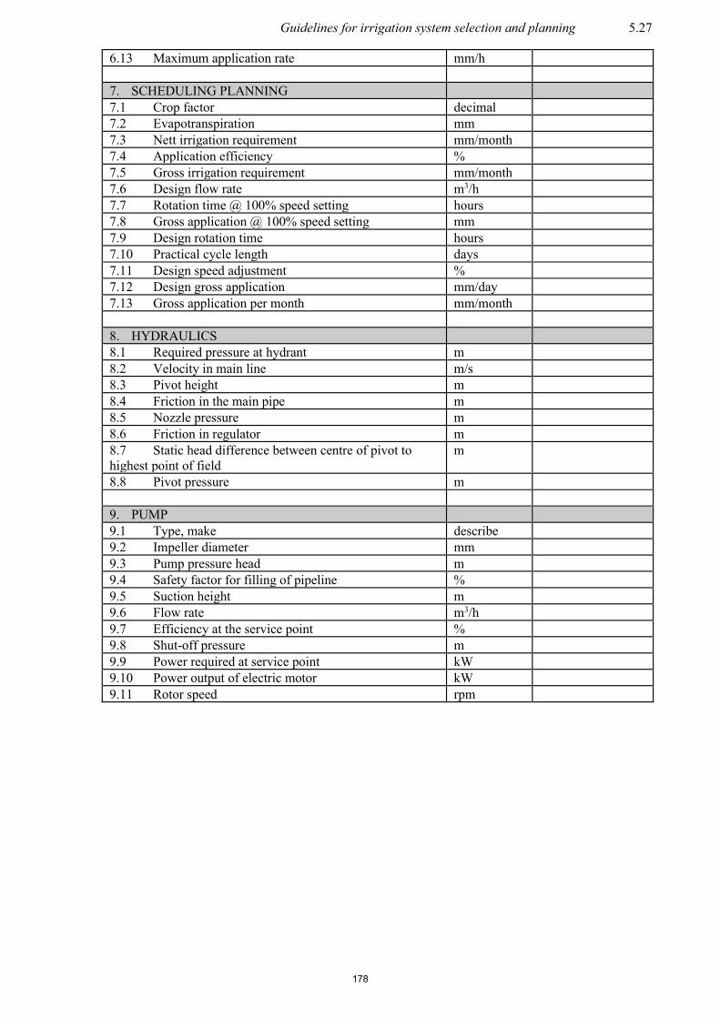
Guidelines for irrigation system selection and planning 5.27
6.13 Maximum application rate mm/h 7. SCHEDULING PLANNING 7.1 Crop factor decimal 7.2 Evapotranspiration mm 7.3 Nett irrigation requirement mm/month 7.4 Application efficiency % 7.5 Gross irrigation requirement mm/month 7.6 Design flow rate m3/h 7.7 Rotation time @ 100% speed setting hours 7.8 Gross application @ 100% speed setting mm 7.9 Design rotation time hours 7.10 Practical cycle length days 7.11 Design speed adjustment % 7.12 Design gross application mm/day 7.13 Gross application per month mm/month 8. HYDRAULICS 8.1 Required pressure at hydrant m 8.2 Velocity in main line m/s 8.3 Pivot height m 8.4 Friction in the main pipe m 8.5 Nozzle pressure m 8.6 Friction in regulator m 8.7 Static head difference between centre of pivot to highest point of field
m
8.8 Pivot pressure m 9. PUMP 9.1 Type, make describe 9.2 Impeller diameter mm 9.3 Pump pressure head m 9.4 Safety factor for filling of pipeline % 9.5 Suction height m 9.6 Flow rate m3/h 9.7 Efficiency at the service point % 9.8 Shut-off pressure m 9.9 Power required at service point kW 9.10 Power output of electric motor kW 9.11 Rotor speed rpm
178

5.28 Irrigation User’s Manual
APPENDIX A1.1: SCHEDULING PLANNING CALCULATIONS FOR PIVOTS Evapotranspiration (mm/month): = A-pan evaporation (mm/month) × crop factor Nett irrigation requirement (mm/month): = Evapotranspiration (mm/month) – effective rainfall (mm/month) Gross irrigation requirement (mm/month):
= al)cy (decimn efficienApplicatio
) (mm/monthquirementsgation reNett irri
Design flow rate (m3/h):
= decimal)ficiency (system efweekays per working dday ours per Working h
(mm/day)quirement gation renett irri70ion (ha) r irrigatArea unde××
××
Rotation time @ 100% speed setting (hour):
= )min/t wheel (meed of las travel sp 60
heel (m)st drive wntre to lace from cetandisπ2×
×
Gross application @ 100% speed setting:
= area (ha)10
ime (hour)rotation t/h)3w rate (mDesign flo×
×
Design speed setting (%):
= ime(hour)rotation tDesign
100 (hour) setting speed 100% @ timeRotation ×
179

Guidelines for irrigation system selection and planning 5.29
APPENDIX A2: PEAK DESIGN FORM FOR SPRINKLER IRRIGATION SYSTEMS 1. GENERAL INFORMATION 1.1 Owner 1.2 Address 1.3 Contact details 1.4 Designer 1.5 Designer contact details 1.6 SABI member 2. CLIMATE 2.1 Month describe 2.2 Weather station describe 2.3 A-pan evaporation mm/month 3. IRRIGATOR’S MANAGERIAL REQUIREMENTS 3.1 Available working days per week days 3.2 Available irrigation hours per day hours 4. CROP 4.1 Type describe 4.2 Area ha 4.3 Plant density plants/ha 4.4 Plant distance m 4.5 Row spacing m 4.6 Natural root depth m 4.7 Planting time date 5. SOIL 5.1 Effective soil depth m 5.2 Effective root depth m 5.3 Soil water capacity (10-100 kPa) mm/m 5.4 Readily available water in root zone mm 5.5 Infiltration rate mm/h 6. SPRINKLER 6.1 Type describe 6.2 Nozzle size mm 6.3 Discharge /h 6.4 Operating pressure m 6.5 Wetted diameter m 6.6 Christiansen’s uniformity coefficient(CU) % 6.7 Application efficiency % 6.8 Pressure control Yes/No 6.9 Pressure control operating range m water 6.10 Type of sprinkler system describe 6.11 Lateral spacing m 6.12 Sprinkler spacing m 6.13 Gross application rate mm/h 7. SCHEDULING PLANNING 7.1 Crop factor decimal 7.2 Evapotranspiration mm/month
180

5.30 Irrigation User’s Manual
7.3 Nett irrigation requirement mm/month 7.4 Gross irrigation requirement mm/month 7.5 Theoretical cycle length days 7.6 Theoretical standing time hours 7.7 Practical cycle length days 7.8 Practical standing time hours 7.9 Working days per week days 7.10 Irrigation hours per day hours 7.11 Practical system moving time per day hours 7.12 Gross application per practical cycle mm 7.13 Gross application per month mm/month 7.14 Sprinklers/set-up number 7.15 Area/set-up ha 7.16 Flow rate/set-up m3/h 8. SCHEDULE OF BLOCKS IRRIGATED
SIMULTANEOUSLY
9. HYDRAULICS 9.1 Allowable pressure difference over lateral/dragline m water 9.2 Required pressure at valve/hydrant m water 9.3 Velocity in mainline m/s 10. PUMPS 10.1 Type/make describe 10.2 Impeller diameter mm 10.3 Pump pressure head m water 10.4 Suction height m water 10.5 Flow rate m3/h 10.6 Efficiency at the service point % 10.7 Shut-off pressure m water 10.8 Power required at service point kW 10.9 Power output of electric motor kW 10.10 Rotor speed rpm
181

Guidelines for irrigation system selection and planning 5.31
APPENDIX A2.1: SCHEDULING PLANNING CALCULATION OF SPRINKLER IRRIGATION SYSTEMS
Evapotranspiration (mm/month): = A-pan evaporation (mm/month) × crop factor Effective rainfall (mm/month): =
2mm 20 - (mm) rainfallmonthly Average
Nett irrigation requirement (mm/month): = Evapotranspiration (mm/month) – effective rainfall (mm/month) Gross irrigation requirement (mm/month):
= (decimal) efficiencyn Applicatio(mm/month)t requiremen irrigationNett
Readily available water (mm): Soil water capacity of relevant soil sample (mm/m) × effective root depth of crop (m) Gross application rate of selected nozzle (mm/h)
= (m)emitter of width strip wetted(m) spacingEmitter
/h)( dischargeEmitter ×
If the wetted strip width > lateral spacing, replace wetted strip width with lateral spacing in the above formula Theoretical cycle length (days)
= spacing(m) Lateral
width(m)strip Wetted(mm/day)t requiremen irrigationNett
water(mm)availableReadily ×
If wetted strip width > lateral spacing, accept:
1spacing Lateral
widthstrip Wetted=
Theoretical standing time:
l)cy (deciman efficienapplicatiote (mm/h)ication raGross applter(mm) ilable waadily avaRe
×
For a practical scheduling technique, the cycle length/standing time can be kept constant, while the other parameter is adjusted accordingly.
182

5.32 Irrigation User’s Manual
Gross application per practical cycle (mm): = Gross application rate on total area (mm/h) × practical standing time (hours) Gross application per month (mm):
= (days)length cycle Practical
month in dayscycle(mm) practicalper n applicatio Gross ×
Sprinklers/set-up:
= m)(m spacing zzle Sprayer/nocyclein days workingdayper ups-Set
000 10(ha) irrigationunder Area×××
×
Area/ set-up (ha) =
000 10 m)(m spacing nozzleup-setper Sprinklers ××
Flow/set-up (/h) =
1000up per set-sprinklers/h)e (argdischSprinkler ×
183

Guidelines for irrigation system selection and planning 5.33
APPENDIX A3.: PEAK DESIGN FORM FOR MICRO IRRIGATION SYSTEMS 1. GENERAL INFORMATION 1.1 Owner 1.2 Address 1.3 Contact details 1.4 Designer 1.5 Designer contact details 1.6 SABI member 2. CLIMATE 2.1 Month describe 2.2 Weather station describe 2.3 A-pan evaporation mm/month 3. IRRIGATOR’S MANAGERIAL
REQUIREMENTS
3.1 Available working days per week days 3.2 Available irrigation hours per day hours 4. CROP 4.1 Type describe 4.2 Area ha 4.3 Plant density plants/ha 4.4 Plant distance m 4.5 Row spacing m 4.6 Natural root depth m 4.7 Planting time date 5. SOIL 5.1 Effective soil depth m 5.2 Effective root depth m 5.3 Soil water capacity (10-100 kPa) mm/m 5.4 Readily available water in root zone mm 6. EMITTER 6.1 Type describe 6.2 Nozzle size mm 6.3 Discharge /h 6.4 Operating pressure kPa 6.5 Application efficiency % 6.6 Emitter spacing m 6.7 Lateral spacing m 6.8 Wetted diameter m 6.9 Gross application rate on the wetted area mm/h 6.10 Flow rate of block m3/h
184

5.34 Irrigation User’s Manual
7. SCHEDULING PLANNING 7.1 Crop factor decimal 7.2 Evapotranspiration mm/month 7.3 Nett irrigation requirement mm /month 7.4 Gross irrigation requirement mm/month 7.5 Theoretical cycle length days 7.6 Theoretical standing time hours 7.7 Practical cycle length days 7.8 Practical standing time hours 7.9 Working days per week days 7.10 Irrigation hours per day hours 7.11 Gross application per practical cycle mm 7.12 Gross application per month mm/month 8. SCHEDULE FOR BLOCKS IRRIGATED
SIMULTANEOUSLY
9. HYDRAULICS 9.1 Emission uniformity (EU) % 9.2 Allowable pressure difference over lateral m water 9.3 Required pressure at valve m water 9.4 Velocity in mainline m/s 10. PUMP 10.1 Type, make describe 10.2 Impeller diameter mm 10.3 Pump pressure head m water 10.4 Suction height m water 10.5 Flow rate m3/h 10.6 Efficiency at the service point % 10.7 Shut-off pressure m water 10.8 Power required at service point kW 10.9 Power output of electric motor kW 10.10 Rotor speed rpm 11. FILTER 11.1 Make, type, size describe 11.2 Number number 11.3 Filter fineness micron 11.4 Pressure drop over filter bank Clean m water Dirty m water
185

Guidelines for irrigation system selection and planning 5.35
APPENDIX A3.1: SCHEDULING PLANNING CALCULATION FOR MICRO IRRIGATION SYSTEMS
Evapotranspiration (mm/month): = A-pan evaporation (mm/month) × crop factor Effective rainfall (mm/month): =
2 mm 20 - rainfallmonthly Average
Nett irrigation requirement (mm/month): = Evapotranspiration (mm/month) – effective rainfall (mm/month) Gross irrigation requirement (mm/month):
= (decimal) efficiencyn Applicatio
(mm/month)t requiremen irrigationNett
Readily available water (mm): Soil water capacity of relevant soil sample (mm/m) × effective root depth of crop (m) Gross application rate of selected sprinkler (mm/h):
(m)emitter of width strip wetted (m) spacingEmitter /h)(delivery Emitter
×
If the wetted strip width > lateral spacing, replace wetted strip width with lateral spacing in the above formula Theoretical cycle length (days):
= spacing(m) Lateral
width(m)strip Wetted(mm/day)t requiremen irrigationNett
) water(mmavailableReadily ×
If wetted strip width > lateral spacing, accept:
1spacing Lateral
widthstrip Wetted=
Theoretical standing time:
(decimal) efficiencyn applicatio(mm/h) raten applicatio Gross ) water(mmavailableReadily
×
For a practical scheduling technique, the cycle length/standing time can be kept constant, while the other parameter is adjusted accordingly.
186

5.36 Irrigation User’s Manual
Gross application per practical cycle (mm): = Gross application rate on total area (mm/h) × practical standing time (hours) Gross application per month (mm):
= (days)length cycle Practical
month in dayscycle(mm) practicalper n applicatio Gross ×
187

IRRIGATION USER MANUAL
CHAPTER 6
Overview of irrigation engineering principles
188

Overview of irrigation engineering principles 6.1
Table of Contents 1 Introduction ................................................................................................................................... 6.1 2 Measurement units ......................................................................................................................... 6.1 3 Terminology .................................................................................................................................. 6.1 4 Hydrostatics ................................................................................................................................... 6.1 5 Hydrodynamics .............................................................................................................................. 6.2 6 Pressure classes.............................................................................................................................. 6.3 7 Flow rate and velocity ................................................................................................................... 6.3 8 Discharge – pressure relationship of emitters ................................................................................ 6.4 9 Application rates ............................................................................................................................ 6.7
9.1 Pressurised irrigation systems .............................................................................................. 6.7 9.2 Surface (flood) irrigation systems ........................................................................................ 6.7
10 Application efficiency ................................................................................................................... 6.8 11 Distribution uniformity ................................................................................................................ 6.10 12 References ..................................................................................................................................... 6.9
All rights reserved Copyright 2019 ARC-Agricultural Engineering (ARC-AE)
189

6.0 Irrigation User Manual 1 Introduction The implementation of any irrigation system requires the irrigation practitioner to have a basic understanding of the hydraulic principles of irrigation design, and a sound knowledge of irrigation equipment that is commercially available. As background, a few basic concepts are briefly discussed here. 2 Measurement units It is important to take note of the correct measurement units for the various parameters referred to in hydraulics, as shown in Table 6.1. Table 6.1 Basic measurement units
Dimension SI unit
Unit Symbol Expression in other SI units, and definition of unit
Length Mass Time Area
meter kilogram second square meters
m kg s
m²
–
Volume cubic meters m³ –
Density kilograms per cubic meter kg/m³ –
Velocity meters per second m/s –
Acceleration meters per second squared m/s² –
Force Newton N kg.m/s²
Energy Joule J N.m
Power Watt W J/s Pressure Pascal Pa N/m²
3 Terminology Different terms are used to describe the components of an irrigation system. Emitters is a collective word for any type of irrigation fitting such as sprinklers, drippers or micro-sprinklers, that apply water onto the plant or growing medium (soil), and are mounted on connecting pipes, usually called laterals, while the laterals are connected to each other with pipes called manifolds, in the case of micro and drip irrigation, or directly to the mainline in the case of sprinkler systems. The mainline will be the pipe conveys the water from the source to the irrigation system. 4 Hydrostatics Water pressure is the force (p or H) exerted by water [kPa or m] per unit of area restricting it, relative to air pressure. This pressure is described as force per unit area.
190

Overview of irrigation engineering principles 6.1
Hydraulic gradient / Energy line
x m
etre
s sta
tic p
ress
ure
A B 100 km
Therefore, the container size (an ocean or a pipe) is irrelevant – the water column (90 m high) determines the amount and therefore the mass of water supported by a unit of area.
Figure 6.1: Water pressure When a column of water is at rest (i.e. static), it makes no difference if it is vertical to a height of "x" metres, or if it gradually descends over a distance of say 100 kilometres – the total static pressure measured at the bottom of each of these columns of water will still be "x" metres height, or 10 × "x" kPa (Figure 6.3).
Figure 6.2: Static pressure Different measurement units are used for pressure: 1 Bar = ±10m height = ±100 kPa. We can therefore say that 6 Bar = 60 meter = 600 kPa. 5 Hydrodynamics Hydrodynamics is the study of moving liquids. When the sum of forces exerted on liquid produced a resultant vector that is not equal to 0 (zero), movement of the fluid will begin in the direction of the unbalanced force. When a liquid move through any conduit like a pipe or canal, friction occurs between the liquid and the wall of the conduit, in other words, irrespective of the lightness of the substance and the smoothness of the conduit, liquid molecules cling (adhesion) to the tube walls. Therefore, friction is one of the factors restricting movement of a liquid through a pipeline, and can be calculated with friction equations or read from friction tables or graphs.
p p
90m or 900kPa 90m or 900kPa
90 m
eter
s wat
er d
epth
191

6.2 Irrigation User Manual Different types of flow can occur inside a conduit, depending on amongst others the velocity of the water. In irrigation, it is important that we distinguish between laminar and turbulent flow. Laminar flow is normally described as viscous or stream line flow. With this flow type, different layers of liquid move relative to each other without any macroscopic intermixing. Therefore laminar flow systems are generally graphically represented by stream lines. No liquid flow occurs across these lines and friction loss is directly proportional to flow velocity. With turbulent flow, an uneven indeterminate movement of liquid against the main flow direction takes place. This is the type of flow that mostly occurs in irrigation pipes, and friction loss is exponentially proportional to flow velocity.
Laminar flow Turbulent flow
Figure 6.3: Different flow conditions Friction losses can also occur due to inevitable equipment on the pipeline such as bends, reducers and valves and not only due to the straight pipe sections. In practice these losses make up such small percentage of the total friction and are nominally allowed for as an estimated percentage of the pipe losses which is then added to the total pressure requirement of the system.
Figure 6.4: Secondary friction losses
6 Pressure classes When specifying pipes and other hydraulic fittings or equipment, it is not only the size (diameter) of the part that is important but also the pressure that it will be able to withstand. The pressure class or rating of a pipe or fitting indicates the amount of pressure it can handle under continuous load. For example, in the case of plastic pipes, a Class 6 pipe can handle 6 bar of pressure. Air trapped in pipes and poor operational conditions (such as electrical supply interruptions or high water velocities in pipes) can cause water hammer to occur, which add additional stress to the pipe wall and fittings and this will reduce the life expectancy of the item. Both static and dynamic pressures can be measured accurately by means of manometers or piezometers, but due to the clumsiness of these instruments, use is normally made of pressure gauges which indicate pressure directly on a calibrated dial. 7 Flow rate and velocity The flow rate (Q) in a pipe is the product of the average velocity (v) and the cross-sectional area (A) of the water flowing in the pipe:
192

Overview of irrigation engineering principles 6.3
Figure 6.5: Flow rate components Q = A x v Equation 6.1 Where Q = flow rate (m3 per second) A = cross sectional area of the water (m2) v = average velocity (meter per second) A more commonly used unit is cubic meters per hour (m3/h) = m3/s x 3600 or litres per hour (l/h) = m3/h x 1000 8 Discharge – pressure relationship of emitters Pressurised irrigation systems include all systems where water is supplied in pipelines under pressure to the emitters, to apply water on or below the soil surface in the root zone, such as centre pivot, sprinkler, micro-sprinkler and drip irrigation systems. Emitters are mounted on connecting pipes, usually called laterals, while the laterals are connected to each other with pipes called manifolds, in the case of micro and drip irrigation, or directly to the mainline in the case of sprinkler systems. The purpose of the emitter is to apply water at a specific rate (as determined during the planning process and called the design emitter discharge, qe) over a specific area of soil in the field. The characteristics of emitters are such that the emitter discharge is determined by the pressure of the water at the emitter – the design discharge will be delivered at a specific pressure called the design operating pressure. At pressures higher than the design operating pressure, the emitter will discharge more than the design discharge, and at pressures lower than the design operating pressure, the emitter will discharge less than the design discharge. The discharge-pressure relationship is characterised by the equation: qe = K x px Equation 6.2 where K = discharge coefficient , include qe and units p = operating pressure x = discharge exponent This relationship is presented graphically below:
A v
Q
193

6.4 Irrigation User Manual
Figure 6.6: Example of emitter discharge – operating pressure relationship of emitters
The discharge coefficient and exponent is unique for every emitter and is provided by the manufacturers of irrigation emitters. In order to design an irrigation system that applies water at an acceptable uniformity across the whole field, the irrigation designer should ensure that all the emitters are operating at approximately the same pressure. This can be achieved either by accurate sizing of the lateral and manifold pipe sizes according to hydraulic principles, by using appropriate pressure regulating valves, or by using pressure compensated emitters, which contain a regulating mechanism, (often a diaphragm), that will ensure the emitter will discharge water at a specific rate as long as the pressure in the lateral is within a specified range. In the case of the hydraulic design approach, the allowable emitter discharge variation is calculated, and the allowable operating pressure variation determined accordingly (Figure 6.8). The lateral and manifold pipe sizes are then selected to ensure that the pressure will always be within the upper and lower limits (see figure below). Correct lay-out (orientation) of laterals and manifolds / mainlines contribute greatly to the uniformity that can be achieved within the in-field irrigation system, and also on the pipe sizes (and classes) that have to be used to achieve this uniformity. Conservative design approaches require that the emitter discharge variation should not exceed 10%. If the emitter has a discharge exponent (x) of 0.5, discharge variation will be less than 10% if the pressure variation is less than 20%.
194

Overview of irrigation engineering principles 6.5
Figure 6.7: Emitter pressure and discharge variations
In the case of pressure compensated emitters, or when regulating devices such as flow controllers are used, the regulating mechanism has an effect on the discharge–pressure relationship of the emitter, so that the discharge will remain constant over a specified pressure range (see figure below). Pressure-compensated emitters are available for all types of pressurised systems but are more expensive than non-compensating emitters.
Figure 6.8: Example – Pressure compensating emitter performance graph
195

6.6 Irrigation User Manual 9 Application rates Some basic calculation of application rates and conversions are shown here. 9.1 Pressurised irrigation systems In agricultural irrigation, the desired amount of water (measured in mm, similar to rainfall) should be applied to soil at a rate (measured in mm per hour) which does not exceed the soil’s infiltration rate (also measured in mm per hour) for the length of the irrigation event (the soil’s infiltration rate is not a fixed value – it decreases as the soil gets wetter during an irrigation event). The application rate of an irrigation system depends on the flow rate or discharge of the emitter (in litre per hour) and the spacing of the emitters in the field: Application rate (mm/h) = discharge (ℓ/h)
(emitter spacing in the row × lateral spacing) Equation 6.3
For example: 40 l/h / (2m x 5m) = 4 mm/h Remember the following rule: 1 mm/h = 1 litre/m2/h and 1 ha = 10 000 m2 Therefore 1 mm/h = 10 000 litre/h/ha = 10 m3/h/ha For example: 4 mm/h = 40 m3/h/ha Thus if the block size is known (for example, 0.6 ha): 0.6 ha x 40 m3/h/ha = 24 m3/h flow rate for a 0.6ha block Furthermore: 1 litre of water spread over 1 m2 = 1 mm depth on 1 m2 Because 1 ha = 10 000 m2: 10 000 litre = 1 mm / 10 000 m2 and therefore 10 m3 / ha = 1 mm / ha If the water requirement is 6 mm/day Use 60 m3 water / day / ha For a block size of 0.6 ha: Volume of water required per block = 0.6 ha x 60 m3 /h = 36 m3 Time required to apply this volume = 36 m3 ÷ 24 m3/h= 1h 30 min /day or Time required to apply this volume = 6mm per day ÷ 4mm per hour = 1.5 hours 9.2 Surface (flood) irrigation systems Flood irrigation makes out more than 70% of all irrigation methods used worldwide. The efficiency of a flood irrigation system is generally lower than pressurised systems but with better layout and design choices, improved soil preparation, less water conveyance losses and more effective management systems, efficiency can be enhanced. The design and management of flood irrigation systems are more complex than for other systems because additional factors, such as soil irregularities and gradients, play a determining role with flood irrigation.
196

Overview of irrigation engineering principles 6.7
With flood irrigation systems, applications are determined by the amount of time the soil surface is covered by the water flowing in the furrow, border or basin. If the flow rate and slope of the field is correct for the type of soil, a uniform application can be given. The contact time or “opportunity time” is determined from the passing of the advance and recession fronts of the water flowing over the surface. 10 Application efficiency Engineering efficiency is defined as the ratio of benefits derived (output) relative to input. Efficiency is therefore an indicator of losses within a specified boundary in a system (see figure below). High efficiency implies that the output is relatively similar to the input and the losses are low. Low efficiency implies higher losses.
Figure 6.9: Definition of efficiency
When considering the performance of irrigation systems, it is helpful to think in terms of the components of the water balance, or the destinations of applied water. Ideally, the bulk of the applied water should contribute to the objective of irrigating: i.e. to preventing undesirable crop water stress. This relates to keeping stomata open, so that photosynthesis is not inhibited. The figure below illustrates the various fractions of water applied which are involved in defining irrigation performance at the field level. The various components of the water balance (destinations of applied water) are: • Deep percolation • Surface runoff/stormflow • Evaporation from the exposed soil surface • Spray evaporation, wind drift and plant interception • Transpiration A well planned and designed irrigation system will ensure that water lost to these components listed above are minimised, thereby ensuring the lowest possible demand from the water source. Some loss of water, however, cannot be avoided and is an inherent characteristic of the irrigation system. The performance of an irrigation system in this regard is defined by means of its system efficiency – the ratio between the amount of water contributing to the objective of irrigation (the net irrigation requirement, NIR), and the amount of water entering the irrigation system (the gross irrigation requirement, GIR). Therefore: System efficiency(%)= NIR
GIR × 100 Equation 6.4
The difference between the NIR and GIR usually consist of various amounts of the following unavoidable losses that can occur in-field: • Non-beneficial spray evaporation and wind drift losses, • In-field conveyance losses,
197

6.8 Irrigation User Manual • Filter backwash and other minor losses
Figure 6.10: Components of the water balance
For example, overhead sprinkler systems lose water through wind drift and evaporation of spray. Drip systems lose water through filter backwashing, and flood irrigation systems with earth canals lose water through seepage. Other minor losses may also occur. The system efficiency figures published in the table below, therefore, are associated with the generally acceptable level of losses which are inherent and unavoidable for each irrigation system. These efficiency figures are used to convert net irrigation requirements (NIR) to gross irrigation requirements (GIR) during the design process. Table 6.2: System efficiency values
Irrigation system
Losses Default system
efficiency (net to gross
ratio) (%)
Non-beneficial
spray evap. and wind
drift losses (%)
In-field conveyance losses (%)
Filter and
minor losses (%)
Total Losses
(%)
Drip (surface and subsurface) 0 0 5 5 95 Micro sprinklers 10 0 5 15 85 Centre Pivot, Linear move 8 0 2 10 90 Centre Pivot LEPA 0 0 5 5 95 Flood: Piped supply 0 0 5 5 95 Flood: Lined canal supplied 0 5 2 7 93 Flood: Earth canal supplied 0 12 2 14 86 Sprinkler permanent 8 0 2 10 90 Sprinkler movable 10 5 2 17 83 Traveling gun 15 5 2 22 78
198

Overview of irrigation engineering principles 6.9
11 Distribution uniformity Irrigation uniformity refers to how evenly water is applied across the field. Non-uniform irrigation implies that some parts of the field are receiving too little water while other parts may be receiving too much. Distribution uniformity is a requirement for irrigation efficiency – irrigation cannot be non-uniform and efficient, as over or under irrigation will always occur somewhere in the field. Ideally irrigation must be both uniform and efficient. Poor system performance can be caused by poor design or system hardware operation and maintenance. During the design process, the irrigation designer must select an emitter that will apply water at a minimum, system specific uniformity. In the case of sprinkler and centre pivot systems, this minimum requirement is given in terms of the uniformity coefficient (CU) value, and in the case of micro irrigation (drippers and micro sprinklers), it is given in terms of the emission uniformity (EU) value. Table 6.3: Irrigation system uniformity indicators
Type of system Uniformity indicator Minimum value Impact sprinklers
84%
Centre pivots
95%
Micro irrigation (micro sprinklers and drippers)
90%
Where The CV is the manufacturer’s coefficient of variation and indicates the variability in the flow rate of a random sample of a given emitter model, just off the production line before any field operation or degradation has taken place. It is therefore an indicator of manufacturing quality, as we would ideally like all emitters to be identically manufactured. The CV is defined as the standard deviation divided by the average flow rate of a sample of emitters, and can be expressed as a fraction (or in some cases as a percentage – 0.1 = 10%). A CV of 0.1 indicates a normal distribution of sampled flow rates with 68% of the flow rates falling within 10% of the mean flow rate. An emitter’s CV should ideally be less than 0.05 but less than 0.1 is acceptable for applications where the wetting patterns overlap. 12 References
1. Koegelenberg, F.H. and Breedt, H. 2002. Evaluation manual. ARC-Institute for Agricultural Engineering, RSA.
Σ×=
nx
xxCU
i --1100
−×=
ii
giiH yR
yyRCU
∑
-∑1100
×
××
e
CV1,27 - 1,0 100 = EUav e
min e
=
xSDCV
199

IRRIGATION USER MANUAL
CHAPTER 7
Irrigation Scheduling
200

Table of Contents
1 Introduction ................................................................................................................................................................................................................................................. 7.1 2 Crop water requirement ................................................................................................................................................................................................................ 7.2 3 Water availability in the Soil .................................................................................................................................................................................................. 7.2 4 Irrigation system .................................................................................................................................................................................................................................... 7.7 4.1 Cycle length ..................................................................................................................................................................................................................................... 7.7 4.2 Gross irrigation requirements per cycle ........................................................................................................................................................... 7.8 4.3 Operating hours per cycle ................................................................................................................................................................................................. 7.9 4.4 Number of groups ...................................................................................................................................................................................................................7.10 4.5 Gross application rate .........................................................................................................................................................................................................7.10 4.6 Standing time............................................................................................................................................................................................................................... 7.10
5 Scheduling strategies .....................................................................................................................................................................................................................7.12
5.1 Fixed depletion level ........................................................................................................................................................................................................7.12 5.2 Fixed irrigation interval ................................................................................................................................................................................................7.12 5.3 Fixed irrigation amount ................................................................................................................................................................................................7.13 5.4 How much to irrigate .......................................................................................................................................................................................................7.14
5.4.1 Irrigate to field capacity ...........................................................................................................................................................................7.14 5.4.2 Apply a leaching fraction .......................................................................................................................................................................7.15 5.4.3 Apply a deficit irrigation strategy .................................................................................................................................................7.16 6 Scheduling techniques .................................................................................................................................................................................................................7.17
6.1 Feel method ................................................................................................................................................................................................................................7.18 6.2 Gravimetrical soil water determination ......................................................................................................................................................7.19 6.3 Determining of the soil’s electric resistance.........................................................................................................................................7.19 6.4 Neutron water meter .........................................................................................................................................................................................................7.21 6.5 Tensiometry ................................................................................................................................................................................................................................7.23 6.6 Pulse delay measuring (Time domain reflectometry, TDR) ..............................................................................................7.26 6.7 Frequency delay measuring .....................................................................................................................................................................................7.28 6.8 Continuous logging capacitance probes ...................................................................................................................................................7.31 6.9 Heat pulse measuring ......................................................................................................................................................................................................7.34 6.10 Chameleon water sensor ............................................................................................................................................................................................7.34 6.11 Fullstop Wetting front detectors .......................................................................................................................................................................7.38 6.12 Scheduling with regard to crop evapotranspiration (ETc) and a water balance sheet .........................7.39
7 Scheduling models ...........................................................................................................................................................................................................................7.40
7.1 BEWAB .............................................................................................................................................................................................................................................7.40 7.2 SWB ........................................................................................................................................................................................................................................................7.40 7.3 VINET 1.1 .......................................................................................................................................................................................................................................7.41 7.4 Canesim ..............................................................................................................................................................................................................................................7.41 7.5 SAPWAT4 ......................................................................................................................................................................................................................................7.41 7.6 Remote sensing ..........................................................................................................................................................................................................................7.42
8 Scheduling calculation ................................................................................................................................................................................................................7.45 9 References .................................................................................................................................................................................................................................................7.49
All rights reserved
Copyright 2019 ARC-Agricultural Engineering (ARC-AE)
201

202

Irrigation scheduling 7.1
1 Introduction The main purpose of irrigation is to supplement the soil water reserve for optimal crop production in regions where rainfall is insufficient. However, to apply irrigation efficiently, it is essential to understand the water requirements of the crop and then apply the correct volume of water in the correct place and at the correct time. This organised way in which water is supplemented, is called irrigation scheduling. Stevens and Buys (2005) describes irrigation scheduling as the compilation of an irrigation program according to crop, soil and climatic factors, and the continuous adjustment according to daily or seasonal changes. The main aim of irrigation scheduling is to minimise wasteful losses of water (deep percolation beyond what is necessary for salt leaching, surface runoff and evaporation) and to maximise transpiration. Transpiration is the beneficial loss of water due to its direct link with dry matter production (Annandale et al., 2011, Stevens and Buys, 2005). In order to schedule correctly, water must be available on demand at all times. If water is only available to a producer, e.g. every four weeks, and there is no storage dam, the producer cannot schedule correctly. A distinction must also be made between intensive irrigation and supplementary irrigation. In the latter case, the soil water supply is only supplemented during occasional drought periods in humid climates, or the crop is only supplied with water during critical growth stages. Strictly spoken, scheduling does not apply in supplementary irrigation. The same amount of water used for irrigation at all times with the same cycle length, is also seen as an incorrect concept of scheduling according to the above definition. The water is applied regularly, but obviously the wrong amounts of water at incorrect times. If irrigation scheduling is applied incorrectly, it can lead to over- or under-irrigation. Under-irrigation mainly restrains the size and quality of the harvest, while over-irrigation can lead to the misuse of water and electricity resources, leaching of expensive fertilisers, pollution of water sources, erosion of top soil and potential yield reductions from anaerobic soil conditions damage the root system that can cause the crop to die. Although plant roots do not grow in dry soil, it remains healthy and undamaged (within limits) until sufficient water is available again. On the other hand, over-irrigation reduces the air content of the soil, which promotes the contamination by anaerobic pathogens, such as Phytophthora. Even in the absence of the pathogens, a low oxygen level in the soil can damage the roots. It is therefore important that the basic principles of irrigation scheduling should always be practiced. Various factors influence the amount of water applied, i.e. the standing time: • The effective root depth of the crop and the critical periods during the growing season of the crop
when water stress must be avoided. • The size of the soil water reservoir, which is dependent on the soil water capacity of the specific
soil and the allowable water depletion from the soil before irrigation. • The irrigation system’s gross application rate on the wetted area and the application efficiency of
the water application. The question when to irrigate (i.e. the cycle length) is influenced by the following: • Climatic factors such as rainfall, humidity, etc. • The evapotranspiration requirements of the crop • The soil factors as mentioned above. • The wetted strip width of the irrigation system, i.e. the percentage wetting. A properly designed irrigation system will be able to apply the maximum water required during the growing season of a crop, also called the peak period. Hence, a scheduling plan is extremely important, because if the irrigation system is always operated at the peak delivery, over irrigation will occur in periods where the crop water requirements are less than the maximum (Van der Stoep, 2015). Information relating to the soil, crop water requirements and irrigation systems are presented in detail in Chapter 3, 4 and 5, respectively. However, since these topics also influence irrigation scheduling, they
203

7.2 Irrigation User Manual are discussed briefly in this chapter. Before the determination of a scheduling plan, it is extremely important to fully understand the subject matter in the above-mentioned chapters. This chapter contains information regarding scheduling techniques obtained from “Class notes and Water management course” of the University of Stellenbosch, as edited by Dr. J.E. Hoffman as well as information from the “Irrigation Management CD” as compiled by J.G. Annandale, N.Z. Jovanovic, J.M. Steyn and G.R. Backeberg. 2 Crop water requirement The detailed methodology to determine crop water requirement can be found in Chapter 4: Crop water requirement. This is important because crops have water requirements that changes over the growing season. It is therefore important to know what the crop’s total seasonal water requirement is going to be before planting. Accordingly, irrigation must be adjusted to match the crop water requirements as they change through the season. Crop water requirement [mm/period] is the depth of water required by the specific crop for evapotranspiration (ET) during a specific period. Crop evapotranspiration (ETc) can be calculated from the reference evapotranspiration (ET0) and a crop coefficient kc (as described in Chapter 4).
ETc = kc × ETo (7.1)
where ETc = crop evapotranspiration [mm/period] ETo = reference evapotranspiration [mm/period] kc = crop coefficient [fraction]
The crop coefficients for selected crops and/or cultivars can be obtained from the Appendix in Chapter 4, or from existing literature or other scientific sources. From crop evapotranspiration (ETc) and effective rainfall (Re), the Net Irrigation Requirement (NIR) can be calculated. NIR [mm/period] is the depth of irrigation water required for the plants' evapotranspiration (ETc) [mm/period] in its specific growth phase and during the specific period.
where NIRd = net irrigation requirement per day [mm]
Re = effective rainfall [mm] n = number of calendar days in relevant month [d]
3 Water availability in the soil In this section, the factors influencing the size of the soil water reservoir are dealt with briefly. For further information, Chapter 3: Soil of this manual, can be consulted. The definitions relating to irrigation scheduling are the following: • Soil water tension or matrix potential [kPa]: the suction power that the roots of a crop must exercise
to extract the soil water.
nR - ET
= NIR ecd (7.2)
204

Irrigation scheduling 7.3
• Field capacity (FC) [mm/m]: the depth of water per meter soil depth after all free water has drained from the saturated soil under gravity. Field capacity usually coincides with a soil water tension of approximately -5 to -15 kPa. This value is considered to be the full point of the soil water reservoir.
• Permanent wilting point (PWP) [mm/m]: the depth of water per meter soil depth when the majority of plants will permanently wilt. PWP typically occurs at a soil water tension of approximately -1 500 kPa. At this point, the water reservoir is empty, but there is still water in the soil that is not available to the plant, because it is too tightly bound to the soil particles.
• Available water capacity or available water content (AWC) (θa) [mm/m]: This is the water held in the soil between field capacity and permanent wilting point and represents the amount of soil water available for crop uptake. The available water capacity (AWC) of a soil is usually expressed in millimetres (water) per metre (soil depth) and differs from soil type to soil type.
• Effective root depth is considered as the minimum (“shallower”) value of the natural root depth (NRD) and the effective soil depth (ESD) according to the following equation:
ERD = min ( NRD a nd ESD ) (7.3)
where ERD = effective root depth [m] NRD = natural root depth [m] ESD = effective soil depth [m] The value is obtained by inspecting both the NRD and ESD values for the month under consideration, and choosing the smaller value.
• Total available water (TAW) [mm]: it is the total depth of water available to the crop within the
effective root depth between FC and PWP. Determining the TAW for your specific site is important for scheduling irrigation. Irrigation applications must be matched to the site-specific TAW, just as irrigation must be matched to the crop water requirement. Figure 7.1 shows a generalisation of the TAW for different soil texture classes. The TAW for loams and clays are generally higher than for sands.
Figure 7.1: Generalised available soil water content as a function of texture.
The Total Available water (TAW) can be determined from the inputs in this section by means of the following equation:
205

7.4 Irrigation User Manual
where TAW = total available water in the soil [mm]
AWC = AWC (available water content/capacity of the soil) [mm/m] ERD = Effective Rooting Depth [m]
• Percentage allowable water depletion (ADL)(α) [%]: the maximum percentage of the total available
water (TAW) that may be extracted from the root zone under given soil and climatic conditions and unlimited evapotranspiration (ET) still taking place (i.e. allowable soil water depletion which does not result in crop stress). In practice, the ADL (α) and the available water capacity of the soil (AWC) can be applied by two different methods: o Laboratory determined available soil water capacity between -10 kPa and -100 kPa (AWC100)
and a determined, adapted set of values of α for the specific crop is used (as in Table 7.2). o On the other hand, the soil water capacity between -10 kPa and -1 500 kPa (AWC1500) is used
with a different set of values for α, with reference to the same crop (as in Table 7.2). Note that, although both methods give almost the same results, care must be taken with the values of α and AWC, so that applicable values can be used for the specific calculation.
A typical example of the relationship between the ADL and the water tension is shown in Table 7.1. Water tension is typically measured by tensiometers. From the table it is clear that a higher allowable depletion corresponds to a higher water tension meter reading and vice versa. In addition, the example in Table 7.1 illustrates that for soils with low AWC (< 50 mm/m), typically characteristic of shallow soils, a smaller allowable depletion is recommended than for soils with a high AWC (>50 mm). The allowable depletion can also vary for different months of the year, depending on temperature and the different crop growth stages and resultant crop water requirements.
Table 7.1: Typical example of the relation between the allowable water depletion and the water tension for able grapes (Scheepers et al., 1991)
Month
Allowable water depletion (α) (%) Maximum tension meter reading within root zone [kPa]
AWC [mm/m] AWC [mm/m] <50 >50 <50 >50
Winter 70 100 50 70 August 70 100 50 70 September 50 70 30 50 October 50 70 30 50 November 50 70 30 50 December 50 70 30 50 January 50 70 30 50 February 50 70 30 50 March 50 70 30 50 April 70 100 50 70
Please note: Similar information for other crops can be obtained by contacting your local crop specialists. The available water capacity in this case corresponded to a soil water tension between -10 kPa and -100 kPa. The fraction of TAW allowed to deplete before stress sets in depends on the sensitivity of the specific crop. For sensitive crops, such as potato, 30 to 40% of TAW is usually allowed before irrigation is initiated,
𝑇𝑇 𝐴𝐴𝐴𝐴 = 𝐴𝐴𝐴𝐴𝐴𝐴 × ERD (7.4)
206

Irrigation scheduling 7.5
while for drought tolerant crops, such as cotton, 60-70% depletion of TAW may be allowed. For most crops a 50% depletion of TAW is considered safe. It is important to note that evaporative demand and water flow resistances in the soil and crop influence the actual degree of water stress experienced. Table 7.2 gives an indication of approximate ADL’s for different crops and evaporative demands (Doorenbos & Kassam, 1979).
Table 7.2 Estimated allowable depletion levels (α) of crops grouped according to water stress sensitivity (Doorenbos & Kassam, 1979)
Crop group
Estimated allowable depletion levels (ADL or α) as a percentage of Total Available Water (TAW) for maintaining the following maximum
evapotranspiration rates (ETm) 2 mm 3 mm 4 mm 5 mm 6 mm 7 mm 8 mm 9 mm 10 mm
1 50 43 35 30 25 23 20 20 18
2 68 58 48 40 35 33 28 25 23
3 80 70 60 50 45 43 38 35 30
4 88 80 70 60 55 50 45 43 40
Group 1 (very sensitive to water stress): Onion, pepper, potato Group 2: Banana, cabbage, pea, tomato Group 3: Alfalfa, bean, citrus, groundnut, pineapple, sunflower, watermelon, wheat Group 4 (least sensitive): Cotton, sorghum, olive, grape, maize, soybean, sugar beet, tobacco
The crop growth stage influences the ADL in two ways: firstly, some crops are more sensitive to water stress in certain growth stages, for example the reproductive stage of maize is more sensitive to water stress than the vegetative stage. The ADL is usually lower in more sensitive crop growth stages. Secondly, the growth stage determines the rooting depth of especially annual crops. Early in the growing season root depth is shallow and the TAW reservoir is therefore also smaller.
• Minimum soil water level (100-α) [%]: the minimum percentage of the available water (AW) that
must always be retained in the root zone for unimpeded evapotranspiration (ETc) and crop growth under given climatic conditions. This value indicates the replenishment point of the soil water reservoir.
• Readily available water (RAW) [mm]: the depth of water available to a certain crop in the effective root depth which allows for unlimited evapotranspiration (ET) and allows crop growth under certain climatic and soil conditions. The term also takes into consideration the allowable water depletion (α )
The readily available water in the root zone can be calculated as follows:
RAW = AWC × E R D ×α
100 (7.5)
where RAW = readily available water in root zone [mm]
AWC = available water capacity of the soil [mm/m] ERD = effective root depth [m] α = allowable water depletion in the root zone [%]
The term RAW and soil water tension are both used to refer to a certain condition, which must be created and maintained in the soil by means of scheduled irrigation. It is, however, also sometimes used to refer to the minimum matric potential that must not be exceeded in the root zone of plants. A value of -50 kPa soil
207

7.6 Irrigation User Manual water tension, means that the matric potential in the root zone must not drop lower than -50 kPa. Each time the matric potential drop to this value, irrigation water must be applied. Both terms are usually used interchangeable and refers to the amount of water to be maintained in the soil. For further information see Chapter 3: Soil of this manual. As described fully in Chapter 3, different soil textures have different water holding capacities that will influence the TAW of a specific situation. Figure 7.2 indicates the relation of soil water tension and percentage extraction of the total available water for different soil textures.
Figure 7.2: Relation between soil water tension and the percentage extraction of total available water
It is clear from the above figure (dash lines) that for clay soils, the water extraction at a 50 kPa soil water tension is only 15%, while for loamy sand the extraction is already 72% of the TAW.
The relationship of all the terms mentioned above is illustrated in Figure 7.3.
10
100
10000 20 40 60 80 100
Soil
wat
er te
nsio
n [k
Pa]
Percentage extraction of the total available water [%]
Clay 170 mm/m
Loam 120 mm/m
Sandy loam 90mm/m
Fine sandy loam 70 mm/m
Loamy sand 60 mm/m
208

Irrigation scheduling 7.7
Source: http://www.intermountainfruit.org/orchard-irrigation/swc
Figure 7.3: Soil water content from saturated to dry. Optimal levels for plant growth are between field capacity and allowable depletion.
The management of the crop water reservoir is extremely important to make effective irrigation possible. More irrigation than what the soil water reservoir can hold must not be applied, as it can lead to wastage of water and nutrients. 4 Irrigation system
4.1 Cycle length The cycle length (calendar days) is determined by dividing the amount of readily available water (RAW) by the plant's daily water requirement (NIRd).
• The percentage wetted area (W) of the irrigation system has to be taken into account here. The soil
water reservoir is often limited by properties of the specific irrigation method (especially features of emitters and their positioning), therefore the plant only has this limited supply to draw from. The limitation per plant is therefore determined by expressing the wetted area per plant as a percentage of the soil area wetted by the irrigation system. This wetted area may vary from single wetted spots (drip system on citrus or single micro sprinklers on large nut trees or avocados), or even wetted strips (drip systems on vineyards or, e.g., strip wetting by means of micro sprinklers on citrus). Recommended values and ranges for W is shown in Table 7.3. Table 7.3: Percentage wetted area for different water application methods:
Wetting event W [%]
Rain, snow 100
Sprinkler irrigation, centre pivot irrigation 100
Basin irrigation 100
Border irrigation 100
Furrow irrigation (every furrow), narrow bed 60-100
Furrow irrigation (every furrow), wide bed 40-60
209

7.8 Irrigation User Manual
Wetting event W [%]
Furrow irrigation (alternative rows) 30-50
Drip irrigation 30-40
Micro sprinklers 50-80
The theoretical cycle length can now be calculated with equation 7.7 and adapted according to the producer’s requirements as this value might not be practical.
where tc = cycle length [calendar days] RAW = readily available water [mm] NIRd = net irrigation requirement per day [mm/d] W = wetted area as percentage of total soil area per emitter [%]
Considerations for a practical cycle length are:
• In practice most producers prefer to schedule their irrigation on a week-based system – once per week (every 7 calendar days), twice per week (every 3½ calendar days), three times per week (every 2,3 calendar days) and even daily irrigation (i.e. every calendar day).
• The shorter the cycle, the more difficult it becomes to sensibly manage the operation, especially if tc is less than 7 days and only a limited number of working days per week are used. It can only run efficiently when irrigation can take place 7 days per week and use is made of a computerised irrigation control system.
• This aspect must be cleared up with the producer before a practical cycle length is chosen (tc). The selected practical cycle length must then be thoroughly tested to the norms and limitations of all inputs possibly influenced by this alteration, especially where the practical cycle is longer than the theoretical figure. The latter situation may cause serious problems in cases where water shortages, which may arise from such a decision, cannot be supplemented in time. A process of multiple iteration may be used to re-assess some or all inputs.
• Other important factors to consider include, for example, pumping hours per week, cost of operating the system possible determined by ESKOM peak and off-peak periods, including the merit and practicality of irrigating at night when the evapotranspiration is lower. More information is available in Chapter 14: Pumps and driving systems.
By selecting a practical cycle length based on the theoretical cycle length, and using the efficiency of the system, the gross irrigation requirement can be calculated.
4.2 Gross irrigation requirement per cycle System efficiency (ηs) [% or fraction] is a reflection of how much water is delivered by the irrigation system to the soil, relative to how much water was taken from the water source. High water losses reflect a lower efficiency and vice versa.
Table 7.4. shows the recommended and minimum values for the efficiency of different types of irrigation systems (Reinders et al, 2010), determined by a water balance approach. The assumption is that the maximum theoretical efficiency of any irrigation system should be 100%. Assumptions are then made for acceptable losses in any system that can occur and the total losses deducted from 100%, to obtain the maximum (recommended) attainable efficiency. The minimum acceptable value is based on the previous norms. The efficiency values shown in Table 7.4. is only applicable to the physical performance of the
100W
NIRRAW = t
dc × (7.6)
210

Irrigation scheduling 7.9
irrigation system and it is assumed that the irrigator applies appropriate and economical management practices.
Table 7.4: System efficiency values (percentage) (Reinders et al, 2010), also as in the SABI norms
Irrigation system Losses Proposed
default system efficiency (net to gross ratio) (%)
Non-beneficial spray evaporation and wind drift (%)
In-field conveyance losses (%)
Filter and minor losses (%)
Total Losses (%)
Min Max Drip (surface and subsurface) 0 0 5 5 90 95 Micro sprinkler 10 0 5 15 80 85 Centre Pivot, Linear move 8 0 2 10 80 90 Centre Pivot LEPA 0 0 5 5 85 95 Flood: Piped supply 0 0 2 5 80 95 Flood: Lined canal supplied 0 5 5 10 70 90 Flood: Earth canal supplied 0 12 5 14 60 86 Sprinkler (permanent) 8 0 2 10 75 90 Sprinkler (movable) 10 5 2 17 70 83 Traveling gun 15 5 2 22 65 78
Modern irrigation systems are not always more efficient, because problems can occur without the correct management. The use of applicable scheduling techniques is therefore of the utmost importance.
The Gross Irrigation Requirement (GIR) [mm/period] is the net irrigation requirement (NIR) of the crop per cycle plus the operating losses of the system. The efficiencies for the different systems can be found in Table 7.4.
ηs
c100 NIR = GIR ×× pd t (7.7)
where GIRc = gross irrigation requirement per cycle [mm]
NIRc = net irrigation requirement per cycle [mm] tp = practical cycle length [days] ηs = system efficiency [%]
At this stage it has been determined that a certain amount of water (GIRc) must be applied every specific number of calendar days (tc).
4.3 Operating hours per cycle The number of hours available to operate the irrigation system (t, hours) per cycle will be determined by the system designer. These number of hours, t, is determined by taking the total number of working hours into account, which in turn depend on practical circumstances (producer, system, labour, etc.). It is also highly recommended that the ESKOM tariff structure applicable to the irrigation system is taken into account when determining the number of hours available for irrigation per day or per week.
211

7.10 Irrigation User Manual
t=t𝑐𝑐′ × 𝑡𝑡ℎ ×𝑡𝑡𝑑𝑑7
(7.8)
where t = operating hours per cycle [hrs] tc = practical cycle length [hrs]
th = working hours per day [hrs] td = working days per week [days]
4.4 Number of groups The system designer will also select the desired number of groups the total irrigated area is subdivided into, and each group irrigated in rotation to complete one cycle. One group does not necessarily have to consist of a geographical area where all adjacent emitters are operated simultaneously. In the case of micro irrigation, one group can consist of a number of blocks of which the combined area makes up the group area, or in the case of moveable sprinkler systems, one group can consist of a number of sprinklers or laterals irrigating simultaneously at different positions across a field. It may be influenced by the producer’s cultivation practices (for instance, where cash crops’ planting dates will be staggered to ensure a continuous supply of produce throughout the season, or it may be determined by soil variability, where different soils can be grouped together to facilitate irrigation scheduling according to soil type).
4.5 Gross application rate The gross application rate can now be determined by comparing the final emitter discharge to the theoretical soil area served by one emitter:
where GAR = gross application rate [mm/h] qe = emitter discharge [/h]
Ld = lateral spacing [m] Le = emitter spacing [m]
This result must comply with the norms for minimum emitter application rate.
4.6 Standing time The number of hours that each group should be irrigated during a cycle can now be calculated. This is called the standing time per cycle (ts ). The answer that is obtained should be confirmed to be practical with the producer and the following facts must be thoroughly considered: • The type of irrigation system (fixed lay-out or moveable) • The availability of labour for moveable systems • The minimum amount of daylight hours for moveable systems • Stage of automation and/or computerisation • Management aspects
A few alternatives may be obtained, by considering different numbers of groups, of which the most acceptable will be used as an initial input in the next step of the process.
( )de
e
LLq
= GAR×
(7.9)
212

Irrigation scheduling 7.11
where ts = total standing time (or irrigation time) of emitter per cycle length [h] G = number of groups
Standing time can also be calculated with equation 7.11
where ts = total standing time (or irrigation time) of emitter per cycle length [h] GIRc = gross irrigation requirement per cycle [mm] GAR = gross application rate [mm/h]
This result must now be checked with the infiltration rate of the soil. A producer can also select to follow a fixed irrigation cycle length and adapting the standing time according to the season. An example for this is where the size of soil water reservoir requires 6 hours of irrigation per day in the peak month, but only 3 hours per day irrigation outside the peak time.
ts = 𝐴𝐴𝐴𝐴𝐴𝐴 × Le
qe × Lg × ηt (7.12)
Where ts = the maximum standing time of irrigation [hours] AWC = available water content/capacity [mm/m]
Le = emitter spacing [m] qe = emitter delivery [/h] Lg = crop spacing [m] ηt = application efficiency [decimal] Example 7.1: A producer wants to irrigate 35 hectare of pears at Wolseley with a micro-irrigation system. From the long-term climatic statistics of the Winter Rainfall Region, the following information were determined: Peak irrigation month: January Crop coefficient: 0,55 Average monthly reference evapotranspiration: 323 mm Average monthly rainfall figure: 12 mm Use the equations as described in Chapter 4 (Crop water requirements) of this manual. Determine the gross irrigation requirement (GIR) if the application efficiency (ηa) of the system is 80%. Solution: Effective rainfall = Rainfall (mm/month) - 20 2 = 12 –20 = 0 mm 2 Evapotranspiration = Monthly reference ET0 (mm/month) × crop coefficient = 323 × 0,55 mm/month = 178 mm/month
Gt = ts (7.10)
GARGIR = ts (7.11)
213

7.12 Irrigation User Manual Nett irrigation requirement = Evapotranspiration (mm/month) – effective rainfall (mm/month) = 178 mm/month = 1 780 m³/ha/ month = 57,42 m³/ha per day Gross irrigation requirement = NIR / ηs
= 57.42 m³/ha / 0,8 = 71,78 m³/ha per day
5 Scheduling strategies According to Steyn and Annandale (2008), the irrigator can follow different strategies to make irrigation decisions. The timing (when to irrigate) can be based on three different approaches, namely irrigate: • When a certain depletion level has been reached • At a fixed irrigation interval • At a fixed irrigation amount 5.1 Fixed depletion level
In a fixed depletion level strategy, the crop is irrigated whenever a certain predetermined fraction of plant available water is depleted from the root zone. The amount of water that can be depleted between irrigation events for maintenance of a non-stress or low stress environment for crop growth is called the allowable depletion level (ADL) (see Section 7.3). The allowable depletion level depends on factors such as the soil texture and structure, type of crop, crop growth stage and rooting depth of the crop. An example with a 50% ADL is illustrated in Figure 7.4.
Figure 7.4: Irrigation scheduling example where a 50% ADL is applied, which is equal to 30 mm of irrigation (Steyn and Annandale, 2008).
214

Irrigation scheduling 7.13
5.2 Fixed irrigation interval
Irrigators sometimes use a fixed irrigation interval to schedule irrigations. In this instance irrigation will be applied at a certain fixed time interval, for example every 7 days. Farmers who receive water allocations on a fixed time schedule basis, e.g. farms on an irrigation scheme, usually follow this type of schedule. Plant water use is monitored using any of the soil-, plant- or atmospheric based scheduling methods (Section 7.6) and the profile is refilled by the deficit amount, by adjusting the stand time, on the day of irrigation. An example of a 7-day fixed irrigation interval is illustrated in Figure 7.5.
Figure 7.5: Irrigation scheduling example where a 7 day fixed time interval is applied (Steyn and Annandale, 2008). 5.3 Fixed irrigation amount For the fixed irrigation amount method the irrigator decides on a certain fixed depletion amount before irrigation is initiated. The fixed amount is usually based on practical on-farm limitations, such as the limited capability of the irrigation system, storage capacity of reservoirs, etc. The time interval between the irrigation events are used to ensure that there is always enough water in the root zone of the crop. Plant water usage is monitored using any of the soil-, plant- or atmospheric based scheduling methods discussed in the following section. Irrigation is initiated when the cumulative crop water usage reaches the fixed irrigation amount. A fixed irrigation amount of 20 mm is used in the example illustrated in Figure 7.6.
215

7.14 Irrigation User Manual
Figure 7.6: Irrigation scheduling example where a 20 mm fixed irrigation amount is applied (Steyn and Annandale, 2008). 5.4 How much to irrigate? After making the decision of when to irrigate, the irrigation manager has several options on the amount (how much) to irrigate. These options are: • Irrigate to field capacity (FC) • Apply a leaching fraction • Apply a deficit irrigation strategy
5.4.1 Irrigate to field capacity (FC) When this option is followed, the irrigation quantity will be the same amount of water as that required to refill the profile to field capacity. This quantity is equal to the profile deficit and can be determined by the use of a soil-, plant- or atmospheric based scheduling method. Figure 7.7. illustrates an example where the profile is refilled to field capacity on every irrigation event.
216

Irrigation scheduling 7.15
Figure 7.7: Irrigation scheduling example where the soil profile is refilled to field capacity on every irrigation event. (Steyn and Annandale, 2008)
5.4.2 Apply a leaching fraction
When this approach is applied, the irrigation amount exceeds the profile or root zone deficit by a certain fraction. The fraction of water that percolates below the root zone is termed the leaching fraction. A leaching fraction is usually added to the irrigation amount to leach salts out of the root zone or when water of a poor quality is used for irrigation. The exact leaching fraction is usually determined by the quality of the irrigation water, salt tolerance of the crop, long-term rainfall and drainage system. The leaching requirement can be calculated as described in Chapter 3:Soils. For the example illustrated in Figure 7.8., a leaching fraction of 5 mm is applied with each irrigation.
217

7.16 Irrigation User Manual
Figure 7.8: Irrigation scheduling example where the soil profile is over irrigated by a leaching fraction (5 mm) to allow for leaching of salts from the root zone (Steyn and Annandale, 2008).
5.4.3 Apply a deficit irrigation strategy Deficit irrigation refers to a strategy that plans for the application of less water than the maximum ET demand. The irrigation amount is therefore less than what can be effectively stored in the root zone and the soil profile is not refilled to field capacity. The goal of deficit irrigation is to increase water-use efficiency. This strategy is usually adopted in an effort to optimally make use of rainfall (the so called “room for rain” strategy). The selected room for rain amount depends on factors such as the sensitivity of the crop to drought stress, the water holding capacity of the soil, the chance for rain and the expected quantity of rain. In the example illustrated in Figure 7.9, 5 mm room is kept for rain.
218

Irrigation scheduling 7.17
Figure 7.9: Irrigation scheduling example where the 5 mm room for rain is kept on every irrigation event (Steyn and Annandale, 2008).
6 Scheduling techniques There is a variety of ways to schedule irrigation, i.e. to determine when and how much to irrigate. The decision of which irrigation scheduling technique to use depends on the producer’s choice. One method is to follow a scheduling plan, calculated by means of the historic evapotranspiration, and then adapt it through the growing season by measurements at strategic points in an irrigation block. The calculation of evapotranspiration can be simplified by the use of computer models as suggested in Section 7.6. Methods to determine when irrigation should take place, can either be plant-based, soil-based or atmospheric based (Annandale et al. 2011). The techniques can be divided broadly into four groups: a) monitoring the soil water content; b) monitoring the matrix potential of the soil; c) computing a daily soil water balance sheet by means calculating crop evapotranspiration; and d) monitoring of the plant.
The first three methods are discussed in this manual. Plant-based measurements include infrared thermometer measurements, leaf water potential measurements using pressure chambers as well as many other plant-based measurements that have been researched in South Africa (e.g. stomatal conductance, CO2
exchange rate, sap flow, leaf extension rate). None of these have evolved into practical irrigation-scheduling methods (Annandale et al. 2011). Most of the methods that measure the plant’s water status are only used for research and contains tedious measurement and processing with expensive apparatus. Plant monitoring is, therefore, not recommended to producers on a commercial basis. Continuous soil-based water measuring is recommended rather than periodic single-point-in-time measurement. This is applicable for normal use as well as for open hydroponics systems where irrigation
219

7.18 Irrigation User Manual is applied daily. The amount of water to be applied depends on how empty the soil water reservoir is at that specific stage. 6.1 Feel method
Determining soil water by means of observation and feeling the soil with your hands is one of the oldest methods. This is a simple method, but practice and experience are necessary. Soil samples taken at different depths in the root zone is collected with a soil auger and inspected for water content by sight and feeling. The soil is classed on the basis of the observation and the soil water can be determined with the aid of tables. The soil water can be determined within 10-15% accuracy with a little practice. Table 7.5. shows the relation between soil water and soil appearance. This method of scheduling will not give a reliable value, but can give an idea of the amount of water in the soil. Since there are more sophisticated methods available, this method is less recommended, but can be used to verify confidence in other methods and is handy when profile holes are used as an irrigation managing tool.
Figure 7.10: Water determination by means of feel and observation Table 7.5: Feel method – relation between soil water and soil appearance (Jordaan, 2001)
Total available water
Coarse (sand, loam-sand)
Slightly coarse (sand-loam, fine
sand-loam)
Medium (loam) Fine (silt-loam, clay-loam)
100% Field capacity
Leaves a wet pattern on the hand
when squeezed (0 mm/m)
Appears very dark, leaves a wet pattern on the hand when squeezed, forms a
short sausage (0 mm/m)
Appears very dark, leaves a wet pattern on the hand when squeezed, forms a sausage of about
25 mm (0 mm/m)
Appears very dark. Leaves slight wet
pattern on the hand when squeezed,
forms a sausage of about 50 mm
(0 mm/m) 70-80% Appears wet, forms
a weak ball (17-25 mm/m)
Dark in colour, forms a hard ball (25-33 mm/m)
Dark in colour, forms a plastic ball, gets a smooth finish when rubbed, forms a sausage of 10 mm
(33-50 mm/m)
Dark in colour, forms a plastic ball,
easily forms a sausage with a smooth finish
(42-58 mm/m) 60-65% Appears slightly
wet, forms weak brittle ball
(33 mm/m)
Dark in colour, forms a good ball
(50 mm/m)
Dark in colour, forms a hard ball,
forms a weak sausage
(67 mm/m)
Dark in colour, forms a hard ball, forms a sausage of
5-10 mm, gets smooth finish when
rubbed (75 mm/m)
50% Appears dry, forms a weak ball or none
at all
Slightly dark, forms a weak ball. (67 mm/m)
Dark in colour, forms a ball, slightly
brittle (83 mm/m)
Will form a ball, small lumps can be
220

Irrigation scheduling 7.19
Total available water
Coarse (sand, loam-sand)
Slightly coarse (sand-loam, fine
sand-loam)
Medium (loam) Fine (silt-loam, clay-loam)
(42 mm/m) pressed flat without crumbling
92-100 mm/m) 35-40% Dry, does not form
a ball (50-58 mm/m)
Slightly discoloured by water, will not
form a ball (75-83 mm/m)
Slightly dark, forms a weak ball
(100-108 mm/m)
Slightly dark, forms a weak ball, lumps
crumble 117-125 mm/m)
Smaller than 20% Very dry, loose, flows through
fingers (67-83 mm/m)
Dry, loose, flows through fingers
(108-133 mm/m)
Light in colour, powdery, dry
(133-167 mm/m)
Hard, baked, cracked, light in
colour (150-208 mm/m)
NOTE: The values in brackets indicate the estimated soil water shortage (in mm/m) to field capacity for uniform soils. Squeezing the soil hard in your hand forms a ball. Rolling the soil between the thumb and index finger forms a sausage.
6.2 Gravimetrical soil water determination
For many years, the gravimetric method was the standard technique according to which the soil water content was determined. The method contains the following steps:
(i) removal of a soil sample from its field condition; (ii) weighing the sample in its wet condition; (iii) drying the sample at 105°C for about 18 hours and (iv) determining the oven-dry mass of the sample.
The mass difference between the “wet” and “dry” sample is then accepted as a percentage of the oven-dry mass. An example is discussed in detail in Chapter 3: Soil of this manual. As this method is not practical for real time irrigation scheduling it is not recommended as an irrigation management tool any more.
6.3 Determining the soil’s electric resistance
The electric resistance of a volume of soil depends, among others, on the soil water content. If the electric resistance of a soil is determined, such a reading can, after calibration, be converted to indicate soil water status. An example of a measuring instrument, which is based on this principle, is the gypsum block (Figure 7.11). The instrument consists of a porous gypsum block in which two electrodes are placed, which are connected to two electric cables. When the block is buried in the soil, the water in the gypsum block will equilibrate with the soil water. Water will move through the pores of the block until the matrix potential (soil water tension) inside and outside the block is the same. The resistance that the electric current experiences in flowing between the two electrodes, can then be determined by means of an ordinary resistance bridge. The resistance is equal to the prevailing soil water tension, but the resistance can also be calibrated against the soil water content (gravimetric or volumetric). Soil water tension can also be directly determined, while the absolute soil water content can be read indirectly from a soil water retention curve. The two electrodes can also be placed in porous nylon or fibreglass blocks.
221

7.20 Irrigation User Manual
Benefits i) The gypsum blocks are relatively cheap and the resistance can be determined with any
commercially available resistance bridge. ii) The blocks function over the entire soil water spectrum (i.e. from dry to wet), but the accuracy
and sensitivity is better in the dry area than in the wet area of the spectrum. The sensitivity of nylon blocks in the wet area is better than that of the gypsum blocks.
iii) After installation of the blocks, the soil water status can be determined at the same spot every time. The blocks can also be buried at any soil depth.
iv) The apparatus can be connected to an automatic data logger. Disadvantages i) Each block must be calibrated individually, since even small differences in the dimensions of
the blocks will cause a change in the resistance reading. ii) The calibration curve also changes with time, especially in the case of the gypsum blocks. iii) Soil characteristics other than the water content also influence the resistance reading. Soluble
salts in the soil solution can also influence the electrical resistance of the soil. The more salts
Source: http://www.angrau.ac.in/media/7380/agro201.pdf
Figure 7.11: Resistance block, the installation and the logger
222

Irrigation scheduling 7.21
there is in the soil, the better the soil will conduct an electric current. The changes in resistance reading are therefore not necessarily only because of a change in the soil water content.
iv) Special set-ups (current circuits) are necessary when more than one sensor (at different depths in the same place) is connected to a data logger.
An example of a calibration curve is shown in Figure 7.12.
Figure 7.12: Calibration curve that indicates the relation between electrical resistance of a
gypsum block and soil water content.
6.4 Neutron water meter
The neutron water meter measures the absolute amount of water in volumetric units in the soil, and will, therefore, also directly give an indication of the amount of water, in mm, to be irrigated. Soil water is measured by means of neutron dispersion and dates back to the 1950’s. It has since been accepted as an effective and reliable technique, but because it only gives point readings and works with radiation it isn’t popular in South Africa any more.
The neutron water meter consists of two main components, namely, i) a probe containing a source of high energy and fast-moving neutrons, as well as a sensor which is sensitive to slow-moving neutrons, and ii) a microprocessor that can register the flow of slow-moving neutrons in the soil. A schematic representation of the most important components that the instrument is given in Figure 7.13.
223

7.22 Irrigation User Manual
Figure 7.13: Schematic representation of the working components of a neutron water meter
The soil water content at a specific depth of a soil is measured by dropping the probe in a pipe, which was installed in the soil beforehand to a desired depth and of which the bottom is closed. A neutron count is then taken for a minimum of 16 seconds, but preferably 32 seconds. It is important to note that a shorter count time reduces the accuracy and dependability. The effective volume of soil which is measured, is determined by the radioactive strength of the neutron source and the degree of wetness of the soil. The effective volume sampled by the neutron water meter, is therefore greater in dry than in wet soil. Generally the radius of the spherical volume of soil in which the soil water content is measured, varies between 0.1 m for a wet and 0.25 m for a dry soil. The practical implications is, that a neutron water meter cannot be used to determine soil water near the soil surface (approximately 0.15 to 0.20 m). A neutron water meter can be calibrated in the laboratory or in the field to determine the relation between the neutron counts and the volumetric soil water content. For calibration of the neutron water meter and other soil water meters, a specialist in this field must be consulted. Benefits (i) Measuring is very fast. A minute per reading, or even less is normally sufficient. (ii) Measurements can be taken repeatedly on the same spot without disturbing the soil. (iii) Many measuring points (as required) can be used without a significant cost increase, i.e. one
instrument can be used on many different spots. (iv) Measurements can be done at any depth, except the uppermost 150 mm, to obtain a continued
profile of soil water with depth. (v) Soil water can be determined over the entire soil water spectrum. (vi) Soil water is measured over a large soil volume and the soil water values are given directly in
volume units, which simplifies irrigation calculations. Disadvantages (i) Health and safety risk. Prolonged use can hold a radiation danger with accompanying problems.
Because of the radioactive source, the instrument is subject to certain regulations (pertaining to use, transport and storage).
224

Irrigation scheduling 7.23
(ii) A large volume of soil is sampled and this can cause problems when non-uniform soil water profiles are determined, e.g. where there is a sharp transition between a wet and a dry soil layer or where there are sharp textural differences in depth, e.g. a duplex soil.
(iii) It cannot be used near the soil surface. (iv) Neutron water measurements are influenced by soil density and soil type therefore many
calibrations are necessary. (v) The cost of the instrument is high (vi) Readings cannot be taken automatically on a continuous basis.
Figure 7.14: Neutron water meter
6.5 Tensiometry
Tensiometry is an indirect way of determining the water content of a soil. A Tensiometer indicates the matrix potential (soil water tension), which is then converted to absolute soil water content by means of a soil water characteristic curve. A tensiometer consists of a porous tip usually made from ceramic. The porous head is connected to a mercury manometer or a vacuum meter by means of a long water-filled tube (Figure 7.16). When the tensiometer is placed in the soil (in such a way that there is close contact between the soil and the porous head) water will move through the pores of the ceramic head.
The water movement is caused by a difference in the soil water tension inside and outside the porous head. If the suction tension of the soil is higher than in the pores of the tensiometer, water will move from the tensiometer to the soil. Since the tensiometer and the manometer, or vacuum meter, forms an airtight closed system, a vacuum will be created in the tensiometer, or, the air pressure in the tensiometer, which will in time come into equilibrium with the air pressure in the soil, which is lower than that of the atmospheric
225

7.24 Irrigation User Manual pressure (i.e. it is negative in relation to atmospheric pressure). These pressure differences (or vacuum amounts) are then registered on the manometer or vacuum meter. Electronic tensiometers that can register automatically, have an electronic vacuum sensor and are connected to data loggers to store the data. If the soil is wetted again, as during a rain shower or by irrigation and the soil water tension in the soil reduces to below that of the tensiometer, the tensiometer will indicate a zero reading when the soil is fully saturated. The fluctuations in the tensiometer reading therefore indicates how the soil water tension reduces (during irrigation) or rises (during drying). A graph showing such fluctuations during an irrigation season is shown in Figure 7.17.
Figure 7.15: Schematic presentation of a tensiometer with a vacuum meter
Figure 7.16: Tensiometer with a vacuum meter
The installation and maintenance of tensiometers require considerable knowledge and attention. New tensiometers must first be examined for possible leakages, all the air must be removed and it must then be set at a zero reading. Directives in this regard are supplied by Piaget (1991). The mercury manometer type tensiometer is more sensitive and accurate than the vacuum meter type, especially in the low water tension area. It is, however, more breakable than the vacuum meter type. Mercury manometer-tensiometers are, therefore, mostly used as research instruments, while the vacuum meter type is better suited for practical application by producers.
226

Irrigation scheduling 7.25
The effective and rational use of tensiometers in irrigated agriculture requires that they should be placed correctly. At least two tensiometers are required for deep-rooted crops. The shallower tensiometer will indicate when irrigated should be started, while the deeper placed tensiometer is used to indicate whether irrigation is done correctly (i.e. that the matrix potential at that depth will not rise substantially higher than approximately -5 kPa, field capacity). For shallow-rooted crops, only one tensiometer is necessary. Note that, with this method, only the matrix potential is monitored. To calculate the soil water content and consequentially the irrigation amount, the soil water characteristics curve of the specific soil must be known.
Figure 7.17: An example of the changes in the tensiometer reading at two depths as a
function of water consumption and irrigation (van Zyl, 1981)
In Figure 7.17, irrigation events are labelled as (a), (b), (c) and (d). The change in the tensiometer readings under the influence of soil water consumption and irrigation for event (a) indicate that irrigation application did not wet the soil deep enough and the deeper tensiometer’s readings kept rising. Irrigation event (b) was slightly too heavy and the tensiometer indicated a water saturated condition for too long (readings smaller than 19 kPa). Irrigation events (c) and (d) was given at the right time and the correct amount of water was applied.
Benefits i) The tensiometer readings are a direct indication of the amount of energy that a plant requires to
take up water from the soil. ii) After installation, the soil water tension is measured on the same spot each time. iii) Changes in the soil matrix potential can continuously be captured with a data logger. iv) Relatively cheap instrument when compared to other. Disadvantages (i) The apparatus is quite fragile – a single crack in the porous head is enough to render the
tensiometer useless. (ii) The tensiometer functions only in a relatively wet area of the soil water spectrum – between 0
and 80 kPa. If the tension rises above 80 kPa, the meniscuses in the pores of the ceramic head breaks and air invades the tensiometer freely. The fact that the tensiometer will only indicate soil water contents which are bound with tensions lower than 80 kPa, is not a substantial problem on coarsely structured soils. In such soils, most of the plant’s available water is in any case bound in the tension area 0 to 80 kPa. In finer textured soils however, a significant amount of the plant’s available soil water can fall outside the mentioned tension area.
227

7.26 Irrigation User Manual
(iii) The apparatus must be serviced regularly. It must be filled with de-aerated water weekly and a vacuum must be created again. This is done with a hand vacuum pump.
6.6 Pulse delay measurements by means of Time Domain Reflectometry (TDR) This method, as well as the frequency delay method, is vested in the principle of measuring the dielectrical constant of materials. The dielectrical constant of a material is the capacity (electrical permissiveness) of a non-conductive material to conduct high frequency electromagnetic waves or pulses. The speed of an electromagnetic signal passing through a material varies with the dielectric of the material. The dielectrical constant of a dry soil varies between 2 and 5, while that of water is 80 at frequencies of between 30 MHz and 1 GHz. Research results have shown that the measuring of a soil water medium’s dielectrical constant reflects an accurate measurement of the soil’s water content. Relatively small differences in a soil’s water content results in large differences in the electromagnetic characteristics of the soil water medium. The soil water content can therefore be determined solely by determining the dielectrical constant of a soil. Two approaches have been developed for measuring the dielectric constant of the soil water media, through calibration. These approaches are: • Time domain reflectometry • Frequency domain reflectometry
The wave conductors inserted into the soil consist of two or three parallel stainless-steel probes arranged approximately 50 mm apart. The wave conductors are usually inserted vertically, horizontally or at an angle of 45° into the soil. Some manufacturers use a wave conductor with three probes. A screened-off parallel connector cable conducts the electromagnetic volumetric wave between the wave conductors and the cable tester. The TDR instrument measure the average volumetric water content (%) over the length of the wave conductors. The sphere of influence of an instrument around the wave conductors (measuring point) has a diameter of approximately 1,5 times the spacing of the parallel probes.
Figure 7.18: Presentation of TDR wave conductors with three probes.
228

Irrigation scheduling 7.27
The wave conductors are permanently installed on the side of a profile hole with conductors, which lie on top of the soil surface. Care must be taken to disturb the soil as little as possible. It is the only method to obtain readings at different depths in one position with the aid of the TDR. Horizontally installed wave conductors give a depth specific reading while wave conductors installed at an angle of 45°, give an integrated larger volume reading, both in the horizontal and vertical directions. Hand TDR meters consisting of a wave conductor probe, can be used like a neutron water meter to determine the water content with the aid of access tubes in the top 45 to 60 cm of soil. The following TDR equipment is currently available (in no specific order of preference): Aquaflex SE 200 soil water meter; Campbell Scientific’s CS615-L hand feel pin wave conductor; Hydrosense from Degacon; Trime from IMKO; Tektronix TDR; Gro point & Moisture point from ESI Environmental Sensors.
Source: http://www.campbellsci.com.au/hydrosense
Figure 7.19: Hydrosense time domain reflectometer from Campbell Scientific
Benefits
(i) Measurements are determined fast. Soil water content can be determined at different depths simultaneously. Readings are taken within one minute.
(ii) The TDR measuring technique is very accurate, if the apparatus is properly installed and calibrated.
(iii) Accurate and dependable readings can be taken near the soil surface. Measurements as shallow as 100 mm to a depth of 5 m is possible.
(iv) Research results show that the dielectrical constant is independent of the gross density of the soil.
(v) Continuous readings and data storage with the aid of data loggers are possible.
Disadvantages (i) The wave conductors should be installed very carefully to ensure good contact along the entire
length of the probes. Vacuum along the probes cause faulty readings. The probes must also remain parallel, else the wave conductors do not function correctly.
(ii) Wave conductors cannot readily be used in stony soils and special precautionary measures must be taken. The access tubes of the probe are installed with a paste of the same soil.
(iii) Cable test apparatus is essential for analyses of the wave patterns.
229

7.28 Irrigation User Manual
(iv) Soil brackishness influences the gross electric conductivity of the soil and, therefore, the attenuation of the electromagnetic pulse in the soil. The higher the salt content, the lower the accuracy of the TDR in the soil. Research is currently being done to find suitable isolating materials for the probes to make it suitable for taking readings in brackish soils.
(v) TDR equipment is very expensive because of the high cost of the cable testing apparatus. TDR soil water meters cost between R48 000 and R90 000. Individual sets of wave conductors cost between R160 and R840, depending on the length.
6.7 Frequency delay measurement by means of Capacitance
Frequency delay measurement is also based on the measurement of the dielectrical constant of soil or materials. The frequency delay measurement is also called the radio frequency (RF) capacitance technique, as it measures the soil’s capacitance. Two, three or four electrode probes are inserted in the soil. The probes are collectively connected to a test pin and some probes types (Delta-T-probe) can screw in if it has to be replaced. A number of commercial apparatus using this technique are available, namely: Netafim Flori; SDEC’s HMS 9 000, Delta-T’s ThetaProbe and the Aquaterr probe.
Figure 7.20: Example of a capacitance test probe (Theta-Probe)
230

Irrigation scheduling 7.29
Figure 7.21: Picture of a capacitance test probe (Theta-Probe)with data logger
These capacitance probes are installed in the same way as TDR wave conductors, in the side of a profile hole. Some manufacturers arrange the electrodes around a cylindrical test probe (rod) at different distances. The test probe is then lowered into a uPVC access tube into the soil. Soil water contents are then determined at the different depths according to the electrode spacing. The depths vary in increments of 100 to 200 mm, and can be customised by some manufacturers based on requests from an end-user. With other types such as the ADCON C-probe and Sentek’s EnviroSCAN, the user can change the spacing. The Troxler Sentry 200-AP apparatus and the DIVINER 2 000 (Sentek) uses an access tube similar to that of a neutron water meter to determine the soil water content at different depths. The test probe of this type of apparatus fits tightly into the access tube and takes readings while it is lowered into the soil. A natural resonant frequency or frequency movement between the radiated and received (reflected) frequency is measured by the test probe. The DIVINER apparatus measures soil water content in volumetric units at pre-programmed depths while it is lowered into the soil. The data is then shown and stored on a data logger. The data can also be downloaded onto a computer and various analyses can be executed thereon. The access tube must be manufactured from a schedule 40 uPVC material. The size and wall thickness of a tube ensures a tight fit of the test probe in the tube. It ensures that the electromagnetic signal is radiated effectively. Installation of the access tube must be such that the tube fits tightly into the soil. In stony soils, a paste is made from the soil. The access tube is then installed in the paste in the soil, so that no air pockets exists around the access tube. The apparatus must be calibrated for the different soils for each depth. The calibration can also be calibrated against a calibrated neutron water meter. The change of gross density with depth also requires calibration at every depth where the soil water content is to be determined. The sphere of influence of measurements (in the absence of vacuum) is not influenced by soil water content and is approximately 100 mm vertical and 250 mm horizontal in diameter. The apparatus is very accurate if it is correctly installed and calibrated.
231

7.30 Irrigation User Manual
Figure 7.22: Sentek EnviroSCAN
.
Figure 7.23: An example of a probe type capacitance sensor used exactly as a neutron watermeter (DIVINER 2 000 from Sentek)
Frequency domain reflectometry (FDR) measures the soil dielectric by placing the soil (in effect) between two electrical plates to form a capacitor. This explains the term “capacitance”, which is commonly used to describe what these instruments measure. When a voltage is applied to the electrical plates, a frequency can be measured. This frequency varies with the soil dielectric. Due to the high
232

Irrigation scheduling 7.31
price of this system, the apparatus is often shared over several sites. This usually results in a point reading when the measurement is taken (like a neutron probe). For this reason, continuous logging capacitance probes are considered to be more cost effective.
6.8 Continuous logging capacitance probes Capacitance probes are permanently installed in the field and can measure up to six depths simultaneously. Automatic rain gauges record rainfall and irrigation. Depending on the manufacturer, data is downloaded via wireless communication with a roaming data logger, radio telemetry or GSM cell phone network. Data and graphics are easily accessible either through desktop software or the internet. User friendly software, ease of access to the data and the real-time nature of the data (hourly or half hourly) have made these probes very popular amongst growers (Olivier, 2016).
There is a concern that dielectric sensing instruments such as capacitance probes generally have a relatively small measurement sphere. Typically, the measurement sphere ranges to a ±10 cm radius, with 95% of the sphere of influence within 5 cm. Since the sampled area is generally representative of the soil which is disturbed during sensor installation, correct installation with the least amount of disturbance to the surrounding soil is therefore critical (Van der Stoep, 2015). Good contact between the probe surface and the soil is essential (i.e. no air pockets). Care should also be taken to install probes in areas that are representative of the field, in terms of soil type, irrigation uniformity and plant growth. There are a few companies that make and distribute capacitance probes in South Africa, of which DFM, Aquacheck, Irricheck and Dacom is the most used. Each one of the companies has either web-based data recovery, downloadable dataloggers or cell-phone applications whereby the data can be accessed from different locations.
Figure 7.24: Capacitance probe connected to tipping bucket rain gauge and transmitter (Olivier, 2016) Benefits
(i) Readings can be taken easily and quickly. The soil water content can be determined
simultaneously at different depths. (ii) The capacitance technique is very accurate if it is correctly installed and calibrated.
233

7.32 Irrigation User Manual
(iii) Accurate readings can be taken near the surface. Readings can be taken as shallow as 100 mm from the surface in increments of 100 to 200 mm.
(iv) Several lengths of probes are available, depending on the root and soil depth. (v) The use of the apparatus is not a health hazard. (vi) Continuous data logging of the soil water content at different depths is possible. The probes
can be connected to any type of data logger with data either being saved on the probe or being sent to the “cloud” from where it can be accessed from anywhere in the world.
(vii) Data is represented on graphs that is easy to interpret with easy to use interfaces with complex processing of data hidden behind it.
Disadvantages
(i) Probes must be placed in the soil very carefully and good contact must be ensured over the
entire length of the probe. Air pockets arising from poor contact with the soil along the rods can result in incorrect readings. A paste must then be made of the soil to ensure good contact.
(ii) A hand test probe must fit tightly into the access tube. Any air pockets around the probe gives inaccurate readings.
(iii) Systems that work at low frequencies (<20 MHz) are influenced by the soil’s salt content. Frequencies of 100 MHz are therefore normally used.
(iv) Capacitance probes or combination rods cost between R500 and R12 000 depending on the length and quality.
(v) The probe must be installed in a representative site for the area that will be monitored. (vi) More than one probe might be necessary when soil textures differs too much in the block that
is monitored.
Figure 7.25. Aquacheck capacitance probes
234

Irrigation scheduling 7.33
Figure 7.26. Demonstration of the installation and operation of a Aquacheck capacitance probe
Figure 7.27. DFM capasitance probes
Placement of capacitance probes Correct placement of soil water monitoring devices is critical. Devices should be placed in a representative position within a field and preferably in more than one position. For example, in sugar cane under overhead irrigation, devices can be placed in close proximity to the cane row (about 15 to 30 cm). For sugarcane with drip irrigation, the placement in relation to the emitters is more critical. As a guide, devices should be placed ¼ of the emitter spacing away from the emitter and ⅓ of emitter spacing away from the crop row. It is highly recommended that a trench be dug to look at the lateral water movement and root distribution in order to determine correct placement of soil water monitoring devices. It is always desirable to place a rain gauge at each measuring position not only to measure the exact application amounts, but also to act as a marker (Olivier, 2016). It is however more important to follow product-specific guidelines for the placing of the probes than general rules.
235

7.34 Irrigation User Manual 6.9 Heat pulse measurements
Heat pulse sensors or Phene cells are made of porous blocks, in which two electrodes are implanted. These blocks are connected to an instrument that determines the water content of the soil. Heat pulse sensors are also made of stainless-steel rods,15 cm long and 10 mm in diameter. The temperature in the sensors is read before and after a small heat pulse. The size of the heat pulse transmitted by the soil is proportional to the water content that forms in the block. In the case of the stainless-steel rod, the size of the reflected heat pulse is an indication of the water content of the sensor. This means that a wetter soil or medium will warm slower than a dry one. The increase in temperature (or cooling) is read with an accurate temperature sensor. It is calibrated at soil water content for the specific soil or sensor.
Benefits
(i) The heat pulse sensors (blocks) are relatively cheap and can be read with a variety of commercial
resistance meters. (ii) The sensors work over the entire soil water spectrum (from wet to dry) but the accuracy is better
in the dryer portion of the spectrum. (iii) The soil water content can continuously be read on the same spot for different depths. The sensors
can be buried at any depth. (iv) Both temperature and soil water content can be determined by the apparatus. (v) It can be connected to a data logger to store data.
Disadvantages
(i) Sensors have a high-power requirement if readings must be taken very regularly. (ii) Each block must be calibrated individually. A small difference in measurement and depth
influence the readings. (iii) The heat pulse sensor must have good contact with the soil, which is not always possible. Poor
contact result in incorrect readings. (iv) The thermic conduction or conductivity readings are also influenced by other soil characteristics
in addition to the water content. Organic materials and humus content can influence the readings adversely. The higher the humus in the soil, the higher the registered water content.
(v) The sensors can also not be installed near the soil surface. A portion of the heat pulse escapes above the surface and a lower reading is then obtained.
6.10 Chameleon Soil Water Sensor
The Chameleon soil water sensor mimics the way a plant experiences the amount of water in the soil by measuring how hard the roots have to suck (the tension required) to extract moisture.
It is designed to be accurate in the range that most plants are sensitive to water stress. Because the Chameleon Sensor measures tension, it does not need to be calibrated to different soil types. Three sensors make up a set – called an array – which monitors soil moisture at three depths. These depths are usually 20 cm, 40 cm and 60 cm, but other depths can also be accommodated if needed. Each of the three sensors is linked to a light on the Reader which can be blue, green or red. This gives a real time reading of the soil moisture status at that depth.
Rigorous testing of each batch of sensors ensures they will perform within a fixed tolerance range.
236

Irrigation scheduling 7.35
(Source: https://via.farm/the-tools/) Figure 7.28: Chameleon sensors
Sensor design
The Chameleon sensor is fabricated with an inner core of sensing material surrounded by an outer coating of gypsum. At the heart of the sensor is two gold-plated electrodes that measure the resistance across a special medium in the centre of the sensor. This special medium is packed into the sensor in such a way as to calibrate the sensor as it is built. Gypsum is then cast as an outer casing. The gypsum allows moisture to move through to the sensing material while dissolving a small amount of gypsum into the water, creating a constant electrical conductivity environment, thus buffering the sensor. When salt levels in the soil exceed 4 dS/m the sensor calibration shifts. This sensor should not be confused with a gypsum block that measures the resistance across gypsum.
The readers
The Chameleon Soil Water Sensor can be read with two different tools:
• The Chameleon Card, shown in Figure 7.29, can be used to read a single sensor at a time and displays the moisture status in colours, via a LED light.
• The Chameleon Wi-Fi Reader, shown in Figure 7.30, is used to read an array of three sensors, display the moisture values in colours, store the data in the reader and upload to via.farm website when Wi-Fi Internet is available.
Source: https://via.farm/chameleon-card/ Figure 7.29: Chameleon Card Reader
237

7.36 Irrigation User Manual How it works
1. Chameleon soil water sensors are buried in the root zone.
2. The 2 m wire is left above ground.
3. The farmer touches the wires to the Chameleon Card and holds in the switch.
4. The Chameleon Card instantly measure the soil water status and displays the value using a coloured LED.
Table 7.6: Meaning of LED colours of the Chameleon Card (Source: https://via.farm/the-tools/)
LED colour Meaning
Blue Wet Soil
Green Moist soil
Red Dry soil
Flashing yellow Sensor wire is not connected
Flashing red Battery needs replacing The Chameleon Card is powered by a low cost, disposable CR2032 watch battery. The battery is expected to last for 1000 readings before it needs to be replaced.
Source: https://via.farm/chameleon-wi-fi-reader/
Figure 7.30: Chameleon Wi-Fi Reader
A very important feature of the system is the storage and interpretation of the data on the website. It gives the history of soil moisture at these measuring points as a pattern over a whole growing season. Farmers find these patterns very informative as they can see the effects of irrigation events and can adapt their irrigation practices to improve their soil moisture pattern. This is why the website is called via.farm. The VIA is an abbreviation for Virtual Irrigation Academy.
The Chameleon Wi-Fi Reader is the tool at the core of the VIA’s advanced-level.
238

Irrigation scheduling 7.37
The Wi-Fi reader has two functions:
1. To read the Chameleon soil water sensors, using colour LED’s to provide the farmer with the information required to make a decision, e.g. How dry is the soil now?
2. To save sensor data in the reader and transfer this data to the cloud/web-based platform via Wi-Fi for wider and longer-term benefits.
The reader can be used in a number of different scenarios:
• Permanently installed with Wi-Fi Where Wi-Fi is available in the field, the reader can be permanently connected to the Sensor Array. Data will be collected every two hours and automatically uploaded.
• Permanently installed without Wi-Fi If Wi-Fi is not available in the field, the reader can still be left permanently connected to the sensor array and the data will be logged in the memory storage of the reader. The farmer then needs to visit the reader periodically to upload the data via a smartphone.
• One reader, multiple Sensor Arrays One reader can be used to read many sensor arrays. The reader is carried with the farmer, connected in turn to each array to collect and store readings. Later the data is uploaded from the reader via Wi-Fi. Having cellular coverage in the field is not required.
The three LED’s represent the soil moisture levels of the three sensors using colour. The top LED to represents the top sensor and so on (https:// via.farm/the-tools)
Table 7.7: Meaning of LED colours of the Chameleon Wi-Fi Reader (Source: https://via.farm/the-tools/)
LED colour Meaning
Blue Wet Soil (less than 20 kPa)
Green Moist soil (20 to 50 kPa)
Red Dry soil (greater than 50 kPa)
No light The sensor wire is likely disconnected and needs maintenance or the soil is very dry
All flashing red The battery needs charging The kPa switch point can vary slightly from the values given above.
The advantages of the system include: - Affordable, while maintaining accuracy. - The soil moisture pattern provides easy to interpret information. - It gives you a real time reading of soil moisture at three depths. - Data analysis for schemes and regions to improve high level management and planning.
Disadvantages of the system are:
- Installations in sandy soil with a very low clay content and a subsequent low water holding capacity are problematic due to the poor contact between the soil and the sensors.
- High salt content or high organic material can have a negative impact on readings.
More information is available on the webpage https://via.farm/ or at www.rieng.co.za.
239

7.38 Irrigation User Manual 6.11 FullStop™ Wetting front detector The FullStop™ Wetting Front Detector shows how deep-water infiltrates into the soil after irrigation or rain. This instrument is a simple funnel shaped tool that is buried in the root zone. The funnel concentrates water into a chamber which triggers a mechanical float (visible aboveground) thereby indicating when water has reached the desired depth. Wetting front detectors can, therefore, inform when to stop irrigating, but not when to start up again. Detectors should be used in pairs; the shallow detector should respond to most irrigation events and the deeper detector should respond occasionally. Wetting front detectors are relatively cheap and easy to install (Olivier, 2016). A soil water sample can be drawn so that the movement of plant nutrients and salt through the soil can be monitored.
The Wetting Front detector can be used to: • find out if you are irrigating too little or too much • assist in the management of fertilizer and salt • show if the soil is water-logged.
Source: https://via.farm/fullstop-wetting-front-detectors/
Figure 7.31: Wetting front detector
240

Irrigation scheduling 7.39
Source: https://via.farm/fullstop-wetting-front-detectors/
Figure 7.32: Different reactions of the Wetting front detector in different situations
More information is available at https://via.farm/fullstop-wetting-front-detectors. 6.12 Scheduling with crop evapotranspiration (ETc) and a water balance sheet
Soil water content can be estimated by accounting for additions or profits (rainfall and irrigation) and removal or losses (crop water use) on a daily basis using a basic spreadsheet as illustrated in Figure 7.33. As discussed in Chapter 4, the ETc can be calculated by the Penman-Monteith method. Irrigation is scheduled once the estimated soil water content reaches a predetermined threshold level (Olivier, 2016). Scheduling models were developed for executing these calculations automatically.
241

7.40 Irrigation User Manual
Source: Steve A. Miller, Biosystems and Agricultural Engineering, Michigan State University, http://www.egr.msu.edu/bae/water/ Figure 7.33. Example of a Soil water balance sheet 7 Scheduling models
Computer models have also been developed for irrigation scheduling. A few of the models are discussed briefly. More information is available from the reports published by Jordaan (2000) and Annandale et al (2011). The accuracy of irrigation scheduling depends largely on the accuracy with which the available amount of water in the soil can be determined. The accuracy of irrigation scheduling can be increased vastly by combining different methods, for example scheduling with a crop model such as MyCanesim® and also monitoring soil water content of the same field with a capacitance probe (Olivier 2016). 7.1 BEWAB
BEWAB (Besproeiingswater Bestuursprogram/Irrigation water management program) is a water balance model that uses research data to make irrigation recommendations. The water consumption of the crop is estimated according to day-to-day irrigation requirement curves, which were fixed by historical readings.
BEWAB was developed by Prof. A.T.P Bennie, as a result of the Water Research Commission’s report. “’n Waterbalansmodel vir besproeiing gebaseer op profielwatervoorsieningstempo en gewasbehoeftes” (Bennie et al, 1988; Singels et al. 2010)
7.2 SWB
SWB (Soil Water Balance) is an irrigation scheduling-model that uses current climatic data to simulate soil water and salt balance for generic crops. With sufficient weather, soil and crop data it gives a complete description of the soil-plant-atmosphere continuum. The model contains sufficient data and equations to simulate the growth of plants mathematically. SWB is based on the improved general crop version of NEWSWB (Annandale et al, 2011).
242

Irrigation scheduling 7.41
The program was developed by the University of Pretoria’s Department of Plant Production and Soil Science and Dr N Benade of NB Systems. The Water Research Commission, University of Pretoria, Chamber of Mines, Agricultural Research Council’s Institute for Vegetable and Ornamental Plants, Potatoes South Africa and Langebaan Foods, funded the program.
SWB can be used for actual real-time irrigation scheduling. Researchers, commercial farmers, irrigation officers and consultants are the main users of the program.
7.3 VINET 1.1
VINET 1.1 (Estimated Vineyard Evapo-transpiration for Irrigation System Design and Scheduling) was designed to aid the producer in the decision-making process on when, how much and for how long irrigation must be applied. In the past, decision-making was made difficult because of the variation between vineyards because there were differences between foliage, soil and climatic factors. Dr PA Myburgh and Mr. C Beukes, both from the ARC-Infruitec-Nietvoorbij, developed VINET 1.1. The research was partly funded by Dried Fruit Technical Services, Deciduous Fruit Producers Trust and Winetech.VINET 1.1 is currently used by commercial farmers, consultants, engineers and small farmers. 7.4 CANESIM
With the advent of automatic weather stations, crop models such as Canesim and Canepro are now widely used to automatically calculate the daily crop water use and soil water budget for sugarcane. It was developed by the South African Sugarcane Research Institute (SASRI). These models use weather data and basic information on the soil, crop and irrigation system to keep track of the soil water balance automatically and to generate irrigation scheduling recommendations. In addition, crop models are capable of accurately predicting final cane and sucrose yields. A user friendly version of the MyCanesim® model is available on the SASRI website (www.sugar.org.za/sasri) (Olivier, 2016; Singels et al., 2010). 7.5 SAPWAT4
SAPWAT4 is an improved version of SAPWAT3, the program that is extensively applied in South Africa and internationally and was developed to establish a decision‐making procedure for the estimation of crop irrigation requirements by irrigation engineers, planners, agriculturalists, administrators, teachers and students. The development of the current SAPWAT4 program, is based on the FAO‐published Irrigation and Drainage Report No. 56, Crop evapotranspiration: Guidelines for computing crop water requirements. The irrigation requirement of crops is dominated by climate, particularly in the yearly and seasonal variation in the evaporative demand of the atmosphere as well as precipitation. It has an installed database with comprehensive weather data that is immediately available to the user as well as providing facilities for importing additional weather data. It has a facility to export irrigation requirement data on crop, field or farm level, or on higher administrative levels to a variety of spreadsheets and similar facilities. The irrigation requirement output is provided in millimetres and cubic metres for the specified irrigated areas. SAPWAT4 utilises the four‐stage crop development curve procedure based on relating crop evapotranspiration in each stage to the short grass reference evapotranspiration (Penman‐Monteith approach) by applying a crop coefficient as well as the corrections published in FAO56. It also makes allowance for the effect of climate, planting date, management strategies or crop varieties on the individual crop development stage lengths or the total irrigation period. It takes into account the system efficiency, the standard DU and includes an enterprise budget module. It also provides a rainwater harvesting module aimed at small areas, typically small farms or household gardens, therefore the water harvesting module is only available if the cultivated and irrigated area is less than 1 ha (Van Heerden & Walker, 2016).
243

7.42 Irrigation User Manual 7.6 Remote sensing
An exciting new development is the use of remotely sensed data via satellite or unmanned aerial vehicles (UAVs) to estimate crop water use (and biomass production) on a high resolution and near real-time basis. High costs and other practical limitations are, however, currently limiting the wide application of this technology.
Fruitlook ® (and its predecessor Grapelook) is an example of a remote sensing model developed in South Africa in collaboration with the Western Cape Dept. of Agriculture and eLEAF. It uses the Surface Energy Balance Algorithm for Land (SEBAL) model together with satellite information, to create a spatial view for water management at the field and farm scale (Gibson et al. 2013). The daily, weekly or monthly values of biomass production, the vegetation and leaf area index (for example as shown in Figure 7.34) can be used to compare with the actual evapotranspiration, evapotranspiration deficit and biomass water use efficiency (for example as shown in Figure 7.36). More information and registration options are available on the website www.fruitlook.co.za.
Source: www.fruitlook.co.za Figure 7.34: The three weekly growth parameters as shown on Fruitlook®, namely Biomass production, Vegetation index and Leaf area index.
244

Irrigation scheduling 7.43
Source: www.fruitlook.co.za Figure 7.35: Biomass production of a tree crop over a nine-month period. (www.fruitlook.co.za)
Source: www.fruitlook.co.za Figure 7.36: The three water use parameters as shown on Fruitlook®, namely Actual evapotranspiration, Evapotranspiration deficit and Biomass water use efficiency.
245

7.44 Irrigation User Manual
Source: www.fruitlook.co.za Figure 7.37: Evapotranspiration deficit of a tree crop over a nine-month period.
While accuracy is important, any scheduling method is better than not scheduling at all (Olivier 2016). Figure 7.38 depicts an example of the decision-making process in order to select an appropriate combination of technology for sugar production. This process can be adapted for most cropping systems and technologies.
246

Irrigation scheduling 7.45
Figure 7.38: Decision tree for choosing the most appropriate irrigation scheduling tool used by SASRI (Olivier, 2016).
8 Scheduling calculations Example 7.2: Complete a scheduling planning for a 1.2 ha block of avocado’s growing in the Tzaneen area with the weather data below:
Month Length kc Daily ETo
Monthly ETo
Effective rainfall
No days
(n) mm/day mm/month mm/month
Apr 30 0.58 2.9 87 8
May 31 0.58 2.4 74.4 0
Jun 30 0.58 2.1 63 0
Jul 31 0.58 2.3 71.3 0
Aug 31 0.58 2.8 86.8 0
Sept 30 0.58 3.5 105 0
Oct 31 0.68 3.8 117.8 23
Nov 30 0.88 4 120 46
247

7.46 Irrigation User Manual
Des 31 0.98 4.1 127.1 58
Jan 31 0.98 4.2 130.2 92
Feb 28 0.88 3.9 109.2 84
Mar 31 0.68 3.4 105.4 55 The soil depth is 0.8 m, and the available water content (AWC) of the soil is 120 mm/m. The irrigation system is a micro-irrigation system with a wetted area (W) of 40% and an efficiency (η) of 85%. An allowable depletion of 50% is allowed for the whole year.
Net irrigation requirement per day (NIRd): n
R - = NIR ed
cET
mm/day Eq. 7.2
Readily available water (RAW): 100
ERD TAW =RAW α
×× mm Eq. 7.5
Irrigation cycle length (tc): 100 NIR RAW = t
dc ×
× W
days Eq. 7.6
Gross Irrigation Requirement per cycle (GIRc): ηs
c100 NIR = GIR ×× pd t
mm Eq. 7.7
248
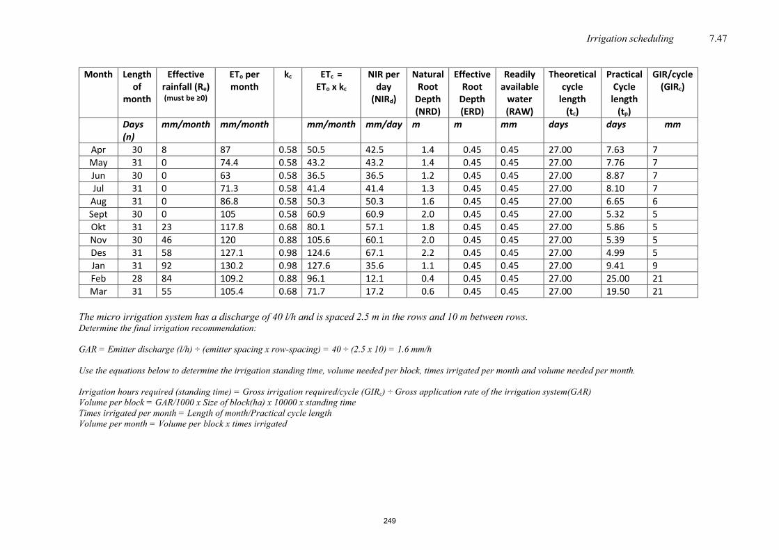
Irrigation scheduling 7.47
Month Length
of month
Effective rainfall (Re) (must be ≥0)
ETo per month
kc ETc = ETo x kc
NIR per day
(NIRd)
Natural Root
Depth (NRD)
Effective Root
Depth (ERD)
Readily available
water (RAW)
Theoretical cycle
length (tc)
Practical Cycle
length (tp)
GIR/cycle (GIRc)
Days (n)
mm/month mm/month mm/month mm/day m m mm days days mm
Apr 30 8 87 0.58 50.5 42.5 1.4 0.45 0.45 27.00 7.63 7 May 31 0 74.4 0.58 43.2 43.2 1.4 0.45 0.45 27.00 7.76 7 Jun 30 0 63 0.58 36.5 36.5 1.2 0.45 0.45 27.00 8.87 7 Jul 31 0 71.3 0.58 41.4 41.4 1.3 0.45 0.45 27.00 8.10 7
Aug 31 0 86.8 0.58 50.3 50.3 1.6 0.45 0.45 27.00 6.65 6 Sept 30 0 105 0.58 60.9 60.9 2.0 0.45 0.45 27.00 5.32 5 Okt 31 23 117.8 0.68 80.1 57.1 1.8 0.45 0.45 27.00 5.86 5 Nov 30 46 120 0.88 105.6 60.1 2.0 0.45 0.45 27.00 5.39 5 Des 31 58 127.1 0.98 124.6 67.1 2.2 0.45 0.45 27.00 4.99 5 Jan 31 92 130.2 0.98 127.6 35.6 1.1 0.45 0.45 27.00 9.41 9 Feb 28 84 109.2 0.88 96.1 12.1 0.4 0.45 0.45 27.00 25.00 21 Mar 31 55 105.4 0.68 71.7 17.2 0.6 0.45 0.45 27.00 19.50 21
The micro irrigation system has a discharge of 40 l/h and is spaced 2.5 m in the rows and 10 m between rows. Determine the final irrigation recommendation: GAR = Emitter discharge (l/h) ÷ (emitter spacing x row-spacing) = 40 ÷ (2.5 x 10) = 1.6 mm/h Use the equations below to determine the irrigation standing time, volume needed per block, times irrigated per month and volume needed per month. Irrigation hours required (standing time) = Gross irrigation required/cycle (GIRc) ÷ Gross application rate of the irrigation system(GAR) Volume per block = GAR/1000 x Size of block(ha) x 10000 x standing time Times irrigated per month = Length of month/Practical cycle length Volume per month = Volume per block x times irrigated
249

7.48 Irrigation User Manual
Month Practical cycle length (tp)
GIR/cycle (GIRc)
Standing time Volume water needed per
block
Times irrigated per month
Volume needed per month
days mm hours m3 m3 Apr 7.63 7 7,3 140 4,3 599,44 May 7.76 7 7,2 138 4,4 609,20 Jun 8.87 7 6,3 120 4,3 515,86 Jul 8.10 7 6,9 132 4,4 583,82
Aug 6.65 6 7,2 138 5,2 710,74 Sept 5.32 5 7,5 143 6,0 859,76 Okt 5.86 5 6,8 130 6,2 806,17 Nov 5.39 5 7,4 141 6,0 848,47 Des 4.99 5 8,0 153 6,2 946,70 Jan 9.41 9 7,6 146 3,4 502,53 Feb 25.00 21 6,7 128 1,3 170,77 Mar 19.50 21 8,6 164 1,5 242,43
250

Irrigation scheduling 7.49
9 References 1. Annandale, J.G., Jovanovic, N.Z., Steyn, J.M. and Backeberg, G.R. 2005. Irrigation Management
CD. Dept. Plant Production and Soil Science, University of Pretoria. RSA 2. Annandale, J.G., Stirzaker, R.J., Singels, A., Van der Laan, M. and Laker, M.C. 2011. Irrigation
scheduling research: South African experiences and future prospects. Water SA Vol. 37 No. 5. WRC 40-Year Celebration Special Edition
3. Bennie, A.T.P., Coetzee, M.J., Van Antwerpen, R. and Van Rensburg, L.D. 1988. ‘n
Waterbalansmodel vir besproeiing gebaseer op profielvoorsieningstempo en gewaswaterbehoeftes. WRC Report nr. 144/1/88
4. Doorenbos, J. and Kassam, A.H. 1979. Yield response to water. FAO Irrigation and Drainage Paper
No. 33. Rome, FAO 5. Gibson, L.A., Jarmain, C., Su, Z., and Eckardt, F.E. 2013. Estimating evapotranspiration using
remote sensing and the Surface Energy Balance System – A South African perspective. Water SA Vol. 39 No. 4 July 2013
6. Heyns, P.J., Burger, J.H., Kleynhans, E.P.J., Koegelenberg, F.H., Lategan, M.T., Mulder, D.J., Smal,
H.S., Stimie, C.M., Uys, W.J., Van der Merwe F.P.J. and Viljoen P.D. 1996. Irrigation Design Manual. ARC-Institute for Agricultural Engineering. RSA
7. Hoffman. J.E. 2002. Klasnota’s opgestel vir die grond en waterbestuur kursus. Department of Soil
science. University Stellenbosch. RSA 8. Jordaan, H. 2000. ‘n Ondersoek na sagteware vir besproeiingskedulering. ARC-Institute for
Agricultural Engineering. RSA 9. Jordaan, H. 2001. Grondwatersensors. ARC-Institute for Agricultural Engineering. RSA 10. Koegelenberg, F.H. 2002. Norms for the design of irrigation systems. ARC-Institute for Agricultural
Engineering. RSA 11. Olivier, F. 2016. SASRI Information sheet 5.4. Irrigation scheduling toolbox.
https://sasri.org.za/publications/ 12. Piaget, J. 1991. Tensiometers: Beskrywing, voorbereiding, opstelling en gebruik. Elsenburg
Agricultural Development Institute for the Winter Rainfall Area. RSA 13. Reinders, F.B. 2010. Water use efficiency from dam wall release to root zone application. Water
Research Commission, Report no TT 466/10, South Africa 14. Scheepers, I., Piaget, J., Kotze, W.A.G. and Myburgh, P.A. 1991. Riglyne vir
Besproeiingskedulering van Permanente Gewasse in die Winterreëngebied Elsenburg Agricultural Development Institute. RSA
15. Singels, A., Annandale, J.G., De Jager, J.M., Schulze R.E., Inman-Bamber, N.G., Durand, W., Van
Rensburg, L.D., Van Heerden, P.S., Crosby, C.T., Green, G.C. and Steyn, J.M. 2010. Modelling crop growth and crop water relations in South Africa: Past achievements and lessons for the future. South African Journal of Plant and Soil, 27:1, 49-65
251

7.50 Irrigation User Manual 16. Stevens, J.B. & Buys, F. 2012. Training material for extension advisors in irrigation water
management. Volume 2, Part 4. Water Research Commission Report number TT 540/4/12. 17. Steyn, J.M. & Annandale J.G. 2008. Irrigation scheduling strategies – when to turn on the pump.
Dept of Plant Production and Soil Science, University of Pretoria. AfgriLand, September-October 2008
18. Van der Stoep, 2015. Irrigation efficiency training material. Water Research Commission Report
number KV 342/1/15 19. Van Heerden, P.S. and Walker, S. 2016. Upgrading of SAPWAT 3 as a management tool to estimate
the irrigation water use of crops. Revised edition SAPWAT 4. WRC Report No. TT662/16 20. Van Zyl, J.L. 1981. Waterbehoefte en besproeiing. In: (Reds. Burger, J. and Deist, J.). Viticulture in
South Africa. ARC-Infruitec-Nietvoorbij, Stellenbosch
252

IRRIGATION USER MANUAL
CHAPTER 8
Irrigation pipes, fittings and valves
253

8.2 Irrigation User Manual
Table of Contents
1 Introduction ........................................................................................................................................................................................................................................ 8.1 2 Pipe types available .................................................................................................................................................................................................................. 8.1
2.1 Asbestos cement pipes ................................................................................................................................................................................................ 8.1 2.1.1 Constant outside diameter (COD) AC pipes .................................................................................................................... 8.1 2.1.2 Constant inside diameter (CID) AC pipes ........................................................................................................................... 8.2 2.1.3 Fittings for AC pipes .................................................................................................................................................................................... 8.2 2.1.4 Transport ........................................................................................................................................................................................................................ 8.2 2.1.5 Handling ......................................................................................................................................................................................................................... 8.2 2.1.6 Storage .............................................................................................................................................................................................................................. 8.3 2.1.7 Installation .................................................................................................................................................................................................................... 8.3 2.1.8 Testing .............................................................................................................................................................................................................................. 8.5
2.2 uPVC pipes .............................................................................................................................................................................................................................. 8.6 2.2.1 Fittings for uPVC pipes ............................................................................................................................................................................ 8.8 2.2.2 Transport ........................................................................................................................................................................................................................ 8.8 2.2.3 Handling ......................................................................................................................................................................................................................... 8.8 2.2.4 Storage .............................................................................................................................................................................................................................. 8.9 2.2.5 Installation ................................................................................................................................................................................................................ 8.10 2.2.6 Testing .......................................................................................................................................................................................................................... 8.11
2.3 mPVC pipes ......................................................................................................................................................................................................................... 8.11 2.4 Polyethylene pipes ....................................................................................................................................................................................................... 8.14
2.4.1 Transport .................................................................................................................................................................................................................... 8.14 2.4.2 Handling ..................................................................................................................................................................................................................... 8.14 2.4.3 Storage .......................................................................................................................................................................................................................... 8.14 2.4.4 Installation ................................................................................................................................................................................................................ 8.14 2.4.5 Testing .......................................................................................................................................................................................................................... 8.15
2.5 Steel pipes .............................................................................................................................................................................................................................. 8.16 2.5.1 Transport .................................................................................................................................................................................................................... 8.17 2.5.2 Handling ..................................................................................................................................................................................................................... 8.18 2.5.3 Storage ........................................................................................................................................................................................................................ 8.18 2.5.4 Installation ................................................................................................................................................................................................................ 8.19 2.5.5 Testing .......................................................................................................................................................................................................................... 8.19
2.6 Klambon pipes .................................................................................................................................................................................................................. 8.20 2.7 Quick coupling irrigation pipes ..................................................................................................................................................................... 8.20
2.7.1 Transport .................................................................................................................................................................................................................... 8.22 2.7.2 Handling ..................................................................................................................................................................................................................... 8.22 2.7.3 Storage .......................................................................................................................................................................................................................... 8.22 2.7.4 Installation ................................................................................................................................................................................................................ 8.22
2.8 Suction pipes ....................................................................................................................................................................................................................... 8.22 2.9 Draglines ................................................................................................................................................................................................................................. 8.23 2.10 Flood pipes ........................................................................................................................................................................................................................ 8.24 2.11 Glass fibre (GRP) pipes ...................................................................................................................................................................................... 8.24 2.12 Pipes for drip irrigation ....................................................................................................................................................................................... 8.24
3 Troubleshooting for pipes ..................................................................................................................................................................................................8.25 4 Valves ...................................................................................................................................................................................................................................................... 8.26
4.1 Sealing mechanisms .................................................................................................................................................................................................... 8.26 4.1.1 Sluice ........................................................................................................................................................................................................................... 8.26 4.1.2 Diaphragm ............................................................................................................................................................................................................. 8.29 4.1.3 Saddle ......................................................................................................................................................................................................................... 8.30 4.1.4 Ball ................................................................................................................................................................................................................................. 8.31
254

Irrigation pipes, fittings and valves 8.3
4.1.5 Butterfly ................................................................................................................................................................................................................... 8.31 4.2 Valve control mechanisms ................................................................................................................................................................................. 8.32
4.2.1 Mechanical control ...................................................................................................................................................................................... 8.32 4.2.2 Hydraulic control ........................................................................................................................................................................................... 8.32 4.2.3 Spontaneous control valves ............................................................................................................................................................... 8.42 4.2.4 Placing of air valves ....................................................................................................... 8.42
5 Troubleshooting for valves ...............................................................................................................................................................................................8.48 6 The measurement system ................................................................................................................................................................................................ 8.50 6.1 Water meters ...................................................................................................................................................................................................................... 8.50 7 References ........................................................................................................................................................................................................................................ 8.53
All rights reserved Copyright 2019 ARC-Agricultural Engineering (ARC-AE)
255

256

Irrigation pipes, fittings and valves 8.1 1 Introduction There is a wide variety of irrigation equipment available on the South African irrigation market. The available equipment has its own unique application area and misplaced use can lead to water wastage and accompanying harvest losses.
This chapter contains information and sketches of the transport, handling, storage, installation and testing after installation of pipes, as described in the publication “Pype in die Landbou” (Smit, 1993). The applicable information for producers originating from the Irrigation Design Manual of the ARC-Institute for Agricultural Engineering regarding the available valves and water meters is also contained in this chapter. 2 Pipe types available
There is a large variety of pipe types available, which can be used in irrigation systems. "Pipes in Agriculture" may be used as a further reference. All irrigation pipes operate under pressure and the selected pipes and fittings must withstand the operating pressure. Hence, the choice of pipe types is very important. The following aspects should be taken into account when choosing a pipe type: • Nature of usage, e.g. permanent main line, temporary main line, lateral for permanent system,
above/below ground, etc. • Size and pressure class of pipe required as certain pipe types are less expensive than others in
certain sizes and pressure classes. • Accessories available. • Installer competence. • Water and soil properties. • Longevity. • The type of site plays a role depending on rocky or sandy conditions. 2.1 Asbestos cement pipes Although these types of pipes are no longer in common use in irrigation systems due to their fragility, Asbestos cement (AC) can still be used as mainline or sub-mainline pipes which are buried underground and not moved during operation. They are manufactured by winding a mixture of asbestos fibres and cement around a mould. The following limiting characteristics of AC pipes should be taken into account with choice of pipe type: • AC pipes are relatively heavy. • Certain chemicals break down the cement fraction in the pipes (they can be protected with
bitumen or epoxy coatings). • AC pipes are brittle and break easily if handled carelessly or laid incorrectly.
2.1.1 Constant outside diameter (COD) AC pipes The pipe pressure class is determined by the wall thickness. With COD pipes the outside diameter of a certain pipe size remains constant while the inside diameter varies between different classes. AC pipes make use of socket-type couplings, which means that the joining sockets and other fittings for COD pipes remain the same for the different classes of the same pipe size. The design procedure is hampered by the variation in inside diameter as the effective diameter changes with a change in class.
257

8.2 Irrigation User Manual Table 8.1: Inside diameters of (COD) AC pipes
Class Working pressure
[m]
Nominal diameter [mm] 50 75 100 150 200 250 300 350
B 60 - - - - 208 260 316 395 C 90 - - 102 156 204 256 308 381 D 120 - 76 100 149 196 243 294 363 E 150 - 74 96 142 187 231 281 347 F 180 5 73 94 139 183 227 274 340
Standard length: 5 m 2.1.2 Constant inside diameter (CID) AC pipes The varying outside diameter means that a different set of couplings and fittings is required for every class of CID pipe of the same diameter. The available fittings are usually class 18, which necessitates the use of class-to-class couplings where fittings must be joined to different classes. The designer's calculations are, however, simplified by the constant inside diameter. CID pipes are available in 5 m lengths which means that less couplings are required. Table 8.2 shows the design data for the available CID pipes. Table 8.2: Outside diameters of (CID) AC pipes
Class Working pressure
[m]
Nominal diameter [mm] 150 200 250 300 350 400
06 30 - - - - 378 430 12 60 168 222 274 328 382 436 18 90 174 229 284 340 396 450 24 120 180 239 295 353 412 468 30 150 188 250 304 365 426 484 36 180 196 262 318 378 440 503
Standard length: 5 m 2.1.3 Fittings for AC pipes A wide range of standard fittings in AC, cast iron and steel is available for AC pipes. Couplings allow a certain amount of deflection (5o for AC couplings and 4o for short collar repair couplings). Besides couplings, other standard fittings like bends, end caps, reducers, cross pieces, T-pieces, flange adapters, saddles, hydrant T-pieces and scour T-pieces are available. In addition to the standard fittings, custom-made steel fittings are manufactured by different companies. 2.1.4 Transport
• Suitable vehicles, of which the floor and sides have even surfaces, should be used. • If surfaces are uneven, planks should be provided from each end at approximately 1/5 of the
pipe length. • The load must be secured with ropes and tensioners. • Pipes must not protrude more than 1 m out of the vehicle. 2.1.5 Handling
• During handling of the pipes, care must be taken to prevent unnecessary impact and damage to the pipes, couplings and fittings.
• The pipes must not be dropped or rolled over uneven surfaces. • Offloading must be as close as possible to the installation point.
258

Irrigation pipes, fittings and valves 8.3
2.1.6 Storage
• It is necessary to place timber runners under the pipes, approximately 1/5 of the pipe length from each end, so that the pipes do not lie on the ground.
• Pipes must be stored separately, i.e. one size and class per stack. • Smaller pipes, i.e. of a diameter up to 150 mm, must be stacked in bundles in pyramid form
and the outer pipes of the bottom layer can be held in position with wooden pegs driven into the ground.
• Larger pipes, i.e. diameter larger than 150 mm, can be either stacked in bundles in pyramid form or in a rectangular form where each layer of pipes are laid on their own timber runners.
• Timber runners must be laid across each other.
2.1.7 Installation
• Trenches must be wide enough to provide safe working conditions and ample working space for workers, so that the pipes can be appropriately laid and joined.
• The recommended maximum width at bed level is D + 0.4 m for pipes of nominal diameter up to 500 mm and D + 0.6 m for pipes with nominal diameter more than 500 mm, where D is the outer diameter of the pipe in metres.
• The minimum width of the trench at excavation level should be 0.6 m (0.8 m for larger pipes). • Great care must be taken with soil that seems stable at excavation, but could become unstable
with wetting or parching. • Where natural soil beds are specified, mechanical excavation should be ceased before the final
bed level is reached. • Manual excavations up to final bed level provides for stricter control and less disturbance of
the in situ material. Where excavations are too deep, all loose material must be removed and the required bed levels must be restored with compacted, fine, granular material.
• In rocky or water bearing soil or where a concrete or granular base is provided, excavations must be done to the required depth for the class and thickness of bed to be used.
• The manner in which a pipe is imbedded, has a specific influence on the support strength of such a pipe. Pipes must therefore be imbedded in a suitable manner and in accordance with the type of base specified in the design.
• Three imbedding methods for asbestos-cement pipes are classified, from the very best to the poorest: Classes A, B and C (Smit, 1993).
Imbedding type A:
The bottom of the trench is compacted with granular material to a minimum height of 10 + (D/10) in cm. The top layers of this granular material are formed concentric with the pipe according to a certain angle 2a. The pipe must be supported evenly in this shaped portion of the refilled trench bottom. Material without clods or stones are placed on the side and above the pipe in layers and up to 30 cm over the pipe and the entire width of the trench is compacted. The remaining portion of the trench or filling is filled with regular or compacted backfill.
Figure 8.1: Imbedding type A
259

8.4 Irrigation User Manual Imbedding type B:
It is recommended for regular soil without clods and large stones. The pipe is laid directly on the bottom of the trench. The hull of the pipe is in continuous contact with the bottom, approximately in line. At each coupling in the pipeline, a groove is dug in the bottom to prevent the coupling from carrying the pipes. Choice filling material is compacted on both sides of the pipe up to a height in accordance with the selected imbedding angle.
Figure 8.2: Imbedding type B
Imbedding type C:
This imbedding type consists mainly of a continuous concrete bed through which the pipe is evenly supported. The minimum width of the bed must be equal to the outer diameter of the pipe plus 20 cm and the thickness must be at least a quarter of the nominal diameter of the pipe with a minimum of 10 cm. The compressive strength of the concrete, tested after 28 days, must not be less than 20 N/mm². Backfill material, without clods or stones, must be compacted in layers of at least 15 cm to a height of 30 cm above the top of the pipe. Above this height, regular backfill is used for backfilling of the trench or the build-up of the filling to the design height.
Figure 8.3: Imbedding type C
• Ensure that the cement couplings are clean, grits can cause leakages. • It is advisable to fit an asbestos-reinforced cement coupling to each pipe before laying them in
the trench. • With the lubricant applied, the coupling must be slid over the pipe end and pushed into
position. The lubricated pipe end must be pushed through the seal ring of the coupling, against the pacer ring, where it will stop and automatically provide the necessary expansion space.
• It is possible to do this manually with pipes of a smaller diameter, e.g. 50 mm and 75 mm. • For pipes of medium diameter, the front face of the coupling must be protected by the timber
while it is forced over the pipe end with the aid of a crowbar. A crowbar is however not always effective in loose sand, mud, hard shale, compacted soil or stone.
• A chain winch is the ideal tool for joining pipes of up to 600 mm in diameter in very soft or very hard trench conditions.
260

Irrigation pipes, fittings and valves 8.5
• For pipes larger than 600 mm special hydraulic tractors can be used. • Let each pipe or coupling down into the trench and fit them in a straight line with the previous
pipe or coupling laid. • Dry asbestos-reinforced cement pipes will, when used for the first time, absorb water and
expand. Therefore, an expansion opening must be left between the pipe ends. • With asbestos-reinforced cement couplings, these openings are automatically provided by the
centre spacing, but where no rings are used, e.g. cast iron couplings, an expansion gap of 10 mm must be provided during the laying of the pipes.
• Trenches must be filled according to the designer’s specifications. • The couplings must be left open until after the testing. • Materials used for partial backfilling, should be placed in the trench in a uniform manner, on
each side of the pipe and over the entire length of the trench, in layers of approximately 150 mm thickness, carefully compacted underneath the pipe and on the sides, so that a good bed without openings is provided (see designer specifications).
• If excavated material is used for backfilling, the density and water content of the compacted backfilling must be as close as possible to the existing undisturbed soil.
• If replacement material is used for backfilling, it should be compacted at the optimum water content to give the maximum density to the satisfaction of the site engineer.
• When using mechanical equipment, care must be taken with backfilling and compacting, since excessive loading can cause damage to the pipes and direct impact can damage the pipes.
• Because of the telescopic nature of couplings normally used with asbestos-reinforced cement pipelines, all risk of movement of the pipeline must be eliminated, by anchoring it with concrete anchors or support blocks.
2.1.8 Testing
• The length of the test section should normally be from 500 m to 1 000 m. Longer sections may be allowed, if the pressure during the test is not less than 0.8 times the pressure at the lowest point.
• The sections to be tested must be sealed at the ends and thoroughly anchored against longitudinal and lateral deflection.
• The test section must be allowed to stand filled with water for at least 24 hours and must be kept filled, so that the asbestos-reinforced cement pipe and coupling walls can absorb their full water requirement and vacuums that formed underneath coupling crowns can be filled.
• After the test section is filled and during the test period before test pressure is built up, a visual inspection of the entire length must be done to determine whether:
there are no obvious leakages signs of pipeline or anchoring block movement is observed air is not escaping anywhere
• Any defects must be corrected immediately. • The site test pressure (STP) should not be less than 1.5 times the actual operating pressure in
the pipeline, where the STP does not exceed 1.0 MPa. It must however not exceed the STP as determined with the expression below: STP = 1.5 OP for OP < 1.0 MPa STP = OP + 0.5 MPa for OP > 1.0 MPa with OP as indicated Operating Pressure
• The site test pressure will never be less than 0.4 MPa, despite the size of the actual operating pressure.
• While the pressure is raised, allowance must be made to expel further released air. • Pump the water into the test section, to obtain the required test pressure at the lowest point of
the section. Care must be taken not to exceed the test pressure. • Maintain the test pressure for at least an hour and repeat the visual inspection, as previously
mentioned, during this period. Treat the test section with care while it is under pressure.
261

8.6 Irrigation User Manual • The pipe will, while it is under pressure, absorb more water and therefore cause a reduction in
pressure that may be seen as an obvious water loss. • If leakages occur, it may be caused by locked-in air and the test must be repeated. • Thereafter, all exposed couplings must be backfilled with the same material used around the
pipes, which are joined by the couplings. • The final backfilling material must be free of stones larger than a fist, vegetation and garbage
and should normally consist of material originating from the trench in which the pipe is. It must be compacted in layers of 30 mm thick over the pipeline until the trench excavation material is approximately 100 mm higher than the natural level of the soil to make provision for settling.
• Pipes should not be left exposed for more than a week. 2.2 uPVC pipes uPVC (unplasticised polyvinyl chloride) pipes are less ductile than polyethylene pipes but do still offer elasticity to absorb mild deflections and uneven ground conditions. Advantages: • Corrosion resistance • Pipes are light and can be easily manhandled • Smooth inner walls have very good flow characteristics (low friction losses) • Pipes are joined quickly and easily by integrated rubber ring joints, solvent welding and
socket fittings • uPVC is resistant to all chemicals pumped through irrigation lines Disadvantages: • uPVC becomes brittle at low temperatures • The permissible working pressure must be lowered at temperatures above 25oC • uPVC has a relatively high thermal expansion coefficient compared to steel Table 8.3 shows the dimensions of uPVC pipes according to SANS 966-1: 2014.
262

Irrigation pipes, fittings and valves 8.7
Table 8.3 SANS 966-1: 2014. Dimensions of uPVC pipes [mm]
Nom. size
Outside diameter Wall thickness Class 4 Class 6 Class 9 Class 12 Class 16 Class 20
Min Max Min Max Min Max Min Max Min Max Min Max Min Max 16 16,0 16,2 1,5 1,8 20 20,0 20,2 1,5 1,8 1,9 2,2 25 25,0 25,2 1,5 1,8 1,9 2,2 2,3 2,7 32 32,0 32,2 1,5 1,8 1,8 2,1 2,4 2,8 2,9 3,3 40 40,0 40,2 1,5 1,8 1,8 2,1 2,3 2,7 3,0 3,5 3,7 4,2 50 50,0 50,2 1,8 2,1 2,2 2,6 2,8 3,2 3,7 4,2 4,6 5,2 63 63,0 63,2 1,9 2,2 2,7 3,1 3,6 4,1 4,7 5,3 5,8 6,5 75 75,0 75,2 1,5 1,8 2,2 2,6 3,2 3,7 4,3 4,9 5,6 6,3 6,9 7,7 90 90,0 90,3 1,8 2,1 2,7 3,1 3,9 4,4 5,1 5,8 6,7 7,5 8,2 9,2
Notes: In pressure classes 4 to 16, minimum and maximum values not shown will be 1,5 and 1,8 respectively In the case of nominal sizes 16 to 90, there is no pressure class 25 Wall thickness of pipes of nominal size ≤ 90 mm are based on an overall service (design) factor C of 2,5; i.e. design stress of 10 MPa. Nom size Outside diameter Wall thickness
Class 6 Class 9 Class 12 Class 16 Class 20 Class 25 Min Max Min Max Min Max Min Max Min Max Min Max Min Max
110 110,0 110,3 2,6 3,0 3,9 4,4 5,1 5,8 6,7 7,5 8,2 9,2 10,0 11,2 125 125,0 125,3 3,0 3,5 4,4 5,0 5,8 6,5 7,6 8,5 9,3 10,4 11,4 12,8 140 140,0 140,4 3,3 3,8 4,9 5,5 6,5 7,3 8,5 9,5 10,4 11,6 12,8 14,2 160 160,0 160,4 3,8 4,3 5,6 6,3 7,4 8,3 9,7 10,8 11,9 13,2 14,6 16,2 180 180,0 180,5 4,3 4,9 6,3 7,1 8,3 9,3 10,9 12,1 13,4 14,9 16,4 18,2 200 200,0 200,5 4,7 5,3 7,0 7,9 9,2 10,3 12,1 13,5 14,9 16,5 18,2 20,2 225 225,0 225,5 5,3 6,0 7,9 8,8 10,3 11,5 13,6 16,1 16,7 18,5 20,5 22,7 250 250,0 250,6 5,9 6,6 8,7 9,7 11,5 12,8 15,1 16,8 18,6 20,6 22,8 25,2 280 280,0 280,6 6,6 7,4 9,8 11,9 12,9 14,3 16,9 18,7 315 315,0 315,6 7,4 8,3 11,0 12,2 14,5 16,1 19,0 21,1 355 355,0 355,7 8,4 9,4 12,4 13,8 16,3 18,1 21,4 23,7 400 400,0 400,7 9,4 10,5 14,0 15,6 18,4 20,5 24,1 26,7 450 450,0 450,8 10,6 11,8 15,7 17,4 20,7 22,9 500 500,0 500,9 11,8 13,1 17,4 19,3 22,9 25,5 560 560,0 561,0 13,2 14,7 19,5 21,6 630 630,0 631,1 14,8 16,4 21,9 24,2
Notes: In the case of nominal sizes 110 to 630, there is no pressure class 4 Wall thickness for pipes of nominal size ≥ 110 mm are based on an overall service (design) factor C of 2,0; i.e. design stress of 12.5 MPa Standard length: 6 m
263

8.8 Irrigation User Manual 2.2.1 Fittings for uPVC pipes uPVC pipes are available in 6 m lengths, with socket joints or rubber ring joints. Although uPVC pipes can absorb a reasonable amount of deflection, care must be taken to avoid sharp bends as the pipe will be deformed into an elliptical shape, leading to possible failure from creep rupture. uPVC pipes should preferably not be stacked in bundles or where they will be exposed to direct sunlight or excessively high temperatures over an extended period of time. A large variety of fittings used with uPVC and mPVC (modified uPVC) pipes may be divided into the following series: • Rubber joints • Solvent welding fittings (uPVC mouldings), 16 bar rated. • Custom-made uPVC fittings (mainly bends, T-pieces, etc., which are fabricated from pipes by
solvent welding and forming under high temperatures). Not recommended above 6 bar. • Cast aluminium fittings with rubber ring joints • Cast iron or SG steel fittings for high pressure (16 bar)
Table 8.4 shows the number of joints to be made with 1 litre of solvent welding adhesive. Sufficient adhesive and cleaner must be provided with the pipes. Ensure that the recommended solvent weld procedures are strictly adhered to, and that sufficient curing time is provided prior to commissioning the pipeline. Table 8.4: Amount of solvent welding liquid required
Nominal diameter [mm] Number of joints per litre 20 140 25 100 32 90 40 80 50 70 63 60 75 40 90 30
110 25 When choosing pipe fittings, the aggressiveness of the soil in contact with the pipe as well as price differences must be kept in mind. Aluminium fittings should be avoided in aggressive conditions. In such a case, only epoxy coated aluminium fittings are to be used for irrigation purposes.
2.2.2 Transport
• Pipes must be transported in such a way that: o contact with sharp corners and protrusions are avoided o the pipes are secured and supported over their entire length o they do not protrude from the transport vehicle’s body
• Sharp protrusions or ridges must be covered with a cushioning material to prevent abrasion between the moving vehicle bed and the pipe.
• It is permissible to stack pipes higher than 1.0 m on the vehicle, on condition that they are immediately offloaded when reaching the destination.
• Extra care is necessary in cold weather, since the strength of the pipe deteriorates at lower temperatures.
2.2.3 Handling
• Pipes must not be dumped from the vehicle, dropped on the ground or rolled (except on timber rollers) during offloading.
• Avoid rough handling and bending of pipes. • Pipes must be carried and not dragged.
264

Irrigation pipes, fittings and valves 8.9
2.2.4 Storage
Outdoors:
• Store in shade or under shelves. • Pipes must be stored on level ground, free from stones and sharp objects and stacked in such a
way that the load of each pipe is spread over the entire pipe. • Pipes with sockets must be stacked in such a way that the sockets in each alternate layer are on
different ends and protruding from the stack. • The height of the stack may not exceed 1 m. • Pipes of different classes and sizes must not be stacked together. • Protective packaging must only be removed just before the pipes are to be used. • Pipes and equipment must be kept free of dirt. • Rubber rings must be kept in a cool dry place where they are free of tension.
Under shelter:
• Pipes must be stored under shelter on pipe shelves that give continuous support over the entire length of the pipe.
• The height of the stack must not exceed 1.5 m or the height of seven layer of pipes. • Pipes with sockets must be stacked as such that the sockets in each alternate layer protrude at
the ends from the stack. • The bottom layer of pipes should lie on supports above the ground at distances of 1-2 m along
the length of the pipes. • The breadth of the supports may not be less than 75 mm.
Figure 8.4: Support of pipes by means of timber struts
Figure 8.5: Support of pipes using bricks
265

8.10 Irrigation User Manual
Figure 8.6: Self-supporting stacking
Figure 8.7: Diagonal stacking
2.2.5 Installation
• The width of the trench at depth equal to the crown of the pipe must be narrow but practical (300 mm larger than nominal diameter of the pipe). The trench must not be dug too long before the pipes are to be laid
• The bottom must be free of stones, hard protrusions, soft portions and other irregularities. The bottom must be backfilled with drainable coarse sand, gravel, loam or powdered soil to a depth of 100 mm and not less than a third of the nominal diameter of the pipe.
• The bed must be thoroughly compacted in layers not exceeding 150 mm. • All levelling pegs and side plates must be removed before laying the pipes. • Pipes that lay in the sun and heated, may not be laid before cooling off to a temperature of
25°C. • Pipelines must not be more than 400 m long to facilitate acceptance test work. • The pipeline must be laid directly on the prepared bed. • Hard objects or bricks must not be used as temporary support. • Rubber ring joining can be done in the trench. Only rubber rings of the same make as the pipe
may be used. The spigots, sockets and rings must be free of any soil, etc. • The pipe end must be chamfered under an angle of approximately 15% and the insertion depth
must be marked on the spigot. • A thin layer of a recommended joint lubricant must be applied to each rubber ring and spigot
up to approximately half of the distance between the spigot end and the mark that indicates the insertion depth.
• After ensuring that both components are horizontal, as well as vertical on one line, effectuate
the joint by pressing the spigot thoroughly into the socket until the insertion depth mark on the spigot-end is even with the outer end of the socket.
266

Irrigation pipes, fittings and valves 8.11
• The joint must be made immediately after the joint adhesive is applied, by pressing the two prepared parts firmly together to the full insertion depth.
• Excess joint lubricant must be wiped away and the components of the joint must be kept tightly together until the adhesive has hardened. The joint must be left undisturbed for 30 minutes and must not be subjected to stress for 24 hours.
• Pipelines must be anchored at each direction change, or valve and end. • Concrete slabs can be used for anchoring, but the pipes must not be enveloped in concrete.
Anchor points should be protected by means of a layer of plastic material before the concrete is cast.
• Where pipelines have to be buried at depths of up to 450 mm, the pipeline must be protected by means of concrete slabs which are laid over the side filling.
• Selected material must be placed carefully and evenly, in layers of uncompacted thickness of 75 mm between the sides of the trench and the pipe, up to the top of the pipe.
Figure 8.8: Installation of uPVC pipes
• The joints must be left exposed until pressure testing of the piple is complete. This helps to
identify leaking joints at installation/commissioning of the pipeline. • Each layer must be manually compacted individually. Note that there is no hollow underneath
the pipe. • Thereafter, fill the rest of the trench with excavated soil over the width to a height equal to
two thirds of the diameter of the pipe (at least 100 mm and no more than 300 mm above the top of the pipe). First compact each layer manually and then with mechanised equipment.
2.2.6 Testing
• The pipe must be free of debris and the portion to be tested must not exceed 400 m. • If joints between consecutive test portions must be tested, the total length must not exceed
1 000 m. • Pipes must not be tested within 24 hours of application of the joint adhesive. • After ensuring that the pipe is free of air and full of water, it can be subjected to
approximately 1 hour of hydraulic pressure, which is equal to 1.5 times the maximum operating pressure of the tested pipe.
• Each joint must be inspected for leakages. • After the test, the joints must be backfilled and compacted just as the rest of the pipe. 2.3 mPVC pipes mPVC stands for "modified" uPVC and the product is more ductile than uPVC, allowing the pipe wall thickness to be about 2/3 of uPVC pipes. mPVC pipes do carry the SANS mark. All standard pipe fittings are compatible with uPVC pipe fittings. Table 8.5 shows the dimensions of mPVC pipes.
267

8.12 Irrigation User Manual
Table 8.5: SANS 996-2:2013. Dimensions of mPVC pipes [mm] Nom Size
Outside diameter Wall Thickness Class 6 Class 9 Class 12 Class 16 Class 20 Class 25
Min Max Min Max Min Max Min Max Min Max Min Max Min Max 50 50,0 50,2 1,5 1,8 1,5 1,8 1,7 2,0 2,2 2,6 2,7 3,1 3,3 3,8 63 63,0 63,2 1,5 1,8 1,6 1,9 2,1 2,5 2,7 3,1 3,4 3,9 4,1 4,7 75 75,0 75,2 1,5 1,8 1,9 2,2 2,5 2,9 3,2 3,7 4,0 4,6 4,9 5,5 90 90,0 90,3 1,8 2,1 2,2 2,6 3,0 3,5 3,9 4,4 4,8 5,4 5,9 6,6
110 110,0 110,3 2,2 2,6 2,7 3,1 3,6 4,1 4,7 5,3 5,8 6,5 7,2 8,1 122 122,0 122,3 2,4 2,8 3,0 3,5 4,0 4,6 5,2 5,9 6,5 7,3 8,0 9,0 125 125,0 125,3 2,5 2,9 3,1 3,6 4,1 4,7 5,4 6,1 6,6 7,4 8,2 9,2 140 140,0 140,4 2,8 3,2 3,5 4,0 4,6 5,2 6,0 6,8 7,4 8,3 9,1 10,2 160 160,0 160,4 3,2 3,7 4,0 4,6 5,2 5,9 6,9 7,7 8,5 9,5 10,4 11,6 177 177,0 177,4 3,5 4,0 4,4 5,0 5,8 6,5 7,7 8,6 9,4 10,5 11,5 12,8 180 180,0 180,5 3,6 4,1 4,4 5,0 5,9 6,6 7,8 8,7 9,5 10,6 11,7 13,0 200 200,0 200,5 3,9 4,4 4,9 5,5 6,5 7,3 8,6 9,6 10,6 11,8 13,0 14,5 225 225,0 225,5 4,4 5,0 5,5 6,2 7,3 8,2 9,6 10,7 11,9 13,2 14,7 16,3 250 250,0 250,6 4,9 5,5 6,1 6,9 8,1 9,1 10,7 11,9 13,2 14,7 16,3 18,1 280 280,0 280,6 5,5 6,2 6,9 7,7 9,1 10,2 12,0 13,4 14,8 16,4 18,2 20,2 315 315,0 315,6 6,2 7,0 7,7 8,6 10,2 11,4 13,5 15,0 16,6 18,4 355 355,0 355,7 7,0 7,9 8,7 9,7 11,5 12,8 15,2 16,9 18,7 20,7 400 400,0 400,7 7,8 8,7 9,8 10,9 13,0 14,5 17,1 19,0 21,1 23,4
Note: Wall thickness of pipes are based on overall service (design) factor C of 1,4 i.e. design stress of 18 MPa
268

Irrigation pipes, fittings and valves 8.13
2.4 Polyethylene pipes Polyethylene (PE) pipes are used for irrigation purposes on a large scale, but mainly in smaller sizes. PE pipes have the same advantages as uPVC pipes but have the added advantage of being more flexible, making it possible to handle pipes in long uncut rolls. The high ductility of this material eases cutting and joining of pipes, but makes pipes susceptible to damage by sharp objects. The permissible working pressure reduces more rapidly with increasing temperatures pipes than with uPVC pipes. PE pipes also have a higher thermal expansion coefficient. PE is not soluble and must therefore be joined mechanically or by thermos-melting (fusion welding). PE pipes are divided into 4 types according to SANS 533 specifications. Further classification is done, based on material and pressure. Table 8.6 shows design data for different pipe classes and types. Types IV and V are joined with external compression fittings (COD) while type I makes use of nylon insert fittings (CID). Table 8.6: PE pipe types and pressure classes to SABS 533
Type Material Joining method Class Working pressure at 25°C [m]
I LDPE (CID)
Nylon insert fittings 3 30 6 60
IV and V HDPE (COD)
External compression fittings
4 40
6 60 10 100 12 120 16 160
Besides pipes which carry the SANS mark, non-SANS pipes are also available. Low density, non-SANS PE pipes are known as utility pipes. There are two classes for non-SANS pipes, namely class A with a maximum working pressure of 300 kPa at 25°C and class B with a maximum working pressure of 600 kPa at 25°C. Non-SANS pipes are not recommended for use in irrigation systems, but are used extensively with a pro-rata replacement guarantee. Table 8.7: Dimensions of PE pipe types
Type Nominal diameter [mm]
Inside diameter [mm] All classes
Class 4 Class 6 Class 9 Class 10 Class 12 Class 16
I 15 15,7 20 20,5 25 26,5 32 34,0 40 40,0 50 51,2 65 61,8 80 77,2
IV 20 - - - 16 15 14 25 - - - 20 19 18 32 - 28 - 26 25 23 40 - 35 - 33 31 29 50 46 44 - 40 39 36
V 25 21 20 19 32 27 26 25 40 34 33 31 50 43 41 39 63 54 51 49 75 64 61 58 90 77 74 70 110 94 90 85
269

8.14 Irrigation User Manual Allowance must be made during compilation of bills of quantities for kinks which occur during installation and prevent the pipe from pulling tightly after installation with reductions in temperature. Normally 3% is allowed for kinking while for the purposes of quantities 5% should be allowed to cover kinking and wastage. 2.4.1 Transport
• Sharp protrusions or edges should be protected with cushioning material to prevent damage by abrasion and cutting during transport.
2.4.2 Handling
• The pipe must not be dropped from the vehicle onto the ground. • The pipe must also be secured with soft straps or protected steel strapping. • Ensure that steel address tags will not damage the pipe. 2.4.3 Storage
• Store in shade as far as possible. • Ensure that the storage area is even and has no sharp protrusions. • The rolls must not be stacked higher than 1 m or 5 rolls one upon another, or the rolls at the
bottom will be squashed flat.
2.4.4 Installation
Type I
• No form of soft soap or lubricants may be used with polyethylene pipes. • The pipe must be heated in clean warm water before the coupling is inserted. • A clamp is then slid over the pipe and the coupling is inserted, so that all the serrations are on
the inside of the pipe. • The clamp is secured with a screwdriver or spanner and the connection is completed.
Figure 8.9: Nylon plastic coupling
Type IV
• The coupling is provided with bolt and nut already lightly screwed on. Slide the pipe into the coupling until it reaches the stopper inside. The pipe end must be cut square and cleaned.
• In the case of male and female couplings and the T-coupling, the body of the compression coupling must be inserted first with a PTFE tape. The body is fitted manually, as tight as possible and then turned just one more time with a spanner.
• After the pipe is slid into the coupling, it is necessary to hold the body of the coupling with one spanner while the nut is turned with another spanner. The nut must be turned until it stops against the body.
• As the nut is tightened, the sealing lip moves on the taper to grip the pipe and seal it.
270

Irrigation pipes, fittings and valves 8.15
Figure 8.10: Compression coupling
For both types
• All pipes must be buried reasonably deep to protect them from mechanical damage. The ideal depth is between 300 mm and 700 mm.
• Stones and sharp objects that may damage the pipes, must be removed from the trench before the pipe is laid.
• The pipe must then be carefully unrolled so that no kinks occur. • If the pipe was in the sun for a long time before being laid and placed in the trench while it is
still warm, ensure that the pipe is thoroughly snaked in the trench. It must preferably be covered while it is cool, i.e. in the early morning, or if it is already in use and cooled by cold water flowing through it. This will make provision for the shrinkage that will take place. Pipes must not be laid in curves with a radius of less than 1 m.
• Pipes can be cut with a hacksaw or sharp knife. • The trench must be just big enough to lay the pipe and the backfilling can be done. • Excavate the trench deeper than the required depth and then bring it to the required depth by
filling with compact, stable material. The depth of the additional excavation will depend on the type of soil on the bottom of the trench. If stone or rock is found, the bottom layer must be at least 100 mm thick and must be of the material used to obtain the final height, sand or stable fine grain soil.
• If the soil is unstable, the bottom of the trench must be stabilised before the pipe is laid. Stabilise the trench by excavating deeper than the required depth and fill with sand, gravel or crushed stone or a mixture of these materials. If the soil water level is higher than the pipe, the sand must be mixed with a coarser layer of material.
• Lay the pipe according to the correct line and slope. Provide even, continuous support to the pipe without laying it on blocks or walls.
• After the pipe is laid firmly and even, the trench must be filled with layers of backfilling material of up to 150 mm, until it is equal to the top of the pipe.
• Compact each layer to 90-95% of its maximum density. Ensure that the pipe does not shift sideways. Ensure that the water quality is within ± 2% of its optimum.
• After the side filling is compacted to the required density, a 300 mm thick layer of the same material must be placed over the pipe and compacted lightly. This layer must not be too heavily compacted, since it can result in deforming of the pipe. Keep water from the trench until the backfilling is done.
• Lay and compact the rest of the backfilling material in even layers so that the trench can be filled completely without empty spaces. Do not use rollers or heavy mechanical equipment before the backfill layer is not at least 600 mm deep.
• Pipe connections and fittings must be exposed until testing for leakages is completed. 2.4.5 Testing
• Before testing is started and the installation directions have been followed, the pipes must be supported in the prescribed manner.
• Set all valves on “OPEN” for the duration of the test and close off the ends of the pipeline temporarily with airtight fittings that are strong enough to withstand test pressure.
• Fill the system slowly and carefully with water and avoid pressure surging. Allow the air in the system to escape while it is being filled with water and ensure that there is no air trapped in any portion of the system.
271

8.16 Irrigation User Manual • Close off all openings as soon as the system is filed with water and inspect the system for
leakages and for sturdiness of the support under load. If everything is satisfactory the test pressure can be applied on the system.
• Although the test pressure can vary according to the type and use of the system, it must normally be at least 1½ times the maximum operating pressure (or a maximum of twice the operating pressure). As soon as the normal test pressure is reached, the system must be isolated from the pressure source without lifting the pressure from the system. The system must be able to withstand the test pressure for 1 hour, without significant loss.
• Repair all defects revealed by the test and repeat the test until satisfactory results are obtained. • Execute a test at normal operating pressure after completing the pressure test. Test all the
valves and other appliances in the system to ensure that it works easily and correctly. Test the subsurface lines before backfilling. If there is a possibility that the end pressure, which develops during the test, will pull joints apart, the pipe must be anchored by means of partial backfilling between the joints and with the aid of temporary or permanent anchors and pressure blocks where necessary.
2.5 Steel pipes
The information contained in this chapter is limited to steel pipes for irrigation pumping stations. Quick coupling pipes are dealt with separately. Compared to other pipes, steel pipes are relatively costly for smaller diameters but work out more economically for large diameters. The high costs and scope of projects where large steel pipes are used, usually require the expertise of a professional engineer who carries full responsibility for the design. Corrosion protection is of great importance with steel pipes. The following methods of protection are generally used: • Galvanizing • Epoxy • Bitumen • Protective wrapping, especially at joints • Electrolytic protection While galvanized pipes are generally rust-proof, problems sometimes occur with soft water. Bacteria, which attack the galvanizing, are also present in some soils. Epoxy coating generally provides good protection but tends to wear and chip with careless handling. Bitumen tends to become brittle when exposed to certain chemicals (e.g. chlorinated water). Steel pipes are manufactured in three classes, namely light, medium and heavy. There are various specifications to which steel pipe is manufactured in South Africa, the SANS specification generally being used nowadays for the sizes and classes for which it is available. SANS specification No 62-1/2013 is used for steel pipes with nominal diameters of up to 150 mm. Table 8.8 indicates design data for steel pipes manufactured to SANS specifications.
272

Irrigation pipes, fittings and valves 8.17
Table 8.8: Dimensions and maximum working pressures for steel pipes to SANS 62-1/2013
Nominal diameter
[mm]
Inside diameter [mm] Working pressure [m] Light Medium Heavy Light Medium Heavy
6 6,7 6,7 5,5 105 210 240 8 10,2 9,6 8,6 105 210 240 10 13,7 13,1 12,1 105 210 240 15 17,6 16,8 15,8 105 210 240 20 22,6 22,3 21,3 105 210 240 25 28,7 28,2 26,8 105 210 240 32 37,4 36,9 35,5 85 170 210 40 42,9 42,8 41,4 85 170 210 50 54,7 53,9 52,5 70 140 170 65 69,6 69,6 68,2 70 140 170 80 82,3 81,8 80,4 70 140 170
100 106,9 106,3 104,7 55 105 140 125 - 131,3 130,3 - 105 140 150 - 156,7 155,7 - 85 105
Steel pipes may be joined in the following ways: • Welding • Flanged couplings • Threaded couplings • External flexible couplings, e.g. Viking Johnson couplings which permit some deflection. The following aspects must be taken into account during planning of steel pipelines: • Coupling, e.g. flanges must be compatible. • Allowance must be made for flexible couplings or for cutting and fitting on site in cases where
a minor deviation of dimensions may occur. • Joints cut and welded on site must be treated against corrosion. • Anchored flexible couplings must be used in cases where one or more of the pipes are not
properly anchored. 2.5.1 Transport
• Place two or more timber supports with wedges on the truck. • If more than one layer of pipes will be transported, each layer's top-end must lie in the
opposite direction. • The pipes must be secured with steel cables or chains. • Place cushioning material between the steel cables or chains and the pipe surface for
protection. • Ensure that the cables are securely fastened.
Figure 8.11: Pipes must be supported by timber supports with wedges on the truck
273

8.18 Irrigation User Manual 2.5.2 Handling
• Before loosening the cables and offloading the pipes, ensure that the wedges of the timber supports are still in place to prevent the pipes from rolling off the truck.
• Pipes must be offloaded from both sides of the truck and not only from one side. • Do not throw pipes off the truck • Do not stand or move beneath the pipes while offloading is in progress.
2.5.3 Storage
• Pipes must be stored on a level surface on timber supports. It is necessary to again place wedges in position to prevent the pipes from rolling off.
• Do not use a rock in place of the wedge. • Ensure that the sockets protrude during stacking to prevent the socket from being flattened. The pipes can be stacked in three different ways, namely:
Figure 8.12: Square stacking
Figure 8.13: Pyramid stacking
Figure 8.14: Bundle stacking
274

Irrigation pipes, fittings and valves 8.19
Corrosion
There are various aspects that lead to corrosion and rust. It is important to note the causes thereof, since it reduces the lifespan of the pipe. The main causes of corrosion are the following: • Subsurface electrical current leakage
It occurs along power lines, e.g. railway lines and high-tension wires. A copper wire can then be installed along the steel pipe so that the copper wire lies between the pipe and the power lines. The copper wire is a better conductor of electricity than steel pipe. This will however not guarantee the full lifespan of the pipe. • Aggressive water
Acid-retaining, brackish or high pH water is corrosive on ungalvanised steel pipe. Rather use galvanised steel pipe or aluminium pipe. • Hard compacted soil Steel pipe installed in an excavated trench without a soft bed, is as good as steel upon steel. As soon as the bed is dug, backfilling must be done by filling the excavated trench up to 100 mm, slightly compacted manually and evened out. The side filling also consists of he loose soil that should be lightly compacted. There must however be a density difference between the loose filling soil and the rest of the surface. • Damaged paint Steel pipe that is not galvanised, but painted with epoxy paint, must be handled carefully to avoid damage to the paint by sharp stones or other objects. Rust starts where paint is damaged and the steel exposed. Note that if flanges are used, washers must be used on both sides of the bolt between the head and the flange and the nuts and the flange. 2.5.4 Installation
• The trench excavated for the pipe must be wide enough for easy installation of the pipe. • The must not be any large stones or sharp protrusions in the trench, especially with small
diameter pipes. • The trench must be filled with loose soil to a depth of 100 mm. • After laying the pipe, fill the sides and ensure that the trench is filled with soil beneath the
pipe and along the sides. • The normal screw-thread pipes are connected with tap and socket thread couplings. • With grooved pipes, the pipes are joined, the rubber seal then fits over both grooves. A clamp
is then fitted over the rubber seal and secured with two bolts that keep the seal and connection in place.
• As soon as the pipe is installed, fill the rest of the trench with soil, but leave the joints exposed to inspect for leakages during the test.
2.5.5 Testing
• The pipe ends must be sealed • After ensuring that the pipe is filled with water and free of air, it can be tested for
approximately 1 hour at the pipe’s test pressure (2x the operating pressure) • Each joint must be inspected for leakages • After the test, the joints areas can be backfilled with soil as the rest of the pipe and the soil
must be compacted.
275

8.20 Irrigation User Manual 2.6 Klambon pipes
These pipes are manufactured from grade 350 WA hot rolled steel and used especially in the mining industry, but are now also available to the agricultural industry. Pipes are joined by means of a Klambon coupling. Pipes are available in different classes and sizes as shown in Table 8.8. Additions to the pipe series have led to the pipes now also being available in agriculture.
Figure 8.15: Klambon coupling Table 8.9: Dimensions and maximum working pressures of LP series Klambon pipes
Nominal diameter [mm] Inside diameter [mm] Working pressure [m water] 32 32 350 40 40 350 50 50 350 65 65 350 80 80 350
100 100 350 125 125 310 150 150 310 200 200 310 250 250 240 300 300 240
Standard length: 6 m 2.7 Quick coupling irrigation pipes
Quick coupling pipes are for rapid, easy and effective coupling purposes. The advantage is that the pipes can withstand rough treatment but are still light enough for manual labour. There are four standard types of quick coupling pipes and each manufacturer has its own characteristic pipe name. The sketches, however, enable the reader to identify the different types and make a choice. • Latch type These pipes are manufactured from cold rolled sheet metal with couplings welded to both ends, the completed pipes being galvanized in molten zinc. This type of pipe has an easy coupling action with no levers and is also available in aluminium.
Figure 8.16: Latch type coupling
276

Irrigation pipes, fittings and valves 8.21
Table 8.10: Design data for latch pipes
Outside diameter [mm] Inside diameter [mm] Working pressure [m] Average mass [kg/6 m] 40 36,5 120 5,0 51 50,1 120 7,0 70 69,1 120 10,5 76 75,1 120 11,5
102 101,0 120 21,5 Standard lengths: 3 m and 6 m • Perrot type These pipes are manufactured from cold rolled sheet metal with couplings welded to both ends, the completed pipes being galvanized in molten zinc. A positive coupling mechanism is used which seals under pressure and suction conditions.
Figure 8.17: Perrot coupling Table 8.11: Design data for Perrot pipes
Outside diameter [mm]
Inside diameter [mm]
Working pressure [m]
Mass [kg/3 m] Mass kg/6 m]
50 49,2 150 4,7 7,8 70 69,2 150 4,7 11,7 89 88,2 150 9,6 14,8
108 107,0 100 15,4 23,6 159 157,7 100 29,3 45,1
Standard length: 6 m • Bauer type These steel pipes are covered with a zinc layer inside and outside. They can withstand rough treatment and the coupling mechanism is the same as for Perrot pipes.
Figure 8.18: Bauer coupling
277

8.22 Irrigation User Manual Table 8.12: Design data for Bauer pipes
Type Outside diameter [mm]
Inside diameter [mm]
Working pressure [m]
Mass [kg/3 m]
Mass [kg/6 m]
50 50 49,2 200 4,5 7,0 70 70 69,2 150 6,0 10,5 76 76 75,2 150 7,2 12,5 89 89 88,2 120 9,0 15,0
108 108 107,0 120 12,9 20,5 159 159 157,7 100 23,0 24,0 194 194 191,6 100 37,0 61,0
Standard length: 3 m, 6 m; except the latch type which is 6 m • Plastic quick coupling pipes These pipes are manufactured from high-density polyethylene with Bauer or latch couplings welded to the ends. Table 8.13: Design data for plastic quick coupling pipes
Outside diameter [mm] Inside diameter [mm] Working pressure [m] 50 44 60 53 55 60 75 66 60
Standard length: 6 m 2.7.1 Transport
• Stack the pipe in such a way that it fits easily on the back of the truck • Ensure that it is not damaged by other objects on the truck 2.7.2 Handling
• Do not throw the pipe down from the truck 2.7.3 Storage
• It can be stored anywhere, under shelter, under a tree or in the sun, as long as it does not get damaged.
2.7.4 Installation
• Fit the one pipe over the other and connect with the galvanised clamp • An aluminium, light duty steel or polyethylene riser pipe can be screwed into the threaded
saddle. 2.8 Suction pipes
Suction pipes for pumps are manufactured from plastic or rubber and are internally reinforced with a steel coil to withstand suction and pressure forces. Steel and quick coupling pipes with positive couplings may also be used as suction pipes.
278

Irrigation pipes, fittings and valves 8.23
Table 8.14: Design data for light, steel reinforced plastic pipes
Inside diameter [mm]
Colour Maximum working pressure [m]
50 Green 62 64 Green 62 75 Green 48
100 Green 38 150 Yellow 24 200 Yellow 24
Table 8.15: Design data for steel reinforced black rubber suction pipes
Inside diameter [mm]
Working pressure [m] Class I Class II Class III
32 35 70 100 38 35 70 100 50 35 70 100 63 35 70 100 75 35 70 100 89 35 70 100
100 35 70 100 150 35 70 100 200 35 70 100 250 35 70 100 300 50 50 50
2.9 Draglines
Some of the smaller diameter pipes are used for dragline irrigation while the larger diameters are used in bigger systems, e.g. travelling irrigators, side roll systems, etc. The expected pipe lifetime is 10 years or more, provided that they are handled with care, are not subjected to excessive pressures, or sustain mechanical damage. Three types will be discussed in this section: • Polyester reinforced pipes This is a combination of uPVC inner lining with polyester fibre reinforcing on the outside, producing a black, flexible pipe. Table 8.16: Design data for polyester reinforced pipes
Inside diameter [mm] Working pressure [m] Medium duty Heavy duty
12,5 110 120 14,0 110 - 20,0 110 120 25,0 - 100
Standard length: 100 m
279

8.24 Irrigation User Manual
• Nylon reinforced pipe This is a uPVC combination with nylon reinforcement, producing a black, flexible pipe. Table 8.17: Design data for nylon reinforced pipes
Inside diameter [mm] Working pressure [m] Standard duty Medium duty Heavy duty
12 350 - 400 14 350 - - 20 350 350 400 25 - - 400
Standard length: 100 m • Lay flat pipe The pipe wall consists of a woven polyester-reinforced layer which is enclosed by an uPVC nitrile or polyurethane layer. The polyurethane layer comes in yellow, red or black. Table 8.18: Design data for lay flat pipes
Inside diameter [mm] Working pressure [m] 50,0 For all diameters:
minimum 30 maximum 250
63,5 75 (3")
102 (4") 154 (6")
Standard length: 100 m or longer on request The pipes should not be used at pressures lower than 30 m as kinks may form. 2.10 Supply pipes for flood irrigation
Flood pipes are discussed in Chapter 12: Surface Irrigation 2.11 Glass fibre pipes
These pipes are manufactured from polyester-reinforced glass fibre, the advantage being that they are lighter than conventional pipes (see Table 8.19). They are especially suited to large diameter main lines where working pressures of up to 100 m are required and can be custom-made to order. Table 8.19: Design data for glass fibre pipes
Inside diameter [mm]
Working pressure: 60 m Working pressure: 100 m Wall thickness
[mm] Mass [kg/m] Wall thickness
[mm] Mass [kg/m]
250 4,2 5,8 4,2 5,8 300 4,4 7,2 4,4 7,2 350 4,3 8,2 4,9 9,5 400 4,3 9,4 4,9 10,9 450 4,4 10,6 5,8 14,6 500 4,9 13,4 5,7 15,8 550 5,4 16,3 6,5 20,1 600 5,8 19,2 7,2 24,4
Standard length: 12 m
280

Irrigation pipes, fittings and valves 8.25
2.12 Pipes for drip irrigation
These pipes are fully discussed in Chapter 9: Drip and Micro-sprinkler Irrigation systems. 3 Troubleshooting for pipes Tables 8.20, 8.21 and 8.22 shows trouble shooting tables for supply systems in general as well as uPVC and polyethylene pipes: Table 8.20: Trouble shooting table for supply systems
Problem Possible causes Solution Capacity of canal reduces
Canal is silted up Clean canal Leakages occur as result of damaged canal
Repair
Outflow sieve blocks Clean sieve Damage to outflow structure Repair
Delivery of pipeline reduces
Burst pipeline Repair Blockage as result of bacterial growth/ lime deposit/iron sediment
Chlorinate/apply acid
Air collection Check operation of air valve or install air valve if absent Build-up of sand in low-lying areas Replace flush valve or flush the valve Pump problems See Chapter 14: Pumps and driving systems Negative pressure in the pipeline Replace and install air valve/s
Table 8.21: Trouble shooting table for uPVC pipes (De Villiers, 2002)
Problems Possible causes Solutions Pipe splits Surge pressure exceeding the
pressure class of the pipe Replace pipe with a higher class Control the pressure
Water hammer in system Put in air valves Reduce flow velocity Change the operational sequence of the system
Poor quality Replace pipe Damaged pipe Replace or repair damaged portion
Pipe bursts in a herringbone fracture along its entire length
Water hammer in the system, usually induced by the rapid revolution of air in the system
Investigate air entrapment in the system and install air relief valves
Pipe flattens causing stress cracking
Negative pressures in the line Provide air valves to allow air into the system. Provide a non-return valve.
Joint leaks - seal pushed into the pipe
No lubrication during jointing Use Gel lubricant No chamfer on the pipe spigot Chamfer pipe to 15o Seal inserted the wrong way round Insert seal correctly
Joint leaks - seal extruded out of the pipe
Air in the line trying to escape Purge the line at low pressure during commissioning. Poor alignment of the joint “Ease” the alignment horizontally and/or vertically
Joint leaks - constant dripping
Sand/grit behind the joint Remove and clean properly Pipe spigot over-inserted into the socket not allowing movement
Ensure pipe is only inserted up to the depth of entry mark.
Poor quality of housing Cut out joint and repair Pipe diameter under size Replace pipe
Solvent cement joint pulls out
Surface not prepared properly Use sandpaper and a solvent cleaner. Solvent cement is “old” and does not “bite” into the surface
Use new pressure cement that has a strong smell and is not too thick
Pipe too small or socket too big Replace pipe or socket
281

8.26 Irrigation User Manual
Problems Possible causes Solutions Solvent cement not cured properly Allow longer curing time, especially at low
temperatures. Pipe splits near a solvent weld joint
Too much solvent cement in the joint area, softens the pipe
Only use sufficient to just cover both surfaces.
Small hole appears in the pipe wall
Foreign particles in the raw material
Repair hole or replace pipe
Table 8.22: Trouble shooting table for low density polyethylene pipes (De Villiers, 2002)
Problem Possible causes Solution Stress cracking at joints
Insert fitting too big Use reputable suppliers Pipe material is of poor quality Replace pipe with SABS quality pipe
Pipe crumbles like a biscuit
Excessive Ultra Violet exposure Bury the pipeline Poor quality of pipe, usually from regrind material
Purchase pipe from reputable manufacturers
Pipe bubbles and splits
Under specification wall thickness on one side
Cut out and replace pipe
Pressure class of pipe is exceeded Use higher class of pipe or reduce pressure Small hole appears in the wall of the pipe
Foreign particles or unmelted pellet in the side wall
Cut out and repair
Joints “pull out”
Not clamped properly Use hose clamps Pipe too big or fitting too small Replace pipe or fitting No allowance for expansion or contraction
Provide expansion loops in long lines exposed to the sun
4 Piped system management 4.1 Sealing mechanisms
Valve are devices which are installed in pipelines to cut off or control the water flow. In this chapter a distinction is made between the different valves according to the sealing and control mechanisms used. Table 8.23: Types of control mechanisms used with different sealing mechanisms
Control mechanism Sealing mechanism Sluice Diaphragm Saddle Ball Butterfly
Mechanical Threaded x x x Lever x x
Hydraulic Single chamber x • Double chamber x Hand-controlled x x Hydraulic remote control
x x
Electric remote control
• x x • •
Automatic pilot control
x x
Spontaneous Air valve x x Foot valve x x Non-return valve x x Float valve • x x
x - General combination • - Possible combination NB: See Chapter on Irrigation Terminology for definitions of control and sealing mechanisms.
282

Irrigation pipes, fittings and valves 8.27
Valves may be subdivided according to the type of mechanism used to cut off or control the water. Five types of sealing mechanisms are used in agriculture: 4.1.1 Sluice The sluice valve is generally used as an isolating valve in agriculture. It consists of a body, sluice, lid and mechanism. The valve closes by means of a sluice which moves between two sealing surfaces by making use of a hand wheel and threaded spindle to move the sluice up and down. These valves are generally manufactured from cast iron. A recent variation on the sluice valve is a rubber-coated sluice which gives a better flow pattern and a drip-free seal. These new generation valves also have internal seals, which virtually do away with maintenance. As the sluice does not move between sealing surfaces, these valves are easier to use although they are more susceptible to damage by rocks, etc. in the pipeline. There are definite advantages in using this type of valve where a drip-free seal is required. • Opening mechanism
The sluice mechanism may operate in one of two ways, namely by rising or non-rising spindle.
Figure 8.19: Sluice valve with non-rising spindle
o Non-rising spindle: With the non-rising spindle, the sluice moves up and down the spindle when the hand wheel is rotated, thereby giving no indication of whether the valve is open or closed. It is, however, the most economical manufacturing method and the valve does not need additional vertical space to operate.
o Rising spindle: With the rising spindle, the spindle moves up and down with the sluice when the hand wheel is rotated, giving an indication of the valve’s position. The spindle is easily lubricated and packing wear is reduced as the spindle does not rotate when the valve is opened or closed. The rising spindle, however, requires sufficient room for the spindle to move in and is more costly to manufacture.
283

8.28 Irrigation User Manual
Figure 8.20: Rubber seal sluice valve with rising spindle
• Uses
o Sluice valves are suitable for isolation o Sluice valves are recommended where minimum friction through the valve is required o Sluice valves are not suited to pressure or flow control as sluice or body damage occurs
when the valve is subjected to high-flow velocities and cavitation As the sluice moves between two sealing rings, it is forced against the downstream sealing ring by the pressure difference across the valve and the fluid momentum. The larger the pressure difference, the greater the friction between the sluice and sealing ring, making it very difficult to open or close a sluice valve at high flow rates and/or pressures. Sluice valves designed for higher pressures are equipped with special gearboxes to facilitate valve control, the hand wheel having been designed to supply sufficient rotational momentum, enabling the valve to be used at the specified working pressure. If it becomes necessary to use additional levers to rotate the wheel of a sluice valve, it is not suited to the situation and a valve which is able to cope normally, must be used. Sluice or spindle damage can occur if levers are used to operate the valve. While sluice valves tend to start leaking with excessive use, they can still be relied upon to provide a relatively good seal after a long inactive period. • Installation Sluice valves should be installed with the spindle in a vertical position if possible, the larger valves are normally not particularly suited to horizontal installation. During installation it must be ensured that the valve is in the closed position as it will prevent deforming of the body to a certain extent. Only a small amount of deforming can result in a leaky valve. It must be ensured that the pipe ends are correctly aligned and that the valve is not used to draw badly aligned pipes together.
284
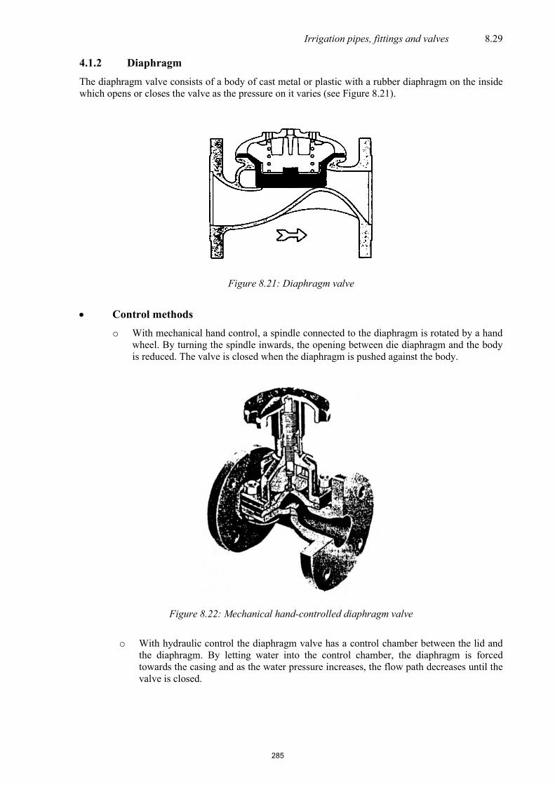
Irrigation pipes, fittings and valves 8.29
4.1.2 Diaphragm The diaphragm valve consists of a body of cast metal or plastic with a rubber diaphragm on the inside which opens or closes the valve as the pressure on it varies (see Figure 8.21).
Figure 8.21: Diaphragm valve
• Control methods
o With mechanical hand control, a spindle connected to the diaphragm is rotated by a hand wheel. By turning the spindle inwards, the opening between die diaphragm and the body is reduced. The valve is closed when the diaphragm is pushed against the body.
Figure 8.22: Mechanical hand-controlled diaphragm valve
o With hydraulic control the diaphragm valve has a control chamber between the lid and
the diaphragm. By letting water into the control chamber, the diaphragm is forced towards the casing and as the water pressure increases, the flow path decreases until the valve is closed.
285

8.30 Irrigation User Manual
Figure 8.23: Hydraulically controlled diaphragm valve
4.1.3 Saddle Saddle valves used in irrigation consist of a number of components (see Figure 8.24). The working principle is that a sealing disc moves up and down in the body on a shaft, changing the flow path area and also sealing the valve.
1. Y-pattern wide body 2. Sealing cap 3. Double chamber activator 4. Diaphragm 5. Seal
Figure 8.24: Saddle valve with double chamber hydraulic control
• Control methods
o This valve may also be hydraulically controlled as a single or double chamber valve by making use of water pressure in the control chambers.
Figure 8.25: Mechanical hand-controlled saddle valve
1. Wheel 2. Spindle 3. Seal
286

Irrigation pipes, fittings and valves 8.31
o The valve may be controlled mechanically by hand by turning the spindle and key piece to which the sealing disc is attached, in or out (see Figure 8.25).
4.1.4 Ball The ball valve is a relatively new design which is now more frequently being used in agriculture. It consists of a body, ball and sealing area.
Figure 8.26: Ball valve The ball valve rotates through 90º between fully open and fully closed. It is maintenance-free with no external seals that need replacing. The hydraulic forces within the valve are balanced and little force is needed to open and close it. Most agricultural ball valves have the same ball opening diameter as the pipeline, making pressure losses across the valve small compared to other valves. Ball valves may be used for flow and pressure regulation. Manufacture is economical and new developments in the plastic industry have made the seals more reliable. They are compact and light and may be installed in any position. NB: Due to the control lever only rotating through 90º these valves may easily be closed too quickly, possibly causing water hammer and pipeline damage. 4.1.5 Butterfly Similar to the ball valve, the butterfly valve is a relatively recent development which may successfully be applied to agriculture. It consists of a body, sealing disc, seal and gearbox or lever.
287

8.32 Irrigation User Manual
Figure 8.27: Butterfly valve
A shaft runs through the middle of the sealing disc, which is located by means of rivets, splines or square shaft. The valve is opened or closed by rotating the sealing disc through 90º by means of a lever or gearbox. In the open position the disc is rotated parallel to the flow and in the closed position it is rotated perpendicular to the flow. A rubber seal in the body or sealing disc provides a drip-free seal. The hydraulic forces in the butterfly valve are balanced due to its design, making its use in pipelines easier. In the open position, only the leading edge of the sealing disc faces the flow, resulting in relatively low losses across the valve. Butterfly valves may also be used for pressure or flow control, but care must be taken that the valve is at least 15-20% open (contact manufacturer). Always ensure that high-quality butterfly valves are used as some low-quality valves easily leak after being used a few times. Butterfly valves are virtually maintenance-free ‒ they are very light and compact and may be installed in any position. The larger models (250 mm and larger) should preferably be installed with the shaft horizontal, ensuring that the load is spread evenly between the supports. It is very important that the valve be in an open position during installation to avoid seal damage. As with the ball valve, the butterfly valve can be closed too quickly, therefore it is advisable to use a gearbox with larger valves, ensuring slower operation. 4.2 Valve control mechanisms Valves may be controlled in three ways, namely mechanically, hydraulically or spontaneously. 4.2.1 Mechanical control These are manually controlled valves with threaded mechanisms or levers to control the valves (see Section 4.1). 4.2.2 Hydraulic control The hydraulic control system makes use of pipeline pressure to open and close the valve. External energy sources (e.g. air pressure) may also be used to close the valve, while certain types (double chamber) can also be opened by these forces. The hydraulic control mechanism may be equipped with a pilot valve, solenoid or relay for automatic valve control. Therefore, various possibilities exist for using hydraulically controlled valves in agriculture and various problems may be solved.
288

Irrigation pipes, fittings and valves 8.33
The following equation is used to determine the force exerted on a surface by a fluid under pressure:
F = PA (8.1) where F = force [N], P = pressure [N/m2], and A = area [m2] This equation shows that there is an increase in force with and increase in area, for the same pressure.
• Different areas If the pressure is the same in the top and bottom of the cylinder, the piston will move downwards due to the difference in area between 1 and 2 (see Figure 8.28). When the upper chamber of the cylinder is opened to atmosphere, releasing the pressure, the piston will move upwards due to pressure in the lower chamber.
Figure 8.28: Hydraulic operation with constant pressures and different areas
• Pressure difference If the surface areas are equal, a difference in pressure across the valve is required to cause different forces. This pressure difference is caused by the spring action and friction when there is flow through the valve. In a no-flow situation, the diaphragm will be pushed downwards by the spring.
Valve closed Valve open
Figure 8.29: Hydraulic operation with equal areas and different pressures
289

8.34 Irrigation User Manual Single chamber control The single chamber valve consists of a body, lid, spring and diaphragm or diaphragm combination.
Figure 8.30: Section through a single chamber valve The single chamber valve operates on the following principle:
- By opening the control chamber to atmosphere, the pressure (if higher than minimum working pressure) in the pipeline will lift the diaphragm, opening the valve. To close the valve, pressure from the upstream side of the valve is applied to the diaphragm chamber, causing a pressure balance above and below the diaphragm. With no flow through the valve the spring will push the diaphragm to the closed position. With flow through the valve, the spring action will initiate the closing action, therefore the diaphragm will start moving to the closed position. Once this action has started, the difference in the upstream and downstream pressures increases progressively, causing the valve to close faster and faster. Care must therefore be taken to control the closing speed with certain types so as to prevent pipeline shocks.
• Double chamber control The double chamber valve has a body and a work-piece which is totally removable and consists of the following parts:
o Sealing disc o Shaft o Separator o Diaphragm o Diaphragm supports o Lid
1. Mechanical choke 2. Opening to upper control chamber 3. Lid 4. Diaphragm 5. Opening to lower control chamber 6. Diaphragm support 7. Shaft 8. Sealing disc 9. Body
10. Sealing area Figure 8.31: Double chamber valve
1. Lid 2. Spring 3. Diaphragm support 4. Diaphragm 5. Flow direction 6. Body
290

Irrigation pipes, fittings and valves 8.35
The double chamber valve operates as follows:
- The diaphragm has a control chamber on both sides (see Figure 8.31). When the upper control chamber is opened to atmosphere, the valve is opened by pipeline pressure. The area of the control chamber diaphragm is considerably larger than the sealing disc area, therefore if upstream pressure is applied to the upper control chamber, valve closing forces are considerably higher than valve opening forces. Initially the closing force is very high, causing the valve to move rapidly for 70% of the distance, where after the diaphragm starts resting on the separator and the pressure difference across the sealing disc increases. The part of the diaphragm which rests on the separator has no influence on the closing action and in this way the effective area of the diaphragm is reduced. The pressure under the sealing disc then increases while the pressure above it decreases, causing the double chamber valve to close relatively slowly over the remaining 30% of the distance. A very smooth action can be obtained in a double chamber valve with sufficient control over closing speed. The valve can also be opened by applying upstream or external pressure to the lower control chamber, which is not possible with single chamber valves.
Figure 8.32: Schematic diagram of the closing action of double and single chamber valves • Manually-controlled hydraulic action
As the hydraulic valve makes use of internal forces to operate, a simple three-way ball valve may be used to open and close the valve. The ball valve connects the valve control chamber to upstream pressure for closing and to atmosphere for opening. The valve opening may be limited, providing a certain amount of control, by making use of mechanical chokes. If the upstream pressure is too low, an external pressure source may be used to supply the required pressure for valve control.
Figure 8.33: Manually-controlled hydraulic action
291

8.36 Irrigation User Manual • Hydraulic remote control With hydraulic remote control, the valve is connected to a control system by means of a pilot tube. This system is used where electricity is unavailable and the PC must be powered by batteries and/or solar panels. A radio system which connects the valves to a satellite station by means of pilot tubes is also available. However, solenoid control must still be used to send the hydraulic signal to the valve. Hydraulic control can also be done manually with a small valve which connects the pilot tube and the valve for opening or closing it.
Figure 8.34: Hydraulic remote-control
• Electrical remote-control A hydraulic valve of any size can be opened or closed by remote-control by making use of an electrical pilot valve or as generally known, a solenoid. The valve may be connected to a computer (PC) or time-switch and activated at pre-set times, making automation of irrigation systems possible.
Figure 8.35: Electrical control
• Automatic pilot controlled hydraulic valves Pilot valves are used to control hydraulic valves. Each hydraulic valve manufacturer has its own range of pilot valves and should be contacted for information on availability and connection of specific valves. The pilot valve consists of a lid, body, spring, diaphragm and control piston. The three-way pilot valve is the most used in irrigation and it has a signal tube connected to the side at which the pressure must be kept constant (downstream for pressure reduction and upstream for maintaining pressure). This tube is also connected to the bottom of the diaphragm. The balancing force of the pilot valve is provided by an adjustable spring at the top of the diaphragm. When the force exerted by the spring balances out the pressure exerted under the diaphragm, the control piston is positioned so that the hydraulic valve is closed. As soon as the system pressure changes sufficiently, the forces between the spring and the diaphragm will become unbalanced and the pilot valve will change the position of the hydraulic valve by sending
292

Irrigation pipes, fittings and valves 8.37
water to the control chamber or by releasing some of the water in the control chamber into the atmosphere. These changes will continue until the system pressure balances out with the spring adjustment. The tighter the spring is set, the higher the pressure allowed in the system by the pilot.
Figure 8.36: Section through a pilot valve
o Pressure reduction:
The pressure reduction valve makes use of a pilot valve to keep the downstream pressure constant at a pre-set value, irrespective of changes in the upstream pressure and/or the flow in the system. Pressure reduction may be used to maintain constant pressures in irrigation systems, thereby ensuring effective and accurate system discharge:
- to reduce pressure at a high pressure zone so that a lower pipe class may be used. - to eliminate excessive pump pressure when irrigating below design flow rate. -
Figure 8.37: Pressure reduction
o Pressure sustaining The pressure sustaining valve maintains a constant pre-set upstream pressure irrespective of changes in pressure and flow through the system. Pressure sustaining may be used:
- to ensure that the pump does not deliver too much water with the filling of pipelines and switching between irrigation blocks;
- to release excessive pressure from the system; and - to ensure that there is sufficient pressure in the system to serve elevated areas.
293

8.38 Irrigation User Manual
Figure 8.38: Pressure sustainment
o Pressure release The pressure release valve discharges excessive pressure to the atmosphere, thereby protecting irrigation systems against sudden pressure increases.
Figure 8.39: Pressure release
o Water hammer suppression
With water hammer an ordinary pressure release valve is sometimes insufficient or too slow to get rid of the shock. In this case a special coupling on a hydraulic valve is used whereby a pilot valve senses the drop in pressure and activates the valve so that it is open when the water hammer strikes. The valve also acts as a high-pressure release valve with excessive pressure increases.
Figure 8.40: Water hammer suppression
o Controlled opening
A hydraulic valve can open in two stages, by making use of special pilot valves, where a pipeline needs to be filled up slowly.
294

Irrigation pipes, fittings and valves 8.39
o Burst control The burst control valve is used where bursting pipes can cause damage. The valve closes when an increase in flow or a decrease in pressure in the system takes place and will not open again, unless it is opened by hand once pipeline repairs have been completed.
o Pump control The pump control valve is used where pumps are switched on and off by remote control. The valve makes use of a limit switch and solenoid to ensure that the pump switches on and off against a closed valve. When the pump is started, the valve is activated and slowly opens. A pilot may also be used to open the valve to a certain point, thereby avoiding overloading the motor and pump cavitation. When shutting the pump down, the valve closes slowly and the pump is then switched off as indicated by the limit switch. In this way the water in the system is gradually brought into motion and to a standstill. The pump control valve prevents pipeline shocks with switching on and off, motor overloading and pump cavitation. Pressure reduction can simultaneously be done with the valve to protect the system against high pressures at low flows. Certain pump control valves also serve as spring loaded non-return valves.
Figure 8.41: Pump control
o Flow control
The flow control valve prevents the flow through the valve from exceeding a pre-set rate. The purpose of this valve is to prevent borehole pumps with large variations in the dynamic water level from over-pumping or to supply the correct flow to numerous users on one pipeline.
o Filter flushing control The filter flushing control mechanism is used with filter back-washing where two valves are normally used. Water enters the filter through a main valve which closes during back-washing, when a flushing valve between the main valve and the filter opens to atmosphere. Water from the other filter or filters in the set then flows through the filter in the opposite direction, back-washing it and is released to the atmosphere. Various models are available and suppliers must be consulted on the precise operation of the flushing valve. It is important that the valves operate correctly and that flow-mixing does not take place while the valves change positions. Certain types of filters require specific back-wash valves. The so-called direct action valves with less complicated operation are now also available.
295

8.40 Irrigation User Manual
Figure 8.42: Filter flushing control
o Water level control Water level may be controlled with hydraulic valves in two ways:
- Modulating: The modulating water level control valve keeps the water level in a reservoir at a constant level. It is used in reservoirs, dams and pressure-reducing chambers.
- Multi-level: The multi-level pilot valve allows the water to drop to a pre-set minimum level. The valve then opens and the reservoir is filled to a pre-set maximum level. It is used in larger reservoirs and where two levels (minimum and maximum) must be maintained. Certain types of multi-level valves make use of external energy sources (water and air pressure) to operate.
Figure 8.43: Water level control
o Non-return valve
The hydraulic valve may be used very successfully as a non-return valve. Care must be taken in choosing a non-return valve. If water hammer is possible, a non-return valve may worsen the situation, or provide a solution to an extent. The non-return valve must either close as soon as the flow rate is interrupted or a valve which closes slowly without causing water hammer, must be used. The double chamber hydraulic valve can close by means of a spring before any return flow occurs in the system. By making use of needle valves a hydraulic valve can close at any adjustable rate without causing pipeline shocks.
296

Irrigation pipes, fittings and valves 8.41
Figure 8.44: Non-return valve
o Volumetric valves
The volumetric valve consists of a water meter combined with a hydraulic valve which is available in one compact body. The valve may be used to close after a pre-set volume of water has passed through or to open another valve by means of a hydraulic signal. It can also form a semi-automatic system by connecting two or more valves with hydraulic tubes.
Figure 8.45: Volumetric valve
o Electrical control mechanism
An electrical control mechanism may be used with a volumetric valve instead of hydraulic control. This type of valve is known as a hydrometer (see Figure 8.46).
Figure 8.46: Hydrometer
1. Water meter control cap 2. Lid 3. Diaphragm 4. Impeller 5. body
297

8.42 Irrigation User Manual 4.2.3 Spontaneous control valves Spontaneous control valves function automatically without external influences. • Air valves Air valves are used to release air from pipelines and to let air into draining pipelines. Trapped air in pipelines can create big problems in the system. Air can reduce the cross-sectional area of a pipe, creating unforeseen pressure losses. An increase in velocity occurs where the water flows through the reduced area and when it becomes high enough to remove the trapped air and the sudden inflow of water may cause pipeline damage. The presence of air in a system can also cause pressure reducing valves to work in cycles, causing pipe breakages. Air in a pipeline also promotes algae growth and the presence of air in a centrifugal pump will break the water column and stop pumping. Basically three types of air valves are available:
o Kinetic The kinetic air valve releases larger volumes of air during pipeline filling and closes in the presence of water. With pipeline drainage air is drawn into the pipeline to prevent it from being flattened by atmospheric pressure.
o Automatic The automatic air valve releases smaller volumes of air when the pipeline is under pressure and cannot be used as an anti-vacuum valve.
o Combination The combination air valve has a kinetic and automatic function.
Figure 8.47: Operation of different air valves
4.2.4 Placing of air valves Air valves must be installed at the following positions on a pipeline: 4.2.4.1 Peaks
Firstly, multi-purpose air valves are required at all possible positions where peaks may arise. Peaks arise wherever the pipeline has a reversal of slope with respect to the hydraulic gradient (which in reality represents the imaginary free water level along the pipeline), creating low-pressure zones where air can accumulate. These peaks can also, under specific circumstances, form peaks with the horizon. Examples of both situations are shown in Figure 8.48.
298

Irrigation pipes, fittings and valves 8.43
Figure 8.48: Pipe section forming peaks i.r.o (a) both the HG and horizon, and
(b) Only the HG
In this way a peak occurs at any section of a pipeline located parallel to the hydraulic gradient (refer to Figure 8.49). Air valves are required at least at the ends of such a pipe section, and possibly also in between, depending on its length.
Figure 8.49: Pipe section parallel to hydraulic gradient constitutes a peak
• Slope changes which do not create peaks
Air can accumulate at any point where a descending slope steepens (refer to Figure 8.50). While a peak is not formed, it is advisable to install at least a small orifice air valve at this point.
Figure 8.50: Descending pipe section with increase in descending gradient
299

8.44 Irrigation User Manual Similarly, it is good practice to install at least a small orifice air valve at any point where an ascending slope levels off (refer to Figure 8.51).
Figure 8.51: Ascending pipe section with decrease in ascending gradient
• Long, ascending pipe sections
A multi-purpose air valve, as required above in Section 4.3.4.1 will in any case be provided at the peak. Additional valves may be required, mainly to accommodate high air flow rates during filling or draining, depending on the length of the section. These air valves will mostly be the large orifice type spaced at approximately 400 – 800 m as shown on Figure 8.52.
• Long, descending pipe sections
Such cases are basically approached in the same way, except that multi-purpose air valves will definitely be used as shown in Figure 8.52.
Figure 8.52: Long, descending pipe section
• Long, horizontal pipe sections (slopes < 1:500)
As previously mentioned, such circumstances must be avoided as far as possible. If, however, they are unavoidable, multi-purpose air valves must in any case be provided at the ends of the section as well as at 400 to 800 m intervals.
300

Irrigation pipes, fittings and valves 8.45
• Precise position where air accumulation occurs
It is important to note that, while air accumulations will occur at peaks, with regard to the horizon, the precise position of the air accumulation is actually situated at the point where a peak with regard to the HG can be identified as shown below in Figure 8.53
Figure 8.53: Actual position of air accumulation and air valve
Therefore, the precise position of the air valve should in all cases be determined with great care. • Vacuum conditions
While the normal placing of air valves in a system mostly makes sufficient provision for air inlet at high flow rates, a need for anti-vacuum valves (air inlet valves) arises under circumstances where air valves would not necessarily have been provided.
Vacuum forming can take place due to:
- Burst pipes - Defective couplings - Closing of automatic valves - Valves being closed - Opening of scour valves
Relatively low-cost, purpose-made valves are commercially available and should be placed especially at the downstream side of irrigation system valves. Note that class 4 uPVC pipes can only withstand 4 to 5 m vacuum before collapse. Low-density polyethylene, especially smaller diameter class 3 pipes, are also not designed to resist any vacuum conditions at all. • The pipeline as a whole
When provision is made for air valves (inlet and outlet) at all positions as individually considered, it is advisable to investigate the pipeline as a whole to ensure that a sufficient number of air valves have been provided in the total design. Generally, more air valves are provided in the first section of a pipeline than the last section. While precise rules cannot be made, air valves can generally be placed as close as 150 m apart at the beginning of a pipeline and as far as 800 m and even 1 000 m apart over the last section. It is generally good practice to ensure that as much air as possible is removed from high pressure sections so that less remains in low-pressure zones to expand and result in closures or shock loads.
301

8.46 Irrigation User Manual • Foot valves
A foot valve is mounted at the end of the suction pipe and is used where the pump is higher than water level. The purpose of a foot valve is to prevent water from flowing backwards from the suction pipe and pump when the pump is switched off. The foot valve is equipped with a strainer to prevent particles that can damage or block the pump from being sucked in.
o Spring-loaded foot valve This type of foot valve is used most often. It is reliable and may be installed horizontally or vertically.
Figure 8.54: Spring-loaded foot valve
o Diaphragm foot valve
This type of foot valve has a reliable operation and it can be installed horizontally or vertically. It is not widely used due to its relatively high cost.
Figure 8.55: Diaphragm foot valve
o Swing foot valve
This type of valve must be installed vertically to ensure correct operation.
Figure 8.56: Swing foot valve
302

Irrigation pipes, fittings and valves 8.47
• Non-return valve The non-return valve forms an integral part of any irrigation system and its function is to allow flow in one direction only. Some of the general non-return valve uses are as follows:
o To prevent pipelines from draining after pumping has stopped o To prevent pumps in parallel from working against each other o To divide pipelines into sections, thereby reducing the occurrence of water hammer o As a bypass with pumps where the pipeline must be fed to prevent column separation o As foot valves with pumps to prevent drainage of suction pipes
A large variety of non-return valves is available on the market. It must be decided which type of non-return valve is to be used in an installation. Heavy-duty non-return valves, anchored on concrete, are usually used in pumping stations to prevent pump damage by water hammer or changing of the alignment between pump and motor. Lighter thin disc non-return valves are used to isolate pumps connected in parallel. Water hammer may be relieved by using a non-return valve which closes before any return flow in the pipeline takes place, the ideal type being the spring-loaded version. Smaller non-return valves may also be used as anti-vacuum valves to allow air to enter draining pipelines. Hydraulic valves may also be used as slow-action non-return valves.
Figure 8.57 Spring-loaded swing non-return valve
• Float valves This is a valve which is controlled by a floating ball attached to a lever. It is used where the water level must be kept at a certain height.
Figure 8.58: Float valve
303
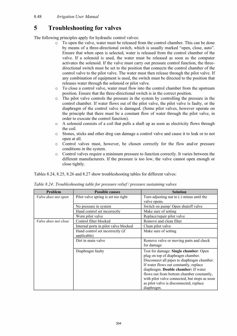
8.48 Irrigation User Manual 5 Troubleshooting for valves The following principles apply for hydraulic control valves:
o To open the valve, water must be released from the control chamber. This can be done by means of a three-directional switch, which is usually marked “open, close, auto”. Ensure that when open is selected, water is released from the control chamber of the valve. If a solenoid is used, the water must be released as soon as the computer activates the solenoid. If the valve must carry out pressure control function, the three-directional switch must be set to the position that connects the control chamber of the control valve to the pilot valve. The water must then release through the pilot valve. If any combination of equipment is used, the switch must be directed to the position that releases water through the solenoid or pilot valve.
o To close a control valve, water must flow into the control chamber from the upstream position. Ensure that the three-directional switch is in the correct position.
o The pilot valve controls the pressure in the system by controlling the pressure in the control chamber. If water flows out of the pilot valve, the pilot valve is faulty, or the diaphragm of the control valve is damaged. (Some pilot valves, however operate on the principle that there must be a constant flow of water through the pilot valve, in order to execute the control function).
o A solenoid consists of a coil that pulls a shaft up as soon as electricity flows through the coil.
o Stones, sticks and other dreg can damage a control valve and cause it to leak or to not open at all.
o Control valves must, however, be chosen correctly for the flow and/or pressure conditions in the system.
o Control valves require a minimum pressure to function correctly. It varies between the different manufacturers. If the pressure is too low, the valve cannot open enough or close tightly.
Tables 8.24, 8.25, 8.26 and 8.27 show troubleshooting tables for different valves: Table 8.24: Troubleshooting table for pressure relief / pressure sustaining valves
Problem Possible causes Solution Valve does not open Pilot valve spring is set too tight Turn adjusting nut to (-) minus until the
valve opens. No pressure in system Switch on pump/ Open shutoff valve Hand control set incorrectly Make sure of setting Worn pilot valve Replace/repair pilot valve
Valve does not close Control filter blocked Remove and clean filter Internal ports in pilot valve blocked Clean pilot valve Hand control set incorrectly (if applicable)
Make sure of setting
Dirt in main valve Remove valve or moving parts and check for damage
Diaphragm faulty Test for damage: Single chamber: Open plug on top of diaphragm chamber. Disconnect all pipes to diaphragm chamber. If water flows out constantly, replace diaphragm. Double chamber: If water flows out from bottom chamber constantly, with pilot valve connected, but stops as soon as pilot valve is disconnected, replace diaphragm.
304

Irrigation pipes, fittings and valves 8.49
Table 8.25: Troubleshooting table for electrical control valves
Problem Possible causes Solution Valve does not open
No electricity supply Check/switch on No pressure in system Switch on pump/ Open isolator valve Solenoid: a) Shaft is stuck b) Ports blocked c) No activation click or coil is damaged
a) Check and clean b) Check and clean c) Replace spool. Ensure that supply current is the
same as solenoid specifications. Hand control set incorrectly Check
Valve does not close
Control filter blocked Remove and clean filter Hand control set incorrectly Check Solenoid: a) Remains switched on b) Ports blocked
a) Switch power off b) Check and clean
Dirt in main valve Remove valve or working parts and check for damage
Diaphragm faulty Test for damage: Single chamber: Open plug at top of diaphragm chamber. Disconnect all pipes to diaphragm chamber. If water flows out constantly, replace diaphragm. Double chamber: If water flows out of bottom chamber constantly with pilot valve connected, but stops as soon as pilot valve is disconnected, replace diaphragm.
Table 8.26: Troubleshooting table for pressure reducing valves
Problem Possible causes Solution Valve does not open
No pressure in system Switch pump on/Open valve No flow in system Switch pump on/Open valve Pilot valve set incorrectly Turn adjusting nut to (+)plus Hand control set incorrectly Check Pilot valve blocked Remove and clean filter
Valve does not close
Control filter blocked Remove and clean filter Hand control set incorrectly Check Dirt in main valve Remove valve or working parts and check for damage Diaphragm faulty Test for damage: Single chamber: Open plug on top of
diaphragm chamber. Disconnect all pipes to diaphragm chamber. If water flows out constantly, replace diaphragm. Double chamber: If water flows out constantly with pilot valve disconnected, replace diaphragm. Take care: This test will cause the valve to go to fully open position. Ensure that no damage will be done to the system.
Valve does not control pressure
Pilot valve is worn Check/Replace/Repair Valve constantly opens and closes
Control valve too large/Pressure difference too great/Flow too low ‒ Replace control valve, delay operating speed or use another type of pilot valve
Air trapped in control chamber Loosen seal at highest point of control chamber and let air escape
305

8.50 Irrigation User Manual Table 8.27: Troubleshooting table for sluice valves
Problem Possible causes Solutions Valve leaks Packing gland faulty/loose Tighten packing gland, replace packing Valve does not function
Screw thread damaged Replace nut and/ or shaft Bush on sluice broken Replace bush Sluice has corroded and rusted Dismantle and clean Valve has difficulty functioning ‒ turns heavily
Relieve tension on packing gland, lubricate screw-thread
6 The measurement system
The high water and pump costs make it essential for producers to know how much they irrigate. The National Water Act also requires that producers’ water be measured to ensure that they do not extract too much water. Wide-scale implementation of measuring devices can be expensive but a phased approach can help manage the expenditure. At the very least, flow into the canal system and all outflows from the system (including deliveries to farms) should be measured to ensure fair and equitable distribution of water. Thereafter, more interim measuring locations can be identified and equipped to assist the WUA with on-scheme efficiency. 6.1 Water meters Water meters are more frequently used in the field of irrigation. The high water and pump costs make it essential for the producer to know how much is applied. The National Water Act also requires that the producer’s water use is measured to ensure that the producer does not extract more than the authorised allocation. Computerised systems also make use of the impulses from the water meter to allow the correct volume of water to the block. The water meter, however, does lose its function if it does not measure correctly. The manufacturer’s prescriptions must, therefore, be strictly adhered to, to ensure that the water meter adheres to the flow and general conditions. In general, irrigation water contains a large amount of physical impurities such as silt and watergrass, which can influence the operation of the meter. The following three types of meters are used for irrigation water metering, but each one is more or less suitable for different conditions, as described below: • Straight-flow water meters The meter consists of a turbine driven by water flow in the pipe. The turbine is connected to a meter by means of mechanical or magnetic connection. This type of meter is suitable for horizontal, vertical or angled mounting. A length of straight pipe must be installed before and after the meter to eliminate turbulence (usually 5 times the diameter before and 3 times the diameter after the meter). Due to the obstruction that the turbine causes in the casing, this type of meter is relatively sensitive to impurities such as watergrass and sticks occurring in the water. It can get stuck in the mechanism of the meter and thus lead to inaccurate readings. Sand and fine silt can easily move through the meter, but it can lead to wear and tear of the casing and/or metering mechanism. The meters are however relatively cheap (depending on the size), usually have an accuracy of ± 5% over a specific series of flow rates and requires no electricity to function.
306

Irrigation pipes, fittings and valves 8.51
Figure 8.59: Straight-flow water meter
• Proportional or “bypass-flow” water meter
This type of meter consists of a casing with a by-pass to a smaller diameter pipe, which leads a proportional share of the flow to be measured, parallel to the mainline through a smaller water meter. The reading on the water meter is brought into relation with the total flow in the mainline by means of a calibration process. The meter allows sticks and large impurities through easily, but the by-pass can become blocked if the water contains a large amount of sand and silt. The meters are slightly cheaper than an equivalent straight-flow meter, because a small measuring mechanism is used and it has the same installation requirements and accuracy as the straight-flow water meters.
Figure 8.60: Proportional water meter
• Electro-magnetic flow meters The function of electro-magnetic flow meters depends on the principle that a potential difference can be induced in a conductor which moves through an electric field. The water stream acts as a conductor and for a certain electrical field strength, the potential difference is proportional to the movement speed of the conductor (i.e. the flow velocity of the water). The meters are particularly suited for irrigation because there are no moving parts or obstructions in the flow path of the water. It is also more accurate than mechanical meters (up to ± 1%). Unfortunately the meters require electricity to function and are three to five times more expensive than the
307

8.52 Irrigation User Manual mechanical meters. It can, however, collect more comprehensive data, as the flow rate as well as the time of the metering can be stored.
Figure 8.61: Electro-magnetic flow meter
308

Irrigation pipes, fittings and valves 8.53
7 References 1. Bermad Control Valves for Waterworks, industrial and irrigation applications. Bermad,
Israel.
2. DPI Plastics. Duroflo. uPVC watermains.
3. Lategan, M.T, Burger, J.H, Heyns, P.J., Mulder, D.J., Kleynhans, E.P.J., Koegelenberg, F.H., Smal, H.S., Stimie, C.M., Uys, W.J. and Van der Merwe, F.P.J., Viljoen, P.D. 1996. Irrigation Design Manual. ARC-Institute for Agricultural Engineering. RSA.
4. Smit, I. 1993. Pype in die Landbou.. Directorate: Irrigation Engineering, Department of
Agriculture, RSA.
5. Van der Stoep, I. 2015. Irrigation efficiency training material. WRC Report No, KV 342/1/15. ISBN 978-1-4312-0716-9
6. Van der Stoep, I., Pott, A., Viljoen, J.J., Van Vuuren, A.M.J. 2012. Guidance for Sustainable On-farm and On-scheme Irrigation Water Measurement. WRC Report No. TT 550/12
7. Volschenk, A. 1996. Personal communication. RSA.
309

IRRIGATION USER MANUAL
CHAPTER 9
Drip and micro-sprinkler irrigation systems
310

Table of Contents
1 Introduction ................................................................................................................................ 9.1
2 Emitters ....................................................................................................................................... 9.1 2.1 Drippers................................................................................................................................. 9.4
2.1.1 Mounting ..................................................................................................................... 9.4 2.1.2 Composition ................................................................................................................. 9.5 2.1.3 Components ................................................................................................................. 9.6 2.1.4 Pressure compensating mechanisms ............................................................................ 9.7
2.2 Micro-sprinklers .................................................................................................................... 9.7 2.2.1 Mounting ..................................................................................................................... 9.7 2.2.2 Composition ................................................................................................................. 9.7 2.2.3 Components ................................................................................................................. 9.8
2.3 Choice ................................................................................................................................. 9.10 2.3.1 Drip or micro ............................................................................................................ 9.10 2.3.2 Pressure sensitive or pressure compensating ............................................................ 9.11 2.3.3 Different drip system concepts ................................................................................. 9.12 2.3.4 Different micros ........................................................................................................ 9.14
3 Laterals and manifolds .............................................................................................................. 9.16
3.1 On-line mounted emitters.................................................................................................... 9.16 3.2 In-line and internally mounted emitters .............................................................................. 9.16 3.3 Flushing .............................................................................................................................. 9.16 3.4 Supply manifolds ................................................................................................................ 9.17 3.5 Flushing manifolds ............................................................................................................. 9.17
4 Filtration ................................................................................................................................... 9.17
4.1 Filter types .......................................................................................................................... 9.18 4.1.1 Screen (mesh) filters .................................................................................................. 9.18 4.1.2 Disc filters .................................................................................................................. 9.19 4.1.3 Media (Sand) filters ................................................................................................... 9.21
4.2 Selection of filter type ........................................................................................................ 9.22 4.2.1 Drip systems .............................................................................................................. 9.22 4.2.2 Micro systems ............................................................................................................ 9.22
4.3 Selection of filter size or filter capacity ............................................................................. 9.22 4.3.1 Maximum flow rate ................................................................................................... 9.22 4.3.2 Dirtiness of the water ................................................................................................. 9.23 4.3.3 Cleaning cycle ........................................................................................................... 9.23
4.4 Pre-filtering and treatment .................................................................................................. 9.24 4.4.1 Settling and aeration .................................................................................................. 9.24 4.4.2 Acid treatment ........................................................................................................... 9.25 4.4.3 Chlorination ............................................................................................................... 9.25 4.4.4 Sand separators ......................................................................................................... 9.26
5 Automation ............................................................................................................................... 9.26
5.1 Mechanical/hydraulic ......................................................................................................... 9.27 5.2 Electric/hydraulic ............................................................................................................... 9.28 5.3 Computerised systems ........................................................................................................ 9.29
5.3.1 Requirements ............................................................................................................. 9.30 5.3.2 Design approach ........................................................................................................ 9.30
6 Installation ................................................................................................................................ 9.32
6.1 Installation of laterals ......................................................................................................... 9.32 6.2 Flushing of irrigation system .............................................................................................. 9.32 6.3 Filter station ........................................................................................................................ 9.32 6.4 Irrigation material ............................................................................................................... 9.33
311

7 Evaluation after installation ...................................................................................................... 9.33
8 Management ............................................................................................................................. 9.36
8.1 Water application ............................................................................................................... 9.36 8.2 Filtering .............................................................................................................................. 9.38 8.3 Pressure control .................................................................................................................. 9.39
9 Maintenance.............................................................................................................................. 9.39
9.1 Water quality ...................................................................................................................... 9.40 9.2 Water purification methods ................................................................................................. 9.42
9.2.1 Solutions for preventing blockages resulting from physical factors ......................... 9.42 9.2.2 Chemical water treatment ......................................................................................... 9.44 9.2.3 Biological blockage control ...................................................................................... 9.50
9.3 Prevention of root penetration ........................................................................................... 9.50 9.4 Maintenance schedules of micro-irrigation systems ......................................................... 9.50
10 Trouble shooting tables ............................................................................................................. 9.54
11 References ................................................................................................................................. 9.54
All rights reserved Copyright 2019 ARC-Agricultural Engineering (ARC-AE)
312

313

Drip and Micro-sprinkler irrigation systems 9.1
1 Introduction The concept of micro irrigation originated during the initial “discovery” and development of drippers and drip irrigation in Israel. However, its inevitable evolutionary process (as well as opposition) consequently led to the invention of micro-sprinklers. The original term "micro spray irrigation" was soon abbreviated to "micro irrigation.” This created some confusion, which prompted the current generation of irrigation experts to stop referring to the concept, but rather to refer in the vernacular to the two main components which are used to apply the concept as - • drippers (drip irrigation systems or drip systems); and • micro-sprinklers, also called micros (or mini-sprinklers by some manufacturers). Micro irrigation, which is discussed as a comprehensive concept in this chapter, therefore includes all irrigation systems which share the following characteristics: • In most cases, partial area wetting is applied • A short cycle approach is followed • A low emitter delivery is maintained (between 0,5 and 300 /h) • Low operating pressures are required (ideally between 50 and 300 kPa). Although care has been taken in this chapter to avoid any kind of confusion between the concept and the system, future references to the system will be drip systems and micro systems, and the emitters will be called drippers and micros. Some manufacturers also have products that are known as midi sprinklers, that delivers water at flow rates typically up to 600 /h. The most important physical characteristics which distinguish between drip and micro systems are given in Table 9.1. 2 Emitters The mechanisms which let out water from the laterals into the atmosphere are known as emitters. Emitters are found in a large variety of characteristics and shapes, covering the whole spectrum from small button-shaped drippers to sprinklers. This chapter concentrates on the two emitters usually associated with the concept of micro irrigation, namely drippers and micros. There is a substantial difference between drippers and micros, mainly due to the disparity in discharge rates, as well as the difference in the methods of applying the water. These characteristics are clearly highlighted in Table 9.1. Table 9.1: Some directives with regard to characteristics of drip and micro systems
Characteristic
Drip systems
Micro systems
Application
Row crops (both permanent and annual crops), also underground on pastures,
sugar, cotton, for instance
Row crops (both permanent and
annual crops), also single plants or large trees (e.g. nuts)
Method of application
of water
Point application by means of drip action, lateral distribution by soil
Surface distribution by means of spray
action (1-10 m diameter)
Potential system efficiency
95% +
85 to 90% +
Mounting of emitter in
relation to lateral
On wall inside lateral, or in-line as integral part of tubing, or directly/ indirectly on outer wall of tubing
On outer wall of lateral (either directly
on pipe, or mostly on micro tubing with plastic stand)
314
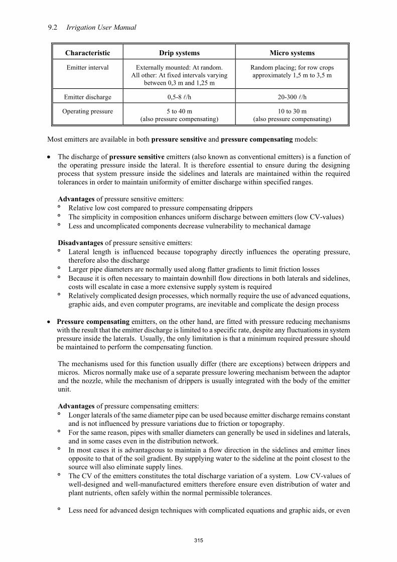
9.2 Irrigation User Manual
Characteristic
Drip systems
Micro systems
Emitter interval
Externally mounted: At random.
All other: At fixed intervals varying between 0,3 m and 1,25 m
Random placing; for row crops approximately 1,5 m to 3,5 m
Emitter discharge
0,5-8 /h
20-300 /h
Operating pressure
5 to 40 m
(also pressure compensating)
10 to 30 m
(also pressure compensating)
Most emitters are available in both pressure sensitive and pressure compensating models: • The discharge of pressure sensitive emitters (also known as conventional emitters) is a function of
the operating pressure inside the lateral. It is therefore essential to ensure during the designing process that system pressure inside the sidelines and laterals are maintained within the required tolerances in order to maintain uniformity of emitter discharge within specified ranges.
Advantages of pressure sensitive emitters: ° Relative low cost compared to pressure compensating drippers ° The simplicity in composition enhances uniform discharge between emitters (low CV-values) ° Less and uncomplicated components decrease vulnerability to mechanical damage
Disadvantages of pressure sensitive emitters: ° Lateral length is influenced because topography directly influences the operating pressure,
therefore also the discharge ° Larger pipe diameters are normally used along flatter gradients to limit friction losses ° Because it is often necessary to maintain downhill flow directions in both laterals and sidelines,
costs will escalate in case a more extensive supply system is required ° Relatively complicated design processes, which normally require the use of advanced equations,
graphic aids, and even computer programs, are inevitable and complicate the design process • Pressure compensating emitters, on the other hand, are fitted with pressure reducing mechanisms
with the result that the emitter discharge is limited to a specific rate, despite any fluctuations in system pressure inside the laterals. Usually, the only limitation is that a minimum required pressure should be maintained to perform the compensating function.
The mechanisms used for this function usually differ (there are exceptions) between drippers and micros. Micros normally make use of a separate pressure lowering mechanism between the adaptor and the nozzle, while the mechanism of drippers is usually integrated with the body of the emitter unit.
Advantages of pressure compensating emitters: ° Longer laterals of the same diameter pipe can be used because emitter discharge remains constant
and is not influenced by pressure variations due to friction or topography. ° For the same reason, pipes with smaller diameters can generally be used in sidelines and laterals,
and in some cases even in the distribution network. ° In most cases it is advantageous to maintain a flow direction in the sidelines and emitter lines
opposite to that of the soil gradient. By supplying water to the sideline at the point closest to the source will also eliminate supply lines.
° The CV of the emitters constitutes the total discharge variation of a system. Low CV-values of well-designed and well-manufactured emitters therefore ensure even distribution of water and plant nutrients, often safely within the normal permissible tolerances.
° Less need for advanced design techniques with complicated equations and graphic aids, or even
315

Drip and Micro-sprinkler irrigation systems 9.3
computer programs for the design process. Sensible application of basic pipe hydraulics is all that is required.
Disadvantages usually associated with pressure compensating emitters:
° Complicated composition involves more components, resulting in increased vulnerability ° The composition of the emitter components makes it difficult to maintain low CV-values ° Higher emitter costs
As discussed in Appendix A of Chapter 5, an emitter’s discharge is pressure sensitive (Figure 9.1) unless the emitter is fitted with a pressure compensating mechanism, in which case it will be able to supply a constant discharge over a certain pressure range (Figure 9.2).
Figure 9.1: Pressure sensitive drippers: Typical discharge graphs
316

9.4 Irrigation User Manual
Figure 9.2: Pressure compensating drippers: Typical discharge graphs
2.1 Drippers The first drippers for irrigation purposes were developed in Israel during the early sixties and launched in South Africa in 1969. An Israeli engineer, Simca Blass, noticed that a leaking pipe connection in a fruit orchard had an unusually positive effect on the single tree where the “fault” was located. He immediately recognised the concept, accepting the challenge of causing artificial leakages to pipes which can function at controlled, ultra-low discharge rates without squirting or blocking. Since then, the development of the concept has led to the availability of a large variety of drippers which can satisfy every imaginable need. 2.1.1 Mounting Drippers can be mounted onto dripper lines in various ways (refer to Figure 9.3):
• Externally on the wall of the pipe
With this approach the diameter of the pipe is irrelevant. Standard, low density polyethylene pipes with small diameters can be used. Likewise, the dripper spacing can be done at random according to the requirements. The only limitation on the size of the emitter is the manufacturing cost. A measure of robustness is also required because of vulnerability to factors such as the movement of people and implements, especially in cases where the dripper is linked to the dripper line by means of extension tubing. These drippers are fitted with a barbed connection which is pressed either into a pre-punched hole in the dripper line, or into the end of the extension tubing.
317

Drip and Micro-sprinkler irrigation systems 9.5
External
External with extensions
Internal
Integral
Figure 9.3: Mounting of drippers to dripper line
• Inside the dripper line
In this variation the dripper is mounted inside the pipe during the manufacturing process of a unique dripper pipe and fixed to the inner wall of the pipe by means of thermal fusing. Standard polyethylene pipes are therefore out of the question. Two kinds of drippers are mainly used: ° Cylindrical drippers are inserted into the pipe, where the wall of the pipe forms the casing
of the dripper. ° Elongated drippers, which are so small that they cause little friction, are fixed to the inner
wall of the pipe during the pipe manufacturing process. • Integral with the wall of the dripper line
In this case the special and unique thin-walled dripper line is manufactured in such a way that the characteristics of the components of a dripper (pressure sensitive or pressure compensating) are formed inside the pipe wall by means of a thermal extrusion process.
2.1.2 Composition Pressure sensitive emitters are usually simple in design and construction, consisting of moulded plastic, while pressure compensating emitters are more complicated in design to incorporate the pressure compensating mechanism, as illustrated in Figure 9.4.
318

9.6 Irrigation User Manual
Figure 9.4: Composition of pressure sensitive (left) and pressure compensating (right) drippers 2.1.3 Components Drippers from different manufacturers vary to such an extent that it is difficult to identify common components. A key component of any dripper, however, is the flow path. The purpose of the flow path is to dissipate the pressure inside the pipe so that water drips rather than sprays out of the dripper. A positive distinction can be made between the two approaches regarding the composition of the flow path: • Long flow path type drippers mainly use friction and turbulence in the flow path to decrease the
lateral pressure until the design discharge is reached. The cross section area of the flow path is usually about 1 mm². Depending on the design approach, the flow path can vary considerably in length, up to 1 m and more. Although flow velocities are relatively low, the flow is regarded as turbulent because of the continuous changes in direction it experiences along the labyrinth.
• Short flow path type drippers usually are physically small and discharge is regulated by means of a built-in mechanism.
The pressure sensitive dripper shown in Figure 9.4 are of the long flow path type, while the pressure compensating emitter has a short flow path.
Common components include the following, among others: 2.1.3.1 Inlet of water from the lateral takes place via the barbed coupling of the type which is mounted on the outside of the lateral. All the other types are provided with openings between the outside of the body and the pressure reducing mechanism, which often is part of the body. This opening is almost always fitted with some kind of grid or screen to prevent dirt that can block the flow path from ending up inside the mechanism. 2.1.3.2 The body houses the pressure reducing mechanism in all cases except the integral type, where the core is situated inside the wall. 2.1.3.3 The casing encloses the body or the active pressure reducing mechanism, and is available in various shapes: • It can be a shell which fits onto the core like the larger button type outside the dripper line • The body and casing can form a homogeneous unit, as with the small button type • It can also be a cylindrical casing which encloses the core like the in-line type • The dripper line itself can form the casing of the dripper, which is mounted inside, as well as
the type which is formed inside the wall of the dripper line (integral drip tape)
319

Drip and Micro-sprinkler irrigation systems 9.7
2.1.3.4 Outlets are provided to all drippers which are exposed to the atmosphere. With all other types, discharge holes are punched into the wall of the dripper line during the manufacturing process. 2.1.4 Pressure compensating mechanisms
These mechanisms are optionally available as components to most tried and tested pressure sensitive emitters. The only known exceptions are the in-line type drippers. In pressure sensitive types, the pressure reducing characteristics of the labyrinth are usually combined with a free-moving diaphragm of which the active part is situated over and on the downstream side of the labyrinth. This diaphragm is manufactured with a high quality synthetic elastic material which is chemically stable in respect of all known chemicals. The water inside the lateral exercises the necessary pressure which causes the diaphragm to distort, thereby reducing the flow opening and keeping the discharge constant. A flushing action usually takes place during the stage that the dripper line is filled with water and before enough pressure is built up to activate the diaphragm.
Typical examples of both types of pressure compensating drippers are illustrated in Figure 9.5.
Figure 9.5: Two examples of typical pressure compensating drippers 2.2 Micro-sprinklers Drippers were soon followed by micros, which initially were in competition with drippers, but later became a welcome supplement to the concept of micro irrigation, filling the many gaps that could not be handled effectively by drippers. 2.2.1 Mounting Due to the nature of their function, these emitters are mounted to the outside of the lateral. Standard low density small diameter polyethylene pipes are therefore used in practice. Spacing may be done completely at will according to requirements. There is therefore no real limitation on the physical size of the emitter, except as far as manufacturing cost is concerned. As in the case of drippers mounted on the outside, a measure of robustness is required due to vulnerability as a result of exposure to environmental factors, such as movement of people and implements. 2.2.2 Composition Most of the micros used in the RSA conform to the general shape and composition as depicted in Figure 9.6.
Cover
Diaphragm
Inlet filter
320

9.8 Irrigation User Manual
2.2.3 Components The following components and variations thereof are shown in Figure 9.6: 2.2.3.1 Inlet coupling The inlet coupling joins the rest of the emitter with the water in the lateral or the extension tube. Two types are generally used: • Screwed fitting: This type is screwed into a pre-punched hole in the lateral, or, alternatively,
screwed into the end of a high-density polyethylene riser pipe. • Barbed fitting: It can be pressed into the lateral through a pre-punched hole, or into the end of
a low density polyethylene or plasticised uPVC extension tube.
Couplings are available as integral parts of the body or as separate components with friction or bayonet type couplings to the body. 2.2.3.2 Body The body or basis structure of a micro is that part which supports or joins together almost all the other components. The body is available as a separate part or it may be an integral part of one or more other components such as a nozzle, and/or the bridge and/or the inlet coupling.
2.2.3.3 Nozzle The nozzle is the component which is designed to regulate the discharge. The shape, length and diameter of the opening determine the discharge at specific pressures. Other characteristics are: • The nozzle may be an integral part of the body or it may be available as a separate,
interchangeable component. • Interchangeable nozzles are usually colour-coded to easily distinguish between the various
diameters (and therefore discharges).
2.2.3.4 Bridge This component has the important function of forming, at the top, either the attachment point for static spreaders, or the bearing in (or on) which the rotating spreader revolves. It is therefore extremely important that the bridge is highly stable to ensure long-term even distribution of water. Other characteristics include: • Usually available as an integral part of the body, but can in exceptional cases also be obtained
as a separate component. • Normally available in the so-called “A” or “G” type shape, depending on the type of
construction of the micro. Removable bridge structures have three supports (for the sake of stability), compared to the single support of the “G” type and the double support of the “A” type.
A type
G type
Rotating Static Rotating Static
Figure 9.6: General composition of micro-sprinklers
321

Drip and Micro-sprinkler irrigation systems 9.9
2.2.3.5 Spreaders Two types of spreaders are normally used. • Rotating type spreaders are water-driven by the stream from the nozzle. The stream of water is
lead along a curved channel in the rotator which changes the stream’s direction of motion to bring about rotation. The shaft is usually supported by the nozzle at the bottom end, and at the top by a bush or pin on the bridge. The only current exception to this composition is the Eintal concept: The spreader in this case is a small shaft which goes through the nozzle and is kept in position by thickened plastic ends (incidentally, this concept has narrow strip wetting and insect proof characteristics).
A large variety of rotating spreaders are available from different manufacturers, each with unique characteristics intended for specific functions. For instance, wide strip, narrow strip and even insect proof type rotating spreaders are available. At no-flow conditions, the latter stops in a position which makes it impossible for insects to penetrate.
• Static spreaders (diffusers) are normally mounted to the bridge, perpendicularly above the
stream of water coming from the nozzle, and in such a way that the stream hits the spreader in the centre. The only known exception to this layout concept is the ‘Microjet’ approach according to which the spreader is mounted directly onto the body in the form of a cap. Distribution takes place through the openings at the top of the vertical walls of the cap.
A wide range of distribution patterns, angles and diameters are available for almost any application, and every manufacturer has unique basic designs for every purpose. Most make use of circular spreaders with flat, convex, concave or ribbed surfaces to spread the water in a specific pattern and to ensure a specific drop size.
Examples of some of the more popular distribution patterns and angles are shown in Figure 9.7.
Figure 9.7: Examples of distribution patterns and angles of some micros
2.2.3.6 Pressure compensators Some manufacturers also provide pressure compensators which are mounted between the micro adaptor and the body and which ensure that any excess pressure in the system is reduced to the design pressure of the emitter. The purpose of this is to ensure that each emitter is subject to identical pressure conditions (resulting in more or less identical discharge rates), as long as the inlet pressures conform to the minimum requirements.
322

9.10 Irrigation User Manual
2.2.3.7 Filter or screen Some manufacturers also supply, as optional equipment, a small mesh filter or screen fitted in a position between the inlet and the body. Its purpose is to trap any dirt that may end up in the lateral before it clogs the nozzle. The screen is easily removable for cleaning purposes. Once again, its utilisation should be physically justifiable and economically beneficial.
2.3 Choice The choice between drip and micro, or between one emitter and another, or even between the concepts of pressure sensitive and pressure compensating emitters, are often done subjectively, or according to preconceived directives, or even based on historical or circumstantial misconceptions. Beware of those commercial designers who are forced to propagate only the agency products of their companies. A situation like this can cause an excellent design to fail dismally. Here are some guidelines according to which this problem can be approached more scientifically:
2.3.1 Drip or micro • Drip irrigation has a higher system efficiency than micro irrigation. • Micros are mechanically more vulnerable than most drip systems. Most drippers are mounted
inside the laterals and under some conditions whole systems can be suspended above ground level.
• Due to the lower emitter discharge of drippers, the standing time is usually longer than that of micros, and the farmer’s operating system should be able to accommodate the choice.
• Cost aspects play a key role and require a careful and objective approach: ° A drip system on citrus, equipped with double dripper lines, can be more expensive than
a micro system. On the contrary, a drip system on a vineyard can be cheaper than a micro system.
° Pressure compensating emitters are generally more expensive than pressure sensitive emitters, but cost savings on the distribution system may completely reverse the picture.
° The role of filtration also cannot be ignored. Cleaner or dirtier water can overturn the cost implications completely in favour of a different type of system.
° Operating pressure also plays an important role from the operational cost point of view and should be considered in the total cost structure.
• Drip systems have limitations because they feature point application, while micros distribute water above-ground. The lateral water spreading capacity of the soil can therefore be a determining factor in the decision-making process.
The shape and size of the wetted profile in the soil are therefore very important for obvious reasons. It should be able to store at least enough water in an area accessible to the feeding roots (or an acceptable part thereof) of the crop. The method of placing irrigation water on top of the soil, as well as the distribution of water in the soil (especially lateral distribution), should correlate well with the nature, shape and extent of the root system, and any limitations affecting these. These aspects are particularly important in cases where no clear-cut decision about drip irrigation can be made. Because characteristics of the crop are normally common knowledge, and limitations from a soil science point of view would have become evident during the soil survey, the only remaining unknown factor is the ability of the soil to distribute irrigation water laterally. Although aspects regarding these characteristics are discussed in more detail in Chapter 3: Soil, attention is once again drawn to the fact that three basic, interactive factors are responsible for this very important characteristic. They are:
° the clay percentage in the soil; and/or ° the percentage fine fraction in the sand; and/or ° the presence of organic material in the soil.
323

Drip and Micro-sprinkler irrigation systems 9.11
The distribution of the water in the soil occurs along the hydraulic gradient between the wet and the dry soil, laterally by means of capillary action and vertically due to gravitation. With point application, this wetting and distribution pattern more or less takes the shape of an onion, as shown in Figure 9.8.
Figure 9.8: Typical water distribution pattern with point application
Micros, on the other hand, distribute the water above-soil. While a much larger wetted area is obtained, it may result in the use of a larger volume of water and shallower wetted depth in the soil. However, it will form the basis for decision-making on the type of system that will eventually be recommended in terms of technical as well as economic considerations. Although these factors are individually quantifiable, their combined effect on the lateral water distribution capacity of the soil as medium, can in no way be calculated theoretically. The only reliable method of establishing this characteristic, is by doing experimental observations and calculations according to specific guidelines.
Procedure for evaluating the soils ability to distribute water laterally: • Lay-out dripper lines, preferably 20 m to 30 m long, on the soil that is to be irrigated, with
different inter dripper spacings. • Connect these to a water source which will render a continuous and stable supply. • Switch on the system at the required operating pressure and irrigate for about 12 hours on the
heavier soils and about six hours on sandy soils. • Allow the water to penetrate the soil for a further 24 and 12 hours respectively, without any
interference, in order that the wet zone can reach its maximum dimensions. • Then dig longitudinal and cross profile furrows and do the necessary observations and
measurements to establish whether the proposed system will satisfy all requirements according to established norms.
2.3.2 Pressure sensitive or pressure compensating Besides the cost aspect discussed in Section 2.3.1, specific technical aspects may necessitate the use of pressure compensating emitters under certain conditions:
• The use of pressure sensitive emitters on very steep inclines may require an impractical number
of branch lines to maintain specified discharge limits. Pressure compensating emitters may possibly provide the only practical solution.
324

9.12 Irrigation User Manual
• Long emitter lines (especially dripper lines with limited diameters), with little or no topographical slope, may have excessive friction losses, and will therefore also not conform to the specified limited discharge tolerances. Additional distribution and/or branch lines, or pressure compensating emitters are the only alternatives.
• Uneven terrain, where topographic features are the only cause for unacceptable emitter discharge deviations, will naturally require pressure compensating emitters.
• Even systems which can easily and economically make use of pressure sensitive emitters, may have sections which will unavoidably endure excess pressure. Pressure compensating emitters will effectively and economically solve the problem.
2.3.3 Different drip system concepts There are mainly two vastly different drip system concepts in use, one of which has not yet been implemented either on large scale or over the long term in South Africa.
2.3.3.1 Conventional concept All systems that make use of the strip wetting principle, both pressure sensitive and pressure compensating modes, fall under this category. Although laterals are traditionally placed above-ground, in some cases it is more beneficial to place them underground. Subsurface (underground) drip irrigation is a specialised application with many specific pros and (especially) cons which requires special care and operational practices. The purpose of the general conventional approach is to create a continuous wet zone in the soil within which sufficient feeding roots of row crops will develop and function satisfactorily. It is therefore important to make maximum use of the lateral water distribution capacity of the soil by means of adequate emitter overlapping. Emitter spacing should therefore be selected sensibly and practically. A pre-assembled dripper line is normally manufactured according to standard manufacturing processes with a wide range of dripper spacing options, ranging from about 0,3 to 1,25 m. Emitter discharge is inevitably a function of emitter spacing. During the scheduling planning process, the required experiments to determine the ideal emitter spacing should therefore already have been completed. The difference between the wetting patterns of, for instance, 2 /h and 4 /h drippers, should also have been sorted out, with due consideration to both the economic and scheduling implications. If this interactive process should eventually determine a discharge rate (considering the limitations of products available in practice) which does not satisfy the requirements, modifications within acceptable boundaries will have to be considered. However, the following factors should be considered: • Standing time can be affected. All factors regarding this and limitations on this should therefore
be taken into account. • Also take economic factors into account, especially the operational costs associated with
possibly increased operating pressure requirements. • Should it be necessary to modify any of the above-mentioned factors, the resulting effect on
other inputs may necessitate reconsideration of the planning phase. When underground application of this concept is considered, some features, guidelines and limitations should be considered. • Circumstances under which the concept can be implemented beneficially are:
° Where regular burning of sugar cane fields occurs ° If the crop and soil combination requires short cycle irrigation ° Where harvesting practices can be simplified, for example mechanical harvesting of
tomatoes or cotton ° With the use of sewage water this method will prevent pathogens from reaching the soil
surface
325

Drip and Micro-sprinkler irrigation systems 9.13
• Crops which are already successfully irrigated with this method include strawberries, sugar cane, chillies, broccoli, lettuce, onions, tomatoes, cotton and watermelon.
• The application of chemicals is important for plant nutrition, insect control and the prevention
of dripper blockages. The necessary equipment for this purpose should therefore be provided at a suitable place in the system.
• Potential root penetration is a serious problem and requires special preventive practices:
° Decreasing the pH of the water regularly can be beneficial, but the soil should be monitored periodically to prevent toxicity in the root zone.
° Drippers that close automatically under low pressure conditions are more resistant to root penetration.
° Shock dosages of chlorine can be applied after harvesting for a period just long enough to fill all the dripper lines.
° Scheduling should be effective in such a way that plants never experience any water stress.
° Plants such as lettuce, asparagus and sweet potato create more problems with root penetration.
° Shallow positioning of dripper lines (5 to 7 cm) can also cause more problems. ° Trefluralin combinations are applied relatively regularly on a four to six months’ basis to
prevent root penetration.
• Potential soil penetration, due to vacuum conditions, especially when the system is switched off, is a common problem. The design should therefore make provision for the following preventative measures: ° Anti-vacuum valves should be supplied downstream of all shut-off valves ° Likewise, anti-vacuum valves should be installed at all high points
• The installation depth (usually between 0,1 m and 0,3 m) depends on the plant root system and
the lateral water distribution capacity of the soil. Water distribution can be improved by implementing the following practices: ° Use drippers with a low discharge (2 /h). ° Plant nutrients containing calcium and nitrates instead of sodium and ammonia can
improve water distribution. ° Apply pulse irrigation.
2.3.3.2 The open hydroponics approach This concept, which is radically different from conventional drip irrigation practices, was originally developed in Spain for the irrigation of citrus orchards. The basic consideration was derived from the philosophy that ideal conditions for the absorption of water and plant nutrients on a daily cycle need to be provided to a volume of as little as 120 to the feeding roots of the tree. This means that the full crop water requirement is applied during the active transpiration period every day. Remarkable success has been achieved thus far, especially regarding marketable quality. The concept has been implemented in a number of countries. • Trees are planted with initially only one emitter each. As demand increases, the original emitter
is either replaced with a larger one, or a second one is added. Dripper positions in relation to the tree are also adjusted during the early developmental stages. This means that the hydraulic design, especially for soils with steep slopes, cannot be finalised from the outset with pressure sensitive emitters because of tolerance limitations. Pressure compensating drippers are therefore strongly recommended.
• Due to the above-mentioned conditions, it is difficult to make use of a system with emitters that are integral with the laterals, and the use of on-line mounted drippers is recommended.
326

9.14 Irrigation User Manual
• If the use of in-line or internally mounted drippers is considered at all, it should be taken into account that the spacing is absolutely plant-bound. The manufacturing specifications should make thorough provision for this, especially regarding the thermal characteristics of the specific dripper line material. The installation of this type of system can also be very complicated as far as layout is concerned, where one or two emitters have to be provided (maybe moved) and maintained for each tree.
• Although the cost of the emitter itself is relatively high in systems with on-line drippers compared to other types, it is partially compensated for by the use of standard polyethylene pipes instead of special dripper lines (refer to Section 3).
• The philosophy also requires that plant nutrients are provided with the water on a daily basis. Providing suitable equipment at both the control centre and individual blocks is therefore also a prerequisite.
• Automation of the operating and management system is recommended. The computer equipment can control the activation of the system, as well as the application of the fertilizer. This can be done by means of sensors that measure the flow rate, EC and /or pH and which give feedback to the automatic control system. The control system must therefore be able to at least handle the input signals of three fertilizer meters, one irrigation water meter, an EC sensor and a pH sensor.
• Laterals should be filled or emptied, in the shortest possible time. • Each block must at least be provided with secondary filters and an anti-vacuum valve at the
downstream side of the block valve, as well as a flush valve at the bottom-end of the manifolds. • All the blocks will be irrigated simultaneously (as contrast from conventional drip), probably
according to a one-day cycle and for a limited number of working hours per day. • Pressure valves can be used to keep descending main lines full, or it may be necessary to install
the pipeline downhill without off-takes and then back ascending, parallel to the descending line, with off-takes for the blocks. Non-return valves on the mainline, before the off-take of each block must also be provided.
• Since the plants are totally dependent on the water and nutrients provided by the irrigation system, as well as the fact that it has to be applied daily, it is important that all pump equipment must always be in working order. Interruption of the applications can lead to serious damage, since the plant does not have access to other reserves.
2.3.4 Different micros Micros apply the water to the soil through the air. This feature requires that some new factors be considered: • There is a larger wetted soil area, which means that a higher evaporation effect has to be taken
into consideration. • Although the discharge rate of micros is significantly higher than those of drippers, the water is
distributed over such a large area that it could reduce the application rate to critical levels in terms of the norms for surface evaporation.
• The principle of a continuous wetted strip as with drip irrigation is no longer an absolute
requirement, but it is mostly maintained with micros due to soil characteristics such as poor lateral water distribution capacity, or potential dangers of alkalinity.
• Micros are usually placed on-line to laterals and are therefore extremely vulnerable to damage as a result of normal movement of implements and people. Sensible strategic positioning can therefore in some cases enjoy higher priority than technically correct, theoretical emitter intervals.
• Evaporation losses between the emitter and the soil are higher than with drip and can reach excessive levels if a poor selection in the type of spreader was made, or at excessive operating pressures. It is important to select the micro within its specified operating pressure range. At excessive pressure levels, misting will generally occur, resulting in high evaporation and increased losses due to wind action. At low pressure levels micros with rotating spreaders are inclined to distribute most of the water in a circular shape on the periphery of the wetted area.
327

Drip and Micro-sprinkler irrigation systems 9.15
Relatively even water distribution is important where nutrients are applied through the system. Where wetting pattern graphs are not available to simplify the selection, test lines will have to be laid out for this purpose. Micro sprinklers can be well utilized to modify the plant’s microclimate by timely irrigation, to prevent plant stress. Climate modifications include combating frost, cooling, bloom retardation, prevention of fruit drop, prevention of sunburn, improvement of fruit colour and mist forming for protection. The effect that can be obtained on different crops is often regionally bound.
Frost protection is the application of water when frost is expected. A slight irrigation application
causes a thin layer of ice on the plants and by means of secretion of latent heat, protects the plant against frost damage. The timing of the application is however very important and it usually requires the entire orchard or vineyard to be irrigated simultaneously or within a very short period.
Cooling of crops, especially fruit, to prevent damage against heat stress can be done by irrigation. Micro sprinklers break up the water into fine drops that can evaporate quickly. The evaporation process uses the heat energy available in the environment and thereby reduces the environmental temperature. As in the case of frost prevention, the requirement is usually that the entire planted area be irrigated within a very short time. 2.3.4.1 Micros with fixed or static spreaders As indicated by the name, these emitters have no moving components (refer to Section 2.2.3.5). The water jet from the nozzle is distributed according to the type of spreader and may vary considerably in pattern and stream break-up features. In case of poor selection, stream break-up can also be a function of operating pressure. Typical micros in this category have the following characteristics and limitations: • Effective wetted radius at 10 m to 15 m operating pressure: 1,5 m to about 2,5 m • Maximum spacing for strip wetting about 3 m • No mechanical wear – low maintenance cost • Relatively high break-up features – fairly sensitive to wind • Stream type spreaders are less sensitive to wind, but more dependent on the lateral water
distribution properties of the soil • Available with spreaders which cover angles smaller than 360°, therefore more versatile 2.3.4.2 Micros with rotating spreaders (rotators) With this concept the water is deflected by rotating spreaders in a wide variety of shapes and patterns (refer to Section 2.2.3.5), each designed for specific results. Characteristics and limitations of typical rotators can be summarised as follows: • With this concept the stream break-up takes place in such a way that droplet sizes are generally
larger and less wind sensitive. However, excessive pressure should be avoided. • The effective wetted radius can basically be divided into two categories:
° Wide-strip rotators distribute the water at lower application rates, with a wetted radius of about 4,0 m. Moderate wind sensitivity may still occur. Maximum spacing for strip wetting can therefore be as much as 4,5 m or more, depending on soil characteristics.
° On the other hand, narrow-strip rotators distribute the water at a higher application rate, with droplet sizes which are less sensitive to wind. With a maximum wetted radius of about 1,5 m to 2,0 m, the maximum spacing for strip wetting will be about 2,5 m. These micros are ideal for orchards which have been established on ridges, as well as crops with narrower rows, such as vineyards.
• Rotating spreaders are subject to mechanical wear and therefore generally require higher maintenance costs.
• Due to the nature of its construction, the rotating spreader can only cover full circles. • Many manufacturers fit their products with insect proof features.
328

9.16 Irrigation User Manual
3 Laterals and manifolds The approach to laterals differs basically according to the positioning of the emitters. 3.1 On-line mounted emitters All micro-sprinklers, as well as all drippers that are not mounted in-line or internally, fall under this group. The big advantage of this concept is that standard polyethylene pipes can be used for the laterals. The higher costs of on-line emitters are therefore subsidised to a certain extent by the lower cost of the pipe. A further advantage is that the designer has a large variety of diameters at his disposal, which allows for more versatility, enabling him to easily conform to tolerance requirements. 3.2 In-line and internally mounted emitters This group includes all types of dripper lines with drippers mounted during the manufacturing process as an integral part of the product (refer to Section 2.1.1). The method of manufacturing, the physical characteristics of the different raw materials involved, as well as the size norms of the countries where most of these emitters were originally developed, contribute to the fact that dripper lines generally do not comply with any recognised local standards, dimensions or norms. Some general guidelines can be summarised as follows: • Diameter and wall thickness
Most dripper lines have a diameter of 12 mm or 16 mm, with varying wall thicknesses (which naturally have a big influence on the cost structure), which depend on operational variables (long-term, no handling; portable or removable) ease of handling (portable or capable of being coiled) and expected or required lifespan (‘permanent’ in the case of permanent crops, or destructible on a seasonal basis, as with certain types of vegetables where recovery is difficult, especially with underground location). Some larger diameters (17 mm and 20 mm) are available for extreme conditions, but the cost aspect restricts their popularity. Dripper lines with drippers mounted integrally with the wall of the pipe are usually available with various wall thicknesses for different applications. • Material composition Most manufacturers of dripper lines use linear low density polyethylene (LLDPE) as basis (varying in composition) to give the pipe more elasticity, to allow drippers to be fitted without the danger of cracking of the pipe. Some also use other polymers for this purpose. These raw materials are inevitably more expensive than standard LDPE, and likewise the process which incorporates the drippers as part of the dripper line. On the contrary, the drippers themselves are mostly less expensive than the on-line equivalent, and the labour (usually manual labour) involved in the mounting process is also eliminated. The cost involved in the laterals is therefore inseparably tied to emitter and labour costs. 3.3 Flushing Water moves from the beginning to the end of the dripper line and the flow within the dripper line decreases towards the end. This also means that the flow velocity is drastically reduced towards the end. All dirt in suspension will collect at the end of the dripper lines, even if the correct filtration system has been installed. Regular flushing of the laterals, even without any chemicals, will address this problem (Netafim South Africa, 2017).
For effective flushing, a flushing velocity of between 0.4-0.6 m/s is recommended to occur at the end of
329

Drip and Micro-sprinkler irrigation systems 9.17
the lateral. It is best to only flush one or two dripper lines together. With pressure sensitive drippers the lower pressure that results from opening the end of the lateral to atmosphere, will also reduce the flow rate of each dripper but pressure compensating drippers will continue to supply their nominal flow rate and flush design is more critical, as the water supply system will have to be able to supply the additional flow (lost during flushing) without forcing the pump.
3.4 Supply manifolds
The manifold supplying water from the block inlet to the laterals can consist of either PVC or PE pipe, depending in the application. PVC pipe has to be buried in trenches while PE pipe can be used above ground.
It is important to give consideration to fittings to be used at the junction between the manifold and the laterals. In the case of internal and integral driplines, a start connector supplied by the manufacturer for the specific dripline, which is compatible with the selected manifold material, must be used. In the case of micro sprinklers, either t-pieces or saddles can be used at the off-take from the manifold.
3.5 Flushing manifolds
It is also possible to reduce the labour requirement for flushing of the laterals by installing flushing manifolds at the end of the laterals. This is also usually done when subsurface drip irrigation is used. A flushing manifold connects the bottom ends of a number of laterals and is fitted with an outlet valve than can be opened manually to flush the group of laterals. The number of laterals that can be connected to one flushing manifold is usually selected on the basis that their combined flow rate should not exceed 10% of the blocks flow rate (Netafim South Africa, 2017). It is however important to note that while the approach of flushing the manifolds reduces the labour needs, it can also introduce risk since it will be difficult to detect if any single line is completely blocked. 4 Filtration Irrigation water is filtered to make it suitable for application by drippers and micros. The physical quality of the water is therefore improved by removing harmful components, such as sand, silt, clay and organic matter, where these occur in extent and concentration which could result in immediate or gradual blocking of emitters. The degree and type of filtering is determined by the type of irrigation system and emitter involved, as well as the physical quality of the water. Filtration cannot improve the chemical or biological quality of irrigation water, because that is only possible by means of chemical treatment as recommended by experts. It is recommended to have irrigation water analysed in a laboratory. Table 9.2 may serve as a guideline to make decisions regarding water treatment, filtration and type of emitter.
330

9.18 Irrigation User Manual
Table 9.2: Water quality norms for quantifying the blockages risk for emitters (Koegelenberg et al, 2002)
Cause Blockage risk
Low Medium High
Physical: Suspended solids, e.g. silt, clay and organic material (mg/)
<50
50-100
>100
Chemical: pH <7,0 7,0-8,0 8,0 Bicarbonate (mg/) <100 100-200 >200 Calsium <10 10-50 >50 Manganese (mg/) <0,1 1,0-1,5 >1,5 Iron (mg/) <0,2 0,2-1,5 >1,5 Total dissolved solids (mg/) <500 500-2000 >2 000
Biological: Bacteria (per m) <10 000 10 000-50 000 >50 000 Conversions: 1dS/m = 100 mS/m = 100 mmhos/m = 1 mmhos/cm = 1 000 μmhos/cm 1 mg/ = 1 ppm equivalent mass = atom mass / loading of ion me/ = mg/ / equivalent mass mmol/ = me/ / loading of ion Sum of cations/anions: me/ = EC (dS/m)×10
4.1 Filter types The need to filter irrigation water originated with the development of the micro irrigation concept in Israel. Initially, mesh filters were used, but the need to filter very dirty water, especially outside Israel, led to the development of more efficient filters which could also handle much higher flow rates. The different types of filters which are currently used in South Africa consist of the following: 4.1.1 Screen (mesh) filters Screen or mesh filters consist of a permeable membrane which is usually located inside a supporting, cylindrical core. Typical constructions are illustrated in Figure 9.9.
331

Drip and Micro-sprinkler irrigation systems 9.19
Automatic screen filter
Manual screen filter
Standard filter ratings:
Micron 300 250 200 130 100 80 mm 0,3 0,25 0,2 0,13 0,1 0,08
Mesh 50 60 75 120 155 200
Figure 9.9: Screen filters and the mesh scale
The screen is usually manufactured of stainless steel or a nylon compound. The filtering qualities are determined by the size of the openings, the total screen area and the facility for cleaning the screen during regular maintenance operations. 4.1.2 Disc filters Disc filters offer a three-dimensional filter action, and therefore have a much higher capacity compared to mesh filters of the same basic dimensions. The filter medium consists of a number of grooved circular plastic discs which are stacked in cylindrical form, tightly positioned together. Water flows from the outside of the cylinder through the discs to the inside. Each disc has grooves running in alternate directions that crisscross when two discs are placed on top of each other, to form a series of meshes. All foreign matter larger than the permeable openings of the specific grooves is retained by the discs.
332

9.20 Irrigation User Manual
Figure 9.10: The grooves and mesh of disc filters (Netafim, 2019)
The dirt is then removed from the discs by flushing with filtered water in the opposite direction through the discs. In some filters the discs can also be loosened from one another, even rotated, during the backflushing action. This results in cleaner discs after backflushing. Figure 9.11 illustrates the flow pattern of a typical disc filter.
Manual disc filter Automatic disc filter bank
Figure 9.11: Filtration and backflush action in disc filters
The discs are available in different filter grades each with a colour code that refers to the fineness of the filter. The smaller grade number refers to a finer grade of filtration, which will cause a higher pressure loss through the filter at the same flow rate. An example is given with Netafim’s Arkal disc filtration grades in Table 9.3.
Table 9.3: Arkal disc filtration grades are colour coded (Netafim, 2019)
Colour Blue Yellow Red Black Green Grey Mesh 40 80 120 140 200 600 Micron 400 200 130 100 55 20
Filter in filtration mode
333

Drip and Micro-sprinkler irrigation systems 9.21
4.1.3 Media (Sand) filters Media filters also offer a three-dimensional filtering action. The particularly large area of the medium means that the total capacity of the sand filter is much higher than that of other types. It also has a finer filter action, which makes it very popular in drip systems. Most manufacturers specify a sand with a wide spectrum of granular sizes capable of removing particles down to 80 microns from the water. The medium area is the determining factor for calculating the filter capacity. The theoretical maximum filter capacity of a "0,8" mm sand is 50 m3/h per square metre sand surface. However, there are two major reasons why it is not advisable to use sand filters to their maximum rate. • The lower the flow rate during filtration, the better the result • At the same time, the backflush intervals increase in inverse proportion to the decline in
utilisation It has been determined in practice that the best backflushing rates of sand filters should be identical to or slightly lower than the maximum filtration rate. Although sand filters require little maintenance, it is important that the filters are backflushed regularly to prevent excessive accumulation of dirt. This could screen off the sand surface, and consequently be forced through the sand due to the increased pressure difference, resulting in a process known as funnelling. It is also recommended that the sand is replaced on a regular basis, but at least once a year.
Sand filters are at all times operated in conjunction with secondary disc or mesh filters. There are two reasons for this: • Under normal circumstances, the secondary filter serves as a check on the performance of the
sand filter. During incidental funnelling, the material will move through the sand and will be intercepted by the secondary filter. This condition serves as a warning to the operator that the sand filter needs to be serviced.
• If the sand filter was damaged internally, the filter sand will be intercepted by the secondary filter and will not land up in the emitters.
The shape and function of typical sand filters are illustrated in Figure 9.12.
Filtration mode
Backflush mode
Figure 9.12: Filtration and backflush action in sand filters
334
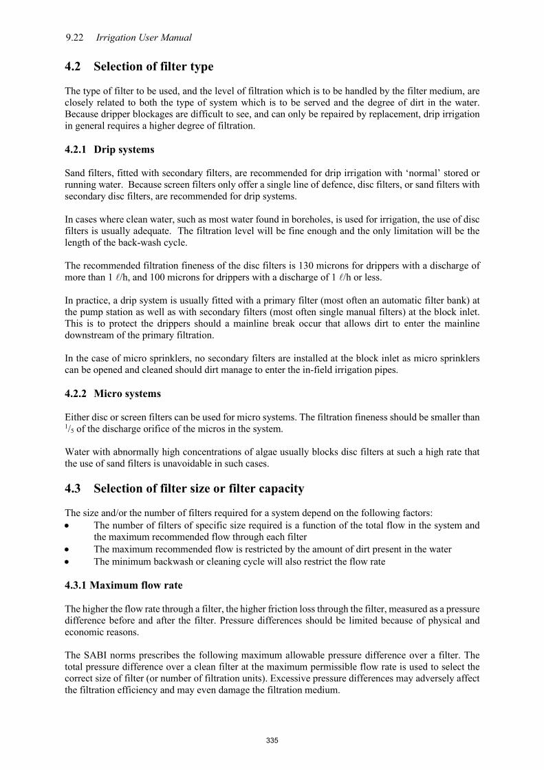
9.22 Irrigation User Manual
4.2 Selection of filter type The type of filter to be used, and the level of filtration which is to be handled by the filter medium, are closely related to both the type of system which is to be served and the degree of dirt in the water. Because dripper blockages are difficult to see, and can only be repaired by replacement, drip irrigation in general requires a higher degree of filtration. 4.2.1 Drip systems Sand filters, fitted with secondary filters, are recommended for drip irrigation with ‘normal’ stored or running water. Because screen filters only offer a single line of defence, disc filters, or sand filters with secondary disc filters, are recommended for drip systems. In cases where clean water, such as most water found in boreholes, is used for irrigation, the use of disc filters is usually adequate. The filtration level will be fine enough and the only limitation will be the length of the back-wash cycle. The recommended filtration fineness of the disc filters is 130 microns for drippers with a discharge of more than 1 /h, and 100 microns for drippers with a discharge of 1 /h or less. In practice, a drip system is usually fitted with a primary filter (most often an automatic filter bank) at the pump station as well as with secondary filters (most often single manual filters) at the block inlet. This is to protect the drippers should a mainline break occur that allows dirt to enter the mainline downstream of the primary filtration. In the case of micro sprinklers, no secondary filters are installed at the block inlet as micro sprinklers can be opened and cleaned should dirt manage to enter the in-field irrigation pipes. 4.2.2 Micro systems Either disc or screen filters can be used for micro systems. The filtration fineness should be smaller than 1/5 of the discharge orifice of the micros in the system. Water with abnormally high concentrations of algae usually blocks disc filters at such a high rate that the use of sand filters is unavoidable in such cases. 4.3 Selection of filter size or filter capacity The size and/or the number of filters required for a system depend on the following factors: • The number of filters of specific size required is a function of the total flow in the system and
the maximum recommended flow through each filter • The maximum recommended flow is restricted by the amount of dirt present in the water • The minimum backwash or cleaning cycle will also restrict the flow rate 4.3.1 Maximum flow rate The higher the flow rate through a filter, the higher friction loss through the filter, measured as a pressure difference before and after the filter. Pressure differences should be limited because of physical and economic reasons. The SABI norms prescribes the following maximum allowable pressure difference over a filter. The total pressure difference over a clean filter at the maximum permissible flow rate is used to select the correct size of filter (or number of filtration units). Excessive pressure differences may adversely affect the filtration efficiency and may even damage the filtration medium.
335

Drip and Micro-sprinkler irrigation systems 9.23
Table 9.4: Norms for the selection of filters for micro irrigation
Type
Allowable pressure difference over clean filter/-bank (kPa)
Allowable pressure build-up
(kPa)
Allowable pressure difference before cleaning / backflushing
(kPa) Single filter Filter bank Single filter Filter bank
Disc-/Mesh filter 10 30 40 50 70
Sand/media filter
10 40 20 30 60
4.3.2 Dirtiness of the water The filter selection must take the dirtiness of irrigation water into account. It is possible to measure the dirtiness, for filtration purposes, with a special but simple apparatus, called the dirt index meter. The dirt index (DI) is measured and expressed as a percentage. For more information on the relevant apparatus, the ARC-Institute for Agricultural Engineering in Silverton may be contacted.
Some filter suppliers have opted for a more subjective but practical way of describing water quality by defining 4 simple categories (Netafim South Africa, 2017): • Good: Groundwater which draws from a steady flowing aquifer, from a properly maintained
borehole, with no presence of iron or manganese or solids. • Average: Rivers, streams and canals which are slow flowing and are found in cold climates, with
a low biological growth. Reservoirs in cold climate, where the suction point from the pump is properly placed – taking into consideration wind direction, sedimentation, and floating suction.
• Bad: Reservoirs, rivers, streams, and canals found in hot climates, with a high biological growth and no chemical treatment. Where the suction point from the pump is not properly placed (wind direction not considered, poor sedimentation and bottom suction). Groundwater which draws from a poor-quality aquifer or collapsed borehole.
• Very bad: Rivers, streams and canals affected by flood. Reservoirs with poor suction conditions. All types of water containing many of dissolved materials, which are solidified when exposed to oxygen.
4.3.3 Cleaning cycle During the filtration process there is an increase in the total pressure difference over the filter due to blockage. The pressure loss through a typical filter with an increase in water volumes illustrated in Figure 9.13 where pressure loss is indicated on the y-axis and the volume of water that has flowed through the filter on the x-axis.
336

9.24 Irrigation User Manual
Figure 9.13: Typical blockage graph of filter
Filter cleaning can be scheduled in the following ways: • Fixed time interval: This can be implemented manually, or preferably, by making use of a
backflush timer on automatic filter banks. • Limited pressure difference: Again, pressure difference can be monitored manually according to
the guidelines provided in Table 9.4 for the allowable pressure difference before cleaning, or backflushing can be triggered by using a pressure differential sensor (which is also preferred for the automatic filter banks).
• Combination: Modern automatic filter banks can also make use of a combination of timers and pressure differential. Backflushing can take place according to a pre-set time period, but if the pressure differential becomes too big, backflushing is triggered earlier.
The backwash cycle therefore depends exclusively on the quality of the water. Dirtier water requires shorter back-wash cycles, and more and/or larger filters. 4.4 Pre-filtering and treatment In some cases, it may be necessary to pre-treat the chemical, biological or physical condition of irrigation water before the water is filtered to the required degree. 4.4.1 Settling and aeration In cases where irrigation water has more solids than 200 ppm in suspension, it is advisable to settle the solids in a dam before it is filtered through the system. If the specific density of these materials is very low, it may even be necessary to flocculate it chemically before settling will be practically possible. Settling can prevent the filters from being overloaded and from unduly being backflushed. Important considerations for a settling dam include the following: • Water should be extracted as far away as possible from the inlet • Backwash water should be dumped as far away as possible from the extraction point • It should be possible to clean the dam with little effort • The clear water that lies above the settled sediment should be extracted for filtering • A long narrow dam is more effective than a square one
337

Drip and Micro-sprinkler irrigation systems 9.25
In Table 9.5 the settling velocity, in metres per minute, of the granule sizes of a variety of soil textures are given. Coarse sand with granule sizes bigger than 0,5 millimetres will settle much quicker than clay granules of less than 0,002 millimetres. Table 9.5: Settling velocity of soil particles of different sizes
Soil texture
Granule size [mm]
Settling velocity [m/min]
Coarse sand
Medium sand
Fine sand
Very fine sand
Silt
Clay
> 0,5
0,25-0,5
0,1-0,25
0,05-0,1
0,002-0,05
< 0,00 2
38 22 5
0,9
0,015
0,000 6
When free iron occurs in the water, it is essential to aerate the water to allow oxidation of the iron. Aeration is the process prior to the settling and is typically in the form of an aeration structure cascading into a settling dam. For best results, it is also advisable to flocculate iron oxide during the settling process. These processes are shown in Figure 9.14.
Figure 9.14: Aeration process and settling dam (Netafim, 2017) 4.4.2 Acid treatment Acid treatment is applied when magnesium, calcium and carbonate salts pose a blockage threat to the emitters. A water sample should be analysed in the laboratory and only then can recommendations be made. 4.4.3 Chlorination Organisms which grow inside the pipelines can block the emitters. Chlorination is the only way to eliminate these and is recommended at a concentration of 6 ppm. Application is done just after the control centre and filter station. Monitoring of the biological activity in the irrigation water will determine how often chlorination will be required. If chlorination is unavoidable, its corrosive effect should be taken into account when selecting system components.
338

9.26 Irrigation User Manual
4.4.4 Sand separators Sand separators are installed to remove sand from the irrigation water by means of a centrifugal action. Although there are advantages to installing the sand separator at the suction side of the pump, careful attention should be paid to the characteristics of such an installation. • The sand separator can protect the pump by removing sand, which causes corrosion. • Any equipment which is installed at the suction side of the pump increases the possibility of air
intrusion and resultant cavitation, which can cause more damage to the pump in the end than sand could ever do.
• To be truly effective, most sand separators will absorb as much as 12 m pressure. If there is not sufficient water pressure on the suction side of the pump for this purpose, cavitation can still occur.
• For effective operation of sand separators, the flow rate through the system should be kept more or less constant, which is very seldom possible.
Figure 9.15: Sand separator
5 Automation Various factors gradually contributed to the increasing demand for automation. • Manual control of systems which resort under the micro irrigation concept, is hampered by the
long working hours and the complicated grouping systems generally encountered. Management expertise and abilities are therefore subjected to strong pressure.
• Reliable labour is also getting scarcer and more expensive. This leads to inconsistencies which often result in over or under-irrigation with the consequential unavoidable damage.
• More accurate control over the scheduling of irrigation can bring about moderate and even dramatic increases in both the quantity and quality of the yields and can therefore contribute to higher profits.
• A reliable and accurate control system inevitably creates peace of mind and security with the farmer.
• Systems that were designed from the outset with automation as a basis, may save enough on capital layout to completely cover the costs of automation.
Automation is normally operated according to one of three basic principles, and/or combinations thereof.
339

Drip and Micro-sprinkler irrigation systems 9.27
5.1 Mechanical/hydraulic Hydraulic valves, combined with water meters, and known as automatic metering valves, are used at the blocks. These valves are each fitted with a mechanical pilot valve. The pilot valves are joined by means of hydraulic sensing tubing filled with water for conveying the signal. The system is usually operated as follows:
• At the beginning of the irrigation cycle each valve is set manually, individually and in a specific
sequence to the volume of water which should be let out to that block during the relevant cycle. • The system is switched on after all the valves have been set. • Valve number 1 will pass the pre-determined volume of water, and the pilot valve will
automatically close that valve and open the following valve in the cycle. • This process repeats itself up to the last valve. The pilot valve will also close this valve, and the
flow-switch will automatically cut off the power to the pump. • The process is repeated in each successive cycle.
Advantages • The control system is totally independent of electric power. • Capital investment is relatively low. • Control is volumetric and therefore independent of time. No form of interruption will
therefore have an effect on the programmed irrigation. • The operator (usually the farmer himself) is obliged to reset the hydrometers at blocks,
forcing him to inspect the system and the crops themselves. Disadvantages • The system has to be physically set for each irrigation cycle. • Calculation of requirements, as well as resetting of the valves, requires schooled labour. • Long lengths of pilot tubing are mechanically vulnerable. • Sensing tubing must be located along smooth gradients and be free of air, something which
is practically very difficult to achieve. Air in the tubes delays (and often stops) operation. • Pilot valves require clean water for effective operation. Any sediment which can harm the
mechanical operation of the components will put the whole system out of action.
Figure 9.16: Typical mechanical/hydraulic follow-through system
340

9.28 Irrigation User Manual
5.2 Electric/hydraulic With this system, operation is generated by means of a time-switch. Time-switches vary between simple single cycle units to types which can repeat fixed inputs several times. The system can be used for any fixed cycle function, such as, for instance, to control irrigation valves or filter backflush valves. The time switch activates an electric relay which can perform one of two functions: • It can activate a hydraulic relay, situated next to the time switch, which in turn relays the
instruction to the hydraulic valve at the block by means of hydraulic sensing tubes. The valve can therefore either be opened or closed in this manner.
• Alternatively, it can convey an electric signal (usually an impulse) to a remotely situated electric/hydraulic solenoid valve, mounted on a hydraulic valve at the block, by means of an electric conductor. The hydraulic valve is therefore activated by means of electric remote control.
Advantages
• Hydraulic activation can be eliminated to a large extent by using electric remote control. It
reduces problems with installing the hydraulic components. • Control is affected by the operator from a central point. • Capital layout is relatively low. Disadvantages • Electric power is a prerequisite. • Electric conduction from the unit to the blocks is mechanically even more vulnerable than the
hydraulic sensing tube. • The system operates on a time and not a volumetric basis. Any disruption in the water supply is
therefore ignored by the time-switch of the scheduling system. Even a reduction in the water supply due to (partially) blocked filters will not be noticed by the time-switch.
• As with the hydraulic system, a schooled operator is required. • Theft of electrical wire • Sensitivity for lightning requires special protection mechanisms • Record keeping is not possible
341

Drip and Micro-sprinkler irrigation systems 9.29
Figure 9.17: Interface of typical time-switch
5.3 Computerised systems Computerised irrigation systems can be of great help to the farmer, despite the high capital layout. Modern, high technology equipment can even handle a large part of the decision-making process.
Figure 9.18: Central computer, integrated with field units
342

9.30 Irrigation User Manual
Inputs of a wide variety of sources are mostly accommodated. • Hard, permanently programmed data and characteristics can be pre-installed in the system. • Varying system characteristics and irrigation requirements can be keyed in on a continuous basis. • Feed-back from monitoring equipment can be interpreted by the computer continuously in an
intelligent way, and can be processed to new or amended instructions, which will then be implemented automatically.
The entire computer function can be conveyed to equipment by means of electric cables. The equipment is activated either electrically or hydraulically. The same cables also convey feed-back from the monitoring equipment. However, cables are vulnerable and also expensive. The more modern technology of radio communication and Wi-Fi is therefore increasingly employed and developed. An automated irrigation system can consist of wireless sensor units (WSU) and wireless information units (WIU) which are linked by radio transceivers to allow for the transfer of data. This data can be transmitted to a web-based platform on a server via the public mobile network by means of a GPRS module. The information can then be presented graphically enabling online remote monitoring through a device that has internet access. Although it is also expensive, it compares well to other methods, especially due to the higher reliability of the concept. 5.3.1 Requirements Some requirements usually expected of computerised equipment, include: • The technology and operation should not be beyond the farmer’s management skills. It is
important that the farmer is evaluated at the outset regarding this aspect. • The system should be user-friendly. Except for the initial training given by the suppliers, the
farmer has to rely on himself for the continuous operation of the system. • Hardware should be of high quality and able to operate reliably without failure. Locally
developed and purpose manufactured equipment (for South African purposes and requirements) should preferably be used.
• It is important that the computer should be able to receive all relevant inputs from both directions (from the operator as well as the monitoring equipment) and generate and implement the correct outputs accordingly.
• Control should be affected on a volumetric basis, with a time-based control system. Continuous feed-back of current actions and conditions is especially important.
• Fault-detection, reporting back, warning and applying emergency measures, are essential characteristics of an effective system. When, for instance, feed-back of ultra-high flow conditions outside the set parameters is received, the computer should be able to interpret it as a possible pipe burst. The least that can be expected of the system is: ° A warning should immediately be sounded to the operator by means of an audio and/or
visual alarm (for instance a siren and/or flashing red light or with modern technology a message or email to the operator’s phone).
° Comprehensive feed-back on all aspects of the problem (location, extent, etc.) should be recorded and shown on the screen.
° The relevant region should automatically be isolated by closing off the necessary valves. ° Irrigation of the following group should automatically commence after identifying the
priority situation and reacting on that information. • As much decision-making as possible should take place totally automatically from scheduling
inputs, both from instrumental feed-back (e.g. climatic data) and manually keyed-in inputs. 5.3.2 Design approach
When computer-based irrigation control is considered, a number of important design aspects should be taken into account:
343

Drip and Micro-sprinkler irrigation systems 9.31
• The computer should firstly, and most importantly, suit the farmer. Many sophisticated computers in the field only operate as very expensive time switches because the farmer or operator does not have the required level of expertise and/or management skills. The guilty party almost always is the designer, who neglected to do a need assessment before the design of the system.
• Similarly, the computer should suit the system design if possible, and not the other way around. This action can be divided into two categories: ° An existing irrigation unit, with an already established infrastructure, limits the
designer's options and opportunities for innovative thinking. In such cases, he is usually forced to adapt the computer to the system. Moderate, low-cost modifications to the system should, however, be a consideration at all times, especially where operating costs can be reduced in the long term.
° New systems and/or extensions offer the biggest opportunity to integrate both the system and control unit around the system requirements. It also offers the opportunity to sub-divide the system into smaller units for better control. Subdivision can be done on logistical, geographical or system pressure zone basis, or any other consideration which may benefit from group formation.
General: The irrigation system must be designed hydraulically correct and must operate with the
necessary protection. It is unfair to expect from the computer to control a hydraulic irrigation system that was incorrectly designed.
Power supply must be constant and “clean”. The use of a UPS (Uninterrupted Power Supply) is of great help.
Installation must be neat and orderly; wires must be marked for future reference. Inspection must be done at joints.
The computer must be installed in a clean, dry place and not be subjected to fertilizer and water. Advantages: • More accurate scheduling management increases earnings. • Central control simplifies management functions. • Management is continuously informed about all activities. • Fault detection features result in automatic and prompt action. • Volumetric control to a large extent eliminates scheduling mistakes. • Reliable execution of instructions reduces instances of damage and creates peace of mind. Disadvantages: • Relatively high capital layout. • Requires high level management and operational expertise. • Specialist maintenance services are required periodically. • Sensitivity to lightning necessitates special protection mechanisms. • High risk and susceptibility to theft, interference or vandalism.
344

9.32 Irrigation User Manual
6 Installation For effective functioning of any irrigation system, the correct method of installation and flushing of the system is essential, before any irrigation can be started. 6.1 Installation of laterals Install laterals as indicated on the plan, because the system is designed on the plan. Especially where systems are designed before the exact rows have been pegged out, deviations of the plan can easily occur. The laterals and supply lines must be installed in correct lengths of each selected diameter according to the plan in the correct positions. Black polyethylene pipes can be left in the sun for a few days until all the bends are straightened out before placing them in position. Place the micro sprayer lateral on the side of the tree row from where the wind direction is. The micro sprinkler lateral can be buried subsurface or tied to a wire held into a position by stakes 300 mm above ground. If the laterals are buried (±50 mm deep), a standing pipe must be used. This pipe must be held in position with a block or stand. If mechanical tilling is used, it is preferable that the laterals must be suspended on a wire. Prevent as far as possible that any soil or material particles are let into the pipes during installation. When sawing and drilling is done to uPVC pipes, prevent borings from falling in, because it can cause blockage at emitters in the laterals. 6.2 Flushing of irrigation system After the installation has been done, all the components must be flushed before they are connected. First flush the main line for 15 to 20 minutes while all valves to the supply line are closed. Manifolds are then flushed one by one for 5 to 10 minutes before being connected to the laterals. Flush the laterals one by one at high pressure until the water at the ends of the laterals are completely clean. Manifolds must preferably be fitted with flush valves at the ends. Alternatively, the end of every lateral can be bent over, so that it is easy to flush each lateral. 6.3 Filter station Check the pressure before and after the filter station after the system has been flushed. Ensure that the flush water of the filter and fertilizer pump is drained away from the irrigation block. The setting of pressure control valves, adjustment of the backwashing frequency and backwashing duration of the filters are of cardinal importance during installation. Check the filter bank for any leakages at the line connection.
345

Drip and Micro-sprinkler irrigation systems 9.33
Figure 9.19: Installed pressure measuring points at a filter bank
6.4 Irrigation material Treat all screw thread against rust. Use bitumen treated and galvanised pipe where possible. Where corrosion is a problem, use uPVC pipes and accessories. Any surface uPVC pipe must be protected by a coat of water-based paint. Valves, filters and control equipment must preferable be protected with roofing. This will prevent plastic and rubber parts from wear. 7 Evaluation after installation The purpose of the evaluation is to ensure that the system functions as described in the design report and whether the system was installed according to the plan. This type of evaluation procedure must be relatively simple, so that the producer can execute it himself and interpret the results. This evaluation can also be conducted by the producer on an annual basis to identify possible problems in time. Figure 9.20 shows an example of the peak design form with specifications against which the system can be evaluated. Some of the measurements that should be executed if a deviation from the design specifications is noticed are described in Table 9.6
346

9.34 Irrigation User Manual
Figure 9.20: Peak design data
347

Drip and Micro-sprinkler irrigation systems 9.35
Table 9.6: Proposed basic evaluation procedure to determine whether an irrigation system is correctly installed and functions according to design specifications Subject / Item Measurement/Evaluation Action if measurements /
evaluation does not conform to the design specifications
Inlet pressure of block Determine the inlet pressure of the blocks with a pressure gauge and compare with the required pressured as specified on the peak design form
Contact designer and adjust set-up schedule if necessary
Emitter pressure and delivery Measure pressure with a pressure gauge and measure the delivery in a container for at least five minutes at the four emitters on four corners of the field.
If a pressure variation of more than 20% of the design pressure or a delivery variation of more than 10% occurs, as specified in the technical report, contact the designer.
System lay-out Examine system layout by measuring the distances between emitters/ laterals, as well as the position of valves with a tape measure. Compare installed pipe diameters with those on the plan. Also take note of the direction of the laterals/emitter lines. If lateral is installed in the wrong direction, then the slope of that lateral is not as per design.
Re-install according to plan
Equipment: model and manufacturer
Compare the model/ manufacturer of the installed pump, electric motor, filter and emitters with the specifications as per design report.
Contact designer for replacement of faulty equipment
Schedule of blocks in simultaneous operation
Compare the blocks that are in simultaneous operation, with the specification as suggested in design report.
Change the blocks that are in simultaneous operation, by either opening the correct taps or reprogramming the irrigation computer.
General installation Examine if any leakages occur in the system
Repair leaks
Operation of equipment Examine operation of filters (e.g. pressure loss and backwashing action), air and pressure control valves
Contact designer for fault detection
System capacity Determine system flow rate by taking the reading from the flow meter/ measuring notch
If a flow rate deviation of more than 10% from the average occurs, as specified in the peak design form, contact the designer.
*See Example 9.2 for determining delivery variation. If a complete system evaluation is required, an irrigation professional can be consulted to perform the evaluation as described in the Irrigation Evaluation Manual of the ARC-Institute for Agricultural Engineering.
348

9.36 Irrigation User Manual
8 Management Practical recommendations on water application, filtering and pressure control in micro systems are made in this section. Scheduling of irrigation water is discussed separately in Chapter 7: Irrigation scheduling. 8.1 Water application The correct decision on water application is very important to ensure optimum production and efficient water use. There are a number of recognized techniques that can be used to schedule irrigation effectively. The smaller the effective root depth and readily available water in the soil, the more critical is accurate scheduling to either prevent saturation or leaching. There is no perfect irrigation-scheduling program and it is therefore recommended that a second method of soil water measuring be used for control purposes. Aids in this continuous decision-making process must be reliable. Chapter 7: Irrigation scheduling gives a complete description of the available scheduling methods and aids. To determine how many mm of water should be applied with an irrigation system, one of the following methods can be used: • Flow measurement It is advisable to have a flow meter on the main supply pipeline to the irrigation system, so that the water use can be measured over the season. The flow measurement can thus be calculated on a monthly basis to mm/month. Example 9.1: Area under irrigation = 5 ha Flow measurement per month = 7 500 m³
Gross application per month = 105500 7× = 150mm/month
• Measuring of emitter delivery The emitter delivery can be measured in the block by collecting the delivery in a measuring cylinder for 5 minutes. Five laterals, distributed in the block are selected and the delivery of five emitters per lateral, distributed on the lateral is measured. The delivery variation can thus be determined by dividing the difference between the maximum and minimum delivery in the block, by the average delivery. By multiplying this by 100, the percentage deviation in delivery can be obtained. A norm of a maximum of 10% variation in delivery between emitters in the block is acceptable. If the delivery variation is >10%, the emitters must be replaced or the system pipe network must be repaired.
Figure 9.21: Delivery test of surface drippers
349

Drip and Micro-sprinkler irrigation systems 9.37
Example 9.2: Dripper delivery as collected in a measuring cylinder for 5 minutes (in m) is as follows:
Delivery at specific distances on the laterals (m/5min) Distance Lateral 0 L/4 L/2 3L/4 L
1 200 180 210 190 180 2 180 190 180 190 200 3 190 195 170 200 190 4 200 170 180 195 180 5 190 190 190 180 195
Convert above delivery in m/5 min to /h
Delivery at specific distances on the laterals (/h) Distance Lateral 0 L/4 L/2 3L/4 L
1 2,4 2,16 2,52 2,28 2,16 2 2,16 2,28 2,16 2,28 2,4 3 2,28 2,34 2,04 2,4 2,28 4 2,4 2,04 2,16 2,34 2,16 5 2,28 2,28 2,28 2,16 2,34
Calculate the total measured deliveries = 56,58 /h
Average delivery = 2558,56
/h = 2,25 /h Maximum measured delivery = 2,52 /h Minimum measured delivery = 2,04 /h
Percentage delivery variation = 2,252,042,52−
× 100 = 21,3%, which is greater than the 10% norm. To calculate the average gross application per month, the number of emitters per block must be multiplied by the average delivery per emitter to obtain the flow rate per block. This value can then be converted to flow per month by multiplying the above value with the number of hours irrigated per month. The gross application per month can then be determined as explained in Example 9.1. The question sometimes arises of how much water (mm) must theoretically be applied per irrigation. The method of calculation can be described by the following example: Example 9.3: Soil water capacity (10-100 kPa) = 90 mm/m Emitter spacing = 2,6 m Effective root depth = 0,6 m Application efficiency = 85% Emitter delivery = 52 /h Lateral spacing = 5,5 m Wetted emitter radius = 1,4 m Assume the crop requires 5mm/day. Solution:
350

9.38 Irrigation User Manual
Determine the standing time for a practical cycle length. Available soil reservoir (mm)
= Wetted surface (decimal) × effective root depth (m) × soil water capacity (mm/m)
= 5,521,4 ×
× 0,6 × 90 mm = 27,5 mm Maximum gross application
/ham 320mm 32
mm 0,8527,5
efficiency nApplicatioreservoir waterAvailable
3=
=
=
=
Standing time required for the gross application
hours 8,8
h 2,65,5
5232/
(mm/h) systemthe of rate napplicatio gross(mm) napplicatio gross Maximum
=
×=
=
Theoretical cycle length:
days 5,5
day 5
27,5(mm/day) tsrequiremen irrigation nett
reservoir waterAvailable
=
=
=
Suppose a practical cycle length of 2× per week is chosen: Standing time for a cycle length of 3,5 days:
hours 5,6
h 8,85,53,5
=
×=
8.2 Filtering The exact stage at which a filter must be cleaned, is usually determined by one of the following: • The allowable reduction of flow in the irrigation system, resulting from the increased resistance
against flow in the blocked filter: It causes reduction in the system efficiency. The flow rate in the system can be measured with a flow meter and must not reduce by more than 10%.
• The allowable pressure drop over the filter elements: A too great pressure drop over a filter element causes dirt to be forced into the element, which hampers later effective cleaning. The sand filters are therefore cleaned when the total pressure drop of 60 kPa over the filter banks are
351

Drip and Micro-sprinkler irrigation systems 9.39
reached, still considering that the flow rate must not drop by more than 10%. This method lends itself to automation.
Table 9.7: Allowable pressure difference over filter banks:
Type Clean filter bank (kPa)
Maximum pressure build-up (kPa
Pressure difference before backwashing (kPa)
Disc / mesh filter 30 40 70
Sand filter 40 20 60
• A further method is to limit time lapse between cleanings. First calculating the volume that can be
safely filtered and then dividing the figure by the flow rate of the filter, is an easy way of calculating the time lapse.
𝑇𝑇 =𝑉𝑉𝑄𝑄
(9.1)
where T = Time lapse (h) V = Volume that can be filtered (m³) Q = Flow rate through the filter (m³/h) The most convenient method is the latter, but problems can occur if the degree of dirtiness of the water changes. 8.3 Pressure control To ensure that the system irrigates at the design pressure, a constant inlet pressure must be maintained at the block inlet. Pressure can be controlled at the irrigation block by either installing a permanent pressure control valve or setting the pressure with a pressure meter. The pressure control valves can be set for a specific pressure and installed on the upstream side to reduce pressure, caused by, e.g., gravity. The different valves are dealt with in Chapter 8. Alternatively, pressure meters can be used for setting the pressure at an irrigation block at the required operating pressure. Pressure meters can be installed permanently, or portable pressure meters can be used. It is advisable to have reliable pressure meters, preferably the type filled with glycerine and provided with a stopcock, so that the mechanism of the pressure meter is not subjected to pressure fluctuations during the entire duration of irrigation. At least one pressure meter point must be installed at each block. 9 Maintenance Drippers and micro sprinklers are inclined to be extremely sensitive to particles that can cause blockages because the flow path openings of the emitters are very small. Although signs of blockage can be observed during visual inspections, it is virtually impossible to identify the causes of blockage on the inside of the dripper without a water analysis.
352

9.40 Irrigation User Manual
9.1 Water quality The quality of the irrigation water determines the measure of blockage. Partial blockage is as much a problem as complete blockage, since it influences the water distribution of the system negatively. It is therefore essential that the water should be analysed to identify possible dangers of blockage. This analysis must be done at the stage that the water quality is at its worst and must be compared to historical figures to monitor any variations in water quality. Table 9.8 indicates the physical, chemical and biological factors that can cause blockage. Table 9.8: Physical, chemical and biological factors that can cause blockages (Bucks et al, 1979)
Physical Chemical Biological - Inorganic materials Sand (50-250 μm) Silt (2-50 μm) Clay (<2 μm) - Organic materials Water plants Phytoplankton Algae Water animals Zooplankton Snails Bacteria (0,4-2 μm) Plastic pipe cuttings Oil
- Alkaline heavy metals Cation Calcium Magnesium Iron Manganese Anion Carbonates Hydroxides Silicates Sulphides - Fertilizers Ammonia Iron Copper Zinc Manganese Phosphate
- Algae - Bacteria Filament Slime - Microbiological activities Iron Manganese Sulphate
• Physical
A certain amount of the particles in irrigation water can get through the filter and can cause blockage problems in emitters. Very fine particles will mostly remain in suspension and may possibly flocculate out at places where the flow rate is low or when the water turbulence reduces. The most likely place where sedimentation will occur is at the end of laterals. It will result in the end emitters getting blocked first. Although a single particle will not necessarily cause blockage, a quantity of particles can form a clump and block emitters. The clump occurs where microbe slime binds suspended solids including algae. Surface water sources usually contain suspended solids especially after high intensity rainfall events which result in runoff and erosion. Organic material such as algae can occur, especially if the water source is rich in nitrate (>10 mg/). Subsurface water sources usually contain a lot of sand and silt that cause blockages. • Chemical
Blockage of emitters caused by the chemical composition of the water is normally the result of a deposit from a chemical reaction. The deposits that can give rise to blockages are the following: Calcium and magnesium carbonate: These deposits can occur outside emitter openings as well as inside laterals and can also lead to sedimentation of the upper sand layer of a sand filter. Calcium and
353

Drip and Micro-sprinkler irrigation systems 9.41
magnesium carbonate deposits are usually formed at dripper openings when the water evaporates; at a pH of greater than 8; by the addition of fertilizers such as ammonia that increases the pH of the water; laterals subjected to extreme heat; and in filters where a pressure loss occurs in water that contains carbon dioxide (Rainbird, 1999). The possibility of deposits forming can be identified by either a water analysis, or by treating the water sample with household ammonia and examining it after 12 hours for deposits that could have formed or when an acid that has formed on the deposit is dripped and makes a “fizzy” sound. The most general method for treating these deposits is by applying acid (Section 9.2.2.2). Iron and magnesium sulphides: The occurrence of sulphides (>0,5 mg/) combined with iron or manganese in the irrigation water, can cause blockage problems. This type of blockage occurs especially in borehole water if oxygen is absent. When the sulphides in the irrigation water are high, sulphides can precipitate out on the stainless steel mesh filters. Hydrogen sulphides have a characteristic rotten-egg odour and are found in nature where sulphates are transformed into sulphides. If chlorine is added to water that contains hydrogen sulphide, a sulphur deposit will be formed and cause blockage (Rainbird, 1990). Iron and manganese oxides: Fe2+ appears in solutions and converts to Fe3+ during oxidation and forms a deposit. It occurs mostly in borehole water that is rich in iron / manganese, as well as the addition of phosphoric acid. The flask test as described below can also be done by the addition of chlorine to the water. Depending on the blockage threat, blockages caused by iron and manganese oxides can be solved by the following: aeration, sedimentation, chlorination and filtering (Table 9.14). The oxidation process of manganese takes place much slower than iron and is therefore difficult to remove effectively. Aeration and sedimentation is therefore necessary in most cases. Before any fertilizer is administered, it must be mixed with the irrigation water in a translucent flask (flask test). If the mixture becomes milky within 24 hours or forms a deposit, it is a good indication that dripper blockage may occur. This type of fertilizer must then be avoided. It is important to buffer the pH of the water at approximately 6,5 to make effective fertilizer application possible. • Biological
Algae growth usually occurs in storage dams rich in nitrites. The identification of the type and the amount of algae that occurs is of little value, because it varies a lot during the irrigation season. Ornamental algae and fibrous algae usually cause blockage of filters (Harding, 2000). A high occurrence of algae requires a larger filter capacity and more frequent backwashing. Algae can be controlled by the application of chemicals such as copper sulphate (~2 mg/) or chlorine (Section 9.2.2). Algae needs light to grow, it therefore does not grow in black polyethylene pipes. The algae residue that seep through filters together with clay particles, serves as a food source for bacterial slime. Iron deposits, i.e. the oxidation of Fe2+ to Fe 3+ is also possible if certain bacteria occur in the irrigation water with Fe2+
concentration of greater than 0,2 mg/.Where fertilizer is applied through the system and where laterals are exposed to the sun, an increase in bacterial slime forming is possible. This slime can block emitters or they can act as bonding agent that binds fine silt and clay particles, which leads to blockage. If a vacuum is created in an irrigation system, bacteria can be sucked in that will lead to slime forming and eventually emitter blockages. The installation of air inlet valves can prevent this. Slime can also be formed if hydrogen sulphide occurring in the irrigation water is oxidised to sulphur by aerobic bacteria (Ford, 1985). Bacterial slime forming can be prevented by chlorination (Section 9.2.2). Blockage material is identified by the colour of the various deposits in the blocked dripper. A carbonate deposit appears white, iron oxides appear rust-coloured and microbiological activities are black. Each type of blockage has a unique solution. A water analysis that indicates the exact nature of the blockage is therefore essential. Chapter 2: Water contains information on sampling and handling requirements for taking samples. The results of the water analysis can be used to quantify the blockage threat for emitters as shown in Table 9.2 in section 4, Filtration.
354

9.42 Irrigation User Manual
Some suppliers of irrigation systems consider water with an iron-content of >0,8 mg/ in storage dams and borehole water with an iron-content of >0,3 mg/ as a high blockage risk for emitters. Water with a manganese-content of >0,3 mg/ is also considered a blockage risk. These causes are interactive with each other, e.g. the removal of organic material will reduce biological activities. Table 9.9 suggests solutions for the different blockage problems that can be experienced. Table 9.9: Solutions for different types of blockage problems (Koegelenberg, 2002)
Blockage risk Solution for different types of blockages Physical Chemical Biological
Low Follow the maintenance schedules of systems (Tables 9.15) and filters (Table 9.10). Extraction point of water from storage dams must be lifted with a float.
Between low and high
Use sand filters for filtering
Chlorinating and acid application (Section 9.2.2)
Chlorinating (Section 9.2.2)
High
Store water in sedimentation dam before pumping the water to the irrigation system
Bicarbonate and calcium: Acid application (Section 9.2.2) iron and manganese: Combination of aeration and sedimentation dams and/or continuous chlorine application for at least 2-3 minutes before water reaches sand filter (Section 9.2.2)
Chlorination (Section 9.2.2)
9.2 Water purification methods The water purification methods depend on the type of blockage problem experienced. 9.2.1 Solutions for preventing blockages resulting from physical factors Depending on the degree of the blockage risk, filtering, sedimentation dams or sand separators or a combination of the above is recommended. 9.2.1.1 Filtering Filtering of irrigation water is of cardinal importance for the effective and efficient functioning of all micro irrigation systems. The system’s pressure and flow rate must be controlled so that it complies with the filter manufacturers recommended working area of the specific filter. Exceeding the recommended flow rate can lead to an increase in blockages. The use of a filter at higher than recommended pressures, can lead to the damage of the filter element. Insufficient flushing cycle duration, incorrectly setting of flushing control valves and the use of filters outside their recommended flow range, are the greatest causes of filter blockage. If mesh filters are used, the mesh must be regularly inspected for holes. Regular inspection is the key to success. Table 9.10 shows a maintenance schedule for filters.
355

Drip and Micro-sprinkler irrigation systems 9.43
Table 9.10: Maintenance schedule for filter with manual control* Monitor With each cycle Monthly Annually Inspect for leakages at filters X Monitor pressure difference over filters X
Inspect sand level depth (± 350 mm) and add sand if necessary X
Service disc filters X Monitor duration of flushing cycle and reset if necessary X
Inspect sand particles and filter elements and replace if necessary X
Service backwashing and air valves on filter bank. X
Check hydraulic and electric connections X
*If filter station is automated, the maintenance schedule can be adapted, e.g. the pressure difference over the filters can be verified over a longer period, e.g. weekly. Where aggressive water occurs, metal parts of the filters must receive epoxy treatment. Lubricants extend the lifespan of synthetic rings in filters where metal and rubber parts are in contact. High viscosity silicon products have proved to be the most suitable product for general usage. Lithium grease, but definitely not oil, is very suitable for valve axles and other moving parts. Backwashing can be done on a time or volume or pressure difference basis. The backwashing on a pressure difference basis is recommended, because it takes water quality changes into consideration. • Backwashing cycle of sand filters
The theoretical backwashing cycle is the time it takes the filter bank to build up a pressure difference of 4 m under normal conditions (at the beginning). A third of this duration is used as the practical backwashing cycle. The duration can change during the season as the water quality changes. If the water is very clean, backwashing should be done once daily to prevent sedimentation of the sand-bed. Stirring the sand with the hand can elevate sedimentation. Bacteria growth on the sand sometimes leads to sedimentation of the sand, resulting in tunnel forming. The bacteria growth can be prevented by means of chemical treatment of the water. A backwashing duration of at least 60 seconds is mostly recommended. It is however good practice to physically backwash the filter and monitoring the time it will take until all the discolouring and alien material disappears from the water. It is also very important to take a sample of the backwashing water with a clean container before the flushing process is completed and to inspect it to ensure that it is clean. Backwashing usually takes place while irrigation continues. It is however beneficial to backwash the system from time to time (bi-weekly), with all blocks closed, so that a greater volume of water can flow through the filters to accomplish a more effective backwashing action. A pressure of ±5 m higher than the normal functioning pressure before the filters during this action is sufficient. The use of air under pressure with a backwashing will aid in the disintegrating of clotted sand. Discolouration of water during the backwashing cycle is normal and indicates the effective functioning of the filters. The backwashing flow rate is very important and must be set to ensure effective backwashing. A too-high flow rate will cause the sand to wash out, while a too low flow rate will prevent impurities from being washed out. • Replacing sand and discs in filters
Replace the sand when the measured time to build up a pressure difference of 2 m over the filter bank
356

9.44 Irrigation User Manual
has reduced to a sixth of the original time. The rule of thumb is to replace the sand annually, however, sand levels need to be inspected on a quarterly basis. Upon inspection, when sand is rubbed between the fingers it must not feel smooth, because this will mean that the sand has been worn down and no longer filters effectively. This may require that the sand be replaced. When replacing sand, the sand particles must be angular and not round. Particle sizes that vary from 0,71 mm to 1,85 mm are recommended. When replacing the sand in the filter, it is essential to half-fill the filter with water before filling it with sand to prevent damage to the roses or fingers in the filter. The water forms a cushion and protects the internal parts. Sand filters normally have a sand depth of ±350 mm. A layer is sometimes formed on the sand that becomes dirty or blocked and even causes sedimentation. It is not necessary to remove all the sand from the filter. The layer can be scraped off and removed and the correct amount of sand can be replaced. It is usually as a result of a low backwashing flow rate or a too long backwashing cycle. Any discs that show signs of mechanical damage should be replaced. Discs with chemically blocked channels must be removed and cleaned chemically. If the discs cannot be cleaned effectively, they must be replaced. Always replace discs with the same colour and from the same manufacturer to ensure that the degree of filter disc remains the same. It is strongly recommended that the disc filters should be removed from time to time and cleaned manually. 9.2.1.2 Sedimentation dam Ensure that algae growth is prevented in sedimentation dams by chlorination. If water seepage through the dam wall is a problem, the necessary maintenance work must be done immediately. Leaves collecting on the water surface or at extraction points must be removed daily. Sedimentation dams are cleaned when the dam no longer functions effectively as sedimentation dam. This can be done as follows: Pump or drain the remaining water from the dam and remove the sediment collected on the bottom. Signs of water that has become excessively dirty and filters of which the backwashing frequency increases are signs that the dam should be cleaned. 9.2.1.3 Sand separators Sand separators require a specific flow rate. Changes in the flow rate can influence the effectiveness of the sand separators negatively and the flow rate must be checked regularly. The dirt collecting in the sand separator’s collection chamber must be removed regularly so that the sand separator does not get blocked. 9.2.2 Chemical water treatment Chemical water treatment is the addition of chemicals to prevent or dissolve deposits or for cleaning of the system. 9.2.2.1 Chlorine application Chlorine is a strong oxidising agent. Chlorine can therefore be used for the oxidation of iron and manganese and for preventing and removing sedimentation from organic materials in an irrigation system. Chlorine is also used for the destruction of bacteria and bacterial slimes (Table 9.11). The recommended chlorine concentration is applied through the irrigation system and the same injection pumps used for the application of fertilizers. The application point must be as close as possible to the system, as residual concentrations are destroyed with time and distance from the application point. If
357

Drip and Micro-sprinkler irrigation systems 9.45
chlorine is however applied to precipitate iron and manganese, it is preferable to administer the chlorine before the filter so that the iron/manganese in the filter can precipitate to prevent blockage in the emitters. Before chlorinating, the laterals must be flushed clean to remove dirt. Chlorine can be added continuously or periodically. Recommended concentrations are given in Table 9.11. The effectiveness of chlorinating depends on the contact time and the pH of the water. Periodic application of chlorine usually takes place during the last 30 to 60 minutes of irrigation. Avoid chlorine concentration of more than 100 mg/ since this can possibly damage dripper diaphragms. After irrigation, the free residual chlorine in the water that remains in the pipes will suppress undesirable microbiological activities. The laterals must then be flushed thoroughly before the next irrigation cycle. The free residual chlorine at the end of the system is an indication that the oxidation process is completed and should be 1-3 mg/ (Table 9.11). Chlorine is also the most effective at a pH of approximately 6,5 and the irrigation water must be acidified if necessary. The acid is applied to reduce the pH of the water to 2-4 for 10-20 minutes and then apply the chlorine. Table 9.11: Recommended chlorine concentrations (Netafim, 1998)
Purpose of chlorination
Chlorination method
Recommended concentration (mg/) at: Injection point End point
Prevention of sedimentation
Continuous 3-5 >1
Periodically 10 >3
Cleansing of system of bacterial slimes
Continuous 5-10 >3
Periodically 15 >5 When the purpose of chlorination is to improve the filtering ability of the sand, chlorine must be applied before the filter bank. For continuous chlorination, the chlorine concentrations downstream of the filter bank must not be less than 1 to 2 mg/ and for periodic chlorination, the figure is 3 to 6 mg/. Free chlorine is easy to measure with a DPD chlorine test apparatus. Total chlorine is the sum of the free chlorine and other chlorine compounds but is of no value for water treatment of dripper systems. The type of chlorine used, depends on the amount required, cost and availability of chlorine and equipment. Chlorine is available in the following forms: • Chlorine gas
Chlorine gas is supplied in 50 kg gas bottles. An adjustable regulator controls the flow of the gas from the bottle. The device for the application of chlorine gas is relatively expensive, although chlorine gas is the cheapest source of chlorine. Special safety precautions must be taken during the administering of the gas because chlorine gas is very dangerous. The following equations are used to calculate the amount of chlorine gas to be applied: (Most gas flow meters read in kg/day)
𝐼𝐼𝑇𝑇 = 0,024 𝑄𝑄𝑄𝑄 (9.2) where IT = injection rate of chlorine solution (kg/day) Q = flow rate of the system (m³/h) K = required concentration (mg/) Example 9.4: The producer wants to apply chlorine gas daily at a concentrate of 3 mg/. The flow rate of the system is 295 m³/h.
358
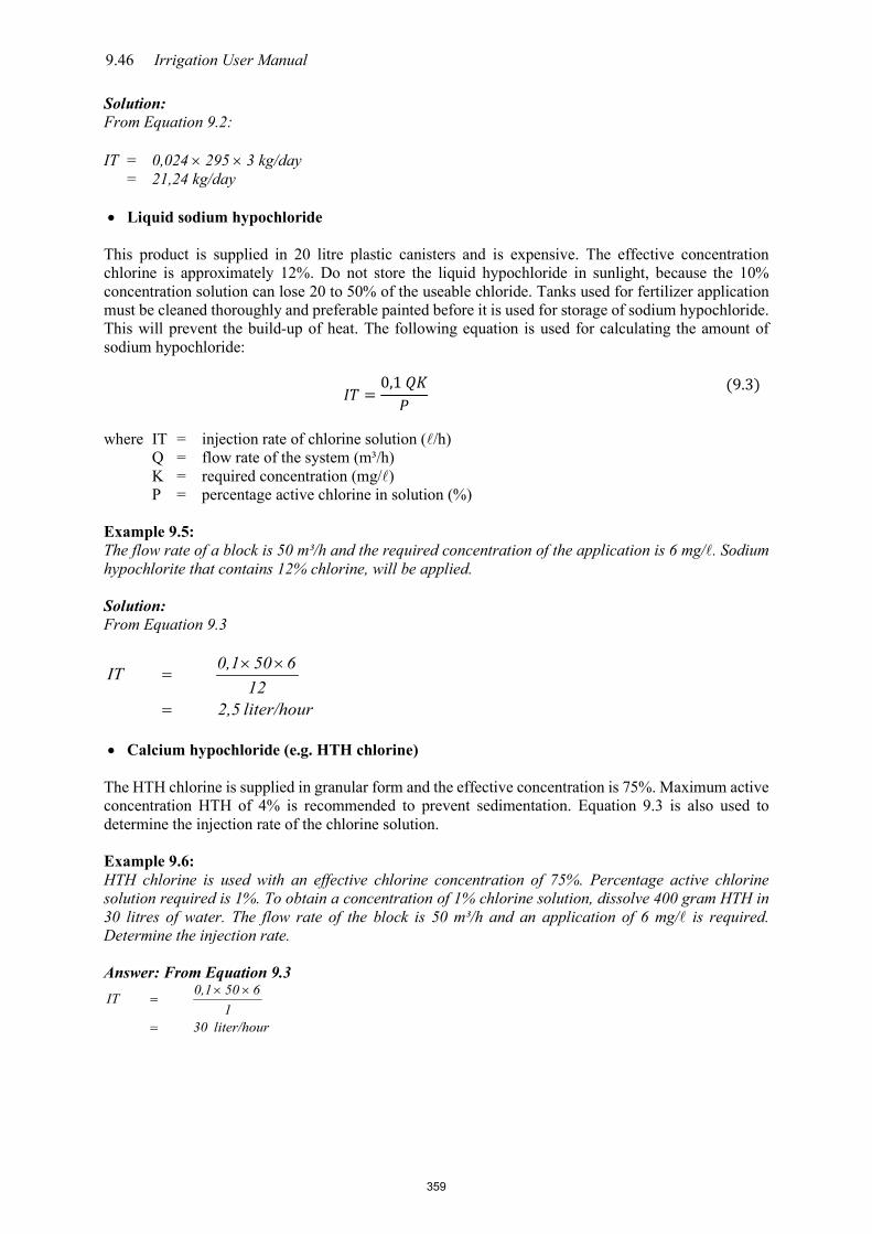
9.46 Irrigation User Manual
Solution: From Equation 9.2: IT = 0,024 × 295 × 3 kg/day = 21,24 kg/day • Liquid sodium hypochloride
This product is supplied in 20 litre plastic canisters and is expensive. The effective concentration chlorine is approximately 12%. Do not store the liquid hypochloride in sunlight, because the 10% concentration solution can lose 20 to 50% of the useable chloride. Tanks used for fertilizer application must be cleaned thoroughly and preferable painted before it is used for storage of sodium hypochloride. This will prevent the build-up of heat. The following equation is used for calculating the amount of sodium hypochloride:
𝐼𝐼𝑇𝑇 =0,1 𝑄𝑄𝑄𝑄𝑃𝑃
(9.3)
where IT = injection rate of chlorine solution (/h) Q = flow rate of the system (m³/h) K = required concentration (mg/) P = percentage active chlorine in solution (%) Example 9.5: The flow rate of a block is 50 m³/h and the required concentration of the application is 6 mg/. Sodium hypochlorite that contains 12% chlorine, will be applied. Solution: From Equation 9.3
liter/hour 2,512
6500,1IT
=
××=
• Calcium hypochloride (e.g. HTH chlorine)
The HTH chlorine is supplied in granular form and the effective concentration is 75%. Maximum active concentration HTH of 4% is recommended to prevent sedimentation. Equation 9.3 is also used to determine the injection rate of the chlorine solution. Example 9.6: HTH chlorine is used with an effective chlorine concentration of 75%. Percentage active chlorine solution required is 1%. To obtain a concentration of 1% chlorine solution, dissolve 400 gram HTH in 30 litres of water. The flow rate of the block is 50 m³/h and an application of 6 mg/ is required. Determine the injection rate. Answer: From Equation 9.3
liter/hour 301
6500,1IT
=
××=
359

Drip and Micro-sprinkler irrigation systems 9.47
Table 9.12: Comparison of different chlorine forms (Rainbird, 1990) Chlorine source Amount required for
application of 500 g C2 Amount required per 1 000 m³ water to apply 1 mg/
Calcium hypochloride 65% chlorine 70% chlorine
769 g 714 g
1 538 g 1 429 g
Sodium hypochloride 5% chlorine 10% chlorine 15% chlorine
10 5
3,3
20 10
6,67 Chlorine gas 500 g 1 kg
9.2.2.2 Acid application The presence of high concentrations of calcium, magnesium and bicarbonate in irrigation water, is usually an indication that carbonate deposits in irrigation water can form (Table 9.10). Acid application is necessary for dissolving these deposits. By maintaining a pH value of < 5,5, the oxidation of iron, i.e. the iron deposits can be prevented. Corrosion of the irrigation material can however accelerate. Find out from the manufacturers whether the material in the apparatus is suitable for acid application. Acid solutions (low pH) can also corrode irrigation system fittings if it is manufactured from steel and aluminium. uPVC and polyethylene fittings are recommended in these cases. Do not use phosphoric acid for a high pH, calcium or bicarbonate water (Netafim, 2000). The injection points must be designed for applying the acid solution in the center of the pipeline in order to blend the water and acid sufficiently, preferably after the filter. The recommended acid solution is usually applied for an hour, after which the system is flushed with clean water. In most cases, hydrochloric acid is used, as it is less dangerous. The following acid concentrations are recommended: Table 9.13: Recommended acid concentration (Netafim, 1998)
Maximum percentage acid in water (%)
Type of acid Concentration of product available on market (%)
0,6 0,6 0,6 0,6
Hydrochloric acid (HCL) Sulphuric acid (H2SO4) Nitric acid (HNO3) Phosphoric acid (H3PO4)
33-35 70 60 85
If the percentage of the acid differs from the above values, the maximum acid percentage must be adjusted. If the available sulphuric acid concentrations are e.g. 98%, the maximum percentage acid in the water must be adapted to 0,4% (70/80 × 0,6). Specialists recommend that a laboratory test should be done on the irrigation water to determine the amount of water necessary to reduce the pH of the water to a specific level. A titration curve is unique for each water source and type of acid applied. A titration curve also changes during the year as the water quality changes. A simple way of determining the amount of acid needed is to fill a 200-litre drum with the irrigation water and adding small amounts of the acid solution until the required pH is reached. Netafim (2000) recommends the following practical directives for acid treatment:
• Connect the fertilizer injection pump at the block that must be treated and get the system to operating pressure.
• Switch on the injection pump at full capacity with clean water and determine the volume of water that is applied within 10 minutes (application volume). Test again by placing the same volume of water in a container to ensure that it is the correct volume in the 10 minutes.
• Apply the acid • After applying the acid, flush clean water through the injection pump to rinse out the acid. • Irrigate for a further hour after the acid is applied. This will ensure that the pH of the root zone will
360

9.48 Irrigation User Manual
return to the value before treatment. • Flush the system. (Only one or two dripper laterals at a time must be flushed, or the flow velocity
will reduce to <0,4 m/s and the rinsing process becomes ineffective).
NB! • Do not store chlorine and acid in the same place • Do not add water to chlorine or acid • Do not mix chlorine and insecticides/herbicides – chlorine weakens the organic compound of the other chemicals • The presence of ammonia and urea in the irrigation water will reduce the effectiveness of the chlorine • Do not mix chlorine and fertilizer. This will lead to an explosion – clean the mixing tank before chorine is used • Avoid contact with eyes and skin; wear protective clothing and eyeglasses to protect the eyes when using chlorine • Do not inhale gasses (chlorine or acid)
Example 9.7 The system’s flow rate is 10 /s. It has been established with a 200 drum that 20 m of acid is required to reduce the pH to 4,0. An injector pump with delivery of 100 /h is used to apply the concentration acid solution within 10 minutes into the system. Determine the injection rate of applying the concentrated acid and the amount of acid required: Solution:
Required acid concentration: 20020
= 0,01%
The injection rate of the concentrated acid in the system is: 10 × 3 600 × 1000,01
= 3,6 /h
∴The amount of acid required for application over a ten-minute period = 3,6 × 6010
= 0,6
Volume of container required: 100 × 6010
=16,7 9.2.2.3 Hydrogen Peroxide Hydrogen peroxide (H2O2) reduces the growth of algae and slime in irrigation systems as well as the occurrence of fungi in soils and growth mediums. It is more aggressive than chlorine in loosening residues in pipes and is not sensitive to high pH like chlorine. The point of injection should be at the block valves. Injection should be continued for an hour or for as long as it takes for one drop to travel from the point of injection to the last dripper. The required standing time for the system is 12 to 36 hours after the injection and the lifespan of the peroxide is a few days after which the system needs to be flushed. Hydrogen peroxide is environmentally friendly, it doesn’t cause dangerous residue and it is very effective. Example 9.8 The flow rate of the block is 30 m³/h. The required hydrogen peroxide concentration at injection is 250 ppm. The product concentration is 50% and the injection rate of the dosing pump is 100 /h and the dosing volume is 150 l. Determine the concentration of hydrogen peroxide in the solution as well as the litres of hydrogen peroxide required: Solution:
361

Drip and Micro-sprinkler irrigation systems 9.49
Concentration H2O2 solution: 250100
× 3010
= 7,5%
Litres of H2O2 required: = 7.5%50%
× 150 = 22,5ℓ of H2O2 In summary: add 22.5 litres hydrogen peroxide (50%) to 150 litres water. This gives a 7.5% hydrogen peroxide solution. Inject this 7.5% solution at a rate of 100 ℓ/h into a system with a flow of 30 m3/h to get the required concentration of 250 ppm hydrogen peroxide at the injection point. 9.2.2.4 Other methods Various other treatment is available in South Africa but must be used with discretion. It is important to find out beforehand what the exact function of these treatments are before they are used. 9.2.2.4 Specific blockage problems with solutions Specialists in the field of water treatment for micro systems recommend different solutions for blockage problems. Table 9.14 is a typical example of possible solutions for blockages. Table 9.14: Specific blockage problems with solutions (Hanson et al, 1992)
Problem Solution Carbonate deposit (whitish colour) HCO3 > 2 me/ pH > 7,5
• Continuous acid application – maintain pH of 5-7
• Shock acid application at end of irrigation cycle – maintain pH of 4 for 30-60 minutes.
Iron deposits (reddish colour) Iron concentration > 0,2 ppm or Manganese deposit (black colour) Mananese concentration > 0,1 ppm
• Aeration and sedimentation of water at source to oxidize iron (especially suited to high iron concentration of 10 ppm or more).
• Two step acid and hydrogen peroxide application to treat iron deposits, applied at BLOCK level:
- Pressurise and flush system. Irrigate for one hour, inject acid (0,6% concentration) for 10 minutes, then flush injection equipment with clean water and do the hydrogen peroxide treatment (500ppm concentration initially, 250ppm follow up treatments) for one hour. Wait for 12-36 hours and flush dripperlines. Do one combination treatment per month; do not exceed one combination treatment per week.
Iron bacteria (reddish slime) Iron concentration > 0,1 ppm
• Application of 1 ppm chlorine (free clorine available) continuously or 10-20 ppm for 0-60 minutes as required.
Sulphur bacteria (white cotton-like slime) Sulphide concentration > 0,1 ppm
• Continuous application of chlorine at 1 ppm per 4-8 ppm sulphur hydroxide.
• Application of chlorine as required until 1 ppm free chlorine is available for 30-60 minutes.
Algae, slime • Application of chlorine at a continuous rate of 0,5-1 ppm or 20 ppm for 20
362

9.50 Irrigation User Manual
Problem Solution minutes at the end of each irrigation cycle.
Iron sulphide (black, sandy material) Iron and sulphide concentration > 0,1 ppm
• Dissolving of iron by continuous acid application to reduce pH to between 5 and 7.
*The mg/ iron concentration must be multiplied by 0,7 to calculate the kg chlorine required per 1 000 m³ irrigation water. 9.2.3 Biological blockage control Blockage as a result of algae growth in storage dams, bacteria in irrigation water and microbiological activities can be solved by the application of chlorine as described in Section 9.2.2.1. Copper sulphate can be used to control algae in dams at a concentration of 2 mg/. 9.3 Prevention of root penetration Prevention of root penetration in subsurface drip systems is important. Plant roots tend to grow towards the area with the highest water content, which is near the drippers in a subsurface drip system and the danger of root penetration is therefore evident. To prevent root penetration, the following is recommended: • Roots are inclined to follow seams in the dripper lines and cause dripper blockages. Fewer
problems are encountered with root penetration in drippers that close their outlet openings after irrigation. Drippers installed shallower than 150 mm (especially with cash crops), experience more root penetration problems.
• Super-chlorinating at 100 to 400 mg/ is also done in the USA, but this must be done after the harvest, for a period just long enough to fill all the dripper lines.
• Specialists believe that, if scheduling is done correctly and the plants are not under soil water tension, root penetration can be prevented.
• Plants such as lettuce, asparagus, tomatoes and sweet potatoes give more problems with root penetration than other crops.
• A herbicide such as, e.g., Trifluralin is used to prevent root penetration. For sandy soils, more regular, but smaller doses are recommended, e.g. 0,1 m/dripper, six to seven times per year. Ensure that all drippers (especially the furthest drippers) are filled with Trifluralin before the system is switched off. Rinse the application equipment with clean water after application of Trifluralin. (The same equipment used for the application of fertilizer).
Wait for at least 4 to 8 hours after Trifluralin application before continuing irrigation. Profile holes must be dug regularly to monitor root penetration. It is currently not known how long the effective release of Trifluralin will take through drippers impregnated with Trifluralin. 9.4 Maintenance schedules of micro-irrigation systems The continuous monitoring of the emitter functioning in an irrigation block is very important. It is recommended that a walk should be taken through an irrigation block after each irrigation cycle to clean blocked emitters and mend leakages. Replace emitters with the same make and type if necessary. Ensure that the system irrigates at the design pressure, because a too low pressure will lead to a lower flow velocity in laterals that improves the possibility of the sedimentation of suspended solids. The effectiveness of the flushing of the laterals is also influenced adversely by lower flow velocity. Practices such as cleaning of storage dams and especially the flushing of laterals must be done regularly
363

Drip and Micro-sprinkler irrigation systems 9.51
(Table 9.15). These measures will not necessarily prevent blockage, but will delay it. Flush the laterals one by one, until the water at the end of the lateral is completely clean. If biological and chemical blockage problems are being experienced, the water must be chemically treated (Section 9.2.2). Air pressure is not recommended, because it can influence the emitter delivery rate by a too high pressure through the irrigation pipes. Flush the system with filtered water at the end of the irrigation system. Flush the filters with clean water and drain all the water from the filters. Filter elements and fertilizer equipment that can be removed can be stored during the winter. Roll up the dripper laterals where cash crops were irrigated. This must preferably be done during the coolest time of the day. First disconnect the laterals before starting the rolling process. Roll up one line at a time. Follow the manufacturer’s manual regarding the rolling process. Store the dripper lines on a shelf, out of reach of rodents. Table 9.15 shows a typical maintenance schedule for micro irrigation systems. Table 9.15: Maintenance schedule for micro-irrigation systems (manual control)*
Monitor With each cycle Monthly Annually
Inspect system for leakages X
Check system pressure and flow rate X
Flush laterals (depending on the water quality X
Service air valves and pressure control valves X
Check hydraulic and electrical connections X
Check functioning of hydraulic valves on filter bank and inspect moving parts
X
Chlorine treatment (depending on the water quality and method of application)
X
Take water sample at end of system and evaluate water quality changes X
*The recommended maintenance schedule can be adapted for automatic systems, e.g. system pressure can be monitored monthly.
364

9.52 Irrigation User Manual
Figure 9.22: Flushing of laterals is important
10 Troubleshooting tables Table 9.16: Troubleshooting table for sand filters
Problem Possible causes Solution Poor filtering Too high a flow through the filters –
causes that sand flushes out or forces dirt through filters to outlet
Reduce flow through filter or create additional filter capacity
Wrong sand in filters Replace sand Too high a pressure difference forces dirt through filters and outlet
Adjust backwashing time
Insufficient sand depth lets dirt through Supplement sand Continuous high pressure drop over filters
Sand has formed a layer by sedimentation or blockages
Remove affected layer of sand and replace with clean sand
Insufficient backwashing flow Adjust backwashing valve Too little sand, causes poor backwashing Supplement sand Wrong choice of filters Replace filters
Sand appears downstream in system
Sand is too fine Replace with correct type of sand Mechanical damage to discs/rosettes Repair or replace
Backwashing valves leak
Dirt in valve seat Clean Diaphragm of valve leaks Replace “O-rings” on shaft damaged Replace and lubricate
Increasing frequency of backwashing action
Backwashing flow or duration is not long enough to clean filter
Adjust backwashing flow
Insufficient sand depth Supplement Diminished water quality at source Create additional filter capacity
or reduce flow or pre-filter Tunnel forming Loosen sand manually or use air
for backwashing Automatic backwashing does not take place
Electrical supply to control-box is off, fuse melts, contact breaker tripped out.
Switch on, check fuse, and repair.
Faulty adjustment of pressure difference switch
Adjust
365

Drip and Micro-sprinkler irrigation systems 9.53
Problem Possible causes Solution Solenoids faulty Test, clean, replace if necessary System pressure insufficient to activate valves
Check system, especially inlet sieve
Sand filter blocked
Flow rate through filters too high Reduce flow or enlarge filter bank
Poor chemical treatment Treat with chlorine/acid Wrong setting of the backwashing valves Adjust backwashing time and
cycle Wrong choice of filters Replace filters
Table 9.17: Trouble shooting table for disc and mesh filters
Problem Possible causes Solution Poor filtering Wrong filtering fineness of disc/mesh Replace discs/ mesh
Too few discs Add discs Too high pressure difference over filter
Adjust backwashing cycle or time
Holes in mesh Replace mesh O-ring damaged Replace O-ring
Continuous high pressure drop over filters
Wrong choice of filters Replace filters Insufficient backwashing time Adjust backwashing time
Backwashing valves leak
Dirt in valve seat Clean Diaphragm of valve leaks Replace O-ring on shaft damaged Replace and lubricate
Increasing frequency of backwashing action
Backwashing flow or duration is not long enough to clean filter
Adjust backwashing flow
Diminished water quality at source Create additional filter capacity or reduce flow or pre-filter
Backwashing action of filters insufficient
Clean by hand
Automatic backwashing does not take place
Electricity off in control-box, fuse melted, contact breaker tripped
Switch on, check fuse and repair
Wrong setting of pressure difference switch
Adjust setting
Solenoids faulty Test, clean, replace if necessary System pressure insufficient to activate valves
Check system, especially inlet sieve
366

9.54 Irrigation User Manual
11 References 1. Bucks, D.A. and Nakayama, F.S. 1979. Trickle irrigation: Chemical treatment of Colorado
River water. ASAE, 2950 Niles Rd, St Joseph. MI, USA.
2. Burt, C.M. and S.W. Styles. 1994. Drip and micro-irrigation for trees, vines and row crops. Irrigation Training and Research Center, California, USA.
3. Doorenbos, J. and Pruitt, W.O. 1975. Crop Water Requirements. FAO Irrigation and Drainage
Paper no 24. Rome.
4. Ford, H.W. 1985. The problem of Dripper Clogging and Methods for Control. SA Irrigation Journal. October/November. University of Florida. USA.
5. Franson, M.H. 1995. 19th edition. Standard Methods for the examination of water and waste
water. Prepared and published jointly by the American Public Health Association, American Water Work Association and Water Environment Federation.
6. Gilbert, R.G. and H.W. Ford. 1986. Operational principles: Emitter clogging in Trickle
Irrigation for crop production, eds. F.S Nakayama and D. A. Bucks. Amsterdam: Elsevier.
7. Goldberg, S.D., Gornat, B & Rimon, D. 1976. Drip Irrigation – Principles, Design and Agricultural Practices. Israel.
8. Hansen, V.E., Israelson, O.W. and Stringham, G.E. 1962. Irrigation Principles and Practices.
Utah, USA.
9. Hanson, B., S. Grattan, T. Prichard and L. Schwankl. 1992. Drip irrigation for row crops. University of California, Davis, California, USA.
10. Harding, W.R. 2000. Personal Communication. Aquatic Ecosystem Services. Helderberg.
RSA.
11. Heyns, P. ., Burger, J.H., Kleynhans, E.P.J., Koegelenberg, F.H., Lategan, M.T., Mulder, D.J. Smal, H.S., Stimie, C.M., Uys, W.J., Van der Merwe, F.P.J., Viljoen, P.D 1996. Irrigation Design Manual. ARC-Institute for Agricultural Engineering. RSA.
12. Jensen, M.E. 1983. Design and Operation of Farm Irrigation Systems. US Department of
Agriculture.
13. Keller, J. and Bliesner, R.D. 1990. Sprinkler and Trickle Irrigation. Chapman & Hall. USA.
14. Koegelenberg, F.H, Reinders F.B., Van Niekerk, A.S., van Niekerk R. and Uys W.J. 2002. Performance of drip irrigation under field conditions. ARC-Institute for Agricultural Engineering. RSA.
15. Netafim. 1998. Thin-Walled Irrigation Dripperline Installation and Maintenance Manual.
Israel.
16. Netafim, 2000. Onderhoud van drupbesproeiingstelsels pamflet. RSA
17. Netafim South Africa. 2017. Netafim South Africa Design Guide.
18. Netafim South Africa. 2019. Netafim South Africa Design Guide: Filtration, Concept and Design
367

Drip and Micro-sprinkler irrigation systems 9.55
19. Rain Bird, 1990. Low volume irrigation system maintenance manual. Rain Bird International, Inc. USA.
20. Reinders, F.B., Grové, B., Benadé, N., Van der Stoep, I. and Van Niekerk, A.S. 2012. Technical
aspects and cost estimating procedures of surface and sub-surface drip irrigation systems: Volume 3 – A manual for irrigation farmers. Water Research Commission. Report No. TT 526/12.
21. Withers, B. and Vipond, S. 1980. Irrigation Design and Practice (second edition). New York,
USA.
References for new images inserted: Figure 9.5: http://www.irrigationglobal.com/contents/en-us/d142_hydro_pc_dripline.html http://www.irrigationglobal.com/contents/media/d5000_dripper_parts.jpg Figure 9.6: http://www.toro.com.au/Handlers/image.ashx?image=/media/1751/waterbird-olive.jpg&constrain=true&width=420&constrain=true&height=437&pad=false&crop=true Figure 9.7 http://www.irrig8right.com.au/images/wetted_patterns_in_onesm.JPG Figure 9.8 http://www.salinitymanagement.org/Salinity%20Management%20Guide/images/module_lz/lz_5_fig8.gif Figure 9.9 https://www.irrigationstore.com.au/Library/t040v.jpg http://www.stf-filtros.com/images/stories/productos/nuevas/filtros-de-malla-autolimpiante.PNG Figure 9.10 Netafim SA. 2019. Filtration Concept Figure 9.11 https://www.sprinklerwarehouse.com/v/vspfiles/images/landing_pages/netafim/disc_filter_diagram.jpg http://www.siamnathan.com/images/stories/ARKAL/arkal-splinklin2.png Figure 9.12 http://www.yardneyfilters.com/tech_auto_backwashing_sys_indst.aspx Figure 9.13 https://1.bp.blogspot.com/-ZHbEGSOT6IM/VX7CsXtKSUI/AAAAAAAAAW8/buq1aogc6Ok/s640/hydrocyclone_filter.jpg Figure 9.16 http://www.irrigationglobal.com/contents/media/ir_900_autometering_shutoff_valve_applications.jpg Figure 9.17 https://i.ytimg.com/vi/EhHTeucdKgA/maxresdefault.jpg Figure 9.18: http://www.smart-farms.net/sites/default/files/Sensor%20Network%20Graphic.jpg
368

IRRIGATION USER MANUAL
CHAPTER 10
Sprinkler irrigation systems
369
Table of Contents 1 Introduction.........................................................................................................................................................................................................................................10.1 2 Types of sprinkler irrigation ............................................................................................................................................................................................10.1 3 Components used in sprinkler irrigation .............................................................................................................................................................10.2
3.1 Main line .......................................................................................................................................................................................................................................10.2 3.2 Hydrant ...........................................................................................................................................................................................................................................10.3 3.3 Lateral ..............................................................................................................................................................................................................................................10.3 3.4 Stand pipe ....................................................................................................................................................................................................................................10.4 3.5 Flow controllers ....................................................................................................................................................................................................................10.4
3.5.1 Flexible flow control .....................................................................................................................................................................................10.4 3.5.2 Spring loaded flow control .....................................................................................................................................................................10.6
3.6 Dragline hoses ......................................................................................................................................................................................................................10.7 3.7 Permanent Overhead Irrigation System ..................................................................................................................................................10.8 3.8 Sprinklers....................................................................................................................................................................................................................................10.8 3.9 Filters ..............................................................................................................................................................................................................................................10.9
4 Installation ........................................................................................................................................................................................................................................ 10.10 5 Evaluation after installation ......................................................................................................................................................................................... 10.11 6 Management ................................................................................................................................................................................................................................... 10.12 7 Maintenance ................................................................................................................................................................................................................................... 10.13
7.1 Water quality ...................................................................................................................................................................................................................... 10.13 7.2 Maintenance plans for sprinkler systems........................................................................................................................................... 10.14
8 Troubleshooting tables ....................................................................................................................................................................................................... 10.15 9 References ........................................................................................................................................................................................................................................ 10.16
All rights reserved Copyright 2019 ARC-Agricultural Engineering (ARC-AE)
370

Sprinkler irrigation systems 10.1
1 Introduction In the sprinkler method of irrigation, water is applied above the ground surface as a spray somewhat resembling rainfall. The spray is developed by the flow of water under pressure through small orifices or nozzles. The pressure is usually obtained by pumping, although it may be by gravity if the water source is high enough above the area to be irrigated. The irrigation water is distributed to the field through pipelines. Sprinkler irrigation is adaptable to most crops, soils and topographical circumstances. However, for an economical system and even water distribution over the total land surface, careful judgement of the design criteria is required. With careful selection of nozzle sizes, riser heights, operating pressure and sprinkler spacing, water can be applied uniformly at a rate lower than the infiltration rate of the soil, thereby preventing runoff and the resulting damage to land and crops. This chapter contains general information as it appears in the Irrigation Design Manual of the ARC-Institute for Agricultural Engineering. Practical information regarding the installation, operation and management of sprinkler systems is also included in this chapter. 2 Types of sprinkler irrigation The various types of sprinkler irrigation systems available are described and illustrated in Chapter 5: Guidelines for System selection. The sprinkler system includes the sprinkler, the stand pipe, the lateral pipe, the main line pipe and often the pumping plant. Cost will vary as a result of: • distance and difference in height between water source and centre of field; • type of power source, i.e. diesel or electric; • spacing of sprinklers; • application rate; • cycle time; • quantity of water; and • type and quality of material. The sprinkler system may be classified as permanent, semi-permanent or portable according to the make-up of the components and the way it is used. The most widely used distribution systems are: • Portable lateral with sprinklers – moved as a whole. • Semi-solid set – only sprinklers are moved. • Dragline – only sprinklers and hoses are moved. • Big gun – with portable supply pipe where gun and supply pipe are moved. • Side-roll – moved as a whole. • Permanent – solid set. • Permanent – lateral pipes and sprinklers supported by overhead cables to allow free movement
of traffic underneath.
371

10.2 Irrigation User Manual 3 Components used in sprinkler irrigation The figure below illustrates various components that can be incorporated into a sprinkler irrigation system.
Figure 10.1: Components of sprinkler irrigation 3.1 Mainline The mainline is a pipe which delivers water from the pump to the laterals. They are normally laid below ground (i.e. permanent) or laid above ground (i.e. portable) and have the largest diameter of the pipes in the system. The table below can be used as a guideline and is based on the cost of the pipes. Table 10.1: Pipe selection guideline Pipe Type Pipe Size (mm) Circumstances uPVC /mPVC ≤ 360 HDPE Dolomitic areas LDPE ≤ 75 Steel Extreme high pressure /
Exposed pipes vulnerable to damage
Deviations from this may occur if you take working pressure, transport distances, installation costs and tender price into account.
372

Sprinkler irrigation systems 10.3
3.2 Hydrant
1. Hydrant valve 2. Valve 3. Main line 4. Lateral
Figure10.2: Hydrant components A main line (supply line) is coupled to a lateral by means of a hydrant. A stopcock and pressure gauge are provided on the hydrant so that water can be delivered to the lateral at the correct pressure. Quick couplings are provided at the hydrant valves so the water can be turned off from the lateral, which can be disconnected and reconnected at a new location without stopping the pump. With permanent underground laterals, hydromatic valves are located at each sprinkler position. The sprinkler pipe is usually coupled to the nearest hydrant, to avoid unnecessarily long connection pipes between the hydrant and sprinkler pipe. It is essential to determine whether at any stage two laterals are operating simultaneously from one specific hydrant. If this is the case, a T-Piece instead of an elbow joint must be used. 3.3 Lateral The lateral is a pipe which delivers water from the main line to the sprinkler. It can either be portable or permanent, and is usually smaller in diameter if compared to the main line. Portable laterals are either aluminium or light steel pipe with plain coupling or lever-type coupling respectively. The different types of quick couple couplings are described in Chapter 8: Irrigation pipes, fittings and valves. It is not advisable to use more than one type of quick-coupling type pipe in the same irrigation system. One method of moving laterals is by hand, where the pipe is uncoupled, moved a length at a time and re-coupled. Permanent laterals are either polyethylene or uPVC pipe with draglines attached. For the sake of convenience, most farmers prefer lateral lines of a single pipe size. Some farmers prefer to use two pipe sizes which can result in a reduction in initial costs. Laterals containing more than two pipe sizes are not recommended.
Pressure-reducing valves are used in laterals where the topography is undulating or too steep to restrict pressure variation in the line to within the 20% limit by the selection of practical pipe sizes or by means of hydrant valves.
373

10.4 Irrigation User Manual 3.4 Stand pipe Stand pipes are smaller diameter pipes which connect the sprinkler to the lateral or dragline hose. In a portable or semi-permanent system mainly galvanised steel stand pipes are used, while in a permanent system use is made of uPVC or polyethylene stand pipes. Stand pipes must be provided in order to remove the turbulence when the direction of flow is changed by diverting a part of the flow to an individual sprinkler. If not removed, this turbulence will carry through the nozzle and cause a premature stream break-up and a reduced diameter of coverage and thereby a poorer distribution pattern. The length of pipe needed to remove turbulence varies with sprinkler discharge. Table 10.2: Recommended minimum stand pipe length
Sprinkler Discharge [ m³ / h ]
Stand Pipe Length [ mm ]
up to 3
150
3-7
225
7-14
300
The sprinkler should be placed at least 0.6 m above the crop. Stand pipes are normally available in the following lengths: 0.2 m; 0.5 m; 1.0 m; 1.2 m; 1.5 m; 2 m and 3 m (they can also be customised) with diameters ranging from 20 to 25 mm. 3.5 Flow controllers Due to the uneven distribution through a sprinkler system caused by field elevation differences, excessive pipe friction loss and variations in pump pressure, there is a need to control the flow. The satisfactory performance of impact-drive rotating sprinkler depends to a large extent on operating flow rate. There is no one place along the pipe where a single flow control can be installed that will handle an entire system. However, control can be exercised by having a flow control at each sprinkler head. More uniform water application can improve crop yields, reduce pumping costs and save in water and chemicals. The bodies are made of brass or moulded plastic. Flow control devices will only reduce the flow, but it will not increase a flow rate that is inadequate. Two methods of flow control are to fit either a flexible flow control device or a spring-loaded flow control to the system. 3.5.1 Flexible flow control There are two types of flexible flow controllers: • Flow control nozzle
o Working - The flow control nozzle is fitted in place of the standard impact sprinkler nozzle
which helps to equalize the flow rate from each sprinkler. - As the pressure increases so the flexible orifice contracts allowing the discharge to
be held constant regardless of pressure fluctuations. - The available flow rate ranges from 0.30 /s to 0.49 /s. - The working pressure range is 14 to 56 m, with recommended operating pressure
17 to 35 m.
374

Sprinkler irrigation systems 10.5
o Advantages - Designed for low pressure operation. - The unique teardrop shaped orifice is designed to produce the most desirable
distribution pattern and droplet size at low pressure. - The single orifice design and self-flushing action minimises plugging. - Maintain flow rate accuracy of plus or minus 10% of the performance curves. - The stream diffusion improves water distribution uniformity of a sprinkler and
reduces the droplet size at low pressures. - Since the stream is discharged across the orifice directly into the atmosphere, the
pressure drop normally associated with flow control devices does not occur.
o Disadvantages - If operated in high wind conditions the wetting pattern is distorted more easily
than the standard nozzle patterns. - Do not use excessively wide sprinkler spacing, optimise at 12 m by 15 m. The
wider spacing will reduce uniformity of application. - The orifice can easily block, which will change the distribution pattern of the
sprinkler. - Due to the material of the device it is susceptible to wear. - The distribution pattern changes with an increase in pressure.
Figure 10.3: Flow control nozzle
• Flexible orifice o Working
- Simple and effective in design and use. - The orifice changes shape to maintain a constant flow rate as the inlet pressure
increases. - Operates on the same principal as the flow control nozzle. - The device is designed to deliver a constant volume of water from any outlet
whether the pressure is 10 m or 85 m. - The controlling mechanism consists of a flexible orifice that varies its area
inversely with the pressure so that a constant flow rate is maintained.
o Advantages - The device is self-cleaning. - The device is not prone to scaling. - Response to pressure variation is instantaneous. - Flow rates are accurate within plus or minus 10% of the normal flow rate. - Considering individual flow controls, the rate will stay within 5% to 8% of the
mean flow rate through the full range.
375

10.6 Irrigation User Manual
o Disadvantages - The orifice can easily block, which will change the distribution pattern of the sprinkler. - Due to the material of the product it is susceptible to wear.
Figure 10.4: Flexible orifice
3.5.2 Spring loaded flow control
• Working o These flow controllers function by means of a regulating spring which is enclosed
in a sealed chamber. The outgoing pressure acts on a diaphragm which compresses the spring and causes a throttling action on the inlet flow.
o There are nine colour-coded reducers varying from 4.3 m to 35 m. o The flow rate which can be handled varies from 0.3 m³/h to 4 m³/h.
• Advantages
o At a pressure below the set regulation pressure, the throttling action is negligible. o Can operate at a maximum continuous pressure of 70 m but can withstand
pressure surges of an extremely short duration. o By placing a reducer at the beginning of each lateral, enables the designer to set
the same pressure at the beginning of each line in the system. o The allowable pressure variation can be restricted to the lateral alone and allow
the use of longer and thinner pipes.
• Disadvantages o Due to the material used it is susceptible to wear. o An expensive item in comparison to the flexible flow controllers.
376

Sprinkler irrigation systems 10.7
3.6 Dragline hoses
Figure 10.6: Dragline hose connection Dragline hoses are used where a sprinkler is connected to one end and a lateral pipe to the other end. The sprinklers can then be moved without displacing the pipeline. The pipe diameters range between 15 mm and 25 mm (inside diameter) and the length of pipe normally varies between 18 m and 45 m and is made of UV treated polyester reinforced PVC material. The most common size of pipe used is 20 mm.
Figure 10.5: Spring loaded flow control (from https://www.senninger.com)
377

10.8 Irrigation User Manual 3.7 Permanent Overhead Irrigation System
A permanent installed overhead cable system is used to support the lateral pipes and emitters, thereby allowing movement of tillage equipment underneath.
The design princils used with the permanent overhead system is basically the same as that of a conventional permanent sprinkler irrigation system. Additional guidelines are: • Filtration with mesh size applicable for the emitter nozzle size is recommended. • A 6 mm cable, strained to a tension of 11-12 kN, supports the laterals and emitters. • Anchor poles (125-150 mm), planted 1.5 m into the ground. • Support poles (75-100 mm), planted 1 m into the ground. • The anchorage of the cables should be sufficient. • The ground clearance of the cables and pipes should be sufficient to allow all
applicable implements to be able to move underneath. 3.8 Sprinklers
(from https;//www.holmanindustries.com.au and http://www.duboisag.com)
Figure 10.7: Sprinkler components Many sprinklers on the market are sold together with technical documentation. When choosing a sprinkler the following must be taken into account: • Uniformity of water application. • Precipitation rate: Function of discharge, wetted diameter and sprinkler spacing. • Drop size distribution: Function of nozzle diameter, pressure and pressure variation. • The cost. • Back-up service Four general types of sprinklers are used: • Rotating sprinklers – agriculture • Floppy sprinklers – agriculture • Fixed nozzles attached to the pipe – horticulture. • Perforated pipe – nursery and gardens.
378

Sprinkler irrigation systems 10.9
The impact-drive rotating sprinkler is the most popular. The impact drive has a weighted spring-loaded drive arm to provide the force to rotate the nozzle assembly. The sprinkling stream deflects the arm sideways and the spring pulls the arm back to the nozzle assembly and into the path of the stream. As the drive arm completes each swing cycle it impacts against the nozzle assembly rotating it slightly. The advantage of the rotating sprinkler is its ability to apply water at a slower rate while using relatively large nozzle openings. Sprinklers can be divided according to pressure required:
Table 10.3: Sprinkler categories
Sprinklers
Pressure [m]
Flow rate [m³/h]
Typical application
Low pressure
< 20
< 0.7
orchards
Medium pressure
25-40
< 3
cash crops
High pressure
> 40
< 50
pastures and sugar-cane
High volume
> 45
20-100
pastures and maize
The constant rotational speed is very important, as a variation will mean a variation in the application uniformity.
Large rotating sprinklers, operating at high pressures, are commonly referred to as big guns. The term big gun is derived from the large gun like nozzle and its ability to distribute large quantities of water over a wide area. They are normally mounted on risers, supported on a tripod or framework.
Water is supplied to the sprinkler through a flexible hose. The terrain of the land to be irrigated should be reasonably smooth. Due to the high pressures, strong winds can influence the effective water distribution.
These are high capacity, high pressure sprinklers, operating at pressures ranging from 40 to 80 m, with a delivery output ranging up to 70 m³/h.
3.9 Filters When using irrigation water that can block sprinklers, a filter with a mesh size of 1/3 of the smallest sprayer size must be installed. With the correct type of pre-filtering, filters are usually not necessary.
4 Installation The following general directions for the installation of a sprinkler system are recommended: • Reference points on the plan must first be identified and pegged out on the field before
installation is begun. • Subsurface pipelines must be laid deep enough so that they are not damaged by soil tilling
practices. • Subsurface pipes must be laid according to plan and installed according to the specifications of
379

10.10 Irrigation User Manual
the manufacturer (see Chapter 8: Irrigation pipes, fittings and valves). Pipes must preferably not be laid during the middle of the day when it is hot. Backfilling of the material on the pipes must be done as soon as possible, but the joints must be left open for inspection. The joints can be covered with soil after evaluation of the system by means of a pressure test.
• It is advisable to place permanent markers at suitable spots on top of the soil to indicate the depth and position of the subsurface pipeline.
• Air valves and flush valves must be installed on the correct points as recommended on the plan.
• Parts that can rust must be treated with a rust-resistant paint. • Hydrants must be installed out of the way and must be painted with a bright-coloured paint to
prevent them from being run over. • All mainlines and laterals must be flushed after installation to get rid of dirt that may have
entered the pipes during installation. • Pressure measuring points must be installed after each control valve at a block or hydrant so
that the design operating pressure of the system can be set at those points. If there is no pressure measuring point, it is very difficult for one person to set the control valve to the correct operating pressure and to measure the pressure at the nearest sprinkler.
Figure 10.8: Pressure verification at hydrant
5 Evaluation after installation To ensure that the irrigation system is installed correctly and function according to design specifications, the following basic evaluation procedure is proposed:
380

Sprinkler irrigation systems 10.11
Table 10.4: Proposed basic evaluation procedure after installation
Subject / Item Measurement/Evaluation Action if measurements / evaluation does not conform to the design specifications
Inlet pressure of block Determine the inlet pressure of the blocks with a pressure gauge and compare with the required pressured as specified on the peak design form
Contact designer and adjust set-up schedule if necessary
Emitter pressure and delivery Measure pressure with a pressure gauge and measure the delivery in a container for at least five minutes at the four emitters on fours corners of the field.
If a pressure variation of more than 20% of the design pressure or a delivery variation of more than 10% occurs, as specified in the technical report, contact the designer.
System lay-out Examine system layout by measuring the distances between emitters/ laterals, as well as the position of valves with a tape measure. Compare installed pipe diameters with those on the plan. Also take note of the direction of the laterals/emitter lines. If lateral is installed in the wrong direction, then the slope of that lateral is not as per design.
Re-install according to plan
Equipment: model and manufacturer
Compare the model/ manufacturer of the installed pump, electric motor, filter and emitters with the specifications as per design report.
Contact designer for replacement of faulty equipment
Schedule of blocks/ movable sprinklers in simultaneous operation
Compare the blocks / sprinklers that are in simultaneous operation, with the specification as suggested in design report.
Change the blocks / sprinklers that are in simultaneous operation, by either opening the correct valves or reprogramming the irrigation computer.
General installation Examine if any leakages occur in the system
Repair leaks
System capacity Determine system flow rate by taking the reading from the flow meter/ measuring notch
If a flow rate deviation of more than 10% from the average occurs, as specified in the peak design form, contact the designer.
381

10.12 Irrigation User Manual
Figure 10.9: Pressure measurement with a pitot tube and pressure gauge 6 Management The system must be irrigated at the design pressure else there will be an uneven distribution of water. A too low sprinkler pressure does not break up the waterjet thoroughly and the so-called doughnut effect with a poor distribution is obtained. With a too high pressure the waterjet is broken up too fine with a mist effect that can cause great losses. It was found in practice that the optimal operating pressure (kPa) of the sprinkler is between 60 and 70 times the nozzle diameter (mm). This is applicable to nozzles of 3 to 7 mm diameter (Table 10.5).
Table 10.5: Optimal operating pressure vs nozzle diameter for sprinklers
Nozzle diameter Operating pressure (kPa) mm inches x60 x70 3,18 1/8
191 222 3,57 9/64
214 250 3,97 5/32
238 278 4,37 11/64
262 306 4,76 3/16
286 333 5,16 13/64
310 361 5,56 7/32
333 389 5,95 15/64
357 427 6,35 1/4
381 445
When the wind speed reaches more than 16 km/h, the effectiveness of the system becomes inefficient and it is better to stop irrigating. Water that sprays too high into the air is more affected by wind. A nozzle that sprays 32° from the horizontal obtains the maximum sprinkler distance. Night irrigation is much more effective than daytime irrigation because of evaporation. If it suits the soil and the crop regarding the available water and allowable depletion level, it could be practical to have set-ups of 11 hours with 1 hour moving time, i.e. sprinklers are only moved mornings and evenings. The water distribution on the field should be tested once a year by setting up rain meters according to the procedure prescribed in the Irrigation Evaluation Manual of the ARC-Institute for Agricultural
382

Sprinkler irrigation systems 10.13
Engineering. System capacity and pressure must also be determined once a year as described in Table 10.4. Recordkeeping of the irrigation events, the amount of irrigation water applied and any other relevant information is a good practice. Refer to Chapter 7: Irrigation Scheduling. 7 Maintenance Observation of wear on sprinkler nozzles is measured with a specially machined apparatus (Figure 10.10). The measurement shows the amount of wear (mm) on the sprinkler nozzle area. If the wear is more than 5%, the nozzles must be replaced. When the area of the nozzle increased by 5%, the diameter of the nozzle has increased by 2.5%, which results in an increase of 10% in delivery and power demand that means additional operating cost and over-irrigating. Measurements can be done when the system is in operation or when switched off.
Figure 10.10: Measuring apparatus for sprinkler nozzle size If a nozzle without a flow guide gets blocked, it can be cleaned with a piece of wire. A sprinkler nozzle with a flow guide must be cleaned carefully (not with wire). 7.1 Water quality
Different indexes are used to identify whether the irrigation water is corrosive or will form a deposit. A single index can create a false impression and it is recommended that as many indexes as possible be used to evaluate the water quality. Tables 10.6 to 10.8 can be used to evaluate the effect of the water on irrigation equipment. Refer to Chapter 2 for a comprehensive discussion of water quality.
Table 10.6: Langelier-index (Du Plessis et al., 2017)
Langelier-index Effect on irrigation equipment
< -0,5 Increasing problems with corrosion
-0,5 to +05 No major problems with either corrosion or scaling of irrigation equipment
> +0,5 Increasing problems with scaling
383

10.14 Irrigation User Manual
Table 10.7: Ryznar-index (DWAF, 1996)
Ryznar-index Effect on irrigation systems
< 6,5 Scale-forming tendency > 6,5 Corrosive tendency
Table 10.8: Corrosion-index (DWAF, 1996)
Corrosion-index Effect on irrigation systems
< 0,1 No major problem with corrosion ≥ 0,1 Increasing problems with corrosion
If the water analysis indicates that the water is corrosive, pipes manufactured from alternative materials – or other irrigation systems – must be considered.
7.2 Maintenance plans for sprinkler systems
The following maintenance schedule is suggested:
Table 10.9: Maintenance schedule for manually controlled* sprinkler irrigation systems (Reinders et al., 2010)
Monitor With each cycle Annually Inspect the system for leakages X Check system pressure and system flow X Service air valves and hydrants X Check sprinklers for wear and replace springs, washers and nozzles where necessary X
Flush mainlines X Replace rubbers at quick coupling pipes where necessary X
*The suggested maintenance schedule can be adapted for automatic permanent systems, e.g. system pressure can be monitored monthly.
After the irrigation season, before the pipes are stored, the following must be done:
• Mark all the holes in quick coupling pipes with paint so that they can be repaired. • Remove all gasket from pipes if they are stored in the sun. • Replace all damaged and hardened gaskets. • Replace all worn male and female pipe fittings. • Replace all dragline pipes that have more than three joints. • Check stand pipes for corrosion and replace if necessary. • Ensure that all stand pipes are the same length and straight.
384

Sprinkler irrigation systems 10.15
Figure 10.11: Leakages on draglines 8 Troubleshooting tables Table 10.10: Troubleshooting table for static and movable systems
Problem Possible causes Proposed solution Emitter pressure incorrect
Distribution system incorrectly designed
Do complete evaluation of distribution system as described in Evaluation Manual
System not installed according to plan, or additions have been made
Compare existing layout to layout on plan, enquire whether producer has added on or increased emitters and look for signs thereof in field
Sprinkler nozzle worn or incorrect nozzle sizes installed
Do evaluation as described in Section 5 and compare nozzle sizes with the specification in the design report.
Leakages Repair leaks Too many emitters Change system set-up
Pump pressure incorrect
Leaks in supply systems Repair leaks
Sprinkler discharge incorrect
Wrong nozzle sizes Replace sprinklers Sprinkler pressure incorrect See causes/solutions above
385

10.16 Irrigation User Manual 9 References 1. De Beer, H. 2002. Prevent corrosion of centre pivots. SA Irrigation. December/January. RSA. 2. DWAF. 1996. South African Water Quality Guidelines Volume 4 Agricultural Use: Irrigation.
RSA.
3. Du Plessis, M., Annandale, J., Benade, N., Van der Laan, M., Jooste, S., Du Preez, C., Barnard, J., Rodda, N., Dabrowski, J., Genth, B. & Nell, P. 2017. Risk based, site specific, irrigation water quality guidelines (Vol 1): Description of decision support system. Water Research Commision. Report No. TT727/17.
4. Scott, K. 2002. Personal communication. ARC-Institute for Agricultural Engineering.
Pretoria, RSA. 5. Viljoen, P. D., Mulder, D. J., Burger, J. H., Heyns, P. J., Kleynhans, E. P. J., Koegelenberg, F.
H., Lategan, M. T., Smal, H. S., Stimie, C. M., Uys, W. J. and Van der Merwe, F. P. J. 1996. Irrigation Design Manual. ARC-Institute for Agricultural Engineering. RSA.
6. Agriplas article: Tinkie Besproeiing 2014. 7. Floppy Sprinkler: Overhead Cable System, Technical information
386

IRRIGATION USER MANUAL
CHAPTER 11
Centre pivots, linear systems and travelling irrigators
387

Table of Contents
1 Introduction ....................................................................................................................................................................................................................................11.1 2 System types ...................................................................................................................................................................................................................................11.1
2.1 Centre pivots .....................................................................................................................................................................................................................11.1 2.1.1 General ....................................................................................................................................................................................................................11.1 2.1.2 Safety of centre pivots ..........................................................................................................................................................................11.4 2.1.3 Application ...........................................................................................................................................................................................................11.6
2.2 Linear systems .................................................................................................................................................................................................................11.7 2.3 Travelling irrigators .................................................................................................................................................................................................11.7 2.4 Rotating boom systems .......................................................................................................................................................................................11.8
3 Installation .........................................................................................................................................................................................................................................11.9 4 Evaluation after installation......................................................................................................................................................................................11.9 5 Management................................................................................................................................................................................................................................ 11.10
5.1 On and off switch...................................................................................................................................................................................................... 11.10 5.2 Water application..................................................................................................................................................................................................... 11.10 5.3 Trouble shooting tables .................................................................................................................................................................................... 11.15
6 Maintenance ................................................................................................................................................................................................................................ 11.16
6.1 Maintenance schedules..................................................................................................................................................................................... 11.16 6.2 Flushing of pivots points ................................................................................................................................................................................. 11.18 6.3 Solution for corrosion problems ...................................................................................... 11.18
7 References .................................................................................................................................................................................................................................. 11.19
All rights reserved Copyright 2019 ARC-Agricultural Engineering (ARC-AE)
388

Centre pivots, linear systems and travelling irrigators 11.1
1 Introduction The number of moving irrigation systems in use in South Africa has increased since 1970. Moving irrigation systems are, as the name indicates, machines with sprinklers or sprayers that move across a field distributing water and are different to systems where pipes and sprinklers are moved by hand. With moving systems, management aspects are simpler, scheduling can be done more accurately and labour problems are largely reduced or eradicated. Growers are mainly persuaded to change from conventional irrigation systems to moving irrigation systems because of labour and management. Labour management and the availability of willing workers, especially in the cold seasons, are important considerations. A further advantage is that it is much easier to apply smaller amounts of water more frequently, for example 15 mm to 30 mm every 2 to 5 days. This is a big advantage with some crops in certain growth stages especially at germination on problem soils. It is also easier to apply fertigation to meet crop demands. Moving systems are mainly applicable to agronomic and gardening crops and pastures. They are not applied to orchards and fruit cultivation, as permanent systems are better suited and not much more costly. The key to economic justification of moving systems is to utilise them maximally. At least two and if practically possible, three crops per year should be irrigated with the same system. For economic justification, therefore, the system should be utilised optimally. 2 System types Moving systems include all systems that move while applying water to the surface of a field. 2.1 Centre pivots A centre pivot consists of steel frames and pipes, which are supported at approximately 50 m intervals by an A-frame on two wheels. It can cover areas from 2 to 200 ha. The first “Self-Propelled Sprinkling Irrigating Apparatus” was invented in 1948 and patented in 1952 by Frank Zybach in eastern Colorado, USA. The early systems were the foundation of the development of modern self-propelled center pivot and linear move irrigation systems. The first centre pivot was introduced in South Africa in 1969 and the number of moving irrigation systems in use in South Africa has increased since 1980. 2.1.1 General All centre pivots are constructed from the following basic components: • Pivot structure This is used to anchor the centre pivot. The whole structure rotates around it. • Span
389

11.2 Irrigation User Manual This is the basic structural unit with which a centre pivot is constructed. A unit consists
of the main pipe in which the water flows, the frame which supports the pipe and the driving mechanism. Spans are distinguished from each other based on the following variables:
390

Centre pivots, linear systems and travelling irrigators 11.3
Table 11.1: General centre pivot spans available
Span length [m] Pipe diameter [mm] Mass [kg]
32 203 2 722
38 203 3 266
45 203 3 196
32 168 2 268
38 168 2 449
45 168 2 631
52 168 2 969
45 150 2 498
52 150 2 759
58 150 3 260
45 127 2 182
52 127 2 388
58 127 2 596
64 102 2 835
Note: There are more options available. Refer to supplier
• Length and pipe diameter
Any combination of pipe sizes and spans on a specific centre pivot may be identified by a model number.
• Crop clearance height
The manufacturer can supply details of the crop clearance height of the different span lengths for a specific type of centre pivot. The crop clearance must be considered where a hill is present between two towers. Depending on the height of the structure, the length of a span and the slope of the hill, the crop clearance of 4 m for the high profile cannot shrink(reduce) to 0,3 m for a low profile 56 m span on a 5% slope.
Figure 11.1: Crop clearance height
• Towability The following restrictions apply to towable centre pivots:
o Soil type and topography
391

11.4 Irrigation User Manual
Guard against clay soils and cross slopes along the towing route.
o Centre pivot length The maximum number of spans for a towable centre pivot must be obtained from the manufacturer.
o Roads
A six metre wide road with a level surface must be made to tow the centre pivot along. Take care where centre pivots have to be towed over contour mounds.
o Span combination
Only certain span combinations may be towed. Contact the manufacturer for relevant details. Seeing that short spans are more stable than long ones, they should always be placed closest to the centre.
o Electricity supply The centre pivot’s electricity supply must be disconnected before the centre pivot is moved to another position.
• Pivot flex A flexible pivot coupling is necessary where the anchor tower is on level ground and the first tower moves on a slope of more than 4% (downhill or uphill) regarding the anchor tower. The manufacturer must be contacted to obtain the flexibility of the centre pivot coupling at the centre of the pivot. The coupling can only accommodate a certain percentage slope (a) between the centre and the first driving unit. The allowable slope differs for the different tower lengths and between different centre pivot models.
Figure 11.2: Pivot flex
• Overhang The overhang is mounted at the end of the centre pivot to irrigate an additional area.
• Slope
When a centre pivot is designed for a specific field, the topography of the land must be thoroughly investigated in addition to the above factors. Each centre pivot has certain slope limitations due to the structural and driving power design.
392

Centre pivots, linear systems and travelling irrigators 11.5
The adaptability of the system to all remaining slopes must be investigated.
Horizontal
Vertical
Slope (%) = x 100Horizontal
Vertical
Figure 11.3: Slope limitations for centre pivots The climbing ability of a centre pivot is limited by structural requirements and driving power. Attention should be given to ascending as well as descending slopes as it may result in variations in speed. The slope absorption at the towers and torque and swivel action at the couplings must be kept within the particular manufacturer's specifications. A slope combination of 14% to 30% is possible (Reinders, 1998).
2.1.2 Safety of centre pivots There are two safety mechanisms for centre pivot irrigation systems. With the first type the pump switches off if the centre pivot should stop and with the second type the centre pivot switches off if the pump should stop. Switching the pump off If the centre pivot should stop after hours, it will discharge at that position until someone switches off the pump. To prevent such over wetting conditions, a signal must be sent to the pump to switch off the moment the centre pivot stops moving. The signal may be transmitted by one of the following methods: • Butterfly valve method
An electrically operated butterfly valve is installed in the pipeline at the centre pivot inlet. The valve solenoid is connected to the centre pivot's 220 V safety circuit. Furthermore a pressure release valve is installed near the centre pivot inlet. A pressure switch or no-flow switch may be installed at the pump.
As soon as the centre pivot switches off, the valve solenoid is activated slowly, closing the valve. Pressure build-up in the pipe causes the pressure switch or no-flow switch to switch the pump off. The pressure release valve limits water hammer in the pipeline. Before this method is used, pipe classes, pump shut-off pressure and adjustment of release and pressure valves must be thoroughly taken into account.
• Cable method
This method makes use of a safety cable which directly connects the centre pivot control panel with the switchboard of an electric or diesel motor. The centre pivot control panel has a standard terminal connection point for a safety cable. The cable is connected in such a way, that it has a supply voltage of 24 V (AC) while the centre pivot is in operation. The pump switch must be connected to a 24 V (AC) relay (normally
393

11.6 Irrigation User Manual
open). As soon as the centre pivot stops, power to the cable will be cut and the relay will switch the pump off.
The following sizes of two-core cable may be used:
Length: Shorter than 1 000 m: 1,5 mm2 1 000-2 000 m: 2,5 mm2
• Radio signals
This method works on the same principle as the cable method except that the pulse from the centre pivot to the pump is given by radio signal.
A radio transmitter is mounted at the centre pivot control panel and a receiver at the switchboard. As soon as the centre pivot switches off, a radio signal is sent to the pump, cutting the power supply.
• Siren If the centre pivot is operating close to a home or if it is always under supervision, a siren may be mounted on it. As soon as the centre pivot switches off, the siren warns someone who then physically switches the pump off. The siren may use 220 V or 24 V.
• Electrical safety
This method may be used if the centre pivot and pump operate from the same transformer. The method is as follows:
A monitor is clamped around one of the live cores of the 4 core supply cable and connected to a relay in the pump starter. Whenever the centre pivot does not draw any current for a specific period, the pump automatically switches off.
Switching the centre pivot off If a short power failure occurs, the pump may switch off, while the centre pivot will continue to move. If this happens after hours, the centre pivot must return dry the following day which could cause falling behind in the cycle. The general remedy is to attach a low pressure switch to the centre pivot. As soon as the pump fails, the centre pivot pressure will drop and the system will shut down.
Low temperature safety Temperature switches are freely available throughout the market place but should be used with great caution on centre pivots. The problem is that water does not always freeze at the same temperature. Depending on atmospheric conditions, freezing may occur at temperatures as high at as 9°C. Depending on the setting on the switch it may cause the centre pivot to switch off unnecessarily or even too late. Wind safety In windy areas centre pivots must be anchored when not in use.
394

Centre pivots, linear systems and travelling irrigators 11.7
2.1.3 Application
Centre pivots can be used for different applications because of the variety of available sprinklers.
Figure 11.4: Schematic classification of pivot points (adapted Reinders, 1998)
2.2 Linear systems Linear systems are very similar to centre pivots with regards to construction except that they do not rotate about a central point. Driving is usually electrical or hydraulic with a diesel motor mounted on the machine or also electrical or hydraulic where an external pump with draglines is used. Water is supplied by: • a channel in the middle or at the side of the field, parallel to the movement direction from
which the linear system's motor pumps the water; • hydrants which are connected to the linear system with a flexible drag-line and make use of
pressure from an external pumping station; and
• an automatic coupling system where the linear system is coupled to the hydrants and use is also made of an external pump.
The system is guided by censors which follow a cable stretched across the length of the field. Linear system routing is further accomplished by switches or valves on each tower which keep each span length in line.
395

11.8 Irrigation User Manual 2.3 Travelling irrigators Travelling irrigators consist of a big gun sprinkler mounted on a trolley. The trolley moves slowly across the field while the sprinkler irrigates. Parallel strips are irrigated in this way. See Figure 11.5
Figure 11.5: Travelling gun
Water is supplied by an underground main line which is laid in the middle of the field. The sprinkler moves perpendicular to the main line in specifically spaced strips. Strip spacing depends on the wetted diameter of the big gun and varies between 60% and 80% of the diameter, depending on wind conditions. A hydrant is installed on the main line opposite each strip, for connection to the sprinkler. Actuation can take place by one of three methods: • A drum on the trolley is hydraulically driven and rolls up a cable which is anchored at the
other end of the field. In this way the sprinkler is dragged across the field. The water source is connected to the sprinkler with a flexible hose which is dragged behind the trolley. A disadvantage of this model is that it has a costly supply pipe which can wear while an advantage is that a strip of up to 400 m can be irrigated per set.
396

Centre pivots, linear systems and travelling irrigators 11.9
• Another model consists of a drum around which the water supply pipe is rolled. The drum is mounted on a trolley. The big gun is connected to the supply pipe and mounted on a smaller trolley or sled. The large trolley is set up in the middle of the field directly opposite the main line. The big gun on the sled is then dragged to the edge of the field by tractor, unrolling the supply pipe from the drum. When the big gun begins to irrigate, the drum is hydraulically driven, rolling up the supply pipe and dragging the big gun in. When the sled reaches the trolley and drum, the trolley is rotated through 180° and the remaining half of the field is irrigated in the same way.
• The drum around which the water supply pipe is rolled and the big gun are mounted on the
same trolley. The supply pipe of ordinary high density polyethylene is connected to the hydrant on the main pipe at one end of the field. The trolley is then dragged to the opposite end of the field by tractor. When the water supply is activated, the trolley is hydraulically driven and moves all along the supply pipe to the hydrant. When the hydrant at the end of the strip is reached, the water supply is automatically cut and the machine is ready to be moved to the next strip.
The advantage of this system is that strips do not necessarily have to follow a straight line. The supply pipe may be laid along the contour and the trolley, which has a steering mechanism, will follow it.
Travelling irrigators are especially suited to pastures and sugar cane, but are also applied to other types of agronomic crops. They still require more labour than centre pivots as they have to be moved once every 12 or 24 hours by tractor. They are generally used on uneven surfaces not suited for centre pivots but where travelling irrigators may be used practically. The moving direction must be such that the pressure difference between the upper and lower ends of a strip does not exceed 20% of the working pressure. The limiting factors with travelling irrigators are the condition of roads, prevailing winds and the high working pressure required. A point of importance with traveling guns is among others the variation in speed with which they travel. The amount to be irrigated will vary in the same relation as the speed. The maximum permissible speed variation between highest and lowest speed is 10%. It is also important to allow the sprinkler at the beginning and end of the strip a specific recommended time to stand and irrigate to obtain an acceptable distribution of water.
2.4 Rotating boom systems The design of rotating booms merely entails reading off applications per hour from manufacturer's tables. A suitable travelling time or standing time can be determined from the crop requirements and the soil water holding capacity.
It is important to note that a triangular spacing is used with a static boom as a rectangular spacing causes weak distribution with a dry area between the four positions. It is advisable to plot the positions and wetted circles on the site plans. With rotating boom systems a strip spacing of 85% of the wetted diameter produces the best distribution efficiency, namely 91%.
397

11.10 Irrigation User Manual 3 Installation It is very important that the limitations as prescribed by the manufacturers for the placing of different towers for towable as well as non-towable models be attended to during design and erection. To simplify installation, installation must preferably be done along a hard surface such as a road. 4 Evaluation after installation A basic evaluation must be done on the system after installation, to ensure that the system complies with the design specifications.
Table 11.2: Proposed basic evaluation procedure after installation
Subject / Item Measurement/Evaluation Action if measurements / evaluation does not conform to the design specifications
Operating pressure Determine the pivot pressure and pressure at the beginning of towers with a pressure gauge and compare with the required pressured as specified on the peak design form
Contact designer for trouble shooting
Emitter delivery Measure the delivery in a container for one minute on at least three emitters on a tower
If a delivery variation of more than 10% occurs, as specified in the technical report, contact the designer.
System lay-out Verify the emitter package by determining whether the correct nozzles and pressure regulators (if applicable) are installed in the correct positions. Compare installed pipe diameters with those on the plan.
Re-install according to plan
Equipment Compare the installed, electric motors, and motor speed with the specifications as per design report. (High-speed motors must be half of the total motors + 1)
Contact designer for replacement of faulty equipment
General installation Examine if any leakages occur in the system
Repair leaks
System capacity Determine system flow rate by taking the reading from the flow meter.
If a flow rate deviation of more than 10% from the average occurs, as specified in the peak design form, contact the designer.
398

Centre pivots, linear systems and travelling irrigators 11.11
5 Management It is important that moving systems are managed correctly to ensure the effective application of water.
Figure 11.6: Placing of rain meters for pivot point evaluation
5.1 Switching on and off The following procedure can be followed when irrigation is to be done with a pivot point: • Ensure that there are no vehicles or any other equipment near the pivot that can cause an
obstruction. • Change the WET/DRY switch to the “WET” position. • Close the mainline’s valve partially. • Switch on the pump. • Open the valve slowly until the mainline is filled with water. • Change the main switch to the “on” position. • Change the STOP/RUN switch to the “run” position. • Set the percentage switch. • Press and select the AHEAD/REVERSE switch (Ahead means clockwise and reverse means
anti-clockwise).
To stop the system, change the STOP/RUN switch to the “stop” position, change the main switch to the “off” position and switch off the pump.
Alignment of centre pivots is very important, since problems with alignment can lead to excessively high tension in the pivot structure that can shorten the life of the motor and gearbox lifespan and can cause structural damage. The manufacturer’s prescriptions must be followed with caution.
399

11.12 Irrigation User Manual 5.2 Water application The development of a computer supported control system for pivots and the use of pressure regulators with nozzles, has simplified the effective control of irrigation.
Figure 11.7: Typical control panels of pivots
It still remains extremely important to operate the system correctly to make effective water application possible. Scheduling aids such as soil water sensors and scheduling programmes are discussed in Chapter 7: Irrigation scheduling.
The following is recommended to limit water losses:
• Do not apply too little water per cycle. It is normally advisable to apply not less than 5 mm
per application. The reason is that with a smaller application, a shallow depth of wetting is obtained and soil water application is less effective, as a result of interception by the leaf cover and evaporation from the soil. A low application can also lead to shallow root development.
• In regions with constant prevailing winds, the distortion can be compensated by making speed adjustment in multiples of half days. This will result in the same spot in the field not being irrigated at the same time of the day. Irrigation must be ceased if the wind speed is greater than 20 km/h (Van der Ryst, 1990).
• Any nozzle that applies water with small drops at high rate, must be avoided. Small drops will be blown away by the wind and lead to evaporation.
• By alternating irrigation during the day and the night, losses will be limited to less than 10% at a time.
• Nozzles must be checked for blockage regularly. A sieve must be installed at the pivot centre to remove material from the system that can cause blockage. The distribution pattern must be inspected once per season to identify and replace worn nozzles.
• The water must be applied as close as possible to the crop to limit losses.
400

Centre pivots, linear systems and travelling irrigators 11.13
During periods of water restrictions, the following can be considered for different types of set-ups. Permanent: • Divide the field into segments and spread out planting dates for the same crop, so that all the
crops do not reach their peak requirements at the same time. This can also reduce the risk if unforeseen breakages are experienced.
• Plant different crops so that the peak requirements are spread out. • If unforeseen circumstances should occur, supplementary irrigation can be applied to a
portion of the field. Seasonally movable:
In some regions, with the correct choice of crops, it is possible to put in two harvests per year. As soon as the requirement for the first crop begins to decrease, the pivot can be moved to a second circle to begin soil preparation. Cycle movable: Never try to handle too many circles with one pivot point. It is difficult to irrigate 3 circles with one pivot. Also consider different crops or the same crop with different planting dates on the various circles. The following is recommended for solving problems regarding infiltration and the forming of wheel tracks: • Some soils tend to compact towards the end of a season. Keep checking the soil for reduction
in infiltration rate and, if required, reduce the amount of water application by adjusting the speed of the pivot.
• For soils with poor infiltration, alternative tilling practices such as deep ripping can be used to correct for compaction, while sodicity and dispersed soils that result in surface crusting can be treated with ameliorants like gypsum and organic matter. Mulching can also help to increase infiltration.
• Some soils tend to make deep tracks early in the season if it is tilled too shallow. If heavy irrigation is applied, water remains in the tracks and the tracks become deeper with each revolution. Deeper tilling or lighter initial irrigation can help to avoid this.
• It is important to first apply a very light irrigation on a tilled field. This ensures that the wheel tracks are not too deep. The onus is on the farmer to ensure that wheel tracks are never deeper than 150 mm. Deep wheel tracks can cause mechanical damage if the machine should it move out of line.
• On soils where problems are experienced with deep tracks, circular tilling can be considered. Tilling can then be done between rows during the season to fill the tracks.
• With corner systems, it must be kept in mind that the extended tower section is much heavier than the other towers. It is also inclined to make deeper tracks. Give attention to tracks with the first revolution. The extended tower section’s wheels cross the trench in which the alignment cables are buried in a few places. Heavy irrigation in the first revolution can possibly cause the pivot to get bogged down.
General pointers: • Do not leave implements standing in the field – they may be in the way of the pivot and cause
damage. • Do not irrigate when it is too cold – the pivot can freeze. • Park the pivot in the service road during tilling. High equipment such as tractors or harvesters
can damage the pivot when they try to move below it. • Use a tractor with adequate power to tow the pivot. Avoid at all times that the pivot is tugged
forward. Also look out for wheel tracks in the towing path.
401

11.14 Irrigation User Manual
Water application of a pivot is changed by changing the running speed of the pivot point and can be determined as follows: The revolution time at 100% speed adjustment can be calculated as follows:
)1.11(1047,0602
vr
vrt ==
π
where t = rotation time at 100% speed setting [hour]
r = distance of pivot to last drive wheel [m] v = travel speed of last wheel at 100% speed setting [mm/m] The gross application per revolution can be determined as follows:
)2.11(10AQtBT =
where BT = gross application at 100% speed setting [mm]
Q = pivot flow rate [m³/h] t = rotation time at 100% speed setting [hour] A = area [ha]
A schedule can now be drawn up for the amount of gross application at different percentage speed settings of the pivot.
)3.11(v
v vt t =
where tv = rotation time at a specific % speed setting [hour]
vv = specific speed setting [fraction]
This equation can only be used as a first approximation for determining the water application. Because of factors beyond the producer’s control, such as soil conditions, wheel slip and pivot pressure, variations can occur. A better schedule can however only be drawn up after installation with physical readings in the field. For the calculation of rotation times and application rates, the applicable information, e.g. motor speed for different types of drives and tyre sizes, can be obtained from the manufacturer.
Table 11.3: Tyres and motors available for pivots
Type of drive
Motor speed [rpm]
Speed (m/min) for different wheel sizes
11,2" × 24" 13,6" × 24" 14,9" × 24" 16,9" × 24" 11,2" × 38"
Worm (standard) 25 1,55 1,65 1,72 1,83 2,12
Worm (high) 47 2,89 3,08 3,21 3,42 3,95
Screw (standard) 28 1,76 1,87 1,88 2,07 2,40
Screw (high) 56 3,51 3,74 3,90 4,16 4,80
402

Centre pivots, linear systems and travelling irrigators 11.15
Tyre pressure is very important for the effective operation of the system and must be checked at least three times during the irrigation season. Low tyre pressure will damage the tyres and propulsion mechanisms. The manufacturer must be consulted about the correct tyre size for a specific pivot point and slope. The following directives can be used: Sandy soils: 11,2 × 24 Heavier soils (>6% clay): 13,6 × 24 (cash crops) 14,9 × 24 (perennial crops) Example 11.1: Determine the revolution time and gross application at a 50% speed setting for the following case: Pivot point length: 308,3m Distance to furthest wheel: 282,8m Pivot flow rate: 101m³/h Motor speed according to manufacturer’s brochure: 1,64 m/min Wheel slip allowed: 3% Solution:
m/min 1,59100
311,64speedDrive
=
−×=
According to Equation 11.1:
hours18,6
h 1,59
282,80,1047v
0,1047rtime Rotation
=
×=
=
Area = πR² = π × 308,3² m2 = 29,85 ha According to equation 11.2:
At a 50% speed setting: According to Equation 11.3:
Similar calculations can be done for any other required speed setting
mm6,3
mm 29,851018,6101
10AQtnapplicatioGross
=××
=
=
mm 12,6
mm 0,56,3GA
hours 37,2
hours 0,5
18,6 tv
=
=
=
=
403

11.16 Irrigation User Manual 5.3 Troubleshooting tables Table 11.4: Troubleshooting table for centre pivots
Problem Possible causes Solution Pivot won’t move
No power at control switchboard Contact electrician Single phase at control switchboard Contact electrician No power at control circuit Contact electrician Timer switch out of order Contact electrician End tower motor out of order Contact electrician Motion sensor timer out of adjustment Contact electrician First tower auxiliary contactor inoperative Contact electrician
Pivots move out of line
Single phase to control switchboard Contact electrician Loose wire or poor connection between switchboard and misaligned tower
Contact electrician
Tower’s heat starter tripped out Contact electrician Tyre pressure too low Pump tyres according to
manufacturer’s specifications Variation in slope of field too great Change tilling methods in field Wheels make too deep tracks in field Repair wheel tracks and change
drainage direction of water Alignment limit switch inoperative Check operation. Replace if
necessary Pivot won’t move back automatically
Reverse switch out of order Contact electrician Control switch in “off” or “manual control” position Change switch to automatic
position Pivot does not stop automatically
Stop limit and stop selector switch is incorrectly wired Contact electrician Control panel badly wired Contact electrician
Movement sensor timer switches pivots off
Movement sensor out of order Contact electrician Timer switch not set Set time switch as prescribed in
operating instructions First tower’s switch out of order Contact electrician Loose wires between first tower and movement sensor time switch
Contact electrician
First tower activating switch out of order Contact electrician Pivot keeps on going/running
Short circuit between wires Contact electrician Contacts of limit switch corroded Replace switch Incorrect wiring of end tower and booster pump Contact electrician
End tower nozzle does not close
Limit switch out of order Contact electrician “Collector ring” wiring faulty Contact electrician Filter of diaphragm valve blocked Clean filter Obstruction in line to diaphragm valve Clean line Weak induction coil in diaphragm valve Contact electrician Relay of end tower badly wired or out of order Contact electrician
Safety circuit “open”
Defective micro switch Contact electrician End tower wiring faulty Contact electrician Pivot’s alignment faulty Contact electrician Broken wire in span cable Remove and replace
404

Centre pivots, linear systems and travelling irrigators 11.17
Problem Possible causes Solution Booster pump out of order
No water in lines Check water source Booster pump switch faulty Contact electrician Booster pump motor turns in wrong direction Contact electrician Booster pump pressure switch set at high pressure Adjust Booster pump wired incorrectly Contact electrician
6 Maintenance All routine services as discussed in the owner’s manual must be followed precisely. Since a pivot consists of moving parts and movement usually takes place as a result of electrical energy, the equipment can be potentially dangerous. Keep the following safety precautions in mind: o Never try to switch on the system before it is thoroughly earthed. o Never use circuit breakers greater than the recommended specifications. o Never remove any panel or open a tower panel before you have switched off the power
yourself. Do not trust anyone else with this task. o Keep the panel cabinet locked as far as possible. This will prevent unnecessary tampering with
the pivot. o Prevent mist spray from the pivot on the skin and inhaling when chemicals are applied through
the system. o Never adjust the end nozzle while it is in operation o Never try to climb on the pivot with a ladder while it is in operation.
Overhang: Since the overhang is suspended on cables, the build-up of sand and silt can cause structural problems – especially if the pivot is towed. It is, therefore, essential that the pivot be flushed regularly. Start with checking how soon the drainage valves get blocked after the pump is switched off. This gives an indication of how regularly the pivot must be flushed. It is no use removing the drainage valves after the pump is switched off. Remove the sand trapper and drainage valves at each tower and rinse out the dirt while the pump is in operation. Sprinklers: As soon as blockages are noticed, the sprinklers must be removed and cleaned. Never use a piece of wire to clean the nozzle from the outside. It is advisable to check the regulator at the same time. In many cases, the regulator blocks up partially before the nozzle gets blocked. If chemicals are applied, sprinklers must be checked for wear at least once per season. Uneven application of irrigation can be catastrophic for the crop. Gearboxes: The lubricants for pivot gearboxes as prescribed by the manufacturers must be used. The oil must be drained from the gearboxes after each irrigation season. 6.1 Maintenance schedules Seasonal maintenance must be done at the end of each growing season. This will protect the pivot during the months when it is not in use and lead to the minimal problems at the start of the next season. A maintenance schedule is proposed in the table below:
405

11.18 Irrigation User Manual Table 11.5: Maintenance schedule of pivots
Action After each revolution
After each 4th revolution Seasonal
Electrical Switch on pivot and listen to each motor and starter. If any abnormal sound is heard, remove and have it serviced.
X
If end tower’s light is out, replace electric bulb and remove dust, insects and water where necessary.
X
Check tower panel and main control cabinet. Clean panels, remove dust, insects e.g. wasps, etc.
X
Inspect condition of wiring of pivot X Inspect electrical motor cable condition, earth conductor and connections
X
Structure Ensure that all bolts and nuts are tightened, Tighten if necessary. Ensure that earth conductors are clean.
X
Grease pivot X Grease pin that holds swing mechanism of towable pivots to prevent rusting
X
Check system for leakages. Repair if necessary X Replace gearbox oil X Drain and replace lubricants in motors X Grease moving parts and roller bearings X Check U-couplings, grease if necessary X Check wheel bolts and adjust as prescribed X Check wheel pressure and adjust as prescribed X Check flange fittings for leakages, secure and replace if necessary X
Inspect framework for sturdiness – tighten bolts if necessary X
Check if all the safety switches work X Check if all the drainage valves work X Clean sand trap if necessary X Sprinklers Check nozzles for wear, replace if necessary X Check if the pressure meter works correctly X Check the condition of the sprinklers X Check pivot pressure and pressure at beginning of towers X Check for blockages in nozzles X Flush the system X Equipment Check functioning of end nozzles and check nozzle for wear
X
Inspect cut-off action of end nozzle – repair or replace if necessary
X
Check stop in slot micro switch, adjust if necessary X Test the automatic reverse-action movement of pivots by switching the hand lever forward and back
X
With linear systems, the following additional measures must be kept in mind when maintenance is done:
406

Centre pivots, linear systems and travelling irrigators 11.19
• Drive: All electrical cables must be checked regularly and replaced if necessary. Check bearings and belts and adjust if necessary.
• Alignment:
Check alignment according to manufacturer’s prescriptions. Where a system uses a supply line that must be towed, the road must be as even and dry as possible to make the towing of pipe easier.
• Wheel tracks: Inspect frequently and fill wheel tracks deeper than 150 mm with timber or stones.
6.2 Flushing of pivot points
The purpose of the flushing of the system is to remove sand and dirt collected in the pipeline. Sand can cause unnecessary wear of the nozzles and the additional weight of the collected sand can damage the structure. The following flushing procedure can be followed:
• Ensure that the main switch is in the “off” position • Remove the sand filter, drainage valves at each tower and the lid at the end of the overhang • Switch on the pump • Flush the system thoroughly • Switch off the pump and replace the sand filter, drainage valves and lid at the end of the
overhang. The flushing procedure will normally be carried out after installation of the system, after repairs are done to the pump and the pivot point structure, at the beginning of the irrigation season and when it seems necessary as a result of sand collection in the system.
6.3 Solutions for corrosion problems Different indexes are used for identifying whether irrigation water is corrosive or will form a deposit. A single index can create the wrong impression and it is therefore recommended that as many indexes as possible is used for estimating the water quality. Tables 10.6-10.8 can be used to evaluate the effect of the water on irrigation equipment.
Table 11.6: Langelier – index (Du Plessis et al., 2017)
Langelier index Effect on irrigation equipment < –0,5 Increasing problems with corrosion
–0,5 to + 0,5 Limited problems with corrosion or deposit forming > + 0,5 Increasing problems with deposit forming
Table 11.7: Ryznar index (DWAF, 1996)
Ryznar index Effect on irrigation systems < 6,5 Tendency to form deposit > 6,5 Tendency to be corrosive
Table 11.8: Corrosion index (DWAF, 1996)
Corrosion index Effect on irrigation systems < 0,1 Limited corrosion problems > 0,1 Increasing corrosion problems
407

11.20 Irrigation User Manual There are two approaches that can be followed to solve the problem of corrosion: • Firstly, the thickness of the galvanising on the pipes can be increased from a minimum of 55
micron as proposed by the SABS, to a value of 100 micron and more. This will lengthen the lifespan of the pipes.
• Alternatively, the pipes can be manufactured from a zinc alloy that contains magnesium, aluminium and lead, or the galvanising can be protected by three coats of epoxy paint (De Beer, 2002). Valley has developed a pipe with polyethylene lining for this purpose.
The owner of the pivot can prevent problems regarding water quality by following maintenance measures, such as by ensuring that the drainage valves function correctly. If the drainage valves are blocked, the fertilizer concentrate will accumulate at the lowest points of the pivot point and aggravate the corrosion process. 7 References 1. De Beer, H. 2002. Prevent corrosion of center pivots. SA Irrigation December/January. RSA.
2. Du Plessis, M., Annandale, J., Benade, N., Van der Laan, M., Jooste, S., Du Preez, C., Barnard, J.,
Rodda, N., Dabrowski, J., Genthe. B. & Nell, P. 2017. Risk based, site-specfic, irrigation water qualty guidelines (Vol 1): Description of decision support system. Water Research Commision. Report No. TT 727/17.
3. Koegelenberg, F.H., Burger, J.H., Heyns, P.J. Kleynhans, E.P.J., Lategan, M.T., Mulder, D.J.,
Smal, H.S., Stimie, C.M., Uys, W.J., Van der Merwe, F.P.J. and Viljoen, P.D. 1996. Irrigation Design Manual. ARC-Institute for Agricultural Engineering, RSA.
4. Peters. U.W. 1990. Designing with travelling irrigators. Directorate Irrigation Engineering,
Silverton. RSA. 5. Reinders. F.B. 1998. Spilpuntbesproeiing. George Farmer’s Association, Farmer’s day. ARC-
Institute for Agricultural Engineering. Silverton. RSA. 6. Valley Irrigation Manual. 1988. Valley Irrigation Equipment (Pty) Ltd. RSA. 7. Van der Ryst. C. 1990. Identifisering, kwantifisering en beperking van waterverliese onder
spilpuntbesproeiingstelsels. WRC Report No 153/1/91. University of Orange-Free State. RSA.
408

IRRIGATION USER MANUAL
CHAPTER 12
Surface irrigation systems
409

Table of Contents
1 Introduction ...................................................................................................................................................................................................................................... 12.1
1.1 Description ............................................................................................................................................................................................................................. 12.1 1.2 Definitions .............................................................................................................................................................................................................................. 12.2 1.3 Types of surface irrigation ................................................................................................................................................................................... 12.3
1.3.1 Basin irrigation .................................................................................................................................................................................................. 12.3 1.3.1.1 Background .................................................................................................................................................................................... 12.3 1.3.1.2 Functioning .................................................................................................................................................................................... 12.3 1.3.1.3 Layout................................................................................................................................................................................................... 12.4 1.3.1.4 Control equipment ................................................................................................................................................................. 12.4 1.3.1.5 Crops ...................................................................................................................................................................................................... 12.4 1.3.1.6 Limitations ...................................................................................................................................................................................... 12.4 1.3.1.7 Advantages of basin irrigation ................................................................................................................................. 12.4
1.3.2 Border irrigation .............................................................................................................................................................................................. 12.5 1.3.2.1 Background .................................................................................................................................................................................... 12.5 1.3.2.2 Functioning .................................................................................................................................................................................... 12.5 1.3.2.3 Layout................................................................................................................................................................................................... 12.6 1.3.2.4 Control equipment ................................................................................................................................................................. 12.7 1.3.2.5 Crops ...................................................................................................................................................................................................... 12.7 1.3.2.6 Limitations ...................................................................................................................................................................................... 12.7 1.3.2.7 Advantages of border irrigation ............................................................................................................................. 12.7
1.3.3 Furrow irrigation ........................................................................................................................................................................................... 12.8 1.3.3.1 Background .................................................................................................................................................................................. 12.8 1.3.3.2 Functioning ................................................................................................................................................................................... 12.8 1.3.3.3 Layout ................................................................................................................................................................................................. 12.8 1.3.3.4 Control equipment ................................................................................................................................................................ 12.9 1.3.3.5 Crops .................................................................................................................................................................................................... 12.9 1.3.3.6 Limitations .................................................................................................................................................................................... 12.9 1.3.3.7 Advantages of furrow irrigation ........................................................................................................................... 12.9
1.3.4 Other types of surface irrigation systems ........................................................................................................................... 12.9 1.3.4.1 Short furrow .................................................................................................................................................................................. 12.9 1.3.4.2 Furrow border........................................................................................................................................................................... 12.10 1.3.4.3 Contour surfacing ................................................................................................................................................................ 12.10
2 Choosing a surface irrigation systems ............................................................................................................................................................. 12.10 3 Control structures ..................................................................................................................................................................................................................... 12.11
3.1 Sluices....................................................................................................................................................................................................................................... 12.11 3.1.1 Sliding sluices .............................................................................................................................................................................................. 12.11 3.1.2 Hinged sluices.............................................................................................................................................................................................. 12.11
3.2 Valves ....................................................................................................................................................................................................................................... 12.12 3.2.1 Surface irrigation valves .................................................................................................................................................................. 12.12 3.2.2 Hydrant valves ............................................................................................................................................................................................ 12.12 3.2.3 Flow control valves ............................................................................................................................................................................... 12.13 3.2.4 Siphon pipes ................................................................................................................................................................................................... 12.13
3.3 Distribution structures .......................................................................................................................................................................................... 12.14 3.4 Measuring structures .............................................................................................................................................................................................. 12.15 3.5 Drop structures ............................................................................................................................................................................................................. 12.15 3.6 Diversion structures ................................................................................................................................................................................................ 12.15
4 Factors which influence surface irrigation ................................................................................................................................................ 12.16
4.1 Soil .............................................................................................................................................................................................................................................. 12.16 4.1.1 Soil type ............................................................................................................................................................................................................... 12.16 4.1.2 Crust formation and resistance to erosion ..................................................................................................................... 12.16 4.1.3 Limiting layers .............................................................................................................................................................................................. 12.16
410

4.1.4 Soil water content ...................................................................................................................................................................................... 12.16 4.1.5 Cultivation ......................................................................................................................................................................................................... 12.17
4.2 Vegetation ............................................................................................................................................................................................................................ 12.17 4.2.1 Crops ........................................................................................................................................................................................................................ 12.17 4.2.2 Weeds ...................................................................................................................................................................................................................... 12.17
4.3 Water .......................................................................................................................................................................................................................................... 12.17 4.4 System ...................................................................................................................................................................................................................................... 12.17
4.4.1 Gradient ................................................................................................................................................................................................................ 12.17 4.4.2 Field preparation ......................................................................................................................................................................................... 12.18 4.4.3 Stream size ........................................................................................................................................................................................................ 12.18 4.4.4 Contact time ..................................................................................................................................................................................................... 12.19 4.4.5 Shape of border, furrow or basin ............................................................................................................................................. 12.19
5 Construction ................................................................................................................................................................................................................................... 12.20
5.1 Basin irrigation ............................................................................................................................................................................................................... 12.20 5.1.1 Staking out .......................................................................................................................................................................................................... 12.20 5.1.2 Cut and fill ........................................................................................................................................................................................................... 12.20
5.2 Border irrigation ........................................................................................................................................................................................................... 12.21 5.2.1 Staking out .......................................................................................................................................................................................................... 12.21 5.2.2 Cut and fill ........................................................................................................................................................................................................... 12.21
5.3 Furrow irrigation .......................................................................................................................................................................................................... 12.21 5.3.1 Staking out .......................................................................................................................................................................................................... 12.21 5.3.2 Cut and fill ........................................................................................................................................................................................................... 12.22 5.3.3 Laser equipment............................................................................................................................................................................................ 12.22
6 Evaluation of surface irrigation systems ....................................................................................................................................................... 12.22
6.1 General information and test procedures ......................................................................................................................................... 12.22 6.2 Pressure readings ......................................................................................................................................................................................................... 12.22 6.3 Delivery tests .................................................................................................................................................................................................................... 12.22 6.4 Distribution tests........................................................................................................................................................................................................... 12.23
7 Management and maintenance ................................................................................................................................................................................. 12.27 7.1 Basin irrigation ............................................................................................................................................................................................................... 12.27 7.2 Border irrigation ........................................................................................................................................................................................................... 12.27 7.3 Furrow irrigation .......................................................................................................................................................................................................... 12.28
8 Troubleshooting tables ....................................................................................................................................................................................................... 12.28 9 References ........................................................................................................................................................................................................................................ 12.29
All rights reserved Copyright 2019 ARC-Agricultural Engineering (ARC-AE)
411

412

Surface irrigation 12.1 1 Introduction The term flood or surface irrigation refers to a kind of irrigation where water flows over the soil surface under controlled conditions with the purpose of allowing the desired amount of water to infiltrate the soil. Although soil gradient is instrumental in setting the irrigation water in motion, the gradient of the water surface itself is in fact what causes the water to flow over level surfaces. This chapter provides mostly information contained in the Irrigation Design Manual of the ARC-Institute for Agricultural Engineering. Basin, border and furrow irrigation are discussed in full. Short-furrow, border-furrow and contour-flooding are only referred to briefly. 1.1 Description Surface irrigation makes out more than 80% of all irrigation methods used worldwide. There is evidence that surface irrigation was in fact used about 5 000 years ago in the Far East. In the Philippines, irrigation terraces built 3 000 years ago are still in use to produce rice. There are many types of surface irrigation. These may be divided into three main categories, namely basin irrigation, furrow irrigation and border strip (or border) irrigation. Every surface irrigation system consists of a source, conveyance and distribution component. The efficiency of a surface irrigation system is generally low in practice. Better layout and design choices, improved soil preparation, less water conveyance losses and more effective management systems, however, will enhance its efficiency. A well-constructed surface irrigation system properly planned and designed and operated correctly, can be as effective as sprinkler irrigation. In some instances the cost of soil preparation and conveyance systems may be a deterrent in selecting surface irrigation. Similarly, soil and crop limitations may render surface irrigation unpractical. The design and management of surface irrigation systems are usually more complex than for other systems. This may be because additional factors, such as soil irregularities and gradients, play a determining role with surface irrigation. The following interdependent factors are crucial when water is flowing over soil and infiltrating into the soil for irrigation purposes: • Soil type • Soil’s tendency to crust formation and resistance to erosion • Limiting layers in the topsoil • Soil water level • Flow resistance due to crops • Weed density • Quality of water • Cultivation practices • Soil finish • Gradient • Soil preparation • Stream size • Contact time between water and soil
413

12.2 Irrigation User Manual The key factor that determines whether surface irrigation is effective and efficient is the user and his irrigation assistant. If the producer ensures that his borders, furrows or basin are correctly constructed, the irrigation done correctly and faults corrected – as they manifest, then he is using his system close to the optimum. Training will contribute largely to the successful operation of the system. Without training this complex system is sure to fail or yield poor results.
1.2 Definitions • Advance front The front of the irrigation stream moving down a border, basin or furrow. • Advance time The time [min] it takes the advance front to move from the beginning of a border, furrow or basin
to a certain point. • Total advance time The time [min] it takes the advance front to move from the beginning of a border, furrow or basin
to the end. • Recession front The tail end of the irrigation stream moving down a border, basin or furrow. • Recession time The time it takes the recession front to travel from the beginning of a border, furrow or basin to a
certain point. • Total recession time The time [min] it takes the recession front to travel from the beginning of a furrow, border or basin
to the end. • Contact time The time [min] of contact between the irrigation water and the soil surface. It is the time lapse
between the advance front and recession front at a specific point which provides the opportunity for infiltration of water into the soil.
• Cut-off time This is the time [min] allowed for the water to flow into a basin, furrow or border from the top. • Irrigation stream The amount of water that flows into a border, furrow or basin per unit of time [m³/h] for irrigation
purposes.
414

Flood irrigation 12.3
The advance and recession fronts may be depicted as follows:
Figure 12.1: Ideal advance and recession time for surface irrigation 1.3 Types of surface irrigation systems 1.3.1 Basin Irrigation
Basins are square, rectangular or circular areas, without any gradient in any direction, bordered by ridges. For the sake of efficiency, the basin should be filled quickly. In South Africa, basins are mostly used for orchard crops. 1.3.1.1 Background
Basin irrigation is used all over the world and is the oldest form of irrigation. The basin is walled with earth ridges. Good examples of basin irrigation are rice paddies, round basins around fruit trees or a lucerne field basin, sometimes as large as 5 ha. These are also called ‘saaidamme’.
1.3.1.2 Functioning
A determined amount of water is diverted into the irrigation basin by means of one or more sluices, openings in the ridge or pipes over the ridge. The quicker the basin is filled with water; the better is the application uniformity. A general rule is that the filling time should be a quarter or less of the infiltration time.
1.3.1.3 Layout of basins
The bed of the basin should be level in all directions. The basin position should be selected in such a way as to require minimum earth moving. The basin size and construction must, however, be practical for tilling purposes and the optimal use of available soil. Provision should also be made for the drainage of surplus water, for instance stormwater.
Square irrigation basins are ideal, but any shape may be used. Even relatively short furrows drawn on a contour may be regarded as basins.
415

12.4 Irrigation User Manual Table 12.1: Minimum recommended flow rates [m³/h] according to basin sizes and soil types
Basin area [m2] 4
25
100
250
500
1 000
2 500
5 000
Sand
5
20
45
70
130
300
-
-
Loam
4
9
30
50
80
200
400
-
Clay
2
6
15
30
50
100
150
350
Please note:
• Recommended maximum flow rate per metre width of basin to prevent excess erosion:
Sand – 30 m³/h per metre (40 m3/h with a well established crop) Loam – 50 m³/h per metre Clay – 80 m³/h per metre
1.3.1.4 Control equipment
Sluices are normally used to let water in or out. With smaller basins, the ridges are opened or siphon pipes are placed over the ridges.
1.3.1.5 Crops
Basin irrigation is suitable for the irrigation of all crops.
1.3.1.6 Limitations
• Proper field preparation, which may be costly, is a prerequisite for effective basin irrigation. • Relatively flat topography requires less construction costs. There are examples of terraces built
on steep gradients, but at very high cost. • For effective basin irrigation it is important that the conveyance system should be able to carry a
large enough stream. • The efficiency of basin irrigation is largely dependant on the competency of the irrigator, for
instance, knowing when to cut off the stream.
1.3.1.7 Advantages of basin irrigation
• Energy costs are insignificant or nothing. • Application uniformity may be 90% or higher with proper construction and management. • Laser equipment may be used to create accurate, level soil surfaces in large irrigation basins. In
the case of small basins, simple equipment, such as a level, may be used effectively. Measured against the advantages of improved uniformity brought about by the levelling, the cost of levelling basins is relatively low in most cases.
• A well-planned basin layout which has been properly constructed usually has a longer lifespan and requires minimal maintenance.
• As soil compacts as a result of irrigation, application uniformity increases because the basin fills up more rapidly.
• A wide spectrum of crops, such as trees and broadcast and row crops may be cultivated in irrigation basins.
• It is a simple system which could easily function at a high level of accuracy. • The system easily lends itself to automation. • Leaching can be applied accurately and with ease. • Soil conservation is virtually inherent to the system. 1.3.2 Border irrigation
416

Flood irrigation 12.5
Borders are wide canals or strips with moderate gradients bordered by soil ridges. In South Africa, grain and fodder crops are commonly planted in borders. In this chapter, a border implies a strip of soil with uniform gradient over the length of the border which is bordered by ridges. A border should not have any cross gradient.
Moderate gradients are used in border irrigation. For effective functioning, the contact time should be the same across the length of the border. This irrigation system requires the use of canals and/or pipes, as well as borders, the finishing and condition of soil and the use of surface drainage.
1.3.2.1 Background
Border irrigation used to be commonly used in South Africa and is still used although not popular anymore. It is generally used for grain crops and is especially suited to grazing crops such as lucerne. Many irrigation areas were established with border irrigation systems, such as Vaalharts, Brits and the Fish River Valley.
1.3.2.2 Layout
The irrigation stream, 50 to 500 m³/h, is diverted into the bed at the top end. Thereafter it flows in a wide front down to the bottom to allow the required amount of water to infiltrate the soil profile.
Figure 12.2: Irrigation furrow ridge is broken to let water into the border (Not recommended for optimal water control)
The bottom part of the surface bed may be closed, open or partially closed. In the USA, borders are usually open. The water is diverted into the border until the furthest end is well irrigated. Over application at the top end is then unavoidable. The water that flows out of the border needs to be drained away in waterways. Closed borders can be very effective provided that the irrigator cuts off the irrigation stream at the right moment. If the stream is cut off too soon, too little or no water will reach the bottom. If it is done too late, over-application will take place or the ridge will break, wasting water and causing flooding and/or waterlogging of neighbouring areas.
417

12.6 Irrigation User Manual 1.3.2.3 Layout
The following table shows the ballpark figures for border irrigation.
Table 12.2: Ballpark figures for gradients, flow rates and border dimensions
Soil Length [m] Width [m] Flow rate –series [m³/h per meter width]
Acceptable gradient
(vert:hor) Sand
50-120
2.5-8
20-40
1:150-1:300
Sandy loam
100-240
3-10
20-40
1:300-1:500
Loam
120-300
4-12
20-50
1:350-1:600
Clay
200-1 000
4-18
20-60
1:600-1:1 000
Please note: • During the construction of border ridges with a ridger (2 ploughing discs that ridge the wall) a
small ditch is inevitable between the ridge and the border level. Because of practical constraints (e.g. unnecessary wheel traffic and compacting of wet soil), it is usually impossible to level this small ditch mechanically before irrigation. Small ridges at regular intervals across the flow direction are therefore necessary to divert the water from these small ditches to ensure uniform water distribution in the border.
• At 1:1 000 gradients, almost no cross banks are necessary in the bed to stop the advance front in the side ditches.
• At 1:650 gradients, cross ridges are needed each ±30 m to stop the advance front from channelling at the edges.
• The ideal is that only a longitudinal gradient and no cross gradient should exist in an irrigation border.
• The type of crop influences the application. Row crops, e.g. maize and cotton, need a flatter gradient than wheat or lucerne. It is however impractical to seasonally change the gradient. It is cost effective to select an average gradient for a semi-permanent and a permanent crop such as lucerne or vineyard.
• Border widths must correspond with implement widths. The minimum width is established according to practical and financial considerations and the maximum width depends of the available topsoil and water distribution.
• Gradients steeper than 1:150 often cause erosion. Gradients flatter than 1:600 must be constructed extremely accurately because height differences are so small (e.g. 150 mm over 100 m).
• The minimum flow rate is based on acceptable water distribution and the maximum on the prevention of erosion.
• Short borders increase the cost of the system and allow only small applications. Long borders may cause uneven distribution over the length and especially over-irrigation at the top end. Borders should preferably not be longer than 400 m. Special care should be taken with long borders to ensure proper distribution.
• Guidelines for optimal application depth, based on 50% of readily available soil water, are: Sand – 40 to 60 mm/m Loam – 50 to 70 mm/m Clay – 60 to 90 mm/m • Borders should preferably not be constructed over more than one soil type. If that is
unavoidable, a surface irrigation expert should be consulted for the design. • A constant gradient is recommended. If more than one gradient should occur over the length of a
border, the steeper one should be first and the flatter one last, and never the other way round. 1.3.2.4 Control equipment
418

Flood irrigation 12.7
With traditional border irrigation systems the irrigation stream is diverted into the border by opening the earth supply furrow while the furrow is being filled. It is difficult to maintain a high degree of efficiency with this kind of system, because the irrigation stream cannot be cut off in time.
Sluices can be used effectively to immediately cut off an irrigation stream. Sluices are common in concrete canals, but may also be used in earth canals if it has an anchoring structure, such as concrete.
Siphon pipes are easy to use and are adaptable. The flow rate may be managed or changed accurately by the irrigator during the process of irrigation. The supply canal should be at least 0,2 m higher than the borders for the siphon to work properly. A constant flow rate in the supply canal is necessary so that the same number of siphon pipes per irrigation can be used. The result of varying supply streams is flooding of the supply canal’s banks.
1.3.2.5 Crops
There is no limitation on the crops that may be cultivated in border irrigation systems. Broadcast crops are especially suited to border irrigation. Semi-permanent crops, such as grazing, may be served with a border irrigation system without hampering normal farm traffic. Crops with a natural root depth of at least 1 m should be considered. Because of the inclination to crust forming on the surface, surface irrigation can be a problem in warmer areas where fine seeds are planted in dry soil and are then irrigated for germination. The surface hardens even before the plants have penetrated the soil surface.
1.3.2.6 Limitations
• Costly field preparation is often necessary to properly construct the borders. Deviations from the
ideal bed level of more than 50 mm are unacceptable because it causes uneven water distribution. • Topsoil depth is also limiting because only half of it may be cut away, especially if there are
steep cross gradients. • For effective irrigation the irrigation stream must be constant, controlled and manageable. An
irrigation stream from a dam varies according to the level of water and makes the task of the irrigator difficult.
• The choice in irrigation applications is limited, compared to those of pressure systems, and small
applications are almost impossible. This limitation may be easily overcome by implementing a relatively long cycle time (≥ 7 days) and by cultivating crops with deep root systems.
1.3.2.7 Advantages of border irrigation
• The system requires little or no energy costs. • With proper construction and management the application uniformity (AU) in border irrigation is
80% or better. • Border gradients can be constructed accurately with the help of laser equipment without much
extra cost and within a shorter time than with conventional equipment. • A good border system has a long lifespan if basic maintenance is done regularly. • Rain is utilised optimally and surplus rainwater is drained away safely. Erosion is inherently
combated by the system in this way because the movement of rainwater from where it lands on the ground is controlled.
• The system readily lends itself to automation.
419

12.8 Irrigation User Manual
1.3.3 Furrow irrigation
A furrow is a V-shaped earth canal with a moderate gradient. Sugar cane, vineyard, vegetables and other row crops cab be irrigated by means of furrows. Furrow irrigation consists of small earth canals constructed at a constant gradient. This irrigation system lends itself especially to the use of equipment such as siphon pipes which simplifies its operation. However, care should always be taken with the design of a furrow irrigation system to ensure that irrigation is adequate and uniform.
1.3.3.1 Background
Furrow irrigation may be used in many applications, from highly sophisticated systems to minimum technology level. It basically consists of small parallel earth canals into which the irrigation water is diverted.
1.3.3.2 Functioning
Irrigation furrows are usually made by means of a tractor and implements. The spacing between furrows varies in the vicinity of one meter and has to comply with the spacing of the tractor wheels.
Furrow irrigation only partially wets the soil surface. Water infiltrates vertically and horizontally into the soil. A group of furrows may receive water simultaneously from a canal or pipe, which then flows down the furrows.
The bottom ends of the furrows may be closed, but rainwater has to be drained off safely to avoid storm water damage to the furrows.
1.3.3.3 Layout
Furrows need to have a uniform moderate gradient in the flow direction. If these requirements could be met with straight furrows, parallel to field edges, it will simplify cultivation. Contours are unfortunately seldom parallel to each other, but with innovation the best may be made of the situation by, for instance, forfeiting a little on the consistency of gradients and furrow lengths.
Furrows may be laid out according to the natural topography. None or little field preparation is necessary for such a layout. Since furrows are now lying in curves, tilling must be adapted accordingly. Contour walls can be used as guides to simplify tilling. Contour walls are unfortunately seldom parallel to each other. However, with innovation the best can be made from any situation by sometimes forfeiting constancy of gradients and furrow lengths.
Table 12.3: Typical cross-cut dimensions, lengths and gradients of furrows
Soil
types Recommended
gradient (vert:hor) Length W
[mm] Y
[mm] Sand
1:150-1:300
50-100
300-500
100-200
Loam
1:200-1:400
100-200
300-600
150-300
Clay
1:200-1:800
200-400
300-700
150-300
• Gradients steeper than 1:150 create a danger of erosion. Furrows may have gradients as flat as
possible, as long as construction is still accurate. • Maximum lengths are determined by the distribution uniformity requirements and minimum
lengths are there to ensure enough contact time and cost-efficiency. • The furrow shape is usually determined by practical construction considerations and to allow for
a larger contact area where infiltration rates are low, and less contact area where infiltration rates
420

Flood irrigation 12.9
are high. • Flow rates for furrows vary between 10 m³/h and 30 m³/h and the flow is usually cut off when
the advance front approaches the bottom end.
1.3.3.4 Control equipment
Furrows are often only supplied with irrigation water by opening the sidewalls of an earth supply channel. It is almost impossible to divide the water uniformly with this system.
Short pipes (diameter 150 mm) with plugs may feed furrows from of the supply furrow, which may be either lined or not. The supply furrow is then dammed up and the plugs are removed to irrigate the required amount of furrows. Two pipes for each furrow will improve the control because it makes flow reduction possible.
1.3.3.5 Crops
Row crops are usually irrigated by means of furrows. Crops of which the leaves should not be wetted are especially suited to furrow irrigation. Crops are commonly planted along the side of the furrow, but in very dry areas they may be planted in the bottom and in wet areas on top of the ridge between furrows.
1.3.3.6 Limitations
• Management has to be of high quality to achieve high levels of efficiency because the application
is sensitive to application time, gradient, furrow length and flow rates. • Farm traffic could be hampered by furrows. • If irrigation or rainwater flows over the edge of a furrow or furrows, it may break the ridges and
cause excessive damage. • It is difficult to divide water equally between furrows during irrigation. • The accumulation of salts between furrows may cause the soil to become brackish. The leaching
of built-up salts is problematic with furrows.
1.3.3.7 Advantages of furrow irrigation
• Furrows could be constructed according to the natural topography, thus leaving no need for expensive field preparation.
• Because partial wetting is applied, irrigation water is used effectively. • The furrows themselves form an excellent surface drainage system for excess rain – if provision
is made for the safe drainage of water at the bottom-ends of the furrows. • Low or no energy levels are required to operate the system. • Relatively small irrigation applications are usually given with furrow irrigation. 1.3.4 Other types of surface irrigation systems
1.3.4.1 Short furrow A variation on furrow irrigation is to divide furrows into shorter parts by means of cross canals in order to create blocks of short furrows. The short furrows of each block are filled individually until the whole land is irrigated. It operates on similar principles as basin irrigation. Although it requires more labour than long furrows, this system is more adaptable and less sensitive for variations in gradient and stream volume. 1.3.4.2 Furrow border (″Potch″ system) Furrow borders are bordered by one or more furrows instead of ridges. The furrow is dammed up at
421

12.10 Irrigation User Manual regular intervals to allow the water to flow over the borders. It is virtually impossible to achieve an even water distribution with this system.
1.3.4.3 Contour flooding Contour flooding is an irrigation system whereby water is directed down a contour ridge and then dammed up to overflow the contour wall in order to irrigate pastures by means of this flooding. This practice is not recommended, as irrigation control is very limited.
2 Choosing a surface irrigation system Choosing a surface irrigation system is relatively complex. There are considerations regarding capital layout, operating costs, complexity, influence on farm workers, vandalism, soil type, crop type and topography. Table 12.4 may assist the farmer to consider a number of interactive factors in order to select an optimum system for him/ her and the farm.
Table 12.4: Factors which may influence the choice in surface irrigation system
Basin
Border
Furrow
Short furrow
Field preparation or capital costs
Low with moderate gradients
Low with moderate gradients
Usually low
Low
Energy costs
No or little
No or little
No or little
No or little
Application efficiency
High with proper layout and management
Good with proper layout and management
Reasonably good with proper layout and management
Good with practical layout and management
Uniformity of distribution
Very good with proper construction
Good with proper construction and management
Reasonably good with proper construction and management
Good with proper use
Topography of available field
Preferably flat because gradients limit soil depth and increase costs
Moderate and uniform gradients preferred
Reasonable gradients with moderate variations may be handled
Reasonable gradients which vary may be handled
Critical soil characteristics
All types except for course sand preferably deeper than 1 m
Preferably loam deeper than 1 m
Loam to clay soil deeper than 0,6 m
System adaptable to all soil types, but conveyance losses should be limited
Crop type
General crops
General crops
Row crops preferred
Row crops, ideal for vegetables
Maintenance requirements
Annually
Annually
Annually, intensive
Annually, little
Management
Important for high efficiency
Critical
Critical
Simple. High efficiency easily achieved
Farm traffic and marketing
Manageable
Manageable with limitations
Hampering
Hampering
Labour
Moderately intensive
Moderately intensive
Intensive
Very intensive
422

Flood irrigation 12.11 3 Control structures Control structures ensure that irrigation water is utilised effectively, while it also important for efficient surface irrigation. 3.1 Sluices Diversion structures in canals have a similar function as valves in pipes. Sluices make it possible to quickly open or cut the irrigation stream and without them effective irrigation would not be possible. 3.1.1 Sliding sluices Sliding sluices are used in canals to cut off or control the water flow. The sliding plate and groove are usually made of steel, while the rest of the structure is constructed with concrete. It is difficult to make this type of sluice watertight, because the cut-off surface is also the sliding surface. If a sluice is out of use for a couple of months, it becomes rusted. Grease will combat rusting of metal slides and improve the sealing properties.
Figure 12.3: Steel sluice structure with concrete works to prevent erosion of an earth wall 3.1.2 Hinged sluices Hinged sluices are hinged at the top to enable them to close tightly against a rubber seal at the closing surface. These sluices close tightly as long as the rubber seal remains in place and the shut-off plate makes good contact with the whole closing surface. Although these sluices are also made of steel, rusting will not affect their working to the same extent as sliding sluices. It is however not possible to control the stream size with a hinged sluice. It is also difficult to open or close the sluice against water flow.
423

12.12 Irrigation User Manual 3.2 Valves 3.2.1 Surface irrigation valve This valve was developed locally for use in border irrigation, but may be used for any kind of surface irrigation. Only 200 mm, 250 mm and 300 mm valves used to be available commercially. A farmer with a basic workshop should be able to produce his own surface valves in the sizes that he requires. Flow control by means of valves is also possible by only partially covering the opening with the removable plate.
Figure 12.4: A typical surface irrigation valve in operation
3.2.2 Hydrant valves These are commercial valves similar to the hydrant valves used in sprinkler irrigation systems. The high purchase cost of hydrant valves limits their application possibilities. It can only be effectively used where water is under pressure in a pipeline system. By spacing hydrants, e.g. 30 m apart and using, e.g., 3 hydrant valves fitted with, e.g., 10 m movable soft pipe (fire fighting pipe), quite a number of borders can be served from one hydrant. There must always be a spare valve and pipe that can be moved to the next border, before the stream to be closed, is closed off.
424

Flood irrigation 12.13
Figure 12.5: Hydrant valve with movable pipe for irrigation of more than one border per hydrant
3.2.3 Flow control valves Diaphragm valves may be used to great advantage for surface irrigation because they ensure constant flow, while at the same time allowing the supply level to be varied. They may also be used to maintain a constant water level in canals, for instance. Another advantage of this valve is that it may be used as a shut-off valve. If the farmer constructs this flow-control valve himself it will be cheaper than a standard shut-off valve. A self-build manual for this valve is available at the ARC-Institute for Agricultural Engineering.
4.2.4 Siphon pipes The use of siphon pipes offers the irrigator a wide range of options, especially regarding flow rate. Soil ridges need not to be broken, there are no sluices and the simple working and handling of the siphon pipe makes it easy to irrigate on a time schedule. Siphon pipes are usually manufactured from uPVC, but any light flexible material may be used, as long as the bent shape is retained. Typical sizes are 50 mm and 75 mm. Pipes (uPVC) eventually become brittle in the sun and are exposed to damage. It is reasonably labour intensive since 15-20 pipes are usually used per supply stream and has to be moved from border to border.
The number of pipes in use and the stream size must be synchronised, else the water in the pipes will stop running or the supply stream will flood. Logistically, the moving of pipes between fields and the storage area is often problematic, because such a great number of pipes must be moved by means of a vehicle like a tractor and trailer.
425

12.14 Irrigation User Manual
Figure 12.6: Siphon pipes in use Table 12.5: Theoretic flow rates (m³/h) of siphon pipes (SCS National Engineering Handbook)
Diameter [mm]
Pressure head of siphon [mm]
50
100
150
200
25
0,9
1,3
1,6
1,8
32
1,5
2,2
2,7
3,1
40
2,4
3,5
4,2
4,8
50
4,7
6.4
7,9
9,2
75
11,6
16,4
20,0
22,7
Please note:
Length of tubes = 1,5 m and tubes are made of aluminium.
3.3 Division structures Division structures may be used to great advantage where there is a need to divide the flow of a canal proportionally. It seems practical not to make the division ratio smaller than 1 to 5, while a one-to-one division is deemed to be ideal. Division structures may either have a permanent division ratio, or an adjustable one. Measurement and division may often be done simultaneously, rendering the structure extremely useful to the farmer or a group of users.
3.4 Measuring structures
426

Flood irrigation 12.15 Measuring of irrigation water is vital for proper irrigation management and development. Parshall flumes, Crump and sharp crested measuring structures may be used for measurement purposes. In the case of already existing canals, a Crump measuring structure will possibly cause the least disruption with installation and utilization 3.5 Drop structures Drop structures are used to safely cope with height differences due to variations in the canal gradient and the soil gradient, or due to the presence of a terrace. These structures are also often used to maintain the required water level in a canal to make irrigation possible. A drop structure may be constructed of concrete, bricks or stones.
Figure 12.7: A simple drop structure 3.6 Diversion structures These are sluice structures designed to divert water from a canal. The description of sluices in Section 3.1 also applies to diversion structures.
427

12.16 Irrigation User Manual 4 Factors which influence surface irrigation Factors which may influence surface irrigation are grouped under soil, water and system. These factors operate separately and are mutually dependant on each other. 4.1 Soil With all types of surface irrigation, water flows over the soil surface while it infiltrates. However, significant percentage irrigation water will infiltrate under ponded conditions. 4.1.1 Soil type • Soil has to be well drained and at least 1 m deep. Surface drainage will, however, have to be
effective to prevent waterlogging of soils with a shallow limiting layer. • Soil texture is a critical surface irrigation factor because the size and quantity of pores in the soil
have the highest influence on infiltration rate. • The infiltration rate is usually low in soils with high clay content, and high in sandy soils. • A very fine sandy soil, on the other hand, may have low infiltration rates because of a compact
structure. • Clay soils which form deep cracks cause uncontrolled infiltration conditions until the cracks close
up due to swelling of the clay. • Soils with low infiltration rates are best irrigated by basin irrigation methods.
4.1.2 Crust formation and resistance to erosion • Many South African soils form crusts after rain or the first irrigation. The infiltration rate of
water through soils with crusts is much lower than in those without. • Crusts on steep inclinations may erode with the following irrigation. This will increase the
infiltration rate, but it causes soil loss. 4.1.3 Limiting layers • In the case of long border strips, limiting layers may increase the speed of the advance front
because little infiltration occurs in the upper part of the border or furrow after saturation point is reached.
• Less irrigation water will infiltrate in parts of a field where limiting layers occur.
4.1.4 Soil water content • A high soil water content usually slows down the infiltration rate. • A low soil water content usually increases the infiltration rate.
428

Flood irrigation 12.17 4.1.5 Cultivation • The infiltration rate and water applied is significantly increased on freshly cultivated soils. • The soil surface is hardened and smoothed with each irrigation. The infiltration rate would
therefore decrease with each successive irrigation, with the greatest difference between the first en second irrigation.
4.2 Vegetation With surface irrigation, water usually flows through vegetation. The influence of vegetation on infiltration will vary according to the growth stage, plant density, and sudden changes such as cutting. 4.2.1 Crops • Dense crops offer greater resistance to flowing water, thus slowing down the advance front and
increasing the contact time, causing greater infiltration depth during irrigation. • Flow resistance, and therefore also infiltration depth, is greater if the water flows across plant
rows, as compared to a flow direction parallel to plant rows. • Roots and other organic material in the soil will usually increase the infiltration rate since it
creates flow openings for water, particularly when it starts to decompose. • Crop resistance to flow increases with plant growth and is decreased when crops are cut.
4.2.2 Weeds • In the case of row crops, weeds may seriously retard the advance front, while the crop will offer
relatively little resistance when it is planted in the direction of flow. • Hoeing of weeds will increase the infiltration rate due to the disturbance of the soil surface.
4.3 Water • Surface irrigation is particularly suited for the use of occasional irrigation because the
infrastructure can be provided at low cost.
• The quality of the water may also have an influence on the infiltration rate. High pH values, for instance, may cause some soil types to ″block″ or seal.
4.4 System The irrigation system consists of constructed borders, basins, furrows and canals or pipes to convey and distribute the water according to the users’ requirements. The operation and management functions are integral elements of the system. 4.4.1 Gradient • The flow rate of water increases and thus decrease the contact time at steeper gradients, that is
when the water is not ponded. • Because gradients are relatively flat, small irregularities, such as humps, depressions or cross
gradients drastically affect water distribution.
429

12.18 Irrigation User Manual 4.4.2 Field preparation • In the case of surface irrigation, field preparation may be seen as the equivalent to the laterals and
emitters of sprinkler and micro-systems. The soil surface serves as the distribution medium for the irrigation water. Distribution uniformity is therefore directly dependant on the standard of the field preparation.
• Water drainage systems should be an integral part of field preparation to prevent damage to
borders, basins and furrows. • Accurately construction of systems, according to a proper design, is required to achieve uniform
water distribution and infiltration depth. • Accurate construction not only improves distribution uniformity, it also increase the utilisation of
rain because the water flow is controlled, allowing more opportunity for infiltration and safe drainage of excess water.
• The use of laser equipment to construct surface irrigation borders with and accuracy within 20
mm of the desired level is affordable and effective. If the gradient is 1:300 or less, it is possible to recover capital input and construction costs within a couple of seasons, because of better yields and water saving because of more effective application.
• Take note that existing fields should be levelled at least every two years to keep the gradients and
uniformity intact. This is because soil is dynamic and small changes in levels will always occur due to vehicle movement and cultivation.
Figure 12.8: The same irrigation stream and inflow time. Borders on the right were finished with laser and those on the left with traditional methods.
4.4.3 Stream size Infiltration depth would be less for larger streams since the contact area between water and soil surface is less per volume of water than in case of a smaller stream. The contact time is also shorter for the same volume of water. 4.4.4 Contact time
430

Flood irrigation 12.19 • The inflow time, as chosen by the irrigator, will to a great extent determine the efficiency of the
irrigation. If the right amount of water is let through to the border, furrow or basin of a well-designed and constructed system, the distribution uniformity will be high.
• In the case of basins, closed beds and furrows, the cut-off time is crucial. If too little time is
allowed, the water will not reach the far end. If it is too long, it may either cause excessive pending at the end, or it may cause the ridges to collapse, which in turn may cause other fields to become waterlogged or eroded.
• With open borders or furrows the irrigator will cut-off the stream the moment sufficient
infiltration depth is reached at the furthest end. Provision should therefore be made for the beneficial use or safe disposal of excess water.
• The inflow time should be adjusted throughout the season to ensure an acceptable level of
efficiency. 2.4.5 Shape of border, furrow or basin The dimensions of a basin, border or furrow determine the movement of the advance front and the amount of water that will infiltrate, as well as the uniformity of the infiltration.
The process of surface irrigation is clearly depicted below by means of graphic illustrations of the advance and recession fronts.
Figure 12.9: Factors which prolong the advance time
Advance time is longer due to one or more of the following:
• Smaller supply stream
• Flatter gradient • Higher infiltration
rate • Higher surface
roughness / resistance
Time
Distance
431
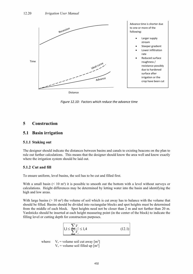
12.20 Irrigation User Manual
Figure 12.10: Factors which reduce the advance time
Advance time is shorter due to one or more of the following:
• Larger supply stream
• Steeper gradient • Lower infiltration
rate • Reduced surface
roughness / resistance possibly due to hardened surface after irrigation or the crop have been cut
Time
Distance
5 Construction 5.1 Basin irrigation 5.1.1 Staking out The designer should indicate the distances between basins and canals to existing beacons on the plan to rule out further calculations. This means that the designer should know the area well and know exactly where the irrigation system should be laid out. 5.1.2 Cut and fill To ensure uniform, level basins, the soil has to be cut and filled first. With a small basin (< 10 m²) it is possible to smooth out the bottom with a level without surveys or calculations. Height differences may be determined by letting water into the basin and identifying the high and low areas. With large basins (> 10 m²) the volume of soil which is cut away has to balance with the volume that should be filled. Basins should be divided into rectangular blocks and spot heights must be determined from the middle of each block. Spot heights need not be closer than 2 m and not further than 20 m. Yardsticks should be inserted at each height measuring point (in the center of the block) to indicate the filling level or cutting depth for construction purposes.
)1.12(4,11,1 ≤≤∑∑
v
s
VV
where: Vs = volume soil cut away [m3]
Vv = volume soil filled up [m3]
432

Flood irrigation 12.21 According to Equation 12.1 more soil has to be cut away than what is needed to fill up. This ratio is commonly accepted and based on practical experience. In any case it makes soil available for ridges and roads if any is left over after the cutting and filling operation.
5.2 Border irrigation 5.2.1 Staking out The final plan should be drafted out in such a way, containing all the necessary information, that it will be possible to use the plan for staking out the field. 5.2.2 Cutting and filling The cutting and filling process is meant to minimise the cross gradients, while making the gradients over the length uniform. Determining the cutting depth and filling level may be done as explained in the section for basin irrigation, but unfortunately it is rather cumbersome to do by hand. Computer programmes may simplify the task considerably. The same principles apply to the cutting and filling process in border and basin irrigation, with the exception of constant gradients in the case of border irrigation. Laser equipment is almost essential for border irrigation, especially where gradients of 1:400 and flatter occur. The capital input or contractor’s fee to construct borders quickly and accurately is usually recovered within a year or two.
Figure 12.11: Final laser levelling 5.3 Furrow irrigation 5.3.1 Staking out Staking out the contour furrows is difficult because of the varying curves. The same staking out method for contour furrows may be used as for contour intervals. Controls should be built in to ensure that furrows are placed correctly. Obvious layout adjustments which become apparent during construction should be made and indicated on the plan. 5.3.2 Cutting and filling
433

12.22 Irrigation User Manual Little or no cutting and filling take place while creating contour furrows. Where artificial gradients are created in furrows, cutting and filling take place as for border irrigation. 5.3.3 Laser equipment Apart from the common use for creating an average flat surface in a field, laser equipment may also be used to accurately stake out gradients. 6 Evaluation of surface irrigation systems As with other types of irrigation systems, a surface irrigation system must also be evaluated before the efficiency thereof can be determined. Furrow and border irrigation systems are evaluated in the same way. Flow measurement can be done by means of weirs (e.g. the Cipoletti or V-notch) or where siphon pipes are used, by means of siphon pipe calibration. 6.1 General information and test procedures The tests and measurements done during an evaluation are described in the following paragraphs. The evaluation must be done while normal irrigation practices are being used. 6.2 Pressure readings
Pressure readings are only done in surface systems where a surface pipe distribution system is used. Test if the operating pressure is in accordance with the design parameters. It will differ from one design to another.
6.3 Delivery tests
The delivery of border irrigation systems can be determined by means of measuring weirs (e.g. the Cipoletti or V-notch). Use a Cipoletti notch with a full length of 457 mm, which is installed at the inlet of the border or furrow (Figure 12.12). Allow for a reasonable size stilling basin in front of the weir, a temporary water retaining structure can be built upstream. Other methods of measuring, such as the V-notch (Figure 12.13), rectangular notch or volumetric method can also be used. If the flow is lower than 100 m3/h, the V-notch can be used. With a certain depth of flow over the crown of the Cipoletti-weir, the flow rate (Q) can be read from Table 12.6.
Figure 12.12: Cipoletti notch
434

Flood irrigation 12.23
Table12.6: Flow rate values (m3/h) for a specific overflow height (mm) for the Cipoletti notch
H (mm)
Q (m3/h)
H (mm)
Q (m3/h)
H (mm)
Q (m3/h)
14 5 73 60 122 130 22 10 77 65 128 140 29 15 81 70 134 150 35 20 85 75 139 160 41 25 88 80 145 170 46 30 92 85 151 180 51 35 96 90 157 190 56 40 99 95 162 200 60 45 102 100 168 210 65 50 109 110 173 220 69 55 115 120 178 230
Figure 12.13: V-notch for flow measuring
Other methods of flow measuring are discussed in Chapter 5: Water of this manual.
6.4 Distribution tests
Surface irrigation is the application of a certain amount of water to the soil where the soil is wetted as the water flows over and infiltrates the soil. The evaluation of surface irrigation systems is done by monitoring the advance and recession times over a certain distance, in order to determine the contact time of the water over the length of the furrow or border.
The furrow or border must be measured and steel or wooden pegs must be driven in on the prescribed intervals on the side of the bed (Figure 11.4). The stream is deflected on the upper end of the border and the strength of the stream and the time is recorded. As the water flows down in the border and the advance front reaches the pegs, the time is recorded. As soon as the water supply at the upper end is cut off, the time is recorded (cut-off time). The difference between this time (cut-off time) and the inlet time, the strength of the stream and the size of the border or furrow (m) can be used to determine the gross application (mm) applied to the border.
435

12.24 Irrigation User Manual
Figure 12.14: Pegs driven into a bed for measurement of the advance front
As the last water flows down the border, the border begins to dry out (recession front). The time is recorded when the area is approximately 80% dried out on both sides of a peg (Figure 11.15). This evaluation technique will be refined by experience. At uneven gradients, it may occur that water dams up at certain points, which means that there is still standing water when the recession front has passed.
Figure 12.15: Drying-off area
The contact time, which is the difference between the advance front and the recession front, is the time that the water is in contact with the soil and therefore an indication of the time the water has to infiltrate the soil. By drawing these fronts on graph paper, the contact time and distribution will be seen. The contact time should be constant to deliver the most uniform irrigation over the length of the border or furrow as possible. To manage the contact time, the irrigator must know which factor has an influence on it – the gradient of the furrow or border, the infiltration rate of the soil and the soil/water conditions, as well as the flow rate of water in the border or furrow. The gradient of the border must be determined by measurement. The volume of water supplied to each border or furrow, is determined by the cut-off time.
436

Flood irrigation 12.25 The actual application is calculated by means of Equation12.2.
)2.12(1000AQTyw =
where wy = average gross application [mm]
Q = flow rate [m3/h] T = time difference between inlet and cut-off time [hours] A = border size [m × m]
The average gross application is the actual application and can be used by the producer to verify his planned scheduled application. The deviation of the average application at each point is determined and from these figures, the Christiansen’s uniformity coefficient (CU) is calculated (Stimie, 2002). The following formula is used:
)3.12(1001 1 ×−
−=∑
=
nT
TTCU
c
n
icic
where CU = Christiansen’s uniformity coefficient [%]
cT = average contact time [mm]
= /n Tn
1=ici∑ ∑
Tci = contact time at peg no i [min] n = number of pegs or measuring points
Typical guidelines for CU-values is as follows (Reinders, 1986): Excellent : CU ≥ 90% Good : 80% ≤ CU ≤ 89% Poor : CU ≤ 79% If the CU < 80%, an infiltration test for the soil must be done and the CU of the application must be determined. This is normally done by using a ring-infiltration meter. The method is described in detail in the Irrigation Evaluation Manual of the ARC-Institute for Agricultural Engineering (2019). The ring is forced into the soil and the infiltration rate is calculated by the time the water level in the ring takes to drop a certain height (mm). The ring infiltration method is however not very accurate because the movement of the soil water through the ring is not always representative of water infiltrating into an irrigation field, especially in very dry soil conditions.
Example 12.1 An irrigation border that was evaluated was 165 m long and 11 m wide. Pegs were driven in each 10 m along the length of the border. The crop on the field was cauliflower and the evaluation was done during a normal irrigation cycle. The farmer planned to apply approximately 75 mm of water. The stream flow was measured with a portable Cipoletti-weir at 150 m³/h. The farmer chose a cut-off time of 51 minutes according to previous experience. The contact time was calculated by measuring the time difference between the advance front and the recession front and is as follows:
437

12.26 Irrigation User Manual
Peg no. Contact time
(min) Peg no. Contact time
(min) Peg no. Contact time
(min) 0 76 6 58 12 68 1 56 7 78 13 62 2 58 8 66 14 55 3 55 9 85 15 51 4 55 10 84 16 56 5 54 11 76
Calculate the average application (mm) and the Christiansen uniformity coefficient. Solution: Average actual application: wy = 1000 QT / A = (1000 × 150 × 51) / (165 × 11 ×60) = 70,25 mm Now calculate the average contact time and make an adjustment to the actual contact time for each peg. It is shown in the table below:
Peg no. Contact time (min.) icc T-T
0 1 2 3 4 5 6 7 8 9
10 11 12 13 14 15 16
76 56 58 55 55 54 58 76 66 85 84 76 68 62 55 51 56
11,83 8,17 6,17 9,17 9,17
10,17 6,17
11,83 1,83
20,83 19,83 11,83 3,83 2,17 9,17
13,17 8,17
17,64Tc = icc
n
1iT-T∑
=
= 163,51
The CU-value is calculated as follows:
good85%=
100×17×64,17
163,51-1=
100×nT
TT -1 =U
c
n
1icic∑
−
−C
Determining the infiltration to determine the CU of the application is therefore not necessary.
438

Flood irrigation 12.27 7 Management and maintenance The practical management of a surface irrigation system demands much effort and knowledge from the producer. It is more complex than managing a mechanical irrigation system. The main reason is the fact that any managerial mistakes made are difficult to rectify, while it is relatively easy to rectify it with a mechanical system. As an example, if the farmer applied 20% less water than he was supposed to, he can immediately apply this water with a sprinkler system, while it is mostly not possible to apply such a small application with a surface system. It is however very important to appreciate that the same basic managerial principles are relevant for a surface system and for a mechanical system. Exactly the same aids such as soil moisture sensors, automatic weather stations, etc. can be used to schedule irrigation. The only difference lies in the practical application of the irrigation water. The instruments in the hands of the manager, with which he can vary the application of water with a surface system, are usually the size of the stream and the cut off time. If planning was done correctly, the length and width of the borders are usually fixed. The other component that determines the size of the stream is the infiltration rate of the soil. This factor can be determined easily in the field and the stream size is therefore the instrument in the manager’s hand with which he can play. It is therefore extremely important in the planning stage to provide the producer with a way of measuring the size of the stream. Just as no mechanical system can function without a pressure meter, there is no surface system that can work without measuring points. The producer must therefore be able to determine the following factors, in order to manage a surface system effectively: • The application depth • The infiltration rate – i.e. the contact time that can vary throughout the growing season • The cut-off time • The size of the stream that can be calculated according to an equation. The maintenance requirements for the different surface systems are as follows: 7.1 Basin irrigation Just as pipes, joints and emitters of sprinkler irrigation systems have to be maintained, the irrigation basin and supply system should also be kept in repair. Soil is dynamic and will not be perfectly level after a season. Basins have to be levelled annually. With these maintenance levelling operations earth moving should normally be minimal, but it is still important for continued good performance by the system. Maintenance should ideally be done immediately when the farmer or irrigator identifies a problem in the system. The reason is that these uneven areas have a very negative impact on the irrigation uniformity. 7.2 Border irrigation
With border irrigation, the basic principle is the regulation of the time duration so that the water remains in contact with the soil to give the required application. At the same time, ensure that the water reaches the end point of the border, while runoff of irrigation water is limited to a minimum. Factors such as infiltration, length, width and gradient cannot change easily. Stream size and cut off time are the only factors the manager has control over to influence application depth and therefore the stream size should be measured by means of a measuring notch. Supply canals, sluices and pipe outlets need to be kept in good condition and leakages need to be repaired timeously to prevent losses, erosion and salination of soil. Ensure that borders ridges and furrows are finished off uniformly and be maintained like that.
439

12.28 Irrigation User Manual 7.3 Furrow irrigation Broken furrow ridges are equivalents of leaking pipes and must be prevented and immediately repaired. Care should be taken at the bottom end of furrows to ensure safe drainage of excess rain and irrigation water. Cultivation should not create local high or low areas. 8 Troubleshooting table Table 12.7: Troubleshooting table for surface systems
Problem Possible causes Solution Water application is irregular
Border measurement incorrect Change layout and/or border widths Incorrect gradient Change gradient Stream size is insufficient Adjust stream size Infiltration rate not considered during design
Re-design
Surface finish insufficient as result of poor equipment and/or finishing
Use suitable equipment to improve finish. Training in correct tillage
Strength of stream not known
No measuring structure Install suitable measuring structure Measuring is not done Establish measurement routine and record
keeping Faulty design Ignorance of designer on complexity of
surface systems Re-design by experienced designer
Gradient incorrect (Cross and length direction)
Faulty design Change gradient (e.g. with Laser level) according to correct design. Change cross gradient to 0%
Supply losses too great
Earth supply canals with high seepage Line canals with concrete, clay or other methods
Concrete canals cracked and leaking Repair cracks Stream size too small Canal blocked with earth and/or organic
material Clean canals according to schedule
Wetting depth insufficient
Stream strength and contact time in unfavourable balance
Adjust stream strength and/or contact time
440

Flood irrigation 12.29 9 References 1. Breedt, H. and Koegelenberg, F.H. 2002. Irrigation Evaluation manual. ARC-Institute for
Agricultural Engineering. RSA. 2. Guidelines for Designing and Evaluating Surface Irrigation Systems. FAO Irrigation and
Drainage paper 45. 3. National Engineering Handbook Section 15-5. Furrow Irrigation. U S A Soil Conservation
Service. 4. Reinders, F.B. 1986. Evaluasie van besproeiingsisteme. Directorate Agriculture-engineering and
Water supplying. RSA. 5. Stimie, C.M., Smal, H.S, Burger, J.H., Heyns, P.J., Kleynhans, E.P.J., Koegelenberg, F.H.,
Lategan, M.T., Mulder, D.J., Uys, W.J., Van der Merwe, F.P.J. and Viljoen, P.D. 1996. Irrigation Design Manual. ARC-Institute for Agricultural Engineering. RSA.
6. Stimie, C.M. 2002. Personal communications. RSA.
441

IRRIGATION USER MANUAL
CHAPTER 13
Greenhouse irrigation systems
442

Greenhouse irrigation systems 13.1
Table of Contents 1 Introduction ........................................................................................................................................................................................................................................... 13.1 2 Greenhouse types .......................................................................................................................................................................................................................... 13.1 3 Growing Media ............................................................................................................................................................................................................................... 13.1
3.1 Soil....................................................................................................................................................................................................................................................... 13.1 3.2 Soilless or substrate media ...................................................................................................................................................................................... 13.1
4 Greenhouse Irrigation practices ................................................................................................................................................................................... 13.2 4.1 Hand watering ..................................................................................................................................................................................................................... 13.2 4.2 Overhead irrigation ....................................................................................................................................................................................................... 13.2
4.2.1 Boom irrigation systems ....................................................................................................................................................................... 13.2 4.2.2 Stationary sprinkler irrigation systems ................................................................................................................................. 13.3 4.2.2.1 Micro-sprinklers and laterals ...................................................................................................................................... 13.3 4.2.2.1.1 Mainlines and submains ........................................................................................................................ 13.4 4.2.2.1.2 Installation ............................................................................................................................................................. 13.4 4.2.2.2 Overhead misting ..................................................................................................................................................................... 13.5 4.2.2.2.1 Design ......................................................................................................................................................................... 13.5 4.2.2.2.2 Installation ............................................................................................................................................................. 13.5
4.3 Drip irrigation ...................................................................................................................................................................................................................... 13.6 4.3.1 Design .......................................................................................................................................................................................................................... 13.7 4.3.1.1 Slopes and levelling ................................................................................................................................................................ 13.7 4.3.1.2 Dripperlines ...................................................................................................................................................................................... 13.7 4.3.1.3 Submains ............................................................................................................................................................................................. 13.7 4.3.1.4 Flushing manifolds .................................................................................................................................................................. 13.7 4.3.1.5 Irrigation blocks .......................................................................................................................................................................... 13.7 4.3.1.6 Mainlines ............................................................................................................................................................................................. 13.8
5 Installation ............................................................................................................................................................................................................................................. 13.8 5.1 Pipelines within the greenhouse ..................................................................................................................................................................... 13.8 5.2 Submains Installation .................................................................................................................................................................................................. 13.8 5.3 Flushing manifolds ........................................................................................................................................................................................................ 13.8 5.4 Mainlines ................................................................................................................................................................................................................................... 13.8
6 Irrigation requirements ......................................................................................................................................................................................................... 13.9
6.1 Net irrigation system flow rate in the soil ....................................................................................................................................... 13.9 6.2 Net irrigation system flow rate for soilless media .............................................................................................................. 13.10 6.3 Design of net irrigation system for soilless media .............................................................................................................. 13.10 6.4 Application rates ........................................................................................................................................................................................................ 13.11
6.4.1 System application rate ..................................................................................................................................................................... 13.11 6.4.2 Instantaneous application rate ................................................................................................................................................... 13.11
7 Drainage ............................................................................................................................................................................................................................................... 13.13
7.1 Design ...................................................................................................................................................................................................................................... 13.13 7.1.1 Slopes and levelling ................................................................................................................................................................................ 13.13 7.1.2 Drainage pipe – Greenhouse drainage pipes .............................................................................................................. 13.13 7.1.3 Drainage pipe – Drainage mainline ...................................................................................................................................... 13.14 7.1.4 Drainage pipes – General .................................................................................................................................................................. 13.14
7.2 Installation........................................................................................................................................................................................................................... 13.14 7.2.1 Drainage pipe – Drainage mainline ...................................................................................................................................... 13.14 7.2.2 Drainage pipes – General .................................................................................................................................................................. 13.14
8 Pump room and head control ....................................................................................................................................................................................... 13.14 9 References .......................................................................................................................................................................................................................................... 13.15
All rights reserved Copyright 2019 ARC-Agricultural Engineering (ARC-AE)
443

13.0 Irrigation User Manual 1 Introduction An irrigation system designed for greenhouse applications are done on the same principles as micro and drip irrigation with a few adaptations to more frequent and intensive irrigation strategies. The technologies used in these systems are more varied with diverse equipment and application techniques. Propagation and greenhouse growers can use from low volume intermittent mist nozzles, travelling booms to drip or microtube irrigation systems. Even ebb and flow systems, trough and capillary mats are used to produce high value products. The intensity ads diversity of irrigation application in greenhouses or under cover as sometimes referred to, the systems require skilled designs, installation and management. It is even more vital that the irrigation system provide uniform water distribution to nursery and greenhouse operations. This can be achieved by the correct design of the system as well as the proper installation and management of the system. (Bilderback et al., 2011). Irrigation management includes proper scheduling, runoff controls, substrate selection to optimize crop production, conservation of water and protection of the environment. A masterplan should be developed and the system should be designed for expansion. This is to prevent costly retrofitting as the business expands. New installations should be designed to allow expansion of the irrigation systems. For existing operations, the design should incorporate the ability to add new equipment or technology as the greenhouse or the nursey grows and modernizes. (Bilderback et al., 2011). As the irrigation system used in greenhouses is an adapted micro or drip irrigation system, the same procedures for the design should be followed as described in Chapter 12: Micro irrigation systems. Filtration needs should also be determined in the same manner as described in this chapter. Sometimes an adapted sprinkler system is used for nurseries with different water requirements. These types of systems should be designed on the same principles as described in Chapter 10: Sprinkler irrigation systems. 2 Greenhouse types Broadly speaking there are two types of greenhouses used in South African agriculture: • A multi-span greenhouse that is large (1 000 m² to 10 000 m² – 0.1 ha to 1.0 ha). • A tunnel that is small (300 m² – 0.03 ha). The irrigation systems differ between the two types according to the sizes and technological advances of the system. 3 Growing media The media used to grow the crop in the greenhouse will have an effect on the determination of the crop water requirements which will determine the volume of water necessary to be distributed at a given time. 3.1 Soil In some tunnels the natural soil on which they are situated is used and the crops are planted directly in the soil. Here the soil texture has the same effect on the water requirement as with normal crop production. (See Chapter 3 Soil and Chapter 4 Crop water requirement). In this situation the crop is usually planted directly in the soil and the water holding capacity of the soil will have an effect on the frequency and scheduling of irrigation. 3.2 Soilless or substrate media. Sometimes a soilless or substrate medium is used. This can comprise of coir (coconut fibre), composted pine bark chips, peat, perlite, vermiculite, polystyrene or different mixtures thereof. The selection of the media is dependent on the specific crop that is grown, as well as the quality and quantity of water available. Other factors like the type of fertigation through the irrigation system will also have an effect on the choice of media. In the case of a soilless media, the crop is usually planted in containers, placed directly on the ground on weed matting, gravel or on raised beds. The container type and size are determined by the specific crop grown and the production system in each situation. (Bilderback et al., 2011).
444

Greenhouse irrigation systems 13.1 4 Greenhouse Irrigation Practices Water is applied in greenhouses with several techniques, including applying water overhead with sprinklers, from below via capillary action, or directly to the surface of the substrate with tubes, spray nozzles, and drip emitters. Mist is used for atmospheric temperature control by increasing the humidity as well as wetting plant material in nurseries where grafting is taking place. 4.1 Hand watering In some situations, hand watering is used to accommodate different sizes of containers, in areas where the water requirements of plants kept in the same area varies as well as supplement irrigation in dryer areas of the greenhouse. It only requires mechanical valves or faucets that can be connected to a hose with nozzle. For difficult to reach areas a portable cart with a pressurised water tank can be used. Manually watering plants by hand is not as easy as it would appear. The operator has to apply water to the substrate, sometimes by avoiding wetting the leaves of the plants. Also, the water has to reach all the cells without under or overwatering. It has several disadvantages as it is more labour intensive, less uniform and less efficient than emitter-based irrigation. Planning the irrigation system inside tunnels should always include several points of connection where hoses can be connected as water is always needed as part of the production process. These points should be marked clearly as not for human consumption if a fertigation system is connected to the irrigation system. (Bilderback et al., 2011). 4.2 Overhead irrigation Overhead irrigation can be done in a greenhouse with either a boom or stationary sprinklers. In both cases, low volume, low pressure nozzles should be used as high-volume sprinklers are unsuitable for most crops grown in greenhouses. Watering with high volumes systems can knock over plants, compress the substrate and flush part of it out of the container. 4.2.1 Boom irrigation systems Boom systems are mobile, moving over the crop with downward facing nozzles spaced along the length of the boom. The booms typically move on overhead rails suspended from the structure supported on both ends or in the middle only. (Figure 13.1, 13.2)
Source: http://www.agriexpo.online/prod/growing-systems-inc/product-178252-34909.html
Figure 13.1: Illustration of an overhead boom irrigation system suspended from rails in the centre
445
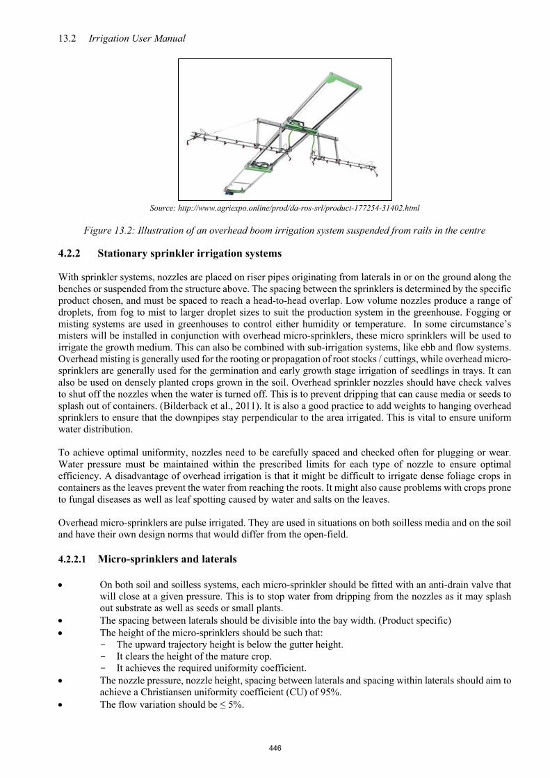
13.2 Irrigation User Manual
Source: http://www.agriexpo.online/prod/da-ros-srl/product-177254-31402.html
Figure 13.2: Illustration of an overhead boom irrigation system suspended from rails in the centre
4.2.2 Stationary sprinkler irrigation systems With sprinkler systems, nozzles are placed on riser pipes originating from laterals in or on the ground along the benches or suspended from the structure above. The spacing between the sprinklers is determined by the specific product chosen, and must be spaced to reach a head-to-head overlap. Low volume nozzles produce a range of droplets, from fog to mist to larger droplet sizes to suit the production system in the greenhouse. Fogging or misting systems are used in greenhouses to control either humidity or temperature. In some circumstance’s misters will be installed in conjunction with overhead micro-sprinklers, these micro sprinklers will be used to irrigate the growth medium. This can also be combined with sub-irrigation systems, like ebb and flow systems. Overhead misting is generally used for the rooting or propagation of root stocks / cuttings, while overhead micro-sprinklers are generally used for the germination and early growth stage irrigation of seedlings in trays. It can also be used on densely planted crops grown in the soil. Overhead sprinkler nozzles should have check valves to shut off the nozzles when the water is turned off. This is to prevent dripping that can cause media or seeds to splash out of containers. (Bilderback et al., 2011). It is also a good practice to add weights to hanging overhead sprinklers to ensure that the downpipes stay perpendicular to the area irrigated. This is vital to ensure uniform water distribution.
To achieve optimal uniformity, nozzles need to be carefully spaced and checked often for plugging or wear. Water pressure must be maintained within the prescribed limits for each type of nozzle to ensure optimal efficiency. A disadvantage of overhead irrigation is that it might be difficult to irrigate dense foliage crops in containers as the leaves prevent the water from reaching the roots. It might also cause problems with crops prone to fungal diseases as well as leaf spotting caused by water and salts on the leaves. Overhead micro-sprinklers are pulse irrigated. They are used in situations on both soilless media and on the soil and have their own design norms that would differ from the open-field. 4.2.2.1 Micro-sprinklers and laterals • On both soil and soilless systems, each micro-sprinkler should be fitted with an anti-drain valve that
will close at a given pressure. This is to stop water from dripping from the nozzles as it may splash out substrate as well as seeds or small plants.
• The spacing between laterals should be divisible into the bay width. (Product specific) • The height of the micro-sprinklers should be such that:
- The upward trajectory height is below the gutter height. - It clears the height of the mature crop. - It achieves the required uniformity coefficient.
• The nozzle pressure, nozzle height, spacing between laterals and spacing within laterals should aim to achieve a Christiansen uniformity coefficient (CU) of 95%.
• The flow variation should be ≤ 5%.
446

Greenhouse irrigation systems 13.3 • The gross instantaneous application rate on the soil should never exceed the infiltration rate of the soil.
Where a soilless medium is used on table trays or in small plugs, the gross instantaneous application rate should be between 12 mm/h and 18 mm/h.
Figure 13.3: Overhead micro irrigation nozzles (Netafim)
Figure 13.4: Installation of overhead micro irrigation nozzles showing downpipes, weights, check valves and
sprinklers (Netafim) 4.2.2.1.1 Mainlines and submains For structural strength, uPVC pipes that are not buried should be a minimum of Class 12, even if the system pressure does not require this class. To negate the need to build-up pressure to open the micro-sprinklers, a pressure tank should be fitted downstream of the system’s pump but before the irrigation valves to maintain a constant high pressure within the mainline. 4.2.2.1.2 Installation The greenhouse structure should be built to accommodate an overhead micro-irrigation system. The greenhouse structure must be fitted with steel beams at either end of the bays; to which steel cables / ropes can be fixed at
447

13.4 Irrigation User Manual the same height as the laterals. Steel cables are normally 5 mm in diameter. Each lateral is tied or strapped directly to one steel cable, one tie for each 0.25 m to 0.30 m length of lateral. (See Figure 13.5).
Figure 13.5 Wire rope support for laterals (Netafim)
The steel ropes to which the laterals are tied should themselves be supported by resting on steel ropes that are secured at right-angles to the laterals. These steel ropes are fitted to the greenhouse posts and are normally 4 m apart depending on the design of the structure. 4.2.2.2 Overhead misting Misting is used for cooling and for propagating cuttings while they have no roots. Having no roots for support or to uptake water, cuttings cannot be irrigated with a normal micro-sprinkler. A mist irrigator needs to produce fine droplets, normally less than 100 microns in diameter. This can be produced normally at a relatively high nozzle pressure of 35 m to 45 m (3.5 to 4.5 bar). 4.2.2.2.1 Design The system should be designed with a maximum of 10 shifts, so that a maximum of 6 second pulse can be given over a maximum of 60 seconds. This will also allow a minimum of 3 seconds pulse every 30 seconds. The flow variation should be ≤ 5%. The rest of the design norms are basically the same as for drip irrigation (mentioned in 1.3.3) 4.2.2.2.2 Installation The installation follows the same procedure as for overhead micro-sprinklers.
Figure 13.6: Overhead misting. Generally used for the rooting or propagation of root stocks /cuttings (Netafim)
448

Greenhouse irrigation systems 13.5 4.3 Drip irrigation
The use of drip irrigation in greenhouses is hampered by the non-uniformity of crops produced, caused by different sized containers, mix of plant varieties and the frequent change in spacing. Nevertheless, more growers are changing over to drip irrigation wherever possible because of the advantages in plant growth and water conservation. There are three types used in greenhouses, integral dripper lines, external/on-line (button) drippers and external/on-line button drippers with micro tubes and arrows. For crops grown in the soil, integral dripper lines or external drippers can be used. This would be applied in the same way as described in Chapter 12 Micro irrigation systems. For soilless media held in troughs, integral dripper lines are used and for bags, individual button-type drippers with or without micro tubes can be used (Figure 13.7). The dripper should have a ‘non-leakage’ function (CNL) and hold water below a specified pressure for all soilless systems.
Figure 13.7: External/on-line button drippers with microtubes and arrows used in soil-less substrates in bags or containers (Netafim) The following drip irrigation norms are mainly for use with a soilless medium. A crop grown in a soilless medium requires accurate pulsed irrigation evenly delivered throughout the greenhouse that is consistent in the quantity of water and content of nutrients. This aspect gives rise to specialised drip irrigation equipment with its own design norms. The norms for misting and micro-sprinklers are generally only mentioned where they differ from drip.
449

13.6 Irrigation User Manual Hydraulically, the drip irrigation of greenhouse crops grown in the soil differs little from the open-field. Its norms are only discussed where they differ, such as the pipe layout within the greenhouse. The rest can be found in Chapter 12 Micro-irrigation systems.
4.3.1 Design 4.3.1.1 Slopes and levelling The main purpose for the slopes of a greenhouse floor is drainage. Such slopes will determine the hydraulics of the drip irrigation design. The ranges of these slopes are described below in section 7 on Drainage. 4.3.1.2 Dripper lines Dripper spacing along the dripper line: • ≤ 0.3 m (Soilless) • ≤ 0.4 m (Soil)
The spacing between dripper lines is a function of the plant row spacing and is usually divisible into the greenhouse bay width. To detract from this could cause a plant row to lie directly underneath a greenhouse gutter, from which it may receive night time condensation dripping from the underside of the gutter. The recommended maximum dripper flow rate is 2.3 ℓ/h. The recommended velocities are: • Maximum irrigating velocity at the inlet to the dripper line ≤ 2.0 m/s • Minimum flushing velocity ≥ 0.5 m/s at the last emitter at the end of the dripper line 4.3.1.3 Sub-mains The sub-mains should be placed at the upper side of the slope. Dripper lines should not run uphill.
The recommended maximum velocities at the inlet to the sub-main should be: • maximum velocity ≤ 3.0 m/s if pipe diameter > 50 mm • maximum velocity ≤ 2.5 m/s if pipe diameter ≤ 50 mm
For structural strength, uPVC pipes that are not buried such as riser pipes for flushing valves should be a minimum of Class 12, even if the system pressure does not require this class. 4.3.1.4 Flushing manifolds The flushing manifold is the pipe into which the ends of the dripper lines are connected: the opposite side of the irrigation block to the sub-main.
If feasible, do not use a flushing manifold to flush several dripper lines at one time; rather flush dripper lines individually.
If unavoidable, the length of the flushing manifold should be kept to a minimum and based on: • The maximum number of flushing valves that the operator is prepared to handle. • The desired limit to the additional flow rate and head that must be incorporated into the irrigation
system pipeline design and the irrigation pump’s design flow and head to accommodate the increased flow rate and head losses that occur during flushing.
Flushing manifold diameters must be sized to achieve the above 0.5 m/s velocity at the ends of the dripper lines.
450

Greenhouse irrigation systems 13.7 4.3.1.5 Irrigation blocks In a soilless system: • All irrigation blocks should where possible be equal in size. • The maximum size of an irrigation block cannot exceed the area that will receive one fertiliser recipe
and irrigation application. • The maximum number of shifts is 12. Normally this number is between 4 and 8.
4.3.1.6 Mainlines In a soilless system, unless the dosing recipe will never change, each irrigation block should have its own mainline. Mainline pipe sizing should be such that the friction head plus the static head combination for each mainline should be the same, provided that: • Longest mainline maximum friction loss ≤ 1.5% • Maximum velocity on all other mainlines ≤ 2.2 m/s
5 Installation 5.1 Pipelines within the greenhouse No pipeline trench edges may come closer than 0.3 m to any greenhouse foundations (5). (See Figure 13.8).
Figure 13.8: Pipeline trench within a greenhouse (Netafim)
5.2 Submains Submains should be buried to a depth of 0.3 m. 5.3 Flushing manifolds These should be buried to a depth of 0.3 m. Where a flushing manifold discharges via a valve into the greenhouse drainage pipe, it must first be vented into the atmosphere and not be joined with a pressure-sealed connection direct to the drainage pipe.
451

13.8 Irrigation User Manual 5.4 Mainlines Mainlines should be installed according to SANS 1200 LB: 1983 and SANS 10112: 2003. Where multiple uPVC pipelines shared one trench, there should be a minimum of 300 mm between the outside of each pipe if the joints are integral rubber ring type (Figure 13.9). If it is not possible to achieve 300 mm between pipelines, solvent-weld joints should be used.
Figure 13.9: Dedicated main lines sharing one trench (Netafim)
6 Irrigation requirements Regardless of its geographic location in South Africa, a greenhouse aims to modify the environment to optimise plant growth so that generally speaking under optimum light conditions, the temperature is about 25°C and the relative humidity of 70-80%. This will differ according to the specific crop grown. 6.1 Net irrigation system flow rate in the soil Under such conditions the net water requirement of a crop with full leaf canopy would be about 6.0 mm/day or 6.0 ℓ/m²/day. In the soil, this daily crop water requirement is used in the design to calculate the net irrigation flow rate of the system.
sCWRNSFR
Ti= (13.1)
where NSFRs = Net system flow rate in soil CWR = Crop water requirement Ti = Hours of operation per day
Example: For a 2 000 m² system in the soil, where irrigation takes place over 7 hours per day.
452

Greenhouse irrigation systems 13.9
×=
=
2 2
s
3
6.0 / m / day 2000mNSFR7h / day
1.71m / h
6.2 Net irrigation system flow rate for soilless media The daily figure calculated for soil cannot be used to determine the net irrigation system flow rate for soilless conditions. This must be an hourly value.
Under the same optimum environmental conditions described above, the net water requirement of a crop with full leaf canopy growing in a soilless medium would be about 0.8 mm/h or 0.8 ℓ/m²/h. Further, drainage for leaching the soilless media must be added to this hourly requirement. Usually in the region of 50% is added.
Leaching requirement (drainage) = Crop water requirement 0.8 ℓ/m²/h × 50% = 0.4 ℓ/m²/h Crop water requirement = 0.8 ℓ/m²/h Leaching requirement (drainage) = 0.4 ℓ/m²/h Total net irrigation requirement for soilless = 1.2 ℓ/m²/h Total net irrigation requirement for soilless = 1.2 mm/h Note. 50% added for leaching is usually referred to as 33% drainage. (Drainage = 1.2 ℓ/m²/day × 33% = 0.4 ℓ/m²/day)
s tNSFR TNIR A= × (13.2)
where NSFRs = Net system flow rate in soil TNIR = Total net irrigation requirement At = Total area
Example: For a 15 000 m² soilless system.
= ×
=
2 2s
3
NSFR 1.2 / m / h 15 000m
18.0m / h
6.3 Design of net irrigation system storage for soilless media The same net water requirement of 6.0 ℓ/m²/day for a crop growing in the soil with full leaf canopy would also apply to a crop growing in a soilless medium. However, the leaching requirement must be added for the soilless crop.
Total daily irrigation requirement in soilless = 6.0 ℓ/m²/day + 50% leaching = 9.0 ℓ/m²/day
This daily figure is used to determine the daily storage requirement for soilless conditions but not the irrigation flow rate.
453

13.10 Irrigation User Manual 6.4 Application rates With an irrigation system in the soil, the net irrigation requirement is normally expressed as mm/day (the application rate of the entire system over one day) and the gross application rate as mm/h (the application rate taking place within an irrigation block at the time that it is being irrigated).(1)
However, in soilless systems, they are both expressed in mm/h or ℓ/m²/h. It is important to distinguish between the two application rates: • Net system application rate • Instantaneous application rate 6.4.1 System application rate This is application rate of the irrigation system over a constant period of time.
NAR = QsysAT
(13.3)
where NAR = Net system application rate AT = Total area irrigated Qsys = Net system flow rate
Example: For the 15 000 m² soilless system above, where the irrigation system flow rate was 18 m³/h.
=
=
218 000 / hNAR15 000m
1.2mm / h
This is the application rate that is used for irrigation scheduling in soilless systems. 6.4.2 Instantaneous application rate The application rate of one irrigation block at the time that it is being irrigated is the instantaneous application rate. This is the application rate that is used to determine the individual designed flow rate and spacing of the emitters, be they drippers or micro-sprinklers.
For an irrigation system with equal-sized irrigation blocks, the net instantaneous application rate is as follows.
NARi = NAR × Ns (13.4)
where NARi = Net instantaneous application rate NAR = Net system application rate Ns = Number of irrigation shifts
Example:
For the 15 000 m² soilless system above, where the net system application rate was 1.2 mm/h and shall be divided into 4 irrigation blocks of 3 750 m² each. One irrigation block shall be irrigated at a time (one shift).
𝑁𝑁𝑁𝑁𝑁𝑁𝑖𝑖 = 1.2 𝑚𝑚𝑚𝑚/ℎ × 4 = 4.8𝑚𝑚𝑚𝑚/ℎ
454

Greenhouse irrigation systems 13.11 For a drip or micro-sprinkler irrigation system, the gross instantaneous application rate is as follows.
GARi = NARiηa
(13.5)
where GARi = Gross instantaneous application rate NARi = Net instantaneous application rate ηa = Application efficiency
Example: For the 15 000 m² soilless system above, where the net instantaneous application rate was 4.8 mm/h, if this system was to be irrigated by drip, which has an application efficiency of 90%. (2).
𝐺𝐺𝑁𝑁𝑁𝑁𝑖𝑖 = 4.8 𝑚𝑚𝑚𝑚/ℎ ÷ 0.9 = 5.3 𝑚𝑚𝑚𝑚/ℎ
In terms of the drip irrigation equipment, the gross instantaneous application rate is as follows. For a drip or micro-sprinkler irrigation system, the gross instantaneous application rate is as follows.
GARi = qeLe× Lave
(13.6)
where GARi = Gross instantaneous application rate qe = Emitter flow rate Le = Emitter spacing within the dripper line Lave = Average lateral spacing
Example: A possible drip configuration for the above, where the gross instantaneous application rate was 5.2 mm/h could be as follows:
𝐺𝐺𝑁𝑁𝑁𝑁𝑖𝑖 =1.0 ℓ/ℎ
0.24𝑚𝑚 × 0.8
= 5.2𝑚𝑚𝑚𝑚/ℎ where
qe = 1.0 ℓ/h Le = 0.24 m Lave = 0.8 m
455

13.12 Irrigation User Manual 7 Drainage 7.1 Design Nutrient enriched irrigation water in soilless media demands continuous leaching, the leachate from which must be drained away. As this drainage is directly related to the irrigation design, specifically the irrigation application rate, it too has its own design norms.
7.1.1 Slopes and levelling
As mentioned, the main purpose for the slopes of a greenhouse floor is drainage. This includes rainfall drainage from the roof and gutters of the greenhouse structure itself and the ground slope must cater for the necessary slopes of this structure.
Parallel to the dripper lines (crop row direction). • Soilless – 1% < slope < 2%. • Soil – 0.5% < slope < 2%.*
At right angle to the dripperlines (parallel to the gable side). • Soilless – 0,25% ≤ slope < 2%. The minimum slope is 0.25% but preferred range is 1-2%. • Soil – 0.5% < slope < 2%.* • The limit of 2% is set by the greenhouse structure. Slopes and levelling must be agreed on by both the irrigation designer and the greenhouse supplier.
7.1.2 Drainage pipe – Greenhouse drainage pipes
The greenhouse drainage pipe is the pipe inside a greenhouse that removes drainage, leachate and discharged flushing water by gravity. It is laid at a right angle to the dripper line direction. It is usually only used where the growing medium is contained in troughs. Where pots, bags or ‘growbags’ are used, an open channel is usually formed into the greenhouse floor.
If the crop row lengths are greater than 20 m, depending on the slope more than one greenhouse drainage pipe will be needed in a greenhouse. Such multiple greenhouse drainage pipes should be laid at the following intervals: • 1.0% slope, interval ≤ 20 m • 1.5% slope, interval ≤ 25 m • 2.0% slope, interval ≤ 30 m
A greenhouse drainage pipe has generally one diameter throughout its length. It should be sized as follows to handle 50% of the irrigation flow rate to the greenhouse. If there is more than one greenhouse drainage pipe in a greenhouse, then this 50% of the total flow may be apportioned accordingly:
GDPFR = QGH2×Ngdp
(13.7)
where GDPFR = Greenhouse drainage pipe flow rate QGH = Irrigation flow rate to the greenhouse Ngdp = Number of greenhouse drainage pipes
456

Greenhouse irrigation systems 13.13 The slope of the pipeline should follow the slope of the ground surface and should not exceed the slope of the surface.
7.1.3 Drainage pipe – Drainage mainline The drainage mainline is the pipe that collects the drainage from two or more greenhouses and takes that drainage by gravity to a collection point. The slope of the drainage mainline is determined by the greenhouse project’s topography. The size of the drainage mainline is such that: • It drains the first greenhouse with half the irrigation flow rate as above. • It also drains the second greenhouse with an addition half of the irrigation flow rate. • The accumulated flow along the drainage mainline to the drainage collection point need never exceed
the full drainage flow rate. This applies only to the area of the greenhouse project controlled by one dosing unit. If there is an area of the greenhouse project that is controlled by a second dosing unit but sharing a common drainage mainline with the first dosing unit, then that mainline would be sized according to the total of the two flow rates.
7.1.4 Drainage pipes – General All drainage pipelines should be designed using Manning’s formula whereby the maximum permissible mean hydraulic depth is 94% of the pipe internal diameter. Drainage pipelines may be uPVC pressure pipe or sewer pipe. 7.2 Installation 7.2.1 Drainage pipe – Greenhouse drainage pipes The drainage pipes should be buried to a depth of 0.5 m. 7.2.2 Drainage pipe – Drainage mainline
This should be installed in the same manner as described above in 5.4 Mainlines.
8 Pump room and head control The pump room and head control are in one building and comprise of: • Electrical switchgear • Electronic controller / computer • Fertiliser dosing unit • Fertiliser mixing and storage • Emergency manual fertiliser dosing system • Filters • Separate pumps for:
o Irrigation o Service water o Cooling water
457

13.14 Irrigation User Manual
The following norms apply: Where dedicated mainlines are used, the site of the head control should be at the lowest elevation of the whole irrigation system. This enables the irrigation valves to be housed in the head control. Suction pipeline. A negative suction for the irrigation pump should not be used. Use a flooded suction: if necessary, use a tank or reservoir.
Velocities: • Suction pipeline – maximum velocity ≤ 1.0 m/s (When all irrigation, service water and cooling water
pumps are operating) • Filter manifolds – maximum velocity ≤ 3.2 m/s • Head control mainlines – maximum velocity ≤ 3.0 m/s All mainline equipment and fittings are to be equal in diameter to the mainline. This includes: • flow meters • control valves • check valves 9 References 1. Bilderback, T.E., Dole, J.M., Sneed, R.E. 2011.Chapter 22: Greenhouse and Nursery Irrigation
Practice. Irrigation, Sixth edition. Irrigation Association, Fairfax, Virginia, USA
2. Greenhouse Irrigation Design Norms: Netafim South Africa Design Guide. 2013.Version 2.00
3. SABI Design Norms. Application Efficiencies. http://www.sabi.co.za/design
4. South African Bureau of Standards. SANS 1200 LB: 1983. Standard specification for civil engineering construction. LB: Bedding (Pipes). Pretoria
5. South African Bureau of Standards. SANS 10112: 2003. The installation of polyethylene and polyvinyl
chloride (PVC-U and PVC-M) pipes. Pretoria
458

IRRIGATION USER MANUAL
CHAPTER 14
Pumps and driving systems
459

Pumps and driving systems 14.1
Table of Contents 1. Introduction ........................................................................................................................................................................................................................................ 14.1 2 Classification of pumps .......................................................................................................................................................................................................... 14.2
2.1 Centrifugal pumps for irrigation ....................................................................................................................................................................... 14.2 2.1.1 General single stage end-suction pumps ................................................................................................................................. 14.2 2.1.2 Submersible single stage end-suction pumps .................................................................................................................... 14.3 2.1.3 Double-suction single stage pumps ............................................................................................................................................... 14.4 2.1.4 Multistage pumps ............................................................................................................................................................................................... 14.5 2.1.5 Submersible multistage pumps ........................................................................................................................................................... 14.5
2.2 Positive displacement pumps for irrigation .......................................................................................................................................... 14.7 2.3 Positive displacement pumps for dosing ................................................................................................................................................. 14.7
3 Selecting a pump ............................................................................................................................................................................................................................ 14.8
3.1 Coupling pumps in series ................................................................................................................................................................................... 14.10 3.2 Coupling pumps in parallel ................................................................................................................................................................................. 14.11 3.3 Nett positive suction height (NPSH) ........................................................................................................................................................ 14.12
4 Typical pump set-up for different water sources ................................................................................................................................. 14.16 4.1 Rivers .......................................................................................................................................................................................................................................... 14.16 4.2 Boreholes ................................................................................................................................................................................................................................ 14.16
4.2.1 Submersible pumps ..................................................................................................................................................................................... 14.16 4.2.2 Hydraulic screw borehole pumps ............................................................................................................................................... 14.18 4.2.3 Turbine pumps .................................................................................................................................................................................................. 14.18
4.3 Sand points ............................................................................................................................................................................................................................ 14.18 4.4 Earth dams ............................................................................................................................................................................................................................. 14.19
5 Protection of pumps against water hammer ............................................................................................................................................... 14.19 6 Installation of pumps ............................................................................................................................................................................................................ 14.19
6.1 General....................................................................................................................................................................................................................................... 14.19 6.2 Suction side .......................................................................................................................................................................................................................... 14.19 6.3 Delivery side ....................................................................................................................................................................................................................... 14.22 6.4 Final finishing of installation ........................................................................................................................................................................... 14.23 6.5 Pump casing ......................................................................................................................................................................................................................... 14.23 6.6 Protection from theft .................................................................................................................................................................................................. 14.24
7 Evaluation of pumps ............................................................................................................................................................................................................. 14.24 8 Operation of pumps ............................................................................................................................................................................................................... 14.27
8.1 De-aeration ............................................................................................................................................................................................................................. 14.28 8.2 Putting pumps into operation ............................................................................................................................................................................. 14.28 8.3 Switching of the pumps............................................................................................................................................................................................ 14.29
9 Maintenance of pumps ....................................................................................................................................................................................................... 14.29 10 Trouble shooting tables ..................................................................................................................................................................................................... 14.31 11 Power sources ............................................................................................................................................................................................................................. 14.37
11.1 General .................................................................................................................................................................................................................................. 14.37 11.2 Electric motors ........................................................................................................................................................................................................... 14.37 11.2.1 Types of electric motors ............................................................................................................................................................................. 14.37 11.2.2 Physical properties ............................................................................................................................................................................................ 14.38
460

14.2 Irrigation User Manual
11.2.2.1 Materials ............................................................................................................................................................................................ 14.38 11.2.2.2 Standard dimensions ............................................................................................................................................................ 14.38 11.2.2.3 Mounting ........................................................................................................................................................................................... 14.39 11.2.2.4 Cooling ................................................................................................................................................................................................ 14.39 11.2.2.5 Protection .......................................................................................................................................................................................... 14.39
11.3 Performance ................................................................................................................................................................................................................... 14.39 11.3.1 Power rating ......................................................................................................................................................................................... 14.40 11.3.2 Motor efficiency.............................................................................................................................................................................. 14.40 11.3.3 Power factor ......................................................................................................................................................................................... 14.41 11.3.4 Rotor speed and direction..................................................................................................................................................... 14.42
11.4 Selecting an electric motor............................................................................................................................................................................ 14.42 11.5 Switch gear ...................................................................................................................................................................................................................... 14.43 11.6 Protection .......................................................................................................................................................................................................................... 14.43 11.7 Supply cables ................................................................................................................................................................................................................ 14.44 11.8 Variable Speed Drives........................................................................................................................................................................................ 14.45
12 Internal combustion engines ...................................................................................................................................................................................... 14.48
12.1 Types of internal combustion engines ............................................................................................................................................. 14.48 12.2 Performance of diesel engines .................................................................................................................................................................. 14.48 12.3 Selecting a diesel engine ................................................................................................................................................................................. 14.49
12.3.1 General ................................................................................................................................................................................................................. 14.49 12.3.2 Required performance ........................................................................................................................................................................ 14.49
13 Coupling............................................................................................................................................................................................................................................ 14.50
13.1 Direct coupling ........................................................................................................................................................................................................... 14.50 13.1.1 Power ratings ................................................................................................................................................................................................ 14.50 13.1.2 Coupling ............................................................................................................................................................................................................. 14.50
13.2 Belt and pulley coupling .................................................................................................................................................................................. 14.50 13.2.1 Determination of the type of belt ........................................................................................................................................... 14.50 13.2.2 Determination of pulley sizes, distance between centre points and belt length .............. 14.50
14 Energy costs.................................................................................................................................................................................................................................. 14.50
14.1 ESKOM tariff structures .................................................................................................................................................................................. 14.50 14.1.1 NIGHTSAVE Rural ............................................................................................................................................................................. 14.51 14.1.2 RURAFLEX .................................................................................................................................................................................................. 14.55 14.1.3 LANDRATE ................................................................................................................................................................................................. 14.57 14.1.4 LANDRIGHT .............................................................................................................................................................................................. 14.59 14.1.5 Determination of electricity costs ......................................................................................................................................... 14.59
14.2 Diesel costs ..................................................................................................................................................................................................................... 14.64 15 References ...................................................................................................................................................................................................................................... 14.65
All rights reserved Copyright 2019 ARC-Agricultural Engineering (ARC-AE)
461

Pumps and driving systems 14.1
1 Introduction
Pumps are widely used in irrigation systems and schemes. When there is a pump in an irrigation system or scheme, the running costs rise dramatically and the most economical pump that is technically suited to the application must be selected. This Chapter contains information that includes descriptions of pumps generally used in irrigation as published in the Chapter on pumps in the Irrigation Design Manual of the ARC-institute for Agricultural Engineering, as well as practical information on the choice, installation, evaluation, operation and maintenance of pumps. Most pumps are able to pump most liquids, with or without solids in suspension, but in this chapter we will only be looking at the pumping of relatively clean water at more or less ambient temperature. The function of a pump in any hydraulic system is to add energy to the system. Figure 14.1 clearly shows that without a pump it would be impossible for the water to flow from point A to point B. If a pump is, however, added to the hydraulic system between points A and B, as indicated in Figure 14.1, and sufficient energy is added to the system, the water will flow from point A to point B.
Figure 14.1: Addition of energy to a hydraulic system
The amount of energy added to the hydraulic system in the form of pressure head will determine the slope of the hydraulic gradient, which in turn will determine the flow therein. In Figure 14.1, the total energy added to the hydraulic system by the pump is represented by H and the hydraulic gradient by the dotted line. A pump is included in a hydraulic system for the purpose of adding sufficient energy to the system. This energy, which is supplied in the form of pressure head, must equal the static head, emitter pressure (e.g. in overhead irrigation systems) and friction and other losses to have the desired effect. The energy that is added to a hydraulic system in the form of pressure head is dependent on the flow in the system. However, a balance should be maintained between the pump head and the pump delivery on the one hand and the energy that has been added to the hydraulic system and the flow therein on the other. 2 Classification of pumps
462

14.2 Irrigation User Manual
Figure 14.2 displays a simplified classification of pumps for irrigation. Most centrifugal pumps are commonly used for irrigation, but as far as the positive displacement pumps are concerned, it is only the progressive cavity rotary type pumps that are sometimes used for irrigation. The latter entails a spiral shaped rotor and horizontal and vertical types being marketed in the Republic of South Africa. These types of pumps, which can very well be commonly used for irrigation, are discussed in Section 2.1 and 2.2. Positive displacement pumps are generally used for the dosing of chemicals and this is discussed in Section 2.3.
Figure 14.2: Classification of pumps for irrigation
2.1 Centrifugal pumps for irrigation
Centrifugal pumps are widely used for irrigation. The most common types will be discussed. 2.1.1 General single stage end-suction pumps This is the pump most commonly used for irrigation. It is the most basic centrifugal pump and all the other types of centrifugal pumps have been developed from this one to satisfy certain specific requirements. These types of pumps are usually equipped with radial-flow impellers, but mixed-flow impellers are also used for pumps with larger pump deliveries against smaller pump heads. One of the different types of volute casings is usually used. The main reason why there is a moving away from these types of pumps is NPSH (nett positive suction head) problems. Parallel and series couplings are also commonly found with these types of pumps. (See Section 3).
463

Pumps and driving systems 14.3
Figure 14.3: General end-suction single stage centrifugal pump (Source: Centrifugal Pump Wikipedia)
2.1.2 Submersible single stage end-suction pumps These types of centrifugal pumps have been specially developed for situations where NPSH problems are being experienced. The two basic types, namely the drive shaft type, of which the axial-flow pumps are best known, and drainage pumps can best be distinguished from each other by the position of their drivers. With the axial-flow pump, the pump is driven by means of a driver that is positioned above ground and the impeller by means of a drive shaft. The pump is installed in such a way that the impeller itself is below the water level and the pump thus has a positive suction head. The impeller itself is also of the axial-flow type and thus the name axial-flow pump. However, mixed-flow impellers are also sometimes used. Tubular shaped casings are used for these types of pumps. They are usually applied where large pump deliveries have to be pumped against small pump heads. These types of pumps, however, also show up as multistage pumps and they are sometimes equipped with mixed-flow impellers.
Figure 14.4: Axial flow pump
(Source: Lawrence Pumps-ABS Engineering & Trading Sdn. Bhd.)
464

14.4 Irrigation User Manual
The electric motor of the other type, which is known in the trade as a drainage or fountain pump, together with the pump, forms a unit. The whole unit can be installed below the water level because the motor is in a watertight compartment. The outlet of the pump is on the side of the unit and the electric motor is mounted on top of the unit.
Figure 14.5: Drainage pump
(Source: General Pump Company)
These two characteristics and the fact that it is a single stage pump distinguishes it from the submersible pump, which is commonly known as a submersible pump (See Section 3.1.5). It is usually used as a portable unit for smaller pump deliveries and heads and thus doesn't play such an important role in irrigation itself. Due to their dimensions, neither of these pumps are as a rule suitable for boreholes. 2.1.3 Double-suction single stage pumps The double-suction single stage pump is basically two general single stage centrifugal pumps mounted back-to-back, each with its own impeller. The two impellers, are, however, driven by the same driver. Strictly speaking, it is therefore two identical pumps coupled in parallel. Just like other pumps coupled in parallel, these types of pumps are meant for larger deliveries. The two types, namely the vertical and the horizontal split, differ from each other in respect of the manner in which their volute casings open. In the former, the casing divides into two vertical sections and in the latter into two horizontal sections. This casing is also classified as an alternate type of casing, namely a horizontal split casing.
465

Pumps and driving systems 14.5
Figure 14.6: Double-suction single centrifugal pump
(Source: Pump Fundamentals) 2.1.4 Multi-stage pumps A multi-stage pump is a centrifugal pump with a series of impellers arranged in series. The water is thus pumped from one impeller to the next, and just as for pumps coupled in series, it is meant for larger pump heads. The two types, namely the ring profile and the cylinder types, differ from each other in the sense that the former has a series of separate units which can be joined together and the latter is mounted in a cylinder to handle higher pressures within the pump.
Figure 14.7: Ring type multi-stage centrifugal pump
(Source: Flowserve-ABS Engineering & Trading Sdn. Bhd.)
2.1.5 Submersible multi-stage pumps Like the submersible single stage pumps, there are also two types of submersible multi-stage pumps, namely the types where the driver is placed above ground and the types where the driver – in the case of an electric motor – is below water level. An example of the former is the vertical turbine that was so popular for boreholes, which in the early days was known as a "bucket pump". The driver is placed
466

14.6 Irrigation User Manual
above ground and the impellers, which are arranged in series, are driven by a shaft. This type of pump is equipped with axial- or mixed-flow impellers. Impellers or "buckets" can be decreased or increased, as desired. This type of pump is now also provided with a submersible motor that is positioned underneath the pump so that it almost resembles the second type. However, it is still known in the trade as a vertical turbine because the "buckets" can be distinguished from one another.
Figure 14.8: Examples of vertical turbines
Pumps that are commonly known as submersible pumps are all classified under the latter group. Unlike the single stage submersible pumps, the electric motors of this group are always mounted underneath the impellers and the water thus flows inside the "pump" until it is let out at the top of the pump. The casing is tubular in shape and axial- or mixed-flow impellers are used. The "buckets" can, however, not be distinguished from one another.
Figure 14.9: Examples of multi-stage submersible pumps
467

Pumps and driving systems 14.7
2.2 Positive displacement pumps for irrigation
Figure 14.10: Horisontal spiral shaped rotary type positive displacement pumps
(Source: Heishin PC Pumps) The spiral shaped rotary type pump is the only positive displacement pump that is currently being used on a significant scale for irrigation. The vertical type that is used in boreholes can especially be considered. The horizontal type can be considered where centrifugal pumps are usually used. The most important characteristic of positive displacement pumps is that they can deliver large pump heads and it is particularly on these grounds that they are worth considering. However, this characteristic is also a disadvantage because if the system delivery should for one reason or another decrease, e.g. if a stopcock in the system should be closed, the system pressure will increase, which could have serious negative consequences: the pipes may, e.g. burst, or the pump itself could be damaged. Pressure release valves can, however, rule out this risk. 2.3 Positive displacement pumps for dosing Piston type reciprocating positive displacement pumps are usually used for dosing chemicals into a system. Here, the characteristic of positive displacement pumps that is normally a disadvantage comes in very handy, because irrespective of the pressure in the system, a constant flow of chemicals is pumped into the system.
Figure 14.11: Piston type dosing pump (Source: Shuang Feng Chemical Co. Ltd)
468

14.8 Irrigation User Manual
3 Selecting a pump
There is no recipe for the selection of the most suitable pump. Various factors would influence the selection, but in the end, economics has to be the decisive factor and this would include capital, maintenance, replacement and energy costs. The following general guidelines apply: Normal installations General single stage end-suction centrifugal
pumps
Large suction heads Submersible pumps Large pump deliveries Double-suction centrifugal pumps, general single
stage end-suction centrifugal pumps coupled in parallel
Large pump heads Multi-stage centrifugal pumps, general end-suction single-stage pumps coupled in series, positive displacement pumps
Large pump deliveries and small pump heads Axial-flow pumps
For each application, there will be a number of suitable types, makes and models, but over the long term, the most economical pump must be chosen. Factors such as after-sales service and personal preferences may also play a part. An example of a pump curve for a centrifugal pump as published by the pump manufacturer is given in Figure 14.12. It contains the following information: • Pressure delivery (HQ) curves for the full impeller, as well as a number of selected smaller
impeller diameter. • Pump efficiency [%] • Nett positive suction height (NPSHrequired) required by the pump [m] • Drive required for the different impeller diameters [kW]. It can however also be determined by
means of the following equations:
η
ρ 000 36
Q H g = P×××× (14.1)
Where P = power required [kW] ρ = density of water [kg/m3] g = acceleration of gravity [m/s2] H = pump head at duty point [m] Q = pump delivery at duty point [m3/h] η = pump efficiency at duty point [%] The drive power required over an irrigation season can be calculated by multiplying the power required at the pump with the number of hours pumped over the irrigation season. The published pump curves for pumps are usually the average of a number of pumps tested, i.e. the curve of a specific pump can deviate from that which was published. The pump that was purchased can therefore be tested upon request. There are costs involved and this is only done if the pump delivery and pressure can be measured reasonably accurate.
469

Pumps and driving systems 14.9
The point on the pump curve where the system curve crosses the pump curve is called the duty point. The system curve is the curve that indicates the required energy (static height difference + friction loss) vs. the flow in the irrigation system. Although it is seldom necessary to determine a system curve for a choice of pump, it can come in very handy with more intricate pump choices as well as in the evaluation of an existing pump installation. Figure 14.12 shows the pump curve of a typical centrifugal pump. A hypothetical duty point for this pump with an impeller of 323 mm is a flow rate of 102 m³/h at a head of 132 m. The pump efficiency is in the order of 68%, the NPSHrequired is 3.8 m and the input power requirement of the pump is 54 kW.
Figure 14.12: Full pump curves of a typical centrifugal pump
470

14.10 Irrigation User Manual
Centrifugal pumps are usually identified by what is known as a pump code. This pump code generally assumes the following form: AAA BBB xxx-yyy where AAA = make, BBB = pump series, xxx = nominal diameter of outlet in mm or sometimes (in cm), and yyy = nominal diameter of impeller in mm or sometimes (in cm). There are, however, certain manufacturers who diverge from this form, but it is the exception rather than the rule. In actual practice, pumps are sometimes identified by means of the inlet and outlet diameters of the pumps if the pump code is not known, but this is not the correct way of doing it. The diameter of the impeller plays a very important part in the performance of centrifugal pumps and the diameter of the full impeller must therefore also be known for correct identification of the pump. The make and series of the pump is just as important for correct identification. 3.1 Coupling pumps in series Pumps can be coupled in series when the required pump head cannot be obtained with only one pump. When two or more pumps are coupled in series, the outlet of the first pump is coupled to the inlet of the second. The same volume of water is thus "pumped" twice. This is exactly what happens with multistage pumps. In a multistage pump, the water is pumped through a series of impellers to deliver a larger pump head. When pumps are coupled in series, a new pump curve has to be drawn for the combined pumps. This is done by adding up the pump heads of the different pumps for the corresponding pump deliveries, as indicated on the pump curves. Through this, a new pump curve can be drawn for the two (or more) pumps in series. In Figure 14.13, curves A and B indicate pump curves for two different pumps and the curve marked A + B, the pump curve for the two pumps coupled in series. Points for the pump curves A + B are derived from adding up the corresponding pump heads for a certain pump delivery, i.e. in Figure 14.13, h3 equals h1 plus h2. Two identical pumps can also be coupled in series in which case the pump heads for two pumps for the corresponding pump delivery will only double. There are two alternatives when coupling pumps in series: The first is to place all the pumps in the same pump-house and the second is to position the pumps at specific places along the length of the same pipe line. In the former alternative, it is necessary to ensure that the pumps, as well as the pipe line, can resist the pressure that will develop. In the second alternative and this is the only motivation for this alternative, pipes of a lower grade can be used because the total pump head is not developed at the water source (first pump station), but along the full length of the pipe line. In such a case, booster pumps are sometimes mentioned. Here, hydraulic gradient must also be carefully considered to comply with the NPSH requirements of all the pumps. A cost estimation will indicate what alternative will give the most economic solution.
471

Pumps and driving systems 14.11
Figure 14.13: Combination of pump curves for pumps coupled in series
With series coupling it must be ensured that one pump does not work without the other. It can be controlled electrically with a no-flow switch between the pumps or with the current measuring of the individual starters. For a diesel unit, it is more difficult, but if the signal as above is observed, solenoid valves can be used for cutting off the fuel supply to the engines. 3.2 Coupling pumps in parallel Pumps can also be coupled in parallel when the required pump delivery is unobtainable with only one pump, but where the required pump head is attainable. When pumps are coupled in parallel, the outlets of both pumps deliver the water into the same pipe line, unlike pumps that are coupled in series, where the outlet of the one pump is coupled to the inlet of the next pump. Here the pump deliveries are added up for corresponding pump heads and not for the pump heads for corresponding pump deliveries as, for pumps coupled in series. In Figure 14.14, the curves marked "pump A" indicate the pump curves of a single pump, while the pump curve marked "2 × pump A" indicates the pump curve for two identical pumps coupled in parallel. In this case, q2 will be equal to 2 times q1.
Figure 14.14: System and pump curves for pumps coupled in parallel
472

14.12 Irrigation User Manual
Furthermore, it is also not worthwhile coupling two pumps in parallel if their respective pump curves are very flat. Pumps with approximately the same shut-off head are recommended for parallel coupling. If from time to time pumps are used on their own, provision should be made for isolating the non-operative pump to prevent through pumping or back pumping. The outlet of each pump must be fitted with a control valve and non-return valve. Each pump must also be fitted with an individual vacuum meter and pressure meter. Each motor must also have a voltage meter and especially an ampere meter for easy fault detection. During separate switching on, the one pump may not achieve joint flow. This will usually be the result of the pump not being thoroughly de-aerated or because the nil-flow pressure is lower than the system pressure. The faults can only be detected once these accessories have been fitted. 3.3 Suction capacity and NPSH (Nett positive suction height) A pump is incapable of suction, but it makes use of atmospheric pressure to push the liquid up into the suction pipe after a partial vacuum has developed at the eye of the impeller due to the displacement of the liquid.
If the pressure at the eye of the impeller should at any stage drop lower than the vapour pressure at that temperature, vapour bubbles will form inside the liquid. As these bubbles move with the liquid through the impeller to the high-pressure area inside the impeller, the vapour bubbles will collapse. The breaking down of the vapour bubbles causes the liquid to hit the surface of the impeller with tremendous velocity and pressure and consequently the impeller can literally be eroded. This process is called cavitation. The only way in which this process can be counteracted, is to ensure that the effective pressure at the eye of the impeller is sufficient to prevent vapour bubbles from forming. In extreme cases, the pump might be unable to deliver water, i.e. if the pressure needed to "push" the water into the impeller is insufficient. The pump manufacturer tests each pump and then determines the desired nett positive suction head over vapour pressure (NPSH)required. NPSHrequired is the sum of the pressure loss between the intake flange of the pump and above the eye of the impeller (∆h), the state of velocity at the intake flange, as well as half of the diameter of the intake flange, so that NPSHrequired can be measured from the middle of the inlet. Pump manufacturers usually indicate NPSHrequired (usually only indicated as NPSH) on the pump curve, but sometimes Hs man is indicated. To ensure optimum functioning of the pump, the NPSHavailable
must be larger than the NPSHrequired. The NPSHavailable is determined as follows:
(14.2) Where hd = atmospheric pressure [m) (Figure 14.16), hf = suction line losses (friction losses and secondary losses in fittings) [m], hvp = vapour pressure of water [m] (Figure 14.17), hs = static suction head [m]
473

Pumps and driving systems 14.13
Figure 14.15: NPSH requirements of centrifugal pump
However, please note that if the NPSHrequired is not indicated on the pump curve for smaller pump deliveries, the curve NPSHrequired may not be extrapolated to the left for these smaller pump deliveries, because it may possibly again rise as the pump delivery drops! Figure 14.16 below indicates atmospheric pressure, and Figure 14.17 the vapour pressure of the water.
Figure 14.16: Atmospheric pressure
474

14.14 Irrigation User Manual
Figure 14.17: Vapour pressure of water
It is however, better to determine the maximum static suction head rather than testing the NPSHavailable. The reason for this is that pump installations at rivers in particular are done in such a way that the pumps can be removed in times of flood. After the flood, the pumps are reinstalled, but it may be at a different location and at a different height above water level due to damage to the bank. In such a situation, the designer will not be available to test NPSHrequired vs. NPSHavailable, but if the maximum suction head is known, the owner can easily test this position. If Hs man (also sometimes indicated as Hs on the pump curve), is indicated on the pump curve, NPSHrequired can either be determined with Equation 14.4 and it can then be compared with the NPSHavailable that was determined with Equation 14.2, or the maximum suction head can be directly determined using Equation 14.5. The equations for these calculations are as follows:
(14.3)
(14.4)
(14.5)
where hd = atmospheric pressure on site [m] (Figure 14.16), Hs man = manometric suction head as indicated on pump curve (sometimes called Hs) [m], Q =pump delivery [m3/h], Ds = diameter of pump inlet [mm], hf = suction line losses (friction losses and secondary losses in fittings) [m], hvp = vapour pressure of water [m] (Figure 14.17)
The "10" in Equations 14.4 and 14.5 refers to atmospheric pressure at sea level, less the vapour pressure of cold water. (The test to determine the manometric suction head is done with cold water).
475

Pumps and driving systems 14.15
The velocity of flow (v) can also be determined as follows:
(14.6) where Q = pump delivery [m3/h], Ds = diameter of pump inlet [mm] Example 14.1: A centrifugal pump is installed alongside a river, 800 m above sea level to pump water at a temperature of 20°C. The suction line losses (friction + secondary losses in the suction pipe and foot valve) are 0.5 m and the object in view is to install the pump on the bank, 4.5 m above the minimum water level in the river. Determine whether the required NPSH of 5.2 m (from the pump curve) is available and also what the maximum static suction head of the pump is in the present instance. Solution: According to equation 14.2:
= − − −
= − − −=
available d f vp sNPSH h h h h
9.45 0.20 0.50 4.504.25m
The NPSHavailable (4.25 m) is thus smaller than the NPSHrequired (5.20 m) and the pump can thus not be installed on the bank. According to equation 14.3:
( ) = − − −
= − − −=
d f vp requireds maxh h h h NPSH
9.45 0.50 0.20 5.203.55m
The pump must therefore be installed maximum 3.55 m higher than the minimum water level, measured from the minimum water level to the centre line of the pump shaft.
Some pump curves indicate the NPSHrequired with a safety factor of 0.50 m. It would, however, be advisable to in any case, maintain a further 0.50 m between NPSHrequired and NPSHavailable or between maximum suction head and the actual suction head. When pumps are coupled in series or parallel (see Section 3.1 and Section 3.2), the NPSH on the pump curve at the corresponding duty point must be determined for each single pump. Please also note that if two or more pumps are coupled in parallel, but are not always switched on at the same time, the NPSH requirements for each duty point may differ and each possible duty point must therefore be investigated.
NPSH requirements are usually a determining factor where pump selection and the choice between types of pumps are concerned. If the NPSH requirements of a certain pump are not complied with, the pump will not be able to function technically correctly. In such a case it would be expedient to either consider another pump, or even another type of pump. Submersible pumps have been specially developed for this. A submersible pump doesn't have a suction pipe and it is installed in such a way that the impeller is below the minimum water level and thus has a positive suction head.
476

14.16 Irrigation User Manual
4 Typical pump positioning for different water sources The following typical positioning of pumps for different water sources is recommended (Eckard, 1998): 4.1 Rivers Extraction points for pumps where erosion of riverbanks occur, must be avoided. The extraction point must preferably be at a point where the river flow is straight. The directives for the minimum required water depth and maximum permissible flow speed, as described in Section 6 must be maintained. If the water depth is insufficient, a reservoir must be built next to the riverbank. The pumps must be installed in the reservoir. It is important that the NPSHrequired by the pump is at all times smaller than the NPSHavailable on the site. River problems can be solved in one of the following ways: • Pumps with multi-impellers that turn slowly (1 450 rpm) with good suction ability, can be
used. Alternatively, a light pump with good suction ability (that can be moved manually and will not cost too much to replace) can be used down by the river, supplying to the main pump that is situated on top of the dam wall, away from the danger zone.
• Mount the pump on a rail and drag it out of the danger zone when necessary. Quick-coupling delivery pipes, and sometimes a windlass, is necessary here.
• Mount the pump on a frame 4 to 5 times higher than the water level, drive the pump with V-belts with the motor or engine above the floodplain.
• Build a reservoir next to the river bank. Mount pipes in the reservoir. Ensure that the river does not raise the reservoir. Install hoisting scaffoldings to raise or remove the pumps. Use submersible pumps for pumping the water.
• Turbine pumps can be installed at an angle, but they are expensive. Axial flow pumps are ideal for pumping the water, but are also expensive and have head limitations.
• Pumps on floats on the river: A typical float consists of 12 plastic drums of 500 used for fire fighting. The drums must be filled with polystyrene that will keep them from sinking, even if they are broken. A float with a sharp edge, such as the prow of a boat, will form a vortex under the float. This keeps silt away from the extraction point. A sieve box can be mounted underneath the float, from which the water is extracted. Holes, preferably larger than 10 mm lets the water through. This combination is ideal for good water flow through the box without leaves and branches being sucked in and blocking it. The float must be able to withstand a rise in the river water when the river is in flood. Scaffolding similar to cantilevers can also keep pumps close to the water level and can then be lifted by means of windlasses in case of floods.
When pumping from a river, it is important to remember that fish can react on a horizontal water speed, but they are not sensitive to horizontal water speed. Therefore, to keep them out of the inlet of the suction pipe, the structure around the suction pipe must be built as such that the water flows horizontally at a low speed (0,15 m/s maximum), so that the fish can escape.
4.2 Boreholes The most popular pumps are the turbine type of pumps used for irrigation and the hydraulic screw for high-pressure conditions and for houses. 4.2.1 Submersible pumps In order to select the correct size submersible pump, it is essential that the delivery of the borehole should be known. If a too large pump is selected, it can run dry very soon and cause great damage. To prevent this, it is absolutely necessary that the constant maximum delivery of the borehole, in which the pump is to be installed, must be tested for at least the duration of the time that pumping will be done. For a pump in a town the test period is 4 hours, a pump on a smallholding that is also used for
477

Pumps and driving systems 14.17
irrigation is 9 hours and for a pump used for major irrigation purposes, the constant maximum flow rate must be determined for 72 hours. The borehole must preferably be tested during the driest time of the year. A pump, of which the flow rate is not more than 60% of the tested flow rate, is then selected. A further protective measure against “running dry” of the pump – that can be used as alternative or as additional – is a switch that switches off the pump automatically if the water in the borehole sinks lower than a specific point. In order to obtain a specific required pressure the number of impellers should be increased until the specific point is reached. The decision on the number of impellers to be used is usually taken by the manufacturer. The increase in pressure is, however, not entirely directly equal to the number of impellers, mainly because of the greater friction that occurs when more impellers, through which the water must flow, are installed. The motor is installed beneath the pump, so that it is still under water when the water in the borehole reduces. Submersible pumps can deliver water from 1 to 100 m³/h. The popular sizes are between 2 and 20 m³/h. The pump unit, with non-return valve, is connected to a 40 to 50 mm class 10 HDPE pipe. It is let down into the borehole by means of a suitable electrical supply cable, plus earth wire and nylon rope. It is a very simple process and special hoisting equipment is not necessary. The switchgear and capacitors are housed above the ground surface in a box. If larger submersible pumps are installed, a pulley hoisting mechanism might be necessary to move the heavier units in and out of the hole. If the water level in the borehole is mainly above the pump, the water around the motor may heat up and not provide sufficient cooling. The problem can be solved by mounting a pipe casing around the pump and motor, so that the stream of water first flows over the casing around the motor and then to the pump. If the water is very sandy, a fine filter can be installed in the form of a pipe underneath the pump and motor. The filter can be as fine as 500 micron. Always ensure that the pump unit is above the solid sand. It is very important to protect the motor unit against lightning. One of the causes of surging on the electrical power line is lightning. If lightning strikes a power line, a great amount of electrical energy is fed into the line. This energy addition causes the tension to increase and is known as surging. This surging seeks a path to earth and can therefore damage electrical wiring and equipment where it switches over to the earth and to the earthed frame. Because the submersible pump with motor, in the nature of its function, is installed in the water below the soil, it is clear that the pump with motor must be thoroughly earthed, which will cause any surging to go through the pump motor. It is, therefore, extremely important that the pump should be protected against these surges, as well as against the surges caused by induced currents that occur with connection with electrical equipment on the line. In many of the single-phase motors, the surge deflector is built into the frame. Since it is not possible to determine whether the surge deflector is in a good condition to perform its task, it is advisable that an additional surge deflector be installed at a point where its condition can be easily inspected and replaced if necessary. There are a few directions to be followed in the installation of surge deflectors (Official test results, 1979): • The switch box with surge deflector must be close to the borehole with pump and motor.
Where this is not possible, a distribution box, in which the power supply cable or wires are connected with the pump’s cable, must be installed near the borehole. The surge deflector must then be installed in the distribution box.
• Ensure that the switch box or distribution box is thoroughly connected with the pump motor by means of the steel riser pipe and/or a cable. If a polythene riser pipe is used, where no steel cables are present, an earth cable must be provided. This can be either a steel cable with a diameter surface of at least 20 mm² (5,5 mm thickness) or a uPVC-coated 10 mm² copper cable. The use of copper or aluminium wire for connections is strongly dissuaded, except if it
478

14.18 Irrigation User Manual
is uPVC-coated over its entire length, because it can lead to corrosion of the pump motor and/or steel pipes.
4.2.2 Hydraulic screw borehole pumps A hydraulic screw borehole pump consists of three components: The hydraulic screw in the borehole, a special steel pipe in which there is a transmition shaft to connect the pump and a power head above the ground. The power supply can then either be an electric motor or an internal combustion engine. The pump functions positively, therefore, ensure that a valve is never installed for switching off the water, because the connection rod can break. The pumps can accomplish very high pressures, up to 500 m and are effective from low to high flow. The flow limits are very similar to the submersible pumps, i.e. from 1 to 100 m³/h. When a driving source is a single- phase motor, switch-on problems will be experienced if the motor is not at least 50% more than the required power source size. The reason is that the pump requires a high starting torsional moment. As soon as it in operation, the drive is less. The installation of pumps is a specialised task and must be erected correctly by an experienced person. Firstly, a hoisting mechanism that must sometimes be able to pick up 1 ton is necessary, depending on the size and length of steel pipe at the bottom of the borehole. The special 3 m lengths of pipe with parallel thread must be thoroughly secured, or the pump will fall into the hole. The rods in the pipe work with counter clockwise thread. After the pump with pipes and rods is let down into the hole, the head must be connected with a portion of pipe, because the last rod used, is not a full length. The rods must then be raised by about 25 mm to facilitate pre-stressing. It is necessary to balance the stretch that the rods will undergo with full load. 4.2.3 Turbine pumps Turbine pumps are available in sizes of 100 mm to 200 mm and even larger. They consist of multiphase impellers in the bottom of the borehole such as those in a submersible pump, as well as steel connection pipes and rods to the head on the surface such as those of the hydraulic screw. The flow rates can be much greater than the two types of pumps discussed above. The power source can be the same as that of the hydraulic screw or a motor or internal combustion engine. Installation requires expertise and heavy equipment is necessary.
4.3 Sand points Centrifugal pumps cannot suck in air, therefore, ensure that the suction pipeline that extracts water from the sand, is filled with water. Two solutions are recommended to prevent the problem (Eckard, 1998). • Drill a 600 mm borehole along the dam wall where the pump is to be installed. Place a 600
mm diameter steel pipe in the hole like a borehole lining. The depth must be such that the total volume in the borehole lining pipe is twice the volume in the sandpit pipe and the sand points. The end of the pipe must be sealed. Place a borehole pump in the lining pipe and seal the connection airtight. Connect the sand point supply pipe to the lining pipe. Fill the lining pipe with water. The water level in the lining pipe will subside. Because everything is sealed airtight, a vacuum will be created. The vacuum will be displaced to the sand points that will suck up the water to the borehole lining-pipe. The sand points will then supplement the displaced water in the lining pipe. The secret is to make all the connections airtight.
• The other system is to connect a centrifugal pump at the bottom end of an air vessle. Of the
same volume as the borehole lining mentioned above. The sand pit suction pipe is connected to the top of the air vessle The air jug is filled with water again. The pump is switched on, the water level in the air vessle drops and a vacuum that sucks water into the sand pit is created.
479

Pumps and driving systems 14.19
Everything must be airtight, the quality of material will determine the life span of the system and the vessle or lining must naturally be strong enough to resist the vacuum.
4.4 Earth dams If the dam wall is not too high (5 m water) a siphon with a vacuum tank can be considered. The purpose of the tank is to keep the suction pipe de-aerated at all times. Water must preferably be extracted from the upper layer of a dam. A sieve on the suction pipe of a pump is recommended when water is pumped directly from a river. Sticks and leaves can be kept out of the filter this way from the very start. A suction pipe that rises 3 m can be as long as 50 m and will function without problems as long as there is a gradual rise. A pump unit on floats can sometimes be considered. Such floats should be anchored thoroughly, because the wind can cause damage. 5 Protection of pumps against waterhammer Water hammer is the increase in pressure in a pipeline resulting from a sudden variation of the water velocity, because e.g. the flow is suddenly started or ceased. If water that flows in the pipeline is suddenly brought to a standstill, by the sudden closing of a valve, an increase in pressure is created resulting from the change in momentum of the water. If water hammer is not controlled, it may cause great damage to the system. It may be necessary to take precautions to lower pressures. Some of these precautions, which can be used under different circumstances, are: • Surge tanks • Air chambers or collectors • Pressure relief valves • One-way valves (supplementary) • Pump flywheels 6 Installation of pumps When receiving the pump, ensure that it is not damaged and that all the parts are present. 6.1 General • Select the pump site as such that it can be reached easily for regular inspection and
maintenance. • Foundations must be sturdy to reduce vibrations and strong enough to prevent distortion.
Where the drive is an electric motor, the foundation must be at least 1,5 times the combined mass of the pump and the motor and for diesel engines at least three times the mass. Also ensure that the foundation surface is large enough so that the permissible pressure is not exceeded.
• Centrifugal pumps should be installed as close as possible to the water source, so that the suction pipe length and static suction head is limited to a minimum. Always ensure that the NPSH requirements of the pump are adhered to.
6.2 Suction side Most pump problems are the result of poor suction side design and installation. The suction side design and installation must be such that turbulence in the pipe is prevented and the imbibing and collection of air at higher places in the suction pipe must be prevented. The following points are important: • Suction pipes must be as short as possible.
480

14.20 Irrigation User Manual
• The flow velocity in suction pipes must be < 1,5 m/s. The greater the flow velocity, the greater the chance that turbulence in the pipe can occur and can result in the pump being fed unevenly. The friction losses are also higher. The chance of vortex forming in the pump hole is also higher and can cause air to be sucked in. The suction pipe must be at least one diameter size larger than the pump inlet.
• Where a 90° bend is used, the radius must be at least (2D + 100 mm), where D is the suction pipe diameter. Where bends are made from welded pieces, a 90° bend must consist of at least 5 segments. Welded seams must be smooth.
Figure 14.18: Bends
• The length of eccentric reducers must be at least 5 (D2-D1), where D2 is the greater and D1 the
smaller suction pipe diameter (See Figure 14.19).
Figure 14.19: Reducers
• If pumping is from a T-piece from the main pipe, there must be a straight section of at least
2D between the T-piece and the reducer. If possible, it is better to use a Y-connection with the main pipe.
481

Pumps and driving systems 14.21
Figure 14.20: T-pieces • The suction pipe must be airtight and without high points where air can collect. The suction
pipe must be laid with a gradual upward slope to the pump. If the pump has a positive suction head, the suction pipe must be installed with a gradual downward slope to the pump to prevent the forming of air bubbles. Therefore, use eccentric reducers at pump inlet with the straight side on top. Where valves are used in a suction pipe, the handle of the valve must lie horizontally to prevent air-filled pockets in the valve. In Figure 14.21, part A indicates the correct method and part B the incorrect method, because air can collect at B in the suction pipe and form a bottleneck in the suction pipe. In part C, a piece of straight pipe with the same diameter as the pump inlet, and a length of at least 5x the diameter is placed directly upstream of the pump inlet. It was found that this pipe has the effect of decreasing flow turbulence.
Figure 14.21: The use of eccentric (A), Concentric (B) fittings and a straight piece of pipe (C)
• The suction pipe must be deep enough beneath the water level to prevent a vortex being formed and air sucked in. Directives are given in Table 14.1, for the minimum water depth above the suction pipe inlet, according to the inlet flow velocity of the water in the suction pipe.
Table 14.1: Minimum water depth above suction pipe inlet
Inlet flow speed (m/s) Minimum water depth (m) 1,0 0,3 2,0 1,1 3,0 2,0
482

14.22 Irrigation User Manual
• It is also important that the distances between suction pipes as shown in Figure 14.22 are maintained in the pump hole.
Figure 14.22: Distances between suction pipes and sides and bottom of pump hole
• Bell-shaped inlets are recommended, because they have the benefit that the flow speed at the
inlet is low and that sand and stones cannot be sucked in as easily. • Free-area of foot valves must be at least one-and-a-half times the suction pipe diameter.
Where suction head is a limiting factor, foot valves, that usually result in a high friction loss, must be avoided.
• The free area of the sieve before the suction pipe must be at least four times that of the suction pipe to prevent alien materials from blocking the foot valve. Guide sieves must be mounted at least eight times the suction pipe diameter before the suction eye of the pump to prevent turbulence that can cause cavitation. If it is necessary to mount the sieve closer to the pump, a stroombelyner current alligner must be mounted.
• Sieves must have holes with a diameter of 6 to 12 mm and the total area of the holes must be six times the suction pipe area.
• Water supply to the pump hole must also be such that it does not cause the suction pipe to suck in air. It is especially a problem where the pump hole is fed by another pipeline. In that case the supply pipeline must be placed away from the suction pipe so that the suction pipe does not suck in air bubbles that form when the water enters the pump hole.
• Suction pipes or drainage pipes must fit naturally and not be forced in by means of flange bolts. It must also be supported independently near the pump so as not to place stress on the pump casing.
6.3 Delivery side • Delivery pipes must never be smaller than the pump outlet. The velocity in the delivery pipe
must be < 3 m/s (KSB). It is recommended that a concentric reducer be connected directly after the pump outlet, so that the pipe diameter enlarges to twice the nominal diameters of the pump outlet. After this, a bend can follow and if necessary, a non-return valve, followed by the sluice valve and if necessary, a second concentric bend that enlarges the pipe diameter to the same size as the delivery pipe. If the pump head is >15 m, or the delivery pipe is very long, a non-return valve must be installed (KSB). The non-return valve protects the pump and foot valve against water hammer when the pump is switched off. Avoid sharp bends that cause unnecessary friction losses. Some pumps are manufactured in such a way that the pump casing can rotate so the pump outlet can be swung to the required direction or as close as possible to it. Give preference to these pumps, if they can be of assistance.
• Pressure meters can also be provided at a pump. A pressure meter just upstream of the sluice valve will show the pressure of the pump head minus the static head and friction upstream
483

Pumps and driving systems 14.23
thereof and is handy when the pump is evaluated. A pressure meter just downstream of the sluice valve will come in handy if the system pressure is to be set by means of the sluice valve to prevent overloading of the motor.
6.4 Completion of the installation • Flush the entire system to get rid of alien materials such as welding beads, dirt, etc., before
the pump is finally mounted. These materials can be sucked into the pump and cause damage. • Test the alignment before the pump is put into operation. This can be done by placing a
straight edge over the connection flanges at four points, 90° apart. This straight edge must rest proportionally on all the points on the flanges to ensure parallel alignment. Also measure the distance between the interfaces with 90° intervals, by using an inside calliper or a taper guage. When measurements are the same at all points, the unit is lined up. When necessary, the lining can be adjusted by means of shims between the base of the pump or the drive bases. A pliable connection will not compensate for disproportionate alignment. Inaccurate alignment causes vibrations and excessive wear.
• Oil is usually drained from the pump before dispatch. Ensure that the oil levels are correct before the pump is put into operation. Also ensure that greased pumps do not have too much grease.
• Ensure that all the rotating parts are free by turning the pump by hand. • Ensure that the electrical wiring has been done correctly so that the pump axle turns in the
right direction. It is definitely worth giving careful attention to the installation to ensure that it is done correctly to eliminate any later problems. 6.5 Pump casing It is evident that motors and engines should be protected against dust and rain. With the erection of the pump house, it must be kept in mind that the pump will at some time or other need attention and provision must be made for easy removal of the pump. The room, in which the pump is installed, must have cross ventilation. There must also be enough space around the pumps for free movement – one meter is sufficient. Hoisting mechanisms for heavy pumps will sometimes be essential. The electric cables of the switchgear must lie in a cement trench and must not be buried. The non-return valves must preferably be anchored on the same foundation as the pumps. Suction pipes must be securely supported to eliminate differential sagging between full-water and empty-pipe conditions. The concrete foundations of a electrical pump unit must be 1,5 times heavier than the electrical pump unit, while and a diesel unit’s foundation must be 3 times heavier than the diesel unit. Concrete foundation must be completely dry before the pump is placed on them. Fittings must effectuate smooth flow as per directions already discussed. Drainage trenches in the pump house are very important to ensure dry conditions inside the pump house.
484

14.24 Irrigation User Manual
Figure 14.23: Ventilation of a pump house.
6.6 Protection from theft It is important that pump station infrastructure be efficiently protected against theft and vandalism. Solutions are available commercially for safeguarding of boreholes, pump stations and valve chambers by means of custom made vaults, manufactured from 60 MPa reinforced concrete and fitted with special doors and locks. Underground cables can be protected by commercially available anchors fitted around the cable. 7 Evaluation of pumps The evaluation of a pump can only be done if the pressure at the pump, as well as the pump delivery can be measured correctly. If the drive is an electric motor and an ampere meter is provided, the current can also serve as an indication whether the pump is still functioning as initially designed. If the motor draws a stronger current, it indicates that the pump delivery has increased, possibly as a result of sprinkler nozzles that become worn, leaks in pipes, etc. If it drops, it may be as a result of the impeller that is worn and no longer satisfies the initial service point. A hydraulic test on the pump can be done as follows (Mulder, 1996) NB. To do this test, there must be a sluice valve on the delivery side of the pump, a pressure gauge between the pump outlet and the sluice valve, as well as a water measuring apparatus somewhere in the system, that can register the full pump flow rate. The water measuring apparatus does not necessarily have to be in the system or be permanently installed. A measuring notch or flume, which is correctly installed, can be sufficient in some cases. If a flow meter has been installed or connected, the flow is measured by taking the volumetric reading on the meter at the beginning and at the end of a certain peak period • Switch on the pump (centrifugal pump only), with a closed sluice valve and measure the
pressure as soon as the pump reached its maximum pump head. Determine the height difference between the measuring point (position of pressure gauge) and the water level in the source (Hs) and add this to the pressure gauge reading to obtain a value for the starting pressure (H0). Therefore, H0 = Hs + pressure gauge reading. The pressure gauge reading must also be converted to metre:
10 kPa= 1 m, and 10 m = 1 bar
485

Pumps and driving systems 14.25
Because there is no flow, the suction side losses will be nil. When a vacuum meter is used upstream of the pump, it can be added to the pressure gauge reading together with height difference between the vacuum meter, to obtain a value for H0. If the vacuum meter registers a reading of nil with a positive suction height, for example, then the pump is lower than the water level of the water source, this pressure can also be determined by means of a pressure gauge. • Open the sluice valve slightly to approximately half of the pumps normal delivery and
measure the pump delivery (Q1), as well as the pressure gauge reading, plus the height difference (Hs), plus the friction losses and secondary losses upstream of the measuring point for Q1 (Hf1), and add this together to obtain the value of the total pressure (H1). Therefore, H1 = Hs + pressure gauge reading + Hf1. A vacuum meter can also be used here as described in the previous step.
If the friction and secondary losses on the suction side cannot be determined, ignore it. It does have an influence and if possible, must be determined, but it will not make the test meaningless if it is not determined. The values for H1 and H2 will be marginally less than the actual values thereof. • Now open the sluice valve completely, measure the pump delivery (Q2) and determine a value
for H2, as in the step above. Therefore, H2 = Hs + pressure gauge reading + Hf2. A vacuum meter can also be used here as described in the previous step. Note that the friction and secondary losses will now be greater as a result of a greater pump delivery. This point should be the point where the system curve and pump curve cut each other under normal circumstances and is actually the service point of the pump.
• Now plot the values for [H0; Q=0], [H1; Q1] and [H2; Q2] on the original pump curve on which
the system curve is indicated and compare it with the following examples to obtain an indication of the problem, if any. The system curve is obtained by plotting the system pressure (H in m) against the system capacity (Q in m3/h) on the pump curve graph.
These three points determined on-site, are the minimum number of points required. It can however be too few to find the problem and then alternative pump delivery points must also be determined. The more points, the better. That is to say, the two points, namely valve completely closed and valve completely open is compulsory, and then at least one in between. The speed, at which the pump is driven, must also be measured, especially if the motor is not an electric motor running at a standard speed. Four representative cases of what can be found with the tests in practice are now discussed. Case 1: The three points determined by the tests fall on the pump curve, but none on the system
curve. The system curve is therefore incorrect and indicates that the design was done incorrectly or the pump is utilised differently from the purpose for which it was initially intended.
486

14.26 Irrigation User Manual
Figure 14.24: Values on curves for pump head and flow rate – Case 1 Case 2: The point H0; Q = O agrees with the pump curve, but not the other two and point H2; Q2 falls
on the system curve. This indicates that there is a problem with the pump, such as a blockage in the impeller, casing or even in the suction pipe.
Figure 14.25: Values on curves for pump head and flow rate – Case 2 Case 3: The points for H0; Q=0 and H1; Q1 falls on the pump curve, but not H2; Q2. This indicates that
the pump functions correctly up to a certain point and is then not able to provide the normal pump head and pump delivery. This can possibly indicate that the pump begins to cavitate at a certain point as a result of a too high suction head.
487

Pumps and driving systems 14.27
Figure 14.26: Values on curves for pump head and flow rate – Case 3
Case 4: None of the points fall on the pump curve, but H2; Q2 falls on the system curve. The pump therefore does not function as on the pump curve and this indicates that the wrong pump was installed, that the pump runs at the wrong speed, that the impeller is cut or that the pump is driven in the wrong direction. A pump that turns in the wrong direction, usually delivers a pump head of approximately two thirds of those on the pump curve.
H ,Q0 011H ,Q
H ,Q2 2
H
Q
Pump curve
System curve
Figure 14.27: Values on curves for pump head and flow rate – Case 4
A hydraulic test on the site is very handy and if possible, it should be done regularly. The provision of an ampere meter is, however, a much simpler method of observing changes in functioning over the life span of a pump. 8 Operation of pumps Centrifugal pumps use the atmospheric pressure to push the liquid up into the suction pipe to a partial vacuum that occurs at the eye of the impeller as a result of the displacement of liquid. If the pressure
488

14.28 Irrigation User Manual
at the eye of the impeller should drop lower than the vapour pressure of the liquid at that temperature at any stage, evaporation will occur within the liquid. As the vapour bubbles move through the high-pressure area with the liquid to the impeller, the bubbles will collapse. The forming and collapsing of gas-filled hollows in the liquid that is being pumped, is known as cavitation. The liquid now strikes the impeller surface with a tremendous speed and the high momentous pressure at these points can consequently erode the metal of the impellers. The detrimental consequences of cavitation are: • Erosion on the surface where cavitation takes place. • The pump does not operate at its optimal efficiency. • Pump noise increases as a result of vibration and pulsing. It is clear that, to prevent cavitation of a pump and to ensure that a pump is functioning effectively, there must be a certain minimum pressure at the eye of the impeller. The pressure at the suction side of the pump becomes the net positive suction head (NSPH required) required from a pump mentioned. It varies from pump to pump and is usually provided by the pump manufacturer (Section 3). The net positive suction head available on the site (NSPHavailable) must be greater than the NSPHrequired of the pump. 8.1 De-aeration Fill the pump casing and suction pipe with water before the pump is switched on. De-aeration can be done in four different ways: • Vacuum pump
A manual pump is installed on the pump casing, which pumps out all the air each time the pump is to be used.
• Foot valves
It is a one-way valve installed on the inlet of the suction pipe which prevents the water from the pump from draining out of the suction pipe as soon as the pump is switched off. However, foot valves clog easily, with consequent high friction losses, and they are seldom totally dependable.
• Priming from supply pipe
A pipe is installed in the supply pipe on the downstream side of the valve and it is attached to the pump casing. The pipe line is also provided with a valve and the pump is then primed by opening this valve to displace the air in the pump casing and suction pipe with the water in the supply pipe.
• Positive suction head
The pump is installed in the pump sump at a lower level than the water level, which ensures that there will always be water in the pump casing and suction pipe. This is the ideal, but not always possible. Problems with NPSH are also ruled out in this way.
8.2 Putting pumps into operation First check the alignment. Ensure that all the rotating parts are free by turning them manually. During commencement of operation, note the quantity of water leaking at the pump gland. If excessive leaking occurs, the gland nuts must be tightened slowly and evenly on both sides until the water just drips slowly. Ensure however that the pump gland is not tightened too much, because it can lead to heat build-up that can damage the pump shaft. Ensure that the pump runs in the right direction during use, by switching it on at closed valve for a while. Look at the rotation direction of the pump shaft and compare it with the direction of the arrow as indicated on the pump. Check the oil levels in oil-filled
489

Pumps and driving systems 14.29
pumps. Greased pumps must be checked for excessive grease. Fill the pump casing and suction pipe with water before switching on the pump. The reason is that when the pump is not switched on at closed valve, it then pumps at a low pump head, causing a high pump-delivery that can lead to overloading and even damage to the motor. If ESKOM power is used, it will also keep the kVA demand low. Open the cooling water on the mechanical seals and bearings if they are part of the unit. Switch on the pump. As soon as the pump runs on full speed and the required pump head is reached, the sluice valve can be opened slowly. Check the reading on the ampere meter to ensure that the permissible value is not exceeded. The pump must not be allowed to operate at closed valve for too long, since overheating can occur. If the pump has been provided with an axial flow impeller, the drive requirement and downstream pressure will drop if the delivery increases. A stop valve is, therefore not necessary. Where a number of pumps are served from one transformer, it is also important to switch on the pumps in order of large to small. It also keeps the peak KVA demand low. 8.3 Switching off the pumps It is advisable to close the sluice valve just before switching off the pump, because it combats water hammer and will also keep water in the pipes that can possibly be used for the next de-aeration of the pump. Also close the small valve that closes off the vacuum meter on the suction side before the pump is switched off. 9 Maintenance of pumps The pump manufacturer usually provides a maintenance schedule that indicates the maintenance to be done. As with any type of equipment, it is very important that the necessary maintenance is done regularly to ensure that the installation can function efficiently and that the life span of the installation is prolonged. The pump must always run smoothly without any vibrations. The water depth on the suction side as well as the power consumption must also be regularly monitored. Over and above the manufacturer’s schedule, the following can serve as directives for the maintenance of the centrifugal pumps: • Check the alignment every six months • Replace the oil every six months if applicable. If the oil level drops, new oil must be added • Check and clean the bearings every 1 000 operating hours • Inspect all wearing parts regularly and do a hydraulic test. A simpler test can also be done by
just closing the sluice valve and taking a reading on the pressure meter that is installed upstream of the sluice valve. If the pressure drops in relation to when the pump was initially installed, it indicates excessive wear. This test should be sufficient for maintenance purposes. If there is a suspicion that the installation does not function correctly, the complete test can be done, as described in Section 6. By monitoring the ampere reading, it can be determined whether the pump’s service point changes with time.
• Inspect the gland leakage regularly. It must leak slightly, because it is lubricated by water. Also feel the pump for excessive vibrations.
It is also worthwhile to dismantle the pump sometimes and to concentrate on the following: • Impeller clearance at collar – skim the impeller neck to give clearance and mount the correct
wear rings. • Inspect the pump shaft for damage • Replace casings if necessary • Clean surfaces of impellers, pump casing, etc., paint if necessary • Replace gaskets, O-rings and bearings • Check all adapter parts.
490

14.30 Irrigation User Manual
The following table can be used as directives for maintenance of centrifugal pumps: Table 14.2: Typical maintenance schedule for pumps
Monitor Monthly 1 000 Operating hours Bi-annually Annually
Check alignment / settings X Replace oil X Inspect bearings and clean X Inspect all parts for wear and do hydraulic test* X
Inspect the gland packing leakage (it must leak slightly, because it is lubricated by water)
X
Replace the gland packing X Inspect cables and electric equipment X *This test can be done by closing the stop valve and taking a pressure reading on the manometer mounted on the outlet of the pump. If the pressure drops, compared to the reading taken when the pump was new, it indicates wear (Section 6). If the gland packing can be compressed with the width of the gasket ring or more (as a result of the tightening up process), it must be replaced. The correct method to repack the pump pressure gasket, is as follows (Mulder, 2002): • Loosen the gland packing nuts slightly, drain the liquid where applicable, remove the gland
packing nuts and pull out the gland packing guide. • Remove the gland packing carefully and clean the gland area. If the gland packing is not
reusable, keep it for later inspection so that the problem can be identified. • Test the shaft for concentricity and whether it is straight. The maximum run-out may not be
more than 0,025 micron. The surface of the shaft must also be free of scratches, grooves or any other irregularities.
• Inspect the gland packing guide for correct fitment and general condition. The inner radial clearance may not be more than 0,4 mm. The outer radial clearance may not be more than half of the inner radial clearance.
• Test the clearance between the bush at the neck of the gland packing clearance and the shaft. If it is more than 0,25 mm, it is possible that the gasket can be pulled through. Precautions must be taken to prevent this.
• Measure the depth of the gland packing clearance to determine how many gasket rings are required.
• Gland packing are usually supplied in spiral form, long pieces or shaped rings. When it is supplied in the shape of continuous lengths, it must first be cut into rings. Roll the gasket around the shaft or other round object of the same diameter. In order to cut the rings correctly, two parallel lines are drawn on the gasket with the distance between the lines equal to the breadth of the gasket.
• Then cut the rings at an angle of 45° with the aid of two parallel lines. • The points of metal and pressed rings can be pulled apart axially to make them fit. If the rings
cannot be pulled open without the possibility of damage, it can be cut with a hinge-cut, by cutting two-thirds through the gasket.
• First test the first ring by packing it around the shaft before any more rings are cut out. If it is compatible with the type of gasket, an anti-seize agent can be applied to the inside and outside of the rings.
• Test if the shaft can turn freely. • Fit each ring separately. A split casing can be used with the gland packing guide to push each
ring into position. By measuring the depth to the ring, a test can be done to determine whether
491

Pumps and driving systems 14.31
each ring is in position. When the graphite of PTFE gaskets is used, the rings must be shifted into position and not be pushed hard or knocked in.
• Ring joints must be spaced at 120°. • Test whether the shaft can be turned after each individual ring is fitted. • Place the pressure gauge perpendicular against the last gasket ring and tighten the nuts with
the fingers. • Turn the shaft to ensure that it does not touch the gland packing guide. • Place pressure on the gland packing by switching on the pump and ensure that there is no air
trapped in the gland packing. A gland packing must leak and leakage must begin soon after the pump is switched on. The pump may overheat before leakage begins, but in that case the pump must be switched off and given time to cool down. When it is switched on again, leakage must occur. If not, the packing must be done from scratch. Gland packing nuts may not be loosened to slacken the gland packing.
• After the pump has run for 10 minutes, the gland packing nut must be tightened with a sixth turn. This process can be repeated, also at 10 minute intervals with a sixth turn until the leakage has reached an acceptable level.
• When this adjustment is completed, there must be a drip leakage, so that overheating does not occur. If the gland packing is carefully and thoroughly run in, the leakage may be eliminated, especially under light working conditions.
• Successive adjustments can be done the same way when the pump is running under normal conditions.
10 Fault detection Problems with pumps can be classified as a mechanical or a functional problem. Both can be as a result of a hydraulic problem. • Mechanical breakdown
Mechanical breakdown is best detected by means of a physical examination. The pump must be dismantled carefully and all the damage and the location thereof examined. To determine the causes of mechanical breakdown, the following can be checked: o Breaks: By inspecting the broken parts, it can be determined whether the break was as a result
of poor materials, weak spots in material or fatigue. In the case of the first two reasons, the part can be replaced without reason for concern. In the third case however, the hydraulic conditions must be checked to determine the specific cause of the breakage.
o Scratches: The location of the scratches can indicate if the pump was manufactured and mounted correctly and the behaviour of the pump shaft. Axial and radial powers on the pump shaft are also influenced by the undesirable and unplanned application of the pump.
o Wear: Distinguish between wear, cavitation and recirculation. Wear occurs as a result of solids particles in the water, cavitation resulting from collapse of air pockets. Bubbles and recirculation resulting from eddying of water in the impeller. The location of the wear will indicate whether it occurred as a result of cavitation or recirculation.
o Corrosion: Distinguish between wear and corrosion by inspecting the surface condition of the metal. Wear will make the surface smooth and corrosion will make it coarse and all the surfaces inside the pump will be affected.
The following photographs show the influence of different factors on pumps impellers (Barnard, 2002):
492

14.32 Irrigation User Manual
Figure 14.28: Impeller condition as a result of excessive application of chlorine with the pump
Figure 14.29: Impeller condition of a pump that had to function against a closed valve for a long period. The casing burst open.
493

Pumps and driving systems 14.33
Figure 14.30: Impeller condition as a result of air leakage on the suction side of the pump (Cavitation at the eye of the impeller)
Figure 14.31: Impeller condition as a result of a key landing up in the suction side of the impeller (The same condition as when the pump has run dry for a while)
494

14.34 Irrigation User Manual
Figure 14.32: Impeller condition as a result of a suction pipe that is too small. The eccentric adapter on the inlet side of the pump is too short. Inside of fins is damaged as a result of cavitation. Ball bearings on suction side of pump became noisy.
Figure 14.33: Impeller condition as a result of sand in the water
495

Pumps and driving systems 14.35
Figure 14.34: Impeller condition as a result of dirty suction sieve or frog catcher. Cavitation causes heat build-up
Figure 14.35: Impeller condition as a result of water-hammer on casing. The base plate was not bolted tight. The pressure control valve closed when power was switched off. Pump casing cracked in the centre) and pieces of fins were wrenched out • Hydraulic problems
If a pump does not function as required, the hydraulic test as discussed in Section 6 can be done. Table 14.3 indicates the more common problems experienced with centrifugal pumps, as well as the possible causes and solutions.
496

14.36 Irrigation User Manual
Table 14.3: Trouble shooting table for pumps (Mulder, 2001)
Problem Possible causes Solution Pump does not deliver
Pump is not sufficiently de-aerated, air is trapped in suction pipe
Switch off pump and de-aerate thoroughly
Air leaks into suction line or stuffing box Repair leaks or re-pack stuffing box Suction pipe inlet not deep enough under water
Ensure that there is sufficient water in the pump sump and that suction pipe inlet is deep enough below water
Impeller turns in wrong direction Change rotation direction of impeller Pump does not run on speed Increase speed Impeller eye too high above water level Mount pump closer to water level
Pump does not deliver the correct amount of water and/or pressure
Impeller damaged or blocked Dismantle pump and replace impeller Pump does not run on speed Increase speed Foot valve or sieve in front of suction pipe inlet blocked
Clean foot valve or sieve
Suction pipe inlet not deep enough under water
Ensure that there is sufficient water in pump sump and that suction pipe inlet is deep enough under water
Unnoticeable leakages in pipe lines Inspect pipe lines for leakages and repair Excessive wear of seals Dismantle pump and repair Pump gasket leaks Replace defective gasket Blockage in impeller or pump casing Remove part of casing and clean Pump head underestimated Test friction losses in pipes, bends, reducers and
valves Obstruction in delivery pipe or incorrect diameter delivery pipe
Clean delivery pipe or install correct diameter delivery pipe
Air leaks into suction line or stuffing box Repair leakages or re-pack stuffing box Air accumulation at high points Lower pump Impeller turns in wrong direction Change direction of driver
Pump loses water after switch-on
NPSH not sufficient Lower pump Air leaks into suction line or gasket casing Repair leakages or re-pack gasket casing Suction pipe inlet not deep enough under water
Ensure that there is enough water in the pump sump and that suction pipe inlet is deep enough under water
Liquid seal after stuffing box choked Clean Pump vibrates excessively/ excessive noise
Pump and motor incorrectly aligned Realign pump and motor Impeller damaged or blocked Dismantle pump, replace or clean impeller Electrical motor in imbalance on shaft Have it checked / balanced Coupling damaged Repair coupling Worn or loose bearings Dismantle pump and replace bearings NPSH exceeded Lower the pump Pump shaft bent Dismantle pump and straighten or replace shaft
Pump uses excessive power
Serious leakage in delivery pipe Repair leak Speed too high Reduce speed Internal components of pump too tight Dismantle pump and test clearances and adjust
where necessary Impeller neck rings excessively worn Dismantle pump and repair Pump bearings defective Replace bearings and inspect lubrication
Bearings Pump and motor incorrectly aligned Realign pump and motor
497

Pumps and driving systems 14.37
Problem Possible causes Solution overheat Oil level too low or too high Fill up or drain to correct level
Wrong grade of oil Drain oil, rinse and refill with correct grade of oil
Bearings too tight Ensure that bearings were correctly installed with the correct spacing. Replace if necessary
Varying pump delivery
Air leaks into suction line or stuffing box Repair leakages or re-pack stuffing box Suction pipe inlet not deep enough under water
Ensure that there is enough water in the pump sump and that suction pipe inlet is deep enough under water
Air or gas trapped in suction pipe Switch off pump and de-aerate thoroughly 11 Power sources 11.1 General The types of power sources being considered for irrigation mainly include electric motors and to a lesser extent internal combustion engines. Economic considerations usually dictate which type of drive systems is used. The cost of electricity is usually lower to that of fuel for an internal combustion engine. Electric motors are consequently usually preferred to internal combustion engines and internal combustion engines are normally only used where three-phase electrical power is unavailable, variable speed is required (which is very unlikely), or where the pump has to be portable. It is also possible to make use of an electric motor for portable pumps, but then every pump station has to be provided with a three-phase power point. Other sources of energy such as solar power may be considered in future, but due to economic considerations, it is not yet widely applied for irrigation purposes. Solar power is mostly being used for pumping water for domestic use and stock watering, where the delivery of the pump is very small and may also be variable. Before a power source is selected for a pump, both the pump speed and the required power on the pump shaft must be known at the operating point, as well as at any possible variations of the operating point. With centrifugal pumps, the required power will always rise if a pipe should burst because the pump will then be operating at a lower pump head and pumping a larger volume of water, which always goes hand in hand with an increase in power requirements, and it may damage the motor. With positive displacement pumps, just the opposite occurs, which is not so critical. It is also necessary to acquire some knowledge of the environmental conditions and what type of protection is preferred for the installation, i.e. will it, for e.g., be housed in a pump house or installed out in the open. 11.2 Electric motors Electric motors are now being widely used in a range of applications and a wide variety of motors are being manufactured. 11.2.1 Types of electric motors Electric motors can be classified as shown in Figure 14.36 Mainly three-phase squirrel-cage motors are used for the driving of pumps, and in this chapter, we will therefore only be concentrating on this type of electric motor. The more expensive slip-ring motors need not be considered for irrigation.
498

14.38 Irrigation User Manual
Figure 14.36: Simple classification of electric motors
11.2.2 Physical properties The physical properties of electric motors exert a strong influence on their success as drivers. 11.2.2.1 Materials
An electric motor consists of copper wiring, insulation, laminated steel and a body manufactured from cast iron, aluminium or rolled steel. Cast iron bodies are robust and handle environmental conditions very well, but are relatively expensive to manufacture. The raw material of aluminium bodies is relatively inexpensive, but manufacturing the bodies from this material is expensive and besides being relatively soft, its ability to resist corrosion is questionable. However, the finished product looks good, performance compares well with that of cast iron, it is relatively light and its heat loss is excellent. Rolled steel bodies are relatively inexpensive and strong. They can also be manufactured so as to improve heat loss and provide a higher power rating. 11.2.2.2 Standard dimensions
Electric motors are also manufactured in such a way that they have certain standard dimensions. A frame size is usually referred to, which involves the difference between the centre point of the shaft and the bottom of the base. A standard series of frame sizes are available so the electric motor of one make can be replaced with another. A few standard dimensions are also linked to the frame size. These standard dimensions are indicated in Figure 14.37.
Figure 14.37: Standard dimensions of electric motors according to frame size
499

Pumps and driving systems 14.39
Frame sizes are specified according to dimension A in Figure 14.34, i.e. a frame size 132 means that dimension A for the motor concerned is 132 mm. The dimensions A, B, C, D and F will be the same for all electric motors of the same frame sizes. 11.2.2.3 Mounting
Electric motors can be mounted in one of the following ways: • Base • Flange • Base/flange • Body A base mount is normally used for the powering of pumps. The so-called mono block pumps, where the motor and pump are sold as an enclosed unit, makes use of flange mounting. No other mountings are used for irrigation purposes. 11.2.2.4 Cooling
Although heat loss also means a loss of energy, the motor has to be cooled to prevent it from overheating and thus being damaged. The IC code in accordance with SANS 1804-2:2012, IEC 34-6 and BS 4999/21 indicates the method of cooling. Of these, the TEFC motor (totally enclosed fan cooled) is the most well-known. The most common methods are the following.
Table 14.4: Cooling methods
Code Type of cooling Common name IC 01 External air is sucked in from outside the motor and blown out again Drip proof IC 01 41 Two separate air-flow paths. External air flows freely over external surface
areas of motor's body. Internal air flows freely over internal surface area of motor.
Totally enclosed fan cooled
IC 00 41 No forced external cooling. Internal air flows over internal surface area of motor
Totally enclosed
IC 01 61 Two separate flow-paths by heat exchanger mounted on top of motor. External and internal air circulated through heat exchanger.
Closed air circuit air
To ensure that effective cooling of the motor takes place, ventilation within the pump house is also very important. 11.2.2.5 Protection
Electric motors are manufactured to offer a certain standard of protection against live and moving parts, foreign objects and water. The IP code is used to indicate this protection. The code consists of IP, followed by two figures. The meaning of these two figures is indicated in Table 14.5. From this it can be seen that IP44 offers protection against contact with delicate tools and the entrance of solid objects larger than 1 mm, as well as against water splashing from any direction. IP 22, IP 44, IP 54 and IP 55 are the most common. Standard electric motors are manufactured for IP 44 protection, although certain manufacturers prefer IP 55.
500

14.40 Irrigation User Manual
Table 14.5: Protection of electric motors
Figure Meaning of first figure Protection against live and moving parts as well as ingress of
solid objects > 50 mm
Meaning of second figure Protection against harmful
ingress of water 0 None No protection 1 Accidental contact of live or moving parts and ingress of
solid objects > 50 mm Water drops that fall vertically
2 Contact with fingers and ingress of solid objects > 12 mm Water drops falling 15° vertically
3 Spraying water 60° of the vertical
4 Contact with delicate tools and ingress of solid objects > 1 mm
Water splashing from any direction
5 Contact and protection against dust Spraying water from any direction
6 Water on ships deck on rough sea
7 Submersing 11.3 Performance
11.3.1 Power rating The power rating of an electric motor is its mechanical output capacity or rate of performance. Every electric motor has a certain maximum power which it is able to deliver. This is known as its power rating and it is thus a characteristic of a specific motor and that is why we refer to a 15 kW or a 22 kW motor. The series of power ratings of electric motors are standard. The standard power rating for three-phase electric motors, which will probably be used for the powering of irrigation pumps, are indicated in Table 14.6. Table 14.6: Standard power ratings of some electric motors [kW]
0,75 3,0 11,0 30 75 160 1,1 4,0 15,0 37 90 185 1,5 5,5 18,5 45 110 200 2,2 7,5 22,0 55 132 220
The power rating of an electric motor is also influenced by the ambient temperature and the height above sea level. The power rating must be reduced according to Tables 14.7 and 14.8, where applicable. If the ambient temperature is above 40°C, the following reductions have to be applied: Table 14.7: Reduction of allowable power rating according to ambient temperature above 40°C
Ambient temperature [°C] Allowable load [%] 40 100 45 95 50 89 55 83 60 67 70 64
501

Pumps and driving systems 14.41
The higher the installation is above sea level, the thinner the air and the less effective the cooling that will take place. If an installation is more than 1 000 m above sea level, the following reductions in power rating must be applied if the ambient temperature is above the allowable ambient temperature. Table 14.8: Reduction of power rating according to height above sea level
Height above sea level [m] Allowable output power [%] Allowable ambient temperature °C] 0 to 1 000 100 40
1 000 to 2 000 92 32 2 000 to 3 000 83 24 3 000 to 4 000 74 16
It means that if the installation is 2 000 m above sea level, the maximum ambient temperature might be 32°C and if not, the power rating must be reduced to 92% of the original power rating. This reduction should, however, seldom be necessary under South African conditions. 11.3.2 Motor efficiency The motor efficiency indicates the relationship between output power and input power and thus makes provision for energy losses that occur in the motor due to heat. The power required to drive the pump, i.e. the utilisable work that the motor performs, is the output power, while the power that has to be supplied to the motor is the input power.
(14.7) where ɳm = motor efficiency [%], Pi = input power [kW] and Pu = output power [kW]. Energy losses in an electric motor is thus equivalent to the input power minus the output power. The motor efficiency varies according to the load of the motor. The nearer the electric motor runs to full power, the higher the motor efficiency will be. This, however, doesn't mean that the motor efficiency of a smaller motor for the same application will necessarily be better than that of a larger motor, because larger motors usually deliver a better motor efficiency. 11.3.3 Power factor
Power factor (cos φ) indicates that portion of the current in an alternating current circuit which the electric motor supplies in the form of energy. The remaining portion is watt-less. It is called reactive power or watt-less current and is not used to perform any work. A kVA demand meter or ammeter will measure the full 100% current, i.e. the input kVA, but a watt meter will only register that portion of the current which is supplied in the form of energy, i.e. input kW. Power factor thus indicates the relationship between input kW and kVA demand.
(14.8) where Cosφ = power factor (Fraction], Pi = input power [kW] and kVA = kVA demand [kVA]. Just as with motor efficiency, the labour factor also varies according to the load of the motor. The nearer the electric motor runs to full power, the larger the power factor will be. This, however, doesn't
502

14.42 Irrigation User Manual
mean that the power factor of a smaller motor for the same application will inevitably be better than that of a larger motor. The power factor can be increased with the installation of static capacitors. The advantage of this is that a smaller kVA demand is required and that the reactive energy would also decrease if the power factor should increase. This may not hold any benefit for the smaller consumer, but it will benefit the larger consumer. 11.3.4 Rotor speed and direction
The rotor speed of electric motors is determined by the synchronous speed of the motor and the torque the motor has to produce. The synchronous speed of the motor is determined by the number of poles of the motor and the frequency of the electric supply current. The number of poles are 2, 4, 6, or 8 (in pairs of 2) with 2 and 4 being the most common for the driving of pumps. The rotor speed itself is slightly lower than the synchronous speed, depending on the torque the electric motor has to produce. The difference between the synchronous speed and the rotor speed is called the slip speed. The synchronous speed of a four pole motor is thus 1 500 r/min and the rotor speed will thus vary to approximately 1 450 r/min, according to the load on the motor. In the USA the standard supply frequency is 60 Hz, i.e., there the synchronous speed of a four pole motor will be 1 800 r/min and the power rating of the motor will be approximately 15% higher for a two pole motor and 20% for a 4, 6, or 8 pole motor than in the RSA. A 60 Hz motor will initially run on the 50 Hz supply, but will overheat after a while and can thus not be used. The standard direction of rotation of the shaft of an electric motor is clockwise if you look at the driving-shaft side of an electric motor. It concurs with the desired direction of rotation for centrifugal pumps. It is, however, possible to change the direction of rotation by changing the connection of the supply current. This must, however, be entrusted to a qualified electrician. 11.4 Selecting an electric motor
It is impossible to select equipment from any manufacturer without the technical information of that manufacturer. When selecting a suitable motor, the following have to be considered: • The speed against which the pump should run
If the pump speed is exactly 1 450 r/min or 2 900 r/min, the motor can be selected according to this. Pump curves are usually drawn for 2 900 r/min and 1 450 r/min. The reason for this is that it is compatible with the rotor speed of a two pole and a four pole motor, respectively and in such a case, where the pump speed is equal to the rotor speed, direct coupling can be used. Where the pump speed is not equal to the rotor speed of the electric motor, belt and pulley coupling should be used and the motor that is selected, should have the rotor speed that is nearest to the pump speed so that the pulley ratio will not be excessively large.
• The required power on the pump shaft
The selection of an electric motor in respect of power must be such that the motor is never overloaded. It is therefore necessary to consider the repercussions, if, for e.g., a pipe should burst, etc. The power of most centrifugal pumps would increase if the pump should pump against a smaller pump head. It would thus be necessary to either select a motor with a power rating that is large enough or to make provision by means of protection. Table 14.9 indicates the norms for minimum power rating of an electric motor for specific output power. The reduction in power rating, as set out in Table 14.7 and 14.8 must also be applied where necessary.
503

Pumps and driving systems 14.43
Table 14.9: Minimum power rating of electric motors for certain output powers
Output power [kW] < 7,5 kW 7,5 kW to 37 kW > 37 kW Minimum power rating of motor Output power + 20% Output power + 15% Output power + 10% • The kVAavailable at the power point
An electric motor should not be selected according to the kVAavailable, but this is sometimes a limitation. The kVA available must, however, be sufficient to satisfy the kVA demand. • The ingress protection (IP) that should be provided for the motor
Standard electric motors are manufactured to provide IP 44 protection. This should be sufficient even though the motor might not be housed. If a cost saving can be effected by selecting a motor with a lower degree of protection, this might be considered where the environmental conditions allow. 11.5 Switch gear Switch gears are used for starting motors. Different switch gears are used with the aim of minimizing voltage disturbances on the supply lines which occur due to increasing starting current surges as motor size increase. High starting current needed by large motors produces a severe voltage drop, which will affect the operation of other equipment. The electricity service provider also set standards to limit excessively high starting currents, which may affect power supply to other consumers. It is important to entrust connection of electrical equipment to qualified electricians. There are mainly two types of starting methods in use, namely: • Direct-on-line starter • Star-delta starter
o Direct-on-line starter
Direct-on-line starters are normally used for small motors (<2 kW) at small installations, which do not draw excessively high current from the supply line during starting. It is a simple and cheap starter for a motor, where the electrical contacts are simply closed by a spring action. However, quick acting automatic voltage regulators (AVR) may still be used to enable large motors to be started direct on line.
o Star-delta starter
Star-delta starters are usually used for irrigation purposes because large motors are usually used to drive irrigation water pumps. The starting current for large motors can be as high as eight times the full load current of the motor. Starting in star keeps the starting current low. When the motor has accelerated and the current is reduced to its normal value, the starter is moved to connect in delta. This is more complicated than the direct-on-line starter. A motor with star-delta starter may not produce sufficient torque to start against full load, so output is reduced in the start position. The motor is thus normally started under a lighter load condition.
11.6 Protection measures
It is important to consider protecting a motor installation against overloading and lightning. Overloading at the switch gear can be prevented by installing a safety switch that reacts to the current. As soon as the motor starts drawing excessive current, the switch will automatically cut off the supply of current. This type of protection also helps to switch off most centrifugal pump types if a pipe should burst and the pump delivery increases dramatically. It is important to use lightning conductors for submersible pumps if there is any danger of lightning striking, for example where there is a windmill near the installation which might attract lightning. This is particularly important because the energy from a bolt of lightning spreads and travels through
504

14.44 Irrigation User Manual
the ground in the form of concentric circles of magnetic force, which can reach and damage the pump. The cost of replacing a damaged pump is much higher than installing a protection device. There are currently various products on the market that offer protection against a whole series of undesirable events and the manufacturers’ catalogues should thus be consulted. 11.7 Supply cables
Cable designs are executed to conform to SANS 10142-1: 2017, which regulate the maximum permissible voltage drop under full load conditions. For example, Regulation 5.2.2.1 dictates that the maximum voltage drop under full-load conditions not exceed 5%. This meant that if the voltage between phases was 400 V then the maximum voltage drop would be restricted to 20 V, and if the voltage between a phase and neutral was 230 V the voltage drop would be restricted to 11,5 V. The full-load current of a motor is the maximum current that an electric motor can draw before overheating. For the designing of cable sizes, it is better to use this current, except in cases where the power rating of the electric motor is much larger than the required power.
505

506

Table 14.10: Maximum cable length [m]
CABLE SIZE
kW HP F.L. Amp 1.5 mm2 2.5 mm2 4 mm2 6 mm2 10 mm2 16 mm2 25 mm2 35 mm2 50 mm2 70 mm2 95 mm2
0.37 0.5 1.1 594 984 1,570 2,352 0.55 0.75 1.65 392 658 1,046 1,570 0.75 1 2.1 307 516 823 1,231 2,057 1.1 1.5 2.75 235 394 629 941 1,570 1.5 2 3.7 175 293 468 698 1,169 1,865 2.2 3 5.3 122 204 326 490 816 1,303 2,021 3 4 7 94 256 247 370 617 986 1,531 4 5.5 8.9 74 122 194 290 487 775 1,205 1,680
5.5 7.5 12.5 53 86 139 206 343 550 852 1,188 1,673 7.5 10 15.8 41 70 110 166 274 437 679 948 1,334 1,843 11 15 23 48 77 113 190 300 466 650 917 1,267 1,663 15 20 31 58 84 142 223 346 482 682 941 1,234
18.5 25 38 70 115 182 283 394 557 766 1,008 22 30 45 96 154 240 334 470 648 850 30 40 61 115 178 247 346 478 629 37 50 76 91 142 197 278 384 504 45 60 91 120 166 233 322 422 55 75 108 101 139 197 271 355 75 100 149 142 197 257 90 120 176 166 218
110 150 218 178 *F.L. = Full load HP = Horse power
507

508

Table 14.10 indicates the maximum cable length for 400 V voltage for different cable sizes that can be used for an electric motor of a certain size. Table 14.10 can also be used for longer cables to determine the most suitable cable size. It is also based on a voltage drop of 5% between phase and neutral. If the cable size is too small, the voltage [V] decreases and this causes the electric motor to draw a higher current. The motor may thus overheat sooner than expected and the energy loss will also increase. It is thus very important not to use cables that are too small. 11.8 Variable Speed Drives A variable speed drive (VSD) is a device that can vary the speed of a normally fixed speed motor. It is a type of adjustable-speed drive used in electro-mechanical drive systems to control motor speed and torque by varying input alternating current frequency and voltage. In irrigation systems, the ability of VSDs to vary motor speeds allow the motor, pump and impeller combinations to supply water at various flow rates and pressure heads (pump duty points). They enable accurate control of motor speeds over a broad range. Therefore, their greatest benefit is realised when the irrigation systems require the pumps to deliver at lower operating pressures or flows than the peak design for considerable amounts of time. Operating the motor at reduced speed in order to deliver water at lower pump duty point reduces the electricity consumed and irrigation cost for that portion of time. Typically, VSD consist of variable frequency power supply systems which use solid state components to produce pulse-width modulated current that vary the power and frequency supplied to the motor. Microprocessor controls in most VSDs provide additional protection against faults such as under-voltage, over-voltage, ground-fault and loss of phase. VSDs also reduce noise generation and wear on mechanical components such as belts and bearings. VSDs have soft starting and overload protection capabilities. If programmed, soft-starting of motors reduce the in-rush of current, and wear on belts and sheaves. While starters are not required when VSDs are used, they may still be provided as back-up so that the motors can run at full speed in cases of VSD failure. VSDs improve the power factor and thus reduce energy losses. Their use avoids the cost of investing in power factor correction equipment. VSDs can be retrofitted on existing motors; however, limitations relating to recommended minimum speeds (e.g. overheating) need to be checked. It is also recommended that checks on requirements for harmonic filters to protect the motor be performed because harmonics can reduce motor efficiency. VSDs are not recommended for systems with high static head and/or pumps that operate under low-flow conditions for extended periods. There is also no benefit in utilizing VSDs on primary pumps because they are always working at the maximum available speed. A further necessary consideration is the operating environment. VSDs and their digital control systems are sensitive to lightning strikes, hence they should not be installed in locations with high likelihood of lightning strikes. 11.8.1 Viability of VSDs The financial viability of installing VSDs depend on motor application and operating hours. VSDs tend to be more economical when fitted to large pumps. The VSDs are connected to control signals and may also require the installation of measurement devices or controllers, whose cost need to be considered. Site-specific analysis to determine if capital investment for VSDs will justify the potential savings in electricity costs need to be done at the planning phase. It is important to emphasize that VSDs are only beneficial when pumps experience multiple operating conditions that require different flow rates at differing operating pressures during different irrigation times. In such cases, the electronic controls of the VSDs vary the frequency and voltage supplied to
509

Pumps and driving systems 14.47
the motor, which regulates the speed and, in turn, adjusts the pump output. The VSDs play a significant role in unlocking energy savings. Example 14.2: A pump operates for 6000 hours per annum at a fixed speed of 1450 RPM delivering 125 m3/hr against a pressure head of 32 m, and absorbs 15.1 kW (Point 1). It is possible to reduce the flow demand by 25% for 60% of the operating time (Point 2). Calculate the associated energy saving potential given an electricity price of R3,00/kW.
Figure 14.38: Adjusting pump duty by VSD control
Firstly, apply the Affinity Laws to calculate the potential power reduction based on the change in flow from 125 m3/hr to 93.75 m3/hr as follows:
• Calculate the speed (flow) reduction ratio
• Calculate the new operating head
• Calculate power absorbed
• Calculate the current consumption rate
• Then calculate the power consumption at the different duty points
• Calculate the annual savings potential
510

14.48 Irrigation User Manual
• Calculate the electrical cost saving
However, it is advised that producers consult with their irrigation designers to check on the feasibility of using VSDs. 12 Internal combustion engines
Internal combustion engines are also commonly used for the driving of pumps, especially where electricity is unavailable. 12.1 Types of internal combustion engines
There are mainly two types of internal combustion engines, namely • Petrol-driven engines, and • Diesel engines
Petrol-driven engines are cheaper and lighter, but with diesel engines the fuel consumption is better, they are able to operate for longer hours and they have a longer life-span. In practice, petrol-driven engines are only considered for smaller portable pumps, while diesel engines occupy the rest of the market. The rest of the discussion on internal combustion engines will thus be devoted to diesel engines. Diesel engines are also sometimes classified according to type of cooling. The two main types of cooling are water and air cooling. 12.2 Performance of diesel engines
A typical performance curve for a diesel engine appears in Figure 14.39. The performance curve indicates the torque [Nm] that the diesel engine will generate, the power ratings and the fuel consumption. Three curves usually indicate the power ratings. In Figure 14.39 they are shown as curves A, B, and C. Curve A indicates the maximum gross power rating of the engine. This, however, is only for information and may not be used to make a selection. Curve B indicates the uninterrupted power rating, i.e. the power the engine will be delivering over short periods. Curve C indicates the continuous power rating, i.e. the power the engine will be delivering when it is operating continuously. For the powering of pumps, curve C will thus have to be used. The power rating of diesel engines is also influenced by height above sea level, air temperature and humidity. The higher the site is above sea level, the higher the temperature and the lower the humidity, the larger the reduction that will have to be applied.
511

Pumps and driving systems 14.49
Figure 14.39: Typical performance curve of a diesel engine
The power rating as indicated in the performance curve is also only applicable on a diesel engine that has already been run in. According to the manufacturers, this takes approximately 50 hours. Ask the manufacturer whether he has any diesel engines that have been run in in the factory. The fuel consumption for the diesel engine in Figure 14.39 shows a decrease from 1 000 r/min to approximately 2 000 r/min, after which it starts climbing again. However, this is not true for all diesel engines because the increase in fuel consumption is proportional to the increase in speed. 12.3 Selecting a diesel engine
When a diesel engine is selected, the following points must be borne in mind: 12.3.1 General
• Aligned engines require less maintenance and less spare parts than V engines with the same power rating.
• Water cooling provides more uniform temperature distribution at parts subject to thermal loads. However, air-cooled engines reach their optimum temperature sooner, which again means less wear and tear.
• Turbo boosting should be considered during the planning stage. • It should be possible to service engines without needing special tools. 12.3.2 Required performance
• The engine should be able to satisfy the power demand. The speed at which this demand is satisfied, is not so important because the required pump speed can be obtained with a suitable coupling. If indirect coupling is preferred, the engine should run at the desired pump speed.
• The engine with the lowest total cost, i.e. purchase price plus running costs such as fuel and
maintenance, should receive preference. Performance is at its best at peak torque.
512

14.50 Irrigation User Manual
13 Coupling The type of coupling, direct or belt and pulley, is mainly determined by the speed of the driver vs. the speed at which the pump must run. If it is equal, direct coupling will probably be the proper method to follow. If not, belt and pulley coupling should be used. 13.1 Direct coupling
A number of types of direct couplings can be used, of which flexible belt coupling is the most commonly used. Manufacturers of direct couplings usually indicate in their catalogues the methods according to which the correct couplings should be selected. Ensure that the coupling fits onto both shafts and therefore get the dimensions from the supplier and compare them. These couplings can also compensate for misalignment to a certain degree. Maximum values can be found in the manufacturer’s catalogues. However, this is no reason to neglect alignment. Direct couplings can be regarded as being 100% efficient. Manufacturers of direct couplers indicate the power ratings of a series of couplers in their catalogues. 13.2 Belt and pulley coupling
The designing of belt and pulley coupling consists of three steps, namely the determination of: • the type of belt, • the exact dimensions of the pulleys, distance between pulleys and belt lengths, and • the number of belts to be used. 13.2.1 Determination of the type of belt The type of belt is mainly influenced by the design power and the speed of the faster shaft. The selection of a type of belt must be done according to the speed of the faster shaft and the design power. Please note that the type of belt cannot be selected without the manufacturer's catalogue. If two types of belts could possibly be suitable, select the belt of which the point of intersection of the design power and the speed of the faster shaft lies nearest to the centre of the two lines. 13.2.2 Determination of pulley sizes, distance between centre points and belt length The pulley sizes are mainly determined by the desired speed ratio, but sometimes belt and pump manufacturers also lay down certain specifications. These specifications appear in the catalogues of the manufacturers concerned. 14 Energy costs
Energy costs play a very important role in the economic viability of a pump installation. In many areas, ESKOM is the only supplier of electricity, while diesel engines are normally used where electricity is unavailable. 14.1 ESKOM tariff structures
ESKOM has tree tariff options for the supply of electricity to rural users. These are NIGHTSAVE Rural, RURAFLEX, and LANDRATE. A brief description of each tariff is given in Table 14.11 below.
513
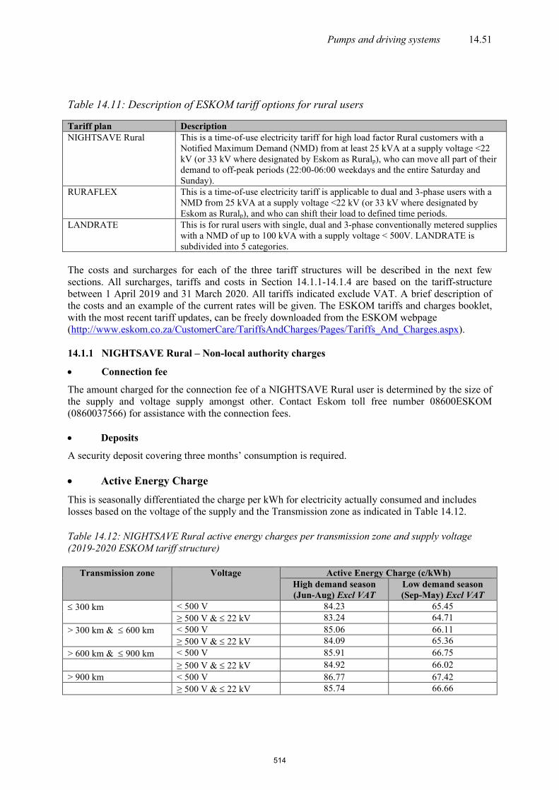
Pumps and driving systems 14.51
Table 14.11: Description of ESKOM tariff options for rural users
Tariff plan Description NIGHTSAVE Rural This is a time-of-use electricity tariff for high load factor Rural customers with a
Notified Maximum Demand (NMD) from at least 25 kVA at a supply voltage <22 kV (or 33 kV where designated by Eskom as Ruralp), who can move all part of their demand to off-peak periods (22:00-06:00 weekdays and the entire Saturday and Sunday).
RURAFLEX This is a time-of-use electricity tariff is applicable to dual and 3-phase users with a NMD from 25 kVA at a supply voltage <22 kV (or 33 kV where designated by Eskom as Ruralp), and who can shift their load to defined time periods.
LANDRATE This is for rural users with single, dual and 3-phase conventionally metered supplies with a NMD of up to 100 kVA with a supply voltage < 500V. LANDRATE is subdivided into 5 categories.
The costs and surcharges for each of the three tariff structures will be described in the next few sections. All surcharges, tariffs and costs in Section 14.1.1-14.1.4 are based on the tariff-structure between 1 April 2019 and 31 March 2020. All tariffs indicated exclude VAT. A brief description of the costs and an example of the current rates will be given. The ESKOM tariffs and charges booklet, with the most recent tariff updates, can be freely downloaded from the ESKOM webpage (http://www.eskom.co.za/CustomerCare/TariffsAndCharges/Pages/Tariffs_And_Charges.aspx). 14.1.1 NIGHTSAVE Rural – Non-local authority charges
• Connection fee
The amount charged for the connection fee of a NIGHTSAVE Rural user is determined by the size of the supply and voltage supply amongst other. Contact Eskom toll free number 08600ESKOM (0860037566) for assistance with the connection fees. • Deposits
A security deposit covering three months’ consumption is required. • Active Energy Charge This is seasonally differentiated the charge per kWh for electricity actually consumed and includes losses based on the voltage of the supply and the Transmission zone as indicated in Table 14.12. Table 14.12: NIGHTSAVE Rural active energy charges per transmission zone and supply voltage (2019-2020 ESKOM tariff structure)
Transmission zone Voltage Active Energy Charge (c/kWh) High demand season (Jun-Aug) Excl VAT
Low demand season (Sep-May) Excl VAT
≤ 300 km < 500 V 84.23 65.45 ≥ 500 V & ≤ 22 kV 83.24 64.71
> 300 km & ≤ 600 km < 500 V 85.06 66.11 ≥ 500 V & ≤ 22 kV 84.09 65.36
> 600 km & ≤ 900 km < 500 V 85.91 66.75 ≥ 500 V & ≤ 22 kV 84.92 66.02 > 900 km < 500 V 86.77 67.42 ≥ 500 V & ≤ 22 kV 85.74 66.66
514

14.52 Irrigation User Manual
• Energy Demand Charges This is seasonally differentiated R/kVA charge based on the voltage of the supply, the Transmission zone and charged on the chargeable demand in peak periods as specified in Eskom’s defined time-of-use periods. The charges are indicated in Table 14.13. Table 14.13: NIGHTSAVE Rural active energy charges per transmission zone and supply voltage (2019-2020 ESKOM tariff structure)
Transmission zone Voltage Energy Demand Charges (R/kVA/m) High demand season (Jun-Aug) Excl VAT
Low demand season (Sep-May) Excl VAT
≤ 300 km < 500 V R282.23 R149.37 ≥ 500 V & ≤ 22 kV R273.48 R144.07
> 300 km & ≤ 600 km < 500 V R285.63 R151.45 ≥ 500 V & ≤ 22 kV R276.82 R146.07
> 600 km & ≤ 900 km < 500 V R289.06 R153.49 ≥ 500 V & ≤ 22 kV R280.14 R148.09 > 900 km < 500 V R292.57 R155.60 ≥ 500 V & ≤ 22 kV R283.56 R150.16 • Network Capacity Charge This is a bundled R/kVA/month Transmission and Distribution charge based on the voltage of the supply, the Transmission zone and the annual utilised capacity measured at the point of delivery (POD) applicable during all time periods as indicated in Table 14.14.
Table 14.14: NIGHTSAVE Rural network capacity charges per transmission zone and supply voltage (2019-2020 ESKOM tariff structure)
Transmission zone Voltage Network Capacity Charges (R/kVA/m) Excl VAT
≤ 300 km < 500 V R14.27 ≥ 500 V & ≤ 22 kV R13.11
> 300 km & ≤ 600 km < 500 V R14.30 ≥ 500 V & ≤ 22 kV R13.16
> 600 km & ≤ 900 km < 500 V R14.44 ≥ 500 V & ≤ 22 kV R13.25 > 900 km < 500 V R14.47 ≥ 500 V & ≤ 22 kV R13.28 • Network Demand Charge This is a c/kWh Distribution network demand charge based on the voltage of the supply and the energy measured at the POD during all the time-of-use periods as indicated in Table 14.15.
Table 14.15 NIGHTSAVE Rural network demand charge per voltage supply (2019-2020 ESKOM tariff structure)
Supply Voltage
Network Demand Charge (c/kWh) in all time-of-use periods Excl VAT
< 500 V 28.39 ≥ 500 V & ≤ 22 kV 24.89
515

Pumps and driving systems 14.53
• Ancillary Service Charge This is a c/kWh service charge based on the voltage of the supply applicable during all time periods as indicated in Table 14.16.
Table 14.16: NIGHTSAVE Rural ancillary service charge per voltage supply (2019-2020 ESKOM tariff structure)
Supply Voltage Ancillary Charge (c/kWh) Excl VAT < 500 V 0.44 ≥ 500 V & ≤ 22 kV 0.44
• Service charge
This a fixed R/account/day charge payable every month, whether electricity is consumed or not, based on the monthly utilised capacity of each POD linked to an account. This fee is a contribution towards ESKOM’s customer service costs and is indicated in Table 14.17.
Table 14.17: NIGHTSAVE Rural service charges per user category (2019-2020 ESKOM tariff structure)
User category Service charge (R/Account/day) Excl VAT ≤ 100 kVA R19.62 > 100 kVA & ≤ 500 kVA R66.90 > 500 kVA & ≤ 1 MVA R205.82 > 1 MVA R205.82 Key Customers R4 033.88
• Administration charge This is a fixed R/POD/day charge that is based on the monthly utilised capacity of each POD linked to an account and is charged whether electricity is consumed or not. This charge covers ESKOM’s costs such as meter reading and billing and is indicated in Table 14.18.
Table 14.18: NIGHTSAVE Rural administration charges per user category (2019-2020 ESKOM tariff structure)
User category Administration charge (R/POD/day) Excl VAT ≤ 100 kVA R5.57 > 100 kVA & ≤ 500 kVA R31.02 > 500 kVA & ≤ 1 MVA R47.61 > 1 MVA R88.34 Key Customers R88.34
• Public Holidays All public holidays for NIGHTSAVE Rural and RURAFLEX tariffs will be treated as the day of the week on which it falls.
516

14.54 Irrigation User Manual
• Transmission surcharge This is calculated as a fixed percentage of active energy, energy demand and network capacity charges after the voltage surcharge has been levied. This percentage depends on the distance from Johannesburg and is indicated in Table 14.19 and the transmission zones in Figure 14.40. Table 14.19: Transmission surcharge levied depending on the distance from Johannesburg to the point of supply (2019-2020 ESKOM tariff structure) Distance from transformer to Johannesburg [km] Transmission surcharge [%]
0-300 0 3010-600 1 601-900 2
> 900 3
Figure 14.40: Transmission zones of Eskom
• Time periods The peak time periods are weekdays from 06:00 until 22:00 and off-peak the rest of the week throughout the year as indicated in Figure 14.41.
Figure 14.41: Time periods for NIGHTSAVE Rural throughout the year
517

Pumps and driving systems 14.55
14.1.2 RURAFLEX– Non-local authorities
• Connection Fee
The amount charged for the connection fee of a RURAFLEX user is determined by the size of the supply and voltage supply amongst other. Contact Eskom toll free number 08600ESKOM (0860037566) for assistance with the connection fees. • Deposits
A security deposit covering three months’ consumption is required. • Active Energy Charge This is seasonally differentiated the charge per kWh for electricity actually consumed and includes losses based on the voltage of the supply and the Transmission zone as indicated in Table 14.20. Table 14.20: RURAFLEX active energy charges per transmission zone and supply voltage (2019-2020 ESKOM tariff structure)
Transmission zone Voltage
Active Energy Charge (c/kWh) High demand season (Jun-Aug) Excl VAT
Low demand season (Sep-May) Excl VAT
Peak Standard Off Peak Peak Standard Off Peak
≤ 300 km < 500 V 345.33 104.62 56.82 112.65 77.52 49.18 ≥ 500 V & ≤ 22 kV 341.92 103.59 56.24 111.55 76.76 48.68
> 300 km & ≤ 600 km
< 500 V 348.80 105.66 57.38 113.77 78.31 49.69 ≥ 500 V & ≤ 22 kV 345.32 104.61 56.82 112.65 77.51 49.18
> 600 km & ≤ 900 km
< 500 V 352.29 106.73 57.95 114.92 79.08 50.18 ≥ 500 V & ≤ 22 kV 348.78 105.65 57.38 113.77 78.31 49.69
> 900 km < 500 V 355.80 107.79 58.52 116.03 79.87 50.68 ≥ 500 V & ≤ 22 kV 352.28 106.73 57.95 114.92 79.08 50.18
• Network Capacity Charge This is a R/kVA/month charge combining the Transmission and Distribution network capacity charges based on the voltage of the supply, the Transmission zone and the annual utilised capacity measured at the POD applicable during all time periods as indicated in Table 14.21. Table 14.21: RURAFLEX network capacity charges per transmission zone and supply voltage (2019-2020 ESKOM tariff structure)
Transmission zone Voltage
Network Capacity Charges (R/kVA/m) Excl VAT
≤ 300 km < 500 V R19.94 ≥ 500 V & ≤ 22 kV R18.28
> 300 km & ≤ 600 km < 500 V R20.00 ≥ 500 V & ≤ 22 kV R18.39
> 600 km & ≤ 900 km < 500 V R20.11 ≥ 500 V & ≤ 22 kV R18.47
> 900 km < 500 V R20.19 ≥ 500 V & ≤ 22 kV R18.48
• Network Demand Charge This is a c/kWh Distribution network demand charge based on the voltage of the supply and the energy measured at the POD during all the time-of-use periods as indicated in Table 14.22.
518

14.56 Irrigation User Manual
Table 14.22: RURAFLEX network demand charge per voltage supply (2019-2020 ESKOM tariff structure)
Supply Voltage Network Demand Charge (c/kWh) in all time-of-use periods Excl VAT
< 500 V 28.39 ≥ 500 V & ≤ 22 kV 24.89
• Ancillary Service Charge This is a c/kWh service charge based on the voltage of the supply applicable during all time periods as indicated in Table 14.23. Table 14.23: RURAFLEX ancillary service charge per voltage supply (2019-2020 ESKOM tariff structure)
Supply Voltage Ancillary Charge (c/kWh) Excl VAT < 500 V 0.44
≥ 500 V & ≤ 22 kV 0.44 • Service charge
This a fixed R/account/day charge payable every month, whether electricity is consumed or not, based on the monthly utilised capacity of each account. This fee is a contribution towards ESKOM’s customer service costs and is indicated in Table 14.24.
Table 14.24: RURAFLEX service charges per User Category (2019-2020 ESKOM tariff structure)
User category Service charge (R/Account/day) Excl VAT ≤ 100 kVA R19.62
> 100 kVA & ≤ 500 kVA R66.90 > 500 kVA & ≤ 1 MV R205.82
> 1 MVA R205.82 Key Customers R4 033.88
• Administration charge This is a fixed R/POD/day charge that is based on the monthly utilised capacity of each POD linked to an account and is charged whether electricity is consumed or not. This charge covers ESKOM’s costs such as meter reading and billing and is indicated in Table 14.25. Table 14.25: RURAFLEX administration charges per user category (2019-2020 ESKOM tariff structure)
User category Service charge (R/Account/day) Excl VAT ≤ 100 kVA R5.57
> 100 kVA & ≤ 500 kVA R31.02 > 500 kVA & ≤ 1 MV R47.61
> 1 MVA R88.34 Key Customers R88.34
519

Pumps and driving systems 14.57
• Public Holidays All public holidays for NIGHTSAVE Rural and RURAFLEX tariffs will be treated as the day of the week on which it falls. • Reactive Energy Charge Reactive energy involves that portion of the current that the electric motor consumes but does not supply in the form of energy during the entire billing period. The power factor indicates that portion of the current which is supplied in the form of energy. A low power factor will thus be the cause of high reactive energy. For rural areas, this only has a bearing on the RURAFLEX tariff during the high-demand season and only reactive energy that exceeds 30% of the active energy consumption is paid for. There is no reactive energy charge for users that have a power factor of 0,96 or better. • Transmission surcharge The transmission surcharge is indicated in Table 14.19 and the transmission zones in Figure 14.40. • Time periods The time periods for RURAFLEX during low demand and high demand seasons are indicated in Figure 14.42.
Figure 14.42: Time periods for RURAFLEX during the low demand and high demand seasons
14.1.3 LANDRATE – Non-local authorities This range of tariffs is for rural supplies with single, dual or three phase conventionally metered supplies with a notified maximum demand of up to 100 kVA. It is usually supplied from an 11 or 22 kV network at a nominal voltage lower than 500 V. • Standard supply sizes There are five LANDRATE packages available:
520

14.58 Irrigation User Manual
Table 14.25: LANDRATE options
Option Number of phases Supply point LANDRATE 1
Single-phase Dual-phase Three-phase
16 kVA (80 A per phase) 32 kVA (80 A per phase) 25 kVA (40 A per phase)
LANDRATE 2 Dual-phase Three-phase
64 kVA (160 A per phase) 50 kVA (80 A per phase)
LANDRATE 3 Dual-phase Three-phase
100 kVA (225 A per phase) 100 kVA (160 A per phase)
LANDRATE 4 Single-phase 16 kVA (80 A per phase) LANDRATE Dx Single-phase 5 kVA (Limited to 5A per phase) LANDRATE 1, 2 and 3 – these are suitable for supplies that use consistently more than approximately 720 kWh per month. LANDRATE 4 – is suitable single-phase supplies where consistently less than approximately 720 kWh are being used each month. LANDRATE Dx – this tariff is for Ruralp* single phase non-metered supplies limited to 5 kVA typically suited to small telecommunication installations where the electricity usage is low enough not to warrant metering for billing purposes. *Ruralp means areas classified as rural by Eskom for the purposes of tariff design and classification • Prepayment supplies If and when the Landrate 1, 2, 3 and 4 is offered as a prepaid supply, the active energy charge, theancillary service charge and the network capacity charge shall be combined into one c/kWh rate and the network demand charge and the service and administration charge (if applicable) shall be combined into a R/POD/day charge. Currently these tariffs cannot be accommodated as a pre-paid supply. If and when this is possible, the combining of the charges is required to accommodate the prepaid vending system.
• Connection fee The amount charged for the connection fee of a LANDRATE user is determined by the size of the supply and voltage supply amongst other. Contact Eskom toll free number 08600ESKOM (0860037566) for assistance with the connection fees. • Deposits
A security deposit covering three months’ consumption is required. • Charges LANDRATE 1, 2 and 3
- Active Energy Charge – c/kWh measured at the POD - Network Capacity Charge – R/day/POD based on the NMD of the supply - Network Demand Charge – c/kWh based on the active energy measured at the POD - Ancillary Service Charge – c/kWh based on the active energy measured at the POD - Service and Administration Charge – R/day for each POD which shall be payable every month
whether electricity is used or not, based on the applicable daily rate and the number of days in the month
LANDRATE 4
- Active Energy Charge – c/kWh measured at the POD - Network Capacity Charge – R/day/POD based on the NMD of the supply
521

Pumps and driving systems 14.59
- Network Demand Charge – c/kWh based on the active energy measured at the POD - Ancillary Service Charge – c/kWh based on the active energy measured at the POD
LANDRATE Dx
- A R/day/POD based on LANDRATE 4 at 200 kWh per month is payable each month for each point of delivery
A summary of the LANDRATE charges is indicated in Table 14.26. Table 14.26: Charges for LANDRATE options excluding VAT (2019-2020 ESKOM tariff structure)
Tariff Energy charge (c/kWh)
Ancillary service charge
(c/kWh)
Network demand charge
(c/kWh)
Network capacity charge
(R/POD/day)
Service charge
(R/POD/day) LANDRATE 1 113.63 0.44 28.39 30.35 25.20 LANDRATE 2 113.63 0.44 28.39 46.65 25.20 LANDRATE 3 113.63 0.44 28.39 74.58 25.20 LANDRATE 4 245.42 0.44 28.39 24.16 0.00
LANDRATE Dx* N/A N/A N/A N/A 54.04 * R/day fixed charge inclusive of the following charges: Energy, Ancillary Service, Network Demand, Network
Capacity and Service Charges 14.1.4 LANDLIGHT – Non-local authorities LANDLIGHT is an electricity tariff that provides a subsidy to low-usage single phase supplies in ruralp areas and is
only offered as a prepaid supply. The LANDLIGHT range of charges are indicated in Table 14.27. Table 14.27: LANDLIGHT range of tariffs
LANDLIGHT 20A Single-phase 20A LANDLIGHT 60A Single-phase 60A
• Charges A single c/kWh active energy charge as indicated in Table 14.28. Table 14.28: LANDLIGHT range of tariffs excluding VAT (2019-2020 ESKOM tariff structure)
Energy Charge (c/kWh) LANDLIGHT 20A 326.73 LANDLIGHT 60A 421.19 Note that this tariff has no fixed charges and the reason why the energy charges are higher than LANDRATE
and is not applicable to authority supplies. 14.1.5 Determination of electricity costs For the determination of electricity costs by the customer support service, the following should be known:
• The size of the motor of every appliance that is being supplied from a specific power point and the input power and power factor of each of these.
• For how many hours per month pumping will take place. If more than one appliance is being supplied with electricity from a specific power point, the consumption of each appliance has to be estimated.
522

14.60 Irrigation User Manual
Example 14.3:
Maize and wheat are being cultivated under the same 40 ha centre pivot (double cropping) in the Van Der Kloof Dam area. The centre pivot is serviced by a centrifugal pump with a pump delivery of 245 m3/h, which requires 38.5 kW on the pump shaft and is being driven by a 45 kW four pole motor. The maize is planted on 15 December and the wheat on 15 June and the crops are irrigated according to the irrigation demands set out in "Estimated Irrigation Requirements for Crops in South Africa, Part 2". The system efficiency can be accepted as 85%. ESKOM supplies the electricity (three-phase) with a 100 kVA transformer. The transformer is approximately 550 km from Johannesburg and ESKOM has built a 700 m power line. (Accept the power consumption for driving the centre pivot as being 2.5 kWh/mm net application and the kVA demand as 6.5 kVA.) Solution:
• Determine the input power of the electric motor:
Motor efficiency according to the manufacturer's catalogue is 91% and according to equation 14.7:
ui
100 PP
100 38.591
42.31 kW
η×
=
×=
=
• Determine the power factor and kVA demand: Power factor from the manufacturer’s catalogue: 0.82 According to equation 14.8:
iPkVA
cos42.310.82
51.60 kVA
φ=
=
=
Add 6.5 kVA for powering the centre pivot:
kVA 51.60 6.558.10 kVA
= +=
• Determine the monthly energy requirement: First obtain the net irrigation requirement using the SAPWAT (or elsewhere, if applicable). The next step is to determine the gross irrigation requirement:
(14.7) where GIR = gross irrigation requirement [mm/period], NIR = net irrigation requirement [mm/period], and ɳs = system efficiency
523

Pumps and driving systems 14.61
ESKOM accounts are presented on a monthly basis so monthly periods are employed. The volume of water to be pumped can then be determined as follows:
(14.8) where V = volume of water to be pumped [m3], A = area to be irrigated [ha], GIR = gross irrigation requirement [mm/period] Thereafter the pumping hours are calculated as follows:
(14.9) where t = pumping hours [h], V = volume of water to be pumped [m3], and Q = pumping rate [m3/h] The total energy requirement per period can then be determined as follows (Optional):
(14.10) where E = total energy requirement per period [kWh], t = pumping hours [h], and Pi = input power [kW] Thus information for maize:
Month Dec Jan Feb Mar Apr Net irrigation requirement [mm/month] 103 312 297 198 27 Gross irrigation requirement [mm/month] 121 367 349 233 32 Volume irrigation [m3/month] 48 400 146 800
139 600 93 200 12 800
Pumping hours [hour/month] 198 599 570 380 52 Energy requirement of pump [kWh/month] 8 377 25 344 24 117 16 078 2 200 Energy requirement of pivot [kWh/month] 257 780 713 495 68
Total energy consumption [kWh/month] 8 635 26 124 24 858 16 573 2 268
Thus, information for wheat:
Month Jun Jul Aug Sep Oct Nov Net irrigation req. [mm/month] 22 55 161 273 258 60 Gross irrigation req. [mm/month] 26 65 189 321 304 71 Volume irrigation [m3/month] 10 400 26 000 75 600 128 400 121 600 28 400 Pumping hours [hour/month] 43 106 309 525 497 116 Energy req. of pump [kWh/month] 1 777 4 485 13 074 22 170 20 986 4 908 Energy req. of pivot [kWh/month] 55 138 402 682 646 151 Total energy cons. [kWh/month] 1 832 4 623 13 475 22 853 21 632 5 059 The following information can thus be given to ESKOM: Size of electric motor: 45.00 kW Input power: 42.31 kW Power factor: 0.82
524

14.62 Irrigation User Manual
Monthly pumping hours and energy requirements:
Month Pump hours
[h]
Energy usage [kWh]
Month Pump hours
[h]
Energy usage [kWh]
Month Pump hours
[h]
Energy usage [kWh]
Dec 198 8 635 Apr 52 2 268 Aug 309 13 475 Jan 599 26 124 May 0 0 Sep 525 22 853 Feb 570 24 858 Jun 43 1 832 Oct 497 21 632 Mar 380 16 573 Jul 106 4 623 Nov 116 5 059
This information will enable ESKOM to determine the best tariff for the specific point. For illustration of the effect of the different tariffs on the energy cost, the energy costs for each tariff was determined by ESKOM’s tariff structure for April 2019 to December 2020 for the above example. However, please note that many variables can influence these costs and these figures should therefore not be regarded as the general tendency. For this example, the LANDRATE 3, NIGHTSAVE Rural and RURAFLEX tariff options are applicable. Furthermore, RURAFLEX and NIGHTSAVE Rural tariffs are sensitive to the exact time that electricity is used. Two different monthly costs were calculated for each of the three tariffs, namely for: • A normal pattern of consumption with the supposition that irrigation will start at 07:00 on
Tuesday morning and continue right through until the weekly irrigation demand has been satisfied, irrespective of time and consumption.
• An optimum pattern of consumption where full use is made of the cheaper periods before
irrigating during the more expensive periods. No optimisation is possible for the LANDRATE 3 tariff option as the same unit costs is charged throughout the day.
Since Energy Demand is not measured during the off peak periods of the NIGHTSAVE Rural tariff, considerable savings can be realised during months where irrigation is possible for less than approximately 252 hours per month (or less than 56 hours off peak per week). If irrigation takes place for more than 30 min during any of the peak hours, Energy Demand will be measured and be payable for the whole month. In this example for instance, it is possible to optimise irrigation by only irrigating during the off peak periods during the months of Dec, Apr, Jun, Jul, and Nov since the irrigation requirements are less than 252 hours per month. Although with example, the NIGHTSAVE Rural option would be the more expensive option, a considerable saving of R102 561 is possible between optimising and not optimising. For the RURAFLEX tariff, the reactive energy cost is only payable during the high demand season (June, July and August) and the cost per kVArh was included in the calculations.
525

Pumps and driving systems 14.63
The breakdown of the number of kWh in each rate category for the two scenarios shown in the table below.
Month RURAFLEX No optimisation [kWh/month]
RURAFLEX Optimised [kWh/month]
Peak Standard Off-peak Peak Standard Off-peak December 2 006 3 838 2 791 0 0 8 635 January 4 012 9 377 12 735 0 10 641 15 482 February 3 489 8 722 12 647 349 12 167 12 342 March 2 617 6 978 6 978 0 1 438 15 473 April 872 1 396 0 0 0 2 268 May 0 0 0 0 0 0 June 436 1 396 0 0 0 1 832 July 1 308 1 913 1 396 0 0 4 623 August 2 965 6 672 3 838 0 0 13 475 September 3 489 8 897 10 467 0 8 417 14 435 October 3 489 8 897 9 246 0 6 149 15 482 November 1 396 2 268 1 396 0 0 5 059
The total monthly costs for the LANDRATE 3, NIGHTSAVE Rural and RURAFLEX tariff options are shown in the Table below. For this example the benefit of timing the use of electricity is evident. In this example, the optimised RURAFLEX option will have the lowest annual costs. However, there are other factors that may influence the choice of tariff structure. For instance, in some regions centre pivots cannot be run at night due to the possibility of water freezing and causing the centre pivot to collapse. Also, certain crops cannot be irrigated at night. Traditionally, irrigation systems are designed for a 24 hour per day application. With the introduction of the Time-of-Use Tariffs (RURAFLEX and NIGHTSAVE Rural) by Eskom, it is important to first determine if the infiltration rate of the soil won’t be exceeded with the higher application rate of irrigation systems when applying water within 19 hours/day instead of 24 hours/day. Month Tariff (R/month)
LANDRATE 3 NIGHTSAVE Rural RURAFLEX No optimised Optimised No optimised Optimised
December 15 367 25 535 10 390 11 939 9 555 January 40 320 42 165 42 165 28 550 26 341 February 38 195 40 873 40 873 26 954 25 927 March 26 728 33 107 33 107 19 473 16 379 April 6 239 19 494 4 349 5 498 4 540 May 3 093 2 211 2 211 2 781 2 781 June 5 631 32 857 4 294 6 410 4 465 July 9 686 36 045 7 482 11 818 7 079 August 22 264 46 100 46 100 27 180 15 296 September 35 554 39 030 39 030 25 483 23 109 October 33 929 37 906 37 906 24 552 21 530 November 10 195 22 130 6 985 8 270 6 727 TOTAL: 247 202 377 454 274 893 198 887 163 729 Optimisation savings per year
102 561 35 158
526

14.64 Irrigation User Manual
The effective average costs/kWh* for the 2019/20 tariff structure of ESKOM (VAT exclusive) and the load factor over a 12-month period is thus:
Average
Tariff (R / month)
Landrate 3 Nightsave Rural Ruraflex
Non-optimised Optimised Non-optimised Optimised
Effective cost/NET mm/ha (Rand) R3.50 R5.34 R3.89 R2.82 R2.32
Effective cost/GROSS mm/ha (Rand) R2.97 R4.54 R3.31 R2.39 R1.97
Effective cost/kWh (c/kWh) 167.07 255.11 185.79 134.42 110.66
Annual Load Factor (%) 21% *The Effective Average Costs/kWh includes all charges applicable to each tariff whether electricity is used or not. Although there was no irrigation during May, all other monthly charges for May were included in determining the effective annual averages. The charges in the table are as per 2019-2020 ESKOM tariff structure. Please note that these comparative costs were done for a specific situation and are not necessarily a general tendency. 14.2 Diesel costs
Determining diesel costs is much simpler than determining the cost of electricity supplied by ESKOM, i.e. if the fuel consumption is known. Example 14.4: Determine the diesel cost for supplying water to the maize crop under the centre pivot mentioned in Section 6.1 if the diesel engine's fuel consumption is 240 g/kWh. (Accept pumping hours similar to those above, the power as 38.5 kW, the density of the diesel as 810 g/ and the cost of diesel as R16.04/). Solution:
Row Month Dec Jan Feb Mar Apr
1 Pumping hours (hour/month) 198 599 570 380 52
2 Energy requirement (kWh/month) 7 623 23 062 21 945 14 630 2 002
3 Diesel consumption (kg/month) 1 829 5 535 5 267 3 511 480
4 Diesel consumption (/month) 2 259 6 833 6 502 4 335 593
5 Diesel cost (R/month) R36 234 R109 601 R104 292 R69 533 R9 512 Row 1: Pumping hours as calculated in example 16.14 (Irrigation Design manual) Row 2: Energy requirement [kWh/month] = row 1 × 38.5 kW Row 3: Diesel consumption [kg/month] = Row 2 × 0.240 kg/kWh Row 4: Diesel consumption [/month] = Row 3 /0.810 kg/ Row 5: Diesel cost [R/month] = Row 4 × R16.04/ Thus, Total diesel cost per season: R329 173 Total diesel cost per ha: R8 229 Average cost per kWh: R4.75 (NB based on Aug 2019 tariffs, VAT included).
527

Pumps and driving systems 14.65
15 References 1. Amptelike toetsverslae. Dompelpompe. 1979. Division Agricultural Engineering. Department of Agriculture and Fishery. Silverton. RSA. 2. Barnard, J. 2002. Personel communication. RSA. 3. Centrifugal Pump Wikipedia. https://en.wikipedia.org/wiki/Centrifugal_pump 4. Eckard, J.H. 1998. Personel communication. RSA 5. ESKOM (Tariffs and Charges Booklet 2019/2020) http://www.eskom.co.za/CustomerCare/TariffsAndCharges/Documents/2019 6. Flowserve-ABS Engineering & Trading Sdn. Bhd. https://admin.minebizs.com/Attachments/Product/Flowserve 7. General Pump Company. https://generalpumps.com.au/ultraflow-drainage-sump-pumps/ 8. Heishin PC Pumps. http://www.heishin.jp/en/structure/ 9. Irrigator Products (Pty) Ltd. VSD Design and Installation Practices 10. KSB. Centrifugal Pumps ETA – B. Johannesburg. RSA. 11. Lawrence Pumps – ABS Engineering & Trading Sdn. Bhd. http://www.abset.com/lawrence-pumps 12. M&B Pumps. Single stage end-suction centrifugal pumps. Servicing and maintenance instructions. RSA. 13 Mulder, D. 2000. Personel communication. RSA 14. Mulder, D.J., Burger, J.H., Heyns, P.J., Kleynhans, E.P.J., Koegelenberg, F.H., Lategan, M.T., Smal, H.S., Stimie, C.M., Uys, W.J., Van der Merwe, F.P.J. and Viljoen, P.D. 1996. Irrigation Design Manual. ARC-Institute for Agricultural Engineering. RSA. 15. Pump Fundamentals. https://www.pumpfundamentals.com/pump 16. SABI magazine: Selection and sizing of electrical cables. December January 2012 edition, technical article translation. 17. SABI Norms for the Design of Irrigation Systems. 2017 18. Shuang Feng Chemical Co. Ltd. http://www.sfchemy.com 19. Venter M, Grové B, Van Der Stoep I. 2017. The optimization of electricity and water use for sustainable management of irrigation farming systems. WRC Report No. TT 717/17, ISBN 978-1-4312-0886-9.
528

IRRIGATION USER MANUAL
CHAPTER 15
Chemigation
529

15.2 Irrigation User Manual
Table of Contents
1 Introduction.........................................................................................................................................................................................................................................15.1 1.1 Classification ........................................................................................................................................................................................................................15.1
1.1.1 Fertigation ................................................................................................................................................................................................................15.1 1.1.2 Herbigation .............................................................................................................................................................................................................15.1 1.1.3 Nematodigation .................................................................................................................................................................................................15.2 1.1.4 Insectigation ..........................................................................................................................................................................................................15.2 1.1.5 Fungigation.............................................................................................................................................................................................................15.2
1.2 Benefits and limitations ...........................................................................................................................................................................................15.2 1.2.1 Benefits .......................................................................................................................................................................................................................15.2 1.2.2 Limitations ..............................................................................................................................................................................................................15.2
1.3 Chemigation considerations ................................................................................................................................................................................15.3 1.3.1 Application .............................................................................................................................................................................................................15.3 1.3.2 Solubility ...................................................................................................................................................................................................................15.3 1.3.3 Volatility....................................................................................................................................................................................................................15.3 1.3.4 Adsorption ...............................................................................................................................................................................................................15.3 1.3.5 Climatic conditions .......................................................................................................................................................................................15.3 1.3.6 Soil factors ..............................................................................................................................................................................................................15.4
1.4 Irrigation system considerations. ..................................................................................................................................................................15.4
2 Fertigation ............................................................................................................................................................................................................................................15.5 2.1 Types of fertiliser products ..................................................................................................................................................................................15.5 2.2 Choice of fertiliser products ...............................................................................................................................................................................15.7
2.2.1 Water soluble fertiliser ............................................................................................................................................................................15.9 2.2.2 Liquid fertiliser ................................................................................................................................................................................................15.9
3 Pesticides ...............................................................................................................................................................................................................................................15.9
3.1 Herbicides ................................................................................................................................................................................................................................15.9 3.2 Insecticides ......................................................................................................................................................................................................................... 15.10 3.3 Fungicides ............................................................................................................................................................................................................................ 15.10
4 Equipment ........................................................................................................................................................................................................................................ 15.10
4.1 Choice of different types of injectors ................................................................................................................................................... 15.11 4.2 Injectors .................................................................................................................................................................................................................................. 15.11
4.2.1 Passive injectors ........................................................................................................................................................................................... 15.12 4.2.2 Active injectors .............................................................................................................................................................................................. 15.14
4.2.2.1 Electrically driven pumps........................................................................................................................................... 15.14 4.2.2.2 Hydraulically driven pumps .................................................................................................................................... 15.15
4.2.3 Injector selection .......................................................................................................................................................................................... 15.16 4.3 Other equipment ............................................................................................................................................................................................................. 15.18
4.3.1 Electrical interlock ..................................................................................................................................................................................... 15.18 4.3.2 Flow sensor ........................................................................................................................................................................................................ 15.18 4.3.3 Chemical injection line check valve...................................................................................................................................... 15.19 4.3.4 Manual valve .................................................................................................................................................................................................... 15.19 4.3.5 Strainer on suction pipe of chemical injector ............................................................................................................. 15.19 4.3.6 Air valve ................................................................................................................................................................................................................ 15.19 4.3.7 Fertiliser tanks ................................................................................................................................................................................................ 15.19 4.3.8 Agitators ................................................................................................................................................................................................................ 15.20 4.3.9 Static in-line mixer .................................................................................................................................................................................... 15.21 4.3.10 Fresh water supply valve ................................................................................................................................................................ 15.21 4.3.11 Filters ..................................................................................................................................................................................................................... 15.21 4.3.12 Equipment for mixing of fertilisers .................................................................................................................................... 15.21
4.4 Electronic control .......................................................................................................................................................................................................... 15.22 4.4.1 Electrical conductivity control ................................................................................................................................................... 15.22 4.4.2 pH-control .......................................................................................................................................................................................................... 15.23
4.5 Safety measures .............................................................................................................................................................................................................. 15.23
530

Chemigation 15.3
5 Injection of fertiliser solutions .................................................................................................................................................................................. 15.24 5.1 Examples for the calculation of injection rates .......................................................................................................................... 15.24
5.1.1 Static systems ................................................................................................................................................................................................. 15.24 5.1.2 Moving systems .......................................................................................................................................................................................... 15.27
6 Legislation in South Africa .......................................................................................................................................................................................... 15.30
6.1 The Environmental Conservation Act ................................................................................................................................................... 15.30 6.2 The Conservation of Agricultural Resources Act .................................................................................................................... 15.30
6.2.1 Regulation 6: Prevention of salinisation and saturation of irrigated land ................................ 15.30 6.3 The Health Act ................................................................................................................................................................................................................. 15.30 6.4 The National Water Act......................................................................................................................................................................................... 15.31
7 Summary ............................................................................................................................................................................................................................................ 15.31 8 References ........................................................................................................................................................................................................................................ 15.31
All rights reserved Copyright 2019 ARC-Agricultural Engineering (ARC-AE)
531

15.0 Irrigation User Manual
1 Introduction Chemigation is the application of agricultural chemicals (fertiliser, fungicides, herbicides, nematodes, soil improvement remedies, growth regulators, sewage and manure water), in an effective and economic way, by means of an irrigation system. Chemigation can be applied by means of any type of irrigation system, although some flood, travelling guns and overhead boom sprinkler irrigation systems may not be suitable for the application of certain types of chemicals, because of poor application uniformity. An irrigation system that delivers chemicals to crops and soils must be designed and managed differently than conventional irrigation. Chemigation can take place via a normal irrigation cycle, but factors like uniformity, rate of application, timing and the need to flush chemicals from the system must be considered (Van der Gulik and Evans, 2011). The careless use of chemicals and over irrigation must also be prevented, because it can lead to pollution of soil and water sources. Adding any chemical to irrigation water requires reliable backflow prevention devices to ensure that the chemicals does not drain or siphon back into the water source (Van der Gulik and Evans, 2011). The prescribed safety measures as described in Section 15.4.5 must be followed meticulously according to the material safety data sheets (MSDS) and product labels which serve as legal documents. It should also clearly indicate that the specific product is registered for application via irrigation systems before it is used. Even if a chemical is registered for application via irrigation systems, the specifications on the label (in terms of concentration, minimum water volume, droplet size, etc.) must strictly be adhered to. Beyond facing legal action, financial penalties, or harming the environment, non-adherence can place human health and safety at high risk (not just the farmer, or his labour, but also members of the public who may be in the vicinity of the irrigation system when the chemicals are being applied). The purpose of this chapter is to serve as guidelines for producers and irrigation designers regarding chemigation. The various suppliers of different chemicals must be consulted to ensure that the product is applied safely and correctly. 1.1 Classification The most important methods of application of agricultural chemicals can be described as follows: 1.1.1 Fertigation Fertigation comprises the application of dissolved nutrients for crops by means of an irrigation system. The total or part requirement of specific elements can be divided and applied through the irrigation system. Uncompounded products or combinations of products and liquid or water-soluble forms can be used. Fertigation is essential in irrigation systems, because the root systems of the crops are limited to the wetted soil volume. 1.1.2 Herbigation The effective application of herbicides by means of an irrigation system depends a great deal on the type of irrigation system in use. Compared to drip irrigation, herbicide application is more successful when applied by means of micro-sprayer, sprinklers and moving systems. The effectiveness of herbicide application depends on the movement of herbicides through soil, which is a function of solubility, volatility and the absorption of the herbicide. 1.1.3 Nematodigation Good nematode control is obtained with nematode substances which are specially formulated for application by means of an irrigation system. The products are very poisonous and systemic and must be used responsibly and with great care. Nematode spray can be applied by means of any irrigation system except with flood irrigation. The type of soil determines the amount of irrigation water to be applied for application of the nematode substances to the required depth.
532

Chemigation 15.1
1.1.4 Insectigation The use of the irrigation system for the control of insects, will depend on the chemical compound of the insecticide, special requirements of the crop during various stages of growth and the effectiveness of the insecticide when applied by means of the irrigation system. Producers must always follow the directives prescribed on the label of the product when insect spraying is applied. Insecticides are mostly applied by means of pivot and sprinkler irrigation systems. 1.1.5 Fungigation The application of fungicides by means of an irrigation system for disease control is called fungigation. Effective application can be obtained by means of pivot, permanent and movable sprinkler systems. The fungicides can be applied on the leaves or on the soil. The accuracy of fungigation is not as critical as with weed spraying, as the crop is not damaged by high applications. Ensure that the leaf cover is always sufficient. The cover depends on the fungicide compound, the amount of cover and the uniformity of the water application by the irrigation system. For effective leaf cover with the fungicides, products that do not wash off easily and a smaller water application must be used. For soil application, the fungicide that washes off easily must be used for sufficient soil coverage. 1.2 Benefits and disadvantages
Just as there are benefits and disadvantages of applying agricultural chemicals by means of conventional methods (ground and air application), chemigation also has benefits and disadvantages.
1.2.1 Benefits
• A well-designed and well-managed irrigation systems can apply agricultural chemicals more uniformly
than an aeroplane or ground equipment. • Chemigation can be done at the most opportune time even if the lands are too wet for tractors or too
misty for application by aeroplane as well as when optimal weather conditions prevail. • The chemicals applied, can be washed into the soil to the required depth and soil moisture can
simultaneously be provided for the effective functioning of certain chemicals. • Chemigation can prevent leaching of especially fertiliser products beneath the root zone with
accompanying pollution of subsurface water sources by applying the correct amount throughout the growing season as the plant’s nutrient requirements changes. Chemicals can be applied in smaller doses over a number of irrigation events, allowing for the supply to be better matched to the crops’ demand.
• Chemigation can be applied under different soil tilling practices. • Mechanical damage to crops is limited to the minimum with chemigation. • Compaction of the soil by tractors is prevented by the use of chemigation. • Chemigation reduces the operator’s exposure to the chemicals. • Chemigation reduces the danger of environmental pollution which normally accompanies water losses
resulting from unfavourable weather conditions. • Time and labour cost are reduced by using chemigation. • Chemigation can reduce energy costs by as much as 90%. • Chemigation of post-emergence, soil-acting herbicides may reduce crop phytotoxicity and increase
activity. • Corrective measures, for example from leaf analysis, can be implemented immediately.
1.2.2 Limitations
• Some chemicals may be corrosive for certain irrigation equipment. • Some additional equipment and capital outlay may be necessary for chemigation, such as injectors, tanks
and safety devices. • Water pollution of the water source is a possibility if the correct backflow prevention valves are not
installed. Safety measures must be strictly adhered to, especially where drinking water is concerned. • Chemigation requires a high standard of management. Staff must therefore be well-trained and must
understand backflow prevention equipment, injector calibration and the operation of the irrigation system.
533

15.2 Irrigation User Manual
• Not all chemicals are suitable for chemigation. • Many chemicals, especially insecticides, fungicides and herbicides may only be used for chemigation
if the product label specifically states that the product can be applied by the specific irrigation system for the correctly registered control.
• Chemigation requires more time than aerial spraying, therefore certain climatic factors (e.g. strong winds) can delay application.
• Chemigation cannot be used when the soil moisture is already near field capacity and irrigation is not needed.
1.3 Chemigation considerations 1.3.1 Application
The quantity of chemicals as well as the uniformity of application must be accurate in accordance with the supplier’s prescriptions. Run-off is not only influenced by the application rate of the irrigation system and the infiltration rate of the soil, but also by the slope of the field, soil coverage, the crop growth and the water content of the soil. Measures to prevent excess run-off, must be instituted timely to prevent pollution. Excess run-off can also have an uneven distribution of the chemicals on the soil.
1.3.2 Solubility
Some chemicals used in agriculture are insoluble in water or not very soluble. If the chemicals are blended together, insoluble matter may be formed, which blocks filters and nozzles. A glass jar may be used to determine the solubility of the chemicals. Add the chemicals to the water in the jar according to the mixing prescription. Mix well and let it stand for a few hours for observation. If precipitation forms, problems can be expected. Highly soluble mixtures usually infiltrate the soil deeper than mixtures which are less soluble. It is also more easily absorbed by the plants if applied near the roots. Not all less-soluble mixtures infiltrate the soil with the water and often collect on the upper layer of the soil and can be poisonous to the plants as a result of the high concentration. The solubility of a mixture will also have an effect on the infiltration-rate and infiltration-depth (Adendorff, 2016).
1.3.3 Volatility
Volatility is the characteristic of a liquid to change into a gas. It is dependent on the vapour pressure. The lower the vapour pressure, the easier the chemical will evaporate, or vice versa. Some chemicals are more volatile than others and will therefore volatilise or evaporate more easily. The finer the drops, the larger the exposed surface will be and the easier the chemical will evaporate and its effectiveness will be influenced.
1.3.4 Adsorption
Adsorption is important for the chemical to be effective, whether by plants or by the soil. Good absorption by plants is obtained by means of ideal weather conditions, e.g. no wind or rain. The measure of movement of a chemical in the soil is a function of solubility, adsorption and volatility. It is important to know how deep a chemical substance will move in the soil. The chemical usually moves only a part of the depth of the water in which it is dissolved as a result of adsorption. Most weed seeds germinate in the upper layer of soil and it is therefore important to apply the chemical to this area. If too much water is used, the chemical will move past the area where it should be placed. Too little water, however, will cause the chemical to be placed too shallow, where it will be exposed to evaporation and breakup by the ultraviolet rays of the sun. The soil also dries out too soon and the chemical is not as active as it should be.
1.3.5 Climatic conditions
Strong winds change the distribution pattern of the spray nozzle, which results in the chemical not being distributed evenly. With moving irrigation systems, the influence of wind is not as high as with static irrigation systems. When the wind speed exceeds 7 km/h, chemigation must be stopped on all systems except with drip systems. It is recommended that chemigation is done during wind still periods. Wind, high temperatures and
534
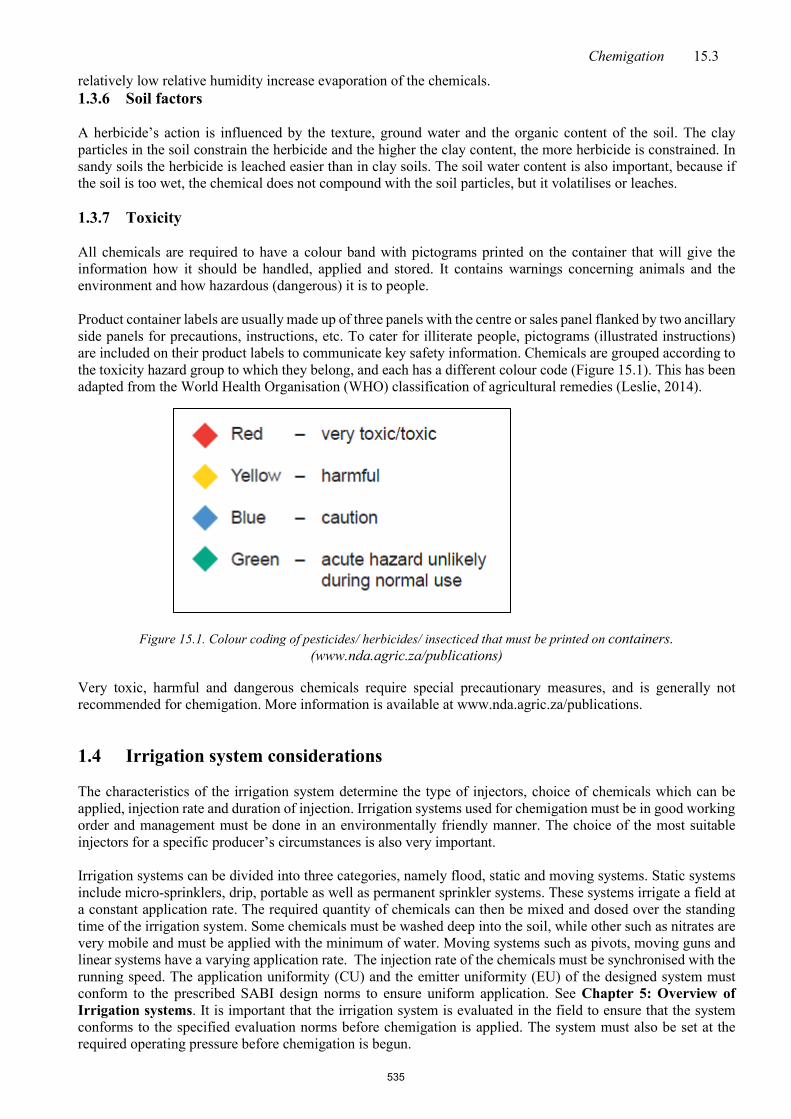
Chemigation 15.3
relatively low relative humidity increase evaporation of the chemicals. 1.3.6 Soil factors
A herbicide’s action is influenced by the texture, ground water and the organic content of the soil. The clay particles in the soil constrain the herbicide and the higher the clay content, the more herbicide is constrained. In sandy soils the herbicide is leached easier than in clay soils. The soil water content is also important, because if the soil is too wet, the chemical does not compound with the soil particles, but it volatilises or leaches.
1.3.7 Toxicity All chemicals are required to have a colour band with pictograms printed on the container that will give the information how it should be handled, applied and stored. It contains warnings concerning animals and the environment and how hazardous (dangerous) it is to people. Product container labels are usually made up of three panels with the centre or sales panel flanked by two ancillary side panels for precautions, instructions, etc. To cater for illiterate people, pictograms (illustrated instructions) are included on their product labels to communicate key safety information. Chemicals are grouped according to the toxicity hazard group to which they belong, and each has a different colour code (Figure 15.1). This has been adapted from the World Health Organisation (WHO) classification of agricultural remedies (Leslie, 2014).
Figure 15.1. Colour coding of pesticides/ herbicides/ insecticed that must be printed on containers.
(www.nda.agric.za/publications) Very toxic, harmful and dangerous chemicals require special precautionary measures, and is generally not recommended for chemigation. More information is available at www.nda.agric.za/publications. 1.4 Irrigation system considerations
The characteristics of the irrigation system determine the type of injectors, choice of chemicals which can be applied, injection rate and duration of injection. Irrigation systems used for chemigation must be in good working order and management must be done in an environmentally friendly manner. The choice of the most suitable injectors for a specific producer’s circumstances is also very important.
Irrigation systems can be divided into three categories, namely flood, static and moving systems. Static systems include micro-sprinklers, drip, portable as well as permanent sprinkler systems. These systems irrigate a field at a constant application rate. The required quantity of chemicals can then be mixed and dosed over the standing time of the irrigation system. Some chemicals must be washed deep into the soil, while other such as nitrates are very mobile and must be applied with the minimum of water. Moving systems such as pivots, moving guns and linear systems have a varying application rate. The injection rate of the chemicals must be synchronised with the running speed. The application uniformity (CU) and the emitter uniformity (EU) of the designed system must conform to the prescribed SABI design norms to ensure uniform application. See Chapter 5: Overview of Irrigation systems. It is important that the irrigation system is evaluated in the field to ensure that the system conforms to the specified evaluation norms before chemigation is applied. The system must also be set at the required operating pressure before chemigation is begun.
535

15.4 Irrigation User Manual
The following procedure can be used as guidelines in the management of a chemigation system:
• Determine the flow rate for the number of blocks, the block surfaces as well as the number of plants per block, before starting chemigation.
• Before chemigation is applied, ensure that the lines’ pressure is at the required operating pressure. • To ensure uniform application, sprinkler systems must spray for at least 1 hour. Chemicals that require
a short injection period must be applied for at least 15 minutes. • The irrigation system must be flushed after chemigation. A flushing time of 30 minutes should be
sufficient for most systems, depending on the system design, e.g. systems with large mainlines may need longer flushing times. A dye may be added to the irrigation water to determine the time it takes for the water to move from the injection point to the emitter.
• The chemicals must preferably be applied per irrigation block, to ensure that the chemicals are applied uniformly and that the irrigation lines are flushed thoroughly.
• If chemicals that may damage the leaves are applied, the irrigation system must preferably irrigate 1 hour after injection is stopped.
2 Fertigation Fertigation contains the application of dissolved nutrients by means of an irrigation system. The total or part requirement for specific elements can be divided and applied by the irrigation system. Uncompounded products or combinations of products in liquid or water-soluble form can be used. The main purpose of fertigation is the maximum production of good quality fruit by means of the optimal utilisation of water and fertiliser, as well as the manipulation of plant physiology processes to ensure optimal vegetative growth. These production objectives (yield and quality) are determined by the market for which production is done and are influenced by the fertigation program followed. The soil or medium in which cultivation is done, is used as storage or buffer (the soil’s resistance to drastic chemical changes) from which the plant can absorb fertilisers freely. A fertigation program is compiled, considering the fertiliser contribution of the irrigation water and the soil’s nutritional balance. The compound of irrigation water and chemicals, as well as the chemical and physical interactions between soil or medium, can however seriously influence the ability of the soil or medium to act as buffer. Fertigation is more important in cases of sandy, gravelly, or stony soil with low nutritional retention ability, as well as chemically poor-balanced soils and irrigation water combinations. The use of localised wetting irrigation systems, e.g. drip irrigation systems, have the result that less dependence is needed from the soil’s provision and buffer ability. The water quality must also be determined as discussed in Chapter 2: Water. This is of an utmost importance when the fertigation program is compiled as it will determine the type and concentration of fertilizer that will have to be used (Grobler, 2018). As this is a very specialised field, it is a better practice to use a consultant to determine the fertigation program. More information is also available in “Fertigation” written by C. Burt, K. O’Connor and T. Ruehr, published by the Irrigation Training and Research Centre (ITRC) at the California Polytechnic State University, San Lois, Obispo, California or the most recent local publication in "Hydroponic nutrient solutions" published by Department of Agronomy, Stellenbosch University (Sunmedia) and written by NJJ Combrink, [email protected]. The same principles used in hydroponics can be applied in fertigation. 2.1 Types of fertiliser products Fertiliser products are available in a water soluble granular, powder or liquid form. The choice between the different types will depend on the storage space available, the available injectors, product stability, ease of handling, injection method, cost and the acidification possibility of the fertiliser.
Based on the primary fertiliser content (N, P, K), fertiliser is given a name consisting of three parts. This relation demonstrates the quantity of nitrogen (N), phosphate (P), and calcium (K) content of the fertiliser in terms of its weight percentage. The compilation of a fertigation program will mostly be the result of the production objectives of the producers, the physiological stage of the crop, the chemical compound of the irrigation water and the soil, as well as the irrigation system in use. Two concepts are at hand when referring to fertigation. The first is when fertiliser products are applied by means of an irrigation system. A time scale of thought is applicable here, e.g. the nutrients can be applied annually, weekly or even daily. This approach does not mean that the nutrients must
536

Chemigation 15.5
be present in the irrigation water each time that irrigation is applied. Single elements, such as only nitrogen, or a combination of elements, such as a combination of nitrogen, phosphate or calcium can be applied together. In general, the shorter the time scale, the more balanced, more expensive and more plant absorbent the fertigation program should be. With localised wetting irrigation systems, e.g. drip systems, the crop usually has an intensive localised root system. The time scale reduces drastically and nutritional supplement must be given at short intervals, e.g. by maintaining continuous nutritional balances within the root zone. The second approach is that water for irrigation must be enriched with nutrients and every time irrigation is applied, completely balanced nutrient elements must be present. This approach is referred to in general as the hydroponic approach and where it is applied under field conditions, it is known as the open hydroponic approach. Where this nutritional approach is followed, the nutrients and the pH of the irrigation water is controlled by means of an irrigation computer and adapted to the physiological stage of the plant.
Fertiliser concentration can be indicated as kg or litre per ha, kg or litre per cubic metre irrigation water and electrical conductivity (EC) at or without a certain pH. Electrical conductivity (EC) is an indication of the irrigation water’s natural salt content and the composition of the fertiliser mixture. If a certain quantity of a certain fertiliser product is applied in water, it will indicate a certain electrical conductivity value. This value is proportional to the quantity of the product in the water and EC can therefore be used to control the quantity of nutrients that is applied. The ideal water-pH with which irrigation is applied, is between 5,6 and 6,2, because in this pH-series, elements are the most absorbent by plants. Plants adapt to a certain pH and EC and a large deviation therefrom causes plants to use the energy which it should have used for production, to adapt to new conditions. This results in accompanying reduction or discontinuance of growth and production. It is exactly the approach to expose plants, to constant EC and pH levels as far as possible with the open system. Hydroponics can lead to maximum production that is not possible by any other means.
• Nitrogen Nitrogen is the element mostly required and therefore applied the most. A suitable nitrogen (N) concentration is dependent on the production objectives and crop requirements. Movement of nitrogen through the soil and absorbency of the nitrogen source depend on the type of nitrogen source and percentage available nitrogen in the source. Different soils will show different reactions with nitrogen through the water and the correct choice of the N-source can, in some cases, result in a significant difference in yield. At low application levels, ammonium (NH+4), which is positive and therefore adsorbs on the negative clay
particles, will have the result that the movement thereof is limited in the soil. As soon as ammonium application is increased and the exchanging capacity of the soil is overcome, the movement of ammonium through the soil will also increase at a rate which is dependent on the soil type. At a soil temperature of 25°C to 30°C, the ammonium will be biologically transformed to a nitrate (NO-3). This process is called nitrification. If the soil
remains too wet as a result of irrigation or rain, the transformation will occur very slowly as a result of a lack of oxygen. Where the soil and irrigation water has a pH of 7 or higher, ammonium will transform into NH3 (ammonium gas) and an N-loss can occur by means of volatility. The solubility of urea is good, is not easily absorbed by the soil and therefore moves into the soil easily ― deeper than, e.g., Ammonium. After the hydrolysis from urea to ammonium, the reactions will be the same as discussed under ammonium. Nitrate (NO-3) is negatively loaded exactly as clay particles and therefore the antagonism has the result that the
NO-3 ions are not strongly bound to the soil particles. The NO-3 ions usually move to the edge of the wetted area.
If over-wetting occurs, the nitrate can be leached out of reach of the plant roots. Any form of applied nitrogen, will eventually be transformed to a nitrate form in the soil and the nitrogen application should therefore take place either periodically or through the irrigation water, or by means of water enrichment on a permanently balanced manner. Except for leaching, denitrifying can result in great N-losses. During the process, NO-3changes to volatile
N-forms. This usually occurs when there is too much water and consequently too little oxygen in the soil. Effective scheduling is therefore a prerequisite to ensure maximum yields under nutritional fertilisation.
537

15.6 Irrigation User Manual
If NH+4 ions are dominant in the soil, H +
-ions will be withdrawn from the root zone, which will lead to the
acidification of the soil solution. The amount of calcium-carbonate required to neutralise the acidity of a specific fertiliser type, is called the calcium carbonate equivalent. When the NO-3 ion is mainly absorbed, HO-1 or HCO −
3
ions will be released with a consequent increase in the pH of the soil solution. High soil-pH will reduce the availability of zinc, iron and phosphates for the plant. • Phosphate The nutritional phosphate-requirements of a crop are the highest during the germination phase or directly after planting. If the water pH (> 7,5) and especially water with bicarbonate (HCO −
3 ) as well as the Ca and Mg content high, sediments of Ca2+ and Mg 2+ phosphates occur very fast. With certain reservations, phosphoric acid can be applied, but the pH must be monitored closely. This must however not be done without the advice of a professional. An incorrect recommendation can result in sedimentation with consequently the total blockage of the entire system. Where pH and the amount of Ca2+, Mg2+ and HCO −
3 ions are low, very few problems will be experienced with P applications. A low pH (< 5,5) for long periods, can, in the long run, increase the possibility of corrosion of metal equipment and damage the plant roots. • Potassium Potassium seldom causes problems such as blockages and precipitates within irrigation lines. The most general sources of potassium, namely potassium sulphate, (K2SO4), potassium chloride (KCl) and potassium nitrate (KNO3) are reasonably soluble in water and will not cause serious problems. Potassium sulphate and potassium nitrate is preferred over potassium chloride, especially with crops which are salt-sensitive. As soon as the potassium is applied, the K cation, K+, will adsorb on the clay particles. When the exchange complex of the clay is saturated, the K+ can descend reasonably easy and move sideways in the soil. • Micro elements Micro elements or trace elements are plant nutrients taken up by plants in very small quantities, but fulfil an essential role in the physiology of the plant. In the absence of one or more of these elements, normal growth and reproduction are not possible. When a shortage of micro-elements is experienced, plants show obvious shortage symptoms. The most important micro-elements which are essential for the normal development of the plants are iron, manganese, boron, copper, zinc and molybdenum. It is important that a definite understanding of the use of these elements must be obtained before a fertigation program is determined. (Grobler, 2018)
2.2 Choice of fertiliser products
Some irrigation water and fertiliser product-combinations can cause detrimental reactions such as corrosion and precipitating (resulting in blockages). It is therefore recommended that a jar test is first done by adding the fertiliser at the correct concentration to the irrigation water. Monitor the mixture for sediments or milkiness over a period of one or two hours. Milkiness will be an indication that blockage problems are possible. Secondary filters at each block can protect the emitters against potential damage. With the choice of fertiliser products, the following must be kept in mind: • When a dry water-soluble fertiliser is used, first fill the tanks halfway to three quarter with water and
then add the fertiliser slowly while stirring the water continuously to prevent the forming of large insoluble lumps. Always add the liquid fertiliser to the water in the tank before the dry water-soluble fertiliser is added, to ensure the solution of all the fertiliser products.
• Fertiliser products that have an acid base, are inclined to cause corrosion of metal and asbestos cement components of an irrigation system. Ensure that the injection and irrigation equipment is resistance to these products. uPVC, polyethylene, polystyrene, Teflon and Grade 316 stainless steel are the most corrosion-resistant commercial materials. Equipment must also be flushed well after use. Furthermore, the lowest possible concentration fertiliser must be used.
• Not all fertiliser products are compatible in concentrate form, e.g. products which contain sulphate, are incompatible with products that contain calcium. The result will be the forming of insoluble gypsum. Phosphates are also incompatible with products containing calcium and magnesium. These products
538

Chemigation 15.7
must be injected separately from different tanks into an irrigation pipeline (See Figure 15.2). This separation will prevent the precipitation of calcium phosphates and calcium sulphate in the mixing tank and irrigation system. Injection from the two tanks must take place at least 0.5 m apart. An extra tank is used when acid for the pH-correction of the irrigation water has to be done. When concentrate products are dissolved in tanks, the acids must be mixed in first, then the neutrals and then the alkaline products.
Ure
a
Am
mon
ium
nitr
ate
Am
mon
ium
sulp
hate
Cal
cium
nitr
ate
Pota
ssiu
m n
itrat
e
Post
assi
um c
hlor
ide
Pota
ssiu
m su
lpha
te
Am
mon
ium
pho
spha
te
Fe, Z
n, C
u, M
n su
lpha
te
Fe, Z
n, C
u, M
n ch
elat
e
Mag
nesi
um su
lpha
te
Phos
phor
ic a
cid
Sulp
huric
aci
d
Nitr
ic a
cid
Urea
Ammonium nitrate
Ammonium sulphate
Calcium nitrate
Potassium nitrate
Potassium chloride
Potassium sulphate
Ammonium phosphate
Fe, Zn, Cu, Mn sulphate
Fe, Zn, Cu, Mn chelate
Magnesium sulphate
Phosphoric acid
Sulphuric acid
Nitric acid
Fully compatible Reduced solubility Incompatible
Figure 15.2: Fertilizer compatibility chart (Van der Gulik and Evans, 2011)
• The different soil and irrigation water combinations can have an acid or alkaline reaction within the root zone. By using specific fertiliser products, this reaction can be counteracted.
• The solubility of dry water-soluble fertiliser products increases as the water temperature rises. Although nitrate containing products are highly soluble, the water temperature can drop with up to 20°C. This reduction has the result that three times more water is required for dissolving the product, than at normal temperatures. This means that the injectors capacity must also increase threefold.
• Do not mix chlorine and fertiliser, as it will lead to an explosion. Always clean the mixing tank before chlorine is used. The presence of ammonia and urea in the irrigation water will decrease the effectiveness of the chlorine. Chlorine and acid or an acid-based fertiliser product must also not be mixed, because a toxic chlorine gas will form. Always add acid to water, not water to acid, because a massive exothermic reaction can take place that will make the liquid splash out. The same applies to chlorine; always add the chlorine to the water.
• If irrigation water of a neutral to alkaline nature is used for irrigation, acid correction must first be done before calcium and phosphates are applied, e.g. high pH values (> 7,5) in the irrigation water can result in the precipitation of calcium and magnesium carbonates and phosphates that could lead to emitter blockages. The pH-correction of the irrigation water will improve the absorbency of the nutrients, and will prevent the precipitation of impermeable compounds thereof. The ideal pH of fertigation is between 5,6 and 6,2.
539

15.8 Irrigation User Manual
2.2.1 Water soluble fertiliser
To apply a fertiliser in granular or powder form, it must be water soluble. The amount of fertiliser that dissolves in a certain volume of water is called the solubility of the mixture. It is recommended that a professional in the field of fertigation be approached on the solubility and miscibility of a specific fertiliser product. A jar test must also be done.
2.2.2 Liquid fertiliser
Fertiliser products in liquid form can be divided into three groups (Buys, 1997):
(i) Slurries This group is seldom if ever produced. It can be compared to a porridge or thick lime solution used for painting walls. In such a solution, a reasonable number of solid particles occur, which can settle within hours. (ii) Suspensions This group can be compared to the lime water after the large lumps have settled. Settling can however still occur, but can take weeks or months. There are currently two types of suspensions: (iii) Nitro-phosphate suspensions It is manufactured by the treatment of rock phosphate with nitric acid. The initial product can then be further treated to deliver various end products. The relationship of N:P in the products is a 3:2 or 4:1. Nitro-phosphates have a high density and are considered heavy suspensions. (iv) Ammonia phosphate suspensions It is manufactured by the reaction of phosphorous with ammonia under controlled conditions. The duration of the reaction and the eventual pH will determine the end product. It can contain a MAP, DAP or both and the N:P-relation is between 2:3 and 3:4. (v) Solutions In this group, all the components are dissolved entirely.
With the exception of N-solution, this group is characterised by low concentrations, seldom higher than 15%. It is mainly as a result of limitations regarding solubility and the necessity to store such products at room temperature without it crystallising. The disadvantage is that transport costs are noticeably higher than for suspensions.
Clear solutions were mainly developed for irrigation farmers to enable them to apply fertilisers through the irrigation system. The accuracy of application and the frequency with which it is done on specialised crops, compensates for the increased cost because of the lower concentration of clear solutions.
Most mixtures are obtainable in dry form, as well as urea ammonia nitrate (UAN), is also available in liquid form. Because of practical reasons, the concentrations differ from liquid and related dry products. 3 Pesticides Product labels of pesticides must be read carefully beforehand and the directives supplied must be strictly adhered to. Only active injectors can be used to apply pesticides (See section 15.4). Pivots with high-speed motors are preferred, especially if pesticides require light application. Avoid application of chemicals on fields where surface water sources occur. The application can have a negative effect on wildlife and especially groundwater quality. 3.1 Herbicides
The movement of herbicides through the soil is dependent on the solubility, volatility and adsorption of the substance to organic material and clay particles. Herbicides will only move a small distance of the distance that the water moves. Sufficient water must therefore be applied to allow the herbicides to move into the germination
540

Chemigation 15.9
zone of the weed seeds. If too little water is applied, the herbicides will be lost as a result of volatility. Wind speed is a most important environmental factor that influences the application of herbicides by means of sprinkler systems. Wind influences the water’s distribution pattern, which causes the herbicides to be distributed unevenly. Herbicide spray must not be applied by means of moving irrigation systems if the wind speed exceeds 7 km/h. For sprinkler systems the maximum recommended wind speed is 3,5 km/h. Wind also increases evaporation that can lead to the increase in the loss of volatile herbicides. High temperatures also lead to a loss of water, with the result that the herbicides cannot be placed in the soil at the required depth.
Spray solution drops on weed leaf surfaces evaporate quickly under low humidity and windy conditions. Remedies, which increase the rate of absorption under these conditions or delay the rate of evaporation, will increase the effectiveness and absorption of herbicides (De Villiers, 1998). Most herbicides are rain resistant after a certain time. The rain will therefore not influence the effectiveness of the herbicide for a certain period after application.
Water sources with a high salt concentration must not be used for herbicide spraying. A good directive is to avoid water sources which contain high levels of calcium, magnesium, sodium and bicarbonate. Muddy dam and river water must also be avoided if possible. Producers worldwide reduce the amount of spraying water if water quality is a problem. Water volumes must however not be lower than label-prescription (De Villiers, 1998).
The soil texture (sand, clay and silt combination) and the organic material influence the action of the herbicides applied on the soil. The organic material binds with the herbicides and thus prevents the movement of the substance in the soil. Volatile herbicides applied on wet soils will lead to volatility of the herbicides.
3.2 Insecticides
The use of irrigation systems for the application of insecticides depends on the type of insecticide, special requirements of the crop during different growth phases and the effectiveness of the insecticide when applied through the irrigation system. The label on the container should supply this information.
Most insecticides must preferably be mixed with an oil before injection to increase effectiveness and also for residual control. An investigation indicated that water-soluble insecticides, which are also soluble in oil, are the most effective. For specific information on the product the local pest control professional must be contacted.
3.3 Fungicides
Fungicides can be applied on the leaves or on the soil. The accuracy of application is not as critical as with pesticides, as there is a slighter risk of crop damage with fungicides than with pesticides. The target area must however be covered thoroughly. It depends on the compound of the fungicide, the amount of water and the application uniformity of the irrigation system. The compound of the fungicide is the most important, e.g. for application to the leaves, the compound must not wash off easily and a smaller water application is preferred. The opposite is required for effective soil application, namely a fungicide that washes off easily, resulting in a higher application.
4 Equipment A variety of equipment for different methods of chemigation is available in the local trade. The choice lies with the producer on how specialised he wants to operate and which equipment will best suit his management style and level of expertise of his staff. Chemigation can, if it is applied correctly, has an enormous cost benefit for the producer, but equipment that fails, can be very costly. Equipment must therefore be of the highest quality, accurate and reliable. The availability of parts and service must also be considered when a choice of equipment is made. Where possible, the most suitable injectors must be used and if possible, positive displacement pumps due to their accurate injection. The initial cost of equipment is small in relation to harvest losses that can occur as a result of failing of the equipment. Refer to Chapter 12: Micro Irrigation systems for information on block delivery design and the irrigation flow design to ensure the correct volume delivery and instantaneous accurate delivery of fertilizer.
541

15.10 Irrigation User Manual
4.1 Choice between different types of injectors
The following factors influence the choice of injectors: • Type of irrigation system • Crop under cultivation • The flow rate of system and possible flow rate changes as result of the different sizes of blocks. • Operating pressure of and additional pressure available in the irrigation system. • Injection rate. • Types and quantities of the different chemicals applied. • Concentration of the chemicals to be applied in water. • Availability of electricity. • Duration of operation. • Possible future expansions. • Safety considerations. • Will EC-control be applied? • Will pH-control be applied by application of acid or alkali? • Potential dangers associated with the use of the chemical. • Equipment must be resistant and reliable. • Will central injection be used or must the equipment be movable? • To what level the injection will be automated. • Must chemicals, e.g. fertiliser mixtures be applied periodically, or can it be injected continually
(enriched water). The above factors can be taken into account as follows, to make a logical choice of injectors:
• Is electricity available? This will influence the choice of equipment drastically. • Examine the operation of the irrigation system and determine whether a constant rate or constant ratio
injectors is required. If the block sizes to be irrigated vary, or if the irrigation system moves, it is often better to use constant ratio equipment.
• Determine the flow rates in the irrigation system as well as the cycle lengths. If the system provides for various sizes of blocks, the minimum and maximum flow rates must also be calculated. The injectors must provide the required quantity of chemicals at all flow rates. The concentration of the chemicals in the irrigation water must also fall within the required limits.
• Determine the operating pressure of the irrigation system. The injectors must be able to overcome this pressure.
• Determine the layout of the equipment, e.g. consider the different safety factors. • Ensure that all the equipment to be used, can withstand the corrosive characteristics of the different
chemicals at different concentrations. • Decide whether EC and/or pH-control will be applied. 4.2 Injectors
Injectors can be categorised into three types, namely passive and active apparatus and a combination of the two. Passive injectors use the energy present in the irrigation system (water from the irrigation pump) or energy in the atmosphere to inject the fertiliser into the water. Active apparatus use an external energy source, e.g. electricity, to inject the fertiliser into the water at a higher pressure than the operating pressure of the irrigation system. A combination of the two types is when the energy in the pipeline is used to drive the pump, which then inject the chemicals into the pipeline. For the injection of pest control remedies, only active injectors are recommended, because of the higher accuracy of the equipment.
Injectors can be further divided into two types, namely constant rate applicators and constant ratio applicators (proportional dividers). Constant rate applicators inject chemicals at a specific rate, irrespective of changes in flow rate.
542

Chemigation 15.11
4.2.1 Passive injectors
The different passive equipment is discussed. Each method uses another way of applying the available energy in the irrigation system (flow and pressure). Only the application of fertiliser mixtures is recommended by means of this type of equipment. • Inlet on the suction side of an irrigation pump The negative pressure generated in the suction pipe by a centrifugal pump, can be used to suck fertiliser mixtures into the suction pipe. Although this is a very economical option, because no additional equipment is required, it is not recommended, because the fertiliser mixtures can corrode and damage the pump components. If the pump should fail and the fertiliser tank is not empty, a one-way valve should be in the line from the fertiliser tank to prevent pollution of the water sources.
Figure 15.3: Injection on the suction side of a centrifugal irrigation pump (Source: AUTHOR of previous version) • Injection with the aid of a venturi Water-flow through a venturi in an irrigation pipeline, causes a local pressure reduction within the venturi. The pressure can drop to below the atmospheric pressure. If the pressure in the venturi drops to lower than atmospheric pressure, it means that atmospheric pressure in the fertiliser tank can force the fertiliser into the pipeline. The fertiliser tank is therefore open and not under pressure. The venturi can be installed directly into the pipeline or in a diversion pipe, if the pipe diameter of the irrigation pipeline is especially large. Flow in the diversion pipe can be obtained by means of a pressure reduction valve in the irrigation pipeline, a booster pump in the diversion pipeline, or placing the diversion pipeline between the delivery and suction side or the irrigation pump. If a negative pressure (a pressure lower than atmospheric pressure) cannot be reached in the venturi, the fertiliser tank can be placed under pressure by extracting water on the upstream side of the venturi and feeding it into the fertiliser tank. A required pressure difference of 1,5 m between the fertiliser tank and the venturi can be reached by using ball valves or other standard equipment such as bushes and connector pieces. Pressure losses required for the operation of a venturi of up to 30% - 50% are caused by some venturis. Accuracy must be monitored regularly.
543

15.12 Irrigation User Manual
Figure 15.4: Injection with the aid of a venture (Source: AUTHOR of previous version) • Injection through a pressure tank (pressure differential injectors) If a difference in pressure occurs between the fertiliser tank and irrigation pipeline, the fertiliser tank is under a higher pressure than the injection point in the irrigation pipeline, the movement of fertiliser can take place from the tank to the irrigation pipeline. Injection with the aid of a pressure tank is only possible with static irrigation systems, as the injection rate from the pressure tank is not constant. The total application per hectare will however still be correct. The fertiliser tank can be converted to a pressure tank (if the tank can handle positive pressure - special pressure tanks are available in the trade), by using the pressure inside the irrigation system. Water is extracted from the irrigation pipeline and flows through the pressure tank, back to the irrigation pipeline. To bring about flow through the pressure tank, there must be a pressure difference between the extraction and injection point. The pressure difference can be reached by using a Pitot tube, venturi or a pressure-reducing valve. With the use of the Pitot tube, access to the irrigation pipeline is obtained at two points with a thin pipe. There is a pressure difference between the two points, caused by the placing of the upstream side of the Pitot tube’s open end that is directed against the flow, while the downstream side of the Pitot tube’s opening is directed in the flow direction or perpendicular to the flow direction of the water. With the use of a pressure reducing valve, water is extracted in front of the pressure reducing valve and after the pressure reducing valve, water is let into the irrigation pipeline. With the use of a venturi/pressure tank combination, a pressure difference is created by means of water extraction upstream of the venturi and fertiliser injection in the venturi itself. The local pressure reduction in the venturi causes that flow takes place through the pressure tank. If the pipe diameter of the irrigation pipeline is quite large, flow through a bypass pipeline can be created by means of a pressure reducing valve in the irrigation pipeline, in which the venturi is installed. In all three cases, water will flow from the higher-pressure side (where water is extracted) through the fertiliser tank (under pressure), back to the low-pressure side of the irrigation pipeline. The fertiliser tank is therefore subjected to the same pressure as the irrigation system’s operating pressure. The fertiliser dissolves or is diluted by the water and is transported by the water from the pressure tank to the irrigation system. The concentration in the pressure tank therefore reduces as the fertiliser in the pressure tank is injected. This must take place before
544

Chemigation 15.13
the irrigation standing time has passed. 4.2.2 Active injectors
Active injectors rely on external energy and mechanical equipment, injecting chemicals into the irrigation pipeline at a higher pressure than the irrigation system’s operating pressure. The pumps can be divided into electrical and hydraulic (water driven) pumps. Pumps must be at least accurate within 1%. This accuracy must be reachable over the entire spectrum of recommended flow rates. The flow rates of pumps must be easily adjustable, parts must be available and it must be manufactured of materials that can withstand the corrosiveness of especially fertiliser mixtures which are to be used. The pump’s technical specifications in terms of minimum and maximum flow, minimum and maximum pressure, recommended injection rate and operating pressure must comply with the system’s requirements. The benefits and disadvantages of the different pumps are described in Table 15.1.
4.2.2.1 Electrically driven pumps
Electrically driven pumps use electric energy to drive a pump mechanism, by means of an electric motor. The pump mechanism can take various forms. Electrically driven pumps can be divided into centrifugal pumps and positive replacement pumps, e.g. hydraulic screw, diaphragm, reciprocating and gear pumps.
• Centrifugal pumps An additional centrifugal pump can be used to inject chemicals in the irrigation pipeline. Although the use of the centrifugal pump is very economical, there are certain requirements to comply with. The centrifugal pump used for this purpose must be able to deliver a higher pressure than the irrigation pump at the injection point. Back-flow can take place freely through the centrifugal pump, therefore additional equipment, e.g. a one-way valve must be installed to prevent back-flow. To obtain sufficient pressure, multi stadia centrifugal pumps can be used. • Screw pumps Screw pumps can apply chemicals at higher pressures than centrifugal pumps. The same benefits and precautions apply as with centrifugal pumps. Screw pumps are generally more expensive than centrifugal pumps. • Diaphragm pumps Injectors mostly used in South Africa are diaphragm pumps driven by an electric motor or solenoid. An adjustable nodius screw on the shaft from the motor is used to change the injection rate. The setting mechanism must be simple, accurate and dependable, as the flow must be accurate at a specific setting for a long period.
Figure 15.5: Diaphragm pump (Source: AUTHOR of previous version)
545

15.14 Irrigation User Manual
• Piston pumps Piston pumps are found as single and double cylinders, with a wide range of injection rates.
Figure 15.6: Piston pumps (Source: https://docplayer.net/59297394-Contents-chemigation.html)
• Peristaltic pumps Although peristaltic pumps are very expensive, they can be used for chemigation. Peristaltic pumps are very accurate and have few moving parts, which mean low maintenance. Only the rubber tube and the pump are in contact with the chemicals. • Gear pumps Gear pumps are also positive displacing pumps. Their efficiency is influenced by the gear shape and the number of gears used.
Figure 15.7: Injection by means of pumps (Source: AUTHOR of previous version)
4.2.2.2 Hydraulic (water-driven) pumps Water-driven pumps use the available operating pressure in the irrigation system. Two types of water-driven pumps are available, e.g. turbine and piston (or diaphragm-) driven pumps. The turbine types use the pressure in the system, but do not waste water. A pressure loss does however occur and this must be taken into account in the design. Piston or diaphragm pumps use a small amount of the water, but no pressure loss takes place. The volume of water usually wasted in the process is about two to three times the volume of chemicals applied. The injection rate can be varied by a change in water pressure and volume and also by limiting the outlet of the system, e.g. with a small opening. A piston-driven pump that does not use water is also available. It is important to determine the minimum and maximum operating pressure at which the water-driven pump still functions effectively and can still deliver the required injection rates.
546

Chemigation 15.15
Figure 15.8: Hydraulic (turbine type) injection pump (Source: AUTHOR of previous version)
Figure 15.9: Hydraulic (piston type) injection pump (Source: https://docplayer.net/59297394-Contents-chemigation.html)
4.2.3 Injector selection
According to Van der Gulik and Evans (2011) proper operation of a chemigation system requires selection an appropriate injector and ensuring that both the irrigation system and injection system are operating near peak performance.
The following steps can be used to select an injector: • Determine the flow rate of the largest zone. The selected injector must be capable of injecting sufficient
volume to achieve the desired concentration of chemicals in the irrigation water. Also, the injector should be capable of injecting the quantity of chemicals in the desired time frame.
• Determine the operating sequence. When more than one zone will be treated at a time, a constant-ratio feeder has an advantage in that the injection time for each zone remains constant. If only one zone at a time is being treated, a diluter system might also work.
• Determine the operating characteristics of the irrigation system. If water is delivered to the irrigation
547

15.16 Irrigation User Manual
system via a pump, the injector needs to be interlocked with the main irrigation pump. An injector pump must be capable of exceeding the operating pressure of the irrigation system. In specific situations, a passive injection system has stricter backflow prevention requirements.
• Determine the availability of power. The type of injector used depends on whether a electrical power source is available at the injection site.
• Determine the type of chemicals that are to be injected. The injector must withstand corrosivity of the injected chemicals. In most cases, a positive displacement pump (diaphragm or piston pump) is required for pesticide injection. (Van der Gulik and Evans, 2011)
Table 15.1: Summary of different injectors
Injectors Benefits Disadvantages
Passive methods Suction side of centrifugal pump
Economical, no additional equipment necessary. Fertiliser tank is not under pressure. Adjustable while in operation.
Irrigation pump is exposed to the eroding properties of the fertiliser mixtures. Pollution of the water source is possible. Injection is very inaccurate. Dissolving time of the fertiliser is sometimes longer than the available irrigation period.
Pressure tank (Pitot tube, pressure reducing valve and venturi)
Cheaper than active methods and low maintenance requirements. Quantities of fertiliser applied per area can be controlled very accurately. No additional power source necessary. Easily movable. Can handle dry fertiliser without first dissolving it.
Fertiliser tank is under pressure. Pressure difference is needed; therefore, a pressure loss takes place in the irrigation system. Cannot be calibrated for constant injection rate (concentration).
Venturi (Venturi with pressure lower than atmospheric pressure)
Low cost. No moving parts and low maintenance. Calibration possible while in operation. No pressure on fertiliser tank. Can be used in the irrigation system in various configurations.
Requires additional pressure for operation, i.e. pressure loss in irrigation system. Calibration is influenced by fertiliser mixture level in tank as well as the irrigation system pressure.
Active methods Centrifugal pump
Irrigation pump is not in contact with chemicals. No additional pressure is needed from irrigation pump. Fertiliser tank is not under pressure. Low cost. Adjustable while in operation.
An additional pump and energy source is required. The injection pump must be able to deliver high pressures. Pump parts must be corrosion resistant. Calibration is influenced by operation pressure of irrigation system.
Screw pump
Irrigation pump is not in contact with chemicals. No additional pressure required from irrigation pump. Fertiliser tank not under pressure. High pressures are reached easily. Calibration can be adjusted while in operation.
An additional pump and energy source is required. The pump must be able to provide high pressures. Pump parts must be corrosive resistant. More expensive than centrifugal pump.
548

Chemigation 15.17
Injectors Benefits Disadvantages
Diaphragm pump
Injection rate is very accurate. Pump has few moving parts. Injection rate is adjustable within limits while operating. Is easily automated. The pump’s components are not exposed to especially the corrosive properties of fertiliser mixtures.
High cost. Non-linear calibration. Calibration is not applied continuously.
Piston pump
Irrigation pump is not in contact with chemicals. No additional pressure needed from irrigation pump. Fertiliser tank is not under pressure. Can be used in any place in irrigation system. High irrigation system operating pressures can be overcome. Calibration is independent of operating pressure of irrigation system.
The cylinder seals are exposed to the chemicals and therefore to corrosion. Calibration is difficult and cannot be done while the pump is in operation, because adjustment is done by setting the stroke length. An adjustable speed drive mechanism can however eliminate this problem. Stroke length is reduced to apply lower volumes. This can cause the pump to lose its suction ability. It is therefore more efficient not to use the pump at its extreme service points. High cost. The injection rate of the chemicals is not constant ― injected by impulses.
Peristaltic pump High resistance to chemicals. Injection rate is adjustable while in operation.
Short tube life. Calibration is influenced by irrigation system operating pressure. Medium to low pressure flow ability.
Gear pump Injection rate is adjustable while in operation.
Calibration is influenced by irrigation system operating pressure. Medium to low pressure flow ability.
Water-driven pumps
Can be implemented anywhere in the irrigation system. No electric power required. Fertiliser tank is not under pressure.
There is a variation in application if system pressure changes. No water is lost from the system and no pressure loss takes place in the irrigation system. Is inaccurate if used in small irrigation blocks.
4.3 Other equipment
Ensure that the use of all equipment relevant to chemigation is safe for man and nature. Valves, connections and pipework must therefore be of good quality, the correct size and pressure strength to handle chemicals over a long lifetime.
4.3.1 Electrical interlock The irrigation pump and injectors must be electrically interlocked. This means that if one of the two switches off, the other will also switch off. The benefit thereof is that over-injection of chemicals cannot take place and if the irrigation pump should stop operating, or the opposite if the injectors should fail. 4.3.2 Flow sensor A flow sensor must be installed in the pipe from the injecting pipe, just before the connection at the irrigation pipeline. If a leakage of some kind then occurs and the flow sensor does not measure the flow, but the injection pump is still operating, the injection pump will automatically switch off the irrigation pump. Flow sensors that transmit electronic impulses are available and they can be used to measure the injection rate. The impulse from the flow sensor can then be used to keep the injection rate constant by means of a programmable control system. 4.3.3 Chemical injection line check valve
549

15.18 Irrigation User Manual
A one-way valve must be installed in the pipe from the fertiliser tank to prevent back-flow of water from the irrigation system to the fertiliser tank. The valve’s mechanism must also be as such so that the gravitational pressure from the fertiliser tank will not open it. Only the increased pressure from the injectors must be able to open the valve. The same task can be done by a solenoid valve which is normally closed. If no injection is done, or a power cut is experienced, the valve will close automatically and water-flow in any direction will be prevented. 4.3.4 Manual valve A normal hand valve must be installed at the outlet of the fertiliser tank to do repair work to the injectors when necessary, without the fertiliser tank running empty. 4.3.5 Strainer on suction pipe of chemical injector The purpose of the strainer is to prevent particles and chemicals from being sucked in. The residue can cause blockages, inaccurate injection rates or leakages. 4.3.6 Air valve An air valve must be installed just after the injection pump. It can be used to bleed air from the system during a calibration or to relief the system pressure before some system components are removed, e.g. service. 4.3.7 Fertiliser tanks Fertigation requires tanks for the transport and storage of chemicals. Fertiliser tanks are manufactured from medium density polyethylene, which is resistant to most agricultural chemicals. They are also resistant to ultraviolet rays and can therefore stand in the field right through the year. The sizes and numbers of tanks required, depend on the following factors: • Is the tank used only for storage of fertiliser? • Must the tank be stationary or must it be moved with a full load of fertiliser? • Will liquid fertiliser be used or will the farmer make his own fertiliser solution from water soluble
fertiliser? • Must the fertiliser in the tank be stirred? • What is the pH of the fertiliser, specific weight and temperature? • What is the volume of fertiliser needed over a certain period, injecting quantities and intervals between
injection? • If liquid fertiliser will be used, how often can the supplier deliver and what is the minimum load that can
be transported at a time?
Green or blue tanks are internationally standardised as water tanks, therefore, other colours such as white natural polyethylene, reddish-brown or black tanks are used for chemicals. The fertiliser supplier also influences the colour of the tank. Black inner walls are recommended, because some iron compounds can precipitate as a result of ultraviolet rays. Algae growth is not a problem, because the concentration of fertiliser mixtures are usually too high for algae growth. Storage tanks are usually round and upright, available in different diameters and height combinations. The bottom is flat, with an outlet slightly above the bottom. If the chemicals remain on the bottom, it will dry out and crystallise with time. The crystals usually dissolve again with the next injection. The tank should be scrubbed after each season. Hollows in the bottom, that are difficult to scrub, can cause the crystals to collect there and tanks with hollows should therefore be avoided. By using a 90° bend, bent downwards from the outlet, the liquid remaining in the tank is limited to the minimum. Transport tanks are usually horizontal, with special base that press on the truck’s wagon. A sized indicator on a tank is very handy.
550
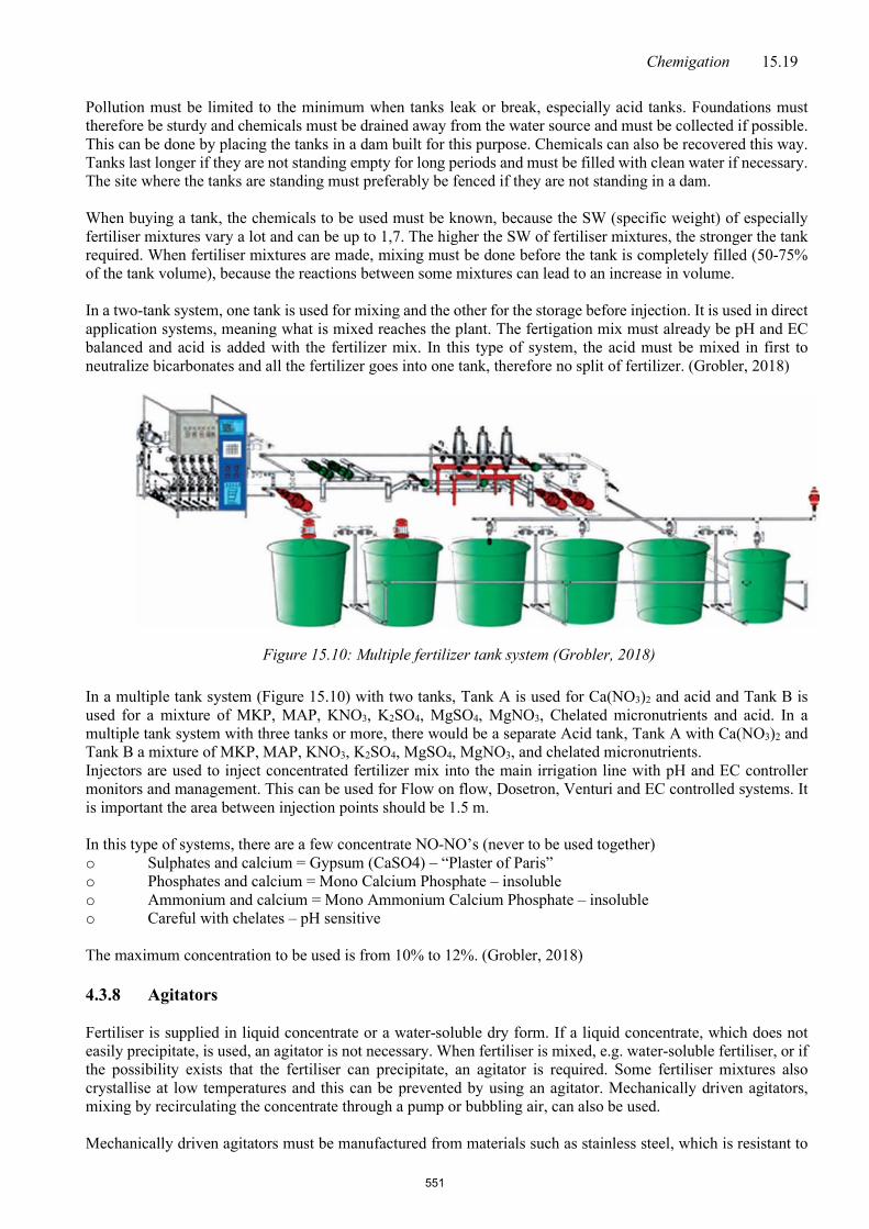
Chemigation 15.19
Pollution must be limited to the minimum when tanks leak or break, especially acid tanks. Foundations must therefore be sturdy and chemicals must be drained away from the water source and must be collected if possible. This can be done by placing the tanks in a dam built for this purpose. Chemicals can also be recovered this way. Tanks last longer if they are not standing empty for long periods and must be filled with clean water if necessary. The site where the tanks are standing must preferably be fenced if they are not standing in a dam. When buying a tank, the chemicals to be used must be known, because the SW (specific weight) of especially fertiliser mixtures vary a lot and can be up to 1,7. The higher the SW of fertiliser mixtures, the stronger the tank required. When fertiliser mixtures are made, mixing must be done before the tank is completely filled (50-75% of the tank volume), because the reactions between some mixtures can lead to an increase in volume.
In a two-tank system, one tank is used for mixing and the other for the storage before injection. It is used in direct application systems, meaning what is mixed reaches the plant. The fertigation mix must already be pH and EC balanced and acid is added with the fertilizer mix. In this type of system, the acid must be mixed in first to neutralize bicarbonates and all the fertilizer goes into one tank, therefore no split of fertilizer. (Grobler, 2018)
Figure 15.10: Multiple fertilizer tank system (Grobler, 2018)
In a multiple tank system (Figure 15.10) with two tanks, Tank A is used for Ca(NO3)2 and acid and Tank B is used for a mixture of MKP, MAP, KNO3, K2SO4, MgSO4, MgNO3, Chelated micronutrients and acid. In a multiple tank system with three tanks or more, there would be a separate Acid tank, Tank A with Ca(NO3)2 and Tank B a mixture of MKP, MAP, KNO3, K2SO4, MgSO4, MgNO3, and chelated micronutrients. Injectors are used to inject concentrated fertilizer mix into the main irrigation line with pH and EC controller monitors and management. This can be used for Flow on flow, Dosetron, Venturi and EC controlled systems. It is important the area between injection points should be 1.5 m.
In this type of systems, there are a few concentrate NO-NO’s (never to be used together) o Sulphates and calcium = Gypsum (CaSO4) – “Plaster of Paris” o Phosphates and calcium = Mono Calcium Phosphate – insoluble o Ammonium and calcium = Mono Ammonium Calcium Phosphate – insoluble o Careful with chelates – pH sensitive The maximum concentration to be used is from 10% to 12%. (Grobler, 2018)
4.3.8 Agitators Fertiliser is supplied in liquid concentrate or a water-soluble dry form. If a liquid concentrate, which does not easily precipitate, is used, an agitator is not necessary. When fertiliser is mixed, e.g. water-soluble fertiliser, or if the possibility exists that the fertiliser can precipitate, an agitator is required. Some fertiliser mixtures also crystallise at low temperatures and this can be prevented by using an agitator. Mechanically driven agitators, mixing by recirculating the concentrate through a pump or bubbling air, can also be used. Mechanically driven agitators must be manufactured from materials such as stainless steel, which is resistant to
551
15.20 Irrigation User Manual
highly corrosive fertiliser mixtures. Mechanical agitators are available in the trade and the choice (size, type of blade, angle, speed, etc.) depends on the volume and dimensions of the tank, the SW of the liquid, the viscosity of the liquid, variable liquid level and electrical energy available. Suppliers of mechanically driven agitators can usually help with the choice. For tanks up to 5 000 , it is recommended that an agitator is installed in the tank at a 15° angle, (Nel, 1999). On tanks larger than 10 000 , it may be necessary to install static mixing fins inside the tank. If mixing is done by means of a recirculating pump or aeration, it can be accepted as a rule of thumb that the tank’s volume must be circulated about 5 times per hour. 4.3.9 Static in-line mixer It is important to obtain good mixing of irrigation water and chemicals in the pipeline during application. This can be done by ensuring that there are enough bends in the pipeline before the first emitter, or by installing a static in-line mixer. 4.3.10 Fresh water supply valve Fresh water must be available for washing purposes, the flushing/rinsing of tanks and injectors after injection. 4.3.11 Filters A very high level of component accuracy is required in a injection pump and the operation thereof can be adversely affected by any wear or blockage caused by residue in the chemicals from the fertiliser tank. It is therefore recommended that a filter of 200 microns is installed on the suction side of the injection pump, preferably at the outlet of the fertiliser tank. If injecting to the main filters of the irrigation system takes place, a separate filter must be installed at the irrigation blocks to prevent that impurities reach the system. 4.3.12 Equipment for mixing of fertilisers It is often necessary to mix fertiliser concentrate with water or to mix different fertiliser combinations in liquid form to obtain the correct concentrations for injection. It is good to have mixing equipment to make the task easier. A centrifugal pump that circulates the contents of the fertiliser tank while mixing takes place, will ease the process. The centrifugal pump must deliver a high flow rate at a relatively low-pressure head and must displace the fertiliser tank volume at least once every two minutes. A funnel with its inlet mounted on the suction side of this circulation pump can also be used to mix the concentrate into the water.
552

Chemigation 15.21
Figure 15.11: The ideal fertigation set-up 4.4 Electronic control
Electronic control of injectors for chemigation, especially fertigation, can be done by monitoring of electrical conductivity (EC) and pH. Electronic control of injectors ensures that a higher measure of accuracy is possible, as these types of systems can be fully automated. Sophisticated equipment is usually used, resulting in high costs. Singular and dual control is possible. Singular control is done where injection takes place from one tank and dual control when injection from two tanks. With dual control, the fertiliser is injected from two tanks and the injection thereof is therefore also proportional. 4.4.1 Electronic conductivity control Electric conductivity (EC) is the measurement of the total dissolved salts in the irrigation water. The conduction is an indication of the irrigation water’s natural salt content and composition of the fertiliser mixture. The EC is measured in milli-siemens per metre (mS/m) or mg/. EC × 0,8 = g/ (concentration of elements).
Electronic control of fertigation can be done by using an EC sensor and control equipment (controller, relays, motorised valve, etc.). The set-up consists of an EC sensor in the irrigation pipeline, a short distance after the fertiliser is applied in the pipeline by the fertiliser pump. (This ensures thorough blending between fertiliser mixture and irrigation water before it arrives at the sensors).
An electronic controller then uses this sign from the EC sensor to open and close a motorised valve by means of a valve driver. This ensures that the correct fertiliser concentrate is always applied from the injection pump to keep the EC of the water and therefore also the concentration of the elements at the required level.
EC-control can also be applied where the fertiliser is applied simultaneously with two pumps. Each valve can have its own valve driver, or one can be shared with mechanical arms between the valves (See Figure 15.10).
553

15.22 Irrigation User Manual
4.4.2 pH-control
It is important to regulate the pH of the irrigation water (between 5,6 and 6,2) to ensure the effective application of the fertiliser. The injection of fertilisers is also inclined to change the pH of the irrigation water and it might be necessary to adjust the pH. This can be done by adding an acid of alkali (depending on the pH) to the irrigation water.
4.5 Safety measures
The following safety measures must always be followed carefully:
• Use the most suitable storage tanks for the specific application. The specific gravity (SG) of the liquid
that the tank can handle is very important. Always install a manual valve directly after the tank’s outlet so that injectors can be serviced.
• Build a bunker wall around the storage tanks. This bunker wall must be able to hold at least 120% of the content that the largest tank can hold for a period of 72 hours. The tank must preferably be placed on a concrete slab, under a shade net or roof. Secure the tanks to the concrete slab with cables. Provision must be made for emptying of the tank, when necessary.
• Always use eye protection and wear an acid protective overall with PVC gloves when using chemicals. • Provide a shower and eyewash bottles at storage sites as well as at the injection points for use during
emergency situations. • Obtain the applicable directions for use from the supplier, especially for the mixing of chemicals to be
used. • Always prevent back-flow of chemicals to the water source, overflow of chemicals from storage tanks,
injection of chemicals into empty irrigation lines and the use of chemicals which are incompatible. • Make provision that equipment can be rinsed with clean water after each use. • Mark pipe networks with different colour paints, e.g. for fertiliser mixtures from tank A, B for clean
water. Also refer to the applicable SABS colour codes for pipelines. 5 Injection of fertiliser solutions The optimal utilisation of a fertigation system does not only contain the use of dependable equipment, but also the accurate calculation of the correct injection rate. The calibration of the injectors after installation must also be done to ensure that the injection pump complies with the manufacturer’s specifications under field conditions. Each set-up will differ and factory conditions will never be found in the field. Injection pumps must be accurate within at least 1%. The following steps are proposed to determine the required injection rate of the injection pump: • Calculate the target area where fertigation will be applied or the number of plants to be served by the
irrigation system. • Obtain the recommendation of a fertiliser consultant on the amount of fertiliser mixture to be applied
per hectare or per plant or per m3 irrigation. • Obtain the applicable information on the specific type of fertiliser mixture to be used, e.g. concentration
and composition. • Calculate the total amount of the fertiliser mixture to be applied (per hectare or per m3 irrigation water). • Determine the duration of the injection (depending on the irrigation system’s standing time and
application rate, time required for the fertiliser solution to move from the injection point to the last emitter, the amount of fertiliser mixture to be injected and the movability of the fertiliser mixture in the soil).
• Determine the injection rate of the injection pump with the aid of the following equation:
554

Chemigation 15.23
kQ AITK T
×=
× (15.1)
where IT = injection rate of the fertiliser mixture (/min) Qk = amount of fertiliser to be applied (kg/ha) A = area (ha) K = required injection concentration of the solution (kg/) T = injection duration (min)
The injection rate will be determined by the maximum capacity of the available injection pump or the flow rate of the irrigation system. The minimum injection rate is usually 10% of the maximum value and must not be exceeded (Wilson, 1996). • Calibrate the injection pump according to the injection rate as calculated. For calibration of the injection
rate, a stopwatch and measuring jug is required. The measuring jug must be clearly and precisely marked in millimetres and must be large enough to hold enough of the fertiliser mixture for 5 minutes of injection. The measuring jug can then be filled with liquid and the time to suck a specific volume of the liquid from the measuring jug, or the amount of liquid that is sucked from the measuring jug in a specific time, is measured with the stop watch. The method of sucking from an open measuring jug is preferred over the method where liquid is pumped into a container, because the back pressure in the container can influence the reading.
5.1 Examples for the calculation of injection rates
The manner in which the injection rate is calculated, is drastically influenced by the type of irrigation system in use. With static systems such as micro and sprinkler irrigation systems, the injection rate is fixed and the amount of fertiliser required is calculated and applied within a certain time. The amount dissolved in the tank, is therefore the amount applied on a specific area, if different sizes of blocks are treated with the same injection apparatus, the fertiliser must be applied proportionally by a injection pump.
With moving systems such as pivots and big guns, the application varies from the irrigation system and fertiliser can only be applied proportionally. With the proportional method, the injection rate is very important, because it determines the amount of fertiliser applied to a specific area. With calibration of the injection pump, the speed of the system and the area on which the fertiliser mixture is applied, must be considered thoroughly.
5.1.1 Static systems Example 15.1 (Wilson, 1996) A permanent sprinkler system with a sprinkler spacing of 18 × 12 m and sprinkler delivery rate of 1 750 /h must be used to apply 50 kg/ha of nitrogen in the form of water-soluble calcium nitrate in a fruit orchard. The sandy loam soil’s easily available water retention ability is 150 mm/m. The nitrogen must be applied to a depth of 300 mm. The effective root depth is 1.0 m. Twenty sprinklers irrigate simultaneously and the standing time is 12 hours. Answer: • Area irrigated per set-up = 20 sprinklers × 18 × 1 m = 0.43 ha • Amount of fertiliser applied: Calcium nitrate has the following properties, according to fertiliser experts: - 15.5% N - solubility = 120 g/100 g H2O by 20°C = 1.2 kg/
555

15.24 Irrigation User Manual
To apply 50 kg/ha nitrogen, the following amount of calcium nitrate is required: 50 kg / ha15.5% N×
= 323 kg calcium nitrate/ha. • Total amount of fertiliser required per set-up = 323 kg calcium nitrate/ha ×0.43 ha = 139 kg.
With a solubility of 1.2 kg/, the minimum amount of water required will be: 139 kg1.2 kg /
= 115 litres. A tank with a capacity of at least 125 litres to provide for the increase in volume as a result of the mixing process is required. • Time required for fertiliser injection: For a sprinkler system, it is recommended that at least 1 hour injection time is used to ensure that the fertiliser is applied as uniformly as possible. • Injection rate From equation 18.1:
kQ AIT
K T323 0.431.2 60
1.92 / min
×=
××
=×
=
The concentration of the solution = injection ratesystem flow rate
= 1.92 6020 1750
××
= 0.0033 0.3%≈ A concentration of < 1% is usually required. This calculated value therefor complies with the guideline. • Depth of infiltration in the soil
Gross application rate = spacingsprinkler sprinklerofdelivery
=
12×181750
= 8.1 mm/hour Total application = gross application rate × standing time = 8.1 mm/h × 12 hours = 97.2 mm
Depth of infiltration = 97.2 1000150×
556

Chemigation 15.25
= 648 mm The required depth to apply nitrogen, is 300 mm Time required for nitrogen to penetrate to 300 mm:
648300 × 12 = 5.555 hours
The application of calcium nitrate must begin after 6.45 hours of irrigation standing time has elapsed and must be applied for 1 hour. The irrigation continues after this for 5.55 hours, which means that the fertiliser has penetrated to a depth of 300 mm into the soil. Example 15.2 (Wilson, 1996) A drip irrigation system is used to irrigate a strawberry field. A liquid fertiliser solution (nitrogen and phosphates) must be used. The spacing of the strawberries is 1.2 × 0.3 m. The length of the rows is 90 m (300 plants per row). The delivery rate of the drippers is 2 /h and the dripper spacing is 0.6 m. Each irrigation block consists of 25 rows. Standing time per block is 1 hour. The producer wishes to apply 1 g of nitrogen and 1.5 g phosphate per plant in five equal parts, weekly. Ammonia poly-phosphate is recommended by his fertiliser advisor as a liquid fertiliser solution. Answer: • Number of plants per block = 25 rows × 300 plants per row = 7500 plants • Amount of fertiliser to be applied with each application: According to the fertiliser advisor, ammonia poly-phosphate has the following properties: - 10% N - 15% P - density = 1.37 kg/litre Amount of the type of fertiliser required:
mixture in fertiliser%× solutionofdensity ×nsapplicatio of numberplants of number×plantperamount
∴ Nitrogen required = 1 75005 1370 0.1
×× ×
=10.95 litres
Phosphates required = 1.5 75005 1370 0.15
×× ×
=10.95 litres
Approximately 11 litres of the fertiliser solution is required. • Injection rate The fertiliser must preferably be applied for a twenty minute period, 30 minutes after the irrigation has begun. This will ensure that the system is at pressure before application and secondly, sufficient flushing time will be available after application.
Injection rate = minute20liter11
= 33 /h The maximum concentration of the fertiliser mixture must preferably not exceed 1%.
557

15.26 Irrigation User Manual
Flow rate per block: 90m length rows0.6m dripper spacing
× 2 /h × 25 rows
= 7.5 m3/h The concentration of the fertiliser mixture in the system is:
= ( )( )
injection rate / hsystem flow rate / h
= 750033
= 0.0044 = 0.44% < 1% The injection rate is therefore acceptable because it is smaller than 1%.
5.1.2 Moving systems The application of fertiliser for a moving system must be adapted to the revolution speed. The revolution speed must be physically determined in the field under wet and dry conditions and at different spots in the field if the slope differs. As general rule, it can be accepted that a fertiliser concentration of 0.2% in the irrigation water is safe, to prevent that leaf-burn occurs with moving systems. The following must be kept in mind when fertigation is done with moving systems:
• The storage tank for the fertiliser mixture must be large enough to keep enough of the mixture for an
entire revolution. • An agitator pump must preferably agitate the mixture continuously during the application process. • The injection pump must be switched off after a revolution is completed, but the pivot must still irrigate
until the system is flushed clean. • The calculation for the application by the end sprinkler of a pivot that switches on and off from time to
time is very difficult and can only be done effectively by means of manual control. • A big gun is very wind sensitive and should not be used for fertigation during windy conditions. Example 15.3 (Wilson, 1996) The flow rate of a pivot with a length of 340 m and an overhang of 10 m, is 160 m3/h. The delivery rate of an end sprinkler that irrigates continuously, is 40 m3/h and irrigates a radius of 45 m. The pivot’s revolution speed was measured as 1.7 m/min. 50 kg of nitrogen/ha must be applied 3 times at the beginning of the irrigation season. The fertiliser advisor suggests urea in granular form. Answer: • Area under irrigation: Total wetting radius (r) = 340 m + 10 m = 395 m Area = π r2 = π × 3952 = 49 ha
558

Chemigation 15.27
• Amount of fertiliser to be applied: According to the fertiliser advisor, urea has the following properties: - 46% N - solubility = 108g ÷ 100g × H2O by 20°C = 1.08 kg/
To apply 50 kg nitrogen/ha, 50kg0.46
= 109 kg urea/ha is required
• Total amount of fertiliser required = 109 kg/ha × 49 ha = 5341 kg • Size of storage tank required:
With a solubility of 1.08 kg/, a storage tank of 5341 kg1.08 kg /
= 4945 litre is required.
A tank of 5000 is available, therefore the concentration of the mixture is 1.07 kg/. • Revolution time of pivot Circumference of circle = 2 π r = 2482.8 m
Revolution time = Circumferencerevolution time
= 2482.8m1.7m / minute
= 1460.5 minutes = 24.4 hours • Injection time From equation 18.1:
IT = Qk AK T
××
= 109 49 / minute1.07 1460.5
××
= 205 /h Example 15.4 (Wilson, 1996) A big gun with a sprinkler that delivers 56.7 m3/h, is used to irrigate a maize field of 400 × 365 m. The wetted diameter of the sprinkler is 105 m. The strip spacing is 60 m and the measured running speed of the machine is 15 m/h. The farmer wants to apply liquid ammonia nitrate (21%) to do one application of 50 kg nitrogen/ha during spring.
559

15.28 Irrigation User Manual
Answer: • Area under irrigation Area = strip spacing × length of the strip = 60 m × 400 m = 2.4 ha • Amount of fertiliser to be applied According to the fertiliser advisor, ammonia nitrate has the following properties: - 21% N - density = 1.27 kg/
To apply 50 kg of nitrogen/ha, 500.21 1.27×
= 187 ammonia nitrate is required
• Total amount of fertiliser required = amount ammonia nitrate/ha × area = 187 /ha × 2.45 ha = 458 The storage tank should be able to hold at least 500 of the solution. • Application time The big gun must irrigate the entire 400 m. The length of the supply pipe = strip length - wetted radius of sprinkler
= 400 m – 2105 m
= 347.5 m
Application time = speedrunningpipe supply of length
= 347.5m15m / h
= 23.2 hours • Injection rate
Injection rate = time nApplicatiorequired fertiliser amount Total
= 45823.2 hours
= 19.74 /h
560

Chemigation 15.29
Concentration of fertiliser mixture in the system
= rate flow systemrate injection
= 319.74 / h56.7m / h
= 0.000348 = 0.0348% < 1%, which is the general guideline 6 Legislation in South Africa Chemigation can have a drastic influence on the environment if mistakes are made. Relevant legislation therefore exists in South Africa regarding the use of chemigation. There are, however, no special permits or regulations to adhere to. The legislation places the responsibility on the user and gives various government departments the power to hold the user responsible for mistakes made. Only a few regulations are discussed and the manager must pay attention to the contents of the complete Act as published in the Government Gazette. More information can be found in the Draft Integrated Pollution and Waste Management White Paper (https://www.gov.za/documents/integrated-pollution-and-waste-management-white-paper-draft). 6.1 The Environmental Conservation Act (Act 73 of 1989) The general environmental policy is contained under Article 2(1) of Act 73 of 1989. It refers inter alia to the right to a safe and healthy environment, the responsibility towards the protection, maintenance and improvement of the natural environment, as well as the relation between the authorities, the community and agricultural organisations. All organisations and their activities that have an impact on the environment, must be encouraged to create and to implement a formal environmental management system. The system must be based on acceptable standards and guidelines, to enable them to execute self-control over any of their activities which may have an influence on the environment. The policy on land use stipulates that specific attempts must be made to protect water and rural resources. The policy on natural resources also determines that methods must be activated to ensure that water resources are utilised responsibly so that optimal provision can be delivered to the various sectors. 6.2 The Conservation of Agricultural Resources Act (Act 43 of 1983) This act makes provision for control over the use of the natural agricultural resources of the Republic, to promote the protection of the soil, the water resources, the vegetation and the control of weeds and intruder plants and for related matters. Regulation 6 of the Act is mostly relevant to chemigation and can be summarised as follows: 6.2.1 Regulation 6: Prevention of salinisation and saturation of irrigated soil Every land user is compelled to protect his/her land by means of one or more of the following methods: • The construction of supply canals, irrigation furrows, storage and catchment dams must be waterproof. • Prevent over-irrigation or irrigation with water with a too high salt concentration. • The construction and maintenance of suitable drainage works to extract excess surface and subsurface
water and transport it, can prevent saturation and salinisation of subjacent soil layers. • Fertiliser or compost which promotes salination must not be applied. • Application of a suitable soil improver on saline soil.
Additional measures can be stipulated by an Executive Officer of the Department of Agriculture.
561

15.30 Irrigation User Manual
6.3 The Health Act (Act 61 of 2003) The Act aims to provide a framework for a structured uniform health system within the Republic, taking into account the obligations imposed by the Constitution and other laws on the national, provincial and local governments with regard to health services; and to provide for matters connected therewith. The Act provides regulation for the protection against the pollution of the environment that would have detrimental health effects upon the local, provincial and/ or national inhabitants. 6.4 The National Water Act (Act 36 of 1998) The purpose of the National Water Act is to ensure that the country’s water sources are protected, used, developed, managed and controlled in a sustainable and fair manner to the benefit of all the people of South Africa. This objective will be reached by, among others, the following separate objectives: • Provision of water for basic human consumption and ecological requirements as the first priority
(collectively called the Reserve). • Promotion of the effective, sustainable and beneficial use of water in public interest. • Facilitation of social and economic development to improve the living standards and the welfare of the
community. • Making provision for increasing water needs, especially for the urban and industrial sectors. • Prevention of pollution and deterioration of water sources, by monitoring the quality of the water. • Planning of measures for the management of floods and droughts. The highest risk is back-flow of treated irrigation water to the water source, with the result that chemical pollution takes place. By installing sufficient safety equipment, back-flow can be prevented. In other countries, special dual one-way valves are used. These valves prevent back-flow through the irrigation pump from the irrigation system. These are unfortunately not widely available in the trade in the RSA. If standard non-return valves are used, ensure that they are corrosion resistant. A low-pressure drainage valve can be installed in front of the non-return valve, so that water that leaks past the non-return valve, can be drained away from the system. A vacuum valve can also be installed in front of the non-return valve. This will prevent that a negative pressure may suck the water through the non-return valve. More information can be found in the Draft White Paper on Water Services at https://www.gov.za/. 7 Summary Chemigation is a handy practice which can be used by the producers to great economic benefit for themselves and agriculture. The requirements for successful chemigation are a high level of management, knowledge of the basic principles of pest control and irrigation, the mastering of the manipulating practical problems and a well-planned and well-designed irrigation system. The ideal is that the producer, agronomist, soil scientist and a chemigation specialist take cognisance of information regarding the crops’ water requirements, chemigation requirements and scheduling thereof and make recommendations to the designer to design an optimal irrigation system. The benefits regarding fertigation, production, economy, management, labour and convenience justify these inputs. There is still a great void within the South African irrigation industry for purposeful co-operation between specialists, with quality production as objective. 8 References
1. Adendorff, M. 2016. Information Sheet 5.5 Chemigation: Principles and fundamental equipment. SASRI
www.SASRI.org.za 2. Audie, M. 1999. Personal communication. Polycan converters South Africa, RSA.
562

Chemigation 15.31
3. Bricknell, M. 1991. Personal communication. Hydrive, RSA. 4. Briedenhann, R. 1999. Personal communication. Omnia Fertilisers (Pty) Ltd., RSA. 5. Buys, A.J. 1997. Bemestingshandleiding. The Fertiliser Association of South Africa, RSA. 6. Combrink, N.J.J. 2019. Personal communication. Department of Agronomy, Stellenbosch University,
RSA, [email protected]. 7. Crafford, D. 1999. Personal communication. Chief-Directorate: Agriculture: Western Cape, RSA. 8. De Bruyn, K. 1985. Toediening van kunsmis deur besproeiingstelsels. Omnia Fertilisers (Pty) Ltd, RSA. 9. De Villiers, B. 1998. Hulpmiddel-, versurings-, en waterkwaliteitseffekte op onkruiddoders. ARC-Small
grain center, RSA. 10. De Wit, P.G. 1986. Kunsmistoediening deur besproeiingstelsels. Department of Agriculture and Fisheries,
RSA. 11. Dosatron. 1999. SA Besproeiing Apr/May 1999. RSA. 12. Du Preez, M. 1986. Misstofbesproeiing. Fruit and Fruit technology Research Institute, Stellenbosch, RSA. 13. Ferreira, I. 1999. Personal communication. Kynoch Fertilisers (Pty) Ltd., RSA.
14. Grobler, L. 2018. Personal communication. Agri-Alchemi, RSA. 15. Hendriks, D. 1999. Personal communication. Alldos, RSA 16. Horn, L. 1999. Personal communication. Netafim South Africa, RSA. 17. Jorgensen, C.S. and Norum, K.S. 1993. Subsurface drip irrigation: Theory, Practices and Application.
CATI Publication number 921001, USA. 18. Keller, J. and Bliesner, R.D. 1990. Sprinkle and trickle irrigation. Utah State University, Logan, USA. 19. Koegelenberg, F.H. and Conradie, G.C. 2000. Voedingsbesproeiing. ARC-Institute for Agricultural
Engineering, RSA.
20. Leslie, G. 2014. Information sheet. 10.6 Understanding the labels on herbicide containers. SASRI. www.sasri.org.za
21. Lombard, A. 1999. Personal communication. Netafim South Africa, RSA. 22. Malan, C. 1998. Die doeltreffende toediening van bemestingstowwe deur besproeiingstelsels. SA Irrigation
Oct/Nov. 1998, RSA. 23. Malan, C. 1999. Personal communication, Netafim South Africa, RSA. 24. Nel, M. 1999. Personal communication. Martin Nel Tanks, RSA. 25. Raphael, R. 1999. Personal communication. ProMinent S.A., RSA. 26. Shapley, T. 1999. Personal communication. Mixtec, RSA. 27. Shneck, M. 1998. Fertigation. Haifa Chemicals Ltd, Israel.
563

15.32 Irrigation User Manual
28. Van der Gulik, T.W. and Evans, R.G. 2011. Chemigation and PAM – Delivering Chemicals to Crops and
Soils Using Irrigation. Irrigation, Sixth edition. Irrigation Association, Fairfax, Virginia, USA 29. Wilson, T. 1996. Chemigation. Irrigation Association, USA.
564

IRRIGATION USER MANUAL
CHAPTER 16 Terminology, conversion tables, design norms and overview of
irrigation scheduling software
565

Terminology 16.1
Table of Contents 1 Introduction ........................................................................................................................................................................................................................................... 16.1 2 Symbols and abbreviations .................................................................................................................................................................................................. 16.1 3 Definitions and concepts ........................................................................................................................................................................................................ 16.2 3.1 Climate-related definitions ...................................................................................................................................................................................... 16.2 3.2 Plant-related definitions .............................................................................................................................................................................................. 16.3 3.3 Soil-related definitions ................................................................................................................................................................................................. 16.4 3.4 Water-related definitions ........................................................................................................................................................................................... 16.7 3.5 Irrigation system-related definitions ............................................................................................................................................................ 16.9 4 Efficiency .............................................................................................................................................................................................................................................. 16.14 5 Units ............................................................................................................................................................................................................................................................ 16.16 6 Conversion factors ...................................................................................................................................................................................................................... 16.17 7 Conversion tables ........................................................................................................................................................................................................................ 16.18
All rights reserved Copyright 2019 ARC-Agricultural Engineering (ARC-AE)
566

16.0 Irrigation User Manual 1 Introduction The purpose of this appendix is to define the basic irrigation concepts for quick reference in advance, so that there is no vagueness regarding the terminology that is used in the Irrigation User’s Manual. However, some concepts are common to more than one subject and have been dealt with under the most appropriate heading. The definitions and concepts are defined in more detail in the relevant chapters, where they are also explained by means of diagrams and sketches. 2 Symbols and abbreviations English Afrikaans A = Area Oppervlakte AWD = Allowable water depletion Toelaatbare wateronttrekking (TWO) B = Width Breedte CU = Christiansen Coefficient of Uniformity Christiansen se uniformiteitskoeffisiënt CV = Coefficient of variation Variasiekoeffisiënt (of manufacturing) (van vervaardiging) CWR = Crop water requirement Gewaswaterbehoefte (GWB) d = Diameter Deursnee (of diameter) η = Efficiency Doeltreffendheid ηf = Field application efficiency Aanwendingsdoeltreffendheid ηi = Irrigation efficiency Besproeiingsdoeltreffendheid ηt = Transportation efficiency Vervoerdoeltreffendheid ηo = Storage efficiency Opbergingsdoeltreffendheid ηd = Distribution efficiency Verspreidingsdoeltreffendheid ηs = System efficiency Stelseldoeltreffendheid ηa = Application efficiency Toedieningsdoeltreffendheid ηc = Conveyance efficiency Toevoerdoeltreffendheid E = Evaporation Evaporasie (verdamping) E0 = Pan evaporation Panverdamping ERD = Effective root depth Effektiewe worteldiepte (EWD) ET = Evapotranspiration Evapotranspirasie ET0 = Reference evapotranspiration Verwysings-evapotranspirasie f = Crop factor Gewasfaktor fp = Pan factor Panfaktor g = Gravitational constant (9,81 m/s2) Gravitasiekonstante (9,81 m/s2) GA = Gross application Bruto toediening (BT) GAR = Gross application rate Bruto toedieningstempo (BTT) GIR = Gross irrigation requirement Bruto besproeiingsbehoefte (BBB) H = Head or pressure head Hoogte of drukhoogte kc = Crop coefficient Gewaskoeffisiënt kp = Pan coefficient Pankoeffisiënt L = Length Lengte m = Mass Massa NA = Nett application Netto toediening (NT) NAR = Nett application rate Netto toedieningstempo (NTT) NIR = Nett irrigation requirement Netto besproeiingsbehoefte (NBB) p = Pressure Druk P = Power Drywing PWP = Permanent wilting point Permanente verwelkpunt (PVP) Q = Flow rate Vloeitempo qe = Emitter discharge Emitterlewering
567

Terminology 16.1 r = Radius Straal (of radius) R = Rainfall or precipitation Reënval Re = Effective rainfall Effektiewe reënval RAW = Readily available water Maklik beskikbare water (MBW) SWC = Soil water capacity Waterhouvermoë (WHV) t = Time Tyd T = Transpiration Transpirasie v = Velocity Snelheid V = Volume Volume 3 Definitions and concepts • Square brackets [ ] indicate the commonly used unit (dimensions) of measurement. • The description of what is being measured is underlined. • Concepts for which definitions are given elsewhere in the chapter appear in bold type. 3.1 Climate-related definitions • Evaporation (E): [mm/day] The loss of water from the soil surface and the top layer of soil before the water is able to
penetrate the soil deeply enough to be useful to the crop. (It forms part of evapotranspiration (ET).)
• Transpiration (T): [mm/day] The loss of water into the atmosphere from the growing plant regulated by physical and
physiological processes in the plant. • Crop evapotranspiration (ETc): [mm/day] The loss of water through transpiration (T) of the growing plant plus evaporation (E) from
the soil surface.
• Reference evapotranspiration (ET0): [mm/day] The crop evapotranspiration (ETc) of a reference crop - green grass of uniform height (80 to
150 mm tall), growing actively, completely shading the ground and not short of water.
• Evaporation pan: A device used for the measurement of the amount of water lost through evaporation from an
open water surface during a specific period. (The American class A pan, which is the standard in South Africa, the Symons pan, the Scheepers pan and the Nelspruit pan are a few examples.)
ETc = E + T ( 1.1)
568

16.2 Irrigation User Manual • Pan evaporation (E0): [mm/day or mm/month] The amount of water that evaporates from an evaporation pan during a certain period. • Crop factor (f): [fraction]
The ratio of crop evapotranspiration (ETc) to pan evaporation (E0) for a crop of a given age, in a certain growth phase, with a certain canopy size, in a certain climatic zone.
• Pan coefficient (kp): [fraction]
The ratio of reference evapotranspiration (ET0) to pan evaporation (E0) for the same period.
• Crop coefficient (kc): [fraction] The ratio of crop evapotranspiration (ETc) to reference evapotranspiration (ET0) for a given crop when growing in large fields under optimum growing conditions.
• Orchard factor: [fraction]
The crop factor (f) for a specific orchard and irrigation system. • Rainfall or precipitation (R): [mm/period]
The depth of precipitation or rainfall registered during a given period by a correctly mounted rain-gauge.
• Effective rainfall (Re): [mm/period]
The rain that falls during a given cycle and that can be used profitably by the plants and that partially or completely replaces scheduled irrigation. (This excludes surface run-off, deep percolation and a portion of interception.)
• Surface run-off
That portion of rainfall or irrigation which runs off without infiltrating the soil. 3.2 Plant-related definitions • Root zone
The area around the plant below the soil surface delimited downwards by the effective root depth (ERD) and sideways by the lateral extension of most of the plant's nutritive roots. Alternative: The root volume of the crop.
• Crop water requirement (CWR): [mm/period] The depth of water required by a given crop for evapotranspiration (ET) over a specific period. Alternative: Nett irrigation requirement (NIR) of a given crop plus effective rainfall (Re). (Operational losses of the system are excluded from the crop water requirement (CWR).)
• Seasonal crop water requirement: [mm] The crop water requirements (CWR) for an entire growing season.
kp = ET0/Eo or ETo = kp E0 ( 1.3)
f = ETc / Eo or ETc = f E0 (1.2)
kc = ETc / ETo or ETc = kc ET0 (1.4)
569

Terminology 16.3 • Peak crop water requirement: [mm/day]
The average daily crop water requirement (CWR) for the period during which it is the highest. • Irrigation requirement
o Nett irrigation requirement (NIR): [mm/period] The depth of irrigation water necessary to meet evapotranspiration (ET) of the crop during a certain period and in a specific growing phase of the crop. Alternative: Gross irrigation requirement (GIR) of a given crop minus operational losses of the system.
o Gross irrigation requirement (GIR): [mm/period] Nett irrigation requirement (NIR) of a given crop plus operational losses of the system. (The contribution of effective rainfall (Re) is excluded.)
• Effective root depth (ERD): [m]
The soil depth within which most of the nutritive roots of a plant occur. (It is the smaller of the natural root depth and the effective soil depth.)
o Natural root depth: [m] The soil depth within which most of the nutritive roots of the relevant crop would have occurred if no soil restrictions were present.
o Effective soil depth: [m] The soil depth to a level at which the growth of the nutritive roots of the plant is restricted by soil-related conditions.
• Equivalent application: [mm]
The average application where all the irrigation water actually applied to a limited area, to be applied uniformly over the total area.
• Shaded area or drip area: [m2] The area of the shade cast by a plant on the ground when the sun is directly overhead.
• Interception
That part of rainfall and irrigation that does not reach ground level as a result of interception by foliage.
3.3 Soil-related definitions
• Soil water Water contained in the voids between the particles of the soil.
• Soil water tension or matrix potential: [kPa]
The tension which must be exerted by the nutritive roots of a crop in order to extract the soil water from the soil.
• Saturation point
The soil water condition when all the soil voids are filled with water (no air present).
• Field capacity (FC): [mm] The depth of water held within the root zone of a crop when the rate of downward movement of soil water has practically stopped. It occurs within a few days of ample irrigation or rainfall. A soil water tension of -10 kPa is usually considered to indicate field capacity.
570

16.4 Irrigation User Manual
• Wilting point: o Temporary wilting point:
The soil water condition when in periods of high crop water requirement (CWR) water cannot be extracted from the soil quickly enough for the plant to meet its needs. (If this condition continues only for short periods, the crop may recover partially or completely.)
o Permanent wilting point (PWP): [mm] The depth of water held within the root zone of the crop when most plants will wilt permanently. (This point is normally reached at a soil water tension of about -1 500 kPa.)
• Soil water capacity (SWC): [mm/m]
A soil characteristic which is reflected by the depth of soil water per metre of soil depth between the limits of field capacity (FC) and permanent wilting point (PWP) of a given crop. (This is normally at soil water tension between -10 kPa and -1 500 kPa.)
• Total available water (TAW): [mm]
The depth of soil water available within the effective root depth of a given crop between the limits of field capacity (FC) and permanent wilting point (PWP) of a given crop. (This is normally at soil water tension between -10 kPa and -1 500 kPa).
• Available water100 (AW100): [mm] The depth of soil water available within the effective root depth of a given crop at soil water tension between -10 kPa and -1 500 kPa).
• Percentage allowable water depletion (α): [%]
The maximum percentage of the available water (AW) which may be extracted from the root zone of a crop and still allowing unrestricted evapotranspiration (ET) to the crop under given soil and climatic conditions.
• Percentage allowable water depletion100 (α100): [%]
The maximum percentage of the available water100 (AW100) which may be extracted from the root zone of a crop and still allowing unrestricted evapotranspiration (ET) to the crop under given soil and climatic conditions.
• Minimum water level (100 - α): [%]
The minimum percentage of the available water (AW) that has to remain in the root zone of a given crop under given soil and climatic conditions and allowing unrestricted evapotranspiration (ET) and drop growth. It is complement of the percentage allowable water depletion (α).
• Available soil water capacity (ASWC): [mm/m] The water depth per metre soil depth, which would allow unlimited evapotranspiration and crop growth (ET) in a particular soil for a given crop under certain climatic conditions.
SWC = FC − PWP (1.5)
TAW = SWC ERD (1.6)
ASWC = SWC α/100 ( 1.7)
571

Terminology 16.5
• Readily available water (RAW): [mm] The water depth which is available for a given crop on the effective root depth and which allows unlimited evapotranspiration (ET) and crop growth under certain climatic and soil conditions. (A soil water tension of -100 kPa is mostly regarded as the readily available water (RAW).
Therefore:
And also:
• Profile available water (PAW) [mm]
The sum of readily available water (RAW) of each soil horizon within the effective root depth (ERD).
• Soil water capacity100 (SWC100): [mm/m] A soil characteristic which is reflected by the depth of soil water per metre of soil depth at soil water between -10 kPa and -100 kPa.)
• Soil water reservoir: [liter]
The volume available water (AW) in the root zone of a plant. • Infiltration
The penetration of water into the soil from the soil surface.
• Infiltration rate: [mm/h] The rate of infiltration of water into soil o Initial infiltration rate: [mm/h]
The initial rate of infiltration of water into soil at the onset of the application of water. o Basic infiltration rate: [mm/h]
The practically constant rate of infiltration of water into wetted soil after a time.
• Lateral distribution: [m] The horizontal component of the movement of water in the soil from the point where it was applied at a certain point on the soil surface.
• Deep percolation:
That part of irrigation and rainfall that percolates through the root zone of the crop before it can be utilised by the crop. (The ideal is to irrigate in such a way that no deep percolation occurs.)
• Tensiometer:
A device with a porous tip of ceramic material, filled with water and placed at a certain depth to register the soil water tension.
RAW = SWC α/100 ERD (1.8)
RAW = ASWC ERD (1.9)
RAW = AW100 α100/100 (1.10)
572

16.6 Irrigation User Manual • Neutron probe:
A device with a radioactive source capable of registering the water content of the soil at different depths.
• Gypsum block:
An electronic sensor inside a block of porous material, buried at a certain depth to measure the total available water (TAW) of the surrounding soil.
3.4 Water-related definitions • Hydraulics:
The science that deals with liquids in motion (hydrodynamics) or at rest (hydrostatics). In irrigation the principles of hydraulics are applied to the behavior of water in pipes and other components of irrigation systems such as pumps, valves, filters, canals and dams.
• Hydrology:
The science of the waters of the earth. The study of the distribution of rainfall, run-off and water quality in rivers, and the occurrence and quality of groundwater.
• Water quality:
The occurrence and concentration of physical, chemical and biochemical substances and of biological organisms in irrigation water.
• Dam (or dam wall): Any structure capable of storing water. Basic types of structures: o Earth dam:
Earth dams are embankments of rock or earth with an impermeable core or upstream blanket for controlling seepage.
o Gravity dam: A gravity dam depends on its own weight for stability.
o Arch dam: An arch dam transmits most of the horizontal thrust of the water behind it to the abutments by arch action.
o Buttress dam: Buttress dams have many variations, but the simplest consists of sloping flat slabs supported at intervals by buttresses. (The first three types are usually constructed of concrete.)
573

Terminology 16.7 • Full supply level: [m]
The elevation (above a certain reference level) of the water surface of the dam when it starts spilling over the spillway.
• Dam capacity: [m3]
The amount of water that can be stored in a dam. • Dam yield: [m3/period]
The amount of water that can be supplied at a given risk by the dam during a fixed period, based on long-term statistical analysis.
• Dam surface area: [ha]
The area of the water surface of a dam. • Spillway The section of the structure built for the safe passage of flood water.
• Discharge structures The structures and equipment built into the dam for the discharge of water.
• Diversion weir A low dam built in a stream in order to raise the water level sufficiently for diversion of all or
part of the water into a canal or furrow, and to control the flow.
• Canal An open furrow in which the water flows under gravity. (It may consist of soil, or it may be lined
with concrete or any other impervious material).
• Sluice-gate A sliding structure for the control of the flow of water in an open conduit.
• Flow rate or flow: [m3/s] The rate of flow of water past a certain point. • Watermeter A device measuring the cumulated amount of water that flowed past a certain point in a pipeline.
• Flowmeter:
A device with which the flow rate in a pipeline or canal is measured.
• Flow measuring weir A structure used exclusively for measuring the flow rate in a canal or stream. Basic types of weirs:
o Rectangular sharp-crested or broad-crested weir o V-notch or Cipoletti weir o Crump or Parshall flume
• Irrigation stream: [m3/h]
The flow rate at which an irrigator may take water from a canal or furrow shared with other irrigators.
574

16.8 Irrigation User Manual
• Water Act The National Water Act (Act 36 of 1998) as amended, and the regulations and proclamations
promulgated there under. • Soil Conservation Act:
The Soil Conservation Act (Act 43 of 1983) as amended and the regulations and proclamations in terms thereof, or any act with which it is replaced.
• Contour channel
A gently sloping channel with a raised bank built across lands of steeper gradient. The gradient of the contour ridge is gentle enough to prevent erosion.
• Waterway
A broad artificial channel which collects the water from several contour ridges and carries it straight down the steepest slope to a natural watercourse.
3.5 Irrigation system-related definition
• Irrigation
The artificial application of water to the soil to meet crop water requirement (CWR).
• Irrigation system or only system The physical components and water bearing structures specially established for the transportation of irrigation water from the source to the crop in order to apply it to the benefit of the crop.
• Distribution lines
o Main line The part of the pipeline from the pump to the inlet to a field. o Sub-main line The part of the pipeline connecting the main line to the manifolds. (Owing to the many different pipeline layouts found in practice, it is often neither easy nor
important to distinguish between main lines and sub-main lines.)
• Manifold: The pipeline from which the laterals branch off.
• Lateral:
The pipeline on which the emitters occur.
• Emitter: A device designed to distribute water onto the soil according to a specific application rate and distribution pattern at a given pressure. (Examples are drippers, microjets, micro sprinklers, sprinklers and big guns).
• Emitter discharge (qe): [volume/h]
The amount of water per hour leaving the emitter at a given pressure.
• Irrigation block: Part of an irrigation system designed as a unit and controlled by a single valve. The whole block is always irrigated during one standing or irrigation time.
575

Terminology 16.9
• Irrigation set A group of irrigation blocks which can be irrigated at the same time.
• Design application: [mm] The maximum application for which the system is designed.
• System capacity: [m3/h of l/s] The maximum rate of delivery of the system.
• Irrigation scheduling
The process of management of an irrigation system with the purpose of applying the correct amount of water at the correct time to meet the crop water requirement (CWR) optimally.
• Cycle length: [days]
The actual time lapse between the commencement of two successive applications for a specific irrigation set.
• Theoretical cycle length: [days]
The calculated time lapse between the commencement of two successive applications by a specific irrigation system when it has to satisfy the peak water requirement of the crop.
• Standing time: [h]
The actual period of time needed by a static irrigation system for a certain nett application (NA).
• Theoretical standing time: [h]
The calculated period of time for which a system has to irrigate to apply the design application.
• Rotation time: [days of h]
The actual time that a mechanized irrigation system must irrigate for a certain nett application (NA).
• Inflow time: [minutes]
The actual period of time necessary for the water supply of a flood irrigation system to be diverted into a flood bed for a certain nett application (NA).
• Pressure (p or H): [kPa or m] The pressure of the water inside the system relative to atmospheric pressure.
• Pressure variation (∆H): [kPa or m]
The difference in pressure between the highest and the lowest pressure in a unit, such as an irrigation set, an irrigation block, a lateral or a filter.
• Pressure loss (δH): [kPa or m]
The difference in pressure between two points in a system as a result of the static pressure and pipe friction.
o Static head (hs): [kPa or m] The difference in altitude between two points in a system. o Pipe friction (hf): [kPa or m] The head loss as a result of laminar and turbulent flow of a viscose liquid (in this case, water)
through the different components of a system.
576

16.10 Irrigation User Manual
• Hydraulic gradient: [m/m] The slope on the line (which would have been followed by a free water level) representing the total energy head in a closed or open conduit.
• Pipe diameter: [mm]
The internal or external diameter of a pipe. o Internal diameter (d): [mm]
The real internal diameter of a pipe. o Nominal diameter: [mm]
The diameter in terms of which a pipe is popularly spoken of.
• Pipe length: [m] The length of a specific section of pipe of constant diameter, class and material.
• Equivalent pipe length: [m]
The length of a specific diameter of pipe producing the same head loss as a specific component of the same diameter under the same flow conditions.
• Application
o Gross application (GA): [mm] The average depth of water that is theoretically applied by the emitter to the wetted area during one standing, irrigation or inflow time at its emitter discharge (qe).
o Nett application (NA): [mm] The depth of water applied to the soil surface during one standing, irrigation or inflow time. Alternative: It is calculated by multiplying the gross application (GA) by the application efficiency (ηa).
NA = ηa GA ( 1.11)
• Application rate o Gross application rate (GAR): [mm/h]
The rate at which the water is theoretically applied by the emitter to the wetted area. o Nett application rate (NAR): [mm/h]
The rate at which the water is applied to the soil surface by the emitter. Alternative: It is calculated by multiplying the gross application rate (GAR) by the application efficiency (ηa).
NAR = ηa GAR ( 1.12)
• Emitter discharge (qe): [volume/h]
The volume of water per hour leaving the emitter at a given pressure.
• Distribution pattern The water pattern according to which the irrigation water is distributed onto the soil surface by the emitter.
577

Terminology 16.11
• Spacings: [m] o Emitter spacing: [m]
Distance between two emitters along a lateral. o Lateral spacing: [m]
Distance between two laterals. o Sprinkler positioning: [m x m]
Distance description of an emitter positioning: (Distance perpendicular to laterals) × (distance parallel to laterals).
o Plant spacing: [m] Distance between two plants in the same row.
o Row spacing: [m] Distance between two adjacent rows in a field.
o Orchard spacing: [m x m] Distance description of the trees in an orchard: (Plant spacing) × (row spacing) or in the case of a tramline spacing: (row spacing) × (row spacing) × (plant spacing)
o Tramline spacing Where two different row spacings are alternated in the same field.
• Effectively wetted area:
That part of the emitter's distribution pattern that may be considered effective for scheduling calculations. (A nett application rate (NAR) of 1 mm/h and higher is mostly considered effective).
• Wetted strip width: [m]
The width of a strip effectively wetted by a row of emitters. (It does not include the lateral distribution of the water in the soil).
• Coefficient of variation (CV): [%]
A statistical parameter determined by the variation of manufacturing of different components in the same model.
• Christiansen Uniformity Coefficient (CU): [%]
A statistical parameter giving a description of how evenly the irrigation water is distributed in an irrigation block, based on measurements of the nett application (NA) on a grid over the given area. The description of Christiansen (1942) is being used. See Chapter 13 for calculations.
• Distribution uniformity (DU): [fraction]
The criteria of the uniformity of distribution determined by measuring and giving an indication of the measure in which under-irrigation is taking place in an irrigation block by calculating the relation between the average of the lowest 25% of the measurements and the average of all the measurements in the block.
• Emitter Uniformity (EU): [%] A static parameter determined by measuring (metering) of delivery and giving an indication of how equally emitters deliver water within an irrigation block. There is a differentiation between design uniformity (for design purposes) and actual emitter uniformity (for evaluation purposes) See Chapter 12 for calculation.
• Operational losses
That portion of irrigation water that does not reach its destination at a specific point in the process. The ideal is to minimize the losses through optimal design, proper installation, operation and maintenance of the irrigation system.
578

16.12 Irrigation User Manual
• Chemigation The application of chemical substances, dissolved or in suspension, to the irrigation water by means of the irrigation system. A distinction can be made between the following: o fertigation, by means of fertilizer application; o herbigation, by means of herbicide application; o fungigation, by means of fungicide application; o insectigation, by means of insecticide application; and o nematodigation, by means of nematode application.
• Filter
A device removing solid and organic material exceeding a certain size from the irrigation water during irrigation.
• Valve
A valve is a device in a pipe line that shuts off or controls the flow of water.
o Shut-off valve That mechanism in a valve that physically shuts off or controls the flow of water. - Gate valve
Valve in which the sealing disc is opened and closed in a linear action by means of a threaded spindle. When open, the water flows horizontally past the bottom end of the sealing disc.
- Diaphragm valve Valve in which the flow opening is shut off with an elastic membrane by means of a positive threading action.
- Saddle valve Valve where the flow opening is shut off when a round, flat sealing disc threads down a shaft onto a circular bed.
- Butterfly valve This valve is opened or closed by rotating a sealing disc through 90º by means of a lever or gearbox.
- Ball valve The flow is shut off by means of a quarter rotation.
o Control mechanisms
That unit that controls the sealing mechanism to have a threaded mechanism or a lever to control the valve.
- Mechanical control Mechanical, manually controlled valves have a threaded mechanism or a lever to control the valve.
- Hydraulic control • Single chamber control
Hydraulic valve with a single chamber inside which the pressure can build up to shut off the flow by means of a diaphragm.
• Double chamber valve Hydraulic valve consisting of two chambers and which seals relatively slowly over the last 30% of the closing action.
• Manual control of hydraulic action Hydraulic valve with simple three-way valve that controls the opening action.
• Hydraulic remote control Hydraulic valve which is operated by means of a remote controlled hydraulic signal.
• Electric remote control Hydraulic valve which is operated by means of a remote controlled electric signal.
579

Terminology 16.13
• Automatic pilot controlled hydraulic valve Consists of a diaphragm with adjustable spring which serves as the control unit for the hydraulic valve.
- Spontaneous control Valve that opens and shuts by itself under a given set of circumstances. • Air valve
Valve that lets out air through a pipeline while it is under pressure and also when it is filled with water, and which lets air into a draining system to prevent the forming of vacuums.
• Foot valve Valve that shuts off the inlet openings to prevent water from flowing backwards from the suction pipe – e.g. when the pump is switched off.
• Non-return valve Valve that prevents the backwards flowing of water in a pipe.
• Float valve (sometimes wrongly called ball valve) Valve which can maintain a constant free water level by means of a floating ball attached to a lever.
4 Efficiency
• Efficiency (η): [% or fraction] The output of a specific operation in relation to the input.
Figure 1.4: The relationship amongst various efficiency concepts
• Transportation efficiency (ηt): [% or fraction] The efficiency of transportation of water from the source to the irrigation dam or draw-off point on the farm boundary.
• Distribution efficiency (ηd): [% or fraction]
The efficiency of distribution of water from the irrigation dam or draw-off point on the farm boundary through the irrigation system to the point where it leaves the emitters. Losses from the irrigation dam are included here.
580

16.14 Irrigation User Manual
• Conveyance efficiency (ηc): [% or fraction]
The efficiency of conveyance of the water from the source to the point where it leaves the emitters.
• Application efficiency (ηa): [% or fraction]
The efficiency with which the water leaving the emitters of the irrigation system falls onto the soil surface.
• System efficiency (ηs): [% or fraction]
The efficiency with which water from the irrigation dam or draw-off point on the farm boundary is delivered through the irrigation system to the point where it falls onto the soil surface.
• Storage efficiency (ηo): [% or fraction]
The efficiency with which the water that falls onto the soil surface, infiltrates the soil and becomes available in the root zone of the plant.
• Field application efficiency (ηf): [% or fraction]
The efficiency with which the water leaving the emitters, infiltrates the soil and becomes available in the root zone of the plants.
• Irrigation efficiency (ηi): [% or fraction]
The efficiency of the total process of irrigation from the source of the water to the point where the water becomes available in the root zone of the plant.
ηc = ηt ηd (1.13)
ηs= ηd ηa (1.14)
ηf = ηa ηo (1.15)
ηi = (ηt ηd) (ηaηo) (1.16) = ηc ηf
581

Terminology 16.15 5 Units South Africa has adopted the SI (Système International d'Unités) which sets certain prescriptions regarding the use of units. The symbol and the name of any unit remain the same in the singular and in the plural and have no full stops. The symbols consist only of lower case letters except where the unit is derived from a person's name. However, if the name of a unit is written out it always consists of lower case letters, for example, N and newton, but g and gram. Some of the more commonly used SI units with their abbreviations and symbols:
Description Length Surface Volume Time Velocity Flow rate Mass Force and weight Pressure Power Temperature Electric current Electric potential
Abbr. L A V t v Q m F p p T I V
Unit metre square metre cubic metre second metre per second cubic metre per second kilogram newton pascal watt degrees Celcius ampère volt
Symbol m m² m³ s m/s m³/s kg N Pa W ºC A V
Symbol T G M k c m µ n
Prefix tera- giga- mega- kilo- centi- milli- micro- nano-
Factor 1012 109
106 103 102 10-3
10-6 10-9
Spoken language billion milliard (USA: billion) million thousand hundred thousandth millionth milliardth (USA: billionth)
E.g. kilopascal [kPa], megawatt [MW] and micrometre [µm] (not micron).
582

16.16 Irrigation User Manual
6 Conversion factors Equivalent SI units for non-SI units: (Equivalents marked with * are exact.)
Units Equivalent in SI units acre 4 046,9 m2 atmosphere (standard) * 101,325 kPa bar * 100 kPa cubic inch * 16,387 cm3 cubic foot 28,317 litre cubic feet per minute 0,471 95 litre cubic feet per second 28,317 litres/s cubic yard 0,764 55 m3 cusec (cubic feet per second) 0,028 317 m3/s cusec hour 101,94 m3 decibar * 10 kPa degree (angle) [º] * π/180 radials degrees Fahrenheit [ºF] t ºC = (t ºF - 32)/1,8 foot * 304,8 mm foot (Cape) * 314,858 mm foot (geodetic Cape) 314,86 mm foot (S.A. geodetic or "English foot") * 304,80 mm feet per minute * 5,08 mm/s feet per second * 0,304 8 m/s feet water column (at 4 0C) 2,989 0 kPa gallon (United Kingdom) 4,546 1 litres gallon (U.S.A.; liquid) 3,785 4 litres hectare [ha] * 10 000 m2 horsepower (electric) * 746 W inch * 25,4 mm mile 1,609 3 km miles per hour 1,609 3 km/h mil (circular) 506,71 mm morgen * 0,856 53 ha morgen feet 2 610,7 m3 pound * 0,453 59 kg pounds force 4,448 2 N pounds force per square inch 6,894 8 kPa revolutions per minute 0,016 667 s-1 square inch * 645,16 mm2 square yard * 0,836 13 m2 square mile 2,581 0 km2 square foot * 0,092 903 m2 tonne (metric) [t] * 1 kg = 1 000 mg ton (2 000 pounds) 0,907 18 t torr 133,32 Pa yard * 0,914 4 m
583

Terminology 16.17
7 Conversion tables
LENGTH inch feet yard metre kilometre miles
1 0,083 33 0,027 778 0,025 4 12 1 0,333 333 0,304 8 36 3 1 0,914 4 0,00 914 0,000 568
39,370 1 3,280 84 1,093 61 1 0,001 0,000 621 1 093,61 1 000 1 0,621 37 1 760 1 609,344 1,609 344 1
VELOCITY ft/min km/h ft/sec mile/h m/sec
1 0,018 288 0,016 667 0,011 364 0,005 08 54,6806 1 0,911 342 0,621 371 0,277 778
60 1,097 283 1 0,681 818 0,304 8 88 1,609 347 1,466 667 1 0,447 04
196,850 3,6 3,280 84 2,236 936 1 AREA
sq. inch sq. feet yard² Sq. metre acre morgen 1 0,006 944 0,000 771 6 0,000 645 2
144 1 0,111 111 0,092 903 1 296 9 1 0,836 127
1 550,003 10,763 9 1,195 990 1 0,000 247 1 0,000 116 75 4 840 4 046,86 1 0,472 471 10 244 8 565,32 2,116 53 1
VOLUME (small) cub. inch litre gal (USA) gal (Imp) cub. feet cub. metre
1 0,016 387 61,024 1 0,264 171 0,219 969 0,035 315 0,001
3,785 1 0,832 68 0,133 681 0,003 785 4,546 09 1,200 94 1 0,160 544 0,004 546 28,316 8 7,480 519 6,228 8 1 0,028 317 1 000 264,171 219,969 35,314 65 1
VOLUME (large) cub. meter acre feet morgen feet ha metre
1 0,000 811 0,000 383 0,000 1 1 233,48 1 0,472 47 0,123 348 2 610,71 2,116 54 1 0,261 071 10 000 8,107 1 3,830 38 1
FLOW RATE (low) /h gal (USA)/h gal (Imp)/h cub. feet /h cub. metre/h 1 0,264 171 0,219 969 0,035 315 0,001
3,785 1 0,832 68 0,133 681 0,003 785 4,546 09 1,200 94 1 0,160 544 0,004 546 28,316 8 7,480 519 6,228 8 1 0,028 317
1 000 264,171 219,969 35,314 7 1 FLOW RATE (medium)
gal (USA)/min gal (Imp)/min cub. metre/h cub. feet/min /sec 1 0,832 68 0,227 1 0,133 681 0,063 083
1,200 94 1 0,272 765 0,160 544 0,075 768 4,402 85 3,666 15 1 0,588 578 0,277 778 7,480 519 6,228 8 1,699 02 1 0,471 948 15,850 26 13,198 14 3,6 2,118 9 1
FLOW RATE (high) /sec gal (USA)/sec gal (Imp)/sec cub. Feet/sec cub. metres/sec
1 0,264 171 0,219 969 0,035 315 0,001 3,785 1 0,832 68 0,133 681 0,003 785
4,546 09 1,200 94 1 0,160 544 0,004 546 28,316 8 7,480 519 6,228 8 1 0,028 317
584

16.18 Irrigation User Manual
1 000 264,171 219, 969 35, 314 7 1 MASS
gram ounce Pound kilogram imp. tonne metric tonne
1 0,035 274 0,002 205 0,001 28,349 5 1 0,0625 0,028 35 453,593 16 1 0,453 592 0,000 5 0,000 454 1 000 35,274 2,204 62 1 0,001 102 0,001
2 000 907,185 1 0,907 185 2 204,62 1 000 1,102 31 1
PRESSURE (g = 9,806 65 m/s²) m water kN/m²
(= kPa) lb/inch² bar atmosphere 1 9,806 65 1,422 334 0,098 067 0,096 784
0,101 972 1 0,145 038 0,01 0,009 869 0,703 07 6,894 76 1 0,068 948 10,197 2 100 1
10,332 313 101,325 3,830 38 1,013 25 1 POWER
watt vt. lb/s kg. m/s horsepower kilowatt 1 0,737 562 0,101 972 0,001 341 0,001
1,355 82 1 0,138 255 0,001 818 0,001 356 9,806 65 7,233 01 1 0,013 151 0,009 807 745,700 550 76,040 2 1 0,745 7 1 000 737,562 101,972 1,341 022 1
585