Irreversible investment withembodied technological progress∗

Bruno Cruz†and Aude Pommeret‡

December 6, 2004

Abstract

This paper proposes a stochastic model of investment with embodied technolog-ical progress, in which firms invest not only to expand capacity but also to replaceold machines. Contrary to exogenous depreciation as in Abel and Eberly (2004), thescrapping is endogenous and stochastic. In this setting, uncertainty may increasethe optimal age of the machines in use and postpone capacity expansion and re-placement. By introducing heterogenous capital units, the model generates lumpyinvestment and gets rid of the usual perfect “procyclicity” of optimal investment.The so-called cleansing effect of recessions appears since replacement can occur evenin bad realizations of the stochastic process.

∗The authors thank Erwan Morellec for his comments. Moreover, they acknowledge the support of theBelgian research programmes “Poles d’Attraction inter-universitaires” PAI P4/01, “Action de RecherchesConcertée” 99/04-235 and ”CAPES”.

†Université Catholique de Louvain and IRES, Place Montesquieu, 3, B-1348 Louvain-la-Neuve (Bel-gium). Email: cruz@ires.ucl.ac.be.

‡University of Lausanne and IRES, University of Lausanne BFSH1, 1015 Lausanne (Switzerland).E-mail: aude.pommeret@hec.unil.ch.

1. Introduction

At the plant level, investment occurs infrequently and in burst. Using a 17 years sam-ple, Doms and Dunne (1998) find that half of all plants experience a year in which thecapital stock rises by 37 percent. Similar evidence has been reported for France by Jamet(2000): on a 13 years sample the three years of largest investments for each firm accountfor 75% of total investment in the French economy. Firms also do not invest for long pe-riods since each year, almost 20% of the firms do not invest. Such observations contrastwith the result of the standard neoclassical model of investment with convex adjustmentcosts. To match the infrequency of investment, Pindyck (1988) develops a model of ca-pacity expansion, showing how uncertainty and irreversibility can affect the decision toinvest. However, this model is not able to reproduce lumpiness of investment. Adjusmentcosts (see Caballero and Engle (1999)) or regime shifts (see Guo et alii (2002)) are thenneeded to generate infrequent lumpy investment. Nevertheless, in these models invest-ment remains highly procyclical and only occurs to expand capacity. In addition, withhomogenous units, all the capacity in place must be used before the firm starts investing,which contradicts the empirical evidence. For instance, Figure 1 presents the distributionof capacity utilization of firms having an annual growth of capital higher than 20 percentin the Spanish manufacturing industry for the period 1991 to 2001. Even if the mode ofthe distribution is at 100 percent, there is still a large fraction of expanding firms usingless than full capacity. Furthermore, the average growth rate of capital for firms with acapacity utilization less than 85% is not much lower than that for firms using full capacity(113.18% against 120.26%)1.

There is also evidence that technological progress is largely investment specific. Forexample, it has been documented that the probability of investment peaks increases withtime (see among others Caballero, Engle and Haltiwanger, (1995), Cooper, Haltiwangerand Power (1999)). Moreover, as time passes, the relative price of capital goods is decliningand the ratio equipment-GDP is rising. Therefore, investment decisions and technolog-ical progress seem to be interrelated. Indeed, technical advances are typically embodied

in capital goods, implying that investment is the unique channel through which theseinnovations can be incorporated into the productive sectors. As a corollary, older capitalunits get less and less efficient over time, eventually leading to a scrapping decision (obso-lescence). It seems then relevant to consider models with embodied technology which areable to generate endogenous scrapping (see for instance Cooley et alii (1997), Boucekkine,Germain and Licandro (1997)) that is, to explain replacement. Nevertheless, these modelsare typically deterministic while it has been recognized that the stochastic nature of theenvironment is essential in explaining firms investment behavior.

1Computations based on the Encuestas Sobre las Estragegias Empresiales a panel for the spanishmanufacturing firms, collected by Fundacion SEPI.

2

Figure 1- Distribution of Capacity Utilization of firms presenting a peakof investment higher than 20% in the Spanish Manufacturing Industry - 1991 to 2001.

Fre

quen

cy

Capacity Utilization in the Spanish Manufacturing Industry5 10 15 20 25 30 35 40 45 50 55 60 65 70 75 80 85 90 95 100

0

2932

Source: Fundacion SEPI - Encuestas sobre Estrategias Empresariales

In this paper, we propose to explain capital accumulation in a stochastic frameworkby taking into account the two main motives for investment. Specifically, firms can eitherinvest to expand capacity or to replace old machines. The model considers irreversibleinvestment under uncertainty and embodied technological progress. It is shown to beconsistent with the following empirical observations:

• Investment is lumpy and infrequent at the firm level

• Firms can invest even if they have not reached full capacity.

• Technological progress is largely investment specific

We extend the model of Pindyck (1988), by introducing embodied technological progress.Firms use irreversible capital and perfectly flexible labor to produce output. Capital andenergy are complementary and the energy price is stochastic. Technological progress isenergy saving ; since it is embodied only the new machines are more efficient in terms ofenergy requirements. Capital units are therefore not homogenous, and this induces firmsto replace old energy-inefficient units by newer and less energy consuming units. Then,firms invest not only to expand capacity, as in Pindyck (1988), but also to replace oldmachines. Following the determination of the value-maximizing investment policy, weexamine the implications of the model for capacity adjusment. We compare cases with

3

disembodied and embodied technological progress under uncertainty, also focusing on theeffect of uncertainty.

Our results differ from those obtained in a deterministic environment (see Boucekkineand Pommeret, 2004) : under uncertainty, the endogenous optimal age of the oldestmachine evolves stochastically ; moreover, the optimal effective stock of capital (the onewhich is effectively used as opposed to the total stock of capital) is no longer constant asit is in the deterministic counterpart of the model. Due to an option value to invest inthe future, the optimal effective capital stock is reduced by uncertainty. Moreover, theoptimal age of the oldest machine increases and replacement is postponed as uncertaintyincreases. Therefore, by allowing for a stochastic environment, this paper contributes tothe literature on embodied technological progress.

Introducing embodied technology in a standard model of irreversible investment underuncertainty leads to some replacement. It is then no longer necessary for the firm to use allthe old units before investing. As far as results are concerned; it allows generating lumpyinvestment and to get rid of the perfect ”procyclical” behavior observed when capitalunits are assumed to be homogenous. Replacement may occur in unfavorable periodswhen firms need to replace old machines by new ones. This may generate a cleansingeffect of recession as pointed out by Bresnahan and Raff (1991) and studied by Caballeroand Hammour (1994, 1996) or Goolsbee (1998)2. Moreover, we take into account the factthat the firm can react to shocks in two ways: through a variation in the rate of new unitsacquisition or through a variation in the rate of destruction. Even without adjustmentcosts or regime shifts, investment may then be lumpy, in order for the firm to replacea non-marginal amount of capital. Therefore, by allowing replacement investment, thispaper also contributes to the literature on irreversible investment under uncertainty.

Finally, this paper is related to the real option literature that focuses on technologicalprogress. Abel and Eberly (2002), (2004), Roche (2003) and Grenadier and Weiss (1997)consider models with stochastic technology. Abel and Eberly (2002) and (2004) studythe optimal adoption of the stochastic latest technology. By constrast, in Roche (2003),it may be optimal for an upgrading firm to keep some distance with the frontier technol-ogy. Grenadier and Weiss (1997) also focuses on investment opportunities in stochastictechnological innovations. In a sequential investment framework, adopting an innovationprovides the firm with an option value to learn. In all these models, technology adoptionis costly and irreversible. This prevents continuous upgrading. As a result, investment innew technologies (and in reversible capital in Abel and Eberly (2002) and (2004)) occursby gulps. Note that contrary to what is proposed in this paper, the firm can only operateone technology at one time and it cannot choose to only upgrade the oldest machines.Our setting extends these papers by allowing firms to operate several technologies at thesame time.

The remainder of the paper is organized as follows. Section 2 presents the model of

2He finds that after the second oil shock, the probability of retirement of a Boeing 707 has more thandoubled in the aircraft industry.

4

investment under uncertainty with embodied technological progress. Section 3 providesexpressions for the value of a marginal unit of capital. Boundary conditions are presentedin section 4. Section 5 derives the optimal age of the oldest machine in use. The optimalinvestment behavior is determined in section 6. Section 7 illustrates the dynamics of themodel. Section 8 concludes.

2. The model

We consider a standard monopolistic competition economy under uncertainty in whichthe technical progress is embodied. It is a partial equilibrium model under continuoustime. Agents are risk neutral and discounts future cash-flows at a constant rate r.

Technology and demand. The infinitely-lived firm produces using capital, labor andenergy. Specifically, capital and labor are inputs in a Cobb-Douglas production functionwith constant returns to scale. There exist operating costs whose size depends on theenergy requirement of the capital3 since we assume that to any capital use corresponds agiven energy requirement. Labour and the energy use may be adjusted immediately andwithout any cost but following Pindyck (1988) and Abel and Eberly (1994), we considerthat investment is irreversible: I(t) = dK(t) ≥ 0 where K(t) represents the firm’s totalcapital stock and investment is denoted by I(t). Nevertheless, any capital unit that hasbeen installed may temporarily not be used for free. Therefore, we distinguish betweenthe capital stock which is effectively used in the production which is denoted byKeff(t),and the capital the firm has installed which encompasses used units and unused units andwhich is denoted byK(t). We note τo the acquisition date of the oldest machine currentlyused. The effective stock of capital is then:

Keff(t) =

∫ t

τo

I(z)dz (2.1)

The firm faces an inverse demand function with a constant price elasticity: P (t) = bQ(t)−θ

with b > 0 and θ < 1 where P (t) is the market price of the good produced by the firmand (−1/θ) is the demand price elasticity. The firm’s revenue, net of flexible factors, isgiven by:

P (t)AKeff(t)βL(t)1−β − Pe(t)E(t)− wL(t) (2.2)

where A is a scale factor, L(t) is labour E(t) stands for the energy use ; w is the con-stant wage rate, and Pe(t) is energy price. Since labor is completely reversible, it isstraightforward to determine the optimal labor use at each point in time by maximizing

3Such a complementarity is assumed in order to be consistent with the results of several studiesshowing that capital and energy are complements (see for instance Hudson and Jorgenson,1974 or Berndtand Wood, 1975).

5

the cash-flow in equation (2.2) with respect to L(t). The optimized value (with respectto labor) of the cash-flow is then

BKeff(t)α − Pe(t)E(t) (2.3)

with α = β(1−θ)[1−(1−β)(1−θ)]

and B = [1−(1−β)(1−θ)][

(A1−θb)[(1−β)(1−θ)/w]−(1−β)(1−θ)

] 1(1−β)(1−θ)−1

.

Embodied technological progress. Technological progress is assumed to make new ma-chines becoming less energy-consuming over time. This means that as time passes, capitalgoods the firm can acquire are more efficient. But the stock of machine the firm alreadyowns is not affected be this technological progress. Therefore, capital is heterogenous interms of energy requirement and there is an incentive for the firm to replace old machinesby the newest ones. This constrasts with the less realistic assumption of disembodiedtechnological progress according to which all the stock of capital goods becomes moreefficient over time whatever the age of the machines. Recall that τo is the acquisitiondate of the oldest machine currently used. Energy use is then:

E(t) =

∫ t

τo

I(z)e−γzdz (2.4)

γ > 0 represents the rate of energy-saving technical progress. We assume4 γ < r.

Dynamics of the stochastic process. The energy price is uncertain and follows a geo-metric Brownian motion5.

dPe(t) = µPe(t)dt+ σPe(t)dz(t)

where Pe(t) is the energy price at time t. µ is the deterministic energy price trend whichis disturbed by exogenous random shocks We assume6 µ < r. dz(t) is the increment of astandard Wiener process (E(dz) = 0 and V (dz) = dt). σ is the size of uncertainty, thatis, it gives the strength with which this price reacts to the shocks.

3. Marginal value of capital

In this section we provide expressions for the value of a marginal unit of capital dependingon whether it is used or not and owned by the firm or not. Since capital is not homogenous,

4It is a standard assumption in the exogenous growth literature since it allows to have a boundedobjective function.

5See Epaulard and Pommeret (2003) for a justification.6If µ > r, the firm has an incentive to infinitely get into debt to buy an infinite amount of energy.

6

expressions for these values differ from the standard ones obtained under disembodied orno technological progress (see Pindyk (1988)). In particular they depend on the acquisitiondate of the marginal unit we value. These values will be fully determined in the nextsection when we consider the boundary conditions.

Using equations (2.3) and (2.4) we obtain that the cash-flow generated between time tand (t+ dt) by one used unit of capital acquired at time τ is: αBKeff(t)

α−1−Pe(t)e−γτ .Note that for bad realizations of the uncertain variable, this cash-flow may be negative .Since we assume that there is no cost to keep the machine unused, it is then optimal forthe firm to stop using it as soon as the marginal cash-flow becomes negative. It can bededuced that cf(t, τ), the cash-flow generated between time t and (t+ dt) by one unit ofcapital acquired at time τ , depends on whether this unit is used or not:

cf(t, τ) = max[0,(αBKeff(t)

α−1 − Pe(t)e−γτ)dt]

(3.1)

We then derive the value of a unit of capital depending on the date of acquisition ofthis unit and on whether this unit is currently used or not.

• The value V (Pe(t), τ , t), of a unit of capital at time t acquired at time τ andcurrently used has to satisfy the following Bellman equation:

rV (t, τ) =(αBKeff(t)

α−1 − Pe(t)e−γτ)dt+Et(dV )

In the inaction region (that is, if it is optimal for the firm first not to reuse old unitsthat were previously unused and second not to invest at time t), this differentialequation leads to the following solution7:

V (t, τ) =αB

rKeff(t)

α−1 −Pe(t)

r − µe−γτ + b1(Keff(t), τ)Pe(t)

β1

where β1 =12−

(µ−γ)σ2

+

√((µ−γ)σ2

− 12

)2+ 2r

σ2> 1 is the positive root of the corre-

sponding quadratic equation. Note that ∂β1/∂σ2 < 0.b1(Keff (t), τ)Pe(t)

β1 givesthe value of the option to stop using the unit ; it is of course an increasing functionof the energy price.

• The valueW (t, τ) at time t of a unit of capital acquired at time τ and not currentlyused does not currently provide any cash-flow. It has to satisfy the following Bellmanequation:

rW (t, τ) = Et(dW )

7An additional term including the negative root of the quadratic equation also enters the generalsolution of the differential equation. Such a term would imply that the value of the unit explodes as theenergy price goes to zero. Therefore we eliminate this term from the solution.

7

and the solution of this differential equation is8: W (t, τ) = b2(Keff(t), τ)Pe(t)β2

where β2 =12−

(µ−γ)σ2

−

√((µ−γ)σ2

− 12

)2+ 2r

σ2< 0 is the negative root of the corre-

sponding quadratic equation. Note that ∂β2/∂σ2 > 0. b2(Keff (t), τ)Pe(t)

β2 gives thevalue of the option to reuse the unit; it is a decreasing function of the energy price.

• Value O(t) at time t of a unit that has not already been acquired has to satisfy

rO(t) = Et(dO)

that is9

O(t) = b3(Keff(t))Pe(t)β2

where β2 < 0 is the same as previously. b3(Keff (t))Pe(t)β2 gives the value of the

option the firm has to give up if investing at time t. Such an option value comesfrom the fact that when acquiring a unit of capital at time t, the firm makes itmore difficult (in the sense that it will require a better realization of the stochasticvariable) to invest next period since the marginal productivity of the effective capitalwill be smaller. Note that this option is a function of the effectively used stock ofcapital and not of the capacity in place. It comes from the fact that it may beoptimal for the firm to invest even if it is not using all the installed units of capital.This contrasts with what happens under disembodied or no technological progress(see Pindyck (1988)) since in these cases, investment only occurs once all the holdunits are used.

4. Capacity choice with embodied technological progress

In this section, by imposing boundary conditions on the expressions for the values of amarginal unit (depending on whether it is acquired or/and used), we provide full deter-mination for these values as well as the rules for utilization and investment. The decisionscheme is not the same as in the case of disembodied or no technological progress. In theselatter cases, the firm has first to decide whether to invest or not depending on the relativevalues of the desired capital stock (given the observed value of the uncertain variable) andof the capacity in place. In the case in which it is not optimal to invest, the firm mustthen decide to use all the capacity in place or only part of it. Since any unit of capital hasthe same characteristics because technological progress benefits to all units, the firm first

8An additional term including the positive root of the quadratic equation also enters the generalsolution of the differential equation. Such a term would imply that the value of the unit explodes as theenergy price increases. Therefore we eliminate this term from the solution.

9See previous footnote.

8

reuses old units before investing into new ones. In a way, the decisions of using installedunits and of investing in new ones are taken independently since there is no incentive forthe firm to replace old units by new ones.It is no longer the case when technological progress is embodied because capital units dif-fer according to their installation date. The intuition is the following: since a new capitalunit may be a lot more energy saving than an old one, it may be interesting for the firmto stop using one old unit and to invest into a new one even if there is an acquisition costfor the new one while there is none if the firm keeps using the old unit. Therefore, thefirm simultaneously has to decide to invest or not and to determine the age of the oldestmachine to use. Indeed, these two decisions are now closely linked.

4.1. Utilization rule

As already stated (see equation (3.1)), a unit of capital will only be used if the cash-flowcoming from its use is positive. For an observed energy price level, the acquisition dateof the oldest machine it is optimal to use, τo∗, has thus to satisfy

αBKeff(t)α−1 = Pe(t)e−γτo

∗

(4.1)

This condition states that the marginal productivity, which is the same for any usedmachine, has to be equal to the marginal cost of using the oldest machine. Moreover, thefirm uses an old machine acquired at time τ until the realization of the energy is Pe∗(t)such that it becomes indifferent between using it or keeping it unused: the value of theoldest machine used must be the same whether it is used or not. The transition betweenthese two values of the unit has also to be smooth for the firm to be at the optimum.These two conditions are the usual value matching and smooth pasting conditions:

V (t, τ) = W (t, τ) for Pe(t) = Pe∗(t) (4.2)

∂V (t, τ)

∂Pe(t)=

∂W (t, τ)

∂Pe(t)for Pe(t) = Pe∗(t) (4.3)

This leads to the expression of the marginal value of a unit acquired at time τ and whichis currently used10:

V (t, τ) =αB

rKeff(t)

α−1 −Pe(t)e−γτ

r − µ+ (4.4)

+β2

β1 − β2

[αBKeff(t)

α−1]1−β1 e−γβ1τ

(1

r−(β2 − 1)

β2(r − µ)

)

︸ ︷︷ ︸b1(Keff (t),τ)

Pe(t)β1

10See appendix 1 for the derivation.

9

The value of the option to stop using the unit (b1(Keff(t), τ)Pe(t)β2) negatively de-

pends on its acquisition date τ : if a unit has been installed early, it is worth having theopportunity to stop using it.

We illustrate this value function using a numerical example. We assume β = 0.3,θ = 0.2 (which correspond to a mark-up of 25%), µ = 0.02 and B = 100. For thetechnological parameter, we choose γ = 2%. Other parameters are those used in Pindyck(1988): r = 0.05; k = 10; σ = 0.2.

The value function is of course a decreasing function of the energy price (see figure 2 inappendix 2). We can also observe (on figure 2 in appendix 2) that for a given energy price,the higher the uncertainty, the higher the value of the marginal unit, which is standard inthe literature of investment under uncertainty. This comes from the value of the option tostop using the unit which rises with uncertainty. Figure 3 also shows that the value of theoption to stop using a unit of generation τ is increasing with Keff(t), since the higherthe stock of the capital, the more it is valuable to have the opportunity to stop using oldunits (this is due to decreasing returns). Again, uncertainty increases the value of thisoption. The interesting result that can be seen on figure 4 is that, for a high enough τ ,the value of a marginal used unit is the same, no matter how large is the uncertaintyparameter. Indeed, for sufficiently recent units, the technological progress will be highenough to reduce drastically the energy requirements. Having the opportunity not to usesuch units is of very low value, whatever the size of uncertainty.

4.2. Investment rule

The firm invests for an energy price realization such that, for a given effective stock ofcapital, it is indifferent between acquiring an additional unit and doing nothing, thatis, until the value of a newly used unit exactly compensates for the constant cost k toacquire it and for the value of the option to invest in the future the firm has to give up (itcorresponds to the value matching condition). For the firm to be at the optimum of thisstochastic program, the standard smooth pasting condition has to be satisfied as well. Forgiven effective capital stock and technology levels, these optimality conditions provide theexpression of the energy price level for which it is optimal for the firm to increase capacity.This expression may also be converted into that of the optimal effective stock of capitalas a function of the observed energy price level and of the current level of technology.

V (t, τ = t) = O(t) + k (4.5)

∂V (t, t)

∂Pe(t)=

∂O(t)

∂Pe(t)(4.6)

Contrary to what would be obtained in the disembodied or no technological progresscase, it is not the total amount of capital in place K(t) but the capital which is effectivelyused that appears in equations (4.5) and (4.6) (see the detailed expressions in appendix1). To decide how much to invest, firms do not care about how much capital they have

10

but about how much capital they use since it is the number of units currently in use thatdetermines the marginal revenue product of capital. Due to the embodied technology, itmay be interesting for the firm to acquire new units that are more energy saving even ifall the old units are not used.

The resolution under disembodied or no technological progress would leave us withtwo conditions (see Pindyck (1988)). One gives a requirement for the use of capital: ifK(t) is greater than Keff(t), the stock K(t) −Keff(t) stays unused. The other gives arequirement for the investment in capital units: if K(t) is less than Kd(t), the firm investsuntil its stock reaches the desired level whereas if K(t) is greater than Kd(t), there is noinvestment11. Since capital is homogenous when technological progress is disembodied,the desired capital does not coincides with the effective one for any realization of theuncertain variable. In fact, the expression for the desired stock of capital is only validfor the effective stock when the uncertain variable reaches its historically most favorablelevel (corrected to take account of the technological progress).

Under embodied technological progress, the stock of capital in place (which may aswell be in excess) is no more determinant for investment. What is more interesting is theeffectively used stock of capital, and since the firm can always decide the age of the oldestcapital unit in use to adjust the used stock to its optimal level, the desired level of usedcapital always coincides with the effective level and the expression for the desired level ofeffectively used capital is valid whatever the realization of the uncertain variable. Thiswill allow to get expressions for the optimal effective stock of capital and for the optimalacquisition date of the oldest machine.

The system (4.5)-(4.6) also provides the expression of the value of the option to invest(see appendix 1). Figure 5 shows that for a given t and Keff , the value of this optiondecreases with the energy price, since the higher this price, the less valuable it is to havethe opportunity to invest. Moreover, the higher the uncertainty, the higher this value.Note that even if uncertainty tends to zero, there will still exist an option to wait fornewer units because of the existence of technological progress12. Figure 6 in appendixsimply reflects decreasing returns: the more one uses the capital, the less worth it is tohold the option to invest in the future. Figure 7 illustrates the fact that as time passes, itbecomes more and more worth to have the opportunity to invest in the future. It comesfrom the fact that units the firm can buy become more and more efficient in terms ofenergy requirements due to technological progress.

Given the observed level of the energy price and the current state of the energy-savingtechnology, it is optimal for the firm to have an effective capital stock equal to Keff

∗(t)

11In models in which both the returns to capital and the purchase cost of capital are stochastic itis convenient to express the optimal policy in terms of trigger values for the ratio of capital’s marginalrevenue product to capital’s purchase price, see Hartman and Hendrickson (2002).12It can be easily checked that if σ2 → 0 and γ = 0, then O(t) = 0.

11

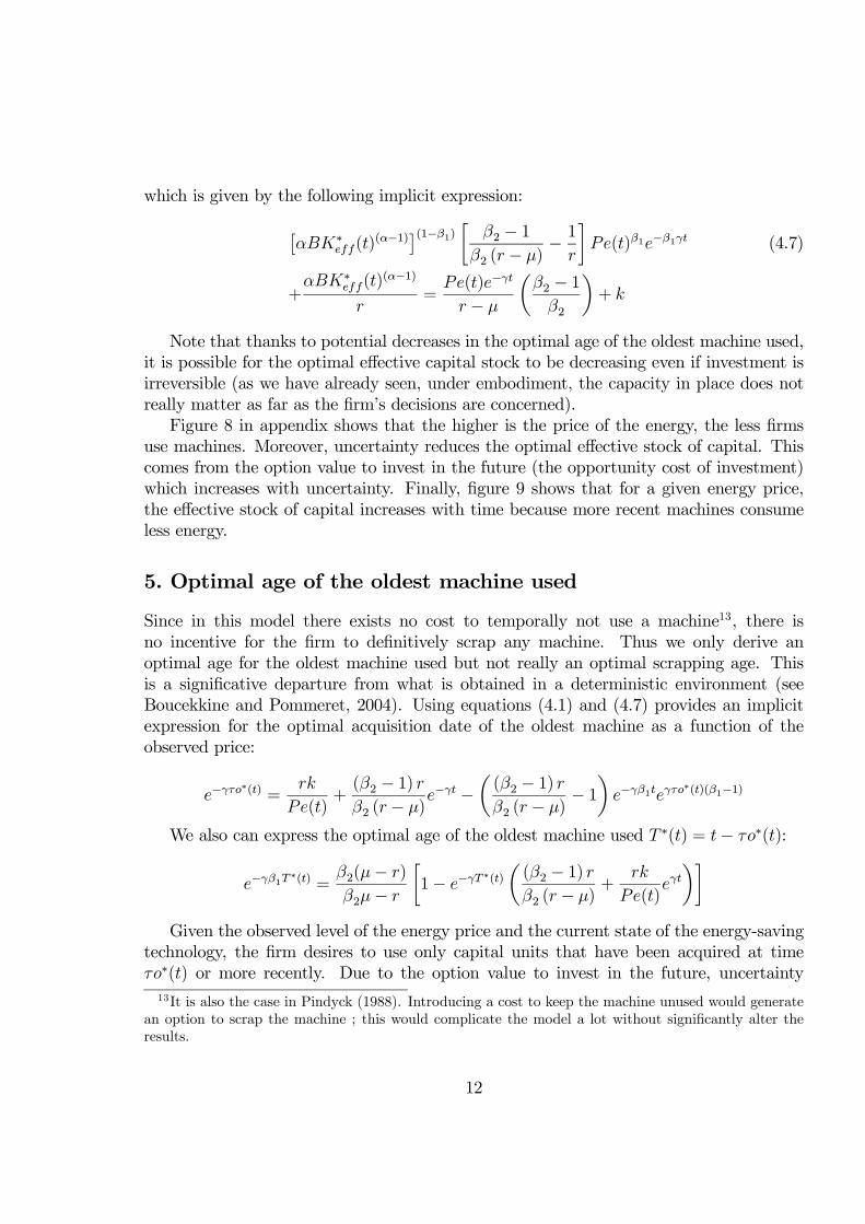
which is given by the following implicit expression:

[αBK∗

eff(t)(α−1)

](1−β1)[

β2 − 1

β2 (r − µ)−1

r

]Pe(t)β1e−β1γt (4.7)

+αBK∗

eff(t)(α−1)

r=

Pe(t)e−γt

r − µ

(β2 − 1

β2

)+ k

Note that thanks to potential decreases in the optimal age of the oldest machine used,it is possible for the optimal effective capital stock to be decreasing even if investment isirreversible (as we have already seen, under embodiment, the capacity in place does notreally matter as far as the firm’s decisions are concerned).

Figure 8 in appendix shows that the higher is the price of the energy, the less firmsuse machines. Moreover, uncertainty reduces the optimal effective stock of capital. Thiscomes from the option value to invest in the future (the opportunity cost of investment)which increases with uncertainty. Finally, figure 9 shows that for a given energy price,the effective stock of capital increases with time because more recent machines consumeless energy.

5. Optimal age of the oldest machine used

Since in this model there exists no cost to temporally not use a machine13, there isno incentive for the firm to definitively scrap any machine. Thus we only derive anoptimal age for the oldest machine used but not really an optimal scrapping age. Thisis a significative departure from what is obtained in a deterministic environment (seeBoucekkine and Pommeret, 2004). Using equations (4.1) and (4.7) provides an implicitexpression for the optimal acquisition date of the oldest machine as a function of theobserved price:

e−γτo∗(t) =

rk

Pe(t)+(β2 − 1) r

β2 (r − µ)e−γt −

((β2 − 1) r

β2 (r − µ)− 1

)e−γβ1teγτo

∗(t)(β1−1)

We also can express the optimal age of the oldest machine used T ∗(t) = t− τo∗(t):

e−γβ1T∗(t) =

β2(µ− r)

β2µ− r

[1− e−γT

∗(t)

((β2 − 1) r

β2 (r − µ)+

rk

Pe(t)eγt)]

Given the observed level of the energy price and the current state of the energy-savingtechnology, the firm desires to use only capital units that have been acquired at timeτo∗(t) or more recently. Due to the option value to invest in the future, uncertainty

13It is also the case in Pindyck (1988). Introducing a cost to keep the machine unused would generatean option to scrap the machine ; this would complicate the model a lot without significantly alter theresults.

12

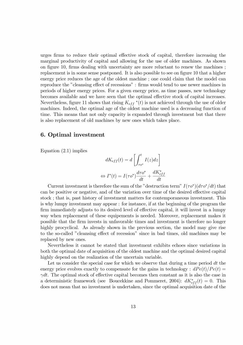
urges firms to reduce their optimal effective stock of capital, therefore increasing themarginal productivity of capital and allowing for the use of older machines. As shownon figure 10, firms dealing with uncertainty are more reluctant to renew the machines ;replacement is in some sense postponed. It is also possible to see on figure 10 that a higherenergy price reduces the age of the oldest machine ; one could claim that the model canreproduce the ”cleansing effect of recessions” : firms would tend to use newer machines inperiods of higher energy prices. For a given energy price, as time passes, new technologybecomes available and we have seen that the optimal effective stock of capital increases.Nevertheless, figure 11 shows that rising Keff

∗(t) is not achieved through the use of oldermachines. Indeed, the optimal age of the oldest machine used is a decreasing function oftime. This means that not only capacity is expanded through investment but that thereis also replacement of old machines by new ones which takes place.

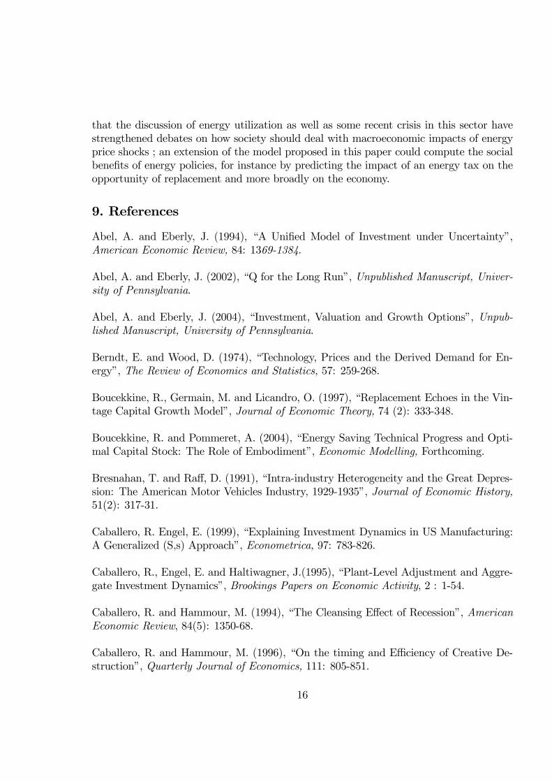
6. Optimal investment

Equation (2.1) implies

dKeff(t) = d

[∫ t

τo∗I(z)dz

]

⇔ I∗(t) = I(τo∗)dτo∗

dt+

dK∗

eff

dt

Current investment is therefore the sum of the ”destruction term” I(τo∗)(dτo∗/dt) thatcan be positive or negative, and of the variation over time of the desired effective capitalstock ; that is, past history of investment matters for contemporaneous investment. Thisis why lumpy investment may appear : for instance, if at the beginning of the program thefirm immediately adjusts to its desired level of effective capital, it will invest in a lumpyway when replacement of these equipements is needed. Moreover, replacement makes itpossible that the firm invests in unfavorable times and investment is therefore no longerhighly procyclical. As already shown in the previous section, the model may give riseto the so-called ”cleansing effect of recession” since in bad times, old machines may bereplaced by new ones.

Nevertheless it cannot be stated that investment exhibits echoes since variations inboth the optimal date of acquisition of the oldest machine and the optimal desired capitalhighly depend on the realization of the uncertain variable.

Let us consider the special case for which we observe that during a time period dt theenergy price evolves exactly to compensate for the gains in technology : dPe(t)/Pe(t) =γdt. The optimal stock of effective capital becomes then constant as it is also the case ina deterministic framework (see Boucekkine and Pommeret, 2004): dK∗

eff(t) = 0. Thisdoes not mean that no investment is undertaken, since the optimal acquisition date of the

13

oldest machine is not constant:

dτo∗(t) =1

γ

dPe(t)

Pe(t)−

αB

γPe(t)eγτo

∗

K∗

eff(t)(α−1)

dK∗

eff(t)

K∗

eff(t)= dt

Therefore, in this special case, the optimal acquisition date of the oldest machineincreases exactly with time and old machines are replaced by new ones:

I∗(t) = I(τo∗)

7. Illustration of the dynamics

This section provides an illustration of the dynamics of the key variables of the model pro-posed in this paper (effective stock of capital, age of the oldest machine and investment).Results are compared with those of the deterministic and/or disembodied counterparts ofthis model.

In this dynamic example, we use the same parameters as previously. Simulations aredriven over 100 periods. In order to get the dynamics of Pe(t), a geometric brownianmotion is simulated using parameters µ = 0.02, σ2 = 0.04 and Pe(0) = 10 as a startingvalue. Figure 12 gives the sample path for Pe(t). The firm observes the energy price andthen decides about utilization and investment.

Replacement. Investment occurs infrequently in all models considered here (in fact,investment irreversibility is sufficient to generate such a characteristics). However it isonly under the assumption of embodied technological progress that replacement is possiblewhich can generate lumpiness. Moreover, in the case of homogenous capital, the firmshould reach full capacity before investing. In such a case, the firm will present a verystrong ”procyclical” behavior, since the energy price should reach its historically lowestlevel (corrected to take account of the rate of technological progress if relevant) to inducethe firm to use all its units and finally invest. In figure 14, it can be seen that, underdisembodied technological progress, firms barely invest : they increase their total stockof capital only twice in this example, at the beginning of the program and at the veryend of the period considered, when there is a significant decrease in the energy price. Inthe embodied case, investment is driven part by the willingness to increase the effectivestock of capital and part by the possibility to acquire a more efficient machine in termsof energy requirements, that is, replacement.

Uncertainty. Comparing the two cases of embodied technology shows (see figure 14)that the echoes effects is no longer identifiable when firms operate in a stochastic envi-ronment. Moreover, the total stock of capital become smaller (see figure 13) and firmsare more reluctant to renew the machines, leading to a higher optimal age for the oldest

14

machine in use14 (see figure 15). For these two reasons, firms under uncertainty will tendto invest less in new capital (see figure 14).

Technological progress. Not surprisingly, a higher rate of embodied technologicalprogress induces more capital accumulation (see figure 16 in appendix) ; investment peaksare higher and more frequent (see figure 17 in appendix). Replacement occurs more in-tensively since the age of the oldest machine used is smaller (see figure 18 in appendix).

Summary of the results:

• Investment occurs in spurts, and the so-called lumpiness of the investment appears

• Since firms can invest even if they are not using all the units they have(which is amuch more realistic assumption), they may invest for very unfavorable realizationsof the uncertain variable in order to replace old machines. The higher the rate oftechnological progress, the more active the replacement. To some extent, this modelsupport the cleansing effect of recessions argument.

• Uncertainty reduces both the total stock of capital and the proportion of new ma-chines in this stock. Both capacity expansion and replacement are postponed.

8. Conclusion

The literature on investment under uncertainty has focused separately on investment intechnology and on irreversible investment and capacity ; however, replacement is an im-portant motive for investment, as suggested by the large literature on vintage capital.This paper has proposed a model of irreversible investment under uncertainty with em-bodied technological progress, in which firms invest not only to expand the capacity butalso to replace old machines. By introducing heterogenous capital, replacement occursand the model no longer requires all old units to be used before the firm invests. Thediscussion on the firms behavior with respect to capital accumulation and on the effectof shocks on the economy is indeed significantly enriched. Investment may be lumpy andthe so-called cleansing effect of recessions appears since replacement can occur for badrealizations of the stochastic process. The scrapping decision or the age of the oldest ma-chine is endogenous; it is no longer constant as in the literature of vintages, and evolvesstochastically. As shown by a dynamic example, uncertainty increases the optimal age ofthe machines in use, and due to uncertainty, not only capacity expansion but replacementas well, are postponed.

One clear extension of this paper is to introduce heterogenous firms to study the dy-namics of the aggregate capital stock, and to eventually test it empirically. Note moreover14Since the firm may not own old enough machines, its maximal age of the oldest machine may be

smaller than the optimal one. This would not affect the effective capital stock which can still be optimal,but it would of course affect investment.

15

that the discussion of energy utilization as well as some recent crisis in this sector havestrengthened debates on how society should deal with macroeconomic impacts of energyprice shocks ; an extension of the model proposed in this paper could compute the socialbenefits of energy policies, for instance by predicting the impact of an energy tax on theopportunity of replacement and more broadly on the economy.

9. References

Abel, A. and Eberly, J. (1994), “A Unified Model of Investment under Uncertainty”,American Economic Review, 84: 1369-1384.

Abel, A. and Eberly, J. (2002), “Q for the Long Run”, Unpublished Manuscript, Univer-

sity of Pennsylvania.

Abel, A. and Eberly, J. (2004), “Investment, Valuation and Growth Options”, Unpub-lished Manuscript, University of Pennsylvania.

Berndt, E. and Wood, D. (1974), “Technology, Prices and the Derived Demand for En-ergy”, The Review of Economics and Statistics, 57: 259-268.

Boucekkine, R., Germain, M. and Licandro, O. (1997), “Replacement Echoes in the Vin-tage Capital Growth Model”, Journal of Economic Theory, 74 (2): 333-348.

Boucekkine, R. and Pommeret, A. (2004), “Energy Saving Technical Progress and Opti-mal Capital Stock: The Role of Embodiment”, Economic Modelling, Forthcoming.

Bresnahan, T. and Raff, D. (1991), “Intra-industry Heterogeneity and the Great Depres-sion: The American Motor Vehicles Industry, 1929-1935”, Journal of Economic History,

51(2): 317-31.

Caballero, R. Engel, E. (1999), “Explaining Investment Dynamics in US Manufacturing:A Generalized (S,s) Approach”, Econometrica, 97: 783-826.

Caballero, R., Engel, E. and Haltiwagner, J.(1995), “Plant-Level Adjustment and Aggre-gate Investment Dynamics”, Brookings Papers on Economic Activity, 2 : 1-54.

Caballero, R. and Hammour, M. (1994), “The Cleansing Effect of Recession”, American

Economic Review, 84(5): 1350-68.

Caballero, R. and Hammour, M. (1996), “On the timing and Efficiency of Creative De-struction”, Quarterly Journal of Economics, 111: 805-851.

16

Cooley, T., Greenwood J. and Yorukoglu, M.(1997), “The Replacement Problem”, Jour-nal of Monetary Economics, 40: 457-499.

Cooper, R., Haltiwanger, J. and Power, L. (1999), “Machine Replacement and the Busi-ness Cycle: Lumps and Bumps”, American Economic Review, 89: 921-946.

Doms, M. and Dunne, T. (1998), “Capital Adjustment Patterns in Manufacturing Plants”,Review of Economic Dynamics, 1 (2): 409-429.

Epaulard, A. and Pommeret, A. (2003), “Optimally Eating a Stochastic Cake: a Recur-sive Utility Approach”, Resource and Energy Economics, 25(2):129-139.

Goolsbee, A. (1998), “The Business Cycle, Financial Performance, and the Retirement ofCapital Goods”, Review of Economic Dynamics, 1(2): 474-96.

Grenadier, S. and Weiss, A. (1997), “Investment in Technological Innovations: an OptionPricing Approach”, Journal of Financial Economics, 44: 397-416.

Guo, X., Miao, J. and Morellec, E.(2004), “Irreversible Investment with Regime Shifts”Journal of Economic Theory, forthcoming.

Hartman, R. and Hendrickson, M. (2002), “Optimal Partially Reversible Investment”,Journal of Economic Dynamics and Control, 26: 483-508.

Hudson, E. and Jorgenson, D. (1975), “US Energy Policy and Economic Growth 1975-2000”, Bell Journal of Economics and Management Science, 5: 461-514.

Jamet, S. (2000), “Heterogeneité des Entreprises et Croissance Economique: Conséquencede l’irréversibilité de l’investissement et de l’incertitude spécifique”, PHD Thesis, Univer-sité Paris I.

Pindyck, R. (1988), “Irreversible Investment, Capacity Choice, and the Value of theFirm”, American Economic Review, 79: 969-985.

Roche, H. (2003), “Optimal Scrapping and Technology Adoption under Uncertainty”,Unpublished Manuscript, Instituto Tecnologico Autonomo de Mexico.

17

10. Figures

Figure 3: Value at time t of the option to stop using a unit of generation τas a function of Keff(t) (Pe(t) = 0.5)

0

0.05

0.1

0.15

0.2

0.25

0.1 0.6 1.1 1.6 2.1 2.6Keff(t)

σ=0.25σ=0.2σ=0.

b1

Figure 4: Value of a marginal used unitas a function of its acquisition date τ (Keff(t) = 1 and Pe(t) = 10)

700

750

800

850

900

950

1000

1050

1100

1 17 33 49 65 81 97

σ=0.25

σ=0.2

σ=0.

ττττ

V(t)

18

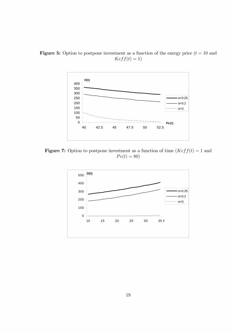
Figure 5: Option to postpone investment as a function of the energy price (t = 10 andKeff(t) = 1)

050

100150200

250300350400

40 42.5 45 47.5 50 52.5Pe(t)

O(t)

σ=0.25

σ=0.2

σ=0.

Figure 7: Option to postpone investment as a function of time (Keff(t) = 1 andPe(t) = 80)

0

100

200

300

400

500

10 15 20 25 30 35 t

O(t)

σ=0.25

σ=0.2

σ=0.

19

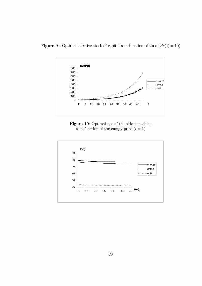
Figure 9 : Optimal effective stock of capital as a function of time (Pe(t) = 10)

0100

200300400

500600

700800

1 6 11 16 21 26 31 36 41 46 t

Keff*(t)

σ=0.25σ=0.2σ=0

Figure 10: Optimal age of the oldest machineas a function of the energy price (t = 1)

25

30

35

40

45

50

10 15 20 25 30 35 40Pe(t)

T*(t)

σ=0.25σ=0.2σ=0.

20

Figure 11 : Optimal age of the oldest machineas a function of time (Pe(t) = 10)

0

10

20

30

40

50

1 6 11 16 21 26 31 36 t

σ=0.25 σ=0.2 σ=0.

T*(t)

Figure 12: Energy Price as a Geometric Brownian Motion, µ = 0.02 and σ2 = 0.04

0

20

40

60

80

100

120

140

1 11 21 31 41 51 61 71 81 91 t

Pe(t)

21

Figure 13 : Total Stock of Capital

0

10

20

30

40

50

60

1 11 21 31 41 51 61 71 81 91

Total stock of capital under embodied technological progressTotal stock of capital under disembodied technological progressTotal stock of capital under no technological progressTotal investment under embodiment in a certain environment

t

Figure 14: Investment

0

5

10

15

20

25

30

1 11 21 31 41 51 61 71 81 91

Investment under embodied technological progress

Investment under disembodied technological progress

Investment under embodiment in a certain environment

t

22

Figure 15: Age of the Oldest Machine

0

10

20

30

40

50

60

1 11 21 31 41 51 61 71 81 91

t

Optimal age under disembodied technological progress

Optimal age of the oldest machine under embodied technological progress

Optimal age of the oldest machine in a certain environment

11. Appendix 1

• The system:

V (t, τ) = W (t, τ) for Pe(t) = Pe∗(t) (11.1)

∂V (t, τ)

∂Pe(t)=

∂W (t, τ)

∂Pe(t)for Pe(t) = Pe∗(t) (11.2)

⇔

αB

rKeff(t)

α−1 −Pe∗(t)e−γτ

r − µ+ b1(Keff(t), τ)Pe

∗(t)β1 = b2(Keff(t), τ)Pe∗(t)β2

(11.3)

−e−γτ

r − µ+ β1b1(Keff(t), τ)Pe

∗(t)β1−1 = β2b2(Keff(t), τ)Pe∗(t)β2−1 (11.4)

Taking into account the fact that αBKeff(t)(α−1) = Pe∗(t)e−γτ , this leads to the

expression of the marginal value of a unit acquired at time τ and which is currentlyused (see equation (4.4)).

• The system:V (t, τ = t) = O(t) + k

23

∂V (t, t)

∂Pe(t)=

∂O(t)

∂Pe(t)(11.5)

may be rewritten:

αB

rKeff(t)

α−1 −Pe(t)

r − µe−γt + b1(Keff(t, τ))Pe(t)

β1 = b3(Keff(t), τ)Pe(t)β2 + k (11.6)

−1

r − µe−γt + β1b1(Keff(t), τ)Pe(t)

β1−1 = β2b3(Keff(t), τ)Pe(t)β2−1 (11.7)

• The system (11.6)-(11.7 ) provides the expression of the value of the option to invest:

O(t) =

[β1

β1 − β2

[αBKeff(t)

α−1]1−β1 e−γβ1tPe∗∗(t)β1−β2

(1

r−(β2 − 1)

β2(r − µ)

)]Pe(t)β2

−e−γtPe∗∗(t)1−β2Pe(t)β2

β2 (r − µ)(11.8)

with Pe∗∗(t) satisfying:

[αBKeff(t)

(α−1)](1−β1)

[β2 − 1

β2 (r − µ)−1

r

]Pe∗∗(t)β1e−β1γt (11.9)

+αBKeff(t)

(α−1)

r=

Pe∗∗(t)e−γt

r − µ

(β2 − 1

β2

)+ k

12. Appendix 2

Figure 2: Value at time t of a marginal unit acquired at time τand currently used as a function of the energy price (Keff(t) = 1 and τo∗(t) = 1)

800

850

900

950

1000

1050

1100

1 4 7 10 13 Pe(t)

V(t)

σ=0.25σ=0.2σ=0.

24

Figure 6: Option to postpone investment as a function of the effective stock of capital(t = 10 and Pe(t) = 50)

0

100

200

300

400

1 3.5 6 8.5 11 13.5Keff(t)

O(t)

σ=0.25

σ=0.2

σ=0.

Figure 8: Optimal effective stock of capitalas a function of the energy price (t = 1)

0

2

4

6

8

10

12

14

10 15 20 25 30 Pe(t)

Keff*(t)

σ=0.25

σ=0.2

σ=0

25

Figure 16 : Total Stock of capital under different rates of embodied technologicalprogress

0

10

20

30

40

50

60

70

80

90

1 11 21 31 41 51 61 71 81 91

t

γ=0.01 γ=0.02 γ=0.03

Figure 17: Investment under different rates of embodied technological progress

0

5

10

15

20

25

30

35

1 11 21 31 41 51 61 71 81 91t

γ=0.01 γ=0.02 γ=0.03

26

Figure 18: Age of the oldest machine under different rates of embodied technologicalprogress

30

35

40

45

50

55

60

65

1 11 21 31 41 51 61 71 81 91 t

γ=0.01 γ=0.02 γ=0.03

27