Investors Behavior and Trading Strategies: Evidence ... - OJK

Investors Behavior and Trading Strategies:

Evidence from Indonesia Stock Exchange

December 2018

Abstract

This study reveals new evidence about the behavior and trading strategies of institutional and

individual investors in the Indonesia Stock Exchange. Firstly, individual (institutional)

investors are most likely to trade frequently (infrequently) with small (large) amounts of

money and short (long) holding period. Secondly, individual (institutional) investors are

consistent to perform contrarian (momentum) strategy. Lastly, past trading activities done by

individual (institutional) investors are significantly affecting the current trading behavior and

strategy of individual investors (both investor types). The above findings related to individual

investors are robust when this study further breakdowns institutional investors into eight

different investor types.

JEL Classifications: G14, G15.

Keywords: Market Microstructure, Emerging Market, Institutional Investors, Individual

Investors, Trading Strategies.

Corresponding author: Inka Yusgiantoro ([email protected]).

The findings and interpretations expressed in this paper are entirely those of the authors and do not

represent the views of Indonesia Financial Services Authority (OJK). All remaining errors and

omissions rest with the authors.

WP/18/04

mailto:[email protected]

1

INTRODUCTION

The technique of conducting research in the capital market already has been changed quite

significantly in several decades. In data source perspectives, the research was mainly

employing the closing daily data, and/or aggregate market trading activities, the later method

starts to consider the market microstructure analysis that using intraday detail transaction

data. In term of the unit of analysis, the analysis shifted from the market aggregate dynamics

to the specific type of investors or trader’s behavior. These types of studies are being the

common and major research methods and used in analyzing many developing economy, the

microstructures research for emerging market has less being study.

Brzeszczyński, Gajdka, and Kutan (2015) stated that there are some important reasons for

conducting microstructure research method in emerging market. First, emerging market

economies grow significantly and more resilience over time. Stronger growth and lower

corporate leverage, alongside with prospects for growth spillovers from advanced economies,

has improved due to their macroeconomic outlook. Second, the biggest support pillar of

emerging market economies to grow fast is significant economic reforms and major structural

changes. It is proven by China’s stock market’s share which currently ranks second right after

the US, surpassing Japan and the European Union. Third, institutional investor desire to trade

in emerging market was increasing, proven by the growth of institutional capital flow until

2015, along with the rise of non-residents capital flow number.

Unfortunately, while the research of microstructure data in emerging markets starts gaining

attention, such as a study is still rare in Indonesia. Most of the capital market research in

Indonesia mainly used daily closing and aggregate data, whereas many other previous

researches used the fundamental data obtained from financial statement. Below are some

evidence to support this argument.

First, it is worth to mention that studies conducted by Comerton-Forde (1999) and Bonser-

Neal, Linnan, and Neal (1999) are among the first study that intensively using the

microstructure approach in Indonesia. Specifically, Comerton-Forde (1999) examines the

impact of opening rules on stock market efficiency in Australia and Jakarta Stock Exchange

(JSX). She finds that the use of a call can increases market efficiency through increased

liquidity and lower volatility at the open. Meanwhile, Bonser-Neal, Linnan, and Neal (1999)

undertake a research about transaction cost in Indonesia and find that JSX execution cost is

surprisingly similar to those non-US developed markets. Moreover, they also find that

execution costs are affected by broker identity and trades initiated by foreigners have

significantly bigger execution costs.

Later on, the more advanced research was conducted by Dvořák (2005) and Agarwal,

Faircloth, Liu, and Rhee (2009) to study the profitability of foreign and domestic investors in

Indonesia. Specifically, Dvořák (2005) finds that domestic clients of global brokerage get

2

more profits than foreign clients of global brokerages, indicating there is an advantage from

the combination of global expertise and local information. In other words, domestic investors

who have better information still need the expertise of foreign firms to make use of that

information into greater profits. Meanwhile, Agarwal, Faircloth, Liu, and Rhee (2009) find

similar results that foreign investors underperform domestic investors. This

underperformance of foreign investors is totally attributable to their non-initiated orders

because they outperform domestic investors in initiated orders.

Unlike those previous researches, this study will address more on the effects of the behavior

of institutional and individual investors in Indonesia, an area that has not been addressed

often. To shows the dynamic behavior, this study uses the longer and more recent data period

of 2013–2015. It is expected to portray the more recent of the behavior both individual and

institutional capital market investors and traders in Indonesia. One of the motivations of this

study seeks the answer why the individual equity ownership is significantly low (around 6-

7%) when compared to the institutional equity ownership (around 93-94%) as documented in

Table 1. At the same time, it is reported by the Indonesia Central Securities Depository in

2018 that the capital market participation is less than one percent of the population.

In addition of using a longer and more recent data set, this study also benefited from the

information of the actual respective type of investors or traders so that it is no need for this

study to proxy the investors type like in previous studies. The data that we used are investors

that classified into one general individual investor and eight different types of institutional

investors, namely corporations, financial institutions, securities firms, insurance firms, mutual

funds, pension funds, foundations, and other institutions. With this detailed transaction data,

it is interesting and possible to research the dynamic interaction of stocks return and players

trading activity of a particular type of institutional investors and individual investors.

Likewise, with this information, we also can study in more detail regarding which type of

investors behavior is having significant effects on the return of Indonesia stock exchange.

The main discussion in this study is focused on examines (1) the dynamics relation of trading

behavior of various institutional and individual investors, (2) the underlying strategy applied

by each investor type in its trading activities, i.e. contrarian and/or momentum, and (3) how

the contemporaneous relationship among players trade and stocks return (herding behavior

activity). All imply the trading dynamics relation amongst investors.

Particularly, this study adopts the idea of the dynamics model of analysis between

institutional and individual trading studied by Griffin, Harris, and Topaloglu (2003), Ng and

Wu (2007), as well Dorn, Huberman, and Sengmueller (2008). This study will also observe

the dynamics of players trading based on studies conducted by Lakonishok, Shleifer, and

Vishny (1992).

3

Finally, Vector Autoregressive (VAR) methodology will be used to estimate this relationship.

The estimation of parameters will use maximum Likelihood Estimation while the standard

error of parameters will be adjusted with heteroscedasticity and autocorrelation using Newey

West (NW) covariance estimation. The implementation of NW in the VAR model follows the

suggestion from Cochrane and Piazzesi (2005).

The remaining contents of this article is organized as follows. Section 2 describes the

literature review. Section 3 explains the institutional background and data. Section 4

elaborates the methodology. Section 5 performs preliminary analysis for determining the

optimal lag selection as well testing the autocorrelation and heteroscedasticity for all models.

Section 6 reports the results of general players. Section 7 documents the results of detailed

players. Finally, Section 8 concludes and provides some policy implications.

LITERATURE REVIEW

Overview of Institutional and Individual Investors

As the detailed data of stocks market transaction become available to researcher today, the

research regarding the behavior of players (both institutional and individual investors) in the

stocks market is gaining much more attention than ever before. In general, institution

investors can be defined as investors that trade on behalf of other interest while individual

investors trade on their interest. Theoretically, institutional investors are viewed as informed

investors with the power to drive the market while individual investors are believed as

proverbial noise trader with a tendency to perform psychological biased in trading (Kyle,

1985; Black, 1985).

Nevertheless, defining institutional and individual investors through transactional data in

stocks market is not easy since in most researches there is only broker name recorded in the

transaction without no detail of who is the player behind it (Khwaja and Mian, 2005;

İmişiker, Özcan, and Taş, 2015; Aaron, Koesrindartoto and Takashima, 2018). Moreover, by

knowing that institutional or individual investors can use more than one brokers to trade in

stocks market, it is not an appropriate way to directly judge a particular broker as an

institutional or individual investor. As an alternative approach, some researches like

Laskonishok, Shleifer, and Vishny (1992), Barber, Odean, and Zhu (2009), as well Ng and

Wu (2007) use a dollar cut-off for a transaction to classify whether the transaction initiated

by a certain broker is executed by institutional or individual investors. Fortunately, as this

study have a direct access to the regulator, namely Indonesian Financial Services Authority,

we did not face this kind of issue, and therefore the results of this study will be free from

biases caused by using a proxy.

4

Then, for the dynamic interaction between the players, the growing literature on this area

gives different findings yet with a decent explanation. In short, the main focus of the research

focus on examining (1) the investor trading strategy based on the relationship between stocks

return and institutional and individual trading behavior, (2) how the players interact each

other and (3) how the contemporaneous relationship between the change in players ownership

to stocks return.

Trading Strategies

The first topic is to understand how players in the stock market buy (sell) stocks tomorrow in

response to increase (decrease) of the return. This behavior is also known as momentum

trading behavior (trend chasing or positive feedback trading) (Griffin, Harris, Topaloglu,

2003). Empirical literature finds different results regarding this behavior toward institutional

and individual investors. Lakonishok, Shleifer, and Vishny (1992) find a weak evidence of

trend chasing behavior in institutional investors in overall. As the analysis goes deep to the

characteristic of the stocks (based on size), however, they find there is some evidence that

institutional investors perform positive-feedback trading in small stock but not in the big

stocks. On the other hand, Grinblatt, Titman and Wermers (1995) show that institutional

investors are trend chasing investors that tend to follow the past price movement.

Moreover, Badrinath and Wahal (2001) explain that momentum trading behavior varies

across the institution types and primarily limited to new equity position and by using detail

transaction data from the Australian market, Foster, Gallagher, and Looi (2011) find that

momentum trading behavior depends on the investment style of institutional investors. They

further argue that growth-oriented investment manager tends to perform momentum trading

while the value-oriented manager is not. In dynamics model, Griffin, Harris, Topaloglu

(2003) find that there is a strong contemporaneous relation between past stock returns and

institutional trading. With a similar thought, Ng and Wu (2007) conduct research in China.

Using the detailed transaction record of 77.12 million trade accounts in Shanghai stocks

market, they find that Chinese institutions are momentum investors.

The other perspective looks the momentum trading behavior of individual investors as a

contrarian. Odean (1998) finds that individual investors tend to sell the winning stock and

hold on to the past losing stock. This condition is also known as disposition effect (Dharma

and Koesrindartoto, 2018). Barber and Odean (2000) explain that individual investors

perform disposition in their trading because they are “anti-momentum” investors. Individual

investors relatively do more buy trades than sell trades when there is an extreme positive

return in the past. However, the value of sell trades that are executed is larger compared to

the value of buy trades. In overall, the individual investor is a net seller in the market

regarding market value following the extreme positive movement in previous days (Barber

5

and Odean, 2008). With the same market data with Barber and Odean (2008), Kaniel, Saar,

and Titman (2008) also find the tendency of individual investors to buy a stock after prices

decrease and sell it after the prices increase. Ng and Wu (2007) explain that the behavior of

individual investors depends on their wealth. The less wealthy individual, in general, behave

as contrarian investors while the wealthiest individual makes the momentum trade like

Chinese institution. Based on that literature, this research believes that while institutional

investors perform momentum trading strategy, individual investors perform anti-momentum

or contrarian trading strategy.

Herding Behavior

The second topic explains how institutional and individual trading activity as well as the

interaction between traders (herding). Lakonishok, Shleifer, and Vishny (1992) find a weak

evidence of herding behavior within the pension funds manager using based on quarterly data

in NYSE. Even though there is an evidence of herding in small stocks, the magnitude of

herding behavior is far from huge. On the other hand, Wermers (1999) uses mutual fund

holding data and find an evidence of herding behavior of mutual funds in small and growth

stocks.

Another literature explains about how individual investors herd one another. In contrast,

Barber, Odean, and Zhu (2009) explain that individual is correlated in their trading and tend

to herd. The results also supported by the research from Dorn, Huberman, and Sengmueller

(2008) that explain individual investors trade similarly based on their sample data from the

large discount brokerage in German.

Then, Kaniel, Saar, and Titman (2008) see a different perspective of how individual trade

toward institutional. They also find that individual investors are contrarian toward

institutional investors. The tendency of contrarian of individual investors leads them to act as

liquidity provider for institutional investors that require immediacy. This argument is also

supported by Grinblatt and Keloharju (2000) that find similar results in Finish stocks market.

Since there is different opinion regarding which investors herd more, Lakonishok, Shilffer,

and Vishny (1992) give a logical explanation of why institution herding is more important

than the individual investors. First, the institution will try to infer information about the

quality of investment from one and another institution. As a result, the institution will have

more understanding about each other trading than individuals so that they will herd to a

greater extent (Shiller and Pound, 1989; Banerjee, 1992). Second, institutional investors have

an incentive to hold the same stocks as another money manager to avoid falling behind a peer

group performance (Scharfstein and Stein, 1990). Third, an institution might react to the same

exogenous signal, and since the signal that is received by the institution is typically the same,

they tend to herd more than individual investors.

6

Besides the explanation above there is also another literature that explains why money

manager (institutional) do herd. Other models explain that institution may trade with the herd

because of slowly diffusing private information (Froot, Scharfstein, and Stein, 1992;

Hirshleifer, Subrahmanyam, and Titman, 1994; Hong and Stein, 1999), or career concerns

(Scharfstein and Stein, 1990). This research believes that both of institution and individual

investors perform herding behaviour to infer same information.

Price Impact

The third topic discusses the contemporaneous relationship between changes in ownership

(usually proxied by players trading imbalances) and stocks return. There is a different time

frame of analysis from quarterly data (Wermers, 1999) and annual data (Nofsinger and Sias,

1999). Sias, Starks, and Titman (2001) use covariance decomposition method to find out how

institutional ownership changes in quarterly data could affect the daily return of stocks. Since

this research will use microstructure perspective, the literature will be more related to the

research that uses daily and intra-daily data.

There is a different perspective in microstructure horizon about which player, institutional or

individual, that has a significant impact toward stock price. In 1993, Barclay and Warner

(1993) discovered medium trade size that between 500 to 10,000 in one transaction has a

price impact toward stocks price compare to another size. Accordingly, Chakravarty (2001)

explains that medium trade size can impact the stock price because it is mainly initiated by

institutional trade. Additionally, Chan and Lakonishok (1995) also find that a sequence of

institutional block trades can give an effect on stock prices and explain that this link can be a

result of institutional trading activity that could predict future return, contemporaneous stock

return, or intra-quarter trend chasing of institutional. Contrarily, Foster, Gallagher, and Looi

(2011) find different results in Australia. They conclude that neither a number of funds

trading nor the volume of shares that are bought or sold by institutional investors correlated

with the contemporaneous return of stocks. Their findings are also supported by Lakonishok,

Shilffer, and Vishny (1992) who discover that institutional investors are neither stabilizing

nor destabilizing stocks price in the US market.

Nonetheless, some literature captures significant findings that individual investors trade can

affect stocks price. Using unique data set from Individual Investor Express Delivery Service

in NYSE, Kaniel, Saar, and Titman (2008) find that individual investors trade (proxied by net

individual trading) significantly can be used to forecast return. Moreover, Barber, Odean, and

Zhu (2009) support previous finding by discovering that stocks that heavily buy (sell) in a

week by individual investors ears strong (poor) returns in a subsequent week.

While those researches observed the impact of players (both institutional and individual

investors) toward stock return independently, recent studies apply dynamics model to observe

7

this. Griffin, Harris, and Topaloglu (2003) use VAR model with five days lag and find that

there is a strong contemporaneous relation between institutional trading and stock return at

daily level while there is no evidence of individual trading. Furthermore, Ng and Wu (2007)

put the same idea on their research in Shanghai stock market and report that only the trading

activity from Chinese institutional and wealthiest individuals can affect future stock

volatility, whereas other Chinese individual investors trade, in general, have no predictive

power for stock future return. Stoffman (2014) also supports above argument by documenting

that, in Finland, stock price, on average, will increase (decrease) due to institutional investors

buy (sell) from individual investors. Also, if price move due to individual trade among

themselves, the impact will quickly revert and vanish. Accordingly, this research believes

that both institutional and individual investors transaction can affect stocks return.

INSTITUTIONAL BACKGROUND AND DATA

Institutional Background

The dataset of this study is coming from the Indonesia Stock Exchange (IDX) that was

originally established in 1912 by Dutch colonials under the name of the Jakarta Stock

Exchange (JSE) due to it is located in the Jakarta, the capital city of Indonesia. Later on, as

the consequences of merging activities in 2007 between the JSE and the Surabaya Stock

Exchange (SSE), the second stock market in Indonesia that was established in 1989 in

Surabaya which intended for supporting the economic development in East Indonesia, the

IDX is established and becoming the sole stock market in Indonesia (Aaron, Koesrindartoto,

and Takashima, 2018). We provide the current landscape of the IDX in Table 1.

Based on the illustration, it is known that there are two general players in the market, namely

institutional and individual investors, where institutional investors can be further divided into

eight different types, such as corporations, financial institutions, securities firms, insurance

firms, mutual funds, pension funds, foundations, and other institutions. Accordingly, it is

obvious that institutional investors are dominating individual investors in the IDX in terms of

equity ownership and trading value even if individual investors have greater number of

players. Among the institutional players, corporations are the biggest player, while financial

institutions and securities firms is placed in the second and third biggest player in terms of

trading value, respectively. One should also note that sometimes the proportion of equity

ownership and trading value might not be strongly correlated and therefore it needs to be

analyzed carefully.

Data

8

This research uses the data from the IDX from January 2013 to December 2015. We provide

our data description in Table 3. Moreover, the following are the details of information that

our dataset comprises of:

1. Daily closing data which consist of stock code, board code, lowest price, highest price,

opening price, closing price, total volume, date, and market capitalization.

2. Transaction data which consist the data consist of the transaction number, transaction

date, transaction time, transaction board, transaction price, transaction lot, transaction

value, buyer and seller broker ID, buyer and seller account ID, buyer and seller investor

type, and transaction order number.

According to Table 2, it is known that during these full three years period, there are 726

trading days, 582 stocks, and more than 285 million past transactions that will be observed

and analyzed. With such a big data (Over 25 GB), it requires sophisticated computational

procedures to clean the data from inappropriate observations, such as missing data elements

and outlier that may disrupt the quality of data. To do so, this study uses SQL, a

programming language that is design specifically for storing and managing data.

METHODOLOGY

Variables Measurement

Portfolio Return

The return that will be used in this research is value weighted return based on stocks market

cap in each day. To construct this variable, first, calculate the daily log return of each stock.

Adjusted closing price is used to adjust the stock price due to corporate ownership action

such as stock split, reverse stock, and to reissue. Then, by using market capitalization data,

calculate the proportion of a particular stock at period t by dividing its market capitalization

with total market capitalization of portfolio. Finally, the value weighted return can be

calculated by aggregated the daily return of the stocks with their weight. We formalize this

equation as follows:

𝑟𝑝,𝑡 = ∑ 𝑤𝑖. 𝑟𝑖,𝑝,𝑡

𝑁

𝑖=1

(1)

Where:

rp,t : Portfolio return at period t

wi,t : Weight of stock i at period t based on the proportion of its market

capitalization in the portfolio at period t

rp,t : Return of stock i at period t

9

Trading Imbalances

As the proxy of trading activity, trading imbalances is used in this research following the

research from (Barber, Odean, and Zhu, 2009; Foster, Gallagher, and Looi, 2011; Griffin,

Harris, and Topaloglu, 2003; Ng and Wu, 2007). Trading imbalances variables for each type

of investor can be easily calculated by by subtracting the total value buy with total value sell

of each type of investor and divide it by its total transaction value. Accordingly, the range of

this variable will be between -1 and 1. We then can interpret this trading imbalances in a very

straightforward way, that is a positive (negative) sign is an implication of accumulation

(distribution) process and the greater trading imbalances toward the certain sign, the greater

accumulation or distribution that occur by the players. The equation for this calculation is

originated by Griffin, Harris, and Topaloglu (2003) and as follows:

𝑇𝑟𝑎𝑑𝑖𝑛𝑔 𝐼𝑚𝑏𝑎𝑙𝑎𝑛𝑐𝑒𝑠𝑖,𝑡 =𝐵𝑢𝑦𝑇𝑉𝑖,𝑡 − 𝑆𝑒𝑙𝑙𝑇𝑉𝑖,𝑡

𝐵𝑢𝑦𝑇𝑉𝑖,𝑡 + 𝑆𝑒𝑙𝑙𝑇𝑉𝑖,𝑡 (2)

Where:

BuyTVi,t : Buy trading value of investor i during period t

SellTVi,t : Sell trading value of investor i during period t

Estimation Methodology

Method Selection

Research in stocks market that is using microstructure has a various statistical approach to

create a model and its inferences. In general, researchers have already got a sense about how

the variables interact by analyzing descriptive statistics of the data. In static point of view,

most of the researches take the basic idea of linear regression under the Fama-Machbeth

procedure to create the relationship model between microstructure variables. One leading

research by (Kaniel, Saar, and Titman, 2008) performs Fama-Machbeth procedure regression

with adjusted standard error using Newey-West correction to analyze how the individual

investors trading activity could affect stocks return. The Newey-West correction is used to

accommodate the heteroscedasticity in the data. Close to the Kaniel, Saar, and Titman (2008)

research, Barber, Odean, and Zhu (2009) also using Fama-Machbeth regression to analyze

whether individual investors can move the market. Foster, Gallagher, and Looi (2011) also do

a research in Australia using similar procedure but with a different focus. They concentrate

on evaluating institutional trading and stocks return relationship.

Although Fama-Machbeth procedure regression is common in analyzing the relationship

between investors trading activity and stocks return, the method is not appropriate to be used

10

in dynamics model. In a static model, we can only evaluate the direct interaction between

investors trading and stocks return, however, dynamics model allowed us to assume all the

variables depend on one and another. This condition required particular statistical method

create inference.

For the market microstructure research, the common method to analyze the dynamics

relationship is Vector Autoregressive (VAR) method. VAR is commonly used instead of

Vector Error Correction Model (VECM) because of the contemporaneous characteristics of

the trading activity variable and stocks return (Dorn, Huberman, and Sengmueller, 2008;

Griffin, Harris, and Topaloglu, 2003; Hasbrouck, 2007). There is some researches in a top

journal that use VAR to analyze dynamics relation in market microstructure research. The

close literature to this study, Griffin, Harris, and Topaloglu (2003) and Dorn, Huberman, and

Sengmueller (2008) use the VAR method to analyze the dynamics of individual, institutional

and stocks return with lag 5. Recent research by Ben-Rephael, Kandel, and Wohl (2012)

using the VAR method to evaluate the dynamics relation of equity funds manager flows and

market return. They use four lags in the VAR model and create the impulse response to see

how one standard deviation shocks in certain variables can affect the system. On the same

year, Moskowitz, Ooi, and Pedersen (2012) research to analyze times series momentum

within asset classes (equity, bond, and currencies) and its impact toward speculators trade.

They use monthly bivariate VAR with 24 months lags of returns and changes in net

speculator position, and as a robustness check 12 months lags are used. They also create the

impulse response from the VAR model using Cholesky decomposition to estimate variance-

covariance matrix of the residuals.

Nevertheless, although VAR is commonly used, there is a concern that has to be addressed.

Supposed that there is a bivariate VAR with k lags in equation 1. The standard estimation for

this VAR model can be done by maximum likelihood (asymptotic sample) or ordinary least

square (finite sample) estimation. Based on the estimation vector of β and λ can be obtained

with its standard error. However, this condition can be applied under the assumption that εt,R

and εt,X has no heteroscedasticity and autocorrelation (white noise) (Hasbrouck, 1991). If

one of the residual vectors in the system contains heteroscedasticity and autocorrelation, the

assumption is violated, and inference of the model can be biased. While the coefficient of the

estimation is robust, the standard error is the cause of bias due to miscalculation. To address

this problem, Cochrane and Piazzesi (2005) propose a modified model on VAR estimation

for bond securities. They still use maximum likelihood to estimate the VAR model but with

adjusted heteroscedasticity and autocorrelation using Generalized Method of Moments

(GMM) covariance estimator with adjusted Newey West standard error calculation. With this

adjustment, the inference from VAR model is expected to be more accurate:

𝑅𝑡 = 𝛼 + ∑ 𝛽𝑖𝑅𝑡−𝑖

𝑘

𝑖=1

+ ∑ 𝜆𝑖𝑋𝑡−𝑖

𝑘

𝑖=1

+ 𝜀𝑡,𝑅 (3)

11

𝑋𝑡 = 𝛼 + ∑ 𝛽𝑖𝑅𝑡−𝑖

𝑘

𝑖=1

+ ∑ 𝜆𝑖𝑋𝑡−𝑖

𝑘

𝑖=1

+ 𝜀𝑡,𝑋 (4)

Based on all the above literature, this research will conduct a preliminary test to select the

lags of VAR model and find whether there are heteroscedasticity and autocorrelation in VAR

residuals. If the assumption of standard VAR is violated, then the inference will be discussed

after adjusting the VAR model with NW standard error.

Vector Auto Regression Methodology

Vector Autoregressive is similar to univariate autoregressive. The intuition behind most

results are similar and carries over by simply replacing scalar with matrices and scalar

operation with matrix operation. The VAR system that will be built in this research is 3-

variate VAR for general players and 10-variate VAR for detailed players. The optimum lag

selection is based on the Akaike Information Criterion (AIC) and Likelihood Ratio (LR) tests

following the idea from Griffin, Harris, and Topaloglu (2003). All variables in VAR equation

are portfolio return and trading imbalance for each type of investor. In general matrix model,

the system can be written as below:

𝑌𝑡 = 𝛼 + ∑ 𝛷𝑌𝑡−𝑖

𝑘

𝑖=1

+ 𝜀𝑡,𝑟 (5)

Where Yt is a T by K variables matrix and Φ is a vector of parameters for the VAR systems.

In this research, Yt contains variable of portfolio return and trading imbalances of each

investor type. The estimation of the coefficient and standard error from the system above will

use maximum likelihood procedure. Maximum likelihood is believed to be more precise than

conditional maximum likelihood and ordinary least square that does not require backtest of

data or errors (Sheppard, 2013):

ℒ(𝜃|𝑦) = −𝑇

2ln(2𝜋) −

𝑇

2ln(Σ) −

1

2𝑣′Σ−1𝑣 (6)

∑ is the covariance matrix of residuals and v is a matrix of the VAR residuals. The

coefficient from the VAR is obtained by maximizing the likelihood function above. For the

standard error, it is achieved from the square of diagonal in the covariance matrix:

Σ𝜃 = Η−1 (7)

The covariance matrix of the coefficient is calculated by inversed the Hessian of maximum

likelihood. However, if there are heteroscedasticity and autocorrelation in residuals, this

procedure to calculate covariance matrix is not relevant anymore. This research believes that

there is heteroscedasticity and autocorrelation in the data due to the high frequency of the

data. To accommodate those issue, the covariance matrix should be adjusted by Newey West

12

(NW) covariance matrix. In general, NW covariance matrix follows the Generalized Method

of Moment (GMM) procedure. GMM covariance matrix calculated by the formula below:

Σ𝜃 =1

𝑇𝑑−1𝑆𝑑−1′

(8)

Where d and S:

𝑑 ≡ 𝐸(𝑥𝑡𝑥𝑡′) (9)

𝑆 = ∑ 𝐸(𝜀𝑡𝑥𝑡𝑥𝑡−𝑗′ 𝜀𝑡−𝑗)

∞

𝑗=−∞

(10)

The adjustment of heteroscedasticity and autocorrelation is on the S matrix or precision

matrix of GMM. Adjusted precision matrix by Newey West become:

𝑆 = ∑𝑘 − |𝑗|

𝑘𝐸(𝜀𝑡𝑥𝑡𝑥𝑡−𝑗

′ 𝜀𝑡−𝑗)

𝑘

𝑗=−𝑘

(11)

Where k is the lag of autocorrelation in residuals and (k-|j|)/k is called weighting matrix. So,

the complete adjusted covariance will be:

Σ𝜃 =1

𝑇𝐸(𝑥𝑡𝑥𝑡

′)−1 [ ∑𝑘 − |𝑗|

𝑘𝐸(𝜀𝑡𝑥𝑡𝑥𝑡−𝑗

′ 𝜀𝑡−𝑗)

𝑘

𝑗=−𝑘

] 𝐸(𝑥𝑡𝑥𝑡′)−1′

(12)

In most research, the lag of autocorrelation in residuals in determined by a mental model of

how investor or traders look historical data. Cochrane and Piazzesi (2005) use 12 months lag

and 18 months lag to check the consistency of their results. This research will choose term

lag of 7 days since it satisfies the general rule of thumb formula 0.75T1/3 for the S matrix

since the variables in this VAR system is contemporaneous. This lag also considers the

trading indicator Moving Average indicator that is usually used by a trader in a short term.

VAR has two exclusive concepts for its analysis (Sheppard, 2013). First is Granger Causality

(GC). GC is the standard method in VAR to determine whether one variable is useful in

predicting other and evidence of Granger Causality is a good indicator that a VAR is needed.

To test the GC, Wald test is used for this specification

𝑦𝑡 = Φ0 + Φ1𝑌𝑡−1 + Φ2𝑌𝑡−2 + ⋯ + Φ𝑝𝑌𝑡−𝑝 + 𝜖𝑡 (13)

{yj,t} does not granger cause {yi,t} if (H0 = Φ𝑖,𝑗,1 = Φ𝑖,𝑗,2 = ⋯ = Φ𝑖,𝑗,𝑃 = 0).

Accordingly, the Wald statistics are written in the equation below and follow distribution

𝑊 = 𝑇[𝑅𝜃1 − 𝑄]′[𝑅Ω𝑅′]−1[𝑅𝜃1 − 𝑄] (14)

Where θ1 is the vector of unrestricted parameter estimates, Ω is the asymptotic covariance

matrix of θ1 and R and Q are matrices based on the restrictions. Under the null hypothesis, the

13

Wald statistic is distributed asymptotically as χ2 where the degrees of freedom equal the

number of zero restrictions being tested

The second concept that exclusive to VAR is impulse response function. In univariate time

series, the ACF is sufficient to understand how the shocks decay. However, the condition is

not the same when analyzing vector of data. A shock to a series of data not only has an

immediate impact on that series but also affect other variables in the system which, in turn,

can feedback to the original variables. After a few iterations of this cycle, it can be difficult to

determine how a shock propagates even in a simple VAR (1) model. To accommodate this

problem, impulse response function is created to see how the shocks of one vector variables

affect others. Impulse response function can be illustrated through Vector Moving Average

(VMA)

𝑦𝑡 = 𝜇 + ϵ𝑡 + Ξ1𝜖𝑡−1 + Ξ2𝜖𝑡−2 + ⋯ (15)

Using this VMA, the impulse response of yi with respect to a shock in ϵj is simply

{1, Ξ1[𝑖𝑖], Ξ2[𝑖𝑖], Ξ3[𝑖𝑖], … }. Then, Ξ1 is calculated by

Ξ1 = Φ1e𝑗 (16)

The second will be

Ξ2 = Φ12e𝑗 + Φ2e𝑗 (17)

The third is

Ξ3 = Φ12e𝑗 + Φ1Φ2e𝑗 + Φ2Φ1e𝑗 + Φ3e𝑗 (18)

This procedure can be continued to compute any Ξj up to specified steps observation ahead.

From the VAR estimation, Granger Causality, and Impulse Response function, the

relationship between institutional trading, individual trading, and stocks return can be clearly

observed.

PRELIMINARY ANALYSIS

Before discussing the results and its analysis, the preliminary analysis will be presented to

discuss the proper estimation environment. First, we determine the optimal lag selection

using Akaike information Criterion (AIC) and sequential modified Likelihood Ratio (LR) test

statistics. Accordingly, based on Table 3, lag 3 (based on AIC) and lag 6 (based on LR) are

selected as the optimal lag for the general players, while lag 1 (based on AIC) and lag 8

(based on LR) are chosen for the detailed players. It is important to notice that AIC and LR

might not give similar results due to the following reason. AIC tells us whether it pays to

14

have a richer model when the goal approximating the underlying data generating process the

best we can in terms of Kullback-Leibler distance, whereas LR tells us whether at a chosen

confidence level we can reject the hypothesis that some restrictions on the richer model hold.

Therefore, it could be implied that AIC is preferable when the goal of our model is to

forecast, while LR is more suitable when the goal of our model is to significance test. Given

our research objectives, thus it could be inferred that LR is preferable for this study.

After we find the optimal for each case, we then test the autocorrelation issue for each

selected lag using Lagrange Multiplier test with no autocorrelation at lag order as the null

hypothesis as well the heteroscedasticity issue for each selected lag using White’s

heteroscedasticity test with the variances for the errors are equal or no heteroscedasticity as

the null hypothesis. Accordingly, Table 3 suggests that although there is no autocorrelation

issue in lag (6) for the general players and lag (8) for the detailed players, all model exhibit

heteroscedasticity problem so that the estimation of VAR should be adjusted with Newey-

West correction for standard errors. The details of this diagnostic tests are provided in Table

3.

RESULTS OF GENERAL PLAYERS

Firstly, we investigate the dynamic behavior and trading strategies of the two general players

in the market, namely individual and institutional investors. The estimation results are

presented in Table 4.

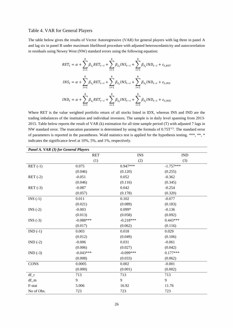
According to the above table, there are several findings that are interested to be discussed. In

term of price impact, it can be seen that both institutional and individual imbalances in lags 3

and 6 that significantly affect the return of stocks. The significant value is very strong and

robust at 1% after the adjustment with lag of NW in 7. Statistically, 1% increase in

institutional (individual) imbalances at t-1 can decrease around 9% (5%) of portfolio return at

time t. This result is consistent with the results from Lakonishok, Shleifer, and Vishny (1992)

and Foster, Gallagher, and Looi (2011). However, this is contrary to the results by Griffin,

Harris, Topaloglu (2003), Ng and Wu (2007), and Stoffman (2014).

Continue on the trading behavior of each types of investors, it is known that individual

investors are contrarian or anti-momentum traders, while institutional investors are

momentum traders. These results are very strong since they are significant at 1% level.

Moreover, this finding aligns with the findings of Barber and Odean (1999) as well Kaniel,

Saar, and Titman (2008) for individual investors and Lakonishok, Shleifer, and Vishny

(1992) as well Grinblatt, Titman and Wermers (1995) for institutional investors. The

contrarian (momentum) behavior is considered as sell (buy) the winning stocks and buy (sell)

the losing stocks according to Odean (1998). Considered only the lag 1, 1% increase in stocks

return will decrease (increase) the imbalances of individual (institutional) investors around

15

175% (95%). It means that individual (institutional) will reverse (strengthen) the position that

they have if there is an increase in stocks price.

Different result is observed in herding behavior on the past imbalances from each investor

type. Individual investors imbalances at time t-3 and t-6 significantly affect in a positive way

the imbalances at time t in 1%. This is an indication that they herd with their own group as

well as their counterpart. Although both imbalances are significant, an increase in

institutional imbalance at t-3 or t-6 will have higher magnitude effect than an increase in

individual imbalance on individual imbalance at time t. Particularly, 1% increase in

institutional imbalances t-1 will increase around 40% of individual imbalances at time t,

while 1% increase in individual imbalances at time t-1 will increase about 20% of individual

imbalances at time t.

Conversely, institutional investors imbalances at time t-3 and t-6 significantly affect in a

negative way the imbalances at time t in 1%. This is an indication that they counter herd with

their own group as well as their counterpart. Although both imbalances are significant, an

increase in institutional imbalance at t-3 or t-6 will have higher magnitude effect than an

increase in individual imbalance on individual imbalance at time t. Particularly, 1% increase

in institutional imbalances t-1 will decrease around 20% of institutional imbalances at time t,

while 1% increase in individual imbalances at time t-1 will decrease about 10% of

institutional imbalances at time t.

As the robustness check to the significant in the VAR system, granger causality is performed

to test simultaneously whether each variable has causality effect toward one and another. The

results of granger causality for the general players are presented in Table 5.

Based on the table above, there is some evidence that consistent with the results above. First,

both individual and institutional imbalances have granger cause the stock return. Second, past

return is granger cause the individual and individual imbalances at time t. This result

confirms the contrarian (momentum) trading behavior performed by individual (institutional)

investors. Then, herding behavior done by individual investors is also fully confirmed by this

test, whereas the counter herding behavior done by institutional investors is partially

confirmed by this test since there is no evidence of granger causality between past individual

imbalances with current institutional imbalances. As the explanation, even though individual

imbalances might have enough evidence to affect the institutional imbalances, it is not

sufficient to reject the null hypothesis of causality.

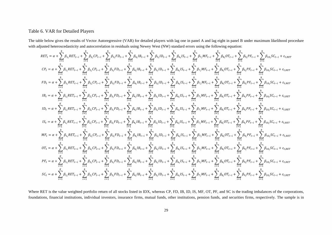
RESULTS OF DETAILED PLAYERS

After investigating the dynamic behavior and trading strategies of two general players in the

market. This study then further breakdowns the general institutional investors into eight

16

different types in order to know in more detail the characteristic of each investor type. Those

specific institutional investors are, corporations, financial institutions, securities firms, other

institutions, insurance firms, mutual funds, pension funds, and foundations. Using the similar

methodology, we present the estimation results and granger causality of this analysis in

Tables 6 and 7.

According to the above table, it could be easily seen that the findings related to the trading

behavior and strategy of individual investors remain the same as the former analysis.

However, there are some cases where the findings related to the trading behavior and strategy

of institutional investor are different with each specific investor type.

More specifically to the detailed institutional type model, while there is understandable

behavior for the corporations, financial institutions, and securities firms, less intuitive

behavior is observed for insurance firms, pension funds, and foundations. It might be because

of both the number of respected institutions and empirical trading data are relatively low and

not significant. Therefore, more observations are needed to be done to make a good behavior

interpretation and policy recommendations. This is the primary agenda for future research.

CONCLUDING REMARKS

Individual investors, although only holding assets in fractions (6%–7%) compared to

institutional (93%-94%), their activities in trading cannot be ignored. Empirical evidence

shows that the total value of their transactions cannot be ignored since they contribute around

one-third from the total transactions. Moreover, individual investors actions have strong

relations with both individual and institutions investors action in the past. It is also discovered

that individual investors also granger affected by both types of investors.

To be more detail, the individual types past action has a stronger cause to the current

individual actions. Institutional investors' action in the past has the relations with both

individual and institutional, however, the relations are stronger on institutional actions.

Interestingly, institutional investors only granger affected by market return and institutional

and not by individual investor past actions.

The effects of the previous market return to the individual and institutional investor can be

seen by looking at the sign of the VAR model. The sign shows that while the institutional

investor is significant and has a positive sign, the individual investor is significant and has a

negative sign, this implies that the institutional investor employs the momentum strategy

while individual uses contrarian strategy.

For the detailed institution model, the individual investors trading behaviors are robust

compared to the general model. Using more detailed institutional investors, robust

observation observed for the institutions that have significant trading values such as the

17

corporations, financial institutions, and security firms. Other institutions are observed to have

mixed results, therefore need further analysis.

The aggregate individual investors tend to conduct daily trading activities at which it can

cause high transaction costs. At the same time, individual investor tends to employ a

contrarian strategy and in term of trading, this behavior might be classified as dispositional

effects (Dharma and Koesrindartoto, 2018). Both activities might hinder the individual

investor to obtain the better return from the market. Related to the current policy, at which to

increase the number of individual investors, the strategy should be simultaneous with

conducting the increasing the capital market literacy. It is also good to mention that the

individual behavior findings are robust for the general model and for the detailed institutional

type model

For the detailed institutional type model, while there is understandable behavior for the

corporations, financial institutions, and securities firms, less intuitive behavior is observed for

insurance firms, pension funds, and foundations. It might be because of both the number of

respected institutions and empirical trading data are relatively low and not significant. More

observations are needed to be done to make a good behavior interpretation and policy

recommendations.

ACKNOWLEDGMENTS

All views expressed herein are solely those of the authors and do not necessarily reflect those

of the Indonesia Capital Market and the Indonesia Financial Services Authority. The authors

thank to the Indonesia Financial Services Authority for the funding support. All errors remain

our responsibility.

18

REFERENCES

Aaron, A., Koesrindartoto, D.P., Takashima, R., 2018. Micro-foundation investigation of

price manipulation in Indonesian capital market. Emerging Markets Finance and

Trade 10, 1–15.

Agarwal, S., Chiu, I.-M., Liu, C., Rhee, S.G., 2011. The brokerage firm effect in herding:

Evidence from Indonesia. Journal of Financial Research 34 (3), 461–479.

Agarwal, S., Faircloth, S., Liu, C., Ghon Rhee, S., 2009. Why do foreign investors

underperform domestic investors in trading activities? Evidence from Indonesia.

Journal of Financial Markets 12 (1), 32–53.

Badrinath, S.G., Wahal, S., 2016. Momentum trading by institutions. The Journal of Finance

71 (4), 1920.

Banerjee, A.V., 1992. A simple model of herd behavior. The Quarterly Journal of Economics

107 (3), 797–817.

Barber, B.M., Odean, T., 2000. Trading is hazardous to your wealth: The common stock

investment performance of individual investors. The Journal of Finance 55 (2), 773–

806.

Barber, B.M., Odean, T., 2008. All that glitters: The effect of attention and news on the

buying behavior of individual and institutional investors. Review of Financial Studies

21 (2), 785–818.

Barber, B.M., Odean, T., Zhu, N., 2009. Do retail trades move markets? Review of Financial

Studies 22 (1), 151–186.

Barclay, M.J., Warner, J.B., 1993. Stealth trading and volatility. Journal of Financial

Economics 34, 281–305.

Ben-Rephael, A., Kandel, S., Wohl, A., 2012. Measuring investor sentiment with mutual fund

flows. Journal of Financial Economics 104 (2), 363–382.

Black, F., 1985. Noise. The Journal of Finance 41 (3), 281–305.

Bonser-Neal, C., Linnan, D., Neal, R., 1999. Emerging market transaction costs: Evidence

from Indonesia. Pacific-Basin Finance Journal 7 (2), 103–127.

19

Brzeszczyński, J., Gajdka, J., Kutan, A.M., 2015. Investor response to public news, sentiment

and institutional trading in emerging markets: A review. International Review of

Economics and Finance 40, 338–352.

Chakravarty, S., 2001. Stealth-trading: Which traders' trades move stock prices? Journal of

Financial Economics 61 (2), 289–307.

Chan, L.K.C., Lakonishok, J., 1995. The behavior of stock prices around institutional trades.

The Journal of Finance 50 (4), 1147–1174.

Cochrane, J.H., Piazzesi, M., 2005. Bond risk premia. American Economic Review 95 (1),

138–160.

Comerton-Forde, Carole, 1999. Do trading rules impact on market efficiency? A comparison

of opening procedures on the Australian and Jakarta stock exchanges. Pacific-Basin

Finance Journal 7, 495–521.

Dharma, W.A., Koesrindartoto, D.P., 2018. Reversal on disposition effect: Evidence from

Indonesian stock trader behavior. International Journal of Business and Society 19

(1), 233–244.

Dorn, D., Huberman, G., Sengmueller, P., 2008. Correlated trading and returns. The Journal

of Finance 63 (2), 885–920.

Douglas Foster, F., Gallagher, D.R., Looi, A., 2011. Institutional trading and share returns.

Journal of Banking and Finance 35 (12), 3383–3399.

Dvorak, T., 2005. Do domestic investors have an information advantage? Evidence from

Indonesia. The Journal of Finance 60 (2), 817–839.

Froot, K.A., Scharfstein, D.S., Stein, J.C., 1992. Herd on the street: Informational

inefficiencies in a market with short-term speculation. The Journal of Finance 47 (4),

1461–1484.

Griffin, J.M., Harris, J.H., Topaloglu, S., 2003. The dynamics of institutional and individual

trading. The Journal of Finance 58 (6), 2285–2320.

Grinblatt, M., Keloharju, M., 2000. The investment behavior and performance of various

investor types: A study of Finland's unique data set. Journal of Financial Economics

55, 43–67.

20

Grinblatt, M., Titman, S., Wermers, R., 1995. Momentum investment strategies, portfolio

performance, and herding: A study of mutual fund behavior. American Economic

Review 85 (5), 1088–1105.

Hasbrouck, J., 1991. Measuring the Information Content of Stock Trades. The Journal of

Finance 46 (1), 179.

Hasbrouck, J., 2007. Empirical Market Microstructure: The institutions, economics, and

econometrics of securities trading. Oxford University Press, Inc., New York.

HIrshleifer, D., Subrahmanyam, A., Titman, S., 1994. Security analysis and trading patterns

when some investors receive information before others. The Journal of Finance 49

(5), 1665–1698.

Hong, H., Stein, J.C., 1999. A Unified Theory of Underreaction, Momentum Trading, and

Overreaction in Asset Markets. The Journal of Finance 54 (6), 2143–2184.

İmişiker, S., Özcan, R., Taş, B.K.O., 2015. Price Manipulation by Intermediaries. Emerging

Markets Finance and Trade 51 (4), 788–797.

Kaniel, R., Saar, G., Titman, S., 2008. Individual investor trading and stock returns. The

Journal of Finance 63 (1), 273–310.

Khwaja, A., Mian, A., 2005. Unchecked intermediaries: Price manipulation in an emerging

stock market. Journal of Financial Economics 78 (1), 203–241.

Kyle, A.S., 1985. Continuous auctions and insider trading. Econometrica 53 (6), 1315–1336.

Lakonishok, J., Shleifer, A., Vishny, R.W., 1992. The impact of institutional trading on stock

prices. Journal of Financial Economics 32 (1), 23–43.

Moskowitz, T.J., Ooi, Y.H., Pedersen, L.H., 2012. Time series momentum. Journal of

Financial Economics 104 (2), 228–250.

Ng, L., Wu, F., 2007. The trading behavior of institutions and individuals in Chinese equity

markets. Journal of Banking and Finance 31 (9), 2695–2710.

Nofsinger, J.R., Sias, R.W., 1999. Herding and Feedback Trading by Institutional and

Individual Investors. The Journal of Finance 54 (6), 2263–2295.

Odean, T., 1998. Are investors reluctant to realize their losses. The Journal of Finance 53 (5),

1775–1798.

21

Scharfstein, D.S., Stein, J.C., 1990. Herd behavior and investment. American Economic

Review 80 (3), 465-479.

Sheppard, K., 2013. Financial Econometrics Notes. University of Oxford, Oxford.

Shiller, R.J., Pound, J., 1989. Survey evidence on diffusion of interest and information among

investors. Journal of Economic Behavior and Organization 12 (1), 47–66.

Sias, R.W., Starks, L.T., Titman, S., 2001. The price impact of institutional trading. SSRN

Electronic Journal.

Stoffman, N., 2014. Who trades with whom? Individuals, institutions, and returns. Journal of

Financial Markets 21, 50–75.

Wermers, R., 1999. Mutual Fund Herding and the Impact on Stock Prices. The Journal of

Finance 54 (2), 581–622.

22

APPENDIX

23

Table 1. Landscape of the Indonesia Stock Exchange based on Investor Types

The table below gives the big picture of the Indonesia Stock Exchange (IDX) based on its investor types in 2015. Generally, investor types in the IDX can be categorized into

individual and institutional investors, but in more specific institutional investors can be further divided into corporations, financial institutions, securities firms, other

institutions, insurance firms, mutual funds, pension funds, and foundations. The detail of each investor type, such as its equity ownership, trading value, number of players,

and average trading value of a player is described in table below. Note that other than the equity ownership data that we obtained from the Statistics of Indonesian Capital

Market published by the Indonesian Financial Services Authority, the remaining contents of this table are derived from our data.

Investor Type

Equity Ownership

as of 30 Dec 2015

Trading Value

in 2015

Number of Players

in 2015 Average Trading Value

of a Player in 2015

(in billion Rp) in trillion Rp in % in billion Rp in % in # in %

Individual Investors 173.65 6.51%

962,808.85 34.24%

151,617 98.61% 6.35

Institutional Investors 2,494.19 93.49%

1,849,113.09 65.76%

2,142 1.39% 863.26

Corporations 833.11 31.23%

770,248.30 27.39%

1,159 0.75% 664.58

Financial Institutions 309.51 11.60%

437,566.08 15.56%

123 0.08% 3,557.45

Securities Firms 230.71 8.65%

311,826.99 11.09%

122 0.08% 2,555.96

Other Institutions 413.73 15.51%

134,279.21 4.78%

158 0.10% 849.87

Insurance Firms 101.69 3.81%

100,136.06 3.56%

85 0.06% 1,178.07

Mutual Funds 418.66 15.69%

53,075.85 1.89%

223 0.15% 238.01

Pension Funds 180.73 6.77%

35,580.83 1.27%

221 0.14% 161.00

Foundations 6.05 0.23% 6,399.77 0.23% 51 0.03% 125.49

Total 2,667.84 100.00% 2,811,921.93 100.00% 153,759 100.00% 18.29

24

Table 2. Data summary

The table below gives the summary of data. The sample is in daily level spanning from 2013-2015. In overall,

our data suggest that there are 726 trading days, 582 stocks, and more than 285 million transactions happened

during our sample period that involve around 8,2 billion shares and around 8,700 trillion rupiah.

Period Trading

Days

Stocks

Traded

Trading

Frequency

Trading

Volume

(in billion)

Trading Value

(in billion Rp)

2013 240 485 73,105,756 2,632.13 2,972,772.82

Q1 60 451 19,393,710 749.69 751,915.62

Q2 59 455 19,550,760 717.81 893,518.60

Q3 61 462 18,983,014 597.89 724,901.16

Q4 60 470 15,178,272 566.74 602,437.43

2014 242 570 103,714,922 2,712.37 2,908,436.33

Q1 60 517 25,813,196 581.73 714,970.69

Q2 59 520 24,344,006 596.07 711,822.75

Q3 60 529 25,947,892 734.29 760,149.79

Q4 63 536 27,609,828 800.28 721,493.11

2015 244 582 108,558,876 2,917.01 2,811,921.93

Q1 62 534 28,807,152 816.08 816,296.24

Q2 61 534 26,570,562 747.32 739,468.62

Q3 60 538 25,127,206 629.87 565,480.00

Q4 61 544 28,053,956 723.75 690,677.07

2013-2015 726 582 285,379,554 8,261.51 8,693,131.08

25

Table 3. Diagnostic Tests

The table below gives the results of diagnostic tests, namely optimal lag selection, autocorrelation and

heteroscedasticity tests. Panel A reports the results of the optimal lag selection using Akaike information

Criterion (AIC) and sequential modified Likelihood Ratio (LR) test statistics. # indicates the lag order selected

by the criterion. Accordingly, lag 3 (based on AIC) and lag 6 (based on LR) are selected as the optimal lag for

the general players, while lag 1 (based on AIC) and lag 8 (based on LR) are chosen for the detailed players.

Panel B reports the results of autocorrelation test for each selected lag using Lagrange Multiplier test with no

autocorrelation at lag order as the null hypothesis. Panel C reports the results of heteroscedasticity test for each

selected lag using White’s heteroscedasticity test with the variances for the errors are equal or no

heteroscedasticity as the null hypothesis. * indicates the violation of null hypothesis for both autocorrelation and

heteroscedasticity tests. The p-value is reported in the parantheses.

Panel A. Optimal Lag Selection

Lag General Players Detailed Players

LR AIC LR AIC

0 NA -14.24 N/A -9.74

1 93.28 -14.34 689.30 -10.43#

2 13.09 -14.34 162.52 -10.39

3 25.36 -14.34# 124.60 -10.29

4 3.86 -14.33 107.88 -10.17

5 4.09 -14.31 122.76 -10.08

6 28.58# -14.33 113.34 -9.97

7 7.05 -14.31 98.129 -9.85

8 10.79 -14.30 124.57# -9.76

Panel B. Autocorrelation Test

Lag General Players Detailed Players

Lag 3 Lag 6 Lag 1 Lag 8

1 2.753

(0.973)

6.845

(0.653) 164.7*

(0.000)

96.09

(0.591)

2 4.095

(0.905)

6.393

(0.700) 117.8

(0.107)

90.65

(0.737)

3 12.24

(0.199)

14.37

(0.109) 112.2

(0.190)

80.46

(0.924)

4 3.886

(0.918)

7.843

(0.550) 120.1

(0.082)

77.67

(0.952)

5 6.058

(0.734)

10.34

(0.323) 122.7

(0.061)

113.7

(0.164)

6 25.46*

(0.002)

9.075

(0.430) 103.1

(0.393)

97.28

(0.558)

7 8.502

(0.484)

10.54

(0.307) 102.9

(0.398)

98.59

(0.520)

8 8.462

(0.488)

8.5499

(0.479)

159.0*

(0.000)

98.21

(0.531)

Panel C. Heteroscedasticity Test

General Players Detailed Players

Lag 3 Lag 6 Lag 1 Lag 8

Chi-Squared 780.8* 1848.2* 4118.9* 9032.8*

(Joint-test) (0.000) (0.000) (0.000) (0.040)

26

Table 4. VAR for General Players

The table below gives the results of Vector Autoregressive (VAR) for general players with lag three in panel A

and lag six in panel B under maximum likelihood procedure with adjusted heteroscedasticity and autocorrelation

in residuals using Newey West (NW) standard errors using the following equation:

𝑅𝐸𝑇𝑡 = 𝛼 + ∑ 𝛽1𝑖𝑅𝐸𝑇𝑡−𝑖

𝑘

𝑖=1

+ ∑ 𝛽2𝑖𝐼𝑁𝑆𝑡−𝑖

𝑘

𝑖=1

+ ∑ 𝛽3𝑖𝐼𝑁𝐷𝑡−𝑖

𝑘

𝑖=1

+ 𝜀𝑡,𝑅𝐸𝑇

𝐼𝑁𝑆𝑡 = 𝛼 + ∑ 𝛽1𝑖𝑅𝐸𝑇𝑡−𝑖

𝑘

𝑖=1


𝑘

𝑖=1


𝑘

𝑖=1

+ 𝜀𝑡,𝐼𝑁𝑆

𝐼𝑁𝐷𝑡 = 𝛼 + ∑ 𝛽1𝑖𝑅𝐸𝑇𝑡−𝑖

𝑘

𝑖=1


𝑘

𝑖=1


𝑘

𝑖=1

+ 𝜀𝑡,𝐼𝑁𝐷

Where RET is the value weighted portfolio return of all stocks listed in IDX, whereas INS and IND are the

trading imbalances of the institution and individual investors. The sample is in daily level spanning from 2013-

2015. Table below reports the result of VAR (k) estimation for all time sample period (T) with adjusted 7 lags in

NW standard error. The truncation parameter is determined by using the formula of 0.75T1/3. The standard error

of parameters is reported in the parantheses. Wald statistics test is applied for the hypothesis testing. ***, **, *

indicates the significance level at 10%, 5%, and 1%, respectively.

Panel A. VAR (3) for General Players

RET INS IND

(1) (2) (3)

RET (-1) 0.075 0.947*** -1.757***

(0.046) (0.120) (0.255)

RET (-2) -0.051 0.052 -0.362

(0.046) (0.116) (0.345)

RET (-3) -0.087 0.042 -0.254

(0.057) (0.178) (0.320)

INS (-1) 0.011 0.102 -0.077

(0.021) (0.089) (0.183)

INS (-2) -0.003 0.099* -0.136

(0.013) (0.058) (0.092)

INS (-3) -0.088*** -0.218*** 0.443***

(0.017) (0.062) (0.116)

IND (-1) 0.003 0.018 0.029

(0.012) (0.049) (0.106)

IND (-2) -0.006 0.031 -0.061

(0.006) (0.027) (0.042)

IND (-3) -0.043*** -0.099*** 0.177***

(0.008) (0.033) (0.062)

CONS 0.0005 0.002 -0.001

(0.000) (0.001) (0.002)

df_r 713 713 713

df_m 9 9 9

F-stat 5.006 16.92 11.76

No of Obs. 723 723 723

27

Table 4. VAR for General Players (Continued)

Panel B. VAR (6) for General Players

RET INS IND

(4) (5) (6)

RET (-1) 0.080* 0.965*** -1.808***

(0.048) (0.125) (0.268)

RET (-2) -0.051 0.041 -0.356

(0.047) (0.118) (0.343)

RET (-3) -0.111* 0.015 -0.160

(0.061) (0.184) (0.330)

RET (-4) -0.041 -0.018 0.111

(0.046) (0.154) (0.284)

RET (-5) 0.015 -0.091 0.0443

(0.059) (0.137) (0.228)

RET (-6) -0.071 0.093 0.241

(0.052) (0.122) (0.363)

INS (-1) 0.007 0.104 -0.064

(0.022) (0.086) (0.172)

INS (-2) -0.006 0.086 -0.120

(0.014) (0.055) (0.084)

INS (-3) -0.090*** -0.226*** 0.463***

(0.018) (0.064) (0.121)

INS (-4) 0.018 0.091 -0.206

(0.017) (0.092) (0.143)

INS (-5) 0.0239 -0.021 -0.042

(0.015) (0.090) (0.138)

INS (-6) -0.081*** -0.149** 0.308***

(0.027) (0.061) (0.098)

IND (-1) 0.001 0.018 0.036

(0.012) (0.047) (0.100)

IND (-2) -0.009 0.023 -0.052

(0.006) (0.026) (0.039)

IND (-3) -0.049*** -0.102*** 0.191***

(0.010) (0.035) (0.065)

IND (-4) 0.006 0.038 -0.101

(0.008) (0.047) (0.075)

IND (-5) 0.013* 0.002 -0.030

(0.008) (0.050) (0.076)

IND (-6) -0.053*** -0.096*** 0.204***

(0.014) (0.026) (0.049)

CONS 0.000 0.002* -0.001

(0.000) (0.001) (0.002)

df_r 701 701 701

df_m 18 18 18

F-stat 4.491 9.891 7.531

No of Obs. 720 720 720

28

Table 5. Granger Causality for General Players

The table below gives the results of Granger causality test for general players based on VAR (3) as reported in

Panel A and VAR (6) in Panel B. RET is the value weighted portfolio return of all stocks listed in IDX, whereas

INS and IND are the trading imbalances of the institution and individual investors. The null hypothesis of this

test is that lagged values of x do not explain the variation in y, or in other words x does not granger cause y. The

p-value of parameters is reported in the parantheses. ***, **, * indicates the significance level at 10%, 5%, and

1%, respectively.

Panel A. Granger Causality for General Players based on VAR (3)

Variables Effect (t)

RET INS IND

Cause

(t-i)

RET 2.296**

(0.033)

16.33***

(0.000)

16.94***

(0.000)

INS 4.233***

(0.005)

9.381***

(0.000)

3.12**

(0.025)

IND 4.137***

(0.006)

1.817

(0.142)

10.44***

(0.000)

Panel B. Granger Causality for General Players based on VAR (6)


RET INS IND

Cause

(t-i)

RET 2.546***

(0.002)

8.750***

(0.000)

9.125***

(0.000)

INS 4.044***

(0.000)

5.359***

(0.000)

2.559**

(0.018)

IND 4.857***

(0.000)

1.778

(0.101)

5.894***

(0.000)

29

Table 6. VAR for Detailed Players

The table below gives the results of Vector Autoregressive (VAR) for detailed players with lag one in panel A and lag eight in panel B under maximum likelihood procedure

with adjusted heteroscedasticity and autocorrelation in residuals using Newey West (NW) standard errors using the following equation:

𝑅𝐸𝑇𝑡 = 𝛼 + ∑ 𝛽1𝑖𝑅𝐸𝑇𝑡−𝑖

𝑘

𝑖=1

+ ∑ 𝛽2𝑖𝐶𝑃𝑡−𝑖

𝑘

𝑖=1

+ ∑ 𝛽3𝑖𝐹𝐷𝑡−𝑖

𝑘

𝑖=1

+ ∑ 𝛽4𝑖𝐼𝐵𝑡−𝑖

𝑘

𝑖=1

+ ∑ 𝛽5𝑖𝐼𝐷𝑡−𝑖

𝑘

𝑖=1

+ ∑ 𝛽6𝑖𝐼𝑆𝑡−𝑖

𝑘

𝑖=1

+ ∑ 𝛽7𝑖𝑀𝐹𝑡−𝑖

𝑘

𝑖=1

+ ∑ 𝛽8𝑖𝑂𝑇𝑡−𝑖

𝑘

𝑖=1

+ ∑ 𝛽9𝑖𝑃𝐹𝑡−𝑖

𝑘

𝑖=1

+ ∑ 𝛽10𝑖𝑆𝐶𝑡−𝑖

𝑘

𝑖=1


𝐶𝑃𝑡 = 𝛼 + ∑ 𝛽1𝑖𝑅𝐸𝑇𝑡−𝑖

𝑘

𝑖=1


𝑘

𝑖=1


𝑘

𝑖=1


𝑘

𝑖=1


𝑘

𝑖=1


𝑘

𝑖=1


𝑘

𝑖=1


𝑘

𝑖=1


𝑘

𝑖=1


𝑘

𝑖=1


𝐹𝐷𝑡 = 𝛼 + ∑ 𝛽1𝑖𝑅𝐸𝑇𝑡−𝑖

𝑘

𝑖=1


𝑘

𝑖=1


𝑘

𝑖=1


𝑘

𝑖=1


𝑘

𝑖=1


𝑘

𝑖=1


𝑘

𝑖=1


𝑘

𝑖=1


𝑘

𝑖=1


𝑘

𝑖=1


𝐼𝐵𝑡 = 𝛼 + ∑ 𝛽1𝑖𝑅𝐸𝑇𝑡−𝑖

𝑘

𝑖=1


𝑘

𝑖=1


𝑘

𝑖=1


𝑘

𝑖=1


𝑘

𝑖=1


𝑘

𝑖=1


𝑘

𝑖=1


𝑘

𝑖=1


𝑘

𝑖=1


𝑘

𝑖=1


𝐼𝐷𝑡 = 𝛼 + ∑ 𝛽1𝑖𝑅𝐸𝑇𝑡−𝑖

𝐾

𝑖=1


𝑘

𝑖=1


𝑘

𝑖=1


𝑘

𝑖=1


𝑘

𝑖=1


𝑘

𝑖=1


𝑘

𝑖=1


𝑘

𝑖=1


𝑘

𝑖=1


𝑘

𝑖=1


𝐼𝑆𝑡 = 𝛼 + ∑ 𝛽1𝑖𝑅𝐸𝑇𝑡−𝑖

𝑘

𝑖=1


𝑘

𝑖=1


𝑘

𝑖=1


𝑘

𝑖=1


𝑘

𝑖=1


𝑘

𝑖=1


𝑘

𝑖=1


𝑘

𝑖=1


𝑘

𝑖=1


𝑘

𝑖=1


𝑀𝐹𝑡 = 𝛼 + ∑ 𝛽1𝑖𝑅𝐸𝑇𝑡−𝑖

𝑘

𝑖=1


𝑘

𝑖=1


𝑘

𝑖=1


𝑘

𝑖=1


𝑘

𝑖=1


𝑘

𝑖=1


𝑘

𝑖=1


𝑘

𝑖=1


𝑘

𝑖=1


𝑘

𝑖=1


𝑂𝑇𝑡 = 𝛼 + ∑ 𝛽1𝑖𝑅𝐸𝑇𝑡−𝑖

𝑘

𝑖=1


𝑘

𝑖=1


𝑘

𝑖=1


𝑘

𝑖=1


𝑘

𝑖=1


𝑘

𝑖=1


𝑘

𝑖=1


𝑘

𝑖=1


𝑘

𝑖=1


𝑘

𝑖=1


𝑃𝐹𝑡 = 𝛼 + ∑ 𝛽1𝑖𝑅𝐸𝑇𝑡−𝑖

𝐾

𝑖=1


𝑘

𝑖=1


𝑘

𝑖=1


𝑘

𝑖=1


𝑘

𝑖=1


𝑘

𝑖=1


𝑘

𝑖=1


𝑘

𝑖=1


𝑘

𝑖=1


𝑘

𝑖=1


𝑆𝐶𝑡 = 𝛼 + ∑ 𝛽1𝑖𝑅𝐸𝑇𝑡−𝑖

𝐾

𝑖=1


𝑘

𝑖=1


𝑘

𝑖=1


𝑘

𝑖=1


𝑘

𝑖=1


𝑘

𝑖=1


𝑘

𝑖=1


𝑘

𝑖=1


𝑘

𝑖=1


𝑘

𝑖=1


Where RET is the value weighted portfolio return of all stocks listed in IDX, whereas CP, FD, IB, ID, IS, MF, OT, PF, and SC is the trading imbalances of the corporations,

foundations, financial institutions, individual investors, insurance firms, mutual funds, other institutions, pension funds, and securities firms, respectively. The sample is in

30

daily level spanning from 2013-2015. Table below reports the result of VAR (k) estimation for all time sample period (T) with adjusted 7 lags in NW standard error. The

truncation parameter is determined by using the formula of 0.75T1/3. The standard error of parameters is reported in the parantheses. Wald statistics test is applied for the

hypothesis testing. ***, **, * indicates the significance level at 10%, 5%, and 1%, respectively.

Table 6. VAR for Detailed Players (Continued)

Panel A. VAR (1) for Detailed Players

RET CP FD IB ID IS MF OT PF SC

(7) (8) (9) (10) (11) (12) (13) (14) (15) (16)

RET (-1) 0.078 0.613 -2.134 0.174 -1.458*** 0.931 0.257 2.061* -2.079 1.342*

(0.057) (0.551) (1.954) (0.527) (0.310) (1.566) (1.138) (1.125) (1.368) (0.765)

CP (-1) 0.001 0.158** -0.163 -0.102* -0.010 0.154 0.026 0.101 0.038 -0.060

(0.004) (0.063) (0.215) (0.058) (0.029) (0.185) (0.122) (0.136) (0.193) (0.079)

FD (-1) -0.001 -0.001 -0.028 -0.031** 0.0022 0.037 -0.056* 0.054* 0.040 0.0053

(0.001) (0.012) (0.039) (0.014) (0.006) (0.040) (0.031) (0.028) (0.036) (0.019)

IB (-1) 0.005 -0.049 -0.063 0.157*** -0.019 -0.142 -0.246** 0.142 -0.133 0.075

(0.003) (0.041) (0.166) (0.043) (0.023) (0.134) (0.096) (0.105) (0.135) (0.049)

ID (-1) 0.008 0.099 0.196 -0.004 0.060 0.012 -0.159 0.310* -0.211 -0.045

(0.008) (0.080) (0.300) (0.088) (0.044) (0.315) (0.243) (0.181) (0.274) (0.123)

IS (-1) 0.000 -0.007 0.000 -0.066*** 0.008 0.554*** -0.015 -0.030 0.037 -0.082***

(0.001) (0.016) (0.044) (0.016) (0.006) (0.051) (0.034) (0.035) (0.042) (0.021)

MF (-1) 0.002 0.048** -0.035 -0.039** 0.008 0.009 0.059 -0.012 -0.044 -0.017

(0.001) (0.018) (0.047) (0.020) (0.008) (0.045) (0.044) (0.030) (0.044) (0.026)

OT (-1) 0.001 -0.010 -0.040 -0.007 0.003 -0.009 -0.056 0.240*** -0.056 0.009

(0.001) (0.018) (0.063) (0.021) (0.009) (0.067) (0.046) (0.043) (0.061) (0.035)

PF (-1) 0.000 0.010 0.068 -0.014 0.004 -0.077 0.093** -0.036 0.184*** -0.001

(0.001) (0.016) (0.057) (0.021) (0.008) (0.051) (0.043) (0.037) (0.051) (0.023)

SC (-1) 0.002 -0.063 -0.023 0.045 -0.005 -0.177 -0.124 0.154** -0.090 0.201***

(0.002) (0.046) (0.113) (0.037) (0.018) (0.109) (0.086) (0.077) (0.091) (0.067)

CONS 0.000 -0.001 0.025 0.000 -0.003 0.037** 0.058*** -0.006 -0.007 0.005

(0.000) (0.005) (0.016) (0.005) (0.002) (0.017) (0.013) (0.011) (0.014) (0.008)

df_r 714 714 714 714 714 714 714 714 714 714

df_m 10 10 10 10 10 10 10 10 10 10

F-stat 1.100 5.199 2.360 10.79 8.418 33.94 4.824 10.05 9.969 14.43

No of Obs. 725 725 725 725 725 725 725 725 725 725

31


Panel B. VAR (8) for Detailed Players – Independent Variables: Return (RETt-i)


(17) (18) (19) (20) (21) (22) (23) (24) (25) (26)

RET (-1) 0.063 0.067 -3.205 0.534 -1.426*** -1.550 -0.064 2.751** -3.193* 2.347***

(0.057) (0.562) (2.155) (0.593) (0.348) (1.673) (1.306) (1.311) (1.666) (0.824)

RET (-2) -0.057 -0.157 4.964** -0.894 -0.327 1.555 -1.367 0.263 1.804 0.117

(0.062) (0.594) (2.361) (0.691) (0.443) (1.678) (1.293) (1.628) (1.796) (0.837)

RET (-3) -0.153* 0.453 4.144* -1.974*** 0.189 2.016 0.979 0.146 0.463 -0.353

(0.079) (0.586) (2.319) (0.636) (0.311) (1.784) (1.289) (1.220) (1.875) (0.877)

RET (-4) -0.036 -0.682 -3.324 -0.341 0.246 1.237 0.241 1.698 -0.734 -0.390

(0.063) (0.657) (2.393) (0.711) (0.378) (1.741) (1.301) (1.298) (1.795) (0.921)

RET (-5) -0.020 -0.605 -1.450 -0.601 0.332 0.899 2.414* 0.068 0.614 -0.232

(0.075) (0.589) (2.129) (0.733) (0.259) (1.905) (1.248) (1.364) (1.978) (0.902)

RET (-6) -0.006 -0.355 1.323 0.153 -0.064 -2.463 1.491 -0.622 -0.287 2.299**

(0.066) (0.586) (2.271) (0.763) (0.459) (2.066) (1.549) (1.340) (1.749) (0.964)

RET (-7) 0.011 -0.409 -0.148 -0.452 -0.010 2.541 -1.354 0.799 -0.681 0.116

(0.077) (0.605) (2.271) (0.637) (0.412) (1.885) (1.550) (1.495) (1.721) (0.834)

RET (-8) -0.009 -1.410** 1.073 -0.067 0.933** 2.124 0.611 -0.317 0.623 0.153

(0.058) (0.619) (2.228) (0.612) (0.421) (1.992) (1.358) (1.393) (1.448) (0.778)

32


Panel B. VAR (8) for Detailed Players – Independent Variables: Corporations (CPt-i)


(17) (18) (19) (20) (21) (22) (23) (24) (25) (26)

CP (-1) 0.001 0.099 -0.135 -0.034 -0.003 -0.017 -0.049 0.092 -0.058 -0.008

(0.005) (0.076) (0.220) (0.061) (0.031) (0.174) (0.134) (0.143) (0.187) (0.078)

CP (-2) 0.003 0.024 0.0513 0.021 -0.063** 0.128 0.075 -0.069 0.048 0.138*

(0.004) (0.063) (0.180) (0.063) (0.029) (0.216) (0.122) (0.156) (0.162) (0.080)

CP (-3) -0.016*** 0.005 0.445** -0.088 0.082** -0.025 -0.056 0.126 0.518*** -0.105

(0.005) (0.065) (0.195) (0.098) (0.034) (0.161) (0.144) (0.126) (0.128) (0.092)

CP (-4) -0.001 0.090** -0.016 -0.119** -0.024 0.165 0.290*** -0.130 -0.020 0.142

(0.005) (0.044) (0.203) (0.057) (0.032) (0.192) (0.109) (0.147) (0.176) (0.102)

CP (-5) 0.007 0.103* 0.021 0.000 -0.024 -0.309* -0.192 0.003 -0.324* -0.061

(0.006) (0.060) (0.195) (0.069) (0.030) (0.166) (0.146) (0.129) (0.179) (0.099)

CP (-6) -0.002 0.044 0.049 -0.135** 0.012 0.047 0.184 0.175 -0.024 -0.110

(0.006) (0.047) (0.216) (0.066) (0.040) (0.181) (0.134) (0.123) (0.195) (0.082)

CP (-7) 0.003 -0.081 -0.133 0.042 -0.012 0.147 0.042 0.153 -0.172 0.038

(0.005) (0.060) (0.218) (0.066) (0.033) (0.172) (0.153) (0.125) (0.190) (0.073)

CP (-8) -0.002 0.051 0.125 0.089 0.006 -0.131 0.062 0.007 0.229 -0.258***

(0.004) (0.061) (0.224) (0.063) (0.033) (0.170) (0.116) (0.117) (0.189) (0.082)

33


Panel B. VAR (8) for Detailed Players – Independent Variables: Foundations (FDt-i)


(17) (18) (19) (20) (21) (22) (23) (24) (25) (26)

FD (-1) -0.001 -0.001 -0.055 -0.031** 0.000 0.044 -0.050 0.055* 0.051 0.005

(0.001) (0.014) (0.045) (0.015) (0.006) (0.040) (0.032) (0.028) (0.038) (0.019)

FD (-2) 0.001 0.023* -0.095** -0.004 -0.004 -0.046 0.002 0.020 0.009 0.0190

(0.001) (0.013) (0.048) (0.015) (0.006) (0.041) (0.029) (0.026) (0.041) (0.019)

FD (-3) -0.001 0.014 0.034 -0.010 -0.002 0.006 0.043 0.031 0.084* -0.024

(0.001) (0.012) (0.047) (0.016) (0.008) (0.040) (0.031) (0.034) (0.043) (0.018)

FD (-4) 0.001 -0.001 -0.031 -0.031** 0.001 -0.027 0.028 0.025 -0.067 0.015

(0.001) (0.012) (0.042) (0.013) (0.006) (0.042) (0.031) (0.030) (0.042) (0.022)

FD (-5) 0.002* -0.019 -0.045 0.033** -0.010 -0.054 0.047* 0.070** -0.091** 0.005

(0.001) (0.013) (0.041) (0.014) (0.006) (0.039) (0.028) (0.028) (0.037) (0.020)

FD (-6) 0.001 -0.004 0.093** -0.017 -0.002 0.007 0.019 0.021 -0.028 0.007

(0.001) (0.012) (0.044) (0.013) (0.005) (0.042) (0.034) (0.030) (0.037) (0.017)

FD (-7) 0.000 0.000 0.037 -0.010 -0.003 0.067 -0.026 -0.016 -0.046 -0.026

(0.001) (0.012) (0.045) (0.016) (0.009) (0.045) (0.031) (0.033) (0.042) (0.019)

FD (-8) -0.001 -0.005 0.028 0.010 0.015* 0.016 -0.054* -0.012 -0.029 -0.041**

(0.001) (0.014) (0.042) (0.015) (0.008) (0.044) (0.030) (0.024) (0.039) (0.019)

34


Panel B. VAR (8) for Detailed Players – Independent Variables: Financial Institutions (IBt-i)


(17) (18) (19) (20) (21) (22) (23) (24) (25) (26)

IB (-1) 0.006* -0.045 -0.129 0.152*** -0.019 -0.043 -0.254*** 0.148 -0.158 0.036

(0.004) (0.041) (0.168) (0.044) (0.025) (0.135) (0.094) (0.111) (0.140) (0.060)

IB (-2) 0.004 -0.018 0.047 0.041 -0.024 -0.013 0.075 0.103 -0.020 0.118*

(0.004) (0.045) (0.143) (0.043) (0.021) (0.149) (0.090) (0.087) (0.117) (0.065)

IB (-3) -0.008* 0.002 0.135 0.004 0.013 0.086 -0.020 0.017 0.167 0.0119

(0.004) (0.044) (0.148) (0.055) (0.029) (0.128) (0.109) (0.093) (0.123) (0.064)

IB (-4) 0.000 -0.023 -0.034 0.003 0.016 0.072 0.002 0.058 -0.001 0.052

(0.003) (0.039) (0.136) (0.039) (0.019) (0.122) (0.093) (0.113) (0.110) (0.066)

IB (-5) 0.002 0.109** 0.058 -0.010 -0.021 -0.349** -0.096 -0.022 -0.164 0.030

(0.003) (0.047) (0.140) (0.048) (0.020) (0.141) (0.106) (0.090) (0.120) (0.061)

IB (-6) -0.002 0.019 -0.177 -0.083* 0.018 0.009 0.158* -0.009 -0.056 -0.092

(0.004) (0.037) (0.157) (0.048) (0.023) (0.139) (0.085) (0.086) (0.130) (0.067)

IB (-7) -0.001 -0.123*** 0.034 0.039 0.014 0.227* 0.005 0.112 0.118 -0.074

(0.004) (0.041) (0.141) (0.054) (0.022) (0.123) (0.110) (0.089) (0.131) (0.063)

IB (-8) 0.000 0.008 0.053 0.067 -0.006 -0.004 0.002 -0.123 0.069 -0.087

(0.004) (0.038) (0.163) (0.049) (0.022) (0.141) (0.088) (0.081) (0.127) (0.062)

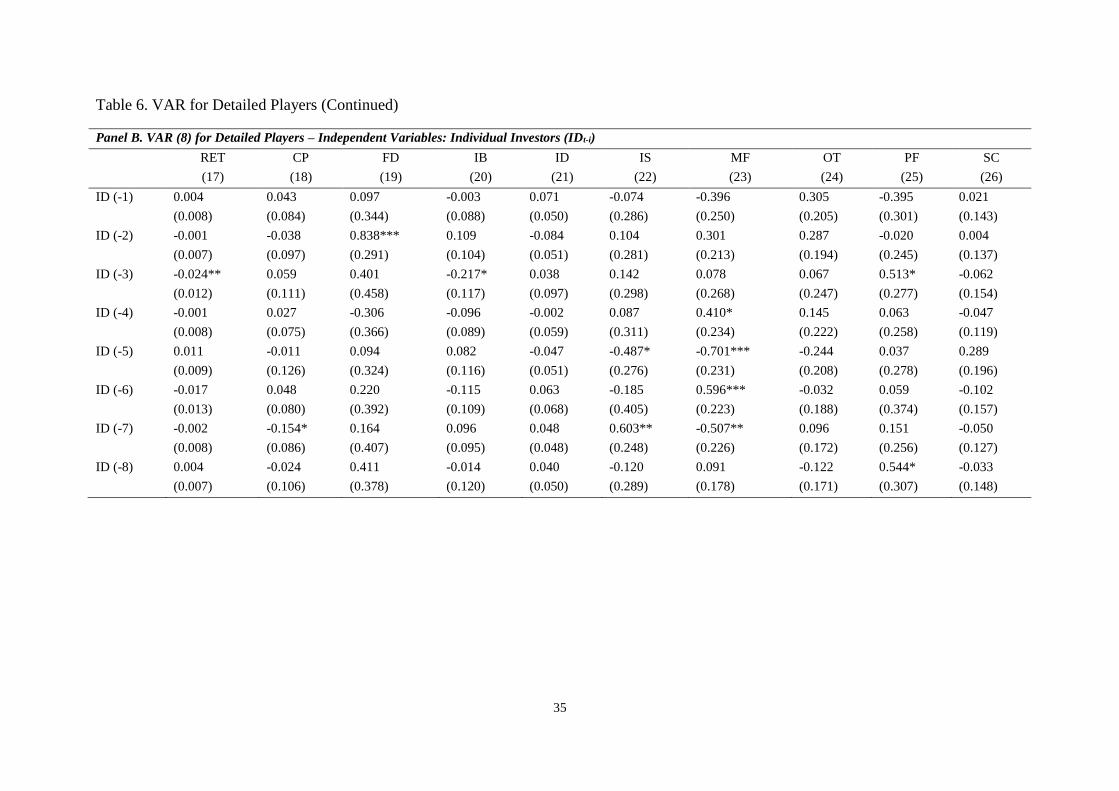
35


Panel B. VAR (8) for Detailed Players – Independent Variables: Individual Investors (IDt-i)


(17) (18) (19) (20) (21) (22) (23) (24) (25) (26)

ID (-1) 0.004 0.043 0.097 -0.003 0.071 -0.074 -0.396 0.305 -0.395 0.021

(0.008) (0.084) (0.344) (0.088) (0.050) (0.286) (0.250) (0.205) (0.301) (0.143)

ID (-2) -0.001 -0.038 0.838*** 0.109 -0.084 0.104 0.301 0.287 -0.020 0.004

(0.007) (0.097) (0.291) (0.104) (0.051) (0.281) (0.213) (0.194) (0.245) (0.137)

ID (-3) -0.024** 0.059 0.401 -0.217* 0.038 0.142 0.078 0.067 0.513* -0.062

(0.012) (0.111) (0.458) (0.117) (0.097) (0.298) (0.268) (0.247) (0.277) (0.154)

ID (-4) -0.001 0.027 -0.306 -0.096 -0.002 0.087 0.410* 0.145 0.063 -0.047

(0.008) (0.075) (0.366) (0.089) (0.059) (0.311) (0.234) (0.222) (0.258) (0.119)

ID (-5) 0.011 -0.011 0.094 0.082 -0.047 -0.487* -0.701*** -0.244 0.037 0.289

(0.009) (0.126) (0.324) (0.116) (0.051) (0.276) (0.231) (0.208) (0.278) (0.196)

ID (-6) -0.017 0.048 0.220 -0.115 0.063 -0.185 0.596*** -0.032 0.059 -0.102

(0.013) (0.080) (0.392) (0.109) (0.068) (0.405) (0.223) (0.188) (0.374) (0.157)

ID (-7) -0.002 -0.154* 0.164 0.096 0.048 0.603** -0.507** 0.096 0.151 -0.050

(0.008) (0.086) (0.407) (0.095) (0.048) (0.248) (0.226) (0.172) (0.256) (0.127)

ID (-8) 0.004 -0.024 0.411 -0.014 0.040 -0.120 0.091 -0.122 0.544* -0.033

(0.007) (0.106) (0.378) (0.120) (0.050) (0.289) (0.178) (0.171) (0.307) (0.148)

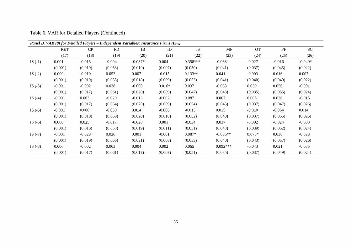
36


Panel B. VAR (8) for Detailed Players – Independent Variables: Insurance Firms (ISt-i)


(17) (18) (19) (20) (21) (22) (23) (24) (25) (26)

IS (-1) 0.001 -0.015 -0.004 -0.037* 0.004 0.358*** -0.038 -0.027 -0.016 -0.040*

(0.001) (0.019) (0.053) (0.019) (0.007) (0.050) (0.041) (0.037) (0.045) (0.022)

IS (-2) 0.000 -0.010 0.053 0.007 -0.015 0.133** 0.041 -0.003 0.016 0.007

(0.001) (0.019) (0.055) (0.018) (0.009) (0.053) (0.041) (0.040) (0.049) (0.022)

IS (-3) -0.001 -0.002 0.038 -0.008 0.016* 0.037 -0.053 0.039 0.056 -0.001

(0.001) (0.017) (0.061) (0.020) (0.009) (0.047) (0.043) (0.035) (0.055) (0.024)

IS (-4) -0.001 0.003 -0.020 -0.013 -0.002 0.087 0.007 0.005 0.026 -0.015

(0.001) (0.017) (0.054) (0.020) (0.009) (0.054) (0.045) (0.037) (0.047) (0.026)

IS (-5) -0.001 0.000 -0.030 0.014 -0.006 -0.013 0.015 -0.010 -0.064 0.014

(0.001) (0.018) (0.060) (0.020) (0.010) (0.052) (0.040) (0.037) (0.055) (0.025)

IS (-6) 0.000 0.025 -0.017 -0.028 0.001 -0.034 0.037 -0.002 -0.024 -0.003

(0.001) (0.016) (0.053) (0.019) (0.011) (0.051) (0.043) (0.039) (0.052) (0.024)

IS (-7) -0.001 -0.023 0.026 0.001 -0.001 0.087* -0.086** 0.075* 0.038 -0.023

(0.001) (0.019) (0.066) (0.021) (0.008) (0.053) (0.040) (0.043) (0.057) (0.026)

IS (-8) 0.000 -0.002 0.063 0.004 0.002 0.065 0.092*** -0.043 0.021 -0.035

(0.001) (0.017) (0.061) (0.017) (0.007) (0.051) (0.035) (0.037) (0.049) (0.024)

37


Panel B. VAR (8) for Detailed Players – Independent Variables: Mutual Funds (MFt-i)


(17) (18) (19) (20) (21) (22) (23) (24) (25) (26)

MF (-1) 0.002 0.039** -0.034 -0.023 0.005 -0.064 0.047 0.008 -0.082* 0.009

(0.001) (0.018) (0.058) (0.022) (0.009) (0.047) (0.042) (0.033) (0.048) (0.027)

MF (-2) 0.000 0.008 -0.024 0.009 -0.006 0.054 0.097** -0.032 0.0075 0.015

(0.001) (0.015) (0.056) (0.016) (0.008) (0.050) (0.041) (0.041) (0.050) (0.021)

MF (-3) -0.002* -0.017 -0.028 -0.013 0.003 0.147*** -0.023 -0.001 0.110** -0.010

(0.001) (0.017) (0.055) (0.018) (0.009) (0.055) (0.038) (0.033) (0.051) (0.026)

MF (-4) -0.001 0.000 0.015 0.008 0.009 0.063 0.018 -0.062* 0.0071 -0.020

(0.001) (0.015) (0.058) (0.019) (0.009) (0.050) (0.041) (0.036) (0.051) (0.021)

MF (-5) 0.000 0.003 -0.042 -0.005 -0.003 -0.060 0.091** 0.011 0.045 0.011

(0.001) (0.021) (0.051) (0.021) (0.008) (0.057) (0.041) (0.041) (0.053) (0.024)

MF (-6) -0.001 0.024 0.009 -0.039** -0.001 0.025 0.077* -0.001 -0.009 -0.038

(0.001) (0.016) (0.053) (0.017) (0.009) (0.055) (0.043) (0.042) (0.051) (0.025)

MF (-7) 0.000 -0.025 -0.014 0.042** 0.001 0.008 -0.051 0.012 -0.004 0.009

(0.001) (0.016) (0.054) (0.018) (0.007) (0.049) (0.041) (0.037) (0.047) (0.023)

MF (-8) -0.001 0.036** 0.067 -0.029 0.002 -0.063 0.113*** -0.038 -0.019 -0.053**

(0.001) (0.016) (0.064) (0.022) (0.008) (0.050) (0.039) (0.034) (0.053) (0.023)

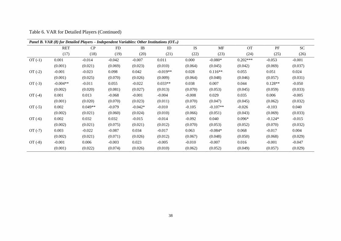
38


Panel B. VAR (8) for Detailed Players – Independent Variables: Other Institutions (OTt-i)


(17) (18) (19) (20) (21) (22) (23) (24) (25) (26)

OT (-1) 0.001 -0.014 -0.042 -0.007 0.011 0.000 -0.080* 0.202*** -0.053 -0.001

(0.001) (0.021) (0.069) (0.023) (0.010) (0.064) (0.045) (0.042) (0.069) (0.037)

OT (-2) -0.001 -0.023 0.098 0.042 -0.019** 0.028 0.116** 0.055 0.051 0.024

(0.001) (0.025) (0.070) (0.026) (0.009) (0.064) (0.048) (0.046) (0.057) (0.031)

OT (-3) -0.004** -0.011 0.055 -0.022 0.033** 0.038 0.007 0.044 0.128** -0.050

(0.002) (0.020) (0.081) (0.027) (0.013) (0.070) (0.053) (0.045) (0.059) (0.033)

OT (-4) 0.001 0.013 -0.068 -0.001 -0.004 -0.008 0.029 0.035 0.006 -0.005

(0.001) (0.020) (0.070) (0.023) (0.011) (0.070) (0.047) (0.045) (0.062) (0.032)

OT (-5) 0.002 0.049** -0.079 -0.042* -0.010 -0.105 -0.107** -0.026 -0.103 0.040

(0.002) (0.021) (0.060) (0.024) (0.010) (0.066) (0.051) (0.043) (0.069) (0.033)

OT (-6) 0.002 0.032 0.032 -0.015 -0.014 -0.092 0.040 0.096* -0.124* -0.015

(0.002) (0.021) (0.075) (0.021) (0.012) (0.070) (0.053) (0.052) (0.070) (0.032)

OT (-7) 0.003 -0.022 -0.087 0.034 -0.017 0.063 -0.084* 0.068 -0.017 0.004

(0.002) (0.021) (0.071) (0.026) (0.012) (0.067) (0.048) (0.050) (0.068) (0.029)

OT (-8) -0.001 0.006 -0.003 0.023 -0.005 -0.010 -0.007 0.016 -0.001 -0.047

(0.001) (0.022) (0.074) (0.026) (0.010) (0.062) (0.052) (0.049) (0.057) (0.029)

39


Panel B. VAR (8) for Detailed Players – Independent Variables: Pension Funds (PFt-i)


(17) (18) (19) (20) (21) (22) (23) (24) (25) (26)

PF (-1) 0.000 -0.012 0.035 0.003 0.001 -0.065 0.089** -0.001 0.157*** 0.007

(0.001) (0.016) (0.06) (0.021) (0.009) (0.056) (0.044) (0.039) (0.055) (0.027)

PF (-2) 0.000 0.002 0.183*** -0.031 0.001 0.041 -0.004 -0.024 0.092 -0.015

(0.001) (0.019) (0.067) (0.021) (0.009) (0.058) (0.045) (0.037) (0.062) (0.024)

PF (-3) -0.003* 0.000 0.041 -0.004 0.017 0.029 -0.035 -0.038 0.016 -0.023

(0.001) (0.017) (0.071) (0.022) (0.011) (0.053) (0.045) (0.049) (0.053) (0.026)

PF (-4) 0.000 -0.026 -0.001 0.010 0.000 -0.010 0.062 0.0207 -0.005 0.035

(0.001) (0.018) (0.078) (0.022) (0.010) (0.059) (0.046) (0.046) (0.055) (0.028)

PF (-5) -0.001 0.035* -0.054 -0.050** 0.014 0.037 -0.024 -0.026 0.013 -0.045*

(0.001) (0.019) (0.068) (0.022) (0.009) (0.065) (0.043) (0.041) (0.053) (0.026)

PF (-6) 0.003** 0.018 -0.019 0.008 -0.019* -0.102* -0.001 0.030 -0.104* 0.043

(0.001) (0.019) (0.065) (0.021) (0.011) (0.061) (0.046) (0.037) (0.058) (0.030)

PF (-7) 0.000 -0.020 -0.084 0.018 -0.008 0.008 0.056 -0.007 0.014 0.041

(0.001) (0.020) (0.068) (0.022) (0.009) (0.063) (0.047) (0.039) (0.057) (0.027)

PF (-8) -0.001 0.000 -0.024 0.013 0.011 -0.022 0.035 -0.044 -0.082 -0.014

(0.001) (0.018) (0.067) (0.018) (0.010) (0.057) (0.044) (0.042) (0.055) (0.023)

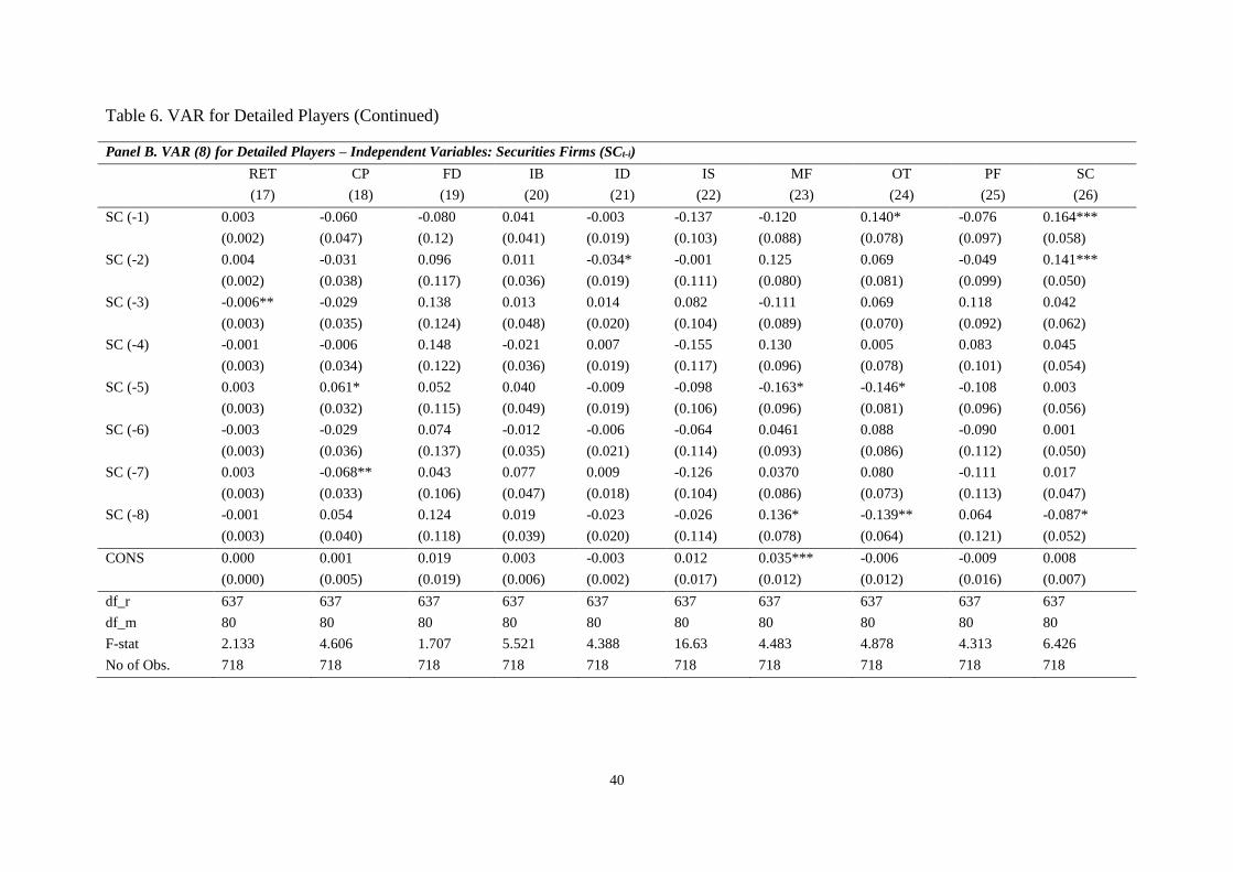
40


Panel B. VAR (8) for Detailed Players – Independent Variables: Securities Firms (SCt-i)


(17) (18) (19) (20) (21) (22) (23) (24) (25) (26)

SC (-1) 0.003 -0.060 -0.080 0.041 -0.003 -0.137 -0.120 0.140* -0.076 0.164***

(0.002) (0.047) (0.12) (0.041) (0.019) (0.103) (0.088) (0.078) (0.097) (0.058)

SC (-2) 0.004 -0.031 0.096 0.011 -0.034* -0.001 0.125 0.069 -0.049 0.141***

(0.002) (0.038) (0.117) (0.036) (0.019) (0.111) (0.080) (0.081) (0.099) (0.050)

SC (-3) -0.006** -0.029 0.138 0.013 0.014 0.082 -0.111 0.069 0.118 0.042

(0.003) (0.035) (0.124) (0.048) (0.020) (0.104) (0.089) (0.070) (0.092) (0.062)

SC (-4) -0.001 -0.006 0.148 -0.021 0.007 -0.155 0.130 0.005 0.083 0.045

(0.003) (0.034) (0.122) (0.036) (0.019) (0.117) (0.096) (0.078) (0.101) (0.054)

SC (-5) 0.003 0.061* 0.052 0.040 -0.009 -0.098 -0.163* -0.146* -0.108 0.003

(0.003) (0.032) (0.115) (0.049) (0.019) (0.106) (0.096) (0.081) (0.096) (0.056)

SC (-6) -0.003 -0.029 0.074 -0.012 -0.006 -0.064 0.0461 0.088 -0.090 0.001

(0.003) (0.036) (0.137) (0.035) (0.021) (0.114) (0.093) (0.086) (0.112) (0.050)

SC (-7) 0.003 -0.068** 0.043 0.077 0.009 -0.126 0.0370 0.080 -0.111 0.017

(0.003) (0.033) (0.106) (0.047) (0.018) (0.104) (0.086) (0.073) (0.113) (0.047)

SC (-8) -0.001 0.054 0.124 0.019 -0.023 -0.026 0.136* -0.139** 0.064 -0.087*

(0.003) (0.040) (0.118) (0.039) (0.020) (0.114) (0.078) (0.064) (0.121) (0.052)

CONS 0.000 0.001 0.019 0.003 -0.003 0.012 0.035*** -0.006 -0.009 0.008

(0.000) (0.005) (0.019) (0.006) (0.002) (0.017) (0.012) (0.012) (0.016) (0.007)

df_r 637 637 637 637 637 637 637 637 637 637

df_m 80 80 80 80 80 80 80 80 80 80

F-stat 2.133 4.606 1.707 5.521 4.388 16.63 4.483 4.878 4.313 6.426

No of Obs. 718 718 718 718 718 718 718 718 718 718

41

Table 7. Granger Causality for Detailed Players

The table below gives the results of Granger causality test for detailed players based on VAR (1) as reported in Panel A and VAR (6) in Panel B. RET is value weighted

portfolio return. ID, CP, IB, SC, OT, IS, MF, PF, and FD is trading imbalances of the individual investors, corporations, financial institutions, securities firms, other

institutions, insurance firms, mutual funds, pension funds, and foundations, respectively. The null hypothesis of this test is that lagged values of x do not explain the variation

in y, or in other words x does not granger cause y. The p-value of parameters is reported in the parantheses. ***, **, * indicates the significance level at 10%, 5%, and 1%,

respectively.

Panel A. Granger Causality for Detailed Players based on VAR (1)


RET ID CP IB SC OT IS MF PF FD

Cause

(t-i)

RET 0.651

(0.753)

23.43***

(0.000)

1.153

(0.283)

0.070

(0.790)

2.619

(0.106)

2.887*

(0.089)

0.267

(0.605)

0.036

(0.849)

1.606

(0.205)

1.283

(0.257)

ID 0.977

(0.323)

6.472***

(0.000)

1.074

(0.300)

0.002

(0.964)

0.108

(0.742)

2.304

(0.129)

0.001

(0.967)

0.486

(0.485)

0.587

(0.443)

0.383

(0.536)

CP 0.046

(0.829)

0.117

(0.731)

3.066***

(0.001)

2.375

(0.123)

0.513

(0.473)

0.665

(0.414)

0.705

(0.401)

0.037

(0.846)

0.053

(0.817)

0.727

(0.394)

IB 1.823

(0.177)

0.758

(0.384)

1.371

(0.242)

7.013***

(0.000)

1.536

(0.215)

2.508

(0.113)

1.147

(0.284)

6.055**

(0.014)

1.206

(0.272)

0.211

(0.646)

SC 0.647

(0.421)

0.106

(0.743)

3.497*

(0.061)

1.370

(0.242)

5.673***

(0.000)

4.517**

(0.033)

2.712*

(0.100)

2.356

(0.125)

0.848

(0.357)

0.045

(0.831)

OT 0.517

(0.472)

0.099

(0.753)

0.253

(0.614)

0.113

(0.735)

0.104

(0.746)

3.907

(0.000)

0.021

(0.883)

1.349

(0.245)

0.929

(0.335)

0.355

(0.551)

IS 0.010

(0.918)

1.424

(0.233)

0.264

(0.607)

16.44***

(0.000)

15.85***

(0.000)

0.997

(0.318)

1.730*

(0.078)

0.219

(0.639)

0.824

(0.364)

0.000

(0.990)

MF 2.144

(0.143)

1.043

(0.307)

9.195***

(0.002)

4.762**

(0.029)

0.592

(0.441)

0.130

(0.718)

0.034

(0.853)

3.520

(0.000)

0.952

(0.329)

0.447

(0.503)

PF 0.164

(0.685)

0.234

(0.628)

0.338

(0.561)

0.505

(0.477)

0.006

(0.937)

0.974

(0.323)

1.994

(0.158)

5.082**

(0.024)

1.663*

(0.094)

1.437

(0.231)

42

FD 0.267

(0.605)

0.114

(0.735)

0.021

(0.884)

4.737**

(0.029)

0.085

(0.770)

4.214**

(0.040)

0.916

(0.338)

3.656*

(0.056)

1.265

(0.260)

1.794*

(0.0659)

Table 7. Granger Causality for Detailed Players (Continued)

Panel B. Granger Causality for Detailed Players based on VAR (8)

Variables

Effect (t)

RET ID CP IB SC OT IS MF PF FD

Cause

(t-i)

RET 77.97

(0.295)

31.94***

(0.000)

8.720

(0.366)

11.80

(0.160)

15.87**

(0.044)

6.393

(0.603)

8.580

(0.379)

6.868

(0.551)

5.236

(0.732)

17.22**

(0.028)

ID 14.49*

(0.070)

129.5***

(0.000)

3.345

(0.911)

7.382

(0.496)

4.967

(0.761)

6.838

(0.554)

7.335

(0.501)

26.06***

(0.001)

9.469

(0.304)

12.40

(0.134)

CP 13.05

(0.110)

11.62

(0.169)

105.2***

(0.007)

134.5***

(0.000)

17.32**

(0.027)

6.574

(0.583)

5.052

(0.752)

8.836

(0.356)

15.29*

(0.054)

6.714

(0.568)

IB 9.612

(0.293)

4.862

(0.772)

15.57**

(0.049)

12.07

(0.148)

12.56

(0.128)

8.423

(0.393)

10.67

(0.221)

10.72

(0.218)

6.788

(0.560)

3.612

(0.890)

SC 10.64

(0.222)

6.203

(0.625)

14.94*

(0.060)

7.450

(0.489)

114.7***

(0.001)

15.75**

(0.046)

8.480

(0.388)

15.81**

(0.045)

6.062

(0.640)

8.150

(0.419)

OT 16.14**

(0.040)

17.40**

(0.026)

12.43

(0.133)

9.606

(0.294)

6.882

(0.549)

91.18*

(0.063)

6.280

(0.616)

16.23**

(0.039)

13.61*

(0.092)

7.270

(0.508)

IS 3.227

(0.919)

5.708

(0.680)

5.282

(0.727)

9.094

(0.334)

10.09

(0.258)

7.092

(0.527)

79.63

(0.251)

12.73

(0.121)

4.639

(0.795)

4.078

(0.850)

MF 8.739

(0.365)

2.468

(0.963)

17.06**

(0.029)

15.05*

(0.058)

10.9

(0.207)

6.341

(0.609)

14.86*

(0.062)

120.4***

(0.000)

9.215

(0.324)

3.487

(0.900)

PF 9.979

(0.266)

11.97

(0.152)

7.866

(0.447)

10.26

(0.247)

10.65

(0.222)

3.953

(0.861)

6.063

(0.640)

9.847

(0.276)

88.71*

(0.088)

16.73**

(0.033)

FD 9.151

(0.330)

8.209

(0.413)

7.014

(0.535)

19.85**

(0.011)

10.46

(0.234)

13.07

(0.109)

9.226

(0.324)

13.64*

(0.092)

19.21**

(0.014)

86.35

(0.119)

Investors Behavior and Trading Strategies: Evidence ... - OJK

Documents

Transcript of Investors Behavior and Trading Strategies: Evidence ... - OJK