
Investigating and Comparing the Effect of Speech and Writing Tools on Consumers’ Behavior in the...
177
European Journal of Scientific Research ISSN: 1450-216X / 1450-202X Volume 99 No 1 April, 2013 Editors-in-Chief Lillie Dewan, National Institute of Technology Co-Editors Chanduji Thakor, Gujarat Technological University Claudio Urrea Oñate, University of Santiago Editorial Board Maika Mitchell, Columbia University Medical Center Prabhat K. Mahanti, University of New Brunswick Parag Garhyan, Auburn University Morteza Shahbazi, Edinburgh University Jianfang Chai, University of Akron Sang-Eon Park, Inha University Said Elnashaie, Auburn University Subrata Chowdhury, University of Rhode Island Ghasem-Ali Omrani, Tehran University of Medical Sciences Ajay K. Ray, National University of Singapore Mutwakil Nafi, China University of Geosciences Felix Ayadi, Texas Southern University Bansi Sawhney, University of Baltimore David Wang, Hsuan Chuang University Cornelis A. Los, Kazakh-British Technical University Teresa Smith, University of South Carolina Ranjit Biswas, Philadelphia University Chiaku Chukwuogor-Ndu, Eastern Connecticut State University M. Femi Ayadi, University of Houston-Clear Lake Emmanuel Anoruo, Coppin State University H. Young Baek, Nova Southeastern University Dimitrios Mavridis, Technological Educational Institute of West Macedonia Jerry Kolo, Florida Atlantic University Mohamed Tariq Kahn, Cape Peninsula University of Technology Publication Ethics and Publication Malpractice Statement Duties of Editors Confidentiality— Editors of the journal must treat received manuscripts for review as confidential documents. Editors and any editorial staff must not disclose any information about submitted manuscripts to anyone other than the corresponding author, reviewers, other editorial advisers, and the publisher. Equal Treatment—Editors of the journal must evaluate manuscripts for their intellectual content and their contribution to specific disciplines, without regard to gender, race, sexual orientation, religious belief, ethnic origin, citizenship, or political philosophy of the authors.
Transcript of Investigating and Comparing the Effect of Speech and Writing Tools on Consumers’ Behavior in the...

European Journal of Scientific Research
ISSN: 1450-216X / 1450-202X Volume 99 No 1 April, 2013 Editors-in-Chief Lillie Dewan, National Institute of Technology Co-Editors Chanduji Thakor, Gujarat Technological University Claudio Urrea Oñate, University of Santiago Editorial Board Maika Mitchell, Columbia University Medical Center Prabhat K. Mahanti, University of New Brunswick Parag Garhyan, Auburn University Morteza Shahbazi, Edinburgh University Jianfang Chai, University of Akron Sang-Eon Park, Inha University Said Elnashaie, Auburn University Subrata Chowdhury, University of Rhode Island Ghasem-Ali Omrani, Tehran University of Medical Sciences Ajay K. Ray, National University of Singapore Mutwakil Nafi, China University of Geosciences Felix Ayadi, Texas Southern University Bansi Sawhney, University of Baltimore David Wang, Hsuan Chuang University Cornelis A. Los, Kazakh-British Technical University Teresa Smith, University of South Carolina Ranjit Biswas, Philadelphia University Chiaku Chukwuogor-Ndu, Eastern Connecticut State University M. Femi Ayadi, University of Houston-Clear Lake Emmanuel Anoruo, Coppin State University H. Young Baek, Nova Southeastern University Dimitrios Mavridis, Technological Educational Institute of West Macedonia Jerry Kolo, Florida Atlantic University Mohamed Tariq Kahn, Cape Peninsula University of Technology Publication Ethics and Publication Malpractice Statement Duties of Editors
Confidentiality— Editors of the journal must treat received manuscripts for review as confidential documents. Editors and any editorial staff must not disclose any information about submitted manuscripts to anyone other than the corresponding author, reviewers, other editorial advisers, and the publisher.
Equal Treatment—Editors of the journal must evaluate manuscripts for their intellectual content and their contribution to specific disciplines, without regard to gender, race, sexual orientation, religious belief, ethnic origin, citizenship, or political philosophy of the authors.

Disclosure and Conflicts of Interest— Editors of the journal and any editorial staff must not use materials disclosed in a submitted manuscript (published or unpublished) for their own research without the author’s written authorization.
Integrity of Blind Reviews—Editors of the journal should ensure the integrity of the blind review process. As such, editors should not reveal either the identity of authors of manuscripts to the reviewers, or the identity of reviewers to authors.
Publication Decisions—Editors of the journal are responsible for deciding which of the manuscripts submitted to the journal should be reviewed or published. However, editors may consult other editors or reviewers in making such decisions.
Cooperative involvement in investigations—Editors of the journal should conduct a proper and fair investigation when an ethical complaint (concerning a submitted or published manuscript) is reported. Such process may include contacting the author(s) of the manuscript and the institution, giving due process of the respective complaint. If the complaint has merits, a proper action should be taken (publication correction, retraction, etc.). Besides, every reported action of unethical publishing behavior should be investigated even if it is discovered years after publication.
Duties of Reviewers
Confidentiality—Reviewers must consider all received manuscripts for review as confidential documents. Received manuscripts must not be seen by or discussed with others, except as authorized by the journal editors or authorized editorial staff.
Objectivity—Reviewers should conduct their reviews objectively. Criticism of the author’s personality or the topic is unprofessional and inappropriate. Reviewers should explain their recommendations clearly and explicitly and provide rational support and justification. Editors Recommendations could be one of the following:
• Accept the publication of the manuscript after compliance with the reviewers’ recommendations.
• Consider the publication of the manuscript after minor changes recommended by its reviewers.
• Consider the publication of the manuscript after major changes recommended by its reviewers.
• Reject the publication of the manuscript based on the reviewers’ recommendations
Fast-Track Reviews—Reviewers are requested to complete their reviews within a timeframe of 30 days. Reviewers also are free to decline reviews at their discretion. For instance, if the current work load and/or other commitments make it impossible for reviewers to complete fair reviews in a short timeframe (e.g., few days for fast-track review), reviewers should refuse such invitations for review and promptly inform the editor of the journal.
Qualifications—Reviewers who believe that they are not qualified to review a received manuscript should inform the journal editors promptly and decline the review process.
Disclosure—Information or ideas obtained through blind reviews must be kept confidential and must not be used by reviewers for personal benefits.
Conflict of Interest —Reviewers should refuse the review of manuscripts in which they have conflicts of interest emerging from competitive, collaborative, or other relationships and connections with any of the authors, companies, or institutions connected to the manuscripts.
Substantial Similarity—Reviewers should inform editors about significant resemblances or overlap between received manuscripts and any other published manuscripts that reviewers are aware of.

Proper and Accurate Citation —Reviewers should identify relevant published work that has not been cited by the authors. Statements that include observation, derivation, or argument (currently or previously reported) should be accompanied by a relevant and accurate citation.
Contribution to Editorial Decisions—Reviewers assist editors in making editorial publication decisions, and also assist authors in improving their submitted manuscripts, through the editorial communications with authors. Therefore, reviewers should always provide explicit and constructive feedback to assist authors in improving their work.
Duties of Authors
Originality—Authors submitting manuscript to the journal should ensure that this submission is original work and is neither currently under consideration for publication elsewhere, nor has been published as a copyrighted material before. If authors have used the ideas, and/or words of others researchers, they should acknowledge that through proper quotes or citations.
Plagiarism—Plagiarism appears into various types, such as claiming the authorship of work by others, copying and paraphrasing major parts of others research (without attribution), and using the results of research conducted by other researchers. However, any type of plagiarism is unacceptable and is considered unethical publishing behavior. Such manuscripts will be rejected.
Authorship of Manuscripts—Authorship of a manuscript should be limited to authors who have made significant contributions and the names of authors should be ranked by efforts. The corresponding author must ensure that all listed coauthors have seen and approved the final version of the manuscript (as it appeared in the proofreading copy) and agreed to its publication in the journal. Authors can permit others to replicate their work.
Multiple or Concurrent Publication— Authors should not publish manuscripts describing essentially the same research in more than one journal. Submitting the same manuscript to more than one journal concurrently constitutes unethical publishing behavior and is unacceptable. This action leads to the rejection of the submitted manuscripts.
Acknowledgement of the Work of Others—Authors should always properly and accurately acknowledge the work of others. Authors should cite publications that have significant contribution to their submitted manuscripts. Unacknowledged work of others contributing to manuscripts is unethical behavior and is unacceptable. Such manuscripts will be rejected.
Reported objectives, discussions, data, statistical analysis, and results should be accurate. Fraudulent or knowingly inaccurate results constitute unethical behavior and are unacceptable. Such manuscripts will be rejected.
Data Access and Retention— Authors may be asked to provide the raw data in connection with manuscripts for editorial review, and should be prepared to provide public access to such data if possible. However, such authors should be prepared to retain data for a reasonable time after publication.
Hazards and Human or Animal Subjects— If a research study involves chemicals, procedures or equipment that have any unusual hazards inherent in their use, the author(s) must clearly identify these in the submitted manuscript. Authors should also inform participating human subjects about the purpose of the study.
Conflicts of Interest— In their manuscript(s), authors should disclose any financial or other substantive conflict of interest that might influence the results or interpretation of their manuscript.

Copyright of Accepted Manuscripts—Authors of accepted manuscripts for publication in the journal agree that the copyright will be transferred to journal and all authors should sign copyright forms. However, those authors have the right to use of their published manuscripts fairly, such as teaching and nonprofit purposes.
Substantial errors in published Manuscripts—When authors discover substantial errors or inaccuracy in their own published manuscripts, it is the authors’ responsibility to promptly inform the journal editors or publisher, and cooperate with them to correct their manuscripts.
Acknowledgement of Indirect Contributors and Financial Supporters—Authors should acknowledge individuals whose contributions are indirect or marginal (e.g., colleagues or supervisors who have reviewed drafts of the work or provided proofreading assistance, and heads of research institutes, centers and labs should be named in an acknowledgement section at the end of the manuscript, immediately preceding the List of References). In addition, all sources of financial support for the research project should be disclosed.
Disclaimer Neither the editors nor the Editorial Board are responsible for authors’ expressed opinions, views, and the contents of the published manuscripts in the journal. The originality, proofreading of manuscripts and errors are the sole responsibility of the individual authors. All manuscripts submitted for review and publication in the journal go under double-blind reviews for authenticity, ethical issues, and useful contributions. Decisions of the reviewers are the only tool for publication in the journal and will be final.

European Journal of Scientific Research Volume 99 No 1 April, 2013
Contents
Investigating and Comparing the Effect of Speech and Writing Tools on
Consumers’ Behavior in the Malaysia ............................................................................................ 7-14
Mohammad YaserMazhari, IndaSukati, YousefSharifpour and Reza Asgharian A Software Quality Model of ERP System in Higher Education Institutions ........................... 15-21
Thamer A. Alrawashdeh, Mohammad Muhairat and Ahmad Althunibat Contribution à l’étude des Groupements à Pistacia atlantica Desf. subsp.atlantica
dans la Plaine de Maghnia (Extrême nord-Ouest Algérien),
Phytosociologie et Dynamique ........................................................................................................ 22-35
Moahamed Amara and Mohammed Bouazza Design of Graphical User Interface Tool for Filter Optimization Techniques.......................... 36-44
R.Parameshwaran, K.Hariharan and C.Manikandan A Stochastic Decision Process Model for Optimization of Railway and Tramway
Track Maintenance by means of Image Processing Technique .................................................. 45-54
Ferdinando Corriere, Dario Di Vincenzo and Marco Guerrieri Effect of Fiber Orientation and Filler Material on Tensile and Impact
Properties of Natural FRP .............................................................................................................. 55-60
B Stanly Jones Retnam, M Sivapragash and P Pradeep A Novel Optimization Strategy Based Cost Differential Evolution
Algorithm for Training Neural Network ...................................................................................... 61-82
I. Chiha and N. Liouane Role of Technology in Banking Sector: A Tale or Reality ........................................................... 83-87
Seyed Ibne-Ali Jaffari, Akmal Shahzad, Asma Nazeer and Tanvir Ahmed Measurement of Airport Efficiency using Data Envelopment Analysis .................................. 88-102
Ashok Babu. J, Jayanth Jacob and Udhayakumar.A Dyslipidemia and Xanthine Oxidoreductase Level in Jordanian Patients
with Rheumatoid Arthritis ......................................................................................................... 103-118
Najah Al- Muhtaseb, Elham Al-Kaissi, Zuhair Muhi eldeen and Naheyah Al-Muhtaseb Feedback Based Predictive Load Balancing for Data Mining in
Heterogeneous Distributed System ............................................................................................ 119-136
M.Eugin Lilly Mary and V.Saravanan
New Algorithm of Low Pass Band Ripple Decimation Filter for SDR Receivers ................. 137-144
Mohamed Ubaed Barrak

Image Coding Using Block Classification and Transmission over
Noisy Channel with Unequal Error Protection (UEP) ............................................................ 145-156
Jigisha. N. Patel, S. Patnaik and Saraiya Mansi Sexual motivation as a Tool to Incriminate Women in the Story of: The
Scheming of Women and their Snare is Mighty, in A Thousand and One Nights ................ 157-164
Sanaa Kamel Shalan A Survey on Soft Switching, Power Factor Correction and
Applications of Interleaved Boost Converters .......................................................................... 165-177
R.Vijayabhasker and S.Palaniswami

European Journal of Scientific Research ISSN 1450-216X / 1450-202X Vol. 99 No 1 April, 2013, pp.7-14 http://www.europeanjournalofscientificresearch.com
Investigating and Comparing the Effect of Speech and Writing
Tools on Consumers’ Behavior in the Malaysia
Mohammad YaserMazhari Faculty of Management and Human Resource Development
Universiti Technologi Malaysia (UTM), 81310 Johor Bahru, Malaysia E-mail: Yasser [email protected]
Tel: +60-14-614-8390
IndaSukati Faculty of Management and Human Resource Development
Universiti Technologi Malaysia (UTM), 81310 Johor Bahru, Johor, Malaysia E-mail: [email protected]
Tel: +60-17-6605148
YousefSharifpour Faculty of Management and Human Resource Development
Universiti Technologi Malaysia (UTM), 81310 Johor Bahru, Johor, Malaysia E-mail: [email protected]
Tel: +60-11-230-37267
Reza Asgharian Faculty of Management and Human Resource Development
Universiti Technologi Malaysia (UTM), 81310 Johor Bahru, Johor, Malaysia E-mail- [email protected]
Tell: +60-17-321-0233
Abstract
The contemporary competitive environment, drawing consumers is challenging and quite difficult to be attained. One remarkable method for marketers to attract customers is through advertisement and its allied tools. This study intends to find out the level of the influence of advertising tools, such as the writing and speech tools, on consumers’ behavior with regards to the purchase of detergents in Johor Bahru (JB) in Malaysia. Likewise, delves into the comparative influences of advertising tools between the two advertising tools. There are 384 costumer-respondents in these studies who are residents of JB. The instrument utilized in data gathering was through a questionnaire survey and the data were analyzed based on Friedman and One-Sample Test model. The findings revealed that there exists significant difference between the two advertising instruments which have been used in this research. Results show that the television (TV) medium is more effective on influencing consumers’ behavior on purchasing detergent than the writing tools. Keywords: Consumer behavior, advertising tools, detergents, Johorbahru Malaysia

Investigating and Comparing the Effect of Speech and Writing Tools on Consumers’ Behavior in the Malaysia 8 1. Introduction In the recent times, most researchers are drawn to study the subject on marketing strategies precisely on the applicability and usefulness of traditional marketing approaches on the contemporary and prevailing conditions. In spite of the unanimity on the application of basic and primary principles of marketing which is to provide the needs of the customers, there is an emerging argument about the use of existing parameters in the market that characterizes fundamental variations, compared to previous strategies, which has introduced necessary changes in the methods of adopting the basic marketing principles.
Christopher(2006)said that in the contemporary market environment, marketers should speak about the mature and perfect markets that have different characteristics compared with the past, and among the most important characteristics can be recognized from the customer's skills and abilities, thereby reducing the effect of advertisements on them.
In these days, market suppliers of industrial and consumer goods have in the one hand the marketing tools and the other hand, the various products available in the market are viewed by consumers as having little difference from one good to the other, since the desired trademark or brand is conspicuously not available in the market. Hence, the consumers easily replace one brand with another brand which consequently contributes to the decline of customer loyalty to the brand. Similarly, price competition has lost its former meaning and instead of focusing on price competition, the market-oriented and customer-centered organizations are more aggressive in keeping and promoting customer's loyalty as an innovative tool in marketing (Christopher, 2006, 55).In the marketing parlance, it is constantly presumed that achieving the organizational goals absolutely depend on determining the requirements, the demands of market goals, and the provision for the customer's satisfaction in a more desired and effective manner than the competitors. In today's competitive world, companies that provide more satisfactions to their customers will be successful. These are the companies that strive not to pursue short term sale and revenue in long duration for customer's satisfaction by presenting the goods and services along with higher and distinct value. With the extremely dynamic market, the customer expects from companies to supply the most values and with the most suitable price, which the companies are constantly seeking for new methods and innovations in generating and offering the value and even call the customer's value under the title of << future source of competitive advantage>> of their own (Khanh and Kandampully, 2004, 396).Organizations and companies in some point in time that have been introduced under the different titles such as knowledge age, post- industrial era, age of information society, age of temporary communities, and the era of globalization, which they should always proceed in order to gain more competitive advantage by identifying and studying the consumers ‘behavior.
In the contemporary business setting, numerous companies and organizations have accepted the new concepts of marketing and perform according to its tenets. These companies have perceived that the focus on the customer’s requirements is mainly drawn from the key assumptions of marketing orientation. Hence, studying and discovering the customer's needs and analyzing the process of consumer behavior, as well as the prioritization of the influential factors on this process, forms the foremost responsibilities of marketers resulting to market goals that are distinct from each other in terms of age, income, taste, level of education and etc… as well as identify and supply the suitable goods or services to that market (Sawhenand Piper 2002, 260).
2. Literature Review 2.1. Writing Tools
Generically, writing tools is one of the most popular forms of advertising. Advertising products and services using the writing tool method can be used in various forms. It can be observed in newspapers and magazines, bills, posters, banners and calendars. When the advertisement is printed on paper, be it

9 Mohammad YaserMazhari, IndaSukati, YousefSharifpour and Reza Asgharian
on newspapers, magazines, newsletters, booklets, flyers, direct mail, or anything else that would be considered a portable printed medium, then it comes under the banner of writing advertising (Salavati, 2010).
2.1.1Advertising on newspapers is very prevalent advertisement medium and are most accessible among other media. The newspapers usually have high circulation and are easily accessible. Many people and corporate owners read newspapers everyday and by advertising on newspaper you can easily choose a special day of the week to have your advertisement published. Advertisement dimensions and measurements are easily changed; and in most cases the companies need not to send any design. The company advertisement staff can read the text over the telephone and the advertisement staff in-charge do the rest in behalf of the company who wants to advertise. In this manner, the company can achieve the quickest results, because most calls are made the first day of the publication, and one of the most significant advantages is the lower cost of being seen in the newspaper and consequently, you can introduce your product or services to customers with a low price.
Presumably, advertising via this widespread media has some disadvantages too which cannot be used as the sole advertising resource for a product. Low print quality of newspaper is one of its worst disadvantages, because usually the newspapers use ordinary or even poor paper to print. The other point is that a small ad is lost in a crowded newspaper page, it means that your ad is not enough eye-catching. However, it should not be forgotten that the effect of advertising in newspaper is usually in the very first days and the company utilizing this medium should not neglect the possibility of print errors in this media.
2.1.2 Advertising by specialized magazine is considered as an influencing media. This is because in specialized magazine, an editorial board is supervising the type and authenticity of advertising in with thorough expertise. It has high print quality, type of paper and different design are among its properties. Although, since this special magazine are dedicated to a special product in a professional way and are sent to industry owners or experts related to that special product, it won’t involve all people and cannot be assumed as a comprehensive and widespread media.
2.1.3 Billboard is used in a large scale of the society and it is assumed as one of the most important road advertising tools. In another words, it is one the methods for communicating with citizens or consuming society. Billboards should have a persistent and climactic effect on customer’s memory in a way that when the viewer keeps out the place he/she still thinks on the ad and its subject. The advertisement on billboards should be readable quickly as much as possible while the car is speeding, and that the passengers should be able to read it or understand the subjective message. Advertising through billboards is too expensive and should be installed in special locations(Osama, 2012).In general, advertising by writing tools (newspaper, specialized magazine and billboard) do not have much influence on attracting the audience (Salavati, 2010). 2.2. Speech Advertising
Generally, oral propaganda talks about products and services among people who are independent of the company's products or service suppliers. These conversations can be bilateral talks or just unilateral recommendations and suggestions. But the main point is that these conversations are done among people who believed and acquired some benefits and by doing so encourages others to use the products as mentioned speech advertising is compounded of video tool. 2.2.1. Video Advertising In stream video advertisements, unlike other forms of display or banner advertising, can be executed in the player environment. The player is responsible for making the advertising call, and interpreting the advertising response from the advertising server. The player also provides the run-time environment for the advertising and controls its lifestyle.
Using advertising functions of media for positive visual production from the organization is assumed as one of the most important approaches for use in public relations. And among all media

Investigating and Comparing the Effect of Speech and Writing Tools on Consumers’ Behavior in the Malaysia 10 devices, the television (TV) has a higher share due to effectiveness of advertisement in short-term, because it is the most important media for feeling the leisure time of the audience (Salavati, 2010).
Studying the effectiveness of TV ads on out-organization audiences (people is included in the public customers, experts and theoreticians) and inter-organization audiences (employees and managers) can be considered as a fundamental research, a research that will sign the certificate for continuing the current procedure or its change in path. For this, we have to get familiar with innate characteristics of TV:
1. TV is an effective media in the short-term. 2. TV can put the cultivation theory (effectiveness of message in short-term) into practice. 3. TV has the power to give excitement and express emotions. 4. TV is a public media that covers the literate and illiterate ones. 5. All these positive characteristics provide this propensity in the organization to move
toward TV to develop and distribute their news and advertisements. 2.2.2. Cultivation Theory George Gerbner(1969)and some other researchers in the School of Relations in Pennsylvania University has developed the Cultivation Theory by using research which is probably the longest running, most significant and immense research undertaking which studies the effects of TV to the audience. The main mechanism in this theory was gained through the systematic content analysis on United States’ TV during several years. This theory provides an analysis on the effect of media on people’s cognitive level including the amount of exposure of the audience to the TV that could conceivably generate and create various impacts on public opinion about the reality on the external world.
The Cultivation Theory is proposed to provide a model of analysis to be indicative of the long-term effect of media which acts substantially in the social understanding level of the society. Moreover, Gerbner believes that the medium of TV is a powerful and influential cultural force due to its depth and remarkable impact. He finds TV as a tool having an advantage which goes hand in hand with that of the social-industrial fixed discipline in service for saving, fixing or reinforcing the traditional system of beliefs, values and behaviors instead of changing, threatening or weakening them. He appreciates the foremost effect of TV in its sociability, meaning, promotion of stability and acceptance of the current situation; and he further recognizes that TV alone would not be an instrument to minimize the changes, but instead it is fulfilled via arrangements with other major cultural institutes. Gerbner asserts that there is a distinctive relationship between watching TV and expressing opinion about world realities.
According to Gerbner, the intensive or high TV watchers had somehow created disagreements against those people with low TV-watching behavior towards life realities. The ‘cultivation theory’ model believes that TV would affect the ideological set-up and value systems for the high watchers and would extensively provide them an integrated TV attitude about realities. Furthermore, Gerbner’s theory has proven the wide-ranging influence of TV on high watchers by distinguishing between ordinary and high-consuming audiences. From the view of high-consuming watchers, Gerbner stated that TV has practically excluded other information resources, thoughts and awareness. The impact of confronting similar messages on TV produces something worthwhile that he calls it the promotion or cultivation and educating the prevalent ideology, roles and values. However, Gerbner likewise believes that the message emanating from TV is far from the realities in several substantial aspects; nevertheless due to its perpetual repetition and reiteration of the message, it is unconditionally imbibed and accepted as the viewpoint agreed by the society. The incessant contact with the TV world can finally lead to the acceptance of TV’s viewpoints that are not always reflective of the accurate reality about the world (Gerbner, 1969).

11 Mohammad YaserMazhari, IndaSukati, YousefSharifpour and Reza Asgharian
3. Research Hypotheses There is a difference among advertising tools in the view point of influencing the consumer's behavior on the purchase of detergents. Secondary Hypotheses
H1: There is a relationship between the advertisement using the speech tools (TV) and the increasing number of detergent consumers.
H2: From the consumers ‘viewpoint, advertisement through writing tools (billboard, newspaper, specialized magazine), do not provide the consumers with adequate information about detergents.
4. Research Methodology This research is descriptive in nature and has employed survey category or survey system. The descriptive method aims to describe existing conditions or reviewed phenomena; while the survey method being part of descriptive method is used for purposes of reviewing the distribution features of the statistical community. In this study, the researcher has described, reviewed and compared the degree of the effect of advertising tools on the consumer's buying behavior of detergents. Thus, the most appropriate method for this research is descriptive method coupled with the survey system. This research also considered the goal which is applied research, and the relationship between variables which is the cross–sectional research. 4.1. Data Collection
The collection of data was heavily based mainly on primary baseline data, while secondary research was used as well. Through the use of questionnaires, the researchers have gained better and more accurate results for. All scales were measured based on the 5- point system of Likert scale ranging from strongly disagree to strongly agree in structured questionnaire presented to respondents. 4.2. Measurement Instrument
After the data collection has been done, the raw data was assimilated into an information format that could be keyed-in into a statistical package such as SPSS. This is to produce useful output and answers on the research questions and objectives set out under section 5.2.Accordingly, Bamett (2002: 179); Jolliffe (1986: 102); Sekaran (2000: 302); Luck (1987:342,366); and Tull&Hawkins (1993: 602) said that primary data obtained from a questionnaire needs to be scaled, coded, edited and tabulated. Additionally, there was a need to have a statistical method to deal with missing data. These were then statistically analyzed using a computer software package, and for the purpose of this study, SPSS version 16 was utilized. 4.3. Research Framework

Investigating and Comparing the Effect of Speech and Writing Tools on Consumers’ Behavior in the Malaysia 12 5. Hypotheses Testing H1: There is a relationship between the advertisement using the speech tools (TV) and the increasing number of detergent consumer.
To check the above hypothesis, Friedman test was used to test the results as presented in Table 1 Table 1: Results Friedman test
Table 1 shows that the advertising medium using the television (TV) has the highest impact, however the advertisement through the writing tools such (billboard, newspaper, specialized magazines) based on 4 studied tools is in the end place.
H2: From the consumers’ viewpoint, the use of advertising medium through the writing tools (billboard, newspaper, specialized magazine), have not provided the consumers with complete information about detergents.
In reviewing the above hypothesis, one-sample test was used and the result of this test is presented in Table 2. Table 2: Result of one-sample Test
Table 2 displays the results of one–sample test showing the opinion of the respondents that writing tools do not provide them with complete information about detergents. Thus, the research hypothesis is confirmed having the confidence level of 95% with the significance level of 5%.
Similarly, the average score of the submitted responses in answering as to the extent that a respondent agrees with the idea that the writing tools do not provide the customers with complete information about detergents is 3.3802 when this response is extended to the statistical community. The average scores of the responses is located within the range of 3.2910 and 3.4694; and since the low level is greater than the threshold level which is 3, therefore the argument that the writing tools do not provide complete information regarding detergents to the customers is equally confirmed.

13 Mohammad YaserMazhari, IndaSukati, YousefSharifpour and Reza Asgharian
6. Conclusion and Implications Basically, advertising is the primary promotion provider of goods, services, companies and ideas that carry various messages to the consumers. The definitive goal of the art of advertising is to create something that is called the memory share or (share of memory) about the product to facilitate memory recall. However, the most important area in advertising is to have the appropriate tool where the advertising shall occur; and what would consequently impact the most influence to the consumers thereby successfully achieving company goals. There are various advertising tools that a company can use according to place, time and the kind of products that can has different effects and appeal on attracting the audience.
The speech tools through television advertisements are considered as the main media in the modern-day period. This kind of medium is more important for the producers to expose and demonstrate their products, and telling the consumers about the product features and to give the consumers the choice and freedom to differentiate among other brand, and directing them when and where to purchase the products. Thus, TV advertisements affect consumers’ behavior by pushing them to create a purchase on specific goods or services. This can happen by means of repetitive and recurring advertisement in order to affect change in consumer attitude toward detergent with the purpose of increasing the demand on it, hence increased volume of sales could lead to more revenue, thus profit. Television advertisement tries to change consumer attitudes towards the desired products by inducing the consumers to purchase instead of being dependent on their preferences. In conclusion, it is therefore recognized that TV advertising is more important media for both producers and consumers by facilitating their operations of selling or buying goods.
By using the writing tools as the advertisement medium, it excludes some segment of the targeted consumers and therefore could not be assumed to have a comprehensive and widespread to the more consumers. The limitation of the writing tools is its exclusivity in readership circulation since these specialized magazines are dedicated to a special product in a professional way and are sent to industry owners or experts related to that special product. Meanwhile, the limitation of advertising in the newspapers is its restricting availability which is usually seen by prospective consumers in the very first day, and the other is the possibility of print errors in this kind of media. Finally, billboards should be installed in special locations.
The study was conducted which was entitled as “Investigating and Comparing the Effect of Speech Tools and Writing Tools on the Consumers’ Behavior in the Malaysia “where the unit of focus was the City of Johor Bahru (JB), and the research was conducted in 2013. The subject area is the comparison between speech tools and writing tools in JB. This study was also compared with the previous survey groups which have a strong theoretical base which this study has further applied, and per mental design is considered as the new aspect and innovation of the research. Acknowledgement I would like to express my gratitude to Universiti Teknologi Malaysia (UTM), which provided me the opportunity to do my PhD and broaden my academic and business horizons. References [1] Barnett, V. (2002) Sample Survey: Principles and Methods. 3rd edition. London: A mold
Publishers [2] Christopher Martin (2006), '' from brand value to customer value '', Journal of marketing
practice, vol 2, No 1, pp 55 – 61 [3] Gerbner, George. "Dimensions of Violence in Television Drama," in R.K. Baker and S.J. Ball
(eds.), Violence in the Media. Staff Report to the National Commission on the causes and Prevention of Violence. Washington: Government Printing Office, 1969(b),311-340

Investigating and Comparing the Effect of Speech and Writing Tools on Consumers’ Behavior in the Malaysia 14 [4] KhanhV.La and Kandampully (2004) ,"Market oriented learning and customer value
Enhancement t, No 5,pp.390-401. [5] Luck, D. J. (1987) Marketing Research. 7th edition, New York: Prentice Hall International Inc. [6] Osama, Z.2012," External advertisements (Billboards Advertisements and impact on sugar-free
consumers in Abdoun Area" International Journal of Scientific and engineering Research (IJSER) vol .3,pp.1-7
[7] Sawhney and Piper, (2002),"Value creation through enriched marketing-operations Iinterface”, Journal of operations management, Vol 20, pp. 259-272.
[8] Sekaran, U. (2000) Research Methods for Business: A Skill Building Approach.3rd edition. New York: John Wiley & Sons.
[9] Tull, D. S. & Hawkins, D. 1. (1993) Marketing Research: Measurement and Method. 6thedition. Ontario: Macmillan Publishing.
European Journal of Scientific Research ISSN 1450-216X / 1450-202X Vol. 99 No 1 April, 2013, pp.15-21 http://www.europeanjournalofscientificresearch.com
A Software Quality Model of ERP System in Higher
Education Institutions
Thamer A. Alrawashdeh Department of software Engineering
Alzaytoonah University of Jordan, Amman, Jordan
Mohammad Muhairat Department of software Engineering, Alzaytoonah
University of Jordan, Amman, Jordan
Ahmad Althunibat Department of software Engineering, Alzaytoonah
University of Jordan, Amman, Jordan
Abstract
Enterprise Resource Planning (ERP) systems have widely been applied by a lot of
higher education institutions over the world; they have replaced their legacy systems to ERP systems due the integration advantages. Although, the institutions have a large investment with the ERP systems, there are several failed ERP attempts. Therefore, this work is interested in developing an appropriate model for evaluating the quality of ERP systems in the higher education institutions. Prior works on the software quality are reviewed and a comparison is made to identify best quality characteristics that should be used in evaluating the ERP systems. Interestingly, the ISO 9126 model has been adapted to evaluate the quality software of the systems, categorizing six quality characteristics including functionality, reliability, usability, efficiency, portability and maintainability. Keywords: Software Quality models, Software Quality Characteristics, ERP systems
Quality Model. 1. Introduction The growth of Information Systems (IS) has an important role in improving the operations of higher education institutions. In this respect, ERP (Enterprise Resource Planning) systems have integrated information systems, in order to control business functions in an organization. Many studies on the ERP systems in different domains found that the information that provided by the ERP systems have a positive effect on the decision making, since they can provide decision makers with valuable information from different functional areas (Madapusi, 2008, Holsapple and Sena, 2005 and Bendoly, 2003). By implementing such system, institutions and organizations expect to improve quality and productivity of business operations. Therefore, higher education institutions have spent millions of dollars and the time taken for ERP systems implementation, sometimes takes more than two years (Swartz and Orgill, 2001).
Thus, the institutions have moved to use the ERP systems for better quality. However, many studies have shown a rather high failure rate in the implementation of ERP systems (Zornada and

Design of Graphical User Interface Tool for Filter Optimization Techniques 16
Velkavrh, 2005). In the educational environment, although a number of research activities have been conducted on the quality of education institutions’ information systems, most of these studies have been conducted to assess the quality of e-learning websites (Abdellatief et al. 2011 and Padayachee et al. 2010). Therefore, the quality of ERP systems is a complex concept, due the lack of studies in this field. As well as, the ERP systems in the education institutions compose technological, organizational, administrative, usage and instructional risk. Hence, how to measure a quality of such systems is still not clear. Therefore, this paper aims to develop a quality model to provide a framework for evaluating the quality of education institutions’ ERP systems.
2. Literature Review In order to propose an appropriate software quality model for ERP systems, this section highlights the most popular software quality models in the literature, their contributions and disadvantages. These models are McCall’s software quality model, Boehm’s software product quality model, Dromey’s quality model, FURPS quality model and ISO\IEC 9126. 2.1. McCall’s Quality Model
McCall’s model is one of the most commonly used software quality models (Panovski, 2008). This model provides a framework to assess the software quality through three levels. The highest level consists eleven quality factors that represent the external view of the software (customers’ view), while the middle level provides twenty three quality criteria for the quality factors. Such criteria represent the internal view of the software (developers’ view). Finally, on the lowest level, a set of matrices is provided to measure the quality criteria (McCall et al. 1977). According to Fahmy et al. (2012) the contribution of the McCall Model is assessing the relationships between external quality factors and product quality criteria. However, the disadvantages of this model are the functionality of a software product is not present and not all matrices are objectives, many of them are subjective (Behkamal et al. 2009). 2.2. Boehm’s Quality Model
In order to evaluate the quality of software products, Boehm proposed quality model based on the McCall’s model. The proposed model has presented hierarchical structure similar to the McCall’s model (Boehm et al. 1978). Many advantages are provided by the Boehm’s model namely taking the utility of a program into account and extending the McCall model by adding characteristics to explain the maintainability factor of software products (Fahmy et al. 2012). However, it does not present an approach to assess its quality characteristics (Panovski, 2008). 2.3. FURPS Quality Model
The FURPS model was introduced by Robert Grady in 1992. It’s worth mentioning that, the name of this model comes from five quality characteristics including Functionality, Usability, Reliability, Performance and Supportability. These quality characteristics have been decomposed into two categories: functional and nonfunctional requirements (Grady, 1992). The functional requirements defined by inputs and expected outputs (functionality), while nonfunctional requirement composes reliability, performance, usability and supportability. However, the one disadvantage of this model is the software portability has not been considered (Al-Qutaish, 2010). 2.4. Dromey’s Quality Model
Dromy’s model extends the ISO 9126: 1991 by adding two high-level quality characteristics to introduce a framework for evaluating the quality of software products. Therefore, this model comprehends eight high-level characteristics. Such characteristics are organized into three quality
17 R.Parameshwaran, K.Hariharan and C.Manikandan
models including requirement quality model, design quality model and implementation quality model (Dromey, 1996). According to Behkamal et al. (2009), the main idea behind Dromey’s model reveals that, formulating a quality model that is broad enough for different systems and assessing the relationships between characteristics and sub-characteristics of software product quality.
The One disadvantage of Droemy’s model is the reliability and maintainability characteristics could not be judged before a product actually implemented (Fahmy et al. 2012). 2.5. ISO 9126 Model
ISO 9126 is an international standard for software quality evaluation. It was originally presented in 1991; then it had been extended in 2004. The ISO 9126 quality model presents three aspects of software quality which address the internal quality, external quality and quality in use (ISO, 2004). Therefore, this model evaluates the quality of software in term the external and internal software quality and their connection to quality attributes. In this respect, the model presents such quality attributes as a hierarchical structure of characteristics and sub-characteristics. The highest level composes six characteristics that are further divided into twenty one sub-characteristics on the lowest level. The main advantage of this model is the model could be applied to the quality of any software product (Fahmy et al. 2012).
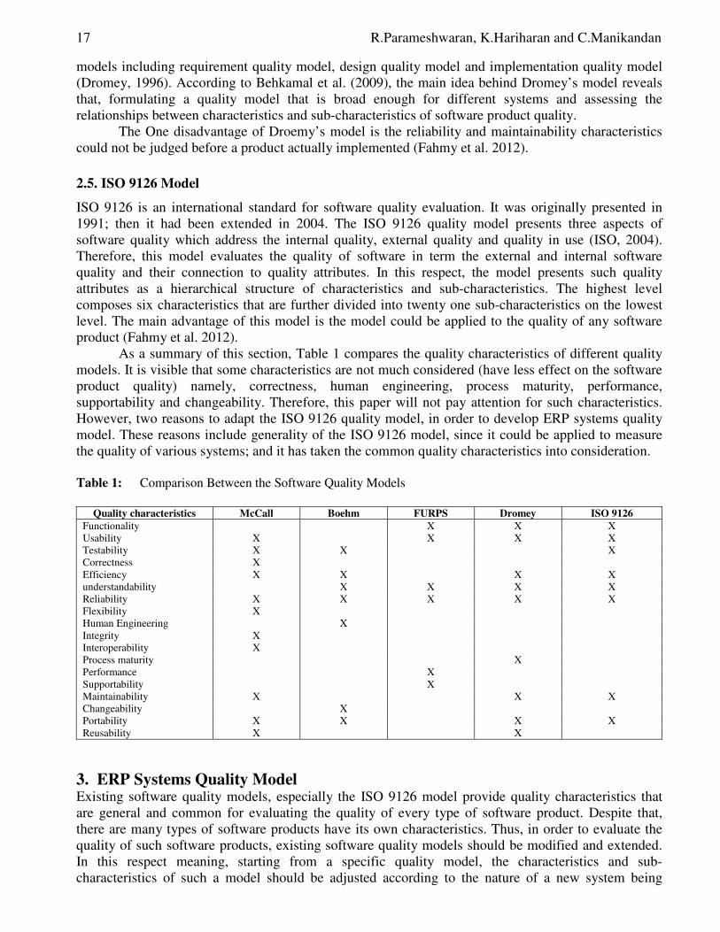
As a summary of this section, Table 1 compares the quality characteristics of different quality models. It is visible that some characteristics are not much considered (have less effect on the software product quality) namely, correctness, human engineering, process maturity, performance, supportability and changeability. Therefore, this paper will not pay attention for such characteristics. However, two reasons to adapt the ISO 9126 quality model, in order to develop ERP systems quality model. These reasons include generality of the ISO 9126 model, since it could be applied to measure the quality of various systems; and it has taken the common quality characteristics into consideration. Table 1: Comparison Between the Software Quality Models
Quality characteristics McCall Boehm FURPS Dromey ISO 9126
Functionality X X X Usability X X X X Testability X X X Correctness X Efficiency X X X X understandability X X X X Reliability X X X X X Flexibility X Human Engineering X Integrity X Interoperability X Process maturity X Performance X Supportability X Maintainability X X X Changeability X Portability X X X X Reusability X X
3. ERP Systems Quality Model Existing software quality models, especially the ISO 9126 model provide quality characteristics that are general and common for evaluating the quality of every type of software product. Despite that, there are many types of software products have its own characteristics. Thus, in order to evaluate the quality of such software products, existing software quality models should be modified and extended. In this respect meaning, starting from a specific quality model, the characteristics and sub-characteristics of such a model should be adjusted according to the nature of a new system being
Design of Graphical User Interface Tool for Filter Optimization Techniques 18
evaluated. Such adapting involves eliminating some characteristics; redefine others, and introducing new characteristics.
Although, the research on the quality software products based on ISO 9126 for the education domain is not newly approach ( Chua and Dyson, 2004; Padayachee et al. 2010; and Fahmy et al. 2012), the studies on adapting ISO 9126 to evaluate the quality of ERP system in education domain are very limited, leading to the novelty of this research. So, as previously mentioned, the focus of this work is on evaluating the quality of ERP systems in higher educational institutions, by adapting the ISO 9126 quality model. It is worth mentioning that, although the ISO 9126 quality model does not provide specific quality requirements, it however presents a general framework to evaluate the quality of software products. This is the main advantages and strength of such model, since it can be used across a variety of systems among of them education institutions’ system i.e. ERP systems.
Many scholars have adapted The ISO 1926 quality model, in order to evaluate a variety of systems. Among such systems are e-book system (Fahmy et al. 2012), web site e-learning systems (Padayachee et al. 2010), computer-based systems (Valenti et al. 2002) and e-government systems (Quirchmayr et al. 2007). The generality of ISO 9126 quality model requires further analysis of characteristics, before it is fully adjusted for evaluating the quality of the ERP system. The ISO 1926 standard defines a quality model with six characteristics including functionality, reliability, usability, efficiency, portability, and maintainability which are further divided into twenty seven sub-characteristics (ISO, 2001). The following includes how these characteristics and sub-characteristics are adapted for this research.
The functionality has been defined by (ISO 2001) as the capability of the software to provide functions which meet the stated and implied needs of users under specified conditions of usage. In order to evaluate such characteristics, it has been divided into five sub-characteristics namely accuracy, suitability, interoperability, security, and functionality compliance (Kumar et al. 2009). Adapting the functionality to the ERP systems in the higher education institutions reveals that the systems software should provide functions and services of higher education institutions as per the requirements when it is used under specific conditions.
The reliability is the capability of the software to maintain its level of performance under stated conditions for a stated period of time. Reliability has four sub-characteristics consist maturity, fault tolerance, recoverability, and reliability compliance (Fahmy et al. 2012). In terms of ERP systems, the reliability refers to the capability of the systems to maintain its service provision under specific conditions for a specific period of time. In other words, the probability of the ERP system fails in a problem within a given period of time.
The usability is the capability of the software to be understood learned, used, and attractive to the users, when used under specified conditions. The usability has set of sub-characteristics including understandability, learnability, operability, and attractiveness (Kalaimagal and Srinivasan, 2008). This characteristic is employed in this study to suggest that the ERP systems should be understood, learned, used and executed under specific conditions.
The efficiency refers to the capability of a system to provide performance relative to the amount of the used resources, under stated conditions. It has also been divided into three sub-characteristics namely time behavior, resource utilization an efficiency compliance (ISO, 2001). Adapting this characteristic to the ERP systems in the higher education institutions suggests that the systems should be concerned with the used resources when providing the required functionality.
The maintainability is the capability of the software to be modified. The maintainability consists five sub-characteristics including analyzability, changeability, stability, testability, and maintainability compliance (Al-Qutaish, 2010, ISO, 2001). In this research, any feature or part of the ERP system should be modifiable. As well as identifying a feature or part to be modified, modifying, diagnosing causes of failures, and validating the modified ERP system should not require much effort.
Finally, the portability of software refers to the capability of the software to be transferred from one environment to one another (ISO, 2001). Therefore, the ERP systems in the higher education institutions should be applied using different operating systems; be applied at different organizations or
19 R.Parameshwaran, K.Hariharan and C.Manikandan
departments; and be applied using a variety of hardware. Similar to the previous quality characteristics, the portability has set of sub-characteristics namely adaptability, installability, coexistence, replaceability, and portability compliance (Fahmy et al. 2012).
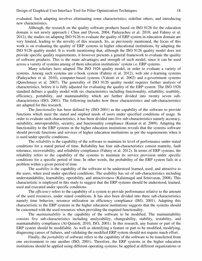
Based on the previous argument, table 2 presents the ERP systems quality model which is based on the ISO 9126. This model includes quality characteristics and sub-characteristics. Additionally, it shows how these characteristics and sub-characteristics influence ERP systems in the higher education institutions.
Table 2: ERP Systems of the Higher Education Institutions Quality Model.
Characteristic Sub-characteristic Description
Functionality
Suitability Can the ERP system’s software perform the required functions? Accurateness Are the results of ERP system’s software as anticipated? Interoperability Can the ERP system’s software interact with other systems Security Can the ERP system prevent unauthorized access? Functionality Compliance Does the ERP system adhere to the applications standards and
regulations of the law?
Reliability
Maturity Have the faults in the ERP system’s software and hardware devices been eliminated over time?
Fault tolerance Is the ERP system capable to maintain a specified level of performance in case of software and hardware errors?
Recoverability Can the ERP system resume working and recover affected data in case of a failure?
Reliability compliance Does the ERP system’s software adhere to the existing reliability standards?
Usability
Understandability Does the ERP system’s user recognize how to use the system easily?
Learnability Can the ERP system be learnt easily? Operability Can the ERP system work with a minimal effort? Attractiveness Does the ERP system’s interface Look good? Usability Compliance Does the ERP system’s software meet the existing usability
standards?
Efficiency
Time behavior How quickly does the ERP system respond? Resource utilization Does the ERP system utilize resources efficiently? Efficiency compliance Does the ERP system’s software adhere to the existing
efficiently standards?
Maintainability
Analyzability Do diagnose faults or identification a part to be modified within the ERP system, require a minimal effort?
Changeability Can the ERP system be modified easily? Stability Can the ERP system continue functioning after the change? Testability Can the modified ERP system be easily validated?
Portability
Adaptability Can the ERP system be moved easily to the other environment? Installability Can the ERP system’s software be installed easily? Portability compliance Does the ERP system adhere to the portability standards? Replaceability Can the ERP system be replaced easily with similar system?
4. Refinement of ERP Systems Quality Characteristics This section presents the criteria that are used to evaluate the ERP systems quality from the user’s perspective. These criteria are related to the quality characteristics of ERP systems in higher education institutions. As previously mentioned, These characteristics are functionality, reliability, usability, efficiency, portability, maintainability.

Design of Graphical User Interface Tool for Filter Optimization Techniques 20
Table 3: Quality Criteria and Characteristics of ERP Systems
Functionality Reliability Usability Efficiency
Access Controabllity Error messages Clarity Input and output devices utilization
Privacy Failure avoidance Completeness of description
Load and response time
Content quality Incorrect operation avoidance
Consistency of layout Processing time
Communication commonality
Mean recovery time Interactivity Flexibility and speed
Information on activities delivery
Preventing errors Help availability Process performance
Payment Security Restart ability Forms and documentation availability
Portability
Output correctness and clarity
Restorability Effectiveness of Navigation tools function
Ease of installation
Network reliability Robustness Effectiveness of search engine Function
Hardware environmental adaptability
Uniformity Terminology Uniformity Ease of performing tasks Hardware Independence
Sit authentication Style Uniformity Ease of understanding information
Software Independence
Printing facilities Download facilities Demonstration accessibility
5. Conclusion
This study proposes a model for evaluating the quality of ERP systems in the higher education institutions, while its quality characteristics and sub-characteristics have been proposed based on the ISO 9126. There are two contributions that are provided by this work including offering comparison between existing quality models and identifying the quality characteristics of ERP systems. The extension of this study will be conducted, in order to rank the main quality characteristics of the proposed model. The provided results will enable a greater understanding of the interrelation and the impact these sub-characteristics have on the quality characteristics. References [1] Al-Qutaish, R. E., 2010. “Quality Models in Software Engineering Literature: An Analytical
and Comparative Study”, Journal of American Science 6, pp. 166-175. [2] Behkamal, B., M., Kahani, and M.K., Akbari, 2009. "Customizing ISO 9126 Quality Model
For Evaluation Of B2B Applications", Journal Information and Software Technology 51, pp. 599-609.
[3] Bendoly, E., 2003. “Theory and Support for Process Frameworks of Knowledge Discovery and Data Mining from ERP Systems”, Information & Management 40, pp. 639-647.
[4] Boehm, B.W., J.R., Brown, H., Kaspar, M., Lipow, G., McLeod, and M., Merritt, 1978. “Characteristics Of Software Quality”, North Holland Publishing, Amsterdam, The Netherlands.
[5] Chua, B.B. and L.E., Dyson, 2004. “Applying The ISO 9126 Model To The Evaluation Of An E-Learning”, in Proceedings of the 21st ASCILITE Conference, pp. 184-190.
[6] Dromey, R. G., 1996. “Concerning The Chimera [Software Quality]”, IEEE Software 13, pp. 33-43

21 R.Parameshwaran, K.Hariharan and C.Manikandan
[7] Fahmy, S., N., Haslinda, W., Roslina, and Z., Fariha, 2012. “Evaluating the Quality of Software in e-Book Using the ISO 9126 Model”, International Journal of Control and Automation 5, pp. 115-122.
[8] Quirchmayr, G., S., Funilkul, and W., Chutimaskul, 2007. ”A Quality Model Of E-Government Services Based On The ISO/IEC 9126 Standard”, on The Proceedings of International Legal Informatics Symposium IRIS, [Online], Available: http://www.sit.kmutt.ac.th/wichian/Paper/eGovServiceQualityModel.pdf. [Accessed Feb. 1, 2013].
[9] Holsapple, C.W. and M.P., Sena, 2005. “ERP plans and decision-support benefits”, Decision Support Systems 38, pp. 575-590.
[10] Padayachee, I., P., Kotze, and A., van der Merwe, 2010. “ISO 9126 External Systems Quality Characteristics, Sub-Characteristics And Domain Specific Criteria For Evaluating E-Learning Systems”, Proceedings of South African Computer Lecturers’ Association (SACLA), Pretoria, SoutAfrica: ACM.
[11] ISO: ISO/IEC 9126-1, 2001, “Software Engineering - Product Quality - Part 1: Quality Model”, International Organization for Standardization,Geneva, Switzerland.
[12] ISO: ISO/IEC TR 9126-4, 2004, “Software Engineerin- Product Quality - Part 4: Quality in Use Metrics”, International Organization for Standardization, Geneva, Switzerland, Switzerland.
[13] Kalaimagal, S. and R., Srinivasan, 2008. “A retrospective on software component quality models”, SIGSOFT Software Engineering 33, PP. 1–10.
[14] Kumar, A., P.S., Grover, and R., Kumar, 2009. “A quantitative evaluation of aspect-oriented software quality model (AOSQUAMO)”, ACM SIGSOFT Software Engineering Notes 34, PP. 1–9.
[15] Madapusi, A., 2008. “ERP Information Quality and Information Presentation Effects on Decision Making”, SWDSI 2008 Proceedings, pp. 628-633
[16] McCall, J. A., P.K., Richards, and G.F., Walters, 1977. “Factors In Software Quality”, US Rome Air Development Center Reports, US Department of Commerce, USA.
[17] Panovski, G., 2008. “Product Software Quality”, Master Thesis, Technishe University Eindhoven, Department of Mathematics and Computing Science
[18] Grady R.B., 1992. "Practical Software Metrics for Project Management and Process Improvement", Prentice Hall, Englewood Cliffs, NJ, USA.
[19] Valenti, S., A., Cucchiarelli, and M., Panti, 2002. “Computer Based Assessment Systems Evaluation via the ISO9126 Quality Model”, Journal of Information Technology Education 1, pp. 157-175.
[20] Swartz, D., and K., Orgill, 2001. “Higher Education ERP: Lessons Learned”, EDUCAUSE Quarterly 2, pp. 20-27.
[21] Zornada, L., and T.B., Velkavrh, 2005. “Implementing ERP systems in higher education institutions”, Proceeding of the 27th International Conference on Information Technology, ICTI, Cavtat, Croatia.
[22] Saini, R., S.K., Dubey, and A., Rana, 2011. “Analytical Study Of Maintainability Models For Quality Evaluation”, Indian Journal of Computer Science and Engineering 2, pp. 449-454.
European Journal of Scientific Research ISSN 1450-216X / 1450-202X Vol. 99 No 1 April, 2013, pp.22-21 http://www.europeanjournalofscientificresearch.com
Contribution à l’étude des Groupements à Pistacia atlantica
Desf. subsp. atlantica dans la Plaine de Maghnia (Extrême nord-
Ouest Algérien), Phytosociologie et Dynamique
Moahamed Amara Institut National de la Recherche Forestière, Algérie
Laboratoire d’écologie et de Gestion des Écosystèmes Naturels Département d’écologie et Environnement
Université Abou Bakr Belkaid, Tlemcen, Algérie E-mail: [email protected]
Mohammed Bouazza
Laboratoire d’écologie et de Gestion des Écosystèmes Naturels Département d’écologie et Environnement
Université Abou Bakr Belkaid, Tlemcen, Algérie E-mail: [email protected]
Abstract
The northwest area of algeria, already subject to a strong worsening climate and excessive anthropogenic activity since several decades, is facing the threat of the alarming deterioration of its natural resources, like Pistacia atlantica which occupies today a meager portion of the territory. This work aims to characterize the groups with Pistacia atlantica both on phytoecological and phytosociological level and to identify its sense of dynamics in these environments that are at the limit of their ecological breakdown. The method of study is based on the phytoecological approach compared to the scale of the ecological station. Digital processing of floristic surveys has been addressed using two complementary statistical methods: the factorial analysis of correspondences (fac) and hierarchical ascendant classification (hac). The analysis of the obtained results allowed us to individualize:
- On the phytoecological level: several groups of species indicating different formations (forest, meadow forest, steppe, meadow steppe, transition toward a group very opened to steppe affinity), most often operated by intensive grazing.
- On the phytosociological: six upper unities were defined: (Pistacio-Rhamnetalia alaterni, Ononido-Rosmarinetea, Ephedro-Juniperetalia, Thero-Brachypodietea, Stellarietea mediae, Pegano-Salsoletea).
We also found that the species Withania frutescens remains the species most associated with Pistacia atlantica despite the presence of Ziziphus lotus. These results suggest that the transition from one group to another responds to launching of desertification processes whose terms differs from one stage to another: Dématorralisation, steppisation, Therophytisation. Keywords: Pistacia atlantica. Desf. subsp. atlantica, extreme nort-west of Algeria,
arid/semi-arid, Phytosociology, Phytoecology, Dynamic, fac.

23 R.Parameshwaran, K.Hariharan and C.Manikandan
1. Introduction La plupart des types de foret méditerranéenne en Afrique du Nord ont subi une extrême dégradation presque partout et elles ont complètement disparu sur de vastes étendues. Certaines ne sont plus représentées aujourd’hui que par de minuscules peuplements relictuels (White, 1986).
Dans le tell oranais, Aimé (1991) a signalé que le tapis végétal naturel est très souvent morcelé par des défrichements abusifs, les lambeaux de végétation naturelle n’étant épargnés par les activités agricoles que dans les zones défavorables .Ces "reliques" étant également fortement dégradées par les activités pastorales (incendie et pâturage).
Le Pistacia atlantica fait partie de ces essences forestières en danger ; situé dans l’extrême Nord-Ouest Algérien ; il occupe actuellement, une bien maigre proportion du territoire qu’il couvrait jadis.
De nombreux auteurs (Quézel et Santa, 1962 ; Monjauze, 1968, 1980, 1982 ; Quézel, 2000 ; Quézel et Médail, 2003 ; Belhadj, 1999 ; Belhadj et al., 2008 ; Al-Saghir et al., 2006 ; Benhassaini, 2003 ; Benhassaini et Belkhodja, 2004 ; Benhassaini et al., 2007) qualifient cette espèce comme hautement résiduelle et en phase de déclin, de sorte que son aire potentielle déborde largement leurs limites actuelles.
D’une manière générale, au-delà de l’épuisement des réserves ligneuses se profilent les dangers liés à l’érosion des sols, au tarissement des eaux, à la progression des zones désertiques (Molinier, 1977).
Concernant Pistacia atlantica, sa rusticité la rend particulièrement intéressante quant à son utilisation dans les programmes de reforestation et de sylviculture dans les zones semi-arides et arides ; puisque elle se régénère et se développe dans les endroits les plus arides où peu d'espèces d'arbres peuvent s’établir et se développer (Belhadj et al., 2008).
Malgré sa large plasticité écologique, sa restauration naturelle semble être un processus lent et difficile, en raison de sa lenteur de croissance et de sa longue période de régénération d’une part, et de la forte dégradation des sols d’autre part.
Sa rareté actuelle est due à sa sensibilité à l’état jeune au bouturage et au feu et à la faible extension des sols profonds lui convenant, en raison s’une érosion considérable (White, 1986).
De plus, la dissémination à distance des graines est assez faible, et la plupart des diaspores sont soumises à la prédation et aux effets du parasitisme (Quézel et Médail, 2003).
Face à cette situation critique, sommes-nous en présence de l’extinction locale de cette rare espèce ? S’agit-il d’un déclanchement des processus de désertisation ?
Pour répondre à cette problématique nous avons essayé : • D’identifier les groupements existants dans la zone d’étude sur le plan phytoécologique et
phytosociologique et de cerner leur sens de dynamique ; • De savoir quelles sont les espèces qui sont intimement liées à Pistacia atlantica dans la
zone d’étude. 2. Sites et Méthodes 2.1. Présentation de la Zone d’étude
2.1.1. Situation Géographique (Figure 1) La zone d’étude se situe à l’extrême occidentale de l’Algérie du Nord. Elle fait partie de l’aire occidentale du Pistacia atlantica dans le secteur oranais. La chaine montagneuse côtière des Trara et les monts de Tlemcen constituent respectivement la limite septentrionale et méridionale de la zone d’étude. Elle est limitée à l’ouest par la frontière marocaine et à l’est par la vallée de l’oued Isser.
Figure 1: Zone d’étude

Design of Graphical User Interface Tool for Filter Optimization Techniques 24
2.1.2. Orographie A l’intérieur du Tell Algérien, des vallées, de hautes plaines, des plateaux séparent ou pénètrent les massifs montagneux.
" L’orographie de la région est très caractéristique, avec un allongement parallèle à la cote des principaux reliefs, formant ainsi des barrières relativement continues, suivies de dépressions accentuées, sur le trajet des masses d’air venant de la mer. Ce fait, joint aux différences d’exposition qui existent entre les adrets et les ubacs, est responsable d’important contrastes microclimatiques" (Aimé, 1991). 2.1.3. Bioclimat La région d’étude est caractérisée par un climat méditerranéen semi-continental. L'enclave aride qui entoure Maghnia se caractérise ainsi par un micro-climat thermique de type continental, froid l'hiver et très chaud l'été. (Aimé et Remaoune, 1988).Le climagramme pluviothermique d’Emberger place la région entre l’étage aride moyen à hiver tempéré (Q2= 26,89 ; m°C = 3,21) et Semi aride inferieur à hiver tempéré (Q2=41,16 ; m°C= 5,5). Les diagrammes ombrothermiques de Bagnouls et Gaussen (1957) pour les stations météorologiques de Zenata et Maghnia durant la période (1980-2007) illustrent bien l’ampleur de la période sècheresse qui atteint les 07 mois (Avril-octobre) (Amara, 2008). La longueur de la saison sèche est généralement corrélative de son intensité ; mais il existe d’importantes différences selon que cette saison sèche annuelle est continue ou non ; c’est-à-dire selon que le régime pluviométrique annuel est monomodal, bimodal multimodal (Le Houérou, 1989-1995).
Les précipitations moyennes annuelles varient entre 249 et 327 mm. Les régimes pluviométriques mensuels se distinguent par deux maximums pluviométriques, l’un en Novembre et l’autre en mars. Le maximum printanier et hivernal permet à plusieurs essences végétales telles que Stipa tenacissima (Bouazza, 1995) ; le chêne vert (Quercus ilex), le pin d’Alep (Pinus halepensis ) (Alcaraz, 1982) d’entamer la saison estivale avec des réserves hydriques relativement importante.
Quant aux températures moyennes annuelles, elles oscillent entre 17,67°C et 20,42°C. Les valeurs extrêmes constituent des facteurs limitants énergiques dont l'efficacité dépend de certains seuils et de leur fréquence d'apparition (Aimé et Remaoune, 1988).Dans notre région les maximas thermiques moyens du mois le plus chaud (M°C) varient entre 32,7°C (Zenata) et 35°,01C (Maghnia) ce qui contribue à l’accentuation de l’évapotranspiration et par conséquent de l’aridité du milieu.

25 R.Parameshwaran, K.Hariharan and C.Manikandan
3. Méthodologie 3.1. Echantillonnage
Afin de répondre a l’objectif de cette étude nous avons suivi la méthode phytosociologique sigmatiste (Braun-Blanquet, 1951) dite aussi zuricho-montpelerienne (relevés floristiques), basée selon (Béguin et al., 1979) sur le principe que l'espèce végétale, et mieux encore l'association végétale, sont considérées comme les meilleurs intégrateurs de tous les facteurs écologiques (climatiques, édaphiques, biotiques et anthropiques) responsables de la répartition de la végétation. Selon Guinochet (1954), lorsqu'on fait des relevés, on se livre obligatoirement à un échantillonnage dirigé.
Au terrain le choix de l’emplacement des relevés a été effectué selon deux niveaux de perceptions :
A l’échelle paysagère deux grandes unités physionomiques se discriminent bien dans l’espace en fonction de leur composition floristique (La végétation steppique et les groupements préforestiers à matorral à une altitude plus élevée).
Une deuxième vision à une échelle plus petite à l'intérieur de ces groupements choisis, a guidé le choix de l’emplacement du relevé et de ses limites.
L’échantillonnage adopté est de type subjectif en tenant compte de l'homogénéité floristique et l'homogénéité écologique de la station. Ce mode subjectif consiste à choisir au niveau de chaque station des échantillons paraissant les plus représentatifs et suffisamment homogènes (Gounot, 1969; Long, 1974), intégrant l'ensemble des situations structurales et de faciès de végétation rencontrés.
Au total 100 relevés floristiques on été effectués durant la période printanière des années 2001 , 2006 et 2011.
La surface des relevés (l’aire minimale) varie de 32 m² au niveau des formations steppiques à 128 m² au niveau des matorrals. Cette aire minimale basée sur la méthode da la courbe aire-espèce, est déterminée par le nombre d’espèces relevés sur des surfaces de plus en plus grandes, jusqu’à ce que le nombre d’espèces recensées n’augmente plus. Guinochet (1968) souligne que l’intérêt principal porté à ces courbes est dû à leur importance pour définir opératoirement des surfaces floristiquement homogène.
Chacun des relevés comprend des caractères écologiques d’ordre stationnel notamment l’altitude, la pente, l’exposition, la nature du substrat, la surface du relevé, la date et lieu d’échantillonnage. En plus de ces renseignements écologiques, les listes floristiques établies, sont complétées par des indications concernant la physionomie, la structure de la végétation, son recouvrement, l‘abondance-dominance et la fréquence.
La détermination des taxons a été faite à partir de la flore de l’Algérie Quezel et Santa (1962) ; de la flore algérienne Gubb (1913) ; du guide vert « les arbres » Durand (1990) ; de la grande flore de Bonnier (1990) ; et de Fleurs d’Algérie Beniston (1984). 3.2. Traitement des Données
Nous avons utilisé le logiciel minitab 15 pour le traitement numérique des données floristiques. L'ensemble des données sont combinées dans un tableau á double entrées (avec les espèces en lignes et les relevés en colonnes) caractérisée par leur coefficient d’abondance-dominance.
Sur l’ensemble des 140 espèces inventoriées, seulement 39 espèces ont été soumises à l’analyse factorielle des correspondances (AFC) et à la classification hiérarchique ascendante (CHA). Selon Frontier (1983) après une analyse multivariable préalable faite à partir d’un dépouillement exhaustif, on pourra dans une seconde phase de l’étude se limiter au recensement des espèces structurantes (qui indiquent les communautés) et des caractéristiques (qui indiquent les réponses aux variations du milieu).
L'analyse factorielle des correspondances, mise au point par Benzecri (1973), elle permet d’établir la correspondance entre le nuage de points des relevés et celui des espèces.

Design of Graphical User Interface Tool for Filter Optimization Techniques 26
Cependant, la représentation graphique ne s’effectue généralement que sur les deux premiers axes factoriels les plus explicatifs de la structure du nuage de points ; l’analyse devient inutile à partir de troisième axe, car les valeurs propres deviennent moins significatives.
La classification ascendante hiérarchique fournit un ensemble de classes de moins en moins fines obtenues par regroupement successif de parties (Bert, 1992). Cette technique permet d’élaborer des groupements de relevés et/ou des espèces d’un ensemble par similitude, afin de faciliter l’interprétation des contributions de l’A.F.C. 4. Résultats et Discussion 4.1. Cartes Factorielles « Espèces Végétales »
Les valeurs propres et les taux d’inertie, relativement élevés pour le premier axe, deviennent faibles à partir du troisième axe. (Tab. 1). Tableau 1: Valeurs propres et taux d’inertie pour les trois Premiers axes de l’A.F.C « espèces »
Axes 1 2 3
Valeur propre 10.604 6.491 2.985 Pourcentage d’inertie 27,9 17,1 7,9
4.1.1. Interprétation de L’axe 1: valeur propre: 10.604 Taux d’inertie: 27.9 (Tableaux 1 et 2,
Figure 02) Tableau 2: Taxons à fortes contributions pour l’axe 1 de l’A.F.C
Coté négatif Coté positif Helianthemum pilosum (-0.74) Artemisia herba-alba (5.03) Erodium moschatum (-0.74) Asparagus stipularis (1.60) Marrubium vulgare (-0.70) Noaea mucronata (1.30) Urginea maritima (-0.62) Calycotome villosa subsp. intermedia (1.05) Bromus rubens (0.90)
Du Coté Négatif Nous avons deux espèces herbacées rudérales nitratophiles appartenant à la classe Stellarietea mediae : Erodium moschatum , Marrubium vulgare se mêlent avec Urginea maritima indiquant ainsi un gradient d’anthropisation . Selon Le Houérou (1995), cette dernière espèce s’intègre dans le groupe rudéral lié au surpâturage prolongé.
Helianthemum pilosum caractéristique des Ononido-Rosmarinetea est définie selon Le Houérou (1995), comme espèces forestières résiduelles ou compagnes vestigiales pouvant se rencontrer dans les écotones forêt-steppe, dans l’aride supérieure. Du Coté Positif Se rassemblent les espèces à affinité steppiques tel que Artemisia herba-alba et Noaea mucronata, Bromus rubens avec les formations xérophytes épineuses qui sont représentées par Asparagus stipularis et l’espèce héliophile Calycotome villosa subsp. intermedia.
Sur le plan bioclimatique ces espèces indiquent aussi l’ambiance aride du milieu. 4.1.2. Interprétation de l’axe 2: valeur propre: 6.491 Taux d’inertie: 17, 1 (Tableaux 1 et 3,
Figures. 02 et 03)

27 R.Parameshwaran, K.Hariharan and C.Manikandan
Tableau 3: Taxons à fortes contributions pour l’axe 2 de l’A.F.C
Coté négatif Coté positif Noaea mucronata (-1.24) Asphodelus microcarpus (3.50) Artemisia herba-alba (-1.08) Calycotome villosa subsp. intermedia (2.26) Bromus rubens (-1.03) Asparagus stipularis (1.73) Delphinium peregrinum (-1) Withania frutescens (1.52) Tetraclinis articulata (-0.96) Pistacia atlantica (1.29) Aegilops triuncialis (-0.74) Olea europaea (1.26)
Du Coté Négatif Le Noaea mucronata a la plus forte contribution (-1.24), caractéristiques des formations steppiques et pré steppiques ( Pégano-Salsoletea). Ces formations constituent selon Aimé (1991), des climax stationnels sur des substrats toujours assez fortement salés et le plus souvent anthropisés par le paturage intense.
Delphinieum peregrinum, espèce steppique psamophile, peu consommée; probablement toxique par les graines, témoigne aussi le surpâturage.
Quant à l’armoise blanche (Artemisia herba-alba), qui semble caractéristique des zones les plus sèches en Oranie ; elle forme des peuplements purs dans le semi-aride et l’aride supérieur ; dans l’aride moyen elle est associée avec Noaea mucronata.
La présence d’une espèce pré forestière thermophile (Tetraclinis articulata) au sein de ce groupement nous semble qu’elle témoigne un état de dégradation avancé ; c’est un groupement donc de transition vers un groupent très ouvert à affinité steppique. A ce sujet Aimé (1988), signale la présence des espèces steppiques dans la vallée de la moyenne Tafna où l’armoise occupe les versants encroûtés, en mélange avec Noaea mucronata.
L’association Noaea mucronatae-Artemisietum herba-albae, c’est le terme ultime de la dégradation du Calicotomo intermediae-oleeteum sylvestris pistacietum atlanticae (Aimé,1991).
Dans les dépressions abritées de l’intérieur, au niveau de la transition avec l’aride supérieur, la sous-association Pistacietosum atlanticae passe par dégradation au Noaea mucronatae-Artemisietum herba-alba (Aimé,1991).
Ces biotopes abritent également les populations les plus stables de Pistacia atlantica signalées par Alcaraz (1969), sous l’appellation « Betoum relituel » en Oranie. Du Coté Positif Sur ce coté, l’ambiance est plus sylvatique ; toutes les espèces (sauf Asphodelus microcarpus) appartiennent à l’ordre des Pistacio-Rhamnetalia . Cet ordre selon Barbero et Quezel (1979), réunit des groupements de lisière, voire matorral arboré, parfois climaciques, en particulier en zone bioclimatique semi-aride,
Dans le domaine de la série du Thermo-mediterranéen du Pistacia atlantica ; Calycotome intermedia caractérise la transition entre le bioclimat semi-aride inférieur et semi-aride supérieur (Achhal et al. , 1980).
Calycotome villosa subsp. intermedia, Asparagus stipularis et Olea europaea s’intègrent selon Alcaraz (1991), dans le groupe d'indicatrices des formations forestiéres et matorrals méditerranéens.
Quant à Withania frutescens , reste selon le même auteur parmi les espèces caractéristiques presqu'exclusives de tous les types de Callitriaie (Tetraclinaie).
On enregistre la plus forte contribution pour l’espèce anthropozoïque au sens d’Alcaraz (1982), Asphodelus microcarpus.
Nous allons voir ci-dessous que ce groupe d’espèce du coté positif représente presque la majorité des espèces les plus fidèles à Pistacia atlantica.
4.1.3. Interprétation de l’Axe 3: valeur propre : 2.985 Taux d’inertie : 7.9 (Tableaux 1 et 4, Figure 03)
L’interprétation de cet axe reste limiter puisque le taux d’inertie ne dépasse guère 10%.
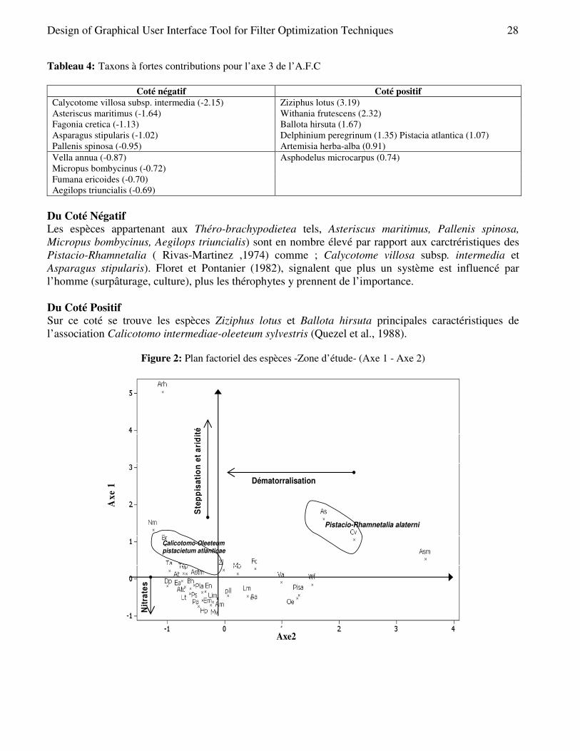
Design of Graphical User Interface Tool for Filter Optimization Techniques 28
Tableau 4: Taxons à fortes contributions pour l’axe 3 de l’A.F.C
Coté négatif Coté positif Calycotome villosa subsp. intermedia (-2.15) Ziziphus lotus (3.19) Asteriscus maritimus (-1.64) Withania frutescens (2.32) Fagonia cretica (-1.13) Ballota hirsuta (1.67) Asparagus stipularis (-1.02) Delphinium peregrinum (1.35) Pistacia atlantica (1.07) Pallenis spinosa (-0.95) Artemisia herba-alba (0.91) Vella annua (-0.87) Asphodelus microcarpus (0.74) Micropus bombycinus (-0.72) Fumana ericoides (-0.70) Aegilops triuncialis (-0.69)
Du Coté Négatif Les espèces appartenant aux Théro-brachypodietea tels, Asteriscus maritimus, Pallenis spinosa, Micropus bombycinus, Aegilops triuncialis) sont en nombre élevé par rapport aux carctréristiques des Pistacio-Rhamnetalia ( Rivas-Martinez ,1974) comme ; Calycotome villosa subsp. intermedia et Asparagus stipularis). Floret et Pontanier (1982), signalent que plus un système est influencé par l’homme (surpâturage, culture), plus les thérophytes y prennent de l’importance. Du Coté Positif Sur ce coté se trouve les espèces Ziziphus lotus et Ballota hirsuta principales caractéristiques de l’association Calicotomo intermediae-oleeteum sylvestris (Quezel et al., 1988).
Figure 2: Plan factoriel des espèces -Zone d’étude- (Axe 1 - Axe 2)
Pistacio-Rhamnetalia alaterni
Dématorralisation
Nit
rate
s
Calicotomo-Oleeteum pistacietum atlanticae
Axe2
Ste
pp
isa
tio
n e
t a
rid
ité
Ax
e 1

29 R.Parameshwaran, K.Hariharan and C.Manikandan
Figure 3: Plan factoriel des espèces -Zone d’étude- (Axe 2 - Axe 3)
Axe 3
Calicotomo-Oleeteum pistacietum atlanticae
Ax
e 2
Pistacio-Rhamnetalia alaterni
D
ém
ato
rra
lis
ati
on
Steppisation et Thérophytisation
Noaea mucronatae-Artemisietum
4.2. Dendrogrammes: (Figure 04)
Nous avons essayé de définir chaque groupe selon le rattachement des espèces aux classes phytosociologiques.
Nous distinguons les 5 groupes suivant : • Groupe 1:
Il est constitué de 3 espèces : Asparagus stipularis , Calycotome villosa subsp. intermedia, Asphodelus microcarpus dont les
deux premières se rattachent au Pistacio-Rhamnetalia alaterni ( Rivas-Martinez ,1974) • Groupe 2: constitué de 28 espèces
On a pu faire ressortir trois sous groupes o Sous groupe A: constitué de 9 espèces Withania frutescens, Pistacia atlantica, Asparagus albus, Vella annua, Olea europaea, Echium
austral, Pallenis spinosa, Aegilops triuncialis , Paronychia argentea. C’est un groupe constitué des espèces caractéristiques des Ephedro-Juniperetalia (Barbéro et
al., 1981), comme (Pistacia atlantica, Asparagus albus) et des espèces appartenant aux Théro-brachypodietea.
o Sous groupe B : (14 espèces) Thapsia garganica, Plantago albicans, Lavandula multifida, Limonium thouini, Plantago
lagopus, Avena sterilis, Euphorbia nicaeensis, Helianthemum pilosum, Erodium moschatum, Salvia verbenaca, Anagallis monelli, Fumana ericoides, Marrubium vulgare et Urginea maritima. C’est un groupe d’Ononido-Rosmarinetea fortement anthropisé vu la forte présence les caractéristiques des Théro-brachypodietea et des Stellarietea mediae.
o Sous groupe C : (5 espèces) Fagonia cretica, Asteriscus maritimus Teucrium polium, Tetraclinis articulata, Atractylis
cancellata. C’est un groupe où les caractéristiques des quatre groupements sont réunies (Pegano-Salsoletea, Théro-brachypodietea, Ononido-Rosmarinetea, Pistacio-Rhamnetalia alaterni)
• Groupe 3 :

Design of Graphical User Interface Tool for Filter Optimization Techniques 30
Ziziphus lotus, Delphinium peregrinum, Ballota hirsute, Lagurus ovatus. L’association Calicotomo intermediae-oleeteum sylvestris, (Barbero et al., 1981) caractérise ce
groupe. • Groupe 4 :
Noaea mucronata, Micropus bombycinus, Bromus rubens. • Gruope 5 : constitué d’une seule espèce
Artemisia herba-alba L’ensemble des groupes 4 et 5 représente l’association : Noaea mucronatae-Artemisietum
herba-albae. Cette association s’inscrit parmi les groupements des Pegano-Salsoletea qui sont des formations steppiques ou présteppiques le plus souvent anthropisées par un pâturage intense.
La succession, du groupe 1 vers les derniers groupes, est assez semblable à la représentation schématique des principaux stades de dégradations des unités supérieures de l’étage thermo-méditerranéen dans la zone d’étude (Figure 05).
Figure 4: Dendrogramme des espèces de la zone d’étude.
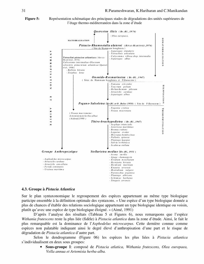
31 R.Parameshwaran, K.Hariharan and C.Manikandan
Figure 5: Représentation schématique des principaux stades de dégradations des unités supérieures de l’étage thermo-méditerranéen dans la zone d’étude
Qu ercetea i l ic is ( Br.-B l. , 19 74)
- Olea europae a .
P istacio-Rha m n etalia a la terni ( R IVAS -M AR TIN EZ ,1974)
( S ite de Ha mm a m boughra ra ) - Asparagus stipularis - T etraclin is articulata - C alyc otom e v illosa sbsp. intermedia - Asparagus albus
On onido -R os m arinetea ( Br. -B l. , 1 947)
( Sites de Ham m am boughrar a e t F illaouc ene ) - Fum ana e ric oides - T euc rium polium - He lian the mum pilosum - Atracty lis carduus - Asparagus a lbus
Peg an o- Salsoletea (B r.B l. et O . Bolos 1958) ( S ite de F illa ouce ne )
- Fagonia c retica - N oaea m ucronata
( N oaea muc rona tae - A rte misie tu m he rba-albae ( Aidoud,1990 )
T héro -b rachypo dietea ( Br.-B l. , 1947) - Ae gilops triunc ialis - Asteriscus maritimus - Bromu s rubens - L agurus ov atus - M ic ropus bomby cinus - Pallenis spinosa - Plantago lagopus - Salv ia ve rbenac a - Sc abio sa stellata
G rou pe A nthro po zoïqu e Ste llarie tea m ed ia e (B r.-B l., 1931 ) - Av ena ste rilis - Ajuga c hamaepy tis - Erodium m osc hatum - He rniaria h irsuta - Ho rde um murinum - K nautia arve nsis - M arrubium vulgare - Parony chia argente a - Plantago albic ans - Sc hism us barbatus - S inapsis arv ensis
DE
MA
TO
RR
AL
IS
AT
IO
N
MA TO RR A LIS A TION S
TE
PP
IS
AT
IO
N
TH
ER
OP
HY
TI
SA
TI
ON
AN
TH
RO
PI
SA
TI
ON
E
T
AR
ID
IT
E
- Asphode lus microc arpus - Atracty lis c arduus - Atracty lis can cellata - Fe rula com munis - Urginea maritim a
Tetraclini- pistacion atlantica e ( R IV AS-M A RT IN EZ , 19 74 ) Calicotomo inte rmediae -Olee teum sylve stris pistac ie tum atlantic ae (Qu ézel et al ., 19 88 ) - Ballota h irsuta - Z iziphus lo tus
4.3. Groupe à Pistacia Atlantica
Sur le plan syntaxonomique le regroupement des espèces appartenant au même type biologique participe ensemble à la définition optimale des syntaxons. « Une espèce d’un type biologique donnée a plus de chances d’établir des relations sociologique appartenant un type biologique identique ou voisin, plutôt qu’avec une espèce de type biologique éloigné. » (Aimé, 1991)
D’après l’analyse des résultats (Tableau 5 et Figures 6), nous remarquons que l’espèce Withania frutescens reste la plus liée (fidèle) à Pistacia atlantica dans la zone d’étude. Ainsi, le fait le plus remarquable est la dominance de l’Asphodelus microcarpus. Cette dernière connue comme espèces non palatable indiquant ainsi le degré élevé d’anthropisation d’une part et le risque de dégradation de Pistacia atlantica d’autre part.
Selon le dendrogramme (Figure 06) les espèces les plus liées à Pistacia atlantica s’individualisent en deux sous groupes:
• Sous-groupe 1: composé de Pistacia atlatica, Withania frutescens, Olea europaea, Vella annua et Artemisia herba-alba.
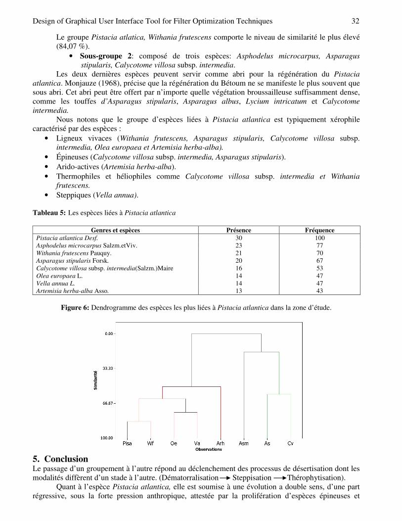
Design of Graphical User Interface Tool for Filter Optimization Techniques 32
Le groupe Pistacia atlatica, Withania frutescens comporte le niveau de similarité le plus élevé (84,07 %).
• Sous-groupe 2: composé de trois espèces: Asphodelus microcarpus, Asparagus stipularis, Calycotome villosa subsp. intermedia.
Les deux dernières espèces peuvent servir comme abri pour la régénération du Pistacia atlantica. Monjauze (1968), précise que la régénération du Bétoum ne se manifeste le plus souvent que sous abri. Cet abri peut être offert par n’importe quelle végétation broussailleuse suffisamment dense, comme les touffes d’Asparagus stipularis, Asparagus albus, Lycium intricatum et Calycotome intermedia.
Nous notons que le groupe d’espèces liées à Pistacia atlantica est typiquement xérophile caractérisé par des espèces :
• Ligneux vivaces (Withania frutescens, Asparagus stipularis, Calycotome villosa subsp. intermedia, Olea europaea et Artemisia herba-alba).
• Épineuses (Calycotome villosa subsp. intermedia, Asparagus stipularis). • Arido-actives (Artemisia herba-alba). • Thermophiles et héliophiles comme Calycotome villosa subsp. intermedia et Withania
frutescens. • Steppiques (Vella annua).
Tableau 5: Les espèces liées à Pistacia atlantica
Genres et espèces Présence Fréquence
Pistacia atlantica Desf. 30 100 Asphodelus microcarpus Salzm.etViv. 23 77 Withania frutescens Pauquy. 21 70 Asparagus stipularis Forsk. 20 67 Calycotome villosa subsp. intermedia(Salzm.)Maire 16 53 Olea europaea L. 14 47 Vella annua L. 14 47 Artemisia herba-alba Asso. 13 43
Figure 6: Dendrogramme des espèces les plus liées à Pistacia atlantica dans la zone d’étude.
5. Conclusion Le passage d’un groupement à l’autre répond au déclenchement des processus de désertisation dont les modalités diffèrent d’un stade à l’autre. (Dématorralisation Steppisation Thérophytisation).
Quant à l’espèce Pistacia atlantica, elle est soumise à une évolution a double sens, d’une part régressive, sous la forte pression anthropique, attestée par la prolifération d’espèces épineuses et

33 R.Parameshwaran, K.Hariharan and C.Manikandan
toxiques, et d’autre part progressive dans ces mêmes touffes favorisant à leur tour la germination des graines piégées de Pistacia atlantica.
Enfin de nombreux auteurs Barbéro et al. (1990), Quézel et Médail (2003), signalent que la résistance aux perturbations est optimale et résulte de la bonne plasticité écologique de ces essences (les espèces du modèle de résistance comme Pistacia atlantica). Qu'elles soient provoquées par l'homme, ou qu'elles résultent d'incendies sauvages ou de chablis, ces perturbations auront pour conséquence une reprise de souche ou une émission de rejets sur rameaux et brins qui assureront une rapide occupation en biovolume. References [1] Achhal, A, Akabli, O., Barbéro, M., Benabid, A., M’hirit, O., Peyre, C., Quézel, P. et Rivas-
Martinez, S., 1980. “A propos de la valeur bioclimatique et dynamique de quelques essences forestières du Maroc”, Ecologia mediterranea, 5, pp. 211-249.
[2] Aidoud, F., 1990. “Analyse syntaxonomique des groupements steppiques du complexe Lygeum spartum – Artemisia herba helba – Stipa tenacissima du sud-ouest algérien”, Doc. Phtosoc. N.S., XII, pp. 103-121.
[3] Aimé, S. et Remaoune, K., 1988. “Variabilité climatique et steppisation dans le bassin de la Tafna (Oranie occidentale)”, Méditerranée, Troisième série, Tome 63, pp. 43-51.
[4] Aime, S. ,1988. “Aspects écologiques de la présence de quelques espèces steppiques (Stipa tenacissima , Lygeum spartum , Artemisia herba-alba , Noaea mucronata) en Oranie littorale”, Biocénoses, T.3, N°1-2, U.R.B.T., Alger, pp. 16-24.
[5] Aimé, S., 1991. “Étude écologique de la transition entre les bioclimats subhumides, semi-arides et aride dans l’étage thermo-méditerranéen du tell oranais (Algérie occidentale)”, Thèse doct. Univ. Aix-Marseille III, 194 p. + Annexes.
[6] Alcaraz, C., 1969. “Étude géobotanique du pin d’Alep dans le tell Oranais”, Thèse doct. 3ème cycle, Fac. Sc. Montpellier, 183 p.
[7] Alcaraz, C., 1982. “La végétation de l’ouest Algérien”, Thèse doct. ès-sciences, Perpignan, 415 p. + annexes, cartes.
[8] Alcaraz, C., 1991. “La tetraclinaie sur terra rossa en sous-étage semi-aride supérieur chaud. TH2 : Groupement à Tetraclinis articulata et Rhus pentaphylla (Variante thermophile) ”, Meditérranea Ser. Biol., 13, pp. 91-104.
[9] AL-Saghir, M.G., Poter, D.M. et Nilsen, E.T., 2006. “Leaf Anatomy of Pistacia species (Anacardiaceae)”, Journal of biological science, 6(2), pp. 242-244.
[10] Amara, M., 2008. “Contribution à l’étude de Pistacia atlantica Desf. dans le Nord-Ouest Algérien: Aspects écologiques et cartographie”, Thèse magistère Univ. Tlemcen, 150p.
[11] Bagnouls, F. et Gaussen, H., 1957. “Les climats biologiques et leurs classifications”, Ann. Geog., 335, pp. 193 – 220.
[12] Barbero, M. et Quezel, P., 1979. “Le problème des manteaux forestiers des Pistacio-Rhamnetalia alaterni en Mediterranee orientale”, Coll. Phytosociologiques, Lille, VIII, pp. 9-20.
[13] Barbéro, M., Quezel, P. et Rivas-martinez, S., 1981.“Contribution à l’étude des groupements forestiers et préforestiers du Maroc”, Phytocoenologia, 9 (3), pp. 311-421.
[14] Béguin, C., Géhu, J.M. et Hegg, O., 1979. “La symphytosociologie : une approche nouvelle des paysages végétaux”, Doc. Phytos., N.S., 4, pp. 49‐68. Lille.
[15] Belhadj, S., 1999. “Les pistacheraies algériennes. Etat actuel et dégradation”, Cahiers Options MED. Vol.56.XI GREMPA meeting on Pistachios and Almonds, Sanliurfa (Turquie), pp. 107-109.

Design of Graphical User Interface Tool for Filter Optimization Techniques 34
[16] Belhadj, S., Derridj, A., Auda, Y., Gers, Ch. et Gauquelin, T., 2008. “Analyse de la variabilité morphologique chez huit populations spontanées de Pistacia atlantica en Algérie”, Botany, 86 (5), pp. 520-532.
[17] Benhassaini, H., 2003. “Contribution à l'étude de l'autoécologie de Pistacia atlantica Desf. sp. atlantica et valorisation”, Thèse doct. Univ. Sidi Bel-Abbès, 93 p.
[18] Benhassaini, H. et Belkhodja, M., 2004. “ Le pistachier de l’Atlas en Algérie : entre survie et disparition”, La feuille et l’aiguille, 54, pp. 1-2.
[19] Benhassaini, H., Mehdadi, Z., Hamel, L. et Belkhodja, M., 2007. “Phytoécologie de Pistacia atlantica Desf. subsp. atlantica dans le Nord-ouest algérien”, Cahiers Sécheresse, 18 (3), pp. 199-205.
[20] Beniston, NT.-WS., 1984. “ Fleurs d’Algérie”, Alger, 359 p. [21] Benzecri, J.P., 1973. “L’analyse des données”, Tome 2. L’analyse des correspondances. Ed.
Dunod, Paris, 619 p. [22] Bert, G., 1992. “Les principaux types de sapinières (Abies alba Mill) dans le massif du Jura
(France et Suisse).Étude phytoécologique”, Ann. Sci. For., 49, pp.161-183. [23] Bonnier, G., 1990.“ La grande flore”, Ed. Belin, Paris, 4 tomes + annexes. [24] Bouazza, M., 1995. “Étude phytoécologique des steppes à Stipa tenacissima L. et à Lygeum
spartum L. au Sud de Sebdou (Oranie, Algérie)”, Thèse doct. Es-Sci. Univ. Tlemcen, 153 p. + annexes.
[25] Braun-Blanquet, J., 1931. “Aperçu des groupements végétaux du bas Languedoc”, Commun. S.I.G.M.A. Montpellier, 9, pp. 35-40.
[26] Braun-Blanquet, J., 1947. “Le tapis végétal de la région de Montpellier et ses rapports avec les sols”, Livret-Guide du Congrès de pédologie, Montpellier.
[27] Braun-Blanquet, J., 1951. “Les groupements végétaux de la France méditerranéenne”, C.N.R.S., Paris, 297 p.
[28] Braun-Blanquet, J., 1974. “Die höheren Geselschaft seinheiten der vegetation des Südero paisen West mediterranen Raumes”, S.I.G.M.A., 204 p.
[29] Braun-Blanquet, J. et De Bolos, O. , 1958.“ Les groupements végétaux du bassin moyen de l’Èbre et leur dynamisme”, Ann. Estac. Exp. Aula Dei, Zaragoza, 5 (1-4), pp. 1-266 + 47 tab.
[30] Durand, R., 1990. “Les arbres: Guide vert”, Édit. Solar, Paris, 382 p. [31] Floret, Ch. et Pontanier, R., 1982. “ L’aridité en Tunisie présaharienne : Climat, sol, végétation
et aménagement”, Mémoire de thèses, Travaux et documents de l’O.R.S.T.O.M., Paris, 544p. [32] Frontier, S., 1983. “ Stratégies d’échantillonnage en écologie”, collection d’écologie 17. Edit.
Masson, 492p. [33] Gounot, M., 1969. “Méthodes d'étude quantitative de la végétation”, Masson éd., Paris, 314 p. [34] Gubb, A. S. , 1913. “La flore algérienne naturelle et acquise”, Édit. Carbonel, Alger, 275p. [35] Guinochet, M., 1968. “ Continu ou discontinu en phytosociologie”, Bot. Rev., 34, pp. 273-290. [36] Guinochet, M., 1954. “Sur les fondements statistiques de la phytosociologie et quelques unes
de leurs conséquences”, Veröff. Geobot. Inst. Rübel, 29, pp. 41‐67. [37] Le Houérou, H.N., 1989. “Classification écoclimatique des zones aride (S.I.) de l'Afrique du
Nord”, Ecologia Mediterranea, XV (3/4), pp. 95-144. [38] Le Houérou, H.N., 1995. “Bioclimatologie et biogéographie des steppes arides du Nord de
l’Afrique”, Options méditerranéennes, série B, N°10, C.I.H.E.A.M., Montpellier, 396 p. [39] Long, G., 1974. “Diagnostic phyto-ecologique et aménagement du territoire : Principes
généraux et méthodes”, Ed. Masson et Cie. ,Paris, Tome 1, 256 p. [40] Molinier, R., 1977. “Les forêts. Encyclopédie de l’écologie”, Édit. Larousse, Paris, pp. 48-60. [41] Monjauze, A. ,1968. “Répartition et Écologie de Pistacia atlantica Desf., en Algérie”, Bull.
Soc. Hist. Nat. Afr. Du N., 56 pp. 1- 128.

35 R.Parameshwaran, K.Hariharan and C.Manikandan
[42] Monjauze, A., 1980. “Connaissance du betoum Pistacia atlantica Desf. Biologie et foret”, Rev. For. Fran., 4 pp. 357–363.
[43] Monjauze, A. 1982. “ Le pays des dayas et Pistacia atlantica Desf. dans le Sahara Algérien”, Rev. For. Fran., 4, pp. 277–291.
[44] Quézel, P. et Santa, S., 1962. “Nouvelle flore de l’Algérie et des régions désertiques méridionales”, C.N.R.S., Paris, 2 vol., 1170 p.
[45] Quézel, P., Barbéro, M., Benabid, A., Loisel, R. et Rivas-Martinez, S., 1988. “Contribution à l’étude des groupements pré forestiers et des matorrals rifains”, Ecologia mediterranea, XIV (1-2), pp. 76 - 122.
[46] Quézel, P., 2000. “ Réflexion sur l'évolution de la flore et de la végétation au Maghreb méditerranéen”, Édit., Ibis press, Paris, 117p.
[47] Quézel, P. et Médail, F., 2003. “Écologie et biogéographie des forêts du bassin méditerranéen”, Elsevier, Paris, 592 p.
[48] Rivas-Martinez, S., 1974. “La végétation de la classe des Quercetea ilicis en Espana y Portugal”, Anal. Inst. Bot., Cavanilles Madrid, 31(2), pp. 205 - 259.
[49] White, F., 1986. “La végétation de l'Afrique: mémoire accompagnant la carte de végétation de l'Afrique”, UNESCO-AETFAT-UNSO, 384p.

European Journal of Scientific Research ISSN 1450-216X / 1450-202X Vol. 99 No 1 April, 2013, pp.36-21 http://www.europeanjournalofscientificresearch.com
Design of Graphical User Interface Tool for Filter
Optimization Techniques
R. Parameshwaran Assistant Professor II, Sastra University
E-mail: [email protected] Tel: 8220293535
K. Hariharan
Assistant Professor II, Sastra University E-mail: [email protected]
Tel: 8220293535
C. Manikandan Assistant Professor II, Sastra University
E-mail: [email protected] Tel: 8220293535
Abstract
This paper aims at integrating various loop optimization techniques for single input
single output IIR and FIR filters. Specifically, the paper proposes to implement the software suite that performs critical path and iteration bound analyses for a given IIR or FIR filter, and utilizes the techniques of loop - unfolding, loop–retiming/pipelining, and look-ahead transformation that optimizes the filter at specified sampling rates. The proposed tool suite provides an integrated environment that allows user specifications of filter definition and various optimization levels. With a graphic user interface (GUI), this tool suite can display the data flow graphs before and after different sorts of transformations. Keywords: Digital signal processing (DSP), graphic user interface (GUI), critical path,
pipelining, unfolding, retiming. I. Introduction Digital signal processing (DSP) is used in numerous applications such as video compression, digital set-top box, cable modems, digital versatile disk, portable video systems/computers, digital audio, multimedia and wireless communications, digital radio, digital still and network cameras, speech processing, transmission systems, radar imaging, acoustic beamformers, global positioning systems, and biomedical signal processing. The field of DSP has always been driven by the advances in DSP applications and in scaled VLSI technologies. Therefore, at any given time, DSP application impose several challenges on the implementations of the DSP systems. These implementations must satisfy the enforced sampling rate constraints of the real-time DSP applications and must require less space and power consumption.

37 R.Parameshwaran, K.Hariharan and C.Manikandan
In this course, several methodologies were addressed, which are needed to design custom or semicustom VLSI circuits for these applications. In the first part of this course, we discussed several high-level architectural transformations that can be used to design families of architectures for a given algorithm. These transformations include pipelining, retiming, unfolding, folding, systolic array design methodology, and look-ahead transformations. Some of these transformations can lower the sampling rate, some can reduce the circuit size, and some can increase the throughput.
In this paper, we implement several of the mentioned transformations, such as pipelining/retiming, loop unfolding and look-ahead transformation using MATLAB. Focusing on IIR/FIR filters, we develop an integrated environment that enable either individual or integrated optimization purposes. This developed tool suit contains three major functionalities that is shown in Fig. 1.1.
Figure 1.1: The mechanism for this project
INTEGRATED IIR LOOP TRANSFORMATION AND OPTIMIZATION TOOL SUITE
LOOP ANALYSIS
LOOP OPTIMIZATION
FILTER
PRESENTATION
CRITICAL PATH
LOOP UNFOLDING
FILTER STRUCTURE
LOOP RETIMING/PIPELING
LOOK AHED TRANSFORMATION
First, the loop analysis tool enables critical path calculation and iteration bound analysis. Second, the loop optimization tool implements unfolding, retiming, pipelining, and look-ahead
transformation. Last, the filter presentation allows our tool suit for IIR/FIR filter. The rest of this paper is organized as follows. Section II introduces the matrix format for the
DFG representation and the way we transfer IIR/FIR filters to the DFG representation and how to use the graphic user interface (GUI) we developed in this paper. Section III presents the algorithms to calculate critical path and iteration bound. In section IV and V, we address the adopted algorithms and implementation details for the three transformations. Observations and results are also given in the section VI and conclude in section VII. II. Graphic Presentation In this section, we explain graph representation for general cases and IIR/FIR filters. A. DFG Representation
Given a directional graph with n nodes, N, which are connect by some edges e, the corresponding matrix representation G is an n x n matrix that can be obtained by the following rules.
G(i,j) = m if e i�j exists and contains m delay elements

Design of Graphical User Interface Tool for Filter Optimization Techniques 38
-1 if e i�j doesn’t exists All the MATLAB codes implemented in this tool suite are based on this data structure. If the
DFG has to specify the input/output nodes, we explicitly pass the indexes of input/output nodes into the desired function. B. How to Use the Graphic Interface
Among the hand-in MATLAB code, gui.m is the main function that display the graphic user interface. Typing gui in MATLAB, the panel is shown in Fig. 2.1.
Figure 2.1: GUI Input the desired order to perform look-ahead transformation.
1. The IIR/FIR coefficients A. 2. The IIR/FIR coefficients B. 3. After typing the values of A and B values in windows 1 and 2, push this button, and the DFG
will display on window 8. Its critical path will also be calculated and shown in window 9. 4. How many copies the user want to unfold. 5. Performs Unfolding. 6. Indicate the desired pipe stage. 7. Performs pipelining. 8. DFG display panel. 9. The length of the critical path. 10. Quit the graphic user interface. 11. Push for cut-set retiming to minimize the critical path.
III. Generate Graph from IIR/FIR Filters The project performs a series of loop analysis and transformation techniques over single-input single output IIR and FIR filters. The integrated tool suite accepts the general z-transformed polynomial coefficients as the unified representation for both IIR and FIR filters. Specifically, any single-input single-output IIR or FIR filter with transfer function
H(z)=B(z)/A(Z) =(b0+b1z
-1+…..+bqz-q)/(a0+a1z
-1+……apz-p)
is presented to the tool suite as two index arrays A and B: A = [1 ax a2 ... ap]; B = [b0 h b2 ... bq];
where p and q are the orders for polynomial A(z) and B(z), respectively.

39 R.Parameshwaran, K.Hariharan and C.Manikandan
The function filter2graph(A,B) transforms the polynomial representation into its corresponding data flow graph (DFG) representation G in direct form II [1]. Specifically, each addition or multiplication operator is mapped to one vertex in G. Moreover, each point that fans out is considered as a null operator and is mapped to one vertex in G. Each edge in G represents a physical connection between two vertices associated to a weight corresponding to the number of delays between the two operators. An edge weight of -1 means that no physical connection exists between the two vertices. Figure 9 illustrates the structure of G. Let Ghave g nodes, where g equals the total number of addition, multiplication, and null operators. The matrix representation of G is a g by g matrix where each element G(i,j) correspond to the weight from operator i to operator j.
[Sx S2 ... Sa] Mx M2 ...Mm; N, N2 ..Nn] �[1 2…a;a+1 a+2 ….a+m;a+m+1 a+m+2…a+m+n] where Si, Mi, and Ni corresponding to the function figure2graph().
IV. Loop Analysis Algorithm A. Critical Path Calculation
In order to find the critical path of a DFG, we implement a longest-path algorithm which is similar to the Dijkstra's shortest-path algorithm [2]. The Dijkstra's is summarized as follows.
DIJKSTRA(G, w, s)
1. INITIALZE-SINGLE-SOUCE(G,s) 2. S ←φ 3. Q ←V[G] 4. while Q ≠φ 5. do u←EXTRACT-MIN(Q) 6. S←SUu 7. for each vertex υ Є Adj [u] 8. bf do RELAX(u,v,w)
With the following changes of the Dijkstra's shortest-path algorithm, we have our longest-path algorithm.
1. The Dijkstra's algorithm initial every node to ∞. Since we need a longest-path algorithm, and we do not have negative edge in our DFG, we assign the initial value of each node —1 instead.
2. The EXTRACT-MIN() function is replaced by EXTRACT-MAX() In order to find the critical path for a given DFG, we perform our single-source longest-path
algorithm for on of the the candidate source nodes. The candidate source nodes are those nodes right after a delay element and the input node itself. Then we exam the longest path to all the candidate sink nodes, which are all the nodes right before a delay elements and the output node itself. After examining all possible combinations of sources and sinks, we can find out which path and how long is the critical path. B. Iteration Bound Analysis
The longest path matrix algorithm described in [3] has been implemented to calculate the iteration bound of a given DFG.
In the longest path matrix (LPM) algorithm [4], a series of matrices is constructed, and the iteration bound is found by examining the diagonal elements of the matrices. Let d be the number of delay in the DFG. These matrices L(m), m = 1, 2, • • •, d are constructed such that the value of the elements li,j
(m) is the longest computation time of all paths from delay element di to dj that pass through exactly m — 1 delays (not including di and dj). If no such path exists, li,j
(m) = — 1. Note that longest path between any two nodes is calculated by the longest-path algorithm presented in the previous subsection.

Design of Graphical User Interface Tool for Filter Optimization Techniques 40
After the first longest path matrix L(1) is calculated the higher order matrices, L(m), m = 2, 3, • • •, d, do not need to be determined directly from the DFG again. Instead, they can be recursively computed according to the following rule.
(1) ( )( 1), , ,( 1, )max mm
i j i k k jk K
l l l+
∈
= − +
where K is the set of integers k in the interval [1,d]. V. Loop Optimization Algorithms In this section, we discuss the three transformation algorithms implemented in this paper and show the result and observation made. A. Cutset Retiming Transformation
Cutset retiming is a useful technique that is a special case of retiming. Cutset retiming only affects the weights of the edges in the cutset. We implement the cutset retiming algorithm addressed in [3]. This algorithm only allows shifting delay elements forward through a node, but not backward. In addition, this algorithm may also result in pipelining, which skews the input and output timing. We figure out this and modify the original algorithm to make it performing as cut-set retiming only.
Two quantities W(U, V) and D(U, V) used in this algorithm are as follows W(U,V) = min{w(p) U→V} D(U,V) = max{t(p) U→V and w(p) = W(U,V)} After W(U, V) and D(U, V) are calculated, given a desired clock period c, there are feasible and
critical path constraints as follows. 1. (feasible constraint) r(U) — r(V) <= w(e) for every edge U→V of G and 2. (critical path constraint) r(U) — r(V) <= W(U, V) — 1 for all vertices U, V', in G such that
D(U,V) > c. In addition for some circuits, the above algorithm may cause pipelining, which skew the input
and output timing. In order to solve this problem, we add one more constraint to the constraint graph, r(input) = r(output), which means we can push delay elements out of the output node, and back into the input node; the number of delay elements go out of the output node should be the same as those push back into the input node to keep the timing constant. B. Pipelining
Pipelining is a special case of retiming. It is feed-forward cut-set retiming. In order to perform the pipelining, we try to find any possible feed-forward cut-set in the DFG. For IIR/FIR examples, the possible feed-forward cut-sets appear to be in the right part of the DFG (shown in Fig. 5.1). Therefore, we naively insert the desired number of pipe stages into the cut-set A shown in Fig. 5.1, and perform the cut-set retiming discussed in the previous section.

41 R.Parameshwaran, K.Hariharan and C.Manikandan
Figure 5.1: Possible Feed-forward cut-sets for pipelining
C. Loop Unfolding
The unfolding technique duplicates any DFG structure into multiple copies in pursuit of parallelism with the additional hardware. The unfolding technique does not alter the iteration bound for the DFG, but it helps the DFG in reducing the critical path to approach the iteration bound. The J-unfolding operation follows that described in [3]
1. For each node U in the original DFG, draw the J nodes U0, U1, ...,UJ-1. 2. For each edge U → V with w delays in the original DFG, draw the J edges Ui→V(i+W)%J with
(i+w/J) delays for i = 0,1,..., J -I. VI. Experimental Results Fig. 6.1 shows a 2nd order IIR filter example generated by our tool set. The critical path is labeled on the figure, and isequal to 7t.u
Figure 6.1: 2nd order IIR Filter
The function unfold() accepts any DFG and the specified order j and produces the unfolded graph. Fig. 6.2 shows the 2-unfolded DFG for a 2nd order IIR filter.
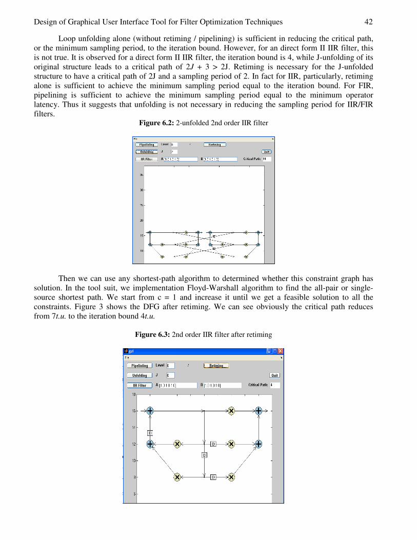
Design of Graphical User Interface Tool for Filter Optimization Techniques 42
Loop unfolding alone (without retiming / pipelining) is sufficient in reducing the critical path, or the minimum sampling period, to the iteration bound. However, for an direct form II IIR filter, this is not true. It is observed for a direct form II IIR filter, the iteration bound is 4, while J-unfolding of its original structure leads to a critical path of 2J + 3 > 2J. Retiming is necessary for the J-unfolded structure to have a critical path of 2J and a sampling period of 2. In fact for IIR, particularly, retiming alone is sufficient to achieve the minimum sampling period equal to the iteration bound. For FIR, pipelining is sufficient to achieve the minimum sampling period equal to the minimum operator latency. Thus it suggests that unfolding is not necessary in reducing the sampling period for IIR/FIR filters.
Figure 6.2: 2-unfolded 2nd order IIR filter
Then we can use any shortest-path algorithm to determined whether this constraint graph has solution. In the tool suit, we implementation Floyd-Warshall algorithm to find the all-pair or single-source shortest path. We start from c = 1 and increase it until we get a feasible solution to all the constraints. Figure 3 shows the DFG after retiming. We can see obviously the critical path reduces from 7t.u. to the iteration bound 4t.u.
Figure 6.3: 2nd order IIR filter after retiming
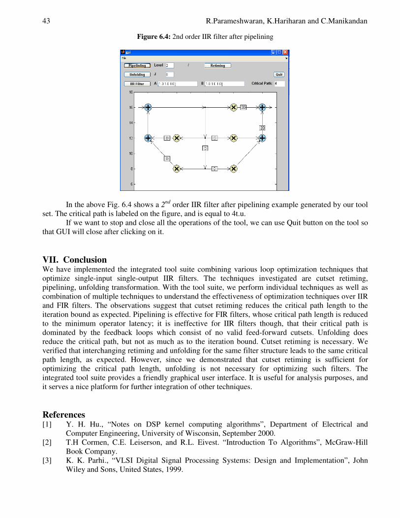
43 R.Parameshwaran, K.Hariharan and C.Manikandan
Figure 6.4: 2nd order IIR filter after pipelining
In the above Fig. 6.4 shows a 2nd order IIR filter after pipelining example generated by our tool set. The critical path is labeled on the figure, and is equal to 4t.u.
If we want to stop and close all the operations of the tool, we can use Quit button on the tool so that GUI will close after clicking on it. VII. Conclusion We have implemented the integrated tool suite combining various loop optimization techniques that optimize single-input single-output IIR filters. The techniques investigated are cutset retiming, pipelining, unfolding transformation. With the tool suite, we perform individual techniques as well as combination of multiple techniques to understand the effectiveness of optimization techniques over IIR and FIR filters. The observations suggest that cutset retiming reduces the critical path length to the iteration bound as expected. Pipelining is effective for FIR filters, whose critical path length is reduced to the minimum operator latency; it is ineffective for IIR filters though, that their critical path is dominated by the feedback loops which consist of no valid feed-forward cutsets. Unfolding does reduce the critical path, but not as much as to the iteration bound. Cutset retiming is necessary. We verified that interchanging retiming and unfolding for the same filter structure leads to the same critical path length, as expected. However, since we demonstrated that cutset retiming is sufficient for optimizing the critical path length, unfolding is not necessary for optimizing such filters. The integrated tool suite provides a friendly graphical user interface. It is useful for analysis purposes, and it serves a nice platform for further integration of other techniques. References [1] Y. H. Hu., “Notes on DSP kernel computing algorithms”, Department of Electrical and
Computer Engineering, University of Wisconsin, September 2000. [2] T.H Cormen, C.E. Leiserson, and R.L. Eivest. “Introduction To Algorithms”, McGraw-Hill
Book Company. [3] K. K. Parhi., “VLSI Digital Signal Processing Systems: Design and Implementation”, John
Wiley and Sons, United States, 1999.

Design of Graphical User Interface Tool for Filter Optimization Techniques 44
[4] S.H. Gerez, S.M.Heemstra deGroot, and O.E.Herrmann, “A polynomial - time algorithm for the computation of the iteration-period bound in recursive dataflow graphs”, IEEE Trans on Circuits and Systems - I: Fundamental Theory and Applications, Jan 1992.
[5] Chao, Liang-Fang, Sha, Edwin Hsing-Mean, Scheduling Data-Flow Graphs via Retiming and Unfolding, TR-396-92, Princeton University Computer Science Technical Reports, October 1992.
[6] Naveed A. Sherwani, Algorithms for VLSI Physical Design Automation, Kluwer Academic Publishers, 1999
[7] H. Kaeslin, Digital Integrated Circuit Design: from VLSI Architectures to CMOS Fabrication, Cambridge University Press, 2008
[8] C. Ifeachor and W. Jervis, Digital Signal Processing– A Practical Approach, Pearson Education, 2002

European Journal of Scientific Research ISSN 1450-216X / 1450-202X Vol. 99 No 1 April, 2013, pp.45-54 http://www.europeanjournalofscientificresearch.com
A Stochastic Decision Process Model for Optimization of Railway and Tramway Track Maintenance by means of
Image Processing Technique
Ferdinando Corriere Departement of Energia, University of Palermo viale delle Scienze Ed.9, Palermo 90100, Italy
E-mail: [email protected]
Dario Di Vincenzo Departement of Energia, University of Palermo viale delle Scienze Ed.9, Palermo 90100, Italy
E-mail: [email protected]
Marco Guerrieri Faculty of Engineering and Architecture
University of Enna “Kore”, Cittadella Universitaria, 94100 Enna, Italy E-mail: [email protected]
Abstract
One of the key targets for an efficient transport network management is the search for proper maintenance policies to guarantee acceptable safety and quality standards in the travel and to optimize available resource allocation. Methodologically, the proposed model presented in this paper uses the stochastic dynamic programming and in particular Markov decision processes applied to the rail wear conditions for the railway and tramway network. By performing the integrated analysis of the classes of variables which characterize the rail quality (in terms of safety), the proposed mathematical approach allows to find the solutions to the decision-making process related to the probability of deterioration of the state variables of the rail over time and to the available resources. The paper takes into account a non-conventional procedure for measuring the transverse profile of rails in operation by means of image-processing technique. Keywords: Rail wear, image processing technique, Markovian stochastic decision process
1. Introduction One of the most frequent and dangerous accidents in the railway field is the derailment which can be caused by a lot of factors, some occasional and statistically insignificant, others much more frequent and due to mismanagement of the superstructure which may be below the minimum safety standards established by the rail management authorities. Generally the derailment occurs when the forward motion of the axle is combined with an excessive ratio of Q/P wheel/rail contact forces.
This usually occurs under conditions of reduced vertical force and increased lateral force that causes the wheel flange to roll onto the top of the rail head. The rail wear and other imperfections on railway and tramway track can be both monitored through low-efficiency equipment or diagnostic

A Stochastic Decision Process Model for Optimization of Railway and Tramway Track Maintenance by means of Image Processing Technique 46 trains which perform track laser scans while monitoring rail travels (Esveld, 2001; Guerrieri, 2012; Guerrieri & Ticali, 2012 a; Guerrieri & Ticali, 2012 b). More recently the potentialities offered by real-time image processing techniques (mono - and stereoscopic methods) to determine the vertical, horizontal and 45° rail wear have been pointed out (Alippi, et al., 2000; Guerrieri, et al., 2012 a; Guerrieri, et al., 2012 b; Guerrieri & Ticali, 2012 c; Guerrieri & Ticali, 2012 d; Karaduman, 2012). The measure of the rails allow to assess the “effectiveness of the railway track” and its evolution over time and consequently to appropriately schedule maintenance works, specifically an “on condition” maintenance type, as well as to optimize human and economic resources, rather than to be driven by a more expensive “logic of emergency” and to do urgent repair work whenever serious defects arise (Di Vincenzo & Guerrieri, 2005; Corriere & Di Vincenzo, 2012). 2. Rails Profile Measurement The main objective of image processing technique is to make the information content of a given image explicit with regard to the reference application type. All the segmentation methods are defined to process an image through specific algorithms which divide that image into distinct and uniform regions according to a set feature. This operation is the first step to distinguish the region enclosing the object of interest (ROI, region of interest) from the other parts or the background. After analyzing the image of the rail the segmentation procedure detects the image contour or “edge” through Canny’s algorithm (Canny, 1986). Only afterwards this procedure solves the problem to compare the two rail profiles (worn-out and new) and to measure - for example - the vertical, horizontal and 45° deviations. The image edge detection phase is necessary in that digital images are definitely realized by high-resolution equipment but some image pixels could be affected by noise thus making the rail edge detection less accurate. More specifically, it is essential to detect the exact position of the image edge even in those parts where it cannot be distinguished, perceptually and/or numerically, from the clear background. Canny’s algorithm examines the behavior of the gradient operator applied to a noisy contour. The algorithm establishes that the pixel located at position (i,j) on the generic chromatic plane p1 of the image A(i,j,p) is a Canny contour pixel if the intensity value of the pixel examined – A(i,j,p) – appears to be superior to given threshold values as established by Canny (Canny, 1986), based upon hysteresis thresholding and non-maximum suppression algorithms. The rail edge points obtained by Canny algorithm, denoted with {C}, are illustrated in the binary image of Fig. 2, which is an enlargement of a part of the original image (cf. Fig. 1). For each contour point {C} some clearer pixels which do not belong to rail microwrinkles can be detected near its edge. For every chromatic plane of the analyzed image, a median filter is applied by following this relation:
M=A*B (1) where template B, in this specific case, has a definite dimension [3x3] and a coefficient equal to (1/9).
1 1 11
* 1 1 19
1 1 1
B
=
(2)
Relation (1) represents the pixel mean of the neighboring eight values. The implemented procedure iteratively applies the previous filter so as to spread the numerical values of all the pixels which certainly belong to a colorimetrically homogeneous region, located at either the background or rail. Therefore the idea is very simple: the image at time t (iteration step) derives from the initial image convolved with the median filter, or:
( ) ( )0, , , ( , , )A i j t A i j M i j t= × (3)
1 “p” is plane index: p=1 Red plane, p=2 Green plane, p=3 Blue plane

47 Ferdinando Corriere, Dario Di Vincenzo and Marco Guerrieri
where (i,j) are the pixel position indices within the original matrix A and “×” represents the convolution operator. Moreover, since the expanded mean filter (3) tends to remove the information on the edge details, this effect should be mitigated by applying another operator which, instead, emphasizes the rail edge.
In light of the above, downstream from the previous convolution (3), an edge extraction operator called range operator was applied (Gonzales et al., 2002; Gonzales et al., 2004). For each deviation (i,j) from template B, the value of the central pixel can therefore be formalized as follows:
( ) i 1, j 1 i 1, j i 1; j 1 i, j 1; i, j i, j 1 i 1, j 1R i, j Max (A ;A ;A ;A A ;A ; ;A− − − − + − + + += …
i 1, j 1 i 1, j i 1; j 1 i, j 1; i, j i, j 1 i 1, j 1Min(A ;A ;A ;A A ;A ; ;A ) − − − − + − + + +− … (4)
To this end the range values of every [3x3] boundary of all the pixels belonging to the original image A have been sought and highlighted. The following equation (5) formalizes the previous difference operation. Therefore, given a generic iteration step t, the suggested algorithm is able to lower the pixel intensities which mark the rail edge of the plane section.
i 1, j 1 i 1, j i 1; j 1 i, j 1; i, j i, j 1 i 1, j 1Min(A ;A ;A ;A A ;A ; ;A )− − − − + − + + +… (5)
It can easily be noticed that, with regard to any direction taken along the rail edge, while relation (3) tends to make numerically uniform the pixel value on the point edge under consideration, relation (4) on the same boundary lowers the values in the darkest regions and therefore colorimetrically near the rail. Then we detected some uncertainty areas along the point edges where the profile in the eight directions marked a rough variation or, in any case, a skip over a precise threshold level, localized by three constants [Ti, To, Ts]. Such constants are automatically determined by the algorithm in relation to the maximum, minimum and mean deviation values of the two profiles. In these areas, for each iterative step t the pixel values fill in the matrixes {Si} and {Gi}, well distinct from the matrixes {S} and {G} which instead are almost certainly background and rail. Therefore, at the iterative step t we have:
( ) ( )S i, j, t J i, j, t,Ti= (6)
( )Si i, j, t J(i, j, t,Ti,To= (7)
( )Gi i, j, t J(i, j, t,To,Ts)= (8)
( ) ( )G i, j, t J i, j, t,Ts= (9)
The suggested algorithm is able to define the matrix CF(i,j) of the final edge, which is formalized by the following relation:
( ) ( ) ( ) ( ) ( )( ), , , , , , , , , , , , ,CF i j t F S i j t Si i j t Gi i j t G i j t= (10)
where F is the function which formalizes the belonging of the pixel to the rail boundary or to the background. Its superimposition on the original image is illustrated in Figure 5.
Figure 1: Grooved Tramway Rail image
Figure 2: Binary image Figure 3: Final result of the algorithm suggested
Figure 4: Binary encoding of the previous rail part
It should be underlined that, downstream from the previous thresholding operations (cf. eq. 9), the procedure is also able to extrapolate not only the exact contour position (cf. eq. 10), but also a first object-based binary encoding which is formalized as follows:
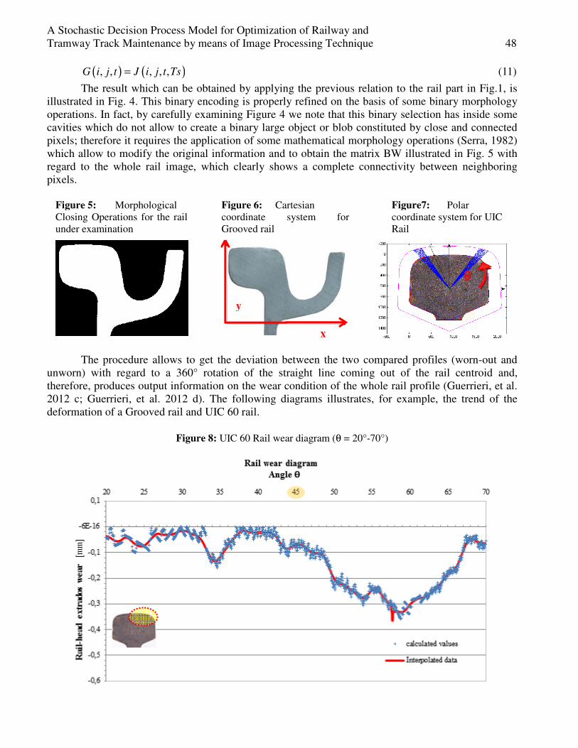
A Stochastic Decision Process Model for Optimization of Railway and Tramway Track Maintenance by means of Image Processing Technique 48
( ) ( ), , , , ,G i j t J i j t Ts= (11)
The result which can be obtained by applying the previous relation to the rail part in Fig.1, is illustrated in Fig. 4. This binary encoding is properly refined on the basis of some binary morphology operations. In fact, by carefully examining Figure 4 we note that this binary selection has inside some cavities which do not allow to create a binary large object or blob constituted by close and connected pixels; therefore it requires the application of some mathematical morphology operations (Serra, 1982) which allow to modify the original information and to obtain the matrix BW illustrated in Fig. 5 with regard to the whole rail image, which clearly shows a complete connectivity between neighboring pixels.
Figure 5: Morphological Closing Operations for the rail under examination
Figure 6: Cartesian coordinate system for Grooved rail
Figure7: Polar coordinate system for UIC Rail
x
y
The procedure allows to get the deviation between the two compared profiles (worn-out and unworn) with regard to a 360° rotation of the straight line coming out of the rail centroid and, therefore, produces output information on the wear condition of the whole rail profile (Guerrieri, et al. 2012 c; Guerrieri, et al. 2012 d). The following diagrams illustrates, for example, the trend of the deformation of a Grooved rail and UIC 60 rail.
Figure 8: UIC 60 Rail wear diagram (θ = 20°-70°)
θ θ θ θ
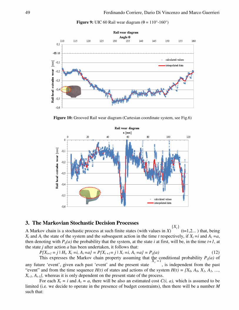
49 Ferdinando Corriere, Dario Di Vincenzo and Marco Guerrieri
Figure 9: UIC 60 Rail wear diagram (θ = 110°-160°)
Figure 10: Grooved Rail wear diagram (Cartesian coordinate system, see Fig.6)
3. The Markovian Stochastic Decision Processes
A Markov chain is a stochastic process at such finite states (with values in X){ }tX
(t=1,2... ) that, being Xt and At the state of the system and the subsequent action in the time t respectively, if Xt =i and At =a, then denoting with Pij(a) the probability that the system, at the state i at first, will be, in the time t+1, at the state j after action a has been undertaken, it follows that:
P{Xt+1 = j | Ht, Xt =i, At =a} = P{Xt +1= j | Xt =i, At =a} = Pij(a) (12) This expresses the Markov chain property assuming that the conditional probability Pij(a) of
any future ‘event’, given each past ‘event’ and the present state tX i=
, is independent from the past “event” and from the time sequence H(t) of states and actions of the system H(t) = {X0, A0, X1, A1, …, Xt-1, At-1}, whereas it is only dependent on the present state of the process.
For each Xt = i and At = a, there will be also an estimated cost C(i, a), which is assumed to be limited (i.e. we decide to operate in the presence of budget constraints), then there will be a number M such that:

A Stochastic Decision Process Model for Optimization of Railway and Tramway Track Maintenance by means of Image Processing Technique 50
|C(i, a)|<M for each i∈I e a∈K (13) The conditions of deterioration of the rails are known to be expressed by means of the values
assumed by the “rails wear”, measured by means traditional or innovative techniques like the processing image (see Figures 8 and 9). The determination of the state of the system will be followed by an action (decision) selected from a finite set of possible actions. A rule applied for the choice of an action at each instant is defined Policy and is denoted by π. In general, the action specified by a policy in the time t, may be dependent not only on the present state Xt, but also on the history Ht and on t itself. A policy can be also randomized in the sense that a probability distribution is assigned to possible actions. An important subset of the set containing all the policies is that of the stationary policies. A policy (or scenario of coordinate activities) is stationary if the action which specifies in the time t is only dependent on the present state Xt and if it is non-randomized (deterministic). In other words, a stationary policy is a function f which traces the state space in the action space by expressing that for each state i, f(i) denotes the action chosen by the policy when the state i occurs. It follows that, if a stationary policy is adopted, then the state sequence {Xn, n = 0, 1, 2, …} forms a Markov chain with a transition probability Pij = Pij(f(i)).
Therefore the process will be referred to as Markov decision process (Derman, 1962; Klein, 1962; Barlow & Proschan, 1965; Kolesar, 1966; Jorgenson, et al., 1967; Kalymon, 1968). In order to determine the most effective actions of intervention it is necessary to establish a criterion for optimality. Given the optimal conditions in terms of operational safety for the user expressed by the functional levels described above, “optimal” will be that maintenance policy which minimizes the average cost per time unit and which, at the same time, achieves the maximum economic efficiency. This can be obtained by solving a linear programming problem through the Simplex Method, in which the objective function to minimize is as follows (Corriere & Di Vincenzo, 2011):
Φ = 0 1
m K
jk jkj k
x c= =
∑∑ (14)
Where xjk stands for the stationary probability to take a decision k when the system is in the state j, and cjk(t)≥ 0 the average cost covered when the system is in the state j in the time t and the decision k is taken. It is assumed that cik(t)=cik, be independent of t.
1 1
( )K K
jk jk jkk i I k
X X q k= ∈ =
=∑ ∑∑ for each j∈I (15)
1 1
1K
jkk k
X= =
=∑∑ (16)
xjk ≥ 0 (17) in which qij(k) expresses the transition probability of a system, being in the state i, to change to the state j in the following step when action k is taken. For each type of action k the sum of all the probabilities that the system, being in the state i, has to change to each state j = 0,1…m:
0
( ) 1m
ijj
q k=
=∑ and qij(k) ≥0 For each i and k set (18)
As previously shown, the optimum solution of (2) is unique for ∑ 0>k
jkx , j∈I, and it satisfies
the optimum non-randomized choice to take action k in the state j, then it follows:
1
jk jkjk K
jjk
k
X XD
Xπ
=
= =
∑ (19)
in which there is, xjk = πjDjk and j jkk
Xπ =∑ , with πj as equilibrium probability distribution (Corriere &
Russo, 2003).

51 Ferdinando Corriere, Dario Di Vincenzo and Marco Guerrieri
4. Application of Markov Decision Process for Optimizing Railway Superstructure Maintenance In order to fully describe the real possibility to use the mathematical model suggested and closely follow the application steps of the method, an exemplification is here reported on a system characterized by possible states for rail wear parameter by possible actions to be undertaken and by actions consistent with every state and every action. For the application of the model four level of 45° rail degradation are take into account (see Table 1) (Corriere & Di Vincenzo, 2007; Corriere & Di Vincenzo, 2010): Table 1: States and levels of degradation
State Level of Degradation Threshold values Wear “W 45°” [mm]
0 Optimal level W 45° < 12 1 Level of attention 12 ≤ W 45° < 14 2 Level of intervention 14 ≤ U 45° ≤ 15 3 Level of safety W 45° > 15
Let us suppose that at each initial period t the railway infrastructure is inspected by means of
image analysis technique and that the 45° rail wear values (see Fig. 8) is classified according to one of the four states illustrated in the table 1.
After the observation of the qualitative state of the superstructure a decision needs to be taken, either to still utilize it without any intervention up to the following inspection period (action c) or to carry out maintenance works in order to restore the best structural and functional conditions (action m). Let us suppose, moreover, that action c is allowed only in the state 0 while action m is permitted only in the state 3.
The probability of transition from every state to the others may be calculated by knowing its decay function F and by carrying out a statistical analysis of the data obtained from the measurements of the structural and functional characteristics (monitoring and survey of the quality indicators).
If you then consider the costs consistent with each state and each action, you can draw the following in table 2.
More specifically, choosing action c implies running costs equal to C(0.0), C(1.0), C(2.0) monetary units for each period, in the states 0, 1 and 2 respectively. Moreover, the infrastructure will be in the state j at the beginning of the following period with probability Pij(c), i=0,1,2. Table 2: Costs and transition probabilities for each state and action
State Action Cost Transition probabilities
i k C(i,k) Pi0(k) Pi1(k) Pi2(k) Pi3(k)
0 c C(0,0) P00(0) P01(0) P02(0) P03(0)
1 c C(1,0) P10(0) P11(0) P12(0) P13(0) m C(1,1) P10(1) P11(1) P12(1) P13(1)
2 c C(2,0) P20(0) P21(0) P22(0) P23(0) m C(2,1) P20(1) P21(1) P22(1) P23(1)
3 m C(3,1) P30(0) P31(0) P32(0) P33(0)
Whereas, selecting action m means carrying out maintenance works in order to restore the
optimal level of the superstructure (state 0); maintenance works will involve intervention costs equal to C(1.1), C(2.1) and C(3.1) monetary unit depending on which state - 1, 2 and 3, respectively - the decision on the action m is to be taken. Lastly, let us assume that the rail quality be in the state j at the beginning of the next period with probability Pij(m) = P0j(k), i = 1,2,3.
The costs C(i,k) and the probabilities Pij(k) are shown in Table 2. The aim is to determine the optimal replacement policy which minimizes the average cost in each period, (Stoka, 1994).

A Stochastic Decision Process Model for Optimization of Railway and Tramway Track Maintenance by means of Image Processing Technique 52
It is assumed that k = 0,1 for actions “c” and “m” respectively, and also that i = 0,1,2,3 for the states of the system.
The objective function (14) and the ties (15) with the problem under consideration will be: min Φ = C(0,0)x00+ C(1,0)x10+ C(1,1)x11+ C(2,0)x20+ C(2,1)x21+ C(3,1)x31 (20) The condition (15) may be explicit, for example with reference to the initial state j = 0, in the
following formal expression: x00+x01 = x00 P00(0) + x01 P00(1) + x10 P10(0) + x11 P10(1) + x20 P20(0) + x21 P20(1) + x30 P30(0) + x31 P30(1) (21)
and similarly, for the states 1.2 and 3 there will be: x10+x11 = x00 P00(0) + x01 P00(1) + x10 P10(0) + x11 P10(1) + x20 P20(0) + x21 P20(1) + x30 P30(0) + x31 P30(1) (22) x20+x21 = x00 P00(0) + x01 P00(1) + x10 P10(0) + x11 P10(1) + x20 P20(0) + x21 P20(1) + x30 P30(0) + x31 P30(1) (23) x30+x31 = x00 P00(0) + x01 P00(1) + x10 P10(0) + x11 P10(1) + x20 P20(0) + x21 P20(1) + x30 P30(0) + x31 P30(1) (24)
in addition, under the conditions that: 1ik
i k
X =∑∑ and xik > 0 for each i, k (25)
The solution to the problem, obtained by the simplex algorithm, will provide the vector x* = (xik) of the probability limit distribution which minimizes the monthly average cost. The vector x* will have the property (Dantzig and Wolfe) according to which, for each i, xik will be equal to zero except for a single value of k, (Datnzig, 1962). Thus, the policy defined by the conditional probability
**
*
1
jkjk K
jkk
XD
X=
=
∑ (26)
to take action k in the state j, is non-randomized, i.e. the action prescribed in the state j is a deterministic function of j. 5. Conclusion The main objective of a railway maintenance plan is to guarantee, by means of suitable mathematical models for optimizing the effectiveness of the interventions, a support system for the decisions required to perform upgrading actions which can ensure the necessary degree of reliability of the structure and at the same time optimize the resource allocation. Therefore, optimizing maintenance processes and other aspects related to environmental quality and operational management allows a general improvement of the “Global Comfort” which involves “safety”, “efficiency” and “quality” and can be formalized as a particular psycho-physical condition in which a user expresses his satisfaction in the relationship with the trinomial vehicle-infrastructure-environment.
Methodologically, the proposed model uses the stochastic dynamic programming and in particular Markov decision processes applied to the Rail wear and allows to find the solutions to the decision-making process in function of the probability of deterioration of the rails over time and of the flow of available resources.
For the examination of the rails wear, a new procedure based on the image processing has been developed. This new non-conventional method, based on the analyses of high resolution photo images, has required the design and implementation of specific mathematical algorithms suitable to provide the cross section geometry of generics worn-out rails and the measurements of its relevant deviations in comparison with new rails of the same type. In the paper has been carried out, by the use of monoscopic technique, the diagrams of the deformations of UIC 60 rails and Grooved rails profiles properly examined in laboratory. With regard to the UIC 60 rails, by means of the the diagram of the

53 Ferdinando Corriere, Dario Di Vincenzo and Marco Guerrieri
deformations, it is possible to work out the values of vertical, horizontal and 45° wear (as required, for instance in Italy, by the Italian Railway Network) and after can be implemented the stochastic Markov decision processes for proper maintenance policies to guarantee acceptable safety and quality standards. References [1] Alippi, C., Casagrande, E., Scotti, F. and Piuri, V. (2000). Composite Real-Time Image
Processing for Railways Track Profile Measurement. IEEE Transactions on instrumentation and measurement, Vol. 49, n. 3.
[2] Barlow E.R., Proschan F. (1965). Mathematical Theory of Reliability. Wiley & Sons, Inc. New York.
[3] Canny J. (1986). A computational approach to edge detection. PAMI(8), No. 6, (pp. 679-698). [4] Corriere, F., Russo, R. (2003). I piani manutentivi per la sicurezza d'esercizio delle
infrastrutture viarie: un modello matematico per la ottimizzazione della efficacia degli interventi. Atti del XIII Convegno Nazionale della SIIV. 30-31/10/2003 Padova, Italy.
[5] Corriere, F., Di Vincenzo, D. (2008). A markovian model as a tool for optimisation of maintenance interventions on railway lines. - Supplemento dei Rendiconti del Circolo Matematico di Palermo - VI International Conference stochastic geometry, convex bodies, empirical measure & applications to engineering of train transport - Milazzo (Messina, Italy), 27 May – 03 June 2007 - Serie II n. 80, pages 101-113, ISSN: 0009-725X
[6] Corriere, F., Di Vincenzo, D. (2011). The optimization of the railway tracks maintenance by a Markov's model: Analysis of a case study - Supplemento dei Rendiconti del Circolo Matematico di Palermo - I° Summer School Quantitative Methods For Economic Agricultural-Food And Enviromental Sciences. Castiglione di Sicilia, 32 22-24 September 2010. - Serie II n. 83, pages 111-130, ISSN: 0009-725X.
[7] Corriere., F., Di Vincenzo., D. (2012). The global comfort criteria as a tool for the optimization of the safety, quality and efficiency in the railway tracks. - Supplemento dei Rendiconti del Circolo Matematico di Palermo, Atti dell’ VIII International Conference Stochastic Geometry, Convex Bodies, Empirical Measure & Applications To Engineering Of Train-Transport. 28-30/09/2011 Taormina (Italy) – SERIE II n.84 – pages 157-166 - ISSN 1592-9531.
[8] Corriere, F., Di Vincenzo, D. (2012). The Rail Quality Index as an indicator of the “Global Comfort” in optimizing Safety, Quality and Efficiency in Railway Rails. Procedia - Social and Behavioral Sciences. 3 October 2012, Volume 53, Pages 1089–1098 - ISSN: 1877-0428.
[9] Di Vincenzo, D., Guerrieri M. (2005). Gestione e diagnostica della sovrastruttura ferroviaria. Un caso studio: la linea Palermo-Messina. RFI Argomenti, n. 7, pages 46-77 - ISSN: 1973-4220.
[10] Di Vincenzo, D., Corriere, F. Diagnostica Predittiva nei Processi di Ottimizzazione dei Protocolli Manutentivi della Rete Ferroviaria. - Qualità AICQ- ISSN. 2037-4186, (in press).
[11] Dantzig, G. B., Wolfe, P. (1962). Linear Programming in a Markov Chain. Operations Research. 10, 702-710.
[12] Derman C. (1962). On Sequential Decision and Markov Chains. Management Science. 9, 16-24, 1962.
[13] Esveld, C. (2001). Modern Railway Track-Second Edition. MRT Productions. [14] Guerrieri, M. (2012). A new type of railway monoblock sleeper. European Railway Review,
Volume 18, Issue 4, 2012, (pagg. 69-72), ISSN: 1351-1599. [15] Guerrieri, M., Ticali, D. (2012 a). High Performance Bi-Block Sleeper for Improvement the
performances of ballasted railway track. AASRI Procedia Journal - ISSN: 2212-6716, ELSEVIER Volume 3, Pages 457–462
[16] Guerrieri, M., Ticali, D. (2012 b). Ballasted track superstructures: performances of innovative railway sleepers. Proceedings of the First International Conference on Railway Technology:

A Stochastic Decision Process Model for Optimization of Railway and Tramway Track Maintenance by means of Image Processing Technique 54
Research, Development and Maintenance, Civil-Comp Press, Stirlingshire, UK, Paper 39, 2012. doi:10.4203/ccp.98.39 (Civil-Comp Proceedings ISSN 1759-3433).
[17] Guerrieri M., Ticali D. (2012 c). Sustainable mobility in park areas: the potential offered by guided transport systems. International Conference on Sustainable Design and Construction, March 23-25, 2011, Kansas City, Missouri, ASCE (2012). Volume: ICSDC 2011, Integrating Sustainability Practices in the Construction Industry, pp. 661-668, ISBN 9780784412046, ASCE Conf. Proc. doi:10.1061/41204(426)81.
[18] Guerrieri, M., Ticali, D. (2012 d). Design standards for converting disused railway lines into greenways. International Conference on Sustainable Design and Construction, March 23-25, 2011, Kansas City, Missouri ASCE (2012). Volume: ICSDC 2011, Integrating Sustainability Practices in the Construction Industry, (pp. 654-660), ISBN 9780784412046, ASCE Conf. Proc. doi:10.1061/41204(426)80.
[19] Guerrieri M., Parla G. and Ticali D. (2012 a). Mono and Stereoscopic Image Analysis for Detecting the Transverse Profile of Worn-Out Rails. Procedia - Social and Behavioral Sciences. ISSN: 1877-0428 Volume 53, 3 October 2012, Pages 611–621
[20] Guerrieri M., Parla G. and Ticali D. (2012 b). A theoretical and experimental approach to reconstructing the transverse profile of worn-out rails. Ingegneria Ferroviaria , January 2012, (pp. 23-37), ISSN: 0020-0956.
[21] Guerrieri M., Parla G. and Ticali D. (2012 c). Image analysis for detecting the transverse profile of worn-out rails. GSTF Journal on Computing (JoC), April 2012, Vol. 2, n. 1 (pagg. 81-87), Print ISSN: 2010-2283, E-periodical: 2251-3043 - doi:10.5176_2010-2283_2.1.132
[22] Guerrieri M., Parla G. and Ticali D., Corriere, F. (2012 d). Tramway Track: a New Approach for Measuring the Transverse Profile of Worn-Out Rails. AASRI Procedia Journal - ISSN: 2212-6716, Volume 3, 2012, Pages 451–456
[23] Gonzales R.C., Woods R. E. (2002). Digital Image Processing 2nd ed. Prentice Hall, Upper Saddle River, New Jersey.
[24] Gonzales R.C., Woods R.E, Eddins S.L. (2004). Digital image processing using Matlab. Prentice Hall, Upper Saddle River (New Jersey).
[25] Jorgenson D.W., Mc Call J.J., Radner R. (1967). Optimal Replacement Policy. The RAND Corporation, Santa Monica, California. North-Holland Publishing Company. Amsterdam.
[26] Kalymon B. A (1972). Machine Replacement with Stochastic Costs. Management Science. 18, 5, 288-298.
[27] Karaduman Gulsah, Mehmet Karakose, and Erhan Akin. (2012). Experimental fuzzy diagnosis algorithm based on image processing for rail profile measurement. MECHATRONIKA, 2012 15th International Symposium. IEEE, 2012.
[28] Klein M. (1962). Inspection-Maintenance-Replacement Schedules Under Markovian Deterioration. Management Science. 9, 25-32.
[29] Kolesar P. (1966). Minimum Cost Replacement Under Markovian Deterioration. Management Science. 12, 9, 694-706.
[30] Stoka M. (1994). Calcolo delle probabilità e statistica. Ed. Cedam.

European Journal of Scientific Research ISSN 1450-216X / 1450-202X Vol. 99 No 1 April, 2013, pp.55-60 http://www.europeanjournalofscientificresearch.com
Effect of Fiber Orientation and Filler Material on
Tensile and Impact Properties of Natural FRP
B. Stanly Jones Retnam Research Scholar, Department of Mechanical Engineering
Noorul Islam Centre for Higher Education, Kumaracoil 629180, India
M. Sivapragash Research Director, Department of Mechanical Engineering
Noorul Islam Centre for Higher Education, Kumaracoil 629180, India
P. Pradeep Assistant Professor, Department of Automobile Engineering
Noorul Islam Centre for Higher Education, Kumaracoil 629180, India E-mail: [email protected]
Tel: 00914652270166 Mobile: 00919443791408
Abstract
This paper reports the tensile and impact behaviour of bamboo–fiber-reinforced polymer composites with respect to orientation. Due to its high strength to weight ratio, the reinforced bamboo can remarkably strengthen the matrix and reduce the total weight of the composite. This exhibit increased modulus, decreased thermal expansion coefficient, increased resistance to solvent and enhanced ionic conductivity when compared to polymer. Here, two different fiber orientations, i.e. FRP composites with and without addition of filler material have developed. Some mechanical properties such as tensile and impact strength were studied. The measurement showed that the tensile strength and impact properties are immensely increased. A plausible explanation for increase of properties has also been discussed. Keywords: Tensile; impact; bamboo; orientation; filler material;
1. Introduction New environmental legislation as well as consumer pressure has forced manufacturing industries to search for new materials. Because of this, in recent years the use of natural fibers as reinforcement in thermoplastic and thermosetting matrices has generated much interest (Rodrigues et al, 2011). Advanced composite, fiber-reinforced polymer (FRP), has been favoured for certain aerospace, military, marine and automotive applications (Nagalingam et al, 2010). Many natural fibers were traditionally employed in weaving, sacking and ropes; present various potentials to be used as reinforcement elements in composites (Tara Sen, Jagannatha Reddy H.N, 2011). The reinforcing materials such as bamboo fiber not only reduce cost but also increase the physical properties of the polymer. Factors like low cost, easy availability and harmless to the environment during service, bamboo has constantly attracted the attention of scientists and engineers to use it as reinforcement in composites (Wu Yaoa and Zongjin Lib, 2003). The bamboo fiber is often brittle compared with other

Effect of Fiber Orientation and Filler Material on Tensile and Impact Properties of Natural FRP 56
natural fibers, because the fibers are covered with lignin. Therefore, a devised process should be adopted to extract the bamboo fibers for reinforcement of composite materials. (Kazuya Okubo et al, 2004). Toughness of a brittle thermosetting polymer such as polyester and epoxy which can be improved through natural fiber reinforcement (Hughes et al, 2002). Composite materials show that the material is strongly sensitive to fiber orientation at the same impact pressure: the initial modulus of elasticity, maximum failure stress, strain at maximum stress and the maximum strain are all dependent on fiber orientation and strain rates (Tarfaoui et al, 2008) .Woven natural bamboo fiber with bi directional (0o/90o and ±45o) is utilised for this work. Natural lignocelluloses have an outstanding potential as reinforcement in thermosets. Coconut shell is one of the natural lignocellulosic material (Husseinsyah et al, 2011). Coconut shell powder is manufactured from matured coconut shells. The manufacture of coconut shell powder is not an organized industry in India. The product finds extensive use in plywood and laminated board industry as a phenolic extruder and as filler in synthetic resin glues, mosquito coils and agarbathis. Coconut shell powder is preferred to other alternate materials available in the market such as bark powder, furfurol and peanut shell powder because of its uniformity in quality and chemical composition, better properties in respect of water absorption and resistance to fungal attack. The product is manufactured in sizes ranging from 80-400 microns. Considering the vast industrial uses, the demand for coconut shell powder appears to be promising. The main requirements for consistent good quality of coconut shell powder are proper selection of shell of proper stage of maturity and efficient machinery.
The shape, size, volume fraction, and specific surface area of such added particles in polymer have been found to affect mechanical properties of the composites (Yamamoto et al, 2003). Coarser particles in micro-composite resisted against solid state sintering. Inclusion of micro fillers reduced the wear rate of composite blend (Nonavinakere S and Reed B E, 1993). Tensile modulus and impact strength increases as particle sizes increases. The optimum properties were observed at 30% filler content and 400µm particle size (Michael et al, 2012). Hardness of the composite increases with increase in coconut shell content though the tensile strength, modulus of elasticity, impact energy and ductility of the composite decreases with increase in the particle content (Agunsoye et al, 2012). Worldwide research is on the way to develop new composite materials with different combinations of fiber and filler materials to be used for different working conditions. The Properties of the composite materials are varied to develop newer composites to increase the strength and modulus. The tensile properties of FRP with 10Wt % of filler material are not satisfactory as compared to the FRP without filler material (Satheesh et al, 2011). Hence optimum amount was selected for the fabrication of composite plates. Another important factor that significantly influences the properties and interfacial characteristics of the composites is the processing parameters used. Therefore, suitable processing techniques and parameters must be carefully selected in order to yield the optimum composite products (Ku et al, 2011).
Fiber reinforced polymer composites plays an important role in almost all parts of our day to day life and the field of natural composites is one of the prime research area in recent decade. Polymers are mostly reinforced with fiber or fillers to obtain better mechanical properties. The properties of the natural fiber reinforced polymer composites can be improved largely by varying the type of filler/fiber, orientation of fiber materials and its volume percentage. Composites properties depend on the size, shape, orientation and other physical properties of the reinforcements.
2. Preparation of Material Polyester resin is used as matrix material and bi-directional bamboo fiber in woven form as reinforcing material. Filler materials used in this research were coconut-shell micro powder. The coconut shell micro powder was brought from SIP India Infra situated at Erode in Tamilnadu, India. Preparation of the specimens has been done in the combination of micro powder, polyester resin and woven bamboo fiber with different orientation and weight percentage.
Samples of polymer composites were prepared by using hand layup method. Moulding box with the required size of 200 mm x 200 mm x 10 mm was prepared and the moulding box surfaces

57 B. Stanly Jones Retnam, M. Sivapragash and P. Pradeep
were applied with wax polish which acts as a releasing agent. Required amount of the polyester resin was mixed with cobalt napthanate which acts as an oxidizer. Measured amount of coconut shell powder was added with the resin and stirred well. Methyl ethyl ketone peroxide was used as catalyst. The woven bamboo fiber was placed on the molding board and the prepared resin mixture was applied over the fiber mat, the trapped air bubbles were removed by rollers to avoid void formation. Then additional fiber mat was placed one over the other and above steps were continued until the required thickness was attained. Table 1: Properties of FRP Composite with and without filler for different orientation
Specimens Orientation Combinations Volume [%] Weight [g]
A 0/90 o Polyester resin 65 650 Bamboo fiber 35 350
B 0 /90 o Polyester resin 65 650 Bamboo fiber 30 300 micro powder 5 50
P ±45 o Polyester resin 65 650 Bamboo fiber 35 350
Q ±45 o Polyester resin 65 650 Bamboo fiber 30 300 micro powder 5 50
Table1 gives the properties of FRP composite with and without coconut shell micro powder as
filler for different orientation. Specimens A and P were prepared with the combination of 65vol% of polyester resin and 35vol% of bamboo fiber only for both 0o/90o and ±45o orientation respectively. Specimens B and Q were prepared with the combination of 65vol% polyester resin, 30vol% of bamboo and with 5vol% of coconut shell micro powder as filler for both 0o/90o and ±45o orientation respectively. The respective orientation is obtained by cutting the specimens in appropriate angle. 3. Test Procedure 3.1. Tensile Test
In this tensile test the specimens were tested in servo controlled universal tensile testing machine. The test specimens were prepared as per ASTM D638 standard. The result of the test helps to optimise the material for different applications. The properties such as final area, yield force, yield elongation, break force, break elongation, tensile strength at yield, tensile strength at break and percentage of elongation were obtained. By using these datas, the properties such as young modulus, ultimate tensile strength and yield strength were obtained. The prepared specimens were pulled until failure at a speed of 2 mm/min. Five specimens were tested for each case and the average value is taken for measuring strength and elongation. Figure 1 shows tensile specimens as per ASTM D 638 standards.
Figure 1: Tensile specimens

Effect of Fiber Orientation and Filler Material on Tensile and Impact Properties of Natural FRP 58
3.2. Impact Test
Charpy impact test is used commonly to evaluate the relative toughness or impact toughness of material and as such is often used in quality control applications for metals, polymers, ceramics and composites, as it is a fast and economical test. The test specimens were prepared as per ASTM D 6110 standards. Test was conducted by placing the specimens in horizontal position using centering jig on the supports against the anvil, so that it will impact on the face against opposite to the notch. After all the specimens were tested, calculate the impact strength in J/mm2 for each individual specimen. Five specimens were tested for each case and the average value is taken. Figure 2 shows Impact specimens with notch as per ASTM D 6110 standards.
Figure 2: Impact specimens
4. Results and Discussion 4.1. Tensile Test
Figure 3 indicates the Ultimate Tensile Strength of the specimen (UTS) in N/mm2 vs. specimens of various combination and orientation. It was found that specimen A yielded 21.23 N/mm2 for 35vol% of bamboo fiber and 0o/90o orientation, P yielded 21.60 N/mm2 for 35vol% of bamboo fiber and 45o orientation. The yield strength increased to about 0.37 N/mm2 by varying the fiber orientation to 45o.Specimen B yielded 22.80 N/mm2 for the addition of 5vol% of micro powder and reduction of 5vol% of fiber for 0o/90o orientation, specimen Q yielded 30.49 N/mm2 for the addition of 5vol% of micro powder and reduction of 5vol% of fiber for 45o orientation. The strengths of the kenaf, sisal and jute composites were approximately 30 N/mm2 at 30% volume fraction with polypropylene (Paul Wambua et al, 2003). The inclusion of 5vol% of filler material along with 45o fiber orientation plays a vital role in increasing the bonding strength between the fiber and polyester resin intern increases the tensile strength. Further increase of filler material may reduce the tensile strength as the fibre content gets reduced. Hence the inclusion of micro powder is kept to an optimum level.
Figure 3: Ultimate Tensile Strength for specimens

59 B. Stanly Jones Retnam, M. Sivapragash and P. Pradeep
4.2. Impact Test
Figure 4 indicates the impact strength of specimens with different combination and orientation in J/mm2 .Specimen A posses an impact strength of 0.15 J/mm2 for the presence of 35vol% of fiber for 0o/90o orientation, specimen P posses an impact strength of 0.18 J/mm2 for 35vol% of fiber and 45o orientation. Specimen B posses an impact strength of 0.2 J/mm2 for the reduction of fiber to 5vol% and increment of filler material to 5vol% for 0o/90o orientation, Specimen Q shows an impact strength of 0.21 J/mm2 for the reduction of fiber to 5vol% and increment of filler material to 5vol% for 45o orientation. Charpy impact strengths of kenaf, sisal, coir, hemp and jute fiber reinforced polypropylene composites vary from 0.01 to 0.03 J/mm2. It is well known that the impact response of fiber composites is highly influenced by the interfacial bond strength, the matrix and fiber properties (Paul Wambua et al, 2003). Addition of filler material and change in orientation to 45o shows slight increase in impact strength for the specimens.
Figure 4: Impact Strength for specimens
5. Conclusions The following conclusions can be summarized based on the test results of this research, the specimen Q yielded a tensile strength of 30.49 N/mm2 which was higher when compared with others. The impact test reveals that the specimen Q shows impact strength of 0.06 J/mm2. The inclusion of 5vol% of filler material along with 45o fiber orientation plays a vital role in increasing the bonding strength between the fiber and polyester resin intern increases the tensile strength and impact strength. References [1] Rodrigues E.F, Maia T F, Mulinari D.R, 2011, Tensile strength of polyester resin reinforced
sugarcane bagasse fibers modified by estherification , Procedia Engineering, 10: 2348-2352. [2] Nagalingam. R, Sundaram. S and Stanly Jones Retnam .B, 2010, Effect of nanoparticles on
tensile, impact and fatigue properties of fibre reinforced plastics, Bull. Material Science, 33: 525–528.
[3] Tara Sen, Jagannatha Reddy H.N, 2011, Application of Sisal, Bamboo, Coir and Jute Natural Composites in Structural Upgradation , International Journal of Innovation, Management and Technology, 2: 186-191.
[4] Wu Yaoa, Zongjin Lib, 2003, Flexural Behaviour of Bamboo Fiber Rein- forced Mortar Laminates, Cement and Concrete Research, 33: 15 -19

Effect of Fiber Orientation and Filler Material on Tensile and Impact Properties of Natural FRP 60
[5] Kazuya Okubo, Toru Fujii, Yuzo Yamamoto, 2004, Development of bamboo-based polymer composites and their mechanical properties, Composites Part A: Applied Science and Manufacturing ,35: 377-383
[6] Hughes. M, Hill C.A.S, Hague J.R.B, 2002, The fracture toughness of bast fiber reinforced polyester composites, Part 1: Evaluation and analysis. J Mater Sci; 37(21): 4669–4676
[7] Tarfaoui .M, Choukri .S, Neme. A, 2008, Effect of fibre orientation on mechanical properties of the laminated polymer composites subjected to out-of-plane high strain rate compressive loadings, Composites Science and Technology ,68: 477-485
[8] Husseinsyah. S and Mostapha @ Zakaria. M, 2011, The Effect of Filler Content on Properties of Coconut Shell Filled Polyester Composites. Malaysian Polymer Journal, 6: 87-97
[9] Yamamoto.I, Higashihara. T and Kobayashi .T, 2003, Effect of Silica-Particle Characteristics on Impact/Usual Fatigue Properties and Evaluation of Mechanical Characteristics of Silica-Particle Epoxy Resins, JSME International Journal, 46: 145-153
[10] Nonavinakere S, Reed B E, 1993, Proc. 10-th Intern. Ash Use Symp, 1,120 [11] Michael Ikpi Ofem and Muneer Umar, 2012, Effect of filler content on the mechanical
properties of periwinkle shell reinforced cnsl resin composites, APRN Journal of Engineering and Applied Sciences, 7: 212-215
[12] Agunsoye J. Olumuyiwa, Talabi S. Isaac, Sanni O. Samuel, 2012, Study of Mechanical Behaviour of Coconut Shell Reinforced Polymer Matrix Composite Journal of Minerals and Materials Characterization and Engineering, 11: 774-779
[13] Satheesh Raja R, Manisekar K, Manikandan V, 2011, Key Engineering Materials, 471-472, 26 [14] Ku H, Wang H Pattarachaiyakoop N and Trada M, 2011, Composites Part B: Engineering, 42
(4), 856 [15] Paul Wambua, Jan Ivens, Ignaas Verpoest, 2003, Composites Science and Technology, 63,
1259

European Journal of Scientific Research ISSN 1450-216X / 1450-202X Vol. 99 No 1 April, 2013, pp.61-82 http://www.europeanjournalofscientificresearch.com
A Novel Optimization Strategy Based Cost Differential
Evolution Algorithm for Training Neural Network
I. Chiha Diploma of Graduate Engineer, National Institute of Applied Science and Technology Master degree in Automation, The High School of Science and Technology of Tunis
N. Liouane
Associate Professor, Electrical Engineering Department, ENIM-Monastir MSEE Degree, ENSET, Tunis University, Ph.D., Ecole Centrale de Lille, France
Abstract
A new heuristic variant of the differential evolution algorithm is presented in this paper to choose mutant vector strategy. Our proposed algorithm called Based cost Differential Evolution (Bc-DE), generated the mutant vector by adding a weighted difference of two cost function multiplied by a vector selected randomly to the best individual vector. The performance of the Bc-DE algorithm is broadly evaluated on several bound-constrained nonlinear and non-differentiable continuous numerical optimization problems and compares with the conventional DE and several others DE variants. It is demonstrated that the new method converges faster and with more certainty than many other acclaimed global optimization methods. Finally, we will try to improve our proposed method by applying the Bc-DE such as a learning algorithm to train neural network for non linear system identification. Simulation results demonstrate that the new tuning method using Based cost Differential Evolution has a better control system performance compared with the others approaches. Keywords: Based cost Differential Evolution, Differential Evolution, global numerical
optimization, Neural Network, Non Linear System Identification. I. Introduction Inspired from genetic algorithms, Differential Evolution algorithm (DE) is a powerful set of global search techniques, evolves a population of potential solutions (individuals) in order to increase the convergence to optimal solutions and employs heuristics to allow escaping from local minima in order to produce good results on a wide class of problems in reasonable time [1,2]. DE successfully applied for solving numerical benchmark and complex engineering optimization problems [3-6]. Indeed, these problems usually appear with objective functions being non-convex, non-linear, multi-dimensional or including many hard constraints.
DE proposed by Storn and Price [7], it has successfully been applied to many real and artificial optimization problems such as nonlinear system identification, aerodynamic optimization [8], automatic image pixel clustering [5], and many others problems. A DE based neural network-training algorithm was first introduced in [9].
In addition, DE is an algorithm population based which use crossover operators, mutation and selection that similar genetic algorithm. In establishing best solutions, the major difference is that the

Role of Technology in Banking Sector: A Tale or Reality 62
genetic algorithms exploit enormously the crossover operator for the exploitation phase while DE algorithm exploits the mutation concept via the differential operator.
The DE algorithm works as follows: A population of solutions (vectors) is dynamically controlled by addition, subtraction, and component swapping, until the population converges to the optimum solution.
Many researchers have recommended many empirical rule for choosing trial vector generation strategies and their associated control parameters. Storn and Price [10] proposed that a practical value for should be between 5D and10D , and an excellent initial choice of F was 0.5. The successful range of values was recommended between 0.4 and 1. The pre-specified crossover rate CR has a role important in the speed of convergence .The first reasonable attempt of choosing CR value can be 0.1. However, if the problem is near unimodal or fast convergence is desired, the value of 0.9 for CR may also be an excellent initial choice. The values of F or NP can be increased, if the population converges too early. Price suggested in [11] to apply the trial vector generation strategy DE/current-to-rand/1 and parameter setting 20NP D= , 0.5CR = , 0.8F = .For DE converges prematurely, the value of NP and F must be increased or the value of CR should be reduced. If we increase the value of F or NP or CR is chosen randomly in the interval [ ]0 1 , the population stagnated. The DE/rand/1/bin strategy along with a
small CR value is also applied. Gämperle et al. [12] proposed different parameter settings for DE on Rastrigin, Sphere and
Rosenbrock functions. Based on their experimental results, they interpreted that the convergence speed and the searching capability are very sensitive to the choice of control parameters , NP F and CR . They suggested that the population size NP be between 3D and 8D , the crossover rate CR be between
[ ]0.3, 0.9 and the scaling factor F equal 0.6.
In recent times, Rönkkönen et al. [13] recommended using 0.9F = being a good initial choice. When the function is separable, the CR values should lie in [ ]0, 0.2 and when the function’s parameters
are dependent, the CR values should lie in[ ]0.9, 1 . Finally, they conclude that it is difficult to choose
the most appropriate CR value in advance when solving a real engineering problem for the reason that the characteristics of the problem are usually indefinite.
There are several conflicting interpretations in the DE literature, which were established with regard to the rules for manually selecting the strategy and control settings to solve scientific and engineering problems. Indeed, researchers and engineers are not well justified there interpretations, therefore their validity is possibly restricted to the problems, strategies, and parameter values considered in the studies.
Many researchers have proposed several techniques to avoid manual choosing of the strategy and control settings such as fuzzy conventional DE [14] , adaptive differential evolution (FADE) [15] , adaptation for DE (ADE) [16], self-adapted DE for multiobjective optimization problems [17], differential evolution with self adapting populations (DESAP) [18], self-adapted DE (SDE)[17], (jDE) [19], Self-adaptative DE (SaDE) [20] …etc. The fuzzy adaptive differential evolution (FADE) algorithm was introduced by Liu and Lampinen using fuzzy logic controllers whose inputs integrate the relative function values and individuals of successive generations to adapt the parameters for the mutation and crossover operations [14]. So, there experimental results applied on test functions showed that the FADE algorithm more efficient than the conventional DE on superior dimensional problems. Zaharie presented the proposal of controlling the population diversity, and implemented a multipopulation approach [16]. He suggested a parameter adaptation for DE (ADE). After this, Zaharie and Petcu considered an adaptive Pareto DE algorithm for multiobjective optimization and analyzed its parallel implementation [21]. In [17], Abbass implemented DE for multiobjective optimization problems by self-adapting the crossover rate. Into each individual, he encoded the crossover rate, to simultaneously evolve with other parameter. From a Gaussian distribution ( )0,1N , he generated the
scaling factor F for each variable. Das et al. have recommended an experiential rule for choosing the

63 Seyed Ibne-Ali Jaffari, Akmal Shahzad, Asma Nazeer and Tanvir Ahmed
control settings by reducing the scaling factor with increasing generation count from a maximum to a minimum value, or randomly varied in the range (0.5, 1) [22]. In [23], they proposed a new hybrid DE variant in which they employed a uniform distribution between 0.5 and 1.5 with a mean value of 1. Omran et al. proposed their approach called SDE and tested on four benchmark functions [24]. In which, the crossover rate CR is generated from a normal distribution ( )0.5, 0.15 N for each individual.
So, they presented a self-adapted scaling factor F parameter analogous to the adaptation of crossover rate in [17]. From Their experimental results they interpreted that their approach performed better than other versions of DE. The Differential evolution with self adapting populations DESAP algorithm was proposed by Teo based on Abbass’s self-adaptive Pareto DE, which serves to adapt the control parameters F or CR [18]. Brest et al. proposed a new approach called jDE [22] by encoding control parameters F and CR into the individuals and tuning by adding two new parameters 1τ and 2τ . They
assigned a set of F values to individuals in the population. Next, in the range of[ ]0,1 , a random number
rand was uniformly generated. If 1rand τ> , the scaling factor F was kept unchanged, otherwise it was
reinitialized to a new random value in the range of[ ]0.1,1 . The same manner used to adapt the CR value
but with a different reinitialization range of[ ]0,1 . In [25], Brest et al. compared the performance of
many self-adaptive and adaptive DE algorithms. In recent times, the self-adaptive neighbourhood search DE algorithm was adopted into a novel cooperative co-evolution gateway [26]. In addition, researchers enhanced the performance of DE; they implemented local search [27] or opposition-based learning [28]. Likewise, several researchers concentrated on the adaptation of the control parameters F and CR .
In this paper, we propose a new a new heuristic variant of the differential evolution algorithm to choose mutant vector strategy. Our proposed algorithm called Based cost differential evolution (Bc-DE), generated the mutant vector by adding a weighted difference of two probabilistic cost function multiplied by a vector selected randomly to the best individual vector. The performance of the Bc-DE algorithm is broadly evaluated on several bound-constrained nonlinear and non-differentiable continuous numerical optimization problems and compares with the conventional DE and several others DE variants. Finally, we will try to improve our proposed method by applying the Bc-DE such as a learning algorithm to train neural network for non linear system identification.
Nonlinear system identification is a hard and complex task, there are several disciplines to construct and estimate models on nonlinear system: automatic control and system identification,[29][30],mathematical statistics [31], Physical mode- ling,[32][33], learning theory and support vector machines[34][35], neural network techniques[36],and several others. Recent results show that neural network technique seems to be very effective to solve the problem of identifying an implicit mathematical model from the observed input-output data when determine model information cannot be obtained. In fact, many authors have discussed the Neural Network (NN) modeling and application to system identification, prediction and control [37], [38], [39], [40], [41].
There are different ways to train neural network learning algorithms: • Gradient methods: the first derivative methods include gradient descent method and
conjugate gradient method • Hessian methods : the second derivative methods include steepest descent method, • Newton-Raphson method, Gauss-Newton method, Pseudo-Newton method and Quasi-
Newton method • Genetic algorithm and evolutionary computing. Many of the training algorithms are based on the conjugate gradient algorithm. It is one of the
most widely used error minimization methods used to train neuron networks. Despite the general success of conjugate gradient method, the slight drawback of the above method is:
• The convergence rate is very low and hence it becomes unsuitable for large problems. • Finding local minima, it is not guaranteed to find a global optimum.

Role of Technology in Banking Sector: A Tale or Reality 64
The remainder of this paper is organized as follows. Section 2 the Differential Evolution method. Section 3 explains the concepts of Based cost Differential Evolution methods based on DE approaches and describes the proposed algorithm. Simulations and comparisons are provided in Section 4. In Section 5, we will try to improve our proposed method by applying the Bc-DE such as a learning algorithm to train neural network for non linear system identification. Last, Section 6 outlines the conclusion with a brief summary of results and future research. II. The Differential Evolution Method Differential Evolution DE is a simple stochastic optimization algorithm and evolves a population of potential solutions (individuals) in order to increase the convergence to optimal solutions. DE is a global search algorithm employ heuristics to allow escaping from local minima.
The main concept of DE is generating trial parameter vectors by adding a weighted difference of two parameters to a third one.
This process is the appropriate genetic mutation operator of evolutionary algorithms. Output vectors are combined with another vector (called the target vector). This operation is called crossover. The result of crossover is a new vector, called the trial vector. The trial vector is accepted as an individual in the new generation if its fitness function value is less than the target vector fitness function value.
DE algorithm is population based like all genetic algorithms and evolutionary strategies algorithms. It uses weighted differences between solution vectors to perturb the population. It evolves generation by generation until the termination conditions would be met [42]. The main difference between genetic algorithm and DE algorithm is the mutation and recombination phase. In the Genetic Algorithms and Evolutionary Strategies the perturbation of the population occurs in accordance with a random quantity. Alternatively, the Differential Evolution algorithm uses the weighted differences between solution vectors to perturb the population.
Several variants of DE algorithm and the convention used for the description is DE/α/β/γ[43]. Where:
-α: represents the vector to be perturbed (Rand: random vector, Best: Best vector), -β: represents the number of difference vectors considered for perturbation, -γ: represents the type of recombination operator (exp: exponential; bin: binomial). Table I summarizes the most commonly used schemes for differential evolutionary algorithms.
Table 1: Differential Evolution (DE) Strategies
Scheme Name DE recombination operator
DE/Rand/1/Bin t t t ti r 3 r 1 r 2v x F ( x - x )= +
DE/Best/1/Bin t t t ti B e s t r 1 r 2v x F ( x x )= + −
DE/Rand/2/Bin t t t t t ti r 5 r1 r 2 r 3 r 4v x F (x x x x )= + − + −
DE/Best/2/Bin t t t t t ti Best r1 r 2 r3 r4v x F(x x x x )= + − + −
DE/RandToBest/1/Bin t t t t t ti r3 Best r3 r1 r2v x F(x x x x )= + − + −
1 2 3 4, , ,r r r r and 5r are mutually distinct integers and also different from the running index, i,
randomly selected with uniform distribution from the set { }1, 2, 3, , 1, 1,i i N P− +… …and NP represents
the population size. In the conventional DE algorithm, three control parameters NP , CR and F are fixed during the
optimization process. In effect, there is a darkness of how to find reasonable differential operator reflecting rational values for given differential values between the sources of the mutation vectors. Another important design decision of the DE algorithm is the choice criterion of the selection strategies which is efficient and fast.

65 Seyed Ibne-Ali Jaffari, Akmal Shahzad, Asma Nazeer and Tanvir Ahmed
There are four processes in DE which are: II.1. DE Initialisation
All parameter vectors in a population are randomly initialized and evaluated using the fitness function. The initial -NP D dimensional vectors are chosen randomly and should cover the entire parameter space 0
ix ; where 1, 2... i NP= and NP is size of population vectors, D is the number of decision variables. II.2. DE Mutation Operator
DE generates new vectors by adding the difference between two vectors to a third one. The mutant vector is generated according to:
.( )1 2vt t t t
x F x xi Best r r= + − (1)
Where vti is a mutant vector; 1r , 2r represent random integer mutually different from index i, F
is a real and constant factor which controls the amplification of the Best vector (practically; 0 2F< < ). II.3. DE Crossover Operator
Considering the each best vector txBest in the current population, a trial vector t
iu is generated by
crossing the best vector with the corresponding mutant vector vti under a pre-specified crossover
rate [0 1]CR ∈ . The mutated vector’s elements are then mixed with the elements of the predetermined Best vector to yield the so-called trial vector. Moreover, choosing a set of crossover points, like crossover operator in genetic algorithms or evolution strategies, the crossover is introduced to increase the diversity of the perturbed parameter vectors.
The trial vector is formulated by: if (Jrand(j) CR) or j=Rnbr(i)
Otherwise
1, 2,...,
tit
i tBest
j D
vu
x
≤
=
=
(2)
Where Jrand(j) is the jth evaluation of a uniform random number generator with outcome[ ]0,1 ,
CR is the crossover constant [ ]0,1 , Rnbr(i) is randomly chosen index from1 to D , where D represents
the number of dimension. II.4. DE Selection
If the trial vector tiu has equal or better fitness function value than that of its corresponding best
vector txBest , it replaces the Best vector. Otherwise, the Best vector remains in the next iteration.
The Differential Evolution algorithm The above algorithm employs the DE/best/1/bin strategy which is a generated case of the
“DE/rand-to-best/1/bin” strategy and will be apply for comparison with F=0.9, 0.5CR = and 0.1F = , 0.5CR = .
Begin
1. Initialise the set of parameters of DE: scale factor F , number of population, crossover probability CR , number of maximum generation max G .
2. Set the iteration k=0 and Randomly initialize population ( )1, , , ,G G NP GPop X X= … Where max 0, ,G G= …

Role of Technology in Banking Sector: A Tale or Reality 66
In network training, each vector contains D network weights (chromosomes of individuals): ( ) , 1, , , , , ,i G i G D i GX x x= … , Where 1, ,i NP= …
While(stop condition is not verified) do • Select random integer 1 2
i (1,..,NP)r r ≠ ∈≠ and select 1krX and 2
krX
• Mutation: Generate the mutant vector
, 1 2.( - )k k k knew i Best r rX X F X X= +
• Crossover: Apply the crossover operator and compute the trial vector: kiU
[ ], ( ) 0,1
knew ik
i ki
if rand CR
Otherwise
XU
X
≤=
• Selection: Evaluate trial vector for each vector 1
( ) ( )
( ) ( )
k k ki i ik
i k k ki i i
U i f L U L XX
X i f L U L X+
≤=
≥
• set 1k k= +
End While (If maximum number of generation is reached III. The Based Cost-Differential Evolution Algorithm The main concept of Bc-DE is generating trial parameter vectors by adding a weighted difference of two cost function multiplied by a vector selected randomly to the best individual vector. A cost function rC is associated for each solution vector r
kx ; it represents the quality of the relative solution.
The probability factors xP represent positive control parameter for scaling the differential operators of
vector x . The Bestkx vector denotes the best individual characterised by the best cost function value BestC
in the population at the current iteration. The new mutant vector strategy is :
1 .( ).new Best Best x rk k k k kv x F P P x+ = + − (3)
Following, the different differential mutation operators used for the Based cost Differential Evolution (Bc-DE) strategies.
• Bc-DE/ Rand/1/Bin 1 2
1 .( ).new r Best x rk k k k kv x F P P x+ = + − (4)
• Bc-DE/Best/1/Bin
1 .( ).new Best Best x rk k k k kv x F P P x+ = + − (5)
Where b e s t
b e s tk b e s t x
CP
C C=
+ and x
xk b e s t x
CP
C C=
+ (6)
F is the mutation parameter controlling the amplification of the reference vector is a positive real between 0 and 1
III.1. Bc-DE Initialisation
Similar to the conventional DE algorithm, all parameter vectors in a population are randomly initialized and evaluated using the cost function. The initial -NP D dimensional vectors are chosen randomly and should cover the entire parameter space 0
ix ; where 1, 2, ,i NP= … and NP is size of population vectors, D is the number of decision variables.

67 Seyed Ibne-Ali Jaffari, Akmal Shahzad, Asma Nazeer and Tanvir Ahmed
III.2. Bc-DE Mutation Operator
Bc-DE generates new vectors by adding a weighted difference of two probabilistic cost function multiplied by a vector selected randomly to the best individual vector.
1 .( ).new Best Best x rk k k k kv x F P P x+ = + − (7)
Where 1newkv + is a mutant vector; r represents random integer, F is a real and constant factor
which controls the amplification of the Best vector (practically; 0 2F≤ ≤ ). The couple ( , )Best xk kP P repre-
sents the probability of using ( , )Best rk kx x vectors.
Fig. 1 represents an example of addition and subtraction vectors showing the Probabilistic DE process for generating 1
newkv + by Bc-DE/Best/1/Bin for 1F < .
Figure 1: Based cost- DE process for generating mutant vector by Bc-DE/Best/1/Bin for F<1
Research space
1 .( ).new Best Best x rk k k k kv x F P P x+ = + −
Bestkx
rkx
1X
2X
.( )Best xk kF P P−
III.3. Bc-DE Crossover Operator
Considering the each best vector Bestkx in the current population, a trial vector t
iu is generated by
crossing the best vector with the corresponding mutant vector tiv under a pre-specified crossover rate
[ ]0,1CR ∈ . The mutated vector’s elements are then mixed where the elements of the predetermined Best vector to yield the so-called trial vector. Moreover, choosing a set of crossover points, like crossover operator in genetic algorithms or evolution strategies, the crossover is introduced to increase the diversity of the perturbed elements vectors.
The trial vector is formulated by:
[ ],
1
( ) 0,1
new iki
k ik
if rand CR
Otherwise
XU
x+
≤=
(8)
Where CR is the crossover constant [ ]0,1 which has to be proposed by the user,
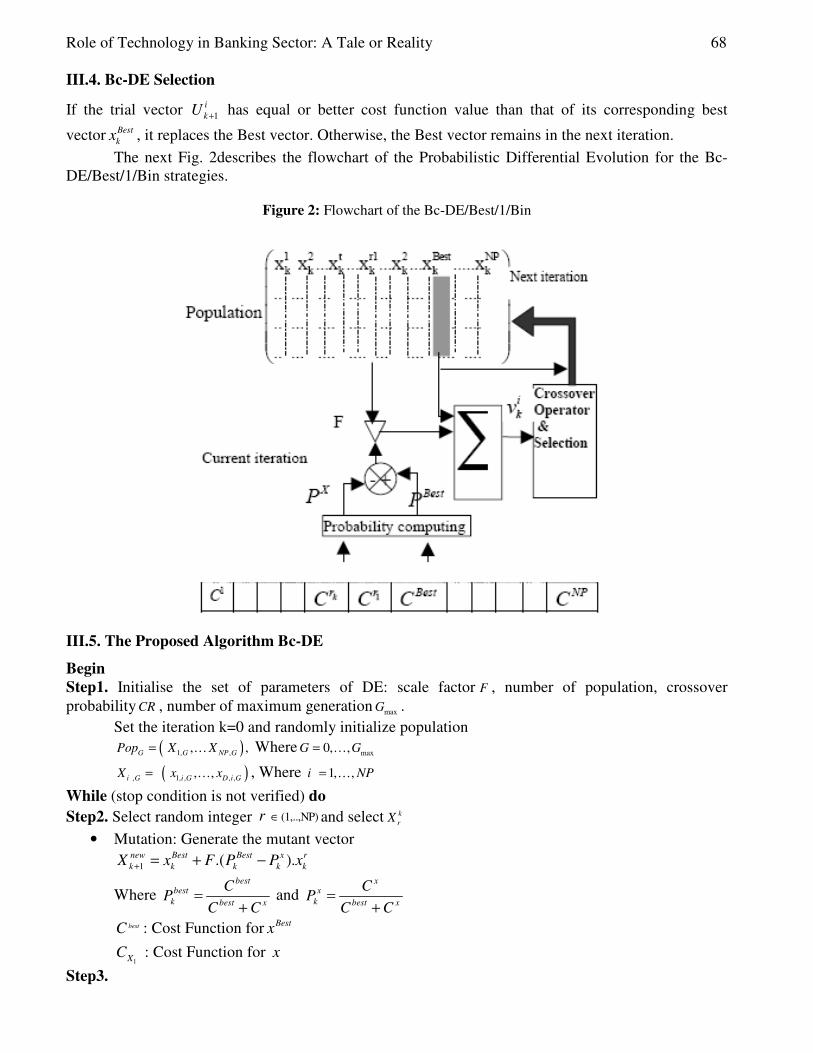
Role of Technology in Banking Sector: A Tale or Reality 68
III.4. Bc-DE Selection
If the trial vector 1ikU + has equal or better cost function value than that of its corresponding best
vector Bestkx , it replaces the Best vector. Otherwise, the Best vector remains in the next iteration.
The next Fig. 2describes the flowchart of the Probabilistic Differential Evolution for the Bc-DE/Best/1/Bin strategies.
Figure 2: Flowchart of the Bc-DE/Best/1/Bin
III.5. The Proposed Algorithm Bc-DE
Begin
Step1. Initialise the set of parameters of DE: scale factor F , number of population, crossover probability CR , number of maximum generation maxG .
Set the iteration k=0 and randomly initialize population ( )1, , , ,G G NP GPop X X= … Where max 0, ,G G= …
( ) , 1, , , , , ,i G i G D i GX x x= … , Where 1, ,i NP= …
While (stop condition is not verified) do Step2. Select random integer (1,..,NP)r ∈ and select k
rX
• Mutation: Generate the mutant vector
1 .( ).new Best Best x rk k k k kX x F P P x+ = + −
Where best
bestk best x
CP
C C=
+ and
xx
k best x
CP
C C=
+
bestC : Cost Function for Bestx
1XC : Cost Function for x
Step3.

69 Seyed Ibne-Ali Jaffari, Akmal Shahzad, Asma Nazeer and Tanvir Ahmed
• Crossover: Apply the crossover operator and compute the trial vector: kiU
[ ],
1
( ) 0,1
new iki
k ik
if rand CR
Otherwise
XU
x+
≤=
Where CR ∈[0, 1]. Step6. The selection between the trial vector and target vector is according to the following rule
1
( ) ( )
( ) ( )
i i ik k ki
k i i ik k k
U i f L U L XX
X i f L U L X+
≤=
≥
Step7. Assuming that the error E is to be minimized, the vector with the lower E value wins a place in the next generation’s population. As a result, all the individuals of the next generation are as good as or better than their counterparts in the current generation. End While ( If maximum number of generation is reached
( )max k G= )
IV. Results and Discussion To validate the effectiveness of our proposed algorithm, we have conducted extensive computer simulations on many benchmark numerical functions frequently used to evaluate and compare optimization algorithms. These functions have two problems:
• The global optimum remains at the middle of the search range. • The local optima is located into the coordinate axes or no linkage between the
variables/dimensions exists. We evaluate four algorithms including the proposed Bc-DE algorithm to minimize possibly the
benchmark numerical functions. The maximum number of function evaluations FEs is set to 500 000 . All experiments were run 50 times, independently. The four algorithms in comparison are listed as follows:
• DE/RAND-BEST/1/BIN 0.9, 0.5F CR= =
• DE/RAND-BEST/1/BIN 0.1, 0.5F CR= =
• BC-DE/RAND-BEST/1/BIN 0.9, 0.5F CR= =
• BC-DE/RAND-BEST/1/BIN 0.1, 0.5F CR= = 1. Rosenbrock's Valley (De Jong's )
Rosenbrock's valley is a standard optimization problem, also it is famed as Banana function. The global optimum is within a long, narrow, parabolic shaped flat valley. To find the valley is trivial, however convergence to the global optimum is difficult and hence this problem has been repeatedly used in assess the performance of optimization algorithms. Function Definition
12 2 2
11
( ) 100 * ( ) (1 )n
i i ii
f x x x x−
+=
= − + −∑ (9)
2.048 2.048ix− ≤ ≤
Global Minimum
( ) 0; ( ) 1, 1f x x i i n= = = …

Role of Technology in Banking Sector: A Tale or Reality 70
2. Rastrigin's Function
Rastrigin's function is based on function 1 with the addition of cosine modulation to produce many local minima. So, the test function is highly multimodal and the location of the minima are regularly distributed. Function Definition
2
1
( ) 10 * ( 10 * cos(2 * * ))n
i ii
f x n x xπ=
= + −∑ (10)
5.12 5.12ix− ≤ ≤
Global Minimum
( ) 0; ( ) 0, 1f x x i i n= = = … 3. Schwefel's Function
Schwefel's function is deceptive in that the global minimum is geometrically distant, over the parameter space, from the next best local minima. Therefore, the search algorithms are potentially prone to convergence in the wrong direction. Function Definition
( )1
( ) * sinn
i ii
f x x x=
= −∑ (11)
500 500ix− ≤ ≤
Global Minimum
( ) * 418.9829; ( ) 420.9687, 1 .f x n x i i n= − = = … 4. Six-Hump Camel Back Function
The 2-D Six-hump camel back function is a global optimization test function. Within the bounded region are six local minima, two of them are global minima. Function Definition
2 4 / 3 21 1 1 1 2
2 22 2
( 1, 2 ) (4 - 2 .1 * ) * *
(-4 4 * )·
S ixhf x x x x x x x
x x
= + +
+ +
(12)
1 2-3 3, - 2 2.x x≤ ≤ ≤ ≤
Global Minimum
1 2
1 2
-1.0316;
(-0.0898, 0.7126), (0.0898, -0.7126)
( , )
( , ) .
f x x
x x
=
=
5. Griewangk's Function
Like Rastrigin's function, Griewangk’s function has many widespread local minima and the location of the minima is regularly distributed.

71 Seyed Ibne-Ali Jaffari, Akmal Shahzad, Asma Nazeer and Tanvir Ahmed
Function Definition 2
1 1
( ) c o s ( ) 14 0 0 0
nni i
i i
x xf x
i= =
= − +∑ ∏ (13)
600 600ix− ≤ ≤
Global Minimum
( ) ( )0; 0, 1 .f x x i i n= = = …
6. Shaffer Function
Schaffer function is a symmetric multimodal function with concentric torus ridges of different heights. This function has many local optimizations and is often used in optimisation tests. Function Definition
2
1
2 2
1
(s in ) 0 .5
( ) 0 .5(1 0 .001 * ( ))
n
ii
n
ii
x
f xx
=
=
−
= +
+
∑
∑
(14)
Global Minimum
( ) 0; ( ) 0, 1f x x i i n= = = … Fig3-8 show the evaluation of all the objective functions presented above by plotting the
convergence characteristics in terms of the best fitness value of the median run of each algorithms.
• DE/RAND-BEST/1/BIN 0.9, 0.5F CR= =
• DE/RAND-BEST/1/BIN 0.1, 0.5F CR= =
• BC-DE/RAND-BEST/1/BIN 0.9, 0.5F CR= =
• BC-DE/RAND-BEST/1/BIN 0.1, 0.5F CR= =
Moreover, the convergence plot of DE/rand-Best/1/Bin 0.9, 0.5F CR= = ,DE/rand-Best/1/Bin 0.1F = 0.5CR = , Bc-DE/rand-Best/1/Bin 0.9, 0.5F CR= = and Bc-DE/rand-Best/1/Bin
0.1, 0.5F CR= = shows that the Bc-DE 0.9, 0.5F CR= = and Bc-DE/rand-Best/1/Bin 0.1, 0.5F CR= = at all times converge faster than others on six problems. From these curves, we can deduce that our proposed approach Bc-DE successfully solve all functions in each run and shows better convergence.
By applying Bc-DE algorithm, the small F ( 0.1F = ) value is an efficient value to optimize Rastrigin's function while It is not a suitable value to optimize Rosenbrock''s function. On the other side, both Bc-DE/rand-Best/1/Bin 0.9, 0.5F CR= = and Bc-DE/rand-Best/1/Bin 0.1,F = 0.5CR = algorithms present the same convergence graph in Griewangk's and Schwefel's function. While it is a bit slower than DE/rand-Best/1/Bin 0.9, 0.5F CR= = to find the optimal solutions in Six-hump camel back’s function
Figure 3: Convergence plot of Rosenbrock''s function
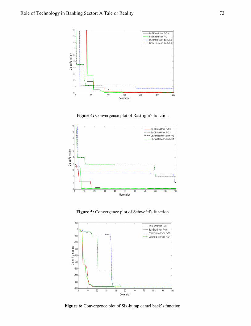
Role of Technology in Banking Sector: A Tale or Reality 72
0 50 100 150 200 250 3000
1
2
3
4
5
6
7
8
9
10
Generation
Co
st
Fu
nc
tio
n
Bc-DE/rand/1/bin F=0.9
Bc-DE/rand/1/bin F=0.1
DE/rand-to-best/1/bin F=0.9
DE/rand-to-best/1/bin F=0.1
Figure 4: Convergence plot of Rastrigin's function
0 10 20 30 40 50 60 70 80 90 1000
1
2
3
4
5
6
7
8
9
10
Generation
Co
st
Fu
nc
tio
n
Bc-DE/rand/1/bin F=0.9
Bc-DE/rand/1/bin F=0.1
DE/rand-to-best/1/bin F=0.9
DE/rand-to-best/1/bin F=0.1
Figure 5: Convergence plot of Schwefel's function
0 10 20 30 40 50 60 70 80 90 100-900
-800
-700
-600
-500
-400
-300
-200
-100
0
100
Generation
Co
st
Fu
nc
tio
n
Bc-DE/rand/1/bin F=0.9
Bc-DE/rand/1/bin F=0.1
DE/rand-to-best/1/bin F=0.9
DE/rand-to-best/1/bin F=0.1
Figure 6: Convergence plot of Six-hump camel back’s function
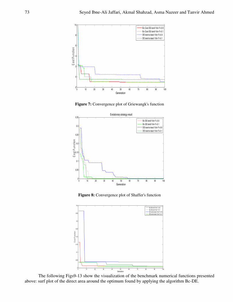
73 Seyed Ibne-Ali Jaffari, Akmal Shahzad, Asma Nazeer and Tanvir Ahmed
0 10 20 30 40 50 60 70 80 90 100-2
0
2
4
6
8
10
Generation
Co
st
Fu
nc
tio
n
Bc-Cost-DE/rand/1/bin F=0.9
Bc-Cost-DE/rand/1/bin F=0.1
DE/rand-to-best/1/bin F=0.9
DE/rand-to-best/1/bin F=0.1
Figure 7: Convergence plot of Griewangk's function
0 10 20 30 40 50 60 70 80 90 1000
0.05
0.1
0.15
0.2
0.25
0.3
0.35
Generation
Co
st
Fu
nc
tio
n
Evolutionary strategy result
Bc-DE/rand/1/bin F=0.9
Bc-DE/rand/1/bin F=0.1
DE/rand-to-best/1/bin F=0.9
DE/rand-to-best/1/bin F=0.1
Figure 8: Convergence plot of Shaffer's function
0 10 20 30 40 50 60 70 80 90 1000
0.05
0.1
0.15
0.2
0.25
0.3
0.35
0.4
Generation
Co
st
Fu
nc
tio
n
Bc-DE/rand/1/bin F=0.9
Bc-DE/rand/1/bin F=0.1
DE/rand-to-best/1/bin F=0.9
DE/rand-to-best/1/bin F=0.1
The following Figs9-13 show the visualization of the benchmark numerical functions presented
above: surf plot of the direct area around the optimum found by applying the algorithm Bc-DE.
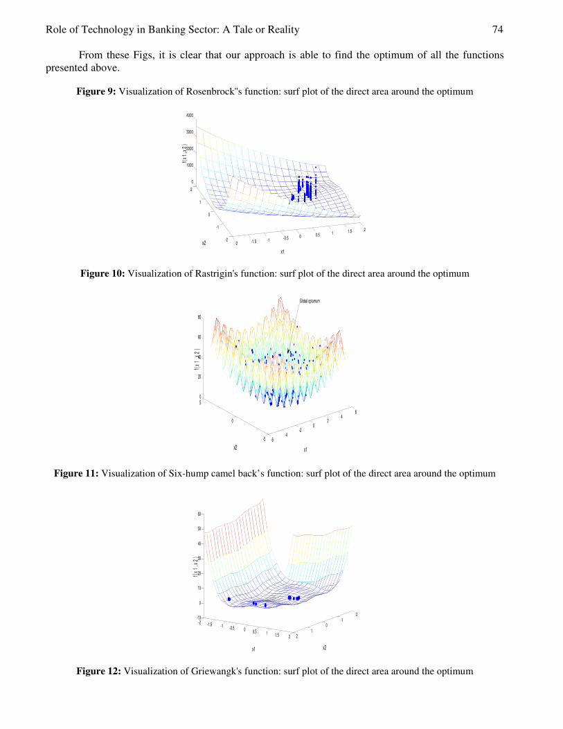
Role of Technology in Banking Sector: A Tale or Reality 74
From these Figs, it is clear that our approach is able to find the optimum of all the functions presented above.
Figure 9: Visualization of Rosenbrock''s function: surf plot of the direct area around the optimum
-2 -1.5 -1 -0.5 0 0.5 1 1.5 2
-2
-1
0
1
2
0
1000
2000
3000
4000
x1
x2
f(x
1,x
2)
Figure 10: Visualization of Rastrigin's function: surf plot of the direct area around the optimum
-6-4
-20
24
6
-5
0
50
20
40
60
80
x1x2
f(x
1,x
2)
Global optumum
Figure 11: Visualization of Six-hump camel back’s function: surf plot of the direct area around the optimum
-2 -1.5 -1 -0.5 0 0.5 1 1.5 2
-2-1
01
2
-10
0
10
20
30
40
50
60
x2x1
f(x
1,x
2)
Figure 12: Visualization of Griewangk's function: surf plot of the direct area around the optimum

75 Seyed Ibne-Ali Jaffari, Akmal Shahzad, Asma Nazeer and Tanvir Ahmed
-1.5-1
-0.50
0.51
-1-0.5
00.5
11.5
0
0.1
0.2
0.3
0.4
0.5
0.6
0.7
x1x2
f(x
1,x
2)
Figure 13: Visualization of Shaffer's function: surf plot of the direct area around the optimum
-10
-5
0
5
10
-10-8-6-4-20246810
0
0.2
0.4
0.6
0.8
1
x2x1
f(x
1,x
2)
V. Practical Exemple In this section, we will try to improve our proposed method by applying the Bc-DE such as a learning algorithm to train neural network for non linear system identification. V.1. Problem Formulation
A majority class of nonlinear dynamic systems with an input u and an output y can be described in discrete time by the NARX (nonlinear autoregressive with exogenous input) input–output model:
( ) ( )( ) 1 y k f x k+ = (15)
Where ( 1) y k + denotes the output predicted at the future time instant 1k + and ( )x k is the regressor vector, consisting of a finite number of past inputs and outputs:
( ) ( ) ( - 1) ( ) ( - 1)T
y ux k y k y k n u k u k n = … + … + (16)
Where n y and nu :the dynamic order of the system
The problem of nonlinear system identification is to deduce the unknown function f in (1) from
some sampled data sequences {( ( ), ( ))}u k y k where 1, 2, , k N= … . In black-box modeling, these functions are approximated by some general function
approximators such as neural networks, neuro-fuzzy systems, etc… The neural network NARX model is described in the Fig. 14
Figure 14: Neural Network NARX model

Role of Technology in Banking Sector: A Tale or Reality 76
u(k)
y(k+1)
Unit delay
The objective of learning is to reduce the error signal ( )k nε so that the desired response will be
close to the actual response ( )k nε at the output of neuron k at iteration n is defined by:
( ) ( ) ( )k k kn x n y nε = − (17)
Where ( )xk n refers to the desired response for neuron k and is used to
compute ( )k nε and ( )ky n refers to the function signal appearing at the output of neuron k at iteration n.
The total error is obtained by summing 212
( )j
nε over all neurons in the output layer. We may thus
write
2
1
1( ) ( )
2
N
k
E n nkε=
∑= (18)
Where N is the total number of all output nodes, The net input to the thj node of layer L is obtained by:
1, *L L L
j j k kk
n et w y −= ∑ (19)
Where ,Lj kw : the weight on the connection from the thi node in layer L-1 to the thj node in layer
L. The activation of a node Lky is defined by a function of its net input:
( )L L
k jy f c t n e t= (20)
Where fct is any activation function As mentioned above, there are different learning algorithms to train neural network. In our
work, we used our proposed approach Bc-DE such as a leaning algorithm to yield a computationally efficient algorithm for training neural network.
Fig.15 describes the concept of NN+Bc-DE strategy for nonlinear system identification.
Figure 15: Principe of NN+ Bc-DE strategy for nonlinear system identification
Network
generator
Mutation
Crossover
Selection
MSE
evaluation
Replacement
process
Population
evolution
In the training process, both the input vector u and the output vector y are known, and the synaptic weights in W are adapted to obtain appropriate functional mappings from the input u to the output y.

77 Seyed Ibne-Ali Jaffari, Akmal Shahzad, Asma Nazeer and Tanvir Ahmed
By using Matlab, there were several training algorithms in the Neural Netwok model, which have a variety of different computation but it does not exist an algorithm which is best suited. In our work, we try to implement our system by using a novel learning method, Bc-DE algorithm, to the weight optimization..
The optimization goal is to minimize the objective function Eby optimizing the values of the network weights W , so a desired correspondence between inputs and outputs of the NN is achieved. V.2. The Proposed Algorithm
Step1. Initialize a population of constant size that consists of NP, real- value vectors, ,i GW , where i
is index to the population and G is the generation to which the population belongs. PopG=( W1,G,…….,WNP,G), Where G=0,………,Gmax
In network training, each vector contains D network weights (chromosomes of individuals): Wi ,G = ( w1,i,G ,……….w D,i,G ), Where i =1,…NP
Step2. The mutant vector is generated as follows:
, , 1 , , , ,.( ).Best xj i G j Best G k k j r Gv W F P P W+ = + −
Where best
bestk best W
CP
C C=
+ and
WW
k best W
CP
C C=
+
bestC : Cost Function for Bestx
WC : Cost Function for W
Where i≠ r∈{1,….NP} randomly selected , j = 1,……D , F∈[0, 1] Step3. Apply crossover to found trial vector
, , 1
, , 1, , ,
[0,1)
j i G j
j i Gj i G
if rand CR
otherwise
vt
W
+
+
≤=
Where CR∈[0, 1]. Step6. The selection between the trial vector and target vector is according to the following rule
, , 1 , , 1 ,
, 1,
( , ( , )) ( , ( , ))
j i G j i G i G
i Gi G
if E y f x t E y f x W
otherwise
tW
W
+ +
+
≤=
Step7. Assuming that the error E is to be minimized, the vector with the lower E value wins a place in the next generation’s population. As a result, all the individuals of the next generation are as good as or better than their counterparts in the current generation.
V.3. Results and Discussion
To validate the effectiveness of our proposed algorithm, we have conducted extensive computer simulations on NARX model identification problems. The simulation results are compared with the NN algorithm.
The NARX input–output model to be identified is expressed by: ( 1) 0.3 ( ) 0.6 ( 1) 0.6 cos( ( ))
0.3 cos(3 ( )) 0.1cos(5 ( ))
p p py k y k y k u k
u k u k
π
π π
+ = + − +
+ +
Where yp(k) is the output of the system at the k-th time step and u(k) is the plant input
2( ) cos( )
250
ku k
π=
Fig.16 show the actual output, ( )y k and identified plant output trained with conjugate gradient
algorithm within the time step of 0 to 500. From this figure, we can interpret that the algorithm is poor to identify the nonlinear system

Role of Technology in Banking Sector: A Tale or Reality 78
Figure 16: Output of the plant and of the identification model trained with only NN.
0 50 100 150 200 250 300 350 400 450 500-10
-5
0
5
Time
y(k
)
y(k)
NN
Fig.17 show the actual output, ( )y k and identified plant output trained with our proposed Bc-
DE algorithm. This result indicates that our proposed method provides better system identification performance in terms of identification capability. From this it is clear that the Bc-DE approach exhibits better identification ability compared to NN approach.
Figure 17: Output of the plant and of the identification model trained with Bc-DE.
0 50 100 150 200 250 300 350 400 450 500-10
-5
0
5
Time
y(k
)
y(k)
NN+Bc-DE
Fig.18 show the error between the actual and identified model for both the identification scheme.
Figure 18: Comparison of error (NN) and error (NN+Bc-DE)

79 Seyed Ibne-Ali Jaffari, Akmal Shahzad, Asma Nazeer and Tanvir Ahmed
0 50 100 150 200 250 300 350 400 450 5000
1
2
3
4
5
6
7
Time
Err
or
Erreur(NN+Bc-DE)
Erreur(NN)
We can see from Fig.18, the convergence of the proposed method is not only faster than other method but also much more stable. TableII summaries the performance of the proposed method for Non Linear System Identification. Table II: Comparaison of performance of two methods
Method Mean Squared Error (MSE) Time of convergence
NN 6.8389 243 NN+Bc-DE 0.0820 48
The results have revealed that Bc-DE algorithm has given quite promising results in terms of
time of convergence and smaller mean squared error (MSE) compared to NN algorithm. VI. Conclusion In this paper, we presented a new heuristic variant of the differential evolution algorithm, Based cost differential evolution (Bc-DE), to choose mutant vector strategy. Our proposed algorithm generated the mutant vector by adding a weighted difference of two probabilistic cost function multiplied by a vector selected randomly to the best individual vector. The performance of the Bc-DE algorithm is broadly evaluated on several bound-constrained nonlinear and non-differentiable continuous numerical optimization problems and compares with the conventional DE and several others DE variants. It is demonstrated that the new method converges faster and with more certainty than many other acclaimed global optimization methods. The new method is robust, easy to use, and presents a good compromise between the simplicity of use and the quality of proposed solutions in a reasonable computing time. Finally, we tried to improve our proposed method by applying the Bc-DE such as a learning algorithm to train neural network for non linear system identification. The Bc-DE algorithm is able to undertake local search with a fast convergence rate. From the simulation study it has been found that this method converges to the global optimum. Acknowledgements This work is partially supported by Laboratory of Automatic Image and Signal Processing (ATSI) in National Engineering School of Monastir, Tunisia .The authors also gratefully acknowledges the helpful comments and suggestions of the reviewers, which have improved the presentation.

Role of Technology in Banking Sector: A Tale or Reality 80
References [1] H. A, Abbass “ The Self-Adaptive Pareto Differential Evolution Algorithm” Proceedings of the
Congress on Evolutionary Computation. Vol. 1, IEEE Press, 2002, pp. 831-836 [2] S.Hajri, N.Liouane, S. Hammadi, P. Borne, ”A controlled genetic algorithm by fuzzy logic and
belief functions for job-shop scheduling, IEEE Transactions on Systems, Man and Cybernetics. Volume 30, 2000, pp. 812-818.
[3] C. S.,Chan and Xu, D. Y., ” Diferential Evolution of Fuzzy Automatic Train Operation for Mass Rapid Transit System”. IEEE Proceedings of Electric Power Applications Vol. 147, 2000, pp. 206-212
[4] R.Storn, “Differential evolution design of an IIR-filter” Proceedings of IEEE International Conference on Evolutionary Computation ICEC'96. IEEE Press, 1996, pp. 268-273
[5] Qing, A., “Dynamic Differential Evolution Strategy and Applications in Electromagnetic Inverse Scattering Problems”, IEEE Transactions on Geoscience and Remote Sensing, Vol. 44, No. 1, 2006, pp. 116-125.
[6] T., Rogalsky, R.W., Derksen, S., Kocabiyik, “Differential Evolution in Aerodynamic Optimization” Proceedings of the 46th Annual Conference of the Canadian Aeronautics and Space Institute, 1999. pp. 29-36
[7] H. Liouane, A.Douik, H.Messaoud,”Design of Optimized State Feedback Controller Using ACO Control Law for Nonlinear Systems Described by TSK Models”, Studies in Informatics and Control.
[8] E.Mezura-Montes, J.Vel´azquez-Reyes,C.A.C.Coelho “Modified Differential Evolution for Constrained Optimization” IEEE Congress on Evolutionary Computation, 2007,pp. 25-32,2006.
[9] T.,Rogalsky, R.W.,Derksen, S.,Kocabiyik, “Differential Evolution in Aerodynamic Optimization” Proceedings of the 46th Annual Conference of the Canadian Aeronautics and Space Institute,1999, pp. 29-36
[10] R.Storn and K. Price, “Differential evolution-a simple and efficient adaptive scheme for global optimization over continuous spaces,”TR-95-012, 1995
[11] K.V.Price,”An introduction to differential evolution,” in New Ideas in Optimization, D. Corne, M. Dorigo, and F. Glover, Eds. London,U.K.: McGraw-Hill, 1999, pp. 79–108.
[12] R.Gämperle, S. D. Müller, and P. Koumoutsakos, “A parameter study for differential evolution,” in Advances in Intelligent Systems, Fuzzy Systems, Evolutionary Computation, A. Grmela and N. E. Mastorakis,Eds. Interlaken, Switzerland: WSEAS Press, 2002, pp. 293–298.
[13] J. Rönkkönen, S. Kukkonen, and K. V. Price, “Real-parameter optimization with differential evolution,” in Proc. IEEE Congr. Evolut.Comput., Edinburgh, Scotland, Sep. 2005, pp. 506–513.
[14] J. Liu and J. Lampinen, “A fuzzy adaptive differential evolution algorithm,”Soft Comput., vol. 9, no. 6, pp. 448–462, Apr. 2005. .
[15] A. K. Qin and P. N. Suganthan, “Self-adaptive differential evolution algorithm for numerical optimization,” in Proc. IEEE Congr. Evolut Comput., Edinburgh, Scotland, Sep. 2005, pp. 1785–1791.
[16] D. Zaharie, “Control of population diversity and adaptation in differential evolution algorithms,” in Proc. Mendel 9th Int. Conf. Soft Comput.,R. Matousek and P. Osmera, Eds., Brno, Czech Republic, Jun. 2003pp. 41–46.
[17] H. A. Abbass, “The self-adaptive Pareto differential evolution algorithm,”in Proc. Congr. Evolut. Comput., Honolulu, HI, May 2002, pp.831–836.
[18] J. Teo, “Exploring dynamic self-adaptive populations in differential evolution,” Soft Comput., vol. 10, no. 8, pp. 637–686, 2006.

81 Seyed Ibne-Ali Jaffari, Akmal Shahzad, Asma Nazeer and Tanvir Ahmed
[19] J. Brest, S. Greiner, B. Boskovic, M. Mernik, and V. Zumer, “Self-adapting control parameters in differential evolution: A comparative study on numerical benchmark problems,” IEEE Trans. Evolut Comput., vol. 10, no. 6, pp. 646–657, Dec. 2006
[20] A. K. Qin, V. L. Huang, and P. N. Suganthan,” Differential Evolution Algorithm With Strategy Adaptation for Global Numerical Optimization”, IEEE Trans. Evolut Comput., vol. 13, no. 2, april 2009.
[21] D. Zaharie and D. Petcu, “Adaptive pareto differential evolution and its parallelization,” in Proc. 5th Int. Conf. Parallel Process. Appl. Math.,Czestochowa, Poland, Sep. 2003, pp. 261–268.
[22] S. Das, A. Konar, and U. K. Chakraborty, “Two improved differential evolution schemes for faster global search,” in ACM-SIGEVO Proc Genetic. Evolut. Comput. Conf., Washington, DC, pp. 991–998.
[23] U. K. Chakraborty, S. Das, and A. Konar, “Differential evolution with local neighborhood,” in Proc. Congr. Evolut. Comput., Vancouver, BC, Canada, 2006, pp. 2042–2049.
[24] M. G. H. Omran, A. Salman, and A. P. Engelbrecht, “Self-adaptive differential evolution,” in Lecture Notes in Artificial Intelligence. Berlin Germany: Springer-Verlag, 2005, pp. 192–199.
[25] J. Brest, B. Boskovic, S. Greiner,V. Zumer, and M. S. Maucec, “Performance comparison of self-adaptive and adaptive differential evolution algorithms,” Soft Comput., vol. 11, no. 7, May 2007, pp. 617–629.
[26] Z. Y. Yang, E. K. Tang, and X. Yao:, “Large scale evolutionary optimization using cooperative coevolution,” Inf. Sci., accepted for publication.
[27] N. Noman and H. Iba, “Accelerating differential evolution using an adaptive local search,” IEEE Trans. Evolut. Comput., vol. 12, no. 1, Feb. 2008, pp 107–125.
[28] S. Rahnamayan, H. R. Tizhoosh, and M. M. A. Salama, “Oppositionbased differential evolution,” IEEE Trans. Evolut. Comput., vol. 12, no.1, pp. 64–79, Feb. 2008.
[29] J. Sjöberg, Q. Zhang, ,L. Ljung, A. Benveniste, B. Delyon, , P.Y. Glorennec, H. Hjalmarsson, and A. Juditsky, Nonlinear black-box modeling in system identification, A unified overview. Automatica, pp.1691–1724, 1995.
[30] L. Ljung, Q.Zhang, P. Lindskog, A. Juditsky and R. Singh, , An integrated system identification toolbox for linear and non-linear models. In: Proc. 14th IFAC Symposium on System Identification. Newcastle, Australia, 2006.
[31] T. Hastie, R.Tibshirani and J. Friedman,. The Elements of Statistical Learning, Springer, 2001. [32] P. Fritzson, Object-oriented Modeling and Simulation with MODELICA 2.1. IEEE Press.
Piscataway,NJ, 2004. [33] T. Bohlin, Practical Grey-box Process Identification.Springer-Verlag. London , 2006. [34] V. Vapnik, Statistical Learning Theory. Wiley, 1998. [35] J.A.K. Suykens, T. Gestel, J De Brabanter, B. De Moor and J. Vandewalle, Least Squares
Support Vector Machines. World Scientific. Singapore and often non-parametric models such as neural networks are used in place of intricate mathematics, 2002.
[36] A.R. Barron, Statistical properteis of artificial neural networks. In: Proceedings of the 28th IEEE Conference on Decision and Control. pp. 280–285, 1989.
[37] K.S. Narendra,.and K. Parthasarathy, Identification and Control of Dynamic Systems using Neural Networks, IEEE Transactions on NNs, pp. 4-27, 1990.
[38] J.T. Connor, R.Martin, and L. Atlas, Recurrent NN and Robust Time Series Prediction. IEEE Transactions on NNs, pp. 240-253, 1994.
[39] P.S. Sastry, G. Santharam, and K.P. Unnikrishnan, Memory Networks for Identification and Control of Dynamical Systems. IEEE Transactions on NNs, pp.306-320 , 1994.
[40] D.T. Pham and S. Yildirim, Robot Control using Jordan Neural Networks. Proc. of the Internat. Conf. on Recent Advances in Mechatronics, Istanbul, Turkey, 1995.

Role of Technology in Banking Sector: A Tale or Reality 82
[41] A.C. Tsoi and A.D .Back, Locally Recurrent Globally Feedforward Networks, A Critical Review of Architectures. IEEE Transactions on NNs, pp. 229-239, 1994.
[42] Qing, A., “Dynamic Differential Evolution Strategy and Applications in Electromagnetic Inverse Scattering Problems”, IEEE Transactions on Geoscience and Remote Sensing, Vol. 44, No. 1, 2006, 116-125.
[43] H. Liouane, I.Chiha, A.Douik, H.Messaoud “Probabilistic Differential Evolution for Optimal design of LQR weighting matrices”,IEEE International Conference on Computational Intelligence for Measurement Systems and Applications, Tianjin, china, July 2012.
[44] I. Chiha, J. Ghabi and N. Liouane,” Tuning PID Controller With Multi-Objective Differential Evolution”, Proceedings of the 5th International Symposium on Communications, Control and Signal Processing,ISCCSP 2012, Rome, Italy, 2-4 May 2012.
[45] M.S RUSU, L. GRAMA, The Design Of A Dc Motor Speed Controller, Dept. Tech. Manag. Eng., Tîrgu Mures Univ.
[46] I. Chiha, H. Liouane, N.Liouane, “A Hybrid Method Based On Multi-objective Ant Colony Optimization and Differential Evolution to Design PID DC Motor Speed Controller”, International Review on Modelling and Simulations (IREMOS),Vol.5, No.2, 2012.

European Journal of Scientific Research ISSN 1450-216X / 1450-202X Vol. 99 No 1 April, 2013, pp.83-118 http://www.europeanjournalofscientificresearch.com
Role of Technology in Banking Sector: A Tale or Reality
Seyed Ibne-Ali Jaffari Assistant Professor, Business Administration Department
Federal Urdu University of Arts, Science & Technology, Islamabad, Pakistan E-mail: [email protected]; [email protected]
Akmal Shahzad
Ph.D. Scholar, Iqra University 5, Khayaban-e-Johar, Islamabad, Pakistan
E-mail: [email protected]
Asma Nazeer Lecturer, Business Administration Department
Federal Urdu University of Arts, Science & Technology, Islamabad, Pakistan E-mail: [email protected]
Tanvir Ahmed
Assistant Professor, AIOU, Islamabad E-mail: [email protected]
Abstract
Information technology not only becomes essential for individual but also gain the strategic position in business sector. No organization lives without latest technology. Banking sector has no exception to adopt new technology. Today, technology is involving every bank operation. IT has changed the operating pattern and customer behavior. This study discusses the role of technology in banking sector theoretically. This study concluded that technological development has reduced the cost and increase the efficiency. Technology has a direct relationship with IRS. These hypothesis need to be tested on empirical data. Keywords: Technology, Bank, Interest Rate Spread, Efficiency, ATM, Online Banking
1. Introduction Information Technology (IT) is necessity not a luxury, as it becomes the lifeblood for the consumer as well as organization. The term IT imparts to facilities and techniques designed to process, transfer, and store data (Pispa & Eriksson, 2003). It means IT does not comprise of computer but it consists of communication software, hardware, and networks. Rapid change in IT changes individual is life style and demands (Manardo, 2000). Ahmed et al. (2011) declared IT a major contributor in corporate globe vision, supply chain management, and to handle cultural diversification. IT has affected all sectors from manufacturing to services departments even banks cannot detach from its effect.
Banking sector is one of critical pillar of the economy whose contribution to the development and economic growth can not completely computed. Basic function of bank is to transfer capital from
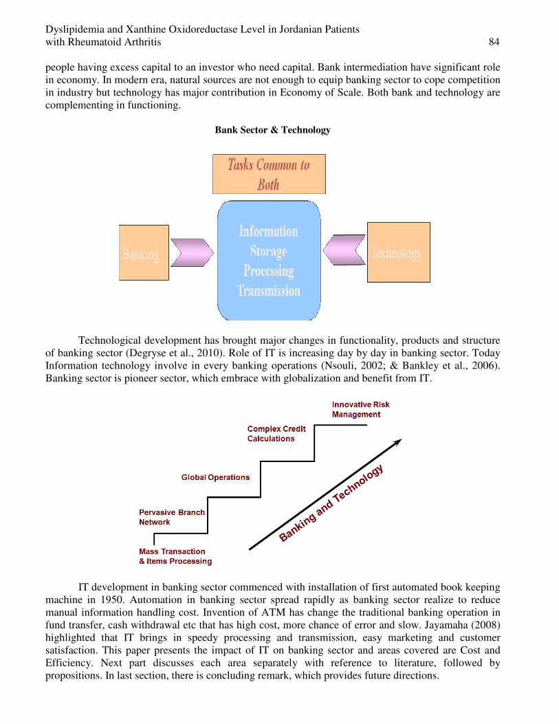
Dyslipidemia and Xanthine Oxidoreductase Level in Jordanian Patients with Rheumatoid Arthritis 84
people having excess capital to an investor who need capital. Bank intermediation have significant role in economy. In modern era, natural sources are not enough to equip banking sector to cope competition in industry but technology has major contribution in Economy of Scale. Both bank and technology are complementing in functioning.
Bank Sector & Technology
Technological development has brought major changes in functionality, products and structure of banking sector (Degryse et al., 2010). Role of IT is increasing day by day in banking sector. Today Information technology involve in every banking operations (Nsouli, 2002; & Bankley et al., 2006). Banking sector is pioneer sector, which embrace with globalization and benefit from IT.
IT development in banking sector commenced with installation of first automated book keeping machine in 1950. Automation in banking sector spread rapidly as banking sector realize to reduce manual information handling cost. Invention of ATM has change the traditional banking operation in fund transfer, cash withdrawal etc that has high cost, more chance of error and slow. Jayamaha (2008) highlighted that IT brings in speedy processing and transmission, easy marketing and customer satisfaction. This paper presents the impact of IT on banking sector and areas covered are Cost and Efficiency. Next part discusses each area separately with reference to literature, followed by propositions. In last section, there is concluding remark, which provides future directions.

85 Najah Al- Muhtaseb, Elham Al-Kaissi, Zuhair Muhi eldeen and Naheyah Al-Muhtaseb
2. Technology and Cost Technological Development (TD) puts pressure on banker to change operating pattern from manual to online. Improved technology implementation caused to reduce cost of banking operation. Technology has a well-recognized role as a strategic drive in literature (EC, 1997 and BISS, 1999). Numerous studies conducted to quantify the effect of technological change on cost. Hunter & Timme (1991) studied the large American commercial bank and found 1% per annual reduction in cost. Larger banks realized more cost reduction as compared to smaller banks. Humphery (1993) declared negative impact of technology on cost. This converse behavior attribute to the deregulation policy in America. Technological role in cost reduction is unstable. Stiroh (1997) observed significant role during 1990 to 1992 and insignificant thereafter in American Banking Sector. In contrast to earlier studies, Stiroh (n) did not find evidence that rate of technological change is associated with bank size. Mckilop et al. (1996) declared that large Japanese bank benefited more from technology than smaller banks. Like Hunter & Timme (1991) and Altunbas (1999), observed that reduction in cost with implementation of new technology and noted that bank size positively relates with the technological change. Wagenvoort & Schure (1999) modeled technological development is an efficient cost frontier for sample 2000 banks in European country by categorizing bank sector as commercial bank and saving banks. The result shows that frontier has no shift for whole sample or commercial bank but shift observes for saving bank with cost reduction of 2% per annum. Lang & Welez’s (1996) confirmed the cost reducing behavior of technological progress while studying the German cooperative banking sector. Similarly, Modus et al. (1996) studied Spanish Banking Sector to draw the same conclusion. Majority of the overall studies recognized the cost reduction behavior of technology. Although controversy still exists whether large, or small bank benefits more. In addition, does its impact increase with time? Following propositions have developed after the discussions.
Proposition 1: Larger bank benefit more than smaller bank Proposition 2: There is positive relationship between technological change and bank
3. Technology and Efficiency Financial institutions are one of largest investor in information technology according to the survey conduct in America. It has observed that banks invested in technological sector in order to improve the efficiency and customer satisfaction. Ledere & Mendelow (1988) declared technology as powerful weapon for bank to capture the market, improve service, shape new products, and reduce the cost of operation. Technology importance compels the institutions to make huge investment in IT sector. Most of banks did heavy investments in IT to transfer manual to electronic process to reduce cost (Koepp, 2000; Franke, 1987; & Martini, 1999). Technological development increases the efficiency by number of ways. Joseph et al. (1999) observed technological use in redelivery banking minimize uncertainty and highlight consumer perception about online banking. Khan (2007) argued that IT security and privacy risk which retard the consumer to adopt new technology. Developed country eliminates or minimizes this risk with invention of new communication hardware and software. Papaionnou & Dimelis (2010) results showed that implementation of new technology in OECD countries remove inefficiency. Numerous studies such as Bhasin (2001, 2008), Bajaj (1999, 2000), Janki (2006) and Clifford (1996) proved the technology role in efficiency of banking and non-banking sector. Arora & Kaur (2008) observed the positive impact of technology on bank efficiency.
Proposition 3: Technology has positive impact on bank efficiency. 3. Conclusion Technology has gain the strategic position in all sectors. New technology barriers to adoption have gradually diminished. New real time soft wares and sophisticated hardware has made the task easy and

Dyslipidemia and Xanthine Oxidoreductase Level in Jordanian Patients with Rheumatoid Arthritis 86
secure. Such developments meet the financial institution requirements, which required more secure and reliable process. This paper studies the impact of technology in banking sector. Most of bankers have recognized it as strategic tool. Literature also supports that technology does not change only traditional banking but also affect the market structure. Furthermore, technology has improved the banking efficiency while operational cost has reduced. These propositions require to be tested empirically. References [1] Ahmed, Irfan; Shahzad, Akmal; Shahzad, K.R. and Khilji, B.A (2011) Information Technology
- Its Impact on Global Management World Applied Sciences Journal 12 (7), pp 1100 -1106 [2] Altunba’, Y., J. Goddard and P. Molyneux (1999) ‘Technical change in banking’, Economics
Letters, 64, pp. 215-221 [3] Arora, S and Kaur, S (2008), “Diversification by Banks in India: What are the Internal
Determinants?” The Indian Banker, Vol. III, No.7, July 2008, pp. 37-41. [4] B. Janki, (2002), “Unleashing Employee Productivity: Need for a Paradigm Shif”', IBA [5] Bajaj, K.K (1999), E-Commerce: The Cutting Edge of Business, Tata McGraw Hill Publishing
Company Ltd, New Delhi. [6] Bajaj, K.K. (2000), “E-Commerce Issues in the Emerging HiTech. Banking Environment”, the
Journal of the Indian Institution of Bankers, Indian Institute of Bankers, Mumbai, March 2000. [7] Bankley W, Scerri M, Saloojee I (2006). Measuring Innovation in OECD and non-OECD
countries: Selected Seminar papers, Cape Town: Human Sciences Research Council. [8] Bhasin, T. M (2008), “Leveraging Technology for Business Growth: How to Increase ROI?”,
The Indian Banker, Indian Banks’ Association, Mumbai, Vol. III, No. 5, 2008, pp. 14-20. [9] Bhasin, T.M. (2001): “E-Commerce In Indian Banking”, IBA Bulletin, Vol. XXIII Nos. 4 and 5
April-May, 2001, Indian Banks’ Association, Mumbai. [10] BIS (1999). Recent Developments in International Interbank Relations (Report prepared by a
Working Group established by the Central Banks of the G10 Countries) (Basle). [11] Clifford E. Kirsch. (1996), The Financial Services Revolution: Understanding the Changing
Roles of Banks, Mutual Funds, and Insurance companies. The McGraw-Hill Publishing Company, Columbus.
[12] Frankel A.B. (1984). “Interest Rate Futures: An Innovation in Financial Techniques for the Management of Risk”, BIS Economic Papers, 12: 19-23
[13] Hans Degryse, Steven Ongena, and Günseli Tümer-Alkan, (2010) Lending technology, bank organization and competition Journal of Financial Transformation pp 24-30
[14] Humphrey, D.B., (1993), ‘Cost and technical change: effects from bank deregulation’, Journal of Productivity Analysis, 4, 9-34.
[15] Hunter, W.C. and S.G Timme (1991), ‘Technological change in large US commercial banks’, Journal of Business, 64, 339-362
[16] Khan, Saadullah (2007) Adoption Issue of Technology in Pakistani Banking Sector, Lulea University of Technology, UK, ISSN 1653 -0187
[17] Manardo, J (2000) Globalization at Internet speed, Strategy & Leadership, pp: 22-27, MCB University Press, ISSN: 1087-8572.
[18] Martins JH, Lobster M, Wyk J (1999) Marketing Research A South African Approach. Unisa Press: Pretoria
[19] Mathew Joseph, Cindy McClure, Beatriz Joseph, (1999) "Service quality in the banking sector: the impact of technology on service delivery", International Journal of Bank Marketing, Vol. 17 Issue: 4, pp.182 – 193
[20] Maudos, J., J.M. Pastor and J. Quesada, (1996), ‘Technical progress in Spanish banking: 1985-1994’, University of Valencia and IVIE Discussion Paper, WP-EC 96-06.

87 Najah Al- Muhtaseb, Elham Al-Kaissi, Zuhair Muhi eldeen and Naheyah Al-Muhtaseb
[21] McKillop, D.G., J. C. Glass and Y Marikina, (1996), ‘The composite cost function and efficiency in giant Japanese banks’, Journal of Banking and Finance, 20, 1651-1671.
[22] Pispa, J. and I.V. Eriksson, (2003) Aligning organizations and their information technology infrastructure: how to make information technology support business, Production Planning & Control, 14(2): 193-200, ISSN: 1366-5871
[23] Sophia p. Dimelis and sotiris k. Papaioannou (2010) Technical efficiency and the role of information technology: a stochastic production frontier study across OECD countries. Centre for planning and economic research no 109
[24] Stiroh, K. J., (1997) ‘the evolution of an industry: US thrifts in the 1990s’, Journal of Banking and Finance, 21, pp. 1375-1394.
[25] Wagenvoort, R. and P. Schure (1999), ‘Who are Europe’s efficient bankers?’ EIB Cahiers Papers, vol. 4, No. 1, pp. 105-126.

European Journal of Scientific Research ISSN 1450-216X / 1450-202X Vol. 99 No 1 April, 2013, pp.88-118 http://www.europeanjournalofscientificresearch.com
Measurement of Airport Efficiency using
Data Envelopment Analysis
Ashok Babu. J Research Scholar, Department of Management Studies
College of Engineering, Anna University, Chennai, India E-mail: [email protected]
Jayanth Jacob
Asst .Professor (Sr. Gr), Department of Management Studies College of Engineering, Anna University, Chennai, India
E-mail: [email protected]
Udhayakumar.A Professor, Dept. of Computer Applications
Hindustan University, Chennai, India E-mail: [email protected]
Abstract
Performance evaluation has become an important aspect for airports to be sustainable in today’s highly competitive environment. Although the evaluation of airport efficiency has been approached from various perspectives, difficulties were encountered when multiple inputs and outputs related to an airport’s performance had to be considered. Data Envelopment Analysis (DEA) a linear programming based technique for measuring the relative performance of organization units has been used. Two analytical methods of DEA-CCR, DEA-BCC models are employed to estimate technical and scale efficiencies of each airport. Results show that out of 17 airports in India 8 airports operate in the frontier under BCC Model and 3 airports operate in the frontier under CCR Model. Twelve airports operate in the area of increasing returns to scale, 4 airports in constant return to scale and one airport in decreasing returns to scale. Keywords: Data Envelopment Analysis (DEA), Returns to scale, Efficiency of airports,
Airport productivity, Decision Making Units (DMU). 1. Introduction During the last two decades there has been a growing interest in measuring the performance and efficiency of airports, while the process of introducing private participation in the operations of airports has started competing with each other to increase their efficiency.
This interest has spurred the growing literature to aim at estimating the efficiency of the airport sector, through the use of Data Envelopment Analysis (DEA) methods. It is a non-parametric mathematical tool for assessing the relative efficiency of homogeneous decision making units (DMU). It has been applied in many sectors including airports, airlines and railways. The objectives of this study are to give a review of the current empirical literature on airport efficiency and productivity

89 Najah Al- Muhtaseb, Elham Al-Kaissi, Zuhair Muhi eldeen and Naheyah Al-Muhtaseb
analysis and to conduct comprehensive efficiency estimation of 17 Indian international airports which offer international and domestic services. This study focuses on domestic services. This research intends to explore the use of DEA as an instrument for investigating the performance indicator of Indian airports. The selection of the model type has been determined after a comprehensive overview of the available and suitable DEA models. In this paper, appropriate inputs and outputs describing primary airport functions are identified. Then the technical characteristics of the airports are assessed for the period from January 2011 to December 2011. Then the efficiency of airports is determined by CCR Model and BCC model and also scale efficiency is measured.
The paper is organized as follows. Section 2 presents the literature review. Section 3 gives an overview of the DEA models. Section 4 describes the methodology and data collected. Section 5 brings out the empirical results and finally Section 6 presents conclusions and suggests recommendations for the future research in the area. 2. Literature Review The chapter reviews previous work directly related to airport productivity. In the field of productivity, the concept of production functions provides an input–output relationship. From the output orientation, a production function shows the maximum output rate that can be achieved from a specified usage rate of inputs. From the input orientation, the production function shows the minimum input usage rate that can produce a specified output rate. Efficiency can then be measured relative to the frontier defined by the production function. Two basic approaches used for calculating efficiency are the parametric and nonparametric approaches. The parametric approach requires an assumption on the functional form of the relationship between inputs and outputs while the nonparametric approach does not require any assumption on the functional form. The vast majority of the studies measuring efficiency of airports have used non-parametric methods to assess the level of efficiency, particularly DEA. This study uses non- parametric approach by Data Envelopment Analysis.
In 1978, Charnes et al developed a tool called Data Envelopment Analysis (DEA) to measure efficiency. DEA was later extended to include variable returns to scale by Banker, Charnes, and Cooper (1994). Some key characteristics of DEA are summarized below:
• DEA is used to measure the efficiency of homogeneous units called decision making units (DMUs), which consume the same type of inputs and produce the same type of outputs.
• DEA is a nonparametric approach; hence, there is no restriction on the functional form that relates inputs to outputs. DEA generalizes the concept of the single-input, single-output technical efficiency measure of Farrell to the multiple-input and multiple-output case by computing a relative efficiency score as a ratio of a virtual output to a virtual input. Specifically, efficiency is defined as a ratio of a weighted sum of outputs to a weighted sum of inputs.
• DEA is an approach focused on frontiers instead of central tendencies. It evaluates the efficiency of each DMU relative to similar DMUs
The DEA models use the optimization method of mathematical programming to generalise the Farrell (1957) single output/input technical efficiency measure to the multiple output/input case. DEA began as a new management tool for technical efficiency analyses of Decision Making Units (DMU). In the airport sector, researchers started using DEA in the late 1990s. Gillen and Lall (1997) applied DEA to assess the performance of 23 US airports over 1989-1993. Murillo et al (1999) applied DEA to assess the performance of 33 Spanish civil airports. Parker (1999) used DEA to study technical efficiency of the British airport before and after privatization and found that privatization had no noticeable impact on technical efficiency. Sakris (2000) used to evaluate the operational efficiencies of 44 major US airports from 1990 to 1994. Martin and Roman (2001) employed DEA to evaluate the performance of 37 Spanish airports in 1997. Fernandez and Pacheco (2002) used DEA to evaluate capacity efficiency of 35 Brazilian airports in 1998. Pels et al (2001) used DEA to evaluate the

Dyslipidemia and Xanthine Oxidoreductase Level in Jordanian Patients with Rheumatoid Arthritis 90
performance of 34 European airports from 1995-1997. Pathomsiri et al (2005) employed DEA to evaluate 72 airports in multiple airport system worldwide. Barros et al (2007) found fully and partially privatised airports are more efficient than publicly owned airports. Malighetti et al (2007) studied the Italian airports efficiency by the DEA method results were that large airports are more efficient than domestic and regional ones. Lam et al (2009) analysed various dimensions of operating efficiencies in major Asia Pacific airports through DEA models accounting for external factors. Assaf (2010) used DEA to evaluate the performance of 27 small and large UK airports. Numerous studies shown in Table
1 evidently confirms that DEA has been a widely utilized method in the literature on airport efficiency and productivity. Table 1: Lists of Publications on airport productivity studies using DEA
Author(s) Sample Year Model Input Output
Gillen and Lall (1997) Year: 1989-1993 Size: 23 of the top U.S. airports
DEA-Output-CRS DEA-Output-VRS
A. Terminal service 1.number of runways 2.number of gates 3.terminal area 4.number of employees 5.number of baggage collection belts 6.number of public parking spaces B. Movements 1.airport area 2.number of runways 3.runway area 4.number of employees
A. Terminal services 1.number of passengers 2.pounds of cargo B. Movements 1.air carrier movements 2.commuter movements
Murillo- Melchor (1999)
Year: 1992-1994 Size:33 Spanish civil airports under management of AENA (Spanish Airports and Air Transport)
DEA-Input –CRS DEA-Input-VRS
1.number of workers 2.accumulated capital stock 3.intermediate expense
1.number of passengers
Parker (1999)
Year: financial year (as of March 31) from 1988/89-1996/97 Size : 22UK Airports, including all of British Airport Authority (BAA)’s major airport
DEA-Input-VRS
1.employment 2.capital stock 3.non labour cost 4.capital cost 5.changes in gross domestic product (GDP)
1.number of passenger 2.cargo and mail
Salazar De la Cruz (1999)
Year: 1993-195 Size: 16 main Spanish airport service mixed domestic and international
DEA-Output-CRS
1.total economic cost e.g. cost for annual operations, current costs and internal interest on the net assets
1.annual passengers 2.total return 3.returns on infrastructure service 4. operative returns 5.final returns

91 Najah Al- Muhtaseb, Elham Al-Kaissi, Zuhair Muhi eldeen and Naheyah Al-Muhtaseb
Graham, A and Holvad, T (2000)
25 European and 12 Australian airports
DEA(CCR and BCC;FDH) and Partial Performance
1. Number of employees 2.capital costs 3. other op.costs
1.number of passengers
Table 1: Lists of Publications on airport productivity studies using DEA (Contnd...)
Sarkis (2000) Year: 1990-1994 Size:44 major US airports
DEA-Input-CRS DEA-Input-VRS
1.operating cost 2.number of airport employees 3.number of gates 4.number of runways
1.operational revenue 2.number of passenger 3.aircraft movement 4.general aviation movements 5.amount of cargo shipped
Fernandes and Pacheco (2001)
Year: 1998 Size: 35 Brazilian Domestic airports
DEA- Non oriented CRS
1.mean number of employees 2.payroll expenditure include direct and indirect benefits 3.operating expenditure 4.apron area 5.depature lounge area 6.number of check-in counters 7.length of curb frontage 8.number of vehicle parking spaces 9.bagges claim area
1.number of passengers 2.cargo plus mai 3.operating revenues 4.commerical revenues 5.other revenues
Martin and Roman (2001)
Year: 1997 Size:37 Spanish airports
DEA- Output-VRS DEA- Output-CRS
1.labour expense 2.capital expense, including amortization of fixed assets 3.material expense
1.air traffic movements 2.number of passengers 3.tonnage of cargo
Pels, Nijkamp and Rietveld (2001)
Year: 1995-1997 Size: 34 European airports
Air Transport Movement (ATM) mode DEA- Input-CRS DEA- Input-VRS Air Passenger Movement (APM) model
1. airport area 2.runway length 3.number of aircraft parking positions at the terminals 4.number of remote aircraft parking positions 1.terminal area 2.number of aircraft parking positions at the terminal 3.number of remote aircraft parking position 4.number of check-in desk 5.number of baggage claim units
1.Air transport movement (ATM) 1.Air passenger Movements (APM)
Yu,M-M. (2001) 14 domestic Taiwanese airports
DEA (directional output distance function with window
1.runway area 2.apron area 3.terminal area
Desirable: 1.number of ATM 2. number of

Dyslipidemia and Xanthine Oxidoreductase Level in Jordanian Patients with Rheumatoid Arthritis 92
analysis with 2 years window)
4. number of connection with other domestic airports
passenger Undesirable: 1.aircraft noise
Table 1: Lists of Publications on airport productivity studies using DEA(Contnd...)
Abbott and Wu (2002)
Year: 1989/1990 to 1999/2000 Size: 12 main Australian Airports Year: 1998/1999 Size: 12 main Australian and 13 other international airports
DEA- Input-CRS DEA- Input-CRS
1.number of staff 2.capital stock 3.runway length 1.number of staff 2.runway length 3.land area 4.number of aircraft standing area
1.number of passengers 2.frieght charge in tons 1.number of passengers 2. freight cargo in tons
Fernandes And Pacheco (2002)
Year:1998 Size: 33 Brazilian major domestic airports
DEA- Output-VRS
1.area of apron 2.area of departure longue 3.number of check-in counters 4.length of frontage curb 5.number of parking spaces 6.baggage claim area
1.domestic passengers
Bazargan and Vasigh (2003)
Year: 1996-2000 Size: Top 45 U.S airports, 15 each from large, medium and small hubs
DEA- Input-CRS
1.operating expenses 2.non-operating expenses 3.number of runways 4.number of gates including gates with jet ways and non-jet ways gates
1.number of passengers 2.air carrier operations 3.number of commuters, GA and military 4.aeronautical revenues 5.non-aeronautical revenues 6.percentage of on-time operations
Pacheco and Fernandes (2003)
Year:1998 Size: 35 Brazilian domestic airports
DEA- Input-VRS
1.average number of employees 2.payroll, including direct and indirect benefits 3.operating expenses
1.domestic passenger 2.cargo plus mai 3.operating revenues 4.commercial revenues 5.other revenues
Chi-Lok, A.and Zhang,A (2003)
25 Chinese (major) airports
DEA and Malmquist DEA
1.runway length 2.terminal size
1.number of passenger 2.cargo 3. number of ATM
Pels, Nijkamp and Rietveld (2003)
Year: 1995-1997 (pooled cross-section time series) Size: 34 European airports
Air Transport movements (ATM) model DEA- Input-CRS DEA- Input-VRS Air Passenger Movements (APM) model
1.airport area 2.number of runways 3.number of aircraft parking positions at the terminal 4.number of remote aircraft parking positions 1.ATM 2.number of check-in
1.Air Transport Movements (ATM) 1.Air Passengers Movements (APM)

93 Najah Al- Muhtaseb, Elham Al-Kaissi, Zuhair Muhi eldeen and Naheyah Al-Muhtaseb
desk 3.number of baggage claim units
Table 1: Lists of Publications on airport productivity studies using DEA(Contnd...)
Pathomsiri and Haghani (2004)
Year: 2000, 2002 Size:63 airports in multiple airport system worldwide
DEA- Output-VRS 1.land area 2.number of runways 3.area of runways
1.aircraft movement 2.number of passenger
Yoshida, Y. and Fujimoto,H. (2004)
67 Japanese airports DEA (CCR and BCC)
1.runway length 2.terminal area 3. number of employees in terminal 4.average access cost (monetary and time costs)
1.number of passenger 2.cargo 3. number of ATM
Sarkis and Talluri (2004)
Year: 1990-1994 Size: 44 major US airports
DEA- Input-CRS
1.operational costs 2.number of airport employees 3.number of gates 4.number of runways
1.operational revenue 2.passengers 3.aircraft movements 4.number of general aviation movements 5.total cargo
Fernandes and Pacheco (2005)
Year: 1998 and 2001 Size: 58 airports administered by the Brazilian Airport
DEA- Input-VRS
1.payroll, including direct and indirect benefits 2.operating and other expenses 3.average number of employees
I. Financial performance 1.operating revenues 2.commercial revenues 3.other revenues II. Operating performance 1.passengers embarked plus disembarked 2.tonnage of cargo embarked plus disembarked
Pathomsiri, Haghani and Schonfeld (2005)
Year: 2000, 2012 Size: 72 airports in multiple airport system worldwide
DEA- Outputs-VRS 1.land area 2.number of runways 3.area of runways
1.aircrafts movements 2.number of passengers
Yokomi,M. (2005) 6BAA airports Malmquist-DEA (Output max)
For Both Sides 1. number of employees 2. other op costs
Aeronautical Analysis ATM 1.Non-Aeronautical Analysis 2.non-aeronautical revenue
Lin, L.andHong.C (2006)
20 major airports
DEA(CCR and BCC; super efficiency for ranking, cross- efficiency and FDH)
1.number of employees 2. number of check in counters runway 3. number of parking spaces 4. number of baggage
1.cargo

Dyslipidemia and Xanthine Oxidoreductase Level in Jordanian Patients with Rheumatoid Arthritis 94
collection belts 5. number of aprons 6. number of gates 7.terminal area
Table 1: Lists of Publications on airport productivity studies using DEA (Contd)
Martin, J.C. and Roman, C. (2006)
34 Spanish airports
SMOP and DEA [cross-efficiency, super-efficiency for ranking (NIRS and BCC ) and Virtual – efficiency]
1.staff costs 2.capital expenditures 3.other op costs
1.number of passenger
Pacheco, R.R., Fernandez, E. and Peixoto de os,M. (2006)
58 Brazilian Airports
DEA (BCC;I input min) 1. number of employees 2.staff costs 3. other op costs
1.operating revenue 2.non- operating revenue 3.other revenue 4. number of passenger 5.cargo
Pathomsiri, Haghani, Dresner and Windle (2006)
Year: 2000-2002 Size: 72 airports in multiple airport system worldwide
DEA- Outputs-VRS 1.land area 2.number of runways 3.area of runways
1.aircraft movements 2.number of passenger
Barros,C.P. and Dieke, P.U.C. (2007)
31 Italian airports
DEA (CCR and BCC; output max.; Cross-Efficiency, Super- Efficiency for ranking )
1.staff costs 2.capital invested 3.other op. costs
1.ATM 2. number of passenger 3.cargo 4.handling revenues 5.aeronautival revenues 6.non-aeronautical revenues
Barros,C.P. and Dieke, P.U.C. (2008)
31 Italian airports DEA (CCR and BCC; output max.)
1.staff costs 2.capital invested 3.other op. costs
1.ATM 2. number of passenger 3.cargo 4.handling revenues 5.aeronautival revenues 6.non-aeronautical revenues
Pathomsiri, S., Haghani, A., Dresner, M and Windle, R.J. (2008)
56 US airports Directional distance function
1.land area 2. number of runways 3. runway area
Desirable Outputs: 1.non-delayed ATM 2. number of passenger 3.cargo Undesirable Outputs: 1.delayed ATM 2. time delays
Martin, J.C. and Roman, C. (2008)
34 Spanish airports of different sizes
DEA [cross- efficiency, super- efficiency
1.staff costs 2.capital expenditures 3.other op costs
1.pax 2.cargo

95 Najah Al- Muhtaseb, Elham Al-Kaissi, Zuhair Muhi eldeen and Naheyah Al-Muhtaseb
Barros,C.P. (2008a) 33 Argentine airports
DEA (BCC; Output max)
1. number of employees 2. runway area 3.apron area 4.pax terminal area
1.number of passenger 2.cargo 3. number of ATM
Barros,C.P. and Assaf.A (2009)
35 major US airports
Malmquist-DEA (Bootstrapping)
Terminal service 1. number of runways 2. number of gates 3.airport area 4.staff costs Movement Model 1. airport area 2. number of runways 3. staff costs
Terminal service 1.number of passenger 2.cargo Movement Model 1.ATM 2.Commuter ATM
Table 1: Lists of Publications on airport productivity studies using DEA (Contd)
Barros,C.P. and Weber W.L. (2009)
27 UK airports Malmquist-DEA 1. number of employees 2.capital stock 3. other op costs
1.number of passenger 2.cargo 3. number of ATM
Lam, S., Low, J.M.W.andTang,L.C. (2009)
11 major Asia-pacific airports
DEA(CCR and BCC; input min; SBM)
1. total costs 2. number of employees 3.price of labour 4.other op. costs 5.price of capita 6.terminal area 7.trade value
1.number of passenger
Assaf.A (2010a) 27 small and large UK airports
DEA (CCR, BCC and NIRS; Bootstrapping)
1. number of employees 2.airport area 3.number of runways
1.number of passenger 2.cargo 3. number of ATM
The DEA Output-oriented has been used by several researchers in airport including Gillen and
Lall (1997, 1998); Fernandez and Pacheco (2002); de la Cruz (1999); Martin and Roman (2001); Pathomsiri and Haghani (2004); Pathomsiri, Haghani and Schonfeld (2005); Pathomsiri, Dresner and Windle (2006a), whereas the DEA input- oriented has been used by several researches including Abbott and Wu (2002); Adler and Berechman(2001);.Bazargan and Vasigh (2003); Murillo-Melchor (1999); Pacheco and Fernandes (2003); Parker (1999); Pels, Nijkamp and Rietveld (2001, 2003); Sarkis (2000); Sarkis and Talluri (2004).
The next section introduces the DEA models and selection of an appropriate model for airport performance evaluation. 3. DEA Models The two basic DEA models are the CCR model and the BCC model. 3.1. The CCR Model
The output-oriented CCR model has been formulated by Charnes et al as follows.
Max g = φ + ε(s+ +s−) φ,λ,s+,s-
s.t. φYq – Yλ + s+ =0

Dyslipidemia and Xanthine Oxidoreductase Level in Jordanian Patients with Rheumatoid Arthritis 96
Xλ+s−= Xq
λ,s+,s−≥0 The input -oriented CCR model has been formulated by Charnes et al as follows.
Min g = φ − ε(s+ +s−) φ,λ,s+s-
s.t. Yq – Yλ + s+ = 0
Xλ + s−= φXq
λ,s+ ,s−≥0 3.2. The BCC Model
Banker et al (1984) developed model the BCC model, based on the CCR model, by adding convexity constraint for analysing variable returns to scale where X is the vector of inputs used by the DMUs; Y the vector of quantities produced by the DMUs; ε the infinitesimal non-Archimedean constant which
assures that no input or output is assigned zero weight, generally indicated as 10-6or 10-8;
eT=(1,1,…..,1); s+, s- the slack vector, respectively, of the outputs and inputs ;φ a scalar variable that represents the possible radial increase to be applied to all outputs;
λ= (λ1,λ2,.....,λn),λ≥0 is the vector whose optimal values form a combination of units which make up the performance of the DMU under study..
The output-oriented BCC model has been formulated by Banker et al as follows.
Max g = φ + ε(eTs++eT s−) φ,λ,s+s-
s.t. φYq – Yλ + s+ =0
Xλ + s−=Xq
eTλ=1
λ,s+ ,s−≥ 0 The input-oriented BCC model has been formulated by Banker et al as follows.
Input-Oriented
min g = φ − ε(eTs+ + eT s−) φ,λ,s+s-
s.t. Yq − Yλ + s+ =0
Xλ + s− = φXq
eTλ=1
λ, s+ ,s−≥0 In figure 1 two models CCR and BCC are shown: the first creates an efficient frontier of
constant return to scale (CRS), which is the straight line passing the origin and the second is the variable return to scale (VRS)
Figure 1: CCR and BCC Models

97 Najah Al- Muhtaseb, Elham Al-Kaissi, Zuhair Muhi eldeen and Naheyah Al-Muhtaseb
The objective value of CCR is to measure the global technical efficiency and the objective value of BCC is to measure the pure technical efficiency. The Global efficiency can be decomposed into a pure technical efficiency and scale efficiency. Martin and Roman 2001, Pathomsiri et al 2006, they assumed that once an airport has invested in the infrastructure it is difficult for airport managers to disinvest to save costs. Consequently, airport managers are more interested to know the probable levels of outputs, given the existing infrastructure from this view point and it is more credible to use airport facilities as intensively as possible. Martin et al justified the use of output orientation in their assessment of Spanish airports. In this paper, an output orientation DEA model has been employed. The following section will continue with methodology for airport performance evaluation. 4. Methodology 4.1. Conceptual Framework
The framework of this study as shown in Figure 2
Figure 2: Conceptual framework
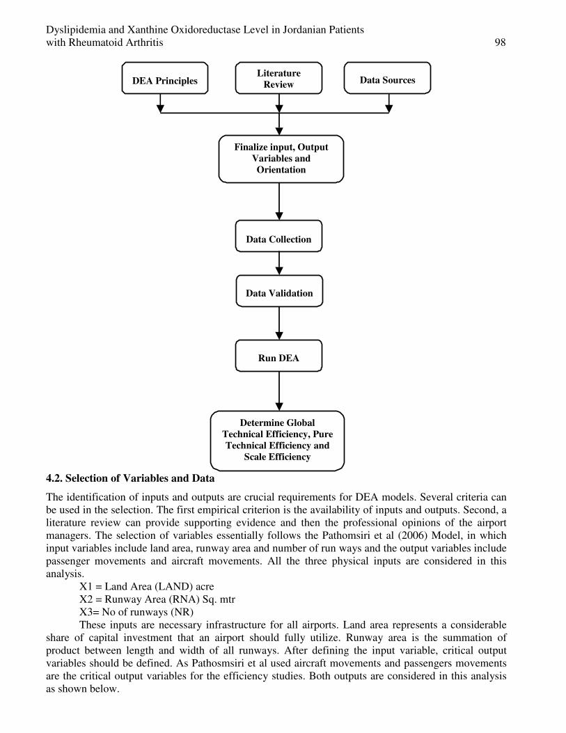
Dyslipidemia and Xanthine Oxidoreductase Level in Jordanian Patients with Rheumatoid Arthritis 98
DEA Principles
Literature
Review
Data Sources
Data Collection
Data Validation
Run DEA
Determine Global
Technical Efficiency, Pure
Technical Efficiency and
Scale Efficiency
Finalize input, Output
Variables and
Orientation
4.2. Selection of Variables and Data
The identification of inputs and outputs are crucial requirements for DEA models. Several criteria can be used in the selection. The first empirical criterion is the availability of inputs and outputs. Second, a literature review can provide supporting evidence and then the professional opinions of the airport managers. The selection of variables essentially follows the Pathomsiri et al (2006) Model, in which input variables include land area, runway area and number of run ways and the output variables include passenger movements and aircraft movements. All the three physical inputs are considered in this analysis.
X1 = Land Area (LAND) acre X2 = Runway Area (RNA) Sq. mtr X3= No of runways (NR) These inputs are necessary infrastructure for all airports. Land area represents a considerable
share of capital investment that an airport should fully utilize. Runway area is the summation of product between length and width of all runways. After defining the input variable, critical output variables should be defined. As Pathosmsiri et al used aircraft movements and passengers movements are the critical output variables for the efficiency studies. Both outputs are considered in this analysis as shown below.

99 Najah Al- Muhtaseb, Elham Al-Kaissi, Zuhair Muhi eldeen and Naheyah Al-Muhtaseb
y1 = passengers movements y2 = Aircraft movements Given the above selected three inputs and two outputs, the assessment may be perceived as the
measurement of productive efficiency of airport operation. 4.3. Data Collection
There are 17 International airports handling international and domestic air services in India. This study focuses on domestic air traffic in India. Table 2 lists the details of these airports used in this analysis and the study for the period Jan 2011 to Dec 2011. Table 2: Airports used in the Analysis
S. No. Airports ICAO* Code IATA** Code
1 Chennai VOMM MAA 2 Kolkata VECC CCU 3 Ahmadabad VAAH AMD 4 Goa VAGO GOI 5 Trivandrum VOTV TRV 6 Calicut VOCL CCJ 7 Guwahati VDGT GAU 8 Jaipur VIJP JAI 9 Srinagar VISR SXR 10 Amritsar VIAR ATQ 11 Port Blair VOPB IXZ 12 Delhi VIDP DEL 13 Mumbai VABB BOM 14 Bangalore VOBL BLR 15 Hyderabad VOHS HYD 16 Cochin VOCI COK 17 Nagpur VANP NAG
*ICAO- International Civil Aviation Organisation **IATA- International Air Transportation Association
For the output variable, statistics on the number of passengers, and aircraft movements were collected from Airports Authority of India publications. Collecting input data was not easy as there was no single source available for all data. Airport Master Record database contains the most recent data on characteristics of Indian airports. The best effort was made to verify this recent data with airport managers.
The number of samples was checked against several applicable rules of thumb to guarantee sufficiency and meaningful interpretation. As difficulty in DEA applications is a lack of discriminatory power between DMUs as a result of an excessive number of measures with respect to the total number of DMUs. The larger the number of input and output measures for a given number of airports results in a less discriminatory model.
To avoid losing discriminatory power, Cooper et al (2000) recommended that the desired number of DMUs exceed m + s several times. They suggested a more stringent rule of thumb in the following formula (Cooper, Seiford and Tone, 2000).
n> max (m x s, 3(m+s)), where n is the number of DMUs, m and s are the numbers of input and output measures respectively.
Substituting m and s, yields the minimum number of samples; n> max (3 x 2, 3(3+2)) = max (6, 15) = 15 The sample size of 17 satisfies this recommendation. In the next section, results from assessing
technical and scale efficiency of 17 airports by DEA model will be presented.

Dyslipidemia and Xanthine Oxidoreductase Level in Jordanian Patients with Rheumatoid Arthritis 100
5. Empirical Results This paper used Max DEA-solver to compute the Global Technical efficiencies, the Pure Technical efficiencies, scale efficiencies and return-to scale characteristics of each airport listed in Tables 3. Table 3: DEA Results
NO DMU
Global Technical
Efficiency
Score(CCR)
Pure Technical Efficiency
Score(BCC) Scale Efficiency Score
Return-to
scale
1 AHMEDABAD 0.381704 0.643769 0.59292 Increasing 2 AMRITSAR 0.066166 0.076868 0.860767 Increasing 3 BANGALORE 1 1 1 Constant 4 CALICUT 0.055939 1 0.055939 Increasing 5 CHENNAI 0.93305 1 0.93305 Increasing 6 COCHIN 0.260404 0.345757 0.753142 Increasing 7 DELHI 0.783298 1 0.783298 Decreasing 8 GOA 1 1 1 Constant 9 GUWAHATI 0.46122 1 0.46122 Increasing 10 HYDERABAD 0.801208 0.801208 1 Constant 11 JAIPUR 0.228735 1 0.228735 Increasing 12 KOLKATA 0.522192 0.53458 0.976828 Increasing 13 MUMBAI 1 1 1 Constant 14 NAGPUR 0.161642 0.17294 0.934672 Increasing 15 PORT BLAIR 0.272715 0.434001 0.628375 Increasing 16 SRINAGAR 0.504165 0.52374 0.962625 Increasing 17 TRIVANDRUM 0.162934 0.248511 0.65564 Increasing
Table 3 shows four different results for the airport included in the sample. The second column
represents the airports for the study, the third column expresses the (CCR) global technical efficiency measure, the fourth column expresses the pure technical efficiency (BCC) measure, the fifth column represents the scale efficiency and the sixth column displays DMUs operating in an area of increasing or decreasing or constant returns to scale.
An examination of Tables 3 reveals that there are 8 out of 17 airports operating in the frontier: Bangalore, Calicut, Chennai, Delhi, Goa, Guwahati, Jaipur and Mumbai under BCC model and other 9 airports are technically inefficient as their scores are less than one. There are 3 airports, namely Mumbai, Bangalore and Goa that form the frontier under CCR model. Twelve airports – Ahmedabad, Amritsar, Calicut, Chennai, Cochin, Guwahati, Jaipur, Kolkata, Nagpur, PortBlair, Srinagar and Trivandrum - operate in the area of increasing returns to scale , 4 airports - Bangalore, Goa, Mumbai and Hyderabad - operate in constant return scale and Delhi airport operates in decreasing returns to scale.
Significant differences in efficiency are prevalent in Indian airports ranging from0.0559 to 1.000 and 0.0768 to 1.000 under CCR model and BCC model respectively. The airports in Bangalore, Calicut, Chennai, Delhi, and Goa, Guwahati, Jaipur and Mumbai have full BCC efficiency but a low CCR efficiency which means they are locally efficient but globally inefficient due to the scale size of DMU. The airports in Ahmadabad, Amritsar, Cochin, Hyderabad, Kolkata, Nagpur, Port Blair, Srinagar and Trivandrum have less than full BCC efficiency and it implies that the DMU ineffectively manages its resources.
Next the scale efficiency is measured by the ratio of global technical efficiency to pure technical efficiency. The remarkable aspect is that one airport has decreasing returns to scale, while 12 airports have increasing returns to scale. Those airports with decreasing returns to scale (DRS) are too large in dimensions whereas those airports with increasing returns to scale (IRS) are too small in

101 Najah Al- Muhtaseb, Elham Al-Kaissi, Zuhair Muhi eldeen and Naheyah Al-Muhtaseb
dimension. Four airports have constant returns to scale. Those with constant return to scale have the adequate dimension. Increasing returns–to–scale imply that the DMU’s can gain efficiency by increasing the outputs while decreasing returns to –scales imply that the DMU’s can gain efficiency by decreasing outputs.
This fact may suggest that a policy of reallocation of traffic from decreasing returns to scale (DRS) airports to increasing returns to scale (IRS), when the airports involved in the reallocation are close. 6. Conclusions and Future research For developing countries like India whose resources are limited, effective operation of airports is important. DEA allows identifying the necessary actions to improve services in a flexible way. However, the rise of the air traffic in India, calls for investments in air transport facilities, in order to meet the potential demands. Hence, the performance of physical and workforce infrastructures required to meet the expectations of passengers should be monitored, so that current capacities of airports can be utilized at optimal level.
There are a number of potential extensions to this paper that could be conducted as future research. Considering all the Indian domestic civil airports, the input measures in this paper may be rather limited to the airside operation. In fact, one may want to see how other capital inputs such as apron area, terminal area and number of gates could have an impact on the productivity of airports. On the output side, a measure of delays and noise pollution could be included as undesirable outputs. It will be very useful if one can extend the study to assess the productivity of airports in the global context so that valuable lessons may be learned from efficient airports. References [1] Adler,N.and Berechman, J.(2001)“Measuring airport quality from the airlines viewpoint”: an
application of data envelopment analysis”. Transport Policy, Vol.8, No.3, pp.171- 181. [2] Amin, G.R. and Toloo, M.(2007) “Finding the most efficient DMUs in DEA:
animprovedintegrated model”, Computers and industrial Engineering, Vol.52, No.1, pp.71-77. [3] Banker, R.D.(1993) “Maximum likelihood, consistency and data envelopment analysis
statistical Foundation”, Management Science, Vol,39, No.10,pp.1265-1273. [4] Charnes, A., Cooper, W.W. and Rhodes, E.L. (1978) “Measuring the efficiency of decision
making units”, European Journal of Operational Research, Vol. 2,No.6, pp.429-444. [5] Farrell, M.J.(1957) “The measurement of productive efficiency”, Journal of the Royal
StatisticalSociety,,Vol.120,No.3,pp.253-281. [6] Farrell M.J.(1957) “The measurement of productive efficiency “Journal of the Royal Statistical
Society, series A,Vol.120,No.3, pp.253-351. [7] Fernandes E.and Pacheco R.R (2001) “Total airport productivity in Brazil”, a Paper presented
at XII thWorld Productivity Congress, Hong Kong, November 2001. [8] Fernandes E.and Pecheco R.R (2005) “Impact of changes in management style on the
performance of Brazilian airports”, Proceedings of the Air Transports Research Society (ATRS) conference,
[9] Gillen D., LallA. (1997) “Developing measures of airports productivity and Performance: an application of Data Envelopment Analysis”. Transportation Research Part E, vol.33, No.4, pp.261-273.
[10] Graham A.(2003) “Managing airports: and international perspective” 2ndEdition, Elsevier, UK.Martin J.C.and Roman C. (2001) “An application of DEA to measure the Efficiency of Spanish airports prior to privatization”, Journal of Air Transport Management, Vol.7, No.3, pp. 149-157.

Dyslipidemia and Xanthine Oxidoreductase Level in Jordanian Patients with Rheumatoid Arthritis 102
[11] Murillo-Melchor C.(1991) “An analysis of technical efficiency and Productivity changes in Spanish airports using the Malmquist index”, International Journal of Transport Economics, Vol.16, No.2, pp. 271-292.
[12] Pacheco R.R .and Fernandes E (2003) “Managing efficiency of Brazilian airports”, Transportation Research Part A, Vol.37, no.8, pp. 667-680.
[13] Parker D. (1999) ‘The performance of BAA before and after privatization’, Journal of Transport Economics and policy, Vol.33, Part 2, pp.133-146.
[14] Pathomsiri S.and, Haghani A. (2004) “Benchmarking efficiency of airports in the competitive multiple – airports systems: the international perspective”, proceedings of the 19th Transport Chicago Conference (CD-Rom), Chicago, IL.
[15] PathosmiriS.and, Haghani A., Schonfield P.S.(2005) “operational efficiency of airports in multiple –airports systems” Transportation Research Board 84thAnnual Meeting Compendium of Papers, (CD-ROM), Washington Dc.
[16] Pathosmiri S., Haghani A.,Dresner M., Windle R.J.(2006c)“Assessment of Airports Performance with Joint consideration of Desirable and undesirable Outputs”, the 10th Annual World Conference Air Transport Research Society (ARTS) Proceedings (CD-ROM), Nagoya, Japan, May 26-28, 2006.
[17] Pathomsiri S., Haghani A., Windle R.J., Dresner M. (2006) “Role of Freight Transportation Services and Reduction of Delayed Flights on Productivity of US Airports”, National Urban Freight Conference 2006 Proceedings (CD-ROM), Long Beach, CA, February-1-2006.
[18] Pels E., Nijkamp P., Rietveld P.(2003) “Inefficiencies and scale economies of European airports Operations”, Transportation Research Part E., Vol. 39, No.5, pp.341-361.
[19] Salazar De La Cruz F. (1999) “A DEA approach to the airport productivity function”, international Journal of Transport Economics, vol.26, No.2, pp.255-270.
[20] Sarkis J.(2000) “An analysis of the operational efficiency of major airports in the United States”Journal of Operations Management, Vol.18, Issues 3, pp.335-351
[21] Sarkis J. Talluri S. (2004) “Performance based clustering for benchmarking of U.S. airports” Transportation Research Part A, Vol.38, issueNo.5, pp.329-346.
[22] Yoshida Y., Fujimoto H.(2004) “Japanese-airport benchmarking with the DEA And endogenous- Weight TFP methods”, Transportation Research Part E 40, 533-546.
[23] Yu M.M.(2004) “Measuring Physical efficiency of domestic airports in Taiwan with undesirable outputs and environmental factors”, journal of Air Transport Management 10, 295-303.

European Journal of Scientific Research ISSN 1450-216X / 1450-202X Vol. 99 No 1 April, 2013, pp.103-118 http://www.europeanjournalofscientificresearch.com
Dyslipidemia and Xanthine Oxidoreductase Level in
Jordanian Patients with Rheumatoid Arthritis
Najah Al- Muhtaseb Associated Prof (Contributed equally)
Department of Pharmaceutics and biotechnology Faculty of Pharmacy, Petra University, Amman, Jordan
E-mail: [email protected]
Elham Al-Kaissi Associated Prof (Contributed equally)
Department of Medicinal chemistry and Pharmacognosy Faculty of Pharmacy, Petra University, Amman, Jordan
P.O. Box 961343 Amman, Jordan. E-mail: [email protected]
Fax 00962-6-5715551, Tel. 00962-6-05715546
Zuhair Muhi eldeen Full Prof, Department of Pharmaceutics and biotechnology
Faculty of Pharmacy, Petra University, Amman, Jordan E-mail: [email protected]
Naheyah Al-Muhtaseb
MD, Rehabitation Medicie (RMS) E-mail: [email protected]
Abstract
Context: Rheumatoid arthritis (RA) is associated with an excess mortality from cardiovascular disease which might be due to an increased prevalence of cardiovascular risk factors such as dyslipidemia, and free radical generating enzyme such as xanthine oxidoreductase (XOR). Thus, they appear to be suitable markers for clinical studies of lipid profile and XOR level in patient with RA and related cardiovascular risk.
Objectives: of the study were to assess the prevalence of blood dislipidemia and the levels of blood and synovial XOR in Jordanian patients with untreated active rheumatoid joint diseases and to investigate the clinical and biological associated factors.
Methods: Synovial fluids and blood were collected from one hundred twenty seven patients with active RA (63 male and 64 female). One hundred eleven age matched individuals were included as control. Blood lipid profile, apolipoproteins (Apo), blood and synovial XOR proteins level were determined.
Results: the levels of patient serum cholesterol (C), low density lipoprotein (LDL)-Cholesterol, Apo B, triglyceride (TG), very low density lipoprotein (VLDL-TG), LDL-TG, Apo C-III, Apo C-III/TG, Apo B/Apo A-I, and LDL-C/high density lipoprotein (HDL)HDL2-C ratios were significantly increased in RA patients. A significant reduction in the levels of HDL-, HDL2-, HDL3-C, serum Apo A-I, ApoA-II, HDL-Apo A-I, and

Dyslipidemia and Xanthine Oxidoreductase Level in Jordanian Patients with Rheumatoid Arthritis 104
HDL2-C/HDL3-C ratio were found in RA patients compared to healthy controls. Increased XOR in serum and synovial fluid were observed in the RA patients studied. .
Conclusions: Abnormalities in lipids, lipoproteins, apolipoproteins and XOR were found in RA patients. Our data favor an enhanced affinity towards atherosclerosis in these patients. Management of dyslipidemia should consider as a part of cardiovascular risk management in RA patients. Attention must be paid to lipids profile for those RA patients with previous history of a cardiovascular event. Keywords: Dyslipidemia, lipid profile, atherogenesis, Synovial fluid, Apolipoprotein
(Apo). 1. Introduction Rheumatoid arthritis (RA) is a chronic inflammatory disease of unknown etiology affecting primarily the synovium, leading to synovial inflammation, joint and bone damages, it affects 1-2% of the population, with mortality ratios ranging from 1.3 to 3.0 (Kimac et al. 2010; Helmick et al. 2008; Nurmohamed 2007; Goodson and Solomon 2006; Georgiadis et al. 2006; Watson et al. 2003; Van Doornum et al. 2002; Lems and Dijkmans 2000). Patients suffering from rheumatoid arthritis (RA) are at greater risk of developing cardiovascular disease with 70% increase in risk of death (Lourida et al. 2007; Soubrier and Dougados 2006; Sattar et al. 2003). Clinical and subclinical vacuities accelerated atherosclerosis and increases cardiovascular morbidity and mortality among RA patients (Georgiadis et al. 2006; Gabriel et al. 2003; Van Doornum et al. 2002; Goodson 2002; Bacon and Kitas 1994; Reilly et al. 1990). This increased cardiovascular risk may resulted from several factors such as dyslipidemia, accelerated atherosclerosis, diabetes mellitus, high blood pressure, higher body mass index (BMI), sex and age (Goodson and Solomon 2006; Dessein et al. 2005; Pincus and Callahan 1986) and finally, the chronic inflammatory components, and the effects of drugs used in RA treatment on the lipid profile (Ku et al. 2009; Chung et al. 2008; Shoenfeld et al. 2005). In recent years, free radicals reactions and other reactive intermediates produced in normal metabolic processes have been implicated in the pathogenic mechanism of a wide range of diseases, including acute coronary syndrome (Cheng-xing et al. 2004 ), in others cardiovascular diseases (Dawson and Walters 2006) and inflammatory diseases (Chung et al. 1997). XOR has generated excited widespread research result in its ability to reduce molecular oxygen, generating free radical superoxide anion (O2
-) and hydrogen peroxide (H2O2) mediating ischemia-reperfusion damage in heart and joint (Almuhtaseb 2012). Studies concerning the levels of total cholesterol (TC), total triglyceride (TG), very low density lipoprotein- triglyceride (VLD-TG), low density lipoprotein-cholesterol (LDL-C) and low levels of high density lipoprotein-cholesterol (HDL-C) particularly HDL2-C and inconclusive in RA patients yielded contradictory data (Arts et al. 2012; Garcia-Gomez et al. 2009; Nurmohamed 2007; Assous et al. 2007; Van halm et al. 2007; Solomon et al. 2004; Park et al. 2002; Park et al. 1999; Austin et al. 1998). Increased levels of total TC, LDL-C and low levels of HDL-C, and HDL2-C are associated with an increased incidence of cardiovascular disease in general population (Choy and Sattar 2009; Castelli et al. 1986). The inflammatory environment and disturbed antioxidant mechanisms due to increased XOR in RA may promote LDL oxidation, thereby facilitating atherogenesis at low ambient lipid concentration and placing RA patients at higher cardiovascular risk (Nurmohamed 2007; Situnayake et al. 1991). Little attention has been given to apolipoproteins, the carriers of structural and functional properties of serum lipoproteins (Knowlton et al. 2012), including Apo A-1, Apo B which differ not only in their apolipoprotein composition but also in their metabolic properties and non-atherogenic and atherogenic capacities (Alaupovic 2003; Blankenhom et al. 1990). Serum apolipoproteins measurement is considered to be better discriminators than the total levels of lipoprotein (Walldius and Jungner 2006). Apo C-II and Apo C-III have also been reported to play an important role in the catabolism of TG and

105 Najah Al- Muhtaseb, Elham Al-Kaissi, Zuhair Muhi eldeen and Naheyah Al-Muhtaseb
hence may contribute to cardiovascular disease (Havel et al. 1973). Apo C-II is activator of lipoprotein lipase (LPL) which hydrolysates TG while Apo C-III inhibits the enzyme (LaRosa et al. 1970). Apo C- III was shown to interfere with binding of Apo B containing lipoprotein to hepatic lipoprotein receptors (Brown and Banginsky 1972) and has link with the inflammatory processes (Clavey et al. 1995; Wang et al. 1985). Recently, new data on dyslipidemia in RA patients have been published which changed our insights about the lipid profile in RA patients (Knowlton et al. 2012; Hemick et al. 2008; Solomon et al. 2003; Wolfe et al. 2003; Koopman 2001). The aim of this study is to assess the prevalence of dyslipidemia and the level of synovial and blood XOR in Jordanian patients with active RA and to investigate the clinical and biological associated factors. . 2. Materials and Methods 2.1. Subjects and Clinical Evaluation
127 RA patients, diagnosed according to the ACR criteria for classification of the disease (Arnett et al 1988), and 111 control subjects, matched for age, sex, smoking status and blood pressure were enrolled after giving informed consent. The patients had active disease, as evaluated by a Disease Activity Score (DAS 28=6.5 ± 0.2) according to EULAR’s recommendations (Fransen and Riel 2005) and 63 were Rheumatoid factor positive. No subject had any symptom or laboratory finding of kidney, liver or thyroid dysfunction, infection, diabetes, malignancy, or was taking drugs affecting plasma lipid or lipoprotein levels. None had been treated with corticosteroids or disease modifying anti-rheumatic drugs prior the study. All subjects had sedentary habits and were not participating in any regular physical exercises. The present investigation was approved by the hospital ethics committee and was in accordance with the principles outlined in the declaration of Helsinki.
After overnight fast (15 h) venous blood samples of all participants (patients and controls) were collected in plain tubes (1.5 mg/ml, Monojet, Division of Sherwood Medical). The samples after their complete coagulation were centrifuged at 4oC (500 g; 15 minutes) to separate clear sera. The sera were divided into two portions, one for detection the levels of IgG and IgM and the other for immediate analysis of rheumatoid factor (RF), C-reactive protein (CRP), Uric acid (Balis 1976), glucose (Trinder 1969), phospholipid (Takayama et al. 1977), and XOR activity (Nishino 1994; Avis et al. 1956). The ultracentrifugal fractionation for VLDL, LDL, Total HDL, HDL2, and HDL3 fractions (for C and TG), serum triglycerides, and total cholesterol, were determined in triplicate with standard enzymatic techniques by using an Abbott VP supersystem autoanalyser (Abbott Diagnostic Division, maidenhead, UK). Erythrocytes sedimentation rate (ESR) was determined for the first hour. 2.2. Separation of Lipoprotein
Separation of lipoproteins was performed by a modified sequential ultracentrifugation method (Havel et al. 1955) in a preparative ultracentrifuge (Sorvall OTD 75B, Bomedical products) in a fixed angle rotor (type TFT 48.6) with appropriate adaptors. The procedure was outlined in (Al-Muhtaseb et al. 1989).
Apolipoproteins A-I, A-II and B, C-П and C-Ш values were determined by immune-turbidimetric method using Daiichi kit (Auto N Daiichi, Daiichi pure chemicals Co. Ltd, Tokyo, Japan) and preceded according to the manufacturer recommendation.
For Apo AI inter assay and intra assay coefficient of variation was less than 3.5% at a level of 150 mg/dl and less than 4% at a level of 100mg/dl. For Apo A-II the coefficient of variation was less than 4.5% at a level of 70mg/dl and less than 4.5% at a level of 40 mg/dl. For Apo B it was less than 4.5% at a level of 70mg/dl. Apoprotein C-II and C-III values, the Inter assay and intra assay coefficient of variation was within the recommended range (below 10%). 2.3. LCAT Activity Assay
The method was according to that reported by Dieplinger and Kostner in 1980.

Dyslipidemia and Xanthine Oxidoreductase Level in Jordanian Patients with Rheumatoid Arthritis 106
2.4. Rheumatoid Factor Detection (RF)
Rheumatoid factor is detected by latex agglutination test using appropriate plates from Behring (Germany) according to the manufacturer recommendations. Fifty µL of latex coated with human IgG was added to different dilutions from each serum sample. Negative and positive sera were used as controls. After two minutes a clear agglutination is observed in the positive indicating the presence of RF. Sera with titer less than 20 IU/ml were considered negative according to the manufacturer recommendation. 2.5. C - Reactive Protein (CRP) Concentration Determination
CRP concentration was determined by latex agglutination test using appropriate plates from Behringer (Germany) and preceded as recommended by the manufacturer. 2.4 µl of patient serum is added to 120 µl buffer solutions (pH 8.5) and mixed with 120 µl suspension of mouse anti-human CRP monoclonal antibody that is bound to latex (2mg/ml) and incubated for 5 minutes. CRP binds to the latex-bound antibody and agglutinates. The resulting agglutination was measured spectrophotometrically at 580 nm, negative and positive control samples were included. Values higher than 9.4 mg/l for females and 8.55 mg/l for males were consider as positive. 2.6. The Erythrocyte Sedimentation Rate (ESR)
Was determined using modified Westergren method (Belin et al. 1981). 2.7. Purification of Xanthine Oxidoreductase
The purification and total protein estimation for XOR enzyme and xanthine oxidase activity assay were determined according to the previous method (Al-Muhtaseb et al. 2012). 2.8. Protein Estimation
Protein was estimated by the method of lowry et al. 1951, using Folin phenol reagent, bovine serum albumin was used as the standard. 2.9. Xanthine Oxidase Activity in the Synovial Fluid Assay
Total xanthine oxidase activity of the synovial fluid was determined by measuring the rate of oxidation of xanthine to uric acid spectrophotometrically at 295 nm in a Cary 100 spectrophotometer, using a molar absorption coefficient (ε ) of 9.6 mM-1 (Avis et al. 1956. 2.10. Assays
Were performed at 25.0 ± 0.2o C in air-saturated 50 mM Na / Bicine buffer, pH 8.3, containing 100µM xanthine. Total (oxidase plus dehydrogenase) activity was determined as above but in the presence of 500 µm NAD+. Dehydrogenase content of an enzyme sample was determined from the ratio of oxidase and total activities 2.11. Assay of Xanthine Oxidase Activity in the Blood (Nishino 1994)
2.11.1. Principle of the Xanthine Oxidase Method Xanthine oxidase
Xanthine + O2 + H2O Uric acid + H2O2

107 Najah Al- Muhtaseb, Elham Al-Kaissi, Zuhair Muhi eldeen and Naheyah Al-Muhtaseb
The rate of formation of uric acid is determined by measuring increased absorbance at 290 nm. A unit of activity is that forming one micromole of uric acid / minute. The procedure was done according to the procedure recommended by abdelhamid et al. 2011. 2.12. Single Radial Immunodiffusion Assay (SRID)
To determine the levels of total IgG and IgM as in (Al-Muhtaseb 2012) 2.13. Statistical Analysis
Statistical analysis was carried out using Student's t test by statistical packages for social science software (SPSS). Values are expressed as mean ± SD and values of p <0.05 were considered statistically significant. The relationships between variables were calculated using Pearson Correlation Coefficients. 3. Results Patients positive for rheumatoid factor labeled as rheumatoid arthritis + (RA+), while seronegative patients were labeled as other joint inflammation (RA-). Latex agglutination used in determining IgM-RF factor showed that, of the 127 patients 63 (32 male, 31 female) were RA+ (Seropositive) and 64 (31 male, 33 female) were RA- (Seronegative), the Clinical and biochemical characters of the participated subjects are shown in table 1. Table 1: Clinical and biochemical characteristics of controls and patients with rheumatoid arthritis, male and
female subjects.
Parameters Males Females
Control RA+ RA- Control RA+ RA-
Number 55 32 31 56 31 33 Age (years) 40.1±9.6 39.9±9.6 38.1±11.6 39.6±9.1 40.8±8.1 38.9±10.3 Height cm 162.9±9.6 161.8±7.9 160.6±10.9 163.6±5.7 161.2±8.9 160.6±10.9 Weight Kg 68.8±8.1 67.3±4.8 66.9±8.9 69.9±6.3 68.9±3.3 70.3±8.3 BMI (kg/m2) 27.3±4.6 28.1±7.7 27.8±4.2 26.1±3.3 27.4±8.3 26.9±10.1 ESR (mm/h) 10.8±6.03 66.9±42.6** 43.3±28.6* 11.9±5.02 67.1±43.2** 42.6±29.8* CRP (mg/dl) - + + - + + IgM rheumatoid factor (+/-) 0/0 45/13 44/13 0/0 46/13 44/13 Glucose mg/dL 95.9±6.8 94.8 ±7.2 92. 9±9.9 91.81±8.3 98.6± 9.1 100.3±11.6 Uric acid mg/dL 4.2±1.6 7.2±1.10* 6.0±1.6* 4.0±1.0 6.9±1.6* 6.6±1.3*
BMI: body mass index, ESR: erythrocytes sedimentation rate, CPR: C-reactive protein. *P < 0.001 significantly different from the corresponding control. ** P < 0.0001, between RA+ compare to RA- Values represent the means ± standard deviation (SD) BMI = weight < [kg/height (m)2]
The mean age and BMI for both rheumatoid arthritis RA+ and other joint inflammation RA- and their control subjects were comparable. ESR ( after one hour) and CRP values were significantly elevated in patients with rheumatoid arthritis (RA+) compared with values in patients with other joint inflammation (RA-) and to those of the control values.
Latex agglutination used in determining IgM-RF showed that of the 127 patients 32 males and 31 females were RA+ (seropositive) and 31 males and 33 females were RA-( seronegative).
Concentrations of fasting plasma glucose were normal in both male and female rheumatoid arthritis (RA+, RA-) patients compared to control subjects. On the other hand, uric acid levels were significantly elevated in male and female rheumatoid arthritis RA+ and RA- patients compared with their controls (P < 0.001).
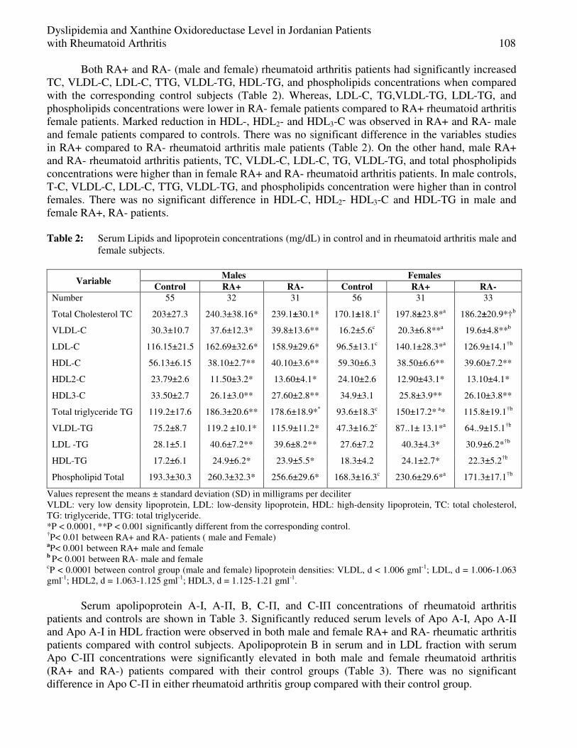
Dyslipidemia and Xanthine Oxidoreductase Level in Jordanian Patients with Rheumatoid Arthritis 108
Both RA+ and RA- (male and female) rheumatoid arthritis patients had significantly increased TC, VLDL-C, LDL-C, TTG, VLDL-TG, HDL-TG, and phospholipids concentrations when compared with the corresponding control subjects (Table 2). Whereas, LDL-C, TG,VLDL-TG, LDL-TG, and phospholipids concentrations were lower in RA- female patients compared to RA+ rheumatoid arthritis female patients. Marked reduction in HDL-, HDL2- and HDL3-C was observed in RA+ and RA- male and female patients compared to controls. There was no significant difference in the variables studies in RA+ compared to RA- rheumatoid arthritis male patients (Table 2). On the other hand, male RA+ and RA- rheumatoid arthritis patients, TC, VLDL-C, LDL-C, TG, VLDL-TG, and total phospholipids concentrations were higher than in female RA+ and RA- rheumatoid arthritis patients. In male controls, T-C, VLDL-C, LDL-C, TTG, VLDL-TG, and phospholipids concentration were higher than in control females. There was no significant difference in HDL-C, HDL2- HDL3-C and HDL-TG in male and female RA+, RA- patients. Table 2: Serum Lipids and lipoprotein concentrations (mg/dL) in control and in rheumatoid arthritis male and
female subjects.
Variable Males Females
Control RA+ RA- Control RA+ RA-
Number 55 32 31 56 31 33
Total Cholesterol TC 203±27.3 240.3±38.16* 239.1±30.1* 170.1±18.1c 197.8±23.8*a 186.2±20.9*†b
VLDL-C 30.3±10.7 37.6±12.3* 39.8±13.6** 16.2±5.6c 20.3±6.8**a 19.6±4.8**b
LDL-C 116.15±21.5 162.69±32.6* 158.9±29.6* 96.5±13.1c 140.1±28.3*a 126.9±14.1†b
HDL-C 56.13±6.15 38.10±2.7** 40.10±3.6** 59.30±6.3 38.50±6.6** 39.60±7.2**
HDL2-C 23.79±2.6 11.50±3.2* 13.60±4.1* 24.10±2.6 12.90±43.1* 13.10±4.1*
HDL3-C 33.50±2.7 26.1±3.0** 27.60±2.8** 34.9±3.1 25.8±3.9** 26.10±3.8**
Total triglyceride TG 119.2±17.6 186.3±20.6** 178.6±18.9** 93.6±18.3c 150±17.2* a* 115.8±19.1†b
VLDL-TG 75.2±8.7 119.2 ±10.1* 115.9±11.2* 47.3±16.2c 87..1± 13.1*a 64..9±15.1†b
LDL -TG 28.1±5.1 40.6±7.2** 39.6±8.2** 27.6±7.2 40.3±4.3* 30.9±6.2*†b
HDL-TG 17.2±6.1 24.9±6.2* 23.9±5.5* 18.3±4.2 24.1±2.7* 22.3±5.2†b
Phospholipid Total 193.3±30.3 260.3±32.3* 256.6±29.6* 168.3±16.3c 230.6±29.6*a 171.3±17.1†b
Values represent the means ± standard deviation (SD) in milligrams per deciliter VLDL: very low density lipoprotein, LDL: low-density lipoprotein, HDL: high-density lipoprotein, TC: total cholesterol, TG: triglyceride, TTG: total triglyceride. *P < 0.0001, **P < 0.001 significantly different from the corresponding control. †P< 0.01 between RA+ and RA- patients ( male and Female) aP< 0.001 between RA+ male and female b P< 0.001 between RA- male and female cP < 0.0001 between control group (male and female) lipoprotein densities: VLDL, d < 1.006 gml-1; LDL, d = 1.006-1.063 gml-1; HDL2, d = 1.063-1.125 gml-1; HDL3, d = 1.125-1.21 gml-1.
Serum apolipoprotein A-I, A-П, B, C-П, and C-IП concentrations of rheumatoid arthritis patients and controls are shown in Table 3. Significantly reduced serum levels of Apo A-I, Apo A-II and Apo A-I in HDL fraction were observed in both male and female RA+ and RA- rheumatic arthritis patients compared with control subjects. Apolipoprotein B in serum and in LDL fraction with serum Apo C-IП concentrations were significantly elevated in both male and female rheumatoid arthritis (RA+ and RA-) patients compared with their control groups (Table 3). There was no significant difference in Apo C-П in either rheumatoid arthritis group compared with their control group.

109 Najah Al- Muhtaseb, Elham Al-Kaissi, Zuhair Muhi eldeen and Naheyah Al-Muhtaseb
Table 3: Serum Apolipoprotein A-1, A-II, B, C-II and C-III concentrations of patients with rheumatoid arthritis and controls.
Males Females
Control RA+ RA- Control RA+ RA-
Number 55 32 31 56 31 33 Serum Apo A-I 150.3±16.3 110.7±13.3* 109.6±14.3* 133.7±11.6c 107.6±20.1* 106.3±19.1* HDL Apo A-I 123.6±11.3 86.3±14.6* 84.9 ±17.6* 118.6±10.6c 83.6±10.3** 80.9±11.6** Serum Apo A-II 50.9±3.7 39.1±3.6 40.1±5.2 48.6±8.6 40.1±7.6 39.6±9.1 Serum ApoB 110.6±9.6 132.3±10.8** 129.6±12.1** 98.6±7.6 c 125.6±10.6** 92.3±11.**ab LDL-Apo B 95.9±12.8 115.2±10.8** 113.9±13.**6 82.3±3.3 c 103.7±9.6** 103.6±150.6**ab Serum apo C-П 4.0±0.08 4.2±0.1 3.8±0.11 3.8±0.06 4.2±0.13 3.9±0.09 Serum apo C-ПI 6.8±0.09 8.6±0.14* 7.8±0.18* 6.0±0.19 8.9±0.1* 7.2±0.01*a
Values represent the means ± standard deviation (SD) in milligrams per deciliter, HDL: high-density lipoprotein, LDL: low-density lipoprotein, apolipoproteins, Apo A-1, Apo A-II, Apo B, Apo C-II, and Apo C-IП. *P< 0.0001, **P< 0.001: significantly different from the corresponding control group. aP< 0.001 between RA+ and RA- patients (male and Female). b P< 0.001 between RA- male and female. c P < 0.001 significantly different between control group (male and female).
Serum Apo A-I, Apo A-II, HDL-Apo A-I, serum Apo B, LDL-Apo B, and serum Apo C-П, levels did not differ between RA+ and RA- rheumatoid arthritis male patients, where as serum Apo A-I, Apo A-II, HDL-Apo A-I, and LDL-Apo B levels did not differ in RA+ and RA- rheumatoid arthritis female patients, but in case of serum Apo B and serum Apo C-ПI were significantly decreased in both RA+ and RA- female rheumatoid arthritis patients and the decrease in RA- were more significant.
In female control subjects, serum Apo A-I, Apo A-II, HDL-Apo A-I, serum Apo B and LDL- Apo B were signicantly lower than in control male subjects.
Serum lecithin cholesterol acyltransferase (LCAT), serum and synovial xanthine oxidase (XO) activities of patients with rheumatoid arthritis and controls are shown in table 4. Table 4: Serum lecithin cholesterol acyltransferase (LCAT), serum and synovial xanthine oxidase (XO)
activities of patients with rheumatoid arthritis and controls.
Males Females
Control RA+ RA- Control RA+ RA-
Number 55 32 31 56 31 33 Serum LCAT mg/dl
127.8±26.7 99.9±13.3* 109.6±30.1* 125.3±23.7 106.7±29.9**c 110.6±28.1**
Serum XO units/mg protein
0.0090±0.003 0.056±0.0046** 0.04±0.004**a 0.0091±0.003 0.063±0.009** 0.048±0.0024**a
Synovial XO,
nmole.min-1.mg-1
NA 98.9±40.6 78.1±29.61 a NA 100.46±45.8 82.81±35.61 a
*P< 0.001, **P< 0.01 significantly different from control a, P< 0.001 between RA+ and RA- in male and female groups.
Serum LCAT was decreased significantly in all rheumatoid arthritis female and male groups compared with healthy controls, while serum xanthine oxidase concentrations were elevated significantly in male and female (RA+ and RA-) rheumatoid arthritis patients groups when compared with control groups.
Serum XO and synovial XO activity were significantly decreased in both male and female RA- rheumatoid arthritis patients compared to RA+ rheumatoid arthritis patients.
Total IgG and IgM (mg/dL) titers in sera of patients with rheumatoid arthritis (RA+), other joint inflammation (RA-), and healthy volunteers, using SRIDA are shown in (Table 5). Both blood IgM and IgG levels were significantly higher in male and female (RA+ and RA-) rheumatoid arthritis patient groups than in control groups. Similarly, the levels were higher in serum of patients with other joint inflammation (RA-) than in RA+ patients (P< 0.01). IgG levels were more elevated in serum of

Dyslipidemia and Xanthine Oxidoreductase Level in Jordanian Patients with Rheumatoid Arthritis 110
patients with rheumatoid arthritis (RA+) compared to other joint inflammation (RA-) in both male and female (P< 0.001). Table 5: Total IgG and IgM titers in sera and synovial fluid of patients with rheumatoid arthritis ( RA+) ,
other joint inflammation (RA-), and healthy volunteers, using SRIDA**
Males Females
Control RA+` RA- Control RA+` RA-
Number 55 32 31 56 31 33 Total IgM
(mg/ml)
Blood 1.61±0,67 2.41±1.61*a 3.79±0.10*a 1.51±0.41 2.61±1.31*a 3.51±0.13*b Synovial NA 1.01±0.61c 0.61±0.22 NA 0.88±0.40 c 0.49±0.31
Total IgG
(mg/ml)
Blood 12.55±10.36 25.61±10.31* 18.67±7.2* 11.9±5.1 22.1±9.1* 14.76±7.2* Synovial NA 14.21±3.9c 10.29±3.0 NA 13.91±4.0 c 9.81±2.11
RA+= rheumatoid arthritis latex agglutination positive **SRIDA= single radial immunodiffusion assay *P< 0.001, significantly different from the corresponding control groups aP< 0.001, between RA+ and RA- patients( male and female) bP< 0.001, between RA- male and female patients cP< 0.01, between RA+ male and female
Total IgM and IgG (mg/dL) levels in serum were significantly higher in male and female rheumatoid arthritis (RA+) in comparison to the levels in patients with other joint inflammation (RA-) both male and female (P< 0.01).
Ratio of lipid fractions and apolipoproteins in control groups, male and female patients with rheumatoid arthritis (RA+ and RA-) are shown in (Table 6) Table 6: Ratios of lipid and lipoprotein fractions in control groups and patients with rheumatoid arthritis Males Females
Control RA+ RA- Control RA+ RA-
Number 55 32 31 56 31 33
T-C/HDL-C 1.95±0.30 6.40±0.51* 5.30±0.65*a 2.83±0.31 5.90±0.61* 4.31±0.035*a LDL-C/HDL-C 1.67±0.31 3.81±0.59* 3.31±0.90* 1.33±0.41 3.61±0.32* 3.71±0.29* HDL-C/Apo A-I 0.39±0.03 0.41±0.06 0.37±0.03 0.40±0.021 0.38±0.04 0.36±0.03 T-C/Apo B 2.61±0.40 2.14±0.30 2.00±0.23 2.31±0.31 2.00±0.22 1.90±0.23 Apo B/.Apo A-I 0.31±0.09 1.08±0.21* 1.03±0.17* 0.29±0.71 0.98±0.18* 0.91±0.15* LDL-C/HDL2-C 4.01±0.061 10.46±3.01* 9.80±2.91* 3.61±0.081 9.81±3.10* 8.91±3.21* HDL2-C/HDL3-C 0.71±0.01 0.47±0.03* 0.52±0.08* 0.69±0.09 0.51±0.09* 0.49±0.08* Apo C-III/TG 0.30±0.04 0.43±0.036 0.50±0.04 0.27±0.033 0.48±0.05 0.47±0.048 Results are means ± SD HDL-C: high density lipoprotein cholesterol, LDL-C: low density lipoprotein cholesterol, T-C: total cholesterol, Apo A-I, Apo A-II and Apo B: apolipoproteins *P < 0.001 significantly different from control subjects aP < 0.01 between RA+ and RA- in both male and female patients
Significantly increased T-C /HDL-C, LDL-C/HDL-C, LDL-C/HDL2-C, Apo B/Apo A-1 and Apo C-III/TG ratios, and reduction in HDL2-C/HDL3-C were observed in the male and female rheumatoid arthritis pateints compared with controls. Where as HDL-C/Apo A-1 and TC/Apo B ratios did not differ when compared with controls (Table 6). On the other hand TC/HDL-C were significantly increased in (RA+) rheumatoid arthritis compared to RA- male and female patients. The remaning ratios did not differ between male and female RA+ with RA- rheumatoid arthritis patients.

111 Najah Al- Muhtaseb, Elham Al-Kaissi, Zuhair Muhi eldeen and Naheyah Al-Muhtaseb
3.1. The Correlations between Variables
For the groups combined HDL-C correlated positively with Apo A-I (r=0.50, P< 0.001), and negatively with TG ( r=-0.60, P< 0.001) and Apo B (r=-0.47, P< 0.001), Triglycerides correlated positively with Apo B (r=0.61, P< 0.001), and with Apo C-III ( r=0.51, P< 0.001). Apo C-III correlated negatively with HDL-C (r= -0.53, P< 0.001) and HDL2-C (r=-0.56 P P< 0.001).
Serum TG and VLDL-TG were correlated positively with serum Apo-B and LDL-Apo B (r=0.62, r=0.5.2, P< 0.001 for both) and Apo-CIII(r=0.43, P< 0.001) and negatively with serum HDL-C, HDL2-C ( r= -0.46, r=-0.50, P< 0.001 for both), serum Apo A-I, HDL-Apo A-I (r=-0.44, r=-0.51, P< 0.001 for both). In the RA+ and RA- both sex group patients. In contrast, serum C and LDL-C correlated positively with TG, serum Apo B, LDL-Apo B (r=0.49, r=0.69, P< 0.001 for both) and negatively with HDL-C, HDL2-C (r= -0.53, r= -0.60, P< 0.001 for both), serum Apo A-I and HDL-Apo A-I ( r=-0.51, r= -0.58, P< 0.001 for both). 4. Discussion The elevated levels of CRP, ESR, beside IgM rheumatoid factors in both male and female patient groups reported in this study indicate inflammation. The slightly higher levels of total IgG and IgM titres in RA+ patients compared to the levels in RA- patients and to the levels in healthy control are inconsistent with other investigators (Arrar et al. 2008; Ng and Lewis 1994; Harrison et al. 1990), which is due to the autoimmune difference in the nature of the disease among individuals. On the other hand the synovial fluids of patients with RA+ and RA-showed lower levels of total IgG and IgM compared to the levels in their sera, these data were not in agreement with the finding of others (Arrar et al. 2008; Ng and Lewis 1994; Harrison et al. 1990). The low synovial levels may be attributed to bound immunoglobulins to the tissue or bound in immune complexes which need to be detected by other more sensitive techniques than SRID. In fact the pathology of RA is attributed to an Arthus like reaction in which immune complexes mediate the crucial role.
Recent research has shown that systemic inflammation plays a pivotal role in development of atherosclerosis (Nurmohamed 2007; Soubrier and Dougados 2006; Rohrer et al. 2004; Saito et al. 2003; Biondi-Zoccai et al. 2003; Lind 2003). Hence, inflammation might explain the increased cardiovascular risk in RA patients (Sattar et al. 2003). In our study, RA+ patients showed dyslipidaemia and mark atherogenic lipid profile compared with the healthy controls. This atherogenic lipid profile includes elevated TC, VLDL-C, LDL-C, TTG, VLDL-TG, LDL-TG and phospholipid levels observed in male RA+ and RA- patients, and in female RA+ patients only is in agreement with some of the previously reported data (Zrour et al. 2011; Yoo 2004; Park et al. 1999), and disagrees with others (Myasoedova et al. 2010; Oliviero 2009). The observations of significant differences found in female RA+ and RA- patients may suggests that the inflammation was more sever in RA+ women or due to a decrease in endogenous estrogen (Magkos et al. 2010; Atsma et al. 2006; Krauss et al. 1979).
Elevated total VLDL-C and LDL-C observed in this study have been previously reported (Walldius and Jungner 2004), this elevation may be due to changes in the inter composition of LDL particles as a consequence of increased flux of VLDL, or due to diet or physical exercise (Metsios et al. 2010). Alternatively, a decreased rate of LDL catabolism arising from increase LDL receptor uptake could explain this observation (Walldius and Jungner 2004). .
Our RA patients had high levels of total, VLDL and LDL-TG than the control group, which agrees with others (Tian et al. 2011; Aberg et al. 1985). The high level of TG may caused by increased production of VLDL-TG or decrease in TG catabolic rate as a result of impairment of LPL activity associated with inflammation (Tian et al. 2011). Alternatively, elevated VLDL-TG in these patients could be due to influx of free fatty acids into the liver as excess substrate for hepatic TG synthesis. And because VLDL-C, LDL-TG levels were elevated, such abnormalities may reflect an elevated concentration of remnant lipoprotein metabolism.

Dyslipidemia and Xanthine Oxidoreductase Level in Jordanian Patients with Rheumatoid Arthritis 112
Low levels of total HDL-C, HDL2-C, HDL3-C, and a high LDL-C, found in our study, is strongly associated with an increased risk of atherosclerosis, which is inconsistent with previous study (Arts et al. 2012; Regnstron et al. 1992), furthermore, the reduction in HDL-C occurs predominantly in the HDL2 subfraction which is conforms with previous reports (Arts et al. 2012; Regnstron et al. 1992). The inverse correlation seen between HDL-C and HDL2-C with VLDL-TG could lead to decreased production of HDL particularly HDL2 from TG-rich lipoproteins (Tian et al. 2011; Nikkila et al. 1987).
Apolipoprotein A-1 is the predominant apolipoprotein in HDL, and apolipoprotein B is the predominant apolipoprotein in LDL (Walldius and Jungner 2004; Jones et al. 2000; Gibbons 1986). The observed high levels of apolipoprotein B and its correlation with other blood lipids reported in male RA+, RA- and female RA+ patients may be associated with the increased production and/ or impaired catabolism of LDL, possibly apolipoprotein B due to inflammation (Van Doornum et al. 2002). In contrast to Apo B, the reduction in serum Apo A-I and Apo A-II levels are in agreement with other studies (Yamada et al. 1998). ApoA-1 is reported to inhibit the production of pro-inflammatory cytokines including IL-1, TNF-α and interactions between T-cell and monocytes (Zhang et al. 2010; Burger and Dayer 2002). This suggests that a less favorable lipid profile stimulates a pro-inflammatory status which might be related to RA disease activity or susceptibility. Our finding is in line with the researchers who believed that serum Apo A-I concentrations should be declined during active phase of RA, and has played an important role as anti-inflammation (Zrour 2011; Zhang et al. 2010; Barry et al. 2004; Burger and Dayer 2002). Chronic inflammation such as RA was also associated with low HDL-C and altered HDL composition (Rohrer et al. 2004). Other researchers reported that Apo A-I and Apo B levels are decreased (Chenaud et al. 2004; Jonas 2000). The reported Low HDL, HDL2-C and apolipoprotein A-1 levels and their inverse correlation with TG, VLDL-TG, phospholipids and apolipoprotein B levels in our study may be due to an increased production of acute phase proteins by the inflamed liver at the expense of lipoprotein production, thereby tending to reduce lipoprotein levels (London et al. 1963).
In the previous studies in autoimmune diseases as RA it were shown that Apo C-III and TG levels are increased (Knowlton 2012; Nicolay et al. 2006; Walldius and Jungner 2004), In our study we found increased levels in total-TG and VLDL-TG in males, females RA+ and RA- patients with increase in Apo C-III but not Apo C-II levels. Furthermore, our finding of high Apo B and lower Apo A-I, HDL-C and HDL2-C with their correlations to Apo C-III, may provide additional information in that Apo C-III level probably reflects an independent risk factor in RA patients (Knowlton 2012). The fact that Apo C-III alone or as one of the protein components of the Apo B-containing lipoprotein sub-classes is linked to inflammatory processes and atherogenesis, underscores its great potential as a new marker and diagnostic test for cardiovascular diseases in RA patients (Knowlton 2012). In a recent study it was shown that only those LDL particles that contain Apo C-III are atherogenic and those particles without Apo C-III are not (Mendivil et al. 2011).
The plasma LCAT, which is activated by Apo A-I, plays role in the metabolism of lipoproteins as co-factor for esterification of free cholesterol (Tian et al. 2011; Walldius and Jungner 2004). The finding of low LCAT activity, low Apo A-I and high level phospholipids in both RA+, RA- male and female patients compared to healthy control may suggest the influence of LCAT on HDL-C level.
The increased ratio of LDL-C/HDL-C, LDL-C/HDL2-C, TC/HDL2-C, Apo B/Apo A-I and Apo C-III/TG as observed in RA+, RA- patients was considered a predisposing factor to increased risk of cardiovascular diseases in RA patients. The higher the value of the Apo B/Apo A-I ratio, the more circulating cholesterol in the plasma compartment (Tian et al. 2011; Walldius and Jungner 2004), this cholesterol is likely to be deposited in the arterial wall, provoking atherogenesis and risk of coronary vascular events.
Assessing the Apo B/ Apo A-1 ratio and total TG levels was recommended to predict high cardiovascular risk patients in the general population (Tian et al. 2011; Walldius and Jungner 2006) in

113 Najah Al- Muhtaseb, Elham Al-Kaissi, Zuhair Muhi eldeen and Naheyah Al-Muhtaseb
our study the ratio was higher in male, female RA+ and RA- patients in comparison to controls, these data in support of cardiovascular risk.
Studies suggest that free radical mediated oxidative stress can influence the plasma lipid concentrations and generate potent proatherogenic mediators (Kowsalya et al. 2011). These free radicals also play an important role in the development of atherosclerosis vascular disease and other complications seen in RA (Mccord 2000; Ross 1999). Our study showed increased activity of serum and synovial XOR in male, female RA+ patients compared to RA- patients, may reflect the severity of the inflammation in RA+ patients. Therefore XOR can not be used as marker for detection of myocardial infarction as recommended by other (Abdelhamid et al. 2011). XOR is an important free radical generator (Hearse et al. 1986; Chambers et al. 1985), acts on hypoxanthine and xanthine with the resultant production of oxygen free radicals (Abdelhamid et al. 2011; Raghuvanshi et al. 2007). Free radical generation result in damage to vascular endothelium (Kundalic et al. 2003), Damage to extracellular matrix, and that changes in matrix structure can play a key role in the regulation of cellular adhesion, proliferation, migration, and cell signaling; furthermore, the extracellular matrix is widely recognized as being a key site of cytokine and growth factor binding, and modification of matrix structure might be expected to alter such behavior (Rees et al. 2008). .
As inflammation only explained a small part of the observed differences in lipids between the persons who later develop RA and the controls we recommend that a less favorable lipid profile might be related to the development of RA by a common or linked background, as socio-economic, ethnic, racial and geographic differences. Both genetic and dietary factors may contribute to high lipoprotein levels, especially increases fat and cholesterol consumption (van Wietmarschen and van der Greef 2012; Cesur et al. 2007). Alternatively, lipids might modulate the susceptibility to RA. 5. Conclusion Our finding support the following finding
a. Lipid profile particularly the Apo B/ Apo A-1 ratio and TG levels, HDL2-C assessments and CRP was recommended to predict high cardiovascular risk patients in the general population.
b. Management of dyslipidemia should considered as a part of cardiovascular risk management in RA patients.
c. Cardiovascular risk factor screening and appropriate treatment in form of antioxidant supplementation or antihyperlipidemic agents may be necessary for reducing the morbidity and mortality in these patients.
Further research to examine the relation between dyslipidemia, the effects of chronic inflammation on lipids, atherosclerosis and cardiovascular mortality may be of importance to both rheumatologists and cardiologists. References [1] Abdelhamid MA, Salim BI, and Abdelsalam KA (2011) Possibility of xanthine and
malondialdehyde as a marker for myocadial infarction. Sudan JMS 6(2): 93-96. [2] Aberg H, Lithell H, Selinus I and Hedstand H (1985) Serum triglycerides are a risk factor for
myocardial infarction but not for angina pectoris. Atherosclerosis 54(1): 89-97. [3] Alaupovic P (2003) The concept of apolipoprotein-defined lipoprotein families and its clinical
significance. Curr Atheroscler Rep 5: 459-467. . [4] Al-Muhtaseb N, Al-Kaissi N, Thawaini AJ, Muhi-Eldeen Z, Al-Muhtaseb S, Al-Saleh B (2012)
The role of human xanthine oxidoreductase (HXOR), anti- HXOR antibodies and microorganisms in synovial fluid of patients with joint inflammation. Rheumatology International 32: 2355-2362.

Dyslipidemia and Xanthine Oxidoreductase Level in Jordanian Patients with Rheumatoid Arthritis 114
[5] Al-Muhtaseb N, Al-Ysuf AR, Abdella N, Fenech F (1989) lipoproteins and apolipoproteins in young nonobese Arab women with NIDDM treated with insulin. Diabetes Care 12: 325-331. .
[6] Austin MA, Hokanson JE, Edwards KL (1998) Hypertriglyceridemia as a cardiovascular risk factor. Am J Cardiol 81: 7B-12B.
[7] Arnett FC, Edworthy SM, Bloch DA, Mcshane DJ, Fries JF, Cooper NS et al . (1988) The American Rheumatism Association revised criteria for classification of rheumatoid arthritis. Rheum 31: 315-324. .
[8] Arrar L, Hanachi N, Rouba K, Charef N, Khennouf S, Baghiani A (2008) Antixanthine oxidase antibodies in sera and synovial fluid of patients with rheumatoid arthritis and other joint inflammations. Saudi Med J 29: 803-807.
[9] Arts E, Fransen J, Lemmers H, Stalenhoef A, Joosten L, van Riel P, and Popa CD (2012) High-density lipoprotein cholesterol subfractions HDL2 and HDL3 are reduced in women with rheumatoid arthritis and may augment the cardiovascular risk of women with RA: a cross-sectional study. Arthritis Res Ther 14: R116.
[10] Assous N, Touze E, Meune C, Kahan A, Allanore Y (2007) Morbimortlite cardiovasculaire au cours de la polyarthrite rhumatoide: etude de cohort hospitaliere monocentrique fencaise. Rev Rhum 74: 72-78.
[11] Atsma F, bartelink ML, Grobbee DE, vander Schouw YT (2006) Postmenopausal status and early menopause as independent risk factors for cardiovascular disease: a meta- analysis. Menopause 13: 265-279.
[12] Avis PG, Bergel F, Bray RC (1956) Cellular constituents. The chemistry of xanthine oxidase. Part III. Estimations of the cofactors and the catalytic functions of enzyme fractions of cows’ milk. J Chem Soc (Perkins, I). 1219-1226. .
[13] Bacon PA, Kitas GD (1994) The significance of vascular inflammation in rheumatoid arthritis. Ann Rheum Dis 53: 621-622.
[14] Balis, M.E (1976) Uric acid metabolism in Man. Adv Clin Chem 18: 213-246. [15] Barry B, Martina G, Oliver FG, Jean MD (2004) Apolipoprotein A-I infiltration in rheumatoid
arthritis synovial tissue: a control mechanism of cytokine production. Arthritis Res Ther 6: 563-566.
[16] Belin DC, Morse E, Weinstein A. Whither Westergren (1981) The sedimentation rate reevaluated. J Rheumatol 8: 331-335.
[17] Biondi-Zoccai GG, Abbate A, Liuzzo G, Biasucci LM (2003) Atherothrombosis, inflammation, and diabetes. J Am Coll Cardiol 41: 1071-1077.
[18] Blankenhom DH, Johnson RL, Mack WJ, el Zein HA, Vailas LI (1990) The influence of diet on the appearance of new lesions in human coronary arteries. J Am Med Assoc 263: 1646-1652. .
[19] Burger D, Dayer JM (2002) High density lipoprotein-associated apolipoprotein A-1: the missing link between infection and chronic inflammation. Autoimmun Rev 1: 111-117. .
[20] Brown WV, Banginsky ML (1972) Inhibition of lipoprotein lipase by an apoprotein of human very low density lipoprotein. Biochem Biophysics Res Commun 46: 375-382. .
[21] Castelli WP, Garrison RJ, Wilson PW, Abbott RD, Kalousdian S, Kannel WB (1986) Incidence of coronary heart disease and lipoprotein cholesterol levels. The Framingham study. JAMA 256: 2835-2838.
[22] Cesur M, Ozbalkan Z, Temel MA, Karaarslan Y (2007) Ethinicity may be a reason for lipid changes and high Lp(a) levels in rheumatoid arthritis. Clin Rheumatol 26(3): 355-361.
[23] Chambers DE, Parks DA, Patterson G, Roy R, McCord JM, Yoshida S, et al. (1985) Xanthine oxidase as a source of free radical damage in myocardial ischemia. J Mol Cell Cardiol 17: 145-152.

115 Najah Al- Muhtaseb, Elham Al-Kaissi, Zuhair Muhi eldeen and Naheyah Al-Muhtaseb
[24] Chenaud C, Merlani PG, Roux-Lombard P, Burger D, Harbarth S, Luyasu S, et al. (2004) low lipoprotein A-I level at intensive care unit admission and systemic inflammatory response syndrome exacerbation. Crit Care Med 32: 632-637.
[25] Cheng-xing S, Hao-zhu C, and Jun-bo G (2004) The role of inflammatory stress in acute coronary syndrome. Chinese medical J 117: 133-139.
[26] Chung CP, Oeser A, Solus JF, Avalos I, Gebretsadik T, Shintani A et al. (2008) Prevalence of the metabolic syndrome is increased in rheumatoid arthritis and is associated with coronary atherosclerosis. Atherosclerosis 196: 756-763.
[27] Chung HY, Baek BS, Song SH, Kim MS, Huh JI, Shim KH, et al. (1997) Xanthine dehydrogenase / Xanthine oxidase and oxidative stress. Age 20: 127-140. .
[28] Choy E, Sattar N (2009) Interpreting lipid levels in the context of high-grade inflammatory states with a focus on rheumatoid arthritis: a challenge to conventional cardiovascular risk actions. Ann Rheum Dis 68: 460-469.
[29] Clavey V, Lestavel-Delattre S, Copin C, Bard JM, Fruchart JC (1995) Modulation of lipoprotein B binding to LDL receptor by exogenous lipds and apolipoproteins CI, CII, CIII and E. Arterioscler Thromb Vasc Biol 15: 963-971.
[30] Dawson J and Walters M (2006) Uric acid and xanthine oxidase: future therapeutic targets in the prevention of cardiovascular disease. Br J Clin Pharmacol 62: 633-644. .
[31] Dessein PH, Joffe BI, Veller MG, Stevens BA, Tobias M, Reddi K, and Stanwix AE (2005) Traditional and nontraditional cardiovascular risk factors are associated with atherosclerosis in RA. J Rheumatol 32: 435-442.
[32] Dieplinger H, Kostner G (1980) The determination of lecithin cholesterol acryltransferase in the clinical laboratory. Clin Chim Acta 106(3): 319-332.
[33] Fransen J, van Riel PL (2005) The disease activity score and the EULAR response criteria . Clin Exp Rheumatol 23: S93-S99.
[34] Gabriel SE, Crowson CS, Kremers HM, Doran MF, Turesson C, O'Fallen WM, Matteson EL (2003) Survival in rheumatoid arthritis: a population- based analysis of trends over 40 years. Arthritis Rheum 48: 54-58.
[35] Garcia-Gomez C, Nolla JM, Valverde J, Gomez-gerique JA, Castro MJ, Pinto X (2009) Conventional lipid profile and lipoprotein (a) concentrations in treated patients with rheumatoid arthritis. J Rheumatol 36: 1365-1370.
[36] Georgiadis AN, Papavasiliou EC, Lourida ES, Alamanos Y, KostaraC, Tselepis A, and Drosos AA (2006) Atherogenic lipid profile is a feature characteristic of patients with early rheumatoid arthritis: effect of early treatment- a prospective, controlled study. Arthritis research and therapy 8:R82.
[37] Goodson N: coronary artery disease and rheumatoid arthritis (2002) Curr Opin Rheumatol. 14: 115-120.
[38] Goodson NJ, Solomon DH (2006) The cardiovascular manifestations of rheumatic diseases. Curr Opin rheumatol 18: 135-140.
[39] Glibbons GF (1986) Hyperlipidaemia of diabetes. Clin Sci 71: 477-486. [40] Harrison R, Benboubetra M, Bryson S, Thomas RD, Elwood PC (1990) Antibodies to xanthine
oxidase: elevated levels in patients with acute myocardial infarction. Cardioscience 1: 183-189. [41] Havel RJ, Fielding GJ, Olivecrona T (1973) Cofactor activity of protein components of human
very low density lipoprotein in hydrolysis of triglycerides by lipoprotein lipase from different sources. Biochemistry 12: 1828-1833.
[42] Havel RJ, Eder HA, Bragdon JH (1955) The distribution and chemical composition of ultracentrifugally separated lipoproteins in human serum. J Clin Invest 34: 1345-1353.
[43] Hearse DJ, Manning AS, Downey JM (1986) Xanthine oxidase: a critical mediator of myocardial injury during ischemia and reperfusion. Acta Ohysiol Scand 548 Suppl: 65-78.

Dyslipidemia and Xanthine Oxidoreductase Level in Jordanian Patients with Rheumatoid Arthritis 116
[44] Helmick CG, Felson DT, Lawrence RC, Gabriel S, Hirsch R, Kwoh CK, et al. (2008) Estimates of the prevelance of arthritis and other rheumatic conditions in the United States. Part I. Arthritis Rheum 58: 15-25.
[45] Jonas A (2000) Lecithin cholesterol acyltransferase. Biochim Biophys Acta 1529: 245-256. . [46] Jones SM, Harris CPD, Lioyd J, Stirling CA. Reckless JPD, McHugh NJ (2000) Lipoproteins
and their subfractions in psoriatic arthritis: identification of an atherogenic profile with active joint disease. Ann Rhem Dis 59: 904-909.
[47] Kimac E, Halabis M, Solski J, Targonska-Stepniak B, Dryglewska M, Majdan M (2010) Abnormal lipid and lipoprotein profiles in rheumatoid arthritis. Annals Universitatis Mariae Curie-Sklodowska Lublin – Polonia 2010XXIII,N2,13: 87-92. .
[48] Koopman Wj (2001) Prospects for autoimmune disease: research advances in rheumatoid arthritis. J Am Med Assoc 285: 648-650.
[49] Kowsalya R, Sreekantha, Vinod Chandran and Remya (2011) Deslipidemia with altered oxidant-antioxident status in rheumatoid arthritis. International J of Pharma and Bio Sciences 2(1): 424-428:www.ijpbs.net.
[50] Knowlton N, Wages JA, Cantola MB, Alaupovic P (2012) apolipoprotein- defined lipoprotein abnormalities in rheumatoid arthritis patients and their potential impact on cardiovascular disease. Scand J Rheumatol 41: 165-169.
[51] Krauss RM, Lindgren FT, Wingerd J, Bradley DD, Ramcharan S (1979) Effects of estrogens and progestins on high density lipoproteins. Lipids 14: 113-118.
[52] Ku IA, Imboden JB, Hsue PY, Ganz P (2009) Rheumatoid arthritis a model of systemic inflammation driving atherosclerosis. Circ J 73: 977-985.
[53] Kundalic S, Kocic G, Cosic V, Jevtovic-Stoimenov T, Dordevic VB (2003) The role of xanthine dehydrogenase / xanthine oxidase in atherosclerosis in patient with hyperlipidemia. Jugoslov Med Biochem 22: 151-158.
[54] LaRosa JG, Levy RI, Herbert P (1970) Specific apoprotein activator for lipoprotein lipase. Biochem Biophysics Res Commun 41: 57-62.
[55] Lems WF, Dijkmans BAC (2000) Rheumatoid arthritis: clinical aspects and its variants. In: Fireestein GS, Panayi GS, Wollheim FA, eds. Rheumatoid arthritis: new frontiers in pathogenesis and treatment. New York: Oxford University Press. pp 213- 225.
[56] Lind L (2003) Circulating markers of inflammation and atherosclerosis. Atherosclerosis 169(2): 203-214.
[57] London MG, Muirden KD, Hewitt JV (1963) Serum cholesterol in rheumatic disease. BMJ 1: 1380-1383.
[58] Lourida EV, Georgiadis AN, Papavasilious EC, Papathhanasiou AI, Drosos EA, Tselepis LD (2007) Patients with early rheumatoid arthritis exhibit elevated auto antibody titers against mildly oxidized low- density lipoprotein and exhibit decreased activity of the lipoprotein- associated phospholipase A2. Arithritis Res Ther 9(1): R19.
[59] Lowry OH, Rosebrough NJ, Farr AL, Randall RJ (1951) Protein measurement with Folin phenol reagent. J Biol Chem 193: 265-275.
[60] Magkos F, Wang X, Mittendorfer B (2010) Metabolic actions of insulin in men and women. Nutrition 26(7-8): 686–693. doi:10.1016/j.nut.2009.10.013.
[61] Mccord JM (2000) The evolution of freeradicals and oxidative stress. Am J Med 108: 652-659. [62] Mendivil CO, Rimm EB, Furtado J, Chiuve SE, Sacks FM (2011) Low- density lipoproteins
containing apolipoprotein C-III and the risk of coronary heart disease. Circulation 124: 2065-2072.
[63] Metsios G, Stavropoulos-Kalinoglou A, Sandoo A, Veldhuijzen van Zanten JJCS, Toms TE, John H and Kitas GD (2010) Vascular function and inflammation in rheumatoid arthritis : the role of physical activity. Open Cardiovasc Med J 4: 89-96.

117 Najah Al- Muhtaseb, Elham Al-Kaissi, Zuhair Muhi eldeen and Naheyah Al-Muhtaseb
[64] Myasoedova E, Crowson CS, Kremers HM, Fitz-Gibbon PD, Themeau TM, Gbriel SE (2010) Total cholesterol and LDL levels decrease before rheumatoid arthritis. ANN Rheum Dis 69(7): 1310-1314.
[65] Ng YLE, Lewis WHP (1994) Circulating immune complexes of xanthine oxidase in normal subjects. Br j biomed Sci 51: 124-127.
[66] Nicolay A, Lombard E, Arlotto E, Saunier V, Lorec-Penet A, Lairon D, Portugal H (2006) Evaluation of new apolipoprotein C-II and apolipoprotein C-III automatized immunoturbidimetric kits. Clin Biochem 39: 935-941.
[67] Nikkila EA, Marja-Riita MD, Taskinen MD, Timosane MD (1987) Plasma high- density lipoprotein concentreation and subfraction distribution in relation to triglyceride metabolism. Am Heart J 113:543-548.
[68] Nishino T (1994) The conversion of xanthine dehydrogenase to xanthine oxidase and the role of the enzyme in reperfusion injury. J Biochem 16: 1-6.
[69] Nurmohamed MT (2007) Atherogenic lipid profiles and its management in patients with rheumatoid arthritis. Vascular Health and Risk management 3(6): 845-852.
[70] Oliviero F, Sfriso P, Baldo G, Dayer JM, Giunco S, Scanu A, et al. (2009) Apolipoprotein A-1 and cholesterol in synovial fluid of patients with rheumatoid arthritis, psoriatic arthritis and osteoarthritis. Clin Exp Rheumatol 27(1): 79-83.
[71] Park YB, Choi HK, Kim MY, Lee WK, Song J, Kim DK, Lee SK (2002) Effects of antirheumatic therapy on serum lipid levels in patients with rheumatoid arthritis: prospective study. Am J Med 113: 188-193.
[72] Park YB, Lee SK, Lee WK, Suh CH, Lee CW, Lee CH, et al. (1999) Lipid profiles in untreated patients with rheumatoid arthritis. J Rheumatol 26(8): 1701-1704.
[73] Pincus T, Callahan L (1986) Taking mortality in rheumatoid arthritis seriously- predictive markers, socioeconomic status and comorbidity. J Rheumatol 13: 841-845. .
[74] Raghuvanshi R, Kaul A, Bhakuni P, Mishra A, Misra MK (2007) Xanthine oxidase as a d marker of myocardial infarction. Indian journal of Clinical Biochemistry 22(2): 90-92.
[75] Rees MD, Kennett EC, Whitelock JM, and Davies MJ (2008) Oxidative damage to extracellular matrix and its role in human pathologies. Free Radical Biology and Medicine 44(12): 1973-2001.
[76] Regnstron J, Nilsson J, Tornwall P, Landdou C, Hamsten A (1992) Susceptibility to low density lipoprotein oxidation and coronary atherosclerosis in man. Lancet 339: 883-887.
[77] Reilly PA, Cosh JA, Maddison PJ, Rasker JJ, Silman AJ (1990) Mortality and survival in rheumatoid arthritis: a 25 year prospective study of 100 patients. Ann Rheum Dis 49: 363-369.
[78] Rohrer L, Hersberger M, and von Eckardstein A (2004) high density lipoproteins in the intersection of diabetes mellitus, inflammation and cardiovascular disease current. Opion in Lipidology 15: 269-278.
[79] Ross R (1999) Atherosclerosis-an inflammatory disease. N Engl J Med 340: 115-126. [80] Saito M, Ishimitsu T, Minami J, Ono H, Ohrui M, Matsuoka H (2003) Relations of plasma
high-sensitivity C-reactive protein to traditional cardiovascular risk factors. Atherosclerosis 167(1): 73-79.
[81] Sattar N, McCarey DW, Cappel H, McInnes IB (2003) Explaining how 'high- grade' systemic inflammation accelerates vascular risk in rheumatoid arthritis. Circulation 108: 2957-2963.
[82] Shoenfeld Y, Gerli R, Doria A, Matsuura E, Cerinic MM, Ronda N et al. (2005) Accelarated atherosclerosis in autoimmune rheumatic disease. Circulation 112: 3337-3347. .
[83] Situnayake RD, Thurnham DI, Kootathep S, Chirico S, Lunee J, Davis M, et al. (1991) Chain breaking antioxidant status in rheumatoid arthritis: clinical and laboratory correlates. Ann Rheum Dis 50: 81-86.
[84] Soubrier M, Dougados M (2006) Atherome et polyarthrite rhunatoide. Rev Med Int 27: 125-136.

Dyslipidemia and Xanthine Oxidoreductase Level in Jordanian Patients with Rheumatoid Arthritis 118
[85] Solomon DH, Curhan GC, Rimm EB, Cannuscio CC, Karlson EW (2004) Cardiovascular risk factors in women with and without rheumatoid arthritis. Arthritis Rheum 50: 3444-3449.
[86] Solomon DH, Karlson EW, Rimm EB, Cannuscio CC, Mandl LA, Manson JE, et al. (2003) Cardiovascular morbidity and mortality in women diagnosed with rheumatoid arthritis. Circulation 107: 1303-1307.
[87] Takayama M, Itoh S, Nagasaki T, and Tanimizu T (1977) A new enzymatic method for determining of serum choline containing phospholipids. Clin Chim Acta 79: 93-98.
[88] Tian L, Xu Y, Fu M, Peng T, Liu Y and Long S (2011) The impact of plasma triglyceride and apolipproteins concentrations on high-density lipoprotein subclasses distribution. Lipids in Health and disease 10: 17 doi:10.1186/1476-511X-10-17.
[89] Trinder P (1969) Determination of glucose in blood using glucose oxidase with an alternative oxygen acceptor. Ann Clin Biochem 6: 24-26.
[90] Van Doornum S, McGoll G, Wicks IP (2002) Accelerated atherosclerosis: an extraarticular feature of rheumatoid arthritis. Arthritis Rheum 46: 862-873.
[91] Van HalmVP, Nielen MMJ, Nurmohamed MT, van Schaardenburg D, Reesink HW, Voskuyl AE, et al. (2007) lipids and inflammation: serial measurement of the lipid profile of blood donors who later develop RA. Ann Rheum Dis 66: 184-188.
[92] van Wietmarschen H, and van der Greef J (2012) Metabolite Space of Rheumatoid Arthritis . British Journal of Medicine and Medical Research 2(3): 469-483.
[93] Walldius G, Jungner I (2006) The apo B/apoA-A ratio: a strong new risk factor for cardiovascular disease and a target for lipid-lowering therapy a review of the evidence. J Intern Med 259: 493-519.
[94] Wang CS, McConathy WJ, Kloer HU, Alaupovic P (1985) Modulation of lipoprotein lipase activity by apolipoproeins. Effect of apolipoprotein C-III. J Clin Invest 75: 384-390.
[95] Watson DJ, Rhodes T, and Guess HA (2003) All-cause mortality and vascular events among patients with rheumatoid arthritis, osteoarthritis, or no arthritis in the UK General Practice Research Database. J Rheumatol 30: 11996-1202.
[96] Wolf F, Freundlich B, Straus WL (2003) Increase in cardiovascular and cerebrovascular disease prevelance in rheumatoid arthritis. J. Rheumatol 30: 36-40.
[97] Walldius G, and Jungner I (2004) Apolipoprotein B and apolipoprotein A-I: risk indicators of coronary heart disease and targets for lipid-modifying therapy. J internal Medicine 255: 188-205.
[98] Yamada T, Ozawa T, Gejyo F, Okuda Y, Takasugi K, Hotta O, Itoh Y (1998) Decrease serum apolipoprotein AII/AI ratio in systemic amyloidosis. Ann Rheum Dis 57: 249-251.
[99] Yoo WH (2004) Dyslipoproteinemia in patients with active rheumatoid arthritis: effects of disease activity, sex, and menopausal status on lipid profiles. J. Rheumatol 31(9): 1746- 1753.
[100] Zhang B, Pu SX, Li BM, Ying JR, Song X W, and Gao C (2010) Comparison of serum Apolipoprotein A-I between Chinese multiple sclerosis and other related autoimuune disease. Lipid in health and disease 9:34 Doi:10.1186/1476-511X-9-3.
[101] Zrour SH, Neffeti FH, Sakly N, Jguirim M, Korbaa W, Younes M, et al. (2011) lipid profile in Tunisian patients with rheumatoid arthritis. Clin Rheumatol 27 April DOI 10.1007/s10067-011-1755-9.
Declaration of Interest
The authors report no declaration of interest.
European Journal of Scientific Research ISSN 1450-216X / 1450-202X Vol. 99 No 1 April, 2013, pp.119-136 http://www.europeanjournalofscientificresearch.com
Feedback Based Predictive Load Balancing for Data
Mining in Heterogeneous Distributed System
M. Eugin Lilly Mary Research Scholar, Bharathiar University, Coimbatore – 641 046, India
E-mail: [email protected]
V. Saravanan Professor & Director, Department of Computer Applications
Sri Venkateswara College of Computer Applications and Management Ettimadai, Coimbatore - 641105, India.
E-mail: [email protected]
Abstract
The Automatic extraction of unknown implicit knowledge from large datasets by scheduling to a set of inter connected processing elements, constitutes distributed data mining. The contributing nodes in a distributed system vary in their hardware resources, software sophistication requiring efficient methods for customizing the datasets, and scheduling to the nodes to ensure fast processing and optimal utilization of the hardware components. Dynamic feedback based techniques predicting the processing time of a task in a node will be a promising solution to resolve the variations of this ubiquitous system. The algorithms Predictive Least Load First (Pre_LLF), Rationalized Least Load First (RLLF), and Dynamic Stream Partitioning (DSP), designed and discussed in this paper are based on the principle of predictive load balancing. The Pre_LLF aims at choosing a node for scheduling a task such that the cumulative measure of the prevailing loads and the predicted processing time of a task in a node are the minimum, thereby considering the heterogeneity of the process. In addition to this measure, the RLLF reinforces the history of the contributing nodes thereby enhancing the heterogeneity of the processors in real time. The DSP aims at splitting the datasets for onward scheduling as ‘one to one mapping’, based on the predictive processing power, thereby enabling the system to closely adhere to the fluctuations of the ubiquitous environment. The performance of the three algorithms is evaluated for executing data mining operations, and compared with the Least Load First (LLF) for a variety of workloads and cluster sizes. The application developed, using Java for classifying water quality datasets is specially deployed at the contributing nodes. It is observed that the Pre_LLF and RLLF stamp more throughput than the LLF on increased cluster sizes, while the DSP excelled in achieving optimality. Keywords: Dynamic Stream Partitioning, Predictive Processing Power
1. Introduction The automated extraction of unknown and implicit knowledge from large datasets is termed as data mining. The data mining techniques include cluster analysis, tree based classification, methods to
Feedback Based Predictive Load Balancing for Data Mining in Heterogeneous Distributed System 120
uncover patterns associated with similarity search, etc, (M.S.Chen et al, 1996). The traditional approach is to apply data mining techniques which have been stored in a central data warehouse (G.Moro et al, 2001). In modern days, data mining applications need the processing of huge volumes of data. Datasets to be mined may arrive at high speed, and at times the same may be in the form of streams requiring fast and secure processing. Most of these applications require scientific computing and high-bandwidth transmission at the server nodes. A promising solution to the problem is to customize the size of the objects, and distribute the data to the available computing nodes to achieve quick response, and optimal utilization of shared components evolving Distributed Data Mining (DDM) strategies.
The DDM is nothing but a complex system focusing on the mining operation to be performed on a set of resources. The data involved may be in various forms, viz., online databases, web pages, data streams, text etc., according to the focus of the study.
Today the DDM has spread its wings to areas like molecular biology, weather forecast, cosmology, space research, nano technology, insurance, sensor networks, risk analysis etc., requiring very high computing power that can be achieved by utilizing a set of interconnected nodes forming clusters. These clusters constitute varying hardware resources, software sophistication, and quality of connectivity, etc. A large cluster is capable of contributing on par with a supercomputer at a fraction of the cost.( Josenildo Costa da Silva et al, 2006) The mining process is computation intensive, and the datasets to be mined may arrive at high speed in the form of streams, requiring fast and secure processing. The challenge is to distribute the tasks to the available computing nodes, so that none of the nodes is overloaded or underutilized, and this art is termed as load balancing. Therefore, load balancing is the key attribute in a DDM system to ensure fast processing and good utilization of the hardware components. Simple load balancing methods include the round robin, randomization approach, minimum connections, weight age methods, minimum misses, hashing etc., that are easy to implement, but are suitable only for homogeneous systems. The strategies can be divided into static or dynamic. Static load balancing distributes the tasks across the computing elements before execution, and the load distribution remains unchanged. In a distributed environment the state of the individual nodes varies, and knowledge of this variation during runtime forms the basis for dynamic load balancing. Therefore dynamic load balancing is termed as an active technology which provides the art of transforming the network traffic and scheduling. In addition, the quality of services, viz., scalability, quick response time, failure handling and fault tolerance can be embedded in the dynamic load balancing strategies. A brief over view of the techniques extracted from the literature is given in Section 2. Although a plethora of load balancing policies are in use, only simple methods (E. Katz et al, 1994) are adopted since they are easy to implement. However, these methods work well for homogeneous systems, and do not perform efficiently for heterogeneous elements or tasks requiring varying processing times. The present scenario is to manage the clusters of varying computing capabilities. To scale up such systems to perform at high level availability, and flexibility, the need arises for more sophisticated software architectures and adaptive methods. The adaptive load balancing strategies suitable for a heterogeneous environment are complex and complicated, and need the prediction of the processing time for any task to be processed in a computing node. The architecture proposed for processing the DNA Database, adopts the message exchange paradigm (Z-Tang et al, 2008) to fetch information such as the queue size and the expected waiting time of a task to be processed in a node. Also, the prediction policies are application specific. The existing scenario uses a generalized system for all types of applications [Yongijian Yang et al, 2005]. As a result, the distributed network experiences traffic due to communication over load and has very limited abilities to handle overloads, load imbalances, and compute-intensive transactions like cryptographic applications, data mining applications and multimedia processing which involve huge data.
The agent based systems emerging recently are able to resolve the above mentioned issues. An agent is an autonomous system capable of performing an action on behalf of its users. Agents are

121 M. Eugin Lilly Mary and V. Saravanan
capable of providing optimized services according to the changing environment. The characteristics of an agent include pro activity, autonomy, goal oriented local views and decentralization (Bakri Yahaya et al, 2011). An agent system itself possesses intelligence. In addition it is capable of making decisions on its own. This social ability enables the multi agent system to handle operations which are impossible for a single agent (Byung Ha Son et al, 2010). An agent system can operate with a single agent, interacting with the users. But the multi agent system (MAS), constituting stationary agents and mobile agents, is considered as an (S.W. Rhee, 2008) effective system satisfying the demand of the ubiquitous system. Stationary agents are decentralized and have only a limited view of the system. This limited view facilitates security as the local stationary agent need not observe the irrelevant surroundings (Vuda Srinivasa Rao, 2009). The mobile agent is capable of migrating freely within the components of the distributed environment, while executing some tasks on behalf of the users (Byung Ha Son et al, 2010). It is also capable of acquiring information in a network at less communication cost.
The feedback from the resources in the distributed environment can thus be effectively obtained in a dynamic environment adopting MAS, and this feedback forms the basis for predicting the computing time required for the next task to be processed. The computation intensive mining operation can be processed at the nodes by means of the stationary agents residing there. A dynamic feedback based predictive load balancing agent system has been proposed in this paper, to achieve effective scheduling in a ubiquitous system employing mobile and stationary agents. The rest of the paper is organized as follows. Section-2 details the related work, Section-3, the proposed work, Section-4, load balancing strategies, Section-5, the Proposed System Architecture, Section-6, Experimental Evaluation Section-7, results and discussion, and Section-8, the Conclusion 2. Related Work The load balancing strategies should be devised to obtain quick responses from the clusters, and effective utilization of the hardware components. A plethora of load balancing methodologies are discussed in the research papers. In this section, we provide a brief outline of the techniques discussed in the paper.
Load balancing may be static or dynamic. Static load balancing methods adopt a predefined strategy for the distribution of loads (G.Cybengo, 1989). Iterative load balancing methods are discussed in [C-Z.Xu et al, 2000]. A Comparative study of static and dynamic load balancing methodologies has been carried out by Willebeek –Lemair and Reeves [Willebeek –Lemair et al, 1991]. Dynamic load balancing methods are based on varying states of the computing elements at runtime, and need stochastic methods for the collection of such mechanisms. Approaches incorporating the changes in the queue sizes are illustrated in R.D.Nelson et al (1993). A threaded architecture proposed for processing DNA databases in a set of parallel computers has been discussed by Z-Tang, and J.D.Birdwell et al( 2008), where the message exchange paradigm fetches information , such as the queue size and the expected waiting time for a task to be processed in a node.
Load balancing becomes complex and complicated in a heterogeneous environment. The CFS is a framework which allocates the number of virtual servers in proportion to the capacity of the computing nodes. Though this system provides a simple solution to shed the overloaded nodes, thrash occurs when some of the virtual severs are removed. Adler et al (2003) proposed a framework which organizes the nodes as the leaves of trees, which in turn, effects load balancing, based on the joining or departure of the leaf nodes. However, aspects such as the heterogeneity of the nodes and varying load distribution have not been discussed. Karger and Ruhl(2003) illustrated methods for balancing loads in a heterogeneous environment, by reassigning the loads of the heavily loaded node to the lightly loaded nodes. There is a possibility of bounds at the heavily loaded nodes (R. Ezumalai et al, 2010) upon load movement, and it is unclear whether the techniques are efficient in practice.

Feedback Based Predictive Load Balancing for Data Mining in Heterogeneous Distributed System 122
The methods discussed so far adopt the message exchange paradigm to collect information regarding the loads. The process of the message passing paradigm causes network traffic, (Neeraj Nehra et al, 2007) and this can be resolved by employing agents.
Recently, dynamic load balancing approaches using the agent system have been evolved. Agents are capable of performing various kinds of operations on behalf of their users. They are employed to move data, intermediate results and models between clusters so that the network load gets reduced (Josenildo Costa da Silva et al, 2006 ) .
The system proposed by Frank Lingen uses mobile agents for the execution of jobs submitted by hand held devices. A combination of two agents LGA and RLBA as been engaged in a framework (Ezhumalai et al, 2010) in which the LGA collects the load status while the RLBA enables load balancing when a node is overloaded. Ezhumalai et al (2010) proposed a framework, which consists of a monitor agent, to collect the information from the nodes, a supervisor agent to analyze the overloaded nodes, and a locate agent to locate the node with light load. However, the experimental setup for this framework has not been discussed. The framework, Messengers [Xu.C.Z, 2000] supports load balancing and dynamic resource utilization with the aid of agents. In the agent based framework, PMADE (Neeraj Nehra et al., 2007), the agents residing at the computing nodes initiate load balancing as and when a node is overloaded. MAS is a framework which (Byung Ha Son et al., 2010) organizes the migration of mobile agents to cope with the current load status. Flash (Y. H. Kim , 2009) is designed to apply load balancing in a cluster system. In the above mentioned agent based framework the changing load conditions of the nodes in the distributed environment form the basis for load balancing.
The operation of the data mining techniques is both process intensive and data intensive, involving huge volume of data and varying operations on those data.
The agents are capable of performing mining operations on behalf of their users. A privacy preserving high performance data mining operation adopting the multi agent based
approach, has been proved to be flexible in a distributed environment. In (Z-Tang et al, 2008), the multi agent system performs the process of mining in a distributed environment. JAM is a multi agent based framework which is used for Meta learning. The model learnt at the distributed sites may be combined and computed. PADMA (H. Kargupta, 2000) collects the cluster models generated at the local nodes and performs a second level clustering at the controlling node. BODHI is effective in a heterogeneous distributed environment. The framework enables the user to correct global and local models with minimized network overload (Josenildo Costa di Silva et al, 2006). That is the parameter pertaining to the mining operation, say; Kernel estimates from the local nodes are collected, to construct the global parameter. This global parameter is propagated to the local nodes so that the mining operation is performed at the local nodes, using the global parameter.
The challenge is to preserve the flow order. There is only limited research in 1oad balancing and scheduling with the concept of the order of flows (Jiani Guo et al, 2006).
Kencl and Boudec implemented a feedback mechanism for adjusting the loads in a distributed environment keeping the order of flow. The cluster based approach; CLARA (Cluster Based Active Router Architecture) [Welling et al, 2001] performs multimedia transcoding tasks on a cluster of nodes instead of on the router. It is shown experimentally that prediction based 1oad balancing performs efficiently. A prediction based 1oad balancing, based on the confirmation mechanism discussed in [Yongjian Yang, 2005], performs the adjustment of loads when the predicted measure and observed value differ significantly. It is shown experimentally that only 4% of the processes need adjustment while the remaining 96% of the processes are in the steady state. But this method holds good for the uniform distribution of loads. A Grey Dynamic model based load balancing mechanism [GMLBM] has been proposed by Liang-Teh Lee et al, (2006) which predicted the load data according to the grey theory.

123 M. Eugin Lilly Mary and V. Saravanan
The overview of the dynamic prediction based load balancing system for performing the mining operation in a cluster based distributed environment, employing a collaborative agent system, is reported in Section 3. 3. Proposed Method The main focus of this research is to propose a centralized feedback based dynamic predictive load balancing algorithm that is suitable for the distributed heterogeneous environment. ‘Heterogeneous environment’ refers to the cluster of computing nodes of varying computer hardware architecture, computing capabilities, operating system and resource availability etc. The load balancers in existence such as the round robin, tree based algorithms, or data parallel applications are suitable only for homogenous tasks.
The task of data mining techniques to be implemented in the nodes is not only data intensive but computation intensive too. For the same size of input stream the processing time differs with respect to the methodology. Hence, the heterogeneity of the tasks plays an important role in forecasting the required time units to process a particular data stream in a node. In such a scenario the prediction based load balancing strategies can enable effective load balancing and scheduling. 3.1. Constructing Predictor Table
The objective is to process the stream of data on a cluster of computing nodes. Predicting the execution time of this parallel processing on a heterogeneous system becomes complex and complicated. This involves resolving three major issues. First, to construct a predictor table with initialized ‘prediction values’, when each of the computing nodes possesses varying capabilities. Second to forecast and update the ‘rate of mining’ on the individual nodes. ‘Rate of mining’ refers to the size of the streams processed in a unit time. Third, to enhance the appropriate weight age with reference to the other quality of services, viz. trustworthy issues, failure analysis, security issues etc .,to the predicted measures. 3.2. Initializing the Predictor Table
The open issue is how to initialize the prediction value. In [Jiani Guo et al,2006], the prediction based load balancing strategy has been analyzed, where the performance of the load balancing strategies adopted for transcoding multimedia units in a cluster based computing environment has been compared, and it is recommended that prediction based load balancing strategies yield more throughput and reduced jitter than the corresponding non predictive algorithm.
Experiments have been conducted to obtain an estimated value of the initial prediction time on a cluster of computing nodes in which a set of ‘n’ nodes are connected via a network.
N = {N1,N2,N3,…Nn} At any epoch, Tk a subsetof Nn is ready for handling the instructions. Nn ={Ni\Fault index(i) < >0} At each node the data mining techniques are specially deployed for processing a subset of the
data stream. Let ‘m’ streams, each of various sizes be routed to all the ‘n’ computing nodes individually. The time taken for performing the mining operation of stream (i,j) at node Ni against the stream size has been observed. Let size (i,j) be the quantum of streams processed at time(i,j); the initial prediction value for node Ni is arrived at using the equation (1)
m m Initial-Prediced_Val(i) =∑ size(i,j) / ∑ time(i,j) (1)
j=1 j=1

Feedback Based Predictive Load Balancing for Data Mining in Heterogeneous Distributed System 124
3.3. Forecasting and Updating the Rate of Mining
Based on the experimental values discussed in the previous section, the estimated time for processing a stream in Node Ni, has been initialized. A predictor which is being incrementally built narrows the gap between the ‘predicted time of processing a stream’ and the ‘actual execution time’; this is discussed in this section. Bravier et al [1998] illustrated that the predictor imparted better performance than the linear model. In our study, the estimation and forecast of the prediction value is dynamically carried out as per the following algorithm depicted in table 2, and the definitions of parameters are illustrated in table 1.
The forecast table T_Predictor is updated at the end of every epoch. The Actual_Time obtained as feedback from the feedback module of the computing nodes forms the basis for forecasting the processing time of the proceeding datasets. The prevailing gap between the predicted time and the actual processing time gets narrowed. As a result, the rate of processing, the Predicted_Time_Ratio approaches the actual rate of processing, the Actual_Time_Ratio.
This forecast of the processing time of a dataset in a specific node forms the basis, on which load balancing algorithms suitable for a heterogeneous environment can be devised. 4. Load Balancing Strategies The predicted measures, as discussed, form the basis for load balancing and scheduling in a distributed, heterogonous environment. Techniques devised to schedule data sets to a cluster of computing elements are described in this section. 4.1. Least Load First & Predictive Least Load First
In a system proposed by Jiani Guo et al [2006]), the least load first algorithm is adopted to schedule multimedia units to a cluster of systems where the process of transcoding is carried out. In this approach, the outstanding loads on the computing nodes form the basis for scheduling in the sense that the least loaded node is prioritized. The underlying concept is applied in our work to schedule the input streams to the processing elements of the distributed environment, where the mining operation is carried out. Prediction based load balancing, P-LLF has been proposed by the same authors, where global predictors are constructed from the local predictors for performing the transcoding operation of multimedia units. Table 1: Definitions of Parameters
Tot_Filesize : Total size of datasets to be processed at that time epoch T k+1 : Present time epoch T k+1 : Proceeding time epoch Ni : Node under consideration j : The serial number of the task Pre_Load_Stat( i ) : The load forecasted at a node Ni Per(i) : Weight age assigned to a node Ni with reference to its performance C(i) : Capacity tokens assigned to a node Ni with reference to the capacity of the node Pre_Val( i,j, T k ) : Forecasted time of processing a task j at node Ni in the time epoch k Pre_Val( i,j, T k+1) : Forecasted time of processing a task j at node Ni in the time epoch k Actual_Time( i,j, T k ) : Actual time observed for processing a task j at node Ni in the time epoch k Predicted_Time_Ratio( i,j,Tk ) : Predicted rate of mining for processing the task j at node Ni in the time epoch k Predicted_Time_Ratio( i,j, T k+1) : Predicted rate of mining for processing the task j at node Ni in the time epoch k+1 Actual Time_Ratio( i,j,T k ) : Actual rate of mining observed for processing the task j at node Ni in the time epoch

125 M. Eugin Lilly Mary and V. Saravanan
Table 2: Algorithm for constructing the forecast table
1. Collect the initial predicted value for node Ni, to initialize. 2. Compute the Predicted_Time_ Ratio for node Ni. 3. Fetch the actual time for executing a task j at node Ni. 4. Compute the Actual-Time_Ratio for executing the task j at node Ni. 5. Compute the difference between (2) and (4). 6. Arrive at the Next-Predicted_Time_Ratio for processing the task(j+1) at node Ni in the proceeding epoch, by minimizing (5) 7. Assign the value obtained in (6) for the Predicted_Time_Ratio of processing the task (j+1) at node Ni for the proceeding epoch. 8. Repeat steps (2) to (7) Input :
Initial_Predicted_Val(i) File_size( i,j, T k ) Predicted_Val( i,j,T k )
Output : Predicted_Val( i,j,T k+1 )
Initialise : When T k = 1 Predicted_Val( i,j,T k ) = Initial_Predicted_Time( i) Predicted_Time_Ratio( i,j,T k ) = File_size( i,j,T k ) / Predicted_Val( i,j,T k )
While (m > n) Get Actual_Time( i,j,T k ) Actual_Time_Ratio( i,j,T k ) = File_size( i,j,T k ) / Actual_Time( i,j,T k ) diff = Actual_Time_Ratio( i,j,T k ) - Predicted_Time_Ratio( i,j,T k ) If (diff >0)
Next_Predicted_Time_Ratio = Predicted_Time_Ratio( i,j,T k ) + diff/2 else
Next_Predicted_Time_Ratio = Predicted_Time_Ratio( i,j,T k ) - diff/2 j = j +1 T k = T k +1 // next epoch Predicted_Time_Ratio( i,j,T k ) = Next_Predicted_Time_Ratio Predicted_val( i,j,T k ) = File_size( i,j,T k ) / Predicted_Time_Ratio( i,j,T k )
Table 3: Algorithm for Pre_LLF
1. Collect the load status of the nodes, Li ( whose fault_index <> 0.) 2. Compute the Predicted_Time_ Ratio for node Ni. 3. Compute the Predicted_Time for processing a task j in node Ni, in the epoch T k+1 ( Pre_val(i,j, T k+1) ) 4. Compute the Pre_Load_stat(i) = Li + Pre_val(i,j, T k+1) 5. Assign the task j to node Ni such that Pre_Load_stat(i) is the minimum Input :
Load status Li File_size( i,j, T k+1 ) Actual_Time( i,j,T k )
Output Selected node Ni for processing task j at Time T k+1
While (m > n) Get File_size( i,j, T k+1 ) //to be processed in T k+1 Compute Next_Predicted_Time_Ratio( i,j, T k+1 ) Pre_val(i,j, T k+1) = Next_Predicted_Time_Ratio( i,j, T k+1 )* File_size( i,j, T k+1 ) Pre_Load_stat(i) = Li + Pre_val(i,j, T k+1) Selected_Node = x such that Pre_Load_stat(x) = min (Pre_Load_stat(i))
The cumulative measure of the load status at a node and this global predictive value forms the
basis for scheduling. A modification of this approach is carried out in our study as applicable for data

Feedback Based Predictive Load Balancing for Data Mining in Heterogeneous Distributed System 126
mining operations and the algorithm Predictive Least Load First(Pre_LLF), constructed is depicted in Table 3.
The forecast measure to perform the mining operation at a node Ni is being reinforced with the load status of the contributing nodes, and this attribute is the basis for scheduling. That is, a task j is scheduled to node Ni in the proceeding epoch Tk+1 in such a way, that the cumulative measure of the estimated time for processing a task j and the load status at node Ni is the lowest, thereby reflecting the heterogeneity of the process in scheduling. 4.2. Rationalized Least Load First (RLLF)
With the view of embedding the quality of services, viz., reliability, fault handling capacities of the nodes, etc, a performance ranking is assigned for the computing elements. The performance of the nodes is observed in a defined observation period that updates the performance table maintained, thus enhancing the heterogeneity of the processors in real time applications. The algorithm Rationalized Least Load First (RLLF) constructed is depicted in Table 4. 4.3. Dynamic Stream Partitioning (DSP)
In the above discussed methods the input datasets are split into a fixed number of tasks almost of the same size, and scheduled to the computing nodes. With the advent of the prediction based methodologies, the input datasets are split up in proportion to the estimated computing capabilities available at the distributed environment at every epoch, and the algorithm constructed is depicted in Table 5.
In all the previous cases, the flow order of the data streams has not been maintained. This algorithm, Dynamic Stream Partitioning (DSP) designed, aims at utilizing the nodes optimally, duly maintaining the flow order, since the size of the input streams are dynamically split up in proportion to the server’s predicted processing power and scheduled to the respective nodes.
A quantum of time duration is fixed as an observation period for fixing up the processing power of the computing nodes.
In our study the observation period is The least value of
1. One hour 2. Time since the user previously updates the processing power 3. The time since the booting up of the servers
Or User specified time
Table 4: Algorithm for RLLF
1. Collect the load status of the nodes, Li ( whose fault_index <> 0.) 2. Compute the Predicted_Time_ Ratio for node Ni. 3. Compute the Predicted_Time for processing a` task j in node Ni, in the epoch T k+1 ( Pre_val(i,j, T k+1) ) 4. Compute the Pre_Load_stat(i) = Li + Pre_val(i,j, T k+1) 5. Collect the performance metrics from the performance table 6. Compute Rate_Load_Stat(i) = Per(i) * Pre_Load_stat(i) 7. Assign the task j to node Ni such that Rate_Load_stat(i) is the minimum Input :
Load status Li File_size( i,j, T k+1 ) Actual_Time( i,j,T k ) Per(i)
Output Selected node Ni for processing the task j at Time T k+1

127 M. Eugin Lilly Mary and V. Saravanan
While (m > n) Get File_size( i,j, T k+1 ) //to be processed in T k+1 Compute Next_Predicted_Time_Ratio( i,j, T k+1 ) Pre_val(i,j, T k+1) = Next_Predicted_Time_Ratio( i,j, T k+1 )* File_size( i,j, T k+1 ) Rate_Load_stat(i) = (Li + Pre_val(i,j, T k+1) )*Per(i) Selected_Node = x such that Rate_Load_stat(x) = min (Rate_Load_stat(i))
Table 5: Algorithm for DSP
1.Update the performance table –Per(i) 2. Update the capacity tokens representing the memory available at that epoch, C(i). 3.Compute the Predicted_Time_Ratio(i,T k+1) 4.Compute the Predicted processing power Ppi for node Ni 5.Compute P(i) = Pp(i) * Per(i) * C(i) 6.Split the dataset in proportion to P(i), and let the input datasets be Split_input(i, T k+1) 7.Assign the split datasets to the respective nodes
Input : Predicted_Time_Ratio Datasets to be mined of size Tot_Filesize C( i ) // Capacity tokens representing the available computing power Per(i) //Performance Metrics
Output Split up datasets , Split_input(i) to be assigned to node Ni While Tot_Filesize > min_size Get Tot_Filesize //Datasets to be processed in time T k+1 Compute Predicted_Time_Ratio( i, T k+1 ) // expected bytes to be processed in a unit time Compute Pp(i) = 1/ Predicted_Time_Ratio( i, T k+1) // Predicted processing power of a node Ni Compute P(i) = Per(i) *C(i)*Pp(i) Compute Split_input(i, T k+1)) = P(i)/∑P(i) * Tot_Filesize Assign Split_input(i, T k+1) to Node Ni
The processing power of the individual servers, that is, bytes processed per millisecond is being
updated in the History table. Based on this, the Predicted_Time_Ratio( i, T k+1) is calculated. Pp (i) = Predicted processing power of server Ni for processing a stream of unit size at time
epoch T k+1 (in bytes/ms) Per (i) = Weight vector associated with the performance metric of nodes as discussed in the
previous section C (i) = The capacity tokens associated with the available memory of the nodes, and ranges from
0 to 1 as per the availability of memory. P (i) = The estimated processing power. P (i) = PP (i)*W (i)*C (i) The input dataset to be processed is split in proportion to the measure P(i), and scheduled to the
nodes by means of one to one mapping Stream_size(i,j, T k+1) = (Pi/∑Pi)*Tot_Filesize By this, the input streams are split in sizes that can be processed in the nodes optimally, and
scheduled to the respective nodes duly maintaining the flow order 5. Proposed System Architecture The feedback being updated contributes a lot to the decision making process in dynamic load balancing. Thus, the forecast table being updated forms the basis for load balancing and scheduling. This can be achieved by employing a collaborative agent system, comprising of mobile and stationary agents. The proactive and reactive features of agents facilitates knowledge discovery by effectively distributing the data to the set of computing nodes.
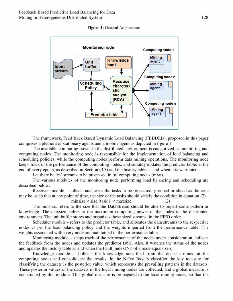
Feedback Based Predictive Load Balancing for Data Mining in Heterogeneous Distributed System 128
Figure 1: General Architecture
The framework, Feed Back Based Dynamic Load Balancing (FBBDLB), proposed in this paper comprises a plethora of stationary agents and a mobile agent as depicted in figure 1.
The available computing power in the distributed environment is categorized as monitoring and computing nodes. The monitoring node is responsible for the implementation of load balancing and scheduling policies, while the computing nodes perform data mining operations. The monitoring node keeps track of the performance of the computing nodes, and suitably updates the predictor table, at the end of every epoch, as described in Section (3.3) and the history table as and when it is warranted.
Let there be ‘m’ streams to be processed in ‘n’ computing nodes (m>n). The various modules of the monitoring node performing load balancing and scheduling are
described below. Receiver module – collects and, sizes the tasks to be processed, grouped or sliced as the case
may be, such that at any point of time, the size of the tasks should satisfy the condition in equation (2) minsize < size (task i) < maxsize. (2)
The minsize, refers to the size that the DataStream should be able to impart some pattern or knowledge. The maxsize, refers to the maximum computing power of the nodes in the distributed environment. The unit buffer stores and organizes these sized streams, in the FIFO order.
Scheduler module - refers to the predictor table, and allocates the data streams to the respective nodes as per the load balancing policy and the weights imparted from the performance table. The weights associated with every node are maintained in the performance table.
Monitoring module – keeps track of the performance of the nodes under consideration, collects the feedback from the nodes and updates the predictor table. Also, it watches the status of the nodes and updates the history table as and when the Fault_index(Ni) of a node equals zero.
Knowledge module – Collects the knowledge unearthed from the datasets mined at the computing nodes and consolidates the results. In the Naïve Baye’s classifier the key measure for classifying the datasets is the posterior value, which represents the prevailing patterns in the datasets. These posterior values of the datasets in the local mining nodes are collected, and a global measure is constructed by this module. This global measure is propagated to the local mining nodes, so that the

129 M. Eugin Lilly Mary and V. Saravanan
mining operation is performed at the nodes on the local data set with the global parameter. Thus, more accurate results can be aimed at, for duly resolving the security issues.
Stationary agents, named mining agents, are deployed at the computing nodes. These agents receive the data stream, perform the mining operation and evaluate the parameters prevailing in the data Streams. The modules in the mining node comprise of the -
Receiver module – receives the data streams allocated to the particular node Knowledge module – performs the mining operation and evaluates the key parameter named
posterior value, prevailing in the local data stream and submits the same for the construction of the global parameters, and performs the mining operation adopting this global measure.
Feedback module – keeps track of the parameters and the performance metrics such as the actual time taken for completing the assigned task and setting the flag, and Fault-index (Ni) to zero whenever the time of execution exceeds the max_threshold_value.
The mobile agent “Resource Characteristic Analyst”(RCA) – while roaming across the network, constructs the global parameters from the local parameters and imparts the updated global parameter to the ‘knowledge module’ of the mining agents. As a result, uncovering of patterns or knowledge can be achieved from the DataStream at the nodes adopting the global parameters. In [Josenildo Costa Da Silvia et al, 2006], the parameter named, ‘Kernel estimators’ pertaining to the local datasets, contributes to the construction of the global estimator, which is the key attribute for data clustering.
In our framework, the global measure of the parameter posterior value, which is calculated from the training datasets, is globally considered and this global measure is propagated to the nodes for performing classification.
The feedback module of the RCA collects the feedback from the mining agents and updates the predictor table of the Monitoring node. 6. Experimental Evaluation The algorithms discussed in sections (4.1), (4.2) and (4.3) are intended for performing data mining operations at the computing elements in the distributed nodes, and to consolidate the results at the monitoring server. Experiments have been conducted with the water sample results. 6.1. Data Base Considered
The data maintained by the Tamil Nadu Water Supply and Drainage Board has been used for the study. The data base in the form of MS Access contains a table with 5 lakh records, containing 38 attributes of the categorical and numerical types. A record shows the constituents of a water sample collected from a water source, like a deep bore well, river etc., along with the location of the source. In this record, 26 attributes, viz, Colour, Odor, Turbidity, Iron, Chlorides, Fluorine, E_Coli, PH etc contribute to classify a water sample as potable or non potable. The data to be analyzed has been converted to the csv format, and then sliced or grouped into subtasks , and scheduled to the nodes as per the algorithms discussed in sections (4.1),(4.2), and(4.3). 6.2. Data Base Schema Designed
The data base designed for recording the observations at run time is as below. The database DDMDatabase consists of 5 tables.
1. M_Mining_Server 2. M_Parameter 3. M_Raw_Files 4. T_Predictor 5. T_Processed_Files
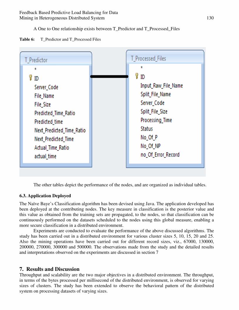
Feedback Based Predictive Load Balancing for Data Mining in Heterogeneous Distributed System 130
A One to One relationship exists between T_Predictor and T_Processed_Files Table 6: T_Predictor and T_Processed Files
The other tables depict the performance of the nodes, and are organized as individual tables. 6.3. Application Deployed
The Naïve Baye’s Classification algorithm has been devised using Java. The application developed has been deployed at the contributing nodes. The key measure in classification is the posterior value and this value as obtained from the training sets are propagated, to the nodes, so that classification can be continuously performed on the datasets scheduled to the nodes using this global measure, enabling a more secure classification in a distributed environment.
Experiments are conducted to evaluate the performance of the above discussed algorithms. The study has been carried out in a distributed environment for various cluster sizes 5, 10, 15, 20 and 25. Also the mining operations have been carried out for different record sizes, viz., 67000, 130000, 200000, 270000, 300000 and 500000. The observations made from the study and the detailed results and interpretations observed on the experiments are discussed in section 7 7. Results and Discussion Throughput and scalability are the two major objectives in a distributed environment. The throughput, in terms of the bytes processed per millisecond of the distributed environment, is observed for varying sizes of clusters. The study has been extended to observe the behavioral pattern of the distributed system on processing datasets of varying sizes.
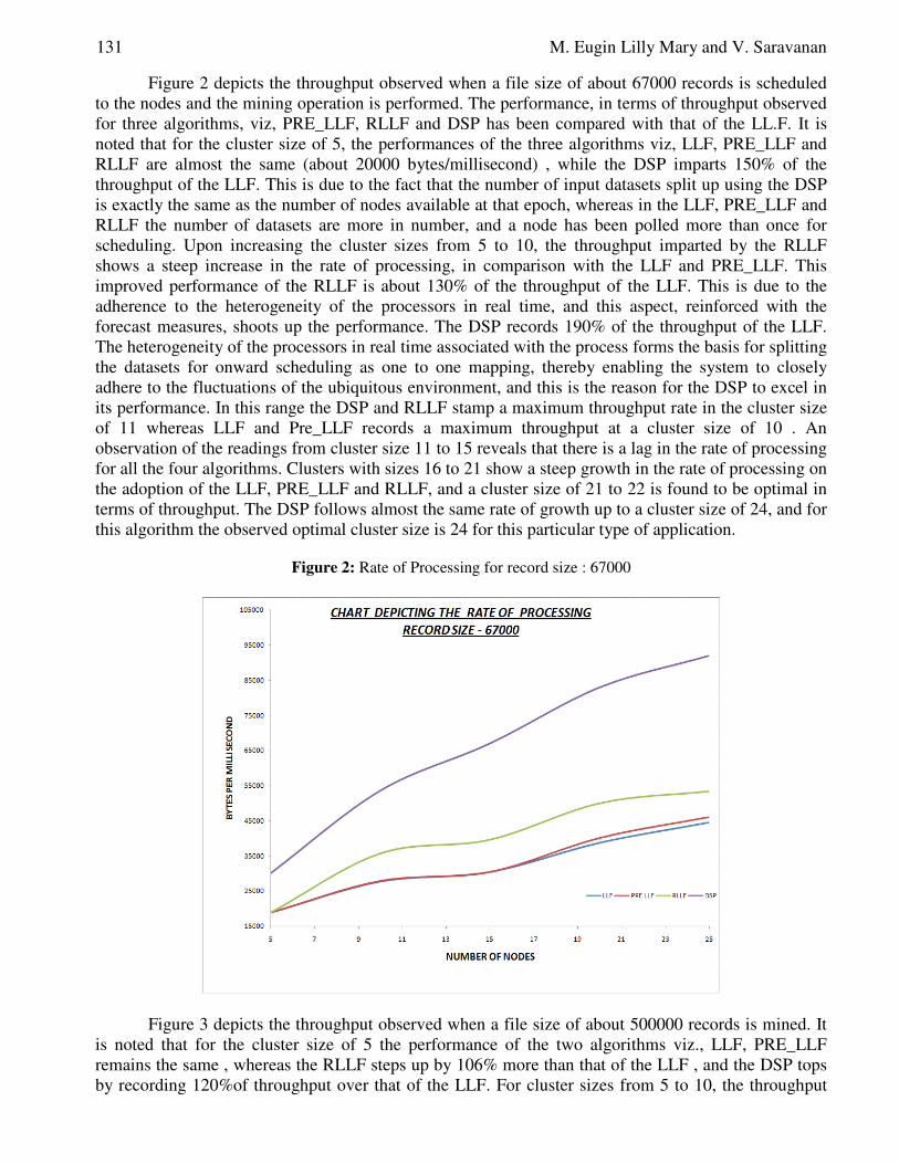
131 M. Eugin Lilly Mary and V. Saravanan
Figure 2 depicts the throughput observed when a file size of about 67000 records is scheduled to the nodes and the mining operation is performed. The performance, in terms of throughput observed for three algorithms, viz, PRE_LLF, RLLF and DSP has been compared with that of the LL.F. It is noted that for the cluster size of 5, the performances of the three algorithms viz, LLF, PRE_LLF and RLLF are almost the same (about 20000 bytes/millisecond) , while the DSP imparts 150% of the throughput of the LLF. This is due to the fact that the number of input datasets split up using the DSP is exactly the same as the number of nodes available at that epoch, whereas in the LLF, PRE_LLF and RLLF the number of datasets are more in number, and a node has been polled more than once for scheduling. Upon increasing the cluster sizes from 5 to 10, the throughput imparted by the RLLF shows a steep increase in the rate of processing, in comparison with the LLF and PRE_LLF. This improved performance of the RLLF is about 130% of the throughput of the LLF. This is due to the adherence to the heterogeneity of the processors in real time, and this aspect, reinforced with the forecast measures, shoots up the performance. The DSP records 190% of the throughput of the LLF. The heterogeneity of the processors in real time associated with the process forms the basis for splitting the datasets for onward scheduling as one to one mapping, thereby enabling the system to closely adhere to the fluctuations of the ubiquitous environment, and this is the reason for the DSP to excel in its performance. In this range the DSP and RLLF stamp a maximum throughput rate in the cluster size of 11 whereas LLF and Pre_LLF records a maximum throughput at a cluster size of 10 . An observation of the readings from cluster size 11 to 15 reveals that there is a lag in the rate of processing for all the four algorithms. Clusters with sizes 16 to 21 show a steep growth in the rate of processing on the adoption of the LLF, PRE_LLF and RLLF, and a cluster size of 21 to 22 is found to be optimal in terms of throughput. The DSP follows almost the same rate of growth up to a cluster size of 24, and for this algorithm the observed optimal cluster size is 24 for this particular type of application.
Figure 2: Rate of Processing for record size : 67000
Figure 3 depicts the throughput observed when a file size of about 500000 records is mined. It is noted that for the cluster size of 5 the performance of the two algorithms viz., LLF, PRE_LLF remains the same , whereas the RLLF steps up by 106% more than that of the LLF , and the DSP tops by recording 120%of throughput over that of the LLF. For cluster sizes from 5 to 10, the throughput
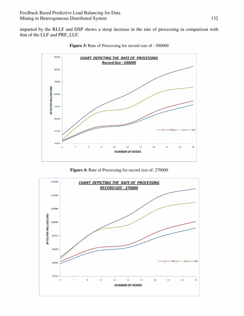
Feedback Based Predictive Load Balancing for Data Mining in Heterogeneous Distributed System 132
imparted by the RLLF and DSP shows a steep increase in the rate of processing in comparison with that of the LLF and PRE_LLF.
Figure 3: Rate of Processing for record size of : 500000
Figure 4: Rate of Processing for record size of: 270000
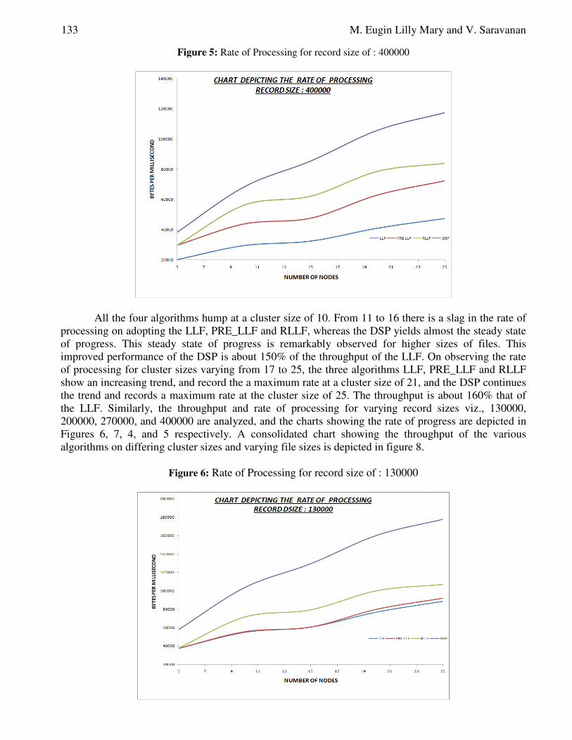
133 M. Eugin Lilly Mary and V. Saravanan
Figure 5: Rate of Processing for record size of : 400000
All the four algorithms hump at a cluster size of 10. From 11 to 16 there is a slag in the rate of processing on adopting the LLF, PRE_LLF and RLLF, whereas the DSP yields almost the steady state of progress. This steady state of progress is remarkably observed for higher sizes of files. This improved performance of the DSP is about 150% of the throughput of the LLF. On observing the rate of processing for cluster sizes varying from 17 to 25, the three algorithms LLF, PRE_LLF and RLLF show an increasing trend, and record the a maximum rate at a cluster size of 21, and the DSP continues the trend and records a maximum rate at the cluster size of 25. The throughput is about 160% that of the LLF. Similarly, the throughput and rate of processing for varying record sizes viz., 130000, 200000, 270000, and 400000 are analyzed, and the charts showing the rate of progress are depicted in Figures 6, 7, 4, and 5 respectively. A consolidated chart showing the throughput of the various algorithms on differing cluster sizes and varying file sizes is depicted in figure 8.
Figure 6: Rate of Processing for record size of : 130000
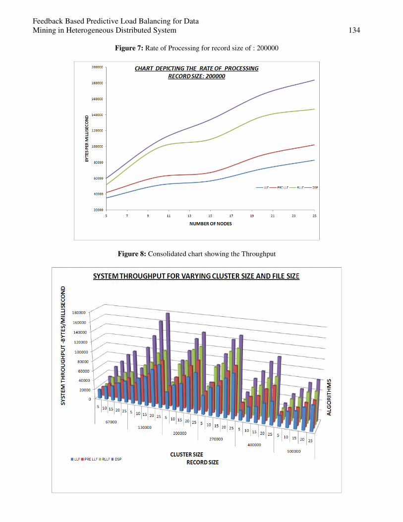
Feedback Based Predictive Load Balancing for Data Mining in Heterogeneous Distributed System 134
Figure 7: Rate of Processing for record size of : 200000
Figure 8: Consolidated chart showing the Throughput

135 M. Eugin Lilly Mary and V. Saravanan
An increase in the rate of mining is noticed as the record size increases from 67000 to 130000
and registers a peak at 130000 for all the four algorithms. The performance of the DSP excelled in cluster sizes of 20 and 25. This peak is continued for record sizes of 200000 and 270000. Beyond this, the rate of processing shows a declining trend as the record size grows. It is inferred that record sizes of about 300000 impart the maximal throughput for this particular type of application.
The scalability of the distributed environment is well observed from the consolidated chart. The throughput grows as the cluster size increases invariably for all the four algorithms analyzed and for varying file sizes. Hence, it is well defined that the system is scalable showing a higher throughput with an increase in the cluster sizes. 8. Conclusion Dynamic load balancing techniques in a distributed system comprising heterogeneous computing elements are discussed in this paper. The feedback based strategies implemented, predict the processing power of a node, with reference to the actual execution time. This forms the key attribute in designing the algorithms, Pre_LLF, RLLF and DSP. A collaborative agent system comprising stationary and mobile agents updates the performance tables dynamically. And this dynamic updating enables the system in predicting the processing power of the computing nodes, closely adhering to the fluctuations. The application constructed for classifying the water quality datasets has been specially deployed at the nodes. Experiments are conducted to compare the performance of the algorithms while classifying the water sample data at the contributing nodes. Observations of various cluster sizes, from 5 to 25, and a variety of workloads, from 670000 records to 500000 records, reveal that the Pre_LLF, RLLF and DSP stamp a better throughput than the LLF. The DSP tops for the various cluster sizes and differing loads. The DSP splits and schedules the datasets, by closely adhering to the fluctuations of the environment, and it is concluded that the DSP is the optimal technique for the ubiquitous distributed system. References [1] Bakri Yahaya, Rohaya Latip, Mohamed Othman, and Azizol Abdullah., 2011. “Dynamic Load
Balancing Policy with Communication and Computation Elements in Grid Computing with Multi-Agent System Integration”, International Journal on New Computer Architectures and Their Applications “ (IJNCAA) 1(3): 780-788
[2] Bravier.A.D, Montz.A.B, Peterson.L.L,1998. “Predicting Mpeg Execution Times, Proceedings of international conference –Measurment and modeling of computer systems”, SIGMETRICS.
[3] Byung Ha Son, Seong Woo Lee, Hee Yong Youn., 2010. “Prediction-Based Dynamic Load Balancing Using Agent Migration for Multi-Agent System”, 2010 12th IEEE International Conference on High Performance Computing and Communications.,pp.485-490
[4] Chen.M.S, Han.J, and Yu.P.S, 1996. “Data mining: an Overview from a database perspective”. IEEE Trans.On Knowledge And Data Engineering, 8:866–883,.
[5] Cybengo.G, 1989. “Dynamic Load Balancing for Distributed Memory Multiprocessors”, Journal of Parallel and Distributed Computing, Vol 7.pp-279-201.
[6] Ezumalai.R, Aghila.G and Rajalakshmi.R, , 2010 . “Design and Architecture for Efficient Load Balancing with Security Using Mobile Agents”, IACSIT International Journal of Engineering and Technology Vol. 2, No.1.,pp.57-60.
[7] Finin.T, Labrou.Y and Mayfield.J, 1997. “ KQML as an agent communication language”, Software Agents, J. Bradshaw, ed.,MIT Press, 1997, pp. 291–316
Feedback Based Predictive Load Balancing for Data Mining in Heterogeneous Distributed System 136
[8] Hinneburg.A and Keim.D.A, 1996. “An efficient approach to clustering in large multimedia databases with noise” , Proceedings of the Fourth International Conference on Knowledge Discovery and Data Mining (KDD-98), 58–65.
[9] Jiani Guo, Laxmi Narayan Bhuyan.,2006 “ Load Balancing in a Cluster-Based Web Server for Multimedia Applications ”, IEEE Transactions On Parallel And Distributed Systems, Vol. 17, No. 11, .pp-1321-1333.
[10] Josenildo Costa da Silvaa, Matthias Kluscha, Stefano Lodi, and Gianluca Moro.,2006. “Privacy-preserving agent-based distributed data clustering, Web Intelligence and Agent Systems”, An international journal 3 , pp.1–18.
[11] Kargupta.H, Park.B, Hershberger.D and Johnson.E, Advances in Distributed and Parallel Knowledge Discovery chapter 5, Collective Data Mining: ANew Perspective Towards
Distributed Data Mining,pp. 131–178. AAAI/MIT Press, 2000 [12] Katz.E, Butler.M, and McGrath.R,1994. “A Scalable Http Server: TheNcsa Prototype,”
Computer Networks and ISDN Systems, vol. 27,pp. 155-164. [13] Kim Y.H,2009. "An Efficient Dynamic Load Balancing Scheme for Multi-agent System
Reflecting Agent work load”, International Conference on Computational Science and Engineering, vol. 1, pp.216- 223.
[14] Liang-Teh Lee, Hung-Yuan Chang , Gei-Ming Chang and Hsing-Lu Chen., 2006. “A Grey Prediction Based Load Balancing Mechanism for Distributed Computing Systems” , ISCIT , pp.177-182
[15] Moro.G, Sartori.C,2001. “Incremental maintenance of multi source views” , Proc. ADC Brisbane, Australia. IEEE Computer Society, pp. 13–20.
[16] Neeraj Nehra, R.B. Patel, V.K. Bhat.,2007. “A Framework for Distributed Dynamic Load Balancing in Heterogeneous Cluster”, Journal of Computer Science 3 (1): pp.14-24.
[17] Nelson.R.D ,.Philips.T.K,1993. “ An approximation for the mean response time for the shortest queue routing with general interval and queue routing and service times ”, Performance Evaluation volume 17, pp 123-139.
[18] Rhee.S.W, 2008. “A Dynamic Weighting Scheme for Providing Fair Communication Service to Nomadic Agents,” Proceeding of ISDA 2008, IEEE, Kaohsiung, , pp. 468-473
[19] Stolfo.S.J, Prodromidis.A.L, Tselepis. S, Lee.W, Fan.D.W and Chan.P.K, JAM: Java agents for meta-learning over distributed databases, In Heckerman et al. [13], pp.74–81
[20] Tang.Z, Birdwell.J.D, Chiasion.J, .Abdallah.C.T, Hayat.M,2008. “Resource constrained Load Balancing for Parallel Database, IEEE transaction on control System Technology”,Vol.16,No.4.,pp.834-841
[21] Vuda Srinivasa Rao.,2010 “Multi-Agent Based Distributed Data Mining-An Overview”, International Journal of Reviews in Computing, pp.83-92
[22] Willeebeek.H and LeMair and A.P.Receves, 1991 “Strategies for load balancing on highly parallel com computers”, IEEE Transactions, Parallel and distributed systems, Vol IV.No9,pp-979-993.
[23] Xu.C.Z, Lau.F.C, 1992, Analysis of the Generalized Dimension Exchange Method for Dynamic Load balancing for distributed memory multiprocessors, Journal of Parallel and Distributed Computing, Vol.16, pp-385-392
[24] Xu, C.-Z. and Wims.B, 2000. Mobile agent based push methodology for global parallel computing Concurrency and Computation: Practice and Experience, vol .14,pp- 705-726
[25] Yongjian Yang, Xiaodong Cao, Jiubin Ju, Yajiun Chen, Research on Prediction Methods for Load Balancing Based on Self-adaptive and Confirmation Mechanism, 2005 International Conference on Control and Automation (ICCA2005),June 27-29, 2005, Budapest, Hungary,IEEE 2005, pp.533-536

European Journal of Scientific Research ISSN 1450-216X / 1450-202X Vol. 99 No 1 April, 2013, pp.137-144 http://www.europeanjournalofscientificresearch.com
New Algorithm of Low Pass Band Ripple
Decimation Filter for SDR Receivers
Mohamed Ubaed Barrak Tikreet University / Iraq.
E-mail: [email protected]
Abstract
This paper presents the development of a novel algorithm to minimize the pass band ripple of Decimation filter for multi-standard software defined radio (SDR) applications. The proposed algorithm incorporates the features of Remez algorithm (used to calculate the filter order) and Chebysheve or minimax algorithm (used to decrease the error by minimizing the filter order). The DDC filter is implemented using MATLAB and System Generator in Xilinx FPGA (Vertix-4). The new algorithm could minimize the power consumption by 20% in terms of FPGA area, compared to the existing designs. Keywords: FIR, DDC, SDR, FPGA, pass band ripple
1. Introduction A key component of wireless communication system is the Decimation filter which can be implemented in a dedicated processing hardware. For example, when a GSM module is activated and connected to the internet via WLAN, it can be reconfigured in the chip which is used for the decimation filter to execute a task. In this case the hardware has a high utilization factor. The algorithm can be performed continuously and only certain parameters may be changed. Any adaptability and spare performance will not be used in this situation [1].
Currently radio frequency transceivers demand high integration devices as well as low cost and low power operations with high efficiency. The system should be able to adapt into multiple communication standards such as software defined radio (SDR). The performance of SDR is greatly influenced by the functioning of Decimation part. Many researchers have attempted to improve the performance of decimation filter, by addressing the following issues:
a. The power consumption of the filter to be minimum, same time maintaining high efficiency
b. Minimize the pass band ripple to avoid the distortion in the received signal Most of the works to tackle the aforementioned problems were based on the Remez algorithm [2]
and the ‘Weighted Chebyshev Approximation’ or ‘Minimax’ algorithm [3]. A low passband error decimation filter to work with Global System for Mobile communications
(GSM) mask frequency was reported by Losada [4, 5] who obtained adjacent band rejection of -105db and passband ripple of about -0.05db. An improved Remez algorithm was presented by Lai and Zhao [6] for the design of minimax FIR filters with inequality constraints in frequency domain. A simple proof of the alternation theorem for minimax FIR filter design was presented by Vaidyanathan and Nguyen [7]. Pérez-Pascual et al. [8] showed that the efficiency of the decimation part was greatly influenced by the relationship between the transition band of the designed filter and its sampling frequency. Decimation filter for multi-standard wireless transceivers using MATLAB with -0.1dB in

New Algorithm of Low Pass Band Ripple Decimation Filter for SDR Receivers 138
passband ripple and -65dB stopband attenuation for GSM, WCDMA and WLAN, was introduced by Shahana [9]. Recently Mehra and Devi [10] presented an optimized System Generator based hardware co-simulation technique to implement GSM based DDC for SDR. Equiripple based polyphase decomposition technique was used to optimize the proposed filter design in terms of speed and area. The DDC filter was implemented in Field Programmable Gate Array (FPGA) by Naina and Gordana [14], Mehra and Devi[10], and Changrui et al [15].
The DDC filter proposed by Losada [4,5] and the commercial GC4016 multi-standard quad DDC presented by Texas Instruments [11, 12] were capable to some extent, to meet the low pass band ripple, adjacent band rejection and blocker requirements; however there is enough scope for further improvement. Accordingly, in the present work, a new algorithm is developed by incorporating the features of Remez and Minimax algorithms, in order to minimize the pass band ripple. Minimax is utilized to decrease the error by minimizing the filter order, and Remez algorithm is used to calculate the filter order. 2. Minimax Algorithm
Table 1 shows four types of FIR filters as proposed by [3, 13]. An error function E (ω) and a weight function W (ω) are defined for a relative value of the error at any given frequency ω. Then, the error function can be expressed as [4, 5]:
( ) ( )[ ( ) ( )]dE W A Aω ω ω ω= − (1) Where Ad (ω) is the desired amplitude response and A(ω) is the actual amplitude response. A
simple weight function W(ω), could be defined as follows:
1, ( )( )
0, ( )passband
Wstopband
ωω
ω
∈=
∈ (2)
and the resulting amplitude response, A(ω) is defined by:
( ) ( ) ( )A F Gω ω ω= (3)
and 0
( ) [ ]cos( )M
k
G b k kω ω=
=∑ (4)
where F(ω) and M are obtained from Table 1. Table 1: Parameters of the four type of FIR filters
To obtain the coefficient of b[k] which can minimize the high value of absolute error |E (ω)| across the specified passband and stopband, a specific algorithm need to be used. Accordingly, the minimax algorithm [3] was used, as expressed by:
( )min max | ( ) |G Eω ωε ω= (5)
where ω is the range of operating frequencies.

139 Mohamed Ubaed Barrak
2.1. Remez Exchange Algorithms
In the Remezalgorithm design approach, an approximation of the filter order N was used. The filter order is given by N = M − 1, and the filter length M can be estimated from Kaisers approximation (Eq. 6) where ∆f is the width of the transition band, δp is the passband tolerance related to the passband ripple Ap in dB, and δs is the stopband tolerance related to the stopband attenuation As in dB. In order to use the Remezapproach, the first step is to solve Eq. 6, and evaluate the filter coefficient to check the minimum stop band attenuation, As. Eq.6 should be iterated until the desired As is obtaind
1020 log ( ) 131,
14 .6 2
p s s pM f
f
δ δ ω ω
π
− − −= + ∆ =
∆ (6)
where, ωp is the passband-edge digital frequency, ωs is the stopband-edge digital frequency, and δp(eq. 7) and δs (eq. 8) are the passband and stopband deviations, respectively.
/20
10/20
110 1, 20 log 0( 0)
110 1
App
p pApp
Aδ
δδ
−−= = − > ≅
++ (7)
1020log 11
ss
p
Aδ
δ= − >
+ (8)
Where Ap and As are the attenuations on the passband and stopband, respectively. The stopband and passband energy E(ω) is given by [4]
21( ) | ( ) |
2 dF
E A dπ
ω ω ωπ
= ∫ (9)
3. Optimum Filter Figure 1 shows the flow chart for the proposed algorithm. The multistage decimator block diagram is shown in Figure 2. The 5-stage CIC filter takes the high-rate input signal and decimates it by a programmable factor. The CIC filter is followed by a 21-tap compensation FIR (CFIR) filter that equalizes the sharp attenuation due to the CIC filter and provides further low pass filtering and decimation by 2. The CFIR is then followed by a 65-tap programmable FIR (PFIR) filter that is used for a final decimation by 2.
In high rate design, the simplest filter is always put at the beginning stage in multistage decimator, and the complexity of the filters is progressively increased in the subsequent stages. In this case, the CIC filter is an attractive filter with high rates since it is capable to perform multiplier less operation and provide a low pass signal filtering by using few adders and delays. The CIC filter also has a drawback; its magnitude response is far from ideal and exhibits a sharp attenuation in the pass band which progressively attenuates signals. The CFIR has relatively simple structure, and has only 21 taps; its primary mission is to compensate the sharp attenuation by the CIC filter. The PFIR filter is the most complex of all the filters, requiring 65 multiplications per sample. Both CFIR and PFIR filters have linear-phase construction for a desirable characteristic in data transmission. The GSM specifications are show in Table 2.
From Equations (6,7 and 8) assume the stop band allowed deviation, δs = 0.01 and pass band ripple As ≤ − 0.012 dB, then the pass band allowed deviation δp was determined by equation (7) about 0.0007. The filter length was determined by Eq.(6):
lengthfilter 65 1 0.239)-(0.28 14.6
0.0007)20log(0.01- M
1/2
====++++××××
====
Therefore; the filter order is: N = M-1 = 65 -1 = 64
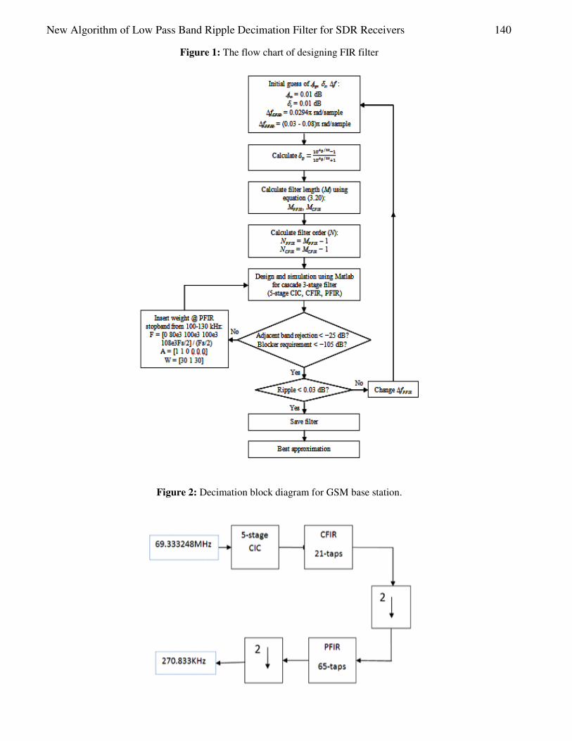
New Algorithm of Low Pass Band Ripple Decimation Filter for SDR Receivers 140
Figure 1: The flow chart of designing FIR filter
Figure 2: Decimation block diagram for GSM base station.

141 Mohamed Ubaed Barrak
Table 2: GSM specifications
Having N=64, the passband ripple has still not achieved the targeted value. In order to get a better passband ripple, a setting of W= [10, 1] will fulfill the requirements; however with significantly less adjacent band attenuation. A trade off can be achieved by setting the design as a lowpass filter with two separate stopband regions, each of them consists of different weight for the optimization purpose.
4. MATLAB Simulation Results The MATLAB simulation is carried out for three conventional GSM Decimation filters. It is clearly shown that the proposed model is more effective in passband region; the lower passband ripple is about -0.077dB better than that in GC-GSM mode, as presented in Table 3. The proposed model has also shown significant improvements on the adjacent band rejection and blocker requirements.
The overall response of CIC*CFIR*PFIR is shown in Figure 3 in which the GSM spectral mask requirement is also illustrated. The requirement that the peak to peak ripple to be less than 0.1 dB, is obtained. The maximum ripple in passband is approximately -0.012dB after zooming to the final GSM mask of the three filters as shown in Figure 4. And the proposed filter is able to compensate the adjacent band rejection and blocker requirements of the GSM system. This development increases the effectiveness of word length and in the sametime it reduces the power consumption. The stopband attenuation can be calculated typically as an absolute specification of the filter using Eq. (8):
As = -20 log10 (0.01) = 40 dB Figure 3: The Combination response of CIC, CFIR, and PFIR filters together with the GSM spectral mask
requirement.
0 200 400 600 800 1000-120
-110
-100
-90
-80
-70
-60
-50
-40
-30
-20
-10
0
10
Magnitude Reponse of Cascaded CIC * CFIR * PFIR -GSM Mode
Frequency (kHz)
Ma
gn
itu
de
(d
B)
Response of all three stages
GSM spectral mask requirement
Improvement in Adjacent Band Rejection
Improvement in Blocker Requirement
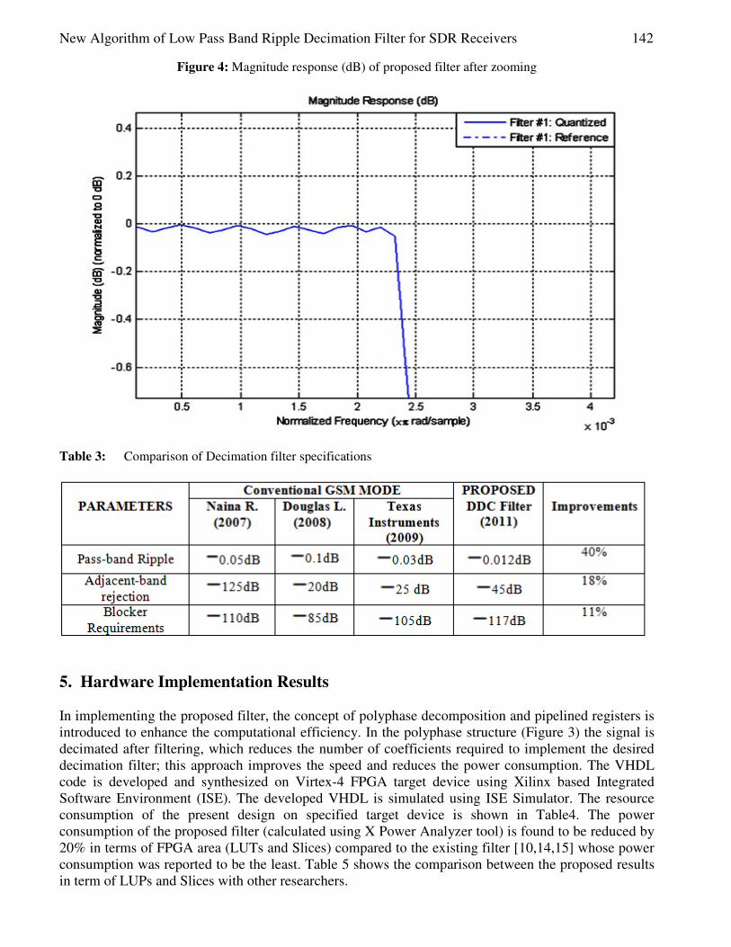
New Algorithm of Low Pass Band Ripple Decimation Filter for SDR Receivers 142
Figure 4: Magnitude response (dB) of proposed filter after zooming
Table 3: Comparison of Decimation filter specifications
5. Hardware Implementation Results In implementing the proposed filter, the concept of polyphase decomposition and pipelined registers is introduced to enhance the computational efficiency. In the polyphase structure (Figure 3) the signal is decimated after filtering, which reduces the number of coefficients required to implement the desired decimation filter; this approach improves the speed and reduces the power consumption. The VHDL code is developed and synthesized on Virtex-4 FPGA target device using Xilinx based Integrated Software Environment (ISE). The developed VHDL is simulated using ISE Simulator. The resource consumption of the present design on specified target device is shown in Table4. The power consumption of the proposed filter (calculated using X Power Analyzer tool) is found to be reduced by 20% in terms of FPGA area (LUTs and Slices) compared to the existing filter [10,14,15] whose power consumption was reported to be the least. Table 5 shows the comparison between the proposed results in term of LUPs and Slices with other researchers.

143 Mohamed Ubaed Barrak
Table 4: Decimation project status and device utilization summary
Table 5: Decimation filter implementation results comparison
6. Conclusion A novel linear-phase FIR filter has been developed to improve the performance of decimation filter in SDR receivers. A new technique to reduce the ripple in passband by minimizing the deviation in a decimation block is introduced. The approach is implemented in a multi-stage, multi-standard decimating filter. The proposed design is simple and leads to good optimal FIR filters compared to

New Algorithm of Low Pass Band Ripple Decimation Filter for SDR Receivers 144
other methods. This technique allows the designer to explicitly control the band edge and relative ripple sizes on each band of interest. Comparing with the existing systems, the pass band ripple, adjacent band rejection, and blocker requirements are significantly improved by the current design. Moreover; the clock of the Decimation filter is also improved thereby allowing it to operate in a multi-standard like GSM, WCDMA, and all other systems that works in the frequency band up to 100MHz.In general, it was observed that the reduction in number of coefficients in each filter stage promises better synthesis results in terms of circuit compactness and power dissipation. It will be interesting to explore efficient multiple partitioning of the filter structure sharing common subsections of different standards. References [1] T. Bijlsma, “An optimal architecture for a DDC” University of Twente, Department of
EEMCS, Netherlands. [2] Remez, E. Ya. "Sur le calculeffectif des polynômesd'approximation de Tschebyscheff."
C. P. Paris, 337-340, 1934. [3] R. LR, McCLellan JH, Parks TW, “FIRdigital filter design techniques using weighted
Chebyshev approximation”, Proc. IEEE, 63, 1975, pp.595-610. [4] R. A. Losada, “Practical FIR filter design in matlab”, The Math Works inc. Revision 1.1 , USA,
2004, PP. 5, 26-27. [5] R. A. Losada, “Practical FIR filter design in MATLAB”, The Math Works inc. Revision 1.1,
USA, 2008, PP. 5, 26-27. [6] X. Lai, R. Zhao, (2006), “On Chebyshev Design of Linear-Phase FIR Filters with Frequency
Inequality Constraints”, IEEE TRANSACTIONS ON CIRCUITS AND SYSTEMS—II: EXPRESS BRIEFS, VOL. 53, NO. 2, PP. 120-124.
[7] Vaidyanathan, P. P. and Nguyen, T. Q. (2007) A Simple Proof of the Alternation Theorem. In: Conference Record of the Forty-first Asilomar Conference on Signals, Systems and Computers. IEEE, Piscataway, NJ, pp. 1111-1115. ISBN 978-1-4244-2109-1.
[8] A. Pérez-Pascual, T. Sansaloni, V. Torres, V. Almenar, J. Valls, (2009), Design of Power and Area Efficient Digital Down-converters for Broadband Communications Systems”, J Sign Process Syst , vol. 56, pp.35–40.
[9] Shahana T. K, “Decimationfilter design toolbox for multi- standard wireless transceivers usingMATLAB” Int. J. of Signal Processing, 5;2 , 2009, PP. 154-163.
[10] RajeshMehra, S. Devi, (2010), “Efficient Hardware Co-Simulation Of Digital Down Convertor For Wireless communication Systems”, International journal of VLSI design & Communication Systems, Vol.1, No.2, pp. 13-21
[11] Texas Instruments, “GC4016 multi-standard quad DDC chip,” Data Sheet Rev. 1.0, 2001, PP. 60-90.
[12] Texas Instruments, “GC4016 multi-standard quad DDC chip data sheet,” Data Manual Revision 1.0, PP. 70-90. Literature Number: SLWS133BAugust 2001–Revised July 2009
[13] M. Kaiser, Handbook for Digital Signal Processing, John Wiley & Sons, 1993. [14] Naina R., Gordana J., (2006), “An Efficient Method to Design Fractional Decimation System”,
National Institute of Astrophysics, Optics, and Electronics, Department of Electronics, Puebla, Mexico, IEEE Xplore, available: http://ieeexplore.ieee.org/stamp/stamp.jsp?arnumber=04367658
[15] Changrui W., Kong Chao1,Xie Shigen2, Cai Huizhi1, (2010), “Design and FPGA Implementation of Flexible and Efficiency Digital Down Converter”, ICSP 2010 proceedings (IEEE), pp.438-441
European Journal of Scientific Research ISSN 1450-216X / 1450-202X Vol. 99 No 1 April, 2013, pp.145-164 http://www.europeanjournalofscientificresearch.com
Image Coding Using Block Classification and Transmission over Noisy Channel with Unequal Error Protection (UEP)
Jigisha. N. Patel ECED, SVNIT, SURAT
E-mail: [email protected]
S. Patnaik ECED, SVNIT, SURAT
E-mail: [email protected]
Saraiya Mansi ECED, SVNIT, SURAT
E-mail: [email protected]
Abstract
Image compression standard JPEG encodes each DCT Transform of block size 8x8. These blocks of image can be classified with similar types of activities like stastical, spectral and perceptual etc. Block classification make possible: design of quantizer for optimum bit allocation or adaptive bit allocation at source coding and implementation of error control scheme like Unequal Error Protection (UEP) in joint source channel coding (JSCC). The unequal importance of compressed bit stream of image coding motivates UEP. The UEP assigns the channel code rate according to significance of compressed bit stream. This paper propose block classification method using modified Equal Mean Normalized Standard Deviation (EMNSD) algorithm and assignment of UEP compressed block stream with JSCC. The different channel code rate generates using Rate Compatible Puncture Convolution (RCPC) channel coder. The simulation carried out for fixed transmission rate and channel condition. The source rate and channel rates are allocated such a way that it minimizes end to end distortion. The simulation result shows that source gain improvement of 0.3-0.5 dB PSNR using bit allocation according to block activity. The significant improvement in PSNR using UEP compare to Equal Error Protection (EEP) is 4.5-5 dB. Keywords: Joint photographic Expert Group (JPEG), Discrete Cosine Transform (DCT),
Quality Factor (QF), Equal Mean Normalized Standard Deviation (EMNSD), Rate Compatible Punture Convolution (RCPC)
1. Introduction In recent years most visual systems use image transformation DCT due to its energy compaction and decorrelation property [1]. Each image block has different degree of spatial feature, detail information, so the transform block reflect corresponding different distribution of coefficients. The block features like edge, texture, smoothness, shape, colour etc can be extracted from DCT transform coefficient distribution. Edge is one of the strong features for characterizing an image block. Vertical, horizontal and diagonal direction edge information can be extracted from DCT coefficient [10]. The two DCT
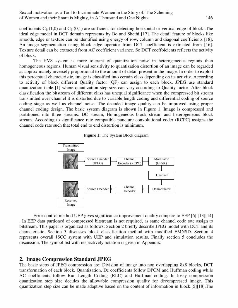
Sexual motivation as a Tool to Incriminate Women in the Story of: The Scheming of Women and their Snare is Mighty, in A Thousand and One Nights 146
coefficients CB (1,0) and CB (0,1) are sufficient for detecting horizontal or vertical edge of block .The ideal edge model in DCT domain represents by Bo and Shethi [17]. The detail feature of blocks like smooth, edge or texture can be identified using energy of row, column and diagonal coefficients [18]. An image segmentation using block edge operator from DCT coefficient is extracted from [16]. Texture detail can be extracted from AC coefficient variance. So DCT coeffoicients reflects the activity of block.
The HVS system is more tolerant of quantization noise in heterogeneous regions than homogeneous regions. Human visual sensitivity to quantization distortion of an image can be regarded as approximately inversely proportional to the amount of detail present in the image. In order to exploit this perceptual characteristic, image is classified into certain class depending on its activity. According to activity of block different Quality factor (QF) can assign to each block. JPEG use standard quantization table [1] where quantization step size can vary according to Quality factor. After block classification the bitstream of different class has unequal significance when the compressed bit stream transmitted over channel it is distorted due to variable length coding and differential coding of source coding stage as well as channel noise. The decoded image quality can be improved using proper channel coding design. The basic system diagram is shown in Figure 1. Image is compressed and partitioned into three streams: DC stream, Homogeneous block stream and heterogeneous block stream. According to significance rate compatible puncture convolutional coder (RCPC) assigns the channel code rate such that total end to end distortion is minimum.
Figure 1: The System Block diagram
Source Encoder
(JPEG)
Source DecoderChannel
DecoderDemodulator
Channel
Modulator
(BPSK)
Channel
Encoder (RCPC)
Transmitted
Image
Received
Image
Error control method UEP gives significance improvement quality compare to EEP [6] [13][14] . In EEP data partioned of compressed bitstream is not required, as same channel code rate assign to bitstream. This paper is organized as follows: Section 2 briefly describe JPEG model with DCT and its characteristic. Section 3 discusses block classification method with modified EMNSD. Section 4 represents overall JSCC system with UEP and simulation results. Finally section 5 concludes the discussion. The symbol list with respectively notation is given in Appendix. 2. Image Compression Standard JPEG The basic steps of JPEG compression are: Division of image into non overlapping 8x8 blocks, DCT transformation of each block, Quantization, Dc coefficients follow DPCM and Huffman coding while AC coefficients follow Run Length Coding (RLC) and Huffman coding. In lossy compression quantization step size decides the allowable compression quality for decompressed image. This quantization step size can be made adaptive based on the content of information in block.[5][18].The

147 Sanaa Kamel Shalan
block based discrete cosine transform (DCT) coding has been widely used in image and video compression standards for reducing inter pixel redundancy, such as JPEG, MPEG, H.26x etc. A transformation is therefore defined to map this spatial (correlated) data into transformed (uncorrelated) coefficients.
Consider image f(x, y) of size N x M. The image divide into block of size Lx L (L =8 in JPEG format). The total blocks of image f(x, y) are B= UxV where U=1,2,3,......N/L and V=1,2,3,......M/L. According to definition of two dimension DCT each block DCT transform CB(u, v) can be represent as
( ) ( )1 1
0 0
2 1 2 12 ( , ) ( ) ( ) ( , ) cos cos
2 2
L L
Bi i
u i v jC u v u v x i j
L L L
π πα α
− −
= =
+ + =
∑∑ (1)
Where { 1/2 01( ) foru
otherwiseuα =
−−−=
The corresponding inverse transform is 1 1
0 0
2 (2 1) (2 1) ( , ) ( ) ( ) ( , )
2 2
L L
Bu v
i u j vx i j u v C u v Cos Cos
L L L
π πα α
− −
= =
+ + =
∑∑ (2)
Where i = j= 0, 1, 2.......7. It is observed from Equation (1) that each DCT coefficient CB (u, v) is a linear combination of
all pixel values within the block. Specific features of DCT coefficients can be concluded as: i. DCT exhibits good decorrelation property [11]. The amplitude of autocorrelation after DCT
operation is very small. ii. DCT exhibits excellent energy compaction property. Figure 2 shows the two images with it’s
DCT transform coefficient value. It is observed that Figure 2(b) has more sharp intensity variation, more high frequency content, so its energy spread out compared to Figure 2(a) at whose energy is packed into the lower frequency region.
Figure 2: DCT transform of image with more (a) Homogeneous block (b)Heterogeneous block
50 100 150 200 250 300 350 400 450 500
50
100
150
200
250
300
350
400
450
200 400 600 800 1000 1200
200
400
600
800
1000
1200
1400
-10
-5
0
5
10
50 100 150 200 250 300 350 400 450 500
50
100
150
200
250
300
350
400
450
500
-10
-5
0
5
10
(a) (b)
iii. Each 8x8 block of the image is represented by 64 frequency components and the DC coefficient
(the first coefficient) represents the average intensity of this block. The total 63 AC coefficients denote the intensity changes among the samples. The colour information as well as shape

Sexual motivation as a Tool to Incriminate Women in the Story of: The Scheming of Women and their Snare is Mighty, in A Thousand and One Nights 148
information can be used for image retrival. G.C Feng and J. Jiang [12] extracted statistical features like moment and central moments directly from DCT coefficients. Consider X is a random variable, the kth moment of X of size LxL block can be defined as the
expectation of Xk , mentioned in Equation (3) 1 1
20 0
1( ) ( . )
L Lk k
ki j
m E X x i jL
− −
= =
= = ∑∑ (3)
where k is an integer. The kth central moment of X is defined as follows:
( )( ) [ ]1 1
20 0
1 ( , ) ( )
L Lk k
ki j
E X E X x i j E XL
µ− −
= =
= − = − ∑∑ (4)
So corresponding second central moment can be represents as 2
2 2 1 m mµ = − (5)
The 1st order moment m1 and the second-order central moment µ2 are referred to as mean and variance of the pixels inside this block. From definitions given in Equation (3) and (5), it is seen that m1 represents the average intensity of the block, and µ2 the difference of intensity among the pixels inside this block. Substitute the Equation (2) in (3) for calculation of m1 and m2. The second central moment µ2 can be calculated as:
1
1(0,0)Bm C
L= (6)
1 12
2 20 0
1( , )
L L
Bu v
C u vL
µ− −
= =
= ∑∑ (u,v)≠(0,0) (7)
The expressions of Equations (6) and (7) shows that the mean m1 can be directly derived from
the DC coefficient, and the second central moment which also refer as variance is just the average summation of all squared AC coefficients [12]. The second central moment we use as one of the parameter in block classification method. 3. Block Classification of Image Coding From DCT coefficient based classification used by Smith in 1977 where they used the parameter AC energy for block classification. But this algorithm requires equal number of blocks in each class [2]. W. A. Pearlman proposed DCT image coding where the block spectral characteristics decide the rate [3]. In 1997 R. L Joshi and his team proposed two algorithms, maximum classification gain and Equal Mean Normalized Standard Deviation (EMNSD) classification which allow unequal number of blocks in each class [4].The block classification algorithm EMNSD is simple algorithm [4] and provide good performance. In this algorithm the parameter used for classification is average gain gn of each block. The average gain can be found from DC and AC coefficients energy. In our method the parameter of classification adopted is the second central moment µ2 of a block. As mentioned in Equation (7) it can be calculated using only AC coefficients. Consider the algorithm for two different class of classification K=2. Each block of image f(x, y), value of µ2 is first calculate using equation (7). The total B blocks organized in an increasing order of their second central moments values 2 nµ where n =
1, 2, 3...B. Then out of total blocks B the first B1 blocks are assigned to class 1, the next B2 blocks to class 2 and so on. Find B1 and B2, such that the coefficient of variation qi defines in Equation (8) in the resulting class is equal. The ‘coefficient of variation’ is a good measure for dispersion and it is defined as[4].
Eii
Ei
qm
σ= (8)

149 Sanaa Kamel Shalan
Where Eiσ is standard deviation and Eim is mean of each class. The idea behind this approach
is the possibility of having a different number of blocks in each class and to have similar statistic properties within each class. An integer B1 such that blocks indexed 1 to B1 belong to the class 1 and the remaining blocks belong to the class 2. B1 is chose such that 1 2q q=
1 2
1 2
E E
E Em m
σ σ=
The mean mEi and standard deviation Eiσ of class i =1...K (K=2 in our case) are defined by 1
1 211
1 Bn
En
mB
µ=
= ∑ (9)
1
2 211
1 Bn
En B
mB B
µ= +
=−
∑ (10)
( )1 2
1 2 111
1 Bn
En
mB
σ µ=
= −∑ (11)
( )1
2
2 2 211
1 Bn
En B
mB B
σ µ= +
= −−
∑ (12)
In simulation the initial value of iteration start from B1=B/2 and iteration number set to i=0.
Compute q1 and q2 for each iteration and find q1 = q2 or
1 2q q ε− ≤
(13) If 1 2, 1 1 1q q setB B B< = + ∆
If 1 2, 1 1 1q q setB B B> = − ∆
Iteration will continue for up till Equation (13) is satisfied. For fast convergence a large 1B∆
can be chosen at the beginning of the iteration and as the iteration number increases 1B∆ must be
gradually decreased to one [4]. The following Figure 3a) shows block wise central moment while b) shows ascending order of central moment. The binary map corresponds to marked region is shown in Figure 4. This map is required at the decoder side for block identification. This activity map consist value 0 for homogeneous block as class 1and 1 for heterogeneous block as class 2. The block classified image is shown in Figure 4 c).
Figure 3: (a) Block variance (b) Ascending order Block variance
(a) (b)
Figure 4: (a) Original image (b) Binary Map of Marked region (c) Block classification of image

Sexual motivation as a Tool to Incriminate Women in the Story of: The Scheming of Women and their Snare is Mighty, in A Thousand and One Nights 150
50 100 150 200 250 300 350 400 450 500
50
100
150
200
250
300
350
400
450
500
0 0 0 0 0 1 0
0 0 1 0 0 1 0
0 1 1 0 0 1 0
1 0 1 0 0 1 0
0 0 1 0 0 1 0
0 0 1 0 0 1 0
0 0 1 0 0 1 0
white=smooth blocks,black=nonsmooth blocks
50 100 150 200 250 300 350 400 450 500
50
100
150
200
250
300
350
400
450
500
(a) (b) (c)
So using this method we classified image blocks into two categories: class1-Homogeneous and
class-2 Heterogeneous blocks. 4. Block Classified Image Transmission with UEP and Simulation Result The block diagram of system is shown in Figure 1. Where image is first compressed then protected with channel coding and transmits through channel. During this transmission span the total distortion DT of received image is source distortion Ds with channel distortion Dc
DT = Ds + Dc (14) The source distortion can be controlled by quantization step size using Quality Factor (QF).
The higher value of QF, less compression and less source distortion. The sour rate Rs can be calculate as
Total Encoded Bits
Image sizesR = Bits per Pixel (BPP)
The QF versus encoded bits of DC coefficients bits , class1 bits and class 2 bits curve is shown in Figure 5 (a).So total bits consists DC coefficient bits and AC coefficients bits. In our case AC coefficient bits are classified as homogeneous bits and heterogeneous bits. Corresponding source rate distortion curve (Rs versus Ds) is also shown in Figure 5 (b). The distortion measured in terms of Mean Square Error (MSE).
Figure 5: (a) QF versus different stream bits (b) source rate distortion curve
0 10 20 30 40 50 60 70 80 900
1
2
3
4
5
6
7
8
9x 10
4
QF
Num
ber
of
bits
QF Vs. Number of bits
DC
ACHO
ACHE
0.05 0.1 0.15 0.2 0.25 0.3 0.35 0.4
20
40
60
80
100
120
140
160
180
Rs
MS
E
source distortion curve
In above simulation result all the blocks have applied same quality factor. After Block classification as homogeneous and heterogeneous, the allocation of QF can be made adaptive according to its activity. The effect of increasing QF for homogeneous blocks and the corresponding
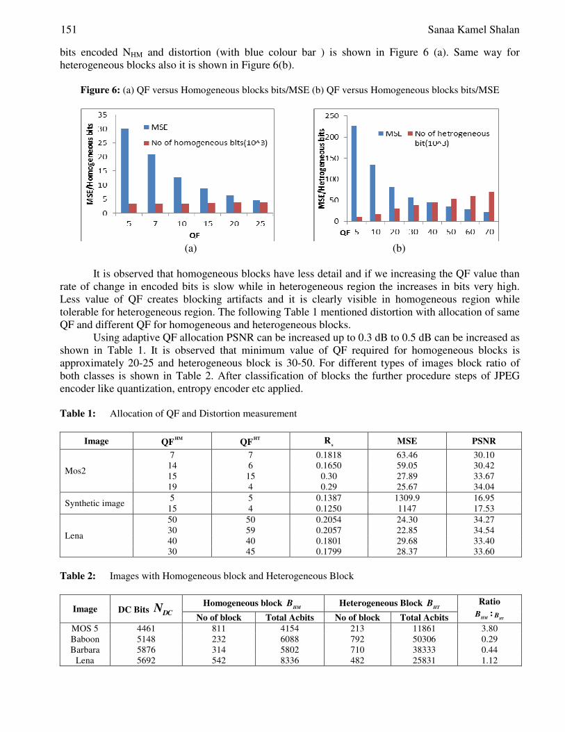
151 Sanaa Kamel Shalan
bits encoded NHM and distortion (with blue colour bar ) is shown in Figure 6 (a). Same way for heterogeneous blocks also it is shown in Figure 6(b).
Figure 6: (a) QF versus Homogeneous blocks bits/MSE (b) QF versus Homogeneous blocks bits/MSE
(a) (b)
It is observed that homogeneous blocks have less detail and if we increasing the QF value than
rate of change in encoded bits is slow while in heterogeneous region the increases in bits very high. Less value of QF creates blocking artifacts and it is clearly visible in homogeneous region while tolerable for heterogeneous region. The following Table 1 mentioned distortion with allocation of same QF and different QF for homogeneous and heterogeneous blocks.
Using adaptive QF allocation PSNR can be increased up to 0.3 dB to 0.5 dB can be increased as shown in Table 1. It is observed that minimum value of QF required for homogeneous blocks is approximately 20-25 and heterogeneous block is 30-50. For different types of images block ratio of both classes is shown in Table 2. After classification of blocks the further procedure steps of JPEG encoder like quantization, entropy encoder etc applied. Table 1: Allocation of QF and Distortion measurement
Image HMQF
HTQF s
R MSE PSNR
Mos2
7 7 0.1818 63.46 30.10 14 6 0.1650 59.05 30.42 15 15 0.30 27.89 33.67 19 4 0.29 25.67 34.04
Synthetic image 5 5 0.1387 1309.9 16.95
15 4 0.1250 1147 17.53
Lena
50 50 0.2054 24.30 34.27 30 59 0.2057 22.85 34.54 40 40 0.1801 29.68 33.40 30 45 0.1799 28.37 33.60
Table 2: Images with Homogeneous block and Heterogeneous Block
Image DC Bits DCN
Homogeneous block HM
B Heterogeneous Block HT
B Ratio
HMB :
HTB
No of block Total Acbits No of block Total Acbits
MOS 5 4461 811 4154 213 11861 3.80 Baboon 5148 232 6088 792 50306 0.29 Barbara 5876 314 5802 710 38333 0.44
Lena 5692 542 8336 482 25831 1.12
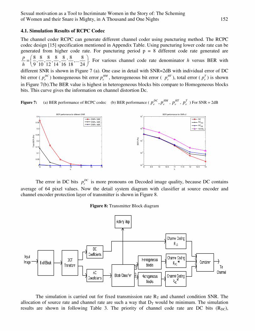
Sexual motivation as a Tool to Incriminate Women in the Story of: The Scheming of Women and their Snare is Mighty, in A Thousand and One Nights 152
4.1. Simulation Results of RCPC Codec
The channel coder RCPC can generate different channel coder using puncturing method. The RCPC codec design [15] specification mentioned in Appendix Table. Using puncturing lower code rate can be generated from higher code rate. For puncturing period p = 8 different code rate generated are
8 8 8 8 8 8 8, , , , ' ,...
9 10 12 14 16 18 24
p
h
=
. For various channel code rate denominator h versus BER with
different SNR is shown in Figure 7 (a). One case in detail with SNR=2dB with individual error of DC bit error ( DC
ep ) homogeneous bit error HMep , heterogeneous bit error ( HT
ep ), total error ( Tep ) is shown
in Figure 7(b).The BER value is highest in heterogeneous blocks bits compare to Homogeneous blocks bits. This curve gives the information on channel distortion Dc.
Figure 7: (a) BER performance of RCPC codec (b) BER performance ( ,DC HMe ep p , HT
ep , Tep ) For SNR = 2dB
9 10 11 12 13 14 150
0.05
0.1
0.15
0.2
0.25
0.3
0.35
0.4
h
Tota
l B
ER
(P
e)
BER performance for different SNR
SNR= 2dB
SNR= 3dB
SNR= 4dB
9 9.5 10 10.5 11 11.5 12 12.5 13
10-3
10-2
10-1
100
101
h
BE
R (
Pe)
BER performance for SNR=2
DC
ACHO
ACHE
TOTAL
The error in DC bits DCep is more pronouns on Decoded image quality, because DC contains
average of 64 pixel values. Now the detail system diagram with classifier at source encoder and channel encoder protection layer of transmitter is shown in Figure 8.
Figure 8: Transmitter Block diagram
The simulation is carried out for fixed transmission rate RT and channel condition SNR. The allocation of source rate and channel rate are such a way that DT would be minimum. The simulation results are shown in following Table 3. The priority of channel code rate are DC bits (RDC),
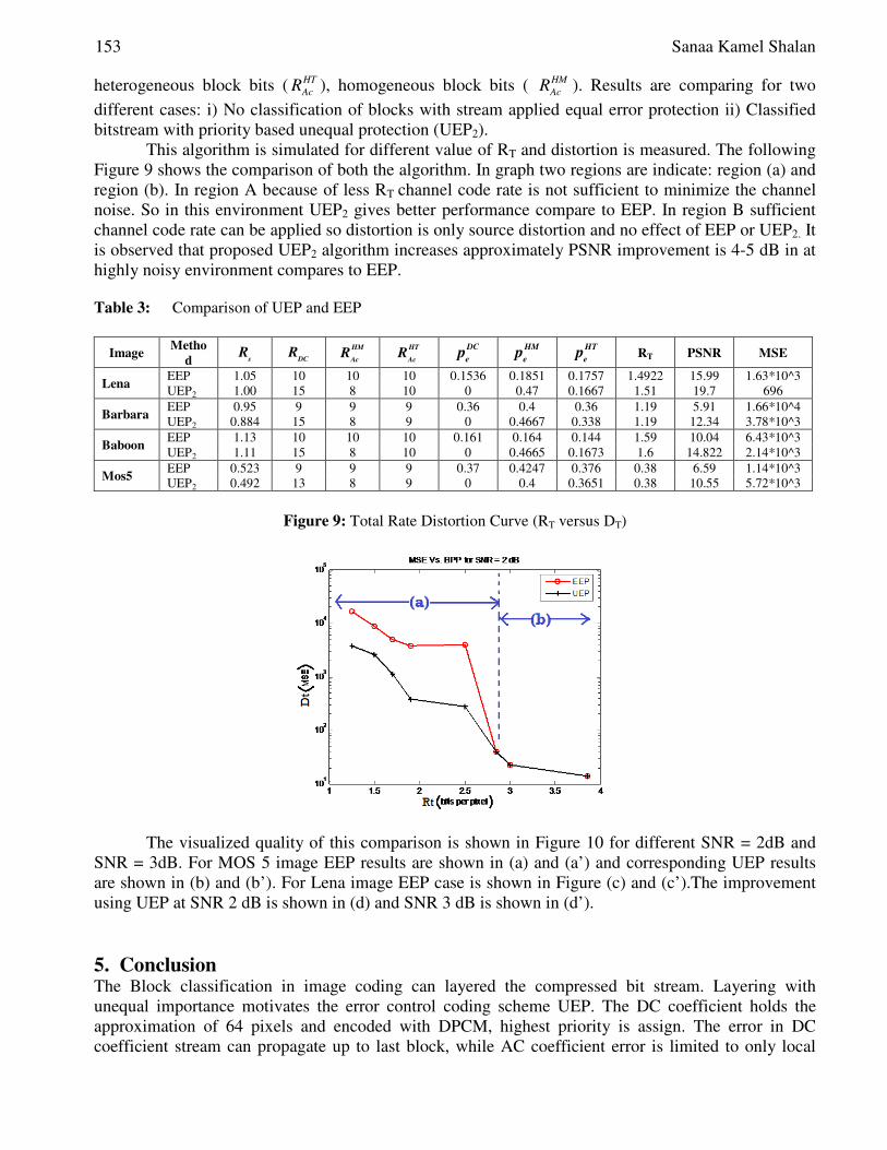
153 Sanaa Kamel Shalan
heterogeneous block bits ( HTAcR ), homogeneous block bits ( HM
AcR ). Results are comparing for two
different cases: i) No classification of blocks with stream applied equal error protection ii) Classified bitstream with priority based unequal protection (UEP2).
This algorithm is simulated for different value of RT and distortion is measured. The following Figure 9 shows the comparison of both the algorithm. In graph two regions are indicate: region (a) and region (b). In region A because of less RT channel code rate is not sufficient to minimize the channel noise. So in this environment UEP2 gives better performance compare to EEP. In region B sufficient channel code rate can be applied so distortion is only source distortion and no effect of EEP or UEP2. It is observed that proposed UEP2 algorithm increases approximately PSNR improvement is 4-5 dB in at highly noisy environment compares to EEP. Table 3: Comparison of UEP and EEP
Image Metho
d sR
DCR
HM
AcR
HT
AcR
DC
ep
HM
ep
HT
ep RT PSNR MSE
Lena EEP 1.05 10 10 10 0.1536 0.1851 0.1757 1.4922 15.99 1.63*10^3 UEP2 1.00 15 8 10 0 0.47 0.1667 1.51 19.7 696
Barbara EEP 0.95 9 9 9 0.36 0.4 0.36 1.19 5.91 1.66*10^4 UEP2 0.884 15 8 9 0 0.4667 0.338 1.19 12.34 3.78*10^3
Baboon EEP 1.13 10 10 10 0.161 0.164 0.144 1.59 10.04 6.43*10^3 UEP2 1.11 15 8 10 0 0.4665 0.1673 1.6 14.822 2.14*10^3
Mos5 EEP 0.523 9 9 9 0.37 0.4247 0.376 0.38 6.59 1.14*10^3 UEP2 0.492 13 8 9 0 0.4 0.3651 0.38 10.55 5.72*10^3
Figure 9: Total Rate Distortion Curve (RT versus DT)
The visualized quality of this comparison is shown in Figure 10 for different SNR = 2dB and SNR = 3dB. For MOS 5 image EEP results are shown in (a) and (a’) and corresponding UEP results are shown in (b) and (b’). For Lena image EEP case is shown in Figure (c) and (c’).The improvement using UEP at SNR 2 dB is shown in (d) and SNR 3 dB is shown in (d’). 5. Conclusion The Block classification in image coding can layered the compressed bit stream. Layering with unequal importance motivates the error control coding scheme UEP. The DC coefficient holds the approximation of 64 pixels and encoded with DPCM, highest priority is assign. The error in DC coefficient stream can propagate up to last block, while AC coefficient error is limited to only local

Sexual motivation as a Tool to Incriminate Women in the Story of: The Scheming of Women and their Snare is Mighty, in A Thousand and One Nights 154
blocks. The heterogeneous blocks gets higher protection compare to homogeneous blocks stream. The work can be extended with different quantization algorithm.
Figure 10: Visualized Comparison of UEP and EEP (a),(b),(c), (d) at SNR 2 dB (a’),(b’),(c’), (d’) at SNR 3 dB
Decoded Image
50 100 150 200 250
50
100
150
200
250
Decoded Image
50 100 150 200 250
50
100
150
200
250
Decoded Image
50 100 150 200 250
50
100
150
200
250
Decoded Image
50 100 150 200 250
50
100
150
200
250
(a) (b) (c) (d)
Decoded Image
50 100 150 200 250
50
100
150
200
250
Decoded Image
50 100 150 200 250
50
100
150
200
250
Decoded Image
50 100 150 200 250
50
100
150
200
250
Decoded Image
50 100 150 200 250
50
100
150
200
250
(a) (b) (c) (d)
Hence using proper bit allocation and protection according to significance end to end distortion
can be reduced. Appendix F(x, y) = NxM Original image size ,x = 0,1,2……..N-1, y = 0,1,2,3…….M-1
( , )BC u v Block DCT transform
J = Lx L Block size, L=8 K No. Of classes X = x(i, j) Block dimension mk = E(Xk) Kth moment of block µk Kth central moment of block ,E[(X-E(x)k] µ2 Second central moment = 2
2 1m m− 2σ Variance of a block
B=U x V Total blocks, U= N/L, V= M/L B1 Total no of blocks in class 1 B2 Total no of blocks in class 2 gn AC energy of Block qi Coefficient of variation mE1 mean value of class 1 mE2 mean value of class 2
1Eσ Standard deviation of class1
2Eσ Standard deviation of class 2
RT Total transmission rate, Image Bits Per Pixel(BPP), Rs Source code rate Rc Channel code rate = p / h =8/8, 8/9, 8/10, 8/11 RDC Channel code rate for DC coefficients bitstream
HM
ACR Channel code rate for Homogeneous block AC coefficient bitstream

155 Sanaa Kamel Shalan
(Continued...) HT
ACR Channel code rate for Hetrogeneous block AC coefficient bitstream
UEP2 Two level block classification UEP method QF Quality factor
HMQF Quality factor for homogeneous block
HTQF Quality factor for heterogeneous block
DCN Total bits of DC coefficients
HMN Total bits of homogeneous block bits
HTN Total bits of homogeneous block bits
p Puncturing period Mc Mother code rate :1/3
DC
ep BER of DC coefficient bitstream
HM
ep BER of Homogeneous block bitstream
HT
ep BER of Heterogeneous block stream
T
ep Total BER
Reference [1] G. K. Wallace, The JPEG still picture compression standard, Special issue on Digital
multimedia systems, Issue 4,vol 34,pp 30-44, April 1991. [2] W.H.Chen and C.H.Smith, “Adaptive coding of monochrome and colour images,IEEE
Transaction Communication,vol.COM-25,pp 1285-1292,Nov 1977. [3] W. A. Pearlman, ”Adaptive Cosine Transform image coding with constant block distortion,
IEEE Trans Communication,vol 38,pp698-703,May 1990. [4] R.L Joshi, H.Jafarkhani, J.H.Kasner, T.R.Fischer, N.Farvadin” Comparison of different
methods of classification in subband coding of image, “IEEE Trans Image processing, vol 6,pp 1473-1485,Nov 1997.
[5] Jianfei Cai an Chang Wen Chen, “Uniform threshold TCQ with block classification for Image transmission over Noisy channels” IEEE Transaction on Circuits and systems for video technology, Vol 11, No 1, January 2001.
[6] Fowdur . T.P& Soyjaaudah, K.M.S, Robust JPEG image transmission using unequal error protection and code combining, International journal of Communication systems , 21, 1-24, wiley Interscience, doi: 10.1002/dac.875, 17 Jan 2007.
[7] Sabir M. F sheikh, H R Heath, R W Jr & Bovik A.C. “A joint source channel distortion model for JPEG compressed image, In Proceedings of the 2004 International conference on Image Processing(ICIP 2004), 3249-3252, Singapor, Oct 24-27, 2004.
[8] David Akopian” On optimal Bit allocation for classification –Based Source Dependent Transform coding, Hindawi Publishing Corporation, research letter in signal processing, doi:10.1155/2008/421650, 1-5,2008.
[9] Hamid Jafarkhanj and Nariman Farvadin,” Adaptive Image coding Using Spectral classification” IEEE Transaction on Image Processing”, Vol 7 , No 4, April 1998.
[10] Hyun Sung Chang , Kyeongok Kang,” A compressed domain scheme for classifying block edge pattern, IEEE Transaction on Image processing, Vol 14,no 2, Feb 2005.
[11] Nuno Roma, Leonel Sousa, “A tutorial overview on the properties of the Discrete Cosine transform for encoded image and video processing” Elsevier signal Processing, 2433-2464.
[12] Guocan Feng, Jianmin Jing, “JPEG Compressed image retrieval via stastical features”, Pattern recognition 36, pp 977-985, 2003.

Sexual motivation as a Tool to Incriminate Women in the Story of: The Scheming of Women and their Snare is Mighty, in A Thousand and One Nights 156
[13] W.X Barbulescu, S. Pietrobon, “Unequal error protection applied to JPEG image transmission using turbo Codes”, IEEE Transaction On Communication, Vol-46,Dec-1998.
[14] Manora Cadera,Hans Jurgen Zepernik, Ian David Holland,” Unequal error protection scheme for Image transmission over fading channels “Wireless Communication Systems, pp 203-207, Sept-2004.
[15] J.Hagenauer,” Rate Compatible Puntured convolutional Codes and their application, “IEEE transaction on Communication, Vol 36pp 389-400, April 1988.
[16] K.J.Qiu, J.Jiang, G.Xiao, ”DCT domain image retrieval via block edge pattern”,ICIAR2006,LNCS 4141,pp 673-684, 2006.
[17] Bo Shen and Ishwar K. Sethi,”Direct feature extraction from compressed images”, SPIE vol 2670, storage & retrival for Image and Video Database IV, 1996.
[18] K W chun,K.W. Lim, H.D. Cho “An adaptive perceptual Quantization algorithm for video coding”,pp 555-558, IEEE Transaction on consumer Electronics,8-10 June 1993.

European Journal of Scientific Research ISSN 1450-216X / 1450-202X Vol. 99 No 1 April, 2013, pp.157-164 http://www.europeanjournalofscientificresearch.com
Sexual motivation as a Tool to Incriminate Women in the Story
of: The Scheming of Women and their Snare is Mighty, in A
Thousand and One Nights
Sanaa Kamel Shalan Assistant professor, Languages Centre
The University of Jordan, Jordan
Abstract
Human narratives often address the sexual motivation of women in different variants relying on conflicting intellectual, cultural and human systems. When we try to approach this sexual motivation we can ask whether this motivation is a positive tool to portray women or otherwise?
This study raises the hypothesis that sexual motivation was a tool to incriminate women as in the story of the Scheming of Women and Their Snare is Mighty from “A Thousand and One Nights” trying to highlight the social and cultural aspects of the details in these stories. The female body, in these stories, is robbed of its natural right of sending thoughtful signals and is confined solely to a body which carries signals of lust. This hypothesis is portrayed in the story of: “The Scheming of Women and Their Snare Is Mighty” which includes a collection of internally multiplying stories created inside that story during the nights extending from night (574) till night (608).
Entering the World of Sexual Taboo: Women’s Lust is an Irreparable Loss In the story of “The Scheming of Women and Their Snare is Mighty “we find that a man gets a Divine Islamic gift when he realised Laylat al Qadr (7). He sees the angels and the doors of heaven open and everything is prostrating to God. He asks God to fulfil three wishes for him. He seeks the advice of his wife in this regard and she suggests that he asks God to enlarge his male organ. That wish was fulfilled and his male organ becomes as big as a big marrow. His wife runs away from him in fear of bedding him so she asks him to ask God to rid him of this male organ, then his male organ disappears and he finds that he has no male organ (4) then he gives away his last wish by asking God to restore his male organ and by doing that the man looses all his wishes because of his wife’s lust without benefiting from these wishes and God’s grace in this life or the life to come.
The story concludes as it mentions clearly in the end of the story “this happens because of the miscalculation of women” (5). The woman is the main culprit for the loss in this story, for if it wasn’t for her lust and her running after sexual pleasure and her insistence on using the wishes to double her sexual pleasure without a careful study of the situation, her husband wouldn’t have lost all these wishes without even obtaining the sexual pleasure they sought. For this reason she is the culprit for this irreparable loss because in this story she is portrayed as someone with no brain, understanding or will but merely as a foolish body looking for fulfilling its sexual desires at all costs. This story enforces this kind of written thinking about women’s body. (7)
What’s worth noticing in this story is that the husband is a Muslim cleric, and this will give us the opportunity to look at the situation from a different perspective. We find that the narrator has failed to exonerate the man from the accusation that he surrendered to his sexual desires which he wants to

Sexual motivation as a Tool to Incriminate Women in the Story of: The Scheming of Women and their Snare is Mighty, in A Thousand and One Nights 158
attribute skilfully to women. The prevalent behaviour in both Eastern and Western societies in the middle Ages is that, clerics indulge in pleasure and sex has infiltrated the structure of the story. So as Collin Wilson says: “The physical part of sex is easy to learn while the mental part is much deeper and more complicated” for this reason we find the game of sex, body and incrimination in the story starts from the notion of a lustful woman to become an incrimination for the whole society which is mired in corruption and sexual pleasures. Deceit as a Tool to Evade Sexual Incrimination Interestingly, deceit, betrayal and scheming are some of these qualities which are found in abundance in the story of “The Scheming of Women and Their Snare is Mighty” and this aspect is very clear especially in the folk literature (9) this leads us to the legitimate question about the cause of such phenomenon and at that time in particular.
In this story we find other economic and social determinants which lead us to a specific society with its own circumstances, the main character in the story is a big dealer and his wife lives in a conservative society where the norm is men and women don’t mix together. (10) But the woman allows a young man to come into her house and bed her after she fell for him and loved him, but her affair is disclosed by the talking bird (A parrot) which was used by her husband to spy on her. The name of the bird is “Addorra”. She decides to get out of her dilemma by outfoxing her husband. So she waited till her husband got out of the house then she took a piece of cloth and covered the birds head with it then she started to spray some water and blew some air on the bird by using a fan and she moved the lamp close to the bird so that it looks like lightning and she started to turn the grinding stone till the morning. (11) “Addorra” thought that rain has fallen in the area. When her husband asked the bird about what he saw, the bird said that he saw nothing because of the rain, the wind and thunder. Her husband thought that the bird was lying and he wouldn’t believe him any more so he killed the bird as punishment for his lies. That was done upon the request of his wife who didn’t want to forgive her husband unless he kills the bird, in this way she can get away with her betrayal by using this trick.
Insisting on ruse to be the woman way out for her from her predicament in this story is an extension of the negative stereotyping of the relationship between men and women. While men are portrayed in a positive manner like courage, prowess, generosity and truthfulness, women are portrayed as being resourceful, moody, evasive, envious and emotional in a way to associate them with negative deeds as if these shortcomings are an imperative of the nature of women. The scientific fact is that the society is responsible for giving these attributes as well as other attributes to the individual. Insisting on associating women with these attributes is a form of the patriarchal superiority towards women. The strange thing is although all the human societies are managed by men which is something accepted by most women and some men (12) yet men are still determined to portray women in a negative and destructive manner although they are their partners in the human construction whether they agree or not. Counter Action and Partnership in Sexual Offences Narrative in this story tends to use the counter action from the perspective that incriminating women is a violent act against them, that’s why “there is no violence that merits counter violence” (14) in an attempt to make the man a main accomplice of the woman in the sexual offence which is a crime that leads women to all sorts of sins and excesses. This inclination equates, in a narrative and logical manner, between the natural partners in the sexual act, and they are the man and the woman (15). In night (589) from the stories of “A thousand and One Nights” we find a belle with exceptional beauty falls in love with the son of a merchant despite being married to another man. Their affair is disrupted when her lover goes to jail because someone made a complaint against him. She decides to help him.

159 Sanaa Kamel Shalan
She goes to the governor of the city asking him to release her lover from jail because she claimed that he is her brother and she doesn’t have any provider other than him. But the governor’s lust moves towards her and he refuses to help her unless he beds her. Then she tries to take her complaint to the country’s judge and the minister and the king but they all incite her to commit adultery with them so they would release her lover. Then she tries to implicate them in a plot by bringing them to her house with the carpenter who makes her wooden wardrobes and imprison them all by using a trick. After she gets them to take off their expensive clothes, she obtains from them an official order to release her lover, she leaves them as prisoners inside the wooden wardrobes then she leaves the city with her lover. Thus she inverts the criminal act to make the men accomplices in the crime. (16) She is not the only one infidel and adulterer but they are all -I mean men – implicated in this deed, they are accomplices and instigators but blatantly get involved in sexual exploitation of that woman by virtue of their influence and their positions.
In this story we can assume that the events had taken place in an Arabic city during the Middle Ages from the description of the political and economic scene because the characters in the story which come mainly from the dominant wealthy middle class and governors, judges, ministers and kings which didn’t exist with names of these positions in any era other than the Middle Ages, besides some special social details of this cultural structure where we see people reading the Quran when they are in a situation of fear like the judge who started to read the Quran in the wardrobe where he was imprisoned so people won’t think that he was a jinn. (17) We also find the male characters in the story wearing Arabic dresses consist of the Abaya (Arabic robe) and the turban. Power Struggle and Triumph to those who are Stronger Sexually or Physically Danmaa wins in ”A Thousand and One Nights (Nights 594 -597) against Bahram the son of the Persian king by virtue of her beauty and not by the virtue of her chivalry as she tried previously. This prince enters the battle ring fighting against her, when she realised that he is about to beat her she took the veil off her beautiful face, he lost his mind and his concentration then she triumphs and defeats him badly in front of everyone and refuses to marry him. That way she beats him by the virtue of her sexual might which was her beauty which stimulates his senses and his hidden desires. Then he decides to beat her by using the same weapon she used to beat him which is sexual might so he tricks her till he rapes her and deflowers her so she had no way out of the scandal other than bowing to him and marrying him.
This story is burdened with social and cultural symbols which belong to its special place and time. We find Princess Danmaa wearing a veil like most Moslem women at that time, she is a virgin and tried hard to not to be deflowered unless that was done by a husband as it is prevalent in the Arabic culture, add to that Prince Bahram was the son of a Persian king and a Persian is any person who is not an Arab and this is a common expression with the Arabs in the Middle Ages, but it is replaced now by the word foreigner. We also find in the story that the prince and the princess own maids and slaves which were a section of the society which existed in abundance at that time.
No wonder we find women at that era begging to be in a position of power by using their body. Women - especially in the Islamic world – because they were denied being in a direct position of power resorted to strategies which are considered by men who don’t lack direct authority as deceitful and crafty.(18) By this logic we can say that women are crafty by nature as long as they represent human weakness against male dominance, this view extended to accept Machiavellian famous saying “Humans are cunning by nature” as long they are in a position of weakness and begging so that they get what they desire and authority is one of those things they desire.

Sexual motivation as a Tool to Incriminate Women in the Story of: The Scheming of Women and their Snare is Mighty, in A Thousand and One Nights 160
Insistence of the “Scheming of Women and their Snare is mighty” to Incriminate Women Sexually The strange thing about the story of “Scheming of Women and Their Snare is Mighty’ is that it insists on incriminating women sexually even if the story is an evidence of her chastity and honour and fidelity to her husband. (19). She says “No” even to the mighty autocratic king. In one of the nights of the main story, in night (574) the king propositioned the maid of his minister but she evades the situation by using a trick. She cooked the king ninety dishes of food all having the same taste so that she can say to the king that all women however they differ in looks have the same taste and she gave him a book full of sermons which deter people from adultery and scare people of its consequences. The king was deterred and was ashamed of his deed and he leaves the maid’s house without touching her. (20).
This story promotes the cultural concepts which tend to interpret the behaviour of women and alter it forcibly into a malicious criminal act even if the details point to the contrary. (21)
We can understand from this insistence on incrimination in the light of inherited human concepts which links incrimination and the feeling of guilt with the body which is sex while linking the concept of purity and spiritual elevation to be as far as possible from the body which they see as unfiled. For this reason the story implicates women in the sexual behaviour with their bodies in order to make them guilty in every situation. Temporal and Spatial Environment for Incrimination If the temporal and spatial environment can accommodate the criteria for knowledge, communication, creation and formation then we can say that its horizon vary in the thoughtful tales, which often tend to be the custodian to the act of incriminating women through their sexual behaviour within boundaries which often tend not to be restricted to a time or place. It resorts to flexibility in defining them. In the story of Omneyat (Wishes) we can’t find a specific place for the events, we never know the name of the place where the events in the story took place but we know that they took place at a time when the wish was realised. We know that the Muslim man’s wish was realised at Laylat Al Qudr but we don’t know when that happened. Perhaps the absence of the precise time and place intensifies the incrimination of women. The story put the emphasis on the ugliness of the behaviour and the enormity of the error which begins with the women’s mistake by following their non-stop sexual desires.
The same thing is repeated in the merchant who owned “Addorra” bird. We don’t know where the events took place but we stop at the details of the woman’s infidelity and her ugly deceit to get away with her infidelity by deceiving her husband using her wicked mind so the bird “Addorra” pays a high price as a result of her wickedness. This act ensures the incrimination of women.
But in the story of the enamoured woman who was propositioned by men in “One Thousand and One Nights” in order to release her lover from jail, we can’t precisely locate the place where the events took place, but we are certain that it was the capital of one of the urban areas of the Islamic state because it would be the only place where governors, judges, ministers, the king and the business class can all be found but we are not able to identify that king with certainty or find the name of that place bar the belief that the events took place in the Middle Ages of the Islamic history where political plots would exist.
In the tale of Princess Danmaa in “One thousand and One Nights” we can conclude from the cultural signs such as the king of Arabs, the king of Persians, maids, slaves let free, swords, spears, arrows and veils that we deal with an urban city of the urban Arabic state in the Middle Ages without being able to specify that with certainty. The same thing is repeated in the story of the maid who managed to get rid of the seduction of the king through the trick of the ninety dishes of food which have similar flavour. We find the same spatial and temporal environment as in the previous story like

161 Sanaa Kamel Shalan
the repetition of words as king, maid, minister, mistress, royal palaces and the military judge to indicate the same environment. The Narrative Structure of the Stories We can say that the stories generated by the main story “ Scheming of Women’s and Their Snare is Mighty” is worded in a style which is modest in eloquence and very close to everyday language so it can be far from linguistic style which puts emphasis on eloquence. Like: “The men always wished in his life” (23) and “Say! God enlarge my male organ” (24) or “The man said to her: What to do?” (25). The narrative style in these stories tends to accelerate the course of events through the use of the techniques of pithiness, short cuts and jumping over times to intensify the narrative in the smallest space of sentences, so the events cascade rapidly in the narrative to accelerate it.
The stories always end with a sentence summarising the narrator’s opinion of the stories he had told. In the story of the man with three wishes in night (592) of “A Thousand and One Nights” for example the story ends with the sentence “ Your majesty, That was because of the misjudgement of women and I only said that to prove how dupe, absurd and bad manager they are” (26)
The dangerous thing in these sentences which summarise the stories is that it starts with individual cases to generalise that to all situations especially when they involve women. We find the narrator blank-label women as they are after their physical enjoyment regardless of the cost. (27). He always assigns the task of persuasion of that generalisation to a character with a point of view in the story. In this way we tend to believe in everything that character says or believes. We may refer to things around that character as facts without tangible explanation (28)
The stories in “A Thousand and One Nights” are reproduced from one main story. They stem from the female narrative where there is bias, reproduction and generation from the female person (29), there is no doubt that this reproductive style in the story is a winning card in the hand of the narrator “Scheherazade”. That helps to stretch the story and keep it going (30). The main story in this tale I mean the tale of “ Scheming of Women and Their Snare is Mighty” is the story of the king and the maid who falsely claimed that king’s son has propositioned her on the other hand we find that all the tales in A Thousand and One Nights are told by the main narrator in the tales which is Scheherazade starts narrating all tales every night with that famous sentence “ I have been told O happy king with wise judgement that” while leaving the internal narrative for the nights to the characters of the tales. Finally she ends every night with the obligatory sentence which is: “Scheherazade was caught up with the morning, so she stopped the permissible talk”.
Repetition of the crises happens very often in the stories of this study from A Thousand and One Nights because some of the stories repeat the same event as we find in the story of the enamoured woman who was propositioned by the governor, the judge, the minister, the king and the carpenter but she outfoxes them five times, she ends each story of the amorous men by saying: “While they were talking a slapper knocked at the door, he asked her: who is that? She said: my husband. He asked: what to do? She said: get up and enter that wardrobe till I send him away and come back to you, don’t worry.” (31)
What’s worth mentioning in this regard is talking about the narrative style in the stories. This study aims to point to the fact that all stories without exception relied on the narrative technique in a horizontal conventional way without using the other narrative techniques like flash back or outlook because that type of narrative suits the oral conveying of the stories which is usually the main conveyor of this kind of stories. The Dilemma of Interpreting and the Meaning in the Story of “Scheming of Women and Their Snare is Mighty” These main stories and the stories which were reproduced from them are based basically on the story of the king and the maid who alleged falsely that the King’s son has propositioned her and started to

Sexual motivation as a Tool to Incriminate Women in the Story of: The Scheming of Women and their Snare is Mighty, in A Thousand and One Nights 162
tell stories to prove his son’s offence and incite him to punish him while the king’s loyal ministers were narrating stories which confirm that women lie and their snare is mighty in order to save the prince from this plot. This tale based in advance on the verse from the holy Quran: “When he saw his shirt that it was torn at the back he said: it is a snare from you women! Truly, mighty is your snare!” (32) She uses it unfairly relying on an interpretation which delves on the deliberate error of generalising an individual case on the whole gender. This holy verse when refers to the mighty snare it describes the conduct of Aziz’s wife who wanted to retaliate against Prophet Yusuf who rejected her advances and does not describe all women but the traditional text such as A Thousand and One Nights and many other sayings tend to generalise this theme quoting this verse from the wholly Quran out of its context and give it an exclusive interpretation forced on it from outside the text while we find Muslim thinkers believe that the snare is limited only in this verse to Aziz’s wife and not to all women (33). It is a tendency which grows in an intellectual environment which detains the meaning in narrow prisons of interpretation. This is what we find in the interpretation of the verses which refer to women in the holy Quran as many Muslims are determined and other non Muslims to interpret these verses in a way to promote the patriarchal thinking in oriental societies. In the verse about polygamy in Islam “Then marry women of your choice, two or three or four but if you fear that you might not be able to deal justly (With them), then marry just one or that your right hand possess. That will be the more suitable, to prevent you from doing injustice)” (34). Islam allows polygamy on the condition that the wives are treated equally in all aspects, something almost impossible to achieve. In this way it implicitly prohibits polygamy as long as the condition of fairness is not met and can’t be otherwise. Still some people insist on making this verse their passport to the world of enjoyment, gratification and women’s bodies using the institution of marriage as a smokescreen. (35)
The problem of interpretation is repeated in the Almighty God saying in the Quran regarding testimony: “If they are not two men, then one man and two women whom you accept as witnesses in case one of the two women errs then the other women will remind her”. Some believe this verse indicates that women are irrational and that Islam has treated them as semi human which is not true. Muslim scholars say that this verse is only related to bearing responsibility for being a witness and not being a witness, which means that for bearing responsibility for being a witness two women are needed because of the possibility of forgetfulness in women, because they often forget, but when it comes to being a witness one woman will do. The presence of another woman is to safeguard against suspicion, but when there is no suspicion and there is no omission and the witness is alert and attentive to details which the court needs and questions her about these details then her testimony will be enough.
In the verse “God directs you as regarding your children’s inheritance, to make the males portion equal to that of two females” (37). The bigger part of inheritance will go to the man is not because he is better than the woman but the man is always the one who supports the woman in Islam, for this reason he is allocated a bigger financial share so he can carry his full responsibility towards her. (38).
Accordingly we find that the title of the story: “Scheming of Women and Their snare is Mighty” tends from the beginning, to incriminate women even before viewing the evidence which supports that. It gives an advanced absolute ruling, with no chance for appeal, which is, women are criminals. Deficiency in Women’s Sexual Perception in the Story “Scheming of Women and Their Snare is Mighty” Women in all the stories of “Scheming of Women and Their Snare is Mighty” suffer from deficiency of understanding the sexual concept. Sex for them deviates from its humanitarian, communicative, interactive and developmental aspects which are at the essence of its existence (39) to become a tool of evil which symbolizes women’s ignorance and their presumed instinctive tendency for corruption. For them sex is a tool which they use for revenge, power, wealth or physical pleasure which is far from any

163 Sanaa Kamel Shalan
system of ethical rules or social boundaries. This leads us to the assumption that this story like other “A thousand and One Nights” stories reflects a collective perception for the image of women in the Arab and Islamic worlds. (40). During that era which they chronicle, it is a picture which combines all the details of people, circumstances and the image of women who sex for them boils down to physical pleasure and realising personal ends away from any social ethics which promote virtue, even at the formal level, is one the most important features of this picture.
This collective perception of women portrays a big section of the society which was indulging in lust and sexual desires. It does not portray in any way the real picture for sex in Islam which doesn’t see it as abomination of the Satan or dirty or impure but legitimate and the duty of satisfaction through the legitimate (Halal) way which is marriage.
What’s confusing in this story is that it always presents women as corresponding to sin, only because they are a symbol of sex and sensuality. Therefore they own a sin even if they are faithful to their husbands and refuse to betray them. Therefore they can’t according to this perception be pure and innocent unless they disown their body which means disowning their nature. (42) Footnotes and References [1] Abdalla El Ghuthami, Culture of Illusion approaches about women, the body and the Language,
1st edition, Arabic Cultural Centre, Morocco, Casablanca P: 83 [2] A Thousand and One Nights, book 5, 5th edition, Education publishing bookshop, Lebanon,
Beirut, 1987, P: 188 – 243. [3] Laylat Al Qadr: A sacred night for Muslims, it falls on the odd nights of the last ten nights of
that month(Ramadan) it brings blessings and grace for them [4] A thousand and One Nights, Part, 3 P: 224 [5] A thousand and One Nights, Part 3 P: 223 [6] Abdalla El Ghuthami, Culture of Illusion, approaches About Women, the Body and the
Language, Page: 14016, Look: Layla Ahmed: Arabic Culture and writing about the body, A section from Women and sex in the Islamic societies. Binar Eclakarkan, translated by: Moueen Al Emam, 1st edition Dar Almada for Culture, Syria, Damascus,2004 pages 71-88. Radwa Ashour: The Hidden Face of Eve. 1st edition, Dar Zed, Britain, London, 1980, Pages: 15-22.
[7] Nawal Saadawi : Men and Sex, 1st edition, The Arabic Institution for studies and Publishing, Cairo, Egypt, 1975. Pages: 15-47. E.S: Sex and culture, translated by: Munir Shahoud, 2nd edition, Dar Al Hewar, Lattakia, Syria,2011, pages: 199-110
[8] Colin Wilson: Sex and the Clever youth, translated by: Ahmed Omar Shahine, 1st edition Dar Al Hadatha, Beirut Lebanon, 2000, page 77
[9] Adnan Hassan: Sexual Orientalism, 1st edition Dar Qadmas for Publishing and Distribution, Beirut, Lebanon, 2003, Page 326. Nawal Saadawi, Men and Sex, pages 20-27.
[10] Fatima Marnissi: what’s behind the Veil, Sex as Social Engineering 1st edition, 5th edition, Arabic Cultural Centre, Morocco, Casablanca, 2009, Pages: 13-17
[11] A thousand and one Nights, Part 2, Page: 192. [12] N.J Beryl: Sex and the Nature of Things. Translated by: Noureddine El Bahloul, 1st edition, Dar
Al Kalema , Damascus, Syria,2000, Page.99 [13] Salim Dawla: the Culture of Cultural Sexism: The Male and Female, Game of the Cradle. 1st
edition, Centre of Cultural Development, Aleppo, Syria, 1999, Pages: 97-98 [14] Authorities and Violence: Ezzedine El Khattabi, 1st edition, Approaches Magazine, Morocco,
Fez, 2009, page: 24 [15] Section: The outlawed Sexology: Ibrahim Mahmoud: The Forbidden enjoyment, 1st edition,
Dar Reyad Arriss for Publishing and Distribution, 2000, pages: 19-45, section: Upbringing and Gender Discrimination: Maha Mohamed Hussein. Virginity and Culture, A Study of Anthropology of the Body, 1st edition, Dal for Publishing and Distribution, Syria, Damascus, 2010, pages: 153-167

Sexual motivation as a Tool to Incriminate Women in the Story of: The Scheming of Women and their Snare is Mighty, in A Thousand and One Nights 164
[16] Chapter of Sex Between Giving and Taking: Khaled Montasser, Love and the Body, 1st edition, Dar Al Khayal, Egypt, Cairo, 1996, pages: 87-123
[17] A thousand and One Nights, Part 3, page 222 [18] Erven. Jamil Shek: Orientalism Sexually, translated by: Adnan Hassan, 1st edition, Dar Qadmus
for Publishing and Distribution, Beirut, Lebanon, 2003, page 326 [19] Psychology of Sexual Fidelity of Men in a Book, 3rd edition, Dar Elmaaref, Egypt, Cairo,
2006,page: 1250131 [20] A thousand and One Nights, part 3, pages: 189-190 [21] Abdalla Al Ghothamy: Culture of Illusion, Approaches About Women, The Body and the
Language, page:81 [22] Nawal Saadawi: Men and Sex pages: 15-47 [23] A Thousand and One Nights, Part 3, page: 222 [24] The same resource, page:218 [25] The same resource, page: 219 [26] A thousand and One Nights, Part 3, page: 123 [27] Abdalla Al Ghothamy: Culture of Illusion, Approaches about Women, the Body and the
Language. Page: 77 [28] Kamaleddine Hussein: The Art of Writing Fantasy and Scientific Fiction, 1st edition, Egyptian
Lebanese Publishers, 2008, page: 101 [29] Abdalla Al Ghothamy: Women and Language, 3rd edition, Arabic Cultural Centre, Morocco,
Casablanca, 2006, pages: 59-60 [30] Jamal Bou Teeb: The Narrative Body, Single Signifier and Multiplicity of References, 1st
edition, IMBH for Publishing and Distribution, Morocco and Jeddah 2006, page: 33 [31] A thousand and One Nights, Part 3, page: 220 [32] The Holy Quran, Surat Yusuf, Verse 28 [33] Interpreting of the Verse in: Ibn Katheer: Interpreting the Holy Quran, Imam Al Hafez Abi Al
Fedaa Ismail Ibn Kaeheer Al Qorashy Addimashqi, died in 774 A.H. 2nd edition, Al Maarefa Publishers, Beirut, Lebanon, page: 2493. Sayed Qotb: In the Shadows of the Holy Quran, 1st edition, part 3, Revival of Arabic Books Publishers, Cairo, Egypt, 1953, pages: 718-734
[34] The Holy Quran, Surat Annesaa (Women) verse number: 3 [35] Interpreting the verse in: Ibn Katheer: Interpreting the Holy Quran, Imam Al Hafez Abi Al
Fedaa Ismail Ibn Katheer Al Qorashy Addimashqi, died in 774 A.H. 2nd edition Part 1, pages: 459-461. Sayed Qotb in the Shadows of the Holy Quran, 1st edition, Part 2, pages: 235-444.54 The Holy Quran, Surat Al Baqarah, verse number: 282.
[36] Fakhreddine Assanei: Women’s Testimony in Islam, 1st edition, Feqh Attaqalain Publications, Saudi Arabia, 2008
[37] The Holy Quran, Surat Annissaa(Women), verse number: 78 [38] Interpreting the verse in: Ibn Katheer: Interpreting the Holy Quran, Imam Al Hafez Abi Al
Fedaa Ismail Ibn Katheer Al Qorashy addimashqi, died in 774 A.H 2nd edition, part 1, pages: 467-470, Sayed Qotb in the Shadows of the Holy Quran, 1st edition, part 2, pages: 244-456
[39] Sexual Concept: Saadoun Al Mashhadany, Sex in the Three Monotheistic Religions, 1st edition, Ward Publishers, Amman, Jordan, 2008, pages: 270-272
[40] Features of Sex in the Arabic and Islamic Era: Kamel El Ajlouny, Sex in Judaism, Christianity and Islam. 1st edition, Deanship of Scientific Research Publications, University of Jordan, Amman, Jordan,2007, pages: 492-495
[41] Ghassan Azohairy: Sexual Life between Men and Women, 2nd edition, Bahsoun Establishment, Beirut, Lebanon, page: 283
[42] Nawal Saadawi: Men and Sex, page: 31.
European Journal of Scientific Research ISSN 1450-216X / 1450-202X Vol. 99 No 1 April, 2013, pp.165-177 http://www.europeanjournalofscientificresearch.com
A Survey on Soft Switching, Power Factor Correction
and Applications of Interleaved Boost Converters
R. Vijayabhasker Assistant Professor, Anna University, Regional Centre, Coimbatore
E-mail: [email protected]
S. Palaniswami Principal, Government College of Engineering, Bodinayakkanur
Abstract
Interleaved Boost Converter (IBC) often used for high current applications, is an efficient converter which can reduce input current ripple, conduction losses and thereby improving the efficiency. The interleaving technique in the power converters is also analysed in terms of size, cost, transient response, high power capability, modularity, current sharing, voltage stress, gain, duty cycle, reverse recovery loss and improved reliability. Soft switching of IBC plays a vital role in reducing switching losses and serious Electro Magnetic Interference (EMI) problem which normally arises in hard switching. The Power Factor Correction (PFC) technique reduces disturbances in utility systems produced by nonlinear loads especially current harmonics. This paper encompass a detailed survey and further analysis on soft switching, PFC and suitable applications of IBC`s. Keywords: Soft Switching, Interleaved Boost Converter, Power Factor Correction, Zero
Voltage Switching, Zero Current Switching. 1. Introduction The boost converter is widely used in single-phase Power Factor Correction (PFC) converters, because its input current is continuous and the topology is simple. In comparison with existing topologies, the boost converters are widely used due to system design, reduced voltage stress on devices, and high conversion efficiency. PFC based on the boost cell is used to achieve unity power factor in high-power (i.e., > 1 kW) single-phase off-line switching regulators. The reason is that the boost converter represents the best practical compromise among several factors: device exploitation, cost, compliance with existing and planned standards on line harmonic currents, and EMI [14]. As the power rating increases, it is often required to associate converters in parallel. For high current applications, IBC`s are preferable, since the currents through the switches are just fractions of the input current. In addition, IBC`s efficiency is much higher, since it reduces the switching losses and current ripple [1].
The Interleaved Boost Convertor (IBC) consists of two single-phase boost converters connected in parallel and then to a single output capacitor. The two Pulse Width Modulation (PWM) signal difference is 180o and each switch is controlled in the interleaving method. Since each inductor current magnitude is decreased according to one per phase, the inductor size and inductance can be reduced and also the input current ripple is decreased [20]. An IBC usually combines more than two conventional topologies, and the current in the element of the IBC is half of the conventional topology

A Survey on Soft Switching, Power Factor Correction and Applications of Interleaved Boost Converters 166
under same power condition. Besides, the input current ripple and output voltage ripple of the IBC are lower than those of the conventional topologies [4].
To overcome the electromagnetic interference and switching losses of hard switching, a soft switching circuit is necessary for the smooth function of IBC. PFC techniques in converters have gained attention in off-line power supplies development in order to improve the Power Factor (PF) and to reduce the Total Harmonic Distortion (THD) [15]. The interleaved PFC is constructed by a number of parallel connected boost cells with the same components and controlled by the same switching strategy. The driving signal of one cell is shifted in time by an appropriate amount to other cells. As the input current of the whole PFC is the sum of the inductor current of all boost cell, the resultant ripple current is reduced. The main objective of this paper is to perform a detailed survey on various soft switching circuit methodologies of IBC, popular techniques to achieve unity power factor in power converters and suitable applications of the same converters based on the requirements. A through insight over literatures with a specific focus on above mentioned factors were carried over for IBC’s. 2. Soft Switching Circuit Methodologies of IBC 2.1. Soft Switching IBC’s
An active soft switching circuit based on interleaving two boost converters and adding two simple auxiliary commutation circuits has been analyzed [11]. An active circuit branch in parallel with the main switches was added, which comprises of an auxiliary switch and a snubber capacitor. Insertion of this interleaved converter topology achieved Zero Current Switching (ZCS) at turn-on and Zero Voltage Switching (ZVS) at turn-off transitions of the main switches. It has considerably reduced the switching loss and increased the efficiency. Also the reverse-recovery loss of boost diode has been reduced with better EMI situation. The auxiliary switches were also in Zero Voltage Transmission (ZVT) during the whole switching transition. The added auxiliary switches caused no extra voltages on the main switches. A simple auxiliary unit was designed without an extra inductor. The gate signals of the auxiliary switches were obtained by shifting the gate signals of the main switches. Furthermore, the circuit actually operates at Discontinuous Conduction Mode (DCM), which made the control of the converter easy. No additional voltage stresses on the main switches and the main diodes occurred. Also, the voltage stresses on the auxiliary switches were equal to the voltage stresses on the main switch. The converter acts as a conventional PWM converter during most of the time, because the snubber cells were active for a very short period of time. Each boost unit of this converter was operated in DCM. Therefore, as long as the active snubber cell and the coupled inductor were designed for the maximum load condition, this converter could be operated over wide line and load ranges. 2.2. A Critical Conduction Mode IBC`s with Zero Current Transmission
A PFC circuit based on IBC`s in Critical Conduction Mode (C-DCM) with a Zero Current Transition (ZCT) circuit has been investigated [5]. Due to the operation in C-DCM, the main switches turn-on occurred naturally under zero current and so the reverse recovery losses of the diodes were minimized. The minimization of the input current ripple was obtained by the use of the IBC’s, with main switch command signals phase-shifted by 180o. The use of auxiliary commutation circuits provided ZCT at main switches turn-off position, minimizing the related turn-off losses. Amongst the different alternatives, the boost converter was used as front-end single-phase PFC circuit operating in Continuous Conduction Mode (CCM) has become the most popular approach. The favorable features of this configuration are: set-up voltage conversion ratio, simple topology, high efficiency and continuous input current. However, the operation of the boost converter in CCM suffered drawbacks such as high reverse recovery losses of the diode and high commutation losses. As a consequence, this resulted in higher EMI and in turn reduced the efficiency of the converter. A positive alternative to cut

167 R. Vijayabhasker and S. Palaniswami
short these drawbacks was the use of IBC’s operating in DCM or C-DCM. The ZCT auxiliary commutation cell forced the reduction of current through main switches to zero, providing zero current turn-off. The principle of the ZCT auxiliary commutation cell was originally used for SCR forced-current commutation inverters. The auxiliary commutation cell has provided ZCS and ZVS at the turn-off position of the main switch, and was placed out of the power path. Therefore, there were no voltage stresses on power semiconductor devices. 2.3. Current Sharing in IBC with Coupled Inductors
A converter consisting of two interleaved and intercoupled boost converter cells was modeled to equalize the current sharing between two parallel connected boost converters [20]. The boost converter cells had very good current sharing characteristics even in the presence of relatively large duty cycle mismatch. The converter was designed to have a simple circuit, excellent current sharing characteristics, low input current ripple, and zero boost-rectifier reverse-recovery loss. Among the available converters, the single-ended boost converter has been widely adopted as a front-end PFC regulator. When two similar but independently controlled boost converters are connected in parallel (with the same input and output voltages), the converter with a larger duty cycle may set operated in Continuous Inductor Current Mode (CICM), while the other will then automatically operate in Discontinuous Inductor Current Mode (DICM). Under this condition, any further additional loading current would be taken up by the converter in CICM operation. Thus, current sharing is very sensitive to the mismatch in duty cycle. To overcome this current sharing problem, a converter has been designed operating on both CICM and DICM by assuming a smooth input current and rectangular input currents of the tightly coupled inductors respectively. Though it has large duty cycle mismatch, the intercoupled cells have only small unbalance in current sharing. No current sensor was required. It is less expensive, since the two boost converter cells share the same magnetic core. 2.4. A Zero-Voltage-Switching and Zero-Current-Switching IBC
An IBC with ZVS and ZCS characteristics has been experimented [25]. By establishing the common soft-switching module, the soft-switching interleaved converter greatly reduced the size and cost. The main switches could achieve the characteristics of ZVS and ZCS simultaneously to reduce the switching loss and improve the efficiency with a wide range of load. This topology has two operational conditions depending on the situation of the duty cycle (i.e., <50% or >50%). The voltage stresses of the main switches and auxiliary switch were equal to the output voltage. The current stress of the main switches was equal to the maximum boost inductor current. The driving circuit could automatically detect whether the driving signals of the main switches were more than 50% or not and get the driving signal of the auxiliary switch. This was achieved by additional inductor and capacitor in auxiliary circuit which acted as a LC resonator to control the driving circuit. The users could only apply the ZVS or ZCS function by the adjustment of the driving circuit. The converter is parallel of two boost converters and their driving signals stagger 180◦ and this made the operation assumed to be symmetrical. 2.5. An IBC with Zero- Voltage Transition
A soft-switching IBC composed of two shunted elementary boost conversion units and an auxiliary inductor has been revealed [24]. This converter is capable to turn-on both the active power switches at zero voltage to reduce their switching losses and evidently raise the conversion efficiency. Since the two parallel-operated elementary boost units were identical, operation analysis and design for the converter module became quite simple. The two active switches were operated with PWM control signals. They were gated with identical frequencies and duty ratios. The rising edges of the two gating signals were separated apart for half a switching cycle. The inductors were likely to operate under CCM; therefore the peak inductor current could be alleviated along with less conduction losses on

A Survey on Soft Switching, Power Factor Correction and Applications of Interleaved Boost Converters 168
active switches. The converter could be controlled by varying switching frequency to deal with the fluctuation of input voltage and output load. 2.6. IBC with Four Interleaved Boost Convert Cells
Based on the IBC with coupled inductors, a converter consisting of four IBC cells has been realized [7]. PFC boost converters operating in CICM have better utilization of power devices, low conduction loss, and lower input current ripple. On the other hand, the boost converters in DICM have lower boost-rectifier reverse-recovery loss and lower transistor switching-on loss. When compared to the boost converter with coupled inductors, this design reduced the input current ripple and output voltage ripple; this might improve the efficiency of conversion. This circuit has two advantages based on comparison with an IBC with coupled inductors. As the ripples were reduced, the efficiency of Boost converter was improved. The converter consisting of more IBC cells e.g. 5 or 6 also can share the input current and reduce the output voltage ripple, and further increase the efficiency, but the cost of the circuit has increased. 2.7. A Soft Switching Auxiliary Circuit with Reduced Conduction Losses for Boost Converter
A ZVT boost converter using a soft switching auxiliary circuit has been presented for PFC applications [19]. The improvement over existing topologies lied in the positioning of the auxiliary circuit capacitors and the subsequent reduction in the resonant current and the conduction losses. The converter was operated in two modes viz, Mode 1 and Mode 2. The converter has been designed using the constraints obtained in Mode 1 to achieve low-loss switching. On the other hand Mode 2 occurs only at high input voltages. ZVT converters solve the problems of low efficiency and excessive EMI by limiting the turn-off dI⁄dt in the output rectifier. The ZVT principle was based on the auxiliary circuit carrying higher current than the steady state boost current for a fraction of the switching cycle to achieve soft-switching for the switches and diodes used in the converter. So ZVT converters have more conduction losses than the conventional hard-switched boost converter but still have higher efficiencies due to reduced switching losses. Its conduction losses while achieving soft-switching for all the switches and diodes were minimized. This converter featured soft switching of both the main switch and the auxiliary switch and reduced voltage stresses across the auxiliary switch. This converter is suitable for single-phase, two stage PFC circuits with universal input voltage range and power levels up to 3kW. 2.8. Compact IBC
The operation, design, implementation, and testing of a compact interleaved boost dc-dc power converter were presented [13]. Optimization of the coupled inductor architecture in terms of AC flux balancing and dc flux cancellation was discussed. The two-phase converter unit was implemented on a rack system with three sections in their own rack: an input section that included the coupled inductor, a power MOSFET section that included the control/driver circuit board, and an output rectifier section that included the filter capacitors. This layout and integration technique supported a modular construction approach and provides a converter system with improved noise immunity. This approach concludes with a discussion on the future goal of testing the converter at higher temperatures (up to 2000C) including the design and selection of power semiconductor and passive (magnetic and capacitive) components. Fluorenyl PolyEster (FPE) capacitor technology, suitable for high temperature operation was applied.

169 R. Vijayabhasker and S. Palaniswami
2.9. Soft-Switching IBC with High Voltage Gain
A soft-switching IBC with high voltage gain and non-dissipative soft switching snubber cell was explained [21]. The high voltage gain converter is far suitable for applications where a high step-up voltage is required, as in some renewable energy systems, which use, for example, photovoltaic panels and/or fuel cells. Besides, in order to guarantee small switching losses and, consequently, a high efficiency, a non-dissipative soft-switching cell with auxiliary commutation circuit was used. The main advantages of the topology were low switching stress, less power loss and the converter’s suitability in various applications. 2.10. ZVT IBC with Built-In Voltage Doubler
An IBC with coupled inductors and switched capacitors has been analyzed [9]. The switched capacitors were used to realize the inherent voltage-double function that increases the voltage gain and reduces the voltage stress of the switch greatly. Therefore, the low-conduction resistance and low-voltage-rated switches could be applied to improve the efficiency of this topology. The load current can automatically be equally shared by each phase as a consequence of the switched capacitors adopted in the output stage. Active clamp circuits were applied for the interleaved two phases to recycle the leakage energy and absorb the voltage spikes caused by the leakage inductance. Both the main and the clamping switches were ZVT switches during the whole switching transition that reduce the switching losses. The current falling rates of the clamping diodes and output diodes were controlled by the leakage inductance so that the diode reverse-recovery problem was alleviated and the EMI noise was suppressed. 2.11. A Passive Lossless Snubber Applied to the Ac–Dc IBC
A passive soft switching lossless snubber circuit applied to the IBC has been illustrated [4]. The use of a soft commutation cell causes the main switches to be turned on and off under null current and null voltage conditions, respectively, as high efficiency results over the entire load range. High switching frequency operation of static power converters is often required to reduce size, weight, and electromagnetic interference levels, at the cost of increased switching losses and reduced efficiency. Switching losses include the current and voltage overlap loss during the switching interval and the capacitance loss during turn-on. The use of passive soft switching methods has been emphasized as a better alternative to active methods, mainly because they have no extra switches or additional control circuitry. The number of components might be seen as a drawback if the topology is compared to other IBC’s. However, it must be mentioned that the converter efficiency at high frequency operation is significantly increased for a wide load range, without the need of using additional switches or control circuitry. Besides, reduced complexity and increased reliability are direct advantages of the circuit. 2.12. Characterizing the Effects of Inductor Coupling on the Performance of an IBC
Magnetically coupled IBC under CICM operation has been designed analytically [12]. The front end inductors in an IBC were magnetically coupled to improve electrical performance and reduce size and weight. The effects of inverse and direct inductor coupling on the key converter performance parameters such as inductor ripple current, input ripple current, minimum load current requirement for achieving CICM operation, and dc and ac flux levels were quantified and experimentally verified. Compared to the direct coupling configuration, inverse coupling provided the advantages of lower inductor ripple current and negligible dc flux levels in the core. Direct inductor coupling provided the advantages of lower input ripple current and reduced ac flux levels. Application specific design with higher ac flux density dependent core loss for inversely coupled inductors versus the higher winding loss associated with a direct coupled winding has been illustrated with various load. Higher levels of conducted electromagnetic emission, associated with the higher input ripple current in an inverse

A Survey on Soft Switching, Power Factor Correction and Applications of Interleaved Boost Converters 170
coupled configuration at higher power levels. An inverse-coupled configuration may be the suitable logical choice for high power IBC’s. Input current ripple is higher in an inverse-coupled converter resulting in a relatively higher level of conducted electromagnetic emission and/or increased size of input capacitive filter. 3. Power Factor Correction With IBC`s 3.1. Interleaved PFC Boost Converter with Intrinsic Voltage-Doubler Characteristic
A two-inductor, interleaved PFC boost converter has been revealed [26] that exhibits voltage-doubler characteristic while operating with a duty cycle greater than 0.5. The voltage-doubler characteristic of the converter makes it quite suitable for universal-line (90-264 V¬¬RMS) PFC applications. Since this PFC boost rectifier operates as a voltage doubler at low line, its low-line range efficiency has greatly improved compared to that of its conventional counterpart. The designed rectifier requires a PFC control circuit and a gate drive circuit that are identical to those of the conventional interleaved PFC rectifier. However, there is an exception for the current sharing circuit. Because blocking capacitor automatically balances the average currents of inductors, the rectifier does not require an active current sharing circuit that is required in the conventional interleaved PFC boost rectifier. The switch conduction loss of the rectifier is approximately two-thirds of the switch conduction loss of the conventional interleaved PFC boost rectifier. In addition, the turn-on and turn-off losses of the switches and the reverse recovery losses of the diodes in the rectifier are much smaller than those of the conventional interleaved PFC boost rectifier, because the voltages across the switches and the diodes are one half of output voltage when they are switching. This PFC converter was not require selecting any range of the switches and can regulate the output voltage at around 400 V in the entire universal range line voltage. 3.2. Power-Factor Preregulator with IBC’s
An IBC in continuous inductor-current mode in a high power-factor preregulator circuit was investigated [15]. Interleaving is a useful technique to increase the power density of the boost power-factor corrector due to the reduction of the size of the boost inductor and the EMI filter without reducing the efficiency. The unequal current sharing in continuous -inductor-current mode and at average current control is a practical problem of the configuration, but it is easy to solve by adding an operational amplifier and two current sense resistors. Power-factor correctors inject a great deal of differential-mode EM in the line. An important advantage of the IBC is that the differential-mode EM current was much reduced compared to the non-interleaved corrector with the same inductive energy-storage capacity. For the practical purpose of differential-mode filter design, the fundamental-frequency component of the differential-mode EMI current can be approximated by the high-frequency RMS line current. To help the design of the differential-mode EMI filter, the high-frequency RMS line current were calculated both for the interleaved and the non-interleaved boost correctors. 3.3. Automatic Current Shared IBC for PFC
A two-phase IBC with low switch voltage stress and automatic current sharing capability has been used for single-phase power factor sharing capability [8]. To reduce the voltage stress of the active switches and diodes an IBC topology has been used. First, an interleaved structure is adapted for reducing the input and output ripples. A forward-type converter was integrated with the first phase to achieve much higher voltage conversion ratio and avoids operating at extreme duty ratio for the entire line period. Due to the shorter duty ratio, not only the output voltage regulation range could be further extended but also the resulting conduction loss can be further reduced. Then, two capacitors were added as voltage dividers for the two phases for reducing the voltage stress of active switches and

171 R. Vijayabhasker and S. Palaniswami
diodes. Therefore, one can adopt lower voltage rating devices to further reduce both switching and conduction losses. Due to the forward type converter integrated and additional capacitors added to the two phases, this converter achieves higher step up voltage gain and lower voltage stress of its switches under low-line input voltage. Furthermore the current could be shared uniformly by each phase without any additional current-sharing control. 3.4. A Zero-Voltage-Transition IBC for PFC
An efficient ZVT based IBC for PFC has been described [16]. Two boost-topology switching cells are interleaved to minimize EMI while operating at lower switching frequency and soft switching to minimize losses. The result is a system with high conversion efficiency, able to operate in a PWM way [16]. Most recent development in high-frequency converter configuration is a hybrid of resonant soft switching and PWM control. The interleaved power conversion refers to the strategic interconnection of two switching cells for which the conversion frequency is identical, but for which the internal switching instants are sequentially phased over equal fractions of a switching period. This arrangement applied to PFC combined with the soft switching technique to lower the switching losses that could reduce the net ripple amplitude and raises the effective ripple frequency of the overall converter without increasing switching losses or main switches stresses. The main goal of this system was to realize savings in filtration and energy storage requirements resulting in improved power conversion densities. The main switches are turned OFF and ON under ZVS conditions. Also the auxiliary switch and the other diodes used in the auxiliary circuit are turned on and/or off with ZVS and/or ZCS conditions. The total switching losses of the interleaved topology were reduced by applying -this auxiliary circuit. 3.5. An Interleaving PF Pre-Regulator for High-Power Converters
The utilization of the line, PFC - a prominent necessity of higher power converter has been imparted [18]. Requirement of bulky inductors and capacitors were developed first by passive solutions, but reduction of bulky solutions was developed by active PFC using a boost topology. The PFC pre-regulators, with the boost converter has continuous input current that can be manipulated with average current mode control techniques to force input current to track changes in line voltage. The output diode, output current is discontinuous and needs to be filtered out by the output capacitor. Interleaving reduces the output capacitor ripple current as a function of duty cycle. Interleaving PFC pre-regulator stages has the added benefit of reducing the output capacitor RMS current. This reduction in RMS current has reduced the electrical stress in the output capacitor and improved the converter’s reliability. Interleaving PFC pre-regulators has the ability to reduce EMI and boost inductor magnetic volume. The amount of reduction varies and depends on the design requirements and design tradeoffs. The designer may choose to reduce either the boost inductor magnetic volume or cut back the switching frequency to reduce the size of the EMI filter. Additionally, phase addition can reduce the size of EMI filter. However, the complexity and cost of the design will increase with each additional phase. This evaluation was based on theoretical design using similar magnetic cores. 3.6. High Efficiency PFC Using Interleaving Techniques
An efficient power factor correction converter for computer application was dealt [2]. Eight boost topology switching cells were operated in the DCM to eliminate diode reverse recovery losses and were switched at a low frequency to achieve very high conversion. The switching frequency turn sets the minimum inductor energy storage necessary for compliance with EMI standard. While numerous trade-off are possible, overall improvements are minimal due to technology limitation such as magnetic material hysteresis and the RC product of modern MOSFET device. Author accounts for, addresses control and system architecture issues related to interleaved conversion and PFC. Use of DCM interleaving lied in simplified control implementation of the high speed inner feedback loop. The

A Survey on Soft Switching, Power Factor Correction and Applications of Interleaved Boost Converters 172
design has an ability of rapidly responding to load current transients has been implemented. The use of interleaving permits DCM operation, resulting in higher conversion efficiency compared to non-interleaved CCM designs. The system design has achieved more efficient extraction of the hold-up capacitor energy during line outage, which has given highly efficient safety isolation and voltage transformation in conjunction with PFC. 4. Applications of Interleaved Soft Switching Boost Converters 4.1. An IBC for Grid Connected PV System
An analytical analysis and design of an auxiliary inductor that is used for reducing the switching loss and switching stress of the IBC in grid connected PV systems was illustrated [6]. For high-power-factor requirements, boost converters are most important especially for applications with dc bus voltage much higher than line input. There are many resonant or quasi-resonant converters with the advantages of ZVS or ZCS. The main problem with these kinds of converters is that the voltage stresses on the power switches are too high in the resonant converters, especially for the high-input dc-voltage applications. Passive snubbers and auxiliary active snubbers were also developed to reduce switching losses. These snubbers have additional circuits to gate the auxiliary switch and synchronize with the main switch. Grid-Connected Single-Phase Photo Voltaic (PV) systems were recognized for their contribution to clean power generation. A primary goal of these systems is to increase the energy injected to the grid by keeping track of the Maximum Power Point (MPP) of the panel, by reducing the switching frequency, and by providing high reliability. In addition, the cost of the power converter is also becoming a decisive factor, as the price of the PV panels has been decreased. This has given rise to a big diversity of innovative converter. The auxiliary inductor can effectively suppress the switching losses of the main switch and main diode without increasing the current and voltage stresses. Here a soft-switching IBC with two shunted elementary boost conversion units and an auxiliary inductor were used. This converter was able to turn on both the active power switches at zero voltage to reduce their switching losses and evidently raise the conversion efficiency. To verify the operation and the performance of the high-efficiency DC-DC boost converter for small grid connected PV systems, PWM boost converter with active resonant snubber has been designed 4.2. Interleaved Soft Switching Boost Converter Fed DC Drive
The modeling and simulation of an interleaved soft switching boost converter fed DC drive system has been experimentally verified [1]. The topology is used to raise the efficiency of the AC/DC converter and minimizes switching losses by adopting a resonant soft switching method. The overall efficiency of interleaved converter was improved when compared to the conventional boost converter system. Converters with high power factor are highly required in industries. Most of the Power Electronic (PE) systems which get connected to AC utility mains use diode rectifiers at the input. The nonlinear nature of diode rectifiers caused significant line current harmonic generation. Thus, the power quality was degraded resulting in increased losses, failure of some crucial medical equipment etc. Therefore, PFC circuits were incorporated in PE systems. The converter has smaller output filter capacitor and lesser component count as compared to other topologies. In addition, it maintained unity power factor and regulated output voltage with ZVS over the wide range of the load even-with unbalanced input voltages. 4.3. IBC for Fuel Cell Systems
A two phase IBC employing CoolMOS transistor and SiC diode for fuel cells, considering variation of input voltage, inductor and switching frequency, has been demonstrated [23]. Fuel cell is one of the most important sources of distributed energy because of its high efficiency, high energy density, plus

173 R. Vijayabhasker and S. Palaniswami
high reliability and long life due to few moving parts. On comparison with the other types of fuel cells, Proton Exchange Membrane (PEM) fuel cell shows charming attraction with its advantages such as low temperature, high power density, fast response and zero emission. Fuel cells operate at low DC voltages. IBC is the best way to minimize the ripples in the production of energy from fuel cell. In addition, interleaving has provided high power capability, modularity and improved reliability. The relationship between phase current ripple, input current ripple versus duty ratio has been analyzed. IBC utilizes two phases since the ripple content reduces with increase in the number of phases. The semiconductor devices chosen for constructing the 2-phase IBC are the CoolMOS transistor and Silicon carbide (SiC) diode. The choice of SiC diode and CoolMOS transistor for IBC has led to reduced switching losses. 4.4. Interleaved Coupled-IBC with Boost Type Snubber for PV System
An IBC with coupled inductor for PV power system was presented [22]. The converter separately adopts coupled inductor and interleaved manner to achieve high step-up voltage ratio and powering capability. To recover the energy trapped in leakage inductor of coupled inductor, an active clamp circuit is used in the converter for increasing the conversion efficiency. Moreover, the converter adopts boost type snubber to achieve soft-switching features at light load condition and to decrease loss duty at heavy load condition. As compared with the conventional interleaved coupled- inductor boost converter with active clamp circuit, the converter can attain a wider operational ranges with soft-switching features and avoid a more serious loss duty. In general, using a single stage circuit as dc/dc converters has been widely used in a PV power system. To apply to grid connection, the PV power system usually needs a higher input to output voltage transfer ratio. For achieving a high step-up voltage ratio, a push-pull, half bridge or full- bridge converter associated with a transformer with high turns ratio can be adopted. As a result, they need a large capacity of soft-switching circuit or snubber to solve the problem, leading to higher cost. Since coupled-inductor techniques possesses transformer features and tightly coupling coefficient, its leakage inductor is lower than that of transformer. Therefore, a coupled-inductor boost converter is adopted to achieve high step-up voltage ratio for PV power system. To meet the requirement, interleaved converter is adopted in PV power system the boost converter can use a set of boost type snubber to achieve ZVS at turn on and ZVT at turn off, reducing switching losses and component counts significantly. The converter is composed of two active boost converters with coupled inductor and two boost type snubbers where the one is operated in an interleaved fashion. The converter can yield the highest conversion efficiency from light load to heavy load. 4.5. IBC for Renewable Energy Source
An IBC topology for renewable energy applications was experimented [14]. The advantages of IBC compared to the classical boost converter are low input current ripple, high efficiency, faster transient response, reduced electromagnetic emission and improved reliability. Two-phase IBC's with (i) the front end inductors magnetically coupled (ii) uncoupled inductors and (iii) inversely coupled inductors performance have been analyzed and compared. The output voltage ripple input current ripple and inductor current ripple of the three types of converters are compared. Renewable energy sources are wonderful options since they are limitless. Also, another great benefit of using renewable energy is that most of them do not pollute our air and water, the way burning fossil fuels does. Any such renewable energy system requires a suitable converter to make it efficient. IBC is one such converter that can be used for these applications. The higher current ripple can be reduced by selecting proper value of duty ratio and coupling coefficient. The results indicate that the directly coupled IBC gives a reduced input current ripple, best suited for fuel cell applications. IBC has so many advantages and is a suitable converter for renewable energy applications. The merits of directly coupled interleaved DC-DC

A Survey on Soft Switching, Power Factor Correction and Applications of Interleaved Boost Converters 174
converter that effectively reduces the overall current ripple compared to that of uncoupled inductors were applied. Therefore directly coupled IBC is a suitable choice for fuel cells. 4.6. IBC for Photovoltaic Power-Generation System
An Interleaved Soft Switching Boost Converter (ISSBC) for a PV power-generation system has been experimented [10]. The topology used raises the efficiency for the dc/dc converter of the PV Power Conditioning System (PVPCS) and minimizes switching losses by adopting a resonant soft-switching method. Recently, PV energy has attracted interest as a next generation energy source capable of solving the problems of global warming and energy exhaustion caused by increasing energy consumption. High efficiency is required for PCS, which transmits power from the PV array to the load. A high efficiency dc/dc boost converter is used to increase the overall efficiency of PV power conditioning system. Since the interleaved method distributes the input current according to each phase, it can decrease the current rating of the switching device. In addition, the input current ripple, output voltage ripple, and size of the passive components are reduced considerably. The MPP voltage is calculated by the MPPT (i.e., P&O MPPT) using detected PV voltage and current. MPP voltage is compared with the detected PV voltage. The difference between the calculated MPP voltage and detected PV voltage is used as an input of the voltage controller (i.e., the first PI controller). The output of the voltage controller is used as a current reference. The current reference is divided by the number of phase. Divided current reference is compared with the current of each phase, and the difference is used as an input of current controller. The gate signal is generated by comparison between the carrier signal and the output of the current controller. Thus, the phase difference between the gate signals of each phase is equal to 180◦ as there are two phases in the ISSBC. 4.7. IBC Using Sic Diodes for PV Applications
The implementation of an IBC using SiC diodes for PV applications was presented [3]. The converter consists of two switching cells sharing the PV panel output current. Their switching patterns are synchronized with 180◦ phase shift. Each switching cell has a SiC Schottky diode and a CoolMOS switching device. The SiC diodes provide zero reverse-recovery current ideally, which reduces the commutation losses of the switches. Such an advantage from the SiC diodes enables higher efficiency and higher power density of the converter system by reducing the requirement of the cooling system. This paper presents also an optimization study of the size and efficiency of the IBC. SiC is classified as a wide-band-gap (WBG) material, and it is becoming the mainstream material for power semiconductors. The design criteria are based on four aspects: topology, semiconductors, magnetic devices, and cooling system. An optimized cooling system has been designed to dissipate the semiconductor losses effectively. Moreover, the loss model of the magnetic devices was determined, with further optimization of overall system’s size and efficiency. Hence, the converter with CoolMOS devices and SiC diodes is very suitable for PV preregulator applications because of the minimized system loss and size reductions. 4.8. A ZVS Interleaved Boost AC/DC Converter Used in Plug-In Electric Vehicles
A novel, yet simple ZVS interleaved boost PFC ac/dc converter used to charge the traction battery of an electric vehicle from the utility mains has been explored [17]. The topology consists of a passive auxiliary circuit, placed between two phases of the interleaved front-end boost PFC converter, which provides enough current to charge and discharge the MOSFETs’ output capacitors during turn-on times. Therefore, the MOSFETs are turned ON at zero voltage. The converter maintains ZVS for the universal input voltage (85 to 265 Vrms), which includes a very wide range of duty ratios (0.07–1). In addition, the control system optimizes the amount of reactive current required to guarantee ZVS during the line cycle for different load conditions. This optimization is crucial in this application since the

175 R. Vijayabhasker and S. Palaniswami
converter may work at very light loads for a long period of time. Since there are no extra semiconductors used in the auxiliary circuit, high efficiency and reliability are the main advantages of the system. Thus, the conduction losses caused by the auxiliary circuit are minimized based on the operating condition. Owing to the change of frequency, the circulating current is optimized for a very wide range of operation. Since the converter is used to charge the traction battery, there is actually a need for very wide range of operating conditions and the converter has to work at very light loads for a long period of time also. Thus, this optimization is imperative in this particular application. 5. Discussions Showcasing a through insight over the literature survey, the following observations are noticed. The converters are designed with ZVS and ZCS during switch transition. The converters are dealt to function either in CCM or DCM. Boost topology is used widely due to its simplicity. Reduction in input current ripple, reverse recovery losses and switching losses, size, cost, voltage stress, power factor improvement, better current sharing, polluted utility voltage, high power density and fast transient response with high efficiency of the circuit were experimented by various authors with different methods of soft switching techniques. Also duty cycle of the converters were analyzed at different conditions.
However, some of the critical issues to be solved were noted and are as follows. The design of converters is mainly focused on the ideal nature of the elements which are contradictory while operating in the real time environment. Usually commutation loss reduction is obtained at minimal range. Current stress of the elements was also available in limited range. The driving circuits were composed of low cost ICs, besides the driving signals of the converters getting affected by each other. Overall reactance of the input circuit has an effect in input current ripple, where the reactance is to be coupled for both switches to operate at lower current ripple. The efficiency of the corresponding load is around 96% with ZCS and ZVS, which should also be improved. In application of converter with wide range of load, it needs impedance matching that is to be achieved by capacitive coupling between the load and converter. The boosting stage should also be reduced to obtain minimum loss. Without increasing the switching losses and main switch stresses, it is necessary to reduce the net ripple and get better EMI.
Yet, by decreasing boost stages with less input current ripple and switching loss, better THD can be obtained in IBC. Thus, it becomes an inevitable fact that the framed objective to design an efficient soft switching circuit with reduced conduction and reverse recovery loss of the diode is the need of the hour. Study of time transient response with respect to change in physical parameter of the device component is necessary to give a detailed explanation of converter for various applications. Hence, the identified problem acts as a concrete bridge to fulfill the gap enlightened in this research area. At this juncture, as per the review dealt over the varieties of researches published, the currently proposed methodology has the ability to deal with short term objective, redundantly and overwhelms the knowledge barrier available in this research field. 6. Conclusion & Future Scope In this paper, a detailed survey and further analysis on soft switching, power factor correction and suitable applications of IBC’s were encountered. It is obvious that all the authors have tried in one way or other to obtain better results than previous works with suitable modification. Even then, further improvement of soft switching circuit will make the IBC work very efficiently with high power factor and should also be applicable for suitable real time systems.
The further research focus will be based on solving the drawbacks that proves to be a long constraint to improve the system.

A Survey on Soft Switching, Power Factor Correction and Applications of Interleaved Boost Converters 176
Further reduction in input current ripple, reverse recovery losses and switching losses, improving the efficiency of converter with a wide range of load depending on the duty cycle, analyzing the operation of the circuit with practical devices instead of assuming the devices as ideal, using the different values of boost inductances instead of assuming the same value, using different values of duty cycle for the main switches, designing efficient current sharing automated interleaved boost convertor to be used for the power factor correction, introducing the efficient combined buck-boost topology without affecting and also to get the better conversion efficiency, replacing the main switches with SCR or TRIODE, as it has the character to change its operating threshold voltage to a desired level by controlling the gate voltage, solving the problem of unequal load sharing between the interleaved power stages practically by average current control method in either DCM or C-DCM instead of continuous conduction mode, modeling the overall parameters of the IBC with efficient mathematical approach, further reduction in complexity of auxiliary unit and commutation circuit of the optimized system, designing an efficient IBC for solar power generation. Study of time transient response with respect to change in physical parameter of the device component is analyzed which enhances the overall design. Upon successful implementation of the new methodology the existing and forecasted drawbacks can be easily handled out. References [1] Anushya.R and Raja Prabhu.R, 2012. “Design And Analysis of Interleaved Soft Switching
Boost Converter Fed DC Drive”, European Journal of Scientific Research, Vol. 85, No. 2, pp.240-247.
[2] Brett A. Miwa, David M. Otten, Martin F. Schlecht, 1992. “High efficiency power factor correction using interleaving techniques”, IEEE Trans. on Power Electronics Vol. 3, No. 2, pp. 557-568
[3] Carlngai-Man Ho, Gerardo Escobar, and Antonio Coccia, 2012. “Practical Design and Implementation Procedure of an Interleaved Boost Converter using SiC Diodes for PV Applications”, IEEE Transactions on Power Electronics, Vol. 27, No. 6, pp.2835-2845.
[4] Carlos Alberto Gallo, Fernando Lessa Tofoli, and Joao Antonio Correa Pinto 2010. “A Passive Lossless Snubber Applied to the AC–DC Interleaved Boost Converter”, IEEE Trans. on Power Electronics, Vol. 25, NO. 3, pp. 775-785
[5] Carlos Marcelo de Oliveira Stein, José Renes Pinheiro, and Hélio Leães Hey, 2002. “A ZCT Auxiliary Commutation Circuit for Interleaved Boost Converters Operating in Critical Conduction Mode”, IEEE Trans. on Power Electronics, Vol. 17, No. 6, pp. 954-962.
[6] Ch.Sravan and Narasimharao D., 2012. “An Interleaved Boost Converter with Zero-Voltage Transition for Grid Connected PV System”, International Journal of Emerging trends in Engineering and Development, Vol. 2, No. 2, pp. 290-301.
[7] Chen Chunliu, Wang Chenghua, and Hong Feng, 2009. “Research of an Interleaved Boost Converter with Four Interleaved Boost Convert Cells”, Vol. 8, No. 9, pp.396-399.
[8] Ching-Tsai Pan, Ching-Ming Lai, Ming-Chieh Cheng and Lan-Ting Hsu, 2009. “A Low Switch Voltage Stress Interleaved Boost Converter for Power Factor Correction”, PEDS, pp. 49-54
[9] Dong Wang, Xiangning He, Rongxiang Zhao, 2008. “ZVT Interleaved Boost Converters with Built-In Voltage Doubler and Current Auto-Balance Characteristic”, IEEE Trans. on Power Electronics, Vol. 23, No. 6, pp. 2847-2854.
[10] Doo-Yong Jung, Young-Hyok Ji, Sang-Hoon Park, Yong-Chae Jung, and Chung-Yuen Won, 2011. “Interleaved Soft-Switching Boost Converter for Photovoltaic Power-Generation System”, IEEE Transactions on Power Electronics, Vol. 26, No. 4, pp.1137-1145.
[11] Gang Yao, Alian Chen, and Xiangning He, 2007. “Soft Switching Circuit for Interleaved Boost Converters”, IEEE Trans. on Power Electronics, Vol. 22, No. 1, pp. 80-86.

177 R. Vijayabhasker and S. Palaniswami
[12] Hiroyuki Kosai, Seana McNeal, Austin Page, Brett Jordan, Jim Scofield, Biswajit Ray, 2009. “Characterizing the Effects of Inductor Coupling on the Performance of an Interleaved Boost Converter”, Jacksonville FL, Vol. 2, NO. 3, pp. 175-185
[13] Hiroyuki Kosai, Seana McNeal, Brett Jordan, James Scofield, Jared Collier, Biswajit Ray, 2011. “Design and Implementation of a Compact Interleaved Boost Converter” IEEE Transactions on Power Electronics.
[14] J.S.Anu Rahavi, T.Kanagapriya, and Dr.R.Seyezhai, 2012. “Design and Analysis of Interleaved Boost Converter for Renewable Energy Source”, International Conference on Computing, Electronics and Electrical Technologies, Vol. 4, No. 12, pp.447-451.
[15] Laszlo Balogh and Richard Redl, 1993. “Power-Factor Correction with Interleaved Boost Converters in Continuous-Inductor-Current Mode”, IEEE Trans. on Power Electronics, Vol. 24, No. 7, pp. 168-174.
[16] Lucio dos Reis Barbosa, 2011. “A Zero-Voltage-Transition Interleaved Boost Converter and its Application to PFC”, Advances in Power Electronics, pp.1-10
[17] Majid Pahlevaninezhad, Pritam Das, Josef Drobnik, Praveen K. Jain, and Alireza Bakhshai, 2012. “A ZVS Interleaved Boost AC/DC Converter used in Plug-In Electric Vehicles”, IEEE Trans. on Power Electronics, Vol. 27, No. 8,pp. 3513-3529.
[18] Michael O’Loughlin, “An Interleaving PFC Pre-Regulator for High-Power Converters”, Texas Instruments, pp.5.1-5.14.
[19] Nikhil Jain, Praveen K. Jain, and Géza Joós, 2004. “A Zero Voltage Transition Boost Converter Employing a Soft Switching Auxiliary Circuit with Reduced Conduction Losses”, IEEE Transactions on Power Electronics, Vol. 19, No. 1, pp.130-139.
[20] Po-Wa LEE, Yim-Shu Lee, David K.W.Cheng and Xiu-Cheng Liu, 2000. “Steady State Analysis of an Interleaved Boost Converter with Coupled Inductors”, IEEE Trans. on Industrial Electronics, Vol. 47, No. 4, pp. 787-795.
[21] Ranoyca N. A. L. Silva, Gustavo A. L. Henn, Paulo P. Praça, Raphael A. da Câmara, Demercil S. Oliveira Jr, Luiz H. S. C. Barreto, 2008. “Soft-Switching Interleaved Boost Converter with High Voltage Gain” Induscon VIII Conferece International on the Appliance Industries.
[22] S.Y.Tseng C.L.Ou S.T.Peng J.D.Lee, 2009. “Interleaved Coupled-Inductor Boost Converter with Boost Type Snubber for PV System”, IEEE Trans. on Power Electronics, Vol. 9, No. 9, pp. 1860-1867.
[23] Seyezhai.R, 2011. “Design Consideration of Interleaved Boost converter for Fuel Cell Systems”, International Journal of Advanced Engineering Sciences and Technologies (IJAEST), Vol. 7, No. 2, pp. 323-329.
[24] Yao-Ching Hsieh, Te-Chin Hsueh, and Hau-Chen Yen, 2009. “An Interleaved Boost Converter with Zero- Voltage Transition”, IEEE Trans. on Power Electronics, Vol. 24, No.4, pp. 973-978.
[25] Yie-Tone Chen, Shin-Ming Shiu, and Ruey-Hsun Liang, 2012. “Analysis and Design of a Zero-Voltage-Switching and Zero-Current-Switching Interleaved Boost Converter”, IEEE Trans. on Power Electronics, Vol. 27, No. 1, pp. 161-173.
[26] Yungtaek Jang and Milan M. Jovanović, “Interleaved PFC Boost Converter with Intrinsic Voltage-Doubler Characteristic”, Manual Script on Power Electronics Laboratory, Research Triangle Park, NC 27709.