Applied Mathematical Modelling 33 (2009) 2845–2852

Contents lists available at ScienceDirect

Applied Mathematical Modelling

journal homepage: www.elsevier .com/locate /apm

Inventory models for defective items incorporating marketingdecisions with variable production cost

B. Mondal a,*, A.K. Bhunia b, M. Maiti c

a Department of Mathematics, Raja N.L Khan Womens’ College, Midnapore 721102, WB, Indiab Department of Mathematics, The University of Burdwan, Burdwan 713104, WB, Indiac Department of Applied Mathematics, Vidyasagar University, Midnapore 721102, WB, India

a r t i c l e i n f o a b s t r a c t

Article history:Received 16 September 2006Received in revised form 3 August 2008Accepted 27 August 2008Available online 2 September 2008

Keywords:Defective itemsFinite replenishmentInventoryVariable production costVariable replenishment

0307-904X/$ - see front matter � 2008 Elsevier Incdoi:10.1016/j.apm.2008.08.015

* Corresponding author. Tel.: +91 3222271400.E-mail address: abm_mondal@rediffmail.com (B

This paper investigates the finite replenishment inventory models of a single product withimperfect production process. In this process, a certain fraction or a random number of pro-duced items are defective. These non-conforming items are rejected or reworked or if theyreached to the customer, refunded. Here, a generalised unit cost function is formulatedincorporating the several factors like raw material, labour, replenishment rate and othersfactors of the manufacturing system. The rate of replenishment is considered to be a var-iable. The selling price of an unit is determined by a mark-up over the production cost.Optimum production of the product is suggested to have maximum profit using a gradientbased mathematical programming technique for optimization. Finally, numerical examplesare given to illustrate the results and the significant features of the production system. As aparticular case, the result of the perfect system (without defective items) are obtained.Also, the effect of changes in the selling rate, defectiveness, production cost and otherparameters on the optimal average profit are graphically presented. Some interesting deci-sions regarding production policy are established.

� 2008 Elsevier Inc. All rights reserved.

1. Introduction

In the manufacturing system, the physical output (i.e., product) of a firm depends upon the combination of productionfactors. These factors are: (a) raw material, (b) technical knowledge, (c) production procedure, (d) firm size, (e) nature ofthe organisation, and (f) quality of the product etc. As these change, production rate and cost are changed too. In the classicalproduction lot size models, both production rate and production cost are assumed to be constant and independent of eachother. Several OR scientists developed inventory models for a single product or multiple products taking constant or variableproduction rate (as a function of demand and/or on-hand inventory). In this connection, one may refer the works of Misra [1],Mandal and Phaujder [2], Mandal and Maiti [3] and Bhunia and Maiti [4]. In their models, the production cost is taken asconstant. However, manufacturing flexibility has become much more important to firms and less expensive to acquire. Dif-ferent types of flexibility in the manufacturing system have been identified in the literature among which volume flexibilityis the most important one. Volume flexibility of a manufacturing system is defined as its ability to be operated profitably atdifferent overall output levels. Khouja [5] developed an EPL model under volume flexibility where unit production cost de-pends upon the raw material used, labour force engaged and tool wearout cost incurred. Here, unit production cost is a func-tion of production rate. Bhandari and Sharma [6] extended the work of Khouja[5] including the marketing cost and taking ageneralized unit cost function.

. All rights reserved.

. Mondal).

2846 B. Mondal et al. / Applied Mathematical Modelling 33 (2009) 2845–2852

In the present competitive market, the marketing policies and promotion of a product in the form of advertisement,display, etc. change the demand pattern of that item amongst the public. The propaganda and canvassing of an itemthrough the well-known media such as Newspaper, Magazine, Radio, T.V, Cinema etc. and also through the sales represen-tatives have a motivational effect on the people to buy more. Also, the selling price of an item is one of the decisive factorsin selecting an item for use. It is commonly seen that lesser selling price causes increase in demand whereas higher sellingprice has the reverse effect. Hence, it can be concluded that the demand of an item is a function of marketing cost andselling price of an item. However, very few OR researchers and practitioners studied the effect of price variation togetherwith the advertising cost. Kotler [7] incorporated marketing policies into inventory decisions and discussed the relation-ship between economic order quantity and decision. Ladany and Sternleib [8] studied the effect of price variation on de-mand and consequently on EOQ. Subramanyan and Kumaraswamy [9], Urban [10], Goyal and Gunasekaran [11], Abad[12,13] and Luo [14] developed inventory models incorporating the effect of price variations and advertisement ondemand.

Normally, a production process is not completely perfect. It may result in producing some defective items from the verybeginning of the commencement of production. Here defective items may be a certain fraction of the total production. On theother hand, it may happen that at the beginning of the production process, all the produced items are non-defective. As theproduction continues, after some time, the production process deteriorates and as a result, a random number of defectiveitems are produced. These non-conformative items can be dealt with in three different ways by the producer i.e. may be re-jected, repaired or refunded (if these items are handed over to the customers). Rosenblatt and Lee [15], Lee and Park [16], Leeand Rosenblatt [17], Urban [10] and Lin [18] formulated an EPL model considering this type of production process.

In this paper, we have considered an EPL model taking into account the following features into account.

(i) The unit production cost depends upon the cost of raw materials, labour charges advertisement cost, produced units,etc.

(ii) Demand rate is a deterministic function of selling price and the advertisement cost.(iii) Selling price is determined by a mark-up over the unit production cost.

It is assumed that in spite of all preventive measures, there may be a possibility of defective items being produced alongwith the good ones when the production rate increases. These non-conforming items may be deterministic or random.Hence, the problem is formulated and solved considering the possibility of different scenarios in which the defective itemscan be rejected, refunded and repaired or reworked. Under these scenarios, optimum order quantities are evaluated in orderto have maximum profit for the cases when the number of defective items per unit time is deterministic or random. As aparticular case, the optimum order quantity has been evaluated for the system without defective items. Optimization ofthe profit function has been carried out using a gradient based non-linear optimization technique. The models have beenillustrated with numerical examples and some sensitivity analyses for the average profit are presented due to the changesin production rate and price mark-up. The variation in unit cost due to the change in production rate is also presented. Twointeresting results regarding production policy are derived.

2. Assumptions and notations

We now formulate an economic production lot size model incorporating marketing decisions with variable productioncost function under the following assumptions and notations.

(i) The demand rate D(A,p) is a deterministic function of selling price, p and advertisement cost, A per unit item i.e., D(A,p) = Ac(a–bp) where a�b,! P 0.

(ii) The production rate R is a variable.(iii) The unit production cost f(R) = Cr + A + L/Ra + KRb.where Cr,L, and K are non-negative real numbers to be chosen to pro-

vide the best fit for the estimated unit cost function. Cr,L, and K represent the raw material cost, labour charges and apositive constant. Also a,b are chosen to provide the feasible solution to the model.

(iv) The production process results in a l (finite and known) – fraction of the produced items, as being defective for thefirst model and a random number of defective units for the second model.

(v) S be the maximum stock level.(vi) Selling price is determined by a mark-up over the unit production cost, f(R) i.e. p = kf(R), k > 1, where k is the mark-up.

(vii) The inventory carrying cost, Ch per unit quantity per unit time, the setup cost C0 are known and constant.(viii) For the defective items, the refunded cost Cv and the reworked cost Ch per unit are known and constant.

(ix) q(t) is the stock level at time t.(x) Z(Q,R) is the profit function (average profit per unit time) for a cycle.

(xi) Shortages are not allowed.(xii) Lead time is assumed to be zero.

(xiii) R1 is the total number of defective items.(xiv) l (>0) is the scaling parameter for defective items (=lRd, 0 < d 6 1) per unit time.(xv) 1/m is the mean of exponential distribution.

B. Mondal et al. / Applied Mathematical Modelling 33 (2009) 2845–2852 2847

(xvi) t1 is the time upto which the production is made i.e. after time t = t1, the production is discontinued.(xvii) T is the one cycle.

3. Mathematical formulation

In the selling environment, to maintain the goodwill of the firm, the defective items, R1 must be rejected, reworked orrefunded, if those are sold to the customer. Considering these situations, we investigate the different scenarios as follows.

3.1. Scenario – I

(a): Q units are produced. All the produced items including the defective ones are sold to the customers at the rate of Dunits as good units and later R1 defective units are refunded from the customer with penalty at a cost of Cv(>p) perunit.

(b): Q units are produced and R1 produced defective units are spotted just after production, repaired against the cost of Ch

per unit and sold as good items to the customer.

3.2. Scenario – II

As Q total produced units gives Q–R1 non-defective units where R1 being the total defective units, to have lot size Q unitsof non-defective items over an inventory production cycle, Q2/(Q–R1) units are to be produced. This implies that the defectiveitems are rejected and discarded immediately at the time of production.

3.3. Scenario – I(a) and I(b)

During the production period 0 6 t 6 t1, the items are produced at a rate R units per unit time. The produced items aredepleted due to demand only. As the production rate is greater than the demand rate, some units of items are accumulated.At time t = t1, the stock level reaches at S. Then the production process is stopped and demands are met from the stock levelduring t1 6 t 6 T. In the interval 0 6 t 6 t1 the production and the demand exist simultaneously and production rate is great-er than demand rate. In the interval t1 6 t 6 T, there is no production, only demand exist

Hence, under the above assumptions, the differential equations satisfied by q(t), at time, t are

dqðtÞ=dt ¼ R� D; 0 6 t 6 t1 ð1ÞdqðtÞ=dt ¼ �D; t1 6 t 6 T ð2Þwith qðtÞ ¼ 0 at t ¼ 0 and t ¼ T ð3Þand qðtÞ ¼ S at t ¼ t1 ð4Þ

3.4. Scenario – II

During the production period 0 6 t 6 t1, the items are produced at a rate R units per unit time. The defective items will beimmediately removed from the inventory.

Following the scenario – I, the differential equations satisfied by q(t), at time, t are

dqðtÞ=dt ¼ R� D� lRd=t1; 0 6 t 6 t1 ð5ÞdqðtÞ=dt ¼ �D; t1 6 t 6 T ð6Þ

with the same conditions given in (3) and (4).Our objective is to find the optimal values of Q and R by maximizing the profit function(average profit per unit time). The

total profit is determined asTotal profit = total revenue – production costs – inventory carrying costs – restitution costs (Scenario – Ia) – Reworked

costs (Scenario – Ib)

4. Model – I: defective items are a certain fraction of the produced quantity

As the defective items are produced at the rate of lRd per unit time. So the total no of defective items are given by

R1 ¼ lRdt1; t1 ¼ Q=R

4.1. Scenario – I(a)

From (1)–(4), we have

S ¼ Q ��DQ=R and T ¼ Q=D ð7Þ

2848 B. Mondal et al. / Applied Mathematical Modelling 33 (2009) 2845–2852

Therefore, for fixed value of the mark-up k, the profit function Z(Q,R) of the system is given by

ZðQ ;RÞ ¼ pD��f ðRÞD� ChQð1� D=RÞ=2��C0D=Q � lCvRd�1D ð8Þ

4.2. Scenario – I(b)

As follows from Scenario – I(a), the profit function Z(Q,R) of the system is given by

ZðQ ;RÞ ¼ pD��f ðRÞD� ChQð1� D=RÞ=2��C0D=Q � lChRd�1D ð9Þ

4.3. Scenario – II

From (5),(6),(3) and (4), we have

S ¼ Q � DQ1=R; T ¼ Q=D and Q1 ¼ Q 2=ðQ � RÞ ð10Þ

As before, for fixed value of the mark-up rate k, the profit function Z(Q,R) of the system is given by

ZðQ ;RÞ ¼ ½pQ ��f ðRÞQ 1 � ChST=2��C0�=T ð11Þ

Obviously, the above profit functions (8), (9) and (11) are concave functions with respect to Q and R. So, the respective opti-mal lot size and production run can easily be evaluated by maximizing Z for a fixed value of k (cf Appendix 1).

4.4. Model – 2 number of defective items is random

As before, we assume that the defective items which are produced in out-control state are reworked, replaced or refundedwith a penalty, if they reach to the customer. Let, the time, s at which in-control state changes to a out-control state is arandom variable and follows exponential distribution with mean 1/m. During each production cycle the number of defectiveitems is a random variable given by

Xðt1Þ ¼0 if s P t1

a1Rðt1 � sÞ if s < t1

�ð12Þ

So, the expected number of total defective items is

R1 ¼ E½Xðt1Þ� ¼ a1Rft1 þ ð1=mÞ expð�mt1Þ � 1=mg; t1 ¼ Q=D ð13Þ

Following the derivations as in model – 1, we haveFor Scenario – I(a):

S ¼ Q � DQ=R and T ¼ Q=D

The expected average profit Z(Q,R) is given by

ZðQ ;RÞ ¼ pD� f ðRÞD� ChQð1� D=RÞ=2� C0D=Q � Cv½a1RfQ=Rþ ð1=mÞ expð�mQ=RÞ � 1=mgD�=Q ð14Þ

For Scenario – I(b):The expected average profit Z(Q,R) is given by

ZðQ ;RÞ ¼ pD� f ðRÞD� ChQð1� D=RÞ=2� C0D=Q � Ch½a1RfQ=Rþ ð1=mÞ expð�mQ=RÞ � 1=mgD�=Q ð15Þ

For Scenario – II:The expected maximum inventory stock level, S is given by

EðSÞ ¼ ðR� DÞt1lZ 1

�1f ðsÞds� aRt2

1lZ 1

�1f ðsÞdsþ aRt1l

Z 1

�1sf ðsÞds

where f(x) is probability density function of corresponding probability distribution. Here the distribution function is expo-nential distribution with mean 1/m.

¼ ðR� DÞt1lZ t1

0f ðsÞds� aRt2

1lZ t1

0f ðsÞdsþ aRt1l

Z t1

0sf ðsÞds

¼ ðR� DÞt1lð1� e�lt1 Þ � aRt21 and t1 ¼ Q=R

¼ ðR� Dþ a1R=mÞf1� expð�mQ1=RÞgðQ 1=RÞ � a1Q 2R

ð16Þ

Obviously maximum lot size and the total time are, respectively

Q1 ¼ Q 2=ðQ � R1Þ ð17Þ

B. Mondal et al. / Applied Mathematical Modelling 33 (2009) 2845–2852 2849

and

Table 1The opt

Scenari

I(a)

I(b)

II

T ¼ Q 1=Rþ S=D ð18Þ

For this system, the average expected profit Z(Q,R) is given by

ZðQ ;RÞ ¼ ½pQ � f ðRÞQ 1 � ChST=2� C0�=T ð19Þ

5. Model – 3: inventory model free from defective items

When the production process is completely perfect i.e., free from defective items, the optimal results in this case are ob-tained from the above expressions putting l = 0.

6. Numerical example

As an illustration, let us consider the data from a local shoe manufacturing company:A small shoe manufacturing company trading the products locally. It makes advertisement locally in the local newspapers

and on the roads through hoardings. Three types of items are produced, out of which only one item – male’s shoe(covered) istaken for investigation.

From the company’s record, for five years (2001–2005), the advertisement cost, selling price, total sale, production, num-ber of different defective units, raw material cost, labour charge, carrying cost, set-up cost are collected. Taking month astime unit, average values are evaluated. Through computer programs, the parameters of unit cost, f(R), distribution for defec-tive units, relation of defective units with production, etc. are obtained. Finally, the following data are used for the analysis ofthe system:

C0 ¼ $100=order; a ¼ 200; b ¼ 0:7; Ch ¼ $3=unit=unit time; Cr ¼ $50=unit; a ¼ 0:7; a1 ¼ 0:001;b ¼ 1:5; m ¼ 0:8; K ¼ 0:01; Cv ¼ $200=unit; L ¼ $1500; Ch ¼ $100=unit; k ¼ 1:2; A ¼ $50;l ¼ 0:08; c ¼ 0:01:

For the above values of different parameters and different values of the parameters l and d, maximizing the objectivefunctions for different models and scenarios with the help of a gradient based optimization algorithm (generalised reducedgradient method), we obtain the results which are shown in Tables 1 and 2.

7. Discussion

As expected, in all scenarios of model – 1, the system free from defective items (l = 0) gives more profit than the systemwith defective units (l – 0). More non-perfect system (l = 0.08, d = 1.0) gives lessprofits in all cases. In defective system, theamount of profit decreases when d = 0.8 is changed to d = 1.0.

In case of model – 2 with random defective items, for all scenarios, profit is less when mean (1/m) of the exponential dis-tribution is less (profit with m = 0.08 is more than that with m = 0.4), though the change in profit with mean is very slow.

8. Th. production rates for minimum unit cost and maximum profit

The production rate that minimizes the unit production cost is given by f0(R) = 0.Now, f0(R) = 0 implies

� aL=Raþ1 þ KbRb�1 ¼ 0

or; R ¼ ðLa=KbÞ1=ðaþbÞ ¼ RmðsayÞð20Þ

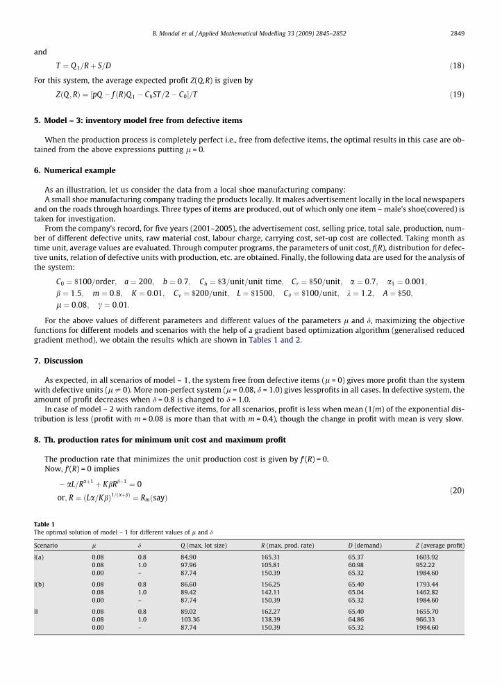
imal solution of model – 1 for different values of l and d

o l d Q (max. lot size) R (max. prod. rate) D (demand) Z (average profit)

0.08 0.8 84.90 165.31 65.37 1603.920.08 1.0 97.96 105.81 60.98 952.220.00 – 87.74 150.39 65.32 1984.60

0.08 0.8 86.60 156.25 65.40 1793.440.08 1.0 89.42 142.11 65.04 1462.820.00 – 87.74 150.39 65.32 1984.60

0.08 0.8 89.02 162.27 65.40 1655.700.08 1.0 103.36 138.39 64.86 966.330.00 – 87.74 150.39 65.32 1984.60

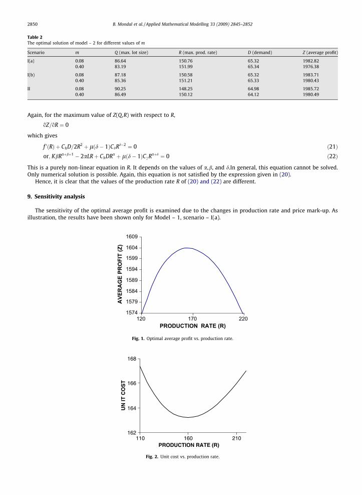
Table 2The optimal solution of model – 2 for different values of m

Scenario m Q (max. lot size) R (max. prod. rate) D (demand) Z (average profit)

I(a) 0.08 86.64 150.76 65.32 1982.820.40 83.19 151.99 65.34 1976.38

I(b) 0.08 87.18 150.58 65.32 1983.710.40 85.36 151.21 65.33 1980.43

II 0.08 90.25 148.25 64.98 1985.720.40 86.49 150.12 64.12 1980.49

2850 B. Mondal et al. / Applied Mathematical Modelling 33 (2009) 2845–2852

Again, for the maximum value of Z(Q,R) with respect to R,

oZ=oR ¼ 0

which gives

f 0ðRÞ þ ChD=2R2 þ lðd� 1ÞChRd�2 ¼ 0 ð21Þor; KbRaþbþ1 � 2aLRþ ChDRa þ lðd� 1ÞCcRaþd ¼ 0 ð22Þ

This is a purely non-linear equation in R. It depends on the values of a,b, and d.In general, this equation cannot be solved.Only numerical solution is possible. Again, this equation is not satisfied by the expression given in (20).

Hence, it is clear that the values of the production rate R of (20) and (22) are different.

9. Sensitivity analysis

The sensitivity of the optimal average profit is examined due to the changes in production rate and price mark-up. Asillustration, the results have been shown only for Model – 1, scenario – I(a).

1574

1579

1584

1589

1594

1599

1604

1609

120 170 220PRODUCTION RATE (R)

AVE

RA

GE

PRO

FIT

(Z)

Fig. 1. Optimal average profit vs. production rate.

162

164

166

168

110 160 210PRODUCTION RATE (R)

UN

IT C

OS

T

Fig. 2. Unit cost vs. production rate.

1160

1360

1560

1760

1960

2160

2360

1.15 1.4 1.65 1.9PRICE MARK - UP

AVE

RA

GE

PRO

FIT

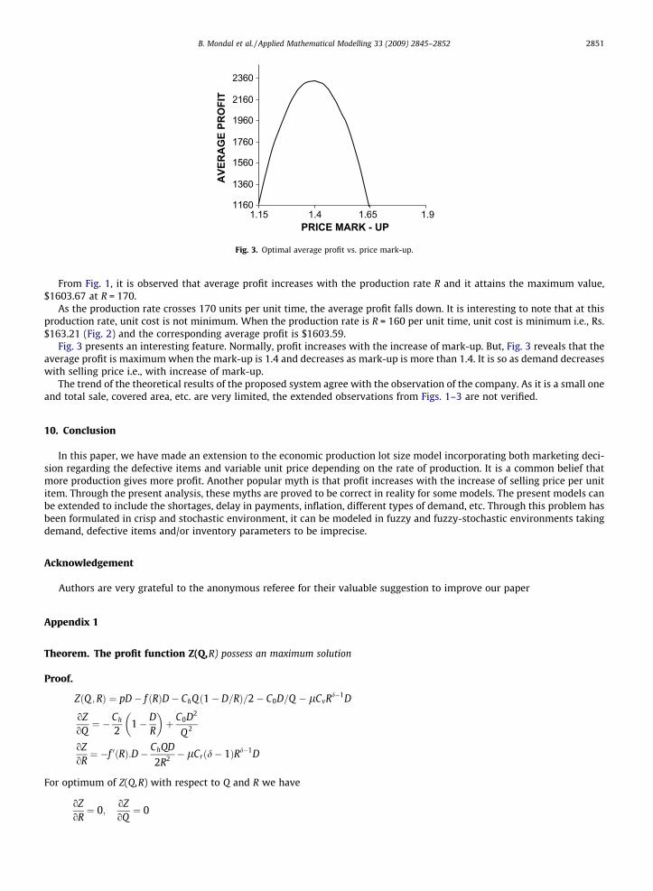
Fig. 3. Optimal average profit vs. price mark-up.

B. Mondal et al. / Applied Mathematical Modelling 33 (2009) 2845–2852 2851

From Fig. 1, it is observed that average profit increases with the production rate R and it attains the maximum value,$1603.67 at R = 170.

As the production rate crosses 170 units per unit time, the average profit falls down. It is interesting to note that at thisproduction rate, unit cost is not minimum. When the production rate is R = 160 per unit time, unit cost is minimum i.e., Rs.$163.21 (Fig. 2) and the corresponding average profit is $1603.59.

Fig. 3 presents an interesting feature. Normally, profit increases with the increase of mark-up. But, Fig. 3 reveals that theaverage profit is maximum when the mark-up is 1.4 and decreases as mark-up is more than 1.4. It is so as demand decreaseswith selling price i.e., with increase of mark-up.

The trend of the theoretical results of the proposed system agree with the observation of the company. As it is a small oneand total sale, covered area, etc. are very limited, the extended observations from Figs. 1–3 are not verified.

10. Conclusion

In this paper, we have made an extension to the economic production lot size model incorporating both marketing deci-sion regarding the defective items and variable unit price depending on the rate of production. It is a common belief thatmore production gives more profit. Another popular myth is that profit increases with the increase of selling price per unititem. Through the present analysis, these myths are proved to be correct in reality for some models. The present models canbe extended to include the shortages, delay in payments, inflation, different types of demand, etc. Through this problem hasbeen formulated in crisp and stochastic environment, it can be modeled in fuzzy and fuzzy-stochastic environments takingdemand, defective items and/or inventory parameters to be imprecise.

Acknowledgement

Authors are very grateful to the anonymous referee for their valuable suggestion to improve our paper

Appendix 1

Theorem. The profit function Z(Q,R) possess an maximum solution

Proof.

ZðQ ;RÞ ¼ pD� f ðRÞD� ChQð1� D=RÞ=2� C0D=Q � lCvRd�1D

oZoQ¼ �Ch

21� D

R

� �þ C0D2

Q 2

oZoR¼ �f 0ðRÞ:D� ChQD

2R2 � lCrðd� 1ÞRd�1D

For optimum of Z(Q,R) with respect to Q and R we have

oZoR¼ 0;

oZoQ¼ 0

2852 B. Mondal et al. / Applied Mathematical Modelling 33 (2009) 2845–2852

Which give

Ch

21� D

R

� �¼ C0D2

Q 2 ðA3:1Þ

and f 0ðRÞ ¼ :� ChQ

2R2 � lCrðd� 1ÞRd�1 ðA3:2Þ

o2Z

oQ2 ¼ �2C0D2

Q 3 ðA3:3Þ

o2ZoQoR

¼ �ChD

2R2 ðA3:4Þ

o2Z

oR2 ¼ �f 00ðRÞ:Dþ ChQD

R3 � lCrðd� 1Þðd� 2ÞRd�3D ðA3:5Þ

Differentiating (A3.2), f(R) and using this expression in (A3.5) we get

o2Z

oR2 ¼aLRa

aþ 1R2 � 2

� �Dþ kbRb b� 1

R� 2

� �D� 2lCrðd� 1ÞRd�3 2

R2 � ðd� 2Þ� �

As d < 1 theno2Z

oR2 < 0 whenaþ 1

R2 < 2;b� 1

R< 2 and

2R2 > ðd� 2Þ

ðA3:6Þ

The function Z(Q,R) has a maximum with respect to Q and R if

o2Z

oQ 2 < 0 ando2Z

oQ2 :o2Z

oR2 �o2Z

oQoR> 0 ðA3:7Þ

For our numerical data the conditions (A3.6) is automatically satisfied and so also the conditions (A3.7) is satisfied. Therefore,the profit function has an maximum solution. h

References

[1] R.B. Misra, Optimum production lot size model for a system with deteriorating inventory, International Journal of Production Research 13 (1975) 495–505.

[2] B.N. Mandal, S. Phaujder, An inventory model for deteriorating items and stock-dependent consumption rate, Journal of Operational Research Society40 (1989) 483–488.

[3] M. Mandal, M. Maiti, Inventory model for damageable items with stock-dependent demand and shortages, Opsearch 34 (1997) 156–166.[4] A.K. Bhunia, M. Maiti, An inventory model for decaying items with selling price, frequency of advertisement and linearly time-dependent demand with

shortages, IAPQR Transactions 22 (1997) 41–49.[5] M. Khouja, The economic production lot size model under volume flexibility, Computer and Operations Research 22 (1995) 515–525.[6] R.M. Bhandari, P.K. Sharma, The economic production lot size model with variable cost function, Opsearch 36 (1999) 137–150.[7] P. Kotler, Marketing Decision Making: A Model Building Approach, Holt Rinehart and Winston, New York, 1971.[8] S. Ladany, A. Sternleib, The intersection of economic ordering quantities and marketing policies, AIIE Transactions 6 (1974) 35–40.[9] S. Subramanyam, S. Kumaraswamy, EOQ formula under varying marketing policies and conditions, AIIE Transactions 13 (1981) 312–314.

[10] T.L. Urban, Deterministic inventory models incorporating marketing decisions, Computers and Industrial Engineering 22 (1992) 85–93.[11] S.K. Goyal, A. Gunasekaran, An integrated production – inventory – marketing model for deteriorating items, Computers and Industrial Engineering 28

(1997) 41–49.[12] P.L. Abad, Supplier pricing and lot-sizing when demand is price sensitive, European Journal of Operational Research 78 (1994) 334–354.[13] P.L. Abad, Optimal pricing and lot-sizing under conditions of perishability and partial back-ordering, Management Science 42 (1996) 1093–1104.[14] W. Luo, An integrated inventory system for perishable goods with backordering, Computers and Industrial Engineering 34 (1998) 685–693.[15] J. Rosenblatt, H.L. Lee, Economic production cycles with imperfect production process, I.I.E. Transactions 18 (1986) 48–55.[16] J.S. Lee, K.S. Park, Joint determination of production cycle and inspection intervals in a deteriorating production, Journal of Operational Research

Society 42 (1991) 775–783.[17] H.L. Lee, J. Rosenblatt, Simultaneous determination of production cycle and inspection schedules in a production system, Management Science 33

(1987) 1125–1136.[18] C.S. Lin, Integrated production inventory models with imperfect production processes and a limited capacity for raw materials, Mathematical and

Computer Modelling 29 (1999) 31–39.