DEPARTMENT OF ECONOMICS

INTERNATIONAL FINANCE

Only Study Guide for ECS303F

© 2011 University of South Africa All rights reserved Printed and published by the University of South Africa Muckleneuk, Pretoria ECS303F/1/2011-2013

iii ECS303F/1/2011-2013

CONTENTS Page

INTRODUCTION 1 THE BALANCE OF PAYMENTS ................................................................................... 1 1.1 Introduction .................................................................................................................... 1 1.2 What is the balance of payments? ................................................................................. 1 1.3 The South African balance of payments ........................................................................ 2 1.4 The significance of imbalances in the balance of payments ........................................ 10 2 FOREIGN EXCHANGE MARKETS AND EXCHANGE RATES ................................. 13 2.1 Introduction .................................................................................................................. 13 2.2 Functions of the foreign exchange markets ................................................................ 14 2.3 Foreign exchange rates ............................................................................................... 14 2.4 Spot and forward rates, currency swaps, futures and options ..................................... 20 2.5 Foreign exchange risks, hedging and speculation ....................................................... 20 2.6 Interest arbitrage and the efficiency of foreign exchange markets ............................... 25 2.7 Eurocurrency or offshore financial markets .................................................................. 27 3 EXCHANGE RATE DETERMINATION ....................................................................... 30 3.1 Introduction .................................................................................................................. 30 3.2 Purchasing power parity theory .................................................................................. 31 3.3 Monetary approach to the balance of payments and exchange rates .......................... 34 3.4 Portfolio balance model and exchange rates ............................................................... 34 3.5 Exchange rate dynamics ............................................................................................. 35 3.6 Empirical tests of the monetary and portfolio balance models and exchange rate

forecasting. ................................................................................................................... 35 4 THE PRICE ADJUSTMENT MECHANISM WITH FLEXIBLE AND FIXED EXCHANGE RATES .................................................................................................... 37 4.1 Introduction .................................................................................................................. 37 4.2 Adjustment with flexible exchange rates ..................................................................... 37 4.3 The effect of exchange rate changes on domestic prices and the terms of trade ....... 38 4.4 Stability of foreign exchange markets .......................................................................... 38 4.5 Elasticities in the real world ......................................................................................... 39 4.6 Adjustment under the gold standard ............................................................................ 39

iv

5 THE INCOME ADJUSTMENT MECHANISM AND SYNTHESIS OF AUTOMATIC ADJUSTMENTS .................................................................................... 41 5.1 Introduction .................................................................................................................. 41 5.2 Income determination in a closed economy ................................................................ 41 5.3 Income determination in a small open economy ......................................................... 41 5.4 Foreign repercussions ................................................................................................. 41 5.5 The absorption approach ............................................................................................. 42 5.6 Monetary adjustments and synthesis of the automatic adjustments ........................... 43 6 OPEN ECONOMY MACROECONOMICS: ADJUSTMENT POLICIES ....................... 45 6.1 Introduction .................................................................................................................. 45 6.2 Internal and external balance with expenditure-changing and expenditure- switching policies: the Swan analysis .......................................................................... 46 6.3 Equilibrium in the goods market, in the money market and in the balance of

payments ..................................................................................................................... 47 6.4 Fiscal and monetary policies for internal and external balance with fixed

exchange rates ............................................................................................................ 47 6.5 The IS-LM-BP model with flexible exchange rates ...................................................... 48 6.6 Policy mix and price changes ...................................................................................... 48 6.7 Direct controls ............................................................................................................... 48 7 PRICES AND OUTPUT IN AN OPEN ECONOMY: AGGREGATE DEMAND AND AGGREGATE SUPPLY ...................................................................................... 51 7.1 Introduction .................................................................................................................. 51 7.2 Aggregate demand, aggregate supply and equilibrium in a closed economy .............. 51 7.3 Aggregate demand in an open economy under fixed and flexible exchange

rates .............................................................................................................................. 52 7.4 The effect of economic shocks and macroeconomic policies on aggregate

demand in open economies with flexible prices ........................................................... 52 7.5 The effect of fiscal and monetary policies in open economies with flexible

prices ............................................................................................................................ 52 7.6 Macroeconomic policies to stimulate growth and adjust to supply shocks ................... 52 8 FLEXIBLE VERSUS FIXED EXCHANGE RATES, THE EUROPEAN

MONETARY SYSTEM AND MACROECONOMIC POLICY COORDINATION ........... 54 8.1 Introduction ................................................................................................................... 54 8.2 The case for flexible exchange rates ............................................................................ 54 8.3 The case for fixed exchange rates ................................................................................ 55 8.4 Optimum currency areas, the European monetary system and the European

monetary union ............................................................................................................. 55 8.5 Currency boards arrangements and dollarisation ......................................................... 55 8.6 Exchange rate bands, adjustable pegs, crawling pegs and managed floating ............. 55 8.7 International macroeconomic policy coordination ......................................................... 56

ECS303F/1

v

9 THE INTERNATIONAL MONETARY SYSTEM: PAST, PRESENT AND FUTURE ...................................................................................................................... 58

9.1 Introduction .................................................................................................................. 58 9.2 The gold standard and the interwar experience ........................................................... 59 9.3 The Bretton Woods system .......................................................................................... 60 9.4 Operation and evolution of the Bretton Woods system ................................................ 61 9.5 US balance of payments deficits and collapse of the Bretton Woods system .............. 62 9.6 The international monetary system: present and future ............................................... 62 9.7 Exchange rate policy and management in South Africa ............................................... 64

vi

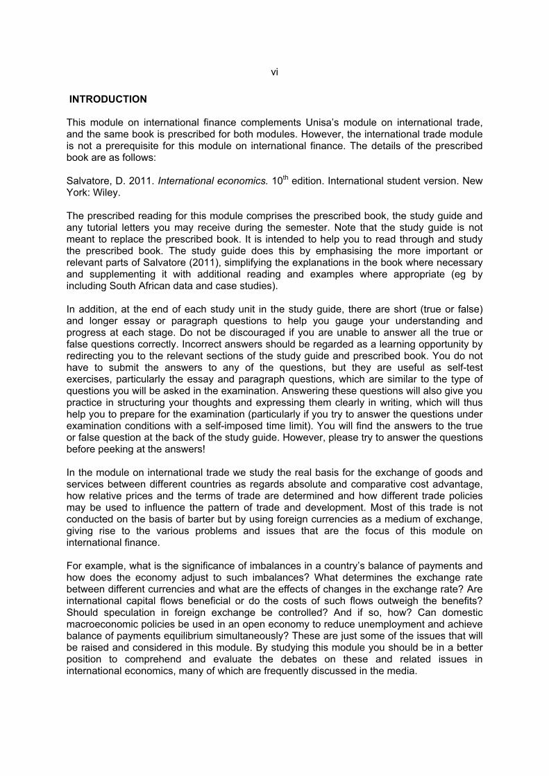
INTRODUCTION This module on international finance complements Unisa’s module on international trade, and the same book is prescribed for both modules. However, the international trade module is not a prerequisite for this module on international finance. The details of the prescribed book are as follows: Salvatore, D. 2011. International economics. 10th edition. International student version. New York: Wiley. The prescribed reading for this module comprises the prescribed book, the study guide and any tutorial letters you may receive during the semester. Note that the study guide is not meant to replace the prescribed book. It is intended to help you to read through and study the prescribed book. The study guide does this by emphasising the more important or relevant parts of Salvatore (2011), simplifying the explanations in the book where necessary and supplementing it with additional reading and examples where appropriate (eg by including South African data and case studies). In addition, at the end of each study unit in the study guide, there are short (true or false) and longer essay or paragraph questions to help you gauge your understanding and progress at each stage. Do not be discouraged if you are unable to answer all the true or false questions correctly. Incorrect answers should be regarded as a learning opportunity by redirecting you to the relevant sections of the study guide and prescribed book. You do not have to submit the answers to any of the questions, but they are useful as self-test exercises, particularly the essay and paragraph questions, which are similar to the type of questions you will be asked in the examination. Answering these questions will also give you practice in structuring your thoughts and expressing them clearly in writing, which will thus help you to prepare for the examination (particularly if you try to answer the questions under examination conditions with a self-imposed time limit). You will find the answers to the true or false question at the back of the study guide. However, please try to answer the questions before peeking at the answers! In the module on international trade we study the real basis for the exchange of goods and services between different countries as regards absolute and comparative cost advantage, how relative prices and the terms of trade are determined and how different trade policies may be used to influence the pattern of trade and development. Most of this trade is not conducted on the basis of barter but by using foreign currencies as a medium of exchange, giving rise to the various problems and issues that are the focus of this module on international finance. For example, what is the significance of imbalances in a country’s balance of payments and how does the economy adjust to such imbalances? What determines the exchange rate between different currencies and what are the effects of changes in the exchange rate? Are international capital flows beneficial or do the costs of such flows outweigh the benefits? Should speculation in foreign exchange be controlled? And if so, how? Can domestic macroeconomic policies be used in an open economy to reduce unemployment and achieve balance of payments equilibrium simultaneously? These are just some of the issues that will be raised and considered in this module. By studying this module you should be in a better position to comprehend and evaluate the debates on these and related issues in international economics, many of which are frequently discussed in the media.

ECS303F/1

vii

NOTE • Except for study unit 1, the study guide follows the exact sequence of the prescribed

textbook (TB) and uses the exact headings of the TB to make reference to this book easier.

• The guide says more on some topics than on others. The fact that it does not say

much on a topic does not mean that it is unimportant. It simply means entails that the TB's version is regarded as sufficient.

• Whenever the words “Read only” appear, it means that no questions will be set on

that topic in the examination, but that it is still important for you, as economists, to note this information.

• Regarding the “case studies” in the TB: The practical side of Economics is always

more interesting, but since we have to limit the content of the module, the case studies are not prescribed, unless specifically mentioned. Please read the case studies, however, because as mentioned above, you are not only students but also economists.

• All “appendices” are not prescribed.

1 ECS303F/1

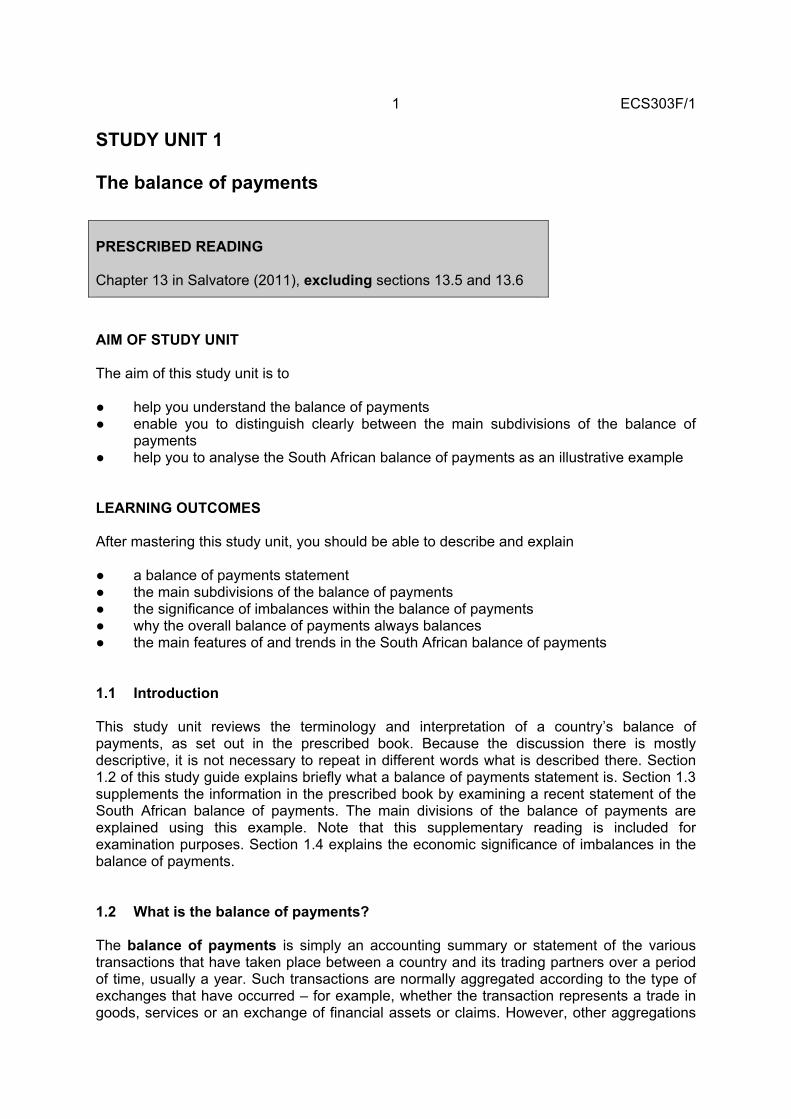
STUDY UNIT 1 The balance of payments PRESCRIBED READING Chapter 13 in Salvatore (2011), excluding sections 13.5 and 13.6

AIM OF STUDY UNIT The aim of this study unit is to ● help you understand the balance of payments ● enable you to distinguish clearly between the main subdivisions of the balance of

payments ● help you to analyse the South African balance of payments as an illustrative example LEARNING OUTCOMES After mastering this study unit, you should be able to describe and explain ● a balance of payments statement ● the main subdivisions of the balance of payments ● the significance of imbalances within the balance of payments ● why the overall balance of payments always balances ● the main features of and trends in the South African balance of payments 1.1 Introduction This study unit reviews the terminology and interpretation of a country’s balance of payments, as set out in the prescribed book. Because the discussion there is mostly descriptive, it is not necessary to repeat in different words what is described there. Section 1.2 of this study guide explains briefly what a balance of payments statement is. Section 1.3 supplements the information in the prescribed book by examining a recent statement of the South African balance of payments. The main divisions of the balance of payments are explained using this example. Note that this supplementary reading is included for examination purposes. Section 1.4 explains the economic significance of imbalances in the balance of payments. 1.2 What is the balance of payments? The balance of payments is simply an accounting summary or statement of the various transactions that have taken place between a country and its trading partners over a period of time, usually a year. Such transactions are normally aggregated according to the type of exchanges that have occurred – for example, whether the transaction represents a trade in goods, services or an exchange of financial assets or claims. However, other aggregations

2

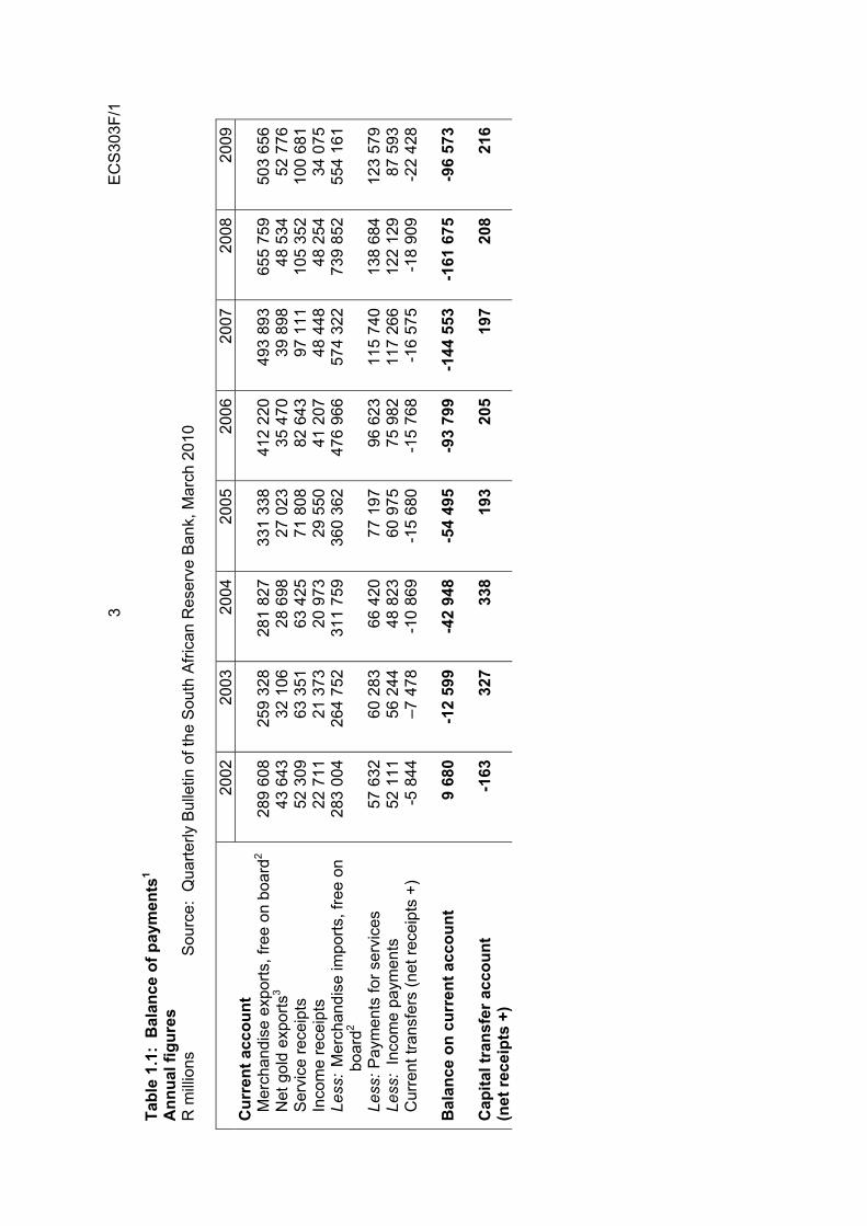
are also possible, along, say, geographic lines. Students, especially accounting students, should guard against confusing the balance of payments with the concept of a national balance sheet. A national balance sheet is a sum-mary-aggregated statement of a country’s assets and liabilities, which is similar to a firm’s balance sheet. The balance of payments is more like a company income statement than a balance sheet. As such, it is a record of the monetary values of the various flows of goods, services and financial assets between countries rather than a measure of the existing national stocks thereof. Obviously, the two measures are related – just as the flow of water from a tap will alter the level (stock) of water in a bath so, for example, will the net flows of foreign exchange resulting from international transactions lead to a change in a country’s stock of foreign exchange reserves. 1.3 The South African balance of payments This section of the study unit supplements the prescribed text by explaining the main items and terms used with reference to a recent statement of the South African balance of payments, reproduced in table 1.1 below. Although the presentation of the balance of payments may differ slightly from country to country, depending on specific circumstances (eg the importance of gold in South African exports), three main divisions are usually present: the current account, the capital or financial account and the change in official net foreign exchange reserves. Each of these is explained with reference to the South African balance of payments. The discussion in the prescribed book explains a condensed version of the balance of payments of the USA (see also the discussion of table 13.1 in the prescribed book).

EC

S30

3F/1

3

Tabl

e 1.

1: B

alan

ce o

f pay

men

ts1

Ann

ual f

igur

es

R m

illio

ns

Sou

rce:

Qua

rterly

Bul

letin

of t

he S

outh

Afri

can

Res

erve

Ban

k, M

arch

201

0

2002

2003

2004

2005

2006

2007

2008

2009

C

urre

nt a

ccou

nt

Mer

chan

dise

exp

orts

, fre

e on

boa

rd2

Net

gol

d ex

ports

3 S

ervi

ce re

ceip

ts

Inc

ome

rece

ipts

L

ess:

Mer

chan

dise

impo

rts, f

ree

on

bo

ard2

Les

s: P

aym

ents

for s

ervi

ces

Les

s: I

ncom

e pa

ymen

ts

Cur

rent

tran

sfer

s (n

et re

ceip

ts +

) B

alan

ce o

n cu

rren

t acc

ount

C

apita

l tra

nsfe

r acc

ount

(n

et re

ceip

ts +

)

289

608

43 6

4352

309

22 7

1128

3 00

4

57 6

3252

111

-5 8

44

9 68

0

-163

259

328

32 1

0663

351

21 3

7326

4 75

2

60 2

83

56 2

44–7

478

-12

599

327

281

827

28 6

9863

425

20 9

7331

1 75

9

66 4

2048

823

-10

869

-42

948

338

331

338

27 0

2371

808

29 5

5036

0 36

2

77 1

9760

975

-15

680

-54

495

193

412

220

35 4

7082

643

41 2

0747

6 96

6

96 6

2375

982

-15

768

-93

799

205

493

893

39 8

9897

111

48 4

4857

4 32

2

115

740

117

266

-16

575

-144

553 19

7

655

759

48 5

3410

5 35

248

254

739

852

138

684

122

129

-18

909

-161

675 20

8

50

3 65

6 52

776

10

0 68

1 34

075

55

4 16

1 12

3 57

9 87

593

-2

2 42

8 -9

6 57

3 21

6

4

20

0220

0320

0420

0520

0620

0720

0820

09

Fina

ncia

l acc

ount

D

irect

inve

stm

ent

Lia

bilit

ies4

Ass

ets5

Net

dire

ct in

vest

men

t P

ortfo

lio in

vest

men

t L

iabi

litie

s

Ass

ets

Net

por

tfolio

inve

stm

ent

Oth

er in

vest

men

t L

iabi

litie

s

Ass

ets

Net

oth

er in

vest

men

t B

alan

ce o

n fin

anci

al a

ccou

nt

Unr

ecor

ded

trans

actio

ns6

1654

041

9520

735

5344

-9

619

-427

5

304

-432

9-4

025

1243

5

-587

2

5 55

0-4

275

1 27

5

7 54

8-1

001

6 54

7

14 5

94-3

6 91

9-2

2 32

5

-14

503

21 9

17

5 15

5-8

721

-3 5

66

46 2

62-5

946

40

316

10 9

44-3

555

7 38

9

44 1

39

35 9

99

42 2

70-5

916

36 3

54

36 1

88-6

123

30 0

65

32 7

35-2

2 89

59

840

76 2

59

12 3

06

-3 5

67-4

1 05

8-4

4 62

5

144

501

-15

044

129

457

60 7

50-3

8 82

321

927

106

759

16 6

27

40 1

20-2

0 89

61

9 22

4

97 4

85

-24

026

73 4

59

58 7

112

119

60 8

30

153

513

38 6

59

74 4

0325

888

100

291

-71

540

-63

325

-134

865

47 7

3082

983

13

0 71

3

96 1

39

91 3

94

48

270

-1

3 42

5 34

845

10

7 19

0 -1

4 72

1 92

469

-4

2 32

3 20

677

-2

1 64

6 10

5 66

8

7

726

EC

S30

3F/1

5

2002

2003

2004

2005

2006

2007

2008

2009

C

hang

e in

net

gol

d an

d ot

her

fore

ign

rese

rves

ow

ing

to b

alan

ce

of p

aym

ents

tran

sact

ions

C

hang

e in

liab

ilitie

s re

late

d to

re

serv

es7

SD

R a

lloca

tions

and

val

uatio

n ad

just

men

ts

Net

mon

etis

atio

n (+

) /

dem

onet

isat

ions

(-) o

f gol

d C

hang

e in

gro

ss g

old

and

othe

r fo

reig

n re

serv

es

Mem

o ite

m:

chan

ge in

cap

ital

trans

fer a

nd fi

nanc

ial a

ccou

nts

incl

udin

g un

reco

rded

tran

sact

ions

16 0

80

-20

090

-20

041

-563

24 6

14

6 40

0

-4 8

58

1 91

1

-11

262

1 13

7

-13

072

7 74

1

37 5

28

2 94

9

-10

617 84

29 9

44

80 4

76

34 2

63

2 57

7

11 0

03

-226

47 6

17

88 7

58

29 7

92

-5 4

53

23 3

50 163

47 8

52

123

591

47 8

16

-7 6

31

5 64

2

169

45 9

96

192

369

26 0

66

-7 7

61

74 2

14 158

92 6

77

187

741

17 0

37

-2 7

24

-38

647

45

-24

289

113

610

6

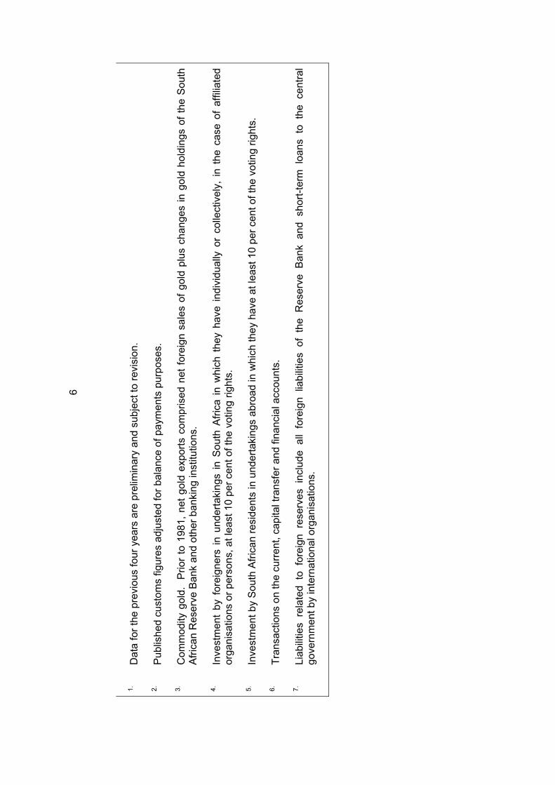
1.

Dat

a fo

r the

pre

viou

s fo

ur y

ears

are

pre

limin

ary

and

subj

ect t

o re

visi

on.

2.

Pub

lishe

d cu

stom

s fig

ures

adj

uste

d fo

r bal

ance

of p

aym

ents

pur

pose

s.

3.

Com

mod

ity g

old.

P

rior

to 1

981,

net

gol

d ex

ports

com

pris

ed n

et fo

reig

n sa

les

of g

old

plus

cha

nges

in g

old

hold

ings

of t

he S

outh

A

frica

n R

eser

ve B

ank

and

othe

r ban

king

inst

itutio

ns.

4.

Inve

stm

ent

by f

orei

gner

s in

und

erta

king

s in

Sou

th A

frica

in w

hich

the

y ha

ve in

divi

dual

ly o

r co

llect

ivel

y, in

the

cas

e of

affi

liate

d or

gani

satio

ns o

r per

sons

, at l

east

10

per c

ent o

f the

vot

ing

right

s.

5.

Inve

stm

ent b

y S

outh

Afri

can

resi

dent

s in

und

erta

king

s ab

road

in w

hich

they

hav

e at

leas

t 10

per c

ent o

f the

vot

ing

right

s.

6.

Tran

sact

ions

on

the

curre

nt, c

apita

l tra

nsfe

r and

fina

ncia

l acc

ount

s.

7.

Liab

ilitie

s re

late

d to

for

eign

res

erve

s in

clud

e al

l fo

reig

n lia

bilit

ies

of t

he R

eser

ve B

ank

and

shor

t-ter

m l

oans

to

the

cent

ral

gove

rnm

ent b

y in

tern

atio

nal o

rgan

isat

ions

.

ECS303F/1

7

1.3.1 The current account The current account may be subdivided into the trade account, net service receipts, net income receipts and current transfers. The trade account comprises trade in physical goods. The trade balance is not shown explicitly in the South African balance of payments but can easily be calculated by subtracting the value of merchandise imports from the value of merchandise exports and net gold exports. Note that because of South Africa’s historical dependence on gold exports, the trade account is recorded as a separate item immediately below merchandise exports. In table 1.1, South Africa’s trade balance for 2008 may be calculated by subtracting merchandise imports to the value of R739 852 m from the value of merchandise exports plus net gold exports (R655 759 m + R48 534 m) to the value of R704 293 m, which thus equals R-35 559 m. Note the declining relative contribution of gold exports to the balance of trade. Net gold exports as a percentage of merchandise exports fell from 12,4 to 7,4 per cent during the period, 2001 to 2008. In 1989 (not shown in table 1.1), gold exports comprised nearly half (50 per cent) of all merchandise exports. Clearly, the recent decline is more than a temporary phenomenon and may be regarded as a continuation of a long-term trend. One of the concerns about the South African economy is the large deficit on the country’s current account. This deficit mushroomed from R-12 599 m in 2003 to a massive R-161 675 m in 2008, as shown in table 1.1. This huge and increasing deficit is largely a result of the growth in merchandise imports. A deficit on the current account means in fact that South Africans borrow in order to spend, and this of course could have the same dire consequences for a country that it has for an individual (as many can tell). What do services and income consist of? The main service items are transport of goods and passengers between countries, freight and merchandise insurance, other financial services, various business, professional and technical services, government services and foreign travel. The main income items are interest, dividends and foreign branch profits. The net deficit as regards income receipts and payments is to be expected of a developing country like South Africa, in which inward foreign investment (and thus the interest and dividend returns on such investment) greatly exceeds outward foreign investment by South African firms and individuals. Why, you might ask, are interest, dividends and net foreign profits included under the current account and not the financial account? After all, various kinds of foreign investment flows are recorded under the financial account, and the word “financial” suggests that this account is the proper place to include such payments and receipts. The reason is that interest, dividends and foreign company profits are properly regarded as ongoing (foreign) investment income flows derived from prior investments of capital abroad. Such income flows belong to the current account. Only adjustments made to desired levels or stocks of domestic versus foreign capital investments (requiring the exchange of asset claims) are included under financial account transactions (see sec 1.3.2 below). To conclude this section, note that South Africa generally experiences a negative balance of net current transfers. This item comprises foreign payments and receipts of government social security payments and taxes, private transfers of income (such as gifts, donations and immigration funds) and the like. Current transfers are treated separately from capital transfers, as shown in table 1.1. The latter comprise one-off government grants of a capital nature, transfers involving changes in the ownership, acquisition or disposal of fixed assets, legacies, debt forgiveness and other such items. South Africa generally runs a small positive balance on its capital transfer account, as indicated in table 1.1.

8

1.3.2 The financial account The financial account (previously referred to as the capital account) records exchanges of international asset claims. For example, if a US bank buys a bond issued by the South African government, a South African company purchases shares in a British company or a foreign company establishes a controlling interest in a local manufacturing concern, the value of these transactions will be reflected in the financial account of the countries concerned. Note that the financial account does not record the stocks of the assets and liabilities. It is the changes in foreign assets and liabilities that are shown in the balance of payments. For example, in 2008, the net change in South Africa’s foreign assets and liabilities, known as the balance on the financial account, was R96 139 m. This is the amount by which flows of inward investment by foreigners exceeded outward investment by South African residents in 2008. The three main subdivisions of the financial account are direct investment, portfolio investment and other investment. Direct investment refers to foreign investments in South Africa (changes in foreign liabilities or inflows) and investments abroad by South African residents (changes in foreign assets or outflows) where the companies or other organisations concerned have a significant share of such investment. The share should be significant in that there should be an intention to have a say in the control or management of the investment. In South Africa, this is defined as at least a 10 per cent share of the voting rights in the investment undertaking concerned. Note that a negative sign implies an outflow of foreign exchange resulting from an increase in outward investment by South African residents. For example, in 2007, South African residents increased their direct investments in foreign assets by R20 896 m, resulting in an equivalent outflow of foreign exchange as indicated by the negative sign in this figure. Net direct investment (changes in foreign liabilities plus the changes in foreign assets) was negative in 2004 and 2006, meaning that foreigners invested less in South Africa than we invested abroad over this period. However, the substantial net inflows of direct investment in 2008 indicate the generally positive view of South Africa as a destination for foreign direct investment. Portfolio investment is the purchase and sale of financial claims such as bonds, treasury bills and equities. Unlike direct investments, there is no intention by the investor to exercise any control over portfolio investments. The justification for such investments is based purely on the expected financial gain or return on investment. Portfolio investments are notoriously fickle because changes in expected returns may trigger speculative buying or selling activity. As indicated in table 1.1, net portfolio investment rose substantially in 2006, but turned markedly negative in 2008. These large swings clearly show the volatility of such investments in South Africa. Other investment includes all financial transactions that are not part of direct or portfolio investment or changes in reserve assets. The main item here is trade credit. For example, when a South African importer purchases goods from a foreign supplier, he or she will usually be granted short-term credit (representing an increase in foreign liabilities). The local or foreign correspondent bank may arrange the credit. Similarly, a foreign purchaser of goods exported by a South African company will normally obtain such credit (an increase in foreign assets). Direct foreign investment is generally considered to be a more desirable form of foreign investment than portfolio investment because it demonstrates a stronger commitment to invest over the longer term. It may thus have a more stable and enduring positive effect on

ECS303F/1

9

the domestic economy than the speculative “hot money” flows that often characterise a large part of foreign portfolio investment. Although there is some theoretical debate whether such speculation is stabilising or destabilising, it is generally agreed that speculative capital movements may prove to be disruptive and difficult for the monetary authorities to counteract. Besides its (hopefully positive) effects on employment, direct foreign investment may also bring with it much needed transfers of scarce skills, technology and innovations from abroad. These considerations are especially significant for a small, open and developing economy such as that of South Africa. Note in table 1.1 that a current account deficit is often associated with a surplus balance on the financial account, and vice versa (this is the case for each year recorded in table 1.1 except 2002 and 2003). This pattern is common in many developing countries, including South Africa. Developing countries typically finance current account deficits through net capital inflows across the financial account. Moreover, if imports exceed exports, this implies that South Africa is receiving more trade credit than it is granting to foreigners, which is reflected in an increase in net other investment. Also, interest rates tend to be higher when the current account is in deficit and lower when there is a surplus. For example, the drain of domestic money resulting from a current account deficit automatically creates tightness in the local money market and puts upward pressure on interest rates. This may be intensified by deliberate monetary policies to reduce domestic demand. The immediate effect of higher interest rates may be to attract increased capital inflows, thus leading to the observed correlation between the current and financial accounts of the balance of payments. 1.3.3 Unrecorded transactions Unrecorded transactions arise from the use of a double-entry accounting system to reconcile the balance of payments. The net sum of debit and credit entries arising from balance of payments transactions should equal the change in the country’s net gold and foreign exchange reserves (see sec 1.3.4 below). However, owing to errors in and omissions from various sources in the compilation of the different divisions of the balance of payments, this is seldom the case. The difference between the recorded change in the net gold and foreign exchange reserves and the sum of the current, capital transfer and financial account balances is classified as unrecorded transactions. Thus, in practice, the value of unrecorded transactions serves as a residual that ensures that the balance of payments accounts always balance. As indicated in table 1.1, the value of such transactions can be substantial, amounting to, for example, R91 394 m in 2008. 1.3.4 The official reserves Changes in the stock of official gold and other foreign exchange reserves reflect the net inflow or outflow of foreign exchange, resulting from (noncentral bank) balance of payments transactions over a certain period. One way of thinking about balance of payments transactions is to imagine their effect in the foreign exchange market. Any transaction that leads to a derived demand for foreign currency can be thought of as a debit (-) item or outflow of foreign exchange. For example, imports of goods and services into South Africa create a demand for foreign currency (and thus a corresponding supply of rand) in the foreign exchange market. Exports of goods and services from South Africa, however, create a supply of foreign currency (demand for rand). Any transaction that leads to a supply of foreign currency in the foreign exchange market can thus be regarded as a credit (+) item or inflow of foreign exchange. Similarly, the purchase by a South African resident of foreign shares or bonds creates a derived demand for foreign currency, whereas the purchase by a nonresident of South African shares creates a supply of foreign currency (demand for rand) in the foreign exchange market.

10

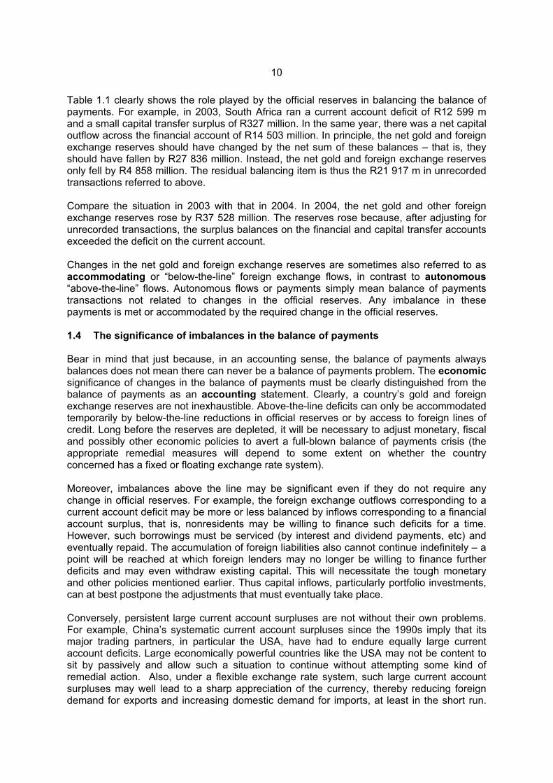
Table 1.1 clearly shows the role played by the official reserves in balancing the balance of payments. For example, in 2003, South Africa ran a current account deficit of R12 599 m and a small capital transfer surplus of R327 million. In the same year, there was a net capital outflow across the financial account of R14 503 million. In principle, the net gold and foreign exchange reserves should have changed by the net sum of these balances – that is, they should have fallen by R27 836 million. Instead, the net gold and foreign exchange reserves only fell by R4 858 million. The residual balancing item is thus the R21 917 m in unrecorded transactions referred to above. Compare the situation in 2003 with that in 2004. In 2004, the net gold and other foreign exchange reserves rose by R37 528 million. The reserves rose because, after adjusting for unrecorded transactions, the surplus balances on the financial and capital transfer accounts exceeded the deficit on the current account. Changes in the net gold and foreign exchange reserves are sometimes also referred to as accommodating or “below-the-line” foreign exchange flows, in contrast to autonomous “above-the-line” flows. Autonomous flows or payments simply mean balance of payments transactions not related to changes in the official reserves. Any imbalance in these payments is met or accommodated by the required change in the official reserves. 1.4 The significance of imbalances in the balance of payments Bear in mind that just because, in an accounting sense, the balance of payments always balances does not mean there can never be a balance of payments problem. The economic significance of changes in the balance of payments must be clearly distinguished from the balance of payments as an accounting statement. Clearly, a country’s gold and foreign exchange reserves are not inexhaustible. Above-the-line deficits can only be accommodated temporarily by below-the-line reductions in official reserves or by access to foreign lines of credit. Long before the reserves are depleted, it will be necessary to adjust monetary, fiscal and possibly other economic policies to avert a full-blown balance of payments crisis (the appropriate remedial measures will depend to some extent on whether the country concerned has a fixed or floating exchange rate system). Moreover, imbalances above the line may be significant even if they do not require any change in official reserves. For example, the foreign exchange outflows corresponding to a current account deficit may be more or less balanced by inflows corresponding to a financial account surplus, that is, nonresidents may be willing to finance such deficits for a time. However, such borrowings must be serviced (by interest and dividend payments, etc) and eventually repaid. The accumulation of foreign liabilities also cannot continue indefinitely – a point will be reached at which foreign lenders may no longer be willing to finance further deficits and may even withdraw existing capital. This will necessitate the tough monetary and other policies mentioned earlier. Thus capital inflows, particularly portfolio investments, can at best postpone the adjustments that must eventually take place. Conversely, persistent large current account surpluses are not without their own problems. For example, China’s systematic current account surpluses since the 1990s imply that its major trading partners, in particular the USA, have had to endure equally large current account deficits. Large economically powerful countries like the USA may not be content to sit by passively and allow such a situation to continue without attempting some kind of remedial action. Also, under a flexible exchange rate system, such large current account surpluses may well lead to a sharp appreciation of the currency, thereby reducing foreign demand for exports and increasing domestic demand for imports, at least in the short run.

ECS303F/1

11

This may lead to reduced aggregate demand, production and employment in the short run. Note that a current account deficit is not necessarily “bad”, and a surplus necessarily “good”. A current account deficit implies that a country is consuming more than it is producing. Imported goods add to consumer welfare, whereas exports represent a sacrifice in the sense of production of goods and services that are not available for domestic consumption. As noted above, such deficits only become problematic over time if foreigners are unwilling to finance them. Finally, it should be noted that changes in the foreign exchange reserves reflect corresponding changes in the domestic money supply (defined here as notes, coins and demand deposits with the private nonbank sector). A decrease in the reserves implies that there has been a net conversion of domestic currency into foreign currency above-the-line and therefore a contraction in the domestic money supply, ceteris paribus. Conversely, an increase in the reserves implies that there has been a net conversion of foreign currency into domestic currency, and thus an expansion of the domestic money supply (which would be offset to the extent of any decrease in domestic credit that may have occurred over the same period). IMPORTANT TERMS AND CONCEPTS Above-the-line transactions Accommodating foreign exchange flows Accounting identity Autonomous foreign exchange flows Balance of payments Balance of payments deficits and surpluses Below-the-line transactions Capital transfer account Changes in foreign assets and liabilities Credit (+) and debit (-) items Current account Current transfers Deficit in the balance of payments Derived demand Direct investment Distinction between income and capital Financial account Foreign assets and liabilities Foreign exchange reserves Portfolio investment Stocks versus flows Surplus in the balance of payments Trade credit Trade account Unrecorded transactions Visible and invisible trade

12

TRUE OR FALSE QUESTIONS (1) The balance of payments is similar to a company’s balance sheet in that it is a state-

ment of a country’s (foreign) assets and liabilities at a particular time. (2) Foreign interest and dividend payments and receipts are recorded under the financial

account of the balance of payments. (3) The nominal rand value of South Africa’s gold exports was greater in 2009 than in

2008. (4) Portfolio investments are generally stable, long-term foreign investments in the

economy. (5) The above-the-line balance of the balance of payments is the sum of the balances on

the current, capital transfer and financial accounts. (6) The balance of payments must balance by definition, because a current account

surplus (deficit) is necessarily offset by an equal but opposite capital account deficit (surplus).

(7) In practice, unrecorded transactions are a residual item, which by definition ensures that the overall balance of payments always balances.

(8) The purchase of South African shares by nonresidents is an example of an accommodating capital inflow.

(9) Deficits (or surpluses) on the above-the-line accounts of the balance of payments do not constitute an economic problem.

(10) A balance of payments deficit cannot occur under a perfectly flexible exchange rate although it may be a problem with a fixed exchange rate.

ESSAY QUESTIONS (1) Explain the main accounts and subdivisions of the balance of payments using South

Africa’s balance of payments in table 1.1 as an example. (2) “The balance of payments always balances by definition and therefore does not

present any economic problems for the country concerned.” True or false? Explain. (3) Explain what is meant by portfolio investment and direct investment. Is the one more

desirable than the other? Evaluate. (4) Explain the difference between autonomous and accommodating foreign exchange

flows and their significance as regards the balance of payments. (5) Discuss the current account of the South African balance of payments.

ECS303F/1

13

STUDY UNIT 2 Foreign exchange markets and exchange rates

PRESCRIBED READING Chapter 14 in Salvatore (2011), excluding sections 14.6D, 14.6E and 14.7

In this study unit, substantial use is made of applications of the relevant concepts with references to actual numbers and to the South African situation. AIM OF STUDY UNIT The aim of this study unit is to ● improve your understanding of the foreign exchange market and exchange rates ● broaden your knowledge of the main activities that occur in the foreign exchange

markets ● make you aware of the different types of risk associated with international transactions LEARNING OUTCOMES After mastering this study unit you should be able to describe and explain ● what a foreign exchange market is and how it functions ● how exchange rates are defined and quoted in the market ● the difference between bilateral, nominal, effective and real measures of exchange

rates ● the difference between the spot and forward foreign exchange markets as well as

swaps, futures and options ● arbitrage, speculation and hedging activities in the foreign exchange markets ● the risks associated with international transactions and how they may be covered 2.1 Introduction (14.1 in TB) Sales turnover in the foreign exchange markets generally far exceeds that of the equity and bond markets. For example, average daily turnover in the South African foreign exchange market in 2009 was around R90 billion, compared to approximately R10 billion and R40 billion in the local equity and bond markets respectively. However, its significance goes well beyond the sheer volume of transactions since it is the market through which the domestic economy is connected to the rest of the world via the balance of payments. Moreover, it is the market in which the country’s exchange rates are determined – which, directly or indirectly, affects decision making throughout the economy. Where we think they are informative, we have used some pertinent South African examples to supplement the examples taken from the USA, as presented in the prescribed book.

14

2.2 Functions of the foreign exchange markets (14.2 inTB) The prescribed book identifies three main functions: • the transfer of purchasing power from one currency to another • the credit function • providing facilities for hedging and speculation 2.3 Foreign exchange rates (14.3 in TB) 2.3.A Equilibrium foreign exchange rates In study unit 1 we pointed out that every international transaction, whether in goods and services, or in physical or financial assets, necessarily gives rise to a derived demand (or supply) of foreign currency. For example, the import into South Africa of a television set from Japan gives rise to a demand for Japanese yen (and thus a supply of rand). The purchase by a German resident of a South African government bond denominated in rand gives rise to a supply of euro (and thus a demand for rand). Typically, as in the foregoing examples, foreigners do not want payment in rand but in their own currency, just as South African residents usually want to convert their foreign currency proceeds into rand (or at some stage are obliged to do so by domestic exchange control regulations). These exchanges of one currency for another are made in the foreign exchange markets. Figure 14-1 in the prescribed book shows a hypothetical supply and demand model of a foreign exchange market. The downward-sloping demand curve represents the flow of euro outpayments (derived from imports of goods and services and outward flows of foreign investment), while the upward-sloping supply curve represents the flow of euro inpayments (derived from exports of goods and services and inward flows of foreign investment). Note that the demand for euro in the foreign exchange market necessarily implies a supply of the other currency, in this case the dollar, while the supply of euro to the market implies a demand for dollars. Like any other supply and demand analysis, the model allows you to determine the equilibrium exchange rate (the price of one currency in terms of another, in this case the price of the euro in terms of the dollar). The equilibrium exchange rate is where the flows of foreign currency (euro) inpayments are just equal to the flows of foreign currency (euro) outpayments such that there is no excess demand for or supply of euro causing the exchange rate to adjust any further. The prescribed book goes on to explain the factors that cause the demand and supply curves to shift thereby influencing the exchange rate. The question of what determines the mentioned demand and supply is covered in study unit 3. Note that a foreign exchange market, like many other financial markets, does not necessarily have a physical location (in contrast to, say, a vegetable market or a flea market). The existence of a foreign exchange market requires only that prospective buyers and sellers of foreign currencies (foreign exchange) can communicate their intentions. This is usually done via the banking system (by telephone, telex or computer links) which therefore acts as a financial intermediary for such transactions. Each day, for example, South African banks receive instructions to both buy and sell many different foreign currencies on behalf of customers and it is the job of the banks’ foreign exchange dealers to reconcile these orders.

ECS303F/1

15

Also note that by far the greater volume of foreign exchange transactions through the formal banking system is in the form of electronic bookkeeping transfers of funds, not physical exchanges of actual notes and coins (indeed, most banks will not exchange foreign coins at all). In some countries, particularly where the authorities try to maintain an overvalued official exchange rate, informal or “parallel” markets in notes and coins may exist. We saw above that international transactions naturally give rise to derived demands for and supplies of different foreign currencies. As in any free market, changes in desired demand and supply are reconciled by adjustments in prices. In this case, the price is what residents must pay in local currency to purchase a unit of foreign currency: Definition: An exchange rate is the domestic price of foreign currency. Note that we could just as easily define the exchange rate the other way around, as the foreign price of domestic currency. For example, if the rand/dollar (ZAR/USD) rate of exchange is 7,5000 (a direct quotation), this would be the same as saying that the dollar/rand (USD/ZAR) exchange rate is 0,1333 (an indirect quotation). It is common practice to quote exchange rates to four decimal places, because the magnitude of many transactions on the foreign exchange markets means that even small changes in exchange rates can give rise to substantial absolute changes in the value of such transactions. Banks often quote some exchange rates both indirectly and directly. To avoid confusion, economists generally adhere to one method or the other. Unless we state otherwise, we shall stick to the convention of using the direct method, whereby the exchange rate refers to the domestic price of foreign currency. It is important to note here that a direct quote (the domestic price of foreign currency) means that a lower price or exchange rate reflects an appreciation of the local currency against the foreign currency, while a higher exchange rate implies a depreciation of the local currency. Thus a fall in the ZAR/USD exchange rate from 7,5000 to say 6,7500 implies an appreciation of the rand against the dollar of 10 per cent (simply because that much fewer rand are needed to purchase the required dollars). Note that in the above examples, we used the currency codes ZAR and USD instead of the more familiar R and $ symbols for the rand and the US dollar respectively. All currencies traded in the foreign exchange markets have a unique three-letter code that foreign exchange dealers and traders use in communicating transactions. This convention is used throughout the rest of this study unit, unless noted otherwise. A list of the currencies and their codes as quoted in the local foreign exchange market is shown in table 2.1 below. It indicates the exchange rates of the South African rand against the major currencies traded in the local foreign exchange market on a particular day. TABLE 2.1 SOUTH AFRICAN EXCHANGE RATES This table indicates First National Bank’s exchange rates in the order of selling, telegraphic transfer (TT) buying, airmail (AM) buying and surface mail (SM) buying, as published in Business Day on 4 March 2010. The rates refer to the previous day’s afternoon fix and apply to amounts of R50 000 or less for dollars and R10 000 or less for other currencies. The first three currencies refer to the rand per foreign currency unit. Subsequent currencies refer to the foreign currency unit per rand.

16

CURRENCY DOLLAR, USD POUND, GBP EURO, EUR AUSTRALIA, AUD BOTSWANA, BWP CANADA, CAD SWISS, CHF DENMARK, DKK HONG KONG, HKD INDIA, INR JAPAN, JPY KENYA, KES MAURITIUS, MUR MALAWI, MWK MOZAMBIQUE, MZM NORWAY, NOK NEW ZEALND, NZD PAKISTAN, PKR SWEDEN, SEK SINGAPORE, SGD UGANDA, UGS ZAMBIA, ZMK

SELLING

7,7094 11,6342

10,5598

0.1421 0,8579 0,1323 0,1385

0,7002 0,9896

5,8734 11,4686 9,6355 3,4957

17,1609 3,6177 0.7607

0,1836 10,7160

0,9201 0.1792

251,6927 533,8937

TT

7,4528 11,1430 10,1147

0,1498

0,9462 0,1409

0,1448 0,7405 1,0629

6,2433 11,9894 10,6752

0,0000 0,0000

0,0000 0,8016 0,1951

11,5511 0,9697 0,1909 275,0912

0,0000

AM

7,3968 11,0946 10,0849

0,1504 0,9584 0,1416 0.1454

0,7448 1,0709 6,2433 12,0135

0,0000 0,0000 0,0000 0,0000 0,8089 0,1959 0,0000 0,9733 0,1923 0,0000 0,0000

SM

7,4453 11,1318

10,1045

0,1499 0,9472 0,1410

0,1450 0,7412 1,0640

6,2496 12,0015 10,6859

0.0000 0.0000 0.0000

0,8024 0,1953

11,5672 0,9707 0,1911

275,3684 0.0000

These are spot exchange rates (for immediate or on-the-spot delivery of foreign exchange, although in practice, this usually means after two working days). The bank quotes the exchange rates as indicative rates for its customers on a particular day. They are not the same as the rates quoted by the bank’s foreign exchange dealers to other currency traders in the interbank market. Nor are you likely to be given exactly the same rate if you phone your bank to buy or sell foreign currency, because the rates change in response to market conditions throughout the day. Other commercial banks may quote slightly different rates for the same currencies, but it is unlikely that they will diverge significantly because the foreign exchange market is a highly competitive market. However, major clients may be quoted better rates than small customers. Until the end of December 2001, the primary foreign currencies exchanged in the local market were the US dollar, British pound, German mark, Japanese yen, French franc, Swiss franc and the Italian lire. However, shortly after the introduction of the euro (EUR) on 1 January 2002, the German mark, the French franc and the Italian lire were removed from

ECS303F/1

17

lists of exchange rate quotations, as were the currencies of all 12 members of the European Monetary Union (Germany, France, Italy, Spain, Portugal, Ireland, Finland, Holland, Belgium, Luxembourg, Austria and Greece). For the time being, the UK, Denmark and Sweden have elected to stay outside the monetary union and to retain their own national currencies, although they remain members of the European Union. Of the currencies listed in table 2.1, the US dollar, the British pound and the euro are quoted directly, as the rand price of the foreign currency. All the other currencies are quoted indirectly, as the foreign price of the rand. For example, the selling rate for the Japanese yen is 11,4686, meaning that it costs 11,4686 yen to buy one rand. Note that on the retail customer side of the market, banks quote four different exchange rates for each currency. There is one selling rate and three different buying rates (by contrast, interbank foreign exchange dealers only quote each other one buying and one selling rate). The exchange rates are quoted from the bank’s perspective, that is, the rate at which it is prepared to sell foreign currencies to and buy them from customers respectively. For currencies that are quoted directly, the selling price is always at a higher domestic price than any of the buying prices for a particular currency. This difference is known as the spread and is the main way in which the banks make a profit from foreign exchange transactions with their customers by buying currencies at a cheaper rate than the price at which they sell (banks also make a smaller profit on commissions and other fees for such transactions in the retail market). The buying prices vary, depending on the form of foreign exchange the customer wants converted by the bank. The exchange rate becomes less favourable (more expensive) to the customer the less convenient and the longer the time to the transaction’s settlement for the bank. The TT or telegraphic transfer buying rate is usually applied to large transfers of funds and is the best buying rate a customer can obtain because it is the most convenient way for the bank to convert and transfer the funds, with settlement within two working days. The SM or surface mail rate is the worst buying rate that applies to a customer wishing to exchange foreign currency notes (surplus notes have to be sent back to the country of origin by surface mail). The AM or airmail rate applies to foreign bank cheques and traveller’s cheques, and falls between the other two rates. For large transactions, most banks will quote more favourable rates than the published exchange rates. The first exchange rate quoted in table 2.1 is the rand/dollar (ZAR/USD) exchange rate, even though the USA is not our major trading partner. The dollar is quoted first because foreign exchange dealers use it as a common currency denominator. All foreign currency transactions first go through the US dollar. For example, if a South African foreign exchange dealer wishes to buy euro, rand will be sold against dollars first and then the dollars will be exchanged for euro. Hence all currencies are quoted against the dollar first, and then converted to calculate exchange rates against the rand. These are known as cross rates. Ignoring the difference between buying and selling prices for the moment, if the ZAR/USD exchange rate is 7,7094 and the USD/EUR exchange rate is 1,3697, then the implied ZAR/EUR exchange rate is 10,5595. The ZAR/EUR exchange rate is found by multiplying the ZAR/EUR rate by the USD/EUR rate (7,7094 x 1,3697 = 10,5596). The slight difference between this and the quoted rate of 10,5598 is simply because of rounding off. All the exchange rates (besides the ZAR/USD rate) in table 2.1 have been derived like this and are thus cross rates. The main reason why banks quote rates this way is to avoid the complex task of giving hundreds of direct quotations for all the different currencies. Moreover, settlement in the local foreign exchange market is typically in rand. The exchange rates quoted in table 2.1 are nominal bilateral exchange rates, that is, the

18

exchange rates between two national currencies in face value or money terms. Sometimes it is useful to know how the domestic currency is faring against more than just one currency at a time. For this purpose, a nominal effective exchange rate (see also sec 14.5A in the prescribed book) can be calculated. This is simply a weighted average of the bilateral exchange rates that thus gives us a composite value for the domestic currency. Note that a simple arithmetic average is unsatisfactory because the importance of one foreign currency may be much greater than another. For example, the US dollar and the British pound have a much greater weighting against the South African rand than, say, the Botswana pula. The foreign country’s share of the trade in the domestic country’s total trade figures (eg imports from the foreign currency country as a percentage of our total imports from abroad) usually determines the weights. Also note that it is first necessary to convert the different exchange rates to index numbers with a common base year before taking an average. This is to avoid the problem of different units of denomination. For example, simply averaging the ZAR/USD and the ZAR/JPY exchange rates does not give a true average measure of the value of the rand against these two currencies. This reflects the fact that, just because more rand are required to purchase dollars than yen at a particular time, it does not necessarily mean that the rand is weaker against the dollar than the yen. The index time series is commonly derived for monthly, quarterly or annual exchange rate data. As with any index, an individual value is uninformative. Only comparisons of the index numbers over time reveal useful information about changes in the relative values of the currencies concerned. Changes in nominal exchange rates give us some idea about how competitive a country’s goods and services are in world markets. For example, a depreciation of the rand against the dollar means that, ceteris paribus, South African goods (denominated in rand) are cheaper (in dollar) for Americans or other buyers with dollars. Conversely, an appreciation of the rand means that South African goods are more expensive (in dollar). However, this is not the whole story. If, for example, an average 15 per cent depreciation in the rand against the dollar over the course of, say, a year corresponds with a 15 per cent increase in the level of domestic prices (inflation) then, in the absence of any change in the prices of US goods, the competitive edge provided by the depreciation has been fully eroded. (Note that we are not specifying for the moment whether the depreciation is either the cause or the effect of the increase in domestic prices or even a combination of both – see the discussion on purchasing power parity theory in study unit 3 for further analysis of these issues.) What if, during the same period, the dollar prices of US goods also rose by, say, 5 per cent? If we subtract US inflation from the inflation in South Africa we end up with an inflation differential of 10 per cent. This does not fully offset the 15 per cent depreciation in the rand against the dollar, so the net effect is that South African goods are 5 per cent cheaper for Americans. The nominal exchange rate adjusted by relative inflation rates is called the real exchange rate. For time series data, real exchange rates are calculated by dividing a foreign price index by the equivalent domestic price index and then multiplying by the relevant exchange rate. Thus the real exchange rate is usually also expressed as an index number. As with nominal exchange rates, it can be calculated as either a bilateral exchange rate against a single foreign currency or as a real effective exchange rate against a weighted basket of currencies. Note that different real exchange rates can be calculated depending on the choice of price or cost indexes (the most common indexes used to calculate real exchange rates being the consumer price index, the wholesale price index and the GDP deflator).

ECS303F/1

19

2.3.B Arbitrage Arbitrage in foreign currencies is essentially no different to arbitrage in commodities. For example, if an identical ton of steel is selling for $1 000 in Johannesburg and only $900 in Tokyo, then a potential profit of $100 per ton of steel is available to anyone buying steel in Tokyo for sale in Johannesburg. The size of the realised profit, if any, will depend on the presence of tariffs or other barriers to trade, on transport costs and on price or exchange rate changes in the period between buying and selling, and so forth. Similarly, foreign exchange arbitrage involves the purchase of a currency where it is relatively cheap for sale in a market in which it is more expensive. The larger the difference in the price (exchange rate) of the currency, the greater the potential profit will be. For such profits to be realised, the difference in currency prices must also be greater than the costs of arbitrage. Arbitrage transactions costs are reflected in the spread between bid and offer prices for the currencies concerned. Such costs are ignored in the examples below, where only a single exchange rate for each currency is quoted. Example: Assume that the USD/GBP exchange rate is 1,9500 in the London foreign exchange market but only 1,9000 in the New York foreign exchange market. A bank or a large company with, say, GBP 10 000 000 starting capital can make arbitrage profits as follows: Sell GBP to buy USD 19 500 000 (GBP 10 000 000 x 1,9500) in the London market. Sell USD to buy GBP 10 263 158 (USD 19 500 000 ÷ 1,9000) in the New York market. Profit is GBP 263 158 (GBP 10 263 158 – GBP 10 000 000). Another way of stating the potential profit is to take the difference between the two exchange rates per unit of currency. In this example it is USD 0.05 or 5 US cents per pound. Activity: Calculate the potential arbitrage profits to be made if the ZAR/GBP exchange rate is 14,0500 in Johannesburg and 14,0000 in London. Assume a starting capital of ZAR 10 000 000. Note that with three currencies, any two exchange rates imply the third. For any two dollar exchange rates, the implied nondollar exchange rate is called a cross rate, as explained above. In such cases, three-point or triangular arbitrage ensures that the exchange rates are consistent. Example: Assume that the following exchange rates prevail in the local foreign exchange market: ZAR/USD 7,5000 USD/GBP 1,9000 ZAR/GBP 14,5000 In this case, the rand is undervalued against the pound since the other two exchange rates imply a ZAR/GBP cross exchange rate of 14,2500 (7,5000 X 1,9000). Assuming a starting capital of ZAR 10 000 000, arbitrage profits can be made as follows: Sell ZAR to buy USD 1 333 333 (ZAR 10 000 000 ÷ 7,5000).

20

Sell USD to buy GBP 701 754 (USD 1 333 333 ÷ 1,9000). Sell GBP to buy ZAR 10 175 433 (GBP 701 754 x 14,5000). Profit is ZAR 175 433 (ZAR 10 175 433 – ZAR 10 000 000). Transaction costs for the banks are typically insignificant and such transactions can be conducted almost instantaneously (by telephone or computer trading). This virtually eliminates the risk of adverse changes in the relevant exchange rates before the transaction is completed. It should be obvious that the presence of large, risk-free profit opportunities is unlikely to last for long. Arbitrage will ensure that the law of one price is upheld by pushing the price of the currency up where it is relatively cheap and down where it is more costly, until the prices (exchange rates) are equalised. In most modern foreign exchange markets, the cross rates are calculated automatically by computers using the relevant dollar exchange rates in each case. Arithmetic mistakes resulting in inconsistent cross rates are thus extremely rare in practice. 2.3C The exchange rate and the balance of payments See to it that you can distinguish between the different scenarios, that is, (1) a fixed exchange rate system (2) a floating exchange rate system (3) a managed floating exchange rate system 2.4 Spot and forward rates, currency swaps, futures and options (14.4 in TB) 2.4.A Spot and forward rates Thus far, our discussion and the examples given above have referred to the prices of different currencies in the spot foreign exchange market. In the spot market, transactions in foreign exchange are for immediate delivery or settlement of the currency concerned. In practice, to allow time for the administration of transactions, this usually means two working days after the transaction has been concluded. By contrast, in the forward foreign exchange market, the amount of foreign currency and the exchange rate are decided now, but the delivery of the currency is for a given date in the future. The forward exchange rate agreed to now is generally not the same as the ruling spot exchange rate. It may be higher or lower than the spot exchange rate, depending on the difference in money market interest rates on the currencies concerned (see later in this section). 2.4.B Currency swaps Currency swaps are useful because there are fewer transactions and therefore smaller transaction costs than entering into a series of separate spot and forward transactions. Note the importance of currency swaps in interbank currency trading. 2.4.C Foreign exchange futures and options Note especially the definitions of and the differences between the respective concepts. 2.5 Foreign exchange risks, hedging and speculation (14.5 in TB)

ECS303F/1

21

2.5.A Foreign exchange risks This section analyses the main forms of risk and uncertainty that may arise in international transactions. It also examines various ways in which these risks can be either wholly or partially covered or hedged by the parties concerned. This section is supplementary prescribed reading, because the prescribed book does not explicitly explain these terms and issues as such. There are two broad categories of international risk: country risk and exchange rate risk. In principle, some types of country risk are no different from certain domestic risks, for example, the credit risk that a foreign debtor may default on the due payment of interest or capital. However, some country risks arise purely because of the actions taken by a sovereign country that may adversely affect foreign investments or other interests. Expropriation or confiscation of foreign property, imposition of foreign exchange controls and adverse monetary or fiscal policies are common examples in this regard. Because different legal systems operate in some countries there is also the risk that contracts may be unenforceable or interpreted differently. Country risks are generally difficult either to assess or to hedge effectively. Once this is done, however, one can only avoid the assessed risk by deciding beforehand to avoid or reduce the desired transactions with the foreign parties concerned. Exchange rate or currency risk is the market risk of an international transaction or investment due to changes in the relevant exchange rate. There are three types of exchange rate risk: transaction risk, economic risk and translation risk. Transaction risk arises whenever an international transaction involves a time lag either in the payment or in the receipt of a foreign currency. For example, a South African exporter may extend three months’ trade credit to a foreign buyer. In this case, if the goods are priced in rand, the foreign buyer bears the exchange rate risk (whereas if they had been priced in the foreign currency, the risk would have been borne by the South African exporter). If the rand appreciates by the end of this period, the foreign buyer or importer will have to pay more foreign currency than if the sale had been settled in cash. As explained in section 2.5B, one way of covering this risk is for the foreign importer to buy a forward exchange contract (FEC). Such contracts may be for the purchase or sale of foreign currency. For example, in a three-month FEC purchase contract for the rand value of the South African exports, the foreign importer applies to a bank for the purchase of rand (in exchange for the importer’s domestic currency) three months hence, but at a price (the forward exchange rate) agreed upon at the time of the contract. Thus no matter what happens to spot exchange rates over this period, the foreign importer knows exactly how much in home currency will have to be paid on the due date. Economic risk is the risk that changes in exchange rates will affect the company’s competitiveness and future profitability. If, for example, the rand appreciates and remains at its stronger levels, then the South African exporter’s competitive position is eroded such that future sales and profits may decline. Note that it is more difficult to cover or hedge this risk using FECs because such contracts rarely extend beyond one year. However, companies can counter the decline in profitability by cutting domestic production costs or by otherwise restructuring the production process to reduce costs. Translation risk is present whenever there is a mismatch between a company’s foreign currency assets and liabilities. The effects of exchange rate changes will become apparent when the company prepares its balance sheet statement for its annual report. For example, if a multinational company reporting in the UK has more dollar assets than liabilities – this is

22

called an open dollar position – then an appreciation of the pound against the dollar will diminish the pound value of its dollar assets more than its liabilities. Depending on the accounting standards or practices of the company, this “loss” may have to be written down, thus reducing bottom-line profits for the reporting period concerned (conversely for a depreciation of the pound against the dollar). The total exposure of the company to exchange risk is the sum of its open positions in different currencies. It may be difficult, if not impossible, for some companies to eliminate translation risk entirely. However, this risk may be reduced if one tries to ensure a better match between foreign currency assets and liabilities. A popular option is the borrow-deposit method, whereby companies try to finance the purchase of foreign currency assets by borrowing or otherwise raising capital in the same currencies. 2.5.B Hedging The basic reason for a forward foreign exchange market is that it allows importers and exporters to hedge the risk of changes in exchange rates that may affect their domestic currency payments and receipts respectively (despite the fact that the forward exchange market may also be used to speculate in foreign currencies, as explained below). Example: A South African importer orders a consignment of television sets from Japan. Payment is on delivery of the consignment in three months’ time. The importer knows how much must be paid in Japanese yen, but not in rand because he does not know what the JPY/ZAR exchange rate will be in three months’ time. To cover the risk of an unfavourable change in the exchange rate, the importer applies at his bank to buy the required amount of Japanese yen in three months’ time at the ruling three-month forward JPY/ZAR exchange rate. The importer is then committed to a forward exchange contract (FEC) on the agreed terms. Suppose the yen cost of the consignment is JPY 500 000 000 and the three-month forward JPY/ZAR exchange rate is 16,5000 (remember that the yen is quoted indirectly against the rand, that is, as the number of yen per rand). To hedge against an unfavourable change in the spot JPY/ZAR exchange rate, the following transactions take place: Today: The South African importer buys a three-month FEC to buy JPY 500 000 000 for ZAR 30 303 030 (JPY 500 000 000 ÷ JPY/ZAR 16,5000 = ZAR 30 303 030). After three months: The South African importer’s bank credits the Japanese exporter’s bank with JPY 500 000 000. The South African importer’s bank debits his account with ZAR 30 303 030. Note that no money changes hand on the day the FEC is signed. That only happens on maturity of the FEC in three months’ time, as in the above example. Also note that the rand amount of the consignment is fixed at ZAR 30 303 030, no matter what the spot JPY/ZAR exchange rate happens to be on that date. The same principle applies to South African exporters with goods denominated in foreign currency wishing to ensure their revenues in rand. In South Africa, this includes mining

ECS303F/1

23

companies whose metals’ and minerals’ dollar export prices are determined in world markets. In this case, the exporter would buy a forward exchange contract to sell dollars in exchange for rand at some future date. The most common or standard forward exchange contracts are for one-, three-, six- and 12-month periods, although FECs can often be tailor-made for a particular client (usually at a slightly higher cost than for the standard contracts). Also note that the forward exchange rates quoted on the different contracts are not the same. For example, on 4 March 2010, the indicative spot and forward ZAR/USD exchange rates quoted by First National Bank were as follows: Spot 7,5388 1 month 7,5901 3 months 7,6883 6 months 7,8358 12 months 8,1269 As explained below, the differences between the spot and forward exchange rates are mainly because of the influence of differences in interest rates on the currencies concerned. Note that a forward exchange contract commits the holder to the terms of the contract. The contract is not allowed simply to lapse, although the holder may cancel it by taking out a reverse contract for the same maturity date. This has consequences for the notional gains and losses arising from changes in the exchange rate. In the above example, if the rand had depreciated strongly against the Japanese yen by the end of the three-month forward exchange contract, the South African importer would have benefited from the contract. The importer would have avoided the increase in the rand cost of the consignment resulting from the depreciation in the rand. Conversely, if the rand had appreciated against the yen, the importer would have been better off without the contract. Hedging against the risk of changes in the exchange rate thus cuts both ways: one eliminates the chance of both gains and losses arising respectively from favourable and unfavourable changes in the value of the currency. The reason for hedging, however, is not to speculate on expected changes in exchange rates but to provide some certainty about future payments and receipts in local currency terms, allowing importers and exporters to plan ahead and budget accordingly. The forward market may also be used to cover financial transactions that are not trade related, although in South Africa, exchange control regulations make this less common than forward cover for trade purposes. For example, a large South African parastatal company like Eskom may borrow in foreign currency to benefit from lower foreign interest rates. The longer the loan repayment period, the greater the risk from adverse changes in the exchange rate will be. To hedge against this exposure, the company could buy the foreign currency forward over the relevant period. The same applies to investments abroad. However, in South Africa, offshore investments and participation in the forward market to cover such exposure are strictly limited by exchange control regulations. 2.5.C Speculation Foreign exchange speculation is the attempt to profit from changes in exchange rates. Such speculation, unlike arbitrage, is based on expected changes in exchange rates over time and thus necessarily involves uncertainty and risk. The speculator deliberately assumes an open position in particular currencies and is thus exposed to the risk of adverse changes in the exchange rate. Although substantial profits stand to be made if the

24

speculator has guessed exchange rate movements correctly, massive losses will occur if exchange rates do not move as anticipated. Example: Assume that the current spot ZAR/USD exchange rate is 7,5000. A speculator with access to, say, ZAR 10 million capital expects the rand to depreciate substantially against the dollar over the next three months. Further, assume that the speculator guesses correctly and that the rand depreciates against the dollar to ZAR 8,0000 in three months’ time. In this case, the speculator will have been able to make a profit as follows: Sell ZAR to buy USD 1 333 333 (ZAR 10 000 000 ÷ 7,5000). After three months: Sell USD to buy ZAR 10 666 664 (USD 1 333 333 x 8,0000). Profit is ZAR 666 664 (ZAR 10 666 664 – ZAR 10 000 000). The speculator makes ZAR 0,5000 for every dollar sold back to the market (ZAR 8,0000 – ZAR 7,5000). Activity: Calculate the profit or loss made by a speculator if the ZAR/USD exchange rate changed to 6,7500 over the three-month period (with all other information staying the same). Forward exchange markets may also be used for speculation, although in South Africa this is also strictly limited by exchange controls. Such speculation is an outright forward ex-change transaction without any underlying foreign exchange commitment derived from either commercial or financial transactions. Example: If the dollar is expected to appreciate strongly against the pound over the next six months, a speculator would buy dollars forward against the pound. Assume that the spot and six-month forward USD/GBP exchange rates are 1,9627 and 1,9856 respectively and that the speculator purchases USD 10 000 000 forward accordingly. Also assume that the speculator’s expectation proved correct, with the spot USD/GBP exchange rate reaching, say, 1,9012 by the end of the six months. Under the terms of the FEC, the bank must deliver USD 10 000 000 at a cost of GBP 5 036 261 to the speculator (USD 10 000 000 ÷ 1,9856), while the speculator can sell the dollars at the existing spot price of 1,9012 USD/GBP to obtain GBP 5 259 836 (USD 10 000 000 ÷ 1,9012). The speculator thus makes a profit of GBP 223 575 (GBP 5 259 836 – GBP 5 036 261). Of course, had such expectations proved incorrect and the dollar had depreciated against the pound, the speculator would have made a loss instead of a profit. Compare this to hedging in the forward market where there is neither a profit nor a loss, no matter what happens to exchange rates over the hedging period. Speculators often prefer the forward market to the spot market, since no money usually has to be paid up front. Hence the speculator can achieve a highly leveraged position. However, most banks impose a limit on purely speculative forward exchange contracts and may insist on a deposit and margin payments by some of their customers. In such cases, margin payments must be made at intervals over the term of the contract if the exchange rate changes against the speculator. This is to help cover the bank against the credit risk of the customer concerned.

ECS303F/1

25

In South Africa, exchange control regulations limit the speculative open positions in foreign currencies that may be taken by banks. Exchange controls also prohibit individuals and companies without a foreign exchange licence from speculating in either the spot or forward exchange market. Every application to buy or sell foreign exchange must be supported by an underlying physical commercial or financial transaction. This does not mean, however, that it is impossible for individuals and companies in South Africa to speculate on changes in exchange rates. A decision not to hedge foreign currency payments or receipts in the forward exchange market is itself a speculative decision. Moreover, importers and exporters can hasten or delay payments for and receipts of foreign currency respectively, depending on their expectations of changes in exchange rates.In South Africa, this has periodically resulted in leads and lags pressure on the foreign exchange market. For example, a delay in the repatriation of foreign exchange proceeds by exporters (up to the maximum 180 days presently allowed by the exchange control regulations) can lead to a scarcity of dollars in the foreign exchange market and depreciation of the rand. This should only be temporary since the leads and lags eventually unwind and the hoarded dollars flow back into the market. However, it can add significantly to volatility in the exchange rate, especially if foreign speculators follow the trend and increase the pressure on the rand accordingly. 2.6 Interest arbitrage and the efficiency of foreign exchange markets (14.6 in TB) 2.6.A Uncovered interest arbitrage Consider this concept carefully and ask yourself whether it resembles speculation in any way. 2.6.B Covered interest arbitrage Arbitrage profits can be made from differences between domestic and foreign interest rates where the foreign investment is hedged or covered by a forward exchange contract. Arbitrageurs seeking the highest available returns internationally would first compare domestic and foreign interest rates. Borrowing money in low interest-yielding currencies to invest in higher interest-yielding currencies is known as the carry trade. However, the total return on a foreign investment also depends on future changes in the exchange rate. For example, if money market interest rates in South Africa are 10 percentage points higher than those in the USA, but the rand depreciated by 15 per cent over the same investment period, then the total return on the rand investment would be minus 5 per cent. Arbitrageurs would have suffered a loss. However, arbitrageurs can avoid the risk of unfavourable changes in exchange rates by buying a forward exchange contract. Hedging carry trade investments in this way is known as covered interest arbitrage (CIA). Thus whether or not arbitrage to take advantage of the higher interest rate on rand is profitable will now also depend on the difference between the spot and forward exchange rates. Example: Assume that prevailing money market interest rates are 15 per cent per annum on South African rand and 5 per cent per annum on US dollars. It appears that borrowing dollars to buy rand offers an arbitrage profit of 10 per cent per annum, the difference in interest rates between the two money markets. But a change in the ZAR/USD exchange rate could easily upset this calculation. If the dollar were to appreciate against the rand (or equivalently, the rand depreciate against the dollar) by more than the 10 per cent interest rate differential over the investment period, a loss instead of a profit would be made. Thus the total return on the investment depends on both the interest rate differential (which is

26

known) and the exchange rate (which is uncertain) when the proceeds in rand are converted back into dollars. However, an arbitrageur can cover the risk of an adverse change in the exchange rate by buying an FEC to sell the rand forward against the dollar. Now arbitrage profits depend on the difference between the spot and forward exchange rate of the ZAR/USD compared to the interest rate differential. Assume that the spot ZAR/USD exchange rate is 7,1253 and the 12-month forward ZAR/USD exchange rate 7,4503. Is it worth borrowing dollars to invest in rand? The total return on rand would have to be greater than the same investment in dollars. Consider a USD 10 000 000 investment at the 5 per cent interest rate prevailing in the dollar money market. After 12 months, such an investment would grow to USD 10 500 000 (USD 10 000 000 x 1,05). What would the same investment be in rand? A USD 10 000 000 investment at the 15 per cent per annum interest rate prevailing in the rand money market will increase to ZAR 81 940 950 after 12 months (USD 10 000 000 x 7,1253 x 1,15). Converting the rand proceeds by the forward exchange rate back to dollars gives USD 10 998 342 (ZAR 81 940 950 ÷ 7,4503). Thus there is a potential USD 498 342 arbitrage advantage to borrowing in dollars for investment in the rand money market (USD 10 998 342 – USD 10 500 000). Note that arbitrage profits are eliminated at a forward ZAR/USD exchange rate of 7,8039 (see also the next section on “covered interest arbitrage parity”). Indeed, the buying and selling activities of arbitrageurs will tend to push the forward exchange rate to this level. Alternatively, the spot exchange rate and/or the interest rates will adjust to ensure that the return on the covered and uncovered investments is the same. In the above example, the demand for rand would lead to an appreciation of the rand against the dollar in the spot market, whereas the forward sales of rand would push the 12-month forward exchange rate upwards (depreciation). Moreover, the flow of investment funds into the rand money market would tend to increase, whereas the dollar money market would experience a decrease. This would tend to increase the interest rate on dollars and decrease the interest rate on rand accordingly. Thus the spot and forward exchange rates and the money market interest rates are determined simultaneously in the markets concerned. Which variables adjust the most depends on conditions in the markets at the time, but generally the relationship between the spot and forward exchange rate tends to adjust according to the level of interest rates (in other words, the interest rates are taken as given and it is the spot and forward exchange rates that adjust accordingly). Note that if the interest rate on dollars were higher than the interest rate on rand, then any profitable arbitrage opportunity that might exist would be exercised in the opposite direction. In this case, an arbitrageur would sell rand to buy dollars in the spot market and simultaneously sell the future dollar proceeds forward in exchange for rand. 2.6.C Covered interest arbitrage parity The equilibrium relationship between the relevant interest rates and the spot and forward exchange rates is called the covered interest parity (CIP) condition. In this instance their values are such that no opportunities for interest arbitrage profits exist. In other words, the equilibrium return on the uncovered asset equals the total return on the covered asset.

ECS303F/1

27

In equilibrium (ie when no arbitrage opportunities exist) the forward premium or discount to the spot exchange rate equals the interest rate differential between the two currencies concerned. Note that in South Africa, exchange controls allow only authorised dealer banks to engage in such arbitrage activities. However, competitive market pressure makes such opportunities scarce, as pointed out above. Moreover, the banks derive their forward exchange rates from prevailing interest rate differences on the currencies concerned. Thus, unless a bank’s foreign exchange dealers make a mistake in calculating a forward exchange rate (which is extremely unlikely because most of these calculations are done automatically by computers), potential arbitrage profits are virtually zero. However, small deviations from CIP may arise because of the presence of transaction costs and possible risks in the form of the possible imposition (or removal) of exchange controls, potential default on government debt instruments and the like. 2.6D Covered interest arbitrage margin Read only. 2.6E Efficiency of foreign exchange markets Read only. 2.7 Eurocurrency or offshore financial markets (14.7 in TB) Read only. IMPORTANT TERMS AND CONCEPTS Appreciation Arbitrage Bilateral exchange rates Borrow-deposit method Buying rates Carry trade Covered interest arbitrage Covered interest parity Cross rate Currency swap Depreciation Destabilising speculation Devaluation Domestic price of foreign currency Effective exchange rates Euro currency European Monetary Union Exchange rate Exchange rate volatility Exchange rates and competitiveness Exchange rate spreads Expected change in exchange rate Exposure Financial intermediary Foreign exchange dealers

28

Foreign exchange brokers Foreign exchange speculation Foreign exchange market Foreign exchange futures Foreign exchange options Forward exchange markets Forward discount/premium Hedging Index number Inflation differentials Interest parity Law of one price Nominal exchange rates Open position Real exchange rates Revaluation Risk: country, currency, transaction, economic and translation risks Seignorage Selling rate Speculation Spot exchange rates Total return on foreign investment Triangular arbitrage Vehicle currency TRUE OR FALSE QUESTIONS (1) Changes in the demand for foreign currencies will affect the balance of payments but

will have no effect on the exchange rate. (2) A bilateral exchange rate is the rate of exchange between one currency and another. (3) A depreciation of the rand against the dollar will make South African export goods

more competitive (cheaper in dollar) in world markets, ceteris paribus. (4) Foreign exchange arbitrage is the buying or selling of foreign currencies to make a

profit based on expected changes in exchange rates. (5) Most foreign exchange speculation is conducted in the spot foreign exchange markets. (6) Neither forward contracts nor futures are options. (7) Foreign exchange speculation may be thought of as a zero-sum game: for every

speculator who makes a cash profit, there must be another party to the transaction who suffers a corresponding cash loss.

(8) Foreign exchange speculation involves the simultaneous purchase and sale of a currency in two different markets, to take advantage of price discrepancies between the markets concerned.

(9) Covered interest arbitrage means that the domestic investment is covered in the forward foreign exchange market.

(10) Economic risk can be eliminated by the purchase of an appropriate forward exchange contract (FEC).

ECS303F/1

29

ESSAY QUESTIONS (1) Explain the different types of exchange rates and their use in economic analysis. (2) Using an example, explain covered interest arbitrage. (3) Explain the differences between foreign exchange arbitrage, speculation and hedging,

giving examples of each. (4) Explain the difference between currency swaps, futures and options. (5) Examine the main types of risk in international transactions and suggest ways in which

they may be covered.

30

STUDY UNIT 3 Exchange rate determination

PRESCRIBED READING Chapter 15 in Salvatore (2011), excluding section15.6

AIM OF STUDY UNIT The aim of this study unit is to ● study the variables that influence the exchange rate ● compare and contrast popular theories or models of the exchange rate LEARNING OUTCOMES After mastering this study unit you should be able to ● identify and explain the main factors influencing the exchange rate ● describe and explain the main theories of exchange rate determination 3.1 Introduction (15.1 in TB) In study unit 2 we stated in general terms that a flexible exchange rate is determined by supply and demand conditions in the foreign exchange market. This study unit examines more closely the fundamental economic forces that may influence these supply and demand conditions and thus the exchange rate. Here, the emphasis is on changes in exchange rates rather than how the level of exchange rates is determined. The main variables studied in this regard are as follows: changes in relative price levels (the purchasing power parity theory), changes in relative money supply and demand (the monetary approach) and the portfolio balance model. Note that explanations of what determines a freely floating exchange rate are symmetrical to explanations of what determines the balance of payments under fixed exchange rates. For example, the monetary approach can be used to explain either the determination of flexible exchange rates or changes in the balance of payments under a fixed exchange rate. The exchange rates of the world’s major currencies such as the US dollar, the euro, the British pound and the Japanese yen are essentially market determined and thus more flexible than fixed, even though the authorities may intervene in the markets from time to time. The South African rand is also largely market determined (although within the ambit of the remaining exchange controls), with limited intervention by the Reserve Bank in the foreign exchange market to manage the exchange rate. We shall cover explanations of balance of payments adjustment processes under flexible and fixed exchange rates in study unit 4.

ECS303F/1

31

3.2 Purchasing power parity theory (15.2 in TB) The purchasing power parity (PPP) theory is often used as an explanation of exchange rates in the long run. The theory was first explicitly formulated in 1916 by the Swedish economist, Gustav Cassel, and has been subject to further clarification, refinement and ongoing debate ever since. The basic idea is that there should be a connection between domestic and foreign price levels and the exchange rate for any two countries over the long run. 3.2A Absolute purchasing power parity theory Absolute PPP refers to the relationship between the levels of the variables concerned: R = P / P*

Causality is specified in this theory: from relative price levels (the independent variable) to the level of the exchange rate (the dependent variable). Note the reasons why the theory can be extremely misleading. 3.2B Relative purchasing power parity theory Relative PPP refers to changes in these variables:

/ /

Causality is also specified in this instance: from changes in the inflation differential to changes in the exchange rate. Because of differences in the weighting of the basket of goods and services between the countries concerned and because tariffs, quotas, transport costs and other barriers to trade produce static differences between relative price levels and the level of the exchange rate, the main focus of the theory here is on relative PPP rather than absolute PPP. The reasoning behind relative PPP is simple – if the prices of domestic goods increase at a faster rate than the prices of an equivalent basket of foreign goods, then one would expect a shift in demand away from domestic goods in favour of the now relatively cheaper foreign goods. Changes in exports and imports between the countries concerned lead to corresponding changes in the supply of and demand for the domestic currency, such that it will depreciate against the foreign currency. For example, an increase in the inflation rate in the USA relative to the inflation rate in the euro zone would make US goods and services less competitive relative to those produced in the euro zone. On average, the euro zone would be able to export more to the USA than before, thereby increasing its supply of dollars. Also, the euro zone would tend to import less from the USA, thereby reducing its demand for dollars. The net effect is for the trade balance of the euro zone with the USA to increase, and for the euro to appreciate against the dollar (which is the same as saying that the dollar will depreciate against the euro). Conversely, if domestic prices in the USA increase at a slower rate than foreign prices in the euro zone, then one would expect the dollar to appreciate against the euro

32

3.2C Empirical tests of the purchasing power parity theory In general, the evidence from empirical tests of PPP does not support the theory as a short-run relationship. This is understandable because many other factors can influence the exchange rate in the short run, besides changes in the trade account of the balance of payments. For example, changes in relative interest rates and speculative capital movements unrelated to trade flow, may have a significant effect on exchange rates, particularly in the short run. Thus nominal exchange rates are frequently observed to overshoot their PPP determined values (see also sec 15.5A in the textbook). However, there is some evidence to suggest that PPP does hold as a long-run relationship in the sense that divergent exchange rates appear to gravitate back towards PPP over time. Although not stated explicitly in the textbook, PPP can also be viewed as a long-run equilibrium constraint rather than as a causal relationship. Accordingly, changes in exchange rates and inflation rates may show a statistically significant degree of correlation over the long run, but are not necessarily causally related. This would be the case if, for example, changes in other independent variables led both exchange rates and inflation rates to move in the same direction. 3.3 Monetary approach to the balance of payments and exchange rates (15.3 in TB) The monetary approach is closely linked to the purchasing power parity theory of exchange rates (see sec 3.2 above). The revival of monetarist thinking in the late 1960s and early 1970s took Cassel’s interpretation of PPP a step further by explaining the determination of price levels in terms of excess supplies of domestic monies (ie money supply growth in excess of the demand for money). 3.3A Monetary approach under fixed exchange rates Under fixed exchange rates, a country cannot control its money supply, and disequilibrium in the domestic money market is regarded as the underlying cause of balance of payments disequilibrium (deficits or surpluses). For example, excess growth in the domestic money supply (ie greater than the growth in the domestic demand for money) results in a balance of payments deficit if the exchange rate is fixed. 3.3B Monetary approach under flexible exchange rates Under flexible exchange rates, the monetary authority is not committed to buying or selling its own currency to maintain a particular exchange rate and money market disequilibrium is seen as the basic cause of changes in the exchange rate. For example, excess growth in the domestic money supply (ie greater than the growth in the domestic demand for money) results in a depreciation of the domestic currency. Note the reference to managed floating in the textbook. 3.3C Monetary approach to exchange rate determination This section formally states the fact that a county’s exchange rate reflects the quantity of domestic money relative to foreign money. Some monetary models (as in sec 15.3C in TB) assume that PPP always holds, even in the short run. These are examples of the flexible-price monetary model. This model implies

ECS303F/1

33

that a country with a higher excess money supply growth rate relative to that of its main trading partners would tend to experience a higher inflation rate, and thus, via the classical PPP relationship, depreciation of the domestic currency against the foreign currencies concerned. Since changes in price levels and trade flows take place relatively slowly in the long run, the flexible-price monetary model has difficulty explaining the observed volatility of exchange rates in the short run. For example, inflation differentials between countries with moderate inflation rates rarely change by more than a per cent or two a month, whereas exchange rates between the currencies concerned may at times adjust by more than five or even 10 per cent over the same period. If the flexible-price monetary model were correct, observed changes in exchange rates would be of a similar order of magnitude to changes in relative price levels (determined in turn by relative excess money supply growth rates). The sticky-price monetary model goes some way to address these concerns. Sticky-price monetary models assume that goods prices adjust more slowly than asset market variables and that PPP only holds in the long run. In the short run, speculative international capital movements determine the exchange rate. Sticky-price monetary models allow a dynamic analysis of exchange rate adjustments from short- to long-run equilibrium in response to a monetary shock. Such an analysis also helps to explain the frequently observed phenomenon of over-shooting (also see sec15.5A in the TB). Overshooting occurs in these models because of the assumption that PPP does not hold in the short run. For example, in response to an increase in the domestic money supply, the full initial burden of adjustment falls on the domestic interest rate to clear the money market. The lower interest rate leads to a sharp initial depreciation in the value of the domestic currency. Over time, however, depending on how slowly goods prices adjust, the domestic price level increases, which implies a decrease in the real money supply. The interest rate consequently rises, and the domestic currency now appreciates back towards its long-run equilibrium PPP value (note that the analysis in the textbook omits discussion of the interest rate in transmitting the effects of changes in the money supply to changes in the exchange rate). 3.3D Expectations, interest differentials and exchange rates Market participants generally do not wait for events and changes in variables before deciding to buy, hold or sell currencies. The foreign exchange market is characterised by speculative behaviour, as are other financial asset markets such as the bond and share markets. Speculators try to anticipate changes in the variables thought to influence exchange rates and to buy and sell the currencies concerned accordingly. This is why sudden changes in exchange rates are often observed upon the release of any new information believed to be relevant to the market. For example, news that import tariffs are to be slashed, exchange controls scrapped or monetary policy eased, may lead speculators to sell (or buy) the currency concerned even before the events actually take place. Hence the mere announcement of such changes could cause the domestic currency to depreciate. However, there is no invariable link between news releases, changes in expectations and exchange rates. For example, news that monetary policy is to be eased will not necessarily cause the domestic currency to depreciate. This will depend on the complex interplay of all the other forces affecting the exchange rate at a particular time. A case in point was the US Federal Reserve Bank’s announcement that interest rates would be lowered to counteract an imminent recession early in 2001. The dollar tended to appreciate rather than depreciate on the view that the cut in interest rates would be good for growth and investment in the

34

USA, thereby increasing the demand for dollars. Political and psychological factors may also influence expectations and affect exchange rates. In South Africa, political considerations have at times been a major factor in determining sentiment, leading to large changes in the external value of the rand. Also note that in its early stages, depreciation or appreciation of a particular currency may feed upon itself, generating self-fulfilling expectations and resulting in a speculative bubble. This seemed to be the case with the appreciation of the US dollar in late 1984. A case in point, locally, was the sharp depreciation of the rand in late 2001. Where interest rates are concerned, it is better to look at the effect of changes in real interest rates rather than in nominal interest rates. A nominal interest rate of 20 per cent in country A appears to be high relative to a nominal interest rate of 5 per cent in country B. However, if inflation in country A is running at 18 per cent per annum and only 2 per cent per annum in country B, then the real interest rates tell a different story: the real interest rate in country A is only 2 per cent, which is lower than the 3 per cent in country B (the explanation in the textbook does not refer to this distinction – however, the ceteris paribus or ”other things being equal” assumption includes factors like inflation rates – which, in the example, implies that the change in nominal interest rates results in exactly the same change in real interest rates.) 3.4 Portfolio balance model and exchange rates (15.4 in TB) The portfolio balance model can be regarded as a more realistic and satisfactory version of the monetary approach. 3.4A Portfolio balance model The portfolio balance approach (or model) assumes that domestic and foreign bonds are imperfect substitutes because of the currency risk associated with foreign assets as well as the possibility of higher default risk. Money is thus viewed as merely one asset of many. The exchange rate is the rate which equates the demand and supply for these (financial) assets. The split between money, domestic bonds and foreign bonds depends upon wealth, relative interest rates, expected appreciation (or depreciation) of the foreign currency and the risk premium. A change in any of these factors will cause a portfolio reallocation and to the degree that foreign bond sales change, the exchange rate will change. 3.4.B Extended portfolio balance model This section extends the model by specifying a more complex set of variables that determines the demand for financial assets. It thus focuses attention on the relationship between all the sectors of the economy. Setting the demand for money balances, domestic bonds and foreign bonds equal to their respective supplies we obtain, among other things, the equilibrium exchange rate. 3.4.C Portfolio adjustments and exchange rates This section illustrates how the portfolio balance model could work in practice. Note the conclusions at the end of the section.

ECS303F/1

35

3.5 Exchange rate dynamics (15.5 in TB) With the high volatility of many floating exchange rates (such as the exchange rate between the South African rand and the currencies of its major trading partners) it is imperative that we look at the change in the exchange rate over time as it moves towards a new equilibrium. 3.5.A Exchange rate overshooting When an exchange rate moves more than is necessary to reach its long-run value, we say that it overshoots. Overshooting is thus per definition more of a short-run phenomenon. The portfolio balance model is used in this section to illustrate the principle. 3.5.B Time path to a new equilibrium exchange rate Read only. 3.6 Empirical tests of the monetary and portfolio balance models and exchange rate

forecasting (15.6 in TB) Read only. IMPORTANT TERMS AND CONCEPTS Absolute versus relative PPP Adjustment in goods versus asset markets Balassa-Samuelson effect Changes versus levels of the exchange rate Correlation versus causation Demand for money Expectations Expected exchange rate Flexible-price versus sticky-price monetary model Floating (flexible) versus fixed exchange rates Inflation differentials Long- versus short-run determination of the exchange rate Monetary approach and the monetary model of exchange rates Overshooting of exchange rates Portfolio balance approach Purchasing power parity Real exchange rate Real versus nominal interest rates Relative interest rates Relative price levels Risk premium Speculative bubble Supply of money Volatility of exchange rates

36

TRUE OR FALSE QUESTIONS (1) Relative PPP states that in the long run the exchange rate is determined by the ratio of

the domestic price level to the foreign price level. (2) The law of one price states that the price of a good is the same everywhere when

expressed in a common currency. (3) Empirical tests suggest that absolute PPP only holds in the long run, while relative

PPP holds in both the short and long run. (4) The difference between absolute and relative PPP is that, in the latter, relative price

levels determine the exchange rate, while in the former, changes in the absolute level of prices in the countries concerned determine the exchange rate.

(5) Monetary models state that relative excess supplies of monies determine the exchange rate.

(6) The monetary approach is unable to explain the phenomenon of exchange rate over-shooting.

(7) Overshooting can only occur if it is assumed that goods prices are perfectly flexible. (8) According to the monetary approach, a currency depreciation results from excessive

money growth in a country over time. (9) In the portfolio balance model, the exchange rate is determined in the process of

reaching equilibrium in one of the financial markets. (10) Foreign bonds carry no risk. ESSAY QUESTIONS (1) Explain the relative purchasing power parity theory. (2) Discuss the monetary model of exchange rate determination. (3) Explain the role played by expectations in determining exchange rates. (4) Illustrate the process of exchange rate determination according to the portfolio balance

model. (5) Explain exchange rate overshooting.

ECS303F/1

37

STUDY UNIT 4 The price adjustment mechanism with flexible and fixed exchange rates PRESCRIBED READING Chapter 16 in Salvatore (2011) AIM OF STUDY UNIT The aim of this study unit is to ● help you understand balance of payments (current account) adjustments under fixed

and flexible exchange rates ● show how demand and supply curves for foreign exchange are derived ● help you understand why government intervention may be necessary to achieve

balance of payments equilibrium LEARNING OUTCOMES After mastering this study unit you should be able to ● discuss the effect of a change in the exchange rate on the nation’s current account ● explain the meaning and importance of the “stability of the foreign exchange market” ● discuss the meaning and importance of the exchange rate “pass-through” ● explain how the gold standard operates 4.1 Introduction (16.1 in TB) This study unit deals with the effects that changes in the exchange rate have on prices and how that in turn affects the current account. This price adjustment mechanism works through supply and demand responses in the goods market – hence autonomous inter-national capital flows are assumed away. Remember that a fixed exchange rate can also change (devaluation and revaluation). 4.2 Adjustment with flexible exchange rates (16.2 in TB) Note: For the sake of consistency, we use the same heading as the textbook, although the heading should in fact have been Adjustment with a change in exchange rates since the section deals with changes in both flexible and fixed exchange rates. Note again the difference between depreciation and devaluation (and of course apprecia-tion and revaluation).

38

4.2.A Balance of payments adjustment with exchange rate changes This section diagrammatically illustrates how a decrease in the exchange value of a currency (a depreciation or devaluation of, in this case, the dollar) can eliminate a deficit on the balance of payments. Note the role played by the elasticity (steepness) of the curves. 4.2.B Derivation of the demand curve for foreign exchange In this and the following section (4.2.c), the demand and supply curves that we saw in figure 16.1 in the textbook are derived. Understanding these two sections requires careful thinking. Practise it until you understand it. Note that (with one exception) a devaluation (or a depreciation) of a currency (dollar in this instance) always leads to a reduction in the quantity demanded of the foreign currency (euro in this instance). The result is that the demand curve for foreign currency is always negatively sloped. Note also the effect of the elasticity of the import demand curve. 4.2.C Derivation of the supply curve for foreign exchange The supply curve of foreign currency (euro in this instance) could be positively or negatively sloped or even be vertical, depending on the demand for imports. As stated above, study this section carefully until you understand it. 4.3 The effect of exchange rate changes on domestic prices and the terms of trade

(16.3 in TB) This section has a significant practical application to South Africa, because some individuals have the perception that a continuous depreciation of the country’s currency (rand) can only be beneficial. Note the following detrimental consequences of a depreciation (or devaluation): • the inflationary impact • the effect on terms of trade 4.4 Stability of foreign exchange markets (16.4 in TB) Note the definitions of stable and unstable. 4.4.A Stable and unstable foreign exchange markets This section supplies us with the theoretical explanation for unstable foreign exchange markets, something that the developing world (including South Africa and of course Zimbabwe) has so often experienced. The conclusions regarding policies and balance of payments equilibrium are mentioned in the last paragraph of the applicable section in the textbook.

ECS303F/1

39

4.4.B The Marshall-Lerner condition You need only study the first two paragraphs of this section. While the Marshall-Lerner condition is definitive only for a narrow range of models, it is a rougher guide to the likelihood of the stable result since it reminds us of the overall pattern that higher demand elasticities yield more stable results. 4.5 Elasticities in the real world (16.5 inTB) 4.5.A Elasticity estimates Only the last paragraph (“lags”) is prescribed. 4.5.B The J-curve effect and revised elasticities Only the first paragraph and figure 16.5 are prescribed. Read the second paragraph only. 4.5.C Currency pass-through Another reason why a change (usually a devaluation or depreciation) in the exchange value of a country’s monetary unit may not have the expected effects is discussed here. 4.6 Adjustment under the gold standard (16.6 in TB) Study this section (16.6 in the textbook) in conjunction with section 21.2 in the textbook. Until recently, the gold standard was considered to be nothing more than history until the worldwide financial collapse in 2008 when suddenly there were voices predicting a return to the gold standard! IMPORTANT TERMS AND CONCEPTS Balance of payments equilibrium Current account deficit/surplus Demand for and supply of exports Demand for and supply of imports Demand for money Devaluation/depreciation versus revaluation/appreciation Domestic and foreign reserve component of the monetary base Dutch disease Elasticities (trade) approach Gold import point Gold standard Inpayments versus outpayments of foreign currency J curve Marshall-Lerner condition Mint parity Monetarism Pass-through Price-specie-flow Price effect

40

Price elasticity of demand (and supply) of exports Price elasticity of demand (and supply) of imports Revaluation/appreciation Short- and long-run price elasticity of demand Stock versus flow equilibrium Supply of money TRUE OR FALSE QUESTIONS (1) The elasticities approach focuses on the relative price effects of devaluation on the

trade balance and ignores quantity effects. (2) Under the elasticities approach, devaluation always improves the competitiveness of

domestic exports on world markets. (3) The more price elastic the demand for imports, the greater the reduction in the foreign

currency value of imports following a revaluation. (4) Elasticities analysis shows that devaluation will reduce the foreign price of domestic

exports and increase the foreign demand for such exports, ceteris paribus. (5) Devaluation increases foreign demand for domestic exports and reduces domestic

demand for imports. Hence devaluation always results in an improvement in the trade balance.

(6) The pass-through from depreciation to domestic prices may be less than complete. (7) The Marshall-Lerner condition tells us whether the foreign exchange market is stable

or unstable. (8) The J curve effect suggests that the price elasticity of the demand for imports and

exports is greater in the short than long run. (9) The foreign exchange market for a country’s currency can be stable when the supply

curve of foreign exchange is negatively sloped. (10) Under the gold standard deficits could go on forever. ESSAY QUESTIONS (1) Illustrate and discuss the process of correcting a deficit in a country’s balance of

payments by a depreciation of its currency. (2) Using a diagram, derive a country’s demand curve for foreign exchange. (3) Evaluate the effect of exchange rate changes on a country’s terms of trade. (4) Discuss the possible lags in the quantity response to price changes in international

trade. (5) Explain the Marshall-Lerner condition.

ECS303F/1

41

STUDY UNIT 5 The income adjustment mechanism and synthesis of automatic adjustments PRESCRIBED READING Chapter 17 excluding sections 17.1 to 17.4

AIM OF STUDY UNIT The aim of this study unit is to • explain how automatic income changes can correct a deficit on the balance of

payments • study the role of monetary adjustments • show how all the automatic adjustments together can bring about complete balance of

payments adjustment LEARNING OUTCOMES After mastering this study unit you should be able to • demonstrate the role of automatic income changes in correcting a deficit on the

balance of payments • describe how the absorption approach works • explain how all the automatic adjustments work together in open economies 5.1 Introduction (17.1 in TB) Most of the topics covered in chapter 17 of the textbook are macroeconomics which form part of material that students studied in earlier modules and which is not prescribed material for this module. However, you should read it. 5.2 Income determination in a closed economy (17.2 in TB) Read only. 5.3 Income determination in a small open economy (17.3 in TB) Read only.

42

5.4 Foreign repercussions (17.4 in TB) Read only. 5.5 The absorption approach (17.5 in TB) In this section we examine the price adjustment mechanism (ch 16 in the textbook) together with the income adjustment mechanism (secs 17.2-17.4 in the textbook). Note that we are still dealing with the effects of a devaluation (or depreciation). In this instance the level of economic activity (whether or not there is full employment) is emphasised. The supply side is stressed and it is implicitly assumed that there is adequate demand for a country’s import substitutes. Also note that the required decline in absorption can either come about automatically or as a result of contractionary monetary or fiscal policies (discussed in chs 18 and 19 in the textbook). The absorption approach was developed during the 1950s as an extension of the standard Keynesian income-expenditure flow analysis of the open economy. Whereas the elasticities approach is a partial equilibrium analysis, the absorption approach views balance of payments adjustment from a macroeconomic perspective. It includes an analysis of domestic price and income effects resulting from a change in the exchange rate that is ignored by the elasticities approach. As previously discussed, the elasticities approach focuses on the demand and supply effects of relative price changes on the quantities of imports and exports following a devaluation of the currency. However, the presence of domestic price and income effects may partially or even completely reverse any increase in the trade balance resulting from devaluation. The main idea behind the absorption approach is that, ex post facto, the trade or current account balance (X – M) (also called net exports or the export surplus) must, in terms of the relevant accounting definitions, equal the difference between domestic production (Y) and domestic spending (A) (absorption):

X – M = Y – A Note that this identity does not imply any cause-and-effect relationships between the different sectors represented in the equation. It is simply an accounting identity that must always be true because of the way in which the above variables are defined. The identity implies that a current account deficit can be reduced either by decreasing domestic spending (absorption) or by increasing output and national income (or both). The opposite applies in the case of a current account surplus. The right-hand side of the equation shows the implicit amount of net saving in the economy and the equation can be rewritten more explicitly in this form: X – M = (S – I) + (T – G) where S, I, T, and G are private saving, investment spending, tax revenue and government spending respectively (keep in mind that this income accounting identity includes any changes in inventories as part of I). In short, the above equation tells us that the current account balance equals the sum of (net) private saving (S – I) and government saving (T – G) (the budget surplus or deficit).

ECS303F/1

43

The effect of devaluation on the current account balance depends on the degree of unemployment and excess capacity in the economy. Devaluation increases foreign demand for exports and domestic demand for locally produced import substitutes. If there are unemployed resources, output can rise to meet the increased demand. Hence Y also rises. However, as income rises, so do induced consumption spending and imports. Thus an increase in the current account balance depends on income rising by more than domestic spending or absorption. The marginal propensity to consume (ie the fraction of an increase in income that is consumed) is typically less than one (owing to the fraction of the increase in income that is saved), although this may not always be the case. Devaluation to improve the current account balance may then require supplementary restrictive monetary or fiscal policies aimed at reducing absorption. If there is full employment, then the increase in demand resulting from devaluation cannot be met by increased output, and prices will rise instead. Thus absorption would have to be reduced for devaluation to improve the current account balance. Although there may be various factors at work tending to reduce absorption automatically, restrictive monetary and fiscal policies are also necessary. 5.6 Monetary adjustments and synthesis of the automatic adjustments (17.6 in TB) 5.6A Monetary adjustments The monetary (automatic) adjustment process is briefly explained. Note that the scenario is an exchange rate that is not freely flexible. 5.6B Synthesis of automatic adjustments The textbook explains in simple terms how all the automatic adjustment mechanisms together are likely to effect complete balance-of-payments adjustment. 5.6C Disadvantages of automatic adjustments Automatic adjustment mechanisms (discussed in chs 16 and 17 in the textbook) sacrifice internal to external balance and countries have often resorted to discretionary policies (fiscal and monetary) to supplant or replace them. Such policies and their effects are discussed in the following two chapters. IMPORTANT TERMS AND CONCEPTS Absorption Absorption approach Automatic adjustments Closed economy Competitive devaluations Interest rates Money supply Synthesis of automatic adjustments Trade balance

44

TRUE OR FALSE QUESTIONS (1) The absorption approach implies that a trade deficit is the result of domestic spending

exceeding the value of domestic output. (2) If there is extensive unemployment, devaluation will not reduce a trade deficit. (3) If saving is less than investment spending and if government spending is greater than

tax receipts, the economy must have recorded a trade deficit for the period. (4) If there is full employment, devaluation will have no effect on real income. (5) When the exchange rate is freely flexible a deficit in the balance of payments tends to

reduce a country’s money supply. (6) A balance of payments deficit tends to increase a country’s money supply. (7) Under a freely flexible exchange rate system, most of the adjustments in the balance

of payments take place through the exchange rate variations. (8) A fixed exchange rate system forces a country to rely on monetary adjustments. (9) Under a freely floating exchange rate, devaluation is necessary to cure a balance of

payments deficit. (10) Automatic adjustment mechanisms can sacrifice internal to external balance. ESSAY QUESTIONS (1) Explain the absorption approach. (2) Explain the difference between the elasticity approach and the absorption approach. (3) Discuss the monetary (automatic) adjustment mechanism. (4) List the disadvantages of automatic adjustments. (5) Explain how the automatic adjustment mechanisms (can) integrate under a fixed

exchange rate system.

ECS303F/1

45

STUDY UNIT 6 Open economy macroeconomics: adjustment policies

PRESCRIBED READING Chapter 18 in Salvatore (2011) AIM OF STUDY UNIT The aim of this study unit is to ● clarify the difference between internal and external balance ● study the difference between policy goals and policy instruments ● show how macroeconomic policies can be used to influence internal and external

balance ● examine some of the problems associated with achieving internal and external balance

simultaneously LEARNING OUTCOMES After mastering this study unit you should be able to ● review the various options available to the authorities in responding to a balance of

payments deficit ● explain how monetary and fiscal policies can be used to influence internal and external

balance ● explain the possibility of policy conflicts relating to these objectives ● show how the effectiveness of monetary and fiscal policies is influenced by the choice

of an exchange rate regime and the mobility of capital 6.1 Introduction (18.1 in TB) In study units 4 and 5 we explained how automatic mechanisms help to restore imbalances on the current account of the balance of payments. In this study unit we shall explain the effects of government policies that could be used to hasten this process if the automatic mechanisms work too slowly or have serious unwanted side effects. We focus on the use of macroeconomic policies to attain full employment and external balance simultaneously. Also, the analysis is extended to the composite balance of payments equilibrium (the current account plus the financial account) and not only the current account balance. In a closed economy, the basic objective of macroeconomic policy is to maintain full employment with price stability. This is called internal balance. In an open economy, there is the additional policy constraint of maintaining balance of payments equilibrium or external balance over the long run. Moreover, this has implications for the effectiveness of the other policies used to achieve the primary objective of internal balance. To achieve these and

46

other economic objectives, nations have several policy instruments at their disposal. Taking a balance of payments deficit as an example, there are five main options or choices: • finance the deficit • allow the exchange rate to float and to be determined by market forces • use expenditure-reducing and expenditure-switching policies • apply direct controls • use a combination of these approaches (a mixed option) The first option is for the central bank to accommodate the imbalance by financing the net outflows of foreign exchange. This means that the central bank allows the stock of foreign exchange reserves (foreign currencies and gold) to be run down, or it draws on credit facilities granted by foreign banks. This is a temporary measure since the stock of foreign exchange reserves is limited, foreign banks will not be willing to extend credit indefinitely and they must eventually be repaid. Also note that such balance of payments deficits only appear where the monetary authority adopts a managed or a fixed exchange rate policy. The basic choice facing the authorities in response to a persistent balance of payments deficit is between the adoption of a floating or a fixed exchange rate system. Under a strict policy of nonintervention and a free foreign exchange market with floating exchange rates, balance of payments deficits and surpluses do not arise. Market forces of supply and demand lead to rapid adjustments in the exchange rate which automatically ensure that the existing stocks of foreign currency are willingly held and that net outflows are zero over time. Alternatively, if the authorities decide on a fixed exchange rate system, fundamental balance of payments deficits throw the burden of adjustment on the domestic economy. Expenditure-reducing and/or expenditure-switching policies can be used to reduce aggregate demand and/or induce spending away from imports towards exports and locally produced import substitutes. Devaluation is the main example of expenditure-switching policy. Restrictive monetary and fiscal policies are examples of expenditure-reducing policies. Besides reducing the demand for imports, such policies also tend to raise the domestic interest rate, thereby attracting greater capital inflows across the financial account. In an attempt to avoid the consequences of these deflationary policies on levels of unemployment, the authorities may apply various direct controls. For example, exchange controls can be used to enable the central bank or a government agency to ration the available inflows of foreign exchange amongst competing demands by residents. Although exchange controls are sometimes also found with floating exchange rates, it is more common for them to be used under a fixed or pegged exchange rate system. Because each of the above options has both advantages and disadvantages, most countries adopt a mixed option and try to find a combination of policies that best suits their particular circumstances. A case in point is the Bretton Woods system of adjustable pegged exchange rates, which was adopted by the main Western countries between 1945 and 1971 (further explained in study unit 9).

6.2 Internal and external balance with expenditure-changing and expenditure

switching policies: the Swan analysis (18.2 in TB) The possibility of a policy conflict arises when we consider internal and external balance

ECS303F/1

47

simultaneously. The Australian economist, Trevor Swan, developed an analysis of this and other possible outcomes for internal and external balance, which was popular during the 1950s and 1960s. The discussion explores the main types of policy conflicts and how they may be resolved using a Swan diagram (see fig 18.1). The question arises whether internal and external balance can be achieved simultaneously by expenditure-changing policies alone, without the use of expenditure-switching policies – a situation that arises whenever the authorities are unwilling to devalue (depreciate) or revalue (appreciate) the currency. This question is addressed next. 6.3 Equilibrium in the goods market, in the money market and in the balance of

payments (18.3 inTB) The Swan analysis depends on the assumption that there are no international capital flows (or that these do not respond significantly to changes in either monetary or fiscal policies). Although this may have been an adequate approximation to reality during the early part of the Bretton Woods era of pegged exchange rates, it became less so with the lowering of exchange controls on capital account transactions during the 1960s. As a description of present-day realities, with large-scale capital flows often many times larger than trade flows and with volatile floating exchange rates, it is clearly unsatisfactory. Work by the economists Mundell and Fleming in the 1960s examined more explicitly the role played by mobile capital flows in macroeconomic theory and policy. The Mundell-Fleming model, as it has become known, extends the closed economy IS-LM analysis to include a balance of payments constraint. The basic idea is that the presence of interest-sensitive capital flows allows internal and external equilibrium to be reached simultaneously, using only expenditure-changing policies. This is because monetary and fiscal policies have different effects on the domestic interest rate and hence on capital flows and the financial account of the balance of payments. For example, in the Mundell-Fleming model, an expansionary monetary policy lowers the domestic interest rate while an expansionary fiscal policy raises the interest rate (via the crowding-out effect). Perfectly elastic or mobile capital flows mean that the domestic interest rate cannot differ from the foreign (world) interest rate. For example, the slightest increase in the domestic interest rate above the foreign interest rate would attract a massive net capital inflow into the country. The resulting excess supply of money on the domestic money market would quickly push the interest rate back down, until it again equalled the foreign interest rate. 6.4 Fiscal and monetary policies for internal and external balance with fixed exchan-

ge rates (18.4 in TB)

The numerous figures in this (and the next) section are mere variations of the same topic and once you understand the principles illustrated you should be able to cope with all the information. 6.4A Fiscal and monetary policies from external balance and unemployment The scenario is one of external balance but internal imbalance (unemployment). The challenge is to cure the unemployment without causing external imbalance.

48

6.4B Fiscal and monetary policies from external deficit and unemployment The scenario is one of both external imbalance (deficit) and internal imbalance (unem-ployment), the challenge being to cure both. 6.4C Fiscal and monetary policies with elastic capital flows The scenario is again one of both external and internal imbalance but with international capital flows more responsive to changes in international interest differentials (a flatter BP curve). This requires a somewhat different use of the policies. 6.4D Fiscal and monetary policies with perfect capital mobility The scenario is once again one of both external and internal imbalance but with international capital flows perfectly responsive (elastic) to changes in international interest rates (a flat or horizontal BP curve). In this instance, monetary policy is completely ineffective. 6.5 The IS-LM-BP model with flexible exchange rates (18.5 in TB) Somewhat different outcomes result under flexible exchange rates since, per definition, the exchange rate is now allowed to adapt to changing circumstances. 6.5A The IS-LM-BP model with flexible exchange rates and imperfect capital mobility The initial scenario is the same as in section 6.4A (18.4A in TB). However, the conse-quences of the policy measures are quite different. Note that equilibrium in all three markets will always be on the BP curve, but now the BP curve will shift. 6.5B The IS-LM-BP model with flexible exchange rates and perfect capital mobility The initial scenario is the same as in section 6.4D (18.4D in TB). In this instance, monetary policy is effective and fiscal policy ineffective. 6.6 Policy mix and price changes (18.6 in TB) Read only. 6.7 Direct controls (18.7 in TB) Direct controls are more specific expenditure-switching policies designed to restrict the outflows (or encourage inflows) of foreign exchange in payment for certain goods, services or assets. With the advance of globalisation, such controls are considerably less frequent than in the past. They may be subdivided into trade and exchange controls. 6.7A Trade controls The popularity of these controls has decreased substantially relative to the past, especially the use of tariffs.

ECS303F/1

49

6.7B Exchange controls Exchange controls vary considerably from one country to the next. Although most of the main industrialised market economies have either greatly reduced or entirely removed them, they are a common feature of smaller developing economies – including the South African economy, which has a long history of exchange control. Such controls may take the form of quantitative restrictions on the purchase or sale of foreign exchange (a common example is the restriction on the purchase of foreign currency for travel abroad) or the use of more market-oriented measures such as multiple exchange rates. For example, separate foreign exchange markets and exchange rates may be put in place for capital and current account transactions. At various times from 1960 until 1995, the South African authorities operated different versions of such a two-tier foreign exchange market and dual exchange rate system. IMPORTANT TERMS AND CONCEPTS Commercial controls Composite balance of payments Devaluation/revaluation Depreciation/appreciation Direct controls Effectiveness of monetary and fiscal policies Elasticity (mobility) of capital flows Exchange controls Exchange rate changes Expenditure-reducing policies Expenditure-switching policies External balance Financing a balance of payments deficit Fiscal controls Fiscal policy Fixed exchange rates Floating (or flexible) exchange rates Inconsistent situations Integration of financial markets Internal balance International capital flows Multiple exchange rates Monetary policy Mundell-Fleming model Policy dilemma Swan diagram and analysis Trade control TRUE OR FALSE QUESTIONS (1) Internal balance means that the domestic economy is in equilibrium. (2) External balance means that the net balance of payments position is zero. (3) A policy dilemma may arise if the economy faces a situation of full employment and a

balance of payments deficit. (4) A dual exchange rate system is an example of exchange control.

50

(5) The Swan analysis shows that internal and external balance can generally only be achieved simultaneously with a combination of monetary and fiscal policies.

(6) The Mundell-Fleming model, unlike the Swan analysis, assumes that there are international capital flows.

(7) Perfectly elastic capital flows imply that international capital markets determine the domestic interest rate.

(8) With flexible exchange rates, monetary policy is only effective to achieve internal balance when capital flows are less than perfectly elastic.

(9) With floating exchange rates and perfectly elastic capital flows, monetary policy is completely ineffective to achieve the goal of internal balance.

(10) Under a fixed exchange rate, monetary policy is ineffective to reduce the domestic interest rate because the monetary authority is obliged to purchase any excess supplies of foreign currency.

ESSAY QUESTIONS (1) Explain the difference between expenditure-changing and expenditure-switching

policies. Give examples of each. (2) Using a diagram, explain the Swan analysis of the economy and the assumptions on

which it is based. (3) Examine the effects of expansionary monetary and fiscal policies using the Mundell-

Fleming model with flexible exchange rates and perfectly elastic capital flows. Use diagrams to illustrate your answer.

(4) Identify and explain the five main ways in which the authorities can respond to a balance of payments deficit.

(5) Discuss direct controls as a measure to affect a country’s balance of payments.

ECS303F/1

51

STUDY UNIT 7 Prices and output in an open economy: aggregate demand and aggregate supply PRESCRIBED READING Chapter 19 of Salvatore (2011)

AIM OF STUDY UNIT The aim of this study unit is to • introduce you to aggregate demand and aggregate supply in order to explicitly

consider the price level and thus inflation • examine the relationship between price and output in an open economy • demonstrate the use of income and fiscal policies to stimulate growth and adjust to

supply shocks in open economies LEARNING OUTCOMES After mastering this study unit you should be able to • explain how equilibrium is reached under different exchange rate regimes • identify how shocks and policies affect aggregate demand and equilibrium • explain how policies can be used to adjust to supply shocks • describe how policies can be used to stimulate growth 7.1 Introduction (19.1 in TB) The content of this study unit incorporates most of that of the previous study units. The assumption of constant prices is relaxed and the aggregate demand (AD) and aggregate supply (AS) model is introduced to consider the price level and thus inflation. 7.2 Aggregate demand, aggregate supply and equilibrium in a closed economy (19.2

in TB) Read only. This section on the closed economy forms part of earlier modules in economics. Make sure you understand it, however, since the tools described are used in the discussion to follow.

52

7.3 Aggregate demand in an open economy under fixed and flexible exchange rates (19.3 in TB)

The primary effect of introducing international transactions on the AD-AS model is on aggregate demand. The effect of international transactions on AD will be different, depending upon the exchange rate system. 7.3A Aggregate demand in an open economy under fixed exchange rates The AD curve is derived using the IS-LM-BP analysis. The AD curve is flatter (more elastic) than the closed-economy AD curve. 7.3B Aggregate demand in an open economy under flexible exchange rates The AD curve in this instance is, in turn, flatter (more elastic) than that under fixed exchange rates. 7.4 The effect of economic shocks and macroeconomic policies on aggregate

demand in open economies with flexible prices (19.4 in TB) In this section, the tools that were explained in the previous section are applied to more real-world phenomena. Note the assumption of flexible prices. 7.4A Real-sector shocks and aggregate demand Note the different results under fixed and flexible exchange rates. 7.4B Monetary shocks and aggregate demand Note again the different results under fixed and flexible exchange rates. 7.4C Fiscal and monetary policies and aggregate demand in open economies A summary of the conclusions of the previous sections are supplied. In technical analysis such as the AD-AS model, it is crucial to continuously keep in mind that the end result of any analysis should always be some conclusion relating to the real world. 7.5 The effect of fiscal and monetary policies in open economies with flexible prices

(19.5 in TB) The analysis of monetary and fiscal policy (as in ch 18 in TB) is extended to the AD-AS framework. Note the different conclusions depending on the exchange rate regime. 7.6 Macroeconomic policies to stimulate growth and adjust to supply shocks (19.6

in TB) 7.6A Macroeconomic policies for growth The principle of stimulating long-run growth in the economy with macroeconomic policies is

ECS303F/1

53

illustrated. Relying primarily on government (which is per definition the case when we talk about policies) to stimulate growth is a socialist point of view. In a capitalist economy, the task of the government is more to create a favourable climate (say, combat crime) for economic growth. 7.6B Macroeconomic policies to adjust to supply shocks Once again we move a little closer to the real world by analysing what a government can do to counter the effects of supply shocks. IMPORTANT TERMS AND CONCEPTS Aggregate demand Aggregate supply Equilibrium Economic policy Growth Long-run average supply Monetary shocks Natural output level Real shocks Short-run aggregate supply Supply shocks Stagflation TRUE OR FALSE QUESTIONS (1) Monetary policy determines the natural output level. (2) The long-run aggregate supply curve depends on prices. (3) It is not possible to attain output levels in excess of a country’s long-run natural output

level. (4) Any shock that affects the real sector of the economy affects a country’s aggregate

demand curve under flexible exchange rates. (5) Any monetary shock affects a country’s aggregate demand curve under fixed

exchange rates. (6) Fiscal policy is effective under fixed exchange rates. (7) A country can correct a recession with expansionary fiscal policy at the expense of

higher prices. (8) Stagflation can be used to cure supply shocks. (9) Governments can try to stimulate growth by increasing their spending. (10) Growth can result in a higher level of natural output. ESSAY QUESTIONS (1) Examine the effect of an autonomous worsening of a country’s trade balance on its

aggregate demand curve under fixed exchange rates. (2) Explain the role of flexible domestic prices in the effectiveness of expansionary fiscal

policy. (3) Explain the derivation of a country’s aggregate demand curve under fixed exchange

rates. (4) Discuss the possible effect on growth of macroeconomic policies. (5) Analyse the possible macroeconomic policies required to adjust to the effects of a

supply shock.

54

STUDY UNIT 8 Flexible versus fixed exchange rates, the European monetary system and macroeconomic policy coordination Prescribed Reading Chapter 20 of Salvatore (2011)

AIM OF STUDY UNIT The aim of this study unit is to • compare the advantages and disadvantages of fixed versus floating exchange rates • examine the benefits and costs of rigidly pegging a country’s exchange rate • examine the advantages and disadvantages of hybrid exchange rate systems LEARNING OUTCOMES After mastering this study unit you should be able to • distinguish between the various exchange rate regimes • evaluate the main arguments for and against different exchange rate regimes • explain the concept of macroeconomic policy coordination 8.1 Introduction (20.1 in TB) Both fixed and flexile exchange rates and other hybrid forms are in existence today. The interesting debate on which one is the better rages on. Note that the advantage of the one is usually the disadvantage of the other. 8.2 The case for flexible exchange rates (20.2 in TB) Most of the major currencies’ exchange value is determined by market forces and is thus “flexible”. The textbook categorises the advantages of this regime into two broad categories: 8.2A Market efficiency 8.2B Policy advantages

ECS303F/1

55

8.3 The case for fixed exchange rates (20.3 in TB) Many smaller countries still peg (fix) the exchange value of their currencies to (mostly) that of their main trading partner(s). The textbook categorises the advantages of this regime under the following headings: 8.3A Less uncertainty 8.3B Stabilising speculation 8.3C Price discipline 8.4 Optimum currency areas, the European monetary system and the European

monetary union (20.4 in TB) 8.4A Optimum currency areas The interesting question is often posed about why the world cannot have one single currency. Zimbabwe, for example, adopted the US dollar as its currency in 2009 after the collapse of its own currency. So why do we not all use the dollar? This section examines the issue. 8.4B European monetary system Read only. 8.4C Transition to the monetary union Read only. 8.4D Creation of the euro Read only. 8.4E The European Central Bank and the common monetary policy Read only. 8.5 Currency boards arrangements and dollarisation (20.5 in TB) 8.5A Currency board arrangements This is the true form of a fixed exchange rate. No fluctuations are allowed. 8.5B Dollarisation This interesting topic is extremely relevant to Southern Africa in the light of the Zimbabwean situation, as mentioned above. 8.6 Exchange rate bands, adjustable pegs, crawling pegs and managed floating

(20.6 in TB) Many exchange rate systems are not truly fixed – neither are they truly floating (flexible). This section is about those “in-between” (hybrid) systems.

56

8.6A Exchange rate bands Most so-called “fixed” exchange rates are in fact determined by market forces within a (usually narrow) band of fluctuation. 8.6B Adjustable peg systems This is about the “devaluations” and “revaluations” that have been mentioned thus often. 8.6C Crawling pegs Read only. 8.6D Managed floating A country’s monetary authorities can intervene in the foreign exchange markets to smooth out short-run fluctuations in exchange rates. The South African Reserve Bank does not formally intervene in such markets, but as one of the participants in the market, it does in fact have an influence. 8.7 International macroeconomic policy coordination (20.7 in TB) With the increase in globalisation and thus interdependence, macroeconomic policy coordination has become essential, but the expected tougher times ahead will be a severe test for such coordination. IMPORTANT TERMS AND CONCEPTS Adjustable peg system Currency board arrangements Dirty floating Dollarisation Euro Freely floating exchange rate system International macroeconomic policy coordination Leaning against the wind Managed floating exchange rate system Optimum currency area TRUE OR FALSE QUESTIONS (1) Fixed exchange rates are often out of equilibrium in the real world. (2) Since 1973, most countries have had freely floating exchange rates. (3) Speculation in the foreign exchange market can be stabilising. (4) Fixed exchange rates impose a price discipline on a country. (5) The formation of an optimum currency area stimulates specialisation in production. (6) Currency board arrangements entail the adoption of a common currency. (7) Dollarisation results in more independent monetary policies. (8) The Bretton Woods system was set up as an adjustable peg system. (9) The aim of managed floating is to affect the long-run trend in exchange rates.

ECS303F/1

57

(10) The increased interdependence in the world economy has sharply increased the effectiveness of national economic policies.

ESSAY QUESTIONS (1) Compare and contrast the advantages and disadvantages of fixed versus freely

floating exchange rates. (2) Discuss currency board arrangements. (3) Explain the benefits and costs of dollarisation. (4) Discuss managed floating. (5) Review the experience with international macroeconomic policy coordination among

the leading industrial countries during the past two decades.

58

STUDY UNIT 9 The international monetary system: past, present and future PRESCRIBED READING Chapter 21 and section 16.6 in chapter 16 in Salvatore (2011)

AIM OF STUDY UNIT The aim of this study unit is to • describe the history and operation of the three main international payment mecha-

nisms that have been in use since 1870 • identify the major international economic problems of today • examine the main changes in exchange rate policy and management in South Africa

since 1960 LEARNING OUTCOMES After mastering this study unit you should be able to • describe the main features of the gold standard, the Bretton Woods adjustable peg

system and the generalised floating exchange rate system • evaluate the current problems in the world’s exchange rate system and possible

solutions to these problems • explain the main changes that have occurred in exchange rate policy and manage-

ment in South Africa 9.1 Introduction (21.1 in TB) The preceding study units explained the main principles and theories of the balance of payments, foreign exchange markets, exchange rates and macroeconomic policy in an open economy. In this study unit we examine parts of the history of the international monetary system and how the system currently works in practice. We also discuss the main agreements and institutions of the international monetary system. The period from 1870 to the present has seen three main international payments mechanisms: the gold standard (1870–1914 & 1925–1931), which is discussed in section 21.2 (TB), the Bretton Woods system of pegged but adjustable exchange rates (1947–1971/1973), as explained in sections 21.3 to 21.5 (TB) and the system of floating exchange rates (1973 to the present), studied in section 21.6 (TB). There were also transition phases of fluctuating and managed exchange rates between these periods. Since the textbook explains all of them satisfactorily, there is no need to repeat in detail what is written there. The sections below merely summarise the main points. The history of the international monetary system and the major events concerning the periods studied make for fascinating

ECS303F/1

59

reading. Section 9.7 in this study unit discusses the recent history of exchange rate policy in South Africa and is supplementary prescribed reading because it is not covered in the textbook. 9.2 The gold standard and the interwar experience (21.2 inTB) 9.2A The gold standard period (1880–1914) The gold standard is an example of a spontaneous international payments mechanism that arose without any formal agreements being negotiated between the member countries concerned. The first period of the gold standard lasted from about 1870 until the outbreak of the First World War in 1914, while the second period lasted for only a few years, from about 1925 to 1931. An idealised gold standard is characterised by the following: ● a willingness on the part of the participating countries to buy and sell gold at a

predetermined value or price in terms of their own currencies (mint parity) ● a free flow of gold between countries ● a direct link between the stock of gold and the domestic money supply ● the assumption of flexible goods prices and wages These characteristics and assumptions mean that the member countries are on a strict fixed exchange rate system and must accept the implications of balance of payments deficits or surpluses for domestic adjustments in their economies. The adjustment process is often called the price-specie-flow mechanism, after the Scottish economist, David Hume, who first explained it. For example, a balance of payments deficit implies an outflow of gold and thus a contraction in the domestic money supply. This results in a decrease in wages and the domestic price level according to the classical quantity theory of money. The decline in prices means that domestic goods are relatively cheaper than before and thus more competitive in foreign markets. Imports fall and exports rise accordingly. This process, which occurs automatically, continues until the deficit has been eliminated and balance of payments equilibrium has been re-established, thus terminating any further outflows of gold. Balance of payments deficits thus lead to domestic deflation and surpluses to inflation. There is little the authorities can do to counteract this if they abide by the rules of the gold standard. The domestic economy is thus hostage to events in the balance of payments. However, in practice, the rules were often not adhered to, particularly in the case of Great Britain, the leading commercial and financial power at the time. For example, instead of allowing the direct deflationary consequences of the outflows of gold associated with a balance of payments deficit, the Bank of England would raise domestic interest rates and thus attract a higher net inflow of foreign capital. It was these capital flows that effectively maintained balance of payments equilibrium – which explains the success of the early gold standard – not the changes in relative prices and trade flows emphasised by the price-specie-flow mechanism. 9.2B The interwar experience Note that the second period of the gold standard was far less successful than the first. Britain returned to the gold standard in 1925 at the old prewar parity to the dollar (about $5 to the pound). Given the changes in the British and US economies after 1914, this implied a

60

significant overvaluation of the pound sterling and contributed to the deflationary pressures and rising unemployment emerging in Britain in the middle to late 1920s. The reduced economic importance and authority of Britain after the war also undermined confidence and led to speculation against the pound sterling and large outflows of gold from the country. Since this situation proved to be untenable, Britain left the gold standard in 1931. Most other countries (including South Africa) soon followed suit. 9.3 The Bretton Woods system (21.3 in TB) 9.3A The gold exchange standard The adverse economic conditions during the Great Depression of the 1930s led to highly unstable international trade and payments relations. To combat deflation and unemployment, many countries devalued their currencies to boost exports and reduce imports. Successive rounds of retaliatory devaluations ensued. In addition, the USA sharply increased tariff barriers to imports. After the hiatus of the Second World War and the emergence of the USA as the world’s largest economy, the time was ripe for the design of a new international monetary system. The Bretton Woods system was the outcome of an international conference held at Bretton Woods, New Hampshire (USA) in 1944. It sought to restore stability and confidence in the international payments mechanism, but without the rigidities of a fixed exchange rate system implied by a pure gold standard. The main features of the Bretton Woods system reflected these concerns. Exchange rates were fixed in terms of different currencies’ par values against the dollar or gold. The dollar was accepted as the world’s main reserve currency and the US government was prepared to convert dollars into gold on demand at the fixed price of $35 per ounce. Currencies were permitted to fluctuate by up to one per cent of their par values. Central banks (other than the Federal Reserve Bank of the USA) were expected to intervene in their foreign exchange markets by drawing on their foreign exchange reserves and/or the credit facilities provided by the International Monetary Fund (IMF) to ensure that changes in the value of their currencies did not exceed these limits. Such measures would normally be sufficient for temporary balance of payments deficits or surpluses. However, a country faced with a more serious payments imbalance could devalue or revalue its currency by up to 10 per cent of its par value without permission from the IMF, although it did have to notify the IMF of such a change. Changes greater than 10 per cent required IMF permission – hence the term “adjustable peg“, which was used to characterise the system. Domestic monetary and fiscal policies were usually necessary to support such devaluations or revaluations. The IMF and the World Bank (then called the International Bank for Reconstruction and Development) both originated at the Bretton Woods Conference in 1944. The IMF’s role is to ensure the smooth operation of the international payments mechanism, and it is the custodian of the pool of national currencies and gold contributed by member countries, which can be drawn upon to help finance fundamental balance of payments deficits. The IMF continues to have this function today, despite the replacement of the Bretton Woods system by the current system of floating exchange rates. Since the 1950s, the World Bank has been concerned with providing long-term loans and other forms of assistance to less developed countries. The textbook gives a more detailed description of the role and functions of the IMF (see also sec 9.4 below).

ECS303F/1

61

9.3B Borrowing from the International Monetary Fund This section provides interesting detail on the technical aspects of borrowing from the IMF. 9.4 Operation and evolution of the Bretton Woods system (21.4 in TB) 9.4A Operation of the Bretton Woods system The adjustable peg mechanism worked relatively well until the early 1960s. After the Second World War there was a general dollar shortage as Europe and Japan rebuilt their economies and imported more US goods. However, with the Korean War in the 1950s and the Vietnam War thereafter, the USA began running increasingly larger current account deficits. This meant that countries like West Germany, France and Japan were steadily accumulating dollar reserve assets. The USA’s ability to meet its commitment to redeeming surplus dollars for gold came into question. By 1965, US short-term dollar liabilities exceeded the value of its stocks of gold and speculation against the dollar in favour of gold intensified. As explained in the textbook, various measures were adopted to forestall any major realignment of the main currencies. Despite pressure from the USA, surplus countries such as Germany and Japan refused to revalue their currencies. The surplus countries did not want a reduction in the competitiveness of their exports, and domestic farmers (a politically strong interest group in these countries) were against the greater competition from foreign imports that such a revaluation would have entailed. Continued speculation against the dollar ultimately led to the decision by the Nixon administration in August 1971 to end the US convertibility of the dollar into gold. This step effectively ended the Bretton Woods system. For a short period between 1971 and 1973 an attempt was made to restore the system under the Smithsonian Agreement negotiated in December 1971. However, the underlying problems of the adjustable peg mechanism could not be resolved. Since 1973 there has been a de facto adoption of floating exchange rates between the major Western economies. There were three main problems with the Bretton Woods adjustable peg exchange rate system. First, in practice, economically powerful countries such as Britain, West Germany and Japan were reluctant to devalue or revalue their currencies, even when experiencing chronic balance of payments deficits or surpluses respectively. Devaluation in particular was regarded as an admission of failure of government economic policy. The authorities would postpone making the required changes to the value of their currency until mounting speculation led to a crisis situation, which would force their hand. Countries with balance of payments deficits, such as Great Britain in the 1960s, would eventually be forced to devalue to avoid running out of foreign exchange reserves. However, surplus countries, such as West Germany and Japan, had no such pressure forcing them to revalue. Second, world trade grew at a much faster rate than the increase in the world’s stock of gold after 1944. Third, this led to a liquidity problem which was met by increasing US balance of payments deficits and an outflow of dollars to other countries. However, the continued accumulation of dollars outside of the USA led to declining confidence in the USA to maintain dollar-gold convertibility at the fixed dollar gold price and to disruptive speculation against the dollar, as explained above.

62

9.4B Evolution of the Bretton Woods system Interesting history on the evolution of the Bretton Woods System is provided. 9.5 US balance-of-payments deficits and collapse of the Bretton Woods system

(21.5 in TB) 9.5A US balance-of-payments deficits One of the main reasons for the collapse of the Bretton Woods System is discussed. 9.5B Collapse of the Bretton Woods system The eventual collapse and the fundamental reason for this are explained. 9.6 The international monetary system: present and future (21.6 in TB) 9.6A Operation of the present system The present system of managed floating exchange rates came into effect by default at the end of the short-lived Smithsonian system in 1973. It was initially deemed to be a temporary informal arrangement that would soon be replaced by a more structured system, but it became accepted as the de facto international payments mechanism and was formalised at an IMF conference in Kingston, Jamaica in 1976. The main features of the new arrangement were as follows: (1) Freedom of choice of exchange rate regime, whereby member countries can choose

the degree of exchange rate flexibility, depending on their individual circumstances. This has led to a wide variety of exchange rate regimes, less than half of which are floating. However, the main currencies (the US dollar, the Japanese yen, the euro, the British pound and the Swiss franc) do float and most of world trade occurs between countries with floating exchange rates.

(2) Monitoring of member countries’ exchange rates by the IMF to promote the adoption of macroeconomic policies that will maintain exchange rate stability. Also, various new credit facilities have been introduced since 1973. Regarding some developing countries, the structural adjustment facility became a thorny issue. Introduced in 1986, it provides concessionary loans to low-income developing countries with serious balance of payments problems. These loans are conditional on the implementation of supportive domestic macroeconomic policies and structural adjustment programmes. These policies are usually deflationary and have therefore had harsh consequences for some countries, in terms of lower growth and higher unemployment.

(3) Abolition of the official fixed gold price and the demonetisation of gold. The IMF sold about one-third of its gold holdings between 1976 and 1980 and is no longer obliged to use gold in certain transactions.

(4) A greater role for special drawing rights (SDR) in international payments. The SDR has to some extent replaced the dollar as a unit of account at the IMF and all quotas and reserves are expressed in SDR. The valuation of the SDR has changed from a gold-based valuation to a basket of currencies including the US dollar, euro and British pound.

ECS303F/1

63

Within the general floating exchange rate system, the European Monetary System (EMS) was a significant exception because it was based on an arrangement similar to that of the Bretton Woods adjustable peg. Payments between the European countries concerned (the most important of which were Germany and France, with the notable exception of Britain before the early 1990s) took place against the fixed but adjustable parities of their currencies against the European Currency Unit (ECU), which, like the SDR, was a composite currency. However exchange rates against currencies outside the EMS, such as the dollar and the yen, floated in response to market forces. The parity band was broadened significantly following the withdrawal of the British pound and the Italian lira from the EMS in September 1992. In accord with the timetable set down by the Maastricht agreements in 1991, 12 European Union countries have accepted the introduction of a common currency, the euro. Full monetary union, whereby the domestic currencies of the member countries have been replaced by the euro, occurred on 1 January 2002. Bear in mind that very few countries have adopted a clean float of their currencies with no intervention by the monetary authority in the foreign exchange markets. Many countries have opted for a floating exchange rate whereby the central bank intervenes in the foreign exchange market to smooth out what it regards as excessive volatility in the exchange rate, but without trying to change the market-determined trend in the value of the currency. This is known as managed floating. This should be distinguished from dirty floating whereby the central bank intervenes to maintain a lower than average market value for the currency (to give a competitive bias favouring the country’s exports in world markets). Under a clean float, the exchange rate adjusts immediately to clear any excess demand for or supply of foreign currency in the foreign exchange market. The central bank does not need to hold foreign exchange reserves since the net balance of payments is always zero. The less the monetary authority intervenes in the foreign exchange market, the more volatile the exchange rate is likely to be, because it must bear the full burden of adjustment in response to changes in demand and supply. The marked volatility of floating exchange rates has been a feature of the system since 1973. The actual and perceived disadvantages of such volatility led many countries to adopt managed floating exchange rate policies and their central banks to continue to hold stocks of foreign exchange reserves so that they could intervene in the markets when deemed necessary. Partly for this reason, domestic macroeconomic policies have been less independent than would have been the case had the authorities maintained a clean float. Periods of excessive exchange rate volatility and speculation regarding the major currencies have been handled by ad hoc meetings to coordinate macroeconomic policies between the countries concerned (sometimes referred to as the G7 or more recently the G9 countries), as in the 1985 Plaza Agreement in New York and the Louvre Accord in 1987. For example, the Plaza Agreement successfully coordinated central bank intervention in the foreign exchange markets, reversing the continued appreciation and overvaluation of the dollar against some of the other major currencies (such as the pound sterling, the mark and the yen) which occurred during the first half of the 1980s. 9.6B Current IMF operation The changes that have occurred at the IMF over time are discussed. 9.6C Problems with present exchange rate arrangements Very relevant recent developments are discussed. The volatility in the exchange rates of the currencies of the major economic powers continues today with the US dollar strengthening

64

once again to $1,34 against the euro in the first quarter of 2010. 9.6D Proposals for reforming present exchange rate arrangements Any reform of exchange rate agreements requires trust amongst the agreeing nations and it is still to be seen if anything substantial will materialise, especially when the going gets tough. 9.6E Financial crises in emerging market economies When studying this section, have another look at “portfolio investment” in study unit 1. It was the massive withdrawal of this and the other short-term liquid fund that triggered these crises. 9.6F Other current international economic problems Read only. 9.7 Exchange rate policy and management in South Africa This section briefly describes the main features of exchange rate policy and management in South Africa since 1960 and is supplementary prescribed reading to the textbook. During the Bretton Woods era, the external value of the rand was largely determined by its link to the British pound and changes in the parity value of the latter against the US dollar. For most of this time, the exchange rate of the rand was relatively stable, supported by strong growth in commodity exports, especially gold. The IMF introduced a two-price system for gold in 1968, separating official from private transactions in gold. The free-market price of gold soon began to increase significantly above the official $35 per ounce, driven higher by the rapid increase in world inflation following the oil price shocks in 1973. After the demise of the Bretton Woods system, the domestic authorities experimented with pegging the value of the rand to the British pound and the US dollar, although neither of these arrangements lasted for long. The rand remained relatively stable for most of the 1970s and was again supported by significant increases in the value of gold exports, this time in the form of sharp increases in the gold price, which peaked at an annual average price of over $600 in 1980. In 1979, the De Kock Commission published its initial findings and recommendations on monetary and exchange rate policy in South Africa. We will focus on events and changes after 1979. The main concern here is with exchange control and the form it took in South Africa after 1979. Exchange controls were first introduced in South Africa in 1939 by the UK in response to the monetary dislocation caused by the onset of the Second World War. They have remained in place until the present day, although the form and severity of the controls have changed significantly during this time. Two main types of exchange controls have been applied in South Africa: direct quantitative controls or rationing of foreign currency to residents, and more market-oriented control over foreign investment by nonresidents through a two-tier foreign exchange market and a dual exchange rate mechanism. The latter saw various changes after the imposition of blocked rand accounts in 1961, the year before. However, the controls culminated in a

ECS303F/1

65

system whereby the foreign exchange market was separated into a market for trade-related foreign exchange flows and another for certain financial account transactions. This implied two different exchange rates for the rand: a commercial rand and a financial rand exchange rate. The commercial rand was generally more stable than the financial rand, which generally stood at a substantial discount to the former. This reflected negative foreign investor sentiment towards South Africa for most of the time during which such exchange controls were applied. One of the main recommendations of the De Kock Commission’s interim report in 1979 was to relax exchange controls significantly and to adopt a unified foreign exchange market, allowing market forces to determine the value of the currency. Hence it envisaged a managed float of the exchange rate with the removal of dual exchange rates and limited quantitative exchange controls on residents. The authorities implemented these recommendations in 1983. In addition, gold-mining companies received the dollar proceeds from their gold sales rather than the rand equivalent paid by the South African Reserve Bank, which had been the practice before. Also, the Reserve Bank ceased to quote the rand/dollar exchange rate and announced steps to develop the forward exchange market. These measures helped the adoption of a managed floating unitary exchange rate system, which remained in place until 1985. The politically inspired events of 1985 led to the forced abandonment of this system and the reintroduction of exchange controls, including once again controls over nonresidents via the financial rand. A moratorium was declared on the repayment of about half of South Africa’s foreign debt, which was rescheduled into longer-term debt with fixed repayments being negotiated up to the year 2001. With the election of the new government of national unity in 1994, foreign perceptions of South Africa changed fundamentally. The authorities took this opportunity to open up the economy to promote competition and efficiency and to encourage greater levels of foreign investment and participation in the economy. This entailed the removal of exchange controls on nonresidents and the partial relaxation of quantitative exchange controls on residents. Until recently, the Reserve Bank followed a fairly active managed floating exchange rate policy, allowing market forces to determine the value of the rand but subject to periodic intervention to smooth out what was regarded as excessive volatility in the exchange rate. This was clearly evident in 1998 in response to intense speculation against the rand following the emerging markets’ crisis at that time. Owing to the limited stock of foreign exchange reserves at this time, the Reserve Bank also intervened heavily via the forward exchange market to defend the exchange rate of the rand. When this failed, it increased interest rates to what were historically near-record levels. Such intervention was deemed necessary to limit the pass-through effect of a sharply depreciating rand on domestic prices and inflation. A huge disadvantage of such intervention was the high net forward liability incurred by the Reserve Bank which reached $25 billion by September 1998. Since then, the Reserve Bank has succeeded in reducing the oversold forward book in stages to a net zero position. At present, the Reserve Bank seldom intervenes in the markets, even when the rand is under intense speculative pressure and appears to be significantly undervalued or overvalued, as the case may be. Nowadays the Reserve Bank’s main concern is to meet the inflation targets set by the government, instead of trying to manage the exchange rate and the external value of the rand. Thus the Reserve Bank’s current exchange rate policy is closer to a clean float than the managed floating exchange rate policy followed before. It is hoped that the elimination of the oversold forward book and the increase in foreign exchange reserves will see greater

66

stability in the local foreign exchange market than has been the case for most of the last decade. For a few years, the Minister of Finance has continually been announcing relaxation of the remaining exchange controls and it could be that the idea is to eventually do away with such controls. IMPORTANT TERMS AND CONCEPTS Adjustable pegged exchange rates Bretton Woods (adjustable peg) system Clean float Commercial rand (SA) Confidence Crawling peg Credit tranches De Kock Commission Demonetisation of gold Dirty float Dollar glut Dollar overhang Dollar shortage Dollar standard Dual exchange rate European exchange rate mechanism European Monetary System Euro currency Exchange rate volatility Financial rand First-credit tranche Foreign debt moratorium (SA) Floating exchange rate system Fundamental disequilibrium General arrangements to borrow Gold standard Gold tranche Group of twenty Independent monetary policy International debt crisis International Monetary Fund (IMF) Intervention currency Jamaica accords Liquidity problem New arrangement to borrow Managed exchange rate Market-oriented exchange control Optimum currency areas Par or parity value Price-specie-flow mechanism Quantitative exchange controls Reserve currency Roosa bonds SDRs

ECS303F/1

67

Seignorage Smithsonian Agreement Speculative bubbles Stabilising versus destabilising speculation in foreign exchange markets Standby arrangements Structural adjustment facility/programme Substitution account Super gold tranche Swap arrangements Target zones Two-tier foreign exchange market Uncertainty and risk in foreign exchange transactions Wide band exchange rate system World Bank TRUE OR FALSE QUESTIONS (1) The gold standard was the result of a long process of negotiations between the

member countries concerned. (2) The Bretton Woods system is an example of a pure gold standard. (3) The centrepiece of the Bretton Woods system was US dollar-gold convertibility at a

fixed dollar gold price. (4) One of the main functions of the IMF is to act as lender of last resort for countries

experiencing fundamental balance of payments problems. (5) The main reason for the breakdown of the Bretton Woods system was persistent

speculation in favour of the dollar and the refusal by other member countries to devalue their currencies.

(6) A feature of floating exchange rates since the early 1970s has been the greater than expected volatility.

(7) A feature of South African exchange rate policy since the 1960s has been the use of a two-tier foreign exchange market.

(8) The Jamaica accords formally recognised the fixed exchange rate system. (9) The dollar overhang refers to the large quantity of dollars held by foreigners. (10) Remaining exchange controls on South African residents are an example of market-

oriented controls. ESSAY QUESTIONS (1) Describe and explain the operation of the Bretton Woods exchange rate system and

give reasons why it broke down in the early 1970s. (2) Explain the main problems encountered in trying to maintain a fixed or pegged

exchange rate. (3) Explain the operation of a managed floating exchange rate. (4) Compare the advantages and disadvantages of fixed and flexible exchange rates. In

your opinion, which option is best suited to the current environment of globalisation and integration of goods and financial markets?

(5) Describe and explain the main features of exchange rate policy and management in South Africa since 1960.

68

ANSWERS TO THE TRUE OR FALSE QUESTIONS Study unit 1 1F 2F 3T 4F 5F 6F 7T 8F 9F 10T Study unit 2

1F 2T 3T 4F 5F 6T 7T 8F 9F 10F Study unit 3 1F 2T 3F 4F 5T 6F 7F 8T 9F 10F Study unit 4 1F 2T 3T 4T 5F 6T 7T 8F 9T 10F Study unit 5 1T 2F 3T 4T 5F 6F 7F 8T 9T 10F Study unit 6 1F 2T 3F 4T 5F 6T 7T 8F 9F 10F Study unit 7 1F 2T 3T 4T 5F 6T 7T 8F 9F 10F Study unit 8 1T 2F 3T 4T 5T 6F 7F 8T 9F 10F Study unit 9 1F 2F 3T 4T 5F 6T 7F 8T 9F 10F

ECS303F/1

69

REFERENCES BOOKS Salvatore, D. 2011. International economics . 10th edition. New York: Wiley. PERIODICALS South African Reserve Bank. 2010. Quarterly Bulletin, March. REPORTS South Africa. De Kock Commission. 1978. Exchange rates in South Africa (first interim report). Pretoria. Government Printer. NEWSPAPERS Business Day, 4 March 2010.