Inter-Session Network Coding with Strategic Users:A Game-Theoretic Analysis of Network Coding

Amir-Hamed Mohsenian-Rad, Jianwei Huang, Vincent W.S. Wong,

Sidharth Jaggi, and Robert Schober

Abstract

A common assumption in the existing network coding literature is that the users are cooperative

and do not pursue their own interests. However, this assumption can be violated in practice. In this

paper, we analyze inter-session network coding in a wired network using game theory. We assume that

the users are selfish and act as strategic players to maximize their own utility, which leads to a resource

allocation game among users. In particular, we study network coding with strategic users for the well-

known butterfly network topology where a bottleneck link is shared by several network coding and

routing flows. We prove the existence of a Nash equilibrium for a wide range of utility functions. We

also show that the number of Nash equilibria can be large (even infinite) for certain choices of system

parameters. This is in sharp contrast to a similar game setting with traditional packet forwarding where

the Nash equilibrium is always unique. We then characterize the worst-case efficiency bounds, i.e., the

Price-of-Anarchy (PoA), compared to an optimal and cooperative network design. We show that by

using a novel discriminatory pricing scheme which charges encoded and forwarded packets differently,

we can improve the PoA in comparison with the case where a single pricing scheme is being used.

However, regardless of the discriminatory pricing scheme being used, the PoA is still worse than for the

case when network coding is not applied. This implies that, although inter-session network coding can

improve performance compared to ordinary routing, it is significantly more sensitive to users’ strategic

behavior. For example, in a butterfly network where the side links have zero cost, the efficiency at

certain Nash equilibria can be as low as 25%. If the side links have non-zero cost, then the efficiency

at some Nash equilibria can further reduce to only 20%. These results generalize the well-known result

of guaranteed 67% worst-case efficiency for traditional packet forwarding networks.

Keywords: Inter-session network coding, butterfly network, resource management, game theory, Nash

equilibrium, price-of-anarchy, efficiency bound, convex optimization, network surplus maximization.

A.H. Mohsenian-Rad, V. W.S. Wong, and R. Schober are with the ECE Department, University of British Columbia,

Vancouver, Canada, email: hamed, vincentw, rschober@ece.ubc.ca. J. Huang and S. Jaggi are with the Information Engineering

Department, Chinese University of Hong Kong, Hong Kong, email: jwhuang, jaggi@ie.cuhk.edu.hk. Part of this paper has

been accepted for presentation at IEEE International Conference on Communications (ICC’09), Dresden, Germany, June 2009.

arX

iv:0

904.

2921

v1 [

cs.I

T]

19

Apr

200

9

1

I. INTRODUCTION

Since the seminal paper by Ahlswede et al. [1], a rich body of work has been reported on

how network coding can improve performance in both wired and wireless networks [2]–[5].

Network coding can be performed by jointly encoding multiple packets either from the same

user or from different users. The former is called intra-session network coding [1], [2] while

the latter is called inter-session network coding [3]–[5]. A common assumption in most network

coding schemes in the literature is that the users are cooperative and do not pursue their own

interests. However, this assumption can be violated in practice. Therefore, assuming that the

users are selfish and strategic, in this paper we ask the following key questions: (a) What is the

impact of users’ strategic behavior on network performance? (b) How does this impact change

with different pricing schemes that we may potentially choose for each link?

It is widely accepted that pricing is an effective approach in terms of improving the efficiency

of network resource allocation, especially in distributed settings. In [6], Kelly et al. showed that

if users are price takers (i.e., they treat network prices as fixed), efficient resource allocation

can be achieved by properly setting congestion prices on each of the shared links. Recently,

Johari et al. studied how the results on efficiency can change in both capacity-constrained [7]

and capacity-unconstrained [8] networks if users are price anticipators who realize that the price

is directly impacted by each individual user’s behavior. In this case, users play a game with each

other, and the efficiency of resource allocation is characterized by the Nash equilibrium of the

game. A key performance metric is the Price-of-Anarchy (PoA), which measures the worst-case

efficiency loss at a Nash equilibrium due to users’ price anticipating behavior. The PoA is equal

to 1 if there is no efficiency loss. A smaller PoA denotes a higher efficiency loss. Other recent

work on resource allocation games and the PoA include [9]–[15]. To the best of our knowledge,

none of the previous works along this line study price anticipation in network coding systems.

The game theoretic analysis of network coding has received limited attention in the literature,

e.g., in [16]–[20]. All results in [16]–[20] focus on the case of intra-session network coding,

whereas we consider inter-session network coding in this paper. In [21], a game theoretic analysis

for inter-session network coding of unicast flows in a single bottleneck link is considered. It is

shown that in some classes of two-user networks, it is possible to use a rate allocation mechanism

to enforce cooperation among users. In this paper, we assume that there are N ≥ 2 users, two

2

of which use network coding while the rest only use routing. This helps us to better understand

the interaction between network coding and routing flows. In fact, we show that the performance

degrades when both network coding and routing sessions share the same link. Our results are

also different from those in [21] since we consider the capacity-unconstrained case instead of

the capacity-constrained case as in [21]. In fact, due to the focus on the capacity region of the

network coding scheme, the work in [21] did not consider the impact of the utility functions of

the users, the cost of the side links, price anticipation, price discrimination, and the PoA.

The key contributions of this paper are as follows:

• New problem formulation: We formulate the problem of maximizing the network aggregate

surplus, i.e., the total utility of all users minus the network cost, for inter-session network

coding. As far as we know, such a problem has not been studied in the literature before.

• Innovative pricing schemes: We consider two pricing schemes: non-discriminatory pricing

and discriminatory pricing. The first one is the traditional approach in networks with routing-

only users. It charges all packets with the same price. The second pricing scheme is a novel

generalization of the first one where the encoded and forwarded packets are charged with

different prices. We show that due to the special properties of network coding, discriminatory

pricing is more reasonable in terms of reflecting the actual load generated by each user.

• Characterization of Nash equilibria: We prove that the existence of a Nash equilibrium for

the formulated game is always guaranteed; however, there can be many (even infinite) Nash

equilibria in the resource allocation game with inter-session network coding.

• Calculation of the PoA in a butterfly network with zero-cost side links: We show that, among

the two aforementioned pricing schemes, a properly chosen discriminatory pricing leads to

a better PoA compared with the non-discriminatory approach. We also show that the PoA is

always smaller (i.e., worse) compared with the case without network coding. In particular,

at certain Nash equilibria, the PoA can be as low as 25%, which is less than the well-known

result of guaranteed 67% worst-case efficiency in [8] for packet forwarding networks.

• Calculation of the PoA in a butterfly network with non-zero-cost side links: We further show

that if the side links in the studied butterfly network topology have non-zero cost, then the

PoA can further reduce to only 20%. This occurs due to the fact that in this case none of the

users have an incentive to participate in network coding. This implies that if the users have

strategic behavior, then it is important to design mechanisms to encourage users to perform

3

network coding; otherwise, we cannot benefit from the advantages of network coding.

The key results of this paper together with a comparison with the related state-of-the-art results

without considering network coding in [8] are summarized in Table I.

The rest of the paper is organized as follows. In Section II, we review some recent results

on resource allocation games with routing. In Section III, we extend those results to the case

when two users can jointly perform inter-session network coding in a butterfly network where

the side links have zero cost. We further extend our analysis to the case where the side links

have non-zero cost in Section IV. Conclusions and future work are discussed in Section V. The

key notations we used in this paper are summarized in Table II.

II. BACKGROUND: RESOURCE ALLOCATION GAME WITH ROUTING FLOWS

In this section, we consider a resource allocation game in which multiple end-to-end users

compete to send their packets through a single shared link as in Fig. 1. By construction, no

inter-session network coding is performed in this case. This is a well-known problem which has

been widely studied in [6]–[11]. Here, we summarize the key results in [8], which present the

proper terminology and serve as a benchmark for our later discussions.

In Fig. 1, a set of users N = 1, . . . , N shares the bottleneck link (i, j) between nodes

i and j. All packets that arrive at node i are simply forwarded to node j through link (i, j).

For each user n ∈ N , we denote the transmitter and receiver nodes by sn and tn, respectively.

Let xn denote the transmission rate of user n ∈ N . We assume that each user n ∈ N has a

utility function Un, representing its degree of satisfaction based on its achievable data rate xn.

On the other hand, the shared link has a cost function C, which depends on the total rate (i.e.,∑n∈N xn). As in [8]–[10], we make the following common assumptions throughout this paper:

Assumption 1 (Users’ Utility Functions): For each user n∈N , the utility function Un(xn) is

concave, non-negative, increasing, and differentiable.

Assumption 2 (Link Cost and Price Functions): There exists a differentiable, convex, and non-

decreasing function p(q) over q ≥ 0, with p(0) ≥ 0 and p(q) → ∞ as q → ∞, such that for

each q ≥ 0, the cost is modeled as C(q) =∫ q

0p(z)dz. Here, C(q) is convex and non-decreasing.

In particular, we assume that there exists a > 0 such that p(q) = aq and C(q) =∫ q

0az dz = a

2q2.

That is, the cost function C(q) is quadratic and the price function p(q) is linear. Notice that

4

linear price functions are the only price functions that satisfy the four well-known axioms of

rescaling, consistency, additivity, and positivity for cost-sharing systems1 [9], [22].

Assumption 1 is often used to model applications with elastic traffic, e.g., for remote file

transfer using the file transfer protocol (FTP) [6]. Examples of utility functions which satisfy

Assumption 1 include the well-known class of α-fair utility functions with α ∈ (0, 1) [23].

Assumption 2 is also a common assumption in the network resource management literature (cf.

[9], [14], [24]). In practice, the cost function C may reflect the actual cost (e.g., in dollars) of

transmitting units of data over link (i, j) or simply the delay that the packets experience over

link (i, j). The more the aggregate data on the link, the higher is the average queueing delay.

Let x = (x1, . . . , xN). Given complete knowledge and centralized control of the network in

Fig. 1, an efficient rate allocation can be characterized as a solution of the following problem:

Problem 1 (Surplus Maximization with Routing):

maximizex

∑Nn=1 Un (xn)− C

(∑Nn=1 xn

)subject to xn ≥ 0, n = 1, . . . , N.

The objective function in Problem 1 is the network aggregate surplus [25]. Network aggregate

surplus maximization is a common network design objective (cf. [9], [10], [14], [24]). Clearly,

Problem 1 is a convex optimization problem. In general, since the utility functions are local

to the users and are not known to each link, efficient resource allocation can be achieved via

pricing. Given the rate vector x from the users, the shared link (i, j) can set a single price

µ(x) = p(∑N

n=1 xn

)(1)

for each unit of data rate it carries. Each user n ∈ N then pays xnµ(x) for its data rate xn.

Next, we analyze how the users determine their rates based on the price set by link (i, j).

First, assume that the users are price takers, i.e., they do not anticipate the effect of a change of

their rates on the resulting price. In that case, each user n ∈ N selects its rate xn to maximize

1The first axiom, i.e., rescaling, requires that the prices should be independent of the units of measurement. The second axiom,

i.e., consistency, requires that two users having the same effect on the cost should face the same price. The third axiom, i.e.,

additivity, requires that if the cost function can be decomposed, then so should the price function. Finally, the fourth axiom, i.e.,

positivity, requires that if the cost is positive, then the price should be at least non-negative. Notice that the last axiom reflects

a notion of fairness toward the service provider. [22].

5

its own surplus, i.e., utility minus payment, by solving the following local problem [6]:

maxxn≥0

(Un(xn)− xnµ) ⇒ xn = U ′n−1

(µ), (2)

where U ′n−1 denotes the inverse of the derivative of utility function Un and price µ is as in (1).

From the first fundamental theorem of welfare economics, if each user n∈N selects its rate as

in (2), then the network aggregate surplus is maximized at equilibrium [25, p. 326].

Next, we consider price anticipating users: each user can anticipate the effect of its selected

data rate on the resulting price. In this case, each user n∈N no longer selects its rate as in (2).

Instead, it strategically selects xn to maximize its surplus given the knowledge that the price

µ(x) is set according to (1) and is not fixed. Clearly, the decision made by user n also depends

on the rates selected by other users, leading to a resource allocation game among all users:

Game 1 (Resource Allocation Game Among Routing Flows):

• Players: Users in set N .

• Strategies: Transmission rates x for all users.

• Payoffs: Pn(xn;x−n) for each user n∈N , where

Pn(xn;x−n) = Un(xn)− xn p(∑N

n=1 xn

),

and x−n denotes the vector of selected data rates for all users other than user n.

In Game 1, each user n ∈ N selects its rate xn ≥ 0 to maximize its payoff Pn(xn;x−n). A

Nash equilibrium of Game 1 is defined as a non-negative rate vector x∗ = (x∗1, . . . , x∗N) such

that for each user n ∈ N , we have Pn(x∗n;x∗−n) ≥ Pn(xn;x∗−n) for any xn ≥ 0. In a Nash

equilibrium x∗, no user n ∈ N can increase its payoff by unilaterally changing its strategy xn.

Definition 1: Let xS =(xS1 , . . . , xSN) be an optimal solution for Problem 1 and x∗ be a Nash

equilibrium for Game 1 for the same choice of system parameters. The efficiency at Nash

equilibrium x∗ is defined as the ratio of the network aggregate surplus at x∗ to the network

aggregate surplus at xS: ∑Nn=1 Un (x∗n)− C

(∑Nn=1 x

∗n

)∑N

n=1 Un (xSn)−C(∑N

n=1 xSn

) . (3)

Definition 2: The price-of-anarchy PoA (Game 1,Problem 1) is defined as the worst-case

efficiency of a Nash equilibrium of Game 1 among all possible selections of system parameters

(i.e., number of users, utility, cost, and price functions) as long as Assumptions 1 and 2 hold.

6

The following key result is based on [8, Theorem 3]:

Theorem 1: Suppose Assumptions 1 and 2 hold. (a) Game 1 always has a unique Nash

equilibrium. (b) We have

PoA (Game 1,Problem 1) =2

3. (4)

From Theorem 1, for any choice of parameters, the network aggregate surplus at a Nash

equilibrium of Game 1 is guaranteed to be at least 23≈ 67% of the optimal network aggregate

surplus. Notice that the PoA indicates how bad the network performance can become due to

strategic behavior of the users. In the rest of this paper, we generalize Theorem 1 to the case where

some of the users can perform inter-session network coding. We show that such a generalization

is non-trivial and the results are drastically different from those in Theorem 1 in several aspects.

III. RESOURCE ALLOCATION GAME WITH INTER-SESSION NETWORK CODING AND

ROUTING FLOWS: THE CASE WITH ZERO COSTS FOR SIDE LINKS

In this section, we reformulate Problem 1 and Game 1 in a network scenario where a bottleneck

link is shared not only by routing flows, but also by some inter-session network coding flows.

We then extend the results in Theorem 1 according to a new network resource allocation game.

We show that the new game setting may have multiple Nash equilibria. In addition, the 67%

efficiency bound in Theorem 1 is no longer guaranteed. In fact, although the efficiency loss is

still bounded, the performance at some Nash equilibria is only 25% of the optimal performance.

A. Problem Formulation

Consider the modified network model in Fig. 2. The network topology in this figure is called

a butterfly network in the network coding literature [5], [26]. The network in Fig. 2 is similar

to the one in Fig. 1, except that it includes two direct side links (s1, tN) and (sN , t1). In this

scenario, the source node of user 1 is located closer to the destination node of user N than to its

own destination node (and vice versa). Thus, users 1 and N can perform inter-session network

coding. In this setting, we can distinguish two different types of users in the system:

• Network Coding Users: Users 1 and N , who can perform inter-session network coding.

• Routing Users: Users 2, . . . , N − 1, who cannot perform inter-session network coding.

Let X1 and XN denote packets sent from source nodes s1 and sN , respectively. Node i can

encode packets X1 and XN jointly, and then send out the resulting encoded packet, denoted by

7

X1 ⊕XN , towards node j (and from there towards t1 and tN ). Given the remedy data X1 from

the side link (s1, tN ) and the remedy data XN from the side link (sN , t1), nodes tN and t1 can

decode the encoded packets that they receive. In fact, in this setting, nodes t1 and tN can decode

both X1 and XN . Clearly, the benefit of network coding is to reduce the traffic load on link

(i, j) (thus reducing the cost) while achieving the same data rates compared to the case that no

network coding is performed. It is worth mentioning that although the network coding scenario in

Fig. 2 is simple, it is the building block for more general network coding scenarios. For example,

in [2], [3], [27] the network is modeled as a superposition of several butterfly networks. Thus,

understanding this model is the key to understand more general networks. Further to Assumptions

1 and 2, in this section, we also assume that:

Assumption 3 (Zero Cost for Side Links): The two side links (s1, tN) and (sN , t1) in Fig. 2

always have zero cost and impose zero prices.

For example, if the link cost is used to model the link delay and the side links (s1, tN) and

(sN , t1) have a higher capacity than the shared link (i, j), then the costs of the side links can

be neglected. The case where the side links have non-zero cost is studied in Section IV.

For the network in Fig. 2, the network aggregate surplus maximization problem becomes:

Problem 2 (Surplus Maximization with Network Coding and Zero-Cost Side Links):

maximizex

N∑n=1

Un (xn)− C

(N−1∑n=2

xn+max(x1, xN)

)subject to xn ≥ 0, n = 1, . . . , N.

Comparing Problems 1 and 2, we can see that the cost term C(∑N

n=1 xn) in Problem 1 is now

replaced by a new cost term C(∑N−1

n=2 xn + max(x1, xN)). The intuition behind the objective

function in Problem 2 is as follows. Since x1 and xN are selected independently by users 1 and

N , in general, we may have x1 6= xN . Thus, regardless of the choice of an efficient network

coding scheme, the intermediate node i can perform network coding only at rate min(x1, xN).

Those packets which are not encoded (e.g., at rate x1 − min(x1, xN) if x1 ≥ xN , and at rate

xN−min(x1, xN) if x1 ≤ xN ) are simply forwarded, leading to an aggregate rate of∑N−1

n=2 xn+

max(x1, xN) on link (i, j). Note that if x1 = xN , then all packets from users 1 and N are jointly

encoded. In fact, this is the case at optimality as the following result suggests:

Theorem 2: Let xS =(xS1 , . . . , xSN) be an optimal solution for Problem 2. We have xS1 = xSN .

8

The proof of Theorem 2 is given in Appendix A. From Theorem 2, users 1 and N should

have equal rates at optimality. Notice that since Problem 2 is a convex optimization problem, it

can be solved in a centralized fashion using convex programming techniques [28]. Distributed

resource allocation can also be done via pricing as explained next.

Following the same pricing scheme as in Section II, the shared link may apply a single price

for all (i.e., coded and routed) packets:

µ(x) = p(∑N−1

n=2 xn + max(x1, xN)). (5)

Each user n pays xnµ(x). However, this leads to double charging for encoded packets. Note that

each encoded packet includes the data from both users 1 and N . Thus, the single pricing model

in (5) leads to more payment from the users than the actual link cost. This can be avoided by

price discrimination, i.e., charging the routed and network-coded packets with different prices.

Let µ(x) in (5) denote the price to be charged for routed packets. Under the discriminatory

pricing scheme, we define another price δ(x) for network coded packets. In general, we have

δ(x) = β µ(x), (6)

where 0<β≤1 is a pricing parameter. If β=1, then there is only a single price. If β<1, then

the encoded packets are charged less than the routed packets as they carry more information

compared to routing packets of the same size. In this paper, we focus on the case of β = 12.

This is the only choice of β that avoids over- or under-charging with two network coding flows.

Based on the this pricing scheme, user 1 pays min(x1, xN)δ(x)+(x1 −min(x1, xN))µ(x). That

is, it pays for transmission of its encoded packets at a price of δ(x) and for transmission of its

forwarded (not coded) packets at a price of µ(x). From (6), the total payment by user 1 is

(x1 − (1− β) min(x1, xN))µ(x). (7)

A similar payment model applies to user N . Notice that each user n = 2, . . . , N−1 pays xnµ(x).

We are now ready to define a resource allocation game for the network setting in Fig. 2, when

users can anticipate prices µ and δ according to (5) and (6), respectively:

Game 2: (Resource Allocation Game with Inter-session Network Coding and Routing Flows

where the Side Links Have Zero Costs and Zero Prices)

• Players: Users in set N .

• Strategies: Transmission rates x for all users.

9

• Payoffs: Qn(xn;x−n) for each user n ∈ N . The network coding users 1 and N have

Q1(x1;x−1) = U1(x1)− (x1 − (1− β) min(x1, xN)) p(∑N−1

r=2 xr + max(x1, xN)),; (8)

QN(xN ;x−N) = UN(xN)− (xN−(1−β) min(x1, xN)) p(∑N−1

r=2 xr + max(x1, xN)), (9)

and each routing user n ∈ N\1, N has

Qn(xn;x−n) = Un(xn)− xnp(∑N−1

r=2 xr + max(x1, xN)).

Comparing Games 1 and 2, we can see that Game 2 introduces significantly more complex

payoff functions. In the rest of this section, we answer the following questions:

1) Does Game 2 always (i.e., for any choice of system parameters) have a Nash equilibrium?

2) If a Nash equilibrium exists for Game 2, is it always unique?

3) What is the worst-case efficiency (i.e., the PoA) at a Nash equilibrium of Game 2?

B. Existence and Non-uniqueness of Nash Equilibria

A Nash equilibrium of Game 2 with both routing and inter-session network coding flows can

be defined as a data rate selection vector x∗ 0, where the inequality is coordinate-wise, such

that for all users n ∈ N , we have Qn(x∗n;x∗−n) ≥ Qn(xn;x∗−n) for any choice of xn ≥ 0.

Theorem 3: There exists at least one Nash equilibrium in Game 2.

The proof of Theorem 3 is given in Appendix B. The key to prove Theorem 3 is to apply

Rosen’s existence theorem for concave N-person games [29, Theorem 1]. In this regard, we show

that for all users n∈N , the payoff function Qn(xn;x−n) is a concave function with respect to

xn, even though Q1 and QN are not differentiable due to the max and min functions.

From Theorem 3, the existence of Nash equilibria for the resource allocation game is still

guaranteed when network coding is applied. However, as we will see in Section III-C, there can

multiple Nash equilibria in this case. This can change the results on efficiency loss and the PoA.

C. Users’ Best Responses

The strategic behavior of users can be modeled based on their best responses. In this regard,

each user n ∈ N selects its data rate as xBn to maximize its own payoff Qn, given x−n:

xBn (x−n) = arg maxxn≥0

Qn(xn;x−n), ∀n ∈ N . (10)

Since the problem in (10) is convex, we can readily show the following for routing users.

10

Proposition 1: For each routing user n∈N\1, N, the best response xBn (x−n) is obtained

as the value of xn which satisfies the following equation (bounded below by 0):

U ′n(xn)− a

(N−1∑

r=2,r 6=n

xr + max(x1, xN)

)− 2axn = 0. (11)

Recall that the linear pricing parameter a is defined in Assumption 2. The proof of Proposition

1 is given in Appendix C. The key idea is to take the derivative of the payoff Qn(xn;x−n) with

respect to xn and solve the resulted Karush-Kuhn-Tucker (KKT) optimality condition [28].

Obtaining the best response functions for network coding users 1 and N is more complex,

mostly due to the non-differentiability of the payoff functions Q1(x1;x−1) and QN(xN ;x−N).

In fact, network coding user 1 should separately examine two scenarios:

(a) Selecting its strategy (data rate) x1 to be greater than or equal to xN :

xB1 (x−1) = arg maxx1≥xN

U1(x1)− (x1 − (1− β)xN) a

(N−1∑n=2

xn + x1

). (12)

(b) Selecting its strategy (data rate) x1 to be less than or equal to xN :

xB1 (x−1) = arg max0≤x1≤xN

U1(x1)− βx1 a

(N−1∑n=2

xn + xN

). (13)

The intuition behind the objective functions in (12) and (13) is as follows. In (12), since the

strategy of user 1, i.e., its data rate x1, is lower bounded by xN , we have: min(x1, xN) = xN and

max(x1, xN) = x1. Thus, the payoff function Q1(x1;x−1) in (8) reduces to the objective function

in (12). On the other hand, in (13), since the data rate x1 is upper bounded by xN , we have:

min(x1, xN) = x1, max(x1, xN) = xN , and x1 − (1− β) min(x1, xN) = x1 − (1− β)x1 = βx1.

Thus, the payoff function Q1(x1;x−1) in (8) reduces to the objective function in (13).

Given xB1 (x−1) and xB1 (x−1), if Q1(xB1 (x−1);x−1) ≥ Q1(xB1 (x−1);x−1), then user 1 selects

its best response xB1 (x−1)= xB1 (x−1); otherwise, it selects xB1 (x−1)= xB1 (x−1). The best response

for user N is obtained similarly. We can show the following for network coding users.

Proposition 2: For network coding user 1, the data rate xB1 (x−1) is obtained as the value of

x1 that satisfies the following equation (bounded below by xN )

U ′1(x1)− a

(N−1∑n=2

xn + x1

)+ a(1− β)xN − ax1 = 0. (14)

Furthermore, if the utility function U1(x1) is non-linear, then xB1 (x−1) is obtained as the value

11

of x1 that satisfies the following equation (bounded between 0 and xN )

U ′1(x1)− βa

(N−1∑n=2

xn + xN

)= 0. (15)

When the utility function U1(x1) is linear (i.e., U ′1(x1) is a constant for all x1 ≥ 0), we have

xB1 (x−1)=xN , if U ′1(x1) > βa(∑N−1

n=2 xn+xN); and xB1 (x−1)=0, if U ′1(x1) < βa(∑N−1

n=2 xn+xN).

In this case, if U ′1(x1) = βa(∑N−1

n=2 xn + xN), then xB1 (x−1) is any value between 0 and xN .

The proof of Proposition 2 is given in Appendix D. The key idea is to solve the KKT optimality

conditions [28] for the optimization problems in (12) and (13) for user 1 (and N ). We can see

that the best responses in Propositions 1 and 2 only depend on the first derivatives of the utility

functions. We will use this key observation to characterize the Nash equilibrium in Section III-D.

D. Nash Equilibrium and Price-of-Anarchy

Given the best response functions in Section III-C, we are now ready to characterize the Nash

equilibria. Let X ∗ denote the set of all Nash equilibria of Game 2. Recall that set X ∗ has at

least one member as shown in Theorem 3. By definition, for any Nash equilibrium x∗ ∈ X ∗,

given x∗−n, the best response for user n ∈ N is the same as its strategy at Nash equilibrium

[30]. That is, xBn (x∗−n) = x∗n for all n ∈ N . Thus, all Nash equilibria of Game 2 can be obtained

using the best response equations in Propositions 1 and 2. Recall from Section III-C that the

best responses in (13), (15), (15) only depend on the first derivatives of the utility functions.

Therefore, for each Nash equilibrium x∗∈X ∗, if we define the following linear utility functions:

Un(xn) = U ′n(x∗n) xn, ∀n ∈ N , (16)

then x∗ continues to be a Nash equilibrium for a new game with new utilities U1(x1), . . . ,UN(xN).

In fact, x∗ is a Nash equilibrium for the family of games with utility functions U1(x1), . . . ,UN(xN)

having their first derivatives equal to U ′1(x∗1), . . . , U ′N(x∗N) at Nash equilibrium, respectively.

Theorem 4: For each Nash equilibrium x∗ ∈ X ∗ of Game 2 and any optimal solution xS of

Problem 2, the following inequality holds:∑Nn=1 Un(x∗n)−C

(∑N−1n=2 x

∗n+max(x∗1, x

∗N))

∑Nn=1 Un(xSn)−C

(∑N−1n=2 x

Sn+max(xS1 , x

SN)) ≥ ∑N

n=1 Un(x∗n)−C(∑N−1

n=2 x∗n+max(x∗1, x

∗N))

maxq≥0 [ σ q − C(q) ],

(17)

where σ = maxU ′2(x∗2), . . . , U ′N−1(x∗N−1), U ′1(x∗1) + U ′N(x∗N)

.

12

The proof of Theorem 4 is given in Appendix E. Notice that maxq≥0 [ σ q − C(q) ] denotes the

optimal objective value of Problem 2 for the special case of having linear utility functions (see

Appendix E). Therefore, for the inequality in (17), the right hand side denotes the efficiency for

linear utility functions while the left hand side denotes the efficiency for any utility functions,

assuming that the rest of the system parameters (i.e., number of users, cost function, and price

functions) are the same. This leads us to the following helpful theorem.

Theorem 5: The worst-case efficiency at a Nash equilibrium of Game 2 with respect to the

optimal solution of Problem 2 occurs when the utility functions are linear for all users. That is,

Un(xn) = γnxn, ∀n ∈ N , (18)

where utility parameter γn > 0 for all users n ∈ N .

From Theorem 5, to obtain the PoA for Game 2 for arbitrary choices of utility functions

(as long as they satisfy Assumption 1), it is enough to only analyze the case when all utility

functions are linear. This key observation can make our analysis significantly more tractable.

Notice that for the case of linear utilities, we have U ′n(xn)=γn for all n ∈ N . As a result, the

best responses for all users can be obtained in closed form using Propositions 1 and 2.

Next, we obtain the exact value(s) of the Nash equilibrium(s) and PoA for Game 2.

Theorem 6: Suppose Assumptions 1, 2, and 3 hold. Also assume that the utility functions are

linear. Consider the case where N ≥ 2 and let x∗ denote the Nash equilibrium for Game 2.

Without loss of generality, assume that γ1 ≥ γN . For notational simplicity, we also define

q∗ =N−1∑n=2

x∗n. (19)

(a) If γN ≤ γ1 ≤(

1 + 1β

)γN − βaq∗, then

max

0,γ1 − aq∗

a(1 + β)

≤ x∗1 = x∗N ≤ max

0,γN − βaq∗

βa

. (20)

(b) If(

1 + 1β

)γN − βaq∗ ≤ γ1 ≤ 2

βγN − aq∗, then

x∗1 =γNβa− q∗, x∗N =

2βγN − γ1

a(1− β)− q∗

1− β. (21)

(c) If γ1 ≥ 2βγN − aq∗, then

x∗1 = max

0,γ1

2a− q∗

2

, x∗N = 0. (22)

13

(d) For any choice of system parameters in (a)-(c), the routing users have the following rates2

x∗n =

0, if γn ≤ a(q∗ + x∗1),

γna− q∗ − x∗1, otherwise,

n = 2, . . . , N − 1. (23)

The proof of Theorem 6 is given in Appendix F. From Theorem 6(a), if the slopes of the

linear utility functions for users 1 and N (i.e., γ1 and γN ) are identical or close, then at Nash

equilibrium, users 1 and N choose to have the same data rates and there are infinite Nash

equilibria. Theorem 6(b) and 6(c) show that if γ1 and γN are not close, then users 1 and N will

choose different rates at the Nash equilibrium. Comparing this with the results in Theorem 2,

we shall expect a drastic efficiency loss, especially if γ1 ≥ 2βγN−aq∗ as it results in x∗N = 0. We

also notice that the Nash equilibrium directly depends on the value of the pricing parameter β.

To study the properties of Nash equilibria of Game 2, we consider two different cases:

1) Two Users Case: Consider the butterfly network in Fig. 2 and assume that N = 2. In

this case, the network includes two network coding users and no routing users. We can obtain

the Nash equilibria using Theorem 6 by setting q∗ = 0. The Nash equilibria when β = 1 and

β = 12

are shown in Fig. 3(a) and (b), respectively. We can see that the data rates at the Nash

equilibria are always less than the optimal rates, except when γ1 = γ2 and β = 12. In addition,

in many cases (i.e., γ1 ≥ 2γ2 for β = 1 and γ1 ≥ 3γ2 for β = 12) we have x∗2 < x∗1. This leads to

further deviation from the optimal performance. Recall from Theorem 2 that at optimality, the

data rates of users 1 and N should be equal. We can show the following in the two-user case:

Theorem 7: In a network as in Fig. 2 with N = 2, under the single pricing scheme (β = 1),

PoA (Game 2,Problem 2) =1

3, (24)

and under the discriminatory pricing scheme with β = 12,

PoA (Game 2,Problem 2) =12

25. (25)

The proof of Theorem 7 is given in Appendix G. Here, PoA (Game 2,Problem 2) denotes the

lowest (i.e., worst-case) ratio of the network aggregate surplus at a Nash equilibrium of Game

2Notice that for each routing user n ∈ N\1, N, the strategy at Nash equilibrium, i.e., data rate x∗n, only depends on q∗

and x∗1, but not x∗N . In fact, since we have assumed that γN ≤ γ1, we indeed have x∗N ≤ x∗1, as shown in (20)-(22). Therefore,

max(x∗1, x∗N ) = x∗1 and neither the cost function nor the price functions for the shared link (i, j) depend on data rate x∗N .

14

2 to the network aggregate surplus at the optimal solution of Problem 2. Theorem 7 extends the

results on efficiency bounds for routing flows in Theorem 1 to the case where two inter-session

network coding users share a link. We can see that even for this simple scenario, the efficiency

bound in Theorem 1 cannot be guaranteed anymore. From Theorem 7, inter-session network

coding with no price discrimination can reduce the PoA from 0.67 down to 13≈ 0.33. On the

other hand, even if we use price discrimination by setting β = 12, i.e., users 1 and N split the

price of encoded packets, the PoA improves only to 1225

= 0.48. This implies that inter-session

network coding is significantly more sensitive to strategic users. Thus, unlike the case of routing

networks, a simple pricing scheme (even with price discrimination) may not be sufficient to

encourage cooperation in inter-session network coding systems.

It is worth mentioning that the above results do not imply superiority of routing versus

network coding. In fact, we can verify that at any Nash equilibrium of Game 2, the network

surplus is higher than or equal to the network surplus at the Nash equilibrium of Game 1 for

the same parameters. In other words, non-cooperative network coding results in an absolute

performance which is no worse than the absolute performance of non-cooperative routing.

However, the relative performance in non-cooperative network coding compared to optimal

cooperative network coding is worse than the relative performance in the routing-only case.

Numerical results on efficiency of the Nash equilibrium of Game 2 for 200 randomly generated

scenarios with different choices of system parameters in the two-user case are shown in Fig.

4. In particular, in each scenario, the utility functions of the users are chosen to be α-fair (cf.

[23]) with a randomly selected utility parameter α ∈ (0, 1). We can see that by using price

discrimination with parameter β = 12, the guaranteed worst-case efficiency bound (i.e., the PoA)

improves from 0.33 to 0.48. For the rest of this paper, we focus on the case with β = 12. That

is, the network coding users split the charge of transmitting their jointly encoded packets.

2) General Case: Next, consider the case where the topology is as in Fig. 2 and there are

N > 2 users in the network. The presence of both network coding and routing users makes the

analysis more complex. To see this, consider the network in Fig. 2 and assume that N=3, a=1,

β = 12, γ1 ≥ γ3, γ3 = 1, and γ2 = 3. In this case, users 1 and 3 are the network coding users

and user 2 is a routing user. From Theorem 6, the Nash equilibria are obtained as shown in Fig.

5. Comparing the results in Fig. 5 with those in Fig. 3, we can see that adding an extra routing

user forces the network coding users 1 and 3 to reduce their data rates at Nash equilibrium.

15

However, there still exist multiple (infinite) Nash equilibria when γ1 and γ3 are close. It is easy

to numerically verify that in this scenario, the worst-case efficiency at Nash equilibrium of Game

2 is 46.5%. Comparing this with the results in Theorem 7, we can expect that adding routing

users will further reduce the PoA. In fact, we can show the next theorem in a general case:

Theorem 8: Consider a network coding system as in Fig. 2 and assume that N ≥ 2.

(a) If the price discrimination parameter β = 12, we have

PoA (Game 2,Problem 2) =1

4. (26)

(b) The worst-case efficiency occurs when N →∞.

The proof of Theorem 8 is given in Appendix H. Comparing the results in Theorem 8 with

those in Theorems 1 and 7, we can see that a resource allocation game with both network coding

and routing users has a worse PoA compared to the routing only and network coding only cases.

IV. RESOURCE ALLOCATION GAME WITH INTER-SESSION NETWORK CODING AND

ROUTING FLOWS: THE CASE WITH NON-ZERO COSTS FOR SIDE LINKS

In Section III, we considered a network coding scenario in a butterfly network where the side

links have zero cost as stated in Assumption 3. In this section, we study the case where the side

links have non-zero cost. We show that the results will be noticeably different. In particular,

the network coding users are no longer interested in participating in network coding. This can

further reduce the efficiency to as low as only 20% of the optimal network coding performance.

A. Problem Formulation

Consider the network in Fig. 6. In this figure, the side link (s1, tN) has price p1 and cost C1

while the side link (sN , t1) has price pN and cost CN . Suppose that Assumption 2 also holds for

the price and cost functions of both side links. In addition, we make the following assumption.

Assumption 4 (Non-Zero Cost for Side Links): The side links (s1, tN) and (sN , t1) in Fig. 6

always have non-zero cost and impose non-zero prices. In particular, the side link (s1, tN) has

price p1(v1) = a1v1 for a1 > 0 and the side link (sN , t1) has price pN(vN) = aNvN for aN > 0.

Clearly, by sending remedy packets over side link (s1, tN), user 1 is helping user N to decode

the encoded packets it may receive. However, due to non-zero cost at the side links, user 1 will

16

be charged for sending these remedy packets. A similar statement is true for user N when it

sends remedy packets on the side link (sN , t1). Therefore, users 1 and N may decide to reduce

the rate at which they send the remedy packets on the side links, compared to the rate at which

they send their own data packets to node i. In other words, they may decide to have partial or no

participation in network coding. Users 1 and N can inform node i about their decision using a

simple packet marking scheme, e.g., by using a flag in the packet header. Let y1 and z1 denote the

rate at which source s1 sends data to node i marked for routing and network coding, respectively.

Similarly, let yN and zN denote the data rate at which source sN sends data to node i marked for

routing and network coding, respectively. Node i may jointly encode only those packets which

are marked for network coding. If the packet is marked for routing, then node i simply forwards

the packet without modifying its content. Furthermore, let v1 and vN denote the data rates at

which sources s1 and sN send remedy packets on side links (s1, tN) and (sN , t1), respectively.

The routing users 2, . . . , N−1 just send routing packets at rates y2, . . . , yN−1, respectively.

Given the above data rates, intermediate node i encodes packets at rate min(z1, zN) and

forwards the rest of packets at rate∑N

n=1 yn + |z1− zN |. As a result, the total rate on link (i, j)

becomes∑N

n=1 yn + max(z1, zN). Let y = (y1, . . . , yN), z = (z1, zN), and v = (v1, vN). For the

butterfly network in Fig. 6, the network aggregate surplus maximization problem becomes

Problem 3 (Surplus Maximization with Network Coding and Non-Zero-Cost Side Links):

maximizey,z,v

N−1∑n=2

Un (yn) + U1 (y1 + min(z1, vN)) + UN (yN + min(zN , v1))

− C

(N∑n=1

yn+max(z1, zN)

)− C1(v1)− CN(vN)

subject to yn ≥ 0, n = 1, . . . , N, z1, zN , v1, vN ≥ 0.

We can see that the objective function in Problem 3 is more complex than the one in Problem

2 and includes the cost of side links (s1, tN) and (sN , t1).

Following a discriminatory pricing model as in Section III-A, we can define a resource

allocation game for the network setting in Fig. 6, when users are price anticipators:

Game 3: (Resource Allocation Game with Inter-session Network Coding and Routing Flows

and Non-zero Costs for Side Links)

• Players: Users in set N .

17

• Strategies: Transmission rates y, z, and v.

• Payoffs: Wn(·) for each user n ∈ N , where

W1(y1, z1, v1;y−1, zN , vN) = U1 (y1 + min(z1, vN))− v1p1(v1)

− (y1 + z1 − (1− β) min(z1, zN)) p(∑N

r=1 yr + max(z1, zN)),

(27)

WN(yN , zN , vN ;y−N , z1, v1) = UN (yN + min(zN , v1))− vNpN(vN)

− (yN + zN − (1− β) min(z1, zN)) p(∑N

r=1 yr + max(z1, zN)),

(28)

Wn(yn;y−n) = Un(yn)− ynp(∑N

r=1 yr + max(z1, zN)), n ∈ N\1, N. (29)

Here, for each user n ∈ N , we have y−n = (y1, . . . , yn−1, yn+1, . . . , yN). Next, we study the

efficiency and the worst-case efficiency (i.e., the PoA) at Nash equilibria of Game 3.

B. Users’ Best Responses

For network coding user 1, the best response is in form of(yB1 (y−1, zN , vN), zB1 (y−1, zN , vN),

vB1 (y−1, zN , vN))

which is obtained as the solution of the following optimization problem(yB1 (y−1,zN ,vN), zB1 (y−1,zN ,vN), vB1 (y−1,zN ,vN)

)= arg maxy1≥0, z1≥0, v1≥0

W1(y1, z1, v1;y−1, zN , vN).

The best response for network coding user N , denoted by(yBN(y−N , z1, v1), zBN(y−N , z1, v1),

vBN(y−N , z1, v1))

is obtained similarly. We can show the following for users 1 and N .

Proposition 3: Users 1 and N always send zero remedy packets at the best responses of Game

3. That is, we always have vB1 (y−1,zN ,vN) = 0 and vBN(y−N ,z1,v1) = 0.

Proposition 3 can be proved by noticing that the payoff W1(y1, z1, v1;y−1, zN , vN) is decreas-

ing in v1 and WN(yN , zN , vN ;y−N , z1, v1) is decreasing in vN . Clearly, if the network coding

users do not receive the remedy data from the side links, they cannot decode any encoded packet

they may receive through the shared link (i, j). In fact, we can further show the following.

Proposition 4: Users 1 and N always send zero network coding packets to intermediate node

i as the best responses of Game 3. That is, zB1 (y−1,zN ,vN) = 0 and zBN(y−N ,z1,v1) = 0.

Notice that if vN = 0, then min(z1, vN) = 0 and the payoff function for user 1 reduces to

U1 (y1)−v1p1(v1)− (y1 + z1 − (1− β) min(z1, zN)) p(∑N

r=1 yr + max(z1, zN)). In that case, the

payoff function is decreasing in z1. A similar statement is true for network coding user N .

18

C. Nash Equilibrium and Price-of-Anarchy

Given the results on users’ best responses in Propositions 3 and 4, we can conclude that at

any Nash equilibrium of Game 3, denoted by (y∗, z∗,v∗), we should indeed have

z∗1 = z∗N = v∗1 = v∗N = 0. (30)

In other words, at a Nash equilibrium of Game 3, none of the users perform network coding.

In that case, the Nash equilibria of Game 3 would be closely related to the Nash equilibria of

Game 1. In fact, for any choice of system parameters, if x∗ is a Nash equilibrium of Game 1,

then y∗ = x∗, z∗ = 0, and v∗ = 0 would be a Nash equilibrium of Game 3 for the same choice

of system parameters. From this, together with the results in Theorem 1(a), we can conclude

that Game 3 always has a unique Nash equilibrium. This leads to the following theorem.

Theorem 9: The worst-case efficiency of Game 3 occurs when the utility functions are linear.

The proof of Theorem 9 is similar to that of [8, Lemma 4]. From Theorem 9, to obtain

the PoA for Game 3 for arbitrary choices of utility functions (as long as the utility functions

satisfy Assumption 1), it is enough to only analyze the case where all utility functions are linear.

Furthermore, we notice that if the side links have a very large cost compared to the cost of the

bottleneck link, the optimal performance is achieved if network coding is not applied. In that

case, the efficiency can be obtained by using Theorem 1. Notice that in this case, the optimal

network aggregate surplus for Problem 3 is the same as the optimal network aggregate surplus

for Problem 1. In addition, the network aggregate surplus is the same at the Nash equilibrium

of Game 3 and Game 1. However, for general choices of a1 > 0 and aN > 0, obtaining the PoA

requires further investigation of the optimal solution of Problem 3.

Theorem 10: Let yS = (yS1 , . . . , ySN), zS = (zS1 , z

SN), and vS = (vS1 , v

SN) denote the optimal

solution for Problem 3. Assume that all utility functions are linear with slope γn for each user

n ∈ N . Define γmax = maxn∈N γn and M = n : γn = γmax with size M = |M|.(a) If γ1 + γN ≥

(1 + a1+aN

a

)γmax, then

zS1 = zSN = vS1 = vSN =γ1 + γN

a+ a1 + aN, ySn = 0, ∀n ∈ N . (31)

(b) If γmax ≤ γ1 + γN ≤(1 + a1+aN

a

)γmax, then

zS1 =zSN =vS1 =vSN =γ1 + γN − γmax

a1 + aN, ySn =

(a+a1+aN )γmax−a(γ1+γN )

aM(a1+aN ), if n∈M,

0, if n∈N\M.(32)

19

(c) If γmax ≥ γ1 + γN , then

zS1 = zSN = vS1 = vSN = 0, ySn =

γmax

aM, if n∈M,

0, if n∈N\M.(33)

Recall that the linear pricing parameters a, a1, and aN are defined in Assumptions 2 and 4,

respectively. The proof of Theorem 10 is given in Appendix I. Combining (30)-(33) with the

results in [8, Section II], we can show the following results on the efficiency loss in Game 3.

Theorem 11: Consider a network coding system as in Fig. 6 and assume that N ≥ 2.

(a) We have

PoA (Game 3,Problem 3) =1

5. (34)

(b) The worst-case efficiency occurs when N →∞.

The proof of Theorem 11 is given in Appendix J. Here, PoA (Game 3,Problem 3) denotes

the lowest (i.e., worst-case) ratio of the network surplus at a Nash equilibrium of Game 3 to

the network surplus at the optimal solution of Problem 3. Comparing Theorem 11 and Theorem

8, we can see that a non-zero cost at the side links can further reduce the PoA in a network

resource allocation game as the users do not perform network coding in this case. If the side link

price parameters a1 and aN are significantly greater than the bottleneck link price parameter a,

then network coding is not an optimal solution and the efficiency loss follows from the results

in Theorem 1. This is shown in Fig. 7. For the results in this figure, the network topology

is assumed to be as in Fig. 6, where N → ∞, γ1 = γN = 1, a = 1, and γn = 45

for all

n ∈ N\1, N. The side link price parameters a1 = aN vary from 0 (non-inclusive) to 10. If

a1 > 0 and aN > 0 tend to zero, the efficiency becomes as low as 15

= 0.2 as Theorem 11

suggests. As a1 = aN increases and tends to infinity, Problem 3 becomes equivalent to Problem 1

(in terms of the optimal network aggregate surplus) and Game 3 becomes equivalent to Game 1

(in terms of network aggregate surplus at Nash equilibrium) which leads to an efficiency higher

than 23≈ 0.67 as Theorem 1 suggests (for the choice of parameters in Fig. 7, the efficiency

approaches 45

= 0.8). Numerical results on the efficiency of the Nash equilibrium of Game 3 for

200 random scenarios with different choices of system parameters in the two-user case are also

shown in Fig. 8. We can see that the simulations confirm Theorem 11.

20

V. CONCLUSION

This paper represents a first step towards understanding the impact of strategic network coding

users on the network resource allocation efficiency. To gain insights, we focus on the case

of the well-known butterfly network topology where there is a single bottleneck link in the

network shared by several users. Two of the users have the capability of performing inter-session

network coding, and the rest are routing only users. Even with this simple setup, the results are

dramatically different from the traditional routing-only case. In particular, there can be many

(even infinite) Nash equilibria in the resulting resource allocation game. This is in sharp contrast

to a similar game setting with traditional packet forwarding where the Nash equilibrium is always

unique. Furthermore, we showed that the efficiency loss can be significantly more severe than for

the case without network coding. The precise values of the PoA and the efficiency loss depend

on the pricing scheme used by the links. Compared with the traditional single pricing approach,

a novel discriminatory pricing, which charges encoded and forwarded packets differently can

improve efficiency. However, regardless of the discriminatory pricing scheme being used, the PoA

is still worse than for the case when network coding is not applied. This implies that, although

inter-session network coding can improve performance compared to routing, it is significantly

more sensitive to users’ strategic behaviors. For example, in a butterfly network when the side

links have zero cost, the efficiency at certain Nash equilibria can be as low as 25%. If the side

links have non-zero cost, then the efficiency at some Nash equilibria further reduces to only

20%. These results generalize the well-known result of guaranteed 67% worst-case efficiency,

shown by Johari and Tsitsiklis in [8] for traditional packet forwarding networks. This motivates

our ongoing work of mechanism design to encourage the strategic users to perform network

coding, e.g., by using a combination of reward and punishment in a dynamic game setting.

APPENDIX

A. Proof of Theorem 2

Let x = (x1, . . . , xN) denote any arbitrary feasible solution for Problem 2 such that x1 6= xN .

Without loss of generality, we assume that x1 > xN . We then define x = (x1, . . . , xN) as another

feasible solution such that xn = xn for all n ∈ N\1, N and x1 = xN = max(x1, xN) = x1.

21

Since for all users, the utility functions are strictly increasing in transmission rates, we haveN∑n=1

Un(xn) =N−1∑n=1

Un(xn) + UN(xN) >N−1∑n=1

Un(xn) + UN(xN) =N∑n=1

Un(xn). (35)

On the other hand, since max(x1, xN) = max(x1, xN),

C

(N−1∑n=2

xn + max(x1, xN)

)= C

(N−1∑n=2

xn + max(x1, xN)

). (36)

From (35) and (36), the feasible solution x results in strictly higher network aggregate surplus

compared to x. Thus, vector x cannot be an optimal solution for Problem 2.

B. Proof of Theorem 3

We prove the existence of Nash equilibrium for Game 2 by using Rosen’s existence theorem

for N -person games [29, Theorem 1]. In this regard, we need to show that for each user n ∈ N ,

the payoff function Qn is continuous and concave in data rate xn. This is not trivial, particularly

for network coding users due to the complexity of the payoff functions.

For user 1, given x−1 = (x2, . . . , xN), we can rewrite the payoff function Q1 as

Q1(x1; x−1) =

G1(x1; x−1), if x1 ≤ xN ,

H1(x1; x−1), if x1 > xN ,(37)

where

G1(x1; x−1) = U1(x1)− βx1 p(∑N−1

n=2 xn + xN

),

and

H1(x1; x−1)=U1(x1)− (x1−(1−β)xN) p(∑N−1

n=2 xn+x1

).

Clearly, G1(xN ; x−1) = H1(xN ; x−1). That is, G1(x1; x−1) is continuous at x1 = xN . Thus, since

G1(xN , x−1) and H1(xN , x−1) are also continuous functions, function Q1(x1, x−1) is continuous

in x1. However, Q1(x1; x−1) may not always be differentiable. Next, we show that Q1(x1; x−1)

is concave. We need to show that for each x1 ≥ 0 and x1 ≥ 0 and for any 0 ≤ θ ≤ 1, we have

Q1(θx1 + (1− θ)x1; x−1) ≥ θQ1(x1; x−1) + (1− θ)Q1(x1; x−1). (38)

Without loss of generality, we assume that x1 ≤ x1. We notice that if x1 ≤ x1 ≤ xN or xN ≤

x1 ≤ x1, then (38) is directly obtained from the fact that G1 and H1 are concave. Thus, we only

consider the case where x1 ≤ xN ≤ x1. We consider two different scenarios for choice of θ:

0 ≤ θ ≤ xN − x1

x1 − x1

, (39)

22

andxN − x1

x1 − x1

≤ θ ≤ 1. (40)

If (39) holds, then θx1 + (1− θ)x1 ≤ xN . In addition, since x1 ≥ xN , we have

(1− β)xN ≤ (1− β)x1 ⇒ βx1 ≤ x1 − (1− β)xN , (41)

and

p

(N−1∑n=2

xn + x1

)≥ p

(N−1∑n=2

xn + xN

). (42)

From (41) and (42), we have

G1(x1) ≥ H1(x1). (43)

Therefore,

Q1(θx1 + (1− θ)x1; x−1) = G1(θx1 + (1− θ)x1; x−1)

≥ θG1(x1; x−1) + (1− θ)G1(x1; x−1),

= θG1(x1) + (1− θ)Q1(x1; x−1),

≥ θH1(x1; x−1) + (1− θ)Q1(x1; x−1),

= θQ1(x1; x−1) + (1− θ)Q1(x1; x−1),

(44)

where the second line results from concavity of G1, the third line results from the fact that

Q1(x1; x−1) = G1(x1; x−1), the fourth line results from (43), and the fifth line is due to

Q1(x1; x−1) = H1(x1; x−1). Next assume that (40) holds. In that case, θx1 + (1 − θ)x1 ≥ xN .

In addition, since x1 ≤ xN , we have

(1− β)xN ≥ (1− β)x1 ⇒ βx1 ≥ x1 − (1− β)xN , (45)

and

p

(N−1∑n=2

xn + x1

)≤ p

(N−1∑n=2

xn + xN

). (46)

From (45) and (46), we have

G1(x1; x−1) ≤ H1(x1; x−1), (47)

Therefore, we can show that

23

Q1(θx1 + (1− θ)x1; x−1) = H1(θx1 + (1− θ)x1; x−1)

≥ θH1(x1; x−1) + (1− θ)H1(x1; x−1),

= θQ1(x1; x−1) + (1− θ)H1(x1; x−1),

≥ θQ1(x1; x−1) + (1− θ)G1(x1; x−1),

= θQ1(x1; x−1) + (1− θ)Q1(x1; x−1).

(48)

From (44) and (48), payoff Q1(x1, x−1) always satisfies (38). Thus, Q1(x1, x−1) is concave.

Similarly, we can show that QN(xN , x−N) is continuous and concave. The same statement is

evidently true for all n∈N\1, N. Thus, Game 2 is a concave N-person game and the existence

of Nash equilibria follows from the Rosen’s existence theorem [29, Theorem 1].

C. Proof of Proposition 1

For each user n∈N\1, N, the KKT optimality conditions for problem (10) become

U ′n(xn)− a(∑N−1

r=2,r 6=n xr+ xn+max(x1, xN))− axn = −λn, (49)

and λnxn=0. Here, λn≥0 denotes the Lagrange multiplier corresponding to inequality constraint

xn ≥ 0. If xn > 0, then λn = 0 and (49) reduces to (11). Otherwise, (11) cannot hold for any

positive xn and we have xn = 0. Recall that the best response is bounded below by zero.

D. Proof of Proposition 2

For user 1, we can write the KKT optimality conditions for optimization problem (12) as

U ′1(x1)− a(∑N−1

n=2 xn + x1)− a(x1 − (1− β)xN) = −λ1, (50)

and λ1 (x1 − xN) = 0. Here, λ1 ≥ 0 denotes the Lagrange multiplier corresponding to constraint

x1 ≥ xN . If x1 > xN , then λ1 = 0 and (50) reduces to (14). Otherwise, x1 takes its lower bound

value, i.e., x1 = xN . It is also easy to verify that (15) is simply the KKT condition for convex

optimization problem (13), as long as the utility function U1(x1) is non-linear (i.e., concave, but

not linear). Therefore, it should hold for user 1’s best response data rate. If the utility function

U1(x1) is linear, then the objective function in optimization problem (13) becomes

x1

(U ′1(x1)− β a

(∑N−1n=2 xn + xN

)), (51)

where U ′1(x1)−βa(∑N−1

n=2 xn +xN) is a constant. In this case, the best response depends on the

sign of the multiplier term U ′1(x1)− βa(∑N−1

n=2 xn + xN) as explained in Proposition 2.

24

E. Proof of Theorem 4

At Nash equilibrium of Game 2, we have xBn (x∗−n) = x∗n for all users n ∈ N . From this,

together with (11), (14), and (15) and also due to β ≤ 1, we can show thatN∑n=1

U ′n(x∗n)x∗n − C

(N−1∑n=2

x∗n + max(x∗1, x∗N)

)≥ 0. (52)

That is, the network aggregate surplus is always non-negative at any Nash equilibrium of Game

2. On the other hand, using concavity of the utility functions, for each user n∈N , we have

Un(xSn) ≤ Un(x∗n) + U ′n(x∗n)(xSn − x∗n

). (53)

Again, by concavity, Un(0) ≤ Un(x∗n) + U ′n(x∗n)(0 − x∗n). Since according to Assumption 1,

Un(0) ≥ 0, we have U ′n(x∗n)x∗n ≤ Un(x∗n). Applying this to all users n ∈ N , we have∑Nn=1 (Un(x∗n)− U ′n(x∗n)x∗n) ≥ 0. (54)

For notational simplicity, we define

C∗ = C(∑N−1

n=2 x∗n + max(x∗1, x

∗N))

and CS = C(∑N−1

n=2 xSn + max(xS1 , x

SN)). (55)

We notice that∑Nn=1 U

′n(x∗n)xSn − CS =

∑N−1n=2 U

′n(x∗n)xSn + (U ′1(x∗1) + U ′N(x∗N))xS1 − CS

≤ σ(∑N−1

n=2 xSn + max(xS1 , x

SN))− CS

≤ maxq≥0

[σq − C(q)] ,

(56)

where q is an auxiliary variable, the equality results from Theorem 2, the first inequality is due to

the definition of σ, and the second inequality results from (55). Clearly, maxq≥0 [σq − C(q)] in

(56) provides an upper bound for the optimal network aggregate surplus when the utility functions

are linear as in (16). First assume that σ = U ′1(x∗1) + U ′N(x∗N). In this case, if we select xSn = 0

for all n ∈ N\1, N and select xS1 = xSN = qS , where qS = arg maxq≥0 [σq − C(q)], then

the network aggregate surplus reaches its upper bound maxq≥0 [σq − C(q)]. Next, assume that

σ = U ′m(x∗m) for some m ∈ N\1, N. In that case, if we select xSn = 0 for all n ∈ N\m and

select xSm = qS , then the network aggregate surplus reaches its upper bound maxq≥0 [σq − C(q)].

25

Therefore, we can conclude that maxq≥0 [σq − C(q)] is indeed equal to the optimal objective

value of Problem 2 for the special case of having linear utility functions. Finally, from (53)-(56),

1 ≥∑N

n=1 Un(x∗n)− C∗∑Nn=1 Un(xSn)− CS

=

∑Nn=1 (Un(x∗n)− U ′n(x∗n)x∗n) +

∑Nn=1 U

′n(x∗n)x∗n − C∗∑N

n=1 Un(xSn)− CS

≥∑N

n=1 (Un(x∗n)− U ′n(x∗n)x∗n) +∑N

n=1 U′n(x∗n)x∗n − C∗∑N

n=1 (Un(x∗n)− U ′n(x∗n)x∗n) +∑N

n=1 U′n(x∗n)xSn − CS

≥∑N

n=1 (Un(x∗n)− U ′n(x∗n)x∗n) +∑N

n=1 U′n(x∗n)x∗n − C∗∑N

n=1 (Un(x∗n)− U ′n(x∗n)x∗n) + maxq≥0 [σq − C(q)]

≥∑N

n=1 U′n(x∗n)x∗n − C∗

maxq≥0 [σq − C(q)]≥ 0,

(57)

where the third line results from (53), the fourth line results from (56), and the last line results

from (52), (54), and (56) and also the fact that maxq≥0 [σq − C(q)] is always non-negative.

F. Proof of Theorem 6

We notice that since the utility functions are linear, we have: U ′n(·) = γn for all n ∈ N . Next,

we prove that due to γ1 ≥ γN , we should always have x∗1 ≥ x∗N . To show thus, assume that

x∗1 < x∗N . Since U ′1(x1) = γ1, from Proposition 2, the inequality x∗1 < x∗N implies that

γ1 ≤ βa (q∗ + x∗N) . (58)

Furthermore, since U ′N(xN) = γN , from (14) and after reordering the terms, we have3

γN = aq∗ + 2ax∗N − a(1− β)x∗1. (59)

From (58), (59), and due to γN ≤ γ1, it is required that

aq∗ + 2ax∗N − a(1− β)x∗1 ≤ βa(q∗ + x∗N)

⇒ q∗(1− β) + x∗N(2− β)− (1− β)x∗1 ≤ 0.(60)

If β = 1, then the inequality in (60) reduces to x∗N ≤ 0 which contradicts the assumption that

x∗N > x∗1 ≥ 0. On the other hand, if 0 < β < 1, then we can further show that

q∗(1− β) + x∗N(2− β)− (1− β)x∗1 ≥ q∗(1− β) + (x∗N − x∗1)(1− β) > 0, (61)

3Notice that (14) in its current format is formulated for user 1; however, it can be reformulated similarly for user N .

26

where the last (strict) inequality results from the assumption that x∗N > x∗1. It is clear that (61)

contradicts (60). Thus, for any 0 < β ≤ 1, the data rate x∗N cannot be greater than x∗1 and we

always have x∗N ≤ x∗1. Next, we prove each part of the theorem separately.

Part (a): We first prove that x∗1 = x∗N by contradiction. If x∗1 6= x∗N , then since x∗1 ≥ x∗N , we

should have x∗1 > x∗N . In that case, from Proposition 2,

x∗1 =γ1 − aq∗ + a(1− β)x∗N

2a> x∗N ⇒ γ1 > (1 + β)ax∗N + aq∗, (62)

and

γN ≤ βax∗1 + βaq∗. (63)

From (62) and (63),

γN ≤ βaq∗ +β

2(γ1 − aq∗ + a(1− β)x∗N)

< βaq∗ +β

2

(γ1 − aq∗ + (1− β)

γ1 − aq∗

1 + β

)=

β

1 + β(γ1 + βaq∗) .

(64)

This implies that (1 +

1

β

)γN − βaq∗ < γ1. (65)

However, this contradicts the assumption in this scenario that γ1 ≤ (1 + 1/β) γN − βaq∗. Thus,

we indeed have x∗1 = x∗N . From this, together with Proposition 2, we have

γ1 ≤ βax∗1 + aq∗ + ax∗1 = aq∗ + (1 + β)ax∗1 ⇒ γ1 − aq∗

a(1 + β)≤ x∗1, (66)

and

γN ≥ βaq∗ + βax∗1 ⇒ x∗1 ≤γN − βaq∗

βa. (67)

Notice that the transmission rates are non-negative. Thus, the best responses are as in (20).

Part (b): We first notice that the condition in this scenario holds if and only if(1 +

1

β

)γN − βaq∗ ≤

2

βγN − aq∗ ⇒ γN ≥ βaq∗. (68)

On the other hand, since γ1 ≤ 2βγN − aq∗, we have 2

βγN − γ1 − aq∗ ≥ 0 and x∗N in (21) is non-

negative. Since x∗1 ≥ x∗N , this also implies non-negativity of x∗1. Next, we consider two cases:

Case I) Assume that x∗N > 0. Following similar steps as in the proof of Part (a), we can show

that in this case, x∗1 > x∗N . From this, together with Proposition 2,

x∗1 =γ1 − aq∗ + a(1− β)x∗N

2a, (69)

27

and

γN = βaq∗ + βax∗1 ⇒ x∗1 =γN − βaq∗

βa=γNβa− q∗. (70)

Replacing (70) in (69), we have

γNβa− q∗ =

γ1 − aq∗ + a(1− β)x∗N2a

⇒ x∗N =

2βγN − γ1 − aq∗

a(1− β). (71)

Case II) Assume that x∗N = 0. In that case, from Proposition 2, we have

x∗1 =γ1 − aq∗

2a, (72)

and

γN ≤ βaq∗ + βax∗1. (73)

Replacing (72) in (73), we have

γN ≤β

2+βaq∗

2⇒ γ1 ≥

2

βγN − aq∗. (74)

From (74) and knowing that γ1 ≤ 2βγN − aq∗, it is required that

γ1 =2

βγN − aq∗

By (72)⇒ x∗1 =γNβa− q∗. (75)

Thus, in both Case I and Case II, the best responses are as in (21).

Part (c): We consider two cases:

Case I) Assume that x∗1 > xN . In that case, (62) and (63) hold. First, assume that γN =

βaq∗+βax∗1. Thus, x∗1 = γNβa− q∗. Replacing this in (62), the data rate for user N is obtained as

x∗N =

2βγN − γ1 − aq∗

a(1− β)≤ 0, (76)

where the inequality results from the fact that γ1 ≥ 2βγN − aq∗. Clearly, since the data rates are

non-negative, the above implies that x∗N = 0. Replacing this in (62), we have

x∗1 =γ1 − aq∗

2a. (77)

Next, assume that (63) holds as a strict inequality. That is,

γN < βaq∗ + βax∗1 ⇒ x∗N = 0. (78)

Replacing this in (62), the data rate model in (22) is obtained.

Case II) Assume that x∗1 = x∗N . In that case, from Proposition 2, we have

γ1 ≤ (1 + β)ax∗1 + aq∗, (79)

28

and

γN ≥ βaq∗ + βax∗1 ⇒ 2

βγN − aq∗ ≥ aq∗ + 2ax∗1. (80)

From (79) and (80) and since by assumption γ1 ≥ 2βγN − aq∗, it is required that

(1 + β)ax∗1 + aq∗ ≥ aq∗ + 2ax∗1 ⇒ a(1− β)x∗1 ≤ 0. (81)

Thus, either x∗1 = x∗N = 0 and γ1 = aq∗ or β = 1 and γ1 = 2ax∗1 + aq∗. In the latter case,

x∗1 =γ1 − aq∗

2a. (82)

In addition, from Proposition 2, we have

x∗1 =γ1 − aq∗ + a(1− β)x∗N

2a. (83)

From (82) and (83), x∗1 = x∗N = 0 and γ1 = aq∗. Clearly, these results satisfy (22).

Part (d): For each node n∈N\1, N, at each Nash equilibrium x∗ ∈X ∗ of Game 2, it is

required that xBn (x∗−n) = x∗n. Thus, in case of having linear utility functions, the derivative of the

objective function in problem (11) with respect to variable xn is obtained as γn−a (q∗ + x∗1)−xna.

If γn ≤ a (q∗ + x∗1), the derivative is always non-positive and the objective function is decreasing

in data rate xn. In that case, x∗n = 0. Otherwise, i.e., if γn ≥ a (q∗ + x∗1), then since the objective

function is convex, we have x∗n = γna− q∗ − x∗1. Together, these two cases result in (23).

G. Proof of Theorem 7

We first obtain the optimal solution of Problem 2 when N = 2. Since Problem 2 is convex,

we can use the KKT optimality conditions and confirm that the optimal data rates are

xS1 = xS2 =γ1 + γ2

a. (84)

Thus, at optimality, the network aggregate surplus becomes

γ1xS1 + γ2x

S2 −

a

2

(maxxS1 , xS2

)2=

(γ1 + γ2)2

a− a

2

(γ1 + γ2

a

)2

=(γ1 + γ2)2

2a. (85)

Next, we examine the efficiency for all the scenarios in Theorem 6(a), (b), (c), where q∗ = 0 as

there is no routing user in the network. First, we assume that

γ2 ≤ γ1 ≤(

1 +1

β

)γ2. (86)

From Theorem 6(a), the Nash equilibria are as in (20). Since there are multiple Nash equilibria,

29

the worst-case efficiency for Game 2 is obtained by solving the following optimization problem

minimizex∗1

(γ1 + γN)x∗1 − a2x∗1

2

(γ1+γ2)2

2a

subject toγ1

(1 + β)a≤ x∗1 ≤

γ2

βa.

(87)

Problem (87) is a concave minimization (not maximization) problem. Thus, the optimality occurs

at one of the boundary points. That is, either at x∗1 = γ2βa

or at x∗1 = γ1(1+β)a

. The derivative of

the objective function in Problem (87) with respect to x∗1 can be written as

2a

(γ1 + γ2)2 ((γ1 + γ2)− ax∗1) . (88)

The sign of the derivative in (88) depends on the choice of parameter β. We assume that12≤ β ≤ 1. This includes the two cases of β = 1

2and β = 1. From (86), we have

γ1β ≥ γ2(1− β) ⇒ γ1 + γ2 ≥γ2

β≥ ax∗1, (89)

where the last inequality is due to constraint x∗1 ≤γ2βa

in (87). From (89), the derivative of the

objective function in Problem (87) is positive. Thus, the objective function is increasing in x∗1

and the minimum occurs at lower-bound x∗1 = γ1a(1+β)

. In this case, the efficiency ratio becomes

2γ1

(1+β) (γ1+γ2)2

(γ1+γ2−

γ1

2(1 + β)

)=

2

1 + β

(1

1 + γ2/γ1

)− 1

(1 + β)2

(1

1 + γ2/γ1

)2

.

For the ease of exposition, we define Γ = 11+γ2/γ1

. Since γ1 ≥ γ2, we have

γ2

γ1

≤ 1 ⇒ 1 +γ2

γ1

≤ 2 ⇒ 1

1 + γ2/γ1

≥ 1

2⇒ Γ ≥ 1

2. (90)

On the other hand, from the lower and upper bounds in problem (87), we also have

1 +γ2

γ1

≥ 1

1 + 1/β+ 1 ⇒ Γ ≤ 1 + β

1 + 2β. (91)

Thus, the worst-case efficiency is obtained by solving the following problem over variable Γ:

minimizeΓ

2

1 + βΓ− 1

(1 + β)2Γ2

subject to1

2≤ Γ ≤ 1 + β

1 + 2β.

(92)

The derivative of the objective function in problem (92) can be obtained as

2

1 + β− 2

(1 + β)2Γ =

2

1 + β

(1− Γ

1 + β

). (93)

30

On the other hand, we can show that

Γ ≤ 1 + β

1 + 2β⇒ Γ

1 + β≤ 1

1 + 2β⇒ 1− Γ

1 + β≥ 1− 1

1 + 2β=

2β

1 + 2β≥ 0. (94)

Thus, the derivative in (93) is always positive and minimum efficiency occurs at the lower bound

Γ = 12. Therefore, the worst-case efficiency when (86) holds is obtained as

2

1 + β× 1

2− 1

(1 + β)2× 1

4=

1

1 + β− 1

4(1 + β)2. (95)

If β = 1, then (95) becomes

1/2− 1/16 = 7/16 ≈ 0.438. (96)

On the other hand, if β = 12, then (95) becomes

6/9− 1/9 = 5/9 ≈ 0.556. (97)

Next, we assume that β < 1 and

(1 + 1/β) γ2 ≤ γ1 ≤2

βγ2. (98)

From Theorem 6, the data rates of users 1 and 2 at Nash equilibrium are as in (21) where q∗=0.

Assuming that γ2 is fixed, the worst-case efficiency is obtained by solving the following problem

minimizeγ1

γ2

(γ1 + γ2)2

(2

(1

β− 1

1− β

)γ1 +

1

β

(4

1− β− 1

β

)γ2

)subject to (1 + 1/β) γ2 ≤ γ1 ≤

2

βγ2.

(99)

The derivative of the objective function in (99) can be obtained as

− 1

(γ1 + γ2)3 (Φ (γ1 − γ2) + 2Ψ) , (100)

where

Φ = 2γ2

(1

β− 1

1− β

)and Ψ =

1

β

(4

1− β− 1

β

)γ2

2. (101)

If β = 12, then Φ = 0 and Ψ = 12γ2

2. Thus, the derivative in (100) is negative and the minimum

in (99) occurs at upper bound γ1 = 2βγ2 = 4γ2. Replacing this in the objective function in (99),

the worst-case efficiency when β = 12

and (98) holds is obtained as

12γ22

(4γ2 + γ2)2 =12γ2

2

(5γ2)2 =12

25= 0.48. (102)

31

Finally, we assume that2

βγ2 ≤ γ1. (103)

From Theorem 6(c), the Nash equilibrium is as in (22) and the worst-case efficiency is obtained

by solving the following optimization problem

minimizeγ1,γ2

γ1γ12a− a

2

(γ12a

)2

(γ1+γ2)2

2a

subject to 0 ≤ 2

βγ2 ≤ γ1.

(104)

The objective function in problem (104) is decreasing in γ2. Thus, the minimum occurs at

upper-bound γ2 = β2γ1. The worst-case efficiency when (103) holds is obtained as

12a− a

2

(12a

)2

(1+β2 )

2

2a

=3

4

(1

1 + β/2

)2

=3

(2 + β)2 . (105)

If β = 1, then (105) becomes3

(2 + 1)2 =1

3≈ 0.33. (106)

On the other hand, if β = 12, then (105) becomes

3(2 + 1

2

)2 =12

25= 0.48. (107)

Considering all the possible choices of system parameters, if pricing parameter β = 1, then

PoA (Game 2,Problem 2)By (96)

=and (106)

min

7

16,1

3

=

1

3. (108)

On the other hand, if β = 12, then

PoA (Game 2,Problem 2)By (97), (102),

=and (107)

min

5

9,12

25,12

25

=

12

25. (109)

This concludes the proof.

H. Proof of Theorem 8

Using the KKT optimality conditions, the optimal network aggregate surplus, i.e., the optimal

solution of Problem 2, for linear utilities is obtained as σ2/(2a). Next, we study two cases:

Case I) We assume that γ1 + γN = σ. Similar to the proof of Theorem 7, here we obtain the

PoA by examining all the scenarios in Theorem 6(a), (b), (c). First, assume that

γN ≤ γ1 ≤ (1 + 1/β) γN − βaq∗, (110)

32

and

γ1 ≥ aq∗. (111)

In that case, Nash equilibrium is obtained as in (20). We notice that

0By (111)≤ γ1 − aq∗

a(1 + β)

By (110)≤ γN − βaq∗

βa. (112)

To obtain the worst-case efficiency for this scenario, we need to solve the following problem

minimizex∗,γ,a,N,q∗

σx∗1 +∑N−1

n=2 γnx∗n − a

2(q∗ + x∗1)2

σ2/(2a)(113)

subject to γn = a (q∗ + x∗n + x∗1) , if x∗n > 0, n = 2, . . . , N − 1, (114)

γn ≤ a(q∗ + x∗1), if x∗n = 0, n = 2, . . . , N − 1, (115)∑N−1n=2 x

∗n = q∗, (116)

γ1 + γN = σ, (117)

γ1 ≥ aq∗, (118)

0 < γn ≤ σ, n = 2, . . . , N − 1, (119)

γN ≤ γ1 ≤ (1 + 1/β) γN − βaq∗, (120)γ1 − aq∗

a(1 + β)≤ x∗1 = x∗N ≤

γN − βaq∗

βa, (121)

x∗n ≥ 0, n = 1, . . . , N. (122)

Here, γ = (γ1, . . . , γN) denotes the vector of utility parameters for all users. We assume, without

loss of generality, that γn = a(q∗ + x∗n + x∗1) for all users n ∈ N\1, N. In fact, if for a

feasible efficiency, we have x∗n > 0 for some n ∈ N\1, N, then this assumption simply

implies constraint (114). On the other hand, if for a feasible efficiency, we have x∗n = 0 for

some n ∈ N\1, N, then assuming γn = a(q∗ + x∗n + x∗1) does not have any impact on the

objective function as the term γnx∗n = 0, regardless of the value of γn. Therefore, we can restrict

our attention only to those feasible solutions for which we have γn = a(q∗ + x∗n + x∗1) for

all n = 2, . . . , N − 1. Having done so, to solve problem (113)-(122), we first assume that all

variables, except for x1 = xN , are fixed. The derivative of the objective function in (113) with

respect to variable x1 is obtained as

2a

σ2(σ − a(q∗ + x∗1)) . (123)

33

For any 12≤ β ≤ 1 and due to the fact that γ1 ≥ γN , we have σ = γ1 + γN ≥ γN

β. By adding

−a(q∗ + x∗1) to both sides of this inequality, we have

σ − a(q∗ + x∗1) ≥ γNβ− a(q∗ + x∗1)

By (110)≥ 0. (124)

Therefore, the derivative in (123) is always non-negative and the worst-case efficiency occurs at

lower bound x∗1 = x∗N = γ1−aq∗a(1+β)

. From this, together with (114), for each n = 2, . . . , N − 1,

γn = ax∗n+a(q∗+x∗1) = ax∗n+a

(γ1

a(1+β)− q∗

1+β+ q∗

)= ax∗n+a

(γ1

a(1+β)+ q∗

(β

1+β

)).

(125)

Thus, the objective function in (113) becomes

2a

σ2

[σ

(γ1−aq∗

a(1+β)

)+N−1∑n=2

a

(γ1

a(1+β)+q∗

(β

1+β

)+x∗n

)x∗n−

a

2

(γ1

a(1+β)+q∗

(β

1+β

))2].

(126)

On the other hand, after reordering the terms, constraint (119) becomes

x∗n ≤σ

a− γ1

a(1 + β)− q∗

(β

1 + β

), n = 2, . . . , N − 1. (127)

The right hand side in (127) is non-negative. In fact, since σ ≥ γ1 and due to (118), we have

(σ − γ1)+β (σ − aq∗) ≥ 0 ⇒ σ(1+β) ≥ γ1+aβq∗ ⇒ σ

a≥ γ1

a(1+β)+q∗

(β

1+β

). (128)

Replacing (125), (126), and (127) in problem (113)-(122), it reduces to the following problem

minimizeγ,a,N,q∗

2a

σ2

[σ(γ1−aq∗)a(1 + β)

+N−1∑n=2

a

(γ1

a(1+β)+q∗β

1+β+x∗n

)x∗n−

a

2

(γ1

a(1+β)+q∗β

1+β

)2]

(129)

subject toN−1∑n=2

x∗n = q∗, (130)

γ1 + γN = σ, (131)

γ1 ≥ aq∗, (132)

0 < γn ≤ σ, n = 2, . . . , N − 1, (133)

γN ≤ γ1 ≤(

1 +1

β

)γN − βaq∗ (134)

x∗n ≤σ

a− γ1

a(1 + β)− q∗

(β

1 + β

), n = 2, . . . , N − 1, (135)

x∗n ≥ 0, n = 2, . . . , N − 1. (136)

34

Problem (129)-(136) is symmetric in x∗2, . . . , x∗N . Therefore, the worst-case efficiency occurs

when at Nash equilibrium we have

x∗2 = x∗3 = . . . = x∗N−2 = x∗N−1 =q∗

N − 2. (137)

From (135) and (127), it is required that

q∗

N − 2≤ σ

a− γ1

a(1 + β)− q∗

(β

1 + β

). (138)

By replacing (137) in (129), the objective function in (129) reduces to

2a

σ2

[σ

(γ1−aq∗

a(1+β)

)+N−1∑n=2

a

(γ1

a(1+β)+q∗β

1+β+

q∗

N−2

)q∗

N−2− a

2

(γ1

a(1+β)+q∗β

1+β

)2].

(139)

The objective function in (139) is increasing in N and constraint (138) becomes less restrictive

as N increases. Thus, the worst-case efficiency occurs as N →∞. We also notice that

limN→∞

N−1∑n=2

a

(γ1

a(1 + β)+

q∗β

1 + β+

q∗

N − 2

)q∗

N − 2= aq∗

(γ1

a(1 + β)+

q∗β

1 + β

). (140)

On the other hand, as N → ∞, constraint (138) becomes 0 ≤ σa− γ1

a(1+β)− q∗β

1+β. However, we

already know that this constraint always holds as shown in (126). Thus, we can simply eliminate

this constraint. By replacing (140) in (139), the objective function becomes

2a

σ2

[σ

(γ1 − aq∗

a(1 + β)

)+ aq∗

(γ1

a(1 + β)+

q∗β

1 + β

)− a

2

(γ1

a(1 + β)+

q∗β

1 + β

)2]. (141)

For notational simplicity, we define q∗ = aq∗. After reordering the terms, (141) becomes

2

σ2(1 + β)

(γ1σ −

γ21

2(1 + β)+ q∗2β

(1− β

2(1 + β)

)+ q∗

(−σ + γ1

(1

1 + β

))). (142)

By looking at the remaining constraints, we can see that constraint (118) can be written as

γ1 ≥ q∗ ≥ 0. (143)

Given the definition of q∗ and by combining constraints (117) and (120), we also have

σ

2≤ γ1 ≤

1 + β

1 + 2βσ − β2q∗

1 + 2β. (144)

Next, we take the derivative of the objective function in (142) with respect to γ1 which yeilds

2

σ2(1 + β)

(σ − γ1

1 + β+

q∗

1 + β

)≥ 2

σ2(1 + β)

(σ − γ1 +

q∗

1 + β

)≥ 0, (145)

where the last inequality is due to σ ≥ γ1 and q∗ ≥ 0. Since the derivative is non-negative, the

35

worst-case efficiency occurs at the lower bound of γ1. Comparing constraints (143) and (144),

σ

2≤ q∗ ⇒ γ1 = q∗, (146)

andσ

2≥ q∗ ⇒ γ1 =

σ

2. (147)

If (146) holds, problem (129)-(136) becomes

minimizeq∗

q∗2

σ2(148)

subject toσ

2≤ q∗ ≤ σ

1 + β. (149)

On the other hand, if (147) holds, problem (129)-(136) becomes

minimizeq∗

2

σ2(1 + β)

(3

8(1 + β)σ2 + q∗2

β(2 + β)

2(1 + β)− σ 1 + 2β

2(1 + β)

)(150)

subject to 0 ≤ q∗ ≤ σ

2. (151)

The objective function in (148) is increasing in q∗, while the objective function in (150) is

decreasing in q∗. Thus, for both optimization problems (148)-(149) and (150)-(151), the worst-

case efficiency occurs at q∗ = σ2. Exploiting this in (148) and (150), the worst-case efficiency

when γ1 + γN = σ and inequalities (110) and (111) hold is obtained as

1

σ2

(σ2

)2

=1

4. (152)

Interestingly, the worst-case efficiency in this scenario does not depend on the choice of pricing

parameter β. Next, assume that condition (110) holds and we have

γ1 ≤ aq∗. (153)

From Theorem 6(a), the Nash equilibria are obtained as 0 ≤ x∗1 = x∗N ≤γN−βaq∗

βa. We can show

that, in this scenario, the worst-case efficiency occurs if N →∞ and we have x∗1 = x∗N = 0 and

aq∗ = 1+2βσ2β2+4β+3

. Thus, the worst-case efficiency when (110) and (153) hold is obtained as

2

2β2 + 4β + 3. (154)

Details are omitted for brevity. Notice that if β = 12, then (154) becomes 4

11≈ 0.36.

Next, we assume that (1 +

1

β

)γN − βaq∗ ≤ γ1 ≤

2

βγN − aq∗. (155)

36

From Theorem 6(b), at Nash equilibrium we have x∗1 = γNβa−q and x∗N =

2βγN−γ1a(1−β)

− q∗

1−β . We can

show that the worst-case efficiency when (155) holds is again as in (154). Finally, we assume

γ1 ≥2

βγN − aq∗. (156)

In that case, from Theorem 6, if γ ≥ aq∗, then x∗1 = γ12a− q∗

2and x∗N = 0. On the other hand, if

γ ≤ aq∗, then x∗1 = x∗N = 0. In either case, the worst-case efficiency is still obtained as in (154).

Case II) We assume that γ1 +γN < σ. Without loss of generality, we also assume that γ2 = σ.

In that case, we can show that the worst-case efficiency in this scenario becomes

2

3≈ 0.67. (157)

In fact, the results in this case are similar to the results in Theorem 1 (see [8, Theorem 3]).

Combining the results from Case I and Case II, if pricing parameter β = 1, then

PoA (Game 2,Problem 2)By (152), (154),

=and (157)

min

1

4,2

9,2

3

=

2

9. (158)

On the other hand, if β = 12, then

PoA (Game 2,Problem 2)By (152), (154),

=and (157)

min

1

4,

4

11,2

3

=

1

4. (159)

This concludes the proof.

I. Proof of Theorem 10

We first notice that at optimality, we always have zS1 = zSN = vS1 = vSN . This can be easily

proved by contradiction. Therefore, we can rewrite the objective function of Problem 3 as

N∑n=1

γnyn + z1 (γ1 + γN)− a1 + aN2

z12 − a

2

(N∑n=1

yn + z1

)2

. (160)

The above objective function is concave in y1, . . . , yN . Using KKT optimality conditions, we

can show that for each n ∈ N\M we have xSn = 0 and for each n ∈M, we have

ySn =

1M

(γmax

a− zS1

), if γmax

a≥ zS1 ,

0, otherwise.(161)

Part (a): Examining both cases γmax

a≥ z1 and γmax

a≤ z1, we can show that optimality occurs if

γmax

a≤ z1. In that case, ySn = 0 for all n ∈ N and the objective function in (160) becomes

z1 (γ1 + γN)− a+ a1 + aN2

z12, (162)

37

which is concave in z1. Thus, at optimality, we have zS1 = γ1+γNa+a1+aN

.

Part (b): We can show that in this case, optimality occurs when γmax

a≥ z1. Replacing (161) in

(160), the objective function becomes

z1 (γ1 + γN − γmax)− a1 + aN2

z12 +

γ2max

2a, (163)

which is concave in z1. Thus,

zS1 =γ1 + γN − γmax

a1 + aN. (164)

By replacing (164) in (161), the data rates in (32) are resulted.

Part (c): Again, we can show that in this case, optimality occurs when γmax

a≥ z1. The objective

function is the same as that in (163). However, since γ1 + γN ≤ γmax, at optimality we have

zS1 = 0. Replacing this in (161), the data rates in (33) are obtained.

J. Proof of Theorem 11

From (30), and given the payoff functions in Game 3, for each user n ∈ N , we have

y∗n =

(γn − a

∑Nr=1,r 6=n y

∗r

)/(2a), if γn > a

∑Nr=1,r 6=n y

∗r ,

0, if γn ≤ a∑N

r=1,r 6=n y∗r .

(165)

First assume that

γ1 + γN ≥(

1 +a1 + aN

a

)γmax. (166)

In that case, from (31), the maximum network aggregate surplus becomes (γ1 + γN)2/(2(a +

a1 + aN)). The worst-case efficiency is obtained by solving the following optimization problem

minimizey∗,γ,a,a1,aN ,N,q∗

∑Nn=1 γny

∗n − a

2q∗2

(γ1+γN )2

2(a+a1+aN )

(167)

subject to γn = aq∗ + ay∗n, if yn > 0, n = 1, . . . , N, (168)

γn ≤ aq∗, if yn = 0, n = 1, . . . , N, (169)∑Nn=1 y

∗n = q∗ ≥ 0, (170)

0 ≤ γn ≤ γmax, n = 1, . . . , N, (171)

γ1 + γN ≥(

1 +a1 + aN

a

)γmax, (172)

y∗n ≥ 0, n = 1, . . . , N. (173)

a, a1, aN > 0. (174)

38

Since the objective function in (167) is increasing in a1 > 0 and aN > 0, the minimum occurs

if a1→0 and aN→0. We can also assume, without loss of generality, that γn = aq∗ + ay∗n for

each n∈N . By replacing (168) in (167), (171), and (172), problem (167)-(174) becomes

minimizey∗,a,N,q∗

2a

(2aq∗+ay∗1 +ay∗N)2

(a(q∗+y∗1)y∗1 +a(q∗+y∗N)y∗N+

N−1∑n=2

a(q∗+y∗n)y∗n−a

2q∗2

)(175)

subject to∑N−1

n=2 y∗n = q∗ − y∗1 − y∗N ≥ 0, (176)

0 ≤ y∗n ≤γmax

a− q∗, n = 1, . . . , N, (177)

aq∗ ≤ γmax, (178)

q∗ ≥ y∗1 + y∗N , (179)

2q∗ + y∗1 + y∗N ≥γmax

a, (180)

a > 0. (181)

Problem (175)-(181) is symmetric in y∗2, . . . , y∗N−1. Thus, the worst-case efficiency occurs if

y∗2 = y∗3 = . . . = y∗N−2 = y∗N−1 =q∗ − y∗1 − y∗N

N − 2. (182)

Furthermore, problem (175)-(181) is decreasing in N . Thus, the worst-case efficiency occurs

when N →∞. From this, together with (182), optimization problem (175)-(181) reduces to

minimizey∗1 ,y

∗N ,a,q

∗

2(y∗21 + y∗2N + q∗2

2)

(2q∗ + y∗1 + y∗N)2(183)

subject to y∗1 + y∗N ≤ q∗ ≤ γmax

a, (184)

2q∗ + y∗1 + y∗N ≥γmax

a(185)

Problem (183)-(185) is symmetric in y1 and yN . In fact, we can show that the worst-case efficiency

occurs at y∗1 = y∗N = q∗

4. Replacing this in the objective function in (183), the worst-case

efficiency when (166) holds is obtained as

2

(2× 1

16+ 1

2

(52)2

)=

1

5. (186)

We can also show that if γmax ≤ γ1 + γN ≤(1 + a1+aN

a

)γmax or γmax ≥ γ1 + γN , then the

worst-case efficiency is equal or higher (i.e., better) than 15. In particular, if γmax ≥ γ1 + γN ,

then the worst-case efficiency is 23

which resembles the results in [8]. Details are omitted here

39

for brevity. In summary, we have

PoA (Game 3,Problem 3)By (186)

= min

1

5,2

3

=

1

5. (187)

This concludes the proof.

REFERENCES

[1] R. Ahlswede, N. Cai, S. Li, and R. Yeung, “Network information flow,” IEEE Trans. on Information Theory, vol. 46, pp.

1204–1216, Apr. 2000.

[2] L. Chen, T. Ho, S. Low, M. Chiang, and J. Doyle, “Optimization based rate control for multicast with network coding,”

in Proc. of IEEE INFOCOM, Anchorage, AK, May 2007.

[3] D. Traskov, N. Ratnakar, D. S. Lun, R. Koetter, and M. Medard, “Network coding for multiple unicasts: An approach

based on linear optimization,” in Proc. of IEEE ISIT, Seattle, WA, July 2006.

[4] A. Eryilmaz and D. S. Lun, “Control for inter-session network coding,” in Proc. of NetCod, San Diego, CA, Jan. 2007.

[5] C. C. Wang and N. B. Shroff, “Beyond the butterfly: Graph-theoretic characterization of the feasibility of network coding

with two simple unicast sessions,” in Proc. of IEEE ISIT, Nice, France, June 2007.

[6] F. P. Kelly, A. Maulloo, and D. Tan, “Rate control for communication networks: Shadow prices, proportional fairness and

stability,” Journal of Operations Research Society, vol. 49, pp. 237–252, Mar. 1998.

[7] R. Johari and J. N. Tsitsiklis, “Efficiency loss in a network resource allocation game,” Mathematics of Operations Research,

vol. 29, pp. 407–435, Aug. 2004.

[8] ——, “A scalable network resource allocation mechanism with bounded efficiency loss,” IEEE J. on Selected Areas in

Commun., vol. 24, no. 5, pp. 992–999, May 2006.

[9] Y. Chen and J. Zhang, “Design of price mechanisms for network resource allocation via price of anarchy,” Technical

Report, IEOR Department, University of California at Berkeley, 2008.

[10] T. Harks and K. Miller, “Efficiency and stability of Nash equilibria in resource allocation games,” Technical Report,

Department of Mathematics, Technische Universitt Berlin, 2008.

[11] S. Sanghavi and B. Hajek, “Optimal allocation of a divisible good to strategic buyers,” in Proc. of IEEE Conference on

Decision and Control (CDC), Atlantis, Bahamas, Dec. 2004.

[12] D. Acemoglu and A. Ozdaglar, “Competition in parallel-serial networks,” IEEE J. on Sel. Areas in Commun., vol. 25, pp.

1180–1192, Aug. 2007.

[13] T. Roughgarden and E. Tardos, “How bad is selfish routing,” Journal of the ACM, vol. 49, pp. 236–259, Feb. 2002.

[14] R. Johari, S. Mannor, and J. N. Tsitsiklis, “Efficiency loss in a network resource allocation game: The case of elastic

supply,” IEEE Trans. on Automatic Control, vol. 50, no. 11, pp. 1712–1724, Nov. 2005.

[15] S. Yang and B. Hajek, “VCG-Kelly mechanisms for allocation of divisible goods: Adapting VCG mechanisms to one-

dimensional signals,” in Proc. of CISS, Princeton, NJ, Mar. 2006.

[16] S. Bhadra, S. Shakkottai, and P. Gupta, “Min-cost selfish multicast with network coding,” IEEE Trans. on Information

Theory, vol. 52, pp. 5077–5087, Nov. 2006.

[17] Z. Li, “Cross-monotonic multicast,” in Proc. of IEEE INFOCOM, Phoenix, AZ, Apr. 2008.

[18] X. Liang, “Matrix games in the multicast networks: Maximum information flows with network switching,” IEEE/ACM

Trans. on Networking, vol. 52, pp. 2433–2466, June 2006.

40

[19] Z. Li, “Min-cost multicast of selfish information flows,” in Proc. of IEEE INFOCOM, Anchorage, AK, May 2007.

[20] X. Zhang and B. Li, “Dice: A game theoretic framework for wireless multipath network coding,” in Proc. of ACM MobiHoc,

Hong Kong, China, May 2008.

[21] J. Price and T. Javidi, “Network coding games with unicast flows,” IEEE Journal on Selected Areas in Commun., vol. 26,

pp. 1302–1316, Sept. 2008.

[22] D. Samet and Y. Tauman, “The determination of marginal cost prices under a set of axioms,” Econometrica, vol. 59, pp.

895–909, 1982.

[23] J. Mo and J. Walrand, “Fair end-to-end window-based congestion control,” IEEE/ACM Trans. on Networking, vol. 8, pp.

556–567, Oct. 2000.

[24] N. Shetty, G. Schwartz, and J. Walrand, “Network neutrality: Avoiding the extremes,” in Proc. of 46th Annual Allerton

Conference on Communications, Control, and Computing, Urbana-Champaign, IL, Sept. 2008.

[25] A. Mas-Colell, M. D. Whinston, and J. R. Green, Microeconomic Theory. Oxford University Press, 1995.

[26] A. Khreishah, C. C. Wang, and N. B. Shroff, “Optimization based rate control for communication networks with inter-

session network coding,” in Proc. of IEEE INFOCOM, Phoenix, AZ, Apr. 2008.

[27] S. E. Rouayheb, A. Sprintson, and C. Georghiades, “On the relation between the index coding and the network coding

problem,” in Proc. of IEEE ISIT, Toronto, Canada, July 2008.

[28] S. Boyd and L. Vandenberghe, Convex Optimization. Cambridge University Press, 2004.

[29] J. B. Rosen, “Existence and uniqueness of equilibrium points for concave n-person games,” Econometrica, vol. 33, pp.

347–351, 1965.

[30] D. Fudenberg and J. Tirole, Game Theory. The MIT Press, 1991.

41

TABLE I

SUMMARY OF THE KEY RESULTS IN THIS PAPER AND COMPARISON WITH

RELATED STATE-OF-THE-ART RESULTS WITHOUT CONSIDERING NETWORK CODING IN [8].

Networking Routing Network Coding and Routing Network Coding and Routing

Setting Only with Zero Side Link Costs with Non-zero Side Link Costs

Optimization Problem 1 Problem 2 Problem 3

Game Game 1 Game 2 Game 3

Number of

Nash One (Unique) Can be infinite One (Unique)

Equilibria

Price-of

Anarchy†2

3

1

4

1

5(PoA)

Theorem Theorem 1 Theorem 8 Theorem 11

Reference [8] This Paper

† Here, the PoA for the network coding scenario with zero side link costs is calculated based on

the assumption that we use price discrimination with parameter β = 0.5. If single pricing is used,

i.e., if β = 1, then the PoA can be less (i.e., worse) than 14

, as discussed in Theorem 7.

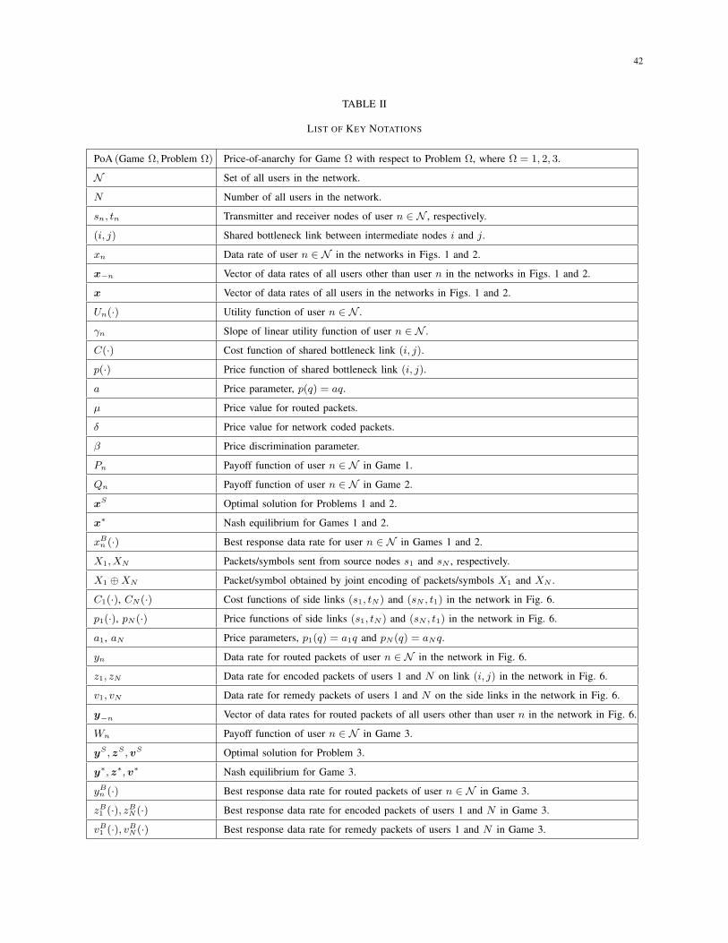
42

TABLE II

LIST OF KEY NOTATIONS

PoA (Game Ω, Problem Ω) Price-of-anarchy for Game Ω with respect to Problem Ω, where Ω = 1, 2, 3.

N Set of all users in the network.

N Number of all users in the network.

sn, tn Transmitter and receiver nodes of user n ∈ N , respectively.

(i, j) Shared bottleneck link between intermediate nodes i and j.

xn Data rate of user n ∈ N in the networks in Figs. 1 and 2.

x−n Vector of data rates of all users other than user n in the networks in Figs. 1 and 2.

x Vector of data rates of all users in the networks in Figs. 1 and 2.

Un(·) Utility function of user n ∈ N .

γn Slope of linear utility function of user n ∈ N .

C(·) Cost function of shared bottleneck link (i, j).

p(·) Price function of shared bottleneck link (i, j).

a Price parameter, p(q) = aq.

µ Price value for routed packets.

δ Price value for network coded packets.

β Price discrimination parameter.

Pn Payoff function of user n ∈ N in Game 1.

Qn Payoff function of user n ∈ N in Game 2.

xS Optimal solution for Problems 1 and 2.

x∗ Nash equilibrium for Games 1 and 2.

xBn (·) Best response data rate for user n ∈ N in Games 1 and 2.

X1, XN Packets/symbols sent from source nodes s1 and sN , respectively.

X1 ⊕XN Packet/symbol obtained by joint encoding of packets/symbols X1 and XN .

C1(·), CN (·) Cost functions of side links (s1, tN ) and (sN , t1) in the network in Fig. 6.

p1(·), pN (·) Price functions of side links (s1, tN ) and (sN , t1) in the network in Fig. 6.

a1, aN Price parameters, p1(q) = a1q and pN (q) = aNq.

yn Data rate for routed packets of user n ∈ N in the network in Fig. 6.

z1, zN Data rate for encoded packets of users 1 and N on link (i, j) in the network in Fig. 6.

v1, vN Data rate for remedy packets of users 1 and N on the side links in the network in Fig. 6.

y−n Vector of data rates for routed packets of all users other than user n in the network in Fig. 6.

Wn Payoff function of user n ∈ N in Game 3.

yS ,zS ,vS Optimal solution for Problem 3.

y∗,z∗,v∗ Nash equilibrium for Game 3.

yBn (·) Best response data rate for routed packets of user n ∈ N in Game 3.

zB1 (·), zBN (·) Best response data rate for encoded packets of users 1 and N in Game 3.

vB1 (·), vBN (·) Best response data rate for remedy packets of users 1 and N in Game 3.

43

Fig. 1. A single wireline bottleneck link shared by N routing flows [8]. Transmission of packets over bottleneck link at each

unit of data rate incurs at cost of C(PNn=1 xn) and imposes price p(

PNn=1 xn). Elastic data rates x1, . . . , xN are selected by

users 1, . . . , N , respectively.

Fig. 2. A butterfly network (cf. [5], [26]) with a single bottleneck link shared by N flows from N users and two side links.

Transmission of packets over bottleneck link at each unit of data rate incurs at cost of C“PN−1

n=2 xn + max(x1, xN )”

and

imposes a price p“PN−1

n=2 xn + max(x1, xN )”

. Since the source node s1 of user 1 is located closer to the destination node

tN of user N (and vice versa), users 1 and N can jointly perform inter-session network coding and reduce the traffic load on

the shared bottleneck link (i, j) (and reduce cost C). The side links (s1, tN ) and (sN , t1) are assumed to be free of charge in

this setting. Here, x1 and xN denote the data rates of source nodes s1 and sN , respectively. On the other hand, X1 and XN

denote the actual packets/symbols sent from nodes s1 and sN , respectively. The notation X1 ⊕XN indicates a network coded

packet/symbol obtained by jointly encoding packets X1 and XN .

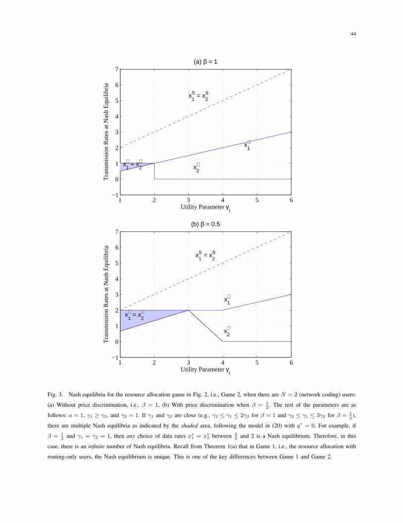
44

1 2 3 4 5 6−1

0

1

2

3

4

5

6

7

Utility Parameter γ1

Tra

nsm

issi

on R

ates

at N

ash

Equ

ilibr

ia

(a) β = 1

x1S = x

2S

x2∗

x1∗

x1∗ = x

2∗

1 2 3 4 5 6−1

0

1

2

3

4

5

6

7

Utility Parameter γ1

Tra

nsm

issi

on R

ates

at N

ash

Equ

ilibr

ia

(b) β = 0.5

x1S = x

2S

x1∗ = x

2∗

x2∗

x1∗

Fig. 3. Nash equilibria for the resource allocation game in Fig. 2, i.e., Game 2, when there are N = 2 (network coding) users:

(a) Without price discrimination, i.e., β = 1, (b) With price discrimination when β = 12

. The rest of the parameters are as

follows: a = 1, γ1 ≥ γ2, and γ2 = 1. If γ1 and γ2 are close (e.g., γ2 ≤ γ1 ≤ 2γ2 for β = 1 and γ2 ≤ γ1 ≤ 3γ2 for β = 12

),

there are multiple Nash equilibria as indicated by the shaded area, following the model in (20) with q∗ = 0. For example, if

β = 12

and γ1 = γ2 = 1, then any choice of data rates x∗1 = x∗2 between 23

and 2 is a Nash equilibrium. Therefore, in this

case, there is an infinite number of Nash equilibria. Recall from Theorem 1(a) that in Game 1, i.e., the resource allocation with

routing-only users, the Nash equilibrium is unique. This is one of the key differences between Game 1 and Game 2.

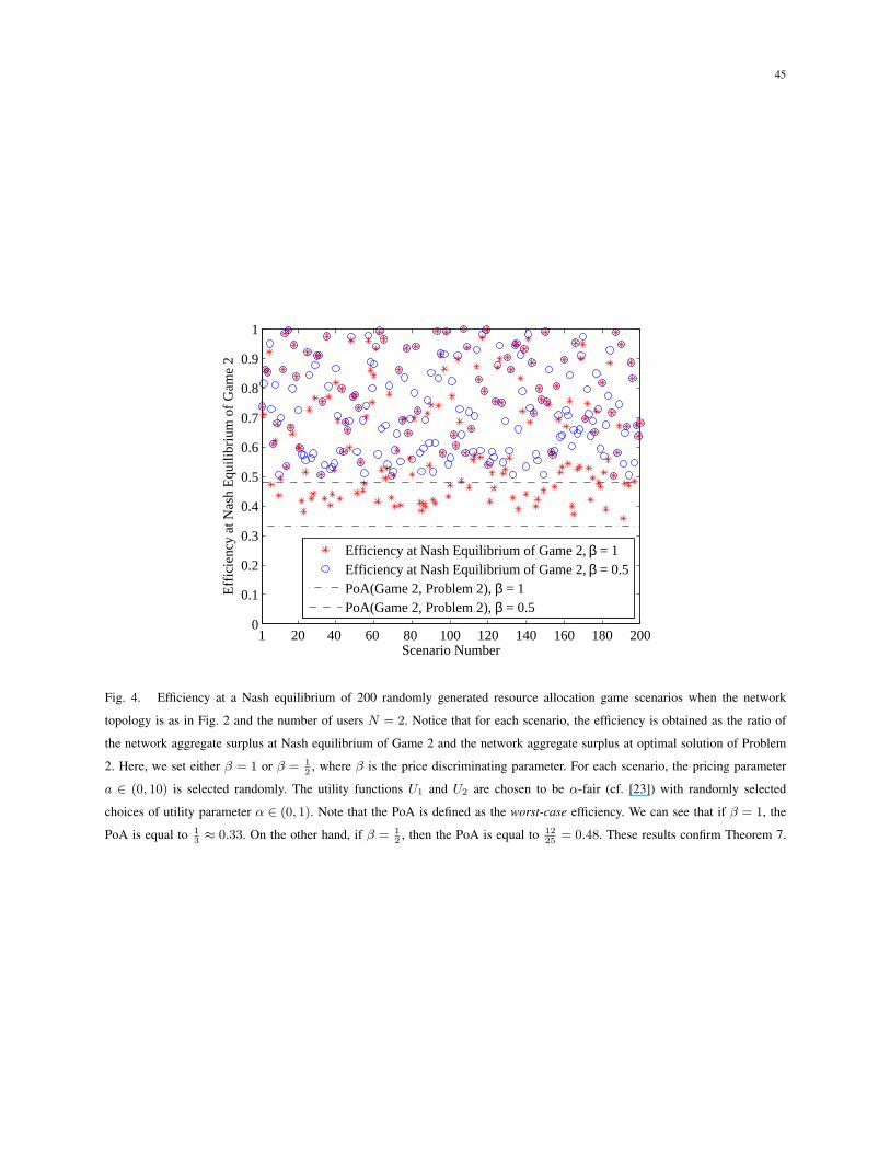
45

1 20 40 60 80 100 120 140 160 180 2000

0.1

0.2

0.3

0.4

0.5

0.6

0.7

0.8

0.9

1

Scenario Number

Eff

icie

ncy

at N

ash

Equ

ilibr

ium

of

Gam

e 2

Efficiency at Nash Equilibrium of Game 2, β = 1Efficiency at Nash Equilibrium of Game 2, β = 0.5PoA(Game 2, Problem 2), β = 1PoA(Game 2, Problem 2), β = 0.5

Fig. 4. Efficiency at a Nash equilibrium of 200 randomly generated resource allocation game scenarios when the network

topology is as in Fig. 2 and the number of users N = 2. Notice that for each scenario, the efficiency is obtained as the ratio of

the network aggregate surplus at Nash equilibrium of Game 2 and the network aggregate surplus at optimal solution of Problem

2. Here, we set either β = 1 or β = 12

, where β is the price discriminating parameter. For each scenario, the pricing parameter

a ∈ (0, 10) is selected randomly. The utility functions U1 and U2 are chosen to be α-fair (cf. [23]) with randomly selected

choices of utility parameter α ∈ (0, 1). Note that the PoA is defined as the worst-case efficiency. We can see that if β = 1, the

PoA is equal to 13≈ 0.33. On the other hand, if β = 1

2, then the PoA is equal to 12

25= 0.48. These results confirm Theorem 7.

46

1 2 3 4 5 6−1

0

1

2

3

4

5

6

7(a)

Utility Parameter γ1

Tra

nsm

issi

on R

ates

at N

ash

Equ

ilibr

ia(U

sers

1 a

nd 3

)

x1∗

x3∗x

1∗ = x

3∗

x1S = x

3S

1 2 3 4 5 6−1

0

1

2

3

4

5

6

7(b)

Utility Parameter γ1

Tra

nsm

issi

on R

ates

at N

ash

Equ

ilibr

ia(U

ser

2)

x2∗x

2∗

x2S

x2S

Fig. 5. Nash equilibria for the resource allocation game in Fig. 2 when N = 3, a = 1, β = 12

, γ1 ≥ γ3, γ3 = 1, and γ2 = 3.

Users 1 and 3 jointly perform inter-session network coding and user 2 is a routing user: (a) Transmission rates for users 1 and

3, (b) Transmission rates for user 2. If γ1 ≤ 2, then γ2 ≥ γ1 + γ3. In that case, at optimality of Problem 2, link (i, j) should

only carry the packets from routing user 2. If γ1 > 2, then γ2 < γ1 + γ3. In that case, at optimality, link (i, j) should only

carry the packets from network coding users 1 and 3.

47

Fig. 6. A single link shared by N flows. Users 1 and N perform inter-session network coding. The side links (s1, tN )

and (sN , t1) have non-zero cost. Thus, users 1 and N need to pay for their transmissions over links (s1, tN ) and (sN , t1),

respectively. Here, y1 and z1 denote the data rate at which source s1 sends data to intermediate node i marked for routing and

network coding, respectively. Similarly, yN and zN denote the data rate at which source sN sends data to node i marked for

routing and network coding, respectively. Node i jointly encodes only those packets which are marked for network coding. On

the other hand, v1 and vN denote the data rates at which sources s1 and sN send remedy packets over side links (s1, tN ) and

(sN , t1), respectively. The routing users 2, . . . , N − 1 send packets to node i all marked for routing with rates y2, . . . , yN−1,

respectively. Notation X1 ⊕XN indicates a network coded packet/symbol obtained by jointly encoding packets X1 and XN .

48

0 1 2 3 4 5 6 7 8 9 100

0.1

0.2

0.3

0.4

0.5

0.6

0.7

0.8

0.9

1

Eff

icie

ncy

at N

ash

Equ

ilibr

ium

of

Gam

e 3

Price Parameters for Side Links, a1 = a

N

45

23

15

Fig. 7. Efficiency at Nash equilibrium of Game 3 when the network topology is as in Fig. 6 and we have: N → ∞,

γ1 = γN = 1, γn = 45

for all n ∈ N\1, N, and a = 1. Side link price parameters a1 = aN vary from 0 (non-inclusive) to

10. Notice that for each choice of parameters a1 = aN , the efficiency is obtained as the ratio of the network surplus at Nash

equilibrium of Game 3 and the network surplus at optimal solution of Problem 3. We can see that the worst-case efficiency in

this case is equal to 15

, as expected from Theorem 11. As the prices on the side links increase, network coding becomes less

beneficial and the efficiency increases to a value (in this case 45

= 0.8) which is higher than 23

, as expected from Theorem 1.

49

1 20 40 60 80 100 120 140 160 180 2000

0.1

0.2

0.3

0.4

0.5

0.6

0.7

0.8

0.9

1

Scenario Number

Eff

icie

ncy

at N

ash

Equ

ilibr

ium

of

Gam

e 3

Efficiency at Nash Equilibrium of Game 3PoA(Game 3, Problem 3)

Fig. 8. Efficiency at Nash equilibrium of 200 randomly generated resource allocation game scenarios when the network

topology is as in Fig. 6 and where N = 2. For each scenario, the pricing parameters a ∈ (0, 10), a1 ∈ (0, 5), and a2 ∈ (0, 5)

are selected randomly. The utility functions U1 and U2 are chosen to be α-fair (cf. [23]) with randomly selected choices of

utility parameter α ∈ (0, 1). Note that the PoA is defined as the worst-case efficiency. We can see that the efficiency of Game

3 is always lower bounded by 15

= 0.2, i.e., the PoA is 15

, as expected from Theorem 11.