Intelligent Antenna Sharing in Cooperative Diversity

Wireless Networks

by

Aggelos Anastasiou Bletsas

Diploma, Electrical and Computer Engineering,Aristotle University of Thessaloniki (1998)

S.M., Media Arts and Sciences,Massachusetts Institute of Technology (2001)

Submitted to the Program of Media Arts and Sciences,,School of Architecture and Planning,

in partial fulfillment of the requirements for the degree of

Doctor of Philosophy in Media Arts and Sciences

at the

MASSACHUSETTS INSTITUTE OF TECHNOLOGY

September 2005

c© Massachusetts Institute of Technology 2005. All rights reserved.

AuthorProgram of Media Arts and Sciences,

August 1, 2005

Certified byAndrew B. Lippman

Principal Research Scientist, Program in Media Arts and SciencesMIT Media Laboratory

Thesis Supervisor

Accepted byAndrew B. Lippman

Chairman, Departmental Committee on Graduate StudiesProgram in Media Arts and Sciences

2

Intelligent Antenna Sharing in Cooperative Diversity Wireless Networks

by

Aggelos Anastasiou Bletsas

Submitted to the Program of Media Arts and Sciences,,School of Architecture and Planning,

on August 1, 2005, in partial fulfillment of therequirements for the degree of

Doctor of Philosophy in Media Arts and Sciences

Abstract

Cooperative diversity has been recently proposed as a way to form virtual antenna arraysthat provide dramatic gains in slow fading wireless environments. However most of the pro-posed solutions require simultaneous relay transmissions at the same frequency bands, usingdistributed space-time coding algorithms. Careful design of distributed space-time codingfor the relay channel, is usually based on global knowledge of some network parameters oris usually left for future investigation, if there is more than one cooperative relays.We propose a novel scheme that eliminates the need for space-time coding and providesdiversity gains on the order of the number of relays in the network. Our scheme firstselects the best relay from a set of M available relays and then uses this ”best” relayfor cooperation between the source and the destination. Information theoretic analysis ofoutage probability shows that our scheme achieves the same diversity-multiplexing gaintradeoff as achieved by more complex protocols, where coordination and distributed space-time coding for M relay nodes is required. Additionally, the proposed scheme increases theoutage and ergodic capacity, compared to non-cooperative communication with increasingnumber of participating relays, at the low SNR regime and under an total transmissionpower constraint.Coordination among the participating relays is based on a novel timing protocol than ex-ploits local measurements of the instantaneous channel conditions. The method is dis-tributed, allows for fast selection of the best relay, compared to the channel coherence timeand a methodology to evaluate relay selection performance for any kind of wireless channelstatistics, is provided. Other ways of network coordination, inspired by natural phenomenaof decentralized time synchronization are analyzed in theory and implemented in practice.The proposed, virtual antenna formation technique, allowed its implementation in a customnetwork of single antenna, half-duplex radios.

Thesis Supervisor: Andrew B. LippmanTitle: Principal Research Scientist, Program in Media Arts and Sciences, MIT Media Lab-oratory

3

4

Intelligent Antenna Sharing in Cooperative Diversity Wireless Networks

by

Aggelos Anastasiou Bletsas

The following people served as readers for this thesis:

Thesis ReaderJoseph A. ParadisoAssociate Professor

Program in Media Arts and Sciences, MIT

Thesis ReaderMoe Win

Associate ProfessorLaboratory for Information and Decision Systems (LIDS), MIT

5

6

Acknowledgements

Your acknowledgement goes here...

7

8

Contents

Abstract 3

1 Introduction 171.1 Wireless terminals (users) as Communication Sensors . . . . . . . . . . . . . 201.2 Research Assumptions . . . . . . . . . . . . . . . . . . . . . . . . . . . . . . 231.3 Background . . . . . . . . . . . . . . . . . . . . . . . . . . . . . . . . . . . . 241.4 Thesis Roadmap . . . . . . . . . . . . . . . . . . . . . . . . . . . . . . . . . 27

2 Opportunistic Relaying 292.1 Motivation . . . . . . . . . . . . . . . . . . . . . . . . . . . . . . . . . . . . 29

2.1.1 Key Contributions . . . . . . . . . . . . . . . . . . . . . . . . . . . . 332.2 Description . . . . . . . . . . . . . . . . . . . . . . . . . . . . . . . . . . . . 34

2.2.1 How well the selection is performed? . . . . . . . . . . . . . . . . . . 382.2.2 A note on Time Synchronization . . . . . . . . . . . . . . . . . . . . 402.2.3 A note on Multi-hop extension . . . . . . . . . . . . . . . . . . . . . 412.2.4 A note on Channel State Information (CSI) . . . . . . . . . . . . . . 412.2.5 Comparison with geometric approaches . . . . . . . . . . . . . . . . 42

2.3 Hardware Implementation . . . . . . . . . . . . . . . . . . . . . . . . . . . . 432.3.1 Signal structure . . . . . . . . . . . . . . . . . . . . . . . . . . . . . . 45

3 Performance 493.1 Diversity-Multiplexing Tradeoff . . . . . . . . . . . . . . . . . . . . . . . . . 50

3.1.1 Channel Model . . . . . . . . . . . . . . . . . . . . . . . . . . . . . . 503.1.2 Digital Relaying - Decode and Forward Protocol . . . . . . . . . . . 533.1.3 Analog relaying - Basic Amplify and Forward . . . . . . . . . . . . . 543.1.4 Discussion . . . . . . . . . . . . . . . . . . . . . . . . . . . . . . . . . 56

3.2 Outage Capacity . . . . . . . . . . . . . . . . . . . . . . . . . . . . . . . . . 583.2.1 Numerical Examples . . . . . . . . . . . . . . . . . . . . . . . . . . . 61

3.3 Power Savings . . . . . . . . . . . . . . . . . . . . . . . . . . . . . . . . . . . 653.3.1 Areas of useful cooperation . . . . . . . . . . . . . . . . . . . . . . . 67

3.4 Collision Probability . . . . . . . . . . . . . . . . . . . . . . . . . . . . . . . 703.4.1 Calculating Pr(Y2 < Y1 + c) . . . . . . . . . . . . . . . . . . . . . . . 713.4.2 Results . . . . . . . . . . . . . . . . . . . . . . . . . . . . . . . . . . 72

4 Scaling and Extensions 79

9

4.1 To Relay or not to Relay? . . . . . . . . . . . . . . . . . . . . . . . . . . . . 794.2 Extensions: Scheduling Multiple Streams . . . . . . . . . . . . . . . . . . . 86

5 Relevant Time Keeping Technologies 895.1 Clock Basics . . . . . . . . . . . . . . . . . . . . . . . . . . . . . . . . . . . . 915.2 Centralized Network Time Keeping . . . . . . . . . . . . . . . . . . . . . . . 93

5.2.1 Problem Formulation . . . . . . . . . . . . . . . . . . . . . . . . . . 935.2.2 Prior Art on Centralized Client-Server Schemes . . . . . . . . . . . . 945.2.3 The Algorithms . . . . . . . . . . . . . . . . . . . . . . . . . . . . . . 965.2.4 Performance . . . . . . . . . . . . . . . . . . . . . . . . . . . . . . . 1015.2.5 Measurements . . . . . . . . . . . . . . . . . . . . . . . . . . . . . . 1055.2.6 Discussion . . . . . . . . . . . . . . . . . . . . . . . . . . . . . . . . . 107

5.3 Decentralized Network Time Keeping . . . . . . . . . . . . . . . . . . . . . . 1085.3.1 Experimental Setup . . . . . . . . . . . . . . . . . . . . . . . . . . . 1105.3.2 The Algorithm and its Implementation in our Embedded Network . 1125.3.3 Results . . . . . . . . . . . . . . . . . . . . . . . . . . . . . . . . . . 1145.3.4 Further Improvements . . . . . . . . . . . . . . . . . . . . . . . . . . 1195.3.5 Spontaneous Order and its Connection to Biological Synchronization 1195.3.6 Relevant Work on Distributed Sync and Discussion . . . . . . . . . . 1205.3.7 Discussion . . . . . . . . . . . . . . . . . . . . . . . . . . . . . . . . . 122

6 Conclusion 123

A 129

B 133

10

List of Figures

1-1 Multiple antenna transceivers improve the efficiency of wireless communi-cation. What if the antennas belonged to different terminals? This thesisstudies this problem and proposes a practical scheme implemented in practice. 19

1-2 LEFT: A transmitter is placed close to a perfect reflector, that could be aconductive wall. Assuming no absorption from the wall (perfect reflection),we calculate the electromagnetic field amplitude at specific region, at the farfield. RIGHT: The calculated field amplitude as a function of space, for thecase depicted in the previous picture. Depending on the phase differencebetween the direct signal and the signal reflected by the wall, there are loca-tions far away from the transmitter, that have stronger field amplitude thanlocations closer to the transmitter. Observe, for example the circled points. 21

1-3 LEFT: Measurement of the received power profile as function of distance at916MHz for an indoor environment [26]. RIGHT: Artificial generation ofa similar profile, using Rayleigh fading and propagation coefficient v takenfrom measurements of the previous figure. . . . . . . . . . . . . . . . . . . . 21

2-1 A transmission is overheard by neighboring nodes. Distributed Space-Timecoding is needed so that all overhearing nodes could simultaneously trans-mit. In this work we analyze ”Opportunistic Relaying” where the relay withthe strongest transmitter-relay-receiver path is selected, among several can-didates, in a distributed fashion using instantaneous channel measurements. 32

2-2 Source transmits to destination and neighboring nodes overhear the commu-nication. The ”best” relay among M candidates is selected to relay infor-mation, via a distributed mechanism and based on instantaneous end-to-endchannel conditions. For the diversity-multiplexing tradeoff analysis, trans-mission of source and ”best” relay occur in orthogonal time channels. Thescheme could be easily modified to incorporate simultaneous transmissionsfrom source and ”best” relay. . . . . . . . . . . . . . . . . . . . . . . . . . . 35

2-3 The middle row corresponds to the ”best” relay. Other relays (top or bottomrow) could erroneously be selected as ”best” relays, if their timer expiredwithin intervals when they can not hear the best relay transmission. Thatcan happen in the interval [tL, tC ] for case (a) (No Hidden Relays) or [tL, tH ]for case (b) (Hidden Relays). tb, tj are time points where reception of theCTS packet is completed at best relay b and relay j respectively. . . . . . . 39

2-4 Low cost embedded radios at 916MHz, built for this work. . . . . . . . . . . 45

11

2-5 Distributed selection of “best” relay path. The intermediate relay nodesoverhear the handshaking between Tx and Rx. Based on the method ofdistributed timers, the relay that has the best signal path from transmitterto relay and relay to receiver is picked with minimal overhead. The receivercombines direct and relayed transmission and displays the received text on astore display. The “best” relay signals with an orange light. The transmittertransmits weather information coming from a 802.11-enabled pda. . . . . . 46

2-6 Laboratory demonstration. Relays and destination are depicted. . . . . . . 46

2-7 Signal structure at the digital output of the Rx radio. The waveforms aremeasured at the receiver using a digital oscilloscope and its associated dataacquisition capabilities. Notice that the time resolution for the plots at themiddle row is the same. . . . . . . . . . . . . . . . . . . . . . . . . . . . . . 48

3-1 The diversity-multiplexing of opportunistic relaying is exactly the same withthat of more complex space-time coded protocols. . . . . . . . . . . . . . . . 56

3-2 Under a total tx power constraint, the practical scheme of opportunisticrelaying increases the outage capacity, compared to direct communication.Selecting the appropriate path at the RF level exploits users as an additionaldegree of freedom, apart from power and rate. Two topologies are used as anexample: the first corresponds to the symmetric case of all relays equidistantto source and destination. The second topology corresponds to relays halfdistance between source and destination, for path loss exponent v = 3, 4. . . 62

3-3 Outage rates for various SNRs in opportunistic relaying. Top: symmetriccase. Bottom: asymmetric case for v=3 and v=4. . . . . . . . . . . . . . . . 63

3-4 Performance of cooperative communication compared to non-cooperative com-munication in left figure (using 8-PSK and various propagation coefficients)and total transmission energy ratio for target Symbol Error Probability(SEP)=10−3 in right figure (using 8-PSK and v = 4), in Rayleigh wirelesschannels. Relay decodes and encodes (digital relay) and it is placed closerto the transmitter, 1/4 the distance between source and destination. Wecan see that cooperative communication is more reliable compared to tradi-tional point-to-point communication, leading to higher reliability or trans-mission energy savings. Left:SEP in 8-PSK for various environments andE = E1 + E2, E1 = E2. Right:corresponding ratio E/(E1 + E2) for SEP=10−3. 68

3-5 Left: v=3. Right: v=5. Regions of intermediate node location where it isadvantageous to digitally relay to an intermediate node, instead of repeti-tively transmit. M=8 and the depicted ratio is the ratio of SEP of repetitivetransmission vs SEP of user cooperative digital communication. The coop-erative receiver optimally combines direct and relayed copy. Distances arenormalized to the point-to-point distance between transmitter and receiver. 69

3-6 Performance in Rayleigh and Ricean fading, for policy I (min) and Policy II(harmonic mean), various values of ratio λ/c and M = 6 relays, clustered atthe same region. Notice that collision probability drops well below 1%. . . . 74

12

3-7 Unequal expected values (moments) among the two path SNRs or amongthe relays, reduce collision probability. M=6 and c/λ = 1/200 for the fourdifferent topologies considered. . . . . . . . . . . . . . . . . . . . . . . . . . 75

4-1 Cumulative Distribution Function (CDF) of H12 (eq. 4.12, 4.13, 4.14), forthe three cases examined (one, all, ”best” relay(s) transmit). The expectedvalue is also depicted, at the bottom of the plot. . . . . . . . . . . . . . . . 82

4-2 Cumulative Distribution Function (CDF) of mutual information (eq. 4.11),for SNR=20dB. Notice that the CDF function provides for the values ofoutage probability. . . . . . . . . . . . . . . . . . . . . . . . . . . . . . . . . 83

4-3 Expected value of mutual information (eq. 4.11), corresponding to the er-godic capacity, as a function of number of relays. Notice that using all relaysincurs a penalty that increases with number of relays, compared to oppor-tunistic relaying. . . . . . . . . . . . . . . . . . . . . . . . . . . . . . . . . . 84

4-4 Relaying as scheduling for multiple streams. . . . . . . . . . . . . . . . . . . 87

5-1 LEFT: Frequency offset φ − 1 and time offset θ of C(t), compared with thesource of “true” time T (t). RIGHT: Exchanging timestamps between clientand time server. Notice that a time difference of δt according to server clockis translated to φδt according to client clock. . . . . . . . . . . . . . . . . . 92

5-2 Assymetry of delays between forward (to server) and reverse (to client) path.LEFT: Gaussian case. RIGHT: Self-similar case. . . . . . . . . . . . . . . . 102

5-3 Gaussian case. LEFT: Frequency offset estimate and standard deviation asa function of N (number of packets used). RIGHT: Time offset estimate andstandard deviation as a function of N (number of packets used). . . . . . . 103

5-4 Simulation in ns-2 with pareto cross traffic. 14 connections per link perdirection. . . . . . . . . . . . . . . . . . . . . . . . . . . . . . . . . . . . . . 104

5-5 LEFT: Predicted inter-arrival and measured inter-arrival interval using theKalman filter for self-similar cross traffic. CENTER: Delay Cn

4 − tn3 from thereverse path and clock line estimation using LP for self-similar cross traffic.RIGHT: Estimation of frequency offset φ− 1 using the ATD technique. Lowpass filtering of data is also plotted. . . . . . . . . . . . . . . . . . . . . . . 105

5-6 Histogram of the frequency offset estimates for self-similar cross traffic. . . . 106

5-7 Self-similar case. LEFT: Frequency offset estimate and standard deviation asa function of number N of packets used in calculation. RIGHT: Time offsetestimate and standard deviation as a function of number N of packets usedin calculation. . . . . . . . . . . . . . . . . . . . . . . . . . . . . . . . . . . . 106

5-8 Demo on a glass wall: each node can communicate with at most 4 immediateneighbors. The network manages to synchronize all nodes so that they can“output” through speakers the same music. At the edges of the network,the nodes are equipped with LED displays instead of speakers, to providefor visual proof of synchrony. All nodes are communicating with immediateneighbors only and there is no point of central control. . . . . . . . . . . . . 109

13

5-9 The individual nodes used in this work. Speakers and displays providedfor audio-visual output. LEFT: 4-IR Pushpin without speaker. The fourIR transceivers provide directional communication only along the horizontaland vertical axis. CENTER: 4-IR Pushpin with speaker. RIGHT: 45-LEDdisplay. A 4-IR Pushpin is connected behind the LED grid. . . . . . . . . . 109

5-10 Topologies for various network diameters d used in this work. The oscillo-scope probes are connected at the edge nodes of the network. The case ford = 4 is shown in the right figure. . . . . . . . . . . . . . . . . . . . . . . . . 111

5-11 Measured average time synchronization absolute error and its standard de-viation in milliseconds, as a function of network diameter. Clock resolutionand transmit time is on the order of milliseconds, limiting the error in themillisecond regime, as expected. Notice that error is not increased linearlywith number of hops, since error depends on the sign of clock drift differencesbetween neighboring nodes (equation 5.37). . . . . . . . . . . . . . . . . . . 116

5-12 Visual proof of synchrony. A “heartbeat” pattern is synchronized over thenetwork and displayed at the edges. The distributed, server-free approach fornetwork synchronization resembles the decentralized coordination of coloniesof fireflies and inspired this work. . . . . . . . . . . . . . . . . . . . . . . . . 119

A-1 Regions of integration of fY1,Y2(y1, y2), for Y1 < Y2 needed in Lemma I forcalculation of Pr(Y2 < Y1 + c), c > 0. . . . . . . . . . . . . . . . . . . . . . 130

14

List of Tables

5.1 Frequency offset estimation using an existing NTP/GPS server. . . . . . . . 1075.2 Period and resolution of each clock, transmission delay and bandwidth used

for timing packets (in packets per second). . . . . . . . . . . . . . . . . . . . 114

15

16

Chapter 1

Introduction

In the era of pervasive computing and communications, another thesis on wireless communi-

cation and networking might seem obsolete or outdated. However, we have all experienced

bad reception while using our cell phone (also known as poor quality of service), we have all

forgotten to recharge the device during the night and subsequently become unable to use

it during the day (energy/battery problems), and we have waited for too long for cellular

technology to mature until we could start exchanging pictures or videos with our friends,

using our cell phones. Even in that case, data speed (throughput) is significantly less than

the speed of Wi-Fi wireless technology we have been using in our homes. Finally, we have

all failed to talk to our friends using our cell phones in large venues such as the celebration

of 4th of July in front of Media Lab, when thousands of people alongside Charles river

gather to enjoy the spectacular fireworks but overload the statistically provisioned cellular

network.

Can we enhance the quality of service (QoS), increase the data speed (throughput) and/or

reduce the required energy (therefore increase battery life), without overusing common

resources such as spectrum or scarce resources like the available battery energy? Can we

further reduce the transmission power levels of every base station and therefore minimize

public health risks due to electromagnetic radiation? Can we create wireless networking

architectures that scale with increasing number of users and, if possible, perform better as

17

the users in the system increase?

Recent developments on multi-antenna transceivers (also known as Multi-Input Multi Out-

put systems) show that for the same bandwidth and power1 resources compared to tradi-

tional single-antenna communication, MIMO systems could increase throughput (multiplex-

ing gain) and/or increase reliability of communication (diversity gain). The extra degree

of freedom (apart from time and frequency) results from space, by exploiting the possible

statistical independence between the transmitting-receiving antenna pairs. The statistics of

the multi-antenna wireless channel could provide independent, parallel spatial communica-

tion channels, at the same carrier frequency and at the same time. In other words, MIMO

systems exploit space and statistical properties of the wireless channel and typically need

intensive signal processing computation for channel estimation and information process-

ing. Apart from extensive computation requirements, engineering and physical limitations

preclude the utilization of many antennas at the mobile terminal (typically no more that

two antennas at the cordless phone) and therefore, multi-antenna transceivers are typically

utilized at the base station side.

What happens when multiple antennas belong to different users? Can we exploit multiple

observations of the same information signal, from users distributed in space, given the

broadcast nature of the wireless medium? Can we earn the benefits of traditional MIMO

theory when the antennas belong to different users? In other words, this thesis explores

users in a network, being an additional degree of freedom, apart from time, frequency and

space, in combination with the intrinsic properties of the wireless channel (figure 1-1).

The problem of user cooperation in wireless communication poses exciting challenges: a)

computation (processing) capabilities of cooperating users are limited, since we assume

they are mobile, with fixed computation capacity and energy consumption b) cooperation

basically means that one user will use their own battery to relay information destined to

a different user, while the receiver will exploit the direct and the relayed transmission.

Therefore, strong incentives should be inherent in any cooperative scheme and c) coordi-

1Average energy and power will be used equivalently, since they are different by a multiplying factor, theinformation symbol duration.

18

Figure 1-1: Multiple antenna transceivers improve the efficiency of wireless communication.What if the antennas belonged to different terminals? This thesis studies this problem andproposes a practical scheme implemented in practice.

nation at the network level among the cooperative nodes should be manifested, requiring

important modifications in existing communication stacks, which have been structured for

point-to-point, non-cooperative communication links that mimic wires.

We are interested in practical schemes that address all the above issues and are applicable

using existing RF hardware architectures. To investigate performance, apart from theo-

retical analysis, we have also implemented proposed solutions, using low cost embedded

radios. Cooperation could lead to substantial total (network) transmission power savings

or increased spectral efficiency (in bits per second per hertz) under certain conditions. The

goal of this thesis is to provide distributed and adaptive cooperation algorithms that can

be applied in practice.

We will extensively study coordination algorithms required for user cooperative commu-

nication. The notion of cooperation can be extended to other important problems: if

users in a network have strong incentives to cooperate for efficient wireless communication,

then they could use cooperative strategies for network time keeping and positioning. We

will show that cooperative communication networks could autonomously maintain a global

19

clock (time keeping), using local computation. Therefore the network becomes the timing

system with specific accuracy and precision performance, again as a function of number of

users. Efficient communication and autonomous timing are considered important problems,

in future wireless sensor networks.

1.1 Wireless terminals (users) as Communication Sensors

Imagine inserting relays, literally anywhere near the receiver or transmitter. The goal is to

find one relay in a “hot spot” that receives the signal well. If that relay is simultaneously

in a hot spot with respect to the ultimate recipient of the information, then this relay can

effectively support the communication. The more relays there are, the more likely we can

find such intermediate.

Let’s start with a simple scenario: in figure 1-2, a transmitter is placed close to a conductive

wall and the received electromagnetic field amplitude is calculated at the far field region,

approximately one hundred wavelengths away. We assume transmission of a single carrier

and we observe that the received amplitude is not constant since there is destructive or

constructive addition of the direct and reflected signals. In this simple scenario, there

might be locations in space where the field amplitude might be larger than that in locations

closer to the transmitter (observe the circled point in figure 1-2). Moving from constructive

to destructive addition of the two rays, involves small physical movements in space, on the

order of a quarter of a wavelength. Antenna sharing techniques described in this thesis,

exploit in a distributed and decentralized way, cooperating users located at those points

where the wireless channel is as “good” as possible. Therefore, the more cooperating users,

the higher the probability to find one of them in a “hot spot”.

In reality, wireless propagation is much more complex than the two-ray model described

above. The wireless channel typically involves many reflectors, scatterers and obstructions.

It changes at a rate interval (coherence time) that depends on wavelength and mobility. A

large number of reflectors corresponds to a complex fading channel coefficient (2-dimensional

20

Received Field

Figure 1-2: LEFT: A transmitter is placed close to a perfect reflector, that could be a con-ductive wall. Assuming no absorption from the wall (perfect reflection), we calculate theelectromagnetic field amplitude at specific region, at the far field. RIGHT: The calculatedfield amplitude as a function of space, for the case depicted in the previous picture. De-pending on the phase difference between the direct signal and the signal reflected by thewall, there are locations far away from the transmitter, that have stronger field amplitudethan locations closer to the transmitter. Observe, for example the circled points.

v = 3.98

0 5 10 15 20 25 30 35 40 45-90

-80

-70

-60

-50

-40

-30

-20

-10

0

10

Distance (m)

Nor

mal

ized

Pow

er (

dB)

Figure 1-3: LEFT: Measurement of the received power profile as function of distance at916MHz for an indoor environment [26]. RIGHT: Artificial generation of a similar profile,using Rayleigh fading and propagation coefficient v taken from measurements of the previousfigure.

21

since there are in-phase and quadrature-phase components) with a normal distribution2.

The amplitude of a circularly symmetric complex Gaussian random variable corresponds

to a Rayleigh-distributed random variable and the amplitude squared, corresponds to an

exponential random variable.

If aij is the (complex) fading coefficient between transmitter i and receiver j, then from

fig. 1-3 we can make an estimate of E[|aij |2], as a function of distance. We assume that

received power Pr ∝ E[|a|2] ∝ 1/dvij , where v is the propagation coefficient and shows how

quickly power decreases, as a function of distance. In free space, since electromagnetic field

drops as 1/d, the received power drops as 1/d2 and v = 2. In practice, there is no free space

and we can see that v could be greater than two, in highly reflective environments or even

less than two, when RF propagation is waveguided.

Using the linear markers in figure 1-3, we can estimate v (v = 3.98). Then we can arti-

ficially create received power profile according to Rayleigh fading, using E[|a|2] = 1/d3.98ij .

Comparing the two plots in fig. 1-3, it appears that Rayleigh fading provides a realistic

approximation of wireless channels and further improvements could be made, by adding

a constant term that models the antenna gain, between the transmitting and receiving

antennas and scales appropriately the results.

Cassioli, Win and Molisch [14] have shown that the path loss can be modelled as a two

slope function in a log-log scale, with propagation coefficient v ' 2 for distances close

to the transmitter and v ' 7 for distances above a threshold. Several researchers have

suggested Lognormal fading as a realistic model of wireless channel power loss while others

have suggested Nakagami fading from which, Rayleigh fading can be seen as a special

case. For the discussion in this proposal, we use Rayleigh fading with various propagation

coefficients v, since Rayleigh is the baseline model used in communication research and a

good approximation of reality, as can be seen from fig. 1-3.

It is interesting to note that in free-space, where transmit and receive antennas are placed at

different heights, received power drops faster than 1/d2 for large d, due to phase difference

2according to the central limit theorem

22

between direct signal and signal reflected by the ground. Therefore, v = 4 is a very realistic

assumption for both indoor or outdoor environments.

1.2 Research Assumptions

1. Algorithms that react to the physics of the environment: Cooperative nodes in the

network adapt their behavior to instantaneous wireless channel realizations. The

algorithms ought to a) scale with increasing number of cooperating users and b)

require deterministic time to converge to a solution, well before the channel changes

(well below the channel coherence time). Therefore, the network reacts to the physics

of the environment in real time, using measured characteristics of that space.

2. Distributed algorithms with unknown network topology: There is no central point of

control that has global knowledge of the network (for example, there is no knowledge

on how many nodes cooperate in the network). There is no knowledge regarding the

topology of the network or distances to neighboring nodes.

3. Realistic wireless channel modeling: the channel model used in this work is based on

experimental measurements and excludes simplistic models of free space propagation

or propagation within a constant radius sphere. The richness and complexity of wire-

less propagation make wireless communication a challenging problem so any attempt

to simplify the corresponding models could provide unrealistic results.

4. Practical solutions for existing hardware: we tried to provide signal processing tech-

niques, as well as modulation, transmission and coordination techniques that could

be applied in existing hardware. Therefore, we do not make the assumption that

wireless beamforming is feasible, where different wireless transmitters “phase” their

transmissions so they can add constructively at the receiver. Implementing wireless

and distributed phased arrays is still an open area of research. Moreover, we will

not assume that any transmitter could fix its transmission radius to a given distance.

Communication range is a function of transmission power as well as wireless channel

characteristics, which are not user-defined.

23

The above components differentiate our work from existing approaches in the field, since

prior research has focused on a subset of the above components. In this work, we devise

system level solutions that would provide for distributed, infrastructure-free networks where

communications are improved with increasing number of cooperating nodes, using simple

hardware and intelligent algorithms, applicable in practice.

1.3 Background

[this section is incomplete - add hassibi, valenti, erkip, azarian, sendonaris, neely/modiano,

bambos etc... it also needs editing since there is overlap with next chapter]

In their 2000 paper [39], Laneman and Wornell described a distributed diversity reception

scheme with three nodes, one transmitter, one relay and one receiver. In that work, they

evaluated a simple modulation scheme (BPSK) in conjunction with maximum ratio com-

bining of direct and relayed transmission. They showed significant (transmission) energy

gains of the cooperative scheme compared to direct communication, at the expense of re-

duced rate, since symbol (bit) transmission would need two consecutive channel usages (one

for direct and one for relayed transmission) instead of one. In that work, they evaluated

among others, two cases of relaying: i) digital decode and re-encode (regeneration) and ii)

analog amplify-and-forward. These two cases of relaying were compared with the relay half-

distance between transmitter and receiver and amplify-and-forward performed significantly

better than the digital scheme. They considered channel known only at the receivers and

Rayleigh fading, supplemented with geometry of the three nodes.

Several research questions emerged after Laneman/Wornell 2000 work: can cooperation

increase throughput in uncoded or coded wireless communication? Why does analog re-

laying perform better than digital regeneration? what are the conditions under which the

cooperative scheme is more efficient than direct communication between any two points? In

section 3.3, we show that the region of successful cooperative digital communication is not

symmetric around the perpendicular, half-way between transmitter and receiver (fig. 3-5).

This is due to the fact that digital regeneration is meaningful, when digital reception at the

24

relay is error free: in other words, the whole cooperative scheme performance is based upon

correct reception of information, at the intermediate relay and it is natural to expect that

the region boundaries would be shifted toward the transmitter.

Consequently, the comparison of digital versus analog relaying, at half distance between

transmitter and receiver, gives results in favor of analog relaying. We extend the results of

[39] in the case of M-PSK (instead of BPSK), discover the regions of cooperative commu-

nication and quantify the spectral efficiency increase of cooperative communication, for the

case of M-PSK uncoded communication, under Rayleigh fading.

In his thesis work [42], Laneman followed an information theoretic approach and analyzed

the three-node scheme of transmitter, relay and receiver, in terms of outage probability

and spectral efficiency, at the high SNR regime. Such analysis facilitates outage probability

as an approximation of probability of error, since when appropriate error correcting codes

are used, fading is the limiting, deteriorating factor. In that case, fundamental limits of

performance, “best achievable performance”, can be sought, without worrying about spe-

cific coding schemes that achieve such performance. In that framework, Laneman found

that digital and analog relaying have similar performance in the high SNR regime. He also

discussed adaptive protocols with limited feedback, analyzed them in the same information

theoretic context and found out improved performance. He did not discuss practical coor-

dination schemes among transmitter, relay and receiver that could achieve those optimal

bounds. This thesis comes to fill that gap.

In [41], the case of several relays cooperating in a 2-hop scenario with digital relaying is

analyzed in the same outage probability-spectral efficiency context. Digital relays are al-

lowed to relay at the same channel, when their received SNR is above a threshold and it is

shown that the diversity gain is on the order of number of relays that participate in that

scheme. Practical space-time codes that can achieve such performance are not described in

detail, even though there is a discussion that such codes can be found. Our opportunistic

relaying approach, discussed in the next chapter, is a practical manifestation of a scheme

with several cooperating relays in a 2-hop scenario. We show that opportunistic relaying

provides higher capacity, when compared to the all-relays retransmit case, for fixed total

25

transmission power. Opportunistic relaying as well as “all relays” case in [?] assume that

the transmitter does not transmit a new information symbol during the second phase of

cooperation when the relay(s) retransmit. If the receiver is allowed to transmit a different

symbol when relay(s) retransmit the previous symbol, then performance (obviously) im-

proves and that was the case discussed in [2], again from an information theoretic point of

view, at the high SNR regime.

In [7] we provided a practical scheme in the context of OFDM wireless networks (like in

802.11a), where cooperative communication could be employed without sacrificing one de-

gree of freedom (one symbol period): direct and relayed transmission could happen within

the same symbol period, due to the special structure of OFDM symbols and properties of

oversampling. Therefore, we could experience the benefits of cooperation, without addi-

tional delay or reduced rate, at the cost of increased computation at each node.

In two different representations of the analog-amplify-and-forward cooperating channel in

[80] and [57], it was shown that ergodic capacity can not be increased if total transmit power

is kept constant and channel side information is known only at the receivers, when compared

to direct communication. The same result was also reported in [40]. Constructive addition

of superimposed signals at the receiver is needed to increase capacity and that can be done

only when the transmitters have channel information and special hardware (beamforming).

We are not assuming any kind of beamforming capability in our work.

For the case of multiple streams and several hops, it is difficult to come up with a concrete

formulation and an analytical solution. Significant work toward this direction has been

reported in [74] where the formulation of rate matrices for each transmit-receive pair in

the network is introduced. The achievable regions for all feasible rates are numerically

searched, for various scenarios including multi-hop, power control, successive interference

cancellation, node mobility and time-varying fading. An interesting aspect of that work is

the introduction of negative rates for nodes that relay information initiated by other nodes.

It is interesting to see what the feasible rate regions are (capacity regions), for the case of

cooperative communication.

In [69], spread spectrum communication is employed and it is shown that when it is com-

26

bined with local scheduling based on local time synchronization, then the network can sus-

tain considerable data traffic. The argument there is that spread spectrum communication,

in contrast to TDMA/FDMA medium access schemes, could survive concurrent transmis-

sions up to a level where Signal-to-Noise-and-Interference-Ratio (SNIR) is not severely de-

graded. By employing multi-hop, low-power transmissions instead of single-hop, high-power

transmissions, higher volumes of traffic could travel larger distances.

Kumar and Gupta in [29] showed that throughput of each node, when n nodes are randomly

placed in a unit area disk, drops as 1/√

n log n instead of 1/n as one might expect. That

result is under the assumption of fixed radius transmission range. Moreover, if nodes are

placed carefully on the disk, individual rates can drop even slower with 1/√

n and the total

distance-throughput of the network can scale with√

n (in meters times bits per second).

This surprising result, is based on perfect scheduling of information routing and non-realistic

wireless channel assumptions. Therefore it serves as an upper bound of “best performance”

in a wireless network3. How closely cooperative communication can reach those bounds,

remains to be seen.

Finally, we mention work on antenna selection in traditional MIMO systems and its perfor-

mance as it is summarized in [54]. Antenna selection, where high-SNR signals are utilized

while lower-SNR signals are discarded, could provide tools and intuition to study antenna

sharing among different users in wireless networking. References in [54] provide state-of-

the-art work, in MIMO systems in general.

1.4 Thesis Roadmap

In the following chapter, we present our proposal for a practical cooperative diversity scheme

and describe its implementation, in a custom, low-cost and embedded wireless network. In

chapter 3, we calculate the diversity-multiplexing tradeoff of our scheme and show that

our scheme incurs no performance loss, when compared to more involved schemes that

3similar scaling laws based on deterministic scheduling, as used in parallel computing, have been reportedin [38]

27

require simultaneous transmissions and space-time coding. We calculate outage and ergodic

capacity as a function of participating relay nodes and show the performance benefits,

in comparison with non-cooperative wireless communication. Transmission and reception

power gains, are also discussed. Coordination performance among the relays is quantified,

with an analysis that apply for various wireless channel statistics. In chapter 4, we analyze

our scheme as a RF scheduling algorithm and show that its power allocation results in

superior performance, compared to prior art. In chapter 5, we present network coordination,

based on centralized or decentralized time keeping, inspired from biological phenomena. We

summarize our findings, in chapter 6.

28

Chapter 2

Opportunistic Relaying

2.1 Motivation

In this chapter, we propose and analyze a practical scheme that forms a virtual antenna

array among single antenna terminals, distributed in space. The setup includes a set of

cooperating relays which are willing to forward received information towards the destination

and the proposed method is about a distributed algorithm that selects the most appropriate

relay to forward information towards the receiver. The decision is based on the end-to-

end instantaneous wireless channel conditions and the algorithm is distributed among the

cooperating wireless terminals.

The best relay selection algorithm lends itself naturally into cooperative diversity protocols

[67, 68, 42, 33], which have been recently proposed to improve reliability in wireless commu-

nication systems using distributed virtual antennas. The key idea behind these protocols

is to create additional paths between the source and destination using intermediate relay

nodes. In particular, Sendonaris, Erkip and Aazhang [67], [68] proposed a way of beam-

forming where source and a cooperating relay, assuming knowledge of the forward channel,

adjust the phase of their transmissions so that the two copies can add coherently at the

destination. Beamforming requires considerable modifications to existing RF front ends

that increase complexity and cost. Laneman, Tse and Wornell [42] assumed no CSI at the

29

transmitters and therefore assumed no beamforming capabilities and proposed the analysis

of cooperative diversity protocols under the framework of diversity-multiplexing tradeoff.

Their basic setup included one sender, one receiver and one intermediate relay node and

both analog as well as digital processing at the relay node were considered. The diversity-

multiplexing tradeoff of cooperative diversity protocols with multiple relays was studied

in [41, 2]. While [41] considered the case of orthogonal transmission1 between source and

relays, [2] considered the case where source and relays could transmit simultaneously. It

was shown in [2] that by relaxing the orthogonality constraint, a considerable improvement

in performance could be achieved, albeit at a higher complexity at the decoder. These

approaches were however information theoretic in nature and the design of practical codes

that approach these limits was left for further investigation.

Such code design is difficult in practice and an open area of research: while space time codes

for the Multiple Input Multiple Output (MIMO) link do exist [21] (where the antennas

belong to the same central terminal), more work is needed to use such algorithms in the

relay channel, where antennas belong to different terminals distributed in space. The relay

channel is fundamentally different than the point-to-point MIMO link since information is

not a priori known to the cooperating relays but rather needs to be communicated over noisy

links. Moreover, the number of participating antennas is not fixed since it depends on how

many relay terminals participate and how many of them are indeed useful in relaying the

information transmitted from the source. For example, for relays that decode and forward,

it is necessary to decode successfully before retransmitting. For relays that amplify and

forward, it is important to have a good received SNR, otherwise they would forward mostly

their own noise [57].

Therefore, the number of participating antennas in cooperative diversity schemes is in gen-

eral random and space-time coding invented for fixed number of antennas should be ap-

propriately modified. It can be argued that for the case of orthogonal transmission studied

1Note that in that scheme the relays do not transmit in mutually orthogonal time/frequency bands.Instead they use a space-time code to collaboratively send the message to the destination. Orthogonalityrefers to the fact that the source transmits in time slots orthogonal to the relays. Throughout this work wewill refer to Laneman’s scheme as orthogonal cooperative diversity.

30

in the present work (i.e. transmission during orthogonal time or frequency channels) codes

can be found that maintain orthogonality in the absence of a number of antennas (relays).

That was pointed in [41] where it was also emphasized that it remains to be seen how such

codes could provide residual diversity without sacrifice of the achievable rates.

Additionally, proposed amplify and forward distributed space-time coding [35] usually as-

sumes that the receiver knows the channel conditions between initial source and all partic-

ipating relays. Even though such assumption is convenient for analysis purposes, it is far

from practical in actual implementations, since the receiver has no way to estimate those

channel conditions which subsequently need to be communicated from the relays to the

destination. Such overhead might be prohibitive in actual implementations.

In short, providing for practical space-time codes for the cooperative relay channel is fun-

damentally different than space-time coding for the MIMO link channel and is still an open

and challenging area of research.

Apart from practical space-time coding for the cooperative relay channel, the formation

of virtual antenna arrays using individual terminals distributed in space, requires signifi-

cant amount of coordination. Specifically, the formation of cooperating groups of terminals

involves distributed algorithms [41] while synchronization at the packet level is required

among several different transmitters. Those additional requirements for cooperative di-

versity demand significant modifications to almost all layers of the communication stack

(up to the routing layer) which has been built according to ”traditional”, point-to-point

(non-cooperative) communication.

In fig. 2-1 a transmitter transmits its information towards the receiver while all the neigh-

boring nodes are in listening mode. For a practical cooperative diversity in a three-node

setup, the transmitter should know that allowing a relay at location (B) to relay infor-

mation, would be more efficient than repetition from the transmitter itself. This is not a

trivial task and such event depends on the wireless channel conditions between transmitter

and receiver as well as between transmitter-relay and relay-receiver. What if the relay is

located in position (A)? This problem also manifests in the multiple relay case, when one

31

A

B

Opportunistic Relaying

Space-Time codingfor M relays

TxRx

Tx

Tx

Rx

Rx

Figure 2-1: A transmission is overheard by neighboring nodes. Distributed Space-Timecoding is needed so that all overhearing nodes could simultaneously transmit. In thiswork we analyze ”Opportunistic Relaying” where the relay with the strongest transmitter-relay-receiver path is selected, among several candidates, in a distributed fashion usinginstantaneous channel measurements.

attempts to simplify the physical layer protocol by choosing the best available relay. In [77]

it was suggested that the best relay be selected based on location information with respect

to source and destination based on ideas from geographical routing proposed in [82]. Such

schemes require knowledge or estimation of distances between all relays and destination

and therefore require either a) infrastructure for distance estimation (for example GPS re-

ceivers at each terminal) or b) distance estimation using expected SNRs which is itself a

non-trivial problem and is more appropriate for static networks and less appropriate for

mobile networks, since in the latter case, estimation should be repeated with substantial

overhead.

In contrast, we propose a novel scheme that selects the best relay between source and

destination based on instantaneous channel measurements. The proposed scheme requires

no knowledge of the topology or its estimation. The technique is based on signal strength

measurements rather than distance and requires a small fraction of the channel coherence

time. All these features make the design of such a scheme highly challenging and the

proposed solution becomes non-trivial. Additionally, the algorithm itself provides for the

necessary coordination in time and group formation among the cooperating terminals.

32

The three-node reduction of the multiple relay problem we consider, greatly simplifies the

physical layer design. In particular, the requirement of space-time codes is completely

eliminated if the source and relay transmit in orthogonal time-slots. We further show that

there is essentially no loss in performance in terms of the diversity-multiplexing tradeoff as

compared to the transmission scheme in [41] which requires space-time coding across the

relays successful in decoding the source message. We also note that our scheme can be used

to simplify the non-orthogonal multiple relay protocols studied in [2]. Intuitively, the gains

in cooperative diversity do not come from using complex schemes, but rather from the fact

that we have enough relays in the system to provide sufficient diversity.

The simplicity of the technique, allows for immediate implementation in existing radio

hardware. An implementation of the scheme using custom radio hardware is described in

section 2.3. Its adoption could provide improved flexibility (since the technique addresses

coordination issues), reliability and efficiency (since the technique inherently builds upon

diversity) in future 4G wireless systems, down to low-cost sensor networks.

2.1.1 Key Contributions

One of the key contribution of this work is to propose and analyze a simplification of user

cooperation protocols at the physical layer by using a smart relay selection algorithm at the

network layer. We take the following steps, towards this end:

• We suggest and analyze a new protocol for selection of the ”best” relay between the

source and destination. This protocol has the following features:

– The protocol is distributed and each relay only makes local channel measure-

ments.

– Relay selection is based on instantaneous channel conditions in slow fading wire-

less environments. No prior knowledge or estimation of topology is required.

– The amount of overhead involved in selecting the best relay is minimal. It is

shown that there is a flexible tradeoff between the time incurred in the protocol

and the resulting error probability.

33

• The impact of smart relaying on the performance of user cooperation protocols is

studied. In particular, it is shown that for orthogonal cooperative diversity protocols

there is no loss in performance (in terms of the diversity-multiplexing tradeoff) if

only the best relay participates in cooperation. Opportunistic relaying provides an

alternative solution with a very simple physical layer to conventional cooperative

diversity protocols that rely on space-time codes. The scheme could be further used

to simplify space-time coding in the case of non-orthogonal transmissions.

Since the communication scheme exploits the wireless channel at its best, via distributed

cooperating relays, we naturally called it opportunistic relaying. The term ”opportunistic”

has been widely used in various different contexts. In [5], it was used in the context of

repetitive transmission of the same information over several paths, in 802.11b networks. In

our setup, we do not allow repetition since we are interested in providing diversity without

sacrificing the achievable rates, which is a characteristic of repetition schemes. The term

”opportunistic” has also been used in the context of efficient flooding of signals in multi-

hop networks [66], to increase communication range and therefore has no relationship with

our work. We first encountered the term ”opportunistic” in the work by Viswanath, Tse

and Laroia [78], where the base station always selects the best user for transmission in

an artificially induced fast fading environment. In our work, a mechanism of multi-user

diversity is provided for the relay channel, in single antenna terminals. Our proposed

scheme, resembles selection diversity that has been proposed for centralized multi-antenna

receivers [54]. In our setup, the single antenna relays are distributed in space and attention

has been given in selecting the “best” possible antenna, well before the channel changes

again, using minimal communication overhead.

2.2 Description

According to opportunistic relaying, a single relay among a set of M relay nodes is selected,

depending on which relay provides for the ”best” end-to-end path between source and des-

tination (fig. 2-1, 2-2). The wireless channel coefficient asi between source and each relay

34

best path @ kT

best path @ (k+1)T

Direct Relayed

|as,i|2 |ai,d|2

Source Destination

SourceSourceSource

|as,j|2 |aj,d|2

Figure 2-2: Source transmits to destination and neighboring nodes overhear the commu-nication. The ”best” relay among M candidates is selected to relay information, via adistributed mechanism and based on instantaneous end-to-end channel conditions. For thediversity-multiplexing tradeoff analysis, transmission of source and ”best” relay occur in or-thogonal time channels. The scheme could be easily modified to incorporate simultaneoustransmissions from source and ”best” relay.

i, as well as the channel coefficient aid between relay i and destination affect performance.

These parameters model the propagation environment between any communicating termi-

nals and change over time, with a rate that macroscopically can be modelled as the Doppler

shift, inversely proportional to the channel coherence time. Opportunistic selection of the

“best” available relay involves the discovery of the most appropriate relay, in a distributed

and “quick” fashion, well before the channel changes again. We will explicitly quantify the

speed of relay selection in the following section.

The important point to make here is that under the proposed scheme, the relay nodes

monitor the instantaneous channel conditions towards source and destination, and decide in

a distributed fashion which one has the strongest path for information relaying, well before

the channel changes again. In that way, topology information at the relays (specifically

location coordinates of source and destination at each relay) is not needed. The selection

process reacts to the physics of wireless propagation, which are in general dependent on

several parameters including mobility and distance. By having the network select the relay

with the strongest end-to-end path, macroscopic features like “distance” are also taken into

35

account. Moreover, the proposed technique is advantageous over techniques that select

the best relay a priori, based on distance toward source or destination, since distance-

dependent relay selection neglects well-understood phenomena in wireless propagation such

as shadowing or fading : communicating transmitter-receiver pairs with similar distances

might have enormous differences in terms of received SNRs. Furthermore, average channel

conditions might be less appropriate for mobile terminals than static. Selecting the best

available path under such conditions (zero topology information, ”fast” relay selection well

bellow the coherence time of the channel and minimum communication overhead) becomes

non-obvious and it is one of the main contributions of this work.

More specifically, the relays overhear a single transmission of a Ready-to-Send (RTS) packet

and a Clear-to-Send (CTS) packet from the destination. From these packets, the relays

assess how appropriate each of them is for information relaying. The transmission of RTS

from the source allows for the estimation of the instantaneous wireless channel asi between

source and relay i, at each relay i (fig. 2-2). Similarly, the transmission of CTS from the

destination, allows for the estimation of the instantaneous wireless channel aid between relay

i and destination, at each relay i, according to the reciprocity theorem[64]2. Note that the

source does not need to listen to the CTS packet3 from the destination.

Since communication among all relays should be minimized for reduced overall overhead, a

method based on time is selected: as soon as each relay receives the CTS packet, it starts a

timer from a parameter hi based on the instantaneous channel measurements asi, aid. The

timer of the relay with the best end-to-end channel conditions will expire first. That relay

transmits a short duration flag packet, signaling its presence. All relays, while waiting for

their timer to reduce to zero (i.e. to expire) are in listening mode. As soon as they hear

another relay to flag its presence or forward information (the best relay), they back off.

For the case where all relays can listen source and destination, but they are ”hidden” from

2We assume that the forward and backward channels between the relay and destination are the samefrom the reciprocity theorem. Note that these transmissions occur on the same frequency band and samecoherence interval.

3The CTS packet name is motivated by existing MAC protocols. However unlike the existing MACprotocols,the source does not need to receive this packet.

36

each other (i.e. they can not listen each other), the best relay notifies the destination with

a short duration flag packet and the destination notifies all relays with a short broadcast

message.

The channel coefficients asi, aid at each relay, describe the quality of the wireless path

between source-relay-destination, for each relay i. Since the two hops are both important

for end-to-end performance, each relay should quantify its appropriateness as an active

relay, using a function that involves the link quality of both hops. Two functions are used

in this work: under policy I, the minimum of the two is selected (equation (2.1)), while

under policy II, the harmonic mean of the two is used (equation (2.2)). Policy I selects the

”bottleneck” of the two paths while Policy II balances the two link strengths and it is a

smoother version of the first one.

Under policy I:

hi = min{|asi|2, |aid|2} (2.1)

Under policy II:

hi =2

1|asi|2 + 1

|aid|2=

2 |asi|2 |aid|2

|asi|2 + |aid|2(2.2)

The relay i that maximizes function hi is the one with the ”best” end-to-end path between

initial source and final destination. After receiving the CTS packet, each relay i will start its

own timer with an initial value Ti, inversely proportional to the end-to-end channel quality

hi, according to the following equation:

Ti =λ

hi(2.3)

Here λ is a constant. The units of λ depend on the units of hi. Since hi is a scalar, λ has

the units of time. For the discussion in this work, λ has simply values of µsecs.

hb = max{hi}, ⇐⇒ (2.4)

Tb = min{Ti}, i ∈ [1..M ]. (2.5)

37

Therefore, the ”best” relay has its timer reduced to zero first (since it started from a smaller

initial value, according to equations (2.3)-(2.5)). This is the ”best” relay that participates

in forwarding information from the source. The rest of the relays, will overhear the ”flag”

packet from the best relay (or the destination, in the case of hidden relays) and back off.

After the best relay has been selected, then it can be used to forward information towards

the destination. Whether that ”best” relay will transmit simultaneously with the source

or not, is completely irrelevant to the relay selection process. However, in the diversity-

multiplexing tradeoff analysis in the next chapter, we strictly allow only one transmission

at each time and therefore we can view the overall scheme as a two-step transmission: one

from source and one from ”best” relay, during a subsequent (orthogonal) time channel (fig.

2-2).

2.2.1 How well the selection is performed?

The probability of having two or more relay timers expire ”at the same time” is zero.

However, the probability of having two or more relay timers expire within the same time

interval c is non zero and can be analytically evaluated, given knowledge of the wireless

channel statistics.

The only case where opportunistic relay selection fails is when one relay can not detect that

another relay is more appropriate for information forwarding. Note that we have already

assumed that all relays can listen initial source and destination, otherwise they do not

participate in the scheme. We will assume two extreme cases: a) all relays can listen to each

other b) all relays are hidden from each other (but they can listen source and destination).

In that case, the flag packet sent by the best relay is received from the destination which

responds with a short broadcast packet to all relays. Alternatively, other schemes based on

”busy tone” (secondary frequency) control channels could be used, requiring no broadcast

packet from the destination and partly alleviating the ”hidden” relays problem.

In fig. 2-3, collision of two or more relays can happen if the best relay timer Tb and one

or more other relay timers expire within [tL, tC ] for the case of no hidden relays (case

38

tL tHtC

Tb ds

dur

tb

tj

|nb-nj|

r r ds+2nb

CTS

CTS

CTS

flag packet

Figure 2-3: The middle row corresponds to the ”best” relay. Other relays (top or bottomrow) could erroneously be selected as ”best” relays, if their timer expired within intervalswhen they can not hear the best relay transmission. That can happen in the interval [tL, tC ]for case (a) (No Hidden Relays) or [tL, tH ] for case (b) (Hidden Relays). tb, tj are time pointswhere reception of the CTS packet is completed at best relay b and relay j respectively.

(a)). This interval depends on the radio switch time from receive to transmit mode ds

and the propagation times needed for signals to travel in the wireless medium. In custom

low-cost transceiver hardware, this switch time is typically on the order of a few µsecs

while propagation times for a range of 100 meters is on the order of 1/3 µsecs. For the

case of ”hidden” relays the uncertainty interval becomes [tL, tH ] since now the duration

of the flag packet should be taken into account, as well as the propagation time towards

the destination and back towards the relays and the radio switch time at the destination.

The duration of the flag packet can be made small, even one bit transmission could suffice.

In any case, the higher this uncertainty interval, the higher the probability of two or more

relay timers to expire within that interval. That’s why we will assume maximum values of

c, so that we can assess worst case scenario performance.

(a) No Hidden Relays:

c = rmax + |nb − nj |max + ds (2.6)

(b) Hidden Relays:

c = rmax + |nb − nj |max + 2ds + dur + 2nmax (2.7)

where:

39

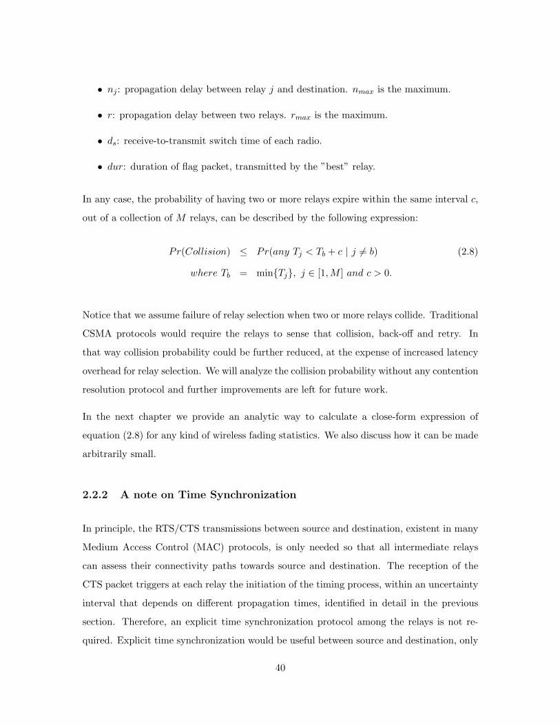
• nj : propagation delay between relay j and destination. nmax is the maximum.

• r: propagation delay between two relays. rmax is the maximum.

• ds: receive-to-transmit switch time of each radio.

• dur: duration of flag packet, transmitted by the ”best” relay.

In any case, the probability of having two or more relays expire within the same interval c,

out of a collection of M relays, can be described by the following expression:

Pr(Collision) ≤ Pr(any Tj < Tb + c | j 6= b) (2.8)

where Tb = min{Tj}, j ∈ [1,M ] and c > 0.

Notice that we assume failure of relay selection when two or more relays collide. Traditional

CSMA protocols would require the relays to sense that collision, back-off and retry. In

that way collision probability could be further reduced, at the expense of increased latency

overhead for relay selection. We will analyze the collision probability without any contention

resolution protocol and further improvements are left for future work.

In the next chapter we provide an analytic way to calculate a close-form expression of

equation (2.8) for any kind of wireless fading statistics. We also discuss how it can be made

arbitrarily small.

2.2.2 A note on Time Synchronization

In principle, the RTS/CTS transmissions between source and destination, existent in many

Medium Access Control (MAC) protocols, is only needed so that all intermediate relays

can assess their connectivity paths towards source and destination. The reception of the

CTS packet triggers at each relay the initiation of the timing process, within an uncertainty

interval that depends on different propagation times, identified in detail in the previous

section. Therefore, an explicit time synchronization protocol among the relays is not re-

quired. Explicit time synchronization would be useful between source and destination, only

40

if there was no direct link between them. In that case, the destination could not respond

with a CTS to a RTS packet from the source, and therefore source and destination would

need to schedule their RTS/CTS exchange by other means. In such cases ”crude” time

synchronization would be useful. Accurate synchronization schemes, server-based [10] or

decentralized [11], do exist and have been studied elsewhere. We will assume that source

and destination are in communication range and therefore no synchronization protocols are

needed.

2.2.3 A note on Multi-hop extension

It is important to emphasize that since the RTS/CTS exchange is needed only at the relays,

the overall scheme can easily be generalized at the case where source and destination are

not in communication range. A solution based on time synchronization was described

above. Alternatively, another simple protocol modification could be devised: the relays,

upon reception of the RTS packet contend for the channel so that one of them could notify

the destination that the relays await for a CTS packet. The contention resolution could

follow the same timer-based approach. Then the destination responds with a CTS packet.

From that point, the algorithm proceeds as described, selecting the relay with the best

”end-to-end” path.

2.2.4 A note on Channel State Information (CSI)

CSI at the relays, [in the form of link strengths (not signal phases)], is used at the network

layer for ”best” relay selection. CSI is not required at the physical layer and is exploited

neither at the source nor the relays. The wireless terminals in this work do not exploit CSI

for beamforming and do not adapt their transmission rate to the wireless channel conditions,

either because they are operating in the minimum possible rate or because their hardware

does not allow multiple rates. We will emphasize again that no CSI at the physical layer is

exploited at the source or the relays, during the diversity-multiplexing tradeoff analysis, in

the following chapter.

41

2.2.5 Comparison with geometric approaches

As can be seen from the above equations, the scheme depends on the instantaneous channel

realizations or equivalently, on received instantaneous SNRs, at each relay. An alternative

approach would be to have the source know the location of the destination and propagate

that information, alongside with its own location information to the relays, using a simple

packet that contained that location information. Then, each relay, assuming knowledge of

its own location information, could assess its proximity towards source and destination and

based on that proximity, contend for the channel with the rest of the relays. That is an idea,

proposed by Zorzi and Rao [82] in the context of fading-free wireless networks, when nodes

know their location and the location of their destination (for example they are equipped

with GPS receivers). The objective there was to study geographical routing and study the

average number of hops needed under such schemes. All relays are partitioned into a specific

number of geographical regions between source and destination and each relay identifies its

region using knowledge of its location and the location of source and destination. Relays at

the region closer to the destination contend for the channel first using a standard CSMA

splitting scheme. If no relays are found, then relays at the second closest region contend

and so on, until all regions are covered, with a typical number of regions close to 4. The

latency of the above distance-dependent contention resolution scheme was analyzed in [83].

Zorzi and Rao’s scheme of distance-dependent relay selection was employed in the context of

Hybrid-ARQ, proposed by Zhao and Valenti [77]. In that work, the request to an Automatic

Repeat Request (ARQ) is served by the relay closest to the destination, among those that

have decoded the message. In that case, code combining is assumed that exploits the direct

and relayed transmission (that’s why the term Hybrid was used)4. Relays are assumed to

know their distances to the destination (valid for GPS equipped terminals) or estimate their

distances by measuring the expected channel conditions using the ARQ requests from the

destination or using other means.

We note that our scheme of opportunistic relaying differs from the above scheme in the

4The idea of having a relay terminal respond to an ARQ instead of the original source, was also reportedand analyzed in [42] albeit for repetition coding instead of hybrid code combining.

42

following aspects:

• The above scheme performs relay selection based on geographical regions while our

scheme performs selection based on instantaneous channel conditions. In wireless

environment, the latter choice could be more suitable as relay nodes located at similar

distance to the destination could have vastly different channel gains due to effects such

as fading.

• The above scheme requires measurements to be only performed once, if there is no

mobility among nodes but requires several rounds of packet exchanges to determine

the average SNR. On the other hand opportunistic relaying requires only three packet

exchanges in total to determine the instantaneous SNR, but requires that these mea-

surements be repeated in each coherence interval. We show in a subsequent section

that the overhead of relay selection is a small fraction of the coherence interval with

collision probability less than 0.6%.

• We also note that our protocol is a proactive protocol since it selects the best relay

before transmission. The protocol can easily be made to be reactive (similar to [77])

by selecting the relay after the first phase. However this modification would require

all relays to listen to the source transmission which can be energy inefficient from a

network sense.

2.3 Hardware Implementation

Simplicity of the proposed cooperative diversity scheme was a design prerequisite, so that

it could be implemented using existing low cost radio hardware. The main problem with

current approaches is that they require simultaneous transmissions (at the same frequency

band and at the same time). It is well known that electromagnetic waves add in a highly non-

linear way, vector-wise, where amplitude, carrier frequency as well as phase are important.

In order for simultaneous transmissions to be effective, all the above parameters need to be

controlled and adjusted, among the participating radios, distributed in space. Most of the

43

cooperative diversity approaches neglect the above implementation difficulties and focus on

a simplified baseband analysis. In that sense, cooperative diversity demonstration had been

left as a future exercise.

From the above we can understand that simultaneous transmissions require radio front ends

that depart from the conventional norm. Even though such endeavor is not impossible,

and research efforts are underway, we choose to devise cooperative diversity protocols that

exploit existing radios and therefore are cost-effective today. We further show in the next

chapter that there is no performance loss, from a diversity-multiplexing tradeoff point of

view.

We were interested in a portable demonstration and therefore we designed the simplest

possible hardware: we used a 916MHz on-off keying radio module from RF Monolithics, with

115kHz bandwidth and part-15 compliant. The module can tranmsit/receive continuous

digital waveforms and it is the duty of the design engineer to built the necessary protocol

on top of this functionality. We interfaced that module to a low-cost 8051 microcontroller

(MCU), driven by a 22.1184MHz crystal oscillator. The mcu/crystal board was designed by

J. Lifton, a fellow colleague and friend, in the context of Pushpin Computing [50]. We chose

the specific MCU since it had a detailed and well-written specification manual. We designed

a new printed circuit board (PCB) using Protel, interfacing the pushping MCU with the

radio module and wrote all the necessary software functions for bit/byte/frame/packet

transmission, synchronization and reception. Additional interfaces based on RS232 were

built and used so that the embedded network could be interfaced to PDAs and the rest of

the digital world. A picture of the hardware built is given in Fig. 2-4.

In order to demonstrate the benefits of cooperative diversity we created a room size demo.

Text information was transmitted from one side of the room towards a receiver connected

to a store display at the other side of the room (Fig. 2-5). Relays at the vicinity of

communication would provide for additional reliability, in the presence of people moving

in the room. Received information would be presented at the store display, demonstrating

that errors would be decreased when opportunistic relaying was used.

44

Figure 2-4: Low cost embedded radios at 916MHz, built for this work.

2.3.1 Signal structure

Information was sent periodically, in blocks corresponding to 16 characters of information,

since that was the selected message length that could be displayed at the store screen. The

message would scroll from left to right with a duration of 2-3 seconds. Therefore, messages

of 16 characters were sent with that period.

Before every message transmission, ”best” relay selection would be performed, according

to the described algorithm. Then, 16 frames would be transmitted from the source, corre-

sponding to the 16 characters of the message. Each frame (out of those 16 frames) would be

repeated from the best relay, provided that it had been correctly decoded from the best re-

lay. That is why the signal structure shown in Fig. 2-7, second row first picture, has empty

slots destined for the transmission of the best relay. Each frame consisted by the necessary

synchronization preamble, followed by 4 bytes (32 bits) that included header information

(source id, destination id, sequence id), data information as well as Cyclic Redundancy

Check (CRC) for error detection purposes. CRC information was required so that the relay

could find out whether it had correctly decoded the message. The destination would receive

information from the source as well as information from the best relay and would decide

about the original message. Even though we could use a Maximum Ratio Combiner (MRC),

we chose to further simplify the receiver structure and rather decode both messages and

45

Store Display

802.11- enabled PDA

Rx

Tx

Relays

Figure 2-5: Distributed selection of “best” relay path. The intermediate relay nodes over-hear the handshaking between Tx and Rx. Based on the method of distributed timers, therelay that has the best signal path from transmitter to relay and relay to receiver is pickedwith minimal overhead. The receiver combines direct and relayed transmission and displaysthe received text on a store display. The “best” relay signals with an orange light. Thetransmitter transmits weather information coming from a 802.11-enabled pda.

RelayRelay

Relay

Relay

Relay

Relay

Rx Display

Rx Display

Left-side view

Right-side view

Figure 2-6: Laboratory demonstration. Relays and destination are depicted.

46

keep the one with the correct message (assertion made with the help of the CRC field).

The signal structure used (fig. 2-7) is a specific example of how opportunistic relaying can

be used in cooperative diversity contexts. It should be viewed as a concrete example for

a specific application, built for demonstration purposes. Additional optimization could be

performed if that was necessary. For example, the time required for ”best” relay selection,

could be further reduced. We did not perform such optimization, since there was no such

need in our slow bit-rate and low duty cycle demonstration. In the performance section of

the next chapter, such optimization is being explored. Additionally, our embedded radios

did not have much computation power given the 8-bit processor structure. More complex

receiver structures, like a Maximum Ratio Combiner receiver or an advanced error correcting

Code Combiner receiver require more powerful computation and could be used if we had

selected a more powerful microprocessor for each embedded radio. Note however that

increased complexity at each receiver increases the necessary required reception energy [52],

having a significant impact on the overall energy budget. We chose to keep the individual

nodes as simple as possible and rather create distributed intelligence at the network layer.

In the following section, we will show that such design choice incurs no performance loss.

47

Direct transmission of 16 frames

Signal structure of each frame

Preamble 32 bits (on-off keying)

CTS Flag �packet

16/32 data frames

Direct and best relay transmission� (16 + 16 = 32 frames)

Figure 2-7: Signal structure at the digital output of the Rx radio. The waveforms aremeasured at the receiver using a digital oscilloscope and its associated data acquisitioncapabilities. Notice that the time resolution for the plots at the middle row is the same.

48

Chapter 3

Performance

In this chapter, we quantify the performance of opportunistic relaying. Using tools from

multiple antenna theory, we show that opportunistic relaying at the network layer, is as

efficient as the most complex space-time coding algorithms at the physical layer, from a

diversity-multiplexing gain point of view. Specifically, in section 3.1 we use the elegant

tool of diversity-multiplexing gain tradeoff, popularized in [79] and show that the balance

between reliability and communication speed of a single, ”best” relay, is as good as having

all relays transmit at the same frequency/time channels.

This rather surprising finding suggests that opportunistic relaying is a simple way to im-

plement cooperative diversity schemes, without performance loss. In section 3.2 we derive

the outage capacity of opportunistic relaying and show the increase of spectral efficiency

(in bps/Hz), especially at the low SNR regime, suggesting that opportunistic cooperation

could be used for faster communication. Power efficiency is also discussed, given the fact

that opportunistic relaying does not require all relays to listen and therefore does not have

reception energy deficiencies, proportional to the number of relays. Additionally, impor-

tant transmission energy savings can be realized, with gains quantified further in section

3.3. Finally, the required overhead for best relay selection, is shown in section 3.4 to be

reasonably small, in slow fading environments.

49

3.1 Diversity-Multiplexing Tradeoff

We now consider the impact of opportunistic relaying on the cooperative diversity scenario.

The main result of this section is that opportunistic relaying can be used to simplify a

number of cooperative diversity protocols involving multiple relays. In particular we focus

on the cooperative diversity protocol in [41] which requires the relays to use a space-time

code while simultaneously transmitting towards the destination. We show that this protocol

can be simplified considerably by simply selecting the best relay in the second stage. Per-

haps surprisingly, this simplified protocol achieves the same diversity multiplexing tradeoff

achieved in [41]. Furthermore, it does not matter whether the relay implements an amplify

and forward or a decode and forward protocol in terms of the diversity-multiplexing trade-

off. We also note that opportunistic relaying can be used to simplify the non-orthogonal

relaying protocols proposed in [2]. However the detailed performance analysis is left for

future work.

3.1.1 Channel Model

We consider an i.i.d slow Rayleigh fading channel model following [42]. A half duplex con-

straint is imposed across each relay node, i.e. it cannot transmit and listen simultaneously.

We assume that the nodes (transmitter and relays) do not exploit the knowledge of the chan-

nel at the physical layer. Note that in the process of discovering the best relay described in

the previous section the nodes do learn about their channel gains to the destination. How-

ever, we assume that this knowledge of channel gain is limited to the network layer protocol.

The knowledge of channel gain is not exploited at the physical layer in order to adjust the

code rate based on instantaneous channel measurements. In practice, the hardware at the

physical layer could be quite constrained to allow for this flexibility to change the rate on

the fly. It could also be that the transmitter is operating at the minimum transmission

rate allowed by the radio hardware. Throughout this section, we assume that the channel

knowledge is not exploited at the physical layer at either the transmitter or the relays.

If the discrete time received signal at the destination and the relay node are denoted by

50

Y [n] and Y1[n] respectively, then:

Y [n] = asdX[n] + Z[n], n = 1, 2 . . .T

2(source transmits destination receives) (3.1)

Y [n] = ardX1[n] + Z[n], n =T

2,T

2+ 1 . . . , T (best relay transmits dest.receives)(3.2)

Y1[n] = asrX[n] + Z1[n] n = 1, 2 . . .T

2(source transmits best relay receives) (3.3)

Here asd, ard, asr are the respective channel gains from the source to destination, best relay

to destination and source to the best relay respectively. The channel gains between any

two pair of nodes are i.i.d N (0, 1)1. The noise Z[n] and Z1[n] at the destination and relay

are both assumed to be i.i.d circularly symmetric complex Gaussian N (0, σ2). X[n] and

X1[n] are the transmitted symbols at the transmitter and relay respectively. T denotes the

duration of time-slots reserved for each message and we assume that the source and the

relay each transmit orthogonally on half of the time-slots. We impose a power constraint

at both the source and the relay: E[|X[n]|2] ≤ P and E[|X1[n]|2] ≤ P . For simplicity, we

assume that both the source and the relay to have the same power constraint. We will

define ρ∆= P/σ2 to be the effective signal to noise ratio (SNR). This setting can be easily

generalized when the power at the source and relays is different.

The following notation is necessary in the subsequent sections of the paper. This notation

is along the lines of [2] and simplifies the exposition.

Definition 1 A function f(ρ) is said to be exponentially equal to b, denoted by f(ρ) .= ρb,

if

limρ→∞

log f(ρ)log ρ

= b. (3.4)

We can define the relation.≤ in a similar fashion.

1The channel gains from the best relay to destination and source to best relay are not N (0, 1). SeeLemma 3 in the Appendix.

51

Definition 2 The exponential order of a random variable X with a non-negative support

is given by,

V = − limρ→∞

log X

log ρ. (3.5)

The exponential order greatly simplifies the analysis of outage events while deriving the

diversity multiplexing tradeoff. Some properties of the exponential order are derived in

Appendix B, lemma 2.

Definition 3 (Diversity-Multiplexing Tradeoff) We use the definition given in [79].

Consider a family of codes Cρ operating at SNR ≡ ρ and having rates R(ρ) bits per chan-

nel use. If Pe(R) is the outage probability (see [73]) of the channel for rate R, then the

multiplexing gain r and diversity order d are defined as2

r∆= lim

ρ→∞

R(ρ)log ρ d

∆= − limρ→∞

log Pe(R)log ρ

(3.6)

What remains to be specified is a policy for selecting the best relay. We essentially use the

policy 1 (equation (2.1)) in the previous section.

Policy 1 Among all the available relays, denote the relay with the largest value of min{|asr|2, |ard|2}

as the best relay.

To justify this choice, we note from fig. 2-3 that the performance of policy I is slightly

better than policy II. Furthermore, we will see in this section that this choice is optimum

in that it enables opportunistic relaying to achieve the same diversity multiplexing tradeoff

of more complex orthogonal relaying schemes in [41]. We next discuss the performance of

the amplify and forward and decode and forward protocols.

2We will assume that the block length of the code is large enough, so that the detection error is arbitrarilysmall and the main error event is due to outage.

52

3.1.2 Digital Relaying - Decode and Forward Protocol

We will first study the case where the intermediate relays have the ability to decode the

received signal, re-encode and transmit it to the destination. We will study the protocol

proposed in [41] and show that it can be considerably simplified through opportunistic

relaying.

The decode and forward algorithm considered in [41] is briefly summarized as follows. In

the first half time-slots, the source transmits and all the relays and receiver nodes listen to

this transmission. Thereafter, all the relays that are successful in decoding the message, re-

encode the message using a distributed space-time protocol and collaboratively transmit it

to the destination. The destination decodes the message at the end of the second time-slot.

Note that the source does not transmit in the second half time-slots. The main result for

the decode and forward protocol is given in the following theorem :

Theorem 1 ([41]) The achievable diversity multiplexing tradeoff for the decode and for-

ward strategy with M intermediate relay nodes is given by d(r) = (M + 1)(1 − 2r) for

r ∈ (0, 0.5).

The following Theorem shows that opportunistic relaying achieves the same diversity-

multiplexing tradeoff if the best relay selected according to policy 1.

Theorem 2 Under opportunistic relaying, the decode and forward protocol with M inter-

mediate relays achieves the same diversity multiplexing tradeoff stated in Theorem 1.

Proof 1 We follow along the lines of [41]. Let E denote the event that the relay is successful

in decoding the message at the end of the first half of transmission and E denote the event

that the relay is not successful in decoding the message. Event E happens when the mutual

information between source and best relay drops below the code rate. Suppose that we select

a code with rate R = r log ρ and let I(X;Y ) denote the mutual information between the

53

source and the destination. The probability of outage is given by

Pe = Pr(I(X;Y ) ≤ r log ρ|E) Pr(E) + Pr(I(X;Y ) ≤ r log ρ|E) Pr(E)

= Pr(

12

log(1 + ρ(|asd|2 + |ard|2)) ≤ r log ρ

)Pr(E) +

Pr(

12

log(1 + ρ|asd|2) ≤ r log ρ

)Pr(E)

≤ Pr(

12

log(1 + ρ(|asd|2 + |ard|2)) ≤ r log ρ

)+

Pr(

12

log(1 + ρ|asd|2) ≤ r log ρ

)Pr(

12

log(1 + ρ|asr|2) ≤ r log ρ

)≤ Pr

(|asd|2 + |ard|2 ≤ ρ2r−1

)+ Pr

(|asd|2 ≤ ρ2r−1

)Pr(|asr|2 ≤ ρ2r−1

)≤ Pr

(|asd|2 ≤ ρ2r−1

)Pr(|ard|2 ≤ ρ2r−1

)+ Pr

(|asd|2 ≤ ρ2r−1

)Pr(|asr|2 ≤ ρ2r−1

).≤ ρ2r−1ρM(2r−1) + ρ2r−1ρM(2r−1) .= ρ(M+1)(2r−1)

In the last step we have used claim 2 of Lemma 3 in the appendix with m = M .

We next study the performance under analog relaying and then mention several remarks.

3.1.3 Analog relaying - Basic Amplify and Forward

3 We will now consider the case where the intermediate relays are not able to decode the

message, but can only scale their received transmission (due to the power constraint) and

send it to the destination.

The basic amplify and forward protocol was studied in [42] for the case of a single relay.

The source broadcasts the message for first half time-slots. In the second half time-slots

the relay simply amplifies the signals it received in the first half time-slots. Thus the

destination receives two copies of each symbol. One directly from the source and the other

3I am grateful to my friend and colleague Ashish Khisti for his help in the derivation of this section.Without his help, the proof would be incomplete.

54

via the relay. At the end of the transmission, the destination then combines the two copies

of each symbol through a matched filter. Assuming i.i.d Gaussian codebook, the mutual

information between the source and the destination can be shown to be [42],

I(X;Y ) =12

log(1 + ρ|asd|2 + f(ρ|asr|2, ρ|ard|2)

)(3.7)

f(a, b) =ab

a + b + 1(3.8)

The amplify and forward strategy does not generalize in the same manner as the decode

and forward strategy for the case of multiple relays. We do not gain by having all the relay

nodes amplify in the second half of the time-slot. This is because at the destination we

do not receive a coherent summation of the channel gains from the different receivers. If

γj is the scaling constant of receiver j, then the received signal will be given by y[n] =(∑Mj=1 γja

jrd

)x[n] + z[n]. Since this is simply a linear summation of Gaussian random

variables, we do not see the diversity gain from the relays. A possible alternative is to

have the M relays amplify in a round-robin fashion. Each relay transmits only one out of

every M symbols in a round robin fashion. This strategy has been proposed in [41], but

the achievable diversity-multiplexing tradeoff is not analyzed.

Opportunistic relaying on the other hand provides another possible solution to analog relay-

ing. Only the best relay (according to policy 1) is selected for transmission. The following

theorem shows that opportunistic relaying achieves the same diversity multiplexing tradeoff

as that achieved by the (more complicated) decode and forward scheme.

Theorem 3 Opportunistic amplify and forward achieves the same diversity multiplexing

tradeoff stated in Theorem 1.

Proof 2 We begin with the expression for mutual information between the source and des-

tination (3.7). An outage occurs if this mutual information is less than the code rate r log ρ.

55

d(r)

r10.51/(M+1)

1

M+1Ideal

Space Time Coding

OpportunisticRelaying

Non-cooperative

Repetition coding

Figure 3-1: The diversity-multiplexing of opportunistic relaying is exactly the same withthat of more complex space-time coded protocols.

Thus we have that

Pe = Pr (I(X;Y ) ≤ r log ρ)

= Pr(log(1 + ρ|asd|2 + f(ρ|asr|2, ρ|ard|2) ≤ 2r log ρ

)≤ Pr

(|asd|2 ≤ ρ2r−1, f(ρ|asr|2, ρ|ard|2) ≤ ρ2r

)(a)

≤ Pr(|asd|2 ≤ ρ2r−1,min (|asr|2, |ard|2) ≤ ρ2r−1 + ρr−1

√1 + ρ2r

)(b).= ρ2r−1ρM(2r−1) = ρ(M+1)(2r−1)

Here (a) follows from Lemma 4 and (b) follows from Lemma 3, claim 1 in appendix B and

the fact that ρr−1√

1 + ρ2r → ρ2r−1 as ρ→∞.

3.1.4 Discussion

Space-time Coding vs. Relaying Solutions

The (conventional) cooperative diversity setup (e.g. [41]) assumes that the cooperating

relays use a distributed space-time code to achieve the diversity multiplexing tradeoff in

Theorem 1. Development of practical space-time codes is an active area of research. Re-

56

cently there has been considerable progress towards developing practical codes that achieve

the diversity multiplexing tradeoff over MIMO channels. In particular, it is known that

random lattice based codes (LAST) can achieve the entire diversity multiplexing tradeoff

over MIMO channels [21]. Moreover, it is noted in [57] that, under certain conditions,

the analytical criterion such as rank and determinant criterion for MIMO links also carry

over to cooperative diversity systems 4. However some practical challenges will have to be

addressed to use these codes in the distributed antenna setting: (a) The codes for MIMO

channels assume a fixed number of transmit and receive antennas. In cooperative diversity,

the number of antennas depends on which relays are successful in decoding and hence is

a variable quantity. (b) The destination must be informed either explicitly or implicitly

which relays are transmitting.

Opportunistic relaying provides an alternative solution to space time codes for cooperative

diversity by using a clever relaying protocol. The result of Theorem 3 suggests that there is

no loss in diversity multiplexing tradeoff5, if a simple analog relaying based scheme is used

in conjunction with opportunistic relaying. Even if the intermediate relays are digital, a

very simple decode and forward scheme that does eliminate the need for space-time codes

can be implemented. The relay listens and decodes the message in the first half of the

time-slots and repeats the source transmission in the second half of the time-slots when

the source is not transmitting. The receiver simply does a maximal ratio combining of the

source and relay transmissions and attempts to decode the message. Theorem 2 asserts

once again, that the combination of this simple physical layer scheme and the smart choice

of the relay is essentially optimum.

The diversity-multiplexing tradeoff is plotted in fig. 3-1. Even though a single terminal

with the “best” end-to-end channel conditions relays the information, the diversity order

in the high SNR regime is on the order of the number M + 1 of all participating terminals.

Moreover, the tradeoff is exactly the same with that when space-time coding across M

relays is used.

4However it is assumed that the destination knows the channel gain between source and relay for Amplifyand Forward.

5compared to the orthogonal transmission protocols in [41]

57

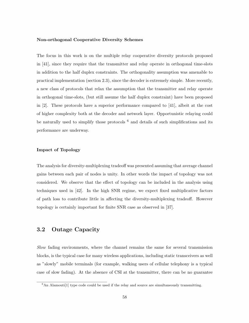
Non-orthogonal Cooperative Diversity Schemes

The focus in this work is on the multiple relay cooperative diversity protocols proposed

in [41], since they require that the transmitter and relay operate in orthogonal time-slots

in addition to the half duplex constraints. The orthogonality assumption was amenable to

practical implementation (section 2.3), since the decoder is extremely simple. More recently,

a new class of protocols that relax the assumption that the transmitter and relay operate

in orthogonal time-slots, (but still assume the half duplex constraint) have been proposed

in [2]. These protocols have a superior performance compared to [41], albeit at the cost

of higher complexity both at the decoder and network layer. Opportunistic relaying could

be naturally used to simplify those protocols 6 and details of such simplifications and its

performance are underway.

Impact of Topology

The analysis for diversity-multiplexing tradeoff was presented assuming that average channel

gains between each pair of nodes is unity. In other words the impact of topology was not

considered. We observe that the effect of topology can be included in the analysis using

techniques used in [42]. In the high SNR regime, we expect fixed multiplicative factors

of path loss to contribute little in affecting the diversity-multiplexing tradeoff. However

topology is certainly important for finite SNR case as observed in [37].

3.2 Outage Capacity

Slow fading environments, where the channel remains the same for several transmission

blocks, is the typical case for many wireless applications, including static transceivers as well

as ”slowly” mobile terminals (for example, walking users of cellular telephony is a typical

case of slow fading). At the absence of CSI at the transmitter, there can be no guarantee

6An Alamouti[1] type code could be used if the relay and source are simultaneously transmitting.

58

for reliable communication and in information theoretic terms, the Shannon capacity is

zero. That doesn’t mean that wireless communication is impossible. It rather emphasizes

that there is no rate of wireless transmission, for which, reception can be achieved with

arbitrarily small probability of error. In such settings cooperative diversity can provide an

attractive solution. On the other hand, in fast fading (also known as ergodic) environments,

the Shannon capacity is non-zero and in that case the transmission/reception scheme ought

to exploit the wireless channel fluctuations.

From the above, it is clear that slow fading is the most difficult case of wireless communica-

tion, since unreliable communication is due not only because of noise at the receiver (error

probability) but also and more importantly, because of the wireless channel fluctuations that

occur for extended periods of time and reduce the information rate that the wireless link can

sustain. Such event is typically called outage event and for point-to-point communication

can be mathematically described by the following relationship:

W log(1 + |asd|2 P/No) ≤ R⇔

|asd|2 ≤ (2R/W − 1)/(P/No)⇔

|asd|2 ≤ (2ρ − 1)/SNR⇔

γsd ≤ Θ (3.9)

In short, the wireless channel conditions as described by the magnitude of the channel

coefficient |asd|2 ≡ γsd, correspond to a received SNR that cannot sustain the desired rate

R (in bps) and spectral efficiency ρ = R/W (in bps/Hz). The probability of the outage

event Pr(γsd ≤ Θ) could be reduced by increasing the transmission power or decreasing

the desired rate or spectral efficiency. In other words, if we use more power or slower

communication, then probability of failure decreases.

In this section we show that opportunistic relaying is an efficient way to combat fading

without sacrificing precious communication resources. We will show with a concrete example

that opportunistic relaying for fixed transmission power and bandwidth can increase the

outage rates (the spectral efficiency in bps/Hz for a given outage probability) by exploiting

59

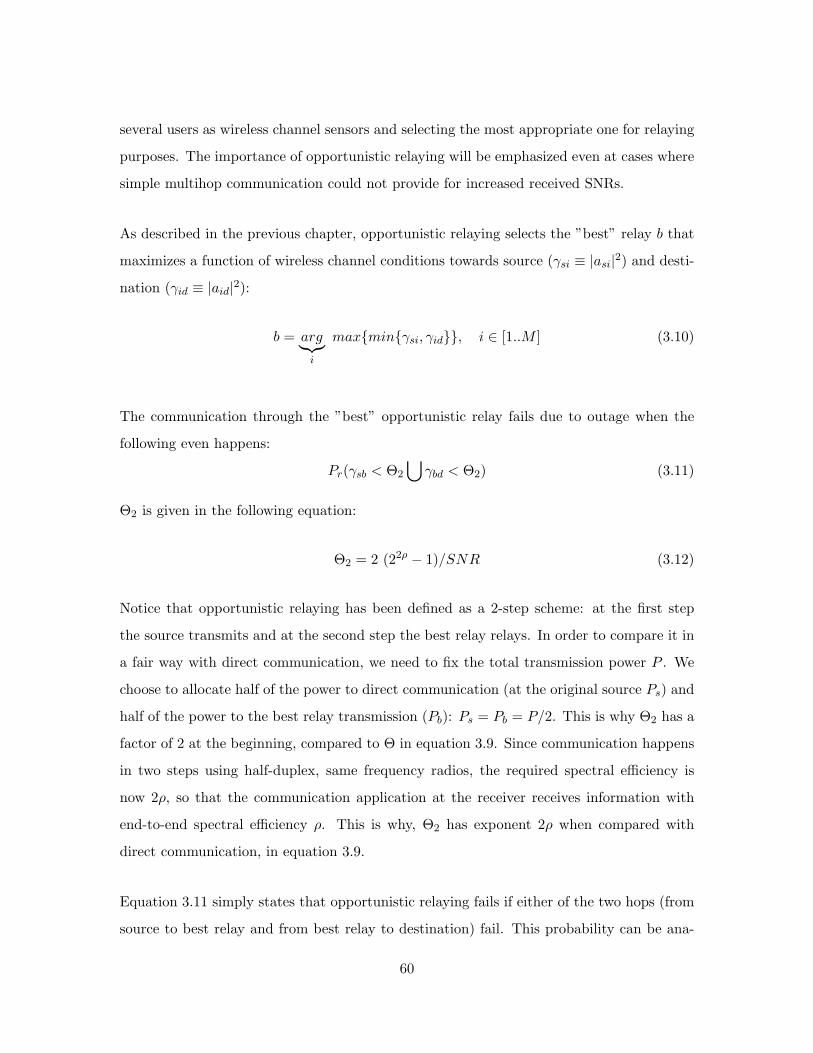
several users as wireless channel sensors and selecting the most appropriate one for relaying

purposes. The importance of opportunistic relaying will be emphasized even at cases where

simple multihop communication could not provide for increased received SNRs.

As described in the previous chapter, opportunistic relaying selects the ”best” relay b that

maximizes a function of wireless channel conditions towards source (γsi ≡ |asi|2) and desti-

nation (γid ≡ |aid|2):

b = arg︸︷︷︸i

max{min{γsi, γid}}, i ∈ [1..M ] (3.10)

The communication through the ”best” opportunistic relay fails due to outage when the

following even happens:

Pr(γsb < Θ2

⋃γbd < Θ2) (3.11)

Θ2 is given in the following equation:

Θ2 = 2 (22ρ − 1)/SNR (3.12)

Notice that opportunistic relaying has been defined as a 2-step scheme: at the first step

the source transmits and at the second step the best relay relays. In order to compare it in

a fair way with direct communication, we need to fix the total transmission power P . We

choose to allocate half of the power to direct communication (at the original source Ps) and

half of the power to the best relay transmission (Pb): Ps = Pb = P/2. This is why Θ2 has a

factor of 2 at the beginning, compared to Θ in equation 3.9. Since communication happens

in two steps using half-duplex, same frequency radios, the required spectral efficiency is

now 2ρ, so that the communication application at the receiver receives information with

end-to-end spectral efficiency ρ. This is why, Θ2 has exponent 2ρ when compared with

direct communication, in equation 3.9.

Equation 3.11 simply states that opportunistic relaying fails if either of the two hops (from

source to best relay and from best relay to destination) fail. This probability can be ana-

60

lytically calculated for the case of Rayleigh fading:

δ = Pr(γsb < Θ2

⋃γbd < Θ2) (3.13)

≡ Pr(min{γsb, γbd} < Θ2) (3.14)

3.10= Pr(max︸︷︷︸i

{ min{γsi, γid}} < Θ2), i ∈ [1..M ] (3.15)

(∗)= Pr(max︸︷︷︸

i

{γsid} < Θ2), i ∈ [1..M ] (3.16)

=M∏i=1

Pr(γsid < Θ2) (3.17)

=M∏i=1

(1− exp(−Θ2/γsid)) (3.18)

where we have exploited in (*) the fact that the minimum of two independent exponentials

is again an exponential random variable, with parameter the sum of the two parameters:

1γsid

=1

γsi

+1

γid

(3.19)

Equation 3.18 provides the outage probability of opportunistic relaying: relaying informa-

tion through the ”best” possible relay. Such calculation is pessimistic in the sense that it

neglects the direct transmission between source and destination. Incorporating the direct

transmission, further reduces the end-to-end outage probability:

P outr = (1− exp(−Θ2/γsd))

M∏i=1

(1− exp(−Θ2/γsid)) (3.20)

3.2.1 Numerical Examples

From equation 3.18, we can calculate the spectral efficiency ρ for a given outage probability

δ. We will study two cases:

• (a) Symmetric case where all relays are equidistant to source and destination, with

distance equal to source-destination distance: dsd = dsi = did,∀i ∈ [1..M ]. Therefore,

there is no multihop gain by choosing to communicate to a nearby intermediate relay

61

1 2 3 4 5 6 7 810

-2

10-1

100

101

Number of relays

bp

s/H

z

Capacity for outage prob.=0.01 and FIXED total transmissionpower (SNR=10)

cooperative with dsd

=dsr

+ drd

(dsr

=drd

)cooperative with d

sd=d

sr=d

rdNon-cooperative, direct

v = 4

v = 3

Figure 3-2: Under a total tx power constraint, the practical scheme of opportunistic relayingincreases the outage capacity, compared to direct communication. Selecting the appropriatepath at the RF level exploits users as an additional degree of freedom, apart from powerand rate. Two topologies are used as an example: the first corresponds to the symmetriccase of all relays equidistant to source and destination. The second topology correspondsto relays half distance between source and destination, for path loss exponent v = 3, 4.

node, towards the final destination.

• (b) Multihop case where all relays are half-way between source and destination: dsd =

dsi+did, dsi = did,∀i ∈ [1..M ]. In that case, choosing to communicate to nearby nodes

towards the destination potentially could offer the advantage of increased average

received SNR due to shorter distance (multihop gain). Two cases of path loss exponent

are presented: γij ∝ 1/dvij for v = 3, 4.

It is straightforward from equation 3.19 that γsid = γsd/2 for case (a) and γsid = 2v−1 γsd

for case (b). Normalizing γsd = 1 and using equations 3.9 and 3.18, we can plot the spectral

efficiency of opportunistic relaying, as a function of number of cooperating relays, for the

two cases considered, having in mind that i) the total transmission power is held fixed (we

do not input tx power to the system by inserting additional relays) and ii) the spectral

efficiency plotted is slightly smaller than the actual, given the fact that equation 3.18 does

62

0 5 10 15 20 25 30 35 400

1

2

3

4

5

6

7

SNR [dB]

bp

s/H

z

Direct communication1 relay2 Opportunistic Relays4 Opportunistic Relays6 Opportunistic Relays8 Opportunistic Relays

Capacity for outage probability=0.01, dsd

= dsr

= drd

0 5 10 15 20 25 30 35 400

1

2

3

4

5

6

7

8

SNR [dB]

bp

s/H

z

Direct communication1 relay2 Opportunistic Relays4 Opportunistic Relays6 Opportunistic Relays8 Opportunistic Relays

v = 3

Capacity for outage probability=0.01, dsd

= dsr

+ drd

0 5 10 15 20 25 30 35 400

1

2

3

4

5

6

7

8

SNR [dB]

bp

s/H

z

Direct communication1 relay2 Opportunistic Relays4 Opportunistic Relays6 Opportunistic Relays8 Opportunistic Relays

v = 4

Capacity for outage probability=0.01, dsd

= dsr

+ drd

Figure 3-3: Outage rates for various SNRs in opportunistic relaying. Top: symmetric case.Bottom: asymmetric case for v=3 and v=4.

not include the direct communication path, between source and destination. Fig. 3-2 plots

the above scaling for outage probability δ = 1% and SNR=10.

ρopport =12

log2(1− ln(1− δ1/M )SNR

2γsid) (3.21)

ρdirect = log2(1− ln(1− δ) SNR γsid) (3.22)

Fig. 3-2 shows that opportunistic relaying increases the outage capacity compared to direct

communication, even for the symmetric case (a) of equidistant relays, where there is no

multihop gain. We emphasize the fact that the comparison assumes same (fixed) total

transmission power: by adding more relays into the network, we do not add power/energy

63

into the system. The increase rates come becomes of the smart relay selection algorithm

that facilitates intelligence at the network level. Notice that a single relay does not increase

the overall capacity for case (a) or for case (b), when v ≤ 3. The latter result is in

coherence with previous reported results, suggesting that a single relay (or a three terminal

cooperative network), could not increase the capacity of wireless communication, when CSI

is not exploited at the transmitters [42].

For different values of SNR, the outage rates are plotted in fig. 3-3. Notice the surprising

gains of opportunistic relaying at the low SNR regime, compared to direct communication.

Those plots suggest that cooperation in the form of opportunistic relaying could be trans-

lated to substantial energy gains: reliability can be achieved with additional relays that

participate in the relay selection but could ”go to sleep mode” after the relay selection,

since only the best relay participates in forwarding the information. Moreover, best relay

selection can be performed in a small fraction of the coherence time of the channel, leaving

the rest for information forwarding, as we will show in a subsequent section. This approach

is in sharp contrast to existing proposals in the field that require all relays to remain in

listening mode until all information is eventually transmitted. Reception energy is not neg-

ligible and especially in communication schemes where error correction is used, reception

energy becomes comparable to transmission energy [52] suggesting that the energy cost of

reliable communication (when all relays are required to listen) increases linearly with the

number of relays. Opportunistic relaying does not have this disadvantage.

From a quick inspection of fig. 3-3, we can see that at transmitted SNR on the order of

20 dB, opportunistic cooperation of a small number of relays, on the order of 6, increases

by a factor of 2 the spectral efficiency. Additionally, for fixed spectral efficiency, a similar

number of opportunistic relays could provide for transmission power gains on the order of

10 dB (a factor of 10) which is also significant. In the following section, we further attempt

to quantify the gains in transmission power of cooperative relaying.

64

3.3 Power Savings

We have already showed that a limited number of opportunistic relays can double the spec-

tral efficiency (in bps/Hz) of wireless communication or lead to substantial energy gains,

without an prior requirements of topology, among the participating nodes. In this section

we will further study the three-node terminal from a practical perspective and show that

cooperation can lead to substantial energy gains, under certain conditions. We provide

answers to previously reported research questions in the field [39] and emphasize the fact

that previously reported solutions to the problem of cooperative diversity communication,

require a priori knowledge of network geometry, in order to be efficient. In contrast, op-

portunistic relaying requires no network topology, since the terminals find out the most

appropriate path using distributed monitoring (sensing) of the wireless environment.

In the case of a single transmitter, single relay and receiver cooperative communication

exploits the direct transmission, as well as the relayed transmission from a neighboring

relay. The receiver combines direct and relayed transmission to detect information. At the

cases where direct transmission is not possible (for example, the receiver is out of range),

multi-hop communication can be viewed as a special case of cooperative communication.

Given the existence of a single relay, it is interesting to see what is the optimal signal

processing strategy at the relay: it could either decode and re-encode (digital regeneration)

or simply, amplify and forward the received information, plus its own noise (analog amplify

and forward) and leave the decision at the destination. Additional strategies could be used

such as compressing the received information and forwarding which has been studied in [37]

building upon the original work on the relay channel by El Gamal and Thomas.

We will concentrate on the two simple strategies of decode or amplify and forward, since

the purpose of this section is to emphasize the importance of network intelligence in cooper-

ative diversity schemes, so that power gains can emerge, regardless of the signal processing

at each individual node. Both strategies can be found in the literature and have different

performance. In [39], it was reported that analog amplify and forward is better than dig-

ital regeneration for a relay located half distance between transmitter and receiver, when

65

a Maximum Ratio Combining (MRC) receiver is used in Rayleigh fading. This is true,

since we have showed that the areas of beneficial relay location are different for the above

relaying techniques: uncoded analog relaying areas are symmetrical half-way distance be-

tween transmitter and receiver [7], while digital regeneration is beneficial only closer to the

transmitter, since the scheme is limited by the probability of error in communication from

transmitter to relay.

In fig. 3-4, we calculate the Symbol Error Probability (SEP) for 8-PSK modulation in

Rayleigh fading with various propagation coefficients v, when MRC combining is used at

the receiver and total transmission energy is split in half among the transmitter and the

relay. Relay decodes and encodes (digital relay) and is placed closer to the transmitter,

1/4 the distance between source and destination. Performance is compared to direct (non-

cooperative) transmission, when all the energy is used for direct, one-hop transmission.

For the digital case, we can calculate the end-to-end symbol error probability as one minus

the probability of correct transmission which is basically the product of probability of

correct reception between transmitter and relay and probability of correct reception of a

MRC receiver when the two copies come from two different paths, one from the transmitter

and one from the intermediate relay:

SEP = 1− (1− SEP1→2)(1− SEP1→32→3

) (3.23)

where the symbol error probabilities for M-PSK, are calculated by the following equations:

SEP1→2 =1π

∫ M−1M

π

0

sin2(θ)sin2(θ) + sin2(π/M) γ1→2

dθ (3.24)

SEP1→32→3

=1π

∫ M−1M

π

0

sin2(θ)sin2(θ) + sin2(π/M) γ1→3

sin2(θ)sin2(θ) + sin2(π/M) γ2→3

dθ (3.25)

66

γi→j = E [‖ai→j‖2]Ei

N0, E [‖ai→j‖2] ∝

1dv

, (3.26)

with ai→j , the wireless channel between transmitter i and receiver j and Ei the symbol

energy transmitted by node i.

We can see from figure 3-4 that the cooperative scheme is more reliable for the same trans-

mission energy used, or it needs less transmission energy for the same performance. For

SEP=1/1000, the plot is inverted and transmission energy savings are depicted in the form

of ratios between transmission energy needed in the non-cooperative case vs the transmis-

sion energy needed in the cooperative case.

We can also observe improved performance, when a dense constellation is used, in combi-

nation with cooperation. For example, using a constellation of 3 bits per symbol (8-PSK)

with cooperative transmission, performs more reliably than a constellation of 1 bit per sym-

bol (2-PSK) of direct communication for rayleigh fading with v ≥ 3 and digital relaying

(we have omitted the plots due to space restrictions). Therefore, cooperation can increase

throughput in uncoded systems by 50%, under certain conditions7.

3.3.1 Areas of useful cooperation

In figure 3-5, the regions where digital relaying is beneficial compared to repetitive transmis-

sion are depicted, for the case of 8-PSK in Rayleigh fading and various signal-to-noise ratios

(SNR) and two propagation coefficients v, normalized to point-2-point distance between

transmitter and receiver. Specifically, we plot the space area where SEP1→31→3

/SEP ≥ 1.

We can see that provided that there is a relay close to transmitter, between transmitter

and receiver, digital relaying (and consecutively cooperation) is beneficial at the low SNR

regime, in highly attenuating propagation environments (v ≥ 3).

Observe also that the regions are not symmetric, but they are ”squeezed” toward the trans-

mitter, since the probability of error is affected by the probability of correct transmission

73 bits per symbol, over two channel usages, one for direct and one for relayed transmission, result in 1.5bits per channel usage versus 1 bit per channel usage for binary constellation and direct transmission.

67

0 5 10 15 20 25 30 35 4010

-7

10-6

10-5

10-4

10-3

10-2

10-1

100

E = E1 + E2

Symbol Error Probability for 8-PSK

noncooperativecooperative digital

v = 2

v = 3

v = 4

v = 5

Energy Gains

0 1 2 3 4 5 6 7

5

10

15

20

25

30

35

40

v

Ratio of Energy without cooperation vs (Total energy with cooperation)

Figure 3-4: Performance of cooperative communication compared to non-cooperative com-munication in left figure (using 8-PSK and various propagation coefficients) and total trans-mission energy ratio for target Symbol Error Probability (SEP)=10−3 in right figure (using8-PSK and v = 4), in Rayleigh wireless channels. Relay decodes and encodes (digitalrelay) and it is placed closer to the transmitter, 1/4 the distance between source anddestination. We can see that cooperative communication is more reliable compared totraditional point-to-point communication, leading to higher reliability or transmission en-ergy savings. Left:SEP in 8-PSK for various environments and E = E1 + E2, E1 = E2.Right:corresponding ratio E/(E1 + E2) for SEP=10−3.

to the relay. Therefore, halfway the distance between transmitter and receiver, is NOT the

optimal location to place a digital relay.

We have also studied analog amplify-and-forward in the context of uncoded M-PSK com-

munication. The regions in that case are symmetric between transmitter and receiver, as

opposed to the digital case. We have omitted the presentation of the plots due to space

restrictions. More results for the analog case can be found in [7]. All the above findings

explain why an analog amplify and forward relay outperforms a digital decode and forward

relay both placed half-way between source and destination, as reported in [39] without thor-

ough justification: the areas of useful cooperation are simply different for the two cases of

signal processing at each relay.

Notice that the above improvements in energy gains are based on the assumption that there

is a relay inside the appropriate area and the transmitter knows that (i.e. the transmitter

has decided that relaying is more beneficial than repetition). Such decision could be based on

knowledge of relay location, at the source! However, such knowledge is not trivial to acquire,

68

1 0.8 0.6 0.4 0.2 0 0.2 0.4 0.6 0.81

0.5

0

0.5

1

1.5

Tx

Rxv=3

SNR=10 dB

SNR=20 dB

SNR=30 dB

1 0.8 0.6 0.4 0.2 0 0.2 0.4 0.6 0.81

0.5

0

0.5

1

1.5

Tx

Rx

1 0.8 0.6 0.4 0.2 0 0.2 0.4 0.6 0.81

0.5

0

0.5

1

1.5

Tx

Rx

1 0.8 0.6 0.4 0.2 0 0.2 0.4 0.6 0.81

0.5

0

0.5

1

1.5

Tx

SNR=20 dB

v=5SNR=10 dB

SNR=30 dB

Figure 3-5: Left: v=3. Right: v=5. Regions of intermediate node location where it isadvantageous to digitally relay to an intermediate node, instead of repetitively transmit.M=8 and the depicted ratio is the ratio of SEP of repetitive transmission vs SEP of usercooperative digital communication. The cooperative receiver optimally combines direct andrelayed copy. Distances are normalized to the point-to-point distance between transmitterand receiver.

especially in the case of mobile nodes. It could be either estimated or provided by other

external means (such as GPS). In such cases, relay location information should be provided

to the source. In other words, transmission energy gains of traditional cooperative diversity

schemes depend on network topology. More importantly, estimation of network topology

might have significant overhead that could cancel the benefits of cooperative diversity and

therefore, such overhead needs to be explicitly identified and quantified. Additionally,

practical schemes for coordination and topology estimation need to be devised before the

above simple three-node scheme could be implemented in practice. Attributing all the

necessary overhead to an external service, such as GPS, might be one solution but is that

a cost-effective solution? What happens when such services are not available (for example

in indoor environments)?

On the other hand, opportunistic relaying not only scales cooperative diversity with larger

than one number of relays, but also provides solutions for the required selection of appropri-

ate relays, using distributed algorithms that require no topology estimation services (such

as GPS). In the following section, we show that the network can react to the instantaneous

channel conditions fast and with reasonably small overhead.

69

3.4 Collision Probability

In this section we provide an analytic way to calculate a close-form expression of equation

(2.8) for any kind of wireless fading statistics. But before doing so, we can easily show that

this probability can be made arbitrary small, close to zero.

If Tb = min{Tj}, j ∈ [1,M ] and Y1 < Y2 < . . . < YM the ordered random variables {Tj}

with Tb ≡ Y1, and Y2 the second minimum timer, then:

Pr(any Tj < Tb + c | j 6= b) ≡ Pr(Y2 < Y1 + c) (3.27)

From the last equation, we can see that this probability can be made arbitrarily small by

decreasing the parameter c. For short range radios (on the order of 100 meters), this is

primarily equivalent to selecting radios with small switch times (from receive to transmit

mode) on the order of a few microseconds.

Given that Yj = λ/h(j), Y1 < Y2 < . . . < YM is equivalent to 1/h(1) < 1/h(2) < . . . <

1/h(M)8, equation (3.27) is equivalent to

Pr(Y2 < Y1 + c) = Pr(1

h(2)<

1h(1)

+c

λ) (3.28)

and Y1 < Y2 < . . . < YM ⇔ h(1) > h(2) . . . > h(M) (h, λ, c are positive numbers).

From the last equation (3.28), it is obvious that increasing λ at each relay (in equation

(2.3)), reduces the probability of collision to zero since equation (3.28) goes to zero with

increasing λ.

In practice, λ can not be made arbitrarily large, since it also ”regulates” the expected time,

needed for the network to find out the ”best” relay. From equation (2.3) and Jensen’s

inequality we can see that

E[Tj ] = E[λ/hj ] ≥ λ/E[hj ] (3.29)

or in other words, the expected time needed for each relay to flag its presence, is lower

bounded by λ times a constant. Therefore, there is a tradeoff between probability of collision

8The parenthesized subscripts are due to ordering of the channel gains.

70

and speed of relay selection. We need to have λ as big as possible to reduce collision

probability and at the same time, as small as possible, to quickly select the best relay, before

the channel changes again (i.e. within the coherence time of the channel). For example, for

a mobility of 0 − 3 km/h, the maximum Doppler shift is fm = 2.5 Hz which is equivalent

with a minimum coherence time on the order of 200 milliseconds. Any relay selection should

occur well before that time interval with a reasonably small probability of error. From figure

3-6, we note that selecting c/λ ≈ 1/200 will result in a collision probability less than 0.6% for

policy I. Typical switching times result in c ≈ 5µs. This gives λ ≈ 1ms which is two orders

of magnitude less than the coherence interval. More sophisticated radios with c ≈ 1µs will

result in λ ≈ 200µs, which is three orders of magnitude smaller than the coherence time 9.

3.4.1 Calculating Pr(Y2 < Y1 + c)

In order to calculate the collision probability from (3.27), we first need to calculate the joint

probability distribution of the minimum and second minimum of a collection of M i.i.d10

random variables, corresponding to the timer functions of the M relays. The following

theorem provides this joint distribution:

Theorem 4 The joint probability density function of the minimum and second minimum

among M ≥ 2 i.i.d. positive random variables T1, T2, . . . , TM , each with probability density

function f(t) ≡ dF (t)dt and cumulative distribution function F (t) ≡ Pr(T ≤ t), is given by

the following equation:

fY1,Y2(y1, y2) =

M (M − 1) f(y1) f(y2) [1− F (y2)]M−2 for 0 < y1 < y2

0 elsewhere.

9Note that the expected value of the minimum of the set of random variables(timers) is smaller than theaverage of those random variables. So we expect the overhead to be much smaller than the one calculatedabove

10The choice of identically distributed timer functions implicitly assumes that the relays are distributed inthe same geographical region and therefore have similar distances towards source and destination. In thatcase, randomization among the timers is provided only by fading. The cases where the relays are randomlypositioned and have in general different distances, is a scenario where randomization is provided not onlybecause of fading, but also because of different moments. In such asymmetric cases the collision probabilityis expected to decrease and a concrete example is provided.

71

where Y1 < Y2 < Y3 . . . < YM are the M ordered random variables T1, T2, . . . , TM .

Proof 3 Please refer to appendix A.

Using Theorem 1, we can show the following lemma that gives a closed-form expression for

the collision probability (equation 3.27):

Lemma 1 Given M ≥ 2 i.i.d. positive random variables T1, T2, . . . , TM , each with prob-

ability density function f(x) and cumulative distribution function F (x), and Y1 < Y2 <

Y3 . . . < YM are the M ordered random variables T1, T2, . . . , TM , then Pr(Y2 < Y1 + c),

where c > 0, is given by the following equations:

Pr(Y2 < Y1 + c) = 1− Ic (3.30)

Ic = M (M − 1)∫ +∞

cf(y) [1− F (y)]M−2 F (y − c) dy (3.31)

Proof 4 Please refer to appendix A.

Notice that the statistics of each timer Ti and the statistics of the wireless channel are

related according to equation (2.3). Therefore, the above formulation is applicable to any

kind of wireless channel distribution.

3.4.2 Results

In order to exploit theorem 4 and lemma 1, we first need to calculate the probability

distribution of Ti for i ∈ [1,M ]. From equation (2.3) it is easy to see that the cdf F (t)

and pdf f(t) of Ti are related to the respective distributions of hi according to the following

equations:

F (t) ≡ CDFTi(t) = Pr{Ti ≤ t} = 1− CDFhi(λ

t) (3.32)

f(t) ≡ pdfTi(t) =d

dtF (t) =

λ

t2pdfhi

(λ

t) (3.33)

72

After calculating equations (3.32), (3.33), and for a given c calculated from (2.6) or (2.7),

and a specific λ, we can calculate probability of collision using equation (3.30).

Before proceeding to special cases, we need to observe that for a given distribution of

the wireless channel, collision performance depends on the ratio c/λ, as can be seen from

equation (3.28), discussed earlier.

Rayleigh Fading

Assuming |asi|, |aid|, for any i ∈ [1,M ], are independent (but not identically distributed)

Rayleigh random variables, then |asi|2, |aid|2 are independent, exponential random vari-

ables, with parameters β1, β2 respectively (E[|asi|2] = 1/β1, E[|aid|2] = 1/β2).

Using the fact that the minimum of two independent exponential r.v.’s with parameters

β1, β2, is again an exponential r.v with parameter β1+β2, we can calculate the distributions

for hi under policy I (equation 2.1). For policy II (equation 2.2), the distributions of the

harmonic mean, have been calculated analytically in [31]. Equations (3.32) and (3.33)

become:

under policy I:

F (t) = e− (β1+β2) λ/t (3.34)

f(t) =λ (β1 + β2)

t2e−(β1+β2) λ/t (3.35)

under policy II:

F (t) =λ√

β1 β2

te−λ (β1+β2)/(2t) K1(

λ√

β1β2

t) (3.36)

f(t) =λ2

2 t3β1 β2 e−λ (β1+β2)/(2t) [

β1 + β2√β1 β2

K1(λ√

β1 β2

t) + 2 K0(

λ√

β1 β2

t)](3.37)

where Ki(x) is the modified Bessel function of the second kind and order i.

Equation (3.30) is calculated for the two policies, for the symmetric case (β1 = β2 =

E[|asi|2] = E[|aid|2] = 1) of M = 6 relays. Monte-Carlo simulations are also performed

73

200 220 240 260 280 300 320 340 360 380 4003

4

5

6

7

8

9

10x 10

-3 Rayleigh and Ricean Fading vs lambda /c, for M=6

lambda /c

Pro

bab

ility

of

Co

llisi

on

Policy II (harmonic), Rayleigh, SimulationPolicy II (harmonic), Rayleigh, AnalysisPolicy I (min), Ricean, SimulationPolicy I (min), Rayleigh, SimulationPolicy I (min), Rayleigh, Analysis

Figure 3-6: Performance in Rayleigh and Ricean fading, for policy I (min) and Policy II(harmonic mean), various values of ratio λ/c and M = 6 relays, clustered at the sameregion. Notice that collision probability drops well below 1%.

under the same assumptions. Results are plotted in fig. 3-6, for various ratios λ/c. We

can see that Monte-carlo simulations match the results provided by numerical calculation

of equation (3.30) with the help of equations (3.34)-(3.37).

Collision probability drops with increasing ratio of λ/c as expected. Policy I (”the mini-

mum”), performs significantly better than Policy II (”the harmonic mean”) and that can

be attributed to the fact that the harmonic mean smooths the two path SNRs (between

source-relay and relay-destination) compared to the minimum function. Therefore, the ef-

fect of randomization due to fading among the relay timers, becomes less prominent under

Policy II. The probability can be kept well below 1%, for ratio λ/c above 200.

Ricean Fading

It was interesting to examine the performance of opportunistic relay selection, in the case

of Ricean fading, when there is a dominating communication path between any two com-

municating points, in addition to many reflecting paths and compare it to Rayleigh fading,

where there is a large number of equal power, independent paths.

74

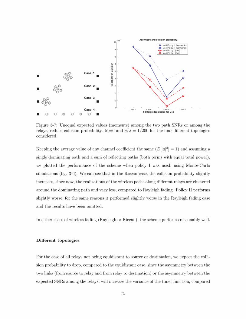
Case 1

Case 2

Case 3

Case 4 Case 1 Case 2 Case 3 Case 4 1

2

3

4

5

6

7

8

9

10x 10

-3

Pro

bab

ility

of

Co

llisi

on

4 different topologies for M=6

Assymetry and collision probability

v=3,Policy II (harmonic)v=4,Policy II (harmonic)v=3,Policy I (min)v=4,Policy I (min)

Figure 3-7: Unequal expected values (moments) among the two path SNRs or among therelays, reduce collision probability. M=6 and c/λ = 1/200 for the four different topologiesconsidered.

Keeping the average value of any channel coefficient the same (E[|a|2] = 1) and assuming a

single dominating path and a sum of reflecting paths (both terms with equal total power),

we plotted the performance of the scheme when policy I was used, using Monte-Carlo

simulations (fig. 3-6). We can see that in the Ricean case, the collision probability slightly

increases, since now, the realizations of the wireless paths along different relays are clustered

around the dominating path and vary less, compared to Rayleigh fading. Policy II performs

slightly worse, for the same reasons it performed slightly worse in the Rayleigh fading case

and the results have been omitted.

In either cases of wireless fading (Rayleigh or Ricean), the scheme performs reasonably well.

Different topologies

For the case of all relays not being equidistant to source or destination, we expect the colli-

sion probability to drop, compared to the equidistant case, since the asymmetry between the

two links (from source to relay and from relay to destination) or the asymmetry between the

expected SNRs among the relays, will increase the variance of the timer function, compared

75

to the equidistant case. To demonstrate that, we study three cases, where M = 6 relays are

clustered half-way (d/2), closer to transmitter (d/3) or even closer to transmitter (d/10)

(case 1,2,3 respectively in fig. 3-7 and d is the distance between source and destination) and

one case where the relays form an equidistant line network between source and destination

(case 4 in fig. 3-7).

Assuming Rayleigh fading, c/λ = 1/200 and expected path strength as a non-linear, decreas-

ing function of distance (E[|aij |2] = 1/βij ∝ (1/dij)v), we calculate the collision probability

for M = 6 relays, using expressions (3.34)-(3.37) into (3.30) for cases 1, 2, 3 while for case 4

we used Monte-Carlo simulation: in case 1, β1 = β2 = 1, in case 2, β1 = (2/3)v, β2 = (4/3)v

and in case 3, β1 = (1/5)v, β2 = (9/5)v. For case 4, β1 = (2/7)v, β2 = (12/7)v for the closest

terminal to source, β1 = (4/7)v, β2 = (10/7)v for the second closest terminal to source,

β1 = (6/7)v, β2 = (8/7)v for the third closest to source terminal. Due to symmetry, the

expected power and corresponding β factors of the paths, for the third closer to destina-

tion, second closer to destination and closest terminal to destination, are the same with the

ones described before (third closer terminal to source, second closer terminal to source and

closest to source terminal respectively), with β1 and β2 interchanged.

We can see in fig. 3-7 that the collision probability of asymmetric cases 2, 3 and 4 is

strictly smaller compared to the symmetric case 1. Policy I performs better than Policy

II and collision probability decreases for increasing factor v (v = 3, 4 were tested). This

observation agrees with intuition that suggests that different moments for the path strengths

among the relays, increase the randomness of the expiration times among the relays and

therefore decrease the probability of having two or more timers expire within the same time

interval.

We note that the source can also participate in the process of deciding the best relay. In

this special case, where the source can receive the CTS message, it could have its own

timer start from a value depending upon the instantaneous |asd|2. This will be important

if the source is not aware whether there are any relays in the vicinity that could potentially

cooperate.

The proposed method as described above, involving instantaneous SNRs as a starting point

76

for each relay’s timer and using time (corresponding to an assessment of how good is a

particular path within the coherence time of the channel) to select space (the best available

path towards destination) in a distributed fashion, is novel and has not been proposed

before, to the best extent of our knowledge.

77

78

Chapter 4

Scaling and Extensions

4.1 To Relay or not to Relay?

One of the major findings in the previous chapter was that opportunistic relay selection and

use of the single ”best” relay, incurs no performance loss, when compared to simultaneous

transmissions of multiple relays which use complex space-time coding. The relevant analysis

was performed with the high SNR tool of diversity-multiplexing gain tradeoff. Because of

the high SNR nature of that tool, power allocation at the relays is meaningless and cannot

be studied: SNR is increased towards infinity and at the same time the spectral efficiency is

increased with log2 SNR, in order to calculate the corresponding tradeoff between diversity

(reliability) and multiplexing gain (rate).

In this section, we attempt to study the problem of power allocation, in the case of multiple

amplify-and-forward relays. We surprisingly discover that distributing the total transmis-

sion power to a set of simple1 relay radios, is suboptimal when compared to opportunistic

relaying and in fact, the penalty of performance loss (or inversely the gain of opportunistic

relaying) increases logarithmicaly with the number of relays. This important result suggests

1Throughout this dissertation, we have excluded beamforming scenarios, since such hardware capabilityis difficult in practice, especially in the case of distributed single antenna radios.

79

that relay selection can provide for important gains in amplify-and-forward relays systems,

when compared to ”all relays-transmit” schemes, proposed in the literature [30], [14].

Total transmission power is an important network resource, especially for battery-operated

applications and networks that seek to maximize network lifetime. Traditional studies of

scalability, tend to examine the performance gains when multiple nodes (with their own

tx power) enter the network [24]. Such studies investigate a communication performance

measure, such as ergodic capacity or outage probability, as a function of number of relay

nodes. Therefore, such studies implicitly assume that total transmission power increases

with the number of participating nodes. In this section, we study scalability with a more

careful treatment of total transmission power. Since we are interested in comparing different

schemes for the same number of participating elements, we will explicitly fix the total

transmission power.

We assume again a two step transmission scheme: during the first phase the source transmits

and the relays and destination listen, while during the second step, the relays relay using a

version of amplify-and-forward. For completeness, we allow the transmitter to transmit a

different symbol, during the second step, even though we will relax this assumption in the

subsequent analysis.

During the first slot, the destination receives yD,1 while each relay Ri receives yRi,1. PSX is

the average normalized received power (or energy if multiplied with an appropriate scaling

factor) between source and terminal X and includes the transmitted power, as well as other

propagation phenomena, like shadowing. hSX is the unit-power fading coefficient, which for

the numerical results of the subsequent section will be assumed complex, circularly sym-

metric, Gaussian random variable, (h = a + jb, where a, b are i.i.d normal r.v’s N (0, 1/2)),

corresponding to Rayleigh fading. Similarly, nx is additive white complex gaussian noise,

with power N0/2 per dimension (n = a + jb, where a, b are i.i.d normal r.v’s N (0, N0/2)).

x1 is the unit power symbol, sent from the source during the first slot. We will further

assume independence among the noise and channel terms among different relays.

80

1st Slot:

yD,1 =√

PSD hSD x1 + nD,1 (4.1)

yRi,1 =√

PSRi hSRi x1 + nRi,1, ∀ i ∈ [1,M ] (4.2)

Notice that the expected power of each symbol received at each relay Ri can be easily

calculated, taking into account the assumptions above: E [|yRi,1|2] = PSRi + N0. Each relay

normalizes its received signal with its average power and transmits yRi,1√E[|yRi,1|2]

. This is a

normalization followed in the three terminal analysis (one source, one destination and one

relay) presented in [57]. Here, we can easily generalize it to the case of multiple relays,

during the second slot:

2nd Slot:

yD,2 =√

PSD hSD x2 +M∑i=1

√PSRi hSRi

yRi,1√E [|yRi,1|2]

+ nD,2 ⇔ (4.3)

yD,2 =√

PSD hSD x2 +M∑i=1

√PSRi

√PRiD√

PSRi + N0hSRi hRiD x1 + nD,2 +

M∑i=1

√PRiD√

PSRi + N0hRiD nRi,1︸ ︷︷ ︸

nD,2

yD,2 =√

PSD hSD x2 +M∑i=1

√PSRi

√PRiD√

PSRi + N0hSRi hRiD x1 + nD,2 (4.4)

Again, here PXD is the average normalized received power (or energy if multiplied with an

appropriate scaling factor) between terminal X and destination and includes the transmitted

power, as well as other propagation phenomena, like shadowing. hXD is the unit power

fading coefficient, which will be assumed complex, circularly symmetric Gaussian random

variable (corresponding to Rayleigh fading), for the numerical results of the subsequent

section. x2 is the unit power symbol, sent from the source during the second slot.

From the last equation, we can see that the received signal at the destination, can be

written as the sum of two terms, corresponding to the two transmitted information symbols

plus one noise term. Assuming that the destination has knowledge of the wireless channel

81

0 0.5 1 1.5 2 2.5 3 3.50

0.1

0.2

0.3

0.4

0.5

0.6

0.7

0.8

0.9

16 relays

CD

F

H21

Selection one random relaySelecting all relaysOpportunistic Relaying

Figure 4-1: Cumulative Distribution Function (CDF) of H12 (eq. 4.12, 4.13, 4.14), forthe three cases examined (one, all, ”best” relay(s) transmit). The expected value is alsodepicted, at the bottom of the plot.

conditions between the relays and itself (for example, the receiver can estimate the channel

using preamble information), the noise term in equation 4.4 becomes complex Gaussian

with power easily calculated2:

E [nD,2 n∗D,2 |HR→D] = N0 (1 +M∑i=1

PRiD |hRid|2

PSRi + N0)︸ ︷︷ ︸

ω2

= ω2 N0 (4.5)

Therefore, the system of the above equations can be easily written in matrix notation:

yD,1

yD,2

ω

=

√PSD hSD 0

1ω

∑Mi=1

√PSRi

√PRiD√

PSRi+N0hSRi hRiD

1ω

√PSD hSD

x1

x2

+

nD,1

nD,2

ω

2Notice that we do not need knowledge of the wireless channels conditions at the receiver between sourceand relays, for the above assumption to hold

82

0 0.5 1 1.5 2 2.5 3 3.5 40

0.1

0.2

0.3

0.4

0.5

0.6

0.7

0.8

0.9

16 relays

CD

F o

f M

utu

al In

form

atio

n

bps/Hz

Selection one random relaySelecting all relaysOpportunistic Relaying

Figure 4-2: Cumulative Distribution Function (CDF) of mutual information (eq. 4.11), forSNR=20dB. Notice that the CDF function provides for the values of outage probability.

The above notation can be summarized as:

y =

√PSD hSD 0

H211ω

√PSD hSD

x + n (4.6)

y = H x + n (4.7)

The noise term, under the above assumptions, has covariance matrix given below,3 where

I2 is the 2x2 unity matrix:

ω2 = (1 +M∑i=1

PRiD |hRid|2

PSRi + N0(4.8)

E[n nT |HR→D] = N0 I2 (4.9)

For the subsequent section, we will further simplify the cooperation scheme and will not

allow the transmission of a new symbol x2 during the second slot, in coherence with the

3The symbols ∗,T correspond to complex-conjugate and conjugate-transpose respectively

83

1 2 3 4 5 6 7 8 9 102

2.5

3

3.5Average spectral efficiency

bp

s/H

z

Number of Relays

Selection one random relaySelecting all relaysOpportunistic Relaying

Figure 4-3: Expected value of mutual information (eq. 4.11), corresponding to the ergodiccapacity, as a function of number of relays. Notice that using all relays incurs a penaltythat increases with number of relays, compared to opportunistic relaying.

communication scheme studied in the previous chapter. In that way, the second column of

the matrix H is zero and H becomes a column vector (the first column of H above).

The mutual information for the above assumptions can be easily calculated for the above

linear system, using the result from Telatar’s work [73]:

IAF =12

log2(1 +PSD

N0|hSD|2 +

|H21|2

N0) (4.10)

Since we are interested in the power allocation of total transmission power PR at the relays,

we further dismiss the direct connection term between source and destination. Practically,

that corresponds to the case when source and destination are not within communication

range or simply, destination does not exploit that connection. PSD corresponds to the power

the source spends during the transmission at the first slot:

IAF =12

log2(1 +PSD

N0|H21|2) (4.11)

We further assume that all relays are equivalent : all relays have the same average power

84

terms PRiD which practically means that PRiD = const for the M relays. We will test three

different cases: a) all power PR is used at one random relay, b) power is distributed at all

relays PRiD = PR/M and c) all power PR is used at the best, opportunistic relay:

|H21|2one =1

PSD+N0PR

+ |hRiD|2|hSRi hRiD|2 (4.12)

|H21|2all =1

PSD+N0

PR/M +∑M

i=1 |hRiD|2|

M∑i=1

hSRi hRiD|2 (4.13)

|H21|2opp =1

PSD+N0PR

+ |hRbD|2|hSRb hRbD|2 (4.14)

where min{|hSRb|2 |hRbD|2} ≥ min{|hSRi|2 |hRiD|2},∀i ∈ [1,M ]

The first term in equations 4.12, 4.14 is greater than the first term in equation 4.13. The

second term in 4.13 corresponds to the magnitude of the sum of complex numbers with

random phases. Therefore, the addition of an increasing number of those terms does not

necessarily results in a proportional increase of the magnitude: that would be possible, only

under equal phases (beamforming).

For PR = PSD � N0 then PSD+N0PR

→ 1, the Cumulative Distribution Function (CDF (x) =

Pr(H21 ≤ x) for the three above cases, is depicted in figure 4-1, for the case of Rayleigh

fading for all coefficients hSRi, hRiD.

In fig. 4-1 it is shown that Pr(|H21|2one ≤ x) ≥ Pr(|H21|2all ≤ x) ≥ Pr(|H21|2opp ≤ x) which

means that, in general, |H21|2one ≤ |H21|2all ≤ |H21|2opp.

Consecutively, the mutual information statistics are depicted in figure 4-2, in the form of

CDF function (corresponding to the outage probability) and in figure 4-3, in the form of

expected values (corresponding to ergodic capacity). Both plots show the superiority of

opportunistic relaying, compared to the case of having all relays transmit. They also show,

that choosing a random relay is a suboptimal technique, compared to the all relays case.

We can see in fig. 4-3 that selecting a single, ”best” relay, provides performance gains that

increase with the number of relays, compared to the ”all-relays transmit” case, under a

85

sum power constraint. This is an important result, given the popularity of the ”all relays-

transmit” approach in the literature. This result clearly suggests that, the advantages of

multiple nodes in a relay network, do not arise because of complex reception techniques,

as the ”all relays transmit” approach requires, but rather emerge because of the fact that

multiple possible paths exist between source, the participating relays and the destination.

Opportunistic relaying, simply exploits the best available path.

In that sense, opportunistic relaying can be viewed as a ”smart” scheduling algorithm of

RF energy, coming from another node (the source) and destined for another user (the

destination). Through the method of distributed timers presented and analyzed in the

previous chapters, the network schedules the transmission over the most appropriate relay

path (relaying as scheduling), via a decentralized way.

In the following section we show that opportunistic relaying can be easily viewed as RF

scheduling, in more involved settings.

4.2 Extensions: Scheduling Multiple Streams

In the previous sections, we described opportunistic relaying as a distributed way to select

the relay b, that maximizes a function of the instantaneous channel conditions between

source/relay and relay/destination. As we saw, the minimum function was a viable solution

and the best relay is the one, according to min{|hSRb|2 |hRbD|2} ≥ min{|hSRi|2 |hRiD|2},∀i ∈ [1,M ],

for the M relays. Assuming similar radio hardware, we can safely further assume that the

thermal noise at all relays has the same average power. Therefore, we can extend the op-

portunistic relaying rule to incorporate instantaneous SNR conditions at each relay, rather

than just instantaneous channel conditions. The timer functions use SNR values and the

two rules are essentially equivalent, both from a conceptual perspective, as well as from a

practical (implementation) point of view :

b = arg︸︷︷︸i

max{min{SNRsi, SNRid}} = max{SNRsid}, i ∈ [1..M ] (4.15)

86

Stream I Stream II

Relay i

Figure 4-4: Relaying as scheduling for multiple streams.

Each relay, willing to assist the transmission stream I (fig. 4-4), for which it has gathered

information overhearing the pilot signals RTS/CTS transmitted initially by the communi-

cating source and destination, is affected by the simultaneous transmission from stream II

(fig. 4-4). Stream II simultaneous transmission affects stream I effective path Signal-to-

Interference-and-Noise Ratio (SINR) and therefore, the path (relay) selection rule caqn be

changed from a notation point of view:

b = arg︸︷︷︸i

max{min{SINRsi, SINRid}} = max{SINRsid}, i ∈ [1..M ] (4.16)

From a practical point of view, taking into account other concurrent streams does not affect

implementations: relays assisting stream I, need not know anything regarding stream II,

since its influence automatically appears in the SINR term.

Following the notation of [3], based on work in [20], we assume N streams and denote

Gij ≡ |h(i)(j)|2, the square magnitude of the channel condition between the source of stream

j and destination of stream i. Stream i is successfully transmitted if its corresponding SINR

is above a threshold θi. Assuming Pj , the transmission power of transmitter in stream j, the

system of equations describing successful communication of the N streams is summarized

87

as follows:

SINRi =GiiPi∑

j 6=i GijPj + ni≥ θi (4.17)

(I− F) P ≥ θ (4.18)

P = (P1 P2 . . . PN )T (4.19)

θ = (θ1 n1

G11

θ2 n2

G22. . .

θN nN

GNN)T (4.20)

Fij = 0, i = j (4.21)

Fij =θi Gij

Gii, i 6= j (4.22)

P ≥ P∗ = (I− F)−1 θ (4.23)

If the requirement of SINRi ≥ θi,∀ N streams, the transmitted power vector should satisfy

equation 4.23 which shows the minimum required transmitted power.

The above compact notation provides a compact way to evaluate performance if interference

needs to be treated explicitly, from a network point-of-view, rather than treating interference

and thermal noise as a single quantity. In terms of best relay selection, in the presence

of multiple streams the algorithm still ”works”, both from a conceptual and a practical

standpoint.

Additional extensions would require extensive coordination among the participating wireless

terminals and are left for future work. Specific techniques for network coordination, based

on network time keeping are presented in the following chapter.

88

Chapter 5

Relevant Time Keeping

Technologies

In chapter 2 we described a method of ”best” relay selection, based on distributed timers,

that exploited functions of the instantaneous channel conditions. We quantified the perfor-

mance of such technique in section 3.4 and explained why an explicit time synchronization

protocol is not required.

However, the notion of network time keeping is of primal importance in distributed environ-

ments and specifically, in scalable wireless networks. Accurately synchronized clocks enable

services and provide the basis for efficient communications. Autonomous sensor array oper-

ation is facilitated by accurate time stamps [61], [60]. Global Positioning System, as well as

proposed Ultra-Wide Band urban and intra-building location systems [58] rely on precise

timing measurements. Internet performance can be evaluated from accurate measurement

of the delay between various nodes in the network. Various important Internet Protocols

such as TCP could benefit from accurate time keeping [62].

Additionally, a common time reference is important for many applications of distributed

sensing, especially when the individual sensor nodes span a large geographical area and

communicate over wireless. Time synchronization among the nodes becomes non-trivial

89

when all the individual nodes are several hops away and therefore a single broadcast signal

from a particular node (a “server”) is not sufficient, as it cannot reach all nodes. Energy

constraints of the individual sensor nodes prohibit extensive communication among them,

complicating further the problem of time synchronization. Sensor Networks ought to self-

configure and work unattended, therefore any synchronization scheme should have minimal

complexity both at the network level (requiring minimal coordination among the nodes) and

also at the individual sensor node level, especially due to its embedded, limited computing

capabilities microprocessor (as measured in floating point operations per second and internal

memory size).

In this chapter, we present two novel approaches to the problem of Network Time Keeping.

In the first approach, we follow the methodology of one of the oldest Internet protocols,

the Network Time Protocol (NTP) [51], where a client node tries to steer its local clock

parameters, using time messages exchanged with a remote time server, over a ”noisy” and

uncontrollable network connection. We propose an adaptive filtering technique, based on

Kalman filtering and contrast it to other techniques in the field, for two cases of noise

(additive Gaussian noise and Self-similar (chaotic) noise). One of the interesting findings

was that our proposed technique can reduce the estimation error, faster than√

N , where N

is the number of messages exchanged (bandwidth), outperforming other techniques based

on a simple averaging (where error decrease on the order of 1/√

N is expected) or more

involved techniques, based on linear programming.

The second proposed approach to the problem of Network Time Keeping, is based on a

completely decentralized technique: no servers are used and time keeping is performed using

schemes inspired by natural phenomena of synchronization: the way fireflies blink in unison,

even though they interact only locally or the way cardiac neurons fire in sync. A simple

demonstration was constructed to illustrate the principles and measurements as well as

theoretical analysis were performed. One of the interesting findings was that synchronization

error does not necessarily increase with diameter of the network: by adding nodes into the

system, the network establishes a common time reference without additional overhead and

might have smaller synchronization error, depending on the individual clock characteristics

90

of the participating wireless nodes.

After presenting basic definitions of clocks and time synchronization, we present in two

distinctive sections the two approaches: the centralized, client-server approach and the

decentralized one.

5.1 Clock Basics

Using the representation C(t) for a clock reading and T (t) = t for true time, the following

definitions are presented:

• time offset: the difference between the time reported from a clock and the “true”

time: C(t)− T (t) = C(t)− t. In this paper we will refer to the time offset calculated

for t = 0 as θ and for t 6= 0 as x.

• frequency offset (also referred as skew): the difference in frequencies between a

clock and the “true” time: C ′(t)− T ′(t) = C ′(t)− 1. In this work, we will refer to

frequency offset as φ− 1.

• drift: the long-term frequency change of a clock. Drift is caused by changes in the

components of the oscillator and its environment.

Typical quartz oscillators (without any type of temperature compensation) exhibit fre-

quency offsets on the order of a few parts per million (PPM). For example a 10 PPM

oscillator will introduce an uncertainty (i.e. error) of 36 msec in one hour. Cesium beam

atomic clocks on the other hand, exploiting the stabilities of the quantum world perform

better with uncertainties close or smaller than 1 nsec in 24 hours.

Modeling a clock as a piecewise linear function of time is a reasonable step since any function

can be approximated in a similar manner. The client should estimate only two parameters,

namely the time and frequency offset θ, φ− 1 respectively, compared to the source of true

91

time T (t) as depicted in fig. (5-1-LEFT), since only two parameters are needed to define a

line.

However, for this model to be realistic, it is important to keep the duration of the mea-

surement process as small as possible, before φ and θ at the client clock are modified. The

parameters φ, θ change with a rate related to the clock drift and it has been found that

for most free running oscillators used in current computer systems, this change happens

at intervals on the order of 1-2 hours or more [45]. That is reasonable to expect since

macroscopic factors that heavily influence crystal oscillators, such as temperature change

no faster than that rate.

Figure 5-1: LEFT: Frequency offset φ−1 and time offset θ of C(t), compared with the sourceof “true” time T (t). RIGHT: Exchanging timestamps between client and time server. Noticethat a time difference of δt according to server clock is translated to φδt according to clientclock.

A statistical tool that provides a stationary measure of the stochastic behavior regarding

time deviation residuals and their associated frequency fluctuation estimates, is the Allan

variance [4]. Allan variance associates frequency fluctuation estimates with specific observa-

tion duration and therefore could be used to quantify how often the above clock parameters

change. For an excellent review of oscillators, Allan variance, time and frequency metrology,

the interested reader could refer to [46].

92

5.2 Centralized Network Time Keeping

5.2.1 Problem Formulation

After describing the clock nomenclature followed in this work, we are ready to formulate

the problem. The client clock C(t) is synchronized to a time source T (t) = t when both

frequency offset φ and time offset θ are estimated.

The client timestamps (C(t1)) a UDP packet according to each own clock C(t) and sends

the message to a time source server which timestamps the packet upon reception and re-

transmission (t2, t3 respectively) back to the originating client (fig. 5-1). The client times-

tamps again the message upon reception and therefore acquires a set of 4 timestamps:

(C(t1), t2, t3, C(t4)). For convenience, we will notate C(t1) as C1 and C(t2) as C2 from now

on. The same process can be repeated for a set of N consecutive messages. Therefore we

should answer the following questions:

• What is the optimal processing of N messages

(C11 , t12, t

13, C

14 ), (C2

1 , t22, t23, C

24 ), . . . , (CN

1 , tN2 , tN3 , CN4 ) so as to obtain unbiased estimates

with minimum error?

• What is the cost of obtaining estimates of φ and θ in terms of bandwidth spent

(number N ,inter-departure time between packets)?

• Do the algorithms employed in the estimation of φ, θ impose special restrictions in

the operation of client (or server) operating system (i.e. are there any major non-

algorithmic modifications in the operation of existing client/time server daemons)?

The number of packets N exchanged between client and server (fig.(5-1-RIGHT)) is a

crucial parameter of any algorithm eventually adopted, considering the heavy load of current

Internet time servers, on the order of 1000− 1200 requests per second and increasing every

year [47]. Moreover, the inter-departure intervals of the NTP-like messages should not be

93

very large since closely spaced packets ensure that the clock parameters are not changing

during the measurements from N packets.

Finally, we need to emphasize that the queuing delay q1 across the forward path (from

client to server) is never constant and generally different from the queuing delay q2 across

the reverse path (from server to client) (fig. (5-1-RIGHT)). Moreover, since the messages are

carried through UDP packets, the forward and reverse routes could be physically different

and therefore the propagations delays 1 d1, d2 could be unequal across the forward and

reverse paths.

d1 + q1 6= d2 + q2 (5.1)

5.2.2 Prior Art on Centralized Client-Server Schemes

NTP estimates the time offset using the 4 timestamps of a message, according to the

following equation:

xn =Cn

1 − tn2 − tn3 + Cn4

2(5.2)

Since the round-trip time (rtt) is on the order of a few msecs, the contribution of the

frequency offset on the error for a single measurement is negligible (e.g. a 10 ppm oscillator

for a 10 msec rtt exhibits 0.1 µsec which is on the order of “noise” due to the operating

system) and therefore excluded from Eq.(5.2). The frequency offset can be estimated using

several measurements of x.

From a closer look on Eq. (5.2), NTP estimates are erroneous by a quantity proportional

to half the difference between forward and reverse path delays (assymetry).

xn = xn +dn

2 + qn2 − dn

1 − qn1

2⇒ (5.3)

xn = xn + wn (5.4)

That is why the NTP error is upper bounded by half the round-trip time. If we make the

1Time needed for the first bit to arrive at the destination as opposed to transmission delay which isrelated to the speed of the link.

94

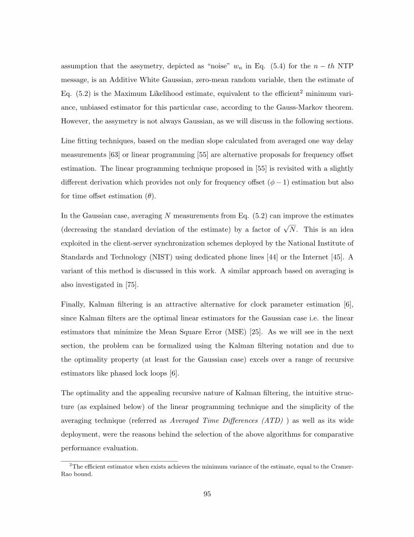
assumption that the assymetry, depicted as “noise” wn in Eq. (5.4) for the n − th NTP

message, is an Additive White Gaussian, zero-mean random variable, then the estimate of

Eq. (5.2) is the Maximum Likelihood estimate, equivalent to the efficient2 minimum vari-

ance, unbiased estimator for this particular case, according to the Gauss-Markov theorem.

However, the assymetry is not always Gaussian, as we will discuss in the following sections.

Line fitting techniques, based on the median slope calculated from averaged one way delay

measurements [63] or linear programming [55] are alternative proposals for frequency offset

estimation. The linear programming technique proposed in [55] is revisited with a slightly

different derivation which provides not only for frequency offset (φ− 1) estimation but also

for time offset estimation (θ).

In the Gaussian case, averaging N measurements from Eq. (5.2) can improve the estimates

(decreasing the standard deviation of the estimate) by a factor of√

N . This is an idea

exploited in the client-server synchronization schemes deployed by the National Institute of

Standards and Technology (NIST) using dedicated phone lines [44] or the Internet [45]. A

variant of this method is discussed in this work. A similar approach based on averaging is

also investigated in [75].

Finally, Kalman filtering is an attractive alternative for clock parameter estimation [6],

since Kalman filters are the optimal linear estimators for the Gaussian case i.e. the linear

estimators that minimize the Mean Square Error (MSE) [25]. As we will see in the next

section, the problem can be formalized using the Kalman filtering notation and due to

the optimality property (at least for the Gaussian case) excels over a range of recursive

estimators like phased lock loops [6].

The optimality and the appealing recursive nature of Kalman filtering, the intuitive struc-

ture (as explained below) of the linear programming technique and the simplicity of the

averaging technique (referred as Averaged Time Differences (ATD) ) as well as its wide

deployment, were the reasons behind the selection of the above algorithms for comparative

performance evaluation.

2The efficient estimator when exists achieves the minimum variance of the estimate, equal to the Cramer-Rao bound.

95

5.2.3 The Algorithms

Kalman Filtering

The motivation behind the adoption of Kalman filtering stems from a simple observation:

a time interval δt according to “true” time is translated to φ δt according to client clock.

Therefore, it is sufficient for the client to send messages at constant intervals δT measured

according to its local clock and estimate the inter-arrival intervals at the server, using the

timestamps {tn2} which correspond to “true” time. Variation of forward and reverse one-way

delays are interpreted as noise in the estimation process.

With the above, the formulation of the problem using Kalman filtering becomes clear: the

client sends the NTP packets at constant intervals δT and estimates the inter-arrival interval

s = δTφ in the presence of network delay variations v, exploiting the measured inter-arrival

intervals yn = tn+12 − tn2 for n ∈ [1..N ].

The measurement and state model of the Kalman filter easily follow (fig. (5-1-RIGHT)):

yn = tn+12 − tn2 (5.5)

= tn+11 + dn+1

1 + qn+11 − (tn1 + dn

1 + qn1 ) (5.6)

= tn+11 − tn1︸ ︷︷ ︸

δt

+(dn+11 + qn+1

1︸ ︷︷ ︸en+1

)− (dn1 + qn

1︸ ︷︷ ︸en

)⇒

yn = δt + en+1 − en = δt + vn, (5.7)

sn ≡ δt =δT

φ, n ∈ [1..N]⇒ (5.8)

yn = sn + vn, measurement model (5.9)

sn+1 = sn + wn, state model (5.10)

The measurement noise vn accounts for the variation of travel time, when the NTP message

is transmitted from client to server and it is assumed a zero mean process throughout

this work. This is the type of noise that depends on the network path between client and

server. Its power can be minimized only if the client selects a shortest path route toward the

server. The state model noise wn accounts for the fact that inter-departure times between

96

consecutive packets from the client could not be constant, possibly due to operating system

delay variations. The power of this noise process is fully controlled by the client and could

be estimated by client’s own timestamps {Cn1 }. Alternatively, we can treat that noise as

additional measurement noise (vn) and simply ignore it (wn = 0). That was the approach

followed in this work.

Assuming vn a zero mean process and en (from Eq. (5.7)) a stationary, non-zero mean

process with uncorrelated consecutive samples, the following equation is derived:

E[vi vj ] =

R i = j

−R/2 i = j + 1

0 otherwise

R = variance(yn), n ∈ 1..N (5.11)

Under the above assumptions and using vector notation, the measurement and state model

equations become:

yn

yn−1

=

δt

δt

+

vn

vn−1

⇒ (5.12)

yn =

1

1

δt + vn, (5.13)

sn+1 = sn = δt, n ∈ 1..N. (5.14)

The Kalman filter “predict” and “update” equations are omitted and could be found in a

relevant textbook [59]. The Kalman filtering technique is a recursive scheme, therefore the

estimate sn converges to the correct value of δt after a number of messages (Cn1 , tn2 , tn3 , Cn

4 ).

The initial predicted value s0|−1 was set to δT while the associated error variance was set

to R. After the Nth packet, the frequency of the client clock is obtained by the output

s = sN |N of the kalman filter:

φ =δT

s=

δT

δt(5.15)

97

From Eq. (5.7), averaging N measurements results in the following equation:

1N

N∑n=1

yn = δt +1N

(e2 − e1︸ ︷︷ ︸v1

+ e3 − e2︸ ︷︷ ︸v2

... + eN+1 − eN︸ ︷︷ ︸vN

) (5.16)

1N

N∑n=1

yn = δt +1N

(eN+1 − e1) (5.17)

The average value of N measurements could be used as a “naive” estimator of δt (and

consecutively of clock rate via Eq. (5.15)). The variance of this estimate, under the same

assumptions for the noise process vn, drops with N2, since var(eN+1 − e1) = 2 var(en) =

var(vn). Despite its attractive simplicity, this estimator provides large errors, compared

to all the other approached presented in this work, especially when small number (N) of

messages are used, as we will see in the following sections.

For the estimation of time offset θ we could use Eq. (5.2). However for a large number

N of packets used, the duration of the experiment multiplied by the frequency skew could

contribute to a significant synchronization error (e.g. 100 packets spaced 1 sec from each

other correspond to an additional time offset of 4 msec for a 40 ppm clock). Therefore the

estimate of the frequency offset should be exploited in the time offset calculation.

From fig. (5-1-RIGHT) we have the following relationships:

Cn1 − φ tn2 = θ − φ (d1 + q1)n (5.18)

Cn4 − φ tn3 = θ + φ (d2 + q2)n (5.19)

⇓

Cn1 − φ tn2 ≤ θ − φ d1 (5.20)

Cn4 − φ tn3 ≥ θ + φ d2 (5.21)

Therefore, an estimate of θ is obtained by the following relationship:

θ =max(Ci

1 − φ ti2) + min(Cj4 − φ tj3)

2(5.22)

98

Alternatively, Kalman filtering could be used again for the estimation of time offset θ.

The estimate of clock rate φ from the above technique could be exploited to “adjust” the

timestamps Cn1 ← Cn

1 /φ, Cn4 ← Cn

4 /φ at the client side. Then measurements of time

offset θ according to Eq. (5.2), could be filtered using standard, one dimensional Kalman

equations, with measurement model given by Eq. (5.4). The output estimate of θ after

Kalman filtering of N measurements is also reported in the experimental results section.

Linear Programming

This line fitting technique exploits both the forward and reverse path timestamps, by esti-

mating a “clock line” that minimizes the distance between the line and the data, leaving

all the data points below the line on a (t2, C1) plane or above the line on a (t3, C4) plane.

The following equations describe the problem and it’s solution:

......forward path

α1 = φ (5.23)

β1 = θ − φ d1

Eq. (5.20)⇒ α1 tn2 + β1 − Cn1 ≥ 0, ∀ n ∈ [1..N ] (5.24)

Find α1, β1 that minimize

f(α1, β1) =N∑

n=1

(α1 tn2 + β1 − Cn1 )

under the constraint of Eq. (5.24)

......reverse path

α2 = φ (5.25)

β2 = θ + φ d2

Eq. (5.21)⇒ Cn4 − α2 tn3 − β2 ≥ 0, ∀ n ∈ [1..N ] (5.26)

99

Find α2, β2 that minimize

f(α2, β2) =N∑

n=1

(Cn4 − α2 tn3 − β2)

under the constraint of Eq. (5.26)

φ =α1 + α2

2(5.27)

θ =β1 + β2

2(5.28)

The simple and intuitive derivation above sets this technique as a strong candidate for clock

parameter estimation.

Averaged Time Differences

This method can be best described by fig. 5-1. The time offset xn is computed according

to the NTP formula (Eq. 5.2) and therefore this method has all the limitations discussed

at the NTP section above. Differences of the time offset estimates provide estimates for

the frequency offset. Particularly, clusters of 25-50 closely spaced messages are used, time

offsets are computed and the results are averaged to a single data point for the time offset.

Then that is used in the following formula for frequency offset estimation.

f(tn+1) =xn+1 − xn

τ(5.29)

f ≡ φ− 1

y(tn+1) =y(tn) + αf(tn+1)

1 + α(5.30)

The value of τ nominally should be equal to tn+1 − tn however this quantity cannot be

measured by the client’s own clock. Nevertheless for small values of the frequency offset

this can be set to C(tn+1)−C(tn), since that is what the client can measure. The estimated

100

frequency offset is averaged again using an exponential filter with a time constant α that

depends on the stability of the local oscillator. Then the filtered frequency offset is used in

the following formula, which is also depicted in fig. (5-1-LEFT).

x(tn+1) = x(tn) + y(tn)(τ) (5.31)

A variant of this method is used in this work. Frequency offsets are calculated using Eq.

(5.29) and then filtered using the above exponential filter with α = 0.5. The final frequency

offset estimation is the mean of all the N exponentially filtered frequency offsets calculated

at each epoch.

The power of this method is its simplicity. For the Gaussian case where consecutive mea-

surements are independent from each other, an increase of samples averaged by a factor of

N reduces the variance of the estimate by a factor of N . Therefore, there is a trade-off

between accuracy achieved and cost of realizing it.

5.2.4 Performance

In this section we evaluate the performance of the three algorithms in two separate cases:

• The “Gaussian case” where the queuing delay difference between two consecutive NTP

messages is a Gaussian random variable. Consequently, the dispersion of the packets

at the server is also a Gaussian random variable. In this experiment, consecutive

measurements are independent.

• The “Self-Similar case” where multiple pareto connections aggregate and form cross-

traffic with long-range dependence.

The estimate, the variance of the estimate and the number N of packets used at each epoch

are reported. In both cases the true clock frequency offset φ−1 was +40 ppm and the time

offset θ was 20 msec. The NTP messages were transmitted at intervals of 1000 msec. Each

experiment was run 300 times.

101

0 10 20 30 40 50 60 70 80 90 100-25

-20

-15

-10

-5

0

5

10

15

20

25

Ass

ymet

ry in

mse

c (G

auss

ian)

Time is sec0 10 20 30 40 50 60 70 80 90 100

-15

-10

-5

0

5

10

15

Ass

ymet

ry in

mse

c (P

aret

o)

Time in sec

Figure 5-2: Assymetry of delays between forward (to server) and reverse (to client) path.LEFT: Gaussian case. RIGHT: Self-similar case.

The Gaussian Case

In fig. (5-2-LEFT) we present the assymetry between forward (to server) and reverse (to

client) path, from a sample run. The average round-trip time was on the order of 40 msecs

and consecutive measurements were independent and identically distributed. In left figure

of (5-3) and right figure of (5-3) we present the average estimate and the standard deviation

of the estimate for the frequency offset φ− 1 and time offset θ respectively, as a function of

number N of packets used.

The Kalman filter performed better when the number of packets N was above the minimum

number of samples needed for convergence (on the order of 25-30 packets). This experimen-

tal finding is validated by the fact that the Kalman filter (at steady-state) is the optimal

linear estimator in the presence of Gaussian noise. The LP technique performed better

than both averaging techniques (ATD and “Naive” estimator), which performed well only

if large number of messages were used.

Frequency offset estimate variance was decreased with number N of packets used. From fig.

(5-3-LEFT) it is shown that the standard deviation of the estimate drops slightly faster than

linearly with N (variance drops with N2) for Kalman filtering, while it drops linearly with

N for the “Naive” estimator, as expected, while the variance as well as the error is smaller

102

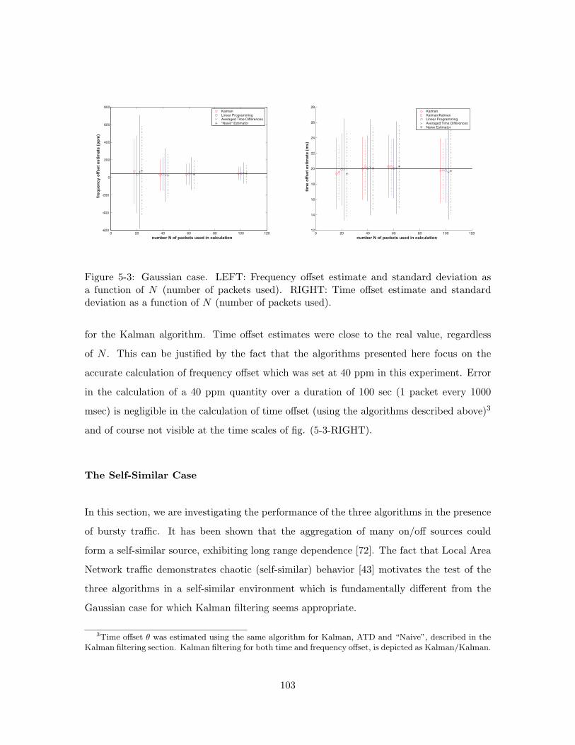
0 20 40 60 80 100 120-600

-400

-200

0

200

400

600

800

number N of packets used in calculation

freq

uenc

y of

fset

est

imat

e (p

pm)

KalmanLinear ProgrammingAveraged Time Differences"Naive" Estimator

0 20 40 60 80 100 12012

14

16

18

20

22

24

26

28

number N of packets used in calculation

time

offs

et e

stim

ate

(ms)

KalmanKalman/KalmanLinear ProgrammingAveraged Time DifferencesNaive Estimator

Figure 5-3: Gaussian case. LEFT: Frequency offset estimate and standard deviation asa function of N (number of packets used). RIGHT: Time offset estimate and standarddeviation as a function of N (number of packets used).

for the Kalman algorithm. Time offset estimates were close to the real value, regardless

of N . This can be justified by the fact that the algorithms presented here focus on the

accurate calculation of frequency offset which was set at 40 ppm in this experiment. Error

in the calculation of a 40 ppm quantity over a duration of 100 sec (1 packet every 1000

msec) is negligible in the calculation of time offset (using the algorithms described above)3

and of course not visible at the time scales of fig. (5-3-RIGHT).

The Self-Similar Case

In this section, we are investigating the performance of the three algorithms in the presence

of bursty traffic. It has been shown that the aggregation of many on/off sources could

form a self-similar source, exhibiting long range dependence [72]. The fact that Local Area

Network traffic demonstrates chaotic (self-similar) behavior [43] motivates the test of the

three algorithms in a self-similar environment which is fundamentally different from the

Gaussian case for which Kalman filtering seems appropriate.

3Time offset θ was estimated using the same algorithm for Kalman, ATD and “Naive”, described in theKalman filtering section. Kalman filtering for both time and frequency offset, is depicted as Kalman/Kalman.

103

... ... ... ...

... ... ... ...

CLIENT SERVER

Figure 5-4: Simulation in ns-2 with pareto cross traffic. 14 connections per link per direction.

Fig. (5-4) displays the simulation setup in Network Simulator 2 (ns-2) [84]. The utilization

of the links was 90%, the average round-trip time on the order of 40 msecs and the assymetry

between the forward and reverse path is depicted in fig. (5-2-RIGHT). The inter-departure

time of NTP packets remains 1000 msecs.

Fig. (5-5-LEFT) shows in a sample run how well the Kalman filter “locks” onto the correct

inter-arrival time δt and frequency offset value (φ− 1). Fig. (5-5-RIGHT) shows how well

the ATD technique (with the exponential filter) “locks” onto the frequency offset value

(φ − 1). The internal line is the filtered waveform through a low pass filter. Fig. (5-5)-

CENTER displays the one-way delay across the reverse path as a function of time. The

trend of the plot is coherent with the following derivation. The “clock line” φ tn3 + θ with

parameters estimated by the LP technique is also depicted.

Eq. (5.21) ⇒ (5.32)

Cn4 − tn3 = (φ− 1) tn3 + φ (dn

2 + qn2 ) + θ ⇒

Cn4 − tn3 ≥ (φ− 1) tn3 + φ dn

2 + θ

Fig. (5-6) shows the histogram of frequency offset estimates for the self-similar case, for N =

100 and fig. (5-7-LEFT) shows the performance of the three algorithms in the estimation

of frequency offset, for various number N of packets used in the calculation. Time offset

104

0 10 20 30 40 50 60 70 80 90 100985

990

995

1000

1005

1010

1015

number of packets used in calculation

Inte

rarr

ival

tim

e (m

sec)

predicted interarrival timeobserved interarrival time

1000 1020 1040 1060 1080 1100 1120 1140 1160 1180 120035

40

45

50

55

60

65

sec

mse

c

observed reverse path delay C4-t3estimated clock parameters line

0 20 40 60 80 100 120 140 160 180 2003000

2000

1000

0

1000

2000

3000

number of packets used in calculation

PP

M

Figure 5-5: LEFT: Predicted inter-arrival and measured inter-arrival interval using theKalman filter for self-similar cross traffic. CENTER: Delay Cn

4 − tn3 from the reverse pathand clock line estimation using LP for self-similar cross traffic. RIGHT: Estimation offrequency offset φ− 1 using the ATD technique. Low pass filtering of data is also plotted.

estimation θ resulted in significant errors due to assymetry between forward and reverse

path, as expected (fig. (5-7)-RIGHT)).

From the above diagrams, it is deduced that the Kalman filtering technique no longer

produces the best estimates with the smallest variance. The noise is no longer Gaussian

so Kalman filtering is not optimal and LP performs better in the presence of bursty traffic

both in terms of estimation error (accuracy) and its variance (precision). For the same

reason (burstiness and asymptotically long range dependence as opposed to the Gaussian

distribution around the mean), ATD and “Naive” estimator perform inferiorly than the

LP technique. All algorithms for frequency offset estimation reduce the standard deviation

(and therefore variance) of the estimate with increased number N of packets used, and the

relation between that improvement and N seems faster than linear for the case of Kalman

filtering and Linear Programming or linear for the case of averaging (therefore variance

drops with N2 ), as can be seen in fig. (5-7-LEFT).

5.2.5 Measurements

In order to emphasize the end-to-end character of the algorithms evaluated (especially for

the case of Kalman filtering and LP), we modified NTP client daemon and exchanged 100

packets at intervals of 1 sec with a stratum-0 server (connected to GPS). The time server

105

-150 -100 -50 0 50 100 150 200 2500

0.01

0.02

0.03

0.04

0.05

0.06

0.07

0.08

0.09

0.1

frequency offset estimate (ppm)

hist

ogra

m v

alue

KalmanLinear ProgrammingAveraged Time Differences

Figure 5-6: Histogram of the frequency offset estimates for self-similar cross traffic.

0 20 40 60 80 100 120-400

-300

-200

-100

0

100

200

300

400

500

number N of packets used in calculation

freq

uenc

y of

fset

est

imat

e (p

pm)

KalmanLinear ProgrammingAveraged Time Differences"Naive" Estimator

0 20 40 60 80 100 120-1500

-1000

-500

0

500

1000

1500

number N of packets used in calculation

time

offs

et e

stim

ate

(ms)

KalmanKalman/KalmanLinear ProgrammingAveraged Time DifferencesNaive Estimator

Figure 5-7: Self-similar case. LEFT: Frequency offset estimate and standard deviation asa function of number N of packets used in calculation. RIGHT: Time offset estimate andstandard deviation as a function of number N of packets used in calculation.

106

was geographically located at Palo Alto CA, 3100 miles away from our client machine, with

average round-trip time 85 msec, 18 hops away. We then processed the packets according

to the algorithms evaluated above and the frequency offset estimation results are presented

at Table 5.1.

Table 5.1: Frequency offset estimation using an existing NTP/GPS server.

Kalman LP ATD

φ− 1 (PPM) 101.6 54.7 122.7

An interesting idea could be averaging the two estimates calculated according to Kalman

and LP since the former performed better at the Gaussian case and the latter at the Self-

similar one.

5.2.6 Discussion

The Kalman filtering technique, optimal for the Gaussian case, needed a considerable num-

ber of packets in order to converge (on the order of 20-30 packets for the formulation

adopted and the experimental setup). Nevertheless, the technique performed well at the

Self-similar case as well, with improved performance in terms of error and variance of the

estimate when the number of packets N increased. The algorithm estimates the variance

of network delay (jitter) and uses that estimate to calculate the frequency and time offset

model variables. The algorithm can be applied without major operation requirements in

the NTP-client daemon and requires no modifications in the NTP-server daemon. It could

be benefitted by scheduled transmission from the client system that ensure minimum delay

variance due to the operating system.

The Linear Prediction technique surpassed all the other techniques at the case of bursty

traffic approximating real-word long-range dependence (chaotic) conditions even though it

had inferior performance when measurements where completely independent. Its intuitive

structure makes it attractive for straightforward implementation.

107

Finally, averaging as exploited and implemented in the Averaging Time Differences tech-

nique (where equal intervals between measurements were used and therefore averaging dif-

ferences of time was equivalent to averaging frequency offset estimates) performed inferiorly

to the LP and Kalman filtering techniques at the Self-similar case where measurements are

not independent. However, its simplicity makes it attractive, especially at the cases where

a small number of measurements are available or a trade-off between accuracy and cost of

realizing it cannot be avoided.

All three techniques showed improvement in terms of frequency offset estimation error and

variance of the estimate with increasing number of packets N . For Kalman filtering, the

relationship between improvement and N seems slightly faster than linear (for standard de-

viation of frequency offset estimate) or quadratic (for variance of frequency offset estimate)

and therefore increased accuracy is expensive in terms of number of packets used (commu-

nication bandwidth). This work tried to quantify that cost, by comparatively evaluating a

number of diverse techniques.

5.3 Decentralized Network Time Keeping

In this work we implement a time synchronization technique for multi-hop, energy, com-

munication, computing constrained sensor networks which is completely beacon (or server)

free. Moreover, it requires no global coordination since all nodes in the network communi-

cate with nearest neighbors for time-synchronization purposes. Therefore the scheme has

no centralized point of control (or failure) and, it has no network routing overhead and it

is appropriate for ad-hoc sensor networks where the topology might change (often due to

mobility) or might be unknown.

Our initial goal was an experimental evaluation of time synchronization in multi-hop net-

works, in a real-world setup. For that cause, we implemented a distributed orchestra, where

each node could have a speaker to output a song, while at the edges of the network, two

nodes were equipped with LED displays (figure 5-8). At the same time, we wanted to quan-

tify in practice, the observed accuracy and precision of the algorithm against its required

108

Figure 5-8: Demo on a glass wall: each node can communicate with at most 4 immedi-ate neighbors. The network manages to synchronize all nodes so that they can “output”through speakers the same music. At the edges of the network, the nodes are equipped withLED displays instead of speakers, to provide for visual proof of synchrony. All nodes arecommunicating with immediate neighbors only and there is no point of central control.

Figure 5-9: The individual nodes used in this work. Speakers and displays provided foraudio-visual output. LEFT: 4-IR Pushpin without speaker. The four IR transceivers pro-vide directional communication only along the horizontal and vertical axis. CENTER: 4-IRPushpin with speaker. RIGHT: 45-LED display. A 4-IR Pushpin is connected behind theLED grid.

109

communication and computation overhead using our embedded wireless network. Eval-

uation of the scheme through implementation in a real-world embedded network reveals

the important limitations on computation, communication and complexity sensor networks

encompass.

Evaluations of synchronization schemes only through simulations usually underestimate the

limited resources in terms of memory, computation and communication of each node and also

assume worst case scenarios that might not reflect reality. Even though experimental study

of time synchronization has been reported before in single-hop embedded wireless networks,

there is a significant gap in measurements of time synchronization error in realizations of

multi-hop wireless embedded networks. To our knowledge, this work is the first to fill this

gap. Video of the demonstration could be found at [85].

The proposed scheme and the implemented demo were inspired by natural phenomena of

synchronization: the way fireflies blink in unison, even though they interact only locally or

the way cardiac neurons fire in sync.

5.3.1 Experimental Setup

The goal in this work was to demonstrate a time synchronization scheme that would be:

a) transparent to the sensing or actuating tasks of any node in the network. Each node

should communicate only locally with its immediate neighbors and avoid explicit connec-

tions to remote servers of “true time” one or more hops away.

b) self-calibrating with no coordination requirements upon deployment or during operation.

The multi-hop network should spontaneously converge to a common time reference without

centralized control.

To make matters more realistic, we chose to evaluate the transparent and self-calibrating

(as defined above) character of the scheme at the extremes: we evaluated the scheme at the

edges of the network, when connectivity is established only through intermediate nodes. RF

communication range could be on the order of hundreds of meters, therefore it would be more

110

Figure 5-10: Topologies for various network diameters d used in this work. The oscilloscopeprobes are connected at the edge nodes of the network. The case for d = 4 is shown in theright figure.

appropriate to utilize short-range and directive communication links in order to demonstrate

multi-hop performance. We used 8051-based micro-controllers (8-bit, 2 Kbytes of RAM and

32 Kbytes of program space) connected to short-range, 4-way infrared transceivers. Those

are the pushpin nodes [50], [87], that we packaged in round battery holders as shown in figure

5-9. Pushpins practically allowed evaluation of the synchronization scheme at the edges of

the network, for several values of network diameter d as shown in fig. (5-10-LEFT). The

experimental setup for d = 4 is shown in fig. (5-10-RIGHT).

The goal was to demonstrate network multi-bit clock synchronization among all nodes in a

distributed fashion, not just synchronization to a reference signal coming from a specialized

server [51], [10] or beacon [18]. No prior knowledge of network topology was assumed and

all nodes would be loaded with the same code. All nodes could be equipped with small

speakers (fig. 5-9) and as a proof of synchrony they would play the same piece of music

at the same time. According to ([15] p.95), the smallest perceivable time difference from

humans is on the order of 30-50 milliseconds, therefore clock synchronization error above

that limit could be perceived.

Apart from the oscilloscope measurements at the edge networks and the audio outputs at

many intermediate nodes, visual patterns at the edge nodes could provide for visual proof

of synchrony. Displays from the rf-Badges [48], [86] were connected to 4-IR pushpins and

used in this work (fig. 5-9).

111

5.3.2 The Algorithm and its Implementation in our Embedded Network

Lamport in his 1978 work in the context of computer clocks and processes synchronization

[49], described a simple algorithm, based on the fact that time is a strictly monotonically-

increasing quantity. Therefore events happening in subsequent times should have times-

tamps ordered accordingly, otherwise a correction in the clocks should be made. Although

Lamport’s work has been extensively referenced in the area of sensor networks time synchro-

nization, there has been no validation and testing in embedded networks so far (at least

to the extent of authors knowledge). Since time is viewed as a non-decreasing quantity

in Lamport’s algorithm, its implementation probably has been considered problematic in

memory-restricted and communication-constrained sensor networks.

• Broadcast: node i transmits its clock value Ci(t) at regular intervals. Time-stamping

occurs just before transmission and the MAC protocol has been modified accordingly.

• Receive and Compare: upon reception from node j of a clock value Ci(t) from node

i, node j compares and keeps the highest value: if Ci(t) > Cj(t) then Cj(t) ← Ci(t)

else ignore.

In this work, we modify Lamport’s algorithm to fit the memory and communication con-

straints of sensor networks and through implementation in a multi-hop, embedded network,

we prove that the new algorithm can sufficiently synchronize the whole network, in a dis-

tributed, transparent and self-calibrating way, satisfying many real-world scenarios.

The first modification in Lamport’s algorithm is that time is no longer considered a mono-

tonically increasing quantity: clock Cj(t) in every network node j is bounded above and

upon reaching that value, time is reset. Therefore, clock function Cj(t) follows a “saw-type”

periodic waveform and its period should be set according to the natural phenomenon which

is sensed by the sensor network. In this work, since the goal was distributed synchronized

play of music, the period T of each clock was set to 13 seconds approximately.

The first reason behind upper bounding time, was the fact that timestamps are commu-

nicated among neighboring nodes and therefore their size in bits should be kept minimal,

112

because of memory, bandwidth and energy constraints. In this work, clock value Cj(t)

of node j is represented by an unsigned 16-bit variable, incremented each time a 16-bit

counter resets. This reset occurs every 5.9 msecs approximately, limiting the resolution of

each clock variable Cj(t) in the millisecond regime. The counter is interrupt driven and

since it controls time increments, it is assigned the highest priority interrupt.

The second reason behind upper bounding time, was our desire to explicitly study self-

calibration capabilities of the algorithm and show in practice that even though clocks reset

periodically (in this case, every 13 seconds ), the network as a whole, re-synchronizes quickly

and unattended (spontaneously) and is able to perform its sensing and actuating tasks.

Note that in this realization, we have time Cj(t) of node j to be represented as 16-bit

integer, with resolution set by another 16-bit counter. However, only the first 16-bit value

is communicated to nearest neighbors. The length in bits of the clock value Cj(t) and

its resolution depend on the physical phenomenon that needs to be sensed. For example,

for environmental sensing of moisture, a 16-bit clock incremented every 1.3 seconds would

need 24 hours approximately, to reset. Therefore, the same “saw-type” definition of time

would suffice, the information communicated over the network would be the same as in the

example of this paper and the only modification would be in the clock resolution in every

node of the network. The network would reset in synchrony every 24 hours instead of 13

seconds. The slower period in this work (and resolution on the order of milliseconds) helped

us quickly validate the fact that the network re-calibrates after every clock variable Cj(t)

expiration, without unwanted periods of instability.

In other words, the length in bits and the resolution of the clock variable Cj(t) depend

on the physical phenomenon to be sensed and the algorithm could be used with success in

many different contexts and applications such as environmental sensing.

The second modification in Lamport’s algorithm, is the fact that broadcasting of time-

stamped information is controlled by an independent timer and not by the clock of each

node. The reason behind such implementation decision was that we wanted to decouple the

two stages of the algorithm (broadcast and receive), simplify design and avoid bootstrap-

ping problems, that might occur if we had used the same timer to control both when as

113

Table 5.2: Period and resolution of each clock, transmission delay and bandwidth used fortiming packets (in packets per second).

T of C(t) res of C(t) tx delay bwr1 13.2 sec 5.9 msec 1.24 msec 0.3 ppsr2 13.2 sec 5.9 msec 1.24 msec 3 pps

well as what to transmit. Time-stamping during the broadcast phase occurred just before

transmission, therefore the Medium Access Control (MAC) protocol in every node had been

modified accordingly.

Table 5.2 lists the clock period T and the resolution of each node’s clock, the time needed for

each node to transmit timing packet information to its neighbors and how often every node

broadcasts its clock value in packets per second (pps), for two scenarios (r1, r2) evaluated

in this work.

It is important to note that the packet each nodes transmits at regular intervals 1bw , con-

tains only the 16-bit time variable, a protocol header byte and one additional byte with

Cyclic Redundancy Check (CRC) information. In other words, the 4-byte packet trans-

mitted contains no information about node source id, destination id or any other kind of

routing information since communication is happening with nearest neighbors. Therefore,

the synchronization scheme is transparent (as defined previously) to the sensing or actuating

task of each node.

The algorithm as modified, customized and implemented in this work is aimed to pro-

vided for distributed, unattended and spontaneous synchronization and will be evaluated

in practice in the following section. Naturally, we called the new scheme “Spontaneous

Synchronization”. Video of the demonstration could be found at [85].

5.3.3 Results

We run experiments with duration 500 seconds each and measured the absolute synchro-

nization error | Ci(t)− Cj(t) | where nodes i, j are the edge nodes of the network as shown

114

in fig. 5-10. To do so, each node output a pulse when its clock variable reached a spe-

cific value (Ci(t) = max/2)4. We have already described that time is represented by an

unsigned 16-bit integer (reaching its maximum value and then resetting every T seconds),

incremented from the overflow of a 16-bit counter (controlled by the crystal oscillator of

each node and overflowing every res milliseconds, from table 5.2). Therefore, we measured

the absolute synchronization error at the edges of the network every T seconds and for

T ' 13 sec, the 500 seconds experiment corresponded to 37 measurements per experiment.

The network managed to synchronize all individual nodes so they could play the same

piece of music repeatedly, as long as the nodes were switched on. That provided a quick

proof of synchronization error smaller than 30 milliseconds, since that is the smallest time

difference perceived by humans ([15], p.95). Moreover, we were assured that time reseting

at each individual node didn’t cause instabilities but on the contrary, the network managed

to re-calibrate and converge to a common time reference, continuously and unattended.

The oscilloscope measurements helped us quantify the performance of the synchronization

scheme (fig. (5-10-RIGHT)). Average absolute error |ε(t)| and its standard deviation for dif-

ferent network diameters are shown in fig. 5-11. All experiments were run twice since apart

from network diameter (d), we wanted to study performance against different bandwidth

(bw from table 5.2) used for broadcasting time (broadcast phase of the algorithm).

From fig. 5-11 we can see that the absolute synchronization error |ε| is on the order of a few

milliseconds. This is not a surprising result since the clock resolution of each network node is

on the order of milliseconds (table 5.2). Moreover, as we will see below, the synchronization

error depends on the transmission delay which is, again, on the order of milliseconds. Ways

to reduce the error because of those two factors down to the µsecond regime are discussed

in section .

What is surprising about these measurement results, is the fact that synchronization error

does NOT increase linearly with the diameter of the network as it has been reported previ-

ously in simulation setups. A simple analysis follow to justify the above findings: we could

4note that max need not be 216 − 1 = 65535 but it could be set to a smaller value: max = Tres

.

115

0 1 2 3 4 5 60

2

4

6

8

10

12

14

Network diameter (maximum number of hops)

Abs

olut

e er

ror

and

stan

dard

dev

iatio

n in

ms

Measured error in ms vs. diameter of the network

r1r2

Figure 5-11: Measured average time synchronization absolute error and its standard devia-tion in milliseconds, as a function of network diameter. Clock resolution and transmit timeis on the order of milliseconds, limiting the error in the millisecond regime, as expected.Notice that error is not increased linearly with number of hops, since error depends on thesign of clock drift differences between neighboring nodes (equation 5.37).

model the timer Ci(t) of each node i as a linear function. Time increases with a rate φi that

depends on the crystal oscillator of each node. The difference φ−1 is called frequency skew

and for the crystals used in our nodes, it is on the order of ± 50 parts per million (ppm).

Let’s ignore for now the fact that time resets at each node and let’s assume that node i

transmits its timestamp at time t0. The packet will be received and processed by neighboring

node j at time t0 + x.

Ci(t0) = φi t0 + θi (5.33)

Cj(t0 + x) = φj (t0 + x) + θj (5.34)

x = propagation delay + (5.35)

+ transmission delay +

+ operating system delay

Time duration x includes the propagation time of the signal which is basically the time

116

needed for the first bit to arrive at the destination (distance/speed of light), the transmission

time which is the time needed for the transmitter electronics to transmit the waveform (tx

delay at table 5.2 in section 5.3.2) and finally the time needed at the operating system at

the receiver to process the received packet. Propagation delay is negligible, on the order of

a couple of µseconds for short range transceivers, therefore x is dominated by tx delay and

os delay. In our system, tx delay is 1.24 msec (since we are using slow transceivers) while

operating system delay has been kept one order of magnitude smaller, given the fact that

we are using pipelined, RISC micro-controllers driven by 22.11084 MHz crystals. Medium

Access Control has been modified in order to avoid adding delays in the transmission of

timing packets. If Ci(t0) > Cj(t0 + x) then Cj(t0 + x)← Ci(t0) and the absolute error | ε |

at time t0 + x becomes:

| ε(t0 + x) | = | Ci(t0 + x)− Cj(t0 + x) |

= | Ci(t0 + x)− Ci(t0) | ⇒

| ε(t0 + x) | = φi x (5.36)

Therefore, the error at time t0 + x is on the order of (1 ± 50 10−6) x ≈ tx delay =

1.24 msec. Thereinafter, the error might increase or decrease depending on the frequency

skew differences of node i, j clocks, since it is not difficult to see that according to this

linear representation of time in equation 5.33, the error at time tc > t0 becomes5:

ε(tc) = Ci(tc)− Cj(tc) =

= ε(t0 + x) + (φi − φj) ∆t (5.37)

∆t = tc − (t0 + x) (5.38)

We can see that the error at time tc might decrease if φi−φj < 0 or increase if φi−φj > 0.

The amount of increase or decrease is on the order of (50 10−6 − (−50 10−6)) T/2 ≈

5provided that there is no time modification during the receive-and-compare phase of the algorithm atnode j

117

650 µsec since we have at least one packet transmission per T seconds. From the above, it

is straightforward to understand that the measured absolute error might decrease below tx

time and there were occasions when the absolute error could drop at the µsecond regime.

The fact that time resets at each node doesn’t affect the above analysis: reseting changes θ

at each clock, not φ (which depends on the crystal oscillator on-board) and time differences

using our algorithm depend on frequency skew differences ∆φ (equation (5.37)), therefore

changes of θ due to reseting, don’t matter.

Even in the case of a node’s clock reseting and then receiving a clock value from another

clock which is close to reset, it can be seen that there are no instabilities in the overall system

since both clocks will eventually reset and the synchronization error between them will start

from φ s and will be increased or decreased depending on the sign of their frequency skew

difference.

From fig. 5-11 we can see that increasing the broadcasting rate from 0.3 packets per second

(r1) to 3 packets per second (r2), doesn’t dramatically affect the overall error, since that

increase of rate just decreases ∆t in equation (5.37) but it doesn’t affect x which is the

dominating factor in the error. Increasing the broadcast rate (or decreasing ∆t) allows

for finer increase or decrease of the error (on the order of 650 µsec/10 = 65 µsec for r2

compared to 650 µsec for r1). Increasing the broadcast rate would make more sense for

oscillators with higher frequency skew, than those used in this work (± 50 ppm).

From the above analysis, it is now obvious why the average absolute error is not increasing

monotonically with the diameter of the network. That is because the error as we saw,

depends on the sign of the frequency skew among the clocks (equation 5.37), therefore

by inserting additional nodes in a chain topology (fig. (5-10-LEFT)), the sign might be

negative, leading to smaller synchronization errors. Analysis that shows that error increases

linearly with the diameter of the network [49] assumes worst case scenarios i.e. the sign of

∆φ in equation (5.37) is always positive, therefore the error builds up with the number of

hops. This interesting behavior as depicted in fig. 5-11 would not have been observed if we

hadn’t implemented our algorithm in a real-world embedded network.

118

Figure 5-12: Visual proof of synchrony. A “heartbeat” pattern is synchronized over thenetwork and displayed at the edges. The distributed, server-free approach for networksynchronization resembles the decentralized coordination of colonies of fireflies and inspiredthis work.

5.3.4 Further Improvements

The synchronization error could be further reduced by minimizing x. That can be achieved

if the packet transmission time (which is deterministic and known) is incorporated in the

transmitted timestamp during the broadcast phase of the algorithm. That basically means

that each node broadcasts at time t, C(t)+tx time instead of C(t). Moreover, the operating

system delays could be minimized or anticipated (and therefore incorporated as well in the

transmitted timestamp). It is also useful to reduce uncertainties due to the channel access

scheme in the MAC layer (allowing for time-stamping at the MAC layer could be one

solution).

We implemented the above modifications in a RF, embedded, single-hop network and the

synchronization error was reduced down to the µsecond regime. The interested reader could

refer to [8] for additional information regarding the RF, single-hop case.

5.3.5 Spontaneous Order and its Connection to Biological Synchroniza-

tion

What we have seen so far, is that coupling between neighboring oscillators with similar (but

not exactly the same) frequency skew and periodic (due to reset) time waveforms, is able

to globally provide network synchrony.

119

This global phenomenon of sync emerged as a consequence of local interactions between

homogeneous elements and resembles similar phenomena found in nature: the way fireflies

manage to globally blink in unison, even though they interact locally or the way millions

of cardiac neurons fire in sync to produce the cardiac pulse. Those phenomena depend on

coupling between oscillators, they have nothing to do with averaging of similar quantities

(like timestamps for example) and they are canonical examples of entrainment ([71], p.72).

In the above examples of entrainment, including our work, synchrony is not controlled by

any centralized authority but it is the natural emergent result of local interactions.

Inspired by the fireflies phenomenon, we attached two display-equipped nodes (fig. 5-9) at

the edges of the network in order to visualize synchrony (fig. 5-12). The displays output a

“heartbeat waveform” synchronized by the distributed scheme presented in this work. The

difference with fireflies is that fireflies need only 1-bit synchronization as opposed to the

16-bit synchronization presented in this work.

5.3.6 Relevant Work on Distributed Sync and Discussion

We were particularly interested in multi-hop time synchronization algorithms. Work using

simulations and reported in [70], [22] and [27] fall into this category. The basic idea is that

each node exchanges two-way timing information with its closest neighbors, its neighbors

with their neighbors and so on, up until the reference node. In [70], the same clock model

of equation 5.33 is used, time offset between two nodes is linear (as we also saw in equation

5.37) and bounds on the time offset between two nodes are derived. Those bounds are used

to outcast redundant information and estimate in a sub-optimal, low complexity scheme

the offset between any two nodes. In [22], the same clock model is used and two-way timing

information is used to estimate time offset between two neighboring nodes using the NTP

algorithm [51]. The major problem with such approach is the fact that delays between any

two nodes are not symmetric in general. In [27] two versions of pair-wise synchronization are

used: one based on the implementation of a spanning tree starting from the reference node

down to the edges and one distributed implementation using node-2-node measurements

from a node that needs synchronization up to the reference node.

120

In all the above implementations there are two distinct differences compared to our Sponta-

neous approach: a) the above need two-way measurements, meaning that each node needs

to send a timing packet and receive its response back, while in our case we need just one way

transmissions and therefore, the overhead is smaller and more importantly b) all the above

approaches need the maintenance of a hierarchy from the edge nodes up to the reference

node in the form of an NTP-like hierarchy ([22], [70] or Spanning tree version in [27]) or find

appropriate communication paths toward the reference path (distributed version in [27]).

This is significant overhead compared to our approach where routing is not needed, since

the edges of the network are coupled through nearest neighbor communication and no relay

of timing packets is needed.

In [65] it was suggested that sensor network nodes need to be able to provide information

about when a specific event happened, according to their own clock instead of trying to

synchronize all nodes to the same reference. Ordering of events matters, according to the

same reasoning and each node should be able to provide an interval, according to each

own clock, on when a specific event happened as an approximation of global time. Bounds

provided by that scheme are a function of network diameter and that is an important

contribution. However, approaches like that would make distributed actuation scenarios

(like in our work) difficult to implement in practice.

Reference signals could be used to trigger time-stamping in different receivers, reducing the

variability of a wireless transmission time due to channel access delay and propagation time

of a signal [18]. Then the two receiving nodes would exchange information to find out their

time offset. Such approach is quadratic in the number of participating nodes and therefore

more expensive than the approaches discussed so far. It also needs special handling in the

case of several beacons and nodes in the vicinity of more than one beacon. Also it is not

an infrastructure-free approach compared with our Spontaneous scheme.

It has been argued that time synchronization might be viewed as an offline problem, de-

pending on the application [19]. Post-facto synchronization in [19] basically suggests that

clocks should be left “free running” and time offsets should be calculated offline, after data

have been time-stamped and gathered. This is true for a large range of potential wireless

121

sensor network applications.

Finally, we should mention the cooperative construction of a propagating signal waveform

across several hops, that could be used for synchronization [32]. It remains to be imple-

mented and evaluated in practice.

5.3.7 Discussion

We presented and practically implemented a simple time synchronization algorithm for wire-

less multi-hop sensor networks, which requires no beacons/servers in the network and no

global coordination but only local communication among the nodes. We quantified its error

as a function of the diameter of the network and theoretically analyzed the observations.

Within certain limitations, the algorithm could practically provide for 16-bit synchroniza-

tion in realistic embedded sensor networks, with msec down to µsec synchronization error

without extensive communication or computing overhead requirements. We experimentally

showed that the synchronization error is not necessarily increased with the number of hops

and provided a simple analytical explanation. Video of the demonstration could be found

at [85].

122

Chapter 6

Conclusion

We proposed a practical cooperative diversity scheme that employees multiple relay radios,

distributed in space. Cooperative diversity has been previously proposed as a solution to

improve wireless communication, especially in slow fading environments. Our proposed

scheme is based on intelligent antenna sharing, where a single relay is used among a collec-

tion of participating nodes.

It was surprising to find out, that using a single relay chosen according to the opportunistic

rule, is as efficient as schemes which require simultaneous transmissions of several relays,

from a diversity-multiplexing gain point-of-view. This finding suggests that the virtual

antenna array formed by opportunistic relays, eliminates the need for complex space-time

coding which is required when all, or many relays transmit (relay) simultaneously.

There is considerable amount of effort in the research community to invent practical space-

time coding for multiple relay systems and to this end, there is no authoritative solution.

The relay channel is fundamentally different from the Multiple Input Multiple Output

(MIMO) channel where antennas belong to the same transmitter, and therefore, space-time

coding invented for MIMO links, is not directly applicable to relay systems. Addition-

ally, simultaneous transmissions (at the same time and frequency bands) require receiver

architectures that deviate from existing RF-front ends, which are based on a single trans-

mission/reception principle. Opportunistic relaying eliminates simultaneous transmissions

123

and required space-time coding at the physical layer, by exploiting relays as sensors at the

network layer. Therefore it is a practical and cost-effective cooperative diversity scheme,

for existing radio hardware.

From a diversity-multiplexing gain tradeoff point of view, the surprising performance of

opportunistic relaying is justified by the fact that there is a large number of relays and a

smart selection is performed, optimizing end-to-end performance. The gains do not arise

from a smart processing at the best relay node and that was effectively demonstrated by the

fact that, as we proved, a simple amplify-and-forward at the best relay, has the same tradeoff

performance as more involved decode-and-forward schemes. Therefore, this thesis suggests

that multiple relay systems should be studied not only as a space-time coding problem

at the physical/link layers, but also as a best relay selection problem, at the link/routing

layers.

At the low SNR regime, we demonstrated two important findings: a) opportunistic relaying

increases the outage rates compared to direct, non-cooperative communication with increas-

ing number of relays and b) opportunistic relaying increases the outage and ergodic rates

compared to schemes where all relays transmit (with amplify and forward), with increasing

number of relays, under a total transmission power constraint (in both cases). Those find-

ings suggest that the number of cooperating relays can be treated as an additional degree

of freedom, apart from transmission power and bandwidth, under opportunistic relaying.

We also demonstrated that opportunistic relaying can provide performance gains even at

cases when a simple two-hop, single relay, scheme fails to do so. That is the case when all

nodes have similar average received SNRs. Performance gains, in terms of spectral efficiency

(bps/Hz) under a transmission power constraint, can also be translated to transmission

power savings for a given spectral efficiency requirement, suggesting that the practical,

antenna array formed by opportunistic relays could be used in applications, where tx power

savings are required.

Furthermore, the fact that a single, ”best” node is used for relaying allows for the remaining,

participating relays to enter ”sleep” mode and therefore, suggests that opportunistic relaying

124

allows for network reception power savings. Reception power, is an important parameter in

the energy budget of any communication receiver and it has been shown that it can become

comparable to transmission power when involved error correction is used. Opportunistic

relaying benefits from multiple relays, without requiring all of them to transmit. In fact,

we can say that opportunistic relaying benefits even from the relays that do not transmit.

Smart selection is performed in a distributed fashion, that minimizes the required communi-

cation overhead among the relays. Specifically, the transmission of maximum two packets is

required, independently of the number of participating relays. We quantified how well that

selection can be performed, treating the selection scheme as an access scheme and showed

that the selection can be performed fast, requiring orders of magnitude smaller time than

the channel coherence time. The relay selection is based on a novel method that exploits

time as function of instantaneous received SNRs at each relay, that characterize the overall

end-to-end path source-relay-destination. We kept the relay selection performance analysis

separate from the communication performance analysis, since in the future, different single

relay selection schemes might be proposed.

The simplicity of the technique allowed us to implement a cooperative diversity demonstra-

tion, with simple radio hardware. To the best extent of out knowledge, this demonstration

is one of the first of its kind. Since diversity benefits come from a smart relaying protocol,

without simultaneous transmissions, we used low-cost, existing radio modules. Opportunis-

tic relaying requires diversity reception at the physical layer, has characteristics of an access

scheme at the link layer and involves several nodes at the routing layer. Therefore, it is

inherently a cross layer approach and in order to realize it, we implemented from scratch

all relevant layers. This might be viewed as a disadvantage, since the whole wireless indus-

try has been structured according to layering that accommodates, mostly, point-to-point,

non-cooperative communication links. This thesis suggests that layering needs to be mod-

ified in order to benefit from multiple, cooperative relays and the specific implementation

presented, can serve as an example. Moreover, this thesis quantifies the important benefits

of practical cooperative diversity schemes, further motivating and justifying modifications

in the existing Open Systems Interconnect (OSI) 7-layers architecture.

125

Time keeping was viewed as a network service that could simplify coordination, in a dis-

tributed wireless network. Two approaches based on client/server or fully decentralized

setups, were presented, analyzed and implemented: the first was based on Kalman filtering

and it was contrasted to Linear Programming and simple Averaging, for two cases of network

noise. The second approach on decentralized time keeping, exploited oscillators’ coupling

and required no routing overhead, since it employed local communication to provide global

network synchronization. It was inspired by biological phenomena of synchronization, as

found in colonies of fireflies or cardiac neurons and was demonstrated in simple hardware.

One of the interesting finding was that by adding local oscillators into the network, global

synchronization error does not necessarily increase but it could decrease, depending on the

individual oscillators characteristics.

Future work on cooperative systems could include application specific studies. For example,

sensing of a physical quantity from multiple nodes, and communicating elements of that

sensed information to the edges of the network, using relay nodes that have already sensed

the same information, provides redundancy at the signal level at each node, that should

be exploited at the communication layer1. In general, large scale sensing, monitoring and

signal processing, that require coverage of large geographical areas, is an application domain

for cooperative relay networks and a fruitful area for future research. Multiple antennas

at each relay, is another interesting option, studied in the recent literature. Such studies

usually focus on the special modulation and coding techniques required for MIMO links.

However, more work is needed for the invention of (really) distributed solutions: practical

relay schemes that provide benefits without requiring global knowledge about the state of

all participating elements, is an art and a field for exciting future reseach endeavors.

Attempts to bridge the gap between information theoretic approaches and practical im-

plementations is usually difficult, given the fact that real world restrictions are in general

different than the initial theoretical assumptions. Therefore, when it comes to implementa-

tion, the initial problem has considerably changed and more research work is needed to solve

1The source-channel separation theorem does not hold for multiple node systems and one relevant studycan be found in [24].

126

it. Consider for example, the case of amplify-and-forward relay networks, where it is not

uncommon in the research community, to assume that the final destination has knowledge

of the wireless channel conditions between the initial source and all participating relays.

Such assumption might simplify analysis but it is highly unpractical, since the destination

has now way to estimate those parameters and the only valid solution is to have all relays

estimate and communicate such information. Regardless of the elegance or sophistication of

the underlying coding algorithm, the above scheme might require significant communication

overhead that cancels the benefits of cooperative diversity, even at the case of slow fading

environments. In this work, we followed a holistic approach to the problem of cooperative

diversity, trying to analyze in theory and implement in practice our solution. Hopefully,

the research methodology used, might set an example for future research in wireless relay

networks.

127

128

Appendix A

Theorem 4 The joint probability density function of the minimum and second minimum

among M i.i.d. positive random variables X1, X2, . . . , XM , each with probability density

function f(x) and cumulative distribution function F (x), is given by the following equation:

fY1,Y2(y1, y2) =

M (M − 1) f(y1) f(y2) [1− F (y2)]M−2 for 0 < y1 < y2

0 elsewhere.

where Y1 < Y2 < Y3 . . . < YM are the M ordered random variables X1, X2, . . . , XM .

Proof 5 fY1,Y2(y1, y2) dy1 dy2 = Pr(Y1 ∈ dy1, Y2 ∈ dy2) =

Pr(one Xi in dy1, one Xj in dy2 (with y2 > y1 and i 6= j), and all the rest X ′is greater than y2) =

= 2(M2

)Pr( X1 ∈ dy1, X2 ∈ dy2 (y2 > y1), Xi > y2, i ∈ [3,M ]) =

= 2(M2

)f(y1) dy1 f(y2) dy2 [1− F (y2)]M−2 =

= M (M − 1) f(y1) f(y2) [1− F (y2)]M−2 dy1 dy2, for 0 < y1 < y2.

The third equality is true since there are(M2

)pairs in a set of M i.i.d. random variables.

The factor 2 comes from the fact that ordering in each pair matters, hence we have a total

number of 2(M2

)cases, with the same probability, assuming identically distributed random

variables. That concludes the proof.

Using Theorem 1, we can prove the following lemma:

129

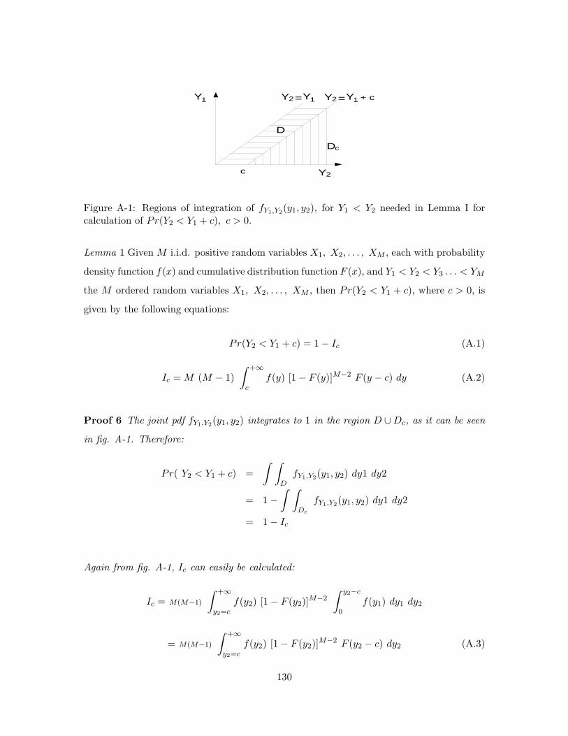
Y1

Y2c

Y2 Y1= Y2 Y1= + c

Dc

D

Figure A-1: Regions of integration of fY1,Y2(y1, y2), for Y1 < Y2 needed in Lemma I forcalculation of Pr(Y2 < Y1 + c), c > 0.

Lemma 1 Given M i.i.d. positive random variables X1, X2, . . . , XM , each with probability

density function f(x) and cumulative distribution function F (x), and Y1 < Y2 < Y3 . . . < YM

the M ordered random variables X1, X2, . . . , XM , then Pr(Y2 < Y1 + c), where c > 0, is

given by the following equations:

Pr(Y2 < Y1 + c) = 1− Ic (A.1)

Ic = M (M − 1)∫ +∞

cf(y) [1− F (y)]M−2 F (y − c) dy (A.2)

Proof 6 The joint pdf fY1,Y2(y1, y2) integrates to 1 in the region D ∪Dc, as it can be seen

in fig. A-1. Therefore:

Pr( Y2 < Y1 + c) =∫ ∫

DfY1,Y2(y1, y2) dy1 dy2

= 1−∫ ∫

Dc

fY1,Y2(y1, y2) dy1 dy2

= 1− Ic

Again from fig. A-1, Ic can easily be calculated:

Ic = M(M−1)

∫ +∞

y2=cf(y2) [1− F (y2)]M−2

∫ y2−c

0f(y1) dy1 dy2

= M(M−1)

∫ +∞

y2=cf(y2) [1− F (y2)]M−2 F (y2 − c) dy2 (A.3)

130

The last equation concludes the proof.

131

132

Appendix B

We repeat Definition 1 and Definition 2 in this section for completeness. The relevant

lemmas follow.

Definition 1: A function f(ρ) is said to be exponentially equal to b, denoted by f(ρ) .= ρb,

if

limρ→∞

log f(ρ)log ρ

= b. (B.1)

We can define the relation.≤ in a similar fashion. Definition 2: The exponential order of a

random variable X with a non-negative support is given by,

V = − limρ→∞

log X

log ρ. (B.2)

Lemma 2 Suppose X1, X2, . . . , Xm are m i.i.d exponential random variables with parame-

ter λ (mean 1/λ), and X = max{X1, X2, . . . Xm}. If V is the exponential order of X then

the density function of V is given by

fV (v) .=

ρ−mv v ≥ 0

0 v < 0(B.3)

and

Pr(X ≤ ρ−v) .= ρ−mv (B.4)

133

Proof 7 Define,

Vρ = − log X

log ρ.

Thus Vρ is obtained from definition 2, without the limit of ρ→∞.

Pr(Vρ ≥ v) = Pr(X ≤ ρ−v)

= Pr(X1 ≤ ρ−v, X2 ≤ ρ−v, . . . Xm ≤ ρ−v)

=m∏

i=1

Pr(Xi ≤ ρ−v)

=(1− exp(−λρ−v)

)m=

λρ−v +∞∑

j=2

(−λ)j

j!ρ−jv

m

Note that Pr(Vρ ≥ v) ≈ ρ−mv. Differentiating with respect to v and then taking the limit

ρ→∞, we recover (B.3).

From the above it can be seen that for the simple case of a single exponential random

variable (m = 1), Pr(X ≤ ρ−v) = Pr(Vρ ≥ v) .= ρ−v.

Lemma 3 For relays, j = 1, 2, . . . ,m, let asj and ajd denote the channel gains from source

to relay j and relay j to destination. Suppose that asr and ard denote the channel gain of

the source to the best relay and the best relay to the destination, where the relay is chosen

according to rule 1. i.e.

min(|asr|2, |ard|2) = max{min(|as1|2, |a1d|2), . . . ,min(|asm|2, |amd|2)}

Then,

1. min(|asr|2, |ard|2) has an exponential order given by (B.3).

2.

Pr(|asr|2 ≤ ρ−v) = Pr(|ard|2 ≤ ρ−v).≤

ρ−mv v ≥ 0

1 otherwise

134

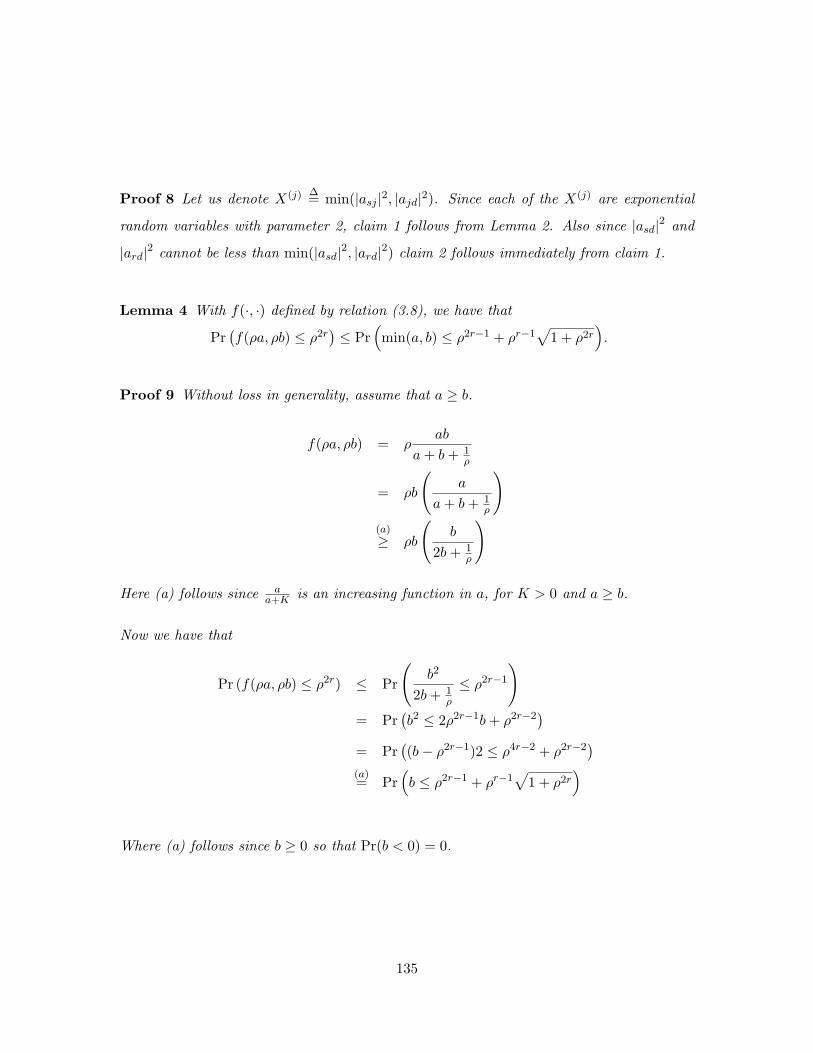
Proof 8 Let us denote X(j) ∆= min(|asj |2, |ajd|2). Since each of the X(j) are exponential

random variables with parameter 2, claim 1 follows from Lemma 2. Also since |asd|2 and

|ard|2 cannot be less than min(|asd|2, |ard|2) claim 2 follows immediately from claim 1.

Lemma 4 With f(·, ·) defined by relation (3.8), we have that

Pr(f(ρa, ρb) ≤ ρ2r

)≤ Pr

(min(a, b) ≤ ρ2r−1 + ρr−1

√1 + ρ2r

).

Proof 9 Without loss in generality, assume that a ≥ b.

f(ρa, ρb) = ρab

a + b + 1ρ

= ρb

(a

a + b + 1ρ

)(a)

≥ ρb

(b

2b + 1ρ

)

Here (a) follows since aa+K is an increasing function in a, for K > 0 and a ≥ b.

Now we have that

Pr (f(ρa, ρb) ≤ ρ2r) ≤ Pr

(b2

2b + 1ρ

≤ ρ2r−1

)= Pr

(b2 ≤ 2ρ2r−1b + ρ2r−2

)= Pr

((b− ρ2r−1)2 ≤ ρ4r−2 + ρ2r−2

)(a)= Pr

(b ≤ ρ2r−1 + ρr−1

√1 + ρ2r

)

Where (a) follows since b ≥ 0 so that Pr(b < 0) = 0.

135

136

Bibliography

[1] S. M. Alamouti, ”A Simple Transmitter Diversity Scheme for Wireless Communica-

tions”, IEEE J. Select. Areas Commun., vol. 1, pp. 1451-58, October 1998.

[2] K. Azarian, H. E. Gamal, and P. Schniter, ”On the Achievable Diversity-vs-multiplexing

Tradeoff in Cooperative Channels”, IEEE Trans. Information Theory, submitted, 2004.

[3] N. Bambos, S. C. Chen, G. J. Pottie, ”Channel Access Algorithms with Active Link

Protection for Wireless Communication Networks with Power Control”, IEEE/ACM

Transactions on Networking, vol. 8, no. 5, October 2000.

[4] J.A. Barnes, et. al. Characterization of Frequency Stability, IEEE Transactions on In-

strumentation and Measurement, Vol. IM-20, No. 2, pp. 105-120, May 1971.

[5] S. Z. Biswas, Opportunistic Routing in Multi-Hop Wireless Networks, M.S. Thesis, MIT,

February 2005.

[6] A. Bletsas, Time Keeping in Myriad Networks: Theories, Solutions and Applications,

M.S. thesis, MIT, June 2001.

[7] A. Bletsas and A. Lippman, ”Efficient Collaborative (Viral) Communication in OFDM

Based WLANs”, Proceedings of IEEE/ITS International Symposium on Advanced Ra-

dio Technologies (ISART 2003), Institute of Standards and Technology, Boulder Col-

orado, March 4-7, 2003.

137

[8] A. Bletsas, A. Lippman, “Natural Spontaneous Order in Wireless Sensor Networks:

Time Synchronization Based on Entrainment”, Technical Report, MIT Media Lab,

December 2003.

[9] A. Bletsas, “Evaluation of Kalman Filtering for Network Time Keeping”, Proceed-

ings of IEEE International Conference on Pervasive Computing and Communications

(PERCOM), Fort-Worth Texas, March 2003.

[10] A. Bletsas, ”Evaluation of Kalman Filtering for Network Time Keeping”, IEEE Trans-

actions on Ultrasonics, Ferromagnetics and Frequency Control, to appear. Available at

http://web.media.mit.edu/ aggelos/papers/tuffc nov04.pdf

[11] A. Bletsas, A. Lippman, ”Spontaneous Synchronization in Multi-hop Embedded Sensor

Networks: Demonstration of a Server-free Approach”, Proceedings of 2nd European

Workshop on Sensor Networks 2005.

[12] A. Bletsas, A. Lippman, D.P. Reed, ”A Simple Distributed Method for Relay Selec-

tion in Cooperative Diversity Wireless Networks, based on Reciprocity and Channel

Measurements”, accepted for publication, IEEE 61st Semiannual Vehicular Technology

Conference May 30 - June 1 2005, Stockholm, Sweden.

[13] A. Bletsas, A. Khisti, D.P. Reed, A. Lippman, ”A Simple Cooperative Diversity Method

based on Network Path Selection”, submitted for publication, IEEE Journal on Selected

Areas of Communication, Special Issue on 4G, January 2005.

[14] D. Cassioli, M. Win, A. Molisch, ”The Ultra-Wide Bandwidth Indoor Channel: From

Statistical Model to Simulations”, IEEE Journal On Selected Areas of Communications,

vol. 20, no. 6, August 2001.

[15] P. R. Cook, Music, Cognition and Computerized Sound. An Introduction to Psychoa-

coustics, MIT Press, Cambridge Massachusetts, 1999

[16] G.M. Crippen, T.F. Havel, Distance Geometry and Molecular Conformation, John

Wiley & Sons, New York 1988.

138

[17] Q. Dong, Z. Wu, ”A Geometric Build-Up Algorithm for Solving the Molecular Distance

Geometry Problem with Sparse Distance Data”, Journal of Global Optimization, no.

26, pp. 321-333, Kluwer Academic Publishers 2003.

[18] J. Elson, L. Girod, D. Estrin, “Fine-Grained Network Time Synchronization using

Reference Broadcasts”, Proceedings of the Fifth Symposium on Operating Systems

Design and Implementation (OSDI), Boston MA, 2002.

[19] J. Elson, K. Romer, “Wireless Sensor Netowkrs: A New Regime for Time Synchro-

nization”, Proceedings of the First Workshop on Hot Topics in Networks, October

2002.

[20] G. J. Foschini, Z. Miljanic, ”A Simple Distributed Autonomous Power Control Algo-

rithm and its Convergence”, IEEE Transactions on Vehicular Technology, vol. 42, no.

4, November 1993.

[21] H.E. Gamal, G. Caire, M.O. Damen, ”Lattice Coding and Decoding Achieve the Opti-

mal Diversity-Multiplexing Tradeoff of MIMO Channels,” IEEE Transactions pp. 968-

985, June 2004.

[22] S. Ganeriwal, R. Kumar and M. Srivastava, “Timing Sync Protocol for Sensor Net-

works”, Proceedings of the First International Conference on Embedded Networked

Sensor Systems, Los Angeles CA, 2003.

[23] D. Ganesan, R. Govindan, S. Shenker and D. Estrin, ”Highly Resilient, Energy Efficient

Multipath Routing in Wireless Sensor Networks”, Mobile Computing and Communica-

tions Review (MC2R), Vol 1., No. 2. 2002.

[24] M. Gastpar and M. Vetterli, ”On the Capacity of Large Gaussian Relay Networks”.

IEEE Transactions on Information Theory, 51(3):765-779, March 2005.

[25] N. Gershenfeld, The Nature of Mathematical Modeling, Cambridge University Press,

2000.

[26] P. Goud Jr, C. Schlegel, W.A. Krzymien, R. Hang, ”Multiple Antenna

Communication Systems - An Emerging Technology”, Canadian Journal of

139

Electrical and Computer Engineering, accepted for publication. Also found in

http://www.ece.ualberta.ca/ hcdc/publications.html

[27] J. V. Greunen, J. Rabaey, “Lightweight Time Synchronization for Sensor Networks”,

Proceedings of the 2nd ACM International Workshop on Wireless Sensor Networks and

Applications, San Diego, CA, September 2003.

[28] M. Grossglauser, D. Tse, ”Mobility increases the capacity of wireless networks”, Pro-

ceedings of IEEE Infocom 2001, Anchorage 2001.

[29] P. Gupta, P.R. Kumar, ”The Capacity of Wireless Networks”, Transactions on Infor-

mation Theory, vol. 46, no. 2, March 2000.

[30] I. Hammerstroem, M. Kuhn, and A. Wittneben, ”Impact of Relay Gain Allocation

on the Performance of Cooperative Diversity Networks”, IEEE Vehicular Technology

Conference, VTC Fall 2004, Los Angeles, Sept. 2004.

[31] M. O. Hasna, M.S. Alouini, ”End-to-End Performance of Transmission Systems With

Relays Over Rayleigh-Fading Channels”, IEEE Transactions on Wireless Communica-

tions, vol. 2, no. 6, November 2003.

[32] A. Hu, S. D. Servetto, “Asymptotically Optimal Time Synchronization in Dense Sensor

Networks”, Proceedings of the 2nd ACM International Workshop on Wireless Sensor

Networks and Applications, San Diego, CA, September 2003.

[33] T. Hunter and A. Nosratinia, ”Cooperation Diversity Through Coding”, in Proc. IEEE

Int. Symp. Information Theory, Lausanne, Switzerland, June 2002, p. 220

[34] M. Janani, A. Hedayat, T.E. Hunter, A. Nostratinia, ”Coded Cooperation in Wireless

Communications: Space-Time Transmission and Iterative Decoding”, IEEE Transac-

tions on Signal Processing, vol. 52, no. 2, February 2004.

[35] Y. Jing, B. Hassibi, ”Distributed Space-time Coding in Wireless Relay Networks-Part

I: Basic Diversity Results”, Submitted to IEEE Trans. On Wireless Communications,

July 2004. Available at http://www.cds.caltech.edu/ yindi/publications.html

140

[36] A. Khandani, J. Abounadi, E. Modiano, L. Zheng, ”Cooperative Routing in Wireless

Networks”, Allerton Conference on Communications, Control and Computing, October

2003.

[37] G. Kramer, M. Gastpar and P. Gupta. ”Cooperative Strategies and Capacity Theorems

for Relay Networks”. Submitted to IEEE Transactions on Information Theory, February

2004. Available at http://www.eecs.berkeley.edu/ gastpar/relaynetsIT04.pdf

[38] S. R. Kulkarni, P. Viswanath, ”A Deterministic Approach to Throughput Scaling in

Wireless Networks”, Transactions on Information Theory, vol. 50, no. 6, pp. 1041-1049,

June 2004.

[39] J.N. Laneman, G.W. Wornell, ”Energy-Efficient Antenna Sharing and Relaying for

Wireless Networks”, Proc. IEEE Wireless Comm. and Networking Conf. (WCNC),

Chicago, IL, Sept. 2000.

[40] J.N. Laneman, Cooperative Diversity in Wireless Networks: Algorithms and Architec-

tures, Ph.D. dissertation, Massachusetts Institute of Technology, Cambridge, MA, Aug.

2002.

[41] J. N. Laneman and G. W. Wornell, ”Distributed Space-Time Coded Protocols for

Exploiting Cooperative Diversity in Wireless Networks”, IEEE Trans. Inform. Theory,

vol. 59, pp. 2415–2525, October 2003.

[42] J. N. Laneman, D. N. C. Tse, and G. W. Wornell, ”Cooperative Diversity in Wireless

Networks: Efficient Protocols and Outage Behavior”, IEEE Trans. Inform. Theory,

Accepted for publication, June 2004.

[43] W. E. Leland, M. S. Taqqu, D. V. Wilson, ”On the Self-Similar Nature of Ethernet

Traffic”, IEEE/ACM Transactions on Networking, vol. 2, February 1994.

[44] J. Levine, An Algorithm to Synchronize the Time of a Computer to Universal Time,

IEEE/ACM Transactions on Networking, vol. 3, no. 1, February 1995.

[45] J. Levine, Time Synchronization Using the Internet, IEEE Transactions on Ultrasonics,

Ferroelectrics and Frequency Control, vol. 45, no. 2, March 1998.

141

[46] J. Levine, Introduction to Time and Frequency Metrology, Review of Scientific Instru-

ments, vol. 70, no. 6, June 1996.

[47] J. Levine, personal communication, NIST, March 2002.

[48] M. Laibowitz, J. Paradiso, Wearable Wireless Transceivers, Circuit Cellar, no.163,

February 2004.

[49] L. Lamport, Time, Clocks, and the Ordering of Events in a Distributed System, Com-

munications of the ACM, vol. 21, no.7, July 1978.

[50] J. Lifton, D. Seetharam, M. Broxton, J. Paradiso, “Pushpin Computing System

Overview: a Platform for Distributed, Embedded, Ubiquitous Sensor Networks”, Per-

vasive 2002, Proceedings of the Pervasive Computing Conference, Zurich Switzerland,

August 2002.

[51] D. L. Mills, “Network Time Protocol (Version 3) Specification, Implementation and

Analysis”, RFC 1305, University of Delaware, March 1992.

[52] R. Min, M. Bhardwaj, Seong-Hwan Cho, N. Ickes, Eugene Shih, Amit Sinha, Al-

ice Wang, Anantha Chandrakasan, ”Energy-Centric Enabling Technologies for Wireless

Sensor Networks”, IEEE Wireless Communications (formerly IEEE Personal Commu-

nications), vol. 9, no. 4, August 2002, pp. 28-39.

[53] R. Min, Personal Communication based on his 2003 Ph.D. work.

[54] A. F. Molisch and M. Z. Win, ”MIMO Systems with Antenna Selection”, IEEE Mi-

crowave Magazine, pp. 46-56, March 2004.

[55] S. B. Moon, P. Skelly, D. Towsley, “Estimation and Removal of Clock Skew from

Network Delay Measurements”, Proceedings of 18th Annual Joint Conf. of the IEEE

Computer and Communications Societies (INFOCOM), 1999.

[56] R. U. Nabar, O. Oyman, H. Bolcskei, A. J. Paulraj, ”Capacity Scaling Laws in MIMO

Wireless Networks”, Allerton Conference on Communication, Control, and Computing,

Monticello, IL, pp. 378-389, Oct. 2003.

142

[57] R. U. Nabar, H. Blcskei, and F. W. Kneubhler, ”Fading Relay Chan-

nels: Performance Limits and Space-time Signal Design”, IEEE Journal on

Selected Areas in Communications, June 2004, to appear, available from

http://www.nari.ee.ethz.ch/commth/pubs/p/jsac03

[58] G. Opshaug, P. Enge, “GPS and UWB for Indoor Navigation”, Institute of Navigation

GPS Conference, Salt Lake City, September 2001.

[59] S. J. Orfanidis, Optimum Signal Processing, An Introduction, 2nd Edition, McGraw-

Hill, 1988.

[60] J. Paradiso, K.Hsiao, J. Strickon, P. Rice, “New Sensor and Music Systems for Large

Interactive Surfaces”, Proceedings of the International Computer Music Conference

(ICMC), August 2000.

[61] J. Paradiso, K. Hsiao, J. Strickon, J. Lifton, and A. Adler, Sensor Systems for In-

teractive Surfaces, IBM Systems Journal, Volume 39, Nos. 3 & 4, October 2000, pp.

892-914.

[62] C. Parsa, J.J. Garcia-Luna-Aceves, “Improving TCP Congestion Control Over Inter-

nets with Heterogeneous Transmission Media”, Proceedings of IEEE, ICNP 99, October

1999.

[63] V. Paxson, Measurement and Analysis of End-to-End Internet Dynamics, Ph.D. thesis,

University of California at Berkeley, April 1997.

[64] T.S Rappaport, Wireless communications: principles and practice, Upper Saddle River,

NJ: Prentice Hall, 1996.

[65] K. Romer, “Time Synchronization in Ad Hoc Networks”, MobiHOC 2001, Long Beach

CA.

[66] A. Scaglione, Yao-Win Hong, ”Opportunistic Large Arrays: Cooperative Transmission

in Wireless Multihop Ad Hoc Networks to Reach Far Distances”, IEEE Transactions on

Signal Processing, vol. 51, no. 8, August 2003.

143

[67] A. Sendonaris, E. Erkip and B. Aazhang. ”User cooperation diversity-Part I: System

description”. IEEE Transactions on Communications, vol. 51, no. 11, pp. 1927-1938,

November 2003.

[68] A. Sendonaris, E. Erkip and B. Aazhang, “User cooperation diversity. Part I: System

description, IEEE Trans. on Communications, vol. 51, no. 11, pp.1927-1938, November

2003.

[69] T.J. Shepard, ”A Channel Cccess Scheme for Large Dense Packet Radio Networks”,

SIGCOMM 1996, Palo Alto California.

[70] M.L. Sichitiu, C. Veerarittiphan, “Simple, Accurate Time Synchronization for Wireless

Sensor Networks”, IEEE WCNC 2003.

[71] S. Strogatz, Sync, The Emerging Science of Spontaneous Order, 1st ed. New York:

Theia, 2003.

[72] M. S. Taqqu, W. Willinger, R. Sherman, ”Proof of a Fundamental Result in Self-Similar

Traffic Modeling”, ACM Computer Communications Review, April 1997.

[73] E. Teletar, ”Capacity of Multi-Antenna Gaussian Channels”, European Transac. on

Telecom. (ETT), vol. 10, pp. 585–596, November/December 1999.

[74] S. Toumpis, A. Goldsmith, ”Capacity regions for wireless ad hoc networks”, IEEE

International Conference on Communications, 28 April-2 May 2002.

[75] G. D. Troxel, Time Surveying: Clock Synchronization over Packet Networks, Ph.D.

thesis, MIT, May 1994.

[76] D. N. C. Tse and P. Viswanath, Fundamentals of Wireless Communications. Working

Draft, 2003.

[77] B. Zhao and M.C. Valenti, ”Practical relay networks: A generalization of hybrid-ARQ”,

IEEE Journal on Selected Areas in Communications (Special Issue on Wireless Ad Hoc

Networks), vol. 23, no. 1, pp. 7-18, Jan. 2005.

144

[78] P. Viswanath, D.N.C. Tse, R. Laroia, ”Opportunistic Beamforming Using Dumb An-

tennas”, IEEE Transactions on Information Theory, vol. 48, no. 6, June 2002.

[79] L. Zheng and D. Tse, “Diversity and Multiplexing: A Fundamental Tradeoff in Multiple

Antenna channels,” IEEE Trans. Inform. Theory, vol. 49, pp. 1073–96, May, 2003.

[80] A. Wittneben, B. Rankov, ”Impact of Cooperative Relays on the Capacity of Rank-

Deficient MIMO Channels”, Proceedings of the 12th IST Summit on Mobile and Wire-

less Communications, Aveiro, Portugal, pp. 421-425, June 2003.

[81] A. Wittneben, I. Hammerstroem, and M. Kuhn, ”Joint Cooperative Diversity and

Scheduling in Low Mobility Wireless Networks”, IEEE Global Telecommunications Con-

ference, Globecom 2004, Nov. 2004.

[82] M. Zorzi, R.R. Rao, ”Geographic Random Forwarding (GeRaF) for Ad hoc and Sensor

Networks: Multihop Performance”, IEEE Trans. on Mobile Computing, vol. 2, Oct.-Dec.

2003.

[83] M. Zorzi, R.R. Rao, ”Geographic Random Forwarding (GeRaF) for Ad hoc and Sensor

Networks: Energy and Latency Performance”, IEEE Trans. on Mobile Computing, vol.

2, Oct.-Dec. 2003.

[84] ns-2, “The Network Simulator-ns-2”, http://www.isi.edu/nsnam/ns/

[85] Demo website,

http://web.media.mit.edu/ aggelos/demos/demos.html

[86] Badge website, http://www.media.mit.edu/resenv/badge

[87] Pushpin website, http://web.media.mit.edu/ lifton/PushPin/

145