Intellectual Property Rights and the Knowledge Spillover Theory of Entrepreneurship

Zoltan J. Acs

George Mason University, Fairfax, Virginia and

Max Planck Institute of Economics Jena, Germany

Mark Sanders

Utrecht School of Economics, Utrecht, Netherlands and

Max Planck Institute of Economics Jena, Germany.

March 2008

Abstract: We develop a model in which stronger intellectual property rights protection

reduces economic growth. We arrive at this conclusion by assuming that entrepreneurs

explore and exploit the knowledge that spills over from the R&D in incumbent firms.

Intellectual property rights protection allows these firms to prevent or discourage the

exploration of that knowledge and thereby reduces the knowledge spillover to

entrepreneurs. This implies losses at the societal level, as incumbent firms typically do

not commercialize all the knowledge that their R&D develops. According to the theory,

allowing incumbent firms to establish ownership and capture the rents that accrue to the

entrepreneurs will reduce the returns to entrepreneurship and thereby reduce economic

growth.

JEL J24, L26, M13, O3

Keywords: Intellectual Property Rights; Endogenous Growth; Entrepreneurship;

Incentives; Knowledge Spillovers; Rents.

2

I. Introduction

This paper is about the perverse role of intellectual property rights protection in an

entrepreneurial economy. Following for example Audretsch (2007) and Acs, Audretsch,

Braunerhjelm and Carlsson (2006), we model an entrepreneurial economy in which

incumbent firms invest resources in R&D to improve upon their existing product lines

and in the course of that generate knowledge that is of no direct commercial value to

them. That knowledge then presents an opportunity for entrepreneurs, willing and able to

take risks in developing and commercializing it. An entrepreneur will do so when the

expected (risk adjusted) returns justify that investment. However, when intellectual

property rights are easily established and enforced, incumbent firms can seriously reduce

this knowledge spillover. Intellectual property rights protection then creates a knowledge

filter (Acs, Audretsch, Braunerhjelm and Carlsson (2004)) and reduces the flow of

innovations in the economy.

Our paper contributes to two debates in the literature by connecting them and

introducing IPR-protection in the context of an entrepreneurial economy. In the empirical

growth literature institutions in general (Barro (1996), Sala-I-Martin (1996) and

Acemoglu et al (2001)) and IPR-protection in particular (Gould and Gruben (1996),

Branstetter et al. (2006) and Allred and Park (2007)), have been identified as significant

contributing variables in explaining the cross-country variance in growth performance.

The theoretical justifications for including indicators of intellectual property

rights protection followed straight from innovation driven endogenous growth models

such as Romer (1986, 1990), Grossman and Helpman (1991) and Aghion and Howitt

(1992). In their models the (temporary) monopoly rents that patent protection and

3

enforcement implied are the prime incentive for R&D and innovation and the source of

endogenous growth. In more recent contributions, however, both the theoretical

arguments and empirical results are being challenged.1 Examples of the former are Kwan

and Lai (2003) and Iwaisako and Futagami (2003), who argue that static losses need to be

weighed against dynamic gains and thus an optimum level of protection can be found.

And Horii and Iwaisako (2007) and Furukawa (2007), who focus on the reduced growth

potential in an economy that has more monopolized sectors. Still these papers stay

strongly committed to the assumption that patent protection is required to provide the

incentives for innovation.

By separating invention and innovation our model provides another perspective

on this debate. In modeling the dual role of patent protection we closely follow Jaffe and

Lerner (2004) who present the compelling story for the United States. They argue that

stricter enforcement and easier establishment of intellectual property has turned the

highly successful US patent system into an impediment to innovation. Their main

argument is that stricter enforcement by the central appeals court has tilted the system

towards the interests of patent holders, whereas the fees-based financing of the patent and

trademark office made patent evaluators directly dependent on the number of patents

granted. Patents thus became easier to obtain and easier to enforce.

The implications of these reforms to strengthen IPR-protection were unintended

and undesirable. Large incumbent firms and individual inventors take out patents on all

potentially valuable knowledge, even if they have no intention of ever commercializing

it. They rather aim at capturing rents once their idea is commercialized by someone else

1 Empirical papers that cast doubt on the strictly positive impact of IPR-protection include e.g. Glaeser et al. (2004) and Greasley and Oxley (2007).

4

and starts to generate profits. Large corporations have even set up specialized patent

enforcement departments that quickly became profit centers in their own right. And of

course the threat of patent infringements suits and rent seeking inventors stifled small

firm competition and strongly reduced the incentives to commercialize and exploit

knowledge that was not 100% home made and patent protected.

This result cannot be understood in the context of a traditional endogenous growth

model. Commercialization in these models is after all, trivial. In the logic of most

innovation driven growth models, more IPR-protection and stronger enforcement would

spur growth by giving more incentives to innovate. In this paper we argue that this

illustrates a fundamental flaw in these models. Innovation driven endogenous growth

models collapse the “process of innovation”: the subsequent generation, exploration and

exploitation of the knowledge that constitutes a commercial opportunity, into one rational

decision that is motivated by downstream rents. Therefore they tend to confuse the

inventor and the entrepreneur. It is the latter that holds the residual claim to any rents that

an invention may generate once he has commercialized it. And these rents are the

entrepreneurs’ reward for seeing the commercial potential, taking the risks, investing the

resources and organizing the production of a new product or service. In our model the

entrepreneur is therefore the one who is motivated to act by the prospective commercial

rents. The residual claim to rents should not rest with the inventor as he is not taking

commercial risks and his efforts are sunk costs.2

2 Even if in reality one individual can be inventor and entrepreneur, the literature has plenty of examples of inventors who either failed to see the commercial potential, did not want to take the risks, could not gather the resources or failed as managers when the innovation took off. This anecdotal evidence shows that it is the entrepreneurial talent that entitles one to the rents, whether one is the inventor or not. We therefore assume that entrepreneurship, not knowledge creation, is driven by expected future profits.

5

In a system where there is no protection of intellectual property, invention may

well be the bottleneck in the innovative cycle. Back in the days that patents were awarded

to benefit the Royal’s favorites, the connection of invention to exclusive property rights

was revolutionary and helped spur invention and arguably paved the way for the

Industrial Revolution.3 Therefore in current patent systems it is the inventor, not the

entrepreneur, who is allowed to establish legal ownership over an invention. This

ownership allows him to extract (some of) the rents of commercialization in reward for

the investments made. But once such a system is in place, a delicate balancing act is

required. In most OECD countries today entrepreneurship, not invention seems to be the

bottleneck in the innovative process (Audretsch, 2007). By enforcing patents more

strictly and allowing inventors to patent much easier, Jaffe and Lerner (2004) argue that

the balance shifts and rents are redistributed away from the entrepreneurs.

In a model where commercialization and invention are separate activities, it is

easy to show that stricter intellectual property rights protection may then backfire and

cause growth to decline. The model we present below is an adaptation of the Romer

(1990) model that is inspired on the knowledge spillover theory of entrepreneurship as

put forward in Acs et al (2004, 2006) and the evidence on the importance of spin-out and

spin-off innovation in the detailed case studies by Klepper (2007).

Our model predicts that strengthening IP-protection is always bad for growth

because incumbent corporate R&D is motivated by efficiency gains for the firm that

require no patent protection. Of course this is a simplification that we have made to make

our point. In many industries today the corporate R&D would not be undertaken without

3 Greasley and Oxley (2007) actually present a compelling case that the Industrial Revolution made patenting more valuable and thus caused the surge in patenting rather than the other way around.

6

some degree of patent protection that allows these firms to recover their R&D

investments. As this mechanism is well understood our paper should be understood as

introducing a reason why the positive relation between economic growth and intellectual

property rights protection is not necessarily monotonous and there is an optimum level of

protection. As such it supports the Jaffe and Lerner (2004) analysis of the recent reforms

in the US patent system that seem to put it over the top.

We add to their analysis a model that embeds the conceptual framework

developed there in a well-established growth model with firm decision theoretical micro-

foundations. The remainder of this paper presents our model in section two and derives

the equilibrium properties and implications of intellectual property rights protection in

section three. Section four examines the comparative static’s and the impact of stronger

patent protection. Section five concludes.

II. The Model

In our model consumers consume a homogenous final good and producers produce that

good using labor and intermediates where the production of intermediates takes place

under monopolistic competition among imperfect substitutes. A key assumption in the

model we develop below is the separation of knowledge creation from

commercialization. The final good producers carry out R&D however, commercial

innovations are also produced by entrepreneurs from knowledge spillovers. The model is

in equilibrium when all agents solve their respective choice problems rationally and the

market prices adjust to equate supply and demand for final and intermediate goods, labor

and capital. In the next subsections we first consider consumers, then producers,

7

intermediate producers and entrants. The decentralized equilibrium is then analyzed in

section 3.

II.1 Consumers

The consumer problem below is standard in the literature (see for example Barro and

Sala-I-Martin (2004)). Consumers maximize their value function:

∫∞

−=0

))(( dttCUeV tρC (1)

Where ρ is the subjective discount rate and U(C(t)) is given by log C(t), the natural log of

consumption, C(t). This value function is maximized subject to the intertemporal budget

constraint:

)()()()()( tCtwtBtrtB −+=& (2)

Where r(t) is the interest rate on the stock of bonds, B(t), held at time t and w(t) is labor

income as we normalize total labor supply to 1. Appendix A shows that the standard

Ramsey-rule applies:

ρtrtCtC

−= )()()(& (3)

8

It is also shown in Appendix A that for any constant interest rate consumers will then

choose consumption level:

tρrrt edttweBρtC )(

0

)()0()( −∞

−

+= ∫ (4)

where B(0) is the level of initial wealth and the integral represents the discounted present

value of life time labor income. Equation (4) merely implies that there is a positive

demand for final goods at all times. To endogenize the equilibrium interest rate and wage

levels we need to specify the production side.

II.2 Producers

Producers produce the homogenous final good and maximize their profits by choosing

the levels of labor, intermediate goods and R&D labor to employ, taking as given the

price level that we normalize to 1. All firms are assumed to have the same production

function:

∑=

−−=)(

0

1),()()()(tn

i

βαj

βPj

αjj tixtLtAtX with 0≤ α+β ≤1 and 0≤ α,β ≤1 (5)

where Xj(t) is the output of final goods producer j, LPj(t) is production labor that earns

wage w(t) and xj(i,t) is the quantity of intermediate i bought at price χ(i,t). Aj(t) represents

9

the level of accumulated knowledge in the firm and n(t) is the number of available

varieties of intermediate goods at time t. All firms maximize the value function:

( )∫ ∑∞

=

−

−+−=

0

)(

0),(),()()()()(

tn

ijRjPjj

rtj tixtiχtLtLtwtXeV (6)

This function is maximized subject to the production function (5) and the R&D

innovation function:

)()()()( 1 tLtntAtA Rjγγ

jj−=& with 0≤ γ ≤1 (7)

The presence of Aj(t) in the latter reflects the intertemporal knowledge spillover. R&D is

more productive when a large knowledge base has been developed in the past but at a

decreasing rate. The presence of n(t) reflects the fact that more variety in intermediates

allows the final goods producing sector to better fine tune the production process and

thereby generate more total factor augmenting technical change for a given level of R&D

effort. Alternatively, one could say that the relevant knowledge base for firm j’s R&D is

a Cobb-Douglas aggregate of public and private knowledge, proxied by n and Aj

respectively. We have chosen a linear specification in R&D labor following Romer

(1990) and thereby introduced the scale effect. Eliminating it would not affect our key

results.4

4 Jones (2006) offers several alternatives to this specification that would not suffer from this problem but as the issue has no bearing on our purpose we chose to stick to the Romer-specification.

10

The firm’s problem is now a dynamic optimization problem due to the R&D

investment decision and, dropping time arguments to save on notation, it is characterized

by the Hamiltonian:

( ) ( )Rjγγ

jj

n

ijRjPj

n

i

βαj

βPj

αj

rtj LnAµixiχLLwixLAeH −

==

−−− +

−+−= ∑∑ 1

00

1 )()()( (8)

where the levels of employment and intermediate use are control variables and the stock

of firm specific knowledge is the state variable. Standard dynamic optimization yields

n+5 first order conditions. For production labor we have:

−==

∂

∂∑=

−−−− wixLAβeLH n

i

βαj

βPj

αj

rt

Pj

j

0

11 )(0 (9)

Which can easily be rewritten into a labor demand function:

wXβ

w

ixAβL j

βn

i

βαj

αj

DPj =

=

−

=

−−∑1

1

0

1)( (10)

This shows that all firms will spend exactly the same share, β, of output, X on wages.5

Summing over all final goods producers we obtain for total production labor demand:

5 As final output is homogenous and we normalized its price to 1, sales equal production.

11

wXβL D

P = (11)

such that the total wage sum for production workers is βX and labor demand is stable as

long as wages and production grow at the same rate in equilibrium.

For intermediates the firm will choose the levels to satisfy:

( )

( )

( ))()()1(0)(

...

)1()1()1(0)1(

)0()0()1(0)0(

nχnxLAβαenx

H

χxLAβαexH

χxLAβαexH

βαj

βPj

αj

rt

j

j

βαj

βPj

αj

rt

j

j

βαj

βPj

αj

rt

j

j

−−−==∂

∂

−−−==∂

∂

−−−==∂

∂

−−−

−−−

−−−

(12)

Appendix B shows that these n conditions can be used to derive the demand for variety i

by final goods producer j:

jn

i

βαβα

βαD

j Xβα

iχ

iχix )1(

)(

)()(

0

1

1

−−=

∑=

+−−

−

+−

(13)

Multiplying (13) by χ(i) and summing over all varieties i shows that total expenditure on

intermediates is (1-α-β)Xj.6

6 Summing over all final goods producers j then yields the result that total expenditure on intermediates in the economy is (1-α-β)X.

12

Together with the result on the wage costs, this implies that the final goods

producer j makes an operating profit of αXj. We assume that final goods producers are

perfectly symmetric, face the same input and output prices, w, χ(i) and 1 respectively. As

they also use the same production technology, increases in the firm’s level of

accumulated knowledge Aj(t) and consequently Xj(t) will cause increases in operating

profit. Firms, however, have to invest labor in R&D to increase their Aj(t).

Formally the stock of knowledge is a firm specific state variable and its optimal

path is determined by choosing the optimal level of R&D labor. The final goods producer

will increase R&D activity as long as the discounted future benefits of doing so exceed

the current labor costs at the margin. As R&D is a deterministic process in our model the

firms can decide to spend on R&D exactly up to that point. The solution is formally

characterized by two first order conditions, one transversality condition and the law of

motion for Aj7:

Rjγγ

jjj

j

jjt

Rjγγ

jj

n

i

βαj

βPj

αj

rtj

j

j

γγjj

rt

Rj

j

LnAAµH

tAtµ

LnAµγixLAeµAH

nAµweLH

−

∞→

−

=

−−−−

−−

==∂

∂

=

−+=−=∂

∂

+−==∂

∂

∑

1

0

11

1

0)()(lim

)1()(

0

&

& (14)

7 Time arguments have been included in the transversality condition as the limit is taken for time to infinity.

13

Where the first condition sets the present value of labor costs equal to the present value of

the marginal product of R&D labor times the shadow price of a marginal increase in Aj,

µj. Solving for that shadow price yields:

γγj

rtj nA

weµ−

−= 1 (15)

Then we take the time derivative and set this expression equal to minus the right hand

side in the second condition to equate the marginal return on Aj to the shadow price:

j

Rjrt

j

jrtγγ

j

rt

j

jj A

wLeγ

AXα

enA

wennγ

AA

γwwrµ −−

−− −−−=

+−+−= )1()1( 1

&&&& (16)

Substituting the law of motion (7) for jA& into (16) and solving for w yields the wage

level at which a positive finite amount of R&D workers will be employed by firm j. This

wage level represents a horizontal demand function or arbitrage condition. If wages

exceed this threshold no R&D workers will be employed by firm j. If wages fall short, all

labor in firm j is reallocated to do R&D. This so-called bang-bang equilibrium is a result

of the constant returns to R&D labor assumption that we have made. It implies that in any

stable equilibrium the wage must equal:

( )nnγwwrnAXα

wγγ

jjj // && +−=

−

(17)

14

But (17) holds for all firms j and the wage must also be equal for all firms j as they are

price takers in the labor market. We also know by the production function in (5) and

equations (10) and (13) that Xj is continuous and strictly proportional in Aj.8 Thus we

obtain the result that at any point in time there is a unique level of Aj that all firms hiring

R&D labor must attain. The mechanism is that the firms with Aj=Amax also have the

highest threshold wage for R&D. They will thus bid up production wages to this

threshold level and employ a positive amount of R&D. Their level of A will then rise

according to (7) and those with Aj<Amax will not hire any R&D and their Aj remains

stable. The rise in Amax pushes up the threshold and thereby the production wage. In any

equilibrium with R&D only those firms that have Aj=Amax can stay in the race, whereas

others are forced to bring down their production employment levels to 0.9 If we assume

therefore that all firms start from the same initial level of Aj(0)=A0 the above implies that

Aj(t)=Amax(t)=A(t) for all j and we obtain for (17) (dropping time arguments):

( )nnγwwrnXAαwγγ

// && +−=

−

(18)

8 It can be shown that the right hand side of (17) is actually positive in Aj when the optimal amounts of labor and intermediates have been employed. In that case output in (5) substituting for labor and

intermediates by (10) and (13) equals: αβαα

βα

αβ

jj nχβα

wβAX

+−−

−−

=

1

1 where χ represents the average

price for intermediates. Plugging this expression in the threshold wage in (17) and solving for the wage yields an expression that is positive and concave in Aj 9 Taken literally this result may strike one as unrealistic and it yields the undesirable result that initial levels of production knowledge have to be exactly equal. At this point, however, it is worth noting that for example uncertainty in the R&D process and fixed costs have been assumed away. In real life the uncertainty in R&D outcomes would create a bandwidth, not a precise level for the threshold wage and fixed costs would cause firms to actually exit when employment levels fall below a critical level. Then the prediction is that a group of technology leaders will be able to survive in the market, where they must “ run to stand still” and a shake out will cause firms with less than efficient production processes to exit in the transition to the steady state. Such processes are well-known in the empirical literature on industrial dynamics (Refs). They are present in a very stylized form in our model.

15

We have shown above that a stable labor demand in production requires an equilibrium in

which wages grow at the same rate as output. Equation (18) shows that the threshold will

also satisfy that constraint as long as A and n grow at the same rate.

Given the total amount of labor employed and the number of firms in the final

goods producing sector, the optimal path for A(t) is now determined. The number of

production workers follows from equations (11) and (18):

)//( nnγwwrnA

αβL

γD

P && −−

= (19)

And given total employment the number of R&D workers could be computed and

plugged into (7) to derive the optimal growth rate of Aj(t)=Amax(t)=A(t). The starting

condition Aj(0)=A0 and the law of motion in (7) thus determine the optimal path for A(t)

and the transversality condition helps to solve for µj(t).

However, the level of employment in final goods production is not yet determined

as labor has one more application in our model. Moreover, this full specification of

optimal paths is not so interesting for our purpose, as we are primarily interested in the

comparative statics of the steady state. Therefore we now turn to the intermediate

producers.

II.3 Intermediate Producers

16

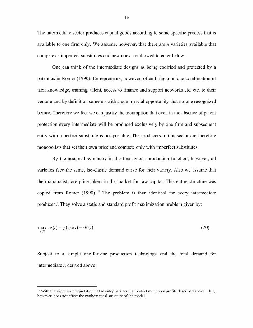
The intermediate sector produces capital goods according to some specific process that is

available to one firm only. We assume, however, that there are n varieties available that

compete as imperfect substitutes and new ones are allowed to enter below.

One can think of the intermediate designs as being codified and protected by a

patent as in Romer (1990). Entrepreneurs, however, often bring a unique combination of

tacit knowledge, training, talent, access to finance and support networks etc. etc. to their

venture and by definition came up with a commercial opportunity that no-one recognized

before. Therefore we feel we can justify the assumption that even in the absence of patent

protection every intermediate will be produced exclusively by one firm and subsequent

entry with a perfect substitute is not possible. The producers in this sector are therefore

monopolists that set their own price and compete only with imperfect substitutes.

By the assumed symmetry in the final goods production function, however, all

varieties face the same, iso-elastic demand curve for their variety. Also we assume that

the monopolists are price takers in the market for raw capital. This entire structure was

copied from Romer (1990).10 The problem is then identical for every intermediate

producer i. They solve a static and standard profit maximization problem given by:

)()()()(:max)(

irKixiχiπiχ

−= (20)

Subject to a simple one-for-one production technology and the total demand for

intermediate i, derived above:

10 With the slight re-interpretation of the entry barriers that protect monopoly profits described above. This, however, does not affect the mathematical structure of the model.

17

Xβα

iχ

iχix

iKix

n

i

βαβα

βαD )1(

)(

)()(

)()(

0

1

1

−−=

=

∑=

+−+

+−

(21)

Substitution into the profit function and setting the first derivative with respect to χ(i) to 0

yields:

βαriχ−−

=1

)( (22)

Which does not vary over i anymore. So every intermediate producer sets his price equal

to this value and by the demand function all intermediates are demanded in the same

quantity. This implies that in equilibrium the stock of raw capital is divided equally

among all n varieties of intermediate goods:

nKix /)( = i∀ (23)

Consequently the capital share in income is given by XβαrK 2)1( −−= , whereas the

monopoly rents in the intermediate sector are given by:

∑=

−−+=

−−+=

n

iXβαβαiπ

nXβαβαiπ

0)1)(()(

)1)(()( (24)

18

These profits accrue to the entrepreneur who organized the intermediate production unit,

as no other inputs or fixed (entry) costs are assumed. Monopoly rents are the reward for

commercialization in our model. But let us now consider the decision to start an

intermediate goods producing venture.

II.4 Entry and Entrepreneurs

The positive (expected) flow of rents attracts entrants. These entrants cannot enter the

existing intermediate variety markets as we assume that these are protected by trade

secrets, unique essential entrepreneurial traits or otherwise (not necessarily by patents).

However, the existence of these rents and the knowledge that there is a latent demand for

new varieties, makes it attractive to enter with a new intermediate variety. As in Romer

(1990) the value of a new intermediate firm that enters at time T is equal to the

discounted current value of an incumbent intermediate firm’s remaining flow of rents

from T to infinity (assuming the impact of one additional intermediate on incumbent

intermediate firms’ profits is infinitely small):

dttntXeβαβαdttiπeTV

T

Rt

T

RtE )(

)()1)((),()( ∫∫∞

−∞

− −−+== (25)

19

Here, however, we start to deviate from the standard Romer (1990) framework. If the

profit flow is at risk, the discount rate, R≡r+ξ, includes a risk premium, ξ, that captures

the flow probability of losing the entire profit.11

As was argued by Jaffe and Lerner (2004), with excessive patent protection this

parameter turns positive in the strength of patent protection. Of course a patent

infringement suit is usually settled out of court and it does not result in the entire profit

flow disappearing. But by assuming that a high probability of losing some profits reduces

the value of the firm to the entrepreneur in the same way as a low probability to lose the

entire profit flow, we can still interpret parameter ξ as reflecting the ease of obtaining and

upholding patents in court.

When inventors and incumbent firms can easily patent their inventions, even if

they have no intention of commercializing, and on top of that have a high probability of

winning infringement suits, they can leverage their patent portfolio to extract rents from

entrepreneurs that commercialize even slightly related products. Of course the

entrepreneur also benefits from patent protection. If the intermediate product can be

patented, the protection secures the profit flow from copy-cat competition. But we agree

with Jaffe and Lerner (2004) that at high levels of protection the disadvantages of even

stronger IPR-protection can easily outweigh the positive effects. We might capture both

effects by assuming that ξ falls and then rises in the strength of patent protection, but to

make our case we will assume the strict positive relationship that remains when patent

protection is not essential to capture entrepreneurial monopoly rents.

11 See for example Walsh (2003) and Aghion and Howitt (1998), who show that a positive flow probability of losing a profit flow can be incorporated by including that probability in the discount rate.

20

Then we assume that an entrepreneur has to organize a new production unit to

capture these rents. We propose further, as opposed to Romer (1990), that this requires

the allocation of time and is therefore costly in terms of wages foregone. Moreover, we

assume that entrants receive their idea free of charge, as a costless knowledge spillover

from downstream final goods producers’ process R&D. One can think of this process as

the spin-out of an employee from the final goods producers’ R&D labs, but it is also

possible that others pick up on their idle ideas. The entry function is given by:

EALφn =& (26)

We have assumed constant returns to entrepreneurial activity, implying that doubling

entrepreneurship leads to doubling the number of entrants for a given number of ideas

spilling over. Moreover, we assume that entry is proportional to the accumulated

knowledge in final goods producers process R&D, A(t). As the process is better

understood, more ideas for new, more specialized, intermediates are likely to emerge.12

We also introduce parameter, φ to reflect the “knowledge filter”. This concept

was first coined by Acs et al. (2004) to describe the institutional, informational and

otherwise existing barriers to knowledge spillover between knowledge creators and

commercializers. In the context of our model one could think of non-disclosure

agreements, labor contract limitations on moving to competing firms and the defensive

patenting strategies in final goods producing firms. Anything the final goods producing

firms does to limit the spillover of knowledge, including legal and other action, will

12 Of course one may consider more general entry functions. Our results are robust to such more general specifications as long as the returns to knowledge are non-diminishing.

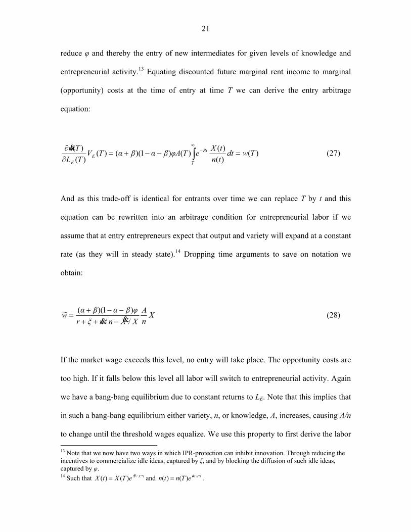
21

reduce φ and thereby the entry of new intermediates for given levels of knowledge and

entrepreneurial activity.13 Equating discounted future marginal rent income to marginal

(opportunity) costs at the time of entry at time T we can derive the entry arbitrage

equation:

)()()()()1)(()(

)()( Twdt

tntXeTAφβαβαTV

TLTn

T

RtE

E

=−−+=∂∂

∫∞

−& (27)

And as this trade-off is identical for entrants over time we can replace T by t and this

equation can be rewritten into an arbitrage condition for entrepreneurial labor if we

assume that at entry entrepreneurs expect that output and variety will expand at a constant

rate (as they will in steady state).14 Dropping time arguments to save on notation we

obtain:

XnA

XXnnξrφβαβαw

//)1)((~

&& −++−−+

= (28)

If the market wage exceeds this level, no entry will take place. The opportunity costs are

too high. If it falls below this level all labor will switch to entrepreneurial activity. Again

we have a bang-bang equilibrium due to constant returns to LE. Note that this implies that

in such a bang-bang equilibrium either variety, n, or knowledge, A, increases, causing A/n

to change until the threshold wages equalize. We use this property to first derive the labor 13 Note that we now have two ways in which IPR-protection can inhibit innovation. Through reducing the incentives to commercialize idle ideas, captured by ξ, and by blocking the diffusion of such idle ideas, captured by φ. 14 Such that tXXeTXtX */)()( &= and tnneTntn */)()( &= .

22

market equilibrium in section 3 and then analyze the comparative statics in the steady

state in section 4.

III The Decentralized Equilibrium

III.1 The Labor Market

The labor market is in equilibrium when wages equate supply (normalized to 1) and

demand in production, R&D and entrepreneurship. All activities therefore earn the same

wage in equilibrium. We have www ~== and ERP LLL ++=1 to determine the

equilibrium but let us first consider what happens out of equilibrium. If ]~,max[ www >

there is no entrepreneurship or R&D activity. That equilibrium is possible and may be

stable but will not be considered further. It will not be a stable equilibrium if consumers

are sufficiently patient and therefore willing to invest in innovations. Also note that

]~,max[ www < cannot be an equilibrium as that would imply the level of production

labor falls to 0. By the concavity of the production function that would imply that the

marginal productivity goes to infinity. Therefore only www ~>= , www >= ~ and

www ~== can be equilibria in the labor market. If www ~>= all labor is allocated to

production and R&D and none to entrepreneurship. This implies A/n will rise. If

www >= ~ instead, all labor is allocated between entrepreneurship and production and

A/n will fall. Such changes in A/n will push the threshold wages towards each other. Only

when www ~== is the labor market allocation stable at positive levels of all activity.

Figure 1 plots the ratio ww /~ against A/n. The above implies that the labor market may

clear at any ratio in the short run, but the corresponding allocation of labor over R&D or

23

entrepreneurship implies that we will move towards the point where this ratio equals 1.

The model, however, is not yet in steady state. The position of the convex curve still

depends on the various growth rates in the model as can be verified in:

+−

+−+−−+

=

+−

nnγwwrnnXXξr

φβαβαα

nA

ww γ

////

)1)((~)1(

&&&&

(29)

Out of steady state equilibrium the labor market will thus ensure that first A/n is at A/n*,

but due to the fact that (29) depends on the growth rates of output, wages, the interest rate

and the growth rate of n, this A/n* is not necessarily the steady state ratio. A steady state

is reached when wages increased to such levels that the levels of employment in R&D

Figure 1: The Labor Market

ww~

A/n

0// => AAnn &&

ww~

1

A/n*

AAnn //0 && <=

24

and entrepreneurship eventually reach the level for which A and n grow at the same rate

and A/n is at A/n*. We analyze that steady state below.

III.2 The Steady State

The model is in steady state equilibrium when all variables expand at a constant rate and

the labor market allocation is stable. Equation (11) has shown that a stable steady state

demand for production workers implies that growth rate of wages must equal the growth

rate of output. From the arbitrage equations (18) and (28) and the analysis of the labor

market above we know that the latter can only be the case when A and n expand at the

same rate.15 Output, by the production function (5) and the fact that all intermediates are

used at level K/n, will then grow at rate:

KKβα

nnβα

AAα

XX &&&&

)1()( −−+++= (30)

Using the fact that output in steady state grows at the same rate as wages, wage income

and consumption, we then know that asset income must also grow at that rate by the

dynamic budget constraint of consumers. Hence, for a constant interest rate, asset and

raw capital accumulation must also take place at the growth rate of output. Using this fact

and equation (30) we obtain:

15 Computing the growth rates for (18) and (28) it can immediately be verified that in any steady state

equilibrium the wage will therefore grow at rate:nn

AA

XX

nn

AAγ

XX

ww &&&&&&&

−+=

−−=

25

nn

AA

βαα

XX &&&

++

= (31)

And as a stable labor allocation requires a constant ratio A/n the steady state growth rates

will be equal to:

++

=−=====βαβα

nnρr

ww

BB

CC

XX

KK 2&&&&&&

(32)

This solves the model if we can obtain the steady state growth rate of n (and A). The first

steady state condition follows from rewriting equation (29) for the steady state. That ratio

is 1 in equilibrium and can be solved for A/n:

γ

nnγρnnξρ

φβαβαα

nA +

+++

−−+=

11

//

)1)(( &&

(33)

which solves in parameters only for the special case that ξ=0 (no risk premium) and ρ=0

(no time preference). Using the condition that in steady state variety expansion equals

productivity growth we can derive a second steady state relation between entrepreneurial

activity and R&D labor using equations (7) and (26):

γ

E

R

nAφ

LL +

=

1

(34)

26

Using equation (33) in (34) we obtain:

nnγρnnξρ

βαβαα

LL

E

R

//

)1)(( &&

+++

−−+= (35)

Which gives the steady state ratio of R&D to entrepreneurial activity for which the

arbitrage wages and the rate of expansion for A and n are equal. It gives the ratio as a

function of the rate of expansion for n and parameters. Using the labor market clearing

condition ERP LLLL ++=* we can compute the steady state level of entrepreneurial

activity, using (35) to eliminate LR and (11), (28) and (33) to eliminate LP. We thus obtain

for entrepreneurial activity in the steady state:

nnγρα

nnξρβαβα

αnnγρ

nnξρφβαβα

φβ

nnξρβαβα

L

γ

E

//)1)((

//

)1)((/

)1)((

*

11

&&

&&&

++

++−−+

+++

−−+−

++−−+

=

+

(36)

Plugging into the entry function in equation (26), dividing both sides by n and using (33)

yields:

*

//)1)((

)/(/)1)((

*/

11

1

L

nnγρα

nnξρβαβα

βnnγρ

αnnξρ

φβαβα

nn

γγγ

&&

&&&

++

++−−+

−

+

++

−−+

=

++

(37)

27

Which determines the steady state growth rate. Appendix C shows that there is only one

positive growth rate of n for which (37) holds, even if we cannot compute the analytical

closed form solution.

VI. Comparative Statics and the Impact of stronger IPR-Protection

We can now verify the negative impact of stronger intellectual property rights protection

on the steady state rate of innovation in our model. The proof for that proposition is

trivially derived from equation (37). As the right hand side of equation (37) is generally

downward sloping in the growth rate and positive in parameter φ it follows that a more

transparent knowledge filter implies a larger steady state growth rate. Similarly, as the

risk premium on entrepreneurial ventures, ξ, has a negative impact on the right hand side,

a lower risk premium creates higher growth in steady state equilibrium.

We feel the intuition for this proposition does require some elaboration. When the

bottleneck in innovation is not knowledge creation but the willingness to commercialize,

than the legal entitlements that provide more incentives for the inventors may well act

against the incentives for innovators. As Jaffe and Lerner (2004) argued, recent reforms

to strengthen patent protection in the United States have done exactly that. Patenting has

accelerated since the reforms and hence knowledge appropriation and arguably creation

have been stimulated as the traditional innovation driven growth models prescribe.16 But

16 Jaffe and Lerner (2004) also give ample evidence that not all knowledge appropriation actually reflects knowledge creation. The patent on the peanut butter and jelly sandwich without crust is a telling anecdote, even if the courts refused to uphold it. They also provide evidence to support the hypothesis that the quality and novelty of US patents has dropped significantly.

28

this has also led to a higher risk for entrepreneurs of being sued for patent infringements

and actually losing these suits as patents are easier to obtain and enforce.

The arguments offered by Jaffe and Lerner (2004) would work primarily through

our risk premium parameter ξ. More patent protection may reduce the incentives to

commercialize the knowledge that spills over from R&D to the entrepreneurs. Forms of

intellectual property rights protection that prevent the actual spillover of knowledge from

R&D to entrepreneurs, obviously have similar growth reducing effects in our model.

Formally that result is even more obvious as Equation (37) has a closed form

analytical solution for the special case that ξ=0 (no risk) and ρ=0 (no time preference). As

ρ=0 implies that the interest rate equals the growth rate of output and wages we obtain

from the equality of (18) and (28) that:

γ

φβαβαγα

nA +

−−+

=1

1

)1)(( (38)

Note at this stage that this steady state ratio of A over n is negative in γ, the parameter that

represents the size of the knowledge spillover externality, and φ, the knowledge filter

transparency in our model. The intuition for both results is straightforward. For larger

values of γ the private incentives to do R&D are reduced and hence in steady state the

ratio will be lower. For larger φ the knowledge filter is more transparent and the ratio of

A over n is lower due to more spillover. Equation (38) implies that the growth rate of

output equals:

29

*)1)((1

)1)(( 1

L

αγβαβα

αβγ

αγφβαβα

nn

γγ

−−+++

−−+

=

+

& (39)

From (39) one immediately sees that our model has a scale effect.17 Increasing total labor

supply increases the growth rate of the economy, as more labor is available for R&D and

entrepreneurship. More interesting are the effects of the knowledge spillover parameter γ

and the knowledge filter transparency φ.

The first parameter captures the relative importance of the knowledge generated

in entrepreneurial ventures for developing more efficient production processes at the final

goods production stage. It is not clear in (39) what the impact of increasing γ is on the

steady state growth rate of n. The first term in the denominator clearly falls in γ but the

second term is ambiguous. This reflects the fact that there is a positive and a negative

impact on growth. The positive impact comes from the fact that for the same growth rate

in n, R&D now receives a larger spillover. The negative impact follows from the

reduction in appropriable firm specific knowledge spillovers, which reduces the private

incentives to invest in R&D.

The effect of a more transparent knowledge filter is unambiguously growth

enhancing as (39) is positive in φ. The intuition of this result is clear. More spillovers to

the entrepreneurs will create more variety and hence increases productivity directly (due

to the love of variety in the production function) and indirectly through a positive

17 Normalization of the total labor supply of course does not eliminate this property. Equation (39) is proportional to the size of the total labor force.

30

spillover on corporate R&D. To the extent that IPR-protection actually prevents

knowledge from spilling over, we thus obtain our result that it is bad for growth.18

VI.1 Discussion

What should be noted is that these result contrasts strongly with the traditional

idea-based growth models of Romer (1990) and others like him who do not separate

knowledge creation and commercialization. In the absence of that separation one would

conclude that internalization of spillovers through (re)enforcing intellectual property

rights of R&D labs is a good idea. Less spillover implies more appropriability and more

R&D, which causes higher growth in the modern growth literature.

However, as we have argued and shown above, that result is put on its head when

commercialization and invention cannot be assumed to collapse into one decision. When

commercialization of new opportunities has to take place outside the existing and

inventing firm, then barriers to the knowledge spillover reduce growth. The risks of being

sued for patent infringement and losing that case in court can also overturn the initial

benefits of being able to legally protect monopoly profits.19 This problem is aggravated

when the patent office allows inventors to patent ideas and knowledge they never intend

to commercialize themselves. The public policy implications of this model are therefore

perhaps unconventional. To facilitate the spilling over of knowledge, governments should

18 Patent protection rarely prevents knowledge spillovers. It rather allows the generator of the knowledge to charge for the commercial use of that knowledge. ξ is therefore a more adequate parameter to catch the strength of patent protection but it also implies the loss of closed form solutions. The impact of for example non-disclosure agreements in labor contracts and institutional constraints on the mobility of workers, however, could all enter as preventing the knowledge from spilling over in the firs place. Such IPR-protection measures would enter our model through the knowledge filter, φ. 19 Particularly in industries where the need for formal and legal protection is not so high.

31

stop enforcing non-disclosure agreements in labor contracts, should stop enforcing

defensive patents, stop patenting knowledge unless a working prototype of a commercial

product can be shown, encourage the dissemination of knowledge and labor mobility

between entrepreneurship and wage-employment and try to facilitate the generation and

diffusion of corporate R&D output.

So following the traditional endogenous growth theorists we argue that there is a

case for R&D to be stimulated, for example through subsidies, but add to that usual result

the qualification that the subsidy must be used as leverage to promote commercialization

of results inside and outside the firm. In that way the government can reduce deadweight

losses (subsidizing R&D the firms would have undertaken anyway) and maximize the

resulting economic growth and innovation.

32

V Conclusions

We present a model that features a knowledge generation and commercialization

structure that is more in line with the stylized facts on rent appropriation. In our model

entrepreneurs invest resources and capture the rents for commercializing new ideas.

They, however, do not produce these ideas. Instead the opportunities are a pure spillover

from incumbent firms’ R&D. Incumbent firms do such R&D to maintain competitiveness

through efficiency improvements on their final output. In our model we then analyze the

impact of intellectual property rights protection and patents.

The implications of using this slightly amended model are more than trivial. R&D

spillovers contribute to growth but as spinout is growth enhancing, non-disclosure

agreements and patenting are now growth inhibiting. Patent protection increases the

incentives to patent knowledge but reduces the incentives to commercialize it. New

growth theory is right in asserting that the knowledge generated by commercial R&D is a

source of steady state growth, but it is wrong in asserting that it is a sufficient

precondition or even the most important one. Protecting and giving incentives for the

generation of knowledge is useful and necessary but doing so using patents and

intellectual property right may shift the balance of power too much towards knowledge

creation eroding the incentives to commercialize. As both the inventor and the innovator

generate large positive spillovers to society, a more balanced approach to intellectual

property rights protection is required.

Knowledge is only valuable, and hence deserves protection, when it is

commercialized in new products and services. The patent system was never intended to

33

enable large firms’ legal departments to bully small competitors out of adjacent market

niches or individual inventors that lack the motivation, talent or means to commercialize

their ideas themselves, to prevent others from doing so.

Our analysis obviously has limitations that future research should address. We

have introduced some uncertainty in our model by introducing a risk premium, but that

issue requires further thought and as was shown above, the closed form solution to the

model is lost when such extensions are made. In addition we have introduced intellectual

property rights protection at a very high abstraction level as part of the knowledge filter,

that contains many other possible impediments to the spillover of knowledge, and as a

risk to future expected profit flows, that also includes many other possible risks.20 In

future work we aim to be more explicit on the issue of risk and derive more precisely

how the ex-ante value of new ventures responds to changes in the patent system.

20 And arguably even Knightian (1921) uncertainty that cannot even be expressed in a risk premium.

34

Appendix A: The full dynamic optimization problem of Consumers.

The Hamiltonian to this problem:

( ))()()()()())(log( tCtwtBtrtµtCeH tρC −++= − (A1)

Yields the first order conditions:

)()()()()()(

0)()(lim

)()()()(

)()(

0)(

tCtwtBtrtBtµ

H

tBtµ

tµtrtµtB

H

tµtC

etC

H

C

t

C

tρC

−+==∂∂

=

=−=∂∂

−==∂∂

∞→

−

&

& (A2)

Taking the first two conditions, solving the first for µ(t), taking the time derivative and

substituting into the second yields:

ρtrtCtC

−= )()()(&

(A3)

For any constant r(t)=r we then obtain21:

21 The assumption of a stable equilibrium interest rate is consistent with a steady state equilibrium later on but convenient to also make here. The interest rate cannot have a positive or negative growth rate as it would imply bond prices going to 0 or infinity, which is not consistent with rational expectations. It is a very common assumption in the literature. See for example (REFS).

35

tρreCtC )()0()( −= (A4)

Now we can use the third and fourth condition to derive C(0) and express final goods

demand in variables that are given to the consumer. First rewrite condition four to:

)()()()( tCtwtrBtB −=−& (A5)

Then multiply both sides with integrating factor e-rt and solve for C(0):

)()()()( tCetwetBredt

tdBe rtrtrtrt −−−− −=−

)()())(( tCetwedt

tBed rtrtrt

−−−

−=

dttCedttwetBed rtrtrt )()())(( −−− −=

∫∫∫∞

−∞

−∞

− −=000

)()())(( dttCedttwetBed rtrtrt (A6)

Which by using the third (transversality) condition in (A2) and the expression for

consumption in (A4) yields:

∫∫∞

−∞

− −=−00

)0()()0( dteCdttweB tρrt (A7)

36

Such that:

+= ∫

∞−

0

)()0()0( dttweBρC rt (A8)

To the consumers initial wealth, interest rate, discount rate and life time wage income are

given, so this determines the optimal consumption path:

tρrrt edttweBρtC )(

0

)()0()( −∞

−

+= ∫ (A9)

37

Appendix B: Derivation of demand for intermediate i.

The n conditions in (12) allow one to derive the demand for intermediate good i in terms

of the relative price and quantity of the nth intermediate:

βαβαj

Dj iχnχnxix +−+= /1/1 )()()()( (B1)

Substituting this demand function into the production function and rewriting in terms of

total output yields:

βPj

αj

jn

i

βαβα

βαβα

βαj

n

i

n

i

βαβαβαβαβαj

βαj

LA

Xiχnχnx

iχnχnxix

==

=

∑

∑ ∑

=

+−+

+−−

−−

= =

+−++−−−−−−

0

111

0 0

)/()1()/()1(11

)()()(

)()()()(

(B2)

From the nth order condition we also know that for all i:

βαnχnxLA βα

jβ

Pα

−−= +

1)()( (B3)

So combining (B2) and (B3) and solving for xj(n) we get:

38

jn

i

βαβα

βαD

j Xβα

iχ

nχnx )1(

)(

)()(

0

1

1

−−=

∑=

+−−

−

+−

(B4)

And by the symmetry in the production function this implies that all varieties i have that

demand function:

jn

i

βαβα

βαD

j Xβα

iχ

iχix )1(

)(

)()(

0

1

1

−−=

∑=

+−−

−

+−

(B5)

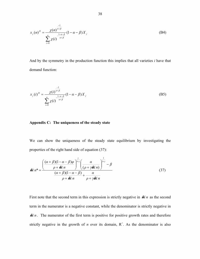
Appendix C: The uniqueness of the steady state

We can show the uniqueness of the steady state equilibrium by investigating the

properties of the right hand side of equation (37):

nnγρα

nnρβαβα

βnnγρ

αnnρ

φβαβα

nn

γγγ

//)1)((

)/(/)1)((

*/

11

1

&&

&&&

++

+−−+

−

+

+

−−+

=

++

(37)

First note that the second term in this expression is strictly negative in nn /& as the second

term in the numerator is a negative constant, while the denominator is strictly negative in

nn /& . The numerator of the first term is positive for positive growth rates and therefore

strictly negative in the growth of n over its domain, R+. As the denominator is also

39

strictly positive and decreasing in the growth rate of n the total effect is not immediately

clear. We do know, however, that in the limit to infinity, the right hand side of (37) will

become negative. For growth rates of 0 the right hand side of (37) simplifies to:

( )αβαβα

βραφβαβαRHSγ

γγ

+−−+−−−+

=+

+

)1)(()1)(( 1

1

1 (C1)

Which is a positive constant for small enough ρ, implying that a positive steady state

growth rate is unique and stable if consumers are patient and do not discount the future

too much. In that case the investments in R&D and entry can actually be financed as their

returns exceed the required return on postponing consumption. This implies there is a

unique steady state growth rate of n for which (37) holds. Q.E.D.

40

References

Acemoglu, D., S. Johnson and J. Robinson,(2001), “The Colonial Origins of Comparative

Development: An Empirical Investigation”, American Economic Review, Vol. 91 (5), pp.

1369-1401.

Acs, Z.J., D. B. Audretsch, P. Braunerhjelm and B. Carlsson, (2004), “The Missing Link: The

Knowledge Filter and Entrepreneurship in Endogenous Growth”, Center for Economic

Policy Research Discussion Paper, No. 4783.

_(2006) “The Knowledge Spillover Theory of Entrepreneurship,” Center for Economic Policy

Research Discussion Paper, No. 5326.

Aghion, P. and P. Howitt, (1992), “A Model of Growth through Creative Destruction.”

Econometrica, Vol. 60, pp. 323-51.

_(1998), Endogenous Growth Theory, MIT-press, Cambridge, MA.

Allred, B. and W. Park, (2007), “The Influence of Patent Protection on Firm Innovation

Investment in Manufacturing Industries”, Journal of International Management, Vol. 13,

pp. 91-109.

Audretsch, D., (2007), The Entrepreneurial Society, Oxford University Press, Oxford.

Barro, R. (1996),”Democracy and Growth”, Journal of Economic Growth, Vol. 1(1), pp. 1-27.

Barro, R. and X. Sala-I-Martin, (2004), Economic Growth, 2nd Ed., MIT-press, Cambridge, MA.

41

Branstetter, L.,. R. Fishman and F. Foley, (2006), “Do Stronger Intellectual Property Rights

Increase International Technology Transfer? Empirical Evidence form US Firm-Level

Panel Data”, Quarterly Journal of Economics, Vol. 121(1), pp. 321-349

Furukawa, Y., (2007),”The Protection of Intellectual Property Rights and Endogenous Growth:

Is Stronger always Better?”, Journal of Economic Dynamics and Control, Vol. 31, pp.

3644-3670.

Glaeser, E., R. La Porta, F. Lopez de Silanes and A. Shleifer, (2004) "Do Institutions Cause

Growth?", Journal of Economic Growth, Vol. 9(3), pp. 271-303.

Gould, D. and W. Gruben, (1996),”The Role of Intellectual Property Rights in Economic

Growth”, Journal of Development Economics, Vol. 48, pp. 323-350.

Greasley, D. and L. Oxley, (2007),”Patenting, Intellectual Property Rights and Sectoral Outputs

in Industrial Revolution Britain, 1780-1851”, Journal of Econometrics, Vol. 139, pp.

340-354.

Grossman, G. and E. Helpman, (1991), Innovation and Growth in the Global Economy, MIT-

press, Cambridge, MA.

Horii, R. and T. Iwaisako, (2007),”Economic Growth with Imperfect Protection of Intellectual

Property Rights”, Journal of Economics, Vol. 90(1), pp. 45-85.

Iwaisako, T. and K. Futagami, (2003), “Patent Policy in an Endogenous Growth Model”, Journal

of Economics, Vol. 78, pp. 239-258.

42

Jaffe, A., and J. Lerner, (2004), Innovation and its Discontents: How our Broken Patent System

is Endangering Innovation and Progress, and What to Do About It, Princeton University

Press, Princeton, NJ.

Jones, C., (2006), “Growth and Ideas,” in: Aghion, P. and S. Durlauf (Eds.), Handbook of

Economic Growth, Vol. 1, Part 2, Elsevier Publishers, New York.

Klepper, Steven (2007) “Disagreements, Spinoffs and the Evolution of Detroit as the Capital of

the U.S. Automobile Industry,” Management Science, Vol., pp..

Knight, F., (1921), Risk, Uncertainty and Profit, Hart, Schaffner & Marx; Houghton Mifflin

Company, Boston, MA.

Kwan, Y. and E. Lai, (2003),”Intellectual Property Rights Protection and Endogenous Economic

Growth”, Journal of Economic Dynamics and Control, Vol. 27, pp. 853-873.

Romer, P., (1986), “Increasing Returns and Long-Run Growth”, Journal of Political

Economy, Vol. 94 (5), pp. 1002-1037.

_(1990), “Endogenous Technological Change”, Journal of Political Economy, Vol. 98, pp. S71-

S102.

Sala-I-Martin, X. (1996), "I Just Ran Two Million Regressions", American Economic Review,

Vol. 87(2), pp. 178-183.

Walsh, C. (1998), Monetary Theory and Policy, The MIT-Press, Cambridge, MA.