NBER WORKING PAPER SERIES

WHEN INCENTIVES BACKFIRE:SPILLOVER EFFECTS IN FOOD CHOICE

Manuela AngelucciSilvia Prina

Heather RoyerAnya Samek

Working Paper 21481http://www.nber.org/papers/w21481

NATIONAL BUREAU OF ECONOMIC RESEARCH1050 Massachusetts Avenue

Cambridge, MA 02138August 2015

We are grateful to Tristin Ganter, Justin Holz, and the rest of the Behavioral and Experimental Economics(BEE) Research Group at the University of Chicago for conducting the experiment, to Meera Mahadevanand Irvin Rojas for their outstanding research assistance, and to Michele Belot, Marianne Bitler, KittCarpenter, David Chan, Silke Forbes, Peter Kuhn, Pedro Rey Biel, Scott Shane and seminar participantsat the NBER Summer Institute, University of Michigan, University of Chicago Harris School, UniversidadPompeu Fabra, Bocconi University, and the World Bank for their comments. We have received fundingfrom the University of Michigan, the University of California-Santa Barbara, and Case Western ReserveUniversity to carry out this research. The views expressed herein are those of the authors and do notnecessarily reflect the views of the National Bureau of Economic Research.

NBER working papers are circulated for discussion and comment purposes. They have not been peer-reviewed or been subject to the review by the NBER Board of Directors that accompanies officialNBER publications.

© 2015 by Manuela Angelucci, Silvia Prina, Heather Royer, and Anya Samek. All rights reserved.Short sections of text, not to exceed two paragraphs, may be quoted without explicit permission providedthat full credit, including © notice, is given to the source.

When Incentives Backfire: Spillover Effects in Food ChoiceManuela Angelucci, Silvia Prina, Heather Royer, and Anya SamekNBER Working Paper No. 21481August 2015JEL No. C93,I1,J13

ABSTRACT

How do peers influence the impact of incentives? Despite much work on incentives, little is knownabout the spillover effects of incentives. We investigate two mechanisms by which these effects canoccur: through peers' actions and peers' incentives. In a field experiment on snack choice (grapes versuscookies), we randomize who receives incentives, the fraction of peers incentivized, and whether ornot it can be observed that peers' choices are incentivized among over 1,500 children in the schoollunchroom. Incentives increase the likelihood of initially choosing grapes. However, peer spillovereffects can be large enough to undo these positive effects.

Manuela AngelucciDepartment of EconomicsUniversity of MichiganLorch Hall, 611 Tappan St.Ann Arbor, MI 48109-1220mangeluc@umich.edu

Silvia PrinaCase Western Reserve UniversityWeatherhead School of Management11119 Bellflower Road, Room 273Cleveland, Ohio 44106-7235silvia.prina@gmail.com

Heather RoyerDepartment of EconomicsUniversity of California, Santa Barbara2127 North HallSanta Barbara, CA 93106and NBERroyer@econ.ucsb.edu

Anya SamekUniversity of Southern Californiaanyasamek@gmail.com

1 Introduction

Incentives are a cornerstone of economics. As such, their use is frequent in many domains,

including education, health, pro-social behavior, and the labor market.1 While often being

successful at improving behaviors or outcomes, incentives can backfire. This is because incentives

can act as both prices and signals. While the price effect of a higher incentive increases takeup,

the signaling effect may increase or decrease takeup.

For example, incentives can signal information about the difficulty of the task (Benabou and

Tirole, 2003) or the quality of the good incentivized (e.g., Nelson (1970); Shapiro (1983); Milgrom

and Roberts (1986)). In addition, incentives may make a subject feel controlled (deCharms,

1968) or, more broadly, convey “bad news” (Gneezy, Meier and Rey-Biel, 2011). Consistent

with this signaling theory, Gneezy and Rustichini (2000) find in two separate experiments that

performance on a task falls when small monetary incentives are offered, compared to offering no

monetary incentives. Fischer et al. (2014) find that the subsequent demand for various products

decreases with their introductory price.2

One limitation of the literature on the signalling effects of incentives is that it focuses on

the effects of incentives on their recipients (the direct effects), neglecting the spillover effects

of incentives.3 For example, consider paying students to read books. The direct effect of the

incentive program, absent the influence of peers, may result in students reading more books. At

the same time, these incentives cause two types of spillover effects. One spillover effect operates

through observing peers’ behavior and a second works through observing peers’ incentives. If

I see my friends read, then I may think that reading is interesting and pleasant. However, if I

see my friends incentivized to read, I may think that reading is hard. That is, the two spillover

effects are not necessarily of the same sign or magnitude. Two implications of considering the

signalling effects of incentives are 1) spillover effects are of indeterminate sign and 2) the overall

effect (i.e., the sum of the direct and spillover effects) may differ from the direct effect.

In this paper, we design and conduct a field experiment to measure the net effect of incentives

and decompose it into its direct effect and its spillover effects. We incentivize the choice of grapes

1A not nearly-exhaustive list of these studies include Volpp et al. (2008, 2009); Charness and Gneezy (2009);Acland and Levy (2015); Babcock and Hartman (2010); Babcock et al. (forthcoming); Cawley and Price (2013);John et al. (2011); Royer, Stehr and Sydnor (2015); Belot, Jonathan and Patrick (2013); List and Samek (2014,2015) for healthy behaviors, Angrist, Lang and Oreopoulos (2009); Bettinger (2012); Fryer Jr (2011); Levitt et al.(2011); Levitt, List and Sadoff (2011) for academic achievement, Ariely, Bracha and Meier (2009); Lacetera andMacis (2010); Lacetera, Macis and Slonim (2013) for pro-social behavior, and Gneezy and List (2006); Fehr andList (2004); Bandiera, Barankay and Rasul (2013); Shearer (2004) for worker effort.

2See Deci, Koestner and Ryan (1999) for a meta analysis of the evidence from psychology and Gneezy, Meierand Rey-Biel (2011) and Kamenica (2012) for evidence from economics.

3Following the taxonomy of Angelucci and Di Maro (2015), we define spillover effects in this paper as peersocial interaction effects.

2

versus cookies of 1,600 children in grades K-8 in a low-income Chicago neighborhood. Almost

a third of US children aged 2-19 are now deemed overweight or obese, and part of the problem

is the habitual decision to consume high calorie, low nutrient foods (Ogden et al., 2010). Thus,

incentivizing the choice of healthy food may be one policy tool to reduce the rates of overweight

and obesity.

We first let students choose grapes or cookies simultaneously while seated at lunch tables,

which define our peer network. Later, students can switch their minds after observing their

peers’ actions. To identify the direct effect of incentives, we randomize who is incentivized

to choose grapes. To isolate the two spillover effects of incentives, we randomize both the

fraction incentivized at each table and whether a student’s choice of incentivized grapes is public

knowledge (our public treatment). Randomizing the fraction of tablemates incentivized allows

us to identify the spillover effects under weaker assumptions than much of the prior literature.4

To separate the spillover effects of peers’ actions from the spillover effects of peers’ incentive

status, we randomize whether incentive status is public information. Lastly, to separate the

direct and spillover effects, we also record the initial and final snack choices

We report three main findings. First, incentives increase the likelihood of initially choosing

grapes by over 50%, from 49% to 75%. Second, the spillover effect of observing peers’ choices is

positive. The effect grows monotonically with the peer fraction incentivized and is between one

third to one half as large as the direct effect of incentives. Third, in contrast, the overall spillover

effect of observing both peers’ food choice and whether they picked incentivized grapes is at first

a positive but then a negative function of the fraction of table mates incentivized. When peer

incentives are visible, the overall effect of incentives (i.e., combining the direct and spillover

effects) is largest when roughly 70% of table mates are incentivized. The takeup of grapes for

the 100% incentivized group is not statistically different from that of the 0% incentivized group.

We attempt to disentangle the mechanisms behind these spillover effects. The results are not

consistent with models of conformity where there is a desire to conform to one’s best friends,

popular kids, or kids of the same gender. We also rule out that the spillover effects are mainly

driven by a desire for anti-conformism and by envy of other children’s incentive status.

Our findings have three broad implications. First, to understand the full impact of incentives,

which is policy relevant, one should design experiments that allow for spillover effects to operate.

4As summarized by Baird et al. (2014), the previous literature identifies spillover effects by not treating somegroup members (e.g., Angelucci and De Giorgi (2009); Barrera-Osorio et al. (2011); Bobonis and Finan (2009);Duflo and Saez (2003); Lalive and Cattaneo (2009); Guiteras, Levinsohn and Mobarak (2015)), by using plausibleexogenous variation in the fractions of peers treated (e.g., Babcock and Hartman (2010); Beaman (2012); Conleyand Udry (2010); Duflo and Saez (2002); Munshi (2003)), and by looking at differential treatment effects withina predetermined peer group (e.g., Banerjee et al. (2013); Chen, Humphries and Modi (2010); Macours and Vakis(2008); Neumark-Sztainer et al. (2012)).

3

Failure to do that might result in imprecise policy recommendations because the direct and

spillover effects can offset one another. For example, in our experiment, the direct effect of

incentives can be larger than the net effect of incentives, when incentives are public.

Second, the presence of non-linearities makes extrapolation and policy scale-up from field

experiments challenging. For example, in our experiment, the overall effect of incentives in

the public treatment is positive when we incentivize up to 70% of table mates. If we had not

incentivized higher fractions of table mates, we may have incorrectly assumed that the treatment

effects would be at least as large as the 70% group and therefore, erroneously deduced that

incentivizing all children maximizes take-up, when in fact incentivizing all children does not

statistically change take-up rates, compared to incentivizing no children. While the existence

of “social multipliers” (Glaeser, Sacerdote and Scheinkman, 2003) is well known, the implicit

assumption – backed by abundant empirical evidence – is that the multiplier is positive and that,

therefore, the direct effect of incentives is a lower bound of its net effect (in absolute level).5

Given that most policies treat subsets of the population, either because of budget constraints

or eligibility cutoffs, the possibility that the social multiplier may be negative has important

practical relevance.

Third, if observing others’ incentives reduces take-up, private incentives may be preferable.

However, keeping incentives private may not be feasible in most settings, as people communicate

and interact.

While one should be cautious in generalizing our results, evaluating the spillover effects of

incentives may be worthwhile in several settings. The first type of setting is one in which the

value of the incentivized action is not well known and in which subjects believe peers and policy

makers may have private information (e.g., new technology adoption). In such settings incentives

allow subjects to learn from peers’ and policymakers’ actions. However, as the signalling effects

of incentives can be both negative and positive, careful consideration should be made when

invoking incentive schemes for public policy. For example, the Physician Payment Sunshine

Act, which requires drugs manufacturers to disclose certain payments to physicians, may reduce

the demand for drugs from the paying manufacturers, if the payments are perceived to signal

that the drugs of a given manufacturer are not as effective as others. The second type of

setting is one in which the incentivized behavior has short-run costs but long-run benefits (e.g.,

nutrition, exercise, education, and other behaviors that increase health and human capital).6

5Examples include the takeup of welfare (Borjas and Hilton, 1996; Bertrand, Luttmer and Mullainathan,2000), employer-sponsored health insurance (Sorensen, 2006), retirement plans (Duflo and Saez, 2003), publicprenatal care (Aizer and Currie, 2004), disability insurance (Rege, Telle and Votruba, 2009) and movie attendance(Moretti, 2011), among others.

6Gneezy, Meier and Rey-Biel (2011) review the evidence of incentives backfiring in this type of setting.

4

In this case, the incentive may increase the salience of the short-term cost over the long-term

benefit of the incentivized action. The third type of setting is in pro-social behaviors, such as

recycling, charitable giving, or blood donation, whose ‘warm-glow’ value exceeds the monetary

value of incentives. Finally, the fourth possible setting is in interesting or pleasant activities,

where incentives may reduce interest in the task.7

2 Theory

In this section, we present a simple model, in the spirit of Benabou and Tirole (2003), that

highlights potential mechanisms that would give rise to both positive and negative direct and

spillover effects.

Consider the choice of grapes versus cookies for child i in a setting with asymmetric informa-

tion. The child decides to pick grapes over cookies if the expected private benefits of this choice

exceed its costs. The child’s beliefs of the benefits, Bi, depend on her idiosyncratic taste, τi, as

well as on the behavior of her peers and of the experimenter, whom the child believes to have

private information about the relative value of grapes over cookies, such as their comparative

health benefits. The child observes the behavior of her peers and of the experimenter to infer

their private information.8 The choice depends also on the monetary (or cash-equivalent) cost

of choosing grapes over cookies, C. This cost is a function of incentives, I.

The child observes a signal of the private information of her peers and of the experimenter

from their actions. In our experiment, she observes i) the fraction of her peers who choose

grapes over cookies, G−i, ii) the fraction of her peers who choose incentivized grapes, I−i, and

iii) whether she is incentivized to pick grapes, I. I−i is a lower bound of the fraction of peers

who were incentivized to choose grapes, TP . In our experiment, we can distinguish behavior in

response to i) versus ii).

In sum, the expected utility of choosing grapes over cookies can be expressed as:

E[U(Gi = 1)− U(Gi = 0)] = Bi(τi, G−i(TP ), I−i(TP ), I)− C(I) (1)

7Kamenica (2012) review the evidence of incentives backfiring for the last two settings.8The benefits of choosing grapes over cookies may also depend on social conformity, as we discuss in Section 8.

Our empirical results, detailed in that section, point against social conformity as an explanation for the behaviorswe find, and, thus, we exclude it from the description of the model below.

5

2.1 Direct Effect of Incentives

Consider first the direct effect of incentives, I on the incentivized person:

∂E[U(Gi = 1)− U(Gi = 0)]

∂I=

∂Bi

∂I−

∂C

∂I(2)

The first right-hand side term, ∂Bi

∂I, is the effect of introducing (or increasing) the incentive

on the child’s belief on the relative value of grapes over cookies. The sign of this effect is

indeterminate. For example, in Benabou and Tirole (2003), being incentivized (or having a

higher-valued incentive) signals “bad news” – e.g., that the action is unpleasant, perhaps because

grapes do not taste as good as cookies.9 This may make her revise her prior beliefs about the

benefits of grapes downward. On the other hand, the incentive may signal that the experimenter

thinks grapes are really good for the child (maybe despite not tasting as good as the cookie),

inducing her to revise her prior belief of the benefits of grapes upward.

Conversely, the second right-hand side term, ∂C∂I

, which represents the effect of the incentives

on cost, is positive, as compensating the child to pick grapes over cookies reduces its cost.

In sum, the sign of the direct effect is unknown, due to the ambiguity of the sign of ∂Bi

∂I.

Note the direct effect we modeled allows for peer influences. For example, a child may

initially choose cookies because she wants to be popular.

2.2 Spillover Effects of Incentives

Now consider the effect of the fraction incentivized. This is what we call the spillover effect. To

do that, consider an increase in the proportion of children who are incentivized to pick grapes,

TP , which affects the fraction of her peers who initially choose grapes over cookies, G−i, and

who initially choose incentivized grapes, I−i.

∂E[U(Gi = 1)− U(Gi = 0)]

∂TP=

∂Bi

∂G−i

∂G−i

∂TP+

∂Bi

∂I−i

∂I−i

∂TP(3)

The first right-hand side term, ∂Bi

∂G−i

∂G−i

∂TP, is the spillover effect of incentives through watching

others pick grapes and has an indeterminate sign. The sign of ∂Bi

∂G−iis positive, if an increase

in the proportion picking grapes sends a positive signal about the value of grapes.10 Therefore,

9In Benabou and Tirole (2003), a principal has private information about attractiveness of an action andmay offer larger incentives for less attractive tasks. The agent, therefore, expects larger incentives to signal moreunpleasant tasks and may be less motivated to do it.

10The sign of ∂Bi

∂G−i

can also be negative. We do not explicitly model this option because it would increase the

number of possible cases, and thus lengthen the exposition, without adding to our main point that the direct andspillover effects may have opposite signs. Moreover, the sign of ∂Bi

∂G−i

is positive in our data, so modelling this

6

the sign of this first term depends on how increasing the proportion incentivized affects the

proportion picking grapes initially, ∂G−i

∂TP. This has the same sign as the direct effect of incentives.

The second right-hand side term, ∂Bi

∂I−i

∂I−i

∂TP, is the spillover effect of incentives through watch-

ing others pick incentivized grapes. It has an indeterminate sign because the signs of its two

parts are both indeterminate. The sign of ∂Bi

∂I−idepends on how children interpret the experi-

menter’s intent to incentivize children to pick grapes and, therefore, has the same sign as ∂Bi

∂I.

∂I−i

∂TPhas the same sign as the direct effect.

There are, therefore, the following 3 cases, also summarized in Table 1:

Case 1: Incentives send a weakly positive signal on the value of grapes (∂Bi

∂I≥ 0). When

this happens, the direct effect of incentives is positive, as ∂Bi

∂I−

∂C(I)∂I

> 0. If the direct effect is

positive, then increasing the proportion incentivized increases the proportion choosing grapes,

incentivized or not, (∂G−i

∂TP> 0 and ∂I−i

∂TP> 0). Moreover, if the incentive sends a weakly positive

signal on value of grapes, then the belief of the value of grapes grows with the proportion of

children choosing incentivized grapes, ∂Bi

∂I−i≥ 0, and, therefore, the spillover effect of incentives

is also positive. That is, in this case the spillover effects reinforce the direct effects.

Case 2: Incentives send a negative signal on the value of grapes (∂Bi

∂I< 0), but the direct

effect is positive, because the cost reduction more than offsets the negative signal for incentivized

children, ∂Bi

∂I<

∂C(I)∂I

. If the incentive sends a negative signal on value of grapes, then the belief

of the value of grapes decreases with the proportion of children choosing incentivized grapes,

∂Bi

∂I−i< 0. Moreover, if the direct effect is positive, then increasing the proportion incentivized

increases the proportion choosing grapes, incentivized or not, (∂G−i

∂TP> 0 and ∂I−i

∂TP> 0). Because

of these opposite effects, the sign of the spillover effect is indeterminate: the first term is positive,

while the second is negative. That is, in this case the spillover effects may either reinforce or

offset the direct effects.

Case 3: Incentives send a negative signal on the value of grapes (∂Bi

∂I< 0) and the direct

effect is negative, because the cost reduction is offset by the negative signal for incentivized

children, ∂Bi

∂I<

∂C(I)∂I

. If the incentive sends a negative signal on value of grapes, then the belief

of the value of grapes decreases with the proportion of children choosing incentivized grapes,

∂Bi

∂I−i< 0. Moreover, if the direct effect is negative, then increasing the proportion incentivized

reduces the proportion choosing grapes, incentivized or not, (∂G−i

∂TP< 0 and ∂I−i

∂TP< 0). Because

of these effects, the sign of the spillover effect is indeterminate: the first term is negative, the

second positive. That is, in this case the spillover effects may either reinforce or offset the direct

effects.

option is not essential in this application.

7

In sum, we have the following 3 broad conclusions. First, we have shown that incentives may

have both a positive and a negative direct effect.11 Second, when incentives are “bad news”

(∂Bi

∂I< 0), the spillover effects of incentives can have both a positive and negative component.

Third, when incentives are “bad news,” the direct and spillover effects of incentives may

offset each other. Therefore, in this model, the direct effect may be a poor approximation of the

overall effect of incentives.

Based on this model, we can use our experiment to identify the direct and spillover effects

of incentives. The actual grape choice, G2, is the sum of the grape choice in the absence of

spillover effects, G1 (the direct effect) and the spillover effects ∆G. That is, G2 = G1 +∆G.

Before we proceed to describe how we identify and estimate the direct and spillover effects

of incentives, note that a model with perfect information but with a short term cost and a long

term benefit of choosing grapes over cookies would generate similar predictions, if the public

incentives make the short term cost more prominent and hence reduce the likelihood of choosing

grapes. This would change the mechanisms behind our findings, but not our empirical setup.

3 Background and Experimental Design

To measure the direct and spillover effects of incentives, we designed an artefactual field exper-

iment (Harrison and List, 2004) in which we offer grapes and cookies to children and randomly

offer incentives to choose grapes.12 This field experiment took place in school cafeterias during

lunch. Nine elementary schools in Chicago Heights, Illinois participated. Lunch is administered

in much the same way in each of these schools. Depending on their size, schools hold either 2,

3 or 4 lunch periods each day, assigning kids to periods based on their school grade. Children

arrive for lunch during their designated lunch period together with their class. They go through

a lunch line where they receive a school lunch and then sit at a table in the cafeteria. Except

for kindergartners, students can typically sit with any other children from their grade and tend

to form groups of 3-10 students at each table. In this school district, children do not have a

choice about their lunch. Moreover, Chicago Heights, Illinois is in a low-income neighborhood

and most children qualify for free or reduced-price lunch, meaning that all kids eat the same

school-provided meal each day.

We conducted the experiment after children had collected their lunch trays and sat down

to eat at their table. Once children were seated, members of the research team came to the

11In empirical settings such as ours, we cannot separately identify the positive and negative direct effects ofincentive, as we observe only their sum.

12Grapes, but not cookies, are sometimes served at lunch.

8

table and read a script announcing the procedures of the experiment.13 To minimize cross-table

contamination, we treated adjacent tables simultaneously. Each child was asked to pick both a

grape card (green on the back) and a cookie card (blue on the back) from a card deck (see Figure

1). To facilitate data collection, each child’s ID number from the experiment was written on

each of his or her cards. Then, each child made a choice: he or she could either choose to have

grapes as an additional food (by placing the grape/green card down on the table), or he or she

could choose to have cookies as an additional food (by placing the cookie/blue card down on the

table). Children were told that they could only choose one snack, and that the actual food item

they had selected would be delivered to their table immediately at the end of the experiment.

The initial choice was always made simultaneously and children were asked not to talk during

the experiment. After the initial choice, children were given a chance to play a different card

after having observed their peers’ choices.

We randomized 1) which child received an incentive to choose grapes, 2) which fraction of

each lunch table received an incentive to select grapes, and 3) in which tables choosing incen-

tivized grapes is visible by peers (public treatment) or not (private treatment). In particular,

for each table, we had a stack of cards, which had either 0, 50, or 100% of cards with incentives.

At tables with the 50% of incentivized cards, the actual fraction of children receiving incentives

varies between 11 and 80 percent. This variation is seen in Table 2.

In all treatments, children were alerted to the possibility that they may be eligible for a

prize depending on the card they draw, and a poster with all possible prizes was displayed to

the kids. The value of the prizes was roughly 50 cents. The prizes included glow-in-the-dark

bouncy balls, small trophies, and bracelets and pens of different types.

If students were eligible for an incentive, their grape card depicted a small gold token. For

the 50 percent incentive treatment, the cards came from a deck where 50 percent of the grape

cards portrayed a gold token. In the 100 percent incentives treatment, all the grapes cards

depicted the coin.

In the private treatment, children play their cards face down, so that children can observe

only the color of the card, but not the presence or absence of the incentives. In the public

treatment, on the other hand, children play their cards face up, so that anyone at the table can

observe whether the chosen grapes are incentivized or not.

With the three levels of randomization, we can divide children into eight groups:

• Private-0 (Group 1): Children in the Private treatment in which none of the grape cards

were incentivized.

13The script of the experiment is reported in Appendix 9.

9

• Public-0 (Group 2): Children in the Public treatment in which none of the grape cards

were incentivized.

• Private-50-no incentive (Group 3): Children in the Private treatment in which 50% of the

grape cards were incentivized but the child’s own card was not incentivized.

• Private-50-incentive (Group 4): Children in the Private treatment in which 50% of the

grape cards were incentivized and the child’s own card was incentivized.

• Public-50-no incentive (Group 5): Children in the Public treatment in which 50% of the

grape cards were incentivized and the child’s own card was not incentivized.

• Public-50-incentive (Group 6): Children in the Public treatment in which 50% of the grape

cards were incentivized and the child’s own card was incentivized.

• Private-100-incentive (Group 7): Children in the Private treatment in which all of the

grape cards were incentivized.

• Public-100-incentive (Group 8): Children in the Public treatment in which all of the grape

cards were incentivized.

We designed the experiment by randomizing each school-by-period table is such a way as to

have one quarter of the school-by-period tables assigned to the 0% and 100% treatments each,

and the remaining half to the the 50% treatment, cross randomizing the public and private

treatment to have half of the school-by-period tables in each group.

We record both the initial food choice, G1, and the final food choice, G2. We use G1 to

measure the direct effect of incentives because this choice occurs simultaneously and, therefore,

before children can observe their peers’ choices and incentives. We use G2 to measure the

spillover effect of incentives because this final choice occurs after having observed peers’ choices

and incentives.

4 The data

4.1 Sample

A total of 1,771 children participated in the experiment, conducted during lunch in the school

cafeteria. Children choose a table to sit at. We drop 14 tables of 10 from the main analysis

because we do not believe that kids can see all others’ decisions at such a large table. The results

in the next section are qualitatively unchanged if we include tables with 10 children.

10

We complement the experimental data with a short survey assessing the social networks of

kids (available upon request). The survey included questions asking children to name up to 5

of their friends. The survey also included questions about each child’s perceived social status

relative to other children, and asked children to name the most popular kid boy and girl in their

class. A total of 1,286 children filled out the questionnaire.

After dropping large tables, our final sample consists of 1,631 children, of whom 1,187 com-

pleted the questionnaire, sitting at 270 school-by-period tables.14

The final size of each of the 8 groups varies because some of the tables in the cafeteria were

empty. Moreover, in various instances we ran out of time and could not reach all the occupied

tables.

4.2 Descriptives, balance tests, and food choice

Table 3 shows the mean and standard deviations of several socioeconomic variables for each

of the eight groups. Lunch tables have on average 6.45 children of which 47 percent are boys.

The average grade is fourth grade, 39% of children at each table are African American and 52%

are Hispanic, and 87% of the children at each table are on the free lunch program. Overall,

looking at Table 3 it appears that these variables are balanced across groups. This is confirmed

in lower panel of Table 3, which shows the F-test of joint significance of the 8 group dummies,

when regressed on each of these variables together with school-by-period strata. All variables

are balanced across groups, consistent with random assignment, since none of the F-tests are

significant at conventional levels.

We also check for balance using the actual fraction of student incentivized. Recall, while the

grape cards for the 50% incentivized tables were drawn from a deck where half of the cards were

incentivized, the actual fraction incentivized deviated from 50%. We regress the proportion of

children incentivized at each table on table size and children’s age, gender, race, grade, and

school lunch status (free, reduced, or none), as well as on school-by-period strata. The F-test of

joint significance of the coefficients of the socioeconomic variables has a p-value of 0.087. This

is driven by a smaller table proportion incentivized for third and six graders. Once we exclude

grade, the F-test of joint significance of the coefficients of the remaining socioeconomic variables

has a p-value of 0.543. For this purpose, and to improve the precision of the estimates, we

control for all the aforementioned variables in all our specifications. The results are qualitatively

unchanged whether we add these variables or not.

14Non-participation in the survey is also due to a number of reasons: either children were too young, or teachersoverseeing the lunch period asked us not to administer the survey, or not enough time was available for all childrento complete the survey.

11

Our two main variables of interest are the initial and final choice of grapes. For the initial

choice, the only systematic variation in grape choice should be due to whether or not the child was

incentivized. At this point of the experiment, the choices of peers are not observed. A student’s

final choice will possibly be the combination of incentive and spillover effects. Table 4 shows that

overall 62% of children choose grapes initially (combining the incentivized and non-incentivized

groups). Not surprisingly, the proportion differs for incentivized and non-incentivized children.

However, the p-value of the F-test of joint significance of the group dummies regressed on initial

choice and controlling for being incentivized is 0.168, consistent with random assignment. The

final snack choice does differ across each of the incentivized groups and separately across the

non-incentivized groups. This is our first evidence of the presence of spillover effects, which we

explore further in detail.

5 Direct effects of incentives

Our first task is to establish the effect of incentives on the recipients, that is, whether receiving

the incentives changes the recipients’ likelihood of initially choosing grapes. This is what we

refer to as the direct effect of the incentives.

We test the hypothesis that incentives have direct effects by comparing the initial grape

choice of incentivized and non-incentivized children. To do so, we regress child i’s initial grape

choice, G1, on a dummy variable, I, that equals 1 for children who receive incentives. To improve

the precision of the estimates, we further condition on the following variables X: school-by-

period strata, table size, child age, gender, race, grade, and school lunch status.

G1i = α0 + α1Ii + α2Xi + ǫi (4)

The coefficient α1 identifies the average treatment effect of incentives on initial grape choice.

This parameter is identified under random assignment, which ensures independence between the

variable I and the error term ǫ. We estimate the parameters of this equation by OLS, clustering

the standard errors by table. We use the same estimator, controls, and clustering for all the

regressions in this paper.

We can also interact the incentive dummy by a dummy for the public (P = 1) and private

(P = 0) treatments:

G1i = λ0 + λ1Ii + λ2Pi + λ3IiPi + λ4Xi + ǫi (5)

12

This way, we can test i) whether the direct effects of incentives are identical in the public and

private treatment (λ3 = 0) and ii) whether the initial grape choice is identical in the public and

private treatments for non-incentivized children (λ2 = 0) and incentivized children (λ2+λ3 = 0).

Table 5 shows the direct effects of incentives on the initial choice of incentivized children

(the estimate of α1 from equation (4)). This estimate is a 26 percentage point, statistically

significant increase in initial grape take-up over a 49.5% take-up rate among non-incentivized

children, i.e. a 53% increase in take-up.

These findings are comparable in size with Just and Price (2013), who increase children’s

consumption of salad by 80% after offering up to $0.25 (or a lottery ticket with the same expected

value), and smaller, but consistent, with List and Samek (2014, 2015), whose incentives have a

two- to four-fold increase in the choice of healthy snacks. Conversely, our effects are larger than

the ones in Belot, Jonathan and Patrick (2013), whose piece-rate incentives to choose an extra

vegetables side dish have a small, statistically insignificant effect.

A child’s initial choice may depend on whether others can observe her incentive status.

Recall that in private treatment, the cards are played face down and, therefore, one can infer

other children’s choices from the color of the card, but not whether a child was incentivized. On

the other hand, for the public treatment, the cards are played face up and the incentives can

be observed. To test whether children behave differently when they know others can observe

whether or not they are incentivized, the second row of Table 5 provides the estimate of the

difference in effect sizes in the public and private treatment (the estimate of λ2 from equation

(5)). This difference is only 0.013 and is statistically insignificant.

The third and fourth rows of the tables show that the initial grape choice is 8.4 and 7.1

percentage point lower in public treatments for both non-incentivized and incentivized children

(the estimates of λ2 and λ2 + λ3 from equation (5)). This is broadly consistent with the views

that incentives may signal “bad news” (e.g., Gneezy, Meier and Rey-Biel (2011)) or make the

short term costs of picking grapes over a cookie more salient.15

6 Spillover effects of incentives

Finding positive direct effects of incentives corresponds to cases 1 and 2 from our theory: seeing

peers choose grapes may have a positive spillover effect on own grape take-up, while seeing

others choose incentivized grapes may have either positive or negative spillover effects. Armed

with this knowledge, we proceed to test how, conditional on one’s initial choice, seeing other

15Note, however, that we cannot separate out the effects of making incentives salient from the effect of playingthe cards face up rather than down, which is the other major difference between the public and private treatments.

13

children pick grapes or pick incentivized grapes affects a child’s likelihood of ending up picking

grapes.

Since spillovers affect the likelihood that a child may change the card played after seeing

others, our dependent variable is the difference between the final and initial grape choice, ∆G =

G2 − G1. Therefore, we begin our analysis of spillover effects by estimating how exogenously

varying the table proportion incentivized, TP ∈ [0, 1], affects ∆G:

∆Gi = β0 + β1TPi + β2TPi ∗ Pi + β3Ii + β4Pi + β5IiPi + β6Xi + ǫi (6)

Children do not observe the variable TP . However, this variable is under the control of the

policy maker, and thus its impact is of policy relevance. Moreover, it is positively correlated

with the fraction of table mates choosing grapes.16 The dummy variable P equals 1 for the public

treatment and 0 for the private treatment. We condition on being incentivized (I) and on the

public treatment dummy because they affect the initial grape choice, which, in turn, affects the

likelihood of ending up with grapes. We add the interaction with the public treatment dummy

because we estimate different parameters for the two treatments.17,18

Under random assignment, the parameter β1 identifies the marginal effect of the proportion

of incentivized children at one’s table in the private treatment, while β2 identifies the difference

in the effect of this proportion between the public and private treatments. β1 and β2 are two

separate spillover effects on one’s own choice: β1 is the reduced-form effect of observing peers’

choices and β2 is the reduced-form effect of observing whether peers’ choices are incentivized.

Table 6 shows the estimates of our parameters of interest, β1 and β2 from equation (6).

Column 1 shows that a 1% increase in the proportion incentivized in the private treatment

increases the likelihood of switching to grapes by 0.09 percentage points (s.e. 0.05). A positive

effect in the private treatment, in which children can observe the food choices of others but not

whether these choices are incentivized, suggests that watching other children pick grapes has a

positive spillover effect on the likelihood of switching to grapes. The second row of estimates in

column 1 shows that the effect of the proportion incentivized changes when the incentives are

public. Relative to private incentives, a 1% increase in the proportion incentivized additionally

decreases one’s likelihood of switching to grapes by 0.18 percentage points (s.e. 0.08). Therefore,

16The correlation coefficient is 0.27.17The results do not change whether we interact by public treatment or not, or whether we estimate the

parameters of equation 6 or of equation G2i = β0 + β1TPi + β2TPi ∗ Pi + f(βIPGIiPiG1i) + β3Xi + ǫi, wherethe term f(βIPG1

IiPiG1i) is the triple interaction of the incentive treatment, public treatment, and initial grapechoice dummies.

18In unreported regressions, we replace the table proportion incentivized with the table proportion incentivizedother than self and the results are qualitatively unchanged.

14

the net spillover effect of public incentives (i.e., the effect from increasing the table proportion

who is incentivized), in the third row, is negative (−0.09 = 0.09− 0.18; s.e. 0.06).

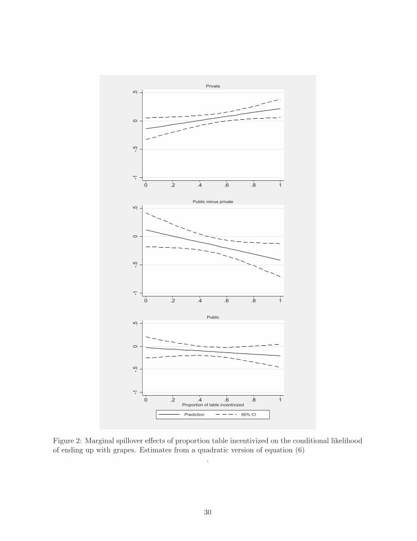
These marginal effects of the table proportion incentivized in public and private treatments

may be non-linear. That is, the effect of the proportion of students who are incentivized does

not have to be linear, as specified in equation (6). To test this hypothesis, we restrict the

sample to tables with a positive proportion of incentivized children (column 2) and with at least

50% of incentivized children (column 3), in which case the overall table proportion incentivized

increases from 50% to 66% (column 2) and to 80% (column 3).19 When we do that, we find that

the two marginal effects become considerably larger (in absolute value), especially the negative

effect of observing other children’s incentivized choices. For this reason, we re-estimate equation

(6), adding the square of the table proportion incentivized and interacting it with the public

dummy: β4TP2i + β5TP

2i ∗Pi. Figure 2 shows the marginal effects of fraction incentivized from

this equation (i.e., estimates of β1 + β2 ∗ Pi + 2β4TPi + 2β5TPi ∗ Pi) . If the effects were linear,

each of those graphs would depict a horizontal line, which they do not. The figure confirms

that the marginal effects grow in absolute level with the proportion incentivized. The marginal

effects become statistically different from zero when 40 to 50 percent of the table is incentivized.

6.1 Heterogeneity in the spillover effects

In this subsection, we consider how the effects can differ along several dimensions: i) the type

of switch - to grapes or to cookies, ii) gender and school grade, and iii) table size.

First, recall that the parameter ∆G is the difference between switching from cookie to grapes,

SG, and from grapes to cookie, SC: ∆G = SG − SC. To have a better understanding of how

spillover effects work in our setting, Table 7 considers both the separate choices of switching from

cookies to grapes and from grapes to cookies. We also examine how these effects vary across

incentivized and non-incentivized children. The estimated marginal effects are consistent with

the main results: the likelihood of switching to grapes increases with the proportion choosing

grapes (i.e., β1 is positive) and decreases with the proportion choosing incentivized grapes (i.e.,

β2 is negative). The opposite is true for the likelihood of switching to cookies. The primary

action is on the dimension of switching to grapes and not switching to cookies, as expected.

Second, we explored how the direct and spillover effects of incentives differ by gender and

grade. We discuss these results in Appendix 9. In short, the direct effects of incentives do not

differ by gender, but the spillover effects of others’ behaviors is stronger for females and the

19The sample restrictions in columns 2 and 3 drop approximately the first quartile and the first two quartilesof the fraction incentivized distribution.

15

negative spillover effect of observing others’ incentivized choices is more substantial for boys.

The direct and spillover effects do not differ significantly across grades, although both spillover

effects seem driven by younger children.

Third, a priori one might expect that the effects would differ across table size. For example,

there may be less interaction at a larger table. We divide the sample into two - above and below

median table size. We note that table size and proportion incentivized are uncorrelated (the

correlation coefficient is 0.005). There is no systematic difference by table size (results available

upon request).

7 Non-linear effects and maximizing take-up

Recall that the total effect of incentives on the final grape choice is the sum of the net direct

effect on the initial choice, G1, which we found to be positive, and the two spillover effects on

changing choice, ∆G, which we found to be one positive and the other negative. We can now

compare the estimates of the direct and spillover (Tables e 5 and 6) effects, as well as compute

their sum, which is the overall effect of incentives.

A 1 percent increase in the proportion of incentivized children has a direct effect on the

likelihood of choosing grapes of 0.26 percentage points (p-value of 0.000) and two spillover

effects. First, observing other people choosing grapes in the private treatment has a positive

effect on one’s likelihood of ending up with grapes. A 1 percent increase in the proportion

incentivized to pick grapes further increases one’s likelihood of ending up with grapes by 0.09,

0.12, and 0.16 percentage points when the proportion of children incentivized are 50, 66, and

80%.20 Therefore, the fraction incentivized that maximizes the likelihood of ending up with

grapes in the private treatment is 100%, as both the direct and spillover effects of incentives are

positive over all ranges of the fraction incentivized. However, the effects of this treatment are

likely to have limited policy relevance. That is, in most environments, the knowledge that one’s

peers are being incentivized would likely diffuse. Therefore, the public, rather than the private

treatment, is likely to be more realistic in a real world policy situation.

In the public treatment, besides the positive spillover effect discussed above, observing that

some of the chosen grapes are incentivized has an additional negative effect on the likelihood of

ending up with grapes. The corresponding point estimates are -0.18, -0.22, and -0.45 percentage

points when the proportion of children incentivized are 50, 66, and 80%. Using the point

estimates above, we find that a 1 percent increase in the proportion incentivized overall increases

20These cutoffs denote the mean incentivized, the threshold for the top 3 quartiles, and the threshold for thetop 2 quartiles.

16

in grapes take-up of 0.17 (0.26+0.09-0.18) and 0.16 (0.26+0.12-0.22) percentage points when

the mean incentivized is 50% and 66%, but reduces grapes take-up by -0.03 (0.26+0.16-0.45)

percentage points when the mean incentivized is 80%. Therefore, the incentive share that

maximizes grape take-up is between 66 and 80% in our experiment.

We can see these total effects (i.e., the combined direct and spillover effects) in Figure 3. This

figure plots the semiparametric total effect of proportion table incentivized on the likelihood

of ending up with grapes for the private and public treatments.21 While the total effect of

incentives grows with the table proportion incentivized in the private treatment, this effect is

non-monotonic in the public treatment. The total effect of incentives grows with proportion

incentivized up until this proportion is about 70%, and declines for higher proportions, to the

extent that there is no statistically significant difference in final grapes take-up between tables

with 0 and 100% incentives.

We can also examine group means. We do this in Figure 4, which reiterates our main findings

that the final grape take-up increases with the proportion of incentivized children in the private

treatment but not in the public treatment.22

8 Interpretation

There are multiple channels through which spillover effects may occur. Two possible mecha-

nisms for the positive spillover effects are learning and social conformity. The latter occurs if

children derive utility from conforming to their peers’ behavior (Sherif, 1937; Asch, 1958; Go-

eree and Yariv, 2014; Haun, Rekers and Tomasello, 2014). For example, consider the theory

discussed earlier, in which we modelled the choice of grapes or cookies for child i in a setting

with asymmetric information. Here we augment the model to include a social conformity term

in the utility function. As before, the child decides to pick grapes over cookies if the expected

private benefits of this choice exceed its costs. In addition, the child may also derive utility from

conforming to her peers’ behavior (Sherif, 1937; Asch, 1958; Goeree and Yariv, 2014; Haun, Rek-

ers and Tomasello, 2014). In that case, her expected utility depends also on a social conformity

parameter γ, which is positive.

21To do so, we use the Robinson’s semiparametric estimator (Robinson, 1988) to control for the effect of thecovariates and then smooth the effect of incentive proportion on final grape choice using a local linear regressionwith a Gaussian kernel and a rule-of-thumb bandwidth. The results are robust to changes in the kernel andbandwidth. We report both the 83% and the 95% confidence intervals. If the 83% confidence intervals aroundtwo point estimates do not overlap, the parameters are statistically different from each other at the 95% level(Peyton, Greenstone and Schenker, 2003).

22This Figure shows the difference, conditional on baseline covariates, in the fraction ending up choosinggrapes between each group and the fraction choosing grapes in group 1 (i.e., private treatment in which nobodyis incentivized), which is 0.64.

17

With social conformity, the expected utility of choosing grapes over cookies becomes:

E[U(Gi = 1)− U(Gi = 0)] = Bi(τi, G−i(TP ), I−i(TP ), I) + γi(G−i(TP ), I−i(TP ))− C(I) (7)

While the direct effect of incentives is as already described, the spillover effects of incentives,

which affect the final choice of grapes, G2, depends also on conformity, the third and fourth

right-hand-side terms in the equations below:

∂E[U(G2i = 1)− U(G2i = 0)]

∂TP=

∂Bi

∂G−i

∂G−i

∂TP+

∂Bi

∂I−i

∂I−i

∂TP+

∂γi

∂G−i

∂G−i

∂TP+

∂γi

∂I−i

∂I−i

∂TP(8)

Children may conform to picking grapes, and, if they are incentivized, also to picking incentivized

grapes. Its first parts, ∂γi∂I−i

and ∂γi∂I−i

, are positive, as children have a taste for conformity. Its

second parts, as we saw, have the same sign as the direct effect. Therefore, the spillover effects

of incentives from conformity have always the same sign as the direct effects of incentives and

do not change the three general cases we considered earlier.

Since incentives increase initial grape take-up, the higher the initial take-up, the more chil-

dren will want to conform, ending up picking grapes too. That is, conformity could explain why

there are positive spillover effects in the private treatment. On the other hand, conformity can-

not explain the negative spillover caused by seeing children pick incentivized grapes. Therefore,

even if children have a taste for conformity, receiving a negative signal about the benefits of

grapes over cookies more than dominates the effect deriving from a preference for conformity.

While conformity cannot explain our findings, we can nevertheless test specific aspects of

social conformity and see to what extent it affects children’s behavior. One way to test for

conformity is to exploit the data collected on best friends, “popular kids,” and the table gender

composition.23 This test is based on the premise that children want to conform the most to their

best friends, to children they perceive as being popular, and to children of their own gender.

If that is the case, the choices of best friends, popular kids, and children of own gender should

affect ones’ choice beyond the effect of the table’s choices as a whole. Conversely, if behaviors

are consistent with our model sketched earlier, then the choices of peers may be equally weighted

leaving the choices of best friends, popular kids, and children of own gender having no additional

effect.

Under social conformity, seeing one’s best friends (or popular kids, or children of own gender)

pick grapes has a positive spillover effect over and above the effect of the proportion of children

incentivized at the table, as the behavior of the best friend (or popular kid, or child of own

23Children report the names of up to 5 best friends and of the boy and girl they consider most popular.

18

gender) induces more conformity than the behavior of the other children at the table. In addition,

seeing one’s best friends (or popular kids, or children of own gender) pick the incentivized grape

has an additional positive spillover effect for incentivized children.

To estimate these effects, we focus on children with at least one best friend (or popular kid,

or child of own gender) sitting at their table. Because of our experiment, whether the best friend

(or popular kid, or child of own gender) is incentivized is random.

To measure the spillover effect of social conformity in picking grapes, we estimate the pa-

rameters of the spillover effect equation, equation (6), adding variables for the table proportions

of best friends (or popular kids, or children of own gender) incentivized:24

∆Gi = δ0 + δ1TPi + δ2TPiPi + δ3TPBFi + δ4TP

BFi Pi + δ5Ii + δ6Pi + δ7IiPi + δ8Xi + ǫi, (9)

where the variable TPBF is the table proportion of incentivized best friends (or popular kids,

or children of own gender), while the other variables are as discussed before.25,26 Under social

conformity of the type described above, the parameter δ3 is positive.

To measure the additional spillover effects of social conformity due to picking incentivized

grapes, we further interact the variable TPBF by the child’s incentive status, TPBF ∗ I:

∆Gi = θ0 + θ1TPi + θ2TPiPi + θ3TPBFi + θ4TP

BFi Pi + θ5TP

BFi Ii + θ6TP

BFi IiPi

+θ7Ii + θ8Pi + θ9IiPi + θ10Xi + ǫi (10)

Under social conformity of the type described above, the parameter θ6 is positive.

Table 8 reports the estimates from these regressions, using, alternatively, the entire sample,

only tables with at least one incentivized child, and tables in which at least half the children are

incentivized. This table shows that none of the estimates of the parameters of interest (i.e., δ3

and θ6) are statistically significant and that many have also a negative, rather than a positive

sign. We interpret this evidence as being inconsistent with a theory of social conformity in

which the children have preferences for conforming with their best friends, with the children

24Before doing that, we checked whether spillover effects vary for children who did not name any best friendor popular kid, for children who did not fill in the questionnaire, and for children without kids of the same gendersitting at the table. The effects for these subgroups do not differ statistically from the main effects. So the factthat we are dropping these children from the regressions may not be as disconcerting.

25For example, if in a table of size 5 there are two child j’s best friends, and one of them is incentivized, forchild j the table proportion of incentivized best friends is 1

5= 0.2.

26The variable TP is the table proportion of incentivized children, which varies from 0 to 100%, and the dummyvariable P equals 1 for the public treatment and 0 for the private treatment, in which the cards are played facedown and, therefore, one can infer other children’s choices from the color of the card, but not whether a child wasincentivized or not, and one for public treatment, in which the cards are played face up and the incentives canbe observed. The X variables are as defined before.

19

they perceive as being popular, or with children of their own gender.

The children’s behavior, and in particular the negative spillover effects, do not seem to be

driven by a form of envy by which non-incentivized children would initially pick grapes, observe

the incentive status of their peers, and then switch to cookies. We rule this out by noticing that

the largest negative spillover effects occur in tables in which everybody is incentivized.

9 Discussion

This paper studies the spillover effects of incentives when incentives act as signals. We decompose

these spillover effects into two components: one due to peers’ behaviors and the other due to

peers’ incentive status. We postulate that spillover effects of the second type could be negative,

leading to an overall effect of incentives of indeterminate sign even when the direct effects of

incentives are positive.

We study these effects in one context in which we expect the spillover effects of incentives

to be large: children’s food choices – specifically, grapes v. cookie – during the school lunch.

The direct effects of incentives are large, increasing grapes takeup by about 50%. However, the

spillover effects of incentives are also large, especially the negative effect caused by observing

peers’ incentivized choices. When peer incentives are visible, the overall effect of incentives

(i.e., combining the direct and spillover effects) initially grows with the fraction of table mates

incentivized, peaking at 70% incentivized, but decreases beyond that. The magnitude of this

non-monotonic effect is such that takeup of grapes for the 100% incentivized group is not sta-

tistically different from that of the 0% incentivized group.

Our findings have several implications for other studies, particularly work on incentives.

First, the possibility of negative spillover effects that counteract the positive direct effects of

incentives should not be overlooked. Since these negative spillover effects can occur in response

to learning about peers’ incentives, it may be preferable not to make incentives public, when

possible. Spillover effects of this kind may occur in environments where the value of the incen-

tivized action is not well-known (e.g., adoption of new technologies or new behaviors), there is a

tradeoff between short-run costs and long-run benefits (e.g., exercise), and pro-social behaviors

are present. Second, separately measuring spillover effects and how these effects vary with the

fraction treated is important for understanding how experimental results may scale-up when

introduced more broadly.

20

Appendix A: Experimental instructions

We are going to play a choice game where you can win these fun prizes!

(Point to the prizes)

Each of you gets two cards. Keep your cards a secret. You cannot trade cards.

One of your cards will be a cookie card and one of them will be a grape card. The game is

to play one of these cards face up (down) on the table.

If you play a cookie card, you get a cookie. If you play a grape card, you get some grapes.

(Point to grapes and cookies)

After you play your card, you will have 20 seconds to change your mind. You may look at

what your neighbors played. After 20 seconds, you cannot change your choice!

Some of the grape cards might have gold tokens on them. If you get a card with a gold token

on it and you play it, you get a prize with your grapes! Here are the prize choices.

(Point to prize board)

You get your prize at the end of the game.

Ok, let me ask everyone a few questions to make sure we all know how to play.

(Have students say out loud answers, and always correct at the end: either, “Yes, each person

gets 2 cards” or “No, each person gets 2 cards” and “Yes, if you play a grape card you get

grapes’)

1. How many cards does each person get? (answer is 2, one cookie one grape)

2. How many cards can each person play? (answer is 1 only)

3. How do you play a card? (answer is put it on the table)

4. What happens if you play a cookie card? (you get a cookie)

5. What happens if you play a grape card? (you get grapes)

6. What happens if you play a grape card with a token? (you get grapes plus a prize)

21

Good job! Let’s play!

Here are your cards. Remember to keep them hidden.

(Wait 10 seconds)

Choose the card you are going to play now. Remember if you play a card you should put it

on the table face UP (DOWN) like this (demonstrate).

(Wait for children to play their cards)

Ok is that your final choice? You can change your mind if you want to.

(Wait exactly 20 seconds)

Ok, the game is over, you can’t change your choice now.

Everyone who played a card with a token on it will get a prize sheet, please fill it out to

claim your prize.

Appendix B: Heterogeneity by child and peer gender and age

We test whether the effects of incentives differ by gender and age, proxied by school grade, as

has been found in different contexts, as we discuss below. While Table B1 shows that we do

not detect any gender or age difference in the direct effect of incentives, Table B2 show that

spillover effects vary by gender. Specifically, the positive effects of seeing others choose grapes is

stronger for girls, while the negative effects of seeing the incentivized choices of others is stronger

for boys. When we pool the two effects we find that the overall spillover effect of incentives is

statistically more negative (and grows faster) for boys than for girls. The magnitude of this

difference is large, with the net effect for boys being at least twice as large (in absolute value)

as the effect for girls. This gender differences in the response to incentives has been also found

in other contexts (e.g., Angrist and Lavy (2009); Angrist, Lang and Oreopoulos (2009); Croson

and Gneezy (2009); Dohmen and Falk (2011)). However, this finding is not consistent in the

literature (as, e.g., neither Lacetera, Macis and Slonim (2013) nor Royer, Stehr and Sydnor

(2015) find evidence of gender differences in the effects of incentives for pro-social or healthful

behavior).

In addition, Table B3 show weak evidence that the spillover effects of incentives are stronger

for younger children: the point estimates of the positive and negative spillover effects are closer

22

to zero for children in above median grades than for younger children. However, the differences

between these two groups are not statistically significant.

References

Acland, Dan, and Matthew Levy. 2015. “Naivete, projection bias, and habit formation in

gym attendance.” Management Science, 61(1): 146–160.

Aizer, Anna, and Janet Currie. 2004. “Networks or neighborhoods? Correlations in the use

of publicly-funded maternity care in California.” Journal of Public Economics, 88(12): 2573–

2585.

Angelucci, Manuela, and Giacomo De Giorgi. 2009. “Indirect Effects of an Aid Program:

How do Cash Injections Affect Ineligibles’ Consumption?” The American Economic Review,

99(1): 486–508.

Angelucci, Manuela, and Vincenzo Di Maro. 2015. “Programme evaluation and spillover

effects.” Journal of Development Effectiveness, 0(0): 1–22.

Angrist, Joshua, and Victor Lavy. 2009. “The effects of high stakes high school achievement

awards: Evidence from a randomized trial.” The American Economic Review, 1384–1414.

Angrist, Joshua, Daniel Lang, and Philip Oreopoulos. 2009. “Incentives and services

for college achievement: Evidence from a randomized trial.” American Economic Journal:

Applied Economics, 136–163.

Ariely, Dan, Anat Bracha, and Stephan Meier. 2009. “Doing good or doing well? Im-

age motivation and monetary incentives in behaving prosocially.” The American Economic

Review, 544–555.

Asch, S. E. 1958. “Effects of Group Pressure upon the Modification and Distortion of Judge-

ments.” Readings in Social Psychology, E. E. Maccoby, T. M. Newcomb, and E. L. Hartley,

eds, 174–183.

Babcock, Philip, Kelly Bedard, Gary Charness, John Hartman, and Heather Royer.

forthcoming. “Letting Down the Team? Evidence of Social Effects of Team Incentives.” Jour-

nal of European Economics Association.

23

Babcock, Philip S, and John L Hartman. 2010. “Networks and workouts: treatment size

and status specific peer effects in a randomized field experiment.” NBER Working Paper No.

16581.

Baird, Sarah, J Aislinn Bohren, Craig McIntosh, and Berk Ozler. 2014. “Designing

Experiments to Measure Spillover Effects.” World Bank Policy Research Working Paper, ,

(6824).

Bandiera, Oriana, Iwan Barankay, and Imran Rasul. 2013. “Team incentives: evidence

from a firm level experiment.” Journal of the European Economic Association, 11(5): 1079–

1114.

Banerjee, Abhijit, Arun G. Chandrasekhar, Esther Duflo, and Matthew O. Jackson.

2013. “The Diffusion of Microfinance.” Science, 341(6144).

Barrera-Osorio, Felipe, Marianne Bertrand, Leigh Linden, and Francisco Perez-

Calle. 2011. “Team incentives: evidence from a firm level experiment.” American Economic

Journal: Applied Economics, 3(2): 167–195.

Beaman, Lori. 2012. “Social Networks and the Dynamics of Labour Market Outcomes: Evi-

dence from Refugees Resettled in the U.S.” The Review of Economic Studies, 79(1): 128–161.

Belot, Michele, James Jonathan, and Nolen Patrick. 2013. “Changing Eating Habits-A

Field Experiment in Primary Schools.”

Benabou, Roland, and Jean Tirole. 2003. “Intrinsic and extrinsic motivation.” The Review

of Economic Studies, 70(3): 489–520.

Bertrand, Marianne, Erzo FP Luttmer, and Sendhil Mullainathan. 2000. “Network

Effects and Welfare Cultures.” The Quarterly Journal of Economics, 115(3): 1019–1055.

Bettinger, Eric P. 2012. “Paying to learn: The effect of financial incentives on elementary

school test scores.” Review of Economics and Statistics, 94(3): 686–698.

Bobonis, Gustavo J., and Frederico Finan. 2009. “Neighborhood Peer Effects in Secondary

School Enrollment Decisions.” Review of Economics and Statistics, 91(4): 695–716.

Borjas, George J, and Lynette Hilton. 1996. “Immigration and the Welfare State: Im-

migrant Participation in Means-Tested Entitlement Programs.” The Quarterly Journal of

Economics, 111(2): 575–604.

24

Cawley, John, and Joshua A Price. 2013. “A case study of a workplace wellness program

that offers financial incentives for weight loss.” Journal of Health Economics, 32(5): 794–803.

Charness, Gary, and Uri Gneezy. 2009. “Incentives to exercise.” Econometrica, 77(3): 909–

931.

Chen, Jiehua, Macartan Humphries, and Vijay Modi. 2010. “Technology Diffusion and

Social Networks: Evidence from a Field Experiment in Uganda.” Working Paper.

Conley, Timothy G., and Christopher R. Udry. 2010. “Gender differences in preferences.”

American Economic Review, 100(1): 35–69.

Croson, Rachel, and Uri Gneezy. 2009. “Gender differences in preferences.” Journal of

Economic literature, 448–474.

deCharms, Richard. 1968. Personal Causation. Academic Press.

Deci, Edward L, Richard Koestner, and Richard M Ryan. 1999. “A meta-analytic

review of experiments examining the effects of extrinsic rewards on intrinsic motivation.”

Psychological bulletin, 125(6): 627.

Dohmen, Thomas, and Armin Falk. 2011. “Performance pay and multidimensional sorting:

Productivity, preferences, and gender.” The American Economic Review, 556–590.

Duflo, Esther, and Emmanuel Saez. 2002. “Participation and investment decisions in a

retirement plan: the influence of colleagues choices.” Journal of Public Economics, 85(1): 121–

148.

Duflo, Esther, and Emmanuel Saez. 2003. “The Role of Information and Social Interactions

in Retirement Plan Decisions: Evidence from a Randomized Experiment.” The Quarterly

Journal of Economics, 118(3): 815–842.

Fehr, Ernst, and John A List. 2004. “The hidden costs and returns of incentivestrust and

trustworthiness among CEOs.” Journal of the European Economic Association, 2(5): 743–771.

Fischer, Greg, Dean Karlan, Margaret McConnell, and Pia Raffler. 2014. “To Charge

or Not to Charge: Evidence from a Health Products Experiment in Uganda.” NBER Working

Paper No. 20170.

Fryer Jr, Roland G. 2011. “Financial Incentives and Student Achievement: Evidence from

Randomized Trials.” The Quarterly Journal of Economics, 126: 1755–1798.

25

Glaeser, Edward L, Bruce I Sacerdote, and Jose A Scheinkman. 2003. “The social

multiplier.” Journal of the European Economic Association, 1(2-3): 345–353.

Gneezy, Uri, and Aldo Rustichini. 2000. “Pay enough or don’t pay at all.” Quarterly journal

of economics, 791–810.

Gneezy, Uri, and John A List. 2006. “Putting behavioral economics to work: Testing for

gift exchange in labor markets using field experiments.” Econometrica, 74(5): 1365–1384.

Gneezy, Uri, Stephan Meier, and Pedro Rey-Biel. 2011. “When and why incentives

(don’t) work to modify behavior.” The Journal of Economic Perspectives, 191–209.

Goeree, Jacob K., and Leeat Yariv. 2014. “Conformity in the Lab.” The Journal of the

Economic Science Association, forthcoming.

Guiteras, Raymond, James Levinsohn, and Ahmed Mushfiq Mobarak. 2015. “Encour-

aging sanitation investment in the developing world: A cluster-randomized trial.” Science,

348(6237): 903–906.

Harrison, Glenn W, and John A List. 2004. “Field experiments.” Journal of Economic

Literature, 1009–1055.

Haun, Daniel BM, Yvonne Rekers, and Michael Tomasello. 2014. “Children conform

to the behavior of peers; other great apes stick with what they know.” Psychological science,

0956797614553235.

John, Leslie K, George Loewenstein, Andrea B Troxel, Laurie Norton, Jennifer E

Fassbender, and Kevin G Volpp. 2011. “Financial incentives for extended weight loss: a

randomized, controlled trial.” Journal of general internal medicine, 26(6): 621–626.

Just, David R, and Joseph Price. 2013. “Using incentives to encourage healthy eating in

children.” Journal of Human Resources, 48(4): 855–872.

Kamenica, Emir. 2012. “Behavioral economics and psychology of incentives.” Annu. Rev.

Econ., 4(1): 427–452.

Lacetera, Nicola, and Mario Macis. 2010. “Do all material incentives for pro-social activities

backfire? The response to cash and non-cash incentives for blood donations.” Journal of

Economic Psychology, 31(4): 738–748.

26

Lacetera, Nicola, Mario Macis, and Robert Slonim. 2013. “Economic rewards to motivate

blood donations.” Science, 340(6135): 927–928.

Lalive, Rafael, and M. A. Cattaneo. 2009. “Social Interactions and Schooling Decisions.”

The Review of Economics and Statistics, 91(3): 457–477.

Levitt, S, J List, and Sally Sadoff. 2011. “The effect of performance-based incentives on

educational achievement: Evidence from a randomized experiment.” Unpublished Manuscript,

University of Chicago.

Levitt, Steven D, John A List, Susanne Neckermann, and Sally Sadoff. 2011. “The

impact of short-term incentives on student performance.” Unpublished mimeo, University of

Chicago.

List, John A, and Anya Savikhin Samek. 2014. “A Field Experiment on the Impact of

Incentives on Milk Choice in the Lunchroom.” Available at SSRN 2558604.

List, John A, and Anya Savikhin Samek. 2015. “The Behavioralist as Nutritionist: Lever-

aging Behavioral Economics to Improve Child Food Choice and Consumption.” Journal of

Health Economics, 39: 135–146.

Macours, Karen, and Renos Vakis. 2008. “Changing Households’ Investments and Aspi-

rations through Social Interactions: Evidence from a Randomized Transfer Program in a

Low-Income Country.” World BankWorking Paper 5137.

Milgrom, Paul, and John Roberts. 1986. “Price and advertising signals of product quality.”

The Journal of Political Economy, 796–821.

Moretti, Enrico. 2011. “Social learning and peer effects in consumption: Evidence from movie

sales.” The Review of Economic Studies, 78(1): 356–393.

Munshi, Kaivan. 2003. “Networks in the Modern Economy: Mexican Migrants in the U.S.

Labor Market.” The Quarterly Journal of Economics, 118(2): 549–599.

Nelson, Phillip. 1970. “Information and consumer behavior.” The Journal of Political Econ-

omy, 311–329.

Neumark-Sztainer, Dianne, Mary Story, Michael D Resnick, and Robert Wm Blum.

2012. “Determinants of Technology Adoption: Peer Effects in Menstrual Cup Take-Up.” Jour-

nal of the European Economic Association, 10(6): 1263–1293.

27

Ogden, Cynthia L, Margaret D Carroll, Lester R Curtin, Molly M Lamb, and

Katherine M Flegal. 2010. “Prevalence of high body mass index in US children and ado-

lescents, 2007-2008.” Jama, 303(3): 242–249.

Peyton, Mark E, Matthew H Greenstone, and Nathaniel Schenker. 2003. “Overlapping

confidence intervals or standard error intervals: What do they mean in terms of statistical

significance?” Journal of Insect Science, 3(1): 34.

Rege, Mari, Kjetil Telle, and Mark Votruba. 2009. “The effect of plant downsizing on

disability pension utilization.” Journal of the European Economic Association, 7(4): 754–785.

Robinson, Peter M. 1988. “Root-N-consistent semiparametric regression.” Econometrica:

Journal of the Econometric Society, 931–954.

Royer, Heather, Mark Stehr, and Justin Sydnor. 2015. “Incentives, Commitments and

Habit Formation in Exercise: Evidence from a Field Experiment with Workers at a Fortune-

500 Company.” American Economic Journal: Applied Economics, 7(3): 51–84.

Shapiro, Carl. 1983. “Premiums for high quality products as returns to reputations.” The

quarterly journal of economics, 659–679.

Shearer, Bruce. 2004. “Piece rates, fixed wages and incentives: Evidence from a field experi-

ment.” The Review of Economic Studies, 71(2): 513–534.

Sherif, M. 1937. “An experimental approach to the study of attitudes.” Sociometry, 1: 90–98.

Sorensen, Alan T. 2006. “Social learning and health plan choice.” RAND Journal of Eco-

nomics, 929–945.

Volpp, Kevin G, Andrea B Troxel, Mark V Pauly, Henry A Glick, Andrea Puig,

David A Asch, Robert Galvin, Jingsan Zhu, Fei Wan, Jill DeGuzman, et al. 2009.

“A randomized, controlled trial of financial incentives for smoking cessation.” New England

Journal of Medicine, 360(7): 699–709.

Volpp, Kevin G, Leslie K John, Andrea B Troxel, Laurie Norton, Jennifer Fassben-

der, and George Loewenstein. 2008. “Financial incentive–based approaches for weight

loss: a randomized trial.” Jama, 300(22): 2631–2637.

28

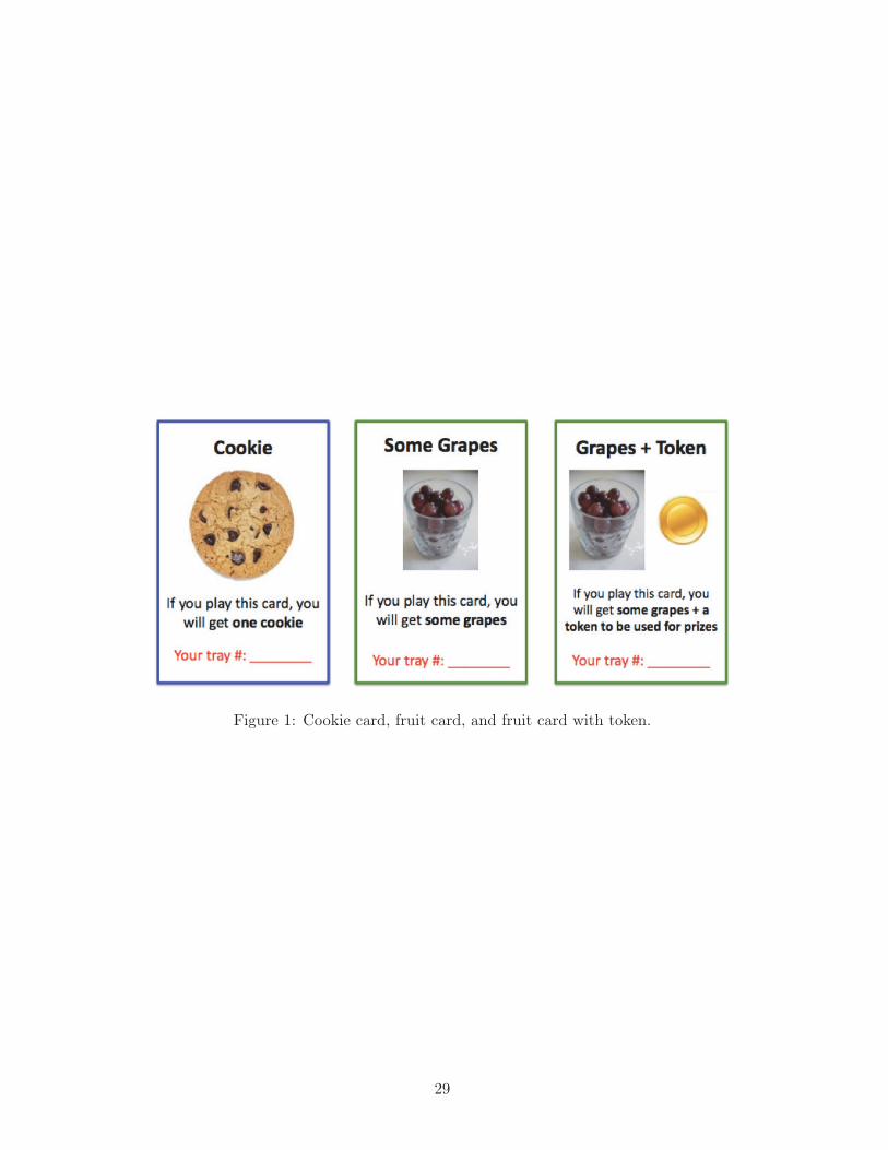
Figure 1: Cookie card, fruit card, and fruit card with token.

29

-1-.

50

.5

0 .2 .4 .6 .8 1

Private

-1-.

50

.5

0 .2 .4 .6 .8 1

Public minus private

-1-.

50

.5

0 .2 .4 .6 .8 1Proportion of table incentivized

Prediction 95% CI

Public

Figure 2: Marginal spillover effects of proportion table incentivized on the conditional likelihoodof ending up with grapes. Estimates from a quadratic version of equation (6)

.

30

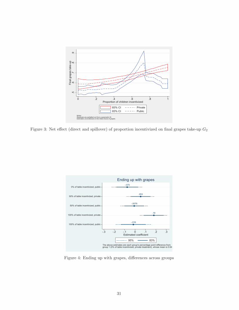
.5.6

.7.8

.9F

ina

l g

rap

es ta

ke

-up

0 .2 .4 .6 .8 1Proportion of children incentivized

83% CI Private

83% CI Public

Notes:Residuals are partialled out from a parametric fit.Estimates unconditional on the initial choice of grapes.

Figure 3: Net effect (direct and spillover) of proportion incentivized on final grapes take-up G2

-.075

.053

-.0076

.18

-.016

0% of table incentivized, public

50% of table incentivized, private

50% of table incentivized, public

100% of table incentivized, private

100% of table incentivized, public

-.3 -.2 -.1 0 .1 .2 .3Estimated coefficient

95% 83%

The above estimates are each group's percentage point difference fromgroup 1 (0% of table incentivized, private treatment), whose mean is 0.64.

Ending up with grapes

Figure 4: Ending up with grapes, differences across groups

31

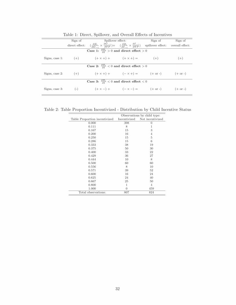
Table 1: Direct, Spillover, and Overall Effects of Incentives

Sign of Spillover effect: Sign of Sign of

direct effect: ( ∂Bi

∂G−i

×∂G

−i

∂TP)+ ( ∂Bi

∂I−i

×∂I

−i

∂TP) spillover effect: overall effect:

Case 1: ∂Bi

∂I> 0 and direct effect > 0

Signs, case 1: (+) (+×+) + (+×+) = (+) (+)

Case 2: ∂Bi

∂I< 0 and direct effect > 0

Signs, case 2: (+) (+×+) + (−×+) = (+ or -) (+ or -)

Case 3: ∂Bi

∂I< 0 and direct effect < 0

Signs, case 3: (-) (+×−) + (−×−) = (+ or -) (+ or -)

Table 2: Table Proportion Incentivized - Distribution by Child Incentive Status

Observations by child type:Table Proportion incentivized Incentivized Not incentivized

0.000 398 00.111 8 10.167 15 30.200 16 40.250 15 50.286 15 60.333 38 190.375 50 300.400 33 220.429 36 270.444 10 80.500 60 600.556 8 100.571 39 520.600 16 240.625 24 400.667 25 500.800 1 41.000 0 459

Total observations: 807 824

32

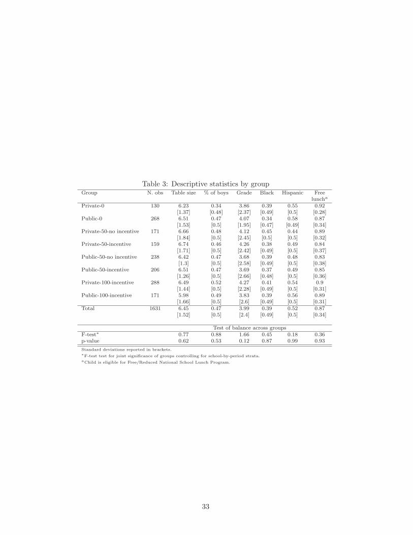
Table 3: Descriptive statistics by groupGroup N. obs Table size % of boys Grade Black Hispanic Free

luncha

Private-0 130 6.23 0.34 3.86 0.39 0.55 0.92[1.37] [0.48] [2.37] [0.49] [0.5] [0.28]

Public-0 268 6.51 0.47 4.07 0.34 0.58 0.87[1.53] [0.5] [1.95] [0.47] [0.49] [0.34]

Private-50-no incentive 171 6.66 0.48 4.12 0.45 0.44 0.89[1.84] [0.5] [2.45] [0.5] [0.5] [0.32]

Private-50-incentive 159 6.74 0.46 4.26 0.38 0.49 0.84[1.71] [0.5] [2.42] [0.49] [0.5] [0.37]

Public-50-no incentive 238 6.42 0.47 3.68 0.39 0.48 0.83[1.3] [0.5] [2.58] [0.49] [0.5] [0.38]

Public-50-incentive 206 6.51 0.47 3.69 0.37 0.49 0.85[1.26] [0.5] [2.66] [0.48] [0.5] [0.36]

Private-100-incentive 288 6.49 0.52 4.27 0.41 0.54 0.9[1.44] [0.5] [2.28] [0.49] [0.5] [0.31]

Public-100-incentive 171 5.98 0.49 3.83 0.39 0.56 0.89[1.66] [0.5] [2.6] [0.49] [0.5] [0.31]

Total 1631 6.45 0.47 3.99 0.39 0.52 0.87[1.52] [0.5] [2.4] [0.49] [0.5] [0.34]

Test of balance across groupsF-test∗ 0.77 0.88 1.66 0.45 0.18 0.36p-value 0.62 0.53 0.12 0.87 0.99 0.93

Standard deviations reported in brackets.∗F-test test for joint significance of groups controlling for school-by-period strata.aChild is eligible for Free/Reduced National School Lunch Program.

33

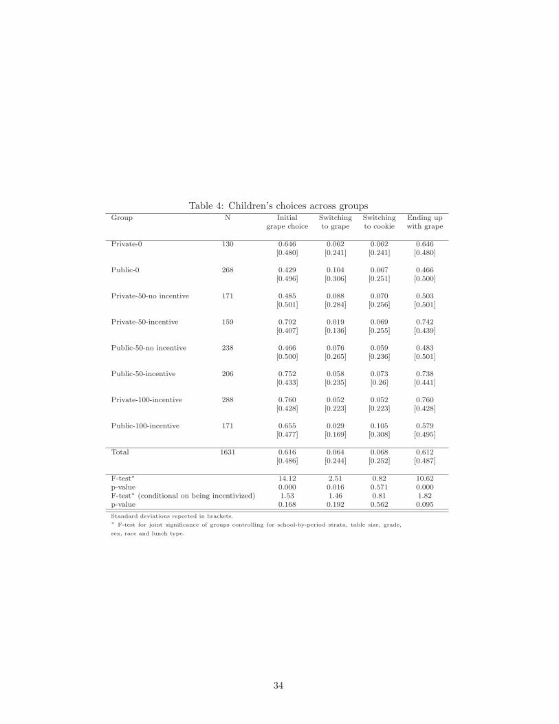
Table 4: Children’s choices across groupsGroup N Initial Switching Switching Ending up

grape choice to grape to cookie with grape

Private-0 130 0.646 0.062 0.062 0.646[0.480] [0.241] [0.241] [0.480]

Public-0 268 0.429 0.104 0.067 0.466[0.496] [0.306] [0.251] [0.500]

Private-50-no incentive 171 0.485 0.088 0.070 0.503[0.501] [0.284] [0.256] [0.501]

Private-50-incentive 159 0.792 0.019 0.069 0.742[0.407] [0.136] [0.255] [0.439]

Public-50-no incentive 238 0.466 0.076 0.059 0.483[0.500] [0.265] [0.236] [0.501]

Public-50-incentive 206 0.752 0.058 0.073 0.738[0.433] [0.235] [0.26] [0.441]

Private-100-incentive 288 0.760 0.052 0.052 0.760[0.428] [0.223] [0.223] [0.428]

Public-100-incentive 171 0.655 0.029 0.105 0.579[0.477] [0.169] [0.308] [0.495]

Total 1631 0.616 0.064 0.068 0.612[0.486] [0.244] [0.252] [0.487]

F-test∗ 14.12 2.51 0.82 10.62p-value 0.000 0.016 0.571 0.000F-test∗ (conditional on being incentivized) 1.53 1.46 0.81 1.82p-value 0.168 0.192 0.562 0.095

Standard deviations reported in brackets.∗ F-test for joint significance of groups controlling for school-by-period strata, table size, grade,

sex, race and lunch type.

34

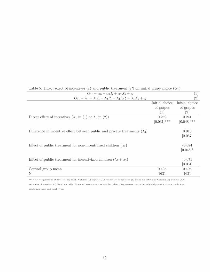
Table 5: Direct effect of incentives (I) and public treatment (P ) on initial grape choice (G1)

G1i = α0 + α1Ii + α2Xi + ǫi (1)G1i = λ0 + λ1Ii + λ2Pi + λ3IiPi + λ4Xi + ǫi (2)

Initial choice Initial choiceof grapes of grapes

(1) (2)

Direct effect of incentives (α1 in (1) or λ1 in (2)) 0.259 0.241[0.031]*** [0.048]***

Difference in incentive effect between public and private treatments (λ3) 0.013[0.067]

Effect of public treatment for non-incentivized children (λ2) -0.084[0.048]*

Effect of public treatment for incentivized children (λ2 + λ3) -0.071[0.051]

Control group mean 0.495 0.495N 1631 1631

***,**,* = significant at the 1,5,10% level. Column (1) depicts OLS estimates of equation (1) listed on table and Column (2) depicts OLS

estimates of equation (2) listed on table. Standard errors are clustered by tables. Regressions control for school-by-period strata, table size,

grade, sex, race and lunch type.

35

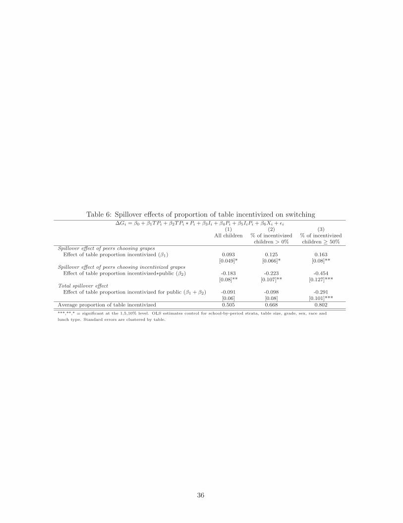
Table 6: Spillover effects of proportion of table incentivized on switching∆Gi = β0 + β1TPi + β2TPi ∗ Pi + β3Ii + β4Pi + β5IiPi + β6Xi + ǫi

(1) (2) (3)All children % of incentivized % of incentivized

children > 0% children ≥ 50%Spillover effect of peers choosing grapes

Effect of table proportion incentivized (β1) 0.093 0.125 0.163[0.049]* [0.066]* [0.08]**

Spillover effect of peers choosing incentivized grapes

Effect of table proportion incentivized∗public (β2) -0.183 -0.223 -0.454[0.08]** [0.107]** [0.127]***

Total spillover effect

Effect of table proportion incentivized for public (β1 + β2) -0.091 -0.098 -0.291[0.06] [0.08] [0.101]***

Average proportion of table incentivized 0.505 0.668 0.802

***,**,* = significant at the 1,5,10% level. OLS estimates control for school-by-period strata, table size, grade, sex, race and

lunch type. Standard errors are clustered by table.

36

Tab

le7:

Spillover

effects

ofproportion

oftable

incentivized

onsw

itchingto

grapes

andcookies

SC

orSG

=β0+

β1TPi+

β2TPi∗Pi+

β3I i

+β4Pi+

β5I iPi+

β6X

i+

ǫ iDep

enden

tvariable:

Switchin

gto

grapes(S

G)

Switchin

gto

cookies(S

C)

(1)

(2)

(3)

(4)

(5)

(6)

(7)

(8)

Children:

All

Incentivized

Non-

Equality

of

All

Incentivized

Non-

Equality

of

incentivized

columns(2)&

(3)

incentivized

columns(6)&

(7)

Spillovereffectofpeers

choosinggrapes

Effectoftable

proportionincentivized

(β1)

0.073

0.101

0.034

p-value

-0.020

-0.080

0.061

p-value

[ 0.036]**

[0.044]**

[0.063]

0.365

[0.041]

[0.054]

[0.057]

0.065

Spillovereffectofpeers

choosingincentivized

grapes

Effectoftable

proportionincentivized

∗public(β

2)

-0.157

-0.172

-0.134

p-value

0.026

0.087

-0.057

p-value

[0.056]***

[0.069]***

[0.090]

0.609

[0.062]

[0.093]

[0.082]

0.207

Totalspillovereffect

Effectoftable

proportionincentivized

forpublic

-0.085

-0.070

-0.100

p-value

0.006

0.007

0.005

p-value

(β1+

β2)

[0.039]**

[0.051]

[0.063]

0.878

[0.045]

[0.074]

[0.055]

0.851

***,**,*

=signifi

cantatth

e1,5,10%

level.

OLS

estim

ate

scontrolforsc

hool-by-p

eriod

stra

ta,ta

ble

size,gra

de,se

x,ra

ceand

lunch

type.Sta

ndard

errors

are

clu

stere

dby

table.

37

Table 8: Testing for conformity in the proportion of incentivized children(1) (2) (3)

All kids % of incentivized % of incentivizedchildren > 0% children ≥ 50%

Panel A: Effect of same-gender incentivized kids

Spillover effect of peers choosing grapes

Effect of table proportion incentivized (δ3) 0.061 0.123 0.054[0.137] [0.136] [0.154]

Spillover effect of peers choosing incentivized grapes

Effect of table proportion of group incentivized*incentive*public (θ6) -0.047 0.013 -0.126[0.219] [0.218] [0.24]

Number of observations 1549 1163 825Panel B: Effect of incentivized best friends

Spillover effect of peers choosing grapes

Effect of table proportion incentivized (δ3) 0.041 0.037 -0.163[0.077] [0.079] [0.111]

Spillover effect of peers choosing incentivized grapes

Effect of table proportion of group incentivized*incentive*public (θ6) 0.27 0.29 0.157[0.161] [0.163] [0.17]

Number of observations 1631 1233 872Panel C: Effect of incentivized popular kids

Spillover effect of peers choosing grapes

Effect of table proportion incentivized (δ3) -0.029 -0.041 0.015[0.091] [0.095] [0.093]

Spillover effect of peers choosing incentivized grapes

Effect of table proportion of group incentivized*incentive*public (θ6) 0.085 0.077 0.27[0.169] [0.168] [0.144]

Number of observations 1631 1233 872

***,**,* = significant at the 1,5,10% level. We report the estimates of the estimates of δ3 and θ6 from the following equations: ∆Gi =

δ0 + δ1TPi + δ2TPiPi + δ3TPBF

i+ δ4TPBF

iPi + δ5Ii + δ6Pi + δ7IiPi + δ8Xi + ǫi and ∆Gi = θ0 + θ1TPi + θ2TPiPi + θ3TPBF

i+

θ4TPBF

iPi + θ5TPBF

iIi + θ6TPBF

iIiPi + θ7Ii + θ8Pi + θ9IiPi + θ10Xi + ǫi. OLS estimates control for school-by-period strata, table size,

grade, sex, race and lunch type. Standard errors are clustered by table.

38

Table B1: Heterogeneity in the direct effects of incentives on initial grape choice, by gender andgrade

Initial grape choice Initial grape choiceIncentive dummy 0.260 0.284

[0.040]*** [0.039]***Incentive*male 0.007

[0.055]Incentive*above median grade -0.045

[0.062]Control group mean 0.495 0.495N 1631 1631

***,**,* = significant at the 1,5,10% level. OLS estimates control for school-by-period strata, table size, grade,

sex, race and lunch type. Standard errors are clustered by table. Column (1) estimates also include a dummy for

male and column (2) estimates include a dummy for grades above the median grade.

39

Table B2: Heterogeneity in spillover effect of proportion of table incentivized on switching tograpes, by gender

∆Gi = η0 + η1TPi + η2TPiPi + η3TPimalei + η4TPiPimalei + η5malei + η6Ii + η7Pi + η8IiPi + η9Xi + ǫi(1) (2) (3)

All children % of incentivized % of incentivizedchildren >0% children ≥ 50%

Spillover effect of peers choosing grapes

Effect of table proportion incentivized (η1) 0.174 0.252 0.279[0.077]** [0.104]** [0.123]**

Effect of table proportion incentivized*male (η3) -0.143 -0.232 -0.241[0.104] [0.118]* [0.149]

Spillover effect of peers choosing incentivized grapes

Effect of table proportion incentivized*public (η2) -0.226 -0.217 -0.367[0.117]* [0.154] [0.168]**

Effect of table proportion incentivized*public*male (η4) 0.08 -0.028 -0.13[0.148] [0.178] [0.245]

Total spillover effect

Effect of table proportion incentivized for public (η1 + η2) -0.052 0.034 -0.088[0.084] [0.114] [0.121]

Effect of table proportion incentivized for public male (η3 + η4) -0.063 -0.26 -0.371[0.106] [0.135]* [0.195]*

Average proportion table incentivized 0.505 0.668 0.802

***,**,* = significant at the 1,5,10% level. OLS estimates control for school-by-period strata, table size, grade, sex, race and lunch type.

Standard errors are clustered by table.

40

Table B3: Heterogeneity in spillover effect of proportion of table incentivized on switching tograpes, by grade

∆Gi = η0 + η1TPi + η2TPiPi + η3TPigi + η4TPiPigi + η5gi + η6Ii + η7Pi + η8IiPi + η9Xi + ǫi(1) (2) (3)

All children % of incentivized % of incentivizedchildren >0% children ≥50%

Spillover effect of peers choosing grapes

Effect of table proportion incentivized (η1) 0.169 0.195 0.188[0.069]** [0.102]* [0.135]

Effect of table proportion incentivized*above median grade (η3) -0.135 -0.139 -0.07[0.098] [0.134] [0.155]

Spillover effect of peers choosing incentivized grapes

Effect of table proportion incentivized*public (η2) -0.245 -0.377 -0.538[0.107]** [0.147]** [0.195]***

Effect of table proportion incentivized*public*above median grade (η4) 0.121 0.339 0.233[0.162] [0.21] [0.265]

Total spillover effect

Effect of table proportion incentivized for public (η1 + η2) -0.076 -0.182 -0.351[0.077] [0.108]* [0.143]**

Effect of table proportion incentivized for public above median grade -0.014 0.200 0.163(η3 + η4) [0.122] [0.165] [0.208]

Average proportion of table incentivized 0.505 0.668 0.802

***,**,* = significant at the 1,5,10% level. gi is a dummy variable equal to 1 if above median grade and 0 otherwise. OLS estimates control

for school-by-period strata, table size, grade, sex, race and lunch type. Standard errors are clustered by table.

41