nt 110 (2007) 287–303www.elsevier.com/locate/rse

Remote Sensing of Environme

Integration of spatial–spectral informationfor the improved extraction of endmembers

D.M. Rogge a, B. Rivard a,⁎, J. Zhang a, A. Sanchez a, J. Harris b, J. Feng a

a Earth Observation Systems Laboratory, Department of Earth and Atmospheric Sciences, University of Alberta, Edmonton, Alberta, Canada, T6G 2E3b Geological Survey of Canada, Continental Geoscience Division, Ottawa, Ontario, Canada, K1A 0E9

Received 6 November 2006; received in revised form 22 February 2007; accepted 26 February 2007

Abstract

Spectral-based image endmember extraction methods hinge on the ability to discriminate between pixels based on spectral characteristicsalone. Endmembers with distinct spectral features (high spectral contrast) are easy to select, whereas those with minimal unique spectralinformation (low spectral contrast) are more problematic. Spectral contrast, however, is dependent on the endmember assemblage, such that as theassemblage changes so does the “relative” spectral contrast of each endmember to all other endmembers. It is then possible for an endmember tohave low spectral contrast with respect to the full image, but have high spectral contrast within a subset of the image. The spatial–spectralendmember extraction tool (SSEE) works by analyzing a scene in parts (subsets), such that we increase the spectral contrast of low contrastendmembers, thus improving the potential for these endmembers to be selected. The SSEE method comprises three main steps: 1) application ofsingular value decomposition (SVD) to determine a set of basis vectors that describe most of the spectral variance for subsets of the image; 2)projection of the full image data set onto the locally defined basis vectors to determine a set of candidate endmember pixels; and, 3) imposingspatial constraints for averaging spectrally similar endmembers, allowing for separation of endmembers that are spectrally similar, but spatiallyindependent. The SSEE method is applied to two real hyperspectral data sets to demonstrate the effects of imposing spatial constraints on theselection of endmembers. The results show that the SSEE method is an effective approach to extracting image endmembers. Specificimprovements include the extraction of physically meaningful, low contrast endmembers that occupy unique image regions.© 2007 Elsevier Inc. All rights reserved.

Keywords: Spatial–spectral; Image endmember extraction; Hyperspectral remote sensing; Spectral mixture analysis

1. Introduction

Spectral mixing is a problem inherent to remote sensing dataand results in few image pixel spectra representing “pure”targets (Settle & Drake, 1993). Linear spectral mixture analysis(SMA) (Adams et al., 1986, 1993) is designed to address theproblem of mixed pixels. It assumes that the pixel-to-pixelvariability in a scene results from varying proportions ofspectral endmembers. The spectrum of a mixed pixel can thenbe calculated as a linear combination of the endmember spectraweighted by the area coverage of each endmember within thepixel, if the scattering and absorption of electromagnetic

⁎ Corresponding author. Tel.: +1 780 492 1822; fax: +1 780 492 2030.E-mail address: benoit.rivard@ualberta.ca (B. Rivard).

0034-4257/$ - see front matter © 2007 Elsevier Inc. All rights reserved.doi:10.1016/j.rse.2007.02.019

radiation is derived from a single component on the surface(Keshava & Mustard, 2002).

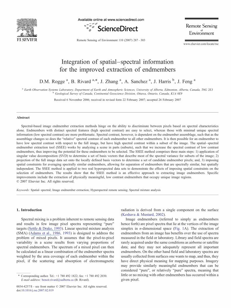
Image endmembers (referred to simply as endmembershence forth) are pixel spectra that lie at the vertices of the imagesimplex in n-dimensional space (Fig. 1A). The extraction ofendmembers from an image has benefits over the use of spectrameasured in the field or laboratory. Library and field spectra arerarely acquired under the same conditions as airborne or satellitedata; and they may not adequately represent all importantendmembers. On the other hand field and laboratory spectra areusually collected from surfaces one wants to map, and thus, theyhave direct physical meaning for mapping purposes. Imagerymay provide similarly meaningful endmembers that can beconsidered “pure”, or relatively “pure” spectra, meaning thatlittle or no mixing with other endmembers has occurred within agiven pixel.

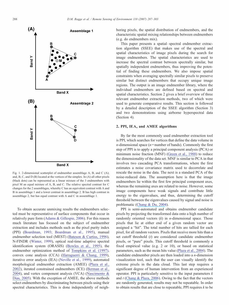
Fig. 1. 2-dimensional scatterplot of endmember assemblage A, B, and C (A);and, B, C, and D (B) located at the vertices of the simplex. In (A) all other pixels(black dots) can be represented as a linear mixture of the 3 endmembers withpixel M an equal mixture of A, B, and C. The relative spectral contrast for Cchanges for the 2 assemblages, whereby C has an equivalent contrast with A andB in assemblage 1 and a lower contrast in assemblage 2. B has high contrast inassemblage 2, but has equal contrast with A and C in asssemblage 1.

288 D.M. Rogge et al. / Remote Sensing of Environment 110 (2007) 287–303

To obtain accurate unmixing results the endmembers selec-ted must be representative of surface components that occur inrelatively pure form (Adams & Gillespie, 2006). For this reasonmuch literature has focused on the subject of endmemberextraction and includes methods such as the pixel purity index(PPI) (Boardman, 1993; Boardman et al., 1995), manualendmember selection tool (MEST) (Bateson & Curtiss, 1996),N-FINDR (Winter, 1999), optical real-time adaptive spectralidentification system (ORASIS) (Bowles et al., 1995), theendmember optimization method of Tompkins et al. (1997),convex cone analysis (CCA) (Ifarraguerri & Chang, 1999),iterative error analysis (IEA) (Neville et al., 1999), automatedmorphological endmember extraction (AMEE) (Plaza et al.,2002), iterated constrained endmembers (ICE) (Berman et al.,2004), and vertex component analysis (VCA) (Nascimento &Dias, 2005). With the exception of AMEE, the above methodsselect endmembers by discriminating between pixels using theirspectral characteristics. This is done independently of neigh-

boring pixels, the spatial distribution of endmembers, and thecharacteristic spatial mixing relationships between endmembers(e.g. do endmembers mix).

This paper presents a spatial–spectral endmember extrac-tion algorithm (SSEE) that makes use of the spectral andspatial characteristics of image pixels during the search forimage endmembers. The spatial characteristics are used toincrease the spectral contrast between spectrally similar, butspatially independent endmembers, thus improving the poten-tial of finding these endmembers. We also impose spatialconstraints when averaging spectrally similar pixels to preservesimilar but distinct endmembers that occupy unique imageregions. The output is an image endmember library, where theindividual endmembers are defined based on spectral andspatial characteristics. Section 2 gives a brief overview of threerelevant endmember extraction methods, two of which wereused to generate comparative results. This section is followedby a detailed description of the SSEE algorithm (Section 3)and two demonstrations using airborne hyperspectral data(Section 4).

2. PPI, IEA, and AMEE algorithms

By far the most commonly used endmember extraction toolis PPI, which searches for vertices that define the data volume inn-dimensional space (n=number of bands). Commonly the firststep of PPI is to apply a principal component analysis (PCA) orminimum noise fraction (MNF) (Green et al., 1988) to reducethe dimensionality of the data set. MNF is similar to PCA in thatinvolves two cascading PCA transformations, where the firstestimates a noise covariance matrix used to decorrelate andrescale the noise in the data. The next is a standard PCA of thenoise-reduced data. The assumption here is that the imageendmembers lie within the first few principal component axes,whereas the remaining axes are related to noise. However, someimage components have weak signals and contribute littleenergy to the eigenvalues, and thus, determining the cutoffthreshold between the eigenvalues caused by signal and noise isproblematic (Chang & Du, 2004).

PPI is semi-automated and obtains endmember candidatepixels by projecting the transformed data onto a high number ofrandomly oriented vectors (k) in n-dimensional space. Thosepixels that lie at either end of a given random vector areassigned a “hit”. The total number of hits are tallied for eachpixel, for all random vectors. Pixels that receive more hits than aset cutoff threshold (t) are considered candidate endmemberpixels, or “pure” pixels. This cutoff threshold is commonly afixed empirical value (e.g. 2 or 10), or based on statisticalparameters, such as the mean hits value (Plaza et al., 2004). Thecandidate endmember pixels are then loaded into a n-dimensionvisualization tool, such that the user can visually identify theextreme pixels in the data cloud. This last step requires asignificant degree of human intervention from an experiencedoperator. PPI is particularly sensitive to the input parameters kand t (Chang & Plaza, 2006). Owing to the fact that the vectorsare randomly generated, results may not be repeatable. In orderto obtain results that are close to repeatable, PPI requires k to be

289D.M. Rogge et al. / Remote Sensing of Environment 110 (2007) 287–303

sufficiently large (e.g. 104), such that the number of endmembercandidate pixels selected levels off asymptotically as a functionof the number of vectors used.

IEA is implemented in the Imaging Spectrometer DataAnalysis System (ISDAS) (Staenz et al., 1998), and is based onthe residual error image generated when a data set is unmixedusing a Weighted Nonnegative Least Squares approach(WNNLS) (Haskell & Hanson, 1981). This method has beenused in endmember comparative studies (e.g. Plaza et al., 2004;Winter & Winter, 2000) and was shown to be a robust extrac-tion tool. IEA works by performing a series of recursive cons-trained unmixing operations on the image, such that theresidual error is minimized. The mean spectrum of the scene isused as the starting endmember to initialize the unmixingprocess. The residual error image is essentially a distance mea-surement in n-dimensional space between the mean spectrumand each pixel spectrum in the image. Pixels within a pre-determined spectral angle that encompass the largest errors forma new endmember, with the mean spectrum discarded. Thisprocess is repeated using the new endmember to find additionalendmembers, but unlike the mean spectrum which was dis-carded, each new endmember is added to the existing end-member set until the number of endmembers specified bythe user is reached or until a specified average error tolerancecondition is met. The main drawback to IEA is that it is com-putationally intensive, specifically as the number of end-members required increases.

AMEE is significantly different from spectral-based methodsas it integrates spatial information in order to extract end-members from an image. AMEE runs on the full data cube withno dimensional reduction. The algorithm begins by searchingspatial neighborhoods around each pixel in the image for themost spectrally pure and mostly highly mixed pixel. This task isaccomplished using the mathematical morphology operatorsdilation and erosion respectively. Each spectrally pure pixel isassigned an “eccentricity” value, which is calculated as thespectral angle distance between the most spectrally pure andmostly highly mixed pixel for the given spatial neighborhood.This process is repeated iteratively for larger spatial neighbor-hoods up to a maximum size that is pre-determined. At eachiteration the “eccentricity” values of the selected pixels are

Fig. 2. (A) Image region showing three endmembers (i, j, and k), where mixing occsquare in (A). (B) 2-dimensional scatter-plot where endmembers i and j are difficult tofor better discrimination of endmembers i and j. Dotted lines in (B), (C), and (D) ar

updated. The final endmember set is obtained by applying athreshold to the resulting greyscale “eccentricity” image. Thereare some limitations to AMEE, particularly a significantincrease in processing time as the maximum size of the spatialneighborhood becomes large; and, the algorithm's ability toselect only one pixel per spatial neighborhood (Plaza et al.,2002). However, AMEE has been shown to produce results thatare comparable to or better than other endmember extractionmethods (Plaza et al., 2002, 2004).

3. Description of the spatial–spectral endmemberextraction (SSEE) algorithm

The selection of endmembers becomes more problematic astheir spectral contrast approaches the detection limits of thegiven sensor (e.g. SNR). Improving the spectral contrastbetween pixels in an image can be accomplished usingspectral-based methods such as transforms (e.g. PCA, MNF)(Adams & Gillespie, 2006), derivative analysis (Tsai & Philpot,1998), and normalization (Clark & Roush, 1984). Masking canalso be used to improve spectral contrast by removing imagecomponents that dominate the spectral variance of the dataresulting in a relative increase in spectral contrast for theremaining image components. However, masking will only beeffective in cases where spectral mixing is minimal, which is notcommonly the case for natural environments. Masking doesillustrate that spectral contrast is variable in an image dependingon the spatial neighborhoods, where for each spatial neighbor-hood the assemblage of endmembers may change.

Fig. 1 provides such an illustration showcasing endmember Cas observed in two different spatial neighborhoods, each with adistinct endmember assemblage. In case 1, C is equivalentlydistinct from both A and B and can be considered to have highspectral contrast relative to A and B. However, in case 2, C isspectrally similar to D, and thus has lower relative spectralcontrast compared with case 1. By conducting the imageextraction on image subsets we can take advantage of the spatialcharacteristics of each endmember, which may result in a givenendmember having higher spectral contrast in a specific imagesubset, thus facilitating its extraction. Fig. 2 illustrates a geologicalexample where two lithologic units are spectrally similar, but

urs between i and k, j and k, but not i and j. Spatial groups shown with dotteddiscriminate. (C) and (D) show scatter-plots for the two spatial groups allowinge the eigenvectors related to the largest eigenvalue for each distribution.

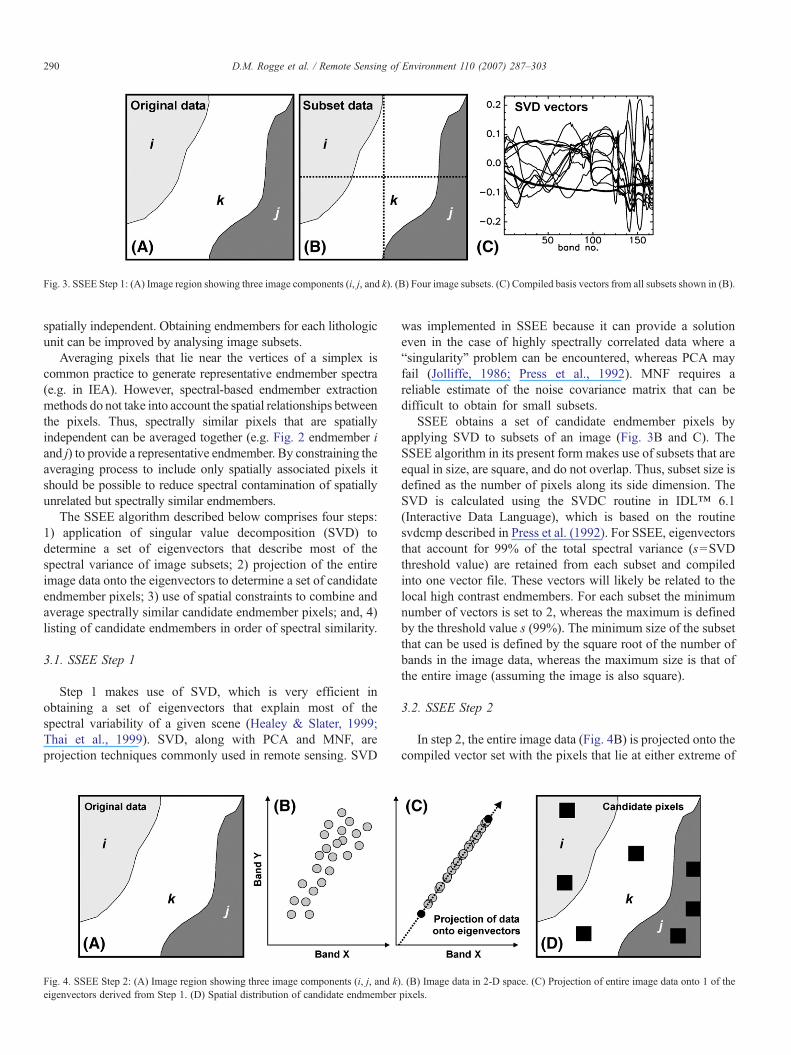
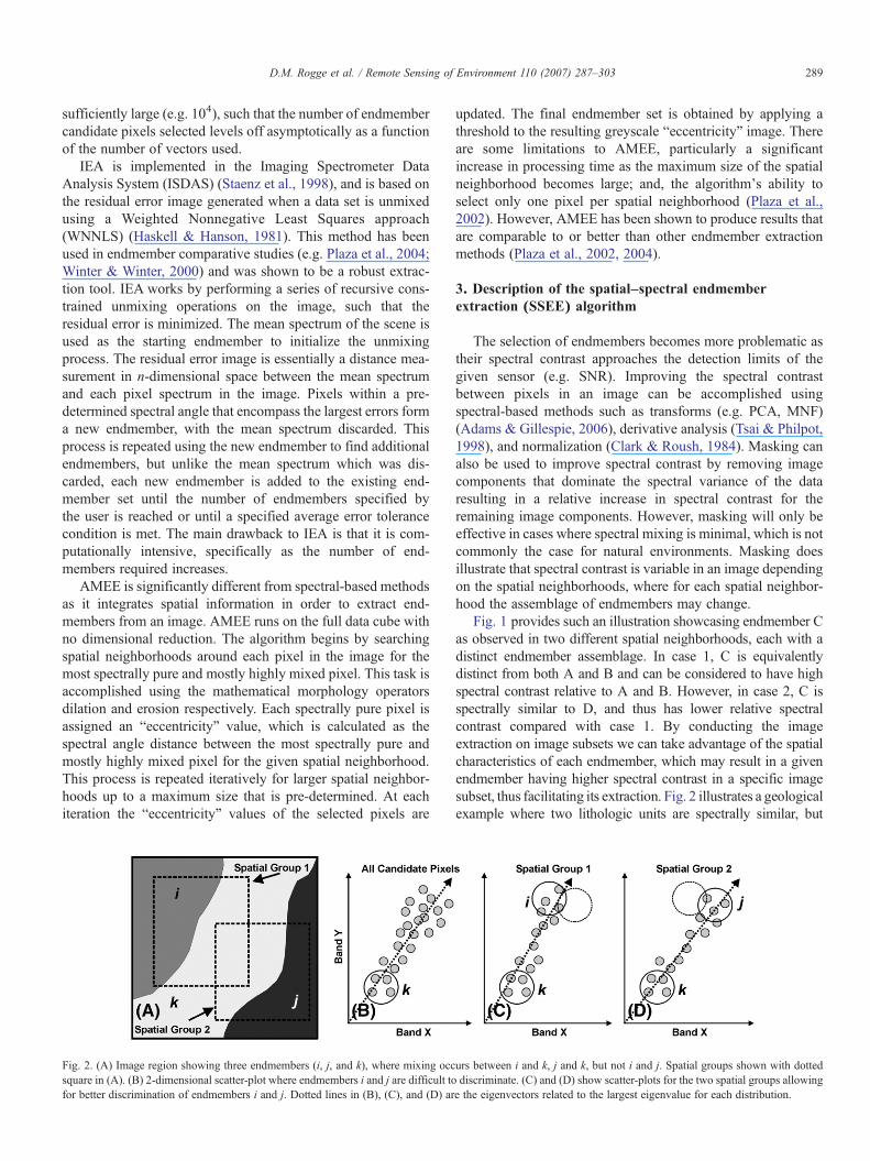
Fig. 3. SSEE Step 1: (A) Image region showing three image components (i, j, and k). (B) Four image subsets. (C) Compiled basis vectors from all subsets shown in (B).

290 D.M. Rogge et al. / Remote Sensing of Environment 110 (2007) 287–303

spatially independent. Obtaining endmembers for each lithologicunit can be improved by analysing image subsets.

Averaging pixels that lie near the vertices of a simplex iscommon practice to generate representative endmember spectra(e.g. in IEA). However, spectral-based endmember extractionmethods do not take into account the spatial relationships betweenthe pixels. Thus, spectrally similar pixels that are spatiallyindependent can be averaged together (e.g. Fig. 2 endmember iand j) to provide a representative endmember. By constraining theaveraging process to include only spatially associated pixels itshould be possible to reduce spectral contamination of spatiallyunrelated but spectrally similar endmembers.

The SSEE algorithm described below comprises four steps:1) application of singular value decomposition (SVD) todetermine a set of eigenvectors that describe most of thespectral variance of image subsets; 2) projection of the entireimage data onto the eigenvectors to determine a set of candidateendmember pixels; 3) use of spatial constraints to combine andaverage spectrally similar candidate endmember pixels; and, 4)listing of candidate endmembers in order of spectral similarity.

3.1. SSEE Step 1

Step 1 makes use of SVD, which is very efficient inobtaining a set of eigenvectors that explain most of thespectral variability of a given scene (Healey & Slater, 1999;Thai et al., 1999). SVD, along with PCA and MNF, areprojection techniques commonly used in remote sensing. SVD

Fig. 4. SSEE Step 2: (A) Image region showing three image components (i, j, and k)eigenvectors derived from Step 1. (D) Spatial distribution of candidate endmember

was implemented in SSEE because it can provide a solutioneven in the case of highly spectrally correlated data where a“singularity” problem can be encountered, whereas PCA mayfail (Jolliffe, 1986; Press et al., 1992). MNF requires areliable estimate of the noise covariance matrix that can bedifficult to obtain for small subsets.

SSEE obtains a set of candidate endmember pixels byapplying SVD to subsets of an image (Fig. 3B and C). TheSSEE algorithm in its present form makes use of subsets that areequal in size, are square, and do not overlap. Thus, subset size isdefined as the number of pixels along its side dimension. TheSVD is calculated using the SVDC routine in IDL™ 6.1(Interactive Data Language), which is based on the routinesvdcmp described in Press et al. (1992). For SSEE, eigenvectorsthat account for 99% of the total spectral variance (s=SVDthreshold value) are retained from each subset and compiledinto one vector file. These vectors will likely be related to thelocal high contrast endmembers. For each subset the minimumnumber of vectors is set to 2, whereas the maximum is definedby the threshold value s (99%). The minimum size of the subsetthat can be used is defined by the square root of the number ofbands in the image data, whereas the maximum size is that ofthe entire image (assuming the image is also square).

3.2. SSEE Step 2

In step 2, the entire image data (Fig. 4B) is projected onto thecompiled vector set with the pixels that lie at either extreme of

. (B) Image data in 2-D space. (C) Projection of entire image data onto 1 of thepixels.

291D.M. Rogge et al. / Remote Sensing of Environment 110 (2007) 287–303

the vectors retained (Fig. 4C). These pixels (Fig. 4D) representthe candidate pixel endmember set, which is used in Step 3.

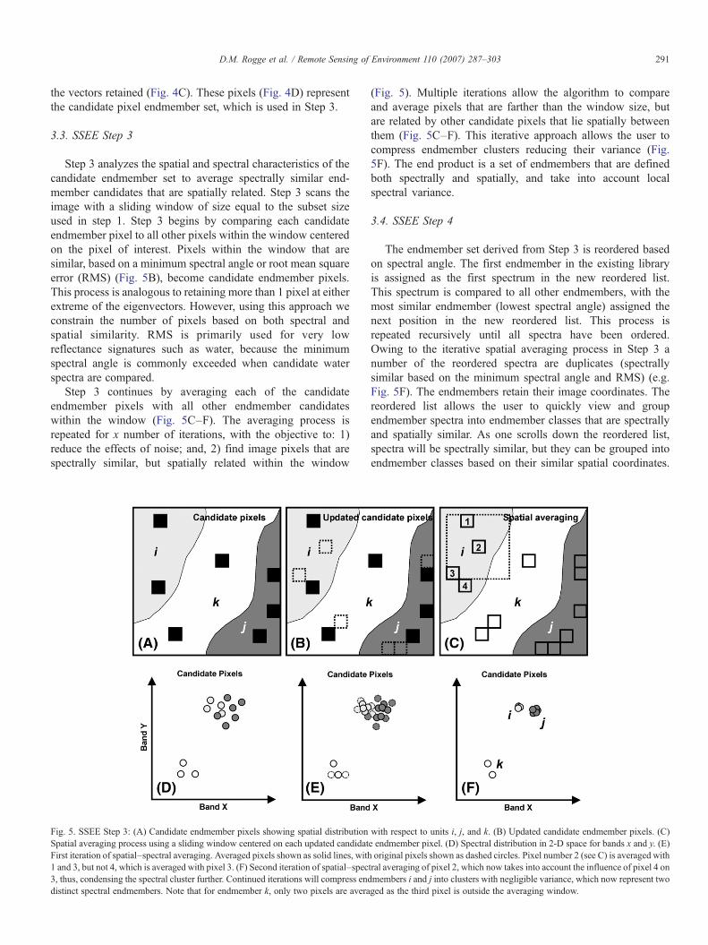
3.3. SSEE Step 3

Step 3 analyzes the spatial and spectral characteristics of thecandidate endmember set to average spectrally similar end-member candidates that are spatially related. Step 3 scans theimage with a sliding window of size equal to the subset sizeused in step 1. Step 3 begins by comparing each candidateendmember pixel to all other pixels within the window centeredon the pixel of interest. Pixels within the window that aresimilar, based on a minimum spectral angle or root mean squareerror (RMS) (Fig. 5B), become candidate endmember pixels.This process is analogous to retaining more than 1 pixel at eitherextreme of the eigenvectors. However, using this approach weconstrain the number of pixels based on both spectral andspatial similarity. RMS is primarily used for very lowreflectance signatures such as water, because the minimumspectral angle is commonly exceeded when candidate waterspectra are compared.

Step 3 continues by averaging each of the candidateendmember pixels with all other endmember candidateswithin the window (Fig. 5C–F). The averaging process isrepeated for x number of iterations, with the objective to: 1)reduce the effects of noise; and, 2) find image pixels that arespectrally similar, but spatially related within the window

Fig. 5. SSEE Step 3: (A) Candidate endmember pixels showing spatial distributionSpatial averaging process using a sliding window centered on each updated candidatFirst iteration of spatial–spectral averaging. Averaged pixels shown as solid lines, with1 and 3, but not 4, which is averaged with pixel 3. (F) Second iteration of spatial–spec3, thus, condensing the spectral cluster further. Continued iterations will compress enddistinct spectral endmembers. Note that for endmember k, only two pixels are avera

(Fig. 5). Multiple iterations allow the algorithm to compareand average pixels that are farther than the window size, butare related by other candidate pixels that lie spatially betweenthem (Fig. 5C–F). This iterative approach allows the user tocompress endmember clusters reducing their variance (Fig.5F). The end product is a set of endmembers that are definedboth spectrally and spatially, and take into account localspectral variance.

3.4. SSEE Step 4

The endmember set derived from Step 3 is reordered basedon spectral angle. The first endmember in the existing libraryis assigned as the first spectrum in the new reordered list.This spectrum is compared to all other endmembers, with themost similar endmember (lowest spectral angle) assigned thenext position in the new reordered list. This process isrepeated recursively until all spectra have been ordered.Owing to the iterative spatial averaging process in Step 3 anumber of the reordered spectra are duplicates (spectrallysimilar based on the minimum spectral angle and RMS) (e.g.Fig. 5F). The endmembers retain their image coordinates. Thereordered list allows the user to quickly view and groupendmember spectra into endmember classes that are spectrallyand spatially similar. As one scrolls down the reordered list,spectra will be spectrally similar, but they can be grouped intoendmember classes based on their similar spatial coordinates.

with respect to units i, j, and k. (B) Updated candidate endmember pixels. (C)e endmember pixel. (D) Spectral distribution in 2-D space for bands x and y. (E)original pixels shown as dashed circles. Pixel number 2 (see C) is averaged with

tral averaging of pixel 2, which now takes into account the influence of pixel 4 onmembers i and j into clusters with negligible variance, which now represent twoged as the third pixel is outside the averaging window.

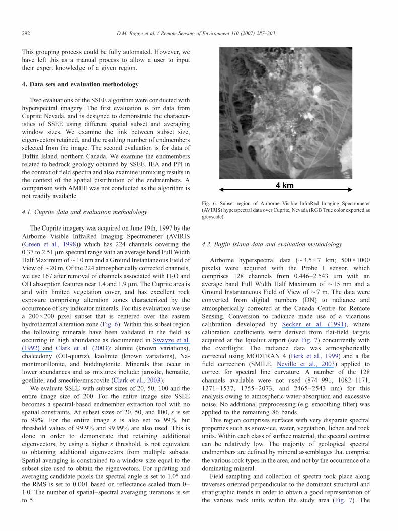
Fig. 6. Subset region of Airborne Visible InfraRed Imaging Spectrometer(AVIRIS) hyperspectral data over Cuprite, Nevada (RGB True color exported asgreyscale).

292 D.M. Rogge et al. / Remote Sensing of Environment 110 (2007) 287–303

This grouping process could be fully automated. However, wehave left this as a manual process to allow a user to inputtheir expert knowledge of a given region.

4. Data sets and evaluation methodology

Two evaluations of the SSEE algorithm were conducted withhyperspectral imagery. The first evaluation is for data fromCuprite Nevada, and is designed to demonstrate the character-istics of SSEE using different spatial subset and averagingwindow sizes. We examine the link between subset size,eigenvectors retained, and the resulting number of endmembersselected from the image. The second evaluation is for data ofBaffin Island, northern Canada. We examine the endmembersrelated to bedrock geology obtained by SSEE, IEA and PPI inthe context of field spectra and also examine unmixing results inthe context of the spatial distribution of the endmembers. Acomparison with AMEE was not conducted as the algorithm isnot readily available.

4.1. Cuprite data and evaluation methodology

The Cuprite imagery was acquired on June 19th, 1997 by theAirborne Visible InfraRed Imaging Spectrometer (AVIRIS(Green et al., 1998)) which has 224 channels covering the0.37 to 2.51 μm spectral range with an average band Full WidthHalf Maximum of∼10 nm and a Ground Instantaneous Field ofView of∼20 m. Of the 224 atmospherically corrected channels,we use 167 after removal of channels associated with H2O andOH absorption features near 1.4 and 1.9 μm. The Cuprite area isarid with limited vegetation cover, and has excellent rockexposure comprising alteration zones characterized by theoccurrence of key indicator minerals. For this evaluation we usea 200×200 pixel subset that is centered over the easternhydrothermal alteration zone (Fig. 6). Within this subset regionthe following minerals have been validated in the field asoccurring in high abundance as documented in Swayze et al.(1992) and Clark et al. (2003): alunite (known variations),chalcedony (OH-quartz), kaolinite (known variations), Na-montmorillonite, and buddingtonite. Minerals that occur inlower abundances and as mixtures include: jarosite, hematite,goethite, and smectite/muscovite (Clark et al., 2003).

We evaluate SSEE with subset sizes of 20, 50, 100 and theentire image size of 200. For the entire image size SSEEbecomes a spectral-based endmember extraction tool with nospatial constraints. At subset sizes of 20, 50, and 100, s is setto 99%. For the entire image s is also set to 99%, butthreshold values of 99.9% and 99.99% are also used. This isdone in order to demonstrate that retaining additionaleigenvectors, by using a higher s threshold, is not equivalentto obtaining additional eigenvectors from multiple subsets.Spatial averaging is constrained to a window size equal to thesubset size used to obtain the eigenvectors. For updating andaveraging candidate pixels the spectral angle is set to 1.0° andthe RMS is set to 0.001 based on reflectance scaled from 0–1.0. The number of spatial–spectral averaging iterations is setto 5.

4.2. Baffin Island data and evaluation methodology

Airborne hyperspectral data (∼3.5×7 km; 500×1000pixels) were acquired with the Probe I sensor, whichcomprises 128 channels from 0.446–2.543 μm with anaverage band Full Width Half Maximum of ∼15 nm and aGround Instantaneous Field of View of ∼7 m. The data wereconverted from digital numbers (DN) to radiance andatmospherically corrected at the Canada Centre for RemoteSensing. Conversion to radiance made use of a vicariouscalibration developed by Secker et al. (1991), wherecalibration coefficients were derived from flat-field targetsacquired at the Iqualuit airport (see Fig. 7) concurrently withthe overflight. The radiance data was atmosphericallycorrected using MODTRAN 4 (Berk et al., 1999) and a flatfield correction (SMILE, Neville et al., 2003) applied tocorrect for spectral line curvature. A number of the 128channels available were not used (874–991, 1082–1171,1271–1537, 1755–2073, and 2465–2543 nm) for thisanalysis owing to atmospheric water-absorption and excessivenoise. No additional preprocessing (e.g. smoothing filter) wasapplied to the remaining 86 bands.

This region comprises surfaces with very disparate spectralproperties such as snow-ice, water, vegetation, lichen and rockunits. Within each class of surface material, the spectral contrastcan be relatively low. The majority of geological spectralendmembers are defined by mineral assemblages that comprisethe various rock types in the area, and not by the occurrence of adominating mineral.

Field sampling and collection of spectra took place alongtraverses oriented perpendicular to the dominant structural andstratigraphic trends in order to obtain a good representation ofthe various rock units within the study area (Fig. 7). The

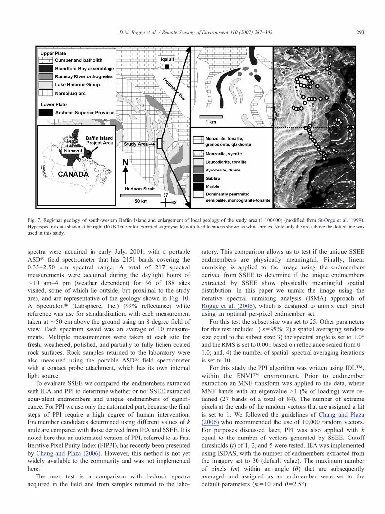
Fig. 7. Regional geology of south-western Baffin Island and enlargement of local geology of the study area (1:100000) (modified from St-Onge et al., 1999).Hyperspectral data shown at far right (RGB True color exported as greyscale) with field locations shown as white circles. Note only the area above the dotted line wasused in this study.

293D.M. Rogge et al. / Remote Sensing of Environment 110 (2007) 287–303

spectra were acquired in early July, 2001, with a portableASD® field spectrometer that has 2151 bands covering the0.35–2.50 μm spectral range. A total of 217 spectralmeasurements were acquired during the daylight hours of∼10 am–4 pm (weather dependent) for 56 of 188 sitesvisited, some of which lie outside, but proximal to the studyarea, and are representative of the geology shown in Fig. 10.A Spectralon® (Labsphere, Inc.) (99% reflectance) whitereference was use for standardization, with each measurementtaken at ∼50 cm above the ground using an 8 degree field ofview. Each spectrum saved was an average of 10 measure-ments. Multiple measurements were taken at each site forfresh, weathered, polished, and partially to fully lichen coatedrock surfaces. Rock samples returned to the laboratory werealso measured using the portable ASD® field spectrometerwith a contact probe attachment, which has its own internallight source.

To evaluate SSEE we compared the endmembers extractedwith IEA and PPI to determine whether or not SSEE extractedequivalent endmembers and unique endmembers of signifi-cance. For PPI we use only the automated part, because the finalsteps of PPI require a high degree of human intervention.Endmember candidates determined using different values of kand t are compared with those derived from IEA and SSEE. It isnoted here that an automated version of PPI, referred to as FastIterative Pixel Purity Index (FIPPI), has recently been presentedby Chang and Plaza (2006). However, this method is not yetwidely available to the community and was not implementedhere.

The next test is a comparison with bedrock spectraacquired in the field and from samples returned to the labo-

ratory. This comparison allows us to test if the unique SSEEendmembers are physically meaningful. Finally, linearunmixing is applied to the image using the endmembersderived from SSEE to determine if the unique endmembersextracted by SSEE show physically meaningful spatialdistribution. In this paper we unmix the image using theiterative spectral unmixing analysis (ISMA) approach ofRogge et al. (2006), which is designed to unmix each pixelusing an optimal per-pixel endmember set.

For this test the subset size was set to 25. Other parametersfor this test include: 1) s=99%; 2) a spatial averaging windowsize equal to the subset size; 3) the spectral angle is set to 1.0°and the RMS is set to 0.001 based on reflectance scaled from 0–1.0; and, 4) the number of spatial–spectral averaging iterationsis set to 10.

For this study the PPI algorithm was written using IDL™,within the ENVI™ environment. Prior to endmemberextraction an MNF transform was applied to the data, whereMNF bands with an eigenvalue N1 (% of loading) were re-tained (27 bands of a total of 84). The number of extremepixels at the ends of the random vectors that are assigned a hitis set to 1. We followed the guidelines of Chang and Plaza(2006) who recommended the use of 10,000 random vectors.For purposes discussed later, PPI was also applied with kequal to the number of vectors generated by SSEE. Cutoffthresholds (t) of 1, 2, and 5 were tested. IEA was implementedusing ISDAS, with the number of endmembers extracted fromthe imagery set to 30 (default value). The maximum numberof pixels (m) within an angle (θ) that are subsequentlyaveraged and assigned as an endmember were set to thedefault parameters (m=10 and θ=2.5°).

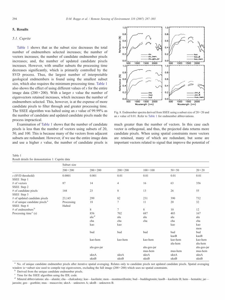
Fig. 8. Endmember spectra derived from SSEE using a subset size of 20×20 andan s value of 0.01. Refer to Table 1 for endmember abbreviations.

294 D.M. Rogge et al. / Remote Sensing of Environment 110 (2007) 287–303

5. Results

5.1. Cuprite

Table 1 shows that as the subset size decreases the totalnumber of endmembers selected increases; the number ofvectors increases; the number of candidate endmember pixelsincreases; and, the number of updated candidate pixelsincreases. However, with smaller subsets the processing timedecreases significantly, which is primarily controlled by theSVD process. Thus, the largest number of interpretablegeological endmembers is found using the smallest subsetsize, which also requires the minimum processing time. Table 1also shows the effect of using different values of s for the entireimage data (200×200). With a larger s value the number ofeigenvectors retained increases, which increases the number ofendmembers selected. This, however, is at the expense of morecandidate pixels to filter through and greater processing time.The SSEE algorithm was halted using an s value of 99.99% asthe number of candidate and updated candidate pixels made theprocess impractical.

Examination of Table 1 shows that the number of candidatepixels is less than the number of vectors using subsets of 20,50, and 100. This is because many of the vectors from adjacentsubsets are redundant. However, if we use the entire image dataand use a higher s value, the number of candidate pixels is

Table 1Result details for demonstration 1: Cuprite data

Subset size

200×200 200×200

s (SVD threshold) 0.0001 0.001SSEE Step 1# of vectors 87 14SSEE Step 2# of candidate pixels 144 23SSEE Step 3# of updated candidate pixels 23,145 299# of unique candidate pixels a Processing 18SSEE Step 4 Halted# of endmembers b 8Processing time c (s) 856

alu d

chakao

bud

kao-hem

alu-geo-jar

uknAuknB

a No. of unique candidate endmember pixels after iterative spatial averaging. Rewindow is=subset size used to compile top eigenvectors, excluding the full image (b Derived from the unique candidate endmember pixels.c Time for the SSEE algorithm using the IDL code.d Mineral abbreviations: alu—alunite; cha—chalcadony; kao—kaolinite; mon—m

jarosite; geo—goethite; mus—muscovite; uknA—unknown A; uknB—unknown B

much greater than the number of vectors. In this case eachvector is orthogonal, and thus, the projected data returns morecandidate pixels. When using spatial constraints more vectorsare retained, many of which are redundant, but some areimportant vectors related to signal that improve the potential of

200×200 100×100 50×50 20×20

0.01 0.01 0.01 0.01

4 16 63 356

8 13 26 55

82 231 390 7327 11 20 32

7 8 10 12702 687 403 167alu alu alu alucha cha cha chakao kao kao

monbud bud bud bud

kaoB kaoBkao-hem kao-hem kao-hem kao-hem

alu-hem alu-hemalu-geo-jar alu-geo-jarmus-hem mus-hem mus-hem

uknA uknA uknA uknAuknB uknB uknB uknB

lates only to candidate pixels not updated candidate pixels. Spatial averaging200×200) which uses no spatial constraints.

ontmorillonite; bud—buddingtonite; kaoB—kaolinite B; hem—hematite; jar—.

295D.M. Rogge et al. / Remote Sensing of Environment 110 (2007) 287–303

obtaining additional endmembers. Unlike the orthogonalvectors obtained using the entire image many of the vectorsretained using spatial constraints will not be orthogonal.

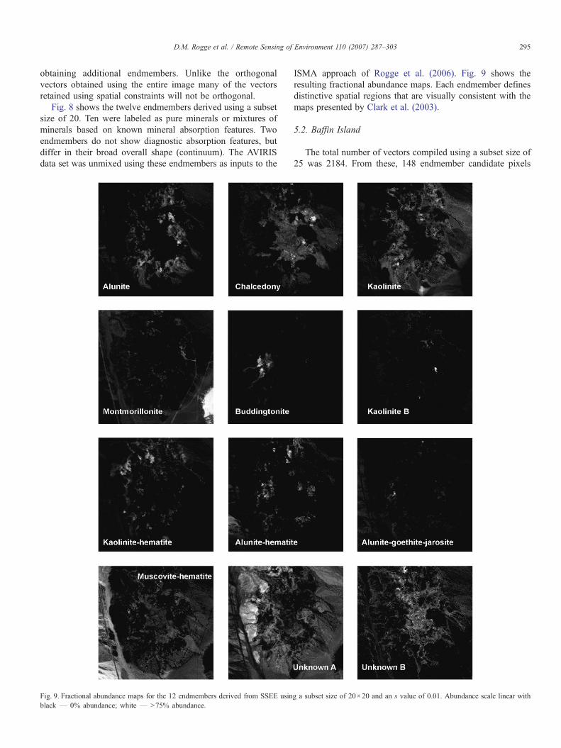
Fig. 8 shows the twelve endmembers derived using a subsetsize of 20. Ten were labeled as pure minerals or mixtures ofminerals based on known mineral absorption features. Twoendmembers do not show diagnostic absorption features, butdiffer in their broad overall shape (continuum). The AVIRISdata set was unmixed using these endmembers as inputs to the

Fig. 9. Fractional abundance maps for the 12 endmembers derived from SSEE usinblack — 0% abundance; white — N75% abundance.

ISMA approach of Rogge et al. (2006). Fig. 9 shows theresulting fractional abundance maps. Each endmember definesdistinctive spatial regions that are visually consistent with themaps presented by Clark et al. (2003).

5.2. Baffin Island

The total number of vectors compiled using a subset size of25 was 2184. From these, 148 endmember candidate pixels

g a subset size of 20×20 and an s value of 0.01. Abundance scale linear with

296 D.M. Rogge et al. / Remote Sensing of Environment 110 (2007) 287–303

were extracted, of which 7 were noisy and left out (e.g. 141total no. of pixels in Table 2). Following the spatial averagingprocedure 28 of the 148 candidate endmember pixels wereexact duplicates. The averaging procedure also results in manyof the remaining candidate pixels showing minimal spectraldifference, further reducing the number of unique end-members and allowing the user to quickly group the spectrainto endmember classes.

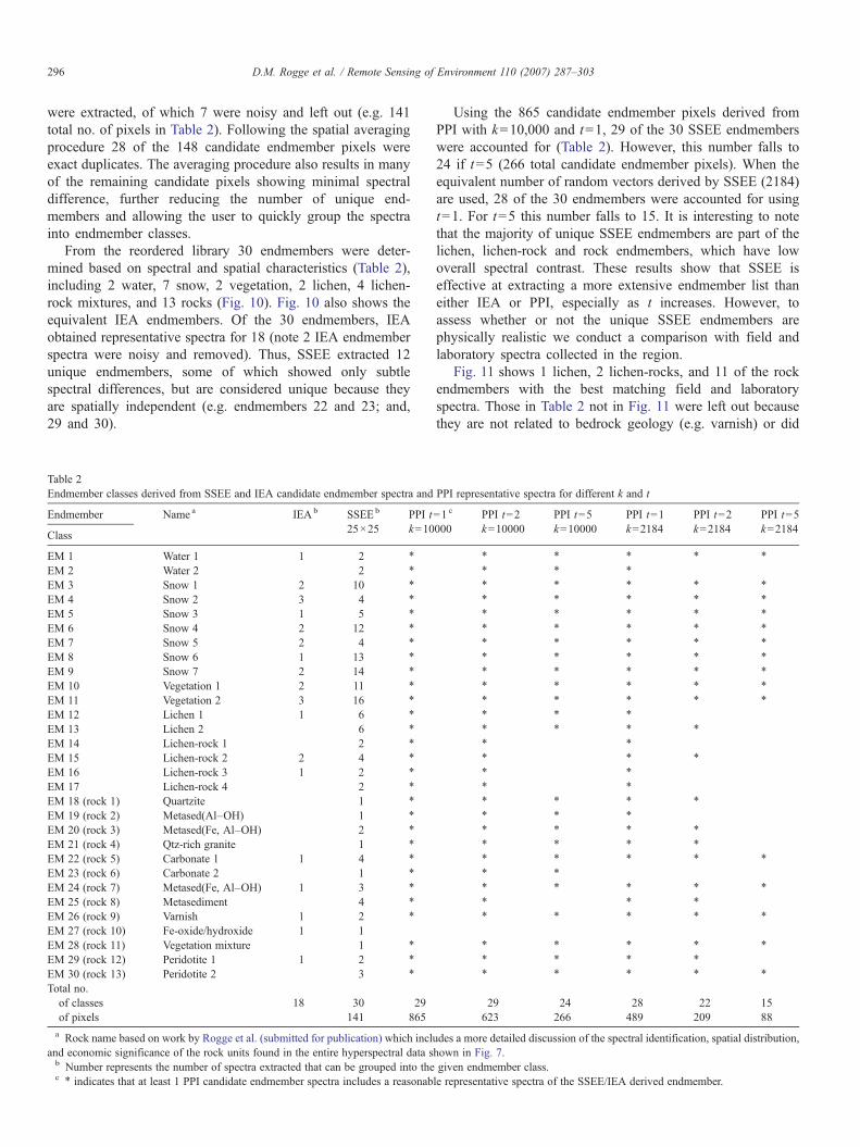
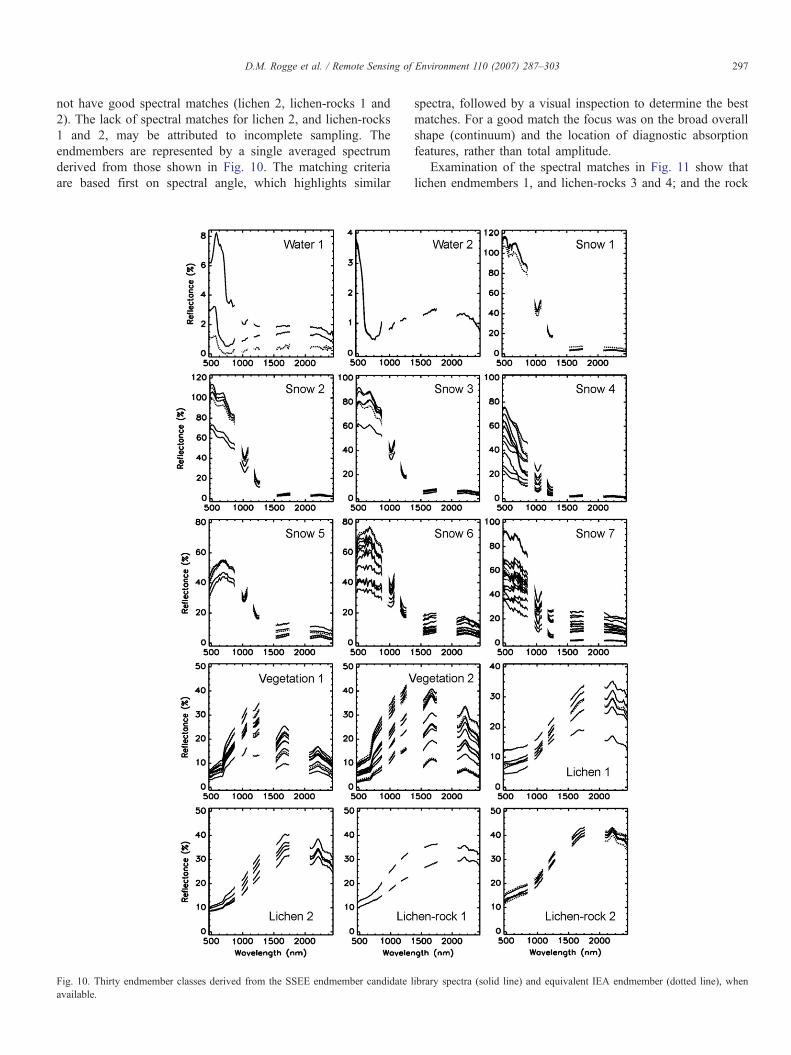
From the reordered library 30 endmembers were deter-mined based on spectral and spatial characteristics (Table 2),including 2 water, 7 snow, 2 vegetation, 2 lichen, 4 lichen-rock mixtures, and 13 rocks (Fig. 10). Fig. 10 also shows theequivalent IEA endmembers. Of the 30 endmembers, IEAobtained representative spectra for 18 (note 2 IEA endmemberspectra were noisy and removed). Thus, SSEE extracted 12unique endmembers, some of which showed only subtlespectral differences, but are considered unique because theyare spatially independent (e.g. endmembers 22 and 23; and,29 and 30).

Table 2Endmember classes derived from SSEE and IEA candidate endmember spectra and

Endmember Name a IEAb SSEEb

25×25PPI tk=10

Class

EM 1 Water 1 1 2 ⁎

EM 2 Water 2 2 ⁎

EM 3 Snow 1 2 10 ⁎

EM 4 Snow 2 3 4 ⁎

EM 5 Snow 3 1 5 ⁎

EM 6 Snow 4 2 12 ⁎

EM 7 Snow 5 2 4 ⁎

EM 8 Snow 6 1 13 ⁎

EM 9 Snow 7 2 14 ⁎

EM 10 Vegetation 1 2 11 ⁎

EM 11 Vegetation 2 3 16 ⁎

EM 12 Lichen 1 1 6 ⁎

EM 13 Lichen 2 6 ⁎

EM 14 Lichen-rock 1 2 ⁎

EM 15 Lichen-rock 2 2 4 ⁎

EM 16 Lichen-rock 3 1 2 ⁎

EM 17 Lichen-rock 4 2 ⁎

EM 18 (rock 1) Quartzite 1 ⁎

EM 19 (rock 2) Metased(Al–OH) 1 ⁎

EM 20 (rock 3) Metased(Fe, Al–OH) 2 ⁎

EM 21 (rock 4) Qtz-rich granite 1 ⁎

EM 22 (rock 5) Carbonate 1 1 4 ⁎

EM 23 (rock 6) Carbonate 2 1 ⁎

EM 24 (rock 7) Metased(Fe, Al–OH) 1 3 ⁎

EM 25 (rock 8) Metasediment 4 ⁎

EM 26 (rock 9) Varnish 1 2 ⁎

EM 27 (rock 10) Fe-oxide/hydroxide 1 1EM 28 (rock 11) Vegetation mixture 1 ⁎

EM 29 (rock 12) Peridotite 1 1 2 ⁎

EM 30 (rock 13) Peridotite 2 3 ⁎

Total no.of classes 18 30 29of pixels 141 865a Rock name based on work by Rogge et al. (submitted for publication) which incl

and economic significance of the rock units found in the entire hyperspectral data sb Number represents the number of spectra extracted that can be grouped into thec ⁎ indicates that at least 1 PPI candidate endmember spectra includes a reasonab

Using the 865 candidate endmember pixels derived fromPPI with k=10,000 and t=1, 29 of the 30 SSEE endmemberswere accounted for (Table 2). However, this number falls to24 if t=5 (266 total candidate endmember pixels). When theequivalent number of random vectors derived by SSEE (2184)are used, 28 of the 30 endmembers were accounted for usingt=1. For t=5 this number falls to 15. It is interesting to notethat the majority of unique SSEE endmembers are part of thelichen, lichen-rock and rock endmembers, which have lowoverall spectral contrast. These results show that SSEE iseffective at extracting a more extensive endmember list thaneither IEA or PPI, especially as t increases. However, toassess whether or not the unique SSEE endmembers arephysically realistic we conduct a comparison with field andlaboratory spectra collected in the region.

Fig. 11 shows 1 lichen, 2 lichen-rocks, and 11 of the rockendmembers with the best matching field and laboratoryspectra. Those in Table 2 not in Fig. 11 were left out becausethey are not related to bedrock geology (e.g. varnish) or did

PPI representative spectra for different k and t

=1 c

000PPI t=2k=10000

PPI t=5k=10000

PPI t=1k=2184

PPI t=2k=2184

PPI t=5k=2184

⁎ ⁎ ⁎ ⁎ ⁎⁎ ⁎ ⁎⁎ ⁎ ⁎ ⁎ ⁎⁎ ⁎ ⁎ ⁎ ⁎⁎ ⁎ ⁎ ⁎ ⁎⁎ ⁎ ⁎ ⁎ ⁎⁎ ⁎ ⁎ ⁎ ⁎⁎ ⁎ ⁎ ⁎ ⁎⁎ ⁎ ⁎ ⁎ ⁎⁎ ⁎ ⁎ ⁎ ⁎⁎ ⁎ ⁎ ⁎ ⁎⁎ ⁎ ⁎⁎ ⁎ ⁎ ⁎⁎ ⁎⁎ ⁎ ⁎⁎ ⁎⁎ ⁎⁎ ⁎ ⁎ ⁎⁎ ⁎ ⁎⁎ ⁎ ⁎ ⁎⁎ ⁎ ⁎ ⁎⁎ ⁎ ⁎ ⁎ ⁎⁎ ⁎⁎ ⁎ ⁎ ⁎ ⁎⁎ ⁎ ⁎⁎ ⁎ ⁎ ⁎ ⁎

⁎ ⁎ ⁎ ⁎ ⁎⁎ ⁎ ⁎ ⁎⁎ ⁎ ⁎ ⁎ ⁎

29 24 28 22 15623 266 489 209 88

udes a more detailed discussion of the spectral identification, spatial distribution,hown in Fig. 7.given endmember class.le representative spectra of the SSEE/IEA derived endmember.

297D.M. Rogge et al. / Remote Sensing of Environment 110 (2007) 287–303

not have good spectral matches (lichen 2, lichen-rocks 1 and2). The lack of spectral matches for lichen 2, and lichen-rocks1 and 2, may be attributed to incomplete sampling. Theendmembers are represented by a single averaged spectrumderived from those shown in Fig. 10. The matching criteriaare based first on spectral angle, which highlights similar

Fig. 10. Thirty endmember classes derived from the SSEE endmember candidate lavailable.

spectra, followed by a visual inspection to determine the bestmatches. For a good match the focus was on the broad overallshape (continuum) and the location of diagnostic absorptionfeatures, rather than total amplitude.

Examination of the spectral matches in Fig. 11 show thatlichen endmembers 1, and lichen-rocks 3 and 4; and the rock

ibrary spectra (solid line) and equivalent IEA endmember (dotted line), when

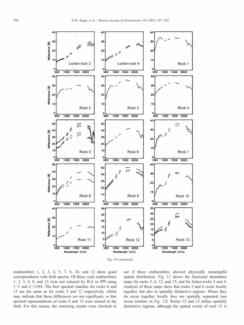
Fig. 10 (continued).

298 D.M. Rogge et al. / Remote Sensing of Environment 110 (2007) 287–303

endmembers 1, 2, 3, 4, 5, 7, 8, 10, and 12 show goodcorrespondence with field spectra. Of these, rock endmembers1, 2, 3, 4, 8, and 13 were not selected by IEA or PPI usingt=5 and k=2184. The best spectral matches for rocks 6 and13 are the same as for rocks 5 and 12 respectively, whichmay indicate that these differences are not significant, or thatspectral representations of rocks 6 and 13 were missed in thefield. For this reason, the unmixing results were checked to

see if these endmembers showed physically meaningfulspatial distribution. Fig. 12 shows the fractional abundancemaps for rocks 5, 6, 12, and 13; and for lichen-rocks 3 and 4.Analysis of these maps show that rocks 5 and 6 occur locallytogether, but also in spatially distinctive regions. Where theydo occur together locally they are spatially separated (seezoom window in Fig. 12). Rocks 12 and 13 define spatiallydistinctive regions, although the spatial extent of rock 13 is

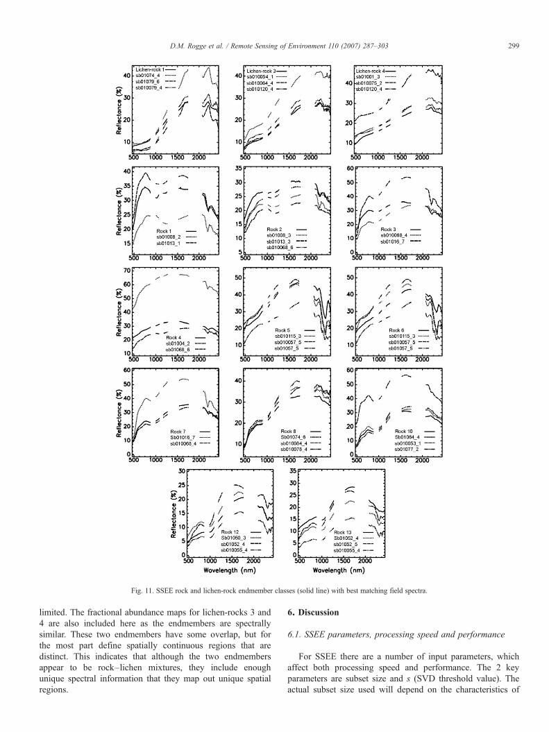
Fig. 11. SSEE rock and lichen-rock endmember classes (solid line) with best matching field spectra.

299D.M. Rogge et al. / Remote Sensing of Environment 110 (2007) 287–303

limited. The fractional abundance maps for lichen-rocks 3 and4 are also included here as the endmembers are spectrallysimilar. These two endmembers have some overlap, but forthe most part define spatially continuous regions that aredistinct. This indicates that although the two endmembersappear to be rock–lichen mixtures, they include enoughunique spectral information that they map out unique spatialregions.

6. Discussion

6.1. SSEE parameters, processing speed and performance

For SSEE there are a number of input parameters, whichaffect both processing speed and performance. The 2 keyparameters are subset size and s (SVD threshold value). Theactual subset size used will depend on the characteristics of

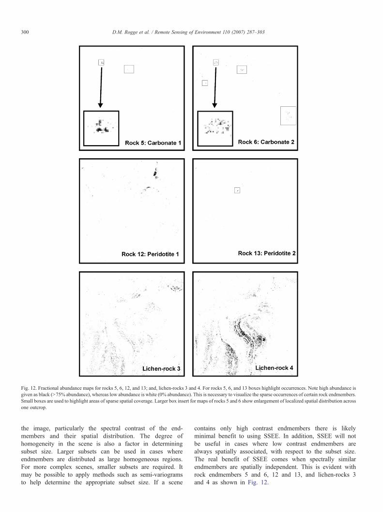
Fig. 12. Fractional abundance maps for rocks 5, 6, 12, and 13; and, lichen-rocks 3 and 4. For rocks 5, 6, and 13 boxes highlight occurrences. Note high abundance isgiven as black (N75% abundance), whereas low abundance is white (0% abundance). This is necessary to visualize the sparse occurrences of certain rock endmembers.Small boxes are used to highlight areas of sparse spatial coverage. Larger box insert for maps of rocks 5 and 6 show enlargement of localized spatial distribution acrossone outcrop.

300 D.M. Rogge et al. / Remote Sensing of Environment 110 (2007) 287–303

the image, particularly the spectral contrast of the end-members and their spatial distribution. The degree ofhomogeneity in the scene is also a factor in determiningsubset size. Larger subsets can be used in cases whereendmembers are distributed as large homogeneous regions.For more complex scenes, smaller subsets are required. Itmay be possible to apply methods such as semi-variogramsto help determine the appropriate subset size. If a scene

contains only high contrast endmembers there is likelyminimal benefit to using SSEE. In addition, SSEE will notbe useful in cases where low contrast endmembers arealways spatially associated, with respect to the subset size.The real benefit of SSEE comes when spectrally similarendmembers are spatially independent. This is evident withrock endmembers 5 and 6, 12 and 13, and lichen-rocks 3and 4 as shown in Fig. 12.

301D.M. Rogge et al. / Remote Sensing of Environment 110 (2007) 287–303

Choosing an appropriate subset size also effects processingspeed. When using smaller subsets the number of vectorsretained increases, such that projecting the data onto thesevectors becomes the controlling factor with respect to proces-sing speed. Subset sizes larger than 50 significantly reduceprocessing speed because of the processing time necessary toobtain vectors via SVD. With larger subset sizes we also reduceour ability to obtain vectors that may be related to low contrastendmembers, therefore reducing performance. Thus, the usermust balance information gained by reducing the subset size,knowing that many of the additional vectors are redundant.Based on work in this study we found that a subset size of 20–25 pixels was effective. For this analysis subsets did notoverlap. However, it may be advantageous to use overlappingsubsets, such that each pixel is compared equally to pixels in alldirections. Subsets could also be of different sizes and shapesdefined by the spatial complexity across the scene (e.g. quadtreedecomposition). It may also be useful to preprocess the vectorsto remove redundant vectors. However, this must done with caresuch that important vectors related to subtle spectral variationsare not removed.

The second key parameter that affects performance is theparameter s. Values set higher than 99% resulted in additionalvectors, many of which are related to noise and only increasedcomputational time. Values set lower than 99% result in fewervectors per subset (minimum of 2 in SSEE), which reduce ourability to select low contrast endmembers. Changing s canevidently have significant effects on the results, thus more workis required to determine an s value that works best for all datasets.

The size of the spatial averaging window was set to be equalto the subset size. This was done originally for consistency.However, for larger subsets an equivalent spatial averagingwindow had a negative impact on the methodology, in thatspatially independent endmembers that are spectrally similarmay be averaged. In addition, a larger window can increase thenumber of updated candidate pixels, which can make spatialaveraging impractical (see Table 1).

The last two parameters used in SSEE are spectral angle andRMS, which are used to update and average the candidateendmember pixels. For this project we used a spectral angle of1° and an RMS value equal to 0.001 based on reflectance scaledfrom 0–1.0. Higher spectral angle and RMS values result in alarger updated candidate endmember list, but also may lead tothe loss of the subtle spectral features that define a low contrastendmember. For this reason we chose to keep these two valuesto a minimum. Note that RMS is primarily used for dark pixels,such as water.

6.2. Comparison with PPI

Of the endmember extraction methods described in Section2, SSEE has most in common with PPI, even though AMEEalso uses spatial information. The similarity between SSEE andPPI relates to the projection of the data onto vectors andretaining those pixels that lie at either end of the vectors. Theprimary benefit of SSEE compared with PPI is the use of non-

random vectors. First and foremost is the fact that SSEE isrepeatable. Secondly, fewer vectors are required. In addition,many of the vectors derived from adjacent subsets areredundant, so the actual number of important vectors is lessthan the total compiled and results in a smaller number ofcandidate pixels that the user must work with, compared withPPI. This is evident from the results, where for an equivalentnumber of random vectors a total of 489 candidate pixels wereselected using PPI, as opposed to 148 for SSEE. For PPI, the useof random vectors results in more spectral variability amongcandidate pixels. For SSEE, vectors are only retained for eachsubset region if they explain a significant percentage of thespectral variance. This reduces the possibility of retainingvectors related to noise, and in turn, selecting pixels that arenoisy.

Because of the high number and spectral variability of thePPI endmembers this requires a great deal of humanintervention to derive a final endmember set. For SSEEhuman intervention is limited to grouping the non-duplicateendmember candidates. This step is simplified by reordering thelist based on spectral similarity, and by using the spatialcoordinates of each candidate endmember pixel.

Steps 1 and 2 of the SSEE methodology make use ofprojecting the data volume onto vectors to derive a set ofcandidate endmember pixels, as used with PPI. However, thekey difference is that for SSEE the vectors are not random, buteigenvectors derived from image subsets. In doing so, the SSEEmethodology by-passes the difficulty of setting an adequatethreshold of eigenvalues encountered when analyzing an entireimage by retaining only the top few vectors related to signal foreach subset region. This approach makes use of the fact thateigenvectors are dependent on the scene statistics, and are thus,spatially dependent.

6.3. Local vectors versus local candidate pixels

It is possible to use the local vectors to select a set of localcandidate pixels for each subset region. However, the keydrawback of this approach is the necessity to filter through amuch larger number of candidate pixels to determine anendmember set for the full image. These local candidate pixelsmay also be partial mixtures, which complicate the selection ofendmembers. To account for this problem we have choseninstead to use local vectors, rather than local endmembers.Then, in turn, scale up to the full image by projecting the dataonto the compiled vector set.

7. Conclusions

The spatial–spectral endmember extraction tool (SSEE)presented in this paper makes primary use of spatial informationto: 1) select local eigenvectors that relate to both high and lowcontrast endmembers within the scene; and, 2) to average onlyspectrally similar endmembers that are also spatially related.This results in a higher number of candidate endmembers thatare defined both spectrally and spatially. The evaluation ofSSEE has shown that the method is capable of extracting unique

302 D.M. Rogge et al. / Remote Sensing of Environment 110 (2007) 287–303

endmembers with subtle spectral variability that are not selectedby other well known spectral-based methods. These uniqueendmembers were shown to be spectrally significant owing tocomparisons with field spectra and through physically realisticspatial distribution.

The two key parameters that affect the processing speed andperformance of SSEE are subset size and s (SVD thresholdvalue). For the two evaluations used in this paper a subset sizeof 20 to 25 pixels squared and an s value of 99% were shown tobe effective at selecting both high and low contrast end-members. The use of local eigenvectors, rather than localendmembers, allows SSEE to retain local information, but alsoapply that information at the scale of the full image. The use ofspatial subsets to select eigenvectors also allows SSEE to by-pass the problems associated with selecting a cutoff thresholdbetween eigenvectors caused by signal versus those related tonoise. However, the usefulness of SSEE is dependent on thespectral contrast and spatial distribution of the endmemberswithin the scene. Thus, SSEE is particularly beneficial forextracting spectrally similar endmembers that are also spatiallyindependent. Overall the SSEE method is quick, repeatable, andrequires minimal user input.

References

Adams, J. B., & Gillespie, A. R. (2006). Remote sensing of landscapes withspectral images: A physical modeling approach (p. 362). New York:Cambridge University Press.

Adams, J. B., Smith, M. O., & Gillespie, A. R. (1993). Imaging spectroscopy:Interpretation based on spectral mixture analysis. In C. M. Pieters, & P. A.Englert (Eds.), Remote geochemical analysis: Elemental and mineralogicalcomposition (pp. 145−166). Cambridge: Cambridge University Press.

Adams, J. B., Smith, M. O., & Johnson, P. E. (1986). Spectral mixture modeling:a new analysis of rock and soil types at the Viking Lander 1 site. Journal ofGeophysical Research, 91, 8098−8112.

Bateson, A., & Curtiss, B. (1996). A method for manual endmember selectionand spectral unmixing. Remote Sensing of Environment, 55, 229−243.

Berk, A., Anderson, G. P., Bernstein, L. S., Acharya, P. K., Dothe, H., Mattew,M. W., et al. (1999). MODTRAN4 radiative transfer modeling foratmospheric correction. SPIE proceedings, optical spectroscopic techniquesand instrumentation for atmospheric and space research III (p. 3756).

Berman, M., Kiiveri, H., Lagerstrom, R., Ernst, A., Dunne, R., & Huntington,J. F. (2004). ICE: A statistical approach to identifying endmembers inhyperspectral images. IEEE Transactions on Geoscience and RemoteSensing, 42, 2085−2095.

Boardman, J. W. (1993). Automating spectral unmixing of AVIRIS data usingconvex geometry concepts. Summaries of the fourth annual JPL airbornegeoscience workshop. JPL Publication 93-26, (pp. 11–14, Vol. 1).

Boardman, J. W., Kruse, F. A., & Green, R. O. (1995). Mapping targetsignatures via partial unmixing of AVIRIS data. Summaries, fifth JPL air-borne earth science workshop. JPL Publication 95-1, (pp. 23–26, Vol. 1).

Bowles, J., Palmadesso, P. J., Antoniades, J. A., Baumback, M. M., &Rickard, L. J. (1995). Use of filter vectors in hyperspectral data analysis.Proceedings SPIE infrared spaceborne remote sensing III (pp. 148−157).

Chang, C.-I., & Du, Q. (2004). Estimation of number of spectrally distinctsignal sources in hyperspectral imagery. IEEE Transactions on Geosciencceand Remote Sensing, 42, 608−619.

Chang, C.-I., & Plaza, A. (2006). A fast iterative algorithm for implementationof Pixel Purity Index. IEEE Transactions on Geoscience and RemoteSensing Letters, 3, 63−67.

Clark, R. N., & Roush, T. L. (1984). Reflectance spectroscopy: quantitativeanalysis techniques for remote sensing applications. Journal of GeophysicalResearch, 89, 6329−6340.

Clark, R. N., Swayze, G. A., Livo, K. E., Kokaly, R. F., Sutley, S. J., Dalton,J. B., et al. (2003). Imaging spectroscopy: Earth and planetary remotesensing with the USGS Tertracorder and expert systems. Journal ofGeophysical Research, 108(E12), 5-1−5-44.

Green, A. A.., Berman, M., Switzer, P., & Craig, M. D. (1988). Atransformation for ordering multispectral data in terms of image quality withimplications for noise removal. IEEE Transactions on Geoscience andRemote Sensing, 26, 65−74.

Green, R. O., Eastwood, M. L., Sarture, C. M., Chrien, T. G., Aronsson, M.,Chippendale, B. J., et al. (1998). Imaging spectroscopy and the AirborneVisible/Infrared Imaging Spectrometer (AVIRIS). Remote Sensing ofEnvironment, 65, 227−248.

Haskell, K. H., & Hanson, R. J. (1981). An algorithm for C linear least squaresproblems with equality and C nonnegativity constraints. MathematicalProgramming, C 21, 98−118.

Healey, G., & Slater, D. (1999). Models and methods for automated materialidentification in hyperspectral imagery acquired under unknown illumina-tion and atmospheric conditions. IEEE Transactions on Geosciencce andRemote Sensing, 37, 2706−2717.

Ifarraguerri, A., & Chang, C. -I. (1999). Multispectral and hyperspectral imageanalysis with convex cones. IEEE Transactions on Geoscience and RemoteSensing, 37, 756−770.

Jolliffe, I. T. (1986). Principle component analysis. New York: Springer Verlag.Keshava, N., & Mustard, J. F. (2002, January). Spectral unmixing. IEEE Signal

Processing Magazine, 44−57.Nascimento, J. M. P., & Dias, J. M. B. (2005). Vertex component analysis: a

fast algorithm to unmix hyperspectral data. IEEE Transactions onGeoscience and Remote Sensing, 43, 898−910.

Neville, R. A., Staenz, K., Szeredi, T., Lefebvre, J., & Hauff, P. (1999, 21–24June). Automatic endmember extraction from hyperspectral data for mineralexploration. Fourth international airborne remote sensing conference andexhibition / 21st Canadian symposium on remote sensing. Ottawa, Ontario,Canada: Natural Resources Canada.

Neville, R. A., Sun, L., & Staenz, K. (2003). Detection of spectral linecurvature in imaging spectrometer data. SPIE Proceedings: Algorithms andTechnologies for Multispectral, Hyperspectral and Ultraspectral Imagery,(pp. 144–154, Vol. 5093).

Plaza, A., Martinez, P., Perez, R., & Plaza, J. (2002). Spatial/spectralendmember extraction by multidimensional morphological operations.IEEE Transactions on Geoscience and Remote Sensing, 40, 2025−2041.

Plaza, A., Martinez, P., Perez, R., & Plaza, J. (2004). A quantitative andcomparative analysis of endmember extraction algorithms from hyperspec-tral data. IEEE Transactions on Geoscience and Remote Sensing, 42,650−663.

Press, W. H., Flannery, B. P., Teukolsky, S. A., & Vetterling, W. T. (1992).Numerical recipes in C: The art of scientific computing, 2nd edition.Cambridge University Press.

Rogge, D. M., Rivard, B., Zhang, J., & Feng, J. (2006). Iterative spectralunmixing for optimizing per-pixel endmember sets. IEEE Transactions onGeoscience and Remote Sensing, 44, 3725−3736.

Rogge, D. M., Rivard, B., Harris, J., & Zhang, J. (submitted for publication).Application of hyperspectral data for remote predictive mapping. BaffinIsland, Canada. Economic Geology.

Secker, J., Staenz, K., Gauthier, R. P., & Budkewitsch, P. (1991). Vicariouscalibration of airborne hyperspectral sensors in operational environments.Remote Sensing of Environement, 76, 81−92.

Settle, J. J., & Drake, N. A. (1993). Linear mixing and the estimation ofground cover proportions. International Journal of Remote Sensing, 14,1159−1177.

Staenz, K., Szeredi, T., & Schwarz, J. (1998). ISDAS — A system forprocessing/analyzing hyperspectral data; technical note. Canadian Journalof Remote Sensing, 24, 99−113.

St-Onge, M. R., Wodicka, N., & Lucas, S. B. (1999). Geology of McKellerBay–Wight Inlet — Frobisher Bay area, southern Baffin Island, NorthwestTerritories. Current Research, 1998-C (pp. 43–53). Geological Survey ofCanada.

Swayze, G. A., Clark, R. N., Sutley, S., & Gallagher, A. (1992). Ground-truthing AVIRIS mineral mapping at Cuprite, Nevada. Summaries of

303D.M. Rogge et al. / Remote Sensing of Environment 110 (2007) 287–303

the third annual JPL airborne geosciences workshop. AVIRISWorkshop, JPL Publication 192-14, (pp. 47–49, Vol. 1). California:Pasadena.

Thai, B., Healey, G., & Slater, D. (1999, February). Invariant subpixel materialidentification in AVIRIS imagery. Proc. JPL AVIRIS workshop, JPLPublication 99-17. California: Pasadena.

Tompkins, S., Mustard, J. F., Pieters, C. M., & Forsyth, D. W. (1997).Optimization of endmembers for spectral mixture analysis. Remote Sensingof Environment, 59, 472−489.

Tsai, F., & Philpot, W. (1998). Derivative analysis of hyperspectral data.Remote Sensing of Environment, 66, 41−51.

Winter, M. E. (1999). Fast autonomous spectral endmember determinationin hyperspectral data. Proceedings of the thirteenth international con-ference on applied geologic remote sensing (pp. 337−344). Vancouver,B.C., Canada, II: ERIM International LTD.

Winter, M. E., & Winter, E. M. (2000). Comparison of approaches fordetermining end-members in hyperspectral data. IEEE Aerospace Confer-ence Proceedings, 3, 305−313.