2010:034

M A S T E R ' S T H E S I S

Integration of hot waterextraction in biomass

based CHP plants- possibilities for green chemicals and increased electricity

production

Sennai Asmelash Mesfun

Luleå University of Technology

Master Thesis, Continuation Courses Sustainable energy systems

Department of Applied Physics and Mechanical EngineeringDivision of Energy Engineering

2010:034 - ISSN: 1653-0187 - ISRN: LTU-PB-EX--10/034--SE

i

ABSTRACT

The main objective of this thesis was to investigate the possibility to increase the steam

temperature in the superheater in biomass (hard wood) fired CHP plants by the integration

of a hemicellulose hot-water extraction process. This was motivated due to the cleaner fuel

(extracted wood chips) obtained after the extraction process.

One important result from the chemical analysis of the extracted wood-chips was the

removal of a large share of the inorganic constituents, except Chlorine and Sulphur, from

the lignocellulosic biomass. Some of those inorganic constituents (alkalis) are believed to be

responsible for the fireside heat exchanger and boiler walls corrosion problems during

combustion. A large portion of the current work aimed to investigate the possibility to

increase the superheated steam temperature in biomass fired boilers. Thermodynamic

equilibrium calculations were performed for the extracted as well as for the original birch

wood chips combustion using FactSage 6.0. The results showed significant differences in

equilibrium concentrations between the fuels, which could be relevant initial step towards

increased temperature operation in biomass fired boilers. Converting those results into

possible operational steam temperature increment is something that needs further

research.

A techno-economic analysis was performed for a new integrated process that produces

ethanol and acetic acid from hardwood (Birch) in addition to electricity and heat. The

process involves the extraction of hemicellulose content of hardwood using water at a

temperature of 160 - 180℃ and a pressure of 7 bars. The extraction process is integrated

into a biomass fired CHP plant. The unit operations considered in this work include a boiler/

turbo-generator which operate on Rankine cycle, extraction and hydrolysis pressurized

vessel, liquid-liquid separation process (for separation of acetic acid and fermentable

sugars), and fermentation and ethanol up-grading processes. The hot-water extraction

process at this stage is assumed to operate batch wise and heat was supplied from boiler

exhaust gases.

Results show low ethanol yield rate from hardwood through the hot-water extraction

pathway, 0.0356 kg/ kg drywood, as compared to the current SHF (Separate Hydrolysis and

Fermentation) technologies from hardwood conversion rate. This is due to the fact that hot-

water extraction process dissolves the hemicellulose portion of the lignocellulosic biomass

and the cellulose remains intact in the extracted chips. In addition to ethanol the process

yields 0.0276 kg/kg drywood of acetic acid.

Under the assumed economic conditions, ethanol can be produced to a cost in the range of

SEK 3.4 to SEK 11 per litre depending on the plant size and annual operational hours.

Electricity can be generated to a cost in the range of SEK 450, for the case with 100MW

plant size and 8400 annual operational hours, to SEK 1120 per MWhel, for the case with

10MW plant size and 2000 operational hours per year.

ii

ACKNOWLEDGEMETNS

First of all I would like to thank the Almighty God for giving me health, courage and strength.

Secondly, I would like to express my deepest gratitude to my thesis supervisor, Dr. Joakim

Lundgren. This work would not have been reached this stage without his guidance, hard

work and expertise idea. I would like to extend my gratitude to Prof. Marcus Öhman and

Ida-Linn Nyström (PhD student, at the Division of Energy Engineering, LTU) for their

continuous, valuable and unreserved assistance with FactSage 6.0 package. I would like to

thank Jonas Helmerius (PhD student, at the Division of Chemical Engineering, LTU) for his

collaboration in demonstrating the lab-scale hot-water extraction process. I would also like

to thank Prof. Carl- Eric Grip for his valuable general advice on how to approach engineering

problems and present results obtained in a transparent manner. And Finally, I would like to

thank Mats Lundberg (Senior Specialist at Sandvik Materials Technology) for sharing

information and his expertise suggestion regarding biomass fired boilers and corrosion

behaviour of extracted woodchips.

iii

Table of Contents

1. BACKGROUND ........................................................................................................................ 1

1.1 Introduction ...................................................................................................................... 1

1.1.1 Hot Water Extraction (HWE) process ........................................................................ 2

1.1.2 Biomass Based Ethanol .............................................................................................. 3

1.1.3 Forest products industry ........................................................................................... 4

1.1.4 High temperature corrosion ...................................................................................... 4

1.2 Concept of biorefinery processes .................................................................................... 5

1.3 Objective and Scope ......................................................................................................... 6

2. METHODOLOGY AND THE INTEGRATED PROCESS DESCRIPTION .......................................... 7

2.1 Methods ........................................................................................................................... 7

2.1.1 Corrosion Prediction ..................................................................................................... 7

2.1.2 Economic Evaluation ..................................................................................................... 7

2.1.2.1 Capital investment estimates ................................................................................. 7

2.1.2.2 Operating cost estimation .................................................................................... 10

2.1.2.3 Cost sharing and assumed economy .................................................................... 10

2.1.2.3 Profitability Analysis ............................................................................................. 11

2.2 Description of the hot-water extraction process integrated ......................................... 11

3. LITERATURE REVEIW ............................................................................................................ 14

3.1 High Temperature Corrosion during biomass Combustion ........................................... 14

3.1.1 Mechanisms of Corrosion ........................................................................................ 14

3.1.1.1 Thermodynamic stability of common metal oxides and chlorides .................. 14

3.1.1.2 Mechanism 1: Corrosion related to Cl and HCl (Gas phase corrosion) ............ 15

3.1.1.3 Mechanism 2: Corrosion from the vapours of NaCl and KCl ............................ 16

3.1.1.4 Mechanism 3: Solid phase corrosion in deposits ............................................. 17

3.1.1.5 Mechanism 4: Sulfation of alkali chlorides in deposits .................................... 18

3.1.1.6 Mechanism 5: Corrosion due to molten chlorides ........................................... 18

3.1.1.7 Mechanism 6: Corrosion due to molten sulphates .......................................... 19

3.1.2 Some relevant results of previous experimental investigations ............................. 20

3.1.3 Indices for predicting corrosion behaviour of biomass fuels .................................. 22

4. RESULTS ................................................................................................................................ 24

4.1 Equilibrium calculation results ....................................................................................... 24

iv

4.1.1 Equilibrium distribution of K, Na and S (400-900℃) (combustion temperature

900℃) ............................................................................................................................... 24

4.1.2 Equilibrium distribution of K, Na, Ca, Cl and S (400-900℃) (combustion temperature

1000℃) ................................................................................................................................. 27

4.1.3 Equilibrium distribution of K, Na and S (400-900℃) (combustion temperature

1100℃) ................................................................................................................................. 31

4.2 Extraction process mass and energy balance results .................................................... 33

4.3 Boiler/turbo-generator energy and mass balance results ............................................. 35

4.4 Economic evaluation results .......................................................................................... 37

4.4.1 Sensitivity analysis ................................................................................................... 38

4.4.2 Profitability analysis results ..................................................................................... 40

5. CONCLUDING DISCUSSION .................................................................................................. 41

Future work .............................................................................................................................. 44

REFERENCES ............................................................................................................................. 45

APPENDIX A .............................................................................................................................. 48

A.1 Elemental analysis of Birch and Extracted wood ........................................................... 48

A.2 Thermodynamic equilibrium calculations ..................................................................... 49

A.3 Boiler/Turbo- generator energy and mass balance ....................................................... 51

A.4 Hot-water extraction energy demand ........................................................................... 58

A.5 Estimation of Ethanol yield from Xylose ........................................................................ 60

A.5.1 Mass and Energy balance of the Hydrolysis-Fermentation processes ................... 60

APPENDIX B: Economic Evaluation .......................................................................................... 62

B.1 Equipment cost estimates .............................................................................................. 62

B.2 Ancillary cost estimation ................................................................................................ 63

B.3 Economic indicators calculation .................................................................................... 64

v

List of Tables

Table 1.1 Average composition of birch (hardwood) and softwoods ....................................... 2

Table 2.1 Process areas for ethanol production ........................................................................ 8

Table 2.2 Equations for estimating installed equipment cost ................................................... 9

Table 2.3 Equations for estimating equipment cost .................................................................. 9

Table 2.4 Parameters assumed in the economic evaluation ................................................... 11

Table 2.5 Hot water extraction and hydrolysis output .......................................................... 12

Table 3.1 Temperature at which metal chlorides vapour pressure is equal to 10�� bar ....... 15

Table 3.2 Melting temperature of pure species and mixtures ................................................ 17

Table 3.3 Alkali free index of some biomass-derived fuels and coal ....................................... 23

Table 4.1 Mass and Energy balance results, per Kg- ethanol yield ......................................... 35

Table 4.2 Annual production and feedstock demand results (8400 hrs/year) ........................ 36

Table 4.3 Total energy efficiency of the system ...................................................................... 36

Table 4.4 Results of economic indicators ................................................................................ 40

Table A.1 Birchwood and Extracted wood chips elemental analysis ...................................... 48

Table A.2 Indices for predicting corrosion behaviour of biomass fuels .................................. 48

Table A.3 FactSage input data ................................................................................................. 49

Table A.4 Data assumed in steam/ electricity and district heat production process .............. 51

Table A.5 Air and exhaust gases fans data .............................................................................. 54

Table A.6 Boiler/ turbo-generator mass and energy balance results ...................................... 55

Table A.7 Heat demand of extraction process (results for 10MW plant size) ........................ 58

Table A.8 Reference SHF process ............................................................................................. 61

Table B.1: Direct and indirect cost estimation ........................................................................ 63

Table B.2 Spreadsheet for economic evaluation (case 100MW, 8400 hr) .............................. 66

vi

List of Figures

Figure 1.1: World primary energy demand (including future forecast) and Total bioenergy

production potential estimates in 2050 .................................................................................... 2

Figure 1.2: From wood to value added chemicals through extraction of woody biomass ....... 3

Figure 2.1: HWE process output for 100 g (DS) of hardwood ................................................. 12

Figure 2.2: CHP plant and the integrated process configuration ............................................ 13

Figure 3.1: The effect of chlorine on the melting behaviour of alkalis sulphates ................... 19

Figure 3.2: Bell shaped curve for the temperature dependence of corrosion rate from

molten sulphides. ..................................................................................................................... 21

Figure 4.1: K- equilibrium distribution at combustion temperature 900℃ ............................ 24

Figure 4.2: Na- equilibrium distribution at combustion temperature 900℃ .......................... 25

Figure 4.3 S-equilibrium distributions at combustion temperature 900 ℃ ............................ 26

Figure 4.4: K- equilibrium distribution at combustion temperature 1000℃ .......................... 27

Figure 4.5: Na- equilibrium distribution at combustion temperature 1000℃ ........................ 28

Figure 4.6: S- equilibrium distribution at combustion temperature 1000℃ .......................... 29

Figure 4.7: Ca- equilibrium distribution at combustion temperature of 1000℃ .................... 29

Figure 4.8: Cl-equilibrium distributions at combustion temperature 1000 ℃ ........................ 30

Figure 4.9: K- equilibrium distribution at combustion temperature 1100℃ .......................... 31

Figure 4.10: Na- equilibrium distribution at combustion temperature 1100℃ ...................... 32

Figure 4.11: S-equilibrium distribution at combustion temperature 1100 ℃ ........................ 33

Figure 4.12: Energy demand of the integrated extraction process per Kg ethanol yield ....... 34

Figure 4.13: Annual production levels of electricity, heat (left-vertical axis) and Ethanol,

acetic acid (right-vertical axis) ................................................................................................. 36

Figure 4.14: Annual production levels of electricity, heat (left-vertical axis) and Ethanol,

acetic acid (right-vertical axis) ................................................................................................. 37

Figure 4.15: Cost of ethanol production at different annual operational hours Vs plant size 37

Figure 4.16: Cost of el. production at different annual operational hours against plant size 38

Figure 4.17: Cost of heat production at different annual operational hours Vs plant size ..... 38

Figure 4.18: Ethanol production cost against cost of other inputs for different plant sizes ... 39

Figure 4.19 heat production cost against cost of feedstock for different plant sizes ............. 39

Figure 4.20: Electricity production cost against cost of feedstock for different plant sizes ... 39

Figure 4.21: IRR (%) against selling price of acetic acid for the different plant sizes .............. 40

Figure A.1: h-s diagram for the steam properties evaluation ................................................. 52

Figure B.1: Equipment cost of A800 against steam flow rate ................................................. 62

Figure B.2: Equipment cost of the different process area against ethanol yield rate ............. 62

Figure B.3: Equipment cost of A100 and extraction vessel against feedstock rate ................ 63

1

1. BACKGROUND

1.1 Introduction

The interest in renewable resources as source of energy have increased because of the

growing environmental concerns, which resulted in more strict national and international

regulations against carbon dioxide emissions, and the shortages and instability of oil

supplies. The ever increasing worldwide energy demand in general and in rapidly growing

economies, developing countries, in particular have necessitated the need for additional

and more reliable energy resource to meet the anticipated consumption. This is especially

bold when it comes to liquid fuels such as gasoline used in transportation.

Biomass is one form of green energy (Carbon-dioxide neutral) sources, in such a way that

the carbondioxide emitted will be taken-up by the forest thereby producing no or little net

effect to the atmosphere. Besides, the use of various biomasses, such as wood, straw,

willow, black liquor, etc., as a source of energy would reduce carbon dioxide discharges as

compared to fossil fuels. The worldwide energy demand can partly be satisfied by using

biomass energy (figure 1.1 shows the potential for bioenergy in 2050). The annual global

production of biomass is equivalent to the 4500 EJ solar energy captured each year.

(Ladanai and Vinterbäck, 2009) This concept can partially be embodied in the idea of a bio-

refinery. A bio-refinery is similar to a traditional petroleum refinery except for the fact that

biomass would be the feedstock rather than crude oil. Contrary to the conventional oil

refinery which mainly uses thermal processing, a bio-refinery could implement both thermal

and biological processes to convert hemicellulose, cellulose and lignin into energy and

different chemicals. The concept of bio-refinery has been advanced by a number of

researchers [Lundgren, 2009; Thomas et al., 2008, 2009; Gable et al., 2008].

The world primary energy demand accounts coal, oil, gas, hydro, biomass and waste (includes traditional and

modern use) and other renewables. Total bioenergy production potentials include surplus forest growth,

agricultural and forest residues, dedicated woody bioenergy crops on surplus agricultural land. a Based on

highest consumption scenario. b Based on an upper limit of the amount of biomass that can come available as

(primary) energy supply without affecting the supply for food crops. c Based on scenario where a type of

2

agricultural management applied is similar to the best available technology in the industrialized regions

(1EJ=1018

Joules)

Figure 1.1: World primary energy demand in 1980, 2000 & 2006 and forecast for 2015, 2030

& 2050, and Total bioenergy production potential estimates in 2050 (Ladanai and

Vinterbäck, 2009)

Chief amongst the available biomass alternatives, for ethanol production, to corn and

sugarcane is lignocellulosic biomass. Lignocellulosic biomass derived ethanol has no

difference in functionality and composition compared to alcohols derived from other

sources and is a reasonable liquid fuel with about two thirds the heating value per litre as

gasoline. (Thomas et al., 2008) Yet, ethanol is used as an additive to increase the octane

number of gasoline thereby increasing the engine efficiency and reducing pollution.

Sweden, certainly has a great deal of potential feedstocks of lignocellulosic biomass as well

as potential to grow much more so it would seem reasonable to turn to this as a contributor

to domestic fuel. One way to achieve such goals is to transform existing CHP plants in to

biorefineries to produce high value- added green chemicals along with the ordinary energy

products such as heat and electricity.

1.1.1 Hot Water Extraction (HWE) process

Lignocellulosic biomass is composed of four main components: cellulose, hemicellulose,

lignin and extractives. Extractives are extractable compounds that can be readily dissolved

with water or organic solvents at room temperature and atmospheric conditions. (Thomas

et al., 2008) Cellulose and hemicellulose are the structural carbohydrates in wood that form

the supporting structure of the plant cell wall. (Helmerius, 2010) Cellulose provides

structure and strength, while hemicellulose and lignin provide bonding to the structure.

Table 1.1 Average composition of birch (hardwood) and softwoods (Helmerius, 2010)

Species Cellulose (%) Hemicellulose (%) Lignin (%) Extractives (%)

Softwoods 42 27 28 3

Hardwood (Birch) 45 30 20 5

In addition, there are inorganic compounds present in lignocellulosic biomass. There are

over 70 metals, earth elements and inorganic compounds found in lignocellulosic biomass,

with Potassium (K) and Calcium (Ca) being the major followed by Magnesium (Mg) and

Phosphorous (P). (Thomas et al., 2008)

Extraction of the readily hydrolysable carbohydrates using hot-water in the absence of

added mineral acids or bases is desirable for facilitating the utilization and the recovery of

the hydrolyzate products. Extracted woodchips have not shown reduction in heating value,

rather it has increased probably due to the removal of most of ash forming minerals during

the extraction process. This could be an advantage from corrosion point of view during

combustion of the extracted chips (this topic is in-fact one of the main issues discussed in

3

this project). Furthermore, the environmental and recovery side effects are avoided since no

sodium or caustic is added to the process streams, at least at this stage. (Helmerius, 2010)

Hot-water extraction process is a self catalytic process due to the acetic acid liberated from

the hemicellulose. The extracted liquid contains high concentration of oligomer and

monomer xylose (5-carbon sugar) which can be utilized as a substrate by organisms in

fermentation processes. (Lundgren, 2009) The process steps are mainly hot-water

extraction, secondary hydrolysis (enzymatic or acid) to depolymerise xylan to xylose, acetic

acid separation and fermentation. Via acetic acid separation, the acid can be a final product

or used in other processes, such as hydrolysis or to extract hemicellulose from softwoods.

Figure 1.2: From wood to value added chemicals through extraction of woody biomass

1.1.2 Biomass Based Ethanol

There are a number of drivers which have increased the interests in bio-ethanol production.

These parameters can broadly be grouped as environmental, political and economical

drivers.

Environmental drivers

The use of bio-ethanol to supplement gasoline and diesel reduces the carbon-dioxide

emissions substantially, by reducing the net CO� accumulation in the atmosphere.

Political drivers

The use of bio-ethanol will reduce the dependence on fossil fuels, which are located in the

world’s politically most unstable regions. Yet, bio-based fuels can have a negative impact on

the world’s food supply chain when produced from sugarcane and corn. This puts

lignocellulosic biomass as a good alternative source for bio-fuel production.

4

Economic drivers

With the continuously increasing price of oil, bio-ethanol and other bio-fuels can potentially

be produced at lower cost than gasoline and diesel. Additionally, bio-ethanol stimulates

economic development of rural agricultural areas.

The chemical processing involved in producing ethanol from sugar based feedstock is much

simpler than that required for the conversion of lignocellulosic materials, such as hardwood.

The reason is that sugar based feedstock is present in simple form for conversion whereas in

lignocellulosic biomass feedstock, the hemicellulose and cellulose has to be first converted

to simple sugars prior to conversion into ethanol.

1.1.3 Forest products industry

Sweden is one of the world’s leading countries in forest products particularly in pulp and

paper industry. (Wikipedia, 2010) In order to compete in the global economy, Swedish

forest industry has to increase revenues by producing bio-energy and bio-materials in

addition to building and paper products. A lot has been done, yet a lot can be done to

improve productivity and efficiency. One way of achieving such goals is considering the

production of highly desired liquid fuel (ethanol) in an integrated manner. Consequently, a

number of bio-ethanol processes are being developed which use wood chips as feedstock;

for example, processes proposed by Wingren et al. (2003, 2004, and 2008) and Sassner

(2008).

1.1.4 High temperature corrosion

There are a few fundamental issues limiting the use of biomass in CHP’s. One of these

limitations is associated with ash-related problems, grate slagging and heat exchanger

surface fouling, because of higher temperatures. Traditional biomass fired boilers have not

experienced great problems with high temperature corrosion, for the fact that metal

temperature of the heat-exchanger tubes has been kept low (in the range 450-480℃, with

few exceptions). A desire to increase the steam temperature will, however, raise concerns

with high temperature corrosion. It is prior known that the power generation efficiency of a

power plant generator is higher the higher the steam pressure and temperature is before

the steam turbine. Hence, it is preferred that steam be superheated to become as hot as

possible, yet without risking the endurance of a power plant. All-coal fired generator plants

reach a steam temperature of more than 550℃ without notable corrosion hazards in the

superheater region. In the process of burning biomass, major corrosion has been discovered

at superheating temperatures less than 500℃.

Corrosion in biomass fired boilers is generally believed to be caused by the complicated

chemical reactions between gaseous species such as HCl, Cl�(g), and SO�in the flue gases

and the super- heater tube material. This occurs particularly in the presence of low melting

salts of heavy metal and alkali metal (sodium, potassium) chlorides and sulphates on the

heat-exchanger surface deposits for temperatures above 300℃. (Gotthjaelp et al., 1996)

5

Although, the relative extent of destruction from individual constituents has not yet being

assessed, experiments have shown that active oxidation, a term used to express a severely

corrosive combustion condition, is mainly due to the presence of alkali metals and chlorine.

The alkali metal of major concern in biomass is potassium. (Nielsen et al., 2000) (Li et al.,

2004, 2007) It has been contemplated that alkali metal sulphates, and especially alkali metal

chlorides, constitute a cause for the accelerated contamination and corrosion rate of heat

transfer surfaces.

Most previous researches with regards to high temperature corrosion problems in biomass

fired boilers concentrate in discovering new corrosion resistant materials or additives to

transform corrosive compounds into more stable and less harmful compounds. Hot-water

extraction of hardwood has revealed that most of the inorganic constituents including those

believed to be responsible for fireside corrosion problems have been removed during the

process. This result could lead to a new approach to the problem. The current work deals, to

a large extent, with investigation of the possibility of increased steam temperature

operation in biomass based CHP for increased electricity output and green chemicals

production due to the cleaner fuel obtained after the extraction process.

1.2 Concept of biorefinery processes

The major constituents of lignocellulosic biomass (Table 1.1) cannot be simultaneously

isolated as polymers and several processes must be employed involving the degradation of

at least one of the polymers at a time.

Cellulose is hard and does not easily break apart by mechanical means or with enzymes, and

the need for an economic process from cellulose to ethanol remains an important research

objective. Still cellulose fibres with glucose in the polymeric form are more valuable than

their derived bio-fuels as paper and particle board products can be made from it and both

have higher market value than the derived bio-fuels. (Thomas et al., 2008) (Helmerius, 2010)

Hemicellulose is softer than cellulose and can be partially extracted from hardwood chips

through solution in water at high temperatures and the resulting liquor (mainly xylose) can

be fermented into ethanol by microorganisms. Xylose may also be used for other products

and chemicals that are currently produced from petroleum. The residual chips can be

processed in to pulp to make paper, converted into other wood products or burned for

steam and power generation. (Helmerius, 2010)(Thomas et al., 2008) This process would

add additional products starting an evolution towards lignocellulosic wood based bio-

refineries.

In the biomass fired CHP’s the primary focus is on electricity and heat, or in paper industries

the primary focus is on cellulose fibres, the philosophy of bio-refinery is to provide an

alternative approach for utilization of lignocellulosic biomass by allowing a higher value

recovery. Lignocellulosic biomass can be fractionated into the main components by

sequential treatments to give separate streams that may be used for different product

6

applications, allowing maximum benefits of the renewable and complex resource that will

become increasingly important as fossil fuels become more and more expensive.

1.3 Objective and Scope

The objective of the current work is to evaluate an integrated hot-water extraction process,

in to a biomass fired combined heat and power plant (CHP), from a techno- economic point

of view. This work compliments the work by Lundgren and Helmerius (2009), in which the

hot-water extraction process was evaluated and the properties and compositions of the

extracted woodchips were determined. In their work, an externally fired gas turbine was

considered for electricity and heat production whereas in the current work the energy plant

operates on Rankine cycle.

The current work mainly includes:

• Estimation of the total energy efficiency of an integrated process with hot-water

extraction, ethanol production and CHP with the steam process temperature

adapted to the washed fuel.

• Literature review on fireside corrosion problems and evaluation of the extracted

wood chips corrosion behaviour based on available literature and thermodynamic

equilibrium calculations of combustion products.

• Estimation of the total production of heat, electricity and ethanol for three different

plant sizes (10, 50 and 100MW).

• Estimation of the production costs of ethanol with reasonable assumptions

regarding prices for feedstock, electricity and heat.

The scope of the project was to develop a model for performing mass and energy balances

for both the energy plant and the hemicellulose extraction process. Via hot-water extraction

many different chemicals can be produced, in this project ethanol and acetic acid were

considered.

7

2. METHODOLOGY AND THE INTEGRATED PROCESS DESCRIPTION

2.1 Methods

This chapter summarizes the methods used in predicting the corrosion behavior of extracted

and birch wood chips and economic evaluations.

2.1.1 Corrosion Prediction

The corrosion behavior of extracted and birch wood chips was initially predicted using

indices available in literature. Later, thermodynamic equilibrium calculations were

performed using FactSage 6.0 package to investigate the equilibrium distribution of the

different inorganic elements believed to be responsible for high temperature corrosion in

biomass fired boilers. The input parameters implemented in equilibrium calculations and

the biomass fuels elemental analysis can be found in appendix A (Table A.1 and A.2).

2.1.2 Economic Evaluation

This section summarizes the methods of the economic analysis performed for the integrated

hemicellulose hot-water extraction process. There is no easy way to perform an economic

evaluation of the process, as it is difficult to obtain all the necessary data from reliable

sources, such as vender quotations. Besides, since economic evaluation must cover a long

period of time at least 15 years and often up to 25 years, the economic estimates are

associated with lots of uncertainties. Such uncertainties may include future inflation rate,

taxes, stricter local and international laws against emission, and fuel prices. The economic

prediction was performed based on the mass and energy balance results and closely follows

the cost estimation database developed by National Renewable Energy Laboratory (NREL).

2.1.2.1 Capital investment estimates

In thermal and chemical process design, equipment cost is often estimated by using the

exponential scaling equation. This law is sometimes referred as the six-tenths rule because

the exponent is often approximately 0.6.

�� ���� ���� = �������� ���� � �� ������������ ���� !"# = �$ � %%$ !"# �2.1�

Where �$ - the original cost of the equipment at size %$ and �� - the new capital cost at

size%. The scaling exponent is commonly obtained from either standard reference books,

vender quotations or by assuming the six-tenths scaling rule applies, i.e. putting the

exponent to be 0.6. The expression can further be simplified by combining the original

equipment cost and original size into a single constant k.

�� = (%!"# ℎ��� ( = �$%$!"# �2.2�

8

Since hot water extraction process is implemented in place of the pre-treatment and

hydrolysis section of the ordinary SHF pathway, estimation of the share of each sub-system

components of the ordinary SHF pathway is relevant.

Wooley et al. (1999), later updated by Mitchell (2006) and then by Mao (2007), divided the

hardwood to ethanol plant in to nine process units (areas) for economic evaluation purpose.

Several of the process units employed in hardwood to ethanol remain similar to those found

in hemicellulose extraction process. This similarity can be useful in scaling the capital cost to

the current project. Process common to both hemicellulose extraction and hardwood to

ethanol processes are feed handling (A100), fermentation of C5 and C6 sugars (A300),

distillation (A500), WWT (A600), storage (A700), Boiler/ turbo-generator (A800) and utilities

(A900). However, there are new areas in the hemicellulose hot water extraction, (1) wood

extraction and hydrolysis vessel and affiliated processes and (2) liquid-liquid separation

process to separate fermentable sugars and to recover acetic acid and furfural. Some of the

process units in hardwood to ethanol which are not applicable to the hemicellulose

extraction process were excluded from the analysis.

Table 2.1 Process areas for ethanol production

Process unit Code

Feed handling A100

Acid pre-treatment and detoxification A200

Fermentation A300

Cellulase production A400

Distillation/ dehydration/ evaporation A500

Waste water treatment (WWT) A600

Product storage A700

Boiler/ turbo-generation equipment A800

Utilities A900

Mitchell (2006) has set equations for equipments cost estimation based on the detailed cost

estimation of the different process units made by Wooley et al. (1999). Mitchell cost

estimation was based on hard wood feed as a size parameter. In hot water extraction

process, 77% wt of the wood chips exit the process at the extraction stage which makes the

need for selecting a more convenient size parameter crucial. Ethanol production rate was

chosen as a more convenient size parameter in capital cost estimation except for A800 and

A100 where steam flow and wood feed rate were used, respectively.

9

Table 2.2 Equations for estimating installed equipment cost

For a 26 MG/year (98.4 MLt/year) hardwood to ethanol plant for the different process units identified by

Wooley et.al (1999), re-calculated by Mitchell (2006)

Process Unit $2005 Installed equipment cost equations

Feed handling (A100) �*+,, = 62709 012 345,.67�7

Pre-treatment/ Detoxification (A200) �*�,, = 154923 012 345,.;7�7

Fermentation (A300) �*<,, = 10559 012 345,.76;=

Cellulase production (A400) �*�,, = 31641 012 345,.=�;�

Distillation (A500) �*6,, = 86294 012 345,.?,;=

WWT (A600) �*;,, = 128499 012 345,.67;<

Storage (A700) �*?,, = 136251 012 345,.;;+,

Boiler/ Turbo-generator (A800) �*=,, = 217961 012 345,.?+;6

Utilities (A900) �*7,, = 20234 012 345,.?6;=

The digression exponents were adapted from Mitchell (2006), originally obtained from

vender quote, NREL database and Peters and Timmerhaus (2003)

The factored estimates made by Wooley et al. (1999) have a probable accuracy of +25%/-

10%.

Table 2.3 Equations for estimating equipment cost

For a 52.2 MG/year (198 Million Lt/year) hardwood to ethanol plant using ethanol yield as a size parameter

re-calculated from Wooley (1999) and Mitchell (2006)

Process Unit $1997 equipment cost equations

Cost of extraction and hydrolysis vessel

plus hydrolyzate storage a,b,c

�!",A = 2745 012 345,.;6;

Feed handling (A100)c �*+,, = 42278 012 345,.67�7

Liquid- liquid separation (A200)d �*�,, = 22645 012 !B35,.;7�7

Fermentation (A300) �*<,, = 236046 012 !B35,.76;=

Cellulase production (A400) �*�,, = 458566 012 !B35,.=�;�

Distillation (A500) �*6,, = 452902 012 !B35,.?,;=

WWT (A600) �*;,, = 791733012 !B35,.67;<

Storage (A700) �*?,, = 85457 012 !B35,.;;+,

Boiler/ Turbo-generator (A800)e �*=,, = 372882 012 CB!DE5,.?+;6

Utilities (A900) �*7,, = 186910 012 !B35,.?6;=

a Cost extraction and hydrolysis vessel $1998. Ethanol yield [Million-litre/year]. b

re-calculated from Helmerius

(2010) c the size parameter for A100 hardwood feed (ton/day).

d it is assumed that liquid-liquid separation can

be estimated using A200 of Wooley [1999]. e

size parameter for boiler (A800) steam flow (ton/hr)

It was further assumed that the liquid-liquid separation unit can be scaled using the pre-

treatment/ detoxification (A200) section of Wooley et al. (1999). And the cost of the

separation equipment was estimated from Peters and Timmerhaus (2003), tray and packed

columns purchased cost curve.

10

2.1.2.2 Operating cost estimation

Operating cost is composed of both variable and fixed operating costs. Variable operating

costs includes the costs of raw materials (RM), Energy (electricity and steam) and waste

disposal charges (WD). Variable operating costs are incurred only when the plant is

operating, so it varies depending on production rate. In this case, the cost of steam and

electricity will not be considered as it is provided from the plant processes.

Fixed operating cost

Fixed operating costs include overhead maintenance (OM), employee salary, tax and

insurance (TI). Often it is expressed as percentage of the total project investment, usually 2-

5%. (Kjellström, 2003)

Variable operating cost

A detailed evaluation of the process streams and their input demands (chemicals, steam,

water or electricity) is required to accurately estimate the variable operating cost. However,

in this work variable operating cost of the ethanol plant was estimated base on previous

work by Wingren (2005), ethanol from softwood, where it was expressed in MSEK/ year

(cost level June 2004). A fairly close result was reported by Gnansounou et al. (2010) but the

latter includes energy plant variable operating cost. In fact this was one of the subjects

considered in sensitivity analysis against cost of ethanol production.

The variable operating cost of the energy plant was taken from (Kjellström, 2003), where it

was expressed in SEK/ MWh of fuel energy used.

2.1.2.3 Cost sharing and assumed economy

The cost sharing of the different processes was performed by calculating the specific

investment of the heat producing part �€/GH!I� based on the equation 2.3. (Kjellström,

2007) Then this was subtracted from the total investment for the boiler/turbo-generator

(A800) and fuel handling (A100) to give the investment on electricity producing part. The

rest of the investment goes to the ethanol processing section. Furthermore, the cost of

feedstock was accounted on the electricity and heat producing parts.

J3!DB = 3384 K3!DB�,.�;6� �2.3�

11

Table 2.4 shows the assumed economic parameters.

Table 2.4 Parameters assumed in the economic evaluation

Interest rate 5%

Economic life time 25

Operation hours variable

Item Cost Unit

Birch wood feedstock 120 SEK/MWh

Cost of other inputs (Ethanol plant) 0.027 SEK/litre ethanol yield

Variable operating cost (Energy plant) 18 SEK/MWh fuel energy

Annual fixed operating cost 2 % of total investment

Acetic acid sales price (Pitt, 2002)

7.6 SEK/litre

2.1.2.3 Profitability Analysis

There are several methods used as economic indicators for determining the profitability of

an engineering project. The most common ones are the Net Present Value (NPV), Payback

Period and Discount cash flow Rate of Return (Internal Return Rate). All these methods take

into account the time value of money. In the current work, payback time combined with the

IRR on the investment was used as an economic indicator in evaluating the profitability of

the hemicellulose hot-water extraction process under the assumed economic parameters.

This was done by using the estimates for the Total Capital Investment (TCI), Total operation

costs and the anticipated Revenue (R) for the process and calculating the net profit over the

lifetime of the plant. It was further assumed that the sales price of the different products to

be 10% more than their respective production cost. No green electricity certificates have

been accounted for.

2.2 Description of the integrated hot-water extraction process

Description of the integrated extraction process

The extraction process is at this stage assumed to be performed batch wise in a pressurized

vessel with a slowly rotating mixer. The hot-water extraction process takes place in the first

90 minutes at temperature range of 160-180℃, then the free liquor is separated from the

wood chips and the temperature of the vessel is decreased to 121℃, the cooling takes

about 30min. Secondary hydrolysis takes place during the next 60 minutes at 121℃, with

diluted sulphuric acid. It is also further assumed that the secondary hydrolysis can be carried

out in the same pressurized vessel. To process on batch takes around 3 hours excluding

water filling. The wood chips after extraction contains water about 70%wt. This water

contains a high sugar concentration; hence the extracted chips will be mechanically pressed

to squeeze out the remaining liquor. Finally, the extracted chips are stored and self-dried

until fed into the boiler combustion chamber. (Lundgren and Helmerius, 2009)

In hot water extraction process, the extracted wood chips exit the process before hydrolysis

and fermentation steps of the HFP. Based on the experiments conducted by Helmerius

12

(2010), the products of the extraction and hydrolysis process were as outlined in figure 2.1

and table 2.5.

The hot-water experiments were conducted for a range of liquid to wood dry matter ratio, L/M1, but in this work the optimum one with reasonable xylose output and low inhibitors

(such as hydroxymethylfurfural (HMF), acetic acid) was considered. And this was found to be

at N OP = 2.4. It should be noted that not only the L/DM affect the yield of extraction process

but also temperature, residence time, and pressure.

Figure 2.1: HWE process output for 100 g (DS) of hardwood (Helmerius, 2010)

Table 2.5 Hot water extraction and hydrolysis output (Helmerius, 2010)

Extraction:

Chip load 100.00 g (DS)

Water input 240.00 g

Chips out 77.00 g (DS)

Chips and liquor out 197.00 g

Free Liquor out 120.00 litre

Xylan 4.80 g (DS)

Xylose 2.40 g (DS)

Acetic acid 1.20 g (DS)

Others 14.60 g (DS)

Hydrolysis of free liquor

Xylose out 7.73 g (DS)

Acetic acid out 2.76 g (DS)

Water + others out 109.51 g

13

Figure 2.2 shows the configuration of the CHP plant with the integrated HWE process.

Figure 2.2: CHP plant and the integrated process configuration

The conditions at the different state points of the CHP plant can be found in the Appendix

A.3.

14

3. LITERATURE REVIEW

3.1 High Temperature Corrosion during Biomass Combustion

3.1.1 Mechanisms of Corrosion

In this survey the current knowledge of high temperature corrosion phenomenon was

summarized. There are several elements recognized that contribute to deposits in biomass

fired boilers. The major contributors being Oxygen (O�), Aluminium (Al), Iron (Fe), Calcium

(Ca), Sodium (Na), Potassium (K), Chlorine (Cl), Sulphur (S) and Silicon (Si); along with several

minor contributors such as Mangan (Mn), Magnesium (Mg), Titanium (Ti), Phosphorus (P)

and Carbon (C).(Liu et al. 2001) These elements exist in many forms with oxides, chlorides,

silicates and sulphates being the common ones. To have a better understanding of

corrosion, a brief knowledge of the thermodynamic stability of the most common metal

oxides and chlorides related to combustion process and the possible mechanisms that

trigger corrosion is relevant.

The primary interest of this survey is to review the different possible mechanisms of high

temperature corrosion in relation to the corrosive minerals in the fuel, proposed by

different authors, regardless of the super-heater or any other heat exchanger materials. For

simplicity and discussion, those mechanisms are explained in relation to Iron (Fe) and

Chromium (Cr). In fact the mechanisms hold true with any other metal or alloy used in heat

exchanger construction with expected differences in the degree of severity of corrosion.

3.1.1.1 Thermodynamic stability of common metal oxides and chlorides

The stability of metal oxides and chlorides is dependent on the partial pressures of Cl� (g)

and O�in the bulk gas, and temperature. At low Cl� (g) partial pressure and high O�partial

pressure, metal oxides are stable; and at high Cl� (g) and low O� partial pressures, metal

chlorides become stable. Metal chlorides are characterized by high vapour pressures, which

lead to vaporization and rapid loss of metal form the surface of the super-heater tubes even

at low temperatures. Volatilization of metal chlorides can be a dominant corrosion

mechanism for metal chlorides vapour pressure above 10-4 bar. (Nielsen et al., 2000) (Zahs

et al., 1999) (Ihara et al., 1981)Table 2.1 shows the melting temperature and the

temperature at which vapour pressures reach 10��bar for the common metal chlorides.

15

Table 3.1 Temperature at which metal chlorides vapour pressure is equal to QR�S bar,

(Nielsen et al., 2000)

Metal Chloride Tmelting ℃ T ℃

FeCl< 676 536

FeCl� 303 167

NiCl� 1030 607

CrCl� 820 741

CrCl< 1150 611

3.1.1.2 Mechanism 1: Corrosion related to Cl and HCl (Gas phase corrosion)

Chlorine can cause super-heater corrosion either by gaseous hydrogen chloride (HCl) or by

alkali chlorides in the deposits. Cl� and /or HCl in the bulk combustion gases facilitate the

corrosion rate of super-heater tubes. Specially, in oxidizing environment the presence of

chlorine or HCl leads to a severe corrosion condition referred to as active oxidation.

When metals are exposed to oxidizing environment, metal oxides layer is formed at the

surface. This layer is dense enough to protect further diffusion of oxygen and most other

gaseous species to the metal. But, Cl� has the ability to penetrate this oxide layer and reacts

with the metal to form metal chlorides. For metal chlorides have high vapour pressure,

continuous evaporation takes place. This process can be explained with the following

governing chemical reactions: (Nielsen et al., 2000) (Salmenoja et al., 1999) (Grabke et al.,

1995)

�T��C� + V2 �� �W� → T���E �C� �2.1�

T��C� + ��� �W� → T���� �C� �2.2�

T��C� + Y���W� → T���� �W� + Y� �W� �2.3�

T���� �C� → T���� �W� �2.4�

The evaporated metal chloride may then diffuse through the oxide scale towards the bulk

gases, as the metal chloride descends through the scale, gets oxidized to metal oxides since

the concentration of oxygen increases with increasing distance from the metal surface. This

process is governed by the following chemical reaction:

2T���� �W� + 32 O� �Z� → T���< �C� + 2��� �W� �2.5�

By this reaction Cl� (g) is released and can diffuse back to the bulk gas or to the metal

surface, thereby forming a cycle for continuous transportation of metals away from the

super-heater tube surface. Most super-heater materials are in forms of alloys with Iron as

16

major component; similar reactions apply to metals which exist in the alloy. (Nielsen et al.,

2000) (Zahs et al., 1999)

When metals are exposed to a reducing atmosphere, where oxide layer is absent or porous,

metal chlorides are formed at the metal surface according to the following reaction:

T� �C� + Cl� �Z� → T�����C� �2.6�

In this case the corrosion rate will be dependent on the temperature, because volatilization

of chlorides is the driving mechanism. (Nielsen et al., 2000) The transportation of metals

from the super-heater surfaces in the form of metal chlorides across the oxide and deposit

layer depends mainly on the flue gas velocity, composition and temperature. (Prescott et al.,

1989) The higher the temperature, the higher will be the vapour pressure of metal

chlorides, the more severe corrosion due to continuous evaporation of metals from the

metal surface of the boiler tubes.

3.1.1.3 Mechanism 2: Corrosion from the vapours of NaCl and KCl

Biomass has high content of alkali metals and chlorine. Most of the alkali metals (specifically

potassium) is released into the gas phase during combustion and is present in the gas phase

as potassium chloride or hydroxide. When it comes in contact with the heat-exchanger

surface it will condense and deposit there in the form of chloride or sulphate. The presence

of NaCl or KCl vapour in the flue gases has the ability to breakdown the protective metal

oxide layer on the tube surface resulting in a markedly increased oxidation rate. (Skrifvars et

al., 2008) The following reactions are proposed for this corrosion mechanism: (Hossain and

Saunders, 1978)

����< �C� + 4�����W� + 6� O� �Z� → 2������� �C, I� + 2��� �W� �2.7�

��� �C� + 2�����W� + 2O� �Z� → ������� �C, I� + ��� �W� �2.8�

Similarly, the presence of KCl vapour has the same effect and is believed to proceed

according to the following reactions: (Li et al., 2007)

����< �C� + 4G���W� + 52 O� �Z� → 2G����� �C, I� + 2��� �W� �2.9�

T���< �C� + 2G���W� + 12 O� �Z� → 2GT��� �C, I� + ��� �W� �2.10�

Reactions 7-10, result in high partial pressures of Chlorine and the corrosion mechanism

proceed as described in gas phase chlorine attack (mechanism 1). (Li et al., 2007) (Nielsen et

al., 2000)

17

3.1.1.4 Mechanism 3: Solid phase corrosion in deposits

Many experimental results agree on the potential of corrosion by chlorides in deposits.

Sodium and lead chlorides are the main concerns in coal fired boilers, whereas potassium

chloride is dominant in biomass combustion. Initially, in the presence of KCl(s) deposit, the

reactions are believed to proceed as follows: (Pettersson et al., 2005)

����<�C� + 4G���C� + 32 ���W� + 2Y���W� → 2G����� �C� + 4Y���W� �2.11�

The liberation of HCl from the above reaction will result in corrosion, as explained in

mechanism 1. Besides, the presence of alkali chlorides causes very high corrosion rates at

temperatures much lower than the melting temperature of the pure salts. (Li et al., 2007)

This is due to the fact that a liquid deposit is formed in direct contact with the tube metal

surface and dissolves the metal resulting in rapid corrosion.

Table 3.2 Melting temperature of pure species and mixtures, (Nielsen et al., 2000)

Constituent Melting point Temp. ℃ Composition (%vol. Alkali)

NaCl 801

KCl 772

FeCl� 677

FeCl< 300

NaCl- FeCl� 370 56

NaCl- FeCl< 151 45.3

KCl- FeCl� 340-393 45.8-91.8

KCl- FeCl< 202 24-47

CrCl� 845

CrCl< 947

NaCl-CrCl� 437 53.7

NaCl-CrCl< 544-593 68-95

KCl-CrCl� 462-475 36-70

KCl-CrCl< 700-795 54-89

The possible explanations for the corrosion from chlorides in deposits include:

• The development of high partial pressures of chlorine compounds in the deposits

near the super-heater surface causes a similar mechanism of corrosion as the gas

phase corrosion.

• The chlorides in the deposits may form low melting salts, which in turn attacks

(fluxes) the oxide layer. (Nielsen et al., 2000) (Karlsson et al., 1990)

18

3.1.1.5 Mechanism 4: Sulfation of alkali chlorides in deposits

Sulfation of deposited alkali chlorides is regarded as responsible for enhanced corrosion.

(Nielsen et al., 2000) (Li et al., 2007) Deposited KCl reacts with SOx, according to the

following reaction, to form potassium sulphate which is thermodynamically stable.

2G�� �C� + [�� �W� + 12 O� �Z� + H�O�Z� → G�[�� �C� + 2Y�� �W� �2.12�

In the absence of water vapour in the flue gas:

2G�� �C� + [�� �W� + O� �Z� → G�[�� �C� + ��� �W� �2.13�

The released HCl and Cl� diffuse towards the super-heater metal surface to form volatile

metal chlorides. The metal chlorides then diffuse outwards to the gas phase where the

partial pressures of oxygen is high enough to form metal oxides, thereby releasing the

chlorine species which will then partly diffuse back to the metal surfaces and partly exhaust

to the atmosphere. The net effect is that there will be continuous transport of metals from

the metal surfaces, similar to the gas phase corrosion. (Nielsen et al., 2000) (Li et al., 2007)

3.1.1.6 Mechanism 5: Corrosion due to molten chlorides

Pure potassium and sodium chlorides have melting temperatures, 772 and 801℃

respectively (data taken from table 2). But, both can form low melting temperature salts

which facilitate corrosion. The reason for this is that:

• Chemical reactions are generally faster in liquid phase than in solid-solid phase.

• A liquid phase provides a path way for electrochemical attack.

These reactions are believed to proceed as follows: (Nielsen et al., 2000)

T���< �C� + 6�����C,I� → 2T���< �W� + 3�����C,I� �2.14�

T���< �C� + 6G���C,I� + 3[�� �W� + 32 �� �W� → 2T���< �C,I,W� + 3G�[�� �C� �2.15�

2T���< �C,I,W� + 3[�� �W� + 3�� �W� → T���[�� �< �C� + 3��� �W� �2.16�

The absence of iron chloride in the corrosion products is explained by equation (16), besides

the low melting temperature and high vapour pressure of iron chloride would substantiate

this result. If reactions (15) and (16) are put together, gives (17) which agree well with the

corrosion products detected. (Nielsen et al., 2000)

2T���< �C� + 12G���C,I� + 12[�� �W� + 9�� �W� → 4G<T���[�� �< �C,I� + 6��� �W� �2.17�

19

The release of chlorine gas, near the metal surface, from reaction (2.17) would then

continue its corrosion process as described in mechanism 1. The molten tri-alkali-metal-tri-

sulphate induces a corrosion mechanism as explained in mechanism 6, below.

3.1.1.7 Mechanism 6: Corrosion due to molten sulphates

Another common mechanism of corrosion is caused by the presence of molten alkali-metal-

tri-sulphates. The inner fouling deposits on the super-heater tubes are found to be rich in

alkali sulphates (sodium and potassium sulphates). When these deposits are subjected to

SOx and metal oxides, liquid alkali-metal-tri-sulphates are formed according the following

reactions: (Nielsen et al., 2000) (Hendrya and Leesb, 1980)

3���[�� �C� + T���< �C� + 3[�� �W� → 2��<T��[���< �C,I� �2.18�

3G�[�� �C� + T���< �C� + 3[�� �W� → 2G<T��[���< �C,I� �2.19�

This type of corrosion mechanism is often referred as basic fluxing model, a corrosive attack

by forming a basic solute of the otherwise protective metal oxide scale. Molten sulphate

corrosion is also enhanced by the presence of chlorides in a way: (Nielsen et al., 2000)

(Grabke et al., 1995) (Skrifvars et al., 1999)

• Chlorides have the ability to break the protective scale, where, otherwise, SOx would

not have penetrated.

• Presence of chlorides in alkali sulphate decreases the melting temperature of the

salt mixture, thereby increasing the severity of the corrosion mechanism even at low

temperatures (less than 500℃).

Corrosion from alkali sulphates is serious in liquid state. According to Karlsson et al. (1990)

these mechanisms exist in temperatures above 624℃ for tri-sodium iron tri-sulphates and

618℃ for tri-potassium iron tri-sulphates.

Figure 3.1: The effect of chlorine on the melting behaviour of alkalis sulphates, (Skrifvars et al.,

1999)

20

As shown in figure 2.1, the melting temperature of alkali sulphates reduces dramatically

from over 900℃ in the absence of Chlorine, to about 500℃ in the presence of traces of

chlorine.

3.1.2 Some relevant results of previous experimental investigations

Strafford et al. (1989), made experiments in atmospheres of varying Cl (partial pressures

from 10-3 to 10-7Pa) and O� (10-11 to 10-15Pa) at temperatures of 800 -1000℃, found that no

corrosion was detected in atmosphere with chlorine partial pressure 10-7Pa. For Cl partial

pressure 10-3, corrosion proceeds according to mechanism 1.

Zahs et al. (1999) conducted experiment in an atmosphere with N2-5% vol., O2and 500-

1500vppm HCl at temperatures 400-700℃, and found that the corrosion proceeds according

to mechanism 1. For temperatures above 500℃, active oxidation was exhibited. Similar

results were reported by Ihara et al. (1981) in an investigation made in atmosphere

containing O2 and HCl at temperatures 300-800℃.

Zhang et al. (2004) reported active oxidation (mechanism 1) is responsible for corrosion and

no or very little chlorine was detected at the scale metal interface which agree well with

mechanism 1 (reducing condition). The experiment was made in a reducing atmosphere

with 0.5% vol. H2, 0.5% vol. HCl, and balance CO2 at temperatures of 500 and 600℃.

Skrifvars et al. (2008) in a corrosion test performed in a temperature range of 450-600℃ in

the presence of synthetic alkali salt deposits (containing K, Na sulphates and traces of

chlorides), found that:

• The presence of melt in the salt deposit increased the corrosion intensity

significantly

• Corrosion took place at temperatures lower than any salt deposits melting

temperature and the presence of chlorine worsens the severity.

• In the absence of chlorine, very low content of corrosion was detected.

And concluded purging chlorine and potassium from the fuel would open the possibility to

increase steam temperatures.

Pettersson et al. (2009) performed experiment in an atmosphere containing KCl deposit, O2

(g) and mixture of O2 (g) and 40%H2O in a temperature range 400-600℃, found that KCl

induced corrosion has a strong temperature dependence. According to the results, at 400℃

no significant attack was detected, but for temperatures 500-600℃ a severe corrosion was

detected; besides a significant loss of KCl was detected at 600℃, which agree with the

corrosion mechanisms 1 and 2.

21

Järdnäs et al. (2008) conducted experiment in an atmosphere containing 100ppm SO� and

mixture of O� (g) and 40%H2O at a temperature of 600℃, found that the presence of SO�

forms metal sulphate on the metal oxide surface, which initially slows the volatilization of

metals, but once the metal oxide is broken SO� interrupts the growth of the oxide scale

resulting in slow growth of protective oxide scale.

Karlsson et al. (1990) performed experiment in an atmosphere containing 50-500ppm SO�,

1-2 g/m3 of alkali chloride dust (KCl, NaCl) and 8-15% O� at temperatures 300-500℃, found

that a liquid phase exists in the system containing iron oxide, alkali chlorides, SO� and O�

and the melting temperature is as low as 310℃. They proposed the reaction proceed

according reaction (16) mentioned in mechanism 5, above.

Nielsen et al. (1999) conducted experiment in an atmosphere containing a synthetic flue gas

(6% vol. O�, 12% CO�, 400ppmv HCl, 60ppmv SO� and balance N2) and the boiler tubes

covered with synthetic deposits of KCl and K�SO� at temperature 550℃, found that the

chlorine attack proceeds according to mechanism 1 coupled with fast sulfation of KCl to K�SO� (mechanism 4) in a melt of KCl, K�SO�, and iron compounds. (Mechanisms 5 and 6)

Hendrya et al. (1980) concluded that the corrosion due to molten sulphates has bell-shaped

temperature dependence, as shown in figure 2 below. The experiment was carried out in a

simulated atmosphere (N2, 15%vol CO�, 1%vol O� and 0.3%vol SO�) in the presence of Na�SO� – K�SO� mixture. The addition of Fe�(SO�)3 drops the melting temperature of the

mixture formed (alkali tri-sulphates) from 820℃ to below 550℃. At temperatures in the

range 550-750℃ the melting behaviour showed bell-shaped temperature dependence. For

temperatures above 720℃ the melt re-solidifies, reducing the rate of corrosion.

(Mechanism 6)

Dotted line indicates theoretical prediction. Adapted from (Nielsen et al., 2000)

Figure 3.2: Bell shaped curve for the temperature dependence of corrosion rate from

molten sulphides.

22

3.1.3 Indices for predicting corrosion behaviour of biomass fuels

There are quite a few indices used in predicting the corrosion behaviour of biomass fuels,

some of them has been used for coal previously. Here only those related to corrosion are

listed.

Alkali free index, %b

Based on experiences, alkali metal hydroxides are formed by free alkali in the process of

burning biomasses. The free alkali indexes of biomasses are so high that sulphur and

chlorine of the fuel are not capable of bonding all alkali into sulphates and chlorides. A

negative %b value indicates that all the K and Na will bond to sulphates and chlorides

(desirable from corrosion point of view). A positive %b indicates excess alkalis, the surplus

alkalis forms hydroxides, which condensate and thus develop a tacky and corrosive molten

phase on super-heater surfaces. In particular, KOH present in a gas phase seems to be a

significant factor in terms of promoting increased contamination and corrosion rate on

super-heater surfaces. Upon condensation on cold heat transfer surfaces, it may form a

melt at much lower temperatures than KCl or K�SO�. (Blomberg, 2004) Table 3.3 shows

alkali free index of some biomass derived fuels and coal.

Ad = �Na + K� − �2S + Cl�LHV [mol GJ⁄ ] AI (fouling/ slagging index)

A value of AI less than 0.17 kg/GJ of fuel energy indicates slugging is not severe (probable).

0.17-0.34 kg/GJ slugging is probable, above 0.34 kg/GJ slugging is certain. (Vamvuka et al.,

2008)

AI = �%wt ash in fuel��%wt. Na�O in ash + %wt. K�O in ash�LHV [(� ��(��� z{⁄ ]

Sulphur to chlorine molar ratio (S/Cl index)

The S/Cl ratio in biomass fuels is used to predict the amount of free chlorine and severity of

corrosion. For S/Cl< 2 severe corrosion, between 2-4 moderate corrosion and >4 corrosion

unlikely. (Hulkkonen, 2006)

Potassium to silicon molar ratio (K/Si index)

The K/Si ratio is used for predicting the release trend of K during biomass combustion. At

high values of K/Si, the release of K will be high and vice versa. (Simone, 2005)

23

Table 3.3 Alkali free index of some biomass-derived fuels and coal (Blomberg, 2004)

Fuels LHV K Na Cl S Ad MJ/kg mol/kg mol/kg mol/kg mol/kg mol/MJ

Straw (wheat) 17.2 0.279 0.010 0.082 0.025 0.0092

Whole tree chips 19.7 0.054 0.005 0.007 0.012 0.0014

Eucalyptus 18.5 0.023 0.029 0.027 0.006 0.0007

Cortex (pine) 20.1 0.029 0.002 0.003 0.009 0.0004

Sawdust (pine) 19.0 0.013 0.002 0.000 0.003 0.0004

Chips (pine) 18.9 0.027 0.001 0.002 0.009 0.0004

Peat, surface 18.5 0.018 0.017 0.005 0.031 −0.0018

Peat, Carex 21.0 0.011 0.014 0.008 0.062 −0.0051

Rhine lignite 24.1 0.004 0.013 0.007 0.094 −0.0074

Iowan Rawhide 26.0 0.015 0.050 0.001 0.156 −0.0096

Bituminous coal

Polish 29.2 0.036 0.020 0.021 0.218 −0.0138

Colombian 28.4 0.066 0.019 0.004 0.312 −0.0191

Illinois No. 6. 25.2 0.092 0.062 0.034 0.905 −0.0670

24

4. RESULTS

4.1 Equilibrium calculation results

The combustion process was simulated for both birch and extracted wood chips at three

different temperatures 900, 1000 and 1100℃. For the simulation of the condensing gases,

the input gases considered were those with a molar concentration equal and above to 10�,7 over temperature range of 400 – 900℃ in all the cases.

4.1.1 Equilibrium distribution of K, Na and S (400-900℃) (combustion temperature 900℃)

Note the different scale in the figures with both side vertical axes. All dotted curves were

plotted against the vertical right axis scale, and continuous curves against the vertical left

(ordinary) axis scale.

Figure 4.1: K- equilibrium distribution at combustion temperature 900℃

It can be inferred from figure 4.1, during the simulation regarding combustion of extracted

wood, K was predicted to be present in form of KCl (s) deposit at lower temperatures and

KCl (g) at temperatures above 650℃. The presence of KCl (s) in deposits is believed to be the

triggering mechanism for the cyclic chloride attack. Furthermore, at higher temperatures no

liquid solution (of K and Ca sulphates and carbonates) was detected. This is probably due to

the low concentration of K in the extracted woods. All of the K will bond to chlorine, leaving

25

no or little chance for KOH formation which is believed to be one of the most contaminant

gases by forming melt at much lower temperatures than KCl and K�SO�.

During combustion of pure birch wood, presence of KCl (s) (at lower temperatures)

and K�SO�(s) (over the entire temperature range evaluated) in the deposits has been

predicted. This is probably due to the abundant concentration of K in the birch wood, which

may lead to the formation KOH (g) at higher temperatures, a liquid solution (of K and Ca

sulphates and carbonates) has been predicted over the temperature range of 750℃-850℃.

Figure 4.2: Na- equilibrium distribution at combustion temperature 900℃

Figure 4.2 shows the equilibrium distribution of Na. The presence of Na in the biomasses

evaluated was insignificant compared to K. The Na distribution during extracted wood case

was predicted to be in NaCl (s) at lower temperatures and in NaCl (g) at higher

temperatures. The presence of Na in sulphate and hydroxide form was very little during the

extracted wood combustion.

During birch wood case, Na was predicted to be in sulphate form up to 750℃, with traces of

it in NaCl (s) at lower temperatures. The NaCl (s) deposit at lower temperatures has

26

decreased compared to the extracted wood case. The reason could be that all the chlorine

will bond to K leaving little chance for the formation of NaCl (s). At temperatures above

750℃, Na was predicted to be in NaOH (g) and NaCl (g).

Figure 4.3 S-equilibrium distributions at combustion temperature 900 ℃

Figure 4.3 shows the equilibrium distribution of sulphur. It has the same trend as K since it

was predicted to bond to K, explained in figure 4.1. During the simulation of extracted wood SO��g� presence was predicted at temperatures above 700℃.

During birch wood simulation SO��g� and traces of SO<�g� has been predicted to exist at

temperatures above 800℃. This is probably due to the presence of abundant K that resulted

in stable sulphate deposits even at higher temperatures.

27

4.1.2 Equilibrium distribution of K, Na, Ca, Cl and S (400-900℃) (combustion temperature 1000℃)

Figure 4.4: K- equilibrium distribution at combustion temperature 1000℃

Figure 4.4 shows the K- equilibrium distribution. The trend of K- distribution remains almost

the same as in the previous case (combustion at 900℃). During the extracted wood

simulation a small, but from the corrosion point of view important, difference has been

predicted that is the KCl (s) deposit at lower temperatures has reduced. The K�SO�(s) on

the other hand has increased. This could be because sulphur becomes more active at higher

combustion temperature and computes with chlorine in boding with K.

During birch wood simulation the amount and temperature range of the melt formation has

increased, 700-850℃, as compared to the previous case. Otherwise, the trend remains

more or less the same as in the previous case (combustion at 900℃).

28

Figure 4.5: Na- equilibrium distribution at combustion temperature 1000℃

Figure 4.5 shows equilibrium distribution of Na. During the extracted wood simulation NaCl

(s) deposits at lower temperature have decreased and Na�SO��s� deposits have increased

(which is good from corrosion point of view).

On the other hand for the birch wood case the trends remain similar as the previous case

(combustion at 900℃). Besides, Na�SO��s� becomes more stable at higher temperatures

compared to the previous case.

29

Figure 4.6: S- equilibrium distribution at combustion temperature 1000℃

Figure 4.6 shows the equilibrium distribution of S. The trend remains similar to the previous

case except traces of CaSO��s� deposits has been predicted during the extracted wood

condensing gases simulation.

For the birch wood case, the K�SO��s� has been predicted to be more stable at higher

temperature than the previous case. SO��g� and SO<�g� exist at temperatures above

850℃.

Figure 4.7: Ca- equilibrium distribution at combustion temperature of 1000℃

30

Figure 4.7 shows Ca- equilibrium distribution. For the extracted wood case Ca was predicted

to be present in a solid phase boding with sulphur.

For the birch wood, calcium was predicted to exist both in solid phase (mainly as lime and

calcium sulphate) and in the liquid solution (as calcium sulphate and carbonate).

Figure 4.8: Cl-equilibrium distributions at combustion temperature 1000 ℃

Figure 4.8 shows the equilibrium distribution of Cl. For the extracted wood case, all the K

and Na were predicted to bond with Cl forming KCl (s) and NaCl (s) deposits at lower

temperatures (400-650℃). The excess Cl was predicted to react with the steam in the flue

gases to form HCl over the entire temperature range evaluated. At higher temperatures Cl

was predicted to be in HCl (g) and KCl (g).

During the birch wood condensing gases simulation, due to higher concentration of K and

Na in the fuel at lower temperatures Cl was predicted to exist as KCl(s) and NaCl(s) and at

higher temperatures above 650℃ it was predicted to exist mainly as KCl (g) and traces of

HCl (g) and NaCl (g).

31

4.1.3 Equilibrium distribution of K, Na and S (400-900℃) (combustion temperature 1100℃)

Figure 4.9: K- equilibrium distribution at combustion temperature 1100℃

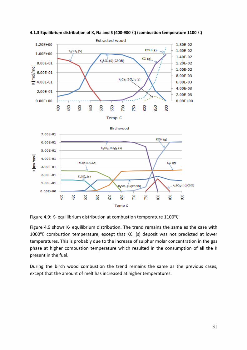
Figure 4.9 shows K- equilibrium distribution. The trend remains the same as the case with

1000℃ combustion temperature, except that KCl (s) deposit was not predicted at lower

temperatures. This is probably due to the increase of sulphur molar concentration in the gas

phase at higher combustion temperature which resulted in the consumption of all the K

present in the fuel.

During the birch wood combustion the trend remains the same as the previous cases,

except that the amount of melt has increased at higher temperatures.

32

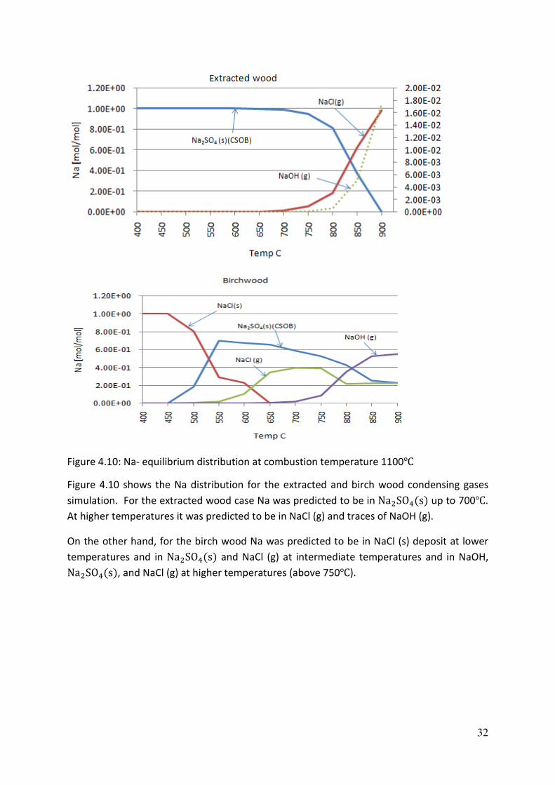
Figure 4.10: Na- equilibrium distribution at combustion temperature 1100℃

Figure 4.10 shows the Na distribution for the extracted and birch wood condensing gases

simulation. For the extracted wood case Na was predicted to be in Na�SO��s� up to 700℃.

At higher temperatures it was predicted to be in NaCl (g) and traces of NaOH (g).

On the other hand, for the birch wood Na was predicted to be in NaCl (s) deposit at lower

temperatures and in Na�SO��s� and NaCl (g) at intermediate temperatures and in NaOH, Na�SO��s�, and NaCl (g) at higher temperatures (above 750℃).

33

Figure 4.11: S-equilibrium distribution at combustion temperature 1100 ℃

Figure 4.11 shows the equilibrium distribution of S for extracted and birch wood. For the

extracted wood case, S distribution remains similar as the previous cases except that the

concentration of SO��g� and SO<�g� has increased in amount and in temperature range of

presence. Besides the sulphur boding to Ca has also increased.

For the birch wood case, S was predicted to be in potassium sulphate (solid- alpha) at lower

temperatures and in potassium sulphate (solid-CSOB) at intermediate and higher

temperatures. The presence of SO��g� was predicted at temperatures above 850℃.

4.2 Extraction process mass and energy balance results

The extraction process heat demand was assumed to be supplied from boiler exhaust gases.

To supply the required heat demand, energy balance calculations indicate that the exhaust

gases must exit the boiler at 300-320℃. Since the boiler will be operated continuously, at

least two extraction vessels are required. The extraction vessels were assumed to operate

simultaneously in such a way that when one vessel is on heating the other will be at steady

state. In this manner the other processes can be operated continuously, while the extraction

process will be batch wise. It should be noted that this is just an assumed suggestion for the

34

configuration of the hot-water extraction process. In this work, estimation the energy

demand of the extraction process was the main concern. The calculations further indicate

that the exhaust gases from the boiler can only supply 15 batches per day.

Figure 4.12: Energy demand of the integrated extraction process per Kg ethanol yield

As indicated in figure 4.12, the process requires 44MJ-per kg of ethanol yield of electricity

which is mainly used for feedstock size reduction and handling, as well as system operation.

The pre-treatment process of the SHF was replaced by a hot water extraction process and

heat, about 39MJ-per kg Ethanol yield, is supplied from boiler exhaust gases instead of

steam. But, steam is still required for distillation, estimated to about 7 MJ-per kg of ethanol

yield.

Table 4.1 summarizes the results for ethanol yield estimation and the mass and energy

balances per kg of ethanol yield.

35

Table 4.1 Mass and Energy balance results, per Kg- ethanol yield

Current plant

Birchwood (LHV) MJ/kg dry 17.19

Extracted wood (LHV) MJ/kg dry 18.69

Theoretical conversion xylose to ethanol kg/kg 1.957

Conversion efficiency % (assumed) 90

Mass balance per Kg ethanol yield (kg) Energy balance per Kg ethanol yield (MJ)

Mass input Energy input

Hot water extraction Hot water extraction

Wood chips (Birch wood) 28.12 Wood chips (Birch wood) (LHV) 483.35

Water 67.48 Electricity (size reduction, system operation) 43.35

Ethanol plant Boiler exhaust gases (extraction process) 39.32

Extraction liquor 33.74 Ethanol plant

Other chemical inputs 0.05 Heat (steam for up-grading)

7.0

Total 95.65 Total 573.02

Mass output Energy output

Ethanol 1.00 Ethanol (LHV) 26.70

Solid extracts + liquor out 38.52 Energy recovery (LHV) (after extraction

process)

404.65

By-product (water + others) 56.13 Energy used + Heat loss 141.67

Conversion efficiency (per kg dry-wood) % 3.56 Conversion efficiency (per MW dry wood) % 5.52

The ethanol yield rate through the HWE pathway was estimated to be about 0.036 kg

ethanol/kg dry birch-wood (Details can be found in appendix A.5). In other words, about 28

kg dry birch wood is required to produce 1 kg of ethanol with hot water extraction pathway.

Results indicate low conversion efficiency for the hardwood input as compared to current

SHF technologies. This is due to the fact that the cellulose in the birch wood remains in the

extracted woodchips. The hot water extraction process dissolves mostly the hemi-cellulose

content. The conversion efficiency as compared to the extraction liquor input to the SHF

agrees well to the ethanol yield rate from lignocellulosic biomass reported by different

literatures.

4.3 Boiler/turbo-generator energy and mass balance results

Ethanol, possible excess electricity, district heat and acetic acid were the products for the

plant configuration considered. The analysis was performed for three plant sizes (10, 50 and

100MW).

36

Table 4.2 Annual production and feedstock demand results (8400 hrs/year)

Boiler capacity (MW) 10 50 100

Annual operating hours 8400 8400 8400

Annual district heat production GWh 53 262 525

Annual birch-wood demand GWh 127 643 1286

Annual extracted wood demand GWh 115 572 1145

Annual ethanol yield (Million litre) 1.3 6.6 13

Annual net electricity to grid GWh 11 54 108

Annual Acetic acid yield (Million litre) 0.76 3.8 7.7

Table 4.3 Total energy efficiency of the system

Energy plant efficiency a

80%

Overall efficiency 55% a the energy plant efficiency stands for the CHP plant efficiency excluding the integrated HWE process.

Figure 4.13 shows annual production levels of electricity, heat, ethanol and acetic acid as a

function of plant size. The annual production rates were calculated base on annual

operational time of 8400 hrs.

Figure 4.13: Annual production levels of electricity, heat (left-vertical axis) and ethanol,

acetic acid (right-vertical axis)

Figure 4.14 shows annual production of electricity, heat, ethanol and acetic acid as function

of plant size, based on annual operational time of 6000 hrs

37

Figure 4.14: Annual production levels of electricity, heat (left-vertical axis) and Ethanol,

acetic acid (right-vertical axis)

4.4 Economic evaluation results

Figure 4.15 shows the resulting ethanol production cost as a function of plant size over a

range of annual operational time.

Figure 4.15: Cost of ethanol production at different annual operational hours against plant

size

Results indicate that the cost of ethanol production can be in the range of SEK 3.4 to SEK 11

per litre depending on the plant size and annual operational hours. Production of ethanol to

an acceptable cost will demand high system reliability, which in-turn increases the total

capital investment.

Figure 4.16 shows the electricity production cost as a function of plant size over a range of

annual operational hours.

38

Figure 4.16: Cost of el. production at different annual operational hours against plant size

The cost of electricity production varies from SEK 450, for the case with 100MW plant size

and 8400 operational hours, to SEK 1120, for the case with 10MW plant size and 2000

operational hours. As it can be inferred from figure 4.16, annual operation hours and plant

size significantly influences the cost of electricity production.

Figure 4.17: Cost of heat production at different annual operational hours against plant size

Figure 4.17 shows the resulting production cost of heat at different annual operational

hours and different plant sizes. Results indicate a cost in the range of SEK/MWh 230-730

depending on the plant size and annual operational hours.

4.4.1 Sensitivity analysis

Figure 4.18, below, shows the effect of cost of other chemicals input on ethanol production

cost. The considered range for the cost of other inputs covers cost data’s reported by

various previous works for different process arrangements.

39

Figure 4.18: Ethanol production cost against cost of other inputs for different plant sizes

Figure 4.19 and Figure 4.20 show the susceptibility of heat and electricity production costs

to the feedstock cost. A careful attention should be given when dealing with feedstock

future cost prediction. As it can be inferred from the figures, heat and electricity production

costs are highly vulnerable to the feedstock cost, and the degree of susceptibility increases

with increasing plant size.

Figure 4.19 heat production cost against cost of feedstock for different plant sizes

Figure 4.20: Electricity production cost against cost of feedstock for different plant sizes

40

Figure 4.21 shows the effect of acetic acid sales on the internal rate of return (IRR). It can be

shown from the curves how important is the market price of acetic acid for the plant

economy.

Figure 4.21: IRR (%) against selling price of acetic acid for the different plant sizes

4.4.2 Profitability analysis results

Table 4.4 Results of economic indicators

Plant size (MW) 10 50 100

Operational hours 8400 8400 8400

Ethanol sales price SEK/litre 7.14 4.47 3.70

Acetic acid sales price SEK/litre 7.60 7.60 7.60

Electricity sales price SEK/MWh 602.89 518.55 494.49

Heat sales price SEK/MWh 332.45 276.10 258.99

i (IRR) % 6.27 7.31 7.89

Investment (TCI) 216.50 664.05 1083.55

R (Annual Revenues) 38.96 158.11 294.73

C (Annual Operating Costs) 21.58 99.54 194.19

Z (Techno/economic life time) 25 25 25

Check equation 0.00 0.00 0.00

Payback time in years 12.5 11.4 10.8

In capital internal rate of return a project is judged to be good, neutral or bad by comparing

the calculated IRR to the cost of capital ‘i’ which in the current work was assumed to be 5%.

(Peters et al., 2003)

����1. J}} >> � = 5% ���� ���� ������� ������V���

����2. J}} = � = 5% ������� ������� ������V���

����3. J}} << � = 5% K��� ������� ������V���

41

5. CONCLUDING DISCUSSION

High Temperature Corrosion: All the corrosion mechanisms described in the literature

review may take place during combustion process. However, the severity of each

mechanism will be dependent on the combustion environment and temperature, steam

temperature and the presence of other corrosive minerals in the fuel. Depending on the

type of fuel available, the need for an experiment is crucial as it is difficult to extrapolate

corrosion phenomenon from previous results. Computer simulations might be helpful in

predicting the equilibrium concentrations of the combustion products, but seldom can be

used for decision making unless substantiated by experiments. From the literature survey

on high temperature corrosion it can be perceived that chlorine (Cl) or hydrogen chloride

(HCl) has the ability to form a self-sustained corrosion mechanism. Careful attention should

be given (if possible to avoid or to reduce) chlorine content in solid fuels, for increased

steam temperature operations in biomass fired CHP’s. Most authors agree, with regards to

biomass fired boilers, that either steam temperature must be kept low to avoid severe

corrosion, new alloys with high corrosion resistance must be found or a way to prevent

potassium (K), sodium (Na) and chlorine from the deposits must be found. Hot-water

extraction process opens the door towards increased temperature operation, by reducing

significantly the K and Na content of lignocellulosic biomass.

It can be inferred from the equilibrium distribution of K, Na, and S that no liquid solution (of

K and Ca sulphates and carbonates) was predicted for all the cases with extracted wood

chips. For the birch wood case a liquid solution was predicted over the temperature range

750℃-850℃, in all the cases, with considerable increase with increasing combustion

temperature. Chemical reactions are more active in liquid phase. This could be a good initial

step towards increased steam temperature operation in biomass fired boilers. Furthermore,

chlorine presence in the extracted wood chips might trigger a cyclic chloride attack,

especially at higher temperatures where the metal chloride vapour pressure reach 10-4 bar

(Table 2.1). According to the literature, the gas phase Cl or HCl attack (corrosion mechanism

1) will play significant role in aggravating corrosion problems when vapour pressure of metal

chlorides reach the limit. From figure 2.4, Cl equilibrium distribution, chlorine was predicted

to be present in the gas phase mainly in the form HCl during extracted wood combustion

and KCl during birch wood combustion. Both of which have been reported to be corrosive

by many previous investigations, though some researchers (Lundberg, 2010) suggest that Cl� (g) or HCl (g) in gas phase has little to do with corrosion rather significant amount of

those gases discharge with the exhaust flow. According to the literature the index S/Cl < 2,

stands for a sever gas phase chloride/ chlorine corrosion. But it is not clearly indicated that

whether this index prediction holds true for biomass with low K and Na content, such as

extracted wood. The different indices evaluated for extracted and birch wood can be found

in appendix A (Table A.2).

42

A balance in alkali and sulphur content of the fuel could be important in such a way that the

alkali chloride deposits at lower temperatures (400 – 600℃) can be reduced resulting in an

increase of alkali sulphate, which are more stable and believed to be not corrosive.

(Lundberg, 2010) An increase in combustion temperature has resulted in reduced KCl

deposit at lower temperatures (prediction from FactSage results); this could be probably

because sulphur becomes more active at higher temperatures and reacts with K to form

stable sulphates. This is desirable from corrosion point of view. Reducing the water vapour

in the flue gas, during extracted wood combustion, could result in free Cl� (g) or less HCl (g)

which could be important for downstream flue gas cleaning.

Furthermore, low presence of Si, precisely high K/Si ratio, (appendix A, Table A.2), in the

birch wood and consequently in the extracted wood has resulted in a total release of the K

and Na, predicted by FactSage, during the combustion process. The presence of Si in the fuel

at high temperature influences the release trend of K. (Simone, 2005)The alkali free index

prediction in the behaviour of the birch and extracted wood chips agrees well with the

results obtained from the equilibrium calculation, which is no or very little presence of KOH

was predicted during the combustion of extracted wood chips. This could be one of the

reasons that avoided the formation of liquid solution during combustion of extracted wood.

KOH is believed to be one of the contaminant gases by forming deposits and eventually

melts at much lower temperatures than KCl and K�SO�.

Extraction process: In this project the extraction process heat demand was supplied from

the boiler exhaust gases. Energy balance calculations have indicated that the exhaust gases

should exit the boiler at temperature of 300-320℃. This temperature is too high, and

compromises the boiler efficiency. As an alternative scenario the extraction process was

evaluated by considering steam extracted from the steam turbine at 25 bars. The overall

and energy plant efficiency remains, more or less, unaltered. However, using steam could

have advantages from operational point of view such as cleaning and low temperature

corrosion problems can be avoided.

Acetic acid: Acetic acid is one of the valuable by-products of the hot-water extraction

process. In this work it was assumed that the acetic acid will be sold. It can be used in the

secondary hydrolysis process as a substitute for sulphuric acid, which could be

advantageous from environmental and the liquid-liquid separation process considerations.

From economic point of view this may not hold true, as acetic acid could have more market

value than sulphuric acid.

Economy: Under the assumed economic parameters, the production cost of ethanol was

estimated to the range in 3.4 – 11 SEK/litre depending on the plant size and annual

operational hours. The annual operational hours has more effect on the production cost of

ethanol than the plant size. This will demand high plant reliability in order to operate in an

economic range, which in-turn will greatly affect the capital investment. Moreover, the

43

100MW plant size has resulted in a promising electricity production cost in relation to the

current cost levels in Sweden. This indicates the importance of the plant size in the plant

economy.

Compared to other process pathways for ethanol production, such as SHF (separate

hydrolysis and fermentation) and SSF (simultaneous saccharification and fermentation),

reported by (Sassner et al., 2008; Wingren et al., 2003, 2004, 2008) the HWE pathway,

taking in to account the heat and net electricity products, has resulted in reasonable cost of

production.

Practical issues: There are practical issues needed to be addressed for improving the

productivity of the assumed plant configuration. It would be advantageous if the hot-water

extraction and hydrolysis could be operated continuously instead of batch wise. In addition

it requires large amount of water which might necessitate the need for effective water

recycling process.

The cellulose portion of the birch wood remains intact in the extracted wood chips which

might raise a question whether it is economical to use it as fuel in CHP plants directly. This

issue was not part of the current work, but hot-water extraction of hardwood could prove

to be more economical when integrated into a kraft pulp mill, for instance. Furthermore,

the extraction process could be more attractive if integrated in CHP’s using softwoods as

fuel. But it should first be investigated whether it will result in the same effect (in removal of

inorganic constituents and xylose yield) when operated with softwoods.

44

Future work

This work was initiated mainly with the intent to investigate the possibility of increased

steam temperature operation in biomass fired boilers from the literature available. It was

based on the results of the work by Lundgren and Helmerius (2009) which indicated very

low levels of the inorganic substances in the extracted woodchips as compared to the

original birch woodchips. The inorganic constituents (mainly alkali metals (K, Na) and Cl),

present in lignocellulosic biomass, are believed to be responsible for fireside corrosion

problems limiting the operational steam temperature. Alkali metals along with other

inorganic substances, except Cl and S, have been washed-out during the hot-water

extraction process.

This could open the door for a new approach to the problem. Almost all previous works

towards the fireside problems, available in the literature, concentrate on discovering

corrosion resistant heat exchanger materials and/or possible additives to reduce the

severity of corrosion during the combustion process.

In the current work, the equilibrium concentrations of the different compounds believed to

be responsible for fireside problems were calculated using FactSage 6.0 package. Results for

the extracted woodchips indicate some improvements in relation to the literature reviewed

and results for the original birch woodchips. Yet, to convert such improvements into

possible increased steam temperature operation is something that needs further research.

Besides, chlorine is known to be the triggering constituent for gas phase corrosion

mechanism and is still present at high level, relative to alkali metals, in the extracted

woodchips. This is again something which needs to be avoided, if possible, or controlled

somehow.

Furthermore, the process evaluated for the ethanol production is based on previous works

by different authors. No one of them is exactly similar to the current work. A more accurate

process and economic evaluation of the hot-water extraction pathway can be achieved by

evaluating the different process in Aspen Plus or other process models. This could again be a

possible future work.

45

REFERENCES

Blomberg T. Methods for positioning superheater in biomass burning steam generators and steam generator [Patent] : US

6672259B2. - United States, 06 Jan 2004.

Charles Y. Wereko-Brobby, Essel B., Hagen Biomass conversion and technology [Book]. - Chichester : John Wiley and Sons

Ltd., 1996. - pp. 84-89. - 0471962465.

Gnansounou E., Dauriat, A. Techno-economic analysis of lignocellulosic ethanol: A review [Journal] // Bioresource

technology. - Lausanne, Switzerland : Elsevier Ltd., 2010. - Vol. 101. - pp. 4980-4991.

Gotthjaelp K., Brondsted, P., Jansen, P., Montgomery, M. High temperature corrosion of superheater materials for power

production through biomass [Journal]. - Denmark : Technical University of Denmark, 1996. - 87-550-2205-7.

Grabke H., J., Reese, E., Spiegel, M. The effects of chlorides, hydrogen chloride and sulfur dioxide in the oxidation of steels

below deposits [Journal] // corrosion Science. - Dusseldorf, Germany : Max-Planck institute for Eisenfoschung, 1995. - 7 :

Vol. 37. - pp. 1023-1043.

Hamelinck C., N., Hooijdonk, G.,V., Faaij, A., Ethanol from lignocellulosic biomass: techno-economic performance in short-,

middle-, and long- term [Journal] // Biomass and Bioenergy. - Utrecht, the Netherlands : Elsevier Ltd., 2005. - Vol. 28. - pp.

384-410.

Helmerius J. Integration of a hemicelluloses extraction step into a forest biorefinery for production of green chemicals

[Report] : Licentiate Thesis / Lulea University of Technology. - Lulea : [s.n.], 2010. - 978-91-7493-081-0/1402-1757.

Hendrya H., Leesb, D.J. Corrosion of austenitic steels in molten sulphate deposits [Journal] // Corrosion Science. - [s.l.] :

Elsevier Ltd., 1980. - 3 : Vol. 20. - pp. 383-404.

Hossain M. K., Saunders, S. R. J. A microstructural study of the influence of NaCl vapor on the oxidation of Ni-Cr-Al alloy at

850 C [Journal] // Oxidation of Metals. - Middlesex, England : Division of Material applications, National Physical Lab,

1978. - 1 : Vol. 12.

Hulkkonen S. CHP generation from biomass fuels [5Eures International training]. - Joensuu : Motiva, 06 June 2006.

Ihara Y., Ohgame, H., Sakiyama, K. The corrosion behaviour of iron in hydrogen chloride gas and gas mixtures of hydrogen

chloride and oxygen at high temperatures [Journal] // Corrosion Science. - Sendai,Japan : Tohoku University, 1981. - 12 :

Vol. 21. - pp. 805-817.

Incropera F., P., Dewitt, D.,P., Bergman, T.,L., Lavine, A.,S. Fundamentals of heat and mass transfer [Book]. - NJ : John

Wiley & Sons, 2007. - Sixth edition. - 978-0-471-45728-2.

Järdnäs A., Svensson, J.-E., Johansson, L.-G. Influence of SO2 on the Oxidation of 304L Steel in O2 + 40%H2O at 600 °C

[Journal] // Oxidation of Metals. - Gothenburg, Sweden : [s.n.], 2008. - 3-4 : Vol. 69. - pp. 249-263.

Karlsson A., Moller, P., J., Johansen, V. Iron and steel corrosion in a system of Oxygen, Sulfates and alkali chloride. The

formation of low melting point salt mixtures [Journal] // Corrosion Science. - Copenhagen, Denmark : Department of

Physical Chemistry, University of Copenhagen, 1990. - 2/3 : Vol. 30. - pp. 153-158.

Kjellstorm B. Thermal Engineering. - Lulea : [s.n.], 2003.

Ladanai S., Vinterbäck, J. Global potential of Sustainalbe Biomass for Energy [Report] / Department of Energy and

Technology. - Uppsala, Sweden : Swedish University of Agricultural Sciences, 2009. - 1654-9406.

Li Y., S., Niu, Y., Spiegel, M. High temperature interaction of Al/Si- modified Fe-Cr alloys with KCl [Journal] // Corrosion

Science. - [s.l.] : Shenyang, China, 2007. - Vol. 49. - pp. 1799-1815.

Li Y., S., Spiegel, M. Models describing the degradation of FeAl and NiAl alloys induced by ZnCl2–KCl melt at 400–450 C

[Journal] // Corrosion Science. - Dusseldorf, Germany : Max Planck Institute, 2004. - Vol. 46. - pp. 2009-2023.

46

Lin W., Lester O. Pordesimo, C. Iganthinathane, William D. Batchelor Process engineering evaluation of ethanol

production from wood through bioprocessing and chemical catalysis [Journal] // Biomass and Bioenergy. - Mississippi,

USA : Mississippi state university, 2009. - Vol. 33. - pp. 255-266.

Liu C., Little J. A., Henderson P. J., Ljung P. Corrosion of TP347H FG stainless steel in a biomass fired PF utility boiler

[Journal] // Journal of material science. - Stockholm, Sweden : [s.n.], 2001. - 4 : Vol. 36. - pp. 1015-1026.

Lundberg M., O. [Interview]. - [s.l.] : Through Telephone and email, mats.lundberg@sandvik.com, Tel:+4626260000 ;

Sandvik Materials Technology, 23 05 2010.

Lundgren J., Helmerius, J. Integration of a hemicellulose extraction process into a biomass based heat and power plant

[Conference]. - Lulea, Sweden : Proceedings of ECOS 2009, 2009.

Mitchell J. Ethanol from Hardwood [Report] : Masters Thesis. - [s.l.] : University of Maine, Chemical Engineering

Department, 2006.

Nielsen H. P., Frandsen, F., J., Dam-Johansen, K. Lab-Scale Investigations of High temperature corrosion phenomena in

Straw-fired boilers [Journal] // Energy and fuels. - Lyngby, Denmark : Department of Chemical engineering, Technical

university of Denmark, 1999. - Vol. 13. - pp. 1114-1121.

Nielsen H.P., Frandsen, F. J., Dam-Johansen, K., Baxter, L. L. The implications of chlorine- associated corrosion on the

operation of biomass-fired boilers [Journal] // Progress in Energy and combustion Science. - Denmark : Department of

chemical engineering, Technical University of Denmark, 2000. - Vol. 26. - pp. 283-298.

Peters M., S., Timmerhaus,K., D., West, R., E. Plant design and Economics for Chemical Engineers [Book]. - New York :

McGraw- Hill Companies, Inc.,, 2003. - 0-07-119872-5.

Petterson J., Svensson, J.-E., Johansson, L.-G. KCl-Induced Corrosion of a 304-type Austenitic Stainless Steel in O2 and in

O2 + H2O Environment: The Influence of Temperature [Journal] // Oxidation of metals. - Goteborg, Sweden : Springer

Netherlands, 2009. - 3-4 : Vol. 72. - pp. 159-177. - 0030-770X (Print) 1573-4889 (Online).

Pettersson J., Asteman, J., Svensson, H., Johansson, J. -E.,. KCl Induced Corrosion of a 304-type Austenitic Stainless Steel at

600°C; The Role of Potassium [Journal] // Oxidation of Metals. - Goteborg, Sweden : Springer Netherlands, 2005. - 1-2 : Vol.

64. - pp. 23-41. - 0030-770X (Print) 1573-4889 (Online).

Pitt Martin IChemE Education Subject Group - Resources [Online] // Cost of chemicals. - 26 February 2002. - 23 April

2010. - http://ed.icheme.org/costchem.html.

Prescott R., Stott, F., H., Elliott, P. The degradation of metals in a hydrogen chloride containing gas at high temperature

[Journal] // Corrosion Science. - Manchester, U.K. : University of Manchester Institute of Science and Technology, 1989. -

4 : Vol. 29. - pp. 465-475.

Salmenoja K., Hupa, M., Backman, R. Laboratory Studies on the Influence of Gaseous HCl on Superheater Corrosion [Book

Section] // Impact of Mineral Impurities in Solid Fuel Combustion / book auth. al. Gupta et. - New York : Springer US,

1999. - 978-0-306-46126-2 (Print) 978-0-306-46920-6 (Online).

Sassner P., Gable, M., Zacchi, G. Techno-economic evaluation of bioethanol production from three different lignocellulosic

materials [Journal] // Biomass and Energy. - Lund, Sweden : Elsevier Ltd., 2008. - Vol. 32. - pp. 422-430.

Simone C., van Lith Release of Inorganic Elements during Wood-Firing on a Grate [Report] : Ph. D. Thesis / Chemical

Engineering ; Technical University of Danmark. - Copenhagen, Danmark : Norhaven Digital A/S, 2005. - 87-91435-29-3.

Skrifvars B.-J., Backman, R., Hupa, M., Salmenoja, K., Vakkilainen, E. Corrosion of superheater steel materials under alkali

salt deposits Part 1: The effect of salt deposit composition and temperature [Journal] // Corrosion Science. - Lappeenranta,

Finland : Lappeenranta University of Technology, 2008. - Vol. 50. - pp. 1274-1282.

Skrifvars B.-J., Laurén, T., Backman, R., Hupa, M. The Role of Alkali Sulfates and Chlorides in Post Cyclone Deposits from

Circulating Fluidized Bed Boilers Firing Biomass and Coal [Book Section] // Impact of mineral impurities in solid fuel

47

combustion / book auth. al. Gupta et. - New York : Springer US, 1999. - 978-0-306-46126-2 (Print) 978-0-306-46920-6

(Online).

Strafford K. N., Datta, P. K., Forster, G. The high temperature chlorination of Iron, Nickel and Some Iron-Nickel model

alloys [Journal] // Corrosion Science. - Newcastle, U.K. : Newcastle upon Tyne Polytechnic, 1989. - 6 : Vol. 29. - pp. 703-716.

Thomas E. A., Christopher D. W., Alan M. S., Yang W. Biorefinery: conversion of woody biomass to chemicals, energy and

materials [Journal] // Biobased materials and bioenergy. - New York : [s.n.], 2008. - Vol. 2. - pp. 100-120.

Vamvuka D., Zografos, D., Alevizos, G. Control methods for mitigating biomass ash-related problems in fluidized beds

[Journal] // Bioresource Technology. - Crete, Greece : Technical Univeristy of Crete, 2008. - Vol. 99. - pp. 3534-3544.

Wagner Mark Boiler Blog, Boiler combustion, Heat transfer and boiler auxilaries [Online]. - 18 september 2007. - 15 April

2010. - http://www.firecad.net/BoilerBlog/post/Sizing-calculations-of-Boiler-Pumps-and-ID--FD-Fans-.aspx.

Wikipedia Pulp and Paper Industry [Online] // Wikipedia, the free encyclopedia. - April 2010. - 20 April 2010. -

http://en.wikipedia.org/wiki/Pulp_and_paper_industry.

Wingren A., Ethanol from Softwood [Report] : PHD thesis. - Lund, Sweden : Lund University, Chemical Engineering

Department, 2005.

Wingren A., Galbe ,M., Zacchi, G. Energy consideration for a SSF based softwood ethanol plant [Journal] // Bioresource

Technology. - Lund, Sweden : Elsevier Ltd., 2008. - Vol. 99. - pp. 2121-2131.

Wingren A., Galbe, M., Zacchi, G. Techno-economic evaluation of producing ethanol from softwood: comparison of SSH

and SHF and Identification of bottlenecks [Journal] // Biotechnology progress. - Lund, Sweden : American chemical society

and American institute of chemical engineers, 2003. - Vol. 19. - pp. 1109-1117.

Wingren A., Soderstrom, J., Gable, M., Zacchi, G. Process consideration and Economic evaluation of two-step steam pre-

treatment for production of fuel ethanol from softwood [Journal]. - Lund, Sweden : American Chemical Society and

American Institute of chemical engineers, 2004. - Vol. 20. - pp. 1421-1429.

Wooley R. Ruth M., Sheehan J., Ibsen K. Lignocellulosic Biomass to Ethanol process design and economic utilizing co-

current dilute acid prehydrolysis and hydrolysis current and futuristic scenarios [Report] : NREL technical report. - [s.l.] :

Nation Renewable Energy Laboratory (NREL), 1999. - NREL/TP-580-26157.

Zahs A., Spiegel, M., Grabke, H., J. Chloridation and oxidation of iron, chromium,nicke and their alloys in chloridizing and

oxidizing atmospheres at 470 - 700 deg C [Journal] // Corrosion Science. - Dusseldorf, Germany : [s.n.], 1999. - Vol. 42. - pp.

1093-1122.

Zhang K., Niu, Y., Al-Omary, M., Wu, W. T. The Corrosion Behavior of Four Commercial Steels in Reducing Atmospheres

Containing HCl At 773–873 K [Journal] // Oxidation of Metals. - Shenyang, China : Springer Netherlands, 2004. - 5-6 : Vol.

62. - pp. 323-340. - 0030-770X (Print) 1573-4889 (Online).

48

APPENDIX A

A.1 Elemental analysis of Birch and Extracted wood

The properties and compositions of birch wood and extracted wood chips were adapted

from the work by Lundgren and Helmerius (2009)

Table A.1 Birchwood and Extracted wood chips elemental analysis

Fuel Analysis

Birchwood Ext. wood Basis

Hi (MJ/kg) 17.19096 18.6913 dry

Ash 0.4 0.1 %wt dry

C 49.4016 50.949 %wt dry

H 6.2748 6.4935 %wt dry

N 0.0996 0.24975 %wt dry

S 0.00498 0.00599 %wt dry O� 43.4256 42.1578 %wt dry

Cl 0.01992 0.02997 %wt dry

Ash elements

CaO 0.125 0.037 %wt dry K�O 0.068 0.01 %wt dry

MgO 0.043 0.008 %wt dry

MnO 0.014 0.004 %wt dry

P2O6 0.024 0.004 %wt dry

SiO� 0.0015 0.0011 %wt dry

Al2O< 0.0005 0.0004 %wt dry Fe�O< 0.0008 0.0009 %wt dry Na�O 0.0002 0.0001 %wt dry

TiO� 0.0001 0 %wt dry

Total 0.2771 0.0655

Undetermined 0.1229 0.0345 %wt dry

Table A.2 Indices for predicting corrosion behaviour of biomass fuels

Birchwood Extracted Unit

Af (alkali free index) 0.3366777 -0.3485009 mol/GJ

AI (alkali index) 0.039672 0.00540359 kg alkali/GJ

S/Cl 0.2764798 0.2211838 mol/mol

Cl/(k+Na) 0.3869337 3.91679145 mol/mol

K/Si 57.845718 11.6000772 mol/mol

49

A.2 Thermodynamic equilibrium calculations

FactSage 6.0 package was used to determine the equilibrium concentrations during

combustion of extracted and birch wood. The input parameters used were listed below.

i. Fuel composition

Table A.3 FactSage input data

Se

No.

Constituent Birchwood

(mol/kg)

Extracted wood

(mol/kg)

1 C 26.8 27.6

2 H2O 19.44 19.44

3 O2 8.82 8.56

4 N2 0.0231 0.058

5 H2 20.4 21.1

6 S 0.001 0.00121

7 Cl 0.0037 0.0056

Ash elements (dry basis)

8 CaO 0.0223 0.0066

9 K�O 0.00722 0.0011

10 MgO 0.011 0.002

11 MnO 0.002 0.0006

12 P2O6 0.002 0.0003

13 SiO2 0.0003 0.0002

14 Al2O6 0.00005 0.00004

15 Fe�O< 0.00005 0.00006

16 Na�O 0.00003 0.00002

17 TiO2 0.000013 0.0

Combustion air (λ=1.3)

18 O2 36.56 38.47

19 N2 137.54 144.63

ii. Combustion temperature 900-1100 ℃, temperature step 100℃, pressure 1 atm

iii. Condensing gases temperature range 400-900℃, temperature step 50℃, pre.1

atm

Besides the FactSage 6.0 compound data base, the following solution databases (including

all the species) were used for the calculations.

Solution Phase FACT-SLAG

The components in FACT-SLAGA for the current calculation were: MgO, FeO, Na�O, CaO, K�O, MgS, CaS, FeS, Na�S, K�S, NaCl, KCl, CaCl�, MgCl�,, FeCl�,

Solution Phase FACT-SALT

50

The components in FACT-SALTA for the current calculation were: NaCl, KCl, NaOH, KOH, Na�SO�, K�SO�, Na�CO<, K�CO<, NaNO<, KNO<

Solution Phase FACT-AClA

AAlkCl-ss NaCl-rock salt structure

The components in FACT-AClA for the current calculation were: NaCl, KCl, CaCl�, and

MgCl�

Solution Phase FACT-CSOB

CO<,SO�/Li,Na,K low lithium content solid solution

The components in FACT-CSOB for the current calculation were: Na�CO<, K�CO<, Na�SO�, K�SO�

Solution Phase FACT-LCSO

liq-K,Ca/CO<,SO� - liquid solution of K,Ca/CO<,SO�

The components in FACT-LCSO for the current calculation were: K�SO�, CaSO�, K�CO<, and

CaCO<

Solution Phase FACT-SCSO

s-K,Ca,/CO<,SO� - solid solution of K,Ca/CO<,SO� (Valid only if K-rich)

The components in FACT-SCSO for the current calculation were: K�SO�, CaSO�, K�CO<, and

CaCO<

Solution Phase FACT-SCMO

s-Ca(SO�),Mg(SO�) - solid solution of Ca(SO�) and Mg(SO�)

The components in FACT-SCMO for the current calculation were: CaSO�, MgSO�

Solution Phase FACT-LSUL

liq-Ca,Mg,Na/SO� - liquid solution of CaSO�, MgSO� and Na�SO�

The components in FACT-LSUL for the current calculation were: CaSO�, MgSO�, and Na�SO�

Solution Phase FACT-LSUL

liq-Ca,Mg,Na/SO� - liquid solution of CaSO�, MgSO� and Na�SO�

The components in FACT-LSUL for the current calculation were: CaSO�, MgSO�, and Na�SO�

Solution Phase FACT-SSUL

51

s-Ca,Mg,Na/SO� - solid solution of CaSO�, MgSO� and Na�SO�

Valid only in Na�SO�-rich regions

The components in FACT-SSUL for the current calculation were: CaSO�, MgSO�, and Na�SO�

A.3 Boiler/Turbo- generator energy and mass balance

Table A.4 Data assumed in steam/ electricity and district heat production process

State

Point

Description

1 Feed water @120 bar

2 Superheated steam @540℃, and 5% pressure drop

3 Exhaust gases from boiler, @ 300℃

4 Steam extraction for ethanol process @ 25bar

5 Steam extraction for ethanol process @ 4bar

6 Steam extraction for feed water heating @ 4bar

7 Steam to district heat @ 2bar

8 Saturated liquid from air pre-heater @ 2bar

9 Condensate from ethanol process, assumed 85% of the steam flow to ethanol process

10 Make-up water, pre-heated to 60℃ by waste water stream from ethanol plant @ 1bar

11 State to be determined by iterative solution, @ 1bar

12 Condensate flow to feed water and de-aerator tank @4 bar, after condensate pump

13 Saturated liquid @ feed water tank pressure (4bar)

14 Air flow to boiler, pre-heated to 100℃

15 Fuel flow to boiler

16 Hardwood feed to extraction process

17 Water feed to extraction process

18 Extracted wood flow from extraction process

19 Condensing steam from district heat condenser to air pre- heater @2 bar

Airflow and Resulting gas flow

Based on the elementary composition of extracted wood chips and an assumed moisture

content of 35% (as received) and a excess air factor of (λ =1.5) the airflow (le) to the

combustion chamber and the resulting gas flow (ge) were calculated from stoichiometric

combustion of the extracted woodchips.

� = 4.8 �V< (� ����� � = 5.67 �V< (� �����

Fuel flow

The required fuel flow is estimated from energy balance for the gas path of the boiler as

follows.

K�C!b�I = V2 b�ℎb + ���Y� + � ∙ ℎD − � ∙ ℎW�� − KI$CC − V2 �ℎ� �%. 1�

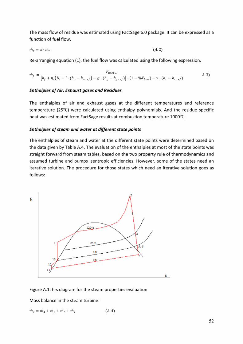
52

The mass flow of residue was estimated using FactSage 6.0 package. It can be expressed as a

function of fuel flow.

V2 � = � ∙ V2 b �%. 2�

Re-arranging equation (1), the fuel flow was calculated using the following expression.

V2 b = K�C!b�I�ℎb + ��0Y� + � ∙ �ℎD − ℎD,�!b5 − � ∙ �ℎW − ℎW,�!b�� ∙ �1 − %KI$CC� − � ∙ �ℎ� − ℎ�,�!b� %. 3�

Enthalpies of Air, Exhaust gases and Residues

The enthalpies of air and exhaust gases at the different temperatures and reference

temperature (25℃) were calculated using enthalpy polynomials. And the residue specific

heat was estimated from FactSage results at combustion temperature 1000℃.

Enthalpies of steam and water at different state points

The enthalpies of steam and water at the different state points were determined based on

the data given by Table A.4. The evaluation of the enthalpies at most of the state points was

straight forward from steam tables, based on the two property rule of thermodynamics and

assumed turbine and pumps isentropic efficiencies. However, some of the states need an

iterative solution. The procedure for those states which need an iterative solution goes as

follows:

Figure A.1: h-s diagram for the steam properties evaluation

Mass balance in the steam turbine:

V2 � = V2 � + V2 6 + V2 ; + V2 ? �%. 4�

53

The steam extraction rate to the feed water heater, V2 ;, at 4 bar from the steam turbine is

obtained by energy and mass balance in the de-aerator and feed water heater.

Mass balance: (de-aerator and feed water heater)

V2 +< = V2 ; + V2 +� = V2 + �%. 5�

And mass balance at the mixing point of the make-up water, V2 +,, condensate from the

ethanol plant, V2 7, and condensate from the district heating, V2 = gives:

V2 ++ = V2 = + V2 7 + V2 +, = V2 +� �%. 6�

Energy balance: (de-aerator and feed water heater tank)

V2 +<ℎ+< = V2 ;ℎ; + V2 +�ℎ+� �%. 7�

And energy balance at the mixing point:

V2 ++ℎ++ = V2 =ℎ= + V2 7ℎ7 + V2 +,ℎ+, �%. 8�

Where,

ℎ=- is assumed to be saturated liquid enthalpy at district heat condenser pressure (2bar).

Procedure for the iterative solution:

1. Assume a reasonable value for ℎ++

2. Assume a reasonable value for V2 =

3. Then calculate ℎ+� from

ℎ+� = ℎ++ + ∆K�#�#�� �%. 9� 4. Calculate V2 ++ from equation (A.6)

5. Calculate V2 ; from equation (A.7)

6. Calculate V2 = = V2 ? from equation (A.4) until the assumed V2 = is equal to the

resulting V2 =

7. Calculate ℎ++ from equation (A.8) and compare it with the assumed value, the

procedure is repeated until the assumed and the one obtained from equation (A.8)

are equal.

Feed-water and Condensate Pumps Power demand

Once the enthalpies at the different state points are known, the power consumption (P) of

the pumps is determined using the following expression:

K = V2 ∆Y�!I �%. 10�

Where,

∆Y- The actual enthalpy difference across the pump (kJ/kg)

54

V2 - Mass flow rate of water (kg/s)

�!I- Pump motor electrical efficiency

Air and Exhaust-gases Fans Power Demand

The power consumption of the furnace air supply and exhaust fans is estimated based on

the following data’s. (Wagner, 2007)

Table A.5 Air and exhaust gases fans data

Fan % of total air Head (mm WC) Fan efficiency (%) Motor effi. (%)

Primary air 70a

230c

75 90

Secondary air 30b

650

75 90

Exhaust gases 300d

75 90 a air that passes through the air pre-heater for combustion purpose,

b air delivered at higher pressure to

disperse the fuel and assist combustion, c accounts for pressure losses across pre-heaters, ducts and others,

d

draft loss (accounts for head losses in boiler, ducts and dust collectors)

The power consumption (P) is estimated with the following equation:

K = ℎ ∙ �2�b�E �%. 11� Where:

ℎ- Head in Pa

�2 - Air or exhaust gas flow in m3/s

�b , �E- Fan and motor efficiency respectively

The energy and mass balance of boiler/ turbo-generator was performed on a spreadsheet in

Excel. Results are shown in Table A.6.

The energy plant efficiency and overall efficiency were evaluated by the following

expressions:

�!# = ����� ��. ������ + M������� ℎ��� + ��������� ����V ������ + ��ℎ. ����� ������ ��������� ��� ������ � %. 12�

�B$BDI = ��� �� ������ �� ���� + M������� ℎ��� + ��ℎ���� ����������ℎ ��� ������ �%. 13�

55

Table A.6 Boiler/ turbo-generator mass and energy balance results

Gas side

Lower heating value of birch wood (MJ/kg) 10.30

Lower heating value of extracted wood (MJ/kg) 11.27 Reference temperature deg C 25.00 Enthalpy of exhaust gases at 25 deg C (kJ/Nm3) 34.00

Enthalpy of air at 25 degC (kJ/Nm3) 32.50 Combustion efficiency 0.90

Air temperature after pre-heater degC 100.00 Exh. Temp after last HEX degC 250.00 Exh. Temp after autoclaves degC 150.00 Power Loss % 2.00 Ambient air temp T1 degC 2.00

Combustion temperature (degC) 1000.00 Cp residues (J/kg K) (fact-sage) 8661.59

mass of residues mr (g/kg fuel) (fact-sage) 0.62 Enthalpy of residues (kJ/kg) 8445.05 Extracted wood moisture content (%wt) 35.00

Cp of air (kJ/kg k) 1.01

From stoichiometric analysis

Required air flow (Nm3/kg fuel) 4.80 Resulting gas flow (Nm3/kg fuel) 5.67 Density of exhaust gases (kg/Nm3) 1.25 Density of Air (kg/Nm3) 1.28

Steam side

Feed water pressure (bar) 120.00 Steam temp after superheater degC 540.00 Steam dome pressure (bar) 2% loss 117.60

Steam pres. after S-heater (bar) 5%loss 114.00 Feedwater tank pressure (bar) 4.00

Enthalpies at different state points

h-air at 100 degC (kJ/Nm3) 129.40 h-exhaust at 320 degC (KJ/Nm3) 448.66 h-exhaust at 160 degC (kJ/Nm3) 219.63

hs'' (kJ/kg) 3455.80

State point 1

density @ 120bar, and saturation temperature @ 4bar 927.00 h-fw (kJ/kg) 619.45

Boiler capacity (MW) 10.00 50.00 100.00

Fuel flow (kg/s) 1.21 6.05 12.11

Air flow (kg/s) 6.67 33.33 66.67

Exhaust flow (kg/s) 7.88 39.39 78.77

Steam flowrate (kg/s) 3.53 17.63 35.26

Fuel flow (kg dry wood/day) to autoclaves (23% more) 83620.46 418102.28 836204.56

Steam Turbine and Pumps

Isentropic efficiency turbine 0.86

56

Isentropic efficiency of pumps 0.85

h2'' (kJ/kg) 3455.80

S2'' (kJ/kg k) 6.62

m2 (kg/s) 3.53 17.63 35.26

State point 4

P4 (first extraction) bar 25.00

h4s'' (kJ/kg) 2997.00

h4'' (kJ/kg) 3061.23

S4'' (kJ/kg k) 6.73

m4 (kg/s) 0.00 0.00 0.00

State points 5 and 6

P5 (second extraction) bar 4.00

h5s'' (kJ/kg) 2669.10

h5'' (kJ/kg) 2724.00

S5'' (kJ/kg k) 6.86

m5 (kg/s) 0.11 0.56 1.13

m6 (kg/s) 0.17 0.84 1.68

State point 7

P7 (district heat condenser) bar 2.00

h7s (kJ/kg) 2601.30

h7 (kJ/kg) 2618.48

Vapour fraction 0.96

m7(kg/s) 3.24 16.22 32.45

Mixing point

Return water flow from process @ 1bar, 70 degC (%) 85.00

Make-up water flow pre-heated by waste water to 60 degC @ 1bar(%) 15.00

State point 8

m8 (kg/s) assumed 3.25 16.24 32.50

m8 (kg/s) resulting 3.24 16.22 32.45

h8 (kJ/kg), hsaturated liquid at condenser pressure 504.70

Air Pre-heater

h19 (kJ/kg) steam enthalpy before air pre-heater 707.26 707.28 707.26

State point 9

m9 (kg/s) return flow 0.10 0.48 0.96

h9 (kJ/kg) 293.10

State point 10

m10 (kg/s) make-up flow 0.02 0.08 0.17

h10 (kJ/kg) 251.20

State point 11

m11 (kg/s) 3.36 16.80 33.63

h11 (kJ/kg) assumed 497.38

h11 (kJ/kg) resulting 496.62 496.86 496.62

density @ 1bar, saturated liquid (kg/m3) 977.00

State point 12

m12 (kg/s) 3.36 16.80 33.63

h12 (kJ/kg) 497.75 497.75 497.75

density @ 4bar, saturated liquid (kg/m3) 923.00

State point 13

57

m13 (kg/s) 3.53 17.63 35.26

h13 (kJ/kg), hsaturated liquid at feedwater tank pressure 4bar 604.70

Steam extraction state 4 state 5 state 4

state 5 state 4 state 5

Process Steam Extractions (MJ/kg dry wood) 0.00 0.32

Extraction Steam energy (MW) 0.00 0.31 0.00 1.53 0.00 3.07

Total Extraction steam flow to ethanol process (kg/s) (m4+m5) 0.11 0.56 1.13

Ethanol yield and electricity demand

Ethanol yield rate (kg/kg drywood) 0.04

Ethanol yield rate (kg/s) 0.03 0.17 0.34

Heating value of ethanol (MJ/kg) 26.70

Ethanol energy (MW) 0.92 4.60 9.19

Electricity demand (MJ/kg ethanol) 43.35

Electricity demand (MW) 1.49 7.46 14.93

Steam turbine output

Generator efficiency 0.99

Turbine Elect output (MW) 2.89 14.47 28.93

Pumps electricity demand

Pumps electrical efficiency 0.95

Ppower demand (MW el) 0.06 0.29 0.59

Air and exhaust fan power demand

Fan efficiency 0.75

Fan motor efficiency 0.90

Primary air fan (70% of total air, 230mm WC head) Mwel 0.01 0.06 0.12

Secondary air fan (30% of total air, 600mm WC head) Mwel 0.01 0.07 0.14

Exhaust gases fan (300mm WC head) Mwel 0.04 0.21 0.43

Total fans power demand MWel 0.07 0.34 0.68

District heat (MW) 6.20 31.00 62.02

Exhaust gases to extraction process (MW) 1.57 7.86 15.73

Energy plant efficiency 0.80

Overall efficiency 0.55

58

A.4 Hot-water extraction energy demand

The energy calculations were performed on a spreadsheet. Results for the 10MW plant size

are shown in Table A.7

Table A.7 Heat demand of extraction process (results for 10MW plant size)

Wood chips load per day 83620.45563 Kg (DS)

Available Exhaust gases 7.877439545 kg/s

Gas flow needed for extraction process 7.78 kg/s

Check net (If +ve OK!) 0.10

Number of batches 15

Number of autoclaves 2

Extraction:

Chip load 5574.70 kg (DS)

Water input 13379.27 kg

Reaction vessel: heating to target temperature (90 min at ~1.6 C/min)

Load 13379.27 kg

Cp 4.22 kJ/kg K

T0 295.00 K

T 433.00 K

deltaT 138.00 K

Q, heating from 295-433 K 7791553.37 kJ

Cp flue gases 1.16 kJ/kg K

Tin flue gases 593.00 K

Tout flue gases 433.00 K

Time 90.00 min

Mass flow rate of flue gases 7.75 kg/s

Mass of flue gases for heating 41872.06237 kg

Reaction vessel: steady-state (90 min. at T(av)~413 K)

T0 295.00 K

T1 (Insulated) 373.00 K

RaD 1.16E+11

NuD 524.7045

k 0.02882 W/m k

Convection coefficient 5.04 W/m2 K

Cs 5.67

epsilon (stainless steel) 0.17

Beta 1.51

Radiation coefficient 1.46 W/m2 K

Height 2.84 m

Diameter 3.00 m

Surface area 8.52 m2

Heat losses 4316.27 W

Time 90.00 min

At steady state 6.47 kWh

Mass flow rate of flue gases 0.023196 kg/s

Mass of flue gases 125.2573 kg

59

The equations used were as follows:

During heating to target temperature 160℃, the ambient temperature was assumed to be

22℃

�3!DB��W = �#,4DB!�∆�4DB!� = V!"�#,!"∆�!" %. 14

Once the target temperature is reached to maintain it at that temperature energy

equivalent to the energy that would have been lost from the cylinder surfaces to the

surrounding should be supplied from exhaust gases. The energy that would have been lost

from the system through radiation and convection is estimated by:

�2 I$CB = �2�$�A + �2�D� = %C��b�ℎ�$�A + ℎ�D��0�C��b − �C��5 = V2 !"�#,!"∆�!" %. 15

Where the heat transfer coefficient were calculated by the following expressions:

ℎ�$�A = (M ��O

ℎ�D� = �� ��C��b� − �C��� ���C��b − �C���

Where the Nusselt and Rayleigh number were calculated using to the following correlations

(Incropera et al., 2007)

��O = �������0.6 + 0.387}�O

+;

 1 + ¡0.559K� ¢ 7+;£=�?

¤��¥��¦

�

, }�O = �§��C − �̈ �M<©ª

ε- Emissivity (stainless steel), ©- kinematic viscosity (m2/s), ª- thermal diffusivity (m2/s)

σ- Stefan Boltzmann constant (W/m2 k4)

k- Thermal conductivity of air (W/m k)

Pr- Prandtl number for air

�- Gravity constant (m/s2)

Expansion coefficient, § = ��«¬­«®� �K�+�

The required exhaust gas flow rate was estimated from equations A.14 and A.15, and then

the sum was compared with the available exhaust gases flow rate from boiler.

The same procedure applies for the 50 and 100MW plant sizes evaluated.

60

A.5 Estimation of Ethanol yield from Xylose

A.5.1 Mass and Energy balance of the Hydrolysis-Fermentation processes

The mass and energy balance of the ethanol process can be simplified by modelling the

entire process as a black box. This was achieved by performing mass and energy balance per

kilogram ethanol yield.

Mass balance

Technically, all the carbon in ethanol comes from the input hardwood. By tracking the

carbon balance in the processing the theoretical maximum yield can be estimated. For

hydrolysis fermentation pathway (HFP), all the sugars come from hydrolysis of the

hardwood chips (in this case from the extraction liquor). Based on sugar (glucose and

xylose) fermentation chemical equations (A.16 and A.17), producing 1 kg of ethanol requires

1.96 kg of sugar, producing 0.96 kg of carbon-dioxide. In other words, about 66.67% of

carbon in sugar can be converted to the carbon in ethanol while the rest is converted to

carbon-dioxide. Or more precisely 1 kg carbon of ethanol requires 1.5 kg carbon of sugar.

�;Y+��; → 2�Y<�Y��Y + 2��� �%. 16�

3�6Y+,�6 → 5�Y<�Y��Y + 5��� �%. 17�

According to Lin (2009), for carbon content in hardwood chips 50-51%wt, only about 64 % of

this carbon content is fermentable, provided that all the feedstock goes to the hydrolysis

and fermentation stages. Producing 1kg ethanol would require about 4.60 kg of hardwood

chips assuming 100% conversion rate of fermentable sugars and 100% ethanol recovery

efficiency. However, the actual consumption of feedstock is generally much higher

depending on the conversion technologies and efficiencies.

Fermentation process

The stoichiometric, chemical equation (A.17), conversion rate from xylose to ethanol is 0.51

kg ethanol/kg xylose. Experiments have shown that fermentation of the dissolved

hemicelluloses can reach 90 % of the theoretical yield. (Thomas et al., 2008)

Energy balance

Similarly, a simplified black box model energy balance of the process was performed per MJ

of ethanol energy. The energy balance includes wood feedstock energy, electricity (mainly

for size reduction and feeding), steam (for purification), and exhaust gas energy (hot water

extraction) as input energy. On the other hand energy output includes ethanol energy,

energy recovered after extraction of hardwood, and energy consumed in processing plus

losses.

61

All the necessary energy data were obtained from experiments made by Lundgren and

Helmerius (2009) and the literature reviewed. The electricity, chemical inputs and LHV of

ethanol were obtained from literatures reviewed (Lin, 2009) while steam demand for

purification was obtained from (Hamelinck, 2005). The current plant was evaluated in

reference to the data tabulated below.

Table A.8 Reference SHF process, (Lin, 2009)

Reference (SHF)

Wood input (kg/kg-ethanol yield) 6

Electricity (MJ/ kg-ethanol yield) 17.67

Other chemical inputs 0.24

Steam demand for up-grading (kg/litre-ethanol yield)a 2.57

Conversion efficiency (%) 16.7 a Steam for up-grading was estimated based on a similar process evaluated by Hamelinck et al (2005) (2.57 Kg

steam at 4 bar/ litre ethanol yield. Since the state temperature is not indicated in their report, in this work it is

assumed to be at the extraction pressure 4 bar and was estimated based on turbine isentropic efficiency)

It was further assumed that the 50% of the electricity goes to the size reduction and 50% for

system operation of the ethanol plant. Scaling electricity demand for the current process

was performed accordingly, that is, 50% was scaled based on the wood input ratio and the

rest 50% based on the ethanol yield ratio of the HWE- pathway to the reference SHF

process.

Ethanol is produced from sugar (xylose) according to the fermentation chemical reaction

(A.17):

Assumed fermentation conversion efficiency 0.9

3�6Y+,�6 → 5�Y<�Y��Y + 5���

Theoretical Mass balance (kg) 1.957 1 0.957

Extraction process xylose yield

per Kg dry wood, and

fermentation to ethanol

assuming conversion efficiency

0.9

0.0773 0.0356 0.0417

Accordingly, about 28 kg dry wood input is required to produce 1 kg of ethanol through the

hot-water extraction pathway.

62

APPENDIX B: Economic Evaluation

B.1 Equipment cost estimates

Figures B.1, B.2 and B.3 show the equipment costs for the different process areas identified

against their respective scaling parameter, over a range of values of the scaling parameter.

The curves were plotted based on the equations in Table 2.3 re-calculated from Mitchell

(2006) and Wooley et al. (1999).

Figure B.1: Equipment cost of A800 against steam flow rate

Figure B.2: Equipment cost of the different process area against ethanol yield rate

63

Figure B.3: Equipment cost of A100 and extraction vessel against feedstock rate

B.2 Ancillary cost estimation

There are a variety of additional costs, which can be separated into direct and indirect costs.

Their description and % estimates used in the economic evaluation are described below.

(Kjellström, 2003)

Table B.1: Direct and indirect cost estimation

Item Estimate

Direct costs

1 Purchased equipment cost (PEC) 1 X PEC

2 Installation 33% of PEC

3 Instrumentation and control 12% of PEC

4 Process piping 35% of PEC

5 Electrical equipment and materials 13% of PEC

6 Civil, structural and architectural work 21% of PEC

Total plant direct cost (TPDC) Sum of (1 - 6)

Indirect costs

Specified Indirect Costs (SIC)

7 Engineering and supervision 8% of TPDC

8 Construction expenses 15% of TPDC

SIC Sum of (1 – 10)

Unspecified Indirect costs (UIC)

10 Project contingency 15% of (TPDC + SIC)

Total plant indirect costs (TPIC) Sum of (7-10)

64

Total plant cost (TPC) (Fixed capital investment) TPDC + TPIC

11 Other costs (OC) Start-up and commissioning costs.

Land, rights-of-way, permits, surveys, and

fees.

Piling, soil compaction/dewatering, unusual

foundations. Sales, use, and other taxes.

Freight, insurance in transit and import duties

on equipment, piping, steel, instrumentation,

etc.

Overtime pay during construction. Field

insurance. Project team. Transportation

equipment, bulk shipping containers, plant

vehicles, etc. Escalation or inflation of costs

over time. Interest on construction loan.

12% of TPC

Total Capital Investment TPC+ OC

B.3 Economic indicators calculation

Pay-Back Time

The payback time for the investment can be estimated by dividing the total investment as a

constant annual capital cost over a reasonable techno/economic life time (in this case 25

years).

The total investment is divided over the techno/economic life time according to the

following expression. (Kjellström, 2003)

%����� ������� ����� = � ∙ JB$BDI Where,

�- The annuity calculated from

� = � ∙ �1 + ��¯�1 + ��¯ − 1

Where,

°- The techno/economic life time (25 years)

�- The real interest rate (5%)

The total annual operating cost, C, is the sum of the annual fixed operating costs and

variable operating costs.

The annual revenue from the CHP plant, R, was estimated by assuming a 10% profit from

the different products ethanol, heat and Electricity. Furthermore acetic acid was considered

as a final product.

65

The difference between the total annual operating cost and the annual revenues from the

sales of the energy products is the net annual income. For constant revenues and

manufacturing costs over the life time of the plant, (Kjellström, 2003)

K�����( ��V�������� = JB$BDI} − � Internal Return Rate (IRR) calculation

IRR is the interest rate which gives an amount equal to the investment at the net present

value of the incomes over the techno/economic life of the plant. This interest rate was

calculated from the following relation: (Kjellström, 2003)

J = �} − �� ∙ �1 + ��¯ − 1� ∙ �1 + ��¯

Where,

� = J}}

Iteration is required to calculate IRR.

66

Table B.2 Spreadsheet for economic evaluation (case 100MW, 8400 hr)

Economic Evaluations

Current plant capacity

Data from system design analysis

Ethanol yield (Million Lt/year)

13.19234269 Wood feed (MT/day) (metric tonne/day)

1286.468548

Annual operation hours (hr)

8400 Annual Birch wood feedstock MWh

1288145.746

Total annual Extracted wood flow to the boiler MWh

1146438.27 Total Steam flow (ton/hr)

126.9238472

Annual electricity demand MWh

125352.568 Total annual electricity production MWh

232349.2679

Total annual district heat production MWh

520929.8499

Total annual net electricity to grid MWh

106996.6998 Annual Acetic acid production (million Lt/year)

7.693081918

Estimated data

Life time for economic calculation (years)

25

Real interest rate %

5 Wood feed-stock price for ethanol production SEK/MWh

120

Costs of other inputs for ethanol plant SEK/litre ethanol yield 0.027 Annual fixed operating cost % of total investment

2

Variable Operating cost for energy Plant SEK/MWh fuel used

18 Digression exponent

0.7

KIP index, level for Mar 2010

302.36

Annuity

0.070952457

Chemical engineering plant cost index (CEPCI) $1997

386.5 $1998

390

$2006

499.6 $2010

632.6

$year Equipment cost Equipment Cost ($2010)

Extraction vessel and acid Hydrolysis Plus hydrolyzate storage 1998 300821.0385 975894.3024

A100 Fuel handling 1997 2949016.511 4783456.012

A200 Liquid-liquid separation unit 1997 135283.0501 219436.0449

A300 Fermentation 1997 2785612.243 4518405.91

A500 Distillation 1997 2804450.472 4548962.484

A600 WWT 1997 3686605.872 5979863.781

A700 Storage 1997 470197.6288 762684.6666

A800 Boiler/ turbo-generator 1997 11988370.1 19445751.09

A900 Utilities 1997 1316716.173 2135781.156

Total installed equipment cost( Million USD)

43.37023545

Total installed equipment cost (MSEK) (May 2010) Rate 7.25 314.434207

Rate € to USD (May 2010)

1.22

Specific investments of Heat producing part (USD /KWheat)

221.2173555

Investment on heat producing part (MUSD)

13.71889569

Investment on electricity producing part (MUSD)

5.726855404

Investment on ethanol plant (MUSD)

19.14102834

67

Cost factors for infrastructure and others (%)

Direct costs (% PEC) Installation 33

Process piping 35 Instrumentation and control 12

Electrical facilities 13 Buildings 15 Foundations 4

Site preparation 7

TPDC MSEK

688.611 TPDC

Heat producing part MSEK

255.7964277

Electricity producing part MSEK

128.9028081

Ethanol plant MSEK

303.9116775

Indirect costs (% TPDC)

Engineering and supervision 8 Construction expenses 15 Specified indirect costs (SIC)

158.381

SIC Heat producing part MSEK

58.83317837

Electricity producing part MSEK

29.64764586

Ethanol plant MSEK

69.89968584

%( TPDC+SIC)

Project contingencies 15

127.049

TPIC MSEK

285.429 TPIC

Heat producing part MSEK

106.0276193

Electricity producing part MSEK

53.43021396

Ethanol plant MSEK

125.9713903

Total plant cost (TPC) TPDC + TPIC (Fixed Capital Investment) 960.306 974.040

TPC Heat producing part MSEK

361.824047

Electricity producing part MSEK

182.3330221

Ethanol plant MSEK

429.8830679

% TPC

Other costs (start-up costs) 12

Total Capital Investment (TPC +OC)

1090.925

TCI Heat producing part MSEK

405.2429326

Electricity producing part MSEK

204.2129847

Ethanol plant MSEK

481.469036

Fixed operating cost (FOC)

Annual fixed operating cost (entire system) MSEK

21.818

FOC Heat producing part MSEK

8.104858653

68

Electricity producing part MSEK

4.084259694

Ethanol plant MSEK

9.629380721

Variable operating cost for energy plant

Variable operating cost for energy plant MSEK

20.636 Wood feedstock cost MSEK

154.577

Variable operating cost for ethanol plant

Other inputs cost MSEK

0.356

Total variable operating cost (entire system)

175.570

Capital costs MSEK

77.404

Capital costs

Heat producing part MSEK

28.75298187

Electricity producing part MSEK

14.48941308

Ethanol plant MSEK

34.16141122

Total annual operating cost for the entire system MSEK

197.388

Total annual operating costs Heat producing part MSEK

95.71154782

Electricity producing part MSEK

91.69094887

Ethanol plant MSEK

9.986

Total annual cost MSEK

274.792

Total annual costs

Heat producing part MSEK

124.4645297

Electricity producing part MSEK

106.1803619

Ethanol plant MSEK

44.14698519

Production costs

Ethanol (SEK/litre)

3.346409824

Electricity (SEK/MWh)

456.9859975

Heat (SEK/MWh)

238.9276209

The same applies for the other plant sizes evaluated.