Integration at a cost: Evidence from volatility impulse

response functions

Ekaterini Panopoulou∗ Theologos Pantelidis†‡

November 2005

Abstract

We investigate the international information transmission between the U.S. and the rest of the

G-7 countries using daily stock market return data covering the last 20 years. A split-sample analy-

sis reveals that the linkages between the markets have changed substantially in the more recent era

(i.e. post-1995 period), suggesting increased interdependence in the volatility of the markets under

scrutiny. Our findings based on a Volatility Impulse Response analysis suggest that this interdepen-

dence combined with increased persistence in the volatility of all markets make volatility shocks to

perpetuate for a significant longer period nowadays compared to the pre-1995 era.

JEL classification: G15, C32

Keywords: volatility spillovers, volatility impulse response functions, stock market, GARCH-

BEKK

∗Department of Banking and Financial Management, University of Piraeus, Greece and Department ofEconomics, National University of Ireland Maynooth. Correspondence to: Ekaterini Panopoulou, Depart-ment of Economics, National University of Ireland Maynooth, Co.Kildare, Republic of Ireland. E-mail:apano@nuim.ie. Tel: 00353 1 7083793. Fax: 00353 1 7083934.

†Department of Banking and Financial Management, University of Piraeus, Greece.‡Acknowledgments: We are grateful to two anonymous referees, T. Flavin, C. Hafner, N. Pittis, M.

Roche, D.Serwa and participants at the 3rd INFINITY Conference and the Global Finance Conference2005 for helpful comments and suggestions. The authors thank the EU for financial support under the“PYTHAGORAS: Funding of research groups in the University of Piraeus” through the Greek Ministry ofNational Education and Religious Affairs. The usual disclaimer applies.

1 Introduction

In the wake of the stock market crash of October 1987, the study of the transmission of

financial shocks across markets or countries has emerged as one of the most intensive research

topics in the international finance literature. The first contributions in the so-called spillover

literature came from Eun and Shim (1989) and Becker et al. (1990) who, based on either a

Vector Autoregressive (VAR) model or a set of single linear equations, tried to capture the

dependence between international equity returns. In a similar way, Koch and Koch (1991)

investigated the evolution of contemporaneous and lead/lag relationships among eight stock

markets and concluded that regional interdependence grows over time and that the influence

of the Japanese market increases at the expense of the US market. However, these studies

focused on the return series and on how returns are correlated across markets, i.e. they

considered only interdependence through the mean of the process.

A second strand of the literature, which is growing rapidly, explicitly focuses on the

volatility of equity returns, suggesting the existence of higher-order dependence stemming

from the second moments. This framework is appropriate when modeling high-frequency

financial time series and its importance has been recognized ever since Engle (1982) in-

troduced the class of Autoregressive Conditional Heteroskedastic (ARCH) models. In this

context, Hamao et al. (1990) employed univariate Generalized ARCH (GARCH) models

to examine the dynamics of international stock markets around the 1987 US stock market

crash. They found evidence of significant price-volatility spillovers from the US to the UK

and Japan and from the UK to Japan for the post-crash period. In contrast, no such spillovers

are found in the pre-crash period. Their results suggest that shocks that originate in the

US are larger and more persistent than the UK and Japanese ones. Lin et al. (1994), using

a signal extraction model with GARCH processes, found a reciprocal relationship between

the price and volatility of the US and Japanese markets. Susmel and Engle (1994) analyzed

the interrelationship between the US and the UK stock markets using hourly returns and

did not find strong evidence of either mean or volatility spillovers between the two markets.

Karolyi (1995) examined the dynamic relationship between the US and Canadian stock mar-

ket returns and return volatilities using a bivariate GARCH model. He found that the effects

1

of shocks originating in the US market on the Canadian market returns and volatility are

smaller and less persistent than those measured with traditional VAR models. Theodossiou

and Lee (1993) studied the relationship between the US, the UK, Canadian, German and

Japanese stock markets using a multivariate GARCH-in-mean model and found mean and

volatility spillovers between some of those markets. The authors also documented that the

US is the major exporter of volatility. More recently, Koutmos and Booth (1995) examined

price volatility spillovers for the US, the UK and Japan in the context of an extensive mul-

tivariate Exponential GARCH (EGARCH) model which can capture possible asymmetries

in the volatility transmission mechanism. The authors found apart from price spillovers,

extensive and reciprocal second moment interactions, which are asymmetric, i.e. negative

innovations in a given market increase volatility in the next market to trade more than posi-

tive innovations. The appearance of the Asian financial crisis in 1997 revived the interest in

the matter and turned the focus away from the major stock markets towards the emerging

ones (see for example Ng, 2000; He, 2001; Chen et al., 2002; Miyakoshi, 2003; Caporale et

al., 2005).

In this study, we focus explicitly on uncovering the volatility dynamics between the US

stock market and the remaining six of the G-7 countries using Volatility Impulse Response

Functions (VIRFs) for multivariate GARCH models introduced by Hafner and Herwartz

(2006). In this vein, we aim at establishing the pattern of information transmission between

these countries. As indicated by Ross (1989), the transmission of information to a market is

related primarily to the volatility of an asset’s price changes in an arbitrage-free economy, i.e.

the second moment is more important than the first one in the flow of information. In this

respect, Engle et al. (1990) attribute movements in volatility to the lag with which market

participants process new information. Furthermore, to the extent that a dynamic change in

stock market integration is depicted on the daily conditional volatility of conditional index

returns and their conditional covariations, we can draw inference on the degree of stock

market integration (see, among others, Bekaert and Harvey, 2003 and Kim et al., 2005).

The present study makes a twofold contribution. First, we estimate a bivariate GARCH

model, for which a BEKK representation is adopted (see Engle and Kroner, 1995), for each

2

of the six countries against the US using daily returns for the last twenty years. This BEKK

formulation enables us to reveal the existence of any “meteor showers”, i.e. transmission of

volatility from one market to another, as well as any “heat waves”, i.e. increased persistence

in market volatility (see Engle et al., 1990). Splitting our sample into two non-overlapping

sub-samples of equal length, we investigate whether the efforts for more economic, monetary

and financial integration have fundamentally altered the “direction” and intensity of volatility

spillovers to the individual stock markets under examination. Second, by using a recently

developed technique, we estimate the corresponding Volatility Impulse Response Functions

implied by the specification of each model. We then assess the impact of two historically

observed shocks, i.e. the 1987 stock market crash and the 1997 Asian financial crisis on the

volatility and co-volatility of the markets. To this end, we do not attempt to address the

issue of contagion since our analysis does not focus on changes in the volatility dynamics in

the aftermath of a crisis. On the contrary, we aim at analyzing two on average calm periods.

The employment of the specific financial crises facilitates the construction of realistic shock

scenarios.

To the best of our knowledge, no other study (except for Hafner and Herwartz, 2006)

has employed this innovative technique of VIRFs to study volatility dynamics in any market.

More importantly, there are several reasons why VIRFs represent a convenient approach to

analyze volatility spillovers. First, this technique allows the researcher to determine precisely

how a shock to one market influences the dynamic adjustment of volatility to another market

and the persistence of these spillover effects. Second, VIRFs depend on both the volatility

state and the unexpected returns vector when the shock occurs. As a result, the asymmetric

response of volatility on negative and positive “news” typically documented in the literature

(see e.g. Koutmos and Booth, 1995) can easily be accommodated.1 Third, contrary to typical

Impulse Response Functions, this specific methodology avoids typical orthogonalization and

ordering problems which would be hardly feasible in the case of highly interrelated and

observed at high frequencies financial time series.

The only study that is closely related to ours is the one by Leachman and Francis (1996).

1Negative “news”, i.e. unexpected returns, in one market can result in a different volatility profile thanpositive “news”, other things being equal.

3

The authors used a two-stage procedure, i.e. they first estimated univariate GARCH models

for the G-7 stock market returns and then the estimated conditional variances were used to

construct a VAR system. This methodology enabled them to employ the standard Impulse

Response analysis and conduct Variance Decompositions in order to determine how a shock

to one market influences the dynamic adjustment of volatility in the remaining markets and

the persistence of these volatility spillovers. They could also quantify the relative significance

of each market in generating and transmitting fluctuations to other markets. Interestingly,

the authors suggested that a multivariate GARCH approach would give more efficient pa-

rameter estimates than their two-stage approach but would not enable the researcher to

obtain impulse response functions, as the latter were not available for GARCH processes at

this time.

It is this gap in the literature that we intend to bridge by estimating the VIRFs for the

G-7 stock market returns accommodated by the aforementioned methodology. Consistent

with the increased integration of capital markets already documented in the literature (see,

for example, Harvey, 1991; Bekaert and Hodrick, 1992; Campbell and Hamao, 1992), our

results suggest that equity markets have become more interdependent in the post-1995 period

compared with the pre-1995 period. This greater integration resulted in a significant increase

in the persistence of volatility shocks for all the countries at hand. The existence of both

elevated “heat waves” and “meteor showers” effects is depicted in the pattern and size of the

VIRFs.

The remainder of this study is organized as follows. Section 2 discusses the econometric

methodology and Section 3 describes the data and presents the empirical findings for both the

pre-1995 period and the post-1995 period. Section 4 offers a summary and some concluding

remarks.

2 Econometric Methodology

In this section, we first present the model we employ to investigate the volatility spillovers

between the stock markets under scrutiny and then provide a brief description of the volatil-

ity impulse response methodology employed to analyze in depth the volatility dynamics

4

operating between the involved variables. This approach enables us to reveal the impact of

volatility shocks on the international stock markets.

2.1 The BEKK Model

The analysis is based on a bivariate VAR(1)-GARCH(1,1) model. Let Yt = (y1t, y2t)0 be

the returns vector, with y2t denoting the US stock market and y1t one of the remaining G-7

countries. The conditional mean of the process is modeled as follows:

Yt = C +M ∗ Yt−1 +Et (1)

where C is a 2 × 1 vector of constants, M is a 2 × 2 coefficient matrix and Et = (e1t, e2t)0

is the vector of the zero-mean error terms. We allow Et to have a time-varying conditional

variance, that is V ar(Et | Ft−1) = Ht where Ft−1 denotes the σ−field generated by allinformation available at time t− 1. We further assume that the conditional variance, Ht, of

Et follows a bivariate GARCH(1,1) model and we, specifically, consider the following BEKK

representation, introduced by Engle and Kroner (1995):

Et = H1/2t ∗ Zt

Ht = Ω ∗Ω0 +A ∗Et−1 ∗ E0t−1 ∗A0 +B ∗Ht−1 ∗B0 (2)

where Ω = [ωij ], i, j = 1, 2 is a 2x2 lower triangular matrix of constants, A = [aij ] and

B = [bij ], i, j = 1, 2 are 2x2 coefficient matrices and Zt = (z1t, z2t)0 ∼ iid(

00

, 1 0

0 1

).Matrix Ameasures the extent to which conditional variances are correlated with past squared

unexpected returns (i.e. deviations from the mean) and consequently captures the effects of

shocks on volatility. On the other hand, matrix B depicts the extent to which current levels

of conditional variances and covariances are related to past conditional variances and covari-

ances. Apart from displaying sufficient generality, this model ensures that the conditional

variance-covariance matrices, Ht = [hij,t], i, j = 1, 2, are positive definite under rather weak

assumptions.2

2Engle and Kroner (1995) show that Ht is positive definite if at least one of Ω or B is of full rank.

5

Compared to alternative multivariate GARCH representations, the BEKK model is more

convenient for estimation, because it involves fewer parameters. Engle and Kroner (1995)

prove that the BEKK model in (2) is second-order stationary if and only if all the eigenvalues

of (A⊗A+B⊗B) are less than unity in modulus. In this case, the unconditional variance ofEt, V ar(Et), can easily be calculated by: vec[V ar(Et)] = [I4−(A⊗A)0−(B⊗B)0]−1∗vec(Ω0Ω)where vec is the operator that stacks the columns of a square matrix to a vector.

More in detail, the conditional variance for each equation can be expanded for the bi-

variate GARCH(1,1) as follows:

h11,t = ω211 + a211e21t−1 + 2a11a12e1t−1e2t−1 + a212e

22t−1 + (3)

+b211h11,t−1 + 2b11b12h12,t−1 + b212h22,t−1

h22,t = ω221 + ω222 + a221e21t−1 + 2a21a22e1t−1e2t−1 + a222e

22t−1 + (4)

+b221h11,t−1 + 2b21b22h12,t−1 + b222h22,t−1

h12,t = ω11ω21 + a11a21e21t−1 + (a11a22 + a12a21)e1t−1e2t−1 + a12a22e

22t−1 + (5)

+b11b21h11,t−1 + (b11b22 + b12b21)h12,t−1 + b12b22h22,t−1

Suppose that we estimate a bivariate system for Canada and the US based on equations

(1) - (2). In such a case, h11,t and h22,t denote the conditional variance for Canada and the US

respectively, while h12,t denotes the conditional covariance between the series. Significance of

any or both the elements b12, a12 suggests that volatility in the Canadian market is affected

by developments in the volatility of the US market through either the past volatility of the US

market, h22,t−1, or the past squared innovations e22t−1 (or even the cross products, e1t−1e2t−1,

of past innovations). Furthermore, indirect feedbacks may exist through the past value of the

conditional covariance h12,t−1. When considering the evolution of the US market volatility

and its dependence on the Canadian one, the reasoning is similar and follows directly from

equation (4). The contemporaneous co-movement in the volatility of the series is given by

6

equation (5) and is a function of past squared innovations, cross products of innovations, past

conditional volatilities and naturally past conditional covariance. This rich parameterization

suggests that even in the case that conditional volatilities between the series are not linked

directly, i.e. b12 = b21 = 0, the interaction between the conditional variances is ensured by

past return innovations.

To cope with the excess kurtosis we find in the estimated standardized residuals under the

assumption of Gaussian innovations, we follow Bollerslev (1987) and evaluate (and maximize)

the sample log-likelihood function under the assumption that innovations are drawn from the

t− distribution with ν degrees of freedom. When modeling high-frequency financial data,

the employment of the t−distribution generates a more efficient estimation for conditionalerrors than the normal distribution (see Susmel and Engle, 1994). In such a case, given a

sample of T observations, a vector of unknown parameters θ and a 2 × 1 vector of returnsYt, the bivariate BEKK model is estimated by maximizing the following likelihood function:

L(θ) =TXt=1

ln(lt(θ)) (6)

with

lt =Γ((T + v)/2)

Γ(v/2)[π(v − 2)]T/2 |Ht|−1/2·1 +

1

v − 2E0tH

−1t Et

¸−(T+v)/2(7)

where ν denotes the degrees of freedom of the t−distribution and Γ(·) is the gamma function.This log-likelihood function is maximized using the Berndt, Hall, Hall and Hausman (1974)

algorithm (BHHH).

Next, we describe the calculation of the Volatility Impulse Response Function (VIRF)

introduced by Hafner and Herwatz (2006) and analyze their behavior for alternative para-

meterizations of the BEKK model that are of particular interest.

2.2 Volatility Impulse Response Functions

Following Hafner and Herwatz (2006) we calculate VIRFs based on an alternative multivari-

ate GARCH representation, namely the vec-representation (introduced by Engle and Kroner,

7

1995), given by:

vech(Ht) = Q+R ∗ vech(Et−1 ∗ E0t−1) + P ∗ vech(Ht−1) (8)

where Q is a 3 × 1 matrix of constants, while R and P are 3× 3 coefficient matrices. vechis the operator that stacks the lower triangular part of a square matrix to a vector. Given

that any BEKK model has, in general, a unique equivalent vec-representation (see Engle and

Kroner, 1995), it is straightforward to derive the necessary assumptions for the equivalence

of the two representations.3 Specifically, the Q, R and P matrices of the vec-model are

linked to the parameters of the BEKK model (2) as follows: Q =

ω211

ω11ω21

ω221 + ω222

, R =

a211 2a11a12 a212

a11a21 a11a22 + a12a21 a22a12

a221 2a21a22 a222

and P =

b211 2b11b12 b212

b11b21 b11b22 + b12b21 b22b12

b221 2b21b22 b222

.Modeling volatility dynamics through the BEKK model and calculating VIRFs through

its equivalent vec-representation reduces the number of parameters to be estimated by 10 by

imposing some specific restrictions on the vec-model. However, this reduction in the number

of parameters comes with virtually no cost in terms of the generality of our model. Our

analysis of VIRFs that follows is based on model (8).

Assume that at time t = 0 the conditional variance is at an initial state H0 and an initial

shock Z0 = (z1,0, z2,0)0 occurs. The VIRF, Vt(Z0), is then defined as follows:

Vt(Z0) = E[vech(Ht) | Ft−1, Z0]−E[vech(Ht) | Ft−1]

The first and third elements of Vt(Z0) (denoted as v1,t and v3,t respectively) represent the

reaction of the conditional variance of the first and second variable respectively to the shock,

Z0, that occurred t periods ago. Similarly, the second element of Vt(Z0) (denoted as v2,t)

represents the reaction of the conditional covariance to the shock, Z0, that occurred t periods

3Two GARCH representations are equivalent if every sequence of errors Et generates the same sequenceof conditional volatilities Ht for both representations.

8

ago. The VIRF can easily be computed recursively based on the following relations:

V1(Z0) = R ∗ vech(H1/20 Z0Z

00H

1/20 )− vech(H0) (9)

Vt(Z0) = (R+ P ) ∗ Vt−1(Z0), t > 1

We should note that the persistence of the volatility shocks depends on the eigenvalues of the

matrix R+P . More specifically, the closer the eigenvalues of R+P are to unity, the higher

would be the persistence of shocks. In the case of greater than unity eigenvalues, the VIRF

would be explosive (i.e. Vt(Z0)t→∞→ ±∞). Contrary to the traditional Impulse Response

Function (IRF) in the conditional mean, which is an odd function of the initial shock, the

VIRF is an even function of the initial shock, that is Vt(Z0) = Vt(−Z0). Finally, the IRF isa linear function, i.e. IRF (k ∗ Z0) = k ∗ IRF (Z0), while the VIRF is not homogeneous ofany degree.

It is important to note that VIRFs depend on the initial volatility, H0. This initial

volatility can be either the volatility state the time the shock occurred, or any other date

chosen arbitrarily from our sample depending on the analysis at hand. For example, if we are

interested in examining the reaction of stock markets immediately after a shock occurred, we

would employ as initial state of volatility the state of volatility the time the shock occurred.

In a more general framework, such as ours, where our interest lies on comparing volatility

dynamics between two sample periods, the initial volatility state has to be fixed at a common

value so as not to mask any real differences in volatility dynamics. To avoid confusion, we

will denote such an initial state of volatility as the baseline state H∗0 .

To facilitate the discussion of our results in the following section, we first comment on the

behavior of the VIRF in three cases of interest, namely the cases of no volatility spillovers,

the case of unidirectional spillovers and the more general one of bidirectional spillovers. As

a measure of the decay of persistence of the volatility shocks we employ the half-life of a

volatility shock defined as the time required for the impact of the shock to reduce to half its

maximum value. Let the 3×1 matrix Ψ be Ψ = [ψi,1] := vech(H∗1/20 Z0Z

00H

∗1/20 )−vech(H∗

0 )

where i = 1, 2, 3. It is obvious that the elements of Ψ are functions of the elements of the

baseline state H∗0 and the elements of the shock Z0.

9

Case I: Diagonal BEKK model (i.e. a12 = a21 = b12 = b21 = 0)

In this case, both R and P (and thus R + P ) are diagonal matrices. It is easy to show

that:

v1,1 = a211ψ1,1 and v1,t = (a211 + b211)

t−1v1,1 for t > 1

v2,1 = a11a22ψ2,1and v2,t = (a11a22 + b11b22)t−1v2,1 for t > 1

v3,1 = a222ψ3,1 and v3,t = (a222 + b222)

t−1v3,1 for t > 1

Therefore, in this particular case there are no volatility spillovers, since both v1,t and v3,t

depend only on their own history. It is important to note that in this case of a diagonal

BEKK model, the half-life of a volatility shock is independent of both the initial shock, Z0

and the baseline state H∗0 .

Case II: a12 = b12 = 0, while a21 6= 0 and/or b21 6= 0In this case, both R and P (and thus R+ P ) are lower triangular matrices. Therefore,

v1,1 = a211ψ1,1 and v1,t = (a211 + b211)

t−1v1,1 for t > 1

v2,1 = a11a21ψ1,1 + a11a22ψ2,1 and v2,t = f(v1,1, v2,1) for t > 1

v3,1 = a221ψ1,1 + 2a21a22ψ2,1 + a222ψ3,1 and v3,t = g(v1,1, v2,1, v3,1) for t > 1

where f is a function of v1,1, v2,1, aij and bij , i.j = 1, 2 and g is a function of v1,1, v2,1, v3,1, aij

and bij , i.j = 1, 2. For example, f(v1,1, v2,1) =(a11a21+b11+b21)[(a211+b

211)

t−1−(a11a22+b11b22)t−1]a211−a11a22+b11(b11−b22)

.

It is clear that in this particular case there are unidirectional volatility spillovers from the

first to the second variable of the system. Consequently, the effect of the shock on the

conditional variance of the first variable of the system does not depend on the behavior of

the second variable of the system. We should note that even if a21 = 0 or b21 = 0, there

are still volatility spillovers from the first to the second variable of the system. Finally, in

this particular case, the half-life of a volatility shock in h11,t is independent of the initial

shock, Z0, and the baseline state H∗0 , while the half-life of a volatility shock in h22,t and h12,t

depends on both the initial shock, Z0, and the baseline state H∗0 .

Case III: a12 6= 0 and/or b12 6= 0, while a21 6= 0 and/or b21 6= 0

10

In this general case, it is easy to verify that bidirectional volatility spillovers exist between

the variables of the system. As expected, the half-life of a volatility shock in h11,t, h22,t and

h12,t depends on both the initial shock, Z0 and the baseline state H∗0 .

3 Empirical Results

3.1 Data

Our dataset comprises daily closing stock market indices from the stock exchanges of the

G-7 countries: (1) S&P/TSX Index (Canada), (2) CAC 40 Index (France), (3) DAX 30

Index (Germany), (4) BCI Index (Italy), (5) NIKKEI 225 (Japan), (6) FTSE 100 Index

(UK) and (7) S&P 500 Index (US). The indices span a period of approximately 20 years

from 31/12/1985 to 08/10/2004, a total of 4896 observations. All stock indices, obtained

from EcoWin, are expressed in US dollars. This denomination of the series in US dollars

suggests that the analysis is conducted from the point of view of a US investor facing the

remaining G-7 equity markets as foreign ones. Moreover, we prefer daily return data to

lower frequency data, such as weekly and monthly returns, because longer horizon returns

can obscure transient responses to innovations which may last for a few days only.4 For

each index, we compute the return between two consecutive trading days, t − 1 and t as

ln(pt)− ln(pt−1) where pt denotes the closing index on day t.Our whole sample spans over an era of economic and monetary policy coordination ini-

tiated by the Plaza Agreement of September 1985 and the subsequent Louvre Accord of

February 1987. Consequently, the period under examination is one marked with attempts

centered on coordinating economic growth, bringing about exchange rate stability and main-

taining lower interest rates. Leachman and Francis (1995) find that the G-7 equity markets

have become more interdependent in the post-1985 period. It is this period of increased

integration over which we conduct our analysis for two non-overlapping subsamples of ap-

proximately equal length. The first subsample ends at 31/12/1994. Our rationale behind the

choice of this date lies basically on developments within the European Union, part of which

4Eun and Shim (1989) and Karolyi and Stulz (1996) suggest that high-frequency data (even intra-day) aremore practical for studying international correlations or spillovers than low-frequency ones.

11

the majority of the countries considered here are. Specifically, in the aftermath of the se-

vere European Monetary System (EMS) crisis over 1992-1993, European stock markets were

heading towards segmentation stemming mainly from uncertainty over the single currency

project, a process that stabilized by roughly 1995. Since then and with the Treaty of Amster-

dam, real integration took place through convergence in macroeconomic fundamentals. Our

first sub-sample period indicates the phase before major changes took effect in the process

of equity markets, while the second sub-sample is comprised of both the pre-euro integration

phase and the post-euro one. Existing evidence suggests that the European Monetary Union

has induced stock market integration not only between European countries but also vis-a-vis

Japan and the US.5

Table 1 reports the descriptive statistics of stock returns for the samples under consid-

eration. Panel A reports the statistics for the full sample, while Panels B and C refer to the

two subperiods considered, namely the pre-1995 and the post-1995 period.

[INSERT TABLE 1]

The UK stock market consistently yields the highest daily returns for the periods under

consideration, although during the post-1995 subperiod, it is closely followed by the US and

Canadian markets. The worst performance in terms of daily returns is Japan’s over the

full sample and the second subperiod. Notably, in the post-1995 period, Japan is the only

country with a negative mean of daily returns. Volatility (as measured by the standard

deviation of the return series) is higher in Japan followed by Germany for all the periods

under consideration, while the least volatile market is Canada. A comparison between the two

sub-samples suggests that the more recent era was the more turbulent one with increased

volatility in all the markets but Italy and the UK. The results of proper statistical tests

indicate that in the cases of Canada, France, Germany, Japan and the US the volatility is

higher during the post-1995 period compared to the pre-1995 period.6 On the contrary, the

tests suggest that in the case of Italy volatility is higher in the first period than in the second

one. Finally, in the case of the UK, most of the tests fail to reject the null hypothesis of

equal volatilities between the two periods. A visual perspective of the volatility of the series

5For a comprehensive analysis on these issues, see Baele (2005) and Kim et al. (2005).6For brevity, the results are not reported but are available upon request.

12

at hand can be gained from the plots of daily returns for each series in Figure 1. The plots

suggest that around 1995, which constitutes the breakpoint in our analysis, the markets were

unusually calm compared with the period preceding 1995 and the one after it.

[INSERT FIGURE 1]

Moreover, all the distributions seem to exhibit asymmetries and fat tails with relation to

the Normal distribution. All the markets have negative skewness, with the exception of Japan

for the full and post-1995 periods. Skewness is higher, in absolute terms, during the pre-1995

era reflecting the effects of the 1987 crash. As expected, the highest skewness is related to

the US, the country from which the crash originated. Fat tails, as depicted in the kurtosis

of the distribution, are also more prominent in the US followed by Canada and the UK. The

above suggest that the distribution of the return series suffers from serious departures from

the Gaussian distribution, which we take into account when modeling volatility returns. On

the whole, this preliminary analysis shows that the nature of the data varies significantly

between the two sub-samples, justifying our modeling strategy.

Next, we analyze our findings with respect to the volatility dynamics between the US

and the rest of the G-7 countries.

3.2 Bivariate Volatility Dynamics

We estimate a bivariate VAR(1)-GARCH(1,1)-BEKK model for each country against the

US based on the specification given by (1) and (2). Our choice of the US as the country

against which all volatility dynamics are modeled stems from the price leadership of the

US equity market. Since the US economy dominates the world economy and trade, it is

natural to expect the existence of economic and financial relationships with the rest of the

world. As a result, information about the US economic fundamentals and equity market

developments are transmitted all over the world and have a significant impact on world-wide

stock markets (see e.g. Eun and Shim, 1989; Hamao et al., 1990; Theodossiou and Lee, 1993;

Lin et al., 1994). Furthermore, the US capital market is by far the largest capital market

in the world, accounting for approximately half the world market capitalization. Japan and

the UK account for 13% and 9.3% of the world market, while the respective figures for the

remaining G7 countries range from 2% to 4% (see, Flavin et al., 2002).

13

As is apparent from the specification of our model, we model both mean and volatility

dynamics for the six pairs of countries. However, since our focus is on the volatility dynamics,

we do not comment on the dependence of the series through the mean and as a result our

discussion is confined to second order dependence.7 Initial values for the estimation of the

BEKK model are taken from the respective univariate GARCH(1,1) estimates for every

series at hand. Diagonal elements of the matrices A and B are taken to be the square

root of the corresponding univariate estimates, while the off-diagonal elements of A and B

are initialized to zero. As aforementioned the estimation of the BEKK model is performed

under the assumption that the conditional distribution of the innovations is t with v degrees of

freedom, which are also estimated through the maximization of the log-likelihood function as

defined in equations (6) and (7) by means of the BHHH algorithm. The estimated parameters

of the conditional variances and covariances with associated standard errors, the estimated

degrees of freedom of the t−distribution and the likelihood function values along with theeigenvalues of the whole system are given in Table 2. Panel A refers to the pre-1995 period,

while the results for the post-1995 period are reported in Panel B. Our interest lies on

the elements of the matrices A and B. Specifically, significant estimates of the off-diagonal

elements of these matrices provide evidence of increased interdependence (“meteor showers”)

between the markets, while any “heat waves” (persistence) effects are to be captured by the

respective diagonal elements.8

The estimates of the two unrestricted models, reported in Table 2, suggest that some of

the parameters of our models are statistically insignificant. Given that insignificant parame-

ters may obscure the results of the impulse response analysis, it is important to clear up our

system from them. In this respect, each model was sequentially re-estimated while testing

down along the lines of the General-to-Specific methodology (see, inter alia, Mizon, 1995),

i.e. we re-estimate our models by dropping the least significant coefficient at a time.9 We

end up with the two restricted models reported in Table 3 (Panels A and B for the pre-1995

7The results regarding the mean equations are available from the authors upon request.8To be more accurate the persistence of the whole system is captured by the eigenvalues of the system.

A crude measure for the persistence of the volatility of each country could be obtained when considering thediagonal elements of the A and B matrices.

9Please note that this applies to the mean equations as well, which are not reported for brevity.

14

and post-1995 periods respectively).

[INSERT TABLES 2-3]

Before discussing the estimated restricted models, we establish the validity of the zero

restrictions imposed on the restricted models by employing the Likelihood Ratio test. More

specifically, the LR statistic is defined as follows

LR− stat = −2(log lre − log lun) (10)

where log lre and log lun refer to the maximum value of the log-likelihood function for the

restricted and the unrestricted models respectively. Under the null hypothesis the zero

restrictions are valid and thus the restricted model is preferable to the unrestricted one. We

should note that since the distribution of (10) under the null depends on nuisance parameters,

we cannot claim that the LR − stat follows asymptotically a X2(k) distribution where k is

equal to the number of restrictions imposed in the restricted model. However, simulation

results reported in previous studies (see Caporale et al., 2005) reveal that the performance

of LR − stat (based on the X2(k) distribution) improves considerably as the sample size

increases, requiring T º 3000 for empirical rejection frequencies to approximate well the

nominal significance level. In our case, we have about 2500 observations in each subsample

and thus we consider the use of the X2(k) distribution for the LR− stat to be meaningful.

The estimated values of the LR− stat for all six pairs of countries are reported in Table

4. Notably, the results indicate the validity of the zero restrictions in all cases, suggesting

that the restricted models (Table 3) are preferable to the unrestricted ones (Table 2). The

largest estimated value of the LR − stat is 11.21 for Japan for the pre-1995 sample. The

corresponding p-value is 19% based on the X2(8) distribution, i.e testing for eight zero

restrictions.10 Thus, we only comment on the estimates of the restricted models and mainly

focus on comparing the results of the two sub-periods.

[INSERT TABLE 4]

On the whole, the conditional variance-covariance equations incorporated in the GARCH-

10Note that the degrees of freedom include restrictions in both the conditional mean and the conditionalvariance of the process.

15

BEKK methodology effectively capture the volatility and cross volatility dynamics among

the markets under consideration. Therefore, useful insights are provided as far as the changes

in volatility linkages between the US and the rest of the G-7 countries are concerned.

Starting with Canada, France and Germany, we find that volatility (conditional variance)

in these countries is directly affected by the US volatility in both periods under examination,

while no evidence of the opposite effect is present. For example, in the case of Canada,

volatility is transmitted through the US past volatility in the pre-1995 period (b12 = 0.0099),

while in the post-1995 period volatility is transmitted not only from the US past volatility

(b12 = −0.0116), but also through the cross product of past innovations and past squaredUS innovations (a12 = 0.0495). On the whole, our findings for these three countries are

consistent with the notion that these are too small to have a significant influence on the

volatility dynamics of the US market.

The same holds for the Italian market, which exhibits a considerable degree of volatility

independence during the pre-1995 period, when the only channel of volatility transmission

seems to be the indirect one through the conditional covariance of the Italian with the US

returns. However, our findings for the post-1995 period suggest that the Italian market

has become more integrated and consequently, more responsive to spillovers from the US.

Specifically, increases in the conditional volatility of the US have a significant positive effect

on the Italian volatility (b12 = 0.0044).

Contrary to the aforementioned countries, the Japanese and the UK stock markets paint

a completely different picture. The behavior of the conditional variances of the series is

starkly different in the periods under examination. During the pre-1995 period, no cross-

market dependencies are apparent, as indicated by the diagonality of the corresponding

BEKK models. However, our estimates for the second subperiod support the increased

integration of both markets with the US stock market, allowing for bidirectional volatility

transmission. Specifically, positive feedbacks are transmitted from the US stock volatility to

the Japanese volatility (b12 = 0.0060), while negative ones are transmitted in the opposite

direction (a21 = −0.0115). Turning to the UK, volatility transmission is likely to be moreintense from the US to the UK than in the opposite direction, since the transmission channel

16

in this case is both through cross-innovations and past US volatility (a12 = −0.0943, b12 =0.0317, a21 = 0.0561).

In general, our results corroborate and extend the results of Hamao et al. (1990), Lin

et al. (1994), Cheung and Ng (1996), Leachman and Francis (1996) and other authors.

However, all these studies were performed prior to 1996 and consequently their results are

comparable to our “pre-1995 period” results. A direct comparison of our results concerning

the post-1995 period to previous studies is not feasible as we are not aware of any recent

study on volatility spillovers for the developed countries.

More importantly, our estimates of the eigenvalues of the BEKK models (reported in

Tables 2-3) suggest that volatility has become more persistent in the recent years, indicating

that the duration of volatility spillovers is likely to increase. Specifically, the eigenvalues of

the system for our earlier sample range between 0.92 and 0.99, while for the recent sample

they are well above 0.95. While this difference in absolute value may seem small, it is quite

important with respect to the persistence of shocks.11 Earlier findings by Billio and Pelizzon

(2003) and other studies have pointed to increased persistence in the volatility of equity

returns.12

This change in the volatility persistence along with the change in volatility linkages is

directly related to the pattern of the volatility impulse response functions presented in the

next section. While it is clear from the aforementioned analysis that volatility transmission

has increased and the markets under examination have become more interdependent during

the recent era, the plethora of transmission channels renders us incapable of quantifying

the responses of each of the G-7 equity markets to a volatility shock, judging only by the

coefficient estimates of our multivariate GARCH model.

3.3 Estimates of Volatility Impulse Response Functions

In this subsection we undertake a more in-depth analysis of volatility spillovers among the

markets. We, specifically, determine how a shock to one market influences the dynamic ad-

11As an example consider that the half-life of a shock (in the mean) of a simple autoregressive model oforder one with autoregressive coefficient equal to 0.92, 0.95 and 0.99 is 8, 263 and 6862 periods, respectively.12Billio and Pelizzon (2003), using a switching regime beta model, find an increase in the world volatility

persistence for the post-1997 period, even for tranquil periods.

17

justment of volatility in the other markets along with the persistence of this shock. This

can be conveniently examined by means of the Volatility Impulse Response Function (VIRF)

described in subsection 2.2. Instead of considering a set of random (and probably controver-

sial) volatility shocks, we investigate two observed historical shocks. In this way, the analysis

is realistic and provides useful insights with respect to the size, pattern and persistence of

volatility spillovers in the international stock markets in the event of a similar crisis. As a

measure of the intensity of the volatility spillover, we calculate the half-life of a shock, i.e.

the time period (in days) required for the impact of the shock to reduce to half its maximum

value. Our analysis is confined to the two sub-periods under scrutiny, in order to reveal

possible changes in the behavior of volatility for the countries under examination.13

First, we compute the historical shocks which are, by construction, the standardized

residuals of our series that have the desirable property of news, that is, they form an iid

sequence. As opposed to traditional impulse response analysis through the mean equations,

our shocks are not shocks in the stock returns and consequently are unobservable. The

first historical shock considered in our study is the 1987 stock market crisis. On October

19, 1987, the estimated residual vector, bEt, and the estimated volatility state, vech( bHt),

were (−0.1162,−0.2295)0 and (0.562× 10−4, 0.764× 10−4, 2.03× 10−4)0 respectively for theCanada-US model. In this case, the initial shock is estimated to be bZ0 = ( bH1/2

t )−1 bEt =

(−9.74,−14.04)0. The corresponding initial shocks for the remaining five models are calcu-lated in a similar way and reported in Table 5.

[INSERT TABLE 5]

As expected this shock is negative for all countries under scrutiny. Furthermore, irre-

spective of the pair of countries considered, the magnitude of the shock is greater in the US,

the country from which the stock market crash originated. Judging from the initial shock,

the worst affected countries seem to be Canada, the UK and Japan, which at that time were

the more developed ones. On the other hand, the shock for France, Germany and Italy was

milder reaching about one fifth or less the US one. The second shock is drawn from our

13Please note that the employment of observed shocks during periods of crises does not imply that weexamine contagion effects. Our analysis is based on two “tranquil”periods on average and does not attemptto discriminate between “crises” and “tranquil” periods.

18

post-1995 period and refers to the Asian financial crisis in 1997. Actually, it is difficult to

decide on a specific date for this crisis, since it actually spanned from July 1997 to December

1998 building upon a series of events that led to a huge drop of stock prices. For example, the

Thai market declined sharply in June, the Indonesian market fell in August and the Hong

Kong market crashed in mid-October. Only then did the press in the West pay attention

to developments in the East and the turmoil start spreading to the developed countries. By

October 27, the crisis had had a worldwide impact. On that day the Dow Jones fell by

7.18% causing stock exchange officials to suspend trading. We calculate the initial shock for

the Asian crisis on this day (see Table 5). Quite strikingly, Canada is the market bearing

the greatest shock on this day, closely followed by the US. Japan, which is the only Asian

country in our sample comes third. It is worth mentioning that France and the UK had

positive shocks on this day, albeit of a small magnitude (0.68 and 0.96, respectively).

Having quantified the two historical shocks, we proceed with the impulse response analy-

sis. As already mentioned, apart from the estimated parameters of the BEKK models and

the corresponding initial shocks, the calculation of the VIRFs requires the definition of a

baseline state of volatility, H∗0 . To make our findings invariant to the choice of initial state,

we select the last day of our sample, i.e. October 8, 2004 and employ this estimated condi-

tional variance-covariance matrix as baseline state in both sub—periods.14 This allows for a

direct comparison of the VIRFs between the two sub-periods under consideration.

We first investigate the size of the effect of each shock on the conditional variance and

covariance of the series under examination. Table 6 reports the maximum value of the VIRF

scaled by the initial conditional variance-covariance matrix facilitating the discussion since

these directly represent percentage changes in the volatility.

[INSERT TABLE 6]

Starting with the effect of the 1987 crash on the conditional volatility dynamics of the

pre-1995 period, we have to note that the country with the greater increase in volatility

is Japan. Specifically, the Japanese conditional volatility increased by 9.5 times the day

after the shock occurred. Of the remaining countries, Canada’s volatility was 7.8 times

14Alternatively, the estimated unconditional variance matrix of Et was employed as an initial state. Ourresults were qualitatively similar to the ones reported and are available upon request.

19

greater the baseline volatility, while the least responsive market seems to be the Italian one.

More importantly, the conditional co-volatility between the US and the remaining of the G-7

countries increased dramatically, ranging from 10 to 30 times the baseline covariation of the

series.

Turning to the more recent era and the hypothetical scenario of a similar crash, we have

to note that the effect of such a crash would be detrimental for the US volatility, which would

be even 21 times higher than the baseline volatility. Similarly, the volatility of Canada and

Germany would be around ten times higher than the baseline volatility. More importantly,

the increases in volatility of the rest of the G-7 countries would be of less magnitude in the

post-1995 period compared with the pre-1995 era. Finally, with the exception of Japan and

the UK, the increase in the covariation of the series is more apparent for the second period.

Turning to the effect of the Asian financial crisis shock, we have to note that the effects of

this crisis on the G-7 stock market volatilities were milder consistent with the reduced mag-

nitude of the respective shock. Table 6 (Panel B) reports the maximum volatility impulses

resulting from this shock for the two sub-periods examined and the six pairs of countries. We

first discuss the impact of this shock in the second sub-period (when it actually occurred)

and we will then reveal any differences with the pre-1995 period. The effect of this second

historical shock is more apparent for Canada. To be more specific, the Canadian volatility

increased by 4.41 times the baseline volatility, while the volatility of Germany and the US

experienced quite mild increases of just 1.31 and around 2.5 times the baseline volatility,

respectively. Quite interestingly, the effect of the shock on the remaining countries was very

mild (e.g. the Japanese and French volatility increased by 24% and 40% respectively). On

the other hand, the covariation of all the countries with the US increased with the exception

of the UK, where the negative sign of the covolatility response (-2.86) suggests that reaction

of the UK market was in the opposite direction of the US market. Finally, had this second

crisis occurred in the pre-1995 period, we would get even milder repercussions in the stock

markets compared to the post-1995 period.

While the preceding analysis quantifies the impact of a shock on the volatility and co-

volatility of markets modeled via a system, it does not provide us with information con-

20

cerning the dynamic adjustment of the system. Better insights on both this adjustment and

the differences in the pattern of volatility spillovers between the two sub-samples can be

gained when the path of the impulse responses in the volatility of each country over time is

considered. Figure 2 plots the VIRFs for the stock market crash of 1987 shock.15

[INSERT FIGURE 2]

With respect to the pre-1995 sample, the VIRF is maximized the day after the shock

occurs for all the G-7 countries and then decreases towards zero. The same is true for the

more recent era for Canada, Japan and the US. However, in the cases of France, Germany,

Italy and the UK, the effect of the shock gradually increases, reaching its maximum value

after many days or even weeks before the VIRFs resume their declining path towards zero.

Similar conclusions can be reached when considering the Asian financial crisis. The evolution

of the relevant VIRFs over time is depicted in Figure 3.

[INSERT FIGURE 3]

Irrespective of the shock, a common finding for all the countries under consideration is

the upward shift of VIRFs induced by the increased persistence of the volatility in the recent

years. The effect of persistence on volatility spillovers can be quantified through the half-life

of the volatility shocks, which are reported in Table 7.16

[INSERT TABLE 7]

Our estimates suggest that with respect to the 1987 stock market crash, it took France

and the UK just 13 days to absorb half the shock. Quite naturally the persistence of the

shock was greater in the US. In this case our half-life estimates range from 60 to 91 days.

The respective figures for the remaining countries stay conformably below 41 days. With

respect to the half-life of the shock to the covolatility between the US and the markets at

hand, our estimates point to a maximum half-life of 46 days for the case of Canada, which is

quite normal given the proximity of the markets. Our results corroborate existing evidence

on the rate of decay of volatility shocks. Specifically, Leachman and Francis (1996) studying

real monthly returns from the G-7 countries for the period of 1973-1993, which has some

15The analysis for the US is based on the Canada-US model, although quantitatively similar results aredrawn from the rest of the bivariate models.16Note that half-lives are calculated after the Initial Shock Amplification (that is, the number of days

needed so that the VIRF reaches its maximum value) has been deducted.

21

overlapping with our first sample, find that volatility shocks that originate in the US die out

within a year.

Turning to the more recent era, the half-lifes of volatility shocks point to significantly

more persistent shocks. Half-lifes for all the countries range from 98 days (US) to even

548 days (Germany), suggesting that a similar to the “1987 crash” shock would induce

volatility spillovers that would last for a significantly longer period nowadays compared

to the pre-1995 period. Volatility shocks that can take more than 2 years to reduce to

half may strike as awkward and are difficult to explain. One explanation for this high

persistence of equity markets in the more recent era could be a reduction in inflation volatility

through coordinated monetary policy. Kearney (2000), employing monthly returns of the G-5

equity markets over the period 1975-1994, finds that inflation volatility is associated with the

opposite sign in stock market volatility. Given that inflation volatility is positively related

to its level, the low-inflation environment in all countries in the more recent era probably

induces the higher persistence in stock market volatility. Furthermore, Baele (2005), using

a large set of economic and financial variables that may influence volatility shock spillover

intensity in the EU, finds that inflation enters in his system negatively for the majority of the

countries in hand. In this vein, a low-inflation environment points to an increase in spillover

intensity, suggesting that equity markets share more information in such an environment.

Another possible explanation could be the existence of time-varying risk premia. Poterba

and Summers (1986) argue that shocks which do not persist for long time periods are not

persistent enough to generate time varying risk premia. Based on this observation and their

finding that shocks take about six months to decay, Leachman and Francis (1996) conclude

that time-varying risk premia were not the source of transmission of volatility in the period

1973-1993. This finding is consistent with ours for the pre-1995 sample as already argued.

The respective calculated half-lifes for the Asian financial crisis are given in Table 7

(Panel B). Our findings are qualitatively similar to the previously analyzed shock. However,

interesting insights can be drawn as far as the sensitivity of the half-lifes to the baseline

state and the shock is concerned. As shown in Section 2.2 (Case I), when there are no direct

interactions between the volatilities of the markets, the half-life of any shock does not depend

22

on either the initial shock or the baseline state. This is true for the cases of Italy, Japan

and the UK and for the first sub-sample. A similar picture emerges when only unidirectional

spillovers exist (Case II). Our estimates for the bivariate dynamics suggest that there are

no spillovers from any country to the US for the first period and for the more recent era

with the exception of Japan and UK. In these cases, the half-lifes of US volatility shocks are

invariant to both the initial shock and the baseline state.

In summary, the empirical findings of this volatility impulse response experiment suggest

that the increased persistence of volatility combined with an increase in the volatility trans-

mission channels between the G7 countries can result in volatility shocks that perpetuate for

a significant longer period nowadays compared to the pre-1995 era.

4 Conclusions

There is extensive empirical work in the literature with respect to interdependencies between

financial markets and more specifically, national stock markets. This paper focuses on second-

order interdependencies, i.e. linkages through the conditional variances of the series. The

analysis was performed using daily closing stock index data from the G-7 stock markets for

the last 20 years. By adopting a bivariate BEKK representation and splitting our sample

into two 10-year sub-samples, we first examined whether stock market linkages between the

US and the remaining of the G-7 countries have changed during the recent years. As a second

step, we employed a new technique developed by Hafner and Herwartz (2006) and estimated

the Volatility Impulse Response Functions (VIRFs) related to each pair of our countries.

This technique enabled us to quantify the size and the persistence of two historical shocks

that have caused turbulence in the stock markets. Furthermore, the significantly different

structure of stock markets in the pre- and post-1995 periods allowed comparisons that shed

some light into the current behavior of stock markets.

Our empirical findings can be summarized as follows. We confirmed the established

view that the US stock market is the major volatility exporter country. Specifically, there

is evidence of significant volatility spillovers from the US to Canada, France and Germany

during the pre-1995 period. For the same period, the rest of the G-7 countries, i.e. Italy,

23

Japan and the UK appear secluded and invulnerable to shocks originating in the US. On

the other hand, our findings for the post-1995 period point to increased integration between

the markets. Specifically, the smaller of the G-7 countries, i.e. Canada, France, Germany

and Italy mainly import volatility from the US. A more important finding, however, is the

evidence in favor of bidirectional volatility spillovers between the US and Japan, as well as

the US and the UK. Our results suggest that shocks originating in the UK affect positively

the volatility of the US stock market while the Japanese ones influence the volatility of the

US market negatively, inducing lower levels of volatility. Our VIRFs analysis of two historical

shocks, namely the 1987 crash and the 1997 Asian financial crash provided useful insights

with respect to the size and persistence of volatility shocks. We specifically found evidence

in favor of increased amplitude and duration of volatility spillovers in the post-1995 sample

compared to the pre-1995 one. This intensity of shocks mainly stems from the increased

interdependence and persistence of the equity market volatilities documented in the recent

era. Consequently, had a shock similar to the one of the 1987 crash occurred in the more

recent years, the time required for this shock to die out would have been extremely longer

nowadays compared to the pre-1995 period.

The method employed here can also be applied to other cases that involve high frequency

data, mainly financial data, to examine linkages and uncover the volatility dynamics between

the series under examination. Volatility spillovers between exchange rate markets or between

stock markets and exchange rates can be detected and quantified through the VIRFs. An-

other promising route for further investigation may be the extension of this bivariate analysis

to a higher order one, allowing for interactions among three or more countries. Both these

extensions will be the object of our future work.

24

References

[1]Baele, L. (2005).Volatility spillover effects in european equity markets. Journal of Finan-

cial and Quantitative Analysis, 40(2).

[2]Becker, K.G., Finnerty, J.E., & Gupta, M. (1990). The intertemporal relation between

the U.S. and Japanese stock markets. Journal of Finance, 45, 1297-1306.

[3]Bekaert, G., & Harvey, C.R. (2003). Emerging markets finance. Journal of Empirical

Finance, 10, 3-55.

[4]Bekaert, G., & Hodrick, R.J. (1992). Characterizing predictable components in excess

returns on equity and foreign exchange markets. Journal of Finance, 47, 467-470.

[5]Berndt, E.K., Hall, B.H., Hall, R.E., & Hausman, J.A. (1974). Estimation and inference

in non-linear structural models. Annals of Economic and Social Measurement, 69, 542-

547.

[6]Billio, M., & Pelizzon, L. (2003). Volatility spillovers before and after EMU in European

stock markets. Journal of Multinational Financial Management, 13, 323-340.

[7]Bollerslev, T. (1987). A conditional heteroskedastic time series model for speculative

prices and rates of return. Review of Economics and Statistics, 69, 542-547.

[8]Campbell, Y., & Hamao, Y. (1992). Predictable stock returns in the United States and

Japan: A study of long-term capital market integration. Journal of Finance, 47, 43-69.

[9]Caporale, G.M., Pittis, N., & Spagnolo, N. (2005). Volatility transmission and financial

crises. Journal of Economics and Finance (forthcoming).

[10]Chen, G., Firth, M., & Rui, O.M. (2002). Stock market linkages: Evidence from Latin

America. Journal of Banking and Finance, 26(6), 1113-1141.

[11]Cheung Y.M., & Ng, L.K. (1996). A causality-in-variance test and its application to

financial market prices. Journal of Econometrics, 72, 33-48.

25

[12]Engle, R.F. (1982). Autoregressive conditional heteroskedasticity with estimates of the

variance of U.K. inflation. Econometrica, 50, 987-1008.

[13]Engle, R.F., Ito, T., & Lin, W.L. (1990). Meteor showers or heat wages? Heteroskedastic

intra-daily volatility in the foreign exchange market. Econometrica, 58, 525-542.

[14]Engle, R.F., & Kroner, K.F. (1995). Multivariate simultaneous generalized ARCH.

Econometric Theory, 11, 122-150.

[15]Eun, C., & Shim, S. (1989). International transmission of stock market movements.

Journal of Financial and Quantitative Analysis, 24, 241-256.

[16]Flavin T., Hurley, M., & Rousseau, F. (2002). Explaining stock market correlation: A

gravity model approach. The Manchester School, 70, 87-106.

[17]Hafner, C., & Herwartz, H. (2006). Volatility Impulse Response Functions for Multivari-

ate GARCH Models: An Exchange Rate Illustration. Journal of International Money

and Finance, forthcoming.

[18]Hamao, Y., Masulis, R., & Ng, V. (1990). Correlations in price changes and volatility

across international stock markets. Review of Financial Studies, 3, 281-307.

[19]Harvey, R. (1991). The world price of covariance risk. Journal of Finance, 46, 111-158.

[20]He, L.T. (2001). Time variation paths of international transmission of stock volatility —

US vs. Hong Kong and South Korea. Global Finance Journal, 12(1), 79-93.

[21]Karolyi, A. (1995). A multivariate GARCH model of international transmission of stock

returns and volatility. Journal of Business, Economics and Statistics, 13, 11-25.

[22]Karolyi, A., & Stulz, R.M. (1996). Why do markets move together? An investigation of

US-Japan stock return comovements. Journal of Finance, 51, 951-986.

[23]Kearney, C. (2000). The determination and international transmission of stock market

volatility. Global Finance Journal, 11, 31-52.

26

[24]Kim, A.J., Moshirian, F., & Wu, E. (2005). Dynamic stock market integration driven by

the European Monetary Union: An empirical analysis. Journal of Banking and Finance,

29, 2475-2502.

[25]Koch, P.D., & Koch,T.W. (1991). Evolution in dynamic linkages across daily national

stock indexes. Journal of International Money and Finance, 10, 231-251.

[26]Koutmos, G., & Booth, G.G. (1995). Asymmetric volatility transmission in international

stock markets. Journal of International Money and Finance, 14, 747-762.

[27]Leachman, L.L., & Francis, B. (1996). Equity market return volatility: Dynamics and

transmission of the G-7 countries. Global Finance Journal, 7(1), 27-52.

[28]Lin, W.-L., Engle, R.F., & Ito, T. (1994). Do bulls and bears move across borders?

International transmission of stock returns and volatility. Review of Financial Studies, 7

(3), 507-538.

[29]Miyakoshi, T. (2003). Spillovers of stock return volatility to Asian equity markets from

Japan and the US. International Financial Markets, Institutions and Money, 13, 383-399.

[30]Mizon, G. (1995). Progressive modelling of macroeconomic time series: the LSE method-

ology. In: K.D. Hoover (Ed.), Macroeconometrics: developments, tensions and prospects

(pp 107-170). Boston: Kluwer Academing Publishing.

[31]Ng, A. (2000). Volatility spillover effects from Japan and the US to the Pacific-Basin.

Journal of International Money and Finance, 19, 207-233.

[32]Poterba, J.M, & Summers L.H. (1986). The persistence of volatility and stock market

fluctuations. American Economic Review, 76(5), 1142-1151.

[33]Ross, S.A. (1989). Information and volatility: The no-arbitrage Martingale approach to

timing and resolution irrelevancy. Journal of Finance, 44, 1-17.

[34]Susmel, R., & Engle, R.F. (1994). Hourly volatility spillovers between international equity

markets. Journal of International Money and Finance, 13(1), 3-25.

27

[35]Theodossiou, P., & Lee, U. (1993). Mean and volatility spillovers across major national

stock markets: Further empirical evidence. Journal of Financial Research, 16, 337-350.

28

29

Table 1: Summary Descriptive Statistics

Panel A: Full Sample (31/12/84-8/10/04) Canada France Germany Italy Japan UK US

Mean 0.00025 0.00035 0.00028 0.00029 9.59*10-5 0.00044 0.00034

Median 0.00049 0.00046 0.00032 0.00037 0.00000 0.00055 0.00025

Maximum 0.08874 0.08289 0.08769 0.07099 0.12883 0.07231 0.09095

Minimum -0.12111 -0.08430 -0.11494 -0.10678 -0.13823 -0.14047 -0.22899

Std. Dev. 0.00960 0.01355 0.01453 0.01304 0.01602 0.01150 0.01093

Skewness -1.17403 -0.22157 -0.29519 -0.36396 0.11682 -0.59935 -2.07463

Kurtosis 17.7069 5.88741 7.16838 6.90276 7.63023 10.6913 47.1517

Panel B: First subsample (31/12/84-31/12/94) Canada France Germany Italy Japan UK US

Mean 0.00016 0.00044 0.00031 0.00027 0.00048 0.00054 0.00033

Median 0.00037 0.00049 0.00000 0.00034 0.00053 0.00054 0.00029

Maximum 0.08874 0.08289 0.08769 0.07099 0.12883 0.07231 0.09095

Minimum -0.12111 -0.08430 -0.11494 -0.10678 -0.13823 -0.14047 -0.22899

Std. Dev. 0.00800 0.01317 0.01351 0.01397 0.01560 0.01179 0.01045

Skewness -2.07996 -0.36377 -0.50435 -0.39156 -0.01657 -1.01165 -4.80774

Kurtosis 43.4971 7.11751 10.3723 7.59009 10.1313 15.5090 108.379

Panel C: Second subsample (1/1/95-8/10/04) Canada France Germany Italy Japan UK US

Mean 0.00034 0.00028 0.00027 0.00029 -0.00025 0.00035 0.00035

Median 0.00064 0.00041 0.00053 0.00045 -0.00043 0.00056 0.00017

Maximum 0.04690 0.06198 0.06837 0.05592 0.12354 0.05797 0.05574

Minimum -0.09033 -0.07362 -0.08559 -0.07543 -0.06592 -0.05886 -0.07114

Std. Dev. 0.01088 0.01389 0.01542 0.01213 0.01639 0.01124 0.01136

Skewness -0.80306 -0.10832 -0.16263 -0.31626 0.22749 -0.16387 -0.10826

Kurtosis 8.96719 4.94645 5.24439 5.42687 5.72985 5.29419 6.25458

30

Table 2: Unrestricted Estimated GARCH(1,1)-BEKK Models Panel A: 1st subsample (31/12/84-31/12/94) Panel B: 2nd subsample (1/1/95-8/10/04)

ω11 α11 α12 b11 b12 d.f. ω11 α11 α12 b11 b12 d.f. ω 21 ω 22 α21 α22 b21 b22

Eigen-values (s.e.) ω 21 ω 22 α21 α22 b21 b22

Eigen-values (s.e.)

Canada 0.0013* 0.2596* -0.0173 0.9387* 0.0149* 0.9885 4.8333* Canada 0.0007* 0.2125* 0.0314 0.9747* -0.0074 0.9963 7.3849* (0.0001) (0.0291) (0.0183) (0.0116) (0.0060) 0.9710 (0.3160) (0.0001) (0.0183) (0.0185) (0.0043) (0.0050) 0.9961 (0.5860) 0.0004* 0.0006* 0.0656* 0.1355* -0.029* 0.9938* 0.9692 LL 0.0005* 0.0006* 0.0344 0.2301* -0.0074 0.9705* 0.9940 LL (0.0001) (0.0002) (0.0331) (0.0193) (0.0128) (0.0062) 0.9625 17066.3 (0.0002) (0.0001) (0.0208) (0.0213) (0.0054) (0.0055) 0.9939 17029.1 France 0.0036* 0.2614* 0.0545* 0.9213* -0.0012 0.9890 5.6514* France 0.0013* 0.2167* -0.0271 0.9692* 0.0110 0.9977 8.4343* (0.0004) (0.0280) (0.0221) (0.0160) (0.0078) 0.9458 (0.4033) (0.0002) (0.0189) (0.0235) (0.0057) (0.0071) 0.9886 (0.8219) 0.0004 0.0007* -0.0110 0.1533* -0.0019 0.9830* 0.9425 LL -0.0003 0.0008* 0.0106 0.2315* 0.0018 0.9682* 0.9883 LL (0.0002) (0.0001) (0.0146) (0.0130) (0.0073) (0.0026) 0.9214 15138.7 (0.0002) (0.0001) (0.0164) (0.0186) (0.0051) (0.0053) 0.9798 15977.8 Germany 0.0028* 0.2738* 0.0423* 0.9339* 0.0044 0.9881 5.2204* Germany 0.0007* 0.2205* 0.0384 0.9733* -0.0055 0.9997 8.4185* (0.0003) (0.0257) (0.0207) (0.0109) (0.0067) 0.9593 (0.3353) (0.0002) (0.0165) (0.0227) (0.0043) (0.0069) 0.9932 (0.8173) -0.0001 0.0008* -0.0064 0.1415* 0.0041 0.9828* 0.9566 LL -0.0003 0.0009* 0.0017 0.2415* 0.0021 0.9656* 0.9931 LL (0.0001) (0.0001) (0.0137) (0.0123) (0.0055) (0.0027) 0.9423 15197.8 (0.0002) (0.0001) (0.0122) (0.0162) (0.0034) (0.0047) 0.9869 15921.2 Italy 0.0021* 0.2436* 0.0132 0.9584* -0.0044 0.9896 5.6541* Italy 0.0017* 0.2409* 0.0068 0.9572* 0.0027 0.9964 8.6927* (0.0003) (0.0223) (0.0163) (0.0076) (0.0046) 0.9786 (0.4018) (0.0002) (0.0205) (0.0180) (0.0074) (0.0053) 0.9863 (0.8834) 0.0002 0.0007* 0.0082 0.1477* -0.0027 0.9836* 0.9784 LL 0.0001 0.0007* 0.0236 0.2293* -0.0067 0.9718* 0.9855 LL (0.0001) (0.0001) (0.0107) (0.0121) (0.0036) (0.0022) 0.9780 14978.5 (0.0002) (0.0001) (0.0180) (0.0165) (0.0064) (0.0042) 0.9745 16219.0 Japan 0.0025* 0.3437* 0.0593* 0.9281* -0.0104 0.9898 5.2258* Japan 0.0020* 0.2072* 0.0069 0.9696* 0.0041 0.9946 8.3958* (0.0002) (0.0235) (0.0279) (0.0089) (0.0074) 0.9808 (0.3588) (0.0003) (0.0170) (0.0249) (0.0050) (0.0063) 0.9902 (0.8265) 0.0002 0.0007* 0.0243* 0.1537* -0.008* 0.9827* 0.9648 LL -0.0002 0.0007* -0.026* 0.2308* 0.0049 0.9709* 0.9893 LL (0.0002) (0.0001) (0.0100) (0.0122) (0.0038) (0.0024) 0.9634 14890.7 (0.0002) (0.0001) (0.0132) (0.0153) (0.0039) (0.0038) 0.9837 15242.6 UK 0.0031* 0.2693* 0.0061 0.9239* 0.0057 0.9864 6.0113* UK 0.0013* 0.2186* -0.095* 0.9574* 0.0320* 0.9976 9.0356* (0.0004) (0.0304) (0.0250) (0.0164) (0.0073) 0.9497 (0.4041) (0.0001) (0.0170) (0.0191) (0.0065) (0.0073) 0.9776 (0.8716) 0.0004 0.0008* -0.0049 0.1656* -0.0020 0.9796* 0.9485 LL -0.000* 0.0008* 0.0565* 0.2343* 0.0003 0.9623* 0.9649 LL (0.0002) (0.0001) (0.0188) (0.0135) (0.0090) (0.0033) 0.9281 15438.0 (0.0002) (0.0002) (0.0182) (0.0209) (0.0075) (0.0072) 0.9506 16512.5

Notes: Standard errors are reported in parentheses. An asterisk indicates significance at the 5% level. d.f. refers to degrees of freedom of the t-distribution. LL refers to the value of the log-likelihood function.

31

Table 3: Restricted Estimated GARCH(1,1)-BEKK Models Panel A: 1st subsample (31/12/84-31/12/94) Panel B: 2nd subsample(1/1/95-8/10/04)

ω11 α11 α12 b11 b12 d.f. ω11 α11 α12 b11 b12 d.f. ω 21 ω 22 α21 α22 b21 b22

Eigen-values (s.e.) ω 21 ω 22 α21 α22 b21 b22

Eigen-values (s.e.)

Canada 0.0010* 0.2161* 0.9567* 0.0099* 0.9923 5.0970* Canada 0.0007* 0.1896* 0.0495* 0.9796* -0.0116* 0.9968 7.3827* (0.0001) (0.0170) (0.0073) (0.0026) 0.975 (0.3232) (0.0001) (0.0132) (0.0164) (0.0028) (0.0042) 0.9956 (0.5843) 0.0007* 0.1580* 0.9835* 0.975 LL 0.0006* 0.0007* 0.2555* 0.9652* 0.9939 LL (0.0001) (0.0125) (0.0022) 0.9619 17065.9 (0.0002) (0.0001) (0.0169) (0.0044) 0.9939 17026.8 France 0.0036* 0.2692* 0.0424* 0.9218* 0.9886 5.6243* France 0.0015* 0.2108* 0.9696* 0.0064* 0.9962 8.4791* (0.0004) (0.0263) (0.0197) (0.0143) 0.9459 (0.3983) (0.0002) (0.0162) (0.0047) (0.0020) 0.9900 (0.8214) 0.0002* 0.0008* 0.1465* 0.9834* 0.9459 LL 0.0008* 0.2375* 0.9694* 0.9900 LL (0.0001) (0.0001) (0.0122) (0.0023) 0.9221 15137.2 (0.0001) (0.0148) (0.0036) 0.9846 15975.4 Germany 0.0028* 0.2667* 0.0545* 0.9373* 0.9881 5.2190* Germany 0.0009* 0.2233* 0.0187* 0.9726* 0.9964 8.4130* (0.0003) (0.0221) (0.0152) (0.0089) 0.9603 (0.3334) (0.0002) (0.0145) (0.0075) (0.0033) 0.9959 (0.8164) 0.0009* 0.1445* 0.9835* 0.9603 LL 0.0009* 0.2358* 0.9700* 0.9959 LL (0.0001) (0.0109) (0.0022) 0.9496 15196.3 (0.0001) (0.0146) (0.0036) 0.9957 15919.6 Italy 0.0021* 0.2426* 0.9596* 0.9898 5.6196* Italy 0.0017* 0.2335* 0.9597* 0.0044* 0.9964 8.6295* (0.0003) (0.0216) (0.0072) 0.9796 (0.3938) (0.0002) (0.0193) (0.0068) (0.0017) 0.9859 (0.8451) 0.0008* 0.1435* 0.9845* 0.9795 LL 0.0008* 0.2336* 0.9705* 0.9859 LL (0.0001) (0.0121) (0.0022) 0.9795 14977.0 (0.0001) (0.0154) (0.0037) 0.9755 16217.8 Japan 0.0025* 0.3386* 0.9317* 0.9891 5.1422* Japan 0.0021* 0.2112* 0.9682* 0.0060* 0.9936 8.4674* (0.0003) (0.0231) (0.0085) 0.9827 (0.3418) (0.0003) (0.0171) (0.0052) (0.0025) 0.9893 (0.8384) 0.0008* 0.1569* 0.9821* 0.9681 LL 0.0008* -0.0115* 0.2323* 0.9712* 0.9874 LL (0.0001) (0.0128) (0.0025) 0.9681 14885.1 (0.0001) (0.0058) (0.0151) (0.0036) 0.9874 15240.8 UK 0.0028* 0.2601* 0.9355* 0.9851 6.0111* UK 0.0014* 0.2192* -0.0943* 0.9575* 0.0317* 0.9976 9.0840* (0.0004) (0.0270) (0.0130) 0.9583 (0.3949) (0.0002) (0.0168) (0.0190) (0.0063) (0.0070) 0.9781 (0.8752) 0.0003* 0.0009* 0.1631* 0.9791* 0.9583 LL -0.0006* 0.0008* 0.0561* 0.2347* 0.9626* 0.9658 LL (0.0001) (0.0001) (0.0130) (0.0028) 0.9428 15437.0 (0.0002) (0.0002) (0.0145) (0.0160) (0.0043) 0.9513 16511.2

Notes: See Table

32

Table 4: Likelihood Ratio Tests Canada France Germany Italy Japan UK

1st subsample

LR-stat. 0.8529 3.1034 3.0371 2.8405 11.2143 2.0793

d.f. 6 6 7 8 8 7

p-value 0.9906 0.7958 0.8815 0.9440 0.1898 0.9553

2nd subsample LR-stat. 4.4864 4.8151 3.1584 2.4012 3.6086 2.6975

d.f. 5 5 5 6 6 2

p-value 0.4817 0.4389 0.3969 0.8794 0.7295 0.2596

Notes: The null hypothesis tested is: Restricted Model preferred to Unrestricted Model.

33

Table 5: Historical Shocks Canada France Germany Italy Japan UK

Crash 1987

Z10 -9.74 -3.99 -2.46 -3.63 -7.28 -8.63

Z20 -14.04 -16.85 -16.97 -17.39 -17.32 -15.74

Asian Crisis

Z10 -8.83 0.68 -0.41 -0.82 -1.37 0.96

Z20 -4.24 -7.47 -7.07 -6.82 -6.85 -7.05

34

Table 6: Maximum Volatility Impulse Responses Panel A: Crash 1987

Canada France Germany Italy Japan UK

1st subsample

v1,1/ h*11,0 7.84 6.86 6.03 1.76 9.50 8.60

v2,1/ h*12,0 13.78 12.56 10.12 15.01 30.78 23.65

v3,1/ h*22,0 6.57 6.36 5.82 6.43 8.27 7.63

2nd subsample

v1,1/ h*11,0 10.01 3.68 8.99 1.69 3.70 6.89

v2,1/ h*12,0 25.15 12.94 13.63 23.51 27.29 16.55

v3,1/ h*22,0 17.18 16.72 15.50 17.03 16.69 20.92

Panel B: Asian Crisis

Canada France Germany Italy Japan UK

1st subsample

v1,1/ h*11,0 4.27 0.17 0.66 0.09 0.40 -0.06

v2,1/ h*12,0 4.12 0.91 1.38 1.62 2.66 0.23

v3,1/ h*22,0 1.06 0.99 0.93 0.95 1.18 1.20

2nd subsample

v1,1/ h*11,0 4.41 0.40 1.31 0.19 0.24 0.40

v2,1/ h*12,0 6.75 1.41 1.99 2.72 2.43 -2.86

v3,1/ h*22,0 2.78 2.61 2.48 2.52 2.46 2.53

Notes: 1-step ahead volatility impulse responses in parentheses. Figures are scaled by the baseline state.

35

Table 7: Half-Life of Volatility Impulse Responses Panel A: Crash 1987

Canada France Germany Italy Japan UK

1st subsample

h11 34 13 25 35 41 13

h12 46 15 22 35 23 18

h22 91 62 60 70 65 48

2nd subsample

h11 130 305 548 274 155 336

h12 164 292 443 249 121 339

h22 219 184 194 195 98 98

Panel B: Asian Crisis

Canada France Germany Italy Japan UK

1st subsample

h11 25 24 30 35 41 13

h12 36 18 23 35 23 18

h22 91 62 60 70 65 48

2nd subsample

h11 119 306 547 273 197 341

h12 142 293 443 272 189 12

h22 219 184 194 195 117 32

Notes: Initial Amplification Shock is deducted. Half-life is expressed in days.

36

Figure 1: Daily Stock Market Returns

-.16

-.12

-.08

-.04

.00

.04

.08

.12

86 88 90 92 94 96 98 00 02 04

CANADA

-.12

-.08

-.04

.00

.04

.08

.12

86 88 90 92 94 96 98 00 02 04

FRANCE

-.12

-.08

-.04

.00

.04

.08

.12

86 88 90 92 94 96 98 00 02 04

GERMANY

-.12

-.08

-.04

.00

.04

.08

86 88 90 92 94 96 98 00 02 04

ITALY

-.15

-.10

-.05

.00

.05

.10

.15

86 88 90 92 94 96 98 00 02 04

JAPAN

-.16

-.12

-.08

-.04

.00

.04

.08

86 88 90 92 94 96 98 00 02 04

UK

-.25

-.20

-.15

-.10

-.05

.00

.05

.10

86 88 90 92 94 96 98 00 02 04

US

37

Figure 2: Volatility Impulse Responses (Crash 1987)

0

2

4

6

8

10

12

250 500 750 1000

1st Subsample 2nd Subsample

CANADA

0

1

2

3

4

5

6

7

250 500 750 1000

1st Subsample 2nd Subsample

FRANCE

0

2

4

6

8

10

250 500 750 1000

1st Subsample 2nd Subsample

GERMANY

0.0

0.4

0.8

1.2

1.6

2.0

250 500 750 1000

1st Subsample 2nd Subsample

ITALY

0

2

4

6

8

10

250 500 750 1000

1st Subsample 2nd Subsample

JAPAN

0

1

2

3

4

5

6

7

8

9

250 500 750 1000

1st Subsample 2nd Subsample

UK

0

4

8

12

16

20

250 500 750 1000

1st Subsample 2nd Subsample

US

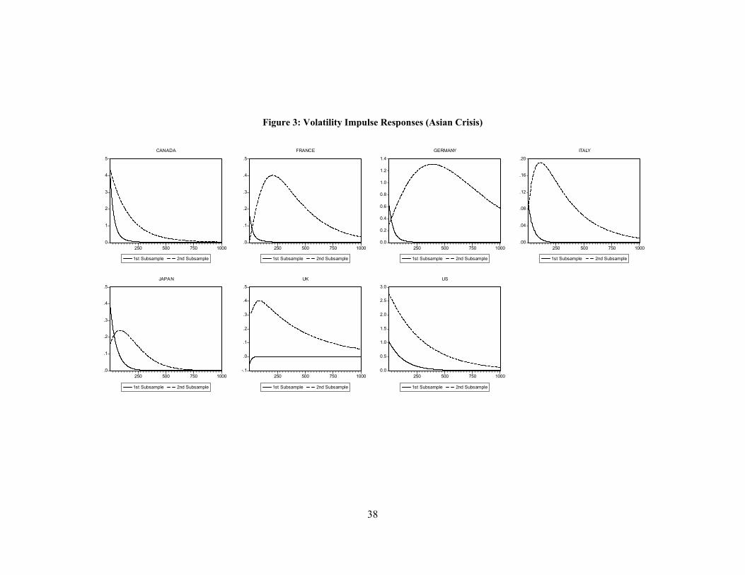
38

Figure 3: Volatility Impulse Responses (Asian Crisis)

0

1

2

3

4

5

250 500 750 1000

1st Subsample 2nd Subsample

CANADA

.0

.1

.2

.3

.4

.5

250 500 750 1000

1st Subsample 2nd Subsample

FRANCE

0.0

0.2

0.4

0.6

0.8

1.0

1.2

1.4

250 500 750 1000

1st Subsample 2nd Subsample

GERMANY

.00

.04

.08

.12

.16

.20

250 500 750 1000

1st Subsample 2nd Subsample

ITALY

.0

.1

.2

.3

.4

.5

250 500 750 1000

1st Subsample 2nd Subsample

JAPAN

-.1

.0

.1

.2

.3

.4

.5

250 500 750 1000

1st Subsample 2nd Subsample

UK

0.0

0.5

1.0

1.5

2.0

2.5

3.0

250 500 750 1000

1st Subsample 2nd Subsample

US