INTEGRATED SOLID WASTE MANAGEMENT MODEL:

THE CASE OF CENTRAL OHIO DISTRICT

DISSERTATION

Presented in Partial Fulfillment of the Requirement for

The Degree Doctor of Philosophy in the Graduate

School of The Ohio State University

By

Rudy S. Prawiradinata, B.S., M.C.R.P

* * * *

The Ohio State University

2004

Dissertation Committee:

Approved by

Professor Burkhard Von Rabenau, Adviser

Professor Jean-Michel Guldmann

Professor Philip A. Viton

(Adviser)

City and Regional Planning Program

ii

ABSTRACT

Solid waste management is an increasing problem, both because of rising waste generation and a declining supply of adequate disposal sites. To deal with the problem waste management methods aim at waste reduction and waste diversion, through increased recycling, composting, and incineration, and changes in consumer behavior.

The dissertation develops an integrated solid waste management (ISWM) model that extends existing models in several ways. First, it uses a more realistic formulation of cost functions allowing economies of scale in waste collection, facility development, and facility operation, but allowing diseconomies associated with separate collection of yard waste, recyclables and mixed waste. Second, the model adds flexibility and realism to facility management options, including the simultaneous use of several disposal facilities, each with its own locational advantages; the export of waste; and the closure and replacement of facilities over time. Third, it allows for the promotion of recycling and hence, the modification of consumer’s propensity to recycle, and it permits these policies to be applied in a spatially differentiated way.

As an initial step, the dissertation develops an analytical model that uses control theory to solve for optimal waste management policies. The system operates in a single waste collection area, has a single disposal site, and waste is either recycled or deposited at the landfill site. The model is solved for different assumptions about cost, including economies of scale.

Based on these initial findings, ISWM is formulated as a mixed integer-programming model, using GAMS for implementation and solution. The model is calibrated to the Central Ohio Solid Waste Management District (the District) and solved under a variety of scenarios. The model is tested and sensitivity analysis is used to determine the impact of changes in disposal capacity, interest rate, and growth of waste generation on recycling policy and landfill life. The model is then applied to the investigation of two further issues.

First, the model is used to derive an aggregate cost of waste management, as a function of key variables such as the size of the system, population density, number of facility options, and recycling tastes. Some of these variables have been found to be

iii

significant in empirical research on the cost of municipal waste management. The cost function estimated here is used to confirm these empirical findings. The function also may be used to serve as a benchmark and as a shorthand method in waste management design. To derive the function, ISWM model is run, generating 2,916 observations (systematically varying eight parameters). The resulting set of pseudo-data is used to regress aggregate cost on the eight variables. The results confirm empirical findings on economies of scale and density. They also suggest the importance of other variables in determining waste management cost, including facility options and recycling taste.

Second, the model is used to derive policy advice for the State of Ohio and the Central Ohio Waste Authority (the Authority). Model findings suggest that the State-mandated 10-15 year planning horizon for waste authorities should be modified to be longer and/or require a minimum terminal disposal capacity. For the Authority, the findings indicate that current recycling levels are close to optimal (based on a 30-year planning horizon), but will have to be redoubled within the next five years. Further, the Authority composting subsidies appear to be excessive, based on an ISWM-estimated shadow price of landfill capacity.

iv

Untuk orang tuaku, isteriku Isti,

dan anakku, sahabatku Irfan

v

ACKNOWLEDGMENTS

I would like to thank my adviser, Professor Burkhard von Rabenau, for his

support, encouragement, and patience in guiding me over the years. My dissertation

would not have been completed without his help. I have learned greatly not only from

his professional knowledge but also from his considerate personality. I am deeply

indebted to him. I am also deeply appreciated and thank to the other member of my

dissertation committee Professor Jean-Michel Guldmann and Professor Philip A. Viton

for their valuable comments and suggestions on my dissertation.

I would like to express my gratitude to my colleague and supervisors at the

National Development Planning Agency, the Republic of Indonesia for their support. I

really appreciated for the opportunity that they have given me.

I want to express my indebtedness and appreciation to my parents for their

endless love and encouragement throughout my life. Finally, my deeply appreciation go

to my beloved wife Isti Surjandari and my best friend, my handsome son Irfan

Prawiradinata for their sacrifice and tremendous understanding over the years. I would

have given up a long time ago without their encouragement and support.

vi

VITA

February 14, 1963.…………….. Born – Bandung, Indonesia 1987………………………… B.S.,

Civil Engineering, Bandung Institute of Technology, Indonesia

1997…………………………… M.C.R.P.,

Department of City and Regional Planning The Ohio State University, Columbus, Ohio

1987 – 1990…....………………. Junior Engineer, Several Private Firms 1998 – 2002……………………. Intern, Public Utilities Commission of Ohio,

Columbus, Ohio 2003 – 2004……………………. Teaching Assistant, Department of Mathematics,

The Ohio State university, Columbus, Ohio 1990 – Present ………………… Urban Planner, National Development Planning

Agency, the Republic of Indonesia.

FIELD OF STUDY

Major Field: City and Regional Planning

Minor Fields: Engineering Economics and Quantitative Method

vii

TABLE OF CONTENTS

Abstract………………………………………………………………………………...

Dedication……………………………………………………………………………...

Acknowledgments……………………………………………………………………..

Vita…………………………………………………………………………………….

List of Tables…………………………………………………………………………..

List of Figures………………………………………………………………………….

Chapters:

1. Introduction…………………….……………………………………………...

1.1. Purpose of the Study……………………………………………………… 1.2. Research Methodology and Outline of the Study……………………..

1.2.1. Methodology of the Study………..……..………….………… 1.2.2. Outline of the Study…………………………………………...

2. Literature Review.……………………………………………………………..

2.1. Waste Management Models…..…………………………………….....

2.1.1. Waste Generation Prediction…………………………………. 2.1.2. Facility Planning and Operation Scheduling.……………….… 2.1.3. Manpower Assignments………………………………………. 2.1.4. Vehicle Management………………………………………….

2.2. Economics of Solid Waste Management……………………………...

Page

ii

iv

v

vi

xii

xiv

1

2 3

3 6

10

10

12 14 26 28

31

viii

3. Analytical Model: Optimization of a Single Landfill’s Life – A Hypothetical Case of Facility Planning……………………………………………………...

3.1. Background…………………………………………………………....

3.2. Model Formulation………………………………………………….…

3.2.1. Fixed Landfill Life……………………………………………. 3.2.2. Variable Landfill Life………………………………………....

3.3. Numerical Analysis……………………………………………………

3.3.1. Mathematical Formulation of the Model……………………… 3.3.2. Fixed Landfill Life……………………………………………. 3.3.3. Variable Landfill Life………………………………………....

3.4. Result Discussion……………………………………………………...

4. Integrated Solid Waste Management Model (ISWM)………………………...

4.1. Extensions of the Model………..…….………………………………..

4.1.1. Composting………………………………………………….… 4.1.2. Landfill Closure and Replacement………………………….… 4.1.3. Multiple Landfill Operations………………………………….. 4.1.4. Economies of Scale…………………………………………… 4.1.5. Promotion of Waste Diversion.……………………………….. 4.1.6. Variety of Collections……………….…………………………

4.2. Statement of the Model………………………………………………..

4.2.1. Illustration of Network Flows……………………………….... 4.2.2. Objective Function………………………………………….…

4.2.2.1. Collection and Transportation Costs………………... 4.2.2.2. Operating Costs……………………………………... 4.2.2.3. Landfill Closure and Replacement Costs…………… 4.2.2.4. New Landfill and Expansion Costs…………………. 4.2.2.5. Revenues……………………………………………..

4.2.3. Constraints……………………………………………………..

4.2.3.1. Mass Balance Constraints………..……………….. 4.2.3.2. Capacity Limitation Constraints…………………...

5. Model Implementation: The Solid Waste Management System in Central

Ohio District……………………..…………………………………………….

Page

42

42

44

44 49

51

52 53 57

59

62

62

63 64 65 66 68 70

71

71 75

76 79 81 82 85

87

87 92

100

ix

5.1. Central Ohio Solid Waste Management System………………………

5.1.1. The Authority……………………………………………….… 5.1.2. Waste Generation……………………………………………... 5.1.3. Waste Collection and Transport…….………………………… 5.1.4. Waste Transfer……….………………………………………... 5.1.5. Waste Processing and Diversion……………………………… 5.1.6. Waste Disposal………………………………………………...

5.2. Model Calibration……………………….…………………………….

5.2.1. Systemic Issues……………………………………………….. 5.2.2. Model Calibration……………………………………………..

5.3. Parameter Estimates and Data Sources……………………………….

6. Model Testing……………………………………………………………….....

6.1. Single Disposal Site - Landfill with Constraint Capacity……………...

6.1.1 Capacity Expansion Under Constant Returns to Scale………… 6.1.2 Capacity Expansion With Economies of Scale………………...

6.2. Multiple Disposal Sites………………………………………………... 6.2.1. Alternative Disposal Site Outside the Study Area………..…....

6.2.1.1. Local Landfill with Infinite Capacity……………... 6.2.1.2. Local Landfill with Finite Capacity………………..

6.2.2. Alternative Disposal Site in the Study Area…………………...

6.2.2.1. Impact of Space on Landfill Replacement……… 6.2.2.2. Impact of Old Landfill Closure Cost on Landfill

Replacement……………………………………….

6.3. Other Disposal Substitutes: Recycling Facility………………………..

6.3.1. New Expensive Landfill………………………………………. 6.3.2. New Cheap Landfill……………………………………………

6.4. Summary………………………………………………………………. 7. Aggregate Cost Function Analysis………………………………………….…

7.1. Background……………………………………………………………. 7.2. The Aggregate Cost…………………………………………………… 7.3. Selected Key Parameters………………………………………………

Page

101

101 103 105 109 110 113

116

119 120

128

142

143

144 144

151 153

153 155

158

159

160

161

162 163

167

169

169 171 172

x

7.4. The Optimization Model and Pseudo Data Generation………………..

7.4.1. Optimization Model…………………………………………… 7.4.2. Pseudo Data Generation……………………………………….

7.5. Empirical Results, Interpretation, and Discussion……………………. 7.6. Summary……………………………………………………………….

8. Model Runs and Optimization Results………………………………………

8.1. Overview: Issues and Approach………………………………………. 8.2. Base Case Scenario – Description.……………………………………. 8.3. Base Case Scenario – Results …………………………………………

8.3.1. Waste Diversion……………………………….……………… 8.3.2. Potential Waste Recycling Areas …………………………….. 8.3.3. Community Responsiveness to Recycling Promotion………… 8.3.4. Landfill Outside the District…………………………………... 8.3.5. Shadow Price of Landfill Capacity……………………………. 8.3.6. Summary of findings…………………………………………..

8.4. Scenario I: Residual Landfill Capacity..………………………………. 8.5. Scenario II: Alternative Landfill Sites…………………………………

8.5.1. New Landfill Capacity Cost is 30% Higher…………………... 8.5.2. New Landfill Capacity Cost is 10% Higher…………………... 8.5.3. New Landfill Capacity and Operating Costs Equal to Current

Landfill Costs…………………………………………………. 8.5.4. Landfill Closure Cost…………………………………………. 8.5.5. New Landfill Location…………………………………………

8.6. Scenario III: Different Planning Horizons…..………………………...

8.6.1. 15-Year Planning Horizon………………………………….…. 8.6.2. 50-Year Planning Horizon……………………………………..

8.7. Summary……………………………………………………………….

9. Conclusions and Areas of Further Research……………………….…………..

Bibliography…………………………………………………………………………...

Page

177

177 179

182 187

189

189 193 195

195 200 205 207 208 214

215 217

218 219

220 222 224

224

225 226

228

230

236

xi

Appendices…………………………………………………………………………….

A Indices, Variables, and Parameters of the ISWM Model……………………... B Resale Value of New Facilities..…………………………..…………………... C Maps…………………………………………………………………………… D Distances Between Waste Sources and Facilities, and Among Facilities……..

Page

245

245 252 255 260

xii

Table

3.1 3.2 5.1 5.2 5.3 5.4 5.5 5.6 5.7 6.1 7.1 7.2 7.3

LIST OF TABLE

Optimum Recycling Shares for Different Fixed Unit Cost of Recycling and Deposit.……………………………………………………………….. Optimum Landfill Life Elasticity of Landfill Closure and Replacement Costs………………………………………………………….……………. Solid Waste Facilities Used in 1990 and 1998 and Included in the Model.. 1990, 2000 and 2001 Population and Area for Waste Generation Areas … Operation and Remaining Capacity of Facilities Included in the Model…. Consumer Price Index – All Urban Consumers…………………………... Economic Parameters……………………………………………………... Technical Parameters……………………………………………………… Decision Variables………………………………………………………… Marginal Cost to Local and Export Landfills and Waste Allocation in the Base Year (1990)………………….………………………………………. Sample Descriptive Statistics……………………………………………… Linear Regression Estimation of the Aggregate Cost……………………... Log- linear Regression Estimation of the Aggregate Cost……….………...

Page

54

59

117

122

127

129

133

137

140

153

183

183

184

xiii

Table

8.1 8.2 8.3 8.4 8.5

Summary of the Scenarios and Their Focus of Discussion……………….. Share of Waste Diverted: Authority’s Plan, Actual Diversion, and the Model Output………………………………….…………………………... Area, Growth, Population, and Density of Three Waste Generation Neighborhoods….…………………………………………………………. Shadow Prices of the Franklin County Landfill Stock Capacity………….. Summary of Costs and revenues of Solid Waste Management Options in Central Ohio District……………………………………………………….

Page

193

197

203

210

211

xiv

Figure 3.1 3.2 4.1 6.1 6.2 6.3 6.4 6.5 6.6 6.7 6.8 6.9 6.10

LIST OF FIGURES

Rate of Change of Recycling Share for Different Unit Cost Deposit Function, T = 15 years…………………………………………………….. Net Present Value of Operation and Replacement Costs………………... Network Representation of the Model……………………………………. Flow (Operating) Capacity and Waste Deposit – Under Constant Returns to Scale …………………………………………………………………… Stock (Storage) Capacity and Waste Deposit – Under Constant Returns to Scale …………………………………………………………………… Flow Capacity and Waste Deposit – Under Increasing Returns to Scale…. Stock Capacity and Waste Deposit – Under Increasing Returns to Scale.... Degree of Scale Economies of Stock Capacity Expansion………………... Waste Deposit and Flow Capacity Expansion – Fixed Cost Doubled……. Waste Deposit and Stock Capacity Expansion – Fixed Cost Doubled…… Waste Deposit and Flow Capacity Expansion – Opportunity Cost of Capital 38% Lower……………………………………………………….. Waste Deposit and Stock Capacity Expansion – Opportunity Cost of Capital 38% Lower……………………………………………………….. Waste Deposit and Flow Capacity Expansion – Waste Growth Rate Quadrupled…………………………………………………………………

Page

56

58

73

144

144

145

145

146

147

147

148

148

149

xv

Figure 6.11 6.12 6.13 6.14 6.15 6.16 6.17 6.18 6.19 6.20 6.21 6.22 6.23 6.24 6.25 6.26 6.27

Waste Deposit and Stock Capacity Expansion – Waste Growth Rate Quadrupled………………………………………………………………… Flow Capacity Expansion – Under Linear Waste Growth Rates………….. Flow Capacity Expansion – Under Semi-Logarithmic Waste Growth Rates……………………………………………………………………….. Amounts of Waste Deposit – Local Landfill Under Constant Returns to Scale Operation, with Infinite Capacity…………………………………… Amounts of Waste Deposit – Local Landfill Under Increasing Returns to Scale Operation, with Infinite Capacity…………………………………… Local Landfill with Flow Capacity Constraint……………………………. Local Landfill with Stock Capacity Constraint………………..………….. Stock Capacity and Cumulative Waste Deposit in the Local Landfill …… Flow Capacity and Annual Waste Deposit in the Local Landfill…………. New Landfill Location Incurs High Delivery Cost for All Waste Sources.. New Landfill Location is Preferred by at Least Some Waste Sources……. Impact of Landfill Closure Cost (The Old Landfill is Never Closed)…….. Impact of Cheap Recycling Costs on Landfill Operation and Replacement – 1………………………………………………………………………….. Impact of Expensive Recycling Costs on Landfill Operation and Replacement – 1…………………………………………………………… Impact of Expensive Recycling Cost on Landfill Operation and Replacement - 2 (RC-0)…………………………………………………… Impact of Cheap Recycling Cost on Landfill Operation and Replacement - 2 (RC-0)………………………………………………………………….. Substitute Location and Landfill Catchment Area…………………………

Page

149

151

151

154

154

156

157

158

158

159

159

160

163

163

164

164

165

xvi

Figure 6.28 6.29 7.1 8.1 8.2 8.3 8.4 8.5 8.6 8.7 8.8 8.9 8.10 8.11 8.12 8.13

Recycling Facility (RC-1) is Closer to the Old Landfill – Impact of Recycling Facility Location on Landfill Operation and Replacement……. Recycling Facility (RC-2) is Closer to the New Landfill – Impact of Recycling Facility Location on Landfill Operation and Replacement……. Simplified Solid Waste Management Area………………………………... Annual Waste Generated, Deposited, Recycled, and Composted, with 30-Year Planning Horizon……….…………………………………………… Annual Shares of Waste Deposit, Recycled, and Composted, with 30-Year Planning Horizon …………………………………………………… Distribution Amounts of Waste Recycled in the District in 2002, 2016, and 2031.…………………………………………………………………... Waste Recycled Shares in the District in 2002, 2016, and 2031 (as % of total waste generated)…………………………………………………….. Waste Generation Area and the Solid Waste Facility Location………….. Annual Shares of Recycled Material From Different Waste Generation Areas (as % of total waste generated)……………………………………... Waste Recycled and Recycling Capacity Expansion Schedule…………… Waste Recycled Shares in the District in 2002, 2016, and 2031 (as % of total waste generated) with Various Value of α………………………….. Amounts of Waste Deposited in Each Landfill…………………………… Shares of Waste Deposited in Each Landfill ……………………………... Annual Shares of Landfill Deposit in Each Facility – Scenario I…………. Annual Shares of Landfill Deposit in Each Facility – Base Case Scenario.. Annual Shares of Waste Deposited, Recycled, and Composted – Scenario I…………………………………………………………………………….

Page

166

166

178

199

199

201

201

203

204

205

206

208

208

216

216

217

xvii

Figure 8.14 8.15 8.16 8.17 8.18 8.19 8.20 8.21 8.22 8.23 8.24

Annual Shares of Waste Deposited, Recycled, and Composted – Base Case Scenario ……………………………………………………………... Amounts of Waste Generated, Deposited, Recycled, and Composted – Two New Landfill Alternatives Exist in the District……………………… Shares of Waste Deposited, Recycled, and Composted – Two New Landfill Alternatives Exist in the District…………………………………. Amount of Waste Deposited to Each Landfill – Two New Landfill Alternatives Exist in the District…………………………………………... Shares of Waste Deposited to Each Landfill – Two New Landfill Alternatives Exist in the District…………………………………………... Change in Waste Diversion Rates Due To Different Costs of New Alternative Landfills………………………………………………………

Impact of Landfill Closure Cost on Annual Shares of Waste Deposited in Each Landfill – Two New Landfill Alternatives Exist in the District…….. Impact of Landfill Closure Cost on Annual Shares of Waste Deposited, Recycled, and Composted – Two New Landfill Alternatives Exist in the District …………………………………………………………………… Annual Shares of Waste Deposit and Diversion With a 15-Year Planning Horizon – Compared to the Base Case Scenario………………………….. Shares of Annual Waste Deposited, Recycled, and Composted – Two New Landfill Alternatives Exist in the District)…………………………... Shares of Annual Waste Deposited in Each Landfill – Two New Landfill Alternatives Exist in the District…………………………………………...

Page

217

219 219

221

221

222

223

223

225

227

227

1

CHAPTER 1

INTRODUCTION

The management of solid waste has become a significant research problem that

combines technical, economic, environmental and social issues. Technical and economic

problems emerge in part because of rising demand due to income and population growth,

a rising level of urbanization, and a decline of suitable disposal sites. These problems

challenge researchers to search for more efficient solid waste management methods.

Environmental and social issues emerge as people become increasingly concerned about

the risks associated with living close to solid waste facilities. For example, many sites

and disposal methods have been found to pollute the air and to contaminate underground

drinking water sources. Some studies also have shown that landfill disposal decreases

neighboring property values. Therefore, residents oppose new facilities. According to

Levenson (1993), many areas in the United States are experiencing a shortfall of landfill

capacity. He also reports that landfill costs are rising as older landfills reach the end of

their expected lives. Stronger state environmental regulations have resulted in the closure

of many substandard landfills, and public opposition makes siting of new landfills and

other facilities difficult.

2

1.1 Purpose of the Study

This study develops a model for the optimal operations, capacity expansions and

locations of solid waste facilities. The purpose of the model is to assist in selecting

strategies that minimize the cost of waste collection, transportation, operation, and

disposal, subject to physical constraints. The model extends earlier solid waste

management models by considering a relatively new type of waste disposal, in addition to

other more standard disposal methods already included in a number of optimization

models. Composting facilities represent an increasingly popular waste management

option, as communities look for ways to divert part of the local waste stream from

landfills (Tchobanoglous et al., 1993). Depending on climatic, demographic, social and

economic factors, composting facilities can divert 10-35% of the residential solid waste

stream from the landfill alternative (Haug, 1993). The proposed model includes the

revenues produced by the sale of composting material generated by the facility. The

model derives an overall solid waste strategy for a community, including the allocation of

solid waste to several alternative modes of treatment, such as recycling, incineration,

landfill, and composting. The model identifies the optimum sites for a combination of

these facilities, choosing from several pre-specified candidates, and schedules operations

at each of these facilities over a given planning period. The model determines the start of

operations at each of the facilities chosen and the possible closure of the facility during

the planning period, the siting and operations of auxiliary facilities, such as transfer

stations, the schedule of waste management operations, and the allocation of the waste

stream from the point of waste generation to waste facilities. The model derives the cost

of transportation and operations over the planning horizon, subject to physical

constraints.

3

The model also determines the optimum levels of promotion for waste diversion

program. For example, greater promotion raises household participation in waste

presorting. This in turn reduces the cost of recycling or raises the maximum amount of

possible recycling. The model determines the optimum level of promotion, so that at the

margin the cost of increased recycling, including the cost of its promotion, equals the

benefits of such promotion through the diversion of waste from solid waste sites.

1.2 Research Methodology and Outline of the Study

The research approach consists of five key elements, including (1) the preparation

of analytical models and qualitative results, (2) the development of a quantitative model

and plausibility analysis, (3) the implementation of the model to a particular case study –

model calibration and parameters estimate, (4) model testing and economic analysis, and

(5) model runs to propose a planning strategy. This study consists of seven chapters, in

line with the key elements of the research methodology. The following discusses the

research methodology and the outline of the study, each in turn.

1.2.1 Methodology of the Study

The following describes the five key elements of the research methodology:

(1) Develop and adapt analytical and qualitative models to guide the development of a

more realistic quantitative model. The advantage of small qualitative models is that

they often can be solved analytically, or at least certain characteristics of their

solution can be derived. On this basis, it is possible to develop expectations about

4

optimal behavior that can later be used to test the plausibility of a more complex

quantitative model that otherwise is beyond verification.

(2) Develop a structural model and extend it in a variety of ways. Most of the extensions

are included in the model and each extension will be tested separately so as to check

it against expectations based on analytical, qualitative, and theoretical results in the

literature. In terms of model substance, the dissertation is concerned with three key

points that will play an increasing role in waste management in the future. These

include the life of disposal sites and methods of extending this life, methods of waste

diversion and reduction as means to reduce dependency on disposal sites, and

behavioral changes as a means to reduce waste deposited in landfills.

(3) Proposed model calibration, data collection and parameter estimation. The model is

calibrated to describe the case of the Central Ohio District. Key data to be collected

include economic parameters (unit cost of operation, costs of construction and

expansion of facilities, waste collection and transportation costs, prices of

recyclables, population and per capita income), and technical parameters (waste

generation rates, facility capacities, distances among facilities). Some of these data

are available directly from Franklin County. However, in some instances there may

be a need to use instead data available from the literature. The estimation of a series

of detailed cost parameters will be based on a single year of cost observations, and

hence, the parameters will not be derived or tested econometrically. Rather, the

methodology is similar to that used for other complex models, such as Computable

General Equilibrium Models, where analysts typically are satisfied estimating data

5

based on a single set of observations. Parameters are supplemented and checked

based on a review of parameters already published in the literature (such as scale

elasticity for different facilities). Selected parameters have also been estimated using

a cross-section of waste management systems.

(4) Model testing and economics analysis. The model is checked regarding its

plausibility, and tests are used, that compare model results with theoretical results.

Other checks include running the model on special assumptions that permit a direct

verification of the results. Further, solution algorithms are tested not only with regard

to speed and efficiency, but also with regard to robustness. This includes checking

the extent to which model solutions are invariant to changes in starting point

assumptions, over a wide variety of parameters. The plan is to use a mixed- integer

program algorithm and to use linear approximations to model variable returns to

scale. Consequently, this may considerably raise the number of integer variables.

The model will also be used to prepare a sensitivity analysis, to determine several key

inputs. Second, sensitivity analysis is used to reflect on the relevance of the model

extensions implemented in the dissertation. There is little point in making models

more complex than need be. Third, it may be possible to check model results against

rules of thumb available in the waste management literature. Different hypothetical

systems will be tested. The model will be run using Central Ohio District parameters

to derive an optimal solution. This solution will then be compared with results from

the literatures, as well as with the known behavior of solid waste systems.

6

(5) Finally, the model will be run using current data and condition of the waste

management system of the Central Ohio District. The idea is to develop a strategy for

future waste management operations instead of comparing the model result to past

operations. For this purpose, the current system is described, including its major

components and the issues it is facing.

1.2.2 Outline of the Study

The five key elements of the research methodology are presented in nine chapters,

beginning with this introduction. The following summarizes chapters 2 to 9, each in turn.

Chapter 2 presents the literature relevant to the modeling of solid waste

management. This review includes not only a wide range of waste management models,

but also deals with empirical studies designed to identify the cost structure of waste

management, the demand for waste services, and the institutional structure of service

provision, so as to develop a good understanding of the stylized facts that must be

incorporated into a model of waste management.

Chapter 3 develops a simple analytical model of a solid waste management

system. It derives both theoretical results and numerical estimates, to illustrate the

consistency of both results. It illustrates model behavior under different cost structures of

landfill and recycling operations, fixed and variable landfill life, and landfill replacement

costs. The model considers landfill sites as a natural resource that is used over time as

the given capacity is filled. In the landfill with variable life, the model derives

simultaneously the optimum recycling and replacement strategy to optimize the life of a

landfill facility.

7

Chapter 4 presents the Integrated Solid Waste Management Model, for the

optimal location of solid waste facilities and their operations. The model extends earlier

solid waste management models in several ways. First, it adds composting to other waste

disposal methods already modeled elsewhere, including landfill, incineration and

recycling. Second, it allows for a much more flexible treatment of landfill sites, including

the closure and replacement of existing landfills, the operation of multiple landfill sites,

and export of waste to landfills outside the management region. Earlier models assumed a

single landfill with sufficient capacity to meet disposal requirements over the planning

horizon – and hence did not deal with one of the key policy problem faced by waste

management companies – how to manage landfill facilities. Third, it allows for

economies of scale, both in the operation of waste facilities, such as landfills, and in the

extension or new construction of landfills. Moreover, it makes a distinction between the

stocks and flow capacity of landfills, and allows for returns to scale in both. Fourth, past

models have treated recycling as inelastic and given. Instead, the model here makes

recycling sensitive to government actions, including promotional activities and public

education. This is important, as limited landfill capacity makes recycling an increasingly

important alternative. Fifth, the model considers different collection methods for

compostable waste, four types of recyclable waste, and mixed waste. It allows

compostable and recyclable waste to be collected separately at the curbside or as part of

mixed waste. The model considers economies of scale in collections by adding a fixed

cost.

Chapter 5 presents the Central Ohio solid waste management system, parameter

estimates, and data collection for model application. It describes the activities and

8

facilities that exist in the area, as well as the firms and organizations that are involved in

waste management, including the Solid Waste Authority of Central Ohio, which will be

referred to as ‘the Authority’. It owns and operates the only landfill in the District, and

three transfer station facilities, and subsidizes two yard-waste composting facilities. This

section also describes model calibration, including parameter estimates. The model

proposed in the previous chapter will be tested using stylized facts of the Central Ohio

District under current conditions.

Chapter 6 performs model testing. It applies the model and validates it through a

series of experiments that compare its results with those of expectations based on

theoretical results in the literature and analytical models. Specifically, the model is tested

for its behavior in response to variations in economies of scale, opportunity cost of

capital, growth of waste generation, and availability of export waste opportunities. It is

well known that the greater the economies of scale, the less frequently will the facilities

be expanded and the greater the excess capacity built at the time of expansion. Similarly,

the higher the opportunity cost of capital, the more frequently will facilities be expanded,

and the smaller the excess capacity built at the time of expansion.

Chapter 7 derives an aggregate waste management cost function based on model-

generated pseudo-data. This permits to ask questions on the aggregate behavior of waste

management cost based on information about the attributes of a waste-management

system. There has been considerable debate in the literature on whether waste

management systems exhibit returns to scale and density, and on the magnitude of such

returns. Other questions are related to the impacts on costs of a recycling option, of

different institutional frameworks, and of variations in wage costs. A variety of values

9

for selected parameters, such as population size and density, are used, and the model is

solved for each set of parameter alternatives. The resulting pseudo data are then subject

to statistical analysis to generate estimates of cost function parameters.

Chapter 8 implements the model for a particular waste management system, to

illustrate its usefulness for realistic decision problems. The application is to the Central

Ohio waste management authority. The Authority faces a problem typical of waste

authorities throughout the United States. It has limited landfill capacity and its incinerator

has been permanently shut down because of pollution. Land for new landfills within

county limits is non-existent. Hence, it wants to manage its overall waste stream so as to

extend the life of its landfill, by raising the share of recycling and composting. The model

is used to analyze alternative ways for increasing the life of the existing landfill.

Chapter 9 concludes the research, by summarizing key results and suggesting

avenues for further research.

10

CHAPTER 2

LITERATURE REVIEW

This literature review focuses on two major research streams. The first is research

on waste management modeling, and the second on the economics of solid waste

management. In the first category, some researchers focus on waste generation

prediction models, while others develop models to optimize facility operations,

investment, and new facility locations, by minimizing the overall costs of waste

management. One optimization model will be used as a basis for model development in

this research and will be discussed in more detail. In the second category, research

mostly deals with product-specific scale economies, economies of scope, or economies of

density in each solid waste activity, including waste collection, operation and expansion

of waste deposit, recycling, composting, and incineration facilities.

2.1. Waste Management Models

Liebman (1975) distinguishes five groups of waste management models, based on

a survey of the literature of the 1960’s and 1970’s: waste generation prediction, fixed

facilities, vehicles routing, manpower assignment, and overall system models. The first

category deal with the forecasting of waste generated in specific areas, based on such

11

variables as population growth, population density, and income. The second category,

fixed facility models, focuses on site selection, capacity expansion, and facility

operations. Examples are models that apply integer programming to select the best site

from among specified alternatives, minimizing operating and transport costs. The third

category, vehicle models, deals with such issues as the timing of vehicle replacement and

the routing of vehicles to provide a required level of service at minimum cost. The

fourth category, manpower models, deals with crew assignment in waste management

operations. Finally, systems models deal with the overall operation of the waste

collection system. At the time of Liebman’s review, these were mainly simulation

models designed to enable the user to study the effects of parameter changes on system

operations. Sometimes, critical variables, such as the amount of waste generated per day,

are treated as stochastic variables to study their impact on truck use, equipment

requirements, and efficiency of crews. Simulation models have also been applied to

queuing problems at the disposal point.

In a more recent survey article (1997), Liebman observes that the foundations of

the current literature date back to the 1960s and 1970s, and later work often merely

extends earlier models. Much of his new survey therefore refers back to the earlier

period, classifying models into network flow, facility siting, vehicle routing, and

simulation models. In contrast to the earlier survey, network flow models have been

added, and manpower and waste generation prediction models have been dropped.

While Liebman is correct that much of the recent literature continues past

modeling traditions, there has been a great deal of methodological innovation and added

realism. Recent models solve problems of much greater complexity than has been

12

possible in the past, they add uncertainty where earlier models were deterministic, and

they use algorithms that did not exist then.

The following review slightly modifies Liebman's classification system. It begins

with models on the waste demand side, that is, waste generation prediction models.

Then, it follows with models on the supply side that optimizes waste management

services. These models are divided into three categories: (1) facility planning and

operation scheduling, (2) manpower assignment, and (3) vehicle management. In some

studies, the output from a facility-planning model may be used as an input to manpower

assignment or vehicle management models.

2.1.1 Waste Generation Prediction

Rao et al. (1971) develop the simplest waste generation model, distinguishing

between residential, commercial, and industrial customers, measured respectively in

terms of number of housing units, establishments and employment. The amount of waste

from each group is then the product of sector size and generation rate. Generation rates

are obtained from regional data averaged over a year and assumed constant over time.

Hence, the model does not account for changes in generation rates as a result of changes

in income or prices. Economic growth is considered in a descriptive manner, by

projecting population, employment and establishment changes over time.

Chang (1991) develops a waste generation sub-model as part a larger solid waste

management model. The model uses econometric analysis to forecast the amount of

waste generated over a planning period of 20 years, dividing the total area into n

generation districts and projecting the waste of each as a linear function of dwelling units,

13

per capita income, and population. The improvement in this model is the consideration

of income as a determinant of waste generation. However, Chang does not differentiate

waste by sector, as in Rao’s model.

Daskalopoulos et al. (1998) develop two models, one to estimate total waste

generation, and the other to estimate waste composition, at the country level, using

aggregate observations on the municipal solid waste of industrialized countries. Total

waste generated (in tons) is found to be a non- linear function of population size and

living standard (represented by GDP per capita). The composition of waste is modeled

by dividing waste into six categories: plastic, paper, glass, metal, organic, and others. The

share of each waste category is then shown to be a non-linear function of the pattern of

consumption as represented by six major product groups: food and drink, clothing and

footwear, furniture, and books and magazines. Most models display a good statistical fit.

Hocket et al. (1995) use a linear regression model to identify and measure the

variables that influence per capita municipal solid waste generation. This study was

conducted using county data in the Southeastern United States. The variables include

disposal fee, per capita retail sales, per capita construction costs, per capita sales of

eateries, merchandise, food stores, apparel stores, per capita income, and urban

population (as a percentage of the county population). The authors show that disposal

fees and retail sales have the greatest impact on waste generation. The higher the

disposal fee, the lower the waste generation, and the higher the retail sales, the higher the

waste generation.

Bruvoll and Ibreholt (1997) model waste generation in the manufacturing sector

based on the sector's use of raw material and intermediate inputs. The authors expected

14

waste generation to be proportional to either the level of production or the amount of

material input, but found that the growth of waste is better explained by the growth of

inputs than by the growth of production.

2.1.2 Facility Planning and Operation Scheduling

Facility planning models often include elements of other models, including waste

prediction, manpower assignment, and vehicle routing. These elements are not discussed

here since they are covered elsewhere. Facility planning models are of four types: (1)

Site selection models, to select facility sites among specified alternatives, by considering

the costs of transportation, construction, and operations; (2) Capacity expansion models,

to determine the optimal size of plants and the timing of their construction, so as to

minimize present value cost; (3) Models of facility characteristics, to analyze facility

operating characteristics, such as the number of loading docks, the size of storage

facilities, and the need for pollution equipment; (4) Models of scheduling operation and

replacement of landfill facilities; and (5) Integrated models, that can have elements of all

four other model categories.

Several studies have focused on evaluating proposed location alternatives for

solid waste facilities. Helms and Clark (1971) use linear programming to select solid

waste disposal facilities among various proposed alternative sites. Marks, Revelle and

Liebman (1970), Marks and Liebman (1971), Gottinger (1986), and Chang (1993, 1996,

and 1997) use mixed- integer programming models to determine the best locations of

waste facilities. Hasit and Werner (1981) and WRAP-EPA (1977) use Walker’s

15

algorithm to determine the least-cost regional system. Esmaili (1973) use a simulation

approach to compute the cost of different combinations of facilities, including facility

siting and expansion over a period of time. Kaila (1987) uses dynamic programming

with a heuristic approach to evaluate waste management systems that include more than

one type of facility. This model chooses the least-cost alternative for collection,

transportation, processing, and disposal activities.

Gottinger (1986) develops a model where potential management facilities are

given. The model minimizes the total cost, which includes fixed and variable facility

costs, and transportation costs. Given a set of potential management facilities, the model

uses a branch-and-bound algorithm to determine which one to build, how to route the

waste, and how to process and dispose of this waste. Ossenbruggen and Ossenbruggen

(1992) develop The Solid Waste Allocation Package (SWAP) a computer package that

finds the minimum cost solution for a waste management district described as a network.

The model approach is similar to that of Gottinger.

Huang et al. (1995) develop grey fuzzy integer programming models to solve the

problem of waste management planning under uncertainty, particularly uncertainty

related to the environment and the economy (prices and costs). The objective of the

model is to identify an optimal facility expansion plan and municipal solid waste flow

allocation. The proposed modeling approach has been applied to a hypothetical planning

problem of regional waste management facility expansion and flow allocation.

16

More specific models have been used to derive a schedule of facility replacements

over a given planning period1. Lund (1990) develops a model that uses recycling as an

instrument to determine the level of annual landfill deposit. This in turn determines the

life of the landfill, and hence the time when a new landfill must be started. The greater

the amount of recycling, the longer the life of a landfill. Recycling postpones the time

when an existing landfill must be replaced, and hence postpones the cost of future landfill

operations. The optimum recycling and replacement strategy is one that minimizes the

cost of recycling and landfill operations over the life of the initial site, plus the terminal

cost of future waste operations beyond its life.

The implementation of Lund’s model is done in two stages. In the initial stage,

the model uses a linear programming approach to determine an optimum recycling

strategy for a given life of the landfill site. This is repeated for every possible lifespan of

the landfill site, and the present value of the cost of all waste operations is recorded. In

the second stage, these costs plus terminal costs are compared, and the optimum lifespan

is selected. The model allows for different types of waste recycling, each with a different

unit cost, and each diverting a given share of the total waste from the landfill. Even a

maximum recycling effort, however, will not eliminate all waste. Hence, there is a

maximum life for the landfill site, say Tmax, beyond which life cannot be extended, even if

all recycling options are utilized all the time. There is also a minimum life for the landfill,

say Tmin. This is the life that the landfill will have if recycling is never used. Hence, the

model examines the recycling strategy for each lifespan T, Tmin<T<Tmax. In general, if

1 This problem could also be treated as a subgroup of the facility planning models.

17

recycling takes place, it will start with the cheapest options, and will gradually add more

expensive options. No recycling will take place if even the cheapest recycling option is

too expensive to use, i.e., if its cost is larger than the savings it generates by postponing

closure of the current landfill (and hence postponing the cost of future waste operations

beyond the life of the current landfill).

The objective function of Lund’s model is expressed as follows:

(2-1) TtT

t

m

i

L

jijtijijitit rCCTCRrRccuncMin −−

= = =

++++

∆−+∑ ∑ ∑ )1]()([)1()(

1 1 111

subject to:

(2-2) CAPRunT

t

m

i

L

jijijtitit ≤

∆−∑∑ ∑

= = =1 1 1

(2-3) ,itijt nR ≤ ijt∀

(2-4) ,0≥ijtR ijt∀

where:

c1 = operating cost of disposing a unit of waste to the landfill ($/yr);

cij = annual cost of recycling option j on a class i waste generator ($/yr);

nit = number of class i waste generators (waste source) in year t;

uit = annual volume of waste generated per class i generator in year t;

it∆ = average volume of waste recycled by class i waste generator

exposed to recycling option j;

Rijt = decision variable: the number of waste generators (waste source) of class i

using recycling option j in year t. For instance, If class i represents

households in neighborhood A and option j represents the weekly curbside

collection of recycled newspaper, and Rijt = 500, then there are 500

households in neighborhood A that have weekly collection of recycled paper

during year t.

18

CR(T) = present value cost of replacing the landfill in year T($);

CC = cost (in year T) of closing the landfill ($);

T = landfill lifetime (years);

r = real discount rate;

CAP = landfill capacity in the first year of analysis.

The summation limits are the landfill’s assumed lifetime T, the number of waste

generator classes m, and the number of recycling options, L.

Timothy Jacobs and Jess Everett (1992) extend and modify Lund’s model in

several ways. First, they consider a fixed horizon, but within this horizon allow for a

chain of landfills, each landfill replacing the next. Further, they determine the optimum

sequence of landfills, by drawing each landfill from a larger set of landfills with known

cost and size characteristics. The first landfill may pre-exist, or it may be chosen as one

of the landfills from the set. However, the other elements of the model are similar to

Lund’s model. The model determines the optimum recycling strategy and optimum

lifespan of each landfill, with the main difference being that there are now several such

landfills instead of just one. As in Lund (1990), the objective is to minimize the costs of

landfill operations and recycling (net of income from recycling).

The model is solved using linear programming. The model always selects

landfills in ascending order of their disposal cost. The first landfill to be brought into

operation is the one with the lowest unit cost, followed by the one with the second lowest

cost, and so on. The model also shows that recycling remains often viable, even if its

cost is higher than the current cost of depositing the same waste in the landfill. This is so

19

because the cost of future landfills eventually exceeds the current recycling cost, and

today's recyc ling postpones these higher future costs. This second point is obvious, but

Lund had not made it explicitly. The optimization model is expressed as follows:

(2-5) lt

L

l

T

tt

ltijt

I

i

J

j

T

tt

ijt Sr

CSR

r

CRMin ∑∑∑∑∑

= == = = ++

+ 1 11 1 1 )1()1(

subject to:

(2-6) ∑ ∑∑ ∑= = = =

=∆+L

l

I

i

J

j

I

iititijtijtlt unRS

1 1 1 1

(2-7) ∑=

≤L

lllt CAPS

1

l∀

(2-8) ijtijt nR γ≤ ijt∀

where:

CRijt = Cost of implementing recycling option j for waste generator i in year t;

CSlt = Cost of landfilling a unit of waste in landfill l in year t;

Slt = Quantity of waste deposited in landfill l in year t;

γijt = Fraction of waste generators of class i served by recycling option j in

year t (in this case study, γijt is assumed to be 1 to simplify the problem).

Note: In Lund’s model, each selected recycling option services all waste

generators of class i. In this case γijt = 1.

CAPl = Capacity of landfill l;

The definitions of the other variables are similar to those in Lund’s model.

A model developed by Chang (1996) extends the facility-siting model. This

model differs from prior work by its consideration of environmental impacts, such as air

pollution from incinerators and leachate in landfill facilities. The model not only

determines the location and capacity of solid waste facilities, but also the level of facility

20

operations over time. Sub-models evaluate leachate impact and air pollution, forecast

waste generation, and determines the residual value of facilities at the end of the planning

period. Chang’s model will be used as a basis for model development and model

extensions proposed in this research. The following reviews Chang's model in greater

detail, including a discussion of the core model and a review of the sub-models dealing

with environmental constraints, waste generation forecasting, and terminal conditions.

Chang's model describes an integrated solid waste management system that

focuses on residential waste generation, and is divided into several regions modeled as

point sources, with multiple processing plants for recycling and incineration, transfer

stations, and disposal sites. The purpose of the model is to assist solid waste authorities

with the overall waste management problem over a given multi-period horizon. For each

time period, the model predicts the amount of waste generated in each generation zone,

and the size of all waste flows and level of facility operations. It determines which of the

facilities are opened or closed, the amount of pollution generated by new capacity and the

level and cost of pollution abatement requirements.

To solve the problem, the model uses a mixed- integer programming approach to

minimize the present value cost of the waste management system subject to constraints

such as capacity limitations, site availability, mass balance, financial constraints, and

pollution constraints.

The remainder of this section first describes in detail the objective function,

followed by two sections, one on model constraints, and the other on the sub-models that

forecast waste generation, air pollution dispersion, leachate impact, and the residual value

of facilities at the end of the planning horizon.

21

a. Objective Function: The objective of the model is to minimize the present value of

total costs net of revenues from operating the waste management system. Revenues

include the sale of recyclable materials and the sale of energy produced by incineration.

Facilities have a residual value at the end of the planning period, based on the benefits

over the facility's remaining life and its salvage value at the end of its life, with proper

discounting.

The cost of waste management facilities consists of operating and investment

expenditures. Operating costs (including cost of maintenance) are of two types: facility

operations and transportations. Both are linear in the amount of refuse handled.

Investment expenditures can be of two types: new facility construction and facility

expansion. New facilities are built with economies of scale, modeled in the form of fixed

and variable linear cost components. Facility expansion involves constant returns to

scale.

b. System Behavior: There are several aspects of system behavior that play a significant

role in the model. These include:

• Transport expenditures are modeled as operating expenditures. Presumably, investment

expenditures for trucks and other equipments are included among the operating

expenditures in annualized form.

• Collection and distance expenditures are not separately modeled, but are included in the

costs of transportation, from waste generation sources to destination facilities. All else

being equal, facilities that are farther away from the waste generation points have

higher transportation costs.

22

• Pollution expenditures are treated as an investment cost, and are taken proportional to

pollution abatement requirements. Maintenance and operating expenditures for such

equipment are not included separately, and hence, must be capitalized into the

investment expenditures to be reflected in the model.

• Facility capacity is measured in terms of annual throughput, i.e., annual volumes of

waste recycled, incinerated, or deposited. Facility capacity is not measured in terms of

cumulative storage capacity – as would be appropriate for landfill sites. Hence, the

model does not track the cumulative consumption of landfill capacity and implicitly

assumes that landfill capacity is sufficient to absorb the waste deposited over the

planning horizon. When the capacity of a landfill is expanded, this is in terms of its

annual absorption capacity. Higher absorption, however, will not reduce the remaining

life of the landfill, as a facility's lifespan is not explicitly modeled. The model does not

deal with the possible replacement of an existing facility or the cost that would result

from it.

c. Constraints: There are two sets of constraints. First, the basic constraint set consists of

mass balance, capacity limitation, site availability, and operating. The special constraints

consist of pollution (leachate impact and air pollution limit) and financial constraints.

These constraints are discussed below:

• Mass Balance Constraints: There are mass balance constraints for each type of nodal

point. In each collection district, the solid waste generated must equal the waste

transported to treatment facilities, transfer stations, and landfill sites. At each treatment

facility, the incoming waste must be equal to the outgoing waste plus the waste lost

23

during the treatment process. At each transfer facility, the incoming waste must equal

the outgoing waste.

• Capacity Limitation Constraints: Each facility has a single capacity constraint, where

capacity is expressed in terms of output or throughput, i.e., in terms of tons per day

incinerated, tons per day recycled, or tons per day transferred. This is also the case for

landfill facilities, where the capacity is described in terms of tons of waste deposited

per day. In the case of landfill sites, however, another constraint is the cumulative

amount of waste that can be deposited before the landfill runs out of space. This

amount depends on the available land and the technology used. As already mentioned,

Chang’s model does not include this type of constraint. This constraint is referred to as

the cumulative deposit constraint, and the former as the annual deposit constraint.

• Site Availability and Conditionality Constraints: There are two types of constraints.

One, called the availability constraint, limits the number of new facility start-ups to the

number of available locations for this type of facility. For each type of facility k there

may be nk locations that are unused initially, but on which a new facility of type k may

be located over the planning horizon. Hence, if there were 3 landfill locations, then at

most three new landfills could be developed. The other, called by Chang the

conditionality constraint, assures that each location can be chosen at most once over the

planning horizon as the site of a new facility of type k.

• Financial Constraints: Financial constraints require that, in each period, the total

expenditures (including annualized investment cost) should be less than or equal to

total revenues from recycling, energy sales, and tipping fees (charged on waste

generated). The constraint determines the tipping fee in each period, but otherwise has

24

no impact on the model, as waste generation is price inelastic. The model does not

permit borrowing against future income, so investment costs must be recovered during

the period of construction. Hence, tipping fees may vary widely from period to period,

which does not represent a realistic approximation of the behavior of these fees in the

real world.

• Air Pollution Constraints: There are two types of air pollution constraints. One

represents the National Ambient Air Quality Standards (NAAQS), and the other the

Prevention of Significant Deterioration (PSD) standards. The two constraints act on the

same air pollutants and the same facilities, but the PSD constraints are more stringent

and hence they are considered in the model. The other constraints must be presented in

compliance with the NAAQS. The PSD constraint limits mass emission rates

(ton/year) of pollutants from specific sources. The NAAQS constraint specifies

maximum concentrations (ppm or µg/m3) of pollutants in the surrounding environment.

Different facilities have different propensities to pollute. This propensity is

measured by an emission factor unique to each facility (and independent of the amount

of waste throughput at the facility). The NAAQS constraint requires that the product of

the emission factor, the dispersion factor (which depends on a facility’s location, wind

pattern, wind speed, and topography), the amount of waste incinerated, and the flue gas

flow rate (conversion factor of the waste burning rate to flue gas flow rate – m3 /ton),

less the necessary removal rate, is less than or equal to the air quality standard at a

given receptor location. The dispersion factor is calculated by an independent sub-

model using a Gaussian diffusion equation. To model the PSD constraint, it is assumed

that emissions are proportional to waste incinerated. The PSD constraint then requires

25

that total emissions less the necessary removal rate are less than or equal to the PSD

emission standard. The removal rates, both for the NAAQS and PSD constraints, are

decision variables. In a case study, however, Chang shows that, for a broad range of

parameters, only the PSD constraints are active. Hence, he includes only the removal

cost related to the PSD constraint in the total cost.

• Leachate Limitation Constraints: Landfill facilities receive two major types of waste:

(1) raw solid waste from recycling, transfer facilities, and source generation, and (2)

combustion ash from incineration facilities. These two types of waste produce different

environmental impacts due to different leachate characteristics. Leachate impacts are

estimated using the base numerical rating (BNR), also called the leachate impact index.

The BNR is an analytical measurement of a pollutant ability to penetrate into an

unsaturated zone. The constraint requires that total leachate impact from both types of

waste is less than or equal to the allowable limit. The BNR is determined by an

independent sub-model. Since parameter estimates are uncertain, this constraint is only

used for risk assessment. Hence, the function of the leachate impact constraints is only

to limit the impact from ash and raw garbage on groundwater environment. There is no

direct cost in the objective function associated with this constraint.

d. Sub-models: Chang's model includes four sub-models that determine important

parameters. Each of these sub-models is run independently and the results are used as

input to the main model. The sub-models do not use information from the main model,

though the main model makes use of the sub-model calculations. Specifically, these sub-

models determine: (1) the air pollution dispersion factor; (2) the leachate impact index,

i.e. BNR; (3) future waste generation; and (4) the residual values of facilities at the end of

26

the planning period. In the model proposed here, only the residual value sub-model is

included, and hence it is further elaborated.

The residual value sub-model determines the resale market value of a facility at

the end of the planning horizon. This residual value is equal to the residual benefits from

this facility over its remaining life, plus its salvage value at the end of its life, discounted

over the planning horizon. Chang calculates the residual value, based on four

assumptions: (a) A facility’s salvage value in constant prices is a fixed fraction of the

initial cost of the facility; (b) A facility's benefits during each year are constant when

calculated in constant prices; and (c) A facility's present-value benefits are exactly equal

to the facility's present-value costs. Hence, the facility's residual benefit at the end of the

planning horizon is proportional (in discounted terms) to the share of the remaining life

of the facility out of its total lifespan. In the published implementation, however, the

residual value is calculated based on a facility lifespan that equals the planning horizon,

resulting in an error that can be fairly large under some conditions.

2.1.3 Manpower Assignments

Manpower models deal with crew assignment, scheduling workload so that it is

evenly distributed among the workers and the right number of workers is employed.

Chang (1997) develops an integer-programming model to determine a "balanced

workload program" by redistributing workers and collection vehicles evenly among

service areas. This model is the second stage in a sequential optimization2. It assigns

2 The first stage uses non-linear programming to allocate waste flow to recycling, treatment, and disposal

facilities so as minimize the cost of transportation and operation.

27

crews to waste flows. In this stage, all workers are re-distributed proportionally to the

amount of waste. Starting with an initial assignment of workers (data), the model

minimizes total crew changes – crew addition and reduction – in all service areas, to

satisfy upper and lower workload constraints. In the absence of prior crew assignment,

the model minimizes the total number of workers by distributing them to satisfy only the

upper bound workload. The mathematical expression of the second stage model is as

follows:

(2-9) )( −+ +∑ i

ii PPMinimize

subject to:

(2-10) iPPLNM iiiupikij ∀+≤+ + ),(

(2-11) iPPLNM iiilowikij ∀−≥+ − ),(

(2-12) 0,, ≥+−iii PPP and integers

where:

+iP = Number of workers that need to be added to service area i;

−iP = Number of workers that need to be eliminated in service area i.

(Both +iP and −

iP are decision variable).

iP = Original number of workers employed in service area i (data);

ijM = Amount of waste hauled from service area i to facility j;

ikN = Amount of waste hauled from service area i to landfill k;

(The Mij and Nik are results from stage one.)

iupL = Upper bound of workload per worker in service area i (given);

ilowL = Lower bound of workload per worker in service area i (given);

28

2.1.4 Vehicle Management

Vehicle management deals with (1) fleet selection and replacement, and (2) the

operation and routing of vehicles through the network. Vehicle selection and

replacement models typically apply integer programming to select the number of vehicles

of various types to be purchased, given the total number of vehicles (and their capacity)

to be replaced. Clark and Helms (1972) develop a variant of this model, using linear

instead of integer programming, and rounding the optimal output to its nearest integer.

Given trucks eligible for replacement, the model selects trucks of different capacities

(from available capacity alternatives) and determines the assignment of each truck to a

collection district so as to minimize average daily operating costs, as given by the

following objective function:

(2-13) kk

kiki k

k tdxcMin ∑∑ ∑ +

where:

ck = average daily operating cost of a truck of type k;

xik = number of vehicles of type k assigned to collection district i;

dk = the average daily crew and amortization cost of the replacement truck k;

tk = the number of replacement trucks of type k.

The constraints are: (a) The number of trucks not to be replaced; (b) the adequate

number of trucks and crews to pick up waste generated daily in a collection district; (c)

29

The total number of one type of trucks assigned to a collection district is equal to the total

number of trucks that will not be replaced plus the number of trucks that will be added to

the fleet; and (d) The total number of replaced trucks equals the total number of

purchased trucks.

Vehicle routing models determine optimal collection routes. There are three

approaches to solving this problem: Integer programming as used for the classic traveling

salesman problem, heuristic methods, and simulation. (a) The classic Traveling Salesman

Problem deals with the minimization of the total distance or total cost of visiting every

node at least once in the network. In this model, waste sources are treated as points to be

visited and serviced. The Chinese Postman’s Problem model also deals with the

minimization of total distance or total cost, but this model requires service along a street

in a network instead of nodes. In this case, each link must be traversed at least once

(Liebman, 1975). (b) An example of a heuristic approach is found in Kirca and Erkip

(1990), who develop a model that deals with both (i) scheduling and (ii) monitoring and

control. A heuristic approach is used for the scheduling problem. In general, a heuristic

approach is a simple algorithm, but tedious, particularly, with high number of nodes.

This approach samples many candidate solutions, and uses each to search for better

solutions within a defined neighborhood (not necessarily a local optimum). Confidence

in the optimality properties of the solution rises if the same solution is reached from

many starting points. However, in general there are no assurances that local optima are

global.

(c) Simulation models solve the problem by simulating the collection route and using

probability distributions of waste production to randomly generate various conditions that

30

occur in the system. Simulation is a way of coping with complex problem, which cannot

be addressed in closed form. Hence, it will never be better than analytical modeling

when the technique is available. Simulation investigates system behavior without

expensive field experimentation. Yet, it can provide insight into cause and effect

relationships within the system. Bodner and Cassell (1971) develop a simulation model

to study the operations of a refuse collection system, and to design and optimize

collection routes for individual vehicles responsible for service in a collection area. The

model can accommodate daily or weekly routings. In this simulation process, the routes

serviced through the street grid are determined randomly at each intersection. When all

streets at the intersection have been serviced, a search is made for the nearest unserviced

street. The process continues until all streets are serviced. At each intersection, three

conditions must be considered in making a routing decision – whether (i) the truck is full,

(ii) the work time is over, and (iii) all streets in the grid have been serviced. If any of

these conditions is true then the vehicle transports the waste to the disposal facility. If

there is time remaining and areas are not yet serviced, then the vehicle will do another

collection. Otherwise, the vehicle will return to the garage. The model accounts for

elapsed time, weight of waste collected, total distance traveled, and crew work hours.3

Bhat (1996) develops a model similar to the one just described, but combining

simulation with optimization. This model minimizes the total cost of travel, waiting, and

3 The model first determines a design route by generating a series of collection routes with fixed waste

production (σ/µ = 0, where σ is standard deviation and µ is mean of waste production) and choosing the design route as the collection route that minimizes miles traveled. Operations on this route are then simulated repeatedly with variable waste production (σ/µ >0), using different combinations of crew size and truck capacity. The optimum crew-vehicle combination is determined based on a multi-criteria objective function using route mileage, overtime, incentive time, and percentage of trips to landfill site in which truck is not full.

31

relay times, by allocating trucks from different zones to disposal sites. A simulation

model estimates the waiting time of trucks arriving during each time slot of a shift at each

disposal sites for a given allocation. To find the optimal allocation of trucks, Bhat uses a

heuristic approach.

2.2 Economics of Solid Waste Management

The focus is on research that deals with product-specific scale economies,

economies of scope, and economies of density in public utility services. The evidence of

their existence in solid waste management services is assessed. Economies of scale and

scope are not always available in production activities. However, their existence in

manufacturing has long been discussed in the literature. Scale economies in

manufacturing are mostly related to plant size and capacity expansion, while economies

of scope are related to joint production (Manne, 1970; Carlino, 1978; Ohanian, 1993;

Teitel, 1993; and Jackson, 1998). In utility services, such as water supply, electricity, gas

distribution, and telecommunications, the presence of these product-specific economies

of scale have long been discussed in the literature. In service industries, scale economies

not only deal with capacity size, but also with distribution and density (Bhattacharyya et

al, 1995; Salvanes and Tjotta, 1998; Mixon Jr., 1999; Yatchew, 2000; and Mizutani and

Urakami, 2001). The following section, first explores product-specific scale economies

in the water supply and electricity industries, and then focuses on solid waste

management services in more detail.

32

In the water supply industry, Bhattacharyya et al. (1995) found that cost-

efficiency is positively related to the size of the utility. As the scale of operation

(production and distribution) is larger, water supply is provided more efficiently,

particularly in public firms. On the other hand, private firms with small production levels

are more cost efficient than public companies of the same size. Furthermore, they

confirm that a water supply firm can increase its cost-efficiency by controlling the

expansion of its service area, pointing to economies of density in water supply services.

Mizutani and Urakami (2001) support these results, using Japanese data and showing that

there are economies of scale in network density, though not of a large magnitude. They

find the optimal population size (766,000 people) for a water supply system, based on the

minimum average cost. However, they also find slight diseconomies of scale in

operations. Mizutani and Urakami use the translog form to model the total cost of water

supply in term of output, input factor prices, and network characteristics. The total cost

represents mostly operating costs (short-term costs), including labor, energy, materials

and capital cost (depreciation and interest payments – payments of corporate bonds and

debt payment for facilities).

As in the water supply case, diverse results are also found in electricity

distribution. Two recent studies explore electricity distribution costs in detail. Yatchew

(2000) estimates an average cost function (total cost per customer) for 81 utilities in

Ontario, Canada. Salvanes and Tjotta (1998) estimate a variable cost function for 91

Norwegian distributors (using cross sectional data). Both studies find evidence of scale

economies in the distribution of electricity, though in Norway the minimum efficient

scale is relatively small, and in Ontario it corresponds to firms with about 20,000

33

customers (above this threshold there are either constant or decreasing returns to scale).

Furthermore, Yatchew finds that those utility companies that also participate in the

delivery of other municipal services, such as sewage and water supply, have costs that are

7-10% lower than firms that only distribute electricity. This indicates the presence of

economies of scope. Hisnanick and Kymn (1999) and Berry and Mixon Jr. (1999) also

find evidence of increasing returns to scale in U.S. electric power companies.

All of these results confirm mostly the presence of scale economies in the supply

of electricity. On the demand side of this industry, there is also evidence of scale

efficiency. Ironmonger et al. (1996) examine energy use and expenditures among adult-

only households and across three types of such households. They find that there are

significant economies of scale in energy use by these household types.

In the case of solid waste management services, some researchers have verified

that, as in other public utility services, there are indeed scale economies in waste services.

Stevens (1978) explores the total cost of waste collection and Dubin and Navarro (1988)

examine the average cost of disposal. Carrol (1995) investigates the impact of several

factors on the average recycling cost per household, and Folz (1999) analyzes the unit

cost of recycling collection. Both studies rely on waste disposal data, due to the lack of

data on recycling. Callan and Thomas (2001), and Antonioli and Filipini (2002) expand

previous research or investigate specific issues in waste services.

Stevens (1978) and Dubin and Navarro (1988) uncover the presence of scale

economies in waste disposal, though only for communities with a population under

20,000. Further, Stevens confirms that constant returns to scale characterize communities

with a population greater than 50,000. Both studies also investigate the presence of

34

economies of density (number of household per square mile) in waste disposal. Their

empirical results are different. Dubin and Navarro, using a linear average cost function,

find significant economies of density in a sample of 261 municipalities. The cost

elasticity of density is -0.037. This elasticity is relatively small, but the density effect is

highly significant. Based on an average collection of 619 cubic yards of refuse per

household per year, they estimate that an increase of 100 households in a square mile

area, leads to an annual refuse collection bill decrease of $1.62 per household. Dubin and

Navarro set their cost function as follows:

(2-14) AC = β0 + β1 freq + β2 curb + β3 yards + β4 compact + β5 temp +

β6 precip + β7 eod + β8 priv + β9 muni + β10 fran

The dependent variable AC is the cost per cubic yard of refuse collected. The

independent variables are defined as follows: freq is the frequency of service (pickups per

week), curb is a dummy variable indicating curbside or backyard collection, yards is the

amount of yard waste collected per household per year, compact is the fraction of refuse

collection trucks that do on-site compaction, temp is the temperature difference between

summer and winter (Fahrenheit), precip is the annual precipitation from snow and rain

(inches), eod is the density (number of households per square mile), and priv, muni, and

fran are dummy variables for private monopoly, public monopoly, and franchise market

organization, respectively.

In contrast, Stevens, estimating a log- linear cost function across a sample of 340

municipalities, does not find any significant impact of density on the cost of refuse

35

collection. She suspects that this result is due to the positive correlation between density

and city size. This could be resolved by regrouping cities by size. However, given the

sample available, this approach would reduce the variations of density within each group

and lead to imprecise estimates. Stevens’ log-linear cost function is:

(2-15) Ln(C) = c0 + c1 ln(w) + c2 ln(Q) + c3 PRM + c4 COM + c5 ln(FRE)

+ c6 ln(PIKB) + c7 ln(QH) + c8 ln(DEN) + c9 ln(TEMP)

The dependent variable C is the total cost of collection. w is the monthly wage paid to a

refuse collector, Q is the total quantity of annual refuse collected (tons), PRM is a dummy

variable for private monopoly, COM is a dummy variable for market structure (= 1 for

competitive market, and = 0 otherwise), FRE is the collection frequency per household

per year, PIKB is a dummy variable for backyard collections, QH is annual amount of

waste collected per household (tons), DEN is the density (number household per square

mile), and TEMP is the temperature difference between July and January (centigrade).

Based on the assumption that there are economies of density in waste collection,

both Stevens and Dubin and Navarro analyze three market structures: (1) public

monopolies – municipalities have their own collection crews; (2) private monopolies –

municipalities contract waste collection to private companies; and (3) competitive market

– households can deal directly with private waste collection companies. They both agree

that waste collection contracted through private monopoly should incur lower costs than

that provided by a public monopoly. Stevens emphasizes that her results are highly

significant for cities with a population of more than 50,000. In addition, Stevens

36

indicates that the competitive market system is significantly more expensive than that the

private monopoly system for all cities of all sizes. Both studies also show that high

frequency of pickups and backyard collections lead to higher disposal costs.

Carroll (1995) focuses his research on the structure of the market for recycling

services in 57 cities in Wisconsin, with curbside recycling, and explains the average cost

per household as a function of household density, population, tons recycled per

household, drop-off collection, collection frequency, and mode (whether the city has

collection crews). In line with Dubin and Navarro (1988), he suggests that the collection

of recyclable material is subject to economies of density, but not economies of scale. The

coefficient estimate for population (number of households in a city) is not statistically

significant. He also does not find any evidence that collection frequency affects costs,

and that drop-off versus curbside collections matters. He does, however, find evidence

that recycling collection with several companies (competitive market) tend to be more

costly than with either a public or private monopoly. This result is similar to the earlier

findings by Stevens (1978).

Folz (1999) investigates the changes in performance of municipal recycling with

curbside collections between 1986 and 1996 across 127 cities (25 states) in the U.S.

Panel data was collected through mail survey in 1990 and 1997. He focuses on recycling

costs and the factors that affect these costs over time, relating the unit recycling cost to

the amount of waste recycled, the recycling participation rate, the participation type

(mandatory or voluntary), the presence of yard waste composting, same day collection

with other waste types, and multifamily households. All estimates are statistically

significant, except for multifamily households.

37

Folz finds that the most important factor in his model is the amount of collected

recyclable waste. It has a negative impact, as expected. A larger amount of waste

recycled in 1996 leads to a lower ‘change in unit recycling cost between 1986 and 1996’,

indicating that the cities that recycled more waste had a lower unit recycling cost. This

finding indeed suggests the presence of scale economies in recycling collection. Folz

also finds that both higher participation rates in the community and the presence of yard

waste composting in a city lead to lower unit costs of recycling. On the other hand, same

day collection for recycled material and other waste types (mixed waste or yard waste)

leads to higher unit recycling costs. He argues that same day collections may require

different types of vehicle. This argument is doubtful, because even though the collection

is carried out on a different day, different types of vehicles may still be needed,

particularly for mixed waste and recyclables collection. The correct argument could be

that the same-day collection may require more vehicles. Yet, his argument that same-day

collections require more crews is acceptable.

Callan and Thomas (2001) expand previous research by analyzing the cost

structure of both disposal and recycling services simultaneously. They argue that the two

activities are related in the multi-product nature of municipal solid waste production, and

test for the presence of economies of scope for both activities, whereby one city that has

both recycling and disposal services would incur lower costs than a city, specialized in

one service to serve residents. They model the costs as a simultaneous system of two

exponential functions, one for disposal and the other for recycling. The empirical

specification of the system of equations is as follows:

38

(2-16) Cmsw(Qdisp, Qrec) = Cdsp + Crec

(2-17) Ln(Cdisp) = α0 + α1 Qdisp + α2 Qrec + α3 QdispQrec + α4 Den +

α5 Prdisp + α6 Freqdisp + α7 Landfill + ε1

(2-18) Ln(Crec) = β0 + β1 Qrec + β2 Qdisp + β3 QdispQrec + β4 Den +

β5 Prrec + β6 Freqrec + β7 MRF + β8 Grant+ ε2

Cdisp is the total annual cost of disposal, Qdisp is the quantity of waste disposed, Qrec is the

quantity of waste recycled, Den is the housing density, Prdisp is a dummy for public

monopoly of waste disposal, Freqdisp is the waste collection frequency, Landfill is a

dummy for cities that own landfill, Prrec is dummy for public monopoly of recycling

services, Freqrec is the recycling collection frequency, MRF is a dummy for city access to

the state’s MRF (material recovery facilities or recycling centers), and Grant is a dummy

for cities that receive grants for recycling activities.

With the assumption that the two error terms ε1 and ε2 are contemporaneously

correlated, the two-equation model is estimated using the Seemingly Unrelated

Regression (SUR) procedure, instead of Ordinary Least Square (OLS). Callan and

Thomas use data on 110 cities and towns in the Commonwealth of Massachusetts and for

1990, 1997, and 1998. The adjusted R2 values of 0.74 and 0.79 for equations (2-11) and

(2-12), respectively, suggest that the models fit the data, with most estimates significant

at the 5% or 1% levels.

Callan and Thomas show that most of their findings are consistent with their prior

expectations and are supported by the literature. Their finding on the production of solid

39

waste disposal is similar to that of Stevens (1978). The results imply constant returns to

scale in waste disposal for a large community. However, in recycling services, display

economies of scale, with a cost elasticity of 0.272. This result is consistent with the

results of Folz, hence the evidence of scale economies in recycling is indeed convincing.

As expected, the provision of solid waste disposal services exhibits economies of

density. The parameter estimate is significant at the 1% level, with an elasticity of

0.2898. This is consistent with the findings of Dubin and Navarro (1988). On the other

hand, the estimate for recycling services is found not to be statistically significant. This

implies that there are no economies of density in recycling. In contrast, Carroll (1995)

was able to identify economies of density.

Callan and Thomas (2001) find that both the disposal and recycling equations

support their hypothesis that the frequency of curbside collection for both services

directly and positively influences costs. In disposal services, if a city adds one collection

trip per month for all residents, the annual cost of waste disposal increases by $103,813

above the mean. One additional recycling collection trip increases the annual recycling

costs by $38,462. This is consistent with the results of Stevens (1978) for waste disposal.

Callan and Thomas also investigate the impact on the annual cost of a state’s access to

recycling facilities, a state’s grants for recycling activities, and cities that own a landfill

facility. Furthermore, they explore the presence of economies of scope in the production

of landfill and recycling services in one city. Meeting their expectations, the parameter

estimate α7 in the waste disposal equation is statistically significant at the 5% level, with

a negative sign, implying that cities that have a landfill facility incur lower costs than

those that do not. In contrast, the parameter estimate β6 (city access to state’s recycling

40

facility) and β7 (state’s grant for recycling activities) are found not to be statistically

significant. These results do not support the prediction that cities with state’s recycling

access or cities that receive state’s grant incur lower recycling cost. The most important

finding in Callan and Thomas (2001) is the evidence of economies of scope. They find

that the parameter estimates α3 and β3 are statistically significant at the 1% level, and the

values of both (α3*Cdisp) and (β3*Crec) are less than zero, as expected. These results

imply that there are economies of scope in the joint production of recycling and disposal

services in one city.

In very recent research, Antonioli and Filipini (2002) analyze the cost structure of

waste collection in Italy. Like Stevens (1978), they investigate economies of scale and

density. They model the cost with a trans- log function, while Stevens used a log-linear

function. The variable cost is a function of the amount waste collected, labor, capital

(number of vehicles used), network size (length of road), collection frequency, and a

dummy variable for companies that not only collect waste, but also own a landfill facility.

To estimate economies of density, they use network size and quantity of waste collected.

The data are from 30 waste collection companies ove r the period 1991-1995. Most

estimates are statistically significant at the 1%, 5%, and 10% levels. They argue that

large size waste collection operations (95,419 tons of waste collected annually and a

collection network of 505.23 km) exhibit both economies of scale and density, with cost

elasticities of 0.92 and 0.68, respectively. The elasticity for scale economies is relatively

close to unity, implying constant return to scale. This supports the result of Stevens that a

community larger than 50,000 exhibits constant returns to scale in waste collection

production. For smaller collection operation size, however, they find diseconomies of

41

both scale and density. This result is contrary to that found by Stevens for scale

economies. The parameter estimate for frequency, as expected, reflects a significant and

positive impact on cost.

42

CHAPTER 3

ANALYTICAL MODEL:

OPTIMIZATION OF A SINGLE LANDFILL’S LIFE –

A HYPOTHETICAL CASE OF FACILITY PLANNING

This chapter develops an optimization model for a single landfill, to be solved

analytically or, when this is not possible, numerically. The model is designed to answer

questions about the optimal lifespan and replacement of a landfill, and about

opportunities to substitute alternative disposal methods for landfill. Because the model is

simple, it provides insights into the more complex and realistic model developed in the

next chapter. The advantage of starting with a simple model is that its behavior can be

more readily understood, and this may assist in testing the plausibility of more complex

quantitative models.

3.1 Background

Sanitary landfills represent an economically and environmentally acceptable

method for the disposal of solid waste. They remain part of any solid waste management

strategy, even as an increasing number of waste diversion options are being considered

(Tchobanoglous et al, 1993). A drawback of landfills is their rising scarcity and the high

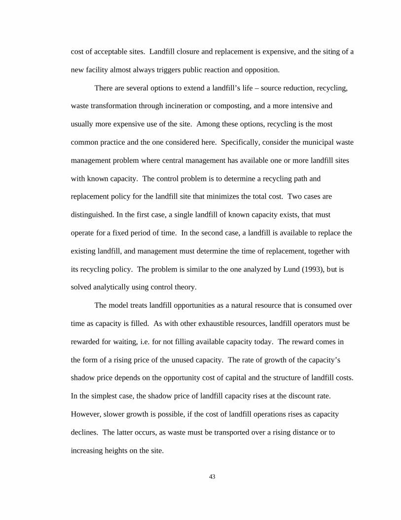
43

cost of acceptable sites. Landfill closure and replacement is expensive, and the siting of a

new facility almost always triggers public reaction and opposition.

There are several options to extend a landfill’s life – source reduction, recycling,

waste transformation through incineration or composting, and a more intensive and

usually more expensive use of the site. Among these options, recycling is the most

common practice and the one considered here. Specifically, consider the municipal waste

management problem where central management has available one or more landfill sites

with known capacity. The control problem is to determine a recycling path and

replacement policy for the landfill site that minimizes the total cost. Two cases are

distinguished. In the first case, a single landfill of known capacity exists, that must

operate for a fixed period of time. In the second case, a landfill is available to replace the

existing landfill, and management must determine the time of replacement, together with

its recycling policy. The problem is similar to the one analyzed by Lund (1993), but is

solved analytically using control theory.

The model treats landfill opportunities as a natural resource that is consumed over

time as capacity is filled. As with other exhaustible resources, landfill operators must be

rewarded for waiting, i.e. for not filling available capacity today. The reward comes in

the form of a rising price of the unused capacity. The rate of growth of the capacity’s

shadow price depends on the opportunity cost of capital and the structure of landfill costs.

In the simplest case, the shadow price of landfill capacity rises at the discount rate.

However, slower growth is possible, if the cost of landfill operations rises as capacity

declines. The latter occurs, as waste must be transported over a rising distance or to

increasing heights on the site.

44

3.2 Model Formulation

Consider a waste management system with two disposal options – waste recycling

and disposal at a landfill. For simplicity, there is a single waste generator producing

waste at the rate Yt for year t. Management decides on the recycling share tδ , where

0= minδ < tδ < maxδ < 1. Hence, the recycling share can be as low as zero, but can never

exceed a maximum share smaller than one, as it is technically unfeasible to recycle all

waste.

The cost of recycling includes the cost of waste collection, processing, and

marketing, minus revenues from the sale of recycled materials. Hence, it depends on

market conditions and may be negative if sales revenues do not exceed collection,

processing and marketing costs. Specifically, the recycling cost is the product of a unit

cost CR ( tδ ) and the recycled share of the total waste stream, tδ Yt, where either CR′( tδ )

= 0 or alternatively, CR′( tδ ) > 0. The latter reflects the fact that unit costs are likely to

rise with a rising recycling share.

The cost of landfill operations is a function of the remaining landfill capacity,

Capt, and is the product of the unit cost CD (Capt) and the non-recycled share of the total

waste stream tt Y)1( δ− . Again, two cases are considered. Either CD′(Capt) = 0 or the

unit cost rises with a declining residual capacity, so CD′(Capt) < 0.

3.2.1 Fixed Landfill Life

The objective is to minimize the cost of recycling plus landfill operations, over a

fixed term T, discounted to the present at rate r,

45

(3-1) { } dteCapCDYCRYMin rtT

ttttttt

t

−

=∫ −+

1

)()1()( δδδδ

,

subject to landfill constraints

(3-2) tt Ydt

dCapCap )1( δ−−==

•

(3-3) Capt ≥ 0

where •

Cap is the rate of change of landfill stock capacity at any time t.

The initial condition is

(3-4) Capt=0 = CAP.

To solve the problem, the Hamiltonian H is minimized at each time t or

(3-5) Min Ht = { } { }ttttttttt YCapCDYCRY )1()()1()( δλδδδ −−−−+

Ht represents the total cost of waste management operations at t. This total

consists not only of the cost of recycling and landfill operations, but also of the landfill

capacity lost as a result of that year’s waste management operations, valued at its shadow

price tλ . If there is a landfill market, tλ provides actionable information for the waste

management operator. If the shadow price exceeds the market price (adjusted for

differences in transport cost), then the operator should use alternative landfill sites for its

disposal (and reduce its recycling effort).

46

The necessary conditions for cost minimization are

(3-6) 0=∂∂

t

Hδ

: ttt

ttt CapCD

CRCR λ

δδ

δδ +=∂

∂+ )(

)()(

(3-7) t

tt

t CapH

rdt

d∂

∂+==

•

λλ

λ

The first condition requires that the marginal cost of disposing waste through

recycling equals the marginal cost of disposal at a disposal site, where the latter equals

the operating cost at the disposal site plus the price of the disposal capacity used up.

The second condition requires that the price of landfill capacity grow at a rate r,

modified by tCapH ∂∂ / . If CD′(Cap)=0, then tCapH ∂∂ / =0, and the price of landfill

capacity rises at a rate r. The landfill owner must be indifferent between retaining

capacity for a year and selling it. If he sells the capacity, he receives a return tλ r.

Keeping the capacity yields a capital gain in the same amount. Instead, if the cost of

landfill disposal rises with declining landfill capacity, then CD′(Cap)<0 and

tCapH ∂∂ / <0. Again the landfill operator must be indifferent between the two options.

Retaining the marginal unit of capacity yields capital gains in the amount •

tλ plus a

reduction in the disposal cost as a result of retaining disposal capacity. This reduction is

equal to )('/ tttt CapCDYCapH δ−=∂∂ . The alternative is selling the marginal unit of

capacity at its price tλ , yielding a return tλ r. In this case, the shadow price of landfill

capacity rises at less than r, the opportunity cost of capital.

47

Finally, consider the behavior of recycling over time. Three possibilities are

considered, depending on the behavior of the costs of recycling and waste disposal. The

first case assumes that the unit cost of recycling is invariant with the recycling share, i.e.,

0)(' =tCR δ , and the unit cost of waste disposal is invariant with the remaining landfill

capacity, i.e., 0)(' =tcapCD . The second case assumes that recycling is produced with a

rising average cost, i.e., )(' tCR δ >0, but retains the assumption that waste disposal is

independent of landfill capacity. The third case retains the assumption of a rising average

recycling cost and, in addition, assumes that waste disposal costs rise with declining

landfill capacity, i.e., )(' tcapCD < 0.

A. Fixed unit cost of recycling and waste deposit: If the unit cost of recycling is

constant, then the Hamiltonian is linear in tδ and the optimal share will assume one of its

two extremes. In addition, if landfill costs are independent of the remaining capacity,

then the optimal tδ will be independent of the available landfill capacity. Hence, since

∂H/∂δ t = (CR – CD – λt)Yt , the sign of (CR – CD – λt) determines the recycling share. If

(CR – CD – λt) > 0, recycling will be set to zero, and if (CR – CD – λt) < 0, recycling will

be as large as technically feasible.

The behavior over time of tδ depends on the price of landfill capacity, tλ .

Equation (3-7) implies that tλ rises with the opportunity cost of capital and hence there

are several possibilities:

(1) If CR ≤ CD, then CDCR t <− =0λ at the initial time t=0. But since tλ is rising, the

optimal policy is to always recycle at the maximum level.

48

(2) If CR > CD, then there are two possib ilities:

• If initially, CDCR t <− =0λ , then again, the optimal policy is to always recycle at

the maximum possible level.

• If initially, 0=− tCR λ > CD, then there may exist a switching time ts. Prior to ts,

there is no recycling, but after t=ts recycling is at its maximum feasible level.

However, it is also possible that such a switching time does not exist, i.e. tCR λ− >

CD for all t and there is never any recycling. This would be the case if there is

ample landfill capacity and the cost of recycling is high relative to the cost of

disposal.

B. Average cost of recycling rising: There is considerable evidence that the unit cost of

recycling rises as more recyclables are extracted from a given quantity of solid waste.

Raising the share of recycled waste requires greater promotion and marketing, increased

incentives, a higher number of drop-off points, and better equipment at transfer and

sorting stations.

Hence, assume CR′( tδ )>0. Then the recycling share must rise over time, given

tλ rise over time. If, in addition, one assumes CR( tδ ) = αδ tCr , where Cr is a positive

constant and α the recycling share cost elasticity, then the recycling path becomes

computable with

(3-8) α

αλ

δ1

)1()(

+

+=∗

CrCapCD tt

t

49

The recycling share is higher with greater operating cost of landfill disposal, CD,

and higher shadow price of landfill capacity, tλ , and with smaller cost of recycling, as

given by the constant Cr.

C. Unit cost of waste disposal increases with declining landfill capacity: There are good

reasons to believe that disposal costs rise with declining landfill capacity. Space for the

movement of trucks and equipment declines. Waste is disposed to higher levels that

require special equipment. Marginal areas come to be used, bypassed during earlier

times. Hence assume CD′(Capt) < 0. Then, as already discussed, tλ rises at a rate less

than the opportunity cost of capital. Further, the recycling share rises both because the

price of capacity rises, and because landfill operating costs rise with declining capacity,

[see equation (3-8)]. Assume that CD = Cd(Cap0/Capt)β , where Cd is a positive constant

and β >0 is the capacity elasticity of landfill cost. Then the path of tλ can be calculated

by solving equation (3-7), with

(3-9) rtt ec=λ

−−

+β

ββδ1

0)1(

t

tt

CapCap

r

CdY

3.2.2 Variable Landfill Life

Consider the landfill described in the previous section, but allow for the option of

closing the landfill and replacing it with a new landfill. The cost of closing a landfill

varies little with landfill age (Lund, 1993) and hence it seems reasonable to assume that

50

both the cost of closure, CLC and the cost of opening a new landfill, CLR, are constant

with time. Then the objective function is:

(3-10) { } ( ) rTrtT

ttttttt eCLRCLCdteCapCDYCRYMin −−

=

++−+∫1

)()1()( δδδ

The necessary conditions, equations (3-6) and (3-7) are augmented by the terminal

condition,

(3-11) T

T

CLRCLCδ

λ∂

+∂=

)(

Since CLC and CLR are fixed and independent of the recycling share and the

landfill capacity, the price of landfill at the terminal time is zero. Additional information

that can be considered is that H is equal to 0 since the terminal time is unknown (landfill

life is variable). Therefore, according to equation (3-5),

(3-12) CLRCLCCapCDYCRY TTTTTT +=−+ )()1()( δδδ

At the terminal time, the total operating cost of recycling and disposal – regardless of

specific cost function assumptions – is equal to the cost of landfill closure plus

replacement. This implies (together with the fact that the value of the existing landfill is

zero at the terminal time) that the landfill operator must close the existing landfill and

replace it with the new facility since there is no more incentive from operating the old

facility.

51

3.3 Numerical Analysis

Analytical solutions provide a general idea about optimal waste management

policies but say little about orders of magnitude, or about the sensitivity of policies to

changes in external conditions. Numerical solutions can provide an idea about the

significance of the results in the context of real- life situations; they can deal with

complex situations where analytical models cannot be solved formally; they can provide

a sensitivity analysis; and they can give numerical rules of thumb. As important,

numerical solutions permit real life complications that could not be analyzed easily with

analytical models. The above analytical model is autonomous, but in real life, the cost of

recycling and the cost of landfill operations may vary over time.

Specifically, environmental regulations can be expected to impose an increasing

financial burden on the cost of landfill operations. What is the impact of rising cost? In a

similar manner, the cost of landfill operations changes, as urban settlements get closer to

locations that were originally far away. Again, this means that operating procedures and

costs are likely to change over time. Recycling costs also change, as the price of most

raw materials grows over time. What is the impact of this on recycling policy? It should

add to recycling incentives over time. All of these effects can be evaluated with a

numerical model. Further, analytical results from the earlier section will be used to

validate the numerical model, to ensure that both results are consistent.

To illustrate a numerical application of the model, consider a small community of

10,000 households, growing by 500 households annually and producing an average of

8,900 lbs of solid waste per household per year (2,225 per capita). The community wants

to schedule recycling operations to optimize its own landfill’s life. The existing landfill

52

has a capacity of 1,000,000 cu yd, which, without recycling, would be filled in 9 years.

Assume further that recycling can reduce landfill deposit by a maximum of 70%. If used

all the time, this would extend the life of the landfill to 21 years.

3.3.1 Mathematical Formulation of the Model

The optimal control problem presented in Equation (3-1) – (3-4) is discretized, on

over a planning horizon made of T discrete periods, so that it can be solved by standard

optimization algorithms. The following presents the objective function of the fixed life

case, minimizing the present value of the total cost of waste management during the

planning period T.

(3-13) { }∑=

−++

T

tttttttt CapCDYCRY

rMin

0

)()1()()1(

1δδδ

subject to landfill constraints:

(3-14) ttt CapY ≤− )1( δ = 111 )1( −−− −− ttt YCap δ ,

(3-15) Capt=o = CAP,

(3-16) Capt ≥ 0

where dt is the decision variable representing the recycling share at time t. Yt is a

parameter: the waste generation at time t. CR(dt) and CD(Capt) are the costs of recycling

and waste disposal, respectively. The recycling cost varies with the recycling share,

according to the function αδ tCr , where α = 0.6. The disposal cost varies with remaining

stock capacity, according to the function ( )βtCapCapCd /0 , where β = 0.15. Both costs

53

are non-linear. In the case that, both costs are invariant (linear), then, α and β are equal

to 0. Capt is the remaining landfill capacity available at time t. The annual amount of

waste deposited in landfill is given by (1-δ t)Yt and cannot exceed the remaining available

capacity, as represented in equation (3-14), where the landfill remaining capacity at time t

is given by Capt-1 – (1-δ t)Yt. At the base year (t=0), stock capacity is equal to the initial

capacity CAP (1,000,000 cu yd), as represented in equation (3-15). The flow capacity

operation is not constrained, as we assumed that the landfill is capable to handle all waste

generated at any time t. r is the discount rate, and equal to 8%.

The objective function can be modified for the case of a variable landfill life, by

including the landfill costs of closure and replacement at the end of the planning horizon:

(3-16) { } )()1(

1)()1()(

)1(1

0

CLRCLCr

CapCDYCRYr

Min T

T

tttttttt +

++−+

+∑=

δδδ ,

where CLC and CLR are the costs of landfill closure and replacement, respectively. The

constraints remain the same as the fixed cost life.

The model is solved using GAMS linear and non- linear programming solvers, for

each possible landfill lifetime ranging from 9 to 21 years (beyond 21 years, the program

has no feasible solution).

3.3.2 Fixed Landfill Life

A. Fixed unit cost of recycling and waste deposit: Three sub-cases are considered in this

first type of cost structure. Each case is related to different values of the fixed unit costs

of recycling and deposit. The landfill life is fixed at 18 years.

54

Sub-cases CR

($/cu yd) CD

($/cu yd) Time switch ts

Optimum recycling

Share *tδ

1. CR < CD 5.00 6.00 No *tδ = maxδ = 0.7 at all time

2. CR = CD 6.00 6.00 No *tδ = maxδ = 0.7 at all time

2. CR > CD 13.00 6.00 At year 4 No recycling before t s

*tδ = maxδ = 0.7 after t s

Table 3.1: Optimum Recycling Shares for Different Fixed Unit Cost of Recycling and

Deposit.

Table 3.1 shows that if the unit cost of recycling is lower than or equal to the unit

cost of disposal, the model recycles at the maximum level maxδ all the time (sub-case one

and two). This represent exactly the analytical results obtained with the optimal control

model. Lower or equal recycling costs make t

Hδ∂

∂ always negative, hence with the

maximum level of recycling over the planning period. In the third sub-case, the result

shows that at the beginning of the period, there is no recycling due to a high operating

cost. However, after some time, there is a switch to the maximum recycling level. The

results show that the recycling option is not operated until year 4. Then, there is a switch

to the maximum recycling effort until the end of the landfill’s life. This outcome is also

consistent with the control model results, where the recycling cost net shadow price is

higher than the deposit cost at the initial time. The switch to operate recycling at the

maximum level is due to the rising landfill price.

This simple model shows that the recycling option often remain cheaper, even if

its net cost is higher than the current cost of depositing the same waste in the landfill.

55

This is due to the fact that, in some cases, there is still an incentive from saving landfill

space by operating the recycling option. However, recycling will not take place if the

unit recycling cost is extremely high relative to the unit cost of deposit. Consequently, all

waste will be deposited in the landfill.

B. Unit cost of recycling increases with the recycling share: In this case, the cost of

recycling is variable, exhibiting diseconomies of scale (α = 0.6). The results point to the

same behavior as the control model results, where, for any fixed landfill's life, the

recycling option is operated at the lower level in the initial period, and then grows with

time. To minimize cost, the model chooses to operate recycling at a level as low as

possible since the recycling unit cost increases with the recycling share. Recycling with a

low recycling share in the initial period reduces landfill space faster, and hence increases

the price of landfill space in later times. Consequently, as the landfill price increases

over time, the optimum level of recycling also increases. For a given landfill life, at one

point in time, the recycling share is set at its maximum until the end of the landfill’s life.

For example, when the landfills’ life T is set at 20 years, the model determines the

recycling share to be equal to 50% in year 1. As the recycling share increases over time,

eventually, in year 8, recycling is operated at its maximum (70%). The model shows that

the lower the constant unit cost Cr relative to Cd, the higher the optimal ∗tδ at the initial

time. Also, the numerical result shows that, for a given landfill life, recycling must be

started earlier than in the previous case.

56

C. Unit cost of waste deposit increases with declining remaining landfill space: In this

case, the cost of landfill is variable ( β = 0.15). The result shows that the optimum-

recycling share tends to increase over time. This behavior is similar to that in the case of

fixed unit disposal cost. However, after some time, the recycling share grows more

slowly than the share in the constant cost case, as illustrated in Figure 3.1. This outcome

is consistent with the results of the control model discussed previously.

0

5

10

15

20

25

30

35

1 2 3 4 5 6 7 8 9 10 11 12 13 14 15

Year

Rec

yclin

g Sh

are

Rat

e of

Cha

nge

Fixed Unit Deposit Cost CD

Increasing Unit Deposit Cost Cd

Figure 3.1: Rate of Change of The Recycling Share for Different

Unit Cost Deposit Function, T = 15 years

For example, in the case of a landfill’s life T equal to 15 years, the optimum

recycling share grows at the same speed up to year 7. From this point, it grows more

slowly, shows that the effect of an increasing landfill cost on the recycling share is

57

smaller than that of the landfill price after some time. Figure 3.1 shows the effect of an

increasing unit deposit cost on the optimum recycling share, compared to the fixed unit

deposit cost.

3.3.3 Variable Landfill Life

In this case, the cost of landfill closure CLC = $ 6 million, and the landfill

replacement cost CLR = $ 55 million at the terminal time (this total cost will be referred

to as the high cost of replacement). Consider different landfill lives T, from Tmin to

Tmax, for each different unit cost of recycling and deposit. The results show that the

optimum landfill lifespan is the time when the saving from deferring landfill closure net

of operation cost reaches a maximum value (see Figure 3.2). Assume that the

replacement costs are fixed; then savings are gained from the discounted value of the

landfill closure postponement. The longer the landfill closure is postponed, the greater

the savings, and, simultaneously, the higher the total cost of operation. By comparing the

savings from deferring landfill closure to the incremental cost of operation, the results

show that at one point in time the savings net of the incremental cost reach a maximum

value, and this time represents the optimal landfill life.

The results for the three different cost function cases demonstrate similar

behavior. In the case of a fixed unit cost of recycling and deposit, the optimum landfill

life is 19 years. In the cases of increasing unit costs of recycling and waste deposit, the

optimum landfill life of 20 years, because increasing recycling costs change recycling

demand. For each fixed landfill life, the recycling starts earlier than the one with fixed

unit recycling cost.

58

-2

0

2

4

6

8

10

12

14

16

18

20

9 10 11 12 13 14 15 16 17 18 19 20 21

Landfill Life T

PV o

f Sa

ving

and

Inc

rem

enta

l Ope

ratio

n C

ost (

$mill

ion)

Saving fromdeferring High LFClosure &Replacement Cost(1a)

Saving fromdeferring Low LFClosure &Replacement Cost(1b)

Incremental Cost ofRecycling and LFOperation (2)

(1a) - (2)

(1b) - (2)

Figure 3.2: Net Present Value of Operation and Replacement Costs

Lower landfill closure and replacement costs produce shorter optimal landfill life.

Figure 3.2 shows the optimum landfill life for different landfill and replacement costs in

the case of recycling cost rising with the recycling share. For a landfill closure cost CLC

= $ 3 millions and CLR = $35 millions (this cost will be referred to as the low cost of

replacement), the optimal landfill life is 11 years. In comparison, the higher cost leads to

an optimal life of 20 years. Consequently, the higher cost will make landfill operators

initiate early recycling activity with a higher optimum share, so that the optimum landfill

life can be achieved.

Furthermore, information of landfill closure and replacement costs (both costs

will be referred to as replacement cost) is really significant in determining the optimum

59

Case

Total Cost of Landfill

Replacement (CLC+ CLR) ($ Million)

% Change of Replacement

Cost

Optimum Landfill

Life (year)

% Change of Optimum Landfill

Life

Replacement Cost

Elasticity of Optimum LF Life

CostChange

lifeLFOptChange%

%

1 (Low Cost) 38 - 11 - -

2 42 10.53% 13 18.18% 1.73

3 46 9.52% 16 23.08% 2.42

4 49 6.52% 17 6.25% 0.96

5 53 8.16% 18 5.88% 0.72

6 57 7.55% 19 5.56% 0.74

7 (High Cost) 61 7.02% 20 5.26% 0.75

Table 3.2: Landfill Closure and Replacement Costs Elasticity of Optimum Landfill Life

landfill life. Table 3.2 presents the replacement cost elasticity of optimum landfill life,

i.e. the percentage change in landfill life, per percentage change in landfill replacement

cost. As shown in the last column, the elasticity declines with rising cost.

3.4 Results Discussion

In general, the optimization of landfill facility is analogous to the optimization of

mining or energy extraction. Landfill capacity can be treated as an exhaustible resource.

As in the case of depletable mining, the price of landfill space rises as long as the real

discount rate is not equal to zero. Hence, there is an incentive for the landfill operator to

utilize the landfill at the minimum level or by maximizing recycling operation today to

save more landfill space for the future. This behavior is independent of the recycling cost

but dependent on the cost of landfill. If the landfill cost does not vary with capacity, then

the price should rise at the real discount rate or the opportunity cost of capital. But, if

60

landfill costs rise with declining landfill capacity, then the optimum price of landfill

disposal will rise at less than the real discount rate. This in turn means that recycling

demand will rise at a lower rate than when landfill cost does not vary with landfill

capacity. In both cases, the landfill price should always increase over time. Yet, if the

landfill operator, for political reasons, is constrained to charge a constant price over time,

he will not behave optimally, i.e., will not conserve landfill capacity in a socially optimal

manner. The recycling cost in the meantime only affects recycling demand. If a landfill

must meet a given life and the cost varies with the recycling share, then recycling must be

started earlier than would be the case otherwise. Also, oversimplifying the cost function

by assuming it linear can lead to a lower recycling share today. This result demonstrates

how important it is to have a good approximation of the cost structure.

In the first three cases of the fixed landfill life model, the model provides the

optimal recycling share and hence the optimal amount of waste deposits to the landfill

annually during its life, so that the overall cost is minimized. Yet, the model does not

provide the optimal landfill life, although it can evaluate all possible landfill lives, from

the minimum to the maximum life possible. Inclusion of the landfill closure and

replacement cost into the model yields the optimum landfill life. The numerical results

show clearly the optimum landfill life for each cost function. The accuracy in predicting

landfill closure and replacement cost is a significant factor for the determination of the

optimum life of existing landfills. The higher this cost, the longer the optimum landfill

life should be.

In general, a lack of good knowledge of the cost structure of landfill operations

(and the cost of alternative sites) will lead to sub-optimal recycling policies. More

61

empirical research is needed to determine the extent to which landfill costs vary with

landfill capacity. This cost is not modeled anywhere in the optimization literature,

although casual empirical observation suggests that it is a significant determinant of

recycling policy.

As is already well recognized in the literature, the replacement cost of a landfill is

a major determinant of the optimal recycling today. The higher this cost the greater the

share of recycling today. In practical terms, the waste management operators should

invest into planning, and into understanding their cost structure – not only today but far

into the future. This does not always appear to be the case.

62

CHAPTER 4

INTEGRATED SOLID WASTE MANAGEMENT MODEL

(ISWM MODEL)

This chapter presents the Integrated Solid Waste Management (ISWM) model.

The model uses the facility-planning model developed by Chang as a basis. As already

discussed, Chang's model is the most advanced of the facility planning models in the

solid waste literature. As a result, however, it is also highly complex and, in many ways,

difficult to amend. The idea of this study is to use a stripped-down and simplified

version of Chang's model, called the revised core model, and then to add to it a number of

novel extensions. Later, for a case study, the ISWM model will be applied to the Central

Ohio Solid waste management district. The section begins with a discussion of various

extensions to the base model, followed by a description of the mathematical model.

4.1 Extensions of the Model

Each of the extensions deals with issues not included in Chang's model, including

among others (i) composting facilities, (ii) landfill closure and replacement cost, (iii)

multiple and simultaneous landfill operations, (iv) economies of scale in landfill and

composting operations and capacity expansion, (v) lifetime capacity – cumulative

63

capacity – of landfill, (vi) promotion of waste diversion programs to consumers, and (vii)

a variety of collection methods at the source and returns to scale in collection. In

addition to these model extensions, there will be an extensive program of empirical

testing and sensitivity analysis, as explained later. The following sections describe the

proposed model extensions:

4.1.1 Composting

Composting is receiving growing attention among communities as a means to

divert waste from landfills. However, it often makes a large demand on land. Introducing

composting into facility planning models allow for an analysis of the trade-offs between

the problems associated with each of the different waste solutions.

Haug (1993) defines composting as a form of waste stabilization. Specifically, he

characterizes composting as “the biological decomposition and stabilization of organic

substrates, under conditions that allow development of thermophilic temperature as a

result of biologically produced heat, to produce a final product that is stable, free of

pathogens and plant seeds, and can be beneficially by applied to land.” Composting

municipal solid waste has gained in popularity since the beginning of the 1980’s. Even

though the processes have been known for a long time, they remained unpopular due to

the poor quality of compost products, odor problems, and their high cost relative to

landfill. Even today, odor control remains a major problem.

There are three principal methods of composting municipal solid waste:

Windrow, aerated static pile, and in-vessel composting technology. Windrow

composting is one of the oldest methods. The process is simple and consists of spreading

64

the waste on an open area and turning it periodically to introduce oxygen and to control

temperature. One of the disadvantages of this technology is the large amount of land

required. Instead, in the aerated static pile method, the material remains static and air is

blown through pipes under the composting material. Less land is required but the method

is more capital intensive. The In-vessel technology is more advanced and requires a

mechanical system inside an enclosed container or vessel. The mechanical systems is

designed to minimize odor and processing time by controlling environmental conditions

such as airflow, temperature, and oxygen concentration.

In modeling composting, the model follows Chang's treatment of incineration and

landfills. Specifically, the model determines whether composting is feasible when

compared to other methods, decides on the optimum composting site and capacity size,

and derives the share of total waste sent to composting sites. The relative cost of

transportation to alternative sites determine composting feasibility.

4.1.2 Landfill Closure and Replacement

Chang, in his case study, considers only one landfill that has sufficient cumulative

capacity to meet disposal requirements over the planning horizon. Consequently, it does

not deal with one of the key problems faced by a waste management authority – landfill

closure and replacement cost. As these two costs are extremely high, inclusion of a

finite landfill capacity and both costs in the model adds significant realism and will

significantly change waste allocation to landfill and overall system behavior.

The extension of a finite cumulative capacity of landfill will challenge the

authority to manage the landfill life optimally. It is expected that the model will send

65

larger amounts of waste to recycling centers even though their operating cost is higher

than that of landfill deposit. The analytical model in Chapter 3 has shown that recycling,

even if the cost is high, is still feasible to operate, and, hence it postpone landfill closure

and replacement. By assuming that both costs are constant over time, the higher cost of

recycling is compensated by savings from discounted landfill closure and replacement

cost due to the postponement.

4.1.3 Multiple Landfill Operations

Chang's model considers a single landfill with sufficient capacity for the planning

horizon. In a non-spatial world, this would usually be optimal, given economies of scale

in landfill operations. With the introduction of space, however, it may well be optimal to

allow for several landfill facilities and even for several such facilities to operate

simultaneously, and the model extension will permit this. While his paper briefly

discusses the possibility of the sequential operation of a second landfill, once the existing

site has run out of capacity, this case appears not to have been operationalized.

There are several possible extensions. The first and possibly most important one

is the sequential operation of landfills, including the special case of a landfill being

replaced by a single new landfill. Such replacement may occur when the existing landfill

has no remaining capacity, or alternatively, when the cost of continuing the existing

landfill is larger than the cost of starting a new landfill – which is possible when

operating costs rise with declining remaining capacity. Hence, old landfills may well

continue to have some capacity, but this capacity is available only at a cost that makes

66

new landfills more attractive. In this case, the decision problem is to determine the

optimal time for the switch between landfills.

The second extension is the simultaneous operation of several landfills. Many

urban areas operate only a single landfill at a time. However, when urban areas are large,

it may well be cheaper to operate more than one landfill, each specializing in waste from

different neighborhoods. The model in this case would determine how many landfills

would operate, and it would determine the optimal waste destination (i.e. optimal landfill

site) for each source of waste (or for each transfer station). Obviously, if landfill sites

operated with increasing returns to scale, this would tend to reduce the number of sites

being operated, as it would be cheaper to operate a single site with a large volume of

deposits than several sites with a small volume. However, even then it may be cheaper to

operate several sites, if the savings in transportation cost exceed the potential savings

arising from economies of scale.

The research will try to deal with both cases – the sequential operation of two

landfills and the simultaneous operation of two landfills. However, it will not try to deal

with the combination of the two problems, i.e. the simultaneous operation of several

landfills and the replacement of landfill sites over time.

4.1.4 Economies of Scale

Chang and others assume that operating costs are constant over time, and constant

regarding the scale of facility operations, facility size, and, in the case of landfills, their

unused capacity. Relaxing these assumptions and permitting economies of scale in the

operations is a major deviation from past modeling, but also adds significant realism.

67

Economies of scale will be applied in landfill facility operations as well as in capacity

expansions of all facility types.

Two extensions are considered. First, there is a possibility that facilities operate

with economies of scale – at least in recycling and landfill facilities (Callan and Thomas,

2001). Second, for landfill sites in particular, there is the possibility that the costs of

operations depend on the remaining capacity of the landfill site. Consider each of these

in turn:

• Economies in Level of Operations: For many facilities one would expect the cost of

operations to decline with an increasing level of operations (at least up to capacity

constraints). For landfill operations in particular, the more waste is deposited per year,

the larger the scale of moving equipment and operations, and the smaller the average

cost. Allowing for economies of scale in operations, however, may increase the

number of local optima and will make it more difficult to find globally optimal

solutions. In general, economies of scale encourage specialization in facility

operations. Rather than using several facilities at part of their capacity, it is cheaper to

use one facility to the exclusion of others (capacity permitting).

• Economies in Remaining Landfill Capacity: For landfill facilities, many studies,

including Chang, assume that the cost of landfill operations is constant over time and

independent of the site's remaining landfill capacity4. Yet in real life, this cost is rising

as capacity nears its limit (Levenson, 1992). For example, overtime, operations may

4 Note that capacity is used here in two very different ways. One meaning is that of operating capacity,

i.e. the capacity to accommodate a waste flow per year. The other is that of a lifetime disposal capacity, i.e. the total cumulative volume of waste that can be deposited on a site over the life of the facility.

68

move to less accessible and more distant areas of the site; or operations may build

mounds that require increasingly sophisticated equipment to climb the rising height of

the mound. In the extreme, a landfill may be abandoned not because its capacity is

exhausted but because the cost of its operation has become higher than that of its

alternatives or farther landfill facilities have become more attractive (see the multiple

landfill operation section).

At any rate, this suggests that the average cost of landfill deposits may rise

overtime. This in turn may significantly alter waste management policies. More than

likely, it would advance the time when a landfill is retired; it would raise the

attractiveness of alternative disposal facilities, including composting and recycling; and

it would raise the share of waste that goes to these disposal alternatives. Extending the

model in this way of course comes at a price, as it increases the complexity of the

solution. Moreover, since landfill capacity is no longer assumed sufficient over the

planning horizon, the cost of landfill disposal should be modeled carefully to avoid

infinite cost when landfill capacity is exhausted, e.g., if landfill disposal cost is set as an

inverse function of the remaining capacity, as shown in Chapter 3.

4.1.5 Promotion of Waste Diversion

As landfill opportunities decline and opposition to incinerators rises, municipal

governments increasingly promote waste diversion strategies such as recycling, or waste

reduction strategies, such as on-site mulching of garden waste and others. However,

some of these strategies require the cooperation of the population, the mobilization of

households and community groups, and the introduction of new services to facilitate

69

recycling. The program must be promoted extensively through promotional campaigns.

Yet, promotion is costly and must be weighed against the benefits from reduced waste

disposal. The extension seeks to model these strategies so as to balance their costs

against the benefits from waste diversion or reduction. More specifically, the extension

assumes that the recycling share – through the participation rate – is a function of the

promotional cost.

The model will incorporate a recycling participation rate as a function of

promotional cost. The promotion acts to raise household participation in recycling

programs, and hence increases the share of total waste that is being recycled.

Promotional activities include advertising and organization of community groups, as well

as other activities not covered by the regular recycling program, including curbside

collection or the establishment and maintenance of centralized collection points. More

specifically, Chang's model is modified by adding a new cost – the promotional cost that

depends on the promotional level and the population in each generation area – and by

considering the share of total waste recycled – through a participation rate – a function of

the level of promotion. Whereas in Chang's model the decision variable is the share of

waste recycled (since everything is linear, the recycling share in each area goes either to

its maximum or its minimum value), in the extended model the decision variable is the

level of promotion.

Other alternatives for promoting waste recycling include:

• Promotion of Recycling I: Here promotion acts to reduce the unit cost of recycling. For

given programs, such as curbside collection of recycled materials, the average cost of

collection will decline as the number of households participating in the program rises.

70

Hence, Chang's model is modified by adding to the total cost of solid waste

management the cost of promotion, and by making the unit cost of recycling a declining

function of rising promotion. The share of the total waste that is recycled, however,

remains determined endogenously.

• Promotion of Waste Reduction: Here promotion acts to reduce waste generated. This

can be the result of changes in consumer behavior, or the result of changing the

behavior of producers. Hence, waste generation is a declining function of promotional

expenses, and the model will seek to trade off the cost of promotion against the cost of

solid waste disposal.

In this research, these two alternative extensions are not developed and remain avenues

for further research.

4.1.6 Variety of Collections

The last extension in this study is that the model allows for a variety of collection

methods. Distinguishing between compostable waste, four types of recyclable waste, and

mixed waste, it allows compostable and recyclable waste to be collected separately at

curbside or as part of mixed waste. The model also allows economies of scale in all

collection method by introducing fixed costs.

Separation of waste adds to the fixed cost of collection, but saves possible later

separation costs. Also, mixed waste may or may not be sent to transfer stations for further

separation by waste type. All of these decisions may vary by neighborhood. Hence, in

areas with small yards for example, it may be best to collect compostable mixed with

other waste, while in areas with large yards it may pay to collect compostable separately.

71

The model, however, does not consider the frequency of collection nor collection through

drop-off points increasingly popular for recyclables. These options represent possible

model extensions.

4.2 Statement of the Model

In this section, a mathematical model is developed to design an optimal solid

waste management system over a specified planning period by minimizing its total cost.

The model deals with a system that consists of a given set of waste generations and five

disposal and processing options – transfer stations, recycling, incinerators (waste to

energy facilities), composting facilities, and landfill sites. The model maintains the

general structure of Chang's model, but includes the extensions discussed above. Mixed-

integer programming (MIP) is used as analysis tool.

The following first describes the network relations between sources and

processing/disposal facilities. This is followed by a discussion of the model's decision

variables, initial conditions, and input variables. The final sections state the model,

including model notations, objective function, and constraints.

4.2.1 Illustration of Network Flows

This section briefly summarizes the waste management system, referring to a

network representation of waste flows in Figure 4.1. The network includes six nodes,

one representing waste generation and the remainder the five sets of processing and

disposal facilities.

72

Waste generation nodes: Wastes are generated at point sources representing

neighborhoods. Decisions at such nodes include the share of waste for recycling, the

level of promotion, the participation rate, and the amount of waste sent to the facilities.

Transfer stations : The first type is regular transfer stations, where wastes are

transferred from smaller collection trucks to bigger trucks. There is no weight reduction

and all wastes are sent to landfills. The other type is transfer station/material recovery

facilities, where wastes are separated into recyclable, combustible, and landfilled waste.

In such facilities the decision is whether all wastes are sent to landfill or some of them are

sent to other facilities after separation.

Incinerators (waste to energy facilities): A change in quality and quantity takes

place at these facilities. Wastes may arrive from generation sites, transfer stations, and

recycling facilities. It is first shredded in one particular facility before it is burned and

converted to energy. The shredder facility is located adjacent to the incinerator, and is

not considered as a separate node. The ashes and by-products from this process and the

excess waste are shipped to landfill sites. Hence, the decision is to determine the share of

incinerated waste.

Recycling centers: While waste may have already been sorted at the source, there

typically is a need for additional processing at the recycling center, to separate waste into

recyclable and non-recyclable (Tchobanoglous, 1993). Therefore, the decisions made at

these centers are the share of the recycled waste and the destination of the non-recyclable

waste, either to landfills, transfer stations, and/or incineration.

Composting facilities: Yard waste is converted to mulch. It is assumed that all

waste materials are composted and sold in the same year, as the composting cycle is less

73

Xwik YLwl YKk Xlk Xij & Xil

Transfer Stations (j) & (l)

node j = 1 to J node l = 1 to L Xjo and Xlo

Composting Facilities, (k) node k = 1 to K

Xnj Xjm

Waste Generations, (i)

Node i = 1 to I Xim Xmo

Xnm

Waste-To-Energy/ Incinerators, (m)

Node m = 1 to M

YMm Recycling Xwin Center (n) node n = 1 to N YNwn Xno

Landfills, (o) node o = 1 to O

Xio

Note: - In Transfer Stations j, there is no waste reduction and separation; - In Transfer Stations/Material Recovery Facilities l, mixed waste is separated for recyclable material.

Figure 4.1: Network Representation of the Model

than a year. As already discussed, most composting sites include a small facility for

disposal of non-compostable materials. Hence, no excess wastes leave the facilities, and

no decisions of any type are made at these sites. Although the small disposal facility may

eventually run out of capacity, this issue is not considered in the model.

Landfill disposal: These facilities attract the excess waste from all other facilities

or directly from the sources. As final destinations, no decisions are being made at landfill

sites (although, of course, there are capacity decisions).

The notations in the model represent time, waste source and facility types as the

origin and destination, and waste types. More specifically, time is identified by t, and

74

waste generation nodes by the index i, i∈I. Transfer stations are identified by the indices j

and l, j∈J and l∈L. At transfer station l mixed wastes are separated for recyclable

material, while at j they are not. Hence, wastes shipped from waste generation node i to

transfer stations j and l at time t is labeled Xijt and Xilt. Composting facilities are

identified by the index k, k∈K, and waste shipped from i to k is denoted Xikt. Recycling

facilities are identified by the index n, n∈N, and the types of waste are identifying by w.

Hence, waste shipped from i to n is denoted Xwint. Incinerator facilities are identified by

the index m, m∈M, and wastes shipped from waste generation nodes to incinerator

facilities are denoted Ximt. Finally, landfills facilities are identified by index o, o∈O, and

the amounts of waste shipped from i to n are denoted Xiot. The labeling of waste shipped

among facilities will use the same pattern. The waste that is processed in recycling and

composting facilities is identified by w. The types of waste consist of paper, glass,

plastic, aluminum, and yard waste.

The unit cost of transshipment from node i to the other node j, k, l, m, n and o are

labeled as TUCijt, TUCikt, TUCilt, TUCimt, TUCint and TUCiot respectively. The operation

and maintenance costs at facilities are labeled Cjt. Ckt. Clt. Cmt. Cnt. and Cot. The output

from composting, recycling, and incinerator facilities are labeled as YKk, YNwn and YLwl,

and YMm, respectively.

The following section presents the mathematical structure of the model. It

presents the model equations and a discussion of the objective function and constraints.

The definitions of all the indices, variables, and parameters are presented in Appendix A.

75

4.2.2 Objective Function

The model is solved with the objective of minimizing the total present value of

waste management cost, accounting for most, though not all, of the private and public

sector costs of the system. Note that, in the model implementation, the model considers

residential and commercial wastes and excludes industrial waste. Specifically, the total

cost includes the cost of transportation and the cost of operating all waste facilities, the

cost of investment in new or expanded facilities, and the cost of facility closure in the

case of landfill sites. Externalities of all types are disregarded, including health impacts

often associated with incinerator operations and odor or air pollution impacts on the

neighbors of composting and landfill sites. Benefits take the form of revenues collected

for recycled material, energy produced, and sale of composting products. These revenues

enter the objective function as a negative cost. The general formulation of the objective

function is as follows:

(4-1) ∑=

T

t

tMinimize1

δ (Costst - Revenuest)

where t

t

r

+=

11

δ is the discount factor at time t, and r is the discount rate.

The following describes the components of the objective function, as represented by

equations (4-2) – (4-24):

76

4.2.2.1 Collection and Transportation costs

The sum of collection costs at all waste sources and transport costs for all waste

flows between all types of nodes. There is separate accounting for different costs of

collecting wastes at their sources – collection cost for mixed waste, recyclable material

(to recycling center) and yard waste (to yard waste composting facilities). These costs

are not part of the transportation costs from sources to facilities. Furthermore, the model

considers different cost structures for transportation and collection. While transport cost

is proportional to the waste load (the average cost is constant), the average cost of

collection declines as more waste is collected, and this is accounted for by adding fixed

costs in collection. Each type of waste has different unit and fixed cost of collection.

While the collection unit cost is independent of the waste generation area, the fixed cost

depends on this area ($/km2). Hence, different areas incur different fixed costs of

collection.

The total cost of mixed waste collection at time t is given by

(4-2) Σi {Ai*FCCMX*ICCMXit + CLCMX*(ΣjXijt+ΣlXilt +ΣoXiot+ΣmXlmt )},

where Ai is the area of neighborhood i; FCCMX is the fixed cost for mixed waste

collection; ICCMXit is a binary variable, as an indicator of the existence of the fixed cost

for mixed waste collection in neighborhood i at time t, that is equal to 1 if there is

collection, or Σi (ΣjXijt+ΣlXilt+ΣoXiot+ΣmXlmt) ≥ 0, and 0 otherwise; CLCMX is the unit

cost of mixed waste collection, and Xijt, Xilt, Ximt, and Xiot, are the amounts of mixed waste

collected in neighborhood i and later transferred to nodes j, l, m, and o, respectively.

77

Similarly, the total collection cost of yard waste is given by

(4-3) Σi(Ai*FCCYW*ICCYWit + CLCYW*Σk Xikt),

where FCCYW is the fixed cost for yard waste collection; ICCYWit is a binary variable, as

an indicator of the fixed cost existence for yard waste collection in neighborhood i at time

t that equals 1 if Σi,k Xikt ≥ 0, and 0 otherwise; CLCYW is the collection unit cost of yard

waste; and Xikt is the amount of yard waste collected in neighborhood i and sent to

composting facility k.

The total cost of recyclable waste collected at time t is given by

(4-4) Σi (Ai*FCCRC*ICCRCit +CLCRC*Σw,n Xwint ),

where Xwint is the amount of recyclable waste type w collected in neighborhood i at time t

(all sorted waste w are sent to recycling center n); CLCRC is the unit cost of recyclable

waste collection; FCCRC is the fixed cost for recyclable waste collection; and ICCRC it is

a binary variable, as an indicator of the fixed cost incurred for recyclable waste collection

in neighborhood i at time t, equal to 1 if Σw,n Xwint ≥ 0, and 0 otherwise,.

TUC is the transportation unit cost between two nodes, per km distance

($/ton/km), e.g., between neighborhood i and landfill o is represented by TUCio. Then,

the distance between these two nodes is represented by Dio, and hence, the transportation

cost to transfer the amount of waste Xiot, at time t, is given by

(4-5) Σi,o(TUCio*Dio*Xiot).

78

The model allows for different transportation unit costs per unit distance. For

example, the transportation unit cost from waste generation area i to all other facilities is

different from that between transfer station facility j and landfill facility o. This will be

explained in more detail in Chapter 5.

Adding up all the above costs yields the total collection and transportation cost, as

given by equation (4-6).

(4-6) Σt dt * [ Σi {Ai*FCCMX*ICCMX it + CLCMX*(ΣjXijt + ΣlXilt + ΣoXiot +

ΣmXlmt )} + Σi (Ai*FCCYW*ICCYWit + CLCYW*Σk Xikt) +

Σi (Ai*FCCRC*ICCRC it + CLCRC*ΣnΣwXwint ) +

Σi,n,w(TUCin*Din*Xwint) + Σi,j(TUCij*Dij*Xijt) + Σi,l(TUCil*Dil*Xilt) +

Σi,m(TUCim*Dim*Ximt) + Σi,o(TUCio*Dio*Xiot) + Σi,k(TUCik*Dik*Xikt)+

Σj,k(TUCjk*Djk*Xjkt) + Σj,l(TUCjl*Djl*Xjlt) + Σj,m(TUCjm*Djm*Xjmt ) +

Σn,j(TUCnj*Dnj*Xnjt ) + Σl,m(TUClm*Dlm*Xlmt) + Σl,k(TUClk*Dlk*Xlkt) +

Σj,o(TUCjo*Djo*Xjot) +Σl,o(TUClo*Dlo*Xlot) + Σm,o(TUCmo*Dmo*Xmot) +

Σn,m(TUCnm*Dnm*Xnmt ) + Σn,o(TUCno*Dno* Xnot ) ]

Allowing for increasing returns to scale in waste collection and for a variety of

collection methods for different types of waste may lead to different decisions in different

neighborhoods. For example, recyclable materials in one neighborhood may not be

collected separately if their amount does not reach a minimum level tha t makes the

average cost sufficiently low. Instead, it may be best to collect them mixed with other

79

waste. In the case of mixed waste collection, the collected waste may be sent to transfer

stations, waste-to-energy facilities, or directly to landfills.

4.2.2.2 Operating Costs

In many models, the operating cost at each facility is a linear function of waste

throughput at that facility, and the total operating cost is the sum of the costs at individual

facilities. Here, the cost of landfill operations increases but at a declining rate, as more

waste is deposited. Therefore, the average operating cost decreases. The model allows

for economies of scale in landfill operation through fixed operation costs.

The operating cost includes the promotional cost of recycling activities in

neighborhood i. This cost is given by

(4-7) NOCit * COPLit,

where NOCit is the number of people in neighborhood i and COPLit is the level of

promotion for recycling activity, that is, the cost per person to promote waste diversion

and to increase community participation in neighborhood i. The model determines

COPLit. The level of promotion may increase the participation of a community in

separating wastes for recyclable materials. This is important to reduce the amount of

waste deposited in the landfill, as the landfill cumulative capacity is limited and its

closure and replacement cost is potentially high. In this case, the participation rate (% of

community) is taken as a linear function of the promotional cost ($/person). The function

is presented in Equation (4-27) as a mass balance constraint at the source.

80

Until Chapter 8, it is assumed that each facility – except for landfill – operates

under constant returns to scale. Hence, the operating cost is the product of operating unit

cost and the amount of waste received. For example, at transfer station j, the operating

unit cost is Cjt, and, the total amount of waste received is (ΣiXijt+ΣnXnjt). Then, the

operating cost of transfer facility j at time t is given by

(4-8) Cjt * (ΣiXijt+ΣnXnjt).

The cost functions of other facilities are similar.

In landfill operations, FOCLFo is a fixed cost and IOCLFot is a binary variable, as

an indicator of the existence the fixed cost FOCLFo. It is equal to 1 if the landfill

receives wastes (ΣiXiot+ΣjXjot+ΣlXlot+ΣmXmot+ΣnXnot > 0), and is equal to 0, otherwise.

The unit variable cost of operation is given by Cot. Hence, the operating cost of landfill o

at time t is given by

(4-9) FOCLFo*IOCLFot + Cot*(ΣiXiot+ΣjXjot+ΣlXlot+ΣmXmot+ΣnXnot).

The fixed cost for landfill operation, FOCLFo, includes the cost to keep the

landfill open for safety and security, routine inspections, and monitoring systems. This

cost is incurred as long as the landfill has a remaining stock capacity, whether the landfill

is operated or not.

The sum of the above costs yields the total operating cost of all facilities, and is

given by

81

(4-10) Σt δ t [Σi{NOCit*COPLit}+Σj{Cjt*(ΣiXijt+ΣnXnjt)}+Σl{Clt*Σi(Xilt+ΣnXnlt)}

+ Σm{Cmt*(ΣiXimt+ΣjXjmt+ΣlXlmt+ΣnXnmt)} + Σn{Cnwt*Σi,wXwin} +

Σk{Ckt* (Σi,w Xwikt+Σj,wXwjkt+Σl,w Xwlkt)} + Σo{FOCLFo*IOCLFot +

Cot*(ΣiXiot+ΣjXjot+ ΣlXlot+ΣmXmot+ΣnXnot)}]

4.2.2.3 Landfill Closure and Replacement Costs

The closure cost varies with the level of hazard associated with waste deposits,

the climate, and the geological conditions of the landfill site. It is associated with site

redevelopment costs, in line with environmental standards, including landfill cover,

control systems for water, drainage and landfill gases, leachate treatment, and an

environmental monitoring system. Well-maintained landfills have low closure costs,

which, according to Lund (1993), vary little with the age of the landfill. Therefore the

closure cost is assumed constant. It is likely, however, that the cost varies with landfill

vintage, i.e., the year the landfill was established – as the year embodies the technology

of the time. The landfill closure and replacement cost at time t is given by

(4-11) Σt ∑o [ δ t CCOLo+ δ t-1 RCOLo],

where CCOLo is the closure cost of landfill o. The end of landfill life depends on its

remaining stock capacity and prediction of annual waste deposit. The closure time may

be postponed by diverting more waste via recycling, composting, or incinerating. If other

82

landfills are available, it may also be postponed by sending the waste to these landfill

alternatives.

RCOLo is replacement cost or investment cost for new landfill. It is assumed that

the new landfill construction begins one year before landfill o is closed, so that

construction can be finished in one year. Hence, at the time landfill o is closed, the new

landfill is ready to receive waste deposits. However, landfill replacement may not

happen if there are other landfills available either in the district or for export.

4.2.2.4 New Facility and Expansion Costs

The costs for both new construction and expansion of existing facilities are

modeled as the sum of fixed and variable costs, an approximation of economies of scale.

In general, the average development cost of larger facilities declines with size – as

quantified by the 0.6 engineering rule (the ratio of incremental to the average cost of a

unit capacity). The problem then would have to be solved through non- linear

programming, a possibility considered in model extensions. It might also be solved

through piecewise linear approximations of the cost functions, by introducing additional

integer variables. It is also possible that the fixed cost for capacity expansions is zero.

The cost structure for construction and expansion is similar for most facilities.

For example, the expansion cost of all recycling center facilities is equal to

(4-12) Σn{FCn*IRCtn+CCn* EXCRCtn },

where, FCn is the fixed cost for capacity expansion; IRCtn is the binary variable as an

indicator of the existence of the fixed cost FCn; CCn is the unit cost of expansion; and

83

EXCRCtn is the expansion capacity determined by the model. Indices, variables, and

parameters for the other facilities are presented in Appendix A.

For most facilities, new construction and capacity expansion deal only with the

capacity of operation. However, specifically for landfill facilities, the model makes a

distinction between operating (flow) capacity and cumulative (stock/storage) capacity.

The cumulative capacity is linked to landfill life. Hence, the model considers different

treatments for both capacities in new and existing facilities.

In the case of new landfill construction, both design capacities of stock and flow

are determined in the same year. The same binary variable ILFto, as an indicator of the

existence of the new landfill guarantees that both capacities will be active in the same

year (the binary variable will be active only once during the planning period). The

construction cost of a new landfill facility is given by

(4-13) {FCFCo*ILFto + CCFo*DCFLFto} + {FCSCo*ILFto + CCSo*DCSLFto},

where FCFCo and FCSCo are the fixed costs; CCFo and CCSo are the construction unit

costs; and DCFLFto and DCSLFto are the design capacities for flow and stock,

respectively.

For existing landfills, the decision to expand both capacities may or may not take

place in the same year t. This decision depends on the need for the landfill. Hence, it is

possible that in year t the model only expands flow capacity, as the stock capacity is still

sufficient. The binary variables, as indicator of the existence of fixed cost of both

capacities are represented by ILFFto for flow, and ILFSto for stock. Then, the expansion

cost of existing landfill o at time t is given by

84

(4-14) FCFCo*ILFFto + CCFo*EXCFLFto,

and

(4-15) FCSCo*ILFSto + CCSo*EXCSLFto,

for flow and stock capacity, respectively, where EXCFLFto is the flow capacity

expansion, and EXCSLFto is the stock capacity expansion.

The construction of new and expansion facilities are assumed to be completed in

one year, and the investment costs are incurred one year earlier than operating costs.

Hence, discount rate for these investment costs is dt-1. Furthermore, as construction

period is one year and the earliest investment time is in the base year, a new facility

and/or expanded facility can be operated, at the earliest, in the second year of the

planning horizon, or in t=1.

The construction and expansion costs of all facilities during the planning period

are then given by

(4-16) Σt=1 dt-1[Σn{FCn*IRCtn+CCn*DCRCtn} + Σn{FCn*IRCtn+CCn*EXCRCtn}+

Σj{FCj*ITSJtj+CCj*DCTStj} + Σj{FCj*ITSJtj + CCj* EXCTStj} +

Σl{FCl*ITSLtl+CCl*DCTSMtl} + Σl{FCl*ITSMtl+CCl*EXCTSMtl} +

Σm{FCm*IWTEtm+CCm*DCWTEtm}+Σm{FCm*IWTEtm+CCm*EXCWTEtm}+

Σk{FCk*ICOMtk+CCk*DCCOMtk}+Σk{FCk*ICOMtk+CCk*EXCCOMtk} +

Σo{FCFCo*ILFto+CCFo*DCFLFto}+Σo{FCSCo*ILFto+CCSo*DCSLFto} +

Σo{FCFCo*ILFFto+CCFo*EXCFLFto}+Σo{FCSCo*ILFSto+CCSo*EXCSLFto}].

85

4.2.2.5 Revenues

They include revenues from selling recyclable materials, compost products, and

energy produced by incinerators (waste to energy), taken as the product of market price

and quantity of product sold. Prices may vary over time, but, for simplicity in

presentation, are assumed constant, hence:

The revenue from energy is measured by the market value of the electricity

generated by the incinerator. Hence, the total revenue is given by

(4-17) Σt δ t {Σm (YMmt * PE)},

where YMmt is the energy produced (electricity, KwH) by incinerator m at time t, and is

given by equation (4-18). PE is the market price of the electricity ($/Kwh).

(4-18) YMmt = {RD * (Σi Ximt + Σj Xjmt + Σl Xlmt+ Σn Xnmt)} * ECFm ,

where RD is the fraction of waste that can be burned in the facility, and ECFm is the

waste-to-energy conversion factor.

The total revenue from the compost product sales is given by

(4-19) Σt δ t {Σk (YKkt * PC)},

where YKkt is the compost product, calculated by equation (4-20), and PC is its market

price.

(4-20) YKkt = CCFk * {RCM * (Σi,w Xwikt + Σj,w Xwjkt + Σl,w Xwlkt )},

86

where RCM is the fraction of yard waste that can be composted, and CCFk is the compost

conversion factor in facility k.

The total revenue from the sales of recycling product is given by

(4-21) Σt δ t {Σw (Σn YNwnt + Σl YLwlt )* PRw },

where YNwnt, calculated by equation (4-22), and YLwlt, calculated by equation (4-23)

represent the recycled material type w produced by recycling centers and transfer

station/material recovery facilities at time t, respectively. They are ready for sale in the

market, and PRw is the market price for each recycled type w.

(4-22) YNwnt = RVNwt*Σi Xwint ,

(4-23) YLwlt = RVLwt*(Σi Xilt+Σn Xnlt ),

where RVNwt is recovery rate of recycled waste type w, collected form neighborhood i

and processed at recycling center facility. RVLwt is recovery rate of recycled waste type

w collected form mixed waste, processed at transfer station/material recovery facility.

The recyclable waste received from the neighborhood is already sorted, and hence the

recovery rate RVNwt is larger than RVLwt as the materia ls processed is mixed waste. Yet,

it is assumed that the quality of the output/recycled material from both facilities is the

same, and the same price is applied for all waste type w.

The revenue from resale/residual value of facilities is given by

(4-24) δ T [Σj(RSVJjT) + Σl(RSVLlT) + Σk(RSVKkT) + Σm(RSVMmT) +

Σn(RSVNnT) + Σo(RSVOoT )],

87

where RSVJT is the resale or residual value of facilities j at the end of the planning

horizon T (they have a life beyond the planning horizon). It is assumed that, during its

lifetime, the facility will generate revenues (net operating cost) are at least equal to the

initial capital investment costs. More specifically, the present value of the annual

revenues is equal to at least annualize investment cost. Hence, at the end of planning

horizon, the residual value of the facility is equal to its remaining lifetime multiplied by

the annualized investment cost plus the salvage value of the facility.

In the case study, revenues are only considered for new composting facilities, but

could be expanded to other new facilities. The detailed formulation of the residual value

is presented in Appendix B. Equation (4-24) represents the residual value of all new

facilities that have a life beyond the planning horizon.

Combining all the above costs and revenues yields the objective function (4-1).

4.2.3 Constraints

The objective function is constrained by mass balance, capacity limitation, and

non-negativity constraints. Consider each in turn:

4.2.3.1 Mass Balance Constraints

Mass balances account for the conservation of mass in the system. At generation

sites, all waste must be sent to either processing or landfill sites. At processing sites

(incinerator, recycling, and transfer station/material recovery facility), all incoming waste

must equal its residue after processing (adjusted for its conversion rate) plus unprocessed

88

waste sent to landfill or other facilities. At composting sites, all incoming waste equals

outgoing waste. At landfills, all incoming waste is absorbed by the landfill.

1. At waste generation node i:

At the source, all waste generated is distributed to facilities existing in the waste

management system, as represented by equation (4-25).

(4-25) WGit = ΣjXijt+Σwk Xwikt+Σl Xilt+Σw,n Xwint +ΣmXimt +Σo Xiot , ∀ i and t ,

where WGit is the amount of waste generated in neighborhood i at time t. The decisions

at the neighborhood level involve determining the share of waste allocation to each

facility, including the share of sorted waste sent to recycling centers. The total amount of

recyclable waste Σw,n Xwint in neighborhood i sent to recycling centers depends on the

community participation rate CPRit and maximum share of recycling material MXSRCi.

Hence, the total amount of recyclable waste cannot exceed (CPRit*WGit*MXSRCi). This

requirement yields equation (4-26).

(4-26) ΣwΣn Xwint ≤ CPRit * WGit * MXSRCi.

The model allows the government, in this case the waste management authority,

to influence the community participation rate through a recycling promotion, including

public education, fliers, and advertisement. The promotion level COPLit is measured by

the dollars spent per person in community i ($/person). It is assumed that, the higher the

promotion, the higher the cost, and the higher the participation rate. However, the level

of participation depends on how a community reacts to the promotions. The same level

89

of promotion may or may not induce the same participation rate in two different

neighborhoods.

The success of the recycling promotion, besides being influenced by the level of

promotion, it is also determined by the awareness of the community. Presumably, two

neighborhoods with different levels of education and income, for example, will have

different responses. In the model, the responsiveness factor is represented by α. Ideally,

α should be determined through survey and analysis in each community, as each

community has its own level of awareness to recycling activities. Unfortunately, to the

best of our knowledge, there are no empirical studies regarding this issue. Hence, in this

research, the value of α is purely hypothetical and is assumed identical for all

neighborhoods. Its selected value is determined through several tests, and a value leading

to a ‘moderate response’ is selected.

(4-27) CPRit = LLOPRi + α * COPLit ≤ ULOPRi.

Given all these assumptions, the community participation rate CPRit in

neighborhood i at time t is equal to (LLOPRi + α*COPLit), as represented in equation (4-

27), where LLOPRi is the lower limit of the participation rate in that neighborhood. This

equation indicates that, even if the model determines not to promote recycling activities

in neighborhood i (or COPLit = 0), there are still a few people who are willing to recycle,

e.g., by sending the sorted waste to drop-off facilities. By contrast, it is assumed that

even with the highest level of promotion, the participation rate never reaches 100%, and

it is limited by the maximum of participation ULOPRi.

90

2. At transfer station node j:

At these facilities, there is no weight reduction or waste separation. The mixed

waste from neighborhoods and other facilities is simply transferred from smaller

collection trucks to bigger trucks. The mixed waste from this facility may be sent to

incinerators, composting facilities, and landfills. The mass balance in this facility is given

by

(4-28) Σi Xijt + Σn Xnjt + Σm Xmjt = Σk Xjkt + Σm Xjmt + Σo Xjot, ∀ j and t.

3. At transfer stations/material recovery facilities node l:

At transfer station/material recovery facilities, mixed waste is separated into

recyclable material, combustible waste, and landfilled waste. After separation of the total

waste ΣwYLwlt, the recycled waste is given by

(4-29) RVLwt*(Σi Xilt+Σn Xnlt ).

These recycled materials are sold directly to buyers. The rest of the waste that is

(ΣkXlkt+ΣmXlmt+ΣoXlot) is equal to

(4-30) (1-RVLwt)*(ΣiXilt+ΣnXnlt).

They may be sent to transfer station facilities or directly to landfills or incinerators. The

mass balance in this facility is represented by equation (4-30)

(4-30) RVLwt*(Σi Xilt+Σn Xnlt ) + (1-RVLwt)*(Σi Xilt+Σn Xnlt ) = ΣwYLwlt +

(ΣkXlkt+ΣmXlmt+ΣoXlot), ∀ l and t.

91

4. At incinerators (waste-to-energy) facilities node m:

The output of these facilities is electricity sold to the City, (in the empirical

application: the City of Columbus) and the residue in the form of ashes. All mixed waste

sent to these facilities are separated for combustible waste. Then, the combustible waste

is shredded before it is burned in the incinerator. The amount of the ashes is computed

by

(4-32) RD*(ΣiXimt+ΣlXlmt+ΣjXjmt+ ΣnXnmt)*ASHCFm,

where RD is the fraction of waste that can be incinerated, and ASHCFm is the waste-to-

ash conversion factor of incinerator m., and the amount of non-combustible waste is

computed by

(4-33) (1–RD)* (ΣiXimt+ΣlXlmt+ΣjXjmt+ ΣnXnmt).

Both ashes and the non-combustible wastes are sent to the landfill facilities.

Equation (4-34) represents the total amount of waste leaving the facilities, Xmot that

consists of ashes and non-combustible waste.

(4-34) (1–RD)*(ΣiXimt+ΣlXlmt+ΣjXjmt+ ΣnXnmt) + RD*(ΣiXimt+ΣlXlmt+ΣjXjmt+

ΣnXnmt )*ASHCFm = Σo Xmot , ∀ m and t.

92

5. At recycling facilities node n:

Recycling centers only receive sorted recyclable material w (glass, paper, plastic,

and aluminum) directly from the waste source (the neighborhood). At these facilities, the

recyclable waste YNwnt is processed to remove contaminated materials before the recycled

material can be sold. The total recycled waste is computed by

(4-35) RVNwn*(Σw,i Xwint),

where RVNwn is the recovery rate of recyclable material w at recycling center n. The

contaminated materials is computed by

(4-36) (1–RVNwn)*(Σw,i Xwint),

and these materials are sent, directly or via transfer stations, to landfills or incinerators.

They are equal to (Σj Xnjt+Σm Xnmt +Σo Xnot ). The mass balance of these facilities is then

given by

(4-37) RVNwn*Σw,i Xwint + (1–RVNwn)*Σw,i Xwint = ΣwYNwnt + (Σj Xnjt+Σm Xnmt

+Σo Xnot ), ∀ n and t.

4.2.3.2 Capacity Limitation Constraints

These constraints express processing (or throughput) limitations for each waste

facility, i.e., the maximum amount of waste per year that can be processed at each of the

facilities or sites. In addition, the model includes a cumulative capacity constraint for

93

landfill sites. This constraint requires that the cumulative volume of waste deposited

between Year 0 and Year t is less than or equal to the remaining landfill capacity,

observed at t=0. Specifically:

1. Transfer station node j

1.a) Existing transfer station:

The total annual amount of mixed waste received from all possible nodes,

neighborhoods, recycling centers, and another transfer station/material recovery facility,

given by (ΣiXijt+ΣkXkjt+ΣmXmjt), cannot exceed the total capacity at any time t as

represented by equation (4-38).

(4-38) Σi Xijt + Σk Xkjt + Σm Xmjt ≤ Σt (ICTSj + EXCTStj) ≤ MAXCTSj , ∀ j and t,

where ICTSj is the initial operating capacity of transfer station j at time t=0. Its size is

given, as the facility is assumed to already exist. EXCTSjt is the capacity expansion at

time t, and is determined by the model. The total cumulative of both capacities,

Σt(ICTSj+EXCTSjt), cannot exceed the maximum capacity MAXCTSj, e.g., due to land

availability. The earliest possible time for capacity expansion is the second year of the

planning period, due to the assumption that construction takes one year. Hence, there is

never capacity expansion in the base year, not only for transfer station facilities, but also

for all other facilities.

1.b) New transfer stations:

The model requires that capacity size of new facility should at least equal to the

94

minimum capacity MINCTSj, as represented in equation (4-39). This may be due to

minimum capacity equipment available.

(4-39) MINCTSj ≤ Σt (DCTSjt + EXCTSjt) ≤ MAXCTSj,

where DCTSjt is the design capacity of a new facility that is constructed at time t.

It is assumed that when a new transfer facility is initially operated in year t, there

is no need for expansion EXCTSjt. Hence, non-zero DCTSjt and EXCTSjt never occur at

the same time t. Furthermore, while DCTSjt occurs only once, and, of course, at least one

year ahead of the expansion, EXCTSjt may occur repeatedly during the planning period.

As in the case of existing facilities, the total cumulative capacity Σt (DCTSjt+EXCTSjt)

cannot exceed the maximum capacity MAXCTSj. Combining all of these requirements

yields equation (4-39).

Similar to the existing facility, the total annual amount of mixed waste received

from all possible nodes, cannot exceed the total capacity at any time t as represented by

equation (4-40).

(4-40) Σi Xijt + Σk Xkjt + Σm Xmjt ≤ Σt (DCTSjt + EXCTSjt), ∀ j and t.

2. Recycling Centers node n

2.a) Existing Recycling Centers:

As for transfer station facilities, the total capacity of recycling center n, given by

Σt(DCRCnt+EXCNnt) and Σt(ICRCn+EXCRCnt) for new and existing facilities,

respectively, cannot exceed its maximum limit MAXCRCn. These constraints are

95

represented by equations (4-41) and (4-42).

(4-41) Σw,i Xwint ≤ Σt (ICRCn + EXCRCnt) ≤ MAXCRCn, ∀ n and t.

2.b) New Recycling Centers:

Furthermore, the design capacity of a new facility, DCRCnt, must meet the

minimum capacity requirement MINCRCn. Total sorted recyclable wastes Σw,i Xwint,

from all neighborhoods must, at most, equal the total capacity, as represented by equation

(4-41) and (4-43).

(4-42) MINCRCn ≤ Σt (DCRCnt + EXCNnt) ≤ MAXCRCn,

(4-43) Σw,i Xwint ≤ Σt (DCRCnt + EXCRCnt) , ∀ n and t.

3. Incinerator facilities (waste-to-energy) node m

The capacity constraints for incinerators (waste-to-energy facility) are represented

by equations (4-44), (4-45), and (4-46), and those for composting facilities, in the

following section, and represented by equations (4-47), (4-48), and (4-49), have similar

characteristics, including maximum capacity expansions for existing and new facilities,

minimum design capacity for new facilities, and total waste received not to exceed the

total operating capacity. The model determines the size of design and expansion

capacity, while the initial capacity is given.

3.a) Existing Incinerator:

(4-44) Σi Ximt +Σi Xjmt +Σl Xlmt ≤ Σt (ICWTEm+EXCWTEmt) ≤ MAXCWTEm ,

∀ m and t.

96

3.b) New Incinerator:

(4-45) MINCWTEm ≤ Σt (DCWTEmt + EXCWTEmt) ≤ MAXCWTEm ,

(4-46) Σi Ximt + Σi Xjmt + Σl Xlmt ≤ Σt (DCWTEmt + EXCWTEmt) , ∀ m and t.

4. Composting facilities node k

4.a) Existing Composting facilities:

(4-47) {Σi Xwikt + Σj Xwjkt + Σl Xwlkt} ≤ Σt(ICCOMk + EXCCOMkt) ≤ MAXCCOMk

, ∀ k and t.

4.b) New Composting facilities:

(4-48) MINCCOMk ≤ Σt (DCCOMkt + EXCCOMkt) ≤ MAXCCOMk ,

(4-49) {∑i Xikt + Σi Xjkt + Σl Xlkt} ≤ Σt (DCCOMkt + EXCCOMkt) , ∀ k and t.

5. Landfill facilities node o

5.a) Existing Landfill facilities:

In contrast to the other facilities, the annual waste deposit at landfill site, given by

(ΣiXiot+Σj Xjot+ΣnXnot+ΣlXlot+ΣmXmot), is constrained by two technical capacity

requirements: CFLFot the total flow (operating) capacity, and CSLFot, the total stock

(storage/cumulative) capacity. These two requirements lead to equations (4-50) and (4-

51), respectively.

(4-50) Σt (Σi Xiot +Σj Xjot +Σn Xnot +Σl Xlot +Σm Xmot ) ≤ CFLFot , ∀ t and o,

97

(4-51) Σt (Σi Xiot +Σj Xjot +Σn Xnot +Σl Xlot +Σm Xmot) ≤ CSLFot , ∀ t and o.

As for the other facilities, the total flow capacity is Σt (ICFLFo+EXCFLFot),

where ICFLFo is the initial flow capacity at time t=0, and EXCFLFot is the expansion

flow capacity at time t (t≠0). It cannot exceed MAXCFLFo, the maximum flow capacity,

leading to equation (4-52).

(4-52) CFLFot = Σt (ICFLFo + EXCFLFot) ≤ MAXCFLFo.

In contrast, the total stock capacity CSLFot decreases over time, except when there

is capacity expansion at time t. This is due to capacity depletion as the landfill

accumulates waste. Equation (4-53) represents this constraint. An illustration of the

behavior of the two landfill capacities is presented in Chapter 6.

(4-53) CSLFot = Σt (ICSLFo + EXCSLFot) - {Σt (Σi Xiot-1 + Σj Xjot-1 + Σn Xnot-1 +

Σl Xlot-1 + Σm Xmot-1)}.

Although the stock capacity decreases over time, its cumulative expansion

remains constrained by MAXCSLFo, because the stock capacity and the expansion are

viewed from different technical aspects. The stock capacity deals with the remaining

space available and the amount of waste that can be received by the landfill, whereas the

expansion capacity deals with the cumulative landfill space, which, at one point, will

reach the maximum available space. This constraint is represented by equation (4-54).

(4-54) Σt (ICSLFo + EXCSLFot) ≤ MAXCSLFo.

98

5.b) New Landfill facilities:

As in the case of an existing facility, the annual waste deposit must meet the

operating and stock capacity constraints, which are represented by equation (4-55) and

(4-56).

(4-55) Σt (Σi Xiot +Σj Xjot +Σn Xnot +Σl Xlot +Σm Xmot ) ≤ CFLFot , ∀ t and o,

(4-56) Σt (Σi Xiot +Σj Xjot +Σn Xnot +Σl Xlot +Σm Xmot) ≤ CSLFot , ∀ t and o.

For the new landfill o, the model determines the design operating capacity

DCFLFot and the design stock capacity DCSLFot at time t. They must meet minimum

capacity standards. The minimum flow capacity is MINCFLFo, and the minimum stock

capacity is MINCSLFo. These requirements may be due to minimum specifications of

equipments, minimum space to maneuver of various vehicles, or to meet minimum

capacity requirement of the waste management authority. These two constraints are

represented by equations (4-57) and (4-58).

(4-57) DCFLFot ≥ MINCFLFo,

(4-58) DCSLFot ≥ MINCSLFo.

Once the landfill is in operation, the capacity expansion requirements are similar

to those of the existing facilities. These capacity constraints are represented by equations

(4-59), (4-60), and (4-61).

(4-59) CFLFot = Σt (DCFLFot + EXCFLFot ) ≤ MAXCFLFo ,

99

(4-60) CSLFot = Σt (DCSLFot + EXCSLFot ) - (Σi Xiot-1+ Σj Xjot-1 + Σl Xlot-1 + Σn

Xnot-1 + Σm Xmot-1 ),

(4-61) Σt (DCSLFot + EXCSLFot ) ≤ MAXCSLFo.

In the next four chapters, the proposed model is implemented with data from the

Central Ohio solid waste management system, tested and analyzed for some economics

issues using only its stylized fact, and finally it will be run to explore future waste

management strategies. The following chapter discusses model implementation. It is

illustrated by the existing conditions including population, waste generation rate per

capita, waste composition, and numbers and types of facility available.

100

CHAPTER 5

MODEL IMPLEMENTATION: THE SOLID WASTE MANAGEMENT SYSTEM IN

CENTRAL OHIO DISTRICT

This chapter presents the implementation of the model with data from the solid

waste management system in Central Ohio District. First, it introduces the existing solid

waste management in Central Ohio District, including the Solid Waste Authority of

Central Ohio – the Authority in short –, and its waste generation and collection, transfer

and transport, processing and diversion, and disposal. The Central Ohio District waste

collection and disposal system, which will be referred to as ‘the District’, consists of a

dominant Authority, with policy, regulatory and global operating functions, and

numerous public and private sector providers that produce specialized and localized

services. In addition to policy and regulatory functions, the District involves

comprehensive waste collection, disposal, and diversion. Next, the chapter describes

how the model is calibrated using District data. This calibration includes adjustment of

the numbers of facilities and setting up waste generation areas. Finally, parameter

estimation is presented.

101

5.1 Central Ohio Solid Waste Management System

The District comprises Franklin County, including all its municipalities and

townships, as well as small portions of Union, Delaware, Fairfield, Licking, and

Pickaway Counties, where Franklin County municipalities were annexed into these

counties. In Franklin County alone, there are 13 cities, 17 townships, and 14 villages,

with a total population of 1,075,803 in 2000 (see Map 1 in Appendix C). The city of

Columbus is the largest city, with a population of 711,470, or more than 66 % of the total

population of Franklin County. Many facilities owned either by the Authority or by

private companies are located within the City of Columbus.

Solid waste demand may be divided into residential, commercial, and industrial

sectors. On the supply side, there is collection, transfer and transport, processing, and

disposal. The key actors are the Authority, with responsibility for plan and program

development, municipalities with responsibility for waste collection, private collectors

with collection franchises, and operators of transfer stations and other waste facilities. In

this system, the Authority has a dominant role: besides being responsible for plan and

program development, it also operates some solid waste facilities. The following

summarizes the Authority’s role, and is followed by a description of each functional

element of the system and its key actors.

5.1.1 The Authority

Franklin County established in 1989 the Solid Waste Authority of Central Ohio as

a result of state enabling legislation (House Bill 592, 1988) that aimed to reduce Ohio’s

102

dependency on landfill facilities for waste disposal. To satisfy this aim, the Bill

envisioned an authority with the capacity to provide incentives, and to regulate and

coordinate the public and private sectors. The Authority's Board of Trustees adopted the

Authority’s mission "to provide a comprehensive, environmentally sound, cost-effective,

and technically reliable solid waste management program for all people living and

working" within its jurisdiction.

To satisfy this mission the Authority has a number of instruments at its disposal.

It can plan, establish reduction programs, manage and set rates for its facilities, regulate

the behavior of private landfill operators, and undertake enforcement actions. Examples

of these actions include preparing a fifteen-year plan that has regulated collection and

disposal, implemented recycling programs, managed disposal sites, and operated transfer

facilities

The Authority is required to develop a solid waste management plan that must

achieve certain goals established in the State Plan. The primary goal of the state plan is

to achieve a 25 percent reduction in the residential and commercial waste stream and a 50

percent reduction in the industrial waste stream. To achieve these goals, the Authority

provides programs aimed at reducing the generation and disposal of solid waste within

the District. These programs include public education and awareness, yard waste

composting, and other waste reduction activities. The Authority coordinates and

supervises all waste reduction and recycling programs, recycled product market

development programs, research development programs, litter and illegal dumping

prevention programs, and educational programs implemented by cities, villages, and

townships. However, waste reduction (i.e. recycling and home composting) and

103

implementation of waste management are carried out with the voluntary cooperation by

residents, businesses, and industries.

The Authority also authorizes facilities and activities through designation

agreements and/or contract with public and private agents. Pursuant to the Ohio Revised

Code (Section 343.01-H2), solid waste may not be accepted, processed or disposed at any

facility that has not been designated by the Authority (unless the Authority provides a

waiver). In addition, the Authority works and negotiates with the public and private

sectors in the development or modification of any necessary facility needed for the

District, i.e., to determine design, construction, or enlargement of facilities. The

Authority also continues to seek the involvement of the public and private sectors to meet

the need for recycling activities and facilities as recycling increases in conjunction with

the plan.

5.1.2 Waste Generation

Historically, the District’s waste has grown rapidly5, spurred by rapid population

and income growth, and life style changes such as increasing consumption of residential

land and its impact on garden waste. Still, during the 1990’s, the District was somewhat

successful in reigning in waste growth, as can be seen by comparison to both local

population and income growth.

5 Waste generation in the District was calculated by adding up the total amounts of waste disposed,

incinerated, composted, and recycled. While the information on the amounts of waste deposited, incinerated, and composted, were respectively gathered from landfills, waste to energy facility, and yard waste composting facilities, the amounts of waste recycled were gathered from numerous recycling brokers/recycling centers. The wastes were generated from residential, commercial, and industrial areas. Later, waste generated from residential and commercial areas will be referred to as municipal solid waste.

104

In 1989, the District generated a total of 1.208 million tons of municipal waste

(i.e. residential and commercial). Over an eleven-year period, this amount had grown by

18.2% to 1.428 million tons in 2000. Over the same period, its population grew by

14.2% and total income by 33.7% – much faster than waste generation. Over the same

period, total waste generation in the nation grew by 17.82% and total income by 35.32%.

The higher waste generation growth of the District suggests that its source reduction

program is less successful than the national one, where the main activities are on-site

waste composting, use of mulching mowers, and reductions in the weight of beverage

containers (EPA-1999).

In per capita terms, the District waste generation also remains surprisingly high.

It grew by 3.5% (3.443 kg/capita/day in 1989 to 3.563 kg/capita/day in 2000 – an annual

growth rate of 0.31%), while income (in constant prices) grew by approximately 17%6.

In the nation, per capita waste generation grew by 3.03% (2.097 kg/capita/day in 1999)7

and per capita income by 18.34%.

There are at least two reasons for the District's high waste generation. First, the

District has a much higher share of commercial waste (61 percent) than the national

average (35-45 percent), reflecting a healthy central city economy that attracts a large

daytime population to work downtown and throughout the county from surrounding

suburban communities. Second, the District's residents generate more residential waste

than the average resident nationally – 1.28 kg/capita/day as compared to between 0.73

6 Approximated, assuming Year 2000 income growth equals that of 1999. 7 Both numbers include residential and commercial waste but exclude industrial waste. See Municipal

Solid Waste in the United States: 1999 Facts and Figures, US-EPA.

105

and 0.94 kg/capita/day for the nation, 8 a fact that may not yet have attracted the attention

it deserves. Among the reasons may be yard waste, which is only 0.35 kg/capita/day 9 in

the nation but as high as 0.60 kg/capita/day in the District.10 This points to the significant

potential of the Authority’s planned waste-composting program in reducing waste

generation.

The above figures are for municipal waste (residential or commercial). In

addition, industrial waste amounted to 402,000 tons in 1989, but has declined to 364,000

tons by 2000. This waste enters the landfill system, and hence must be considered in

landfill capacity constraints. However, it is not modeled in the ISWM. In order to avoid

inconsistencies, the ISWM model capacity constraints are adjusted and reduced by the

expected amount of industrial deposits to yield the net available capacity for municipal

waste.

5.1.3 Waste Collection and Transport

Waste collection includes collection from various places and transportation to the

locations where the collection vehicles are unloaded. In the model, however, the costs of

these two activities are considered separately. In the District, the municipalities have

8 EPA numbers suggest that 35-45 percent of the municipal waste of 2.097 kg/c/d is commercial; resulting

in the cited range for residential waste, see Municipal Solid Waste in the United States: 1999 Facts and Figures, US-EPA.

9 This is based on EPA estimates for 1990, that 17.1percent of MSW was yard waste, applied to per capita

waste MSW for 1990 of 2.043 kg/c/d. 10 This is based on estimates by the Greater Cincinnati Public Works Department, that 17.3 percent of its

1989 MSW was yard waste, applied to an estimated 1989 per capita MSW for the District of 3.443 kg/c/d. Cincinnati data are substituted for those of Franklin County, as the District has never surveyed waste composition, but uses Cincinnati waste characteristics as a proxy for its own District, based on the similarity of its demographic and economic characteristics. The two districts have the same yard waste acceptance policies.

106

overall responsibility for waste collection, though businesses, including residential

complexes, have the right to contract collection directly with private suppliers. Of the 13

municipalities in the District, five have their own public sector waste hauling system,

while the other eight hire private haulers. In 1990, as many as 71 waste collection

companies operated in the District (including 5 public haulers), though many were small

or handled mostly industrial waste.

Waste collection can be described in terms of type of waste collected and method

used for collection and payment systems. Consider first the type of waste collected. In

general, the waste collected can be broadly divided into three different types: recyclable,

compostable, and mixed wastes. More specifically, recyclable waste consists of mixed

glass, plastic, aluminum, and mixed paper. These are the types of wastes commonly

accepted in curbside recycling and drop-off center in the District. Compostable waste is

represented only by yard waste, since composting facilities used in the District only

process yard trimming waste. Mixed wastes are mostly uncompostable and/or

unrecyclable wastes. Collection of recycling material differs from collection of either

mixed waste or yard waste. Each of these wastes is put in different bins and collected by

different collection crews, and – most likely – on different days. The following

summarizes each collection type.

(1) Recyclable waste collection: The District currently uses at least four systems:

curbside collection, free drop-off points that can be either temporary or stationary,

buyback programs, and collection of raw waste for processing and sorting.

107

• Curbside collection: households deposit commingled recyclables at the curb for

collection and later sorting by type of recyclable.

• Drop-off points: Individuals must sort recyclables by type and drive them to this

facility. Most municipalities have organized free drop-off points.

• Buy-back programs: Buy-back centers accept sorted or single stream recyclable

items. In some areas, one company provides reversed vending machines for

aluminum cans available for public use. Currently, this system is limited.

• Mixed waste processing: Mixed waste is usually transported to landfill sites, but, in

at least one case, is first sorted for recyclables, usually at material recovery facilities

or at large integrated transfer station/material recovery facilities.

(2) Yard waste collection: There are two systems of yard waste collection currently used

in the District: collection at curbside and free drop off points. All municipalities and

other political subdivisions provide curbside collection service to their communities.

The Authority provides free drop-off point service at two locations: Groveport and

Upper Arlington yard waste composting facilities.

(3) Mixed waste collection: All municipalities and other political subdivisions provide

collection of mixed waste. Different types of areas, such as residential, apartment,

and commercial, usually are served by different type of vehicles.

Municipalities have different policy for payment of waste collection. Most

provide free collection service funded by property taxes. Yet, in some cities, waste

collection, either for curbside recycling or for mixed and yard waste collection, is

charged. In many municipalities, several systems work side by side. In the City of

108

Columbus, a public sector department hauls unsorted trash from more than 280,000

households, or about 98% of its residents. In addition, the city cooperates with a private

hauler to collect curbside recycled waste for a monthly fee to any resident who

subscribes. This company is also responsible for yard waste pick-up, which is free to

residents. Private haulers also work with the City to establish recycling centers, where

residents deposit their waste free of charge.

Since 1992, the City of Upper Arlington (UA) has started an innovative “Trash

Sticker Program” or "Pay as you Throw" collection system. It is part of the city’s

commitment to reduce waste from the source and to improve resident’s recycling habits.

The city requires its residents to buy stickers to be placed on every trash or yard waste

container11 (only container with paid sticker are collected by UA public haulers). During

fall season, the city provides free-of-charge leaf collection from the end of October to

early December. Alternatively, residents may take advantage of free drop-off at the

Authority’s composting facility, which is also open for other acceptable yard waste (other

municipalities may also take advantage of this service). As part of the program, the city

provides free collection service for recyclable waste.

In the Cities of Worthington and Dublin, private companies collect trash and yard

waste. They also collect curbside recyclable waste free of charge. While each household

is entitled to receive free recycling bins in Dublin, this is the case only for subscribed

residents in Worthington. Both cities apply extra charges for extra recycling bins. In the

11 The sticker should be placed on a container (i.e. plastic bag or refuse can) that cannot exceed 33 gallons

in capacity. The weight of the container and waste cannot exceed 50 pounds. Appliances and some bulk items may require more than one sticker. The rate for a solid waste sticker is $2.25 (effective January 2001) and it may be purchased at given places.

109

city of Westerville, public haulers collect trash, recycling, and yard waste on a different

day. In general, the other municipalities and political subdivisions have one of these

typical collection systems.

5.1.4 Waste Transfer

The District had five transfer stations in 2000. The function of these stations is to

raise transport efficiency, by transferring waste hauled by smaller trucks to larger

vehicles for a trip to landfill sites. Of the five District transfer stations, two are privately

owned and operated. In these facilities, waste is sorted. The remaining three facilities –

with a combined capacity of 2,721 tons per day – were established and fully operated in

1995; following closure of the incineration plant,12 and are owned and operated by the

Authority. Waste is not sorted at any of these three transfer stations.

District haulers also use four transfer stations located outside the District, both for

hauls that end in landfill sites outside the District, and for hauls that return to the Franklin

Sanitary Landfill Site. Overall, the scale of these transfer stations is very small, and these

stations will not be modeled.

An interesting development is the declining use of District transfer stations, all of

which have large excess capacity. In absolute terms, the amount of waste hauled through

all transfer stations has declined between 1996 and 2000 from 448,000 tons to 413,000

tons. The amount of waste through District Transfer Stations has declined from 406,000

tons to 319,000 tons. Of the total waste hauled from municipal sources to landfills,

12 Prior to their use as transfer stations, they were used as satellite shredder stations for the Incinerator Plant

(waste to energy facility), and hence were transfer stations for waste on the way to incineration.

110

41.2% went through transfer stations in 1996, and only 34.2% in 2000. One reason for

this decline is almost certainly the changes in collection and transport technology, that

has reduced the efficiency differential between small and large vehicles. For example,

the City of Columbus switched from vehicles using a collection crew (including driver)

of 4 to a vehicle that uses only a driver. This substantially reduces the cost of using the

same vehicle to make a full trip to the landfill station.

5.1.5 Waste Processing and Diversion

Waste processing activities deal with the recovery of waste material and recycling

activities. Meanwhile, waste diversion deals with the transformation of solid waste

through combustion or incineration and through composting. For recycling activities,

there are several companies that have operated in the District during the 1990’s.

However, only two of them, Rumpke and Smurfit Stone Co., can be considered to have a

significant role in reducing waste deposits. Currently, they continue to operate and have

significant operations. Only one waste-to-energy facility exists in the District, and has

not been operated since 1994. For composting activities, there are three companies that

operated during the 1990’s, but only two of them, located at Groveport and Upper

Arlington, continue to operate. The following summarizes each activity.

(1) Processing centers for recyclables: Recycling has assumed an increasing importance

in the District. Recycling systems can vary greatly, and can be described in terms of

activities and facilities used for processing. There are also variations in terms of

111

pricing, incentive programs, promotion, and community involvement and

participation.

The demands on these recycling facilities vary with the level of pre-sorting

that has taken place prior to collection. The total number of recycling centers

(including recycling waste brokers) that received recyclable material from the District

has grown from twenty-four in 1990 to forty-six in 1998. Some of them continue to

operate, despite a considerable drop in market prices for recyclables since then.

Specifically, the Rumpke facilities sort significant amounts of commingled

recyclables collected from the curbside or drop-off points. Meanwhile, Smurfit Stone

facilities sort significant amounts of commingled recyclables collected mostly from

the commercial sector. Mid American Waste System and Recycle America Facility

(also a transfer station) handle both mixed residential waste and commingled

recyclables.

(2) Waste to Energy facility: Until 1994, the City of Columbus employed an Incineration

Facility, also called here the Waste-to-Energy Facility. The facility was originally

constructed in the late 1970’s, but was discontinued because it no longer met

emission standards, and because the cost of upgrading the facility to higher standards

would have been too costly. The Authority incorporated this facility in 1993 as part

of its plan, through a long-term lease agreement with the City of Columbus. Under

the terms of the lease agreement, the City of Columbus agreed to deliver all waste

collected to the facility. The idea was twofold: first, to reduce waste deposited at

landfills, and second, to guarantee the Authority incineration fees to pay for the lease

from the City of Columbus.

112

(3) Composting Facilities: Composting is another instrument to reduce waste flows to

landfill. There are two major types of waste composting: mixed waste and yard

waste. While mixed waste composting takes advantage of the high percentage of

organic components in municipal solid waste, such as paper, food waste, yard

trimmings, wood, and other organic materials, yard waste composting only processes

yard trimming waste, and it is much more common than mixed waste composting. In

general, yard waste composting uses simpler technology, hence with lower capital

and operating costs, and has much less odor problems than mixed waste composting.

Yet, mixed waste composting can potentially divert more waste. Due to odor

problems, mixed waste composting is more stringently regulated and may require

compliance with state or local permitting procedures. It is likely to require

sophisticated technologies to control odors. In contrast, yard waste composting is not

governed by stringent regulations and typically relies on regular turning of windrows

to mitigate odors.

In the District, composting facilities are available only for yard waste. In

1990, two major facilities, O.M. Scott & Sons and Kurtz Bros. Yard Waste

Management Facilities in Groveport, served the District and were designated13 by the

Authority. Yet, only one facility continues to operate. The former, located outside

the District, was closed in 1996. The Upper Arlington Composting Facility (formerly

used as transfer facility for yard waste) has been promoted to a composting facility.

Hence, since 1998, two composting centers have served the District: Groveport and 13 Facilities or firms that have been approved by the Authority to collect, transfer, and/or process waste

under the Ohio Revised Code. Further, no person, municipal corporation, township, or other political subdivision shall deliver, or cause deliver of, any solid wastes generated within a county or joint districts to any other facilities other than the designated facilities.

113

Bill R. Holbrook Composting Facility (in Upper Arlington). The same private

company operates them, and they provide disposal services for yard waste material at

no cost. The Authority subsidizes these two facilities. Since the District has only

yard waste composting facilities, the odor problem need not be modeled here.

5.1.6 Waste Disposal

Currently, there are sixteen landfill sites used to dispose of District waste,

although only one of them is significant: the Franklin County Sanitary Landfill Site, with

a maximum daily capacity of 3,628 tons (3,023 tons in 1990). It has about 86% of the

available remaining capacity in the District, and, in recent years, made up 85% of the

total landfill disposal. 14 This disposal facility is the only landfill located within the

District and is owned and operated by the Authority. It is also designated by the

Authority, so that all waste haulers must deposit District’s waste into this facility, except

when they have a waiver15. The other landfill operations are located outside the District,

and some of them are operated as special purpose sites.

The number of landfills used to dispose of the District’s waste has changed since

1990. During the period of 1990 - 2000, the total number of landfills used has grown

from nine to sixteen facilities. Of the nine landfills in 1990, two of them, Franklin

County Sanitary Landfill and Bedford I landfill, received the major share of wastes, and

14 Based on the Comprehensive Annual Financial Report, Fiscal Year ended December 31, 2000, Solid

Waste Authority of Central Ohio. 15 No individual, public or private corporation, partnership, political subdivision or agency thereof, or other

entity shall deliver, or cause the delivery of, any solid waste generated within the District to any solid waste facility other than facilities designated by the Authority. However, they may do so if they have a delivery waiver permit from the Authority.

114

both facilities are located in the District. The Authority designated both landfills (see

Table 5.1). In the early 1990s, the Franklin County Sanitary Landfill was expected to

have a remaining capacity of seven years, and the Bedford I Landfill was expected to be

closed by the end of 1995. Under these conditions, the Authority proposed to expand

Franklin County landfill capacity.

During this period, despite the fact that some landfills were closed or, for some

reason, stopped receiving District waste, there were an additional eleven landfills used to

dispose District’s waste. All of them are located outside the District.

The increasing number of landfills used, besides reflecting the shortage of landfill

capacity in central Ohio, may also reflect the increasing amount of waste deposited at

landfills. Although the share (relative to waste generated) of waste deposited in landfill

facilities declined from 73% in 1996 to 67.6% in 2000, the amount of waste deposit

increased from 1.062 million tons to 1.211 million tons. Of the total waste deposited,

most is residential and commercial waste (municipal waste), and only less than 10% is

industrial waste. The following discusses municipal solid waste and industrial waste

deposited in landfills.

• Municipal waste: In the past five years of the planning period, from 1996 to 2000, the

share of municipal solid waste deposited in landfills has declined from 81.2% to 76.8%.

Yet, because of the growth of waste generation, disposal has grown nonetheless in

absolute terms, from 1.087 to 1.208 million tons per year (Annual Report, 2000).

Hence, while alternative waste disposal methods – recycling and composting – have

115

been successful, they need to be used more intensively to reduce landfill disposal in

absolute terms.

• Industrial waste: During the same period, 1996 to 2000, the share of industrial waste

deposited in landfills does not display a specific pattern, ranging from 31% to 38% of

the total amount of industrial waste generated (most industrial waste was recycled).

However, in absolute terms, this waste has grown from 265,000 tons to 401,000 tons

annually. Relative to the total waste deposited in landfill, the share of industrial waste

ranges from 7% to 10%.

The Authority regulates both incoming and outgoing waste. In general, no waste

from outside the District can be deposited in Franklin County sites, and, except with

special permit, waste from the District cannot be deposited outside Franklin County.

Hence, the District system is largely closed and self-contained, and there is no need to

project waste streams across District borders. The waste generated is either recycled,

composted, and/or disposed locally.

In general, centralized facilities in the District, such as landfills, transfer stations,

and composting facilities, are owned in part by the Authority and in part by private sector

providers. During the period 1990-2000, twenty landfills, eleven transfer stations, three

composting facilities, and one incinerator (waste-to-energy) facilities were used to

process district wastes. While some of them were closed during this period, or, for some

reasons, no more district waste was sent to these facilities, other facilities – not

necessarily new – started to receive district waste during the same period.

116

Table 5.1 summarizes the facilities and activities that were used in the District in

1990 and 1998, and also indicates those facilities that received significant amounts of

waste, and particularly industrial waste. This information will be used to determine

which facilities are to be included in the model (those that received significant amounts

of residential and commercial waste only).

5.2 Model Calibration

This section presents the calibration of the model with the data available for

Central Ohio and the Authority. It considers two issues. First, it reviews in general terms

the extent to which the Central Ohio waste management system can be described by the

proposed model. There are a number of systemic differences between the model and

reality. These include the fact that (i) the District is decentralized, with many actors,

whereas the model is one of a centralized single agency; and (ii) District agents react to

price and non-price stimuli, whereas the model assumes an inelastic demand for waste

collection. Second, any model representation requires simplifications, as may be required

by a lack of data, the need to limit model calculations, or specific assumptions about cost

and transport functions. This section will discuss the specific form the model takes,

including the number and types of facilities represented in the model, and the number and

types of collection areas. Model parameters representing the District will be estimated.

These estimates include technical and behavioral parameters, and initial conditions (for

all stock variables).

117

Existing Facilities Name County Designated Used in Used in Significant District's Mostly Industrial Included in Or Activities Facility *) 1990 1998 Waste Process /Specific Waste the Model

Landfill Facilities 1. Franklin Co. sanitary Landfill Franklin Y Y Y Y - Y 2. Bedford I landfill Franklin Y Y - Y - Y 3. Fairfield Co. Sanitary Landfill Fairfield - Y - Y - Y 4. Suburban South/Waste Management Landfill Perry - Y Y Y - Y 5. Cherokee Run Landfill Logan - Y Y Y Y - 6. Beech Hollow Sanitary Landfill Jackson - - Y Y - Y 7. American Landfill Stark - - Y - Y - 8. American Tire Monofil Stark - - Y - Y - 9. Athens Hocking Reclamation Center Athens - - Y Y Y - 10. Bigfoot Run Sanitary Landfill Warten - Y Y - - - 11. Browning-Ferris/Carbon Limestone Landfill Mahoning - - Y - Y - 12. Evergreen Recycling and Disposal Facility Wood - - Y - - - 13. Rumpke Waste Brown - - Y - - - 14. BFI Ottawa County Landfill Ottawa - - Y - - - 15. Owens Corning Fiberglass Landfill Licking - - Y - Y - 16. Rumpke Sanitary Landfill Hamilton - Y Y - - - 17. San-lan/Hocking Environmental Company Landfill Seneca - - Y - - - 18. Wyandot Sanitary Landfill Wyandot - - Y - - - 19. Fayette County Landfill Fayette - Y - - n/a - 20. ELDA Recycling and Disposal Facility Hamilton - Y - - n/a -

Transfer Stations/ 1. Georgesville Rd. Transfer Station Franklin Y Y Y Y - Y Material Recovery 2. Morse Rd. Transfer Station Franklin Y Y Y Y - Y Facilities (waste is 3. Jackson Pike Rd. Transfer Station Franklin Y Y Y Y - Y

sorted) 4. Alum Creek Rd. Transfer Station Franklin - Y - - - - 5. Recycle America Transfer Facility Franklin - Y Y Y - Y 6. The Ohio State University Franklin - Y - - - - 7. Mid American Transfer and Recycling Facility Franklin - - Y Y - Y 8. Rumpke Transfer Station Pickaway - - Y - - - 9. Koogler-Suburban Transfer Green - - Y - - - 10. Montgomery County South Transfer Montgomery - - Y - - - 11. Montgomery County North Transfer Montgomery - - Y - - -

Source: SWM plan 1993 & 2000 Note: 'Y' = Yes and ' - ' = No; Example of 'Specific Waste' is tires *) Facilities that have been approved by the Authority to receive and/or process waste.

(continued) Table 5.1: Solid Waste Facilities Used in 1990 and 1998 and Included in the Model

118

Table 5.1: (continued)

Existing Facilities Name County Designated Used in Used in Significant District's Mostly Industrial Included in or Activities Facility *) 1990 1998 Waste Process /Specific Waste the Model

Waste to Energy 1. Waste Recovery Facility/Jackson Pike Rd. Franklin Y Y - Y - Y Recycling Centers 1. Rumpke Recycling (Curbside& Drop-off Recycling) Franklin n/a Y Y Y - Y

2. Grossman Indusrties, Inc Franklin n/a Y - Y Y - Recycling Activities: 3. I.H. Schlezinger, Inc Franklin n/a Y Y Y Y -

- Curbside Recycling 4. Rose Wiping Cloths, Inc. Franklin n/a Y - n/a Y - - Drop-off Center 5. Ohio Waste Paper Co., Inc Franklin n/a Y - - - - - Buy-back Center 6. Ohio Wood Recycling, Inc. Franklin n/a Y - - n/a -

7. Columbus Scrap Corp. Franklin n/a Y Y Y Y - 8. Smurfit Stone Recycling Franklin n/a - Y Y - Y

9. USA Waste Service Franklin n/a - Y - - - 10. J. Topy and Sons Franklin n/a - Y Y Y - 11. Royal Paper Stock Franklin n/a Y Y Y Y - 12. Joyce Iron Franklin n/a - Y Y Y -

Yard Waste Facilities 1. O.M. Scott & Sons Yard Waste Management Facility Union Y Y - Y - Y 2. Groveport Compost Facility/ Kurtz Bros Franklin Y Y Y Y - Y

3. Bill R. Holbrook Composting Facility/Upper Arlington Franklin Y - Y Y - Y

Source: SWM plan 1993 & 2000 Note: 'Y' = Yes and ' - ' = No; Example of 'Specific Waste' is tires *) Facilities that have been approved by the Authority to receive and/or process waste.

Table 5.1: Solid Waste Facilities Used in 1990 and 1998 and Included in the Model

119

5.2.1 Systemic Issues

The model assumes a single waste management system with control over waste

collection, transfer stations, waste-to-energy facilities and landfill operations independent

of political subdivisions. In reality, each municipality manages its own waste, or hires a

waste operator. One municipality applies a pricing system, while others do not. One

municipality charges households for curbside recycling, while others provide free-of-

charge collection. Some municipalities have their own collection crews, while others use

private companies. In short, political subdivision and other agents react to many prices

and non-price stimuli for waste collection demand.

The following summarizes the assumptions for a centralized system and waste

collection demand.

(1) Centralized System : This assumption is based on the current waste management

practice that all wastes generated in the District should be sent to designated facilities

owned and operated by the Authority – except with an Authority waiver. No political

subdivision or private sector agent can modify their facilities – i.e. capacity

expansion, design alteration – without authorization from the Authority. It is also

assumed that centralized system will present a better solution, as it may improve costs

of waste management over the decentralized system that currently exists in the

District.

(2) Waste Collection Demand: The model assumes that demand for waste collection in

the District is inelastic, at least for two reasons: First, only the city of Upper

Arlington applies a pricing system, and, in term of population and geographical area,

120

it is a relatively small part of the District. Hence, its elastic demand is likely to have

little impact on total waste collection demand in the District. Second, regarding non-

pricing stimuli, most cities in the District, except Columbus, provide free collection

service for recyclable material, encouraging households to separate recyclable

material from refuse and to reduce the waste stream.

5.2.2 Model Calibration

First, we consider the major elements of the Central Ohio waste system to be

represented by the model. This includes in particular the spatial representation of waste

generation and facilities. As the system includes a greater number of facilities than can

be easily modeled, some will be eliminated due to their small size or waste specialization.

Second, we describe the method used to calibrate the parameters for the model.

A. Major Elements of the System

The following discusses the spatial representation of waste generation and the

facilities to be represented by the model.

(1) Waste Generation: Ideally, the model would disaggregate Franklin County into city

blocks or areas served by a collection route. Unfortunately, such data is not available,

and indeed, there do not exist spatially disaggregated waste source data. Individual

jurisdictions, including those pricing waste, such as Upper Arlington, do not have

information on the total waste collected within their jurisdiction. They only have

residential waste data, as private collection companies collect most commercial waste.

This is also the case for the City of Columbus. In Worthington, the city collects only

121

waste from residential areas and condominiums. Hence, the data excludes waste from

apartments and from the commercial sector. In most cities, private companies collect

waste from the commercial sector and public/private institutions, including schools. As a

unique case, The Ohio State University has its own collection crew. One major problem

in dealing with private companies (besides the fact that there are many private waste

collection companies in the District) is that, in the last ten years, many of them have gone

out of business, hence the difficulty to collect data for commercial sources and

public/private institutions. For the same reason, there are no waste source data for

alternative geographical areas, such as census tracts, ZIP code areas, or for the

catchments areas of individua l collectors.

Given this lack of primary data, waste generation is estimated based on

population distribution and average waste generation. Specifically, the model divides

Central Ohio into the 30 Planning Areas, as used by the City of Columbus for

comprehensive and other planning purposes. The number of these planning areas is

manageable for the model and does not require excessive computation times. The

number of these areas is sufficiently large and, hence, the size of each area is sufficiently

small to result in representative distances. The average diameter of each area is less than

4 kilometers and, even in the largest area, this diameter does not exceed 8 kilometers. A

map with Columbus Planning Areas is shown in Figure C.2 (see Appendix C), and Table

5.2 presents the total area, the 1990, 2000 and 2001 populations, and the annual growth

rate for each sub-area.

122

Area Population

Solid Waste generation (wg) Area (km2) Code 1990 2000 Annual Growth Rate1990-2000 2001

1 wg1 Dublin Planning Area 61.77 Pa1 15,533 30,100 6.84% 32,159

2 wg2 Far Northwest Planning Area 34.08 Pa2 37,491 40,087 0.67% 40,356

3 wg3 Josephinum/Spring Hollow Planning Area 38.33 Pa3 38,524 41,977 0.86% 42,339

4 wg4 Northeast Planning Area 167.06 Pa4 52,450 71,982 3.22% 74,297

5 wg5 Northwest Planning Area 27.20 Pa5 30,405 35,788 1.64% 36,376

6 wg6 Northland Planning Area 40.15 Pa6 69,821 72,991 0.45% 73,316

7 wg7 Hilliard Planning Area 94.95 Pa7 17,966 43,137 9.15% 47,086

8 wg8 West Scioto Planning Area 30.95 Pa8 17,475 25,835 3.99% 26,865

9 wg9 West Olentangy Planning Area 49.16 Pa9 61,344 59,966 -0.23% 59,830

10 wg10 Clintonville Planning Area 15.98 Pa10 27,466 26,344 -0.42% 26,234

11 wg11 North Linden Planning Area 28.54 Pa11 55,941 54,831 -0.20% 54,721

12 wg12 Agler/Cassady Planning Area 41.08 Pa12 22,721 22,857 0.06% 22,871

13 wg13 Near North/University Planning Area 11.94 Pa13 61,017 54,691 -1.09% 54,096

14 wg14 South Linden Planning Area 17.77 Pa14 27,357 22,384 -1.99% 21,939

15 wg15 Hilltop Planning Area 40.46 Pa15 64,083 66,092 0.31% 66,296

16 wg16 Franklinton Planning Area 7.20 Pa16 16,653 12,790 -2.60% 12,457

17 wg17 Greenlawn/Frank Road Planning Area 26.37 Pa17 11,930 14,785 2.17% 15,106

18 wg18 Downtown Planning Area 6.22 Pa18 3,060 2,973 -0.29% 2,964

19 wg19 Near East Planning Area 9.66 Pa19 25,082 22,607 -1.03% 22,373

20 wg20 Eastmoor/Walnut Ridge Planning Area 45.64 Pa20 83,197 81,202 -0.24% 81,005

21 wg21 Far East Planning Area 38.67 Pa21 34,873 45,599 2.72% 46,838

22 wg22 Near South Planning Area 23.41 Pa22 48,810 43,444 -1.16% 42,941

23 wg23 Buckeye Planning Area 18.03 Pa23 11,986 14,395 1.85% 14,661

24 wg24 Marion-Franklin Planning Area 20.85 Pa24 12,133 12,551 0.34% 12,594

25 wg25 Eastland/Brice Planning Area 43.15 Pa25 37,670 43,139 1.36% 43,728

26 wg26 Southwest One Planning Area 199.30 Pa26A 35,560 52,728 4.02% 54,847

27 wg27 Southwest Two Planning Area 91.56 Pa26B 24,329 32,688 3.00% 33,668

28 wg28 Southeast One Planning Area 47.42 Pa27A 4,496 4,350 -0.33% 4,336

29 wg29 Southeast Two Planning Area 94.02 Pa27B 10,075 13,830 3.22% 14,275

30 wg30 Southeast Three Planning Area 28.75 Pa27C 1,282 1,655 2.59% 3,560

Average: 46.65 Total: 960 ,730 1,071,798 1.10% 1,083,588

Table 5.2: 1990, 2000 and 2001 Population and Area for Waste Generation Areas

Other forms of spatial disaggregation have been considered. The 252 Franklin

County Census Tracts would be too detailed and make excessive computational demands.

The same is true for ZIP code areas, which, in addition, change over time. Still, the

choice of spatial disaggregation is not without problems. Of particular concern is that the

123

Columbus Planning Areas are not consistent with political jurisdictions or the catchments

areas of waste collecting agencies. Hence, it is not possible to compare the waste

generation or transportation cost data generated by the model with those from these

agencies, should they become available.

(2) Physical Facilities: During the 1990’s, the District used a total of forty seven

facilities – twenty landfills, eleven transfer stations (two of which also served as material

recovery facilities), one incinerator, three yard waste composting facilities, and twelve

recycling centers (see Table 5.1). Most of these facilities are located inside the District.

In the model, the number of these facilities has been reduced to sixteen – five landfills,

five transfer stations, one incinerator, three composting facilities, and two recycling

centers. In general, facilities were eliminated if they were small or had a small share of

the market, or if they specialized in waste other than municipal waste. Specifically,

facilities that predominantly serve industrial waste were eliminated. The following

briefly discusses the criteria used in eliminating facilities and the data adjustments made

in the deletion process.

• Landfills: Of the five landfill sites modeled, four were in use in 1990 and one – Beech

Hollow – started to receive district waste in 1996. Of the four facilities present in 1990,

two continue to operate today: Franklin County and Suburban South Landfill, while the

other two – Bedford and Fairfield County – were closed in 1992 and 1997, respectively.

Additional changes during the 1990s have been a permit in 1997 to expand the Franklin

County landfill facility by approximately a factor of 6.

124

Of the thirty-one facilities not modeled, thirteen were eliminated because they

served industrial waste. No further adjustment in data was needed for them. The other

eighteen facilities were eliminated because they were of small size. Their loads were

distributed over the relevant facilities remaining in the model. However, the location of

the facilities included in the model was not changed – although some have been

adjusted to become the weighted-average of different locations.

For a model run using 1990’s data, all five landfill sites are included for the

entire planning horizon, each represented by three variables: actual and potential stock

capacity, and capacity already utilized. Hence, utilizing the Beech Hollow facility is

treated as a decision variable in the model, rather than a parameter, and need not occur

in 1996. The expansion permit for the Franklin County site is treated as a parameter,

i.e., an increase in the potential stock capacity in 1997. However, the actual expansion

is treated as a decision variable in the model. While this expansion did occur in 1997,

the model is free to select another starting date.

While the closure of Bedford is also treated as a decision variable, the closure of

Fairfield County facilities is treated as a parameter, since the operation of this facility is

beyond the control of the Authority, as it is located outside the District and owned by a

private company.

For model runs using 2000 data, only three landfills are included: Franklin

County, Beech Hollow, and Suburban South Landfill. In addition, the model includes

two hypothetical landfills for future alternative disposal. This will be discussed in more

detail in the Chapter 8.

125

• Transfer Stations: Of the eleven transfer stations, six are eliminated because they have

small share of the total flow. Their loads are redistributed over the five stations

retained in the model, again without changes in locations. Of the five transfer stations,

three were operated until 1994 as shredders to feed the incinerator, and afterwards as

transfer facilities only, without sorting capability. This is modeled by constraining their

output to the incinerator until 1994, and to any landfill facility thereafter. The other

two transfer stations also operate as sorting facilities and their output may go to any

landfill. Hence, their output allocation remains unconstrained in the model.

• Waste-to-Energy Facility: This facility was operated only up to 1994. It reduces the

waste input by approximately 75% through incineration, with the energy recovered

used for electricity generation. In the model, the ashes resulting from this incineration

and non-combustible wastes from this facility may be disposed in any landfill (in

reality, they were sent only to Franklin County Landfill).

Two scenarios are considered in the model. First, the WTE facility is

considered to operate during the whole planning period (never closed). Hence, the

model results may be compared to the original plan (1993 Plan). Second, the facility is

closed in 1994 and the model will treat the closure as a parameter. The model results of

waste allocation may be compared to the actual allocation. In Chapter 8, however, this

facility is not included, as it has been already closed.

• Recycling Center: Out of twelve recycling centers, two facilities were considered in the

model. The other ten were eliminated – seven because they served industrial waste,

and the other because they processed insignificant amounts of waste. Again, there is no

126

adjustment for industrial waste. The small shares from these three facilities are

reallocated to the two facilities retained in the model, without adjustments in locations.

Of the two recycling centers modeled, one – Rumpke – was in use in 1990, and

one – Smurfit Stone – started to receive district recyclable waste in 1994. They both

continue to operate today. In the model run with 1990 data, the operation of Smurfit

Stone is treated as a parameter in the model, since the establishment of this company is

beyond the control of the Authority. These two facilities only received recyclable

waste from waste sources. Hence, the model is constraining the input to the facilities to

be only sorted wastes (glass, paper, aluminum, and plastic). Contaminants (recyclable

waste that cannot be sold) may go either to landfills or to transfer stations.

• Yard Waste Composting Facility: Of the three facilities considered in the model. The

two – O.M. Scott and Groveport Compost facilities – have been operated since 1990.

The Groveport facility continues to operate, while O.M. Scott was closed in 1996. The

closure of this facility is treated as a parameter instead of as a variable since its

operation is beyond the control of the Authority and is located outside the District. The

third facility, Upper Arlington yard waste composting, has been fully operated since

1998. However, utilizing this facility is treated as a decision variable in the model,

rather than as a parameter, and need not occur in 1998. The reason for this approach is

that the site has been a potential location for a yard waste composting facility since

1994. Yard wastes collected from waste sources are only sent to yard waste

composting facilities. This is modeled by constraining the collection only to any yard

waste composting facility.

127

Operation Capacity (tons/year) Existing facility or Activities Name/Location County

Designated Facilitya

1990 1998 2001 Landfill 1. Franklin Co. sanitary Landfill at London Groveport Franklin Yes 785,988 943,280 943,280 Remaining Capacity (tons and years) 36,620,438 35,405,692 or 31 yrs 31,831,843 or 28 yrs 2. Bedford I landfill Franklin Yes 302,722 (closed, 1992) - Remaining Capacity (tons and years) 605,444 (closed, 1992) - 3. Fairfield Co. Sanitary Landfill Fairfield - 498,234 (closed, 1997) - Remaining Capacity (tons and years) 1,465,712 (closed, 1997) -

4. Suburban South/Waste Management Landfill Perry - 480,712 480,712 480,712 Remaining Capacity (tons and years) 16,199,986 12,835,002 or 26.7 yrs 11,969,720 or 24.9 yrs

5. Beech Hollow Sanitary Landfill Jackson - - 196,105 196,105 Remaining Capacity (tons and years) - 11,295,676 or 57.6 yrs 10,795,608 or 55.1 yrs Transfer Station/ 1. Georgesville Rd. Transfer Station Franklin Yes 331,055 397,266 397,266 Material Recovery 2. Morse Rd. Transfer Station Franklin Yes 331,055 397,266 397,266 Facility 3. Jackson Pike Rd. Transfer Station Franklin Yes 331,055 397,266 397,266 4. Recycle America Transfer Facility Franklin - 84,895 b 163,022 b 163,022 b

5. Mid American Transfer and Recycling Facility Franklin - - 257,385 257,385 Waste-to-Energy 1. Waste Recovery Facility/Jackson Pike Rd. Franklin Yes 662,110 (Closed, 1994) -

Recycling Center/ 1. Rumpke Recycling (Residential and Commercial waste) Franklin n/a 104,370 115,967 115,967

Recycling Activities: 2. Smurfit Stone Recycling (Commercial waste) Franklin n/a - 70,478 b 70,478 b

- Curbside Recycling

- Drop-off Center - Buy-back Center Yard Waste Composting 1. O.M. Scott & Sons Yard Waste Management Facility Union 45,350 (closed, 1996) - Facility 2. Groveport Compost Facility/Kurtz Bros. Franklin 90,700 113,375 113,375 3. Bill R. Holbrook Composting Facility at Upper Arlington Franklin - 31,745 31,745

Source: 1. SWM plan 1993 & 2000 2. 1998 Ohio Solid Waste Facility Data Report, Ohio -EPA Note: a. The facilities that have been approved by the Authority to receive and/or process waste. b. In the plan report, some of the facilities do not have “operating capacity” information. Hence, their capacities (in this table) are based on annual amount of

waste processed/ received. Consequently, the actual operation capacity may be higher than that stated above.

Table 5.3: Operation and Remaining Capacity of the Facilities Included in the Model

128

5.3 Parameter Estimates and Data Sources

In some cases, it is necessary to estimate or use national data, due to the lack of

district data. This section discusses model parameter estimation, so that the data

approximate the real condition of Central Ohio solid waste system.

Most information collected represents secondary data gathered from various

sources. These include the original and updated plan, the Authority’s Comprehensive

Annual Financial Report (1998, 1999, 2000, and 2001), Ohio’s State Solid Waste

Management Plan, Ohio Department of Development, Mid-Ohio Regional Planning

Commission, Bureau of Economic Analysis, various reports from the Ohio and US-

Environmental Protection Agency (EPA), and other reports from related institutions.

Other information has been gathered from discussions with Authority personnel, facility

operators (plant managers), and company managers. .

(1) Economic Parameters: All cash flows are counted in 1990 and 2001 dollars. Hence, a

time adjustment has to be made for data that are not collected on the 1990 and 2001

bases. The time adjustment uses the consumer price index-all urban consumers (CPI-U).

The CPI-U is compiled by the Bureau of Labor Statistics, and is based on a 1982 base of

100. The index is presented in Table 5.4.

All unit costs and prices are assumed constant over time. The model uses the

adjusted average cost or price. The 1990 data is used in Chapter 6 (Model Testing) and

Chapter 7 (Aggregate Cost Function Analysis). The 2001 data is used in Chapter 8

(Model Run and Optimization Results). Table 5.5 presents the economic parameters used

in the model.

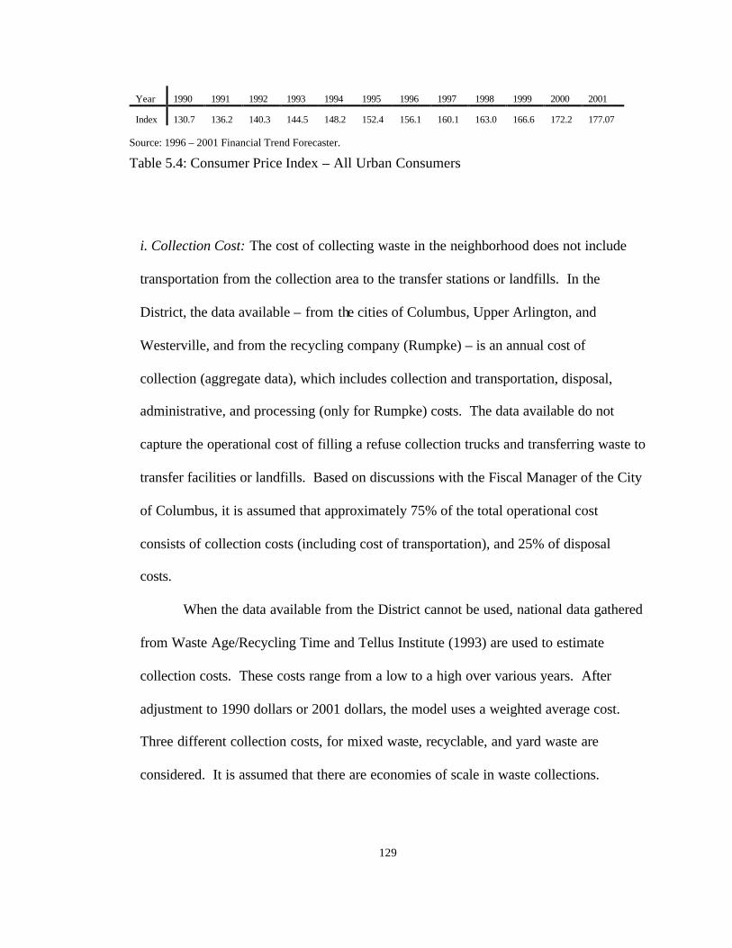
129

Year 1990 1991 1992 1993 1994 1995 1996 1997 1998 1999 2000 2001

Index 130.7 136.2 140.3 144.5 148.2 152.4 156.1 160.1 163.0 166.6 172.2 177.07 Source: 1996 – 2001 Financial Trend Forecaster.

Table 5.4: Consumer Price Index – All Urban Consumers

i. Collection Cost: The cost of collecting waste in the neighborhood does not include

transportation from the collection area to the transfer stations or landfills. In the

District, the data available – from the cities of Columbus, Upper Arlington, and

Westerville, and from the recycling company (Rumpke) – is an annual cost of

collection (aggregate data), which includes collection and transportation, disposal,

administrative, and processing (only for Rumpke) costs. The data available do not

capture the operational cost of filling a refuse collection trucks and transferring waste to

transfer facilities or landfills. Based on discussions with the Fiscal Manager of the City

of Columbus, it is assumed that approximately 75% of the total operational cost

consists of collection costs (including cost of transportation), and 25% of disposal

costs.

When the data available from the District cannot be used, national data gathered

from Waste Age/Recycling Time and Tellus Institute (1993) are used to estimate

collection costs. These costs range from a low to a high over various years. After

adjustment to 1990 dollars or 2001 dollars, the model uses a weighted average cost.

Three different collection costs, for mixed waste, recyclable, and yard waste are

considered. It is assumed that there are economies of scale in waste collections.

130

Hence, the cost function is represented by fixed cost per square kilometer area, and by a

waste collection cost proportional to loading.

ii. Transportation Cost: There are three types of transportation flows. The first is

transportation from a waste source to facilities. The second is transportation from a

transfer station to a landfill or other facilities. The third is transportation from one

facility to other facilities. Unit transportation costs from waste sources are slightly

different for different waste types (mixed, recycled, and yard waste collection), because

each collection uses a different type of truck and crew size. Mixed waste collection, for

example, has the lowest transportation cost. The cost data available in the District

represents total waste collection, transportation and disposal costs. The transportation

costs from transfer station facilities to landfills are included in the aggregate cost of

transfer station operation. Therefore, the model uses transportation costs estimated

from national data gathered from the Waste Age/Recycling Time and Tellus Institute

(1993). The data is used after adjustment to 1990 or 2001 dollars.

iii. Operating Cost: Data on the operating cost of each facility is gathered from the

Authority’s report for the facilities operated by the Authorities, and interviews with

company managers.

• Landfill: For Franklin County Landfill, fixed and variable costs of operation are taken

directly from the Authority SWACO-Financial Report. For landfill facilities outside

the District, the model uses a charge per ton of waste, instead of the real operating

131

cost to deposit waste at the landfill, as the charge per ton of waste is the real cost that

has to be paid by the haulers.

• Transfer Station: The operating unit costs of transfer stations are estimated by

subtracting the cost of transporting waste to landfills (or other facilities) and charge of

landfill disposal, from the cost of waste transfer charged to haulers. The data are

gathered from the Authority’s financial report.

• Incinerator: The processing cost of this facility in 1986 was $36.59 per ton of waste.

The data is from the Authority’s report, and is adjusted to 1990 or 2001 dollars.

• Yard Waste Composting: Processing costs for the Groveport and Upper Arlington

facilities in 2001 are $62.44 and $63.65 per ton, respectively (from interview with the

Procurement Manager of Kurtz Brother). These costs are adjusted to 1990 or

2001dollars.

• Recycling: As the process of separating recyclable material improved significantly

during the 1990s, the cost of processing changed drastically. According to Rumpke’s

manager, in the early 1990s processing and separating recyclable material was mostly

done by workers. In contrast, in 2000, most work was done by machines. When

workers predominant in the separation process, costs were high. Differentiating by

recyclable materials, there are processing costs for paper, plastic, glass, and

aluminum. With machinery as the only processing cost for all materials, each

material has the same processing cost. To accommodate different processing costs

for two different methods and periods, the model takes the weighted average of the

processing cost for each recyclable material (after adjustment to 1990 or 2001

dollars). Furthermore, for each different recyclable material (glass, paper, plastic and

132

aluminum), the processing cost is the weighted average cost of various material

classifications. For example, the processing cost of glass is the average cost of

processing clear, brown, green, and mixed glass.

iv. Expansion and Construction Capacity Costs: The model considers the expansion of

Franklin County Landfill and the construction cost/investment of Upper Arlington and

Groveport yard waste composting facilities. For Franklin County Landfill, the model

considers either to schedule the expansion stage-by-stage or one-time construction.

Costs are taken as the real construction costs of each facility, adjusted to 1990 or 2001

dollars. The model also considers expansion of other landfill facilities outside the

District, by assuming that they are under the control of the Authority through a

contract, i.e., for a specified flow and stock capacity. Meanwhile for the other facility

options, such as transfer stations, the capacities available were underutilized during the

1990’s and have large excess capacity. Hence, there is no point to consider expansion

of these facilities.

v. Prices: The prices or values of different recyclable waste materials and yard waste

compost are gathered directly from recycling and composting companies, combined

with the data from the literature when direct data is not available.

• Recycling material: The price of recyclable materials depends on the market and

varies significantly over years. However, there is only limited historical data. Hence,

the model will use the weighted average from various sources and assume price

constant over time.

133

Economic Parameters

Model Notation

Unit Cost or Price (in Year)

1990 Cost or Price

1990 Model Parameter

2001 Cost or Price

2001 Model Parameter

Sources

1. Discount Rate (δ) % - 7 8 8

2. Collection cost

- Mixed wastea CLCMX $/t 54.00 – 61.00 (93) 49.00–55.00 52.00 66.00 – 75.00 70.50 National dataa + d

- Curbside Recyclable b CLCRC $/t 72.50 – 78.00 (93) 65.58–70.55 68.56 88.85–95.58 92.22 National dataa + d

- Yard waste CLCYW $/t 66.00 (93) 60.00 60.00 81.00 81.00 National dataa + d

3. Transportation cost

• Source locations to solid waste facilities

- Mixed wastea TUCi* $/t/km 0.21 (93) 0.19 0.19 0.26 0.26 National dataa + d

- Recyclable waste a TUCin $/t/km 0.25 (93) 0.23 0.23 0.31 0.31 National dataa + d

- Yard wastea TUCik $/t/km 0.25 (93) 0.23 0.23 0.31 0.31 National dataa + d

• Transfer Stat. to LF TUCjo $/t/km 0.05 (93) 0.045 0.045 0.06 0.06 National dataa + d

• Facility to other facl TUC** $/t/km 0.31 (01) 0.29 0.29 0.31 0.31 Rumpke

4. Technical Operating cost

• Landfill Facilities

- Franklin Co. Lf Co $/t 8.94 (01) 6.60 6.60 8.94 8.94 SWACO

Fixed Cost FCCLF o $ 2,878,420.00 (01) 2,124,637.00 2,124,637.00 2,878,420.00 2,878,420.00 SWACO

- Bedford I Lf Co $/t 28.28 (95) 24.25 24.25 32.86 32.86 SWACO

- Fairfield Co. Lf Co $/t 35.83 (97) 29.25 29.25 43.91 43.91 SWACO

- Suburban South Lf Co $/t 25.91 (01) 21.14 21.14 25.91 25.91 Suburban Sth LF

- Beech Hollow Lf Co $/t 24.63 (01) 18.18 18.18 24.63 24.63 Rumpke/BeechH

• Transfer Facilities

- Georgesville Rd. Cj $/t 12.78 (01) 9.43 9.43 12.78 12.78 SWACO

- Morse Rd. Cj $/t 12.78 (01) 9.43 9.43 12.78 12.78 SWACO

- Jackson Pike Cj $/t 12.78 (01) 9.43 9.43 12.78 12.78 SWACO

- Recycle America Cj $/t 47.18 (01) 34.68 34.68 47.18 47.18 Recycle America

- Mid-American Cj $/t 46.99 (01) 34.68 34.68 46.99 46.99 Mid-America

• Incinerator/WTE Cm $/t 36.59 (86) 43.62 43.62 49.57 49.57 SWACO

• Composting Facilities

- O.M. Scott & Sons Ck $/t 62.43 (93) 56.46 56.46 76.50 76.50 SWACO

- Groveport Ck $/t 75.89 (01) 56.02 56.02 75.89 75.89 Kurtz Brother

- Upper Arlington Ck $/t 75.89 (01) 56.02 56.02 75.89 75.89 Kurtz Brother

Notes: a. Tellus Institute, 1993. b. Waste Age/Recycling Times, 1995, for a typical suburban route.

c. t = ton d. City of Columbus, Upper Arlington, and Worthington.

(Continued)

Table 5.5: Economic Parameters

134

Table 5.5: (Continued)

Economic Parameters

Model Notation

Unit Cost or Price (in Year)

1990 Cost or Price

1990 Model Parameter

2001 Cost or Price

2001 Model Parameter

Sources

• Recycling Center

- Rumpke Recycling $/t

* Paper Cnw $/t 41.65 (92) & 47.00 (01) 34.69 - 38.80 36.74 47.00 - 52.57 49.78 National datab and Rumpke

* Glass Cnw $/t 38.71 (92) & 47.00 (01) 34.69 - 36.06 35.38 47.00 - 48.86 47.93 National datab and Rumpke

* Plastic Cnw $/t 116.28 (92) & 47.00 (01) 34.69 -108.30 71.50 47.00 -146.75 96.88 National datab and Rumpke

* Aluminum Cnw $/t 204.96 (92) & 47.00 (01) 34.69 - 0.94 112.82 47.00 -258.68 152.8 4 National datab and Rumpke

- Smurfit Stone $/t

* Paper Cnw $/t 41.65 (92) & 47.00 (01) 34.69 - 38.80 36.74 47.00 - 52.57 49.78 National datab

* Plastic Cnw $/t 116.28 (92) & 47.00 (01) 34.69 -108.30 71.50 47.00 -146.75 96.88 National datab

* Glass Cnw $/t 38.71 (92) & 47.00 (01) 34.69 - 36.06 35.38 47.00 - 48.86 47.93 National datab

* Aluminum Cnw $/t 204.96 (92) & 47.00 (01) 34.69 - 90.94 112.82 47.00 -258.68 152.84 National datab

5. Landfill Expansion Cost

- Unit var. cost Flow EXCFLF k $/t 11.49 (92) 10.71 10.71 14.51 14.51 SWACO

- Unit var. cost Stock EXCSLF k $/t 13.92 (92) 12.97 12.97 17.57 17.57 SWACO

6. Expansion Cost of Composting Faci.

- Fixed cost FCk $ 1,000,000.00 (97) 816,365.00 816,365.00 1,105,996.00 1,105,996.00 SWACO

- Unit var. cost EXCCOMk $/t 4.29 (97) 3.59 3.59 4.75 4.75 SWACO

7. Prices

- Yard Waste Compost PC $/t 49.06 – 69.38 (01) 36.21 - 51.21 43.71 49.06 - 69.38 59.22 Kurtz Brother

- Recyclable Paper PRw $/t 50.49 – 53.75 (01) 37.27 - 39.67 38.47 50.49 - 53.75 52.12 National datab and Rumpke

- Recyclable Glass PRw $/t 40.00 – 53.00 (90) 40.00 - 53.00 46.50 54.19 - 71.80 63.00 National datab and Rumpke

- Recyclable Plastic PRw $/t 154.00 – 236.00 (01) 113.67- 174.2 143.94 154.00- 236.0 195.00 National datab and Rumpke

- Recyclable Aluminum PRw $/t 245.00 – 518.00 (93) 221.52- 468.9 436.42 300.1 -635.24 467.68 National datab and Rumpke

- Electric energy WTE PE $/kWh 0.028 – 0.040 (90’s) 0.026 - 0.030 0.028 0.034 - 0.049 0.042 SWACO

Notes: a. Tellus Institute, 1993. b. Waste Age/Recycling Times, 1995 (The price is the average price for various types of materials in the same category). c. t = ton d. City of Columbus, Upper Arlington, and Worthington

Table 5.5: Economic Parameters

135

• Compost material: Yard waste composting facilities produce various types of

compost material. Each of them had a relatively stable price during the 1990s.

Hence, assuming a constant price is a good approximation. The model uses the

average price of different materials produced by the composting facility.

vi. Discount Factor: The model uses a dynamic approach for multiyear planning, and

hence a discount factor is necessary for each planning year to optimize the present

value of the objective function. The discount rate in the base year, 1990, is 7%.

However, the model will use the discount rate of 8%, due to the fact that during the

period of 1990 – 2000, the range of discount rates used in the District was 8-10%.

(2) Technical Parameters: As the population and its annual growth vary among sub-areas,

the waste generation also varies among sub-areas. The distances between sub-areas and

facilities and the distances between facilities are measured through map analysis.

The following summarizes all the technical parameters used in the model,

including population and annual growth, waste generation, waste composition, capacity

of facilities, waste-to-energy conversion factor, and waste reduction factor. Table 5.6

presents these technical parameters.

i. Population and annual growth: The population in each waste generation area is from

the Columbus Planning Office, based on the 1990 and 2000 Censuses. The base-year

population for the model is the 1990 and 2001 population in each waste source area.

The annual population growth in each area is the real population growth experienced

between 1990 and 2000. Hence, all waste generation sources have different population

growth rates. As shown in the Table 5.2, some areas have experienced a negative

136

growth, while others have grown by more than 5% annually. Yet, in its plan, the

Authority used a 1% annual growth rates based on MORPC and ODOD predictions.

This is close to the real population growth (1.10%) in Franklin County between 1990

and 2000.

ii. Waste Generation: Waste generation for each Planning Area is estimated by

assuming that waste generation per capita is equal to that of the District (3.44 kg per

person) and is the same for all sources. Waste generation in each Planning Area is then

assumed to grow at the same rate (3.5%) as experienced by the District (see Section

5.1.2), resulting in a 2000 waste generation rate of 3.56 kg/capita/day. These

assumptions are not ideal, as population growth has varied a great deal among the

Planning Districts and because, more than likely, waste generation varies by income

and other population attributes, and may have grown at different rates for different

Planning Areas. The simplifying assumptions are needed because of a lack of better

data.

iii. Waste Composition: The composition and distribution of waste types – compostable

(yard waste), recyclable (mixed glass, plastic, aluminum, and mixed paper), and other

waste – is assumed the same in each area. The model uses the 1993 SWACO Plan

projection of municipal solid waste composition. This projection uses 1989 Cincinnati

data as a proxy. The share of each type of waste is used as the upper limit for what can

be processed. For example, the share of mixed glass, plastic, aluminum, mixed paper,

and mixed metal is the upper limit of recyclable materials either in recycling centers or

material recovery facilities.

137

Unit Model Parameter Sources

- Population people See table 6.3 SWACO, MORPC, and ODOD

- Annual Population Growth % See table 6.3 SWACO, MORPC, and ODOD

- Waste Generation Rate kg/capita/day 3.44 (90) & 3.56 (01) SWACO

tons/capita/year 1.256 (90) & 1.303 (01) SWACO

- Annual Growth of Waste Generation/cap/year % 0.312 SWACO

- Waste Composition (Percentage)

1. Compostable Waste (Yard Waste) % 16.08 SWACO 2. Recyclable Waste % 61.11 a. Mixed glass % 5.10 SWACO b. Plastic % 9.45 SWACO c. Aluminum % 2.55 SWACO d. Mixed paper % 44.10 SWACO

3. Other waste % 22.80 SWACO

Total : 100.00 - Contaminants in mixed waste % a. Mixed glass % 40.00 National Datab b. Plastic % 40.00 National Datab c. Aluminum % 20.00 National Datab d. Mixed paper % 30.00 National Datab - Contaminant of Yard Waste at Yard Waste

Compost facilities % 17.50 Kurtz Brother

- Contaminant of recyclable waste (separated by Hh)

% 3.00 Rumpke

- Base Year Landfill Cumulative Capacity

1. Landfill Facilities tons/year See table 6.4 SWACO

2. Transfer Facilities tons/year See table 6.4 SWACO

3. Waste to Energy/WTE Facilities tons/year See table 6.4 SWACO

4. Recyclin g Plants tons/year See table 6.4 SWACO

- Operation Capacity

1. Landfill Facilities tons/tyear See table 6.4 SWACO

2. Transfer Facilities tons/year See table 6.4 SWACO

3. Waste to Energy/WTE Facilities tons/year See table 6.4 SWACO

4. Recycling Plants tons/year See table 6.4 SWACO

- Upper limit of waste to be incinerated % 90.00 SWACO - WTE Transfer Factor kWh/ton 3942 SWACO & Tchobanoglous’93 - Waste reduction ratio of WTE facility % 75.00 SWACO

- Distances Km See Appendix D MapQuest

Source: a. 1993 Franklin County Solid Waste Plan – waste generated in 1989/1990 b. Contaminant for recyclable waste process directly from mixed waste, Waste Age/Recycling

Times, 1995

Table 5.6: Technical Parameters

138

Recyclable and compostable materials are often contaminated to some degree

when collected from the waste source as mixed waste (for example, newspaper gets wet

or mixed with food). The contaminated materials will be hard to sell. Hence, they are

eventually disposed in landfills. Table 5.6 indicates the contamination level of each

recyclable material. The data for recyclable materials are gathered from Waste

Age/Recycling Times, and are used because data from the District is not available.

Contaminant data for sorted material and yard waste compost material is gathered from

interviews with managers of Rumpke and Kurtz Brother at Groveport Yard Waste

Composting Facility, respectively.

For recyclable material separated by household, on average the contamination

after processing is about 3%. This information was gathered from interview with the

plant manager of the Rumpke recycling company.

iv. Capacity: All data on facility capacity are gathered form the 1993 and 2000 Solid

Waste Plan (Solid Waste Authority of Central Ohio ) and the 1998 Ohio Solid Waste

Facility Data Report (Ohio-EPA). The data is used as is in the model, after adjustment

is made for the base year 1990 and 2001. Three different types of capacity are

considered for landfill facilities. As shown in Table 5.3, the three capacities for

landfills are the actual or the remaining capacity, the potential stock capacity (for

expansion or potential for utilization), and the annual operating capacity. The actual

capacity in the base year is the 1990 remaining capacity of each landfill. For the other

facilities, the model only considers the annual operating capacity, which is the

maximum amount of waste that can be processed each year.

139

v. Waste-to-Energy transfer factor and waste reduction ratio: The waste-to-energy

factor is calculated based on the heat energy content of each material contained in 1 ton

of municipal solid waste (Tchobanoglous, 1993). Then, this heat energy is transferred

to electric power (kwh/ton) based on the mechanical equivalent of heat and the

efficiency of the incinerator. A waste reduction ratio of 75% (25% left as residue/ash)

is used directly from the SWACO report.

vi. Distance: All distances between sources and facilities or among facilities are

gathered using MapQuest – a map and driving directions site on the Internet – based on

address of location. To determine distance from waste source to facility, one point at

the center of the waste source area is initially chosen. Then, from this point, the

distance to each facility is measured using MapQuest (see Appendix D).

(3) Decision Variables: One purpose of the analysis is to determine an optimal allocation

of waste flows into management option/facilities. Hence, the amount of waste at each

facility and through each path is a decision variable.

Waste generated from each household consists of various waste materials. Each

material may contribute to the system performance differently, because each material has

particular characteristics with regard to energy content (BTU), ash content, and market

price for recyclable and compost materials. Alternatives such as recycling may alter

waste composition due to removal of specific material and, hence, may affect the

performance of processes such as incinerators/waste-to-energy facilities. The decision

variables are listed in Table 5.7.

140

Decision Variables Unit - Waste allocation to each facility Tons

- Share of waste recycled %

- Share of waste composted %

- Share of waste incinerated %

- Share of waste landfilled % - Level promotion of recycling activity $/person

- Stock Capacity Expansion of Landfills Tons/year

- Flow Capacity Expansion of Landfills Tons/year

- Capacity Expansion of Recycling Facilities Tons/year

- Capacity Expansion of Composting Facilities Tons/year

- Schedule of Landfill Stock Capacity Expansion In year

- Schedule of Landfill Flow Capacity Expansion In year

- Schedule of Composting Capacity Expansion In year

- Schedule of Recycling capacity Expansion In year

- Schedule of Landfill Closure In year

- Schedule of utilization Export Landfill In year

- Schedule of construction new Landfill Facilities In year

- Schedule of construction new Recycling Facilities In year

- Schedule of construction new Yard Waste Composting Facilities In year

Table 5.7: Decision Variables

The model determines the amount of materials recovered through recycling and

composting, incinerated in waste-to-energy facilities, and deposited in landfills. The

model determines schedules of landfill expansion, closure, and utilization. The

expansion of Franklin County Sanitary Landfill and the utilization of landfills outside the

District have become critical in the early 1990s, as the Authority faced a shortage of

landfill capacity while total waste generated increased annually.

The model also determines the schedule of construction/upgrading of yard waste

composting facilities, and the optimal time to expand the capacity of the Upper Arlington

141

and Groveport yard waste composting facilities, since total yard waste generated in the

District increases annually.

The model is to be applied to the current Central Ohio solid waste management

system in the next two chapters. To ensure that the model behaves as expected, several

runs of the model will be used to test the validity of the extensions, including economies

of scale in operation and capacity expansion, multiple landfill operations, and landfill

closure and replacement. Meanwhile, an aggregate cost analysis will be conducted to

assess the economics of solid waste management using pseudo data generated by the

model, in particular economies of scale, economies density, and recycling promotion.

142

CHAPTER 6

MODEL TESTING

This chapter tests the model on various issues related to the extensions, and

applies it to several simplified waste management systems using Central Ohio data. It

analyzes a number of model runs to demonstrate that the model 'works', i.e., that it

behaves as expected based on the theoretical results in the literature and the specific

analytical results presented in Chapter 3. It presents three set of experiments: (1) Single

disposal site, (2) Multiple disposal site, space and time, and (3) Other disposal

substitutes. In these experiments, the model is applied with the simplest scenario

possible to show how it consistently deals with a specific condition. It only considers

landfills and recycling facilities, while excluding transfer stations, incinerators, and

composting facilities. The experiments uses the stylized Central Ohio system presented

in the previous chapter, including the original 30 waste generation demand sites, the

matrix of distances between facilities and waste sources, and the 1990 data on economic

and physical conditions. The planning period is 21 years, from 1990 to 2010. Basic

assumptions, such as inelastic demands and a centralized system, are retained, but some

specific assumptions may vary across experiments, e.g., capacity constraints, facility

locations, and fixed cost for landfill capacity expansion.

143

The first set of experiments considers only one landfill and no recycling facilities.

It deals with a single local landfill with finite flow and stock capacity, just sufficient for

initial operating and storage demand. It explores the expansion of landfill facilities. The

second set considers multiple landfills and, again, no recycling facilities. This

experiment deals with the schedule of capacity expansion and other landfill alternatives,

such as export landfills. It also deals with landfill replacement, as the old landfill stock

capacity is exhausted and there is no space for expansion. The final set allows for

landfills and recycling facilities. It deals with the impact of recycling – as substitute

disposal – on landfill closure and replacement schedule.

6.1 Single Disposal Site – Landfill with Constrained Capacity

This single disposal site is assumed to have infinite stock (storage) and flow

(operating) capacities, i.e., neither needs expansion (see Chang, 1996). Alternatively, a

disposal site could have finite stock and flow capacities, in which case expansion of one

or both may be necessary. If there are constant returns to scale in the cost of expansion,

then expansion can be expected to take place incrementally, as needed. If there are

returns to scale, then expansion will be lumpy. Lumpiness will vary with a number of

parameters, including economies of scale, the opportunity cost of capital, and the rate of

growth in waste demand. The greater the economies of scale, the lower the opportunity

cost of capital, and the more rapid the growth of waste generation, the lumpier is the

expansion of stock and flow disposal capacity. The model behaves consistently with

these expectations throughout, as shown in the following section. This experiment

consists two major cases: (1) expansion with constant returns to scale, (2) expansion with

economies of scale.

144

6.1.1 Capacity Expansion Under Constant Returns to Scale

In this case, the expansion cost rises linearly at a rate of $11 per ton for

throughput capacity, and at a rate of $14 per ton for storage capacity. As expected, under

an optimal management program, both capacities are expanded incrementally each year

as needed. The results are illustrated in Figures 6.1 and 6.2.

1,150

1,250

1,350

1,450

1,550

1,650

1,750

90 92 94 96 98 00 02 04 06 08 10

Year

Was

te D

epos

it &

Flo

w C

apac

ity (,

000

tons

/yea

r)

Waste Deposit

Flow Capacity

Figure 6.1: Flow (operating) Capacity and Waste Deposit – Under Constant

Returns to Scale

750

1,250

1,750

2,250

2,750

3,250

3,750

4,250

4,750

90 92 94 96 98 00 02 04 06 08 10

Year

Was

te D

epos

it (0

00 to

ns/y

ear)

& U

nuse

d St

ock

Cap

acity

(,0

00 to

ns)

Waste Deposit

Unused Stock Capacity

Figure 6.2: Stock (storage) Capacity and

Waste Deposit – Under Constant Returns to Scale

There is never any excess capacity after each expansion, except, of course, in the

early years, when the initial stock capacity exceeds capacity requirement.

6.1.2 Capacity Expansion with Economies of Scale

This is modeled by assuming that expansion cost rises linearly, but with a fixed

cost incurred each time capacity is expanded. Six experiments are conducted, starting

with a base case and followed by a sensitivity analysis with five sets of parameter

changes.

145

(1) Base Case: The fixed costs of expanding flow and stock capacity are fixed at

$300,000 and $800,000 respectively. Variable costs, proportional to the scale of

expansion, are as discussed in the case of constant returns. The opportunity cost of

capital (OCC) is 8%, and waste grows annually at a rate of about 3.85 % – the result

of a population growth of 1.10% per year and per capita waste generation growth of

0.31% per year.

As expected, the landfill expansion is now lumpy. Over the 21-year horizon,

the flow capacity is expanded twice, or roughly every ten years. The stock capacity is

expanded four times, or about every 4-5 years, as illustrated in Figures 6.3 and 6.4.

1,150

1,250

1,350

1,450

1,550

1,650

1,750

90 92 94 96 98 00 02 04 06 08 10

Year

Was

te D

epos

it &

Flo

w C

apac

ity (,

000

tons

/yea

r)

Waste DepositFlow Capacity

Figure 6.3: Flow Capacity and Waste Deposit – Under Increasing Returns to

Scale

750

1,750

2,750

3,750

4,750

5,750

6,750

7,750

90 92 94 96 98 00 02 04 06 08 10

Year

Was

te D

epos

it (,0

00 to

ns/y

ear)

& U

nuse

d St

ock

Cap

acity

(,00

0 to

ns)

Waste DepositUnused Stock Capacity

Figure 6.4: Stock Capacity and Waste Deposit – Under Increasing Returns to

Scale

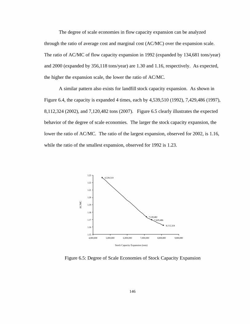
146

The degree of scale economies in flow capacity expansion can be analyzed

through the ratio of average cost and marginal cost (AC/MC) over the expansion scale.

The ratio of AC/MC of flow capacity expansion in 1992 (expanded by 134,681 tons/year)

and 2000 (expanded by 356,118 tons/year) are 1.30 and 1.16, respectively. As expected,

the higher the expansion scale, the lower the ratio of AC/MC.

A similar pattern also exists for landfill stock capacity expansion. As shown in

Figure 6.4, the capacity is expanded 4 times, each by 4,539,510 (1992), 7,429,486 (1997),

8,112,324 (2002), and 7,120,482 tons (2007). Figure 6.5 clearly illustrates the expected

behavior of the degree of scale economies. The larger the stock capacity expansion, the

lower the ratio of AC/MC. The ratio of the largest expansion, observed for 2002, is 1.16,

while the ratio of the smallest expansion, observed for 1992 is 1.23.

4,539,510

7,120,4827,429,486

8,112,324

1.15

1.16

1.17

1.18

1.19

1.20

1.21

1.22

1.23

4,000,000 5,000,000 6,000,000 7,000,000 8,000,000 9,000,000

Stock Capacity Expansion (tons)

AC

/MC

Figure 6.5: Degree of Scale Economies of Stock Capacity Expansion

147

(2) Rise in Fixed Cost: The first sensitivity analysis doubles the fixed costs to $600,000

for flow capacity, and to $1.6 million for stock capacity. As expected, the lumpiness

of investments rises. The operating capacity is now expanded only once over the 21-

year horizon, rather than twice in the Base Case. Stock capacity is expanded only

twice over 21 years, rather than four times in the Base Case, as illustrated in Figures

6.6 and 6.7.

1,150

1,250

1,350

1,450

1,550

1,650

1,750

90 92 94 96 98 00 02 04 06 08 10

Year

Was

te D

epos

it &

Flo

w C

apac

ity (,

000

tons

/yea

r)

Waste Deposit Flow Capacity

Figure 6.6: Waste Deposit and Flow Capacity Expansion – Fixed Costs

Doubled

750

2,750

4,750

6,750

8,750

10,750

12,750

14,750

90 92 94 96 98 00 02 04 06 08 10

Year

Was

te D

epos

it (,0

00 to

ns/y

ear)

& U

nuse

d St

ock

Cap

acity

(,0

00 to

ns)

Waste Deposit Unused Stock Capacity

Figure 6.7: Waste Deposit and Stock Capacity Expansion – Fixed Costs

Doubled

(3) Decline in the Opportunity Cost of Capital (OCC): In this experiment, the OCC is

reduced from 8% to 5%, thus making it cheaper to hold idle capacity. As expected,

the lumpiness of investment rises relative to the Base Case (Figures 6.8 and 6.9). The

operating capacity is expanded only once, and the stock capacity three times.

148

1,150

1,250

1,350

1,450

1,550

1,650

1,750

90 92 94 96 98 00 02 04 06 08 10

Year

Was

te D

epos

it &

Flo

w C

apac

ity (,

000

tons

/yea

r)Waste Deposit Flow Capacity

Figure 6.8: Waste Deposit and Flow Capacity – Opportunity Cost of Capital

38% Lower

500

2,000

3,500

5,000

6,500

8,000

9,500

11,000

90 92 94 96 98 00 02 04 06 08 10

Year

Was

te D

epos

it (,0

00 to

ns/Y

ear)

& U

nuse

d St

ock

Cap

acity

(,0

00 to

ns)

Waste Deposit Unused Stock Capacity

Figure 6.9: Waste Deposit and Stock

Capacity – Opportunity Cost of Capital 38% Lower

.

(4) Increase in Growth Rate: In this experiment, the rate at which waste generation

grows is quadrupled, by both increasing the rate of population growth (2.20%) and

the rate of per capita waste generation (0.62%). Theory and the literatures suggests

that, in the case of exponential growth, capacity will be expanded in constant absolute

increments, independent of the rate of growth in demand.16 Hence, with a higher rate

of growth, expansion must happen more frequently. The numerical results roughly

mirror the theoretical expectations. In the Base Case, demand for landfill throughput

grew by about 500,000 tons over the 21-year horizon, requiring two expansions, with

an average 250,000 tons. In the current case, demand grows by about 2,000,000 tons,

leading to six expansions, at an average 330,000 tons per expansion, as shown in

Figure 6.10 and 6.11.

16 Recall that these theoretical results refer to the case of an infinite planning horizon. In the current case, the horizon

is finite, and hence, our numerical results likely will only approximate the theoretical results.

149

.

1,000

1,250

1,500

1,750

2,000

2,250

2,500

2,750

3,000

3,250

90 92 94 96 98 00 02 04 06 08 10

Year

Was

te D

epos

it &

Flo

w C

apac

ity (

,000

tons

/yea

r)

Waste Deposit Flow Capacity

Figure 6.10: Waste Deposit and Flow Capacity – Waste Growth Rate

Quadrupled

750

1,750

2,750

3,750

4,750

5,750

6,750

7,750

8,750

9,750

90 92 94 96 98 00 02 04 06 08 10Year

Was

te D

epos

it (,0

00 to

ns/y

ear)

& U

nuse

d St

ock

Cap

acity

(,

000

tons

)

Waste Deposit Unused Stock Capacity

Figure 6.11: Waste Deposit and Stock Capacity – Waste Growth Rate

Quadrupled

(5) Linear and Semi-logarithmic Growth Rate: The following two cases involve

experiments with two different functions of the waste generation growth rate: the first

is linear, and the second is semi- logarithmic. These experiments demonstrate how the

waste growth function may significantly impact the schedule of capacity expansion

under economies of scale. In both cases, the focus is on flow capacity expansion, as

the stock capacity paths are relatively similar.

150

In the first case, the landfill deposit grows at a constant rate of about 35,000

tons annually – based on a population growth of 2.20% and per capita waste

generation growth of 0.62%. The staged expansion is illustrated in Figure 6.12. The

demand for landfill deposit grows by about 750,000 tons over the 21-year horizon,

requiring three expansions with an average 250,000 tons. Since waste grows at a

constant rate over time, the model expands flow capacity every seven years,

specifically for the first and second expansions. The last expansion is sufficient to

handle the flow of waste up to the end of the planning period.

In the second case, waste generation grows at a semi- logarithmic rate, as a

result of the combination of the following function:

(6-1) PG = IP * t pgr

(6-2) PCWG = IPCWG * t pcwgr.

where IP is the initial population, t is time (year), and pgr is the population growth

rate. Then the population at time t is given by PG, as represented by equation (6-1).

Similarly, the per capita waste generation, PCWG, is computed according to equation

(6-2), where IPCWG is the initial per capita waste generation, and pcwgr is the per

capita waste growth rate.

Under these conditions, the landfill deposit increases at a decreasing rate, by

only about 120,000 tons over the 21-year period. There is only one flow capacity

expansion during the planning period, as illustrated in Figure 6.13.

151

1,100

1,300

1,500

1,700

1,900

2,100

90 92 94 96 98 00 02 04 06 08 10

Year

Was

te D

epos

it &

Flo

w C

apac

ity (,

000

tons

/yea

r)

Waste Deposit Flow Capacity

Figure 6.12: Flow Capacity Expansion – Under Linear Waste Growth Rate

1,200

1,225

1,250

1,275

1,300

1,325

1,350

90 92 94 96 98 00 02 04 06 08 10

Year

Was

te D

epos

it &

Flo

w C

apac

ity (,

000

tons

/yea

r)

Waste deposit Flow Capacity

Figure 6.13: Flow Capacity Expansion – Under Semi- logarithmic Waste Growth

Rate

6.2 Multiple Disposal Sites

The second set of experiments considers the presence of further disposal sites, in

the form of a second local disposal site and/or an export site. Since these facilities exist in

space, each will have a catchment area from which it attracts waste. In general, the lower

the production cost at the site, the lower the transport costs, and the higher the cost of

alternative sites, the larger the catchment area of a particular disposal site. If there are

constant returns to scale throughout, then the size of the catchment area can be

determined in a straightforward manner. Waste from any place of origin will go to the

cheapest disposal site, considering the unit cost of collection, transportation and

production at the site. However, if there are economies of scale in the operation or

expansion of disposal facilities, then disposal decisions become more complex. In

general, one would expect that each waste generating area would send waste to the site

152

with the smallest marginal (transport plus production) cost. However, when there are

economies of scale, then it is possible that directing waste to a site with what appears (at

its current outputs) to be higher marginal costs is optimal. Shifting a waste stream to a

particular disposal site may raise its scale to a level that permits operations, when

operation would otherwise not be optimal. Again, the model behavior is consistent with

these expectations, as shown in the following section.

This set of experiments also focuses on the staging of multiple disposal sites. In

the presence of economies of scale, it may pay to postpone a needed expansion. This

makes it possible to make each expans ion greater and thus to reduce the average cost of

facility expansion. In the meantime, other facilities must absorb the capacity shortfall.

The experiments show that the model correctly identifies these strategies, and is sensitive

in its behavior to changes in the interest rate and economies of scale. The experiment

also focuses on landfill replacement, which becomes necessary as the old landfill stock

capacity is exhausted and there is no possibility for expansion. This section will also

show that several factors, such as operating cost, space, closure cost, and expansion cost

significantly impact the time for replacement.

The local landfill operations are analyzed when other landfill facilities are

available as alternatives. One experiment assumes an alternative landfill outside the

study area, to which waste is exported, and explores the management of the local landfill

under different initial conditions, i.e., production functions and capacity limitations. The

other experiment assumes an alternative landfill within the study area, and explores the

replacement strategy of the old landfill when its stock capacity has been used up and no

possibility for expansion exists.

153

Marginal Costs Waste Allocation Constant Returns to

Scale Economies of Scale

with Fixed Cost Waste Source

Local Landfill

Export Landfill

Amount of Waste

Generated Local LF Export LF

Local LF Export LF wg1 73.31 73.89 19,509.45 19,509.45 - - 19,509.45 wg4 73.50 72.69 65,877.20 - 65,877.20 - 65,877.20 wg13 71.85 71.60 44,663.36 - 44,663.36 - 76,637.35 wg21 72.96 69.48 43,800.49 - 43,800.49 - 43,800.49 wg26 70.49 72.80 44,663.36 44,663.36 - - 44,663.36 wg30 72.50 70.05 1,610.19 - 1,610.19 - 1,610.19 Total 252,098.04 64,172.81 187,925.23 - 252,098.04

Note: 1. Lo wer marginal cost in boldface 2. LF = Landfill

Table 6.1: Marginal Costs to Local and Landfill Export and Waste Allocation in the Base Year (1990)

6.2.1 Alternative Disposal Site Outside the Study Area – Export Waste

Different capacity limitations are considered: 1) the local landfill has infinite flow

and stock capacities, and 2) the local landfill has finite capacities.

6.2.1.1 Local Landfill with Infinite Capacity

This case focuses on the waste deposit strategy when the local landfill operates

either under constant return to scale or under increasing return to scale. As expected, in

the case of constant return to scale, the waste from any source area is transported to the

landfill with the cheapest marginal cost (collection, transportation and operating cost), as

illustrated in Table 6.1, where only the flow from six waste generation areas are

presented. The catchment area of the local landfill includes waste generation areas, wg1

and wg26, because there have lower marginal costs to this local landfill. The others are

catchment areas of the export landfill.

154

If the local landfill operates with economies of scale, however, the waste from all

source areas is deposited in the export landfill over some initial period, although the

marginal costs from the two areas wg1 and wg26 to the export landfill are higher than

those to the local one (see Table 6.1). This is due to the fact that the total amount of

waste generated from the two sources is not sufficient to be deposited in the local landfill

to reach a lower average cost than the export landfill (because of the fixed cost

component). As the waste generated grows and the total amount of waste from these two

areas reaches the point where the average cost of the local landfill is lower than that of

the export landfill, the waste flow shifts to the local landfill, as illustrated in Figures 6.14

and 6.15 (note, LF = landfill). The shifting time is 1996.

0

100

200

300

400

500

90 92 94 96 98 00 02 04 06 08 10

Year

Was

te D

epos

it (,0

00 to

ns/y

ear)

Local LF Deposit

Export LF Deposit

Total Deposit

Figure 6.14: Amounts of Waste Deposit – Local Landfill Under Constant Returns to Scale Operation, with Infinite Capacity

0

100

200

300

400

500

90 92 94 96 98 00 02 04 06 08 10

Year

Was

te D

epos

it (,0

00 to

ns/y

ear)

Local LF Deposit

Export LF Deposit

Total Deposit

Figure 6.15: Amounts of Waste Deposit – Local Landfill Under Increasing Returns to

Scale Operation, with Infinite Capacity

155

In general, this case shows that if the alternative landfill for waste exports has a

lower marginal cost, then there will be export. Because of the fixed cost in the local

landfill, exports may be used even with a higher marginal cost, at least for some period of

time. If the fixed cost is extremely high, all waste sources may use the export landfill all

the time. Note that, in this case, idle or unused capacity is considered costless. In reality,

even an idle landfill incurs operating costs for safety and security, routine inspections,

and monitoring systems. Once these costs are included they will discourage waste

export, except when there is a capacity constraint in the local landfill.

6.2.1.2 Local Landfill with Finite Capacity

In this case, the cost of flow and stock capacity expansions and operation of the

local landfill are characterized by economies of scale (with fixed cost). As expected, the

model postpones expansion of the local landfill by temporarily sending more waste to the

export landfill as a substitute disposal option – even if the export is more expensive. This

action postpones capital costs associated with capacity expansion and raises the size of

the expansion, and, therefore, given economies of scale, reduces the average cost of

expansion.

To show that the model behaves as expected, three different cases are considered.

The first case assumes that the local landfill is constrained in term of flow capacity only;

the second case assumes stock capacity constraint only; finally, both capacity constraints

are included.

(1) Flow Capacity Constraints: The optimal strategy involves sending some waste to the

export substitute site for at least some of the time. Once the flow capacity has been

156

reached, an increasing number of sources export their waste, starting with those for

which the cost of this alternative is the smallest. Eventually, the flow capacity of the

local landfill is expanded and all sources return to the local landfill, as illustrated in

Figure 6.16.

0

200

400

600

800

1,000

1,200

1,400

1,600

1,800

90 92 94 96 98 00 02 04 06 08 10

Year

Was

te D

epos

it &

Loc

al L

F Fl

ow C

apac

ity (t

ons/

year

)

Local LF Deposit Export LF Deposit

Total Waste Deposit Local LF Flow Capacity

Figure 6.16: Local Landfill with Flow Capacity Constraint

(2) Stock Capacity Constraint: As the stock capacity constraint draws near, an increasing

number of sources send their waste to the export landfill with higher cost, as shown in

Figure 6.17. This strategy postpones the time of expansion (saving interest cost) and

benefits from the greater economies of scale that come from larger (and less frequent)

expansion.

157

0

2,000

4,000

6,000

8,000

10,000

12,000

14,000

90 92 94 96 98 00 02 04 06 08 10

Year

Loc

al L

F C

umul

ativ

e D

epos

it , L

ocal

LF

Stoc

k C

apac

ity, &

Ann

ual

Exp

ort D

epos

it (,0

00 to

ns)

Local LF Stock Capacity

Local LF Cumulative Deposit

Annual Export Deposit

Figure 6.17: Local Landfill with Stock Capacity Constraint

(3) Flow and stock capacity constraints: As in the previous case, more waste is exported

every time the stock capacity constraint draws near, even if this leaves some idle flow

capacity. Due to the two constraints, the export landfill is used more intensively to

postpone expansion. Figure 6.18 points to the intensive use of the export landfill

before the stock and flow expansion of the local landfill takes place in 1995 and 1996

respectively.

158

0

3,000

6,000

9,000

12,000

15,000

18,000

21,000

90 92 94 96 98 00 02 04 06 08 10

Year

Loc

al L

F C

umul

ativ

e D

epos

it, L

ocal

LF

Stoc

k C

apac

ity &

A

nnua

l Exp

ort D

epos

it (,0

00 to

ns)

Local LF Stock Capacity

Local LF Cummulative DepositAnnual Export Deposit

Figure 6.18: Stock Capacity and Cumulative Waste Deposit in the Local

Landfill

0

200

400

600

800

1,000

1,200

90 92 94 96 98 00 02 04 06 08 10

Year

Ann

ual D

epos

it of

Loc

al L

F &

Exp

ort a

nd

Loc

al L

F Fl

ow C

apac

ity (,

000

tons

/yea

r)

Annual Export Deposit Local LF Flow Capacity

Local LF Deposit

Figure 6.19: Flow Capacity and Annual Waste Deposit in the Local Landfill

6.2.2 Alternative Disposal Site in the Study Area - Landfill Replacement

In this experiment, strategies of replacing an existing landfill by a new one is

explored – the closure and start-up of disposal sites. It is assumed that demand is

inelastic, and all waste is disposed in landfills, i.e., there are no disposal substitutes such

as recycling and composting facilities that could lengthen the life of a landfill. Substitute

disposal options are considered in the next experiment.

Disposal sites may be closed because they are more expensive to operate than a

new one, or because they are out of stock capacity. Note that in the former case, because

existing sites are usually located closer to the urban area they serve, closure may generate

external environmental benefits, thereby increasing attractiveness of the option.

However, these benefits are not modeled here. In the latter case, replacement of a landfill

becomes necessary because there are no opportunities for further stock expansion at the

existing site, or because expansion is more expensive than the development of a new site.

159

The following briefly considers these possibilities.

In the literature, the common assumption is that an old landfill will be closed

when the new landfill starts. But, this may not be optimal – (1) because of the impact of

space, and (2) because of closure costs. Hence, it is entirely possible that the change from

old to new landfill is gradual, or that the old landfill is never closed.

6.2.2.1 Impact of Space on Landfill Replacement

It is possible that all collection districts experience higher delivery costs to the

new landfill than to the old landfill. In this case, one would expect the old landfill to be

utilized by all collection districts until it closes. At the time of closure, all districts would

shift over to the new landfill. In this case, there would be an immediate changeover, as

illustrated in Figure 20. It is quite possible, however, that the new landfill has a location

that reduces delivery costs for at least some collection districts. In this case, the

changeover from one landfill to the other is likely be gradual (see Figure 6.21).

0

200

400

600

800

1,000

1,200

1,400

1,600

1,800

90 92 94 96 98 00 02 04 06 08 10

Year

Was

te D

epos

it (,0

00 to

ns/y

ear)

New LF Deposit Old LF Deposit

Figure 6.20: New Landfill Location Incurs High Delivery Cost for All Waste Sources

0

200

400

600

800

1,000

1,200

1,400

1,600

1,800

90 92 94 96 98 00 02 04 06 08 10

Year

Was

te D

epos

it (,0

00 to

ns/y

ear)

New LF Deposit Old LF Deposit

Figure 6.21: New Landfill Location is

Preferred by at Least Some Waste Sources

160

6.2.2.2 Impact of Old Landfill Closure Costs on Landfill Replacement

When an existing site is closed, numerous costs arise, associated with site

redevelopment in line with environmental standards, including landfill cover, control

systems for water drainage and landfill gases, leachate treatment, and an environmental

monitoring system. When such costs are added to the model, the obvious response is to

avoid them by retaining some idle capacity to postpone closure. Put differently, all waste

will go to the new site, yet the old site will never be closed, as illustrated in Figure 6.22.

0

900

1,800

2,700

3,600

4,500

5,400

6,300

7,200

8,100

9,000

90 92 94 96 98 00 02 04 06 08 10

Year

Was

te D

epos

it (,0

00 to

ns/y

ear)

& O

ld L

F St

ock

Cap

acity

(,0

00 to

ns)

New LF Deposit

Old LF Deposit

Old LF Unused Stock Capacity

Figure 6.22: Impact of Landfill Closure Cost (The Old Landfill is Never Closed)

There are two ways to avoid this outcome. One is to add a sufficiently high cost

for idle operations, the one that is included in the model. Once such costs are added, the

site will be closed. The other is to allow for benefits from closure (terminal value) that

may exceed closing costs. Such benefits could be the result of urban, industrial or

161

recreational re-use of the land, or at least the value of land itself as a non-depreciable

cost. The higher the terminal value and the lower the landfill closure cost, the earlier the

closure. In both cases, the switch from the existing landfill to a new one will be similar to

that in Figures 6.20 and 6.21.

6.3 Other Disposal Substitutes – Recycling Facility

The final set of experiments introduces other substitutes to local disposal, such as

recycling and composting facilities. Since these facilities exist in space, each will have a

catchment area, and, in general, these catchment areas will vary with transport costs and

production costs. To the extent that there are economies of scale in disposal, recycling

and composting, strategies will be lumpy, and disposal streams become interdependent

and discontinuous.

This case explores the impact of disposal substitutes to landfill replacement – in

this case recycling facility, and how the recycling facility impacts the closure and start up

times of disposal sites. Demand is inelastic, and waste is recycled and/or disposed in

landfills. Recycling reduces waste deposit and may lengthen the life of the old landfill.

The experiment focuses on two different conditions for the new landfill facility.

In the first case, all sources experience high marginal costs (collection, transportation and

operation) for the new landfill facility. In the second case, the new landfill is the least

expensive way to dispose of waste, for at least some sources. In this case, the operating

unit cost of Franklin County Landfill (see Table 5.5) is used for that the old landfill. The

operating unit costs of the new cheap and expensive landfills are 4% and 10% higher than

that of the old landfill, respectively. The operating unit cost of Rumpke Recycling Center

162

(see Table 5.5) is used for that the cheaper recycling facility. Then, it is assumed that the

expensive recycling unit operating cost is 30% higher than the cheaper one.

6.3.1 New Expensive Landfill

When all sources experience high marginal costs for the new landfill facility, the

old landfill is used until it reaches its stock capacity limit, followed by the operation of

the new landfill. This is an immediate replacement, and the availability of recycling only

impacts the timing of landfill replacement, which may happen sooner or later, depending

on the marginal cost of the recycling facility. Two cases for this marginal cost are

considered.

(1) Low marginal cost of recycling: With recycling, one would expect that the new

landfill would start when the old landfill nears its stock capacity limit. The lower the

cost of recycling, the more waste recycled, and the less the waste deposited. At the

beginning, since the new landfill is not yet active, recycling eventually extends the

old landfill lifetime, and hence postpones its replacement time, as illustrated in Figure

6.23. The replacement takes place in 1999.

(2) High marginal cost of recycling: In this case, less waste is recycled at the beginning

of the period, as illustrated in Figure 6.24. Consequently, more waste is deposited in

the old landfill and this shortens its life. Hence, as the stock capacity of the old

landfill is exhausted, the shift to the new landfill takes place sooner than that in the

previous case. The replacement year is 1998.

163

0

200

400

600

800

1,000

1,200

1,400

90 92 94 96 98 00 02 04 06 08 10

Year

Was

te D

epos

it &

Rec

ycle

d (,0

00 to

ns/y

ear)

New LF Deposit Old LF Deposit

Waste Recycled

Figure 6.23: Impact of Cheap Recycling Costs on Landfill Operation

and Replacement - 1

0

200

400

600

800

1,000

1,200

1,400

90 92 94 96 98 00 02 04 06 08 10

Year

Was

te D

epos

it &

Rec

ycle

d (,0

00 to

ns/y

ear)

New LF Deposit Old LF Deposit

Waste Recycled

Figure 6.24: Impact of Expensive

Recycling Costs on Landfill Operation and Replacement - 1

The above analysis illustrates how the relative cost of recycling impacts the

landfill replacement time. The lower the marginal recycling cost the later the

replacement time. Unfortunately, as the marginal costs of recycling includes not only

cost of operation, but also various costs of transportation from, fixed and variable costs of

collection, and costs of promotion in different neighborhoods, they are not presented here

(this is also apply for the following Section 6.3.2). Moreover, the analysis also illustrate

that even with high operation cost, recycling is a significant option to postpone expensive

landfill closure and replacement, as was also demonstrated with the analytical model

presented in Chapter 3

6.3.2 New Cheap Landfill

In this case, the new landfill is preferred by at least some sources. Again, as

expected, the replacement of the old landfill takes place gradually. In this case, the

164

existence of recycling may have an impact in two different ways: (1) because of its

relative cost and (2) because of its location.

(1) Relative cost of Recycling: As in the last two cases, recycling postpones the gradual

changeover from the old to the new landfill. The cheaper the marginal cost of

recycling, the later the changeover. The postponement is by one year, as illustrated in

Figure 6.25 and 6.26. With expensive recycling, the gradual replacement takes place

from 1998 to 2000. With cheaper recycling, the gradual replacement is postponed by

one full year, or to the period of 1999 – 2001. Note that both replacements take place

over three years.

0

200

400

600

800

1,000

1,200

1,400

90 92 94 96 98 00 02 04 06 08 10

Year

Was

te D

epos

it &

Rec

ycle

d (,0

00 to

ns/y

ear)

New LF Deposit Old LF DepositWaste Recycled

Figure 6.25: Impact of Expensive

Recycling Cost on Landfill Operation and Replacement - 2 (RC-0)

0

200

400

600

800

1,000

1,200

1,400

90 92 94 96 98 00 02 04 06 08 10

Year

Was

te D

epos

it &

Rec

ycle

d (,0

00 to

ns/y

ear)

New LF Deposit Old LF DepositWaste Recycled

Figure 6.26: Impact of Cheap Recycling Cost on Landfill Operation and

Replacement - 2 (RC-0)

165

Again, this case shows that the relative marginal cost of recycling matters in

postponing landfill replacement. The location of the recycling facility (RC-0) is

relatively at the same distance to both landfills, as shown in Figure 6.27.

Figure 6.27: Substitute Location and Landfill Catchment Area (Red is catchments area of the new landfill)

Figure 6.27 also shows three locations of recycling centers (RC-0, RC-1, and RC-

2). These three RC’s do not exist at the same time. RC-0 is the recycling facility used in

166

the previous case (case-1). Figure 6.27 also shows the remote locations of the substitute

recycling facilities (RC-1 and RC-2) and the catchment area of each landfill.

(2) Location of the Recycling Facility: The location of a recycling facility may extend or

shorten the period of gradual changeover between the two landfills. This analysis

uses the cheap recycling cost of case-1. If the recycling facility is located closer to

the old landfill than to the new one, more waste from the old landfill catchment area

is recycled and this extends its lifetime. In the meantime, the catchment area of the

new landfill is relatively unaffected. However, less waste is recycled from these

sources, hence the facility operates earlier. Consequently, the changeover period is

longer than in case-1, lasting 6 years, from 1996 to 2002. Figure 6.28 illustrates the

case where the recycling facility (RC-1) is close to the old landfill (see Figure 6.27).

0

200

400

600

800

1,000

1,200

1,400

90 92 94 96 98 00 02 04 06 08 10

Year

Was

te D

epos

it &

Rec

ycle

d (,0

00 t

ons/

year

)

New LF Deposit

Old LF DepositWaste Recycled

Figure 6.28: Recycling Facility (RC-1) is Closer to the Old Landfill – Impact of

Recycling Facility Location on Landfill Operation and Replacement

0

200

400

600

800

1,000

1,200

1,400

90 92 94 96 98 00 02 04 06 08 10

Year

Was

te D

epos

it &

Rec

ycle

d ('

000

tons

/yea

r)

New LF DepositOld LF DepositWaste Recycled

Figure 6.29: Recycling Facility (RC-2) is Closer to the New Landfill – Impact of Recycling Facility Location on Landfill

Operation and Replacement

167

The result is totally different, when the recycling facility (RC-2) is relatively

closer the new landfill, and the changeover period is much shorter. This is illustrated

in Figure 6.29. The changeover lasts only 2 years, from 1998 to 1999, as less waste

from the catchment area of the old landfill is recycled. Consequently, more waste is

deposited at this facility, which shortens its life. On the other hand, more waste from

the catchment area of the new landfill is recycled and delays the new landfill

operation. In all cases, waste recycled remains unaffected, as this facility operates at

low cost, and hence it always operates to its maximum capacity, regardless of its

location.

6.4 Summary

The primary objective of this chapter has been to test the model extensions,

including economies of scale in landfill capacity expansions and operations, multiple and

simultaneous landfill operations, landfill closure cost, and, lifetime capacity (cumulative)

of landfill. It has been demonstrated that each extension works as expected. Specifically,

the results show that:

(1) Scale economies have a significant impact on landfill operation and capacity

expansion. Furthermore, the sensitivity analysis dealing with the fixed cost

component of capacity expansion, the opportunity cost of capital, and the waste

168

growth rate, suggests that these parameters are crucial in landfill management, as they

have significant impacts on capacity expansion strategy.

(2) The opportunity to export waste may help the local landfill to extend its life and will

affect capacity expansion strategy, if the local landfill has capacity constraints.

(3) The operating cost of new landfills, closure cost of old landfills, and landfill location

may lead to immediate or gradual landfill replacement.

(4) The cost of alternative disposal (recycling), as well as its location, relative to the old

or new landfills, significantly impacts landfill replacement, shortening or extending

the landfill replacement period.

These results show that the model, under different initial conditions and

assumptions, behaves consistently with expectations based on theoretical result in the

literatures and the analytical results in Chapter 3.

169

CHAPTER 7

AGGREGATE COST FUNCTION ANALYSIS

This chapter presents regression analyses of aggregate cost pseudo data, which are

generated by solving a simplified version of the ISWM optimization model through

several runs. The estimated cost function can help assess the presence of economies of

scale and density, the role of recycling, composting, and landfill opportunities, and the

impacts of the number of facilities, community preferences and tastes, and technical

characteristics associated with waste generation.

7.1 Background

There is an econometric literature stream on the issues of economies of scale and

scope in solid waste management. Stevens (1978) and Dubin and Navarro (1988) find

that, in communities with less than 20,000 people, there are economies of scale in refuse

collection. Callan and Thomas (2001) show that there are also economies of scale in

recycling services. Furthermore, they confirm that the average cost of waste management

in a community that provides both landfill disposal and recycling services is lower than it

would be if the community specialized only in either of these services, pointing to

economies of scope in disposal and recycling services. Callan and Thomas, confirming

170

the results of Dubin and Navarro (1988), also find economies of density in the provision

of disposal services.

To assess these empirical findings, this section presents an analysis of the

aggregate cost of solid waste management, using pseudo data. Compared to conventional

time-series and/or cross-section data, the pseudo data approach offers numerous

advantages: (1) it avoids the constraints of a limited historical sample since the data can

be freely generated, and (2) it avoids multicollinearity (Griffin, 1977). However, the

method still raises skepticism. Maddala and Roberts (1977) state that “the elasticity

estimates obtained from a single equation summarization of data generated from the

process model are likely to be unstable and thus not of much use”. The R2 from the

estimated cost function tends to be very high, even for a very simplistic model. Further,

Maddala and Roberts argue that, as the pseudo-data generation involves optimization

programming, the data output will depend on how the optimization (objective function

and constraints) is set up. Yet this approach has been widely used (Griffin, 1977, Shen,

1996, and, Kucukmehmetoglu, 2002).

This section consists of four sub-sections, beginning with a discussion of the

aggregate cost. Next, some key parameters are selected, based on their theoretical

interest, and a range of values is selected for each parameter. Third, a simplified solid

waste district is defined, because many of the parameters variations cannot be easily

modeled within the confines of the Central Ohio Waste Management System, which is

highly idiosyncratic (incinerator closure, etc.). Hence, the waste management system is

simplified and its stylized facts are used in the optimization model. 1990 is used as the

base year of a ten-year planning period. The model is applied to this simplified system,

171

while varying the values of the selected parameters (with the other characteristics of the

Central Ohio Waste District remaining unchanged). The model is run for each

combination of parameter values to generate pseudo data. Finally, the selected

parameters are used as independent variables in a multiple regression analysis that

attempts to explain the aggregate cost of waste generation as a function of these

variables. Several functional forms are examined, and the parameter estimates are

interpreted. The function may be represented by

(7-1) Cmsw = ƒ(X1, X2, … Xn),

where Cmsw is the aggregate cost, and X1, X2, … Xn are the selected parameters.

7.2 The Aggregate Cost

The total cost represents primarily the cost of waste operations. Investment costs

are included to the extent that new investments are required over the planning horizon.

Investment requirements are small, however, for several reasons. First, waste generation

is assumed fixed over the horizon. Second, the model assumes that the facilities for

composting, recycling and transfer have a life beyond the planning horizon (i.e.,

equivalent to an infinite life). Since these facilities must have sufficient capacity for the

needs of the first year to allow the model to run, they are likely adequate for the full

horizon, and, hence, little new investment will result. Third, the size of facilities has been

assumed to be large (and in fact, a little larger than required by demand), further limiting

investment needs. To the extent that investment costs are included, they are likely the

result of expansion in landfill stock capacity, which, in all runs, is assumed to represent

about two years of waste generation.

172

Alternative runs, in which capital replacement costs are included, have been

estimated, but the generation of pseudo data and regression analysis is left to future

research. Capital costs are estimated assuming a population that is initially zero and

grows to its full size by the second period, forcing the model to build an optimal disposal

system from scratch.

7.3 Selected Key Parameters

The model minimizes the aggregate cost of solid waste management based on the

input of several hundred parameter values. However, many of these parameter values are

invariant, such as distances between waste generation and waste facilities, or unit

transport costs. The focus is on parameters that are expected to affect economies of scale

and density. Some parameters are selected to assess whether facility dispersion, share of

recyclable waste, and unit cost of landfill stock capacity expansion have an impact on the

total cost.

Eight parameters are selected: population, population density, unit cost of landfill

stock capacity expansion, community response to recycling promotion, maximum share

of recyclable waste, number of facilities available, a dummy variable for the availability

of two facility types (=1, if either landfill and recycling, or landfill and composting exist

in the waste system, and =0, otherwise), and a dummy variable for the availability of

three facility types (=1 if landfill, recycling, and composting exist in the system, and =0,

otherwise). For each parameter, three values are chosen: one is the actual value

originally assigned to the parameter, and the other two values are multiples, for example,

twice and one half the actual value. These parameters are further described below.

173

• Pop is the total population in the base year, and is varied in all sub-areas in the same

proportion. Pop is used as a proxy for the scale of solid waste disposal. All runs

assume that population and income growth are zero. Hence, the base year waste

generation applies throughout the planning horizon. As population is proportional to

waste generation, Pop can be used as proxy for total waste generation. Given that

there are economies of scale in the operation of most facilities, as well as in the

expansion of landfill stock capacity, one would expect the population elasticity of the

total cost to be less than unity. The values of population are 411,000, 616,500, and

822,000.

• Den is the average population density (people/km2), implemented first by changing

the total area of the District (so as to hold population and waste generation constant),

and second by changing the distances among facilities and among waste collection

districts and facilities. Assuming that the relative locations of all facilities remain

unchanged on a grid, the change in distance is simply measured by the square root of

the change in area. If the area is doubled, then the distance is multiplied by the factor

2 . The expectation is that an increase in density will reduce the cost of waste

management in at least two ways: (1) it will reduce transport costs between waste

sources and facilities, as well as among facilities; (2) it will reduce collection cost.

The values for population density Den are 1028, 1542, and 2056 (people/km2).

• Lfecc is the marginal cost of expanding landfill stock capacity ($/ton). The higher

this cost (while keeping the fixed cost constant), the greater Cmsw. A higher marginal

cost will impact Cmsw even if, in fact, the landfill capacity is not increased, because a

higher landfill cost will encourage greater use of alternatives (to avoid the landfill),

174

such as composting and recycling, at a greater cost than would have been the case at a

lower landfill expansion cost. The values of Lfecc are 12.97, 16.21, and 19.45

($/ton).

• Alpha is the community responsiveness to recycling promotion (percent per dollar),

representing the marginal change in community participation for every dollar change

in the cost of promotion. The higher Alpha, the greater the participation rate one

would expect for the same promotion cost, hence, the lower the recyc ling cost. The

minimum participation rate is set to 1%. If there is no recycling promotion at all at

any waste source, at least 1% of the community is expected to recycle waste. Alpha

is expected to have a negative impact on the total cost.

For the sake of simplicity, a simple linear relationship between Alpha and the

promotional cost is assumed. It might be more realistic to assume a non- linear

relationship, but there are no background data or past research results to support it. It

is also assumed, again because of a lack of information, that in all waste source areas

the community responsiveness to recycling programs is the same. Hence, variations

in income and education, that may have a significant impact on this parameter, are

ignored. The values of Alpha are 0.0150, 0.0225, and 0.0300.

• Mxsrc is the share of potentially recyclable waste (%). The higher this share, the

greater the recycling opportunities and the lower the cost of recycling. The model

includes three major categories of wastes – recyclable, compostable, and mixed

waste. It is assumed that the share of compostable waste is constant. Hence, the sum

of the share of recyclable material (Mxsrc) and the share of mixed waste is constant.

Recyclable waste consists of four types of materia ls – glass, plastic, paper and

175

aluminum. Mxsrc is the total share of all of the recyclable materials, and the

distribution of the four basic materials is assumed to remain the same. The values of

Mxsrc are 61.11%, 67.22%, and 73.33%.

• Nof represents the number of facilities available in the study area (facility density).

Nof = 1 means that each type of facility appears at only one location; Nof = 2 means

that each facility (landfill, recycling, composting) appears at two locations, but at half

the size. A greater number of facilities therefore means that each facility operates at a

smaller scale. To the extent that there are economies of scale in operations, the

average cost will rise if facilities operate simultaneously at smaller scale. At the same

time, the greater the number of facilities, the shorter the average distance to the

facility, resulting in savings of transport costs. Therefore, the impact on the total cost

cannot be predicted, and can be positive or negative. The values of Nof are 1, 2, and

3.

In each model run, Nof remains unchanged over the planning period. As the

landfill has a stock capacity constraint, its behavior will be slightly different from that

of recycling and composting. Consider first recycling and composting facilities. It

has been assumed that (i) the actual size of the initially available facilities matches

their potential use (adequate to process the material to the upper limit of its share in

the waste composition), and (ii) the operating cost is only a function of the capacity

used and not of the idle capacity. When the model starts with two or three facilities

of a given type, it has a greater number of options than if it had only one facility.

However, the operation capacity is only one-half and one-third of the one facility

capacity, respectively. Hence, if recyclable and yard wastes have a high potential

176

(i.e., as high as that with the operating capacity of one facility), the model will use all

available facilities. Hence, a greater the number of facilities does not necessarily lead

to smaller cost if the savings from transportation are smaller than those from

economies of scale in facility operations. In contrast, if the recyclable and yard

wastes have a low potential, there is still the choice to use only one facility out of

several facilities.

Consider next landfill operations. Here, the initial stock capacity is small,

although the operating capacity is large, as it is for the other types of facilities.

Further, it is the same in aggregate, whether it is one, two or three facilities. One

would expect, therefore, that this capacity is first used up, and then the model makes a

decision to expand at one, two, or three locations. One must also consider the cost to

keep the landfill open. Hence, in the case of two or three locations, with the option to

use only one facility to avoid the cost of unused/idle stock capacity, the optimal

strategy is likely first to use all facilities until their stock capacity is exhausted, and

then to expand only one facility. This may happen if the savings from transportation

are smaller than those from economies of scale in facility operations. Otherwise, the

model may expand more than one facility, and continue to use them all.

• D2f and D3f are dummy variables for two and three types of facilities operated in the

District, respectively (facility diversity). It is assumed that landfill facilities always

exist, and it is expected that the existence of two or more other facility types in one

district will lower the total operating cost. The initial stock capacity of the landfill is

assumed to be equal to twice the first year waste generation in all cases. If waste

generation is 1 million tons annually and there is one landfill option only, then the

177

initial landfill operating capacity is sufficient for all waste. If there is landfill and

recycling, the operating capacity of the landfill remains the same, and the recycling

capacity is added, that is more than sufficient to recycle all potentially recyclables.

The same assumption holds if landfill, recycling and composting facilities exist. It is

also assumed that all facility types are located in the same area. The value of D2f is

equal to 1, if two facility types exist (landfill and recycling, or, landfill and

composting), and 0 otherwise, and D3f is equal to 1 if three facility types exist

(landfill, recycling, and composting), and 0 otherwise.

7.4 The Optimization Model and Pseudo Data Generation

7.4.1 The Optimization Model

The optimization model has been designed to fit the Central Ohio waste

management system. However, for the purpose of pseudo data generation and in order to

change population, population density, and distances in model runs, as discussed in

Section 7.3, only stylized facts of that system are used. The number of neighborhoods

modeled has been reduced to 16, and each is an identical 5 km by 5 km square area, as

shown in Figure 7.1. The population is assumed constant. The planning horizon is only

10 years, to reduce excessive computation time, and 1990 is chosen as the base year. The

Columbus incineration plant has operated for only a limited period in the 1980s and early

1990s, and has since ceased operation. Hence, it is deleted as a waste management

option. Similarly, transfer stations are not modeled, leaving only landfills, recycling

centers, and yard waste composting facilities in the model. The three possible locations

for these facilities are set at three corners of the study areas (see Figure 7.1). Distances

178

between waste sources and facilities are measured as straight- line distances between

center of area and facility location.

2

Wga-1

Wga-2

Wga-3

Wga-4

Wga-5

Wga-6

Wga-7

Wga-8

Wga-9

Wga-10

Wga-11

Wga-12

Wga-13

Wga-14

Wga-15

Wga-16

1 3 Note: Location of facilities

Figure 7.1: Simplified Solid Waste Management Area

The model determines the optimal allocation of waste to different types of

facilities for disposal and storage. Specifically:

• Waste is generated in 16 point neighborhoods for collection and transport;

• Waste disposal takes place through recycling and composting (each generating some

revenues) and landfill deposit;

2

179

• Collection is of three types: curb-side collection of mixed waste sent to landfills,

curb-side collection of recyclable waste sent to recycling centers, and curb-side

collection of yard waste sent to composting facilities;

• Facilities are described in terms of their operating capacity and the cost of capacity

expansion. Landfill facilities are described both in terms of their flow capacity

(throughput per year) and their stock capacity (tons of storage capacity), and only

stock capacity can be expanded;

• Economies of scale are generated by fixed costs, present in the operation and

expansion of landfills;

• The model determines the optimal allocation of waste to various facilities, the

expansion of landfill stock capacity, and the optimal promotion of household

participation in recycling programs, by minimizing the total cost ne t of revenues from

waste products (compost and mulch, and recycled glass, aluminum, paper, and

plastic).

7.4.2 Pseudo Data Generation

The program is run using combinations of values for the eight selected

parameters, and the optimal (present value) aggregate cost of waste management is

recorded. Among the eight selected parameters, five of them Pop, Den, Lfecc, Alpha, and

Mxsrc are evaluated over all the combinations of their values. As each parameter takes

three values, there are 35 = 243 combinations of parameter values. Hence, the model is

run 243 times.

180

To include the other three parameters (Nof, D2f, and D3f), different scenarios are

considered. A scenario is a combination of type and number of facilities included in the

simplified system. There are three values of Nof (number of facilities – 1, 2, and 3), and

two values for each dummy variables D2f and D3f. Hence, there are 12 scenario

combinations. We set these scenarios into four groups, each consisting of three

scenarios.

In the first group, scenario-1 includes only one landfill located at corner 1;

scenario-2 includes two landfills, located at corners 1 and 2; and scenario-3 includes three

landfills, located at corners 1, 2, and 3.

In the second group, scenario-1 includes one landfill and one recycling facility,

both located at corner 1; scenario-2 includes two landfills and two recycling facilities,

with both types of facilities at corners 1 and 2; and scenario-3 includes three landfills and

three recycling facilities, at each corners 1, 2, and 3.

The third group of scenarios is similar to the second group, but corresponds to the

combination of landfill and composting facilities (instead of landfill and recycling

facilities).

In the last group of scenarios, scenario-1 includes one landfill, one recycling

facility, and one composting facility, all located at corner 1; scenario-2 includes three

landfills and three recycling facilities, located at corners 1 and 2; and the last scenario

includes three landfills, three recycling facilities, and three composting facilities, at

corners 1, 2, and 3. Note that, in each scenario, a landfill facility always exists.

181

The idea of the four groups of scenarios can be explained as follows:

(1) Each scenario in all four groups represents a value of the parameter Nof. In all

groups, scenario-1 represents Nof = 1 (only one facility of each type). Scenarios-2

and 3 represent Nof = 2 and Nof = 3 (2 and 3 facilities of each type, respectively).

(2) The first group of scenarios consists of only one type of facility – landfill. Hence,

this scenario group represents both dummy variables D2f and D3f = 0.

(3) The second and third groups of scenarios consist of two types of facilities (regardless

of the number of facilities), either landfills and recycling facilities, or landfills and

composting facilities. Hence, these scenarios represent the dummy variables D2f = 1,

and D3f = 0.

(4) The fourth group consists all three types of facilities, and hence it represents D3f = 1

and D2f = 0.

For each scenario, the model is run 243 times. Hence, the total number of

observation based on the combination of all parameter values and all scenarios is 2,916,

and each combination generates the minimum aggregate cost (present value) of solid

waste management.

It is expected that these parameter variations will shed light on the determinants

of waste management cost, including economies of scale related to population size and

density, economies from the increased availability of waste management options, and the

impact of waste composition and environmental consciousness among the population.

Other impacts may be considered in the future, including the impact of landfill distance

(an increasing problem for many waste management systems). It may also be possible to

182

shed light on possible economies of scope between recycling, composting, and landfill, as

recently discussed in the literature. However, this would require treating their costs

separately as multi-output production of disposal, recycling, and composting services

(Callan and Thomas, 2001), rather than as an aggregate cost of an overall waste disposal

system.

7.5 Empirical Results, Interpretation and Discussion

The eight selected parameters are used as independent variables in a multiple

regression analysis estimating the aggregate cost of waste management function.

There are 2,916 observations generated by the model runs. The aggregate cost function is

represented by:

(7-2) Cmsw = f(Pop, Den, Lfecc, Alpha, Mxsrc, Nof, D2f, D3f).

The linear and log- linear specifications of the cost function are:

(7-3) Cmsw = ß0 + ß1 Pop+ ß2 Den + ß3 Lfecc + ß4 Alpha + ß5 Mxsrc +

ß6 Nof + ß7 D2f + ß8 D3f

(7-4) Cmsw = γ0 + γ1 ln(Pop)+ γ2 ln(Den) + γ3 ln(Lfecc) + γ4 ln(Alpha) +

γ5 ln(Mxsrc) + γ6 Nof + γ7 D2f + γ8 D3f

where ßi and γi are the generic coefficients of the explanatory variables. In the case of the

log- linear form, γi represents the constant elasticity of the cost with regard to the related

variable (except in the case of the Nof and dummy variable). The elasticity of the cost

Cmsw with respect to the variable x is calculated by

183

Mean Variable (n = 2916 ) Standard Deviation Minimum Maximum Cmsw 408,960,000 97,666,000 257,090,000 589,510,000 Pop 616,500 167,820 411,000 822,000 Den 1,542 419.75 1,028 2,056 Lfecc 16.21 2.65 12.97 19.45 Alpha 0.0225 0.0061 0.0150 0.0300 Mxsrc 0.6722 0.0499 0.6111 0.7333 Nof 2 0.82 1 3 D2f 0.50 0.50 0 1 D3f 0.25 0.43 0 1

Table 7.1: Sample Descriptive Statistics

Linear Function

Variables Parameter Estimate t-Stat

Cost Elasticity at the Sample Mean, ε

Intercept ß 0 = 110,960,000 19.66

Pop ß 1 = 553 270.40 0.83 Den ß 2 = -5,834 -7.12 -0.02

Lfecc ß 3 = 2,776,900 21.38 0.11 Alpha ß 4 = -940,020,000 -16.75 -0.05

Mxsrc ß 5 = -45,786,000 -6.65 -0.08 Nof ß 6 = 1,498,700 3.56 0.01 D2f ß 7 = -30,769,000 -36.55 -0.04

D3f ß 8 = -60,489,000 -62.23 -0.04

Notes: - Adjusted R2 = 0.9639

- All variables are significant at the 0.01 and 0.05 level

Table 7.2: Linear Regression Estimation of the Aggregate Cost

(7-5) msw

msw

Cx

xC∂

∂=ε .

Sample descriptive statistics are presented in Table 7.1. The regression estimates for

both cost functions are presented in Tables 7.2 (linear) and 7.3 (log- linear). All the

independent variables are statistically significant (0.05 and 0.01 levels). The adjusted R2

184

Log-Linear Function Variables Parameter Estimate t-Stat

Intercept ? 0 = 8.64 199.74 Ln(Pop) ? 1 = 0.82 311.70

Ln(Den) ? 2 = -0.02 -7.84 Ln(Lfecc) ? 3 = 0.10 22.13

Ln(Alpha) ? 4 = -0.05 -17.64 Ln(Mxsrc) ? 5 = -0.08 -7.59 Nof ? 6 = 0.01 4.42

D2f ? 7 = -0.07 -39.68 D3f ? 8 = -0.15 -68.89

Note: - Adjusted R2 = 0.9724

- All variables are significant at the 0.01 and 0.05 level

Table 7.3: Log-linear Regression Estimation of the Aggregate Cost

of both regression are also high, 0.972 for the log- linear and 0.964 for the linear

functions. This suggests that the estimated functions reasonably fit the data, and most

findings are consistent with prior expectations and are supported by the literature. The

high t-statistics indicate that the number of sample points for each independent variable is

sufficient to correctly approximate the function. This is consistent with the piecewise

linear structure of the cost function as generated by the linear program. The cost surface

is either concave or convex, but smooth, without kinks.

In order, to choose between the two regression functions, the test proposed by

MacKinnon, White, and Davidson or MWD test (Gujarati, 1995) is used. The null

hypothesis H0 is that the linear model is the true model, and the alternative H1 is that the

log- linear model is the true one. The t-statistic of Z117 is –21.12 at the 95% significance

17 Z1 is an additional variable that is equal to the log value of the estimated Y of the linear model subtracted

by the estimate ln(Y) of the log linear model. In the MWD test, Y is regressed on all variables and the Z1. If the coefficient of Z1 is statistically significant by the usual t test, then the H0 is rejected.

185

level. This result implies rejection of H0, pointing to the superiority of the log-linear

model. The following discussion focuses on the log- linear model results.

The variable Pop is a proxy to measure scale elasticity of solid waste disposal. In

the log- linear function, the cost elasticity of Pop – represented directly by the parameter

estimates γ1 – is equal to 0.82, demonstrating that indeed there are scale economies in

disposal services (elasticity < 1). This finding is consistent with results from earlier

research (Stevens, 1978; Dubin and Navarro, 1988; and Callan and Thomas, 2001).

However, this finding is not related to a product-specific scale, i.e., recycling services,

landfill disposal, or refuse collection, and instead deals with the totality of waste disposal

services in the waste management system.

The cost elasticity of the density variable is -0.02 (Table 7.3). Since the estimate

is negative, it is clear that there are economies of density in solid waste disposal services:

the greater the density, the lower the average cost. This finding is consistent with the

results of Callan and Thomas (2001) and Dubin and Navarro (1988). These economies of

density are clearly related to the totality of collection services, but, again, are not related

to any specific type of waste collection (mixed, recycled, and yard waste).

The coefficient estimate for the unit expansion cost of stock capacity (Lfecc) is

positive and statistically significant at the 1% level. An increase of 1% in Lfecc leads to

only a 0.10% increase in the total cost, or about $408,960 at the sample mean, because a

higher landfill expansion unit cost promotes a larger use of alternative disposals to avoid

landfill expansion (this higher total cost is not necessarily related to capacity expansion).

The coefficient estimate for Alpha, the community response to recycling

promotion, is negative and significant, as expected. An increase in Alpha by 1%, leads to

186

a 0.05% decrease in the total cost, or about $20,448, at the sample mean, per year. The

higher Alpha, the higher the participation rate (for the same level of promotion –

$/person), and, hence, the lower the total cost. Information on Alpha is important for the

authority and/or local community delineating a strategy to promote recycling. More

specifically, if Alpha varies across neighborhoods, recycling promotion can be focused

on the more promising neighborhoods, in order to efficiently reduce the annual aggregate

cost of waste management.

Mxsrc is the share of potentially recyclable waste (%). The empirical result

confirms the negative relationship between the total cost and this share. An increase of

1% in this share leads to a 0.08% decrease in the total cost. The higher this share, the

greater the recycling opportunities, and therefore, the lower the total cost. Waste

composition data for each neighborhood (supposedly, different neighborhoods with

different annual incomes will produce different waste compositions) is critical in

planning a recycling strategy. If this information is combined with the information on

community responsiveness to recycling promotion (Alpha), both available in each

neighborhood, the Authority may sharpen its strategy on recycling programs, not only to

increase recycling output and hence reduce the annual aggregate cost, but also to reduce

waste disposal and lengthen the life of the landfill.

The coefficient estimate of the variable Nof (facility dens ity) is positive. The

addition of 1 facility leads to a 1% increase in the total cost, or about $4,089,600, at the

sample mean. The more facilities, thus the higher the facility density, the higher the

aggregate cost. This result indicates that the savings from declining transportation costs,

187

as more facilities become available, does not compensate for the increased cost in facility

operations due to the loss of economies of scale.

Finally, the coefficients of the dummy variables D2f and D3f are negative, as

expected, implying that the higher the diversity of facilities (landfill, recycling, and

composting facilities) in the system, the lower the annual aggregate cost. This result

could be expected because: (1) it is assumed that landfills always exist in the system; (2)

the additional facility options do not need to be used, and hence, cost can only decline

and cannot rise; and (3) the additional facilities are targeting different waste types in the

waste stream. Hence adding these types of facility into the system may reduce the annual

aggregate cost.

7.6 Summary

This chapter has presented regression analyses of the aggregate waste

management cost, using pseudo-data generated by the model. The analysis shows that

there are economies of scale and density in disposal services. These results are consistent

with other findings in the literature. As expected, the unit cost of capacity expansion for

landfills has a positive impact on the total cost, even if there is no expansion, due to the

larger use of alternative disposals to avoid the expansion. Community response to

recycling promotion and the share of potentially recyclable waste are both significant and

have a negative relationship with the total cost. These two parameters are important

factors for developing better strategies for recycling. The analysis has also revealed that

facility density, via the Nof variable, has a positive impact on the total cost, indicating

188

that savings from transport cost are lesser than the increase in operating costs. Finally,

variety of facility, as expected, reduces the total cost.

189

CHAPTER 8

MODEL RUNS AND OPTIMIZATION RESULTS

This chapter applies the ISWM model to waste management planning in the

Central Ohio District. The District currently diverts as much as 25 percent of its solid

waste to recycling and composting facilities, and hopes to further raise this percentage in

the future. While current planning is limited to ten years, there is an expectation that,

with rising diversion efforts, the ava ilable landfill capacity will last longer than 20 years.

However, without a longer-term plan and without a model to analyze alternative

management paths, it is difficult to asses whether current waste management policies are

optimal or, at least, appropriate.

8.1 Overview: Issues and Approach

Some of the questions Central Ohio waste management planners may wish to

answer include the following. First, what is the appropriate planning horizon, and how

does this horizon affect current policy? What are the implications of using a short

planning horizon, e.g., a 15-year, as mandated by the State Legislature? How will the

planning horizon impact current waste management policies? The Authority has chosen

190

a horizon of 15 years, but has diversion policies in place that guarantee a positive landfill

capacity at the end of that horizon. What matters is not only the term of the horizon but

also the capacity in place at the end of the horizon. Drawing down most or all capacity

within the short time of 15 years while possible under state regulations, may be highly

suboptimal in the long term.

Second, what should current diversion levels be, given the existing landfill

capacity, and where should diversion activity be concentrated, given economies of scale

in collection and facility operation? Columbus already offers composting and recycling

pick-up in selected areas. To increase diversion rates, it is possible to both intensify

diversion in given areas, and to extend diversion to areas not yet covered by recycling

and composting alternatives. What overall level of diversion should the Authority

choose, and where should it focus its diversion activities?

Third, what is the shadow price of landfill capacity, and by how much should the

Authority subsidize diversion activities to save landfill capacity? Diversion activities

may well represent an alternative that has a lower social cost than landfill, even if it is not

privately profitable. The Authority has already started to subsidize composting. But the

selected level of subsidies seems to reflect the financial needs of the private operator,

rather than the resource value of landfill capacity.

Fourth, how will future landfill alternatives impact diversion policies? The

Authority does not appear to have an inventory of potential alternatives to its existing

landfill. Given Central Ohio District’s location at the heart of a 7-county Metropolitan

Area, it is not clear that future landfill sites can be located in the District itself. It is quite

191

possible, therefore, that future replacement landfills must be located outside the District,

or even outside the Metropolitan Area. The locations and operating costs of these

alternatives could have a major impact on current management policies. While it may

not be possible to predict which of these alternatives may eventually be implemented, the

model results can be used to provide order-of-magnitude estimates for worst-case

scenarios.

This chapter aims at answering the four sets of questions outlined above, using the

ISWM model. The model is run for horizons of 15, 30, and 50 years, with different

remaining capacities and landfill alternatives. The following is a summary of the selected

scenarios, including key inputs.

(1) A Base Case Scenario is designed to reflect the current state of information from the

Authority.

(i) Horizon: The existing landfill capacity in 2001 is sufficient for 28 or more

years, consistent with a 30-year planning horizon.

(ii) Existing Landfill: The landfill has a stock capacity as it existed in 2001 (based

on capacity expansion approval in 1997), and a closure cost as estimated by the

Authority.

(iii) Landfill Alternatives: Alternatives to the existing landfill have not yet been

identified, and, hence, alternatives that might replace the current landfill

capacity do not exist.

(iv) Export Facilities: There are landfill facilities outside the District, which provide

a way to reduce waste deposits to the Franklin County Landfill.

192

(v) Diversion Options: Diversion options are limited to recycling and composting.

(vi) Terminal Landfill Conditions: This is related to the landfill capacity available at

the end of 30 years – the terminal condition. In the Base Case Scenario, the

Authority draws this capacity down to zero.

(2) Scenario I changes assumption (vi) above. Specifically, it assumes that at the end of

the 30-year horizon, the Authority wishes to retain a terminal landfill capacity. The

purpose of this scenario is to evaluate the optimal diversion over time, as an

aggregate capacity of local and export landfills is available at the end of the planning

horizon.

(3) Scenario II changes assumption (ii) and (iii) above. Specifically, it is assumed that

there are two alternative landfill sites, neither yet in use, which could be opened

during the 30-year planning horizon, either to replace or to augment the existing

landfills.

(4) Scenario III changes assumption (i) above. Specifically, it assumes planning horizons

of 15-years and 50-years. The purpose of this scenario is to evaluate the impact of

the planning horizon on diversion rate.

A summary of the scenarios and their focus of discussion are presented in Table 8.1.

193

Scenario Parameters: Base case I II III 1. Planning Horizon - 15 Years – – – v - 30 Years v v v – - 50 Years – – – v 2. Landfill Alternative - Landfill Export v v v v - New Landfills – – v v 3. Terminal Landfill Condition - Allowing stock capacity to be drawn to zero at the

end of the planning horizon v – v v

- Retaining some capacities at the end of the planning horizon

– v – –

Focus of Discussion: 1. Planning Horizon v v – v

2. Capacity available at the end of the planning horizon v v – – 3. Availability of alternative new landfills, their costs,

and locations – – v v

4. Waste diversion and composition v v v v 5. Closure costs for Franklin County Landfill v v v v 6. Potential waste recycling neighborhoods/areas v – – – 7. Community responsiveness to recycling promotion v – – – 8. Export waste v v v v 9 Shadow price of Franklin County Landfill v – – – Notes: ’v’ = is included and discussed; ’–’ = is not included or discussed

Table 8.1: Summary of the Scenarios and Their Focus of Discussion

8.2 Base Case Scenario – Description

The following section analyzes key aspects of the Base Case Scenario, including

the appropriate planning horizon, waste diversion level, export waste, and shadow price

of landfill capacity. The model is allowed to draw all the stock capacity of Franklin

County Landfill down to zero at the end of the planning horizon.

194

Two landfills outside the District are considered to which waste can be exported,

Suburban South and Beech Hollow. The Suburban South landfill is located in Perry

County, east of the District, about 74 km from Columbus Downtown. The Beech Hollow

landfill is located in Jackson County, southeast of the District, or about 134 km from

Columbus Downtown. Both landfills are beyond the control of the Authority and only a

portion of their capacity is available for District waste. The model tracks the use of this

capacity.

House Bill 592 of 1988 requires that each of Ohio’s Solid Waste Management

District (SWMD) prepare a plan for the “safe and sanitary management of solid wastes

generated within the SWMD for a minimum of 10 years” but allows planning horizons of

15 and more years. 10-year plans must be updated every three years, while plans of 15 or

more years must be updated every five years. Hence, planning appears to take the form

of a revolving plan and capacities can never fall much below ten-year needs.18 The

Authority has chosen a 15-year planning period and prepared its first plan in 1993, with a

horizon of 2008. This plan was updated without extending its horizon, and was approved

in February 2000. A new plan is currently being prepared for completion in June 2004,

likely with a 15-year horizon.

All of the Authority planning relies on the Franklin County Landfill as the

principal source of landfill capacity. This capacity was estimated to be sufficient up to at

least 2018 without waste diversion, and to 2028 with an appropriate diversion strategy. 19

18 It seems plausible that plan updating requires the extension of the plan – though in the case of the

Authority, we know that its update in the Year 2000 did not extend the plan horizon. 19 The Year 2018 assumes that all waste generated is deposited to landfill, resulting in a 20 year life. The

Year 2028 assumes disposal at its 1998 rate (as a percent of waste generation) resulting in a 30-year life.

195

In contrast to the Authority’s horizon, the base case uses a 30-year horizon (2001

to 2030) for several reasons. First, in most of the literature (Chang 1996, Everett 1996,

and Lund 1993), horizons of at least 20 and up to 30 years are used. Second, landfill

planning requires a long lead time, as securing potential sites at a distance not too far

from urban settlements requires zoning and land acquisition many years in advance of

site use. Third, landfill sites are typically planned for a life of 20 - 30 years, as is the case

of Franklin County Landfill. If the model horizon is too short, then replacement and

expansion options cannot be examined. However, it will be of interest to examine the

implications of both a shorter and longer planning horizon and hence, a sensitivity

analysis will be conducted for two alternative horizons: 15 and 50 years.

8.3 Base Case Scenario – Results

This section discusses the optimal plan under the Base Case assumptions, and

compares them, where appropriate, with the Authority’s predicted plan. A key element

of the Authority’s waste management plan is the diversion of wastes to alternative uses.

The focus is here on five aspects of waste management: waste diversion, potential waste

recycling areas, community responsiveness to recycling promotion, landfill outside the

District, and the shadow price of landfill capacity.

8.3.1 Waste Diversion

The model results with 30-year horizon approximately confirm the Authority

Plan’s total diversion goals for the years where both data from the Plan and the Model

output (2001 and 2002) are available. This is presented in Table 8.2, showing the

planned and actual diversions by year, the diversion recommended by the optimization

196

model under then Base Case Scenario (30-year planning horizon) and the diversion under

Scenario III (15-year and 50-year planning horizons). The Plan calls for 25-27%

diversion for the two years, the actual diversion in both years was 25%, and the Model

results call for 27% in 2001 rising to 31 percent by 2002 (see Table 8.2). This means that

the Authority’s diversion plans and achievements are relatively close to optimal results

for the 30-year planning horizon (though a little bit on the low side for 2002).

For comparison purposes, the State of Ohio requires only a 10-15 year horizon

and indeed, the Authority currently is revising its plan based on a 15-year horizon. When

the model is run with a 15-year horizon, in fact, the model suggests an optimal diversion

of only 18%20 in 2002. Put differently, the Authority seems to be too aggressive in its

diversion goals and achievements, based on its own 15-year horizon. (For an explanation,

see later reference to its planning horizon for the landfill in Section 8.5.1).

If instead a longer horizon is used, such as 50 years, current diversion objectives

are too modest. Diversion should be 46% in 2002, rather than the 25% actually

achieved21. The 50-year planning horizon leads to a higher diversion rate, because the

model results indicate that, at some point within the planning horizon, the stock capacity

of the Franklin County Landfill will be exhausted. Therefore, starting in the early years,

the optimal results are to recycle and compost waste to the highest-level possible.

20 This refers to the second year of the model run. Outcomes in the first year are heavily dependent on

initial installed capacity, and it takes until the second year before capacity has been installed that allows to change diversion rates (See note 2 in Table 8.2).

21 In these discussions, we do not look at the Model’s first year result for 2001 – which calls for 29%

diversion – as the 1st year always reflects starting point constraints. It takes one year to adjust capacities to where they should be, and hence, the second year of a model run is a better indicator of desirable diversion outcomes

197

Share of Waste Diversion, as % of Municipal Solid Waste (MSW) Generated Authority’s Target Plan Actual Model Output from Different Planning Horizons

30-years 15-years 50-years Year Recycled Composted Total %

Diverted

Recycled Composted Total % Diverted

Recycled Composted Total %

Diverted Recycled Composted Total %

Diverted Recycled Composted Total % Diverted

1998 15.42 6.77 22.19 14.56 6.00 20.56 - - - - - - - - - 1999 15.64 6.80 22.44 18.68 7.03 25.72 - - - - - - - - - 2000 16.36 6.83 23.19 18.11 8.39 26.49 - - - - - - - - -

2001 18.50 6.74 25.24 15.52 9.75 25.27 17.43 10.22 27.65 17.78 7.49 25.27 18.38 10.22 28.60 2002 21.09 6.64 27.73 15.00 10.38 25.38 17.40 14.07 31.47 16.06 1.80 17.86 30.41 16.08 46.49 2003 21.68 6.55 28.23 - - - 18.27 13.28 31.56 14.82 1.76 16.58 31.32 16.08 47.40 2004 22.28 6.48 28.76 - - - 18.43 13.18 31.62 16.05 2.13 18.17 30.86 16.08 46.94

2005 22.96 6.46 29.43 - - - 18.60 13.08 31.68 14.47 1.99 16.46 33.71 16.08 49.79 2006 23.54 6.44 29.98 - - - 18.43 12.97 31.41 18.36 7.74 26.10 35.67 16.08 51.75 2007 24.15 6.42 30.57 - - - 18.06 12.86 30.93 16.57 6.70 23.27 37.50 16.08 53.58

2008 24.78 6.40 31.18 - - - 18.16 12.75 30.91 16.97 8.18 25.15 37.27 16.08 53.35 2009 - - - - - - 19.83 13.86 33.69 16.30 10.04 26.34 40.48 16.08 56.56 2010 - - - - - - 21.54 13.83 35.36 16.36 9.95 26.31 41.00 16.08 57.08

Note: 1. Share as percentage of total waste generated 2. The first year in the model run, capacity constrains in more strict since expansion capacity may only take place in the second year (see Chapter 4). Source: 2000 – Approved SWACO Solid Waste Management Plan 2001 & 2002 – SWACO Financial Report Table 8.2: Share of Waste Diverted: Authority’s Plan, Actual Diversion, and Model Output.

Of course, others parameters, such as Franklin County Landfill closure costs and new

landfill capacity and operating costs, also affect the waste diversion rates, but the

planning horizon indeed significantly impacts the optimal waste diversion. Among the 3-

planning horizon cases, the optimal result for the 30-year plan is closer to the actual and

the Authority’s behavior.

Regarding the composition of waste diversion, the Authority’s Plan puts greater

emphasis on recycling relative to composting than the Authority either achieved or the

Base Scenario recommends. The reason why actual composting is so much higher than

planned composting, is that composting subsidies may be more effective than was

thought. It is also possible, that the plan was derived without anticipating the subsidies.

The reason why the Model results recommend a greater reliance on composting than on

recycling obviously is, that based on our data, it is cheaper than recycling22. The fact that

the composting share of the Model is closer to the share achieved in reality, suggests that

the Authority’s subsidies lead to the results optimal under the 30-year planning horizon,

at least at the current stage. To the extent that the Authority’s subsidy is a crucial

determinant of the composting share, it suggests that this subsidy achieved optimal

outcomes. However, this may be by accident rather than design.

The Authority’s planning extends to 2008 for diversion objectives, and to the

2020s for its objectives regarding landfill life. The results of the Base Scenario go beyond

this horizon and may assist the Authority in formulating an extended waste management

plan. What are the highlights of such a plan?

22 Recycling costs include cost of promotions, collections, transportations, and operations, in which the

promotion cost is endogenous variable and the others are exogenous.

198

0

500

1,000

1,500

2,000

2,500

3,000

3,500

4,000

01 03 05 07 09 11 13 15 17 19 21 23 25 27 29 31

Year

Am

ount

of w

aste

dep

osit

(,000

tons

)

Generated Deposited

Recycled Composted

Figure 8.1: Annual Waste Generated, Deposited, Recycled, and Composted,

with 30-Year Planning Horizon

0%

10%

20%

30%

40%

50%

60%

70%

80%

01 03 05 07 09 11 13 15 17 19 21 23 25 27 29 31

Year

Shar

e of

was

te (%

of t

otal

was

te g

ener

ated

)

% Deposited % Recycled

% Composted

Figure 8.2: Annual Shares of Waste Deposited, Recycled, and Composted,

with 30-Year Planning Horizon

• The model results indicates that increased diversion is not an immediate problem, and

indeed, the Authority’s diversion objectives for the Year 2008 are entirely in line with

the optimum under a 30-Year Scenario. Both call for diversion in 2008 of 31%.

While the model suggests that 31% should be reached almost immediately rather than

gradually, over the six-year period, as proposed by the Authority, these differences

are small. However, over the longer-term, the model suggests much higher levels of

diversion than have yet been mentioned anywhere by the Authority. Based on a 30-

year horizon, the model suggests that optimal diversion levels should rise rapidly after

2010, to a level of close to 45% in the next 15 years, and to 58% by the early 2030s.

The model further suggests that this increase in diversion should come almost entirely

from increased recycling, as composting is already reach its maximum (see Figure 8.1

and 8.2). By the 2030, there will be three times as much recycling as composting.

199

• Further, the extension of the planning horizon to 50 years would raise diversion

objectives even higher, to a level of about 60%. Finally, if the Authority were to use

a 15-year horizon, as it might under State of Ohio law, it may significantly

underestimate diversion goals. Under such a scenario, the diversion objectives would

be 25% in 15 years, rather than the 45% under the 30-year horizon.

More discussions and illustrations on the 15-year and 50-year planning horizons

are presented in Section 8.5 (Scenario III).

8.3.2 Potential Waste Recycling Areas

Potentially, all areas can become recycling areas. However, there is a fixed cost

involved, as recycling requires a separate collection run. In particular, if an area is

selected for collection, there is a fixed cost associated with collection. This fixed cost is a

function of the size of the area being served and the type of collection. If an area receives

only mixed collection, this fixed cost is incurred just once. If recycling is introduced then

a second fixed cost is incurred. Only areas that have sufficient density will by selected

for recycling (or similarly, for composting). The population or density threshold that an

area must overcome to receive recycling (or composting) varies by area and over time, as

the benefits of such additional collection runs may change (for example, due to changing

size and location of transfer facilities, changing prices of recyclables, and other

variables). This is illustrated by Figure 8.3 and 8.4, where, because of their small

populations, some areas are not initially selected for recycling. However, as their

200

wg1

wg2

wg3

wg4

wg5

wg6

wg7

wg8

wg9

wg1

0

wg1

1

wg1

2

wg1

3

wg1

4

wg1

5

wg1

6

wg1

7

wg1

8

wg1

9

wg2

0

wg2

1

wg2

2

wg2

3

wg2

4

wg2

5

wg2

6

wg2

7

wg2

8

wg2

9

wg3

0

2002

2016

20310.00

100.00

200.00

300.00

400.00

500.00

600.00

Ann

ual W

aste

Rec

ycle

d fr

om E

ach

Nei

ghbo

rhoo

d (i

n ,0

00 to

ns)

Waste Generation Area

Figure 8.3: Distribution of Amounts of Waste Recycled in the District in 2002, 2016, and 2031 (thousand tons)

wg1

wg2

wg3

wg4

wg5

wg6

wg7

wg8

wg9

wg1

0

wg1

1

wg1

2

wg1

3

wg1

4

wg1

5

wg1

6

wg1

7

wg1

8

wg1

9

wg2

0

wg2

1

wg2

2

wg2

3

wg2

4

wg2

5

wg2

6

wg2

7

wg2

8

wg2

9

wg3

0

2002

2016

20310.00%

2.00%

4.00%

6.00%

8.00%

10.00%

12.00%

14.00%

16.00%

Was

te R

ecyc

led

Shar

es o

f Ea

ch

Nei

ghbo

hood

(as

% o

f w

aste

gen

erat

ed)

Waste Generation Area

Figure 8.4: Waste Recycled Shares in the District in 2002, 2016, and 2031

(as % of total waste generated)

201

population increases, they will be selected. On the other hand, as some areas lose

population, an initially optimal recycling can be shut down.

Figure 8.1 and 8.2 show that waste diversion begins to increase in 2008, possibly

indicating the impact of scale economies in collection. In the early years, only a few

neighborhoods have potential for recycling and its promotion. Figures 8.3 and 8.4 show

the amount and share of waste sent to recycling centers from each neighborhood. A high

bar points to an area with high potential. For example, wg5, wg10, wg11, wg13, wg19,

and wg22 are considered potential areas in 2002, and all have a high population density.

Over time, as population growth rates vary over the District, areas with high

population density and high population growth always have potential for recycling

collection. However, some neighborhoods have negative growth (see Table 5.2), and,

although initially attractive, may become unattractive in the future. The model results

point to more potential neighborhoods at the end of the planning horizon, suggesting that

recycling becomes more attractive due to declining Franklin County Landfill capacity

and population growth.

This is further illustrated for three individual areas, Hilliard (area wg7),

Clintonville (area wg10), and Hilltop (area wg15) – See Figure 8.5 and Table 8.3.

Specifically:

202

2002 2031 Waste Generation

Area (km2)

Annual Population

Growth Population Density

(Pop/km2) Population Density

(Pop/km2) Hilliard, wg7 94.95 9.15% 51,396 541 651,757 6,864 Clintonville, wg10 15.98 -0.42% 26,125 1,635 23,149 1,449 Hilltop, wg15 40.46 0.31% 66,501 1,644

72,729 1,798

Table 8.3: Area, Growth, Population, and Density for Three Waste Generation Neighborhoods

Notes: CF = Composting Facility; RC = Recycling Centers

Figure 8.5: Waste Generation Areas and Solid Waste Facility Locations

203

(1) Hilliard illustrates the case of an area with a large population (51,396) in early years.

Yet, because population density is low, there is no recycling. As its population grows

(9.15% per annum)23, by 2014 its density justifies recycling, see Figure 8.6.

0.00%

2.00%

4.00%

6.00%

8.00%

10.00%

12.00%

14.00%

16.00%

01 03 05 07 09 11 13 15 17 19 21 23 25 27 29 31

Year

Shar

e of

was

te re

cycl

ed (%

of t

otal

was

te g

ener

ated

) wg7

wg10

wg15

Figure 8.6: Annual Shares of Recycled Material from Different Waste Generation

Areas (as % of total waste generated)

(2) Clintonville illustrates how recycling depends on density (which is about three times

that of Hilliard). Even with a modest population decline, the density remains

sufficient to support recycling, see Figure 8.6.

(3) Hilltop, located southwest of Columbus Downtown illustrates a case where no

recycling takes place despite a high initial population density. The reason is Hilltop’s

proximity to the Franklin County Landfill site, which makes landfill cheaper than

recycling. However, as the landfill capacity declines, recycling becomes more

23 The model assumes exponential growth, which over a long horizon may not be realistic. This could be

changed in future model versions.

204

attractive, and under the Base Case Scenario recycling begins in 2013, at the same

time as recycling capacity is expanded, see Figure 8.7.

0

200

400

600

800

1,000

1,200

01 03 05 07 09 11 13 15 17 19 21 23 25 27 29 31

Year

Am

ount

of w

aste

recy

cled

and

cap

acity

ope

ratio

n (,

000

tons

)

Recyled at Rumpke Recyled at Smurfit

Rumpke Capacity Smurfit Capacity

Figure 8.7: Waste Recycled and Recycling Capacity Expansion Schedule

8.3.3 Community Responsiveness to Recycling Promotion

Whether and how much recycling takes place also depends on whether the

Authority promotes recycling in the area, and the community’s responsiveness to such

promotion. This response may differ among communities. For example, Clintonville is

one of the most active recycling neighborhoods in Columbus. Residents voluntarily pay

for recycling collection, and are assumed highly responsive to promotion. Other areas

however, may not be similarly receptive to promotion.

The following considers changes of community responsiveness to recycling. In

the previous model runs, it was assumed that all neighborhoods have the same

205

responsiveness (parameter α24). Instead here, the value of α is varied across

neighborhoods (with three different values). The first value is the original one (0.0035).

The second and the third values are 10% and 20% higher than the original value,

respectively. The previous analysis shows that with an identical value across the District,

only a few neighborhoods are selected for recycling by the model in the early years.

The 10% higher value of α is applied to neighborhoods wg11, wg21, and wg22,

and the 20% one to wg1, wg2, wg3, wg4, wg5, wg6, wg7, wg8, wg9, wg10, wg13, wg16,

and wg30 (See Figure 8.5). The other neighborhoods retain their original values.

wg1

wg2

wg3

wg4

wg5

wg6

wg7

wg8

wg9

wg1

0

wg1

1

wg1

2

wg1

3w

g14

wg1

5

wg1

6

wg1

7

wg1

8

wg1

9

wg2

0

wg2

1w

g22

wg2

3

wg2

4

wg2

5

wg2

6

wg2

7w

g28

wg2

9

wg3

0

2002

2016

20310.00%

2.00%

4.00%

6.00%

8.00%

10.00%

12.00%

14.00%

16.00%

Waste Generation Area

Was

te R

ecyc

led

Shar

es o

f E

ach

Nei

ghbo

rhoo

d (a

s %

of

Was

te

Gen

erat

ion)

Figure 8.8: Waste Recycled Shares in The District in 2002, 2016, and 2031

(as % of total waste generated) With Various Values of α.

24 Likely, community responsiveness varies with income and level of education. However, because these

relationships are unknown, arbitrary variations are used.

206

The model output indicates that, indeed, a higher community response (α)

impacts the potential of some neighborhoods for recycling activity. Figure 8.8 shows

that, with the new values of α (20% higher), neighborhoods wg6 (Northland), wg9

(Upper Arlington), and wg16 (Franklinton) are involved in recycling in 2002, whereas

they were not so with the baseline α value. However, higher α values do not necessarily

guarantee recycling, as this depends on other variables such as population density. Some

of the neighborhoods with a 20% higher α and all the neighborhoods with a 10% higher

α remain unattractive, due to their relatively low population density.

Note that, wg11 and wg13, with their original α value, are already potential areas

for recycling (see Figure 8.4), and increasing their α does not increase the recycling share

from these neighborhoods, as they already recycle the maximum share. However, their

higher α reduces the promotion cost per person needed to reach the same level of

participation rates that is achieved with the original α, and, hence it reduces collection

costs in these neighborhoods. Compared to the earlier case (identical α over the

neighborhoods), this sensitivity analysis scenario has reduced the total present value cost

of waste management to $2.36 billion, a value 2.9% lower than the cost of waste

management with identical α. This shows the significance of α and the level of detail the

model can provide to shape waste management policies.

8.3.4 Landfills Outside the District

In addition to composting and recycling, exporting waste is another option to

extend the life of the local landfill. Of the two landfills, Suburban South has a lower

207

0

200

400

600

800

1,000

1,200

1,400

01 03 05 07 09 11 13 15 17 19 21 23 25 27 29 31

Year

Am

ount

of w

aste

dep

osit

(,000

tons

)

Franklin Co. LF

Suburban South LF

BeechHollow LF

Figure 8.9: Amounts of Waste Deposited in Each Landfill

0%

10%

20%

30%

40%

50%

60%

70%

01 03 05 07 09 11 13 15 17 19 21 23 25 27 29 31

Year

Shar

e of

was

te (%

of t

otal

was

te g

ener

ated

)

% to Franklin Co. LF

% to Suburban South LF

% to BeechHollow LF

Figure 8.10: Shares of Waste Deposited in Each Landfill

marginal cost than Beech Hollow Landfill. The former is much closer to the District and

has a larger capacity. The model recommends to immediately exploit Suburban South,

and continue to use it until 2020, when available capacity runs out. Although the export

of waste is relatively costly, it is still recommended under the Base Case Scenario. It

contributes to the postponement of the high cost associated with local landfill closure, see

Figure 8.9 and 8.10.

8.3.5 Shadow Price of Landfill Capacity

Earlier results indicated that both actual and model-determined yard waste

composting rates are higher than the Authority target rates. Clearly, yard waste

composting is a highly attractive option for waste diversion. The high rate of

composting indicates that the subsidies paid to composting firms are successful.

208

However, are these subsidies justified? The answer to this question depends upon the

social cost of composting and landfill. If the social cost of composting is lower than that

of landfill, then composting is socially desirable. Yet, it may not be privately profitable,

and then a subsidy would be justified. The social cost of composting is given by its

operating cost net of sales revenues, which can be easily calculated. The social cost of

landfill is the sum of landfill operating cost and the value of the landfill capacity lost.

This value in the model is represented by the shadow price of landfill capacity.

Shadow prices (or dual prices) are an output of optimization problem – in this

case is linear programming (L.P.) – that is associated with the constraints. The L.P.

provides a non-zero value for a shadow prices only when the constraint is binding. The

particular shadow price discussed in this section is associated with the landfill stock

capacity constraint, measuring the marginal cost for an additional 1 ton of landfill stock

capacity. However, since the model in this research is a mixed- integer linear program,

the shadow prices may not correctly price the landfill stock capacity. Indeed, the shadow

prices are those of the L.P. corresponding to the selected optimal node in the branch-and-

bound tree explored by the mixed-integer algorithm, and hence do not account for the

marginal effects associated to (0,1) variables. Hence, in order to more realistically

estimate the shadow price, a sensitivity analysis is conducted. This determines the price

of landfill capacity by adding 1, 1,000, 10,000, 100,000, and 1,000,000 tons of stock

capacity to the initial capacity. The model is then solved for each case. The change in

the total cost is determined and the shadow price is the change in total cost divided by the

incremental stock capacity.

209

Initial Total Cost of Change in Total Cost Run Stock Capacity Waste the Total Change per Ton

Of the Landfill Management Cost (decreases) Additional Capacity

($) ($) ($/ton) - Base Case Scenario 2,445,604,214.41 - - 1 Add 1 ton 2,445,604,209.25 -5.16 -5.16 2 Add 1,000 tons 2,445,594,904.20 -9,310.21 -$9.31 3 Add 10,00 tons 2,445,504,676.06 -99,538.35 -$9.95 4 Add 100,000 tons 2,444,562,285.43 -1,041,928.99 -$10.42

5 Add 1,000,000 tons 2,434,085,650.38 -11,518,564.03 -$11.52 Table 8.4: Shadow Prices of the Franklin County Landfill Stock Capacity

The results of the sensitivity analysis are presented in Table 8.4, showing that, the

shadow price increases with rising capacity increment. This is due to the fact that the

model includes many types of economies of scale, and hence a small change in capacity

leaves lumpy decision in place, but saves in marginal (mainly operating) cost. A greater

addition to landfill capacity allows greater changes in waste management decisions, such

as postponing by a year the expansion for recycling and/or landfill capacity, or

eliminating the need for a facility expansion altogether. The shadow price of landfill

capacity in the base year ranges from $5.16 to $11.52 per ton, as presented in Table 8.4.

Hence, when accounting for a landfill operating cost of $11.55/ton (see Table 8.5), the

social cost of landfill deposit ranges from $16.71 to $23.07 per ton.

For a policy of diverting waste from the landfill to be optimal, the social cost of

diversion (recycling or composting) must be less than the social cost of the landfill. To

achieve waste diversion through the private sector however, it may be necessary to

subsidize waste diversion firms.

210

210

Mixed Waste Yard Waste Recyclable Waste Transfer Station Mixed Waste Mixed Waste Yard Waste Yard Waste Drop-off & Provision

Landfill Operation Collection & Collection & Composting Collection Recycling Curbside of Drop-off Operation plus Transport to Transport to and and Operation Collection and Facility and

Transfer to LF LF or TS LF or TS Operation Transportation Transportation other

(The Authority) (The Authority) (Columbus) (Upper Arlington) (Kurtz & Bro.) (Rumpke) (Rumpke) (Rumpke) Total +) (The Authority) Expenses:

Fixed Cost $3.61/t - $15.74/t $16.36/t $5.09/t $15.25/t - $15.60/t

Variable Cost $8.94/t $12.78/t $56.30/t $65.42/t $75.89/t $79.82/t $86.85/t $82.99/t Total Cost $11.55/t $12.78/t $72.04/t $81.78/t $80.98/t $95.07/t $86.855/t $98.59/t $185.44/t $26.28/t Income:

Sales/charge $16.65/t *) $11.68/t +++) - - $59.22/t - $194.45/t ++) - -

$15.60/t *) $0.45/t +++)

Authority's Subsidy - - - - $23.86/t ++++) - - - $26.28/t

Household fees - - - - - - - $107.43/t **) -

City Property Tax - - $72.04/t ***) $83.54/t ****) - - - - - Contract with Cities - - - - - $87.66/t - - - Total Revenue $32.25/t $12.13/t $72.04/t $83.54 $83.08/t $87.66/t $194.45/t $107.43/t $301.88/t $26.28/t

Sources: SWACO - 2002 Comprehensive Annual Report, SWACO - 2001 Operating and Capital Improvement Budget, 2001 City of Columbus Budget Report, 2002 City of Upper Arlington Comprehensive Annual Financial Report, Public Services Department of the Columbus and Upper Arlington Cities, Rumpke, and Kurtz & Bro. Notes: 1. t = tons; LF = Landfill; TS = Transfer Stations; WTE = Waste to Energy 2. In the cost components, fixed and variable costs are included in the model. But, in the Income component, only sales or charges are included. 3. Recycling promotional cost ($/person) is not displayed in the Table as it is endogenous variable.

*) Total charge to Haulers is $32.25/ton. The $16.65/ton is income from tipping fee. It is used to landfill operating costs. The other $15.60/ton is generating and other fees (this may be considered as “Landfill Price”). It is used to fund waste diversion program and closed facility, such as WTE facility.

**) Based on monthly fee subscription $4/Hh. Total amount of recyclable material collected from 10,000 Hh. is 4,467.88 tons. (It is not included in the model)

***) Refuse collection cost in the City Columbus is funded by the city. The source of fund is property tax. (It is not included in the model) ****) Refuse in the City of Upper Arlington is collected with a fee directly to the community through a program of "pay as you throw". (It is not included in the model)

+) For recycling activity, both operations and collections are handled under one management, Rumpke. ++) Average weighted price of all recyclable material -- from various sources and years. Among recyclable materials, aluminum price is the highest, but its share is the lowest.

+++) Total charge to haulers is $44.38/ton. After net of waste deposit in landfill, the fee is $12.13/ton. It consists of $11.68 transfer fee and $0.45/ton of other fees. There is no fixed cost in transfer facility operation.

++++) The Authority pays service fee for every ton of yard waste sent to the Composting Facilities

Table 8.5: Summary of Costs and Revenues of Solid Waste Management Options in Central Ohio District

211

Some diversion options are not privately profitable even though they are socially

desirable. This sometimes is the case for composting, and in this case subsidizing

composting is justified. In fact, the Authority currently pays composting firms $ 23.86

per ton for yard waste sent to their facilities, with the aim to divert compostable waste to

other uses and away from landfill. The model results (and the estimated landfill shadow

prices in particular) can assist us in better understanding this decision. It can also be used

to determine, whether this type of subsidization is justified. As shown below, the model

suggests that the subsidization policy is only marginally justified, and in fact may not be,

depending on the value of shadow prices used.

Consider first the highest estimate of the landfill shadow price, $11.52. The

social cost of landfill disposal is $23.07 per ton. The net cost of composting is $21.76

($80.98 of operating cost, net of $59.22 in revenues from compost sales, see Table 8.5).

Hence, composting is socially preferable to landfill disposal. But it will not be

implemented without a subsidy that covers the deficit of $21.76 of private compost

producers.

Consider next the lowest estimate of the landfill shadow price, $5.16. In this case,

the social cost of landfill is $ 16.71 ($5.16 + $11.55). The social cost of composting

again is $21.76. Hence, the cost of composting is higher than the cost of landfill, and no

composting should be undertaken.

The results for composting subsidies are therefore ambiguous. Only in the upper

range of shadow price estimates is the cost of composting lower than the cost of landfill,

and hence are composting subsidies justified. Moreover, even at that upper limit, the

212

savings from such diversion are only a tiny fraction of the subsidies that must be paid to

composting forms. Specifically, the savings are at most $1.31 (=$23.07-21.76) per ton,

or 5.5% of the current subsidies paid, $23.86 per ton.

These results indicate two possibilities that may “justify” the subsidies: (1) the

Authority likely is convinced otherwise and believes that the social cost of disposal is

much higher than suggested by the Base Scenario. Indeed, one would not be surprised, if

the Authority believed that the social savings are at least equal to the transfer payments

made. Obviously, this is possible. Alternative scenarios can be constructed, where this

would be true. For example, a 50-year Scenario with much more costly landfill

replacement alternatives may result in the shadow prices that will justify this belief. (2)

The Authority wants to comply with the 25% waste diversion target, as mandated by state

legislature. Hence, even though, they realize that the subsidies are not socially optimal,

they subsidize the composting firms anyway, since composting is not profitable. In this

case, they want to divert waste from composting, in order to reach the 25% target of

waste diversion.

For recycling, based on the 2001 sales value of recyclable material (aluminum,

glass, paper, and plastic) and its cost, the recycling business is profitable (see Table 8.5).

The firms make a profit and, hence, there is no need to subsidize them. However, as the

previous result shows, the high recycling rate depends not only on the profit of the private

operator, but also on the participation rate of the community, both for curbside and drop-

off recycling. In this case, the Authority’s involvement may still be needed, through

recycling promotion.

213

8.3.6 Summary of Findings

This analysis, has led to seven key important findings. The first is that a short

planning horizon, such as mandated by the State of Ohio, significantly underestimates the

potential of waste diversion, and eventually, it leads to early landfill replacement. The

State could partially rectify the problem while retaining a horizon requirement of 10 - 15

years, if it stipulated that planning proceed with a minimum disposal capacity at the end

of the horizon, say another 10 years of disposal capacity. The second is that the Franklin

County Landfill can be used until 2031 by diverting waste through recycling and

composting and by sending waste to landfills outside the District, suggesting that

postponing Franklin County Landfill closure is an optimal strategy, at least under current

conditions. The third finding is that subsidies may be justified, particularly at the upper

range of the shadow price estimates of Franklin County Landfill, but the saving is

marginal even at the upper limit. This finding suggests that the shadow price of landfill

stock capacity is significant factor in determining subsidy policy. The fourth finding is

that, sending waste to landfills outside the District is a potential alternative for waste

disposal, extending the local landfill lifespan. The fifth finding is that the success of

recycling activities depends not only on high sales price of recyclable material, but also

on population density, proximity of facilities, community participation rate, and

population growth in the long run. The sixth finding is that information of the

community responsiveness to recycling promotion is crucial in developing a recycling

plan. If the Authority has information on community responsiveness to participate in

214

recycling activity, it can focus recycling promotion on specific neighborhoods and

provide facilities to encourage the community, e.g., providing free recycling bins for each

household. Meanwhile, in areas with relatively less potential, the Authority may provide

drop-off centers, and do more intensive promotion, such as educational program. The

last finding is that location matters in waste allocation, as shown by neighborhood wg15

– Hilltop. Location of the neighborhood relative to waste facilities significantly impacts

waste allocation.

8.4 Scenario I: Residual Landfill Capacity

This scenario retains the 30-year horizon, but requires a terminal landfill stock

capacity equivalent to five years of disposal demand. This is a way to deal with landfill

replacement at the end of the planning period. We also assume: (i) The deposit rate for

these 5 years, as a percentage of the waste generation, is taken equal to the deposit rate at

the end of the planning horizon and assumed constant over time. (ii) The residual

capacity is not necessarily in Franklin County Landfill, but may be the accumulated

residual capacity of several landfills that receives district waste, including those outside

the District. (iii) The Authority does not have to preserve land early on, during the

planning horizon. The 5-year extra time is assumed sufficient for the Authority to

identify a site, to process permit and land acquisition, and eventually to construct a new

landfill. Therefore, the Authority can avoid the opportunity cost of preserving land for a

landfill (if there is no intermittent use that yields revenues).

215

0%

10%

20%

30%

40%

50%

60%

70%

01 03 05 07 09 11 13 15 17 19 21 23 25 27 29 31

Year

Shar

e of

was

te d

epos

it (%

of t

otal

was

te g

ener

ated

)% to Franklin Co. LF

% to Suburban South LF

% to BeechHollow LF

Figure 8.11: Annual Shares of Landfill Deposit in Each Facility – Scenario I

0%

10%

20%

30%

40%

50%

60%

70%

01 03 05 07 09 11 13 15 17 19 21 23 25 27 29 31

Year

Shar

e of

was

te (%

of t

otal

was

te g

ener

ated

)

% to Franklin Co. LF

% to Suburban South LF

% to BeechHollow LF

Figure 8.12: Annual Shares of Landfill Deposit in Each Facility – the Base Case

Scenario

Essentially, in this scenario, waste diversion and export are used more intensively.

However, this has increased the total present value cost of waste management to $2.543

billon, a value 4.65% higher than the cost of waste management in the Base Case

Scenario. As would be expected, requiring a terminal capacity leads to increased waste

diversion and exports. Specifically, compare Figures 8.11 with 8.12 for the impact on

landfill operation, and compare Figures 8.13 with 8.14 for the impact on diversion. This

scenario should be used if the Authority is mandated to use a short planning horizon, e.g.

15-year.

216

0%

10%

20%

30%

40%

50%

60%

70%

80%

1 3 5 7 9 11 13 15 17 19 21 23 25 27 29 31

Year

Shar

e of

was

te (%

of t

otal

was

te g

ener

ated

)

% Deposited

% Recycled

% Composted

Figure 8.13: Annual Shares of Waste

Deposited, Recycled, and Composted - Scenario I

0%

10%

20%

30%

40%

50%

60%

70%

80%

01 03 05 07 09 11 13 15 17 19 21 23 25 27 29 31

Year

Shar

e of

was

te (%

of t

otal

was

te g

ener

ated

)

% Deposited % Recycled

% Composted

Figure 8.14: Annual Shares of Waste

Deposited, Recycled, and Composted - Base Case Scenario

8.5 Scenario II: Alternative Landfill Sites

In this scenario, two hypothetical alternative landfills are considered. Both have

identical economical and technical characteristics, including identical operating costs,

construction and expansion costs of stock and flow capacity, all with economies of scale,

and maximum technical stock and flow capacities. One landfill is assumed to be located

in the southwestern part of the District, relatively close to the current landfill, and the

other landfill in the southeastern part of the District. One major assumption in this

scenario is that the land for both landfills is available for construction at any time;

therefore the Authority has preserved this land from the very beginning of the planning

period. The cost of this option is zero, based on the assumption that land reserved for

landfill can be utilized at all times by intermediate, temporary uses that cover its

217

opportunity cost (see Section 8.2). In future research, other assumptions can be

modeled25.

The overall point of this scenario is to analyze the impact of landfill options on

landfill management in the District, in particular, the impact of construction and

operating costs of the new landfills and their locations. If new landfills are relatively

cheap to operate then this will reduce diversion needs. If landfills are located faraway,

and costly then this will raise diversion needs. Five cases are discussed: The first three

deal with three different capacity and operating costs for the new landfills. The other two

deal with the closure cost of the current landfill and different location for the new

landfills.

8.5.1 New Landfill Capacity Cost is 30% Higher

In the first model run, in order to anticipate new and stricter environmental

standards for landfill construction in the future, it is assumed that the cost of capacity

construction for new landfills is 30% higher than for the current landfill, and that the

operating cost is 10% higher. However, under these conditions, costs are too high, and,

the optimal strategy is to build no new landfill facilities. This model output is similar to

that in the base case scenario.

25 For example, among several alternative potential sites, if one or more sites are selected by the model, the

opportunity cost of preserving land for these facilities is incurred from the beginning of the planning horizon. The later the facility selected, the greater the present value of future opportunities cost.

218

8.5.2 New Landfill Capacity Cost is 10% Higher

In this case, we retain the assumption of a 10% rise in operating cost, but now

suppose that the cost of new landfill capacity is only 10% higher than the current cost

(down from 30% in the previous case). It is now efficient to build new landfills.

The new model results differ from those of the previous model: with a lower

capacity cost of landfill, recycling becomes relatively less attractive in the early years,

and the Southeast Landfill starts operations 8 years before the end of the planning

horizon, while the old landfill is used until the end of the planning horizon, as illustrated

in Figure 8.15 and 8.16. The model results also suggest that, eventually, recycling must

be intensified, in order to keep the old landfill active during the planning period and to

prevent the new one from being overused, because of its high operating cost. The

overlapping operations of the two landfills show that the location of the facilities relative

0

500

1,000

1,500

2,000

2,500

3,000

3,500

4,000

01 03 05 07 09 11 13 15 17 19 21 23 25 27 29 31

Year

Am

ount

of w

aste

(,00

0 to

ns)

Generated Deposited

Recycled Composted

Figure 8.15: Amounts of Waste Generated, Deposited, Recycled, and Composted –

Two New Landfill Alternatives Exist in the District

0%

10%

20%

30%

40%

50%

60%

70%

80%

01 03 05 07 09 11 13 15 17 19 21 23 25 27 29 31

Year

Shar

e of

was

te (%

of t

otal

was

te g

ener

ated

)

% Deposited % Recycled

% Composted

Figure 8.16: Shares of Waste Deposited, Recycled, and Composted – Two New

Landfill Alternatives Exist in the Distric t

219

to the waste sources matters. Yard waste composting is unaffected by the presence of the

new landfill alternatives. As shown in Figure 8.16, the share of composting is stable,

about 15% to 16%, indicating that composting is a significant option for waste diversion,

and is relatively cheaper than landfill disposal.

Figure 8.17 and 8.18 show that, during the first few years, most of the waste is

sent to the Franklin County Landfill (the annual waste deposited is relatively constant)

and less waste is exported. As the stock capacity of Franklin County Landfill nears its

limit, and, at the same time, the stock capacity of the Suburban South Landfill (the closest

landfill for export to the district) is exhausted in 2023, the model results suggest

developing a new landfill, and then operating it in the following year. The model results

show that, landfill closure should be postponed to the latest time possible, even if a new

landfill should be built. In the early years of the new landfill operations, 2025 to 2031,

Franklin County Landfill receives more waste, reducing overuse of the new landfill and

avoiding its high operating cost. For this purpose, the model recommends retaining some

stock capacity at the Franklin County Landfill, and uses it during this period.

8.5.3 New Landfill Capacity and Operating Cost Equal to Current Landfill Costs

In this case, the cost of the new landfill is assumed equal to that of the current

landfill. Both new landfills are operated, but the Southeast Landfill is started much

earlier, because its location is farther away from the old landfill. Thus providing it with

locational advantages relative to some waste generation areas. The waste diversion rate

220

0

100

200

300

400

500

600

700

800

900

1,000

01 03 05 07 09 11 13 15 17 19 21 23 25 27 29 31

Year

Am

ount

of w

aste

dep

osit

(,000

tons

)

Franklin Co. LF Suburban South LF

BeechHollow LF SouthEast FC-LF

Figure 8.17: Amount of Waste Deposited to Each Landfill – Two New Landfill

Alternatives Exist in the District

0%

10%

20%

30%

40%

50%

60%

70%

01 03 05 07 09 11 13 15 17 19 21 23 25 27 29 31

Year

Shar

e of

was

te (%

of t

otal

was

te g

ener

ated

)

% to Franklin Co. LF % to Suburban South LF

% to BeechHollow LF SouthEast FC-LF

Figure 8.18: Shares of Waste Deposited to Each Landfill – Two New Landfill Alternatives Exist in the District

declines even more as the model decides to operate the new landfill much earlier. These

results show that the costs of alternative landfills have a significant impact on the waste

diversion rate. The annual waste diversion declines as alternative landfills become

cheaper, as shown in Figure 8.19. This has reduced the present value cost of waste

management to $2.276 billion, a value 6.34% lower than the cost of waste management

in the Base Case Scenario.

The main result of this scenario analysis is that the availability of alternative

landfill sites does not necessarily mean that they will be used. Whether they will be used

depends on the cost of operation, and development, and their location relative to demand.

If the cost is low enough, the new landfill and old landfill may be used simultaneously.

The continued use of the original facility is the result of a complex interplay of closure

costs, sunk investment costs, economies of scale, and the cost of diversion alternatives.

The cheaper the new landfill the sooner it will be operated.

221

20.00%

25.00%

30.00%

35.00%

40.00%

45.00%

50.00%

55.00%

60.00%

65.00%

01 03 05 07 09 11 13 15 17 19 21 23 25 27 29 31

Year

Shar

e of

was

te (%

of t

otal

was

te g

ener

ated

)

% Diverted (The cost is 30%higher than old LF)

% Diverted (The cost is 10%higher than old LF)

% Diverted (the same cost as the old LF)

Figure 8.19: Change in Waste Diversion Rates Due To

Different Costs of New Alternative Landfills

The next two cases analyze the impact of the closure cost of the existing landfill

on the start-up of new landfills, and the impact of new landfills on the total cost. We

continue to assume that the capacity and operating costs of the new landfills are 30% and

10% higher than the corresponding costs of the old landfill.

8.5.4 Landfill Closure Cost

First, suppose the closure cost of Franklin County Landfill is 40% of the closure

cost in the base case. Because the operating cost of the new landfill is higher, the

optimal strategy is to close the old landfill as late as possible; as Figure 8.20 shows, the

old landfill operates until 2028, and the new one begins operation in the following year.

Two strategies make this late replacement possible. First, there are aggressive waste

exports to the Suburban South landfill in the early years, as shown in Figure 8.20,

222

0%

10%

20%

30%

40%

50%

60%

70%

80%

90%

01 03 05 07 09 11 13 15 17 19 21 23 25 27 29 31

Year

Shar

e of

was

te (%

of t

otal

was

te g

ener

ated

)

% to Franklin Co. LF % to Suburban South LF

% to BeechHollow LF SouthEast FC-LF

Figure 8.20: Impact of Landfill Closure Cost on Annual Shares of Waste Deposited

in Each Landfill – Two New Landfill Alternatives Exist in the District

0%

10%

20%

30%

40%

50%

60%

70%

80%

90%

100%

01 03 05 07 09 11 13 15 17 19 21 23 25 27 29 31

Year

Shar

e of

was

te (%

of t

otal

was

te g

ener

ated

)

% Deposited

% Recycled

% Composted

Figure 8.21: Impact of Landfill Closure Cost on Annual Shares of Waste Deposited, Recycled, and Composted – Two New Landfill Alternatives

Exist in the District

significantly reducing deposits to Franklin County Landfill, up to 2006. Once the export

opportunities are exhausted, the model reverts to using Franklin County Landfill more

intensively.

223

Second, there is aggressive landfill disposal and less recycling and composting,

particularly in the early years; see Figure 8.21. In the case of a high landfill closure cost,

composting is a highly significant to reduce the waste stream to landfills. The model

starts extensive composting in 2010, and extensive recycling 5 years later, in 2015.

8.5.5 New landfill location

In this case, the new landfill location is moved 10 km and 20 km away from

downtown Columbus. The results show that the impact of the new locations on the total

management cost is relatively small. The overall cost increases by only 0.058% and

0.063%, respectively. This is due to the fact that the new landfill is used only for a few

years before the end of the planning horizon. Hence, relocating these landfills, with such

capacity and operating costs, does not have a significant impact on the total cost.

In summary, the analysis shows that the presence of new landfill alternatives in

the District may or may not impact waste allocation, recycling and composting, and

landfill replacement. These impacts depend on the cost of landfill closure, the cost of

new landfills, the presence of economies of scale, and the cost of alternative disposals.

8.6 Scenario III: Different Planning Horizons

In this scenario, the model is run under two different planning horizons: 15 years

and 50 years. It elaborates the model behavior in more detail, particularly for the 50-year

plan, including the landfill replacement, which could not be discussed in the earlier

section. The purpose of the 15-years analysis is to evaluate the impact of the planning

horizon on the optimal diversion rate. Specifically, the impact of abundant landfill stock

224

capacity over the planning period on the total waste diversion rate is assessed. The

purpose of the 50-year analysis is to explore an overall waste management strategy that

includes optimal waste allocation and landfill replacement as current landfills are

eventually exhaus ted and new landfill must be operated.

8.6.1 15-Year Planning Horizon

In this case, all the assumptions are the same as in the Base Case Scenario, except

for a planning horizon of 15 years (vs. 30 years in the base case). Under this condition,

only 42% of the landfill capacity is used, despite diversion rates 20%-40% below those of

the Base Case, see Figure 8.22. Since there is idle landfill capacity throughout, the

shadow price of this capacity is zero. While these results are optimal for the 15-year

0%

10%

20%

30%

40%

50%

60%

70%

80%

90%

01 03 05 07 09 11 13 15 17 19 21 23 25 27 29 31

Year

Shar

e of

was

te (%

of t

otal

was

te g

ener

ated

)

% Deposited (the base case)

% Diverted (the base case)

% Deposited (15 yrs)

% Total Diversion (15 yrs)

% Recycled (15 yrs)

% Composted (15 yrs)

Figure 8.22: Annual Shares of Waste Deposit and Diversion With a 15-Year Planning

Horizon – Compared to the Base Case Scenario

225

horizon, they underestimate the need for waste diversion relative to a longer horizon.

This can be remedied by requiring a terminal landfill capacity, as discussed in Section

8.3. However, this is not required by State legislation. This result indicates that the

planning horizon has a significant impact on the optimal waste management strategy.

8.6.2 50-Year Planning Horizon

The model run covers the period 2001 - 2051. Even without landfill alternatives

in the District, the current landfill capacity is sufficient for 30 years. The issue here is:

What is the optimal strategy for solid waste management over a long planning horizon,

i.e. 50 years?

The assumptions used in the first model run of Scenario II are used here. The

alternative landfill capacity cost is 30% higher and its operating cost is 10% higher than

those of the old landfill. In this model run, the presence of the two alternative landfills

did not affect waste allocation; because their costs were too high and aggressive waste

diversion and export were better options. With a longer planning horizon, the current

landfill stock capacity will eventually be exhausted, and the issue is whether the optimal

results will suggest: (1) same postponement of the landfill closure, possibly to the end of

the planning horizon; (2) the replacement of the existing landfill by one or more new

landfills; and (3) the simultaneous or consecutive operation of landfills.

The model results suggest postponing the old landfill closure to 2035, followed by

the immediate opening of a new landfill located in the southwestern part of the District.

It also suggests a more aggressive recycling policy, as shown in Figure 8.23. While the

226

0%

10%

20%

30%

40%

50%

60%

70%

80%

01 03 05 07 09 11 13 15 17 19 21 23 25 27 29 31 33 35 37 39 41 43 45 47 49 51

Year

Shar

e of

was

te (%

of t

otal

was

te g

ener

ated

)

% Deposited % Recycled % Composted

Figure 8.23: Shares of Annual Waste Deposited, Recycled, and Composted –

Two New Landfill Alternatives Exist in the District)

0%

10%

20%

30%

40%

50%

60%

70%

01 03 05 07 09 11 13 15 17 19 21 23 25 27 29 31 33 35 37 39 41 43 45 47 49 51

Year

Shar

e of

was

te (%

of t

otal

was

te g

ener

ated

)

% to Franklin Co. LF % to Suburban South LF % to BeechHollow LF SouthWest FC-LF SouthEast FC-LF

Figure 8.24: Shares of Annual Waste Deposited in Each Landfill – Two New Landfill Alternatives Exist in the District

old landfill is active, the waste diversion rate is the highest possible, i.e. at the constraint.

As the old landfill is closed in 2035, or 7 years beyond its predicted life, waste diversion

declines, suggesting that, under the new landfill costs and capacities, diversion becomes

relatively less attractive.

227

Figure 8.24 shows that, immediately after the old landfill is closed, a new one is

operated in the following year (2036). It also shows that aggressive recycling since the

early years reduces the intensity of waste export, so that the closest landfill outside the

District, the Suburban South landfill, can be used up to 2024.

Another finding in this scenario is that, as the waste generated increases over

time, another landfill located in the Southeastern part of the District starts operating in

2046, or ten years after the first new one started operations. This indicates that, in the

long run, the saving from the cost of waste transportation and capacity expansion are

larger than the costs to develop another landfill. This is so because both landfill

alternatives have identical cost structures and technical characteristics. If both landfills

are identical, why are they not operated at the same time, soon after the old landfill has

been closed? The answer is that development of a new landfill requires a minimum

initial design capacity, and the model also considers economies of scale in landfill

capacity. Hence, two landfills initiated at the same time may not be cost effective.

8.7 Summary

This case study shows that the planning horizon is crucial in determining the

optimal waste diversion. If the planning horizon is short and landfill stock capacity is

abundant, diversion rates are low. In this case the shadow price of landfill is zero or low,

as the model assumptions imply that there is no need for landfill beyond the short

horizon. Terminal stock capacity requirements also significantly impact the annual waste

allocation. The higher the terminal capacity requirements the greater waste diversion

rates and exports. Hence, if a short planning horizon is used by the Authority (i.e., due to

228

the state mandate), they should plan requiring a high terminal landfill capacity. If longer

planning periods are considered, some key information, such as landfill closure costs and

future landfill option including their location, capacity, and operating costs, are required

to design planning strategies.

The landfill capacity shadow price should play a significant role in the

Authority’s policy to subsidize waste diversion firms. The case study indicates that a

subsidy to composting firms is justified only at the upper range of the landfill shadow

price, but even with the highest shadow price, the saving from the social cost is marginal.

Shadow prices however were calculated only for the 30-year horizon, and higher shadow

prices would result from a longer horizon, making the Authority’s current subsidy policy

more plausible.

To increase diversion rates with recycling, in addition to information on

population, population growth, population density, and proximity to disposal facilities,

the Authority needs to identify community responses to recycling promotion and waste

composition in each neighborhood. The results suggest focusing only on potential and

responsive neighborhoods for curbside recycling collection, and leaving the others with

drop-off facilities.

In general, this case study has shown that the optimal waste diversion policy

today depends mainly on the planning horizon, future alternative landfills, including their

costs and locations, terminal landfill conditions and closure costs, population density and

population growth, availability of export landfills, and, eventually, community

responsiveness to recycling program. Hence, the Authority should focus on these critical

aspects in their future strategic planning.

229

CHAPTER 9

CONCLUSIONS AND AREAS OF FURTHER RESEARCH

In this dissertation, an analytical model of a single landfill, and an Integrated

Solid Waste Management (ISWM) model have been formulated as optimization models.

The simple analytical model, using optimal control theory, is designed to answer

questions about the optimal lifespan and replacement of a landfill, and about

opportunities to substitute alternative disposal methods for landfill. Moreover, it

provides insight into the more complex and realistic model. The advantage of the simple

model is that it can help explain the behavior of a solid waste system and assist in testing

the plausibility of more complex quantitative models, such as the ISWM model.

The ISWM model, a mixed-integer linear program, is formulated to help solid

waste management authorities in the long-term planning of future facilities and the

possible implementation of recycling and composting options. The model can determine

the optimal design capacity and operations of new facilities, the optimal capacity

expansion and operations of existing facilities, and the optimal expansion of landfill stock

capacity. Furthermore, it can handle multiple existing and future landfills, recycling

programs with promotion costs, and a variety of waste collections. The model also

230

accounts for landfill closure and replacement costs in its scheduling of multiple solid

waste facility operations over a long-term planning period.

The optimization model is driven by the minimization of the operation,

construction and expansion costs of all existing and possible future facilities, of the

collection and transportation costs for each waste type, net of the revenues from recycling

and composting. To illustrate the model, a case study of Central Ohio solid waste

management is presented. Various tests have been presented to validate the ISWM

model, including: (1) capacity expansion of a single landfill, under economies of sale,

with various initial conditions and waste generation growth rate functions; (2) expansion

and operation of a single landfill with alternative landfills available (multiple landfills

operation); and (3) expansion and operation of a single landfill with alternative disposals

(recycling centers available). Furthermore, a regression analysis with pseudo data

generated by the ISWM model, has been presented, illuminating important issues, such as

economies of scale and density in solid waste services, and clarifying the role of some

other key parameters of the model.

The model shows that an appropriate planning horizon is crucial in determining

the optimal waste diversion, the appropriate shadow price of the landfill that reflects the

scarcity of its capacity, and, eventually, the landfill life. The planning horizon is the first

key parameter to be carefully selected in designing a solid waste management plan. If

too short, it will lead to a plan that is sub optimal in the long-term. This may suggests

that the state legislature should not select a planning horizon of 10 to 15 years,

particularly, for a District that has abundant landfill capacity available. The model shows

231

that the plan needs a long-term vision to optimize the landfill’s life (in the long run, its

shadow price may be larger than the price of land, and hence, it may divert more waste to

alternative disposal) and design landfill replacement strategies, since its closure and

replacement costs are high and the siting of a new facility almost always triggers public

reaction and opposition.

The model solutions also demonstrate the ability of the model to optimally

schedule expansion capacity, facility closure, processing, conversion, and landfill

options, and to calculate the long-term minimum cost of a solid waste management

system. As expected, when the capacity of low-cost or nearby landfills is depleted, more

expensive or distant landfill alternatives are selected. Because the model includes

capacity expansion, closure and replacement costs for landfill facilities, as long as the

present value of expansion costs is lower than the costs of exporting waste to alternative

landfills (more expensive or distant landfills), the model expands existing landfills to

their maximum expansion capacity. Otherwise, more waste may be recycled and

composted, and expensive alternative landfills are used to postpone the expansion of the

existing landfill. The case study shows that, as alternative landfills outside the District

are available, the scheduling of landfill capacity expansion is also driven by expansion

costs and disposal costs of the alternative landfills. The same logic also applies to landfill

closure and replacement costs. Closure costs should always be included in scheduling

facilities, because these costs are unavoidable (contrary to the landfill replacement cost).

When these costs are relatively high and the opportunity to export waste is available, the

model tends to postpone landfill closure by using its capacity at the lowest level possible,

232

through recycling, composting, and exporting more waste to the alternative landfills.

However, if the cost to keep the landfill open is also included and this cost is relatively

high, then landfill closure is scheduled earlier.

The model shows that recycling activities should focus on areas with high

population densities. Economies of scale make it cheaper to be implemented. In

addition, the proximity of the waste sources to the facilities has a significant impact in

determining potential areas for recycling collection. In the long term, population growth

may also determine whether recycling activities are cheaper in the future, because of

changes in population density. Although the study area includes one large region (i.e.

one county) consisting of multiple cities, landfills, and other alternative disposal

facilities, it is still necessary to consider the existence of potent ial facilities outside the

region. More specifically, the opportunity to export waste outside the study area should

always be considered, particularly if the model takes into account high landfill closure

and replacement costs.

This research can be expanded in several directions. One research stream would

include a comprehensive analysis of recycling options and costs, including promotional

costs, community response to recycling activities, a more in-depth study of landfill

technologies and costs, and the role of disposal of industrial waste. Another research

stream could focus on the environmental issues that have not been formally considered in

the optimization model, such as the odor from composting facilities. A third research

stream would focus on pricing of landfill services, whereby landfill operations are

operated to maximize profits rather than to minimize cost. In this case, the demand for

233

landfill operations would depend on tipping fees, with higher tipping fees raising the use

of landfill alternatives. However, one of the problems with current waste management

models is their reliance on cost minimization and a price- inelastic demand. Future

models should include price variables to adequately model ‘pay as you throw’

alternatives increasingly being employed in waste management.

Other possible extensions are as follows: (i) Modeling alternative institutional

arrangements and different market structures for both disposal and collection services,

and their impacts on costs. The market structure may include public monopoly, private

monopoly, or a competitive system. Disposal and collection services may be considered

separately and handled by different firms. (ii) Modeling collection methods in greater

detail, in order to make decisions on the frequency of collection, number of stops, the use

and spacing of drop-off points, and incentive programs for increased backyard use of

compostable waste. This may also involve including population (or house) density and

distance, as waste collection costs factors, in the model, instead of including fixed costs

of collection as function of the area of each neighborhood. (iii) Pollution is an important

consideration in the location of all waste facilities, but in particular for composting and

landfill sites, and has been treated extensively by Chang (1996) in the case of

incinerators. Pollution has been omitted in the current model because of its modeling

complexity. It may, however, be possible to consider the effects of pollution through

decay function, or via hedonic price equations, taking into account existing and future-

neighboring land uses. (iv) The population in some neighborhoods that are close to new

landfill facility sites may be considered an endogenous variable, rather than a parameter,

234

as people prefer to stay away from landfills. (v) In its present form, the cost function

disregards the private costs of alternative waste management methods. For example, the

introduction of drop-off collection shifts some collection costs to households. Refusal to

collect compostable waste shifts costs to households in the form of the inconvenience of

backyard mulching and loss of backyard use. These private costs could be included in a

future waste management model.

235

BIBLIOGRAPHY

Alpert, Joel E. and Wu, Nerissa T., “Odor Modeling as a Tool in Site Planning.” BioCycle, October 1997, pp.75-80.

Anex Jr., Robert Phillip et al, “GIGO: Spreadsheet-Based Simulation for MSW

Systems.” Journal of Environmental Engineering, April 1996, pp. 259-261. Anex Jr., Robert Phillip, “Systems and Economic Analysis of Municipal Solid Waste

Hazardous Waste Management.” PhD Dissertation, University of California Davis, 1995.

Antonioli, Barbara and Filippini, Massimo, “Optimal Size in the Waste Collection

Sector.” Review of Industrial Organization, 2002, 20, pp. 239-252. Athanassopoulos, Antreas D. and Giokas, Dimitris, “Technical Efficiency and Economies

of Scale in State Owned Enterprises: The Hellenic Telecommunications Organization.” European journal of Operational Research, 1998, 107, pp. 62-75.

Ayres, Robert U., “Metals recycling: Economics and Environmental Implications.”

Resource, Conservation, and Recycling, 1997, 21, pp. 145-173. Bazaraa, Mokhtar S. et al, Linear Programming and Network Flows. New York, NY:

John Wiley and Sons, Inc., 1990. Berman, Edward B., “WRAP: a Model for Regional Solid Waste Management Planning

– user’s guide -.” U.S. Environmental Protection Agency, 1977. Berry, Dan M. and Mixon Jr., Franklin G., “Multi-product Outputs and Scale Economies

in Electric Power Production: Some New Estimates.” Review of Industrial Organization, 1999, 15, pp. 65-76.

Bertsekas, Dimitri P., Nonlinear Programming, Belmont, MA.: Athena Scientific, 1995.

236

Bhat, Vasanthakumar N., “A Model for the Optimal Allocation of Trucks for Solid Waste management.” Journal of Waste Management and Research, 1996, 14, pp.87-96.

Bhattacharyya, Arunava et al, “Specification and Estimation of the Effect of Ownership

on the Economic Efficiency of the Water Utilities.” Regional Science and Urban Economics, 1995, 25, pp. 759-784.

Bodner , Richard M. and Cassell, Alan E., “Optimal Routing of Refuse Collection

Vehicles.” Journal of the Sanitary Engineering Division, Proceeding of the American Society of Civil Engineers, August 1970, pp. 893-904.

Bloch, Harry et al, “Economies of Scale and Scope in Australian Telecommunications.”

Review of Industrial Organization, 2001, 18, pp. 219-227. Brooke, A. et al, GAMS: A User’s Guide. GAMS Development Corporation, 1998 Bruvoll, Annegrete and Ibenholt, Karin, “Future waste generation: Forecast on the basis

of a macroeconomic model.” Resources, Conservation and Recycling, 1997, 19, pp.137-149.

Callan, Scott J. and Thomas, Janet M., “Economies of Scale and Scope: A Cost Analysis

of Municipal Solid Waste Services.” Land Economics, 2001, 77 (4), pp. 548-560 Carroll, Wayne, “The Organization and Efficiency of Residential Recycling Services.”

Eastern Economic Journal, 1995, 21 (2), pp. 215-225. Chang, Ni Bin, “Environmental System Analysis of Solid Waste management.” PhD

Dissertation, Cornell University, 1991. Chang, Ni Bin, Shoemaker, Christine A., and Schuler, Richard E., “Solid Waste

Management System Analysis with Air Pollution and Leachate Impact Limitation.” Waste management & Research, 1996, 14, pp.463-481.

Chang, Ni Bin and Lin Y.T., “An Analysis of Recycling Impacts on Solid Waste

Generation by Time Series Intervention Modeling.” Resources, Conservation, and Recycling, 1997, 19, pp. 165-186.

Chang, Ni Bin, Chang, Ying-Hsi, and Chen, Y.L., “Cost-Effective and Equitable

Workload Operation in Solid waste Management Systems.” Journal of Environmental Engineering, ASCE, February, 1997, 123, pp.178-190.

Clark, Robert M., ”Economic of Solid Waste Investment Decision.” Journal of the

Urban Planning and Development Division, ASCE, March 1970, pp. 65-79.

237

Clark, Robert M. and Gillean James I., ”System Analysis and Solid Waste Planning.” Journal of the Environmental Engineering Division, ASCE, February 1974, pp. 7-24.

Clark, Robert M., ”Cost of Residential Solid Waste Collection.” Journal of Sanitary

Engineering Division, Proceedings of the ASCE, October 1971, pp. 563-567. Clark, Robert M., Solid Waste: Management and Models, Chapter 14: Models for

Environmental Pollution Control, Rolf Deininger (ed.), Ann Arbor Science Publisher, Inc., 1978, Ann Arbor Michigan, pp. 269-305.

Dasgupta, P.S. and Heal, G.M., Economic Theory and Exhaustible Resources, Cambridge

University Press, 1979. Daskalopoulos, E., Badr, O., and Probert, S.D., “Municipal Solid Waste: a prediction

methodology for the generation rate and composition in the European Union countries and the United States of America.” Resources, Conservation, and Recycling, May, 1998, 24, pp.155-166

Dubin, Jeffrey A. and Navarro, Peter, “How Markets for Impure Public Goods Organize:

The Case of Household Refuse Collection.” Journal of Law, Economics, and Organization, 1998, 4 (2), pp. 217-241.

Dorfman, Robert, Economic Theory and Public Decisions, Selected Essays of Robert

Dorfmann, Edward Elgar, Brooksfield, U.S., 1997. Erkip, Nesim and Kirca, Omer, “Solid Waste management Systems: An Approach for

Analysis and System Design”, Dept. of Industrial Engineering, Middle East Technical University, Ankara, Turkey, Proceedings of the sixth International Conference on Solid Waste management and Secondary Materials, Philadelphia, PA, December, 1990.

Esmaili, Houshang, “Facility Selection and Haul Optimization Model”, Journal of

Sanitary Engineering Division, ASCE, December 1972, pp. 1005-1021. Everett, Jess and Jacobs, Timothy, “Optimal Scheduling of Consecutive Landfill

Operations with Recycling.” Journal of Environmental Engineering, ASCE, May/June, 1992, Vol. 118, No.3, pp. 420-429.

Everett, Jess and Jacobs, Timothy, “Optimal Scheduling of Composting, Recycling, and

Landfill Operation in an Integrated Solid waste management System.” Journal of Resource Management and Technology, 1993, Vol.21, No.9, pp. 16-26.

Fisher, Anthony C., Resource and Environmental Economics, Cambridge Survey of

Economic Literature, 1983.

238

Folmer, Henk and Gabel, H. Landis, Principles of Environmental and Resource Economics: A Guide for Students and Decision Makers, Edward Elgar Publishing Ltd., 2000.

Folz, David H., “The Economics of Municipal Recycling: A Preliminary Analysis.”

Public Administration Quarterly, 1995, 19 (3), pp. 299-320. Folz, David H., “Municipal Recycling Performance: A Public Sector Environmental

Success Story.” Public Administration Review, 1999, 59 (4), pp. 336-345. Fuertes, Louis, “Solid Waste Management: Equity Trade-Off Models.” Journal of the

Urban Planning and Development Division. ASCE, November 1974, pp.155-171. Gottinger, H.W., “A Computational Model for Solid Waste management with

Applications.” Applied Mathematical modeling, October 1986, pp.330-338. Greene, W.H. Econometric Analysis. New York: McMillan Publishing Company, 2000. Griffin, James M., “Long Run Production Modeling with Pseudo Data: Electric Power

Generation.” The Bell Journal of Economics, 1977, 8, pp. 112-127. Griffin, James M., “The Econometrics of Joint Production: Another Approach.” The

Review of Economics and Statistics, May 1980, 62 (2), pp.389-399. Griffin, James M., “Alternative Functional Forms and Errors of Pseudo Data Estimation:

A Reply.” The Review of Economics and statistics, November 1977, 59, pp.327-328.

Greenberg, Michael R., et al, Solid Waste Planning in Metropolitan Regions, The Center

for Urban Policy Research, Rutgers University, 1976. Gujarati, D.N. Basic Econometrics. New York, NY: McGraw-Hill, Inc., 1995. Haith, Douglas A., “Material Balance for Municipal Solid Waste Management.” Journal

of Environmental Engineering, January 1998, pp. 67-75. Hasit, Yakir and Warner, Dennis, “Regional Solid Waste Planning with WRAP”,

Journal of of the Environmental Engineering Division, ASCE, June, 1981, pp.511-525.

Haug, Roger T., The Practical Handbook of Compost Engineering, Lewis Publisher,

Boca Raton, FL., 1993 Heckberg, Bruce A. et al, Mixed Plastics Recycling Technology, Moyes Data

Corporation, 1992.

239

Helms, Billy P. and Clark, Robert M., “Selecting Solid Waste Disposal Facilities”,

Journal of the Sanitary Engineering Division, ASCE, August 1971, pp.443-451. Helms, Billy P. and Clark, Robert M., “Locational Models for Solid Waste

Management.” Journal of the Urban Planning and Development Division, April 1971, pp.1-13.

Highfill, Jannett and McAsey, Michael, “Municipal Waste Management: Recycling and

Landfill Space Constraints” Journal of Urban Economics, 1997, 41, pp. 118-136. Hirshfeld, Stephen, Vesilind, Aarne P., and Pas, Eric I., “Assessing the True Cost of

Landfills.” Waste Management & Research, 1992, Vol. 10, pp.471-484. Hisnanick, John J. and Kymn, Kern O., “Modeling Economies of Scale: The case of US

Electric Power Companies.” Energy Economics, 1999, 21, pp. 225-237. Hochman, Oded, “Cities, Scale Economies, Local Goods and Local Governments.”

Urban Studies, 1990, 27 (1), pp. 45-66. Hocket, Daniel, Lober, Douglas J., and Pilgrim, Keith, “Determinants of per capita

municipal solid waste generation in the Southeastern United States.” Journal of Environmental Management, 1995, 45, pp.205-217.

Hoitink, Harry A.J. and Keener, Harold M., Science and Engineering of Composting:

Design, Environmental, Microbiological, and Utilization Aspects, The Ohio State University, 1993.

Hong, Seonghoon, “The Effect of Unit Pricing System Upon Household Solid Waste

Management: The Korean Experience.” Journal of Environmental Management, 1999, 57, pp.1-10.

Horsch, Werner Z., “Cost Function of an Urban Government Service: Refuse

Collection.” The Review of Economics and Statistics, 1965, 47, pp.87-92. Ironmonger, D.S. et al, “Economies of Scale in Energy Use in Adult-Only Households.”

Energy Economics, 1995, 17 (4), pp.301-310. Jackson, Dudley, Profitability, Mechanization and Economies of Scale, Ashgate, 1998. Jenkins, Robin R., The Economics of Solid Waste Reduction, Edward Elgar, 1993. Kaila, Juha, “Mathematical Model for Strategy Evaluation of Municipal Solid Waste

Management Systems.” Ph.D. thesis, Helsinki University of Technology, September 1987.

240

Kaneko, Atsushi, “Solid Waste Systems Analysis and Landfill Utilization Policy”, PhD

Dissertation, North Carolina State University, 1995. Kuhner, Jochen and Heiler, Bernard, “Regional Planning for Solid Waste Management”,

Chapter 16: Models for Environmental Pollution Control, Rolf Deininger (ed.), Ann Arbor Science Publisher, Inc., Ann Arbor Michigan, pp. 327-374.

Lawver, Renee, Lund, J.R., and Tchobanoglous, G., “GIGO - A Solid Waste

Management Model for Municipalities”, Dept. of Civil Engineering, University of California at Davis, Proceedings of the sixth International Conference on Solid Waste management and Secondary Materials, Philadelphia, PA, December, 1990.

Levenson, H., “Municipal Solid Waste Reduction and Recycling – Implication for

Federal Policy Makers.” Resource Conservation and Recycling, January 1993, 8 (1-2), pp. 296-314.

Liebman, Jon C., “Model in Solid Waste Management”, A Guide to Models in

Governmental Planning and Operations, Gass, Saull and Sisson, Roger (Eds), Sauger Books, Potomac, Maryland, 1975.

Liebman, Jon C., “Solid Waste Management”, Chapter 5: Design Operation of Civil and

Environmental Engineering Systems, ReVelle, Charles and McGarity, Arthur E., John Willey and Sons, Inc, New York, 1997.

Lund, Herbert F., The McGraw-Hill Recycling Handbook, McGraw-Hill: 1993. Lund, Jay, “Least-Cost Scheduling of Solid Waste Recycling”, Journal of Environmental

Engineering, ASCE, February, 1990, pp.182-197. Lund, Jay et al, “Linear Programming for Analysis of Material Recovery Facility”,

Journal of Environmental Engineering, ASCE, October 1990, 120 (5), pp.1082-1094.

MacDonald, Marianne L., “Solid Waste Management Models: a State of the Art

Review”, Journal of Solid Waste Technology and Management, May 1996, Vol.23, No.2, pp.73-83.

Maddala, G.S. and Robert, R. Blaine, “Alternative Functional Forms and Errors of

Pseudo Data Estimation.” The Review of Economics and statistics, May 1980, 62 (2), pp.323-327.

Manne, Alan S., Investments for Capacity Expansion: Size, Location, and Time-Phasing,

Cambridge, MA: The MIT Press, 1967.

241

Marks, David H., ReVelle, Charles, and Liebman, Jon C. “Mathematical Models of Location: A Review”, Journal of the Urban Planning and Development Division, ASCE, March 1970, pp.81-93.

Mizutani, Fumitoshi and Urakami, Takuya, “Identifying Network Density and Scale

Economies for Japanese Water Supply.” Regional Science, 2001, 80, pp. 211-230. Movassaghi, Kam, “Optimality in a Regional Waste management System”, Proceedings

of the eighth International Conference on Solid Waste management and Secondary Materials, Philadelphia, PA, December, 1992.

Nemoto, Jiro and Asai, Sumiko, “Scale Economies, Technical Change and Productivity

Growth in Japanese Local Telecommunications Services.” Japan and the World Economy, 2002, 14, pp. 305-320.

Ohio EPA, Division of Solid Waste and Infectious Waste Management, State Solid Waste

Management Plan 1995. State of Ohio Environmental Protection Agency, 1995. Ohio EPA, Division of Solid Waste and Infectious Waste Management, Review of the

1995 State Solid Waste Management Plan. State of Ohio Environmental Protection Agency, June 1998.

Ohio EPA, Division of Solid Waste and Infectious Waste Management, 1998 Ohio Solid

Waste Facility Data Report. State of Ohio Environmental Protection Agency, 1998.

Ohio EPA, Division of Solid Waste and Infectious Waste Management, 1997 Summary of

Solid Waste Management in Ohio: Recycling, Reduction, Incineration, & Disposal. State of Ohio Environmental Protection Agency, 1997.

Ohio Department of Development, Office of Strategic Research, Ohio Metropolitan Area

and County Populations: Census Counts and Intercensal Estimates. Population Series, A State Affiliate of the U.S. Census Bureau, April 2000.

Ossenbruggen, Paul J., and Ossenbruggen, Paul C., “SWAP: A Computer Package for

Solid Waste Management.” Computer, Environmental, and Urban System, 1992, Vol.16, pp.83-100.

Ossenbruggen, Paul J., System Analysis for Civil Engineer, John Wiley and Sons, 1984. Rao, H,S., Richardson, M.H., and Wismer, D.A., “System Analysis in Solid Waste

Management Planning.” Joint National Conference on Major System, Anaheim, CA., 1971. Pp.24-30.

242

Renkow, M. and Keeler, Andrew G., “Determining the Optimal Landfill Size: Is Bigger Always Better?” Journal of Environmental Management, 1996, Vol. 46, pp.67-75.

Salvanes, Kjell G., “A Test for Natural Monopoly with Application to Norwegian

Electricity Distribution.” Review of Industrial Organization, 1998, 13, pp. 669-685. Shore, Michael, “Solid Waste Management: True Costs and Benefits.” Resource

Recycling, July 1997. SWACO, Franklin County Solid Waste Management Plan. Solid Waste Authority of

Central Ohio, Columbus, 1993. SWACO, Approved Solid Waste Authority of Central Ohio Solid Waste Management

Plan. Solid Waste Authority of Central Ohio, Columbus, February 2000. SWACO, Comprehensive Annual Financial Report. Solid Waste Authority of Central

Ohio, Columbus, December 1998-2002. Stevens, Barbara J., “Scale, Market Structure, and the Cost of Refuse Collection.” The

Review of Economics and Statistics, August 1978, 60, pp. 438-448. Tchobanoglous, George, Theisen, Hilary, and Vigil, Samuel, Integrated Solid Waste

Management: Engineering Principles and Management Issues, McGraw-Hill Inc., 1993.

Teitel, Simon, Industrial and Technological Development, Washington, D.C.: John

Hopkins University Press, 1993. Truitt, Marcus M. et al, Mathematical Modeling of Solid Waste Collection Policies, US

Department of Health, Education, and Welfare, 1970. US-EPA, Municipal Solid Waste in the United States: 1999 Facts and Figures. U.S.

Environmental Protection Agency, Washington, July 2001. US-EPA, Comprehensive Studies of Solid Waste management, U.S. Environmental

Protection Agency, Washington, 1971. US-EPA, Solid Waste Collection Practice, American Public Works Association,

Chicago, IL, 1975. US-EPA, Decision-Makers Guide in Solid Waste Management, U.S. Environmental

Protection Agency, Washington, 1976. US-EPA, WRAP A Model for Regional Solid Waste Management Planning: User’s

Guide, U.S. Environmental Protection Agency, Washington, 1977.

243

Wilson, David Gordon, Handbook of Solid Waste Management, Massachusetts Institute

of Technology, 1977. Yatchew, A., “Scale Economies in Electricity Distribution: A Semiparametric Analysis.”

Journal of Applied Econometrics, 2000, 15, pp. 187-210.

244

APPENDIX A

INDICES, VARIABLES, AND PARAMETERS

OF THE ISWM MODEL

245

Indices

I: Demand nodes, waste generation area j, k, l, m, n, & o: Supply nodes, transfer stations, composting facilities, transfer

station/material recovery facilities, incinerator (waste to energy facilities), recycling centers, and landfills

w: waste types, including glass, paper, aluminum, plastic, and yard waste t: time (year)

Variables

Xijt: Amount of waste transfers from waste generation area i to transfer station j at time t (ton),

Xilt: Amount of waste transfers from waste generation area i to transfer station/material recovery facility l at time t (ton),

Ximt: Amount of waste transfers from waste generation area i to incinerator m at time t (ton),

Xiot: Amount of waste transfers from waste generation area i to landfill o at time t (ton),

Xwint: Amount of sorted waste type w (glass, paper, aluminum, and plastic ) transfers from waste generation area i to recycling center n at time t (ton),

Xwikt: Amount of sorted waste type w (yard waste) transfers from waste generation area i to composting facility k at time t (ton),

Xjot: Amount of waste transfers from transfer station j to landfill o at time t (ton),

Xmot: Amount of waste transfers from incinerator m to landfill o at time t (ton), Xlot: Amount of waste transfers from transfer station/material recovery facility l

to landfill o at time t (ton), Xlmt: Amount of waste transfers from transfer station/material recovery facility l

to incinerator m at time t (tons), Xjmt: Amount of waste transfers from transfer station j to incinerator m at time t

(tons), Xnmt: Amount of waste transfers from recycling center n to incinerator m at time

t (tons), Xnjt: Amount of waste transfers from recycling center n to transfer station j at

time t (tons), Xnot: Amount of waste transfers from recycling center n to landfill o at time t

(tons), CPRit: Community participation rate in neighborhood i (%), YNwnt: Recycled material of type w from recycling center n at time t (tons) YLwlt: Recycled material of type w from transfer station/material recovery

facility l at time t (tons) YMmt: Energy/electricity produced by incinerator m at time t (KwH),

246

YKwt: Compost product/mulch produced by composting facility k at time t (tons), ICCMXit: Binary variable for fixed cost of mixed waste collection in neighborhood i

at time t. 1 if there is mixed waste collection at area i, (Xijt+Xilt+Ximt+Xiot) > 0, and 0 otherwise,

ICCYWit: Binary variable for fixed cost of yard waste collection in neighborhood i at time t. 1 if there is yard waste collection at area i, Xwikt >0, and 0 otherwise,

ICCRCit: Binary variable for fixed cost of recyclable material collection in neighborhood i at time t. 1 if there is recyclable material collection at area i, Xwint > 0, and 0 otherwise,

IOCLFot: Binary variable for fixed operating cost of landfill o at time t. 1 if landfill receive waste, (Σi Xiot+Σj Xjot+Σl Xlot+Σm Xmot) > 0, and 0 otherwise,

ILFot: Binary variable for fixed cost of both design operating (flow) and storage

(stock) capacity of a new landfill facility o at time t. 1 if new landfill is constructed, and 0 otherwise,

ILFFot: Binary variable for fixed cost of operating capacity expansion of existing landfill facility o at time t. 1 if there is expansion of operating capacity, and 0 otherwise,

ILFSot: Binary variable for fixed cost of stock capacity expansion of existing landfill facility o at time t. 1 if there is expansion of stock capacity, and 0 otherwise,

ITSJjt: Binary variable for fixed cost of design or expansion capacity operation of transfer station j at time t.

ITSMlt: Binary variable for fixed cost of design or expansion capacity operation of transfer station/material recovery facility l at time t,

IRCnt: Binary variable for fixed cost of design or expansion capacity operation of recycling center n at time t,

IWTEmt: Binary variable for fixed cost of design or expansion capacity operation of incinerator/WTE m at time t,

ICOMkt: Binary variable for fixed cost of design or expansion capacity operation of composting facility k at time t,

COPLit: Level of promotion for recycling activity. Cost to promote waste diversion

and to increase community participation in neighborhood i and time t ($/person),

EXCTSjt: Capacity expansion of existing transfers station j at time t (tons/year), EXCTSMlt: Capacity expansion of existing transfers station/material recovery facility l

at time t (tons/year), EXCRCtn: Capacity expansion of existing recycling center n at time t (tons/year), EXCWTEmt: Capacity expansion of existing incinerator m at time t (tons/year), EXCCOMkt: Capacity expansion of existing composting facility k at time t (tons/year),

247

EXCFLFot: Flow (operating) capacity expansion of existing landfill facility o at time t (tons/year),

EXCSLFot: Stock (storage) capacity expansion of existing landfill facility o at time t (tons),

DCTSjt: Design capacity of new transfer station j at time t (tons/year), DCTSMlt: Design capacity of new transfer station/material recovery facility l at time

t (tons/year), DCRCnt: Design capacity of new recycling center n at time t (tons/year), DCWTEmt: Design capacity of new incinerator m at time t (tons/year), DCCOMkt: Design capacity of new composting facility k at time t (tons/year), DCFLFot: Design flow (operating) capacity of new landfill facility o at time t

(tons/year), DCSLFot: Design stock (storage) capacity of new landfill facility o at time t (tons), CFLFot: Flow (operating) capacity of landfill facilities o at time t (tons/year), CSLFot: Stock (storage) capacity available of landfill facilities o at time t

(tons/year), Parameters

Ai: Area of waste generation i (km2), NOCit: Number of people in neighborhood i at time t, WGit: Waste generated at node i at time t (tons), α: Level of community responsiveness to participate in waste

diversion/recycling activities at node i at time t – the higher the awareness of one community the higher alpha,

ULOPRi: Upper limit of participation in neighborhood i (%), LLOPRi: Lower limit of participation in neighborhood i (%), RD: Fraction of mixed waste that can be incinerated in the incinerator facilities

(%), RCM: Fraction of yard waste that can be processed in composting facilities (%), RVNwn: Fraction of recyclable waste material of type w from recycling center n.

They are processed from sorted wastes (recovery rate in %), RVLwl: Fraction of recyclable waste material of type w from transfer

station/material recovery facility l. They are processed from mixed wastes (recovery rate in %),

ECFm: Waste to energy conversion factor for burning one ton of solid waste in

incinerator m, (KwH/ton), CCFk: Compost conversion factor, for converting one ton of compostable waste

in composting facility k,

248

ASHCFm: Waste to ash conversion factor for burning one ton of solid waste in incinerator m,

FCCMX: Fixed cost of mixed waste collection ($/km2), FCCYW : Fixed cost of yard waste collection ($/km2), FCCRC: Fixed cost of recyclable waste collection ($/km2), FOCLFo: Fixed cost for landfill operation ($), FCFCo: Fixed cost of flow (operating) capacity expansion of landfill o ($), FCSCo: Fixed cost of stock (storage) capacity expansion of landfill o ($), FCj: Fixed cost of capacity expansion of transfer station j ($), FCl: Fixed cost of capacity expansion of transfer station/material recovery

facility l ($), FCm: Fixed cost of capacity expansion of incinerator m ($), FCn: Fixed cost of capacity expansion of recycling center n ($), FCk: Fixed cost of capacity expansion of composting facility k ($), CLCMX: Collection unit cost of mixed waste ($/ton), CLCYW : Collection unit cost of yard waste ($/ton), CLCRC: Collection unit cost of recyclable waste ($/ton), TUCijt: Transportation unit cost from waste generation area i to transfer station j

($/ton/km), TUCikt: Transportation unit cost from waste generation area i to composting

facility k ($/ton/km), TUCilt: Transportation unit cost from waste generation area i to transfer

station/material recovery facility l ($/ton/km), TUCimt: Transportation unit cost from waste generation area i to incinerator m

($/ton/km), TUCint: Transportation unit cost from waste generation area i to recycling center n

($/ton/km), TUCiot: Transportation unit cost from waste generation area i to landfill o

($/ton/km), TUCjot: Transportation unit cost from transfer station j to landfill o ($/ton/km), TUClot: Transportation unit cost from transfer station/material recovery facility l to

landfill o ($/ton/km), TUCmot: Transportation unit cost from incinerator m to landfill o ($/ton/km), TUCnot: Transportation unit cost from recycling center n to landfill o ($/ton/km), TUCjmt: Transportation unit cost from transfer station j to incinerator m ($/ton/km), TUCnmt: Transportation unit cost from recycling center n to incinerator m

($/ton/km), TUClmt: Transportation unit cost from transfer station/material recovery facility l to

incinerator m ($/ton/km), TUCnjt: Transportation unit cost from recyc ling center n to transfer station j

($/ton/km),

249

Cjt: Operating unit costs for transfer station j at time t ($/ton), Clt: Operating unit costs for transfer station/material recovery facility l at time

t ($/ton), Ckt: Operating unit costs for composting facility k at time t ($/ton), Cmt: Operating unit costs for incinerator m at time t ($/ton), Cot: Operating unit costs for landfill facility o at time t ($/ton), Cnwt: Operating unit costs for recycling center n at time t ($/ton), CCOLo(To): Closure cost of landfill o at year To ($), RCOLo(To): Replacement cost or investment cost for new landfill o at year To ($), CCFo: Unit cost of flow (operating) capacity expansion of landfill o ($/ton), CCSo: Unit cost of stock (storage) capacity expansion of landfill o ($/ton), CCj: Unit cost of Design/Expansion capacity of transfer station j ($/ton), CCl: Unit cost of Design/Expansion capacity of transfer station/material

recovery facility l ($/ton), CCn: Unit cost of Design/Expansion capacity of recycling center j ($/ton), CCm: Unit cost of Design/Expansion capacity of incinerator m ($/ton), CCk : Unit cost of Design/Expansion capacity of composting facility k ($/ton), PE: Price of energy ($/KwH), PC: Price of compost product/mulch ($/ton), PRw: Price of recycled material type w ($/ton), RSVJjT: Residual value of new transfer station j at the end of planning horizon T

($), RSVLlT: Residual value of new transfer station/material recovery facility l at the

end of planning horizon T ($), RSVMmT: Residual value of new incinerator m at the end of planning horizon T ($), RSVOoT: Residual value of new landfill facility o at the end of planning horizon T

($), RSVKkT: Residual value of new composting facility k at the end of planning horizon

T ($), RSVNnT: Residual value of new recycling center n at the end of planning horizon T

($), ICTSj: Initial capacity of existing transfer station j at time t=0 (tons/year), MINCTSj: Minimum possible initial design capacity operation of new transfer station

j (tons/year), MAXCTSj: Maximum possible cumulative capacity operation of transfer station j

(tons/year), ICRCn: Initial capacity of existing recycling center n at time t=0 (tons/year), MINCRCn: Minimum possible initial design capacity operation of new recycling

center n (tons/year),

250

MAXCRCn: Maximum possible cumulative capacity operation of recycling center n (tons/year),

ICWTEm: Initial capacity of incinerator/waste to energy facility m at time t=0

(tons/year), MINCWTEm: Minimum possible initial design capacity operation of new

incinerator/WTE m (tons/year), MAXCWTEm: Maximum possible cumulative capacity operation of incinerator/WTE m

(tons/year), ICCOMk: Initial capacity operation of existing composting facility k at time t=0

(tons/year), MINCCOMk: Minimum possible initial design capacity operation of new composting

facility k (tons/year), MAXCCOMk: Maximum possible cumulative capacity operation of composting facility k

(tons/year), ICFLFo: Initial flow (operating) capacity of landfill facilities o at time t=0

(tons/year), MINCFLFo: Minimum possible initial design flow (operating) capacity of new landfill

facility o (tons/year), MAXCFLFo: Maximum possible cumulative flow (operating) capacity of landfill

facility o (tons/year), ICSLFo: Initial stock (storage) capacity of existing landfill facilities o at time t=0

(tons/year), MAXCSLFo: Maximum possible cumulative stock (storage) capacity of landfill facility

o (tons/year),

251

APPENDIX B

RESALE VALUE OF NEW FACILITIES

252

This appendix deals with revenues from the resale/residual value of a new facility at the

end of the planning horizon (see the objective function of the ISWM model), if it has a

life beyond the planning horizon, as illustrated in Figure A.1. A facility with a life k and

operating at time t has a resale value equal to the present value of the total annual costs of

the unused remaining facility life plus its salvage value at the end of its life, at time (k+t),

measured at the end of the planning horizon T. The greater the remaining life, the greater

the total unused annual cost is. This is illustrated in Figure A.1.

Residual Value Facility life k Salvage Value of the facility 0 t T k+t i

Constant benefit B in each time period

Figure A.1. The residual value of facilities, with life k and operating at time t, at the end of the planning horizon T

Where:

i is a time index 0 is the initial time of the planning horizon

t is the initial time of facility operation T is the end of the planning horizon T > t k is the life of a facility. T < (k+t)

The present value of the total cost is at least equal to present value of the total benefits

plus its salvage value at the end of its life (see Figure A.1).

253

(A-1) ∑+

=

+

++

+≤

+

tk

ti

itkt

rB

rTOCS

rTOCS

11

*1

1**

11

* γ

or

(A-2) t

tk

ti

i

k

r

rBr

TOCSTOCS

+

++

+≤

∑+

=

111

1

*1

1**γ

Where:

TOCS = Total cost of facility with a life k at time t

γ = Fixed fraction of the total cost

r = Discount rate

B = The constant benefit

t

rTOCS

+11

* = Present value of cost at time 0

The lower bound of the benefit in constant price is

(A-3) TOCS

r

rBk

i

i

k

*

11

1

1

1*1

1∑

=

++

+−

=γ

Therefore, the residual value (for a facility operating at time t) at the end of planning

horizon T, discounted to present time, is

(A-4) tktk

Ti

i

kT rTOCS

rBRSVK

++

=

++

+= ∑ 1

1**1

1* γ

254

APPENDIX C

MAPS

255

Source: Mid Ohio Regional Planning Commission (MORPC)

Figure C.1: Franklin County

256

Cities Townships Villages Bexley Columbus Dublin Gahanna Grandview Heights Grove City Hilliard Pickerington Reynoldsburg Upper Arlington Westerville Whitehall Worthington

Blendon Brown Clinton Franklin Hamilton Jackson Jefferson Madison Mifflin Norwich Perry Plain Pleasant Prairie Sharon Truro Washington

Brice Canal Winchester Groveport Harrisburg Lincoln Marble Cliff Minerva Park New Albany New Rome Lockbourne Obetz Riverlea Urbancrest Valleyview

Table C.1: Political Subdivision in Franklin County District

257

Source: City of Columbus Planning Division

Figure C.2: Sub-Area of Waste Generation Sources

258

Waste Generation

Area

Planning Area

Number Planning Area

WG-1 PA #1 Dublin Planning Area WG-2 PA #2 Far Northwest Planning Area WG-3 PA #3 Josephinum/Spring Hollow Planning Area WG-4 PA #4 Northeast Planning Area WG-5 PA #5 Northwest Planning Area WG-6 PA #6 Northland Planning Area WG-7 PA #7 Hilliard Planning Area WG-8 PA #8 West Scioto Planning Area WG-9 PA #9 West Olentangy Planning Area WG-10 PA #10 Clintonville Planning Area WG-11 PA #11 North Linden Planning Area WG-12 PA #12 Agler/Cassady Planning Area WG-13 PA #13 Near North/University Planning Area WG-14 PA #14 South Linden Planning Area WG-15 PA #15 Hilltop Planning Area WG-16 PA #16 Franklinton Planning Area WG-17 PA #17 Greenlawn/Frank Rd. Planning Area WG-18 PA #18 Downtown Planning Area WG-19 PA #19 Near East Planning Area WG-20 PA #20 Eastmoor/Walnut Ridge Planning Area WG-21 PA #21 Far East Planning Area WG-22 PA #22 Near South Planning Area WG-23 PA #23 Buckeye Planning Area WG-24 PA #24 Marion-Franklin Planning Area WG-25 PA #25 Eastland/Brice Planning Area WG-26 PA #26a Southwest One Planning Area WG-27 PA #26b Southwest Two Planning Area WG-28 PA #27a Southeast One Planning Area WG-29 PA #27b Southeast Two Planning Area WG-30 PA #27c Southeast Three Planning Area

Table C.2: Columbus Planning Areas

259

APPENDIX D

DISTANCES BETWEEN WASTE SOURCES AND

FACILITIES AND AMONG FACILITIES

(USING MAPQUEST)

260

No Name Facilities Located in 1.

2.

3.

4.

5.

6.

7.

8.

9.

10.

11.

12.

13.

14.

15.

16.

17.

18.

LFFrnkCo

LFSubrbS

LFBeechH

LFBedfrd

LFFairfld

LFSWestF

LFSEastF

RFRumpke

RFSmurft

CFGroveP

CFUppArl

CFOmSsn

TSMorseR

TSGeorgV

TSJacksP

TSMidAmr

TSRecAmr

WTEfaclt

Franklin County Landfill

Suburban South Landfill

Beech Hollow Landfill

Bedford Landfill

Fairfield Landfill

Southwestern Franklin County Landfill (hypothetical)

Southeastern Franklin County Landfill (hypothetical)

Rumpke Recycling Center

Smurfit Recycling Center

Groveport Yard Waste Composting Facility

Upper Arlington Yard Waste Composting Facility

O.M. Scott and Sons, Yard Waste Composting Facility

Morse Road Transfer Station

Georgesville Road Transfer Station

Jackson Pike Transfer Station

Mid American Transfer Station/Material Recovery Facility

Recycling American Transfer Station/Material Recovery Facility

Waste-to-Energy Facility

Franklin County

Perry County

Franklin County

Jackson County

Fairfield County

Franklin County

Franklin County

Franklin County

Franklin County

Franklin County

Franklin County

Union County

Franklin County

Franklin County

Franklin County

Franklin County

Franklin County

Franklin County

Table D.1: List of Facilities and Their Location

261

Waste Generation Area Landfill Facilities Composting Facilities New Landfill Facilities

No. Planning Area PA Number LFFrnkCo LFBedfrd LFFairfld LFSubrbS LFBeechH CFOmSsn CFGroveP CFUppArl LFSWestF LFSEastF

WG-1 Dublin Planning Area PA #1 40.1 40.5 97.3 94.6 160.0 23.1 45.1 14.7 23.1 51.0 WG-2 Far Northwest Planning Area PA #2 44.4 37.1 101.9 92.2 164.2 31.9 49.4 19.0 36.0 55.9 WG-3 Josephinum/Spring Hollow Planning Area PA #3 44.5 31.1 93.4 90.6 164.6 39.1 47.8 26.2 42.6 45.8 WG-4 Northeast Planning Area PA #4 42.0 12.4 92.3 82.6 171.3 57.2 44.2 44.3 59.8 40.7 WG-5 Northwest Planning Area PA #5 37.9 38.3 86.8 84.0 158.0 35.8 39.1 22.9 33.3 44.5 WG-6 Northland Planning Area PA #6 37.5 24.7 86.4 79.8 157.6 43.1 41.5 30.2 48.0 44.1 WG-7 Hilliard Planning Area PA #7 32.8 42.5 89.8 87.0 152.6 30.7 37.8 7.4 24.6 44.6 WG-8 West Scioto Planning Area PA #8 31.6 41.6 88.8 86.1 151.4 33.7 36.6 6.2 22.7 43.8 WG-9 West Olentangy Planning Area PA #9 31.4 28.5 80.3 77.6 152.4 39.5 32.6 6.9 26.6 38.3 WG-10 Clintonville Planning Area PA #10 31.9 31.7 80.8 78.0 152.0 41.6 33.1 28.7 36.4 37.9 WG-11 North Linden Planning Area PA #11 31.3 20.9 85.7 76.0 151.4 52.9 37.7 29.6 39.8 37.6 WG-12 Agler/Cassady Planning Area PA #12 31.0 12.5 77.3 67.6 151.1 56.7 29.3 29.3 38.7 36.0 WG-13 Near North/University Planning Area PA #13 25.5 21.6 74.4 71.7 145.6 48.8 26.8 23.8 29.2 31.3 WG-14 South Linden Planning Area PA #14 25.8 18.6 74.7 72.0 145.9 52.9 27.0 24.1 34.2 32.2 WG-15 Hilltop Planning Area PA #15 24.7 43.1 86.8 80.6 144.7 44.9 29.7 11.2 13.3 33.6 WG-16 Franklinton Planning Area PA #16 17.9 25.3 72.6 69.8 138.0 50.1 23.2 16.4 25.9 29.5 WG-17 Greenlawn/Frank Rd. Planning Area PA #17 14.6 26.9 70.2 74.4 133.8 53.1 19.9 19.4 16.3 26.0 WG-18 Downtown Planning Area PA #18 21.0 20.4 69.9 67.1 141.1 52.9 22.2 19.2 27.8 27.0 WG-19 Near East Planning Area PA #19 21.9 17.1 67.9 65.1 142.0 53.8 20.2 20.1 31.1 25.2 WG-20 Eastmoor/Walnut Ridge Planning Area PA #20 32.6 7.9 65.9 62.7 145.3 60.1 18.2 30.9 35.5 23.9 WG-21 Far East Planning Area PA #21 36.6 10.2 70.4 50.0 149.5 67.6 22.4 38.4 42.9 22.1 WG-22 Near South Planning Area PA #22 18.9 22.8 66.2 66.0 134.9 55.2 18.5 21.6 26.0 22.5 WG-23 Buckeye Planning Area PA #23 15.5 26.9 70.6 71.6 128.2 58.6 13.5 25.0 23.5 17.0 WG-24 Marion-Franklin Planning Area PA #24 20.6 20.9 59.9 65.7 133.6 63.8 6.5 30.1 29.2 13.5 WG-25 Eastland/Brice Planning Area PA #25 24.1 19.5 57.9 57.5 140.8 62.3 11.1 28.6 32.5 15.2 WG-26 Southwest One Planning Area PA #26a 11.9 39.0 82.7 83.7 140.4 46.5 25.5 12.9 6.3 31.7 WG-27 Southwest Two Planning Area PA #26b 9.2 31.9 75.6 79.2 133.4 55.0 18.5 21.4 18.0 24.4 WG-28 Southeast One Planning Area PA #27a 19.3 25.7 69.4 70.5 127.0 60.3 5.1 26.6 25.7 16.1 WG-29 Southeast Two Planning Area PA #27b 24.9 23.9 54.3 68.7 137.8 68.0 5.5 34.4 34.5 4.7

WG-30 Southeast Three Planning Area PA #27c 32.0 16.0 52.5 56.2 117.3 70.5 15.2 36.8 39.2 12.9

Table D.2: Distances Between Waste Sources and Facilities (km)

262

Waste Generation Area Transfer Stations Recycling Facilities WTE

No. Planning Area PA Number TSMorseR TSGeorgV TSJacksP TSMidAmr TSRecAmr RFRumpke RFSmurft WTEfaclt

WG-1 Dublin Planning Area PA #1 27.3 24.3 31.4 50.2 31.9 31.8 35.0 31.3 WG-2 Far Northwest Planning Area PA #2 24.0 28.5 35.7 54.8 28.6 28.4 39.2 35.5 WG-3 Josephinum/Spring Hollow Planning Area PA #3 18.0 35.7 33.4 46.2 22.8 22.7 36.9 33.2 WG-4 Northeast Planning Area PA #4 8.3 53.9 30.9 45.1 34.0 22.2 43.8 30.7 WG-5 Northwest Planning Area PA #5 25.2 32.5 26.8 39.6 18.5 18.1 30.3 26.6 WG-6 Northland Planning Area PA #6 11.6 39.8 26.4 39.2 15.8 15.7 29.9 26.2 WG-7 Hilliard Planning Area PA #7 35.9 16.9 23.8 42.7 26.0 25.6 27.4 23.7 WG-8 West Scioto Planning Area PA #8 35.0 15.8 22.9 41.7 25.1 24.7 26.5 22.8 WG-9 West Olentangy Planning Area PA #9 25.3 18.4 20.3 33.2 12.1 11.7 23.9 20.2 WG-10 Clintonville Planning Area PA #10 13.1 32.4 20.8 33.7 10.2 10.1 24.4 20.7 WG-11 North Linden Planning Area PA #11 7.7 31.8 20.2 38.6 9.6 9.5 23.8 20.1 WG-12 Agler/Cassady Planning Area PA #12 9.3 31.5 19.9 30.2 11.6 11.3 23.5 19.8 WG-13 Near North/University Planning Area PA #13 18.5 26.0 14.4 27.3 3.9 2.1 18.0 14.3 WG-14 South Linden Planning Area PA #14 15.4 26.3 14.7 27.6 4.2 4.0 18.3 14.6 WG-15 Hilltop Planning Area PA #15 32.5 7.7 10.5 39.7 19.5 19.2 23.7 10.6 WG-16 Franklinton Planning Area PA #16 21.7 18.4 6.8 25.4 8.8 8.4 10.4 6.7 WG-17 Greenlawn/Frank Rd. Planning Area PA #17 26.3 10.2 6.1 23.1 13.4 13.0 7.1 6.2 WG-18 Downtown Planning Area PA #18 17.3 21.5 9.9 22.8 4.3 4.0 13.5 9.8 WG-19 Near East Planning Area PA #19 13.9 22.4 10.8 20.8 3.5 5.0 5.3 10.7 WG-20 Eastmoor/Walnut Ridge Planning Area PA #20 12.8 33.1 21.5 18.8 13.2 12.9 11.8 21.4 WG-21 Far East Planning Area PA #21 20.2 36.8 29.1 23.3 25.5 25.1 21.9 28.9 WG-22 Near South Planning Area PA #22 21.6 19.4 7.8 19.1 8.7 8.3 1.6 7.7 WG-23 Buckeye Planning Area PA #23 36.9 15.8 6.4 23.4 17.4 17.1 7.2 6.2 WG-24 Marion-Franklin Planning Area PA #24 30.9 20.9 12.3 12.8 17.8 17.4 7.5 12.2 WG-25 Eastland/Brice Planning Area PA #25 29.5 24.6 13.0 10.7 15.7 15.3 8.5 12.8 WG-26 Southwest One Planning Area PA #26a 38.5 1.9 15.9 35.5 25.5 25.2 19.5 15.8 WG-27 Southwest Two Planning Area PA #26b 31.2 12.2 8.6 28.5 18.2 17.8 12.2 8.4 WG-28 Southeast One Planning Area PA #27a 35.7 17.4 11.3 22.3 22.4 22.0 8.9 11.1 WG-29 Southeast Two Planning Area PA #27b 33.9 25.2 21.9 3.8 24.6 24.3 17.4 21.8

WG-30 Southeast Three Planning Area PA #27c 26.0 32.3 21.6 4.9 23.9 23.5 17.1 21.4

Table D.3: Distances Between Waste Sources and Facilities (km)

263

Transfer Station WTE Landfill Facilities Recycling Facilities New Landfill Facilities

No. WTEfaclt LFFrnkCo LFBedfrd LFFairfld LFSubrbS LFBeechH RFRumpke RFSmurft LFSWestF LFSEastF

1 Morse Rd. TSMorseR 24.8 36.1 15.3 80.1 70.4 159.2 16.3 31.6 46.3 30.9 2 Geogeville Rd. TSGeorgV 14.1 18.9 37.3 81.0 82.1 138.7 23.5 17.9 8.5 38.0 3 Jackson Pike Rd. TSJacksP 0.1 12.6 26.2 69.6 70.1 133.1 13.5 6.5 25.4 25.6 4 Mid American transfer TSMidAmr 21.6 32.1 23.8 51.1 68.6 115.9 24.1 17.2 44.2 9.2

5 Recycle America Transfer TSRecAmr 10.9 22.1 19.5 71.1 68.3 142.2 1.6 14.6 34.8 27.8

6 Waste to Energy facility WTEfclty - 12.7 26.1 69.4 69.9 133.0 - - - -

Table D.4: Distances Between Transfer Stations and Waste-to-Energy Facility and the Other Facilities (km)

Recycling Facilities Landfill Facilities WTE New Landfill Facilities

No. LFFrnkCo LFBedfrd LFFairfld LFSubrbS LFBeechH WTEfaclt LFSWestF LFSEastF

1 Rumpke Recycling Facility RFRumpke 25.1 19.4 73.9 71.2 145.1 13.8 34.3 28.0

2 Smurfit Stone Recycling Facility RFSmurft 17.7 21.6 65.0 65.4 133.7 6.4 28.2 21.2

Table D.5: Distances Between Recycling Centers and Other Facilities (km)

Recycling Facilities Transfer Stations

No. TSMorseR TSGeorgV TSJacksP TSMidAmr TSRecAmr

1 Rumpke Recycling Facility RFRumpke 16.3 25.6 14.0 26.8 1.7

2 Smurfit Stone Recycling Facility RFSmurft 31.6 18.2 6.6 17.8 17.0

Table D.6: Distances Between Recycling Centers and Transfer Stations (km)

264