processes

Article

Integral Sliding Mode Control for Maximum Power PointTracking in DFIG Based Floating Offshore Wind Turbine andPower to Gas

Lin Pan 1,2,3,4 , Ze Zhu 1,*,† , Yong Xiong 5,† and Jingkai Shao 6,†

�����������������

Citation: Pan, L.; Zhu, Z.; Xiong, Y.;

Shao, J. Integral Sliding Mode Control

for Maximum Power Point Tracking

in DFIG Based Floating Offshore

Wind Turbine and Power to Gas.

Processes 2021, 9, 1016. https://

doi.org/10.3390/pr9061016

Academic Editor: Krzysztof

Rogowski

Received: 13 May 2021

Accepted: 4 June 2021

Published: 9 June 2021

Publisher’s Note: MDPI stays neutral

with regard to jurisdictional claims in

published maps and institutional affil-

iations.

Copyright: © 2021 by the authors.

Licensee MDPI, Basel, Switzerland.

This article is an open access article

distributed under the terms and

conditions of the Creative Commons

Attribution (CC BY) license (https://

creativecommons.org/licenses/by/

4.0/).

1 School of Logistics Engineering, Wuhan University of Technology, Wuhan 430063, China;lin.pan@whut.edu.cn

2 Shaoxing Institute of Advanced Research, Wuhan University of Technology, Shaoxing 312300, China3 Zhongshan Institute of Advanced Engineering Technology of WUT, Zhongshan 528437, China4 Key Laboratory of Marine Power Engineering and Technology (Ministry of Transport),

Wuhan University of Technology, Wuhan 430063, China5 School of Navigation, Wuhan University of Technology, Wuhan 430063, China; xiong@whut.edu.cn6 Guangxi LiuGong Machinery Co., Ltd., Liuzhou 545007, China; jingkaishao@hotmail.com* Correspondence: zhuze1202@whut.edu.cn† These authors contributed equally to this work.

Abstract: This paper proposes a current decoupling controller for a Doubly-fed Induction Generator(DFIG) based on floating offshore wind turbine and power to gas. The proposed controller realizesMaximum Power Point Tracking (MPPT) through integral sliding mode compensation. By using theinternal model control strategy, an open-loop controller is designed to ensure that the system hasgood dynamic performance. Furthermore, using the integral Sliding Mode Control (SMC) strategy,a compensator is designed to eliminate the parameter perturbation and external disturbance ofthe open-loop control. The parameters of the designed controller are designed through Grey WolfOptimization (GWO). Simulation results show that the proposed control strategy has better responsespeed and smaller steady-state error than the traditional control strategy. This research is expected tobe applied to the field of hydrogen production by floating offshore wind power.

Keywords: floating offshore wind turbine; doubly-fed induction generator (DFIG); integral slidingmode control (ISMC); maximum power point tracking (MPPT); power to gas

1. Introduction

Since the industrial revolution, energy has become the fundamental power for hu-man production and development. On the one hand, natural reserves of non-renewableresources such as oil and coal are limited. After being consumed by humans for centuries,such resources are gradually depleted. On the other hand, after the combustion of variousfossil fuels, a large amount of toxic gas (including nitrogen oxides and sulfur oxides) andparticulate matter will be emitted, which will increase the risk of respiratory diseases [1].Under such circumstances, various renewable energy utilization schemes such as windenergy and solar energy have been proposed [2]. Due to its unique advantages, Doubly-fedInduction Generators (DFIG) occupy a large proportion in the field of wind power gen-eration. The performance of the drive control system is directly related to the operatingperformance of the generator [3]. Therefore, the generator control strategy is the key toaffecting generator performance.

Including doubly-fed induction generators, the induction motors are multi-variableand strongly coupled systems. The vector control is the strategy, which transforms thethree-phase asynchronous motor system into the DC motor system through coordinatetransformation, thereby achieving independent control of torque and flux components [4].The vector control will overlap the coordinate system with a certain vector of the motor.

Processes 2021, 9, 1016. https://doi.org/10.3390/pr9061016 https://www.mdpi.com/journal/processes

Processes 2021, 9, 1016 2 of 23

They are the available vectors, such as stator flux, stator voltage, air gap flux, rotor flux,etc. [5]. Generally, a DFIG wind power system using vector control is designed as a doubleclosed loop structure. The two PI controllers are used to control the speed and reactivepower separately in the outer loop. At the same time, the two PI controllers are used tocontrol the d-axis current component and the q-axis current component, respectively, inthe inner loop [6]. In [7], the author proposed a robust proportional-integral (PI) controllerwith its parameters designed by constrained population extremal optimization for theload frequency control problem. Zeng proposed a hybrid method combined adaptivecontrol, neural network, and PID and proved its effectiveness for a nonlinear system in [8].For this control structure, some studies have adjusted the parameters of the PI controllerby applying a heuristic algorithm to obtain better power capture performance [9,10]. Qiinvestigated the event-triggered L∞ control for network-based switched linear systemswith transmission delay in [11] and proposed H∞ filtering for networked switched systemsin [12].

With the development of floating offshore wind turbines over the world, their reliabil-ity and dynamic performance requirements have gradually increased [13,14]. Althoughvector control theory can be used to convert a doubly-fed floating offshore wind turbinesystem into a linear system. However, in fact, the doubly-fed wind turbine system is stillnonlinear, and it often contains a large amount of time delay and coupling components inthe actual working environment [15–17]. With the increase of coupling effect, its torque mayproduce transient distortion, which affects the dynamic performance of the system, andthen causes the maximum power point to not coincide with the actual working state [18].Therefore, it has been difficult for the simple PI control system to meet the increasinglyhigh work requirements, and more advanced controllers need to be designed accordingto modern control technology. It is worth mentioning that floating offshore wind energydevelops rapidly in developing countries in recent years, such as China.

Floating offshore wind power generation technology provides new ideas for solvingthe problem of wind curtailment. It is of great significance for solving the problem offloating offshore wind power consumption, and development of decentralized wind powergeneration technology, realizing multi-channel and efficient use of renewable energy [19].Wind power generation hydrogen is the method by using electrolysis of water energystorage. On the one hand, it can integrate hydrogen as a clean and high-energy fuel intothe existing gas supply network and realize the complementary conversion of electricity togas. On the other hand, it can directly use hydrogen energy in high-efficiency and cleantechnologies such as fuel cells. For example, Figure 1 shows the description of floatingoffshore wind turbines and power to gas [20]. Usually, the floating offshore wind turbinesare located in the deep sea and have the advantages of abundant wind resources.

Sliding mode control is a nonlinear control method, which is characterized by discon-tinuous control. It can make the system switch from one continuous structure to anothercontinuous structure in the state space, so this is a variable structure control method. Thecontrol design of sliding mode control will change the dynamic characteristics of the sys-tem so that the state trajectory moves along the boundary of the control structure. Thisboundary is called the sliding surface. The sliding surface can be designed as required,and the movement of the system trajectory on the sliding surface is not affected by theparameters of the controlled object and external interference. Therefore, sliding modecontrol has the advantages of fast response and insensitivity to external interference [21].

In recent years, with the development of computer technology and high-power elec-tronic switching elements, the realization of sliding mode control has become easier. Forsuch complex nonlinear systems as wind power systems, it is suitable to use sliding modecontrol theory to design controllers that meet performance requirements. It can improvethe dynamic performance of wind turbines by using the sliding mode controller instead ofthe PI controller for speed control [22,23]. In Ref. [24], SMC is used for direct power controlof a doubly-fed induction generator wind turbine operating in unbalanced grid voltageconditions. In Ref. [25], an improved strategy of SMC is used for the controller design of

Processes 2021, 9, 1016 3 of 23

a variable speed wind turbine with a fractional order doubly fed induction generator. InRef. [26], a combination of sliding mode control and phase-locked loop estimator is used forthe sensorless vector control strategy of a rotor-tied doubly fed induction generator system.In Ref. [27], an adaptive gain second-order sliding mode direct power control strategyis proposed, which can work normally in a DFIG wind turbine system with unbalancedgrid voltage.

Figure 1. The description of floating offshore wind turbines and power to gas.

In view of the rich characteristics of floating offshore wind energy resources, thisstudy focuses on high-power floating offshore wind power generation systems. Based onthe above studies, in order to solve the problem of insufficient dynamic performance androbustness of traditional dual closed-loop PI controllers, this paper proposes a new MPPTcontrol strategy. According to the principle of internal model control, an internal modelopen-loop controller is designed. In addition, in order to improve the controller’s ability toresist external disturbances, the sliding mode theory is used to compensate the errors of theinternal-mode open-loop controller. The novelty of this study is the use of a new slidingmode controller structure. In the proposed control method, a sliding mode controller isused to compensate the output error instead of directly outputting the control signal. Thisis different from most DFIG wind turbine systems based on sliding mode control. In orderto verify the accuracy and reliability of the proposed controller, the proposed controllerwas simulated and verified in Matlab software.

The structure of the article is as follows: Section 2 describes the DFIG floating offshorewind turbine system model. Section 3 introduces the design of the proposed controllerand gives a detailed proof of system stability. In Section 4, the proposed control method issimulated, and the simulation results are analyzed. Finally, it is summarized in Section 5.

Processes 2021, 9, 1016 4 of 23

2. DFIG Floating Offshore Wind Turbine System Modeling

The doubly-fed floating offshore wind turbine system is shown in Figure 2. Thegenerator used in this power generation system is a Doubly-Fed Induction Generator [28].The floating offshore wind turbine is connected to the generator rotor through a gearbox.At the same time, the rotor is excited by a power converter, and the generator stator isconnected to the grid. A variable-speed constant-frequency power generation system usinga doubly-fed floating offshore wind turbine is one of the popular forms of current windenergy conversion systems. Decoupling control of active and reactive power in floatingoffshore wind turbine systems can be achieved by applying dual PWM converters. Thiskind of wind energy conversion system has the regulation capability similar to that ofa synchronous motor, and can regulate the voltage and frequency of the power grid. Inaddition, the power converter is located on the rotor side, and the power of the rotor sidecircuit depends on the generator slip power. Therefore, its actual power is only about 30%of the generator capacity, which greatly reduces the size and cost of the power converter.Due to such advantages of the doubly-fed floating offshore wind turbine system, theindustry has conducted in-depth research on the converter control strategy of this system.

Figure 2. Description of the DFIG wind power system.

2.1. Floating Offshore Wind Turbine Model

In the doubly-fed floating offshore wind turbine system, the floating offshore windturbine is used to convert wind energy into mechanical energy, and the generator is usedto convert mechanical energy into electrical energy. The mechanical energy is transmittedbetween the floating offshore wind turbine and the generator through a transmissionstructure such as a transmission shaft and a gearbox. The total amount of mechanicalenergy output by a floating offshore wind turbine is mainly determined by the wind speedand the aerodynamic characteristics of the floating offshore wind turbine. At the same time,the mechanical energy characteristics delivered to the generator are also closely related tothe mechanical characteristics of the transmission system. The wind energy captured by anfloating offshore wind turbine is usually described by Equation (1) [29]:

Pm = 0.5Cp(λ, β)ρAv3 (1)

where Pm is the output power of the floating offshore wind turbine, Cp is the powercoefficient, and it is related to the tip speed ratio λ and pitch angle β, ρ is the air density, Ais the area swept by the pales of the turbine, and v is the wind speed.

The power coefficient can be written as Equation (2) [30]:Cp(λ, β) = c1

(c2

λi− c3β− c4

)e−

c5λi + c6λ

1λi

=1

λ + 0.08β− 0.035

β3 + 1

(2)

The definition of tip-speed-ratio λ is as the follows. The ratio of the linear velocity ofthe floating offshore wind turbine blade tip to the wind speed is λ, that is, λ = ωR/v,

Processes 2021, 9, 1016 5 of 23

ω is the angular speed of the floating offshore wind turbine, R is the blade length, andci(i = 1, 2, 3, 4, 5, 6) are constants related to the characteristics of the floating offshore windturbine. The parameters used in this study are c1 = 0.22, c2 = 116, c3 = 0.4, c4 = 5, c5 = 12.5,and c6 = 0.

The relationship between power coefficient, tip speed ratio, and pitch angle is shownin Figure 3.

1 2 3 4 5 6 7 80

0.1

0.2

0.3

0.4

0.5

0.6

Cp

= 0 = 5 = 10 = 15

Figure 3. Aerodynamic characteristics of floating offshore wind turbines.

It can be known from the above analysis that there is an optimal tip speed ratio λopt,which makes the captured wind energy the largest by the floating offshore wind turbine atthis tip speed ratio. Therefore, the reference value of the rotational speed of the floatingoffshore wind turbine can be given by Equation (3):

ω∗r = λoptv/R (3)

2.2. DFIG Model

The mathematical model of an induction motor has the characteristics of multi-variable, strong coupling, nonlinearity, and time-varying. It is very inconvenient to analyzeit. The original model can be transformed by vector control theory to obtain the state equa-tion of DFIG in the synchronous rotating coordinate system [28]. Its dynamic characteristicscan be described by Equations (4) and (5):

usdusqurdurq

=

Rs 0 0 00 Rs 0 00 0 Rr 00 0 0 Rr

isdisqirdirq

+

p −ω1 0 0

ω1 p 0 00 0 p ωr −ω10 0 ω1 −ωr p

ψsdψsqψrdψrq

(4)

Processes 2021, 9, 1016 6 of 23

Te =32

np(ψsdisq − ψsqisd) = TL +J

np

dωr

dt+

Dnp

ωr (5)

where usd and usq are voltage components of the stator in d-axis and q-axis, urd and urq arevoltage components of the rotor in d-axis and q-axis, isd and isq are current componentsof the stator in d-axis and q-axis, ird and irq are current components of the rotor in d-axisand q-axis, Rs and Rr are the resistances of the stator and rotor, ψsd and ψsq are the fluxcomponents of the stator in d-axis and q-axis, and ψrd and ψrq are the flux componentsof the rotor in d-axis and q-axis. ω1 is the synchronous electromagnetic angular velocity,ωr is the rotor electromagnetic angular velocity, p is the differential operator, Te is theelectromagnetic torque, np is the number of pole pairs, TL is the external load, J is themoment of inertia, and D is the damping coefficient.

The relationship between flux and current is shown in Equation (6):ψsdψsqψrdψrq

=

Ls 0 Lm 00 Ls 0 Lm

Lm 0 Lr 00 Lm 0 Lr

isdisqirdirq

(6)

where Ls is the stator inductance, Lr is the rotor inductance, and Lm is the mutual inductance.In stator flux orientation vector control, the direction of the stator flux is coincident

with the d-axis of the synchronous rotation coordinate system. Assuming that the DFIGwinding is directly connected to an infinitely large power grid, parameters such as thevoltage amplitude, phase, and angular frequency of the grid can be considered as theconstant, and the stator flux can be regarded as a fixed value. If the stator resistance isignored, ψsd = ψs and ψsq = 0. One has the following results in Equations (7) and (8):{

usd = pψs = 0

usq = ω1ψs = us(7)

isd =

ψs

Ls− irdLm

Ls

isq = −irqLm

Ls

(8)

Substituting Equations (7) and (8) into (4), we know thatdirddt

= − Rr

σLrird + (ω1 −ωr)irq +

1σLr

urd

dirq

dt= − Rr

σLrirq − (ω1 −ωr)(

Lm

σLsLrψs + ird) +

1σLr

urq

(9)

where σ is the leakage coefficient, and its definition is shown in Equation (10):

σ = 1− L2m

LsLr(10)

It can be known from the above analysis that the decoupling of active power and reactivepower of the stator has been realized by vector control. Generator stator active power can becontrolled by the rotor current q-axis component, and stator reactive power can be controlledby the rotor current d-axis component. Considering that the rotor voltage balance is notcompletely decoupled, the feedforward term is defined as shown in Equation (11):

urd′ = (ω1 −ωr)σLrirq

urq′ = −(ω1 −ωr)(

Lm

Lsψs + σLrird)

(11)

Processes 2021, 9, 1016 7 of 23

where urd′ and urq

′ are voltage feedforward components of the rotor in d-axis and q-axis.The d-axis and q-axis current component can be decoupled, and the entire system can beregarded as a first-order inertial system. The transfer function of the system is shown inEquation (12): [

ird(s)irq(s)

]= G(s)

[urd0(s)urq0(s)

]=

[1

Rr+sσLr0

0 1Rr+sσLr

][urd0(s)urq0(s)

] (12)

where urd0 and urq0 are voltage components of the rotor in d-axis and q-axis after decoupling.Equation (12) shows that, if the grid voltage is constant, the electromagnetic torque of DFIGis proportional to the current component of the rotor in q-axis, that is, the electromagnetictorque can be controlled by the rotor q-axis current.

In summary, the DFIG equivalent model under stator flux orientation vector controlis shown in Figure 4. By controlling the q-axis component of the rotor current, the activepower of the DFIG can be controlled. By controlling the d-axis component of the rotorcurrent, the DFIG reactive power can be controlled. Therefore, controlling the d-axis andq-axis components of the DFIG rotor current can control the output power of the generator.Since the electromagnetic torque can also be controlled by the rotor current, the DFIG speedcontrol can be further realized.

Figure 4. DFIG-model under stator flux orientation vector control.

3. Current Decoupling Based on Integral Sliding Mode Control3.1. Internal Model Controller

Internal model control is based on the process mathematical model for the controllerdesign. It was proposed and applied to wind turbine in 2018 [31]. This control method hasa good effect on solving tracking problems and anti-jamming problems, and it also hasrobustness to model uncertainty problems. Its basic control structure is shown in Figure 5.

In Figure 5, where G(s) is the system model transfer function, M(s) is the internalmodel transfer function, C(s) is the controller transfer function, F(s) is the internal modelcontrol transfer function, R(s) is the reference input signal, E(s) is the error signal, U(s)is the control system output signal, D(s) is the interference signal, and Y(s) is the systemoutput signal.

Processes 2021, 9, 1016 8 of 23

Figure 5. Description of internal model control.

According to Figure 5, the system input–output transfer function is shown in Equa-tion (13).

Y(s) =C(s)G(s)

1 + Cs[Gs−Ms]R(s) +

1− C(s)G(s)1 + Cs[Gs−Ms]

D(s) (13)

It is assumed that the internal model can be fully described by the system model, thatis, M(s) = G(s). When C(s) = M−1(s), there is Y(s) = R(s). In this ideal state, it is notnecessary to adjust any control parameters to make the output of the system fully track thereference input. In addition, since the system output does not include interference signalcomponents, the controller can be considered to be able to overcome any interference signals.

However, in an actual system, the above ideal controller is difficult to implement forthe following reasons:

(i) When the controlled system G(s) contains time-delay components, the controllerC(s) will contain lead components, which does not conform to physical reality and isdifficult to achieve;

(ii) When the right half-plane zeros exist in the controlled system G(s), the controller C(s)will contain the right half-plane poles, and the controller will be unstable at this time,which will affect the stability of the entire system;

(iii) When the order of the denominator polynomial in the controlled system G(s) ishigher than the numerator, the controller C(s) will include a differentiator. Since thedifferentiator is extremely sensitive to signal noise, it is not suitable for practical use;

(iv) When there is a model error, that is, M(s) 6= G(s), the ideal controller will notguarantee the stability of the system.

Due to the above reasons, there are two steps in the designing of the controller. First,the controlled system G(s) is been decomposed. The smallest phase part has been foundthat does not include the time delay components and the zero point in the right halfplane. The minimum phase part is the internal mode M(s) of the control system. Then,the controller is constructed by inverting the internal model and adding a filter, which isshown in Equation (14):

C(s) =L(s)M(s)

(14)

where L(s) is a low-pass filter, as shown in Equation (15):

L(s) =α

(s + α)(15)

where α is a modulation coefficient.Combined with Equation (12), the internal model controller can be obtained as shown

in formula (16):

F(s) = α(Rr

s+ σLr) (16)

Processes 2021, 9, 1016 9 of 23

The controller proposed according to the internal model theory is not difficult fromthe PI controller in form, but the internal model controller has only one parameter thatneeds to be adjusted.

If the internal model parameters are completely consistent with the actual systemparameters, the actual input signal can be replaced by the internal model’s response to theoutput signal. Giving the definition of the system output estimate Y(s), which is shown inEquations (17) and (18):

Y(s) =[

ird(s)irq(s)

]=

1Rr + sσLr

[urd0(s)urq0(s)

](17)

ur′ =

[urd′

urq′

]=

[−(ω1 −ωr)σLr irq

(ω1 −ωr)(LmLs

ψs + σLr ird)

](18)

An open-loop internal model controller is obtained, which is shown in Figure 6.

Figure 6. Description of the internal model open-loop controller.

3.2. Integral Sliding Mode Compensation

Due to external disturbances in the actual system, the model parameters may notbe accurate enough. The estimated current of the open-loop controller will deviate fromthe actual current. Therefore, in order to improve the robustness of the control system,a sliding mode control strategy is introduced. The tracking error function is defined asshown in Equation (19):

e =[

irdirq

]+ z

z =Rr

σLr

[irdirq

]− 1

σLr

[urd − urd

′

urq − urq′

]z(0) = [0 0]T

(19)

Processes 2021, 9, 1016 10 of 23

The open-loop controller is designed based on the internal model control theory. It canachieve good performance when the system reaches the equilibrium position, but whenthe system state is unbalanced at the initial moment and there is external interference, theinternal-mode open-loop controller cannot obtain good control performance. For suchapplications, the integral sliding mode theory can be introduced to design the integralsliding mode surface. According to the integral sliding mode theory, the sliding modesurface is usually defined according to Equation (20):

S(t) =(

δ +ddt

)r−1e(t) + ki

∫ ∞

0e(t)dt (20)

where r is the system order, δ is a positive real number, and ki is a sliding gain. It can beknown from Equation (18) that r = 1 and δ = 1.

Integral sliding mode control adds an integral part to the basic sliding mode controlmethod to improve the performance of sliding mode control. Sliding mode control is robustto disturbances only in the sliding mode phase, but it is not robust in the arrival phase.Since the integral sliding mode control includes an integral part, a sliding surface can bedesigned so that the system is in the sliding mode phase at the initial moment. Thus, theentire state trajectory of the system is on the sliding surface [32]. The designed slidingsurface is shown in Equation (21):

S(t) = e(t) + ki

∫ ∞

0e(t)dt (21)

The current estimate satisfies Equation (22):

ddt

[ird(t)irq(t)

]=

1σLr

[urd0(t)urq0(t)

]− Rr

σLr

[ird(t)irq(t)

](22)

Substituting Equation (22) into Equation (9), the derivative of the sliding mode surfaceis shown in Equation (23):

S =1

σLr

[urd0 + urd

′ − urdurq0 + urq

′ − urq

]+

Rr

σLr

[ird − irdirq − irq

]+ kie (23)

The stability of sliding mode control can usually be judged by Lyapunov function, asshown in Equation (24):

V =12

S2 (24)

In order to ensure that Lyapunov function is negative definite, that is, V ≤ 0, thecontrol law is designed as shown in Equation (25):[

urdurq

]=

[urd0 + urd

′

urq0 + urq′

]+ Rr

[ird − irdirq − irq

]+ σLr[kie + εsign(S)] (25)

Substituting the above Equation (25) into the Lyapunov function Equation (24), Equation (26)can be obtained:

V = ST(−εsign(S)) (26)

Therefore, as long as the constant ε > 0 is satisfied, V ≤ 0 can be ensured.Considering the impact of uncertainties and disturbances on the system, the sliding

mode surface can be rewritten into the form of Equation (27):

S =1

σLr

[urd0 + urd

′ − urdurq0 + urq

′ − urq

]+

Rr

σLr

[ird − irdirq − irq

]+ kie + τd (27)

Processes 2021, 9, 1016 11 of 23

where τd is the influence of the uncertainties and disturbances on the sliding surface.Equation (26) can be rewritten as:

V = ST(−εsign(S) + τd) (28)

As long as ε > |τd| is satisfied, V ≤ 0 can be ensured. This shows that the proposedcontrol method can ensure stability under disturbances.

Remark 1. According to the characteristics of sliding mode control, the state trajectory of the systemwill be limited to the sliding surface after the system state moves to the sliding surface. However,in practical systems, due to the inertia of the controlled system and the delay of the switchingcomponents, the switching frequency of sliding mode control cannot be infinite. This will cause thetrajectory of the system state to not stay on the sliding surface, but to traverse back and forth onthe boundary of the sliding surface or to perform periodic motion near the equilibrium point. Thishigh-frequency oscillation phenomenon is called chattering. Chattering affects the control accuracyof the system and cause frequent switching of switching components, shortening the componentoperation cycle and increasing power consumption.

Remark 2. For floating offshore wind turbine systems, if chattering occurs in the DFIG drivecontrol system, it may cause speed fluctuations, torque ripples, and current harmonics. If chatteringoccurs in the voltage or flux observer, it will cause observation noise and reduce system stability.Although sliding mode control has the advantage of good robustness, to some extent, chatteringphenomenon hinders its control advantage. Therefore, the suppression of chattering has become theprimary issue in practical application research of sliding mode control.

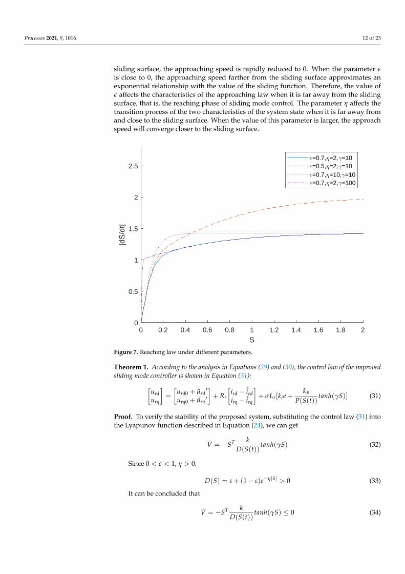
In the sliding mode control system of this study, due to the introduction of integralsliding mode control, the initial state of the system can be located on the sliding surface.Therefore, the design of the approach law should mainly be considered as the suppressionof chattering. Based on the above analysis, the control law is shown by Equation (29):

S(t) = − kD(S(t))

tanh(γS(t))

D(S) = ε + (1− ε)e−η|S|(29)

where 0 < ε < 1, η > 0, and γ > 0, tanh(S) is a hyperbolic tangent function, and itsexpression is shown in Equation (30):

tanh (S) =eS − e−S

eS + e−S (30)

The relationship between the sliding function and its derivative under different pa-rameter values is shown in Figure 7.

It can be known from Figure 7 that the approaching speed of the system is related tothe current value of the sliding function. The larger the value of the sliding function, thefaster the approaching speed. When the state of the system is close to the sliding surface,that is, the sliding function approaches 0, and the properties of the law of approximationapproximate the hyperbolic tangent function. At this time, the characteristics of the systemare basically determined by parameter γ. The hyperbolic tangent function is a continuousodd function. When it is far from the zero point on the positive semi-axis, its functionvalue is approximately 1. When it is close to the zero point, its function value will rapidlydecrease to 0. This characteristic allows the approach law to retain the robustness of thesliding mode control while suppressing chattering. When the parameter ε is close to 1,the characteristic of the law of approximation over the entire state space is similar to thehyperbolic tangent function. That is, when the system state is far from the sliding surface,the approaching speed is approximately constant. When the system state is close to the

Processes 2021, 9, 1016 12 of 23

sliding surface, the approaching speed is rapidly reduced to 0. When the parameter εis close to 0, the approaching speed farther from the sliding surface approximates anexponential relationship with the value of the sliding function. Therefore, the value ofε affects the characteristics of the approaching law when it is far away from the slidingsurface, that is, the reaching phase of sliding mode control. The parameter η affects thetransition process of the two characteristics of the system state when it is far away fromand close to the sliding surface. When the value of this parameter is larger, the approachspeed will converge closer to the sliding surface.

0 0.2 0.4 0.6 0.8 1 1.2 1.4 1.6 1.8 2

S

0

0.5

1

1.5

2

2.5

|dS

/dt|

=0.7, =2, =10=0.5, =2, =10=0.7, =10, =10=0.7, =2, =100

Figure 7. Reaching law under different parameters.

Theorem 1. According to the analysis in Equations (29) and (30), the control law of the improvedsliding mode controller is shown in Equation (31):[

urdurq

]=

[urd0 + urd

′

urq0 + urq′

]+ Rr

[ird − irdirq − irq

]+ σLr[kie +

kp

P(S(t))tanh(γS)] (31)

Proof. To verify the stability of the proposed system, substituting the control law (31) intothe Lyapunov function described in Equation (24), we can get

V = −ST kD(S(t))

tanh(γS) (32)

Since 0 < ε < 1, η > 0.

D(S) = ε + (1− ε)e−η|S| > 0 (33)

It can be concluded that

V = −ST kD(S(t))

tanh(γS) ≤ 0 (34)

Processes 2021, 9, 1016 13 of 23

The equal sign holds if and only if S = 0. Therefore, it can be proved that the proposedsliding mode controller meets the stability requirements.

Taking the current d-axis component as an example, the structure of the proposedinternal model-integral sliding model controller(IM-ISMC) is shown in Figure 8. As wecan see in the figure, in the block diagram of the internal model-integral sliding modelcontroller, an improved approach law has been used on ui. Moreover, the tracking errorcalculation has been used on error e, and the final output is urd.

Figure 8. Description of block diagram of the IM-ISMC.

In summary, by using the IM-ISMC controller instead of the PI controller in vectorcontrol, an IM-ISMC-based floating offshore wind turbine system can be obtained, asshown in Figure 9. As we can see in the figure, an IM-ISMC controller has been used at theback of PI controller. Moreover, the coordinate transformation has been used on PWM andIGBT, and angle calculation has been used at the back of DFIG.

The proposed control system is based on vector control theory. The relationshipbetween the q-axis component of the rotor current and the speed can be better describedby a linear system, and it can be controlled by a PI controller. The relationship betweenthe d-axis component of the rotor current and the reactive power is similar. The current isdecoupled by the IM-ISMC controller.

The proposed control strategy contains many undetermined parameters, which in-clude modulation coefficient α, sliding gain ki, and related parameters of sliding modecontrol law kp, ε, η, and γ. The Grey Wolf Optimization (GWO) will be used to optimizethese parameters.

Grey Wolf Optimization is a meta-heuristic algorithm proposed by Mirjalili of GriffithUniversity [33]. This algorithm is inspired by the hunting behavior and cooperative behav-ior in the hunting process of gray wolves. The gray wolf family has a strict hierarchicalmanagement system. According to leadership, the wolf group can be divided into fourlevels: α, β, δ, and ω.

Processes 2021, 9, 1016 14 of 23

Figure 9. Description of floating offshore wind turbine system based on IM-ISMC.

After obtaining the position of the prey, the gray wolves will surround the prey. Thisprocess can be expressed by Equation (35):{

Dp = |C · Xp(k)− X(k)|X(k + 1) = Xp(k)− A · Dp

(35)

Among them, k is the number of iterations, X(k) is the position vector of the graywolf after performing the kth iteration, Xp(k) is the position vector of the prey afterperforming the kth iteration, A and C are coefficient vectors, and the expressions are shownin Equation (36): {

A = 2ar1 − a

C = 2r2(36)

Among them, r1 and r2 are random numbers in the range of [0,1]. a is a variable thatlinearly decreases with the number of iterations, and its value gradually decreases from 2to 0.

Through the above iterative process, the individual can be redirected to any positionaround the prey. However, this is not enough to reflect the group wisdom in the graywolves. When gray wolves are hunting prey, the higher-level gray wolves play a key role inthis process. After the encirclement process is completed, the gray wolves will hunt under

Processes 2021, 9, 1016 15 of 23

the leadership of wolves with three levels of α, β, and δ. This process can be described bythe following equations:

Dα = |C1 · Xα(k)− X(k)|Dβ = |C2 · Xβ(k)− X(k)|Dδ = |C3 · Xδ(k)− X(k)|

(37)

X1 = Xα(k)− A1Dα

X2 = Xβ(k)− A2Dβ

X3 = Xδ(k)− A3Dδ

(38)

X(k + 1) =X1 + X2 + X3

3(39)

When the process of encirclement and hunting has been completed by the gray wolves,they will attack the prey. This stage is manifested as the convergence of the solution in theprocess of solving the optimization problem.

In the offshore wind power generation system proposed in this paper, a set of pa-rameters satisfying the definition are regarded as feasible solutions, and all combinationsof parameters satisfying the definition constitute the solution space of the optimizationproblem. Using the gray wolf optimization algorithm to search in the solution space, thesub-optimal solution can be obtained in a limited time.

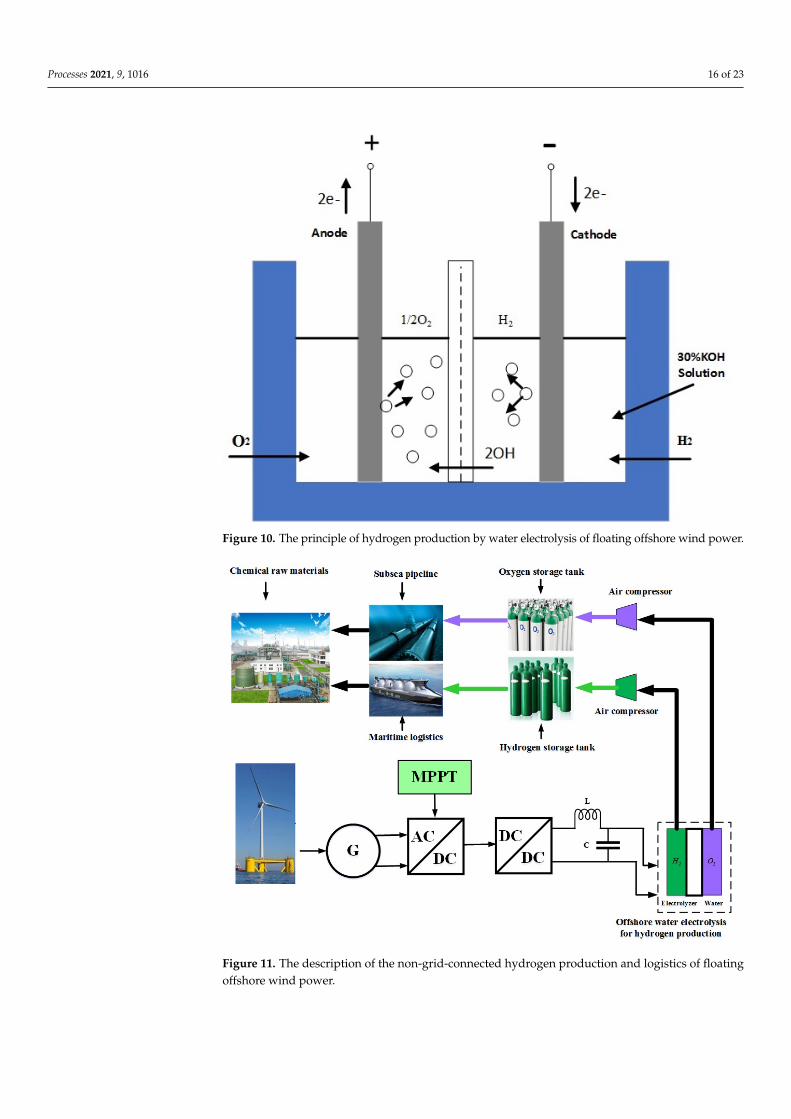
Usually, the basic method of power to gas from floating floating offshore wind poweris using electrolysis of sea water to produce hydrogen. The principle of electrolyzing waterto produce hydrogen is shown in Figure 10. It can be seen from the figure that the loss ofelectrons at the anode produces oxygen, and the electrons at the cathode produce hydrogen.The solution mixed in water increases the conductivity of the electrolyte. That is to say,the electrolysis of water is to immerse the cathode and anode in the electrolytic cell inwater and apply direct current, respectively. The water will be decomposed and producehydrogen at the cathode and oxygen at the anode. The main chemical reaction equationsof the electrode reaction are as follows:

In the water,H2O = H+ + OH− (40)

The point of cathode,4H+ + 4e+ = 2H2 (41)

The point of anode,4OH− − 4e− = 2H2O + O2 (42)

The chemical equation for the overall reaction is:

2H2Oelectrolysis−→ 2H2 + O2 (43)

The industrial experiment intends is to use a megawatt-class floating offshore windturbine and hydrogen production equipment to verify the optimization effect of the controlsystem. From the perspective of the system, concrete floating foundation, offshore wind tur-bine, hydrogen production equipment, the theory, method, and algorithm of this researchcan be verified step by step. At the same time, during the verification process, the floatingoffshore wind power sensing device is used to obtain the real-time status information of theintelligent control operation energy conversion online, and the controller data acquisitiondevice is used to obtain the status information related to the wind power operation and thehydrogen production process. All relevant data are collected and aggregated through thedistributed information network system. The non-grid-connected hydrogen productionand logistics of floating offshore wind power to be used in industrial experiments areshown in Figure 11.

Processes 2021, 9, 1016 16 of 23

Figure 10. The principle of hydrogen production by water electrolysis of floating offshore wind power.

Figure 11. The description of the non-grid-connected hydrogen production and logistics of floatingoffshore wind power.

Processes 2021, 9, 1016 17 of 23

4. Simulation Results

To verify the effectiveness of the proposed controller, MATLAB/Simulink is usedfor simulation verification. The DFIG parameters used in the simulation are shown inTable 1. The values of the parameters in the table are selected with reference to real 2 MWwind turbines.

Table 1. DFIG parameters.

Name Value Unit

Rated power 2000 kWStator voltage 690 VNumber of pole pairs (p) 2Voltage frequency 50 HzStator resistance (Rs) 0.0025 ohmRotor resistance (Rr) 0.003 ohmMutual inductance (Lm) 2.5 mHStator inductance (Ls) 2.51 mHRotor inductance (Lr) 2.51 mHMoment of inertia (J) 120 kg·m2

The effect of the controller is evaluated by testing the response of the control systemat random wind speeds. Considering that the maximum point tracking operation of thefloating offshore wind turbine is between the cut-in wind speed and the rated wind speed,the wind speeds used in the simulation are in the interval from 3 m/s to 12 m/s. It isshown in Figure 12.

Figure 12. Wind speed characteristics.

Figure 13 shows the variation curve of the rotor speed under the random wind speedwhen the proposed controller and PI controller are used. Figures 14–16 are the rotor speedin the intervals of 3 s, 7 s, 7 s, 11 s, and 11 s, 15 s, which are obtained by magnifying thethree parts of Figure 13. Due to the mechanical inertia of the generator, there is a certaindelay between the actual speed and the reference speed. Overall, the proposed controllerhas better dynamic response speed than the PI controller.

Processes 2021, 9, 1016 18 of 23

Figure 13. Simulation results of rotor speed.

3 3.5 4 4.5 5 5.5 6 6.5 7

time(s)

60

80

100

120

140

160

180

roto

r sp

ee

d(r

ad

/s)

reference

IM-ISMC

PI

Figure 14. Rotor speed 3–7 s enlarged view.

Processes 2021, 9, 1016 19 of 23

7 7.5 8 8.5 9 9.5 10 10.5 11

time(s)

80

100

120

140

160

180

200

220

roto

r speed(r

ad/s

)

reference

IM-ISMC

PI

Figure 15. Rotor speed 7–11 s enlarged view.

11 11.5 12 12.5 13 13.5 14 14.5 15

time(s)

100

120

140

160

180

200

220

roto

r sp

ee

d(r

ad

/s)

reference

IM-ISMC

PI

Figure 16. Rotor speed 11–15 s enlarged view.

Figure 17 shows the corresponding reactive power curves of the two controllers. Thereference value of reactive power is 0 W. The proposed controller can converge faster,

Processes 2021, 9, 1016 20 of 23

but the PI controller will oscillate near the equilibrium position. Therefore, the proposedcontroller has better steady-state performance than the PI controller.

Figure 17. Simulation results of reactive power.

Figure 18 shows the simulation results of the power coefficient. The maximum powercoefficient is 0.438 approximately. The proposed controller can adjust the rotor speedaccording to the change of wind speed, so the power coefficient of IM-ISMC controller islarger than PI controller in general. The purpose of the maximum power point tracking is tocapture wind energy as much as possible, and the offshore wind energy power coefficientcan be used as the basis for determining the amount of captured offshore wind energy.This means that floating offshore wind turbine systems can capture more offshore windenergy by using the proposed controller.

Figure 18. Simulation results of power coefficient.

Processes 2021, 9, 1016 21 of 23

Figure 19 shows the different active power between the PI controller and the proposedcontroller. They are obtained by subtracting the active power value of the PI controllerfrom the active power value of the proposed controller. At the beginning of the simulation,the power differential reaches its maximum value of 90 kW or so. In general, the proposedcontroller has higher active power than a PI controller at all times, especially in the time ofthe rotor increasing speed.

0 5 10 15

time(s)

-1

0

1

2

3

4

5

6

7

8

9

active

po

we

r(W

)

104

Figure 19. The active power between the PI controller and the proposed controller.

5. Conclusions

A current decoupling controller is presented for DFIG wind power systems on afloating offshore wind turbine to achieve MPPT. By using the internal model control strat-egy, an internal model open-loop controller is designed to simplify the parameter design.Moreover, the sliding mode control theory is used to achieve dynamic compensation basedon the internal model open-loop controller, whereas the integral sliding mode controlleris used to compensate the output error of the open-loop controller, and the parametersof proposed controller are designed through Gray Wolf Optimization. In addition, theperformance of the controller is verified by testing the response of the controller underrandom wind speed in simulation software. Simulation results show that the proposedcontroller is superior to traditional PI controllers in terms of dynamic response and steady-state error. However, the proposed controller is not implemented on real floating offshorewind turbines. At the same time, how the controller parameters affect the control resultshas not been studied in depth. In future research, it is possible to build an experimen-tal platform to conduct further research on the field of hydrogen production by floatingoffshore wind power.

Author Contributions: L.P.: Conceptualization, Methodology, Software, Data curation, Supervision,Writing—review & editing, Formal analysis, Resources; Z.Z.: Conceptualization, Visualization, Inves-tigation, Software, Validation, Funding acquisition, Project administration; Y.X.; Writing—review &editing, Formal analysis, Resources, Software; J.S.: Visualization, Investigation, Software, Validation,Writing—original draft. All authors have read and agreed to the published version of the manuscript.

Funding: This work was supported by the Foundation of Zhongshan Institute of Advanced Engineer-ing Technology of WUT (Grant No. WUT202001), China. This work was also supported by projectsfrom Key Lab. of Marine Power Engineering and Tech. authorized by MOT (KLMPET2020-01), the

Processes 2021, 9, 1016 22 of 23

Fundamental Research Funds for the General Universities (WUT: 2021III007GX) and Shaoxing CityProgram for Talents Introduction, China.

Institutional Review Board Statement: Not applicable.

Informed Consent Statement: Not applicable.

Data Availability Statement: The study did not report any data.

Acknowledgments: This work was supported by the Foundation of Zhongshan Institute of AdvancedEngineering Technology of WUT (Grant No. WUT202001), China. This work was also supported byprojects from the Key Lab of Marine Power Engineering and Tech authorized by MOT (KLMPET2020-01), the Fundamental Research Funds for the General Universities (WUT: 2021III007GX), and ShaoxingCity Program for Talents Introduction, China.

Conflicts of Interest: The authors declare no conflict of interest.

References1. Chatzinikolaou, S.D.; Oikonomou, S.D.; Ventikos, N.P. Health externalities of ship air pollution at port-Piraeus port case study.

Transp. Res. Part Transp. Environ. 2015, 40, 155–165. [CrossRef]2. Pfeifer, A.; Krajacic, G.; Ljubas, D.; Duic, N. Increasing the integration of solar photovoltaics in energy mix on the road to low

emissions energy system-Economic and environmental implications. Renew. Energy 2019, 143, 1310–1317. [CrossRef]3. Cardenas, R.; Peña, R.; Alepuz, S.; Asher, G. Overview of control systems for the operation of DFIGs in wind energy applications.

IEEE Trans. Ind. Electron. 2013, 60, 2776–2798. [CrossRef]4. Akhbari, A.; Rahimi, M. Control and stability analysis of DFIG wind system at the load following mode in a DC microgrid

comprising wind and microturbine sources and constant power loads. Int. J. Electr. Power Energy Syst. 2020, 117, 105622. [CrossRef]5. Kadri, A.; Marzougui, H.; Aouiti, A.; Bacha, F. Energy management and control strategy for a DFIG wind turbine/fuel cell hybrid

system with super capacitor storage system. Energy 2020, 192, 116518. [CrossRef]6. Xiahou, K.; Liu, Y.; Li, M.; Wu, Q. Sensor fault-tolerant control of DFIG based wind energy conversion systems. Int. J. Electr.

Power Energy Syst. 2020, 117, 105563. [CrossRef]7. Lu, K.; Zhou, W.; Zeng, G.; Zheng, Y. Constrained population extremal optimization-based robust load frequency control of

multi-area interconnected power system. Int. J. Electr. Power Energy Syst. 2019, 105, 249–271. [CrossRef]8. Zeng, G.Q.; Xie, X.Q.; Chen, M.R.; Weng, J. Adaptive population extremal optimization-based PID neural network for multivari-

able nonlinear control systems. Swarm Evol. Comput. 2019, 44, 320–334. [CrossRef]9. Zhang, C.; Zhang, Y.; Shi, X.; Almpanidis, G.; Fan, G.; Shen, X. On Incremental Learning for Gradient Boosting Decision Trees.

Neural Process. Lett. 2019, 50, 957–987. [CrossRef]10. Pan, L.; Wang, X. Variable pitch control on direct-driven PMSG for offshore wind turbine using Repetitive-TS fuzzy PID control.

Renew. Energy 2020, 159, 221–237. [CrossRef]11. Qi, Y.; Liu, Y.; Fu, J.; Zeng, P. Event-triggered L∞ control for network-based switched linear systems with transmission delay. Syst.

Control. Lett. 2019, 134, 104533. [CrossRef]12. Qi, Y.; Liu, Y.; Niu, B. Event-Triggered H∞ Filtering for Networked Switched Systems With Packet Disorders. IEEE Trans. Syst.

Man Cybern. 2019, 51, 2847–2859. [CrossRef]13. Hamed, Y.S.; Aly, A.A.; Saleh, B.; Alogla, A.F.; Alharthi, M.M. Nonlinear Structural Control Analysis of an Offshore Wind Turbine

Tower System. Processes 2020, 8, 22. [CrossRef]14. Chen, Z.; Wang, X.; Kang, S. Effect of the Coupled Pitch–CYaw Motion on the Unsteady Aerodynamic Performance and Structural

Response of a Floating Offshore Wind Turbine. Processes 2021, 9, 290. [CrossRef]15. Mozayan, S.M.; Saad, M.; Vahedi, H.; Fortin-Blanchette, H.; Soltani, M. Sliding mode control of PMSG wind turbine based on

enhanced exponential reaching law. IEEE Trans. Ind. Electron. 2016, 63, 6148–6159. [CrossRef]16. Bossoufi, B.; Karim, M.; Lagrioui, A.; Taoussi, M.; Derouich, A. Observer backstepping control of DFIG-Generators for wind

turbines variable-speed: FPGA-based implementation. Renew. Energy 2015, 81, 903–917. [CrossRef]17. Yang, B.; Yu, T.; Shu, H.; Dong, J.; Jiang, L. Robust sliding-mode control of wind energy conversion systems for optimal power

extraction via nonlinear perturbation observers. Appl. Energy 2018, 210, 711–723. [CrossRef]18. Kazmi, S.M.R.; Goto, H.; Guo, H.J.; Ichinokura, O. A novel algorithm for fast and efficient speed-sensorless maximum power

point tracking in wind energy conversion systems. IEEE Trans. Ind. Electron. 2010, 58, 29–36. [CrossRef]19. Pan, L.; Shao, C. Wind energy conversion systems analysis of PMSG on offshore wind turbine using improved SMC and Extended

State Observer. Renew. Energy 2020, 161, 149–161. [CrossRef]20. Li, M.; Xiao, H.; Pan, L.; Xu, C. Study of Generalized Interaction Wake Models Systems with ELM Variation for Off-Shore Wind

Farms. Energies 2019, 12, 863. [CrossRef]21. Colombo, L.; Corradini, M.; Ippoliti, G.; Orlando, G. Pitch angle control of a wind turbine operating above the rated wind speed:

A sliding mode control approach. ISA Trans. 2020, 96, 95–102. [CrossRef]

Processes 2021, 9, 1016 23 of 23

22. Laina, R.; Lamzouri, F.E.Z.; Boufounas, E.M.; El Amrani, A.; Boumhidi, I. Intelligent control of a DFIG wind turbine using a PSOevolutionary algorithm. Procedia Comput. Sci. 2018, 127, 471–480. [CrossRef]

23. Youness, E.M.; Aziz, D.; Abdelaziz, E.G.; Jamal, B.; Najib, E.O.; Othmane, Z.; Khalid, M.; Bossoufi, B. Implementation andvalidation of backstepping control for PMSG wind turbine using dSPACE controller board. Energy Rep. 2019, 5, 807–821. [CrossRef]

24. Xiong, L.; Li, P.; Wang, J. High-order sliding mode control of DFIG under unbalanced grid voltage conditions. Int. J. Electr. PowerEnergy Syst. 2020, 117, 105608. [CrossRef]

25. Abolvafaei, M.; Ganjefar, S. Maximum power extraction from wind energy system using homotopy singular perturbation andfast terminal sliding mode method. Renew. Energy 2020, 148, 611–626. [CrossRef]

26. Mbukani, M.W.K.; Gule, N. Evaluation of an STSMO-based estimator for power control of rotor-tied DFIG systems. IET Electr.Power Appl. 2019, 13, 1871–1882. [CrossRef]

27. Han, Y.; Ma, R. Adaptive-Gain Second-Order Sliding Mode Direct Power Control for Wind-Turbine-Driven DFIG under Balancedand Unbalanced Grid Voltage. Energies 2019, 12, 3886. [CrossRef]

28. Nguyen, T.T. A Rotor-Sync Signal-Based Control System of a Doubly-Fed Induction Generator in the Shaft Generation of a Ship.Processes 2019, 7, 188. [CrossRef]

29. Asghar, A.B.; Liu, X. Estimation of wind turbine power coefficient by adaptive neuro-fuzzy methodology. Neurocomputing 2017,238, 227–233. [CrossRef]

30. Dai, J.; Liu, D.; Wen, L.; Long, X. Research on power coefficient of wind turbines based on SCADA data. Renew. Energy 2016,86, 206–215. [CrossRef]

31. Mohammadi, E.; Fadaeinedjad, R.; Moschopoulos, G. Implementation of internal model based control and individual pitchcontrol to reduce fatigue loads and tower vibrations in wind turbines. J. Sound Vib. 2018, 421, 132–152. [CrossRef]

32. Nayeh, R.F.; Moradi, H.; Vossoughi, G. Multivariable robust control of a horizontal wind turbine under various operating modesand uncertainties: A comparison on sliding mode and H∞ control. Int. J. Electr. Power Energy Syst. 2020, 115, 105474. [CrossRef]

33. Mirjalili, S.; Mirjalili, S.M.; Lewis, A. Grey wolf optimizer. Adv. Eng. Softw. 2014, 69, 46–61. [CrossRef]