YNT~

INSTRAW @>(.<()

VALUATION OF HOUSEHOLD PRODUCTION

AND THE SATELLITE ACCOUNTS

Copyright - 1996 (INSTRAW) All rights reserved

Printed in the Dominican Republic English: 1996-1,000 INSTRAW/SER.B/52 ISBN 92-1-127053-7 Sales No. E.96.ill.C.4

Desktop composition and design: Jeannette Canals

Cover: Design Ninon Leon de Saleme Printed at Amigo de/ Hogar

TEAM FOR THE PREPARATION OF THE REPORT:

Programme Officer Corazon P. Narvaez (INSTRAW)

Consultants Andrew S. Harvey Meena Acharya

VALUATION OF HOUSEHOLD PRODUCTION

ANDTHE SATELLITE ACCOUNTS

9(2) UNITED NATIONS

INTERNATIONAL RESEARCH AND TRAINING INSTITUTE

FOR THE ADVANCEMENT OF WOMEN

ONSTRAW)

SANTO DOMINGO, DOMINICAN REPUBLIC

1996

I I

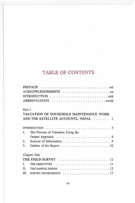
TABLE OF CONTENTS

PREFACE .............. ... ............. xvi ACKNOWLEDGEMENTS .. ............ .. .. ... xx INTRODUCTION . . . . ...................... xxii ABBREVIATIONS ................. .. ..... xxviii

Part I VALUATION OF HOUSEHOLD MAINTENANCE WORK AND THE SATELLITE ACCOUNTS, NEPAL . ...... 1

INTRODUCTION . . . . . . . . . . . . . . . . . . . . . . . . . . . . . 3 1. The Process of Valuation Using the

Output Approach . . . . . . . . . . . . . . . . . . . . . . . . 6 2. Sources of Information . . . . . . . . . . . . . . . . . . . . . 9 3. Outline of the Report . . . . . . . . . . . . . . . . . . . . . . IO

Chapter One

THE FIELD SURVEY .... . . ..... ..... .... ... 11 I. THE OBJECTIVES . ... ..........• ...... ...• 11 Il. THE SAMPLE DESIGN . . . . . . . . . . . . . . . . . . . ... 12

III. SURVEY INSTRUMENTS ..................... 17

vii

IV. LIMITATIONS ...•• .• •..• •• .• ••. .• .• .• •.• 21

Chapter Two SURVEY FINDINGS I. GENERAL CHARACTERISTICS OF THE

SAMPLE POPULATION • ...........• • ....... • 23 II. ACTIVITY CLASSIFICATION AND TIME USE . . • . • . . . . . 31 III. TIME ALLOCATION . . . . • • •• ............ • .•• 35

Chapter Three DEVELOPMENT OF NORMATIVE VALUES .. ... . . 39 I. MEAL PREPARATION . . .........•••...... . • • 39

II. THE PROCESS OF CALCULATION . •.. ..... ....••• 42 III. OTHER ACTIVITIES . . . . . . . . . . . . . . . . . . . . • . • • 46

Chapter Four

GDP AND THE HOUSEHOLD MAINTENANCE SATELLITE ACCOUNTS ....... . . . . . .. .. .. ... 51 I. GENDER CONTRIBUTION TO REGULAR GDP •......... 51 II. ADDITIONAL GDP AND WOMEN'S CONTRIBUTION ..... . 54 III. HOUSEHOLD MAINTENANCE WORK AND THE

SATELLITE ACCOUNT ..... . ................ 55

IV. WOMEN'S CONTRIBUTION TO TOTAL

PRODUCTION . . . . . . . . • . . . • . . . . . . . . . . . . . . 58

Chapter Five

EVALUATION OF THE METHODOLOGY APPLIED . . ... ......... .... . . ........... 63 I. THE SURVEY . . . . . . . . . . . . . . . . . .. . . .•. ... 63

II. APPLICABILITY OF THE THEORETICAL

FRAMEWORK AND RECOMMENDATIONS FOR

THE FUTURE . . . . . . . . • • • . . . . . . • . . . . ..... 67

viii

REFERENCES ............................. 73 ANNEXES .... ..... .. . ....... ..... . .. .. ... 75

A List of Products Prepared in Sample Households . . . . . . . . . . . ............ 77

B Subsidiary Tables

B.1 Gross Value Added at Factor Cost and Labour Force by Industry . . . . . . . . . . . . . . . . 83

B.2 Average Time Input by Adult Population on Conventional and

Subsistence Economic Activities . . . . . . . . . . . . . . . 84 B.3 Population by Place of Residence . . . . . . . . . . .... 85 B.4 Average Hours of Household

Maintenance Work per Day by Place of Residence and Sex . . . . . . . . . . . . . . . . . . . . . . 86

B.S Population 10 Years Old and Above . . . . . . . . . . . . 87

C , Survey Questionnaire . . . . . . . . . . . . . . . . . . . . . . 89

D Frequency Distribution from Files A, B, and C . . . . . . . . . . . . . . . . . . . . 98

Part 2 A MACRO APPROACH TO VALUING HOUSEHOLD OUTPUTS: CANADA AND FINLAND . . 103

INTRODUCTION .... . ...... . .............. 105

Chapter One VALUING UNPAID WORK 109 I. APPROACHES TO THE MEASUREMENT AND

VALUATION OF HOUSEHOLD OUTPUT ... . .•• .•. .• 109

ix

1. The Input Approach . . . . . . . . . . . . . . . . . . . . . 109 2. The Output Approach . . . . . . . . . . . . . . . . . . . . 111

Chapter Two TOWARD AN OUTPUT-BASED VALUATION OF HOUSEHOLD PRODUCTION . . . . . . . . . . . . . . . . . 115 I. CATEGORIES OF HOUSEHOLD OUTPUT . . . . . . . • . . . 115 II. THE OUTPUT MEASURE OF HOUSEHOLD

OUTPUT: METHODOLOGY ........................ 122

Chapter Three PREVIOUS OUTPUT-ORIENTED STUDIES OF HOUSEHOLD PRODUCTION ... ...... ... .. 131 I. THE FINNISH HOUSEWORK STUDY ...... .. . . .. . . 131 II. DETERMINING THE VALUE OF UNPAID

HOUSEWORK ... . .. ..... ....... ........ 132 1. Meal Preparation . . ..... ....... ...... .. . 132 2. Cliild Care ....... ........... ... .. . ... 134 3. House Cleaning . ... . ............. ... ... 135 4. Special Care .......... . ...... . . ... ... . 136 5. Laundry . .......... . ................. 136 6. Handicrafts .. ............ . ........ . ... 137 7. Fitzgerald/Wicks Study ................... 137 III. MEASUREMENT AND VALUATION

USING INPUT-OUTPUT TABLE:

FINLAND 1992 . . . . . . . . . . . . . . . . . . . . . . . . . . 144

Chapter Four

OUTPUT ESTIMATES OF VALUE ADDED BY HOUSEHOLD PRODUCTION: CANADA AND FINLAND ... ......... . .. . .... 151 1. Time-Use Data ..... . .......... . . . ..... 151 2. Family Expenditure Data . . . ........ .. ..... 153

x

3. File Linking ................ . ......... 157 I. CANADIAN HOUSEHOLD OUTPUTS .... . ......... 158 A. SATELLITE ACCOUNTS ACTIVITIES AND

OUTPUT VALUATION . .. ................... 158 1. Meal Preparation . . . . . . . . . . . . . . . . . . . . . . . 158 2. Child Care . . . . . . . . . . . . . . . . . . . . . . . . . . . 169 3. Housekeeping . . . . . . . . . . . . . . . . . . . . . . . . . 171 4. Clothing Care (Laundry) ................... 175 5. Volunteerism ..... . . ......... . .... . .... 178 6. Personal Development .................... 179 B. CANADIAN UNPAID WORK: AN OVERVIEW ......... 183

Data Strengths and Weaknesses ........... ... 184

II. FINNISH HOUSEHOLD OUTPUTS ............... 186 A. SATELLITE ACTIVITIES AND

OUTPUT VALUATION .................... . . 186 1. Meal Preparation ....................... 186 2. Child Care ........................... 189 3. Housekeeping . . . . . . . . . . . . . . . . . . . . . . . . . 192 4. Clothing Care (Laundry) ................... 194 B. FINNISH UNPAID WORK: AN OVERVIEW .... ... .... 198

Comparison of Estimates . . . . . . . . . . . . . . . . . . 198 III. COMPARISON OF FINNISH AND

CANADIAN ESTIMATES . . . . . . . . . . . . . . . . . . . . 201 IV. A GENDER PERSPECTIVE ON PRODUCTION . . . . . . . . . 203

REFERENCES ............ .. .. . .......... . 209 ANNEX .. ............ ........... ....... 217

CONCLUSIONS AND OBSERVATIONS .. ......... 227

xi

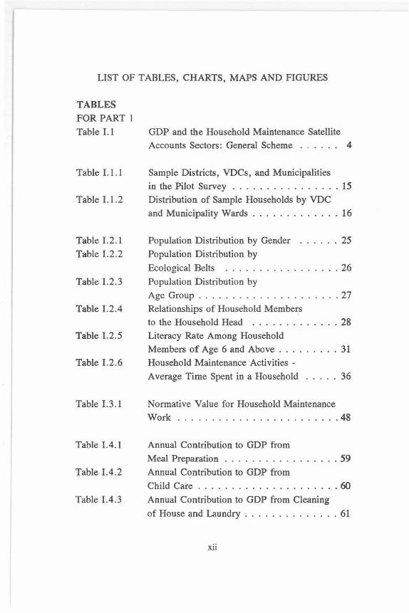
LIST OF TABLES, CHARTS, MAPS AND. FIGURES

TABLES FOR PART 1

Table 1.1

Table 1.1. l

Table 1.1.2

Table 1.2.l Table 1.2.2

Table 1.2.3

Table 1.2.4

Table 1.2.5

Table 1.2.6

Table 1.3.l

Table 1.4.1

Table 1.4.2

Table 1.4.3

GDP and the Household Maintenance Satellite Accounts Sectors: General Scheme . . . . . . 4

Sample Districts, VDCs, and Municipalities in the Pilot Survey ... . . ........... 15 Distribution of Sample Households by VDC and Municipality Wards ..... ..... . . . 16

Population Distribution by Gender Population Distribution by Ecological Belts . . . . . .

Population Distribution by

. . 25

. 26

Age Group . . . . . . . . . . . . . . . . . . . 27 Relationships of Household Members to the Household Head . . . . . . . . . . . . 28 Literacy Rate Among Household Members of Age 6 and Above . . . . . . 31 Household Maintenance Activities -Average Time Spent in a Household . . . . . 36

Normative Value for Household Maintenance Work .. . ..................... 48

Annual Contribution to GDP from Meal Preparation . . . . . . . . . . . . . . . . . 59 Annual Contribution to GDP from Child Care . . . . . . . . . . . . . . . . . . . . . 60 Annual Contribution to GDP from Cleaning

of House and Laundry .............. 61

xii

Table 1.4.4

FOR PART 2

Table 11.2.1

Table 11.2.2

Table II. 3 .1 Table 11.3.2

Table 11.3.3

Table 11.3.4

Table 11.3.5

Table 11.3.6

Table 11.3.7

Table 11.3.8

Table 11.4.1

Table 11.4.2

Table 11.4.3

Table 11.4.4

Gender Contribution to GDP and Household Maintenance . . . . . . . . . . . . . . . . . . . . 62

Types of Household Production . . . . . . . 116

Characteristics and Content of Household Work ................ 119.

Time-Use Data, Finland 1979 . .. . . ... 133

Finnish Housework Study, 1982 .... ... 133

Mean Annual Values of Household Production ..... . .... . ......... 138

Quality of Household Production

Compared with Quality of Equivalent Available in Market . . . . . . . . . . . . . . 140 Mean Annual Values of Household Production for Various Types of Adult Members of Household . . . . . . . . 141

Members of Household by Number of Children . ...... . . ............ 143

Households by Age Measured by the Direct Output Approach . . . . . . . . . . . . 143

Input-Output Table for Household Activities . . . . . . . . . . . . . . . . . . . . . 146

Characteristics of Time Use and

Expenditure Data ......... ... .... 155

Daily Meals by Time and Location . .. . . 161

Estimated Meals Per Household Per Year . . . . . . . . . . . . . . . . . . 163

Output Derivation of VHW for Meal Preparation Based on Market Price . . . . . 166

xiii

Table 11.4.5

Table 11.4.6

Output Derivation of VHW for Meal Preparation Based on Expansion of Purchased Inputs . . . . . . . . . . . . . . . . 168 Output Derivation of VHW for Family (Child) Care ....... . . .. ..... . 172

Table 11.4. 7 A Estimated Person/Nights per

Household per Year . . . . . . . . . . . . . . 173 Table II.4. 7B Housekeeping Related to RME . . . . 174

Table 11.4.8

Table 11.4.9

Table II.4.10 Table 11.4.11

Table 11.4.12

Table 11.4.13

Table 11.4.14

Table 11.4.15

Table 11.4.16 Table 11.4.17

Table 11.4.18

Table II.4.19

Table II.4.20

Table II.4.21

Output Derivation of VHW for Housekeeping Based on Market Price Output Derivation of VHW for

176

Clothing Care Based on Market Price 177 Non-Outlay Costs of Education ....... 182 Output Derivation of VHW for Unpaid Work Based on Market Price . . . . 185 Output Derivation of VHW for Meal Preparation Based on Market Price Purchased Inputs (RME)-Meal

Preparation . .............. . Output Derivation of VHW for

188

189

Child Care Based on Market Price ..... 191 Output Derivation of VHW for Housekeeping Based on Market Price . . . 193 Purchased Inputs (RME)-Housekeeping 194 Output Derivation of VHW for Clothing Care Based on Market Price ... 196 Output Derivation of VHW for Unpaid

Work Based on Market Price ... .

Comparison of Finnish and Canadian

197

Estimates . . . . . . . . . . . . . . . . . . . . 202 Gender Division of Time Allocation to Unpaid Work .......... ...... 204 Gender Division of Unpaid Work Time . . 207

xiv

CHARTS Chart 1.1.1

Chart 1.2.1

Chart 1.2.2

MAPS Map 2.1 Map 2.2

FIGURES Figure 1

Figure 11.4.1

Average Time for Completion of a Questionnaire . . . . . . . . . . . . . . . . 20 Sample Population by Socio-Economic Variables . .. . .. . .. . .. ... 24 Literacy Status by Age and Gender . . . . . . 30

District of Nepal . . . . . . . . . . . . . . . . . 13

Study Sample Districts .. . .... . . . ... 14

SNA-Based Activity Classification Framework, INSTRA W Time Use Measurement and Unpaid Work Project xxiii

Segmentation Analysis of Meals at Home or Other Residence .. .... . .. 159

xv

PREFACE

The need to account for unpaid

household production has moved from the realm of "it would

be nice", to the realm of "how do we do it?" This is clearly

the message delivered over the last few years in national and

international fora and in the 1993 revision of the System of

National Accounts (SNA). The call to account for household

production has become sufficiently consistent and impelling.

Arguments against the need and desirability of properly and

officially accounting for it are becoming less frequent. The

call has come from both lay groups and practitioners. It was

clearly echoed at the recently held Fourth World Conference

on Women in China (1995) and the Platform for Action

specifically defined the need to "seek to develop a more

comprehensive knowledge of work and employment through,

inter alia, efforts to measure and better understand the type,

extent and distribution of unremunerated work, and encourage

the sharing and disseminatio11 of information on studies and experience in this field, including the development of methods

for assessing its value in quantitative terms, for possible

reflection in accounts that may be produced separately from,

but consistent with, core national accounts". 1

In 1983, INSTRAW, convened a consultative meeting

with a group of eminent economists to analyze women's

position in the world economy. The conclusions of this

meeting which were later published in Women and the World

Economy (1985) emphasized the need to improve the subordi­nate position of women in the economy. They stressed the

importance of making women's social and economic contribu­

tion visible in statistics and indicators that measure the wealth

and productivity of a nation. Increasingly attention is being

directed towards the means of doing so. Estimates of the

value of household production have by now been developed

in a number of countries. Ten years after the first experience,

in 1992, INSTRAW launched a long-term programme

designed to develop methods of collecting and analyzing data

to measure and value paid and unpaid work as well as

methods for ensuring that they are properly reflected in the

national accounts . As first result of the above long-term

programme in 1995, a monograph Measurement and Valua­

tion of Unpaid Contribution: Accounting through Time and

Output was published based on the results of the initial

research conducted in several countries (Canada, Dominican

1 United Nations Department of Public Infonnation, Platfonnfor Action, and the Beijing Declaration, 1996, p. 119.

xviii

Republic, Hungary, Nepal, Tanzania, and Venezuela). In the monograph, a framework for the classification of activities

was recommended on the basis of which, a "satellite account on household production" could be established. The strengths

and weaknesses of various methods of time-use data collection and techniques for valuing unremunerated work taking into

account the structure and objectives of the System of National

Accounts (SNA), are also discussed.

The present report, Valuation of Household Production and the Satellite Accounts, is a sequel to the Measurement and Valuation monograph. It explores approaches to the develop­ment of output measures of "satellite accounts" on household

production and pr~sents some original output-based valuations

in Canada, Finland, and Nepal using the above-mentioned

framework. The selection of these three countries was primarily based on 1) availability and quality of time-use and

other collateral data collected at the national level [from developed and developing countries]; 2) accessibility to these

data; and 3) availability of local expertise who could carry out

the study. The primary objective of this exercise was to assess

the viability of achieving a common understanding and

agreement on the framework and methods for measurement

and valuation of unpaid work and its reflection in economic

indicators through "satellite accounts".

The results and conclusions contained in this report, besides identifying measurement and valuation problems,

make recommendations to help reach this goal. However, it

must be noted here that this is just part of a long-term project

in progress. Hence, potential users of this report which

xix

include statisticians, economists, researchers, development

planners and policymakers are encouraged to forward their

substantive observations and comments on the report to

INSTRAW.

The completion of the remaining part of this project and

the full realization of its primary objectives, i.e., to fully

recognize women's contribution to society, will undoubtedly

draw a great deal from those comments and suggestions.

Acting Director

xx

ACKNOWLEDGEMENTS

INSTRA W wishes to thank the following for their support to this project and publication:

the Government of The Netherlands for the funds made available to the project;

the Time-Use Research Programme (TURP) of Saint Mary's University, Halifax, Nova Scotia, Canada and the Institute for Integrated Development Studies (IIDS), Kathmandu, Nepal, for their substantive and administra­tive support to the implementation of the case studies in Canada/Finland and Nepal, respectively;

Mr. Arun K. Mukhopadhyay for his assistance to the preparation of the report of the case studies in Canada and Finland;

Ms Luisella Goldschmit-Clermont for her invaluable comments and suggestions on the preliminary results of the valuation exercises, and

Dr. Krishna Ahooja-Patel and Dr. Surendra Patel for their generosity in sharing their expertise and time to further enrich the text.

Ms Jeannie Ash de Pou for editing and proofreading the manuscript.

The comments and s·uggestions received from individual experts who attended the INSTRAW Panel on Time-Use Statistics and Recognition of Women's and Men's work, at the NGO Forum in China during the Fourth World Confer­ence on Women on 30 August 1995, have also been useful in the final preparation of this report.

xxii

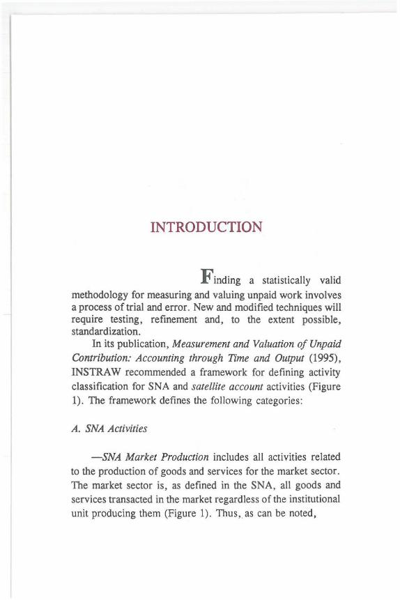
INTRODUCTION

Finding a statistically valid

methodology for measuring and valuing unpaid work involves a process of trial and error. New and modified techniques will require testing, refinement and, to the extent possible, standardization.

In its publication, Measurement and Valuation of Unpaid Contribution: Accounting through Time and Output (1995), INSTRA W recommended a framework for defining activity classification for SNA and satellite account activities (Figure 1). The framework defines the following categories:

A. SNA Activities

-SNA Market Production includes all activities related to the production of goods and services for the market sector. The market sector is, as defined iri the SNA, all goods and services transacted in the market regardless of the institutional unit producing them (Figure 1). Thus , as can be noted,

...-1

~ :::3 bl)

ii:

SNA Based Activity Classification Framework INSTRAW, Time-Use Measurement and Unpaid Work Project

I ACTIVITIES I

I SNAActivities

I I HousdJOldS.Ctors

Non-household Sectors I

I I Non-SNA Activities I Non-Market Production

I

Non-financial Oxporations ] MARKET PloaxJcnoN - own use prcxiuction ProrucDon ol goods and services for sole by -11naociaJ oorporatio~ Government & NPISHs* I -Non-financial corporalioas Goods supplied free or at -Oovcmm<:1111 NPISHs non-sigruficant pnces

I Production o( Goods - Production and and Scniccs for the iwocessing of primary Market by Hausd>olds products foc own use

- Production of o<her goods for own use

- Production off1Xed assets for own use

I Current SNA Accounts J All Goods and SNA Services

- - --

• Non-profit institutions serving households, based on Table 6.1, 1993 SNA

I H oosaiot.0 M AlrmNA.NCE - Meal preparation - Housework - Shopping - Repair services - Financia1 services - Related travel

CAAJNG

- Child Ci!Ie

- Elder Ci!Ie

- Others - Relakdtravel

P8saHAl DEVaOPME><T - Elk:alion - Skill dcvclopmcm - Rdatcdtravel

I -v <x.u>mnING

Household Satellite Accounts

Non-SNA Services

I

I

I PERSONAL MAINTENANCE - Sle<p - Eat - Wash, toilet - Medical care of self - Relakd travel

I

PERSONAL ~TION - Media - Games - Socializing - Sports - Walking - Attendance events - Relall:dtravel

Non-SN A Non-Satellite

Accounts

market output emanates from activities of financial corpora­tions including private enterprises , non-financial corporations, governments, non-profit institutions serving households , and the households themselves.

-SNA Non-market Production also covers the non­market activities currently included in the SNA. These include goods and services produced for own use by non-financial corporations, governments and non-profit institutions. And it includes, from the household standpoint, the inputed value of home ownership, goods consumed in kind, etc. (Figure 1). It also includes-as a result of the 1993 revision-all goods production whether sold in the market or not. It includes, for example, the production/storage of agricultural and related products; other primary products, the processing of agricul­tural and related products , and other kinds of processing such as cloth and dress making, etc.

B. Non-SNA Activities

Non-SN A activities are comprised of two distinct sets of services. One set consists of service activities that can be relegated tQ another person and thus can be traded in the market. The other set consists of services that cannot be relegated to others but must be done for oneself. The former should thus be accounted for in an overall accounts frame­work, through the construction of satellite accounts.

-Satellite account activities should include household maintenance activities, caring activities, personal development and volunteering, as proposed by INSTRAW and as reflected in Figure 1. Household maintenance includes meal prepara-

xxv

tion, household cleaning, domestic and repair services, time attending to financial services (includes banking and paying bills), legal services, etc. Caring activities carried out by the household include people-related tasks done for others, primarily for children and the elderly. INSTRA W argues that in addition to the foregoing, the satellite account should also include personal development (education) of those receiving education. Volunteering essentially involves activities under­taken with no or minimal pay for another institutional unit. In essence, volunteering is the household equivalent of govern­ment and non-profit institution outputs provided at an insig­nificant price.

-Non-satellite activities fall into two major groups: personal maintenance and personal recreation-defined by the 'recipient criterion', which simply put says that activities that 'cannot be received for another' are non-tradeable and thus should be considered consumption rather than productive activities. Thus, watching TV, eating, sleeping, etc., would fall outside the SNA and the satellite accounts proposed by INSTRAW.

The use of the output-based approach for valuing unpaid activities was also recommended and illustrated in the Measurement and Valuation of Unpaid Contribution: Account­ing through Time and Output.

Following these recommendations, the Institute conducted three case studies in 1995, using data from Canada, Finland, and Nepal, to test the viability of output-based valuation tech­niques to establish satellite accounts on household production and the gender division of production using time-use data. These case studies are merely intended to test the feasibility of the recommended framework, test techniques for estab-

xx vi

lishing satellite accounts and identify measurement issues and problems. They were not undertaken to produce an accurate account.

It was clearly emphasized in an earlier publication of INSTRA W (1995) that, in order to implement the output­based valuation approach, a combination of data from different sources would be required. Some new auxiliary data would also have to be collected to define certain norms such

as prices , units of measurement used in specific activities and the volume and value of inputs applied to produce certain outputs . The case study in Nepal represented a scenario where such norms had to be determined through collection of new data. For Canada and Finland, however, the valuation was conducted using existing secondary data.

For the case study conducted in Nepal , the valuation exercise included not only the production of satellite accounts on household production but also an estimation of the value of the "other goods and services produced for own consump­tion". The latter are technically within the SNA production boundary but have been consistently left out in the accounting process due to lack of data.

The satellite accounts for Nepal include household maintenance activities such as cooking, cleaning, laundry, caring, dishwashing, mending, and similar activities. To impute values to these activities or their equivalent outputs, some new auxiliary data had to be collected in order to develop normative values for each kind of activity. This report describes the development of these normative values based on a small-scale survey and their application to an existing time-use data set which was generated from a national survey conducted in 1984/1985 (Nepal Multipurpose House­hold Budget Survey).

xx.vii

The satellite accounts do not include, however, the categories related to gaining an education, and volunteer work due to a lack of statistical information which could only be collected through a more comprehensive time-use survey.

Similarly, the studies of Canada and Finland were designed to test the feasibility of developing macro estimates of output measures using large-scale time-use data and collateral data from existing data sources such as establish­ment or industry data. While some difficulties were encoun­tered, such an approach is clearly feasible for developing estimates for, at least, some of the components of unpaid work with existing data. Estimates of other components, while apparently feasible, will require that attention be paid to one or more problems related to definition and measurement. For example, a reasonable value for volunteer work and education were estimated for Canada using existing data. However, due to lack of data, estimates of the value of unpaid educational activity or volunteer work could not be derived for Finland.

As in the case of Nepal, in both Canada and Finland women account for the major share of the unpaid work. Their shares are approximately 67 and 69 per cent, respectively , based on time allocations to unpaid activities.

xx viii

CH AID

CMA

CREST

FAMEX

FIM GDP

GNP

GSS

HES

INSTRAW

LFS

MPHBS

RME

SNA

TUS

VA

VDC

VHO

ABBREVIATIONS

Chi-square based Automated Interactive Detector

Census of Metropolitan Area

Canada Research on Statistics

Canadian Family Expenditure Survey

Finnish Markka

= Gross Domestic Product

Gross National Product

General Social Survey

Household Expenditure Survey

United Nations International Research and Train­

ing Institute for the Advancement of Women

Canadian Labour Force Survey Nepal Multipurpose Household Budget Survey

= Raw materials and energy

= System of National Accounts

Finnish Time-Use Survey

Value added

Village Development Committee

Valuation of Household Outputs

Part 1

VALUATION OF HOUSEHOLD MAINTENANCE WORK

AND THE SATELLITE ACCOUNTS

NEPAL2

Meena Acharya

2 In collaboration with the Institute for Integrated Development Studies (IIDS) , Kathmandu, Nepal.

INTRODUCTION

Fol lowing previously presented SNA-based framework for activity classification, a tentative structure for a complete account of human productive activi­ties disaggregated by sex is developed for Nepal and is presented in Table 1. Part I of this table contains GDP generated in the market sector, and Part II contains the imputed value of non-market products. Currently, GDP statistics include all market production and part of the non­market production. Major components of the non-market production, which enter GDP are comprised of imputed values of own-account agricultural products and self-occupied housing. According to the revised manual of SNA (1993), future GDP statistics shall include imputed values of addition­al non-market products which include all goods produced for own consumption, such as agricultural products generated from own backyards, fuel-wood and water collected for home use, by-products of secondary processing, and the like.

3

TABLE l.l GDP AND THE HOUSEHOLD MAINTE,NANCE

SATELLITE ACCOUNTS SECTORS: GENERAL SCHEME

Sections/Sectors Male Female Total

I. FORMAL/ORGANIZED SECTOR 1. Agriculture 2. Manufacturing 3. Electricity, Gas and Water 4. Construction 5. Trade & Commerce 6. Transport, Communic. & Storage 7. Finance & Business 8. Community, Social & Pers. Serv.

SUB-TOTAL

II. INFORMAL/OWN ACCOUNT SECTOR 1. Agriculture 2. Manufacturing 3. Electricity, Gas and Water 4. Construction 5. Trade & Commerce 6. Transport, Communic. & Storage 7. Finance & Business 8. Community, Social & Pers. Serv.

SUB-TOTAL

ill. HOUSEHOLD MAINTENANCE 1. Subsistence 2. Child care 3. Other Services

SUB-TOTAL

IV. EDUCATION

GRAND TOTAL

4

The problem, nevertheless, lies in capturing all such products . Particularly in countries which are at an early stage of development such as Nepal , subsistence production consti­tutes a large part of total household resources. But, much of this is left out of GDP statistics due to the scattered nature of the activities and a lack of reliable methods for accurate estimations (Acharya, 1994) .

The issue as to how much and how many of such products are included in GDP is specific to each country and needs to be examined within the country context. Due to cost and time limitations, this issue has not been covered in detail in this study. An ad-hoc method based on the proportion of time input in conventional economic and subsistence economic activities has been used to derive estimates of what is left out of the non-market products in current GDP statistics of Nepal. Conventional economic activities include agriculture, produc­tion, trade and commerce, services, and construction. Subsis­tence economic activities include fuel/fodder collection, fetching water, house repair and construction (own use), hunting, and gathering and processing food.

The focus of the current study is on household mainten­ance activities. Despite recognition that the division of activities as productive and non-productive is tenuous and that a more accurate measurement of human activities is desirable (SNA, 1993), household maintenance activities still remain outside the boundary of SNA. The major arguments advanced for the exclusion of these activities from SNA boundary are lack of data and difficulty of measurement as well as lack of historical comparability. Nevertheless, SNA does not exclude the possibility of constructing satellite accounts through the development of innovative measurement techniques and the collection of additional data.

5

To make such an account comparable to those of other products included in SNA, it is necessary to develop and devise a product-based valuation system. The current study has been designed specifically to test such a methodology.

1. The Process of Valuation using the Output Approach3

The following steps for the valuation of production and services for non-market (within SNA) and household mainte­nance (non-SNA) activities were recommended.

a) Generating large scale (national) time-use data for all activities.

b) Generating output data for a much smaller sub-sample from the same group.

c) Deriving values for time input on the basis of this smaller sample, in order of preference as listed below:

i) Output value derived from the price of comparable or equivalent market product. For comparable products which are for the market as well as for home consumption, valuation is not a serious problem. For example, food may be cooked for part sale and part domestic use. In such cases, the part that is consumed domestically should be valued at the same price of the part which is sold.

ii) Net return to labour, exclusive of intermediate inputs used in market-oriented activities performed

3 This chapter is extracted from the INSTRA W publication Measure­ment and Valuation of Unpaid Contribution: Accounting through Time and Output, (1995).

6

by the household and similar or even identical to domestic activities, e.g., cooking for self and cooking for other households.

iii) Net return to labour in other comparable non-mone­tary productive activities for which output related valuations can be performed. For example, if a per­son devotes two hours to child care (a type of service done exclusively for own children), this time may be valued at net average returns to her Jabour input in other activities, the products of which are sold.

iv) Wages ofpolyvalent household workers (inclusive of income in kind) adjusted for skill level and mana­gerial responsibilities.

The process of output-based valuation, thus, requires: (a) an estimate of the household output; (b) an estimate of the intermediate consumption; and (c) determination of the market prices to be used for the conversion of physical volumes of outputs and inputs.

The steps for' output-based valuations which would provide an approximate total figure of household production for comparison with what is included in the SNA and an estimate of women's contribution to the total productive process in the society would be:

Step 1 Estimating women's contribution to Regular GDP on the basis of available information on male/female earnings (if available), male/female labour force and gender-disaggregated wage rates.

Step 2 Estimating SNA included output generated in the household e.g., kilograms of paddy, vegetables,

7

fruits and similar goods; number of mats, carpets; kilograms of milk, meat, wool, etc. This is neces­sary primarily for two reasons: (a) most of the food and other processing activities are continuous with pre-cooking domestic processing, and to capture such processing, a careful recording is necessary at least to develop norms; and (b) since the SNA still retains a caveat that if the products generated in the household are not important for a country's econo­my they may be ignored, it is first crucial to collect data on all products so that a decision on their significance can be taken. Situations in each country may warrant some variation on the details of activity and product listing, but the process remains the same. All products and activities must be listed.

Step 3 Estimating the volume of household output in the various domestic activities, e .g., number of meals cooked, number of older persons and children cared for, quality and contents of the meals, quality and frequency of child-care activities, etc.

Step 4 Valuing this product at the market price of products when they are sold in part. When they are not sold, the prices of equivalent goods and services produced in the market may be used. Where this is not possible, wage-based methods may be used as discussed above.

Step 5 Deducting intermediate consumption of both market­purchased and home-produced goods valued at market prices of equivalent goods to derive the

8

value added within the household sec;tor. One should be careful to avoid double counting. This process should be carried out for each product category separately. If outside labour is employed in the process of generating this value added, the costs of employing such labour must be deducted at this stage in order to derive the value added by the household members . Payments to outside labour must also be disaggregated by gender, in order to derive gender disaggregated wage income from the household sector.

Step 6 Allocating the value, thus calculated, to various members of the household according to their respec­tive labour inputs in production of various goods and services. This labour input must also include time devoted to management.

The analysis followed in this chapter, however, starts with the third step i.e., estimation of volume of products and services generated by household maintenance activities . Own account SNA-included products are not being covered by the present survey . This presents several difficulties in the application of a product-based valuation system to household maintenance activities as proposed above which are discussed in chapter five of this document.

2. Sources of Information

The study will use both primary as well as secondary information. The source of primary data is the pilot survey conducted in eight different districts of Nepal which is

9

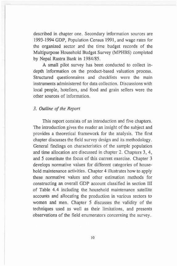
described in chapter one. Secondary information sources are 1993-1994 GDP, Population Census 1991, and wage rates for the organized sector and the time budget records of the Multipurpose Household Budget Survey (MPHBS) completed by Nepal Rastra Bank in 1984/85.

A small pilot survey has been conducted to collect in­depth information on the product-based valuation process. Structured questionnaires and checklists were the main instruments administered for data collection. Discussions with local people, hoteliers, and food and grain sellers were the other sources of information.

3. Outline of the Repon

This report consists of an introduction and five chapters. The introduction gives the reader an insight of the subject and provides a theoretical framework for the analysis . The first chapter discusses the field survey design and its methodology . General findings on characteristics of the sample population and time allocation are discussed in chapter 2. Chapters 3, 4, and 5 constitute the focus of this current exercise. Chapter 3 develops normative values for different categories of house­hold maintenance activities. Chapter 4 illustrates how to apply these normative values and other estimation methods for constructing an overall GDP account classified in section III of Table 4.4 including the household maintenance satellite accounts and allocating the production in various sectors to women and men. Chapter 5 discusses the validity of the techniques used as well as their limitations, and presents observations of the field enumerators concerning the survey.

10

Chapter One THE FIELD SURVEY

I. THE OBJECTIVES

The pilot survey was conducted to evaluate the practicability of the product-based valuation method to identify reasonable means of resolving the difficul­ties involved in its implementation. Subsequently, the field survey was carried out to generate information on:

a) output data, i.e., products generated in the households, (what, how frequently, how much, etc.);

b) volume and prices of inputs involved in each product; c) time and labour used to produce the products, i.e.,

contribution by whom and how much; d) market price for all products and services generated by

household maintenance activities.

11

II. THE SAMPLE DESIGN

Primarily, the survey was an attempt to collect auxiliary information required to adapt the valuation techniques described earlier. The survey was carried out in eight districts of Nepal (see Map 1 and Map 2). Even though the study could not draw a representative sample at a national level, attempts were made to provide reasonably representative random samples. One district from each of the five Develop­ment Regions and three Ecological Belts4 were selected so as to capture both the geographical and ecological variations (see Map 1 and Map 2). Special attention was paid to ensuring the inclusion of rural and urban samples. A total of 276 house­holds was surveyed, drawing a sample of 26 from each municipality and 18 from each VDC selected from the sample districts. Two wards from each municipality as well as from each VDC in the sample were chosen by the interviewers themselves. Nine households from each VDC, except for the municipality of Dasharathachand in which two extra house­holds were interviewed, and thirteen households from each municipality ward were selected. Because the data collected from the two additional households were considered to be consistent with the remainder of the cases, they were, there­fore, kept in the analysis.

To simplify the selection of households and at the same time follow the scientific sampling techniques, the total number of households of a sample ward was divided by the total number of households to be interviewed in that ward.

4 Nepal is divided in three Ecological Belts, five Development Regions, and 75 Districts. The 75 Districts comprise of 3 ,995 villages-termed as Village Development Committees (VDCs)-and each VDC is divided in 9 wards. Similarly, there are 36 municipalities having from 9 to 34 wards.

12

FAR WESTERN REGION

LEGE N D .......... -....... ,. .. --• Co,., . ........

0 ,_ ~~

50

DISTRICT MAP OF NEPAL

SCALE 0 50

Kilometre~

II'::')

CH IN A

IND I A

WESTERN REGION

~-----·~·-..,/\ / KA1HMAl<lU _.,,> ~ ·--·" /------!

,.,... ... • /~.Alt.Jtj I 1 '-... ,, ,:;... J r i..:Wj "'~/ : \ )

) ! i :.....; (

( "1 \:- ~ ~-~·--..\ ........

z 0

)>

~ .§ ,_.

N

~ ~

FAR WESTERN REGION

LEGEND

~ bd

CH IN A

MOUNTAIN HIU

TARAI

NEPAL

STUD Y SAMPLE DISTRICTS

C H IN A

SCALE

50 0 so 100

Kilometrtu

z 0

)>

v .....

This resulted in a number showing the sampling interval between two households to be selected. For the first inter­view, a household was chosen at random. After the random start, the next household was the one located at the sampling interval derived from the above calculations. Other households were located in a similar manner.

The detailed information on sample sites and sample distribution are featured in Tables 1.1. l and 1.1.2 respectively.

TABLE 1.1.1 SAMPLE DISTRICJ'>S, VDCs, AND MUNICIPALITIES IN

THE PILOT SURVEY

Development Mountain Hill Tarai Region Areas* Areas Areas

1. Eastern Dhankuta(D) Morang(D) Dhankuta(M) Biratnagar(M) Belhara(V) Tankisinuwar(V)

2. Central Kathmandu(D) Chitwan(D) Kathmandu(M) Bharatpur(M) Kapan(V) Gitanagar(V)

3. Western Baglung(D) Laharepipal(V)

4. Mid-Western Banke(D) Nepalgunj(M) Paraspur(V)

5. Far-Western Jumla(D) Baitadi(D) Dillichaur(V) Dasharathachand(V)

D = District, M = Municipality, V = Village Development Committee (VDC)

*) Mountain region has no urban areas i.e. , municipalities.

15

TABLE I.1.2

DISTRIBUTION OF SAMPLE HOUSEHOLDS BY VDC AND

MUNICIPALITY WARDS

VDC/ Average Num. of Num. of Num. of Municipality Number of Wardf HouselwltU HouselwltU

Ho1_43eholdf Selected per Ward Selected

VILLAGE DEVELOPMENT

COMMITTEES

1. Belhara 97 2 9 18

2. Tankisinuwar 227 2 9 18

3. Kapan 98 2 9 18

4. Gitanagar 233 2 9 18

5. Laharepipal 55 2 9 18

6. Paraspur 67 2 9 18

7. Dillichaur 48 2 9 18

8. Dasharathachand 58 2 10 20

MUNICIPALITIES

1. Dhankuta 404 2 13 26

2. Biratnagar 1093 2 13 26

3. Kathmandu 2318 2 13 26

4. Bharatpur 780 2 13 26

5. Nepalgaunj 484 2 13 26

TOTAL 26 276

Source: Population of Nepal by Districts, Village Development Committees/ Municipalities, CBS 1991 Census, 1994.

16

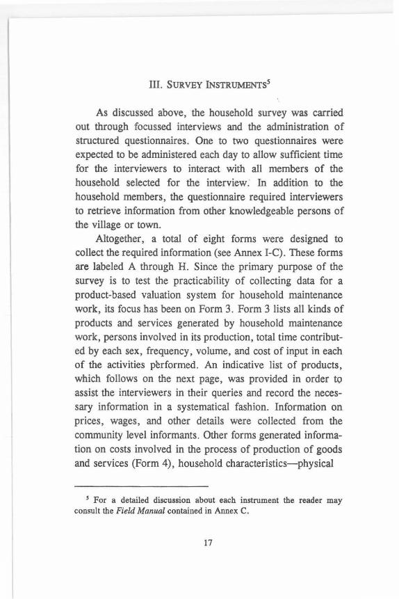
Ill. SURVEY INSTRUMENTS5

As discussed above, the household survey was carried out through focussed interviews and the administration of structured questionnaires. One to two questionnaires were expected to be administered each day to allow sufficient time for the interviewers to interact with all members of the household selected for the interview: In addition to the household members, the questionnaire required interviewers to retrieve information from other knowledgeable persons of the village or town.

Altogether, a total of eight forms were designed to collect the required information (see Annex 1-C). These forms are labeled A through H. Since the primary purpose of the survey is to test the practicability of collecting data for a product-based valuation system for household maintenance work, its focus has been on Form 3. Form 3 lists all kinds of products and services generated by household maintenance work, persons involved in its production, total time contribut­ed by each sex, frequency, volume, and cost of input in each of the activities p~rformed. An indicative list of products, which follows on the next page, was provided in order to assist the interviewers in their queries and record the neces­sary information in a systematical fashion. Information on prices, wages, and other details were collected from the community level informants. Other forms generated informa­tion on costs involved in the process of production of goods and services (Form 4), household characteristics-physical

5 For a detailed discussion about each instrument the reader may consult the Field Manual contained in Annex C.

17

AN INDICATIVE LIST OF PRODUCTS

TAKEN FROM FORM 3

1. MEAL PREPARA110N

Tea Lentils Rice (Bhat) Vegetable Curry Pickle (Chat) Meat Chapa tis Boiled Eggs Porridge

3. FUEL

Wood Kerosene Electricity Gas

5. CARE Child Elderly Sick

7. EDUCA110N

Personal Education Teaching children within the household

2. CLEANING

Room Washing Clothes Sweeping yard/patio Garden Bathroom/Toilet Drainage

4. TRANSPORTA110N

Market School/Office Temples

6. FINANCIAL SERVICES

Bank Loan Repayment

8. OTHER

Mending Gardening Carrying water Social services etc.

Note: Activities performed by domestic servants were excluded, since their services should already be included in regular GDP ac­counts.

18

and socio-economic (Form 7), and demographic variables (Form 2).

Information from the rest of the forms facilitated cross­checking and enabled related calculations for Form 3. Thus, Form 3 was designed to record all the household maintenance work for a product-based valuation system. Activities were listed in column 2. Similarly, the total amount of products/ services generated at the household was recorded in column 5. The household production cost of each item was calculated separately in Form 4 and the corresponding per unit cost placed in column 6. Another important variable recorded in Form 3 (column 11) was the time input in each activity. Thus, all the inputs necessary for the valuation of household maintenance activities were recorded in Form 3. Only the information on market prices was collected from the commu­nity level institutions such as hotels, shops, and other knowl­edgeable people. Collecting price information from each and every household was found to be rather impractical.

Form 5 was designed to record information for calculat­ing the depreciation cost. In particular, the price of utensils, the cost involved in repair and services, and the total duration (years) of their use were recorded.

-Average Time for Completion of a Questionnaire . More than 91.3% of the interviews were completed in one visit. The average time for completing an interview was 145 minutes (about 2.5 hours) with 47 minutes standard deviation. The interview time increased proportionally with the level of illiteracy of the interviewee and underdevelopment of the area. This is more clearly illustrated in Chart I.1.1.

19

M

N

u

T

E

s

M

N

u

T

E

s

Chart I.1 .1

Average Time for Completing a Questionnaire By Urban/Rural

200 - - -

180 - -160 - -

. 140 - -

120 - -

100 -

80 - -

60 -

40 -

20 - -

URBAN RURAL

Average Time for Completing a Questionnaire By Ecological Belt

200 -

180 -

160 - -140 -

120 - -

100 - -

80 - -

60 - -40 -

20 - -

MOUNTAIN HILL TARA!

20

IV. LIMITATIONS

The survey has limitations in that it attempts to gather and impute market prices to goods which have not undergone common market transactions. It argues that such imputations can be made because similar imputations are made for many items which enter SNA, e .g., value of self-consumed agricul­tural products, self-owned housing, etc. The household sector makes large contributions to the human reproduction process and complements the market sector. For this reason, and to simplify matters, the study has focussed on the development of a methodology for valuation of household maintenance work rather than· determining the exact value of household products.

The survey was not designed to represent the national sample but an attempt has been made to include samples covering most of the heterogeneous factors that influence the division of labour between the sexes. Similarly, the urban/ rural division of sample does not reflect national proportions.

In rural areas, the concept of time varies greatly. In addition, exact measurements of quantities cooked could not be made, as households used different informal units of measurement such as glass and bowls for daily cooking. Goods produced for home consumption and those for market also differ substantially in quality. Home produced goods have always been regarded as of better quality than those sold in the market. What is captured, then, is only the minimum value of comparable products. A further complication derived

from the open-ended questions has further diversified the responses .

21

Chapter Two

SURVEY FINDINGS

I. GENERAL CHARACTERISTICS OF

THE SAMPLE POPULATION

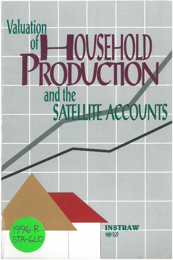
The survey was designed to include sample households from all geographical and ecolo­gical regions of Nepal, and from both urban and rural areas. As the type, quality, and time in performing a particular activity may also depend on the economic status and ethnicity of the households, these factors have also been taken into account when designing the survey. However, for sampling purposes, households were stratified only on the basis of geographical, ecological, and residential parameters. Most of the general socio-economic factors influencing the activity pattern are expected to be represented by such a classification (see Chart I.2.1).

23

Chart I.2.1 SAMPLE POPULATION BY Soc10/ECONOMIC v ARIABLES

FEMALE 4 9 . 4 %

RU R A L 5 2 . 9 %

GENDER

RESIDENCE

L 0 W 2 0 . 7

ECONOMIC STATUS

24

M A L E 5 0 . 8 %

U R B A N 4 7 . 1 %

MEDIUM 7 4 . 6 %

Three parameters, namely Gender (male and female), Residence (urban and rural), and Economic Status (high, medium, and low), are assumed to play key roles in the composition and distribution of the household maintenance activities. The information on key variables is presented below to highlight the coverage of the sample population.

-Gender. The sample population is about equally distributed among males and females. This composition is very close to the 1991 national census statistics (see Table I.2.1).

Gender

Male Female

TABLE I.2.1 POPULATION DISTRIBUTION BY GENDER

(In per cent)

Study Sample

50.6 49.4

N (Household members) 1,733

Census 1991

49.9 50.1

18,491,097

-Residence. The national figure for urban population is only 9. 2 per cent. But, since this survey was designed to contain sufficient number of households from urban areas to facilitate the analysis, the proportion of urban households is 47.1 per cent in the study sample. Normative values, have been derived separately for rural and urban areas.

-Economic Status. The economic status, as perceived by the interviewer has been reported. Visits to the household, hours of interaction with the household members, and the reported assets and income are subject to the interviewers'

25

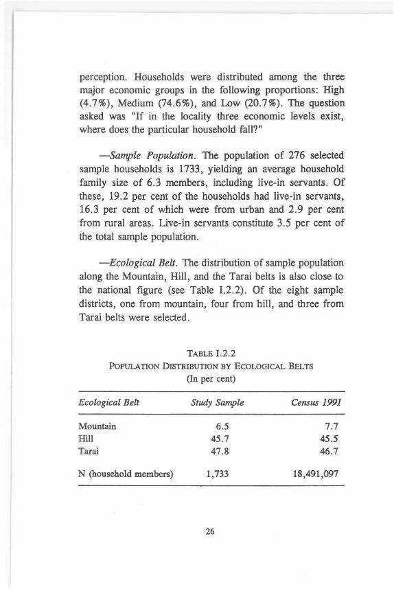
perception. Households were distributed among the three major economic groups in the following proportions: High (4.7%), Medium (74.6%), and Low (20.7%). The question asked was "If in the locality three economic levels exist, where does the particular household fall?"

-Sample Population. The population of 276 selected· sample households is 1733, yielding an average household family size of 6.3 members, including live-in servants. Of these, 19.2 per cent of the households had liv~-in servants, 16.3 per cent of which were from urban and 2.9 per cent from rural areas. Live-in servants constitute 3.5 per cent of the total sample population.

-Ecological Belt. The distribution of sample population along the Mountain, Hill, and the Tarai belts is also close to the national figure (see Table 1.2.2). Of the eight sample districts, one from mountain, four from hill, and three from Tarai belts were selected.

TABLE l.2.2 POPULATION DISTRIBUTION BY ECOLOGICAL BELTS

(In per cent)

Ecological Belt Study Sample

Mountain 6.5 Hill 45.7 Tarai 47.8

N (household members) 1,733

26

Census 1991

7.7 45.5 46.7

18,491,097

-Age Distribution. Division of sample population in various age groups as reflected in Table I.2.3 follows the Multipurpose Household Budget Survey of Nepal Rastra Bank (survey conducted in 1984/85). The contribution to household maintenance work of children between six and nine (6-9) years of age, particularly in rural areas, is significant. This group is separately classified so as to capture their contribu­tion to household maintenance activities.

TABLE 1.2.3 POPULATION DISTRIBUTION BY AGE GROUP

(In per cent)

Age Completed Study Group (years) Sample

Less than one year 2.0 1 - 5 9.2 6 - 9 9.5

10 - 14 14.5 15 - 25 23.3 26 - 50 30.5 51+ 11.0

Census 1991

3.1 15.0 11.7 12.6 20.7 26.9 10.0

N (household members) 1,733 18,491,097

-Relationship to Household Head. Besides gender it is important to cover activities of all other members in the households as they carry differential work burdens. For example, the role of daughters-in-law is crucial in a Hindu society as they are the ones who carry the major burden of the household work.

27

TABLE 1.2.4 RELATIONSHIPS OF HOUSEHOLD MEMBERS

TO THE HOUSEHOLD HEAD (In per cent)

Relationship to

Household Head Total Male Female

Household Head 15.9 14.6 1.3 Spouse 14.4 0.1 14.3 Daughter/Son 42.1 25.6 16.5 Daughter-in-law 6.6 6.6 Grand-Daughter/Son 11.7 5.6 6.1 Mother/Father 1.7 0 .2 1.5 Mother/Father-in-law 0 .1 0.1 Sister/Brother 1.8 1.4 0.4 Niece/Nephew 0.9 0 .7 0.2 Not a Relation 0 .2 0 .1 0.1 Live-in-Servant 3.5 1.5 2 .0 Others 1.1 0.5 0.6

N (household members) 1,733 877 856

Contributions made by the live-in servants are already included in the national accounts and, hence, their share in different household activities and products generated therein has been excluded from current calculations. Live-in servants were found in 53 households, of which 45 were from urban areas. The distribution of population by relationship to the household head is featured in Table 1.2.4.

-Education. The census figure for literate population in Nepal is 39.3 per cent whereas only 24.7 per cent females

28

are literate. The study sample contains more than proportion­ate literate population (Chart 1.2.2 and Table 1.2.5). This is understandable as the sample is disproportionately skewed towards urban areas.

29

Chart 1.2.2 LITERACY STATUS BY AGE AND GENDER

Literacy Status by Age Group and Gender/MALE

p 100 -89 89.2

90 -E

80 -

R 70 -

60 - -c

so - -

E 40 - -

30 - -N

20 - -

T 10 - -

6 - I 4 I 5 +

Literacy Status by Age Group and Gender/FEMALE

p 100 -

90 - -E

2'5.f 80 -

R 70 -

60 - - - I - - _57) - -c

E 40 - -

30 -N

20 -

T 10 - -

6 - I 4 I 5 +

I - I LL ITER ATE c::::::.::J LITERATE

30

TABLE 1.2.5 LITERACY RATE AMONG HOUSEHOLD MEMBERS OF

AGE 6 AND ABOVE

(In per cent)

Sex Study Census Sample 1991

Male 78.8 54.l Female 55.0 24.7 All 67.1 39.3

N (Households) 1,733 18,491,097

II. ACTIVITY CLASSIFICATION AND TIME USE

Activities found in the sample households are categorized in 17 different types of household maintenance work, and sub-classified in 132 sub-activities (see Annex I-A).

1. Meal Preparation

All activities performed in relation to meal preparation fall within this category. This includes all types of dishes prepared and the activities performed in preparing them such as washing or cutting vegetables, etc. A total of 92 products were generated by these activities . These have been listed in Annex I-A.

2. Cleaning of Kitchen and Dishes

This covers activities such as washing the dishes and mopping kitchen areas, mud plastering kitchen, etc. This has

31

been separated from other cleaning activities because, it is felt that time spent on such activities should be combined with cooking for valuation purposes.

3. Fuel Collection

Any activity performed to provide fuel for the household is listed under this category. Types of fuel encountered were wood, kerosene, gas and/or electricity. Time might have been spent in the collection of fuel wood or buying kerosene or gas cylinders from the market. Similarly, paying the electricity bill or drying cow dung for fuel also consumes one's time. Time spent in all of these types of activities is put under this category.

4. Water Collection

Water collection is one of the major activities in house­holds, particularly in rural areas. Although, according to the revised manual this activity is to be included in SNA, in Nepal this remains outside the national accounts. Time dedicated to this activity is directly related to meal prepara­tion and therefore should be combined with meal preparation time for valuation purposes.

5. Shopping

Time spent on going to the market for shopping and buying goods for the household use are recorded under this category.

32

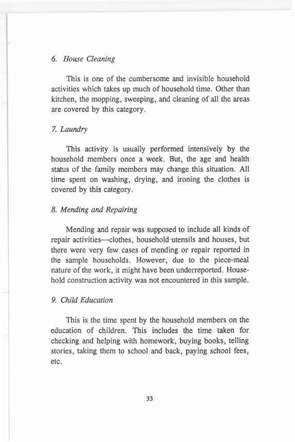
6. House Cleaning

This is one of the cumbersome and invisible household activities which takes up much of household time. Other than kitchen, the mopping, sweeping, and cleaning of all the areas are covered by this category.

7. Laundry

This activity is usually performed intensively by the household members once a week. But, the age and health status of the family members may change this situation. All time spent on washing, drying, and ironing the clothes is covered by this category.

8. Mending and Repairing

Mending and repair was supposed to include all kinds of repair activities-clothes, household-utensils and houses, but there were very few cases of mending or repair reported in the sample households. However, due to the piece-meal nature of the work, it might have been underreported. House­hold construction activity was not encountered in this sample.

9. Child Education

This is the time spent by the household members on the education of children. This includes the time taken for checking and helping with homework, buying books, telling stories, taking them to school and back, paying school fees, etc.

33

10. Child Care

Caring for children involves many activities such as cleaning and washing them, watching and playing with them, feeding them, etc.

11. Elder Care

This is also a major time-consuming activity and, hence, is categorized separately. This includes time spent on care of elderly people at home.

12. Sick Care

This category includes time spent for caring at home and accompanying the sick to the health post/hospital, etc. How­ever, on the day of interview, very few cases with sick persons were found.

13. Self Travel

Time consumed in travelling is recorded under this category. Such travel may be to school, office, field, reli­gious places, etc.

14. Personal Development

Personal development plays an important role in human lives. Therefore, any activity performed towards that is considered to be productive and the time spent on it is recorded separately. Personal development could be related to education or skill. These, however, have not been valued in the current analysis due to lack of data.

34

15. Religious Activities

In a religious country like Nepal, this activity plays an important role and takes up much of household time. It covers items such as visits to the religious places, worship­ing, picking leaves for plates, making leaf plates, making cotton swabs and other materials for oil lamps used in wor­ship, etc.

16. Social Services

Social services include activities such as helping other members of the community, attending social gatherings, labour contribution to community work, etc.

17. Other Household Work

All other household maintenance activities, besides the ones mentioned above, were included in the category 'other'. Each activity in this group was encountered only in a few cases.

III. TIME ALLOCATION

Thus all together a total of 132 household maintenance activities (products/services) were observed in 276 sample households, which were later classified into 17 major groups. Time spent per day (hours) by the households on 17 different activities in urban and-rural areas is presented in Table 1.2.6 below. This information has also been extracted from Form 2.

35

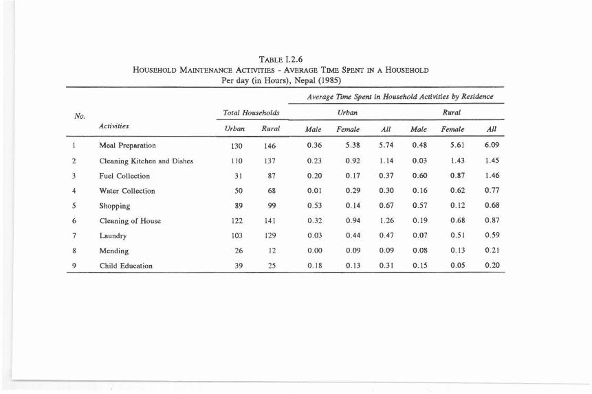
TABLE 1.2.6 HOUSEHOLD MAINTENANCE ACTIVITIES - AVERAGE TIME SPENT IN A HOUSEHOLD

Per day (in Hours), Nepal (1985)

Average Time Spenl in Household Activities by Residence

No. Tora/ Households Urban Rural

Activities Urban Rural Male Female All Male Female All

Meal Preparation 130 146 0.36 5.38 5.74 0.48 5.61 6.09

2 Cleaning Kitchen and Dishes 110 137 0.23 0.92 1.14 0.03 1.43 1.45

3 Fuel Collection 31 87 0.20 0 . 17 0.37 0 .60 0.87 1.46

4 Water Collection 50 68 0.01 0 .29 0.30 0.16 0 .62 0.77

5 Shopping 89 99 0.53 0 .14 0.67 0.57 0.12 0.68

6 Cleaning of House 122 141 0.32 0.94 1.26 0.19 0.68 0.87

7 Laundry 103 129 0.03 0.44 0 .47 0.07 0 .51 0.59

8 Mending 26 12 0 .00 0 .09 0 .09 0.08 0 . 13 0.21

9 Child Education 39 25 0 . 18 0 .13 0 .31 0. 15 0 .05 0 .20

TABLE 1.2.6: HOUSEHOLD MAINTENANCE ACTNITIES ... (CONT.)

Average Time Spenr in Household Activities by Residence

Toral Households Urban Rural

No. Activities Urban Rural Male Female All Male Female All

10 Child Care 37 58 0.18 1.22 1.40 0.28 1.64 1.92

11 Elder Care 5 2 0.02 0.07 0.09 0.00 0.02 0.02

12 Sick Care 3 0 0.04 0.04

13 Self Travel 28 22 1.35 0.13 1.48 0.52 0 .06 0.58

14 Personal Development 49 51 1.16 0.86 2.01 0.71 0.29 1.00

15 Religious Activities 38 31 0.02 0.19 0.22 0. 12 0 .14 0.26

16 Social Services 11 13 0 .06 0.05 0. 12 0.10 0.01 0 . 10

17 Other Household Work 70 65 0.09 0.07 0.16 0.10 0.00 0 .1 1

Chapter Three DEVELOPMENT OF

NORMATIVE VALUES

The data reported on Form 3 of the survey questionnaire (see Annex I-C) was used for the calculation of norms, i.e., monetary value of products or services generated per unit of time spent on each category of household maintenance activities. All products and services generated within the household, input costs involved, time required and volume as well as prices of products generated were recorded on this form as discussed in chapter one.

I. MEAL PREPARATION

Output from meal preparation involved an extremely complicated list of 92. products. Service categories were valued at wage rates and did not present many problems. For

39

meal preparation, various activities had to be regrouped to derive total time input in preparation of meals which needed to be comparable to that available in the market. The product 'meal' which is available in the market is an end product of an activity chain-shopping, cleaning, cooking, servicing, etc.

Moreover, the meal price in the market also includes costs involved in cleaning table , dishes, kitchen, etc. Theoret­ically, the time involved in collecting water for cooking, washing dishes and kitchen, etc. , should also be included under meal preparation. But no information on various other uses of collected water were recorded. Hence, all water collection time enters as a time input in meal preparation. However, in the present calculation, water collection has been included in SNA non-market activities . This represents some double counting which is assumed to be minimum.

Similarly, shopping time could not be estimated separate­ly for food and non-food items. Therefore, it has been assumed, on an ad-hoc basis, that 80 per cent of the shopping time is devoted to food purchases. People in urban areas shop for food items everyday both because they lack purchasing power for lump-sum amounts and also because very few people have refrigerators to preserve fresh food. Besides, fresh vegetables are the major elements of daily purchases. In rural areas food items purchased may be much smaller since many of them are produced at home. But shops and markets involve longer travel time due to the distances to be covered.

As such, to create a category of time input spent on meal preparation comparable to that available in the market, the total time spent on cooking meals, cleaning of kitchen and dishes, collection of fuel and water, and shopping had to be

40

added. This time was calcµlated from column 11 in Form 3. These time records had to be slightly modified to account for cooking two meals a day. Form 3 recorded the time required to prepare each item at a time. Product records were for the day. For meals which are cooked twice a day, this time had to be multiplied by two.

The calculation of total inputs involved in the production of goods and services generated by household maintenance activities was made directly from columns 5 and 6 of Form 3. A few items, however, need specific discussion. Sample households were found to use gas, electricity, kerosene as well as firewood, husk, and cow-dung for preparing meals. Usually, in rural areas people use firewood which they collect from the nearby forest. In such cases the norm value can be estimated by imputing value to the time spent for fuel collec­tion. On the other hand, for the estimation of fuel consump­tion of those households which do not go for firewood collection themselves and find it profitable to buy fuel from the market, the cash expenditure on fuel was also recorded.

In the case of urban households, the average fuel con­sumption was cakulated on the basis of expenditures in those households which spent money on fuel consumption. On the average, each household consumed fuel worth Rs 2.006 per hour of cooking time. Additionally, in urban areas the time spent on other fuel related activities namely, bill payments or kerosene buying, the charge for transporting the gas cylinders to home, etc., were also included. In the case of rural areas, the only major input involved was the time spent on fuel­wood collection. Total fuel-related time, therefore, enters the

6 1US$ = 56.80 Rs (Rupees) at the time the study was conducted.

41

value calculation as time input, i.e., added to the total time involved in meal preparation in calculation of returns to time.

The average depreciation cost per hour use of household utensils is calculated from Form 5, where the parameters for calculating the depreciations have been recorded. Here the basic assumption made is that the depreciation of household utensils for all sizes or quality is the same. Initially, attempts were made to record the depreciation cost of each pot used

for a specific purpose. For example, as the kettles are used for tea preparation, the depreciation cost of kettles was calculated separately so that it could be added to the cost of making a glass of tea. But it was found that people use different utensils to prepare tea. While kettles also may be used for other purposes. Irrespective of what a particular pot's intended use is, it is used in the kitchen for multiple purposes. Hence, the calculation of an overall depreciation cost of household utensils as a single unit was found to be more practical and appropriate. Further, this value could be calculated only in terms of hours of use. The average depre­ciation cost per hour use of household utensils is calculated at Rs 0.07.

II. THE PROCESS OF CALCULATION

Form 3 is the main source of information for calculating the value added. In this form, the average market price for each product and service was recorded as discussed in chapter one. Per-unit price and per-unit household production cost were multiplied by the total volume of products generated in each household. The difference of the sum of such series gives the first approximation of value added. This value

42

minus total depreciation and fuel costs is the net value added generated in the household.

The following formula has been used to calculate the normative values.

x~ J

pl

• C11 =

Total volume of product j, generated in household h.

Market price of product j .

Per unit amount of inputi, used in the production of product j, in household h.

Price of input i.

Total depreciation cost of household utensils for a day.

Total value added in the Survey Households = H

LY11

lt- 1

where H = 276

Value added per hour of work in meal preparation is calculated as

where t is time spent by member l on activity k.

k = 1.. ... .5 (five activities, i.e., cooking, kitchen and dish cleaning, fuel collection, water collection, and shopping.)

l = 1 ...... L (individual members)

43

Normative values for the urban households are calculated below according to the above formula.

The total market value of the products generated in the sample households in a day was equal to Rs 133272.50. This total was derived by summing up the series of values o~tained by multiplying column (5) for urban households in Form 3 by the respective product prices.

Total household input cost (except fuel) equals Rs 76403. This figure was derived by multiplying the per unit cost in column 6 in Form 3 by the amount of products generated in the household and totalling the values thus obtained.

Total time used for the preparation of meal in 130 urban households per day was derived from column 11 of Form 3. The time in Form C was recorded in minutes which has been converted into hours as given below:

1. Cooking 1,175.92 2. Kitchen and dish cleaning 148.20 3. Time spent on fuel related activities 48.10 4. Water collection 39.00 5. Shopping (80%- of the total) = 69.68

Total time (hours) for meal preparation = 1,480.90

From those sample households who were paying bills for electricity or gas or kerosene, the average expense for per hour of fuel consumption/energy use was calculated at Rs 2. As the total cooking time is 1, 17 5. 92, the cost for total fuel consumed in the urban households was estimated at Rs 2,352.

The depreciation cost (Form 4) is calculated at Rs 0.07 per hour. Therefore, the total value of depreciation for all the

44

urban households is Rs 82.31. Thus, the value of household time per hour spent on meal preparation in urban areas is:

{133,272.50 - (76,402.92 + 2,351.84 + 82.31)} I 1,480.90 = (133,272.50 - 78,837.07) I 1,480.90

54,435.43/1,480.90 Rs 36.76/hour

The calculations for rural households follow a similar procedure. Accordingly, the total market value of the prod­ucts generated for the rural sample households in a day equals Rs 82,306.75.

Total household production cost equals Rs 50, 699 .19. Total time used for the preparation of meals in 146 rural

households (in hours):

1. Cooking 1,375.56 2. Cleaning Kitchen and dishes = 211.70 3. Fuel collection 213 .16 4. Water collection 112.42 5. Shopping (80 % of total) 79.42

Total time (hours) for meal preparation 1,992.26

For the rural sample households only the time for collec­tion of fuel has been considered. Only one or two rural households were found to be spending cash on fuel. There­fore, no cash cost of energy has been deducted from the production cost in rural areas .

Total depreciation cost for rural households is Rs 96.29. Thus, the value of per unit time spent on the meal

preparation in rural areas is:

45

{82306.75 - (50699.19 + 96.29)} I 1992.26 (82306.75 - 50795.48) I 1992.26 31511.27 I 1992.26 Rs 15.82 I hour

The quality and the unit of production services produced in the household are assumed to be comparable to goods and services available in the market. Those products which were not available in the market were excluded from the present calculations.

Thus the normative values of each hour of meal prepa­ration time at home are Rs 36. 76 for urban areas and Rs 15.82 for rural areas. These values had to be calculated separately for rural and urban areas because the sample is disproportionately skewed towards urban areas . For more proportionate samples a single value may suffice. Further, male and female time input in household maintenance work has been assumed to be of equal value in terms of per unit returns. This probably causes slight over estimation of value of the male time input, as generally women are efficient in household maintenance activities . Such details , however, need not deflect the methodological significance of such calcula­tions.

III. OTHER A CTIVITIES

Wage rates had to be used as normative values for activities other than meal preparation (Table I.3.1). Although specific per-piece and monthly rates were available, the time­use data in MPHBS to which the normative values had to be

46

applied, laundry and cleaning house were lumped in one group. Therefore, wages of polyvalent workers had to be used to calculate the value of such activities. For child care services no market transaction existed separately in rural areas.

47

TABLE l.3.1 NORMATNE VALUE FOR HOUSEHOLD MAINTENANCE WORK

Nonn Value per Unit s Product (Rs) No. Activities Remarks

Urban Rural

1 Meal preparation 36.76/hr 15.82/hr Per hour of work

2 Cleaning of kitchen 1,300./m 1,100./m Wage and dishes

3 Fuel collection 50./bhari 35./bhari Per bhari or 130./Qt. 100./Qt. per Qt.

4 Water collection 1,300./hr 1,100./m Wage

5 Shopping 50./day Wage

6 Cleaning of house 1,300./m 1,100./m Wage

7 Laundry 7./piece Per piece

8 Child education 150./hr/m 50./hr/m Per hour/

month

9 Child care 700./m Wage

10 Elder care 1,300./m 1,100./m Wage

11 Sick care 1,300./m 1,100./m Wage

12 Other household 1,300./m 1,100./m Wage

work

Note: Im =Per month /Bhari = Per load /Qt = Per quintal

48

In some urban areas such services were paid on monthly basis. But for comparability purposes, wages of a polyvalent worker have been used both for rural and urban areas. Child education has been valued at monthly prices paid for similar services at home.

49

I I

~

Chapter Four GDP AND THE

HOUSEHOLD MAINTENANCE SATELLITE ACCOUNTS

Calculations in the previous chapter have given us normative values per unit input of time in household maintenance activities. This chapter establishes a global account that includes regular GDP, and an estimated value of non-marketed goods, which have remained outside of the national accounts, and a satellite account on household maintenance activities . Gender contribution to each sector is also reflected.

I. GENDER CONTRIBUTION TO REGULAR GDP

Procedures for estimating women's contribution to regular GDP will depend on the availability of gender dis-

51

aggregated data on wage payments and earnings. In Nepal, such statistics are not available. GDP or value added at factor cost, number of male and female workers by industry and male/female wage rates for agricultural and construction labourers are available. Details on GDP and labour-force data are given in Annex I-B, Table Bl.

This information has been used to derive male/female contribution to four major groups of products within the category househokl maintenance (see Table I.4.4) . Sectoral GDP and labour force data have been regrouped in three

sectors (i.e., agriculture; trade, restaurants and hotels; and others) because female/male wage ratios are available only for agricultural and construction sectors. On the basis of available data, the ratio of female/male wages in agriculture is assumed to be 0.85 and in construction 0.60. The wage differential in the construction sector has been assumed to approximate general male/female differential in non-agricul­tural wages except in trade, restaurant and hotel groups. In the trade, restaurant, and hotel sector, male/female wage ratio has been assumed to be one because this sector employs a large number of women workers, and there seems to be no particular difference in the distribution of male and female workers between high and low paying jobs (subjective evaluation). Furthermore, own-account small business estab­lishments are mostly run by women. Therefore, female/male wage rates are assumed to be equal in this sector.

The methodology applied uses the following formula for calculation of male/female contributions:

(1) Male contribution (MC) + Female contribution (FC) = GDPs. (2) MC = Male wage rate (MW) x Number of male labourers (ML) (3) FC = Female wage rate (FW) x Number of female labourers (FL)

52

. MW- GDPs .. , ML+(FW/MW)xFL

GDPs = Sectoral GDP.

For example, in the agricultural sector male and female contributions are calculated in the following manner:

GDPc.,ricuhure> FW/MW ML FL

= Rs 55,368. million = 0.85 = 3,278.6 thousand = 2,683.2 thousand

GDPs ANNUAL (Mff? = ------­

ML + (FW/Mff? X FL

= 9,959. (million) - Male contribution (MC) = 9,959.5 x 3,278.6 thousand

= 32,653.3 (million) - Female Contribution (FC) = GDPs-MC = 55,368-32,653 =

22,714.8 (million)

A similar formula was used by Shamin Hamid to calcu­late women's contribution to GDP in Bangladesh in her paper "Non-market Work & National Income: The Case of Bangla­desh" (Hamid, 1993) . In the absence of data on male/female earnings, this seems to be an acceptable alternative for such estimations.

53

II. ADDITIONAL GDP AND

WOMEN'S CONTRIBUTION

Although according to the new SNA manual (1993) GDP should include all products and processing activities undertak­en within the households, GDP figures in Nepal still leave out many products and services as discussed by Acharya (1994). Since the current survey is not designed to generate data on such activities, an approximate method has been used to derive some estimates of such activities . The MPHBS pro­vides information on time use classified by conventional economic (termed regular here) and subsistence economic activities. As discussed in Chapter one, subsistence economic activities include fuel/fodder collection and fetching water, house repair and construction (self use), hunting and gather­ing and food processing. Conventional economic activities, on the other hand, include agriculture, production, trade and commerce, services and construction.-lt is assumed that prod­ucts generated by conventional economic and subsistence economic activities are proportional to time input in these two sectors by men and women. Annex 1-B Table B2 gives time input in these activities by region. Population weights (Annex 1-B Table B3) have been used to calculate the national aver­age for daily time inputs in these two categories of activities by men and women. The ratios of these time inputs in urban and rural areas have been used to derive men and women's additional contributions, which is not reflected in regular GDP, e.g., male contribution to additional non-market prod­ucts (section II in Table 1.4.4) equals:

54

Daily time input in subsistence economic activities by men

Daily time input in regular economic activities by men

X Male contribution to regular GDP

e.g. , male daily time input in conventional economic activities equals 4. 758 hours, and male daily time input in subsistence economic activities equals 1.221

1.221 Ratio -- = 0.2566

4.758

Therefore, male contribution to additional non-market products equals 0.2566 * 84,242 = 21,616 million. Female contributions may be calculated applying similar formula.

III. HOUSEHOLD MAINTENANCE WORK AND

THE SATELLITE ACCOUNT

In Chapter 3, normative values for major categories of household work were derived. In the current chapter these values have been applied to time-use data from MPHBS to derive national averages for normative values of each unit of time input in household maintenance activities classified in three major groups, cooking, serving and cleaning dishes and pots; laundry and cleaning of house,· child care; and shopping and other works. For the last category, i.e., shopping and other work, no values have been imputed, because this aggregates qualitatively different kinds of activities such as sick care and shopping. Further, 80 per cent shopping time is already accounted for in the calculations as time input in meal

55

preparation. The calculations here have been complicated because national averages have to be derived from regional time input data. Population distribution figures by region have been used as weights to derive first rural and urban averages for daily time input by adults (15 years+) of both men and women in each category of activity. Urban and rural daily time-inputs have been multiplied by the normative value of each hour of work in each category, and national averages were calculated once again on the basis of population weights. The outcome has been multiplied by number of days in the year (365) and number of adult male and female population in each category separately. Thus, annual value added from meal preparation generated by women (FCm) has been calculated according to the following formula:

FCm (DTIUm x NVUm x PFPU + DITRm x NVRm x PFPR) x 365 x TFP

where:

DTIUm

NVUm

PFPU

DTIRm

NVRm

PFPR

365 TFP

Daily time input in meal preparation by women in urban areas in hours. Value of per hour time input in meal preparation in urban areas. Proportion of urban women 10 years and older to total female population. Daily time input in meal preparation by women in rural areas in hours. Value of per hour time input in meal preparation in rural areas. Proportion of rural women 10 years and older to total female population. Days in a year. Total female population 10 years and older.

56

A numerical example of this calculation is presented in

Table I.4.1.

For deriving the value of time input in the categories of laundry and cleaning and child care, the following formula

has been used:

(MWU xD17JlixPFPU+ MWR xD17RixPFPK)x36SxTFP 30x10 30xl0

where : i = ch = child care, i = le = laundry & cleaning.

Variables DTIUch and DTIRch represent daily time

inputs by women in child care activities in urban and rural

areas respectively.

MWU 30x10

MWR

30x10

Hourly wage of polyvalent domestic workers in urban areas, derived on the assumption of 10 hours working day and 30 working days in a month.

Hourly wage of polyvalent domestic workers m rural areas derived on similar assumptions.

Variables PFPR and TFP follow the same definition

applied for meal preparation. The daily time inputs and

population figures reflected in tables B4 and BS, respectively (Annex 1-B), have also been applied in calculating female and

male contributions to child care, laundry, and cleaning.

Tables I.4.2 and 1.4.3 illustrate the numerical calculations for these activities .

57

IV. WOMEN'S CONTRIBUTION TO

TOTAL PRODUCTION

The final outcome of all above calculations is presented in Table 1.4.4. Addition of the value generated by additional non-market products and household maintenance activities more than doubles the regular GDP. While women contribute 27.5 per cent of regular GDP, their contribution to additional non-market (but within SNA) products amounts to 58.3 per cent, and to household maintenance activities to 92.8 per cent. In total, women contribute 62.9 per cent of the expand­ed GDP including the household maintenance satellite ac­count.

58

TABLE 1.4.1 ANNUAL CONTRIBUfION TO GDP

FROM MEAL PREPARATION

BY SEX

I. Norm value per hour (In Rs) 1

II. Weighted average time (in hours) per day per person (male)2

ill. Proportion of males in total male population"

Daily value (I*II*Ill)

MALE (6,240,910)4

National norm value per day i.e., weighted average of urban and rural (In Rs)

Annual national contribution to GDP (In million Rs) (Rs 3.06 * 365 * 6,141)

Urban Rural

36.76 15.82

0.22 0.16

0.0957 0.9043

0. 7739 2.2890

3.06 6,971

I. Norm value per hour (In Rs) 36.76 15.82

II. Weighted average time (in hours) per day per person (female) 3.10 2.85

ill. Proportion of females in total female population 0.0878 0.9122

Daily value (I*II*Ill) 10.0053 41.1284

FEMALE (6,466,918t

National norm value per day i.e., weighted average of urban and rural (In Rs)

Annual national contribution to GDP (In million Rs) (Rs 51.13 * 365 * 6,467)

Notes: 1 INSTRA W /IIDS Pilot Survey, 1995 2 Annex B, Table B4 3 Population Census 1991, CBS, 1993 4 Total Male population age 10+ years 5 Total Female population age 10+ years

59

51.13 120,690

I.

TABLE 1.4.2 ANNuAL CONfRIBlITION TO GDP

FROM CHILD CARE

BY SEX

Norm value per hour (In Rs)

II. Weighted average time per day per male (In hours)

ID. Proportion of males in total male population

Daily value (l*Il*III)

MALE (6,240,910)

National norm value per day i.e., weighted average of urban and rural (In Rs)

Annual national contribution to GDP (In million Rs) (Rs 1.20 * 365 * 6241 thousand)

I. Norm value per hour (In Rs)

II. Weighted average time (in hours) per day per person (female)

ill. Proportion of females in total female population

Daily value (l*II*III)

FEMALE (6,466,918)

National norm value per day i.e., weighted average of urban and rural (In Rs)

Annual national contribution to GDP (In million Rs) (Rs 3.59 * 365 * 6467 thousand)

60

Urban Rural

4.27 3.62

0.29 0.33

0.0957 0.9043

0.1185 1.0803

1.20 2,733

4.27 3 .62

0.95 0.98

0.0878 0.9122

0.3561 3 .2361

3.59 8,474

TABLE l.4.3 ANNuAL CONTRIBUTION TO GDP

FROM CLEANING OP HOUSE AND LAUNDRY

BY SEX

I. Norm value per hour (In Rs)

II. Weighted average time (in hours) per day per person (:i:nale)

III. Proportion of males in total male population

Daily value (l*II*III)

MALE (6,240,910)

National norm value per day i.e., weighted average of urban and rural (In Rs)

Annual national contribution to GDP (In million Rs) (Rs 0.39 * 365 * 6241 thousand)

I. Norm value per hour (In Rs)

II. Weighted average time (in hours) per day per person (female)

III. Proportion of females in total female population

Daily value (l*II*III)

FEMALE (6,466,918)

National norm value per day i.e., weighted average of urban and rural (In Rs)

Annual national contribution to GDP (In million Rs) (Rs 2. 80 * 365 * 6467 thousand)

61

Urban Rural

4.27 3 .62

0.15 0.10 0.0957 0.9043

0.0613 0.3274

4.27

1.0410

0.0878

0.3899

0 .39 888

3.62

0.7385

0.9122

2.4106

2.80 6,609

TABLE I.4.4 GENDER CONfRIBtrrIONS TO GDP AND HOUSEHOLD MAINTENANCE

SATELLITE ACCOUNTS 19911

(In million Rs2)

Male Female Total

I. REGULAR GDP 84,242 31,886 116, 128

1. Agriculture 2 ,653 22,715 55,368

2 . Trade, restaurants & hotels 9 ,848 3 ,054 12,902

3. Others 41,741 6,117 47,858

II. ADDITIONAL NON-MARKET

PRODUCTS 21,616 30,186 51,802

ill. HOUSEHOLD MAINTENANCE 10,592 135,773 146 ,365

(Satellite Accounts)

1. Cooking, serving and clean-

ing dishes and pots 6 ,971 120,690 127,661

2. Laundry and cleaning

of house 888 6 ,609 7 ,497

3. Child care 2,733 8,474 11,207

4. Shopping and other work3 - - -

Total I + II + III 116,450 197,845 314,295

Source: GDP Economic Survey, 1993-1994.

Notes: 1 1990/1991 GDP was applie-0 because the labour force data use-0 were taken from the 1991 survey.

2 US$ 1 = Rs 50.00 3 ' Value could not be impute-0 to this category because activities

include-0 in this category have different values.

62

Chapter Five EVALUATION OF THE

METHODOLOGY APPLIED

The first section of this chapter summarizes some of the difficulties encountered by the enume'rators in implementing the survey together with some suggestions they have put forth. In the second section, the methodology applied for the imputation of monetary values to different outputs of several unpaid activity groups has been evaluated against the proposed theoretical framework.

I. 'DIE SURVEY

In general, the methodology applied for the small-scale survey conducted in several districts of Nepal, has successful­ly provided additional information/data required for establish­ing norms and values to certain unpaid activities. However,

63

several problems and difficulties have also been encountered which must be carefully taken into account when similar methodology is replicated in another country.

1. Issues/Problems

The following is a list of issues/problems the data collectors identified during the survey:

a) Calculation of per unit cost was made difficult by the differing units of measurement of the input materials.

b) People in the rural areas projected different concepts of time and a majority of them did not wear a watch. This posed a problem in recording the daily time-use pattern as the respondents could not tell exactly how much time they spent in a particular activity .

c) Respondents were reluctant to report on their salary I income 'and wealth because this question had them sus­pecting that the interviewers had been sent by the gov­ernment to evaluate their property for tax purposes.

d) The units of measurement of land differed from place to place. This became a problem as the questionnaire required all units to be converted to ropani (Hill) and bigha (Tarai) .

e) The respondents could not tell the exact price at which they bought the animals/birds, house, etc. Similar difficulties were encountered in determining the rate of

64

hired live-in domestic worker, as major proportion of their salary was paid in kind,

f) Much time was spent in explaining the goal of the research and the questionnaire to the respondents and also in convincing them to respond to the questionnaire.

g) Quantitative measures can be taken only as approxima­tions since the respondents could not determine the accurate amount of products they cooked or clothes they washed each time, water or fuel they fetched each time and so on.

h) It was not possible to get market price for some of the products because these products are normally not being sold in the market. These goods were generally given for free if a small amount was requested or they were expected to be paid back with the same product or with raw material if the amount was large.

i) Some households did not want to disclose the type of food prepared in the house. This was because food is considered a symbol of social status. Better off house­holds, for example, eat rice daily (which is associated with higher social status) while others have to eat corn. Similarly, even though meat was cooked only once a month, they told the interviewer that they ate meat every day.

65

2. Recommendations

Most of the suggestions listed below were submitted by the interviewers who administered the actual survey:

a) The interview should be limited to only one hour at a time.

b) The questionnaire should be divided into different sections for different activities and services.

c) It is important for the interviewer to have a common unit of measurement among themselves so that they can better estimate the amounts cooked in each household.

d) In areas where the conventional concept of time is not commonly used, the interviewers will have to take the responsibility and initiative of obtaining additional information that can help establish the amount of time spent in performing a particular activity and the number of activities carried out simultaneously.

e) When inquiring about the income and other types of wealth, it is important to explain to the respondents that such information is necessary only to determine the economic status of the household and that it will be kept highly confidential.

f) It is important to cross-check with other villagers the information on value and amount of land or other assets reported by individual households .

66

g) A local interpreter is a necessity in areas where the

national language (Nepali) cannot be understood by the villagers .

h) Close supervision of interviewers in the field must be

provided throughout the survey.

II. APPLICABILITY OF THE

THEORETICAL FRAMEWORK

AND RECOMMENDATIONS FOR THE FUTURE

1. This survey has shown that it is possible to impute mon­

etary values to household maintenance activities in coun­

tries like Nepal under following limitations:

a) Quality of the product is completely ignored. This

results in underestimation of the value given to unpaid work considering that the quality of products generated at home for own consumption are estab­

lished to be better than those available in the market.

b) It is accepted that quantities or monetary values

derived are only approximations, because the units of

measurement are numerous and are primarily based on utensils of daily use such as plate, bowl, glass,

etc.

c) Further, due to the lack of a market for services in

rural areas, no product-based valuation is possible

for services such as child care, sick care, etc., in a

67

practical survey of household maintenance activities. In a more complete survey including all non-market activities, approximate value-based calculations as described in the introduction (Le.iii) may be per­

formed.

2. The recommended product-based valuation could not be applied in its totality in the current survey because:

a) The survey did not collect data on SNA-included productive but non-market activities and so imputa­tion of net return to labour in other comparable non­monetary productive activities for which output related valuations can be performed could not be applied. One major difficulty, is the largely compul­

sory nature of some household maintenance activities e.g., care of children and the sick. In many places there is no choice for the household whether to perform such activities or not, given that there is no market for such activities. The only choice is to hire someone else to perform such activities and a re­placement cost (wage) based valuation seems most appropriate in such situations.

b) No households which produced household mainte­nance goods and services both for home consumption

and market were encountered in the sample. Not all products used domestically were found in the market.

Hence, such products have been completely left out in present calculations. The valuation process thus involved goods which were more or less traded in

68

the market and services for which only labour market transactions for polyvalent domestic workers were encountered.

3. Local market retail prices have been used for all calcu­lations. As there is no taxation on local food stall sales and no delivery services involved, these may be assumed to equal producer prices.

4. Imputed values per hour of cooking obtained from the current survey are Rs36.76 for urban areas and Rs15.82 for rural areas . Given that each household spends 9-10 hours on cooking and related activities and that daily wages for an unskilled labourer amounts to Rs 100 per day in urban areas and Rs 60-70 in rural areas, these figures do seem to be an overestimation. But in Nepal, there is a vast difference between market and non-mar­ket share as far as costs are concerned. Eating out is still very expensive if compared to home cooking. Therefore, imputed values of home cooking will tend to be higher than expected.

5. The application of norms derived from the survey to a larger sample of existing time-use data was further complicated by the fact that available time-use data (MPHBS) were grouped under only four categories, namely cooking, servicing, and cleaning dishes and pots; laundry and cleaning of house; child care; and shopping and other domestic work. The problem arises from the fact that laundry and cleaning of house belong to the same category, different valuation techniques had to be

69

applied for each activity. While product-based valuation may be feasible for laundry, only wage-based valuation can be applied to cleaning houses and it was not possible to average the estimated value from both techniques. A primary necessity , therefore, seems to be that valuation should be performed for a sub-sample of a large scale time-use survey. Survey information collected in two far removed time periods and covering different sample population cannot be used to derive reliable values for household maintenance activities. The valuations present­ed in this study are presented, therefore, only as meth­odological examples.

6. For deriving reliable data on contribution of women to formal sector GDP one needs the following information: (1) GDP by sectors; (2) share of wages in its compo­sition; and (3) male/female sectoral earnings. In the absence of the above information, as exemplified in the case of Nepal, the number of economically-active wom­en/men and their wage rates may be used to derive approximate contributions. This assumes that the share of capital is negligible in the GDP, which may not be true at all. In other situations, where wage and earnings data are available by gender, this assumption is not necessary.

7. Once again, because this survey did not cover the non­market SNA products and analyze how much of this is included in GDP and how much is not, some other method had to be used to derive values for products and services which fall conceptually within SNA, but are

70

excluded in Nepal's GDP calculations. Otherwise, women's contribution to GDP would have been signifi­cantly underestimated. The figures in part II of Table 4.1 are derived totally on the basis of ratios of time allocated to economic and subsistence economic activi­ties as defined in the MPHBS. This method has been used only because available data do not allow the use of more accurate methods such as direct measurement.

8. For a more accurate estimation of non-market SNA activities and a more complete product based valuation of household maintenance activities, it is necessary to collect information on all SNA and non-SNA activities performed in the household.

9. However, it would perhaps be best to design separate forms for collecting data on products, prices, and costs generated in the household and detailed recall interviews for all household members, identified by product codes in a separate column if possible. Form C of the ques­tionnaire used in the current survey generated several difficulties in the calculation of time spent on each product. Several products were cooked simultaneously and it seems more practical to record time by individual rather than by product. The products must be listed in detail to capture the total value of household mainte­nance activities, but time cannot be allocated to each product accurately.

71

REFERENCES

Acharya, Meena, (1994). Time-Use Surveys and Valuations of Women, Men and Children's Work (A case of Nepal), IIDS, Kathmandu, Nepal.

Central Bureau of Statistics (CBS) (1993). Population Census -1991, Urban Tables, Vol 1, pp . 325.

___ (1994). Population Census - 1991, Urban Tables, Vol. II, pp. 72-88.

___ (1994). Statistical Pocket Book of NepaL.

(1994) . Sub-National Population Projection, Nepal 1991-2011.

Hamid Shamin (1993) . Non-market Work and National Income. The Case of Bangladesh, BIDS: Dhaka. April.

Institute for Integrated Development Studies (IIDS) (1994). Valua­tion of Household Maintenance Work and the Satellite SNA, Kathmandu (Report Submitted to INSTRAW).

Institute for Integrated Development Studies (IIDS) (1995). Field Survey Manual: Valuation of Household Maintenance Work and the Satellite SNA - Nepal Pilot Survey, Kathmandu.

Ministry of Finance (1994). Economic Survey, Fiscal Year 1993-1994, His Majesty's Government, Kathmandu.

INSTRAW (1991). Measuring and Valuing Unpaid Contributions to Social and Economic Development: Accounting Through Time-Use . . Proposal for INSTRAW, Harvey, A.S., Santo Domingo.

____ (1994) . Measuring and Valuing Unpaid Contribution: Accounting Through Time-Use : Draft Report, Santo Domingo.

Nepal Rastra Bank (1989). Multipurpose Household Budget Survey, (A Study on Income Distribution, Employment, and Consumption Patterns in Nepal), Kathmandu.

United Nations (1993) . System of National Accounts, Eurostat, IMF, OECD, UN, and WB, Washington.

74

ANNEXES PART I

ANNEX I-A

LIST OF PRODUCTS PREPARED IN

SAMPLE HOUSEHOLDS

Items

I. MEAL PREPARATION

Tea/Coffee 1. Tea 2. Coffee 3. Boiled Mille 4. Lassi(Yogurt drink) 5. Yogurt 6. Sugar Candy Juice

Bread 7. Bread 8. Rice bread 9. Wheat Bread 10. Parotha (Fried Bread) 11. Puri (Fried Bread) 12. Millet Bread 13. Com Bread 14. Black Gram Bread 15. Fried Com Flour

Rice 16. Rice 17. Pokhteli Rice 18. Mansuli Rice (Govt.) 19. Mansuli + Com Rice 20. Moto Rice 21. Hilly Rice 22. Cooked Rice Fried

77

Units

Glass Glass Glass Glass Glass Glass

Piece Piece Piece Piece Piece Piece Piece Piece Plate

Plate Plate Plate Plate Plate Plate Plate

ANNEX I-A LIST OF PRODUCTS PREPARED IN SAMPLE HOUSEHOLDS (Cont . .. )

Items Units

23. Uncooked Rice Fried Plate 24. Rice Pudding Plate 25. Carrot Pudding Plate 26. Pulao Plate 27. Potato Pulao Plate 28. Com Porridge Plate 29. Rice + Porridge Plate 30. Khichadi Plate 31. Jaulo (Salted rice porridge) Plate

Pulses/Soup 32. Pulses(Mixed) Bowl 33. Gahat (Pulse) Bowl 34. Masuro (Pulse) Bowl 35. Soup Bowl 36. Black Gram (Soup) Bowl 37. Jwano (Special soup prepared

for Lactating women) Bowl

Vegetables 38. String Beans Bowl 39. Soybean Bowl 40. Pigeon Pea Bowl 41. Potato + Spinach Plate 42. Potato & Cauliflower Plate 43. Potato & Cabbage Plate 44. Potato & Eggplant Plate 45. Potato & Turnip Plate 46. Potato & Radish Plate 47. Potato Kebab Plate 48 . Potato & Beans Plate

78

ANNEX I-A LIST OF PRODUCTS PREPARED IN SAMPLE HOUSEHOLDS (Cont...)

Items Units

Vegetables (Cont . .. ) 49. Potato & maseura (Masted & dried

pulses & vegetables) Plate 50. Potato & Gundruk (Fermented & dried

green vegetables) Plate 51. Potato & Yam Plate 52. Fried Potato Plate 53. Boiled Potato Plate 54. Spinach Plate 55. Gundruk/Sinki (Fermented Radish) Plate 56. Radish Plate 57. Vegetable Stew Plate 58. Tubers Plate

Meat 59. Mutton Plate ro. Chicken Plate 61. Pigeon Plate 62. Fish Plate 63. Buff (Buffalo meat) Plate 64. Pork Plate 65. Boiled Egg Piece 66. Omelet Piece

Pickles 67. Mixed Plate 68. Coriander Plate 69. Peas Plate 70. Sesame Plate 71. Tomato Plate 72. Green Salad Plate 73. Samosa Piece 74. Kachauri Piece

79

ANNEX I-A LIST OF PRODUCTS PREPARED IN SAMPLE HOUSEHOLDS (Cont ... )

Items

Snacks 75. Sabadana Paapad 76. Potato Paapad 77. Dahibada 78. Namkin 79. Pakoda 80. Beaten Rice (Flattened Rice) 81. Beaten Rice & Egg 82. Fried Beaten Rice 83. Beaten Rice Pulao 84. Pop Com & Soybean 85. Noodles

Sweets 86. Ice Cream 87. Sweets (Condensed Mille) 88. Sewai 89. Sel Roti 90. Malpuwa 91. Anarasa 92. Khajuri

II. CLEANING OF KITCHEN & DISHES 93. Cleaning Kitchen 94. Washing Dishes 95. Mopping Kitchen

III. FuEL COLLECTION 96. Fuel Wood 97. Husk, Bran/Oriel Cow dung

IV. WATER COLLECTION 98. Carrying Water

80

Units

Piece Piece Piece Plate Plate Plate Plate Plate Plate Plate Plate

Piece Plate Bowl Piece Piece Piece Piece

ANNEX I-A LIST OF PRODUCTS PREPARED IN SAMPLE HOUSEHOLDS (Cont ... )

Items

V. SHOPPING 99. Visit for shopping

VI. CLEANING OF HOUSE 100. Sweeping 101. Cleaning Room 102. Cleaning Ropm/Bed 103. Cleaning the Garden 104. Cleaning Front Yard 105. Cleaning Bathroom/Toilet 106. Cleaning Aquarium 107. Mopping the House 108. Collection of red earth for daily

aplication in floor cleaning

VII. LAUNDRY

109. Wash Clothes 110. Ironing

VIII. MENDING 111. Sewing 112. Knitting 113. Repair brooms

IX. CHILD EDUCATION

114. Pay School Fees 115. Teach Children 116. Fetch Child to School/Back

X. CHILD CARE

117. Clean/Wash Children 118. Baby Care

81

Units

ANNEX I-A LIST OF PRODUCTS PREPARED IN SAMPLE HOUSEHOLDS (Cont . .. )

Items

XI. ELDER CARE 119. Care of Elder

XII. SICK CARE 120. Helping the Sick Person

XIII. SELF TRAVEL 121. Travel to School 122. Travel to Work Station

XIV. PERSONAL DEVELOPMENT 123. Listening Radio/Watching TV/

Reading News Papers 124. Skill Development (Learning Sewing)

XV. RELIGIOUS ACTIVITIES 125. Visit to Religious Place 126. Pick Leaves for making plates

for worship 127. Worship 128. Making the Batti (cotton swab and

similar material for worship) 129. Making Leaf Plates

XVI. SOCIAL SERVICE 130. Social Activities

XVII. OTHER WORK 131. Payment of Taxes 32. Payment of Bills

82

Units

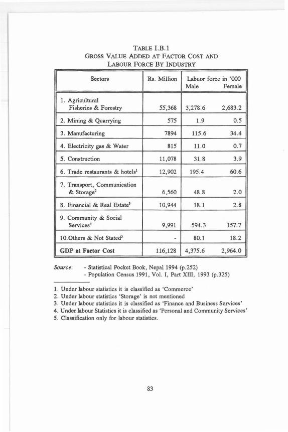
TABLE l.B.l GROSS VALUE ADDED AT FACTOR COST AND

LABOUR FORCE BY INDUSTRY

Sectors Rs. Million Labuor force in '000 Male Female

1. Agricultural Fisheries & Forestry 55,368 3,278.6 2,683.2

2. Mining & Quarrying 575 1.9 0.5

3. Manufacturing 7894 115.6 34.4

4. Electricity gas & Water 815 11.0 0.7

5. Construction 11,078 31.8 3.9

6. Trade restaurants & hotels' 12,902 195.4 60.6

7. Transport, Communication & Storage2 6,560 48.8 2.0

8. Financial & Real Estate3 10,944 18.1 2 .8

9. Community & Social Services4 9,991 594.3 157.7

10.0thers & Not Stated5 - 80.1 18.2

GDP at Factor Co.st 116,128 4,375.6 2,964.0

Source: - Statistical Pocket Book, Nepal 1994 (p.252) - Population Census 1991, Vol. I, Part XIII, 1993 (p.325)

1. Under labour statistics it is classified as 'Commerce' 2. Under labour statistics 'Storage' is not mentioned 3. Under labour statistics it is classified as 'Finance and Business Services' 4. Under labour Statistics it is classified as 'Personal and Community Services' 5. Classification only for labour statistics.

83

Convent.

TABLE l.B.2 AVERAGE TIME INPUT BY ADULT POPULATION ON CONVENTIONAL

AND SUBSISTENCE ECONOMIC ACTIVITIES

(In hours)

Urban Rural

Male Female Male Subsist. Convent. Subsist. Convent. Subsist. Convent.

Female

&on.Activ. &on.Activ. &on.Activ. &on.Activ.

Mountain - - -

Hill 5 .19 0.41 1.90 Terai 5.90 0.34 1.32

Source: MPHBS., 1989

Convent.Econ.Activ. = Conventional Economic Activity Susbsist. = Subsistence

- 4.74 1.80 1.27 4.21 1.60 1.10 5.10 1.70

All Nepal population weights from 1991 Censuses have been applied to derive the national averages.

Convent. Economic Activity (A) Male 4 .768 Female 2 .107

Subsistence Economic Activity (B) Male 1.243 Female 2.130

Male Female

3 .57 2.68 1.70

Ratio of B/ A.

Subsist.

2.43 2.54 1.86

0.2607 1.0100

Regions Male

Mountains -

Hills 483,780 (0.0525)

Terai 398,221 (0.0392)

Total 882,001 (0.0957)

Total Population

Source: Population Censuses 1991.

TABLE l.B.3 POPULATION BY PLACE OF REsIDENCE

(In Number)

Urban Rural

Female Male Female . - 715,~47 727,283

(0.0776) (0.0785)

450,572 3,625,757 3,859,780 (0.3932) (0.3932) (0.4164)

3,997,369 3,997,369 3,869,342 (0.4335) (0.4335) (0.4174)

813,718 8,338,973 8,456,405 (0.0878} (0.9043) (0.9122)

Notes: 1) Mountains have no urban areas.

Total

Male Female

715,847 727,283 (0.0785) (0.0785)

4,109,537 4,310,352 (0.4457) (0.4650)

4,395,590 4,232,488 (0.4767) (0.4566)

9,220,974 9,270,123 (100.00) (100.00)

18,491,097

2) Figures in parenthesis are the proportion to respective total male/female population.

TABLEl.B.4 AVERAGE HOURS OF HOUSEHOLD MAINTF.NANCE WORK PER DAY

By Place of Residence and Sex

Activities Urban Rural Male Female Male Female

1 Cooking, serving and Cleaning dishes

Mountain - - 0 .22 2.78 Hill 0.26 3.02 0.18 2.76 Terai 0.18 3 .19 0 .14 2.96 All Nepal 0.22 3 .10 0 .16 2.85

2 Laundry & cleanings or house

Mountain - - 0.24 0 .64 Hill 0.17 0.99 0 .10 0 .68 Terai 0.14 1.10 0 .08 0 .79 All Nepal 0 .15 1.04 0 .10 0 .73

3 Child care

Mountain Hill - - 0.38 0 .71 Terai 0.25 0 .76 0.40 1.00 All Nepal 0.33 1.14 0 .25 0.98

0 .29 0 .95 0.33 0.98

4 Shopping and other domestic works

Mountain - - 1.35 1.10 Hill 0.73 0 .84 1.39 0 .95 Terai 0.94 1.91 1.32 1.09 All Nepal 0.82 0 .91 1.35 1.03

Source: Multipurpose Household Budget Survey, NRB, 1988 (pp 356-360)

Note: Averages are derived applying 1991 population ratios living in respective regions, as featured in total in the annex.

86

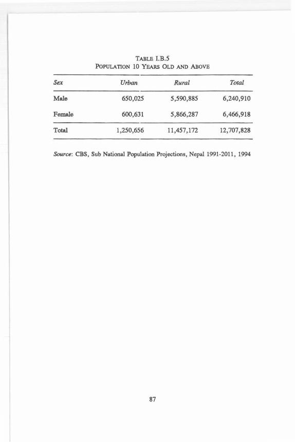
TABLE l.B.5 POPULATION 10 YEARS OLD AND ABOVE

Sex Urban Rural Total

Male 650,025 5,590,885 6,240,910

Female 600,631 5,866,287 6,466,918

Total 1,250,656 11,457,172 12,707,828

Source: CBS, Sub National Population Projections, Nepal 1991-2011, 1994

87

ANNEX I-C

SURVEY QUESTIONNAIRE

A: Introduction of the Selected Survey Sites and Households - (Form 1)

1. House No .... . ..•..................... . .. • .•. •. ...•.. . •....

2. Ward No •.. .... ...... . .....•...............•...............

3. VDC/Municipality ...... . ..•......... . ................•.....

01. Dhakuta Municipality 07. Tankisunwari V.D . C. 02. Biratnagar Municipality 08. Kapan v.o.c 03. Kathmandu Municipality 09. Gitanagar V.D.C 04. Bharatpur Municipality 05. Nepalgunj Municipality 06. Belhara V.D.C.

4. District .• ..... ..... ........ 01. Dhankuta 03. Kathmandu 05. Baglung 07. Jumla

10. Paraspur V.D.C 11. Laharepipal V.D . C 12. Dillichaur V.D.C 13. Dashrath Chand V.D.C

02. Morang 04. Chitwan 06. Banke 08. Baitadi

5. Household Head ....... .. . .......... ........ ................•

(spouse) Mr./Mrs .................. .. ............ ... •.•.• •.•

6. Respondent's Name ........••..... . ... . .. • .. . ............. . . •

. Name ................ . ... .......... ..... ....•..

7. Name of Interviewer ............. . ................. . ... . ... . Interview taken 01. No. of times 02. Date 03, Starting time 04. Ending time 05. Total time taken for

the interview (minutes)

89

B : Information of the Household Members - (Form 2)

Respon- Name of Household dent's Members and live-in Serial Servants (Write HH Number Head's Name First)

(1)

01 02 03 04 OS 06 07 08 09 10 11

Relation to Household Head

01 Household Head 02 Mr./Mrs.(Spouse) 03 Son/Daughter 04 Daughter in law

( 2)

05 Grand-daughter/Grand-son 06 Father/Mother 07 Mother/Father in law 08 Brother/Sister 09 Nephew/Niece 10 Not a Relation 11 Live in Servant 12 Other (Specify)

Sex

1. Male 2. Female

Relation to

Household Head

(3)

Mari tat Status

1. Not Marr ied 2. Married 3. Iii dow/llidower 4. Divorced/Separated

Age For 5 yrs & Above Sex (0

if<l Marital yr) Status

(4) 5) (6)

Educat ion

00 Illiterate 01 Grade one completed 09 Grade nine/Test pass 10 S.L.C. 11 Intermediate 12 Bachelor 13 Master 14 Literate

Edu ca- Occupa- Place tion tion

( 7) (8)

Occupation

0 llorking at Home 1 Agr i cut tu re 2 llage Earner 3 Student 4 Service 5 Business 6 Industry

of Work

(9)

Pl ace of work

1 Own 2 Other's 3 Officer 4 School

0

°'

IO .....

c Products Generated or Work Done at Home and Input Therein - (Form 3)

Code Product/Activity Frequency of time Products/Activit i es the Product Gene- Unit of Average Per Unit cost of

rated or Activities Measure- Quantity Preparation at Performed ment Produced Home (to be calcu-

at a time lated from form 4) aw per column 3

(1) (2) (3) (4) (5) (6)

Respondent's Time Spent per product/ Serial No. Name per activity, each time

(9) (10) (11)

•A c°""lmentary Product/Activity list is a lso supplied to f ill-in the infonNtion.

Total Persona Involved in Serial Making the No. Product

(7) (8)

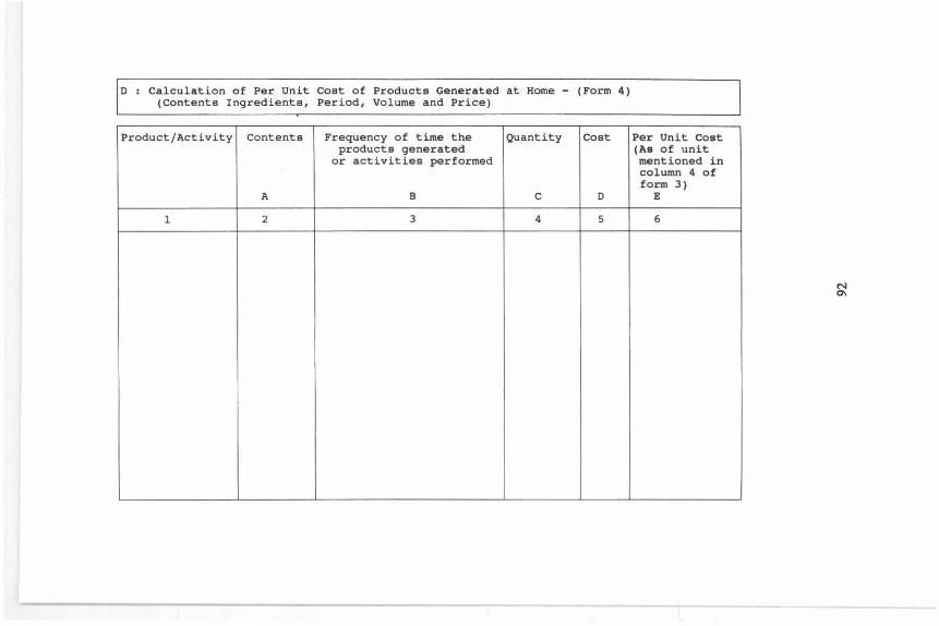
D : Calculation of Per Unit Coat of Products Generated at Home - (Form 4) (Contents Ingredients, Period, Volume and Price)

Product/Activity Contents Frequency of time the Quantity Coat products generated

or activities performed

A B c D

1 2 3 4 5

Per Unit Coat (A• of unit mentioned in column 4 of form 3)

E

6

~

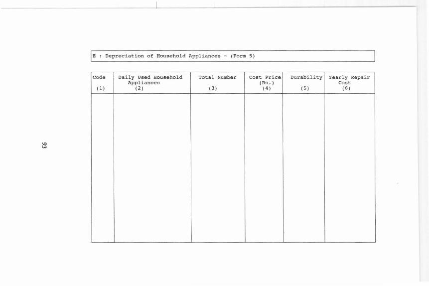
IO w

E : Depreciation of Household Appliances - (Form 5)

Code Daily Used Household Total Number Cost Price Appliances (Rs.)

( 1) (2) (3) (4)

Durability Yearly Repair Cost

(5) ( 6 )

--+

F: Daily Time Use Budget of Household Members - (Form 6)

Daily Time Use Pattern of a Member of the Household who is older than five years .

l . Serial No: ••• .. . .• ..•.. 2. Respondent serial No: .••.•.••.•..•

3. Name: ......••.. •. .. ••.••• . •... ....•... .. ......•. •.•.•..••..•.•• •

4. Sex: •..•.......••...•.•.•.•. 5. Age: ..•.••....••.•..•..•• ••.•

Code Activities Time Minutes To - From M p

(6) (7) (B) (9) (10)

94

jc Household Information - (Form 7)

1. Household economic statue in the respondent's view.

1) Rich 2) Kiddle Clase 3) Poor

2. How much areable Land do you own?

Unit Irrigated Field Non-Irrigated Field/garden

Ropani/Bigha

Coat/Value(Ra)

3. What animals/birds do you own?

Animals/Birds Adult Inf ant

Cow/Ox

Buffalo/Bull

Goat/Sheep

Pig/Boar

Horse/Mule

Chicken/Duck/Pigeon

Fish

Others (Specify)

Cost

Total Price

4. Income and Wealth

(a) Total salary/pension of the household members. Ra • ••••• • •

(b) Other source of income •.•••.••••• (e.g., Business, house

rent, etc.) Ra ••••.•••••• •

95

s. Information of House/Building

6.

(a) How many stories is your house made up of?

l. one Story 2 . Many Stories

(b) What type of a house do you own?

l. Mud 2. Br i ck/ Stone 3. Cemented

(a) Rooms in use

(b) Total area of the house

(c) Area occupied by patio, garden, kitchen garden, etc.

(d) current coat of building the house (excluding the occupied land) .••• • •• • .

(e) Price of the patio, garden, kitchen garden and land occupied by the house •.•• . ••• • •

7 . Toilet •• • . •• ...•

1) Inside the house

8 . Electricity

2) outside the Houae 3) Does not exist

1) Yea

9 . Telephone

l) Yes

10 . (a) Drinking water

1) Tap inside the house

2) No

31 No

2) Well/Tap outside the Houaa (front-yard) 3) Other sources away from the house

(b) If tap i s not inside the house, time consumed in carrying water into the house (minutes ) .••••••

11. Local daily wage rate (labour) (Ra.) ........ .

12. Total coat of employing a person on a monthly basis

Cash ..••••• • •. ; Kind •• • ••.•.• •I Total amount (Ra.)

13. Evaluation of the interview Coda for the answer1

l 2 . 3 11 Explanation of questionnaire Excessive Some Little 2) Need of local interpreter Yea No 3) Evaluation in total High Medium Low

96

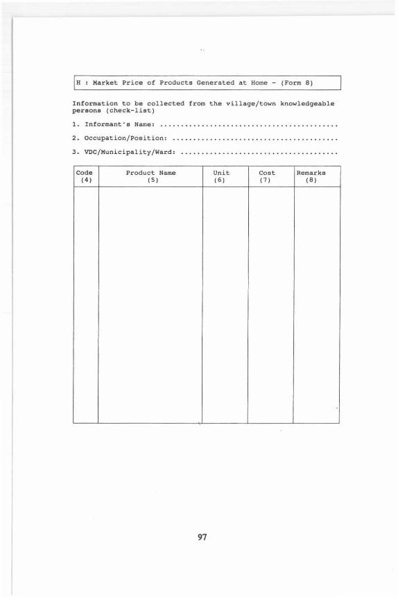
H : Market Price of Products Generated at Home - {Form 8)

Information to be collected from the village/town knowledgeable persons {check-list)

1. Informant's Name:

2. Occupation/Position: ...•..••...........•.•........•.••••.••.

3. VDC/Municipality /Ward: •...•.•.•........•.•••..•.....•...•...

Code Product Name Unit Cost Remarks (4) (S) (6) (7) (8)

97

ANNEX D: FREQUENCY DISTRIBUTION Fll.E A: INTRODUCTION OF THE SELECTED SURVEY SITES

AND HOUSEHOLDS - (Form 1)

Nl.lnber Per cent

Total Resoo111de11t 276 100. 0X

A3 Municiealit~lVOe 1 Dhankuta Muni. 26 9.4% 2 Bi ratnagar Muni • 26 9.4% 3 Kathmandu Muni • 26 9.4% 4 Bharatpur Muni. 26 9.4% 5 Nepalgunj Muni . 26 9.4% 6 Belhara voe 18 6.5% 7 Tankisunuwari voe 18 6.5% 8 Kapan voe 18 6.5% 9 Gitanagar voe 18 6.5% 10 Paraspur voe 18 6.5% 11 Laharepipal voe 18 6.5% 12 Dillichaur voe 18 6.5% 13 Dasharathchanda voe 20 7. 2%

NA3 Residence 1 Urban 130 47.1% 2 Rural 146 52.9%

A4 District 1 Dhank.uta 44 15.9% 2 Morang 44 15.9% 3 Kathmandu 44 15.9% 4 ehitwan 44 15.9% 5 Bag lung 18 6.5% 6 Bank.e 44 15 .9% 7 Jun la 18 6.5% 8 Baitadi 20 7. 2%

llA4 Ecological Belt 1 Mountain 18 6. 5% z Hill 126 45.7% 3 Terai 132 47.8%

Total Resoondent 276 100.0X

A8 NlJ!i>er of Visits 1 One Time 252 91.3% z Two Times . 22 8.0% 3 Three Times 1 .4% 8 Missing 1 . 4%

TIME Total time for Average Std.Dev eQ!!l!leting Ques.

Cin minutes) 144.7 47. 0

98

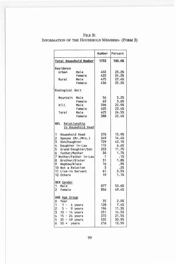
FILE B: INFORMATION OF THE HOUSEHOLD MEMBERS- {FORM 2)

NU!t>er Percent

Total Household Melllber 1733 100.0X

Residence Urban Male 402 23.2X

Female 420 24.2X Rural Male 475 27.4X

Female 436 25.2X

Ecological Belt

Mountain Male 56 3.2X Female 63 3.6X

Hill Male 396 22.9X Female 405 23.4X

Terai Male 425 24.5X Female 388 22.4X

REL Relationshi12 to Household Head

, Household Head 276 15.9X 2 Spouse CMr./Mrs.) 249 14.4X 3 Son/Daughter 729 42. ix 4 Daughter in-Law 115 6.6X 5 Grand· Daughter/Son 203 11. 7% 6 Father/Mother 30 1.7% 7 Mother/Father in- Law 1 .1X 8 Brother/Sister 31 1.8X 9 Nephew/Niece 16 .9X 10 Not a Relation 3 .2X 11 Live-in Servant 61 3.5X 12 Others 19 1.1X

SEX Gender , M~ an 50.6X 2 Female 856 49.4X

AGE Age Grou12 0 Year 35 2.ox· , 1 . 4 years 128 7.4X 2 5 . 9 years 196 11.3X 3 10 . 14 years 251 14.5X 4 15 · 24 years 372 21.5X 5 25 · 49 years 535 30.9X 6 50 + years 216 12.5X

99

(FILE B: CONTD •.• )

Nl.Jl'ber Per cent

Household Mellt>er 1733 100.0X

AGE Age Group (Male) 877 50.6X O Year 15 0.9X 1 1 - 4 years 60 3.5X 2 5 - 9 years 101 5.8X 3 10 - 14 years 126 7.3X 4 15 - 24 years 199 11.5X 5 25 - 49 years 262 15.1X 6 50 + years 114 6.6X

AGE Age Group (Female) 856 49.4X 0 Year 20 1. 2X 1 1 - 4 years 68 3.9X 2 5 - 9 years 95 5.5X 3 10 - 14 years 125 7. 2X 4 15 - 24 years 173 10.0X 5 25 - 49 years 273 15.8X 6 50 + years 102 5.9X

MAR Marital Status 1 Urwarried 767 44.3X 2 Married 733 42.3" 3 Widow/Widower 59 3.4" 4 Divorced/Se~arated 11 .6X 7 Not Applica le 163 9.4X

EDU Education 0 Illiterate 388 22 .4X 1 Grade One C~lete 67 3.9X 2 " Two 53 3.1X 3 Three 62 3 .6X 4 Four 58 3.3X 5 Five 90 5.2% 6 Six 47 2.7" 7 Seven 60 3.5" 8 Eight 76 4.4% 9 Nine 132 7 .6X 10 SLC 163 9.4X 11 Intermediate 103 5.9X 12 Bachelor 61 3 .5X 13 Master 60 3.5X 14 Can Read/Write 150 8.7" 77 Not Applicable 163 9.4X

OCQJP Occueation 0 Working at Home 365 21 . 1X 1 Agriculture 266 15 .3X 2 IJage Earner 67 3.9X 3 Student 598 34.5X 4 Service 153 8.8X 5 Business 106 6. 1X 6 Industry 15 .9X 7 Not App icable 163 9.4X

WORICP IJorking Place 1 Own 708 40.9X 2 Other's 111 6.4X 3 Office 153 8.8X 4 School 598 34.5% 7 Not Applicable 163 9.4X

100

FILE C: HOUSEHOLD INFORMATION - (FORM 7)

Nl.JTlber Per cent

Total Respondent 276 100.0X

G1 Economic Status 1 High 13 4.7% 2 Medi un 206 74.6% 3 Low 57 20. 7°!.

GSA Stories of House 1 One Story 114 41 .3% 2 Many Stories 162 58. 7°/.

GSB T~pe of House 1 Mud 74 26.8% 2 Brick/Stone 125 45.3% 3 Cemented 77 27.9%

G6A Rooms in Use 1 1 - 4 Rooms 155 56.2% 2 5 - 7 Rooms 82 29. 7°!. 3 8 -12 Rooms 37 13.4% 4 13+ 2 0. 7°!.

G7 Toilet 1 Inside House 67 24.3% 2 In Courtyard 118 42.8% 3 Not at all 91 33.0%

I G8 Electricit~ 1 Yes 204 73.9% 2 No 72 26.1%

G9 Telephone 1 Yes 64 23 .2% 2 No 212 76.8%

G10A Drinking Water 1 Inside House 53 19.2% 2 Outside House 129 46. 7°!. 3 Other Source 94 34.1%

G13A Explanation 1 Excessive 35 12.7% 2 Some 137 49.6% 3 Litt le 104 37. 7°!.

G13B Local Interpreter 1 Yes 45 16.3% 2 No 231 83. 7°/.

G13COveral l Evaluation 1 High 86 31 .2% 2 Mediun 177 64.1% 3 Low 13 4. 7°/.

101

Part 2

A MACRO APPROACH TO VALUING

HOUSEHOLD OUTPUTS CANADA AND FINLAND1

Andrew Harvey

1 In collaboration with the Time-Use Research Program, Department of Economics, Saint Mary's University, Halifax, Canada.

INTRODUCTION

Ultimately, estimation of the value of household production will require, as does the estimation of many economic phenomena, the use of a variety of approaches. This is true for at least two reasons. First, a single approach cannot be expected to be applicable to all cases, thus variety is needed to ensure that there are sufficient approaches to develop exhaustive measures. Even where good measures of a phenomena exist it is helpful to be able to derive confirmatory estimates by other approaches. This chapter explores one approach, a macro approach to the estimation of household production. The major intent of the work presented here is to explore ways of developing estimates of household output and to .highlight data deficiencies and needs. The exercise while striving to generate reasonable estimates for Canada and Finland· has been less rigorous and more exploratory than recent estimates developed by Statistics Canada and Statistics Finland.

105

The previous part of this book presented an approach which can be denoted the micro approach to output estimation. It is dependent on the collection, in a common instrument at the household level, of the various values needed to calculate the quantity and value of household production. The micro approach has been used, but not well analyzed or reported, in studies such as the World B~ Living Standard Measurement Studies and the UN Housing Capability Surveys. These studies focus, often in great detail, on specific productive activities but not in a manner that permits accurate integration to account for overall production. The work reported above on Nepal attempts to present a more complete micro picture to permit a proper overall accounting of household production.

This study takes, in contrast, a different approach by attempting to use data collected by a range of vehicles including representative time diary and consumer expenditure surveys to derive estimates cutting across the range of activity undertaken in households. The approach used here, while not without difficulties, looks at households providers of food, shelter and clothing and child/elder care. The premise is that the output must be measured from the consumption side rather than the input side. That is, the outputs are meals, receipt of accommodation, receipt of care to clothes and person. It is the identification, measurement and valuing of these outputs which is the focus here.

Simply put, the approach used here calculates, for specific activities, the volume of output that volume times average price gives the total value of the activities output . . It constitutes household production. However, in order to incorporate that value in a satellite account compatible with

106

the SNA the value of inputs already included in the SNA, purchased inputs (RME) and the value of owner occupied dwellings must be deducted. When this is done the remaining value reflects the services from household capital, and household profit.

The objective was not to provide answers but to raise questions. The work carried out clearly identified both conceptual and data problems associated with the task of valuing household output. It is hoped that these problems can be more extensively explored, and solutions sought, as efforts for fully accounting for household production move forward.

107

Chapter One VALUING UNPAID WORK

I. APPROACHES TO THE

MEASUREMENT AND VALUATION

OF HOUSEHOLD OUTPUT

Over the past two decades ,

increasing attention has been paid to the measurement and valuation of the output generated by unpaid activities in households. Goldschmidt-Clermont (1983, 1987) provides a good review of the approaches used which can be broadly classified as an input or output approach.

1. The Input Approach

Input approaches to the valuation of household pro­duction have traditionally focused on labour inputs to the production process, deriving the value of household output as

109

the value of labour that goes into its production. [See, for · example, Adler and Hawrylyshyn (1978), Murphy (1978, 1982), Chadeau (1985), Gronau (1980)]. The first major shortcoming of this approach is its failure to account for household inputs other than labour. Any productive output is typically viewed as emanating from a combination of input resources namely, land, labour, capital and entrepreneurial ability . To restrict the value of household production only to the embodied labour fails to portray accurately either the process or the value of household production.

A second shortcoming of the input approach is its failure to account for joint production in the household emanating from the simultaneous activities undertaken by individuals engaged in household production. Often, household workers are engaged in more than one process at a time. Varjonen claims that farm wives in Finland had on average 2.5 activity processes in progress simultaneously (Varjonen, 1991).

Another major shortcoming of the labour input approach is the lack of clear valuation criteria. There are two main methods of valuing labour inputs. The first relates to the labour equivalent chosen while the second relates to the labour value used. The labour equivalent may be defined in several ways. First it may be taken to be the opportunity cost of the time expended on household productive activities by any given individual. This means that the exact same activity undertaken by two individuals with different marginal time values wm have different values, and different activities with a priori different values per unit time would have the same value for any given individual. Alternatively, it may be defined in terms of replacement workers which may be defined in terms of a 'global substitute' (i.e., housekeeper) or

110

in terms of functional replacements (i.e., cook, cleaner, gardener, etc.). Having defined the labour equivalent, the labour value of that equivalent remains to be determined. The appropriate value base is not straightforward. What is the appropriate opportunity cost for the worker? Should replace­ment values be determined as an average of all workers, or on a gender specific basis, or in terms of particular workers? And, should it be net or gross with respect to costs?

In spite of these shortcomings the input approach has, until recently, provided the operational household production valuation method. The chief reason for its popularity has been the existence of time-use data which has provided the much needed information on time allocated to household work (INSTRAW, 1991). More recently, attempts have been made to improve the input approach by broadening it to include non-labour inputs as well (Ironmonger, 1989; Thoen, 1993; Schafer and Schwarz, 1995; Aslaksen and Gravingsmyhr, 1995; and Rydenstam and Wadeskog, 1995). The extensions have been made by drawing on additional household data collected by central statistical bodies.

2. The Output Approach

In a seminal work on the role of time use in under­standing household production it was stated that "the time spent on the household work activities (input) equals the goods and services produced (output)" (Walker and Woods, 1974, p.3). The study noted that this assertion assumes, of course, that labour is the only factor input. The study ob­served that while outputs of goods and services could be measured or quantified the quantities were calculated in

111

disparate units such as meals, pounds of wash, etc. and thus were not amenable to summation. However, if these outputs can be expressed in dollar values using realistic prices the problem of aggregation disappears. Use of time to measure household production poses the problem, noted by Walker and Woods, of disentangling time allocated to an array of household activities carried out both concurrently and consec­utively.

Despite the shortcomings of the labour input approach, experimentation using the output approach has been slow in coming. Very few studies embodying the output approach have been undertaken and not one of these has been executed within a central statistical office. Curiously, however, an output type approach was used in what may have been the very first attempt to estimate the aggregate value of house­hold output in the economy, Colin Clark (1958) inferred the value of unpaid household activities from the cost of main­taining adult and child inmates in homes .and institutions run by local authority welfare services in Britain. The value he thus derived is attributable to the inputs of labour and man­agement. Although the cost of capital is not included in the estimated value, this is essentially an output approach where the institutional cost has been assumed to reflect market value.

Goldschmidt-Clermont (1983) argued in favour of adopting the output approach and defined the value of house­hold productive activity as the difference between the market cost of buying a good or service and the household's mone­tary outlay in producing an equivalent product. Fitzgerald and Wicks (1990) and Dulaney et al. (1992) have used the direct output approach by defining household outputs and conduct-

112

ing a sample survey to collect data on the defined outputs and their prices. Elements of the output approach were used in an extensive study undertaken by the Ministry of Social Affairs and Health of Finland in the late 1970s. The Finnish study did not exclusively use an output approach but incorporated such an approach into its comparative study. The product approach was used for meals (Suviranta, 1982); houseclean­ing (Suviranta and Kiplio, 1982); and laundry (Suviranta, 1982). Sanik and Stafford (1983) estimated the value of home food production using a product accounting approach and Chadeau and Forquet (1981) estimated values for meals and housecleaning.

113

Chapter Two

TOW ARD AN OUTPUT-BASED VALUATION OF

HOUSEHOLD PRODUCTION

The output approach identified

the value of a good or service produced by a household as the market value of a similar product sold by businesses, less the cost of raw materials, energy, and the use of other fixed assets that go into producing it. As explained later, this basic definition will be slightly modified for the purposes of including the estimates of theses values in the non-SNA Satellite account.

I. CATEGORIES OF HOUSEHOLD OUTPUT

As the first step in developing the output based measure­ment, the following question'Reeds to be asked: What are the

115

outputs produced by a household? In various studies, numer­ous household productive activities have been identified. Table 11.2.1 provides a comprehensive list of these activities at a very disaggregated level (Fitzgerald and Wicks, 1990).

TABLE 11.2.1 TYPF.S OF HOUSEHOLD PRODUCTION

.Activity Unit Definition

A. CLEANING

1. Garbage disposal bag

2. Vacuuming room (each time)

3. General pick-up room

4 . Kitchen floor mopping floor

5. Other kitchen surfaces kitchen

6 . Bathroom floor mopping bathroom

7. Bathroom, other surface cleaning bathroom

8. Basin, tub, tile, commode cleaning bathroom

9. Bedroom other surface cleaning bedroom

10. Bed making bed

11. Bed linen changing bed

12. Other rooms floor cleaning floor

13. Other rooms surface cleaning room

14. Lawn mowing lawn

15. Wmdow cleaning window

16. Refrigerator or freezer defrosting refrigerator

17. Stove cleaning stove

18. Cupboard cleaning cupboard

19. Garage cleaning garage

20. Patio cleaning patio

21. Snow shovelling sidewalk/driveway

22. Yard raking yard

23 . Yard litter pick-up yard

116

TABLE 11.2.1 - TYPES OF HOUSEHOLD PRODUCTION (Continued)

Activity Unit Definition

B. CHll.D CARE

24. Child feeding child/each time

25. Child changing child

26. Child bathing child

27. Child transporting mile

c. MEALS

28. Meal preparation and cleanup meal for one person

D. CARE OF CLOTHING

29. Washing and drying machine load

30. Ironing article of clothing

31. Mending article

32. Alteration article

E . REPAIR AND MAINTENANCE

33. Chimney sweeping chimney

34. Electrical repair job

35. Plumbing repair job

36. Interior painting room

37. Exterior painting room

38. Structural repair value of job

39. Landscaping job

40. Vehicle cle1ming, washing car

41. Vehicle tune-up job

42. Vehicle lubrication job

43. Vehicle tire changing tire

44. Other vehicle repair job

45. Other appliance and

equipment repair job

117

TABLE 11.2.1 - TYPF.S OF HOUSEHOLD PRODUCTION (Continued)

Activity.

F. FOOD PRODUCTION

46. Homegrown food

47. Livestock

48. Hunting harvest

49. Fishing harvest

50. Berry gathering

G. MISCELLANEOUS

51. House upgrading

52. Yard ui;~rading

53 . Tax preparation

54. Household furnishing

and hobby production

H. ACTIVITIF.S FOR WHICH

OUTPUT IS TIME

55. Child sitting 56. Care of elderly 57. Care of sick

Unit Definition

Market value

Market value

Pounds

Pounds

Pounds

Market value of particular job

Job Federal/State return

Market value of particular job

Hour

Hour

Hour

Source: Fitzgerald,J. & Wicks,J. (1990). "Measuring the value of household output: A comparison of direct and indirect approaches", Review of Income and Weallh, 36(2): 129-141.

However, it is argued here, in reality the major house­hold outputs are far fewer than activities undertaken to produce them. Since the prime purpose of the present macro approach to valuation is to develop reasonable estimates of aggregate household production it is argued that there exists a parsimonious approach to defining and valuing household outputs. The approach here is based on, and adopts with a slight modification, the five major dimensions of household

118

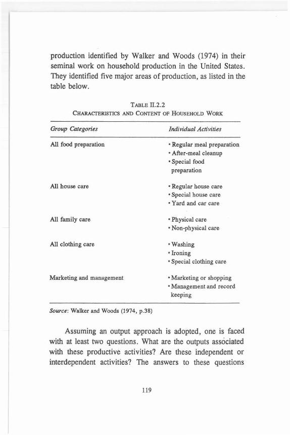
production identified by Walker and Woods (1974) in their seminal work on household production in the United States. They identified five major areas of production, as listed in the table below.

TABLE Il.2.2 CHARACTERISTICS AND CONTENT OF HOUSEHOLD WORK

Group Categories

All food preparation

All house care

All family care

All clothing care

Marketing and management

Source: Walker and Woods (1974, p.38)

Individual Activities

•Regular meal preparation • After-meal cleanup • Special food

preparation

• Regular house care • Special house care • Yard and car care

• Physical care •Non-physical care

•Washing •Ironing • Special clothing care

•Marketing or shopping •Management and record keeping

Assuming an output approach is adopted, one is faced with at least two questions. What are the outputs associated with these productive activities? Are these independent or interdependent activities? The answers to these questions

119

suggest that, in fact, the outputs are far less complex than the activities pursued in their production.

-Food preparation: This consists of regular meal prepa­ration, cleanup and special food preparation. While meals have traditionally been valued by means of valuing the activities used to produce them (cooking, clean up etc.) the reality is that the total value of meals produced at home hinges on the meals eaten and is the summation of the value of all consumed meals produced at home. Assuming appropri­ate values 'prices' can be found for meals, pricing meals obviates many of the steps previously involved in the provi­sion of meals. In reality meal provision entails activities much broader than those proposed above. The price of meals provided in the market represents the sum of the value added in delivering the meal and incorporates a wide array of household activities which combine to produce meals. These activities include at least, menu planning, provisioning (shopping), cooking, serving, cleanup, and garbage disposal.

-Household upkeep: Regular housework can be viewed as consisting of house cleaning and maintenance of cleanli­ness and order (Walker and Woods, 1974, p. 138). Special house care consists of occasional or seasonal home care and repair and upkeep of the house, furniture and equipment. Yard and car care are distinguishable from special house care since they take place outside the dwelling and are often seasonal in nature.

-Family care: Family care consists of both physical and non-physical care (Walker and Woods, 1974). The dominant component of family care is child care. The output of child

120

care is, in fact, getting the child from day to day. Except for when a child's care is handed over to a third party someone in the household has responsibility for each child. When children are in day care, or in school, or placed in the hands of a baby sitter or child minder the immediate responsibility on the part of the household is suspended. However, at all other times someone in the household is responsible for the care of the child. It thus seems reasonable to value child care on a per child/hour basis. However, while this approach may be accepted as a reasonable treatment of children; how such valuation during children's sleeping time is handled represents a real issue.

-Clothing Care: Clothing care consists of washing, ironing and special clothing care. Special clothing care includes a wide variety of activities, construction of clothing, hand washing, mending, shoe care, etc. (Walker and Woods, 1974).

-Residual Marketing and Management: Marketing consist of all shopping for all goods, whether or not purchas­es were made. It consisted of all aspects of acquiring goods and services by phone, mail, travel, and time putting purchas­es away (Walker and Woods, 1974). This category of house­hold activity is a 'residual' one because much of these activi­ties are included in the previous categories of food prepara­tion. Thus , the value created by shopping for food is included in the output of meals and. should not be counted separately. The residual group consists of only those marketing and management activities which are not already included in any of the output categories listed above.

121

II. THE OUTPUT MEASURE OF

HOUSEHOLD OUTPUT: METHODOLOGY

Using the output approach, the value of a non-SNA good or service produced within a household is measured as ~

VO = P - RMB - UOD

where

VO the value of 1 unit of household output

P the market price, net of taxes and subsidies, of the good or service of like quality

RMB the cost of Raw Materials and Energy used per unit of outp-gt. Raw materials include those goods which are produced by the household itself and are includ­ed in the SNA GDP.

UOD the cost of the Use Of (a portion of) Dwelling per unit of output.

Noting that value added (VA) is defined as:

VA = P - RMB,

our measure of household output is:

VO = VA - UOD,

with VA being calculated net of taxes and subsidies on the product.

The value of household production thus incorporates the contributions of labour, household equipment, and entrepre-

122

neurship. Subtracting the user cost of dwelling from value added represents a departure from the current notion of calculating the value of household output. This is done here in order not to double-count the user cost of dwelling when relating the GDP of the Satellite SNA account with the SNA GDP. In contrast, the user cost of household equipment, such as kitchen appliances and washing machines, is not included in the SNA GDP, and we include it in the value of household output (VHO). Thereby, we view these equipments as capital stock rather than final consumption items. Some household goods output, such as garden vegetables, are included in SNA GDP, and their values are excluded from VHO by virtue of being a part of RME.

The procedure for estimating the value added (VA) of a unit of household output involves the following steps:

1. Identify broad categories of (non-SN A) output generating activities of households . As explained above, these are:

• Food preparation • Household upkeep • Family care • Clothing care • Residual Marketing and Management

Each of these categories subsumes within it all activities generating the end product implied by that category. For example, food preparation involves management, shop­ping, cooking, dish washing, etc. , but these specific activities do not constitute separate categories. Instead, all the activities that go into the production of meals are included in the category of food production.

123

2. Identify items of goods and services produced within each category. For example, the outputs of food prepa­ration are: breakfast, lunch, dinner, snacks, etc. Con­ceptually, it is possible to come up with dozens of items within each category by making fine distinctions, i.e., a lunch may be light, heavy or sumptuous, and any one of them could be further described by varying details . Such distinctions are only useful if corresponding data exist allowing estiml:ltions of value created by types. When working with existing data for only breakfast, lunch, and dinner, the identified items under the food preparation category would be necessarily restricted to these three categories, resulting in approximation errors. However, it is useful to bear in mind that the classification of items can be better devised if an opportunity arises to gather detailed data either from existing sources or through a specially designed sample survey.

3. For each item of each category, estimate the quantity (X) and, where relevant and possible, identify the quality of output produced per person in a household per unit of time.

4. For each .good (or service) produced by households , estimate the market price (P) of a good of similar quali­ty . Market price is defined as price to the purchaser and includes taxes and/or subsidies. Identify these taxes and subsidies to calculat~ the producer's price (called "basic price" in SNA). Available sources may include aggre­gate industry statistics, price information collected by statistical agencies, and any available industry sources.

124

5. Identify the raw material and energy components of each item produced by the households. RME is the total cost of these components. There are two distinct sources of data for the RME per unit of output:

a) business establishments producing and selling the good or service;

b) households producing and consuming the product.

Since price data originate only at the business establish­ments, the value of RME at the business end will have the best item-wise match with price data in the process of calculating value added for each item. Using business RME (with tax adjustments) may, therefore, be the preferred option if data on both price (which is the value of sale per unit of output) and the unit cost of raw material and energy are available for each item in a category of household production. Lacking such infor­mation, it will be necessary to use any available data on households' use of RME. A major source, for example, is family expenditure surveys. The values of some household goods outputs (e.g., vegetables from kitchen gardens) are already included in SNA GDP, and need to be excluded from the Satellite account in order to avoid double counting. The values of these outputs, therefore, are to be appropriately included in the calculation of RME of households. This will be done only when household expenditure data are used to estimate RME to arrive at VA, and not when estimating VA using RME for businesses. This is because the value of home produced output that is used as raw materials

125

does not show up in family expenditure data, whereas business RME includes all materials.

6. Value added (VA) is then calculated for each item as ((P*Q) - RME). However, data limitations will -likely exclude the possibility of calculating value added for each item in a category. For example, when using family expenditure data on RME, we cannot distinguish the raw material components of different types of meals (breakfast, lunch, dinner), and can only estimate the value added for all food preparations together .

7. The price of household output that is to be used in calculating VA is what is defined as "basic price" in SNA. Basic pris;e is the price to the purchaser less any tax plus any subsidy on the product. For example, in Canada purchaser's price for most goods includes Pro­vincial Sales Tax and Goods and Services Tax. These taxes are deducted from the market price (purchaser's price to arrive at the basic price. SNA currently includes . some goods produced by the hosuehold for own con-sumption, and these are valued at basic prices; likewise, -satellite accounts should do the same, estimating the basic price of a similar good that is sold in the market. The fundamental reason why household output should be valued at basic price and not market price is that when the government does not impose any tax on a product, no tax can be imputed without violating the identities in national income accounting. For example, suppose that food bought from restaurants is tax-exempt if less than $4 of food is purchased. In this case, tax should not be

126

imputed in calculating market value of the tax-exempt food just because the same food bought in larger quanti­ties would be taxed. Doing so would make GDP as calculated by the output measure exceed the total income of households, firms and the government together. In the case of non-SN A household output, one might argue that the imputed tax could be considered a part of household income, thus not violating the national income identities. However, this does create a disparity with the proce­dures in SNA, and for no good reason. Taxation is purely a prerogative of the government, and when a tax is not actually imposed by the government, there does not exist any implicit value which can be imputed to it. Using the same argument, there should not be any adjustment for tax in calculating the cost of intermediate goods (RME). The cost of these goods to the households includes taxes, while businesses often do not pay some of the taxes or get tax refund for inputs as in the system of VAT (Value Added Tax). To this extent, the cost of producing a good at home is higher than the cost of producing the same thing in a business establishment. Correspondingly, the VA of household output is less, and should be so recorded in the Satellite SNA. If the tax amount is deducted from the cost of raw materials in the process of calculating household VA, then the contribution of household output in GDP would increase by that amount in the Satellite Account while, at the same time, the tax as collected by the government is already being counted in SNA GDP. This is because GDP at market prices = Output (at basic prices) + Taxes, less subsidies, on products - Intermediate Con-

127

sumption. An input purchased by a household is consid­ered a final output in the SNA, and any tax on it is included in the GDP by the above equation.

8. To measure UOD for each activity, a portion of the imputed or actual rental of a dwelling needs to be as­signed to the activity. For example, some 20 % of the rental may be ascribed to food preparation and consump­tion. House cleaning will have no UOD component. To estimate the rental, a macro measure can be used, dividing the SNA household rental figure by the total number of dwellings in the nation. This amount will then be divided by the number of meals prepared in a year in the household.

9. To arrive at the value of household production at suc­cessively higher levels of aggregation, the following notations are used:

a) For each item in a category, the per-unit value of ho1 .ehold output is:

VO= VA - UOD,

and the corresponding total value is:

IVO = Q x VO,

where Q is the quantity of output of an item, and IVO stands for the total value of output of an item.

b) The total value produced by a household in a particu­lar category of activity is:

128

CVO = Sum of 1yo, when the summation is taken over all items in the category.

CVO stands for category-wise value of activities.

c) The total value of a household 's output is:

TVO = Sum of CVO, when the summation is taken over all categories of activities.

d) Aggregating over all households in the economy, the totals for all households are:

SACVO = Sum of CVO over all households, with SACVO standing for "Satellite Account CVO";

SATVO = Sum of TVO over all households, with SATVO standing for "Satellite Account TVO"

Output based- and input based-valuation methods repre­sent, to a great extent, mirror images of each other. Using the traditional input approach to valuation, one determines the inputs and sums them to arrive at an estimate of total output. Using this method the value of the labour input is itself an input into the valuation process. In contrast, using the output valuation approach output is valued in terms of the market price of equivalent outputs in the market or in terms of prices of closely related goods. Having determined market value of the output, and adjusting for taxes, the value added by the household is determined by subtracting the value of purchased

129

inputs. The resulting value added consists of two components: one is the value of labour used in the production process and the other is the contribution of household capital. Using the input approach entails the necessity of deriving estimates of the services flowing from household capital in order to calculate the total value of household output. However, no such requirement is imposed by the output approach. Under the output approach, it is only necessary to derive estimates of the services flowing from household capital if one wishes to isolate the contributions of labour and capital to produc­tion. The use of the dwelling component is treated differently only because it is included in the SNA. The SNA does not include any estimates of the flow of services from household capital since such "capital" was recorded as consumption in the SNA.

130

Chapter Three PREVIOUS OUTPUT-ORIENTED

STUDIES OF HOUSEHOLD PRODUCTION

I. THE FINNISH HOUSEWORK STUDY

This study is presented in con­

siderable detail since it represents a landmark study in the

measurement and valuation of household production. It incorporated both input and output valuation approaches.

The basic research unit was private households in

Finland. A household was comprised of the family and any

persons living within it who share meals at least partly or

who pool their income in other ways. Sampling involved

2,000 households selected in a stratified two-stage cluster

sample. Data was collected by means of interviews, individu­

al housework diaries and meal forms completed by the person

in charge of keeping the household . The main data modules

131

in the interview were: a) structural data on the household; b) data on the dwelling; c) household appliances; d) use of paid domestic help; e) household members receiving special care; and f) occasional activities, with questions concerning, frequency of the task, what products are produced by the household itself and how much is produced by the household itself. The data in the meal form captured data on the number of meals eaten at home, the number of persons taking part in meals at home, the foods eaten at home, and the source or stage of processing of the foods eaten.

Unpaid housework was divided into eight activities: cooking; home chores and laundering; child care; other family care; handicrafts, wood, and metal work; maintenance work, shopping and errands; and other unpaid housework (Tables 11.3.1 and 11.3.2). A division was made between the work done by the wife, the husband, children age 10 to 17, and other members of the family . Work done by outsiders was not included.

II. DETERMINING THE VALUE OF

UNPAID HOUSEWORK

1. Meal Preparation

In the Finnish study meal preparation included all the work involved in preparing food and eating meals: cooking, setting and clearing tables, and washing dishes . It was assumed that the value of all meals eaten at home is the same as those bought and eaten outside the home, and that the value of the work performed in cooking these meals is the same for food prepared at home or outside the home. A meal

132

TABLE 11.3.l TIME-USE DATA, FINLAND 1979

FAMILIES WITH CHILDREN FAMILY HOUSEWORK - PER FAMILY MEMBER

(Hours per day)

Children Other aged 10 family

Activity Wife Husband to 17 members

Cooking 2 .0 0.3 0 .1 0 .1 Home laundering 1.2 0.1 0.1 0.1 Child care 1.6 0 .6 0 .1 0 . 1 Other family care 0 .0 0.0 0.0 0.0 Handicraft wood and metal work 0.3 0 .1 0 .1 0 .0

Maintenance work 0.3 0.6 0.1 0 .1 Shopping 0.4 0.3 0 .1 0.0 Other 0.2 0. 1 0 .1 0.0

Total 6 .0 2.1 .7 .4

TABLE 11.3 .2 FINNISH HOUSEWORK STUDY, 1982

REsULTS OP ESTI}{ATES OP UNPAID WORK VALUE (In %)

Total

2.5 1.5 2 .4 0 .0

0.5 1.1 0 .8 0.4

9 .2

Activity Share of GDP

Cooking Home, laundry, and clothes care Child care Handicrafts, wood and metal work Maintenance work

Shopping and errands Other unpaid housework

Total unpaid housework

Note: Data based on 1979 time-use survey and 1982 prices .

133

13.3 6.9 6.4 2 .9 5.8

4.1 2.3

41.7

was defined as the food eaten by one person at one time, i.e., breakfast, lunch, afternoon tea, dinner , evening snack, or packed meal.

The price of a meal bought outside the home includes the costs of raw materials and labour. Labour costs were assumed to be equal to the value of the corresponding work done in the home. The prices chosen were taken from the cafeterias operated by the State Catering Centre, because they include only the costs incurred in the provision of meals, and did not include the cost of maintaining facilities and equip­ment. The number of meals eaten at home were based on the data collected in the Finnish Housework Study.

The total value of the country's unpaid cooking work (CW) is then derived as:

• cw-EN,• u ""'

in which

i : represents the type of meal (break.fast, lunch, etc.); N: the number of meals per year; and LP: the labour cost price of one meal.

By dividing the figure by the average time used per household , it was possible to arrive at a computational hourly wage.

2. Child Care

The price of the service purchased on the market deter­mines the value of unsalaried child care at home.

134

The valuation approach used was as follows :

• the hourly volume of annual child care for families with different number of children was computed.

• the hourly wage rate for a municipal child minder multiplied by the volume provided the value of a single family ' s annual unsalaried child care, per family size.

• the value of child care of each family group was multiplied by the actual number of farpilies of that size in the population. This gave the actual aggregate cost of total child care per family size (market and non-market.)

• lastly all the groups were aggregated and the volume of market ehild care multiplied by the same wage rate was deducted from the calculation thus providing the aggregate value of non-market child care.

3. House Cleaning

House cleaning was defined as the unpaid regular and special house cleaning done by household members in their own homes. The cleaning work done in a children's day-care centre was chosen for comparison; because it was considered to correspond in large measure to home conditions.

Value of unpaid house cleaning was computed as:

in which

K• A• r • ' - - U , , ...... "

~ = total dwelling area of nation Ls = unit rate for cleaning day-care centres

135

r = portion of total cleaning cost U, = value of outside cleaning help.

The hourly rate for outside cleaning help was determined by the average labour costs for city cleaners.

The computational hourly wage for house cleaning was obtained by using the average time spent in cleaning with adjustments for special house cleaning (interview datd).

4. Special Care

Special care includes the care (feeding, bathing, dress­ing, nursing, and accompanying outdoors) of the elderly, handicapped, or chronically ill persons (asthma, allergies), including those on special diets; and cleaning or laundry work. Wage rate of a municipal home helper was applied in the imputation of value to child care including benefits. This also include time actually spent plus 20% of the time spent in attendance (follo'1.'ing the employment agreement for munici­pal helpers.)

The value of special care was computed as:

Time spent "' wage rate

5. Laundry

Laundry includes the preliminary handling, actual washing and final handling of laundry. The amount of laun­dry accumulating in households and the price of washing it outside the home were estimated from information provided in the househork study. The prices for laundry services were obtained from the Finnish Association of Laundries and Dry

136

Cleaners. It was assumed that household cost was equal to commercial laundering.

The value of laundry activities was computed as:

LW • K •LP

in which

K: the annual amount of laundry for all households in kilograms

LP: the labour cost price for one kilogram of laundry.

6. Handicrafts

Handicrafts includes cloth making and other textile work; wood and metal work; and other handicrafts.

Product volume was obtained from the study. Wage costs were obtained from companies in the textile and furni­ture industries manufacturing similar products.

7. Fitzgerald/Wicks Study

One of the first attempts to compare the labour-value (input) approach and the direct (output) approach was con­ducted by Fitzgerald and Wicks and published in 1990. In their study, 480 residents of Missoula, Missouri were person­ally interviewed to reveal the output of, and hours devoted to, 57 different output items in eight household production categories, as shown in Table II.3.3.

In addition, a survey was conducted of local businesses to determine the average market price within each output category with the prices of intermediate goods netted out. Subsequently, the survey design allowed for a direct and relatively easy computation of the value added within each

137

TABL"! 11.3.3 MEAN ANNUAL VALUES OF lloUSEHOLD PRODUCTION FOR

ADULT MEMBERS OF HOUSEHOLOS OF MISSOULA, MO EsTIMATED

BY DIRECT-OUTPUT AND LABOUR-VALUE APPROACHES

(1985 U.S. Dollars)

Output Category

Interior cleaning

Exterior cleaning Meal preparation Clothing care Repairs, maintenance, and

home improvements Child care Home produced food Miscellaneous

Total

PROPORTION OF TOTAL

(In percentages)

Interior cleaning

Exterior cleaning Meal preparation Clothing care Repairs, maintenance, and

home improvements Child care Home produced food

Miscellaneous

Total

138

Direct Output

Approach

951 228

2,781 725

309 445

28 147

5,614

16.9 4.1

49.5 12.9

5.5 7.9 0.5 2.6

100.0

lAbour Value

Approach

812 108

1,517 403

161 764

37

135

3,937

20.6 2.7

38.5 10.2

4.1

19.4 0.9 3.4

100.0

production category as the netted average market price was multiplied by the unit outputs. Alternatively, the labour value method utilized average wage data in 24 different occupa­tions. The results of the two approaches appear in Table II.3 .3.

Aggregated, the direct output approach exceeds the labour value approach by 43 per cent and the difference between these approaches is statistically significant at the one per cent level. Overall, six out of the eight household produc­tion categories yielded higher results as measured by the direct output method; whereas child care and home produced food yielded lower results. As Table Il.3.3 indicates, meal preparation represents the largest proportion of total house­hold production, representing 49.5 per cent and 38.5 per cent followed by interior cleaning representing 16.9 per cent and 20.6 per cent as measured by the output and labour value approaches respectively.

To account for the difference between both approaches, Fitzgerald and Wicks suggest that the labour value approach may underestimate the output approach because the labour value approach typically characterizes an activity on the basis of its primary product and ignores any secondary products. Consequently, the output method provides a superiour esti­mate of household production since it inherently captures all activities, both primary and secondary.

Compromising the accuracy of the output method, Fitzgerald and Wicks believe that there is a difference in the qualities of household- and marketplace-produced goods. In order to test their hypothesis , a survey of 175 Missoula area residents was conducted to assess the quality of his or her household output compared with the quality of similarly

139

available items in the market. As Table II.3.4 indicates, the survey respondents

perceive household production to be worth 32 per cent more than the market equivalent. Only in the case of "do-it-yourself" projects produced by single-head families was household production viewed as having less worth (10 per cent less) . Consequently, the above out{>ut estimates may be undervalued and thus represent the minimum household production values.

TABLE II.3.4 QUALITY OF HOUSEHOLD PRODUCTION COMPARED WITH

QUALITY OF EQUIVALENT AVAILABLE IN MARKET

AS ASSESSED BY HOUSEHOLDS, MISSOULA, MO.

Type of Output

Cleaning Child care Meal preparation

Clothing care ftDo-it-yourself"

projects

Totals

Average Percentage by which Household Production is Assessed by HollSeholds as

Better (+) or Worse (-) than Market Equivaknt

Married Single All Couples Heads Households

+42 +21 +31 +66 +27 +54 +56 +15 +37 +50 +28 +41

+26 -10 +26

+46 +15 +32

Another finding of the survey, all.hough unsurprising, is that women (wives and female household heads) have higher

140

overall household production than men (husbands and single male heads), as shown in Table 11.3.5. The aggregated average wives' and single female heads' household production values are $9 ,694 and $6,572, respectively, compared to husbands and single male heads with household production values of $3,172 and $5,058. Males have higher household production values in exterior cleaning, repairs and mainte­nance, and home-produced food; however, these activities represent only a small fraction of total household output, as indicated by Table 11.3.5.

TABLE II.3.5 MEAN ANNUAL VALUES OF HOUSEHOLD PRODUCTION FOR

VARIO US TYPES OF ADULT MEMBERS OF HOUSEHOLD MEASURED BY THE DIRECT OUTPUT APPROACH ADJUSTED TO

REFLECT AVERAGE U.S. URBAN AREA LIVING COSTS (in 1986 U.S. Dollars)

Sing/,e Sing/,e Ma/,e Fema/,e All

Output Category Husbands Wives Heads Heads Adults

Interior cleaning 386 1,729 773 1,351 983 Exterior cleaning 358 190 358 173 236 Meal preparation 1,236 5,100 2,591 3,258 2,875 Clothing care 184 1,419 622 827 750 Repairs, maintenance home improvements 569 174 465 172 320

Child care 250 914 0 544 460 Home produced food 52 15 59 3 29 Miscellaneous 137 153 190 244 152

Totals 3,172 9,694 5,058 6,572 5,805

141

TABLE Il.3.5 MEAN ANNUAL v ALUES OF HOUSEHOLD PRODUCTION . .. (Contd.)

Single Single

Male Female AU Output Category Husbands Wives Heads Heads Adults

PROPORTION OF TOTALS (in per cent)

Interior cleaning 12.2 17.8 15.3 20.6 16.9 Exterior cleaning 11.3 2.0 7.1 2.6 4.1 Meal preparation 39.0 52.6 51.2 49.6 49.5

Clothing care 5.8 14.6 12.3 12.6 12.9 Repairs, maintenance home improvements 17.9 1.8 9.2 2.6 5.5

Child care 7.9 9.4 0.0 8.3 7.9 Home-produced food 1.6 0.2 1.2 0.0 0.5 Miscellaneous 4.3 1.6 3.8 3.7 2.6

Totals 100.0 100.0 100.0 100.0 100.0

Also worth noting from the survey is that the average value of household production increases as the number of children increases and is highest for the mother, as shown in Table II.3.6. In addition, the age of adult members also has an impact on the average value of household production and is highest for wives between the ages of 26 to 39, as shown in Table II.3.7.

142

TABLE II.3.6 MEMBERS OF HOUSEHOLDS BY NUMBER OF CHILDREN

MEASURED BY THE OUTPUT APPROACH ADJUSTED TO REFLECT

AVERAGE U.S. URBAN AREA LIVING COSTS

(in U.S. Dollars)

Number of Children in Household

Type of Member 0 1 2 or more

Husband 2,754 2,983 Wife 6,044 9,732 Single Male Head 4,394 * Single Female Head 4,849 8,634

* Sample size was ten or less.

TABLE Il.3.7 HOUSEHOLDS BY AGE MEASURED BY THE DIRECT

OUTPUT APPROACH ADJUSTED TO REFLECT A VERA GE

U.S. URBAN AREA LIVING COSTS

(in 1985 U.S. Dollars)

Member's Age

Type of Member 18-25 26-39 40-61

Husband 2,654 3,956 3,444

Wife 10,569 11,935 7,533

Single Male Head * 5,331 5,436

Single Female Head * 7,386 4,886

* Sample size was ten or less.

143

3,425 12,464

* *

62 and older

2,795

6,079

* 6,025

III. MEASUREMENT OF HOUSEHOLD PRODUCTION

USING INPUT-OUTPUT TABLE: FINLAND, 1992

More recently, Statistics Finland developed estimates of household production, based upon previous work conducted in Australia and Canada, that attempt to measure aggregate national household output via an input-output table that breaks household production into functional categories, for example, meal preparation and child care, that require the use of material, capital, and labour inputs . The household is viewed as a productive entity as it converts these three inputs into valueadded outputs, Table II.3 .8. The idea behind the input­output table is that the sum of the inputs is equivalent to the value of the output.

Material inputs, which form the rows of the input-output table, are derived from the 1990 Household Expenditure Survey's consumption goods expenditure (foodstuffs, dwell­ing, fuel, light, power, etc.) and are allocated to the house­hold production functional categories. Productive activities in the household are subject to the third-person criterion in which an activity is productive if it can be done by someone other than the person who gains its benefit. The activities form the columns of the input-output table, where expendi­tures are allocated according to the appropriateness and importance of the material input to each household activity. For example, expenditure on washing powder was allocated to cleaning and laundry. However, the allocation of inputs to functional categories becomes difficult when the expenditure must be divided among categories. For example, clothes are assumed to be necessary for all productive activities. To overcome this problem, the author suggests that the best way

144

to allocate the expenditure is in proportion to the time spent on each category of household activity, which can be obtained from the 1987-1988 Time Use Survey (assuming of course that the breakdown of time use in 1987-1988 is identical to that of 1990). Forms of consumption that do not contribute to household production activities are allocated to leisure activi­ties. Within each functional category, the row entries are vertically summed to arrive at a total purchases entry that can be regarded as material inputs.

The second input, capital consumption, is derived from the 1990 National Account's consumption of fixed capital on durable goods (furniture, household appliances, vehicles, recreation equipment, etc.) according to the perpetual inven­tory model, where consumption is estimated by dividing the value of the purchased durables evenly over the period they are in use. The supply and costs of durable goods are allocat­ed in proportion to consumption.

The third input, labour, is derived from the data in the 1987-1988 Time-Use Survey. The survey shows how many hours are allocated to each household functional category. The total hours in each category are multiplied by an hourly wage rate to derive total labour cost. The author uses the housekeeper replacement cost (hourly wage including social security contributions, holiday pay, and the consumption of capital) since it is assumed that the tasks performed by household members are broadly equivalent to those of a housekeeper and therefore can be assigned an appropriate value in terms of the wages that a housekeeper commands.

However, there are two problems associated with this method, known as the global substitute method. First, wages of housekeepers vary from one region to another. Second, not

145

TABLE 11.3.8 INPUT-OUTPUT TABLE FOR HOUSEHOLD ACTIVITIES

FINLAND, 1990 (in millions of PIM per year)

lnpuls

Adult Material Capital Value of To1al Activity per Week Purchases Cons ump- Labour Output

(in millfons) lion

Meal preparat ion 24 41, 139 1,097 63,836 106,072 Cleaning and

laundry 16 4,138 882 43,323 48,343 Repair and 9 2,397 218 22,676 25,291

Other housework 5 1,187 53 14,053 15,293

Child care 8 5,906 58 20,513 26,477

Shopping and errands 11 1,900 25 30,160 32,085

Gardening and pet care 6 1,399 726 15 ,277 17,402

Housework travels 9 6,923 3,580 22,622 33,125

Total 88 64,989 6,639 232,460 304,088

PROPORTION OF TOTALS (in per cent)

Meal preparation 27.27 63 .30 16.52 27.46 34.88

Cleaning and

laundry 18.18 6.37 13 .29 18 .64 15.90

Repair and 10.23 3 .69 3.28 9.75 8.32

Other housework 5.68 1.83 0 .80 6.05 5.03 Child care 9 .09 9.09 0 .87 8.82 8.71

Shopping and errands 12.50 2.92 0 .38 12.97 10.55

Gardening and pet care 6.82 2.15 10.94 6.57 5.72

Housework travels 10.23 10.65 53 .92 9.73 10.89

Total 100.00 100.00 100.000 100.00 100.00

146

- ,

TABLE 11.3.8 INPUT-OUTPUT TABLE FOR HOUSEHOID ACTIVITIES

Inputs

Adult Material Capital Value of Total Activity per Week Purchases Cons ump- Labour Output

(in millions) ti on

FACTOR DISTRIBUTION (in per cent)

Meal preparation 38.78 1.03 60.18 100.00 Cleaning and

laundry 8.56 1.82 89.62 100.00 Repair and 9.48 0 .86 89.66 100.00

Other housework 7.76 0 .35 91.89 100.00 Child care 22.31 0.22 77.47 100.00

Shopping and errands 5.92 0.08 94.00 100.00

Gardening and pet care 8.04 4.17 87.79 100.00

Housework travels 20.90 10.81 68.29 100.00

Total 21.37 2.18 76.44 100.00

all productive activities in the household are such that they would normally be performed by a housekeeper. Subsequent­ly, the author suggests essentially two alternative methods: the specialist substitute method and the opportunity cost method. Obviously, each method will yield different output values.

Finally, there are two areas that can be further devel­oped and explored from this input-output table . The first is the accounting of internal relations between various activities within the household, which is not done in this table. As the author suggests, the inclusion of internal relationships in the

147

intermediate consumption of households would increase the value of the total output of each activity and bring it closer to the market value. The second recommendation is that separate input-output tables be constructed for different kinds of households so that comparisons can be made between house­holds with, for instance, different income levels and different degrees of participation in paid work.

Goldschmidt-Clermont

In a major departure from previous work Goldschmidt­Clermont (1983) applied a microanalytical approach using the price of market-produced goods and services similar to those produced at home in order to value household production. She argued, among other arguments against using wage valuation methods, that one might expect great differences in efficiency between market and household workers and thus, the use of a market wage may be inappropriate for valuing household time inputs. therefore, she deemed it more app~o­priate to take a product-oriented approach. To illustrate this approach, she provided a detailed analysis of the preparation of four litres of plain yogurt identifying the inputs of goods, equipment and time. Her conclusion was that the resulting product evaluated against a comparable market product which would have cost $11.36 in the market entailed an outlay of $2.41 for inputs and 18 minutes of production time. This amounted to an $8.95 savings in 18 minutes yielding an implicit hourly wage of $29.83 (Goldschmidt-Clermont, 1983).

Examining a variety of products, Goldschmidt-Clermont found the imputed hourly household wage ranged from a

148

negative $1.30 for a hand-knit cardigan to the $29.83 for the yogurt. She also argued that the implicit hourly wage tendetl to over or understate the value of time in home production depending on whether the product was inferior or superior to the market product. In general, the homemade product was deemed to be of higher quality thus suggesting a tendency for the imputed wage to be understated. As the author pointed out the report was based on a wide variety of very particular­istic data which could be expected to raise reservations concerning the findings. Notwithstanding, she suggests some clearly defensible conclusions. First, she notes the wide range of observed implicit wages, ranging from negative to about $30.00 per hour. Second, she notes the effect of production circumstances, for example, the number of persons for whom food was prepared, on the results. Finally, she argues that differences in non-economic variables such as preferences may also affect value.

149

Chapter Four

OUTPUT ESTIMATES OF VALUE ADDED BY

HOUSEHOLD PRODUCTION: CANADA AND FINLAND

This project, used two separate primary data files one with time use and one with family expenditure data for both Canada and Finland to derive estimates of household production output units and their related expenditures. Time-use data files reveal how individu­als allocate their efforts throughout the day and provide basic data for estimating outputs. Expenditure files capture purchas­es made-consumption goods and intermediate inputs-at the household level. These files are briefly described b~low,

including details on their population, sample size, stratifica­tion, and weighting structure. These data were supplemented, where necessary, by data from various secondary sources, as noted.

151

1. Time-Use Data

Time-use data is typically presented in terms of time allocations to various activities or in terms of rates of partici­pation in activities. However, time-diaries used to collect sequential time allocation data provide a much richer source of information than that represented by simple durations and participation rates. More specifically, diaries make it possible to determine when and how often certain events occur. For example, they provide information on the amount of time spent eating, on how many meals people eat, and where and when they eat them.

This approach to the data has not been previously exploited in studies valuing household output. The data has gone unexploited for two main reasons. First, the valuation of household production has centered around the measurement of household labour inputs to household production. This approach draws heavily on duration data. Secondly, time use studies fall short of providing the detail necessary to accurate­ly identify household outputs, a problem which exists in the data used for this study. This study shows that a small elaboration of data collected would greatly enhance the value of the use of time allocation studies for the measurement of inputs and outputs in household production. Shortcomings and recommendations for improved data collection in the future have been identified and will be elaborated below.

In Canada, the General Social Survey (GSS) time-use study was conducted from the third week of January to the third week of December 1992. The GSS contains diary data on 8,996 individuals representing the population of all ten Canadian provinces (excluding the Yukon and Northwest

152

territories) 15 years of age and older (Table ll.4.1). Random Digit Dialing, a telephone sampling method, was used in the GSS. The data was collected by the interviewer over the phone from a randomly selected respondent in each house­hold. The respondent was asked general questions relating to time perceptions; unpaid work within the household; educa­tional, cultural, and recreational activities of the respondent; socio-economic background questions for the purpose of classification, etc. A time-use diary was completed for which the respondent indicated what he or she was doing, when the activity started and ended, the place of the activity, and who was with the respondent for a twenty-four hour period commencing at 4:00 a.m.

The Finnish Time-Use Survey (TUS) was conducted by Statistics Finland between April 1, 1987 and March 31, 1988. The population consisted of all persons over the age of ten. In total 7 ,758 people participated in the study, where each person kept a diary for two consecutive days-only 7 ,594 people actually kept diaries for both days (Table 11.4.1). Diary entries were made for primary and secondary activities in ten-minute intervals. Background socio-economic informa­tion was also collected through a sub-sample of relevant companies.

2. Family Expenditure Data

The Canadian Family Expenditure Survey (F AMEX) was carried out by Statistics Canada in January, February, and March 1993 and refers to the calendar year 1992. The survey contains data on 9,492 private households throughout Canada's ten provinces (Table 11.4.1). A multi-stage clustered

153

sample, derived from the Canadian Labour Force Survey (LFS) sampling frame, was used. The sampling methodology of the FAMEX is similar to that employed by the LFS.

The Canadian FAMEX data was collected by an inter­viewer who asked the respondent to recall the type and amount of household expenditure, where household expendi­ture is a pooled spending unit of the household members. In the case of larger purchases consisting of more expensive items, such as automobiles and other consumer durable goods, respondent recollection was relatively easy. However, purchases of smaller, less expensive items, such as groceries and health-care products, were more difficult for the respon­dent to recall; therefore compromising the survey' s accuracy. To overcome this problem, the respondents provided weekly or monthly expenditure detail, which was then annualized. To aid recall respondents could refer to documentary evidence indicating the type and amount of the expenditure, usually from receipts, canceled checks, or contractual agreements.

The Household Expenditure Survey (HES) was carried out by Statistics Finland in a slightly different manner than the Canadian F AMEX survey. The HES data is derived from 8,258 households stratified geographically (Table 11.4.1). The expenditure amounts and types were derived in different ways, depending on the category of the expenditure. Soft consumer goods expenditure were tallied by means of a two-week diary wpich was subsequently annualized. Semi­durable goods expenditure was derived by four-week recall, which was then annualized. Finally, for houses and cars, the interview relied on recall over the entire year.

154

TABLE 11.4.l CHARACTERISTICS OF TIME USE AND EXPENDITURE DAT A

Target Sample Method Sample Respons Stratification Weighting Data File Population Size Rate

GSS-7 All persons over Random digit 12,765 9,815 Province, Non-response, (Canada 15 years of age dialing with (77.0%) Census multiple 1992) (excluding Yukon random selection 8996 Metropolitan telephone,

and Northwest within each Diaries Area (CMA) province, age, Territories) household (70.5 %) sex, day of

week

TUS All Finns aged 10 Simple random 10,500 7,758 Region Region, sex, (Finland to 64 years of age sample (73.9%) (metropolitan) and age 1987-1988) sex, and age

7,594 Diaries

TABLE 11.4.1. CHARACTERISTICS OF TIME USE AND EXPENDITURE DATA (Cont. .. )

Data File Target Population Sample Sample Respons Stratification Weighting Method Size Rate

FAMEX All private Multi-stage 12,862 9,492 By province Geography, (Canada households in Canada stratified (73.8%) household 1992) (excluding Northwest cluster type, and non-

Territories, Yukon, response rate institutional, and

Indian reserves)

HES All Finnish Simple random 12,000 8,258 Geographically Sample based (Finland households (except sample (68.8%) cell 1990) institutional) reweighting

3. File Linking

Since data adequate for the purposes of the present project did not exist in one data set data linkage was neces­sary. The project required combined information on both time and money expenditures for each. household. There are a number of techniques which can be used to link files or data from separate files in order to carry out analyses not possible with the separate files. Such procedures are known as statisti­cal matching. A common approach is to transfer means aggregated from one file A to another file B. Another ap­proach is to use regression analysis to predict values for variables in one file thus estimating regression parameters which can be used in other files having comparable indepen­dent variables. This procedure, called regression imputation or model-based predicting was used in matching the Finnish family expenditure and time use data, in an earlier evaluation of Finnish household production (Djerf, 1993).

The segmentation approach used in this study, also a model-based procedure, examined the relationship between focus or dependent variables-meals eaten or child care-and independent variables, common to the data files such as age, household characteristics etc. The means for significantly different subgroups were calculated using CHAID/CART analysis, implemented by means of a statistical package, Knowledge Seeker. The approach facilitates segmentation of a data set by producing a classification tree which splits the dependent variable in sequential sub-groups until a predetermined level of groups has been reached. The data get sequentially split to maximize differences (variance) in the value of the dependent variable among the sub-groups.

157

Various aspects of the approach are treated by Morgan and Sonquist (1963); Kass (1975); Brieman et al. (1984); and Biggs, de Ville and Suen (1991). The variables and values best reflecting meaningful differences among subgroups and for which there was common data in both data sets were determined. Those variables and values which were found to best segment the dependent variable (e.g. meals per day, child care hours) were . used to generate values of the dependent variable in the sending fiJe-ihe time-use file-to be added to the recipient- file-the family expenditure file. This approach made the best use of the information contained in the sending and receiving files limited, however, by the lowest common denominator between the files. Consequently, it is important for statistical bureaus during data collection, file construction and data release. operations to ensure the compatibility of significant demogrcmnic variables across related data files. Figure II.4.1 shows a tree giving mean values for the number of meals pef day. The segmenting variables, age group and labour force status of respondents and spouses provide optimally different means, as discussed below, which were integrated into the family expenditure file given knowledge of the number of weeks persons in the various age groups spent in the household during 1992.

I. CANADIAN HOUSEHOLD OUTPUTS

A. SATELLITE ACTIVITIES AND OUTPUT VALUATION

1. Meal Preparation

The basic output of all food related activities is the number of meals eaten. Not all meals are eaten at home; not

158

Figure II.4.1

plus 2.83 29n676.2

u

5·5412.42 5•62975 1;

2.26 21290568

n d

25-44 2.1 15-17 10289509

18-24 1.87 2565437 .2

u

Figure U.4.1 SEGMENTATION ANALYSIS OF MEALS

AT HOME OR Ol'HER REsIDENCE

ESP. · PT EMPLOY,SP.·Pl EMPLOY -fLl8I ~

RESP. ·NO EMPLOY, SP. - NO EMPLOY ESP. ·PT EMPLOY, SP. -NO EMPLOY 3.0

RESP. ·NO EMPLOY, SP. - Pl EMPLOY 1431038.4 RESP. - Pl EMPLOY, SP. - FT EMPLOY

RESP. · NO EMPLOY, NO SP IN HHLD RESP. ·Pl EMPLOY, SP. -NO EMPLOY 2.74 RESP . · NO EMPLOY, SP.· fT EMPLOY 1316320.6

NO STATED RESP. · PT EMPLOY,NO SP IN HHLD ESP.·FT EMPLOY,NO SP IN HHLD 2.3

RESP. · FT EMPLOY,SP. - fl EMPLOY 220235.6 RESP. · FT EMPLOY,SP . ·FT EMPLOY

RESP. ·NO EMPLOY, SP. - NO EMPLOY RESP. · NO EMPLOY,SP.·FT EMPLOY 2.3 ESP.·NO EMPLOY,NO SP IN HHLD 2051400.8

RESP. · NO EMPLOY, SP.·Pl EMPLOY

RESP. · FT EMPLOY,SP. ·Pl EMPLOY RESP . ·RT EMPLOY, SP. · FT EMPLOY ~

OT STATED 2.38 RESP.·PT EMPLOY,SP.·ND EMPLOY 889987 RESP. · PT EMPLOY, JrilO SP IN HHLD RESP. · PT EMPLOY ,SP. -PT EMPLOY

RESP. · fl EMPLOY,SP.·fT EMPLOY 2.16 RESP. · FT EMPLOY, SP .NO EMPLOY 1952532

1.98 ESP .·fT EMPLOY,NO SP IN HHLO 569045. 9

,RESP. · NO EMPLOY,SP.·fT EMPLOY RESP . ·Pl EMPLOY, SP. · FT EMPLOY

ESP. · NO EMPLOY,SP.·NO EMPLOY 2.62 RESP. ·NO EMPLOY ,SP. · Pl EMPLOY 1981608.4 RESP. ·PT EMPLOY ,SP. · PT EMPLOY

ESP .·NO EHPLOY,NO SP IN HHLD 2.21 RESP. · Pl EMPLOY,SP.·NO EMPLOY 1297337. 5

RESP . ·FT EMPLOY, SP,· fl EMPLOY 2.0 ESP. · fl EMPLOY, SP. · fl EMPLOY 4393387 .6

RESP. ·PT EMPLOY,NO SP IN HHLD

RESP .-fl EMPLOY,NO SP IN HHLD 1.83 RESP .· fT EMPLOY, SP. · Pl EMPLOY 2617176.2 NOT STATED

ESP. - PT EMPLOY,SP.·PT EMPLOY~ 4866.4

RESP.·NO EMPLOY,SP.·FT EMPLOY 2.25 RESP. · NO EMPLOY, SP. · NO EMPLOY 182205.5

RESP. · NO EMPLOY, NO SP IN HHLD RESP. - PT EMPLOY, NO SP IN HHLD RESP. · fl EMPLOY,SP. - NO EMPLOY 1.98 NOT STATED 1269604.8 RESP. - Pl EMPLOY,SP. ·fl EMPLOY RESP. -fl EMPLOY,SP. · Pl EMPLOY

RESP. -PT EMPLOY ,NO SP IN HHLD 1.67 RESP. - F'f EMPLOY ,SP. · Pl EMPLOY 1108758.6 ESP. - NO EMPLOY ,SP.-fl EMPLOY

159

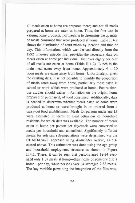
all meals eaten at home are prepared there; and not all meals prepared at home are eaten at home. Thus, the first task in valuing home production of meals is to determine the quantity of meals consumed that were produced at home. Table II.4.2 shows the distribution of adult meals by location and time of day. This information, which was derived directly from the 1992 time-use episode file, provides the necessary data on meals eaten at home per individual. Just over eighty per cent of all meals' are eaten at home (Table II.4.2). Lunch is the main meal eaten away from home. Approximately 4 in 10 noon meals are eaten away from home. Unfortunately, given the existing data, it is not possible to identify the proportion of meals eaten away from home, particularly those eaten at school or work which were produced at home. Future time­use studies should gather information on the origin, home prepared or purchased, of food consumed. Additionally, data is needed to determine whether meals eaten at home were produced at home or were brought in or ordered from a carry-out food establishment. Meals for persons under age 15 were estimated in terms of meal behaviour of household residents for which data was available. The number of meals eaten at home per person per day /week were converted to meals per household and annualized. Significantly different means for relevant sub-populations were determined via the CHAID/CAR.T approach using Knowledge Seeker, as dis­cussed above. This estimation was done using the age group and household employment structure as shown in Figure II.4.1. There, it can be seen that persons aged 18-24 aver­aged only 1.87 meals at home-their home or someone else's home-per day, while persons over 64 averaged 2. 83 meals . The key variable permitting the integration of the files was,

160

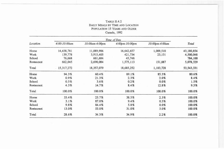
TABLE ll.4 .2 DAILY MFALS BY TIME AND LocATION

POPUIATION 15 YEARS AND OLDER Canada, 1992

--Time oiDg;J.

Location 4:00-JO:OOam I 0:00am-4:00pm 4:00pm-1 O:OOpm I 0:00pm-4:00am Total

Home 14,438,781 11,089,906 16,642,657 1,000,510 43,180,854 Work 139,778 3,915,405 421,734 23,131 4,500,048 School 76,668 661,684 45,748 784,100 Restaurant 662,045 2,690,084 1,575,113 151,087 5,078,329

Total 15,317,272 18,357,079 18,685,252 1,183,728 53,543,331

Home 94.3% 60.4% 89.l % 85.3% 80.6% Work 0 .9% 21.3% 2.3% 2.0% 8.4% School 0 .5% 3.6% 0.2% 0.0% 1.5% Restaurant 4 .3% 14.7% 8.4% 12.8% 9.5%

Total 100.0% 100.0% 100.0% 100.0% 100.0%

Home 33.4% 25.7% 38.5% 2.3% 100.0% Work 3.1 % 87.0% 9.4% 0.5% 100.0% School 9.8% 84.4% 5.8% 0.0% 100.0" Restaurant 13.0% 53.0% 31.0% 3.0% 100.0%

Total 28.6% 34.3% 34.9% 2.2% 100.0%

as discussed elsewhere, age of the respondents. The Family Expenditure File incorporated variables showing the number of weeks per year/persons of differing age groups were members in households. Basically, this variable provided a time-based link. Time-use data showed how many meals individuals of different age groups ate per day. This data was readily convertible into meals eaten per week. Thus, using relevant demographic variables, as elucidated by the analysis, and matching age groups in the two data sets it was possible to construct annual household meal outputs in terms of person weeks per year composition by the several household mem­bers.

In total, 21.4 billion meals are eaten at home in a year (Table II.4.3). Further refinement of this figure would require that take-out meals be separated out. Meals not pre­pared at home would make a smaller, but not necessarily insignificant, contribution to household output. The shopping component as well as cleanup would remain. On the other hand, meals eaten at work may well have been prepared at home and thus should be counted as part of home meals. However, such meals would not make the same contribution to household output as meals eaten at home since some of the associated costs would accrue away from home. Since these two forces operate in opposite directions they offset each other to an unknown extent. Their relative shares in meal consumption need to be identified. Given the number of . meals, the average value (price) of a meal produced can be determined.

Several possible avenues were explored to determine the appropriate price of meals. The first meal price estimate was made by calculating the average number of restaurant meals

162

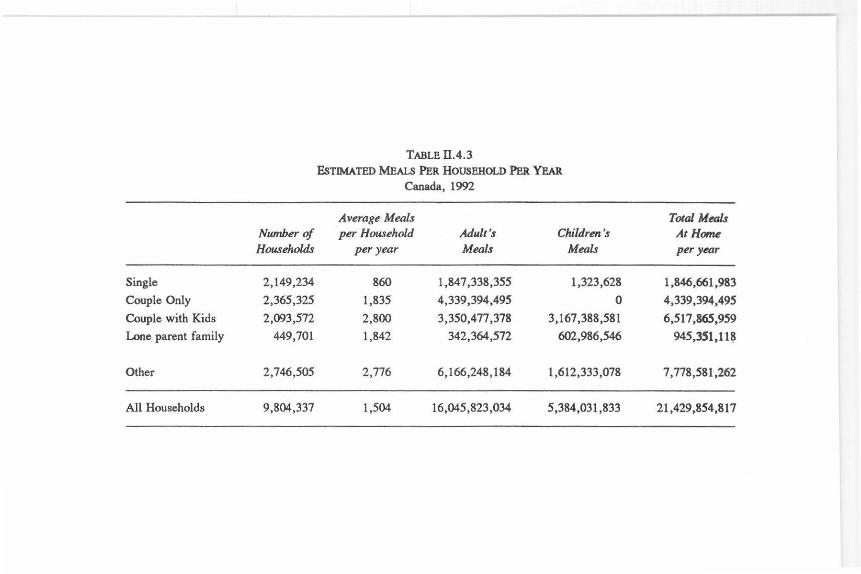
TABLE 11.4.3 EsTIMATBD MEALS PER HOUSEHOLD PER YEAR

Canada, 1992

Average Meals Total Meals Number of per Household Adult's Children's At Home Households per year Meals Meals per year

Single 2,149,234 860 1,847 ,338,355 1,323,628 1,846,661,983

Couple Only 2,365,325 1,835 4,339,394,495 0 4,339,394,495

Couple with Kids 2,093,572 2,800 3,350,477 ,378 3,167,388,581 6,517 ,865,959

Lone parent family 449,701 1,842 342,364,572 602,986,546 945,351,11~

Other 2,746,505 2,776 6,166,248,184 1,612,333,078 7,778,581,262

All Households 9,804,337 1,504 16,045,823,034 5,384,031,833 21,429,854,817

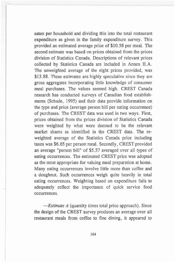
eaten per household and dividing this into the total restaurant expenditure as given in the family expenditure survey. This provided an estimated average price of $10.58 per meal. The second estimate was based on prices obtained from the prices division of Statistics Canada. Descriptions of relevant prices collected by Statistics Canada are included in Annex II.A. The unweighted average of the eight prices provided, was $13.88. These estimates are highly speculative since they are gross aggregates incorporating little knowledge of consumer meal purchases. The values seemed high. CREST Canada research has conducted surveys of Canadian food establish­ments (Schade, 1995) and their data provide information on the type and price (average person bill per eating occurrence) of purchases. The CREST data was used in two ways. First, prices obtained from the prices division of Statistics Canada were weighted by what were deemed to be the relevant market shares as identified in the CREST data. The re­weighted average of the Statistics Canada price including taxes was $6. 65 per person meal. Secondly, CREST provided an average "person bill" of $5.57 averaged over all types of eating occurrences. The estimated CREST price was adopted as the most appropriate for valuing meal preparation at home. Many eating occurrences involve little more than coffee and a doughnut. Such occurrences weigh quite heavily in total eating occurrences. Weighting based on expenditure fails to adequately reflect the importance of quick service food occurrences.

-Estimate A (quantity times total price approach). Since the design of the CREST survey produces an average over all restaurant meals from coffee to fine dining, it appeared to

164

provide the best estimate of price (P). One value used to estimate the value of output of the meals was the average restaurant expenditure per meal of $5.57 taken from the CREST survey. The 21.4 billion meals consumed at home in Canada, at $5.57 per meal, gives a total output value of $119.4 billion as shown in Table 11.4.4. The cost of pur­chased and non-purchased (self produced or gifts) inputs and capital consumption (RME) entering into the gross value needs to be subtracted in order to estimate VHW-the value added by the household. The value of the inputs, food purchased from stores, utility inputs and transport expendital, must also be subtracted from the gross value total to arrive at an unduplicated value of household production on an SNA basis. The national total for this is $48.2 billion (FAMEX, 1992). It was assumed that one and one-half rooms in a household are used for meal preparation and serving. Canadi­an homes have an average of six rooms (FAMEX); therefore, one quarter of the value of housing should also be deducted from VHW on meal preparation. The imputed net residential rent amounted to $20,552 million in 1992 (Statistics Canada, 13-201). UOD, assuming it equals one quarter of this value, is 5,130 million. Making these two adjustments, the value added for meals comes to $66.1 billion, Table II.4.4.

-Estimate B (quantity times net price approach). The price of $5 .57 per meal included taxes. This price was adjusted for taxes using the before- and after-tax prices for meals obtained from the prices division of Statistics Canada. Calculations using that data indicated that the average before­tax price was 89 per cent of the final price. The use of this factor yields a before-tax price of $4.96 which translates into

165

TABLE 11.4.4 OUTPUT DERIVATION OF VHW FOR MEAI. PREPARATION BASED ON MARKET PRICE

Canada, 1992

Value of Use of VHW of Meals

Quantiry (Q) Price (P) Output Purchased Inputs Dwelling for Satellite

Output '000 Can$* $'000 (RME) $'000 (UOD) $'000 $'000

A. Meals (after tax) 21, 429,855 5.51 119,364,292 48, 154,778 5,130,000 66,079,514

B. Meals (before tax) 21 , 429,855 4.96 106,292,081 48,154,778 5,130,000 53,007,303

* 1US$ = l.36Can$ at the time the study was conducted.

a total household meal output of $106,292,081. Adjusting for purchased inputs (RME) and dwelling cost (UOD) leaves an estimated value of meals produced of $53,007,303 (Table II.4.4).

-Estimate C (expansion of inputs approach). An alterna­tive approach to estimating the value of a meal is to use knowledge of the relationship between the cost of the pur­chased inputs and the value of the meals produced. Review of data from the 1993 Canadian Restaurant Industry Operations Report (Peat, Marwick, Stevenson, & Kellog 1993) shows that the proportion of purchased inputs in Canadian restau­rants varies from 29.5 per cent in a Quick Service Restaurant to 35 .4 per cent in a Fine Dining Restaurant. This value, in conjunction with the household use of purchased and non­purchased (self-produced or gifts) inputs, provides an alternative approach for determining the value of home consumed meals .

Information on purchased and non-purchased inputs is available from the F AMEX survey. Given the total value of purchased inputs of $48.2 billion indicated above and assuming households matched the average value (32.7), suggests a gross value of food produced at home of $147.4 billion [(l/.327) * $48.2). This yields an implicit price of $6.86 per meal (Table 11.4.5). Subtracting the $48.2 billion of purchased and non-purchased inputs (RME) leaves a total value of $98.8 billion before allowance for other deductions. Deducting $5 .1 billion for the use of the dwelling (UOD) leaves a VHW of meals of $93.8 billion.

In the foregoing the actual cost of purchased inputs was used. That amounted to approximately $48 billion.

167

TABLE Il.4.5 OUTPUT DERIVATION OF VHW FOR MEAL PREPARATION BASED ON EXPANSION OF PURCHASED INPUTS

Canada, 1992 -

Value of Purchased and VHWofFood Implicit Output non-purchased Use of Preparation for

Output Quantity (Q) Price (P) $'()()() Inputs (RME) Dwelling Satellite '()()() $ RME*J.058 $ '()()() (UOD),$ $ '()()()

Meals 21, 429,855 6.86 147,094,801 48,154,778 5,130,000 93,764,801

2. Child Care

Child care constitutes the main family caring activity. The output of child care, or any dependent individual, can be considered to be a child (dependent person) hour or child (dependent person) day. Thus, if an individual is directly responsible for three children for a 24-hour period, the output would be 72 child hours or three child days. While individual direct child care time may be much less, the individual is committed to caring for the children during all hours of direct responsibility. Banke (1988) denotes such time as "stand-by care." Similarly, as one approach, the authors of the 1979 Finnish study adopted what they believed was the broadest possible concept of child care. "The volume of home care refers to the time when children are at home at the same time with and under the control of some older member of house­hold (Suviranta and Heinonen, 1980)." However, they considered only children under seven years of age.

Prior to the measurement of child (dependent person) output major decisions must be made. First, for what ages of children should care be measured? Second, what time per day is to be included in child care time? Should only direct care be counted, or standby care as well? Third, what level of commitment or weight should be given to secondary or standby child care time? Direct child care poses little prob­lem. However, secondary or standby child care, in which one is responsible for children while doing other things, may represent a different level of commitment which needs to be recognized. Does one consider time spent while the children are sleeping to bear the same weight as time spent when they are playing or studying?

In the Canadian study, child care was defined as direct

169

child care, such as feeding, clothing, etc., plus indirect or secondary child care, which is being responsible for a child. For this exercise the quantity of child care was determined using the time-use episode file . Child care was totalled for each individual in the episode file. Again, segmentation analysis using Knowledge Seeker was used with the time-use episode file to produce averages of child care time for individuals to merge into the family expenditure file. Age group of the household parents and the number of children in the family best segmented child care time. Averages were produced for the matrix of these two estimators. From the F AMEX file it was determined that 11. 98 billion hours of household child care are provided at the national level.

With the time spent on child care estimated for the families in the expenditure file , an output based value had to be associated with this time. The cost of full-day care service was used as the value of child care time. These prices were obtained from a study by Child-care Resource and Research Institute (1994). The market price of $1.93 per child care hour was obtained by using a provincially weighted average of monthly prices, adjusted assuming 21 days per month and nine hour days. Since the child care time estimate does not differentiate between infant, preschool and school-age child care, a weighted average of the prices of these types of child care was used. The figures of 11.98 billion child care hours at $1.93 per hour, gives a value of home child care of $23.13 billion (Table 11.4.,6). Part of the market price of child care includes the cost of the building (UOD) in which the care takes place. Since the cost of one's home is already included in the System of National Accounts , this must be subtracted from the value of child care to arrive at net value added beyond what is included in the SNA figures .

170

A Cost, Quality and Outcome Study conducted in the United States provides some guidance on the portion of day care costs attributable to shelter (Helbum et al., 1995). It suggests that 6.22 % of the cost of child care in the market place, comes from the occupancy cost of the building. Thus, the value of child care is 19 .1 billion-i.e., $23 .12 billion less purchased inputs (RME) of $2. 7 billion and less the imputed shelter cost of $1.4 billion (Table II.4.6).

Care of others, which should also be captured, is not included. Currently, there are no good output measures for this element of household production. It is important that appropriate measures be developed. This is particularly true as health systems push patients out of the market health sector into the unpaid sector shifting the burden of care.

3. Housekeeping

Another major output provided by the household is shelter. A fairly wide range of activities are subsumed in this value including cleaning, general building and grounds maintenance, purchasing household supplies, some aspects of household planning and management. This component of household output is the most difficult to characterize opera­tionally at the category and item level. At this stage in the development it is being defined in terms of nights of accom­modation provided by the household. A similar approach was used by Chadeau and Fouquet (1986).

The number of potential person nights of accommoda­tion was calculated in the family expenditure file which provides an accounting of the total weeks individuals spend in household unit. This number was then reduced by the number

171

TABLE II.4.6 OUTPUT DERNATION OF VHW FOR FAMILY (CHILD) CARE

BASED ON MARKET PRICE

Canada, 1992

Child Hourly Care Hours Price Value of Purchased Use of VHWfor

Output Quantity (Q) (P) Output Inputs (RME) Dwelling (UOD) Child Care '()()() $ $'000 $'000 $'()()() $'000

Child Care 11,983,623 1.93 23,128,392 2,607,954 1,438,586 19,081,852

of nights , on average, spent outside of the home. An analysis of the time-use episode file showed that 96.9% of nights are spent at home. Another 1.6% of nights are spent at other's homes. The total of this, 98.5%, was the amount used for person nights of accommodation, since a night spent at one's own home or another's home both have value that needs to be measured. Single persons in Canada averaged about one week a year away from home, spending 358 nights a year at home (Table Il.4.7A).

TABLE II .4.7A EsTIMATED P ERSON/ NIGHTS PER HOUSEHOLD PER YEAR

Canada, 1992

Average Nights Total Nights Total Nights Number of per Household At Home at other 's Households per year p er year Home

per year

Single 2, 149,234 358 769,425,772 12,704,657 Couple Only 2,365,325 713 1,686,476,725 27,846,881 Couple

with Kids 2,093 ,572 1,375 2,878,661 ,500 47,532,078 Lone-parent

family 449,701 942 423,618 ,342 6,994,730 Other 2,746 ,505 1,240 3 ,405 ,666,200 56,233 ,910

Total Households 9,804,337 935 9, 163 ,848 ,539 151,312,256

The market price used f©r housekeeping is, therefore, based on the price of a motel room. The Canadian average price of motel room accommodations was $51.21 per night, for two person accommodations, or $25.61 per person. The

173

9.31 billion nights (total nights at home plus total nights at others' home) at $25.61 per night, has a value of $238.6 billion. Purchased inputs (RME) amounted to $16.4 billions (Table 11.4. 7B). Once again, the cost of the portion of the dwelling used must be subtracted from the above value.

TABLE Il.4.7B HOUSEKEEPING RELATED RME

Canada 1992

Water, fuel, electricity

Cleaning and polishing preparations

Linen cleaning etc.

Disinfectants and deodorizers

Paper, plastic, and foil household supplies

Horticultural goods and services

Other household supplies

Transportation

Total per household

Total expenditure housing

Expenditure per household

1,075 62

62

27

187 154 68

40 1,675

16,422,266,639

The average home has 2. 7 bedrooms, out of a total of six rooms (F AMEX). The adjustment for UOD is equal to 45 % of the imputed rental value which amounts to $10.3 billion. Thus, the value of household work (VHW) in the provision of housekeeping services is $211.9 billion, as shown in Table 11.4. 8.

174

4. Clothing Care (Laundry)

Laundry consists of both personal and household compo­nents. Clothing care or personal laundry fall outside services typically included in shelter" or accommodation costs and must be estimated separately. However, the component of laundry related to shelter maintenance would be included in shelter costs and thus should be excluded when evaluating clothing care output. Kilograms of laundry were used as the measure of household output in the Finnish study, outlined above. Here, machine loads of washing have been used. Typically, one can be converted into the other. However, given the variety and nature of current fabrics, loads may not directly translate into kilograms, or vice versa.

Assuming the output measure to be loads of laundry, it is necessary to quantify the number of loads generated, or produced, in households and the extent to which they are produced at home or in the market. Laundry outputs were based on work in progress in the U.S. (Sanik, 1995). Based

on the U.S. survey data on laundry activity, it was estimated for this study that single and couple households average 4 loads of laundry each week while other households average eight loads. This generated 3.1 billion loads of laundry per year.

175

Output

Housekeeping

TABLE 11.4.8 OUTPUT DERNATION OF VHW FOR HOUSEKEEPING BASED ON MARKET PRICE

Canada, 1992

Use of

Price Value of Purchased Dwelling Quantity (Q) (P) Output Inputs (RME) (UOD)

'()()() $ $ '()()() $ '()()() $'()()()

9,315,161 25.61 238,561,273 16,422,267 10,276,000

VHWfor

Household Upkeep $ '()()()

211,863,006.5

TABLE Il.4.9 OUTPUT DERIVATION OF VHW FOR CLOTHING CARE BASED ON MARKET PRICE

Canada, 1992

Price Value of Purchased Inputs Use of Dwelling VHWfor Output Quantity (Q) Units (P) Output (RME) (UOD), aothing

'()()() $ $'()()() $ '()()() $ '()()() Care

Clothing Care 1,569,790 loads $3.60 5,651,244 607,869 In housekeeping 5,043,375

However, part of the weekly laundry is subsumed in the housekeeping output and must be excluded to prevent double counting. The assumption made here is that half the laundry relates to household care and half relates to clotfifng care. Thus, clothing care is estimated as 1.6 billion loads per year (Table II.4.9) . The price used is based on per load costs for use of commercial laundromats for which Statistics Canada collects price data. However, the Statistics Canada data do not reflect charges beyond the machine charges in laundro­mats . The price of $3.60 per load used here includes wash­ing, drying and a service charge per load for laundry dropped off and processed by laundromat staff. Purchased inputs (RME)-detergents and bleach, and fabric softeners-were· calculated from the household expenditure data . This amount­ed to 9.2 billion. The decision was made to leave UOD in the housekeeping figure and not calculate a separate UOD for clothing care.

5. Volunteerism

Measurement of voluntary or unpaid community orient­ed activity poses special problems to researchers and there was no current data on this activity for Canada. The problems are the two-fold problems facing any attempt to quantify unpaid activity, determining its extent and valuing it. Much work is needed to solve these problems. Some insight, however, into the value of volunteer activity is available for Canada (Ross, 1990). While the approach used, based on inputs, deviates from the attempts here to measure and value outputs it is useful to suggest the possible magnitude of this sector. Volunteer time estimates were derived from data

178

collected by means of a special volunteer activity survey. The time was valued using estimated average wages for the class of activities denoted 'community, business, and personal services' since it was deemed that this group best reflected the work o'f volunteers . Ross made initial calculations, an estimated annual contribution of $12.0 billion, for 1986/87, to correspond with the time data (Ross, 1990). He then projected that forward at the rate of inflation for an estimated $13.2 billion in 1990. That figure was further adjusted for the rate of inflation to derive a rough estimate, $14.7 billion, of volunteer activity for 1992. This provides only a very crude estimate of the value of volunteer work but it does provide insight into its relative dimension with respect to other unpaid work activity.

6. Personal Development

Previous valuation studies have ignored the educational component of non-market production. One reason for this is that time devoted to education has been viewed as a consump­tion good since it does not fit the 'third person criterion' for defining production. Another, more practical reason is that national accounts statisticians have so far avoided incorporat­ing human capital into the accounting process. Since captur­ing the flow has implications for handling the stock of human capital, there has been a hesitancy to incorporate it.

As argued in the monograph Measurement and valuation of unpaid contribution: Accounting through time and output (INSTRA W, 1995), however, education represent personal and, hence, household investment which yields a return over time. While there is no separation of producer and receiver

179

there is separation between the time input to education and hence its production and the returns from it.

While outlays on education are highly significant in eco­nomic terms, the outlay-based approach to the measurement of educational investment ignores ... the lengthy gestation period between the application of educational inputs-main­ly the services of teachers and the time of their students (emphasis added)-and the emergence of human capital embodied in the graduates of educational institutions ... (Jorgenson and Fraumeni, 1991, p.22).

The authors go on to point out that comparisons between two sets of human capital estimates, one an outlay-based ap­proach and the other their income-based approach showed the latter to be much greater than the former (Jorgenson and Fraumeni, 1992). Thus, the authors argue that "the appropri­ate value of education is given by its impact on the indivi­dual's lifetime income" (Jorgenson and Fraumeni, 1991, p.23) .

Suggesting that the value of education can be either a cost-based approach, or an income approach lies close to the heart of the concerns which motivate the current work of INSTRA W. To assume that the value of an activity or output is equal to its cost, assumes, minimally , that the cost of all

· inputs have been accounted for. To consider the value of an education to consist only of the cash outlays made to obtain it greatly underestimates the value of those outlays.

A recent study of the costs and returns to education in Nova Scotia, Canada, showed the costs of an undergraduate university education to be carried roughly half by the individ­ual student, 40 per cent by the government, and 10 per cent

180

by other sources (Harvey et al. , 1995). Of the students contribution to costs, foregone income was a major compo­nent, 63 per cent for males and 48 per cent for females. The reduced importance of foregone income for females being attributable to their experienced lower market incomes. Individual rates of return were estimated at 5.25 per cent for males and 7.04 per cent for females (Harvey et al., 1995). The rates of return to society as a whole from an undergradu­ate education were 7 .29 per cent for males and 13.28 per cent for females. These rates were calculated by setting what were considered the full costs of obtaining the degree against the estimated increased flow of income generated by the degree. Costs included both direct outlays by individuals and society and the individuals foregone income attributable to their student status. The study showed that loss of foregone income is a significant productive input into the generation of human capital. An increased income flow is the return.

For this study, also, lost income attributable to student status was taken as the cost 'price' of education. The income differential between students and non-students was calculated for the population aged 12-27 years . Income calculations were made for labour (wages and salary plus self-employ­ment) income using the public-use sample data of individuals from the 1991 Canadian census. For women, the difference, for the census income year, between students and non-stu­dents ranged from $809.53 (aged 12-17 years) to $6,841.85 (aged 24-27 years). For men, the comparable range was from $1,362.44 to $11,904.07. The analysis here actually under­states the full cost of time allocated to education since it was limited to full time students. A total of 1,251,765 women and 1,257,432 men were full time students. Further work needs

181

to be undertaken to expand estimates to include part time study as well.

The total cost of education in terms of lost income from paid work was $8.3 billion (Table II.4.10). The major share of that, $5. 2 billion was attributable to men. The lost income from market work, however, only addresses part of the cost of obtaining and education.

Females Males

Total

TABLE Il.4.10 NON-OUTLAY COSTS OF EDUCATION

Canadians aged 12-27, 1992

Paid Work

3,160,589,321 5,183,697,163

8,344,286,483

Unpaid Work

10,500,349,200 4,343,339,511

14,843 ,688, 711

Total

13,660,938,521 9,527,036,673

23,187,975,194

Non-market work is also a productive activity and to the extent to which it is diminished as a result of student status, total productive activity is diminished. This realization is often as important a detriment to further education of student as is the need to get money income. Particularly in develop­ing countries family alternatives may involve not a trade off between whether one works in the market or not but whether one works in the market or at home so someone else, say a parent can work to earn income.

The value of non-market production foregone for educa­tion can be determined using the time-use data to provide a measure of the time cost and using implicit labour returns

182

from the valuation of the household and caring components of non-market production to provide a value for that time. Male students registered 374 hours less unpaid work per year than their non-student counterparts while female students regis­tered 935 hours per year less than their counterparts. Assum­ing the implicit value of the time lost in unpaid work per hour, and given the number of students indicated above, the value of foregone unpaid production by women was $10.5 billion and for men $4.3 billion.

Combining both paid and unpaid contributions to educa­tion the total cost is $23.2 billion per year.

B. CANADIAN UNPAID WORK: AN OVERVIEW

The components of household output valued here account for total household production in 1992 of over $411 billion dollars and for a total value added by household work of over $327 billion or 47.5 % of GDP {Table II.4.11). This estimate does not include care to other than children. Inclu­sion of this would expand the household's contribution to unpaid work. In comparison, Statistics Canada estimates the total value added by household work to be $234.5 billion in 1992 using the generalists replacement cost approach. The Statistics Canada does incorporate care of others. Thus, for Canada the estimates derived here using primarily the output approach yield a higher value added by unpaid work than does the generalists input approach used by Statistics Canada.

The shelter component, housekeeping, accounts for the largest share of total household output followed by meals.

183

Housekeeping makes about three and one-half times the contribution of meals. Purchased inputs (RME) and the contribution of dwelling (UOD) represent a major portion, about fifty per cent of total household output of meals. For the other components, however, RME and UOD are relative­ly minor components of each, ranging from ten to 20 per cent.

1. Data Strengths and Weaknesses

A major strength of the Canadian Family Expenditure file utilized in this study was that it provided a crucial link, weeks of household membership by age group, between the household expenditure data and the individual time use data. A major shortcoming was the fact that the age groups in the family expenditure data were not gender specific. Thus, only the total number of months that a specific age group contrib­uted to the household "time budget" was known. It was not possible to distinguish months by women and by men. The age group variables, expressed in terms of weeks per year are ideal for integrating the time and expenditure data where time-use data is at the individual level. Attention should be given to the construction of gender-specific age groups. They should be sufficiently disaggregated to capture the significant time-use and expenditure patterns. Failure to distinguish the type of meal eaten was a major shortcoming of the time-use study data. The time-use data provided little clue, other than time of day and a limited number of eating situations, to the nature of the eating episode. Was an eating episode a com­plete meal? Was this episode one of eating an apple? Clearly these should be valued differently. Additionally, the time-use

184

TABLE 11.4.11 OUTPUT DERIVATION OF VHW FOR UNPAID WORK BASED ON MARKET PR.ICE

Canada, 1992

Purchased Use of Value of Inputs Dwelling

Output Quantity Units Price Output (RME) (UOD) VHW '()()() $ $ '()()() $ '()()() $ '()()() $ '()()()

. Meal Preparation 21,429,855 meals 4.96 106,292,081 48,154,778 5,130,000 53,007 ,303 Housekeeping 9,315,161 nights 25 .61 238,561,273 16,422,267 10,276,000 211,863 ,006 Clothing Care 1,569,790 loads 3.60 5,651,244 607,869 in housekeeping 5,043,375 Child Care 11,983,623 hours 1.93 23,128,392 2,607,954 1,438,586 19,081,852

Household Maintenance - - - 373,632,989 67,792,868 16,844,586 288,995 ,535

Per cent of GDP 54.2% 9.8% 2.4% 41.9% Input share 100.0% 18.1 % 4.5% 77.3%

Volunteer Work 14,730,234 14,730,234 Education - - 23 ,187,975 23,187,975

Total 411,551,199 67,792,868 16,844,586 326,913 ,745 Input Shares 100.0% 16.5% 4.1% 79.4% As% of GDP - - - 59.7% 9.8% 2.4% 47.4%

data do not distinguish between a meal brought from home and eaten at work and a meal which is purchased at or near work. Such detail would greatly improve the accuracy of valuations based on meals as outputs.

Failure to distinguish for each episode individual recipi­ents of child care time or time with children presented a real obstacle to getting a precise measure of demand for child care. Better detail on child care and adequate detail on other household members being cared for is necessary. It is also necessary to capture-by some survey instrument-details on household laundry. Very few questions on a related instrument would provide data which could be integrated with the time-use and family expenditure data to improve the laundry estimates. In particular, it would be useful to have separate volume estimates for clothing and for other household laundry.

II. FINNISH HOUSEHOLD OUTPUTS

A. SATELLITE ACTIVITIES AND OUTPUT VALUATION

1. Meal Preparation

Meals eaten at home were estimated, as they were for Canada, from the time use file. For Canada, the estimated meals were linked to the household expenditure file via the age of respondent variable since it was the age variable that was designed to provide information on the overall annual composition of the household in terms of person days . A different method was used by Statistics Finland to capture annual composition. The Finnish consumption file captures

186

annual household composition by aggregating the number of months each of the members spend in one ·or a combination of several occupational classes. Thus the total household composition for a year is the sum of months spent by its members as workers, students, disabled/ill, homemakers, pensioners, etc. Consequently, for Finland, total household meals were determined by using the occupational variable. Since all members of the household are broken down in various occupation categories, these final estimates include both children and adults. Analysis using Knowledge Seeker indicated that meal estimates were improved by also using level of education and household total annual consumption per consumption unit as independent variables . Thus, average number of meals by main occupation, were incorporated into the consumer expenditure file on level of education and household annual consumption per consumption unit.

Following integration of the meals eaten at home into the consumer expenditure file it was estimated that the Finns ate a total of approximately 3.9 billion meals at home and 1793 per household, per year, for an average of 2.14 meals per person, per day (Table II.4.12). The average price of a meal away from home was estimated, from the consumer expenditure survey data, to be 22.3 FIM. This price, approximately $7 .16 Canadian is somewhat higher than the estimated Canadian price of approximately $5.00. The estimated value of meals consumed at home was $86.1 billion FIM. From the value of output it is necessary to deduct purchased inputs (RME) of 39. 3 billion FIM (Table II. 4.13) and estimate of the value of use of dwelling (UOD) of 11.2 billion FIM (Table II..4.12). This leaves a value of housework estimate for meals of 35. 7 billion FIM.

187

TABLE II.4.12 OUTPUT DERIVATION OF VHW FOR MEAL PREPARATION BASED ON MARKET PRICE

Finland, 1990

Output Quantity (Q) Price (P) Value of Purchased Use of VHWof '()()() FIM Output Inputs Dwelling Meals for

000 FIM (RME) (UOD) Satellite

'<XXJ FIM '<XXJ FIM '<XXJ FIM

Meals 3,862,248,299 22.3 86,128,137.1 39,315,000.0 11,150,442.0 35 ,662,695.1

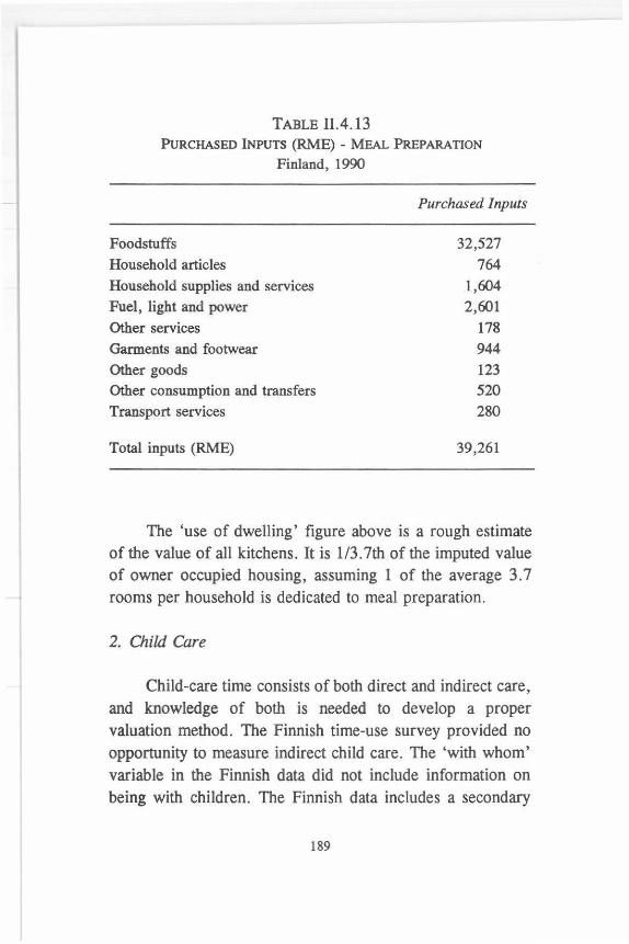
TABLE 11.4.13 PuRCHASED INPUTS (RME) - MEAL PREPARATION

Finland, 1990

Purchased Inputs

Foodstuffs 32,527 Household articles 764 Household supplies and services 1,604 Fuel, light and power 2,601 Other services 178 Garments and footwear 944 Other goods 123 Other consumption and transfers 520 Transport services 280

Total inputs (RME) 39,261

The 'use of dwelling' figure above is a rough estimate of the value of all kitchens. It is 1/3.7th of the imputed value of owner occupied housing, assuming 1 of the average 3.7 rooms per household is dedicated to meal preparation.

2. Child Care

Child-care time consists of both direct and indirect care, and knowledge of both is needed to develop a proper valuation method. The Finnish time-use survey provided no opportunity to measure indirect child care. The 'with whom' variable in the Finnish data did not include information on being with children. The Finnish data includes a secondary

189

activity variable which does have a record of child care as a secondary activity; however, that measures direct child care as a second activity, not indirect child care. After attempts to develop child-care time estimates from the Finnish data it was concluded that another approach was required.

The approach applied was the one used in the Finnish Ministry study (Suviranta and Heinon, 1980) to calculate child care hours. It reflects only hours for children under 7 years. Total possible hours were calculated by multiplying the number of children under seven derived from the household consumption file by 365 days per year times 24 hours per day. In 1990 there were 430,672 children under the age of seven, up just slightly from the 427 ,000 recorded for 1978 in the Ministry Study. This generated a total of 3, 773 million child care hours per year. This number was then adjusted for paid child care hours by subtracting 227.5 million hours given by dividing total child care expenditures from the family expenditure study by the average hourly price for child care of 6.08 FIM. The share of paid day care was up just slightly over the decade from 6. 82 per cent of the total to 7. 36 per cent. This left 3 ,545. 2 million unpaid hours of which 1,414.8 million were between 10 pm and 7 am and 2,357.9 million were between 7 am and 10 pm. Assuming that all paid hours came out of the daytime hours there were 2,130.4 million unpaid daytime hours. The distinction be­tween daytime and nighttime hours was drawn in keeping with the Ministry study approach which noted that hourly wages for child care during the night hours were one-half what they were during the daytime hours. This is an area where procedural agreement must be reached in order to ensure inter-temporal and international comparability.

190

TABLE 11.4. 14 OUTPUT DERNATION OF VHW FOR CHILD CARE BASED ON MARKET PRICE

Finland, 1990

Output Quantity Price Value Inputs Use of Value

Child Care (FIM) Dwelling Added

Hours '()()()

Child Care 3,545,204.2 4.87 17,265,144.5 1,946,248.8 1,073,197.5 14,245,698.3

Child-care hours were valued at 6.08 FIM per hour, derived from the consumer-price data based on an average monthly child-care cost per child of 1,216 FIM and assuming 200 hours per month of care. This amount, $1.95, when converted into Canadian Dollars is virtually identical to the hourly cost of day care in Canada of $1.93. In the absence of better data on RME and UOD recourse was made to the Canadian estimates for estimating ratios . Thus, as in Canada, UOD was assumed to be 6 .22 per cent of the price (value) of child care, based on the US Cost, Quality and Income Study (Helburn, et al. , 1995). Canadian estimates suggested that purchased inputs amounted to 11.28 per cent of the total value of child care. Thus, 17 ,254 million FIM is the sum of daytime hours times 6.08 FIM plus nighttime hours times 3.04 FIM, on average 4.87 FIM per hour. These give a total value added of 14.2 billion FIM for child care (Table II.4.14).

3. Housekeeping

Derivation of the value of housekeeping for Finland was the same as for Canada. There was no problem deriving the number of nights accommodation provided by Finnish households based on time use data. An estimated 98.3 per cent of all nights were spent at home or at someone else's home. The value of night accommodations was obtained from a Statistics Finland survey of accommodations started in 1993. For the purposes of this study, the 1993 estimate of 147 FIM was adjusted to 1990 using the consumer price index. This provided an estimate of 135. 8 FIM per person per night.

192

TABLE Il.4.15 OUTPUT DERIVATION OF VHW FOR HOUSEKEEPING BASED ON MARKET PR.ICE

Finland, 1990

Output Quantity (Q) Implicit Value of Purchased Use of VHWof

Price (P) Output Inputs (RME) Dwelling Household

FIM '000 FIM '000 FIM (UOD) Maintenance

'000 FIM for Sale/lite

'000 FIM

Nights 1, 774,586, 794.6 135.8 241 ,024,379.2 13,970,361 28,159,944.6 198,894,073

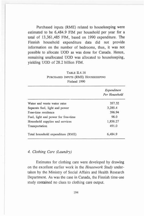
Purchased inputs (RME) related to housekeeping were estimated to be 6,484.9 FIM per household per year for a total of 13,361,485 FIM, based on 1990 expenditure. The Finnish household expenditure data did not provide information on the number of bedrooms, thus, it was not possible to allocate UOD as was done for Canada. Hence, remaining unallocated UOD was allocated to housekeeping, yielding UOD of 28.2 billion FIM.

TABLE Il.4.16

PuRCHASED INPUTS (RME) HOUSEKEEPING

Finland 1990

Water and waste water rates

Separate fuel, light and power

Free-time residence

Fuel, light and power for free-time

Household supplies and services

Transportation

Total household expenditure (RME)

4. Clothing Care (Laundry)

Expenditure

Per Household

357.32

3,285.4

396.94

98.0

1,856.27

491.0

6,484.9

Estimates for clothing care were developed by drawing on the excellent earlier work in the Housework Study under­taken by the. Ministry of Social Affairs and Health Research Department. As was the case in Canada, the Finnish time-use study contained no clues to clothing care output.

194

Time-use studies provide only an indication of the input time. Without, the necessary research and data on the produc­tivity of such time it is not possible to convert it to outputs. However, work undertaken for the Housework Study in 1979 determined a figure, 143 kilograms for the average annual kilograms per person of laundry (Suviranta and Mynttinen, 1981). This value was used as the basis for estimating clothing care output here. Taking this figure, the population of approximately 4.9 million would generate in excess of 700 billion kilograms of laundry in 1990, which includes laundry relating to household care and that which relates to clothing care. Using the same assumption applied for Canada, it is estimated that half (353 kg.) of the total laundry relate to clothing care (Table 11.4.17) .

Unlike Canada, Finland lacks laundromats where individuals can do their own laundry, the source of a price for valuing Canadian laundry output. Thus, an alternative valuation approach was necessary. Again, this study drew on the Housework Study. The Finnish study derived the value of labour used for laundry using the average per-kilogram price obtained from the Finnish Association of Laundries and Dry Cleaners and the associated cost distribution (Suviranta and Mynttinen, 1981). Unfortunately, the survey used to provide that data is no longer collected. For this study, a check of major laundry firms indicated a price of 13.5 FIM per kilogram would be appropriate for use in valuing home laundry. That value was used. As with Canada, use of the dwelling (UOD) attributable to clothing care was assumed to be incorporated into the housekeeping component. Additional­ly, lacking a better allocator for purchased inputs related to clothing care, they were assumed to be the same proportion of total output, 10. 74 per cent, as they were in Canada.

195

Output

TABLE II.4.17 OUTPUT DERN ATION OF VHW FOR CLOTHING CARE BASED ON EsTIMATED MARKET PRICE

Finland, 1990

Kg. of Laundry Price

per year '000 (FIM)

Value '()()()

Inputs '000

Use of

Dwelling

Value Added '()()()

Clothing Care 353,283,071.4 13.5 4,769,321.9 512,702.1 4,256,620.0

TABLE Il.4.18 OUTPUT DERIVATION OF VHW FOR UNPAID WORK BASED ON MARKET PRICE

Finland, 1990

Output Quantity Unit Price Value of Purchased Use of VHWof (Q) (P) Output Inputs Dwelling Meals '()()() FIM OOOFIM (RME) (UOD) OOOFIM

'OOOFIM

Meal Preparation 3,862.248.3 meals 22.30 86,128,137.1 39,261,000.0 11, 150,442.0 35,716,695.1

Housekeeping 1,774,586.8 nights 135.82 241,024,379 .2 13,970,361.4 28, 159,944.6 198,894,073.2

Child Care 3,545,204.2 child hours 4.87 17,265,144.5 1,946,248.8 1,073, 197.4 14,245,698.3

Clothing Care 353,283.1 kilograms 13 .50 4,769,321.9 512,702.1 - 4,256,620.0

Total VHW - - - 349,186,982.7 55,690,312.3 40,383,584.0 253, 113,086.6

Per cent of GDP 67.7 10.8 7.8 49.1

Input Share ( 3) - - - 100.0 15.9 11.6 72.5

B. FINNISH UNPAID WORK: AN OVERVIEW

The total estimated value of household production (VHW) in 1990 was $253.1 billion FIM amounting to 49.1 per cent of the 1990 GDP (Table II.4.18). However, this estimate represents a lower boundary for estimated household production since it does not include production related to education or to volunteer work.

Comparison of estimates

For Finland there exist two other sets of estimates of the value of household production. The first set is contained in the very detailed Housework Study undertaken by the Re­search Department of the Ministry of Social Affairs and Health around 1980. The second set, prepared at Statistics Finland, is for the period, 1990, covered by this study draws on major survey data regularly collected by the Statistical Bureau. Both are excellent pieces. The work presented here, essentially draws on the same data as that used in the recent Statistics Finland study and develops estimates for the same year.

This study and that of Statistics Finland take two differ­ent approaches. The focus of attention in this study is house­hold output as determined by quantity and price. The focus of the Statistics Finland study was on the value of output derived as the summation of the value of the inputs. The latter ap­proach makes sense if one can assume, as does neo-classical production theory, that in the long run in a perfect market, price will equal the average cost of production. However, it is highly possible that such conditions do not hold for house­holds. Due to structural rigidities, however, such conditions

198

may well not hold; households do not cease to exist because they are inefficient producers. Only if it is possible to derive independent values for the inputs and outputs of household production, will it be possible to evaluate the functioning of households as economic production units and appropriately measure their output in a manner consistent with the SNA.

The recent Statistics Finland estimate, using the general­ists replacement approach of 232 billion FIM, equaling 45.1 per cent of national GDP, was lower than the estimate here. Comparison of the Statistics Finland input-output approach and the output approach used here suggests some very fundamental differences in the estimates.

According to the output estimates developed here the value of household work for meals is 86.1 billion FIM which is 6.9 per cent of the 1990 GDP of 515 billion FIM. In comparison, the earlier Ministry study found that cooking plus related shopping amounted to 15.6 per cent of total GDP of 186.8 billion FIM in 1980. It contrasts even more with the approximately 117. 7 billion dollars for meal preparation (106.0 billion FIM) and shopping (11.7 billion FIM) derived in the Statistics Finland study which are estimated to account for 22.9 per cent of GDP. For Canada, meals were about 7.7 per cent of GDP compa?ed with 6.9 for Finland. Interesting­ly, these shares, both derived by the output approach, are similar. Their divergence from input-based estimates raise interesting questions: Are there problems with the estimates? Or, do the output estimates, in comparison with input esti­mates, reveal that home-meal production is significantly inefficient relative to the market?

The approach to child care taken here was to use the price for one hour of care for an individual child in a day-

199

care setting. The input-output approach used a value per hour for the child care giver. The present and input-output ap­proaches yielded estimates of 14.2 billion FIM and 20.5 billion FIM respectively. Thus the estimate here is just a little over two-thirds that of the one by Statistics Finland. Since the approach used here was limited to care of children under 7 years, it is reasonable to assume that a major part of the difference is attributable to the more inclusive definition used by Statistics Finland, however, they used time spent caring, not children cared for, as their measure.

The estimaton approach chosen here limited child care giving to children under age seven. All else equal this would be expected to yield a lower figure since the estimate is based on many fewer children. However, all else was not equal. The Finnish input-output study based its valuation on only direct child care time. This approach to quantifying child care is highly questionable. Frederick showed for Canada that child care time measured by parental contact, a specific child care diary and a direct question were each about four times as great as direct child care time measured on the time diary (Frederick, 1994). Further work is needed to develop a measure of the extent of care-giving required for children seven and over. Additionally, it is likely that one would want to assign a different price for care-giving for older children. Additionally, the child care hour and its price is a very different value from the housekeeper hour and its wage rate.

The estimate here of 86.1 billion for meal preparation (which includes shopping and other meal related components) contrasts sharply with the approximately 117. 7 billion dollars for meal preparation-( 106. 0 billion FIM) and estimated (here for comparison) meal related shopping (11. 7 billion

200

FIM)-derived in the Statistics Finland study. Again, the output approach yielded an estimate approximately two-thirds of that given by the input-output approach. Using the Statis­tics Finland values the implied average price of a meal is 28.9 FIM in contrast to the 22.3 FIM used here, a difference in price of about 30 per cent.

III. COMPARISON OF FINNISH AND

CANADIAN ESTIMATES

In constructing the estimates, research decisions between the two countries were essentially made independently as necessary, although the distribution of the components of household activity is very similar between the two. The housekeeping component of household activity accounts for about three quarters of the total value of household output while meals account for 18.3 and 14.1 per cent of the total value of household output in Canada and Finland respectively (Table 11.4.19). In Canada, the value of household work (VHW) is about 42 per cent of GDP, while VHW for Finland is 40 per cent of GDP, excluding volunteerism and education.

Comparisons with other Canadian and Finnish estimates are also enlightening. Technically, it is to be expected that estimates derived by means of the output approach would, all else equal, be higher than estimates based on a generalists replacement basis. The output approach encompasses value added through the contribution of household capital services and profit and is thus larger by definition. Failure of the output approach to truly reflect reality must rest with one or a combination of two factors, either the quantity of output is

201

TABLE Il.4.19 COMPARISON OF FINNISH AND CANADIAN EsTIMATES

Value of Share of Value of Share of Share of Hhold. Output GDP(%) Household Work GDP(%) Maintenance (%)

Canada $'000 Meal Preparation 106,29'2,080.8 15.4 53,007,302.8 7.7 18.3 Housekeeping 238,561,273.0 3,4.6 211 ,863,006.0 30.7 73.3 Child Care 23, 128,39'2.4 3.4 19,081,852.4 2 .8 6.6 Clothing Care 5,651,244.2 0.8 5,043,375.2 0.7 1.8 Total Household Maintenance 373,632,990.4 54.1 288,995,536.4 42.0 100.0

Volunteer Work. 14,730,234.0 2.1 14, 730,234.0 2 .1 Education 23,187,975.0 3.4 23,187,975.0 3.4 Total 411,551,199.4 59.7 326,913, 745.4 47.5

GDP 689 ,652,941.2 100.0 689,652,941.2 100.0

Finland '000 FIM Meal Preparation 86,128,137.1 16.7 35,716,695.1 6.9 14.1 Housekeeping 241,024,379.2 46.8 198,894,073.2 38.6 78.6

Child Care 17,265,144.5 3.3 14,245,698.3 2.8 5.6 Clothing Care 4,769,321.9 0.9 4,256,620.0 0.8 1.7 Total Household Maintenance 349,186,982.7 67.7 253,113,086.6 49.1 100.0

Volunteer Work. n/a n/a Education n/a n/a Total 349,186,982. 7 67.7 253,113,086.6 49.1

GDP 515,430,000.0 100.0 515,430,000.0 100.0

inaccurate or the assigned price is inaccurate. On, the other hand if the generalists replacement approach is inaccurate, the explanation must lie with the estimated input quantity or the value assigned to that quantity.

IV. A GENDER PERSPECTIVE ON PRODUCTION

One characteristic of output measures is that output is gender neutral. One might determine who is consuming the output but there is no direct link between output and individu­als generating the output. To determine the relative roles of women and men in the generation of output one needs to turn to data on the inputs to the household production process. Time-use study data provides the best means of doing this. A comparative set of gender division of time allocation to unpaid work for Canada and Finland is shown in Table II.4.20.

The cross activity patterns are very similar. However, there is a tendency for women to carry a heavier share of the load in Finland than in Canada in all activities except inside house cleaning. The division presented here assumes equal productivity for women and men in each activity. One of the avenues for future research is the relative productivity levels of men and women on the various household tasks.

Work below presents a parallel examination of house­hold production in Canada and Finland. Gender division of the value of household work (VHW) for each activity group was computed by applying the gender division of time allocation provided in Table II.4.20.

There are clear gender differences in the distribution of paid and unpaid work. However, there are no official series

203

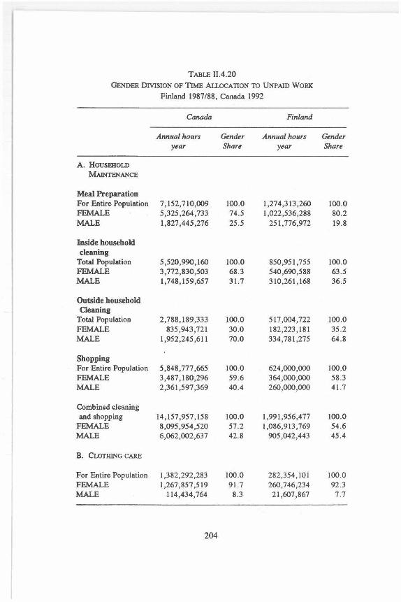
TABUl 11.4.20 GENDER DIVISION OF nME ALLocATION TO UNPAID WORK

Finland 1987/88, Canada 1992

Canada Finland

Annual hours Gender Annual hours Gender year Share year Share

A. HOUSEHOI.D MAINTENANCE

Meal Preparation For Entire Population 7,152,710,009 100.0 1,274,313,260 100.0 FEMALE 5,325,264,733 74.5 1,022,536,288 80.2 MALE 1,827 ,445,276 25 .5 251,776,972 19.8

Inside household cleaning

Total Population 5,520,990,160 100.0 850,951,755 100.0 FEMALE 3,772,830,503 68.3 540,690,588 63 .5 MALE 1,748, 159,657 31.7 310,261,168 36.5

Outside household Cleaning

Total Population 2,788,189,333 100.0 517,004,722 100.0 FEMALE 835 ,943,721 30.0 182,223 ,181 35.2 MALE 1,952,245,611 70.0 334 ,781 ,275 64.8

Shopping For Entire Population 5,848,777,665 100.0 624,000,000 100.0 FEMALE 3,487 ,180,296 59.6 364,000,000 58.3 MALE 2,361,597,369 40.4 260,000,000 41.7

Combined cleaning and shopping 14, 157,957,158 100.0 1,991,956,477 100.0

FEMALE 8,095,954,520 57.2 1,086,913,769 54.6 MALE 6,062,002,637 42.8 905 ,042,443 45.4

B. CwrHING CARE

For Entire Population 1,382,292,283 100.0 282,354, 101 100.0 FEMALE 1,267 ,857 ,519 91.7 260,746,234 92.3 MALE 114,434,764 8.3 21,607 ,867 7.7

204

TABLE 11.4.20- GENDER DMSION OF TIME ALLocATION .. . (Contd.)

Canada Finland

Annual hours Gender Annual hours Gender year Share year Share

C. CARING

Child care For Entire Population 3,328,772,513 100.0 478,348,698 100.0 FEMALE 2,393 ,536,466 71.9 351,848,406 73.6 MALE 935,236,047 28.l 126,500,293 26.4

0. VOLUNTEERISM

Volunteer(l986-1987) 1,017,548,000 100.0 n/a FEMALE 554,988,000 54.5 n/a MALE 462,560,000 45.5 n/a

E. PERSONAL DEVELOPMENT

Education 344,672,134 100.0 n/a FEMALE 170 ,485 ,880 49.5 n/a MALE 174,185,374 50.5 n/a

which provide data on GDP by gender. These, however, can be explored through attribution of GDP to gender based on contributions to its production. Market GDP was distributed between males and females based on their relative time inputs to the market weighted by their wage bills . This approach, while conventional and essentially necessary, is gravely flawed. The flaw lies in the statement 'weighted by wages' Since women's wages are typically significantly lower than men's for the same work using gender-based wages distorts contributions in favour of men. Consequently, shares attribut­ed to men here must be considered the upper boundary of

205

their contribution. Using labour input weighted by wages males account for 63 per cent of Canadian GDP and 59 per cent of Finnish GDP (Table 11.4.21).

The gender division of unpaid production runs exactly counter to that paid production in Canada and in Finland. While in Canada males account for 63 of market GDP, females account for 61 per cent of unpaid production (see Table 11.4.21). In Finland, while males account for 59 per cent of market GDP, females account for 59 per cent on unpaid production. Total production, then, is much more equitably spread. In Canada, males account for 55 per cent of total production and females account for 45 per cent (see Table II.4.21). In the case of unpaid production, the time contributions are not gender weighted by wage bills. If such a weighting were imposed, it would have the same effect as in the case of market production: it would inflate the contri­bution of men. However, unlike the market case there is no clearly justifiable set of wage data to use in the weighting process. Indeed, one of the chief issues in input-based valua­tion methods is choice of the appropriate wage rates to use.

Taken together, in Canada, females account for 45 per cent of total (paid and unpaid) production, while in Finland, women account for 4 7 per cent.

206

TABLE 11.4 .21 GENDER DIVISION OF UNPAID WORK TIME

Canada (1992) and Finland (1990)

Canada1 Finland1

Female '()()() Male '000 Total '()()() Female '()()() Male '000 Total '000

Regular GDP 253, 792,282.4 435,860,658.8 689,652,941.2 211,326,300.0 304, 103,700.0 515,430,000.0 Gender Shares (%) 36.8 63.2 100.0 41.0 59.0 100.0

Meal Preparation 39,490,440.6 i3,516,862.2 53,()()7,302.8 28,644, 789.5 7,071,905 .6 35,716,695.l Housekeeping 116,524,653.3 95,338,352. 7 211,863,006.0 108,596,164.0 90,297,909.2 198,894,073.2 Clothing Care 4,624,775.l 418,600.l 5,043,375.2 3 ,928,860.3 327,759.7 4,256,620.0 Household Maintenance 160,639,868.9 109,273,815.1 269,913,684.0 141,169,813.7 97,697,574.6 238,867,388.3 Gender Shares (%) 59.5 40.5 100.0 59.l 40.9 100.0

Child Care 13,719,851 .9 5,362,000.5 19,081,852.4 10,484,833.9 3,760,864.4 14,245,698.3 Volunteer Work 8,027,977.5 6,702,256.5 14,730,234.0 Personal Development 11,478,047.6 11,709,927.4 23,187,975.0

Total Satellite Accounts 193,865,746.6 133,047,999.8 326,913,745.4 151,654,647.6 101,458,439.0 253,113,086.6 Gender Shares (%) 59.3 40.7 100.0 59.9 40.l 100.0

Total GDP + Satellite 447,658,028.9 568,908,685.7 1,016,566,686.6 362,980,947 .6 405,562, 139 .0 768,543,086.6 Gender Shares (%) 44.0 56.0 100.0 47.2 52.8 100.0

1 GDP in Canadian Dollars. 1992 estimates from Statistics Canada. National Income and Expenditure Accounts: Annual Estimates. No.

13201, Ottawa, Canada, 1994. 1 GDP in FIM. 1990 estimates based on the study ofMarjut Vihavainen (1995) Calculating lhe value of household production in Finland in 1990:

1he inpUl-oUlpUl iable.

REFERENCES PART II

Adler , H. J., & Hawrylyshyn, 0. (1978). "Estimates of the value of

household work: Canada, 1961 and 1971 ", The Review of

Income and Wealth, 24(4) .

Aslaksen, lulie and Hanne A. Gravingsmyhr (1985). "Measuring house­hold production -in an input-output framework: The Norwegian experience." Working Paper No. 22, Joint ECE/INSTRAW Work Session on Statistics of Women, Conference of European Statisti­cians, Geneva.

Beutler, Ivan F., Alma J. Owen, Colien Hefferan (1988). "The boundary question in household production: A systems model approach" Home Economics Research Journal Vol. 16, No. 4, June.

Biggs, D., B. de Ville, -e. Suen (1991). "A method of choosing multi-way partitions for classification and decision trees". in G.K. Kanji (ed.), Applied Statistics: Special issue on expert systems and

statistics. 18:1. 49-62.

Brieman, L., J.H. Friedman, R.A. Olsen, and C.J. Stone (1984). Classifi­cation and regression trees. Wadsworth.

Bonke, J. (1988). Husligt arbejde - hvad er det vaerd! I:Den okanda vardagen -om arbetet i hemmem. B. Aker fl. Forlaget Akademilit­

teratur. Referenced in Jens Bonke, "The concepts of work and

209

care - an economic perspective applied to Britain and Denmark." unpublished paper.

Canadian Restaurant & Food-services Association (1994). Food Services Facts 1994.

Chadeau, Ann (1985). "Measuring household activities: Some international comparisons." The review of income and wealth, No. 31(3), pp. 237-253.

Chadeau, A. and A. Fouquet (1981). "Peut-on measurer le travail domest­ique?" Economie et Statistique, No. 36 Paris: INSEE.

Chadeau, A. (1993) "Defining and measuring unpaid services produced by households for own use". Conference of European statisticians. OECD Paper No. 11. Geneva, 13-15 September.

Chandler, B. (1994) "The value of household work in Canada, 1992." National Income and Expenditure Accounts, Fourth Quarter 1993, Statistics Canada. Catalogue No. 13-001, March.

Chandler, William (1994). "The value of household work in Canada, 1992." Canadian Economic Observer, April.

Childcare Resource and Research Unit (1994). Child care in Canada: Provinces and territories 1993. Toronto, Ontario: Childcare Resource and Research Unit, Centre for Urban and Community Studies, University of Toronto.

Clark, C. (1958) "The Economics of housework". Quarterly Bulletin of the Oxford University Institute of Statistics 20.

Cost, Quality, and Outcomes Study Team (1995). Cost quality and child outcomes in child care centers: Key findings and recommenda­tions. Young Children, May, pp. 40-44.

Dulaney, R.A. et al (1992). "Market valuation of household production" Journal of Forensic Economics. Vol. 5, No 2, pp. 115-125.

Fitzgerald, J. and J. Wicks (1990). "Measuring the value of household output: a comparison of direct and indirect approaches" The Rev{ew of Income and Wealth. Vol. 36, No. 2, June 1990. pp. 129-142.

Frederick, Judith (1994). "Measuring child care and sleep. " Fifteenth reunion of the International Association for Time-Use Research. Amsterdam: NIMMO.

Glezer, H . (1984) "Changes in marriage and sex-role attitudes among young married women: 1971-1982", in Australian Family Re-

210

search Conference Proceedings, Family Formation, Structure, Values Vol. 1. Melbourne: Institute of Family Studies.

Goldschmidt-Clermont, L. (1993). "Does Housework Pay? A product­related microeconomic approach". Journal of Women in Culture and Society, Vol. 9, No. 1.

___ . (1983). "Output related evaluations of unpaid household work: a challenge for time-use studies". Home Economic Research Jour­nal. Vol. 12, No. 2, December; pp. 127-132.

Harvey, A. (1990). Guidelines for time-Use data collection. Statistics Canada. General Social Survey, Working Paper No. 5.

Harvey, A. (1992). Time-use model of the general social survey. Statistics Canada. General Social Survey, Working Paper No 8.

Helbum, S. et al. (1995). "Cost, quality, and child outcomes in child care centers: Key findings and recommendations". Uncover, Vol. 50, No. 4, 01 May; pp. 40-44

Hill. M. S. (1985). "Investments of time in houses and durables". Time, goods, and well-being, Michigan: Institute for Social Research, the University of Michigan.

INSTRA W (1995). Measurement and Valuation of Unpaid Contribution: Accounting through Time and Output, Santo Domingo.

Ironmonger, D. (1989) Households Work: Productive activities, women and income in the household economy. Wellington, New Zealand. Allen & Unwin.

Jackson, C. (1993). Definition of unpaid work and implications for the design of time use activity classifications. IATUR Conference, Amsterdam, Netherlands. June 15-18.

Jorgenson, D. W. and B. M. Fraumeni (1991). "Investment in Education and U.S. Economic Growth". Cambridge:Harvard Institute of Economic Research, Harvard University, Discussion Paper No. 1573, October.

Kass, G.V. (1975). "Significance testing in automatic interaction detec­tion". Applied Statistics 24:2, pp. 175-189.

Kinnunen, A. (1993) Consumer Price Index 1990=100. Statistics Finland, Helsinki.

Ministry of Social Affairs and Health (1980). "The concept of unpaid housework and the determination of its value". Housework Study, Part I. Finland, Helsinki.

211

___ . (1980). "Description of the study and sample". Housework Study, Part II. Finland, Helsinki.

___ . (1981). "The value of unpaid cooking work in 1980". Housework Study, Part VI. Finland, Helsinki.

___ . (1982). "Unpaid housework: time use and value". Housework Study, Part VIII. Finland. Helsinki.

___ . (1986). "Determining the value of unpaid housework: method comparison", Housework Study, Part XIT. Finland, Helsinki.

Morgan, J.N. and J.A. Sonquist (1963). "Problems in the analysis of survey data and a proposal". Journal of the American Statistical Association, 58, 426.

Murphy, M. (1978). "The value of non-market household production: Opportunity cost vs. market cost estimates", The Review of Income and Wealth, Sept.

----. (1982). · "Comparative estimates of the value of household work in the United States for 1976", The Review of Income and Wealth, March.

Peat, Marwick, Stevenson, & Kellog (1993). Canadian restaurant industry operations report. Canadian Restaurant and Foodservices Associa­

tions. Robinson, J.P. and A. Bostrom (1994). "The overestimated workweek?

what time diary measures suggest". Monthly Labour Review. August, pp. 11-23.

Ross, David P. (1990). Economic dimensions of volunteer work in Cana­da. Ottawa: Department of the Secretary of State.

Rubin, R.M. and M. Nieswiadomy (1994). "Expenditure patterns of retired and non-retired persons". Monthly Labour Review. April, pp. 10-21.

Rydenstam, Klas and Anders Wadeskog (1995). "A statistical system on household production and consumption." Working Paper No. 12, Joint ECE/INSTRA W Work Session on Statistics of Women, Conference of European Statisticians, Geneva.

Sanik, M.M. & Stafford K. (1983). "Product-accounting approach to valuing food production", Home Economics Research Journal, 12(2).

Sanik, Margaret (1995). Personal Communication.

212

Santti, R., R. Otva, E. Kilpio (1981). "The value of unpaid special care in 1980". Housework Study, Part V. Finland, Helsinki: Ministry of Social Affairs and Health. August.

___ , R., H. Valiaho (1982). "Unpaid housework in families and value". Housework Study, Part IX. Finland, Helsinki: Ministry of Social Affairs and Health.

___ . (1982). "Men's, women's, and children's input in unpaid house­work". Housework Study, Part X. Finland, Helsinki: Ministry of Social Affairs and Health.

__ , R., U. Husa "Child care" (1982). Housework Study, Part XI. Finland, Helsinki: Ministry of Social Affairs and Health.

Santti, R., H . Vesikkala (1983). "Cooking work". Housework Study, Part XII. Finland, Helsinki Ministry of Social Affairs and Health.

Santti, R. (1983). "Handicrafts and wood and metal work". Housework Study, Part XIII. Finland, Helsinki: Ministry of Social Affairs and Health.

Schafer, D . and N. ~chwarz (1995). Value of household production in Gennany in 1992. Paper presented to the Joint ECE/ INSTRAW work session on Statistics of Women. Part of the Conference of European Statisticians. Geneva: 6-8 March.

Statistics Canada (1993). Family food expenditure in Canada 1992. Statistics Canada. Household Surveys Division. Family Expendi­tures Surven Section.

Schade, C. (1995). Average Eater Check and Sampling Procedure. CREST Canada. Ontario, Willowdale.

Schafer, D., N. Schwarz (1995). "Value of Household production in Germany in 1992". Paper submitted by Federal statistical Office of Germany to the Joint ECE/INSTRAW Work Session on Statistics of Women at the Conference of European Statisticians, Geneva, 6-8 March.

Statistics Canada (1992). The consumer price index (1992). Statistics Canada. Catalogue 62-001.

___ . (199 ). Guide to the /EA, Statistics Canada. National accounts and Environment Division Publication 13-603E.

___ . (1992). Homeowner repair and renovation expenditure in Canada 1992. Statistics Canada. Catalogue 62-201 Annual.

213

___ . (1992). Household facilities and equipment 1992. Statistics Canada. Catalogue 64-202 Annual.

___ . (119 ). 1he size of the underground economy in Canada. Studies in national accounting. Statistics Canada Catalogue 13-603E, No. 2 occasional.

___ . (199 ). Family food expenditure in Canada 1992. Statistics Canada. Household Surveys Division. Family expenditures surveys section.

___ . (1992). Family expenditure in Canada. 1992 Statistics Canada. Household Surveys Division. Family expenditures Surveys Section.

Statistics Canada (1994). National Income and Expen4iture Accounts Annual. Estimates 1982-1993.· System of National Accounts. Statistics Canada. National Accounts and Environment Division, Catalogue No. 13-201. Ottawa.

Statistics Norway (1995). Measuring household production in an input­output framework: The Norwegian experience. Paper presented to the Joint ECE/INSTRA W work session on Statistics of Women. Part of the Conference of European Statisticians. Geneva: 6-8 March.

Statistics Sweden (1995). A statistical system on household production and consumption. Paper presented to the Joint ECE/INSTRA W work session on Statistics of Women. Part of the Conference of Europe­an Statisticians. Geneva: 6-8 March.

Suviranta, A. and M. Heinonen (1980). 1he value of unsalaried home care of children under the age of seven in 1979. Part Ill of Housework Study. Helsinki:Ministry of Social Affairs and Health, Research Department.

Suviranta, A. and.A. Mynttinen (1981). Value of unpaid house cleaning in 1980. Housework Study, Part IV. Finland, Helsinki: Ministry of Social Affairs and Health, Research Department. February.

___ . (1981). The value of unpaid cooking work in 1980. Housework Study. Part VI. Finland, Helsinki: Ministry of Social Affairs and Health.

__ . (1980). The value of unpaid laundry work in 1980. Housework Study, Part VII. Finland, IJelsinki: Ministry of Social Affairs and

214

Health. Teillet, P. "A concept of satellite accounts in the revised SNA" The

Review of Income and Wealth, Vol. 34, No. 4, December 1988. pp. 411-440.

Thoen, Michael (1993). The value of household production in Canada 1981-1986, Statistics Canada. National Accounts-and Environment Division. April.

United Nations (1995). Declaration and programme of action of the world summit for social development. World Summit for Social Develop­ment. Copenhagen, Denmark. March.

___ . (1994). Summary of conclusions, Conference of European Statisti­cians. Statistical Commission and Economic Commission for Europe. Economic and Social Council. Paris: 13-17 June.

Varjonen, J . (1991). Simultaneity of activities in household work. Univer­sity of Helsinki. Publications of the Department of Household Economics. Helsinki.

Vihavainen, Marjut (1995). Calculating the value ofhosuehold production in Finland in 1990: The input-output table. Helsinki: Statistics Finland.

Viinisalo, Mirja, Riitta Santi and Elia Kilpio (1987). "Palkattoman Ruokataloud-Tyon Arvo." Helsinki: Kotilaous-Ja Kuluttaja-Asian Tutkimuskeskus.

Walker and Woods. Time-Use: A Measure of Household Production of Family Goods and Services. Washington, D.C., USA. Center for the Family of the American Home Economics Association, 1976.

215

ANNEX PART II

. 1

! . I

Activity

Breakfast Meal-1

Breakfast Meal-3

Luncheon Meal-1

Description

Egg(s) and Meat (ham, ba­con, or aausage), toast and coffee.

Plain pancakes or French Toast, with syrup and coffee

The most representative hot sandwich plate. If typical, the meal can include soup, vege­tables, small salad or cole­slaw, bread and butter. In­clude a beverage of either tea, coffee or milk.

Annex PRICE DEFINITIONS

Standard quantity

As above

Unit of Measure

1 EA

I EA

Alternate UofM

CH

CH

Special Instruction

If representatives added extras, such as jam, are to be included in the price of the meal; the description of meals, including quantities, should be detailed on the pricing form and checked at each pricing. Prices are to be obtained from cafeteria, coffee shops or luncheon outlet (casual sit-down restaurant) .

Description of meals, including quantities, should be detailed on the pricing form and checked at each pricing. Prices are to be obtained from cafeteria, coffee chops or luncheon type outlet (casual sit-down restau­rant).

ANNEX - PRICE DEFINITIONS (Contd.)

Activity Description Standard Unit of Alternate Special Instruction quantity Measure UofM

Luncheon The most representative fish As above Meal-2 platter. Include same items.as

in Luncheon Meal-1.

Luncheon Other plate selections such as As above Meal-3 roast turkey, pasta,

shepherd's pie, etc. Include same items as in Lun-cheon Meal-1

Dinner Full-course evening meal with I EA CH Total price of meal to be shown on Meal-1 beef entree. Include the most pricing form with breakdown for

popular soup or juice, bread, separately priced items if applicable. vegetable and/or salad, des- A complete description of the meal, sert, tea or coffee. including quantities if available,

should be detailed on the pricing form and checked at each pricing. Select representative outlet for eve-ning meals (i .e., steak house or din-ing lounge).

Dinner Full-course evening meal with As above Meal-2 chicken, veal or pork entree.

ANNEX - PR.ICE DEFINITIONS (Contd.)

Activity Description Standard Unit of Alternate Special Instruction quantity Measure UofM

Dinner Full-<:ourse evening meal with As above Meal-3 seafood entree (fish or shell-

fish)

Snacks Snack food such as ham- 1 EA CH Price the most representative snack burger and fries with a soft and size/type of soft drink in each drink. Extra such as onion outlet and price on a continuous rings, coleslaw, etc. should basis. Description of snack, size of not be priced unless part of a portions and type and size of soft combination. drink are to be indicated on the

pricing form and checked at each pricing. If the size of the soft drink is not available in OL or ML, indi-cate small, medium or large prices should be obtained primarily in chain type of outlets.

Take Home One order picked up (not 1 UT CH A complete description of the meal, Fried Chicken eaten on premises). Nominal- including quantities should be de-

ly priced order of up to 3 tailed on the pricing form and pieces of chicken, deep fried checked at each pricing. If more in batter. Order may include representative in an outlet, BBQ fries or baked potato, chicken or chicken nuggets (approx

6) may be priced consistently.

ANNEX - PRICE DEFINITIONS (Contd.)

Activity

Take Home Chinese Food

Take Home Pizza

Description

coleslaw, roll of bread and should include condiments, serviettes, etc.

One order of Chinese food, packaged in 16 to 20 OL con­tainer, picked up . Choose the most representa­tive of fried rice, beef, or chicken, chop suey, beef or pork; sweet and sour chicken balls or spare ribs.

Pizza, combination, picked up, 10 to 14 inches in diame­ter. Most representative com­bo of 3 toppings (usually pepperoni, mushroom, and green peppers) .

Standard quantity

Unit of Measure

160L

I EA

Alternate UofM

ML

CH

Special Instruction

Description and size of container (the volume and not the mass) should be entered on pricing schedule and checked at each price. Do not price meals including soup, beverage, etc. or orders on a deliv­ered basis.

Type and size selected to be priced on a continuous basis. The size and toppings are to be en­tered on the pricing form and checked at each pricing. If more representative, the Hawaiian pizza may be priced on a continuous basis.

ANNEX - PRICE DEFINITIONS (Contd.)

Activity

Hotel Accommoda­tion

Motel Accommod­ation

Description

The non-business rate for one hotel room for one night (a Mon, tues, Wed, or Thurs) for 2 adults. A hotel room is a room located in a main building and can be accessed only from the interior. Rooms accessible directly from both the exterior and interior are acceptable as a hotel room.

The non-business rate for one motel room for one night (a Mon, Tues, Wed, or Thurs) for two adults . A motel room is a room which is accessible only from the exterior.

Standard quantity

Not appli­cable

As above

Unit of Measure

Alternate UofM

Special Instruction

The rate reported should include all taxes except PST. Tax values and the effective date of the tax/tax change are to be indicated in the comments section of the pricing form. Select the most representative rate for non-business travelers. Indicate on the pricing form total number of units in the establish­ment, the number of rooms to which the rate quoted is applicable, the number and type of bed for the room selected and any extras(break­fast, newspaper, pay TV) which are included in the selected rate. If the rate applies to more than one type of room, choose the most represen­tative type.

ANNEX - PRICE DEFINITIONS (Contd.)

Activity

Day Care Centres

Baby-Sitting

Description

Hotel rooms as described above are not included.

Day care rates (most repre­sentative, daily, weekly, or monthly) in a licensed or provincialiy approved (centre or private home) which pro­vides care for a four year old child outside his/her own home, for 8 to 10 hours per day, between 7:00-10:00 hours.

Total cost for five hours of baby sitting by a teenage babysitter (8 pm to 1 pm) on a week-day evening (exclud­ing official holidays). Report transportation charge if any.

Standard quantity

Not appli­cable

Not appli­cable

Unit of Measure

Alternate UofM

Special Instruction

Rates must include at least lunch and one snack. The rates must exclude all subsidies given to the parents. Do not price centres which operate on hourly rates

Data should be obtained from Re­gional Office personnel, neighbors or relative paying for the service. Different parts of the city should be represented.

ANNEX - PRICE DEFINITIONS (Contd.)

Activity Description Standard Unit of Alternate Special Instruction quantity Measure UofM

Home Cleaning The rate as per frequency of Not appli- The description of the typical house cleaning for a typical house cable is to be entered on the pricing form: within the city limits. square footage, number of rooms,

levels in the house, number of bathrooms, flooring type, etc. The typical frequency of cleaning, the number of cleaners in team, the number of hours the team is in the house, if the client must sign a contract, the method in calculating the discount must be included on the pricing form.

Dry Cleaning Regular Cash and Carry or 1 EA CH Do not price same day or 24-hour Men's Pick up and Delivery dry service if extra charge is made.

cleaning and pressing service. Indicate price for the most popular service. Exclude insurance charge, if any.

Dry Cleaning As per above As above Women's

Coin operated Self-service coin operated 12 LB KG Enter price for washing and size of laundry laundry. the load. Where an establishment

has more than one type or size of

ANNEX· PRICE DEFINITIONS (Contd.)

Activity

Coin Operated Laundry

Beer Consump­tion

Description

As per above

One 12 fluid ounce bottle (341 ml.) Most representative domestic brand of bottled ale or lager served with a glass at a bar or table at about 17:00 hrs.

Source: Statistics Canada

Standard quantity

Unit of Measure

lOMT

12 OL

Alternate UofM

ML

Special Instruction

machine, record data for the most popular machine. Change of size load and other pertinent details should be recorded on the CFCF form. Enter price for drying and amount of drying time. Where an establish­ment has more than one type or size of machine, record data for the most popular machine. Change of drying time and other pertinent details should be recorded on the CFCF form.

If Happy Hour prices are in effect at about 17 :00 hrs, they are accept­able. Indicate Happy Hour in the Comments seetion of the pricing form and the time. Do not price imported brands or alcoholic content over S .S % .

CONCLUSIONS AND OBSERVATIONS

The comparative values

derived for Nepal, Canada and Finland illustrate different cases (generally defined by the type of data available) in which the INSTRA W recommended framework for establish­ing "satellite accounts" on unpaid household production and the output-based valuation method can be applied. In each scenario, certain data limitations were encountered, and in the cases of Nepal and Finland, these prevented the study from deriving imputed values for all the activities and products that theoretically fall within the boundary set for the proposed "satellite accounts".

Time allocated to personal development (studying, apprenticeships and related activities) and voluntary work cannot be determined from the time-use database available in Nepal and Finland. Hence, the estimated value of unpaid production represents only those products related to house­hold maintenance activities for these countries. In Nepal , the application of output-based valuation was limited to meal preparation on which more detailed information on products/ outputs and relevant normative values could be derived. A

replacement cost approach had to be adopted in valuing the other "satellite accounts" activities.

Notwithstanding these limitations which consequently underestimate the total worth of unpaid household production, the values derived indicate a pattern of interdependence between the market (paid) and household (unpaid) production. In Canada and Finland, the value of unpaid production equals nearly half that of paid production, while in Nepal, the value more than equalled that of GDP (Table C.l). For Canada, unpaid production, by the most inclusive definition, equalled 47.4 per cent of GDP in 1992 while in Finland, by a less inclusive definition (volunteerism and personal development were not included), unpaid production was 49 per cent of GDP in 1990. Not including volunteer work and personal development, unpaid production in Nepal equalled 126.04 per cent of GDP.

The levels of unpaid output derived in this report, for Canada and Finland, fall well in line with other unpaid work estimates for the same populations and time periods. No similar comparisons could be made, however, for the results derived for Nepal, as this study was the first one that attempt­ed to value unpaid production in the country at a wider scale.

228

TABLE C.1

UNPAID WORK AS PERCENTAGE OF GDP Comparative Estimates: Canada, Finland, and Nepal

CANADA 1992

GDP at Market Prices - $ '000,000,000

Opportunity cost before tax Opportunity cost after tax Replacement cost-specialist Replacement cost-generalist Output basis-Household maintenance

and caring Output basis-HouseholcV

caring/education/volunteering

FINLAND 1990

GDP at market Prices - FIM '000,000,000

Opportunity cost-household maintenance/caring

Replacement cost-generalist­household maintenance/ caring

Output basis-household maintenance/caring

NEPAL

GDP at Market prices Rs '000,000,000

Replacement cost-specialist

229

Percentage Value of GDP

689.7

374.1

221.1 296.6 234.5

289.6

326.9

515.4

302.0

232.5 253.1

116.1

146.4

100.00

54.24 32.06

43.00 34.00

42.00

47.40

100.00

58.60

45.11 49.11

100.00

126.04

Nepal

Results of the study in Nepal concluded that it is possi­ble to construct satellite accounts for household production using a combination of data from large scale time-use surveys and a small scale survey that provides normative values for goods and services generated by various activities.

Although it involves a complicated list of products and calculation of inputs that entered into the preparation of meals, imputation of values to meal outputs was not impossi­ble. However, for services such as laundry, child care, cleaning the house, and related activities, wage rates had to be used as normative values due to the limitations of the time­use data applied (i.e., these activities were not processed separately). Wages of polyvalent workers were used to calculate the value of such activities. The study in Nepal has, therefore, provided estimated values of satellite accounts on household production using a combination of output-based and replacement cost-specialist approaches.

For a more accurate and consistent estimation of unpaid production, particularly household maintenance activities, it is necessary to collect information on all SNA and non-SNA activities performed in the household in a time-use survey. There is a need to carry out household time expenditure surveys which would parallel in sampling, design and collec­tion of current household budget surveys. Such initiative could draw on the extensive experience accumulated in the collection of household expenditure studies. Greater attention will need to be paid to linkage variables so these vehicles can more efficiently contribute to the task of developing output values unless time and money budget studies are integrated in

230

the future. While there is, to be sure, concern over response burden, a fifteen minute or shorter time-use module collected as part of an extensive household budget survey is unlikely to generate a very significant response revolt. Currently, efforts are being made to develop a more efficient time-use instru­ment which could be geared specifically to the needs of data for income account purposes.

Canada and Finland

While output-based production levels calculated here for Canada and Finland are consistent with levels derived by input-based approaches, distribution by activity are less so. The output based results presented here show that meal preparation, even though it is a broader concept than in related input based estimates, is a much smaller proportion of GDP or total household maintenance activity than has hereto­fore been reported using input measures. Findings suggest that the input measures, which are cost measures, are higher, approximately double than the output-based values. A reason­able explanation of this is that household meal production is an inefficient process relative to meal production in the market. Consequently, meal preparation consumes a volume of time incommensurate with the value it produces.

This study shows, as have other studies (Fouquet and Chadeau, 1981:Fitzgerald and Wicks, 1990:Goldschmidt­Clermont, 1993) that output-based valuations are possible for both developed and developing countries. The work highlights both the possibilities and the problems associated with the development of adequate output based measures of household output. First, it illustrates the potential for measuring outputs

231

l

using time use data. Secondly, it identifies, clearly, three major challenges facing attempts to fully implement an output-based strategy. One is the need for refined and broadly accepted definitions of household outputs. Second is the need to establish market-based prices for valuing those outputs. Third, is the need to identify adjustments required to the estimated value of unpaid production to bring it into line with the existing SNA accounting framework.

Recent work has gone beyond the traditional approach pf limiting estimates of household output to estimates of' the value of labour inputs by incorporating non-labour inputs (Ironmonger, 1989; Thoen, 1993; Rydenstam and Wadeskog, 1995; Aslaksen and Gravingsmyhr, 1995; Vihavainen, 1995; Schafer and Schwarz, 1995). This is to be commended. Household output is generated by both labour and non-labour household inputs and both must be counted. The value of household output, derived via an input approach, is calculated as the summation of the value of labour inputs and the non­labour inputs. 1'pe problem, however, is that the computed sum represents the cost of producing the unpaid production but not necessarily its market value. To obtain the value ·of unpaid output there are further, sometimes difficult, steps to be taken. This became obvious in the approach adopted here.

The first challenge is, assuming an accepted definition of household production, to define household outputs. Recent studies, while reflecting the general underlying principle of the third-person criteria, have used disparate household production classification schemes (Vihavainen, 1995; Schafer and Schwarz, 1995; Aslaksen and Gravingsmyhr, 1995; Rydenstam and Wadeskog, 1995; Chandler, 1994; Thoen, 1993). Thus, not only are the outputs unclear, but there is

232

ambiguity with respect to the components of household production. There is an urgent need to develop an acceptable international standard with respect to the categorization of unpaid production.

The approach taken here was to characterize household maintenance production in terms of the most commonly accepted basic needs, namely food, shelter and clothing. Thus, for Canada and Finland, the outputs of household production are measured in terms of the quantity of meals produced at home, the number of day/nights of shelter services provided, the kilograms of clean clothing produced, and the child hours of care.

Time-use data provided a basis for estimating three of the major household outputs, meals eaten, nights of residen­tial accommodation and child care. Since time-use studies have not, to date, even considered the output dimension of activities, the data collected is less useful than it could be if survey instruments encompassed elements designed to provide necessary output information. The time-use data used for both countries provided a count of meals eaten and where and when they were eaten. It provided an indication of home or other residential nights of accommodation. And, finally, for Canada, it provided a reasonable estimate of time allocated to child care drawing on social contact data collected on the diary. There were problems estimating child-care time from the Finnish data as indicated below.

The measurement of meals was fairly straightforward. Similarly, it seems evident in the work undertaken here that it is possible to establish appropriate estimates for meal preparation. There are, however, adjustments to the data collection required to provide a more accurate accounting of

233

meals. What is needed is to know the number of meals prepared at home, not just those eaten at home, as it was necessary to use here. It must be possible, either as part of the time diary or from ancillary data, to identify the number or proportion of meals eaten out of home, say at work, that were carried from home and the number of meals eaten at home that are carried into the home. With this information, it is possible to more accurately measure the number of home­prepared meals. Further, it may be more appropriate to develop a classification of meals, an approach used in the Finnish Housework Study, to allow for differential pricing (Viinisalo, Santti and Kilpio, 1987).

The Finnish social contact data precluded its use in developing a realistic child-care output measure. In lieu of the diary data, an alternative approach was used to measure child-care time in Finland. It covered only children under age 7 years. Child-care hours based on hours of care received is the most logical output metric. However, as discussed above, there are a number of issues which need to be resolved with respect to the definition and measurement of child-care time. It was possible to get reasonably good prices for child care but which hours are to be counted (for what part of the day and for what ages) poses significant problems. Should all hours receive the same rate or should one draw a

0

distinction between certain classes of hours as was done here by assign­ing a lower price to nighttime hours. The same issues hold true for caring for the elderly or infirm, an area not ad-

. dressed in this study . Time-use data is relevant in all viable solutions either as a measure of care given or a measure of care received. In the latter case, it will be necessary to have child-level time-use data.

234

Shelter or housekeeping poses a problem with respect to definition and measurement. As indicated above, housekeep­ing encompasses a wide range of activities related to inside and outside dwelling. The sheer size of it in the final valua­tion estimates attests to the need to better. understand and measure it. In this report, an overall value of housekeeping, which can theoretically and statistically provide an appropri­ate measure, leaves one wanting for finer detail with respect to characteristics of the dwelling, lot and nature of the accommodation. Use of shelter or accommodation appears to be detectable by time-use studies. However, the accuracy with which the studies are able to identify home use depends greatly on the sampling and reporting rules adopted in time­use studies. Only if the studies adopt a truly random designat­ed day approach to sampling and reporting will the resultant data accurately reflect time/days/nights spent at home and those spent away from home. This presents a challenge to survey designers.

The clothing care output is currently not measurable via time-use studies. While studies show time allocated to laundry and clothes maintenance, they provide no indication of what that time produces. However, the Finnish Housework Study (Suviranta and Mynttinen, 1981) as well as work undertaken in the United States (Sanik, 1995) indicates that it is possible to develop measures of household output in terms of a volume measure such as loads or kilograms. Rough approxi­mations of such estimates were used here.

The foregoing has characterized components of house­hold outputs in rather discrete terms. Similarly, recent input­output table approaches have cast household productions in terms of discrete commodities and industries. Household input-output work, to date, having defined a set of household

235

activities, has been concerned with estimating and valuing the inputs into each activity. The work has not appropriately recognized the jointness of production which exists in house­holds. Meal preparation, housekeeping, and child care are often co-occurring and valuing time allocated to one or the other inadequately reflects total production. How the outputs are produced is not the issue, rather it is how much of what kind of output is produced.

However, a different kind of jointness of production plagues output-based measurement. Meal preparation is not independent of shopping, cleaning, and travelling. Laundry may be done at one and the same time as clothing for indi­viduals and as bedding for accommodation maintenance. The relevance and the frustration of this realization emerges when, as was tried here, one attempts to define and measure outputs rather than inputs. Having measured and valued total output, it is necessary to adjust for purchased inputs (RME) and dwelling (UOD). To do so, it is necessary to allocate expenditures across the major activities. Thus, for example, how much travel is attributable to meals, to accommodation related activities or to child care? Similarly, how does one reflect purchases such as soap, cleaners, and detergent in the appropriate RME. The problems are not insolvable but they must be faced. Additionally, from both an aggregate account­ing viewpoint and when one is trying to study societal change, the overlap is not inconsequential. There is always a potential for altering the inputs required to produce a given output.

In order to accurately account for all household produc­tion it is necessary, as in consumer studies, to provide a mea­sure of household composition over the accounting period. It

236

is not enough to simply rely on cross-section data. In the current project, weeks per year for several age groups in Canada and months per year in main occupations in Finland

provided a link between the time use and consumption data. In particular, there is a need to provide the measures on a gender specific basis.

Output-based measures of household production are possible and are necessary if researchers and national accoun-,, tants are to fully grasp and measure the nature of household production. While there needs to be a shift of emphasis in household production, research toward developing output­based measures work also needs to continue on input-based measures as well. There is a need to understand both the

input and the output side of household production. Only when both are fully understood will it be possible to have full confidence in production estimates and to develop appropriate public policies with respect to households and household maintainers.

237