Initial Relative-Orbit Determination Using Second-Order ...
112
Initial Relative-Orbit Determination Using Second-Order Dynamics and Line-of- Sight Measurements by Shubham Kumar Garg A thesis submitted to the Graduate Faculty of Auburn University in partial fulfillment of the requirements for the Degree of Master of Science Auburn, Alabama May 10, 2015 Keywords: nonlinear dynamics, orbit determination, angle-only navigation Copyright 2015 by Shubham Kumar Garg Approved by Andrew Sinclair, Chair, Associate Professor of Aerospace Engineering David Cicci, Professor of Aerospace Engineering John Cochran, Professor Emeritus of Aerospace Engineering
-
Upload
khangminh22 -
Category
Documents
-
view
0 -
download
0
Transcript of Initial Relative-Orbit Determination Using Second-Order ...

Initial Relative-Orbit Determination Using Second-Order Dynamics and Line-of-
Sight Measurements
by
Shubham Kumar Garg
A thesis submitted to the Graduate Faculty of
Auburn University
in partial fulfillment of the
requirements for the Degree of
Master of Science
Auburn, Alabama
May 10, 2015
Keywords: nonlinear dynamics, orbit
determination, angle-only navigation
Copyright 2015 by Shubham Kumar Garg
Approved by
Andrew Sinclair, Chair, Associate Professor of Aerospace Engineering
David Cicci, Professor of Aerospace Engineering
John Cochran, Professor Emeritus of Aerospace Engineering
ii
Abstract
This thesis addresses the problem of determining the initial relative-orbit state
between a chief and a deputy satellite using line-of-sight unit vectors. An analytical
solution is investigated for estimating the deputy satellite’s initial states relative to the chief
satellite, assuming circular chief orbit. The line-of-sight measurements and the relative
motion of the deputy satellite, captured with a closed-form second-order solution of relative
motion, leads to the nonlinear measurements equation. The measurement equations are
transformed using the new proposed formulation which solves directly for the unknown
ranges. The new formulation is applied to two solution procedures to solve the relative-
orbit determination problem. Within the first solution method, the new formulation is
computationally faster and requires fewer measurements, than the previous formulation.
The second solution method requires the minimal number of measurements, but the new
formulation provides reduced algebraic complexity in comparison to the previously
published formulation.

iii
Acknowledgment
I would like to thank my parents and elder sister for making my dream of higher
education become possible. You all have been a motivation and a reason for me to focus
on my work each and every day. I would also like to thank my cousin Mr. Ruchit Garg and
his wife Mrs. Veebha Garg to have been my close family in this country. Without them
being here, this experience would have been much less fun.
This work could not have been completed without the help and support of many
individuals. I would like to sincerely appreciate Dr. Andrew J. Sinclair for his constant
advice, patience and kindness throughout my study at Auburn University. He went above
and beyond to help me succeed. His suggestions from time to time have been imperative
to this work. Working with him has been a tremendous learning experience for me. I am
very thankful for the insights and valuable time of my committee members Dr. David Cicci
and Dr. John Cochran. I would like to thank Dr. Anwar Ahmed, Dr. Brian S. Thurow, and
Dr. Normam Speakman, they all provided valuable support and suggestions whenever I
needed. I would also like to thank the Department of Aerospace Engineering at Auburn
University for giving me an opportunity to work as a teaching assistant. Being a TA has
taught me a lot and given me an opportunity to understand how it feels to be on other side.
I can’t imagine life without friends and would like to thank Aditya Agarwal, Amey
Rane, Micah Bowden, Mikhail Zade, and Prachi Sangle for their tremendous support both
during good and tough times. They all are like a second family to me. As an international
student, sometime we all miss love of parents and home cooked food, I would like to thank

iv
Mrs. Niranjana Nayak, Mr. Rajesh Nayak and Gayatri didi for being here and
fulfilling that role. Their family has always showered us with love, respect, and the
delicious home cooked food. I will be ever grateful for their assistance, and am sorry that
Mr. Nayak has not lived to see me graduate. I would also like to appreciate the work that
me and my committee member has done for Indian Student Association. It has been a
wonderful and learning experience working with them for these two years. I must thank
Dr. Sushil Bhavnani, faculty advisor, Hasitha Athotha, President, and all the members of
Indian Student Association for relieving me of my duties during the preparation of this
thesis.
There are many other people that I met during this period like Ajit bhai, Nakul bhai,
Shantanu bhai, Kunal bhai, Jasma di, Vishai bhai, Bhumi di, Robin and they all helped me
in gaining something good. I am sorry that I cannot write everyone’s name and their
importance, which would be whole another thesis, but I am thankful for everything that
happened during this time. Thank you all.
v
Table of Contents
Abstract ............................................................................................................................... ii
Acknowledgments ............................................................................................................. iii
List of Tables ..................................................................................................................... vi
List of Illustrations ........................................................................................................... viii
1. Introduction ....................................................................................................................1
2. Second-order Dynamics Model .....................................................................................5
3. Redundant-Measurement Solution Using Cartesian-Component Formulation .............14
Discard Method for Calculating the Scalar Ambiguity .......................................21
4. Redundant-Measurement Solution Using Separation-Magnitude Formulation ............24
Cartesian-Enforcement Method for Calculating the Scalar Ambiguity ...............30
Applying Discard method to Separation-Magnitude Formulation ......................36
Performance Analysis ..........................................................................................37
5. Macaulay Resultant Method ........................................................................................61
7. Minimal-Measurement Solution Using Separation-Magnitude Formulation…………72
Performance Test .................................................................................................78
8. Conclusions ....................................................................................................................97
References ........................................................................................................................99
vi
List of Tables
1. Solved Initial Conditions ..............................................................................................36
2. Estimated Initial Conditions .........................................................................................43
3. RMS Error of Angle Residual & of Range Ratio .........................................................43
4. Initial Conditions with Process Noise & Varying Level of Measurement Noise. .........45
5. RMS with Process Noise & Varying Level of Measurement Noise .............................45
6. Estimated Initial Conditions with Varying Time Interval ............................................49
7. RMS with Varying Sample Time Period ......................................................................49
8. Estimated Initial Conditions for Non-drifting Orbit .....................................................56
9. RMS for Non-drifting orbit ...........................................................................................57
10. Estimated Initial Conditions with Time Step of 150 s ................................................60
11. RMS for Fast Sample Rate .........................................................................................61
12. Estimated Initial Conditions with Slow Time Step of 10000 s ...................................62
13. RMS for Large Sample rate ........................................................................................62
14. Estimated Initial Conditions with Process Noise & Measurement Noise……………83
15. Estimated Initial Conditions with Process Plus Varying Measurement Noise.……...85
16. Estimated Initial Conditions with Varying Time Interval ..........................................90
17. RMS with Varying Sample Time Period ....................................................................90
18. Estimated Initial Conditions with Time Step of 150 s ................................................96
19. RMS with Fast Sample rate of 150 s ..........................................................................96

vii
20. Estimated Initial Conditions with Time Step of 14000 s…………………………….98
21. RMS with Large Time Step of 14000 s ......................................................................98
viii
List of Illustrations
1. Families of Relative Orbits with Common LOS histories ..............................................2
2. Relative Motion between Chief and Deputy Satellite .....................................................5
3. Relative Motion trajectory with First-Order Solution ...................................................15
4. Relative Motion trajectory with Second-Order Solution ...............................................16
5. Relative Motion Geometry ...........................................................................................14
6. Relative Orbit with Process Noise plus Measurement Noise, Time Step of 1000 s .....41
7. Relative Orbit with varying Measurement Noise, Time Step of 1000 s………………44
8. Relative Orbit with Process plus Measurement Noise, Time Step of 1000 s…………48
9. Relative Orbit with Process plus Measurement Noise, Time Step of 2000 s ................49
10. Relative Orbit with Process plus Measurement Noise, Time Step of 3000 s ..............50
11. Relative Orbit with Process plus Measurement Noise, Time Step of 4000 s ..............51
12. Relative Orbit with Process plus Measurement Noise, Time Step of 5000 s ..............52
13. Relative Trajectory of Non-drifting Orbit with Process Noise only ............................55
14. Relative Trajectory of Orbit with Sample Time Period of 150 s .................................57
15. Relative Orbit with Time Period of 10000 s, Process plus Measurement Noise .........60
16. Relative Trajectory of orbit with Process plus Measurement Noise............................81
17. Relative Trajectory of orbit with Process plus Measurement Noise of 10-8 rad ..........84
18. Relative Trajectory of orbit with Process plus Measurement Noise of 10-3 rad ..........85
19. Relative Orbit with Process plus Measurement Noise, Time Step of 1000 s ..............88
20. Relative Orbit with Process plus Measurement Noise, Time Step of 2000 s ..............89
21. Relative Orbit with Process plus Measurement Noise, Time Step of 4000 s ..............90
22. Relative Orbit with Process plus Measurement Noise, Time Step of 5000 s ..............91

ix
23. Relative Orbit with Process plus Measurement Noise, Time Step of 7000 s ..............92
24. Relative Orbit with Process plus Measurement Noise, sample period of 150 s ..........95
25. Relative Orbit with Process plus Measurement Noise, sample period of 14000 s ......96

1
CHAPTER 1
INTRODUCTION
A major area in the field of orbital mechanics is the dynamics of multiple space
objects with respect to each other, specifically when the relative distance between two
objects is small in comparison to the distance from the central gravitational body. Knowing
the dynamics of relative motion is very important for proximity operations because orbit
maneuvers are performed not to correct the inertial orbit about the central body, but rather
to adjust and control the relative orbit between two vehicles. The satellite from which all
other satellites are referred is called ‘chief’ and the rest of the satellites are called ‘deputy’.
Relative-orbit determination has been fundamental for several decades with the beginning
of human spaceflight in 1961. For example, rendezvous and docking in the context of
mission staging, maintenance and supply, interferometric sensing, and cooperative flight
depend on accurate knowledge of the relative-motion state. The theory and application of
relative motion continues to receive high attention focused on precision, autonomous, multi-
vehicle formation flight and close proximity operations.
In performing relative-orbit determination for satellites in close proximity, two types
of observation sensors are typically used. These are cameras and range sensors onboard the
satellites. The problem discussed here is a case of using only cameras. This means the only
observation that can be obtained is line-of-sight (LOS) unit direction vectors. Woffinden
and Geller1 concluded that relative-orbit determination is an unobservable problem when
the following three conditions are satisfied:
2
angle-only measurements are taken,
a linear Cartesian model of relative motion is used to estimate the dynamics, such as
the Clohessy-Wiltshire (CW) model2,
there are no thrusting maneuvers during the span of measurements.
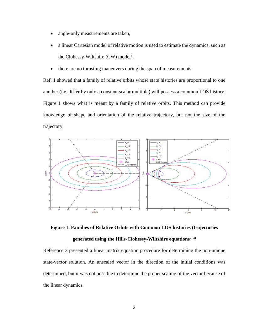
Ref. 1 showed that a family of relative orbits whose state histories are proportional to one
another (i.e. differ by only a constant scalar multiple) will possess a common LOS history.
Figure 1 shows what is meant by a family of relative orbits. This method can provide
knowledge of shape and orientation of the relative trajectory, but not the size of the
trajectory.
Figure 1. Families of Relative Orbits with Common LOS histories (trajectories
generated using the Hills-Clohessy-Wiltshire equations2, 3)
Reference 3 presented a linear matrix equation procedure for determining the non-unique
state-vector solution. An unscaled vector in the direction of the initial conditions was
determined, but it was not possible to determine the proper scaling of the vector because of
the linear dynamics.

3
Current research is investigating the use of second-order nonlinear relative equations
of motion to capture the motion between the chief and the deputy satellite. These equations
offers two distinct advantages: first, these are able to capture the relative motion of two
satellites better than the linear CW solution due to its inclusion of nonlinear terms; second,
the nonlinear terms facilitate determination of the unique scaling of the state vector,
rendering the Initial Relative-Orbit Determination (IROD) problem observable. References
4, 5 and 6 have applied a nonlinear relative dynamic model with angular measurements to
remove the unobservability associated with linear dynamics. The second-order dynamics
model and angle-only measurements produce a system of quadratic equations for the
unknown initial conditions.
Two different solution procedures have been considered. The first method,
minimum-measurement solution, provides direct solution of the quadratic equations by
Macaulay polynomial resultant with minimal number of measurements. It requires a
minimum number of measurements and is computationally very complex. The Macaulay
resultant theory is a less familiar subject in engineering disciplines, when compared to linear
algebra. In this theory, the system of multivariate polynomial equations is projected to a
single univariate polynomial equation: the resultant polynomial equation: Using a matrix
polynomial structure, this equation can be solved by computing a generalized Eigen
decomposition.11-16 Because the resultant polynomial is zero if and only if the polynomial
system has a common root, this procedure is often interpreted as a means to finding the
intersection of algebraic curves. The second method, redundant-measurement solution,
treats the linear and quadratic components as independent variables and transforms the
original second-order dynamics solution to a linear homogenous matrix equation with the

4
use of redundant measurements. The steps are to, first, solve the measurements for an
eigenvector with linear and quadratic components; second, discard the quadratic
components and reform them again using the scaled linear components; and third, substitute
the reformed vector back into the measurement equations to solve for the scaling.
The main aim of this research is to determine the initial relative position vector and
the velocity vector of the deputy satellite with respect to the chief satellite using angle-only
measurements, i.e. to estimate the x0, y0, z0, x0, y0, z0 components of the relative position
vector and the relative velocity vector using azimuth and elevation angle observations
provided by an on-board camera on the chief satellite. In this thesis, development of a new
method for estimating the deputy satellite initial relative state with respect to the chief
satellite is discussed. Compared to previous methods, the linear measurement equations of
the proposed method are reformulated in a different set of unknowns. The reformulation of
the measurement equations means that in the minimum-measurement solution, lower
computational complexity is required, and in the redundant-measurement solution, fewer
measurements are needed to perform the IROD. Also, another method for calculating the
scalar ambiguity which utilizes all the constraint equations is studied along with its failure
to give an accurate result. To illustrate the results, they are evaluated along several relative
motions in the presence of varying noise types, noise levels, and sample periods.
5
CHAPTER 2
SECOND-ORDER DYNAMICS MODEL
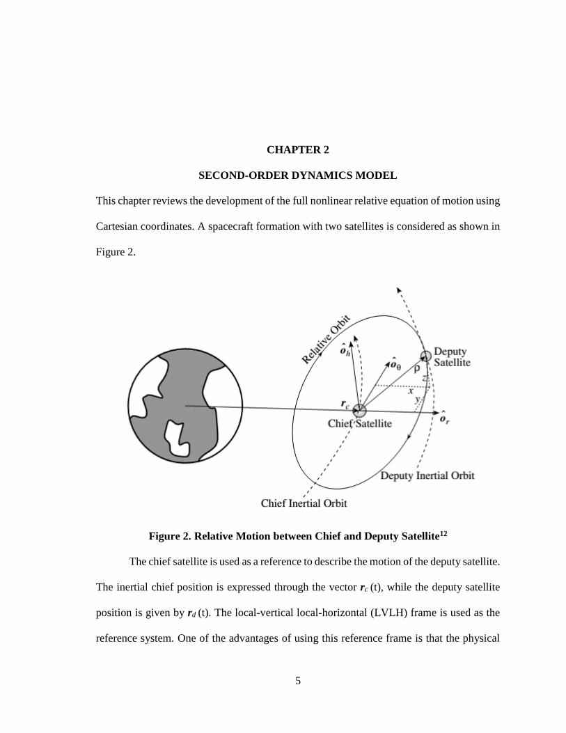
This chapter reviews the development of the full nonlinear relative equation of motion using
Cartesian coordinates. A spacecraft formation with two satellites is considered as shown in
Figure 2.
Figure 2. Relative Motion between Chief and Deputy Satellite12
The chief satellite is used as a reference to describe the motion of the deputy satellite.
The inertial chief position is expressed through the vector rc (t), while the deputy satellite
position is given by rd (t). The local-vertical local-horizontal (LVLH) frame is used as the
reference system. One of the advantages of using this reference frame is that the physical
6
dimensions of the relative orbit can be clearly visualized. The (x, y) coordinates defines the
relative-orbit motion in the chief satellite’s orbital plane and the z coordinate indicates the
relative motion out of plane. Its origin is at the chief satellite position and its orientation is
given by the vector triad {𝒐r, ��θ, ��h} shown in Figure 2.
The vector ��r points in the direction of chief satellite radius, the vector ��h is in the
direction of angular momentum of the chief satellite and the vector ��θ completes the right-
handed coordinate system. Mathematically, the three unit direction vector can be shown as
��r =
c
c
r
r
��h = h
h (h = rc × ��c)
��θ = ��h × ��r
(1)
Cartesian-coordinate Description
The relative orbit can be described in both Cartesian coordinates as well as orbital
elements. Here, the relative orbit is described in terms of Cartesian coordinates. The relative
position of the deputy satellite with respect to the chief satellite is the vector ρ expressed in
LVLH frame as
ρ = [x, y, z] T (2)
From Figure 2, we can write the deputy satellite position vector as
rd = rc + ρ = (rc + x) ��r + y ��θ + z ��h (3)
Where rc is the orbital radius of the chief satellite at any point of time. The angular velocity
vector of the rotating LVLH frame is given by
ω = 𝑓��h (4)
7
Where f is the chief’s true anomaly. Double differentiation of the position vector of the
deputy satellite with respect to the inertial frame will give the acceleration vector of deputy
satellite as
��𝒅 = (��𝑐 + �� − 2��𝑓 − 𝑓𝑦 − 𝑓 2(𝑟𝑐 + 𝑥))��𝑟 + (�� + 2𝑓(��𝑐 + ��) +
𝑓(𝑟𝑐 + 𝑥) − 𝑓2)��𝜃 + ����ℎ
(5)
Keeping in mind that the chief satellite angular momentum h is constant for Keplerian
motion and is given by h =𝑟𝑐2��, the first derivative of it yields
ℎ = 0 = 2𝑟𝑐��𝑐�� + 𝑟𝑐2𝑓 (6)
Equation (6) can be used to solve for the true anomaly acceleration:
𝑓 = −2
��𝑐𝑟𝑐
𝑓 (7)
Further, we can write the chief satellite position as rc = rc ��r. Taking the double derivative
of the chief satellite position vector with respect to the inertial frame and equating it with
orbit equation of motion can be expressed as:
��𝑐 = (��𝑐 − 𝑟𝑐 𝑓2)��𝒓 = −
𝜇
𝑟𝑐3 𝒓𝑐 = −
𝜇
𝑟𝑐2 ��𝒓 (8)
Equating vector component in Eq. (8), the chief satellite orbit acceleration can be
expressed as:
��𝑐 = 𝑟𝑐𝑓 − 𝜇
𝑟𝑐2 = 𝑟𝑐𝑓2(1 −
𝑟𝑐𝑝) (9)
Substituting Eq. (7) and Eq. (8) into Eq. (5), the deputy satellite acceleration vector will
reduce to:
��𝑑 = (�� − 2𝑓(�� − 𝑦
��𝑐𝑟𝑐
) − 𝑥𝑓2 − 𝜇
𝑟𝑐2)��𝒓 + (�� + 2𝑓(�� − 𝑥
��𝑐𝑟𝑐
) − 𝑦𝑓2)��𝜃
+ ����ℎ
(10)
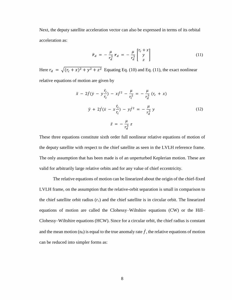
8
Next, the deputy satellite acceleration vector can also be expressed in terms of its orbital
acceleration as:
��𝑑 = −
𝜇
𝑟𝑑3 𝒓𝑑 = −
𝜇
𝑟𝑑3 [
𝑟𝑐 + 𝑥𝑦𝑧
] (11)
Here 𝑟𝑑 = √(𝑟𝑐 + 𝑥)2 + 𝑦2 + 𝑧2 Equating Eq. (10) and Eq. (11), the exact nonlinear
relative equations of motion are given by
�� − 2𝑓(�� − 𝑦
��𝑐𝑟𝑐
) − 𝑥𝑓2 − 𝜇
𝑟𝑐2 = −
𝜇
𝑟𝑑3 (𝑟𝑐 + 𝑥)
�� + 2𝑓(�� − 𝑥��𝑐𝑟𝑐
) − 𝑦𝑓2 = − 𝜇
𝑟𝑑3 𝑦
�� = − 𝜇
𝑟𝑑3 𝑧
(12)
These three equations constitute sixth order full nonlinear relative equations of motion of
the deputy satellite with respect to the chief satellite as seen in the LVLH reference frame.
The only assumption that has been made is of an unperturbed Keplerian motion. These are
valid for arbitrarily large relative orbits and for any value of chief eccentricity.
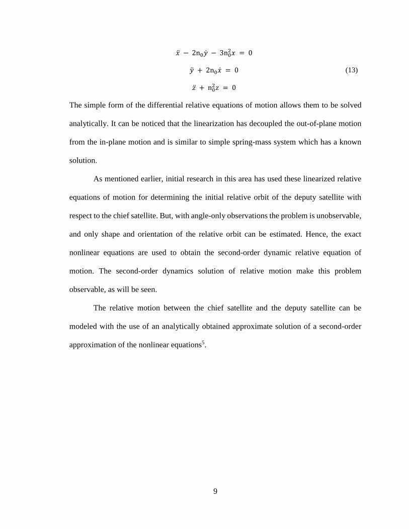
The relative equations of motion can be linearized about the origin of the chief-fixed
LVLH frame, on the assumption that the relative-orbit separation is small in comparison to
the chief satellite orbit radius (rc) and the chief satellite is in circular orbit. The linearized
equations of motion are called the Clohessy–Wiltshire equations (CW) or the Hill–
Clohessy–Wiltshire equations (HCW). Since for a circular orbit, the chief radius is constant
and the mean motion (n0) is equal to the true anomaly rate 𝑓, the relative equations of motion
can be reduced into simpler forms as:
9
�� − 2n0�� − 3n02𝑥 = 0
�� + 2n0�� = 0
�� + n02𝑧 = 0
(13)
The simple form of the differential relative equations of motion allows them to be solved
analytically. It can be noticed that the linearization has decoupled the out-of-plane motion
from the in-plane motion and is similar to simple spring-mass system which has a known
solution.
As mentioned earlier, initial research in this area has used these linearized relative
equations of motion for determining the initial relative orbit of the deputy satellite with
respect to the chief satellite. But, with angle-only observations the problem is unobservable,
and only shape and orientation of the relative orbit can be estimated. Hence, the exact
nonlinear equations are used to obtain the second-order dynamic relative equation of
motion. The second-order dynamics solution of relative motion make this problem
observable, as will be seen.
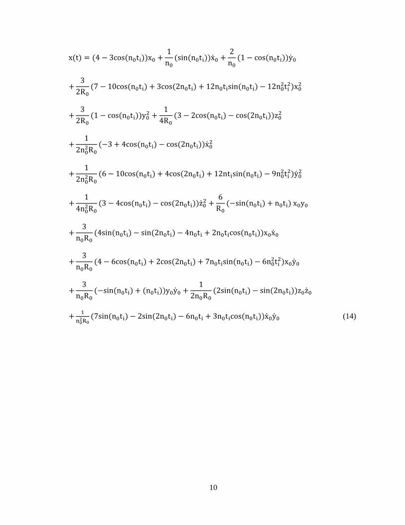
The relative motion between the chief satellite and the deputy satellite can be
modeled with the use of an analytically obtained approximate solution of a second-order
approximation of the nonlinear equations5.
10
x(t) = (4 − 3cos(n0ti))x0 +1
n0(sin(n0ti))x0 +
2
n0(1 − cos(n0ti))y0
+3
2R0(7 − 10cos(n0ti) + 3cos(2n0ti) + 12n0tisin(n0ti) − 12n0
2ti2)x0
2
+3
2R0(1 − cos(n0ti))y0
2 +1
4R0(3 − 2cos(n0ti) − cos(2n0ti))z0
2
+1
2n02R0
(−3 + 4cos(n0ti) − cos(2n0ti))x02
+1
2n02R0
(6 − 10cos(n0ti) + 4cos(2n0ti) + 12ntisin(n0ti) − 9n02ti
2)y02
+1
4n02R0
(3 − 4cos(n0ti) − cos(2n0ti))z02 +
6
R0(−sin(n0ti) + n0ti) x0y0
+3
n0R0(4sin(n0ti) − sin(2n0ti) − 4n0ti + 2n0ticos(n0ti))x0x0
+3
n0R0(4 − 6cos(n0ti) + 2cos(2n0ti) + 7n0tisin(n0ti) − 6n0
2ti2)x0y0
+3
n0R0(−sin(n0ti) + (n0ti))y0y0 +
1
2n0R0(2sin(n0ti) − sin(2n0ti))z0z0
+1
n02R0
(7sin(n0ti) − 2sin(2n0ti) − 6n0ti + 3n0ticos(n0ti))x0y0 (14)
11
y(t) = 6(sin(n0ti) − n0ti)x0 + {1}y0
+2
n0(−1 + cos(n0ti))x0 +
1
n0(4sin(n0ti) − 3n0ti)y0
+3
4R0(40sin(n0ti) + 3sin(2n0ti) − 22n0ti − 24n0ticos(n0ti))x0
2
+3
R0(sin(n0ti) − n0ti)y0
2 +1
R0(4sin(n0ti) + sin(2n0ti) − 6n0ti)z0
2
+1
4n02R0
(8sin(n0ti) − sin(2n0ti) − 6n0ti)x02
+1
n02R0
(10sin(n0ti) + sin(2n0ti) − 6n0ti − 6n0ticos(n0ti))y02
+1
4n02R0
(8sin(n0ti) − sin(2n0ti) − 6n0ti) z02 +
3
R0(1 − cos(n0ti))x0y0
+3
2n0R0(−5 + 4cos(n0ti) + cos(2n0ti) + 4n0tisin(n0ti))x0x0
+3
n0R0(12sin(n0ti) + sin(2n0ti) − 7n0ti − 7n0ticos(n0ti))x0y0
+1
3n0R0(−sin(n0ti) + n0ti)y0x0
+1
2n0R0(−3 + 4cos(n0ti) − cos(2n0ti))z0z0
+1
n02R0
(−3 + 2cos(n0ti) + cos(2n0ti) + 3n0tisin(n0ti))x0y0
12
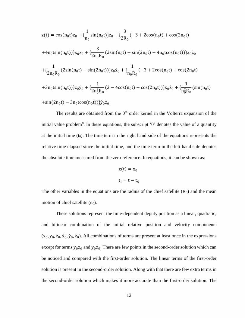
z(t) = cos(n0t)z0 + {1
n0sin(n0t)}z0 + {
3
2R0(−3 + 2cos(n0t) + cos(2n0t)
+4n0tsin(n0t))}x0z0 + {3
2n0R0(2sin(n0t) + sin(2n0t) − 4n0tcos(n0t))}x0z0
+{1
2n0R0(2sin(n0t) − sin(2n0t))}z0x0 + {
1
n0R0(−3 + 2cos(n0t) + cos(2n0t)
+3n0tsin(n0t))}z0y0 + {1
2n02R0
(3 − 4cos(n0t) + cos(2n0t))}x0z0 + {1
n02R0
(sin(n0t)
+sin(2n0t) − 3n0tcos(n0t))}y0z0
The results are obtained from the 0th order kernel in the Volterra expansion of the
initial value problem8. In these equations, the subscript ‘0’ denotes the value of a quantity
at the initial time (t0). The time term in the right hand side of the equations represents the
relative time elapsed since the initial time, and the time term in the left hand side denotes
the absolute time measured from the zero reference. In equations, it can be shown as:
x(t) = x0
ti = t − t0
The other variables in the equations are the radius of the chief satellite (R0) and the mean
motion of chief satellite (n0).
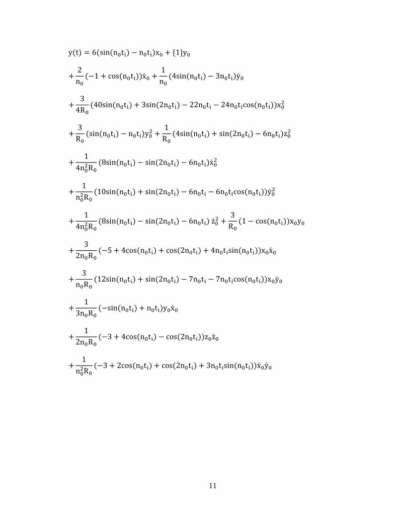
These solutions represent the time-dependent deputy position as a linear, quadratic,
and bilinear combination of the initial relative position and velocity components
(x0, y0, z0, x0, y0, z0). All combinations of terms are present at least once in the expressions
except for terms y0z0 and y0z0. There are few points in the second-order solution which can
be noticed and compared with the first-order solution. The linear terms of the first-order
solution is present in the second-order solution. Along with that there are few extra terms in
the second-order solution which makes it more accurate than the first-order solution. The
13
first-order solution has only one secular term, in the y equation, but the second-order
solution has introduced new secular terms in x, y, and z. Secular terms in x include not,
notcos(not), notsin(not), (not)2, while secular terms in y include only not, notcos(not),
notsin(not), and secular terms in z are limited to just notcos(not), notsin(not). The secular term
in the first-order solution provides the drift in only transverse (y) axis, but the secular terms
in the second-order solution reflects the local three-dimensional drift of the deputy satellite
away from the chief satellite in radial (x) and normal (z) axes also. Although the second-
order solution is able to capture the true relative motion between the deputy and chief
satellite, it will eventually fail since the secular terms will grow with time, and cause it to
diverge from the true solution. Also, it is true that for a given separation distance between
the chief and deputy satellite, the second-order solution may provide higher accuracy than
first-order solution, but the error growth rate associated with second-order solution may
exceed the level of first-order solution as the separation distance gets larger. Further, the
cross-track and in-track motion is coupled in the full nonlinear equation and the second-
order solution but it is lost in the first-order solution.
The problem is unobservable when the first-order solution is used with angle-only
observations, and observable when the second-order solution is used with angle-only
observations. Figure 3 and 4 show how the change in dynamic model helped in achieving
the observability. Figure 3 shows the relative motion of a deputy satellite with respect to the
chief satellite, captured with the first-order solution. The trajectory generated with true
initial conditions is labelled as “First-Order Motion”. For this trajectory, the three line-of-
sight direction of the deputy satellite at three different time in future are shown with black
color. The trajectory generated with initial conditions that are twice of the true initial

14
conditions, is labelled as “First-Order Motion with 2 time initial condition”. For this
trajectory, the line-of-sight direction of the deputy satellite at three different time in future
are shown with green color. It can be seen, the line-of-sight unit-direction-vectors of the
two different trajectory are overlapping each other. With these line-of-sight unit-direction-
vector as measurements, the initial conditions cannot be estimated with first-order dynamic
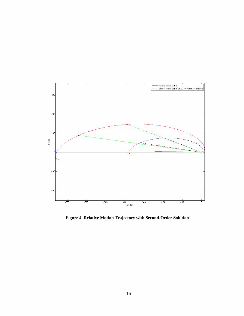
model since a family of trajectory will provide same unit-direction vector. Figure 4 shows
the relative motion of a deputy satellite with respect to the chief satellite, captured with
second-order solution. The trajectory generated with true initial conditions is labelled as
“Second-Order Motion”. For this trajectory, the three line-of-sight direction of the deputy
satellite at three different time in future are shown with black color. The trajectory generated
with initial conditions that are twice of the true initial conditions, is labelled as “Second-
Order Motion with 2 time initial condition”. For this trajectory, the line-of-sight direction
of the deputy satellite at three different time in future are shown with green color. It can be
seen, different set of measurements of unit-direction-vectors will estimate the trajectory
corresponding to it. Hence, the second-order model is used to design a method which can
estimate the initial conditions with line-of-sight measurements.

15
Figure 3. Relative Motion trajectory with First-Order Solution
16
Figure 4. Relative Motion Trajectory with Second-Order Solution

17
CHAPTER 3
REDUNDANT-MEASUERMENT SOLUTION USING
CARTESIAN-COMPONENT FORMULATION
The Cartesian-component formulation has been previously introduced in the
literature. As the name suggests, this method determines the Cartesian-components of the
initial relative position vector and velocity vector using the second-order dynamics and
angle-only observation8. The redundant-measurement solution method can be divided into
parts. First, the second-order solution is reformulated into a linear homogenous matrix
equation using angular measurements, and second, determination of the unique scaling of
the computed null vector. The solution is reviewed here, particularly because the second
part of this method will be used in later chapters.
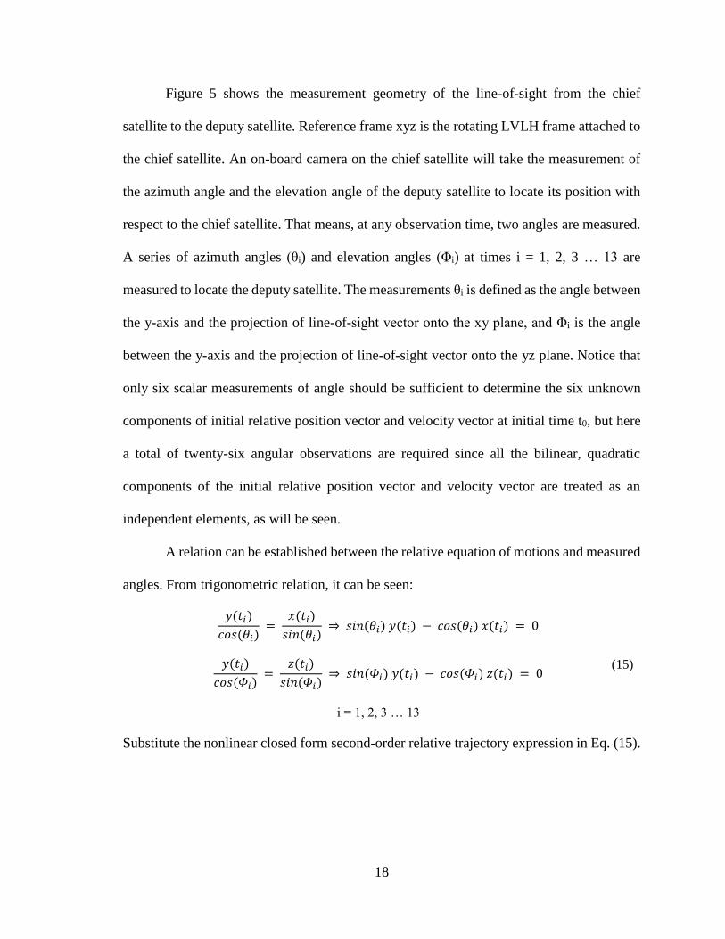
Figure 5. Relative Orbit Determination Geometry8
18
Figure 5 shows the measurement geometry of the line-of-sight from the chief
satellite to the deputy satellite. Reference frame xyz is the rotating LVLH frame attached to
the chief satellite. An on-board camera on the chief satellite will take the measurement of
the azimuth angle and the elevation angle of the deputy satellite to locate its position with
respect to the chief satellite. That means, at any observation time, two angles are measured.
A series of azimuth angles (θi) and elevation angles (Φi) at times i = 1, 2, 3 … 13 are
measured to locate the deputy satellite. The measurements θi is defined as the angle between
the y-axis and the projection of line-of-sight vector onto the xy plane, and Φi is the angle
between the y-axis and the projection of line-of-sight vector onto the yz plane. Notice that
only six scalar measurements of angle should be sufficient to determine the six unknown
components of initial relative position vector and velocity vector at initial time t0, but here
a total of twenty-six angular observations are required since all the bilinear, quadratic
components of the initial relative position vector and velocity vector are treated as an
independent elements, as will be seen.
A relation can be established between the relative equation of motions and measured
angles. From trigonometric relation, it can be seen:
𝑦(𝑡𝑖)
𝑐𝑜𝑠(𝜃𝑖) =
𝑥(𝑡𝑖)
𝑠𝑖𝑛(𝜃𝑖) ⇒ 𝑠𝑖𝑛(𝜃𝑖) 𝑦(𝑡𝑖) − 𝑐𝑜𝑠(𝜃𝑖) 𝑥(𝑡𝑖) = 0
𝑦(𝑡𝑖)
𝑐𝑜𝑠(𝛷𝑖) =
𝑧(𝑡𝑖)
𝑠𝑖𝑛(𝛷𝑖) ⇒ 𝑠𝑖𝑛(𝛷𝑖) 𝑦(𝑡𝑖) − 𝑐𝑜𝑠(𝛷𝑖) 𝑧(𝑡𝑖) = 0
i = 1, 2, 3 … 13
(15)
Substitute the nonlinear closed form second-order relative trajectory expression in Eq. (15).
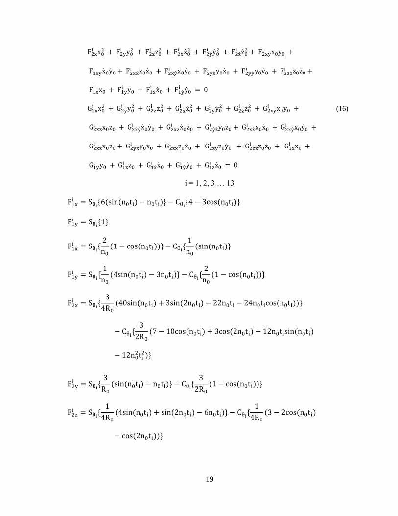
19
F2xi x0
2 + F2yi y0
2 + F2zi z0
2 + F2xi x0
2 + F2yi y0
2 + F2zi z0
2 + F2xyi x0y0 +
F2xyi x0y0 + F2xx
i x0x0 + F2xyi x0y0 + F2yx
i y0x0 + F2yyi y0y0 + F2zz
i z0z0 +
F1xi x0 + F1y
i y0 + F1xi x0 + F1y
i y0 = 0
G2xi x0
2 + G2yi y0
2 + G2zi z0
2 + G2xi x0
2 + G2yi y0
2 + G2zi z0
2 + G2xyi x0y0 +
G2xzi x0z0 + G2xy
i x0y0 + G2xzi x0z0 + G2yz
i y0z0 + G2xxi x0x0 + G2xy
i x0y0 +
G2xzi x0z0 + G2yx
i y0x0 + G2zxi z0x0 + G2zy
i z0y0 + G2zzi z0z0 + G1x
i x0 +
G1yi y0 + G1z
i z0 + G1xi x0 + G1y
i y0 + G1zi z0 = 0
(16)
i = 1, 2, 3 … 13
F1xi = Sθi
{6(sin(n0ti) − n0ti)} − Cθi{4 − 3cos(n0ti)}
F1yi = Sθi
{1}
F1xi = Sθi
{2
n0(1 − cos(n0ti))} − Cθi
{1
n0(sin(n0ti)}
F1yi = Sθi
{1
n0(4sin(n0ti) − 3n0ti)} − Cθi
{2
n0(1 − cos(n0ti))}
F2xi = Sθi
{3
4R0(40sin(n0ti) + 3sin(2n0ti) − 22n0ti − 24n0ticos(n0ti))}
− Cθi{
3
2R0(7 − 10cos(n0ti) + 3cos(2n0ti) + 12n0tisin(n0ti)
− 12n02ti
2)}
F2yi = Sθi
{3
R0(sin(n0ti) − n0ti)} − Cθi
{3
2R0(1 − cos(n0ti))}
F2zi = Sθi
{1
4R0(4sin(n0ti) + sin(2n0ti) − 6n0ti)} − Cθi
{1
4R0(3 − 2cos(n0ti)
− cos(2n0ti))}
20
F2xi = Sθi
{1
4n02R0
(8sin(n0ti) − sin(2n0ti) − 6n0ti)} − Cθi{
1
2n02R0
(−3 + 4cos(n0ti)
− cos(2n0ti))}
F2yi = Sθi
{1
n02R0
(10sin(n0ti) + sin(2n0ti) − 6n0ti − 6n0ticos(n0ti))} − Cθi{
1
2n02R0
(6
− 10cos(n0ti) + 4cos(2n0ti) + 12ntisin(n0ti) − 9n02ti
2)}
F2zi = Sθi
{1
4n02R0
(8sin(n0ti) − sin(2n0ti) − 6n0ti)} − Cθi{
1
4n02R0
(3 − 4cos(n0ti)
− cos(2n0ti))}
F2xyi = Sθi
{3
R0(1 − cos(n0ti))} − Cθi
{6
R0(−sin(n0ti) + n0ti)}
F2xyi = Sθi
{1
n02R0
(−3 + 2cos(n0ti) + cos(2n0ti) + 3n0tisin(n0ti))}
− Cθi{
1
n02R0
(7sin(n0ti) − 2sin(2n0ti) − 6n0ti + 3n0ticos(n0ti))}
F2xxi = Sθi
{3
2n0R0(−5 + 4cos(n0ti) + cos(2n0ti) + 4n0tisin(n0ti))}
− Cθi{
3
n0R0(4sin(n0ti) − sin(2n0ti) − 4n0ti + 2n0ticos(n0ti))}
F2xyi = Sθi
{3
n0R0(12sin(n0ti) + sin(2n0ti) − 7n0ti − 7n0ticos(n0ti))} − Cθi
{3
n0R0(4
− 6cos(n0ti) + 2cos(2n0ti) + 7n0tisin(n0ti) − 6n02ti
2)}
F2yxi = Sθi
{3
n0R0(−sin(n0ti) + (n0ti))}
F2yyi = −Cθi
{1
3n0R0(−sin(n0ti) + n0ti)}

21
F2zzi = Sθi
{1
2n0R0(−3 + 4cos(n0ti) − cos(2n0ti))} − Cθi
{1
2n0R0(2sin(n0ti)
− sin(2n0ti))}
G1xi = Sϕi
{6(sin(n0ti) − n0ti)}
G1xi = Cϕi
{2
n0(−1 + cos(n0ti))}
G1yi = Sϕi
{1}
G1yi = Sϕi
{1
n0(4sin(n0ti) − 3n0ti)}
G1zi = −Cϕi
{cos(n0ti)}
G1zi = −Cϕi
{1
n0sin(n0ti)}
G2xi = Sϕi
{3
4R0(40sin(n0ti) + 3sin(2n0ti) − 22n0ti − 24n0ticos(n0ti))
G2xi = Sϕi
{1
4n02R0
(8sin(n0ti) − sin(2n0ti) − 6n0ti)}
G2yi = Sϕi
{3
R0(sin(n0ti) − n0ti)}
G2yi = Sϕi
{1
n02R0
(10sin(n0ti) + sin(2n0ti) − 6n0ti − 6n0ticos(n0ti))}
G2zi = Sϕi
{1
4R0(4sin(n0ti) + sin(2n0ti) − 6n0ti)}
G2zi = Sϕi
{1
4n02R0
(8sin(n0ti) − sin(2n0ti) − 6nti)}
G2xyi = Sϕi
{3
R0(1 − cos(n0ti))}
G2xzi = −Cϕi
{3
2R0(−3 + 2cos(n0ti) + cos(2n0ti) + 4n0tisin(n0ti))}
22
G2xyi = Sϕi
{1
n02R0
(−3 + 2cos(n0ti) + cos(2n0ti) + 3n0tisin(n0ti))}
G2xzi = −Cϕi
{1
2n02R0
(3 − 4cos(n0ti) + cos(2n0ti))}
G2yzi = −Cϕi
{1
n02R0
(sin(n0ti) + sin(2n0ti) − 3n0ticos(n0ti))}
G2xxi = Sϕi
{3
2n0R0(−5 + 4cos(n0ti) + cos(2n0ti) + 4n0tisin(n0ti))}
G2yxi = Sϕi
{3
n0R0(−sin(n0ti) + (n0ti))}
G2xyi = Sϕi
{3
n0R0(12sin(n0ti) + sin(2n0ti) − 7n0ti − 7n0ticos(n0ti))}
G2xzi = −Cϕi
{3
2n0R0(2sin(n0ti) + sin(2n0ti) − 4n0ticos(n0ti))}
G2zxi = −Cϕi
{3
2n0R0(2sin(n0ti) − sin(2n0ti))}
G2zyi = −Cϕi
{1
n0R0(−3 + 2cos(n0ti) + cos(2n0ti) + 3n0tisin(n0ti))}
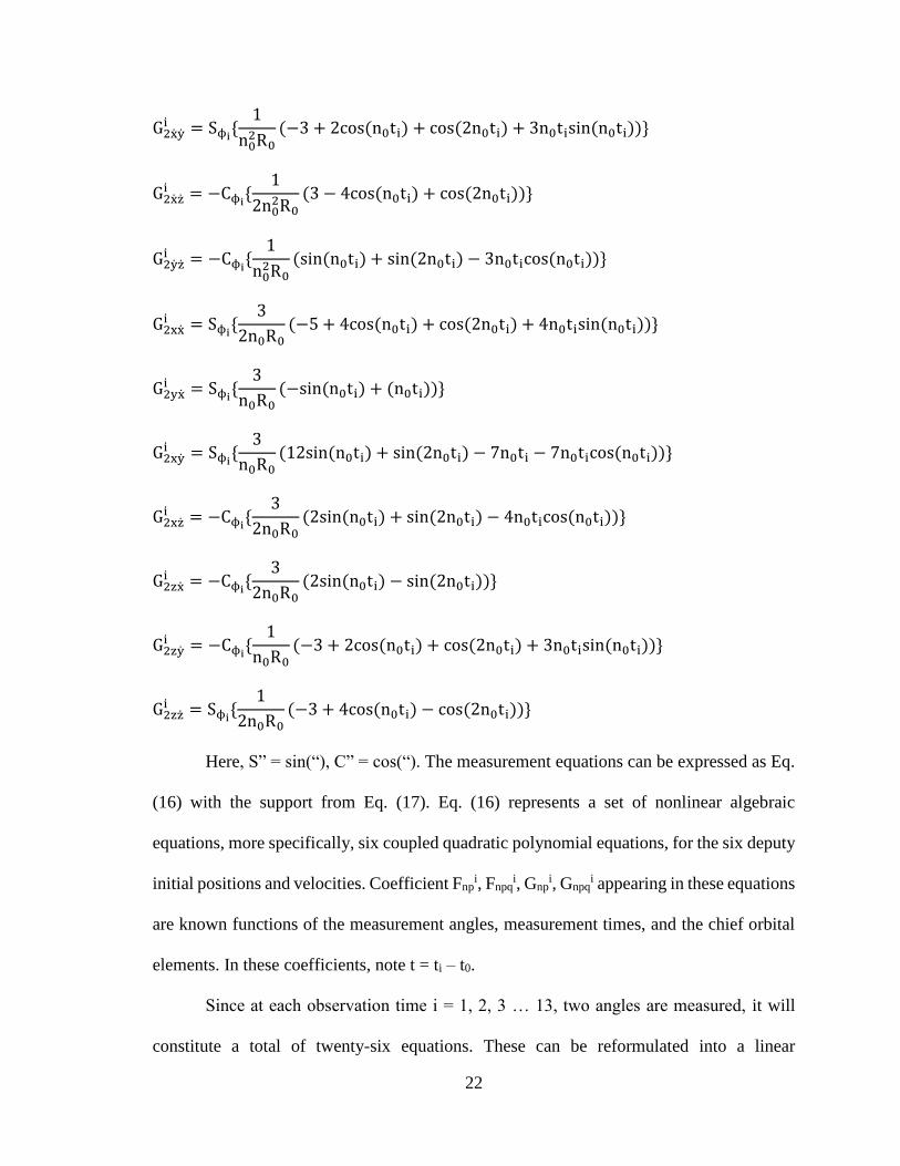
G2zzi = Sϕi
{1
2n0R0(−3 + 4cos(n0ti) − cos(2n0ti))}
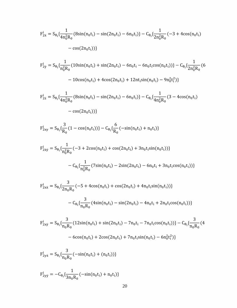
Here, S” = sin(“), C” = cos(“). The measurement equations can be expressed as Eq.
(16) with the support from Eq. (17). Eq. (16) represents a set of nonlinear algebraic
equations, more specifically, six coupled quadratic polynomial equations, for the six deputy
initial positions and velocities. Coefficient Fnpi, Fnpq
i, Gnpi, Gnpq
i appearing in these equations
are known functions of the measurement angles, measurement times, and the chief orbital
elements. In these coefficients, note t = ti – t0.
Since at each observation time i = 1, 2, 3 … 13, two angles are measured, it will
constitute a total of twenty-six equations. These can be reformulated into a linear
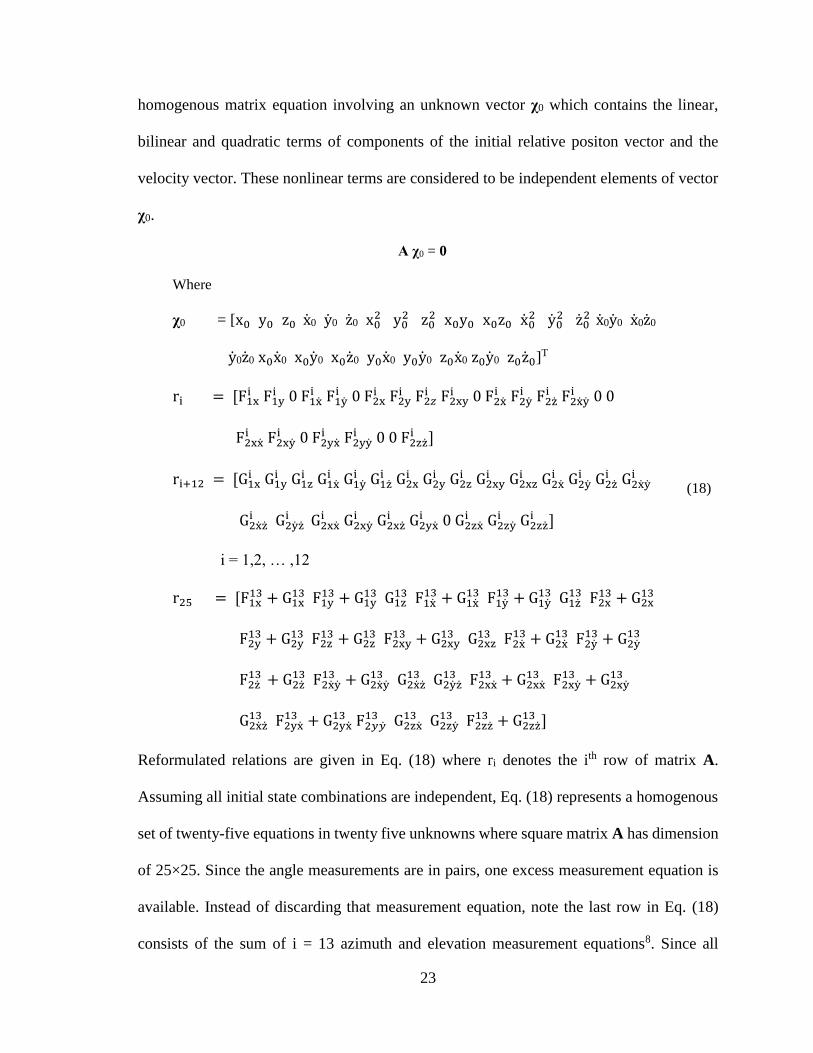
23
homogenous matrix equation involving an unknown vector χ0 which contains the linear,
bilinear and quadratic terms of components of the initial relative positon vector and the
velocity vector. These nonlinear terms are considered to be independent elements of vector
χ0.
A χ0 = 0
Where
χ0 = [x0 y0 z0 x0 y0 z0 x02 y0
2 z02 x0y0 x0z0 x0
2 y02 z0
2 x0y0 x0z0
y0z0 x0x0 x0y0 x0z0 y0x0 y0y0 z0x0 z0y0 z0z0]T
ri = [F1xi F1y
i 0 F1xi F1y
i 0 F2xi F2y
i F2𝑧i F2xy
i 0 F2xi F2y
i F2zi F2xy
i 0 0
F2xxi F2xy
i 0 F2yxi F2yy
i 0 0 F2zzi ]
ri+12 = [G1xi G1y
i G1zi G1x
i G1yi G1z
i G2xi G2y
i G2zi G2xy
i G2xzi G2x
i G2yi G2z
i G2xyi
G2xzi G2yz
i G2xxi G2xy
i G2xzi G2yx
i 0 G2zxi G2zy
i G2zzi ]
i = 1,2, … ,12
r25 = [F1x13 + G1x
13 F1y13 + G1y
13 G1z13 F1x
13 + G1x13 F1y
13 + G1y13 G1z
13 F2x13 + G2x
13
F2y13 + G2y
13 F2z13 + G2z
13 F2xy13 + G2xy
13 G2xz13 F2x
13 + G2x13 F2y
13 + G2y13
F2z 13 + G2z
13 F2xy13 + G2xy
13 G2xz13 G2yz
13 F2xx13 + G2xx
13 F2xy13 + G2xy
13
G2xz13 F2yx
13 + G2yx13 F2𝑦��
13 G2zx13 G2zy
13 F2zz13 + G2zz
13 ]
(18)
Reformulated relations are given in Eq. (18) where ri denotes the ith row of matrix A.
Assuming all initial state combinations are independent, Eq. (18) represents a homogenous
set of twenty-five equations in twenty five unknowns where square matrix A has dimension
of 25×25. Since the angle measurements are in pairs, one excess measurement equation is
available. Instead of discarding that measurement equation, note the last row in Eq. (18)
consists of the sum of i = 13 azimuth and elevation measurement equations8. Since all
24
elements are considered to be independent, it is possible that the solution of the vector χ0
may not satisfy the original nonlinear relations because connections between the last
nineteen variables and the first six variables has been severed. So an additional nineteen
constraint equations are needed to get the precise results.
A Non-trivial vector χ0 which satisfies Eq. (18), or eigenvectors corresponding to
zero eigenvalues of the matrix A, are sought. Based on physical arguments and assuming
zero plant noise, at least one zero eigenvalue and associated eigenvector exist corresponding
to the unknown initial conditions8. The eigen value-vector decomposition of matrix A,
denoted by λi and ϕi for i = 1, 2, 3 … 25 is calculated.
A ϕi = λi ϕi where |λ1| ≤ |λ2| ≤ . . . ≤ |λ25| (19)
Discard Method for Calculating the Scalar Ambiguity
The null vector ϕ1 will be the non-unique solution of unknown vector χ0. To remove
the ambiguity, an unknown scaling factor α must be included to scale the computed
eigenvector. The uniform scaling of all vector components does not allow determination of
α, since upon back substitution into any measurement equation, α will cancel from each
term. Hence, a non-uniform scaling is essential. It is obtained by enforcing the neglected
constraints from the original nonlinear formulation. To implement the constraints, the last
nineteen quadratic and bilinear elements of the scaled null vector (αϕ) are discarded, and
then reformed again using the retained first six linear elements of the scaled null vector.
The vector χ0 is:
χ0 = [x0 y0 z0 x0 y0 z0 x02 y0
2 z02 x0y0 x0z0 x0
2 y02 z0
2 x0y0 x0z0
y0z0 x0x0 x0y0 x0z0 y0x0 y0y0 z0x0 z0y0 z0z0]T
(20)
25
Suppose eigenvector ϕ1 is given as:
ϕ1 = [ϕ01 ϕ02 ϕ03 ϕ04 ϕ05 ϕ06 ϕ07 ϕ08 ϕ09 ϕ10 ϕ11 ϕ12 ϕ13 ϕ14 ϕ15 ϕ16
ϕ17 ϕ18 ϕ19 ϕ20 ϕ21 ϕ22 ϕ23 ϕ24 ϕ25]T
(22)
According to this method, last nineteen elements of constraints are discarded from the
original null vector ϕ1 and replaced by the combinations of scaled linear terms.
The last nineteen nonlinear terms are replaced with combinations of linear terms as
shown below:
(ϕ07) = (αϕ01)2; (ϕ08) = (αϕ02)2; (ϕ09) = (αϕ03)2; (ϕ10)=(αϕ01)(αϕ02)
(ϕ11) = (αϕ01) (αϕ03); (ϕ12) = (αϕ04)2; (ϕ13) = (αϕ05)2; (ϕ14) = (αϕ06)2;
(ϕ15) = (αϕ04) (αϕ05); (ϕ1-16) = (αϕ04) (αϕ06); (ϕ17) = (αϕ05) (αϕ06);
(ϕ18) = (αϕ01) (αϕ04); (ϕ19) = (αϕ01) (αϕ05); (ϕ20) = (αϕ01) (αϕ06);
(ϕ21) = (αϕ02) (αϕ04); (ϕ22) = (αϕ02) (αϕ06); (ϕ23) = (αϕ03) (αϕ01);
(ϕ24) = (αϕ03) (αϕ02); (ϕ25) = (αϕ03) (αϕ06);
(22)
Hence, the transformed scaled null vector (αϕ1) which satisfy the constraints is
written as:
[αϕ01 αϕ02 αϕ03 αϕ04 αϕ05 αϕ06 (αϕ01)2 (αϕ02)2 (αϕ03)2 (αϕ01)(αϕ02)
(αϕ01)(αϕ03) (αϕ04)2 (αϕ05)2 (αϕ06)2 (αϕ04)(αϕ05) (αϕ04)(αϕ06) (αϕ05)(αϕ06)
(αϕ01)(αϕ04) (αϕ01)(αϕ05) (αϕ01)(αϕ06) (αϕ02)(αϕ04) (αϕ02)(αϕ06) (αϕ03)(αϕ01)
(αϕ03)(αϕ02) (αϕ03)(αϕ06)]
(23)
This new scaled null vector is substituted into the linear homogenous matrix equation to
solve for the value of scalar ambiguity.
A(i,1:6) αϕ1(1:6) + A(i,7:25) α2ϕ1(7:25) = 0
i = 1, 2, 3 … 25
(24)
26
In a case with no process noise, i.e. the measurements are generated using the second-order
dynamics solution, and no measurement noise, each of the measurement equation yields an
identical value of α, and the true initial conditions are recovered precisely. In a case with
process noise and/or measurement noise, each of the measurement equation yields a
different value of α. It is then suggested to compute the mean of these different values of α
as the appropriate scale factor8.
It has been shown that this method of determining the initial relative state vector of
the deputy satellite with respect to the chief satellite is very effective in results8. The method
is evaluated in presence of varying noise types, noise levels, and sample periods. In
summary, the Cartesian-component formulation uses a total of thirteen observations, each
observation includes measurement of two angles, so a total of twenty-six angle
measurements which generate a square matrix of dimension 25 × 25. By comparison, the
method proposed in the next chapter will need a total of eight unit-direction-vector
observations, generating a square matrix of 21 × 21, therefore requiring fewer observations
and lower computational expense.
27
CHAPTER 4
REDUNDANT-MEASUREMENT SOLUTION USING
SEPARATION-MAGNITUDE FORMULATION
The main aim of the IROD problem is to determine the initial relative position vector
and the velocity vector of the deputy satellite with respect to the chief satellite using unit-
direction-vector observations. A camera on-board the chief satellite will observe the
location of the deputy satellite relative to the chief. The initial time can arbitrarily be chosen
as the time of the first observation. This observation means the initial direction of the deputy
satellite with respect to the chief satellite is already known, and it is only the relative
magnitude that needs to be computed for complete knowledge of relative position vector.
u(t) = r(t)/||r(t)| (25)
The problem is reduced with the remaining unknowns being the relative magnitude of
position vector and relative-velocity vector of the deputy satellite with respect to the chief
satellite.
In general, the Cartesian-component formulation was a two-step method: first, to
reformulate the second-order dynamics solution as a linear matrix homogenous equation
with the total of 13 observations; second, calculation of scalar ambiguity to remove the
unobservability problem using discard method. Similar to this, the Separation-Magnitude
formulation is also a two-step method: first, use the second-order dynamics model of
relative motion with the total of eight observation measurements to form a linear
homogenous matrix equation; second, calculate the scalar ambiguity. A new, constraint-
28
enforcement method is also proposed for the scalar-ambiguity calculation, which as will be
seen, proved ineffective in estimating the true initial conditions.
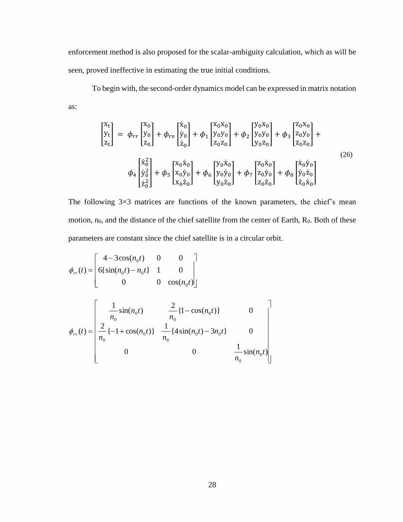
To begin with, the second-order dynamics model can be expressed in matrix notation
as:
[
xt
yt
zt
] = 𝜙𝑟𝑟 [
x0
y0
z0
] + 𝜙𝑟𝑣 [
x0
y0
z0
] + 𝜙1 [
x0x0
y0y0
z0z0
] + 𝜙2 [
y0x0
y0y0
y0z0
] + 𝜙3 [
z0x0
z0y0
z0z0
] +
𝜙4 [
x02
y02
z02
] + 𝜙5 [
x0x0
x0y0
x0z0
] + 𝜙6 [
y0x0
y0y0
y0z0
] + 𝜙7 [
z0x0
z0y0
z0z0
] + 𝜙8 [
x0
y0
z0
y0
z0
x0
]
(26)
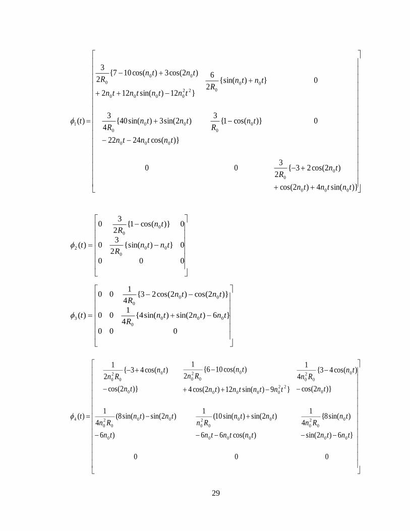
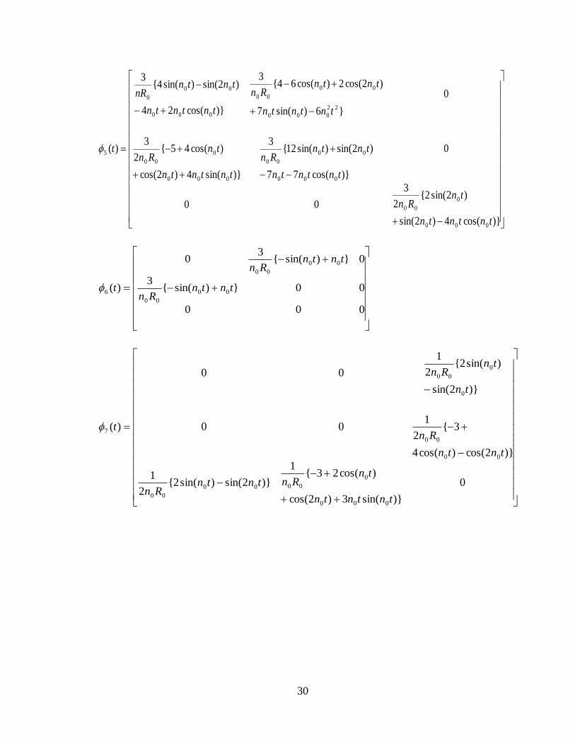
The following 3×3 matrices are functions of the known parameters, the chief’s mean
motion, n0, and the distance of the chief satellite from the center of Earth, R0. Both of these
parameters are constant since the chief satellite is in a circular orbit.
)cos(00
01}){sin(6
00)cos(34
)(
0
00
0
tn
tntn
tn
trr
)sin(1
00
0}3)sin(4{1
)}cos(1{2
0)}cos(1{2
)sin(1
)(
0
0
00
0
0
0
0
0
0
0
tnn
tntnn
tnn
tnn
tnn
trv
29
)}sin(4)2cos(
)2cos(23{2
300
0)}cos(1{3
)}cos(2422
)2sin(3)sin(40{4
3
0}){sin(2
6
}12)sin(122
)2cos(3)cos(107{2
3
)(
000
0
0
0
0
000
00
0
00
022
0000
00
0
1
tntntn
tnR
tnR
tntntn
tntnR
tntnR
tntntntn
tntnR
t
000
0}){sin(2
30
0)}cos(1{2
30
)( 00
0
0
0
2 tntnR
tnR
t
000
}6)2sin()sin(4{4
100
)}2cos()2cos(23{4
100
)( 000
0
00
0
3 tntntnR
tntnR
t
000
}6)2sin(
)sin(8{4
1
)cos(66
)2sin()sin(10(1
)6
)2sin()sin(8(4
1
)}2cos(
)cos(43{4
1
}9)sin(12)2cos(4
)cos(106{2
1
)}2cos(
)cos(43{2
1
)(
00
0
0
2
0
000
00
0
2
0
0
00
0
2
0
0
0
0
2
0
22
0000
0
0
2
0
0
0
0
2
0
4
tntn
tnRn
tntntn
tntnRn
tn
tntnRn
tn
tnRn
tntntntn
tnRn
tn
tnRn
t
30
)}cos(4)2sin(
)2sin(2{2
3
00
0
)}cos(77
)2sin()sin(12{3
)}sin(4)2cos(
)cos(45{2
3
0
}6)sin(7
)2cos(2)cos(64{3
)}cos(24
)2sin()sin(4{3
)(
000
0
00
000
00
00
000
0
00
22
000
00
00
000
00
0
5
tntntn
tnRn
tntntn
tntnRn
tntntn
tnRn
tntntn
tntnRn
tntntn
tntnnR
t
000
00})sin({3
0})sin({3
0
)( 00
00
00
00
6 tntnRn
tntnRn
t
0
)}sin(3)2cos(
)cos(23{1
)}2sin()sin(2{2
1
)}2cos()cos(4
3{2
100
)}2sin(
)sin(2{2
1
00
)(
000
0
0000
00
00
00
0
0
00
7
tntntn
tnRntntn
Rn
tntn
Rn
tn
tnRn
t
31
)}2cos(
)cos(43{2
1
)}cos(3
)2sin(){sin(1
0
00
)}sin(3)2cos(
)cos(23{1
00
)}cos(36
)2sin(2)sin(7{1
)(
0
0
0
2
0
00
00
0
2
0
000
0
0
2
0
000
00
0
2
0
8
tn
tnRn
tntn
tntnRn
tntntn
tnRn
tntntn
tntnRn
t
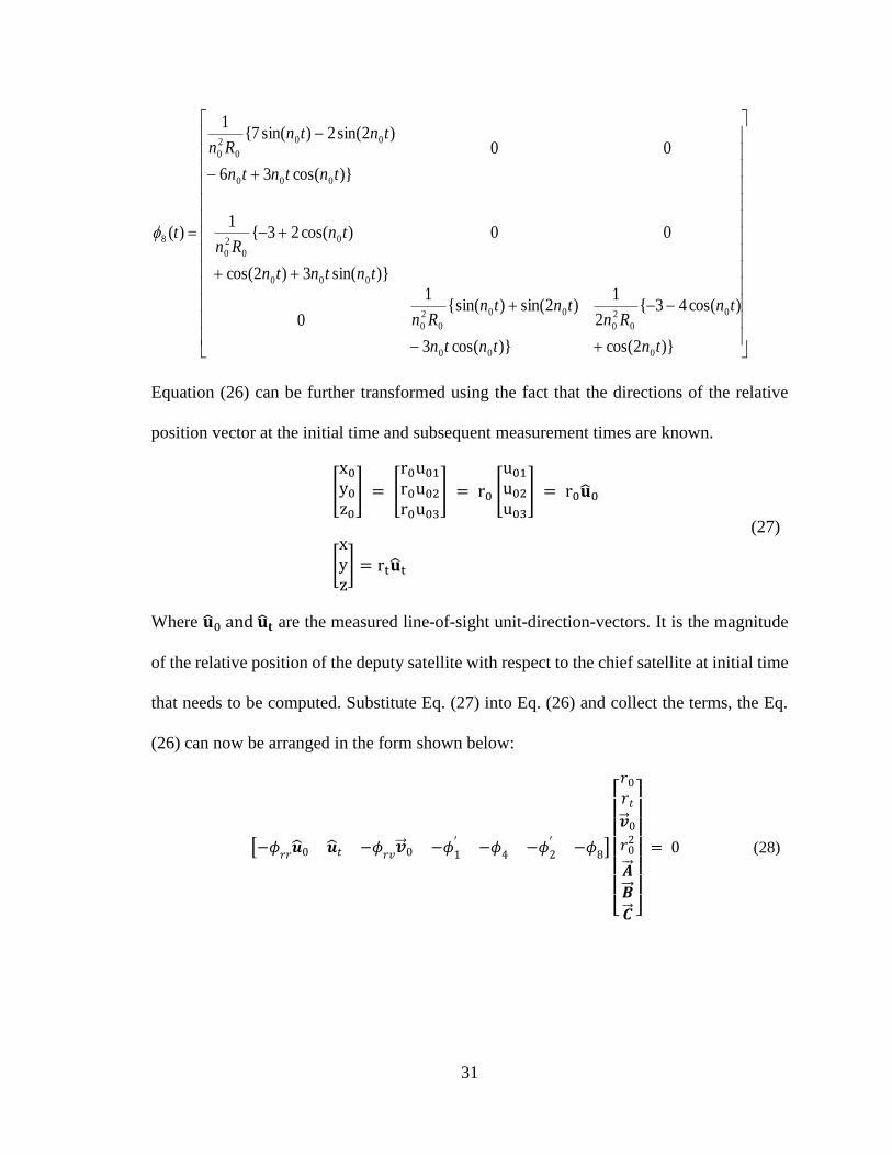
Equation (26) can be further transformed using the fact that the directions of the relative
position vector at the initial time and subsequent measurement times are known.
[
x0
y0
z0
] = [
r0u01
r0u02
r0u03
] = r0 [
u01
u02
u03
] = r0��0
[xyz] = rt��t
(27)
Where ��0 and ��𝐭 are the measured line-of-sight unit-direction-vectors. It is the magnitude
of the relative position of the deputy satellite with respect to the chief satellite at initial time
that needs to be computed. Substitute Eq. (27) into Eq. (26) and collect the terms, the Eq.
(26) can now be arranged in the form shown below:
[−𝜙𝑟𝑟
��0 ��𝑡 −𝜙𝑟𝑣
�� 0 −𝜙1′ −𝜙
4−𝜙
2′ −𝜙
8]
[ 𝑟0
𝑟𝑡
�� 0𝑟02
��
��
�� ]
= 0 (28)
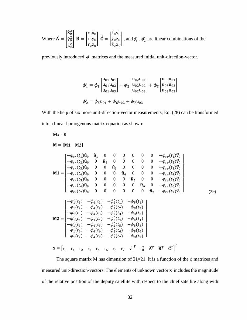
32
Where �� = [
x02
y02
z02
] �� = [
r0x0
r0y0
r0z0
] 𝐂 = [
x0
y0
z0
y0
z0
x0
] , and1 , 2 are linear combinations of the
previously introduced matrices and the measured initial unit-direction-vector.
𝜙1′ = 𝜙1 [
u01u01
u01u02
u01u03
] + 𝜙2 [
u02u01
u02u02
u02u03
] + 𝜙3 [
u03u01
u03u02
u03u03
]
𝜙2′ = 𝜙5u01 + 𝜙6u02 + 𝜙7u03
With the help of six more unit-direction-vector measurements, Eq. (28) can be transformed
into a linear homogenous matrix equation as shown:
Mx = 0
𝐌 = [𝐌𝟏 𝐌𝟐]
𝐌𝟏 =
[ −𝜙𝑟𝑟(𝑡1)��0 ��1 0 0 0 0 0 0 −𝜙𝑟𝑣(𝑡1)�� 0−𝜙𝑟𝑟(𝑡2)��0 0 ��2 0 0 0 0 0 −𝜙𝑟𝑣(𝑡2)�� 0−𝜙𝑟𝑟(𝑡3)��0 0 0 ��3 0 0 0 0 −𝜙𝑟𝑣(𝑡3)�� 0−𝜙𝑟𝑟(𝑡4)��0 0 0 0 ��4 0 0 0 −𝜙𝑟𝑣(𝑡4)�� 𝟎−𝜙𝑟𝑟(𝑡5)��0 0 0 0 0 ��5 0 0 −𝜙𝑟𝑣(𝑡5)�� 𝟎−𝜙𝑟𝑟(𝑡6)��0 0 0 0 0 0 ��6 0 −𝜙𝑟𝑣(𝑡6)�� 𝟎−𝜙𝑟𝑟(𝑡7)��0 0 0 0 0 0 0 ��7 −𝜙𝑟𝑣(𝑡7)�� 𝟎
]
𝐌𝟐 =
[ −𝜙1
′ (𝑡1) −𝜙4(𝑡1) −𝜙2′ (𝑡1) −𝜙8(𝑡1)
−𝜙1′ (𝑡2) −𝜙4(𝑡2) −𝜙2
′ (𝑡2) −𝜙8(𝑡2)
−𝜙1′ (𝑡3) −𝜙4(𝑡3) −𝜙2
′ (𝑡3) −𝜙8(𝑡3)
−𝜙1′ (𝑡4) −𝜙4(𝑡4) −𝜙2
′ (𝑡4) −𝜙8(𝑡4)
−𝜙1′ (𝑡5) −𝜙4(𝑡5) −𝜙2
′ (𝑡5) −𝜙8(𝑡5)
−𝜙1′ (𝑡6) −𝜙4(𝑡6) −𝜙2
′ (𝑡6) −𝜙8(𝑡6)
−𝜙1′ (𝑡7) −𝜙4(𝑡7) −𝜙2
′ (𝑡7) −𝜙8(𝑡7)
]
𝐱 = [r0 r1 r2 r3 r4 r5 r6 r7 �� 0𝐓
r02 �� T �� T 𝐂 T]
T
(29)
The square matrix M has dimension of 21×21. It is a function of the ϕ matrices and
measured unit-direction-vectors. The elements of unknown vector x includes the magnitude
of the relative position of the deputy satellite with respect to the chief satellite along with
33
linear and quadratic combinations of the initial relative position magnitude and the relative
velocity vector. These nonlinear terms are initially considered to be independent elements
of the vector x. Later, these nonlinear terms will help in determining the scalar ambiguity
and hence the initial state vector. The vector x has twenty-one unknowns of which the first
eleven terms are linear and rest of the ten terms are quadratic and bilinear combinations of
the first eleven terms.
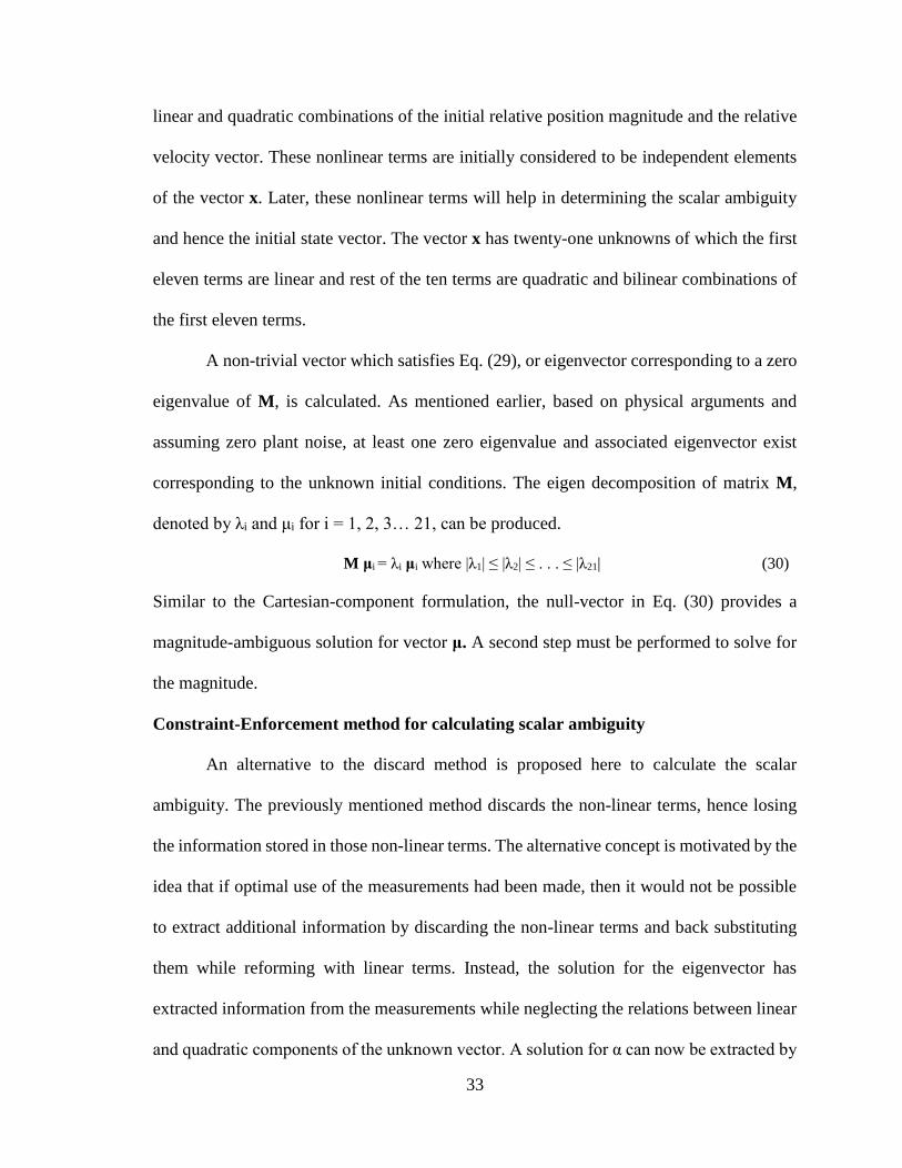
A non-trivial vector which satisfies Eq. (29), or eigenvector corresponding to a zero
eigenvalue of M, is calculated. As mentioned earlier, based on physical arguments and
assuming zero plant noise, at least one zero eigenvalue and associated eigenvector exist
corresponding to the unknown initial conditions. The eigen decomposition of matrix M,
denoted by λi and μi for i = 1, 2, 3… 21, can be produced.
M μi = λi μi where |λ1| ≤ |λ2| ≤ . . . ≤ |λ21| (30)
Similar to the Cartesian-component formulation, the null-vector in Eq. (30) provides a
magnitude-ambiguous solution for vector μ. A second step must be performed to solve for
the magnitude.
Constraint-Enforcement method for calculating scalar ambiguity
An alternative to the discard method is proposed here to calculate the scalar
ambiguity. The previously mentioned method discards the non-linear terms, hence losing
the information stored in those non-linear terms. The alternative concept is motivated by the
idea that if optimal use of the measurements had been made, then it would not be possible
to extract additional information by discarding the non-linear terms and back substituting
them while reforming with linear terms. Instead, the solution for the eigenvector has
extracted information from the measurements while neglecting the relations between linear
and quadratic components of the unknown vector. A solution for α can now be extracted by
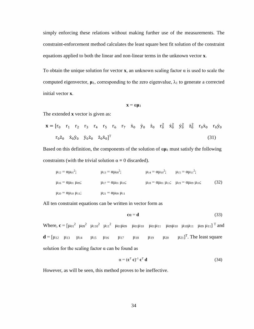
34
simply enforcing these relations without making further use of the measurements. The
constraint-enforcement method calculates the least square best fit solution of the constraint
equations applied to both the linear and non-linear terms in the unknown vector x.
To obtain the unique solution for vector x, an unknown scaling factor α is used to scale the
computed eigenvector, μ1, corresponding to the zero eigenvalue, λ1 to generate a corrected
initial vector x.
x = αμ1
The extended x vector is given as:
𝐱 = [r0 r1 r2 r3 r4 r5 r6 r7 x0 y0 z0 r02 x0
2 y02 z0
2 r0x0 r0y0
r0z0 x0y0 y0z0 z0x0]T (31)
Based on this definition, the components of the solution of αμ1 must satisfy the following
constraints (with the trivial solution α = 0 discarded).
μ12 = αμ012; μ13 = αμ09
2; μ14 = αμ102; μ15 = αμ11
2;
μ16 = αμ01 μ09; μ17 = αμ01 μ10; μ18 = αμ01 μ11; μ19 = αμ09 μ10;
μ20 = αμ10 μ11; μ21 = αμ09 μ11
(32)
All ten constraint equations can be written in vector form as
cα = d (33)
Where, c = [μ012
μ092 μ110
2 μ112 μ01μ09 μ01μ10 μ01μ11 μ09μ10 μ10μ11 μ09 μ11]
T and
d = [μ12 μ13 μ14 μ15 μ16 μ17 μ18 μ19 μ20 μ21]T. The least square
solution for the scaling factor α can be found as
α = (cT c)-1 cT d (34)
However, as will be seen, this method proves to be ineffective.
35
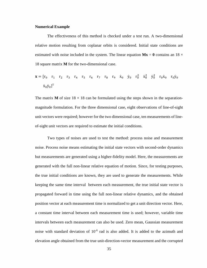
Numerical Example
The effectiveness of this method is checked under a test run. A two-dimensional
relative motion resulting from coplanar orbits is considered. Initial state conditions are
estimated with noise included in the system. The linear equation Mx = 0 contains an 18 ×
18 square matrix M for the two-dimensional case.
𝐱 = [r0 r1 r2 r3 r4 r5 r6 r7 r8 r9 x0 y0 r02 x0
2 y02 r0x0 r0y0
x0y0]T
The matrix M of size 18 × 18 can be formulated using the steps shown in the separation-
magnitude formulation. For the three dimensional case, eight observations of line-of-sight
unit vectors were required; however for the two dimensional case, ten measurements of line-
of-sight unit vectors are required to estimate the initial conditions.
Two types of noises are used to test the method: process noise and measurement
noise. Process noise means estimating the initial state vectors with second-order dynamics
but measurements are generated using a higher-fidelity model. Here, the measurements are
generated with the full non-linear relative equation of motion. Since, for testing purposes,
the true initial conditions are known, they are used to generate the measurements. While
keeping the same time interval between each measurement, the true initial state vector is
propagated forward in time using the full non-linear relative dynamics, and the obtained
position vector at each measurement time is normalized to get a unit direction vector. Here,
a constant time interval between each measurement time is used; however, variable time
intervals between each measurement can also be used. Zero mean, Gaussian measurement
noise with standard deviation of 10-6 rad is also added. It is added to the azimuth and
elevation angle obtained from the true unit-direction-vector measurement and the corrupted
36
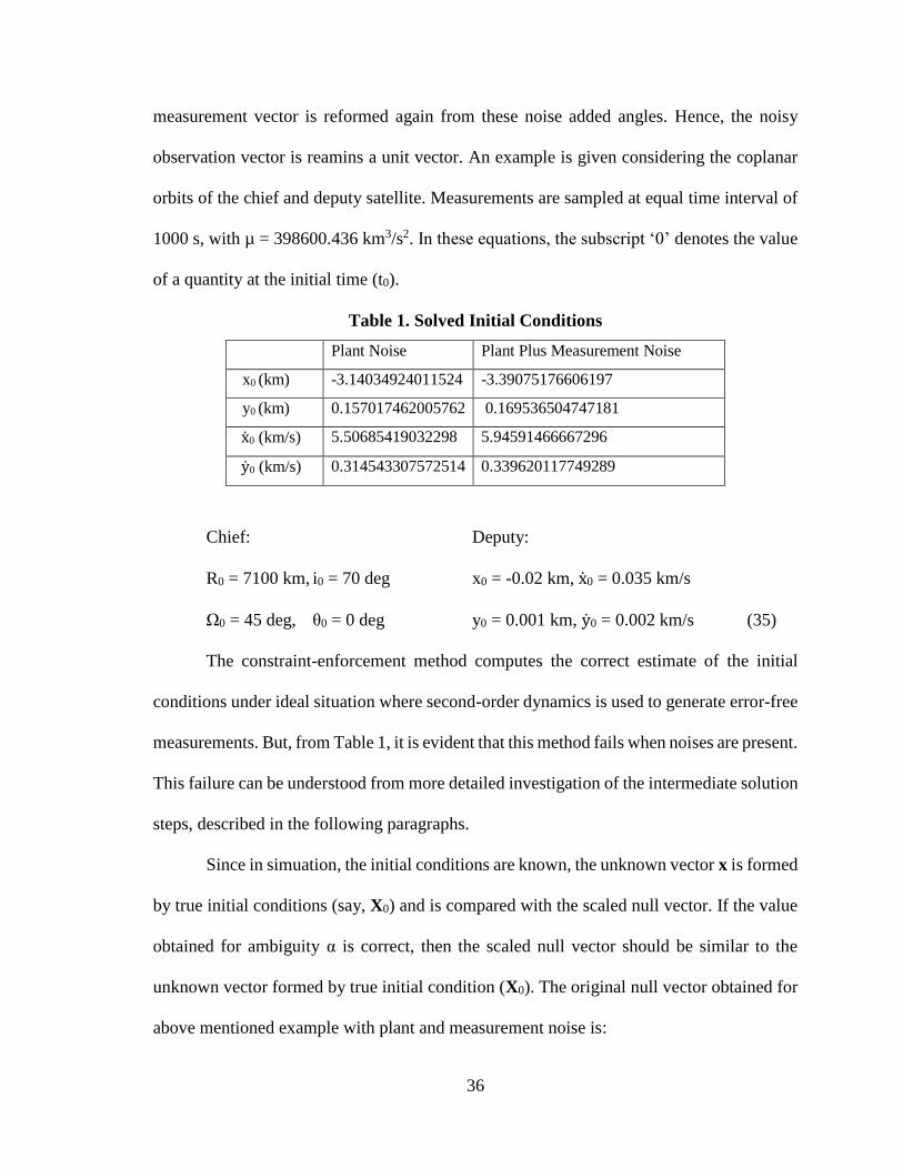
measurement vector is reformed again from these noise added angles. Hence, the noisy
observation vector is reamins a unit vector. An example is given considering the coplanar
orbits of the chief and deputy satellite. Measurements are sampled at equal time interval of
1000 s, with µ = 398600.436 km3/s2. In these equations, the subscript ‘0’ denotes the value
of a quantity at the initial time (t0).
Table 1. Solved Initial Conditions
Plant Noise Plant Plus Measurement Noise
x0 (km) -3.14034924011524 -3.39075176606197
y0 (km) 0.157017462005762 0.169536504747181
x0 (km/s) 5.50685419032298 5.94591466667296
y0 (km/s) 0.314543307572514 0.339620117749289
Chief: Deputy:
R0 = 7100 km, i0 = 70 deg x0 = -0.02 km, x0 = 0.035 km/s
Ω0 = 45 deg, θ0 = 0 deg y0 = 0.001 km, y0 = 0.002 km/s (35)
The constraint-enforcement method computes the correct estimate of the initial
conditions under ideal situation where second-order dynamics is used to generate error-free
measurements. But, from Table 1, it is evident that this method fails when noises are present.
This failure can be understood from more detailed investigation of the intermediate solution
steps, described in the following paragraphs.
Since in simuation, the initial conditions are known, the unknown vector x is formed
by true initial conditions (say, X0) and is compared with the scaled null vector. If the value
obtained for ambiguity α is correct, then the scaled null vector should be similar to the
unknown vector formed by true initial condition (X0). The original null vector obtained for
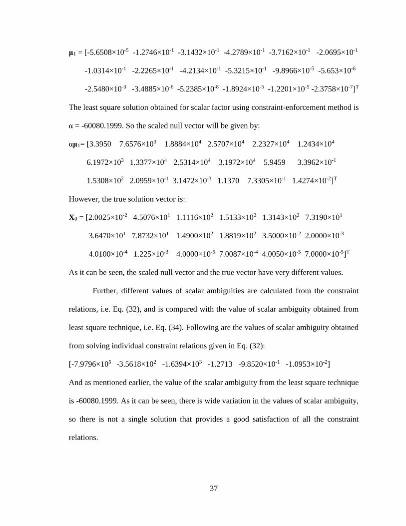
above mentioned example with plant and measurement noise is:
37
μ1 = [-5.6508×10⁻⁵ -1.2746×10⁻¹ -3.1432×10⁻¹ -4.2789×10⁻¹ -3.7162×10⁻¹ -2.0695×10⁻¹
-1.0314×10⁻¹ -2.2265×10⁻¹ -4.2134×10⁻¹ -5.3215×10⁻¹ -9.8966×10⁻⁵ -5.653×10⁻⁶
-2.5480×10⁻³ -3.4885×10⁻⁶ -5.2385×10⁻⁸ -1.8924×10⁻⁵ -1.2201×10⁻⁵ -2.3758×10⁻⁷]T
The least square solution obtained for scalar factor using constraint-enforcement method is
α = -60080.1999. So the scaled null vector will be given by:
αμ1= [3.3950 7.6576×10³ 1.8884×10⁴ 2.5707×10⁴ 2.2327×10⁴ 1.2434×10⁴
6.1972×10³ 1.3377×10⁴ 2.5314×10⁴ 3.1972×10⁴ 5.9459 3.3962×10⁻¹
1.5308×10² 2.0959×10⁻¹ 3.1472×10⁻³ 1.1370 7.3305×10⁻¹ 1.4274×10⁻²]T
However, the true solution vector is:
X0 = [2.0025×10⁻² 4.5076×101 1.1116×10² 1.5133×10² 1.3143×10² 7.3190×101
3.6470×101 7.8732×101 1.4900×10² 1.8819×10² 3.5000×10⁻² 2.0000×10⁻³
4.0100×10⁻⁴ 1.225×10⁻³ 4.0000×10⁻⁶ 7.0087×10⁻⁴ 4.0050×10⁻⁵ 7.0000×10⁻⁵]T
As it can be seen, the scaled null vector and the true vector have very different values.
Further, different values of scalar ambiguities are calculated from the constraint
relations, i.e. Eq. (32), and is compared with the value of scalar ambiguity obtained from
least square technique, i.e. Eq. (34). Following are the values of scalar ambiguity obtained
from solving individual constraint relations given in Eq. (32):
[-7.9796×10⁵ -3.5618×10² -1.6394×10³ -1.2713 -9.8520×10⁻¹ -1.0953×10⁻²]
And as mentioned earlier, the value of the scalar ambiguity from the least square technique
is -60080.1999. As it can be seen, there is wide variation in the values of scalar ambiguity,
so there is not a single solution that provides a good satisfaction of all the constraint
relations.
38
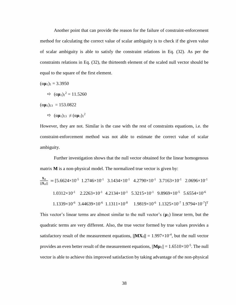
Another point that can provide the reason for the failure of constraint-enforcement
method for calculating the correct value of scalar ambiguity is to check if the given value
of scalar ambiguity is able to satisfy the constraint relations in Eq. (32). As per the
constraints relations in Eq. (32), the thirteenth element of the scaled null vector should be
equal to the square of the first element.
(αμ1)1 = 3.3950
(αμ1)12 = 11.5260
(αμ1)13 = 153.0822
(αμ1)13 ≠ (αμ1)12
However, they are not. Similar is the case with the rest of constraints equations, i.e. the
constraint-enforcement method was not able to estimate the correct value of scalar
ambiguity.
Further investigation shows that the null vector obtained for the linear homogenous
matrix M is a non-physical model. The normalized true vector is given by:
𝐗0
||𝐗0|| = [5.6624×10⁻⁵ 1.2746×10⁻¹ 3.1434×10⁻¹ 4.2790×10⁻¹
3.7163×10⁻¹ 2.0696×10⁻¹
1.0312×10⁻¹ 2.2263×10⁻¹ 4.2134×10⁻¹ 5.3215×10⁻¹ 9.8969×10⁻⁵ 5.6554×10⁻⁶
1.1339×10⁻⁶ 3.44639×10⁻⁶ 1.1311×10⁻⁸ 1.9819×10⁻⁶ 1.1325×10⁻⁷ 1.9794×10⁻⁷]T
This vector’s linear terms are almost similar to the null vector’s (µ1) linear term, but the
quadratic terms are very different. Also, the true vector formed by true values provides a
satisfactory result of the measurement equations, ||MX0|| = 1.997×10⁻⁴, but the null vector
provides an even better result of the measurement equations, ||Mµ1|| = 1.6510×10⁻⁵. The null
vector is able to achieve this improved satisfaction by taking advantage of the non-physical
39
degrees of freedom in the quadratic components of the unknown vector. But this results in
a non-physical solution.
Hence, to implement the constraint relations the discard method will be a good
choice for calculating the scalar ambiguity, where the null-vector is forced to maintain the
physical model by initially discarding the bilinear and quadratic combinations and then
forming them again using scaled initial vector, Eq. (22). Constraint-enforcement method
works only in ideal conditions when there is no noise, but for practical purposes, when
noises are there, constraint-enforcement method will fail.
Applying Discard method to Separation-Magnitude Formulation
From the previous discussion, the eigenvector obtained from the linear homogenous
matrix equation was a non-physical solution and the constraint-enforcement method failed
in estimating an accurate scalar ambiguity. Hence, to force the physical solution on the
eigenvector, the discard method is used with separation-magnitude formulation. The
measurement equations are set up by the separation-magnitude method and the discard
method is used for calculating the scalar ambiguity α.
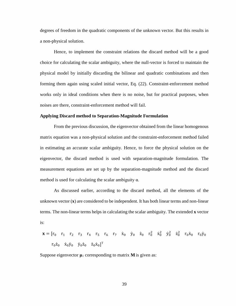
As discussed earlier, according to the discard method, all the elements of the
unknown vector (x) are considered to be independent. It has both linear terms and non-linear
terms. The non-linear terms helps in calculating the scalar ambiguity. The extended x vector
is:
𝐱 = [r0 r1 r2 r3 r4 r5 r6 r7 x0 y0 z0 r02 x0
2 y02 z0
2 r0x0 r0y0
r0z0 x0y0 y0z0 z0x0]T
Suppose eigenvector μ1 corresponding to matrix M is given as:
40
[μ01 μ02 μ03 μ04 μ05 μ06 μ07 μ08 μ09 μ10 μ11 μ12 μ13 μ14 μ15 μ16 μ17 μ18 μ19
μ20 μ21]T
Since μ1 is a non-unique vector, a scalar factor is calculated to obtain a unique scaled null-
vector. The constraint relations which were severed earlier will be used to calculate a unique
scaled null-vector (αμ1). First, the last ten non-linear elements of scaled null-vector are
discarded, and then reformed again by linear and bilinear combinations of the first eleven
linear terms using the method described in the chapter of Cartesian-component formulation.
The reformed bilinear and quadratic components can be written as:
μ12 = α2μ012; μ13 = α2μ09
2; μ14 = α2μ102; μ15 = α2μ11
2; μ16 = α2μ01 μ09
μ17 = α2μ01 μ10; μ18 = α2μ01 μ11; μ19 = α2μ09 μ10; μ20 = α2μ10 μ11; μ21 = α2μ09 μ11
(3)
Hence, the reformed null-vector will be given as:
[αμ01 αμ02 αμ03 αμ04 αμ05 αμ06 αμ07 αμ08 αμ09 αμ10 αμ11 (αμ01)2 (αμ09)2
(αμ10)2 (αμ11)2 (αμ01)(αμ09) (αμ01)(αμ10) (αμ01)(αμ11) (αμ09)(αμ10) (αμ10)(αμ11)
(αμ09)(αμ11)]T
(37)
The transformed null-vector is now substituted back into the linear homogenous matrix
equation, Eq. (29), and solved for the values of scalar ambiguity, similar to Eq. (24), while
discarding the trivial solution. If there is no noise in the system, the obtained values of α is
similar but on adding noise, the variation in different values of α will increase. In that case,
the mean value of all different values of α will be used as the scaling factor. This method
proves to be effective as it will be shown via numerical example.
Performance Analysis
Several numerical examples are considered to test the IROD performance and to
estimate the initial state vector. One considered performance metric is to simply compare
the known initial state test values with the computed initial states. The quantity used to
41
evaluate the performance is root-mean-square (RMS) of the angle residual. Angle residual
is the difference of the computed line-of-sight angle obtained from the propagation of
computed initial states to the measurement time using the second-order dynamics solution
and the true measurement angle obtained from the propagation of true initial states with the
full non-linear equations. A root-mean-square value of the angle residual that is close to
zero indicates that the predicted angles are close to the originally collected measurement
angles. The largest and worst possible RMS error value is equal to π radians away from its
corresponding true line-of-sight measurement. This RMS error metric is valuable because
in a real-world application of this problem, the true initial states would be unknown and
therefore not available to compare against the calculated initial states.
Another way to evaluate the performance of this method is to calculate the range
ratio RMS. It is calculated by taking the root-mean-square of the ratio of the chief-deputy
separation distance predicted by the propagation of the computed initial conditions with the
second-order dynamics solution over the true separation distance obtained from the full
nonlinear equations at all measurement times. A value near one indicates the predicted
ranges are close to the true ranges. Range ratio RMS helps in establishing the validity of the
application of the initial relative orbit determination method during numerical simulation.
In a real-world application, the collected observations are angles-only measurements and
the range data is unknown. Thus, the predicted range values have no basis for comparison
in a real-time in-flight situation using angles-only observations.
Several factors including noise type and level, sample rate, and deputy drift rate are
varied to explore certain aspects of the IROD performance. Two types of noise are used to
test this IROD technique: process noise and process plus the measurement noise. As
42
mentioned earlier, the term process noise refers to generating the measurements with a
higher fidelity model than the model on which the estimation solution is based, i.e. the
second-order model. Measurement noise level is considered across the range 10-8 to 10-3
radians. Measurement sample rate is varied across a wide range of cases from 150 seconds
to 10000 seconds to show dependency on temporal distribution of the measurements.
Estimating initial conditions with process noise and measurement noise
The IROD solution reformulated using the separation-magnitude formulation and
the discard method is tested and validated here. A two-dimensional coplanar orbit is
considered again. For the nonlinear simulation, the true measurements are generated by
choosing a set of initial conditions and propagating them forward using two-body dynamics
and a fourth order Runge-Kutta numerical integrator with time step equal to one second.
Both process noise and process plus measurement noise cases are considered. Process noise
is introduced by using the second-order dynamics solution to estimate the initial conditions.
In the case with measurement corruption, Gaussian noise with a standard deviation of σ =
10-6 rad is added to each measurement. For simplicity, measurements are taken at equal time
steps. It is not necessary that measurements always be taken at equal time increments, but
the time at which a measurement is taken must be recorded. Measurements for this case are
sampled at equal time step increments of 1000 s. The initial conditions for this case are
given below, in terms of circular chief orbit elements and the deputy’s relative states with
µ = 398600.436 km3/s2.
Chief: Deputy:
R0 = 7100 km, i0 = 70 deg x0 = -0.02 km, x0= 0.035 km/s
Ω0 = 45 deg, θ0 = 0 deg y0 = 0.001 km, y0 = 0.002 km/s
43
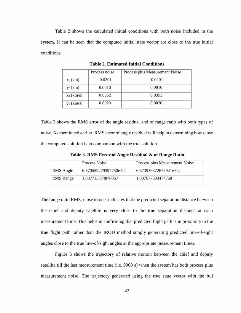
Table 2 shows the calculated initial conditions with both noise included in the
system. It can be seen that the computed initial state vector are close to the true initial
conditions.
Table 2. Estimated Initial Conditions
Process noise Process plus Measurement Noise
x0 (km) -0.0201 -0.0201
y0 (km) 0.0010 0.0010
x0 (km/s) 0.0352 0.0353
y0 (km/s) 0.0020 0.0020
Table 3 shows the RMS error of the angle residual and of range ratio with both types of
noise. As mentioned earlier, RMS error of angle residual will help in determining how close
the computed solution is in comparison with the true solution.
Table 3. RMS Error of Angle Residual & of Range Ratio
Process Noise Process plus Measurement Noise
RMS Angle 6.370559479397730e-04 6.373936322672941e-04
RMS Range 1.007713574870067 1.007677503474768
The range ratio RMS, close to one, indicates that the predicted separation distance between
the chief and deputy satellite is very close to the true separation distance at each
measurement time. This helps in confirming that predicted flight path is in proximity to the
true flight path rather than the IROD method simply generating predicted line-of-sight
angles close to the true line-of-sight angles at the appropriate measurement times.
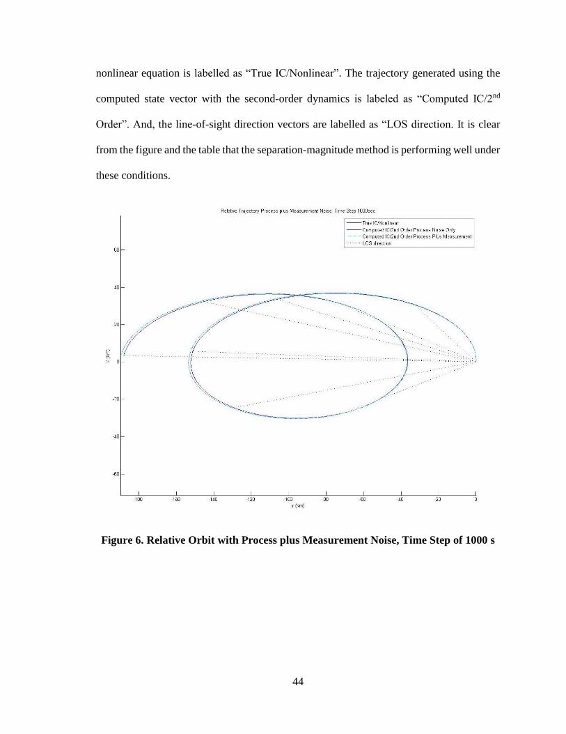
Figure 6 shows the trajectory of relative motion between the chief and deputy
satellite till the last measurement time (i.e. 9000 s) when the system has both process plus
measurement noise. The trajectory generated using the true state vector with the full
44
nonlinear equation is labelled as “True IC/Nonlinear”. The trajectory generated using the
computed state vector with the second-order dynamics is labeled as “Computed IC/2nd
Order”. And, the line-of-sight direction vectors are labelled as “LOS direction. It is clear
from the figure and the table that the separation-magnitude method is performing well under
these conditions.
Figure 6. Relative Orbit with Process plus Measurement Noise, Time Step of 1000 s
45
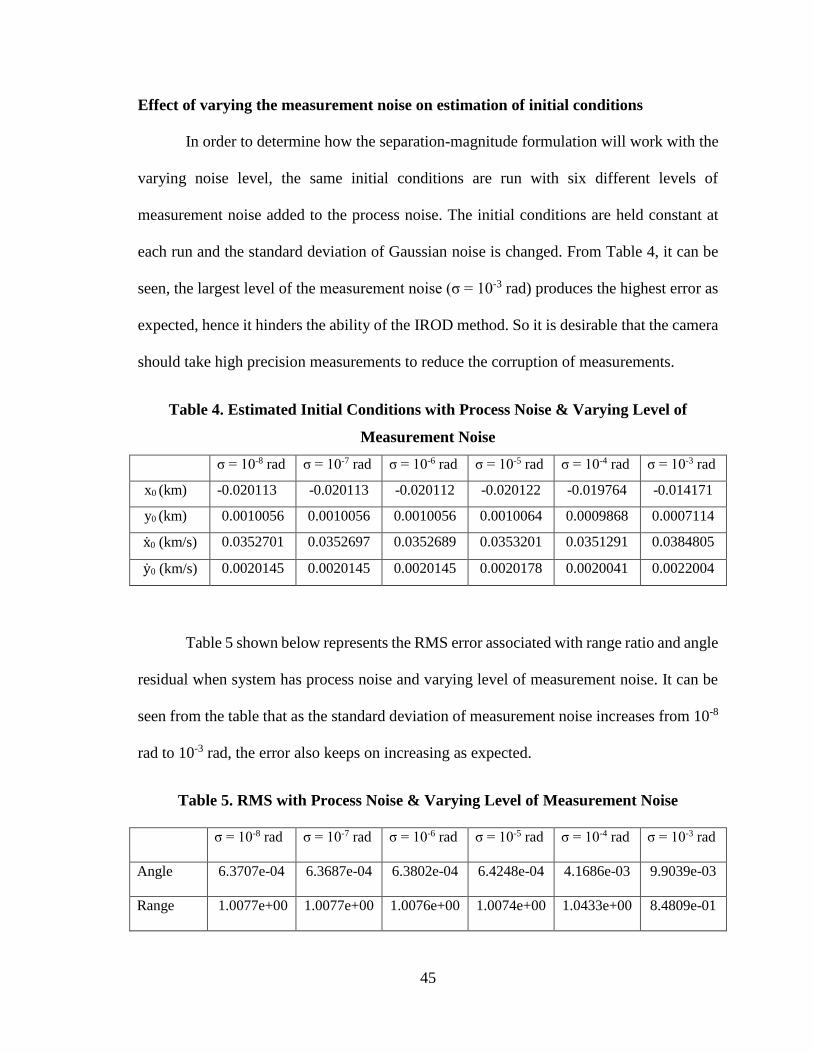
Effect of varying the measurement noise on estimation of initial conditions
In order to determine how the separation-magnitude formulation will work with the
varying noise level, the same initial conditions are run with six different levels of
measurement noise added to the process noise. The initial conditions are held constant at
each run and the standard deviation of Gaussian noise is changed. From Table 4, it can be
seen, the largest level of the measurement noise (σ = 10-3 rad) produces the highest error as
expected, hence it hinders the ability of the IROD method. So it is desirable that the camera
should take high precision measurements to reduce the corruption of measurements.
Table 4. Estimated Initial Conditions with Process Noise & Varying Level of
Measurement Noise
σ = 10-8 rad σ = 10-7 rad σ = 10-6 rad σ = 10-5 rad σ = 10-4 rad σ = 10-3 rad
x0 (km) -0.020113 -0.020113 -0.020112 -0.020122 -0.019764 -0.014171
y0 (km) 0.0010056 0.0010056 0.0010056 0.0010064 0.0009868 0.0007114
x0 (km/s) 0.0352701 0.0352697 0.0352689 0.0353201 0.0351291 0.0384805
y0 (km/s) 0.0020145 0.0020145 0.0020145 0.0020178 0.0020041 0.0022004
Table 5 shown below represents the RMS error associated with range ratio and angle
residual when system has process noise and varying level of measurement noise. It can be
seen from the table that as the standard deviation of measurement noise increases from 10-8
rad to 10-3 rad, the error also keeps on increasing as expected.
Table 5. RMS with Process Noise & Varying Level of Measurement Noise
σ = 10-8 rad σ = 10-7 rad σ = 10-6 rad σ = 10-5 rad σ = 10-4 rad σ = 10-3 rad
Angle 6.3707e-04 6.3687e-04 6.3802e-04 6.4248e-04 4.1686e-03 9.9039e-03
Range 1.0077e+00 1.0077e+00 1.0076e+00 1.0074e+00 1.0433e+00 8.4809e-01
46
Figure 7 shows the relative trajectory of the deputy satellite with respect to the chief
satellite for the period of 9000 s when the system has process plus measurement noise. The
trajectory generated using the true state vector with the full nonlinear equation is labelled
as “True IC/Nonlinear”. The trajectory generated using the computed state vector with the
second-order dynamics is labeled as “Computed IC/2nd Order”. And, the line-of-sight
direction vectors are labelled as “LOS direction”. In Figure 7 the estimated relative
trajectory generated with the process plus measurement noise having 10-3 rad of standard
deviation is compared with the estimated relative trajectory generated with the process plus
measurement noise having 10-8 rad of standard deviation in the system and also with the
true relative trajectory. It is clear from the figure and the tables that the separation-
magnitude method is performing well when the measurements are less corrupted.
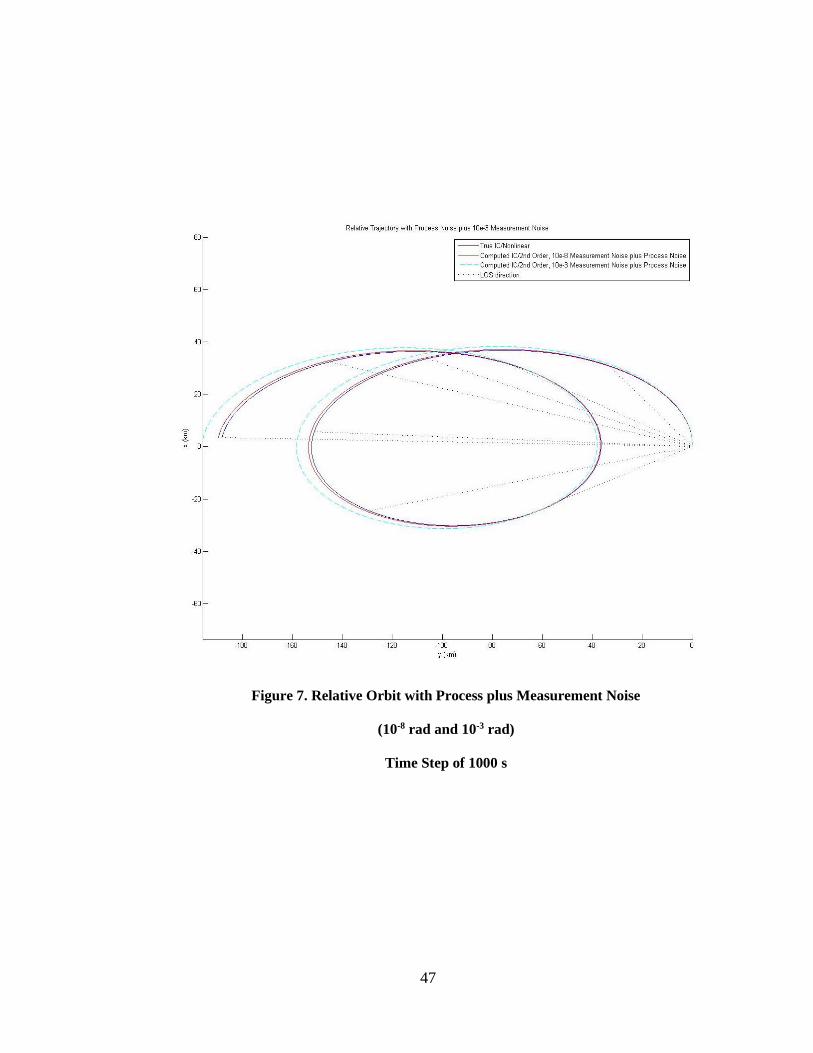
47
Figure 7. Relative Orbit with Process plus Measurement Noise
(10-8 rad and 10-3 rad)
Time Step of 1000 s
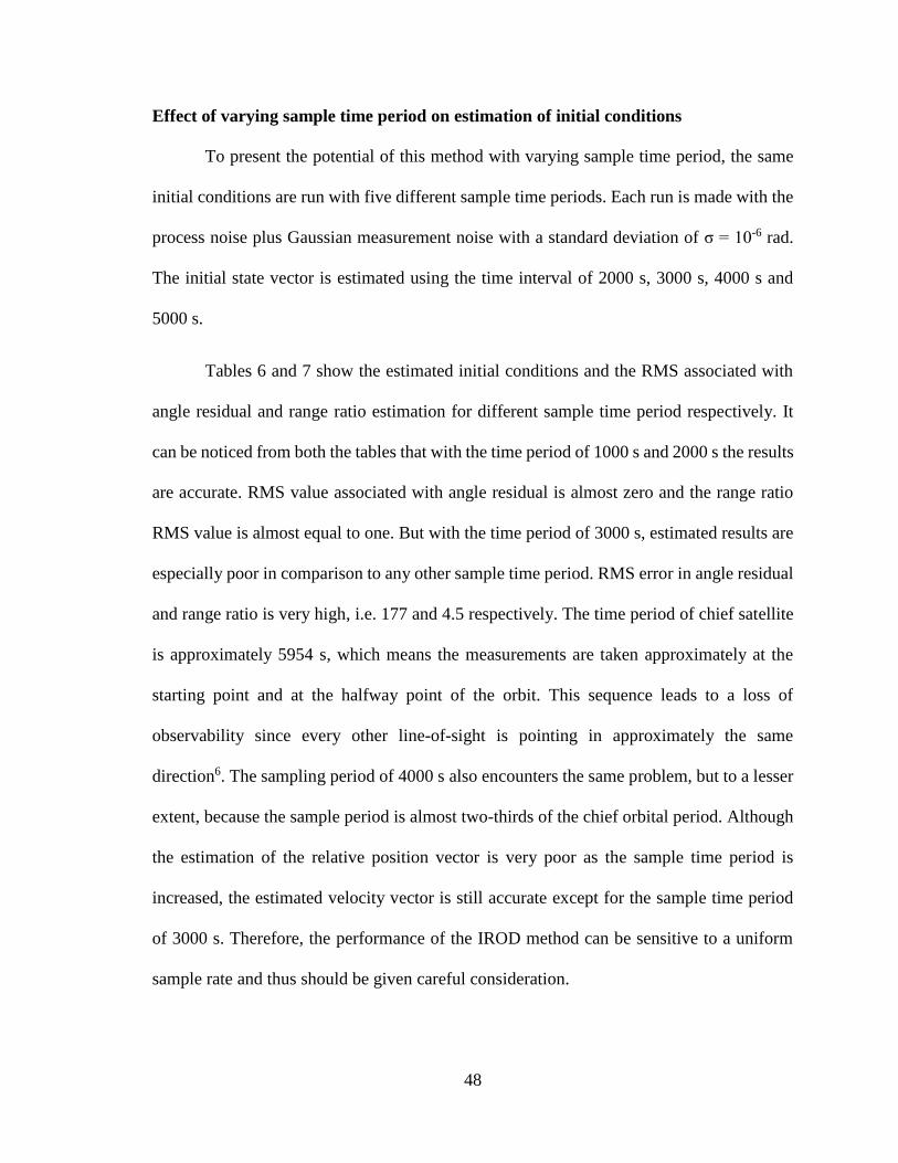
48
Effect of varying sample time period on estimation of initial conditions
To present the potential of this method with varying sample time period, the same
initial conditions are run with five different sample time periods. Each run is made with the
process noise plus Gaussian measurement noise with a standard deviation of σ = 10-6 rad.
The initial state vector is estimated using the time interval of 2000 s, 3000 s, 4000 s and
5000 s.
Tables 6 and 7 show the estimated initial conditions and the RMS associated with
angle residual and range ratio estimation for different sample time period respectively. It
can be noticed from both the tables that with the time period of 1000 s and 2000 s the results
are accurate. RMS value associated with angle residual is almost zero and the range ratio
RMS value is almost equal to one. But with the time period of 3000 s, estimated results are
especially poor in comparison to any other sample time period. RMS error in angle residual
and range ratio is very high, i.e. 177 and 4.5 respectively. The time period of chief satellite
is approximately 5954 s, which means the measurements are taken approximately at the
starting point and at the halfway point of the orbit. This sequence leads to a loss of
observability since every other line-of-sight is pointing in approximately the same
direction6. The sampling period of 4000 s also encounters the same problem, but to a lesser
extent, because the sample period is almost two-thirds of the chief orbital period. Although
the estimation of the relative position vector is very poor as the sample time period is
increased, the estimated velocity vector is still accurate except for the sample time period
of 3000 s. Therefore, the performance of the IROD method can be sensitive to a uniform
sample rate and thus should be given careful consideration.
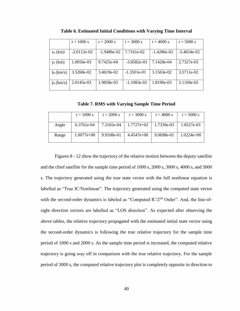
49
Table 6. Estimated Initial Conditions with Varying Time Interval
t = 1000 s t = 2000 s t = 3000 s t = 4000 s t = 5000 s
x0 (km) -2.0112e-02 -1.9486e-02 7.7161e-02 -1.4286e-02 -5.4654e-02
y0 (km) 1.0056e-03 9.7425e-04 -3.8582e-03 7.1428e-04 2.7327e-03
x0 (km/s) 3.5268e-02 3.4619e-02 -1.3501e-01 3.1563e-02 3.5711e-02
y0 (km/s) 2.0145e-03 1.9858e-03 -1.1083e-02 1.8190e-03 2.1169e-03
Table 7. RMS with Varying Sample Time Period
t = 1000 s t = 2000 s t = 3000 s t = 4000 s t = 5000 s
Angle 6.3761e-04 7.3165e-04 1.7727e+02 1.7339e-03 1.8527e-03
Range 1.0077e+00 9.9108e-01 4.4547e+00 9.0698e-01 1.0224e+00
Figures 8 - 12 show the trajectory of the relative motion between the deputy satellite
and the chief satellite for the sample time period of 1000 s, 2000 s, 3000 s, 4000 s, and 5000
s. The trajectory generated using the true state vector with the full nonlinear equation is
labelled as “True IC/Nonlinear”. The trajectory generated using the computed state vector
with the second-order dynamics is labeled as “Computed IC/2nd Order”. And, the line-of-
sight direction vectors are labelled as “LOS direction”. As expected after observing the
above tables, the relative trajectory propagated with the estimated initial state vector using
the second-order dynamics is following the true relative trajectory for the sample time
period of 1000 s and 2000 s. As the sample time period is increased, the computed relative
trajectory is going way off in comparison with the true relative trajectory. For the sample
period of 3000 s, the computed relative trajectory plot is completely opposite in direction to

50
the true relative trajectory. Hence, it is required that special attention should be given to the
sample period.

51
Figure 8. Relative Orbit with Process plus Measurement Noise, Time Step of 1000 s
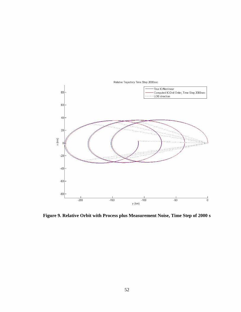
52
Figure 9. Relative Orbit with Process plus Measurement Noise, Time Step of 2000 s
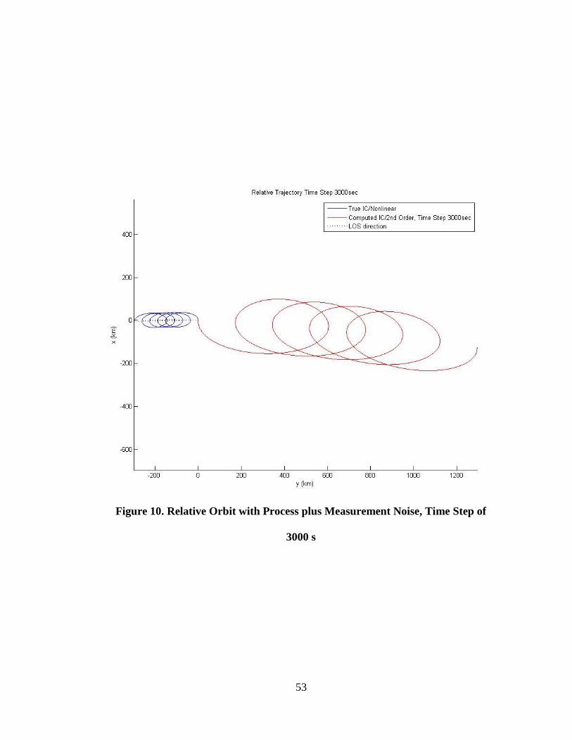
53
Figure 10. Relative Orbit with Process plus Measurement Noise, Time Step of
3000 s
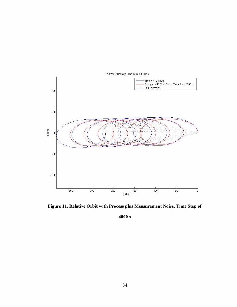
54
Figure 11. Relative Orbit with Process plus Measurement Noise, Time Step of
4000 s
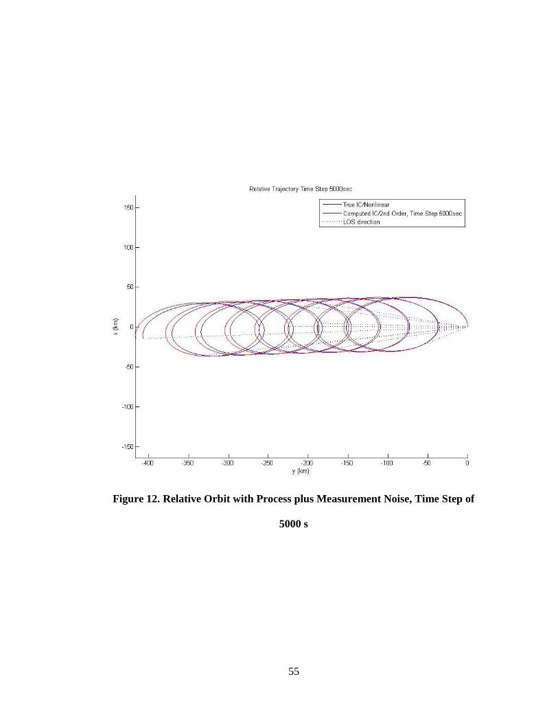
55
Figure 12. Relative Orbit with Process plus Measurement Noise, Time Step of
5000 s
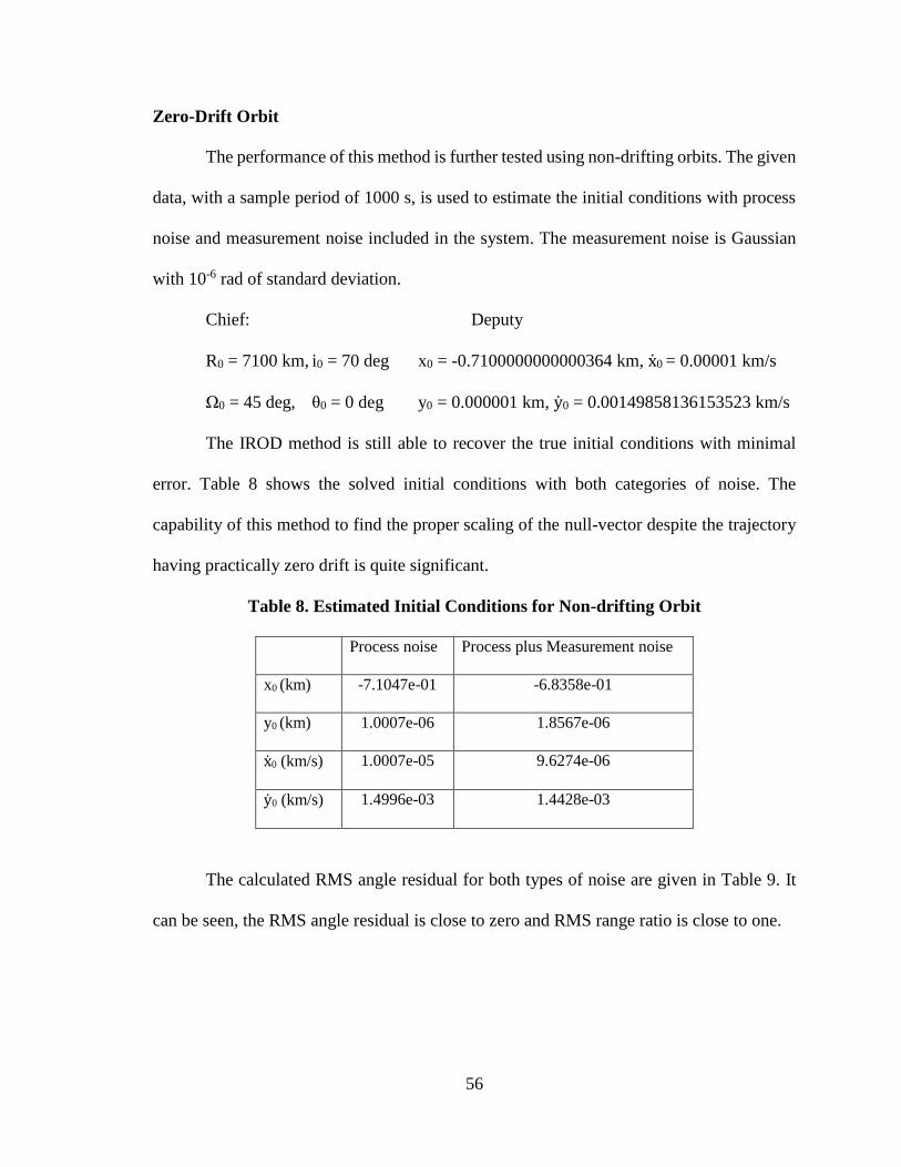
56
Zero-Drift Orbit
The performance of this method is further tested using non-drifting orbits. The given
data, with a sample period of 1000 s, is used to estimate the initial conditions with process
noise and measurement noise included in the system. The measurement noise is Gaussian
with 10-6 rad of standard deviation.
Chief: Deputy
R0 = 7100 km, i0 = 70 deg x0 = -0.7100000000000364 km, x0 = 0.00001 km/s
Ω0 = 45 deg, θ0 = 0 deg y0 = 0.000001 km, y0 = 0.00149858136153523 km/s
The IROD method is still able to recover the true initial conditions with minimal
error. Table 8 shows the solved initial conditions with both categories of noise. The
capability of this method to find the proper scaling of the null-vector despite the trajectory
having practically zero drift is quite significant.
Table 8. Estimated Initial Conditions for Non-drifting Orbit
Process noise Process plus Measurement noise
x0 (km) -7.1047e-01 -6.8358e-01
y0 (km) 1.0007e-06 1.8567e-06
x0 (km/s) 1.0007e-05 9.6274e-06
y0 (km/s) 1.4996e-03 1.4428e-03
The calculated RMS angle residual for both types of noise are given in Table 9. It
can be seen, the RMS angle residual is close to zero and RMS range ratio is close to one.

57
Table 9. RMS for Non-drifting orbit
Process Noise Process plus Measurement Noise
RMS Angle 9.8815e-06 3.2818e-04
RMS Range 1.0007e+00 9.6279e-01
Figure 13 shows the relative trajectory plot with the process plus measurement noise
respectively. The trajectory generated using the true state vector with the full nonlinear
equation is labelled as “True IC/Nonlinear”. The trajectory generated using the computed
state vector with the second-order dynamics is labeled as “Computed IC/2nd Order”. And,
the line-of-sight direction vectors are labelled as “LOS direction”.
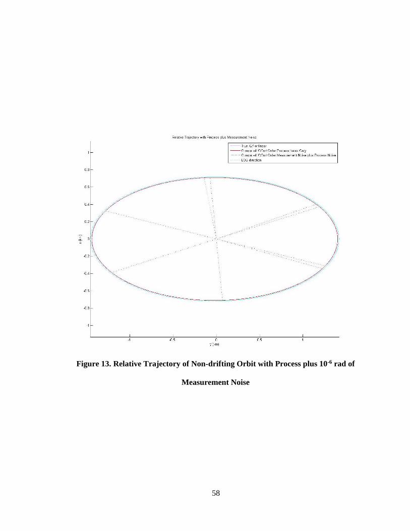
58
Figure 13. Relative Trajectory of Non-drifting Orbit with Process plus 10-6 rad of
Measurement Noise

59
Limitations of the IROD Method
A few factors can limit the success of the IROD method. Poor measurements will
adversely affect the result of this method. Obviously extremely noisy measurements will
result in the IROD method failing to properly recover the true initial orbit. Also, the
measurements must be chosen wisely over time. Measurements that are too close together
may result in failure to recover the initial orbit. Taking measurements of the same, or close
to the same, line-of-sight angles over multiple orbits will also give poor results. However,
the situations can be easily avoided by proper scheduling of observations. For best results,
the measurements taken should be a good sampling of the orbit geometry in order to get a
good idea of the shape of the orbit.
Fast Sample Rate
In order to show the effect of fast sample rate, the same model parameters are run
with sample period of 150 s. The only difference is, the earlier sample time period was 1000
s, but in this case, the sample time period is changed to 150 s. Both process noise and the
standard measurement noise of 10-6 rad is added to the system.
In Figure 6, the relative orbit and line-of-sight representations were plotted for the
sample rate of 1000 s. Similarly, the orbit and line-of-sight measurements for sample period
of 150 s are plotted in Figure 14. The longer time step from the original run allows for a
good sampling of the entire orbit and its drift behavior. However, Figure 14 shows that the
short time step creates measurements which are closely packed and only captures slightly
over a quarter of the orbit. Such a small sample does not give much information on the shape
and drift behavior of the relative orbit trajectory.
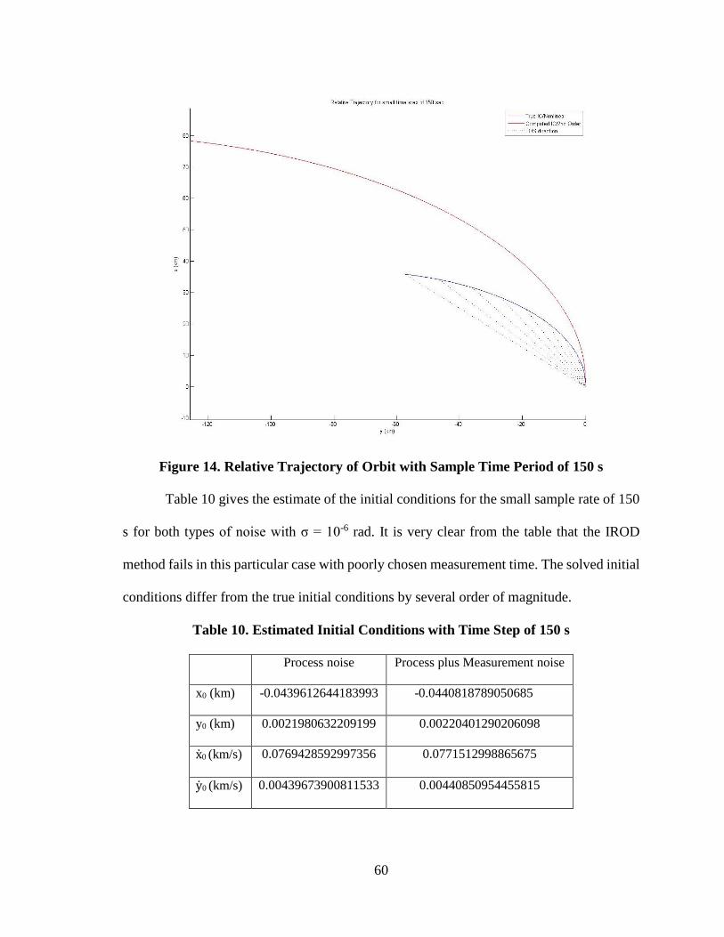
60
Figure 14. Relative Trajectory of Orbit with Sample Time Period of 150 s
Table 10 gives the estimate of the initial conditions for the small sample rate of 150
s for both types of noise with σ = 10-6 rad. It is very clear from the table that the IROD
method fails in this particular case with poorly chosen measurement time. The solved initial
conditions differ from the true initial conditions by several order of magnitude.
Table 10. Estimated Initial Conditions with Time Step of 150 s
Process noise Process plus Measurement noise
x0 (km) -0.0439612644183993 -0.0440818789050685
y0 (km) 0.0021980632209199 0.00220401290206098
x0 (km/s) 0.0769428592997356 0.0771512998865675
y0 (km/s) 0.00439673900811533 0.00440850954455815
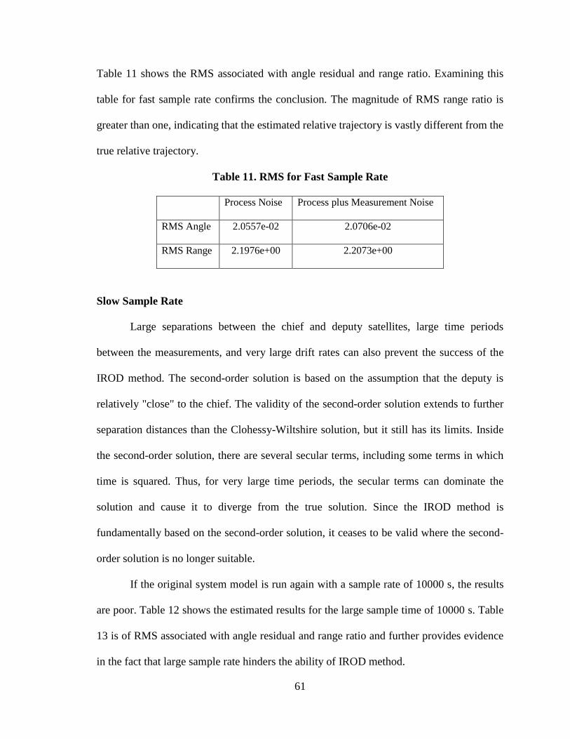
61
Table 11 shows the RMS associated with angle residual and range ratio. Examining this
table for fast sample rate confirms the conclusion. The magnitude of RMS range ratio is
greater than one, indicating that the estimated relative trajectory is vastly different from the
true relative trajectory.
Table 11. RMS for Fast Sample Rate
Process Noise Process plus Measurement Noise
RMS Angle 2.0557e-02 2.0706e-02
RMS Range 2.1976e+00 2.2073e+00
Slow Sample Rate
Large separations between the chief and deputy satellites, large time periods
between the measurements, and very large drift rates can also prevent the success of the
IROD method. The second-order solution is based on the assumption that the deputy is
relatively "close" to the chief. The validity of the second-order solution extends to further
separation distances than the Clohessy-Wiltshire solution, but it still has its limits. Inside
the second-order solution, there are several secular terms, including some terms in which
time is squared. Thus, for very large time periods, the secular terms can dominate the
solution and cause it to diverge from the true solution. Since the IROD method is
fundamentally based on the second-order solution, it ceases to be valid where the second-
order solution is no longer suitable.
If the original system model is run again with a sample rate of 10000 s, the results
are poor. Table 12 shows the estimated results for the large sample time of 10000 s. Table
13 is of RMS associated with angle residual and range ratio and further provides evidence
in the fact that large sample rate hinders the ability of IROD method.
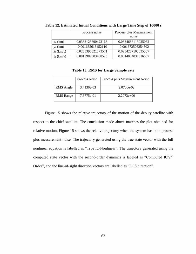
62
Table 12. Estimated Initial Conditions with Large Time Step of 10000 s
Process noise Process plus Measurement
noise
x0 (km) 0.0333123690422163 0.0334686113025062
y0 (km) -0.001665618452110 -0.001673506354602
x0 (km/s) 0.0253396821873571 0.0254287103035307
y0 (km/s) 0.0013989003488525 0.0014034037316567
Table 13. RMS for Large Sample rate
Process Noise Process plus Measurement Noise
RMS Angle 3.4130e-03 2.0706e-02
RMS Range 7.3775e-01 2.2073e+00
Figure 15 shows the relative trajectory of the motion of the deputy satellite with
respect to the chief satellite. The conclusion made above matches the plot obtained for
relative motion. Figure 15 shows the relative trajectory when the system has both process
plus measurement noise. The trajectory generated using the true state vector with the full
nonlinear equation is labelled as “True IC/Nonlinear”. The trajectory generated using the
computed state vector with the second-order dynamics is labeled as “Computed IC/2nd
Order”, and the line-of-sight direction vectors are labelled as “LOS direction”.
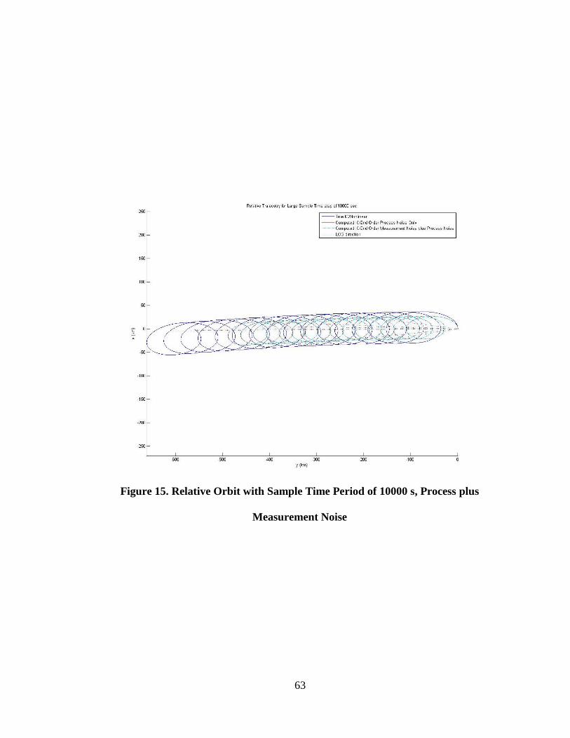
63
Figure 15. Relative Orbit with Sample Time Period of 10000 s, Process plus
Measurement Noise
64
CHAPTER 5
MACAULAY RESULTANT METHOD
The problem of initial relative-orbit determination requires estimation of three
components of the relative position vector and three components of the relative velocity
vector between the chief and deputy satellite. So there are a total of six unknowns that satisfy
six coupled second-degree polynomial equations. In earlier discussed methods, the
polynomial nature of the measurement equations was not exploited. The nonlinear
combinations of the initial states were considered to be independent which increased the
number of unknowns from six to twenty-five in the Cartesian-component formulation and
up to twenty-one in the separation-magnitude formulation. In this method, the multivariate
polynomial system of equations are solved using Macaulay resultant. Resultant theory
appears to be a less familiar subject in engineering disciplines, when compared to linear
algebra13. In this theory, the system of multivariate polynomial equations is projected to a
single univariate polynomial equation, the resultant polynomial equation; and using a matrix
polynomial structure, this equation can be solved by computing a generalized eigen
decomposition. Because the resultant polynomial is zero if and only if the polynomial
system has a common root, this procedure is often interpreted as a means to finding the
intersection of algebraic curves.
65
Resultant Polynomial Formulation
Consider a set of m coupled or multivariate polynomial equations in n variables
given in Eq. (38). Polynomial pj(xi) for j = 1,2 … m and i = 1,2 … n has degree dj, i.e., the
monomial appearing in pj(xi) with the largest exponent sum equals dj. Coefficient ckj denotes
a constant multiplier for monomial k appearing in the jth equation.
p1(x1, x2… xn) = 0
p2(x1, x2… xn) = 0
…
pm(x1, x2,… xn) = 0
(38)
When m > n, one should expect no solutions are possible except in special cases. On the
other hand when m < n, an infinite number of non-unique solutions exist. The case where
m = n occurs most often when the equation set represents an applied system, such as in
relative initial-orbit determination problem. Reference 11 gives a summary of the various
resultant polynomial forms that can be used in the cases m > n, m < n, and m = n. When m
= n, one should expect a finite number of unique solutions. When the number of equations
and variables is equal (m = n), and when the equation set is homogenous, the Macaulay
resultant polynomial is a popular technique. Polynomial equations are considered
homogenous in each equation, when all the terms have the same degree. If this is not the
case, it can be homogenized by a simple process of introducing an extra variable. To
homogenize Eq. (38), replace every variable xi by xi/xh and clear all denominators in all
equations, where xh denotes the new homogenizing unknown variable11. After this process,
every monomial in the jth equation will have degree equal to dj.
For a homogenous m = n equation set, the Macaulay resultant polynomial R is
expressed as12,13,14
66
R =
det 𝐍
det 𝐃 (39)
Where R is of scalar dimension, N has dimension nN×nN, and D has dimension nD×nD.
Although dimension nD is not easily expressed by a simple formula, dimension nN is given
generally by the relation
nN = (n-1+d)!/(n-1)!d! (40)
Where parameter d, sometimes called the system degree, is defined as
d = 1 + ∑(dj − 1)
m
j=1
(41)
Square matrices N and D are constructed from the polynomial coefficients, and either a set
of unspecified coefficients cxi originating from an appended equation, which can be required
to recover an equal number of equations and variables, or one of the unknown variables xi*
(i.e., xi with i = i*) chosen to be solved for first. Rows of the N matrix represents elementary
members and, through the determinant combinations, resultant R is a special kind of
member of modular system. The basic tenet of resultant theory is that R = 0, or equivalently
N is rank deficient, if and only if the equation set has a finite solution, assuming matrix D
is full rank. If matrix D is rank deficient, then matrix N (and D) must be modified by a
reduction process. If R = 0, null space vector χi are computed from
N χi = 0 for i = 1, 2… q (42)
Where q denotes the rank deficiency of N. Elements of the vector χi are proportional to
monomial functions of the variables. By taking certain combinations of the χi elements, the
unknown variables can be computed.
The matrix N is constructed by first labelling the columns and rows through a
systematic monomial combinatory process. Denote the monomial x1a1 … xn
an as xa where a
67
= (a1, … an) with integer ai’s. Define XN as the set of all monomials of degree d across the
n variables xi as12
XN = {xa | a1 + … + an = d} (43)
For example, with n = 3 representing x1,x2,x3 and d = 3, the set XN is
XN = {x13, x1
2x2, x12x3, x1x2
2, x1x32, x1x2x3, x2
3, x22x3, x2x3
2, x33} (44)
Note nN = 10 and the set XN contains ten monomial elements, which are used to label the
ten columns of matrix N. Next define the ith subset of XN as
XiN = {xa | ai ≥ di and aj < dj for all j < i} for i = 1, 2 … n (45)
In this example with d1 = 1, d2 = 2, and d3 = 2, the subset X1N, X2
N, X3N of XN are
X1N = {x1
3, x12x2, x1
2x3, x1x22, x1x3
2, x1x2x3}
X2N = {x2
3, x22x3}
X3N = {x2x3
2, x33}
(46)
Sets of homogenous degree d polynomials PiN corresponding to the subsets Xi
N are now
constructed. The general syntax for the ith polynomial subset is PiN is
PiN =
XiN
xi
di pi (47)
Continuing the specific example, the subsets P1N, P2
N, P3N of PN are
P1N = {x1
2p1, x1x2p1, x1x3p1, x22p1, x3
2p1, x2x3p1}
P2N = {x2p2, x3p2}
P3N = {x2p3, x3p3}
(48)
And thus the polynomial set is
PN = {x12p1, x1x2p1, x1x3p1, x2
2p1, x32p1, x2x3p1, x2p2, x3p2, x2p3, x3p3} (49)
The set PN contains ten polynomial elements, which are used to label the ten rows of matrix
N. The coefficients in these polynomials are then inserted into the entries of the N matrix

68
based on the row and column labels. Suppose the original three equations in three variables
are12
p1 = cx11 x1 + cx2
1 x2 + cx31 x3 = 0
p2 = cx1x12 x1
2 + cx2x22 x2
2 + cx3x32 x3
2 + cx1x22 x1x2 + cx2x3
2 x2x3 + cx3x12 x3x1 = 0
p3 = cx1x23 x1
2 + cx2x23 x2
2 + cx3x33 x3
2 + cx1x23 x1x2 + cx2x3
3 x2x3 + cx3x13 x3x1 = 0
(50)
Matrix N is constructed as7
𝑥13 𝑥1
2𝑥2 𝑥12𝑥3 𝑥1𝑥2
2 𝑥1𝑥32 𝑥1𝑥2𝑥3 𝑥2
3 𝑥22𝑥3 𝑥2𝑥3
2 𝑥33
𝑵 =
[ 𝑐𝑥11 𝑐𝑥2
1 𝑐𝑥31 0 0 0 0 0 0 0
0 𝑐𝑥11 0 𝑐𝑥2
1 0 𝑐𝑥31 0 0 0 0
0 0 𝑐𝑥11 0 𝑐𝑥3
1 𝑐𝑥21 0 0 0 0
0 0 0 𝑐𝑥11 0 0 𝑐𝑥2
1 𝑐𝑥31 0 0
0 0 0 0 𝑐𝑥11 0 0 0 𝑐𝑥2
1 𝑐𝑥31
0 0 0 0 0 𝑐𝑥11 0 𝑐𝑥2
1 𝑐𝑥31 0
0 𝑐𝑥1𝑥12 0 𝑐𝑥1𝑥2
2 0 𝑐𝑥3𝑥12 𝑐𝑥2𝑥2
2 𝑐𝑥2𝑥32 𝑐𝑥3𝑥3
2 0
0 0 𝑐𝑥1𝑥12 0 𝑐𝑥3𝑥1
2 𝑐𝑥1𝑥22 0 𝑐𝑥2𝑥2
2 𝑐𝑥2𝑥32 𝑐𝑥3𝑥3
2
0 𝑐𝑥1𝑥13 0 𝑐𝑥1𝑥2
3 0 𝑐𝑥3𝑥13 𝑐𝑥2𝑥2
3 𝑐𝑥2𝑥33 𝑐𝑥3𝑥3
3 0
0 0 𝑐𝑥1𝑥13 0 𝑐𝑥3𝑥1
3 𝑐𝑥1𝑥23 0 𝑐𝑥2𝑥2
3 𝑐𝑥2𝑥33 𝑐𝑥3𝑥3
3]
𝑥12𝑝1
𝑥1𝑥2𝑝1
𝑥1𝑥3𝑝1
𝑥22𝑝1
𝑥32𝑝1
𝑥2𝑥3𝑝1
𝑥2𝑝2
𝑥3𝑝2
𝑥2𝑝3
𝑥3𝑝3
(51)
Here, matrix N is constructed in terms of the polynomial coefficients. But as
mentioned earlier, it can also be constructed with the polynomial coefficients along with
either a set of unspecified coefficients cxi originating from an appended equation; hence, the
resultant is written as R (ckj,ci*) or the variables xi* chosen to be solved for first; hence, the
resultant is written as R (ckj,xi*). For the latter method, the polynomial equations are first
restructured such that xi* is imbedded as part of the coefficients. This imbedding process
subtracts one variable from the system making the total count of unknown’s n-1. The
69
homogenization process is then performed and adds one variable to the system making the
total count of unknowns equal to the original value of n. Thus, no additional equation is
needed here (m = n). In this thesis, matrix N is constructed with the polynomial coefficients
and a variable xi* which is chosen to be solved for first.
Once matrix N is available, matrix D is formed by well-defined procedure described
here.11 As mentioned earlier, reference 11 provides a summary for various resultant cases.
Matrix D is the minor of matrix N and the procedure determines which columns and rows
of N are to be retained to form D. In the next section, some of these monomials will be
reduced depending upon whether the exponents are “big” or “small”.
Each variable will be associated with a particular equation. For example the first
variable, x1, will be associated with the first equation, p1. The second variable, x2, will be
associated with the second equation, p2, etc. The degrees of the associated equation define
“bigness” for the exponents of that variable. Specifically, since d1 (the degree of p1) is 1, if
the exponent of x1 is greater than or equal to 1, it is considered big. Since d2 = 2, whenever
the exponent of x2 is greater than or equal to 2, it is considered big. The degree of p3 is 2,
therefore, whenever the exponent of x3 is greater than or equal to 3, it considered big. For
example, consider the monomial x12x3. The exponent of x1 is 2. This is greater than d1, and
is considered big. The exponent of x3 is 1. This is less than d3, and is therefore small.
Next step in forming matrix D is to determine the reduced monomials. If for a
particular monomial of degree d the exponent of only one variable is big, the monomial is
said to be reduced. For example, in the monomial x12x2, the exponent of x1 is greater than
d1, hence considered big, and the exponent of x2 is less than d2, hence considered small.
Here, the exponent of one variable is small and other exponent is big so the monomial x12x2
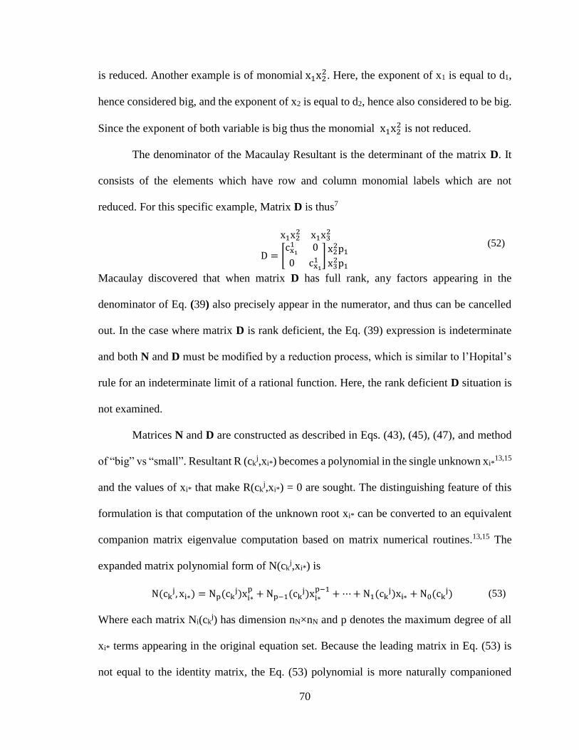
70
is reduced. Another example is of monomial x1x22. Here, the exponent of x1 is equal to d1,
hence considered big, and the exponent of x2 is equal to d2, hence also considered to be big.
Since the exponent of both variable is big thus the monomial x1x22 is not reduced.
The denominator of the Macaulay Resultant is the determinant of the matrix D. It
consists of the elements which have row and column monomial labels which are not
reduced. For this specific example, Matrix D is thus7
x1x22 x1x3
2
D = [cx11 0
0 cx11 ]
x22p1
x32p1
(52)
Macaulay discovered that when matrix D has full rank, any factors appearing in the
denominator of Eq. (39) also precisely appear in the numerator, and thus can be cancelled
out. In the case where matrix D is rank deficient, the Eq. (39) expression is indeterminate
and both N and D must be modified by a reduction process, which is similar to l’Hopital’s
rule for an indeterminate limit of a rational function. Here, the rank deficient D situation is
not examined.
Matrices N and D are constructed as described in Eqs. (43), (45), (47), and method
of “big” vs “small”. Resultant R (ckj,xi*) becomes a polynomial in the single unknown xi*
13,15
and the values of xi* that make R(ckj,xi*) = 0 are sought. The distinguishing feature of this
formulation is that computation of the unknown root xi* can be converted to an equivalent
companion matrix eigenvalue computation based on matrix numerical routines.13,15 The
expanded matrix polynomial form of N(ckj,xi*) is
N(ckj, xi∗) = Np(ck
j)xi∗p
+ Np−1(ckj)xi∗
p−1+ ⋯+ N1(ck
j)xi∗ + N0(ckj) (53)
Where each matrix Ni(ckj) has dimension nN×nN and p denotes the maximum degree of all
xi* terms appearing in the original equation set. Because the leading matrix in Eq. (53) is
not equal to the identity matrix, the Eq. (53) polynomial is more naturally companioned
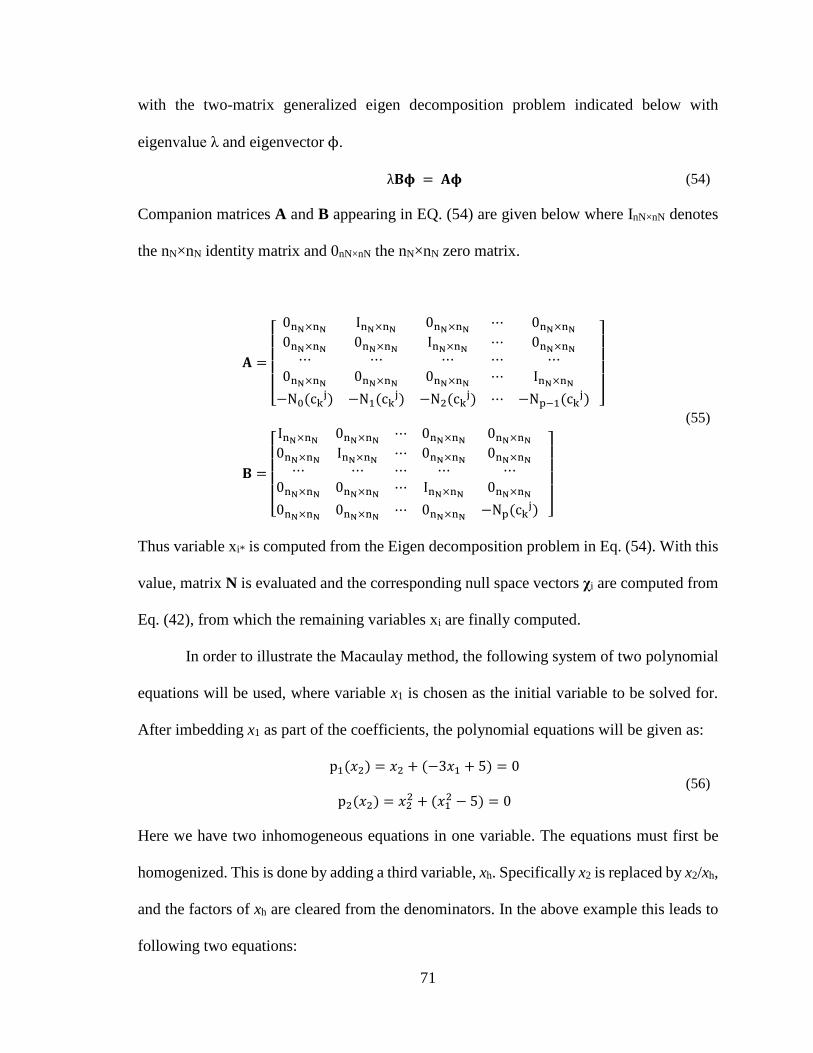
71
with the two-matrix generalized eigen decomposition problem indicated below with
eigenvalue λ and eigenvector ϕ.
λ𝐁𝛟 = 𝐀𝛟 (54)
Companion matrices A and B appearing in EQ. (54) are given below where InN×nN denotes
the nN×nN identity matrix and 0nN×nN the nN×nN zero matrix.
𝐀 =
[
0nN×nNInN×nN
0nN×nN⋯ 0nN×nN
0nN×nN0nN×nN
InN×nN⋯ 0nN×nN
⋯ ⋯ ⋯ ⋯ ⋯0nN×nN
0nN×nN0nN×nN
⋯ InN×nN
−N0(ckj) −N1(ck
j) −N2(ckj) ⋯ −Np−1(ck
j)
]
𝐁 =
[ InN×nN
0nN×nN⋯ 0nN×nN
0nN×nN
0nN×nNInN×nN
⋯ 0nN×nN0nN×nN
⋯ ⋯ ⋯ ⋯ ⋯0nN×nN
0nN×nN⋯ InN×nN
0nN×nN
0nN×nN0nN×nN
⋯ 0nN×nN−Np(ck
j)
]
(55)
Thus variable xi* is computed from the Eigen decomposition problem in Eq. (54). With this
value, matrix N is evaluated and the corresponding null space vectors χi are computed from
Eq. (42), from which the remaining variables xi are finally computed.
In order to illustrate the Macaulay method, the following system of two polynomial
equations will be used, where variable x1 is chosen as the initial variable to be solved for.
After imbedding x1 as part of the coefficients, the polynomial equations will be given as:
p1(𝑥2) = 𝑥2 + (−3𝑥1 + 5) = 0
p2(𝑥2) = 𝑥22 + (𝑥1
2 − 5) = 0
(56)
Here we have two inhomogeneous equations in one variable. The equations must first be
homogenized. This is done by adding a third variable, xh. Specifically x2 is replaced by x2/xh,
and the factors of xh are cleared from the denominators. In the above example this leads to
following two equations:
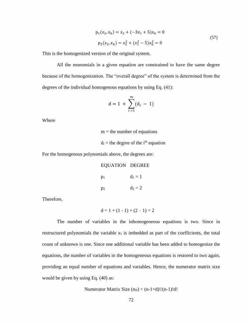
72
p1(𝑥2, 𝑥ℎ) = 𝑥2 + (−3𝑥1 + 5)𝑥ℎ = 0
p2(𝑥2, 𝑥ℎ) = 𝑥22 + (𝑥1
2 − 5)𝑥ℎ2 = 0
(57)
This is the homogenized version of the original system.
All the monomials in a given equation are constrained to have the same degree
because of the homogenization. The “overall degree” of the system is determined from the
degrees of the individual homogenous equations by using Eq. (41):
d = 1 + ∑(d𝑖 − 1)
𝑚
𝑖 =1
Where
m = the number of equations
di = the degree of the ith equation
For the homogenous polynomials above, the degrees are:
EQUATION DEGREE
p1 d1 = 1
p2 d2 = 2
Therefore,
d = 1 + (1 - 1) + (2 – 1) = 2
The number of variables in the inhomogeneous equations is two. Since in
restructured polynomials the variable x1 is imbedded as part of the coefficients, the total
count of unknown is one. Since one additional variable has been added to homogenize the
equations, the number of variables in the homogeneous equations is restored to two again,
providing an equal number of equations and variables. Hence, the numerator matrix sixe
would be given by using Eq. (40) as:
Numerator Matrix Size (nN) = (n-1+d)!/(n-1)!d!
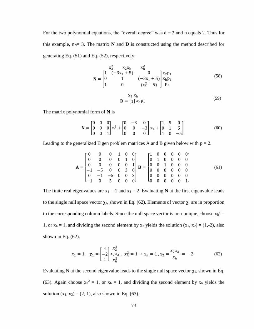
73
For the two polynomial equations, the “overall degree” was d = 2 and n equals 2. Thus for
this example, nN= 3. The matrix N and D is constructed using the method described for
generating Eq. (51) and Eq. (52), respectively.
x22 x2xh xh
2
𝐍 = [
1 (−3x1 + 5) 00 1 (−3x1 + 5)
1 0 (x12 − 5)
]
x2p1
xhp1
p2
(58)
x2 xh
𝐃 = [1] xhp1 (59)
The matrix polynomial form of N is
𝐍 = [
0 0 00 0 00 0 1
] 𝑥12 + [
0 −3 00 0 −30 0 0
] 𝑥1 + [1 5 00 1 51 0 −5
] (60)
Leading to the generalized Eigen problem matrices A and B given below with p = 2.
𝐀 =
[
0 0 0 1 0 00 0 0 0 1 00 0 0 0 0 1
−1 −5 0 0 3 00 −1 −5 0 0 3
−1 0 5 0 0 0]
𝐁 =
[ 1 0 0 0 0 00 1 0 0 0 00 0 1 0 0 00 0 0 0 0 00 0 0 0 0 00 0 0 0 0 1]
(61)
The finite real eigenvalues are x1 = 1 and x1 = 2. Evaluating N at the first eigenvalue leads
to the single null space vector χ1, shown in Eq. (62). Elements of vector χ1 are in proportion
to the corresponding column labels. Since the null space vector is non-unique, choose xh2 =
1, or xh = 1, and dividing the second element by xh yields the solution (x1, x2) = (1,-2), also
shown in Eq. (62).
𝑥1 = 1, 𝛘1 = [4
−21
]
𝑥22
𝑥2𝑥ℎ
𝑥ℎ2
, 𝑥ℎ2 = 1 → 𝑥ℎ = 1 , 𝑥2 =
𝑥2𝑥ℎ
𝑥ℎ = −2 (62)
Evaluating N at the second eigenvalue leads to the single null space vector χ1, shown in Eq.
(63). Again choose xh2 = 1, or xh = 1, and dividing the second element by xh yields the
solution (x1, x2) = (2, 1), also shown in Eq. (63).
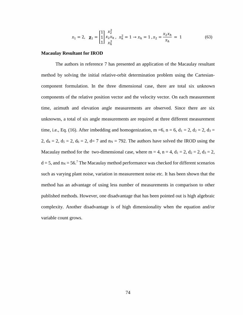
74
𝑥1 = 2, 𝛘1 = [111]
𝑥22
𝑥2𝑥ℎ
𝑥ℎ2
, 𝑥ℎ2 = 1 → 𝑥ℎ = 1 , 𝑥2 =
𝑥2𝑥ℎ
𝑥ℎ = 1 (63)
Macaulay Resultant for IROD
The authors in reference 7 has presented an application of the Macaulay resultant
method by solving the initial relative-orbit determination problem using the Cartesian-
component formulation. In the three dimensional case, there are total six unknown
components of the relative position vector and the velocity vector. On each measurement
time, azimuth and elevation angle measurements are observed. Since there are six
unknowns, a total of six angle measurements are required at three different measurement
time, i.e., Eq. (16). After imbedding and homogenization, m =6, n = 6, d1 = 2, d2 = 2, d3 =
2, d4 = 2, d5 = 2, d6 = 2, d= 7 and nN = 792. The authors have solved the IROD using the
Macaulay method for the two-dimensional case, where m = 4, n = 4, d1 = 2, d2 = 2, d3 = 2,
d = 5, and nN = 56.7 The Macaulay method performance was checked for different scenarios
such as varying plant noise, variation in measurement noise etc. It has been shown that the
method has an advantage of using less number of measurements in comparison to other
published methods. However, one disadvantage that has been pointed out is high algebraic
complexity. Another disadvantage is of high dimensionality when the equation and/or
variable count grows.
75
CHAPTER 6
MINIMAL-MEASUREMENT SOLUTION USING
SEPARATION-MAGNITUDE FORMULATION
The Macaulay Resultant method requires a total of six angle measurements when
the IROD problem is solved using the Cartesian-component formulation with the three-
dimensional case, which leads to the matrix N of size 792×792. To reduce algebraic
complexity, and high dimensionality, the Macaulay resultant method is used with the
separation-magnitude formulation. The separation-magnitude formulation was based on the
fact that at the time of the first observation, the initial direction of the deputy satellite with
respect to the chief satellite is already known, and it is only the relative magnitude that needs
to be computed for complete knowledge of relative position vector. Thus, reducing the
number of unknowns, i.e. the relative position magnitude and the relative velocity vector
component, to four in the three-dimensional case. The Macaulay method is applied on the
IROD problem using the concept of separation-magnitude formulation and now a total of
four measurement equations are required, which leads to the matrix N of size 56×56. This
shows that the separation-magnitude formulation succeed in overcoming the disadvantages
related to the Cartesian-component formulation. The number of measurement equations is
reduced to four, and the algebraic complexity is also reduced because of the decrease in the
size of matrix N.
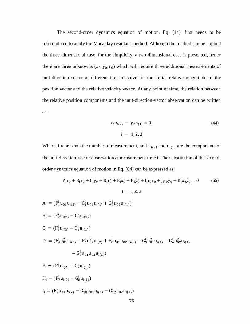
76
The second-order dynamics equation of motion, Eq. (14), first needs to be
reformulated to apply the Macaulay resultant method. Although the method can be applied
the three-dimensional case, for the simplicity, a two-dimensional case is presented, hence
there are three unknowns (x0, y0, r0) which will require three additional measurements of
unit-direction-vector at different time to solve for the initial relative magnitude of the
position vector and the relative velocity vector. At any point of time, the relation between
the relative position components and the unit-direction-vector observation can be written
as:
𝑥𝑖𝑢𝑖(2) − 𝑦𝑖𝑢𝑖(1) = 0 (44)
i = 1, 2, 3
Where, i represents the number of measurement, and ui(2) and ui(1) are the components of
the unit-direction-vector observation at measurement time i. The substitution of the second-
order dynamics equation of motion in Eq. (64) can be expressed as:
Air0 + Bix0 + Ciy0 + Dir02 + Eix0
2 + Hiy02 + Iir0x0 + Jir0y0 + Kix0y0 = 0 (65)
i = 1, 2, 3
Ai = (F1i u01ui(2) − G1
i u01ui(1) + G2i u02ui(1))
Bi = (F2i ui(2) − G3
i ui(1))
Ci = (F3i ui(2) − G4
i ui(1))
Di = (F4i u01
2 ui(2) + F5i u02
2 ui(2) + F8i u01u02ui(2) − G5
i u012 ui(1) − G6
i u022 ui(1)
− G9i u01u02ui(1))
Ei = (F6i ui(2) − G7
i ui(1))
Hi = (F7i ui(2) − G8
i ui(1))
Ii = (F9i u01ui(2) − G10
i u01ui(1) − G12i u02ui(1))
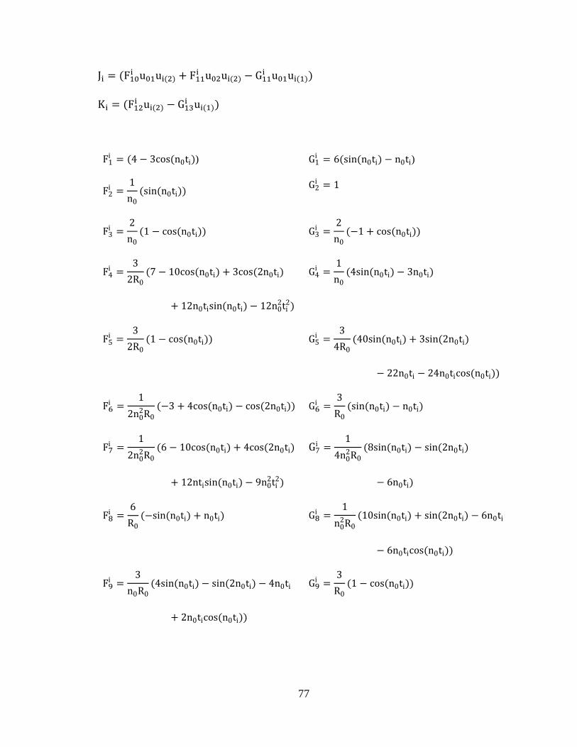
77
Ji = (F10i u01ui(2) + F11
i u02ui(2) − G11i u01ui(1))
Ki = (F12i ui(2) − G13
i ui(1))
F1i = (4 − 3cos(n0ti)) G1
i = 6(sin(n0ti) − n0ti)
F2i =
1
n0
(sin(n0ti)) G2
i = 1
F3i =
2
n0
(1 − cos(n0ti)) G3i =
2
n0
(−1 + cos(n0ti))
F4i =
3
2R0
(7 − 10cos(n0ti) + 3cos(2n0ti)
+ 12n0tisin(n0ti) − 12n02ti
2)
G4i =
1
n0
(4sin(n0ti) − 3n0ti)
F5i =
3
2R0
(1 − cos(n0ti))
G5i =
3
4R0
(40sin(n0ti) + 3sin(2n0ti)
− 22n0ti − 24n0ticos(n0ti))
F6i =
1
2n02R0
(−3 + 4cos(n0ti) − cos(2n0ti)) G6i =
3
R0
(sin(n0ti) − n0ti)
F7i =
1
2n02R0
(6 − 10cos(n0ti) + 4cos(2n0ti)
+ 12ntisin(n0ti) − 9n02ti
2)
G7i =
1
4n02R0
(8sin(n0ti) − sin(2n0ti)
− 6n0ti)
F8i =
6
R0
(−sin(n0ti) + n0ti) G8i =
1
n02R0
(10sin(n0ti) + sin(2n0ti) − 6n0ti
− 6n0ticos(n0ti))
F9i =
3
n0R0
(4sin(n0ti) − sin(2n0ti) − 4n0ti
+ 2n0ticos(n0ti))
G9i =
3
R0
(1 − cos(n0ti))
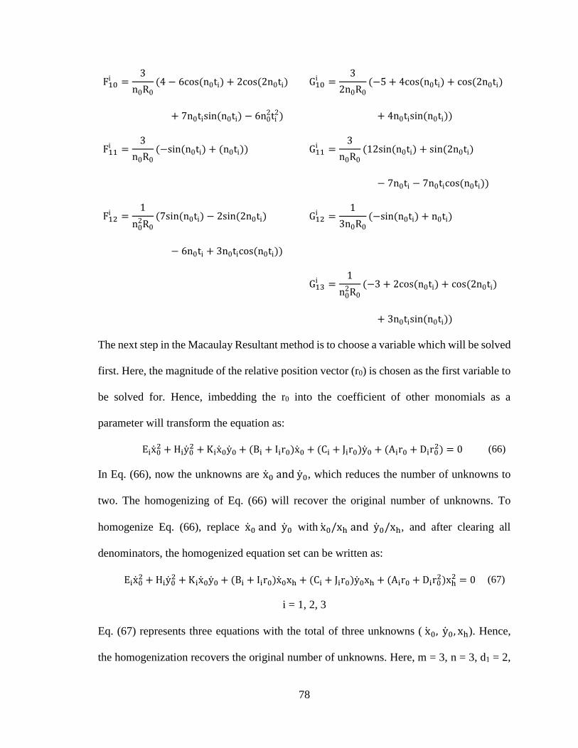
78
F10i =
3
n0R0
(4 − 6cos(n0ti) + 2cos(2n0ti)
+ 7n0tisin(n0ti) − 6n02ti
2)
G10i =
3
2n0R0
(−5 + 4cos(n0ti) + cos(2n0ti)
+ 4n0tisin(n0ti))
F11i =
3
n0R0
(−sin(n0ti) + (n0ti)) G11i =
3
n0R0
(12sin(n0ti) + sin(2n0ti)
− 7n0ti − 7n0ticos(n0ti))
F12i =
1
n02R0
(7sin(n0ti) − 2sin(2n0ti)
− 6n0ti + 3n0ticos(n0ti))
G12i =
1
3n0R0
(−sin(n0ti) + n0ti)
G13
i =1
n02R0
(−3 + 2cos(n0ti) + cos(2n0ti)
+ 3n0tisin(n0ti))
The next step in the Macaulay Resultant method is to choose a variable which will be solved
first. Here, the magnitude of the relative position vector (r0) is chosen as the first variable to
be solved for. Hence, imbedding the r0 into the coefficient of other monomials as a
parameter will transform the equation as:
Eix02 + Hiy0
2 + Kix0y0 + (Bi + Iir0)x0 + (Ci + Jir0)y0 + (Air0 + Dir02) = 0 (66)
In Eq. (66), now the unknowns are x0 and y0, which reduces the number of unknowns to
two. The homogenizing of Eq. (66) will recover the original number of unknowns. To
homogenize Eq. (66), replace x0 and y0 with x0/xh and y0/xh, and after clearing all
denominators, the homogenized equation set can be written as:
Eix02 + Hiy0
2 + Kix0y0 + (Bi + Iir0)x0xh + (Ci + Jir0)y0xh + (Air0 + Dir02)xh
2 = 0 (67)
i = 1, 2, 3
Eq. (67) represents three equations with the total of three unknowns ( x0, y0, xh). Hence,
the homogenization recovers the original number of unknowns. Here, m = 3, n = 3, d1 = 2,
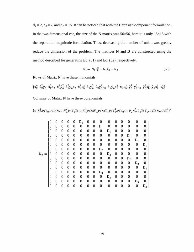
79
d2 = 2, d3 = 2, and nN = 15. It can be noticed that with the Cartesian-component formulation,
in the two-dimensional cae, the size of the N matrix was 56×56, here it is only 15×15 with
the separation-magnitude formulation. Thus, decreasing the number of unknowns greatly
reduce the dimension of the problem. The matrices N and D are constructed using the
method described for generating Eq. (51) and Eq. (52), respectively.
N = N2r02 + N1r0 + N0 (68)
Rows of Matrix N have these monomials:
{x04 x0
2y0 x03xh x0
2y02 x0
2y0xh x02xh
2 x0y03 x0y0
2xh x0y0xh2 x0xh
3 y04 y0
3xh y02xh
2 y0xh3 xh
4}
Columns of Matrix N have these polynomials:
{p1x02,p1y0,p1x0xh,p1y0,
2 p1y0xh,p1xh,2 p2x0y0,p2x0xh,p2y0
2,p2y0xh, p2xh2, p3x0y0, p3x0xh, p3xh
2}T
N2 =
[ 0 0 0 0 0 D1 0 0 0 0 0 0 0 0 00 0 0 0 0 0 0 0 D1 0 0 0 0 0 00 0 0 0 0 0 0 0 0 D1 0 0 0 0 00 0 0 0 0 0 0 0 0 0 0 0 D1 0 00 0 0 0 0 0 0 0 0 0 0 0 0 D1 00 0 0 0 0 0 0 0 0 0 0 0 0 0 D1
0 0 0 0 0 0 0 0 D2 0 0 0 0 0 00 0 0 0 0 0 0 0 0 D2 0 0 0 0 00 0 0 0 0 0 0 0 0 0 0 0 D2 0 00 0 0 0 0 0 0 0 0 0 0 0 0 D2 00 0 0 0 0 0 0 0 0 0 0 0 0 0 D2
0 0 0 0 0 0 0 0 D3 0 0 0 0 0 00 0 0 0 0 0 0 0 0 D3 0 0 0 0 00 0 0 0 0 0 0 0 0 0 0 0 0 D3 00 0 0 0 0 0 0 0 0 0 0 0 0 0 D3]
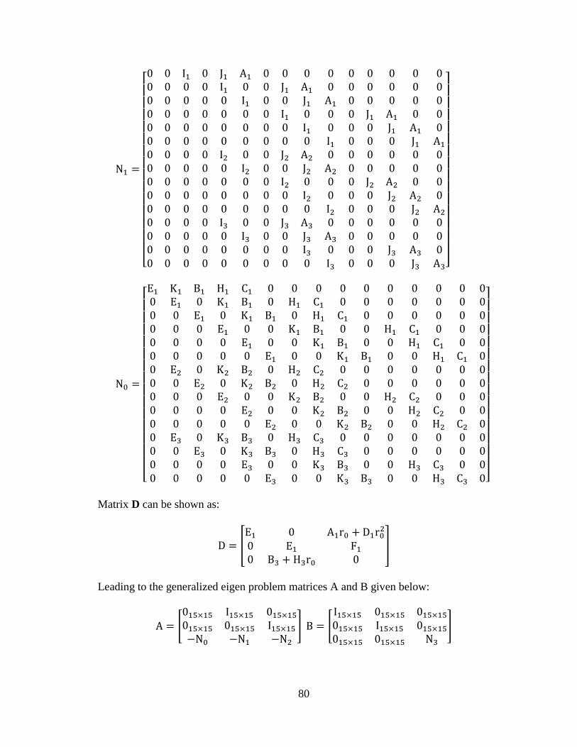
80
N1 =
[ 0 0 I1 0 J1 A1 0 0 0 0 0 0 0 0 00 0 0 0 I1 0 0 J1 A1 0 0 0 0 0 00 0 0 0 0 I1 0 0 J1 A1 0 0 0 0 00 0 0 0 0 0 0 I1 0 0 0 J1 A1 0 00 0 0 0 0 0 0 0 I1 0 0 0 J1 A1 00 0 0 0 0 0 0 0 0 I1 0 0 0 J1 A1
0 0 0 0 I2 0 0 J2 A2 0 0 0 0 0 00 0 0 0 0 I2 0 0 J2 A2 0 0 0 0 00 0 0 0 0 0 0 I2 0 0 0 J2 A2 0 00 0 0 0 0 0 0 0 I2 0 0 0 J2 A2 00 0 0 0 0 0 0 0 0 I2 0 0 0 J2 A2
0 0 0 0 I3 0 0 J3 A3 0 0 0 0 0 00 0 0 0 0 I3 0 0 J3 A3 0 0 0 0 00 0 0 0 0 0 0 0 I3 0 0 0 J3 A3 00 0 0 0 0 0 0 0 0 I3 0 0 0 J3 A3]
N0 =
[ E1 K1 B1 H1 C1 0 0 0 0 0 0 0 0 0 00 E1 0 K1 B1 0 H1 C1 0 0 0 0 0 0 00 0 E1 0 K1 B1 0 H1 C1 0 0 0 0 0 00 0 0 E1 0 0 K1 B1 0 0 H1 C1 0 0 00 0 0 0 E1 0 0 K1 B1 0 0 H1 C1 0 00 0 0 0 0 E1 0 0 K1 B1 0 0 H1 C1 00 E2 0 K2 B2 0 H2 C2 0 0 0 0 0 0 00 0 E2 0 K2 B2 0 H2 C2 0 0 0 0 0 00 0 0 E2 0 0 K2 B2 0 0 H2 C2 0 0 00 0 0 0 E2 0 0 K2 B2 0 0 H2 C2 0 00 0 0 0 0 E2 0 0 K2 B2 0 0 H2 C2 00 E3 0 K3 B3 0 H3 C3 0 0 0 0 0 0 00 0 E3 0 K3 B3 0 H3 C3 0 0 0 0 0 00 0 0 0 E3 0 0 K3 B3 0 0 H3 C3 0 00 0 0 0 0 E3 0 0 K3 B3 0 0 H3 C3 0]
Matrix D can be shown as:
D = [E1 0 A1r0 + D1r0
2
0 E1 F1
0 B3 + H3r0 0]
Leading to the generalized eigen problem matrices A and B given below:
A = [015×15 I15×15 015×15
015×15 015×15 I15×15
−N0 −N1 −N2
] B = [
I15×15 015×15 015×15
015×15 I15×15 015×15
015×15 015×15 N3
]
81
Thus the variable r0 is computed from the eigen decomposition problem in Eq. (54). With
this value, matrix N is evaluated and the corresponding null space vectors are computed
from Eq. (42), from which the remaining variables x0, and y0 are finally computed.
Performance Test
To test and evaluate the performance of the new relative IROD solution, a two-
dimensional xy planar numerical example is presented. As mentioned in chapter 4, the RMS
of angle residual and of range ratio will be calculated to check the performance metric. A
root-mean-square value of the angle residual that is close to zero indicates that the predicted
angles are close to the originally collected measurement angles. The largest and worst
possible RMS error value is equal to π radians away from its corresponding true line-of-
sight measurement. For range ratio RMS, a value near one indicates the predicted ranges
are close to the true ranges.
Several factors including noise type and level, and sample rate are varied to explore
certain aspects of the IROD performance. Two types of noise are used to test this IROD
technique: process noise and process plus the measurement noise. As mentioned earlier, the
term process noise refers to generating the measurements with a higher fidelity model
(nonlinear simulation) than the model on which the estimation solution is based (i.e., the
second-order model). Measurement noise level is considered across the range 10-8 to 10-3
radians. Measurement sample rate is varied across a wide range of cases from 100 seconds
to 10000 seconds to show dependency on temporal distribution of the measurements.
Estimating initial conditions with process noise and measurement noise
The IROD solution calculated using the Macaulay Resultant method is tested and
validated here. A two-dimensional coplanar orbit is considered again. For the nonlinear
82
simulation, the true measurements are generated by choosing a set of initial conditions and
propagating them forward using two-body dynamics and a fourth order Runge-Kutta
numerical integrator with time step equal to one second. Both process noise and process
plus measurement noise cases are considered. Process noise is introduced by using the
second-order solution in the IROD technique. In the case with measurement corruption,
Gaussian noise with a standard deviation of σ = 10-6 rad is added to each measurement. For
simplicity, measurements are taken at equal time steps. It is not necessary that measurements
always be taken at equal time increments, but the time at which a measurement is taken
must be recorded. Measurements for this case are sampled at equal time step increments of
1000 s. The initial conditions for this case are given below, in terms of circular chief orbit
elements and the deputy’s relative states with µ = 398600.436 km3/s2.
Chief: Deputy: Sample:
(69)
R0 = 7100 km x0 = 0.2 km t1 = 1000 s
Ω0 = 45 deg, y0 = 0 km t2 = 2000 s
θ0 = 0 deg x0 = 0.002 km/s t3 = 3000 s
i0 = 70 deg y0 = 0.02 km/s
Five real finite roots from the Macaulay resultant polynomial are computed for Eq. (69).
These roots are equivalent to the orbit determination solution for r0. After taking each of
these solutions and generating the associated null space vector, the remaining two initial
states x0, y0 for the orbit determination solutions are computed. Table 14 shows the five root
values and the initial state conditions. Based on comparison of individual initial states with
the known exact values, the fifth solution in Table 14 indicates the IROD method using the
Macaulay resultant framework is able to successfully recover the true initial conditions with
process noise plus measurement noise. One point worth mentioning is when all five solution
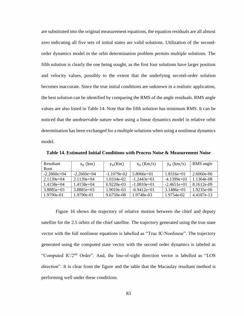
83
are substituted into the original measurement equations, the equation residuals are all almost
zero indicating all five sets of initial states are valid solutions. Utilization of the second-
order dynamics model in the orbit determination problem permits multiple solutions. The
fifth solution is clearly the one being sought, as the first four solutions have larger position
and velocity values, possibly to the extent that the underlying second-order solution
becomes inaccurate. Since the true initial conditions are unknown in a realistic application,
the best solution can be identified by comparing the RMS of the angle residuals. RMS angle
values are also listed in Table 14. Note that the fifth solution has minimum RMS. It can be
noticed that the unobservable nature when using a linear dynamics model in relative orbit
determination has been exchanged for a multiple solutions when using a nonlinear dynamics
model.
Table 14. Estimated Initial Conditions with Process Noise & Measurement Noise
Resultant
Root x0 (km) y0(Km) x0 (Km/s) y0 (km/s) RMS angle
-2.2660e+04 -2.2660e+04 -1.1079e-02 5.8066e+01 1.8316e+01 2.6060e-06
2.1139e+04 2.1139e+04 1.0334e-02 -1.2443e+01 -4.1399e+01 1.1364e-08
1.4158e+04 1.4158e+04 6.9220e-03 -1.0810e+01 -2.4651e+01 8.1612e-09
3.8885e+03 3.8885e+03 1.9010e-03 -6.9412e+01 3.1486e+01 1.9235e-06
1.9790e-01 1.9790e-01 9.6750e-08 1.9748e-03 1.9754e-02 4.4187e-13
Figure 16 shows the trajectory of relative motion between the chief and deputy
satellite for the 2.5 orbits of the chief satellite. The trajectory generated using the true state
vector with the full nonlinear equations is labelled as “True IC/Nonlinear”. The trajectory
generated using the computed state vector with the second order dynamics is labeled as
“Computed IC/2nd Order”. And, the line-of-sight direction vector is labelled as “LOS
direction”. It is clear from the figure and the table that the Macaulay resultant method is
performing well under these conditions.

84
Figure 16. Relative orbit with Process plus Measurement Noise, time step of
1000 s
Effect of varying the measurement noise on estimation of initial conditions
In order to determine how the Macaulay resultant method will work with varying
noise level, the same initial conditions are run with six different levels of measurement noise
added to the process noise. The initial conditions are held constant at each run and the
standard deviation of Gaussian noise is changed. Table 15 shows the values of the initial
state conditions for the different values of standard deviation of Gaussian noise. Finite real
roots from the Macaulay resultant polynomial are computed for each run having different
value of standard deviation of Gaussian noise. These roots are equivalent to orbit
85
determination solution for r0. After taking each of these solutions and generating the
associated null space vector, the remaining two initial states x0, y0 for the orbit
determination solutions are computed. RMS angle is also listed in Table 15. From Table 15,
it can be seen, the largest level of the measurement noise (σ = 10-3 rad) produces the highest
error as expected, hence it hinders the ability of the IROD method. So it is desirable that the
camera should take high precision measurement to reduce the corruption of the solution.
Figures 17 and 18 show the relative trajectory of the deputy satellite with respect to
the chief satellite for 2.5 orbits of the chief satellite when the system has process plus
measurement noise. The trajectory generated using the true state vectors with the full
nonlinear equations is labelled as “True IC/Nonlinear”. The trajectory generated using the
computed state vectors with the second-order dynamic is labeled as “Computed IC/2nd
Order”. And, the line-of-sight direction vector is labelled as “LOS direction”. In Figure 17
the relative trajectory is propagated with measurement noise of 10-8 rad standard deviation.
And, as expected, the relative trajectory propagated with the second-order dynamics and the
estimated initial conditions is able to follow the true relative trajectory. In Figure 18 the
estimated relative trajectory generated with the process plus the measurement noise of 10-3
rad is compared with the true relative trajectory. It is clear from the figure and the table that
the separation-magnitude formulation is performing well with the Macaulay resultant
method when the measurements are less corrupted.
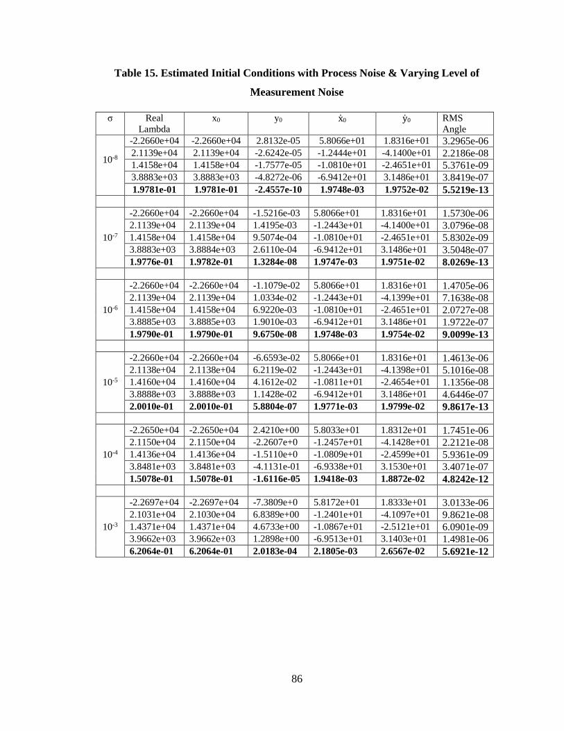
86
Table 15. Estimated Initial Conditions with Process Noise & Varying Level of
Measurement Noise
σ Real
Lambda
x0 y0 x0 y0 RMS
Angle
10-8
-2.2660e+04 -2.2660e+04 2.8132e-05 5.8066e+01 1.8316e+01 3.2965e-06
2.1139e+04 2.1139e+04 -2.6242e-05 -1.2444e+01 -4.1400e+01 2.2186e-08
1.4158e+04 1.4158e+04 -1.7577e-05 -1.0810e+01 -2.4651e+01 5.3761e-09
3.8883e+03 3.8883e+03 -4.8272e-06 -6.9412e+01 3.1486e+01 3.8419e-07
1.9781e-01 1.9781e-01 -2.4557e-10 1.9748e-03 1.9752e-02 5.5219e-13
10-7
-2.2660e+04 -2.2660e+04 -1.5216e-03 5.8066e+01 1.8316e+01 1.5730e-06
2.1139e+04 2.1139e+04 1.4195e-03 -1.2443e+01 -4.1400e+01 3.0796e-08
1.4158e+04 1.4158e+04 9.5074e-04 -1.0810e+01 -2.4651e+01 5.8302e-09
3.8883e+03 3.8884e+03 2.6110e-04 -6.9412e+01 3.1486e+01 3.5048e-07
1.9776e-01 1.9782e-01 1.3284e-08 1.9747e-03 1.9751e-02 8.0269e-13
10-6
-2.2660e+04 -2.2660e+04 -1.1079e-02 5.8066e+01 1.8316e+01 1.4705e-06
2.1139e+04 2.1139e+04 1.0334e-02 -1.2443e+01 -4.1399e+01 7.1638e-08
1.4158e+04 1.4158e+04 6.9220e-03 -1.0810e+01 -2.4651e+01 2.0727e-08
3.8885e+03 3.8885e+03 1.9010e-03 -6.9412e+01 3.1486e+01 1.9722e-07
1.9790e-01 1.9790e-01 9.6750e-08 1.9748e-03 1.9754e-02 9.0099e-13
10-5
-2.2660e+04 -2.2660e+04 -6.6593e-02 5.8066e+01 1.8316e+01 1.4613e-06
2.1138e+04 2.1138e+04 6.2119e-02 -1.2443e+01 -4.1398e+01 5.1016e-08
1.4160e+04 1.4160e+04 4.1612e-02 -1.0811e+01 -2.4654e+01 1.1356e-08
3.8888e+03 3.8888e+03 1.1428e-02 -6.9412e+01 3.1486e+01 4.6446e-07
2.0010e-01 2.0010e-01 5.8804e-07 1.9771e-03 1.9799e-02 9.8617e-13
10-4
-2.2650e+04 -2.2650e+04 2.4210e+00 5.8033e+01 1.8312e+01 1.7451e-06
2.1150e+04 2.1150e+04 -2.2607e+0 -1.2457e+01 -4.1428e+01 2.2121e-08
1.4136e+04 1.4136e+04 -1.5110e+0 -1.0809e+01 -2.4599e+01 5.9361e-09
3.8481e+03 3.8481e+03 -4.1131e-01 -6.9338e+01 3.1530e+01 3.4071e-07
1.5078e-01 1.5078e-01 -1.6116e-05 1.9418e-03 1.8872e-02 4.8242e-12
10-3
-2.2697e+04 -2.2697e+04 -7.3809e+0 5.8172e+01 1.8333e+01 3.0133e-06
2.1031e+04 2.1030e+04 6.8389e+00 -1.2401e+01 -4.1097e+01 9.8621e-08
1.4371e+04 1.4371e+04 4.6733e+00 -1.0867e+01 -2.5121e+01 6.0901e-09
3.9662e+03 3.9662e+03 1.2898e+00 -6.9513e+01 3.1403e+01 1.4981e-06
6.2064e-01 6.2064e-01 2.0183e-04 2.1805e-03 2.6567e-02 5.6921e-12
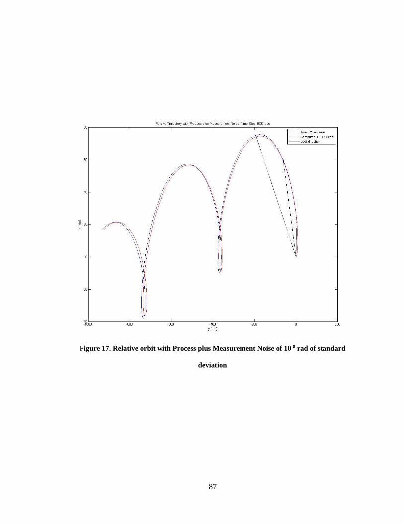
87
Figure 17. Relative orbit with Process plus Measurement Noise of 10-8 rad of standard
deviation
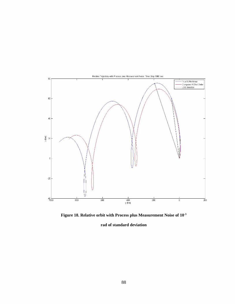
88
Figure 18. Relative orbit with Process plus Measurement Noise of 10-3
rad of standard deviation
89
Effect of varying sample time period on estimation of initial conditions
To present the potential of this method with varying sample time, the same initial
conditions are run with five different sample time periods. Each run is made with the process
noise plus Gaussian measurement noise with a standard deviation of σ = 10-6 rad. The initial
state vector is estimated using the time interval of 2000 s, 4000 s, 5000 s and 7000 s. As
mentioned earlier, the basic tenet of the Macaulay resultant method is the matrix N has to
be rank deficient. With the time period of 3000 s, and 6000 s, the matrix N was full rank,
hence those are not discussed in this thesis.
Tables 16 and 17 show the estimated initial conditions and the RMS associated with
angle residual and range ratio estimation for different sample time period, respectively. It
can be seen from both tables that the Macaulay resultant method is able to estimate the initial
conditions. One thing to notice is, although the estimation of relative position vector is poor
as the sample time period is increased, the estimation of the velocity vector is still accurate.
The performance of the IROD method can be sensitive to a uniform sample rate and thus
should be given careful consideration.
Figures 19 - 23 show the trajectory of the relative motion between the deputy
satellite and the chief satellite for the sample time period of 1000 s, 2000 s, 4000 s, 5000 s,
and 7000 s. The trajectory generated using the true state vector with the full nonlinear
equations is labelled as “True IC/Nonlinear”. The trajectory generated using the computed
state vector with the second-order dynamics is labeled as “Computed IC/2nd Order”. And,
the line-of-sight direction vector is labelled as “LOS direction”. As expected after observing
the above tables, the relative trajectory propagated with the estimated initial state vector
using the second-order dynamics is following the true relative trajectory. In the redundant-
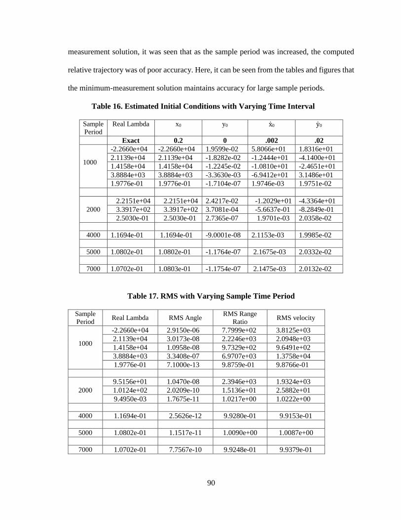
90
measurement solution, it was seen that as the sample period was increased, the computed
relative trajectory was of poor accuracy. Here, it can be seen from the tables and figures that
the minimum-measurement solution maintains accuracy for large sample periods.
Table 16. Estimated Initial Conditions with Varying Time Interval
Sample
Period
Real Lambda x0 y0 x0 y0
Exact 0.2 0 .002 .02
1000
-2.2660e+04 -2.2660e+04 1.9599e-02 5.8066e+01 1.8316e+01
2.1139e+04 2.1139e+04 -1.8282e-02 -1.2444e+01 -4.1400e+01
1.4158e+04 1.4158e+04 -1.2245e-02 -1.0810e+01 -2.4651e+01
3.8884e+03 3.8884e+03 -3.3630e-03 -6.9412e+01 3.1486e+01
1.9776e-01 1.9776e-01 -1.7104e-07 1.9746e-03 1.9751e-02
2000
2.2151e+04 2.2151e+04 2.4217e-02 -1.2029e+01 -4.3364e+01
3.3917e+02 3.3917e+02 3.7081e-04 -5.6637e-01 -8.2849e-01
2.5030e-01 2.5030e-01 2.7365e-07 1.9701e-03 2.0358e-02
4000 1.1694e-01 1.1694e-01 -9.0001e-08 2.1153e-03 1.9985e-02
5000 1.0802e-01 1.0802e-01 -1.1764e-07 2.1675e-03 2.0332e-02
7000 1.0702e-01 1.0803e-01 -1.1754e-07 2.1475e-03 2.0132e-02
Table 17. RMS with Varying Sample Time Period
Sample
Period Real Lambda RMS Angle
RMS Range
Ratio RMS velocity
1000
-2.2660e+04 2.9150e-06 7.7999e+02 3.8125e+03
2.1139e+04 3.0173e-08 2.2246e+03 2.0948e+03
1.4158e+04 1.0958e-08 9.7329e+02 9.6491e+02
3.8884e+03 3.3408e-07 6.9707e+03 1.3758e+04
1.9776e-01 7.1000e-13 9.8759e-01 9.8766e-01
2000
9.5156e+01 1.0470e-08 2.3946e+03 1.9324e+03
1.0124e+02 2.0209e-10 1.5136e+01 2.5882e+01
9.4950e-03 1.7675e-11 1.0217e+00 1.0222e+00
4000 1.1694e-01 2.5626e-12 9.9280e-01 9.9153e-01
5000 1.0802e-01 1.1517e-11 1.0090e+00 1.0087e+00
7000 1.0702e-01 7.7567e-10 9.9248e-01 9.9379e-01

91
Figure 19. Relative Orbit with Process plus 10-6 rad of Measurement Noise, Time Step
of 1000 s
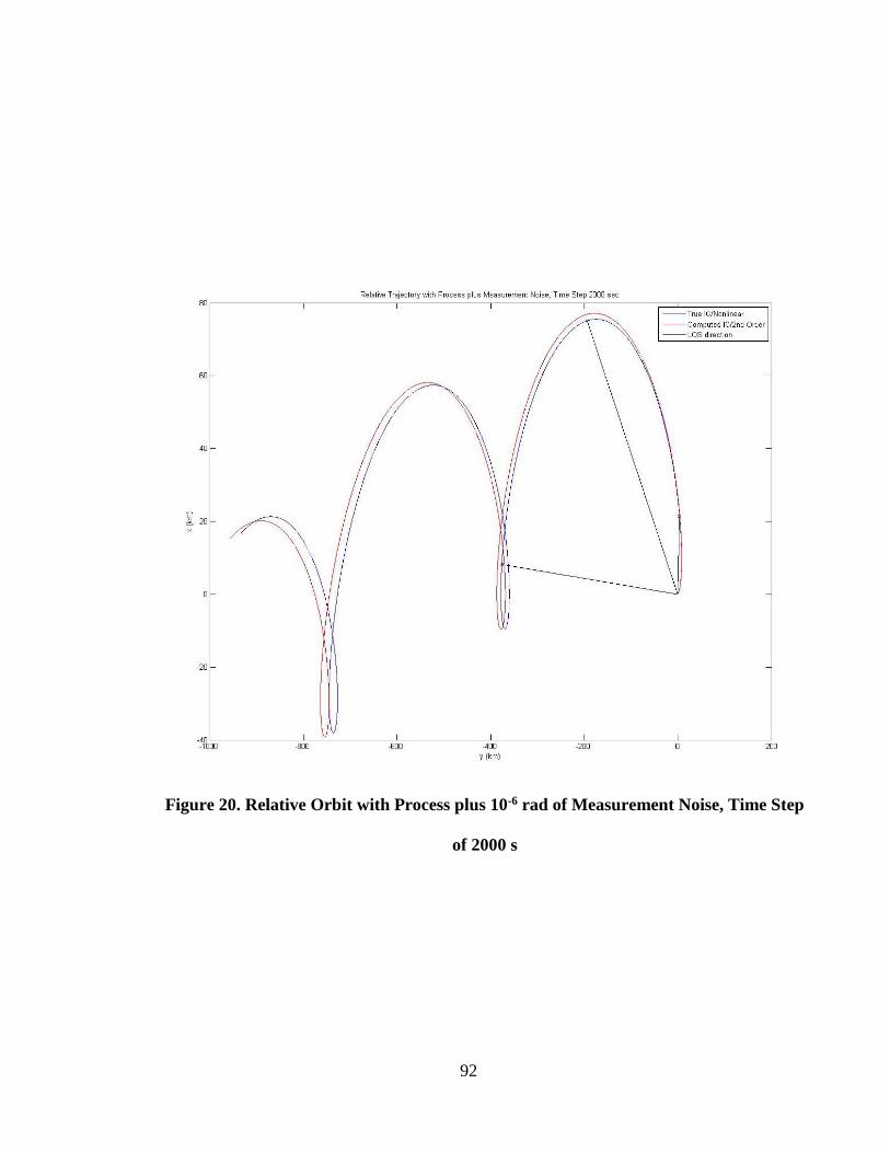
92
Figure 20. Relative Orbit with Process plus 10-6 rad of Measurement Noise, Time Step
of 2000 s
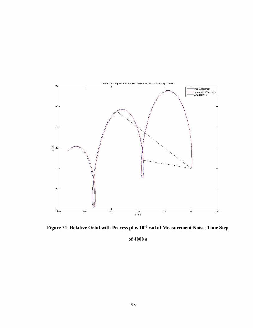
93
Figure 21. Relative Orbit with Process plus 10-6 rad of Measurement Noise, Time Step
of 4000 s
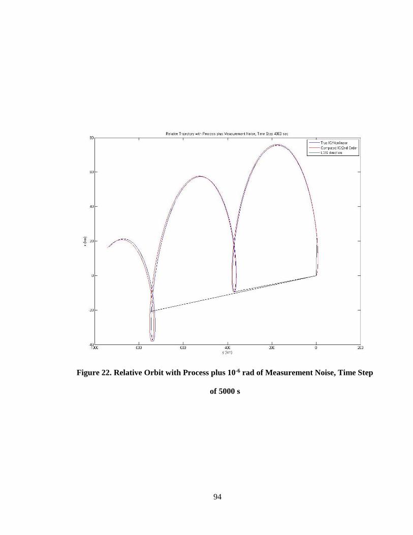
94
Figure 22. Relative Orbit with Process plus 10-6 rad of Measurement Noise, Time Step
of 5000 s
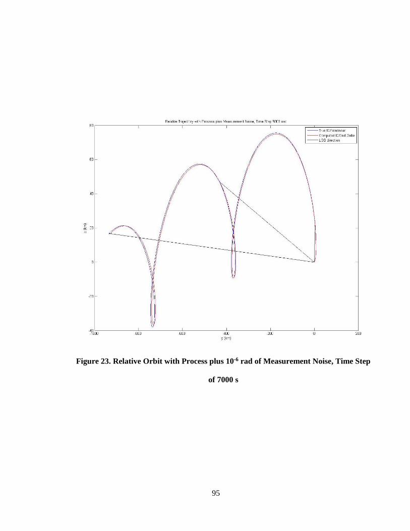
95
Figure 23. Relative Orbit with Process plus 10-6 rad of Measurement Noise, Time Step
of 7000 s
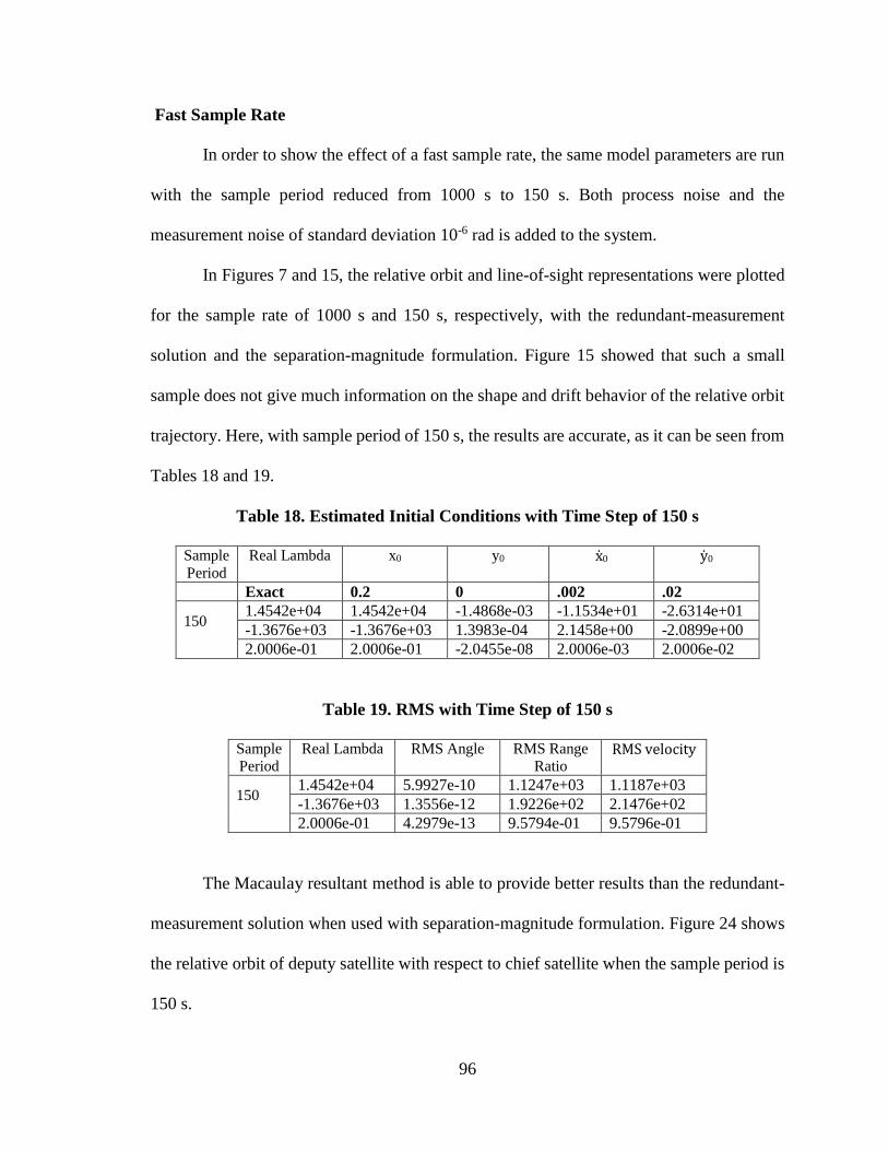
96
Fast Sample Rate
In order to show the effect of a fast sample rate, the same model parameters are run
with the sample period reduced from 1000 s to 150 s. Both process noise and the
measurement noise of standard deviation 10-6 rad is added to the system.
In Figures 7 and 15, the relative orbit and line-of-sight representations were plotted
for the sample rate of 1000 s and 150 s, respectively, with the redundant-measurement
solution and the separation-magnitude formulation. Figure 15 showed that such a small
sample does not give much information on the shape and drift behavior of the relative orbit
trajectory. Here, with sample period of 150 s, the results are accurate, as it can be seen from
Tables 18 and 19.
Table 18. Estimated Initial Conditions with Time Step of 150 s
Sample
Period
Real Lambda x0 y0 x0 y0
Exact 0.2 0 .002 .02
150
1.4542e+04 1.4542e+04 -1.4868e-03 -1.1534e+01 -2.6314e+01
-1.3676e+03 -1.3676e+03 1.3983e-04 2.1458e+00 -2.0899e+00
2.0006e-01 2.0006e-01 -2.0455e-08 2.0006e-03 2.0006e-02
Table 19. RMS with Time Step of 150 s
Sample
Period
Real Lambda RMS Angle RMS Range
Ratio RMS velocity
150
1.4542e+04 5.9927e-10 1.1247e+03 1.1187e+03
-1.3676e+03 1.3556e-12 1.9226e+02 2.1476e+02
2.0006e-01 4.2979e-13 9.5794e-01 9.5796e-01
The Macaulay resultant method is able to provide better results than the redundant-
measurement solution when used with separation-magnitude formulation. Figure 24 shows
the relative orbit of deputy satellite with respect to chief satellite when the sample period is
150 s.

97
Figure 24. Relative Orbit with Process plus 10-6 rad of Measurement Noise, Fast
sample period of 150 s
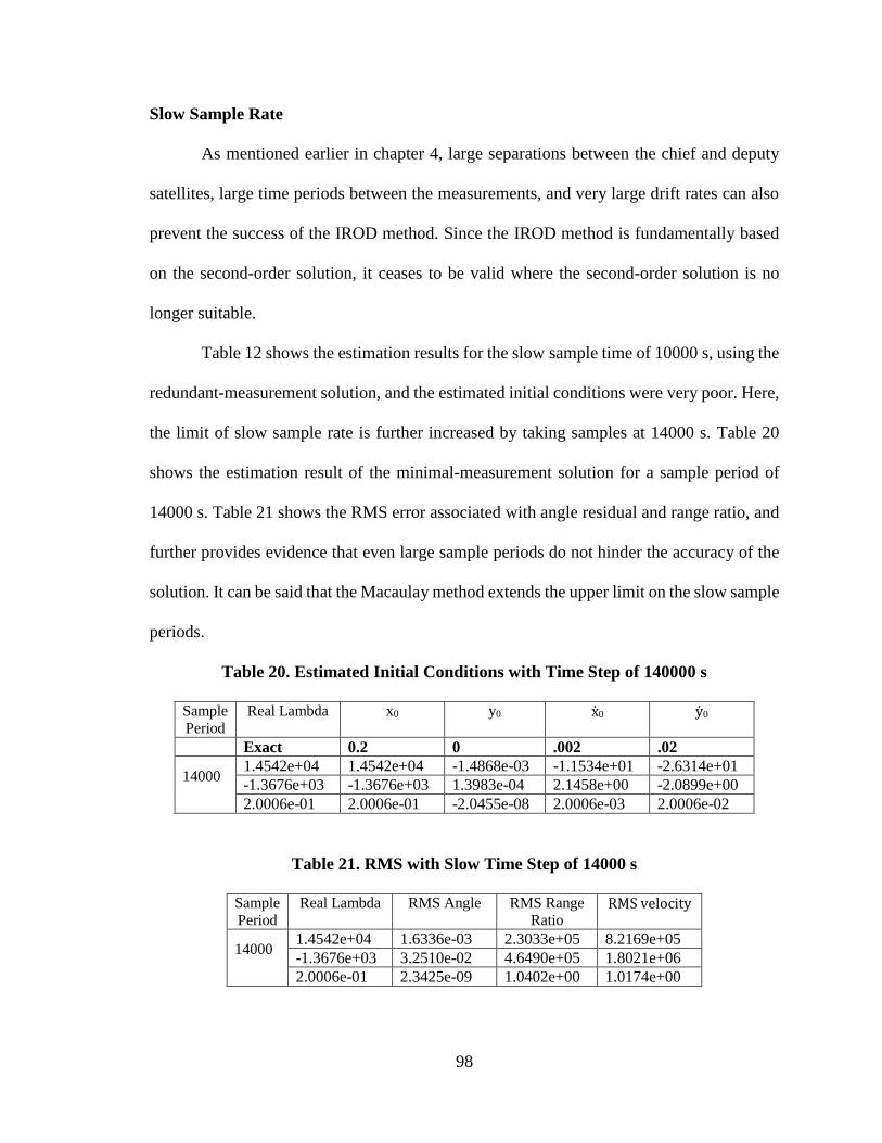
98
Slow Sample Rate
As mentioned earlier in chapter 4, large separations between the chief and deputy
satellites, large time periods between the measurements, and very large drift rates can also
prevent the success of the IROD method. Since the IROD method is fundamentally based
on the second-order solution, it ceases to be valid where the second-order solution is no
longer suitable.
Table 12 shows the estimation results for the slow sample time of 10000 s, using the
redundant-measurement solution, and the estimated initial conditions were very poor. Here,
the limit of slow sample rate is further increased by taking samples at 14000 s. Table 20
shows the estimation result of the minimal-measurement solution for a sample period of
14000 s. Table 21 shows the RMS error associated with angle residual and range ratio, and
further provides evidence that even large sample periods do not hinder the accuracy of the
solution. It can be said that the Macaulay method extends the upper limit on the slow sample
periods.
Table 20. Estimated Initial Conditions with Time Step of 140000 s
Sample
Period
Real Lambda x0 y0 x0 y0
Exact 0.2 0 .002 .02
14000
1.4542e+04 1.4542e+04 -1.4868e-03 -1.1534e+01 -2.6314e+01
-1.3676e+03 -1.3676e+03 1.3983e-04 2.1458e+00 -2.0899e+00
2.0006e-01 2.0006e-01 -2.0455e-08 2.0006e-03 2.0006e-02
Table 21. RMS with Slow Time Step of 14000 s
Sample
Period
Real Lambda RMS Angle RMS Range
Ratio RMS velocity
14000
1.4542e+04 1.6336e-03 2.3033e+05 8.2169e+05
-1.3676e+03 3.2510e-02 4.6490e+05 1.8021e+06
2.0006e-01 2.3425e-09 1.0402e+00 1.0174e+00
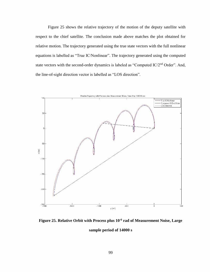
99
Figure 25 shows the relative trajectory of the motion of the deputy satellite with
respect to the chief satellite. The conclusion made above matches the plot obtained for
relative motion. The trajectory generated using the true state vectors with the full nonlinear
equations is labelled as “True IC/Nonlinear”. The trajectory generated using the computed
state vectors with the second-order dynamics is labeled as “Computed IC/2nd Order”. And,
the line-of-sight direction vector is labelled as “LOS direction”.
Figure 25. Relative Orbit with Process plus 10-6 rad of Measurement Noise, Large
sample period of 14000 s

100
CONCLUSION
A method has been presented for computing the initial state vector using line-of-
sight direction vectors. For three dimensional estimations, a total of eight measurements of
unit-direction-vectors is required, generating a 21×21 matrix of linear equations. This
method requires redundant measurements, but requires less measurements than other
published methods. Also, it requires less computational effort than any other published
method. With ideal assumptions, the method is able to estimate exact initial conditions, and
with more realistic enviornment the technique can recover the initial conditions with a level
of precision, depending upon the corruption of measurement noise and the fidelity of the
nonlinear solution model. The only requirement will be to use a high precision camera so
that the measurements are relatively free of corruptions. It should also be mentioned that
the separation-magnitude method uses the unit-direction-vector of initial relative position
between the chief and the deputy satellite as a basis for the solution, and may be particularly
sensitive to erros in this observation.
The application of the Macaulay resultant method has also been presented in this
thesis. The minimal-measurement solution using the separation-magntiude formulation
computes the intitial relative position vector and velocity vector of the deputy satellite with
respect to the chief satellite. It provides all the imaginary and real solutions possible to the
problem of IROD. This method requires minimal number of measurements in comparsion
to the published methods, and the redundant-measurement solution method. However, it
101
adds algebraic complexity to the procdeure which is high in comparison to the redundant-
measurement solution method but very less in comparision to the published method. In
published method, for the three dimensional case, the matrix obtained has dimension of
792×792 utilizing a total of six angular measurements, but in the presented method the
matrix size is of 56×56 processing only two more unit-direction-vector measurement. The
Macauly Resultant method is highly dependent on number of measurements and unknowns.
Althought the Macaulay Resultant method has some algebraic compleixty in comparison to
the discard method, but it improves the limit placed on the IROD method by the redundant-
measurement method. The redundant-measurement method provides satisfactory result with
the fast sample rate of 150 s and the slow sample rate of 10000 s but the Macaulay Resultant
method provides similar satisfactory result with 100 s of fast sample rate and 14000 s of
slow sample rate.
102
REFRENCES
1. Woffinden, D. C. and Geller, D. K., “Observability Criteria for Angles-Only Navigation,”
IEEE Transactions on Aerospace and Electronic Systems, Vol. 45, No. 3, July, 2009, pp.
1194-1208.
2. G.W. Hill, “Researches in the Lunar Theory,” American Journal of Mathematics, Volume
1, 1878, pp. 5-26
3. Chohessy, W. H. and Wiltshire, R. S., “Terminal Guidance System for Satellite
Rendezvous”, Journal of the Aerospace Sciences, Vol. 27, No. 9, September, 1960, pp. 653-
658
4. Patel, H., Lovell, T. A., Allgeier, S., Russell, R., and Sinclair, A. J., “Relative
Navigation for Satellites in Close Proximity Using Angle-Only Observations,”
AAS- 2012-212, Proceedings of the AAS-AIAA Spaceflight Mechanics Meeting,
Charleston, South Carolina, January-February, 2012
5. Newman, B., Lovell, T. A., and Pratt, E., “Second Order Nonlinear Initial Orbit
Determination for Relative Motion using Volterra Theory,” AAS-2014-286,, Proceedings
of the AAS- AIAA Spaceflight Mechanics Meeting, Santa Fe, New Mexico, January, 2014
6. Pratt, E., Lovell, T. A., and Newman, B., “ A Second Order Method for Initial Relative Orbit
Determination Using Angle-Only Observations,” AAS-2014-293, Proceedings of the AAS-
AIAA Spaceflight Mechanics Meeting, Santa Fe, New Mexico, January, 2014
7. Newman, B., Lovell, T. A., Pratt, E., and Duncan, E., “Quadratic Hexa-Dimensional
Solution for Relative Orbit Determination,” AIAA 2014-4309, Proceedings of the AIAA-
AAS Astrodynamics Specialist Conference, San Diego, California, August, 2014
103
8. Stringer, M. T., Newman, B., Lovell, T. A., and Omran, A., ‘Second Order Nonlinear Initial
Value Solution for Relative Motion Using Volterra Theory,” AAS-2013-469, Proceedings
of the AAS-AIAA Spaceflight Mechanics Meeting, Lihue, Hawai, February, 2013.
9. Newman, B., Lovell, T. A., and Pratt, E., “Second Order Nonlinear Initial Orbit
Determination for Relative Motion using Volterra Theory,” AAS-2014-286, Proceedings of
the AAS-AIAA Spaceflight Mechanics Meeting, Santa Fe, New Mexico, January, 2014.
10. Schaub, H., Junkins, J. L., “Analytical Mechanics of Space Systems,” American Institute of
Aeronautics and Astronautics, Inc., Reston, Virginia
11. Stiller, P. F., “An Introduction to the Theory of Resultants,” ISC-96-02-MATH, Institute
for Scientific Computation, Texas A&M University, College Station, Texas 1996.
12. Bajaj, C., Garrity, T., and Warren, J., “On the Applications of Multi-Equational Resultants,”
CSD-TR-826
13. LeGrand, K.A., DeMars, K. J., and Darling, J. E., “Solutions of Multivariate Polynomial
System using Macaulay Resultant Expressions,” AAS-104-229, Proceedings of the AAS-
AIAA Spaceflight Mechanics Meeting, Santa Fe, New Mexico, January, 2014.
14. Manocha, D., “Computing Selected Solutions of Polynomial Equations,”
Proceedings of the ACM International Symposium on Symbolic and Algebraic
Computation, Oxford, England, July, 1994, pp. 1-8.
15. Manocha, D. and Krishnan, S., “Solving Algebraic Systems Using Matrix
Computations,” ACM Special Interest Group on Symbolic and Algebraic
Manipulation Bulletin, Vol. 30, No. 4, December, 1996, pp. 4-21.
16. Jonsson, G.F. and Vavasis, S. A., “Accurate Solution of Polynomial Equations
Using Macaulay Resultant Matrices,” Mathematics of Computation, Vol. 74, No.
249, July, 2004, pp. 221-262.