Information Systems - CiteSeerX
178
Information Systems (“Informationssysteme”) Prof. Dr. Marc H. Scholl [email protected] Summer 2008 Dept. of Computer & Information Science Databases and Information Systems Group Marc H. Scholl (DBIS, Uni KN) Information Systems 1 Organizational matters The lectures of this course will be recorded (presentation, audio, video). Recordings will be available for your offline review from a streaming server. Details will be published on the course’s Web site. Have an occasional look at the recordings. We look forward to your feedback. Let us know your assessment of the value towards the end of the term. Bear with us, if technical problems arise . . . Marc H. Scholl (DBIS, Uni KN) Information Systems 2 Course “Information Systems” This course is the “continuation” of Information Management. There, we focused on the modeling aspects of information (structure, behavior). What is information? Entity-Relationship (E/R) modeling. Automata & Petri Nets for dynamic behavior. We also started to look at how to work with information systems (different declarative languages). Now, we’ll be concentrating on operational issues: Declarative languages in detail. Transactional processing. How to make IS fast. Marc H. Scholl (DBIS, Uni KN) Information Systems 3 Coarse Outline Query languages Relational algebra & calculus, SQL, DATALOG Updates, integrity constraints, & views Security & privacy, access control Data warehouses & OLAP Transactional processing Multi-user operation, concurrency control, recovery DBMS architecture File organization & indexes, query processing & optimization Marc H. Scholl (DBIS, Uni KN) Information Systems 4
-
Upload
khangminh22 -
Category
Documents
-
view
0 -
download
0
Transcript of Information Systems - CiteSeerX

Information Systems(“Informationssysteme”)
Prof. Dr. Marc H. [email protected]
Summer 2008
Dept. of Computer & Information ScienceDatabases and Information Systems Group
Marc H. Scholl (DBIS, Uni KN) Information Systems 1
Organizational matters
The lectures of this course will be recorded (presentation, audio, video).Recordings will be available for your offline review from a streamingserver. Details will be published on the course’s Web site.
Have an occasional look at the recordings.
We look forward to your feedback.
Let us know your assessment of the value towards the end of theterm.
Bear with us, if technical problems arise . . .
Marc H. Scholl (DBIS, Uni KN) Information Systems 2
Course “Information Systems”
This course is the “continuation” of Information Management. There,we focused on the modeling aspects of information (structure,behavior).
What is information?Entity-Relationship (E/R) modeling.Automata & Petri Nets for dynamic behavior.
We also started to look at how to work with information systems(different declarative languages).
Now, we’ll be concentrating on operational issues:
Declarative languages in detail.
Transactional processing.
How to make IS fast.
Marc H. Scholl (DBIS, Uni KN) Information Systems 3
Coarse Outline
Query languagesRelational algebra & calculus, SQL, DATALOG
Updates, integrity constraints, & views
Security & privacy, access control
Data warehouses & OLAPTransactional processing
Multi-user operation, concurrency control, recovery
DBMS architectureFile organization & indexes, query processing & optimization
Marc H. Scholl (DBIS, Uni KN) Information Systems 4
Presentation material (1)
. . . will be available online from the course’s Web site.
Visual formatting:
Definitions (formal or informal, often just other important material)
. . . will be highlighted like this.
Examples (like this)
. . . will be given when appropriate.
Quizzes, Assignments, Hints on further reading
. . . will be indicated in a box like this.
Marc H. Scholl (DBIS, Uni KN) Information Systems 5
Presentation material (2)
Math diversionsWe will—occasionally—divert into formal notations and highlight them likethis.
Theorem (Formal Properties)
Sometimes we might even be giving our observations in the formal formof a theorem or proposition.
Proof.
(. . . most of the time: without a proof.)
Marc H. Scholl (DBIS, Uni KN) Information Systems 6
Part I
Relational Algebra
Marc H. Scholl (DBIS, Uni KN) Information Systems 7
Outline of this part (I)
1 Introduction: Selection, ProjectionIntroductionSelectionProjectionCombining Operators
2 Product, JoinProductJoin
3 Set Operations4 Derived Operators
DivisionOuter Join
5 Formalities, A Bit of TheorySyntaxSemantics
Marc H. Scholl (DBIS, Uni KN) Information Systems 8
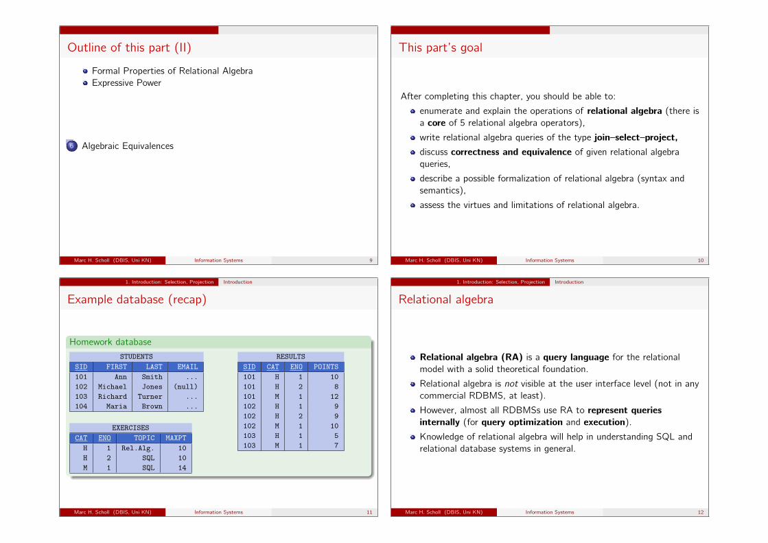
Outline of this part (II)
Formal Properties of Relational AlgebraExpressive Power
6 Algebraic Equivalences
Marc H. Scholl (DBIS, Uni KN) Information Systems 9
This part’s goal
After completing this chapter, you should be able to:
enumerate and explain the operations of relational algebra (there isa core of 5 relational algebra operators),
write relational algebra queries of the type join–select–project,discuss correctness and equivalence of given relational algebraqueries,
describe a possible formalization of relational algebra (syntax andsemantics),
assess the virtues and limitations of relational algebra.
Marc H. Scholl (DBIS, Uni KN) Information Systems 10
1. Introduction: Selection, Projection Introduction
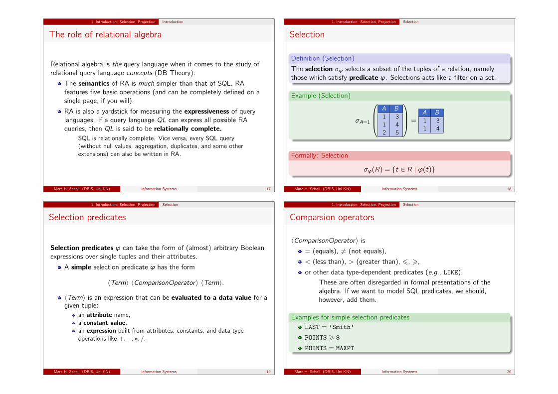
Example database (recap)
Homework database
STUDENTSSID FIRST LAST EMAIL101 Ann Smith ...102 Michael Jones (null)103 Richard Turner ...104 Maria Brown ...
EXERCISESCAT ENO TOPIC MAXPT
H 1 Rel.Alg. 10H 2 SQL 10M 1 SQL 14
RESULTSSID CAT ENO POINTS101 H 1 10101 H 2 8101 M 1 12102 H 1 9102 H 2 9102 M 1 10103 H 1 5103 M 1 7
Marc H. Scholl (DBIS, Uni KN) Information Systems 11
1. Introduction: Selection, Projection Introduction
Relational algebra
Relational algebra (RA) is a query language for the relationalmodel with a solid theoretical foundation.
Relational algebra is not visible at the user interface level (not in anycommercial RDBMS, at least).
However, almost all RDBMSs use RA to represent queriesinternally (for query optimization and execution).Knowledge of relational algebra will help in understanding SQL andrelational database systems in general.
Marc H. Scholl (DBIS, Uni KN) Information Systems 12

1. Introduction: Selection, Projection Introduction
Mathematical algebras
In mathematics, an algebra is a
set (the “carrier”), together with
operations that are closed with respect to the set.
Example
(N, {∗,+}) forms an algebra.
In case of the relational algebra,
the carrier is the set of all finite relations.We will get to know the operations of RA in the sequel (one suchoperation is, for example, ∪).
Marc H. Scholl (DBIS, Uni KN) Information Systems 13
1. Introduction: Selection, Projection Introduction
Relational algebra: Selection
Another operation of relational algebra is selection.In contrast to operations like + in N, the selection σ isparameterized by a simple predicate.
For example, the operation σSID=101 selects all tuples in the input relationthat have the value 101 in column SID.
σSID=101
RESULTSSID CAT ENO POINTS101 H 1 10101 H 2 8101 M 1 12102 H 1 9102 H 2 9102 M 1 10103 H 1 5103 M 1 7
=
SID CAT ENO POINTS101 H 1 10101 H 2 8101 M 1 12
Marc H. Scholl (DBIS, Uni KN) Information Systems 14
1. Introduction: Selection, Projection Introduction
Relational algebra: Composition of expressions
Since the output of any RA operation is some relation R again, Rmay be the input for another RA operation.
The operations of RA nest to arbitrary depth such that complexqueries can be evaluated. The final result will always be arelation.
A query is a term (or expression) in this relational algebra.
A query
πFIRST,LAST(STUDENTS 1 σCAT=’M’(RESULTS))
Marc H. Scholl (DBIS, Uni KN) Information Systems 15
1. Introduction: Selection, Projection Introduction
Relational algebra vs. SQL
There are some differences between the two query languages RA andSQL:
Null values are usually excluded in the definition of relational algebra,except when operations like outer join are defined.
Relational algebra treats relations as sets, i.e., duplicate tupleswill never occur in the input/output relations of an RA operator.
Remember: In SQL, relations are multisets (bags) and maycontain duplicates. Duplicate elimination is explicit in SQL(SELECT DISTINCT).
SQL contains much more functionality than the algebraic core.
Marc H. Scholl (DBIS, Uni KN) Information Systems 16
1. Introduction: Selection, Projection Introduction
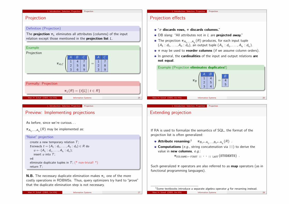
The role of relational algebra
Relational algebra is the query language when it comes to the study ofrelational query language concepts (DB Theory):
The semantics of RA is much simpler than that of SQL. RAfeatures five basic operations (and can be completely defined on asingle page, if you will).
RA is also a yardstick for measuring the expressiveness of querylanguages. If a query language QL can express all possible RAqueries, then QL is said to be relationally complete.
SQL is relationally complete. Vice versa, every SQL query(without null values, aggregation, duplicates, and some otherextensions) can also be written in RA.
Marc H. Scholl (DBIS, Uni KN) Information Systems 17
1. Introduction: Selection, Projection Selection
Selection
Definition (Selection)
The selection σϕ selects a subset of the tuples of a relation, namelythose which satisfy predicate ϕ. Selections acts like a filter on a set.
Example (Selection)
σA=1
A B
1 31 42 5
=A B
1 31 4
Formally: Selection
σϕ(R) = {t ∈ R | ϕ(t)}
Marc H. Scholl (DBIS, Uni KN) Information Systems 18
1. Introduction: Selection, Projection Selection
Selection predicates
Selection predicates ϕ can take the form of (almost) arbitrary Booleanexpressions over single tuples and their attributes.
A simple selection predicate ϕ has the form
〈Term〉 〈ComparisonOperator〉 〈Term〉.
〈Term〉 is an expression that can be evaluated to a data value for agiven tuple:
an attribute name,a constant value,an expression built from attributes, constants, and data typeoperations like +,−, ∗, /.
Marc H. Scholl (DBIS, Uni KN) Information Systems 19
1. Introduction: Selection, Projection Selection
Comparsion operators
〈ComparisonOperator〉 is= (equals), 6= (not equals),
< (less than), > (greater than), 6, >,or other data type-dependent predicates (e.g., LIKE).
These are often disregarded in formal presentations of thealgebra. If we want to model SQL predicates, we should,however, add them.
Examples for simple selection predicatesLAST = ’Smith’
POINTS > 8
POINTS = MAXPT
Marc H. Scholl (DBIS, Uni KN) Information Systems 20

1. Introduction: Selection, Projection Selection
Preview: Implementing selections
Actually, we do not want to know, how an RDBMS implements itsoperators. Since we’re all sort of curious, though, let’s have a sneakpreview. . .σϕ(R) may be implemented as:
“Naive” selectioncreate a new temporary relation T ;foreach t ∈ R dop ← ϕ(t); (* evaluate ϕ on current input tuple *)if p then
insert t into T ; (* collect matches *)fi
odreturn T ;
If index structures are present (e.g., a B-tree index), it is possible toevaluate σϕ(R) without reading every tuple of R.Marc H. Scholl (DBIS, Uni KN) Information Systems 21
1. Introduction: Selection, Projection Selection
Selection trivia
A few corner cases
σC=1
A B1 31 42 5
= (schema error)
σA=A
A B1 31 42 5
=
A B1 31 42 5
σ1=2
A B1 31 42 5
= A B
Marc H. Scholl (DBIS, Uni KN) Information Systems 22
1. Introduction: Selection, Projection Selection
Compound predicates
More complex selection predicates may be expressed using the Booleanconnectives (and the usual preference rules among them):
ϕ1 ∧ ϕ2 (“and”),ϕ1 ∨ ϕ2 (“or”),¬ϕ1 (“not”).
Notice:σϕ1∧ϕ2(R) = σϕ1(σϕ2(R)).
∨ and ¬Are the Boolean connectives ∨,¬ strictly needed?
The selection predicate must permit evaluation for each input tuplein isolation.
Thus, exists (∃) and for all (∀) or nested relational algebraqueries are not permitted in selection predicates. Actually, suchpredicates do not add to the expressiveness of RA.
Marc H. Scholl (DBIS, Uni KN) Information Systems 23
1. Introduction: Selection, Projection Selection
Selection in SQL
σϕ(R) corresponds to the following SQL query:
SELECT *FROM R
WHERE ϕ
N.B.A different relational algebra operation called projection correspondsto the SELECT clause. Source of confusion.
�SQL allows for more complicated forms of predicates.
Marc H. Scholl (DBIS, Uni KN) Information Systems 24
1. Introduction: Selection, Projection Projection
Projection
Definition (Projection)
The projection πL eliminates all attributes (columns) of the inputrelation except those mentioned in the projection list L.
Example
Projection
πA,C
A B C
1 4 72 5 83 6 9
=
A C
1 72 83 9
Formally: Projection
πL(R) = {t[L] | t ∈ R}Marc H. Scholl (DBIS, Uni KN) Information Systems 25
1. Introduction: Selection, Projection Projection
Projection effects
“σ discards rows, π discards columns.”DB slang: “All attributes not in L are projected away.”The projection πAi1 ,...,Aik (R) produces, for each input tuple(A1 : d1, . . . , An : dn), an output tuple (Ai1 : di1 , . . . , Aik : dik ).
π may be used to reorder columns (if we assume column orders).
In general, the cardinalities of the input and output relations arenot equal.
Example (Projection eliminates duplicates!)
πB
A B
1 42 53 4
=B
45
Marc H. Scholl (DBIS, Uni KN) Information Systems 26
1. Introduction: Selection, Projection Projection
Preview: Implementing projections
As before, since we’re curious. . .
πAi1 ,...,Aik (R) may be implemented as:
“Naive” projectioncreate a new temporary relation T ;foreach t = (A1 : d1, . . . , An : dn) ∈ R dou ← (Ai1 : di1 , . . . , Aik : dik );insert u into T ;
odeliminate duplicate tuples in T ; (* non-trivial! *)return T ;
N.B. The necessary duplicate elimination makes πL one of the morecostly operations in RDBMSs. Thus, query optimizers try hard to “prove”that the duplicate elimination step is not necessary.
Marc H. Scholl (DBIS, Uni KN) Information Systems 27
1. Introduction: Selection, Projection Projection
Extending projection
If RA is used to formalize the semantics of SQL, the format of theprojection list is often generalized:
Attribute renaming:1 πB1←Ai1 ,...,Bk←Aik (R) .
Computations (e.g., string concatenation via ||) to derive thevalue in new columns, e.g.:
πSID,NAME← FIRST || ’ ’ || LAST (STUDENTS) .
Such generalized π operators are also referred to as map operators (as infunctional programming languages).
1Some textbooks introduce a separate algebra operator % for renaming instead.Marc H. Scholl (DBIS, Uni KN) Information Systems 28
1. Introduction: Selection, Projection Projection
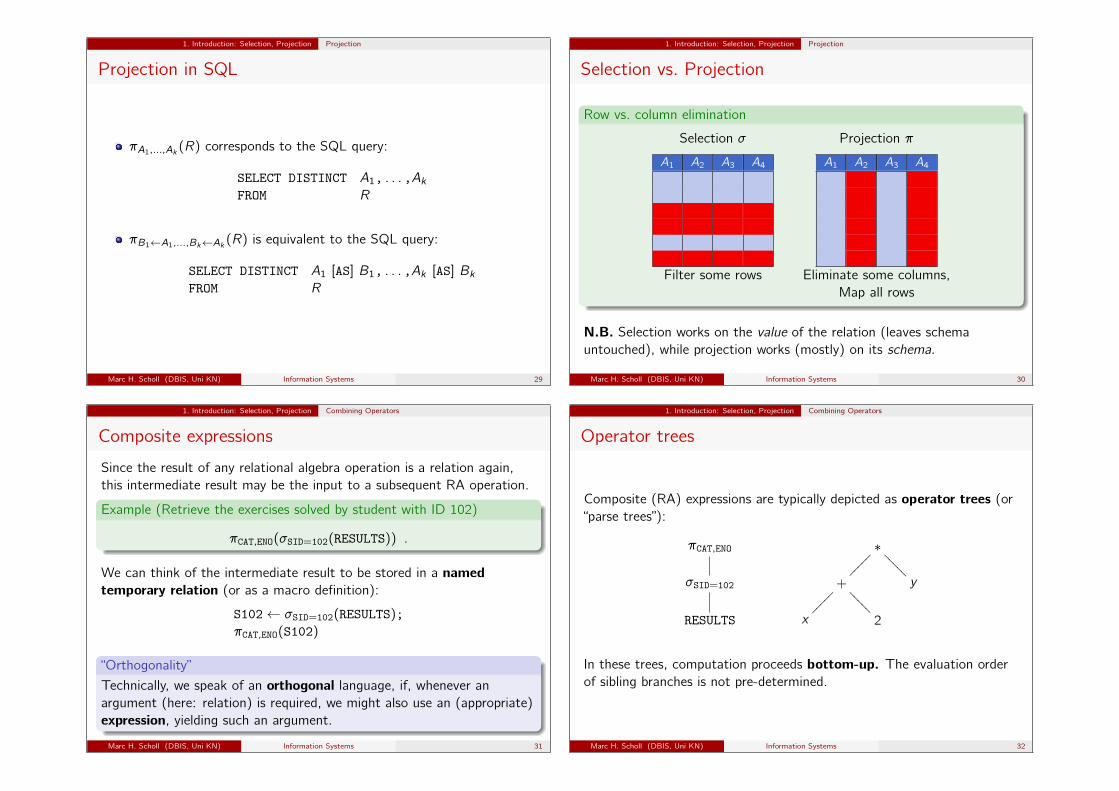
Projection in SQL
πA1,...,Ak (R) corresponds to the SQL query:
SELECT DISTINCT A1, . . . ,AkFROM R
πB1←A1,...,Bk←Ak (R) is equivalent to the SQL query:
SELECT DISTINCT A1 [AS] B1, . . . ,Ak [AS] BkFROM R
Marc H. Scholl (DBIS, Uni KN) Information Systems 29
1. Introduction: Selection, Projection Projection
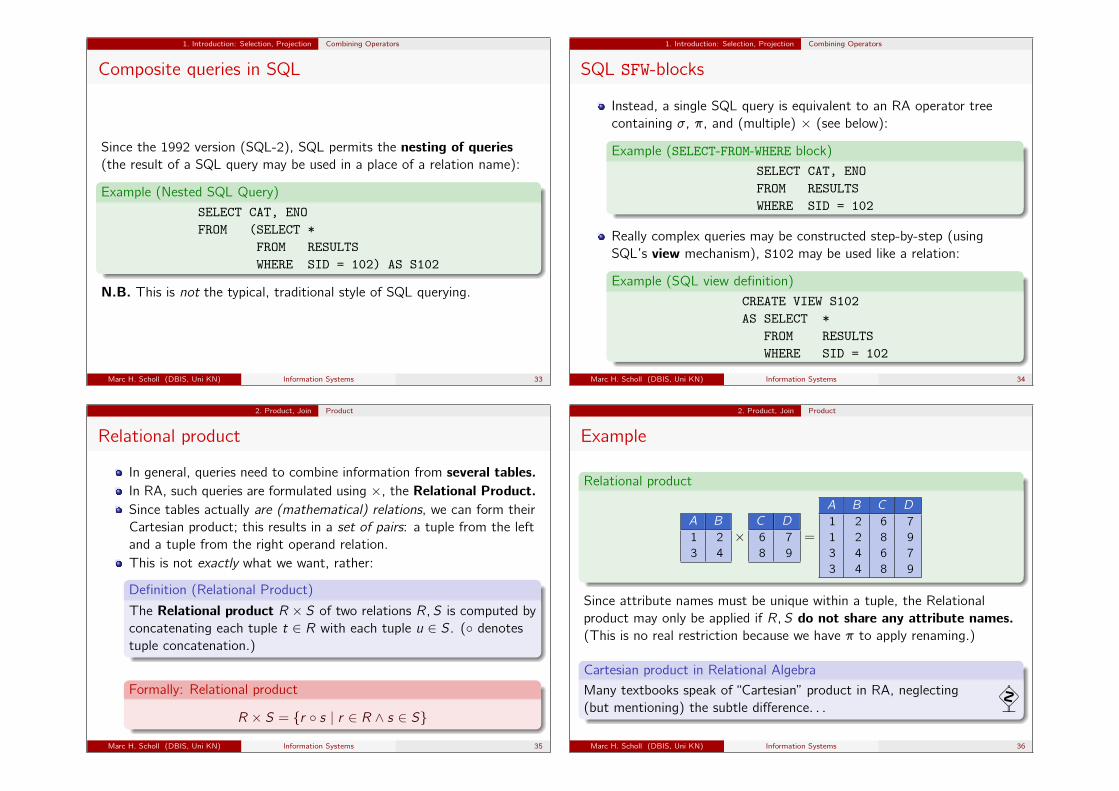
Selection vs. Projection
Row vs. column elimination
Selection σ Projection π
A1 A2 A3 A4 A1 A2 A3 A4
Filter some rows Eliminate some columns,Map all rows
N.B. Selection works on the value of the relation (leaves schemauntouched), while projection works (mostly) on its schema.
Marc H. Scholl (DBIS, Uni KN) Information Systems 30
1. Introduction: Selection, Projection Combining Operators
Composite expressions
Since the result of any relational algebra operation is a relation again,this intermediate result may be the input to a subsequent RA operation.
Example (Retrieve the exercises solved by student with ID 102)
πCAT,ENO(σSID=102(RESULTS)) .
We can think of the intermediate result to be stored in a namedtemporary relation (or as a macro definition):
S102← σSID=102(RESULTS);πCAT,ENO(S102)
“Orthogonality”
Technically, we speak of an orthogonal language, if, whenever anargument (here: relation) is required, we might also use an (appropriate)expression, yielding such an argument.
Marc H. Scholl (DBIS, Uni KN) Information Systems 31
1. Introduction: Selection, Projection Combining Operators
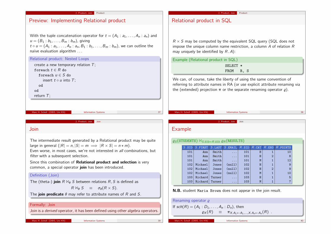
Operator trees
Composite (RA) expressions are typically depicted as operator trees (or“parse trees”):
πCAT,ENO
σSID=102
RESULTS
∗
+�����
x�����
2????? y
?????
In these trees, computation proceeds bottom-up. The evaluation orderof sibling branches is not pre-determined.
Marc H. Scholl (DBIS, Uni KN) Information Systems 32
1. Introduction: Selection, Projection Combining Operators
Composite queries in SQL
Since the 1992 version (SQL-2), SQL permits the nesting of queries(the result of a SQL query may be used in a place of a relation name):
Example (Nested SQL Query)SELECT CAT, ENOFROM (SELECT *
FROM RESULTSWHERE SID = 102) AS S102
N.B. This is not the typical, traditional style of SQL querying.
Marc H. Scholl (DBIS, Uni KN) Information Systems 33
1. Introduction: Selection, Projection Combining Operators
SQL SFW-blocks
Instead, a single SQL query is equivalent to an RA operator treecontaining σ, π, and (multiple) × (see below):
Example (SELECT-FROM-WHERE block)SELECT CAT, ENOFROM RESULTSWHERE SID = 102
Really complex queries may be constructed step-by-step (usingSQL’s view mechanism), S102 may be used like a relation:
Example (SQL view definition)CREATE VIEW S102AS SELECT *
FROM RESULTSWHERE SID = 102
Marc H. Scholl (DBIS, Uni KN) Information Systems 34
2. Product, Join Product
Relational product
In general, queries need to combine information from several tables.In RA, such queries are formulated using ×, the Relational Product.Since tables actually are (mathematical) relations, we can form theirCartesian product; this results in a set of pairs: a tuple from the leftand a tuple from the right operand relation.This is not exactly what we want, rather:
Definition (Relational Product)
The Relational product R× S of two relations R,S is computed byconcatenating each tuple t ∈ R with each tuple u ∈ S. (◦ denotestuple concatenation.)
Formally: Relational product
R × S = {r ◦ s | r ∈ R ∧ s ∈ S}Marc H. Scholl (DBIS, Uni KN) Information Systems 35
2. Product, Join Product
Example
Relational product
A B
1 23 4
×C D
6 78 9
=
A B C D
1 2 6 71 2 8 93 4 6 73 4 8 9
Since attribute names must be unique within a tuple, the Relationalproduct may only be applied if R,S do not share any attribute names.(This is no real restriction because we have π to apply renaming.)
Cartesian product in Relational Algebra
Many textbooks speak of “Cartesian” product in RA, neglecting(but mentioning) the subtle difference. . .
�Marc H. Scholl (DBIS, Uni KN) Information Systems 36
2. Product, Join Product
Preview: Implementing Relational product
With the tuple concatenation operator for t = (A1 : a1, . . . , An : an) andu = (B1 : b1, . . . , Bm : bm), givingt ◦ u = (A1 : a1, . . . , An : an, B1 : b1, . . . , Bm : bm), we can outline thenaïve evaluation algorithm . . .
Relational product: Nested Loops
create a new temporary relation T ;foreach t ∈ R doforeach u ∈ S doinsert t ◦ u into T ;
ododreturn T ;
Marc H. Scholl (DBIS, Uni KN) Information Systems 37
2. Product, Join Product
Relational product in SQL
R × S may be computed by the equivalent SQL query (SQL does notimpose the unique column name restriction, a column A of relation Rmay uniquely be identified by R.A):
Example (Relational product in SQL)SELECT *FROM R, S
We can, of course, take the liberty of using the same convention ofreferring to attribute names in RA (or use explicit attribute renaming viathe (extended) projection π or the separate renaming operator %).
Marc H. Scholl (DBIS, Uni KN) Information Systems 38
2. Product, Join Join
Join
The intermediate result generated by a Relational product may be quitelarge in general (|R| = n, |S| = m =⇒ |R × S| = n ∗m).Even worse, in most cases, we’re not interested in all combinations, butfilter with a subsequent selection.
Since this combination of Relational product and selection is verycommon, a special operator join has been introduced.
Definition (Join)
The (theta-) join R 1θ S between relations R,S is defined as
R 1θ S ≡ σθ(R × S).
The join predicate θ may refer to attribute names of R and S.
Formally: Join
Join is a derived operator, it has been defined using other algebra operators.
Marc H. Scholl (DBIS, Uni KN) Information Systems 39
2. Product, Join Join
Example
%S(STUDENTS) 1S.SID=R.SID %R(RESULTS)
S.SID S.FIRST S.LAST S.EMAIL R.SID R.CAT R.ENO R.POINTS101 Ann Smith ... 101 H 1 10101 Ann Smith ... 101 H 2 8101 Ann Smith ... 101 M 1 12102 Michael Jones (null) 102 H 1 9102 Michael Jones (null) 102 H 2 9102 Michael Jones (null) 102 M 1 10103 Richard Turner ... 103 H 1 5103 Richard Turner ... 103 M 1 7
N.B. student Maria Brown does not appear in the join result.
Renaming operator %
If sch(R) = (A1 : D1, . . . , An : Dn), then%X(R) ≡ πX.A1←A1,...,X.An←An(R) .
Marc H. Scholl (DBIS, Uni KN) Information Systems 40

2. Product, Join Join
Preview: Implementing join
R 1θ S can be evaluated by “folding” the above procedures for σ,×:Nested Loop Join
create a new temporary relation T ;foreach t ∈ R doforeach u ∈ S doif θ(t ◦ u) then
insert t ◦ u into T ;fi
ododreturn T ;
Marc H. Scholl (DBIS, Uni KN) Information Systems 41
2. Product, Join Join
Join eliminates some tuples
Join combines tuples from two relations and acts like a filter: tupleswithout join partner are removed.N.B. if the join is used to follow a foreign key relationship, thenno tuples are filtered:
Join follows a foreign key relationship (dereference)
RESULTS 1SID=S.SID πS.SID←SID,FIRST,LAST,EMAIL(STUDENTS)
There are join variants which act like filters only: left and rightsemi-join (n,o):
R nθ S ≡ πsch(R)(R 1θ S) ,
or do not filter at all: outer join (see below).
Marc H. Scholl (DBIS, Uni KN) Information Systems 42
2. Product, Join Join
Natural Join
The natural join provides another useful abbreviation (“RA macro”).In the natural join R 1 S, the join predicate θ is defined to be aconjunctive equality comparison of attributes sharing the same namein R,S.Natural join automatically handles the necessary attribute renaming andprojection.
Example (Natural Join)
Assume R(A,B, C) and S(B,C,D). Then:
R 1 S = πA,B,C,D(σB=B′∧C=C′(R × πB′←B,C′←C,D(S)))
(Note: shared columns occur only once in the result.)
Marc H. Scholl (DBIS, Uni KN) Information Systems 43
2. Product, Join Join
Joins in SQL
In SQL, R 1θ S is can be written in a variety of ways, most prominently:
Join in SQL (“classic” and SQL-92)
SELECT ∗FROM R,SWHERE θ
orSELECT ∗FROM R JOIN S ON (θ)
Note: the left query is the exact SQL equivalent of σθ(R × S) we haveseen before.
SQL is a declarative language: it is the task of the SQLoptimizer to infer that this query may be evaluated using a joininstead of a Cartesian product.
Marc H. Scholl (DBIS, Uni KN) Information Systems 44

2. Product, Join Join
Algebraic equivalence laws
Joins obey some very useful algebraic laws, e.g.,
Associativity: (R 1 S) 1 T ≡ R 1 (S 1 T ) .
Hence, in “join chains”, parentheses can be omitted: R 1 S 1 T .
Commutativity: depending on whether we consider attribute ordersignificant, join iscommutative by itself, or only if followed by a projection (column reordering):
R 1 S ≡ S 1 R ,
or onlyπL(R 1 S) ≡ πL(S 1 R) .
Selection push-down: If ϕ refers to attributes in S only, thenσϕ(R 1 S) ≡ R 1 σϕ(S) .
Selection push-down
Why is selection push-down considered one of the most significant alge-braic optimizations?
Marc H. Scholl (DBIS, Uni KN) Information Systems 45
2. Product, Join Join
A common query pattern
The following operator tree structure is very common:
Select-Project-Join (SPJ) queries
πA1,...,Ak
σϕ
1θ11θ2 ooo
1θn−1Rn
oooRn−1
OO R2
OOOO R1
OOOO
1 Join all tables needed to answer the query,2 select the relevant tuples,3 project away all irrelevant columns.
Marc H. Scholl (DBIS, Uni KN) Information Systems 46
2. Product, Join Join
Select-project-join queries in SQL
The select-project-join query
πA1,...,Ak (σϕ(R1 1θ1 R2 1θ2 · · · 1θn−1 Rn))
has the obvious SQL equivalent
SELECT DISTINCT A1, . . . ,AkFROM R1, . . . ,RnWHERE ϕ
AND θ1 AND · · · AND θn−1
It is a common source of errors to forget a join condition: think of thescenario R(A,B), S(B,C), T (C,D) when attributes A,D arerelevant for the query output.
�Marc H. Scholl (DBIS, Uni KN) Information Systems 47
2. Product, Join Join
Algebra quiz (entry level)
Homework database (recap)
STUDENTSSID FIRST LAST EMAIL101 Ann Smith ...102 Michael Jones (null)103 Richard Turner ...104 Maria Brown ...
EXERCISESCAT ENO TOPIC MAXPTH 1 Rel.Alg. 10H 2 SQL 10M 1 SQL 14
RESULTSSID CAT ENO POINTS101 H 1 10101 H 2 8101 M 1 12102 H 1 9102 H 2 9102 M 1 10103 H 1 5103 M 1 7
Marc H. Scholl (DBIS, Uni KN) Information Systems 48
2. Product, Join Join
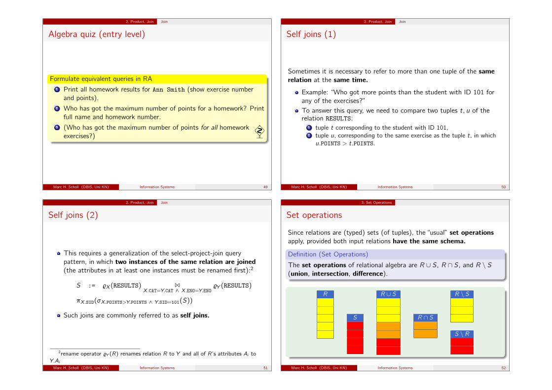
Algebra quiz (entry level)
Formulate equivalent queries in RA1 Print all homework results for Ann Smith (show exercise number
and points).2 Who has got the maximum number of points for a homework? Print
full name and homework number.3 (Who has got the maximum number of points for all homework
exercises?)�
Marc H. Scholl (DBIS, Uni KN) Information Systems 49
2. Product, Join Join
Self joins (1)
Sometimes it is necessary to refer to more than one tuple of the samerelation at the same time.
Example: “Who got more points than the student with ID 101 forany of the exercises?”To answer this query, we need to compare two tuples t, u of therelation RESULTS:
1 tuple t corresponding to the student with ID 101,2 tuple u, corresponding to the same exercise as the tuple t, in whichu.POINTS > t.POINTS.
Marc H. Scholl (DBIS, Uni KN) Information Systems 50
2. Product, Join Join
Self joins (2)
This requires a generalization of the select-project-join querypattern, in which two instances of the same relation are joined(the attributes in at least one instances must be renamed first):2
S := %X(RESULTS) 1X.CAT=Y.CAT ∧ X.ENO=Y.ENO
%Y (RESULTS)
πX.SID(σX.POINTS>Y.POINTS ∧ Y.SID=101(S))
Such joins are commonly referred to as self joins.
2rename operator %Y (R) renames relation R to Y and all of R’s attributes Ai toY.AiMarc H. Scholl (DBIS, Uni KN) Information Systems 51
3. Set Operations
Set operations
Since relations are (typed) sets (of tuples), the “usual” set operationsapply, provided both input relations have the same schema.
Definition (Set Operations)
The set operations of relational algebra are R ∪ S, R ∩ S, and R \ S(union, intersection, difference).
R
S
R ∪ S
R ∩ S
R \ S
S \ R
Marc H. Scholl (DBIS, Uni KN) Information Systems 52
3. Set Operations
Preview: Implementing set operations
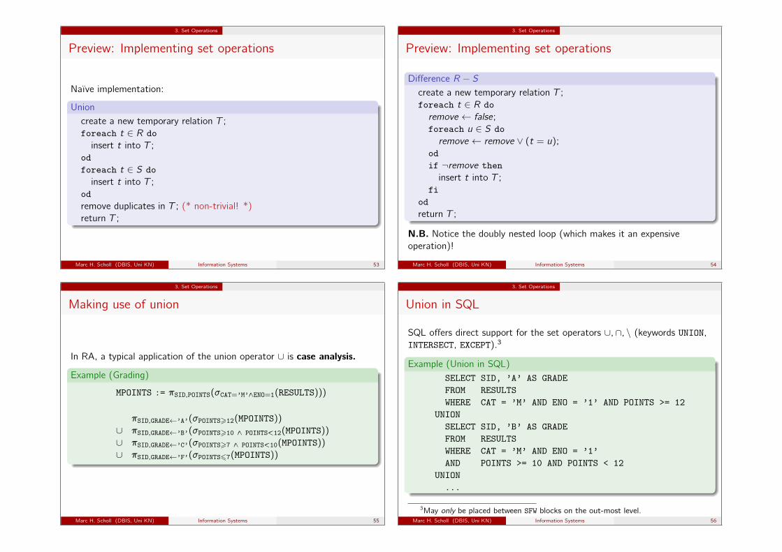
Naïve implementation:
Unioncreate a new temporary relation T ;foreach t ∈ R doinsert t into T ;
odforeach t ∈ S doinsert t into T ;
odremove duplicates in T ; (* non-trivial! *)return T ;
Marc H. Scholl (DBIS, Uni KN) Information Systems 53
3. Set Operations
Preview: Implementing set operations
Difference R − Screate a new temporary relation T ;foreach t ∈ R do
remove ← false;foreach u ∈ S do
remove ← remove ∨ (t = u);odif ¬remove theninsert t into T ;
fiodreturn T ;
N.B. Notice the doubly nested loop (which makes it an expensiveoperation)!
Marc H. Scholl (DBIS, Uni KN) Information Systems 54
3. Set Operations
Making use of union
In RA, a typical application of the union operator ∪ is case analysis.
Example (Grading)
MPOINTS := πSID,POINTS(σCAT=’M’∧ENO=1(RESULTS)))
πSID,GRADE←’A’(σPOINTS>12(MPOINTS))
∪ πSID,GRADE←’B’(σPOINTS>10 ∧ POINTS<12(MPOINTS))
∪ πSID,GRADE←’C’(σPOINTS>7 ∧ POINTS<10(MPOINTS))
∪ πSID,GRADE←’F’(σPOINTS67(MPOINTS))
Marc H. Scholl (DBIS, Uni KN) Information Systems 55
3. Set Operations
Union in SQL
SQL offers direct support for the set operators ∪,∩, \ (keywords UNION,INTERSECT, EXCEPT).3
Example (Union in SQL)SELECT SID, ’A’ AS GRADEFROM RESULTSWHERE CAT = ’M’ AND ENO = ’1’ AND POINTS >= 12
UNIONSELECT SID, ’B’ AS GRADEFROM RESULTSWHERE CAT = ’M’ AND ENO = ’1’AND POINTS >= 10 AND POINTS < 12
UNION...
3May only be placed between SFW blocks on the out-most level.Marc H. Scholl (DBIS, Uni KN) Information Systems 56
3. Set Operations
What’s special about Set Difference?
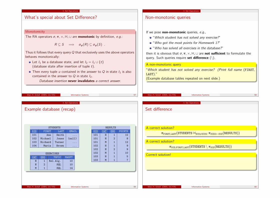
Monotonicity
The RA operators σ, π,×,1,∪ are monotonic by definition, e.g.:
R ⊆ S =⇒ σϕ(R) ⊆ σϕ(S) .
Thus it follows that every query Q that exclusively uses the above operatorsbehaves monotonically:
Let I1 be a database state, and let I2 = I1 ∪ {t}(database state after insertion of tuple t).
Then every tuple u contained in the answer to Q in state I1 is alsocontained in the answer to Q in state I2.
Database insertion never invalidates a correct answer.
Marc H. Scholl (DBIS, Uni KN) Information Systems 57
3. Set Operations
Non-monotonic queries
If we pose non-monotonic queries, e.g.,
“Which student has not solved any exercise?”
“Who got the most points for Homework 1?”
“Who has solved all exercises in the database?”
then it is obvious that σ, π,×,1,∪ are not sufficient to formulate thequery. Such queries require set difference (\).A non-monotonic query
“Which student has not solved any exercise? (Print full name (FIRST,LAST).”(Example database tables repeated on next slide.)
Marc H. Scholl (DBIS, Uni KN) Information Systems 58
3. Set Operations
Example database (recap)
STUDENTSSID FIRST LAST EMAIL101 Ann Smith ...102 Michael Jones (null)103 Richard Turner ...104 Maria Brown ...
EXERCISESCAT ENO TOPIC MAXPTH 1 Rel.Alg. 10H 2 SQL 10M 1 SQL 14
RESULTSSID CAT ENO POINTS101 H 1 10101 H 2 8101 M 1 12102 H 1 9102 H 2 9102 M 1 10103 H 1 5103 M 1 7
Marc H. Scholl (DBIS, Uni KN) Information Systems 59
3. Set Operations
Set difference
A correct solution?
πFIRST,LAST(STUDENTS 1SID 6=SID2 πSID2←SID(RESULTS))
A correct solution?
πSID,FIRST,LAST(STUDENTS \ πSID(RESULTS))
Correct solution!
NO_SOL := πSID(STUDENTS) \ πSID(RESULTS)
πFIRST,LAST(STUDENTS 1 NO_SOL)
Marc H. Scholl (DBIS, Uni KN) Information Systems 60

3. Set Operations
Anti-Join
A typical RA query pattern involving set difference is the anti-join.
Example
Given R(A,B) and S(B,C), retrieve the tuples of R that do not have a(natural) join partner in S: (Note: sch(R) ∩ sch(S) = {B})
R 1 (πB(R) \ πB(S)) .
Or, equivalently: R \ πsch(R)(R 1 S).
Anti-Join
There is no common symbol for this anti-join, but RnS seemsappropriate (complemented semi-join): RnS ≡ R \ (R n S).
Marc H. Scholl (DBIS, Uni KN) Information Systems 61
3. Set Operations
SQL quiz (intermediate level)
While SQL now has explicit operators for all kinds of joins, there isneither a semi- nor an anti-join operator available in SQL.Semi-Join and Anti-Join in SQL?How would you express the equivalents of those two operators in SQL?
Marc H. Scholl (DBIS, Uni KN) Information Systems 62
3. Set Operations
Set operations and compound selection predicates
Once we have the set operations, we don’t actually need complexselection predicates any more.
Predicate simplification rules
σϕ1∧ϕ2(Q) ≡ σϕ1(Q) ∩ σϕ2(Q)
σϕ1∨ϕ2(Q) ≡ σϕ1(Q) ∪ σϕ2(Q)
σ¬ϕ(Q) ≡ Q \ σϕ(Q)
RDBMS implements complex selection predicates anyway!
Why?
Marc H. Scholl (DBIS, Uni KN) Information Systems 63
3. Set Operations
Relational algebra quiz (intermediate level)
Again, we refer to the HOMEWORK database schema:
RESULTS (SID → STUDENTS,(CAT, ENO) → EXERCISES, POINTS)STUDENTS (SID,FIRST,LAST,EMAIL)EXERCISES (CAT,ENO,TOPIC,MAXPT)
Formulate equivalent queries in RA1 Who got the most points (of all students) for Homework 1?
RES_SID = πsid(STUDENTS) \πX.sid(%X(σcat=’H’∧eno=1(RESULTS))
1X.points<Y.points
%Y (σcat=’H’∧eno=1(RESULTS)))
πS.first,S.last(%S(STUDENTS) 1S.sid=X.sid %X(RES_SID))
Marc H. Scholl (DBIS, Uni KN) Information Systems 64
3. Set Operations
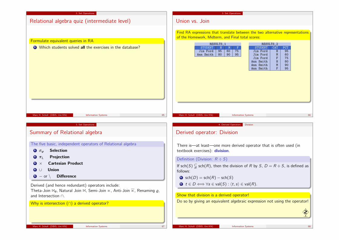
Relational algebra quiz (intermediate level)
Formulate equivalent queries in RA2 Which students solved all the exercises in the database?
RES_SID = πsid(STUDENTS) \ πX.sid(
(πsid(STUDENTS)× πcat,eno(EXERCISES))
\πsid,cat,eno(RESULTS) )
πfirst,last(STUDENTS 1 RES_SID)
Marc H. Scholl (DBIS, Uni KN) Information Systems 65
3. Set Operations
Union vs. Join
Find RA expressions that translate between the two alternative representationsof the Homework, Midterm, and Final total scores:
RESULTS_1STUDENT H M FJim Ford 95 60 75
Ann Smith 80 90 95
RESULTS_2STUDENT CAT PCTJim Ford H 95Jim Ford M 60Jim Ford F 75
Ann Smith H 80Ann Smith M 90Ann Smith F 95
RESULTS_1 → RESULTS_2:RESULTS_2 → RESULTS_1:
πSTUDENT,CAT←’H’,PCT←H(RESULTS_1)
∪ πSTUDENT,CAT←’M’,PCT←M(RESULTS_1)
∪ πSTUDENT,CAT←’F’,PCT←F(RESULTS_1)
Marc H. Scholl (DBIS, Uni KN) Information Systems 66
3. Set Operations
Summary of Relational algebra
The five basic, independent operators of Relational algebra1 σϕ Selection2 πL Projection3 × Cartesian Product4 ∪ Union5 − or \ Difference
Derived (and hence redundant) operators include:Theta-Join 1θ, Natural Join 1, Semi-Join n, Anti-Join n, Renaming %,and Intersection ∩.Why is intersection (∩) a derived operator?
R ∩ S ≡ R − (R − S)
Marc H. Scholl (DBIS, Uni KN) Information Systems 67
4. Derived Operators Division
Derived operator: Division
There is—at least—one more derived operator that is often used (intextbook exercises): division.
Definition (Division: R ÷ S)If sch(S) $ sch(R), then the division of R by S, D = R÷S, is defined asfollows:
1 sch(D) = sch(R)− sch(S)
2 t ∈ D ⇐⇒ ∀s ∈ val(S) : 〈t, s〉 ∈ val(R).
Show that division is a derived operator!
Do so by giving an equivalent algebraic expression not using the operator!
�Marc H. Scholl (DBIS, Uni KN) Information Systems 68
4. Derived Operators Division
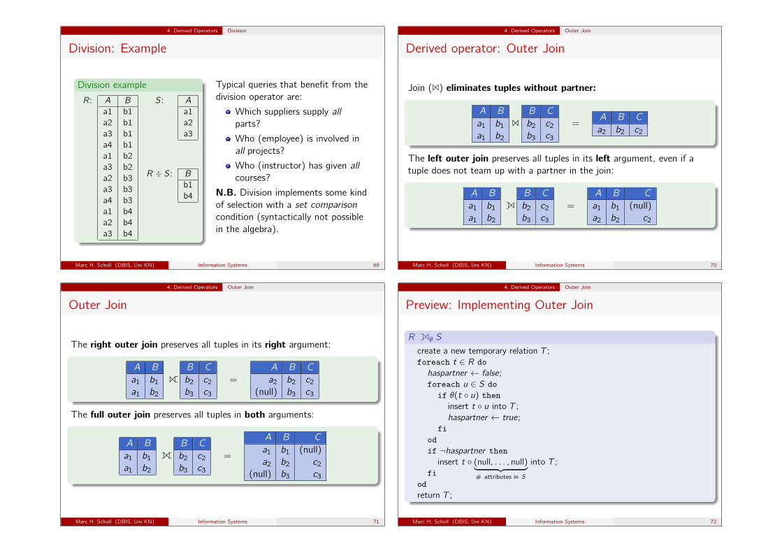
Division: Example
Division example
R: A B
a1 b1a2 b1a3 b1a4 b1a1 b2a3 b2a2 b3a3 b3a4 b3a1 b4a2 b4a3 b4
S: A
a1a2a3
R ÷ S: B
b1b4
Typical queries that benefit from thedivision operator are:
Which suppliers supply allparts?
Who (employee) is involved inall projects?
Who (instructor) has given allcourses?
N.B. Division implements some kindof selection with a set comparisoncondition (syntactically not possiblein the algebra).
Marc H. Scholl (DBIS, Uni KN) Information Systems 69
4. Derived Operators Outer Join
Derived operator: Outer Join
Join (1) eliminates tuples without partner:
A B
a1 b1a1 b2
1B C
b2 c2b3 c3
=A B C
a2 b2 c2
The left outer join preserves all tuples in its left argument, even if atuple does not team up with a partner in the join:
A B
a1 b1a1 b2
1B C
b2 c2b3 c3
=
A B C
a1 b1 (null)a2 b2 c2
Marc H. Scholl (DBIS, Uni KN) Information Systems 70
4. Derived Operators Outer Join
Outer Join
The right outer join preserves all tuples in its right argument:
A B
a1 b1a1 b2
1B C
b2 c2b3 c3
=
A B C
a2 b2 c2(null) b3 c3
The full outer join preserves all tuples in both arguments:
A B
a1 b1a1 b2
1B C
b2 c2b3 c3
=
A B C
a1 b1 (null)a2 b2 c2
(null) b3 c3
Marc H. Scholl (DBIS, Uni KN) Information Systems 71
4. Derived Operators Outer Join
Preview: Implementing Outer Join
R 1θ Screate a new temporary relation T ;foreach t ∈ R do
haspartner ← false;foreach u ∈ S do
if θ(t ◦ u) theninsert t ◦ u into T ;haspartner ← true;
fiodif ¬haspartner then
insert t ◦ (null, . . . , null)︸ ︷︷ ︸# attributes in S
into T ;fi
odreturn T ;
Marc H. Scholl (DBIS, Uni KN) Information Systems 72
4. Derived Operators Outer Join
Example
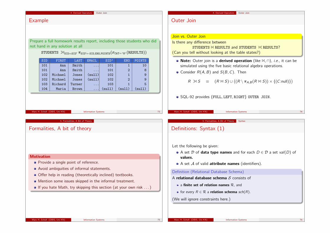
Prepare a full homework results report, including those students who didnot hand in any solution at all
STUDENTS 1SID=SID′ πSID′←SID,ENO,POINTS(σCAT=’H’(RESULTS))
SID FIRST LAST EMAIL SID’ ENO POINTS101 Ann Smith ... 101 1 10101 Ann Smith ... 101 2 8102 Michael Jones (null) 102 1 9102 Michael Jones (null) 102 2 9103 Richard Turner ... 103 1 5104 Maria Brown ... (null) (null) (null)
Marc H. Scholl (DBIS, Uni KN) Information Systems 73
4. Derived Operators Outer Join
Outer Join
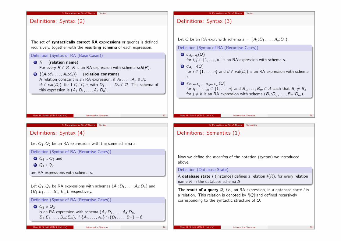
Join vs. Outer JoinIs there any difference between
STUDENTS 1 RESULTS and STUDENTS 1 RESULTS?(Can you tell without looking at the table states?)
Note: Outer join is a derived operation (like 1,∩), i.e., it can besimulated using the five basic relational algebra operations.
Consider R(A,B) and S(B,C). Then
R 1 S ≡ (R 1 S) ∪ ((R \ πA,B(R 1 S))× {(C:null)})SQL-92 provides {FULL, LEFT, RIGHT} OUTER JOIN.
Marc H. Scholl (DBIS, Uni KN) Information Systems 74
5. Formalities, A Bit of Theory
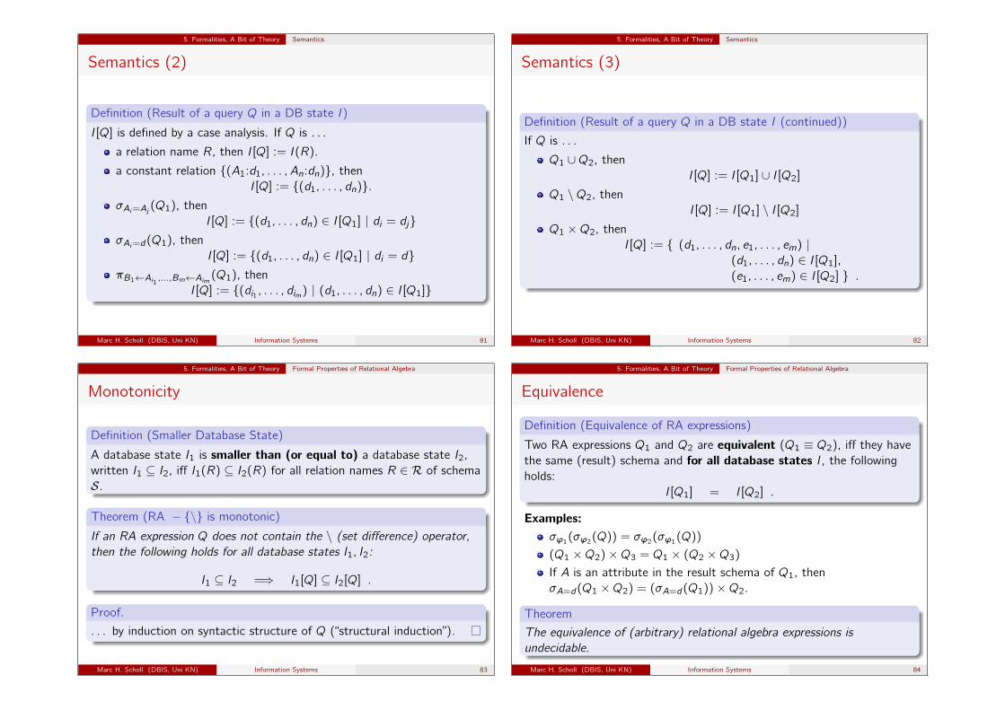
Formalities, A bit of theory
MotivationProvide a single point of reference.
Avoid ambiguities of informal statements.
Offer help in reading (theoretically inclined) textbooks.
Mention some issues skipped in the informal treatment.
If you hate Math, try skipping this section (at your own risk . . . )
Marc H. Scholl (DBIS, Uni KN) Information Systems 75
5. Formalities, A Bit of Theory Syntax
Definitions: Syntax (1)
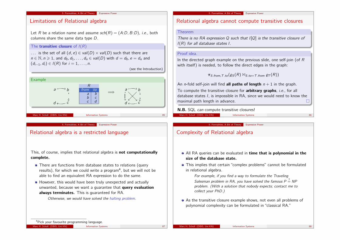
Let the following be given:
A set D of data type names and for each D ∈ D a set val(D) ofvalues.A set A of valid attribute names (identifiers).
Definition (Relational Database Schema)
A relational database schema S consists of
a finite set of relation names R, andfor every R ∈ R a relation schema sch(R).
(We will ignore constraints here.)
Marc H. Scholl (DBIS, Uni KN) Information Systems 76
5. Formalities, A Bit of Theory Syntax
Definitions: Syntax (2)
The set of syntactically correct RA expressions or queries is definedrecursively, together with the resulting schema of each expression.
Definition (Syntax of RA (Base Cases))1 R (relation name)
For every R ∈ R, R is an RA expression with schema sch(R).2 {(A1:d1, . . . , An:dn)} (relation constant)
A relation constant is an RA expression, if A1, . . . , An ∈ A,di ∈ val(Di), for 1 6 i 6 n, with D1, . . . , Dn ∈ D. The schema ofthis expression is (A1:D1, . . . , An:Dn).
Marc H. Scholl (DBIS, Uni KN) Information Systems 77
5. Formalities, A Bit of Theory Syntax
Definitions: Syntax (3)
Let Q be an RA expr. with schema s = (A1:D1, . . . , An:Dn).
Definition (Syntax of RA (Recursive Cases))3 σAi=Aj (Q)
for i , j ∈ {1, . . . , n} is an RA expression with schema s.4 σAi=d(Q)
for i ∈ {1, . . . , n} and d ∈ val(Di) is an RA expression with schemas.
5 πB1←Ai1 ,...,Bm←Aim (Q)
for i1, . . . , im ∈ {1, . . . , n} and B1, . . . , Bm ∈ A such that Bj 6= Bkfor j 6= k is an RA expression with schema (B1:Di1 , . . . , Bm:Dim).
Marc H. Scholl (DBIS, Uni KN) Information Systems 78
5. Formalities, A Bit of Theory Syntax
Definitions: Syntax (4)
Let Q1, Q2 be an RA expressions with the same schema s.
Definition (Syntax of RA (Recursive Cases))6 Q1 ∪Q2 and7 Q1 \Q2
are RA expressions with schema s.
Let Q1, Q2 be RA expressions with schemas (A1:D1, . . . , An:Dn) and(B1:E1, . . . , Bm:Em), respectively.
Definition (Syntax of RA (Recursive Cases))8 Q1 ×Q2
is an RA expression with schema (A1:D1, . . . , An:Dn,
B1:E1, . . . , Bm:Em), if {A1, . . . , An} ∩ {B1, . . . , Bm} = ∅.
Marc H. Scholl (DBIS, Uni KN) Information Systems 79
5. Formalities, A Bit of Theory Semantics
Definitions: Semantics (1)
Now we define the meaning of the notation (syntax) we introducedabove.
Definition (Database State)
A database state I (instance) defines a relation I(R), for every relationname R in the database schema S.The result of a query Q, i.e., an RA expression, in a database state I isa relation. This relation is denoted by I[Q] and defined recursivelycorresponding to the syntactic structure of Q.
Marc H. Scholl (DBIS, Uni KN) Information Systems 80
5. Formalities, A Bit of Theory Semantics
Semantics (2)
Definition (Result of a query Q in a DB state I)
I[Q] is defined by a case analysis. If Q is . . .
a relation name R, then I[Q] := I(R).
a constant relation {(A1:d1, . . . , An:dn)}, thenI[Q] := {(d1, . . . , dn)}.
σAi=Aj (Q1), thenI[Q] := {(d1, . . . , dn) ∈ I[Q1] | di = dj}
σAi=d(Q1), thenI[Q] := {(d1, . . . , dn) ∈ I[Q1] | di = d}
πB1←Ai1 ,...,Bm←Aim (Q1), thenI[Q] := {(di1 , . . . , dim) | (d1, . . . , dn) ∈ I[Q1]}
Marc H. Scholl (DBIS, Uni KN) Information Systems 81
5. Formalities, A Bit of Theory Semantics
Semantics (3)
Definition (Result of a query Q in a DB state I (continued))
If Q is . . .
Q1 ∪Q2, thenI[Q] := I[Q1] ∪ I[Q2]
Q1 \Q2, thenI[Q] := I[Q1] \ I[Q2]
Q1 ×Q2, thenI[Q] := { (d1, . . . , dn, e1, . . . , em) |
(d1, . . . , dn) ∈ I[Q1],
(e1, . . . , em) ∈ I[Q2] } .
Marc H. Scholl (DBIS, Uni KN) Information Systems 82
5. Formalities, A Bit of Theory Formal Properties of Relational Algebra
Monotonicity
Definition (Smaller Database State)
A database state I1 is smaller than (or equal to) a database state I2,written I1 ⊆ I2, iff I1(R) ⊆ I2(R) for all relation names R ∈ R of schemaS.
Theorem (RA − {\} is monotonic)
If an RA expression Q does not contain the \ (set difference) operator,then the following holds for all database states I1, I2:
I1 ⊆ I2 =⇒ I1[Q] ⊆ I2[Q] .
Proof.
. . . by induction on syntactic structure of Q (“structural induction”).
Marc H. Scholl (DBIS, Uni KN) Information Systems 83
5. Formalities, A Bit of Theory Formal Properties of Relational Algebra
Equivalence
Definition (Equivalence of RA expressions)
Two RA expressions Q1 and Q2 are equivalent (Q1 ≡ Q2), iff they havethe same (result) schema and for all database states I, the followingholds:
I[Q1] = I[Q2] .
Examples:σϕ1(σϕ2(Q)) = σϕ2(σϕ1(Q))
(Q1 ×Q2)×Q3 = Q1 × (Q2 ×Q3)
If A is an attribute in the result schema of Q1, thenσA=d(Q1 ×Q2) = (σA=d(Q1))×Q2.
Theorem
The equivalence of (arbitrary) relational algebra expressions isundecidable.
Marc H. Scholl (DBIS, Uni KN) Information Systems 84
5. Formalities, A Bit of Theory Expressive Power
Limitations of Relational algebra
Let R be a relation name and assume sch(R) = (A:D,B:D), i.e., bothcolumns share the same data type D.
The transitive closure of I(R)
. . . is the set of all (d, e) ∈ val(D)× val(D) such that there aren ∈ N, n > 1, and d0, d1, . . . , dn ∈ val(D) with d = d0, e = dn and(di−1, di) ∈ I(R) for i = 1, . . . , n.
(see the Introduction)
Example
a b,,
c��
d ll
Rfrom to
a bb cc d
=⇒ a b,,
c��
d ll
�� ��???????
���������
Marc H. Scholl (DBIS, Uni KN) Information Systems 85
5. Formalities, A Bit of Theory Expressive Power
Relational algebra cannot compute transitive closures
Theorem
There is no RA expression Q such that I[Q] is the transitive closure ofI(R) for all database states I.
Proof idea.
In the directed graph example on the previous slide, one self-join (of Rwith itself) is needed, to follow the direct edges in the graph:
πS.from,T .to(%S(R) 1S.to=T .from %T (R))
An n-fold self-join will find all paths of length n + 1 in the graph.
To compute the transitive closure for arbitrary graphs, i.e., for alldatabase states I, is impossible in RA, since we would need to know themaximal path length in advance.
N.B. SQL can compute transitive closures!Marc H. Scholl (DBIS, Uni KN) Information Systems 86
5. Formalities, A Bit of Theory Expressive Power
Relational algebra is a restricted language
This, of course, implies that relational algebra is not computationallycomplete.
There are functions from database states to relations (queryresults), for which we could write a program4, but we will not beable to find an equivalent RA expression to do the same.
However, this would have been truly unexpected and actuallyunwanted, because we want a guarantee that query evaluationalways terminates. This is guaranteed for RA.
Otherwise, we would have solved the halting problem.
4Pick your favourite programming language.Marc H. Scholl (DBIS, Uni KN) Information Systems 87
5. Formalities, A Bit of Theory Expressive Power
Complexity of Relational algebra
All RA queries can be evaluated in time that is polynomial in thesize of the database state.This implies that certain “complex problems” cannot be formulatedin relational algebra.
For example, if you find a way to formulate the TravelingSalesman problem in RA, you have solved the famous P
?= NP
problem. (With a solution that nobody expects; contact me tocollect your PhD.)
As the transitive closure example shows, not even all problems ofpolynomial complexity can be formulated in “classical RA.”
Marc H. Scholl (DBIS, Uni KN) Information Systems 88
5. Formalities, A Bit of Theory Expressive Power
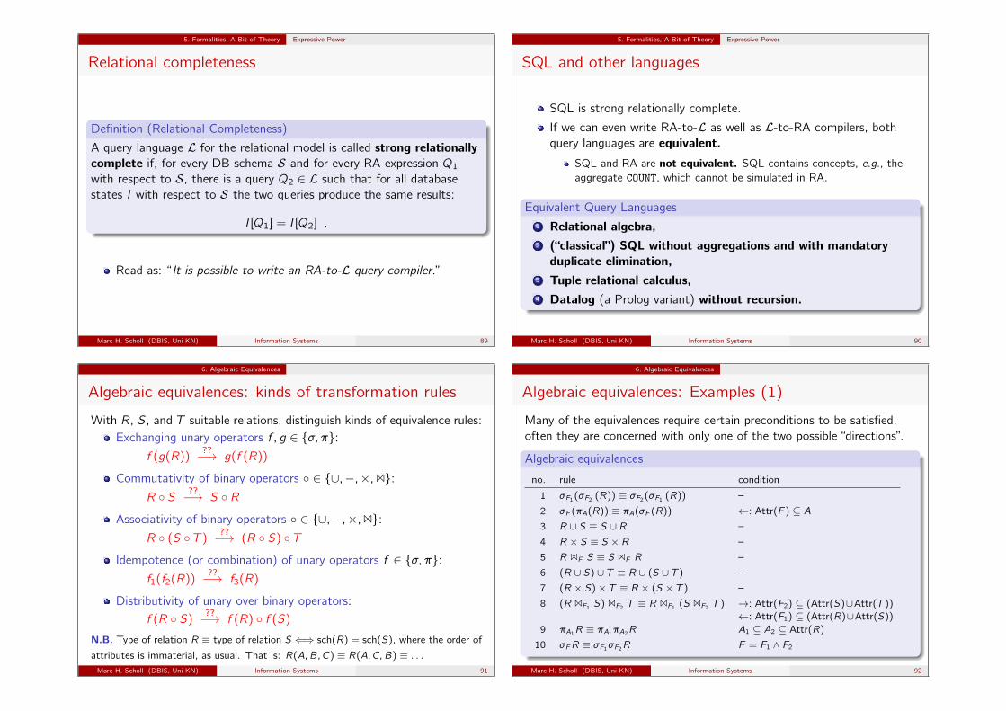
Relational completeness
Definition (Relational Completeness)
A query language L for the relational model is called strong relationallycomplete if, for every DB schema S and for every RA expression Q1
with respect to S, there is a query Q2 ∈ L such that for all databasestates I with respect to S the two queries produce the same results:
I[Q1] = I[Q2] .
Read as: “ It is possible to write an RA-to-L query compiler.”
Marc H. Scholl (DBIS, Uni KN) Information Systems 89
5. Formalities, A Bit of Theory Expressive Power
SQL and other languages
SQL is strong relationally complete.
If we can even write RA-to-L as well as L-to-RA compilers, bothquery languages are equivalent.
SQL and RA are not equivalent. SQL contains concepts, e.g., theaggregate COUNT, which cannot be simulated in RA.
Equivalent Query Languages1 Relational algebra,2 (“classical”) SQL without aggregations and with mandatory
duplicate elimination,3 Tuple relational calculus,4 Datalog (a Prolog variant) without recursion.
Marc H. Scholl (DBIS, Uni KN) Information Systems 90
6. Algebraic Equivalences
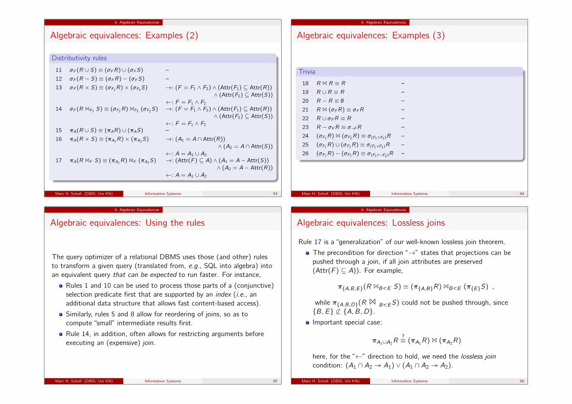
Algebraic equivalences: kinds of transformation rules
With R, S, and T suitable relations, distinguish kinds of equivalence rules:Exchanging unary operators f , g ∈ {σ, π}:
f (g(R))??−→ g(f (R))
Commutativity of binary operators ◦ ∈ {∪,−,×,1}:R ◦ S ??−→ S ◦ R
Associativity of binary operators ◦ ∈ {∪,−,×,1}:R ◦ (S ◦ T )
??−→ (R ◦ S) ◦ TIdempotence (or combination) of unary operators f ∈ {σ, π}:
f1(f2(R))??−→ f3(R)
Distributivity of unary over binary operators:
f (R ◦ S)??−→ f (R) ◦ f (S)
N.B. Type of relation R ≡ type of relation S ⇐⇒ sch(R) = sch(S), where the order of
attributes is immaterial, as usual. That is: R(A,B, C) ≡ R(A,C,B) ≡ . . .Marc H. Scholl (DBIS, Uni KN) Information Systems 91
6. Algebraic Equivalences
Algebraic equivalences: Examples (1)
Many of the equivalences require certain preconditions to be satisfied,often they are concerned with only one of the two possible “directions”.
Algebraic equivalences
no. rule condition
1 σF1(σF2 (R)) ≡ σF2(σF1 (R)) –
2 σF (πA(R)) ≡ πA(σF (R)) ←: Attr(F ) ⊆ A3 R ∪ S ≡ S ∪ R –
4 R × S ≡ S × R –
5 R 1F S ≡ S 1F R –
6 (R ∪ S) ∪ T ≡ R ∪ (S ∪ T ) –
7 (R × S)× T ≡ R × (S × T ) –
8 (R 1F1 S) 1F2 T ≡ R 1F1 (S 1F2 T ) →: Attr(F2) ⊆ (Attr(S)∪Attr(T ))←: Attr(F1) ⊆ (Attr(R)∪Attr(S))
9 πA1R ≡ πA1πA2R A1 ⊆ A2 ⊆ Attr(R)
10 σFR ≡ σF1σF2R F = F1 ∧ F2
Marc H. Scholl (DBIS, Uni KN) Information Systems 92
6. Algebraic Equivalences
Algebraic equivalences: Examples (2)
Distributivity rules
11 σF (R ∪ S) ≡ (σFR) ∪ (σFS) –
12 σF (R − S) ≡ (σFR)− (σFS) –
13 σF (R × S) ≡ (σF1R)× (σF2S) →: (F = F1 ∧ F2) ∧ (Attr(F1) ⊆ Attr(R))∧ (Attr(F2) ⊆ Attr(S))
←: F = F1 ∧ F214 σF (R 1F3 S) ≡ (σF1R) 1F3 (σF2S) →: (F = F1 ∧ F2) ∧ (Attr(F1) ⊆ Attr(R))
∧ (Attr(F2) ⊆ Attr(S))←: F = F1 ∧ F2
15 πA(R ∪ S) ≡ (πAR) ∪ (πAS) –
16 πA(R × S) ≡ (πA1R)× (πA2S) →: (A1 = A ∩ Attr(R))∧ (A2 = A ∩ Attr(S))
←: A = A1 ∪ A2
17 πA(R 1F S) ≡ (πA1R) 1F (πA2S) →: (Attr(F ) ⊆ A) ∧ (A1 = A− Attr(S))∧ (A2 = A− Attr(R))
←: A = A1 ∪ A2
Marc H. Scholl (DBIS, Uni KN) Information Systems 93
6. Algebraic Equivalences
Algebraic equivalences: Examples (3)
Trivia
18 R 1 R ≡ R –
19 R ∪ R ≡ R –
20 R − R ≡ ∅ –
21 R 1 (σFR) ≡ σFR –
22 R ∪ σFR ≡ R –
23 R − σFR ≡ σ¬FR –
24 (σF1R) 1 (σF2R) ≡ σ(F1∧F2)R –
25 (σF1R) ∪ (σF2R) ≡ σ(F1∨F2)R –
26 (σF1R)− (σF2R) ≡ σ(F1∧¬F2)R –
Marc H. Scholl (DBIS, Uni KN) Information Systems 94
6. Algebraic Equivalences
Algebraic equivalences: Using the rules
The query optimizer of a relational DBMS uses those (and other) rulesto transform a given query (translated from, e.g., SQL into algebra) intoan equivalent query that can be expected to run faster. For instance,
Rules 1 and 10 can be used to process those parts of a (conjunctive)selection predicate first that are supported by an index (i.e., anadditional data structure that allows fast content-based access).
Similarly, rules 5 and 8 allow for reordering of joins, so as tocompute “small” intermediate results first.
Rule 14, in addition, often allows for restricting arguments beforeexecuting an (expensive) join.
Marc H. Scholl (DBIS, Uni KN) Information Systems 95
6. Algebraic Equivalences
Algebraic equivalences: Lossless joins
Rule 17 is a “generalization” of our well-known lossless join theorem.
The precondition for direction “→” states that projections can bepushed through a join, if all join attributes are preserved(Attr(F ) ⊆ A)). For example,
π{A,B,E}(R 1B<E S) ≡ (π{A,B}R) 1B<E (π{E}S) ,
while π{A,B,D}(R 1 B<ES) could not be pushed through, since{B,E} 6⊂ {A,B,D}.Important special case:
πA1∪A2R
?≡ (πA1R) 1 (πA2
R)
here, for the “←” direction to hold, we need the lossless joincondition: (A1 ∩ A2 � A1) ∨ (A1 ∩ A2 � A2).
Marc H. Scholl (DBIS, Uni KN) Information Systems 96
6. Algebraic Equivalences
Relational algebra is a declarative language (?)
Relational algebra is declarative, since
it is “far” from an algorithmic implementation,
it provides equivalence rules for “high-level” transformations,
it leaves choices for the concrete implementation.
Relational algebra can be considered “less declarative” than otherlanguages (esp. Relational Calculus, see next), since
it “suggests” an order of executing the operators in an expression(inside-out),
it is “closer to” an implementation than other, even more abstract,languages.
N.B. Compared to actual DBMS implementation languages (such as, Cor Java), algebra is certainly declarative (it could be viewed as afunctional DB programming language).Marc H. Scholl (DBIS, Uni KN) Information Systems 97
6. Algebraic Equivalences
The role of relational algebra in RDBMSs
Relational algebra is certainly not suited for the actual user interfaceof an RDBMS product.
Even though, at least some (early) RDBMS prototypes had RAinterfaces.
RA is a valuable vehicle for learning the principles of relational DBlanguages.
(Almost) all RDBMS products use RA internally, for optimizationpurposes (algebraic query optimization).
Properly extended (“physical”) algebras serve as the interface oflow-level engines (RDBMS “virtual machine”).
RA (together with the Calculus) serves as a formal reference for DBlanguages, e.g., for “relational completeness”.Many (practically relevant) queries can not be expressed in algebra.
Marc H. Scholl (DBIS, Uni KN) Information Systems 98
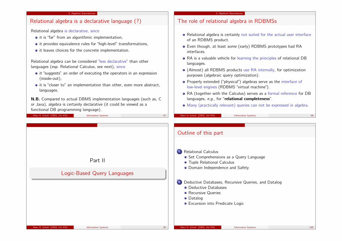
Part II
Logic-Based Query Languages
Marc H. Scholl (DBIS, Uni KN) Information Systems 99
Outline of this part
7 Relational CalculusSet Comprehensions as a Query LanguageTuple Relational CalculusDomain Independence and Safety
8 Deductive Databases, Recursive Queries, and DatalogDeductive DatabasesRecursive QueriesDatalogExcursion into Predicate Logic
Marc H. Scholl (DBIS, Uni KN) Information Systems 100
This part’s goal
After completing this chapter, you should be able to:
explain the concepts of (tuple) relational calculus,write relational calculus queries equivalent to relational algebraexpressions,
discuss and check safety and domain-independence of relationalcalculus queries,
assess the virtues and limitations of relational calculus and itsequivalence to relational algebra,
understand the challenges of recursive queries and formulate themin a rule-based language, Datalog.
Marc H. Scholl (DBIS, Uni KN) Information Systems 101
7. Relational Calculus Set Comprehensions as a Query Language
Relational Calculus: Set comprehensions as queries
We’ve been discussing earlier that Predicate Logic (1PL) could also serveas a query language by using the construct
Syntax
Q := {t|F (t)}
where Q is the name of the query result, t is a tuple variable, and F is a1PL formula parameterized by t (and typically referring to some databaserelations).This query is naturally interpreted as
Informal Semantics
Get all tuples t that satisfy condition F (t).
N.B. Condition F (t) will have to specify, among others, the structureand the “origin” of the result tuples t.
Marc H. Scholl (DBIS, Uni KN) Information Systems 102
7. Relational Calculus Set Comprehensions as a Query Language
Calculus vs. Algebra
Relational Algebra (RA) has been presented as a declarative language.Tuple Relational Calculus (TRC) could be considered “even moredeclarative”:
RA: In the algebra, the query result is constructed in a stepwiseprocess of applying operators to inputs so as to produceoutputs; the algebraic expression specifies an order ofoperator application.
TRC: A calculus formula gives no a priori hint on how to evaluateit; it can be considered purely declarative.
N.B. We should keep in mind that, in fact, declarativeness is a “fuzzy”notion: a “high-level” specification vs. a “lower level” implementation. . .
Marc H. Scholl (DBIS, Uni KN) Information Systems 103
7. Relational Calculus Set Comprehensions as a Query Language
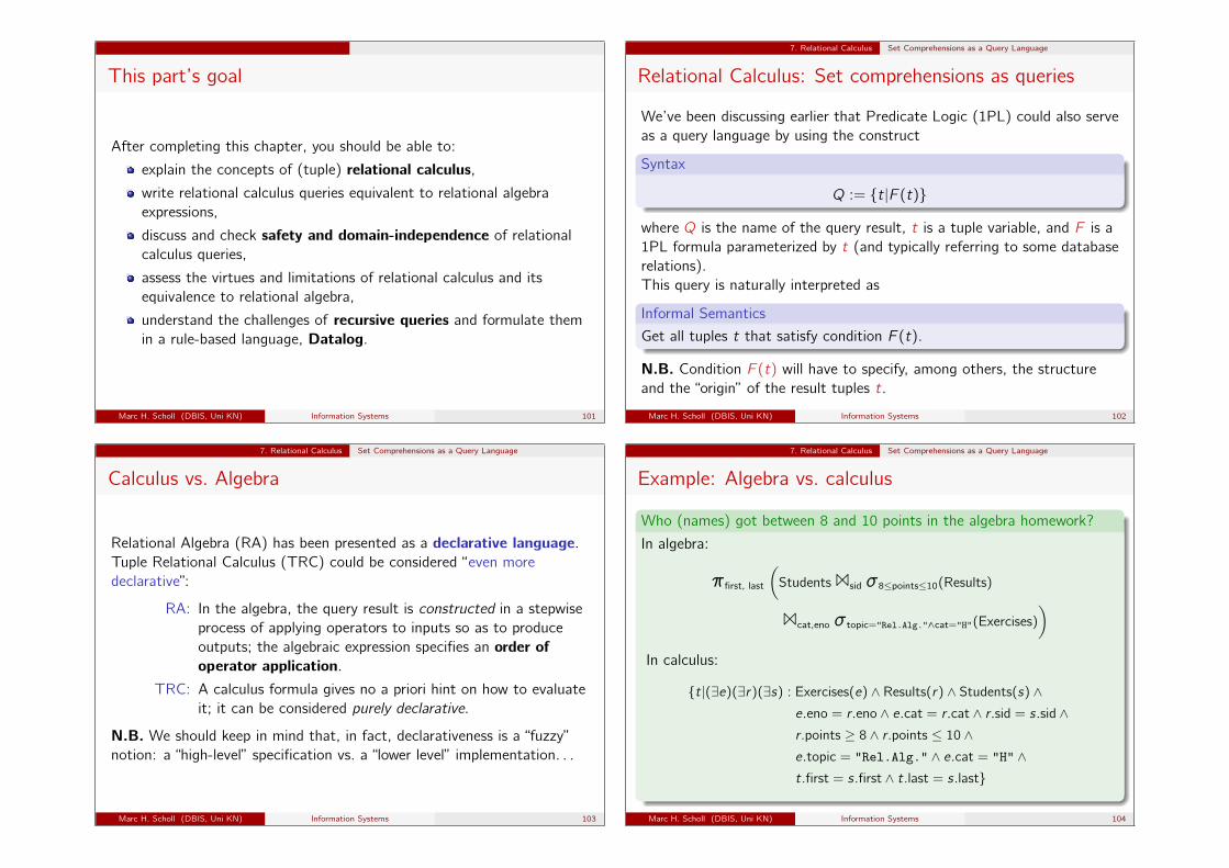
Example: Algebra vs. calculus
Who (names) got between 8 and 10 points in the algebra homework?
In algebra:
πfirst, last
(Students 1sid σ8≤points≤10(Results)
1cat,eno σtopic="Rel.Alg."∧cat="H"(Exercises))
In calculus:
{t|(∃e)(∃r)(∃s) : Exercises(e) ∧ Results(r) ∧ Students(s) ∧e.eno = r.eno ∧ e.cat = r.cat ∧ r.sid = s.sid ∧r.points ≥ 8 ∧ r.points ≤ 10 ∧e.topic = "Rel.Alg." ∧ e.cat = "H" ∧t.first = s.first ∧ t.last = s.last}
Marc H. Scholl (DBIS, Uni KN) Information Systems 104
7. Relational Calculus Set Comprehensions as a Query Language
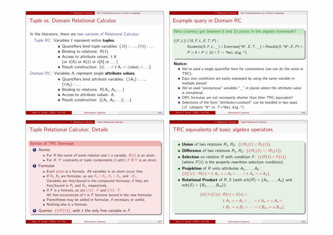
Tuple vs. Domain Relational Calculus
In the literature, there are two variants of Relational Calculus:
Tuple RC: Variables t represent entire tuples.Quantifiers bind tuple variables: (∃t) : . . ., (∀t) : . . .
Binding to relations: R(t).Access to attribute values: t.A(or t(A) or A(t) or t[A] or . . . )Result construction: {t| . . . ∧ t.Ai = 〈value〉 ∧ . . .}
Domain RC: Variables Ai represent single attribute values.Quantifiers bind attribute variables: (∃A1) : . . .,(∀A2) : . . .
Binding to relations: R(A1, A2, . . .)
Access to attribute values: AiResult construction: {(A1, A2, . . .)| . . .}
Marc H. Scholl (DBIS, Uni KN) Information Systems 105
7. Relational Calculus Set Comprehensions as a Query Language
Example query in Domain RC
Who (names) got between 8 and 10 points in the algebra homework?
{(F, L)| (∃S, F, L, E, T, P ) :
Students(S, F, L,_) ∧ Exercises("H", E, T,_) ∧ Results(S, "H", E, P ) ∧P ≥ 8 ∧ P ≤ 10 ∧ T = "Rel.Alg."}
Notice:We’ve used a single quantifier here for convenience (we can do the same inTRC).Equi-Join conditions are easily expressed by using the same variable inmultiple places!We’ve used “anonymous” variables “_” in places where the attribute valueis immaterial.DRC formulae are not necessarily shorter than their TRC equivalent!Selections of the form “attribute=constant” can be handled in two ways(cf. category "H" vs. T="Rel.Alg.")
Marc H. Scholl (DBIS, Uni KN) Information Systems 106
7. Relational Calculus Tuple Relational Calculus
Tuple Relational Calculus: Details
Syntax of TRC formulae1 Atoms
For R the name of some relation and t a variable, R(t) is an atom.For X, Y constants or tuple components (t.attr) X Θ Y is an atom.
2 FormulaeEach atom is a formula. All variables in an atom occur free.If F1, F2 are formulae, so are F1 ∧ F2, F1 ∨ F2, and ¬F1.Variables are free/bound in the compound formulae, if they arefree/bound in F1 and F2, respectively.If F is a formula, so are (∃t) : F and (∀t) : F .All free occurrences of t in F become bound in the new formulae.Parentheses may be added in formulae, if necessary or useful.Nothing else is a formula.
3 Queries: {t|F (t)}, with t the only free variable in F .
Marc H. Scholl (DBIS, Uni KN) Information Systems 107
7. Relational Calculus Tuple Relational Calculus
TRC equivalents of basic algebra operators
Union of two relations R1, R2: {t|R1(t) ∨ R2(t)}.Difference of two relations R1, R2: {t|R1(t) ∧ ¬R2(t)}.Selection on relation R with condition F : {t|R(t) ∧ F (t)}(where F (t) is the properly rewritten selection condition).
Projektion of R onto attributes A1, . . . , Ak :{t|(∃r) : R(r) ∧ t.A1 = r.A1 ∧ . . . ∧ t.Ak = r.Ak}.Relational Product of R,S (with sch(R) = {A1, . . . , An} andsch(S) = {B1, . . . , Bm}):
{t|(∃r)(∃s) :R(r) ∧ S(s) ∧t.A1 = r.A1 ∧ . . . ∧ t.An = r.An ∧t.B1 = s.B1 ∧ · · · ∧ t.Bm = s.Bm}.
Marc H. Scholl (DBIS, Uni KN) Information Systems 108
7. Relational Calculus Domain Independence and Safety
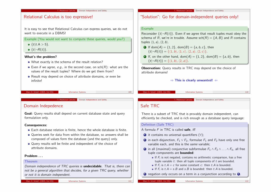
Relational Calculus is too expressive!
It is easy to see that Relational Calculus can express queries, we do notwant to execute in a DBMS!
Example (You would not want to compute these queries, would you?)
{t|t.A > 5}.{t|¬R(t)}.
What’s the problem?What exactly is the schema of the result relation?
Even if we agree, e.g., in the second case, on sch(R): what are thevalues of the result tuples? Where do we get them from?
Result may depend on choice of attribute domains, or even beinfinite!
Marc H. Scholl (DBIS, Uni KN) Information Systems 109
7. Relational Calculus Domain Independence and Safety
“Solution”: Go for domain-independent queries only!
Example
Reconsider {t|¬R(t)}. Even if we agree that result tuples must obey theschema of R, we’re in trouble. Assume sch(R) = {A,B} and R containstuples 〈1, a〉, 〈2, b〉.
1 If dom(A) = {1, 2}, dom(B) = {a, b, c}, then{t|¬R(t)} = {〈1, b〉, 〈1, c〉, 〈2, a〉, 〈2, c〉}.
2 If, on the other hand, dom(A) = {1, 2}, dom(B) = {a, b}, then{t|¬R(t)} = {〈1, b〉, 〈2, a〉}.
Observation: Query results in TRC may depend on the choice ofattribute domains!
⇒ This is clearly unwanted! ⇐
Marc H. Scholl (DBIS, Uni KN) Information Systems 110
7. Relational Calculus Domain Independence and Safety
Domain Indepedence
Goal: Query results shall depend on current database state and queryformulation only.
Consequences:Each database relation is finite, hence the whole database is finite.Queries seek for data from within the database, so answers shall becomposed of values form the database (and the query) only.Query results will be finite and independent of the choice ofattribute domains.
Problem . . .
TheoremDomain independence of TRC queries is undecidable. That is, there cannot be a general algorithm that decides, for a given TRC query, whetheror not it is domain independent.
Marc H. Scholl (DBIS, Uni KN) Information Systems 111
7. Relational Calculus Domain Independence and Safety
Safe TRC
There is a subset of TRC that is provably domain independent, canefficiently be checked, and is rich enough as a database query language:
Definition (Safe TRC)
A formula F in TRC is called safe, iff1 it contains no universal quantifiers (∀);2 in each disjunction, F1 ∨ F2, formulae F1 and F2 have only one free
variable each, and this is the same variable;3 in all (maximal) conjunctive subformulae F1 ∧ F2 ∧ . . . ∧ Fk , all free
tuple components are bounded:If Fi is not negated, contains no arithmetic comparison, has a freetuple variable t: then all tuple components of t are bounded.If Fi is t.A = c for some constant c : then t.A is bounded.If Fi is t.A = s.B and s.B is bounded: then t.A is bounded.
4 negation only occurs on a term in a conjunction according to 3 .
Marc H. Scholl (DBIS, Uni KN) Information Systems 112
7. Relational Calculus Domain Independence and Safety
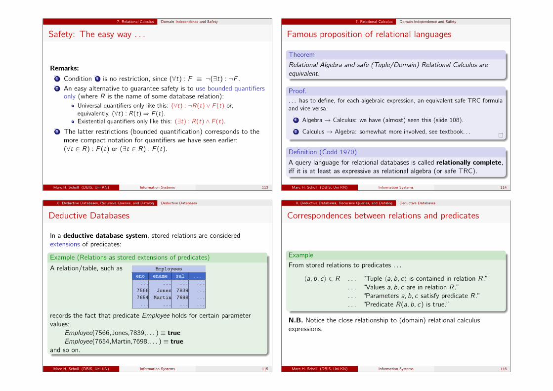
Safety: The easy way . . .
Remarks:1 Condition 1 is no restriction, since (∀t) : F ≡ ¬(∃t) : ¬F .2 An easy alternative to guarantee safety is to use bounded quantifiers
only (where R is the name of some database relation):Universal quantifiers only like this: (∀t) : ¬R(t) ∨ F (t) or,equivalently, (∀t) : R(t)⇒ F (t).Existential quantifiers only like this: (∃t) : R(t) ∧ F (t).
3 The latter restrictions (bounded quantification) corresponds to themore compact notation for quantifiers we have seen earlier:(∀t ∈ R) : F (t) or (∃t ∈ R) : F (t).
Marc H. Scholl (DBIS, Uni KN) Information Systems 113
7. Relational Calculus Domain Independence and Safety
Famous proposition of relational languages
Theorem
Relational Algebra and safe (Tuple/Domain) Relational Calculus areequivalent.
Proof.. . . has to define, for each algebraic expression, an equivalent safe TRC formulaand vice versa.
1 Algebra → Calculus: we have (almost) seen this (slide 108).
2 Calculus → Algebra: somewhat more involved, see textbook. . .
Definition (Codd 1970)
A query language for relational databases is called relationally complete,iff it is at least as expressive as relational algebra (or safe TRC).
Marc H. Scholl (DBIS, Uni KN) Information Systems 114
8. Deductive Databases, Recursive Queries, and Datalog Deductive Databases
Deductive Databases
In a deductive database system, stored relations are consideredextensions of predicates:
Example (Relations as stored extensions of predicates)
A relation/table, such as Employeeseno ename sal ...... ... ... ...7566 Jones 7839 ...7654 Martin 7698 ...... ... ... ...
records the fact that predicate Employee holds for certain parametervalues:
Employee(7566,Jones,7839,. . . ) ≡ true
Employee(7654,Martin,7698,. . . ) ≡ true
and so on.
Marc H. Scholl (DBIS, Uni KN) Information Systems 115
8. Deductive Databases, Recursive Queries, and Datalog Deductive Databases
Correspondences between relations and predicates
Example
From stored relations to predicates . . .
〈a, b, c〉 ∈ R . . . “Tuple 〈a, b, c〉 is contained in relation R.”. . . “Values a, b, c are in relation R.”. . . “Parameters a, b, c satisfy predicate R.”. . . “Predicate R(a, b, c) is true.”
N.B. Notice the close relationship to (domain) relational calculusexpressions.
Marc H. Scholl (DBIS, Uni KN) Information Systems 116
8. Deductive Databases, Recursive Queries, and Datalog Deductive Databases
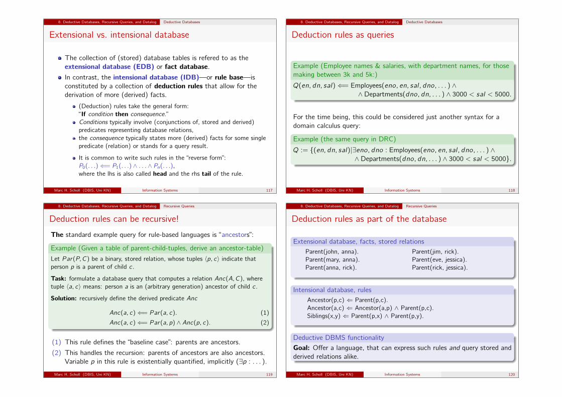
Extensional vs. intensional database
The collection of (stored) database tables is refered to as theextensional database (EDB) or fact database.In contrast, the intensional database (IDB)—or rule base—isconstituted by a collection of deduction rules that allow for thederivation of more (derived) facts.
(Deduction) rules take the general form:“If condition then consequence.”Conditions typically involve (conjunctions of, stored and derived)predicates representing database relations,the consequence typically states more (derived) facts for some singlepredicate (relation) or stands for a query result.
It is common to write such rules in the “reverse form”:P0(. . .)⇐= P1(. . .) ∧ . . . ∧ Pn(. . .),where the lhs is also called head and the rhs tail of the rule.
Marc H. Scholl (DBIS, Uni KN) Information Systems 117
8. Deductive Databases, Recursive Queries, and Datalog Deductive Databases
Deduction rules as queries
Example (Employee names & salaries, with department names, for thosemaking between 3k and 5k:)
Q(en, dn, sal)⇐= Employees(eno, en, sal , dno, . . . ) ∧∧Departments(dno, dn, . . . ) ∧ 3000 < sal < 5000.
For the time being, this could be considered just another syntax for adomain calculus query:
Example (the same query in DRC)
Q := {(en, dn, sal)|∃eno, dno : Employees(eno, en, sal , dno, . . . ) ∧∧Departments(dno, dn, . . . ) ∧ 3000 < sal < 5000}.
Marc H. Scholl (DBIS, Uni KN) Information Systems 118
8. Deductive Databases, Recursive Queries, and Datalog Recursive Queries
Deduction rules can be recursive!
The standard example query for rule-based languages is “ancestors”:
Example (Given a table of parent-child-tuples, derive an ancestor-table)
Let Par(P, C) be a binary, stored relation, whose tuples 〈p, c〉 indicate thatperson p is a parent of child c .
Task: formulate a database query that computes a relation Anc(A,C), wheretuple 〈a, c〉 means: person a is an (arbitrary generation) ancestor of child c .
Solution: recursively define the derived predicate Anc
Anc(a, c)⇐= Par(a, c). (1)
Anc(a, c)⇐= Par(a, p) ∧ Anc(p, c). (2)
(1) This rule defines the “baseline case”: parents are ancestors.
(2) This handles the recursion: parents of ancestors are also ancestors.Variable p in this rule is existentially quantified, implicitly (∃p : . . . ).
Marc H. Scholl (DBIS, Uni KN) Information Systems 119
8. Deductive Databases, Recursive Queries, and Datalog Recursive Queries
Deduction rules as part of the database
Extensional database, facts, stored relationsParent(john, anna).Parent(mary, anna).Parent(anna, rick).
Parent(jim, rick).Parent(eve, jessica).Parent(rick, jessica).
Intensional database, rulesAncestor(p,c) ⇐ Parent(p,c).Ancestor(a,c) ⇐ Ancestor(a,p) ∧ Parent(p,c).Siblings(x,y) ⇐ Parent(p,x) ∧ Parent(p,y).
Deductive DBMS functionality
Goal: Offer a language, that can express such rules and query stored andderived relations alike.
Marc H. Scholl (DBIS, Uni KN) Information Systems 120
8. Deductive Databases, Recursive Queries, and Datalog Recursive Queries
More examples
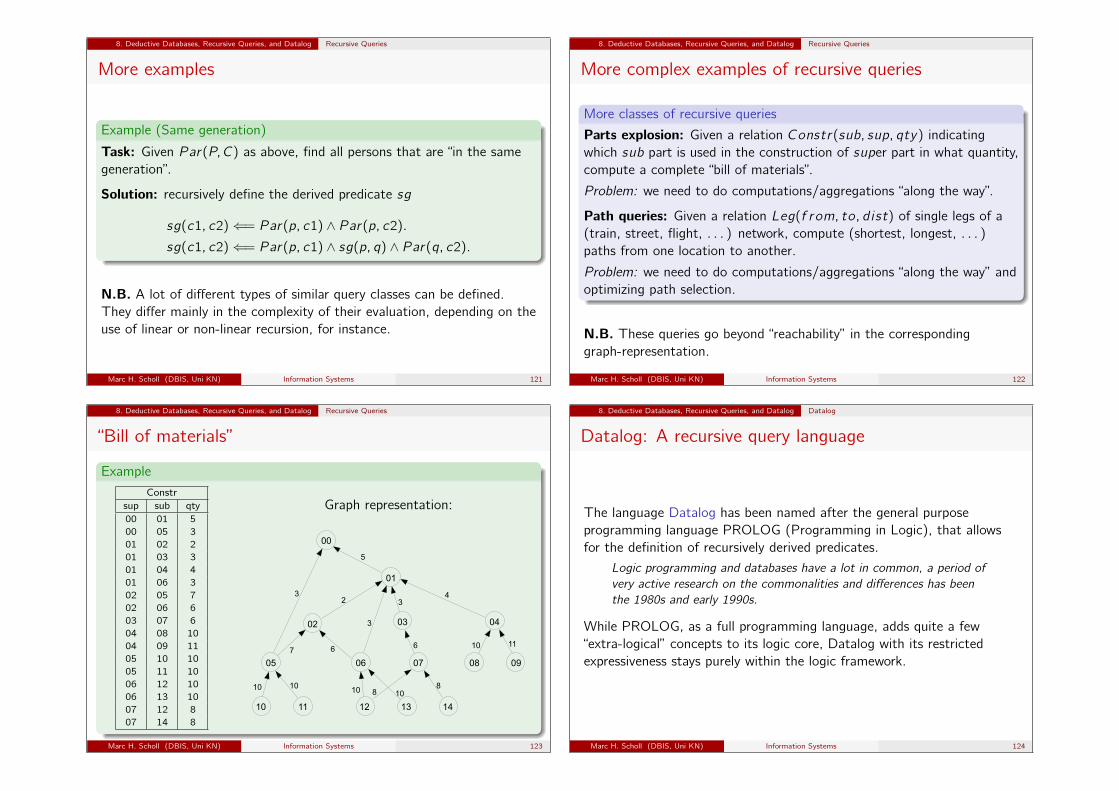
Example (Same generation)
Task: Given Par(P, C) as above, find all persons that are “in the samegeneration”.
Solution: recursively define the derived predicate sg
sg(c1, c2)⇐= Par(p, c1) ∧ Par(p, c2).
sg(c1, c2)⇐= Par(p, c1) ∧ sg(p, q) ∧ Par(q, c2).
N.B. A lot of different types of similar query classes can be defined.They differ mainly in the complexity of their evaluation, depending on theuse of linear or non-linear recursion, for instance.
Marc H. Scholl (DBIS, Uni KN) Information Systems 121
8. Deductive Databases, Recursive Queries, and Datalog Recursive Queries
More complex examples of recursive queries
More classes of recursive queries
Parts explosion: Given a relation Constr(sub, sup, qty) indicatingwhich sub part is used in the construction of super part in what quantity,compute a complete “bill of materials”.
Problem: we need to do computations/aggregations “along the way”.
Path queries: Given a relation Leg(f rom, to, dist) of single legs of a(train, street, flight, . . . ) network, compute (shortest, longest, . . . )paths from one location to another.
Problem: we need to do computations/aggregations “along the way” andoptimizing path selection.
N.B. These queries go beyond “reachability” in the correspondinggraph-representation.
Marc H. Scholl (DBIS, Uni KN) Information Systems 122
8. Deductive Databases, Recursive Queries, and Datalog Recursive Queries
“Bill of materials”
ExampleConstr
sup sub qty00 01 500 05 301 02 201 03 301 04 401 06 302 05 702 06 603 07 604 08 1004 09 1105 10 1005 11 1006 12 1006 13 1007 12 807 14 8
Graph representation:
01
00
02 03 04
05 06 07 08 09
10 11 12 13 14
5
3
7 6
2
3
34
6 10 11
8810
1010 10
Marc H. Scholl (DBIS, Uni KN) Information Systems 123
8. Deductive Databases, Recursive Queries, and Datalog Datalog
Datalog: A recursive query language
The language Datalog has been named after the general purposeprogramming language PROLOG (Programming in Logic), that allowsfor the definition of recursively derived predicates.
Logic programming and databases have a lot in common, a period ofvery active research on the commonalities and differences has beenthe 1980s and early 1990s.
While PROLOG, as a full programming language, adds quite a few“extra-logical” concepts to its logic core, Datalog with its restrictedexpressiveness stays purely within the logic framework.
Marc H. Scholl (DBIS, Uni KN) Information Systems 124
8. Deductive Databases, Recursive Queries, and Datalog Datalog
Datalog vs. PROLOG
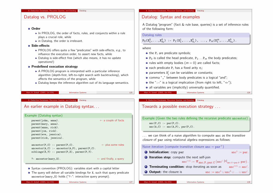
OrderIn PROLOG, the order of facts, rules, and conjuncts within a ruleplays a crucial role, whilein Datalog, the order is irrelevant.
Side-effectsPROLOG offers quite a few “predicates” with side-effects, e.g., toinfluence the execution order, to assert new facts, whileDatalog is side-effect free (which also means, it has no updateoperations!)
Predefined execution strategyA PROLOG program is interpreted with a particular inferencealgorithm (depth-first, left-to-right search with backtracking), whichaffects the semantics of the program, whileDatalog keeps the inference algorithm out of its language semantics.
Marc H. Scholl (DBIS, Uni KN) Information Systems 125
8. Deductive Databases, Recursive Queries, and Datalog Datalog
Datalog: Syntax and examples
A Datalog “program” (fact & rule base, queries) is a set of inference rulesof the following form:
Datalog rules
P0(X01,...,X0n0) :- P1(X11,...,X
0n1), ..., Pm(Xm1 ,...,X
0nm).
where
the Pi are predicate symbols;
P0 is called the head predicate, P1. . . Pm the body predicates;
rules with empty bodies (m = 0) are called facts;
each predicate Pi has a fixed arity ni ;
parameters Xij can be variables or constants;
comma “,” between body predicates is a logical “and”;
the “:-” is a logical implication (from right to left, “⇐”);
all variables are (implicitly) universally quantified.Marc H. Scholl (DBIS, Uni KN) Information Systems 126
8. Deductive Databases, Recursive Queries, and Datalog Datalog
An earlier example in Datalog syntax. . .
Example (Datalog syntax)parent(john, anna). ← a couple of factsparent(mary, anna).parent(anna, rick).parent(jim, rick).parent(eve, jessica).parent(rick, jessica).
ancestor(P,C) :- parent(P,C). ← plus some rulesancestor(A,C) :- ancestor(A,P), parent(P,C).siblings(X,Y) :- parent(P,X), parent(P,Y).
?- ancestor(mary,X). ← and finally, a query
Syntax convention (PROLOG): variables start with a capital letterThe query will deliver all variable bindings for X, such that query predicateancestor(mary,X) holds (“?-”: interactive query prompt).
Marc H. Scholl (DBIS, Uni KN) Information Systems 127
8. Deductive Databases, Recursive Queries, and Datalog Datalog
Towards a possible execution strategy . . .
Example (Given the two rules defining the recursive predicate ancestor)anc(P,C) :- par(P,C).anc(A,C) :- anc(A,P), par(P,C).
. . . we can think of a naive algorithm to compute anc as the transitiveclosure of par using relational algebra expressions as follows:
Naive iteration (compute transitive closure anc = par+)1 Initialization: copy par anc1 := par.
2 Iteration step: compute the next self-joinanci+1 := πanc.P, par.C
(anci 1anc.C=par.P par
).
3 Terminating condition: stop iterating as soon as anci+1 = anci .
4 Output: the closure is anc := anc1 ∪ anc2 ∪ . . . ∪ anci .
Marc H. Scholl (DBIS, Uni KN) Information Systems 128

8. Deductive Databases, Recursive Queries, and Datalog Datalog
Naive iteration
In a more compact notation, with operator “A ◦ B” defined as5
A ◦ B ≡ πA.1, B.2 (A 1A.2=B.1 B), we can see the following
Fixed-point iteration
par1 = par(P, C)
par2 = par(P,X1), par(X1, C) = par ◦ par
par3 = par(P,X1), par(X1, X2), par(X2, C) = par ◦ par ◦ par
...
pari = par ◦ · · · ◦ par| {z }
i times
anc = par+ =
∞[i=1
pari = par ∪ par
2 ∪ par3 ∪ . . .
anc = LFP(x = x ◦ par ∪ par) . . . LFP = least fixed-point
5using attribute positions rather than namesMarc H. Scholl (DBIS, Uni KN) Information Systems 129
8. Deductive Databases, Recursive Queries, and Datalog Datalog
Observations on the LFP iteration
The LFP operator computes the least fixed-point of a recursiveequation of the form x = f (x).
Theorem: Termination is guaranteed.Proof idea: par is finite; ◦ is monotonic; hence, anc is finite andtermination is guaranteed. 2PROLOG would use a very different execution strategy.(set-oriented computation here, record-at-a-time in PROLOG)
The use of negation (i.e., difference in the algebra) complicatesmatters significantly (since monotonicity is lost)!→ Either disallow negation, or use a careful interpretation(“negation as failure”).
Non-recursive Datalog without negation ≡ RA without negation(“monotonic RA”).
Non-recursive Datalog with (appropriate) negation ≡ RA.
Marc H. Scholl (DBIS, Uni KN) Information Systems 130
8. Deductive Databases, Recursive Queries, and Datalog Excursion into Predicate Logic
Excursion into Predicate Logic
Let us, for a moment, have a closer look at the particular form of logicalderivation rules used in Datalog (or PROLOG alike).
Horn clausesDatalog rules of the form
P0(· · · ) :- P1(· · · ), . . . , Pn(· · · ).are interpreted, logically, as
∀ · · · : P0(· · · ) ⇐ P1(· · · ) ∧ . . . ∧ Pn(· · · )where the universal quantifier binds all variables in the Pi .
This particular form of logical formulae is used since it allows for aneffective automatic proof algorithm. . .
Marc H. Scholl (DBIS, Uni KN) Information Systems 131
8. Deductive Databases, Recursive Queries, and Datalog Excursion into Predicate Logic
Propositional Logic (German: “Aussagenlogik”)
Formulae in propositional logic are composed of Boolean variablesAi , which can assume values true (1) or false (0), and the logicalconnectives ¬,∧,∨,⇒,⇔.
Each formula represents a Boolean function in its Boolean variables.
Definition (Formulae of Propositional Logic)
Let A1, . . . , An be a given set of atomic formulae. A (propositionallogic) formula (over this set of atomic formulae) is defined inductivelyas:
1 If F = 0 or F = 1 or F = Ai is an atomic formula, then F is apropositional formula.
2 If F is a formula, so is ¬F (“negation”).3 If F and G are formulae, so are (F ∧ G) (“conjunction”) and (F ∨ G)
(“disjunction”).
Marc H. Scholl (DBIS, Uni KN) Information Systems 132
8. Deductive Databases, Recursive Queries, and Datalog Excursion into Predicate Logic
Remarks
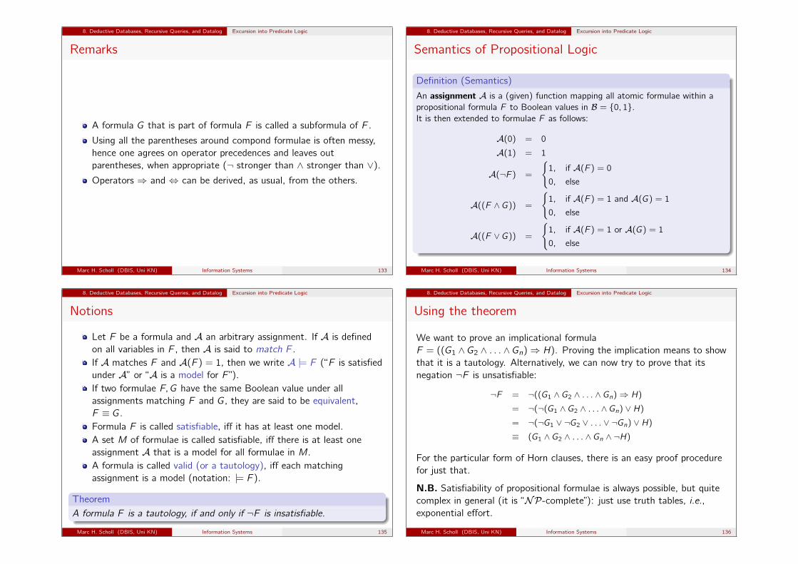
A formula G that is part of formula F is called a subformula of F .
Using all the parentheses around compond formulae is often messy,hence one agrees on operator precedences and leaves outparentheses, when appropriate (¬ stronger than ∧ stronger than ∨).Operators ⇒ and ⇔ can be derived, as usual, from the others.
Marc H. Scholl (DBIS, Uni KN) Information Systems 133
8. Deductive Databases, Recursive Queries, and Datalog Excursion into Predicate Logic
Semantics of Propositional Logic
Definition (Semantics)
An assignment A is a (given) function mapping all atomic formulae within apropositional formula F to Boolean values in B = {0, 1}.It is then extended to formulae F as follows:
A(0) = 0
A(1) = 1
A(¬F ) =
{1, if A(F ) = 0
0, else
A((F ∧ G)) =
{1, if A(F ) = 1 and A(G) = 1
0, else
A((F ∨ G)) =
{1, if A(F ) = 1 or A(G) = 1
0, else
Marc H. Scholl (DBIS, Uni KN) Information Systems 134
8. Deductive Databases, Recursive Queries, and Datalog Excursion into Predicate Logic
Notions
Let F be a formula and A an arbitrary assignment. If A is definedon all variables in F , then A is said to match F .If A matches F and A(F ) = 1, then we write A |= F (“F is satisfiedunder A” or “A is a model for F ”).If two formulae F,G have the same Boolean value under allassignments matching F and G, they are said to be equivalent,F ≡ G.Formula F is called satisfiable, iff it has at least one model.A set M of formulae is called satisfiable, iff there is at least oneassignment A that is a model for all formulae in M.A formula is called valid (or a tautology), iff each matchingassignment is a model (notation: |= F ).
TheoremA formula F is a tautology, if and only if ¬F is insatisfiable.
Marc H. Scholl (DBIS, Uni KN) Information Systems 135
8. Deductive Databases, Recursive Queries, and Datalog Excursion into Predicate Logic
Using the theorem
We want to prove an implicational formulaF = ((G1 ∧ G2 ∧ . . . ∧ Gn)⇒ H). Proving the implication means to showthat it is a tautology. Alternatively, we can now try to prove that itsnegation ¬F is unsatisfiable:
¬F = ¬((G1 ∧ G2 ∧ . . . ∧ Gn)⇒ H)
= ¬(¬(G1 ∧ G2 ∧ . . . ∧ Gn) ∨H)
= ¬(¬G1 ∨ ¬G2 ∨ . . . ∨ ¬Gn) ∨H)
≡ (G1 ∧ G2 ∧ . . . ∧ Gn ∧ ¬H)
For the particular form of Horn clauses, there is an easy proof procedurefor just that.
N.B. Satisfiability of propositional formulae is always possible, but quitecomplex in general (it is “NP-complete”): just use truth tables, i.e.,exponential effort.
Marc H. Scholl (DBIS, Uni KN) Information Systems 136
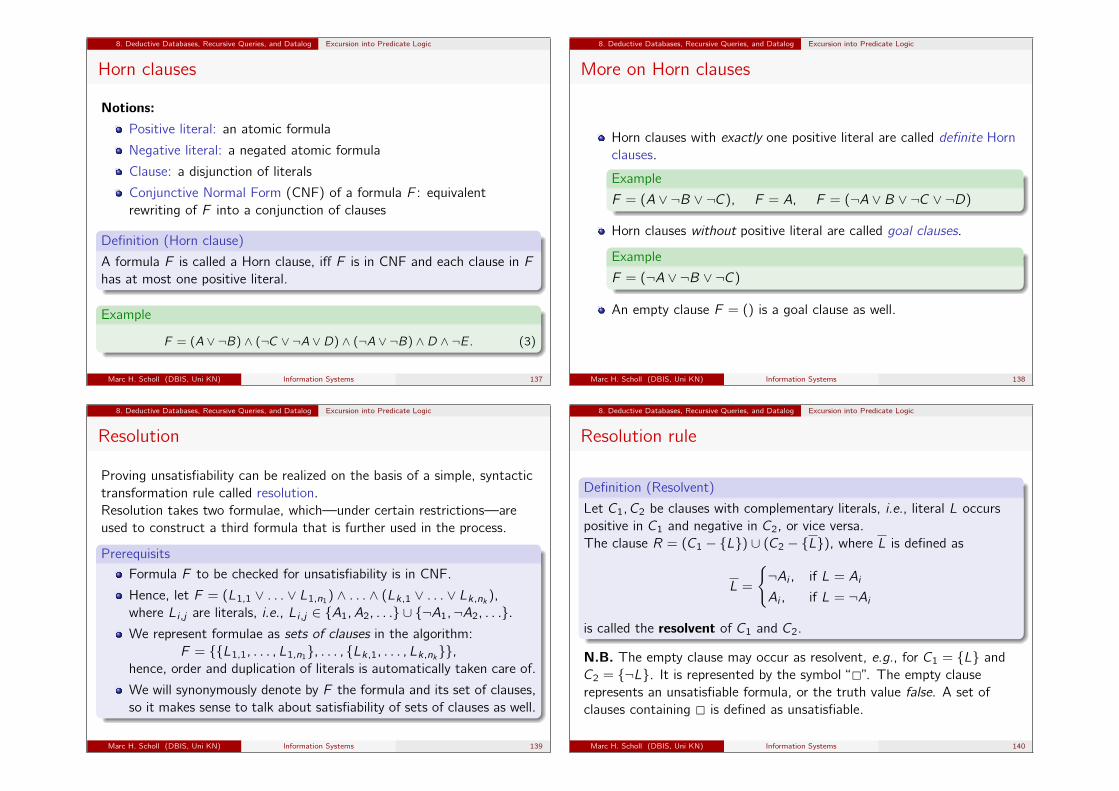
8. Deductive Databases, Recursive Queries, and Datalog Excursion into Predicate Logic
Horn clauses
Notions:Positive literal: an atomic formula
Negative literal: a negated atomic formula
Clause: a disjunction of literals
Conjunctive Normal Form (CNF) of a formula F : equivalentrewriting of F into a conjunction of clauses
Definition (Horn clause)
A formula F is called a Horn clause, iff F is in CNF and each clause in Fhas at most one positive literal.
Example
F = (A ∨ ¬B) ∧ (¬C ∨ ¬A ∨D) ∧ (¬A ∨ ¬B) ∧D ∧ ¬E. (3)
Marc H. Scholl (DBIS, Uni KN) Information Systems 137
8. Deductive Databases, Recursive Queries, and Datalog Excursion into Predicate Logic
More on Horn clauses
Horn clauses with exactly one positive literal are called definite Hornclauses.
Example
F = (A ∨ ¬B ∨ ¬C), F = A, F = (¬A ∨ B ∨ ¬C ∨ ¬D)
Horn clauses without positive literal are called goal clauses.
Example
F = (¬A ∨ ¬B ∨ ¬C)
An empty clause F = () is a goal clause as well.
Marc H. Scholl (DBIS, Uni KN) Information Systems 138
8. Deductive Databases, Recursive Queries, and Datalog Excursion into Predicate Logic
Resolution
Proving unsatisfiability can be realized on the basis of a simple, syntactictransformation rule called resolution.Resolution takes two formulae, which—under certain restrictions—areused to construct a third formula that is further used in the process.
Prerequisits
Formula F to be checked for unsatisfiability is in CNF.
Hence, let F = (L1,1 ∨ . . . ∨ L1,n1) ∧ . . . ∧ (Lk,1 ∨ . . . ∨ Lk,nk ),where Li ,j are literals, i.e., Li ,j ∈ {A1, A2, . . .} ∪ {¬A1,¬A2, . . .}.We represent formulae as sets of clauses in the algorithm:
F = {{L1,1, . . . , L1,n1}, . . . , {Lk,1, . . . , Lk,nk}},hence, order and duplication of literals is automatically taken care of.
We will synonymously denote by F the formula and its set of clauses,so it makes sense to talk about satisfiability of sets of clauses as well.
Marc H. Scholl (DBIS, Uni KN) Information Systems 139
8. Deductive Databases, Recursive Queries, and Datalog Excursion into Predicate Logic
Resolution rule
Definition (Resolvent)
Let C1, C2 be clauses with complementary literals, i.e., literal L occurspositive in C1 and negative in C2, or vice versa.The clause R = (C1 − {L}) ∪ (C2 − {L}), where L is defined as
L =
{¬Ai , if L = Ai
Ai , if L = ¬Aiis called the resolvent of C1 and C2.
N.B. The empty clause may occur as resolvent, e.g., for C1 = {L} andC2 = {¬L}. It is represented by the symbol “2”. The empty clauserepresents an unsatisfiable formula, or the truth value false. A set ofclauses containing 2 is defined as unsatisfiable.
Marc H. Scholl (DBIS, Uni KN) Information Systems 140
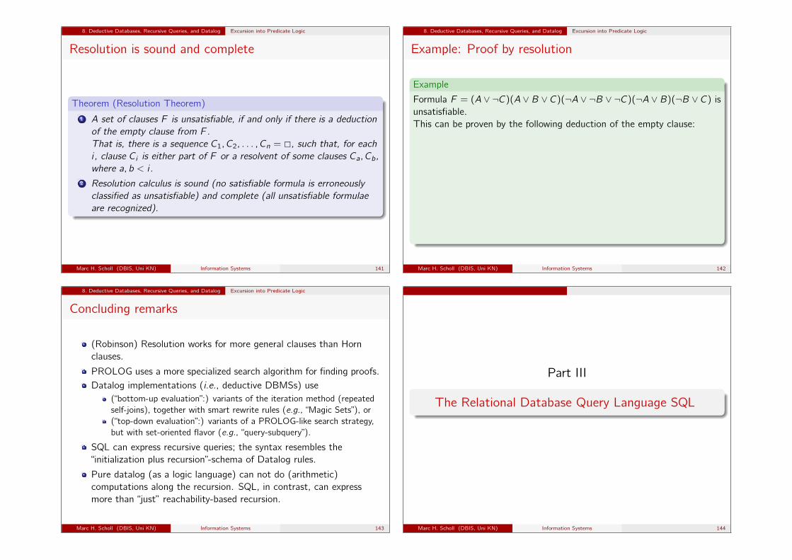
8. Deductive Databases, Recursive Queries, and Datalog Excursion into Predicate Logic
Resolution is sound and complete
Theorem (Resolution Theorem)1 A set of clauses F is unsatisfiable, if and only if there is a deduction
of the empty clause from F .That is, there is a sequence C1, C2, . . . , Cn = 2, such that, for eachi , clause Ci is either part of F or a resolvent of some clauses Ca, Cb,where a, b < i .
2 Resolution calculus is sound (no satisfiable formula is erroneouslyclassified as unsatisfiable) and complete (all unsatisfiable formulaeare recognized).
Marc H. Scholl (DBIS, Uni KN) Information Systems 141
8. Deductive Databases, Recursive Queries, and Datalog Excursion into Predicate Logic
Example: Proof by resolution
Example
Formula F = (A ∨ ¬C)(A ∨ B ∨ C)(¬A ∨ ¬B ∨ ¬C)(¬A ∨ B)(¬B ∨ C) isunsatisfiable.This can be proven by the following deduction of the empty clause:
Beispiel Resolutionsbeweis
Die Formel
F = (A ∨ ¬C)(A ∨ B ∨ C)(¬A ∨ ¬B ∨ ¬C)(¬A ∨ B)(¬B ∨ C)
ist unerfullbar. Dies zeigt die folgende Deduktion, dargestellt anhand eines”Beweisgraphen“:
{A,¬C} {A,B, C} {¬A,¬B,¬C} {¬A,B} {¬B,C}
{A,B} {¬B,¬C}
{B} {¬B}
2
c© M. Scholl, 2005/06 – Informationssysteme: 6. Wissensbasierte Informationssysteme 6-30
Marc H. Scholl (DBIS, Uni KN) Information Systems 142
8. Deductive Databases, Recursive Queries, and Datalog Excursion into Predicate Logic
Concluding remarks
(Robinson) Resolution works for more general clauses than Hornclauses.
PROLOG uses a more specialized search algorithm for finding proofs.Datalog implementations (i.e., deductive DBMSs) use
(“bottom-up evaluation”:) variants of the iteration method (repeatedself-joins), together with smart rewrite rules (e.g., “Magic Sets”), or(“top-down evaluation”:) variants of a PROLOG-like search strategy,but with set-oriented flavor (e.g., “query-subquery”).
SQL can express recursive queries; the syntax resembles the“initialization plus recursion”-schema of Datalog rules.
Pure datalog (as a logic language) can not do (arithmetic)computations along the recursion. SQL, in contrast, can expressmore than “just” reachability-based recursion.
Marc H. Scholl (DBIS, Uni KN) Information Systems 143
Part III
The Relational Database Query Language SQL
Marc H. Scholl (DBIS, Uni KN) Information Systems 144
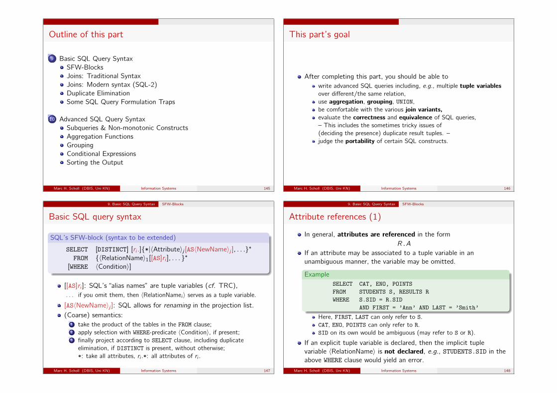
Outline of this part
9 Basic SQL Query SyntaxSFW-BlocksJoins: Traditional SyntaxJoins: Modern syntax (SQL-2)Duplicate EliminationSome SQL Query Formulation Traps
10 Advanced SQL Query SyntaxSubqueries & Non-monotonic ConstructsAggregation FunctionsGroupingConditional ExpressionsSorting the Output
Marc H. Scholl (DBIS, Uni KN) Information Systems 145
This part’s goal
After completing this part, you should be able towrite advanced SQL queries including, e.g., multiple tuple variablesover different/the same relation,use aggregation, grouping, UNION,be comfortable with the various join variants,evaluate the correctness and equivalence of SQL queries,– This includes the sometimes tricky issues of(deciding the presence) duplicate result tuples. –judge the portability of certain SQL constructs.
Marc H. Scholl (DBIS, Uni KN) Information Systems 146
9. Basic SQL Query Syntax SFW-Blocks
Basic SQL query syntax
SQL’s SFW-block (syntax to be extended)
SELECT [DISTINCT] [ri .]{*|〈Attribute〉j [AS〈NewName〉j ], . . .}∗FROM {〈RelationName〉1[[AS]ri ], . . . }∗
[WHERE 〈Condition〉]
[[AS]ri ]: SQL’s “alias names” are tuple variables (cf. TRC),. . . if you omit them, then 〈RelationNamei 〉 serves as a tuple variable.
[AS〈NewName〉j ]: SQL allows for renaming in the projection list.(Coarse) semantics:
1 take the product of the tables in the FROM clause;2 apply selection with WHERE-predicate 〈Condition〉, if present;3 finally project according to SELECT clause, including duplicate
elimination, if DISTINCT is present, without otherwise;*: take all attributes, ri .*: all attributes of ri .
Marc H. Scholl (DBIS, Uni KN) Information Systems 147
9. Basic SQL Query Syntax SFW-Blocks
Attribute references (1)
In general, attributes are referenced in the formR.A
If an attribute may be associated to a tuple variable in anunambiguous manner, the variable may be omitted.
ExampleSELECT CAT, ENO, POINTSFROM STUDENTS S, RESULTS RWHERE S.SID = R.SID
AND FIRST = ’Ann’ AND LAST = ’Smith’
Here, FIRST, LAST can only refer to S.CAT, ENO, POINTS can only refer to R.SID on its own would be ambiguous (may refer to S or R).
If an explicit tuple variable is declared, then the implicit tuplevariable 〈RelationName〉 is not declared, e.g., STUDENTS.SID in theabove WHERE clause would yield an error.
Marc H. Scholl (DBIS, Uni KN) Information Systems 148

9. Basic SQL Query Syntax SFW-Blocks
Attribute references (2)
Consider this query:�
Erroneous SQL!SELECT ENO, SID, POINTS, MAXPTFROM RESULTS R, EXERCISES EWHERE R.ENO = E.ENO
AND R.CAT = ’H’ AND E.CAT = ’H’
Although forced to be equal by the join condition, SQL requires theuser to specify unambiguously which of the ENO attributes (bound toR or E) is meant in the SELECT clause.
The ambiguity rule is purely syntactic and does not depend on thequery semantics.
Marc H. Scholl (DBIS, Uni KN) Information Systems 149
9. Basic SQL Query Syntax SFW-Blocks
Expressions in the SELECT & WHERE clause
SQL allows for expressions in the SELECT clause.
Example (For each RESULT, compute precentage of POINTS achieved)
SELECT SID, R.CAT, R.ENO, (100*POINTS/MAXPOINTS) as PCTFROM RESULTS R NATURAL JOIN EXERCISES E
. . . and in the WHERE clause as well.
Example (Select RESULTs with more than 80% POINTS achieved)SELECT R.*FROM RESULTS R NATURAL JOIN EXERCISES EWHERE POINTS > 0.8*MAXPOINTS
N.B. The kind of expressions depends on the collection of basic datatypes supported.
Marc H. Scholl (DBIS, Uni KN) Information Systems 150
9. Basic SQL Query Syntax Joins: Traditional Syntax
Joins—The traditional way
Example database (again)
STUDENTSSID FIRST LAST EMAIL101 Ann Smith ...102 Michael Jones (null)103 Richard Turner ...104 Maria Brown ...
EXERCISESCAT ENO TOPIC MAXPT
H 1 Rel.Alg. 10H 2 SQL 10M 1 SQL 14
RESULTSSID CAT ENO POINTS101 H 1 10101 H 2 8101 M 1 12102 H 1 9102 H 2 9102 M 1 10103 H 1 5103 M 1 7
Marc H. Scholl (DBIS, Uni KN) Information Systems 151
9. Basic SQL Query Syntax Joins: Traditional Syntax
Expressing joins in traditional SQL (SQL:1989)
Consider a query with two tuple variables:
SELECT A1, . . . ,AnFROM STUDENTS S, RESULTS RWHERE C
S will range over 4 tuples in STUDENTS, R will range over 8 tuples inRESULTS. In principle, all 4 · 8 = 32 combinations will be considered incondition C:
Naive(!) implementationforeach S ∈ STUDENTS do
foreach R ∈ RESULTS doif C then
print A1, . . . , Anfi
odod
This formulation of joins in SQL re-sembles the (derived) join definition:
1 ≡ π ◦ σ ◦ ×,where ◦ is operator composition(from right to left).
Marc H. Scholl (DBIS, Uni KN) Information Systems 152

9. Basic SQL Query Syntax Joins: Traditional Syntax
Implementing joins
A good DBMS will use a better evaluation algorithm (dependingon the condition C).
This is the task of the query optimizer. For example, if Ccontains the join condition S.SID = R.SID, the DBMS mightloop over the tuples in RESULTS and find the correspondingSTUDENTS tuple by using an index over STUDENT.SID (manyDBMS automatically create an index over the key attributes).
In order to understand the semantics of a query, however, thesimple nested foreach algorithm suffices.
The query optimizer may use any algorithm that produces theexact same output, although possibly in different tuple order.
Marc H. Scholl (DBIS, Uni KN) Information Systems 153
9. Basic SQL Query Syntax Joins: Traditional Syntax
Explicit join conditions in the WHERE clause (1)
In that join syntax, join conditions needs to be explicitly specified in theWHERE clause:
ExampleSELECT DISTINCT R.CAT, R.ENO, R.POINTSFROM STUDENTS S, RESULTS RWHERE S.SID = R.SID -- Join Condition
AND S.FIRST = ’Ann’ AND S.LAST = ’Smith’
Output of this query?SELECT DISTINCT S.FIRST, S.LASTFROM STUDENTS S, RESULTS RWHERE R.CAT = ’H’ AND R.ENO = 1
Marc H. Scholl (DBIS, Uni KN) Information Systems 154
9. Basic SQL Query Syntax Joins: Traditional Syntax
Explicit join conditions in the WHERE clause (2)
Guideline: it is almost always an error if there are two tuples variableswhich are not linked (directly or indirectly) via join conditions.
In this query, all three tuple variables are connected:SELECT E.CAT, E.ENO, R.POINTS, E.MAXPTFROM STUDENTS S, RESULTS R, EXERCISES EWHERE S.SID = R.SID AND R.CAT = E.CAT AND R.ENO = E.ENO
AND S.FIRST = ’Ann’ AND S.LAST = ’Smith’
The tuple variable connection works as follows:'&%$ !"#SS.SID = R.SID
'&%$ !"#RR.CAT = E.CAT
AND R.ENO = E.ENO
'&%$ !"#EThe conditions correspond to key–foreign key–relationships betweentables. Omission of a join condition will usually lead to numerousduplicates in the query result.
The use of DISTINCT does not fix the error in such a case!
Marc H. Scholl (DBIS, Uni KN) Information Systems 155
9. Basic SQL Query Syntax Joins: Traditional Syntax
Join graph (1)
Formulate the following query in SQL
“Which are the topics of all exercises solved by Ann Smith?”
To formulate this query,
consider that Ann Smith is a student, requiring a tuple variable, Ssay, over STUDENTS and the identifying condition S.FIRST = ’Ann’AND S.LAST = ’Smith’.
Exercise topics are of interest, so a tuple variable E over EXERCISESis needed, and the following piece of SQL can already be generated:
SELECT DISTINCT E.TOPIC
Several exercises may have the same topic (hence the DISTINCT).
Marc H. Scholl (DBIS, Uni KN) Information Systems 156
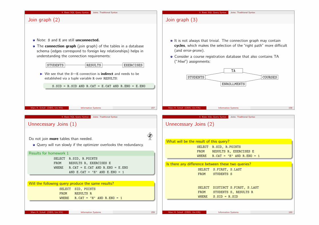
9. Basic SQL Query Syntax Joins: Traditional Syntax
Join graph (2)
Note: S and E are still unconnected.The connection graph (join graph) of the tables in a databaseschema (edges correspond to foreign key relationships) helps inunderstanding the connection requirements:
STUDENTS RESULTS EXERCISES
I We see that the S—E connection is indirect and needs to beestablished via a tuple variable R over RESULTS:
S.SID = R.SID AND R.CAT = E.CAT AND R.ENO = E.ENO
Marc H. Scholl (DBIS, Uni KN) Information Systems 157
9. Basic SQL Query Syntax Joins: Traditional Syntax
Join graph (3)
It is not always that trivial. The connection graph may containcycles, which makes the selection of the “right path” more difficult(and error-prone).
Consider a course registration database that also contains TA(“Hiwi”) assignments:
TA
STUDENTS
eeeeeeeeeee
YYYYYYYYY COURSES
YYYYYYYYYYY
eeeeeeeee
ENROLLMENTS
Marc H. Scholl (DBIS, Uni KN) Information Systems 158
9. Basic SQL Query Syntax Joins: Traditional Syntax
Unnecessary Joins (1)
Do not join more tables than needed.�
Query will run slowly if the optimizer overlooks the redundancy.
Results for homework 1SELECT R.SID, R.POINTSFROM RESULTS R, EXERCISES EWHERE R.CAT = E.CAT AND R.ENO = E.ENO
AND E.CAT = ’H’ AND E.ENO = 1
Will the following query produce the same results?SELECT SID, POINTSFROM RESULTS RWHERE R.CAT = ’H’ AND R.ENO = 1
Marc H. Scholl (DBIS, Uni KN) Information Systems 159
9. Basic SQL Query Syntax Joins: Traditional Syntax
Unnecessary Joins (2)
What will be the result of this query?SELECT R.SID, R.POINTSFROM RESULTS R, EXERCISES EWHERE R.CAT = ’H’ AND R.ENO = 1
Is there any difference between these two queries?SELECT S.FIRST, S.LASTFROM STUDENTS S
SELECT DISTINCT S.FIRST, S.LASTFROM STUDENTS S, RESULTS RWHERE S.SID = R.SID
Marc H. Scholl (DBIS, Uni KN) Information Systems 160
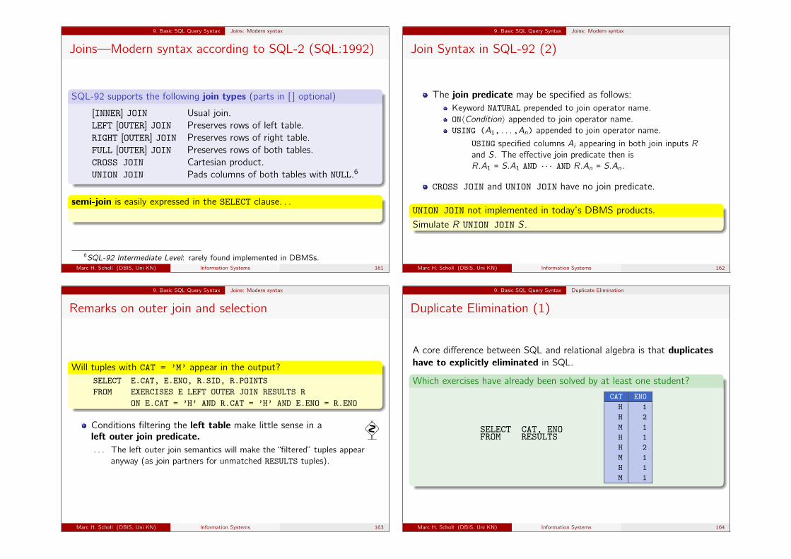
9. Basic SQL Query Syntax Joins: Modern syntax
Joins—Modern syntax according to SQL-2 (SQL:1992)
SQL-92 supports the following join types (parts in [ ] optional)
[INNER] JOIN Usual join.LEFT [OUTER] JOIN Preserves rows of left table.RIGHT [OUTER] JOIN Preserves rows of right table.FULL [OUTER] JOIN Preserves rows of both tables.CROSS JOIN Cartesian product.UNION JOIN Pads columns of both tables with NULL.6
semi-join is easily expressed in the SELECT clause. . .
SELECT DISTINCT R.* FROM R NATURAL JOIN S.
6SQL-92 Intermediate Level: rarely found implemented in DBMSs.Marc H. Scholl (DBIS, Uni KN) Information Systems 161
9. Basic SQL Query Syntax Joins: Modern syntax
Join Syntax in SQL-92 (2)
The join predicate may be specified as follows:Keyword NATURAL prepended to join operator name.ON〈Condition〉 appended to join operator name.USING (A1, . . . ,An) appended to join operator name.
USING specified columns Ai appearing in both join inputs Rand S. The effective join predicate then isR.A1 = S.A1 AND · · · AND R.An = S.An.
CROSS JOIN and UNION JOIN have no join predicate.
UNION JOIN not implemented in today’s DBMS products.
Simulate R UNION JOIN S.
Marc H. Scholl (DBIS, Uni KN) Information Systems 162
9. Basic SQL Query Syntax Joins: Modern syntax
Remarks on outer join and selection
Will tuples with CAT = ’M’ appear in the output?SELECT E.CAT, E.ENO, R.SID, R.POINTSFROM EXERCISES E LEFT OUTER JOIN RESULTS R
ON E.CAT = ’H’ AND R.CAT = ’H’ AND E.ENO = R.ENO
Conditions filtering the left table make little sense in aleft outer join predicate.
�. . . The left outer join semantics will make the “filtered” tuples appear
anyway (as join partners for unmatched RESULTS tuples).
Marc H. Scholl (DBIS, Uni KN) Information Systems 163
9. Basic SQL Query Syntax Duplicate Elimination
Duplicate Elimination (1)
A core difference between SQL and relational algebra is that duplicateshave to explicitly eliminated in SQL.
Which exercises have already been solved by at least one student?
SELECT CAT, ENOFROM RESULTS
CAT ENOH 1H 2M 1H 1H 2M 1H 1M 1
Marc H. Scholl (DBIS, Uni KN) Information Systems 164
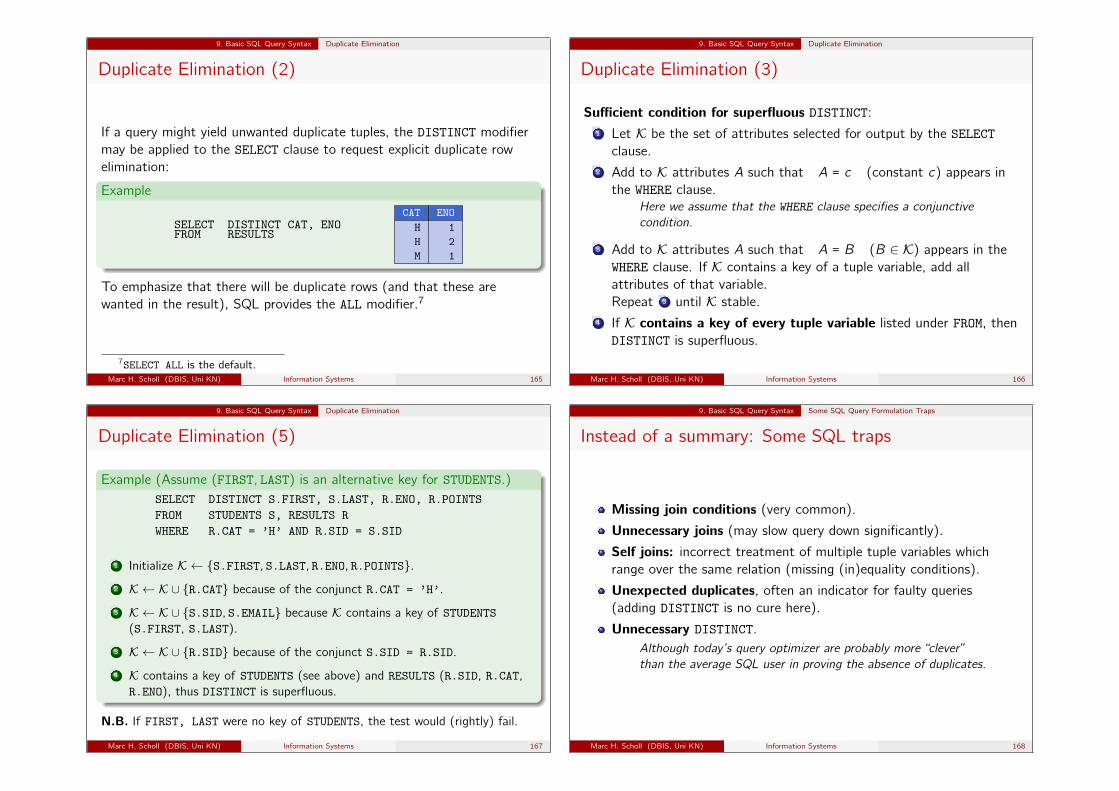
9. Basic SQL Query Syntax Duplicate Elimination
Duplicate Elimination (2)
If a query might yield unwanted duplicate tuples, the DISTINCT modifiermay be applied to the SELECT clause to request explicit duplicate rowelimination:
Example
SELECT DISTINCT CAT, ENOFROM RESULTS
CAT ENOH 1H 2M 1
To emphasize that there will be duplicate rows (and that these arewanted in the result), SQL provides the ALL modifier.7
7SELECT ALL is the default.Marc H. Scholl (DBIS, Uni KN) Information Systems 165
9. Basic SQL Query Syntax Duplicate Elimination
Duplicate Elimination (3)
Sufficient condition for superfluous DISTINCT:1 Let K be the set of attributes selected for output by the SELECT
clause.2 Add to K attributes A such that A = c (constant c) appears in
the WHERE clause.Here we assume that the WHERE clause specifies a conjunctivecondition.
3 Add to K attributes A such that A = B (B ∈ K) appears in theWHERE clause. If K contains a key of a tuple variable, add allattributes of that variable.Repeat 3 until K stable.
4 If K contains a key of every tuple variable listed under FROM, thenDISTINCT is superfluous.
Marc H. Scholl (DBIS, Uni KN) Information Systems 166
9. Basic SQL Query Syntax Duplicate Elimination
Duplicate Elimination (5)
Example (Assume (FIRST, LAST) is an alternative key for STUDENTS.)SELECT DISTINCT S.FIRST, S.LAST, R.ENO, R.POINTSFROM STUDENTS S, RESULTS RWHERE R.CAT = ’H’ AND R.SID = S.SID
1 Initialize K ← {S.FIRST, S.LAST, R.ENO, R.POINTS}.2 K ← K ∪ {R.CAT} because of the conjunct R.CAT = ’H’.
3 K ← K ∪ {S.SID, S.EMAIL} because K contains a key of STUDENTS(S.FIRST, S.LAST).
3 K ← K ∪ {R.SID} because of the conjunct S.SID = R.SID.
4 K contains a key of STUDENTS (see above) and RESULTS (R.SID, R.CAT,R.ENO), thus DISTINCT is superfluous.
N.B. If FIRST, LAST were no key of STUDENTS, the test would (rightly) fail.
Marc H. Scholl (DBIS, Uni KN) Information Systems 167
9. Basic SQL Query Syntax Some SQL Query Formulation Traps
Instead of a summary: Some SQL traps
Missing join conditions (very common).
Unnecessary joins (may slow query down significantly).
Self joins: incorrect treatment of multiple tuple variables whichrange over the same relation (missing (in)equality conditions).
Unexpected duplicates, often an indicator for faulty queries(adding DISTINCT is no cure here).
Unnecessary DISTINCT.Although today’s query optimizer are probably more “clever”than the average SQL user in proving the absence of duplicates.
Marc H. Scholl (DBIS, Uni KN) Information Systems 168
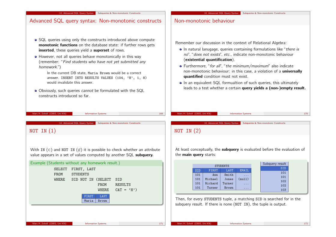
10. Advanced SQL Query Syntax Subqueries & Non-monotonic Constructs
Advanced SQL query syntax: Non-monotonic constructs
SQL queries using only the constructs introduced above computemonotonic functions on the database state: if further rows getsinserted, these queries yield a superset of rows.However, not all queries behave monotonically in this way(remember: “Find students who have not yet submitted anyhomework.”)
In the current DB state, Maria Brown would be a correctanswer. INSERT INTO RESULTS VALUES (104, ’H’, 1, 8)would invalidate this answer.
Obviously, such queries cannot be formulated with the SQLconstructs introduced so far.
Marc H. Scholl (DBIS, Uni KN) Information Systems 169
10. Advanced SQL Query Syntax Subqueries & Non-monotonic Constructs
Non-monotonic behaviour
Remember our discussion in the context of Relational Algebra:
In natural lanugage, queries containing formulations like “there isno”, “does not exists”, etc., indicate non-monotonic behaviour(existential quantification).Furthermore, “for all”, “the minimum/maximum” also indicatenon-monotonic behaviour: in this case, a violation of a universallyquantified condition must not exist.
In an equivalent SQL formualtion of such queries, this ultimatelyleads to a test whether a certain query yields a (non-)empty result.
Marc H. Scholl (DBIS, Uni KN) Information Systems 170
10. Advanced SQL Query Syntax Subqueries & Non-monotonic Constructs
NOT IN (1)
With IN (∈) and NOT IN ( 6∈) it is possible to check whether an attributevalue appears in a set of values computed by another SQL subquery.
Example (Students without any homework result.)SELECT FIRST, LASTFROM STUDENTSWHERE SID NOT IN (SELECT SID
FROM RESULTSWHERE CAT = ’H’)
FIRST LASTMaria Brown
Marc H. Scholl (DBIS, Uni KN) Information Systems 171
10. Advanced SQL Query Syntax Subqueries & Non-monotonic Constructs
NOT IN (2)
At least conceptually, the subquery is evaluated before the evaluation ofthe main query starts:
STUDENTSSID FIRST LAST EMAIL101 Ann Smith ...101 Michael Jones (null)101 Richard Turner ...101 Turner Brown ...
Subquery resultSID101101102102103
Then, for every STUDENTS tuple, a matching SID is searched for in thesubquery result. If there is none (NOT IN), the tuple is output.
Marc H. Scholl (DBIS, Uni KN) Information Systems 172
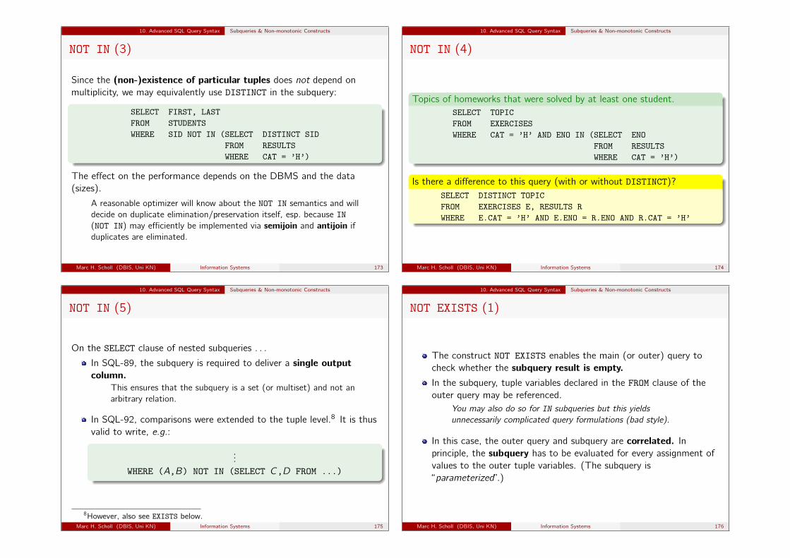
10. Advanced SQL Query Syntax Subqueries & Non-monotonic Constructs
NOT IN (3)
Since the (non-)existence of particular tuples does not depend onmultiplicity, we may equivalently use DISTINCT in the subquery:
SELECT FIRST, LASTFROM STUDENTSWHERE SID NOT IN (SELECT DISTINCT SID
FROM RESULTSWHERE CAT = ’H’)
The effect on the performance depends on the DBMS and the data(sizes).
A reasonable optimizer will know about the NOT IN semantics and willdecide on duplicate elimination/preservation itself, esp. because IN(NOT IN) may efficiently be implemented via semijoin and antijoin ifduplicates are eliminated.
Marc H. Scholl (DBIS, Uni KN) Information Systems 173
10. Advanced SQL Query Syntax Subqueries & Non-monotonic Constructs
NOT IN (4)
Topics of homeworks that were solved by at least one student.SELECT TOPICFROM EXERCISESWHERE CAT = ’H’ AND ENO IN (SELECT ENO
FROM RESULTSWHERE CAT = ’H’)
Is there a difference to this query (with or without DISTINCT)?SELECT DISTINCT TOPICFROM EXERCISES E, RESULTS RWHERE E.CAT = ’H’ AND E.ENO = R.ENO AND R.CAT = ’H’
Marc H. Scholl (DBIS, Uni KN) Information Systems 174
10. Advanced SQL Query Syntax Subqueries & Non-monotonic Constructs
NOT IN (5)
On the SELECT clause of nested subqueries . . .
In SQL-89, the subquery is required to deliver a single outputcolumn.
This ensures that the subquery is a set (or multiset) and not anarbitrary relation.
In SQL-92, comparisons were extended to the tuple level.8 It is thusvalid to write, e.g.:
...WHERE (A,B) NOT IN (SELECT C,D FROM ...)
8However, also see EXISTS below.Marc H. Scholl (DBIS, Uni KN) Information Systems 175
10. Advanced SQL Query Syntax Subqueries & Non-monotonic Constructs
NOT EXISTS (1)
The construct NOT EXISTS enables the main (or outer) query tocheck whether the subquery result is empty.In the subquery, tuple variables declared in the FROM clause of theouter query may be referenced.
You may also do so for IN subqueries but this yieldsunnecessarily complicated query formulations (bad style).
In this case, the outer query and subquery are correlated. Inprinciple, the subquery has to be evaluated for every assignment ofvalues to the outer tuple variables. (The subquery is“parameterized”.)
Marc H. Scholl (DBIS, Uni KN) Information Systems 176
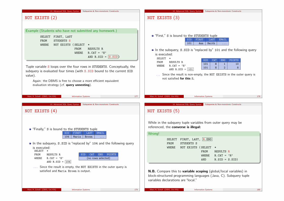
10. Advanced SQL Query Syntax Subqueries & Non-monotonic Constructs
NOT EXISTS (2)
Example (Students who have not submitted any homework.)
SELECT FIRST, LASTFROM STUDENTS SWHERE NOT EXISTS ( SELECT *
FROM RESULTS RWHERE R.CAT = ’H’
AND R.SID = S.SID )
Tuple variable S loops over the four rows in STUDENTS. Conceptually, thesubquery is evaluated four times (with S.SID bound to the current SIDvalue).
Again: the DBMS is free to choose a more efficient equivalentevaluation strategy (cf. query unnesting).
Marc H. Scholl (DBIS, Uni KN) Information Systems 177
10. Advanced SQL Query Syntax Subqueries & Non-monotonic Constructs
NOT EXISTS (3)
“First,” S is bound to the STUDENTS tupleSID FIRST LAST EMAIL101 Ann Smith ...
In the subquery, S.SID is “replaced by” 101 and the following queryis executed:SELECT *FROM RESULTS RWHERE R.CAT = ’H’
AND R.SID = 101
SID CAT ENO POINTS101 H 1 10101 H 2 8
. . . Since the result is non-empty, the NOT EXISTS in the outer query isnot satisfied for this S.
Marc H. Scholl (DBIS, Uni KN) Information Systems 178
10. Advanced SQL Query Syntax Subqueries & Non-monotonic Constructs
NOT EXISTS (4)
“Finally,” S is bound to the STUDENTS tupleSID FIRST LAST EMAIL104 Maria Brown ...
In the subquery, S.SID is “replaced by” 104 and the following queryis executed:SELECT *FROM RESULTS RWHERE R.CAT = ’H’
AND R.SID = 104
SID CAT ENO POINTS(no rows selected)
. . . Since the result is empty, the NOT EXISTS in the outer query issatisfied and Maria Brown is output.
Marc H. Scholl (DBIS, Uni KN) Information Systems 179
10. Advanced SQL Query Syntax Subqueries & Non-monotonic Constructs
NOT EXISTS (5)
While in the subquery tuple variables from outer query may bereferenced, the converse is illegal:
Wrong!
SELECT FIRST, LAST, R.ENOFROM STUDENTS SWHERE NOT EXISTS ( SELECT *
FROM RESULTS RWHERE R.CAT = ’H’AND R.SID = S.SID)
N.B. Compare this to variable scoping (global/local variables) inblock-structured programming languages (Java, C). Subquery tuplevariables declarations are “local.”
Marc H. Scholl (DBIS, Uni KN) Information Systems 180
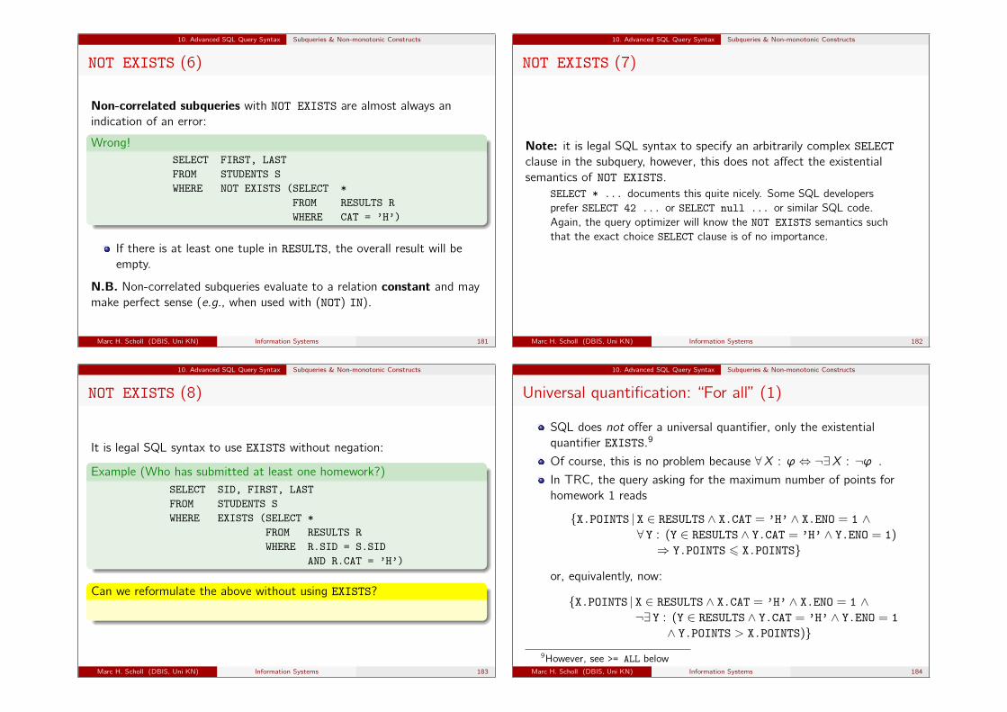
10. Advanced SQL Query Syntax Subqueries & Non-monotonic Constructs
NOT EXISTS (6)
Non-correlated subqueries with NOT EXISTS are almost always anindication of an error:
Wrong!SELECT FIRST, LASTFROM STUDENTS SWHERE NOT EXISTS (SELECT *
FROM RESULTS RWHERE CAT = ’H’)
If there is at least one tuple in RESULTS, the overall result will beempty.
N.B. Non-correlated subqueries evaluate to a relation constant and maymake perfect sense (e.g., when used with (NOT) IN).
Marc H. Scholl (DBIS, Uni KN) Information Systems 181
10. Advanced SQL Query Syntax Subqueries & Non-monotonic Constructs
NOT EXISTS (7)
Note: it is legal SQL syntax to specify an arbitrarily complex SELECTclause in the subquery, however, this does not affect the existentialsemantics of NOT EXISTS.
SELECT * ... documents this quite nicely. Some SQL developersprefer SELECT 42 ... or SELECT null ... or similar SQL code.Again, the query optimizer will know the NOT EXISTS semantics suchthat the exact choice SELECT clause is of no importance.
Marc H. Scholl (DBIS, Uni KN) Information Systems 182
10. Advanced SQL Query Syntax Subqueries & Non-monotonic Constructs
NOT EXISTS (8)
It is legal SQL syntax to use EXISTS without negation:
Example (Who has submitted at least one homework?)SELECT SID, FIRST, LASTFROM STUDENTS SWHERE EXISTS (SELECT *
FROM RESULTS RWHERE R.SID = S.SID
AND R.CAT = ’H’)
Can we reformulate the above without using EXISTS?
. . . sure, it’s a semi-join (and for that: see above)!
Marc H. Scholl (DBIS, Uni KN) Information Systems 183
10. Advanced SQL Query Syntax Subqueries & Non-monotonic Constructs
Universal quantification: “For all” (1)
SQL does not offer a universal quantifier, only the existentialquantifier EXISTS.9
Of course, this is no problem because ∀X : ϕ⇔ ¬∃X : ¬ϕ .
In TRC, the query asking for the maximum number of points forhomework 1 reads
{X.POINTS | X ∈ RESULTS ∧ X.CAT = ’H’ ∧ X.ENO = 1 ∧∀ Y : (Y ∈ RESULTS ∧ Y.CAT = ’H’ ∧ Y.ENO = 1)
⇒ Y.POINTS 6 X.POINTS}or, equivalently, now:
{X.POINTS | X ∈ RESULTS ∧ X.CAT = ’H’ ∧ X.ENO = 1 ∧¬∃ Y : (Y ∈ RESULTS ∧ Y.CAT = ’H’ ∧ Y.ENO = 1
∧ Y.POINTS > X.POINTS)}9However, see >= ALL below
Marc H. Scholl (DBIS, Uni KN) Information Systems 184
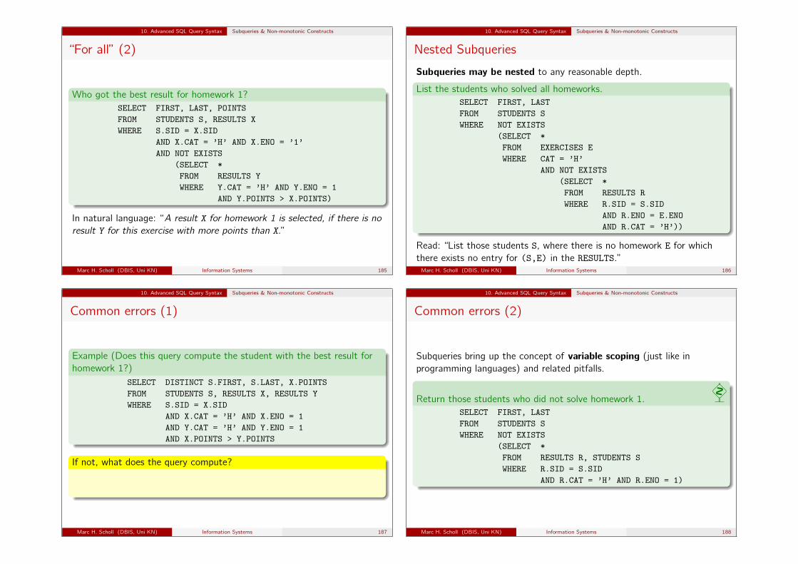
10. Advanced SQL Query Syntax Subqueries & Non-monotonic Constructs
“For all” (2)
Who got the best result for homework 1?SELECT FIRST, LAST, POINTSFROM STUDENTS S, RESULTS XWHERE S.SID = X.SID
AND X.CAT = ’H’ AND X.ENO = ’1’AND NOT EXISTS
(SELECT *FROM RESULTS YWHERE Y.CAT = ’H’ AND Y.ENO = 1
AND Y.POINTS > X.POINTS)
In natural language: “A result X for homework 1 is selected, if there is noresult Y for this exercise with more points than X.”
Marc H. Scholl (DBIS, Uni KN) Information Systems 185
10. Advanced SQL Query Syntax Subqueries & Non-monotonic Constructs
Nested Subqueries
Subqueries may be nested to any reasonable depth.
List the students who solved all homeworks.SELECT FIRST, LASTFROM STUDENTS SWHERE NOT EXISTS
(SELECT *FROM EXERCISES EWHERE CAT = ’H’
AND NOT EXISTS(SELECT *FROM RESULTS RWHERE R.SID = S.SID
AND R.ENO = E.ENOAND R.CAT = ’H’))
Read: “List those students S, where there is no homework E for whichthere exists no entry for (S,E) in the RESULTS.”Marc H. Scholl (DBIS, Uni KN) Information Systems 186
10. Advanced SQL Query Syntax Subqueries & Non-monotonic Constructs
Common errors (1)
Example (Does this query compute the student with the best result forhomework 1?)
SELECT DISTINCT S.FIRST, S.LAST, X.POINTSFROM STUDENTS S, RESULTS X, RESULTS YWHERE S.SID = X.SID
AND X.CAT = ’H’ AND X.ENO = 1AND Y.CAT = ’H’ AND Y.ENO = 1AND X.POINTS > Y.POINTS
If not, what does the query compute?
Returns those students who got more points in homework 1 than someother student. (This is monotonic.)
Marc H. Scholl (DBIS, Uni KN) Information Systems 187
10. Advanced SQL Query Syntax Subqueries & Non-monotonic Constructs
Common errors (2)
Subqueries bring up the concept of variable scoping (just like inprogramming languages) and related pitfalls.
Return those students who did not solve homework 1.�
SELECT FIRST, LASTFROM STUDENTS SWHERE NOT EXISTS
(SELECT *FROM RESULTS R, STUDENTS SWHERE R.SID = S.SID
AND R.CAT = ’H’ AND R.ENO = 1)
Marc H. Scholl (DBIS, Uni KN) Information Systems 188
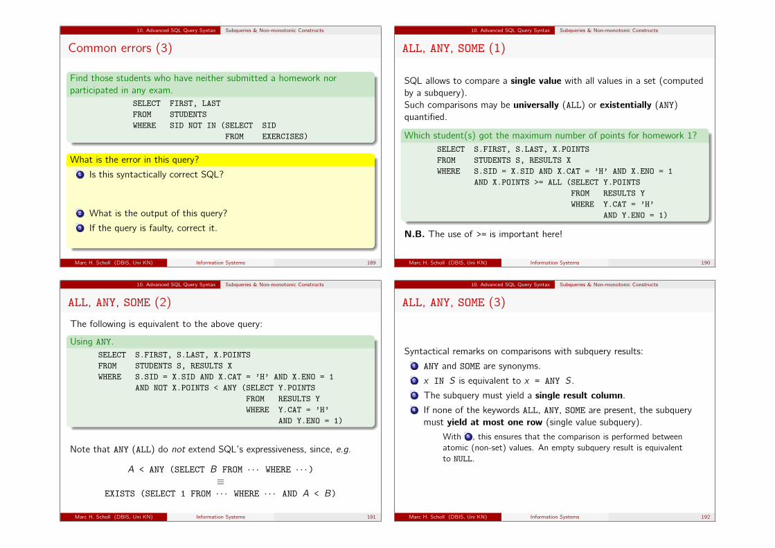
10. Advanced SQL Query Syntax Subqueries & Non-monotonic Constructs
Common errors (3)
Find those students who have neither submitted a homework norparticipated in any exam.
SELECT FIRST, LASTFROM STUDENTSWHERE SID NOT IN (SELECT SID
FROM EXERCISES)
What is the error in this query?1 Is this syntactically correct SQL?
– Yes, reference to SID in subqueryis OK (but it references SID of STUDENTS since there is not SID inEXERCISES!)
2 What is the output of this query?
– Empty (subquery is correlated).
3 If the query is faulty, correct it.
– Replace EXERCISES by RESULTS(and optionally introduce tuple variables to make intention explicit).
Marc H. Scholl (DBIS, Uni KN) Information Systems 189
10. Advanced SQL Query Syntax Subqueries & Non-monotonic Constructs
ALL, ANY, SOME (1)
SQL allows to compare a single value with all values in a set (computedby a subquery).Such comparisons may be universally (ALL) or existentially (ANY)quantified.
Which student(s) got the maximum number of points for homework 1?SELECT S.FIRST, S.LAST, X.POINTSFROM STUDENTS S, RESULTS XWHERE S.SID = X.SID AND X.CAT = ’H’ AND X.ENO = 1
AND X.POINTS >= ALL (SELECT Y.POINTSFROM RESULTS YWHERE Y.CAT = ’H’
AND Y.ENO = 1)
N.B. The use of >= is important here!
Marc H. Scholl (DBIS, Uni KN) Information Systems 190
10. Advanced SQL Query Syntax Subqueries & Non-monotonic Constructs
ALL, ANY, SOME (2)
The following is equivalent to the above query:
Using ANY.SELECT S.FIRST, S.LAST, X.POINTSFROM STUDENTS S, RESULTS XWHERE S.SID = X.SID AND X.CAT = ’H’ AND X.ENO = 1
AND NOT X.POINTS < ANY (SELECT Y.POINTSFROM RESULTS YWHERE Y.CAT = ’H’
AND Y.ENO = 1)
Note that ANY (ALL) do not extend SQL’s expressiveness, since, e.g.
A < ANY (SELECT B FROM · · · WHERE · · · )≡
EXISTS (SELECT 1 FROM · · · WHERE · · · AND A < B)
Marc H. Scholl (DBIS, Uni KN) Information Systems 191
10. Advanced SQL Query Syntax Subqueries & Non-monotonic Constructs
ALL, ANY, SOME (3)
Syntactical remarks on comparisons with subquery results:1 ANY and SOME are synonyms.2 x IN S is equivalent to x = ANY S.3 The subquery must yield a single result column.4 If none of the keywords ALL, ANY, SOME are present, the subquery
must yield at most one row (single value subquery).
With 3 , this ensures that the comparison is performed betweenatomic (non-set) values. An empty subquery result is equivalentto NULL.
Marc H. Scholl (DBIS, Uni KN) Information Systems 192

10. Advanced SQL Query Syntax Subqueries & Non-monotonic Constructs
Single value subqueries (1)
Who got full points for homework 1?SELECT S.FIRST, S.LASTFROM STUDENTS S, RESULTS RWHERE S.SID = R.SID AND R.CAT = ’H’ AND R.ENO = 1
AND R.POINTS = (SELECT MAXPTFROM EXERCISESWHERE CAT = ’H’ AND ENO = 1)
Comparisons with subquery results (note: no ANY, SOME, ALL) arepossible, iff the subquery returns at most one row.
[Why is this guaranteed here?]Use (non-data dependent) constraints to ensure this condition, theDBMS will yield a runtime error, if the subquery returns two or morerows!
Marc H. Scholl (DBIS, Uni KN) Information Systems 193
10. Advanced SQL Query Syntax Subqueries & Non-monotonic Constructs
Single value subqueries (2)
If the subquery has an empty result, the null value is returned.
Example (Bad style!)SELECT FIRST, LASTFROM STUDENTS SWHERE (SELECT 1
FROM RESULTS RWHERE R.SID = S.SID
AND R.CAT = ’H’ AND R.ENO = 1) IS NULL
Rather, use . . . ?
Marc H. Scholl (DBIS, Uni KN) Information Systems 194
10. Advanced SQL Query Syntax Subqueries & Non-monotonic Constructs
Orthogonal SQL: Nesting in the FROM clause
Since the result of a SQL query is a table, it seems most natural touse a subquery result whereever a table might be specified, i.e., inthe FROM clause.
This principle of (query) language construction is known asorthogonality: language constructs may be combined in arbitraryfashion as long as the semantic/typing/. . . rules of the language areobeyed.
Relational algebra is an orthogonal query language.
SQL versions prior to SQL-92 were not orthogonal in this sense.
Apart from stepwise querying, like in algebra, one other use ofsubqueries under FROM are nested aggregations (see further below).
Marc H. Scholl (DBIS, Uni KN) Information Systems 195
10. Advanced SQL Query Syntax Subqueries & Non-monotonic Constructs
Nested subqueries under FROM (1)
In the following example, the join of RESULTS and EXERCISES iscomputed in a subquery (this might result from a view definition, seebelow).
Example (Points (in %) achieved in homework exercise 1.)
SELECT X.SID, (X.POINTS * 100 / X.MAXPT) AS PCTFROM (SELECT E.CAT, E.ENO, R.SID, R.POINTS, E.MAXPT
FROM EXERCISES E, RESULTS RWHERE E.CAT = R.CAT AND E.ENO = R.ENO) AS X
WHERE X.CAT = ’H’ AND X.ENO = 1
N.B. Inside the subquery, tuple variables introduced in the same FROMclause may not be referenced!
Marc H. Scholl (DBIS, Uni KN) Information Systems 196
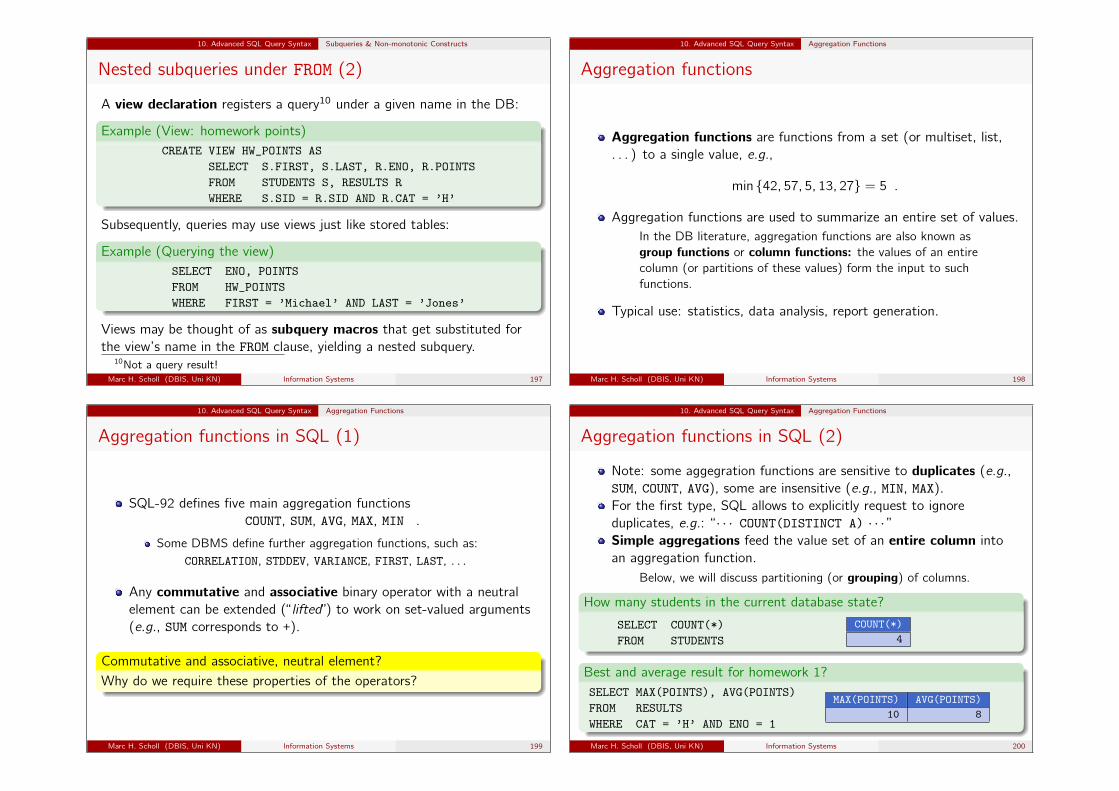
10. Advanced SQL Query Syntax Subqueries & Non-monotonic Constructs
Nested subqueries under FROM (2)
A view declaration registers a query10 under a given name in the DB:
Example (View: homework points)CREATE VIEW HW_POINTS AS
SELECT S.FIRST, S.LAST, R.ENO, R.POINTSFROM STUDENTS S, RESULTS RWHERE S.SID = R.SID AND R.CAT = ’H’
Subsequently, queries may use views just like stored tables:
Example (Querying the view)SELECT ENO, POINTSFROM HW_POINTSWHERE FIRST = ’Michael’ AND LAST = ’Jones’
Views may be thought of as subquery macros that get substituted forthe view’s name in the FROM clause, yielding a nested subquery.
10Not a query result!Marc H. Scholl (DBIS, Uni KN) Information Systems 197
10. Advanced SQL Query Syntax Aggregation Functions
Aggregation functions
Aggregation functions are functions from a set (or multiset, list,. . . ) to a single value, e.g.,
min {42, 57, 5, 13, 27} = 5 .
Aggregation functions are used to summarize an entire set of values.In the DB literature, aggregation functions are also known asgroup functions or column functions: the values of an entirecolumn (or partitions of these values) form the input to suchfunctions.
Typical use: statistics, data analysis, report generation.
Marc H. Scholl (DBIS, Uni KN) Information Systems 198
10. Advanced SQL Query Syntax Aggregation Functions
Aggregation functions in SQL (1)
SQL-92 defines five main aggregation functionsCOUNT, SUM, AVG, MAX, MIN .
Some DBMS define further aggregation functions, such as:CORRELATION, STDDEV, VARIANCE, FIRST, LAST, . . .
Any commutative and associative binary operator with a neutralelement can be extended (“ lifted”) to work on set-valued arguments(e.g., SUM corresponds to +).
Commutative and associative, neutral element?Why do we require these properties of the operators?
Marc H. Scholl (DBIS, Uni KN) Information Systems 199
10. Advanced SQL Query Syntax Aggregation Functions
Aggregation functions in SQL (2)
Note: some aggegration functions are sensitive to duplicates (e.g.,SUM, COUNT, AVG), some are insensitive (e.g., MIN, MAX).For the first type, SQL allows to explicitly request to ignoreduplicates, e.g.: “ · · · COUNT(DISTINCT A) · · · ”Simple aggregations feed the value set of an entire column intoan aggregation function.
Below, we will discuss partitioning (or grouping) of columns.
How many students in the current database state?
SELECT COUNT(*)FROM STUDENTS
COUNT(*)4
Best and average result for homework 1?SELECT MAX(POINTS), AVG(POINTS)FROM RESULTSWHERE CAT = ’H’ AND ENO = 1
MAX(POINTS) AVG(POINTS)10 8
Marc H. Scholl (DBIS, Uni KN) Information Systems 200

10. Advanced SQL Query Syntax Aggregation Functions
Examples: Simple aggregations . . .
Example (How many students have submitted a homework?)
SELECT COUNT(DISTINCT SID)FROM RESULTSWHERE CAT = ’H’
COUNT(DISTINCT SID)3
Example (What is the total number of points student 101 got for herhomeworks?)
SELECT SUM(POINTS) AS "Total Points"FROM RESULTSWHERE SID = 101 AND CAT = ’H’
Total Points18
Marc H. Scholl (DBIS, Uni KN) Information Systems 201
10. Advanced SQL Query Syntax Aggregation Functions
. . . Examples: Simple aggregations
What average percentage of the maximum points did the students reachfor homework 1?
SELECT AVG(R.POINTS / E.MAXPT) * 100FROM RESULTS R, EXERCISES EWHERE R.CAT = ’H’ AND E.CAT = ’H’
AND R.ENO = 1 AND E.ENO = 1
Homework points for student 101 plus 3 bonus points.
SELECT SUM(POINTS) + 3 AS "Total Homework Points"FROM RESULTSWHERE SID = 101 AND CAT = ’H’
Marc H. Scholl (DBIS, Uni KN) Information Systems 202
10. Advanced SQL Query Syntax Aggregation Functions
Aggregation queries and SQL semantics
Basically, there are three different types of queries in SQL:1 Queries without aggregation functions and without GROUP BY and
HAVING. (Discussed above.)2 Queries with aggregation functions in the SELECT clause but no
GROUP BY (simple aggregations). Yield exactly one row.3 Queries with GROUP BY.
Each type has different syntax restrictions and is evaluated in a differentway.
Notice again: when speaking of “evaluation”, we refer to the SQLsemantics here. A DBMS is free to implement these semantics as itsees fit.
Marc H. Scholl (DBIS, Uni KN) Information Systems 203
10. Advanced SQL Query Syntax Aggregation Functions
Possible evaluation (1)
1 First, evaluate the FROM clause.Conceptually, form all possible tuple combinations of the sourcetables (Relational product).
2 Evaluate the WHERE clause.The Relational product produced in 1 is filtered (restricted) andonly those tuple combinations satisfying the filter conditionremain.
3 If no aggregation, GROUP BY or HAVING: evaluate the SELECTclause.
Evaluate projection list (terms, scalar expressions) for each tuplecombination produced in 2 and print resulting tuples.
Marc H. Scholl (DBIS, Uni KN) Information Systems 204
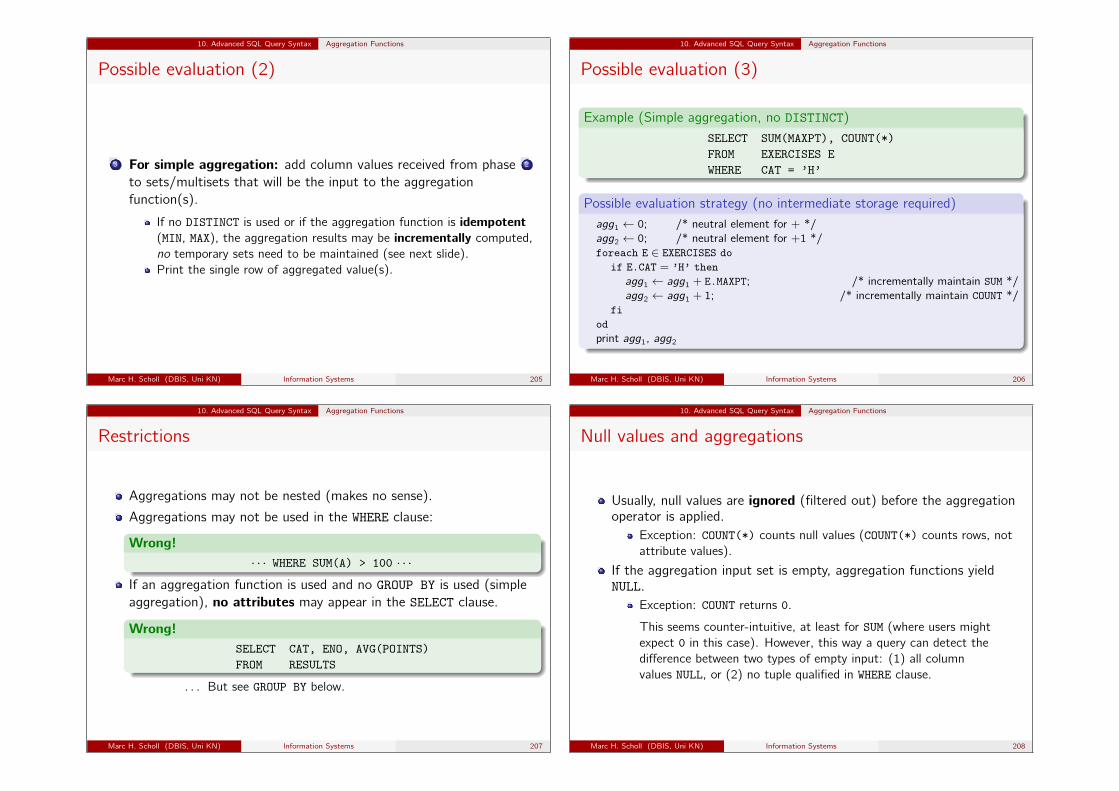
10. Advanced SQL Query Syntax Aggregation Functions
Possible evaluation (2)
3 For simple aggregation: add column values received from phase 2
to sets/multisets that will be the input to the aggregationfunction(s).
If no DISTINCT is used or if the aggregation function is idempotent(MIN, MAX), the aggregation results may be incrementally computed,no temporary sets need to be maintained (see next slide).Print the single row of aggregated value(s).
Marc H. Scholl (DBIS, Uni KN) Information Systems 205
10. Advanced SQL Query Syntax Aggregation Functions
Possible evaluation (3)
Example (Simple aggregation, no DISTINCT)
SELECT SUM(MAXPT), COUNT(*)FROM EXERCISES EWHERE CAT = ’H’
Possible evaluation strategy (no intermediate storage required)agg1 ← 0; /* neutral element for + */agg2 ← 0; /* neutral element for +1 */foreach E ∈ EXERCISES do
if E.CAT = ’H’ thenagg1 ← agg1 + E.MAXPT; /* incrementally maintain SUM */agg2 ← agg1 + 1; /* incrementally maintain COUNT */
fiodprint agg1, agg2
Marc H. Scholl (DBIS, Uni KN) Information Systems 206
10. Advanced SQL Query Syntax Aggregation Functions
Restrictions
Aggregations may not be nested (makes no sense).
Aggregations may not be used in the WHERE clause:
Wrong!· · · WHERE SUM(A) > 100 · · ·
If an aggregation function is used and no GROUP BY is used (simpleaggregation), no attributes may appear in the SELECT clause.
Wrong!SELECT CAT, ENO, AVG(POINTS)FROM RESULTS
. . . But see GROUP BY below.
Marc H. Scholl (DBIS, Uni KN) Information Systems 207
10. Advanced SQL Query Syntax Aggregation Functions
Null values and aggregations
Usually, null values are ignored (filtered out) before the aggregationoperator is applied.
Exception: COUNT(*) counts null values (COUNT(*) counts rows, notattribute values).
If the aggregation input set is empty, aggregation functions yieldNULL.
Exception: COUNT returns 0.
This seems counter-intuitive, at least for SUM (where users mightexpect 0 in this case). However, this way a query can detect thedifference between two types of empty input: (1) all columnvalues NULL, or (2) no tuple qualified in WHERE clause.
Marc H. Scholl (DBIS, Uni KN) Information Systems 208
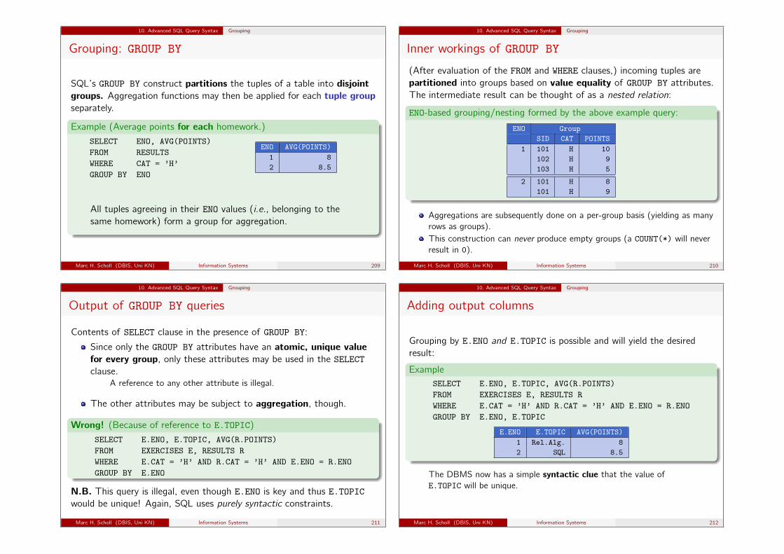
10. Advanced SQL Query Syntax Grouping
Grouping: GROUP BY
SQL’s GROUP BY construct partitions the tuples of a table into disjointgroups. Aggregation functions may then be applied for each tuple groupseparately.
Example (Average points for each homework.)
SELECT ENO, AVG(POINTS)FROM RESULTSWHERE CAT = ’H’GROUP BY ENO
ENO AVG(POINTS)1 82 8.5
All tuples agreeing in their ENO values (i.e., belonging to thesame homework) form a group for aggregation.
Marc H. Scholl (DBIS, Uni KN) Information Systems 209
10. Advanced SQL Query Syntax Grouping
Inner workings of GROUP BY
(After evaluation of the FROM and WHERE clauses,) incoming tuples arepartitioned into groups based on value equality of GROUP BY attributes.The intermediate result can be thought of as a nested relation:
ENO-based grouping/nesting formed by the above example query:
ENO GroupSID CAT POINTS
1 101 H 10102 H 9103 H 5
2 101 H 8101 H 9
Aggregations are subsequently done on a per-group basis (yielding as manyrows as groups).This construction can never produce empty groups (a COUNT(*) will neverresult in 0).
Marc H. Scholl (DBIS, Uni KN) Information Systems 210
10. Advanced SQL Query Syntax Grouping
Output of GROUP BY queries
Contents of SELECT clause in the presence of GROUP BY:
Since only the GROUP BY attributes have an atomic, unique valuefor every group, only these attributes may be used in the SELECTclause.
A reference to any other attribute is illegal.
The other attributes may be subject to aggregation, though.
Wrong! (Because of reference to E.TOPIC)
SELECT E.ENO, E.TOPIC, AVG(R.POINTS)FROM EXERCISES E, RESULTS RWHERE E.CAT = ’H’ AND R.CAT = ’H’ AND E.ENO = R.ENOGROUP BY E.ENO
N.B. This query is illegal, even though E.ENO is key and thus E.TOPICwould be unique! Again, SQL uses purely syntactic constraints.
Marc H. Scholl (DBIS, Uni KN) Information Systems 211
10. Advanced SQL Query Syntax Grouping
Adding output columns
Grouping by E.ENO and E.TOPIC is possible and will yield the desiredresult:
ExampleSELECT E.ENO, E.TOPIC, AVG(R.POINTS)FROM EXERCISES E, RESULTS RWHERE E.CAT = ’H’ AND R.CAT = ’H’ AND E.ENO = R.ENOGROUP BY E.ENO, E.TOPIC
E.ENO E.TOPIC AVG(POINTS)1 Rel.Alg. 82 SQL 8.5
The DBMS now has a simple syntactic clue that the value ofE.TOPIC will be unique.
Marc H. Scholl (DBIS, Uni KN) Information Systems 212
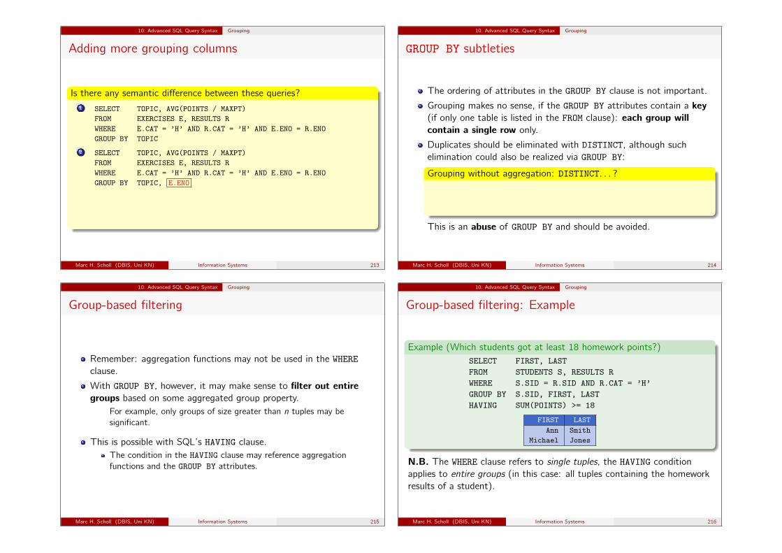
10. Advanced SQL Query Syntax Grouping
Adding more grouping columns
Is there any semantic difference between these queries?1 SELECT TOPIC, AVG(POINTS / MAXPT)
FROM EXERCISES E, RESULTS RWHERE E.CAT = ’H’ AND R.CAT = ’H’ AND E.ENO = R.ENOGROUP BY TOPIC
2 SELECT TOPIC, AVG(POINTS / MAXPT)FROM EXERCISES E, RESULTS RWHERE E.CAT = ’H’ AND R.CAT = ’H’ AND E.ENO = R.ENOGROUP BY TOPIC, E.ENO
Yes: if table EXERCISES contains multiple exercises with the same TOPIC(these will then be grouped together which may not be what was desired).
Marc H. Scholl (DBIS, Uni KN) Information Systems 213
10. Advanced SQL Query Syntax Grouping
GROUP BY subtleties
The ordering of attributes in the GROUP BY clause is not important.
Grouping makes no sense, if the GROUP BY attributes contain a key(if only one table is listed in the FROM clause): each group willcontain a single row only.
Duplicates should be eliminated with DISTINCT, although suchelimination could also be realized via GROUP BY:
Grouping without aggregation: DISTINCT. . . ?
SELECT CAT, ENOFROM RESULTSGROUP BY CAT, ENO
This is an abuse of GROUP BY and should be avoided.
Marc H. Scholl (DBIS, Uni KN) Information Systems 214
10. Advanced SQL Query Syntax Grouping
Group-based filtering
Remember: aggregation functions may not be used in the WHEREclause.
With GROUP BY, however, it may make sense to filter out entiregroups based on some aggregated group property.
For example, only groups of size greater than n tuples may besignificant.
This is possible with SQL’s HAVING clause.The condition in the HAVING clause may reference aggregationfunctions and the GROUP BY attributes.
Marc H. Scholl (DBIS, Uni KN) Information Systems 215
10. Advanced SQL Query Syntax Grouping
Group-based filtering: Example
Example (Which students got at least 18 homework points?)SELECT FIRST, LASTFROM STUDENTS S, RESULTS RWHERE S.SID = R.SID AND R.CAT = ’H’GROUP BY S.SID, FIRST, LASTHAVING SUM(POINTS) >= 18
FIRST LASTAnn Smith
Michael Jones
N.B. The WHERE clause refers to single tuples, the HAVING conditionapplies to entire groups (in this case: all tuples containing the homeworkresults of a student).
Marc H. Scholl (DBIS, Uni KN) Information Systems 216
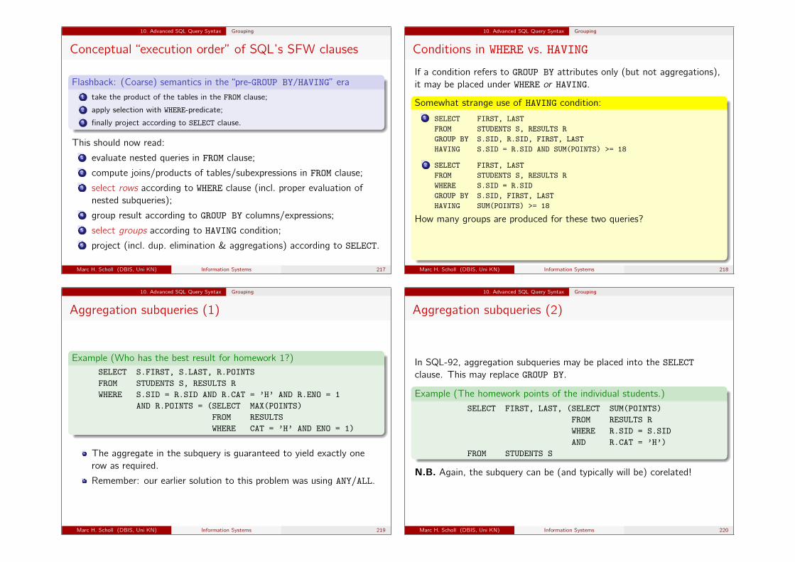
10. Advanced SQL Query Syntax Grouping
Conceptual “execution order” of SQL’s SFW clauses
Flashback: (Coarse) semantics in the “pre-GROUP BY/HAVING” era1 take the product of the tables in the FROM clause;2 apply selection with WHERE-predicate;3 finally project according to SELECT clause.
This should now read:1 evaluate nested queries in FROM clause;2 compute joins/products of tables/subexpressions in FROM clause;3 select rows according to WHERE clause (incl. proper evaluation of
nested subqueries);4 group result according to GROUP BY columns/expressions;5 select groups according to HAVING condition;6 project (incl. dup. elimination & aggregations) according to SELECT.
Marc H. Scholl (DBIS, Uni KN) Information Systems 217
10. Advanced SQL Query Syntax Grouping
Conditions in WHERE vs. HAVING
If a condition refers to GROUP BY attributes only (but not aggregations),it may be placed under WHERE or HAVING.
Somewhat strange use of HAVING condition:1 SELECT FIRST, LAST
FROM STUDENTS S, RESULTS RGROUP BY S.SID, R.SID, FIRST, LASTHAVING S.SID = R.SID AND SUM(POINTS) >= 18
2 SELECT FIRST, LASTFROM STUDENTS S, RESULTS RWHERE S.SID = R.SIDGROUP BY S.SID, FIRST, LASTHAVING SUM(POINTS) >= 18
How many groups are produced for these two queries?
1 12 = 4 · 3 (4 different SIDs in STUDENTS, 3 SIDs in RESULTS)2 3 (3 matching join tuples)
Marc H. Scholl (DBIS, Uni KN) Information Systems 218
10. Advanced SQL Query Syntax Grouping
Aggregation subqueries (1)
Example (Who has the best result for homework 1?)SELECT S.FIRST, S.LAST, R.POINTSFROM STUDENTS S, RESULTS RWHERE S.SID = R.SID AND R.CAT = ’H’ AND R.ENO = 1
AND R.POINTS = (SELECT MAX(POINTS)FROM RESULTSWHERE CAT = ’H’ AND ENO = 1)
The aggregate in the subquery is guaranteed to yield exactly onerow as required.
Remember: our earlier solution to this problem was using ANY/ALL.
Marc H. Scholl (DBIS, Uni KN) Information Systems 219
10. Advanced SQL Query Syntax Grouping
Aggregation subqueries (2)
In SQL-92, aggregation subqueries may be placed into the SELECTclause. This may replace GROUP BY.
Example (The homework points of the individual students.)
SELECT FIRST, LAST, (SELECT SUM(POINTS)FROM RESULTS RWHERE R.SID = S.SIDAND R.CAT = ’H’)
FROM STUDENTS S
N.B. Again, the subquery can be (and typically will be) corelated!
Marc H. Scholl (DBIS, Uni KN) Information Systems 220

10. Advanced SQL Query Syntax Grouping
Nested Aggregations
Nested aggregations require a subquery in the FROM clause.
What is the average number of homework points (excluding thosestudents who did not submit anything)?
SELECT AVG(X.HW_POINTS)FROM (SELECT SID, SUM(POINTS) AS HW_POINTS
FROM RESULTSWHERE CAT = ’H’GROUP BY SID) X
XSID HW_POINTS101 18103 18103 5
AVG(X.HW_POINTS)13.67
Marc H. Scholl (DBIS, Uni KN) Information Systems 221
10. Advanced SQL Query Syntax Grouping
Maximizing Aggregations (1)
Who has the best overall homework result (maximum sum of homeworkpoints)?
SELECT FIRST, LAST, SUM(POINTS) AS TOTALFROM STUDENTS S, RESULTS RWHERE S.SID = R.SID AND R.CAT = ’H’GROUP BY S.SID, FIRST, LASTHAVING SUM(POINTS) >= ALL (SELECT SUM (POINTS)
FROM RESULTSWHERE CAT = ’H’GROUP BY SID)
N.B.Conditions in the HAVING clause can contain nested subqueries!
Alternatively, we could use a view to solve this problem (next slide).
Marc H. Scholl (DBIS, Uni KN) Information Systems 222
10. Advanced SQL Query Syntax Grouping
Maximizing Aggregations (2)
View: total number of homework points for each student.CREATE VIEW HW_TOTALS ASSELECT SID, SUM(POINTS) AS TOTALFROM RESULTSWHERE CAT = ’H’GROUP BY SID
Alternative formulation of query on previous slide.SELECT S.FIRST, S.LAST, H.TOTALFROM STUDENTS S, HW_TOTALS HWHERE S.SID = H.SID
AND H.TOTAL = (SELECT MAX(TOTAL)FROM HW_TOTALS)
N.B. This (use of views) is a standard way of nesting aggregationfunctions in SQL.Marc H. Scholl (DBIS, Uni KN) Information Systems 223
10. Advanced SQL Query Syntax Conditional Expressions
Conditional expressions: Case analysis
We have seen earlier that UNION is a common way (in algebra and inSQL) to deal with case analysis.
In SQL, it is possible to combine (on the outermost nesting levelonly) the results of two queries by UNION.
UNION is strictly needed, since there is no other method to constructone result column that draws from different tables/columns.
This is necessary, for example, if specializations of a concept(“subclasses”) are stored in separate tables. For instance, theremay be GRADUATE_COURSES and UNDERGRADUATE_COURSEStables (both of which are specializations of the general conceptCOURSE).11
11see our discussion of how to map generalization hierachies to the relational modelMarc H. Scholl (DBIS, Uni KN) Information Systems 224
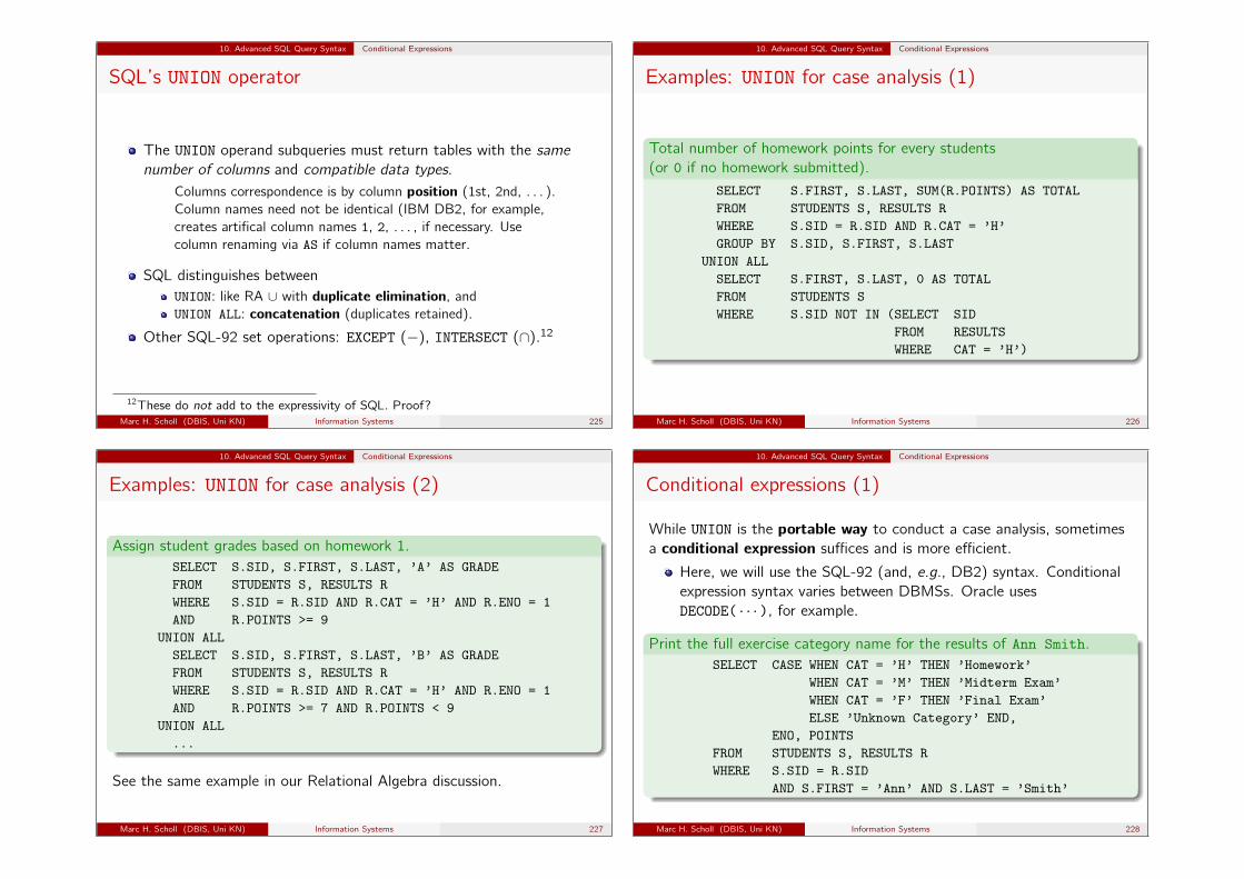
10. Advanced SQL Query Syntax Conditional Expressions
SQL’s UNION operator
The UNION operand subqueries must return tables with the samenumber of columns and compatible data types.
Columns correspondence is by column position (1st, 2nd, . . . ).Column names need not be identical (IBM DB2, for example,creates artifical column names 1, 2, . . . , if necessary. Usecolumn renaming via AS if column names matter.
SQL distinguishes betweenUNION: like RA ∪ with duplicate elimination, andUNION ALL: concatenation (duplicates retained).
Other SQL-92 set operations: EXCEPT (−), INTERSECT (∩).12
12These do not add to the expressivity of SQL. Proof?Marc H. Scholl (DBIS, Uni KN) Information Systems 225
10. Advanced SQL Query Syntax Conditional Expressions
Examples: UNION for case analysis (1)
Total number of homework points for every students(or 0 if no homework submitted).
SELECT S.FIRST, S.LAST, SUM(R.POINTS) AS TOTALFROM STUDENTS S, RESULTS RWHERE S.SID = R.SID AND R.CAT = ’H’GROUP BY S.SID, S.FIRST, S.LAST
UNION ALLSELECT S.FIRST, S.LAST, 0 AS TOTALFROM STUDENTS SWHERE S.SID NOT IN (SELECT SID
FROM RESULTSWHERE CAT = ’H’)
Marc H. Scholl (DBIS, Uni KN) Information Systems 226
10. Advanced SQL Query Syntax Conditional Expressions
Examples: UNION for case analysis (2)
Assign student grades based on homework 1.SELECT S.SID, S.FIRST, S.LAST, ’A’ AS GRADEFROM STUDENTS S, RESULTS RWHERE S.SID = R.SID AND R.CAT = ’H’ AND R.ENO = 1AND R.POINTS >= 9
UNION ALLSELECT S.SID, S.FIRST, S.LAST, ’B’ AS GRADEFROM STUDENTS S, RESULTS RWHERE S.SID = R.SID AND R.CAT = ’H’ AND R.ENO = 1AND R.POINTS >= 7 AND R.POINTS < 9
UNION ALL...
See the same example in our Relational Algebra discussion.
Marc H. Scholl (DBIS, Uni KN) Information Systems 227
10. Advanced SQL Query Syntax Conditional Expressions
Conditional expressions (1)
While UNION is the portable way to conduct a case analysis, sometimesa conditional expression suffices and is more efficient.
Here, we will use the SQL-92 (and, e.g., DB2) syntax. Conditionalexpression syntax varies between DBMSs. Oracle usesDECODE( · · · ), for example.
Print the full exercise category name for the results of Ann Smith.SELECT CASE WHEN CAT = ’H’ THEN ’Homework’
WHEN CAT = ’M’ THEN ’Midterm Exam’WHEN CAT = ’F’ THEN ’Final Exam’ELSE ’Unknown Category’ END,
ENO, POINTSFROM STUDENTS S, RESULTS RWHERE S.SID = R.SID
AND S.FIRST = ’Ann’ AND S.LAST = ’Smith’
Marc H. Scholl (DBIS, Uni KN) Information Systems 228
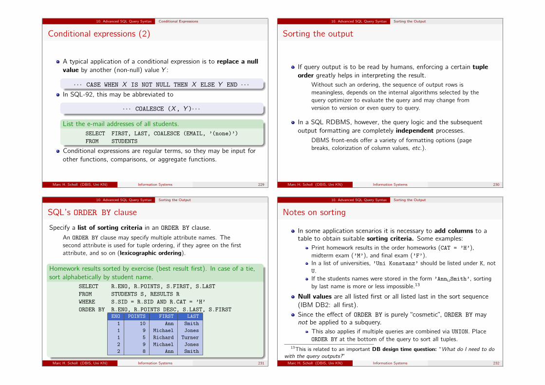
10. Advanced SQL Query Syntax Conditional Expressions
Conditional expressions (2)
A typical application of a conditional expression is to replace a nullvalue by another (non-null) value Y :
· · · CASE WHEN X IS NOT NULL THEN X ELSE Y END · · ·In SQL-92, this may be abbreviated to
· · · COALESCE (X, Y )· · ·
List the e-mail addresses of all students.SELECT FIRST, LAST, COALESCE (EMAIL, ’(none)’)FROM STUDENTS
Conditional expressions are regular terms, so they may be input forother functions, comparisons, or aggregate functions.
Marc H. Scholl (DBIS, Uni KN) Information Systems 229
10. Advanced SQL Query Syntax Sorting the Output
Sorting the output
If query output is to be read by humans, enforcing a certain tupleorder greatly helps in interpreting the result.
Without such an ordering, the sequence of output rows ismeaningless, depends on the internal algorithms selected by thequery optimizer to evaluate the query and may change fromversion to version or even query to query.
In a SQL RDBMS, however, the query logic and the subsequentoutput formatting are completely independent processes.
DBMS front-ends offer a variety of formatting options (pagebreaks, colorization of column values, etc.).
Marc H. Scholl (DBIS, Uni KN) Information Systems 230
10. Advanced SQL Query Syntax Sorting the Output
SQL’s ORDER BY clause
Specify a list of sorting criteria in an ORDER BY clause.
An ORDER BY clause may specify multiple attribute names. Thesecond attribute is used for tuple ordering, if they agree on the firstattribute, and so on (lexicographic ordering).
Homework results sorted by exercise (best result first). In case of a tie,sort alphabetically by student name.
SELECT R.ENO, R.POINTS, S.FIRST, S.LASTFROM STUDENTS S, RESULTS RWHERE S.SID = R.SID AND R.CAT = ’H’ORDER BY R.ENO, R.POINTS DESC, S.LAST, S.FIRST
ENO POINTS FIRST LAST1 10 Ann Smith1 9 Michael Jones1 5 Richard Turner2 9 Michael Jones2 8 Ann Smith
Marc H. Scholl (DBIS, Uni KN) Information Systems 231
10. Advanced SQL Query Syntax Sorting the Output
Notes on sorting
In some application scenarios it is necessary to add columns to atable to obtain suitable sorting criteria. Some examples:
Print homework results in the order homeworks (CAT = ’H’),midterm exam (’M’), and final exam (’F’).In a list of universities, ’Uni Konstanz’ should be listed under K, notU.If the students names were stored in the form ’Ann Smith’, sortingby last name is more or less impossible.13
Null values are all listed first or all listed last in the sort sequence(IBM DB2: all first).Since the effect of ORDER BY is purely “cosmetic”, ORDER BY maynot be applied to a subquery.
This also applies if multiple queries are combined via UNION. PlaceORDER BY at the bottom of the query to sort all tuples.
13This is related to an important DB design time question: “What do I need to dowith the query outputs?”Marc H. Scholl (DBIS, Uni KN) Information Systems 232
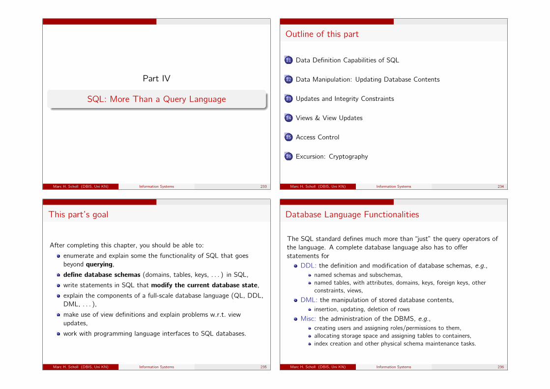
Part IV
SQL: More Than a Query Language
Marc H. Scholl (DBIS, Uni KN) Information Systems 233
Outline of this part
11 Data Definition Capabilities of SQL
12 Data Manipulation: Updating Database Contents
13 Updates and Integrity Constraints
14 Views & View Updates
15 Access Control
16 Excursion: Cryptography
Marc H. Scholl (DBIS, Uni KN) Information Systems 234
This part’s goal
After completing this chapter, you should be able to:
enumerate and explain some the functionality of SQL that goesbeyond querying,define database schemas (domains, tables, keys, . . . ) in SQL,
write statements in SQL that modify the current database state,explain the components of a full-scale database language (QL, DDL,DML, . . . ),
make use of view definitions and explain problems w.r.t. viewupdates,
work with programming language interfaces to SQL databases.
Marc H. Scholl (DBIS, Uni KN) Information Systems 235
Database Language Functionalities
The SQL standard defines much more than “just” the query operators ofthe language. A complete database language also has to offerstatements for
DDL: the definition and modification of database schemas, e.g.,named schemas and subschemas,named tables, with attributes, domains, keys, foreign keys, otherconstraints, views,
DML: the manipulation of stored database contents,insertion, updating, deletion of rows
Misc: the administration of the DBMS, e.g.,creating users and assigning roles/permissions to them,allocating storage space and assigning tables to containers,index creation and other physical schema maintenance tasks.
Marc H. Scholl (DBIS, Uni KN) Information Systems 236
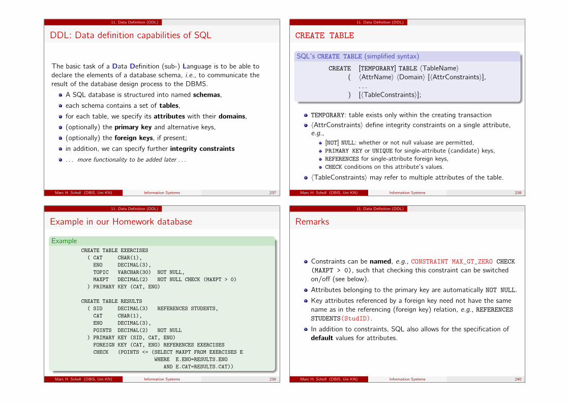
11. Data Definition (DDL)
DDL: Data definition capabilities of SQL
The basic task of a Data Definition (sub-) Language is to be able todeclare the elements of a database schema, i.e., to communicate theresult of the database design process to the DBMS.
A SQL database is structured into named schemas,each schema contains a set of tables,for each table, we specify its attributes with their domains,(optionally) the primary key and alternative keys,
(optionally) the foreign keys, if present;in addition, we can specify further integrity constraints. . . more functionality to be added later . . .
Marc H. Scholl (DBIS, Uni KN) Information Systems 237
11. Data Definition (DDL)
CREATE TABLE
SQL’s CREATE TABLE (simplified syntax)
CREATE [TEMPORARY] TABLE 〈TableName〉( 〈AttrName〉 〈Domain〉 [〈AttrConstraints〉],
. . .) [〈TableConstraints〉];
TEMPORARY: table exists only within the creating transaction〈AttrConstraints〉 define integrity constraints on a single attribute,e.g.,
[NOT] NULL: whether or not null valuase are permitted,PRIMARY KEY or UNIQUE for single-attribute (candidate) keys,REFERENCES for single-attribute foreign keys,CHECK conditions on this attribute’s values.
〈TableConstraints〉 may refer to multiple attributes of the table.
Marc H. Scholl (DBIS, Uni KN) Information Systems 238
11. Data Definition (DDL)
Example in our Homework database
ExampleCREATE TABLE EXERCISES( CAT CHAR(1),
ENO DECIMAL(3),TOPIC VARCHAR(30) NOT NULL,MAXPT DECIMAL(2) NOT NULL CHECK (MAXPT > 0)
) PRIMARY KEY (CAT, ENO)
CREATE TABLE RESULTS( SID DECIMAL(3) REFERENCES STUDENTS,
CAT CHAR(1),ENO DECIMAL(3),POINTS DECIMAL(2) NOT NULL
) PRIMARY KEY (SID, CAT, ENO)FOREIGN KEY (CAT, ENO) REFERENCES EXERCISESCHECK (POINTS <= (SELECT MAXPT FROM EXERCISES E
WHERE E.ENO=RESULTS.ENOAND E.CAT=RESULTS.CAT))
Marc H. Scholl (DBIS, Uni KN) Information Systems 239
11. Data Definition (DDL)
Remarks
Constraints can be named, e.g., CONSTRAINT MAX_GT_ZERO CHECK(MAXPT > 0), such that checking this constraint can be switchedon/off (see below).
Attributes belonging to the primary key are automatically NOT NULL.
Key attributes referenced by a foreign key need not have the samename as in the referencing (foreign key) relation, e.g., REFERENCESSTUDENTS(StudID).
In addition to constraints, SQL also allows for the specification ofdefault values for attributes.
Marc H. Scholl (DBIS, Uni KN) Information Systems 240
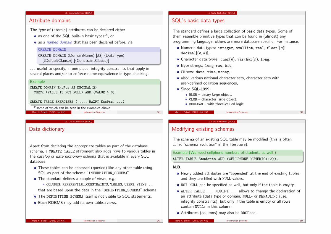
11. Data Definition (DDL)
Attribute domains
The type of (atomic) attributes can be declared either
as one of the SQL built-in basic types14, or
as a named domain that has been declared before, via
CREATE DOMAIN
CREATE DOMAIN 〈DomainName〉 [AS] 〈DataType〉[〈DefaultClause〉] [〈ConstraintClause〉]
. . . useful to specify, in one place, integrity constraints that apply inseveral places and/or to enforce name-equivalence in type checking.
ExampleCREATE DOMAIN ExcPts AS DECIMAL(2)
CHECK (VALUE IS NOT NULL) AND (VALUE > 0)
CREATE TABLE EXERCISES ( ..., MAXPT ExcPts, ...)14some of which can be seen in the examples above
Marc H. Scholl (DBIS, Uni KN) Information Systems 241
11. Data Definition (DDL)
SQL’s basic data types
The standard defines a large collection of basic data types. Some ofthem resemble primitive types that can be found in (almost) anyprogramming language, others are more database specific. For instance,
Numeric data types: integer, smallint, real, float[(n)],decimal[(n, k)],
Character data types: char(n), varchar(n), long,
Byte strings: long raw, bit,
Others: date, time, money,
also: various national character sets, character sets withuser-defined collation sequences,Since SQL-1999:
BLOB – binary large object,CLOB – character large object,BOOLEAN – with three-valued logic
Marc H. Scholl (DBIS, Uni KN) Information Systems 242
11. Data Definition (DDL)
Data dictionary
Apart from declaring the appropriate tables as part of the databaseschema, a CREATE TABLE statement also adds rows to various tables inthe catalog or data dictionary schema that is available in every SQLdatabase.
These tables can be accessed (queried) like any other table usingSQL as part of the schema “INFORMATION_SCHEMA”.The standard defines a couple of views, e.g.,
COLUMNS, REFERENTIAL_CONSTRAINTS, TABLES, USERS, VIEWS, . . .
that are based upon the data in the “DEFINITION_SCHEMA” schema.
The DEFINITION_SCHEMA itself is not visible to SQL statements.
Each RDBMS may add its own tables/views.
Marc H. Scholl (DBIS, Uni KN) Information Systems 243
11. Data Definition (DDL)
Modifying existing schemas
The schema of an existing SQL table may be modified (this is oftencalled “schema evolution” in the literature).
Example (We need cellphone numbers of students as well.)
ALTER TABLE Students ADD (CELLPHONE NUMERIC(12)).
N.B.Newly added attributes are “appended” at the end of existing tuples,and they are filled with NULL values.
NOT NULL can be specified as well, but only if the table is empty.
ALTER TABLE ... MODIFY ... allows to change the declaration ofan attribute (data type or domain, NULL- or DEFAULT-clause,integrity constraints), but only if the table is empty or all rowscontain NULLs in this column.
Attributes (columns) may also be DROPped.
Marc H. Scholl (DBIS, Uni KN) Information Systems 244
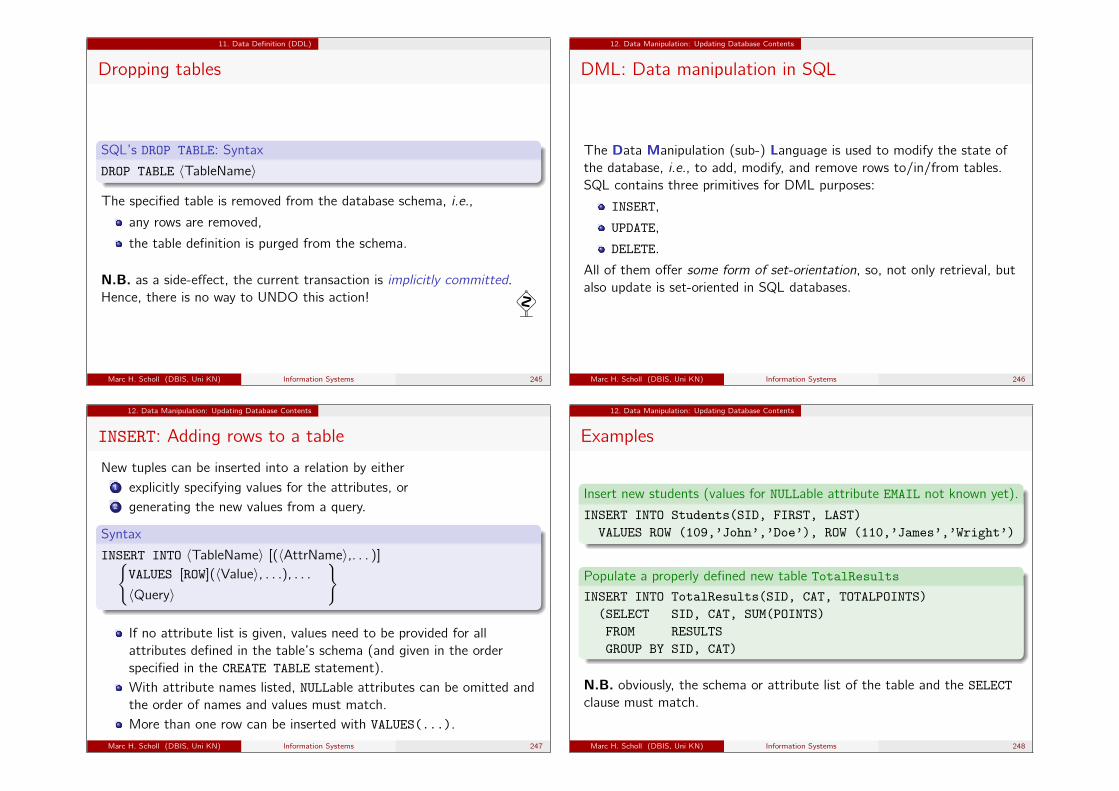
11. Data Definition (DDL)
Dropping tables
SQL’s DROP TABLE: Syntax
DROP TABLE 〈TableName〉
The specified table is removed from the database schema, i.e.,
any rows are removed,
the table definition is purged from the schema.
N.B. as a side-effect, the current transaction is implicitly committed.Hence, there is no way to UNDO this action! �
Marc H. Scholl (DBIS, Uni KN) Information Systems 245
12. Data Manipulation: Updating Database Contents
DML: Data manipulation in SQL
The Data Manipulation (sub-) Language is used to modify the state ofthe database, i.e., to add, modify, and remove rows to/in/from tables.SQL contains three primitives for DML purposes:
INSERT,
UPDATE,
DELETE.
All of them offer some form of set-orientation, so, not only retrieval, butalso update is set-oriented in SQL databases.
Marc H. Scholl (DBIS, Uni KN) Information Systems 246
12. Data Manipulation: Updating Database Contents
INSERT: Adding rows to a table
New tuples can be inserted into a relation by either1 explicitly specifying values for the attributes, or2 generating the new values from a query.
Syntax
INSERT INTO 〈TableName〉 [(〈AttrName〉,. . . )]{VALUES [ROW](〈Value〉, . . .), . . .〈Query〉
}
If no attribute list is given, values need to be provided for allattributes defined in the table’s schema (and given in the orderspecified in the CREATE TABLE statement).With attribute names listed, NULLable attributes can be omitted andthe order of names and values must match.More than one row can be inserted with VALUES(...).
Marc H. Scholl (DBIS, Uni KN) Information Systems 247
12. Data Manipulation: Updating Database Contents
Examples
Insert new students (values for NULLable attribute EMAIL not known yet).
INSERT INTO Students(SID, FIRST, LAST)VALUES ROW (109,’John’,’Doe’), ROW (110,’James’,’Wright’)
Populate a properly defined new table TotalResults
INSERT INTO TotalResults(SID, CAT, TOTALPOINTS)(SELECT SID, CAT, SUM(POINTS)FROM RESULTSGROUP BY SID, CAT)
N.B. obviously, the schema or attribute list of the table and the SELECTclause must match.
Marc H. Scholl (DBIS, Uni KN) Information Systems 248

12. Data Manipulation: Updating Database Contents
DELETE: Removing rows from tables
Tuples matching a given search criterion can be removed from a relation.Notice the set-oriented flavor of this update.
Syntax
DELETE FROM 〈TableName〉 [WHERE 〈SearchCondition〉]
Where 〈SearchCondition〉 can be an arbitrarily complex condition (like in“SELECT * FROM 〈TableName〉 WHERE 〈SearchCondition〉”). If the searchcondition is omitted, all tuples are deleted.
Example (Remove students without any results)DELETE FROM StudentsWHERE SID NOT IN (SELECT SID FROM Results)
Marc H. Scholl (DBIS, Uni KN) Information Systems 249
12. Data Manipulation: Updating Database Contents
UPDATE: Changing attribute values in existing rows
Syntax
UPDATE 〈TableName〉
SET
〈AttrName〉 = 〈NewValue〉, . . .(〈AttrName〉, . . .) = (〈SubQuery〉), . . .ROW = (〈SubQuery〉)
[WHERE 〈SearchCondition〉]
〈NewValue〉 can be an appropriately typed value expression or asubquery computing the new value,
the SELECT clause of the 〈SubQuery〉 in the second form mustmatch the attribute list on the lhs of the assignment,
the SELECT clause of the 〈SubQuery〉 in the third form must matchthe schema of the updated table,
the first and second forms can be mixed in one UPDATE.
Marc H. Scholl (DBIS, Uni KN) Information Systems 250
12. Data Manipulation: Updating Database Contents
Examples
Give 2 more maximum points to all SQL exercises.UPDATE Exercises
SET MAXPT = MAXPT + 2WHERE TOPIC = ’SQL’
Set maximum points of midterm exercise 1 to the maximum pointsachieved by any student.UPDATE ExercisesSET MAXPT = (SELECT MAX(POINTS) FROM Results
WHERE CAT=’M’ AND ENO=1)WHERE CAT = ’M’ AND ENO = 1
Marc H. Scholl (DBIS, Uni KN) Information Systems 251
12. Data Manipulation: Updating Database Contents
Set-orientation vs. state changes
While set-orientation and (read-only) queries go together well,set-oriented updates to the database state pose theoreticalchallenges.
Bulk retrieval, i.e., computing a whole set of rows as a query result,works fine, and the order of rows in the result set is immaterial.
A (naive) implementation could iterate (in any order) over the inputset to collect the result tuples.Doing the same for set-oriented updates may result in ill-definedsemantics!
Different orders of iteration may yield different results!None of these results might coincide with the intended semantics.
Marc H. Scholl (DBIS, Uni KN) Information Systems 252
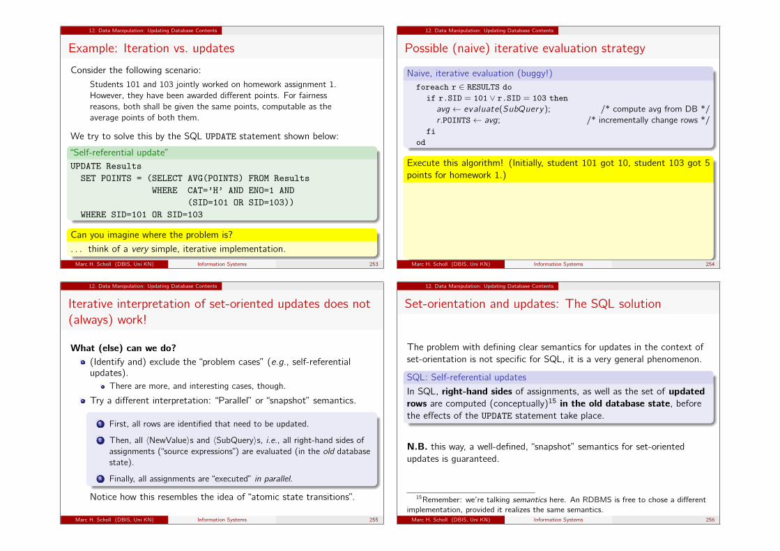
12. Data Manipulation: Updating Database Contents
Example: Iteration vs. updates
Consider the following scenario:
Students 101 and 103 jointly worked on homework assignment 1.However, they have been awarded different points. For fairnessreasons, both shall be given the same points, computable as theaverage points of both them.
We try to solve this by the SQL UPDATE statement shown below:
“Self-referential update”UPDATE Results
SET POINTS = (SELECT AVG(POINTS) FROM ResultsWHERE CAT=’H’ AND ENO=1 AND
(SID=101 OR SID=103))WHERE SID=101 OR SID=103
Can you imagine where the problem is?
. . . think of a very simple, iterative implementation.Marc H. Scholl (DBIS, Uni KN) Information Systems 253
12. Data Manipulation: Updating Database Contents
Possible (naive) iterative evaluation strategy
Naive, iterative evaluation (buggy!)foreach r ∈ RESULTS do
if r.SID = 101 ∨ r.SID = 103 thenavg ← evaluate(SubQuery); /* compute avg from DB */r.POINTS← avg; /* incrementally change rows */
fiod
Execute this algorithm! (Initially, student 101 got 10, student 103 got 5points for homework 1.)
1 If we iterate in the order: 101, then 103 over the RESULTS:
First, student 101 gets (10 + 5)/2 = 7.5 points;then, student 103 gets (7.5 + 5)/2 = 6.25 points.
2 If we iterate in the order: 103, then 101:
First, student 103 gets (10 + 5)/2 = 7.5 points; �then, student 101 gets (10 + 7.5)/2 = 8.75 points.
Marc H. Scholl (DBIS, Uni KN) Information Systems 254
12. Data Manipulation: Updating Database Contents
Iterative interpretation of set-oriented updates does not(always) work!
What (else) can we do?(Identify and) exclude the “problem cases” (e.g., self-referentialupdates).
There are more, and interesting cases, though.
Try a different interpretation: “Parallel” or “snapshot” semantics.
1 First, all rows are identified that need to be updated.
2 Then, all 〈NewValue〉s and 〈SubQuery〉s, i.e., all right-hand sides ofassignments (“source expressions”) are evaluated (in the old databasestate).
3 Finally, all assignments are “executed” in parallel.
Notice how this resembles the idea of “atomic state transitions”.
Marc H. Scholl (DBIS, Uni KN) Information Systems 255
12. Data Manipulation: Updating Database Contents
Set-orientation and updates: The SQL solution
The problem with defining clear semantics for updates in the context ofset-orientation is not specific for SQL, it is a very general phenomenon.
SQL: Self-referential updates
In SQL, right-hand sides of assignments, as well as the set of updatedrows are computed (conceptually)15 in the old database state, beforethe effects of the UPDATE statement take place.
N.B. this way, a well-defined, “snapshot” semantics for set-orientedupdates is guaranteed.
15Remember: we’re talking semantics here. An RDBMS is free to chose a differentimplementation, provided it realizes the same semantics.Marc H. Scholl (DBIS, Uni KN) Information Systems 256

13. Integrity Constraint Checking
Updates and integrity constraints
Updates to the database state are the (only) source of potentialviolations of integrity constraints. For instance,
Insertion of new tuples can possiblyintroduce illegal values for attributes,lead to duplicate key values,store “dangling” foreign key values.
Deletions mayleave “widowed” foreign key references.
Updates may introduce all these kinds of inconsistencies.
In many cases, more than one update statement is required to transformthe current database state into a new, valid database state.(→ This is part of the motivation for database transactions.)
Marc H. Scholl (DBIS, Uni KN) Information Systems 257
13. Integrity Constraint Checking
Integrity constraints and database transactions
Database (ACID-) transactions are the unit of integrity preservation.16
Hence, the DBMS is obliged to check (all relevant) integrity constraintsby the end of each transaction.
Conceptually, each database transaction takes the form:
DB-transaction
〈BOT〉 /* begin of transcation */. . .(sequence of SQL statements). . .
〈EOT〉 /* end of transcation */
N.B. SQL’s 〈EOT〉 reads “COMMIT WORK”, there is no explicit 〈BOT〉.
16This is what the “C”in ACID stands for: consistency.Marc H. Scholl (DBIS, Uni KN) Information Systems 258
13. Integrity Constraint Checking
Constraints in SQL
A database schema in SQL can contain various kinds of integrityconstraints in several places.
Kinds of contraints:Keys and candidate keys
Foreign keys
NOT NULL
CHECK (〈SearchCondition〉)Places:
within an attribute declaration
within a table (or view) declaration
within a DB schema:CREATE ASSERTION 〈AssertionName〉 (〈SearchCondition〉)
Marc H. Scholl (DBIS, Uni KN) Information Systems 259
13. Integrity Constraint Checking
Deferred vs. immediate constraint checking
The semantics of the transaction construct requires the DBMS tocheck constraints at the end of the transaction (“deferredconstraint checking”).
Within a transaction, the consistency of the database may be(temporarily) violated.
At 〈EOT〉, all constraints need to be satisfied again.
It may be quite costly, though, to defer constraint checking, since alot of bookkeeping is required to avoid having to check all definedconstraints.
Often, it is much cheaper, to check constraints during the update orat least at the end of each update statement (“immediate constraintchecking”).
Marc H. Scholl (DBIS, Uni KN) Information Systems 260
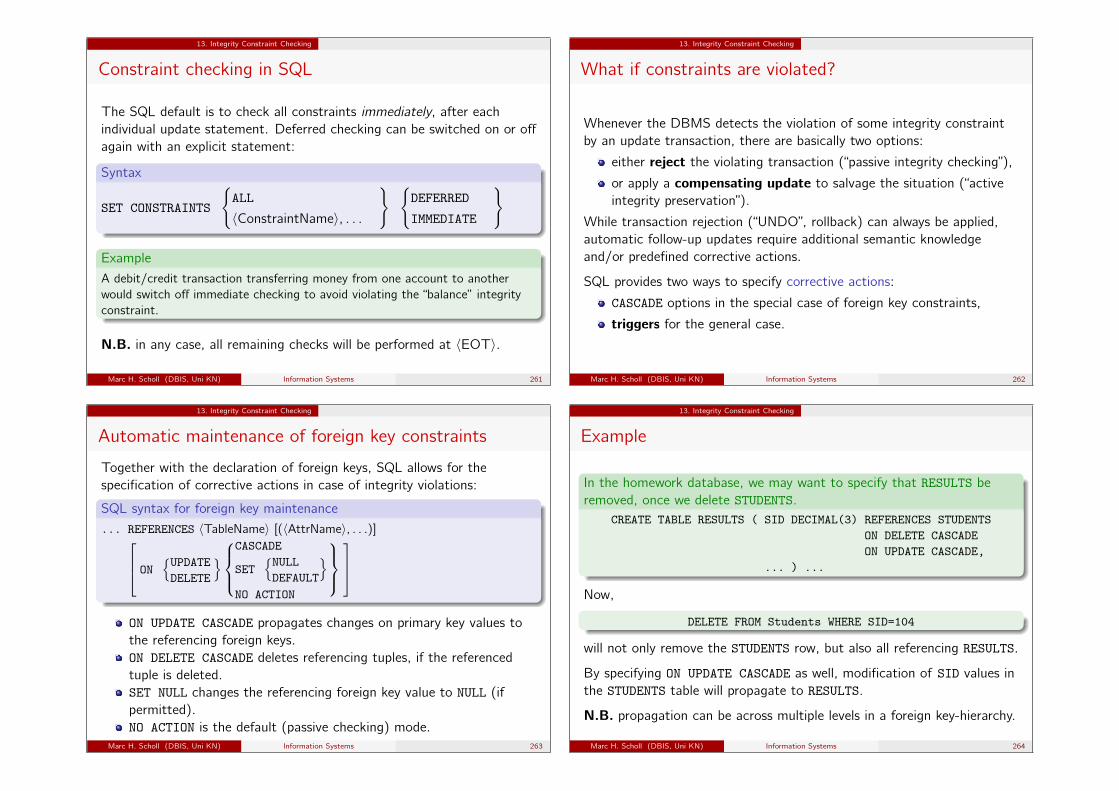
13. Integrity Constraint Checking
Constraint checking in SQL
The SQL default is to check all constraints immediately, after eachindividual update statement. Deferred checking can be switched on or offagain with an explicit statement:
Syntax
SET CONSTRAINTS
{ALL
〈ConstraintName〉, . . .
} {DEFERRED
IMMEDIATE
}
Example
A debit/credit transaction transferring money from one account to anotherwould switch off immediate checking to avoid violating the “balance” integrityconstraint.
N.B. in any case, all remaining checks will be performed at 〈EOT〉.
Marc H. Scholl (DBIS, Uni KN) Information Systems 261
13. Integrity Constraint Checking
What if constraints are violated?
Whenever the DBMS detects the violation of some integrity constraintby an update transaction, there are basically two options:
either reject the violating transaction (“passive integrity checking”),
or apply a compensating update to salvage the situation (“activeintegrity preservation”).
While transaction rejection (“UNDO”, rollback) can always be applied,automatic follow-up updates require additional semantic knowledgeand/or predefined corrective actions.
SQL provides two ways to specify corrective actions:
CASCADE options in the special case of foreign key constraints,
triggers for the general case.
Marc H. Scholl (DBIS, Uni KN) Information Systems 262
13. Integrity Constraint Checking
Automatic maintenance of foreign key constraints
Together with the declaration of foreign keys, SQL allows for thespecification of corrective actions in case of integrity violations:
SQL syntax for foreign key maintenance
... REFERENCES 〈TableName〉 [(〈AttrName〉, . . .)] ON{UPDATEDELETE
}CASCADE
SET{NULLDEFAULT
}NO ACTION
ON UPDATE CASCADE propagates changes on primary key values tothe referencing foreign keys.ON DELETE CASCADE deletes referencing tuples, if the referencedtuple is deleted.SET NULL changes the referencing foreign key value to NULL (ifpermitted).NO ACTION is the default (passive checking) mode.
Marc H. Scholl (DBIS, Uni KN) Information Systems 263
13. Integrity Constraint Checking
Example
In the homework database, we may want to specify that RESULTS beremoved, once we delete STUDENTS.
CREATE TABLE RESULTS ( SID DECIMAL(3) REFERENCES STUDENTSON DELETE CASCADEON UPDATE CASCADE,
... ) ...
Now,
DELETE FROM Students WHERE SID=104
will not only remove the STUDENTS row, but also all referencing RESULTS.
By specifying ON UPDATE CASCADE as well, modification of SID values inthe STUDENTS table will propagate to RESULTS.
N.B. propagation can be across multiple levels in a foreign key-hierarchy.
Marc H. Scholl (DBIS, Uni KN) Information Systems 264
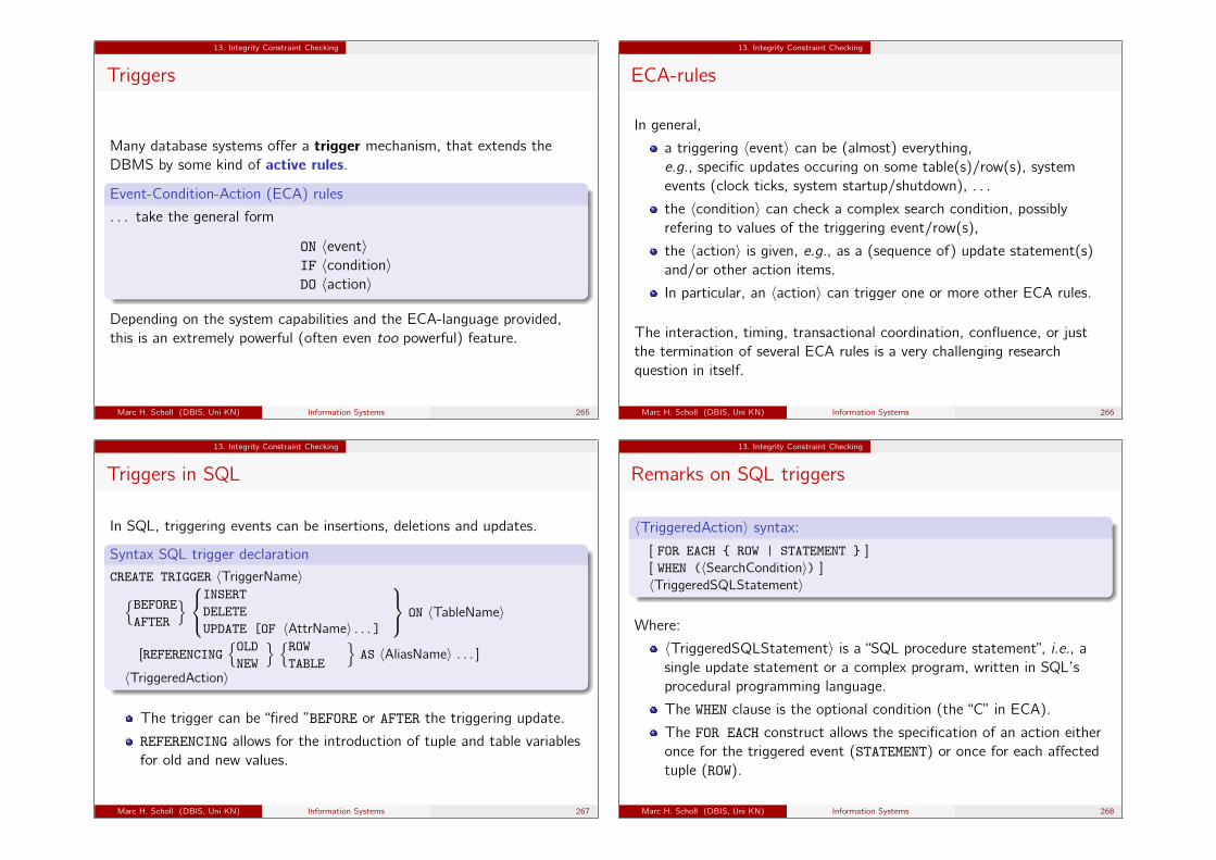
13. Integrity Constraint Checking
Triggers
Many database systems offer a trigger mechanism, that extends theDBMS by some kind of active rules.
Event-Condition-Action (ECA) rules
. . . take the general form
ON 〈event〉IF 〈condition〉DO 〈action〉
Depending on the system capabilities and the ECA-language provided,this is an extremely powerful (often even too powerful) feature.
Marc H. Scholl (DBIS, Uni KN) Information Systems 265
13. Integrity Constraint Checking
ECA-rules
In general,
a triggering 〈event〉 can be (almost) everything,e.g., specific updates occuring on some table(s)/row(s), systemevents (clock ticks, system startup/shutdown), . . .
the 〈condition〉 can check a complex search condition, possiblyrefering to values of the triggering event/row(s),
the 〈action〉 is given, e.g., as a (sequence of) update statement(s)and/or other action items.
In particular, an 〈action〉 can trigger one or more other ECA rules.
The interaction, timing, transactional coordination, confluence, or justthe termination of several ECA rules is a very challenging researchquestion in itself.
Marc H. Scholl (DBIS, Uni KN) Information Systems 266
13. Integrity Constraint Checking
Triggers in SQL
In SQL, triggering events can be insertions, deletions and updates.
Syntax SQL trigger declaration
CREATE TRIGGER 〈TriggerName〉{BEFOREAFTER
} INSERTDELETEUPDATE [OF 〈AttrName〉 . . . ]
ON 〈TableName〉
[REFERENCING{OLDNEW
} {ROWTABLE
}AS 〈AliasName〉 . . . ]
〈TriggeredAction〉
The trigger can be “fired ”BEFORE or AFTER the triggering update.
REFERENCING allows for the introduction of tuple and table variablesfor old and new values.
Marc H. Scholl (DBIS, Uni KN) Information Systems 267
13. Integrity Constraint Checking
Remarks on SQL triggers
〈TriggeredAction〉 syntax:[ FOR EACH { ROW | STATEMENT } ][ WHEN (〈SearchCondition〉) ]〈TriggeredSQLStatement〉
Where:
〈TriggeredSQLStatement〉 is a “SQL procedure statement”, i.e., asingle update statement or a complex program, written in SQL’sprocedural programming language.
The WHEN clause is the optional condition (the “C” in ECA).
The FOR EACH construct allows the specification of an action eitheronce for the triggered event (STATEMENT) or once for each affectedtuple (ROW).
Marc H. Scholl (DBIS, Uni KN) Information Systems 268
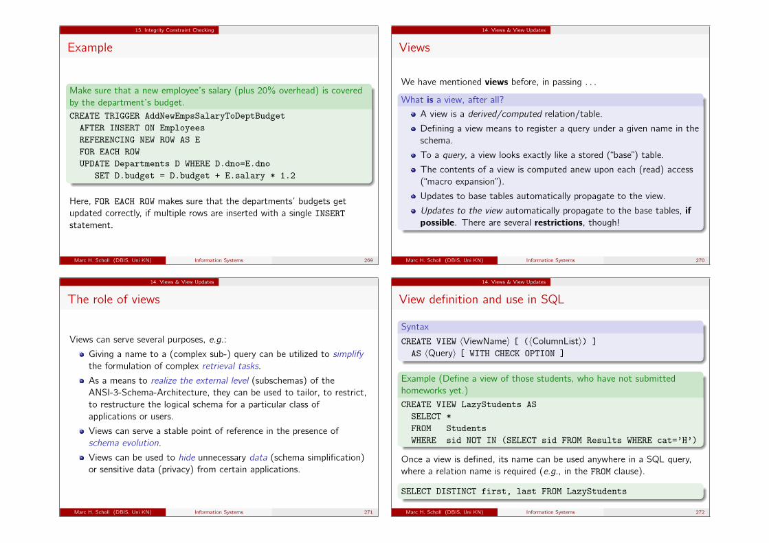
13. Integrity Constraint Checking
Example
Make sure that a new employee’s salary (plus 20% overhead) is coveredby the department’s budget.CREATE TRIGGER AddNewEmpsSalaryToDeptBudget
AFTER INSERT ON EmployeesREFERENCING NEW ROW AS EFOR EACH ROWUPDATE Departments D WHERE D.dno=E.dno
SET D.budget = D.budget + E.salary * 1.2
Here, FOR EACH ROW makes sure that the departments’ budgets getupdated correctly, if multiple rows are inserted with a single INSERTstatement.
Marc H. Scholl (DBIS, Uni KN) Information Systems 269
14. Views & View Updates
Views
We have mentioned views before, in passing . . .
What is a view, after all?
A view is a derived/computed relation/table.
Defining a view means to register a query under a given name in theschema.
To a query, a view looks exactly like a stored (“base”) table.
The contents of a view is computed anew upon each (read) access(“macro expansion”).
Updates to base tables automatically propagate to the view.
Updates to the view automatically propagate to the base tables, ifpossible. There are several restrictions, though!
Marc H. Scholl (DBIS, Uni KN) Information Systems 270
14. Views & View Updates
The role of views
Views can serve several purposes, e.g.:
Giving a name to a (complex sub-) query can be utilized to simplifythe formulation of complex retrieval tasks.
As a means to realize the external level (subschemas) of theANSI-3-Schema-Architecture, they can be used to tailor, to restrict,to restructure the logical schema for a particular class ofapplications or users.
Views can serve a stable point of reference in the presence ofschema evolution.
Views can be used to hide unnecessary data (schema simplification)or sensitive data (privacy) from certain applications.
Marc H. Scholl (DBIS, Uni KN) Information Systems 271
14. Views & View Updates
View definition and use in SQL
Syntax
CREATE VIEW 〈ViewName〉 [ (〈ColumnList〉) ]AS 〈Query〉 [ WITH CHECK OPTION ]
Example (Define a view of those students, who have not submittedhomeworks yet.)CREATE VIEW LazyStudents ASSELECT *FROM StudentsWHERE sid NOT IN (SELECT sid FROM Results WHERE cat=’H’)
Once a view is defined, its name can be used anywhere in a SQL query,where a relation name is required (e.g., in the FROM clause).
SELECT DISTINCT first, last FROM LazyStudents
Marc H. Scholl (DBIS, Uni KN) Information Systems 272

14. Views & View Updates
View substitution
Processing a query on a view is—in principle—quite easy: simplysubstitute the view definition for the view name in the query using theview.
ExampleSELECT DISTINCT first, last FROM LazyStudents
↓SELECT DISTINCT first, last FROM
(SELECT *FROM StudentsWHERE sid NOT IN (SELECT sid FROM Results WHERE cat=’H’))
N.B. If SQL were really, fully orthogonal, it could be as simple as that.Since there are certain limitations, however, (also because nesting in theFROM clause was not allowed before SQL:1992) the actual algorithm issomewhat more involved.Marc H. Scholl (DBIS, Uni KN) Information Systems 273
14. Views & View Updates
View updates
Applying database updates through views is far from trivial!
Example (Ambiguity)
Consider a view definition with a UNION operator:CREATE VIEW U AS SELECT * FROM R UNION SELECT * FROM S.
If you INSERT new tuples into this view U, what should the DBMS do?
Insert the new row into table R?
Insert the new row into table S?
Insert the new row into both tables?
There is no obvious answer!
Some (few) view updates can, others (many) can not be translateduniquely into updates to base tables.
Marc H. Scholl (DBIS, Uni KN) Information Systems 274
14. Views & View Updates
Criteria for view updates
When translating view updates to base tables, you will want
Conformity: the effect of an update to a view shall be the same as ifthe view were a stored base table.
Minimality: a minimal set of updates to the base tables shall begenerated that guarantees the effect (cf. the INSERT into the UNIONview: do not insert into both base tables).
Consistency preservation: updates to a view must not violateintegrity constraints on base tables.
Privacy: if the view was introduced to hide sensitive data, this datamust not be affected by the update.
Uniqueness: the translation must not be ambiguous ornon-deterministic.
Marc H. Scholl (DBIS, Uni KN) Information Systems 275
14. Views & View Updates
Some view update problems (1)
Example (Projection view)
View definition:CREATE VIEW Mailinglist AS
SELECT DISTINCT first, last, email FROM Students.
Update:INSERT INTO Mailinglist VALUES (’John’,’Doe’,’[email protected]’).
Problem: No value can possibly be given for non-projected attributes.
If these attributes are NULLable, or if a DEFAULT value is declared,can use these values.
If (parts of) primary key is not projected: possibly duplicates havebeen removed, so 1 view row might “represent” multiple base tablerows!
Consequence: Keep keys, no DISTINCT.Marc H. Scholl (DBIS, Uni KN) Information Systems 276
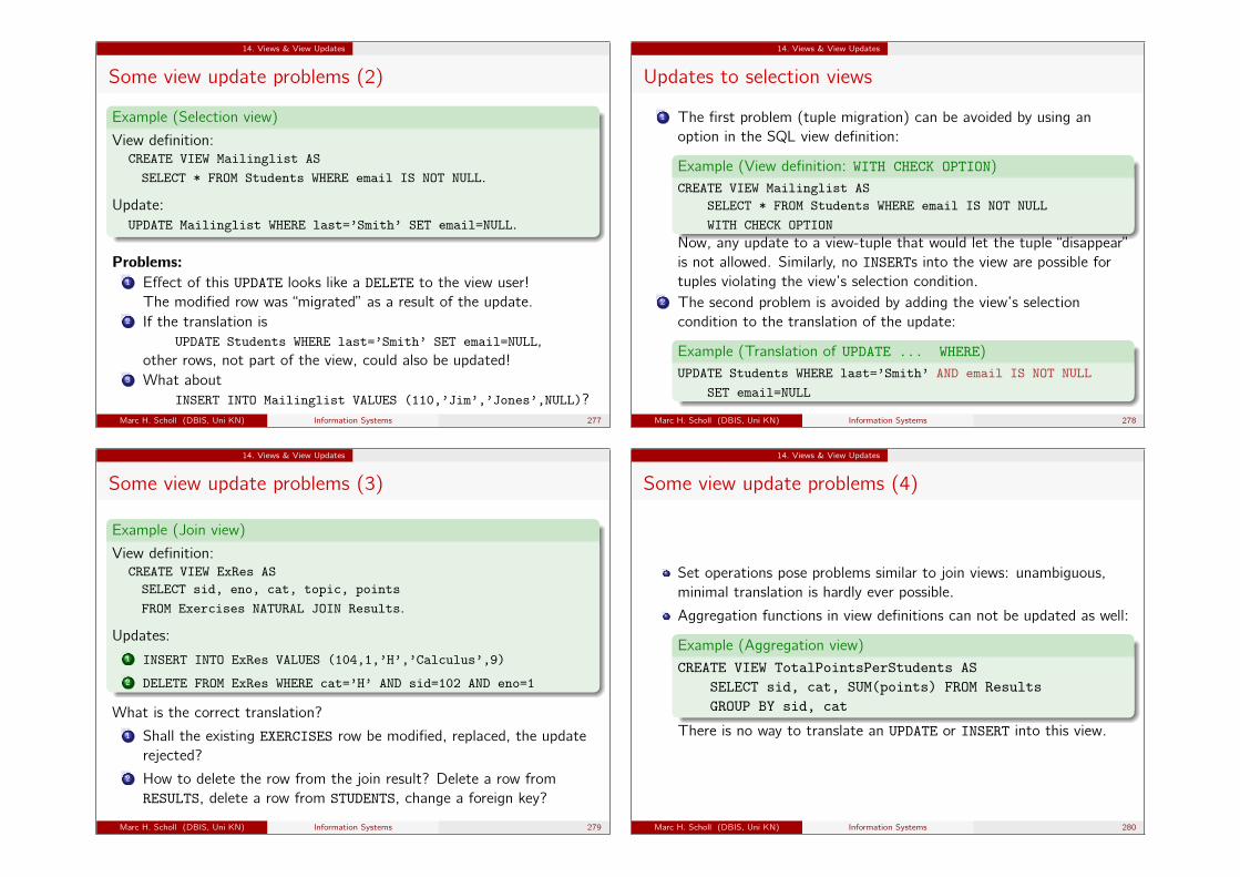
14. Views & View Updates
Some view update problems (2)
Example (Selection view)
View definition:CREATE VIEW Mailinglist AS
SELECT * FROM Students WHERE email IS NOT NULL.
Update:UPDATE Mailinglist WHERE last=’Smith’ SET email=NULL.
Problems:1 Effect of this UPDATE looks like a DELETE to the view user!
The modified row was “migrated” as a result of the update.2 If the translation is
UPDATE Students WHERE last=’Smith’ SET email=NULL,other rows, not part of the view, could also be updated!
3 What aboutINSERT INTO Mailinglist VALUES (110,’Jim’,’Jones’,NULL)?
Marc H. Scholl (DBIS, Uni KN) Information Systems 277
14. Views & View Updates
Updates to selection views
1 The first problem (tuple migration) can be avoided by using anoption in the SQL view definition:
Example (View definition: WITH CHECK OPTION)CREATE VIEW Mailinglist AS
SELECT * FROM Students WHERE email IS NOT NULL
WITH CHECK OPTION
Now, any update to a view-tuple that would let the tuple “disappear”is not allowed. Similarly, no INSERTs into the view are possible fortuples violating the view’s selection condition.
2 The second problem is avoided by adding the view’s selectioncondition to the translation of the update:
Example (Translation of UPDATE ... WHERE)UPDATE Students WHERE last=’Smith’ AND email IS NOT NULL
SET email=NULL
Marc H. Scholl (DBIS, Uni KN) Information Systems 278
14. Views & View Updates
Some view update problems (3)
Example (Join view)
View definition:CREATE VIEW ExRes ASSELECT sid, eno, cat, topic, points
FROM Exercises NATURAL JOIN Results.
Updates:1 INSERT INTO ExRes VALUES (104,1,’H’,’Calculus’,9)
2 DELETE FROM ExRes WHERE cat=’H’ AND sid=102 AND eno=1
What is the correct translation?1 Shall the existing EXERCISES row be modified, replaced, the update
rejected?2 How to delete the row from the join result? Delete a row from
RESULTS, delete a row from STUDENTS, change a foreign key?
Marc H. Scholl (DBIS, Uni KN) Information Systems 279
14. Views & View Updates
Some view update problems (4)
Set operations pose problems similar to join views: unambiguous,minimal translation is hardly ever possible.
Aggregation functions in view definitions can not be updated as well:
Example (Aggregation view)CREATE VIEW TotalPointsPerStudents AS
SELECT sid, cat, SUM(points) FROM ResultsGROUP BY sid, cat
There is no way to translate an UPDATE or INSERT into this view.
Marc H. Scholl (DBIS, Uni KN) Information Systems 280
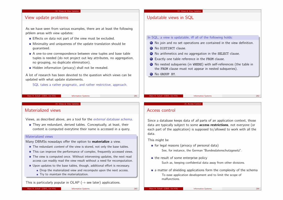
14. Views & View Updates
View update problems
As we have seen from various examples, there are at least the followingprblem areas with view updates:
Effects on data not part of the view must be excluded.
Minimality and uniqueness of the update translation should beguaranteed.
A one-to-one correspondence between view tuples and base tabletuples is needed (do not project out key attributes, no aggregation,no grouping, no duplicate elimination).
Hidden information (privacy) shall not be revealed.
A lot of research has been devoted to the question which views can beupdated with what update statements.
SQL takes a rather pragmatic, and rather restrictive, approach.
Marc H. Scholl (DBIS, Uni KN) Information Systems 281
14. Views & View Updates
Updatable views in SQL
In SQL, a view is updatable, iff all of the following holds:1 No join and no set operations are contained in the view definition.2 No DISTINCT clause.3 No arithmetics and no aggregation in the SELECT clause.4 Exactly one table reference in the FROM clause.5 No nested subqueries (in WHERE) with self-references (the table in
the FROM clause must not appear in nested subqueries).6 No GROUP BY.
Marc H. Scholl (DBIS, Uni KN) Information Systems 282
14. Views & View Updates
Materialized views
Views, as described above, are a tool for the external database schema.
They are redundant, derived tables. Conceptually, at least, theircontent is computed everytime their name is accessed in a query.
Materialized viewsMany DBMSs nowadays offer the option to materialize a view.
The redundant content of the view is stored, not only the base tables.
This can improve the performance of complex, frequently accessed views.
The view is computed once. Without intervening updates, the next readaccess can readily read the view result without a need for recomputation.
Upon updates to the base tables, though, additional effort is necessary.
Drop the materialized view and recompute upon the next access.Try to maintain the materialization.
This is particularly popular in OLAP (→ see later) applications.
Marc H. Scholl (DBIS, Uni KN) Information Systems 283
15. Access Control
Access control
Since a database keeps data of all parts of an application context, thosedata are typically subject to some access restrictions, not everyone (oreach part of the application) is supposed to/allowed to work with all thedata.
This might be
for legal reasons (privacy of personal data)See, for instance, the German “Bundesdatenschutzgesetz”.
the result of some enterprise policySuch as, keeping confidential data away from other divisions.
a matter of shielding applications form the complexity of the schemaTo ease application development and to limit the scope ofmalfunctions.
Marc H. Scholl (DBIS, Uni KN) Information Systems 284
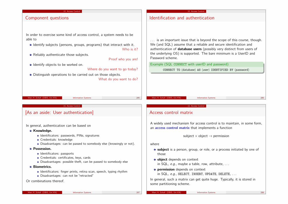
15. Access Control
Component questions
In order to exercise some kind of access control, a system needs to beable to
Identify subjects (persons, groups, programs) that interact with it.Who is it?
Reliably authenticate those subjects.Proof who you are!
Identify objects to be worked on.Where do you want to go today?
Distinguish operations to be carried out on those objects.What do you want to do?
Marc H. Scholl (DBIS, Uni KN) Information Systems 285
15. Access Control
Identification and authentication
. . . is an important issue that is beyond the scope of this course, though.We (and SQL) assume that a reliable and secure identification andauthentication of database users (possibly very distinct from users ofthe underlying OS) is supported. The bare minimum is a UserID andPassword scheme.
Example (SQL CONNECT with userID and password)
CONNECT TO 〈database〉 AS 〈user〉 IDENTIFIED BY 〈password〉
Marc H. Scholl (DBIS, Uni KN) Information Systems 286
15. Access Control
[As an aside: User authentication]
In general, authentication can be based onKnowledge.
Identificators: passwords, PINs, signaturesCredentials: knowledgeDisadvantages: can be passed to somebody else (knowingly or not).
Possession.Identificators: passportsCredentials: certificates, keys, cardsDisadvantages: possible theft, can be passed to somebody else
Biometrics.Identificators: finger prints, retina scan, speech, typing rhythmDisadvantages: can not be “retracted”
Or combinations thereof.
Marc H. Scholl (DBIS, Uni KN) Information Systems 287
15. Access Control
Access control matrix
A widely used mechanism for access control is to maintain, in some form,an access control matrix that implements a function
subject× object→ permission
where
subject is a person, group, or role, or a process initiated by one ofthose
object depends on contextin SQL, e.g., maybe a table, row, attribute, . . .
permission depends on contextin SQL, e.g., SELECT, INSERT, UPDATE, DELETE, . . .
In general, such a matrix can get quite huge. Typically, it is stored insome partitioning scheme.
Marc H. Scholl (DBIS, Uni KN) Information Systems 288
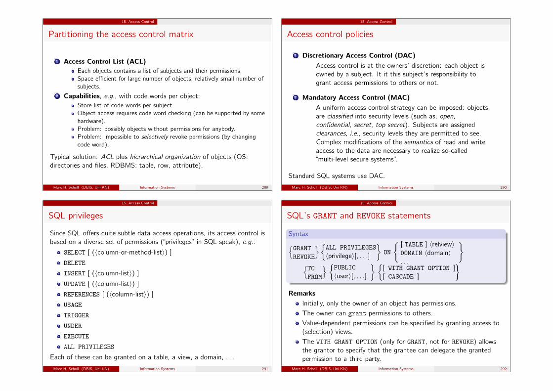
15. Access Control
Partitioning the access control matrix
1 Access Control List (ACL)Each objects contains a list of subjects and their permissions.Space efficient for large number of objects, relatively small number ofsubjects.
2 Capabilities, e.g., with code words per object:Store list of code words per subject.Object access requires code word checking (can be supported by somehardware).Problem: possibly objects without permissions for anybody.Problem: impossible to selectively revoke permissions (by changingcode word).
Typical solution: ACL plus hierarchical organization of objects (OS:directories and files, RDBMS: table, row, attribute).
Marc H. Scholl (DBIS, Uni KN) Information Systems 289
15. Access Control
Access control policies
1 Discretionary Access Control (DAC)Access control is at the owners’ discretion: each object isowned by a subject. It it this subject’s responsibility togrant access permissions to others or not.
2 Mandatory Access Control (MAC)A uniform access control strategy can be imposed: objectsare classified into security levels (such as, open,confidential, secret, top secret). Subjects are assignedclearances, i.e., security levels they are permitted to see.Complex modifications of the semantics of read and writeaccess to the data are necessary to realize so-called“multi-level secure systems”.
Standard SQL systems use DAC.
Marc H. Scholl (DBIS, Uni KN) Information Systems 290
15. Access Control
SQL privileges
Since SQL offers quite subtle data access operations, its access control isbased on a diverse set of permissions (“privileges” in SQL speak), e.g.:
SELECT [ (〈column-or-method-list〉) ]
DELETE
INSERT [ (〈column-list〉) ]
UPDATE [ (〈column-list〉) ]
REFERENCES [ (〈column-list〉) ]
USAGE
TRIGGER
UNDER
EXECUTE
ALL PRIVILEGES
Each of these can be granted on a table, a view, a domain, . . .
Marc H. Scholl (DBIS, Uni KN) Information Systems 291
15. Access Control
SQL’s GRANT and REVOKE statements
Syntax{GRANTREVOKE
}{ALL PRIVILEGES〈privilege〉[, . . .]
}ON
{[ TABLE ] 〈relview〉DOMAIN 〈domain〉. . .
}{TOFROM
} {PUBLIC〈user〉[, . . .]
} {[ WITH GRANT OPTION ]
[ CASCADE ]
}Remarks
Initially, only the owner of an object has permissions.The owner can grant permissions to others.Value-dependent permissions can be specified by granting access to(selection) views.The WITH GRANT OPTION (only for GRANT, not for REVOKE) allowsthe grantor to specify that the grantee can delegate the grantedpermission to a third party.
Marc H. Scholl (DBIS, Uni KN) Information Systems 292
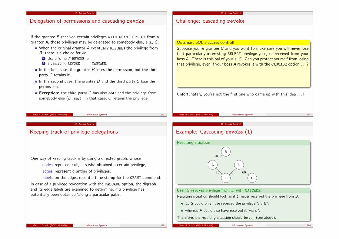
15. Access Control
Delegation of permissions and cascading revoke
If the grantee B received certain privileges WITH GRANT OPTION from agrantor A, those privileges may be delegated to somebody else, e.g., C.
When the original grantor A eventually REVOKEs the privilege fromB, there is a choice for A:
1 Use a “simple” REVOKE, or2 a cascading REVOKE ... CASCADE.
In the first case, the grantee B loses the permission, but the thirdparty C retains it.
In the second case, the grantee B and the third party C lose thepermission.
Exception: the third party C has also obtained the privilege fromsomebody else (D, say). In that case, C retains the privilege.
Marc H. Scholl (DBIS, Uni KN) Information Systems 293
15. Access Control
Challenge: cascading revoke
Outsmart SQL’s access control!Suppose you’re grantee B and you want to make sure you will never losethat particularly interesting SELECT privilege you just received from yourboss A. There is this pal of your’s, C. Can you protect yourself from losingthat privilege, even if your boss A revokes it with the CASCADE option . . . ?
B: GRANT 〈your pretious privilege〉 TO C WITH GRANT OPTION.C: GRANT 〈your pretious privilege〉 TO B WITH GRANT OPTION.
Et voilà!
Unfortunately, you’re not the first one who came up with this idea . . . !
Marc H. Scholl (DBIS, Uni KN) Information Systems 294
15. Access Control
Keeping track of privilege delegations
One way of keeping track is by using a directed graph, whose
nodes represent subjects who obtained a certain privilege,
edges represent granting of privileges,
labels on the edges record a time stamp for the GRANT command.
In case of a privilege revocation with the CASCADE option, the digraphand its edge labels are examined to determine, if a privilege haspotentially been obtained “along a particular path”.
Marc H. Scholl (DBIS, Uni KN) Information Systems 295
15. Access Control
Example: Cascading revoke (1)
Resulting situation
A
B
C
D
F
10
20 50 60
User B revokes privilege from D with CASCADE.Resulting situation should look as if D never received the privilege from B.
E, G could only have received the privilege “via B”,
whereas F could also have received it “via C”.
Therefore, the resulting situation should be . . . (see above).
Marc H. Scholl (DBIS, Uni KN) Information Systems 296

15. Access Control
Example: Cascading revoke (2)
With different time stamps in the initial situation, we obtain. . .B: REVOKE. . . FROM D CASCADE
A
B
C
D
E
F
G10
20
30
70
40
50
60
−→ A
B
C
D
10
20 70
Marc H. Scholl (DBIS, Uni KN) Information Systems 297
15. Access Control
Example: Non-cascading revoke
Revoking without CASCADE requires adjustments
A
B
C
D
E
F
G10
20
30
50
40
70
60
B: REVOKE. . . FROM D −→ A
B
C
D
E
F
G10
20
40
70
50
70
60
Marc H. Scholl (DBIS, Uni KN) Information Systems 298
15. Access Control
Outsmarting will no longer work!
You (B) and your pal (C) . . .
A B Ct1
t2 > t1
t3 > t2
Marc H. Scholl (DBIS, Uni KN) Information Systems 299
15. Access Control
Principal problems
Depends heavily on reliable and secure user identification andauthentication.Privileges (objects implementing them) are extremely sensitive⇒ may need even stronger protection.Privileges protect data objects, not the information contained within.⇒ implicit transfer (and even extension!) of permissions is possible!
Example (DAC dilemma)
User A has SELECT permissions on object O,
user B has no permissions on O.
User A has no permission to grant access on O to B.Yet, A can give read access to O’s content to B:
1 A creates a new object O′, copies O’s content into O′.2 A—as the owner of object O′—grants read access on O′ to B.
Problem source: discretionary access control. It all up to the user. . .Marc H. Scholl (DBIS, Uni KN) Information Systems 300
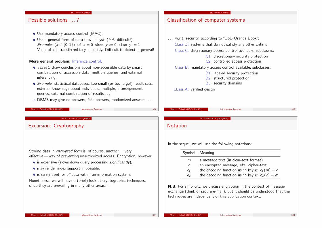
15. Access Control
Possible solutions . . . ?
Use mandatory access control (MAC).
Use a general form of data flow analysis (but: difficult!).Example: (x ∈ {0, 1}) if x = 0 then y := 0 else y := 1
Value of x is transferred to y implicitly. Difficult to detect in general!
More general problem: Inference control.
Threat: draw conclusions about non-accessible data by smartcombination of accessible data, multiple queries, and externalinferencing.
Example: statistical databases, too small (or too large!) result sets,external knowledge about individuals, multiple, interdependentqueries, external combination of results . . .
→ DBMS may give no answers, fake answers, randomized answers, . . .
Marc H. Scholl (DBIS, Uni KN) Information Systems 301
15. Access Control
Classification of computer systems
. . . w.r.t. security, according to “DoD Orange Book”:
Class D: systems that do not satisfy any other criteria
Class C: discretionary access control available, subclasses:C1: discretionary security protectionC2: controlled access protection
Class B: mandatory access control available, subclasses:B1: labeled security protectionB2: structured protectionB3: security domains
CLass A: verified design
Marc H. Scholl (DBIS, Uni KN) Information Systems 302
16. Excursion: Cryptography
Excursion: Cryptography
Storing data in encrypted form is, of course, another—veryeffective—way of preventing unauthorized access. Encryption, however,
is expensive (slows down query processing significantly),
may render index support impossible,
is rarely used for all data within an information system.
Nonetheless, we will have a (brief) look at cryptographic techniques,since they are prevailing in many other areas. . .
Marc H. Scholl (DBIS, Uni KN) Information Systems 303
16. Excursion: Cryptography
Notation
In the sequel, we will use the following notations:
Symbol Meaning
m a message text (in clear-text format)c an encrypted message, aka. cipher-textek the encoding function using key k : ek(m) = c
dk the decoding function using key k : dk(c) = m
N.B. For simplicity, we discuss encryption in the context of messageexchange (think of secure e-mail), but it should be understood that thetechniques are independent of this application context.
Marc H. Scholl (DBIS, Uni KN) Information Systems 304
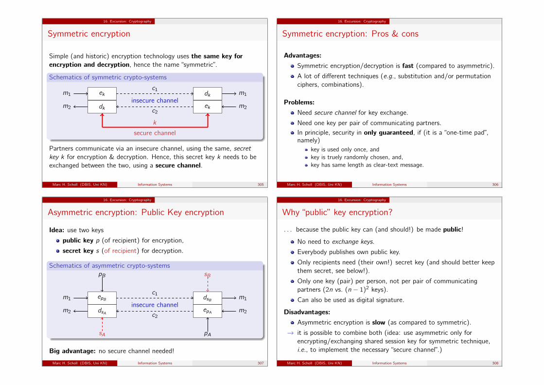
16. Excursion: Cryptography
Symmetric encryption
Simple (and historic) encryption technology uses the same key forencryption and decryption, hence the name “symmetric”.
Schematics of symmetric crypto-systems
ek
dk
dk
ek
m1c1
m1
m2c2
m2
insecure channel
secure channel
k
Partners communicate via an insecure channel, using the same, secretkey k for encryption & decryption. Hence, this secret key k needs to beexchanged between the two, using a secure channel.
Marc H. Scholl (DBIS, Uni KN) Information Systems 305
16. Excursion: Cryptography
Symmetric encryption: Pros & cons
Advantages:Symmetric encryption/decryption is fast (compared to asymmetric).
A lot of different techniques (e.g., substitution and/or permutationciphers, combinations).
Problems:Need secure channel for key exchange.
Need one key per pair of communicating partners.In principle, security in only guaranteed, if (it is a “one-time pad”,namely)
key is used only once, andkey is truely randomly chosen, and,key has same length as clear-text message.
Marc H. Scholl (DBIS, Uni KN) Information Systems 306
16. Excursion: Cryptography
Asymmetric encryption: Public Key encryption
Idea: use two keys
public key p (of recipient) for encryption,
secret key s (of recipient) for decryption.
Schematics of asymmetric crypto-systems
epB
dsA
dsB
epA
m1c1
m1
m2c2
m2
insecure channel
sA pA
pB sB
Big advantage: no secure channel needed!
Marc H. Scholl (DBIS, Uni KN) Information Systems 307
16. Excursion: Cryptography
Why “public” key encryption?
. . . because the public key can (and should!) be made public!
No need to exchange keys.
Everybody publishes own public key.
Only recipients need (their own!) secret key (and should better keepthem secret, see below!).
Only one key (pair) per person, not per pair of communicatingpartners (2n vs. (n − 1)2 keys).
Can also be used as digital signature.
Disadvantages:Asymmetric encryption is slow (as compared to symmetric).
→ it is possible to combine both (idea: use asymmetric only forencrypting/exchanging shared session key for symmetric technique,i.e., to implement the necessary “secure channel”.)
Marc H. Scholl (DBIS, Uni KN) Information Systems 308
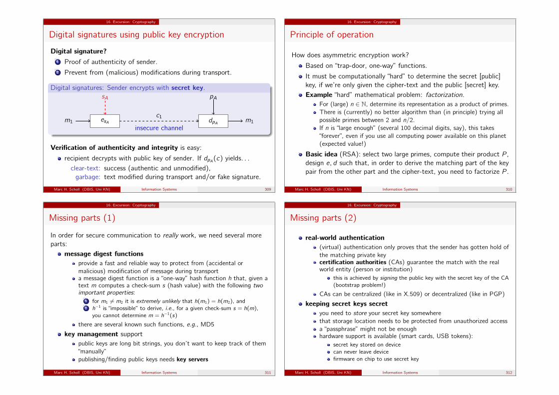
16. Excursion: Cryptography
Digital signatures using public key encryption
Digital signature?1 Proof of authenticity of sender.2 Prevent from (malicious) modifications during transport.
Digital signatures: Sender encrypts with secret key.
esA dpAm1c1
m1
insecure channel
sA pA
Verification of authenticity and integrity is easy:
recipient decrypts with public key of sender. If dpA(c) yields. . .clear-text: success (authentic and unmodified),garbage: text modified during transport and/or fake signature.
Marc H. Scholl (DBIS, Uni KN) Information Systems 309
16. Excursion: Cryptography
Principle of operation
How does asymmetric encryption work?
Based on “trap-door, one-way” functions.
It must be computationally “hard” to determine the secret [public]key, if we’re only given the cipher-text and the public [secret] key.Example “hard” mathematical problem: factorization.
For (large) n ∈ N, determine its representation as a product of primes.There is (currently) no better algorithm than (in principle) trying allpossible primes between 2 and n/2.If n is “large enough” (several 100 decimal digits, say), this takes“forever”, even if you use all computing power available on this planet(expected value!)
Basic idea (RSA): select two large primes, compute their product P ,design e, d such that, in order to derive the matching part of the keypair from the other part and the cipher-text, you need to factorize P .
Marc H. Scholl (DBIS, Uni KN) Information Systems 310
16. Excursion: Cryptography
Missing parts (1)
In order for secure communication to really work, we need several moreparts:
message digest functionsprovide a fast and reliable way to protect from (accidental ormalicious) modification of message during transporta message digest function is a “one-way” hash function h that, given atext m computes a check-sum s (hash value) with the following twoimportant properties:
1 for m1 6= m2 it is extremely unlikely that h(m1) = h(m2), and2 h−1 is “impossible” to derive, i.e., for a given check-sum s = h(m),
you cannot determine m = h−1(s)
there are several known such functions, e.g., MD5
key management supportpublic keys are long bit strings, you don’t want to keep track of them“manually”publishing/finding public keys needs key servers
Marc H. Scholl (DBIS, Uni KN) Information Systems 311
16. Excursion: Cryptography
Missing parts (2)
real-world authentication(virtual) authentication only proves that the sender has gotten hold ofthe matching private keycertification authorities (CAs) guarantee the match with the realworld entity (person or institution)
this is achieved by signing the public key with the secret key of the CA(bootstrap problem!)
CAs can be centralized (like in X.509) or decentralized (like in PGP)
keeping secret keys secretyou need to store your secret key somewherethat storage location needs to be protected from unauthorized accessa “passphrase” might not be enoughhardware support is available (smart cards, USB tokens):
secret key stored on devicecan never leave devicefirmware on chip to use secret key
Marc H. Scholl (DBIS, Uni KN) Information Systems 312
16. Excursion: Cryptography
Putting it all together
Draw a diagram how a secure communication between two parties worksand how and where the components mentioned above come into play!
Marc H. Scholl (DBIS, Uni KN) Information Systems 313
16. Excursion: Cryptography
Summary cryptography
Encryption could be used on several system layers, e.g.,Operating systemUsers’ private keysApplication signatures
In order to be secureEncryption must be used everywhere (despite the run-time effort)(Secret) key must be kept secret, reliablyAlgorithm must be trustworthy, secured from modifications &circumvention
AdvantagesPrevents from unauthorized read accessPrevents from unauthorized insert, update, deletePrevents from spreading of malware
DisadvatangesRun-time effortDatabase operations typically only possible on decrypted data
Marc H. Scholl (DBIS, Uni KN) Information Systems 314
Part V
Programmatic Access to SQL Databases
Marc H. Scholl (DBIS, Uni KN) Information Systems 315
Outline of this part
17 Programming and Database AccessEmbedded SQLSQL Programming Extensions
Marc H. Scholl (DBIS, Uni KN) Information Systems 316
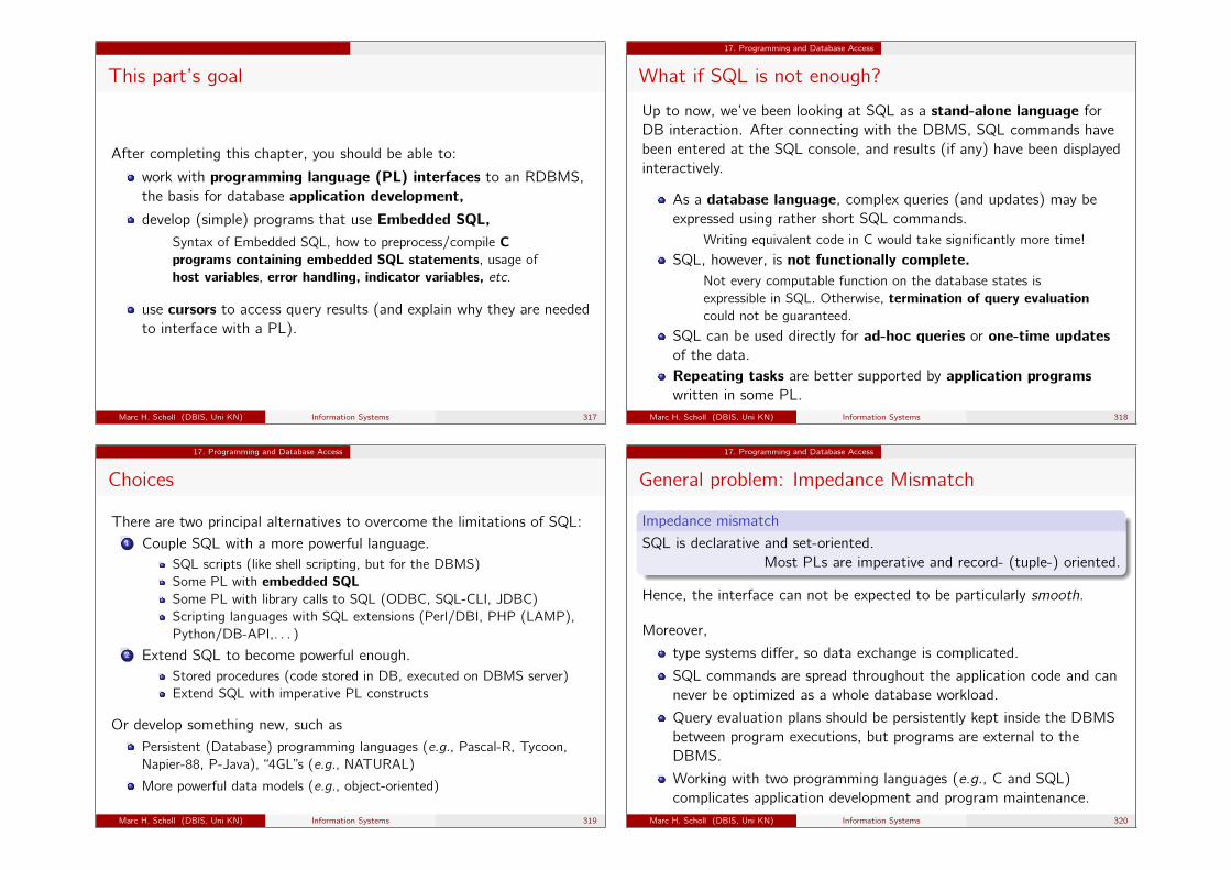
This part’s goal
After completing this chapter, you should be able to:
work with programming language (PL) interfaces to an RDBMS,the basis for database application development,develop (simple) programs that use Embedded SQL,
Syntax of Embedded SQL, how to preprocess/compile Cprograms containing embedded SQL statements, usage ofhost variables, error handling, indicator variables, etc.
use cursors to access query results (and explain why they are neededto interface with a PL).
Marc H. Scholl (DBIS, Uni KN) Information Systems 317
17. Programming and Database Access
What if SQL is not enough?
Up to now, we’ve been looking at SQL as a stand-alone language forDB interaction. After connecting with the DBMS, SQL commands havebeen entered at the SQL console, and results (if any) have been displayedinteractively.
As a database language, complex queries (and updates) may beexpressed using rather short SQL commands.
Writing equivalent code in C would take significantly more time!
SQL, however, is not functionally complete.Not every computable function on the database states isexpressible in SQL. Otherwise, termination of query evaluationcould not be guaranteed.
SQL can be used directly for ad-hoc queries or one-time updatesof the data.Repeating tasks are better supported by application programswritten in some PL.
Marc H. Scholl (DBIS, Uni KN) Information Systems 318
17. Programming and Database Access
Choices
There are two principal alternatives to overcome the limitations of SQL:1 Couple SQL with a more powerful language.
SQL scripts (like shell scripting, but for the DBMS)Some PL with embedded SQLSome PL with library calls to SQL (ODBC, SQL-CLI, JDBC)Scripting languages with SQL extensions (Perl/DBI, PHP (LAMP),Python/DB-API,. . . )
2 Extend SQL to become powerful enough.Stored procedures (code stored in DB, executed on DBMS server)Extend SQL with imperative PL constructs
Or develop something new, such asPersistent (Database) programming languages (e.g., Pascal-R, Tycoon,Napier-88, P-Java), “4GL”s (e.g., NATURAL)
More powerful data models (e.g., object-oriented)
Marc H. Scholl (DBIS, Uni KN) Information Systems 319
17. Programming and Database Access
General problem: Impedance Mismatch
Impedance mismatch
SQL is declarative and set-oriented.Most PLs are imperative and record- (tuple-) oriented.
Hence, the interface can not be expected to be particularly smooth.
Moreover,
type systems differ, so data exchange is complicated.
SQL commands are spread throughout the application code and cannever be optimized as a whole database workload.
Query evaluation plans should be persistently kept inside the DBMSbetween program executions, but programs are external to theDBMS.
Working with two programming languages (e.g., C and SQL)complicates application development and program maintenance.
Marc H. Scholl (DBIS, Uni KN) Information Systems 320
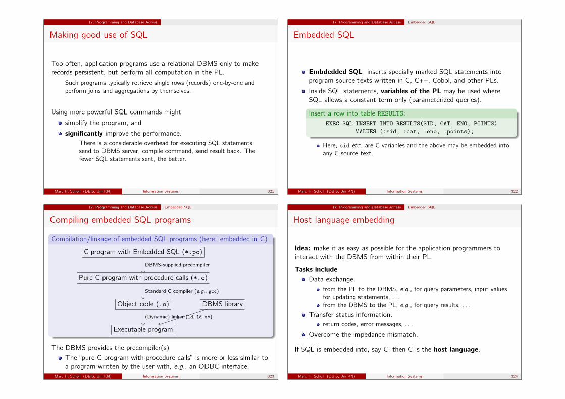
17. Programming and Database Access
Making good use of SQL
Too often, application programs use a relational DBMS only to makerecords persistent, but perform all computation in the PL.
Such programs typically retrieve single rows (records) one-by-one andperform joins and aggregations by themselves.
Using more powerful SQL commands might
simplify the program, and
significantly improve the performance.There is a considerable overhead for executing SQL statements:send to DBMS server, compile command, send result back. Thefewer SQL statements sent, the better.
Marc H. Scholl (DBIS, Uni KN) Information Systems 321
17. Programming and Database Access Embedded SQL
Embedded SQL
Embdedded SQL inserts specially marked SQL statements intoprogram source texts written in C, C++, Cobol, and other PLs.
Inside SQL statements, variables of the PL may be used whereSQL allows a constant term only (parameterized queries).
Insert a row into table RESULTS:EXEC SQL INSERT INTO RESULTS(SID, CAT, ENO, POINTS)
VALUES (:sid, :cat, :eno, :points);
Here, sid etc. are C variables and the above may be embedded intoany C source text.
Marc H. Scholl (DBIS, Uni KN) Information Systems 322
17. Programming and Database Access Embedded SQL
Compiling embedded SQL programs
Compilation/linkage of embedded SQL programs (here: embedded in C)
C program with Embedded SQL (*.pc)
DBMS-supplied precompiler��
Pure C program with procedure calls (*.c)
Standard C compiler (e.g., gcc)��
Object code (.o)
(Dynamic) linker (ld, ld.so)��
DBMS library
ttiiiiiiiiiiiiiiii
Executable program
The DBMS provides the precompiler(s)The “pure C program with procedure calls” is more or less similar toa program written by the user with, e.g., an ODBC interface.
Marc H. Scholl (DBIS, Uni KN) Information Systems 323
17. Programming and Database Access Embedded SQL
Host language embedding
Idea: make it as easy as possible for the application programmers tointeract with the DBMS from within their PL.
Tasks includeData exchange.
from the PL to the DBMS, e.g., for query parameters, input valuesfor updating statements, . . .from the DBMS to the PL, e.g., for query results, . . .
Transfer status information.return codes, error messages, . . .
Overcome the impedance mismatch.
If SQL is embedded into, say C, then C is the host language.
Marc H. Scholl (DBIS, Uni KN) Information Systems 324
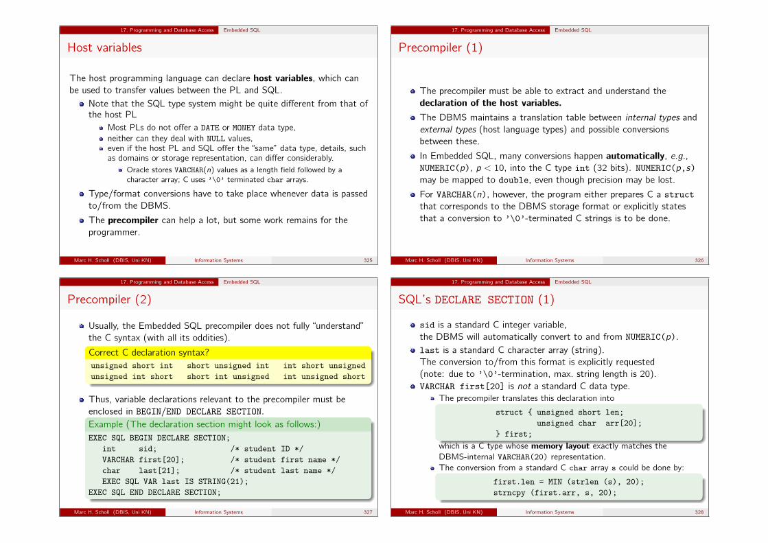
17. Programming and Database Access Embedded SQL
Host variables
The host programming language can declare host variables, which canbe used to transfer values between the PL and SQL.
Note that the SQL type system might be quite different from that ofthe host PL
Most PLs do not offer a DATE or MONEY data type,neither can they deal with NULL values,even if the host PL and SQL offer the “same” data type, details, suchas domains or storage representation, can differ considerably.
Oracle stores VARCHAR(n) values as a length field followed by acharacter array; C uses ’\0’ terminated char arrays.
Type/format conversions have to take place whenever data is passedto/from the DBMS.
The precompiler can help a lot, but some work remains for theprogrammer.
Marc H. Scholl (DBIS, Uni KN) Information Systems 325
17. Programming and Database Access Embedded SQL
Precompiler (1)
The precompiler must be able to extract and understand thedeclaration of the host variables.The DBMS maintains a translation table between internal types andexternal types (host language types) and possible conversionsbetween these.
In Embedded SQL, many conversions happen automatically, e.g.,NUMERIC(p), p < 10, into the C type int (32 bits). NUMERIC(p,s)may be mapped to double, even though precision may be lost.
For VARCHAR(n), however, the program either prepares C a structthat corresponds to the DBMS storage format or explicitly statesthat a conversion to ’\0’-terminated C strings is to be done.
Marc H. Scholl (DBIS, Uni KN) Information Systems 326
17. Programming and Database Access Embedded SQL
Precompiler (2)
Usually, the Embedded SQL precompiler does not fully “understand”the C syntax (with all its oddities).
Correct C declaration syntax?unsigned short int short unsigned int int short unsignedunsigned int short short int unsigned int unsigned short
Thus, variable declarations relevant to the precompiler must beenclosed in BEGIN/END DECLARE SECTION.Example (The declaration section might look as follows:)EXEC SQL BEGIN DECLARE SECTION;
int sid; /* student ID */VARCHAR first[20]; /* student first name */char last[21]; /* student last name */EXEC SQL VAR last IS STRING(21);
EXEC SQL END DECLARE SECTION;
Marc H. Scholl (DBIS, Uni KN) Information Systems 327
17. Programming and Database Access Embedded SQL
SQL’s DECLARE SECTION (1)
sid is a standard C integer variable,the DBMS will automatically convert to and from NUMERIC(p).last is a standard C character array (string).The conversion to/from this format is explicitly requested(note: due to ’\0’-termination, max. string length is 20).VARCHAR first[20] is not a standard C data type.
The precompiler translates this declaration into
struct { unsigned short len;unsigned char arr[20];
} first;
which is a C type whose memory layout exactly matches theDBMS-internal VARCHAR(20) representation.The conversion from a standard C char array s could be done by:
first.len = MIN (strlen (s), 20);strncpy (first.arr, s, 20);
Marc H. Scholl (DBIS, Uni KN) Information Systems 328
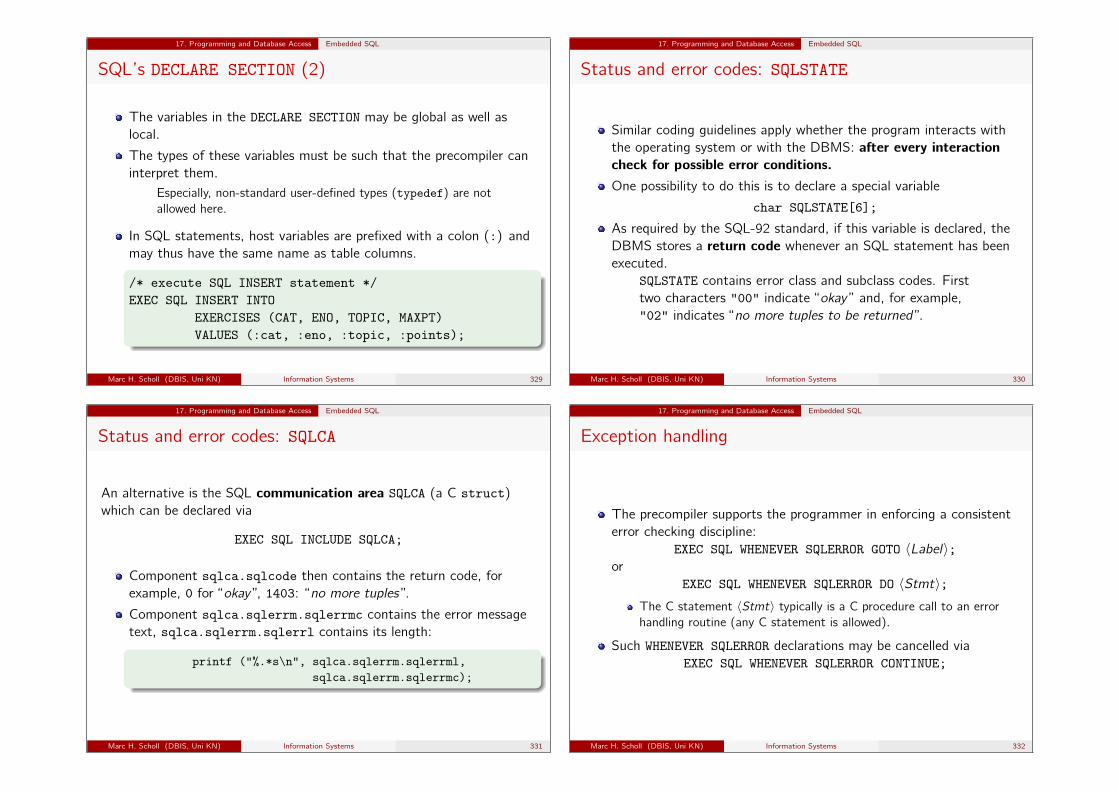
17. Programming and Database Access Embedded SQL
SQL’s DECLARE SECTION (2)
The variables in the DECLARE SECTION may be global as well aslocal.
The types of these variables must be such that the precompiler caninterpret them.
Especially, non-standard user-defined types (typedef) are notallowed here.
In SQL statements, host variables are prefixed with a colon (:) andmay thus have the same name as table columns.
/* execute SQL INSERT statement */EXEC SQL INSERT INTO
EXERCISES (CAT, ENO, TOPIC, MAXPT)VALUES (:cat, :eno, :topic, :points);
Marc H. Scholl (DBIS, Uni KN) Information Systems 329
17. Programming and Database Access Embedded SQL
Status and error codes: SQLSTATE
Similar coding guidelines apply whether the program interacts withthe operating system or with the DBMS: after every interactioncheck for possible error conditions.One possibility to do this is to declare a special variable
char SQLSTATE[6];
As required by the SQL-92 standard, if this variable is declared, theDBMS stores a return code whenever an SQL statement has beenexecuted.
SQLSTATE contains error class and subclass codes. Firsttwo characters "00" indicate “okay ” and, for example,"02" indicates “no more tuples to be returned ”.
Marc H. Scholl (DBIS, Uni KN) Information Systems 330
17. Programming and Database Access Embedded SQL
Status and error codes: SQLCA
An alternative is the SQL communication area SQLCA (a C struct)which can be declared via
EXEC SQL INCLUDE SQLCA;
Component sqlca.sqlcode then contains the return code, forexample, 0 for “okay ”, 1403: “no more tuples ”.
Component sqlca.sqlerrm.sqlerrmc contains the error messagetext, sqlca.sqlerrm.sqlerrl contains its length:
printf ("%.*s\n", sqlca.sqlerrm.sqlerrml,sqlca.sqlerrm.sqlerrmc);
Marc H. Scholl (DBIS, Uni KN) Information Systems 331
17. Programming and Database Access Embedded SQL
Exception handling
The precompiler supports the programmer in enforcing a consistenterror checking discipline:
EXEC SQL WHENEVER SQLERROR GOTO 〈Label〉;or
EXEC SQL WHENEVER SQLERROR DO 〈Stmt〉;The C statement 〈Stmt〉 typically is a C procedure call to an errorhandling routine (any C statement is allowed).
Such WHENEVER SQLERROR declarations may be cancelled viaEXEC SQL WHENEVER SQLERROR CONTINUE;
Marc H. Scholl (DBIS, Uni KN) Information Systems 332
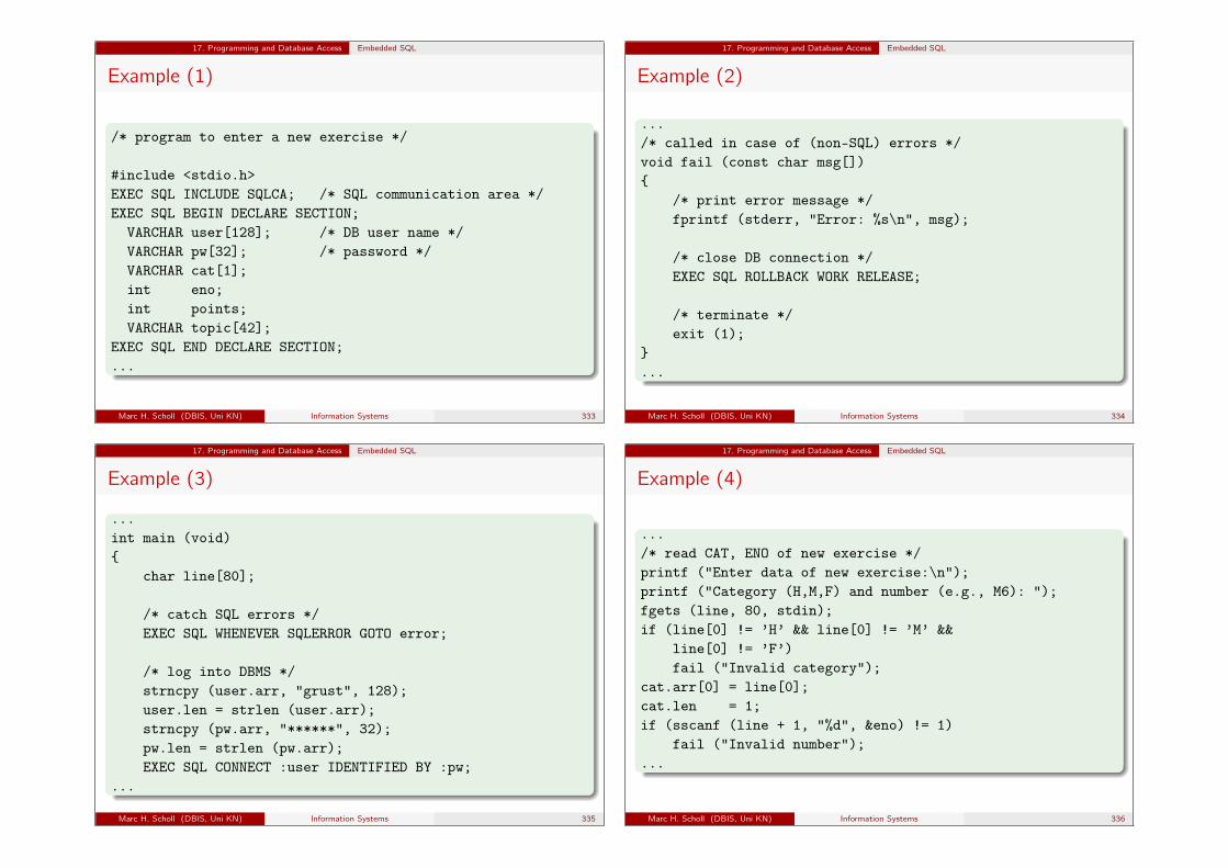
17. Programming and Database Access Embedded SQL
Example (1)
/* program to enter a new exercise */
#include <stdio.h>EXEC SQL INCLUDE SQLCA; /* SQL communication area */EXEC SQL BEGIN DECLARE SECTION;
VARCHAR user[128]; /* DB user name */VARCHAR pw[32]; /* password */VARCHAR cat[1];int eno;int points;VARCHAR topic[42];
EXEC SQL END DECLARE SECTION;...
Marc H. Scholl (DBIS, Uni KN) Information Systems 333
17. Programming and Database Access Embedded SQL
Example (2)
.../* called in case of (non-SQL) errors */void fail (const char msg[]){
/* print error message */fprintf (stderr, "Error: %s\n", msg);
/* close DB connection */EXEC SQL ROLLBACK WORK RELEASE;
/* terminate */exit (1);
}...
Marc H. Scholl (DBIS, Uni KN) Information Systems 334
17. Programming and Database Access Embedded SQL
Example (3)
...int main (void){
char line[80];
/* catch SQL errors */EXEC SQL WHENEVER SQLERROR GOTO error;
/* log into DBMS */strncpy (user.arr, "grust", 128);user.len = strlen (user.arr);strncpy (pw.arr, "******", 32);pw.len = strlen (pw.arr);EXEC SQL CONNECT :user IDENTIFIED BY :pw;
...
Marc H. Scholl (DBIS, Uni KN) Information Systems 335
17. Programming and Database Access Embedded SQL
Example (4)
.../* read CAT, ENO of new exercise */printf ("Enter data of new exercise:\n");printf ("Category (H,M,F) and number (e.g., M6): ");fgets (line, 80, stdin);if (line[0] != ’H’ && line[0] != ’M’ &&
line[0] != ’F’)fail ("Invalid category");
cat.arr[0] = line[0];cat.len = 1;if (sscanf (line + 1, "%d", &eno) != 1)
fail ("Invalid number");...
Marc H. Scholl (DBIS, Uni KN) Information Systems 336
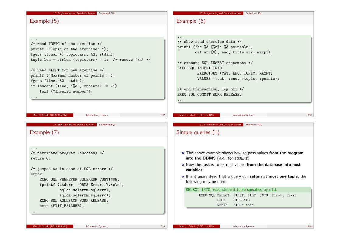
17. Programming and Database Access Embedded SQL
Example (5)
.../* read TOPIC of new exercise */printf ("Topic of the exercise: ");fgets ((char *) topic.arr, 42, stdin);topic.len = strlen (topic.arr) - 1; /* remove ’\n’ */
/* read MAXPT for new exercise */printf ("Maximum number of points: ");fgets (line, 80, stdin);if (sscanf (line, "%d", &points) != -1)
fail ("Invalid number");...
Marc H. Scholl (DBIS, Uni KN) Information Systems 337
17. Programming and Database Access Embedded SQL
Example (6)
.../* show read exercise data */printf ("%c %d [%s]: %d points\n",
cat.arr[0], eno, title.arr, maxpt);
/* execute SQL INSERT statement */EXEC SQL INSERT INTO
EXERCISES (CAT, ENO, TOPIC, MAXPT)VALUES (:cat, :eno, :topic, :points);
/* end transaction, log off */EXEC SQL COMMIT WORK RELEASE;...
Marc H. Scholl (DBIS, Uni KN) Information Systems 338
17. Programming and Database Access Embedded SQL
Example (7)
.../* terminate program (success) */return 0;
/* jumped to in case of SQL errors */error:
EXEC SQL WHENEVER SQLERROR CONTINUE;fprintf (stderr, "DBMS Error: %.*s\n",
sqlca.sqlerrm.sqlerrml,sqlca.sqlerrm.sqlerrc);
EXEC SQL ROLLBACK WORK RELEASE;exit (EXIT_FAILURE);
...
Marc H. Scholl (DBIS, Uni KN) Information Systems 339
17. Programming and Database Access Embedded SQL
Simple queries (1)
The above example shows how to pass values from the programinto the DBMS (e.g., for INSERT).
Now the task is to extract values from the database into hostvariables.If is it guaranteed that a query can return at most one tuple, thefollowing may be used:
SELECT INTO: read student tuple specified by sid.EXEC SQL SELECT FIRST, LAST INTO :first, :last
FROM STUDENTSWHERE SID = :sid
Marc H. Scholl (DBIS, Uni KN) Information Systems 340
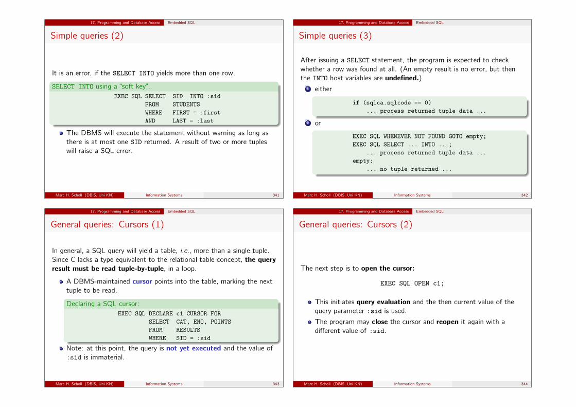
17. Programming and Database Access Embedded SQL
Simple queries (2)
It is an error, if the SELECT INTO yields more than one row.
SELECT INTO using a “soft key”.EXEC SQL SELECT SID INTO :sid
FROM STUDENTSWHERE FIRST = :firstAND LAST = :last
The DBMS will execute the statement without warning as long asthere is at most one SID returned. A result of two or more tupleswill raise a SQL error.
Marc H. Scholl (DBIS, Uni KN) Information Systems 341
17. Programming and Database Access Embedded SQL
Simple queries (3)
After issuing a SELECT statement, the program is expected to checkwhether a row was found at all. (An empty result is no error, but thenthe INTO host variables are undefined.)
1 either
if (sqlca.sqlcode == 0)... process returned tuple data ...
2 or
EXEC SQL WHENEVER NOT FOUND GOTO empty;EXEC SQL SELECT ... INTO ...;
... process returned tuple data ...empty:
... no tuple returned ...
Marc H. Scholl (DBIS, Uni KN) Information Systems 342
17. Programming and Database Access Embedded SQL
General queries: Cursors (1)
In general, a SQL query will yield a table, i.e., more than a single tuple.Since C lacks a type equivalent to the relational table concept, the queryresult must be read tuple-by-tuple, in a loop.
A DBMS-maintained cursor points into the table, marking the nexttuple to be read.
Declaring a SQL cursor:EXEC SQL DECLARE c1 CURSOR FOR
SELECT CAT, ENO, POINTSFROM RESULTSWHERE SID = :sid
Note: at this point, the query is not yet executed and the value of:sid is immaterial.
Marc H. Scholl (DBIS, Uni KN) Information Systems 343
17. Programming and Database Access Embedded SQL
General queries: Cursors (2)
The next step is to open the cursor:
EXEC SQL OPEN c1;
This initiates query evaluation and the then current value of thequery parameter :sid is used.
The program may close the cursor and reopen it again with adifferent value of :sid.
Marc H. Scholl (DBIS, Uni KN) Information Systems 344
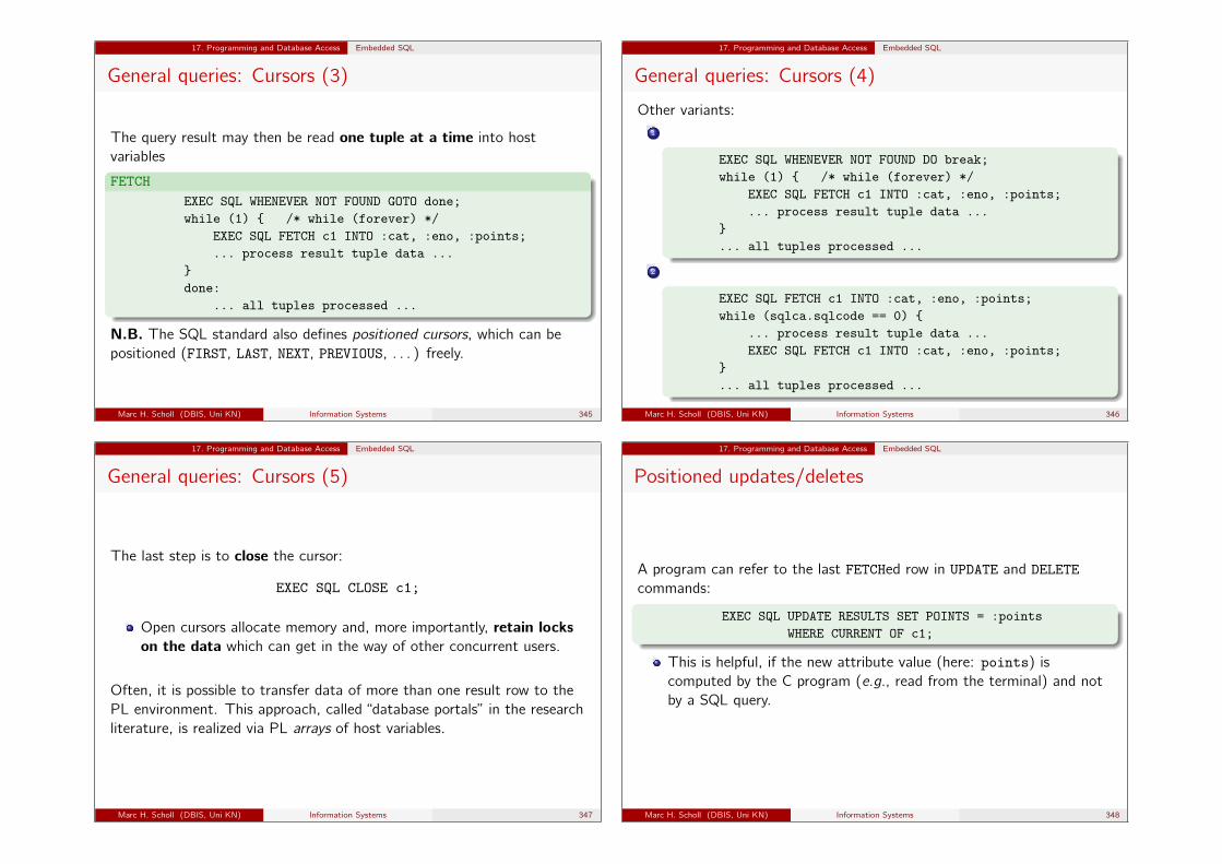
17. Programming and Database Access Embedded SQL
General queries: Cursors (3)
The query result may then be read one tuple at a time into hostvariables
FETCHEXEC SQL WHENEVER NOT FOUND GOTO done;while (1) { /* while (forever) */
EXEC SQL FETCH c1 INTO :cat, :eno, :points;... process result tuple data ...
}done:
... all tuples processed ...
N.B. The SQL standard also defines positioned cursors, which can bepositioned (FIRST, LAST, NEXT, PREVIOUS, . . . ) freely.
Marc H. Scholl (DBIS, Uni KN) Information Systems 345
17. Programming and Database Access Embedded SQL
General queries: Cursors (4)
Other variants:1
EXEC SQL WHENEVER NOT FOUND DO break;while (1) { /* while (forever) */
EXEC SQL FETCH c1 INTO :cat, :eno, :points;... process result tuple data ...
}... all tuples processed ...
2
EXEC SQL FETCH c1 INTO :cat, :eno, :points;while (sqlca.sqlcode == 0) {
... process result tuple data ...EXEC SQL FETCH c1 INTO :cat, :eno, :points;
}... all tuples processed ...
Marc H. Scholl (DBIS, Uni KN) Information Systems 346
17. Programming and Database Access Embedded SQL
General queries: Cursors (5)
The last step is to close the cursor:
EXEC SQL CLOSE c1;
Open cursors allocate memory and, more importantly, retain lockson the data which can get in the way of other concurrent users.
Often, it is possible to transfer data of more than one result row to thePL environment. This approach, called “database portals” in the researchliterature, is realized via PL arrays of host variables.
Marc H. Scholl (DBIS, Uni KN) Information Systems 347
17. Programming and Database Access Embedded SQL
Positioned updates/deletes
A program can refer to the last FETCHed row in UPDATE and DELETEcommands:
EXEC SQL UPDATE RESULTS SET POINTS = :pointsWHERE CURRENT OF c1;
This is helpful, if the new attribute value (here: points) iscomputed by the C program (e.g., read from the terminal) and notby a SQL query.
Marc H. Scholl (DBIS, Uni KN) Information Systems 348

17. Programming and Database Access Embedded SQL
Null values (1)
If a column value in a query result can possibly contain NULL, theprogram is required to declare two host variables: one variable willreceive the data value (if any), the other will indicate whether thevalue is NULL.
Such variables are called indicator variables (normally of C typeshort).The indicator variable will be set to -1, if NULL was returned by thequery (otherwise set to 0).
Marc H. Scholl (DBIS, Uni KN) Information Systems 349
17. Programming and Database Access Embedded SQL
Null values (2)
Cursor declared to fetch student data:EXEC SQL DECLARE stud CURSOR FOR
SELECT FIRST, LAST, EMAILFROM STUDENTS;
An indicator variable may be attached to any variable in a SQLstatement, e.g.:
EXEC SQL FETCH stud INTO :first, :last,:email INDICATOR :null;
It is an error to FETCH a NULL value without indicator variables setup (this includes the result of aggregation fuctions!).
Indicator variables may also be used during INSERT to insert NULLcolumn values into the DB.
Marc H. Scholl (DBIS, Uni KN) Information Systems 350
17. Programming and Database Access Embedded SQL
Dynamic SQL (1)
Up to here, table and column names were already known at programcompile time. At runtime, the current value of host variables is insertedinto these static SQL statements.
In the case of static SQL, the precompiler checks the existence oftables and columns (via lookups in the DBMS data dictionary).In some systems (e.g., IBM DB2), static queries are alreadyoptimized at compile time and the resulting query evaluation plansare stored in the database.
In contrast, it is also possible to compose strings containing dynamicSQL statements at runtime and then to ship the string to the DBMSfor execution.
This is exactly how the the SQL console application is built.
Marc H. Scholl (DBIS, Uni KN) Information Systems 351
17. Programming and Database Access Embedded SQL
Dynamic SQL (2)
If the SQL command is not a query (whose result needs to beconsumed), dynamic execution works as follows:
EXEC SQL EXECUTE IMMEDIATE :sql_cmd;
In general, a problem of the dynamic SQL approach is that thecommand has to be compiled (into a query evaluation plan) everytime it is submitted to the DBMS. Query optimization may be costly.
The DBMS may cache recent query evaluation plans. Thesemay be reused, if a query is re-issued (possibly with differenthost variable values).
If a SQL statement is executed several times with different hostvariables values, the DBMS can explicitly be asked to precompile(“prepare”) the query using EXEC SQL PREPARE and then calling
EXECUTE ... USING 〈Variables〉;
Marc H. Scholl (DBIS, Uni KN) Information Systems 352
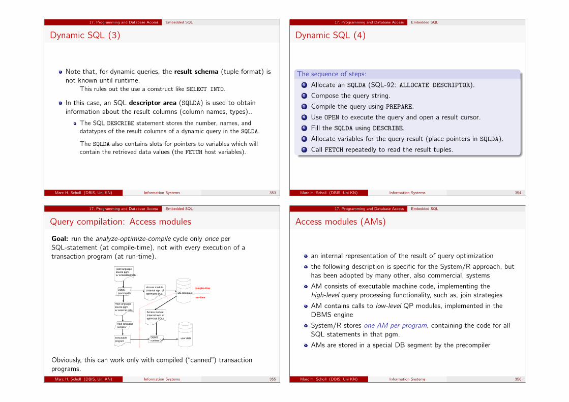
17. Programming and Database Access Embedded SQL
Dynamic SQL (3)
Note that, for dynamic queries, the result schema (tuple format) isnot known until runtime.
This rules out the use a construct like SELECT INTO.
In this case, an SQL descriptor area (SQLDA) is used to obtaininformation about the result columns (column names, types)..
The SQL DESCRIBE statement stores the number, names, anddatatypes of the result columns of a dynamic query in the SQLDA.
The SQLDA also contains slots for pointers to variables which willcontain the retrieved data values (the FETCH host variables).
Marc H. Scholl (DBIS, Uni KN) Information Systems 353
17. Programming and Database Access Embedded SQL
Dynamic SQL (4)
The sequence of steps:1 Allocate an SQLDA (SQL-92: ALLOCATE DESCRIPTOR).2 Compose the query string.3 Compile the query using PREPARE.4 Use OPEN to execute the query and open a result cursor.5 Fill the SQLDA using DESCRIBE.6 Allocate variables for the query result (place pointers in SQLDA).7 Call FETCH repeatedly to read the result tuples.
Marc H. Scholl (DBIS, Uni KN) Information Systems 354
17. Programming and Database Access Embedded SQL
Query compilation: Access modules
Goal: run the analyze-optimize-compile cycle only once perSQL-statement (at compile-time), not with every execution of atransaction program (at run-time).
Host languagesource pgmw/ embedded SQL
DBMSprecompiler
Host languagesource pgmw/ external calls
Host languagecompiler
executableprogram
Access module(internal repr. ofoptimized SQL) DB catalogue
Access module(internal repr. ofoptimized SQL)
DBMSruntime QP
user data
compile−time
run−time
Obviously, this can work only with compiled (“canned”) transactionprograms.Marc H. Scholl (DBIS, Uni KN) Information Systems 355
17. Programming and Database Access Embedded SQL
Access modules (AMs)
an internal representation of the result of query optimization
the following description is specific for the System/R approach, buthas been adopted by many other, also commercial, systems
AM consists of executable machine code, implementing thehigh-level query processing functionality, such as, join strategies
AM contains calls to low-level QP modules, implemented in theDBMS engine
System/R stores one AM per program, containing the code for allSQL statements in that pgm.
AMs are stored in a special DB segment by the precompiler
Marc H. Scholl (DBIS, Uni KN) Information Systems 356
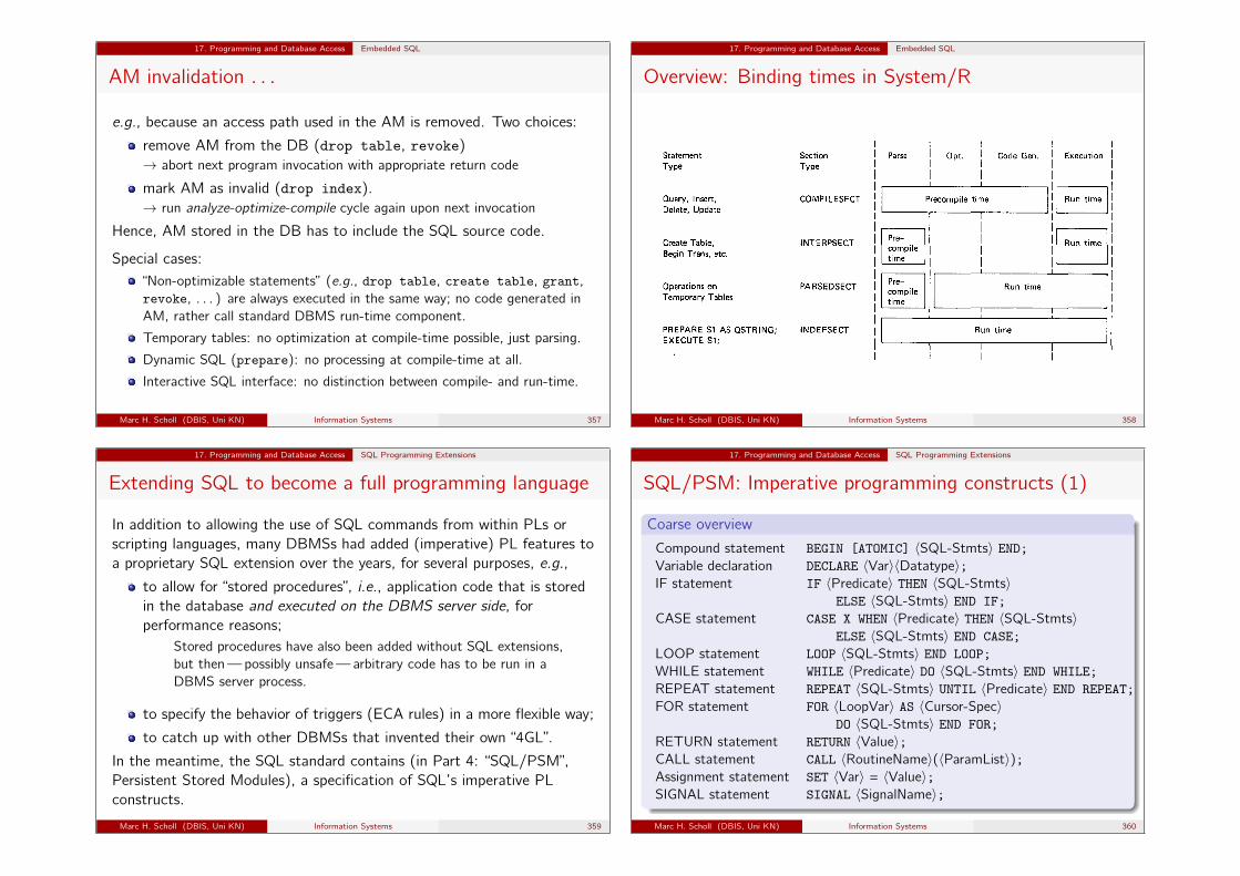
17. Programming and Database Access Embedded SQL
AM invalidation . . .
e.g., because an access path used in the AM is removed. Two choices:
remove AM from the DB (drop table, revoke)→ abort next program invocation with appropriate return code
mark AM as invalid (drop index).→ run analyze-optimize-compile cycle again upon next invocation
Hence, AM stored in the DB has to include the SQL source code.
Special cases:“Non-optimizable statements” (e.g., drop table, create table, grant,revoke, . . . ) are always executed in the same way; no code generated inAM, rather call standard DBMS run-time component.
Temporary tables: no optimization at compile-time possible, just parsing.
Dynamic SQL (prepare): no processing at compile-time at all.
Interactive SQL interface: no distinction between compile- and run-time.
Marc H. Scholl (DBIS, Uni KN) Information Systems 357
17. Programming and Database Access Embedded SQL
Overview: Binding times in System/R
Repetitive Transactions and Ad Hoc Queries in System R * 83
Statement Type
Section Tvpe
Query, Insert, Delete, Update
COMPI LESECT
Create Table, Begin Trans, etc.
INTERPSECT
Operations on Temporary Tables
PARSEDSECT
Parse Opt. Code Gen. Execution
Precompile time
-1 I I 1 Pre- 1
I I I compile 1 time L-l
1;;1*,
PREPARE Sl AS QSTRING; INDEFSECT Run time EXECUTE Sl; I I I
I
I I I I
Fig. 6. Spectrum of binding times in System R.
numbers. The ORDERS table contains a set of outstanding orders for parts. The QUOTES table contains a set of price quotes for parts. Each price quote is identified by a particular supplier number and part number and the minimum and maximum quantities for which the quote applies. Typically, a given combi- nation of supplier and part numbers may have several quotes: one for quantities from 1 to 100, another for quantities from 101 to 10,000, etc.
The following structural and statistical information completes our description of the example database.
(1) The total size of database (including data records but not indexes) equals 7.44 megabytes.
(2) The data values in the sample database were randomly generated according to the following rules:
(a) The number of different part descriptions equals 1024. (b) The .number of different supplier numbers equals 1000. (c) Each part number has exactly three outstanding orders and three price
quotes from each of three different suppliers.
(3) Clustering method: The three tables are stored on disk in an interleaved fashion, ordered by PARTNO. Each PARTS record is followed by all the ORDERS and QUOTES for that part number, then by the next PARTS record, etc. Fifteen percent free space is preserved on each data page to allow for future insertions, which will also be clustered by PARTNO.
A two-part experiment was performed on the example database. The first part involved measurement of three example queries submitted via the User-Friendly Interface (UFI) of System R. For each query, the CPU time and number of I/OS were measured for each step in processing the query: parsing, optimization, code generation, and fetching of the answer set.
The second part of the experiment involved writing a PL/I program to process three types of “canned transactions“ against the sample database. This program
ACM Transactions on Database Systems, Vol. 6, No. 1, March 1961.
Marc H. Scholl (DBIS, Uni KN) Information Systems 358
17. Programming and Database Access SQL Programming Extensions
Extending SQL to become a full programming language
In addition to allowing the use of SQL commands from within PLs orscripting languages, many DBMSs had added (imperative) PL features toa proprietary SQL extension over the years, for several purposes, e.g.,
to allow for “stored procedures”, i.e., application code that is storedin the database and executed on the DBMS server side, forperformance reasons;
Stored procedures have also been added without SQL extensions,but then—possibly unsafe—arbitrary code has to be run in aDBMS server process.
to specify the behavior of triggers (ECA rules) in a more flexible way;
to catch up with other DBMSs that invented their own “4GL”.
In the meantime, the SQL standard contains (in Part 4: “SQL/PSM”,Persistent Stored Modules), a specification of SQL’s imperative PLconstructs.
Marc H. Scholl (DBIS, Uni KN) Information Systems 359
17. Programming and Database Access SQL Programming Extensions
SQL/PSM: Imperative programming constructs (1)
Coarse overview
Compound statement BEGIN [ATOMIC] 〈SQL-Stmts〉 END;Variable declaration DECLARE 〈Var〉〈Datatype〉;IF statement IF 〈Predicate〉 THEN 〈SQL-Stmts〉
ELSE 〈SQL-Stmts〉 END IF;CASE statement CASE X WHEN 〈Predicate〉 THEN 〈SQL-Stmts〉
ELSE 〈SQL-Stmts〉 END CASE;LOOP statement LOOP 〈SQL-Stmts〉 END LOOP;WHILE statement WHILE 〈Predicate〉 DO 〈SQL-Stmts〉 END WHILE;REPEAT statement REPEAT 〈SQL-Stmts〉 UNTIL 〈Predicate〉 END REPEAT;FOR statement FOR 〈LoopVar〉 AS 〈Cursor-Spec〉
DO 〈SQL-Stmts〉 END FOR;RETURN statement RETURN 〈Value〉;CALL statement CALL 〈RoutineName〉(〈ParamList〉);Assignment statement SET 〈Var〉 = 〈Value〉;SIGNAL statement SIGNAL 〈SignalName〉;
Marc H. Scholl (DBIS, Uni KN) Information Systems 360
17. Programming and Database Access SQL Programming Extensions
SQL/PSM: Imperative programming constructs (2)
With the “object-relational” extensions of SQL:1999, these programmingconstructs can also be used to implement methods and user-definedfunctions that can be defined as part of a database schema.17
User-defined functions (UDFs) can be used similar to built-infunctions.
Methods can be attached to classes (“structured types”), much likein any object-oriented programming language.
17We will discuss these SQL:1999 extensions in a separate chapter later.Marc H. Scholl (DBIS, Uni KN) Information Systems 361
Part VI
Data Warehousing and OLAP
Marc H. Scholl (DBIS, Uni KN) Information Systems 362
Outline of this part
18 What is a Data Warehouse?
19 Multidimensional Data Model
20 Relational RepresentationRepresenting Cubes in TablesQuerying CubesSQL: OLAP ExtensionsOLAP Benchmarks
21 Summary
Marc H. Scholl (DBIS, Uni KN) Information Systems 363
This part’s goal
After completing this chapter, you should be able to:
describe the major characteristics of a data warehouse,
disinguish online transaction processing (OLTP) from onlineanalytical processing (OLAP) requirements,
enumerate some of the challenges for RDBMSs to satisfy thoseOLAP requirements,
formulate basic OLAP queries using appropriate SQL extensions.
Marc H. Scholl (DBIS, Uni KN) Information Systems 364

18. What is a Data Warehouse?
What is a Data Warehouse?
Database of a single supermarket:
Revenue,Portfolio Marketing
Marc H. Scholl (DBIS, Uni KN) Information Systems 365
18. What is a Data Warehouse?
Once we’re successful . . .
Several branches:
DB Site1 DB Site2 DB Site3
Data Warehouse
MarketingRevenue,Portfolio
Marc H. Scholl (DBIS, Uni KN) Information Systems 366
18. What is a Data Warehouse?
Sample OLAP queries
How many bottles of Coke did we sell last month?
Show the sales history of last year w.r.t. alcoholic beverages.
Who are our top customers?
Which of our suppliers delivers the most beer?
Which branch was top-selling w.r.t. beer, wine, soda?
Compare the sales figures of soda and beer over the last fivesummers.
Some challenges
A lot of diverse data sources might be needed (e.g., suppliers, stock,customers, cash registers).
Queries may span data sources.
Data have a temporal dimension.
Queries may get quite complex, often a lot of statistics.Marc H. Scholl (DBIS, Uni KN) Information Systems 367
18. What is a Data Warehouse?
Data Warehousing
The process of supporting (strategic) business decisions by quantitativeanalysis of data, obtained by aggregating own, day-to-day operationalbusiness data, possibly extended by several other data, obtained fromexternal sources is often called data warehousing or business intelligence.
Decision support: target audience is strategic management.
Quantitative analysis: data is statistically analyzed.
Aggregation: data is condensed, individual business case isirrelevant.
External sources: often, general economic data is needed, not alldata from one database.
(Some) challenges: sheer data volume, appropriate data modeling, dataintegration, OLAP queries
Marc H. Scholl (DBIS, Uni KN) Information Systems 368
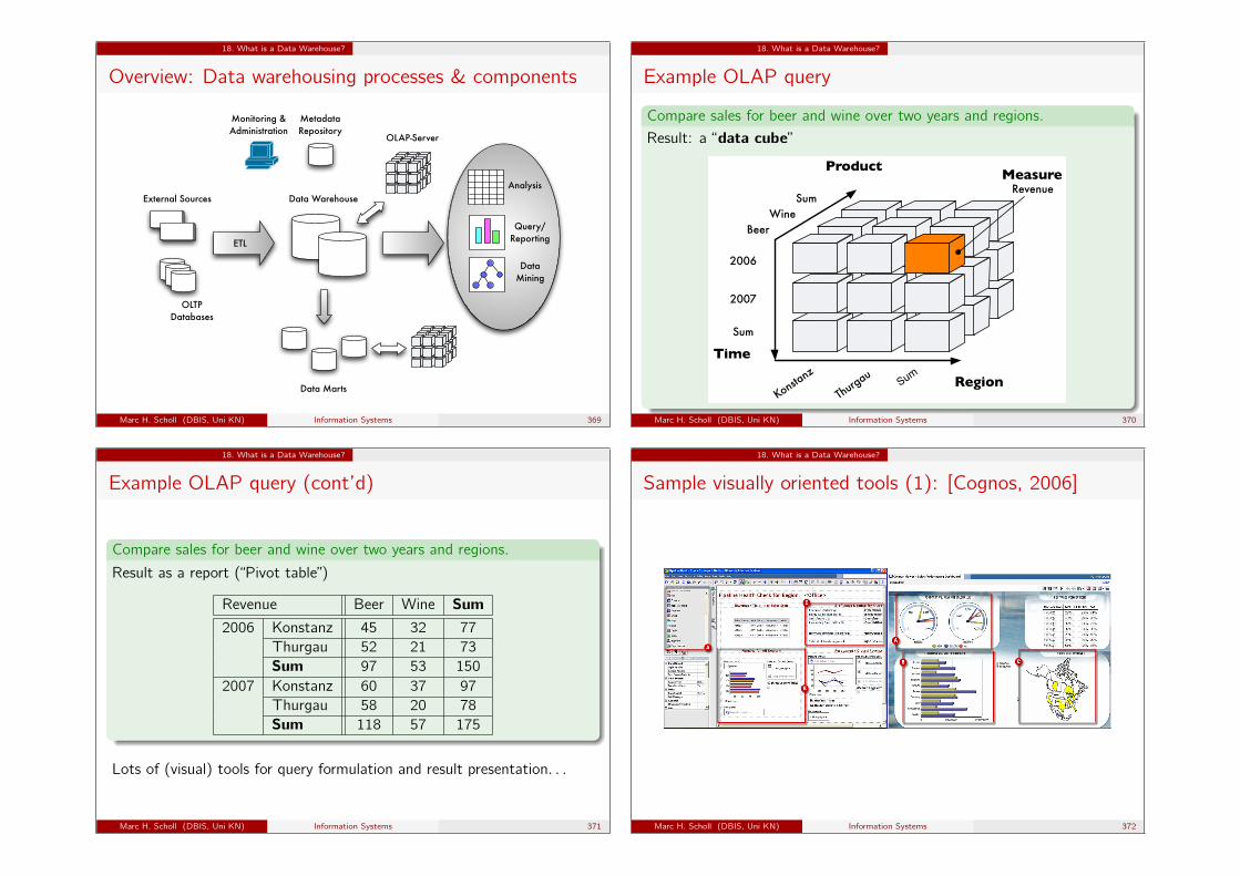
18. What is a Data Warehouse?
Overview: Data warehousing processes & components
ETL
OLTPDatabases
External Sources
Monitoring & Administration
MetadataRepository
Data Marts
Data Warehouse
OLAP-Server
Analysis
Query/Reporting
DataMining
Marc H. Scholl (DBIS, Uni KN) Information Systems 369
18. What is a Data Warehouse?
Example OLAP query
Compare sales for beer and wine over two years and regions.
Result: a “data cube”
Product
Region
Time
Measure
BeerWine
Sum
Thurga
u
Konst
anz Sum
2006
2007
Sum
Revenue
Marc H. Scholl (DBIS, Uni KN) Information Systems 370
18. What is a Data Warehouse?
Example OLAP query (cont’d)
Compare sales for beer and wine over two years and regions.
Result as a report (“Pivot table”)
Revenue Beer Wine Sum2006 Konstanz 45 32 77
Thurgau 52 21 73Sum 97 53 150
2007 Konstanz 60 37 97Thurgau 58 20 78Sum 118 57 175
Lots of (visual) tools for query formulation and result presentation. . .
Marc H. Scholl (DBIS, Uni KN) Information Systems 371
18. What is a Data Warehouse?
Sample visually oriented tools (1): [Cognos, 2006]
Marc H. Scholl (DBIS, Uni KN) Information Systems 372
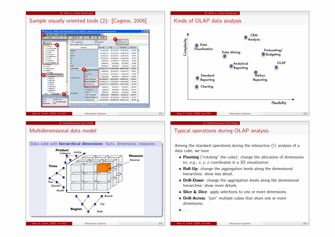
18. What is a Data Warehouse?
Sample visually oriented tools (2): [Cognos, 2006]
Marc H. Scholl (DBIS, Uni KN) Information Systems 373
18. What is a Data Warehouse?
Kinds of OLAP data analysis
Flexibility
Com
plex
ity
DataVisualization
Charting
AnalyticalReporting
Ad-hocReporting
OLAP
CRMAnalysis
Forecasting/BudgetingData Mining
StandardReporting
Marc H. Scholl (DBIS, Uni KN) Information Systems 374
19. Multidimensional Data Model
Multidimensional data model
Data cube with hierarchical dimensions: facts, dimensions, measures
Product
Region
Time
MeasureRevenue
Branch
City
State
Category Article
YearQuarter
Month
Marc H. Scholl (DBIS, Uni KN) Information Systems 375
19. Multidimensional Data Model
Typical operations during OLAP analysis
Among the standard operations during the interactive (!) analysis of adata cube, we have
Pivoting (“rotating” the cube): change the allocation of dimensionsto, e.g., x, y , z coordinates in a 3D visualization.
Roll-Up: change the aggregation levels along the dimensionalhierarchies: show less detail.
Drill-Down: change the aggregation levels along the dimensionalhierarchies: show more details.
Slice & Dice: apply selections to one or more dimensions.
Drill-Across: “join” multiple cubes that share one or moredimensions.
. . .
Marc H. Scholl (DBIS, Uni KN) Information Systems 376
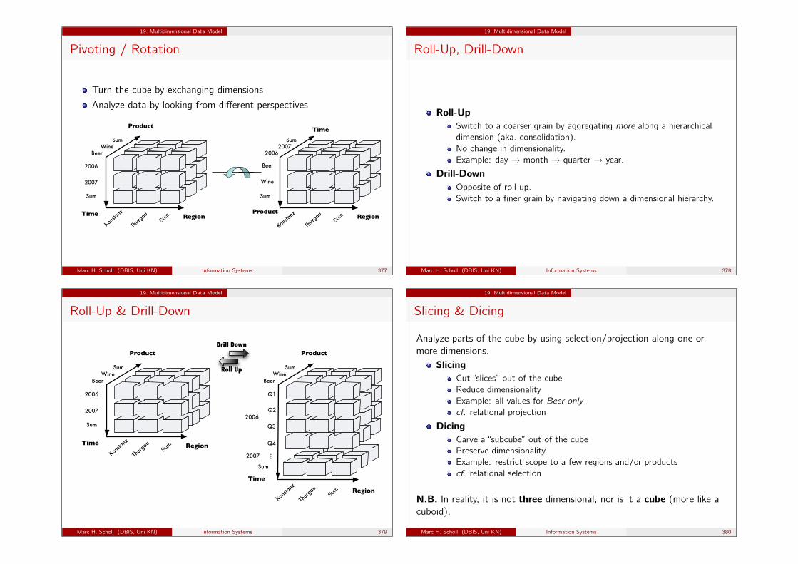
19. Multidimensional Data Model
Pivoting / Rotation
Turn the cube by exchanging dimensions
Analyze data by looking from different perspectives
Product
RegionTime
BeerWine
Sum
Thurg
au
Konstanz
Sum
2006
2007
Sum
ProductRegion
Time
Beer
Wine
Sum
Thurg
au
Konstanz
Sum
20062007
Sum
Marc H. Scholl (DBIS, Uni KN) Information Systems 377
19. Multidimensional Data Model
Roll-Up, Drill-Down
Roll-UpSwitch to a coarser grain by aggregating more along a hierarchicaldimension (aka. consolidation).No change in dimensionality.Example: day → month → quarter → year.
Drill-DownOpposite of roll-up.Switch to a finer grain by navigating down a dimensional hierarchy.
Marc H. Scholl (DBIS, Uni KN) Information Systems 378
19. Multidimensional Data Model
Roll-Up & Drill-Down
Product
RegionTime
BeerWine
Sum
Thurg
au
Konstanz
Sum
2006
2007
Sum
Product
Time
BeerWine
Sum
Q1
Q2
Q3
Q4
2006
2007
Sum
...
Drill Down
Roll Up
Region
Thurg
au
Konstanz
Sum
Marc H. Scholl (DBIS, Uni KN) Information Systems 379
19. Multidimensional Data Model
Slicing & Dicing
Analyze parts of the cube by using selection/projection along one ormore dimensions.
SlicingCut “slices” out of the cubeReduce dimensionalityExample: all values for Beer onlycf. relational projection
DicingCarve a “subcube” out of the cubePreserve dimensionalityExample: restrict scope to a few regions and/or productscf. relational selection
N.B. In reality, it is not three dimensional, nor is it a cube (more like acuboid).
Marc H. Scholl (DBIS, Uni KN) Information Systems 380
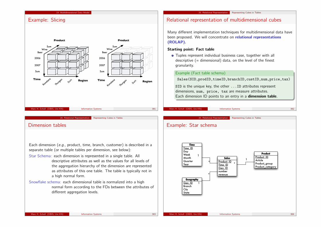
19. Multidimensional Data Model
Example: Slicing
Product
RegionTime
BeerWine
Sum
Thurg
au
Konstanz
Sum
2006
2007
Sum
Product
RegionTime
Thurg
au
Konstanz
Sum
BeerWine
2006
2007
Sum
Sum
Marc H. Scholl (DBIS, Uni KN) Information Systems 381
20. Relational Representation Representing Cubes in Tables
Relational representation of multidimensional cubes
Many different implementation techniques for multidimensional data havebeen proposed. We will concentrate on relational representations(ROLAP).
Starting point: Fact tableTuples represent individual business case, together with alldescriptive (= dimensional) data, on the level of the finestgranularity.
Example (Fact table schema)
Sales(SID,prodID,timeID,branchID,custID,num,price,tax)
SID is the unique key, the other ...ID attributes representdimensions, num, price, tax are measure attributes.Each dimension ID points to an entry in a dimension table.
Marc H. Scholl (DBIS, Uni KN) Information Systems 382
20. Relational Representation Representing Cubes in Tables
Dimension tables
Each dimension (e.g., product, time, branch, customer) is described in aseparate table (or multiple tables per dimension, see below):
Star Schema: each dimension is represented in a single table. Alldescriptive attributes as well as the values for all levels ofthe aggregation hierarchy of the dimension are representedas attributes of this one table. The table is typically not ina high normal form.
Snowflake schema: each dimensional table is normalized into a highnormal form according to the FDs between the attributes ofdifferent aggregation levels.
Marc H. Scholl (DBIS, Uni KN) Information Systems 383
20. Relational Representation Representing Cubes in Tables
Example: Star schema
Product_IDTime_IDGeo_IDnumberrevenue
Sales Product_IDArticleProduct_groupProduct_category
Product
Geo_IDBranchCityState
Geography
Time_IDDayWeekMonthQuarterYear
Time
*
1
*
1
1
*
Marc H. Scholl (DBIS, Uni KN) Information Systems 384
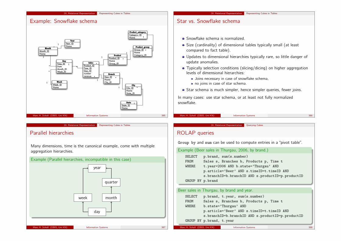
20. Relational Representation Representing Cubes in Tables
Example: Snowflake schema
Product_IDTime_IDGeo_IDnumberrevenue
Sales
Product_IDNameGroup_ID
Product
Geo_IDNameCity_ID
Branch
Time_IDDateMonth_IDWeek_ID
Day
*1
*1
1
*
Group_IDNameCategory_ID
Product_group
Category_IDName
Product_category
City_IDNameState_ID
City
State_IDName
State
1
*
1
*
1
*
1
*Week_IDName
Week
Month_IDName
Month
Year_IDName
Year
1
*
1
*
1*
Marc H. Scholl (DBIS, Uni KN) Information Systems 385
20. Relational Representation Representing Cubes in Tables
Star vs. Snowflake schema
Snowflake schema is normalized.
Size (cardinality) of dimensional tables typically small (at leastcompared to fact table).
Updates to dimensional hierarchies typically rare, so little danger ofupdate anomalies.Typically selection conditions (slicing/dicing) on higher aggregationlevels of dimensional hierarchies:
Joins necessary in case of snowflake schema,no joins in case of star schema.
Star schema is much simpler, hence simpler queries, fewer joins.
In many cases: use star schema, or at least not fully normalizedsnowflake.
Marc H. Scholl (DBIS, Uni KN) Information Systems 386
20. Relational Representation Representing Cubes in Tables
Parallel hierarchies
Many dimensions, time is the canonical example, come with multipleaggregation hierarchies.
Example (Parallel hierarchies, incompatible in this case)
day
week month
quarter
year
Marc H. Scholl (DBIS, Uni KN) Information Systems 387
20. Relational Representation Querying Cubes
ROLAP queries
Group by and sum can be used to compute entries in a “pivot table”.
Example (Beer sales in Thurgau, 2006, by brand.)
SELECT p.brand, sum(s.number)FROM Sales s, Branches b, Products p, Time tWHERE t.year=2006 AND b.state=’Thurgau’ AND
p.article=’Beer’ AND s.timeID=t.timeID ANDs.branchID=b.branchID AND s.productID=p.productID
GROUP BY p.brand
Beer sales in Thurgau, by brand and year.SELECT p.brand, t.year, sum(s.number)FROM Sales s, Branches b, Products p, Time tWHERE b.state=’Thurgau’ AND
p.article=’Beer’ AND s.timeID=t.timeID ANDs.branchID=b.branchID AND s.productID=p.productID
GROUP BY p.brand, t.year
Marc H. Scholl (DBIS, Uni KN) Information Systems 388
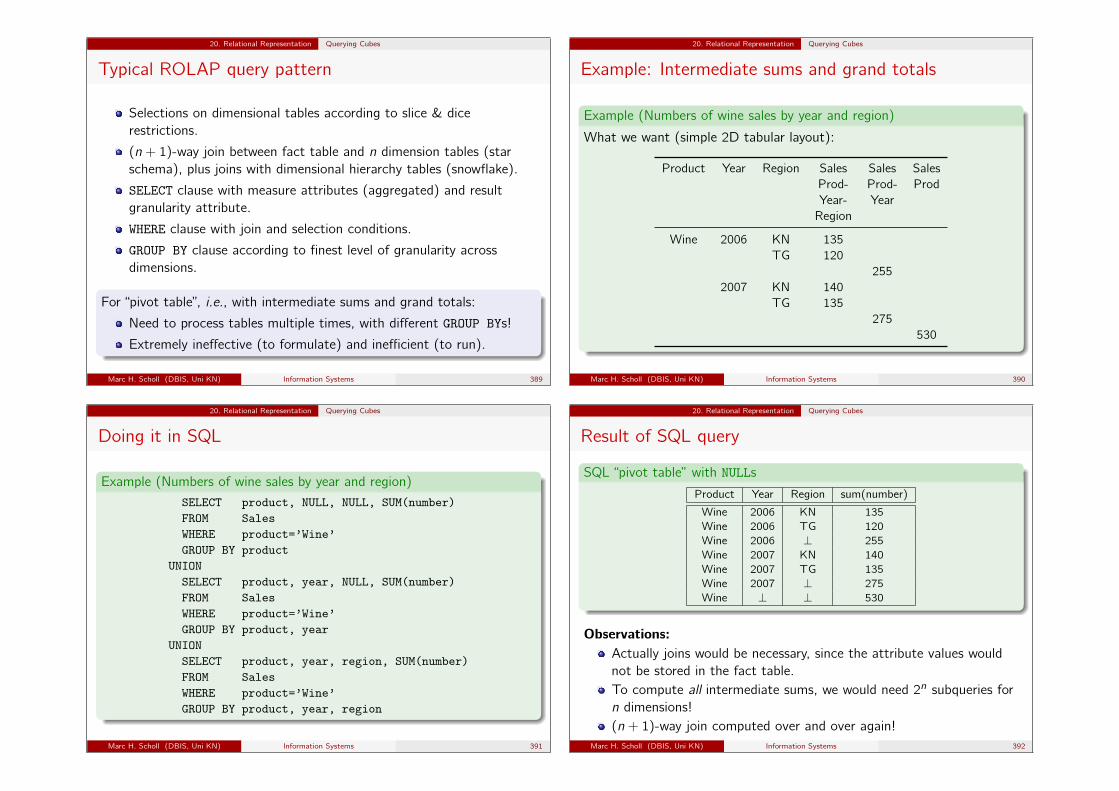
20. Relational Representation Querying Cubes
Typical ROLAP query pattern
Selections on dimensional tables according to slice & dicerestrictions.
(n + 1)-way join between fact table and n dimension tables (starschema), plus joins with dimensional hierarchy tables (snowflake).
SELECT clause with measure attributes (aggregated) and resultgranularity attribute.
WHERE clause with join and selection conditions.
GROUP BY clause according to finest level of granularity acrossdimensions.
For “pivot table”, i.e., with intermediate sums and grand totals:
Need to process tables multiple times, with different GROUP BYs!
Extremely ineffective (to formulate) and inefficient (to run).
Marc H. Scholl (DBIS, Uni KN) Information Systems 389
20. Relational Representation Querying Cubes
Example: Intermediate sums and grand totals
Example (Numbers of wine sales by year and region)
What we want (simple 2D tabular layout):
Product Year Region Sales Sales SalesProd- Prod- ProdYear- YearRegion
Wine 2006 KN 135TG 120
2552007 KN 140
TG 135275
530
Marc H. Scholl (DBIS, Uni KN) Information Systems 390
20. Relational Representation Querying Cubes
Doing it in SQL
Example (Numbers of wine sales by year and region)
SELECT product, NULL, NULL, SUM(number)FROM SalesWHERE product=’Wine’GROUP BY product
UNIONSELECT product, year, NULL, SUM(number)FROM SalesWHERE product=’Wine’GROUP BY product, year
UNIONSELECT product, year, region, SUM(number)FROM SalesWHERE product=’Wine’GROUP BY product, year, region
Marc H. Scholl (DBIS, Uni KN) Information Systems 391
20. Relational Representation Querying Cubes
Result of SQL query
SQL “pivot table” with NULLs
Product Year Region sum(number)
Wine 2006 KN 135Wine 2006 TG 120Wine 2006 ⊥ 255Wine 2007 KN 140Wine 2007 TG 135Wine 2007 ⊥ 275Wine ⊥ ⊥ 530
Observations:Actually joins would be necessary, since the attribute values wouldnot be stored in the fact table.To compute all intermediate sums, we would need 2n subqueries forn dimensions!(n + 1)-way join computed over and over again!
Marc H. Scholl (DBIS, Uni KN) Information Systems 392
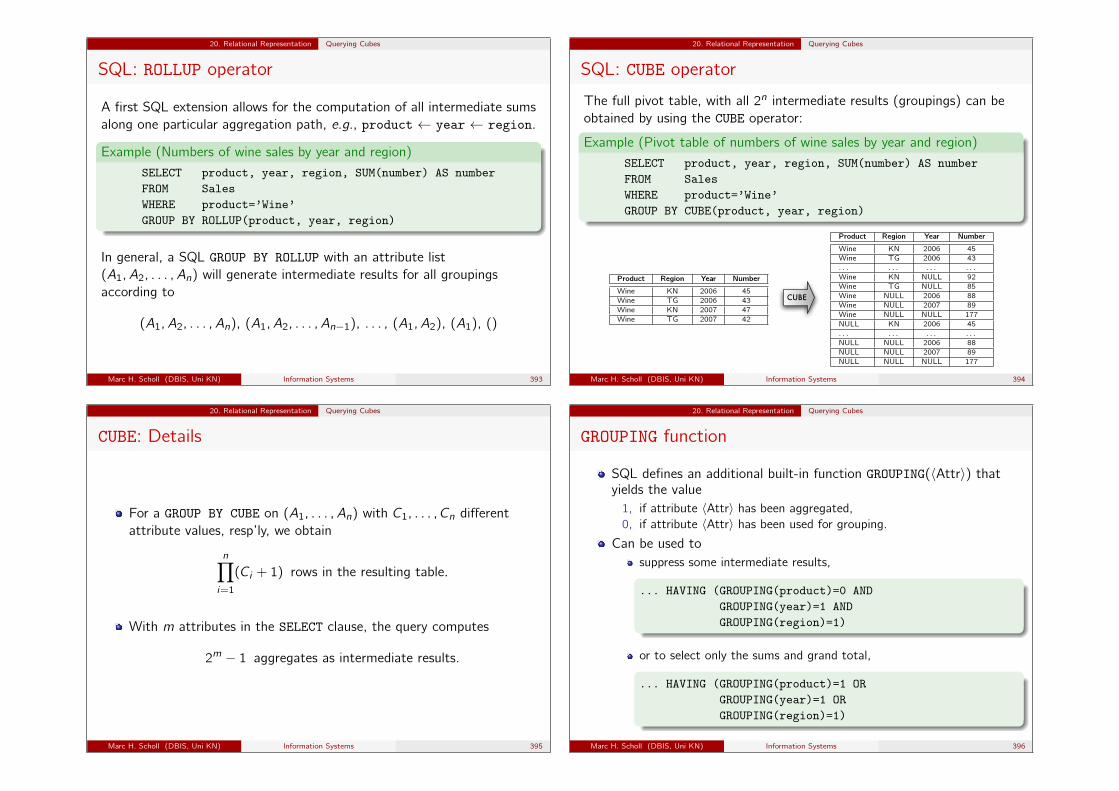
20. Relational Representation Querying Cubes
SQL: ROLLUP operator
A first SQL extension allows for the computation of all intermediate sumsalong one particular aggregation path, e.g., product ← year ← region.
Example (Numbers of wine sales by year and region)
SELECT product, year, region, SUM(number) AS numberFROM SalesWHERE product=’Wine’GROUP BY ROLLUP(product, year, region)
In general, a SQL GROUP BY ROLLUP with an attribute list(A1, A2, . . . , An) will generate intermediate results for all groupingsaccording to
(A1, A2, . . . , An), (A1, A2, . . . , An−1), . . . , (A1, A2), (A1), ()
Marc H. Scholl (DBIS, Uni KN) Information Systems 393
20. Relational Representation Querying Cubes
SQL: CUBE operator
The full pivot table, with all 2n intermediate results (groupings) can beobtained by using the CUBE operator:
Example (Pivot table of numbers of wine sales by year and region)
SELECT product, year, region, SUM(number) AS numberFROM SalesWHERE product=’Wine’GROUP BY CUBE(product, year, region)
Product Region Year Number
Wine KN 2006 45Wine TG 2006 43Wine KN 2007 47Wine TG 2007 42
CUBE
Product Region Year Number
Wine KN 2006 45Wine TG 2006 43. . . . . . . . . . . .Wine KN NULL 92Wine TG NULL 85Wine NULL 2006 88Wine NULL 2007 89Wine NULL NULL 177NULL KN 2006 45. . . . . . . . . . . .NULL NULL 2006 88NULL NULL 2007 89NULL NULL NULL 177
Marc H. Scholl (DBIS, Uni KN) Information Systems 394
20. Relational Representation Querying Cubes
CUBE: Details
For a GROUP BY CUBE on (A1, . . . , An) with C1, . . . , Cn differentattribute values, resp’ly, we obtain
n∏i=1
(Ci + 1) rows in the resulting table.
With m attributes in the SELECT clause, the query computes
2m − 1 aggregates as intermediate results.
Marc H. Scholl (DBIS, Uni KN) Information Systems 395
20. Relational Representation Querying Cubes
GROUPING function
SQL defines an additional built-in function GROUPING(〈Attr〉) thatyields the value
1, if attribute 〈Attr〉 has been aggregated,0, if attribute 〈Attr〉 has been used for grouping.
Can be used tosuppress some intermediate results,
... HAVING (GROUPING(product)=0 ANDGROUPING(year)=1 ANDGROUPING(region)=1)
or to select only the sums and grand total,
... HAVING (GROUPING(product)=1 ORGROUPING(year)=1 ORGROUPING(region)=1)
Marc H. Scholl (DBIS, Uni KN) Information Systems 396
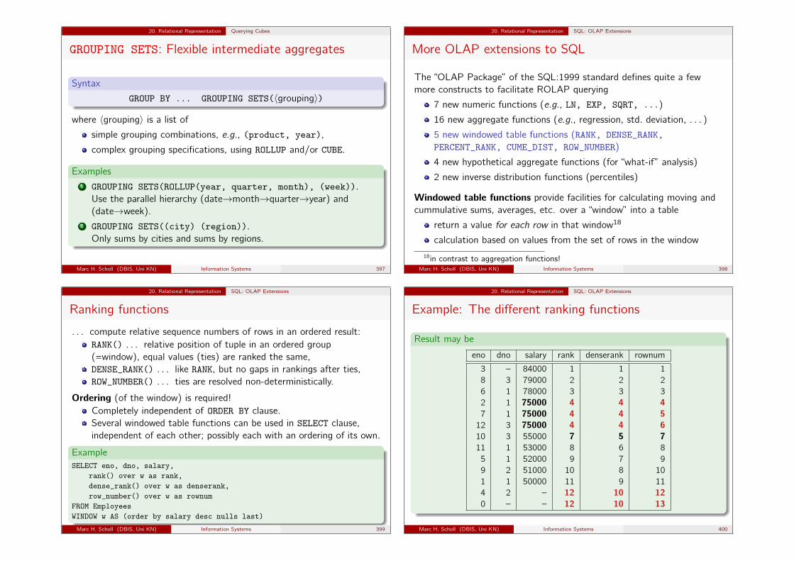
20. Relational Representation Querying Cubes
GROUPING SETS: Flexible intermediate aggregates
Syntax
GROUP BY ... GROUPING SETS(〈grouping〉)
where 〈grouping〉 is a list of
simple grouping combinations, e.g., (product, year),
complex grouping specifications, using ROLLUP and/or CUBE.
Examples1 GROUPING SETS(ROLLUP(year, quarter, month), (week)).
Use the parallel hierarchy (date→month→quarter→year) and(date→week).
2 GROUPING SETS((city) (region)).Only sums by cities and sums by regions.
Marc H. Scholl (DBIS, Uni KN) Information Systems 397
20. Relational Representation SQL: OLAP Extensions
More OLAP extensions to SQL
The “OLAP Package” of the SQL:1999 standard defines quite a fewmore constructs to facilitate ROLAP querying
7 new numeric functions (e.g., LN, EXP, SQRT, ...)
16 new aggregate functions (e.g., regression, std. deviation, . . . )
5 new windowed table functions (RANK, DENSE_RANK,PERCENT_RANK, CUME_DIST, ROW_NUMBER)
4 new hypothetical aggregate functions (for “what-if” analysis)
2 new inverse distribution functions (percentiles)
Windowed table functions provide facilities for calculating moving andcummulative sums, averages, etc. over a “window” into a table
return a value for each row in that window18
calculation based on values from the set of rows in the window
18in contrast to aggregation functions!Marc H. Scholl (DBIS, Uni KN) Information Systems 398
20. Relational Representation SQL: OLAP Extensions
Ranking functions
. . . compute relative sequence numbers of rows in an ordered result:RANK() . . . relative position of tuple in an ordered group(=window), equal values (ties) are ranked the same,DENSE_RANK() . . . like RANK, but no gaps in rankings after ties,ROW_NUMBER() . . . ties are resolved non-deterministically.
Ordering (of the window) is required!Completely independent of ORDER BY clause.Several windowed table functions can be used in SELECT clause,independent of each other; possibly each with an ordering of its own.
ExampleSELECT eno, dno, salary,
rank() over w as rank,dense_rank() over w as denserank,row_number() over w as rownum
FROM EmployeesWINDOW w AS (order by salary desc nulls last)
Marc H. Scholl (DBIS, Uni KN) Information Systems 399
20. Relational Representation SQL: OLAP Extensions
Example: The different ranking functions
Result may be
eno dno salary rank denserank rownum
3 – 84000 1 1 18 3 79000 2 2 26 1 78000 3 3 32 1 75000 4 4 47 1 75000 4 4 512 3 75000 4 4 610 3 55000 7 5 711 1 53000 8 6 85 1 52000 9 7 99 2 51000 10 8 101 1 50000 11 9 114 2 – 12 10 120 – – 12 10 13
Marc H. Scholl (DBIS, Uni KN) Information Systems 400
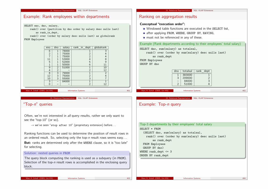
20. Relational Representation SQL: OLAP Extensions
Example: Rank employees within departments
SELECT eno, dno, salary,rank() over (partition by dno order by salary desc nulls last)
as rank_in_dept,rank() over (order by salary desc nulls last) as globalrank
FROM Employees
eno dno salary rank_in_dept globalrank6 1 78000 1 32 1 75000 2 47 1 75000 2 4
11 1 53000 4 85 1 52000 5 91 1 50000 6 119 2 51000 1 104 2 – 2 128 3 79000 1 2
12 3 75000 2 410 3 55000 3 73 – 84000 1 10 – – 2 12
Marc H. Scholl (DBIS, Uni KN) Information Systems 401
20. Relational Representation SQL: OLAP Extensions
Ranking on aggregation results
Conceptual “execution order”:Windowed table functions are executed in the SELECT list,after applying FROM, WHERE, GROUP BY, HAVING,must not be referenced in any of these.
Example (Rank departments according to their employees’ total salary)
SELECT dno, sum(salary) as totalsal,rank() over (order by sum(salary) desc nulls last)
as rank_deptFROM EmployeesGROUP BY dno
dno totalsal rank_dept1 383000 13 209000 2– 84000 32 51000 4
Marc H. Scholl (DBIS, Uni KN) Information Systems 402
20. Relational Representation SQL: OLAP Extensions
“Top-n” queries
Often, we’re not interested in all query results, rather we only want tosee the “top-10” (or so).
→ we’ve seen “stop after 10” (proprietary extension) before. . .
Ranking functions can be used to determine the position of result rows inan ordered result. So, selecting only the top-n result rows seems easy. . .
But: ranks are determined only after the WHERE clause, so it is “too late”for selecting.
Solution: nested queries in FROM
The query block computing the ranking is used as a subquery (in FROM).Selection of the top-n result rows is accomplished in the enclosing queryblock.
Marc H. Scholl (DBIS, Uni KN) Information Systems 403
20. Relational Representation SQL: OLAP Extensions
Example: Top-n query
Top-3 departments by their employees’ total salarySELECT * FROM
(SELECT dno, sum(salary) as totalsal,rank() over (order by sum(salary) desc nulls last)
as rank_deptFROM EmployeesGROUP BY dno)
WHERE rank_dept <= 3ORDER BY rank_dept
Marc H. Scholl (DBIS, Uni KN) Information Systems 404
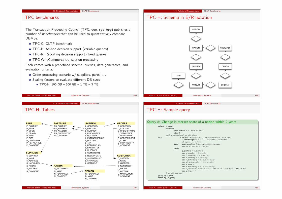
20. Relational Representation OLAP Benchmarks
TPC benchmarks
The Transaction Processing Council (TPC, www.tpc.org) publishes anumber of benchmarks that can be used to quantitatively compareDBMSs.
TPC-C: OLTP benchmark
TPC-H: Ad-hoc decision support (variable queries)
TPC-R: Reporting decision support (fixed queries)
TPC-W: eCommerce transaction processing
Each comes with a predefined schema, queries, data generators, andevaluation criteria.
Order processing scenario w/ suppliers, parts, . . .Scaling factors to evaluate different DB sizes
TPC-H: 100 GB – 300 GB – 1 TB – 3 TB
Marc H. Scholl (DBIS, Uni KN) Information Systems 405
20. Relational Representation OLAP Benchmarks
TPC-H: Schema in E/R-notation
REGION
NATION
SUPPLIER
PARTSUPP LINEITEM
ORDERS
CUSTOMER
PART
Marc H. Scholl (DBIS, Uni KN) Information Systems 406
20. Relational Representation OLAP Benchmarks
TPC-H: Tables
Marc H. Scholl (DBIS, Uni KN) Information Systems 407
20. Relational Representation OLAP Benchmarks
TPC-H: Sample query
Query 8: Change in market share of a nation within 2 yearsselect o_year,
sum(casewhen nation = "’ then volumeelse 0
end) / sum(volume) as mkt_sharefrom ( select extract(year from o_orderdate) as o_year,
l_extendedprice * (1 - l_discount) as volume,n2.n_name as nation
from part,supplier,lineitem,orders,customer,nation n1,nation n2,region
wherep_partkey = l_partkeyand s_suppkey = l_suppkeyand l_orderkey = o_orderkeyand o_custkey = c_custkeyand c_nationkey = n1.n_nationkeyand n1.n_regionkey = r_regionkeyand r_name = "’and s_nationkey = n2.n_nationkeyand o_orderdate between date ’1995-01-01’ and date ’1996-12-31’and p_type = "’
) as all_nationsgroup by o_yearorder by o_year;
Marc H. Scholl (DBIS, Uni KN) Information Systems 408
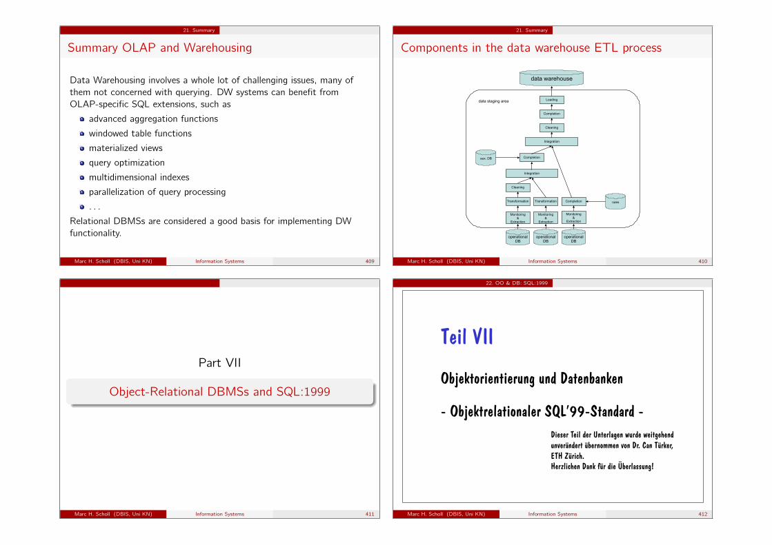
21. Summary
Summary OLAP and Warehousing
Data Warehousing involves a whole lot of challenging issues, many ofthem not concerned with querying. DW systems can benefit fromOLAP-specific SQL extensions, such as
advanced aggregation functions
windowed table functions
materialized views
query optimization
multidimensional indexes
parallelization of query processing
. . .
Relational DBMSs are considered a good basis for implementing DWfunctionality.
Marc H. Scholl (DBIS, Uni KN) Information Systems 409
21. Summary
Components in the data warehouse ETL process
operationalDB
Transformation
Monitoring&
Extraction
Monitoring&
Extraction
Monitoring&
Extraction
Transformation Completion rules
Integration
Cleaning
Completionaux. DB
Integration
Cleaning
Completion
Loading
data warehouse
operationalDB
operationalDB
data staging area
Marc H. Scholl (DBIS, Uni KN) Information Systems 410
Part VII
Object-Relational DBMSs and SQL:1999
Marc H. Scholl (DBIS, Uni KN) Information Systems 411
22. OO & DB: SQL:1999
Teil VII
Objektorientierung und Datenbanken
- Objektrelationaler SQL’99-Standard -
Dieser Teil der Unterlagen wurde weitgehend unverändert übernommen von Dr. Can Türker, ETH Zürich. Herzlichen Dank für die Überlassung!
Marc H. Scholl (DBIS, Uni KN) Information Systems 412

22. OO & DB: SQL:1999
4-2
Überblick
Motivation
„Klassische SQL-Tabellen“
Erweiterungen des Datenmodells in SQL 1999 – neue (Basis-) Datentypen – neue Typkonstruktoren – Objekttypen
… und daraus resultierende Erweiterungen bei den Operationen
Marc H. Scholl (DBIS, Uni KN) Information Systems 413
22. OO & DB: SQL:1999
4-3
“Advanced applications need advanced data structures!”
Ziel: 1 Anwendungsobjekt in 1 Datenbankobjekt abbilden
“Real World”
DBMS
!!!
Marc H. Scholl (DBIS, Uni KN) Information Systems 414
22. OO & DB: SQL:1999
4-4
Beispiel: RDBMS in technischen Anwendungen
consist of
Robot has
Arms
Axes degreesoffreedom
can workwith
Effector
(1,n)
(1,1)
(1,n)
(1,1)
(4,4) (1,1)
(0,n)
(0,n)
matrix rows
Robot Effector
Rob_ID Rob_Descr Eff_ID Function Rob1 Speedy 400 ............... GR600 Greifer Typ 600 .............................. Rob2 Speedy 600 ............... GR700 Greifer Typ 700 .............................. Rob3 Colossus MX-3 ......... LS1 Laserschweißer Typ 1 .................... : : PS1350 Punktschweißer Typ 1350 ..............
PS1380 Punktschweißer Typ 1380 .............. PS1510 Punktschweißer Typ 1510 .............. SR200 Schrauber Typ 200 .........................
Axes Robot_Arms Rob_I
D Arm_I
D AchsNr GW_min GW_max Masse Beschl Rob_ID ArmID
Rob1 links 1 -90 90 40,0 1,0 Rob1 links Rob1 links 2 -170 180 30,5 1,5 Rob1 rechts Rob1 links 3 -190 180 20,0 3,0 Rob2 solo
: : : : : : : Rob3 links Rob3 mitte Rob3 rechts
Matrices CanWorkWith Rob_ID Arm_ID AchsNr ZNr Sp1 Sp2 Sp3 Sp4 Rob_ID Eff_ID Rob1 links 1 1 1 0 0 1 Rob1 SR200 Rob1 links 1 2 0 0 1 0 Rob1 SR300 Rob1 links 1 3 0 -1 0 80 Rob1 PS1380 Rob1 links 1 4 0 0 1 1 Rob1 GR700 Rob1 links 2 1 0 0 0 60 : : : : : : : : : : Rob2 SR200 Rob1 links 3 4 0 -1 0 70 Rob2 SR300
Marc H. Scholl (DBIS, Uni KN) Information Systems 415
22. OO & DB: SQL:1999
4-5
Beispiel: SQL Query
SELECT r.Rob_ID, r.Rob_Descr, ar.Arm_ID, ac.AxisNo, m.ZNo, m.Sp1, m.Sp2, m.Sp3, m.Sp4, ac.GW_min, ac.GW_max, ac.Mass, ac.Accel, re.Eff_ID, e.Function FROM Robot r, Robot_Arms ar, Axes ac, Matrices m, CanWorkWith re, Effectors e WHERE r.Rob_ID = 'Rob1' AND r.Rob_ID = ar.Rob_ID AND ar.ROB_ID = ac.Rob_ID AND ar.Arm_ID = ac.Arm_ID AND ac.Arm_ID = m.Arm_ID AND ac.Rob_ID = m.Rob_ID AND ac.AxisNo = m.AxisNo AND r.Rob_ID = re.Rob_ID AND re.Eff_ID = e.Eff_ID
Marc H. Scholl (DBIS, Uni KN) Information Systems 416
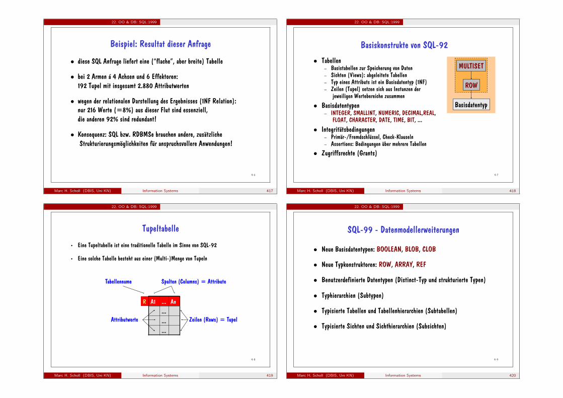
22. OO & DB: SQL:1999
4-6
Beispiel: Resultat dieser Anfrage
diese SQL Anfrage liefert eine (“flache”, aber breite) Tabelle
bei 2 Armen á 4 Achsen und 6 Effektoren: 192 Tupel mit insgesamt 2.880 Attributwerten
wegen der relationalen Darstellung des Ergebnisses (1NF Relation): nur 216 Werte (=8%) aus dieser Flut sind essenziell, die anderen 92% sind redundant!
Konsequenz: SQL bzw. RDBMSe brauchen andere, zusätzliche Strukturierungsmöglichkeiten für anspruchsvollere Anwendungen!
Marc H. Scholl (DBIS, Uni KN) Information Systems 417
22. OO & DB: SQL:1999
4-7
Basiskonstrukte von SQL-92
Tabellen – Basistabellen zur Speicherung von Daten – Sichten (Views): abgeleitete Tabellen – Typ eines Attributs ist ein Basisdatentyp (1NF) – Zeilen (Tupel) setzen sich aus Instanzen der
jeweiligen Wertebereiche zusammen
Basisdatentypen – INTEGER, SMALLINT, NUMERIC, DECIMAL,REAL,
FLOAT, CHARACTER, DATE, TIME, BIT, ...
Integritätsbedingungen – Primär-/Fremdschlüssel, Check-Klauseln – Assertions: Bedingungen über mehrere Tabellen
Zugriffsrechte (Grants)
MULTISET
ROW
Basisdatentyp
Marc H. Scholl (DBIS, Uni KN) Information Systems 418
22. OO & DB: SQL:1999
4-8
Tupeltabelle
• Eine Tupeltabelle ist eine traditionelle Tabelle im Sinne von SQL-92
• Eine solche Tabelle besteht aus einer (Multi-)Menge von Tupeln
R A1 ... An ... ... ...
Marc H. Scholl (DBIS, Uni KN) Information Systems 419
22. OO & DB: SQL:1999
4-9
SQL-99 - Datenmodellerweiterungen
Neue Basisdatentypen: BOOLEAN, BLOB, CLOB
Neue Typkonstruktoren: ROW, ARRAY, REF
Benutzerdefinierte Datentypen (Distinct-Typ und strukturierte Typen)
Typhierarchien (Subtypen)
Typisierte Tabellen und Tabellenhierarchien (Subtabellen)
Typisierte Sichten und Sichthierarchien (Subsichten)
Marc H. Scholl (DBIS, Uni KN) Information Systems 420
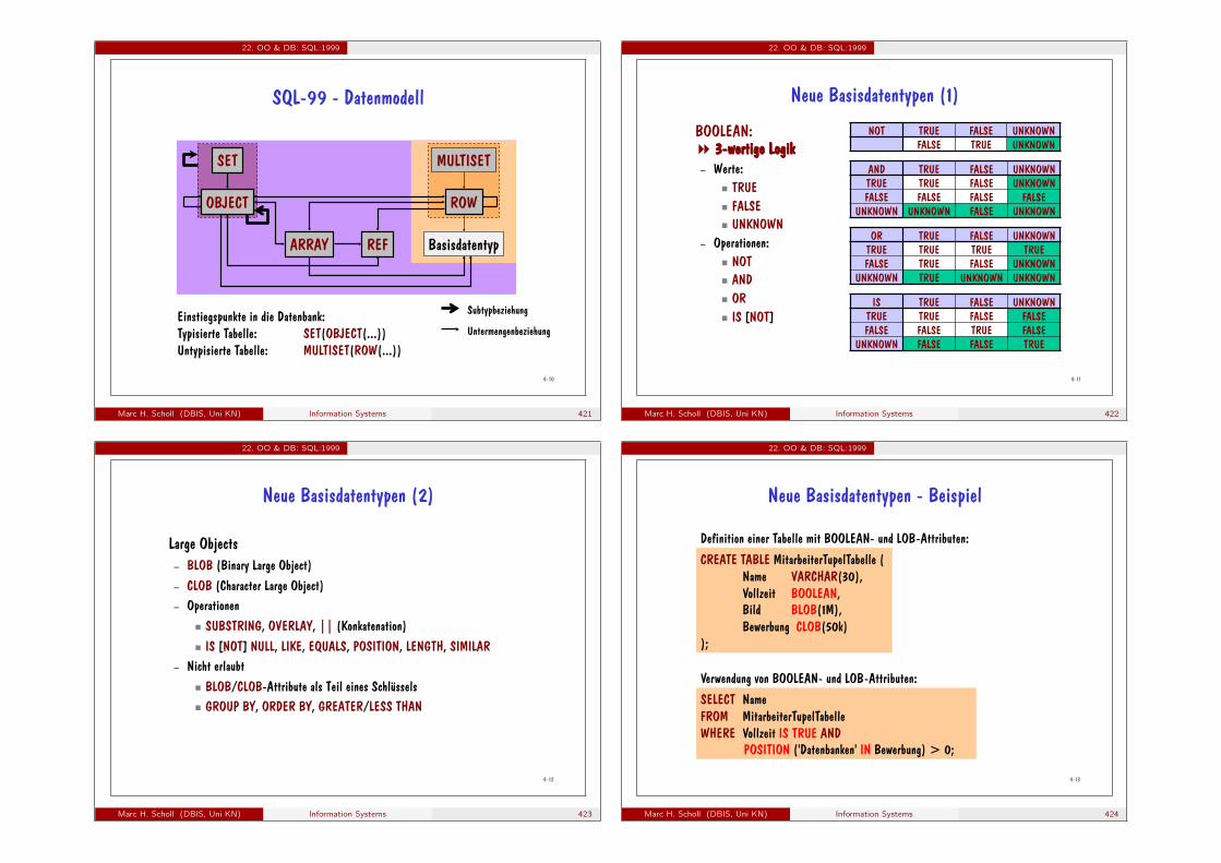
22. OO & DB: SQL:1999
4-10
SQL-99 - Datenmodell
MULTISET
ROW
Basisdatentyp REF ARRAY
SET
OBJECT
Einstiegspunkte in die Datenbank: Typisierte Tabelle: SET(OBJECT(...)) Untypisierte Tabelle: MULTISET(ROW(...))
Subtypbeziehung
Untermengenbeziehung
Marc H. Scholl (DBIS, Uni KN) Information Systems 421
22. OO & DB: SQL:1999
4-11
BOOLEAN: 3-wertige Logik
– Werte: TRUE FALSE UNKNOWN
– Operationen: NOT AND OR IS [NOT]
Neue Basisdatentypen (1)
AND TRUE FALSE UNKNOWN TRUE TRUE FALSE UNKNOWN FALSE FALSE FALSE FALSE
UNKNOWN UNKNOWN FALSE UNKNOWN
OR TRUE FALSE UNKNOWN TRUE TRUE TRUE TRUE FALSE TRUE FALSE UNKNOWN
UNKNOWN TRUE UNKNOWN UNKNOWN
IS TRUE FALSE UNKNOWN TRUE TRUE FALSE FALSE FALSE FALSE TRUE FALSE
UNKNOWN FALSE FALSE TRUE
NOT TRUE FALSE UNKNOWN FALSE TRUE UNKNOWN
Marc H. Scholl (DBIS, Uni KN) Information Systems 422
22. OO & DB: SQL:1999
4-12
Large Objects – BLOB (Binary Large Object) – CLOB (Character Large Object) – Operationen
SUBSTRING, OVERLAY, || (Konkatenation) IS [NOT] NULL, LIKE, EQUALS, POSITION, LENGTH, SIMILAR
– Nicht erlaubt BLOB/CLOB-Attribute als Teil eines Schlüssels GROUP BY, ORDER BY, GREATER/LESS THAN
Neue Basisdatentypen (2)
Marc H. Scholl (DBIS, Uni KN) Information Systems 423
22. OO & DB: SQL:1999
4-13
Neue Basisdatentypen - Beispiel
CREATE TABLE MitarbeiterTupelTabelle ( Name VARCHAR(30), Vollzeit BOOLEAN, Bild BLOB(1M), Bewerbung CLOB(50k)
);
Verwendung von BOOLEAN- und LOB-Attributen: SELECT Name FROM MitarbeiterTupelTabelle WHERE Vollzeit IS TRUE AND POSITION ('Datenbanken' IN Bewerbung) > 0;
Definition einer Tabelle mit BOOLEAN- und LOB-Attributen:
Marc H. Scholl (DBIS, Uni KN) Information Systems 424
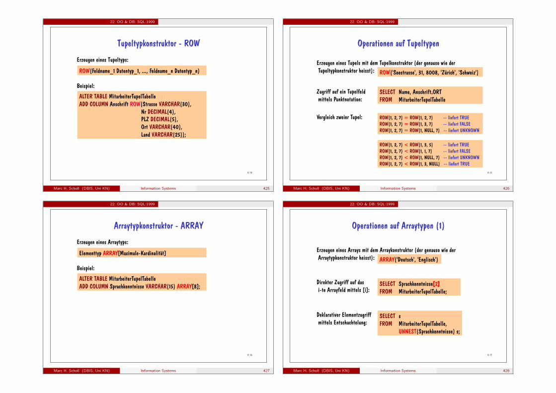
22. OO & DB: SQL:1999
4-14
Tupeltypkonstruktor - ROW
Erzeugen eines Tupeltyps:
Beispiel:
ROW(Feldname_1 Datentyp_1, ..., Feldname_n Datentyp_n)
ALTER TABLE MitarbeiterTupelTabelle ADD COLUMN Anschrift ROW(Strasse VARCHAR(30),
Nr DECIMAL(4), PLZ DECIMAL(5), Ort VARCHAR(40), Land VARCHAR(25));
Marc H. Scholl (DBIS, Uni KN) Information Systems 425
22. OO & DB: SQL:1999
4-15
Operationen auf Tupeltypen
ROW('Seestrasse', 31, 8008, 'Zürich', 'Schweiz')
SELECT Name, Anschrift.ORT FROM MitarbeiterTupelTabelle
ROW(1, 2, 7) = ROW(1, 2, 7) -- liefert TRUE ROW(1, 2, 7) = ROW(1, 3, 7) -- liefert FALSE ROW(1, 2, 7) = ROW(1, NULL, 7) -- liefert UNKNOWN
ROW(1, 2, 7) < ROW(1, 3, 5) -- liefert TRUE ROW(1, 2, 7) < ROW(1, 1, 7) -- liefert FALSE ROW(1, 2, 7) < ROW(1, NULL, 7) -- liefert UNKNOWN ROW(1, 2, 7) < ROW(1, 3, NULL) -- liefert TRUE
Erzeugen eines Tupels mit dem Tupelkonstruktor (der genauso wie der Tupeltypkonstruktor heisst):
Vergleich zweier Tupel:
Zugriff auf ein Tupelfeld mittels Punktnotation:
Marc H. Scholl (DBIS, Uni KN) Information Systems 426
22. OO & DB: SQL:1999
4-16
Arraytypkonstruktor - ARRAY
Erzeugen eines Arraytyps:
Beispiel:
Elementtyp ARRAY[Maximale-Kardinalität]
ALTER TABLE MitarbeiterTupelTabelle ADD COLUMN Sprachkenntnisse VARCHAR(15) ARRAY[8];
Marc H. Scholl (DBIS, Uni KN) Information Systems 427
22. OO & DB: SQL:1999
4-17
Operationen auf Arraytypen (1)
ARRAY('Deutsch', 'Englisch') Erzeugen eines Arrays mit dem Arraykonstruktor (der genauso wie der Arraytypkonstruktor heisst):
SELECT Sprachkenntnisse[2] FROM MitarbeiterTupelTabelle;
Direkter Zugriff auf das i-te Arrayfeld mittels [i]:
SELECT s FROM MitarbeiterTupelTabelle,
UNNEST(Sprachkenntnisse) s;
Deklarativer Elementzugriff mittels Entschachtelung:
Marc H. Scholl (DBIS, Uni KN) Information Systems 428

22. OO & DB: SQL:1999
4-18
Operationen auf Arraytypen (2)
UPDATE MitarbeiterTupelTabelle SET Sprachkenntnisse[1] = 'Türkisch';
Änderung eines einzelnen Arrayelements:
UPDATE MitarbeiterTupelTabelle SET Sprachkenntnisse = ARRAY['Türkisch'];
Änderung des kompletten Arraywerts:
CARDINALITY(ARRAY['Deutsch', Türkisch']) -- liefert den Wert 2
Kardinalität liefert Anzahl der Arrayelemente:
Marc H. Scholl (DBIS, Uni KN) Information Systems 429
22. OO & DB: SQL:1999
4-19
Operationen auf Arraytypen (3)
ARRAY['Deutsch', 'Türkisch'] ||ARRAY['Englisch'] -- erzeugt ARRAY['Deutsch', 'Türkisch', 'Englisch']
Konkatenation zweier Arrays:
Vergleich zweier Arrays:
— Zwei Arrays sind vergleichbar g.d.w. ihre Elementtypen vergleichbar sind
— Zwei vergleichbare Array A1 und A2 sind gleich (A1=A2) g.d.w (1) sie die gleiche Kardinalität besitzen und (2) alle Elemente paarweise gleich sind
ARRAY['Deutsch', 'Türkisch'] <> ARRAY['Deutsch', 'Türkisch', 'Englisch'] -- liefert TRUE ARRAY['Deutsch', 'Türkisch'] = ARRAY['Deutsch', 'Türkisch', NULL] -- liefert FALSE
Marc H. Scholl (DBIS, Uni KN) Information Systems 430
22. OO & DB: SQL:1999
4-20
Referenztypkonstruktor - REF
Erzeugen eines Referenztyps:
– referenzierter Typ muss ein strukturierter Typ sein – Instanzen eines Referenztyp können nur dann dereferenziert werden, wenn eine
entsprechend typisierte Tabelle als Wertebereich (Scope) festgelegt wurde
Beispiel:
– AbteilungsTyp sei hier ein strukturierter Typ und Abteilung eine auf diesem Typ basierende typisierte Tabelle
REF(Strukturierter-Typ) [SCOPE (TypisierteTabelle)]
ALTER TABLE MitarbeiterTupelTabelle ADD COLUMN Abteilung REF(AbteilungsTyp) SCOPE Abteilungen;
Marc H. Scholl (DBIS, Uni KN) Information Systems 431
22. OO & DB: SQL:1999
4-21
Operationen auf Referenztypen
Erzeugen einer Referenz auf ein Objekte durch Zuweisung der zugehörigen OID an ein Referenzattribut bzw. Referenzvariable
SELECT Abteilung->Name FROM MitarbeiterTupelTabelle;
Dereferenzierung mittels Pfeil-Operator:
SELECT DEREF(Abteilung) FROM MitarbeiterTupelTabelle;
Referenzauflösung mittels DEREF-Operator:
Vergleich zweier Referenzen: — Zwei Referenzen sind vergleichbar g.d.w. ihre referenzierten Typen gleich sind — Zwei vergleichbare Referenzen R1 und R2 sind gleich (R1=R2) g.d.w sie
denselben Referenzwert aufweisen (d.h. auf dasselbe Objekte verweisen)
Marc H. Scholl (DBIS, Uni KN) Information Systems 432
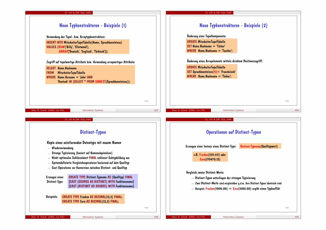
22. OO & DB: SQL:1999
4-22
Neue Typkonstruktoren - Beispiele (1)
Zugriff auf tupelwertige Attribute bzw. Verwendung arraywertiger Attribute:
SELECT Name.Nachname FROM MitarbeiterTupelTabelle WHERE Name.Vorname = 'John' AND
'Deutsch' IN (SELECT * FROM UNNEST(Sprachkenntnisse));
Verwendung des Tupel- bzw. Arraytypkonstruktors: INSERT INTO MitarbeiterTupelTabelle(Name, Sprachkenntnisse) VALUES (ROW('Billy', 'Clintwood'), ARRAY['Deutsch', 'Englisch', 'Türkisch']);
Marc H. Scholl (DBIS, Uni KN) Information Systems 433
22. OO & DB: SQL:1999
4-23
Neue Typkonstruktoren - Beispiele (2)
Änderung eines Arrayelements mittels direktem Positionszugriff:
UPDATE MitarbeiterTupelTabelle SET Sprachkenntnisse[4]= 'Französisch' WHERE Name.Nachname = 'Türker';
Änderung einer Tupelkomponente: UPDATE MitarbeiterTupelTabelle SET Name.Nachname = 'Türker' WHERE Name.Nachname = 'Tuerker';
Marc H. Scholl (DBIS, Uni KN) Information Systems 434
22. OO & DB: SQL:1999
4-24
Distinct-Typen
Kopie eines existierenden Datentyps mit neuem Namen – Wiederverwendung – Strenge Typisierung (basiert auf Namensäquivalenz) – Nicht-optionales Schlüsselwort FINAL schliesst Subtypbildung aus – Systemdefinierte Vergleichsoperatoren basierend auf dem Quelltyp – Cast-Operatoren zur Konversion zwischen Distinct- und Quelltyp
Erzeugen eines Distinct-Typs:
CREATE TYPE Distinct-Typname AS (Quelltyp) FINAL [CAST (SOURCE AS DISTINCT) WITH Funktionsname] [CAST (DISTINCT AS SOURCE) WITH Funktionsname]
CREATE TYPE Franken AS DECIMAL(12,2) FINAL; CREATE TYPE Euro AS DECIMAL(12,2) FINAL;
Beispiele:
Marc H. Scholl (DBIS, Uni KN) Information Systems 435
22. OO & DB: SQL:1999
4-25
Operationen auf Distinct-Typen
Distinct-Typname(Quelltypwert) Erzeugen einer Instanz eines Distinct-Typs:
z.B. Franken(1311.69) oder Euro(170470.13)
Vergleich zweier Distinct-Werte: — Distinct-Typen unterliegen der strengen Typisierung — Zwei Distinct-Werte sind vergleichbar g.d.w. ihre Distinct-Typen identisch sind
— Beispiel: Franken(1000.00) = Euro(1000.00) ergibt einen Typkonflikt
Marc H. Scholl (DBIS, Uni KN) Information Systems 436

22. OO & DB: SQL:1999
4-26
Verwendung von Distinct-Typen (1)
Anfrage ergibt Typkonflikt: Schweizer Franken und Euro sind nicht vergleichbar → Typkonvertierung ist notwendig! → CAST-Funktionen
CREATE TABLE CHBank(Nr INTEGER, Stand Franken); CREATE TABLE EuroBank(Nr INTEGER, Stand Euro);
Beispiel: Distinct-Typen in Tabellendefinitionen:
SELECT e.Nr FROM CHBank c, EuroBank e WHERE c.Nr= 234302 AND c.Stand > e.Stand;
Anfrage basierend auf Distinct-Typen:
Marc H. Scholl (DBIS, Uni KN) Information Systems 437
22. OO & DB: SQL:1999
4-27
Verwendung von Distinct-Typen (2)
Problem: Derartige Konvertierungen sind nicht immer "semantisch" sinnvoll!
Oftmals sind benutzerdefinierte Cast-Funktionen notwendig, die nicht nur den Typ, sondern auch den Wert konvertieren bzw. neu berechnen.
SELECT e.Nr FROM CHBank c, EuroBank e WHERE c.Nr= 234302 AND c.Stand > CAST(CAST(e.Stand AS DECIMAL(12,2)) AS Franken);
Vorherige Anfrage nun mit expliziter Konvertierung von Euro nach Franken:
Marc H. Scholl (DBIS, Uni KN) Information Systems 438
22. OO & DB: SQL:1999
4-28
Benutzerdefinierte Cast-Funktionen
CREATE CAST (Typ1 AS Typ2) WITH Konvertierungsfunktion(Parameter Typ1) [AS ASSIGNMENT]
Konversion zwischen unterschiedlichen Datentypen
Syntax:
– Typ1 oder Typ2 muss ein benutzerdefinierter Typ oder ein Referenztyp sein – Konvertierungsfunktion
– hat genau einen Parameter vom Typ Typ1 und Typ2 als Rückgabetyp – ist deterministisch und liest und ändert keine SQL-Daten
– AS ASSIGNMENT: Implizite Cast-Funktion (wird automatisch aufgerufen)
Marc H. Scholl (DBIS, Uni KN) Information Systems 439
22. OO & DB: SQL:1999
4-29
CREATE CAST (Euro AS Franken) WITH Franken(Euro);
Explizite Cast-Funktionen - Beispiel
Definition einer expliziten Cast-Funktion:
Definition einer Konvertierungsfunktion:
CREATE FUNCTION Franken(e Euro) RETURNS Franken RETURN CAST(CAST(e AS DECIMAL(12,2)) * 1.5 AS Franken);
SELECT e.Nr FROM CHBank c, EuroBank e WHERE c.Nr= 234302 AND c.Stand > Franken(e.Stand);
Vorherige Anfrage nun mit direkter Konvertierung von Euro nach Franken:
Marc H. Scholl (DBIS, Uni KN) Information Systems 440
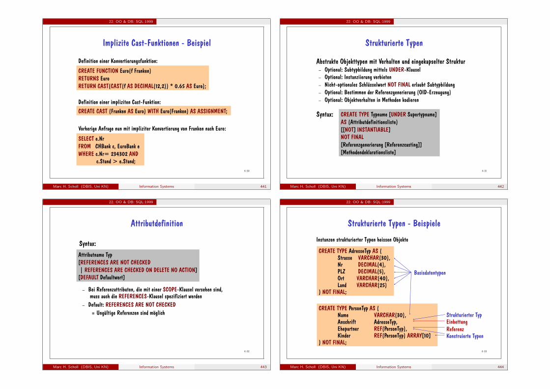
22. OO & DB: SQL:1999
4-30
CREATE CAST (Franken AS Euro) WITH Euro(Franken) AS ASSIGNMENT;
Implizite Cast-Funktionen - Beispiel
Definition einer impliziten Cast-Funktion:
Definition einer Konvertierungsfunktion:
CREATE FUNCTION Euro(f Franken) RETURNS Euro RETURN CAST(CAST(f AS DECIMAL(12,2)) * 0.65 AS Euro);
SELECT e.Nr FROM CHBank c, EuroBank e WHERE c.Nr= 234302 AND c.Stand > e.Stand;
Vorherige Anfrage nun mit impliziter Konvertierung von Franken nach Euro:
Marc H. Scholl (DBIS, Uni KN) Information Systems 441
22. OO & DB: SQL:1999
4-31
Strukturierte Typen
CREATE TYPE Typname [UNDER Supertypname] AS (Attributdefinitionsliste) [[NOT] INSTANTIABLE] NOT FINAL [Referenzgenerierung [Referenzcasting]] [Methodendeklarationsliste]
Abstrakte Objekttypen mit Verhalten und eingekapselter Struktur – Optional: Subtypbildung mittels UNDER-Klausel – Optional: Instanziierung verbieten – Nicht-optionales Schlüsselwort NOT FINAL erlaubt Subtypbildung – Optional: Bestimmen der Referenzgenerierung (OID-Erzeugung) – Optional: Objektverhalten in Methoden kodieren
Syntax:
Marc H. Scholl (DBIS, Uni KN) Information Systems 442
22. OO & DB: SQL:1999
4-32
Attributdefinition
Attributname Typ [REFERENCES ARE NOT CHECKED | REFERENCES ARE CHECKED ON DELETE NO ACTION] [DEFAULT Defaultwert]
– Bei Referenzattributen, die mit einer SCOPE-Klausel versehen sind, muss auch die REFERENCES-Klausel spezifiziert werden
– Default: REFERENCES ARE NOT CHECKED Ungültige Referenzen sind möglich
Syntax:
Marc H. Scholl (DBIS, Uni KN) Information Systems 443
22. OO & DB: SQL:1999
4-33
Strukturierte Typen - Beispiele
CREATE TYPE PersonTyp AS ( Name VARCHAR(30), Anschrift AdresseTyp, Ehepartner REF(PersonTyp), Kinder REF(PersonTyp) ARRAY[10]
) NOT FINAL;
CREATE TYPE AdresseTyp AS ( Strasse VARCHAR(30), Nr DECIMAL(4), PLZ DECIMAL(5),
Ort VARCHAR(40), Land VARCHAR(25)
) NOT FINAL;
Basisdatentypen
Strukturierter Typ Einbettung Referenz Konstruierte Typen
Instanzen strukturierter Typen heissen Objekte
Marc H. Scholl (DBIS, Uni KN) Information Systems 444

22. OO & DB: SQL:1999
4-34
Operationen auf strukturierten Typen (1)
z.B. AdresseTyp() oder PersonTyp()
Erzeugen einer Instanz eines strukturierten Typs mit dem Default-Konstruktor, der genauso heisst wie der zugehörige strukturierte Typ:
Attributzugriff erfolgt mittels Funktionsaufrufe sowie Punkt-Operator
Vergleich zweier Objekte (Instanzen strukturierter Typen): — keine Ordnungsrelationen implizit bereitgestellt — benutzerdefinierte Ordnungsfunktionen können aber definiert werden
Marc H. Scholl (DBIS, Uni KN) Information Systems 445
22. OO & DB: SQL:1999
4-35
Operationen auf strukturierten Typen (2)
Objekt IS [NOT] OF (Typnamensliste) Typtest:
— Prädikat IS OF wird TRUE, wenn die Liste den Typ des Objekts bzw. einen Subtyp davon enthält
— Letzteres kann durch die Verwendung von ONLY ausgeschlossen werden, z.B.
m IS OF (ONLY(Mitarbeiter))
Temporäre Typanpassung entlang einer Typhierarchie:
(Objekt AS Supertypname) -- Anpassung nach oben TREAT(Objekt AS Subtypname) -- Anpassung nach unten
Marc H. Scholl (DBIS, Uni KN) Information Systems 446
22. OO & DB: SQL:1999
4-36
Einkapselung von strukturierten Typen
Observer: FUNCTION Strasse(AdresseTyp) RETURNS VARCHAR(30); FUNCTION Nr(AdresseTyp) RETURNS DECIMAL(4); FUNCTION PLZ(AdresseTyp) RETURNS DECIMAL(5);
FUNCTION Ort(AdresseTyp) RETURNS VARCHAR(40); FUNCTION Land(AdresseTyp) RETURNS VARCHAR(25);
Vollständige Einkapselung – Attribute nur über Methoden zugreifbar – Attributzugriffe und Methodenaufrufe gleich behandelt
Implizite Observer- und Mutator-Methoden für jedes Attribut
Mutator: FUNCTION Strasse(AdresseTyp, VARCHAR(30)) RETURNS AdresseTyp; FUNCTION Nr(AdresseTyp, DECIMAL(5)) RETURNS AdresseTyp; FUNCTION PLZ(AdresseTyp, DECIMAL(5)) RETURNS AdresseTyp; FUNCTION Ort(AdresseTyp, VARCHAR(40)) RETURNS AdresseTyp; FUNCTION Land(AdresseTyp, VARCHAR(25)) RETURNS AdresseTyp;
Marc H. Scholl (DBIS, Uni KN) Information Systems 447
22. OO & DB: SQL:1999
4-37
Attributzugriff bei Instanzen eines strukturierten Typs
BEGIN DECLARE p PersonTyp; SET p.Name = ‘Luke Skywalker’; SET p.Anschrift.Ort = ‘Hollywood’;
END;
Zugriff über Funktionsaufrufe oder Punkt-Operator – X.Attributname entspricht Attributname(X) – SET X.Attributname = Wert entspricht Attributname(X, Wert)
Pfadausdrücke: Nacheinander Anwendung des Punkt-Operators – Navigierende Zugriffe
Beispiel:
Marc H. Scholl (DBIS, Uni KN) Information Systems 448

22. OO & DB: SQL:1999
4-38
Erzeugen von Instanzen eines strukturierten Typs
CREATE FUNCTION PersonTyp (n VARCHAR(30)) RETURNS PersonTyp BEGIN
DECLARE p PersonTyp; SET p = PersonTyp(); SET p.Name = n; RETURN p;
END;
Verwendung des Default-Konstruktors Initialisierung mittels
– Mutator-Methoden – Redefiniertem Konstruktor (kann beliebig überladen werden)
Beispiel für das Überladen eines Konstruktors:
Aufruf des Default-Konstruktors
Marc H. Scholl (DBIS, Uni KN) Information Systems 449
22. OO & DB: SQL:1999
4-39
Subtypbildung - Aufbau von Typhierarchien
Subtypdefinition mittels UNDER-Klausel – Subtyp erbt alle Attributen und Methoden des Supertyps – Supertyp muss selbst ein strukturierter Typ sein – Subtyp darf maximal einen direkten Supertyp haben
Keine (direkte) Mehrfachvererbung möglich – Subtyp kann geerbte Methoden überschreiben und überladen
Strukturierte Typen, die keine Subtypen sind, heissen Wurzeltypen
Marc H. Scholl (DBIS, Uni KN) Information Systems 450
22. OO & DB: SQL:1999
4-40
Subtypen - Beispiele
CREATE TYPE MitarbeiterTyp UNDER PersonTyp AS ( PNr INTEGER, Bewerbung CLOB(50K), Bild BLOB(5M), Vorgesetzter REF(MitarbeiterTyp), Projekte REF(ProjektTyp) ARRAY[50], Gehalt Franken
) NOT FINAL;
CREATE TYPE ManagerTyp UNDER MitarbeiterTyp AS ( Leitet REF(ProjektTyp) ARRAY[100], Bonus Franken
) NOT FINAL;
Marc H. Scholl (DBIS, Uni KN) Information Systems 451
22. OO & DB: SQL:1999
4-41
Referenzgenerierung & Referenzcasting
REF USING Typ | REF FROM (Attributliste) | REF IS SYSTEM GENERATED
– REF USING Typ OID-Werte sind von einem bestimmten Typ, etwa INTEGER
– REF FROM (Attributliste) OID aus vorhandenen Attributwerten eines Schlüssels funktional bestimmt
– REF IS SYSTEM GENERATED OID-Generierung durch das System (Defaulteinstellung)
Nur für Wurzeltypen definierbar
Syntax: CAST (SOURCE AS REF) WITH Funktionsname CAST (REF AS SOURCE) WITH Funktionsname
Marc H. Scholl (DBIS, Uni KN) Information Systems 452
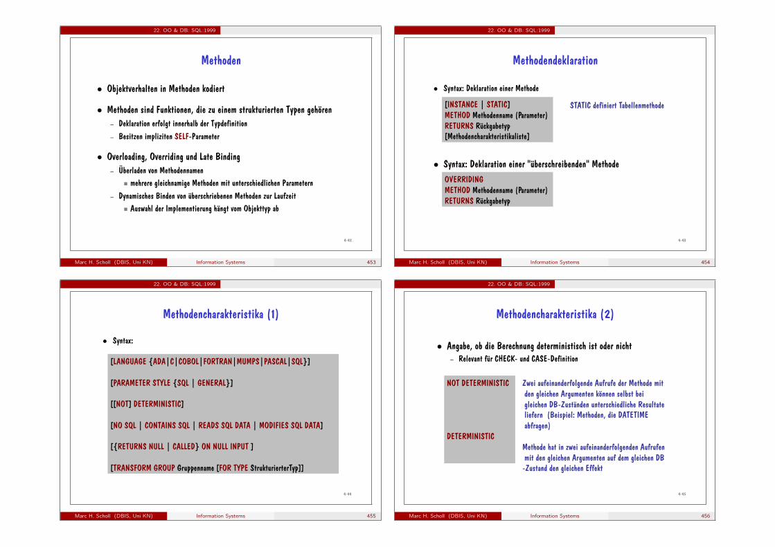
22. OO & DB: SQL:1999
4-42
Methoden
Objektverhalten in Methoden kodiert
Methoden sind Funktionen, die zu einem strukturierten Typen gehören – Deklaration erfolgt innerhalb der Typdefinition – Besitzen impliziten SELF-Parameter
Overloading, Overriding und Late Binding – Überladen von Methodennamen
mehrere gleichnamige Methoden mit unterschiedlichen Parametern – Dynamisches Binden von überschriebenen Methoden zur Laufzeit
Auswahl der Implementierung hängt vom Objekttyp ab
Marc H. Scholl (DBIS, Uni KN) Information Systems 453
22. OO & DB: SQL:1999
4-43
Methodendeklaration
[INSTANCE | STATIC] METHOD Methodenname (Parameter) RETURNS Rückgabetyp [Methodencharakteristikaliste]
Syntax: Deklaration einer Methode
OVERRIDING METHOD Methodenname (Parameter) RETURNS Rückgabetyp
Syntax: Deklaration einer "überschreibenden" Methode
STATIC definiert Tabellenmethode
Marc H. Scholl (DBIS, Uni KN) Information Systems 454
22. OO & DB: SQL:1999
4-44
Methodencharakteristika (1)
Syntax:
[LANGUAGE {ADA|C|COBOL|FORTRAN|MUMPS|PASCAL|SQL}]
[PARAMETER STYLE {SQL | GENERAL}]
[[NOT] DETERMINISTIC]
[NO SQL | CONTAINS SQL | READS SQL DATA | MODIFIES SQL DATA]
[{RETURNS NULL | CALLED} ON NULL INPUT ]
[TRANSFORM GROUP Gruppenname [FOR TYPE StrukturierterTyp]]
Marc H. Scholl (DBIS, Uni KN) Information Systems 455
22. OO & DB: SQL:1999
4-45
Methodencharakteristika (2)
Angabe, ob die Berechnung deterministisch ist oder nicht – Relevant für CHECK- und CASE-Definition
NOT DETERMINISTIC
DETERMINISTIC
Zwei aufeinanderfolgende Aufrufe der Methode mit den gleichen Argumenten können selbst bei gleichen DB-Zuständen unterschiedliche Resultate liefern (Beispiel: Methoden, die DATETIME abfragen)
Methode hat in zwei aufeinanderfolgenden Aufrufen mit den gleichen Argumenten auf dem gleichen DB-Zustand den gleichen Effekt
Marc H. Scholl (DBIS, Uni KN) Information Systems 456
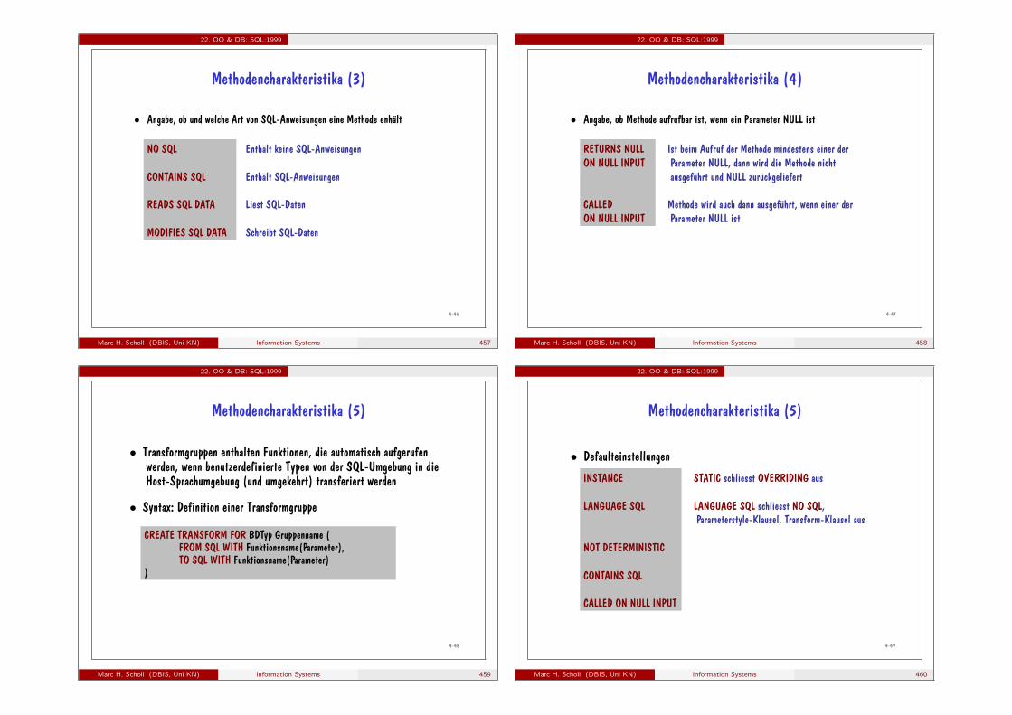
22. OO & DB: SQL:1999
4-46
Methodencharakteristika (3)
Angabe, ob und welche Art von SQL-Anweisungen eine Methode enhält
NO SQL
CONTAINS SQL
READS SQL DATA
MODIFIES SQL DATA
Enthält keine SQL-Anweisungen
Enthält SQL-Anweisungen
Liest SQL-Daten
Schreibt SQL-Daten
Marc H. Scholl (DBIS, Uni KN) Information Systems 457
22. OO & DB: SQL:1999
4-47
Methodencharakteristika (4)
Angabe, ob Methode aufrufbar ist, wenn ein Parameter NULL ist
RETURNS NULL ON NULL INPUT
CALLED ON NULL INPUT
Ist beim Aufruf der Methode mindestens einer der Parameter NULL, dann wird die Methode nicht ausgeführt und NULL zurückgeliefert
Methode wird auch dann ausgeführt, wenn einer der Parameter NULL ist
Marc H. Scholl (DBIS, Uni KN) Information Systems 458
22. OO & DB: SQL:1999
4-48
Methodencharakteristika (5)
Transformgruppen enthalten Funktionen, die automatisch aufgerufen werden, wenn benutzerdefinierte Typen von der SQL-Umgebung in die Host-Sprachumgebung (und umgekehrt) transferiert werden
Syntax: Definition einer Transformgruppe
CREATE TRANSFORM FOR BDTyp Gruppenname ( FROM SQL WITH Funktionsname(Parameter), TO SQL WITH Funktionsname(Parameter)
)
Marc H. Scholl (DBIS, Uni KN) Information Systems 459
22. OO & DB: SQL:1999
4-49
Methodencharakteristika (5)
INSTANCE
LANGUAGE SQL
NOT DETERMINISTIC
CONTAINS SQL
CALLED ON NULL INPUT
Defaulteinstellungen
STATIC schliesst OVERRIDING aus
LANGUAGE SQL schliesst NO SQL, Parameterstyle-Klausel, Transform-Klausel aus
Marc H. Scholl (DBIS, Uni KN) Information Systems 460
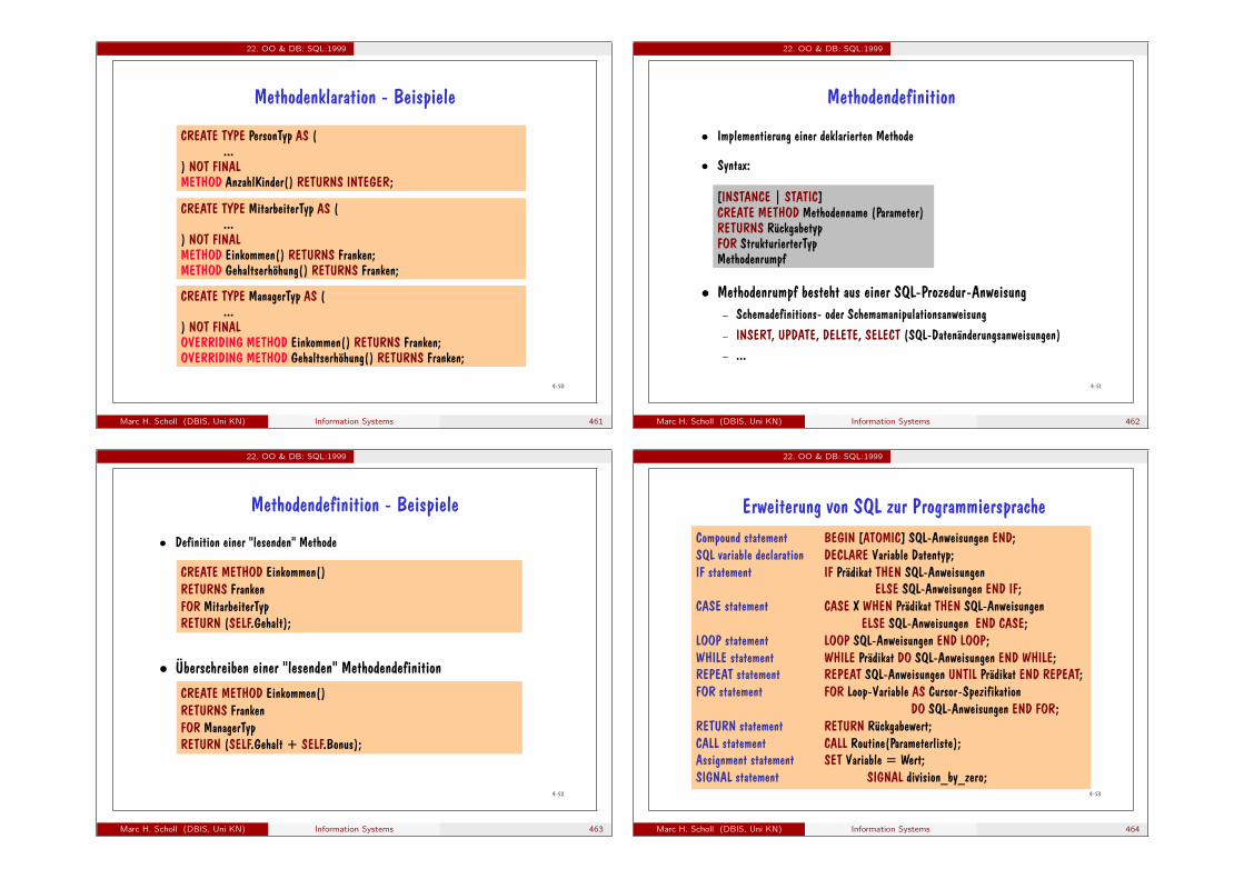
22. OO & DB: SQL:1999
4-50
Methodenklaration - Beispiele
CREATE TYPE PersonTyp AS ( ...
) NOT FINAL METHOD AnzahlKinder() RETURNS INTEGER;
CREATE TYPE MitarbeiterTyp AS ( ...
) NOT FINAL METHOD Einkommen() RETURNS Franken; METHOD Gehaltserhöhung() RETURNS Franken;
CREATE TYPE ManagerTyp AS ( ...
) NOT FINAL OVERRIDING METHOD Einkommen() RETURNS Franken; OVERRIDING METHOD Gehaltserhöhung() RETURNS Franken;
Marc H. Scholl (DBIS, Uni KN) Information Systems 461
22. OO & DB: SQL:1999
4-51
Methodendefinition
[INSTANCE | STATIC] CREATE METHOD Methodenname (Parameter) RETURNS Rückgabetyp FOR StrukturierterTyp Methodenrumpf
Implementierung einer deklarierten Methode
Syntax:
Methodenrumpf besteht aus einer SQL-Prozedur-Anweisung – Schemadefinitions- oder Schemamanipulationsanweisung – INSERT, UPDATE, DELETE, SELECT (SQL-Datenänderungsanweisungen) – ...
Marc H. Scholl (DBIS, Uni KN) Information Systems 462
22. OO & DB: SQL:1999
4-52
Methodendefinition - Beispiele
CREATE METHOD Einkommen() RETURNS Franken FOR MitarbeiterTyp RETURN (SELF.Gehalt);
Definition einer "lesenden" Methode
CREATE METHOD Einkommen() RETURNS Franken FOR ManagerTyp RETURN (SELF.Gehalt + SELF.Bonus);
Überschreiben einer "lesenden" Methodendefinition
Marc H. Scholl (DBIS, Uni KN) Information Systems 463
22. OO & DB: SQL:1999
4-53
Erweiterung von SQL zur Programmiersprache Compound statement BEGIN [ATOMIC] SQL-Anweisungen END; SQL variable declaration DECLARE Variable Datentyp; IF statement IF Prädikat THEN SQL-Anweisungen
ELSE SQL-Anweisungen END IF; CASE statement CASE X WHEN Prädikat THEN SQL-Anweisungen
ELSE SQL-Anweisungen END CASE; LOOP statement LOOP SQL-Anweisungen END LOOP; WHILE statement WHILE Prädikat DO SQL-Anweisungen END WHILE; REPEAT statement REPEAT SQL-Anweisungen UNTIL Prädikat END REPEAT; FOR statement FOR Loop-Variable AS Cursor-Spezifikation
DO SQL-Anweisungen END FOR; RETURN statement RETURN Rückgabewert; CALL statement CALL Routine(Parameterliste); Assignment statement SET Variable = Wert; SIGNAL statement SIGNAL division_by_zero;
Marc H. Scholl (DBIS, Uni KN) Information Systems 464
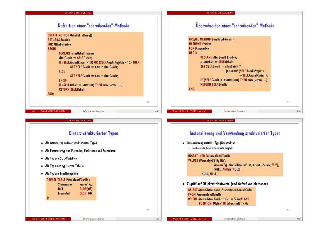
22. OO & DB: SQL:1999
4-54
Definition einer "schreibenden" Methode
CREATE METHOD GehaltsErhöhung() RETURNS Franken FOR MitarbeiterTyp BEGIN DECLARE altesGehalt Franken; altesGehalt = SELF.Gehalt; IF (SELF.AnzahlKinder < 3) OR (SELF.AnzahlProjekte < 2) THEN SET SELF.Gehalt = 1.03 * altesGehalt; ELSE SET SELF.Gehalt = 1.05 * altesGehalt; ENDIF IF (SELF.Gehalt > 500000) THEN raise_error(…); RETURN SELF.Gehalt; END;
Marc H. Scholl (DBIS, Uni KN) Information Systems 465
22. OO & DB: SQL:1999
4-55
Überschreiben einer "schreibenden" Methode
CREATE METHOD GehaltsErhöhung() RETURNS Franken FOR ManagerTyp BEGIN
DECLARE altesGehalt Franken; altesGehalt = SELF.Gehalt;
SET SELF.Gehalt = altesGehalt * (1+0.01*(SELF.AnzahlProjekte +SELF.AnzahlKinder));
IF (SELF.Gehalt > 25000000) THEN raise_error(…); RETURN SELF.Gehalt;
END;
Marc H. Scholl (DBIS, Uni KN) Information Systems 466
22. OO & DB: SQL:1999
4-56
Einsatz strukturierter Typen
Als Attributtyp anderer strukturierter Typen
Als Parametertyp von Methoden, Funktionen und Prozeduren
Als Typ von SQL-Variablen
Als Typ einer typisierten Tabelle
Als Typ von Tabellenspalten
CREATE TABLE PersonTupelTabelle ( Stammdaten PersonTyp, Bild BLOB(1M), Lebenslauf CLOB(50k)
);
Marc H. Scholl (DBIS, Uni KN) Information Systems 467
22. OO & DB: SQL:1999
4-57
Instanziierung und Verwendung strukturierter Typen
Instanziierung mittels (Typ-)Konstruktor – Geschachtelte Konstruktoraufrufe möglich
INSERT INTO PersonenTupelTabelle VALUES (PersonTyp('Billy Bär', AdresseTyp('Seefeldstrasse', 31, 8008, 'Zurich', 'CH'), NULL, ARRAY(NULL)), NULL, NULL);
SELECT Stammdaten.Name, Stammdaten.AnzahlKinder FROM PersonenTupelTabelle WHERE Stammdaten.Anschrift.Ort = 'Zürich' AND POSITION('Diplom' IN Lebenslauf) > 0;
Zugriff auf Objektattributwerte (und Aufruf von Methoden)
Marc H. Scholl (DBIS, Uni KN) Information Systems 468
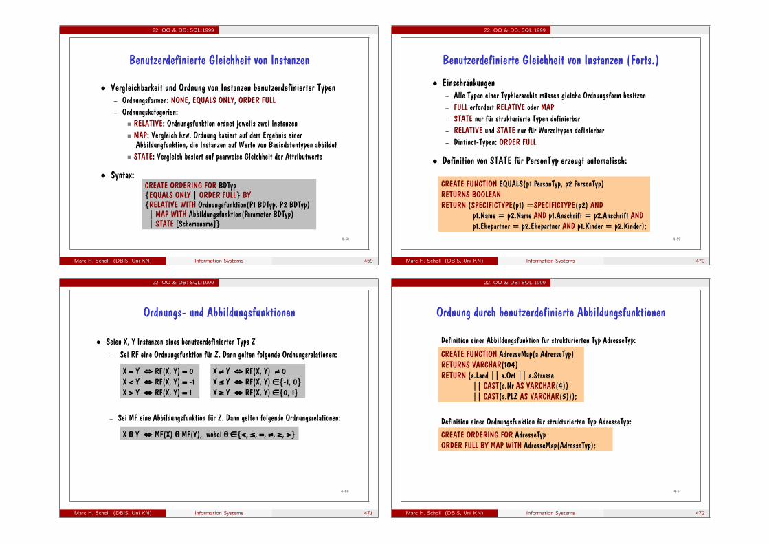
22. OO & DB: SQL:1999
4-58
Vergleichbarkeit und Ordnung von Instanzen benutzerdefinierter Typen – Ordnungsformen: NONE, EQUALS ONLY, ORDER FULL – Ordnungskategorien:
RELATIVE: Ordnungsfunktion ordnet jeweils zwei Instanzen MAP: Vergleich bzw. Ordnung basiert auf dem Ergebnis einer
Abbildungfunktion, die Instanzen auf Werte von Basisdatentypen abbildet STATE: Vergleich basiert auf paarweise Gleichheit der Attributwerte
Syntax:
Benutzerdefinierte Gleichheit von Instanzen
CREATE ORDERING FOR BDTyp {EQUALS ONLY | ORDER FULL} BY {RELATIVE WITH Ordnungsfunktion(P1 BDTyp, P2 BDTyp) | MAP WITH Abbildungsfunktion(Parameter BDTyp) | STATE [Schemaname]}
Marc H. Scholl (DBIS, Uni KN) Information Systems 469
22. OO & DB: SQL:1999
4-59
Einschränkungen – Alle Typen einer Typhierarchie müssen gleiche Ordnungsform besitzen – FULL erfordert RELATIVE oder MAP – STATE nur für strukturierte Typen definierbar – RELATIVE und STATE nur für Wurzeltypen definierbar – Dintinct-Typen: ORDER FULL
Definition von STATE für PersonTyp erzeugt automatisch:
Benutzerdefinierte Gleichheit von Instanzen (Forts.)
CREATE FUNCTION EQUALS(p1 PersonTyp, p2 PersonTyp) RETURNS BOOLEAN RETURN (SPECIFICTYPE(p1) =SPECIFICTYPE(p2) AND p1.Name = p2.Name AND p1.Anschrift = p2.Anschrift AND p1.Ehepartner = p2.Ehepartner AND p1.Kinder = p2.Kinder);
Marc H. Scholl (DBIS, Uni KN) Information Systems 470
22. OO & DB: SQL:1999
4-60
Ordnungs- und Abbildungsfunktionen
Seien X, Y Instanzen eines benutzerdefinierten Typs Z – Sei RF eine Ordnungsfunktion für Z. Dann gelten folgende Ordnungsrelationen:
– Sei MF eine Abbildungsfunktion für Z. Dann gelten folgende Ordnungsrelationen:
X = Y ⇔ RF(X, Y) = 0 X < Y ⇔ RF(X, Y) = -1 X > Y ⇔ RF(X, Y) = 1
X ≠ Y ⇔ RF(X, Y) ≠ 0 X ≤ Y ⇔ RF(X, Y) ∈{-1, 0} X ≥ Y ⇔ RF(X, Y) ∈{0, 1}
X θ Y ⇔ MF(X) θ MF(Y), wobei θ ∈{<, ≤, =, ≠, ≥, >}
Marc H. Scholl (DBIS, Uni KN) Information Systems 471
22. OO & DB: SQL:1999
4-61
Ordnung durch benutzerdefinierte Abbildungsfunktionen
Definition einer Abbildungsfunktion für strukturierten Typ AdresseTyp:
CREATE FUNCTION AdresseMap(a AdresseTyp) RETURNS VARCHAR(104) RETURN (a.Land || a.Ort || a.Strasse || CAST(a.Nr AS VARCHAR(4)) || CAST(a.PLZ AS VARCHAR(5)));
CREATE ORDERING FOR AdresseTyp ORDER FULL BY MAP WITH AdresseMap(AdresseTyp);
Definition einer Ordnungsfunktion für strukturierten Typ AdresseTyp:
Marc H. Scholl (DBIS, Uni KN) Information Systems 472
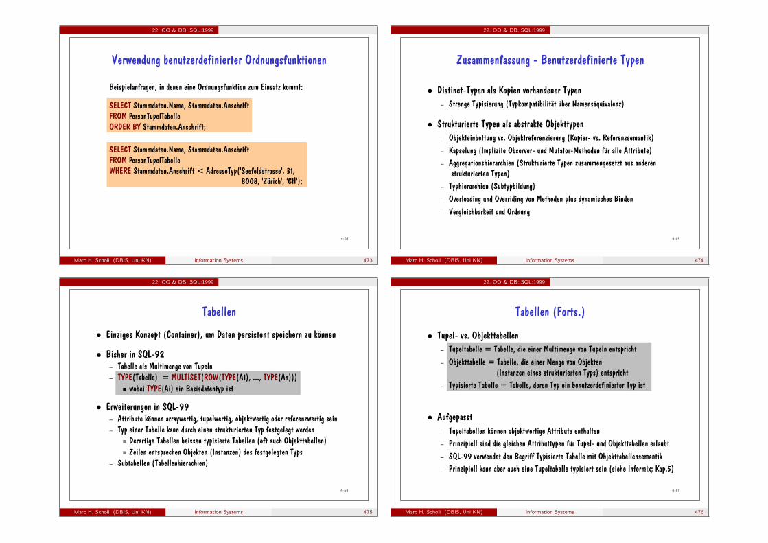
22. OO & DB: SQL:1999
4-62
Verwendung benutzerdefinierter Ordnungsfunktionen
SELECT Stammdaten.Name, Stammdaten.Anschrift FROM PersonTupelTabelle ORDER BY Stammdaten.Anschrift;
Beispielanfragen, in denen eine Ordnungsfunktion zum Einsatz kommt:
SELECT Stammdaten.Name, Stammdaten.Anschrift FROM PersonTupelTabelle WHERE Stammdaten.Anschrift < AdresseTyp('Seefeldstrasse', 31, 8008, 'Zürich', 'CH');
Marc H. Scholl (DBIS, Uni KN) Information Systems 473
22. OO & DB: SQL:1999
4-63
Zusammenfassung - Benutzerdefinierte Typen
Distinct-Typen als Kopien vorhandener Typen – Strenge Typisierung (Typkompatibilität über Namensäquivalenz)
Strukturierte Typen als abstrakte Objekttypen – Objekteinbettung vs. Objektreferenzierung (Kopier- vs. Referenzsemantik) – Kapselung (Implizite Observer- und Mutator-Methoden für alle Attribute) – Aggregationshierarchien (Strukturierte Typen zusammengesetzt aus anderen
strukturierten Typen) – Typhierarchien (Subtypbildung) – Overloading und Overriding von Methoden plus dynamisches Binden – Vergleichbarkeit und Ordnung
Marc H. Scholl (DBIS, Uni KN) Information Systems 474
22. OO & DB: SQL:1999
4-64
Tabellen
Einziges Konzept (Container), um Daten persistent speichern zu können
Bisher in SQL-92 – Tabelle als Multimenge von Tupeln – TYPE(Tabelle) = MULTISET(ROW(TYPE(A1), ..., TYPE(An)))
wobei TYPE(Ai) ein Basisdatentyp ist
Erweiterungen in SQL-99 – Attribute können arraywertig, tupelwertig, objektwertig oder referenzwertig sein – Typ einer Tabelle kann durch einen strukturierten Typ festgelegt werden
Derartige Tabellen heissen typisierte Tabellen (oft auch Objekttabellen) Zeilen entsprechen Objekten (Instanzen) des festgelegten Typs
– Subtabellen (Tabellenhierachien)
Marc H. Scholl (DBIS, Uni KN) Information Systems 475
22. OO & DB: SQL:1999
4-65
Tupel- vs. Objekttabellen – Tupeltabelle = Tabelle, die einer Multimenge von Tupeln entspricht – Objekttabelle = Tabelle, die einer Menge von Objekten
(Instanzen eines strukturierten Typs) entspricht – Typisierte Tabelle = Tabelle, deren Typ ein benutzerdefinierter Typ ist
Aufgepasst – Tupeltabellen können objektwertige Attribute enthalten – Prinzipiell sind die gleichen Attributtypen für Tupel- und Objekttabellen erlaubt – SQL-99 verwendet den Begriff Typisierte Tabelle mit Objekttabellensemantik – Prinzipiell kann aber auch eine Tupeltabelle typisiert sein (siehe Informix; Kap.5)
Tabellen (Forts.)
Marc H. Scholl (DBIS, Uni KN) Information Systems 476
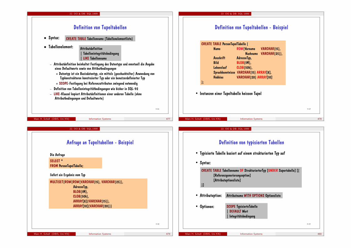
22. OO & DB: SQL:1999
4-66
Definition von Tupeltabellen
Syntax:
Tabellenelement:
– Attributdefinition beinhaltet Festlegung des Datentyps und eventuell die Angabe eines Defaultwerts sowie von Attibutbedingungen Datentyp ist ein Basisdatentyp, ein mittels (geschachtelter) Anwendung von
Typkonstruktoren konstruierter Typ oder ein benutzerdefinierter Typ SCOPE-Festlegung bei Referenzattributen zwingend notwendig
– Definition von Tabellenintegritätbedingungen wie bisher in SQL-92 – LIKE-Klausel kopiert Attributdefinitionen einer anderen Tabelle (ohne
Attributbedingungen und Defaultwerte)
CREATE TABLE Tabellenname (Tabellenelementliste)
Attributdefinition | Tabellenintegritätsbedingung | LIKE Tabellenname
Marc H. Scholl (DBIS, Uni KN) Information Systems 477
22. OO & DB: SQL:1999
4-67
Definition von Tupeltabellen - Beispiel
CREATE TABLE PersonTupelTabelle ( Name ROW(Vorname VARCHAR(15), Nachname VARCHAR(25)), Anschrift AdresseTyp, Bild BLOB(1M), Lebenslauf CLOB(50k), Sprachkenntnisse VARCHAR(15) ARRAY[8], Hobbies VARCHAR(20) ARRAY[10]
);
• Instanzen einer Tupeltabelle heissen Tupel
Marc H. Scholl (DBIS, Uni KN) Information Systems 478
22. OO & DB: SQL:1999
4-68
Anfrage an Tupeltabellen - Beispiel
SELECT * FROM PersonTupelTabelle;
MULTISET(ROW(ROW(VARCHAR(15), VARCHAR(25)), AdresseTyp, BLOB(1M), CLOB(50k), ARRAY[8](VARCHAR(15)), ARRAY[10](VARCHAR(20)))
liefert ein Ergebnis vom Typ
Die Anfrage
Marc H. Scholl (DBIS, Uni KN) Information Systems 479
22. OO & DB: SQL:1999
4-69
Definition von typisierten Tabellen
CREATE TABLE Tabellenname OF StrukturierterTyp [UNDER Supertabelle] [( [Referenzgenerierungsoption] [Attributoptionsliste]
)]
• Typisierte Tabelle basiert auf einem strukturierten Typ auf
• Syntax:
Attributname WITH OPTIONS Optionsliste • Attributoption:
SCOPE TypisierteTabelle | DEFAULT Wert | Integritätsbedingung
• Optionen:
Marc H. Scholl (DBIS, Uni KN) Information Systems 480

22. OO & DB: SQL:1999
4-70
Legt OID-Attribut und die Generierung der OIDs fest
Muss für jede typisierte Wurzeltabelle angegeben werden
Darf nicht bei Subtabellen angegeben werden
Referenzgenerierungsoptionen – REF IS oid USER GENERATED
OID-Generierung durch den Benutzer – REF IS oid SYSTEM GENERATED
OID-Generierung durch das System – REF IS oid DERIVED (Attributliste)
OID aus vorhandenen Attributwerten eines Schlüssels funktional bestimmt
Referenzgenerierung
Marc H. Scholl (DBIS, Uni KN) Information Systems 481
22. OO & DB: SQL:1999
4-71
Definition von typisierten Tabellen - Beispiel
CREATE TABLE Personen OF PersonTyp ( REF IS oid SYSTEM GENERATED, Ehepartner WITH OPTIONS SCOPE Personen, Kinder WITH OPTIONS SCOPE Personen
);
Instanzen einer typisierten Tabelle heissen Objekte
Nur Instanzen einer typisierten Tabelle können mittels eines Referenzattributs referenziert werden!
– SCOPE-Klausel bestimmt die typisierte Tabelle, die referenziert wird
Marc H. Scholl (DBIS, Uni KN) Information Systems 482
22. OO & DB: SQL:1999
4-72
Anfrage an typisierte Tabellen - Beispiel
SELECT * FROM Personen;
Was ist der Ergebnistyp der folgenden Anfrage?
SET(PersonTyp) Vielleicht
MULTISET(ROW(REF(PersonTyp), VARCHAR(30), AdresseTyp, REF(PersonTyp), ARRAY[10](REF(PersonTyp))))
Oder doch
Marc H. Scholl (DBIS, Uni KN) Information Systems 483
22. OO & DB: SQL:1999
4-73
Einfügen und Ändern in typisierten Tabellen - Beispiel
Erzeugen von Tabelleninhalten (impliziter Aufruf des PersonTyp-Konstruktors):
INSERT INTO Personen VALUES ('Billy Bär', AdresseTyp('Seefeldstrasse', 31, 8008, 'Zurich', 'CH'), (SELECT REF(p) FROM Personen p WHERE p.Name = 'Mama Bär'), ARRAY(NULL));
Belegen von Referenzattributen:
UPDATE Personen SET Kinder[1] = (SELECT REF(p) FROM Personen p WHERE p.Name = 'Baby Bär') WHERE Name = 'Billy Bär';
Marc H. Scholl (DBIS, Uni KN) Information Systems 484
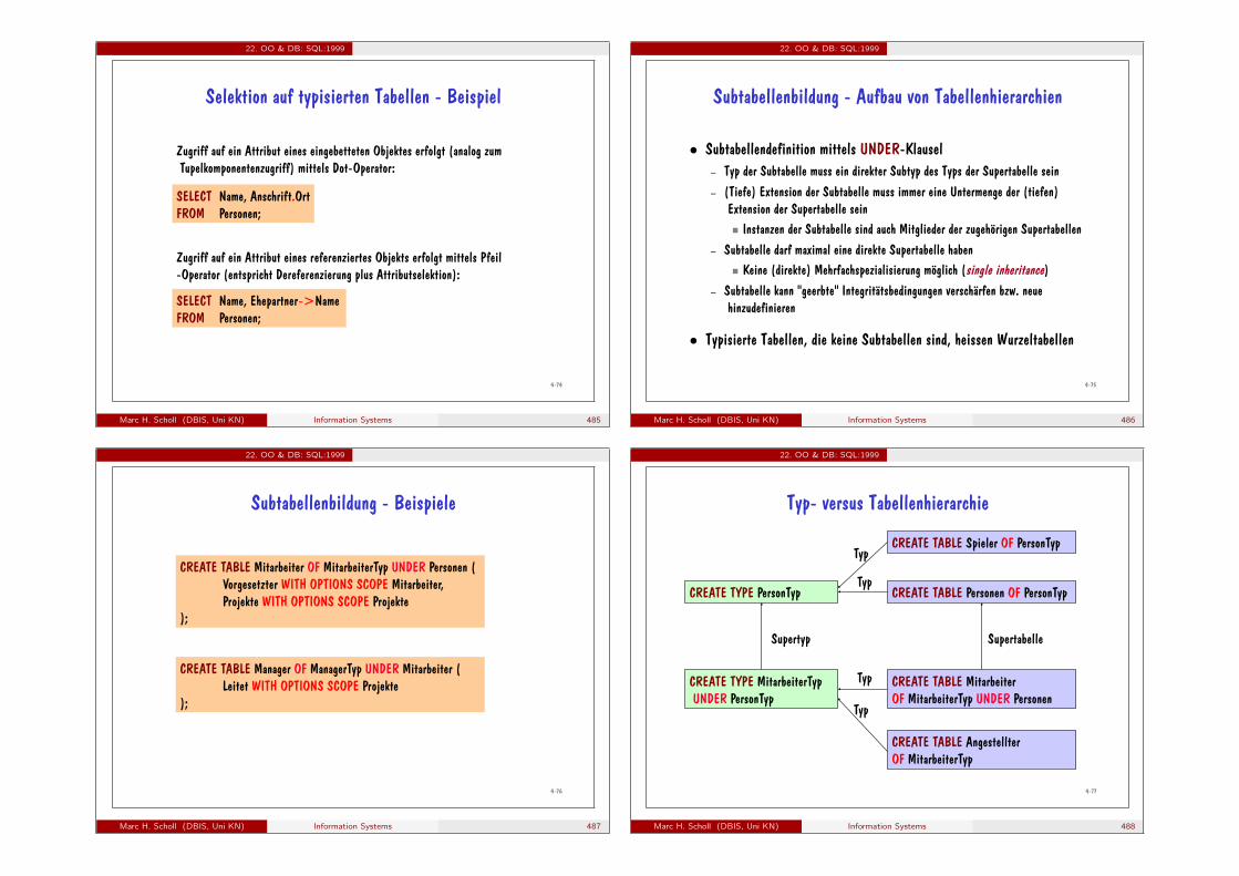
22. OO & DB: SQL:1999
4-74
Selektion auf typisierten Tabellen - Beispiel
Zugriff auf ein Attribut eines referenziertes Objekts erfolgt mittels Pfeil-Operator (entspricht Dereferenzierung plus Attributselektion):
SELECT Name, Ehepartner->Name FROM Personen;
Zugriff auf ein Attribut eines eingebetteten Objektes erfolgt (analog zum Tupelkomponentenzugriff) mittels Dot-Operator:
SELECT Name, Anschrift.Ort FROM Personen;
Marc H. Scholl (DBIS, Uni KN) Information Systems 485
22. OO & DB: SQL:1999
4-75
Subtabellenbildung - Aufbau von Tabellenhierarchien
Subtabellendefinition mittels UNDER-Klausel – Typ der Subtabelle muss ein direkter Subtyp des Typs der Supertabelle sein – (Tiefe) Extension der Subtabelle muss immer eine Untermenge der (tiefen)
Extension der Supertabelle sein Instanzen der Subtabelle sind auch Mitglieder der zugehörigen Supertabellen
– Subtabelle darf maximal eine direkte Supertabelle haben Keine (direkte) Mehrfachspezialisierung möglich (single inheritance)
– Subtabelle kann "geerbte" Integritätsbedingungen verschärfen bzw. neue hinzudefinieren
Typisierte Tabellen, die keine Subtabellen sind, heissen Wurzeltabellen
Marc H. Scholl (DBIS, Uni KN) Information Systems 486
22. OO & DB: SQL:1999
4-76
Subtabellenbildung - Beispiele
CREATE TABLE Mitarbeiter OF MitarbeiterTyp UNDER Personen ( Vorgesetzter WITH OPTIONS SCOPE Mitarbeiter, Projekte WITH OPTIONS SCOPE Projekte
);
CREATE TABLE Manager OF ManagerTyp UNDER Mitarbeiter ( Leitet WITH OPTIONS SCOPE Projekte
);
Marc H. Scholl (DBIS, Uni KN) Information Systems 487
22. OO & DB: SQL:1999
4-77
Typ- versus Tabellenhierarchie
CREATE TYPE MitarbeiterTyp UNDER PersonTyp
CREATE TYPE PersonTyp
CREATE TABLE Mitarbeiter OF MitarbeiterTyp UNDER Personen
CREATE TABLE Personen OF PersonTyp
Supertyp Supertabelle
Typ
Typ
CREATE TABLE Angestellter OF MitarbeiterTyp
Typ
CREATE TABLE Spieler OF PersonTyp Typ
Marc H. Scholl (DBIS, Uni KN) Information Systems 488
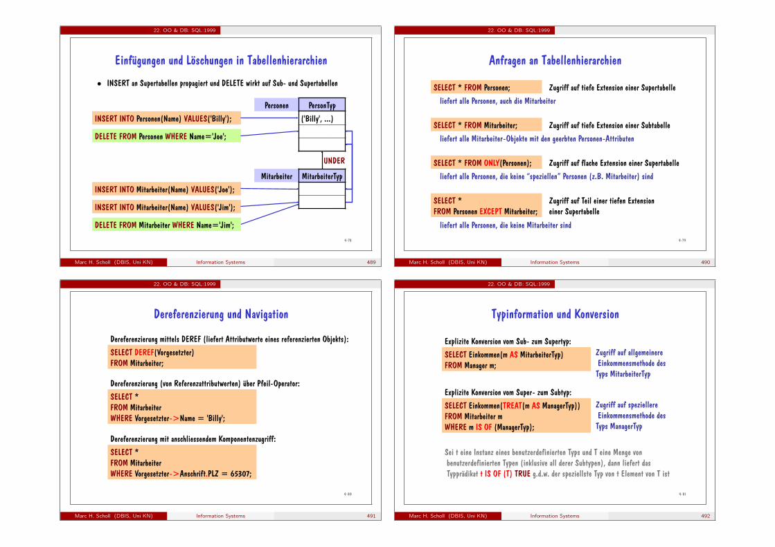
22. OO & DB: SQL:1999
4-78
Personen PersonTyp
Einfügungen und Löschungen in Tabellenhierarchien
INSERT INTO Personen(Name) VALUES('Billy');
Mitarbeiter MitarbeiterTyp
('Billy', ...)
INSERT INTO Mitarbeiter(Name) VALUES('Joe'); ('Joe', ...)
('Joe', ...) DELETE FROM Personen WHERE Name='Joe';
INSERT INTO Mitarbeiter(Name) VALUES('Jim');
DELETE FROM Mitarbeiter WHERE Name='Jim';
('Jim', ...)
('Jim', ...)
UNDER
INSERT an Supertabellen propagiert und DELETE wirkt auf Sub- und Supertabellen
Marc H. Scholl (DBIS, Uni KN) Information Systems 489
22. OO & DB: SQL:1999
4-79
Anfragen an Tabellenhierarchien
SELECT * FROM Personen; liefert alle Personen, auch die Mitarbeiter
SELECT * FROM ONLY(Personen); liefert alle Personen, die keine “speziellen” Personen (z.B. Mitarbeiter) sind
Zugriff auf flache Extension einer Supertabelle
SELECT * FROM Mitarbeiter; liefert alle Mitarbeiter-Objekte mit den geerbten Personen-Attributen
Zugriff auf tiefe Extension einer Subtabelle
Zugriff auf tiefe Extension einer Supertabelle
SELECT * FROM Personen EXCEPT Mitarbeiter;
liefert alle Personen, die keine Mitarbeiter sind
Zugriff auf Teil einer tiefen Extension einer Supertabelle
Marc H. Scholl (DBIS, Uni KN) Information Systems 490
22. OO & DB: SQL:1999
4-80
Dereferenzierung und Navigation
SELECT DEREF(Vorgesetzter) FROM Mitarbeiter;
SELECT * FROM Mitarbeiter WHERE Vorgesetzter->Name = 'Billy';
SELECT * FROM Mitarbeiter WHERE Vorgesetzter->Anschrift.PLZ = 65307;
Dereferenzierung mittels DEREF (liefert Attributwerte eines referenzierten Objekts):
Dereferenzierung (von Referenzattributwerten) über Pfeil-Operator:
Dereferenzierung mit anschliessendem Komponentenzugriff:
Marc H. Scholl (DBIS, Uni KN) Information Systems 491
22. OO & DB: SQL:1999
4-81
Typinformation und Konversion
SELECT Einkommen(TREAT(m AS ManagerTyp)) FROM Mitarbeiter m WHERE m IS OF (ManagerTyp);
SELECT Einkommen(m AS MitarbeiterTyp) FROM Manager m;
Explizite Konversion vom Super- zum Subtyp:
Explizite Konversion vom Sub- zum Supertyp:
Zugriff auf speziellere Einkommensmethode des Typs ManagerTyp
Zugriff auf allgemeinere Einkommensmethode des Typs MitarbeiterTyp
Sei t eine Instanz eines benutzerdefinierten Typs und T eine Menge von benutzerdefinierten Typen (inklusive all derer Subtypen), dann liefert das Typprädikat t IS OF (T) TRUE g.d.w. der speziellste Typ von t Element von T ist
Marc H. Scholl (DBIS, Uni KN) Information Systems 492
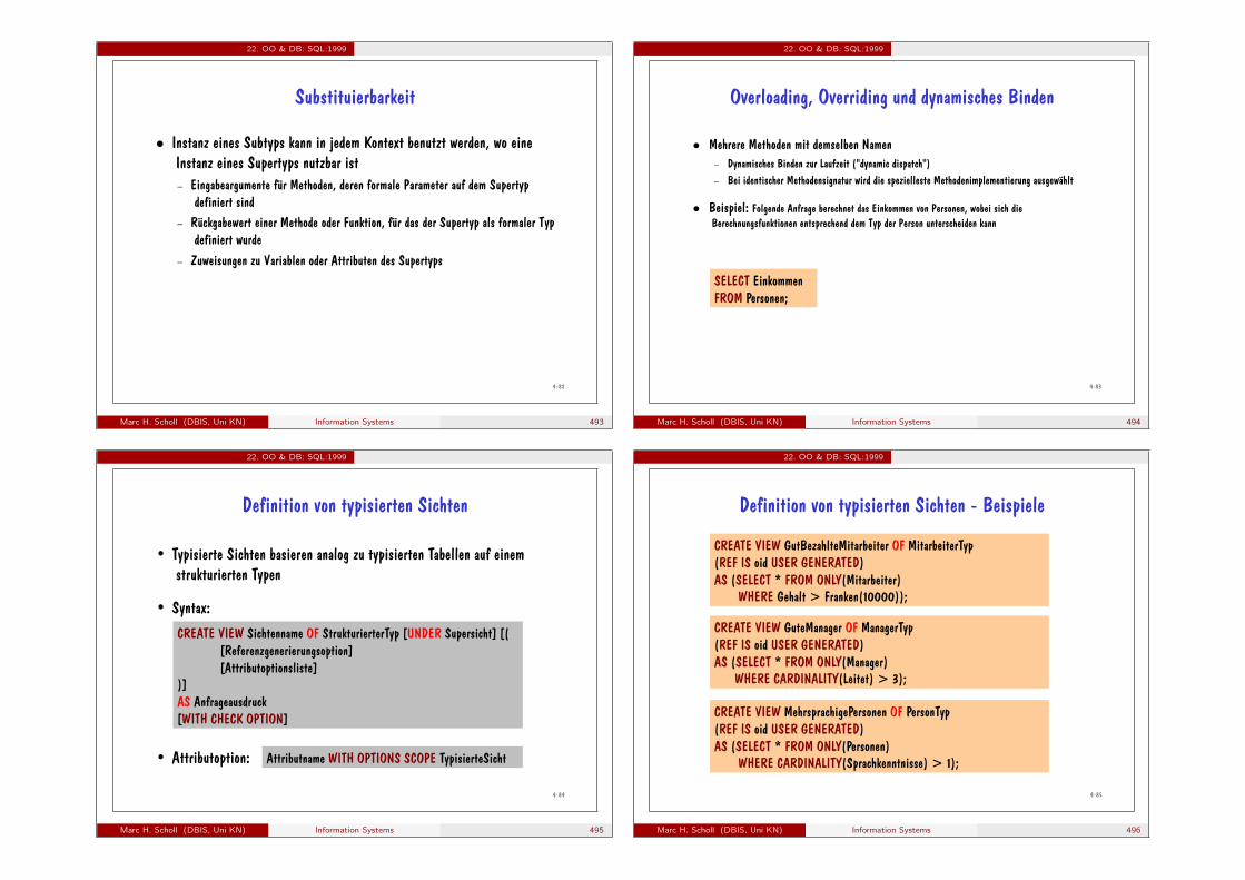
22. OO & DB: SQL:1999
4-82
Substituierbarkeit
Instanz eines Subtyps kann in jedem Kontext benutzt werden, wo eine Instanz eines Supertyps nutzbar ist
– Eingabeargumente für Methoden, deren formale Parameter auf dem Supertyp definiert sind
– Rückgabewert einer Methode oder Funktion, für das der Supertyp als formaler Typ definiert wurde
– Zuweisungen zu Variablen oder Attributen des Supertyps
Marc H. Scholl (DBIS, Uni KN) Information Systems 493
22. OO & DB: SQL:1999
4-83
Overloading, Overriding und dynamisches Binden
Mehrere Methoden mit demselben Namen – Dynamisches Binden zur Laufzeit ("dynamic dispatch") – Bei identischer Methodensignatur wird die spezielleste Methodenimplementierung ausgewählt
Beispiel: Folgende Anfrage berechnet das Einkommen von Personen, wobei sich die Berechnungsfunktionen entsprechend dem Typ der Person unterscheiden kann
SELECT Einkommen FROM Personen;
Marc H. Scholl (DBIS, Uni KN) Information Systems 494
22. OO & DB: SQL:1999
4-84
Definition von typisierten Sichten
CREATE VIEW Sichtenname OF StrukturierterTyp [UNDER Supersicht] [( [Referenzgenerierungsoption] [Attributoptionsliste]
)] AS Anfrageausdruck [WITH CHECK OPTION]
• Syntax:
Attributname WITH OPTIONS SCOPE TypisierteSicht • Attributoption:
• Typisierte Sichten basieren analog zu typisierten Tabellen auf einem strukturierten Typen
Marc H. Scholl (DBIS, Uni KN) Information Systems 495
22. OO & DB: SQL:1999
4-85
Definition von typisierten Sichten - Beispiele
CREATE VIEW GutBezahlteMitarbeiter OF MitarbeiterTyp (REF IS oid USER GENERATED) AS (SELECT * FROM ONLY(Mitarbeiter) WHERE Gehalt > Franken(10000));
CREATE VIEW GuteManager OF ManagerTyp (REF IS oid USER GENERATED) AS (SELECT * FROM ONLY(Manager) WHERE CARDINALITY(Leitet) > 3);
CREATE VIEW MehrsprachigePersonen OF PersonTyp (REF IS oid USER GENERATED) AS (SELECT * FROM ONLY(Personen) WHERE CARDINALITY(Sprachkenntnisse) > 1);
Marc H. Scholl (DBIS, Uni KN) Information Systems 496
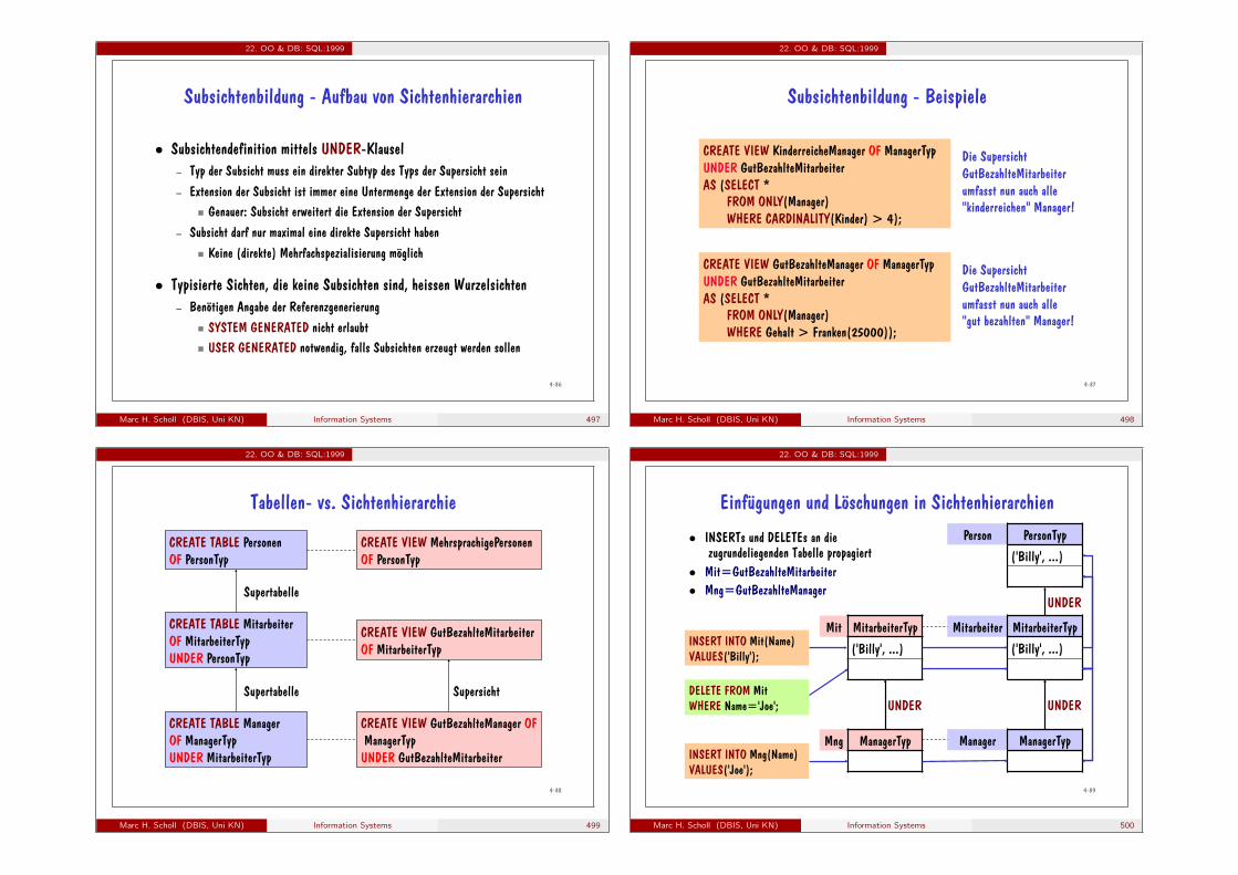
22. OO & DB: SQL:1999
4-86
Subsichtenbildung - Aufbau von Sichtenhierarchien
Subsichtendefinition mittels UNDER-Klausel – Typ der Subsicht muss ein direkter Subtyp des Typs der Supersicht sein – Extension der Subsicht ist immer eine Untermenge der Extension der Supersicht
Genauer: Subsicht erweitert die Extension der Supersicht – Subsicht darf nur maximal eine direkte Supersicht haben
Keine (direkte) Mehrfachspezialisierung möglich
Typisierte Sichten, die keine Subsichten sind, heissen Wurzelsichten – Benötigen Angabe der Referenzgenerierung
SYSTEM GENERATED nicht erlaubt USER GENERATED notwendig, falls Subsichten erzeugt werden sollen
Marc H. Scholl (DBIS, Uni KN) Information Systems 497
22. OO & DB: SQL:1999
4-87
Subsichtenbildung - Beispiele
CREATE VIEW KinderreicheManager OF ManagerTyp UNDER GutBezahlteMitarbeiter AS (SELECT * FROM ONLY(Manager) WHERE CARDINALITY(Kinder) > 4);
Die Supersicht GutBezahlteMitarbeiter umfasst nun auch alle "kinderreichen" Manager!
CREATE VIEW GutBezahlteManager OF ManagerTyp UNDER GutBezahlteMitarbeiter AS (SELECT * FROM ONLY(Manager) WHERE Gehalt > Franken(25000));
Die Supersicht GutBezahlteMitarbeiter umfasst nun auch alle "gut bezahlten" Manager!
Marc H. Scholl (DBIS, Uni KN) Information Systems 498
22. OO & DB: SQL:1999
4-88
Tabellen- vs. Sichtenhierarchie
CREATE VIEW GutBezahlteMitarbeiter OF MitarbeiterTyp
CREATE VIEW GutBezahlteManager OF ManagerTyp UNDER GutBezahlteMitarbeiter
Supersicht
CREATE TABLE Mitarbeiter OF MitarbeiterTyp UNDER PersonTyp
CREATE TABLE Personen OF PersonTyp
Supertabelle
CREATE TABLE Manager OF ManagerTyp UNDER MitarbeiterTyp
Supertabelle
CREATE VIEW MehrsprachigePersonen OF PersonTyp
Marc H. Scholl (DBIS, Uni KN) Information Systems 499
22. OO & DB: SQL:1999
4-89
Mng ManagerTyp
Mit MitarbeiterTyp
('Joe', ...)
('Joe', ...)
Einfügungen und Löschungen in Sichtenhierarchien
INSERT INTO Mit(Name) VALUES('Billy'); ('Billy', ...)
INSERT INTO Mng(Name) VALUES('Joe');
DELETE FROM Mit WHERE Name='Joe'; UNDER
INSERTs und DELETEs an die zugrundeliegenden Tabelle propagiert
Mit=GutBezahlteMitarbeiter Mng=GutBezahlteManager
Mitarbeiter MitarbeiterTyp
Manager ManagerTyp
('Billy', ...)
('Joe', ...)
('Joe', ...)
UNDER
Person PersonTyp ('Billy', ...) ('Joe', ...)
UNDER
Marc H. Scholl (DBIS, Uni KN) Information Systems 500
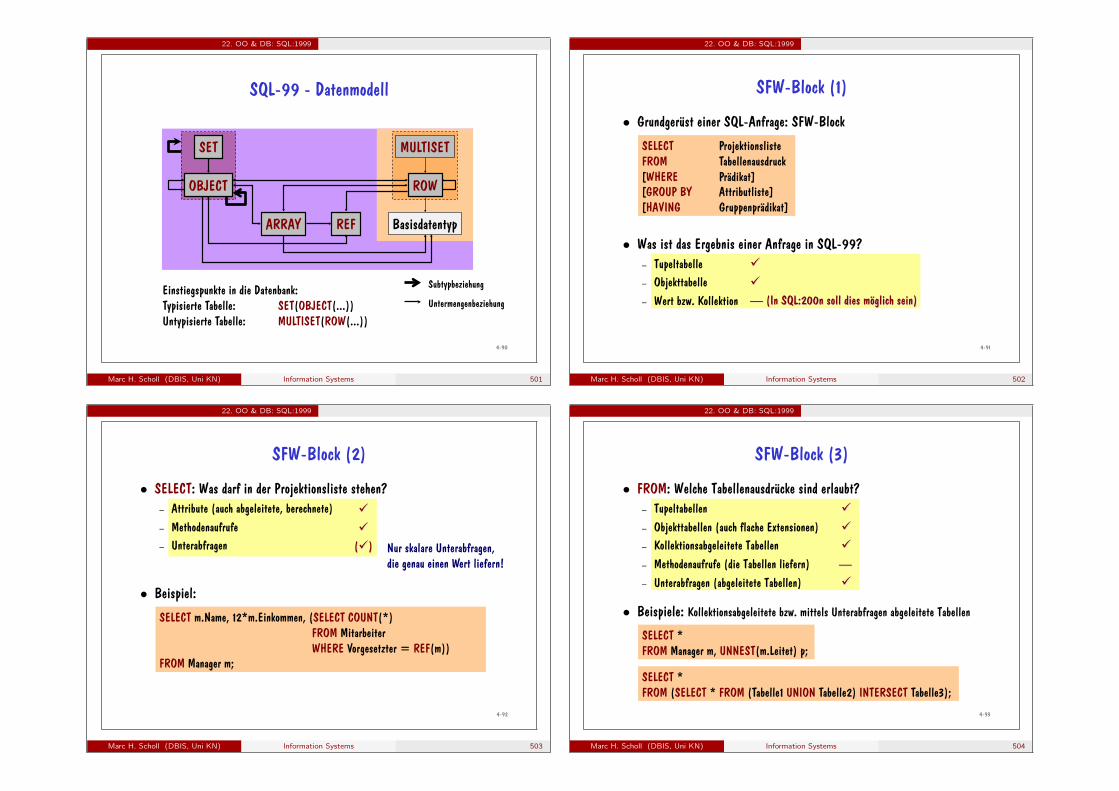
22. OO & DB: SQL:1999
4-90
SQL-99 - Datenmodell
MULTISET
ROW
Basisdatentyp REF ARRAY
SET
OBJECT
Einstiegspunkte in die Datenbank: Typisierte Tabelle: SET(OBJECT(...)) Untypisierte Tabelle: MULTISET(ROW(...))
Subtypbeziehung
Untermengenbeziehung
Marc H. Scholl (DBIS, Uni KN) Information Systems 501
22. OO & DB: SQL:1999
4-91
SFW-Block (1)
Grundgerüst einer SQL-Anfrage: SFW-Block
Was ist das Ergebnis einer Anfrage in SQL-99? – Tupeltabelle – Objekttabelle – Wert bzw. Kollektion
SELECT Projektionsliste FROM Tabellenausdruck [WHERE Prädikat] [GROUP BY Attributliste] [HAVING Gruppenprädikat]
Marc H. Scholl (DBIS, Uni KN) Information Systems 502
22. OO & DB: SQL:1999
4-92
SELECT: Was darf in der Projektionsliste stehen? – Attribute (auch abgeleitete, berechnete) – Methodenaufrufe – Unterabfragen
Beispiel:
SFW-Block (2)
SELECT m.Name, 12*m.Einkommen, (SELECT COUNT(*) FROM Mitarbeiter WHERE Vorgesetzter = REF(m)) FROM Manager m;
Nur skalare Unterabfragen, die genau einen Wert liefern!
Marc H. Scholl (DBIS, Uni KN) Information Systems 503
22. OO & DB: SQL:1999
4-93
FROM: Welche Tabellenausdrücke sind erlaubt? – Tupeltabellen – Objekttabellen (auch flache Extensionen) – Kollektionsabgeleitete Tabellen – Methodenaufrufe (die Tabellen liefern) – Unterabfragen (abgeleitete Tabellen)
Beispiele: Kollektionsabgeleitete bzw. mittels Unterabfragen abgeleitete Tabellen
SFW-Block (3)
SELECT * FROM (SELECT * FROM (Tabelle1 UNION Tabelle2) INTERSECT Tabelle3);
SELECT * FROM Manager m, UNNEST(m.Leitet) p;
Marc H. Scholl (DBIS, Uni KN) Information Systems 504
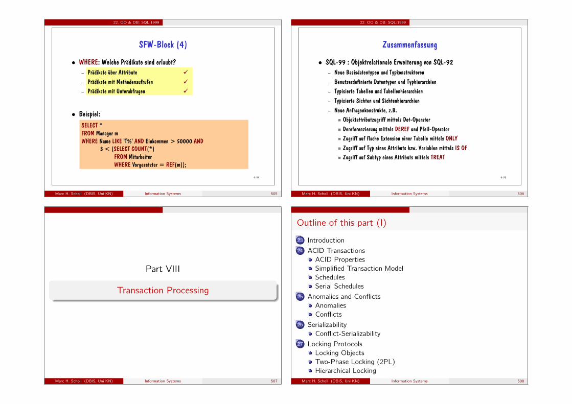
22. OO & DB: SQL:1999
4-94
SFW-Block (4)
WHERE: Welche Prädikate sind erlaubt? – Prädikate über Attribute – Prädikate mit Methodenaufrufen – Prädikate mit Unterabfragen
Beispiel: SELECT * FROM Manager m WHERE Name LIKE 'T%' AND Einkommen > 50000 AND 3 < (SELECT COUNT(*) FROM Mitarbeiter WHERE Vorgesetzter = REF(m));
Marc H. Scholl (DBIS, Uni KN) Information Systems 505
22. OO & DB: SQL:1999
4-95
Zusammenfassung
SQL-99 : Objektrelationale Erweiterung von SQL-92 – Neue Basisdatentypen und Typkonstruktoren – Benutzerdefinierte Datentypen und Typhierarchien – Typisierte Tabellen und Tabellenhierarchien – Typisierte Sichten und Sichtenhierarchien – Neue Anfragenkonstrukte, z.B.
Objektattributzugriff mittels Dot-Operator Dereferenzierung mittels DEREF und Pfeil-Operator Zugriff auf flache Extension einer Tabelle mittels ONLY Zugriff auf Typ eines Attributs bzw. Variablen mittels IS OF Zugriff auf Subtyp eines Attributs mittels TREAT
Marc H. Scholl (DBIS, Uni KN) Information Systems 506
Part VIII
Transaction Processing
Marc H. Scholl (DBIS, Uni KN) Information Systems 507
Outline of this part (I)
23 Introduction24 ACID Transactions
ACID PropertiesSimplified Transaction ModelSchedulesSerial Schedules
25 Anomalies and ConflictsAnomaliesConflicts
26 SerializabilityConflict-Serializability
27 Locking ProtocolsLocking ObjectsTwo-Phase Locking (2PL)Hierarchical Locking
Marc H. Scholl (DBIS, Uni KN) Information Systems 508
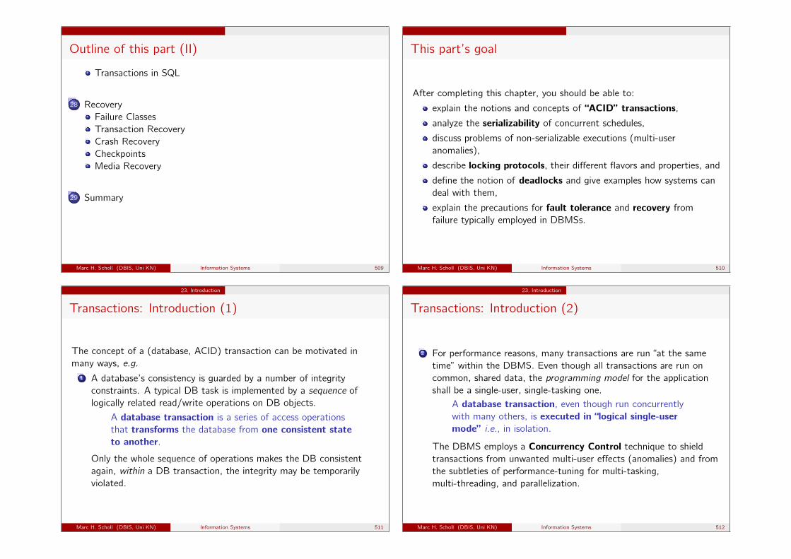
Outline of this part (II)
Transactions in SQL
28 RecoveryFailure ClassesTransaction RecoveryCrash RecoveryCheckpointsMedia Recovery
29 Summary
Marc H. Scholl (DBIS, Uni KN) Information Systems 509
This part’s goal
After completing this chapter, you should be able to:
explain the notions and concepts of “ACID” transactions,analyze the serializability of concurrent schedules,
discuss problems of non-serializable executions (multi-useranomalies),
describe locking protocols, their different flavors and properties, and
define the notion of deadlocks and give examples how systems candeal with them,
explain the precautions for fault tolerance and recovery fromfailure typically employed in DBMSs.
Marc H. Scholl (DBIS, Uni KN) Information Systems 510
23. Introduction
Transactions: Introduction (1)
The concept of a (database, ACID) transaction can be motivated inmany ways, e.g.
1 A database’s consistency is guarded by a number of integrityconstraints. A typical DB task is implemented by a sequence oflogically related read/write operations on DB objects.
A database transaction is a series of access operationsthat transforms the database from one consistent stateto another.
Only the whole sequence of operations makes the DB consistentagain, within a DB transaction, the integrity may be temporarilyviolated.
Marc H. Scholl (DBIS, Uni KN) Information Systems 511
23. Introduction
Transactions: Introduction (2)
2 For performance reasons, many transactions are run “at the sametime” within the DBMS. Even though all transactions are run oncommon, shared data, the programming model for the applicationshall be a single-user, single-tasking one.
A database transaction, even though run concurrentlywith many others, is executed in “logical single-usermode” i.e., in isolation.
The DBMS employs a Concurrency Control technique to shieldtransactions from unwanted multi-user effects (anomalies) and fromthe subtleties of performance-tuning for multi-tasking,multi-threading, and parallelization.
Marc H. Scholl (DBIS, Uni KN) Information Systems 512
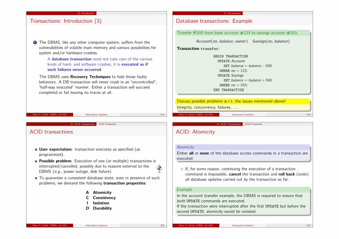
23. Introduction
Transactions: Introduction (3)
3 The DBMS, like any other computer system, suffers from thevulnerabilities of volatile main memory and various possibilites forsystem and/or hardware crashes.
A database transaction need not take care of the variouskinds of hard- and software crashes, it is executed as ifsuch failures never occurred.
The DBMS uses Recovery Techniques to hide those faultybehaviors. A DB transaction will never crash in an “uncontrolled”,“half-way executed” manner. Either a transaction will succeedcompleted or fail leaving no traces at all.
Marc H. Scholl (DBIS, Uni KN) Information Systems 513
23. Introduction
Database transactions: Example
Transfer ¤500 from bank account #123 to savings account #333.
Account(no, balance, owner ) Savings(no, balance)
Transaction transfer:
BEGIN TRANSACTIONUPDATE Account
SET balance = balance − 500
WHERE no = 123;
UPDATE Savings
SET balance = balance + 500
WHERE no = 333;
END TRANSACTION
Discuss possible problems w.r.t. the issues mentioned above!
Integrity, concurrency, failures, . . .
Marc H. Scholl (DBIS, Uni KN) Information Systems 514
24. ACID Transactions ACID Properties
ACID transactions
User expectation: transaction executes as specified (asprogrammed).
Possible problem: Execution of one (or multiple) transactions isinterrupted/cancelled, possibly due to reasons external to theDBMS (e.g., power outage, disk failure).
�To guarantee a consistent database state, even in presence of suchproblems, we demand the following transaction properties:
A AtomicityC ConsistencyI IsolationD Durability
Marc H. Scholl (DBIS, Uni KN) Information Systems 515
24. ACID Transactions ACID Properties
ACID: Atomicity
Atomicity
Either all or none of the database access commands in a transaction areexecuted.
. If, for some reason, continuing the execution of a transactioncommand is impossible, cancel the transaction and roll back (undo)all database updates carried out by the transaction so far.
Example
In the account transfer example, the DBMS is required to ensure thatboth UPDATE commands are executed.If the transaction were interrupted after the first UPDATE but before thesecond UPDATE, atomicity would be violated.
Marc H. Scholl (DBIS, Uni KN) Information Systems 516
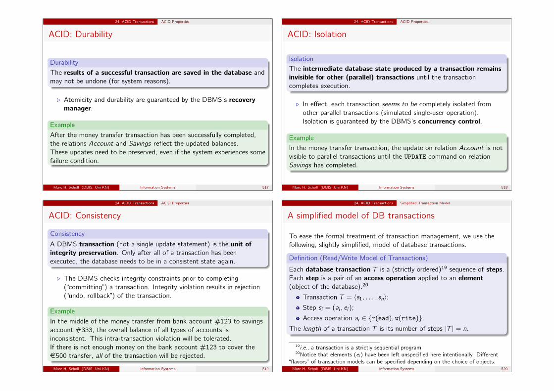
24. ACID Transactions ACID Properties
ACID: Durability
Durability
The results of a successful transaction are saved in the database andmay not be undone (for system reasons).
. Atomicity and durability are guaranteed by the DBMS’s recoverymanager.
Example
After the money transfer transaction has been successfully completed,the relations Account and Savings reflect the updated balances.These updates need to be preserved, even if the system experiences somefailure condition.
Marc H. Scholl (DBIS, Uni KN) Information Systems 517
24. ACID Transactions ACID Properties
ACID: Isolation
IsolationThe intermediate database state produced by a transaction remainsinvisible for other (parallel) transactions until the transactioncompletes execution.
. In effect, each transaction seems to be completely isolated fromother parallel transactions (simulated single-user operation).Isolation is guaranteed by the DBMS’s concurrency control.
Example
In the money transfer transaction, the update on relation Account is notvisible to parallel transactions until the UPDATE command on relationSavings has completed.
Marc H. Scholl (DBIS, Uni KN) Information Systems 518
24. ACID Transactions ACID Properties
ACID: Consistency
Consistency
A DBMS transaction (not a single update statement) is the unit ofintegrity preservation. Only after all of a transaction has beenexecuted, the database needs to be in a consistent state again.
. The DBMS checks integrity constraints prior to completing(“committing”) a transaction. Integrity violation results in rejection(“undo, rollback”) of the transaction.
Example
In the middle of the money transfer from bank account #123 to savingsaccount #333, the overall balance of all types of accounts isinconsistent. This intra-transaction violation will be tolerated.If there is not enough money on the bank account #123 to cover the¤500 transfer, all of the transaction will be rejected.
Marc H. Scholl (DBIS, Uni KN) Information Systems 519
24. ACID Transactions Simplified Transaction Model
A simplified model of DB transactions
To ease the formal treatment of transaction management, we use thefollowing, slightly simplified, model of database transactions.
Definition (Read/Write Model of Transactions)
Each database transaction T is a (strictly ordered)19 sequence of steps.Each step is a pair of an access operation applied to an element(object of the database).20
Transaction T = 〈s1, . . . , sn〉;Step si = (ai , ei);
Access operation ai ∈ {r(ead), w(rite)}.The length of a transaction T is its number of steps |T | = n.
19i.e., a transaction is a strictly sequential program20Notice that elements (ei) have been left unspecified here intentionally. Different
“flavors” of transaction models can be specified depending on the choice of objects.Marc H. Scholl (DBIS, Uni KN) Information Systems 520
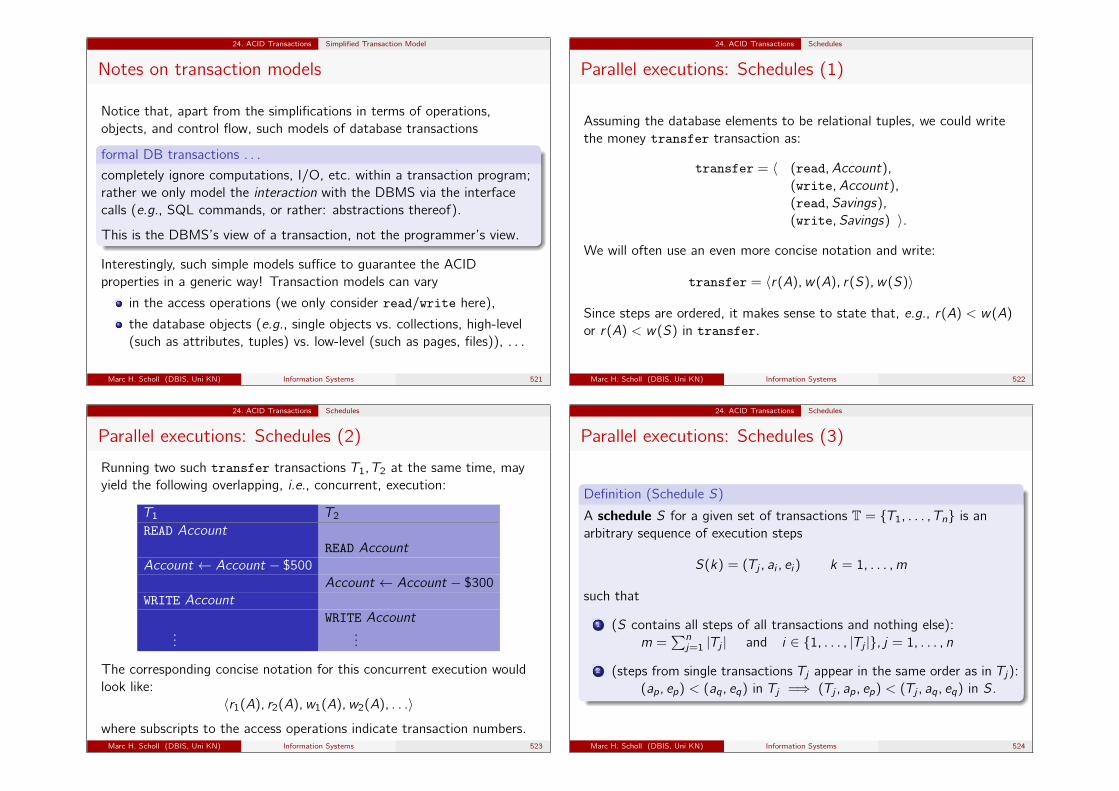
24. ACID Transactions Simplified Transaction Model
Notes on transaction models
Notice that, apart from the simplifications in terms of operations,objects, and control flow, such models of database transactions
formal DB transactions . . .
completely ignore computations, I/O, etc. within a transaction program;rather we only model the interaction with the DBMS via the interfacecalls (e.g., SQL commands, or rather: abstractions thereof).
This is the DBMS’s view of a transaction, not the programmer’s view.
Interestingly, such simple models suffice to guarantee the ACIDproperties in a generic way! Transaction models can vary
in the access operations (we only consider read/write here),
the database objects (e.g., single objects vs. collections, high-level(such as attributes, tuples) vs. low-level (such as pages, files)), . . .
Marc H. Scholl (DBIS, Uni KN) Information Systems 521
24. ACID Transactions Schedules
Parallel executions: Schedules (1)
Assuming the database elements to be relational tuples, we could writethe money transfer transaction as:
transfer = 〈 (read,Account),
(write,Account),
(read,Savings),
(write,Savings) 〉.
We will often use an even more concise notation and write:
transfer = 〈r(A), w(A), r(S), w(S)〉
Since steps are ordered, it makes sense to state that, e.g., r(A) < w(A)
or r(A) < w(S) in transfer.
Marc H. Scholl (DBIS, Uni KN) Information Systems 522
24. ACID Transactions Schedules
Parallel executions: Schedules (2)
Running two such transfer transactions T1, T2 at the same time, mayyield the following overlapping, i.e., concurrent, execution:
T1 T2READ Account
READ Account
Account ← Account − $500
Account ← Account − $300
WRITE Account
WRITE Account...
...
The corresponding concise notation for this concurrent execution wouldlook like:
〈r1(A), r2(A), w1(A), w2(A), . . .〉where subscripts to the access operations indicate transaction numbers.Marc H. Scholl (DBIS, Uni KN) Information Systems 523
24. ACID Transactions Schedules
Parallel executions: Schedules (3)
Definition (Schedule S)
A schedule S for a given set of transactions T = {T1, . . . , Tn} is anarbitrary sequence of execution steps
S(k) = (Tj , ai , ei) k = 1, . . . , m
such that
1 (S contains all steps of all transactions and nothing else):m =
∑nj=1 |Tj | and i ∈ {1, . . . , |Tj |}, j = 1, . . . , n
2 (steps from single transactions Tj appear in the same order as in Tj):(ap, ep) < (aq, eq) in Tj =⇒ (Tj , ap, ep) < (Tj , aq, eq) in S.
Marc H. Scholl (DBIS, Uni KN) Information Systems 524
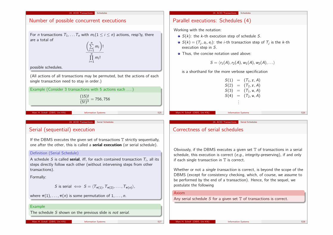
24. ACID Transactions Schedules
Number of possible concurrent executions
For n transactions T1, . . . Tn with mi(1 ≤ i ≤ n) actions, resp’ly, thereare a total of (
n∑i=1
mi
)!
n∏i=1
mi !
possible schedules.
(All actions of all transactions may be permuted, but the actions of eachsingle transaction need to stay in order.)
Example (Consider 3 transactions with 5 actions each . . . )
(15)!
(5!)3= 756, 756
Marc H. Scholl (DBIS, Uni KN) Information Systems 525
24. ACID Transactions Schedules
Parallel executions: Schedules (4)
Working with the notation:
S(k): the k-th execution step of schedule S.
S(k) = (Tj , ai , ei): the i-th transaction step of Tj is the k-thexecution step in S.
Thus, the concise notation used above:
S = 〈r1(A), r2(A), w1(A), w2(A), . . .〉
is a shorthand for the more verbose specification
S(1) = (T1, r, A)
S(2) = (T2, r, A)
S(3) = (T1, w, A)
S(4) = (T2, w, A)...
Marc H. Scholl (DBIS, Uni KN) Information Systems 526
24. ACID Transactions Serial Schedules
Serial (sequential) execution
If the DBMS executes the given set of transactions T strictly sequentially,one after the other, this is called a serial execution (or serial schedule).
Definition (Serial Schedule)
A schedule S is called serial, iff, for each contained transaction Ti , all itssteps directly follow each other (without intervening steps from othertransactions).
Formally:
S is serial ⇐⇒ S = 〈Tπ(1), Tπ(2), . . . , Tπ(n)〉,
where π(1), . . . , π(n) is some permutation of 1, . . . , n.
Example
The schedule S shown on the previous slide is not serial.
Marc H. Scholl (DBIS, Uni KN) Information Systems 527
24. ACID Transactions Serial Schedules
Correctness of serial schedules
Obviously, if the DBMS executes a given set T of transactions in a serialschedule, this execution is correct (e.g., integrity-preserving), if and onlyif each single transaction in T is correct.
Whether or not a single transaction is correct, is beyond the scope of theDBMS (except for consistency checking, which, of course, we assume tobe performed by the end of a transaction). Hence, for the sequel, wepostulate the following
AxiomAny serial schedule S for a given set T of transactions is correct.
Marc H. Scholl (DBIS, Uni KN) Information Systems 528

25. Anomalies and Conflicts Anomalies
Problems in concurrent schedules
In general, non-serial concurrent executions of transactions that access(in particular: modify) shared data may lead to a number of problems(“anomalies” of unsynchronized parallel access).
Example (Concurrent Schedule S (reconsidered))
T1 T2
READ Account
READ Account
Account ← Account − $500
Account ← Account − $300
WRITE Account
WRITE Account...
...
Notice how the modification to the Account record issued by T1 will not“survive” the update by T2 (a so-called “lost update”).
Marc H. Scholl (DBIS, Uni KN) Information Systems 529
25. Anomalies and Conflicts Anomalies
Lost Update
If two concurrent transactions T1, T2 update a shared object in anuncontrolled, arbitrary sequence, one of the updates might get lost:
T1 T2READ a
READ a
a← f (a)
a← g(a)
WRITE a
WRITE a
Both transactions read the same old state of DB element a, the update(by the write on a) issued by the first transaction is over-written by thesecond.
Marc H. Scholl (DBIS, Uni KN) Information Systems 530
25. Anomalies and Conflicts Anomalies
Dirty Read
If a transaction T2 reads a DB element modified by another transactionT1 before the completion of T1, this will cause problems, if ultimately T1does not/can not commit:
T1 T2READ a
a← f (a)
WRITE a
READ a
a← g(a)
ABORT
WRITE a
The update on a performed by T1 will be undone by the DBMS as part ofthe ABORT processing. Hence, T2 has read a data value for element athat—logically—never existed!
Marc H. Scholl (DBIS, Uni KN) Information Systems 531
25. Anomalies and Conflicts Anomalies
Unrepeatable/Inconsistent Read
If transaction T1 reads multiple, related objects while a concurrentupdate transaction T2 modifies (some of) them, the reading transactionmay observe inconsistent database states. In the most simple case, T1just reads the same DB element twice:
T1 T2READ a
READ a
WRITE a
READ a
The reading transaction T1 “sees” some of the DB elements’ statesbefore the execution of T2 and some of them after T2.
Marc H. Scholl (DBIS, Uni KN) Information Systems 532
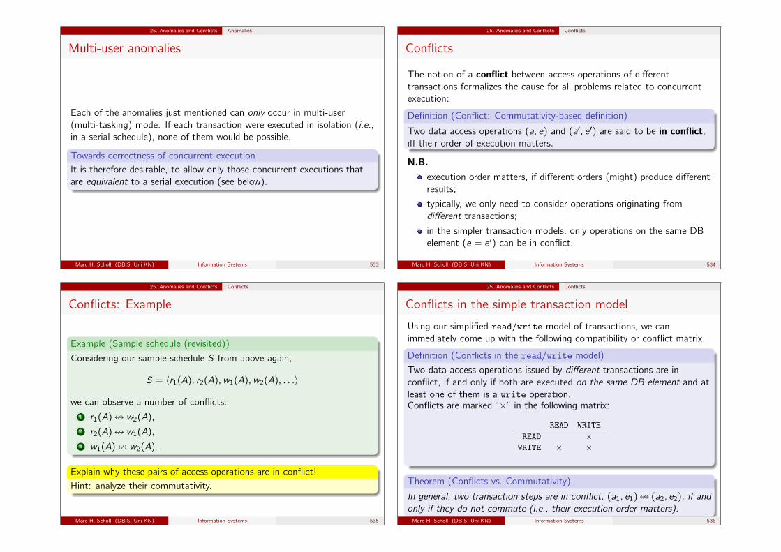
25. Anomalies and Conflicts Anomalies
Multi-user anomalies
Each of the anomalies just mentioned can only occur in multi-user(multi-tasking) mode. If each transaction were executed in isolation (i.e.,in a serial schedule), none of them would be possible.
Towards correctness of concurrent executionIt is therefore desirable, to allow only those concurrent executions thatare equivalent to a serial execution (see below).
Marc H. Scholl (DBIS, Uni KN) Information Systems 533
25. Anomalies and Conflicts Conflicts
Conflicts
The notion of a conflict between access operations of differenttransactions formalizes the cause for all problems related to concurrentexecution:
Definition (Conflict: Commutativity-based definition)
Two data access operations (a, e) and (a′, e ′) are said to be in conflict,iff their order of execution matters.
N.B.execution order matters, if different orders (might) produce differentresults;
typically, we only need to consider operations originating fromdifferent transactions;
in the simpler transaction models, only operations on the same DBelement (e = e ′) can be in conflict.
Marc H. Scholl (DBIS, Uni KN) Information Systems 534
25. Anomalies and Conflicts Conflicts
Conflicts: Example
Example (Sample schedule (revisited))
Considering our sample schedule S from above again,
S = 〈r1(A), r2(A), w1(A), w2(A), . . .〉
we can observe a number of conflicts:1 r1(A) = w2(A),2 r2(A) = w1(A),3 w1(A) = w2(A).
Explain why these pairs of access operations are in conflict!
Hint: analyze their commutativity.
Marc H. Scholl (DBIS, Uni KN) Information Systems 535
25. Anomalies and Conflicts Conflicts
Conflicts in the simple transaction model
Using our simplified read/write model of transactions, we canimmediately come up with the following compatibility or conflict matrix.
Definition (Conflicts in the read/write model)
Two data access operations issued by different transactions are inconflict, if and only if both are executed on the same DB element and atleast one of them is a write operation.Conflicts are marked “×” in the following matrix:
READ WRITE
READ ×WRITE × ×
Theorem (Conflicts vs. Commutativity)
In general, two transaction steps are in conflict, (a1, e1) = (a2, e2), if andonly if they do not commute (i.e., their execution order matters).Marc H. Scholl (DBIS, Uni KN) Information Systems 536
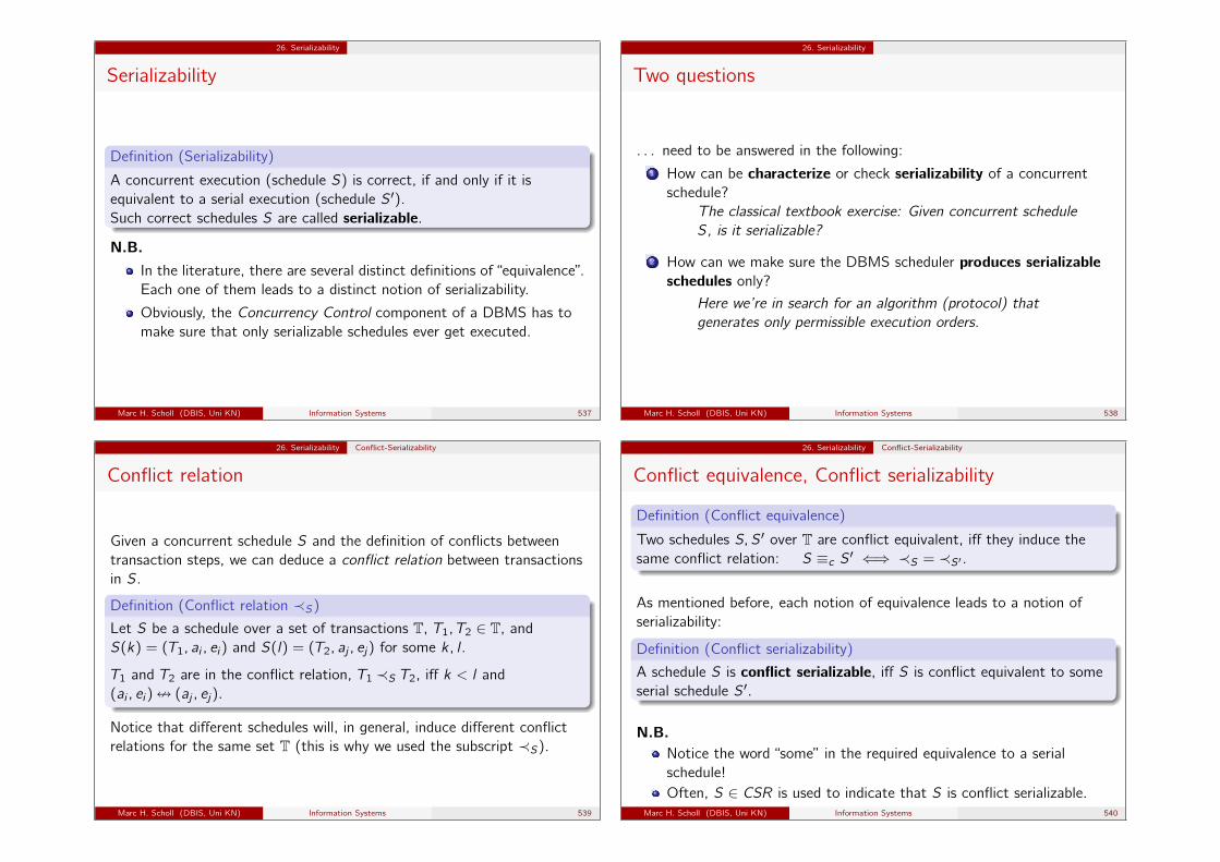
26. Serializability
Serializability
Definition (Serializability)
A concurrent execution (schedule S) is correct, if and only if it isequivalent to a serial execution (schedule S′).Such correct schedules S are called serializable.
N.B.In the literature, there are several distinct definitions of “equivalence”.Each one of them leads to a distinct notion of serializability.
Obviously, the Concurrency Control component of a DBMS has tomake sure that only serializable schedules ever get executed.
Marc H. Scholl (DBIS, Uni KN) Information Systems 537
26. Serializability
Two questions
. . . need to be answered in the following:1 How can be characterize or check serializability of a concurrent
schedule?The classical textbook exercise: Given concurrent scheduleS, is it serializable?
2 How can we make sure the DBMS scheduler produces serializableschedules only?
Here we’re in search for an algorithm (protocol) thatgenerates only permissible execution orders.
Marc H. Scholl (DBIS, Uni KN) Information Systems 538
26. Serializability Conflict-Serializability
Conflict relation
Given a concurrent schedule S and the definition of conflicts betweentransaction steps, we can deduce a conflict relation between transactionsin S.
Definition (Conflict relation ≺S)Let S be a schedule over a set of transactions T, T1, T2 ∈ T, andS(k) = (T1, ai , ei) and S(l) = (T2, aj , ej) for some k, l .
T1 and T2 are in the conflict relation, T1 ≺S T2, iff k < l and(ai , ei) = (aj , ej).
Notice that different schedules will, in general, induce different conflictrelations for the same set T (this is why we used the subscript ≺S).
Marc H. Scholl (DBIS, Uni KN) Information Systems 539
26. Serializability Conflict-Serializability
Conflict equivalence, Conflict serializability
Definition (Conflict equivalence)
Two schedules S, S′ over T are conflict equivalent, iff they induce thesame conflict relation: S ≡c S′ ⇐⇒ ≺S = ≺S′ .
As mentioned before, each notion of equivalence leads to a notion ofserializability:
Definition (Conflict serializability)
A schedule S is conflict serializable, iff S is conflict equivalent to someserial schedule S′.
N.B.Notice the word “some” in the required equivalence to a serialschedule!Often, S ∈ CSR is used to indicate that S is conflict serializable.
Marc H. Scholl (DBIS, Uni KN) Information Systems 540
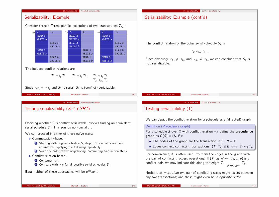
26. Serializability Conflict-Serializability
Serializability: Example
Consider three different parallel executions of two transactions T1,2:
S1 T1 T2
READ a
WRITE a
READ a
WRITE a
READ b
WRITE b
READ b
WRITE b
S2 T1 T2
READ a
WRITE a
READ b
WRITE b
READ a
WRITE a
READ b
WRITE b
S3 T1 T2
READ a
WRITE a
READ a
WRITE a
READ b
WRITE b
READ b
WRITE b
The induced conflict relations are:
T1 ≺S1T2 T1 ≺S2
T2 T1 ≺S3T2
T2 ≺S3T1
Since ≺S1= ≺S2
and S2 is serial, S1 is (conflict) serializable.
Marc H. Scholl (DBIS, Uni KN) Information Systems 541
26. Serializability Conflict-Serializability
Serializability: Example (cont’d)
The conflict relation of the other serial schedule S4 is
T2 ≺S4T1 .
Since obviously ≺S36= ≺S2
and ≺S36= ≺S4
we can conclude that S3 isnot serializable.
Marc H. Scholl (DBIS, Uni KN) Information Systems 542
26. Serializability Conflict-Serializability
Testing serializability (S ∈ CSR?)
Deciding whether S is conflict serializable involves finding an equivalentserial schedule S′. This sounds non-trivial . . .
We can proceed in either of these naïve ways:Commutativity-based:
1 Starting with original schedule S, stop if S is serial or no morealternatives, applying the following repeatedly:
2 Swap the order of two neighboring, commuting transaction steps.
Conflict relation-based:1 Construct ≺S.2 Compare with ≺S′ for all possible serial schedules S′.
But: neither of these approaches will be efficient.
Marc H. Scholl (DBIS, Uni KN) Information Systems 543
26. Serializability Conflict-Serializability
Testing serializability (1)
We can depict the conflict relation for a schedule as a (directed) graph.
Definition (Precedence graph)
For a schedule S over T with conflict relation ≺S define the precedencegraph as G(S) = (N,E):
The nodes of the graph are the transaction in S: N = T.Edges connect conflicting transactions: (Ti , Tj) ∈ E ⇐⇒ Ti ≺S Tj .
For convenience, it is often useful to mark the edges in the graph withthe pair of conflicting access operations. If (Ti , ak , e) = (Tj , al , e) is aconflict pair, we may indicate this along the edge: Ti −−−−−−−→
ak(e)<al (e)Tj .
Notice that more than one pair of conflicting steps might exists betweenany two transactions; and these might even be in opposite order.
Marc H. Scholl (DBIS, Uni KN) Information Systems 544
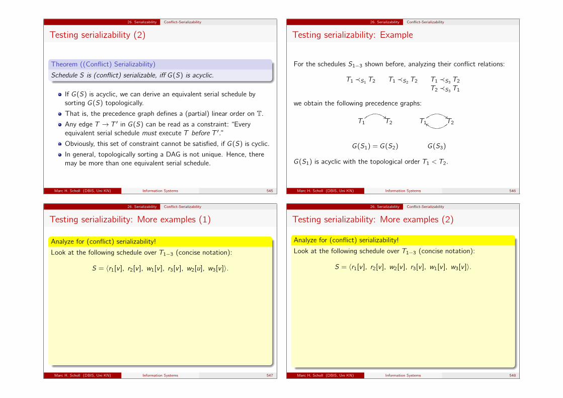
26. Serializability Conflict-Serializability
Testing serializability (2)
Theorem ((Conflict) Serializability)
Schedule S is (conflict) serializable, iff G(S) is acyclic.
If G(S) is acyclic, we can derive an equivalent serial schedule bysorting G(S) topologically.
That is, the precedence graph defines a (partial) linear order on T.Any edge T → T ′ in G(S) can be read as a constraint: “Everyequivalent serial schedule must execute T before T ′.”Obviously, this set of constraint cannot be satisfied, if G(S) is cyclic.
In general, topologically sorting a DAG is not unique. Hence, theremay be more than one equivalent serial schedule.
Marc H. Scholl (DBIS, Uni KN) Information Systems 545
26. Serializability Conflict-Serializability
Testing serializability: Example
For the schedules S1−3 shown before, analyzing their conflict relations:
T1 ≺S1T2 T1 ≺S2
T2 T1 ≺S3T2
T2 ≺S3T1
we obtain the following precedence graphs:
T1 T2""
G(S1) = G(S2)
T1 T2""
bb
G(S3)
G(S1) is acyclic with the topological order T1 < T2.
Marc H. Scholl (DBIS, Uni KN) Information Systems 546
26. Serializability Conflict-Serializability
Testing serializability: More examples (1)
Analyze for (conflict) serializability!
Look at the following schedule over T1−3 (concise notation):
S = 〈r1[v ], r2[v ], w1[v ], r3[v ], w2[u], w3[v ]〉.
Conflicts between transaction steps:r1[v ] < w3[v ] =⇒ T1 → T3 ∈ Er2[v ] < w1[v ] =⇒ T2 → T1 ∈ Er2[v ] < w3[v ] =⇒ T2 → T3 ∈ Ew1[v ] < r3[v ] =⇒ T1 → T3 ∈ Ew1[v ] < w3[v ] =⇒ T1 → T3 ∈ E
Precedence graph G(S):
T1
T3T2
Graph G(S) is acyclic, hence S is serializable.Equivalent serial schedule: T2 < T1 < T3.
Marc H. Scholl (DBIS, Uni KN) Information Systems 547
26. Serializability Conflict-Serializability
Testing serializability: More examples (2)
Analyze for (conflict) serializability!
Look at the following schedule over T1−3 (concise notation):
S = 〈r1[v ], r2[v ], w2[v ], r3[v ], w1[v ], w3[v ]〉.
Conflicts between transaction steps:a) r1[v ] < w2[v ] =⇒ T1 → T2 ∈ Eb) r2[v ] < w1[v ] =⇒ T2 → T1 ∈ Ec) w2[v ] < r3[v ] =⇒ T2 → T3 ∈ Ed) r3[v ] < w1[v ] =⇒ T3 → T1 ∈ Ee) w1[v ] < w3[v ] =⇒ T1 → T3 ∈ E
Precedence graphG(S):
T2
T1
a)
b)
T3c)
d)
e)
Graph G(S) is cyclic, hence S is not serializable.
Marc H. Scholl (DBIS, Uni KN) Information Systems 548

27. Locking Protocols Locking Objects
Concurrency Control
A concurrency control protocol is an algorithm (or set of rules), appliedby the DBMS scheduler so as to produce only serializable schedules.
transactions
scheduler
TransactionManager
BOT /EOTcommit(s)abort(s)active(s)trans(s)
Data Manager
input schedule
serializable output schedule s
database
Marc H. Scholl (DBIS, Uni KN) Information Systems 549
27. Locking Protocols Locking Objects
Concurrency Control protocols
DBMS scheduler can implement a vast variety of protocols to guarantee(different notions of) serializability.
Pessimistic CC: starts from the assumption that conflicts do occur,need to be taken care of, and non-serializable schedules have to beavoided by proper precautions.Optimistic CC: starts from the assumption that while conflicts dooccur, they are rather rare; hence expensive precautions should beavoided, at the cost of an occasional transaction abort (& restart).
A long-lasting rivalry between the two cannot really be decided in fullgenerality. Characteristics of the application can make the one or theother more efficient.
In this course . . .We will concentrate on pessimistic CC, particularly on locking protocols.
Marc H. Scholl (DBIS, Uni KN) Information Systems 550
27. Locking Protocols Locking Objects
Locking protocols
The basic idea behind locking protocols is simple:1 before a transaction can access a data item, it needs to acquire a
lock,2 once (and only if) the necessary lock has been granted, the
transaction may operate on the data element,3 when the data element is no longer needed, the lock is freed.4 If a requested lock can not be granted, the requesting transaction is
put in a wait queue.
If the transaction manager (CC component) never grants locks forconflicting operations, this can be used to serialize schedules.
Trivial caseThe most simple locking protocol manages exactly one lock. Alltransactions have to acquire this lock upon start and release it uponcompletion. This yields serial schedules only.
Marc H. Scholl (DBIS, Uni KN) Information Systems 551
27. Locking Protocols Locking Objects
Lockable objects
To increase the potential for concurrency, typical DBMSs support a largenumber of locks, one for each object at a certain level of dataabstraction. Possible lock granularities include
Database tables
Rows of database tables
Column values of tuples in database tables
Entries in auxiliary internal data structures (such as indexes)
Pages/blocks of the underlying storage management
Typically, CC provides locking at only one (or a few) level(s) ofgranularity.
Marc H. Scholl (DBIS, Uni KN) Information Systems 552
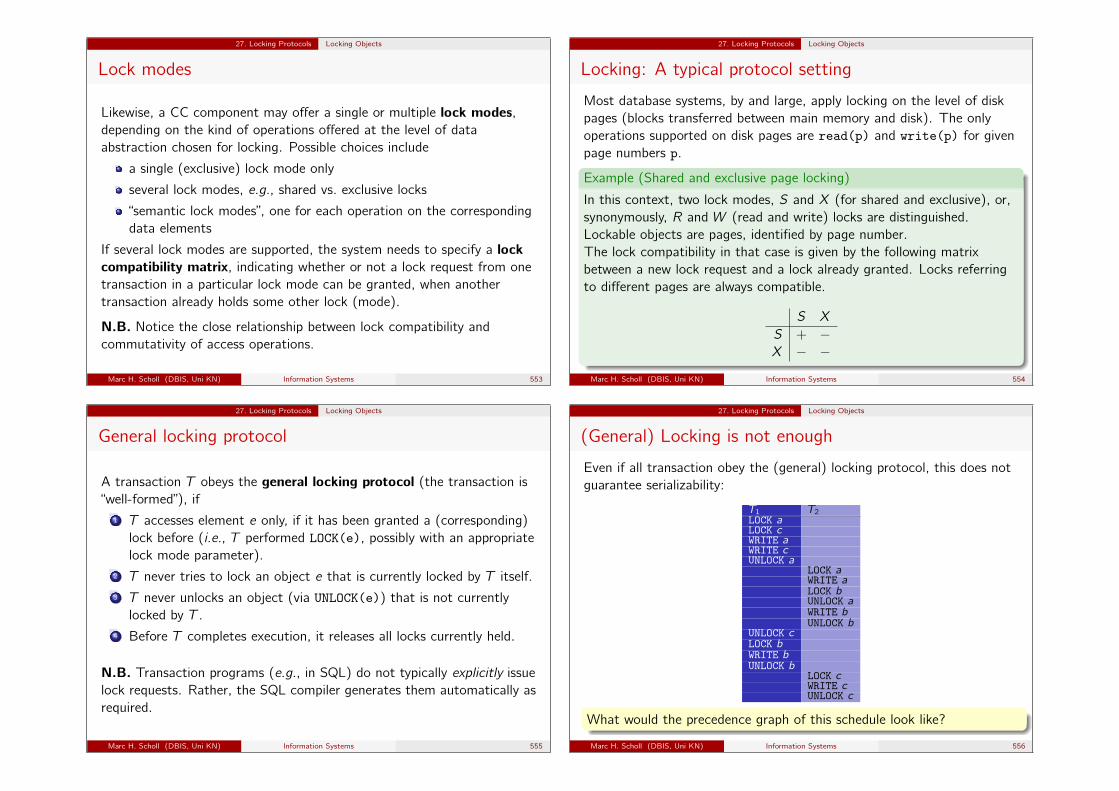
27. Locking Protocols Locking Objects
Lock modes
Likewise, a CC component may offer a single or multiple lock modes,depending on the kind of operations offered at the level of dataabstraction chosen for locking. Possible choices include
a single (exclusive) lock mode only
several lock modes, e.g., shared vs. exclusive locks
“semantic lock modes”, one for each operation on the correspondingdata elements
If several lock modes are supported, the system needs to specify a lockcompatibility matrix, indicating whether or not a lock request from onetransaction in a particular lock mode can be granted, when anothertransaction already holds some other lock (mode).
N.B. Notice the close relationship between lock compatibility andcommutativity of access operations.
Marc H. Scholl (DBIS, Uni KN) Information Systems 553
27. Locking Protocols Locking Objects
Locking: A typical protocol setting
Most database systems, by and large, apply locking on the level of diskpages (blocks transferred between main memory and disk). The onlyoperations supported on disk pages are read(p) and write(p) for givenpage numbers p.
Example (Shared and exclusive page locking)
In this context, two lock modes, S and X (for shared and exclusive), or,synonymously, R and W (read and write) locks are distinguished.Lockable objects are pages, identified by page number.The lock compatibility in that case is given by the following matrixbetween a new lock request and a lock already granted. Locks referringto different pages are always compatible.
S X
S + −X − −
Marc H. Scholl (DBIS, Uni KN) Information Systems 554
27. Locking Protocols Locking Objects
General locking protocol
A transaction T obeys the general locking protocol (the transaction is“well-formed”), if
1 T accesses element e only, if it has been granted a (corresponding)lock before (i.e., T performed LOCK(e), possibly with an appropriatelock mode parameter).
2 T never tries to lock an object e that is currently locked by T itself.3 T never unlocks an object (via UNLOCK(e)) that is not currently
locked by T .4 Before T completes execution, it releases all locks currently held.
N.B. Transaction programs (e.g., in SQL) do not typically explicitly issuelock requests. Rather, the SQL compiler generates them automatically asrequired.
Marc H. Scholl (DBIS, Uni KN) Information Systems 555
27. Locking Protocols Locking Objects
(General) Locking is not enough
Even if all transaction obey the (general) locking protocol, this does notguarantee serializability:
T1 T2LOCK aLOCK cWRITE aWRITE cUNLOCK a
LOCK aWRITE aLOCK bUNLOCK aWRITE bUNLOCK b
UNLOCK cLOCK bWRITE bUNLOCK b
LOCK cWRITE cUNLOCK c
What would the precedence graph of this schedule look like?
Marc H. Scholl (DBIS, Uni KN) Information Systems 556
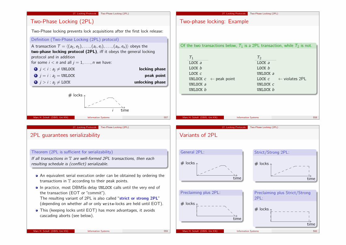
27. Locking Protocols Two-Phase Locking (2PL)
Two-Phase Locking (2PL)
Two-Phase locking prevents lock acquisitions after the first lock release:
Definition (Two-Phase Locking (2PL) protocol)
A transaction T = 〈(a1, e1), . . . , (ai , ei), . . . , (an, en)〉 obeys thetwo-phase locking protocol (2PL), iff it obeys the general lockingprotocol and in additionfor some i < n and all j = 1, . . . , n we have:
1 j < i : aj 6= UNLOCK locking phase2 j = i : aj = UNLOCK peak point3 j > i : aj 6= LOCK unlocking phase
OO
//
i
lllllll
__
@@
@@
time
# locks
Marc H. Scholl (DBIS, Uni KN) Information Systems 557
27. Locking Protocols Two-Phase Locking (2PL)
Two-phase locking: Example
Of the two transactions below, T1 is a 2PL transaction, while T2 is not.
T1LOCK a
LOCK b
LOCK c
UNLOCK c ← peak pointUNLOCK a
UNLOCK b
T2LOCK a
LOCK b
UNLOCK a
LOCK c ← violates 2PLUNLOCK c
UNLOCK b
Marc H. Scholl (DBIS, Uni KN) Information Systems 558
27. Locking Protocols Two-Phase Locking (2PL)
2PL guarantees serializability
Theorem (2PL is sufficient for serializability)
If all transactions in T are well-formed 2PL transactions, then eachresulting schedule is (conflict) serializable.
An equivalent serial execution order can be obtained by ordering thetransactions in T according to their peak points.
In practice, most DBMSs delay UNLOCK calls until the very end ofthe transaction (EOT or “commit”).The resulting variant of 2PL is also called “strict or strong 2PL”(depending on whether all or only write-locks are held until EOT).
This (keeping locks until EOT) has more advantages, it avoidscascading aborts (see below).
Marc H. Scholl (DBIS, Uni KN) Information Systems 559
27. Locking Protocols Two-Phase Locking (2PL)
Variants of 2PL
General 2PL:
OO
//
lllllll
__
@@
@@
time
# locks
Strict/Strong 2PL:
OO
//
lllllll
____
���
time
# locks
Preclaiming plus 2PL:
OO
//
���
________
@@
@@
time
# locks
Preclaiming plus Strict/Strong2PL:
OO
//
���
__________
���
time
# locks
Marc H. Scholl (DBIS, Uni KN) Information Systems 560
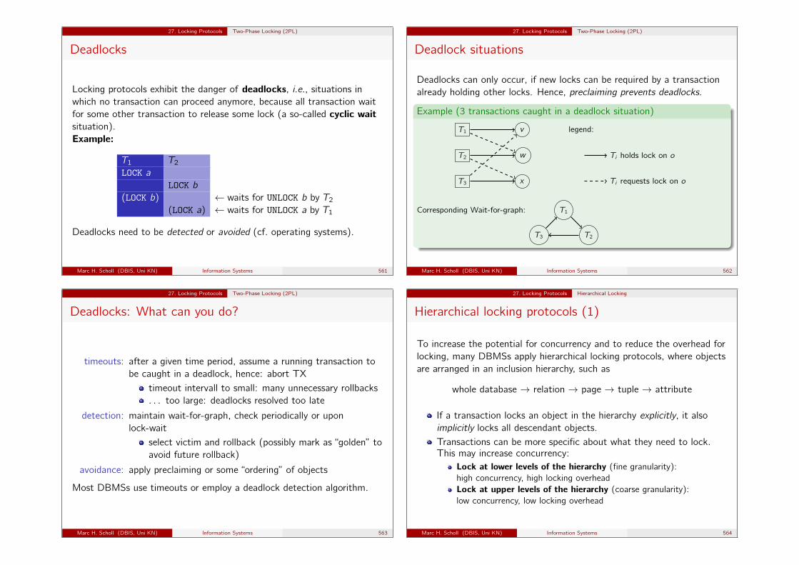
27. Locking Protocols Two-Phase Locking (2PL)
Deadlocks
Locking protocols exhibit the danger of deadlocks, i.e., situations inwhich no transaction can proceed anymore, because all transaction waitfor some other transaction to release some lock (a so-called cyclic waitsituation).Example:
T1 T2LOCK a
LOCK b
(LOCK b) ← waits for UNLOCK b by T2(LOCK a) ← waits for UNLOCK a by T1
Deadlocks need to be detected or avoided (cf. operating systems).
Marc H. Scholl (DBIS, Uni KN) Information Systems 561
27. Locking Protocols Two-Phase Locking (2PL)
Deadlock situations
Deadlocks can only occur, if new locks can be required by a transactionalready holding other locks. Hence, preclaiming prevents deadlocks.
Example (3 transactions caught in a deadlock situation)
T1
T2
T3
v
w
x
legend:
Ti holds lock on o
Ti requests lock on o
Corresponding Wait-for-graph: T1
T2T3
Marc H. Scholl (DBIS, Uni KN) Information Systems 562
27. Locking Protocols Two-Phase Locking (2PL)
Deadlocks: What can you do?
timeouts: after a given time period, assume a running transaction tobe caught in a deadlock, hence: abort TX
timeout intervall to small: many unnecessary rollbacks. . . too large: deadlocks resolved too late
detection: maintain wait-for-graph, check periodically or uponlock-wait
select victim and rollback (possibly mark as “golden” toavoid future rollback)
avoidance: apply preclaiming or some “ordering” of objects
Most DBMSs use timeouts or employ a deadlock detection algorithm.
Marc H. Scholl (DBIS, Uni KN) Information Systems 563
27. Locking Protocols Hierarchical Locking
Hierarchical locking protocols (1)
To increase the potential for concurrency and to reduce the overhead forlocking, many DBMSs apply hierarchical locking protocols, where objectsare arranged in an inclusion hierarchy, such as
whole database → relation → page → tuple → attribute
If a transaction locks an object in the hierarchy explicitly, it alsoimplicitly locks all descendant objects.Transactions can be more specific about what they need to lock.This may increase concurrency:
Lock at lower levels of the hierarchy (fine granularity):high concurrency, high locking overheadLock at upper levels of the hierarchy (coarse granularity):low concurrency, low locking overhead
Marc H. Scholl (DBIS, Uni KN) Information Systems 564
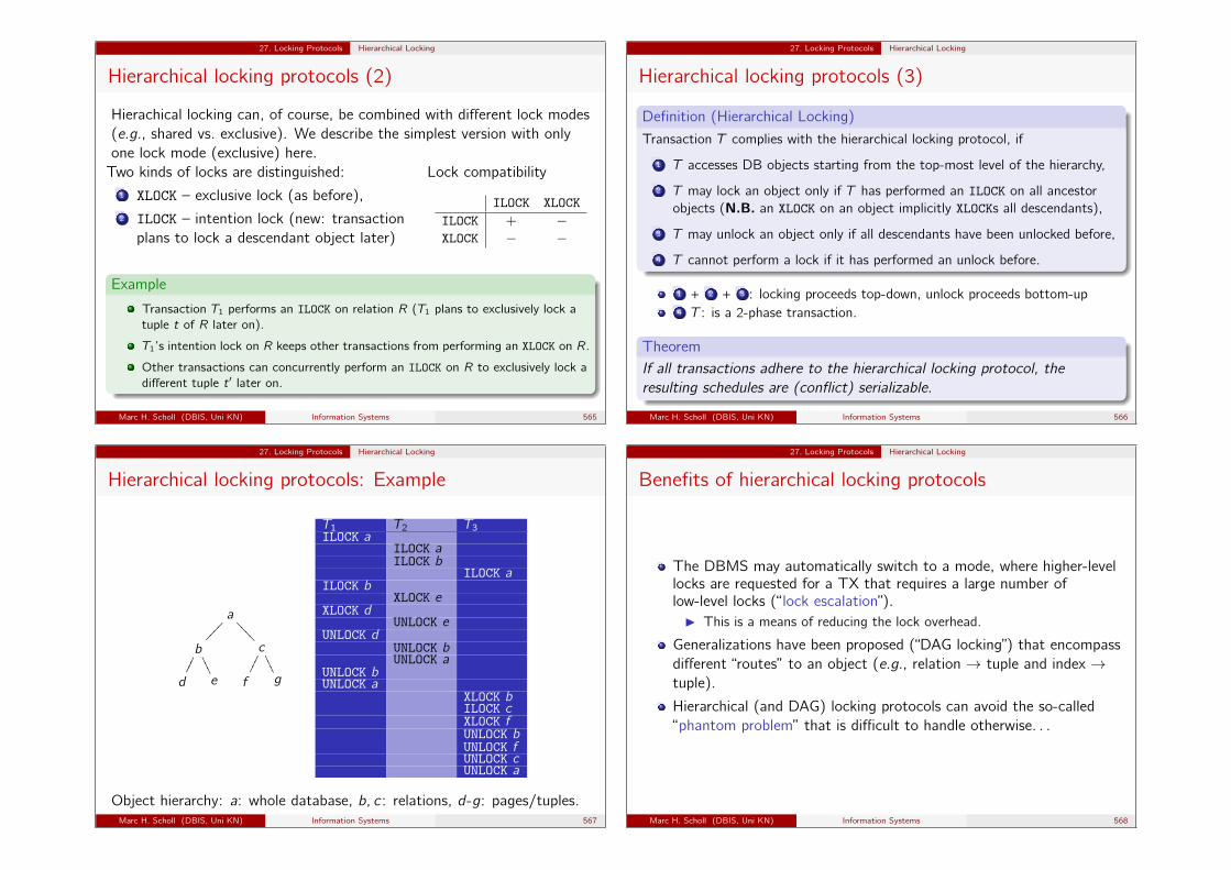
27. Locking Protocols Hierarchical Locking
Hierarchical locking protocols (2)
Hierachical locking can, of course, be combined with different lock modes(e.g., shared vs. exclusive). We describe the simplest version with onlyone lock mode (exclusive) here.Two kinds of locks are distinguished:
1 XLOCK – exclusive lock (as before),2 ILOCK – intention lock (new: transaction
plans to lock a descendant object later)
Lock compatibility
ILOCK XLOCK
ILOCK + −XLOCK − −
Example
Transaction T1 performs an ILOCK on relation R (T1 plans to exclusively lock atuple t of R later on).
T1’s intention lock on R keeps other transactions from performing an XLOCK on R.
Other transactions can concurrently perform an ILOCK on R to exclusively lock adifferent tuple t ′ later on.
Marc H. Scholl (DBIS, Uni KN) Information Systems 565
27. Locking Protocols Hierarchical Locking
Hierarchical locking protocols (3)
Definition (Hierarchical Locking)
Transaction T complies with the hierarchical locking protocol, if
1 T accesses DB objects starting from the top-most level of the hierarchy,
2 T may lock an object only if T has performed an ILOCK on all ancestorobjects (N.B. an XLOCK on an object implicitly XLOCKs all descendants),
3 T may unlock an object only if all descendants have been unlocked before,
4 T cannot perform a lock if it has performed an unlock before.
1 + 2 + 3 : locking proceeds top-down, unlock proceeds bottom-up4 T : is a 2-phase transaction.
TheoremIf all transactions adhere to the hierarchical locking protocol, theresulting schedules are (conflict) serializable.
Marc H. Scholl (DBIS, Uni KN) Information Systems 566
27. Locking Protocols Hierarchical Locking
Hierarchical locking protocols: Example
a
b����
d���
e
... c>>>>
f���
g
...
T1 T2 T3ILOCK a
ILOCK aILOCK b
ILOCK aILOCK b
XLOCK eXLOCK d
UNLOCK eUNLOCK d
UNLOCK bUNLOCK a
UNLOCK bUNLOCK a
XLOCK bILOCK cXLOCK fUNLOCK bUNLOCK fUNLOCK cUNLOCK a
Object hierarchy: a: whole database, b, c : relations, d-g: pages/tuples.Marc H. Scholl (DBIS, Uni KN) Information Systems 567
27. Locking Protocols Hierarchical Locking
Benefits of hierarchical locking protocols
The DBMS may automatically switch to a mode, where higher-levellocks are requested for a TX that requires a large number oflow-level locks (“lock escalation”).I This is a means of reducing the lock overhead.
Generalizations have been proposed (“DAG locking”) that encompassdifferent “routes” to an object (e.g., relation → tuple and index →tuple).
Hierarchical (and DAG) locking protocols can avoid the so-called“phantom problem” that is difficult to handle otherwise. . .
Marc H. Scholl (DBIS, Uni KN) Information Systems 568
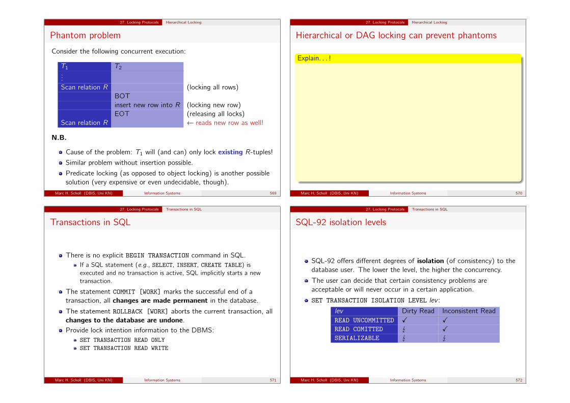
27. Locking Protocols Hierarchical Locking
Phantom problem
Consider the following concurrent execution:
T1 T2...Scan relation R (locking all rows)
BOTinsert new row into R (locking new row)EOT (releasing all locks)
Scan relation R ← reads new row as well!
N.B.
Cause of the problem: T1 will (and can) only lock existing R-tuples!Similar problem without insertion possible.
Predicate locking (as opposed to object locking) is another possiblesolution (very expensive or even undecidable, though).
Marc H. Scholl (DBIS, Uni KN) Information Systems 569
27. Locking Protocols Hierarchical Locking
Hierarchical or DAG locking can prevent phantoms
Explain. . . !
Marc H. Scholl (DBIS, Uni KN) Information Systems 570
27. Locking Protocols Transactions in SQL
Transactions in SQL
There is no explicit BEGIN TRANSACTION command in SQL.If a SQL statement (e.g., SELECT, INSERT, CREATE TABLE) isexecuted and no transaction is active, SQL implicitly starts a newtransaction.
The statement COMMIT [WORK] marks the successful end of atransaction, all changes are made permanent in the database.
The statement ROLLBACK [WORK] aborts the current transaction, allchanges to the database are undone.Provide lock intention information to the DBMS:
SET TRANSACTION READ ONLYSET TRANSACTION READ WRITE
Marc H. Scholl (DBIS, Uni KN) Information Systems 571
27. Locking Protocols Transactions in SQL
SQL-92 isolation levels
SQL-92 offers different degrees of isolation (of consistency) to thedatabase user. The lower the level, the higher the concurrency.
The user can decide that certain consistency problems areacceptable or will never occur in a certain application.
SET TRANSACTION ISOLATION LEVEL lev :
lev Dirty Read Inconsistent ReadREAD UNCOMMITTED X XREAD COMITTED XSERIALIZABLE
Marc H. Scholl (DBIS, Uni KN) Information Systems 572

28. Recovery Failure Classes
Transaction Recovery
A DBMS’s recovery manager is responsible for ensuring atomicity anddurability of transactions. Its main task is to establish a well-defined,consistent database state after
a transaction abort (due to concurrency control or semanticconstraint violation),
a system failure (updates have not been completely written tosecondary storage), or
a disk failure (all updates on disk since the last backup are lost).
Depending on the class of failure, we speak of
transaction,crash, ormedia recovery, resp’ly.
Marc H. Scholl (DBIS, Uni KN) Information Systems 573
28. Recovery Failure Classes
Recovery: Example
Transactions T1, T2, and T3 were already committed before systemcrashed, T4,5 still running.
������������
crash //
time
T5
T4
T3
T2
T1
Durability: ensure that results of T1,2,3 are preserved after restart.Atomicity: need to rollback transactions T4, T5.
Marc H. Scholl (DBIS, Uni KN) Information Systems 574
28. Recovery Transaction Recovery
Transaction recovery (“rollback”/“abort”)
In case a single transaction cannot be completed successfully, its effectsneed to be “wiped out”. Possible reasons for a transaction rollback include
self-initiated UNDO: the transaction program (or the integrity checker)detects a semantic constraint violation, the runtimesystem initiates a runtime exception (e.g., zero-devide orarray out of bounds), or the user interrupts programexecution;
DBMS initiated transaction cancellation: e.g., for concurrency controlreasons or because of a deadlock detection.
Partially executed transactions may not leave any visible effects at all(atomicity): backward recovery (UNDO, backout, rollback).
Marc H. Scholl (DBIS, Uni KN) Information Systems 575
28. Recovery Transaction Recovery
Implementing transaction rollback
How can we implement transaction rollback (UNDO)?Basically, there are two options:
1 Avoid dirty writes.Make sure no transaction writes any updates into the shareddatabase prior to its commit point. Use private workspace copies ofmodified data, if necessary; copy these back into shared DB uponcommit.⇒ Rollback implemented by deleting private workspace copy.
2 Prepare for UNDO of updates.If modified data may (potentially) be written back to shareddatabase by running transaction, save information to reconstruct oldDB state in an UNDO log file. Snapshots of old DB object’s state istypically called a before image (BFIM).⇒ Implement rollback by copying BFIM back into shared database.
Marc H. Scholl (DBIS, Uni KN) Information Systems 576

28. Recovery Transaction Recovery
Write-ahead log principle (WAL)
In the second case (modified data may end up in the DB before EOT),the DBMS must guarantee that
WAL principle
before a write of an updated page from the buffer pool to the databaseis initiated, the corresponding UNDO information, e.g., the BFIM, hasbeen successfully written to the log file.
N.B. this requires a synchronous I/O (with wait for completion) to thelog file!
Marc H. Scholl (DBIS, Uni KN) Information Systems 577
28. Recovery Transaction Recovery
Non-recoverable executions: Reads-from relationship
Consider the “reads-from” relationship between transactions describedinformally as:
Tj reads o from Ti
//
time
Tj
TiWRITE(o)
READ(o)
�
�
������
︷ ︸︸ ︷no Tk writes o
Marc H. Scholl (DBIS, Uni KN) Information Systems 578
28. Recovery Transaction Recovery
Non-recoverable executions: Cascading rollback
In some situations, properties atomicity and durability may contradict!
��������
crash //
time
T3
T2
T1READ(x) READ(y)
READ(x) WRITE(y)
WRITE(x)
FF
66llll
=={{
{{
Recovery needs to roll back T3 (atomicity).
T1 and T2 both read from T3 ⇒ also roll back T1,2 for concistency.
But T1,2 were successfully committed before the crash(contradicts durability)!
�Marc H. Scholl (DBIS, Uni KN) Information Systems 579
28. Recovery Transaction Recovery
Cascading rollback
Problem:Successfully committed transactions may need to be rolled back in acascading fashion. This violates durability.
Solution:A writing transaction T releases its intermediate results not beforeT can guarantee its successful completion (isolation).
In practice:The writing transaction T holds all write locks until the COMMITstatement is executed (“Strict 2PL”, see above).
In general, schedulers avoiding the cascading rollback problem are said toproduce “ACA” (avoids cascading abort) executions.
Marc H. Scholl (DBIS, Uni KN) Information Systems 580
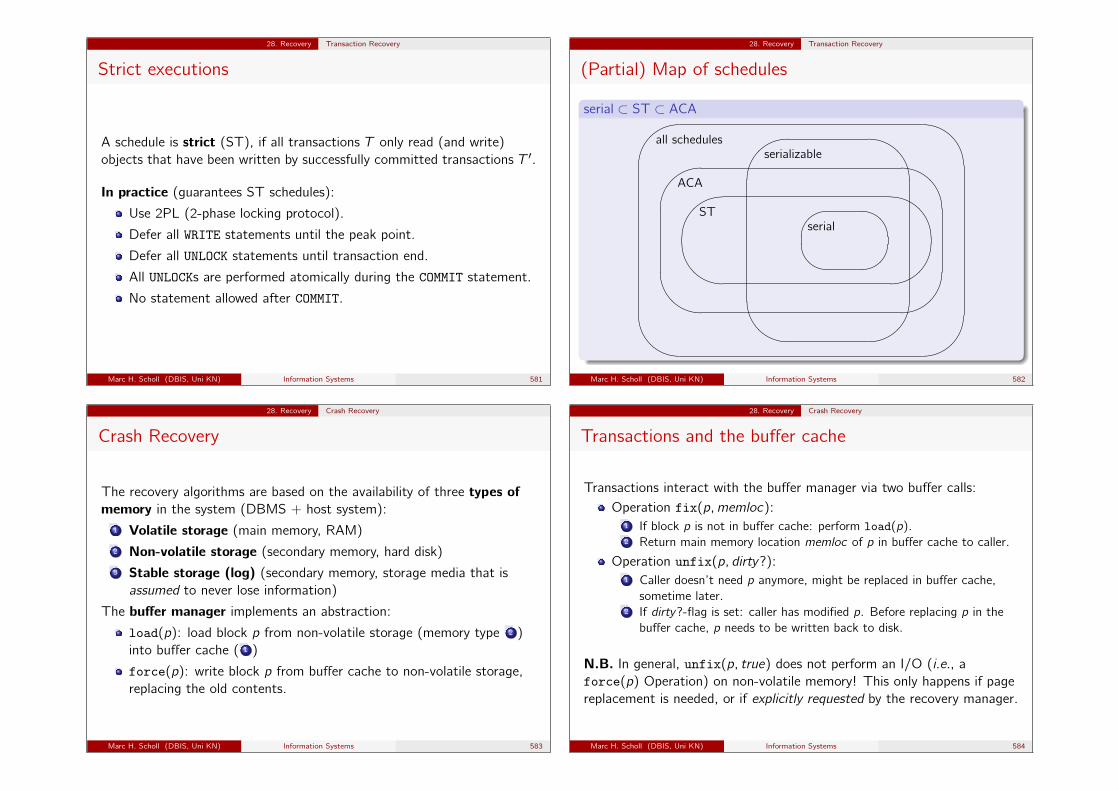
28. Recovery Transaction Recovery
Strict executions
A schedule is strict (ST), if all transactions T only read (and write)objects that have been written by successfully committed transactions T ′.
In practice (guarantees ST schedules):
Use 2PL (2-phase locking protocol).
Defer all WRITE statements until the peak point.
Defer all UNLOCK statements until transaction end.
All UNLOCKs are performed atomically during the COMMIT statement.
No statement allowed after COMMIT.
Marc H. Scholl (DBIS, Uni KN) Information Systems 581
28. Recovery Transaction Recovery
(Partial) Map of schedules
serial ⊂ ST ⊂ ACA
�~ }|
xy z{
�~ }|
xy z{
�~ }|
xy z{�~ }|xy z{gf ed`a bc
all schedulesserializable
ACA
STserial
Marc H. Scholl (DBIS, Uni KN) Information Systems 582
28. Recovery Crash Recovery
Crash Recovery
The recovery algorithms are based on the availability of three types ofmemory in the system (DBMS + host system):
1 Volatile storage (main memory, RAM)2 Non-volatile storage (secondary memory, hard disk)3 Stable storage (log) (secondary memory, storage media that is
assumed to never lose information)
The buffer manager implements an abstraction:
load(p): load block p from non-volatile storage (memory type 2 )into buffer cache ( 1 )
force(p): write block p from buffer cache to non-volatile storage,replacing the old contents.
Marc H. Scholl (DBIS, Uni KN) Information Systems 583
28. Recovery Crash Recovery
Transactions and the buffer cache
Transactions interact with the buffer manager via two buffer calls:Operation fix(p,memloc):
1 If block p is not in buffer cache: perform load(p).2 Return main memory location memloc of p in buffer cache to caller.
Operation unfix(p, dirty ?):1 Caller doesn’t need p anymore, might be replaced in buffer cache,
sometime later.2 If dirty ?-flag is set: caller has modified p. Before replacing p in the
buffer cache, p needs to be written back to disk.
N.B. In general, unfix(p, true) does not perform an I/O (i.e., aforce(p) Operation) on non-volatile memory! This only happens if pagereplacement is needed, or if explicitly requested by the recovery manager.
Marc H. Scholl (DBIS, Uni KN) Information Systems 584

28. Recovery Crash Recovery
System crash: Example
(fix(pa, ·) means: place block containing object a into cache.)
T10 fix(pa, ·)
a← a − 501 unfix(pa, true)
fix(pb, ·)b ← b + 50
2 unfix(pb, true)
Before 0 : buffer diska = 1000
b = 2000
After 1 : buffera = 950
diska = 1000
b = 2000
After 2 : buffera = 950
b = 2050
diska = 1000
b = 2000
Crash Marc H. Scholl (DBIS, Uni KN) Information Systems 585
28. Recovery Crash Recovery
System crash
Possible causes for inconsistent database states after a system crash:1 Updates by COMMITted transaction Tc are in buffer cache, but have
not been written to non-volatile storage yet.
Recovery manager needs to perform REDO for transaction Tc .
2 Updates of partial transaction Tp (COMMIT has not been reached yet)have already been written to non-volatile storage.
Recovery manager needs to perform UNDO for transaction Tp.
After a system crash, the DBMS needs to identify “winner” (type Tc) and“loser” (type Tp) transactions to react properly.
N.B. System crashes can occur during recovery!⇒ UNDO and REDO need to be idempotent:
UNDO(UNDO(T )) = UNDO(T )
REDO(REDO(T )) = REDO(T )
Marc H. Scholl (DBIS, Uni KN) Information Systems 586
28. Recovery Crash Recovery
DO/UNDO/REDO
old value // DO //
''PPPPPPPPPPPP new value
log protocol entry
new(?) value //____ UNDO // old value
log protocol entry
66nnnnnnnnnnnnn
old(?) value //____ REDO // new value
log protocol entry
66nnnnnnnnnnnnn
Marc H. Scholl (DBIS, Uni KN) Information Systems 587
28. Recovery Crash Recovery
Recovery after system crash: Example
������������
crash //
time
T4
T3
T2
T1
oo_ _ _ _ _ _ _ _ _ _ _ _ _ _ _ _ _ _ _ _UNDO
//_______ REDO
//________ REDO
//____________ REDO
Actions to be performed by recovery algorithm:UNDO(T4),REDO(T1), REDO(T2), REDO(T3)
Restart T4.Marc H. Scholl (DBIS, Uni KN) Information Systems 588
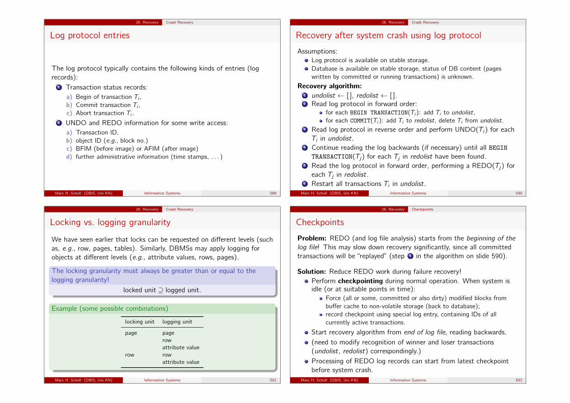
28. Recovery Crash Recovery
Log protocol entries
The log protocol typically contains the following kinds of entries (logrecords):
1 Transaction status records:a) Begin of transaction Ti ,b) Commit transaction Ti ,c) Abort transaction Ti .
2 UNDO and REDO information for some write access:a) Transaction ID,b) object ID (e.g., block no.)c) BFIM (before image) or AFIM (after image)d) further administrative information (time stamps, . . . )
Marc H. Scholl (DBIS, Uni KN) Information Systems 589
28. Recovery Crash Recovery
Recovery after system crash using log protocol
Assumptions:Log protocol is available on stable storage.Database is available on stable storage, status of DB content (pageswritten by committed or running transactions) is unknown.
Recovery algorithm:1 undolist ← [ ], redolist ← [ ].2 Read log protocol in forward order:
for each BEGIN TRANSACTION(Ti): add Ti to undolist,for each COMMIT(Ti): add Ti to redolist, delete Ti from undolist.
3 Read log protocol in reverse order and perform UNDO(Ti) for eachTi in undolist.
4 Continue reading the log backwards (if necessary) until all BEGINTRANSACTION(Tj) for each Tj in redolist have been found.
5 Read the log protocol in forward order, performing a REDO(Tj) foreach Tj in redolist.
6 Restart all transactions Ti in undolist.Marc H. Scholl (DBIS, Uni KN) Information Systems 590
28. Recovery Crash Recovery
Locking vs. logging granularity
We have seen earlier that locks can be requested on different levels (suchas, e.g., row, pages, tables). Similarly, DBMSs may apply logging forobjects at different levels (e.g., attribute values, rows, pages).
The locking granularity must always be greater than or equal to thelogging granularity!
locked unit ⊇ logged unit.
Example (some possible combinations)
locking unit logging unit
page pagerowattribute value
row rowattribute value
Marc H. Scholl (DBIS, Uni KN) Information Systems 591
28. Recovery Checkpoints
Checkpoints
Problem: REDO (and log file analysis) starts from the beginning of thelog file! This may slow down recovery significantly, since all committedtransactions will be “replayed” (step 5 in the algorithm on slide 590).
Solution: Reduce REDO work during failure recovery!Perform checkpointing during normal operation. When system isidle (or at suitable points in time):
Force (all or some, committed or also dirty) modified blocks frombuffer cache to non-volatile storage (back to database);record checkpoint using special log entry, containing IDs of allcurrently active transactions.
Start recovery algorithm from end of log file, reading backwards.(need to modify recognition of winner and loser transactions(undolist, redolist) correspondingly.)Processing of REDO log records can start from latest checkpointbefore system crash.
Marc H. Scholl (DBIS, Uni KN) Information Systems 592
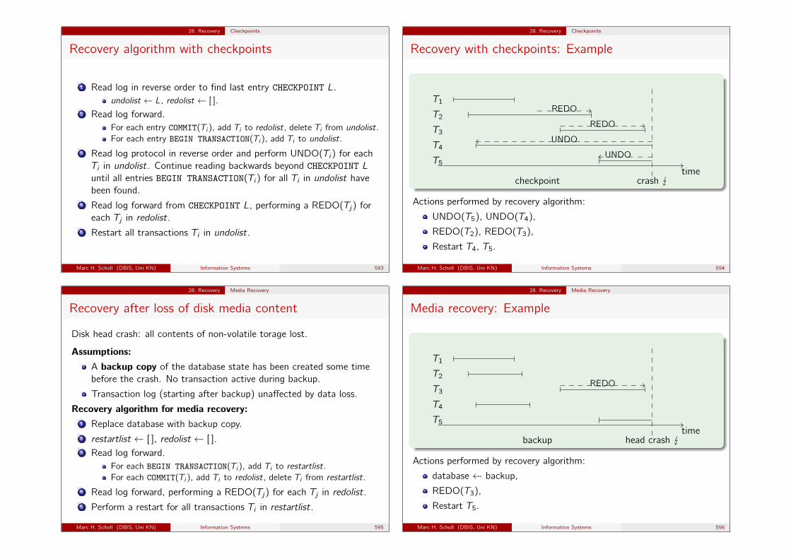
28. Recovery Checkpoints
Recovery algorithm with checkpoints
1 Read log in reverse order to find last entry CHECKPOINT L.undolist ← L, redolist ← [ ].
2 Read log forward.For each entry COMMIT(Ti), add Ti to redolist, delete Ti from undolist.For each entry BEGIN TRANSACTION(Ti), add Ti to undolist.
3 Read log protocol in reverse order and perform UNDO(Ti) for eachTi in undolist. Continue reading backwards beyond CHECKPOINT Luntil all entries BEGIN TRANSACTION(Ti) for all Ti in undolist havebeen found.
4 Read log forward from CHECKPOINT L, performing a REDO(Tj) foreach Tj in redolist.
5 Restart all transactions Ti in undolist.
Marc H. Scholl (DBIS, Uni KN) Information Systems 593
28. Recovery Checkpoints
Recovery with checkpoints: Example
����������
crash checkpoint
//
timeT5
T4
T3
T2
T1
oo_ _ _ _ _ _ _ _ _ _ _ _ _ _ _ _ _ _ _ _UNDO
oo_ _ _ _ _ _UNDO
//______ REDO
//__________ REDO
Actions performed by recovery algorithm:
UNDO(T5), UNDO(T4),
REDO(T2), REDO(T3),
Restart T4, T5.
Marc H. Scholl (DBIS, Uni KN) Information Systems 594
28. Recovery Media Recovery
Recovery after loss of disk media content
Disk head crash: all contents of non-volatile torage lost.
Assumptions:A backup copy of the database state has been created some timebefore the crash. No transaction active during backup.
Transaction log (starting after backup) unaffected by data loss.
Recovery algorithm for media recovery:1 Replace database with backup copy.2 restartlist ← [ ], redolist ← [ ].3 Read log forward.
For each BEGIN TRANSACTION(Ti), add Ti to restartlist.For each COMMIT(Ti), add Ti to redolist, delete Ti from restartlist.
4 Read log forward, performing a REDO(Tj) for each Tj in redolist.5 Perform a restart for all transactions Ti in restartlist.
Marc H. Scholl (DBIS, Uni KN) Information Systems 595
28. Recovery Media Recovery
Media recovery: Example
����������
head crash backup
//
timeT5
T4
T3
T2
T1
//__________ REDO
Actions performed by recovery algorithm:
database ← backup,
REDO(T3),
Restart T5.
Marc H. Scholl (DBIS, Uni KN) Information Systems 596
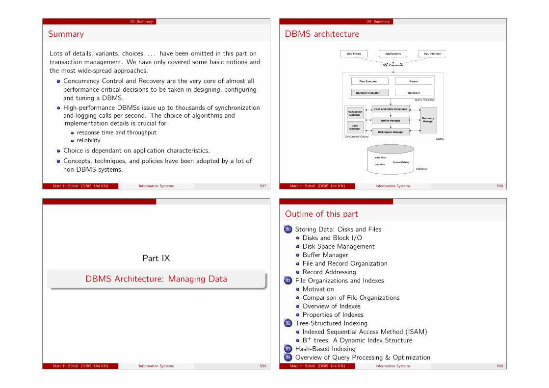
29. Summary
Summary
Lots of details, variants, choices, . . . have been omitted in this part ontransaction management. We have only covered some basic notions andthe most wide-spread approaches.
Concurrency Control and Recovery are the very core of almost allperformance critical decisions to be taken in designing, configuringand tuning a DBMS.High-performance DBMSs issue up to thousands of synchronizationand logging calls per second. The choice of algorithms andimplementation details is crucial for
response time and throughputreliability.
Choice is dependant on application characteristics.
Concepts, techniques, and policies have been adopted by a lot ofnon-DBMS systems.
Marc H. Scholl (DBIS, Uni KN) Information Systems 597
29. Summary
DBMS architecture
Files and Index Structures
Buffer Manager
Disk Space Manager
RecoveryManager
Plan Executor
Operator Evaluator Optimizer
Parser
ApplicationsWeb Forms SQL Interface
SQL Commands
Query Processor
Concurrency ControlDBMS
Database
Index Files
Data FilesSystem Catalog
TransactionManager
LockManager
Marc H. Scholl (DBIS, Uni KN) Information Systems 598
Part IX
DBMS Architecture: Managing Data
Marc H. Scholl (DBIS, Uni KN) Information Systems 599
Outline of this part
30 Storing Data: Disks and FilesDisks and Block I/ODisk Space ManagementBuffer ManagerFile and Record OrganizationRecord Addressing
31 File Organizations and IndexesMotivationComparison of File OrganizationsOverview of IndexesProperties of Indexes
32 Tree-Structured IndexingIndexed Sequential Access Method (ISAM)B+ trees: A Dynamic Index Structure
33 Hash-Based Indexing34 Overview of Query Processing & Optimization
Marc H. Scholl (DBIS, Uni KN) Information Systems 600
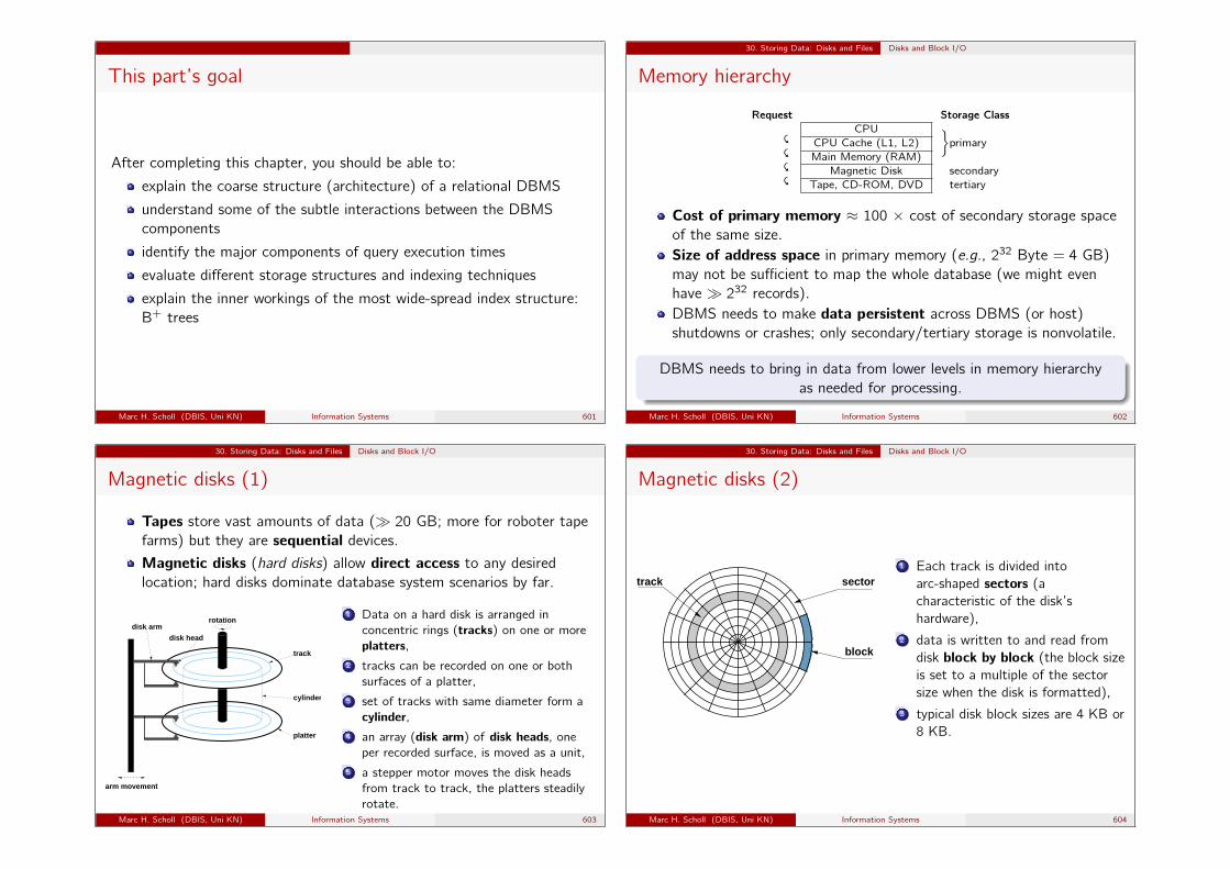
This part’s goal
After completing this chapter, you should be able to:
explain the coarse structure (architecture) of a relational DBMS
understand some of the subtle interactions between the DBMScomponents
identify the major components of query execution times
evaluate different storage structures and indexing techniques
explain the inner workings of the most wide-spread index structure:B+ trees
Marc H. Scholl (DBIS, Uni KN) Information Systems 601
30. Storing Data: Disks and Files Disks and Block I/O
Memory hierarchy
Request Storage Class
&CPU
&CPU Cache (L1, L2)
ffprimary
&Main Memory (RAM)
&Magnetic Disk secondary
Tape, CD-ROM, DVD tertiary
Cost of primary memory ≈ 100 × cost of secondary storage spaceof the same size.Size of address space in primary memory (e.g., 232 Byte = 4 GB)may not be sufficient to map the whole database (we might evenhave � 232 records).DBMS needs to make data persistent across DBMS (or host)shutdowns or crashes; only secondary/tertiary storage is nonvolatile.
DBMS needs to bring in data from lower levels in memory hierarchyas needed for processing.
Marc H. Scholl (DBIS, Uni KN) Information Systems 602
30. Storing Data: Disks and Files Disks and Block I/O
Magnetic disks (1)
Tapes store vast amounts of data (� 20 GB; more for roboter tapefarms) but they are sequential devices.Magnetic disks (hard disks) allow direct access to any desiredlocation; hard disks dominate database system scenarios by far.
arm movement
rotation
platter
cylinder
track
disk head
disk arm
1 Data on a hard disk is arranged inconcentric rings (tracks) on one or moreplatters,
2 tracks can be recorded on one or bothsurfaces of a platter,
3 set of tracks with same diameter form acylinder,
4 an array (disk arm) of disk heads, oneper recorded surface, is moved as a unit,
5 a stepper motor moves the disk headsfrom track to track, the platters steadilyrotate.
Marc H. Scholl (DBIS, Uni KN) Information Systems 603
30. Storing Data: Disks and Files Disks and Block I/O
Magnetic disks (2)
track sector
block
1 Each track is divided intoarc-shaped sectors (acharacteristic of the disk’shardware),
2 data is written to and read fromdisk block by block (the block sizeis set to a multiple of the sectorsize when the disk is formatted),
3 typical disk block sizes are 4 KB or8 KB.
Marc H. Scholl (DBIS, Uni KN) Information Systems 604
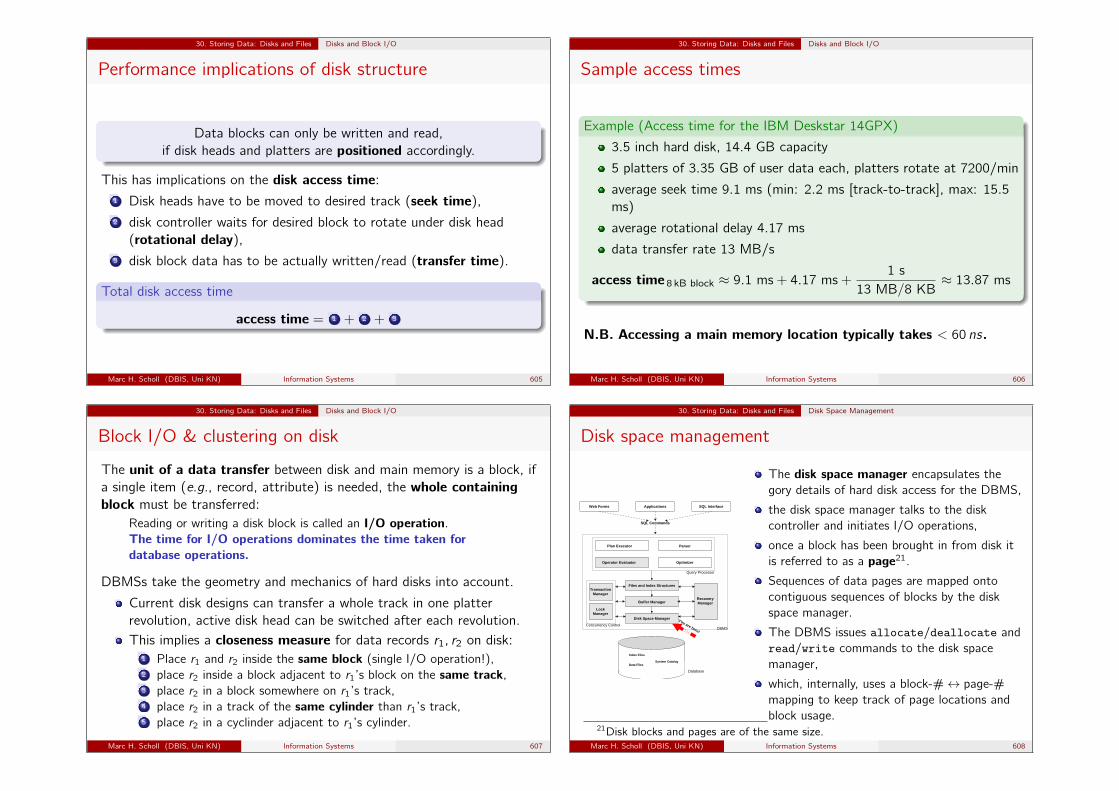
30. Storing Data: Disks and Files Disks and Block I/O
Performance implications of disk structure
Data blocks can only be written and read,if disk heads and platters are positioned accordingly.
This has implications on the disk access time:1 Disk heads have to be moved to desired track (seek time),2 disk controller waits for desired block to rotate under disk head
(rotational delay),3 disk block data has to be actually written/read (transfer time).
Total disk access time
access time = 1 + 2 + 3
Marc H. Scholl (DBIS, Uni KN) Information Systems 605
30. Storing Data: Disks and Files Disks and Block I/O
Sample access times
Example (Access time for the IBM Deskstar 14GPX)
3.5 inch hard disk, 14.4 GB capacity
5 platters of 3.35 GB of user data each, platters rotate at 7200/min
average seek time 9.1 ms (min: 2.2 ms [track-to-track], max: 15.5
ms)
average rotational delay 4.17 ms
data transfer rate 13 MB/s
access time 8 kB block ≈ 9.1 ms + 4.17 ms +1 s
13 MB/8 KB≈ 13.87 ms
N.B. Accessing a main memory location typically takes < 60 ns.
Marc H. Scholl (DBIS, Uni KN) Information Systems 606
30. Storing Data: Disks and Files Disks and Block I/O
Block I/O & clustering on disk
The unit of a data transfer between disk and main memory is a block, ifa single item (e.g., record, attribute) is needed, the whole containingblock must be transferred:
Reading or writing a disk block is called an I/O operation.The time for I/O operations dominates the time taken fordatabase operations.
DBMSs take the geometry and mechanics of hard disks into account.
Current disk designs can transfer a whole track in one platterrevolution, active disk head can be switched after each revolution.This implies a closeness measure for data records r1, r2 on disk:
1 Place r1 and r2 inside the same block (single I/O operation!),2 place r2 inside a block adjacent to r1’s block on the same track,3 place r2 in a block somewhere on r1’s track,4 place r2 in a track of the same cylinder than r1’s track,5 place r2 in a cyclinder adjacent to r1’s cylinder.
Marc H. Scholl (DBIS, Uni KN) Information Systems 607
30. Storing Data: Disks and Files Disk Space Management
Disk space management
You are here!
Files and Index Structures
Buffer Manager
Disk Space Manager
RecoveryManager
Plan Executor
Operator Evaluator Optimizer
Parser
ApplicationsWeb Forms SQL Interface
SQL Commands
Query Processor
Concurrency ControlDBMS
Database
Index Files
Data FilesSystem Catalog
TransactionManager
LockManager
The disk space manager encapsulates thegory details of hard disk access for the DBMS,
the disk space manager talks to the diskcontroller and initiates I/O operations,
once a block has been brought in from disk itis referred to as a page21.Sequences of data pages are mapped ontocontiguous sequences of blocks by the diskspace manager.
The DBMS issues allocate/deallocate andread/write commands to the disk spacemanager,
which, internally, uses a block-#↔ page-#mapping to keep track of page locations andblock usage.
21Disk blocks and pages are of the same size.Marc H. Scholl (DBIS, Uni KN) Information Systems 608

30. Storing Data: Disks and Files Disk Space Management
Keeping track of free blocks
During database (or table) creation it is likely that blocks indeed canbe arranged contiguously on disk.
Subsequent deallocations and new allocations however will, ingeneral, create holes.To reclaim freed space, the disk space manager either uses
a free block list:1 keep a pointer to the first free block in a known location on disk,2 when a block is no longer needed, append/prepend this block to the
free block list for future use,3 next pointers may be stored in disk blocks themselves,
or free block bitmap:1 reserve a block whose bytes are interpreted bit-wise (bit n = 0: blockn is free),
2 toggle bit n whenever block n is (de-)allocated.
Free block bitmaps allow for fast identification of contiguoussequences of free blocks.
Marc H. Scholl (DBIS, Uni KN) Information Systems 609
30. Storing Data: Disks and Files Buffer Manager
Buffer manager
Files and Index Structures
Buffer Manager
Disk Space Manager
RecoveryManager
Plan Executor
Operator Evaluator Optimizer
Parser
ApplicationsWeb Forms SQL Interface
SQL Commands
Query Processor
Concurrency ControlDBMS
Database
Index Files
Data FilesSystem Catalog
TransactionManager
LockManager
You are here!
Size of the database on secondary storage� size of available primary memory
To scan an entire 20GB table, a DBMS needs to1 bring in pages as they are needed for
in-memory processing,2 overwrite (replace) such pages when these
become obsolete for query processing andnew pages require in-memory space.
The buffer manager manages a collection ofpages in a designated main memory area, thebuffer pool,once all slots (frames) have been occupied, areplacement policy is used to decide which frameto overwrite when a new page needs to bebrought in.
Marc H. Scholl (DBIS, Uni KN) Information Systems 610
30. Storing Data: Disks and Files Buffer Manager
Buffer pool
Page replacement
Simply overwriting a page in the buffer pool is not sufficient, if this pagehas been modified after it has been brought in. Such so-called dirtypages need to be written back to disk first.
pinPage / unpinPage
disk page
free frame
disk
buffer pool
main memory
database
Marc H. Scholl (DBIS, Uni KN) Information Systems 611
30. Storing Data: Disks and Files Buffer Manager
Simple buffer manager interface
Indicate that page p is needed for further processing
pinPage(p):if buffer pool already contains p then
pinCount(p)← pinCount(p) + 1;return address of frame for p;
select a victim frame p′ to be replaced using the replacement policy;if dirty(p′) then
write p′ to disk;read page p from disk into selected frame;pinCount(p)← 1;dirty(p)← false;
Indicate page p no longer needed and whether p was modified (flag d)
unpinPage(p, d):pinCount(p)← pinCount(p)− 1;dirty(p)← d ;
Marc H. Scholl (DBIS, Uni KN) Information Systems 612
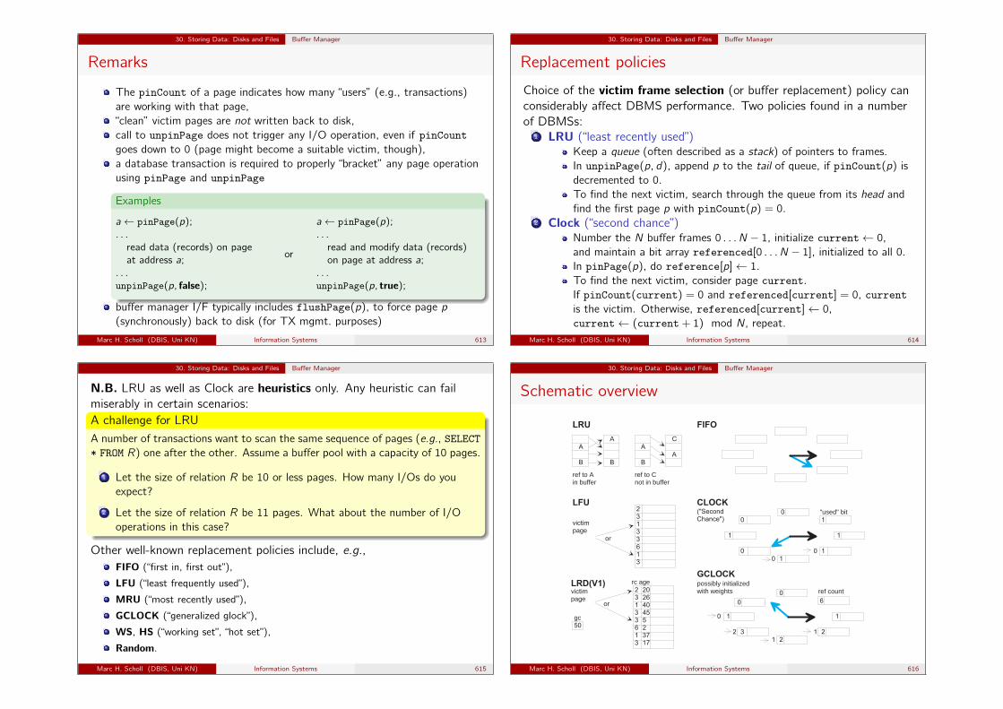
30. Storing Data: Disks and Files Buffer Manager
Remarks
The pinCount of a page indicates how many “users” (e.g., transactions)are working with that page,“clean” victim pages are not written back to disk,call to unpinPage does not trigger any I/O operation, even if pinCountgoes down to 0 (page might become a suitable victim, though),a database transaction is required to properly “bracket” any page operationusing pinPage and unpinPage
Examples
a← pinPage(p);. . .read data (records) on pageat address a;
. . .unpinPage(p, false);
or
a← pinPage(p);. . .read and modify data (records)on page at address a;
. . .unpinPage(p, true);
buffer manager I/F typically includes flushPage(p), to force page p(synchronously) back to disk (for TX mgmt. purposes)
Marc H. Scholl (DBIS, Uni KN) Information Systems 613
30. Storing Data: Disks and Files Buffer Manager
Replacement policies
Choice of the victim frame selection (or buffer replacement) policy canconsiderably affect DBMS performance. Two policies found in a numberof DBMSs:
1 LRU (“least recently used”)Keep a queue (often described as a stack) of pointers to frames.In unpinPage(p, d), append p to the tail of queue, if pinCount(p) isdecremented to 0.To find the next victim, search through the queue from its head andfind the first page p with pinCount(p) = 0.
2 Clock (“second chance”)Number the N buffer frames 0 . . . N − 1, initialize current← 0,and maintain a bit array referenced[0 . . . N − 1], initialized to all 0.In pinPage(p), do reference[p]← 1.To find the next victim, consider page current.If pinCount(current) = 0 and referenced[current] = 0, currentis the victim. Otherwise, referenced[current]← 0,current← (current + 1) mod N, repeat.
Marc H. Scholl (DBIS, Uni KN) Information Systems 614
30. Storing Data: Disks and Files Buffer Manager
N.B. LRU as well as Clock are heuristics only. Any heuristic can failmiserably in certain scenarios:A challenge for LRU
A number of transactions want to scan the same sequence of pages (e.g., SELECT* FROM R) one after the other. Assume a buffer pool with a capacity of 10 pages.
1 Let the size of relation R be 10 or less pages. How many I/Os do youexpect?
2 Let the size of relation R be 11 pages. What about the number of I/Ooperations in this case?
Other well-known replacement policies include, e.g.,FIFO (“first in, first out”),
LFU (“least frequently used”),
MRU (“most recently used”),
GCLOCK (“generalized glock”),
WS, HS (“working set”, “hot set”),
Random.
Marc H. Scholl (DBIS, Uni KN) Information Systems 615
30. Storing Data: Disks and Files Buffer Manager
Schematic overview
�
�
�
�
�
�
�
�
� � � �
ref to Ain buffer
ref to Cnot in buffer
��������
� � �
victimpage
� �
��������
� � � � �victimpage
� �
� �� � � !!�� "� "
rc age
gc! �
�
�
�
�
�
�
�
�
"used" bit
�
�
ref count�
�
� �
�
�
�
�
�
��
�
� � �
� � � � ( ) � � � � � �� � � � � ) *
possibly initializedwith weights
� � � � �
Marc H. Scholl (DBIS, Uni KN) Information Systems 616
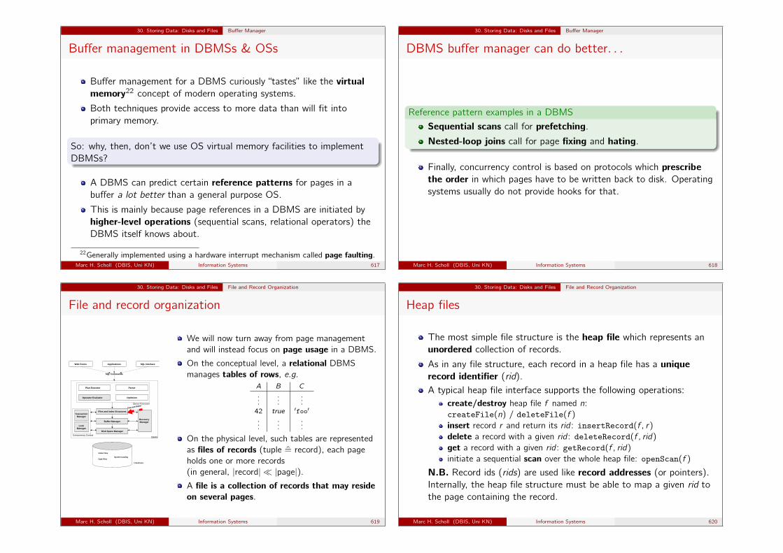
30. Storing Data: Disks and Files Buffer Manager
Buffer management in DBMSs & OSs
Buffer management for a DBMS curiously “tastes” like the virtualmemory22 concept of modern operating systems.
Both techniques provide access to more data than will fit intoprimary memory.
So: why, then, don’t we use OS virtual memory facilities to implementDBMSs?
A DBMS can predict certain reference patterns for pages in abuffer a lot better than a general purpose OS.
This is mainly because page references in a DBMS are initiated byhigher-level operations (sequential scans, relational operators) theDBMS itself knows about.
22Generally implemented using a hardware interrupt mechanism called page faulting.Marc H. Scholl (DBIS, Uni KN) Information Systems 617
30. Storing Data: Disks and Files Buffer Manager
DBMS buffer manager can do better. . .
Reference pattern examples in a DBMS
Sequential scans call for prefetching.Nested-loop joins call for page fixing and hating.
Finally, concurrency control is based on protocols which prescribethe order in which pages have to be written back to disk. Operatingsystems usually do not provide hooks for that.
Marc H. Scholl (DBIS, Uni KN) Information Systems 618
30. Storing Data: Disks and Files File and Record Organization
File and record organization
Files and Index Structures
Buffer Manager
Disk Space Manager
RecoveryManager
Plan Executor
Operator Evaluator Optimizer
Parser
ApplicationsWeb Forms SQL Interface
SQL Commands
Query Processor
Concurrency ControlDBMS
Database
Index Files
Data FilesSystem Catalog
TransactionManager
LockManager
You are here!
We will now turn away from page managementand will instead focus on page usage in a DBMS.
On the conceptual level, a relational DBMSmanages tables of rows, e.g.
A B C
......
...42 true ′foo′...
......
On the physical level, such tables are representedas files of records (tuple = record), each pageholds one or more records(in general, |record| � |page|).A file is a collection of records that may resideon several pages.
Marc H. Scholl (DBIS, Uni KN) Information Systems 619
30. Storing Data: Disks and Files File and Record Organization
Heap files
The most simple file structure is the heap file which represents anunordered collection of records.
As in any file structure, each record in a heap file has a uniquerecord identifier (rid).A typical heap file interface supports the following operations:
create/destroy heap file f named n:createFile(n) / deleteFile(f )
insert record r and return its rid : insertRecord(f , r)
delete a record with a given rid : deleteRecord(f , rid)
get a record with a given rid : getRecord(f , rid)
initiate a sequential scan over the whole heap file: openScan(f )
N.B. Record ids (rids) are used like record addresses (or pointers).Internally, the heap file structure must be able to map a given rid tothe page containing the record.
Marc H. Scholl (DBIS, Uni KN) Information Systems 620
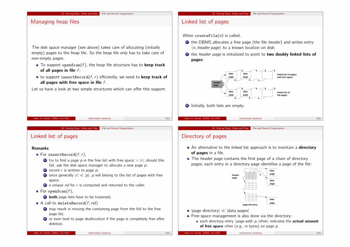
30. Storing Data: Disks and Files File and Record Organization
Managing heap files
The disk space manager (see above) takes care of allocating (initiallyempty) pages to the heap file. So the heap file only has to take care ofnon-empty pages.
To support openScan(f ), the heap file structure has to keep trackof all pages in file f ;to support insertRecord(f , r) efficiently, we need to keep track ofall pages with free space in file f .
Let us have a look at two simple structures which can offer this support.
Marc H. Scholl (DBIS, Uni KN) Information Systems 621
30. Storing Data: Disks and Files File and Record Organization
Linked list of pages
When createFile(n) is called,1 the DBMS allocates a free page (the file header) and writes entry〈n, header page〉 to a known location on disk;
2 the header page is initialized to point to two doubly linked lists ofpages:
data
page page
page page full pages
with free spacelinked list of pages
data data
data
linked list of
pageheader
3 Initially, both lists are empty.
Marc H. Scholl (DBIS, Uni KN) Information Systems 622
30. Storing Data: Disks and Files File and Record Organization
Linked list of pages
RemarksFor insertRecord(f , r),
1 try to find a page p in the free list with free space > |r |; should thisfail, ask the disk space manager to allocate a new page p;
2 record r is written to page p;3 since generally |r | � |p|, p will belong to the list of pages with free
space;4 a unique rid for r is computed and returned to the caller.
For openScan(f ),1 both page lists have to be traversed.
A call to deleteRecord(f , rid)1 may result in moving the containing page from the full to the free
page list,2 or even lead to page deallocation if the page is completely free after
deletion.
Marc H. Scholl (DBIS, Uni KN) Information Systems 623
30. Storing Data: Disks and Files File and Record Organization
Directory of pages
An alternative to the linked list approach is to maintain a directoryof pages in a file.The header page contains the first page of a chain of directorypages; each entry in a directory page identifies a page of the file:
headerpage
data
data
data
page
page
pagepage directory
|page directory| � |data pages|Free space management is also done via the directory:
each directory entry 〈page addr p, nfree〉 indicates the actual amountof free space nfree (e.g., in bytes) on page p.
Marc H. Scholl (DBIS, Uni KN) Information Systems 624
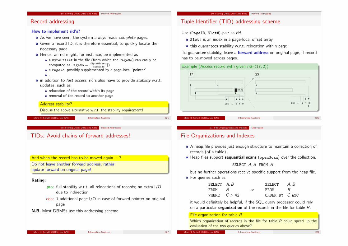
30. Storing Data: Disks and Files Record Addressing
Record addressing
How to implement rid’s?As we have seen, the system always reads complete pages.Given a record ID, it is therefore essential, to quickly locate thenecessary page.Hence, an rid might, for instance, be implemented as
a ByteOffset in the file (from which the PageNo) can easily becomputed as PageNo = d ByteOffset
PageSizee)
a PageNo, possibly supplemented by a page-local “pointer”. . .
in addition to fast access, rid’s also have to provide stability w.r.t.updates, such as
relocation of the record within its pageremoval of the record to another page
Address stability?Discuss the above alternative w.r.t. the stability requirement!
Marc H. Scholl (DBIS, Uni KN) Information Systems 625
30. Storing Data: Disks and Files Record Addressing
Tuple Identifier (TID) addressing scheme
Use 〈PageID, Slot#〉-pair as rid.Slot# is an index in a page-local offset array
this guarantees stability w.r.t. relocation within page
To guarantee stability, leave a forward address on original page, if recordhas to be moved across pages.
Example (Access record with given rid=〈17, 2〉)
���� � �� � � ���� � �� � �
� � � �
� � � �
Marc H. Scholl (DBIS, Uni KN) Information Systems 626
30. Storing Data: Disks and Files Record Addressing
TIDs: Avoid chains of forward addresses!
And when the record has to be moved again. . . ?
Do not leave another forward address, rather:update forward on original page!
Rating:pro: full stability w.r.t. all relocations of records; no extra I/O
due to indirection
con: 1 additional page I/O in case of forward pointer on originalpage
N.B. Most DBMSs use this addressing scheme.
Marc H. Scholl (DBIS, Uni KN) Information Systems 627
31. File Organizations and Indexes Motivation
File Organizations and Indexes
A heap file provides just enough structure to maintain a collection ofrecords (of a table).Heap files support sequential scans (openScan) over the collection,
SELECT A,B FROM R,
but no further operations receive specific support from the heap file.For queries such as
SELECT A,B
FROM R
WHERE C > 42
orSELECT A,B
FROM R
ORDER BY C ASC
it would definitely be helpful, if the SQL query processor could relyon a particular organization of the records in the file for table R.
File organization for table RWhich organization of records in the file for table R could speed up theevaluation of the two queries above?
Marc H. Scholl (DBIS, Uni KN) Information Systems 628
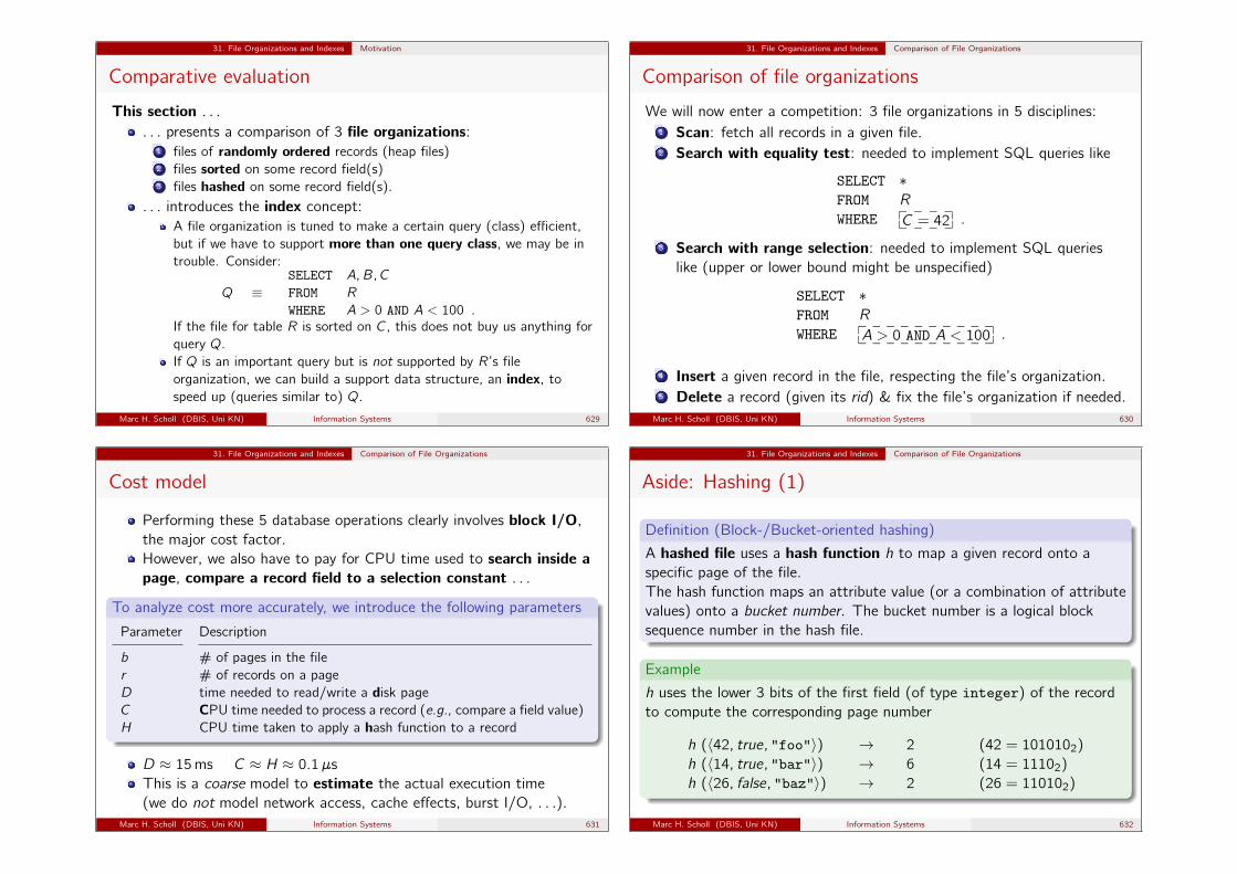
31. File Organizations and Indexes Motivation
Comparative evaluation
This section . . .. . . presents a comparison of 3 file organizations:
1 files of randomly ordered records (heap files)2 files sorted on some record field(s)3 files hashed on some record field(s).
. . . introduces the index concept:A file organization is tuned to make a certain query (class) efficient,but if we have to support more than one query class, we may be introuble. Consider:
Q ≡SELECT A,B, C
FROM R
WHERE A > 0 AND A < 100 .If the file for table R is sorted on C, this does not buy us anything forquery Q.If Q is an important query but is not supported by R’s fileorganization, we can build a support data structure, an index, tospeed up (queries similar to) Q.
Marc H. Scholl (DBIS, Uni KN) Information Systems 629
31. File Organizations and Indexes Comparison of File Organizations
Comparison of file organizations
We will now enter a competition: 3 file organizations in 5 disciplines:1 Scan: fetch all records in a given file.2 Search with equality test: needed to implement SQL queries like
SELECT ∗FROM R
WHERE_ _ _ _��
��_ _ _ _C = 42 .
3 Search with range selection: needed to implement SQL querieslike (upper or lower bound might be unspecified)
SELECT ∗FROM R
WHERE_ _ _ _ _ _ _ _ _ _��
��
_ _ _ _ _ _ _ _ _ _A > 0 AND A < 100 .
4 Insert a given record in the file, respecting the file’s organization.5 Delete a record (given its rid) & fix the file’s organization if needed.
Marc H. Scholl (DBIS, Uni KN) Information Systems 630
31. File Organizations and Indexes Comparison of File Organizations
Cost model
Performing these 5 database operations clearly involves block I/O,the major cost factor.However, we also have to pay for CPU time used to search inside apage, compare a record field to a selection constant . . .
To analyze cost more accurately, we introduce the following parameters
Parameter Description
b # of pages in the filer # of records on a pageD time needed to read/write a disk pageC CPU time needed to process a record (e.g., compare a field value)H CPU time taken to apply a hash function to a record
D ≈ 15ms C ≈ H ≈ 0.1µsThis is a coarse model to estimate the actual execution time(we do not model network access, cache effects, burst I/O, . . .).
Marc H. Scholl (DBIS, Uni KN) Information Systems 631
31. File Organizations and Indexes Comparison of File Organizations
Aside: Hashing (1)
Definition (Block-/Bucket-oriented hashing)
A hashed file uses a hash function h to map a given record onto aspecific page of the file.The hash function maps an attribute value (or a combination of attributevalues) onto a bucket number. The bucket number is a logical blocksequence number in the hash file.
Example
h uses the lower 3 bits of the first field (of type integer) of the recordto compute the corresponding page number
h (〈42, true, "foo"〉) → 2 (42 = 1010102)
h (〈14, true, "bar"〉) → 6 (14 = 11102)
h (〈26, false, "baz"〉) → 2 (26 = 110102)
Marc H. Scholl (DBIS, Uni KN) Information Systems 632
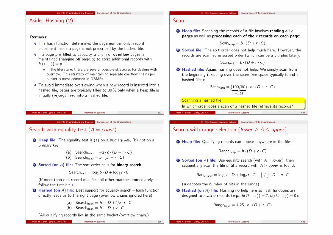
31. File Organizations and Indexes Comparison of File Organizations
Aside: Hashing (2)
Remarks:The hash function determines the page number only; recordplacement inside a page is not prescribed by the hashed file.If a page p is filled to capacity, a chain of overflow pages ismaintained (hanging off page p) to store additional records withh (〈. . . 〉) = p.
In the literature, there are several possible strategies for dealing withoverflow. This strategy of maintaining separate overflow chains perbucket is most common in DBMSs.
To avoid immediate overflowing when a new record is inserted into ahashed file, pages are typically filled to 80 % only when a heap file isinitially (re)organized into a hashed file.
Marc H. Scholl (DBIS, Uni KN) Information Systems 633
31. File Organizations and Indexes Comparison of File Organizations
Scan
1 Heap file: Scanning the records of a file involves reading all bpages as well as processing each of the r records on each page:
Scanheap = b · (D + r · C)
2 Sorted file: The sort order does not help much here. However, therecords are scanned in sorted order (which can be a big plus later):
Scansort = b · (D + r · C)
3 Hashed file: Again, hashing does not help. We simply scan fromthe beginning (skipping over the spare free space typically found inhashed files):
Scanhash = (100/80)︸ ︷︷ ︸=1.25
· b · (D + r · C)
Scanning a hashed file
In which order does a scan of a hashed file retrieve its records?Marc H. Scholl (DBIS, Uni KN) Information Systems 634
31. File Organizations and Indexes Comparison of File Organizations
Search with equality test (A = const)
1 Heap file: The equality test is (a) on a primary key, (b) not on aprimary key:
(a) Searchheap = 1/2 · b · (D + r · C)
(b) Searchheap = b · (D + r · C)
2 Sorted (on A) file: The sort order calls for binary search:
Searchsort = log2 b ·D + log2 r · C(If more than one record qualifies, all other matches immediatelyfollow the first hit.)
3 Hashed (on A) file: Best support for equality search – hash functiondirectly leads us to the right page (overflow chains ignored here):
(a) Searchhash = H +D + 1/2 · r · C(b) Searchhash = H +D + r · C
(All qualifying records live in the same bucket/overflow chain.)
Marc H. Scholl (DBIS, Uni KN) Information Systems 635
31. File Organizations and Indexes Comparison of File Organizations
Search with range selection (lower ≥ A ≤ upper)
1 Heap file: Qualifying records can appear anywhere in the file:
Rangeheap = b · (D + r · C)
2 Sorted (on A) file: Use equality search (with A = lower), thensequentially scan the file until a record with A > upper is found:
Rangesort = log2 b ·D + log2 r · C +⌊n/r⌋ ·D + n · C
(n denotes the number of hits in the range)3 Hashed (on A) file: Hashing no help here as hash functions are
designed to scatter records (e.g., h(〈7, . . . 〉) = 7, h(〈8, . . . 〉) = 0):
Rangehash = 1.25 · b · (D + r · C)
Marc H. Scholl (DBIS, Uni KN) Information Systems 636
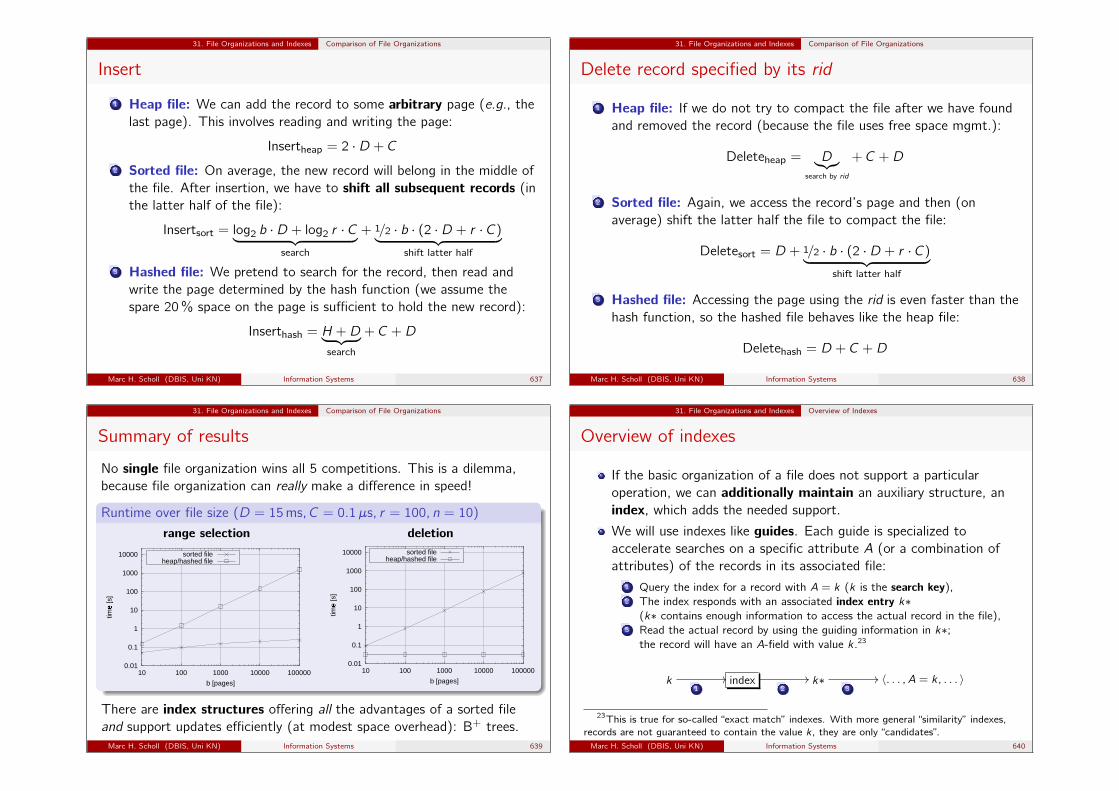
31. File Organizations and Indexes Comparison of File Organizations
Insert
1 Heap file: We can add the record to some arbitrary page (e.g., thelast page). This involves reading and writing the page:
Insertheap = 2 ·D + C
2 Sorted file: On average, the new record will belong in the middle ofthe file. After insertion, we have to shift all subsequent records (inthe latter half of the file):
Insertsort = log2 b ·D + log2 r · C︸ ︷︷ ︸search
+ 1/2 · b · (2 ·D + r · C)︸ ︷︷ ︸shift latter half
3 Hashed file: We pretend to search for the record, then read andwrite the page determined by the hash function (we assume thespare 20 % space on the page is sufficient to hold the new record):
Inserthash = H +D︸ ︷︷ ︸search
+ C +D
Marc H. Scholl (DBIS, Uni KN) Information Systems 637
31. File Organizations and Indexes Comparison of File Organizations
Delete record specified by its rid
1 Heap file: If we do not try to compact the file after we have foundand removed the record (because the file uses free space mgmt.):
Deleteheap = D︸︷︷︸search by rid
+ C +D
2 Sorted file: Again, we access the record’s page and then (onaverage) shift the latter half the file to compact the file:
Deletesort = D + 1/2 · b · (2 ·D + r · C)︸ ︷︷ ︸shift latter half
3 Hashed file: Accessing the page using the rid is even faster than thehash function, so the hashed file behaves like the heap file:
Deletehash = D + C +D
Marc H. Scholl (DBIS, Uni KN) Information Systems 638
31. File Organizations and Indexes Comparison of File Organizations
Summary of results
No single file organization wins all 5 competitions. This is a dilemma,because file organization can really make a difference in speed!
Runtime over file size (D = 15ms, C = 0.1µs, r = 100, n = 10)
range selection
0.01
0.1
1
10
100
1000
10000
10 100 1000 10000 100000
time
[s]
�
b [pages]
sorted fileheap/hashed file
deletion
0.01
0.1
1
10
100
1000
10000
10 100 1000 10000 100000
time
[s]
�
b [pages]
sorted fileheap/hashed file
There are index structures offering all the advantages of a sorted fileand support updates efficiently (at modest space overhead): B+ trees.Marc H. Scholl (DBIS, Uni KN) Information Systems 639
31. File Organizations and Indexes Overview of Indexes
Overview of indexes
If the basic organization of a file does not support a particularoperation, we can additionally maintain an auxiliary structure, anindex, which adds the needed support.
We will use indexes like guides. Each guide is specialized toaccelerate searches on a specific attribute A (or a combination ofattributes) of the records in its associated file:
1 Query the index for a record with A = k (k is the search key),2 The index responds with an associated index entry k∗
(k∗ contains enough information to access the actual record in the file),3 Read the actual record by using the guiding information in k∗;
the record will have an A-field with value k.23
k1
// index2
// k∗3
// 〈. . . , A = k, . . . 〉
23This is true for so-called “exact match” indexes. With more general “similarity” indexes,records are not guaranteed to contain the value k, they are only “candidates”.Marc H. Scholl (DBIS, Uni KN) Information Systems 640
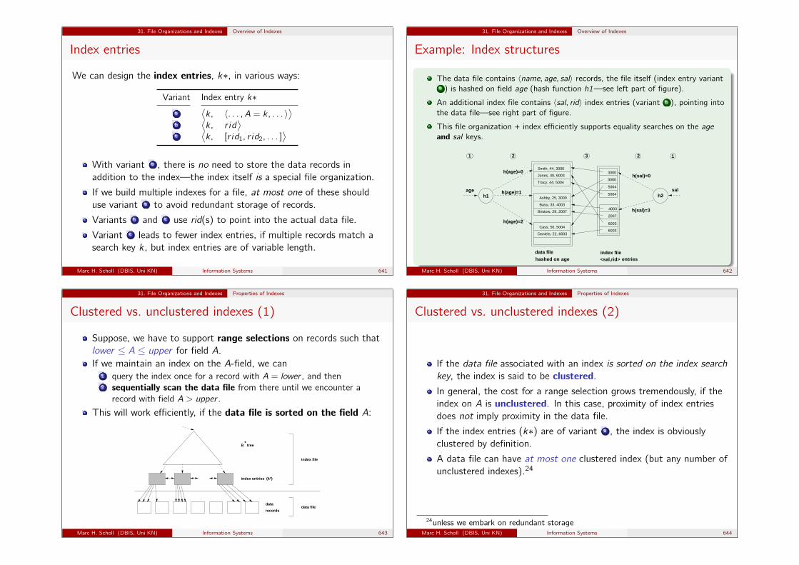
31. File Organizations and Indexes Overview of Indexes
Index entries
We can design the index entries, k∗, in various ways:
Variant Index entry k∗a
⟨k, 〈. . . , A = k, . . . 〉⟩
b⟨k, r id
⟩c
⟨k, [r id1, r id2, . . . ]
⟩With variant a , there is no need to store the data records inaddition to the index—the index itself is a special file organization.
If we build multiple indexes for a file, at most one of these shoulduse variant a to avoid redundant storage of records.
Variants b and c use rid(s) to point into the actual data file.
Variant c leads to fewer index entries, if multiple records match asearch key k , but index entries are of variable length.
Marc H. Scholl (DBIS, Uni KN) Information Systems 641
31. File Organizations and Indexes Overview of Indexes
Example: Index structures
The data file contains 〈name, age, sal〉 records, the file itself (index entry varianta ) is hashed on field age (hash function h1—see left part of figure).
An additional index file contains 〈sal, rid〉 index entries (variant b ), pointing intothe data file—see right part of figure.
This file organization + index efficiently supports equality searches on the ageand sal keys.
2 121
data filehashed on age
index file<sal,rid>
h(age)=2
h(age)=0
h(age)=1
h(sal)=3
h(sal)=0
salage
3
entries
Jones, 40, 6003
Tracy, 44, 5004
Basu, 33, 4003
Cass, 50, 5004
Smith, 44, 3000
Ashby, 25, 3000
6003
6003
2007
4003
3000
3000
5004
5004
Daniels, 22, 6003
h1 h2
Bristow, 29, 2007
Marc H. Scholl (DBIS, Uni KN) Information Systems 642
31. File Organizations and Indexes Properties of Indexes
Clustered vs. unclustered indexes (1)
Suppose, we have to support range selections on records such thatlower ≤ A ≤ upper for field A.If we maintain an index on the A-field, we can
1 query the index once for a record with A = lower , and then2 sequentially scan the data file from there until we encounter a
record with field A > upper .
This will work efficiently, if the data file is sorted on the field A:
(k*)
+B tree
index file
data filedata
records
index entries
Marc H. Scholl (DBIS, Uni KN) Information Systems 643
31. File Organizations and Indexes Properties of Indexes
Clustered vs. unclustered indexes (2)
If the data file associated with an index is sorted on the index searchkey, the index is said to be clustered.In general, the cost for a range selection grows tremendously, if theindex on A is unclustered. In this case, proximity of index entriesdoes not imply proximity in the data file.
If the index entries (k∗) are of variant a , the index is obviouslyclustered by definition.
A data file can have at most one clustered index (but any number ofunclustered indexes).24
24unless we embark on redundant storageMarc H. Scholl (DBIS, Uni KN) Information Systems 644
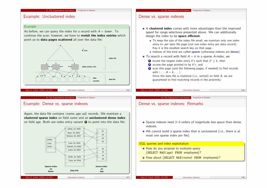
31. File Organizations and Indexes Properties of Indexes
Example: Unclustered index
Example
As before, we can query the index for a record with A = lower . Tocontinue the scan, however, we have to revisit the index entries whichpoint us to data pages scattered all over the data file:
(k*)
B tree+
index entries
index file
data
recordsdata file
Marc H. Scholl (DBIS, Uni KN) Information Systems 645
31. File Organizations and Indexes Properties of Indexes
Dense vs. sparse indexes
A clustered index comes with more advantages than the improvedspeed for range selections presented above. We can additionallydesign the index to be space efficient:
To keep the size of the index file small, we maintain only one indexentry k∗ per data file page (not one index entry per data record).Key k is the smallest search key on that page.Indexes of this kind are called sparse (otherwise indexes are dense).
To search a record with field A = k in a sparse A-index, we1 locate the largest index entry k ′∗ such that k ′ ≤ k , then2 access the page pointed to by k ′∗, and3 scan this page (and the following pages, if needed) to find records
with 〈. . . , A = k, . . . 〉.Since the data file is clustered (i.e., sorted) on field A, we areguaranteed to find matching records in the proximity.
Marc H. Scholl (DBIS, Uni KN) Information Systems 646
31. File Organizations and Indexes Properties of Indexes
Example: Dense vs. sparse indexes
Again, the data file contains 〈name, age, sal〉 records. We maintain aclustered sparse index on field name and an unclustered dense indexon field age. Both use index entry variant b to point into the data file:
Ashby, 25, 3000
Smith, 44, 3000
Ashby
Cass
Smith
22
25
30
40
44
44
50
Sparse Indexon
Name Data File
Dense Indexon
Age
33
Bristow, 30, 2007
Basu, 33, 4003
Cass, 50, 5004
Tracy, 44, 5004
Daniels, 22, 6003
Jones, 40, 6003
Marc H. Scholl (DBIS, Uni KN) Information Systems 647
31. File Organizations and Indexes Properties of Indexes
Dense vs. sparse indexes: Remarks
Sparse indexes need 2–3 orders of magnitude less space than denseindexes.
We cannot build a sparse index that is unclustered (i.e., there is atmost one sparse index per file).
SQL queries and index exploitation
How do you propose to evaluate query(SELECT MAX(age) FROM employees
)?
How about(SELECT MAX(name) FROM employees
)?
Marc H. Scholl (DBIS, Uni KN) Information Systems 648
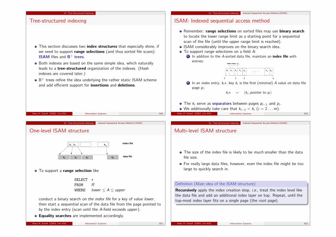
32. Tree-Structured Indexing
Tree-structured indexing
This section discusses two index structures that especially shine, ifwe need to support range selections (and thus sorted file scans):ISAM files and B+ trees.Both indexes are based on the same simple idea, which naturallyleads to a tree-structured organization of the indexes. (Hashindexes are covered later.)
B+ trees refine the idea underlying the rather static ISAM schemeand add efficient support for insertions and deletions.
Marc H. Scholl (DBIS, Uni KN) Information Systems 649
32. Tree-Structured Indexing Indexed Sequential Access Method (ISAM)
ISAM: Indexed sequential access method
Remember: range selections on sorted files may use binary searchto locate the lower range limit as a starting point for a sequentialscan of the file (until the upper range limit is reached).ISAM considerably improves on the binary search idea.To support range selections on a field A:
1 In addition to the A-sorted data file, maintain an index file withentries:
p p p k p
index entry *
kk
k
0 1 1 2 2 m m
1
2 In an index entry, ki∗, key ki is the first (minimal) A value on data filepage pi :
ki∗ = 〈ki , pointer to pi 〉
The ki serve as separators between pages pi−1 and pi .We additionally take care that ki−1 < ki (i = 2 . . . m).
Marc H. Scholl (DBIS, Uni KN) Information Systems 650
32. Tree-Structured Indexing Indexed Sequential Access Method (ISAM)
One-level ISAM structure
2
data file
index filekkk
p p pp0 1 2
1 N
N
To support a range selection like
SELECT ∗FROM R
WHERE lower ≤ A ≤ upper
conduct a binary search on the index file for a key of value lower ,then start a sequential scan of the data file from the page pointed toby the index entry (scan until the A-field exceeds upper).
Equality searches are implemented accordingly.
Marc H. Scholl (DBIS, Uni KN) Information Systems 651
32. Tree-Structured Indexing Indexed Sequential Access Method (ISAM)
Multi-level ISAM structure
The size of the index file is likely to be much smaller than the datafile size.
For really large data files, however, even the index file might be toolarge to quickly search in.
Definition (Main idea of the ISAM structure)
Recursively apply the index creation step, i.e., treat the index level likethe data file and add an additional index layer on top. Repeat, until thetop-most index layer fits on a single page (the root page).
Marc H. Scholl (DBIS, Uni KN) Information Systems 652
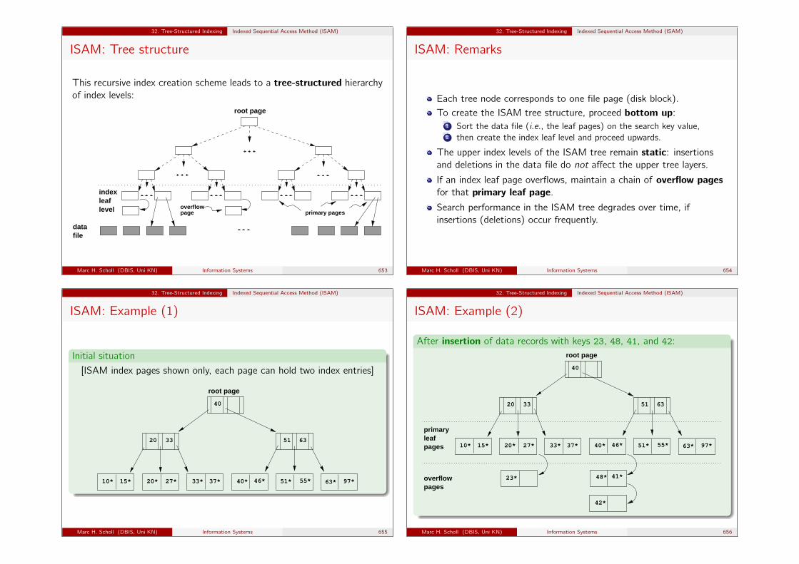
32. Tree-Structured Indexing Indexed Sequential Access Method (ISAM)
ISAM: Tree structure
This recursive index creation scheme leads to a tree-structured hierarchyof index levels:
root page
indexleaflevel
datafile
overflow page primary pages
Marc H. Scholl (DBIS, Uni KN) Information Systems 653
32. Tree-Structured Indexing Indexed Sequential Access Method (ISAM)
ISAM: Remarks
Each tree node corresponds to one file page (disk block).To create the ISAM tree structure, proceed bottom up:
1 Sort the data file (i.e., the leaf pages) on the search key value,2 then create the index leaf level and proceed upwards.
The upper index levels of the ISAM tree remain static: insertionsand deletions in the data file do not affect the upper tree layers.
If an index leaf page overflows, maintain a chain of overflow pagesfor that primary leaf page.Search performance in the ISAM tree degrades over time, ifinsertions (deletions) occur frequently.
Marc H. Scholl (DBIS, Uni KN) Information Systems 654
32. Tree-Structured Indexing Indexed Sequential Access Method (ISAM)
ISAM: Example (1)
Initial situation
[ISAM index pages shown only, each page can hold two index entries]
root page
10* 15* 20* 27* 33* 37* 40* 46* 51* 55* 63* 97*
20 33 51 63
40
Marc H. Scholl (DBIS, Uni KN) Information Systems 655
32. Tree-Structured Indexing Indexed Sequential Access Method (ISAM)
ISAM: Example (2)
After insertion of data records with keys 23, 48, 41, and 42:root page
10* 15* 20* 27* 33* 37* 40* 46* 51* 55* 63* 97*
20 33 51 63
40
23* 48* 41*
42*
primary
overflowpages
leafpages
Marc H. Scholl (DBIS, Uni KN) Information Systems 656

32. Tree-Structured Indexing Indexed Sequential Access Method (ISAM)
IASM: Example (3)
After deletion of data records with keys 42, 51, and 97:root page
10* 15* 20* 27* 33* 37* 40* 46* 55*
20 33 51 63
40
23* 48* 41*
primary
overflowpages
leafpages 63*
Marc H. Scholl (DBIS, Uni KN) Information Systems 657
32. Tree-Structured Indexing Indexed Sequential Access Method (ISAM)
ISAM: Static index structure
NB:The non-leaf levels of the ISAM structure have not been touched atall by the data file updates.
This may lead to index key entries which do not appear in the indexleaf level (key value 51 above).Orphaned index key entries. . .
Does an index key entry like 51 above lead to problems during indexsearches?
To preserve the separator property of the index key entries, we haveto maintain overflow chains.
As a result, the ISAM structure may lose balance after heavyupdating.
Marc H. Scholl (DBIS, Uni KN) Information Systems 658
32. Tree-Structured Indexing Indexed Sequential Access Method (ISAM)
ISAM: Assessment
Despite the deficiencies of ISAM, it is a very efficient order-aware index:Let N be the number of pages in the data file, and let F denote thefan-out of the ISAM tree, i.e. the maximum number of children perindex node (the fan-out in the previous example is 3).When index searching starts, the search space is of size N. With thehelp of the root page we are guided into a subtree of size
N · 1/F .
As we step down the tree, we repeatedly reduce the search space bya factor of F :
N · 1/F · 1/F · 1/F · · · .Index searching ends after s steps when the search space has beenreduced to size 1 (i.e. we have reached the leaf level and found apointer to the page containing the wanted record):
N · (1/F)s!
= 1 ⇔ s = logF N
Marc H. Scholl (DBIS, Uni KN) Information Systems 659
32. Tree-Structured Indexing Indexed Sequential Access Method (ISAM)
Typical ISAM characteristics
Since F � 2 (typically F ≈ 1000), ISAM is significantly faster thanaccess via binary search (log2N).
Example
With F = 1000, an ISAM tree of height 3 can index a file of one billion(= 109) pages (i.e., 3 page I/O operations are sufficient to locate thedata file page wanted).
The presence of overflow pages, however, can easily spoil thisimpressive I/O behavior.
Unbalanced insertions in the data file can ultimately lead to linearsearch in long overflow chains.
Marc H. Scholl (DBIS, Uni KN) Information Systems 660

32. Tree-Structured Indexing B+ trees: A Dynamic Index Structure
B+ trees: A dynamic index structure
The B+ tree index structure is derived from the ISAM idea andrepresents the successful attempt to eat the cake and have it, too:
1 Search performance is only dependant on the height of the B+ tree(because of high fan-out F , the height of B+ trees is rarely > 3).
2 No overflow chains develop, the B+ tree remains balanced all thetime,
3 B+ trees offer efficient insert/delete procedures, the underlyingdata file can grow/shrink dynamically,
4 B+ tree nodes (despite the root page) are guaranteed to have aminimum occupancy of 50 % (typically 67 %).
Marc H. Scholl (DBIS, Uni KN) Information Systems 661
32. Tree-Structured Indexing B+ trees: A Dynamic Index Structure
Format of a B+ tree node (1)
In a B+ tree, non-leaf nodes use the same internal layout as in theISAM case:
p p p k pkk
index entry
0 1 1 2 2 m m
The minimum and maximum number of entries in a node is boundedby the order d of the B+ tree:
d ≤ m ≤ 2 · d
(i.e., no node has less than 50 % entries actually occupied—with theexception of the root node which is allowed to have 1 ≤ m ≤ 2 · dentries).
Marc H. Scholl (DBIS, Uni KN) Information Systems 662
32. Tree-Structured Indexing B+ trees: A Dynamic Index Structure
Format of a B+ tree node (2)
Non-leaf nodes with m entries contain m+ 1 pointers to child nodes.Pointer pi (i = 1 . . . m − 1) points to a subtree in which all keyvalues k are such that
ki ≤ k < ki+1
(pointer p0 points to a subtree with key values < k1, pm points to asubtree with key values ≥ km).Unlike the ISAM case, B+ tree entries in leaf nodes point to datarecords, not data pages. A leaf node entry with key value k isdenoted as k∗ as usual.
Marc H. Scholl (DBIS, Uni KN) Information Systems 663
32. Tree-Structured Indexing B+ trees: A Dynamic Index Structure
Format of a B+ tree node (3)
Note that we can use all index entry variants a . . . c to implementthe leaf entries:
for variant a , the B+ tree represents the index as well as the data fileitself (i.e., in a leaf node, the pi are the actual data records):
ki∗ =⟨ki , 〈. . . 〉
⟩.
for variants b and c , the B+ tree lives in a file distinct from theactual data file; the pi are rids pointing into the data file:
ki∗ = 〈ki , r id〉 .
Marc H. Scholl (DBIS, Uni KN) Information Systems 664
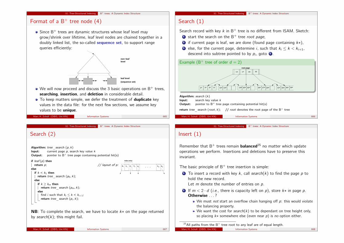
32. Tree-Structured Indexing B+ trees: A Dynamic Index Structure
Format of a B+ tree node (4)
Since B+ trees are dynamic structures whose leaf level maygrow/shrink over lifetime, leaf level nodes are chained together in adoubly linked list, the so-called sequence set, to support rangequeries efficiently:
non−leaflevel
leaf level
(sequence set)
We will now proceed and discuss the 3 basic operations on B+ trees,searching, insertion, and deletion in considerable detail.To keep matters simple, we defer the treatment of duplicate keyvalues in the data file: for the next few sections, we assume keyvalues to be unique.
Marc H. Scholl (DBIS, Uni KN) Information Systems 665
32. Tree-Structured Indexing B+ trees: A Dynamic Index Structure
Search (1)
Search record with key k in B+ tree is no different from ISAM. Sketch:1 start the search on the B+ tree root page,2 if current page is leaf, we are done (found page containing k∗),3 else, for the current page, determine i , such that ki ≤ k < ki+1,
descend into subtree pointed to by pi , goto 2 .
Example (B+ tree of order d = 2)root page
17 24 30
2* 3* 5* 7* 14* 16* 19* 20* 22* 24* 27* 29* 33* 34* 38* 39*
13
Algorithm: search (k)
Input: search key value kOutput: pointer to B+ tree page containing potential hit(s)
return tree_search (root, k); // root denotes the root page of the B+ tree
Marc H. Scholl (DBIS, Uni KN) Information Systems 666
32. Tree-Structured Indexing B+ trees: A Dynamic Index Structure
Search (2)
Algorithm: tree_search (p, k)
Input: current page p, search key value kOutput: pointer to B+ tree page containing potential hit(s)
if leaf (p) thenreturn p; // layout of p: p p p k pkk
index entry
0 1 1 2 2 m m
elseif k < k1 then
return tree_search (p0, k);else
if k ≥ km thenreturn tree_search (pm, k);
elsefind i such that ki ≤ k < ki+1;return tree_search (pi , k);
NB: To complete the search, we have to locate k∗ on the page returnedby search(k); this might fail.
Marc H. Scholl (DBIS, Uni KN) Information Systems 667
32. Tree-Structured Indexing B+ trees: A Dynamic Index Structure
Insert (1)
Remember that B+ trees remain balanced25 no matter which updateoperations we perform. Insertions and deletions have to preserve thisinvariant.
The basic principle of B+ tree insertion is simple:1 To insert a record with key k , call search(k) to find the page p to
hold the new record.Let m denote the number of entries on p.
2 If m < 2 · d (i.e., there is capacity left on p), store k∗ in page p.Otherwise . . . ?
We must not start an overflow chain hanging off p: this would violatethe balancing property.We want the cost for search(k) to be dependant on tree height only,so placing k∗ somewhere else (even near p) is no option either.
25All paths from the B+ tree root to any leaf are of equal length.Marc H. Scholl (DBIS, Uni KN) Information Systems 668
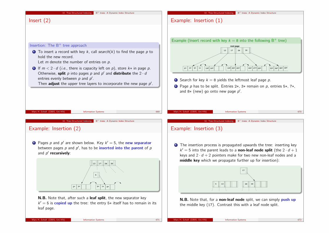
32. Tree-Structured Indexing B+ trees: A Dynamic Index Structure
Insert (2)
Insertion: The B+ tree approach1 To insert a record with key k , call search(k) to find the page p to
hold the new record.Let m denote the number of entries on p.
2 If m < 2 · d (i.e., there is capacity left on p), store k∗ in page p.Otherwise, split p into pages p and p′ and distribute the 2 · dentries evenly between p and p′.Then adjust the upper tree layers to incorporate the new page p′.
Marc H. Scholl (DBIS, Uni KN) Information Systems 669
32. Tree-Structured Indexing B+ trees: A Dynamic Index Structure
Example: Insertion (1)
Example (Insert record with key k = 8 into the following B+ tree)root page
17 24 30
2* 3* 5* 7* 14* 16* 19* 20* 22* 24* 27* 29* 33* 34* 38* 39*
13
1 Search for key k = 8 yields the leftmost leaf page p.2 Page p has to be split. Entries 2∗, 3∗ remain on p, entries 5∗, 7∗,
and 8∗ (new) go onto new page p′.
Marc H. Scholl (DBIS, Uni KN) Information Systems 670
32. Tree-Structured Indexing B+ trees: A Dynamic Index Structure
Example: Insertion (2)
3 Pages p and p′ are shown below. Key k ′ = 5, the new separatorbetween pages p and p′, has to be inserted into the parent of pand p′ recursively:
13 17 24 30
2* 3* 5* 7* 8*
5
N.B. Note that, after such a leaf split, the new separator keyk ′ = 5 is copied up the tree: the entry 5∗ itself has to remain in itsleaf page.
Marc H. Scholl (DBIS, Uni KN) Information Systems 671
32. Tree-Structured Indexing B+ trees: A Dynamic Index Structure
Example: Insertion (3)
4 The insertion process is propagated upwards the tree: inserting keyk ′ = 5 into the parent leads to a non-leaf node split (the 2 · d + 1
keys and 2 · d + 2 pointers make for two new non-leaf nodes and amiddle key which we propagate further up for insertion):
5 24 30
17
13
N.B. Note that, for a non-leaf node split, we can simply push upthe middle key (17). Contrast this with a leaf node split.
Marc H. Scholl (DBIS, Uni KN) Information Systems 672
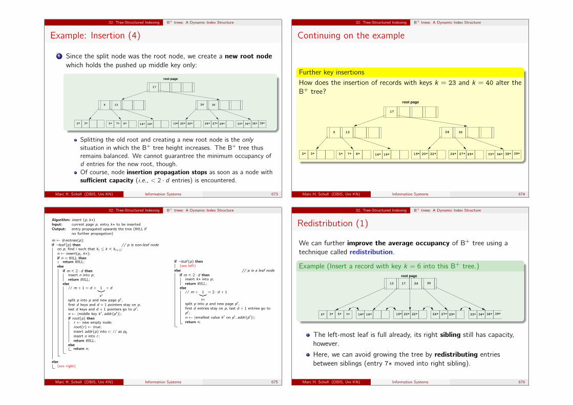
32. Tree-Structured Indexing B+ trees: A Dynamic Index Structure
Example: Insertion (4)
5 Since the split node was the root node, we create a new root nodewhich holds the pushed up middle key only:
root page
2* 3*
17
24 30
14* 16* 19* 20* 22* 24* 27* 29* 33* 34* 38* 39*
135
7*5* 8*
Splitting the old root and creating a new root node is the onlysituation in which the B+ tree height increases. The B+ tree thusremains balanced. We cannot guarantree the minimum occupancy ofd entries for the new root, though.Of course, node insertion propagation stops as soon as a node withsufficient capacity (i.e., < 2 · d entries) is encountered.
Marc H. Scholl (DBIS, Uni KN) Information Systems 673
32. Tree-Structured Indexing B+ trees: A Dynamic Index Structure
Continuing on the example
Further key insertions
How does the insertion of records with keys k = 23 and k = 40 alter theB+ tree?
root page
2* 3*
17
24 30
14* 16* 19* 20* 22* 24* 27* 29* 33* 34* 38* 39*
135
7*5* 8*
Marc H. Scholl (DBIS, Uni KN) Information Systems 674
32. Tree-Structured Indexing B+ trees: A Dynamic Index Structure
Algorithm: insert (p, k∗)Input: current page p, entry k∗ to be insertedOutput: entry propagated upwards the tree (NULL if
no further propagation)
m ← #entries(p);if ¬leaf (p) then // p is non-leaf node
on p, find i such that ki ≤ k < ki+1;n ← insert(pi , k∗);if n = NULL then
return NULL ;else
if m < 2 · d theninsert n into p;return NULL ;
else// m + 1 = d + 1|{z}
k ′+ d
split p into p and new page p′,first d keys and d + 1 pointers stay on p,last d keys and d + 1 pointers go to p′;n ← 〈middle key k ′, addr(p′)〉;if root(p) thenr ← new empty node;root(r)← true;insert addr(p) into r ; // as p0insert n into r ;return NULL ;
elsereturn n;
else(see right)
if ¬leaf (p) then(see left)
else // p is a leaf nodeif m < 2 · d then
insert k∗ into p;return NULL ;
else// m + 1|{z}
k∗
= 2 · d + 1
split p into p and new page p′,first d entries stay on p, last d + 1 entries go top′;n ← 〈smallest value k ′ on p′, addr(p′)〉;return n;
Marc H. Scholl (DBIS, Uni KN) Information Systems 675
32. Tree-Structured Indexing B+ trees: A Dynamic Index Structure
Redistribution (1)
We can further improve the average occupancy of B+ tree using atechnique called redistribution.
Example (Insert a record with key k = 6 into this B+ tree.)root page
17 24 30
2* 3* 5* 7* 14* 16* 19* 20* 22* 24* 27* 29* 33* 34* 38* 39*
13
The left-most leaf is full already, its right sibling still has capacity,however.
Here, we can avoid growing the tree by redistributing entriesbetween siblings (entry 7∗ moved into right sibling).
Marc H. Scholl (DBIS, Uni KN) Information Systems 676
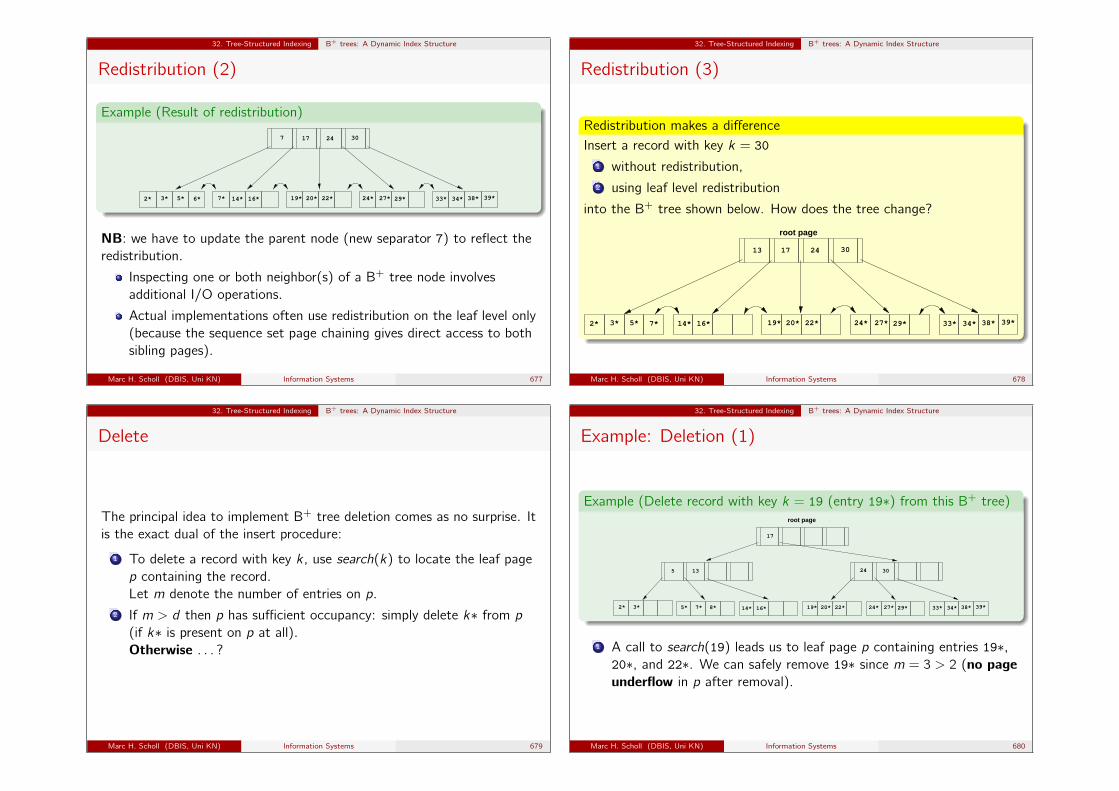
32. Tree-Structured Indexing B+ trees: A Dynamic Index Structure
Redistribution (2)
Example (Result of redistribution)
17 24 30
2* 3* 5* 6* 14* 16* 19* 20* 22* 24* 27* 29* 33* 34* 38* 39*7*
7
NB: we have to update the parent node (new separator 7) to reflect theredistribution.
Inspecting one or both neighbor(s) of a B+ tree node involvesadditional I/O operations.
Actual implementations often use redistribution on the leaf level only(because the sequence set page chaining gives direct access to bothsibling pages).
Marc H. Scholl (DBIS, Uni KN) Information Systems 677
32. Tree-Structured Indexing B+ trees: A Dynamic Index Structure
Redistribution (3)
Redistribution makes a differenceInsert a record with key k = 30
1 without redistribution,2 using leaf level redistribution
into the B+ tree shown below. How does the tree change?
root page
17 24 30
2* 3* 5* 7* 14* 16* 19* 20* 22* 24* 27* 29* 33* 34* 38* 39*
13
Marc H. Scholl (DBIS, Uni KN) Information Systems 678
32. Tree-Structured Indexing B+ trees: A Dynamic Index Structure
Delete
The principal idea to implement B+ tree deletion comes as no surprise. Itis the exact dual of the insert procedure:
1 To delete a record with key k , use search(k) to locate the leaf pagep containing the record.Let m denote the number of entries on p.
2 If m > d then p has sufficient occupancy: simply delete k∗ from p
(if k∗ is present on p at all).Otherwise . . . ?
Marc H. Scholl (DBIS, Uni KN) Information Systems 679
32. Tree-Structured Indexing B+ trees: A Dynamic Index Structure
Example: Deletion (1)
Example (Delete record with key k = 19 (entry 19∗) from this B+ tree)root page
2* 3*
17
24 30
14* 16* 19* 20* 22* 24* 27* 29* 33* 34* 38* 39*
135
7*5* 8*
1 A call to search(19) leads us to leaf page p containing entries 19∗,20∗, and 22∗. We can safely remove 19∗ since m = 3 > 2 (no pageunderflow in p after removal).
Marc H. Scholl (DBIS, Uni KN) Information Systems 680

32. Tree-Structured Indexing B+ trees: A Dynamic Index Structure
Example: Deletion (2)
2 Subsequent deletion of 20∗, however, lets p underflow (p hasminimal occupancy of d = 2 already).We now use redistribution and borrow entry 24∗ from the rightsibling p′ of p(since p′ hosts 3 > 2 entries, redistribution won’t let p′ underflow).The smallest key value on p′ (27) is the new separator of p and p′
in their common parent:
ppage page p’
root page
2* 3*
17
27 30
14* 16* 22* 24* 33* 34* 38* 39*
135
7*5* 8* 27* 29*
Marc H. Scholl (DBIS, Uni KN) Information Systems 681
32. Tree-Structured Indexing B+ trees: A Dynamic Index Structure
Example: Deletion (3)
3 We continue and delete entry 24∗ from p. Redistribution is nooption now (sibling p′ only has minimial occupancy of d = 2).However: we now have mp +mp′ = 1 + 2 < 2 · d .B+ tree deletion thus merges leaf nodes p and p′.Move entries 27∗, 29∗ from p′ to p, then delete page p′:
30
22* 27* 29* 33* 34* 38* 39*
NB: the separator 27 between p and p′ is no longer needed and thusdiscarded (recursively deleted) from the parent.
Marc H. Scholl (DBIS, Uni KN) Information Systems 682
32. Tree-Structured Indexing B+ trees: A Dynamic Index Structure
Example: Deletion (4)
4 The parent of p experiences underflow. Redistribution is no option,so we merge with left non-leaf sibling.After merging we have d︸︷︷︸
left
+ (d − 1)︸ ︷︷ ︸right
keys and d + 1︸ ︷︷ ︸left
+ d︸︷︷︸right
pointers
on the merged page:
30
17
135 17
The missing key value, namely the separator of the two nodes (17),is pulled down (and thus deleted) from the parent to form thecomplete merged node. The // pointer in the parent node is nolonger needed and thrown away.Contrast this with a leaf node merge.
Marc H. Scholl (DBIS, Uni KN) Information Systems 683
32. Tree-Structured Indexing B+ trees: A Dynamic Index Structure
Example: Deletion (5)
5 Since we have now deleted the last remaining entry in the root, wediscard the root (and make the merged node the new root):
root page
2* 3* 7* 14* 16* 22* 27* 29* 33* 34* 38* 39*5* 8*
30135 17
N.B. This is the only situation in which the B+ tree heightdecreases. The B+ tree thus remains balanced.
Marc H. Scholl (DBIS, Uni KN) Information Systems 684

32. Tree-Structured Indexing B+ trees: A Dynamic Index Structure
Example: Deletion (6)
6 We have now seen leaf node merging and redistribution as well asnon-leaf node merging. The remaining case of non-leaf noderedistribution is straightforward:
Suppose during deletion we encounter the following intermediary B+
tree:
root page
14* 16*
135
17* 18* 20*
17 20
22
33* 34* 38* 39*
30
22* 27* 29*21*7*5* 8*3*2*
The non-leaf node with entry 30 underflowed. Its left sibling has twoentries (17 and 20) to spare.
Marc H. Scholl (DBIS, Uni KN) Information Systems 685
32. Tree-Structured Indexing B+ trees: A Dynamic Index Structure
Example: Deletion (7)
6 (Continued)We redistribute entry 20 by “rotating it through” the parent (andpush down the former parent entry 22):
root page
14* 16*
135
17* 18* 20*
17
33* 34* 38* 39*22* 27* 29*21*7*5* 8*3*2*
3022
20
N.B. Notice how the pointer (to the right of entry 20) is rotatedtogether with the corresponding separating key values.
Marc H. Scholl (DBIS, Uni KN) Information Systems 686
32. Tree-Structured Indexing B+ trees: A Dynamic Index Structure
Algorithm: delete (p, k)Input: current page p, key value k to be deletedOutput: key value to be deleted in p’s parent
(NULL if no further deletion in parent)
m ← #entries(p);if ¬leaf (p) then // p is a non-leaf node
find i such that ki ≤ k < ki+1;n ← delete(pi , k);if n = NULL then
return NULL;else
remove entry with key n from p;if root(p) ∧m = 1 then
// last root entry deleted, new rootroot(addr(p0))← true;delete p;return NULL;
if m > d thenreturn NULL;
else // underflow in pp′ ← sibling(p) // wlog: p′ right sibling of p;if #entries(p′) > d then // non-leaf redistrib.
move smallest entry of p′ (= 〈k ′, p′0〉) into p;swap(separator(p, p′), key value k ′ in p);return NULL;
else // merge non-leafs p, p′insert separator(p, p′) into p;move all entries from p′ to p;delete p′;return separator(p, p′);
else(see right)
if ¬leaf (p) then(see left)
else // p is a leaf nodeif k∗ found on p then
remove k∗ from p;else
return NULL;
if m > d thenreturn NULL;
else // underflow in pp′ ← sibling(p) // wlog: p′ right sibl. of p ;if #entries(p′) > d then // leaf redistrib.
move entry from p′ to p;separator(p, p′)← smallest key value on p′;return NULL;
else // merge leafs p, p′move all entries from p′ to p;delete p′;return separator(p, p′);
separator(p, p′) represents the separating key kin the common parent of siblings p and p′.#entries(p) computes the number of actuallyoccupied entries in B+ tree node p.
swap(x, y) exchanges the values of x and y .
Marc H. Scholl (DBIS, Uni KN) Information Systems 687
32. Tree-Structured Indexing B+ trees: A Dynamic Index Structure
Duplicates
As discussed here, the B+ tree search, insert, and delete proceduresignore the presence of duplicate key values.Often this is a reasonable assumption:
If the key field is a primary key for the data file (i.e., for theassociated relation), the search keys k are unique by definition.
Other approaches to make B+ trees aware of duplicates are:1 Use variant c to represent the index entries k∗:
k∗ =⟨k, [r id1, r id2, . . . ]
⟩Each duplicate record with key field k makes the list of rids grow.B+ tree search and maintenance routines largely unaffected. Indexentry size varies, however (affects the B+ tree order concept).
2 Treat duplicate key values like any other value in insert and delete.This affects the search procedure.
Marc H. Scholl (DBIS, Uni KN) Information Systems 688
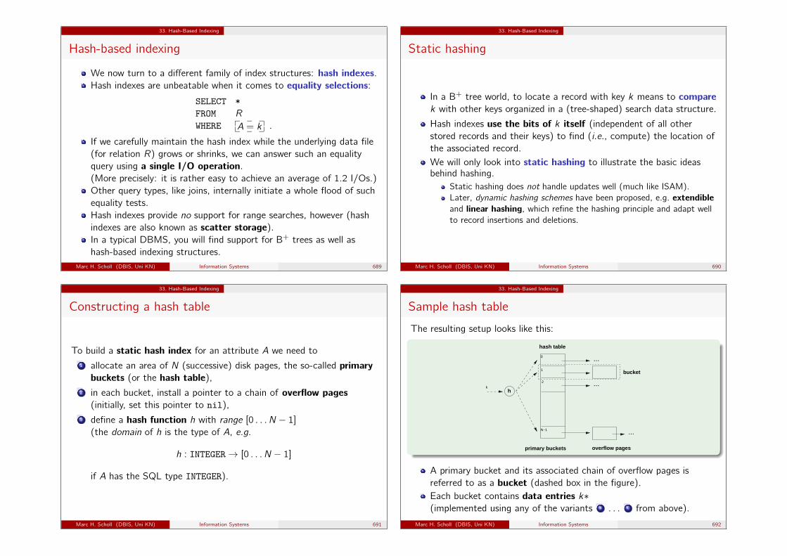
33. Hash-Based Indexing
Hash-based indexing
We now turn to a different family of index structures: hash indexes.Hash indexes are unbeatable when it comes to equality selections:
SELECT *FROM R
WHERE_ _ _��
��_ _ _A = k .
If we carefully maintain the hash index while the underlying data file(for relation R) grows or shrinks, we can answer such an equalityquery using a single I/O operation.(More precisely: it is rather easy to achieve an average of 1.2 I/Os.)Other query types, like joins, internally initiate a whole flood of suchequality tests.Hash indexes provide no support for range searches, however (hashindexes are also known as scatter storage).In a typical DBMS, you will find support for B+ trees as well ashash-based indexing structures.
Marc H. Scholl (DBIS, Uni KN) Information Systems 689
33. Hash-Based Indexing
Static hashing
In a B+ tree world, to locate a record with key k means to comparek with other keys organized in a (tree-shaped) search data structure.
Hash indexes use the bits of k itself (independent of all otherstored records and their keys) to find (i.e., compute) the location ofthe associated record.We will only look into static hashing to illustrate the basic ideasbehind hashing.
Static hashing does not handle updates well (much like ISAM).Later, dynamic hashing schemes have been proposed, e.g. extendibleand linear hashing, which refine the hashing principle and adapt wellto record insertions and deletions.
Marc H. Scholl (DBIS, Uni KN) Information Systems 690
33. Hash-Based Indexing
Constructing a hash table
To build a static hash index for an attribute A we need to1 allocate an area of N (successive) disk pages, the so-called primary
buckets (or the hash table),2 in each bucket, install a pointer to a chain of overflow pages
(initially, set this pointer to nil),3 define a hash function h with range [0 . . . N − 1]
(the domain of h is the type of A, e.g.
h : INTEGER→ [0 . . . N − 1]
if A has the SQL type INTEGER).
Marc H. Scholl (DBIS, Uni KN) Information Systems 691
33. Hash-Based Indexing
Sample hash table
The resulting setup looks like this:
h
hash table
0
1
2
N−1 ...
...
...
k
primary buckets overflow pages
bucket
A primary bucket and its associated chain of overflow pages isreferred to as a bucket (dashed box in the figure).Each bucket contains data entries k∗(implemented using any of the variants a . . . c from above).
Marc H. Scholl (DBIS, Uni KN) Information Systems 692
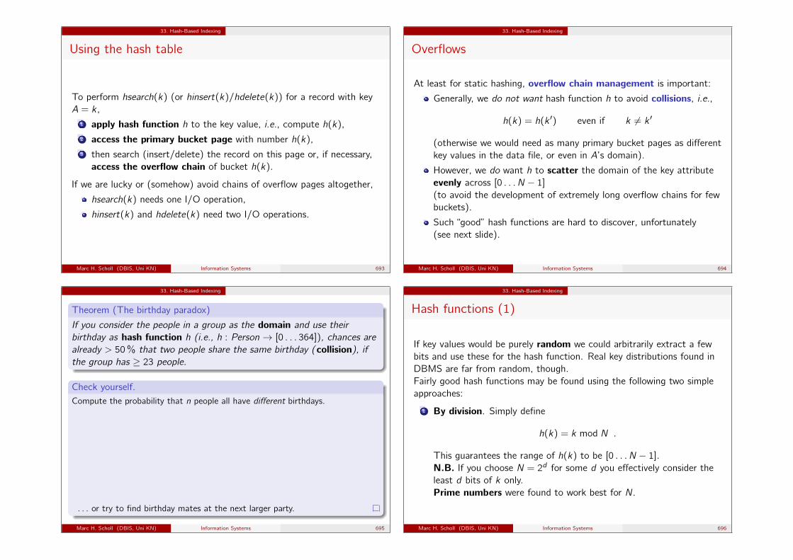
33. Hash-Based Indexing
Using the hash table
To perform hsearch(k) (or hinsert(k)/hdelete(k)) for a record with keyA = k ,
1 apply hash function h to the key value, i.e., compute h(k),2 access the primary bucket page with number h(k),3 then search (insert/delete) the record on this page or, if necessary,
access the overflow chain of bucket h(k).
If we are lucky or (somehow) avoid chains of overflow pages altogether,
hsearch(k) needs one I/O operation,
hinsert(k) and hdelete(k) need two I/O operations.
Marc H. Scholl (DBIS, Uni KN) Information Systems 693
33. Hash-Based Indexing
Overflows
At least for static hashing, overflow chain management is important:
Generally, we do not want hash function h to avoid collisions, i.e.,
h(k) = h(k ′) even if k 6= k ′
(otherwise we would need as many primary bucket pages as differentkey values in the data file, or even in A’s domain).
However, we do want h to scatter the domain of the key attributeevenly across [0 . . . N − 1]
(to avoid the development of extremely long overflow chains for fewbuckets).
Such “good” hash functions are hard to discover, unfortunately(see next slide).
Marc H. Scholl (DBIS, Uni KN) Information Systems 694
33. Hash-Based Indexing
Theorem (The birthday paradox)
If you consider the people in a group as the domain and use theirbirthday as hash function h (i.e., h : Person → [0 . . . 364]), chances arealready > 50 % that two people share the same birthday (collision), ifthe group has ≥ 23 people.
Check yourself.Compute the probability that n people all have different birthdays.
different_birthday (n):=if n = 1 then
return 1
elsereturn
different_birthday (n − 1)︸ ︷︷ ︸probability n − 1 persons have different birthdays
× 365− (n − 1)
365︸ ︷︷ ︸probability nth person has birthday different from firstn − 1 persons
. . . or try to find birthday mates at the next larger party.
Marc H. Scholl (DBIS, Uni KN) Information Systems 695
33. Hash-Based Indexing
Hash functions (1)
If key values would be purely random we could arbitrarily extract a fewbits and use these for the hash function. Real key distributions found inDBMS are far from random, though.Fairly good hash functions may be found using the following two simpleapproaches:
1 By division. Simply define
h(k) = k mod N .
This guarantees the range of h(k) to be [0 . . . N − 1].N.B. If you choose N = 2d for some d you effectively consider theleast d bits of k only.Prime numbers were found to work best for N.
Marc H. Scholl (DBIS, Uni KN) Information Systems 696
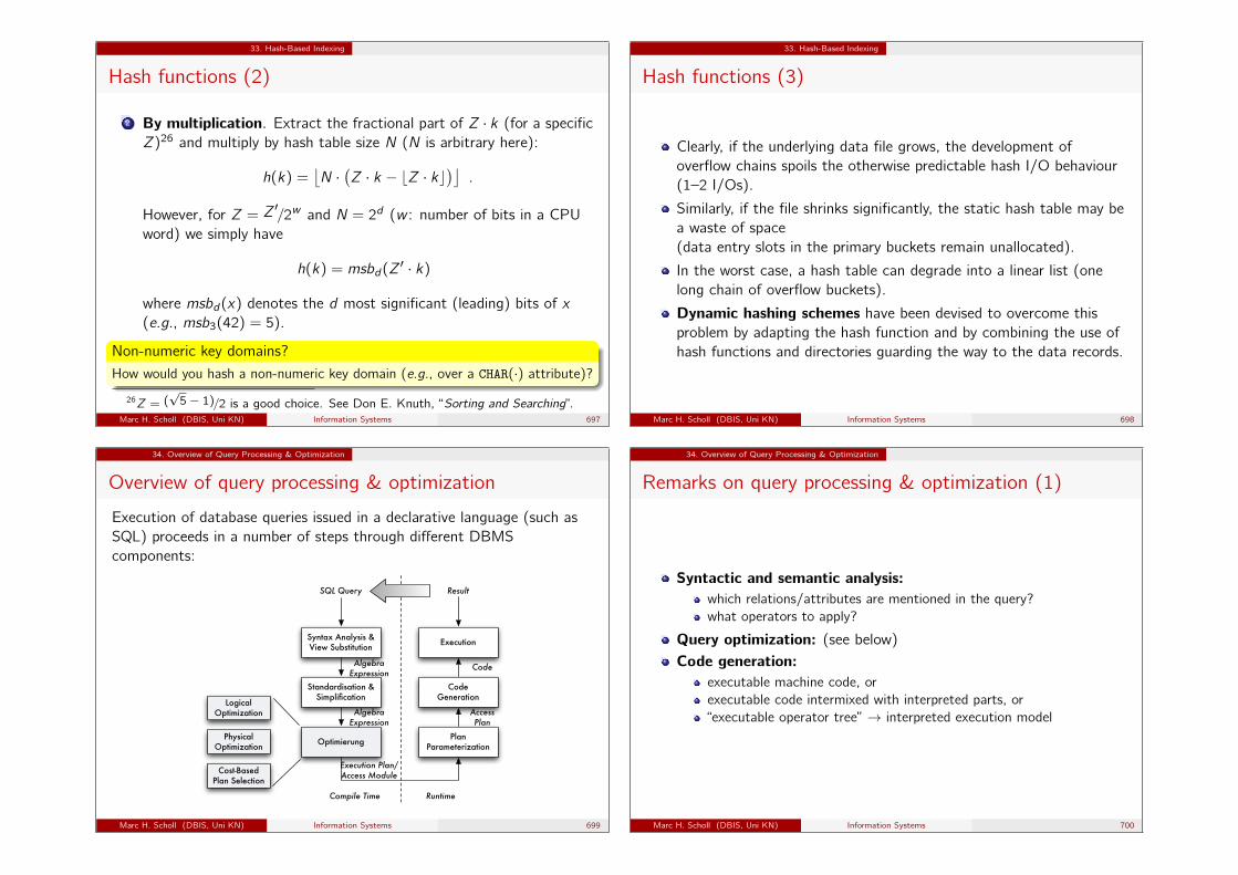
33. Hash-Based Indexing
Hash functions (2)
2 By multiplication. Extract the fractional part of Z · k (for a specificZ)26 and multiply by hash table size N (N is arbitrary here):
h(k) =⌊N · (Z · k − bZ · kc)⌋ .
However, for Z = Z′/2w and N = 2d (w : number of bits in a CPUword) we simply have
h(k) = msbd(Z′ · k)
where msbd(x) denotes the d most significant (leading) bits of x(e.g., msb3(42) = 5).
Non-numeric key domains?
How would you hash a non-numeric key domain (e.g., over a CHAR(·) attribute)?
26Z = (√5− 1)/2 is a good choice. See Don E. Knuth, “Sorting and Searching”.
Marc H. Scholl (DBIS, Uni KN) Information Systems 697
33. Hash-Based Indexing
Hash functions (3)
Clearly, if the underlying data file grows, the development ofoverflow chains spoils the otherwise predictable hash I/O behaviour(1–2 I/Os).
Similarly, if the file shrinks significantly, the static hash table may bea waste of space(data entry slots in the primary buckets remain unallocated).
In the worst case, a hash table can degrade into a linear list (onelong chain of overflow buckets).
Dynamic hashing schemes have been devised to overcome thisproblem by adapting the hash function and by combining the use ofhash functions and directories guarding the way to the data records.
Marc H. Scholl (DBIS, Uni KN) Information Systems 698
34. Overview of Query Processing & Optimization
Overview of query processing & optimization
Execution of database queries issued in a declarative language (such asSQL) proceeds in a number of steps through different DBMScomponents:
Syntax Analysis &View Substitution
Standardisation &Simplification
Optimierung PlanParameterization
CodeGeneration
Execution
AlgebraExpression
AlgebraExpression
Execution Plan/Access Module
AccessPlan
Code
ResultSQL Query
Compile Time Runtime
LogicalOptimization
PhysicalOptimization
Cost-Based Plan Selection
Marc H. Scholl (DBIS, Uni KN) Information Systems 699
34. Overview of Query Processing & Optimization
Remarks on query processing & optimization (1)
Syntactic and semantic analysis:which relations/attributes are mentioned in the query?what operators to apply?
Query optimization: (see below)Code generation:
executable machine code, orexecutable code intermixed with interpreted parts, or“executable operator tree” → interpreted execution model
Marc H. Scholl (DBIS, Uni KN) Information Systems 700
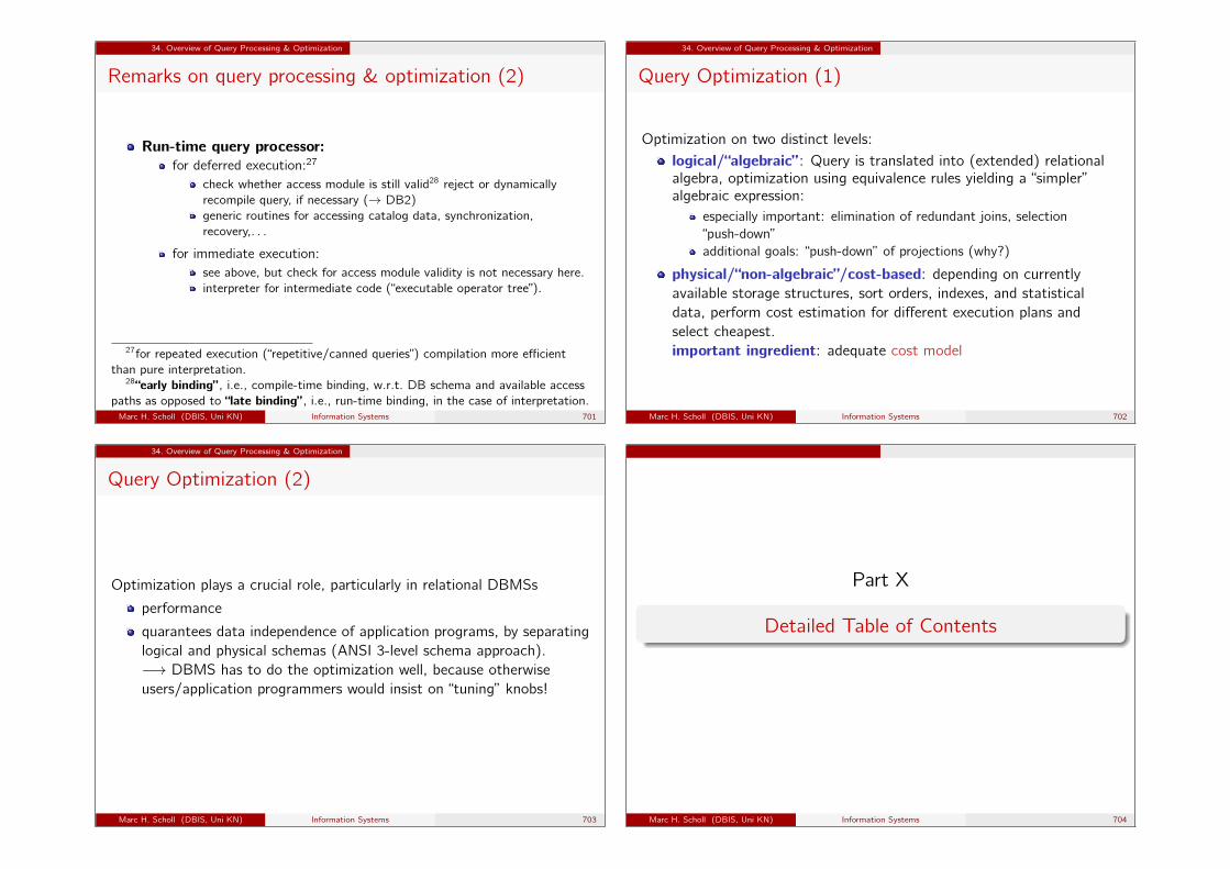
34. Overview of Query Processing & Optimization
Remarks on query processing & optimization (2)
Run-time query processor:for deferred execution:27
check whether access module is still valid28 reject or dynamicallyrecompile query, if necessary (→ DB2)generic routines for accessing catalog data, synchronization,recovery,. . .
for immediate execution:see above, but check for access module validity is not necessary here.interpreter for intermediate code (“executable operator tree”).
27for repeated execution (“repetitive/canned queries”) compilation more efficientthan pure interpretation.
28“early binding” , i.e., compile-time binding, w.r.t. DB schema and available accesspaths as opposed to “late binding” , i.e., run-time binding, in the case of interpretation.Marc H. Scholl (DBIS, Uni KN) Information Systems 701
34. Overview of Query Processing & Optimization
Query Optimization (1)
Optimization on two distinct levels:logical/“algebraic” : Query is translated into (extended) relationalalgebra, optimization using equivalence rules yielding a “simpler”algebraic expression:
especially important: elimination of redundant joins, selection“push-down”additional goals: “push-down” of projections (why?)
physical/“non-algebraic”/cost-based: depending on currentlyavailable storage structures, sort orders, indexes, and statisticaldata, perform cost estimation for different execution plans andselect cheapest.important ingredient: adequate cost model
Marc H. Scholl (DBIS, Uni KN) Information Systems 702
34. Overview of Query Processing & Optimization
Query Optimization (2)
Optimization plays a crucial role, particularly in relational DBMSs
performance
quarantees data independence of application programs, by separatinglogical and physical schemas (ANSI 3-level schema approach).−→ DBMS has to do the optimization well, because otherwiseusers/application programmers would insist on “tuning” knobs!
Marc H. Scholl (DBIS, Uni KN) Information Systems 703
Part X
Detailed Table of Contents
Marc H. Scholl (DBIS, Uni KN) Information Systems 704
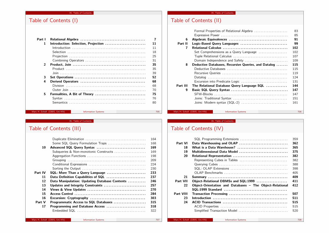
35. Table of Contents
Table of Contents (I)
Part I Relational Algebra . . . . . . . . . . . . . . . . . . . . . . . . . . . . . . . . . . . . . . . . 71 Introduction: Selection, Projection . . . . . . . . . . . . . . . . . . . . . . . . . 11
Introduction . . . . . . . . . . . . . . . . . . . . . . . . . . . . . . . . . . . . . . . . . . . . . . 11Selection . . . . . . . . . . . . . . . . . . . . . . . . . . . . . . . . . . . . . . . . . . . . . . . . . 18Projection . . . . . . . . . . . . . . . . . . . . . . . . . . . . . . . . . . . . . . . . . . . . . . . . 25Combining Operators . . . . . . . . . . . . . . . . . . . . . . . . . . . . . . . . . . . . . . 31
2 Product, Join . . . . . . . . . . . . . . . . . . . . . . . . . . . . . . . . . . . . . . . . . . . . . 35Product . . . . . . . . . . . . . . . . . . . . . . . . . . . . . . . . . . . . . . . . . . . . . . . . . . 35Join . . . . . . . . . . . . . . . . . . . . . . . . . . . . . . . . . . . . . . . . . . . . . . . . . . . . . . 39
3 Set Operations . . . . . . . . . . . . . . . . . . . . . . . . . . . . . . . . . . . . . . . . . . . . 524 Derived Operators . . . . . . . . . . . . . . . . . . . . . . . . . . . . . . . . . . . . . . . . 68
Division . . . . . . . . . . . . . . . . . . . . . . . . . . . . . . . . . . . . . . . . . . . . . . . . . . 68Outer Join . . . . . . . . . . . . . . . . . . . . . . . . . . . . . . . . . . . . . . . . . . . . . . . . 70
5 Formalities, A Bit of Theory . . . . . . . . . . . . . . . . . . . . . . . . . . . . . . . 75Syntax . . . . . . . . . . . . . . . . . . . . . . . . . . . . . . . . . . . . . . . . . . . . . . . . . . . 76Semantics . . . . . . . . . . . . . . . . . . . . . . . . . . . . . . . . . . . . . . . . . . . . . . . . 80
Marc H. Scholl (DBIS, Uni KN) Information Systems 705
35. Table of Contents
Table of Contents (II)
Formal Properties of Relational Algebra . . . . . . . . . . . . . . . . . . . . . 83Expressive Power . . . . . . . . . . . . . . . . . . . . . . . . . . . . . . . . . . . . . . . . . . 85
6 Algebraic Equivalences . . . . . . . . . . . . . . . . . . . . . . . . . . . . . . . . . . . . 91Part II Logic-Based Query Languages . . . . . . . . . . . . . . . . . . . . . . . . . . . . . 99
7 Relational Calculus . . . . . . . . . . . . . . . . . . . . . . . . . . . . . . . . . . . . . . . . 102Set Comprehensions as a Query Language . . . . . . . . . . . . . . . . . . 102Tuple Relational Calculus . . . . . . . . . . . . . . . . . . . . . . . . . . . . . . . . . . 107Domain Independence and Safety . . . . . . . . . . . . . . . . . . . . . . . . . . . 109
8 Deductive Databases, Recursive Queries, and Datalog . . . . . . . 115Deductive Databases . . . . . . . . . . . . . . . . . . . . . . . . . . . . . . . . . . . . . . 115Recursive Queries . . . . . . . . . . . . . . . . . . . . . . . . . . . . . . . . . . . . . . . . . 119Datalog . . . . . . . . . . . . . . . . . . . . . . . . . . . . . . . . . . . . . . . . . . . . . . . . . . 124Excursion into Predicate Logic . . . . . . . . . . . . . . . . . . . . . . . . . . . . . 131
Part III The Relational Database Query Language SQL . . . . . . . . . . . . . 1449 Basic SQL Query Syntax . . . . . . . . . . . . . . . . . . . . . . . . . . . . . . . . . . . 147
SFW-Blocks . . . . . . . . . . . . . . . . . . . . . . . . . . . . . . . . . . . . . . . . . . . . . . 147Joins: Traditional Syntax . . . . . . . . . . . . . . . . . . . . . . . . . . . . . . . . . . 151Joins: Modern syntax (SQL-2) . . . . . . . . . . . . . . . . . . . . . . . . . . . . . 161
Marc H. Scholl (DBIS, Uni KN) Information Systems 706
35. Table of Contents
Table of Contents (III)
Duplicate Elimination . . . . . . . . . . . . . . . . . . . . . . . . . . . . . . . . . . . . . . 164Some SQL Query Formulation Traps . . . . . . . . . . . . . . . . . . . . . . . . 168
10 Advanced SQL Query Syntax . . . . . . . . . . . . . . . . . . . . . . . . . . . . . . 169Subqueries & Non-monotonic Constructs . . . . . . . . . . . . . . . . . . . . 169Aggregation Functions . . . . . . . . . . . . . . . . . . . . . . . . . . . . . . . . . . . . . 198Grouping . . . . . . . . . . . . . . . . . . . . . . . . . . . . . . . . . . . . . . . . . . . . . . . . . 209Conditional Expressions . . . . . . . . . . . . . . . . . . . . . . . . . . . . . . . . . . . . 224Sorting the Output . . . . . . . . . . . . . . . . . . . . . . . . . . . . . . . . . . . . . . . . 230
Part IV SQL: More Than a Query Language . . . . . . . . . . . . . . . . . . . . . . . . 23311 Data Definition Capabilities of SQL . . . . . . . . . . . . . . . . . . . . . . . . 23712 Data Manipulation: Updating Database Contents . . . . . . . . . . . 24613 Updates and Integrity Constraints . . . . . . . . . . . . . . . . . . . . . . . . . . 25714 Views & View Updates . . . . . . . . . . . . . . . . . . . . . . . . . . . . . . . . . . . . 27015 Access Control . . . . . . . . . . . . . . . . . . . . . . . . . . . . . . . . . . . . . . . . . . . . 28416 Excursion: Cryptography . . . . . . . . . . . . . . . . . . . . . . . . . . . . . . . . . . 303
Part V Programmatic Access to SQL Databases . . . . . . . . . . . . . . . . . . . . 31517 Programming and Database Access . . . . . . . . . . . . . . . . . . . . . . . . 318
Embedded SQL . . . . . . . . . . . . . . . . . . . . . . . . . . . . . . . . . . . . . . . . . . . 322
Marc H. Scholl (DBIS, Uni KN) Information Systems 707
35. Table of Contents
Table of Contents (IV)
SQL Programming Extensions . . . . . . . . . . . . . . . . . . . . . . . . . . . . . . 359Part VI Data Warehousing and OLAP . . . . . . . . . . . . . . . . . . . . . . . . . . . . . . 362
18 What is a Data Warehouse? . . . . . . . . . . . . . . . . . . . . . . . . . . . . . . . 36519 Multidimensional Data Model . . . . . . . . . . . . . . . . . . . . . . . . . . . . . . 37520 Relational Representation . . . . . . . . . . . . . . . . . . . . . . . . . . . . . . . . . . 382
Representing Cubes in Tables . . . . . . . . . . . . . . . . . . . . . . . . . . . . . . 382Querying Cubes . . . . . . . . . . . . . . . . . . . . . . . . . . . . . . . . . . . . . . . . . . . 388SQL: OLAP Extensions . . . . . . . . . . . . . . . . . . . . . . . . . . . . . . . . . . . . 398OLAP Benchmarks . . . . . . . . . . . . . . . . . . . . . . . . . . . . . . . . . . . . . . . . 405
21 Summary . . . . . . . . . . . . . . . . . . . . . . . . . . . . . . . . . . . . . . . . . . . . . . . . . 409Part VII Object-Relational DBMSs and SQL:1999 . . . . . . . . . . . . . . . . . . . 411
22 Object-Orientation and Databases – The Object-RelationalSQL:1999 Standard . . . . . . . . . . . . . . . . . . . . . . . . . . . . . . . . . . . . . . .
412
Part VIII Transaction Processing . . . . . . . . . . . . . . . . . . . . . . . . . . . . . . . . . . . . 50723 Introduction . . . . . . . . . . . . . . . . . . . . . . . . . . . . . . . . . . . . . . . . . . . . . . 51124 ACID Transactions . . . . . . . . . . . . . . . . . . . . . . . . . . . . . . . . . . . . . . . . 515
ACID Properties . . . . . . . . . . . . . . . . . . . . . . . . . . . . . . . . . . . . . . . . . . 515Simplified Transaction Model . . . . . . . . . . . . . . . . . . . . . . . . . . . . . . . 520
Marc H. Scholl (DBIS, Uni KN) Information Systems 708
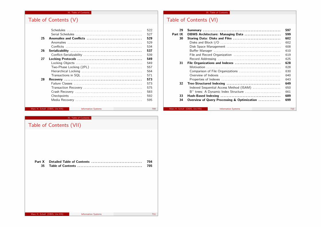
35. Table of Contents
Table of Contents (V)
Schedules . . . . . . . . . . . . . . . . . . . . . . . . . . . . . . . . . . . . . . . . . . . . . . . . 522Serial Schedules . . . . . . . . . . . . . . . . . . . . . . . . . . . . . . . . . . . . . . . . . . . 527
25 Anomalies and Conflicts . . . . . . . . . . . . . . . . . . . . . . . . . . . . . . . . . . . 529Anomalies . . . . . . . . . . . . . . . . . . . . . . . . . . . . . . . . . . . . . . . . . . . . . . . . 529Conflicts . . . . . . . . . . . . . . . . . . . . . . . . . . . . . . . . . . . . . . . . . . . . . . . . . 534
26 Serializability . . . . . . . . . . . . . . . . . . . . . . . . . . . . . . . . . . . . . . . . . . . . . 537Conflict-Serializability . . . . . . . . . . . . . . . . . . . . . . . . . . . . . . . . . . . . . . 539
27 Locking Protocols . . . . . . . . . . . . . . . . . . . . . . . . . . . . . . . . . . . . . . . . . 549Locking Objects . . . . . . . . . . . . . . . . . . . . . . . . . . . . . . . . . . . . . . . . . . . 549Two-Phase Locking (2PL) . . . . . . . . . . . . . . . . . . . . . . . . . . . . . . . . . 557Hierarchical Locking . . . . . . . . . . . . . . . . . . . . . . . . . . . . . . . . . . . . . . . 564Transactions in SQL . . . . . . . . . . . . . . . . . . . . . . . . . . . . . . . . . . . . . . . 571
28 Recovery . . . . . . . . . . . . . . . . . . . . . . . . . . . . . . . . . . . . . . . . . . . . . . . . . 573Failure Classes . . . . . . . . . . . . . . . . . . . . . . . . . . . . . . . . . . . . . . . . . . . . 573Transaction Recovery . . . . . . . . . . . . . . . . . . . . . . . . . . . . . . . . . . . . . . 575Crash Recovery . . . . . . . . . . . . . . . . . . . . . . . . . . . . . . . . . . . . . . . . . . . 583Checkpoints . . . . . . . . . . . . . . . . . . . . . . . . . . . . . . . . . . . . . . . . . . . . . . 592Media Recovery . . . . . . . . . . . . . . . . . . . . . . . . . . . . . . . . . . . . . . . . . . . 595
Marc H. Scholl (DBIS, Uni KN) Information Systems 709
35. Table of Contents
Table of Contents (VI)
29 Summary . . . . . . . . . . . . . . . . . . . . . . . . . . . . . . . . . . . . . . . . . . . . . . . . . 597Part IX DBMS Architecture: Managing Data . . . . . . . . . . . . . . . . . . . . . . . 599
30 Storing Data: Disks and Files . . . . . . . . . . . . . . . . . . . . . . . . . . . . . . 602Disks and Block I/O . . . . . . . . . . . . . . . . . . . . . . . . . . . . . . . . . . . . . . . 602Disk Space Management . . . . . . . . . . . . . . . . . . . . . . . . . . . . . . . . . . . 608Buffer Manager . . . . . . . . . . . . . . . . . . . . . . . . . . . . . . . . . . . . . . . . . . . 610File and Record Organization . . . . . . . . . . . . . . . . . . . . . . . . . . . . . . 619Record Addressing . . . . . . . . . . . . . . . . . . . . . . . . . . . . . . . . . . . . . . . . 625
31 File Organizations and Indexes . . . . . . . . . . . . . . . . . . . . . . . . . . . . . 628Motivation . . . . . . . . . . . . . . . . . . . . . . . . . . . . . . . . . . . . . . . . . . . . . . . . 628Comparison of File Organizations . . . . . . . . . . . . . . . . . . . . . . . . . . . 630Overview of Indexes . . . . . . . . . . . . . . . . . . . . . . . . . . . . . . . . . . . . . . . 640Properties of Indexes . . . . . . . . . . . . . . . . . . . . . . . . . . . . . . . . . . . . . . 643
32 Tree-Structured Indexing . . . . . . . . . . . . . . . . . . . . . . . . . . . . . . . . . . 649Indexed Sequential Access Method (ISAM) . . . . . . . . . . . . . . . . . . 650B+ trees: A Dynamic Index Structure . . . . . . . . . . . . . . . . . . . . . . . 661
33 Hash-Based Indexing . . . . . . . . . . . . . . . . . . . . . . . . . . . . . . . . . . . . . . 68934 Overview of Query Processing & Optimization . . . . . . . . . . . . . . 699
Marc H. Scholl (DBIS, Uni KN) Information Systems 710
35. Table of Contents
Table of Contents (VII)
Part X Detailed Table of Contents . . . . . . . . . . . . . . . . . . . . . . . . . . . . . . . . 70435 Table of Contents . . . . . . . . . . . . . . . . . . . . . . . . . . . . . . . . . . . . . . . . . 705
Marc H. Scholl (DBIS, Uni KN) Information Systems 711