Influence of Land Cover and Soil Moisture on the Horizontal Distribution of Sensibleand Latent Heat Fluxes in Southeast Kansas during IHOP_2002 and CASES-97

MARGARET A. LEMONE, FEI CHEN, JOSEPH G. ALFIERI,* AND MUKUL TEWARI

National Center for Atmospheric Research,� Boulder, Colorado

BART GEERTS AND QUN MIAO

Department of Atmospheric Sciences, University of Wyoming, Laramie, Wyoming

ROBERT L. GROSSMAN

Colorado Research Associates, Boulder, Colorado

RICHARD L. COULTER

Argonne National Laboratory, Chicago, Illinois

(Manuscript received 18 August 2005, in final form 9 June 2006)

ABSTRACT

Analyses of daytime fair-weather aircraft and surface-flux tower data from the May–June 2002 Interna-tional H2O Project (IHOP_2002) and the April–May 1997 Cooperative Atmosphere Surface ExchangeStudy (CASES-97) are used to document the role of vegetation, soil moisture, and terrain in determiningthe horizontal variability of latent heat LE and sensible heat H along a 46-km flight track in southeastKansas. Combining the two field experiments clearly reveals the strong influence of vegetation cover, withH maxima over sparse/dormant vegetation, and H minima over green vegetation; and, to a lesser extent, LEmaxima over green vegetation, and LE minima over sparse/dormant vegetation. If the small number ofcases is producing the correct trend, other effects of vegetation and the impact of soil moisture emergethrough examining the slope �xyLE/�xyH for the best-fit straight line for plots of time-averaged LE as afunction of time-averaged H over the area. Based on the surface energy balance, H � LE � Rnet � Gsfc,where Rnet is the net radiation and Gsfc is the flux into the soil; Rnet � Gsfc � constant over the area impliesan approximately �1 slope. Right after rainfall, H and LE vary too little horizontally to define a slope. Aftersufficient drying to produce enough horizontal variation to define a slope, a steep (��2) slope emerges.The slope becomes shallower and better defined with time as H and LE horizontal variability increases.Similarly, the slope becomes more negative with moister soils. In addition, the slope can change with timeof day due to phase differences in H and LE. These trends are based on land surface model (LSM) runs andobservations collected under nearly clear skies; the vegetation is unstressed for the days examined. LSMruns suggest terrain may also play a role, but observational support is weak.

1. Introduction

This paper explores the relationship of surface het-erogeneity to low-level fluxes of sensible heat and la-tent heat, using aircraft and surface-based data col-

lected in May–June 2002 in southeast Kansas as part ofthe International H2O Project (IHOP_2002; Weck-werth et al. 2004), and data collected in April–May 1997as part of the Cooperative Surface Atmosphere Ex-change Study (CASES-97; LeMone et al. 2000). Thisstudy is possible because aircraft data were collectedalong the same flight track in both experiments. Thetrack (the “eastern track” in Fig. 1; also see Fig. 2) ischaracterized by a mix of mostly grassland and winterwheat, with trees bordering many fields and waterways.The track extends across the eastern side of the WalnutRiver watershed and into the watershed to the east.While the vegetation types were similar for both fieldexperiments, the phase in their seasonal cycles was

* Current affiliation: Purdue University, West Lafayette, Indi-ana.

� The National Center for Atmospheric Research is sponsoredby the National Science Foundation.

Corresponding author address: Margaret A. LeMone, NCARFoothills Laboratory, 3450 Mitchell Lane, Boulder, CO 80301.E-mail: lemone@ucar.edu

68 J O U R N A L O F H Y D R O M E T E O R O L O G Y VOLUME 8

DOI: 10.1175/JHM554.1

© 2007 American Meteorological Society

JHM554

quite different. This contrast allows the results to emergewith a clarity not possible otherwise.

Since the 1980s, Anthes (1984), Segal et al. (1988),Pielke et al. (1991), Chen et al. (2001), and others haveused numerical simulations to document the impor-tance of land surface characteristics to local weatherand climate. Chen et al. (2001) demonstrated that re-placing the older “bucket” soil-moisture model with theOregon State University (OSU) Land Surface Model(LSM; Pan and Mahrt 1987; Chen et al. 1996) improved24–48-h precipitation forecasts in the Eta Model, asmuch as doubling the horizontal resolution. Trier et al.(2004) provide two specific examples of surface pro-cesses reinforcing convective initiation in the southernGreat Plains: in one case the air is destabilized throughenhanced PBL growth over warmer surfaces and in thesecond forcing and destabilization results from 100-km-scale circulations generated by differential surface heat-ing.

The goal of IHOP_2002 is to improve prediction ofconvective precipitation in numerical weather predic-tion models by improving the collection and use of wa-ter vapor data, and improving representation of theevolution of water vapor. Surface processes are empha-sized because of their importance in the initiation andevolution of precipitating convection. This paper fo-cuses on the relationship of surface characteristics (landcover, soil moisture, soil type, elevation) to surfacefluxes on fair-weather days. The data and results dis-cussed herein will be used to evaluate and improve theNoah land surface model (Ek et al. 2003) and the per-formance of the Weather Research and Forecasting

(WRF) model in representing fair-weather boundarylayer evolution. The impact of these improvements willbe tested through evaluations of IHOP_2002 convec-tive-initiation simulations.

This paper demonstrates that land cover has a sig-nificant impact on the horizontal distribution of near-surface sensible heat flux H and latent heat flux LEalong the eastern track during IHOP_2002 and CASES-97, but soil moisture appears to influence the relativemagnitude of their horizontal variability. The data col-lection and analysis strategy are discussed in section 2.Section 3 presents the horizontal flux distribution andrelates it to surface properties. Section 4 looks at hori-zontal flux variability in more detail, and uses observeddata and LSM results to investigate the conditions driv-ing the horizontal flux variability (rainfall, land cover,soil type, terrain). The results are discussed and sum-marized in section 5.

2. Data collection and data analysis

a. Aircraft data: Fluxes, surface characteristics, andboundary layer depth

Aircraft data for both field experiments were col-lected using the University of Wyoming King Air gust-probe aircraft. For CASES-97, aircraft-relative windswere measured by a Rosemount 858AJ/1332 differen-tial pressure gust-probe system. Aircraft position andmotion relative to the ground were measured by a Hon-eywell Laseref SM inertial navigation system. Aircraftaltitude was based on a King KRA5 radar altimeter forheights below 610 m and an APN159 radar altimeter for

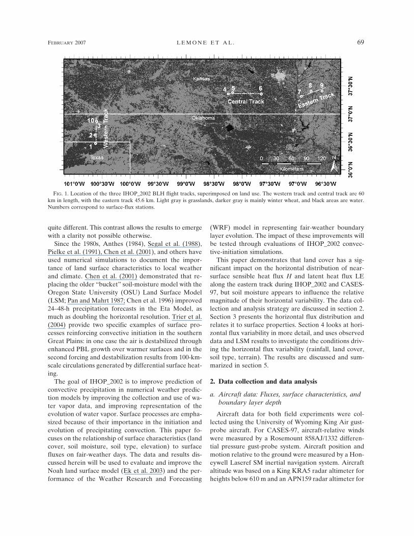
FIG. 1. Location of the three IHOP_2002 BLH flight tracks, superimposed on land use. The western track and central track are 60km in length, with the eastern track 45.6 km. Light gray is grasslands, darker gray is mainly winter wheat, and black areas are water.Numbers correspond to surface-flux stations.

FEBRUARY 2007 L E M O N E E T A L . 69

heights above 610 m. The mixing ratio Q was measuredusing the LiCor 6262 gas analyzer, the radiometric sur-face temperature Ts was measured with a PRT-5 radi-ometer, and potential temperature � was calculatedfrom the pressure from a Rosemount 1201 sensor andair temperature measured as described in Friehe andKhelif (1992). Data were recorded at 50 Hz.

The King Air instrument package and software wereslightly different for IHOP_2002. The normalized dif-ferential vegetation index (NDVI) was estimated froman Exotech radiometer, using the relationship

NDVI �r4 � r3

r4 � r3, �1�

where r4 is the amount of electromagnetic radiationreflected in the near-infrared at 0.762–0.898 m, and r3

is the amount of electromagnetic radiation reflected inthe red at 0.629–0.687 m. The aircraft location was

corrected using GPS to within 100 m horizontally (A.Rodi 2006, personal communication), so that Ts, NDVI,and aircraft video images could easily be correlatedwith surface features. A reverse flow thermometermeasured air temperature, and a Heiman KT-19.85 ra-diometer sensed Ts. Data were recorded at 25 Hz.

Figure 1 shows the three tracks used for IHOP_2002Boundary Layer Heterogeneity (BLH) missions, whichwere designed to document the effects of the surface onBL thermodynamic fluxes and structure. The flight-track locations extended from the Oklahoma Pan-handle to southeastern Kansas, to sample a large rangeof precipitation, soils, and land-cover types. This paperfocuses on the eastern track, shown in Fig. 2; fluxes onthe western track are documented by Kang et al.(2007). From Table 1, the eastern track has greener anddenser vegetation (higher NDVI), cooler Ts, and higherrainfall than the western track. The central track hasintermediate characteristics.

Each King Air mission consisted of multiple straight-and-level legs along a single track, interspersed withsoundings to check convective boundary layer depth(Table 2). In the IHOP_2002 BLH missions, some legswere always flown at �70 m above ground level(AGL), with at least one other height within the bound-ary layer (BL) represented. The flight pattern changedwith the research emphasis, with more 70-m legs forflux missions, and legs divided more evenly betweentwo and four heights for BL structure missions. Fortypical CASES-97 missions, four sets of legs at fourlevels within the BL were flown along the IHOP_2002eastern track, with the lowest level at 30–40 m AGL.The lowest legs (below 100–150 m) were flown at aroughly constant height above the ground, while thehigher legs were flown according to pressure altitude,so that altitude above the ground varied around thespecified leg height.

“Total” grand-average IHOP_2002 and CASES-97fluxes along the eastern track for a given day were cal-culated in a multiple-step procedure following LeMoneet al. (2003). First, time series for �, Q, and verticalvelocity W for each leg were detrended by subtractingout the best-fit line based on linear regression. Second,the mixing ratio was shifted 0.30 s earlier and the tem-perature 0.1 s earlier to correct for instrument time lagand the physical separation of the thermodynamic sen-sors from the vertical-velocity sensors on the aircraft.1

1 For IHOP_2002, the lag time for mixing ratio was 0.32 s, theresult of a coarser data resolution and a compromise between the0.3 s used for CASES-97 data analysis and the 0.35 based onlooking at the relationship between vertical velocity and mixing ra-tio at 70 m.

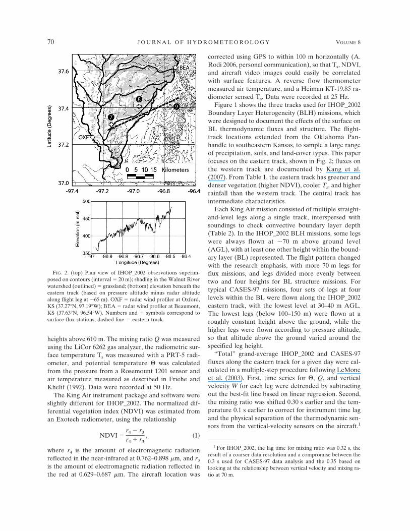
FIG. 2. (top) Plan view of IHOP_2002 observations superim-posed on contours (interval � 20 m); shading in the Walnut Riverwatershed (outlined) � grassland; (bottom) elevation beneath theeastern track (based on pressure altitude minus radar altitudealong flight leg at �65 m). OXF � radar wind profiler at Oxford,KS (37.27°N, 97.19°W); BEA � radar wind profiler at Beaumont,KS (37.63°N, 96.54°W). Numbers and � symbols correspond tosurface-flux stations; dashed line � eastern track.

70 J O U R N A L O F H Y D R O M E T E O R O L O G Y VOLUME 8

Third, the resulting time series [(t), q(t), and w(t)]were multiplied to form (t)w(t) and q(t)w(t) time se-ries. Fourth, these products were averaged into incre-ments (0.01° longitude for CASES-97, 1 km forIHOP_2002) and converted to H and LE. For each leg,this procedure resulted in a set of 0.97- or 1-km seg-ments whose fluxes, when averaged, are close to theleg-average fluxes. Fifth, data for each leg were smoothedusing a 4-km running-mean average. Finally, thesmoothed fluxes at corresponding points were averagedto form the grand-average leg. For IHOP_2002, the1-km data for each leg were interpolated to commongeographical points before averaging in time. While theinterpolation has the effect of smoothing the 1-km dataslightly, this should not significantly alter fluxes aftersmoothing with running means 4 km and longer to ob-tain statistical robustness.

For comparison, we calculated “high frequency”fluxes for the IHOP_2002 days using a procedure simi-lar to that for the total fluxes except that the 1-kmaverage fluxes for each leg were calculated using fluc-tuations relative to the corresponding 1-km mean.

We focus on the total fluxes because their magni-

tudes should be similar to measured and modeled sur-face fluxes. In the First International Satellite LandSurface Climatology Project (ISLSCP) Field Experi-ment (FIFE), high-pass filtering the data to removefluctuations of wavelength �5 km resulted in underes-timates in both H and LE (Grossman 1992; Kelly et al.1992); in a more complete analysis, Lenschow et al.(1994) obtain a similar result. For the IHOP_2002 casesexamined (Table 3), the leg-averaged high-frequencyfluxes were between 77% and 88% of the leg-averagedtotal fluxes. The disadvantage is that the total fluxesinclude “mesoscale” motions, whose larger scales leadto more random error, and which may lead to a longer“memory” of the upstream surface. Further, linear-trend removal is not optimum when the time seriesinclude an abrupt change.

Table 4 shows estimates of the fractional random er-ror �*(F) for average total H and LE for each day. Wecalculated �*(F) for each leg following Mann and Len-schow (1994) via

�*�F�L � �2�F

L �1�2�1 � rw,s2

rw,s2 �1�2

, �2�

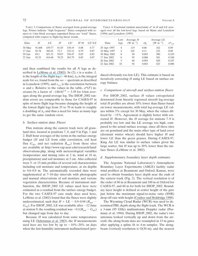
TABLE 2. Boundary layer King Air flights and environmental conditions along eastern track for CASES-97 (C) and IHOP_2002 (I);zi � boundary layer depth. Numbers in parentheses refer to equations in the text.

Date65-mlegs

Otherheights

Days afterrainfall

65-m wind(m s�1)

zi centertime (m)

�L (4)(m)

Lco (3)(km) Clouds

29 Apr 97C 4b 12 �7 S 10a 850 100 3.6 Broken Ci10 May 97C 4b 12 2 SSW 5–6a 1200 26 2.5 Clear27 May 02I 8 7 0 161°/5.5 — 98c — Ci, CiSt, AltoCu, small Cu later30 May 02I 8 8 3/5.5d 159°/3.9 900 21c 1.8 Ci; small Cu; haze at BL top17 Jun 02I 6 12 1.7 201°/7.7 1240 115c 4.4 Cu hu streets20 Jun 02I 5 9 4.7 162°/5.3 1250 46c 3.3 Scat Cu hu and Ci22 Jun 02I 10 9 6.7 179°/9.4 1260 218c 5.8 Cu hu streets

a Wind estimate from aircraft and profilers combined; from Table 1 of LeMone et al. (2003).b 30–40 m AGL.c D. Strassberg (2005, personal communication).d Three days after light (5–10 mm) rain on 27 Jun; 5.5 days after heavy rain.

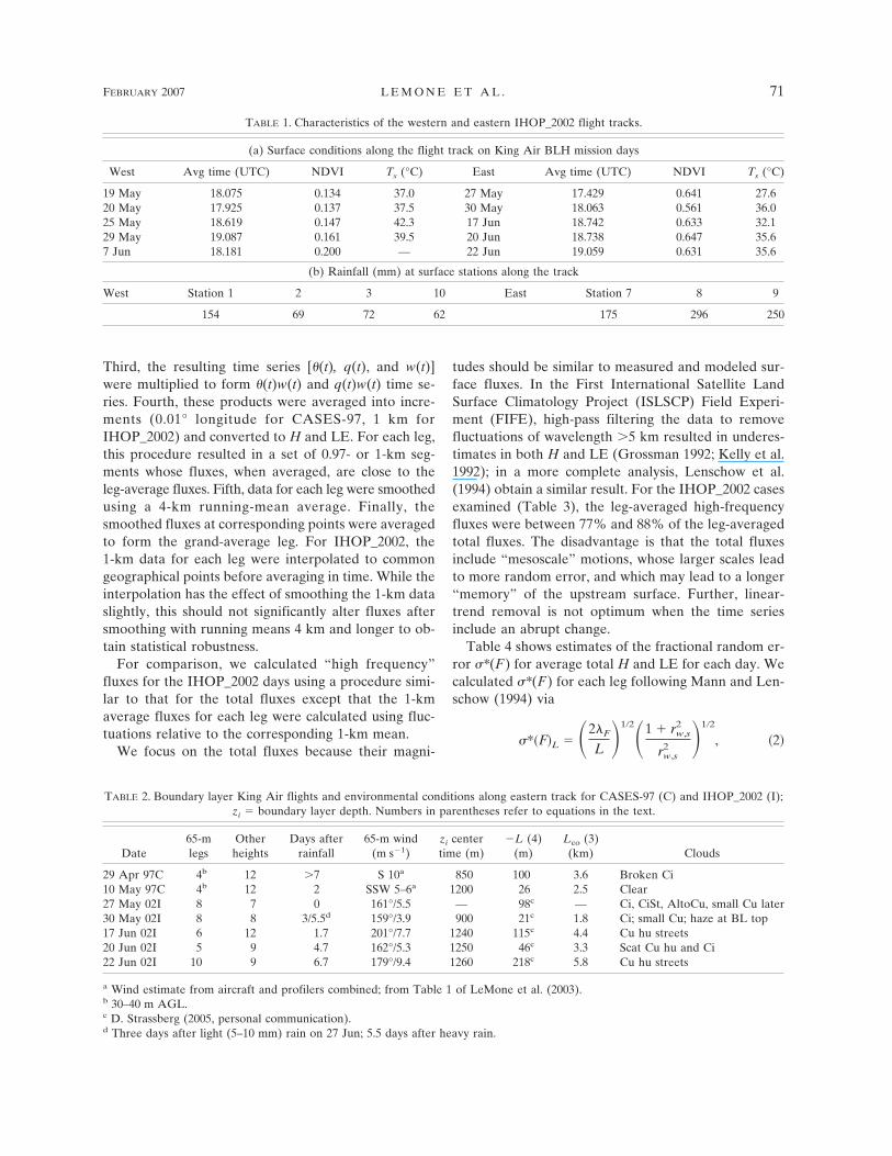
TABLE 1. Characteristics of the western and eastern IHOP_2002 flight tracks.

(a) Surface conditions along the flight track on King Air BLH mission days

West Avg time (UTC) NDVI Ts (°C) East Avg time (UTC) NDVI Ts (°C)

19 May 18.075 0.134 37.0 27 May 17.429 0.641 27.620 May 17.925 0.137 37.5 30 May 18.063 0.561 36.025 May 18.619 0.147 42.3 17 Jun 18.742 0.633 32.129 May 19.087 0.161 39.5 20 Jun 18.738 0.647 35.67 Jun 18.181 0.200 — 22 Jun 19.059 0.631 35.6

(b) Rainfall (mm) at surface stations along the track

West Station 1 2 3 10 East Station 7 8 9

154 69 72 62 175 296 250

FEBRUARY 2007 L E M O N E E T A L . 71

and then combined the results for all N legs as de-scribed in LeMone et al. (2003). In (2), s is a scalar, Lis the length of the flight leg (�46 km), F is the integralscale for ws, found from the ws � spectrum as describedin Lenschow (1995), and rw,s is the correlation betweenw and s. Relative to the values in the table, �*(F) in-creases by a factor of �(46/4)1/2 � 3.39 for 4-km aver-ages along the grand-average leg. The IHOP_2002 ran-dom errors are comparable to those for CASES-97 inspite of more flight legs because changing the height ofthe lowest flight legs from 35 to 70 m leads to roughlya doubling of F and thus a need for twice as many legsto get the same random error.

b. Surface-station data: Fluxes

Flux stations along the eastern track were all grass-land sites, located at positions 7, 8, and 9 in Figs. 1 and2. Half-hour averages of the terms in the surface energybudget (H and LE from eddy correlation, soil heatflux Gsfc, and net radiation Rnet) from these sitesare available at http://www.rap.ucar.edu/research/land/observations.php, along with meteorological variables(temperature and mixing ratio at 2 m, wind at 10 m,precipitation) and soil moisture at 5 cm. Also collectedwere 5- or 15-min profiles of several soil characteristicsincluding soil moisture and temperature, at six depthsto 0.6–0.9 m. The automatically recorded data weresupplemented at 7–10-day intervals with photographsand manual observations of soil moisture and variousvegetation characteristics. Because of instrument mal-function, the IHOP_2002 LE values used here wereestimated as a residual from the surface energy budget.For the two CASES-97 case study days used here,LeMone et al. (2002) found that the fluxes were slightlyunderestimated, such that H � LE � 0.9–0.94 (Rnet �Gsfc). For IHOP_2002, LE was available after �12 Juneat station 9; the resulting residual was �0.1(Rnet � Gsfc)but changed sign from day to day.

Because H was calculated from sonic temperaturesusing LE (Schotanus et al. 1983), the H measurementsused here are too low by up to �10%–20% on dayswhen the fast-humidity instrument malfunctioned (pro-

duced obviously too low LE). This estimate is based oniteratively correcting H using LE based on surface en-ergy balance.

c. Comparison of aircraft and surface-station fluxes

For IHOP_2002, surface H values extrapolateddownward from linearly regressed aircraft leg-averagetotal H profiles are about 10% lower than fluxes basedon tower measurements, with total leg-average LE val-ues within 5% except for 30 May, when the values dif-fered by �15%. Agreement is slightly better with cor-rected H. However, the H average for stations 7–9 isprobably too low and the LE average too high, com-pared to the actual surface average, since all three sitesare on grassland and the main other type of land cover(dormant winter wheat) should have higher H andlower LE than the green grasses. During CASES-97,King Air LE was similar to surface values given thelarge scatter, but H was up to 30% lower than the sur-face fluxes (LeMone et al. 2002).

d. Supplementary boundary layer depth estimates

The Argonne National Laboratory’s AtmosphericBoundary Layer Experiments (ABLE) facility radarwind profilers at Beaumont and Oxford, Kansas, wereused to obtain boundary layer depth near the ends ofthe eastern track (Fig. 2). The vertical resolution is ofthe order of 60 m at Beaumont and 100 m at Oxford forCASES-97, and 60 m for both for IHOP_2002. Bound-ary layer height is defined as center height of the gatejust below the maximum signal-to-noise ratio (SNR)drop-off rate with height (Coulter and Holdridge 1998).

The Wyoming Cloud Radar (WCR) was used to de-termined PBL depth along the flight track. The WCR isa 3-mm (95 GHz) multiantenna Doppler radar (Paz-many et al. 1994). During IHOP_2002, the radar’s twoantennas looked vertically up and down from the air-craft; the along-beam data are resampled in 15-m gatesafter applying a spline fit to 4-m samples. The along-beam (vertical) resolution is O(30 m), and the nearest

TABLE 4. Fractional random uncertainty �* in H and LE aver-aged over all the low-level legs, based on Mann and Lenschow(1994) and Lenschow (1995).

DateLowlegs

Average H(W m�2) �*H

Average LE(W m�2) �*LE

29 Apr 1997 4 119 0.06 162 0.0910 May 1997 4 102 0.11 232 0.0830 May 2002 8 94 0.063 380 0.10317 Jun 2002 6 95 0.086 381 0.10620 Jun 2002 5 68 0.093 420 0.10722 Jun 2002 10 92 0.063 423 0.080

TABLE 3. Comparisons of fluxes averaged from grand-averagelegs. Primes indicate “high frequency” fluxes computed with re-spect to 1-km block averages; unprimed fluxes are “total” fluxes,computed with respect to flight-leg linear trends.

Date H LE H� LE� H�/H LE�/LE

30 May 91.606 439.77 81.05 338.19 0.88 0.7717 Jun 92.78 382.01 73.3 333.12 0.79 0.8720 Jun 69.1 421.31 59.07 356.47 0.85 0.8522 Jun 92.55 416.68 78.25 363.79 0.85 0.87

72 J O U R N A L O F H Y D R O M E T E O R O L O G Y VOLUME 8

reliable gates are centered 120 m below and 105 mabove the aircraft, resulting in a 225-m “blind” zoneapproximately centered on the aircraft. Echo strengthis measured in terms of equivalent reflectivity, which isderived from power under the assumption that the scat-terers are spherical water droplets.

The WCR BL depth zi_WCR is determined from theequivalent reflectivity above plumes (Miao et al. 2006)after vertical (three gates or 45 m) and horizontal (10 sor �830 m) smoothing. Usually, zi_WCR is found fromthe upward-looking beam, and defined as where therange-corrected reflectivity reaches a minimum—be-tween the drop-off at plume top and the increase inreflectivity due to range-corrected noise. For the down-ward-looking beam, zi_WCR is taken as the height of anarbitrary reflectivity value ranging between �28 and�26 dBZ. This level is characterized by a large reflec-tivity gradient. Since the scatterers are small insectstrying to fly downward, reflectivity becomes small be-tween plumes and BL depth is often not detectablethere (Geerts and Miao 2005).

3. Results

a. Environmental conditions

With the exception of 27 May (IHOP_2002) whenlight rain fell, the days examined (Table 2) had clearskies to scattered clouds, and wind from �SSW–SE,with speeds ranging from slightly less than 4 m s�1 on30 May 2002 to 10 m s�1 on 29 April 1997. From Fig. 3,the rain and associated cloudiness significantly alteredthe surface energy budget on 27 May. Since our focus ison the effects of surface heterogeneity, 27 May will notbe included in the analysis. The curves for net radiation(Rnet), H, LE, and heat flux into the soil (Gsfc), arerelatively smooth on the remaining six days, consistentwith the lack of significant cloudiness (Fig. 3; Fig. 3 ofLeMone et al. 2002; Fig. 9 of LeMone et al. 2000). TheJune days represent a single dry-down event (Table 2).

The land-use maps (Figs. 1, 2) show a higher densityof crops (mainly winter wheat) to the west and mainlygrasslands to the east, relative to the eastern track andfor at least 100 km to the south. The band of winterwheat extends south to the Oklahoma–Kansas border;south of the border, the winter wheat band extendssouthwestward to beyond the Oklahoma–Texas border.Aircraft videos and surface site visits show land usealong the flight track to be similar for CASES-97 andIHOP_2002. The dominant soil type along the flighttrack is silty clay loam (State Soil Geographic Data-base). Rainfall was ample (Table 1; Yates et al. 2001)and frequent (Chen et al. 2003, 2007) for both fieldprograms, so the vegetation was not stressed.

b. Horizontal variability in low-level fluxes alongthe flight track

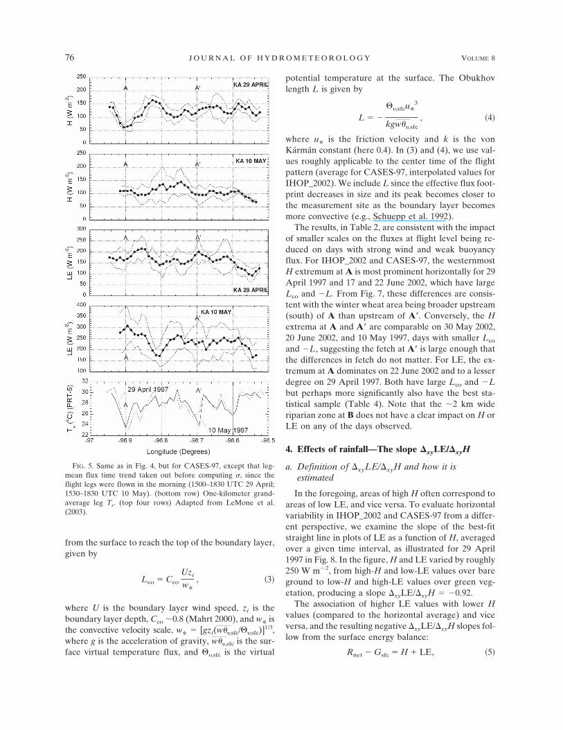
The H patterns, in Fig. 4 for IHOP_2002 and Fig. 5for CASES-97, have consistent behavior for both ex-periments. For the IHOP_2002 days, there are Hmaxima around �96.9° (A) and �96.7° (A�), separatedby a minimum from �96.77° to �96.8°. The pattern isreversed for CASES-97, with a well-defined H mini-mum around A on 29 April 1997 and a broader H mini-mum on 10 May 1997 spanning the same location; andsecondary H minima around A� on 10 May, and slightlywest of A� on 29 April. At the east end of the track, Hincreases eastward on three of the four IHOP_2002days, and decreases eastward on the two CASES-97 days.

The LE patterns in Figs. 4 and 5 are not as welldefined as the H patterns, with horizontal fluctuationssometimes less than the temporal standard deviations.Such behavior has also been noted by Mahrt (2000).However, there are LE minima around A� for all theIHOP_2002 days except 22 June, corresponding to theIHOP_2002 H maxima. On 22 June, the LE minimumat A corresponds to the major H maximum, and the LEmaximum corresponds to the H minimum east of A�.Also, the CASES-97 data show LE maxima near A thatcorrespond roughly with the westernmost CASES-97 Hminima and IHOP_2002 H maxima.

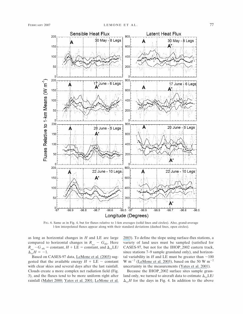
Except for the expected smaller values, amplitudes,and standard deviations, the IHOP_2002 fluxes relativeto 1-km averages in Fig. 6 resemble those in Fig. 4closely. The similarity of the flux trends near the legends suggests that linear trend removal to produce thefluxes in Figs. 4 and 5 did not have a significant effect.

Comparing Figs. 4–6 to Fig. 7, the major features inthe flux patterns are correlated with Ts, NDVI, andland-use patterns along the flight track. The Ts maximaand NDVI minima for IHOP_2002 correspond to areasof senescent-to-harvested (�15 June) winter wheat,with the broadest extrema at A and A�, and more lo-calized extrema at the riparian zone B. Locations A andA� tend to have high H values and, to a lesser degree,low LE values. The low-Ts, high-NDVI areas corre-spond to green grass, low H, and to a lesser degree, highLE. In CASES-97, the patterns reverse, with low H,high LE, low Ts, and high NDVI over the winter wheat,which grows rapidly in late April through middle May;and high H, low LE, high Ts, and low NDVI over thegrasslands, which are largely dormant on 29 April, andstarting to green up by 10 May. The association of Hand LE with Ts is discussed in more detail for CASES-97 in Grossman et al. (2005). The small horizontal Ts

variability on 17 June 2002 relates to rain on 15–16 June(Table 2).

FEBRUARY 2007 L E M O N E E T A L . 73

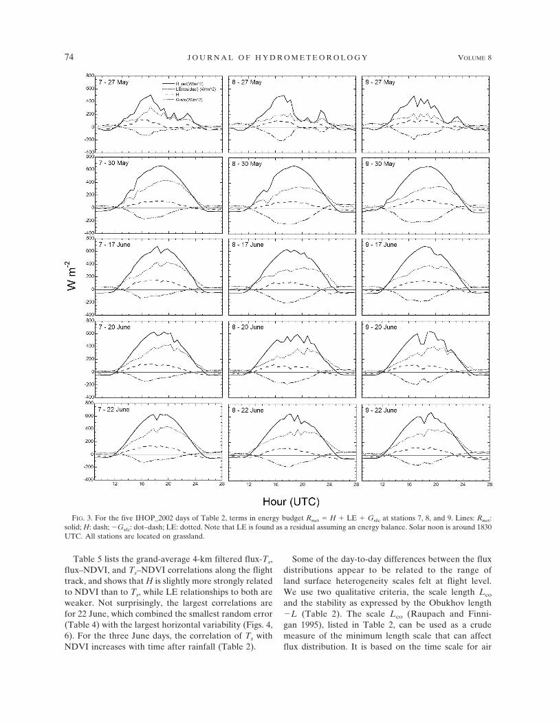
Table 5 lists the grand-average 4-km filtered flux-Ts,flux–NDVI, and Ts–NDVI correlations along the flighttrack, and shows that H is slightly more strongly relatedto NDVI than to Ts, while LE relationships to both areweaker. Not surprisingly, the largest correlations arefor 22 June, which combined the smallest random error(Table 4) with the largest horizontal variability (Figs. 4,6). For the three June days, the correlation of Ts withNDVI increases with time after rainfall (Table 2).

Some of the day-to-day differences between the fluxdistributions appear to be related to the range ofland surface heterogeneity scales felt at flight level.We use two qualitative criteria, the scale length Lco

and the stability as expressed by the Obukhov length�L (Table 2). The scale Lco (Raupach and Finni-gan 1995), listed in Table 2, can be used as a crudemeasure of the minimum length scale that can affectflux distribution. It is based on the time scale for air

FIG. 3. For the five IHOP_2002 days of Table 2, terms in energy budget Rnet � H � LE � Gsfc at stations 7, 8, and 9. Lines: Rnet:solid; H: dash; �Gsfc: dot–dash; LE: dotted. Note that LE is found as a residual assuming an energy balance. Solar noon is around 1830UTC. All stations are located on grassland.

74 J O U R N A L O F H Y D R O M E T E O R O L O G Y VOLUME 8

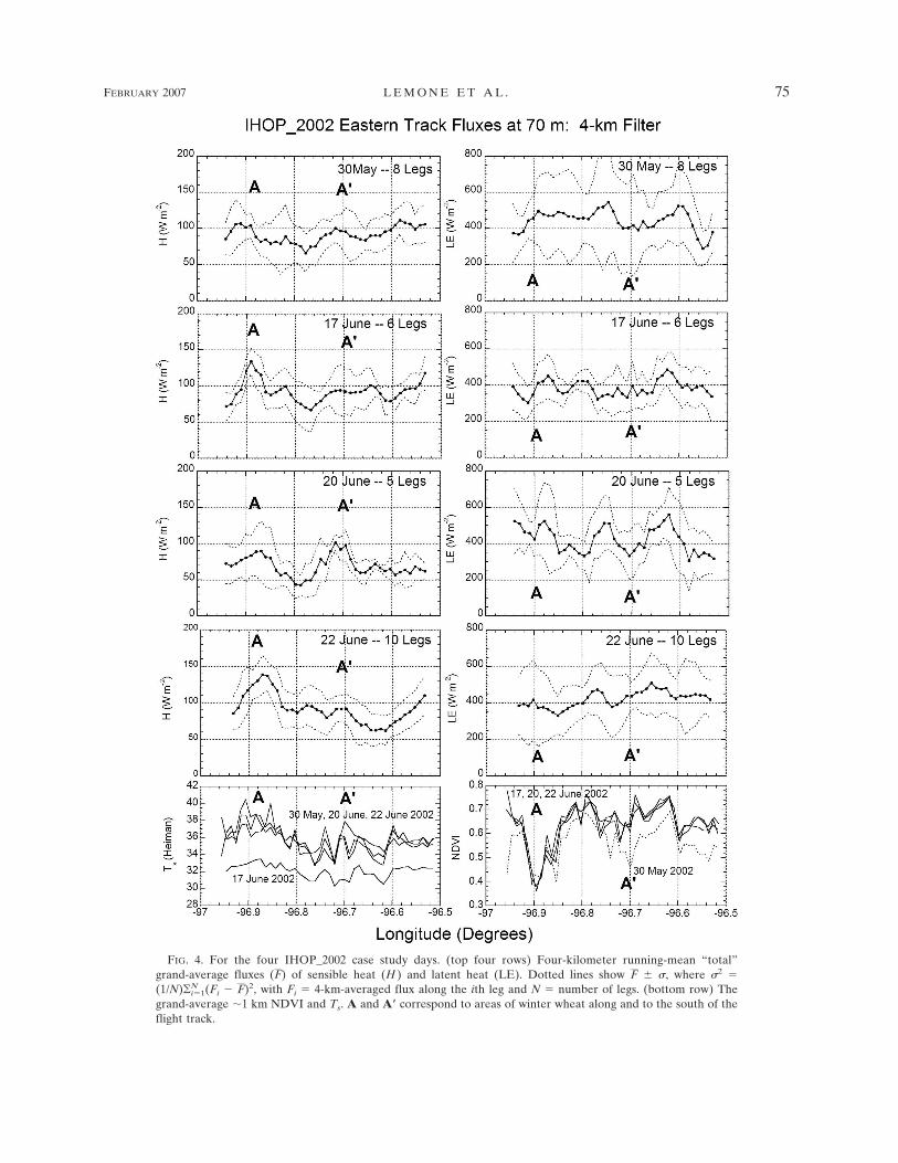
FIG. 4. For the four IHOP_2002 case study days. (top four rows) Four-kilometer running-mean “total”grand-average fluxes (F) of sensible heat (H ) and latent heat (LE). Dotted lines show F � �, where �2 �(1/N)�N

i�1(Fi � F)2, with Fi � 4-km-averaged flux along the ith leg and N � number of legs. (bottom row) Thegrand-average �1 km NDVI and Ts. A and A� correspond to areas of winter wheat along and to the south of theflight track.

FEBRUARY 2007 L E M O N E E T A L . 75

from the surface to reach the top of the boundary layer,given by

Lco � Cco

Uzi

w*, �3�

where U is the boundary layer wind speed, zi is theboundary layer depth, Cco �0.8 (Mahrt 2000), and w* isthe convective velocity scale, w* � [gzi(w�,sfc/��,sfc)]

1/3,where g is the acceleration of gravity, w�,sfc is the sur-face virtual temperature flux, and ��,sfc is the virtual

potential temperature at the surface. The Obukhovlength L is given by

L � �

��,sfcu*3

kgw��,sfc

, �4�

where u* is the friction velocity and k is the vonKármán constant (here 0.4). In (3) and (4), we use val-ues roughly applicable to the center time of the flightpattern (average for CASES-97, interpolated values forIHOP_2002). We include L since the effective flux foot-print decreases in size and its peak becomes closer tothe measurement site as the boundary layer becomesmore convective (e.g., Schuepp et al. 1992).

The results, in Table 2, are consistent with the impactof smaller scales on the fluxes at flight level being re-duced on days with strong wind and weak buoyancyflux. For IHOP_2002 and CASES-97, the westernmostH extremum at A is most prominent horizontally for 29April 1997 and 17 and 22 June 2002, which have largeLco and �L. From Fig. 7, these differences are consis-tent with the winter wheat area being broader upstream(south) of A than upstream of A�. Conversely, the Hextrema at A and A� are comparable on 30 May 2002,20 June 2002, and 10 May 1997, days with smaller Lco

and �L, suggesting the fetch at A� is large enough thatthe differences in fetch do not matter. For LE, the ex-tremum at A dominates on 22 June 2002 and to a lesserdegree on 29 April 1997. Both have large Lco and �Lbut perhaps more significantly also have the best sta-tistical sample (Table 4). Note that the �2 km wideriparian zone at B does not have a clear impact on H orLE on any of the days observed.

4. Effects of rainfall—The slope �xyLE/�xyH

a. Definition of �xyLE/�xyH and how it isestimated

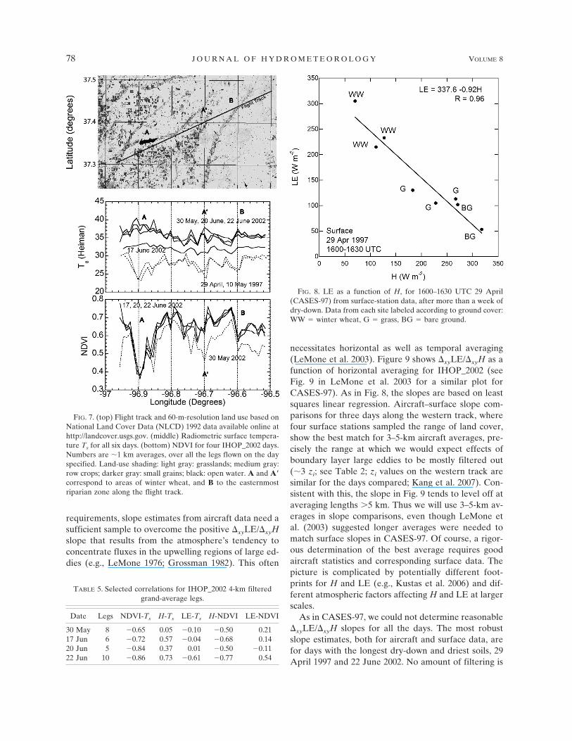
In the foregoing, areas of high H often correspond toareas of low LE, and vice versa. To evaluate horizontalvariability in IHOP_2002 and CASES-97 from a differ-ent perspective, we examine the slope of the best-fitstraight line in plots of LE as a function of H, averagedover a given time interval, as illustrated for 29 April1997 in Fig. 8. In the figure, H and LE varied by roughly250 W m�2, from high-H and low-LE values over bareground to low-H and high-LE values over green veg-etation, producing a slope �xyLE/�xyH � �0.92.

The association of higher LE values with lower Hvalues (compared to the horizontal average) and viceversa, and the resulting negative �xyLE/�xyH slopes fol-low from the surface energy balance:

Rnet � Gsfc � H � LE, �5�

FIG. 5. Same as in Fig. 4, but for CASES-97, except that leg-mean flux time trend taken out before computing �, since theflight legs were flown in the morning (1500–1830 UTC 29 April;1530–1830 UTC 10 May). (bottom row) One-kilometer grand-average leg Ts. (top four rows) Adapted from LeMone et al.(2003).

76 J O U R N A L O F H Y D R O M E T E O R O L O G Y VOLUME 8

as long as horizontal changes in H and LE are largecompared to horizontal changes in R

net� Gsfc. Here

Rnet

�G sfc � constant, H � LE � constant, and �xyLE/�xyH � �1.

Based on CASES-97 data, LeMone et al. (2003) sug-gested that the available energy H � LE � constantwith clear skies and several days after the last rainfall.Clouds create a more complex net radiation field (Fig.3), and the fluxes tend to be more uniform right afterrainfall (Mahrt 2000; Yates et al. 2001; LeMone et al.

2003). To define the slope using surface-flux stations, avariety of land uses must be sampled (satisfied forCASES-97, but not for the IHOP_2002 eastern track,since stations 7–9 sample grassland only), and horizon-tal variability in H and LE must be greater than �100W m�2 (LeMone et al. 2003), based on the 50 W m�2

uncertainty in the measurements (Yates et al. 2001).Because the IHOP_2002 surface sites sample grass-

land only, we turned to aircraft data to estimate �xyLE/�xyH for the days in Fig. 4. In addition to the above

FIG. 6. Same as in Fig. 4, but for fluxes relative to 1-km averages (solid lines and circles). Also, grand-average1-km interpolated fluxes appear along with their standard deviations (dashed lines, open circles).

FEBRUARY 2007 L E M O N E E T A L . 77

requirements, slope estimates from aircraft data need asufficient sample to overcome the positive �xyLE/�xyHslope that results from the atmosphere’s tendency toconcentrate fluxes in the upwelling regions of large ed-dies (e.g., LeMone 1976; Grossman 1982). This often

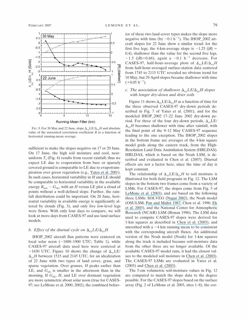
necessitates horizontal as well as temporal averaging(LeMone et al. 2003). Figure 9 shows �xyLE/�xyH as afunction of horizontal averaging for IHOP_2002 (seeFig. 9 in LeMone et al. 2003 for a similar plot forCASES-97). As in Fig. 8, the slopes are based on leastsquares linear regression. Aircraft–surface slope com-parisons for three days along the western track, wherefour surface stations sampled the range of land cover,show the best match for 3–5-km aircraft averages, pre-cisely the range at which we would expect effects ofboundary layer large eddies to be mostly filtered out(�3 zi; see Table 2; zi values on the western track aresimilar for the days compared; Kang et al. 2007). Con-sistent with this, the slope in Fig. 9 tends to level off ataveraging lengths �5 km. Thus we will use 3–5-km av-erages in slope comparisons, even though LeMone etal. (2003) suggested longer averages were needed tomatch surface slopes in CASES-97. Of course, a rigor-ous determination of the best average requires goodaircraft statistics and corresponding surface data. Thepicture is complicated by potentially different foot-prints for H and LE (e.g., Kustas et al. 2006) and dif-ferent atmospheric factors affecting H and LE at largerscales.

As in CASES-97, we could not determine reasonable�xyLE/�xyH slopes for all the days. The most robustslope estimates, both for aircraft and surface data, arefor days with the longest dry-down and driest soils, 29April 1997 and 22 June 2002. No amount of filtering is

TABLE 5. Selected correlations for IHOP_2002 4-km filteredgrand-average legs.

Date Legs NDVI-Ts H-Ts LE-Ts H-NDVI LE-NDVI

30 May 8 �0.65 0.05 �0.10 �0.50 0.2117 Jun 6 �0.72 0.57 �0.04 �0.68 0.1420 Jun 5 �0.84 0.37 0.01 �0.50 �0.1122 Jun 10 �0.86 0.73 �0.61 �0.77 0.54

FIG. 7. (top) Flight track and 60-m-resolution land use based onNational Land Cover Data (NLCD) 1992 data available online athttp://landcover.usgs.gov. (middle) Radiometric surface tempera-ture Ts for all six days. (bottom) NDVI for four IHOP_2002 days.Numbers are �1 km averages, over all the legs flown on the dayspecified. Land-use shading: light gray: grasslands; medium gray:row crops; darker gray: small grains; black: open water. A and A�

correspond to areas of winter wheat, and B to the easternmostriparian zone along the flight track.

FIG. 8. LE as a function of H, for 1600–1630 UTC 29 April(CASES-97) from surface-station data, after more than a week ofdry-down. Data from each site labeled according to ground cover:WW � winter wheat, G � grass, BG � bare ground.

78 J O U R N A L O F H Y D R O M E T E O R O L O G Y VOLUME 8

sufficient to make the slopes negative on 17 or 20 June.On 17 June, the high soil moisture and cool, near-uniform Ts (Fig. 4) results from recent rainfall; thus weexpect LE due to evaporation from bare or sparselycovered ground is comparable to LE due to evapotrans-piration over green vegetation (e.g., Yates et al. 2001).In such cases, horizontal variability in H and LE shouldbe comparable to horizontal variability in the availableenergy Rnet � Gsfc, with an H versus LE plot a cloud ofpoints without a well-defined slope. Further, the rain-fall distribution could be important. On 20 June, hori-zontal variability in available energy is significantly al-tered by clouds (Fig. 3), and only five low-level legswere flown. With only four days to compare, we willlook at more days from CASES-97 and use land surfacemodels.

b. Effect of the diurnal cycle on �xyLE/�xyH

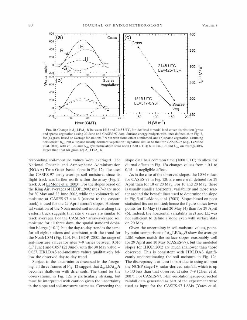
IHOP_2002 aircraft flux patterns were centered onlocal solar noon (�1800–1900 UTC; Table 1), whileCASES-97 aircraft data used here were centered at�1630 UTC. Figure 10 shows the change of �xyLE/�xyH between 1515 and 2145 UTC, for an idealizationof 22 June with two types of land cover, grass, andsparse vegetation. Over grasses, H peaks earlier thanLE, and Gsfc is smaller in the afternoon than in themorning. If Gsfc, H, and LE over dormant vegetationare more symmetric about solar noon (true for CASES-97; see LeMone et al. 2000, 2002), the combined behav-

ior of these two land-cover types makes the slope morenegative with time (by �0.1 h�1). The IHOP_2002 air-craft slopes for 22 June show a similar trend: for thefirst five legs, the 4-km-average slope is �1.25 (|R| �0.4), shallower than the value for the second five legs,�1.5 (|R|�0.66), again a �0.1 h�1 decrease. ForCASES-97, half-hour-average plots of �xyLE/�xyHfrom half-hour-averaged surface-station data centeredfrom 1745 to 2115 UTC revealed no obvious trend for10 May, but 29 April slopes became shallower with time(�0.05 h�1).

c. The association of shallower �xyLE/�xyH slopeswith longer dry-down and drier soils

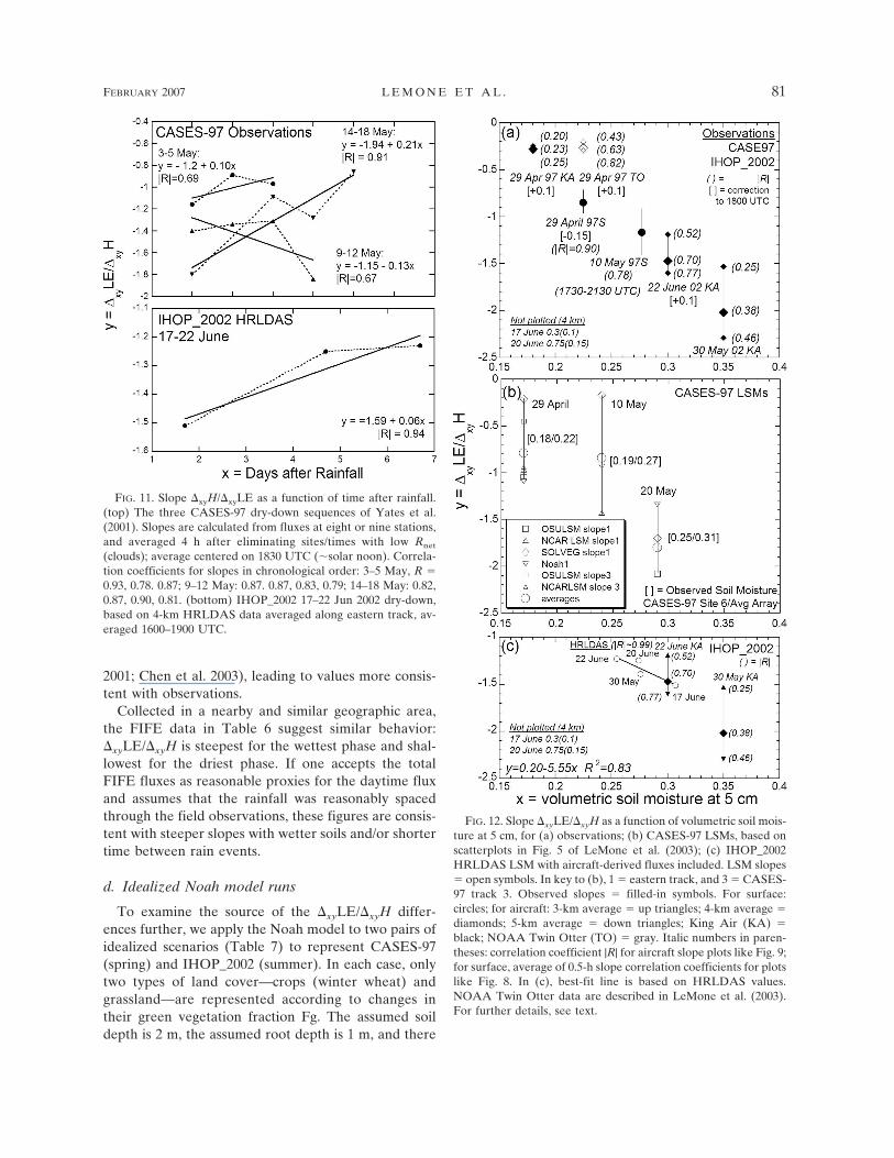
Figure 11 shows �xyLE/�xyH as a function of time forthe three observed CASES-97 dry-down periods de-scribed in Fig. 7 of Yates et al. (2001), and for themodeled IHOP_2002 17–22 June 2002 dry-down pe-riod. For three of the four dry-down periods, �xyLE/�xyH becomes shallower with time after rainfall, withthe final point of the 9–12 May CASES-97 sequenceleading to the one exception. The IHOP_2002 slopesin the bottom frame are averages of the 4-km squaremodel grids along the eastern track, from the High-Resolution Land Data Assimilation System (HRLDAS).HRLDAS, which is based on the Noah LSM, is de-scribed and evaluated in Chen et al. (2007). Diurnaleffects are not a factor here, since the time of day iskept constant.

The relationship of �xyLE/�xyH to soil moisture isillustrated for both field programs in Fig. 12. The LSMslopes in the bottom two frames come from a variety ofLSMs. For CASES-97, the slopes come from Fig. 5 ofLeMone et al. (2003), and are based on the followingthree LSMs: SOLVEG (Nagai 2002), the Noah model(OSULSM; Pan and Mahrt 1987; Chen et al. 1996; Eket al. 2003), and the National Center for AtmosphericResearch (NCAR) LSM (Bonan 1996). The LSM dataused to compute CASES-97 slopes were derived for1-km squares as described in Chen et al. (2003), andsmoothed with a �4 km running mean to be consistentwith the corresponding aircraft fluxes. An additionalversion of the Noah model (Noah) for 1-km squaresalong the track is included because soil-moisture datafrom the other three are no longer available. Of theavailable CASES-97 model runs, it had the closest val-ues to the modeled soil moisture in Chen et al. (2003).The CASES-97 LSMs are evaluated in Yates et al.(2003) and Chen et al. (2003).

The 5-cm volumetric soil-moisture values in Fig. 12are computed to match the slope data to the degreepossible. For the CASES-97 slopes based on the surfacearray (Fig. 2 of LeMone et al. 2003, sites 1–8), the cor-

FIG. 9. For 30 May and 22 June, slope �xyLE/�xyH and absolutevalue of the associated correlation coefficient R as a function ofhorizontal running-mean average.

FEBRUARY 2007 L E M O N E E T A L . 79

responding soil-moisture values were averaged. TheNational Oceanic and Atmospheric Administration(NOAA) Twin Otter–based slope in Fig. 12a also usesthe CASES-97 array average soil moisture, since itsflight track was farther north within the array (Fig. 2,track 3, of LeMone et al. 2003). For the slopes based onthe King Air, averages of IHOP_2002 sites 7–9 are usedfor 30 May and 22 June 2002, while the volumetric soilmoisture at CASES-97 site 6 (closest to the easterntrack) is used for the 29 April aircraft slopes. Horizon-tal variation of the Noah model soil moisture along theeastern track suggests that site 6 values are similar totrack averages. For the CASES-97 array-averaged soilmoisture for all three days, the spatial standard devia-tion is large (�0.1), but the day-to-day trend is the samefor all eight stations and consistent with the trend forthe Noah LSM (Fig. 12b). For IHOP_2002, the range ofsoil-moisture values for sites 7–9 varies between 0.016(17 June) and 0.057 (22 June), with the 30 May value �0.027. HRLDAS soil-moisture values qualitatively fol-low the observed day-to-day trend.

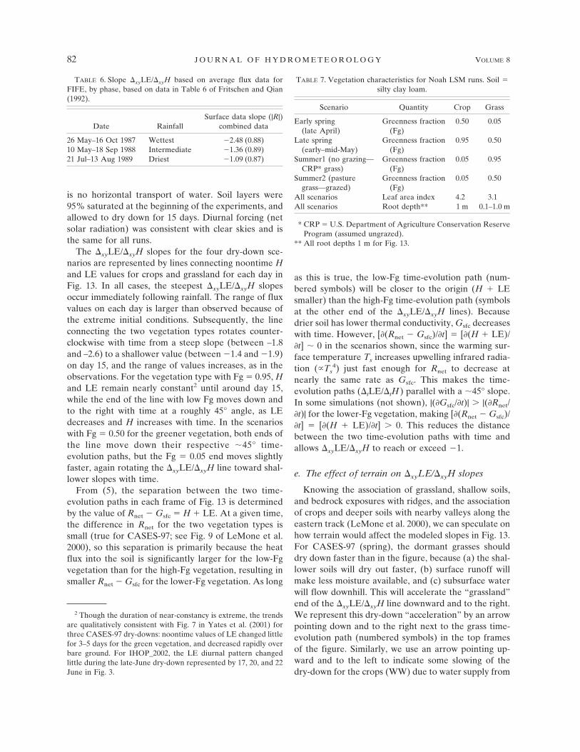
Subject to the uncertainties discussed in the forego-ing, all three frames of Fig. 12 suggest that �xyLE/�xyHbecomes shallower with drier soils. The trend for theobservations, in Fig. 12a is particularly striking, butmust be interpreted with caution given the uncertaintyin the slope and soil-moisture estimates. Correcting the

slope data to a common time (1800 UTC) to allow fordiurnal effects in Fig. 12a changes values from �0.1 to0.15—a negligible effect.

As in the case of the observed slopes, the LSM valuesfor CASES-97 in Fig. 12b are more well defined for 29April than for 10 or 20 May. For 10 and 20 May, thereis usually smaller horizontal variability and more scat-ter around the best-fit lines used to determine the slopein Fig. 5 of LeMone et al. (2003). Slopes based on poorstatistical fits are omitted; hence the figure shows fewerpoints for 10 May (3) and 20 May (4) than for 29 April(6). Indeed, the horizontal variability in H and LE wasnot sufficient to define a slope even with surface dataon 20 May.

Given the uncertainty in soil-moisture values, point-by-point comparisons of �xyLE/�xyH show the averageLSM values match the surface slopes reasonably wellfor 29 April and 10 May (CASES-97), but the modeledslopes for IHOP_2002 are much shallower than thoseobserved. This is consistent with HRLDAS signifi-cantly underestimating the soil moisture in Fig. 12c.The discrepancy is at least in part due to using as inputthe NCEP stage-IV radar-derived rainfall, which is upto 1/3 less than that observed at sites 7–9 (Chen et al.2007). For CASES-97, 1-km-resolution gauge-correctedrainfall data generated as part of the experiment wereused as input for the CASES-97 LSMs (Yates et al.

FIG. 10. Change in �xyLE/�xyH between 1515 and 2145 UTC, for idealized bimodal land-cover distribution (grassand sparse vegetation) using 22 June and CASES-97 data. Surface energy budgets with lines defined as in Fig. 3,for (a) grass, based on average for stations 7–9 but with cloud effect eliminated, and (b) sparse vegetation, assuming“cloudless” Rnet but a “sparse mostly dormant vegetation” signature similar to that for CASES-97 (e.g., LeMoneet al. 2000), with H, LE, and Gsfc symmetric about solar noon (1830 UTC); H � 0.82 LE and Gsfc on average 40%larger than that for grass. (c) �xyLE/�xyH.

80 J O U R N A L O F H Y D R O M E T E O R O L O G Y VOLUME 8

2001; Chen et al. 2003), leading to values more consis-tent with observations.

Collected in a nearby and similar geographic area,the FIFE data in Table 6 suggest similar behavior:�xyLE/�xyH is steepest for the wettest phase and shal-lowest for the driest phase. If one accepts the totalFIFE fluxes as reasonable proxies for the daytime fluxand assumes that the rainfall was reasonably spacedthrough the field observations, these figures are consis-tent with steeper slopes with wetter soils and/or shortertime between rain events.

d. Idealized Noah model runs

To examine the source of the �xyLE/�xyH differ-ences further, we apply the Noah model to two pairs ofidealized scenarios (Table 7) to represent CASES-97(spring) and IHOP_2002 (summer). In each case, onlytwo types of land cover—crops (winter wheat) andgrassland—are represented according to changes intheir green vegetation fraction Fg. The assumed soildepth is 2 m, the assumed root depth is 1 m, and there

FIG. 11. Slope �xyH/�xyLE as a function of time after rainfall.(top) The three CASES-97 dry-down sequences of Yates et al.(2001). Slopes are calculated from fluxes at eight or nine stations,and averaged 4 h after eliminating sites/times with low Rnet

(clouds); average centered on 1830 UTC (�solar noon). Correla-tion coefficients for slopes in chronological order: 3–5 May, R �0.93, 0.78. 0.87; 9–12 May: 0.87. 0.87, 0.83, 0.79; 14–18 May: 0.82,0.87, 0.90, 0.81. (bottom) IHOP_2002 17–22 Jun 2002 dry-down,based on 4-km HRLDAS data averaged along eastern track, av-eraged 1600–1900 UTC.

FIG. 12. Slope �xyLE/�xyH as a function of volumetric soil mois-ture at 5 cm, for (a) observations; (b) CASES-97 LSMs, based onscatterplots in Fig. 5 of LeMone et al. (2003); (c) IHOP_2002HRLDAS LSM with aircraft-derived fluxes included. LSM slopes� open symbols. In key to (b), 1 � eastern track, and 3 � CASES-97 track 3. Observed slopes � filled-in symbols. For surface:circles; for aircraft: 3-km average � up triangles; 4-km average �diamonds; 5-km average � down triangles; King Air (KA) �black; NOAA Twin Otter (TO) � gray. Italic numbers in paren-theses: correlation coefficient |R| for aircraft slope plots like Fig. 9;for surface, average of 0.5-h slope correlation coefficients for plotslike Fig. 8. In (c), best-fit line is based on HRLDAS values.NOAA Twin Otter data are described in LeMone et al. (2003).For further details, see text.

FEBRUARY 2007 L E M O N E E T A L . 81

is no horizontal transport of water. Soil layers were95% saturated at the beginning of the experiments, andallowed to dry down for 15 days. Diurnal forcing (netsolar radiation) was consistent with clear skies and isthe same for all runs.

The �xyLE/�xyH slopes for the four dry-down sce-narios are represented by lines connecting noontime Hand LE values for crops and grassland for each day inFig. 13. In all cases, the steepest �xyLE/�xyH slopesoccur immediately following rainfall. The range of fluxvalues on each day is larger than observed because ofthe extreme initial conditions. Subsequently, the lineconnecting the two vegetation types rotates counter-clockwise with time from a steep slope (between –1.8and –2.6) to a shallower value (between �1.4 and �1.9)on day 15, and the range of values increases, as in theobservations. For the vegetation type with Fg � 0.95, Hand LE remain nearly constant2 until around day 15,while the end of the line with low Fg moves down andto the right with time at a roughly 45° angle, as LEdecreases and H increases with time. In the scenarioswith Fg � 0.50 for the greener vegetation, both ends ofthe line move down their respective �45° time-evolution paths, but the Fg � 0.05 end moves slightlyfaster, again rotating the �xyLE/�xyH line toward shal-lower slopes with time.

From (5), the separation between the two time-evolution paths in each frame of Fig. 13 is determinedby the value of Rnet � Gsfc � H � LE. At a given time,the difference in Rnet for the two vegetation types issmall (true for CASES-97; see Fig. 9 of LeMone et al.2000), so this separation is primarily because the heatflux into the soil is significantly larger for the low-Fgvegetation than for the high-Fg vegetation, resulting insmaller Rnet � Gsfc for the lower-Fg vegetation. As long

as this is true, the low-Fg time-evolution path (num-bered symbols) will be closer to the origin (H � LEsmaller) than the high-Fg time-evolution path (symbolsat the other end of the �xyLE/�xyH lines). Becausedrier soil has lower thermal conductivity, Gsfc decreaseswith time. However, [�(Rnet � Gsfc)/�t] � [�(H � LE)/�t] � 0 in the scenarios shown, since the warming sur-face temperature Ts increases upwelling infrared radia-tion (�Ts

4) just fast enough for Rnet to decrease atnearly the same rate as Gsfc. This makes the time-evolution paths (�tLE/�tH) parallel with a �45° slope.In some simulations (not shown), |(�Gsfc/�t)| � |(�Rnet/�t)| for the lower-Fg vegetation, making [�(Rnet � Gsfc)/�t] � [�(H � LE)/�t] � 0. This reduces the distancebetween the two time-evolution paths with time andallows �xyLE/�xyH to reach or exceed �1.

e. The effect of terrain on �xyLE/�xyH slopes

Knowing the association of grassland, shallow soils,and bedrock exposures with ridges, and the associationof crops and deeper soils with nearby valleys along theeastern track (LeMone et al. 2000), we can speculate onhow terrain would affect the modeled slopes in Fig. 13.For CASES-97 (spring), the dormant grasses shoulddry down faster than in the figure, because (a) the shal-lower soils will dry out faster, (b) surface runoff willmake less moisture available, and (c) subsurface waterwill flow downhill. This will accelerate the “grassland”end of the �xyLE/�xyH line downward and to the right.We represent this dry-down “acceleration” by an arrowpointing down and to the right next to the grass time-evolution path (numbered symbols) in the top framesof the figure. Similarly, we use an arrow pointing up-ward and to the left to indicate some slowing of thedry-down for the crops (WW) due to water supply from

2 Though the duration of near-constancy is extreme, the trendsare qualitatively consistent with Fig. 7 in Yates et al. (2001) forthree CASES-97 dry-downs: noontime values of LE changed littlefor 3–5 days for the green vegetation, and decreased rapidly overbare ground. For IHOP_2002, the LE diurnal pattern changedlittle during the late-June dry-down represented by 17, 20, and 22June in Fig. 3.

TABLE 7. Vegetation characteristics for Noah LSM runs. Soil �silty clay loam.

Scenario Quantity Crop Grass

Early spring(late April)

Greenness fraction(Fg)

0.50 0.05

Late spring(early–mid-May)

Greenness fraction(Fg)

0.95 0.50

Summer1 (no grazing—CRP* grass)

Greenness fraction(Fg)

0.05 0.95

Summer2 (pasturegrass—grazed)

Greenness fraction(Fg)

0.05 0.50

All scenarios Leaf area index 4.2 3.1All scenarios Root depth** 1 m 0.1–1.0 m

* CRP � U.S. Department of Agriculture Conservation ReserveProgram (assumed ungrazed).

** All root depths 1 m for Fig. 13.

TABLE 6. Slope �xyLE/�xyH based on average flux data forFIFE, by phase, based on data in Table 6 of Fritschen and Qian(1992).

Date RainfallSurface data slope (|R|)

combined data

26 May–16 Oct 1987 Wettest �2.48 (0.88)10 May–18 Sep 1988 Intermediate �1.36 (0.89)21 Jul–13 Aug 1989 Driest �1.09 (0.87)

82 J O U R N A L O F H Y D R O M E T E O R O L O G Y VOLUME 8

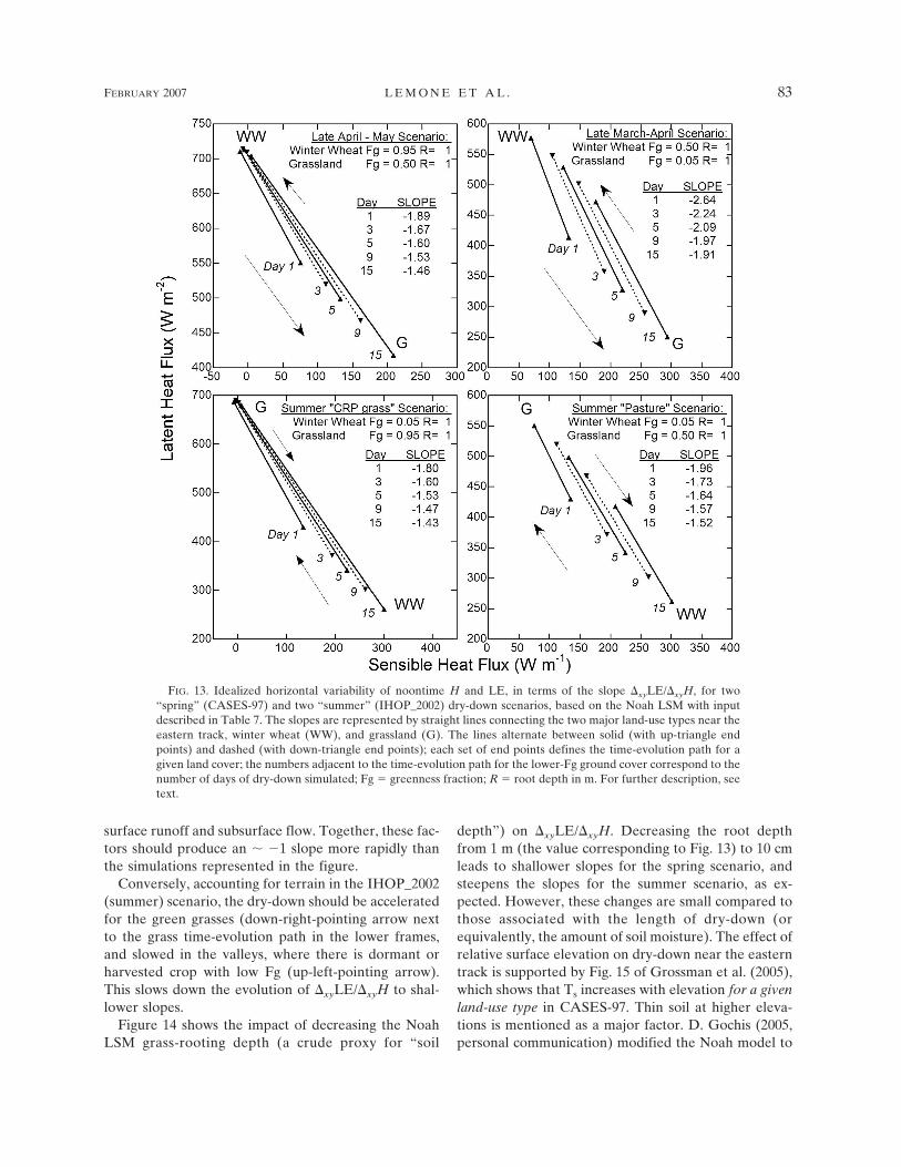
surface runoff and subsurface flow. Together, these fac-tors should produce an � �1 slope more rapidly thanthe simulations represented in the figure.

Conversely, accounting for terrain in the IHOP_2002(summer) scenario, the dry-down should be acceleratedfor the green grasses (down-right-pointing arrow nextto the grass time-evolution path in the lower frames,and slowed in the valleys, where there is dormant orharvested crop with low Fg (up-left-pointing arrow).This slows down the evolution of �xyLE/�xyH to shal-lower slopes.

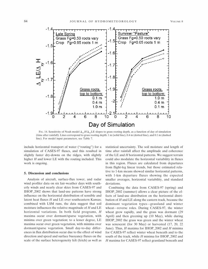
Figure 14 shows the impact of decreasing the NoahLSM grass-rooting depth (a crude proxy for “soil

depth”) on �xyLE/�xyH. Decreasing the root depthfrom 1 m (the value corresponding to Fig. 13) to 10 cmleads to shallower slopes for the spring scenario, andsteepens the slopes for the summer scenario, as ex-pected. However, these changes are small compared tothose associated with the length of dry-down (orequivalently, the amount of soil moisture). The effect ofrelative surface elevation on dry-down near the easterntrack is supported by Fig. 15 of Grossman et al. (2005),which shows that Ts increases with elevation for a givenland-use type in CASES-97. Thin soil at higher eleva-tions is mentioned as a major factor. D. Gochis (2005,personal communication) modified the Noah model to

FIG. 13. Idealized horizontal variability of noontime H and LE, in terms of the slope �xyLE/�xyH, for two“spring” (CASES-97) and two “summer” (IHOP_2002) dry-down scenarios, based on the Noah LSM with inputdescribed in Table 7. The slopes are represented by straight lines connecting the two major land-use types near theeastern track, winter wheat (WW), and grassland (G). The lines alternate between solid (with up-triangle endpoints) and dashed (with down-triangle end points); each set of end points defines the time-evolution path for agiven land cover; the numbers adjacent to the time-evolution path for the lower-Fg ground cover correspond to thenumber of days of dry-down simulated; Fg � greenness fraction; R � root depth in m. For further description, seetext.

FEBRUARY 2007 L E M O N E E T A L . 83

include horizontal transport of water (“routing”) for asimulation of CASES-97 fluxes, and this resulted inslightly faster dry-downs on the ridges, with slightlyhigher H and lower LE with the routing included. Thiswork is ongoing.

5. Discussion and conclusions

Analysis of aircraft, surface-flux tower, and radarwind profiler data on six fair-weather days with south-erly winds and nearly clear skies from CASES-97 andIHOP_2002 shows that land-use patterns have stronginfluence on the horizontal distribution of sensible andlatent heat fluxes H and LE over southeastern Kansas;combined with LSM runs, the data suggest that soilmoisture influences the relative magnitude of H and LEhorizontal variations. In both field programs, Hmaxima occur over dormant/sparse vegetation, withminima over green vegetation; to a lesser degree, LEmaxima occur over green vegetation, with minima overdormant/sparse vegetation. Small day-to-day differ-ences in flux distribution occur due to the effect of winddirection and speed and surface buoyancy fluxes on thescale of the surface heterogeneity felt (fetch) as well as

statistical uncertainty. The soil moisture and length oftime after rainfall affect the amplitude and coherenceof the LE and H horizontal patterns. We suggest terraincould also modulate the horizontal variability in fluxesin this region. Fluxes are calculated from departuresfrom flight-leg linear trends, but those estimated rela-tive to 1-km means showed similar horizontal patterns,with 1-km departure fluxes showing the expectedsmaller averages, horizontal variability, and standarddeviations.

Combining the data from CASES-97 (spring) andIHOP_2002 (summer) allows a clear picture of the ef-fects of land-use distribution on the horizontal distri-bution of H and LE along the eastern track, because thedominant vegetation types—grassland and winterwheat—reverse roles. During CASES-97, the winterwheat grew rapidly, and the grass was dormant (29April) and then greening up (10 May), while duringIHOP_2002 the grass was green and the winter wheatwas senescent (for 30 May) or harvested (17, 20, 22June). Thus, H maxima for IHOP_2002 and H minimafor CASES-97 reflect winter wheat beneath and to thesouth of the track, while H minima for IHOP_2002 andH maxima for CASES-97 reflect grassland beneath and

FIG. 14. Sensitivity of Noah model �xyH/�xyLE slopes to grass rooting depth, as a function of day of simulation(time after rainfall). Lines correspond to grass rooting depth: 1 m (solid line), 0.4 m (dotted line), and 0.1 m (dashedline). For model input parameters, see Table 7.

84 J O U R N A L O F H Y D R O M E T E O R O L O G Y VOLUME 8

to the south of the track. For LE there is a weakertendency for higher values over the green vegetationand lower values over the dormant vegetation. Consis-tent with this, high H values correspond to high Ts andlow values of NDVI, while, to a lesser degree, highvalues of LE correspond to high NDVI and low Ts forboth field programs.

For days with few or no clouds, using observationsand LSMs to quantify H and LE horizontal variabilityin terms of the slope �xyLE/�xyH for plots of LE as afunction of H at a given time suggests the followingtime sequence: right after rainfall, H and LE are rela-tively uniform with no well-defined slope, after which aslope emerges (��2), which gets shallower (��1) andbetter defined with time during soil dry-down. Consis-tent with this behavior, moister soil tends to be associ-ated with steeper slopes. Rainfall is ample, so the veg-etation never becomes stressed. Noah model runs foridealized CASES-97 and IHOP_2002 scenarios suggestthat flux into the soil has an important role in deter-mining the slope by reducing the available energy Rnet

� Gsfc for the less-green or dormant vegetation. Be-cause H, LE, and Gsfc can peak at different times atsome locations, the slope can also vary as a function oftime of day, but this effect is small since slopes werecomputed for similar times.

Other things being equal, the idealized Noah runsalso suggest that the relationship of vegetation with ter-rain could lead to steeper slopes for IHOP_2002 (June–July) than for CASES-97 (April–mid-May), but the ef-fect is small. The association of grass with ridges (due toshallow soil and bedrock exposures) and winter wheatwith valleys (deep enough soil to cultivate) should af-fect the rate of dry-down and the associated evolutionof H and LE. In the spring, the dormant grass on theridges should dry down faster than for no terrain, be-cause of shallower soil and surface and subsurface run-off (less water available), while the dry-down of thegreen winter wheat should be slowed by water suppliedfrom higher elevations. This should accelerate the trendof the slopes to shallower values for CASES-97. Con-versely, in IHOP_2002, the accelerated dry-down of thegreen grasses and slowed dry-down of the dormant orharvested winter wheat should slow the tendency of theslope to become shallower with time.

The relationship of �xyH/�xyLE to length of dry-down and soil moisture are suggestive, but more dataare needed to obtain definitive results, and the analysisis limited to one geographic area. IHOP_2002 slopesare based on aircraft data, and CASES-97 slopes pri-marily on surface data, and there are only a few cases todraw from. There are no IHOP_2002 surface-station-based slopes along the eastern track for deciding what

filter length is best to calculate aircraft-derived slopes,so we chose 4 km based on western-track aircraft andsurface data. Four LSMs suggest an association ofsteeper slopes with moister soils, and one (HRLDAS)was used to document shallower slopes with time afterrainfall; it would be desirable to use the same LSM(s)for the whole dataset. Looking at soil moisture throughthe root zone would be of interest, but such data are notavailable for CASES-97. Idealized LSM runs and theresults of Grossman et al. (2005) suggest terrain effectscould lead to steeper slopes for IHOP_2002, but defini-tive observational evidence is lacking.

While several investigators have used aircraft data toevaluate surface fluxes (e.g., Schuepp et al. 1992; Mahrt2000; Song and Wesely 2003; Isaac et al. 2004; Kustas etal. 2006), statistical uncertainties continue to plaguesuch comparisons. Many investigators have used high-pass filtering to reduce the uncertainty, and LeMone etal. (2003) suggest horizontally averaging the aircraftdata to remove the effects of concentration of fluxes bylarge eddies and to increase statistical robustness, andthen applying an equivalent filter to the LSM data tomake the two datasets comparable. However, the pos-sibility that source regions for H and LE might not beequivalent (Kustas et al. 2006), and the possibility thatatmospheric processes could affect H and LE differ-ently at larger scales, leads to questions of how filteringaffects the effective sources and hence �xyLE/�xyH.Spring and summer data are needed from an array ofsurface-flux stations over representative land-use types,and repeated aircraft flux measurements are needed toquantify seasonal surface heterogeneity effects and de-termine the best way to filter aircraft data.

Future plans include comparisons of the estimatedfluxes with surface-flux and soil-moisture maps gener-ated using the Noah model, initialized with HRLDAS(Chen et al. 2007), and comparisons with satellite prod-ucts, building on the results of Chen et al. (2003). Bothcomparisons will enable a more quantitative assessmentof the effects of the upstream flux footprint, followingSchuepp et al. (1992), Song and Wesely (2003), andothers. In addition, we wish to explore the evolution of�xyLE/�xyH in the Noah model and other LSMs, andlook at other datasets to see if similar patterns emerge.

Acknowledgments. This work would not have beenpossible without the commitment, enthusiasm, and ex-pertise of the Wyoming King Air aircrew, the staffmaintaining the Wyoming Cloud Radar, National Cen-ter for Atmospheric Research staff maintaining the sur-face-flux instruments, and the students taking themanual observations at the flux sites. The NCAR por-tion of this research was supported by USWRP Grant

FEBRUARY 2007 L E M O N E E T A L . 85

NSF 01 and the NCAR Water Cycle Initiative. RLG’sparticipation in IHOP_2002 was supported by NSFGrant ATM-0296159. RC’s work was supported by theU.S. Department of Energy, Office of Biological andEnvironmental Research, under Contract W-31-109-Eng-38. We also thank Ken Davis, Ronald Dobosy,Peter Isaac, and a fourth anonymous reviewer for con-tributing significantly to tightening the final manu-script, and John Finnigan for useful discussions.

REFERENCES

Anthes, R. A., 1984: Enhancement in convective precipitation bymesoscale variations in vegetative covering in semiarid re-gions. J. Climate Appl. Meteor., 23, 541–554.

Bonan, G. B., 1996: A land surface model (LSM version 1.0) forecological, hydrological, and atmospheric studies: Technicaldescription and users guide. NCAR Tech. Note NCAR/TN-417�STR, 150 pp. [Available from NCAR Library, P.O. Box3000, Boulder, CO 80307.]

Chen, F., and Coauthors, 1996: Modeling of land-surface evapo-ration by four schemes and comparison with FIFE observa-tions. J. Geophys. Res., 101, 7251–7268.

——, R. Pielke Sr., and K. Mitchell, 2001: Development and ap-plication of land-surface models for mesoscale atmosphericmodels: Problems and promises. Observation and Modelingof Land Surface Hydrolological Processes, V. Lakshmi, J.Alberston, and J. Schaake, Eds., Amer. Geophys. Union,107–135.

——, D. N. Yates, H. Nagai, M. LeMone, K. Ikeda, and R. Gross-man, 2003: Land surface heterogeneity in the CooperativeAtmosphere Surface Exchange Study (CASES-97). Part I:Comparing modeled surface flux maps with surface-fluxtower and aircraft measurements. J. Hydrometeor., 4, 196–218.

——, and Coauthors, 2007: Description and evaluation of thecharacteristics of the NCAR High-Resolution Land Data As-similation System. J. Appl. Meteor. Climatol., in press.

Coulter, R. L., and D. Holdridge, 1998: A procedure for the au-tomatic estimation of mixed layer height. Proc. Eighth Atmo-spheric Radiation Measurement (ARM) Program ScienceTeam Meeting, Tucson, AZ, Department of Energy Office ofEnergy Research, 177–180.

Ek, M. B., K. E. Mitchell, Y. Lin, E. Rogers, P. Grummann, V.Koren, G. Gayno, and J. D. Tarplay, 2003: Implementation ofthe Noah land-use model advances in the NCAP operationalmesoscale Eta Model. J. Geophys. Res., 108, 8851,doi:10.1029/2002JD003296.

Friehe, C. A., and D. Khelif, 1992: Fast response aircraft tempera-ture sensors. J. Atmos. Oceanic Technol., 9, 784–795.

Fritschen, L., and P. Qian, 1992: Variation in energy balance com-ponents from six sites in the native prairie for three years. J.Geophys. Res., 97 (D17), 18 651–18 661.

Geerts, B., and Q. Miao, 2005: The use of millimeter Dopplerradar echoes to estimate vertical air velocities in the fair-weather convective boundary layer. J. Atmos. Oceanic Tech-nol., 22, 225–246.

Grossman, R. L., 1982: An analysis of vertical velocity spectraobtained in the BOMEX fair-weather trade-wind boundarylayer. Bound.-Layer Meteor., 23, 323–357.

——, 1992: Sampling errors in the vertical fluxes of potential tem-

perature and moisture measured by aircraft during FIFE. J.Geophys. Res., 97 (D7), 18 439–18 443.

——, D. Yates, M. A. LeMone, M. L. Wesely, and J. Song, 2005:Observed effects of horizontal radiative surface temperaturevariations in the atmosphere over a Midwest watershed dur-ing CASES 97. J. Geophys. Res., 110, D06117, doi:10.1029/2004JD004542.

Isaac, P. R., J. McAneney, R. Leuning, and J. M. Hacker, 2004:Comparison of aircraft and ground-based flux measurementsduring OASIS95. Bound.-Layer Meteor., 110, 39–67.

Kang, S., K. Davis, and M.A. LeMone, 2007: Observations of theABL structures over a heterogeneous surface duringIHOP_2002. J. Hydrometeor., in press.

Kelly, R. D., E. A. Smith, and J. I. MacPherson, 1992: Compari-son of surface sensible and latent heat fluxes from aircraftand surface measurements in FIFE 1987. J. Geophys. Res., 97(D17), 18 445–18 453.

Kustas, W. P., M. C. Anderson, A. M. French, and D. Vickers,2006: Using a remote sensing field experiment to investigateflux-footprint relations and flux sampling distributions fortower and aircraft-based observations. Adv. Water Resour.,29, 355–368.

LeMone, M. A., 1976: Modulation of turbulence energy by longi-tudinal rolls in an unstable boundary layer. J. Atmos. Sci., 33,1308–1320.

——, and Coauthors, 2000: Land–atmosphere interaction re-search and opportunities in the Walnut River watershed insoutheast Kansas: CASES and ABLE. Bull. Amer. Meteor.Soc., 81, 757–779.

——, and Coauthors, 2002: CASES-97: Late-morning warmingand moistening of the convective boundary layer over theWalnut River watershed. Bound.-Layer Meteor., 104, 1–52.

——, R. L. Grossman, F. Chen, K. Ikeda, and D. Yates, 2003:Choosing the averaging interval for comparison of observedand modeled fluxes along aircraft transects of a heteroge-neous surface. J. Hydrometeor., 4, 179–195.

Lenschow, D. H., 1995: Micrometeorological techniques for mea-suring biosphere-atmosphere trace-gas exchange. BiogenicTrace Gases: Measuring Emissions from Soil and Water, P.Matson and R. Harriss, Eds., Blackwell Science, 126–163.

——, J. Mann, and L. Kristensen, 1994: How long is long enoughwhen measuring fluxes and other turbulence statistics? J.Oceanic Atmos. Technol., 11, 661–673.

Mahrt, L., 2000: Surface heterogeneity and vertical structure ofthe boundary layer. Bound.-Layer Meteor., 96, 33–62.

Mann, J., and D. H. Lenschow, 1994: Errors in airborne flux mea-surements. J. Geophys. Res., 99, 14 519–14 526.

Miao, Q., B. Geerts, and M. A. LeMone, 2006: Vertical velocityand buoyancy characteristics of coherent echo plumes in theconvective boundary layer, detected by a profiling airborneradar. J. Appl. Meteor. Climatol., 45, 838–855.

Nagai, H., 2002: Validation and sensitivity analysis of a new at-mosphere–soil–vegetation model. J. Appl. Meteor., 41, 160–176.

Pan, H.-L., and L. Mahrt, 1987: Interaction between soil hydrol-ogy and boundary-layer development. Bound.-Layer Meteor.,38, 185–202.

Pazmany, A., R. McIntosh, R. Kelly, and G. Vali, 1994: An air-borne 94 GHz dual-polarized radar for cloud studies. IEEETrans. Geosci. Remote Sens., 32, 731–739.

Pielke, R. A., G. Dalu, J. Snook, T. Lee, and T. Kittell, 1991:Nonlinear influence of mesoscale land use on weather andclimate. J. Climate, 4, 1053–1069.

86 J O U R N A L O F H Y D R O M E T E O R O L O G Y VOLUME 8

Raupach, R. R., and J. J. Finnigan, 1995: Scale issues in boundary-layer meteorology: Surface energy balances in heterogeneousterrain. Hydrol. Processes, 9, 589–612.

Schotanus, P., F. T. M. Niewstadt, and H. A. R. DeBruin, 1983:Temperature measurements with a sonic anemometer and itsapplication to heat and moisture fluctuations. Bound.-LayerMeteor., 26, 81–93.

Schuepp, P. H., J. I. MacPherson, and R. L. Desjardins, 1992: Ad-justment of footprint corrections for airborne flux mappingover the FIFE site. J. Geophys. Res., 97, 18 455–18 466.

Segal, M., R. Avissar, M. McCumber, and R. Pielke, 1988: Evalu-ation of vegetation effects on the generation and modifica-tion of mesoscale circulations. J. Atmos. Sci., 45, 2268–2292.

Song, J., and M. L. Wesely, 2003: On comparison of modeledsurface flux variations to aircraft observations. Agric. For.Meteor., 117, 159–171.

Trier, S. B., F. Chen, and K. W. Manning, 2004: A study of con-

vection initiation in a mesoscale model using high-resolutionland-surface initiation conditions. Mon. Wea. Rev., 132, 2954–2976.

Weckwerth, T., and Coauthors, 2004: An overview of the Inter-national H2O Project (IHOP_2002) and some preliminaryhighlights. Bull. Amer. Meteor. Soc., 85, 253–277.

Yates, D. N., F. Chen, M. LeMone, R. Qualls, S. Oncley, R.Grossman, and E. Brandes, 2001: A Cooperative Atmo-sphere–Surface Exchange Study (CASES) dataset for ana-lyzing and parameterizing the effects of land surface hetero-geneity on area-averaged surface heat fluxes. J. Appl. Me-teor., 40, 921–937.

——, ——, and H. Nagai, 2003: Land-surface heterogeneity in theCooperative Atmosphere Surface Exchange Study (CASES-97). Part II: Analysis of spatial heterogeneity and its scaling.J. Hydrometeor., 4, 219–234.

FEBRUARY 2007 L E M O N E E T A L . 87