Influence de la condition à l'interface air-eau sur la stabilité d ...
212
THÈSE DE DOCTORAT DE SORBONNE UNIVERSITÉ Spécialité : Mécanique des Fluides École doctorale nº391: Sciences Mécaniques, Acoustique, Electronique et Robotique de Paris réalisée au Laboratoire d’Informatique pour la Mécanique et les Sciences de l’Ingénieur sous la direction de Laurent MARTIN WITKOWSKI présentée par Antoine FAUGARET pour obtenir le grade de : DOCTEUR DE SORBONNE UNIVERSITÉ Sujet de la thèse : Influence of air-water interface condition on rotating flow stability : experimental and numerical exploration. soutenue le 25 septembre 2020 devant le jury composé de : M. Valéry BOTTON Rapporteur M. David FABRE Rapporteur M. Arnaud ANTKOWIAK Président M me Laurette TUCKERMAN Examinatrice M me Emmanuelle RIO Examinatrice M. Yohann DUGUET Co-encadrant M. Laurent MARTIN WITKOWSKI Directeur de thèse
-
Upload
khangminh22 -
Category
Documents
-
view
0 -
download
0
Transcript of Influence de la condition à l'interface air-eau sur la stabilité d ...

THÈSE DE DOCTORATDE SORBONNE UNIVERSITÉ
Spécialité : Mécanique des FluidesÉcole doctorale nº391: Sciences Mécaniques, Acoustique, Electronique et Robotique de
Paris
réalisée
au Laboratoire d’Informatique pour la Mécanique et les Sciences del’Ingénieur
sous la direction de Laurent MARTIN WITKOWSKI
présentée par
Antoine FAUGARET
pour obtenir le grade de :
DOCTEUR DE SORBONNE UNIVERSITÉ
Sujet de la thèse :
Influence of air-water interface condition on rotating flowstability : experimental and numerical exploration.
soutenue le 25 septembre 2020devant le jury composé de :
M. Valéry BOTTON RapporteurM. David FABRE RapporteurM. Arnaud ANTKOWIAK PrésidentMme Laurette TUCKERMAN ExaminatriceMme Emmanuelle RIO ExaminatriceM. Yohann DUGUET Co-encadrantM. Laurent MARTIN WITKOWSKI Directeur de thèse


Remerciements
Si le choix a été fait de rédiger cette thèse en anglais, par soucis de continuitéavec l’article qu’elle incorpore, et pour en faciliter l’accès aux éventuels doctorants (ouchercheurs) étrangers qui pourraient être amenés à étudier des sujets connexes, l’ensembledes personnes qui ont rendu ce travail de thèse possible sont francophones ou, tout dumoins, parlent couramment français. Aussi, avant de rentrer dans le vif du sujet, voiciquelques mots dans la langue de Molière afin de les remercier.
Je souhaite en premier lieu exprimer tout ma gratitude à Laurent Martin-Witkowski,qui m’a proposé cette thèse. Je le remercie pour l’initiation de la recherche sous sa di-rection, ainsi que pour m’avoir renouvelé sa confiance après deux stages de master. Je leremercie également pour les échanges riches d’enseignements au cours de ces années dethèse et pour l’autonomie qu’il m’a laissé au cours de son déroulement.
Cette thèse, ainsi que l’article, ne seraient pas ce qu’ils sont sans l’implication deYohan Duguet que je remercie pour son intérêt et sa contribution au sujet. Je le remercieégalement pour les discussions enrichissantes et sources de nombreuses hypothèses qui ontpermis l’avancement de la thèse.
Je remercie Yann Fraigneau, pour sa collaboration à l’article, ainsi que son supportdans le développement et l’exploitation du code de calcul Sunfluidh.
Cette thèse a également connu des contributeurs au delà des murs du LIMSI. Ainsi,les mesures de déplacement des disques n’auraient pas été permises sans les apports deYves Bernard et de Laurent Daniel du GeePS.
Je pense ici également aux membres du Jury : Mesdames Laurette Tuckerman etEmmanuelle Rio, Messieurs Arnaud Antkowiak, Valéry Botton et David Fabre. Ma re-connaissance envers ce jury est d’autant plus grande qu’ils ont dû subir le report de lasoutenance pour cause de COVID. Je tiens donc à les remercier tous pour leur patience,mais aussi pour le temps consacré à lire, et peut être relire, ce manuscrit. Je souhaiteremercier tout particulièrement Valéry Botton et David Fabre, pour avoir accepté la tâchede rapporteur, et pour tout l’intérêt et la conviction qu’ils y ont porté.
Je tiens à remercier François Lusseyran pour le partage de la LDV, les nombreuxéchanges qui s’en sont suivis, et son support avec Dantec. Par ailleurs, cette partie ex-périmentale n’aurait pas été permise sans le prêt ou la cannibalisation des matériels de
i

ii
Smaïn Kouidri, Marie-Christine Duluc et de Diana Baltean, mais aussi de précédentesexpériences du FAST. Mes remerciements à eux pour leur apport à ces travaux.
De façon plus globale, je remercie l’ensemble du département mécanique du LIMSI,pour l’ambiance et le cadre dont j’ai pu bénéficier au cours de ces années de thèse. Unepensée plus spécifique pour Ivan Delbende, qui a permis de faire démarrer cette thèse.Et comme le LIMSI ne se limite pas à ses chercheurs, j’ai également une pensée pourles équipes techniques, l’équipe CTEMO en particulier, qui a pris une part active dansla fabrication des bancs expérimentaux. Je remercie aussi la direction du LIMSI qui apermis mon accueil dans le laboratoire, et l’équipe administrative pour leurs réponses etleur patiente face aux diverses démarches.
Et parce que LIMSI ne serait pas au complet sans ses doctorants, je les remercie dem’avoir supporté durant ces longs mois, et pour les soirées crêpes, jeux de société, ouautres bons moments qui sont venus égayer la vie du bureau. Un merci particulier à WenYang pour nos échanges de codes, de retours d’expériences, ou de techniques expérimen-tales.
Enfin, ma prose est bien incapable de retranscrire le soutien indéfectible de mes parentsau cours de toutes ces années d’études, et je n’ai donc à leur offrir que la simplicité et lasincérité d’un seul mot : Merci.
Contents
Introduction ix.1 Fluids, rotation and instability : a never ending story . . . . . . . . . . . ix
.1.1 From space to laboratory . . . . . . . . . . . . . . . . . . . . . . . . ix
.1.2 Instability : an essential quest. . . . . . . . . . . . . . . . . . . . . . x.2 Electroactive actuators ? . . . . . . . . . . . . . . . . . . . . . . . . . . . . xi
.2.1 A quick glance at the studied case . . . . . . . . . . . . . . . . . . . xiii.3 Science is made of bounces . . . . . . . . . . . . . . . . . . . . . . . . . . . xiii.4 Organisation . . . . . . . . . . . . . . . . . . . . . . . . . . . . . . . . . . . xiv
I Problem description 1I.1 Description of the configuration . . . . . . . . . . . . . . . . . . . . . . . . 2I.2 Bibliography . . . . . . . . . . . . . . . . . . . . . . . . . . . . . . . . . . . 2
I.2.1 Early works . . . . . . . . . . . . . . . . . . . . . . . . . . . . . . . . 3a) Semi infinite domain . . . . . . . . . . . . . . . . . . . . . 3b) Flows between two discs of infinite radius . . . . . . . . . 3
I.2.2 Confined rotating flows. . . . . . . . . . . . . . . . . . . . . . . . . . 3a) Vortex Breakdown . . . . . . . . . . . . . . . . . . . . . . 4b) Unstable flows between two discs . . . . . . . . . . . . . . 6c) Free surface with deformation . . . . . . . . . . . . . . . 8d) Flat free surface . . . . . . . . . . . . . . . . . . . . . . . 9
I.3 History of rotating flows at LIMSI . . . . . . . . . . . . . . . . . . . . . . . 11
II Article published in Journal of Fluid Mechanics 13
III Experimental tools 45III.1 First cavity . . . . . . . . . . . . . . . . . . . . . . . . . . . . . . . . . . . . 46III.2 Second cavity . . . . . . . . . . . . . . . . . . . . . . . . . . . . . . . . . . . 48III.3 Driving and monitoring the rotation. . . . . . . . . . . . . . . . . . . . . . 49III.4 Data Acquisition . . . . . . . . . . . . . . . . . . . . . . . . . . . . . . . . . 49
III.4.1 Laser Doppler Velocimetry . . . . . . . . . . . . . . . . . . . . . . . 49III.4.2 Optical corrections . . . . . . . . . . . . . . . . . . . . . . . . . . . . 50III.4.3 Zeroing lasers intersection . . . . . . . . . . . . . . . . . . . . . . . . 50
III.5 Experimental protocol . . . . . . . . . . . . . . . . . . . . . . . . . . . . . . 51III.6 Fluids & Markers . . . . . . . . . . . . . . . . . . . . . . . . . . . . . . . . 52
III.6.1 Fluids . . . . . . . . . . . . . . . . . . . . . . . . . . . . . . . . . . . 52
iii

iv CONTENTS
III.6.2 Markers . . . . . . . . . . . . . . . . . . . . . . . . . . . . . . . . . . 53
IV Governing equations 55IV.1 Basic equations . . . . . . . . . . . . . . . . . . . . . . . . . . . . . . . . . . 56
IV.1.1 Dimensionless form . . . . . . . . . . . . . . . . . . . . . . . . . . . . 57IV.2 Boundary conditions. . . . . . . . . . . . . . . . . . . . . . . . . . . . . . . 57
IV.2.1 Cavity side wall . . . . . . . . . . . . . . . . . . . . . . . . . . . . . . 57IV.2.2 Disc. . . . . . . . . . . . . . . . . . . . . . . . . . . . . . . . . . . . . 58IV.2.3 Liquid-Gas Interface . . . . . . . . . . . . . . . . . . . . . . . . . . . 58
a) A few words on the flat surface hypothesis . . . . . . . . 58b) Kinematic boundary conditions . . . . . . . . . . . . . . . 59c) Dynamic boundary conditions . . . . . . . . . . . . . . . 60
V Numerical methods 61V.1 Linear stability analysis : computing with ROSE . . . . . . . . . . . . . . 62
V.1.1 About ROSE . . . . . . . . . . . . . . . . . . . . . . . . . . . . . . . 62V.1.2 Equations . . . . . . . . . . . . . . . . . . . . . . . . . . . . . . . . . 62
a) Base flow . . . . . . . . . . . . . . . . . . . . . . . . . . . 63b) Perturbations . . . . . . . . . . . . . . . . . . . . . . . . . 64
V.1.3 Boundary conditions . . . . . . . . . . . . . . . . . . . . . . . . . . . 65a) Base flow . . . . . . . . . . . . . . . . . . . . . . . . . . . 65b) Perturbations . . . . . . . . . . . . . . . . . . . . . . . . . 66c) Validation & Mesh . . . . . . . . . . . . . . . . . . . . . . 66
V.2 DNS code : Sunfluidh . . . . . . . . . . . . . . . . . . . . . . . . . . . . . . 67V.2.1 Motivations . . . . . . . . . . . . . . . . . . . . . . . . . . . . . . . . 67V.2.2 Introduction to Sunfluidh . . . . . . . . . . . . . . . . . . . . . . . . 67V.2.3 Boundary conditions . . . . . . . . . . . . . . . . . . . . . . . . . . . 68
a) Mesh & Performance . . . . . . . . . . . . . . . . . . . . 69V.2.4 Critical Reynolds determination using DNS . . . . . . . . . . . . . 70
a) Domain limitation in θ . . . . . . . . . . . . . . . . . . . 71V.2.5 Validation . . . . . . . . . . . . . . . . . . . . . . . . . . . . . . . . . 71
VI Free surface flow 73VI.1 G=1/14 : Numerical approach . . . . . . . . . . . . . . . . . . . . . . . . . 74
VI.1.1 Numerical critical Reynolds number . . . . . . . . . . . . . . . . . . 74a) Instability pattern at Rec . . . . . . . . . . . . . . . . . . 76b) Frequency of the most unstable mode at Rec . . . . . . . 77
VI.1.2 Mode transition for Re > Rec and long time simulation dynamics 78VI.1.3 Spin-down in DNS : hysteresis in numerics ? . . . . . . . . . . . . . 80
VI.2 G=1/14 : Experimental results . . . . . . . . . . . . . . . . . . . . . . . . 82VI.2.1 Threshold detection : markers and fluids . . . . . . . . . . . . . . . 83
a) Kalliroscope . . . . . . . . . . . . . . . . . . . . . . . . . 83b) Ink . . . . . . . . . . . . . . . . . . . . . . . . . . . . . . 83c) LDV . . . . . . . . . . . . . . . . . . . . . . . . . . . . . . 84d) Viscosity . . . . . . . . . . . . . . . . . . . . . . . . . . . 85
VI.2.2 Mismatches beyond Rec . . . . . . . . . . . . . . . . . . . . . . . . . 85

CONTENTS v
VI.2.3 Mode transition as Re increases . . . . . . . . . . . . . . . . . . . . 87VI.2.4 G=1/14 : Conclusion . . . . . . . . . . . . . . . . . . . . . . . . . . 90
VI.3 G=0.25 . . . . . . . . . . . . . . . . . . . . . . . . . . . . . . . . . . . . . . 90VI.3.1 Experimental results . . . . . . . . . . . . . . . . . . . . . . . . . . . 91VI.3.2 Numerical results . . . . . . . . . . . . . . . . . . . . . . . . . . . . . 93VI.3.3 Conclusion on G=0.25 . . . . . . . . . . . . . . . . . . . . . . . . . . 97
VI.4 Exploration of higher aspect ratios . . . . . . . . . . . . . . . . . . . . . . 97VI.4.1 G=2 . . . . . . . . . . . . . . . . . . . . . . . . . . . . . . . . . . . . 98VI.4.2 G=1.5 . . . . . . . . . . . . . . . . . . . . . . . . . . . . . . . . . . . 100VI.4.3 G=1 . . . . . . . . . . . . . . . . . . . . . . . . . . . . . . . . . . . . 102
VI.5 Conclusion . . . . . . . . . . . . . . . . . . . . . . . . . . . . . . . . . . . . 105
VII Evaluating the vertical displacement of the disc surface 107VII.1 Oscilloscope as a bridge . . . . . . . . . . . . . . . . . . . . . . . . . . . . . 109
VII.1.1 Method. . . . . . . . . . . . . . . . . . . . . . . . . . . . . . . . . . . 109VII.1.2 Measurement and post processing . . . . . . . . . . . . . . . . . . . 109
a) First attempt with the brass disc . . . . . . . . . . . . . . 109b) Comparison of two discs . . . . . . . . . . . . . . . . . . . 110c) Detection of a peak . . . . . . . . . . . . . . . . . . . . . 112d) Displacement of the cavity . . . . . . . . . . . . . . . . . 112
VII.2 New acquisition chain . . . . . . . . . . . . . . . . . . . . . . . . . . . . . . 114VII.2.1 π phase shift. . . . . . . . . . . . . . . . . . . . . . . . . . . . . . . . 115VII.2.2 Linearity of the slope . . . . . . . . . . . . . . . . . . . . . . . . . . . 116
VII.3 Conclusion . . . . . . . . . . . . . . . . . . . . . . . . . . . . . . . . . . . . 117
VIII Effect of the boundary condition at the interface 119VIII.1 Frozen surface . . . . . . . . . . . . . . . . . . . . . . . . . . . . . . . . . . 120
VIII.1.1 New condition at the interface . . . . . . . . . . . . . . . . . . . . . 120VIII.1.2 G=1/14 . . . . . . . . . . . . . . . . . . . . . . . . . . . . . . . . . . 121
a) Influence on the base flow . . . . . . . . . . . . . . . . . . 121b) Instability threshold . . . . . . . . . . . . . . . . . . . . . 123c) Instability pattern in numerics . . . . . . . . . . . . . . . 125d) Hysteresis in frozen surface simulations ? . . . . . . . . . 126
VIII.1.3 G=0.25. . . . . . . . . . . . . . . . . . . . . . . . . . . . . . . . . . . 128a) Instability threshold . . . . . . . . . . . . . . . . . . . . . 128b) Base flow . . . . . . . . . . . . . . . . . . . . . . . . . . . 128
VIII.1.4 Higher aspect ratios . . . . . . . . . . . . . . . . . . . . . . . . . . . 129a) G=1 . . . . . . . . . . . . . . . . . . . . . . . . . . . . . 131b) G=1.5 . . . . . . . . . . . . . . . . . . . . . . . . . . . . 131c) G=2 . . . . . . . . . . . . . . . . . . . . . . . . . . . . . 134
VIII.1.5 Conclusion on the frozen surface model . . . . . . . . . . . . . . . . 135VIII.2 Hybrid modelling. . . . . . . . . . . . . . . . . . . . . . . . . . . . . . . . . 137
VIII.2.1 Robin condition at the interface . . . . . . . . . . . . . . . . . . . . 137VIII.2.2 Parametric study on G=1/14 . . . . . . . . . . . . . . . . . . . . . . 138VIII.2.3 Evolution of the base flow regarding κ . . . . . . . . . . . . . . . . . 140VIII.2.4 G=0.25 . . . . . . . . . . . . . . . . . . . . . . . . . . . . . . . . . . . 141

vi CONTENTS
VIII.2.5 G=2 . . . . . . . . . . . . . . . . . . . . . . . . . . . . . . . . . . . . 141VIII.2.6 Conclusion on the Robin condition . . . . . . . . . . . . . . . . . . . 143
IX Surface tension gradient as a boundary condition 145IX.1 Surface tension and surfactant . . . . . . . . . . . . . . . . . . . . . . . . . 146
IX.1.1 Bibliography . . . . . . . . . . . . . . . . . . . . . . . . . . . . . . . . 148IX.1.2 New boundary conditions in z = G. . . . . . . . . . . . . . . . . . . 150IX.1.3 Closure equation . . . . . . . . . . . . . . . . . . . . . . . . . . . . . 151IX.1.4 Convection-Diffusion equation at the surface . . . . . . . . . . . . . 152
a) Base flow . . . . . . . . . . . . . . . . . . . . . . . . . . . 153b) Perturbation . . . . . . . . . . . . . . . . . . . . . . . . . 154
IX.1.5 Boundary conditions for velocities on wall and disc . . . . . . . . . 154IX.1.6 Validity and Validation. . . . . . . . . . . . . . . . . . . . . . . . . . 155
IX.2 Effect of pollutant concentration . . . . . . . . . . . . . . . . . . . . . . . . 156IX.2.1 Discussion on the Péclet number . . . . . . . . . . . . . . . . . . . . 156IX.2.2 G=1/14 . . . . . . . . . . . . . . . . . . . . . . . . . . . . . . . . . . 157IX.2.3 G=0.25 . . . . . . . . . . . . . . . . . . . . . . . . . . . . . . . . . . . 159IX.2.4 G=1.5 . . . . . . . . . . . . . . . . . . . . . . . . . . . . . . . . . . . 161IX.2.5 G=2 . . . . . . . . . . . . . . . . . . . . . . . . . . . . . . . . . . . . 164IX.2.6 Conclusion on the pollutant model . . . . . . . . . . . . . . . . . . . 165
IX.3 Sensitivity to mixed conditions : a second glance on the frozen interfacecondition . . . . . . . . . . . . . . . . . . . . . . . . . . . . . . . . . . . . . 166
IX.3.1 G=0.25 . . . . . . . . . . . . . . . . . . . . . . . . . . . . . . . . . . . 166IX.3.2 Higher aspect ratios . . . . . . . . . . . . . . . . . . . . . . . . . . . 167IX.3.3 Discussion on mixed conditions . . . . . . . . . . . . . . . . . . . . . 167
X Conclusion & outlooks 169X.1 Conclusion . . . . . . . . . . . . . . . . . . . . . . . . . . . . . . . . . . . . 170X.2 Outlooks . . . . . . . . . . . . . . . . . . . . . . . . . . . . . . . . . . . . . 173
A Stokes theorem 175
B Evaluation of the error 177
C LDV corrections 181
Bibliography 187

Nomenclature
α dimensioned parameter used in model for K1 vitamin
β dimensionless parameter used in pollutant model
∆R absolute uncertainty on the cavity radius
∆H absolute uncertainty on the fluid height
∆h surface deflection
ε convergence criterion
εR gap between the disc and the cavity wall
Γ angular momentum
κ dimensionless parameter used in Robin condition model
κs surface dilatational viscosity
λ eigenvalue
τ tangential vector
µ dynamic viscosity
µs surface shear viscosity
ν kinematic viscosity
Ω angular frequency of the disc
ω vorticity
ωθ azimuthal vorticity
ωz axial vorticity
ψ stream function
ρ density
σ0 reference surface tension
vii

viii CONTENTS
σ surface tension
θ angle or phase
c dimensionless pollutant concentration
C0 reference pollutant concentration
cd dimensioned pollutant concentration
Ca capillary number
D diffusion coefficient
f frequency
Fr Froude number
G aspect ratio
H height of fluid
i imaginary unit
m azimuthal wave number
Ma Marangoni number
n normal vector
p pressure
Pe Péclet number
R radius of the cavity
Rd radius of the disc
Re Reynolds number
Rec critical Reynolds number¯S constraints tensor, or Cauchy stress tensor¯T viscous constraints tensor
t time
u velocity vector
Ur, Uθ, Uz base flow velocity components in radial, azimuthal, and axial directions, re-spectively
ur, uθ, uz velocity components in radial, azimuthal, and axial directions, respectively
u∗r , u∗θ, u
∗z velocity components of perturbations in radial, azimuthal, and axial directions,
respectively

Introduction
Fluids, rotation and instability : a never ending story
From space to laboratoryEarth. There are probably as many definitions of this little planet we live on as the
numbers of souls on its surface. But imagine seeing this beauty from space, for the firsttime, like a space traveller only equipped with his ignorance. What would you see, howcould you describe it ? A sphere that rotates quietly around its axis, mostly composedof water, and surrounded by a thin layer of gas. And there we are. The simplest visionof our world already enters the heart of the matter : the combination of rotation and fluids.
Figure .1 – Rossby wave around the North pole (animation from NASA’s GoddardSpace Flight Center).
The combination of these two elements gives rise to large scale phenomena, in oceansand in the atmosphere, such as Rossby waves illustrated in figure .1. At much smallerscale, interactions between rotation and fluids are still present. Turbomachines areabundant in the industry, where, no matter what the configuration (sphere(s), disc(s),blades,...) and the phase (gas, liquid), the flow drives or is driven by a rotating element.
This omnipresence of rotating fluids in nature and in human technical challengesjustifies their importance in research. But whereas rotation and fluids are easily observableeverywhere around us, one ingredient is still missing in our triptych : instabilities.
ix

x Introduction
Figure .2 – Turbojets are a good example of turbomachines in which the flow is firstlydriven by the rotor of the compressor, and then drives the turbine that rotates the
compressor. Here, on this Rolls Royce Nene engine, the centrifugal compressor is at theintake (in pale green), while the turbine is at the end of the shaft, at the outlet of
combustion chambers.
Instability : an essential quest
A system in an equilibrium state is called stable if a perturbation does not cause it toevolve towards another state. By extension, the system is said unstable if a small pertur-bation produces a deviation from the equilibrium state to another state. One commonexample is the pendulum with a rigid rod in a gravity field.
Figure .3 – Cavitation surge instability on a naval propeller. This instability ischaracterized by a periodic fluctuation in the cavitation extent, generating dramaticpressure fluctuations on the propeller. This can force vibrations of the shaft, and
damage it. Cavitation can also destroy propeller blades and therefore many studies aredevoted to its understanding, in order to avoid it.
.2 Electroactive actuators ? xi
Past this naive vision of instabilities are hidden complex phenomena with multiplefaces. Their impact can be as negligible, positive, such as increasing mixing in chemicalreactors, or detrimental : increasing the drag, vibrations, and even destroying the ma-chine (figure .3).
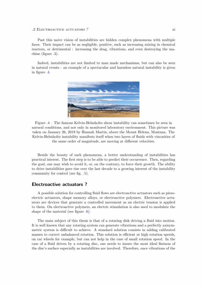
Indeed, instabilities are not limited to man made mechanisms, but can also be seenin natural events : an example of a spectacular and harmless natural instability is givenin figure .4.
Figure .4 – The famous Kelvin-Helmholtz shear instability can sometimes be seen innatural conditions, and not only in monitored laboratory environment. This picture wastaken on January 26, 2019 by Hannah Martin, above the Mount Helena, Montana. TheKelvin-Helmholtz instability manifests itself when two layers of fluids with viscosities of
the same order of magnitude, are moving at different velocities.
Beside the beauty of such phenomena, a better understanding of instabilities haspractical interest. The first step is to be able to predict their occurrence. Then, regardingthe goal, one may wish to avoid it, or, on the contrary, to force their growth. The abilityto drive instabilities gave rise over the last decade to a growing interest of the instabilitycommunity for control (see fig. .5).
Electroactive actuators ?A possible solution for controlling fluid flows are electroactive actuators such as piezo-
electric actuators, shape memory alloys, or electroactive polymers. Electroactive actu-ators are devices that generate a controlled movement as an electric tension is appliedto them. On electroactive polymers, an electric stimulation is also used to modulate theshape of the material (see figure .6).
The main subject of this thesis is that of a rotating disk driving a fluid into motion.It is well known that any rotating system can generate vibrations and a perfectly axisym-metric system is difficult to achieve. A standard solution consists in adding calibratedmasses to correct unbalanced rotation. This solution is efficient at high rotation speeds,on car wheels for example, but can not help in the case of small rotation speed. In thecase of a fluid driven by a rotating disc, one needs to insure the most ideal flatness ofthe disc’s surface especially as instabilities are involved. Therefore, once vibrations of the

xii Introduction
(a) Natural Flow. (b) Controlled flow.
Figure .5 – An exemple of instability control on the von Karman street underdevelopment at LIMSI. The goal is to reduce the drag behind three cylinders with a
rotation of the two rear cylinders at a minimal cost : the energy spent to spin cylindersmust not exceed the energy gain of the drag reduction (private communication with theauthor of the figures, G. Y. Cornejo Maceda). In figure .5a, cylinders are fixed, while infigure .5b, the top rear cylinder rotates clockwise and the bottom rear cylinder rotates
counter clockwise, while the front cylinder does not rotate. This "boat tailing"configuration reduces the vortices in the wake, and therefore reduces the drag compared
to the single cylinder configuration.
Figure .6 – Electroactive polymer under several tension. This polymer is composed oftwo layers of conductor material, separated by an insulating material. The potential
difference between the two conductor layers forces the bending of the polymer.
disc are fully quantified, the adaptation of electroactive actuators should compensate theimperfections of the disc. If the imperfections are small, the use of piezo electric devicescan be sufficient. If large deformations are targeted then electroactive polymers or shapememory alloys should be used. This can also lead to a second application which consistsof shaping the disc surface to a desired pattern, in order to control instability.
Examples of applications of both solutions can be found in aeronautics, in order tocontrol the flow around a wing (fig. .7). Piezoelectric actuators generate a travelingwave of the trailing edge, and allows to split large vortices structures into smaller ones.This ripple, inspired from birds’ plumage movement, reduces the drag of the wing. Otherprojects use piezoceramic composite actuator to vary the camber of the wing, in order toadapt it regarding the flight envelope.

.3 Science is made of bounces xiii
Figure .7 – Morphing wing prototype from the Institut de Mécanique des Fluides deToulouse (IMFT), using piezoelectric actuators for the oscillating trailing edge, and an
electroactive polymer for the camber variation.
A quick glance at the studied case
The configuration considered in this thesis is one of the simplest rotating flow exper-iments : a flat disc rotating at the bottom of a fixed cylindrical cavity. A liquid partiallyfills the cavity above the disc, and the upper interface of this liquid is only in contact withambient air, without further constraint. Despite this simplicity, two different instabilitiestake place in such a configuration : at high rotation rates, deformations of the surfacecan draw polygons. But even without reaching such regimes, a first instability occurswhile the surface is still flat. Only visible when a marker is added to the flow, this quietinstability appeared more complex than expected (fig. .8).
The observed instabilities raise three fundamental questions :
• Is this instability reproducible ?
• How sensitive are instabilities to mechanical vibrations ?
• Can instabilities be controlled with a dynamic shaping of the disc surface ?
Science is made of bounces
To answer these questions, an ANR project has been set up around the collaborationbetween the Laboratoire d’Informatique pour la Mécanique et les Sciences de l’Ingénieur(LIMSI) and the Génie électrique et électronique de Paris (GeePs) laboratory, using their

xiv Introduction
(a) Low rotation speed, flat surface (b) High rotation speed, shaped interface
Figure .8 – Two different instabilities generated by a rotating disc in a fixed cylindricalcavity (observed from above the disk in the present work setup). On the left, the surfaceis flat, and the pattern is only visible when marker is introduced (ink). On the right, theair water interface is heavily deformed, such as the disc is dewetted at its center, and
along each arm of the pattern.
complementary skills. Indeed, this thesis was initially entitled "Rotating flow and elec-troactive actuator", with the same title as the ANR project that funded this work. How-ever, the first measurements of vibrations of the experimental bench quickly invalidatethe hypothesis of a premature growing of instabilities due to a mechanical noise forcing.Therefore, before expecting to control instabilities, we had to redirect our research inorder to better understand the instability.
The use of very accurate velocity measurement devices such as Laser Doppler Ve-locimetry (LDV) and comparison with numerical simulations quickly convinced us thatthe ait water interface condition plays a major role on the instability at low rotation speed.For this reason, the major part of this thesis does not actually deal with actuators, butinvestigates and models the role played by the interface on the instability.
Organisation
The first chapter is dedicated to a survey of articles that are linked to the subjectof this thesis, and a brief history of this configuration in LIMSI is also presented. Thesecond chapter enters more directly into the subject. It is a stand-alone paper, submittedto Journal of Fluid Mechanics (JFM), that gathers almost all the results of the mainstudied case for a given fluid filling in the cavity.
The rest of this thesis extends the findings of the second chapter, but applied todifferent fluid filling heights. The pertinent key results of the article are summarized in

.4 Organisation xv
each chapter’s introduction in order to make the reading easier. Repetitions were avoidedas much as possible. However some points, such as experimental set-ups, and numericalcodes details, are necessary both in the paper, and in the thesis. More details are givenin the thesis chapters, especially on equations used in codes. Chapters III to V arerespectively dedicated to experimental tools, equations and numerical methods. ChapterVIth focuses on matches and mismatches between experimental results and simulationsperformed with a traditional free slip condition at the surface. Chapter VII deviates fromfluid mechanics, and concentrates on the study of the vibrating disc surface. After thissolid mechanics interlude, the next chapter gathers first and second attempt to modifythe condition at the surface : both are linked to a sudden change of the radial velocity atthe flow surface. The last chapter before the conclusion of this thesis is a bit more sizable.It is dedicated to the building of a more complex model, taking into account the quantityof undetermined pollutants at the interface. These pollutants, acting like surfactants,modify the surface tension of the fluid : regarding the concentration of pollutants, thesurface is more or less "stiffen". In order to clarify this model, the first part of the chapteris devoted to a small bibliography, listing articles that helped us in the construction ofthe model. Equations used are also detailed in this part. The second part of the chaptergroups results of this model obtained on the same cases as in previous chapters. Finally,a third part revisits former simulations that were deemed of minor interest before thepollutant based model shed new light on them.

xvi Introduction

Chapter I
Problem description
1

2 Chapter I. Problem description
Description of the configurationThe flow considered in this study is generated by a spinning disk located at the
bottom of a fixed cylindrical cavity. This cavity is filled with a liquid. The top surfaceof the fluid remains free (only in contact with ambient air). For more convenience in theupcoming chapter, the aspect ratio G and the Reynolds number are introduced. The firstone is defined as the ratio between the radius of the cavity R and the height H of fluidabove the disk : G = H/R, while the second compares inertia forces to diffusive forces :Re = R2Ω/ν. Here, Ω denotes the disc rotation rate, while ν is the kinematic viscosity.
Figure I.1 – Sketch of the cavity. R is the radius of the cavity, H is the height of thefluid at rest (in blue) above the rotating disc (in yellow). A more detailed description of
the set-up is given in Chapter III : Experimental tools.
BibliographyThis chapter is dedicated to an exploration of the bibliography that is linked, in one
way or another, to instabilities in a rotating flow with a free surface. Since only few ar-ticles effectively deal with this precise topic, many of the papers quoted below introducemore global concerns on rotating flows, or on some specific phenomenons observed in suchconfiguration.
Therefore, this bibliography starts with global thoughts about the flow described aboveor between infinite discs. Then bounding the domain in the radial direction, we get closerto our configuration and introduce the first concern of science in bounded rotating flows,with or without a free surface. After a parenthesis on experimental set-ups used to re-produce geostrophic flows, a fourth part focuses on the instability that occurs when high

I.2 Bibliography 3
rotation rates are reached with a large deformation of the free surface. The final part ofthis bibliography focuses on flat free surface rotating flows.
A last section returns to what has already been developed in the laboratory on rotatingflows and sets the logical and chronological framework within which this thesis falls.
Early works
Semi infinite domain
In the beginning of the 20th century, Ekman published in [1] the solution for a rotatingdisc in a steady flow. His result, known as Ekman transport, brings a new light ongeophysical flows, as it explains the deviation of the flow near the ground, under combinedeffects of wind and the Coriolis force. A bit later, in 1921, von Kármán solved the problemof a flow initially at rest above an infinite rotating disc ([2]). Bödewadt then brought thesolution to the “opposite” problem of a fluid in solid body rotation flow above an infiniteplane. These three flows were gathered under the name of "BEK Flows" (Bödewadt,Ekman, and von Karman) by Lingwood [3]. In this configuration, the domain extends toinfinity in both axial and radial directions.
Flows between two discs of infinite radius
Six years after the end of the second world war, Batchelor published results for thetwo boundary layers that develop between two co-rotating discs ([4]). Stewartson alsoused the two disc configuration, but while one is rotating, the second remains fixed. Inthis rotor-stator configuration, and despite what Batchelor predicted two years earlier,Stewartson demonstrated the existence of a single boundary layer on the rotor, while thetangential velocity of the flow remains zero everywhere else ([5]). This led to a controversythat lasted thirty years, only settled in 1983, when Kreiss and Parter [6] demonstratedthe co-existence of the two solutions...
All these works can be considered to be cornerstones to studies of flow above andbetween rotating discs. It also illustrates the depth of rotating flow studies, highlightinghow what could be considered as minor change in the configuration can have a majorimpact on the solution of the problem.
Confined rotating flows
In many practical applications, the flow is not only bounded in the axial direction,but also in the radial direction. Indeed, rotating fluids in confined geometry have beenwidely used through the ages. An example can be found as early as in the IVth cen-tury B.C. In the Hanging Gardens of Babylon, a device for pumping water was used toobtain lush vegetation. This device was later known as "Archimedes’ screw". Enclosedrotating flows are not just ghosts of a fallen civilization’s technology, but are also presentin most modern turbines used in aircraft or naval propulsion, or for electricity production.

4 Chapter I. Problem description
In scientific research, configurations studied rely on simpler geometries, composed ofa fixed cylinder with a rotating disc. Two variants are mainly used. In the first one, alid, attached to the fixed cylindrical wall, is placed in direct contact with water. In thesecond one, the surface remains in contact with ambient air, as illustrated in figure I.1.
In both cases, when the disc is spinning, fluid is set into rotation in its vicinity.Provided that the upper layers of fluid rotate slower than the disc, the fluid is also flushedtoward the periphery. Since the radial extent of the cavity is finite, the fluid is forced tochange direction and to flow vertically along the cylinder wall. By continuity, the fluidflows along the upper bound of the fluid, and returns toward the rotating disc along theaxis. This creates a large recirculation in the meridional plane.
Vortex Breakdown
For a certain range of parameters (G and Re), the fluid may flow in opposite directionto this main meridional circulation in a limited region along the axis. This creates a smallrecirculation bubble called vortex breakdown.
Surprisingly, this phenomenon was firstly observed in a completely different config-uration : in 1957 by Peckham and Atkinson, described in [7] the sudden change in thephysiognomy of a columnar vortex at the tip of a delta wing, and gave it the name ofvortex breakdown. By extension, this name was later used in a closed cylindrical cavity,as described above.
Figure I.2 – Vortex Breakdown on a delta wing. (Lambourne & Bryer, 1962, [8])
Returning to the cylindrical closed configuration (with a lid), H.U. Vogel experimen-tally determined in 1968 pairs of parameters (G,Re) for which vortex breakdown occurs[9].
H.L. Lugt then conducted in 1982 the first simulation of vortex breakdown in a closedcylindrical cavity of aspect ratio 1.58 [10], and found good agreement with Vogel’s pre-dictions.

I.2 Bibliography 5
Two years later, M.P. Escudier published an article entitled “Observation of the flowproduced in a closed cylindrical container by a rotating end wall” [11], where he exper-imentally highlights the formation of recirculation bubbles along the rotation axis of avertical cylinder, identified as the vortex breakdown (figure I.3).
(a) Re=1002 (b) Re=1449 (c) Re=1492
Figure I.3 – Evolution of the columnar vortex (the white vertical line at the axis ofrotation in figure I.3a) in a meridional plane, in function of Re, for G=2. The bubble is
clearly visible on the axis of ration in figure I.3c. Pictures extracted from [11].
It has been thought that the recirculation bubble is necessarily located on the rota-tion axis. However, when the upper lid is removed, the recirculation bubble may then bedetached from the axis.
This was highlighted in 1993, when A. Spohn et al. repeated the experiment of Es-cudier, but this time without the lid [12]. Spohn studied many aspect ratios, from G=0.5to G=4, with a step of 0.25. Unlike the previous set-up that used a lid, Spohn describedthe existence of vortex breakdown for its lowest aspect ratio. But the measurement of theReynolds number for which bubbles appear was only carried out for aspect ratios higherthan G=1. One of the other differences he showed was the location of the bubble : in theabsence of a lid, bubbles are attached to the free surface and not to the axis of rotation(figure I.4).
Figure I.4 – Recirculation bubbles for Re=2075 and G=2. Although G is the same as infigure I.3, the experiment introduced here had no lid at the top, on the contrary to [11].
Picture extracted from [12].

6 Chapter I. Problem description
Much more recently, E. Serre has numerically investigated vortex breakdown in acylinder of aspect ratio G=4, with a free surface ([13] and [14]). And in 2005, M. Pivaintroduced a new parameter into the experiment, with the variation of the rotating discdiameter [15].
Figure I.5 – Vortex Breakdown in a cylinder of aspect ratio G=1, with a free surface.Figure extracted from [15].
In the same year, R. Iwatsu [16] published a very complete numerical study for aspectratios from G=0.25 to G=4, including discussions of previous publications.
The occurrence of Vortex breakdown and its origin has been the subject of debate.It has been sometimes believed that the vortex breakdown is triggered by an instability.Actually, this is not the case, but in confined rotating flows, instabilities are responsiblefor other captivating phenomena that we are now presenting.
Unstable flows between two discs
Configurations used to study instabilities in confined flows put into motion by a ro-tating disc are numerous. Therefore, we do not claim here to conduct an exhaustiveinventory of publications dealing with the subject, but simply to reference a sample ofarticles that show an instability pattern close to the flat free surface case detailed in afurther section.
In 1984, H. Niino and N. Misawa used an experimental apparatus to reproduce thebarotropic instability that occurs in oceans and atmosphere [17]. Their set-up is quitecomplex, composed of a cylindrical cavity that rotates with the lid in one direction whilethe disc placed at the bottom spins in exact counter rotation, plus another smaller discthat can rotate independently. The whole set up is placed on a rotating table (see fig.I.6). Despite this complexity, they were able to find a good agreement between the linearstability analysis and their experimental determination of the critical Reynolds number.Although they used a lid, their configuration gave rise to vortices that look similar tothose observed in our flat free surface configuration.
Still with the aim of reproducing an atmospheric phenomenon in the laboratory, A.C.Barbosa Aguiar et al. published an article about a model of Saturn’s North pole hexagon[18]. To do so, they built a set up with a rotating cavity that was used in two config-urations. The first one is a closed rotating cavity with only an annulus at the top that

I.2 Bibliography 7
(a) m=2 (b) m=3 (c) m=4
Figure I.6 – Vortices observed in [17]. Black lines are distribution belts.
spin in counter rotation. In the second one, the external part of the cavity (lid, wall andbottom) spins in one direction while the central part (one disc at the top and one at thebottom around the axis) spins in the other direction. Note that the bottom is not flat :it displays a slope of 5°, with its highest point at the axis.
(a) experimental model of Saturnhexagon, from [18].
(b) Saturn North pole hexagon (picturetook by the Cassini orbiter, november 2012).
Figure I.7 – Experimental attempt to reproduce the Saturn North pole Hexagon in alaboratory.
A more common configuration is a fixed cylindrical cavity where the flow is driven bya rotating lid, as the one used by M.P. Escudier in 1984. Many articles based on suchconfigurations deals with instability patterns that occur in small aspect ratio. Here we canquote, among many others, the article published by A.Y. Gelfgat in 2015 [19]. This paperincludes a wide bibliography and many aspect ratios from 0.1 to 1.0. Another interesting

8 Chapter I. Problem description
publication is the numerical study by O. Daube and P. Le Quéré, on the first bifurcationfor an aspect ratio of 0.1 [20]. The authors showed the highly subcritical behaviour ofthe bifurcation, and observed a huge gap between their numerical prediction of the firstinstability compared to the results obtained by G. Gauthier in his thesis, in 1998 [21].Indeed the critical Reynolds numbers differ by a factor of 10 between direct simulationsand experimental results.
Free surface with deformation
One of the first experiments of a free surface deformation in a rotating flow is prob-ably Newton’s bucket. However, the initial goal of this experiment did not concern fluidmechanics : it was an illustration of a philosophical question on rotation and its associ-ated relative frame of reference. Still, in this experience, the rotation moulds the fluidwhose surface takes the shape of a parabola. This case configuration is a bit differentfrom previously considered cavities, since the wall rotates with the bottom. Therefore,one may ask whether the result is the same when the vertical wall is stationary ?
H. Goller started to answer this question in his article in 1968 about measurements ofthe shape of the free surface in a fixed cylinder, with a flow driven by a bottom rotatingplate [22].
A. Siginer computed in 1993 the shape of the surface for several aspect ratios from1/4 to 4 ([23]), while the more classical case of Newton’s bucket has been re-visited in2015 by J. Mougel et al. [24].
A new breath in free surface rotating fluid was given in 1990 [25], when G.H. Vatistaspublished an article about the discovery of a polygonal shaped interface for sufficientlylarge values of the Froude and Reynolds number. This article was followed by many oth-ers in the three last decades, such as [26] from which are extracted the pictures of figure I.8.
Figure I.8 – Rotating polygons described in [26].
This polygonal shaping of the interface was “rediscovered“ more recently in 2006, byT.R.N Jansson [27] and was followed by several other papers : [28], [29], [30], [31], high-lighting the attractiveness of the instability with surface deformation.

I.2 Bibliography 9
Even for much smaller rotation rates, and while the interface remains flat, anotherinstability occurs. This instability, harder to visualize, is the main content of this thesis.
Flat free surface
According to our research, the first publication on rotating flow in a vertical cylindri-cal cavity, with a flat free surface is a numerical study released in 1985, by Jae Min Hyun[32]. In this article, the author describes the base flow in the exact same configurationas ours, for aspect ratios from 0.1 to 1. It gives an interesting framework for numericalapproaches, with the dimensionless Navier Stokes equations in the (ω, ψ,Γ) formulation(vorticity, stream function and angular velocity, respectively - see section V.1.2) and theboundary conditions associated with, including the justification of the hypothesis of theflat free surface. Computation were carried out with a finite difference method, mostlywith a 41× 41 grid. Results include plots of stream function and azimuthal velocity con-tours in a meridional plane, revealing a recirculation along the outer border.
In 2004, Iwatsu realized an analysis of steady flows [33] and according to the aspectratio, distinguished the cases G 1 and G 1. Thanks to progress, both in hardwareand in computer science, this paper brings more details on the flow topology than theprevious analysis by Hyun.
The two previous papers only deal with steady flows. The first article that evoked theexistence of an instability in a fixed cylindrical cavity, with a free surface, dates back, toour knowledge, to 1993 [12]. Actually this article was already referenced in section VortexBreakdown, since it was the main interest of this paper. However, among their experi-mental observations, Spohn et al. noticed radial oscillations of bubbles in a meridionalplane. For aspect ratios from G=0.5 to G=2.75, they reported a transition from steadyto unsteady flow for a Reynolds number around 2150. For G=3.0 to 4.0, this Reynoldsnumber increases up to 2920. Asides from the oscillations of bubbles, no visualizationwas made of an instability pattern.
Two years later, D.L. Young et al. [34] noticed the appearance of an oscillation in theirLDV measurements of the azimuthal velocity, for a Reynolds number around 1900. Theirexperience was built around a cylindrical cavity of 184mm of internal diameter. The fluidis put into motion by the 182mm disk placed at the bottom of the cavity. The aspectratio used in their experiences is G=2. The main topic of this article is the illustration ofperiod doubling of the oscillations for a Reynolds number around 2200 and the transitionto chaos for higher Reynolds numbers.
It was only in 2002 that a new article [35] dealing with our exact configuration ispublished. It is the work of A.H. Hirsa, J.M. Lopez and R. Miraghaie. This is the firstarticle out of three published on the subject : this one and the second [36] are fairly short,and most of their results are gathered in the third, published in 2004 [37]. In all thesepublications, two aspect ratios are investigated : G=2 and G=0.25. Their experimentalset-up is small since the glass cylinder that composes the cavity is only 5cm diameter

10 Chapter I. Problem description
wide. Here, the disc is not inside the cavity, but the cavity is held fixed above a rotatingdisk made of glass. The disk is driven by a stepper motor. In their numerical simulations,the authors used an ”extended system“ of twice the height of the considered aspect ratio,with two co-rotating disks : one at each end of the cylinder. The baseflow is correctlyreproduced by such an ”extended system“ as the symmetry mimics the free slip boundarycondition at the free surface. But the authors enable an odd or even parity with respectto the mid height, leading to the growth of different instability modes, which do not existin the experiment : the ”extended system“ deeply modifies the instability modes, boththeir pattern and theirs critical Reynolds numbers for which they growth.
M.J. Vogel et al., used the same experimental apparatus in 2004 [38], but with asmall difference : they added insoluble surfactant at the surface that forms a Langmuirmonolayer (an insoluble layer of one-molecule thickness), and reported the patterning ofthe initially uniformly distributed monolayer to a mode 3 for a Reynolds number of 2000(the aspect ratio used is 0.25). This short paper merges two previous studies from J.M.Lopez et al.. The first one has been described above, and the second one deals with theinfluence of a monolayer on the base flow in an annular channel. This article ([39]) is notdescribed here, but will be developed in the second bibliography, in chapter IX.
As for the first article introduced in this section, publications from Serre et al. ([13]and [14]) previously quoted in section Vortex Breakdown deserve a second quotation here.Indeed, its authors ran simulations above the critical Reynolds number, showing azimuthalpattern with two or three vortices, and describing the instability as a Neimark–Sacker bi-furcation.
In 2007, a group from IRPHE performed an exhaustive study of the symmetry break-ing. In their article S. Poncet and M.P. Chauve [40] used a rheoscopic marker, Kalliro-scope, to experimentally visualize the pattern, and to determine the critical Reynoldsnumbers of the instability threshold and the Reynolds number of the secondary bifur-cations. They explored numerous aspect ratios, from 0.0179 to 0.107, highlighting theexistence of a hysteresis cycle and arguing in favour of a subcritical bifurcation. Theirexperiment eventually included a "hub", i.e. an inner cylinder rotating withe the disc.The authors reported that below a certain radius (that depends on the aspect ratio), thepresence of the hub has no influence on the instabilities (neither on the threshold, nor onthe mode).
Using papers from Vogel et al. [38] and Hirsa et al. [39] as a framework for their pa-per [41], YY. Kwan et al. proposed, in 2010, an intensive mathematical proof to build amodel for incompressible flow with a surfactant monolayer. Then, they briefly comparedtheir model to the previous experiment of J.M. Vogel et al., with a fast-spectral methodsimulation that shows the surfactant clearing in the vicinity of the external wall, and agood agreement with experiments.
More recently, in his thesis at LIMSI [42], L. Kahouadji returned to the results ofPoncet et al. [40]. He performed the linear stability analysis of the same aspect ratiosas in these experiments. Agreements are very good, both on the mode and the critical

I.3 History of rotating flows at LIMSI 11
Reynolds number for aspect ratio higher than 0.0714, but deteriorate quickly when theaspect ratio drops below this value. Some of these results were published in [43].
Figure I.9 – Comparison of numerical results of [42] (blue line with red triangles) andexperimental results of [40] (black segments) for several values of G. The case G=1/14(≈0.714) is the limit of the interval of agreement between experiments and numerics.
Figure extracted from [42].
In the same period, Cogan et al. performed a complete numerical study for G=1.5([44]). The authors started with a linear stability analysis for the four first modes, andthen conducted several direct numerical simulations (DNS) approaches to show the nonlinear dynamics of the flow and the pattern of the instability. The agreement betweenDNS and linear stability analysis appeared to be excellent.
History of rotating flows at LIMSI
LIMSI has several years of expertise in rotating flows, with many publications onrotor-stator or rotor-rotor configurations such as [20], [45], [46] and [47]. The open cavitysubject is more recent. It started in 2008 with the thesis of L. Kahouadji [42], and thepublication of the article [43]. Numerical simulation of the free surface shape publishedin this thesis were used in 2012 as the basis for a Master internship [48]. A first demon-strator was build in order to experimentally quantify the deformation of the free surface.But this experiment had many flaws : large vibrations, non rectified plexiglas cylinder,

12 Chapter I. Problem description
irregular rotation...
In 2013 a much more ambitious project was achieved with a second Master internship[49] : a larger experiment was built, with a perfectly controlled rotation speed. The firstruns tried to reproduce the 2007 experiment from the IRPHE [40]. Despite the sameexperimental protocol, noticeable discrepancies were observed on the critical Reynoldsnumber. Experiments were reproducible, but it was already noted that Kalliroscope, afluid with particles used as marker to reveal vortices under a certain light, may modifythe flow and thus, instability thresholds.
These results were extended in 2014, with another Master internship [50], investigat-ing many hypotheses for the causes of discrepancies. This included geometrical issuesof the cavity, viscosity check, new aspect ratios, rotation regularity check, new marker(ink), new fluid (water glycerol mixture), validation with in a rotor-stator configuration,addition of surfactants... But none of the prospected paths bring a clue about discrepan-cies. The report ended with the possible stimulation of an instability by the mechanicalvibrations of the rotation.
In parallel to this present work, W. Yang led a study on rotating polygons using thesame experimental set up [51].

Chapter II
Article published in Journal of FluidMechanics
13

14 Chapter II. Article published in Journal of Fluid Mechanics

J. Fluid Mech. (2020), vol. 900, A42. © The Author(s), 2020.Published by Cambridge University Press
900 A42-1
doi:10.1017/jfm.2020.473
Influence of interface pollution on the linearstability of a rotating flow
Antoine Faugaret1,2, Yohann Duguet2, Yann Fraigneau2 andLaurent Martin Witkowski2,3,†
1Collège Doctoral, Sorbonne Université, F-75005 Paris, France2Université Paris-Saclay, CNRS, LIMSI, 91400 Orsay, France
3Faculté des Sciences et Ingénierie, UFR d’Ingénierie, Sorbonne Université, F-75005 Paris, France
(Received 6 January 2020; revised 19 April 2020; accepted 5 June 2020)
The boundary conditions at a liquid–gas interface can be modified by the presence ofpollutants. This can in turn affect the stability of the associated flow. We consider thisissue in the case of a simple open cylindrical cavity flow where a liquid is set in motionby the rotation of the bottom. The problem is addressed using an experimental set-up,a linear stability code and direct numerical simulation. A robust mismatch betweennumerical and experimental predictions of the onset of instability is found. We modelthe possible effect of unidentified pollutants at the interface using an advection–diffusionequation and a closure equation linking the surface tension to the superficial pollutantconcentration. The chosen closure is inspired by studies of free-surface flows withsurfactants. Numerical stability analysis reveals that the base flow and its linear stabilitythreshold are strongly affected by the addition of pollutants. Pollutants tend to decreasethe critical Reynolds number; however, the nonlinear dynamics is less rich than withoutpollutants. For sufficiently high pollution levels, the most unstable mode belongs to adifferent family, in agreement with experimental findings.
Key words: rotating flows
1. Introduction
Fluid flow simulations rely on a mathematical formulation associating given governingequations with specific boundary conditions. The choice for the boundary conditions issometimes not trivial, in particular in the presence of a liquid–gas interface. Beyond thedifficulties stemming from a deformable interface, it appears that, in practice, the correctboundary conditions are not well known even for a perfectly flat interface. The classicalboundary condition considered in textbooks is commonly deduced from the balance oftangential stresses at the interface. For a gas–liquid interface, where the dynamic viscosityof the gas is negligible with respect to that of the liquid, this leads to a ‘free slip’condition, which is simple to implement in simulation codes. Unfortunately this idealboundary condition is not necessarily representative of realistic experiments, even forliquids as common as plain water. Contamination by pollutants present in the ambient air
† Email address for correspondence: [email protected]
http
s://
doi.o
rg/1
0.10
17/jf
m.2
020.
473
Dow
nloa
ded
from
htt
ps://
ww
w.c
ambr
idge
.org
/cor
e. B
iblio
Uni
vers
ite P
ierr
e et
Mar
ie C
urie
, on
18 A
ug 2
020
at 0
7:37
:08,
sub
ject
to th
e Ca
mbr
idge
Cor
e te
rms
of u
se, a
vaila
ble
at h
ttps
://w
ww
.cam
brid
ge.o
rg/c
ore/
term
s.

900 A42-2 A. Faugaret, Y. Duguet, Y. Fraigneau and L. Martin Witkowski
can influence the rheology of the interface and drastically impact the effective boundaryconditions (Lopez & Hirsa 2000; Martín & Vega 2006). Such modifications can deeplyalter the flow and, as a consequence, the numerical predictions with a free-surfacecondition are no longer representative of the true physical flow. Considering how difficult itis to experimentally ensure that a gas–liquid interface is free from any chemical pollution,it is crucial to know how to model the interface, without necessarily knowing all thephysical properties in detail. Such issues arise for instance in flow where Marangonieffects (modifications of the surface tension due to, for example, temperature effects) mayinterfere with and impact the flow dynamics. The simplified phenomenology of surfacepollutants assumes that, although the precise chemical composition of the pollutants isin essence unknown, their qualitative effect is to reduce the effective surface tension(Ponce-Torres & Vega 2016). This suggests an effect akin to that of insoluble surfactantsadded on the free surface. In several studies of free-surface flow with controlled amountsof surfactants (Lopez & Hirsa 2000; Hirsa, Lopez & Miraghaie 2001), the amount ofpollutants is supposed so small that they are confined to a Langmuir monolayer located atthe interface. We assume therefore for simplicity that pollutants do not penetrate the bulkof the flow. Advected by the local velocity field tangent to the interface, the pollutantscluster at some given locations, their accumulation being only resisted by weak diffusion.The resulting inhomogeneity of the concentration field at the interface induces a localchange in the surface tension. The gradients of effective surface tension lead to additionalstresses that modify the global stress balance.
In this investigation we choose a flow case feasible in the laboratory as well as innumerical simulations, where such ideas can be tested. In particular, we focus on a simpleflow likely to develop instability modes via a classical Hopf bifurcation scenario. Theselected most unstable mode, its growth rate and the associated onset Reynolds numberserve as quantitative indicators of how reliable a given set of boundary conditions are.The flow consists of a cylindrical cavity partially filled with liquid, in most cases water.The top of the cavity is open while its bottom rotates at constant angular velocity. Thesidewalls do not rotate and are fixed in the laboratory frame. For simplicity, we restrictourselves to the parameter regime where the fluid interface remains approximately flateven as the instability develops and saturates. A sketch of the experimental set-up can befound in figure 1. The two main parameters for this flow are the geometric aspect ratioG = H/R, where H is the undisturbed liquid height and the inner cylinder radius R, andthe Reynolds number Re = ΩR2/ν where Ω is the rotation rate and ν is the kinematicviscosity. This flow has been previously studied both numerically and experimentally. Theearliest publication we found about this configuration is a numerical investigation of thebase flow for an aspect ratio G between 0.1 and 1 (Hyun 1985). Under the assumption thatthe flow remains axisymmetric, the transition to unsteadiness has been studied numericallyfor G = 2 by Daube (1991) and the transition point was found near Re = 2975. Evidencefor an instability breaking the axisymmetry of the base flow was given only later. In Young,Sheen & Hwu (1995), no visualisation of the pattern was shown; however, laser Dopplervelocity measurements revealed the growth of an instability near Re = 2000 for a G = 2geometry. This is consistent with Re = 1910, the value found in a numerical simulationby Lopez et al. (2004). The first experimental visualisations of non-axisymmetry wereperformed by Hirsa, Lopez & Miraghaie (2002b) and Lopez et al. (2004) in the samegeometry, and compared with numerical results for G = 2 and G = 1/4 in Lopez et al.(2004). For the larger aspect ratio (G = 2), numerical predictions and experimental resultstend to agree, yet for the shallower configuration, mismatches in critical Reynolds numberand azimuthal wavenumber m were reported. In particular, the wavenumber selectionwas described in these works as sensitive to the presence of surface contaminants.
http
s://
doi.o
rg/1
0.10
17/jf
m.2
020.
473
Dow
nloa
ded
from
htt
ps://
ww
w.c
ambr
idge
.org
/cor
e. B
iblio
Uni
vers
ite P
ierr
e et
Mar
ie C
urie
, on
18 A
ug 2
020
at 0
7:37
:08,
sub
ject
to th
e Ca
mbr
idge
Cor
e te
rms
of u
se, a
vaila
ble
at h
ttps
://w
ww
.cam
brid
ge.o
rg/c
ore/
term
s.

Influence of interface pollution 900 A42-3
Ω
uθ(r, z)
(ur, uz) (r, z)
H
R
FIGURE 1. Sketch of the axisymmetric base flow for small aspect ratio G = H/R.
Among recent publications, the experimental work by Poncet & Chauve (2007) surveysmany aspect ratios ranging from G = 0.0179 to 0.107. Larger aspect ratios G from 0.3 to 4have been studied numerically as well (Iwatsu 2004; Serre, Tuliszka-Sznitko & Bontoux2004; Cogan, Ryan & Sheard 2011). For higher rotation rates, a different regime takesover, with strong deformations of the interface and sometimes mode switching (Suzuki,Iima & Hayase 2006; Tasaka & Iima 2009). Polygonal patterns at the deformed interfacehave been reported by Vatistas, Wang & Lin (1992), Jansson et al. (2006), Iga et al. (2014)and modelled by Tophøj et al. (2013).
In the present investigation, we revisit the primary instability mechanism using a jointexperimental and numerical approach. We focus on the primary instability in the caseof an approximately flat interface. For small enough angular velocities the centrifugalacceleration remains much smaller than gravity and the curvature of the fluid interface canbe indeed neglected in the small Froude number hypothesis. The main aspect ratio underscrutiny corresponds to G = 1/14. As shown in table 1, the experimentally determinedthresholds are lower by least 75 % than those of Poncet & Chauve (2007). The variouspossible reasons for this discrepancy have been reviewed in our experimental set-up withgreat care, among them residual vibrations, lack of axisymmetry of the cavity, finitecurvature of the free surface, presence of a meniscus, ionisation of the water. In allcases these hypotheses were ruled out as quantitatively insignificant. Note that quantitativediscrepancies with experimental measurements have been also already reported earlier forthis flow for low G. In Kahouadji, Martin Witkowski & Le Quéré (2010), the stabilitythresholds in Re determined by linear-stability analysis (LSA) were compared with Poncetand Chauve’s experimental estimates for varying values of G. In both studies the thresholdvalue Rec increases with decreasing G. The agreement between numerics and experimentsis very satisfying; however, it deteriorates for G ≤ 0.07–0.08 (see figure 3a in Kahouadjiet al. 2010), with a mismatch on Rec of 100 % for G ≈ 0.04. Following Lopez andco-authors, we assign such a mismatch between experiments and linear stability analysis tothe unavoidable presence of pollutants at the interface, and hence to the simplistic free-slipmodel for the boundary conditions at the liquid interface. The present investigationis devoted to a quantitative analysis of the influence of these pollutants, via a simplephenomenological model, on the linear stability threshold of this flow.
The outline of the paper is as follows. In § 2, we give a brief description of the flowand its primary instability. We detail the experimental methods as well as the numericalmethods for the linear and nonlinear stability. Section 3 is devoted to a critical comparison
http
s://
doi.o
rg/1
0.10
17/jf
m.2
020.
473
Dow
nloa
ded
from
htt
ps://
ww
w.c
ambr
idge
.org
/cor
e. B
iblio
Uni
vers
ite P
ierr
e et
Mar
ie C
urie
, on
18 A
ug 2
020
at 0
7:37
:08,
sub
ject
to th
e Ca
mbr
idge
Cor
e te
rms
of u
se, a
vaila
ble
at h
ttps
://w
ww
.cam
brid
ge.o
rg/c
ore/
term
s.

900 A42-4 A. Faugaret, Y. Duguet, Y. Fraigneau and L. Martin Witkowski
Experiment (LDV) Poncet ROSE Sunfluidh
Rec [3160–4230] [14 367–16 420] 17 006 [17 000–17 100]fm = 5 [Noise–0.764] — 0.709 [0.707–0.699]
TABLE 1. Critical Reynolds number and angular frequency of the pattern for the m = 5instability for G = 1/14. For Sunfluidh, linear interpolation leads to Rec = 17 010. Whenrelevant, a lower and an upper bound are given for Rec, with the corresponding values for thefrequency. Experimental results by Poncet & Chauve (2007) are included for comparison.
between experimental and numerical results. In § 4, we introduce a new model for the freesurface where surface pollution is taken into account. Section 5 discusses the possiblesimplification of the model in the limit of high surface pollution. The final § 6 containsa summary of the present investigation together with open questions and perspectives forfuture work.
2. Flow set-up and related investigation techniques
2.1. Base flow descriptionWe briefly recall the main features of the base flow as described by Iwatsu (2004) and Yanget al. (2019). It is axisymmetric with three non-zero velocity components. Its structure forsmall aspect ratio G is sketched in figure 1. We use a classical direct cylindrical coordinatesystem (r, θ, z), where r is the radial distance, θ the azimuthal angle and z the distancefrom the rotating bottom. In the vicinity of the instability threshold, the azimuthal velocityprofile possesses a simple radial structure almost independent of z except in the boundarylayers. In the regimes we focus on, the azimuthal velocity increases with the radial distancefrom r = 0 to r ≈ 0.67 − 0.68R, where R is the radius of the set-up, and decreases tozero as the wall is approached. The latter zone is labelled ‘outer region’. This azimuthalvelocity is driven by the steady rotation of the disc at angular velocity Ω at the bottomof the cavity. Just above this rotating disc, the fluid is pushed radially outwards towardsthe fixed cylindrical end wall in a boundary layer similar to a von Kármán boundary layer.This generates a recirculation in the meridional plane, confined approximately to the outerregion. For r ≤ 0.5R the flow is in perfect solid body rotation.
Above a given rotation rate, this base flow is known to support an instability breakingits axisymmetry. Ignoring in a first stage the geometrical and rheological parameters, asimplistic explanation for this symmetry breaking is as follows: a shear instability, akin toa Kelvin–Helmholtz instability along a curved streamline, develops where the azimuthalvelocity profile displays the strongest curvature. Given the cylindrical geometry, a directanalogy with the instability of Stewartson layers in the split disc configuration (Stewartson1957) has been suggested in order to justify the relative size of the instability region(Poncet & Chauve 2007). Beyond this simple picture, the bifurcation scenarios leadingto the presence of different non-axisymmetric patterns with a dominating wavenumberm /= 0 as in figure 2, are not entirely clear from the literature. Lopez et al. (2004) describethe bifurcation as a standard Hopf bifurcation. Experiments in Poncet & Chauve (2007)reveal the existence of hysteresis, suggesting a possibility for subcritical bifurcation. Inthe present work, we focus on the emergence of a m = 5 mode, the most unstable onepredicted by linear instability theory for the aspect ratio G considered. A competing
http
s://
doi.o
rg/1
0.10
17/jf
m.2
020.
473
Dow
nloa
ded
from
htt
ps://
ww
w.c
ambr
idge
.org
/cor
e. B
iblio
Uni
vers
ite P
ierr
e et
Mar
ie C
urie
, on
18 A
ug 2
020
at 0
7:37
:08,
sub
ject
to th
e Ca
mbr
idge
Cor
e te
rms
of u
se, a
vaila
ble
at h
ttps
://w
ww
.cam
brid
ge.o
rg/c
ore/
term
s.

Influence of interface pollution 900 A42-5
(a) (b) (c)
FIGURE 2. Instability patterns breaking the axisymmetry of the flow. Photograph taken fromabove (ink visualisation) in our experimental set-up. Modes m = 3, 4 and 5 obtained fordifferent aspect ratios and different values of Re above the effective Rec; (a) m = 3, G = 3.5/14,Re = 2160, (b) m = 4, G = 1.5/14, Re = 5623, (c) m = 5, G = 1/14, Re = 4714.
unstable mode with m = 4, though theoretically expected to appear for parameters wherethe mode m = 5 is already unstable, has also been investigated.
2.2. Experimental techniqueThe main element of the experimental set-up is a cylindrical shaped Plexiglas cavity. Itsinternal radius is R = 140.3 ± 0.05 mm, and the thickness of the Plexiglas is 6.8 mm. Thevalue of R is used to define the Reynolds number Re = ΩR2/ν. The cavity was engineeredfrom a single block, so that the cylinder and the bottom are monolithic, preventing any riskof leak. Its bottom is drilled along its axis in order to mount a brass foot that hosts the shaftof the rotating disc, itself also made of brass. The radius of the disc is Rd = 139.6 mm,its thickness 8.5 mm and its mass 5 kg. The shaft is held in place with two ball bearings,and the sealing is insured by a spring-loaded double-lip seal. An aluminium rigid sleevecoupling, relying on a thrust ball bearing, is used to connect the disc shaft and the motorreducer unit. The motor used is a direct current motor (Parvex RX320E-R1100) with a1 : 12 reducer. The rotation speed is controlled using a closed-loop tachometer. Specialattention was paid to minimising the gap between the disc edge and the vertical wall of thecavity. The liquids used in this experimental investigation are tap water, de-ionised waterand a water–glycerol mixture. As the cavity is not thermo-regulated, the fluid temperatureis monitored continuously, with a digital thermometer that allows it to be known withan accuracy of 0.1 K. The corresponding kinematic viscosity is then evaluated usingan empirical formula (Cheng 2008). The experimental Reynolds number, based on theangular velocity Ω , the radius and the kinematic viscosity are hence known within a givenaccuracy of the order of a per cent for the range of parameters investigated. The relativeerror is expected to increase as the rotation rate decreases.
Flow measurements are made using a laser Doppler velocimetry (LDV) device,composed of a Dantec Laser linked to a BSAFlow processor. The liquid is seeded withDantec 10 micrometre diameter silver coated hollow glass spheres (S-HGS-10). Theseare not provided as suspension and thus prevent the introduction of additional surfactant.We also avoided to premix the particles without any additional solutant. Because ofthe cylindrical geometry, as the laser beams are placed for the acquisition of uθ theyundergo a deviation that both shifts the location of the focus and impacts the quantitativemeasurements. This is fixed at the post-processing stage using the technical corrections
http
s://
doi.o
rg/1
0.10
17/jf
m.2
020.
473
Dow
nloa
ded
from
htt
ps://
ww
w.c
ambr
idge
.org
/cor
e. B
iblio
Uni
vers
ite P
ierr
e et
Mar
ie C
urie
, on
18 A
ug 2
020
at 0
7:37
:08,
sub
ject
to th
e Ca
mbr
idge
Cor
e te
rms
of u
se, a
vaila
ble
at h
ttps
://w
ww
.cam
brid
ge.o
rg/c
ore/
term
s.

900 A42-6 A. Faugaret, Y. Duguet, Y. Fraigneau and L. Martin Witkowski
(a) (b) (c) (d )
FIGURE 3. Instability growth for a m = 5 mode for a water + Kalliroscope mixture initiallyat rest: G = 1/14, Reynolds number Re = 16 550; (a) t = 52 s, (b) t = 60 s, (c) t = 71 s,(d) t = 99 s.
suggested in Huisman, van Gils & Sun (2012). For visualisations such as in figure 2, theflow patterns were highlighted by injecting either Kalliroscope or ink into the fluid. Theprotocol to find experimentally the critical Reynolds number is to progressively increasethe azimuthal velocity with steps of 0.5 r.p.m. for the water and for the 20 % water–glycerolmixture, and steps of 1 r.p.m. for the 55 % water–glycerol mixture. After each increase ofthe rotation speed, a waiting time of 5–10 min is followed by LDV acquisition performedover another five minutes duration. This procedure allows the base flow to be almostestablished before the instability grows.
2.3. Experimental evidence for m = 5 instabilityWe describe the experimental instability leading to a steadily rotating m = 5 mode, usingKalliroscope visualisations or pointwise LDV measurements. The flow is initially atrest. The angular velocity is directly set to a finite value defining the target Reynoldsnumber Re, the value used in figure 3 being Re = 16 650. For low enough Reynoldsnumbers, the flow remains axisymmetric as in figure 3(a). Above threshold, an annuluscharacterised by stronger shear appears around r = 0.7R (figure 3b). An m = 5 modeemerges (figure 3c) and evolves towards a steadily rotating configuration with 5 co-rotatingvortices (figure 3d). In the time sequence presented, the Reynolds number is well abovethe threshold as will be seen later. In such a case, the emergence of the instabilityis almost concomitant with that of the base flow, which is here approximately 80 s.A similar scenario occurs for other values of m, in particular for m = 4 which has beenobserved for other nearby values of Re. The vortex pattern rotates with a constant angularvelocity smaller than Ω . The angular frequency f of the pattern can be deduced usingf = 2πfd/(mΩ), where fd is the dimensional frequency obtained experimentally usingpointwise LDV measurements at a location fixed in the laboratory frame. The mainfrequency f varies moderately over the range Re = [4230, 16 300]. A Fourier transformof the time series is shown in figure 4 in the case m = 5 for Re = 4230 and Re = 16 300.The main frequency and the related harmonics dominate the spectrum.
2.4. Numerical methodology for free-slip interfacesAs a complementary part of this investigation, we have used numerical tools based onthe incompressible Navier–Stokes equations in order to investigate both the linear andnonlinear aspects of the symmetry-breaking instability. The present section first introducesthe numerical methods used. It also features a comparison with the experimental resultsof § 2.3.
http
s://
doi.o
rg/1
0.10
17/jf
m.2
020.
473
Dow
nloa
ded
from
htt
ps://
ww
w.c
ambr
idge
.org
/cor
e. B
iblio
Uni
vers
ite P
ierr
e et
Mar
ie C
urie
, on
18 A
ug 2
020
at 0
7:37
:08,
sub
ject
to th
e Ca
mbr
idge
Cor
e te
rms
of u
se, a
vaila
ble
at h
ttps
://w
ww
.cam
brid
ge.o
rg/c
ore/
term
s.

Influence of interface pollution 900 A42-7
0.020
0.015
0.010
0.005
0 1 2 3 4Frequency
Am
plitu
de
Re = 16 300Re = 4230
5 6 7
FIGURE 4. Experimental frequency amplitude spectrum of azimuthal velocity componentmeasured at radius 0.76R and height 0.9H for the saturated m = 5 regime at Re = 4230 andRe = 16 300. The maximum amplitudes correspond to the non-dimensional frequencies f = 0.76and f = 0.73, respectively.
2.4.1. Mathematical modelWe adopt the point of view of a single-phase flow. The velocity field u(r, θ, z, t) inside
the liquid is governed by the incompressible Navier–Stokes equations in the (non-rotating)laboratory frame
∇ · u = 0, (2.1)
∂u∂t
+ (u · ∇)u = −∇p + 1Re
∇2u. (2.2)
Equations (2.1)–(2.2) have been non-dimensionalised using the length scale R and thetime scale Ω−1, and the dimensionless fluid density is taken as unity. From here on all thevariables are non-dimensional except when explicitly noted.
The flow obeys no slip at all solid boundaries. This implies
ur = uθ = uz = 0 (2.3)
at the fixed vertical boundary at r = 1, whereas
ur = uz = 0, uθ = r (2.4a,b)
on the rotating disc at z = 0.The boundary condition at the liquid–gas interface at z = G is classically derived from
the stress balance at the interface. As the viscosity of the air is much smaller than thewater one, we can neglect the gas phase altogether. We first consider the generic free-slipboundary conditions
∂ur
∂z= 0,
∂uθ
∂z= 0, uz = 0 at z = G. (2.5a–c)
A few precautions are necessary to justify the plane interface hypothesis. A numericalestimation of the height h(r) as a function of the rotation speed is possible for the steadybase flow. This is achieved using the variation of the numerical code ROSE with coordinatetransformations used in Yang et al. (2020). Two sets of parameters typical of the present
http
s://
doi.o
rg/1
0.10
17/jf
m.2
020.
473
Dow
nloa
ded
from
htt
ps://
ww
w.c
ambr
idge
.org
/cor
e. B
iblio
Uni
vers
ite P
ierr
e et
Mar
ie C
urie
, on
18 A
ug 2
020
at 0
7:37
:08,
sub
ject
to th
e Ca
mbr
idge
Cor
e te
rms
of u
se, a
vaila
ble
at h
ttps
://w
ww
.cam
brid
ge.o
rg/c
ore/
term
s.

900 A42-8 A. Faugaret, Y. Duguet, Y. Fraigneau and L. Martin Witkowski
range of interest have been considered. The first set is a least favourable parameter case(G = 1/14, Ω = 0.95 rad s−1), i.e. Re = 18 620 and Fr = (Ω2R)/g = 0.013 where g isthe gravity. In this case, the total height variation from the centre to the periphery isΔh = h(r = 1) − h(r = 0) = 6.8 % of the undisturbed fluid height. The second set is forthe rotation rate at which the instability is first detected (Re ∼ 3000), Ω = 0.15 rad s−1
and Fr = 3.34 × 10⁻⁴, Δh is less than 0.2 %. Such small values, respectively 0.68 and0.017 mm (too small to be measured experimentally for the latter), justify the flat interfacehypothesis considered in the numerical part.
As in all mesh-based numerical methods, the singularities of the velocity field occurringat both corners (r = 1, z = 0) and (r = 1, z = G) are smoothed out in practice by thefinite mesh without the need, as for spectral methods, for regularising functions (Serre &Bontoux 2007) or singular splitting (Duguet, Scott & Le Penven 2005). This is consistentwith the ‘natural’ regularisation occurring in the experiment in the presence of a very thingap.
2.4.2. Linear stability analysisIn order to determine the critical Reynolds number Rec for the onset of instability, we
use an in-house linear stability solver named ROSE, based on a finite difference methodin r and z. The technique as well as the equations written in cylindrical coordinates arefound in Kahouadji, Houchens & Martin Witkowski (2011). The steady axisymmetricbase flow is first determined by solving (2.1) and (2.2) together with the associatedboundary conditions using a Newton–Raphson solver. The steady solution is solved forin an (ω,ψ, uθ , c) formulation, where
ω = ∂ur
∂z− ∂uz
∂r, ur = 1
r∂ψ
∂z, uz = −1
r∂ψ
∂r. (2.6a–c)
The Newton–Raphson solver allows for additional scalar fields c(r, z) such as temperatureor concentration, as further discussed in § 4.
Let (U, P) represent the velocity-pressure field for such a steady axisymmetric solutionof (2.2), and let (u∗, p∗) be a small-amplitude perturbation to (U, P). The dynamics of theperturbation is governed by the linearised stability equations
∇ · u∗ = 0, (2.7)
∂u∗
∂t+ (U · ∇)u∗ + (u∗ · ∇)U = −∇p∗ + 1
Re∇2u∗. (2.8)
It is associated with Dirichlet boundary conditions u∗ = 0 on all solid boundariestogether with a boundary condition on u∗ at the interface similar to that for u in (2.5). Thevelocity field and the pressure field are decomposed using a complex ansatz of the formeλt+i mθ , as will be detailed in § 4.2. The neutral curve corresponds to parameter valueswhere the real part Re(λ) = 0, and it is identified in practice using a one-dimensionalsecant method. All meshes used are Cartesian in the meridional plane (O, r, z). ForG = 1/14 the mesh consists of 701 × 101 grid points.
2.4.3. Direct numerical simulationFor the nonlinear validation of the stability thresholds we have used the direct numerical
simulation (DNS) code Sunfluidh developed at LIMSI for incompressible flows. It isbased on a projection method to ensure a divergence-free velocity field. The equations are
http
s://
doi.o
rg/1
0.10
17/jf
m.2
020.
473
Dow
nloa
ded
from
htt
ps://
ww
w.c
ambr
idge
.org
/cor
e. B
iblio
Uni
vers
ite P
ierr
e et
Mar
ie C
urie
, on
18 A
ug 2
020
at 0
7:37
:08,
sub
ject
to th
e Ca
mbr
idge
Cor
e te
rms
of u
se, a
vaila
ble
at h
ttps
://w
ww
.cam
brid
ge.o
rg/c
ore/
term
s.

Influence of interface pollution 900 A42-9
discretised on a staggered structured non-uniform grid using a finite volume approach witha second-order centred scheme in space. A second-order backward Euler differentiation isused for time discretisation. Details can be found in Yang et al. (2020). The interfacecondition is as in (2.3) and (2.4). The code offers the possibility to enforce a givenrotational symmetry Rm characterised by a fundamental azimuthal wavenumber m ≥ 0,such that every velocity field verifies
(Rmu)(r, θ, z) = u
r, θ + 2π
m, z
= u(r, θ, z) (m /= 0), (2.9)
or axisymmetry for m = 0. If m /= 0 the simulation only needs to be carried out overan angular sector 0 ≤ θ ≤ 2π/m with azimuthal periodicity. For the simulations withoutsymmetry imposed, we have used a mesh consisting of 180 × 180 × 64 cells in r, θ and z,respectively.
3. Critical comparison of the different approaches
3.1. Comparison between the numerical methodsFor identical parameters, we report excellent agreement between the base flows computedby the two methods for all Re. Whereas the base flow can be converged for all Re usingthe Newton method, it is only accessible for Re < Rec using time stepping. However, sincethe base flow is apparently the only axisymmetric solution of the system, it is also foundusing DNS for all Re by simply imposing m = 0 (two-dimensional axisymmetric case)and stepping forward in time. The value of Rec for m = 5 is first identified by LSA using asecant method. In the DNS code, the procedure used to identify Rec is different; above andbelow Rec, an arbitrary perturbation of finite but small amplitude is applied to the systemafter an initial transient, with the R5 symmetry imposed or not. This impulse responseleads to either exponential decay towards the base flow, or exponential growth towards anonlinear regime at large times. A linear interpolation of these rates leads to an evaluationof the critical threshold Rec. Both approaches agree quantitatively very well regardingthe prediction of Rec for m = 5 since the relative error is close to 0.3 % (see table 1).Interestingly, this comparison, as well as the lack of unstable impulse response for Re <Rec (even for larger-amplitude impulses), both suggest that the instability is supercriticaland not subcritical, at least for a clean interface obeying the boundary condition (2.5). Notethat the ROSE computation in table 1 was performed using a 701 × 101 grid. Numericalcomparison with Kahouadji et al. (2010) confirms that this resolution is sufficient for anestimation of Rec with an accuracy of less than one per cent. Two additional computationswere performed using different meshes. The Rec was estimated to 17 032 with a 351 × 51grid, and to 16 992 with a 1401 × 201 grid. The maximum variation of Rec is less than0.16 % compared to the value in table 1.
3.2. Mean flow structureSince both numerical approaches yield a truly similar base flow solution, a comparisonwith the experimental base flow measured using LDV would be relevant at this point. Aswe shall see, measurements below Rec turn out to be experimentally difficult. Anothercomparison, which is easier to perform, concerns the mean velocity profiles obtained forRe > Rec by either temporal or spatial average. Such a comparison is displayed in figure 5.For the eigenmodes computed using ROSE, their average is by construction zero. Hence,only the base flow obtained by LSA is included in figure 5, whereas the spatial average is
http
s://
doi.o
rg/1
0.10
17/jf
m.2
020.
473
Dow
nloa
ded
from
htt
ps://
ww
w.c
ambr
idge
.org
/cor
e. B
iblio
Uni
vers
ite P
ierr
e et
Mar
ie C
urie
, on
18 A
ug 2
020
at 0
7:37
:08,
sub
ject
to th
e Ca
mbr
idge
Cor
e te
rms
of u
se, a
vaila
ble
at h
ttps
://w
ww
.cam
brid
ge.o
rg/c
ore/
term
s.

900 A42-10 A. Faugaret, Y. Duguet, Y. Fraigneau and L. Martin Witkowski
0.8
0.7
0.6
0.5
0.4
0.3
0.2
0.1
00.5 0.6 0.7 0.8 0.9 1.0
LDVDNS spatial averageBase flow
r
uθ
FIGURE 5. Velocity profiles of uθ (r) below the free surface (z = 0.8G) for G = 1/14 andRe = 18 620. Comparison between the base flow, spatially averaged DNS and the temporalaverage for LDV (experiment). LDV acquisition timespan is much larger than the instabilityperiod.
taken for the DNS data and the time average for experimental LDV data. A common valueof Re = 18 620 is chosen for the comparison. Although the agreement is satisfactory, anoticeable overshoot appears around r ≈ 0.67 in all numerical azimuthal velocity profiles,with no equivalent in LDV measurements despite sufficient measurement accuracy. Thesame mismatch, presence of the overshoot area in numerics, but not in experiments,was also reported for comparable parameters in Yang et al. (2019). The computationsperformed on different meshes all display this overshoot, which rules out a numericalartefact.
3.3. Threshold detectionThe most dramatic mismatch between numerics and experiments concerns the criticalReynolds number. While both numerical simulations agree on a critical Reynolds numberof approximately 17 000 (see table 1), LDV measurements display persistent oscillationsin the azimuthal velocity field for Re as low as 4200, with a normalised frequencyf5 = 0.76, indicative of the presence of the m = 5 mode. This upper bound on thevalue of Rec is smaller by a factor of 4 than the previous experimental estimates byPoncet & Chauve (2007). These values can be found in table 1. The discrepanciesare robust; although the exact same spin-up protocol as Poncet & Chauve (2007) wasobserved, the respective ranges of Rec differ. We note that the threshold detection byPoncet & Chauve (2007) is based on Kalliroscope visualisations. Kalliroscope appearsin our set-up as a poor diagnostic for Rec for this flow case; the threshold detection iserratic and protocol dependent. Indeed the estimation of Rec fluctuates between 6200to 9300. At times, Kalliroscope is even unable to detect the instability, even well abovethe value of Rec predicted numerically. The use of ink for visualisation, and LDV forquantitative measurements, both confirm that the thresholds detected with Kalliroscopeare over-evaluated. The saturated mode is displayed in figure 2 at a value of Reapproximately 4 times lower than the theoretical threshold Re(LSA)
c . Its spatial structureis directly comparable to that of the saturated flow above Re(LSA)
c displayed in figure 3(d).On the one hand, there is perfect numerical agreement between LSA and DNS
about the estimation of Rec, on the other hand, there is a troubling match with
http
s://
doi.o
rg/1
0.10
17/jf
m.2
020.
473
Dow
nloa
ded
from
htt
ps://
ww
w.c
ambr
idge
.org
/cor
e. B
iblio
Uni
vers
ite P
ierr
e et
Mar
ie C
urie
, on
18 A
ug 2
020
at 0
7:37
:08,
sub
ject
to th
e Ca
mbr
idge
Cor
e te
rms
of u
se, a
vaila
ble
at h
ttps
://w
ww
.cam
brid
ge.o
rg/c
ore/
term
s.

Influence of interface pollution 900 A42-11
Lopez et al. Experiment Experiment ROSE ROSEWater 55 % glycerol 20 % glycerol
m 3 3 3 3 2Rec 2000 [1850–2160] [1875–2520] 4690 3480
TABLE 2. Critical Reynolds number for G = 1/4. Comparison between experiments by Lopezet al. (2004), present experiments and LSA. The percentage of glycerol indicated is a weightpercentage.
Poncet & Chauve (2007) at odds with the experimental/numerical discrepancy we report.We have hence carried out an exhaustive investigation of the possible reasons forsuch a discrepancy by focusing on experimental imperfections. A classical reason fordiscrepancies in rotating machines is the presence of mechanical noise that could force aninstability by direct or parametric resonance. The experimental displacement of the discsurface was measured using a pair of LK-G10 sensors, and their associated LK-GD500controller. Displacements were evaluated to approximately 10−4 m, with a mean frequencycorresponding to the disc rotation, yet no link with the pattern frequency was found. Thisdoes not suggest any obvious experimental flaw in our experimental methodology.
Eventually, in order to confirm our experimental approach, we switch temporarily toa different geometry with G = 1/4 where a direct and favourable comparison with theexperimental results of Lopez et al. (2004) can be made. For these parameters there is alsoa robust mismatch between experiments and numerics; LSA predicts the most unstablemode m = 2 with Rec = 3500, whereas Lopez’s experiments at Re = 2000 show a modem = 3, predicted using LSA to be unstable only for Re ≥ 4600. We have then conductedour own experiments with two different mixtures of water with 20 % and 55 % glycerol.The motivation for these two different mixtures is to allow for a wider span of rotationspeeds; using water the instability would have occurred for rotation speed below 1 r.p.m.where the signal-to-noise ratio in the LDV degrades. In both cases the mode m = 3 isdetected, either using ink or LDV, for Re = 2160 in the 55 % glycerol fluid (see figure 2a)and Re = 2520 in the 20 % glycerol fluid. All the results are gathered in table 2. This sidestudy confirms, in good agreement with Lopez et al. (2004) that numerics overestimatethe experimental thresholds in Re. The discrepancy reported here for G = 1/14 has hencea robust physical origin, which the rest of this paper is devoted to.
3.4. Nonlinear dynamicsThe mismatch between numerics and experiments for G = 1/14 is even more dramaticfurther above Rec. Although DNS initially displays an azimuthal wavenumber m = 5 closeto Rec (see figure 6a at Re = 17 100), the instability pattern evolves towards m = 7 asRe is pushed to 18 620, less than 9 % above Rec. Poncet & Chauve (2007) have alsoreported an evolution of the modal content of the flow with Re, yet with m decreasingas Re is increased. A similar decrease of m with Re was also observed qualitatively in ourexperiment for Re sufficiently higher than Rec. However, the wavenumber m = 5 remainsexperimentally stable from Re = 4200 to at least Re = 18 620. The frequency spectrumis shown in figure 7(a) for Re = 18 620. Given such a mismatch, larger values of Rewere not investigated, neither experimentally nor numerically. Differences in the nonlineardynamics for Re = 18 620 also emerge in velocity measurements; while experimentaltime series display a single frequency, the signals from DNS display a broader spectrum
http
s://
doi.o
rg/1
0.10
17/jf
m.2
020.
473
Dow
nloa
ded
from
htt
ps://
ww
w.c
ambr
idge
.org
/cor
e. B
iblio
Uni
vers
ite P
ierr
e et
Mar
ie C
urie
, on
18 A
ug 2
020
at 0
7:37
:08,
sub
ject
to th
e Ca
mbr
idge
Cor
e te
rms
of u
se, a
vaila
ble
at h
ttps
://w
ww
.cam
brid
ge.o
rg/c
ore/
term
s.

900 A42-12 A. Faugaret, Y. Duguet, Y. Fraigneau and L. Martin Witkowski
1.5
1.0
0.5
–0.5
–1.0
–1.5
0
2
1
0
–1
–2
–3
(a) (b)
FIGURE 6. DNS axial vorticity fluctuation for the free-surface condition, Re = 17 100 slightlyabove Rec (a), and Re = 18 620 (b). With the increase of Re, the mode m = 5 selected at Recevolves into a modulated m = 7 pattern.
0.015
0.010
0.005
0 5 10 15
3.53.02.52.01.51.00.5
0 5 10 15Frequency
Am
plitu
de
Frequency
(×10–3)(a) (b)
FIGURE 7. Comparison of frequency amplitude spectra for uθ (t) measured at r = 0.76,z = 0.8G, for the saturated m = 5 regime at Re = 18 620. (a) Experimental data, maximumpeak at f = 4.15. (b) DNS with free-surface condition, same parameters. The frequencies arenot normalised by the azimuthal wavenumber.
and richer dynamics, see figure 7. In addition to the mismatch in the modal behaviourbetween experiments and DNS, the vorticity patterns (figures 6a and 6b) do not matchthe experimental (figures 2 and 3d) very convincingly. This raises doubts about whetherthe mode predicted in the numerics does indeed correspond to the structure observedexperimentally.
3.5. Limitations of the clean interface hypothesisLopez et al. (2004) have suggested that mismatches in critical Reynolds numbers betweentheoretical and experimental predictions arise due to the presence of pollutants at theinterface. The main idea is that the pollutants change the boundary condition at theinterface. One can draw a parallel with the evolution from free slip to no slip examined byPeaudecerf et al. (2017) in a channel flow with superhydrophobic surfaces, in presence ofcarefully added surfactants. As it is nearly impossible, in standard laboratory conditions,to achieve an experiment with a perfectly clean interface at all times, it is necessary totake additional effects into account in order to properly model the behaviour of the fluid ata realistic liquid–gas interface. Previous publications with a similar experimental set-up,in which the adsorption of pollutants at the interface was carefully controlled, already
http
s://
doi.o
rg/1
0.10
17/jf
m.2
020.
473
Dow
nloa
ded
from
htt
ps://
ww
w.c
ambr
idge
.org
/cor
e. B
iblio
Uni
vers
ite P
ierr
e et
Mar
ie C
urie
, on
18 A
ug 2
020
at 0
7:37
:08,
sub
ject
to th
e Ca
mbr
idge
Cor
e te
rms
of u
se, a
vaila
ble
at h
ttps
://w
ww
.cam
brid
ge.o
rg/c
ore/
term
s.

Influence of interface pollution 900 A42-13
demonstrated the crucial influence of pollution of the base flow (Hirsa et al. 2001; Hirsa,Lopez & Miraghaie 2002a). There, pollutants were assimilated to a monolayer of vitaminK1, considered as a surfactant, yet any insoluble (or weakly soluble) surfactant would havea similar effect.
In the next section, we model explicitly the presence of pollutants at the interface in theNavier–Stokes equations and investigate its qualitative as well as quantitative influence onthe linear stability of the flow.
4. Modelling of interface pollution
4.1. Modification of the effective surface tensionThe present modelling of the pollution at the interface is directly inspired by the modellingin Hirsa et al. (2001) and Kwan, Park & Shen (2010). Let cd(r, θ, t) be the dimensionalinstantaneous concentration of the pollutants at the interface, the closure equation betweenthe surface tension σ and cd reads
σ = σ0
1 − α
2σ0c2
d
, (4.1)
where σ0 is the reference surface tension of the solvent (for water, σ0 = 72.8 mN m−1); αis a dimensional constant coming from the Taylor expansion around cd = 0 of the modelin Kwan et al. (2010), and depends from the chemical species of the pollutant. Equation(4.1) is non-dimensionalised as
σ = 1 − αC20
2σ0c2, (4.2)
where σ = σ/σ0 and c = cd/C0. Here, C0 represents the average mass concentration ofpollutant at the interface, such as
C0 = 1πR2
2π
0
R
0cd(r, θ, t)r dr dθ . (4.3)
Since the ambient pollution is undetermined, the value of the α coefficient is unknown.Thus (4.2) is modified as follows
σ = 1 − βCa2
c2, (4.4)
where Ca = μΩR/σ0 is a capillary number, μ is the dynamic viscosity and β is a newnon-dimensional control parameter defined by
β = αC20
μΩR. (4.5)
Note that β can be linked to a Marangoni number, based on C0 and the diffusion Ds suchthat Ma = (αC2
0R)/(Dsμ), and to the Péclet number Pes = ΩR2/Ds so that β = Ma/Pes.We assume that pollutants are advected by the velocity field of the fluid while diffusing
with a simple non-dimensional diffusion coefficient Ds. Moreover, we assume that notransport occurs from the surface to the bulk of the flow, so that the bulk concentrationcan be neglected (Bandi et al. 2017). In practice, β is limited by chemistry considerations;
http
s://
doi.o
rg/1
0.10
17/jf
m.2
020.
473
Dow
nloa
ded
from
htt
ps://
ww
w.c
ambr
idge
.org
/cor
e. B
iblio
Uni
vers
ite P
ierr
e et
Mar
ie C
urie
, on
18 A
ug 2
020
at 0
7:37
:08,
sub
ject
to th
e Ca
mbr
idge
Cor
e te
rms
of u
se, a
vaila
ble
at h
ttps
://w
ww
.cam
brid
ge.o
rg/c
ore/
term
s.
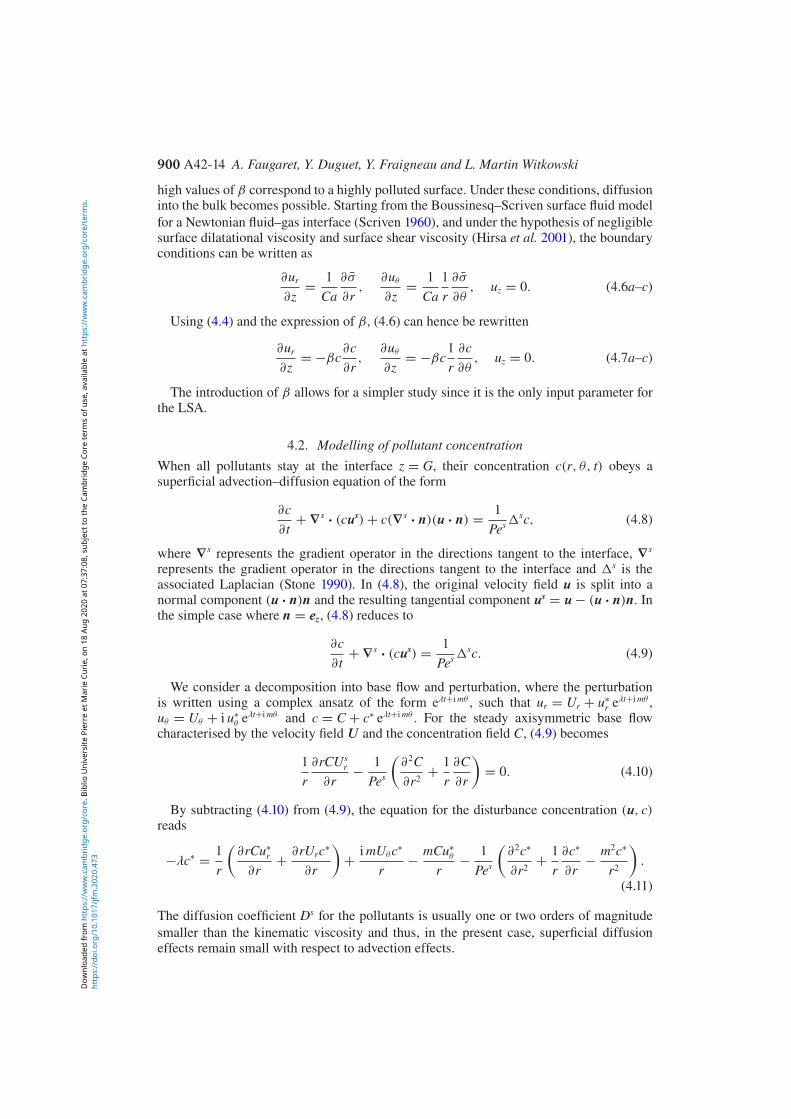
900 A42-14 A. Faugaret, Y. Duguet, Y. Fraigneau and L. Martin Witkowski
high values of β correspond to a highly polluted surface. Under these conditions, diffusioninto the bulk becomes possible. Starting from the Boussinesq–Scriven surface fluid modelfor a Newtonian fluid–gas interface (Scriven 1960), and under the hypothesis of negligiblesurface dilatational viscosity and surface shear viscosity (Hirsa et al. 2001), the boundaryconditions can be written as
∂ur
∂z= 1
Ca∂σ
∂r,
∂uθ
∂z= 1
Ca1r
∂σ
∂θ, uz = 0. (4.6a–c)
Using (4.4) and the expression of β, (4.6) can hence be rewritten
∂ur
∂z= −βc
∂c∂r
,∂uθ
∂z= −βc
1r
∂c∂θ
, uz = 0. (4.7a–c)
The introduction of β allows for a simpler study since it is the only input parameter forthe LSA.
4.2. Modelling of pollutant concentrationWhen all pollutants stay at the interface z = G, their concentration c(r, θ, t) obeys asuperficial advection–diffusion equation of the form
∂c∂t
+ ∇s · (cus) + c(∇s · n)(u · n) = 1Pes Δ
sc, (4.8)
where ∇s represents the gradient operator in the directions tangent to the interface, ∇s
represents the gradient operator in the directions tangent to the interface and Δs is theassociated Laplacian (Stone 1990). In (4.8), the original velocity field u is split into anormal component (u · n)n and the resulting tangential component us = u − (u · n)n. Inthe simple case where n = ez, (4.8) reduces to
∂c∂t
+ ∇s · (cus) = 1Pes Δ
sc. (4.9)
We consider a decomposition into base flow and perturbation, where the perturbationis written using a complex ansatz of the form eλt+i mθ , such that ur = Ur + u∗
r eλt+i mθ ,uθ = Uθ + i u∗
θ eλt+i mθ and c = C + c∗ eλt+i mθ . For the steady axisymmetric base flowcharacterised by the velocity field U and the concentration field C, (4.9) becomes
1r
∂rCUsr
∂r− 1
Pes
∂2C∂r2
+ 1r
∂C∂r
= 0. (4.10)
By subtracting (4.10) from (4.9), the equation for the disturbance concentration (u, c)reads
−λc∗ = 1r
∂rCu∗
r
∂r+ ∂rUrc∗
∂r
+ i mUθc∗
r− mCu∗
θ
r− 1
Pes
∂2c∗
∂r2+ 1
r∂c∗
∂r− m2c∗
r2
.
(4.11)
The diffusion coefficient Ds for the pollutants is usually one or two orders of magnitudesmaller than the kinematic viscosity and thus, in the present case, superficial diffusioneffects remain small with respect to advection effects.
http
s://
doi.o
rg/1
0.10
17/jf
m.2
020.
473
Dow
nloa
ded
from
htt
ps://
ww
w.c
ambr
idge
.org
/cor
e. B
iblio
Uni
vers
ite P
ierr
e et
Mar
ie C
urie
, on
18 A
ug 2
020
at 0
7:37
:08,
sub
ject
to th
e Ca
mbr
idge
Cor
e te
rms
of u
se, a
vaila
ble
at h
ttps
://w
ww
.cam
brid
ge.o
rg/c
ore/
term
s.

Influence of interface pollution 900 A42-15
0.05
0z
z
z
z
0.2 0.4 0.6 0.8 1.0
0.05
0 0.2 0.4 0.6 0.8 1.0
0.05
0 0.2 0.4 0.6 0.8 1.0
0.05
0 0.2 0.4r
0.6 0.8 1.0
(a)
(b)
(c)
(d)
FIGURE 8. Evolution of the streamfunction ψ for the base flow with increasing concentrationβ, Re = 18 620 and G = 1/14. The same contour values are chosen for all cases. Negativesand positives contours use different scales to highlight the weak recirculation bubble. Negativescontour values (dashed): four equispaced levels in [ψmin − ψmin/5]. Positives contour values:(solid lines): nine values equispaced levels in [ψmax/10 − ψmax ]. Zero contour level (solidblack lines). ψmin = −8.1 × 10⁻⁵ and ψmax = 2.3 × 10⁻³; (a) β = 0, (b) β = 0.1, (c) β = 0.2,(d) β = 0.5.
The constraint (4.3) reads in non-dimensional form
1π
2π
0
1
0c(r, θ, t)r dr dθ = 1, (4.12)
and reduces for the steady axisymmetric base flow to
2 1
0C(r)r dr = 1. (4.13)
For the base flow, axisymmetry implies ∂C/∂r = 0 at the axis. The constraint (4.13) alsoimposes a zero mass flux at r = 1. For the perturbation field c∗, the boundary conditionsdepend on the value of the azimuthal wavenumber m (Kahouadji et al. 2011). For m ≥ 1(the case of interest), c∗ = 0 is imposed at the axis and ∂c∗/∂r = 0 at the outer wall. Allsuperscripts ∗ are from here on dropped for simplicity.
4.3. Structure of the modified base flowAs demonstrated in Lopez & Chen (1998), the presence of a surfactant layer at the interfacemodifies the structure of the base flow. However, the potential influence on its linearstability has not been investigated yet. In this subsection, we study the influence of thepollution concentration β, modelled using the surfactant law (4.1), on the base flow forG = 1/14 and Re = 18 620. Increasing β causes a small but monotonic decrease of thelength of the meridional recirculation, see figure 8. This is accompanied by the progressivedisappearance of the overshoot in Uθ , evident in figure 9. This observation is directlyconsistent with the experimental measurements, in which no overshoot has been found forz = 0.8G.
http
s://
doi.o
rg/1
0.10
17/jf
m.2
020.
473
Dow
nloa
ded
from
htt
ps://
ww
w.c
ambr
idge
.org
/cor
e. B
iblio
Uni
vers
ite P
ierr
e et
Mar
ie C
urie
, on
18 A
ug 2
020
at 0
7:37
:08,
sub
ject
to th
e Ca
mbr
idge
Cor
e te
rms
of u
se, a
vaila
ble
at h
ttps
://w
ww
.cam
brid
ge.o
rg/c
ore/
term
s.

900 A42-16 A. Faugaret, Y. Duguet, Y. Fraigneau and L. Martin Witkowski
0.05
0 0.2 0.4 0.6 0.8 1.0
0.05
0 0.2 0.4 0.6 0.8 1.0
0.05
0 0.2 0.4 0.6 0.8 1.0
0.05
0 0.2 0.4r
0.6 0.8 1.0
(a)z
z
z
z
(b)
(c)
(d)
FIGURE 9. Evolution of the azimuthal velocity Uθ for the base flow for increasing β, Re =18 620 and G = 1/14. 21 equispaced levels in [0–1]. Translucent red patches represent overshootareas, i.e. locations where Uθ ≥ 1.01 r; (a) β = 0, (b) β = 0.1, (c) β = 0.2, (d) β = 0.5.
4.4. Linear instability thresholds for G = 1/14The present model is based on four independent non-dimensional parameters G, Re, Pes
and β. We have investigated quantitatively the influence of β on the instability thresholdsRec for m = 4 and 5, with G fixed to 1/14 except when noted. The numerical resolution isunchanged compared to the pollution-free case. The Péclet number, although in principlelarger, is hence limited to Pe = 103 in order to prevent steeper gradients and numericalissues. The focus on m = 4 and 5 mirrors the modal selection predicted for the referencecase β = 0, and is also consistent with experimental findings at onset.
The neutral curves Rec(β) obtained as β is varied are shown in figure 10, where neutralmodes m = 4 and 5 appear as squares and five-pointed stars, respectively. The neutralcurves have been determined by identifying the parameters where Re(λ) = 0 using asecant method. In some intervals of β the curve Rec(β) happens to be multi-valued, seee.g. β = 0.3 for m = 4; several thresholds can be found for this value of β, although notrivial physical interpretation has been found. In such cases, the code was modified todetermine the critical value of β for a given value of Re. Note that the influence of thenumerical resolution on Rec for β = 5 has been verified using the same numerical gridsas for β = 0 (351 × 51 and 1401 × 201), with variations below 0.58 %.
The most striking result in figure 10 is the dramatic drop in Rec occurring at β ≈ 0.48for m = 4 and β ≈ 0.14 for m = 5. The asymptotic value of Rec predicted for large βand approached for β as small as 0.2, is also below 3000 in much closer agreementwith experimental estimations (shown as the blue stripe in figure 10) than the numericalprediction with β = 0. These results suggest that a minute amount of surfactants candramatically impact the flow stability, while additional pollution does not worsen thephenomenon further. In other words the effect of pollution is almost binary; either theinterface is perfectly clean and the stability of the flow obeys the classical prediction from§ 3, or it is not and the stability characteristics of the flow are of a fully different kind. Thisscenario is consistent with the experimental reproducibility of Rec.
For the mode m = 5, a sharp change of slope is evident for Rec = 17 259, β = 0.14.This marks the presence of a codimension-two point, where two different marginal curves
http
s://
doi.o
rg/1
0.10
17/jf
m.2
020.
473
Dow
nloa
ded
from
htt
ps://
ww
w.c
ambr
idge
.org
/cor
e. B
iblio
Uni
vers
ite P
ierr
e et
Mar
ie C
urie
, on
18 A
ug 2
020
at 0
7:37
:08,
sub
ject
to th
e Ca
mbr
idge
Cor
e te
rms
of u
se, a
vaila
ble
at h
ttps
://w
ww
.cam
brid
ge.o
rg/c
ore/
term
s.

Influence of interface pollution 900 A42-17
2.5
2.0
1.5
1.0
0.5
0 0.5 1.0 1.5 2.0 2.5 3.0
3800
3400
3000
2600101 102
Mode D4Mode C4Mode D5Mode C5LDV
β
Rec
×104
FIGURE 10. Neutral curve Rec(β) estimated from LSA for G = 1/14 and for the modes m =4 (squares) and m = 5 (stars). The blue stripe corresponds to the experimental value of Rec,independent of the model based on β. The thickness of the stripe is based on lower and upperbounds for Rec from table 1. The inset figure represents in semi-log coordinates the continuationof the curves for β ∈ [3:100].
for two different modes m = 5 intersect in a double Hopf bifurcation; on each side ofthe corresponding value of β, these are not the same family of eigenmodes that gounstable first, despite a common azimuthal wavenumber m. The crossing of eigenvaluesis confirmed in figure 11 where the pair of eigenvalues is displayed on each side of thecrossing. In each case, the branch taking over for larger β does apparently not extenddown to β = 0; it corresponds to a new instability not found in the clean interface case.The computation of the branches beyond the codimension-two point was performed bya restriction of the number of eigenvalues computed around a shift. This shift was setequal to the angular frequency of the most unstable eigenvalue for the previous couple ofparameters (Rec, β). The evolution of the two leading eigenvalues as functions of both βand Re is detailed in figure 12(a). The least stable eigenvalue for the ‘clean’ case β = 0is labelled ‘Cm’, where m = 5, whereas the least stable eigenvalue for the ‘dirty’ caseβ 1 is simply labelled ‘Dm’. From figure 12(a) it appears that the trajectories of theeigenvalues C5 and D5 in the complex plane, for variations of Re and β, follow differentroutes; C5 becomes destabilised by increasing Re but stabilised by increasing β, whereasD5 is destabilised by both increasing β and increasing Re.
In the case m = 4, an equivalent codimension-two point can be identified in figures 10and 11, at Rec = 18 869, β = 0.17. For this mode, the drop in Rec is more dramatic thanfor m = 5, and does not occur immediately after the codimension-two point. Instead, thenew branch (in green in figure 10) continues to increase until at Rec = 20 951, β = 0.48where it turns back. Again the trajectory of the corresponding eigenvalues C4 and D4 isdocumented in figure 12(b). The trajectories of C4 in the complex plane are similar to thoseof C5. However, the scenario for D4 differs from that for D5; an increase in Re stabilisesthe corresponding eigenmode whereas an increase in β destabilises it.
Interestingly, the asymptotic value of Rec for m = 4 as well as the corresponding valueof β at which the lowest values of Rec(β) are reached, seem to match that for m = 5.This suggests that the value of Rec does not, for large β, depend on the value of m, at
http
s://
doi.o
rg/1
0.10
17/jf
m.2
020.
473
Dow
nloa
ded
from
htt
ps://
ww
w.c
ambr
idge
.org
/cor
e. B
iblio
Uni
vers
ite P
ierr
e et
Mar
ie C
urie
, on
18 A
ug 2
020
at 0
7:37
:08,
sub
ject
to th
e Ca
mbr
idge
Cor
e te
rms
of u
se, a
vaila
ble
at h
ttps
://w
ww
.cam
brid
ge.o
rg/c
ore/
term
s.

900 A42-18 A. Faugaret, Y. Duguet, Y. Fraigneau and L. Martin Witkowski
2.00
1.95
1.90
1.85
1.80
1.75
1.70
1.65
1.60
1.550.10 0.15 0.20 0.25
Mode D4Mode C4Mode D5Mode C5
β
Rec
×104
FIGURE 11. Zoom on codimension-two points of figure 10 in the (β, Rec) plane, for G = 1/14,m = 4 and m = 5.
–0.3 –0.2 –0.1 0 0.1Re(λ) Re(λ)
–5.0
–4.5
–4.0
–3.5
–3.0
Im(λ
)
C5C4
D4D5
Re
Re
Stable Unstable Stable Unstable
–0.4 –0.2 0 0.2–4.5
–4.0
–3.5
–3.0
–2.5
–2.0
Re
Re
ββ
ββ
(a) (b)
FIGURE 12. Evolution of the eigenvalues associated with the most dangerous modes (‘clean’mode C and ‘dirty’ mode D) as a function of Re and β for G = 1/14; (a) m = 5 and (b) m = 4.The two evolutions start at Re = 15 000 and β = 0. The C and D eigenvalues follow the linesindicated by the red arrows as Re is increased from 15 000 to 17 200 while β = 0. The eigenvaluesevolve with varying β (at constant Re = 15 000, blue arrows) with equally spaced steps from 0to 0.18 for m = 5, and from 0 to 0.5 for m = 4.
least for this value of G. Preliminary computations for G = 1/4 have not confirmed thisobservation. A parametric study of Rec as a function of both G and m would shed light onthis question, but this lies outside the present scope.
The evolution of the angular frequency of the pattern at Re = Rec is displayed infigure 13 for both m = 4 and 5 as β is varied. Direct comparison of this figure withfigure 10 shows that each jump to a new branch corresponds to a discontinuity in angularfrequency. Again, the quantitative match with the experimental angular frequency is muchmore satisfying at finite β than around β = 0. For large β, the data approach the bluestripe in figure 13 within 1 % or less.
http
s://
doi.o
rg/1
0.10
17/jf
m.2
020.
473
Dow
nloa
ded
from
htt
ps://
ww
w.c
ambr
idge
.org
/cor
e. B
iblio
Uni
vers
ite P
ierr
e et
Mar
ie C
urie
, on
18 A
ug 2
020
at 0
7:37
:08,
sub
ject
to th
e Ca
mbr
idge
Cor
e te
rms
of u
se, a
vaila
ble
at h
ttps
://w
ww
.cam
brid
ge.o
rg/c
ore/
term
s.

Influence of interface pollution 900 A42-19
0 0.5 1.0 1.5 2.0 2.5 3.0
101 102
Mode D4Mode C4Mode D5Mode C5LDV
β
1.0
0.9
0.8
0.7
Ang
ular
freq
uenc
y
0.77
0.76
0.75
FIGURE 13. Angular frequency of the pattern −Im(λ)/m at Re = Rec(β) for G = 1/14,obtained using LSA for the modes m = 4 (squares) and m = 5 (stars). The blue line correspondsto the experimental value obtained using LDV (cf. table 1). The inset figure represents insemi-log coordinates the continuation of the curves for β ∈ [3 : 100].
1.0
0.5
–0.5
–1.0
0
1.0
0.5
–0.5
–1.0
0
(a) (b)
FIGURE 14. Vorticity ωz(r, θ) at the fluid interface (normalised by its maximum) for the leaststable eigenmode m = 5 at Re = 18 620; (a) β = 0, (b) β = 5.
Visualisations in physical space of the different modal families for a commonwavenumber m are displayed in figure 14. From figures 10 and 13 it is now clear thatthese two eigenmodes correspond to two different modal families. For the β = 0 case themarginal eigenmode corresponds to the one found in Kahouadji et al. (2011).
Closer to the codimension-two point, the representation of ωz as in figure 14 does nothighlight the discrepancies between the two modes. However, the differences betweenthem stand out again when representing the perturbation kinetic energy in a meridionalplane (cf. figure 15); for the dirty mode the kinetic energy is much more localised closeto r ≈ 0.7 than for the clean mode. As for the eigenfrequencies, the variations in angularfrequency are less dramatic than those in Rec, nevertheless angular frequencies predictedfor large β are in much better agreement with experimental values than the ones predictedfor β = 0.
http
s://
doi.o
rg/1
0.10
17/jf
m.2
020.
473
Dow
nloa
ded
from
htt
ps://
ww
w.c
ambr
idge
.org
/cor
e. B
iblio
Uni
vers
ite P
ierr
e et
Mar
ie C
urie
, on
18 A
ug 2
020
at 0
7:37
:08,
sub
ject
to th
e Ca
mbr
idge
Cor
e te
rms
of u
se, a
vaila
ble
at h
ttps
://w
ww
.cam
brid
ge.o
rg/c
ore/
term
s.

900 A42-20 A. Faugaret, Y. Duguet, Y. Fraigneau and L. Martin Witkowski
0.05
0 0.2 0.4 0.6 0.8 1.0
0.05
0 0.2 0.4r
0.6 0.8 1.0
(a)z
z(b)
FIGURE 15. Meridional sections of local kinetic energy of the eigenmodes (normalised by itsmaximum) for the clean branch (a) and the dirty branch (b) at the codimension-two point (Re =17 259, β = 0.14). The ten isolines are equispaced between 0 (dark blue) and 1 (bright yellow).
0
–0.05
–0.10
–0.15
–0.200 0.2 0.4 0.6 0.8 1.0
0.2 0.4 0.6 0.8 1.0
0 0.2 0.4 0.6 0.8 1.0
0 0.2 0.4 0.6 0.8 1.00
0.70.60.50.40.30.20.1
1.41.21.00.80.60.40.2
10
–10–20–30–40–50–60
0
r r
Ur
C
Uθ
ωθ
β = 1β = 2β = 5Frozen
β = 1β = 2β = 5Frozen
β = 1β = 2β = 5
β = 1β = 2β = 5
Frozen
(a) (b)
(c) (d)
FIGURE 16. Comparison of several fields of the base flow at the interface, for a few values of β,at Re = 18 620. (a) Radial velocity Ur, (b) azimuthal velocity Uθ , (c) pollutant concentration C,(d) azimuthal vorticity ωθ . The results for the frozen surface condition are also included.
In order to evaluate the amount of pollution needed to switch from one family ofbranches to another, owing to (4.4), it is possible to estimate the variation of the surfacetension at some point on the neutral curve. For instance, at onset β = 1, Rec = 2241 (seefigure 10), the non-dimensional concentration variation for C is O(1), consistently withthe finding in figure 16(c) (even if the value of Re is smaller, the concentration jump is thesame. The main effect of decreasing Re is to soften the slope). Equation (4.4) reduces toσ = 1 − Ca so that the capillary number is now a direct measure of the variation of surfacetension. For the regime of interest with water, Ca = 10−3, so that the surface tensionvaries by less than 1 %, which is indeed small and nevertheless leads to a large changein Rec.
All the results above support the numerical prediction for finite β (non-clean interface)being consistent, both regarding the base flow and its marginally unstable eigenmodes,
http
s://
doi.o
rg/1
0.10
17/jf
m.2
020.
473
Dow
nloa
ded
from
htt
ps://
ww
w.c
ambr
idge
.org
/cor
e. B
iblio
Uni
vers
ite P
ierr
e et
Mar
ie C
urie
, on
18 A
ug 2
020
at 0
7:37
:08,
sub
ject
to th
e Ca
mbr
idge
Cor
e te
rms
of u
se, a
vaila
ble
at h
ttps
://w
ww
.cam
brid
ge.o
rg/c
ore/
term
s.

Influence of interface pollution 900 A42-21
with the experimental findings, whereas the clean interface (β = 0) hypothesisis not.
5. Frozen interface condition
5.1. Search for a simpler parameter-free interface conditionThe results from the previous section have shown that a simple surface pollution modelcan capture qualitatively and quantitatively well the main features of the instability underinvestigation without any description of the physical processes related to the surfacecontamination. While it is possible to make the model quantitatively closer to the realcase by adding more parameters, we search in this section for an even simpler modelfor the interfacial conditions. In particular, we would ideally like to have an analyticallysimple boundary condition for the velocity at the liquid–gas interface that is parameterfree and does not request simulating additional concentration fields. This would make theimplementation of such a model easy to achieve in practice in existing numerical codes,without depending on the precise (and usually unknown) details on the adsorption at theinterface. The results of § 4 suggest the presence of a well-established asymptotic regimefor large β, and the synthetic interfacial condition sought for is requested to match thelarge β limit. Several authors have already reported that the presence of pollutants isnot compatible with the traditional hypothesis of free slip at the interface (Magnaudet& Eames 2000; Hirsa et al. 2002b; Martín & Vega 2006; Peaudecerf et al. 2017; Rastello,Marié & Lance 2017). In particular, whereas in our flow case the larger azimuthal velocityremains weakly affected by pollutants, the radial component of the velocity is severelydiminished, making the hypothesis of vanishing ur at the interface plausible (Spohn &Daube 1991; Lopez & Hirsa 2000). This is achieved in the numerical codes by changingthe free-slip boundary conditions at the interface from (2.5) into
ur = 0,∂uθ
∂z= 0, uz = 0 at z = G. (5.1a–c)
The prime advantage of such an interfacial condition is its simplicity; as requested itis parameter free, chemistry free, it does not request coupling with an equation for theconcentration and it does not rely on any closure for the effective surface tension. In thefollowing, we assess numerically whether imposing this interfacial condition Ur = 0 forthe base flow is a satisfying hypothesis.
5.2. Base flowWe estimate first how much the ‘frozen’ condition (5.1) is consistent with large valuesof β by assessing the spatial structure of the base flow. Note that ‘frozen’ refers here tothe no-slip condition at the interface in contrast to free slip, and not to the fact that theinterface is not allowed to deform. Figure 16 shows various radial profiles at the interfacefor the base flow, as β is increased beyond the values shown previously. Values of β up to102 or 104 have been considered in order to monitor the dependence of the base flow onβ. Figure 16(a,b) displays the radial and the azimuthal velocity components, respectivelyUr(r) and Uθ(r) evaluated at z = G. The length of the radial interval where the radialvelocity Ur is non-zero decreases with increasing β, and the minimum value of Ur alsoapproaches zero, suggesting absolute convergence to a homogeneous Ur = 0 profile. Thisjustifies, for β large enough, Ur = 0 as an interfacial boundary condition, in agreementwith previous experimental observations.
http
s://
doi.o
rg/1
0.10
17/jf
m.2
020.
473
Dow
nloa
ded
from
htt
ps://
ww
w.c
ambr
idge
.org
/cor
e. B
iblio
Uni
vers
ite P
ierr
e et
Mar
ie C
urie
, on
18 A
ug 2
020
at 0
7:37
:08,
sub
ject
to th
e Ca
mbr
idge
Cor
e te
rms
of u
se, a
vaila
ble
at h
ttps
://w
ww
.cam
brid
ge.o
rg/c
ore/
term
s.

900 A42-22 A. Faugaret, Y. Duguet, Y. Fraigneau and L. Martin Witkowski
0.05
0 0.2 0.4 0.6 0.8 1.0
0.05
0 0.2 0.4 0.6 0.8 1.0
(a)z
z
r
(b)
FIGURE 17. Comparison of ψ between β = 5 and the frozen surface condition at Re = 18 620(computed with ROSE). Iso-contour levels as in figure 8; (a) β = 5, (b) frozen surface.
0.05
0 0.2 0.4 0.6 0.8 1.0
(a)z
z
r
0.05
0 0.2 0.4 0.6 0.8 1.0
(b)
FIGURE 18. Meridional (r, z) cut for β = 5 and the frozen surface condition for Re = 18 620(computed with ROSE). Iso-contour levels as in figure 9; (a) β = 5, (b) frozen surface.
The major difference in the concentration curves (16c) is the non-zero concentration ofpollutants, observed for every radial position when β 5. For smaller values of β, theconcentration is advected towards the axis by the meridional recirculation, allowing fora small clean area to remain close to the outer wall. This leads to completely differentvorticity profiles at the interface; for smaller values of β the vorticity is gathered aroundthe radial position where the drop of concentration occurs. However, for β ≈ 5 and above,the vorticity is stretched over a larger radial range, and converges to the frozen interfacecase. Interestingly, despite the fact that Ur is not exactly zero at the interface, all base flowprofiles between β = 5 and the frozen surface condition appear identical, as is visuallyclear from figures 17 and 18.
5.3. Nonlinear dynamicsThe condition (5.1) is here explicitly imposed in the nonlinear DNS calculations too. Thesimulation has been conducted with the same spatial resolution as in § 2. The newlycomputed instability pattern is shown in figure 19 past the initial transient. Withoutimposing any rotational symmetry, we see that, above Rec, the most unstable modeemerges with an azimuthal wavenumber m = 5. Compared with simulations based onfree slip (see figure 7b), the present nonlinear regime is much more predictable; thism = 5 mode persists for the whole observation time of up to t = 1400 time units) andthe frequency spectrum remains limited to multiples of the fundamental frequency. Thecomparison between the numerical and experimental pointwise spectra is displayed infigure 20 for the same value of Re, and deserves to be compared with figure 7. Fromsuch a cross-comparison, it is a non-ambiguous fact that the frozen condition leads toa much better spectral reproduction of the experimental flow. In addition, although suchcomments are subjective, we report that the aspect of the pattern in figure 19 is visually
http
s://
doi.o
rg/1
0.10
17/jf
m.2
020.
473
Dow
nloa
ded
from
htt
ps://
ww
w.c
ambr
idge
.org
/cor
e. B
iblio
Uni
vers
ite P
ierr
e et
Mar
ie C
urie
, on
18 A
ug 2
020
at 0
7:37
:08,
sub
ject
to th
e Ca
mbr
idge
Cor
e te
rms
of u
se, a
vaila
ble
at h
ttps
://w
ww
.cam
brid
ge.o
rg/c
ore/
term
s.
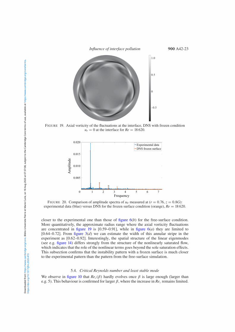
Influence of interface pollution 900 A42-23
1.0
0.5
0
–0.5
FIGURE 19. Axial vorticity of the fluctuations at the interface, DNS with frozen conditionur = 0 at the interface for Re = 18 620.
0.020
0.015
0.010
0.005
0 1 2 3 4 5 6 7Frequency
Experimental dataDNS frozen surface
Am
plitu
de
FIGURE 20. Comparison of amplitude spectra of uθ measured at (r = 0.76, z = 0.8G):experimental data (blue) versus DNS for the frozen surface condition (orange), Re = 18 620.
closer to the experimental one than those of figure 6(b) for the free-surface condition.More quantitatively, the approximate radius range where the axial vorticity fluctuationsare concentrated in figure 19 is [0.59–0.91], while in figure 6(a) they are limited to[0.64–0.72]. From figure 3(d) we can estimate the width of this annular stripe in theexperiment as [0.62–0.92]. Interestingly, the spatial structure of the linear eigenmodes(see e.g. figure 14) differs strongly from the structure of the nonlinearly saturated flow,which indicates that the role of the nonlinear terms goes beyond the sole saturation effects.This subsection confirms that the instability pattern with a frozen surface is much closerto the experimental pattern than the pattern from the free-surface simulation.
5.4. Critical Reynolds number and least stable modeWe observe in figure 10 that Rec(β) hardly evolves once β is large enough (larger thane.g. 5). This behaviour is confirmed for larger β, where the increase in Rec remains limited.
http
s://
doi.o
rg/1
0.10
17/jf
m.2
020.
473
Dow
nloa
ded
from
htt
ps://
ww
w.c
ambr
idge
.org
/cor
e. B
iblio
Uni
vers
ite P
ierr
e et
Mar
ie C
urie
, on
18 A
ug 2
020
at 0
7:37
:08,
sub
ject
to th
e Ca
mbr
idge
Cor
e te
rms
of u
se, a
vaila
ble
at h
ttps
://w
ww
.cam
brid
ge.o
rg/c
ore/
term
s.

900 A42-24 A. Faugaret, Y. Duguet, Y. Fraigneau and L. Martin Witkowski
β m = 4 m = 5
5 3139 2934100 3632 3330
TABLE 3. Critical Reynolds number estimated by LSA for G = 1/14.
u∗ free u∗ frozen
U free 17 006 18 959U frozen 2776 10 555
TABLE 4. Value of Rec for m = 5 and four sets of boundary conditions for the couple (U , u∗).
The instability pattern appears similar to those shown in figure 14, which suggests thatthe most unstable mode of the frozen condition again belongs to an unstable branchdifferent from the ‘clean’ unstable mode identified with the free-slip condition. Sincethe base flows for either large β or for the frozen interface condition have a verysimilar structure, we expect, for the frozen surface condition, a critical Reynolds numberquantitatively comparable to those reported in table 3. However, it appears that for this newcondition, LSA predicts Rec = Rec5 = 10 555 for m = 5, confirming DNS (Rec = 10 584).While this represents a drop of 39 % compared to the original critical Reynolds numberfor the free-surface condition (Rec = 17 006), it is still well above the experimental valueby a factor of approximately 3. Similarly, using the same frozen condition, the thresholdfor the mode m = 4 at Rec4 = 11 152 and remains very close to Rec5.
5.5. Conclusions on the frozen surface conditionThe nonlinear dynamics captured in DNS using the frozen surface condition is inexcellent qualitative match with experimental measurements both from the point of viewof the dynamics and the modal content of the saturated flow. This is again confirmed bythe good agreement between the amplitude spectra shown in figure 20. The base flow withthe frozen surface condition is hardly distinguishable from the base flow obtained using thepollutant model for β ≥ 5. Nevertheless, once again, the comparison of the values of Recis not favourable, as for the frozen surface Rec is 260 % (10 555 vs 2934) higher than forβ = 5, which discredits the frozen condition as a direct substitute to the free-slip condition.This negative conclusion is further confirmed for G = 1/4 (the value considered by Lopezet al. 2004), where the most unstable mode remains poorly representative of experimentalvisualisations and Rec is pushed even further up. These quick tests reveal how sensitivethe instability threshold is to the choice of boundary conditions.
The quantitative discrepancy in Rec can eventually be resolved by introducing a newboundary condition of a mixed type. Whereas the hypothesis of vanishing Ur is satisfyingfor the steady base flow and large enough values of β (see § 5.2), it is not justified fortime-dependent perturbations. We suggest separating the velocity field u into its base flowcomponent U and its perturbations u∗ and applying a different set of boundary conditionsto U and u∗. The situation is summed up in table 4, where the four possible combinationsof boundary conditions are considered and Rec has been re-computed using ROSE for eachcase. Consistently with the previous arguments, we focus on the mixed-type boundary
http
s://
doi.o
rg/1
0.10
17/jf
m.2
020.
473
Dow
nloa
ded
from
htt
ps://
ww
w.c
ambr
idge
.org
/cor
e. B
iblio
Uni
vers
ite P
ierr
e et
Mar
ie C
urie
, on
18 A
ug 2
020
at 0
7:37
:08,
sub
ject
to th
e Ca
mbr
idge
Cor
e te
rms
of u
se, a
vaila
ble
at h
ttps
://w
ww
.cam
brid
ge.o
rg/c
ore/
term
s.

Influence of interface pollution 900 A42-25
1.0
0.5
–0.5
–1.0
0
1.0
0.5
–0.5
–1.0
0
(a) (b)
FIGURE 21. Vorticity ωz(r, θ) at the fluid interface (normalised by its maximum) for the leaststable eigenmode m = 5 at Re = 18 620. (a) Frozen surface, (b) mixed condition. The mixedcondition corresponds to a frozen surface condition for the base flow, and free-surface conditionfor the perturbation field.
condition where the base flow obeys a frozen condition whereas the perturbation obeysthe free-slip condition. The value of Rec is now 2776, much lower than the fully frozenthreshold value of 10 555. The quantitative mismatch is now reduced down to 6 % (2779vs 2934) and 31 % (2779 vs 4230) compared to β = 5 and experimental Rec, respectively,while the spatial structure (see figures 14 and 21 for the eigenmodes) is compatible withthe frozen case.
6. Discussions and perspectives
The hydrodynamic instability occurring inside a fixed, cylindrical cavity with a rotatingbottom has been investigated for a small form factor depth/radius G = 1/14. The selectionof a least stable mode with azimuthal wavenumber m = 5, predicted by linear instabilityanalysis, is verified experimentally, as well as numerically using DNS assuming no stressat the liquid interface. Using water – the most widespread liquid – as the experimentalfluid, a robust quantitative and qualitative mismatch is evidenced between our experimentsand our numerics. The mismatch concerns the presence of an overshoot in the azimuthalvelocity profile and, crucially, the value of Rec for the development of the instability isoverestimated in the numerics by a factor of more than 4. Regarding the mismatch betweenour experimental estimation of Rec and the literature, the use of Kalliroscope as a marker(used precisely for the identification of instability thresholds) is our best suspect to explainthe discrepancy. The results obtained here using LDV, quantitatively safer, demonstratethat thresholds formerly deduced from visualisation using markers, are over-evaluated.The linear and nonlinear numerical approaches, however, report a robust threshold Rec,that still differs strongly from the experimental one. After a cautious search for possibleexperimental flaws, the standard free-slip interface condition (σ = cst, h = cst, free-slipinterface) used in the simulations emerged as the most credible source of mismatch, inline with former investigations by Spohn & Daube (1991) and Hirsa et al. (2002a); inexperiments, such an ideal interfacial condition cannot be matched due to residual ambientair pollution. The inevitable presence of pollutants at the interface modifies the surfacetension of the flow and, as a consequence, impacts the velocity field of the base flow andshifts the instability threshold. A pollution model has been implemented into the linearstability solver, based on a modification of the effective surface tension by the presence ofa superficial concentration of unknown pollutants. Using a quadratic closure between the
http
s://
doi.o
rg/1
0.10
17/jf
m.2
020.
473
Dow
nloa
ded
from
htt
ps://
ww
w.c
ambr
idge
.org
/cor
e. B
iblio
Uni
vers
ite P
ierr
e et
Mar
ie C
urie
, on
18 A
ug 2
020
at 0
7:37
:08,
sub
ject
to th
e Ca
mbr
idge
Cor
e te
rms
of u
se, a
vaila
ble
at h
ttps
://w
ww
.cam
brid
ge.o
rg/c
ore/
term
s.

900 A42-26 A. Faugaret, Y. Duguet, Y. Fraigneau and L. Martin Witkowski
tension surface and the superficial pollutant concentration inspired by surfactant studiesyields results quantitatively consistent with experiments; for sufficiently large value of β(the parameter that pilots the surface contamination), Rec drops by more than 80 % andthe mismatch on Rec goes down approximately from 400 % to 30 %.
Interestingly, the instability mode selected for finite pollutant concentrations does notbelong to the same modal families as predicted by linear stability theory in the cleaninterface case; new branches of ‘dirty’ modes destabilise for small yet finite concentrationlevels and take over as least stable modes. The corresponding eigenmodes are verystable for clean interface conditions and have not been identified before. In terms ofbifurcations, the robust mismatch in Rec, angular frequency and flow structure betweennumerics and experiments can hence be explained, at least for the case of the modesm = 4 and 5 investigated here, as a jump from one modal family to another one as thecontamination of the surface increases. The spatial structure of the base flow is also moreconsistent with LDV measurements; the meridional recirculation length is reduced andthe overshoot in azimuthal velocity vanishes. For β 5, the flow at the interface verifiesan approximate no-slip condition for the radial velocity component. As a consequence,in an effort to deliver a simpler parameter-free model boundary condition for uncleanliquid/gas interfaces, the ‘frozen condition’ ur = 0 was also simulated. Whereas it displaysbetter qualitative agreement as well as simpler nonlinear dynamics consistent now withexperiments, at least for low G, the threshold value Rec remains too high compared toexperiments. This new quantitative mismatch is eventually resolved once and for all byconsidering an interfacial boundary condition of a mixed type; frozen for the steady baseflow and free slip for the unsteady perturbations.
Interfacial experiments involving water have long had the reputation of being ‘difficult’in the sense that Marangoni effects linked with variations of the surface tension are hard totame. The present hypothesis of a modification of the surface tension by pollution effectsis one such illustration. The surprising effect of this pollution is, despite relatively smallmodifications of the structure of the base flow, an important quantitative impact on thestability thresholds. Besides, not only does the instability mode change its growth rate,it also belongs to another family of destabilised modes compared to the clean interfacecase. From such a simple conclusion it is tempting to critically revisit the discrepanciesbetween experimental studies and to deduce that higher values of Rec (as reported inPoncet & Chauve 2007) are linked to a cleaner interface due to different experimentalconditions. While this is a priori possible (and very difficult to assess rigorously), itdoes not remove the caveat that Kalliroscope visualisations are not reliable in terms ofmeasurements. Besides an interaction of the marker itself with the solvent cannot beexcluded for high Kalliroscope concentrations. We are hence not in a position to concludeabout the values reported by various teams using Kalliroscope or other markers, andencourage instead the use of non-intrusive techniques such as LDV for more reliableestimations. Other experimental improvements could here be useful, such as measuringsimultaneously several velocity components, including smaller components such as theaxial one and the radial component near the interface. This could allow for a criticalevaluation of the model interfacial condition suggested in § 5.
While the present study is essentially a proof of concept that the stability characteristicsof a given flow case depend heavily on the surface pollution, the simplicity of theanalytical model in § 4 must be kept in mind. The advantage of such a simple modelis a straightforward identification of the mechanisms altering the spatial structure of thebase flow. The main difficulty lies in the mathematical parametrisation of a chemicallycomplex phenomenon. Adsorption of pollutants by the interface is an unsteady processthat depends on the precise chemical composition of the ambient particles in the air and
http
s://
doi.o
rg/1
0.10
17/jf
m.2
020.
473
Dow
nloa
ded
from
htt
ps://
ww
w.c
ambr
idge
.org
/cor
e. B
iblio
Uni
vers
ite P
ierr
e et
Mar
ie C
urie
, on
18 A
ug 2
020
at 0
7:37
:08,
sub
ject
to th
e Ca
mbr
idge
Cor
e te
rms
of u
se, a
vaila
ble
at h
ttps
://w
ww
.cam
brid
ge.o
rg/c
ore/
term
s.
Influence of interface pollution 900 A42-27
of the exact properties of the liquid. None of these hypotheses have been included inthe present model, resulting in a simple law parametrised by one unique real parameterβ and unable to cope with different chemical compositions and solubility effects.Further chemical complications can occur for increased concentration levels, notably bulkdiffusion (necessitating a volumetric model rather than a superficial one) and later theformation of micelles inside the bulk of the fluid. Ideally, the modelling of pollution effectsshould be compared with an experimental set-up where the superficial concentration ofeach pollutant can be quantitatively controlled and properly modelled. It is not excludedthat each different pollutant contributes differently to the final surface tension rather thanall obeying the quadratic law of equation (4.1).
Finally, the present set-up is still academically simple in the sense that no deformationof the interface needs to be considered at such low rotation rates. A first way to incorporatemore realistic effects is to consider the possibility for small deformations of the interfacecoupled with oscillations within the fluid. This situation might lead to the existence ofadditional families of eigenmodes and even richer dynamics. While this is technicallymuch more involved, especially on the numerical side (see e.g. Yang et al. 2020),one can wonder whether pollution effects can also affect the thresholds in the largedeformation regime investigated by many others (Vatistas, Abderrahmane & Siddiqui2008; Tophøj et al. 2013) also in the presence of additional surfactants (Jansson et al.2006). These regimes involve not only finite deformations of the fluid interface but alsopartial dewetting, which makes the dynamics of the concentration field more complex byinvolving moving triple contact lines. Eventually, it will be interesting to see how the trendevidenced in the present study (the decrease of Rec by ambient pollution despite a calmernonlinear regime) can be extended to other unstable flow configurations.
Acknowledgements
This work was supported by the French Agence Nationale de la Recherche under theANR ETAE Project no. ANR-16-CE08-0011. HPC resources from GENCI-IDRIS (grantno. 2017-2a10308) are also acknowledged. The authors thank I. Delbende, F. Gallaire,W. Herreman, F. Lusseyran, W. Yang for fruitful discussions, the technical team CTEMOat LIMSI, as well as F. Moisy and M. Rabaud for their help on the experimental facility.
Declaration of interests
The authors report no conflict of interest.
REFERENCES
BANDI, M. M., AKELLA, V. S., SINGH, D. K., SINGH, R. S. & MANDRE, S. 2017 Hydrodynamicsignatures of stationary Marangoni-driven surfactant transport. Phys. Rev. Lett. 119 (26), 264501.
CHENG, N. S. 2008 Formula for the viscosity of a glycerol-water mixture. Ind. Engng Chem. Res. 47 (9),3285–3288.
COGAN, S. J., RYAN, K. & SHEARD, G. J. 2011 Symmetry breaking and instability mechanisms inmedium depth torsionally open cylinder flows. J. Fluid Mech. 672, 521–544.
DAUBE, O. 1991 Numerical simulation of axisymmetric vortex breakdown in a closed cylinder. InVortex Dynamics and Vortex Methods (ed. C. R. Anderson & C. Greengard), Lectures in AppliedMathematics, vol. 28, pp. 131–152. American Mathematical Society.
DUGUET, Y., SCOTT, J. F. & LE PENVEN, L. 2005 Instability inside a rotating gas cylinder subject toaxial periodic strain. Phys. Fluids 17 (11), 114103.
http
s://
doi.o
rg/1
0.10
17/jf
m.2
020.
473
Dow
nloa
ded
from
htt
ps://
ww
w.c
ambr
idge
.org
/cor
e. B
iblio
Uni
vers
ite P
ierr
e et
Mar
ie C
urie
, on
18 A
ug 2
020
at 0
7:37
:08,
sub
ject
to th
e Ca
mbr
idge
Cor
e te
rms
of u
se, a
vaila
ble
at h
ttps
://w
ww
.cam
brid
ge.o
rg/c
ore/
term
s.

900 A42-28 A. Faugaret, Y. Duguet, Y. Fraigneau and L. Martin Witkowski
HIRSA, A. H., LOPEZ, J. M. & MIRAGHAIE, R. 2001 Measurement and computation of hydrodynamiccoupling at an air/water interface with an insoluble monolayer. J. Fluid Mech. 443, 271–292.
HIRSA, A. H., LOPEZ, J. M. & MIRAGHAIE, R. 2002a Determination of surface shear viscosity viadeep-channel flow with inertia. J. Fluid Mech. 470, 135–149.
HIRSA, A. H., LOPEZ, J. M. & MIRAGHAIE, R. 2002b Symmetry breaking to a rotating wave in alid-driven cylinder with a free surface: experimental observation. Phys. Fluids 14 (6), 29–32.
HUISMAN, S. G., VAN GILS, D. P. M. & SUN, C. 2012 Applying laser Doppler anemometry inside aTaylor–Couette geometry using a ray-tracer to correct for curvature effects. Eur. J. Mech. B/Fluids36, 115–119.
HYUN, J. M. 1985 Flow in an open tank with a free surface driven by the spinning bottom. J. Fluids Engng107 (4), 495–499.
IGA, K., YOKOTA, S., WATANABE, S., IKEDA, T., NIINO, H. & MISAWA, N. 2014 Various phenomenaon a water vortex in a cylindrical tank over a rotating bottom. Fluid Dyn. Res. 46 (3),031409.
IWATSU, R. 2004 Analysis of flows in a cylindrical container with rotating bottom and top underformablefree surface. JSME Intl J. 47 (3), 549–556.
JANSSON, T. R. N., HASPANG, M. P., JENSEN, K. H., HERSEN, P. & BOHR, T. 2006 Polygons on arotating fluid surface. Phys. Rev. Lett. 96 (17), 174502.
KAHOUADJI, L., HOUCHENS, B. C. & MARTIN WITKOWSKI, L. 2011 Thermocapillary instabilities in alaterally heated liquid bridge with end wall rotation. Phys. Fluids 23 (10), 104104.
KAHOUADJI, L., MARTIN WITKOWSKI, L. & LE QUÉRÉ, P. 2010 Seuils de stabilité pour un écoulementà surface libre engendré dans une cavité cylindrique tournante à petit rapport de forme. Mécaniqueet Industries 11 (5), 339–344.
KWAN, Y. Y., PARK, J. & SHEN, J. 2010 A mathematical and numerical study of incompressible flowswith a surfactant monolayer. Discrete Continuous Dyn. Syst. 28 (1), 181–197.
LOPEZ, J. M. & CHEN, J. 1998 Coupling between a viscoelastic gas/liquid interface and swirling vortexflow. J. Fluids Engng 120 (4), 655–661.
LOPEZ, J. M. & HIRSA, A. 2000 Surfactant-influenced gas-liquid interfaces: nonlinear equation of stateand finite surface viscosities. J. Colloid Interface Sci. 229 (2), 575–583.
LOPEZ, J. M., MARQUES, F., HIRSA, A. H. & MIRAGHAIE, R. 2004 Symmetry breaking in free-surfacecylinder flows. J. Fluid Mech. 502, 99–126.
MAGNAUDET, J. & EAMES, I. 2000 The motion of high-Reynolds-number bubbles in inhomogeneousflows. Annu. Rev. Fluid Mech. 32 (1), 659–708.
MARTÍN, E. & VEGA, J. M. 2006 The effect of surface contamination on the drift instability of standingFaraday waves. J. Fluid Mech. 546, 203–225.
PEAUDECERF, F. J., LANDEL, J. R., GOLDSTEIN, R. E. & LUZZATTO-FEGIZ, P. 2017 Traces ofsurfactants can severely limit the drag reduction of superhydrophobic surfaces. Proc. Natl Acad.Sci. 114 (28), 7254–7259.
PONCE-TORRES, A. & VEGA, E. J. 2016 The effects of ambient impurities on the surface tension. EPJWeb Conf. 114, 02098.
PONCET, S. & CHAUVE, M. P. 2007 Shear-layer instability in a rotating system. J. Flow Visual. ImageProcess. 14 (1), 85–105.
RASTELLO, M., MARIÉ, J. L. & LANCE, M. 2017 Clean versus contaminated bubbles in a solid-bodyrotating flow. J. Fluid Mech. 831, 592–617.
SCRIVEN, L. E. 1960 Dynamics of a fluid interface: equation of motion for Newtonian surface fluids.Chem. Engng Sci. 12 (2), 98–108.
SERRE, E. & BONTOUX, P. 2007 Vortex breakdown in a cylinder with a rotating bottom and a flatstress-free surface. Intl J. Heat Fluid Flow 28 (2), 229–248.
SERRE, E., TULISZKA-SZNITKO, E. & BONTOUX, P. 2004 Coupled numerical and theoretical study ofthe flow transition between a rotating and a stationary disk. Phys. Fluids 16 (3), 688–706.
SPOHN, A. & DAUBE, O. 1991 Recirculating flows in a cylindrical tank. In Proceedings of the 5thInternational Conference on Computational Methods and Experimental Measurement (ed. A. Sousa,C. A. Brebbia & G. M. Carlomagno), pp. 155–166. Elsevier.
STEWARTSON, K. 1957 On almost rigid rotations. J. Fluid Mech. 3, 17–26.
http
s://
doi.o
rg/1
0.10
17/jf
m.2
020.
473
Dow
nloa
ded
from
htt
ps://
ww
w.c
ambr
idge
.org
/cor
e. B
iblio
Uni
vers
ite P
ierr
e et
Mar
ie C
urie
, on
18 A
ug 2
020
at 0
7:37
:08,
sub
ject
to th
e Ca
mbr
idge
Cor
e te
rms
of u
se, a
vaila
ble
at h
ttps
://w
ww
.cam
brid
ge.o
rg/c
ore/
term
s.

Influence of interface pollution 900 A42-29
STONE, H. 1990 A simple derivation of the time-dependent convective-diffusion equation for surfactanttransport along a deforming surface. Phys. Fluids 2 (1), 111–112.
SUZUKI, T., IIMA, M. & HAYASE, Y. 2006 Surface switching of rotating fluid in a cylinder. Phys. Fluids18 (10), 101701.
TASAKA, Y. & IIMA, M. 2009 Flow transitions in the surface switching of rotating fluid. J. Fluid Mech.636, 475–484.
TOPHØJ, L., MOUGEL, J., BOHR, T. & FABRE, D. 2013 Rotating polygon instability of a swirling freesurface flow. Phys. Rev. Lett. 110 (19), 194502.
VATISTAS, G. H., ABDERRAHMANE, H. A. & SIDDIQUI, M. H. K. 2008 Experimental confirmation ofKelvin’s equilibria. Phys. Rev. Lett. 100 (17), 174503.
VATISTAS, G. H., WANG, J. & LIN, S. 1992 Experiments on waves induced in the hollow core of vortices.Exp. Fluids 13 (6), 377–385.
YANG, W., DELBENDE, I., FRAIGNEAU, Y. & MARTIN WITKOWSKI, L. 2019 Axisymmetric rotatingflow with free surface in a cylindrical tank. J. Fluid Mech. 861, 796–814.
YANG, W., DELBENDE, I., FRAIGNEAU, Y. & MARTIN WITKOWSKI, L. 2020 Large axisymmetricsurface deformation and dewetting in the flow above a rotating disk in a cylindrical tank: spin-upand permanent regimes. Phys. Rev. Fluids 5 (4), 044801.
YOUNG, D. L., SHEEN, H. J. & HWU, T. Y. 1995 Period-doubling route to chaos for a swirling flow in anopen cylindrical container with a rotating disk. Exp. Fluids 18 (5), 389–396.
http
s://
doi.o
rg/1
0.10
17/jf
m.2
020.
473
Dow
nloa
ded
from
htt
ps://
ww
w.c
ambr
idge
.org
/cor
e. B
iblio
Uni
vers
ite P
ierr
e et
Mar
ie C
urie
, on
18 A
ug 2
020
at 0
7:37
:08,
sub
ject
to th
e Ca
mbr
idge
Cor
e te
rms
of u
se, a
vaila
ble
at h
ttps
://w
ww
.cam
brid
ge.o
rg/c
ore/
term
s.

44 Chapter II. Article published in Journal of Fluid Mechanics

Chapter III
Experimental tools
45

46 Chapter III. Experimental tools
The configuration of the cavity, which appears to be basic, still hides many difficul-ties in its realization. Many rotating flow experiments use a lid, as this configurationis actually easier to build : the "lid" is at the bottom, while the spinning disc is at thetop, avoiding sealing issue around the shaft, and allowing for an easier cleaning. In ourconfiguration, with a free surface, we can’t use such artifice. Our disc is located at thebottom of the cylindrical cavity (see fig. III.1). Hence, the shaft crosses the cavity, and wehave to insure a perfect sealing around it. The second issue is the quality of the rotation,both in term of regularity of the rotation speed, and to prevent unbalanced rotation. Ifthis last requirement is not met, it may add a translation to the fluid movement, and givebirth to a sloshing phenomenon. Since the gap between the cavity vertical wall and thedisc is small, any translation or precession movement could make the disc scrap the cavity.
Figure III.1 – Simplified view of the largest cavity, with correct proportions. R is theradius of the cavity, H is the height of the undisturbed fluid (in blue) above the disc (in
yellow), and Ω is the disc rotation rate.
Most of the technical elements of the main cavity are given in chapter II. Here we comeback on these technical data, and add details that were not provided earlier, includinga second experimental bench. We also give further information on the acquisition chain,measurement tools, markers, and fluids used in our experiments.
First cavityAt the beginning of the project, a first apparatus was built with the same geometrical
characteristics as the one used at IRPHE by Poncet and Chauve ([40]). The cylindri-cal cavity, made of plexiglas, was borrowed from a former set-up (FAST [52]). Motorreducer unit, control card and power supply were also recycled from this former experi-ment. However, the disc was initially belt-driven. This system was changed to a simplerdirect coupling and therefore, a new frame and a new aluminium foot were machined tocarry the cavity. The motor reducer unit is screwed into this foot, and suspended belowthe table, in the same alignment as the rotation axis of the disc. The coupling betweenthe reducer shaft and the disc is done with an aluminium sleeve. We recall that the

III.1 First cavity 47
internal radius of this cavity is R = 140.3 mm. The thickness of the wall is e=6.8 mm,and the maximal height above the surface of the disc is H ≈ 71.5 mm. The rotatingdisc is placed at the bottom of the cavity. Two different discs can be used. The one thatwas mainly used is made of brass. Its radius is R − εR=139.6 mm, where εR representthe gap between the edge of the disc and the vertical wall. In the rest of this thesis, wewill use R for both cavity and disc radius. The thickness of this disc is 8.5 mm and itsmass is close to 5 kg. The maximum displacement of its surface while put into rotation isestimated to 0.3 mm. This measurement was made using both a mechanical comparatorand a Keyence LK-G10 laser sensor. More details on surface displacements are given inchapter VII. The second disc is made of aluminium and was only used in preliminarytests about the influence of the flatness of the disc, since its surface was not accuratelymachined. Shafts are cohesive with their respective discs : they are screwed into it, andcrosses the bottom of the cavity.
Figure III.2 – Photography of the large cavity, made of plexiglas. The brass disc iscoated with a thin white plastic film, to enhance contrast with ink. The foot is made of
aluminium.
The main advantage of this cavity is its size : as the radius is large, it is easier tocontrol the height of the fluid H for small aspect ratios. But its main drawback is thatthis set-up is limited to aspect ratios below G ∼0.5.

48 Chapter III. Experimental tools
Second cavity
The need for a higher cavity in the study of rotating polygons ([51]), and the will toexplore higher aspect ratio leads us to design a second experiment. As we were confidentin the motor and its servo solution (see below), we choose to keep this base, and to builda new structure to host the cavity.
Figure III.3 – Photography of the small cavity, made of aluminium, brass (disc) andglass (cylindrical wall). One can see at the bottom the Oldham coupling for rotation
irregularities absorption.
The previous rigid sleeve coupling is now replaced by an Oldham coupling, in orderto prevent any misalignment of the disc shaft and the motor shaft. To manage enoughspace to place this coupling, the base of the cavity is raised by three braces. This base ismachined in aluminium, and includes two conical bearings in a back-to-back arrangementto steer the rotation of the shaft. The disc material is brass, and its dimensions areR − εR=68 mm for the radius and 10.1 mm for the thickness. The sealing is donebelow the disc, and no more on the shaft, but still with a single lip spring loaded seal.The vertical wall of the cavity is a glass cylinder, which inner radius is R=70 mm andthickness is 5.2 mm. This cylinder is fitted on the base, and an O-ring ensures the sealingbetween those two elements. The height H=114 mm of the cavity allows one to reachaspect ratios up to G=1.5.

III.3 Driving and monitoring the rotation 49
Driving and monitoring the rotation
Both experimental set-ups use the same direct current motor (Parvex RX320E-R1100),coupled with a 1:12 reductor. A tachymeter deliver a tension of 6 mV per round of themotor, or 72 mV per round of the disc. This difference is due to the presence of thereducer. A voltmeter Agilent 34401A is used to monitor the rotation of the disc. Therotation speed is controlled with a servo loop, done by a Parvex card. This card hasan ±10 V input to control the motor speed. We coupled this input to an Mbed micro-controller. If required, this allows us to perfectly control spin up and spin down phases.
Data Acquisition
There are two kinds of data we can acquire from our experiment. The first one areimages, or movies, captured by an IDS camera (UI-3370CP), mounted at the vertical ofthe cavity. This camera uses a 11.264×11.264 mm2 sensor of 4.19 Mpx, coupled with a35 mm F1.4 Fujinon lense (CF35HA-1). The camera is linked to a computer by USB3,and allows to record movies at 80 frames per seconds with a 2048×2048 resolution, up to12 bits grey scale. In practice, an 8 bits greyscale was used.
For more quantitative measurements of the velocity, we used a Dantec laser dopplervelocimetry device (LDV). It is composed of a laser head Flow Explorer, coupled to aBSAFlow processor. It allows the acquisition of the local velocity of only one component.To do so, the fluid has to be seeded with particles that will be detected by the laser. Theparticles we employed are also provided by Dantec, and are silver coated hollow glass,with a size of 10 µm.
Laser Doppler Velocimetry
The principle of LDV relies on detection of particles across fringe pattern, such asobtained with a Michelson interferometer in the fringes of equal thickness configuration :two coherent laser beams cross and create a pattern of alternatives bright and dark stripes(see fig. III.4). The frequency fr of reflected beams on coated particles crossing thebrightening fringes are detected by a sensor. We suppose here that particles are smalland with a comparable density than that of the fluid to be carried at the same speed thanthe flow, without influencing it. If we denote by di the inter-fringe gap, i.e. the widthof brightening fringe, the velocity of the particle up is given by the relation up = frdi.di depends on the wave length λ of the laser and of the angle θL of beams through therelation di = λ/(2sin(θL/2)). One can pair both previous relations through the equation :
up = frλ
2sin(θL/2) . (III.1)
However, equation (III.1) does not give any information about the direction of theflow : the measured frequency would be the same for both flows of same velocity, butopposed direction. Therefore, a Bragg cell generate a scrolling of the fringes. Knowing

50 Chapter III. Experimental tools
Figure III.4 – Fringes of equal thickness obtained with a Michelson interferometer. Forthe LDV device we used, in the air, inter-fringe gap is ≈6 µm.
this scrolling speed (and thus its direction), one can access to the direction of the flow.
Optical correctionsDue to the triple medium crossed by the laser (which implies three different optical in-
dices), we had to apply a geometrical correction to the position of convergence of the twolaser beams. Indeed, as di is paired with θL, a variation of the angles of beams implies anerroneous evaluation of the fringes width, and thus of the velocity. Using Snell-Descarteslaws, and intersection coordinates between a line and a circle, one can easily calculate theposition of the effective point of measurement. These corrections were published in [53].Details are given in appendix C
Zeroing lasers intersectionCorrections described above require lasers intersection to match the axis of rotation.
Laser can easily be translated along the X and Z axis, relatively to the laboratory frame,thanks to a motorised horizontal stage and a manually operated vertical displacement(see fig. III.5). Stages are mounted on an aluminium plate relying on three micrometerscrews, in order to adjust horizontality.
Nevertheless, no device allows for an easy rotation of the global laser group around itsz axis, and it has to be placed manually on the table to try to cross the optical axis of thelaser and the rotation axis of the disc. This leads to inaccuracies in positioning that mayexplain later the mismatch between experimental and numerical velocity profiles. Evenif the laser optical axis is perfectly merged with the radius of the disc, the operator stillhave to adjust the position of the beam at the vertical of the center of the disc. Thispoint location is also prone to inaccuracy. Two solutions were use to locate it. The first

III.5 Experimental protocol 51
Figure III.5 – Dantec LDV head, gathering laser and photosensitive cell. The head ismounted on a manual screw driven vertical stage. The assembly is fixed on a motorized
horizontal stage.
one relied on perpendicular bisectors of a triangle inscribed on the disc to place its center.Then, a solid shape was placed on the disc, with one of its edge orthogonal to the disc’ssurface, at the vertical of the center. The convergence of the beam was then adjusted onthis edge. The second solution to find the center uses the camera above the disc. Thedimensions of the disc on its image taken by the camera allows for finding the coordinatesof the pixel corresponding to the disc’s center. Then, using the live capture of the camera,the intersection of the beam was adjusted to match these coordinates. Note that this lastsolution is only suitable for azimuthal measurements.
Experimental protocol
The increase of Re is obtained by an increase of the disc rotation rate Ω. As long asan instability is not triggered and no hysteresis is present, the protocol to increase Ω doesnot matter. On the opposite, as soon as an instability may occur, the threshold detectionmay be protocol dependent. Velocity was increased by steps, and held constant on aplateau between two steps. The requested time to accelerate the disc from one plateau to

52 Chapter III. Experimental tools
another is very short compared to the timespan of the plateau itself. Even if the disc isquite heavy, and thus has an important inertia, the motor has enough torque for the ac-celeration of the disc to be almost instantaneous. The spin-up time for the fluid is alwaysmuch larger than the time required for the disc to accelerate. If the flow is dominatedby viscous effects then the transition time would scale as R2/ν, H2/ν, or RH/ν. In ourcase, the regime is always dominated by convective effects with boundary layers and thusthe time evolution of the system is given by the Ekman time tEk = R√
νΩ .
Initially, following the protocol used by Poncet and Chauve in [40], we used the Ek-man time as reference for each plateau with a given Ω. As tEk decreases with the increaseof Ω, plateau are increasingly shorter. For exemple, for Ω=1 rpm, tEk ≈ 433s, while forΩ=8 rpm, tEk ≈ 153s. However, there is no reason to link the base flow spin-up time tothe growth rate of the instability. Therefore we switched to a constant timespan for eachplateau. We chose an arbitrary timespan between 10 min to 15 min; followed by 5 minof acquisition when LDV was used. This crude and empirical protocol does not guaranteeeither that at a given Re, the growth rate of the instability is large enough to observe theinstability. However, our hope is that during the plateau, the noise level is large enoughto feed the instability so that it can be observed.
The accuracy on Rec determination is also limited by the step of 1 rpm between eachplateau. At times, this step was reduced to 1/2 rpm or 1/3 rpm. An alternate option toincrease the accuracy of the bounding of the instability threshold is to use a more viscousfluid. Doing so allows one to reach higher rotation rates for a given Re, and also to reducethe issue of particles sedimentation (see below section Markers). However, increasing therotation rate also increases the surface deformation, and an increased caution must beobserved during experiment to stay in admissible Ω values to keep valid the flat surfacehypothesis.
Fluids & Markers
Fluids
Although we mostly used water as experimental fluid (tap, de-ionized or distilled wa-ter), we also used water glycerol mixtures. The reason for the choice of glycerol is that itis non toxic and fully soluble in water. It thus allows an easy adjustment of the viscosity,and can easily be cleaned, in contrast to silicon oils.
Solutions of water diluted glycerol have been widely studied, so that the propertiesof such mixtures are well tabulated in many articles such as [54] or handbooks of physicsand chemistry. Especially, one can easily access to the optical indices of such mixtures([55]), and to their viscosity, regarding the mass percentage of glycerol and temperature.Indeed, with the use of glycerol, temperature becomes a major focus : compared to water,water-glycerol solutions have an increased dependency of their viscosity to temperature,especially for high percentage of glycerol. As none of our cavity are thermo-regulated,temperature has to be monitored continuously. Viscosity was then estimated according toan experimentally fitted analytical expression given in [56]. This expression was already

III.6 Fluids & Markers 53
checked with rheology measurements during the very first experiments, back in 2013, andestimated adequate compared to the inaccuracies of low viscosity measurements.
Ethanol was also marginally experimented, but experimental restrictions (alcohol-plexiglas reaction, vapours) limited these experiments.
MarkersTo obtain visualisation of the pattern, markers are needed. The first one we used was
Kalliroscope. This rheoscopic fluid was created in 1960 by the artist Paul Matisse. It iscomposed of small particles of crystalline guanine that are supposed to orient themselvesaccording to vorticity of the flow. Crystalline guanine particles average dimensions are6 × 30 × 0.07µm3 with a density of 1.62 g.cm−3, according to [57]. Depending on theirorientation, and thanks to their high index of refraction (1.85), the reflection of light onthese flakes produces a greyscale visualization. This marker was widely used, including,among others, Taylor-Couette (fig. III.6), or Rayleigh-Bénard experiments. This wasalso the visualisation tool used in [40]. Note that due to the drop of Crystalline guanineproduction, Kalliroscope is no longer sold since 2014.
Figure III.6 – Taylor-Couette instabilities revealed thanks to Kalliroscope.
Some issues with the reproducibility of our results forced us to re-consider the neu-trality of Kalliroscope, and thus, the use of this marker. We kept it only for visualisationpurpose, without any quantitative aspect. For a better detection of thresholds we switchedto ink diluted into water. This marker is less intrusive, and fully soluble into water. Theink was injected at the surface at a single random location, for one disc rotation, using asyringe. This advantage is also its main flaw : in highly mixing flow, the ink is adsorbedtoo quickly to allow for any visualisation. Even in slowly rotating flows, the fluid has tobe seeded with ink repeatedly. However it gives great results on higher density fluids,such as water glycerol mixture.
The influence of Kalliroscope flakes on rotating flows was reported as early as 1985([58]) : in vertically oriented Couette-Taylor experiment, Kalliroscope flakes influenced

54 Chapter III. Experimental tools
the size of Taylor vortices. It was observed that particles were clustering in the coreof vortices, resulting in a coupling with the gravitational field. Although Matisse andGorman claimed the neutrality of Kalliroscope ([59]), the results from Dominguez etal. ([58]) are consistent with our observations about sedimentation and clustering ofKalliroscope particles.

Chapter IV
Governing equations
55

56 Chapter IV. Governing equations
Basic equationsSince we remain in the approximation of a continuous medium, and since we restrain
the study to Newtonian fluids, we can describe the motion of the flow with Navier-Stokesequations :
• Mass conservation equation :
∂ρ
∂t+∇ · (ρu) = 0
where ρ is the volumetric mass density of the fluid, and u is the velocity field.
• Momentum conservation equation :
∂ρu∂t
+∇ · (ρu⊗ u) = ρF−∇p+∇ · (µ∇u)
where µ is the dynamic viscosity of the fluid.
For the rest of this thesis, we will make the assumption that the flow is incompressible(∇·u=0) and we will neglect volume forces, except gravity (F = g). For the pressure, wewill use the reduced pressure p = P0 + ρgz. We can now simplify the previous equations :
∇ · (u) = 0
∂u∂t
+ (u · ∇)u = −1ρ∇p+ ν∆u
where ν = µρ is the kinematic viscosity of the fluid, and ∆ = ∇2. µ is assumed to be
constant.
Regarding to the geometry, it is convenient to use cylindrical coordinates. The com-ponents of the velocity field u are now defined as u = (urer +uθeθ+uzez). Navier-Stokesequations become :
1r
∂(rur)∂r
+ 1r
∂uθ∂θ
+ ∂uz∂z
= 0
∂ur∂t
+ ur∂ur∂r
+ uθr
∂ur∂θ
+ uz∂ur∂z− u2
θ
r= −1
ρ
∂p
∂r+ ν
[∆ur −
urr2 −
2r2∂uθ∂θ
]∂uθ∂t
+ ur∂uθ∂r
+ uθr
∂uθ∂θ
+ uz∂uθ∂z
+ uruθr
= − 1ρr
∂p
∂θ+ ν
[∆uθ −
uθr2 + 2
r2∂ur∂θ
]∂uz∂t
+ ur∂uz∂r
+ uθr
∂uz∂θ
+ uz∂uz∂z
= −1ρ
∂p
∂z+ ν∆uz

IV.2 Boundary conditions 57
where ∆ξ = 1r∂∂r (r ∂ξ∂r ) + 1
r2∂2ξ∂θ2 + ∂2ξ
∂z2 is the Laplacian operator in cylindrical coordinates,and ξ any component of the velocity field.
Dimensionless form
In order to obtain the dimensionless form of previous Navier-Stokes equations, weused the radius of the cavity R and the angular frequency Ω of the disc to build thecharacteristic scales :
u = RΩu
t→ t
Ωp→ ρ(RΩ)2p
r → Rr
Applying these changes to Navier-Stokes equations leads to :
∂ur∂r
+ urr
+ 1r
∂uθ∂θ
+ ∂uz∂z
= 0
∂ur∂t
+ ur∂ur∂r
+ uθr
∂ur∂θ
+ uz∂ur∂z− u2
θ
r
= −∂p∂r
+ 1Re
[∆(ur)−
urr2 −
2r2∂uθ∂θ
]∂uθ∂t
+ ur∂uθ∂r
+ uθr
∂uθ∂θ
+ uz∂uθ∂z
+ uruθr
= −1r
∂p
∂θ+ 1Re
[∆(uθ)−
uθr2 + 2
r2∂ur∂θ
]∂uz∂t
+ ur∂uz∂r
+ uθr
∂uz∂θ
+ uz∂uz∂z
= −∂p∂z
+ 1Re
∆(uz)
(IV.4)
where Re is the Reynolds number, defined as Re = R2Ων .
Boundary conditions
Cavity side wall
On the vertical wall of the cavity, boundary conditions are assumed to be imperme-ability and non slip. As the wall is immobile, this can be translated this to velocitycomponents :
ur = uθ = uz = 0 (IV.5)

58 Chapter IV. Governing equations
Disc
As for the wall, we suppose non slip condition and impermeability of the disc. Butthis "wall" is not immobile in the laboratory frame. Indeed, it rotates at an angular speedof Ω, hence the velocity components become :
ur = uz = 0uθ = rΩ
which can be written in a dimensionless form :
ur = uz = 0, uθ = r
Liquid-Gas Interface
A few words on the flat surface hypothesis
In real flows, the centrifugal force increases with rotation speed, and pushes the fluidoutward, digging the surface in the centre of the disc. The most well-known example isNewton’s bucket parabolic surface, that leads nowadays to liquid mirror telescope tech-nology (fig. IV.1).
Approaches with surface deformation were realized in [42], [51] and [15]. Withoutentering too deeply in surface deformation analysis, such as in the two first references,one can consider the leading order of the free surface deflection, ∆h. According to [15],starting from the normal stress balance, and considering that the pressure in the flowwrites pl = p− ∆h
Fr , we obtain :
∆hFr− p+ 2
Re
∂uz∂z
= 0
Here, a new dimensionless number is introduced : the Froude number Fr, defined asFr = Ω2R
g , and that compares centrifugal forces to gravity. Previous equation can easilybe rewritten as :
∆h = Fr
(p− 2
Re
∂uz∂z
)This equation gives an excellent first approximation of the shape of the free surface,
even for heavily deformed interface ([60]), and although the pressure and the velocity arecomputed with a flat free surface.
For the hypothesis of flat surface remains valid, we need to check that ∆h → 0, andthus, that Fr → 0. This can only be achieved if the disc rotation rate Ω is small enough.Practically, rotation rates in experiments never goes up to 20rpm, and were even mostly

IV.2 Boundary conditions 59
Figure IV.1 – The almost paraboloid surface of Large Zenith Telescope, the largestLiquid Mirror Telescope. The shape of the surface is due to the rotation of the container
in which a reflective liquid (mercury) is held.
below 8rpm. In the largest cavity, that indeed generates the largest Fr, a rotation at20rpm gives Fr=0.06. For such value of the Froude number, computation using the codedevelopped in [42] shows a maximum deflection of 20% at r=0 and for G=1/14, whichis the aspect ratio that is mainly studied in this thesis. However, as it will be seen, theregion where the instability takes place is around r=0.7. There, the interface is barelydeformed. Thus, and since Fr 1 over the whole rotation speed span, the flat surfacehypothesis is a quite good approximation. This scenario will be retained in the rest ofthis thesis, and will deeply simplify the numerical simulations. Experimentally we willbe mindful not to take a too viscous fluid to avoid the need of a higher rotation speed todestabilize the flow. The influence of moderate deformations of the interface was numer-ically checked in [42]. The author demonstrated that it has minor to no impact on theinstability threshold, at least for small G.
Now that this assumption is made, one can detail the boundary condition at thesurface within this context.
Kinematic boundary conditions
The kinematic boundary conditions came from the non miscibility condition betweenthe two phases :

60 Chapter IV. Governing equations
ul = ug
This impermeability condition does not imply any constraint on ur and uθ compo-nents, but leads to a condition on uz :
uz = 0 (IV.7)
Dynamic boundary conditions
As long as the motion is not driven by the gas, a liquid-gas interface is often consideredas a stress-free boundary. This is the assumption adopted in the first part of this thesis.Other approaches are detailed in chapters VIII and IX.
To determine the dynamic boundary conditions at the interface, a no-shear condition(µl µg) is assumed in the two tangential directions to the surface :
τ . S.n = 0,
Since the surface is assumed to remain flat, τ can either be eθ or er and n= ez.S = −p1 + T is the Cauchy stress tensor. The surface tension is here assumed to beconstant, and thus, does not play any role. The fluid is supposed to be Newtonian, henceT = 2µD + λLtr(D), where λL is the first Lamé parameter, and D is the symmetricalpart of the velocity gradient, such as D = 1
2
(∇u +T ∇u
). We made the hypothesis that
the flow is incompressible, thus λLtr(D) = ∇ · u = 0, and the system finally reduces to :
∂ur∂z
= 0, ∂uθ∂z
= 0 (IV.8)
The jump condition on the normal constraint reads :
nl. Sl.nl − ng. Sg.ng = 0 (IV.9)
where ng = −ez and nl = ez.
Since the interface is flat, there is no pressure jump due to surface tension : pl = pg,where indices l and g respectively refer to liquid and gas medium. Thus, equation (IV.9)can be shortened to nl. Sl.nl = 0. Using the same tensor as detailed above, this jumpcondition simply leads to :
∂uz∂z
= 0 (IV.10)

Chapter V
Numerical methods
61

62 Chapter V. Numerical methods
One of the strengths of this thesis is to cross experimental and numerical approaches.After the introduction of experimental tools in the chapter III : Experimental tools, focusis now on numerical codes that were used.
Numerical simulation is closely interrelated to modern fluid mechanics. The powerof numerical simulation is to provide a large quantity of data that is inaccessible - orhardly accessible - in experiments. This allows for an in-depth immersion into the flow,and for an accurate knowledge of it. Although some could think simulations make exper-iments obsolete, this work actually blurs boundaries between experimental and numericalapproaches : even in the simple configuration considered, only their complementarity al-lowed for a deeper understanding.
Our numerical simulations rely on two in-house codes. The first one, called ROSE, is alinear stability analysis code, while the second, Sunfluidh, is a direct numerical simulation(DNS) of Navier Stokes equations. Both of them are introduced in details in this chapter,and validated by comparison to literature.
Linear stability analysis : computing with ROSE
About ROSE
ROSE stands for ROtating Surface Evolution. This code was previously developedby L. Kahouadji and L. Martin Witkowski [42] and more recently upgraded by W. Yang[51] to track surface deformation, where it earns its current name. The code gets someinspiration on the method published by Ryskin and Leal [61],[62],[63] for solving fluid me-chanics problems with or without boundary deformation. ROSE allows for fast simulationof steady flows in cylindrical geometry, and a search of the critical Reynolds number forwhich the flow becomes unstable, for a prescribed azimuthal wave number m.
Its limits are the intrinsic ones of linear stability analysis (LSA) : it is only validclose to the critical Reynolds number, and under the hypothesis of zero nonlinear effects.Transient growth ([64]) is another issue that is not addressed by ROSE.
Equations
For more convenience, and since only dimensionless velocities will be used, the nota-tion . for dimensionless quantities is dropped from here.
Linear stability analysis relies on a splitting of the solution into two parts : the baseflow on the one hand, and the perturbations on the other hand. Both are treated in-dependently due to the linearization. The perturbations are cast around the base flowsolution, with an ansatz of the form ξ(r,z)eλt+imθ, where m ≥ 0 is the azimuthal wavenumber and ξ(r,z) is any component of the velocity or pressure field.

V.1 Linear stability analysis : computing with ROSE 63
For each field, the ansatz take the form :ur =Ur + ε<(u∗reλt+imθ)uθ =Uθ + ε<(iu∗θeλt+imθ)p =P + ε<(p∗eλt+imθ)
These equations are injected into equations (IV.4) that are then linearized to the firstorder, and split in two systems thanks to linearity. The first one will be the systemof equations for the base flow, and the second will be the system of equations for theperturbations.
Base flow
Considering only the base flow related elements, which is assumed steady and axisym-metric, Navier-Stokes equations can be rewritten withouh any time and θ derivatives, andthus come down to :
∂Ur∂r
+ Urr
+ ∂Uz∂z
= 0
Ur∂Ur∂r
+ Uz∂Ur∂z− U2
θ
r= −∂P
∂r+ 1Re
(∆Ur −
Urr2
)Ur∂Uθ∂r
+ Uz∂Uθ∂z
+ UrUθr
= 1Re
(∆Uθ −
Uθr2
)Ur∂Uz∂r
+ Uz∂Uz∂z
= −∂P∂z
+ 1Re
∆Uz
(V.2)
Since the base flow is axisymmetric, it is computed in 2D in a plane (O,er,ez), ona Cartesian grid. It is convenient to introduce a ω − ψ − Γ formulation, where ω is theazimuthal vorticity, ψ is the stream function, and Γ is the angular momentum. Therelations between those new variables, and the primitive variables Ur,Uθ,Uz are :
Ur = 1r
∂ψ
∂z, Uz = −1
r
∂ψ
∂r, ω = ∂Ur
∂z− ∂Uz
∂r, Γ = rUθ
Using these new variables, and after few operations on (V.2), the system can berewritten as :
0 =rω −(∂2ψ
∂r2 −1r
∂ψ
∂r+ ∂2ψ
∂z2
)
0 = ∂
∂r
(1r
∂ψ
∂zω
)− ∂
∂z
(1r
∂ψ
∂rω
)− ∂
∂z
(Γ2
r3
)
− 1Re
(∂2ω
∂r2 + 1r
∂ω
∂r− ω
r2 + ∂2ω
∂z2
)
0 = ∂
∂r
(∂ψ
∂zΓ)− ∂
∂z
(∂ψ
∂rΓ)− r
Re
(∂2Γ∂r2 −
1r
∂Γ∂r
+ ∂2Γ∂z2
).
(V.3a)
(V.3b)
(V.3c)

64 Chapter V. Numerical methods
The stream function-vorticity (V.3a) equation is easily derived from the definition ofthe azimuthal vorticity. The angular momentum transport equation (V.3c) came fromthe equation on Uθ, multiplied by r2. The last equation for the vorticity transport (V.3b)is the result of the subtraction of the cross derivatives of the equations on Ur and Uz.
Once discretized on the Cartesian grid with the standard finite differences, the non-linear system for the unknown on grid points (V.3) is solved iteratively with a Newton-Raphson method : it consists in approximating the function as its first order Tay-lor expansion in order to find a root. φ(x) = 0, where φ are the discretized Navier-Stokes equations and x are the unknown on each grid point, is approximated by 0 =φ(xn) − φ′(xn)(xn − xn+1), where φ′(xn) is actually a Jacobian of the system. Thus,φprime(xn)(xn+1 − xn) = −φ(xn) is solved iteratively until xn+1 − xn ≤ ε where ε is theselected convergence criterion. At each Newton iteration, Pardiso solver is used to solvethe large sparse nonsymmetric linear system.
u=0 is an appropriate initial guess for the Newton method to reach convergence formoderate Re values. For larger Reynolds numbers, it is usually necessary to start from apreviously converged solution for a lower Re. This is the basic continuation method.
Perturbations
The equations for the perturbations do not use the same ω − ψ − Γ formulation asthe base flow, but keep primitive variables ur, uθ, uz,p. Here, we only consider first orderterms related to perturbations in the linearized Navier-Stokes equations :
0 =1r
∂ru∗r∂r− mu∗θ
r+ ∂u∗z
∂z
−λv∗r =2r
∂
∂r(ru∗rUr)−
1r
(mu∗θUr − imu∗rUθ + 2iu∗θUθ)
+ ∂
∂z(u∗rUz + u∗zUr) + ∂p
∂r
− 1Re
[∂2u∗r∂r2 + 1
r
∂u∗r∂r− 1r2
((1 +m2)u∗r + 2mu∗θ
)+ ∂2u∗r
∂z2
]
−λv∗θ =1r
∂
∂r(ru∗θUr) + 1
r
(u∗θUr + 2imu∗θUθ − iu∗rUθ − i
∂
∂r(ru∗rUθ)
)− ∂
∂z(iu∗zUθ − u∗θUz) + mp
r
− 1Re
[∂2u∗θ∂r2 + 1
r
∂u∗θ∂r− 1r2
((1 +m2)u∗θ − 2mu∗r
)+ ∂2u∗θ
∂z2
]
−λv∗z =1r
∂
∂r(ru∗rUz + rUru
∗z) + 1
r(imu∗zUθ −mu∗θUz) + ∂
∂z(2u∗zUz + p)
− 1Re
[∂2u∗z∂r2 + 1
r
∂u∗z∂r− m2u∗z
r2 + ∂2u∗z∂z2
]

V.1 Linear stability analysis : computing with ROSE 65
ROSE solves this generalized eigenvalue problem using the ARPACK library withshift invert strategy. It provides a selected number of eigenvalues around a given shift,and for a prescribed azimuthal mode. The flow is said to be unstable when at leastone eigenvalue has a real part greater than zero, meaning that the growth rate of theinstability is positive. ROSE uses a secant method to converge to Rec.
Boundary conditions
The boundary conditions come directly from equations (IV.5), (IV.6), (IV.8), (IV.10)and (IV.7). Along the vertical wall and on the disc, we impose a no slip condition, whilethe free surface is treated like a symmetry plane. Note that the axis is not formally aphysical boundary condition. Still, the choice of the cylindrical coordinates imposes aspecial treatment at r=0.
Base flow
The boundary conditions have to be recast into the ω − ψ − Γ formulation.
• Axis (r=0) :ω = ψ = Γ = 0.
• Wall (r=1) :
ω = 1r
∂2ψ
∂r2 , ψ = Γ = 0.
• Disc (z=0) :ω = ψ = 0, Γ = r2.
• Gas-liquid interface (z=G) :
ω = ψ = 0, ∂Γ∂z
= 0. (V.5)

66 Chapter V. Numerical methods
Perturbations
• Axis : m =0 : u∗r = u∗θ = ∂u∗z
∂r= 0
m =1 : ∂u∗r
∂r= ∂u∗θ
∂r= u∗z = 0
m ≥2 : u∗r = u∗θ = u∗z = 0
• Wall :u∗r = u∗θ = u∗z = 0
• Disc :u∗r = u∗θ = u∗z = 0
• Gas-liquid interface :∂u∗r∂z
= ∂u∗θ∂z
= u∗z = 0
Validation & Mesh
To validate the LSA code, we set the aspect ratio to G=1.5 : this aspect ratio wasnumerically investigated in a former article, in light of both linear stability analysis andDNS, with a spectral-element solver, in [44]. The results of the comparison between ROSEand this publication are gathered in table V.1.
m=1 m=3Cogan et al. (LSA) 2152 2525ROSE (301×201) 2146 2515
Table V.1 – Validation of Rec determined with ROSE on the case G=1.5. Referenceused for comparison is [44].
Although the compared codes use different numerical methods, excellent agreementwas found between ROSE results and previously published works : only 0.3% and 0.7%relative error are observed on Rec of modes 1 and 3, respectively.
The classical mesh used for G=1/14 was 701 × 101 in r and z, respectively. ForG=0.25, the grid used 401 × 101 nodes. Comparisons of Rec values with a grid refinedtwice in each direction are given in the next chapter.

V.2 DNS code : Sunfluidh 67
DNS code : Sunfluidh
Motivations
In addition to linear stability analysis, we performed direct numerical simulations(DNS) of the flow using Sunfluidh. The DNS approach directly solves the Navier-Stokesequations (V.2) without additional modelling of the nonlinear terms. This provides com-putational results that are as close as possible to real physics of the flow. The simulationtakes into account non linear effectsand thus allows for a study of complex time dynamic.However, computations come at an heavier time and hardware cost compared to the linearstability analysis. Using two codes (LSA and DNS) with completely different methods tosolve the Navier-Stokes equations also gives the opportunity to perform a cross validationdirectly in our configuration.
The DNS code outputs include instantaneous fields of velocity and pressure, timeaveraged velocity fields, and velocity time series on specified probes. We recall here thataveraged velocity fields are not necessarily equivalent to the base flow, unless it remainssteady. However, averaged fields are easily comparable to mean velocity measured byLDV : DNS is the ideal bridge between LSA and experiments.
Introduction to Sunfluidh
Sunfluidh is a finite volume code based on a staggered grid to discretize velocities (inthe middle of edges), and pressure (in the center of cells). It was initially developed forsimulations of both 2D and 3D unsteady incompressible flows, or flows in the low Machnumber hypothesis. The code is maintained by Y. Fraigneau.
The equations solved are the Navier-Stokes equations :
ρ
(∂u
∂t+ (u · ∇)u
)= −∇p+∇ · ¯S,
where p is the pressure, and
Sij = µ
(∂ui∂xj
+ ∂uj∂xi
)is the stress tensor. As the flow is incompressible, the continuity equation is reduced to
∇ · u = 0
Spatial discretization uses a second order centered conservative scheme, while thetemporal discretization is done with a second order backward differentiation formulation(BDF2). Here, the method is semi implicit : only the viscous terms of the Navier-Stokesequations are evaluated at tn+1, while convective terms are explicitly evaluated from

68 Chapter V. Numerical methods
known fields at tn and tn−1. The stability of the numerical scheme is therefore improved,and timesteps can be larger. The stability mostly relies on the Courant–Friedrichs–Lewy(CFL) condition. Typical values are chosen in the interval [0.3-0.4]. We remind that inthree dimensions, the CFL is given by :
CFL = ∆t( 3∑i=1
|uxi |∆xi
).
The equations V.2.2 are solved by a projection method, that required two steps.Firstly, during the prediction stage, the velocity is estimated at a time tn+1. Secondly, inthe correction stage, the pressure field at tn+1 is computed, and the velocity determinedpreviously is corrected with the verification of the divergence-free of the momentum equa-tions V.2.2. Incompressibility is imposed at this stage with a Poisson equation on pressure.More detailed explanations are given in the appendix of [65].
Depending on if the domain is reduced or not in the azimuthal direction (see below,Domain limitation in θ ), this equation is solved in two different ways. If the domainis complete (0 ≤ θ ≤ 2π), partial diagonalization of the Laplacian operator is preferred.This direct method is efficient, is not currently implemented for domains limited to acertain angle in θ. Therefore, for the few times we were faced with this case, we used asuccessive over relaxed (SOR) method coupled to a multigrid cycle.
Boundary conditions
Unlike in the LSA, there is only one set of boundary conditions for the whole flow. Onthe outer vertical wall, the standard no-slip condition is applied, plus the impermeabilityof the wall :
ur = uθ = uz = 0.
The disc is treated as an impermeable no-slip wall, with an azimuthal velocity r :
ur = uz = 0, uθ = r
At the axis, there is no special constraint on the axial velocity and ur is the onlycomponent required to compute the discrete fluxes. Therefore the discussion is limited toa plane orthogonal to the axis ez. Considering uxex + uyey, the velocity into this plane,where ex and ey are the unit vectors in Cartesian coordinates, the azimuthal velocitycomponent can be expressed as uθ = −ux sin(θ) + uy cos(θ). Taking the limit as r → 0gives :
limr→0
uθ = −u0xsin(θ) + u0
ycos(θ) (V.7)

V.2 DNS code : Sunfluidh 69
where u0xex+u0
yey is the velocity at the axis. In order to obtain u0x and u0
y, we multiplythe equation(V.7) by sin(θ) and cos(θ), respectively. Then the integration over a circlearound the axis gives :
u0x = lim
r→0
(− 1π
∫ 2π
0uθ(r,θ′) sin(θ′)dθ′
)u0y = lim
r→0
( 1π
∫ 2π
0uθ(r,θ′) cos(θ′)dθ′
)In practice, the integration is performed over a radius whose size is half the radial
length of the first cell, and over the finite number of cells in the azimuthal direction. Theprojection on ur finally gives :
limr→0
ur = u0xcos(θ) + u0
ysin(θ)
The interface is also impermeable and remains flat, thus the boundary conditions im-posed at the surface are equivalent to a free-slip :
∂ur∂z
= ∂uθ∂z
= 0, uz = 0
The computational domain is like a parallelepiped that is bent on itself in the az-imuthal direction, to form a torus with a zero inner radius. Therefore, we have to insurethe continuity of the flow across the two walls that face each other : periodicity conditionsare imposed on these walls.
Mesh & Performance
DNS was mostly used in the G=1/14 case. The mesh used for this aspect ratio con-tains 2073600 nodes, distributed on a refined grid with 180 cells in r, 180 cells in θ, and64 in z. This grid appears to be sufficiently refined with a decent physical time of com-putation : the performance time index is around 10−6s/cell/timestep.
Sunfluidh allows for both sequential and parallelised procedures. Most runs were doneuning OpenMP parallelization, on six threads of an Intel Xeon E5-2643 v3 processor ofthe local LIMSI cluster. This choice was made after scalability tests, as shown in table V.2
Thread count physical time elapsed (s) CPU time (s)1 80.32 80.322 48.08 95.144 32.52 117.106 22.86 122.548 19.45 136.1312 16.51 172.46
Table V.2 – Sunfluidh scalability test on 50 iterations, with OpenMP parallelization.
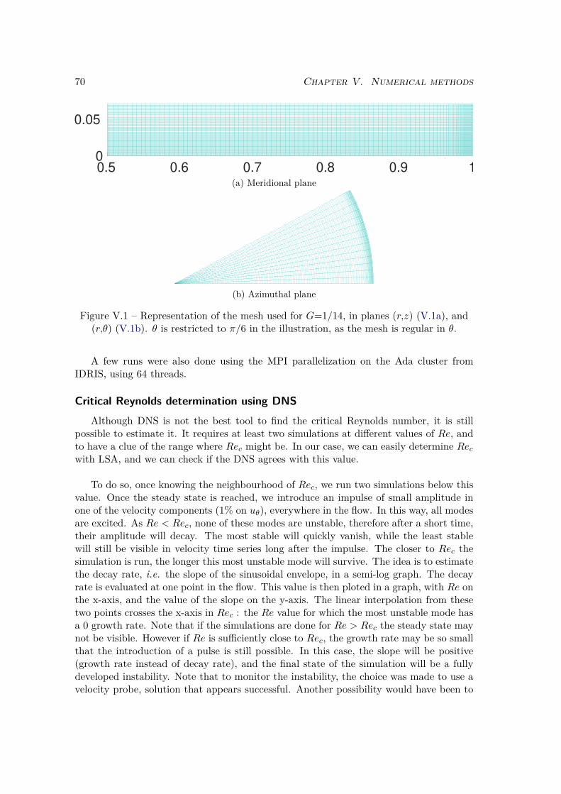
70 Chapter V. Numerical methods
0.5 0.6 0.7 0.8 0.9 10
0.05
(a) Meridional plane
(b) Azimuthal plane
Figure V.1 – Representation of the mesh used for G=1/14, in planes (r,z) (V.1a), and(r,θ) (V.1b). θ is restricted to π/6 in the illustration, as the mesh is regular in θ.
A few runs were also done using the MPI parallelization on the Ada cluster fromIDRIS, using 64 threads.
Critical Reynolds determination using DNSAlthough DNS is not the best tool to find the critical Reynolds number, it is still
possible to estimate it. It requires at least two simulations at different values of Re, andto have a clue of the range where Rec might be. In our case, we can easily determine Recwith LSA, and we can check if the DNS agrees with this value.
To do so, once knowing the neighbourhood of Rec, we run two simulations below thisvalue. Once the steady state is reached, we introduce an impulse of small amplitude inone of the velocity components (1% on uθ), everywhere in the flow. In this way, all modesare excited. As Re < Rec, none of these modes are unstable, therefore after a short time,their amplitude will decay. The most stable will quickly vanish, while the least stablewill still be visible in velocity time series long after the impulse. The closer to Rec thesimulation is run, the longer this most unstable mode will survive. The idea is to estimatethe decay rate, i.e. the slope of the sinusoidal envelope, in a semi-log graph. The decayrate is evaluated at one point in the flow. This value is then ploted in a graph, with Re onthe x-axis, and the value of the slope on the y-axis. The linear interpolation from thesetwo points crosses the x-axis in Rec : the Re value for which the most unstable mode hasa 0 growth rate. Note that if the simulations are done for Re > Rec the steady state maynot be visible. However if Re is sufficiently close to Rec, the growth rate may be so smallthat the introduction of a pulse is still possible. In this case, the slope will be positive(growth rate instead of decay rate), and the final state of the simulation will be a fullydeveloped instability. Note that to monitor the instability, the choice was made to use avelocity probe, solution that appears successful. Another possibility would have been to

V.2 DNS code : Sunfluidh 71
monitor a global quantity such as the kinetic energy.
Numerical values of Rec are given in the next chapter.
Domain limitation in θ
In LSA, the user can select the azimuthal mode m to be studied. At first sight, thisdoes not seem possible in DNS. However, with a limitation of the domain to 2π/m inθ direction, one can force the azimuthal wavenumber by filtering modes that are not mor its harmonics. Such a procedure is used later in this thesis in order to avoid complexnonlinear behaviour interfering with the mode of interest.
ValidationIn order to check the ability of Sunfluidh to perform accurate simulations of the case
considered, we used the results of [15], for G=1, and Re=1120. Since Re is below Rec,only steady flows will be compared. Indeed, LSA predicts the most unstable mode to bem=1 at Rec=2007. Other computations at Re=6000 are also given in [66]. However atsuch a Reynolds number the flow is turbulent and therefore comparison appears risky.The only other publication that may have served as reference for a comparison of the com-puted azimuthal mode is [37], yet in this paper, simulations were performed with a doublegeometry which is not representative of our cavity. Thus, validation is limited here tothe axisymmetric flow. The determination of the most unstable mode and its Rec will becross validated with ROSE in the next chapter, and somehow validate the 3D simulation..
The computed base flows, both with Sunfluidh and ROSE, show a good agreementbetween each other (see figure V.2). But the comparison with M. Piva and E. Meiburg([15]) is more difficult as isocontours are unfortunately not indicated in this publication.The width of the recirculation bubble at the free surface can still be compared : theisocontour ψ=0 that delimits the recirculation bubble hits the surface in r=0.25 for thethree codes. There is small discrepency on the location where this isocontour intersectsthe z axis. But this is a straight criterion.

72 Chapter V. Numerical methods
(a)
0 0.5 1
r
0
0.2
0.4
0.6
0.8
1
z
(b)
0 0.5 1
r
0
0.2
0.4
0.6
0.8
1
z
(c)
Figure V.2 – Meridian streamlines comparison between ROSE (left), Sunfluidh (center),and [15] (right), for Re=1120 and G=1. 15 isocontours are quadratically spaced
between ψmin = −2.31× 10⁻⁴ and 0 (solid lines) and 15 more are quadratically spacedbetween 0 and ψmax = 9.52× 10⁻³ (dotted lines). The isocontour ψ=0 is plotted as asolid black curve. The grid used with ROSE is 301×301, while the used with Sunfluidh
is 100×300×100 in (r,θ,z) respectively. Both are cartesian and regular.

Chapter VI
Free surface flow
73

74 Chapter VI. Free surface flow
In this chapter are compared experimental results and numerical simulations using afree surface condition : as a first approach, the surface of the flow is considered perfectlystress-free. The corresponding boundary conditions are those previously given in equa-tions IV.8, IV.10 and IV.7 and developed for both codes in chapter V.
First we will return to experiments carried out for G=1/14. As we saw in the chap-ter I, [40] and [42] shared, for this aspect ratio, good agreement both on the azimuthalwave number of the most unstable mode, and on its critical Reynolds number. However,our own experiments reveal discrepancies with numerics. Details about experiments andnumerics are introduced, as well as some hypotheses that were investigated to understandthese discrepancies.
Secondly, we will study aspect ratios G=0.25, 1, 1.5 and 2. Still in order to identifythe causes for discrepancies, these specific values of G were chosen since they were alreadypartially explored in former publications. For G=2, we were limited by the size of our glasscylinder that did not allow us to reach such an aspect ratio. Therefore, all experimentalresults are extracted from [35].
G=1/14 : Numerical approach
The first aspect ratio we focus on is 1/14. This ratio was previously studied exper-imentally in [40], where the first unstable mode is reported to have an azimuthal wavenumber m=5, and to start growing at Rec=16420. It was numerically investigated in[43], where it was revealed to be close to the limit of agreement between experiments andnumerics (see figure I.9). For smaller G, the uncertainty on the height of the fluid ∆H isless and less negligible compared to the height of the fluid H itself, and so is the verticaldisplacement of the surface of the disc. In addition, in [40], detection of the mode onlyrelies on visualizations, that can be very tricky for low values of G. All these reasonsmay have explain the causes of discrepancies for such G. But as exposed in chapter II,discrepancies were actually already existent for G=1/14, that neither ∆H nor the discsurface defects could explain.
Numerical critical Reynolds numberAfter ROSE was validated in section Validation & Mesh, influence of the mesh on Rec
is now evaluated. The results are exposed in table VI.1.
nRcells× nZcells
701×51 ([43]) 351×51 701×101 1401×201Rec 16972 17032 17006 16992
Table VI.1 – Comparisons of ROSE Rec computations on several grids, for G=0.0714and m=5. First column correspond to the grid used in [43].
One can see that Rec does not evolve much (0.35% of the maximum Rec) and staysaround 17000 although the mesh size is multiplied by 4 between columns 2 & 3, and 3 & 4.

VI.1 G=1/14 : Numerical approach 75
We specify here that ROSE shares the same core as the code used in [43]. Therefore itis no surprise that the match on Rec is excellent and it also explains why [43] was notused as a reference for the validation. It is interesting to observe that Rec apparentlydoes not display the same sensitivity to refinement in each direction : an increase of theradial cells number lowers Rec (columns 2 & 1), while an increase of the axial cell numberincreases Rec (columns 1 & 3). When both are increased with the same ratio, i.e. theaspect ratio of cells remains constant, the lowering effect of the axial cells number seemsto be predominant (columns 2, 3 & 4). According to these results, the choice was made tokeep the 701×101 grid as the standard grid for G=1/14. Indeed, this grid shows an errorof less than 0.1% compared to the 1401×201 grid, for a less expensive (yet unevaluatedquantitavely) time cost.
Following the method given in section V.2.4 : Critical Reynolds determination usingDNS , we cross validated this value Rec value with DNS computations. With a gridresolution of (180×180×64) in (r,θ,z), respectively, we evaluate the slope a at Re=16900and 17000, for a time span between timpulse+1400 and timpulse+2000. For Re=16900,timpulse=200, while for Re=17000, timpulse=300.
Re 16900 17000a -0.0028993 -0.0002765
Table VI.2 – Decay rate of the most unstable mode between t=timpulse+1400 andtimpulse+2000, for Re=16900 and 17000.
1400 1500 1600 1700 1800 1900 2000
t
-30
-28
-26
-24
-22
-20
-18
-16
(log(U
-U s
teady
))
y = - 0.0028993*x - 13.032
(log(U -U steady
))
Linear approximation
Figure VI.1 – Estimation of the decay rate at Re=16900 for G=1/14.
According to the slopes given in VI.2, one can estimate Rec ≈17010. Taking ROSE’sprediction for three different grids (351×51, 701×101 and 401×201), and performing aRichardsons extrapolation allows for an evaluation of Rec=16976. Thus, the differencebetween the predictions of ROSE and Sunfluidh is only of 0.2%. Some explanation on

76 Chapter VI. Free surface flow
the Richardson extrapolation can be found in the appendixes of [42]. To be perfectlyrigourous, extrapolations should also have been performed with Sunfluidh, both on re-fined timesteps and refined grids. However, this come to a cost of a longer computationtime. Since the agreement already revealed to be excellent, such computations were notperformed.
Instability pattern at Rec
The agreement on the Rec value between the two codes is excellent, but the unstablemode that grows in the DNS is unknown : a mismatch is still possible on the wavenumber.To clarify this, we can check visually the azimuthal wavenumber in a (O,r,θ) plane in DNS.To do so, it was chosen to represent the axial vorticity ωz :
ωz = 1r
(∂(ruθ)∂r
− ∂ur∂θ
)In order to identify the perturbations, one can subtract the mean flow from the com-
plete velocity fields. This mean flow can be a temporal mean through a selected timespan (we used 10×2π period, or 10 disc rotations) or spatial, on (θ). These two waysto calculate the mean flow appeared almost equivalent, once the flow is fully established.Therefore, we preferentially used the spatial average, that naturally satisfies the periodic-ity. Alternatively, the base flow can also be computed in 2D, with imposed axisymmetry.The comparison of LSA and DNS perturbations is displayed in figure VI.2.
(a) (b) (c)
Figure VI.2 – ωz perturbations in the (O,r,θ) plane, for G=1/14, z=G, Re=17100.VI.2a are perturbations from LSA, normalized with respect to the DNS value of
max(ωz). VI.2b are fluctuations from DNS, at t=4200, computed by subtracting of the2D axisymmetric base flow, while VI.2c are fluctuations from DNS at the same time,
but computed from the subtraction of the spatially averaged mean flow.The wave number m=5 is easily visible in the vorticity stripes, around r=0.67 : a
pattern of alternatively positive and negative values of ωz is repeated 5 times over the2π radian angle. The mesh used is given in figure V.1, page 70.
Thanks to the figure VI.2 we can conclude that the two codes agreed both on Rec andon the wave number m=5 of the most unstable mode, for G=1/14.

VI.1 G=1/14 : Numerical approach 77
Frequency of the most unstable mode at Rec
The frequency of the mode is defined as the inverse of the time required for one vortexto travel 2π radians. This frequency is normalized regarding the frequency of the disc.If we denote fm and fd the frequencies of the mode and of the disc, respectively, we canobtain their dimensionless form with respect to f∗ :
fmfd
= fmf∗
fdf∗
Now, considering that f∗ = 1t∗ , and that t was non-dimensionalized as t = tt∗ = t
Ωd,
we obtain :
f = fmfd
= Ωm
Ωd= fm
fd,
where Ωm and Ωd are respectively the angular velocities of the mode and of the disc.In conclusion, this ratio is the same, whether we deal with frequency or angular velocity.Thus, we will keep calling "frequency" both the normalised frequency and the angularfrequency (noted f). In the case of ROSE, this value is easily accessible, as it is theimaginary part of the most unstable eigenvalue, divided by the wave number m.
nRcells× nZcells
701×51 351×51 701×101 1401×201f 0.711 0.711 0.709 0.709
Table VI.3 – Comparisons of the normalized frequency of the m=5 mode computed withROSE on different grid size, for G=0.071. Respective Rec values are given in table VI.1.
We did not observe the same influence of the mesh size on the frequency as on Rec.The perturbations are reduced to 0.28% of the maximum f value. Therefore, the rest ofROSE simulations on the case G=1/14 were realized with the 701×101 mesh, as it seemsto be a good balance between accuracy and computation time.
With DNS, the frequency is not given so directly, and it has to be evaluated with aFourier transform applied to velocity temporal series. This was done essentially on theuθ component(VI.3a).
From figure VI.3b, one can extract the frequency value of the main peak : f=0.699.Other peaks are only harmonics of the main frequency. One can note that the Reynoldsnumber used in this simulation is 0.53% above the previously determined Rec. This valuewas chosen in order to stay in the neighbourhood of Rec, but with a growth rate thatallows for moderate simulation time. This can be compared to the ROSE prediction forRe=17100: f=0.710. The difference on frequency between DNS and LSA for Re=17100 isless than 1.55%. Note that for Re=17000 (just below Rec), the frequency of the decayingm=5 mode is 0.707, even closer to ROSE prediction at Rec. The increase of 0.59% of Rein DNS implies a frequency drop by 1.13%. With ROSE, the variation of +0.55% of theReynolds number only produces a decrease of 0.14% on f .

78 Chapter VI. Free surface flow
(a)
4300 4305 4310 4315 4320
t
0.7
0.705
0.71
0.715
u
(b)
0 1 2 3 4 5
Frequency
0
1
2
3
4
5
Am
plit
ude
10-3
Figure VI.3 – uθ signal (VI.3a) for G=1/14, Re=17100, and the corresponding Fouriertransform (VI.3b). The probe is located at (0.68,0.0,0.9G).
Mode transition for Re > Rec and long time simulation dynamics
In chapter II, we briefly mentioned that for Re=18620 the mode m=5 quickly transitsto a m=7. Such an evolution of the azimuthal wavenumber is the opposite of what isreported in [40], where for a given G, the wave number decreases with increasing Re. Thisdecay of the azimuthal wave number was also observed in our experiments.
900 1000 1100 1200 1300 1400 1500 1600
t
0.65
0.7
0.75
u
Figure VI.4 – Azimuthal velocity captured in DNS by a probe located at(0.68,0.0,0.9G), for G=1/14 and Re=18620.
The time series extracted from a DNS computation and plotted in figrure VI.4 showsa complex evolution as soon as the instability grows, around t=900. This evolution is

VI.1 G=1/14 : Numerical approach 79
better seen on the tracking of the kinetic energy of each unstable mode, represented infigure VI.5. From t=900 to ≈ 1020, the modes m=4 and m=5 grow slowly with a slightprevalance of m=5 between t=1000 to t=1075. Nenertheless, the vorticity pattern rathershows m=4 (figure VI.6a) at t=1020, while it only prevails between t=1075 to t=1115.Then, it transits to a temporary m=6 mode (fully established around t=1130, figureVI.6b), before a m=7 azimuthal wave number dominates after t=1295, and becomes wellvisible for t > 1330 (figure VI.6c). However, this m=7 does not completely prevail, and acompetition with mode m=6 still occurs between t=1430 and 1600. The simulation wasnot carried further. In addition to the competition between two modes, one can noticean asymmetric damping of the intensity of the axial vorticity that may be due to a lowfrequency mode. A similar damping is barely visible in the figure VI.6a, where vorticityat the bottom of the figure is not as strong as on top.
900 1000 1100 1200 1300 1400 1500 1600
t
0
0.5
1
1.5
2
Kin
etic e
nerg
y
10-5
m=1
m=2
m=3
m=4
m=5
m=6
m=7
m=8
Figure VI.5 – Evolution of the Kinetic energy of the modes 3 to 8, between t=900 andt=1600, for G=1/14 and Re=18620.
The growth rate of each mode at Re=18620 was evaluated with ROSE. Results aredisplayed in table VI.4. According to this table, mode m=4 is the less unstable, whilem=7 is clearly predominant. This is a completly different story from what the non lineardynamics highlighted in figure VI.5. Of course, this is not surprising, since Re=18620 isalready 9.5% above Rec : the transition from m=5 to m=4 is already a secondary bifur-cation and thus, the axisymmetric base flow computed with ROSE is no longuer effectiveto determine thresholds and growth rates. Fixing this would require to consider the modem=5 as the new base flow, and then to compute the perturbations around this new state.This would imply an in-depth rewriting of ROSE, and thus, this was not performed here.
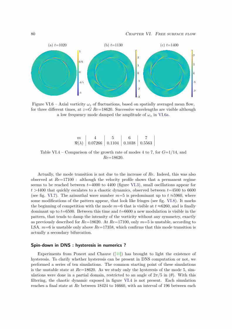
80 Chapter VI. Free surface flow
(a) t=1020 (b) t=1130 (c) t=1400
Figure VI.6 – Axial vorticity ωz of fluctuations, based on spatially averaged mean flow,for three different times, at z=G Re=18620. Successive wavelengths are visible although
a low frequency mode damped the amplitude of ωz in VI.6a.
m 4 5 6 7<(λ) 0.07266 0.1104 0.1038 0.5563
Table VI.4 – Comparison of the growth rate of modes 4 to 7, for G=1/14, andRe=18620.
Actually, the mode transition is not due to the increase of Re. Indeed, this was alsoobserved at Re=17100 : although the velocity profile shows that a permanent regimeseems to be reached between t=4000 to 4400 (figure VI.3), small oscillations appear fort >4400 that quickly escalates to a chaotic dynamics, observed between t=4500 to 6600(see fig. VI.7). The azimuthal wave number m=5 is predominant up to t ≈5960, wheresome modifications of the pattern appear, that look like fringes (see fig. VI.8). It marksthe beginning of competition with the mode m=6 that is visible at t ≈6260, and is finallydominant up to t=6500. Between this time and t=6600 a new modulation is visible in thepattern, that tends to damp the intensity of the vorticity without any symmetry, exactlyas previously described for Re=18620. At Re=17100, only m=5 is unstable, according toLSA. m=6 is unstable only above Re=17358, which confirms that this mode transition isactually a secondary bifurcation.
Spin-down in DNS : hysteresis in numerics ?
Experiments from Poncet and Chauve ([40]) has brought to light the existence ofhysteresis. To clarify whether hysteresis can be present in DNS computation or not, weperformed a series of ten simulations. The common starting point of these simulationsis the unstable state at Re=18620. As we study only the hysteresis of the mode 5, sim-ulations were done in a partial domain, restricted to an angle of 2π/5 in (θ). With thisfiltering, the chaotic dynamic exposed in figure VI.4 is not present. Each simulationreaches a final state at Re between 18424 to 16660, with an interval of 196 between each

VI.1 G=1/14 : Numerical approach 81
Figure VI.7 – Evolution of azimuthal velocity in DNS for G=1/14, Re=17100. Theprobe is located at (0.68,0.0,0.9G).
Figure VI.8 – Azimuthal wavenumber m=6 visible in the axial vorticity ofperturbations, at t=6500, for G=1/14 and Re=17100.

82 Chapter VI. Free surface flow
of them.
800 900 1000 1100 1200
t
0.55
0.6
0.65
0.7
0.75
u
Re =18620
Re =18228
Re =17836
Re =17444
Re =17052
Re =16660
Figure VI.9 – Azimuthal velocity uθ as a function of time, computed with Sunfluidharound the stability threshold. Starting from Re=18620 at t=800, ten simulationsbetween Re=18424 and Re=16600 have been performed. However, for a better
visibility, only five simulations are represented, with a step in Reynolds number of 392between each of them. The probe is located at (0.82,0.63,0.5G).
For all simulations with final Re between 18424 and 17052, the decrease of Re onlyaffects the amplitude of the oscillations. As soon as Re gets closer to Rec it seems harderfor the instability to survive, and for Re=17052, it takes around 200 time units for thepattern to develop while it was much faster for higher Reynolds numbers (≈75% fasterfor Re=17444). As soon as Re < Rec oscillation are damped and instability vanishes.Thus, there is no numerical evidence in favour of the existence of hysteresis.
G=1/14 : Experimental results
Following the procedure described in the section III.5 (page 51), we searched for theexperimental critical Reynolds number for G=1/14. It quickly appears that the instabil-ity was not difficult to trigger, and the first observed unstable mode has an azimuthalwavenumber m=5, which matches with the numerical prediction for this value of G. Butthe instability started to be visible for Reynolds numbers far below the numerically de-termined critical Reynolds number. Mismatches with numerics reveal to be not limitedto Rec : the base flow and the azimuthal pattern also show heavy differences. Detailswere already reported in chapter II : experimental Rec below 4200 (more than 75% smallerthan the numerical prediction), absence of overshoot in experimental uθ profile, absence of
VI.2 G=1/14 : Experimental results 83
similarity in the pattern... Note that from time to time it happens that the first detectedunstable mode had a wave number m=4. These minor cases were not judged relevant :it is reported in [42] that the critical Reynolds numbers for m=4 and m=5 are close,and according to [37] and [40], the mode selection is sensitive to variations in the experi-mental protocol. Since the adoption of the protocol based on extended constant-durationplateaus, only the mode m=5 was observed.
Threshold detection : markers and fluids
Kalliroscope
The choice to use Kalliroscope as a marker appears to be natural considering thatmany publications on rotating flows used such marker, especially in Taylor-Couette flow([67] and [68] are examples among many others). Moreover, Kalliroscope was used in [40]to visualize transition from steady to unsteady flow, and azimuthal patterns. However,we had never been able to match the reported Rec by Poncet and Chauve. Globally, ourexperiments appear to be reproducible, and Rec was first estimated around 9800. But,in some cases, we were not able to detect any azimuthal wavelength, even well above thenumerical Rec. There, only a chaotic flow was revealed by the marker. We noticed thatthis behaviour was more probable when the flow was heavily seeded, but we failed atestablishing an obvious quantitative connection between Kalliroscope concentration andthreshold detection.
Another issue encountered is the sedimentation rate. According to [59], Kalliroscopein water have a sedimentation velocity around 0.1 cm/h, which means it should require 10hours for flakes in calm water to drop from the interface to the disc. However we observedthat sedimentation can occur over a much lower time interval, that was incompatible withthe time required in experiments. Indeed, experiments with Kalliroscope were mostlybased on the Ekman time, according to the protocol used in [40]. There it takes at least16 min to reach 3 rpm. Added to the time of observation, this was sometimes sufficientfor most of the particles to fall to the bottom of the cavity. Despite the later increase ofthe rotation speed, the layer of particles remains stuck to the disc, and no visualisationwas possible. In later experiments with LDV, we used plateaus of 10 to 15 min plusat least 5 min of acquisition. These long plateaus make it difficult to use Kalliroscopefor critical Reynolds number detection as the observed sedimentation time is close to theplateau duration.
Ink
The flaws of Kalliroscope forced us to repeat our experiments with the same initialprotocol, but with the injection of diluted blue ink at the end of each plateau. Introducedwith a syringe and a thin needle, the total volume of ink added to the cavity was less than1 mL, so that the total volume inside the cavity can be considered as constant. In thresh-old detection experiments, the amount of ink that is introduce into the cavity is smallenough that the fluid does not turn completly blue. Indeed, if the threshold Reynoldsnumber is so high that it requires too many repeated injections, the fluid becomes blue.

84 Chapter VI. Free surface flow
Then, contrast is no longer sufficient to allow visualisations. Therefore, highlighting hys-teresis with this marker is hardly possible.
Figure VI.10 – Instability pattern visualized with ink in a 40% mass glycerol mixture,for G = 1/14, and Re ≈ 4700.
With this marker, the critical Reynolds number was evaluated between 3300 and 6200.If we consider the highest boundary of the previous estimation of Rec with Kalliroscope,this Rec was over evaluated by 55%. New experiments were done with smaller amountsof Kalliroscope : both modes 4 and 5 were observed for Rec=6476 and Rec=6507, re-spectively. No evident conclusion can be made on the behaviour of Kalliroscope, but it isclear that its use has to be considered with the highest precaution, especially for quanti-tative results. It also confirms that instabilities are present far below the Rec predictednumerically.
LDV
Experiments done with LDV locate the critical Reynolds number between 3160 and4230 with water. Compared to previous experiments with ink and Kalliroscope (andbased on the Ekman time), the upper bound is here 30% lower. This gap corresponds toonly 1 rpm. This very small difference reinforces the hypothesis that the Ekman time isnot suitable for the instability detection protocol. The LDV measurement were repeatedwith a 20% glycerol mixture, and confirmed that Rec is between 2520 and 3780.
Besides Rec determination, LDV brings a quantitative aspect with measurements offrequencies and velocities. However, in the absence of qualitative visualization, it is haz-ardous to conclude on the wavenumber only with LDV acquisitions. A cautious look at thesurface can sometimes reveal the mode by direct visualization : the particle concentration

VI.2 G=1/14 : Experimental results 85
is higher in the vortices, which makes the identification of the main mode straightforward.A misinterpretation of the mode would lead to an error on the corresponding frequency.
Viscosity
In addition to the sensitivity of the instability to each marker, we performed a veri-fication of the influence of viscosity on Rec. These results are shown in table VI.5. Asexplained in chapter III, increasing the viscosity should lead to better accuracy in thethreshold detection, as well as a reduction of transient times.
Glycerol % 0 20 20 25 40ν (×10−6) 0.971 1.63 1.53 1.78 3.35T (°C) 21.5 20.6 23.0 22.9 19.9
Detection method LDV LDV ink ink inkRec [stable-unstable] [3160-4230] [3181-3780] [2690-4030] [2300-3450] [3070-3680]
Table VI.5 – Experimental critical Reynolds number Rec of the first unstable modem=5, for G=1/14, with various viscosities. All these experiments were done in the largecavity. The steps were 0.5 rpm, and 1 rpm, for LDV and Ink experiments, respectively.
Glycerol addition does not seem to have any obvious influence on Rec. For the rangeof concentration considered - 0 to 40% in mass - Rec stays between 2700 and 4200,approximately.
Mismatches beyond Rec
Until now, only Rec values obtained with both numerics and experiments have beencompared. Since no match was observed, we formulated the hypothesis that an experi-mental flaw may be responsible for an early triggering of the instability. The possibilitiesto explore the flow with LDV brought new elements that cannot be justified by the vi-brations of the bench.
Indeed, the LDV hardware allows for analysis of the flow beyond the sole criticalReynolds number detection. Acquiring velocities at several points along a radius makes itpossible to draw a velocity profile that can be compared to the base flow from ROSE, andto mean flow from DNS. These comparisons reveal a clear mismatch between numericsand experiments. Note that LDV hardware was installed after the quantification of thedisc vibrations (chap. VII).
In figure VI.11, we compare four different velocity profiles. The two DNS profilesconfirm the equivalence of mean velocities, whether they are calculated using a spatial ora temporal average. The comparison of ROSE base flow, and DNS mean flow highlightsthat, although the flow is fully unstable (Re=18620> Rec), mean flow and base flow arevery close. The only noticeable deviations are located just before the boundary layer, at

86 Chapter VI. Free surface flow
0.5 0.6 0.7 0.8 0.9 1
r
0
0.2
0.4
0.6
0.8u
LDVDNS temporal averageDNS spatial averageROSE base flow
Figure VI.11 – Comparison of uθ velocity profile, in z=0.8G , at Re=18620, for G=1/14.
r=0.97, and in the "bump" at r=0.67. This last point is especially important. In numer-ics, the bump corresponds to an overshoot of the velocity, i.e. uθ|z=G > uθ|z=0. Thisovershoot is not seen in experimental points, and the associated velocity profile is actuallymuch smoother than numerical ones. One can see that despite the optical correction onLDV measurements, a gap still exists between experimental and numerical velocities inthe solid body rotation area ( r <0.6). Solid body rotation and overshoot are illustratedin the meridional plane, in figure VI.12.
Figure VI.12 – uθ base flow iso values computed with ROSE, at Re=18620, for G=1/14.Red patch correspond to uθ > 1.01r. 21 iso values are equally spaced between 0 and 1.
The mismatch in the mean flow is even more apparent for the uz component. Notethat measurements were made at z=0.5G to allow for a wider range accessible with LDV,avoiding any problem of reflection of the beams on the surface, or collision with the edgeof the disc. Figure VI.13 shows larger differences between mean flow and base flow. How-ever, the radius for the minimum value of uz is still located around r=0.7. Despite aninsufficient discretization in experiments between r=0.8 and r=0.9, the radius where uz isminimal can still be evaluated around r=0.86. This means that the length of the recircu-lation in the meridional plan is over-evaluated by ∼20% in numerics. If the recirculationis expected to be present only for r >0.86, uz should be almost zero for r <0.86. Thenegative values in experimental data may be due to an imperfect horizontality of the laser,

VI.2 G=1/14 : Experimental results 87
0.5 0.6 0.7 0.8 0.9 1
r
-0.05
0
0.05
0.1
uz
LDV
DNS mean flow
ROSE base flow
Figure VI.13 – Comparison of uz velocity profiles, at z=0.5G , for Re=18620, andG=1/14. The three colors for the dot symbols correspond to three repeated experiments.
leading to the acquisition of the projection of uθ. Indeed uθ is quite large compared to uz.Recirculation in numerics can easily be seen with the stream function ψ, as representedin figure VI.14.
0 0.2 0.4 0.6 0.8 10
0.05
Figure VI.14 – Streamfunction ψ of the base flow computed with ROSE, at Re=18620,for G=1/14. The values of ψ are given in chapter II : Article published in Journal of
Fluid Mechanics.
Ideally, the comparison of base flows should have been done for Re < Rec. However,in experiments, Rec corresponds to a very low rotation speed around 2rpm, leading tothe acquisition of a small magnitude velocity signal, with a lot of noise. Therefore, tohave something fully comparable, we chose a Reynolds number sufficiently high for theinstability to be developed both in numerics and in experiments. The value of Re waschosen far enough from Rec in order to allow for a fast natural growth of the instabilityin DNS, and thus, to reduce the computation time.
Mode transition as Re increasesIt was reported in [40] that the increase of the rotation rate, and therefore, of the
Reynolds number, was followed by a second transition, when Re=36945. There, theazimuthal wave number evolves from m=5 to m=4 ( fig. VI.16). We looked for thismode switching, firstly with Kalliroscope, which is more adapted than ink for such an

88 Chapter VI. Free surface flow
experiment, since it allows for a continuous visualization of the flow without additionalseeding. With Kalliroscope, the transition was observed for Re between 25750 and 27910.The experiment was repeated twice using LDV device. As displayed in figure VI.15, thetransition Re was then evaluated around 30000. Note that in figure VI.15, in order toillustrate the transition between m=5 and m=4, the frequencies are not divided by m,but only normalized with the disc frequency. It also confirms the good reproducibility ofmean velocity measurements, although a deviation corresponding to 1 rpm is observedbetween the transition Reynolds numbers of the two runs.
Figure VI.15 – Evolution of the frequency f as a function of Re. Colours represent twodifferent acquisitions series for G=1/14.
It is interesting to note that the Reynolds numbers for which the secondary bifurcationoccurs are under-evaluated by ≈7% in experiments using Kalliroscope, and compared toLDV measurements. This is unexpected, since the first threshold was more easily over-evaluated when using Kalliroscope. Here, agreement is fairly good, and we can supposethat Kalliroscope is more "effective" in high mixing flows than in quiet flows.
Actually, the experiment with Kalliroscope was an attempt to highlight hysteresis (seefig. VI.17). Although its existence has been called into question by numerical simulation,hysteresis was easily observed during this experiment. However the Re values for which isobserved the mode transition do not match with the results of Poncet and Chauve. Notethat this experiment was performed before the instability threshold was found to be aslow as Rec ≤4200. Since this experiment was not repeated with LDV, we cannot concludeif the hysteresis is effectively present in this flow, or if it is a perverse effect of a shift of thethresholds during the spin-up phase, and attributable to Kalliroscope. Indeed, the lasttransition from m=5 to m=0 during the spin-down phase matches the first threshold ofour spin-up phase, while the last transition of our spin-down phase occurs for Re ≈4300,which matches the Rec determined using the LDV.

VI.2 G=1/14 : Experimental results 89
Figure VI.16 – Despite the low contrast between particles of Kalliroscope in suspension,and particles lying on the disc, the azimuthal wave number m=4 is still visible for
G=1/14 and Re=26500.
0 1 2 3 4 5
m
0
1
2
3
4
5
6
7
8
Re
104
Spin-up (Poncet & Chauve)
Spin-down (Poncet & Chauve)
Spin-up
Spin-down
Figure VI.17 – Comparison of spin-up and spin-down phases between our experimentand the experiment of Poncet and Chauve ([40]). Spin-up phases are the solid lines, andspin-down phases are the dotted lines. Note that the "horizontal lines" are a guide for
the eye but have no physicall relevance, as m can only be an integer.
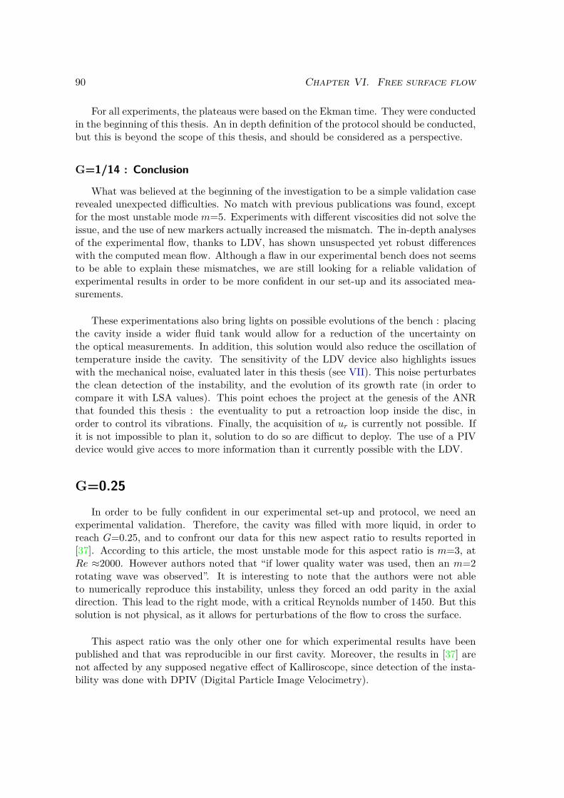
90 Chapter VI. Free surface flow
For all experiments, the plateaus were based on the Ekman time. They were conductedin the beginning of this thesis. An in depth definition of the protocol should be conducted,but this is beyond the scope of this thesis, and should be considered as a perspective.
G=1/14 : Conclusion
What was believed at the beginning of the investigation to be a simple validation caserevealed unexpected difficulties. No match with previous publications was found, exceptfor the most unstable mode m=5. Experiments with different viscosities did not solve theissue, and the use of new markers actually increased the mismatch. The in-depth analysesof the experimental flow, thanks to LDV, has shown unsuspected yet robust differenceswith the computed mean flow. Although a flaw in our experimental bench does not seemsto be able to explain these mismatches, we are still looking for a reliable validation ofexperimental results in order to be more confident in our set-up and its associated mea-surements.
These experimentations also bring lights on possible evolutions of the bench : placingthe cavity inside a wider fluid tank would allow for a reduction of the uncertainty onthe optical measurements. In addition, this solution would also reduce the oscillation oftemperature inside the cavity. The sensitivity of the LDV device also highlights issueswith the mechanical noise, evaluated later in this thesis (see VII). This noise perturbatesthe clean detection of the instability, and the evolution of its growth rate (in order tocompare it with LSA values). This point echoes the project at the genesis of the ANRthat founded this thesis : the eventuality to put a retroaction loop inside the disc, inorder to control its vibrations. Finally, the acquisition of ur is currently not possible. Ifit is not impossible to plan it, solution to do so are difficut to deploy. The use of a PIVdevice would give acces to more information than it currently possible with the LDV.
G=0.25
In order to be fully confident in our experimental set-up and protocol, we need anexperimental validation. Therefore, the cavity was filled with more liquid, in order toreach G=0.25, and to confront our data for this new aspect ratio to results reported in[37]. According to this article, the most unstable mode for this aspect ratio is m=3, atRe ≈2000. However authors noted that “if lower quality water was used, then an m=2rotating wave was observed”. It is interesting to note that the authors were not ableto numerically reproduce this instability, unless they forced an odd parity in the axialdirection. This lead to the right mode, with a critical Reynolds number of 1450. But thissolution is not physical, as it allows for perturbations of the flow to cross the surface.
This aspect ratio was the only other one for which experimental results have beenpublished and that was reproducible in our first cavity. Moreover, the results in [37] arenot affected by any supposed negative effect of Kalliroscope, since detection of the insta-bility was done with DPIV (Digital Particle Image Velocimetry).

VI.3 G=0.25 91
Experimental resultsThe first tests were done in the largest cavity. Since the critical Reynolds number is
expected to be low, we used a 55% in weight water glycerol mixture, in order to have awider span of rotating speed : the experimental threshold determined in [37] (Re=2000),is reached for a rotation speed below 1rpm if the fluid is pure water. Initial experimentsused Kalliroscope, and the protocol was the same as detailed in III.5. The flow started toshow an ellipse for R ≈3540, followed by a less symmetric pattern, kind of a intermediatebetween m=2 and 3, was observed for Re ≈5950. This pattern is visible in figure VI.18b.Finally a clear m=2 pattern was visible for Re ≈6340.
(a) Re=3540 (b) Re=5950 (c) Re=6340
Figure VI.18 – Sequence of instability growing in a 55% glycerol mixture seeded withKalliroscope, for G=0.25.
Switching the marker to ink initially brings similar results, but with different Reynoldsnumbers. The symmetry is lost at Re ≈5030, where the flow displayed an ellipse aroundits core region. The transition pattern, although not as clearly seen as with Kallirsocope,is supposed to be present for Re ≈5350, before the mode m=2 became well determined,at Re ≈5940. The whole sequence is shown in figure VI.19.
(a) Re=4760 (b) Re=5030 (c) Re=5350 (d) Re=5940
Figure VI.19 – Sequence of instability growing in a "dirty" 55% glycerol mixture, forG=0.25.
Based on these experiments, the critical Reynolds number is hard to evaluate. If theloss of symmetry is considered as the threshold, Rec is at least 151% higher than in the

92 Chapter VI. Free surface flow
experimental results of Lopez et al., in the most favourable case with ink. However itis interesting to note that the experiment with ink was performed in a fluid that restedfor two to three days in the cavity. If we consider that, despite the lid which we coveredthe setup when it was not used, the fluid has become dirty, an interesting parallel can bemade with “low quality water“ effects described by Lopez et al. Using such fluid, the firstmode they observed was m=2. Unfortunately, no associated value of Rec is given in thiscase.
(a) (b)
Figure VI.20 – Azimuthal wave number m=3 observed with ink in a 55% weight waterglycerol mixture, at Re=2160, and for G=0.25 (left). On the right is displayed an
experimental visualization from Miraghaie et al. ([36]).
(a) Re=3700 (b) Re=4930 (c) Re=5240 (d) Re=5545
Figure VI.21 – Sequence of instability growing in a clean 55% glycerol mixture, forG=0.25.
The experiment was repeated with a clean water glycerol mixture. Using ink, the firstmode observed has an azimuthal wave number m=3, and grew for Rec ≈2150, as shownin figure VI.20a. This time, the difference with the results of Lopez et al. and Miraghaieet al. is only 7.5%. Increasing Re interestingly gives almost the same sequence as shownin figure VI.19 with dirty water glycerol mixture : after the flow has lost its symmetryat Rec=2150, a circle is observable again at Re ≈3700. The ellipse is clearly visible atRe ≈4930, and is followed by the undefined pattern, at Re ≈5240 (see fig VI.21). Them=2 pattern then grows for Re ≈5545. The reproducibility of this sequence suggests

VI.3 G=0.25 93
that pollution may not be the only cause of the lack of detection of the mode m=3 inprevious experiments. Indeed we previously reported that Kalliroscope seemed to fail toreveal the low Reynolds threshold, for G=1/14. The experimental protocol may also bean issue, with inadequate times for the plateaus for the lowest Reynolds numbers values.
In order to confirm the excellent agreement on experimental Rec, the threshold detec-tion was also realized with LDV. Results are summed up in table VI.6.
Lopez et al. 20% glycerol 55% glycerolRec ≈2000 [1900-2520] [1790-2150]
Table VI.6 – Experimental critical Reynolds number of the wave number m = 3, forG = 1/4. The experiment with the 20% glycerol mixture used LDV to detect the
threshold, while the other experiment, with 55% glycerol, was based on ink visualization.
From this table, one can see that our experimental critical Reynolds numbers havethe same order of magnitude, very close to the result published in [37]. Experiment vs.experiment confrontation does not show the same difference as observed previously forG=1/14. Yet, our experimental apparatus dimensions are not comparable at all with [37],while they were identical with [40]. Both our results displayed in table VI.6 were obtainedwith the largest cavity. The frequency corresponding to the LDV measurement (secondcolumn of the table) is f=0.597. An experiment with water in the smaller experimentalset-up exhibited instability at Rec as low as 1615. The associated frequency is f=0.618.
Numerical results
On the numerical side, we used ROSE with a 401×101 cell mesh to obtain the criticalReynolds number. In [37], authors used a doubled geometry to simulate the free surface :their geometry is twice as high as the real one, and the top is a spinning disc in exactco-rotation with the bottom disc. Actually, this configuration is not similar to the freesurface configuration. Although the base flows are the same, the double geometry allowsunstable modes to cross the median plane (uz 6= 0 on this plane for the perturbations),while, for the free surface case, uz=0 both for the base flow and the perturbations.. Itappears that the most unstable mode in the double geometry is actually a mode thatcrosses the median plan (in z=h/2), as shown in figure VI.22.
For this configuration, the critical Reynolds number of the mode m=3 obtained withROSE is Rec=1456. This value is very close to the critical Reynolds number reported in[37], which is 1450. But the real geometry has very different results (see table VI.7). Theauthors themselves recognized that their model is not acceptable although their numericalresults get closer to experiments than the stress free surface model. They explained mis-matches by imperfections of the surface : surfactant contamination and a surface which isnot perfectly flat. But this last point does not seem to hold, since, according to [42], theeffect of deformation on Rec appears to be irrelevant to justify the observed mismatch :for G=1/14; variation of Rec with and without surface deformation is smaller than 4%.

94 Chapter VI. Free surface flow
Figure VI.22 – Azimuthal vorticity ωθ of the fluctuations of the mode m=3 in ameridional plane, in the case of the double geometry for G=0.25, at Rec=1456. The
median plane is represented by the red dotted line at z=0.25. This should correspond tothe free surface, yet, ωθ 6=0 and therefore, the free surface condition (ωθ = 0) is not
respected by this unstable mode.
Lopez et al. (doubled) ROSE (doubled) ROSEm=3 m=3 m=2 m=3
Rec 1450 1456 3481 4691
Table VI.7 – Numerical critical Reynolds number of the most unstable modes forG=0.25. The mention “doubled” refers to a doubled height geometry, with two rotors in
exact co-rotation, one at the bottom and the second at the top.
With the flat free surface condition, the most unstable mode has an azimuthal wavenumber of 2, and starts growing at Rec=3481. The mode m=3 is unstable only af-ter Rec=4691. The frequencies of modes 2 and 3 are respectively fm=2=0.553 andfm=3=0.576, which is in very good agreement with experiments. Indeed, the relativeerrors with experimental frequencies (≈0.6) are only 8% and 4%, respectively.
The comparison of the mean flow for Re=1895 corroborates previous observationsfor G=1/14 : computed velocity profiles show an overshoot of uθ at r ≈0.5 for the caseG=0.25 (see figure VI.23a), that is not observed in LDV measurements. The axial velocityprofile shows an over evaluation of the length of recirculation in a meridional plane, as itwas reported for G=1/14. This is exhibited in the figure VI.23b, where the minimum of uzin the simulation is located at a radius below 0.6, while in the experiment, this minimumis rather around r=0.7. Note that the Reynolds number considered here was supposedbelow Rec. Therefore, since base flow and mean flow are equivalent for Re < Rec, thecomparison of ROSE base flow with LDV azimuthal velocities is fully legitimate. Yet,

VI.3 G=0.25 95
later experiments reveal that Rec was overevaluated, and that for Re=1895, the flow canalready be unstable.
(a) uθ in z=0.8G
0 0.2 0.4 0.6 0.8 1
r
0
0.1
0.2
0.3
0.4
0.5
u
LDV
ROSE free surface
(b) uz in z=0.5G
0 0.2 0.4 0.6 0.8
r
-0.1
-0.05
0
0.05
0.1
uz
LDV
ROSE free surface
Figure VI.23 – Comparison of velocity profiles : ROSE base flow and LDVmeasurements, for G=0.25 and Re=1895.

96 Chapter VI. Free surface flow
Since G=1/14 shows a chaotic behaviour over long timescales and for Re ≈1.1Rec, asimulation was done at Re=3829, corresponding to a Reynolds number 10% above theRec value reported in table VI.7 (this gap was 9.5% in the case of G=1/14).
(a) (b)
Figure VI.24 – uθ signal for G=0.25 and Re=3829. The small peak at t=1500corresponds to the introduction of a pulse, to stimulate the growth of the instability.
The probe is located at (0.5,0,0.8G).
Figure VI.24 illustrates that no evolution is visible in the azimuthal velocity profile,once the instability is fully developed. Indeed, the pattern of velocity oscillations staysunchanged over 3600 time units, which represents almost 573 rotations of the disc. It isinteresting to note that the vorticity pattern at this Re matches well with experimentalobservations at Re=5545.
(a) Re=3829 (b) Re=5545 (c) Re=5545
Figure VI.25 – Numerical axial vorticity patterns at t=5900 for Re=3829 (left) andRe=5545 (center), compared to experimental visualization at Re=5545 (right), for
G=0.25.
As in the case G=1/14, the simulation for G=0.25 at Re=5545 shows a modulationin its velocity timeseries. The simulation was extended, and confirmed the existence ofthis modulation on more than 2000 time units (318 disc revolutions). Another run, forRe=6000 was done, in order to look for a possible chaotic behaviour, like for G=1/14.But once again, the width modulation remains constant, this time over 2400 time units,

VI.4 Exploration of higher aspect ratios 97
or 382 disc revolutions (see fig. VI.26a). This modulation can be seen in the loss of thecentral symmetry of the mode m=2 between Re=3829 and Re=5545, in figure VI.25b.Figure VI.26b suggests that this might correspond to the beginning of the asymmetrictransition pattern described earlier in VI.3.1.
(a) (b)
Figure VI.26 – uθ time series for G=0.25 and Re=6000 (left), and the correspondingvorticity pattern for perturbations at t=2900. The probe is located at (0.5,0,0.8G). Thefive red isofurfaces are equally spaced in [0,4.93] in red, and the five blue isosurfaces are
equally spaced in [-2.73,0].
Conclusion on G=0.25For G=0.25, we have obtained very good agreement in both experiments vs. experi-
ments and numerics vs. numerics, compared to [37]. However, we were confronted withthe same trouble as these authors : comparison of experiments with simulation presentslarge disagreements, as for G=1/14. Indeed, simulations with a stress-free interface donot seem able to reproduce the experimental flow, since both m and Rec values did notmatch between experiment and numerical prediction, and even base flows differ. However,increasing G apparently delays the emergence of the rich spectrum observed in long timesimulations and for Re ≈1.1Rec.
Exploration of higher aspect ratios
In addition to G=0.25, the authors of [37] also explored G=2, both numerically andexperimentally. Their conclusions for this aspect ratio are completely different from thosefor G=0.25. Firstly, their experimentally determined Rec is in good agreement with [34].Secondly, their numerics also match experiments. Note that in their simulation, they stillused the double geometry discussed above for G=0.25. But here simulations are valid,because the most unstable mode does not cross the median horizontal plan. This agree-ment suggests that for larger aspect ratios, instability is less sensitive to any experimentalperturbation responsible for the premature triggering for smaller G. Unfortunately, noneof our cavities allow us to study G=2 and thus our comparison will be based on data

98 Chapter VI. Free surface flow
given in previously quoted articles. However we can access G=1.5, the aspect ratio usedto validate ROSE and extensively explored in [44]. We also compared LDV measurementsto numerics for G=1 at Re=1120.
G=2
The experimental results are not much developed in [37], but their data can be foundin the former publication [35]. Therefore, in the upcoming section, experiments refer to[35], while [37] is used for numerics. The first comparison we focused on was, one moretime, the determination of Rec, which was only done with ROSE. Table VI.8 gathers Recvalues of previously quoted articles, and prediction from ROSE. The grid used contained201×401 cells.
Hirsa et al. [35] Lopez et al. [37] Young [34] ROSEm=4 m=4 - m=4
Rec [1900-2000] 1910 [1850-1900] 1914f at Re=2100 0.156 - 0.160 0.161
Table VI.8 – G=2, comparison of Rec and f for Re=2100 (Re > Rec). The frequencyfrom Hirsa et al. was determined by a graph interpretation.
ROSE matches Rec and m given in reference articles. In [34], the mode was notvisualised in the azimuthal plane, but only LDV signals around Rec were given. Thefrequency of the oscillations in the velocity signal at Re=2100 is fY dim=2.345Hz, whichcorresponds to a dimensionless frequency of m × fY=0.639, according to experimentaldata given in the article. Interestingly, the fluid used in these experiments was composedat 85% glycerine by volume (≈87,7% in mass percentage). This frequency is not adjustedregarding the azimuthal wave number : if we suppose that m=4, then fY=0.16, which isconsistent with values in [35] : for Re=2100, the dimensionless frequency is fH ≈0.156, form=4. For Re=2100, ROSE estimates f=0.161, which confirms the excellent agreementbetween numerics and experiments for this G. Note that for Rec, ROSE predicts f=0.157.
No visualisation such as figure VI.20a is given for G=2, except some DPIV slices,where patterns are not as visible as in pictures with ink or Kalliroscope. Thus compari-son of vorticity patterns is not as insightful as for lower G.
The simulation from which figure VI.27 is extracted, was extended up to t=12000, tocheck for the long time scale evolution. Although this extension from t=10000 to t=12000corresponds to more than 318 disc rotations, no complex dynamics was observed, unlikewhat we reported for G=1/14. Only a purely sinusoidal oscillation is present in azimuthalvelocity time series (fig. VI.28). The frequency of this oscillation is f=0.156, only 0.64%smaller than the frequency obtained with ROSE and reported above.

VI.4 Exploration of higher aspect ratios 99
Figure VI.27 – Axial vorticity isosurfaces of fluctuations from DNS, for Re=1950, andfor G=2. This snapshot was taken at t=10400, once the instability is fully established.Isosurfaces are divided in two subspaces : 5 red isofurfaces equally spaced in [0,0.11] in
red, and 5 blue isosurfaces equally spaced in [-0.15,0]. Translucence indicates thevorticity intensity : translucence increases when ωz tends to 0.
Figure VI.28 – Long time scale simulation for Re=1950, and G=2. The probe is locatedat (0.5,0,0.5G). The displayed time span is equivalent to a bit more than 318 rotation of
the disc.

100 Chapter VI. Free surface flow
G=1.5In section Validation & Mesh, we validated ROSE for the aspect ratio G=1.5. We
found that the most unstable mode occurs at Rec ≈2150, with a wave number m=1,which is in perfect agreement with [44]. The new feature of this mode is its frequencyf=-0.0487, i.e. the rotating wave counter-rotates very slowly with respect to the disc,with a period around 20 times longer.
m 0 1 2 3 4Re 2655 2150 2664 2520 2806f 0.222 -0.00487 0.303 0.321 0.328
Table VI.9 – Rec and f for m=0 to 4, and G=1.5, computed with ROSE.
Table VI.9 gathers Rec and f for the five first modes. Corresponding simulations wereperformed on a 245×381 grid. With the exception of m=0 and m=1, all other modesshare almost the same frequency. Experiments were done in the small cavity, as it is theonly one with a sufficiently high cylinder. Three different fluids were used : water, 20%and 40% water-glycerol mixtures. The corresponding theoretical periods of the modem=1 for these three fluids are given in table VI.10.
fluid water 20% glycerol 40% glycerolΩc (rpm) 3.67 5.93 11,57Tm=1 (s) 336 208 106
Table VI.10 – Evaluation of the period T of the mode m=1 in the small cavity, forG=1.5, and Re=2150, with a fluid temperature of 26°C. These estimations are based on
ROSE computations.
Experiments with this aspect ratio display a very long transient (see fig. VI.29a),that makes threshold detection tedious and risky. Indeed, the experiment from which isextracted figure VI.29a lasts four hours. Visualization with ink did not prove to be effi-cient either. At Re=2356, after a long transient, velocity time series acquired with LDVshows three states. The first one, for t between 2350 and 4160 has a main frequency ofm×f=0.401. This is followed by a short transition, between t=4160 and t=4490, then, athird state appears, and last up to t=6770. This state is marked by a very low frequencymode corresponding to the increase of the mean velocity. In addition to this mode, themain frequency is m× f=0.538, followed by a second oscillation of close amplitude, witha frequency m × f=0.838. We note that this second peak was also present in the firststate, at m× f=0.806. None of these frequencies are normalized regarding the azimuthalnumber, as we have no clue about it, and thus, they are reported as m× f instead of f .Despite a rich spectrum, no evidence of a mode m=1 with f=0.0487 was observed.
Other experiments were performed on this aspect ratio, including a spin-down phase

VI.4 Exploration of higher aspect ratios 101
(a)
1000 2000 3000 4000 5000 6000
t
0
0.02
0.04
0.06
0.08
0.1
0.12
0.14
0.16
u
(b)
0 1000 2000 3000 4000
t
0
0.02
0.04
0.06
0.08
u
Figure VI.29 – Transients for G=1.5, experimental on the left, and numerical on theright. In the experiment, the flow (water) is initially at rest, and the disc is set inmotion at Ω=4.59 rpm. The temperature evolves from 18.1°C to 20.3°C which
translates into a Re value between 2232 and 2356. The measurement point is located atr=0.84, z=0.99G. Time and azimuthal velocity are dimensionless. In numerics, theprobe is located at r=0.6, z=0.75G. A small impulse was introduced at t=500.
0
0.5
1
1.5
Am
plit
ude
10-4
0 1 2 3 4 5
m f
Figure VI.30 – Fourier transform of the LDV acquired azimuthal velocity time series atRe=2356 (figure VI.29a). Blue peaks correspond to the signal between t=2350 andt=4160, while orange peaks correspond to the signal between t=4490 and t=6770.
Frequency is normalised according to the disc rotation rate.

102 Chapter VI. Free surface flow
from Re=3620 to 1820 in steps of 360. Except for Re=2540 and Re=2180, no otherReynolds number shows a clear dominance of a single frequency in Fourier spectrum. Forthese two Re values, main frequency is around m× f=[0.48,0.49]. For Re=2900 to 3620,Fourier spectrum shows competition between two frequencies of comparable amplitude.Table VI.11 gives the value of theses frequencies, and shows that the second frequencyat each Re corresponds to the main frequency of the lower Re step. This suggests thatseveral modes have very close instability thresholds. For Re=1820, up to six frequenciesare present. Note that this Re is below the numerical Rec, that the two successive ac-quisitions at this Re do not show the same frequencies on their respective spectrum, andthat the amplitude of the last acquisition seems to be decreasing. In addition to the longtransient, we can suspect that Re=1820 is indeed below Rec.
Re 3620 3260 2900m× f 0.9 | 1.0 1.0 | 0.54 0.56 | 0.47
Table VI.11 – Frequencies of oscillation of highest amplitude for Re between 2900 and3620, and G=1.5. The main frequency is on the left, and the second on the right.
Frequencies are not normalised regarding the mode, that is unknown. Therefore, theyare given as m× f .
Although probes are not located at the same position and, therefore, the direct com-parison is not possible between figures VI.29a and VI.29b, one can see with this last figurethat simulations performed at Re=2356 also display a long transient state, despite theintroduction of a perturbation at t=500 to stimulate the growth of the instability. Thesimulation was extended to t=5600. There, the instability is not yet fully established.However simulation was not pursued further as its time cost appears prohibitive (morethan 48 hours for 400 time units) and that our main concern remained G=1/14. How-ever, the pseudo-frequency in the time span t=[5200,5600] is f=0.0479, which is only1.6% smaller than ROSE prediction. The corresponding azimuthal wavenumber is indeedm=1, as shown in figure VI.31. Note that for t=4000 instability is not fully developed andthus vorticity magnitude are not representative of the final state flow. Obviously, sincethe simulation was not prolonged, we have no clue about the long timescale evolution ofthe flow, and we can only suggest that it should be similar to that for G=2.
G=1
We saw in section V.2.5 that we had a good agreement between our DNS results and[15] for G=1 and Re=1120, for the base flow. Using our smallest cavity, we choose tocompare experimental and numerical base flows, since Re=1120 is well below Rec. Indeed,ROSE predicts, forG=1, the growth of an azimuthal wave numberm=1, only atRe=2007.
On figure VI.32, one can observe that the experimental profile is close to the numericalone : fitting is not perfect, but order of magnitude of extremal values and their locationtend to match well. We recall that the axial velocity is one order of magnitude smaller

VI.4 Exploration of higher aspect ratios 103
Figure VI.31 – Axial vorticity pattern of fluctuations for G=1.5, at Re=2356. Left :vorticity at z=G, corresponding to an instantaneous field at t=4000 in figure VI.29b.
Right : isosurfaces of ωz=±0.1.
0 0.2 0.4 0.6 0.8 1
r
-0.08
-0.06
-0.04
-0.02
0
0.02
0.04
0.06
uz
LDV
DNS
ROSE
Figure VI.32 – Axial velocity profile uz(r), at z=0.5G for Re=1120, and G=1.

104 Chapter VI. Free surface flow
than the azimuthal velocity, and thus harder to measure experimentally.
Although no experiments were done for threshold detection, table VI.12 gives themost unstable modes predicted by ROSE. One can see that Rec for m=2 is only 8.2%larger than Rec for m=1. Once again, the frequency for m=1 is negative, and the modecounter-rotates with respect to the disc.
m 1 2 3Rec 2007 2172 2304f -0.148 0.380 0.392
Table VI.12 – ROSE prediction of Rec and f of the three first unstable modes, for G=1.
As for larger G values introduced above, DNS required long time scales to observe thegrowth of instability. Indeed, the simulation at Re=2075 was run up to t=8400 (morethan 1330 revolutions), and the saturation was not reached yet (fig. VI.33). As for G=1.5,the computation was not extended further.
Figure VI.33 – DNS probe recording of uθ at Re=2075, for G=1. The probe is locatedat (0.55,0,0.5G).
Although the growing mode shows an azimuthal wave number m=1 (fig. VI.34), thecorresponding pseudo-frequency for t between 8100 and 8400 is f=0.0235, which is 84%smaller than the prediction using ROSE reported in table VI.12. This numerical mismatchwas completely unexpected and it was the only time it was observed.
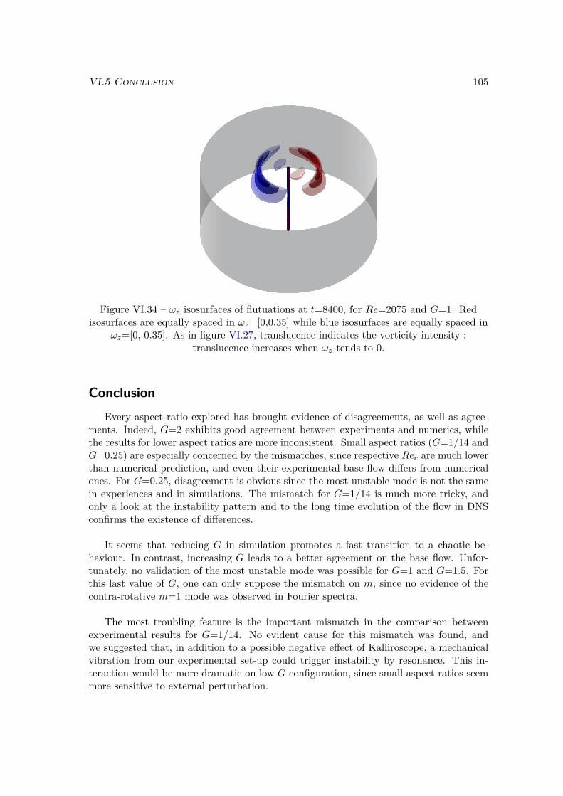
VI.5 Conclusion 105
Figure VI.34 – ωz isosurfaces of flutuations at t=8400, for Re=2075 and G=1. Redisosurfaces are equally spaced in ωz=[0,0.35] while blue isosurfaces are equally spaced in
ωz=[0,-0.35]. As in figure VI.27, translucence indicates the vorticity intensity :translucence increases when ωz tends to 0.
ConclusionEvery aspect ratio explored has brought evidence of disagreements, as well as agree-
ments. Indeed, G=2 exhibits good agreement between experiments and numerics, whilethe results for lower aspect ratios are more inconsistent. Small aspect ratios (G=1/14 andG=0.25) are especially concerned by the mismatches, since respective Rec are much lowerthan numerical prediction, and even their experimental base flow differs from numericalones. For G=0.25, disagreement is obvious since the most unstable mode is not the samein experiences and in simulations. The mismatch for G=1/14 is much more tricky, andonly a look at the instability pattern and to the long time evolution of the flow in DNSconfirms the existence of differences.
It seems that reducing G in simulation promotes a fast transition to a chaotic be-haviour. In contrast, increasing G leads to a better agreement on the base flow. Unfor-tunately, no validation of the most unstable mode was possible for G=1 and G=1.5. Forthis last value of G, one can only suppose the mismatch on m, since no evidence of thecontra-rotative m=1 mode was observed in Fourier spectra.
The most troubling feature is the important mismatch in the comparison betweenexperimental results for G=1/14. No evident cause for this mismatch was found, andwe suggested that, in addition to a possible negative effect of Kalliroscope, a mechanicalvibration from our experimental set-up could trigger instability by resonance. This in-teraction would be more dramatic on low G configuration, since small aspect ratios seemmore sensitive to external perturbation.

106 Chapter VI. Free surface flow

Chapter VII
Evaluating the vertical displacementof the disc surface
107

108Chapter VII. Evaluating the vertical displacement of the disc surface
The mismatches reported in previous chapters were quickly associated to an experi-mental flaw. Indeed, previous publications ([40] and [43]) displayed a strong agreementbetween experiments and numerics for G ≥1/14. Several tests were realized before thebeginning of this thesis, including viscosity monitoring, influence of the gap between thedisc edge and the cavity wall, non neutrality of the marker, switching of the disc and eventhe switching of the direction of rotation. But none of them was concluding. Therefore,we suspected vibrations of the experimental set-up to force instabilities growth by reso-nance. We knew from comparator estimations that the displacement of the disc surfacein the largest cavity was close to 0.3 mm. But we had no clue about the frequency ofthis phenomenon. To evaluate this frequency, we used two Keyence LK-G10 sensors, ableto measure displacement of a surface in the ± 1.0 mm range with an accuracy around10 µm. These sensors are connected to a Keyence LK-GD500 controller, which deliversa tension of ± 10 V , regarding a given measurement span. The smallest sensitivity is 1mm/10V , but distance window can be reduced, for an accuracy gain. All the followingmeasurements were made on or inside the largest cavity. Note that all the spectra in-cluded in this chapter have their amplitude multiplied by four, so that the amplitudes ofthe peaks match with the measurements of the vertical displacement.
Figure VII.1 – LK-GD500 controller (left), with Keyence LK-G10 sensor (right) .
Recording the signal of sensors through several revolutions gives a periodic signal fromwhich can be estimated the frequencies with Fourier transform. It also gives the displace-ment amplitude of the disc surface. Nevertheless, this measurement is only local, and toobtain the global topology of the surface it would require synchronised measurements formany radii. Here, we only expect to find the frequencies of the main modes of verticaldisplacement.
In addition to the brass disc used in our experiments, a second disc made of aluminiumwas also tested. This disc is thinner and lighter than the brass disc. Its surface was notaccurately machined and is thus prone to larger imperfections. This disc was also usedin early tests, which demonstrated that the premature growth of the instabilities was

VII.1 Oscilloscope as a bridge 109
independent from the disc mounted in the experiment.
Oscilloscope as a bridge
Method
At the beginning of the measurement campaign, we only had access to one Keyencesensor. The bridge between this sensor and the computer was insure by a LeCroy WaveAce202 numerical oscilloscope. The time of acquisition depended on the calibre, and so wasthe timestep : signals were discretised on 3000 dots in time, whatever was the signallength, and on 256 values (8 bits) for the tension measurement. Keyence sensor sensitiv-ity was set between 20 µm/10V and 250 µm/10V . To estimate the displacement of thedisc surface we needed to know the vertical calibre Vc used on the oscilloscope and thesensitivity Ss of the sensor. Then, by counting the number nv of vertical divisions, wehave Ad = nv×Vc×Ss/256, where Ad is the displacement amplitude of the surface. In thesame way, we can evaluate the period T of the signal just by counting the number nh ofhorizontal division and by knowing the horizontal calibre Hc : T = nh ×Hc/(3000× np),where np is the count of periods. Figure VII.2 shows the signal obtained on the oscillo-scope.
Figure VII.2 – Raw signal acquired from the oscilloscope, for the brass disc, atr=124mm. Oscilloscope calibres were 1 s/div and 2 V/div, while sensor sensitivity was
set to 25µm/V .
Measurement and post processing
First attempt with the brass disc
Once data was transferred to the computer, post-processing was performed with Mat-Lab. Using the measurement made on the brass disc surface, the displacement amplitudeof the disc surface can be estimated thanks to the relations given above : in r=124 mm,displacement is evaluated to ∼205 µm. Then the frequencies of the main modes are ob-tained with a Fourier transform, after the mean value of the signal is subtracted (see fig.VII.2). The amplitude of each mode is normalized with respect to the radius where mea-surements were made, and frequencies with respect to the disc rotation rate. According

110Chapter VII. Evaluating the vertical displacement of the disc surface
to this, the main peak occurs for f=1, which probably corresponds to an inclination ofthe disc surface. The second peak is at f=3, that can be understood with the signalprofile in figure VII.2 : on each side of the positive peak, one can see two plateaus thatmay be small variations in the slope of the inclination.
0
0.5
1
1.5
Am
plit
ude
10-3
0 5 10 15
f
Figure VII.3 – Main frequencies of oscillation of the largest cavity with the brass disc,using same data as figure VII.2.
This first measurement did not show any obvious connection between the instabilitymode frequency and the oscillatory frequency of the disc surface. Yet the discretizationon the frequencies scope is not dense enough to catch values with a step smaller thanf=0.5.
Comparison of two discs
We repeated this measurement for both discs, but with a better sensitivity. We triedto focus the sensor on the same radius in both cases, however, a small difference remains :in the absence of a dedicated support, the sensor was found hard to Zero. Actually, thesensor has to be placed at a certain distance from the disc, corresponding to half the fieldof measurement of the sensor. But the higher is the accuracy, the harder it is to remain inthis “zero zone“ : tightening a screw can drive the sensor out of position. The radii com-pared in figure VII.4 are r=115 mm for the aluminium disc, and r=118 mm for the brassdisc. For acquisitions with the aluminium disc, sensor sensitivity was 37.5 µm/V , whilefor the brass disc, it was 15 µm/V . For both discs, oscilloscope calibres were 2 V/div(vertically) and 10 s/div (horizontally).
From figure VII.4b we observe once again predominant peaks for f=1 and f=3, forboth discs. For these two wavenumbers, amplitudes of the aluminium disc are approxi-mately twice times larger than those of the brass disc : as expected, the flatness of thealuminium disc is worse than the one of the brass disc. Note that for the aluminium disc,a strong peak is observed for f=2. Its absence in the brass disc signal confirms that it

VII.1 Oscilloscope as a bridge 111
(a) Signal
0 20 40 60 80 100 120
t (s)
-200
-100
0
100
200
Am
plit
ude (
µm
)
Aluminium disc, r=115mm
Brass disc, r=118mm
(b) Fourier transform
0
0.5
1
1.5
2
Am
plit
ude
10-3
0 5 10 15
f
Aluminium disc, r=115mm
Brass disc, r=118mm
Figure VII.4 – Surface displacement for the aluminium (in blue) and the brass disc (inorange). VII.4b shows the associated Fourier transform. As observed in VII.4a, theamplitudes of the aluminium disc are twice as large as those of the brass disc. The
aluminium disc also displays an additional mode of vibration m=2.

112Chapter VII. Evaluating the vertical displacement of the disc surface
only involves a flaw of the aluminium disc surface, such as a fold along the diameter.
As for today, it is hard to tell if peaks for f=1 and f=3 are due to imperfections ofthe surface of discs only, or if a flaw in the rigid sleeve coupling or the thrust ball bearingcan be responsible for a non-negligible part of the displacement.
Detection of a peak
During these previous acquisitions, we periodically saw a negative peak on the oscillo-scope screen, without being able to record it. We get more lucky on later measurements,as shown in figure VII.5.
100 105 110 115 120
t (s)
-150
-100
-50
0
50
100
Am
plit
ude (
µm
)
Figure VII.5 – Example of peak with a strong periodicity, on the brass disc, for r=79mm.
We were very doubtful on the origin of this peak : it did not appear on each measure-ments, but when it did, it shown a periodicity that could imply a phenomenon on thedisc surface, such as a brutal vertical motion, even from a small amplitude, that wouldresult in a stall from the sensor. This ”drop peak“ was observed for several rotation speedand radius, and with both disc, and always resulted in a drop of the tension to the lowerlimit of the sensor. Once this peak was discovered, we had strong expectations it couldpartially explain mismatches reported in previous chapters. However, this peak can alsobe an artefact due to a defect from the sensor or from the acquisition chain.
Displacement of the cavity
Some other measurements were made with this first acquisition chain, directly on theedge of the cavity, and on the aluminium sleeve of the foot : if the shaft is bent, or ifthe misalignment between the shaft of the disc and the rigid sleeve is too pronounced,this leads to a forcing on the guiding ball bearings and the whole cavity would show a

VII.1 Oscilloscope as a bridge 113
precession movement (see figure VII.6).
Figure VII.6 – Illustration on a spinner of the precession mouvement compared torotation.
The evaluation of vertical and horizontal displacements of the plexiglas container canhelp to discriminate the origin of displacements : if the cavity displacement amplitude iscomparable to the displacement of the disc surface, this would incriminate a major flawin coaxiality. Results of axial and radial displacements of the cavity are summed up intable VII.1. Displacement of the cavity with the aluminium disc mounted is twice largerthan with the brass disc. This factor 2 echoes a previous comparison between both discs.From figure VII.7d, below the domination of f=1, we can see the presence of small peaksfor f=2 and f=3 for the aluminium disc, while for the brass disc (fig. VII.7b), thereis no noticeable peak for f=3. Therefore, modes 2 and 3 observed previously for thealuminium disc can be partially caused by a flaw in the shaft, while the mode 3 reportedfor the brass disc seems to be mostly attributable to the disc surface deformation.
brass disc aluminium discvertical (µm) 13 27
horizontal (µm) 15 38
Table VII.1 – Amplitude of displacement taken on the upper edge of the cylindricalcavity.
We can conclude that there exists a small precession movement, but the displacementamplitude of the cavity is approximately one hundred time smaller than these of reportedat the surface of both discs. The precession movement itself depends on the selecteddisc : with the aluminium one, displacements of the cavity are two times larger than withthe brass one. At this point, we may suggest that the movement of each disc surface isessentially caused by small deformations of their respective surface, or to an orthogonalitydefect between the shaft and the disc.

114Chapter VII. Evaluating the vertical displacement of the disc surface
0 2 4 6 8 10 12
t (s)
-10
-5
0
5
10
Am
plit
ud
e (
µm
)
(a) Signal
0
1
2
3
4
5
6
Am
plit
ude
10-5
0 5 10 15
f
(b) Fourier transform
0 20 40 60 80 100 120
t (s)
-20
-10
0
10
20
Am
plit
ud
e (
µm
)
(c) Signal
0
0.5
1
1.5
Am
plit
ud
e
10-4
0 5 10 15
f
(d) Fourier transform
Figure VII.7 – Measurements on the cavity upper edge. Figures VII.7a and VII.7bcorrespond to measurements with the brass disc, while figures VII.7c and VII.7d were
made with the aluminium disc. For both of them, orange plots are radial displacements,and blue plots are axial displacements.
New acquisition chainIn order to avoid the limits of the oscilloscope, we switched to a National Instrumen-
tal dAq, directly linked to MatLab. Data are now acquired through 600 s, with 1000samples.s−1. We also add a second sensor. Initially, we used a LK-G150, with a maxi-mum displacement of ±400 mm. A rigid frame with aluminium mounts simplified initialplacement of sensors, and robustness of measurements (see figure VII.8). Nevertheless,after zeroing sensors, it remains a small drift leading to an incertitude of ∼10 µm. Weexpected that the larger range of LK-G150 could catch without saturation the peak dis-cussed earlier. But this sensor has been quickly changed for another LK-G10 sensor, moreadapted to our discs displacements : their amplitudes are small enough for the LK-G150to never get out of its ”zero zone”.
With this two sensors set-up, three kinds of measurements were performed :• Two sensors placed in r=109 mm, but with a π phase shift.
• One sensor in r=109 mm, and the second in r=54 mm, with no phase shift.
• One sensor in r=109 mm, and the second in r=0 mm.These configurations of sensors location should allow us to determine whether the
surface displacement is due to a vertical jump of the whole disc, to local surface defects,or to some precession movement. Every acquisition was done with a 100 µm/V sensitivity.

VII.2 New acquisition chain 115
Figure VII.8 – Rigid frame with LK-G10 and LK-G150 sensors.
π phase shiftThis new measurement campaign was started with the two sensors in phase opposi-
tion, in order to check whether the drop can be detected in the same time on both sensors,of with a phase shift of π. The first case would alleged in favour of vertical drop of thewhole disc, while the second would imply a groove in the disc surface. Sensors are placedin r=109 mm, on each side of the disc center, on the same diameter. This radius waschosen because it is approximately the radius were vortices are visible with a fluid fillingof h=10 mm.
Figure VII.9a gives many interesting insights :• The drop occurs at the beginning of the descending phase, while we previously saw
it during the ascending phase. This confirms that if it has a physical reality, it isnot linked to the disc, but to the thrust ball bearing or the rigid sleeve couplingsince only the variation of position of the shaft in the sleeve can explain this changein the location of the peak.
• Despite the much higher data rate, the drop is not present at each period. Itsapparition remains slightly random although, when it was captured, it was alwayson the same position at each period.
• The second sensor never recorded the peak. One could suppose that sensors arenot placed at the exact same radius and therefore, do not capture the exact samesignal. However the peak was observed both for smaller and higher radius in previousmeasurements.
Sensors were then inverted, and so was their plug in the controller. Each time, thepeak appeared in only one of the acquired series, always linked to the same sensor. It was

116Chapter VII. Evaluating the vertical displacement of the disc surface
0 100 200 300 400 500 600
t (s)
-400
-300
-200
-100
0
100A
mplit
ude
(a) Signal
(b) Fourier transform
Figure VII.9 – Sensors in phase opposition, at r=109 mm. Maximum displacementamplitudes in figure VII.9a are 285 µm and 274 µm.
then obvious that this peak resulted from a faulty sensor.
The same measurements were repeated for the aluminium disc, with the exact sameconclusions. With this disc, the two sensors gave the same maximum displacement am-plitude of 487 µm.
Linearity of the slope
Since we can not scan the whole surface of the disc with our control set-up, we chooseto simply evaluate the linearity of the slope with two points, and to check for any tracesof residual vertical movement of the whole disc, with a sensor placed at the vertical ofthe rotation axis. Measurements for r=0 mm, r=54 mm and r=109 mm are reported inthe table VII.2. Note that they were only realized on the brass disc.

VII.3 Conclusion 117
r (mm) 0 54 109displacement (µm) 34 91 189
Table VII.2 – Amplitude of displacement for three radius of the brass disc.
Two antagonist observations can be made from table VII.2 :
• The existence of a displacement in r=0 mm is synonym of a vertical translation ofthe whole disc, probably caused by irregularity in the thrust ball bearing.
• Amplitudes reported for r=109 mm is 2.08 times larger than for r=54 mm. Thismatch very well with the 2.02 factor between radius, and therefore supports thehypothesis of a linear slope of the surface, with a zero vertical displacement of therotation axis. A non perfect placement of the sensor in r=0 mm does not fullyjustify the non zero displacement : if the surface slope was perfectly linear, a 34µm displacement would only be observed in r ≈20 mm, which is too far from thecenter.
The global movement of the surface can hardly be associated to a simple and uniquecause but more probably to a combination of at least two flaws, making them harder toidentify and correct. However, the amplitude displacement remains small, with less than300 µm. For G=1/14, the smallest aspect ratio considered in this thesis, the height of thefluid above the disc is H=10 mm, and vertical displacements then represent 3% of H.
Comparison of figures VII.10a and VII.9a reveals that the amplitude for r=109 mmis smaller in later measurements. The replacement of the three ball bearings betweenthese two measurement campaigns is probably responsible for the amelioration of therotation quality. Indeed, we suspected ball bearings to be partially rusty and plannedtheir replacement in order to reduce noise and small amplitude vibrations while operatingthe experiment.
ConclusionAn in-depth study of the vertical displacement of the largest cavity was conducted in
order to try to identify causes of oscillations in the disc surface. The main frequencies ofthese oscillations were also estimated, in order to check for a relation with flow instabilityfrequencies. It appeared difficult to isolate only one reason of the movement. Althoughthe amplitudes of displacement are small compared to the height of the fluid, even forG=1/14. Yet, if our system was sensistive to an oscillary forcing, this amplitude wouldbe large enough to promote the instability. Still no oscillatory mode of the disc shares afrequency with the instability that occurs in the flow for G=1/14. As a consequence, thehypothesis of forced instability by resonance with an oscillatory mode of the disc doesnot seem relevant any more for this flow. Nevertheless, the replacement of ball bearingsbrings a small improvement to the rotation quality.

118Chapter VII. Evaluating the vertical displacement of the disc surface
0 100 200 300 400 500 600
t (s)
-200
-100
0
100
200
Am
plit
ude (
µm
)
r=109mm
r=54mm
r=0mm
(a) Signal
(b) Fourier transform
Figure VII.10 – Vertical displacements of the disc surface for three radius of the brassdisc.

Chapter VIII
Numerical investigation of the effectof the boundary condition at the in-terface
119

120 Chapter VIII. Effect of the boundary condition at the interface
The hypothesis of an instability triggered by a mechanical noise was heavily questionedduring the quantification of disc displacements. Moreover, the absence of major flaw ofthe experimental set-up, added to the good agreement on experimental comparison forG=0.25 and G=1 discussed in VI.4, exculpate the experimental bench to be responsiblefor the early growth of instabilities. Even legitimated, experimental results still showimportant mismatches with numerics for small G, and every preliminary test had to bereassessed in order to find an other admissible hypothesis that could explain these dis-agreements.
The only promising clue was a single ROSE simulation done with an improvisedboundary condition. Although the initial suggestion behind the new boundary conditionapplied in this computation relied on an observation made during one of our experimentalcampaign, its numerical counterpart can seem somewhat brutal. Actually, this approachof the air water interface founds its origin in [69]. There, the authors suggested thatthe radial velocity ur tends to 0 when the surface is polluted. However, with this newsurface condition, their code failed to match experimental velocity profiles for G=1.75at Re=1850. Echoes of this idea can found in some others articles, such as [70]. There,authors noted that in presence of a sufficiently high concentration of surfactant at the sur-face, “the Marangoni stress acts like a no-slip surface”. This behaviour was also describedin [71]. In 2003, a new observation of the role of the surface cleanliness was introducedin [37] for G =0.25 : as discussed in chapter VI, Lopez et al. noticed that if the fluid hada higher amount of surface-contaminants, the most unstable mode switches from m=3 tom=2.
The role of the radial velocity at the surface was actually, after viscosity and irregu-larity of the rotation rate, one of the first investigated possibilities for mismatches : fromexperiments with Kalliroscope, we observed almost immobile particles at the surface, andquickly came to the same conjecture than in the articles quoted above. However the com-plete cancellation of the radial velocity seemed excessive, and ROSE prediction on Recremained far from experimental findings. Therefore, this investigation was not pursuedfurther. The advent of LDV and, as a consequence, the ability to acquire velocity profiles,motivated us to reconsider this boundary condition : simulations with zero radial velocityat the interface revealed changes on the base flow compared to previous simulations withthe standard free slip condition, and the comparison with experimental velocity profileconcluded that the new condition was not as incoherent as we once thought.
Frozen surface
New condition at the interface
As explained above, the first alternative to the free slip condition at the flow surfaceconsisted in considering the extreme case of a completely "frozen" radial velocity compo-nent. Right now, the boundary condition that was used at the interface corresponds toequations (IV.7), (IV.8) and (IV.10). Where ∂ur
∂z =0 was imposed, we now set ur=0. Thisis translated on the base flow of ROSE by a simple modification of the equation (V.5) ofthe boundary conditions at the interface. These boundary conditions become :
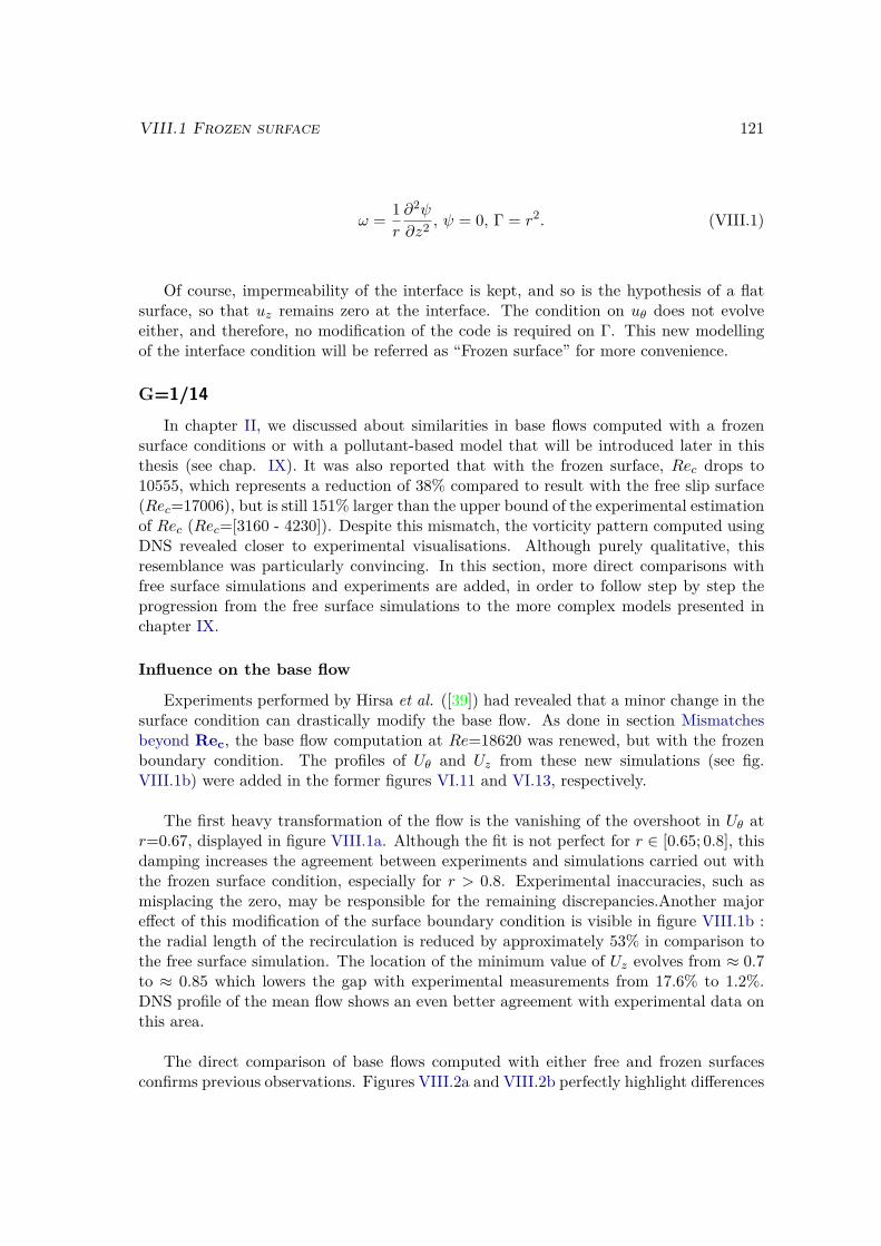
VIII.1 Frozen surface 121
ω = 1r
∂2ψ
∂z2 , ψ = 0, Γ = r2. (VIII.1)
Of course, impermeability of the interface is kept, and so is the hypothesis of a flatsurface, so that uz remains zero at the interface. The condition on uθ does not evolveeither, and therefore, no modification of the code is required on Γ. This new modellingof the interface condition will be referred as “Frozen surface” for more convenience.
G=1/14
In chapter II, we discussed about similarities in base flows computed with a frozensurface conditions or with a pollutant-based model that will be introduced later in thisthesis (see chap. IX). It was also reported that with the frozen surface, Rec drops to10555, which represents a reduction of 38% compared to result with the free slip surface(Rec=17006), but is still 151% larger than the upper bound of the experimental estimationof Rec (Rec=[3160 - 4230]). Despite this mismatch, the vorticity pattern computed usingDNS revealed closer to experimental visualisations. Although purely qualitative, thisresemblance was particularly convincing. In this section, more direct comparisons withfree surface simulations and experiments are added, in order to follow step by step theprogression from the free surface simulations to the more complex models presented inchapter IX.
Influence on the base flow
Experiments performed by Hirsa et al. ([39]) had revealed that a minor change in thesurface condition can drastically modify the base flow. As done in section Mismatchesbeyond Rec, the base flow computation at Re=18620 was renewed, but with the frozenboundary condition. The profiles of Uθ and Uz from these new simulations (see fig.VIII.1b) were added in the former figures VI.11 and VI.13, respectively.
The first heavy transformation of the flow is the vanishing of the overshoot in Uθ atr=0.67, displayed in figure VIII.1a. Although the fit is not perfect for r ∈ [0.65; 0.8], thisdamping increases the agreement between experiments and simulations carried out withthe frozen surface condition, especially for r > 0.8. Experimental inaccuracies, such asmisplacing the zero, may be responsible for the remaining discrepancies.Another majoreffect of this modification of the surface boundary condition is visible in figure VIII.1b :the radial length of the recirculation is reduced by approximately 53% in comparison tothe free surface simulation. The location of the minimum value of Uz evolves from ≈ 0.7to ≈ 0.85 which lowers the gap with experimental measurements from 17.6% to 1.2%.DNS profile of the mean flow shows an even better agreement with experimental data onthis area.
The direct comparison of base flows computed with either free and frozen surfacesconfirms previous observations. Figures VIII.2a and VIII.2b perfectly highlight differences

122 Chapter VIII. Effect of the boundary condition at the interface
(a) uθ in z=0.8G
0.5 0.6 0.7 0.8 0.9 1
r
0
0.1
0.2
0.3
0.4
0.5
0.6
0.7
0.8
u
LDV
DNS frozen surface
ROSE frozen surface
DNS free surface
ROSE free surface
(b) uz in z=0.5G
0.5 0.6 0.7 0.8 0.9 1
r
-0.05
0
0.05
0.1
uz
LDV
DNS frozen surface
ROSE frozen surface
DNS free surface
ROSE free surface
Figure VIII.1 – Comparison of velocity profiles : ROSE base flow, DNS mean flow(forboth free and frozen condition) and LDV measurements, for G=1/14 and Re=18620.
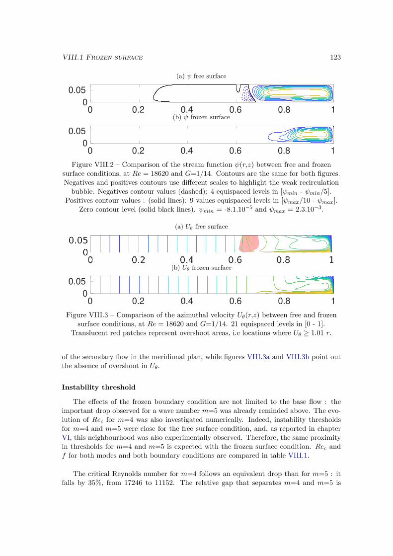
VIII.1 Frozen surface 123
(a) ψ free surface
0 0.2 0.4 0.6 0.8 10
0.05
(b) ψ frozen surface
0 0.2 0.4 0.6 0.8 10
0.05
Figure VIII.2 – Comparison of the stream function ψ(r,z) between free and frozensurface conditions, at Re = 18620 and G=1/14. Contours are the same for both figures.Negatives and positives contours use different scales to highlight the weak recirculation
bubble. Negatives contour values (dashed): 4 equispaced levels in [ψmin - ψmin/5].Positives contour values : (solid lines): 9 values equispaced levels in [ψmax/10 - ψmax].
Zero contour level (solid black lines). ψmin = -8.1.10−5 and ψmax = 2.3.10−3.
(a) Uθ free surface
(b) Uθ frozen surface
0 0.2 0.4 0.6 0.8 10
0.05
Figure VIII.3 – Comparison of the azimuthal velocity Uθ(r,z) between free and frozensurface conditions, at Re = 18620 and G=1/14. 21 equispaced levels in [0 - 1].
Translucent red patches represent overshoot areas, i.e locations where Uθ ≥ 1.01 r.
of the secondary flow in the meridional plan, while figures VIII.3a and VIII.3b point outthe absence of overshoot in Uθ.
Instability threshold
The effects of the frozen boundary condition are not limited to the base flow : theimportant drop observed for a wave number m=5 was already reminded above. The evo-lution of Rec for m=4 was also investigated numerically. Indeed, instability thresholdsfor m=4 and m=5 were close for the free surface condition, and, as reported in chapterVI, this neighbourhood was also experimentally observed. Therefore, the same proximityin thresholds for m=4 and m=5 is expected with the frozen surface condition. Rec andf for both modes and both boundary conditions are compared in table VIII.1.
The critical Reynolds number for m=4 follows an equivalent drop than for m=5 : itfalls by 35%, from 17246 to 11152. The relative gap that separates m=4 and m=5 is

124 Chapter VIII. Effect of the boundary condition at the interface
free surface frozen surfacem=4 m=5 m=4 m=5
hub no hub hub no hub hub no hub hub no hubRec 17536 17246 17019 17006 10217 11152 10486 10555f 0.692 0.688 0.711 0.709 0.816 0.811 0.817 0.814
Table VIII.1 – Comparisons on Rec and f for modes 4 and 5 for G=1/14, and bothboundary condition. Influence of the hub is also inspected. The hub radius is 0.5.
Meshes used are 351×51 and 701×101, with and without hub, respectively.
therefore wider for the frozen boundary condition with slightly less than 6% gap, whenit was only 1.4% for the free surface. The drop in Rec is followed by a small increase ofthe frequency f , that respectively gains 18% and 15% for m=4 and m=5. For this lastwavenumber, the comparison with experimental value (f=0.764) does not evolve much :from 7.2% to 6.5%, compared to free and frozen surface conditions, respectively.
Table VIII.1 also contains results for computation done with a hub of 0.5R. Many ofour first simulations were done with a such hub, in a effort to limit the computationalcosts. Regarding the minor variations of Rec and f , it could be easy to conclude that thepresence of the hub has minor effects on the instability. However the under-evaluationof Rec for the frozen surface leads to predict m=4 as the most unstable mode, insteadof m=5. The hub influence is not the same, whether simulation is performed with thefree or the frozen condition. In the first case, the hub tends to over-evaluate Rec and f ,but in the second case, the trend is not as clear : Rec is lowered, but f is a bit higher.The maximum gap on Rec is observed for m=4, in the frozen case, with 8.4% differencebetween simulations with and without hub. This is also the less favourable case for thefrequency, with a 0.62% gap.
Following the same protocol than for the free surface condition, as explained in sectionV.2.4 (page 70), we cross-checked the value of Rec with DNS computations. Note that inDNS, the change in the boundary condition is easily applied, as we simply impose ur = 0,in z = G for the frozen case.
Re 10200 10300a -0.0079264 -0.0058641
Table VIII.2 – Decay rates a of the most unstable mode (m=5) betweent=timpulse+1200 and timpulse+2100, for Re=10200 and 10300, with the frozen boundary
condition. For both cases, timpulse = 300.
According to the slopes values reported in table VIII.2, Rec is estimated at 10584,which represents a gap of only 0.27% compared to LSA prediction.

VIII.1 Frozen surface 125
Instability pattern in numerics
In order to compare instability pattern with the free surface case, we performed a DNSrun at Re=18620, without any restriction on θ, and therefore, no forcing nor filtering of themode. Figure VIII.4 represents the axial vorticity at the surface at this Reynolds number.
Figure VIII.4 – Axial vorticity pattern fort Re=18620 and G=1/14. Red areascorrespond to ωz > 0, and blue areas to ωz < 0. Intensity of vorticity is translated bytranslucence of 5 isosurfaces between ωz=-1.73 to 0 for negative values, and of 5 otherisosurfaces for positives values of ωz, between 0 to 2.44. This snapshot correspond to
t=1200.
The wave number m=5 is perfectly visible in figure VIII.4, with a completely differentface compared to the computed pattern for the free surface, that are shown in chapter II.With time series, the corresponding frequency was evaluated to f=0.809, i.e only 0.6%lower than predicted by ROSE prediction. Time series also present a simpler dynamicsthan in the free surface case : figure VIII.5 displays a purely sinusoidal signal, qualita-tively closer to experimental data.
We previously observed in chapter VI that ROSE and DNS match nicely on vorticitypattern of fluctuations at the surface. For the frozen surface and close to Rec, this agree-ment still occurs, as shown in figures VIII.6a and VIII.6b.
However, as soon as Re moves away too much from Rec, ROSE does not seem tobe able to reproduce the instability pattern. Figure VIII.7 illustrates differences in thevorticity pattern of fluctuations between ROSE and DNS, at Re=18620. These figurescorresponds to the fluctuations part of the flow shown in figure VIII.4. Note that fig-ures VIII.7b and VIII.7c computed with Sunfluidh at Re=18620 show a better agreementwith the experiment than the simulations performed for a Reynolds number closer to

126 Chapter VIII. Effect of the boundary condition at the interface
6000 6020 6040 6060 6080 6100
t
0.655
0.66
0.665
0.67
0.675
u
Figure VIII.5 – Temporal series of uθ for G=1/14 and Re=10700. The right figure is azoom of the last iteration of the code, between t=6000 to 6100. The probe is located at
(0.68,0,0.5G).
(a) ROSE (b) DNS - base flow (c) DNS - mean flow
Figure VIII.6 – Vorticity pattern of fluctuations obtained with ROSE (left) andSunfluidh (middle and right) in z=G, for G=1/14 and Re=10700. Figure VIII.6b
correspond to fluctuations obtained by the subtraction of the 2D axisymmetric baseflow, while figure VIII.6c was obtained by subtraction of the spatial averaged mean flow.The vorticity field from ROSE was normalized with respect to the maximum absolute
value of vorticity of figure VIII.6b. The colorbar was also restricted to the samevorticity span.
Rec, where a pentagon shape is only barely visible when the mean flow is subtracted (fig.VIII.6c). Indeed, none of the visualizations of the figure VIII.7 convincingly reproducesthe patterns observed in the experiment.
Hysteresis in frozen surface simulations ?
Like we did in section VI.1.3, we performed a series of simulation using DNS, to checkfor the existence of hysteresis. Starting from an initial state for Re=18620, the value ofRe is lowered to [10780,10192], by steps of 196. The five simulations are displayed infigure VIII.8.
We recall that for Re=18620 and a frozen surface, the velocity time series is purelysinusoidal, without the complicated dynamics observed for the free surface. For lower

VIII.1 Frozen surface 127
(a) ROSE (b) DNS - base flow (c) DNS - mean flow
Figure VIII.7 – Vorticity pattern of fluctuations obtained with ROSE (left) andSunfluidh (middle and right) in z=G, for G=1/14 and Re=18620. Pattern from ROSEwas normalized with respect the absolute value of the minimum of vorticity obtained in
the DNS with subtraction of the 2D axisymmetric base flow (middle). Right figurecorresponds to the fluctuations observed from the subtraction of the spatially averaged
mean flow.
800 900 1000 1100 1200
t
0.63
0.64
0.65
0.66
0.67
0.68
0.69
u
Re =18620
Re =10780
Re =10584
Re =10388
Re =10192
Figure VIII.8 – Numerical spin-down phases with a frozen surface, from Re=18620 toRe= [10780,10192], by steps of 196. The probe is located at (0.68,0,0.9G).

128 Chapter VIII. Effect of the boundary condition at the interface
values of Re, the signals remain sinusoidal. Yet, as soon as Re < Rec, the amplitudeof the oscillations is decreasing in time. Rec was estimated between 10555 and 10584,according to ROSE and Sunfluidh predictions, respectively. Indeed, the decrease of theamplitude is clearly visible on the green curve (Re=10192). It is also existent for thepurple curve (Re=10388), although less visible due to the small decay rate in the vicinityof Rec. Still, this vanishing of the instability for Re > Rec in a spin-down phase is theevidence of the non-existence of hysteresis in simulations with a frozen surface.
G=0.25The choice for the frozen condition in the case of G=1/14 was globally positive,
although quantitative gaps with experiments remained. The application of this conditionto G=0.25 is also expected to have a positive influence on numerical results and therefore,to get closer to experiments. In particular, the switching of the most unstable modeobserved with the hub for G=1/14 lets expect a possible changeover from m=2 to m=3for G=0.25.
Instability threshold
In section VI.3, we saw that the most unstable mode predicted by ROSE has got anazimuthal wave number m=2, while in experiments, the mode m=3 growth first. Usingthe same grid as before (401×101), new ROSE computations were performed to determineRec with the frozen condition.
free surface frozen surfacem=2 m=3 m=2 m=3
Rec 3481 4691 4516 5320
Table VIII.3 – Evolution of Rec between free and frozen surface boundary conditions forazimuthal numbers m=2 and m=3, in the case G=0.25.
The results gathered in table VIII.3 show a completely unexpected behaviour of the in-stability threshold : while the frozen condition lowered Rec for G=1/14, here, for G=0.25,it pushes Rec even higher, increasing relative difference with the experimental value ofRec (around 2000). The absolute difference between m=2 and m=3 remains almost con-stant : 1210 for the free surface, and 1204 for the frozen surface. No mode switching ispresent, and the most unstable one, according to linear stability analysis, is still m=2.
Base flow
The evolution of the base flow for G=0.25 is similar to the case G=1/14 : applicationof the frozen condition cancels the overshoot in uθ, and reduces the length of the recircu-lation.
However these modifications, visible in figure VIII.9, seem less dramatic than forG=1/14. It also means that no connection exists between the vanishing of the overshoot
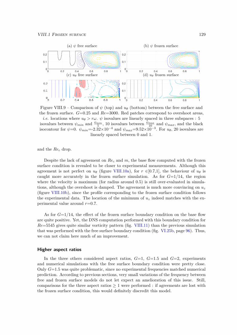
VIII.1 Frozen surface 129
(a) ψ free surface
0 0.2 0.4 0.6 0.8 10
0.1
0.2
(b) ψ frozen surface
0 0.2 0.4 0.6 0.8 10
0.1
0.2
(c) uθ free surface (d) uθ frozen surface
0 0.2 0.4 0.6 0.8 10
0.1
0.2
Figure VIII.9 – Comparison of ψ (top) and uθ (bottom) between the free surface andthe frozen surface. G=0.25 and Re=3000. Red patches correspond to overshoot areas,
i.e. locations where uθ > rω. ψ isovalues are linearly spaced in three subspaces : 5isovalues between ψmin and ψmin
5 , 10 isovalues between ψmax
10 and ψmax, and the blackisocontour for ψ=0. ψmin=-2.32×10⁻⁴ and ψmax=9.52×10⁻³. For uθ, 20 isovalues are
linearly spaced between 0 and 1.
and the Rec drop.
Despite the lack of agreement on Rec and m, the base flow computed with the frozensurface condition is revealed to be closer to experimental measurements. Although thisagreement is not perfect on uθ (figure VIII.10a), for r ∈[0.7,1], the behaviour of uθ iscaught more accurately in the frozen surface simulation. As for G=1/14, the regionwhere the velocity is maximum (for radius around 0.5) is still over-evaluated in simula-tions, although the overshoot is damped. The agreement is much more convincing on uz(figure VIII.10b), since the profile corresponding to the frozen surface condition followsthe experimental data. The location of the minimum of uz indeed matches with the ex-perimental value around r=0.7.
As for G=1/14, the effect of the frozen surface boundary condition on the base floware quite positive. Yet, the DNS computation performed with this boundary condition forRe=5545 gives quite similar vorticity pattern (fig. VIII.11) than the previous simulationthat was performed with the free surface boundary condition (fig. VI.25b, page 96). Thus,we can not claim here much of an improvement.
Higher aspect ratios
In the three others considered aspect ratios, G=1, G=1.5 and G=2, experimentsand numerical simulations with the free surface boundary condition were pretty close.Only G=1.5 was quite problematic, since no experimental frequencies matched numericalprediction. According to previous sections, very small variations of the frequency betweenfree and frozen surface models do not let expect an amelioration of this issue. Still,comparisons for the three aspect ratios ≥ 1 were performed : if agreements are lost withthe frozen surface condition, this would definitely discredit this model.

130 Chapter VIII. Effect of the boundary condition at the interface
(a) uθ in z=0.8G
0 0.2 0.4 0.6 0.8 1
r
0
0.1
0.2
0.3
0.4
0.5
u
LDV
ROSE free surface
ROSE frozen surface
(b) uz in z=0.5G
0 0.2 0.4 0.6 0.8
r
-0.1
-0.05
0
0.05
0.1
uz
LDV
ROSE free surface
ROSE frozen surface
Figure VIII.10 – Comparison of velocity profiles : ROSE base flow and LDVmeasurements, for G=0.25 and Re=1895.

VIII.1 Frozen surface 131
(a) (b)
Figure VIII.11 – Axial vorticity pattern for G=0.25 and Re=5545. Figure on the left iscomposed of 10 isosurfaces : 5 red surfaces equally spaced in [0,2.16], and 5 blue surfaces,
equally spaced in [-1.07,0]. Bounds corresponds to ωz max and ωz min. Tuning thesescales allows to see spots of negative vorticity (ωz ∈ [-0.06,0]) in the figure on the right.
G=1
For G=1, only Uz profiles for Re < Rec were confronted. Since below Rec, base flowand mean flow are identical, only computed profiles using ROSE are compared in thefigure VIII.12.
A quick glance on the comparison of Uz profiles suggests that the modification of theboundary condition at the surface produces only minor changes in the base flow. Thisis confirmed by the comparison of ψ and uθ in figure VIII.13. On the stream functionisovalues (fig. VIII.13a), only changes are a small reduction of the size of the bubbleattached to the axis, and a tiny vertical crush of the main recirculation in the merid-ional plan. This last evolution is not surprising, since ur=0 at the surface, and that suchphenomenon was observed for G ≤0.25. The modification of the isovalues of uθ are alsolimited. Note that no overshoot is present, even with the free surface condition. G=1seems almost insensitive to variations of the surface boundary condition.
G=1.5
For G=1.5, experiments and numerics were compared slightly above Rec, at Re=2356.Unfortunately, it was not expected that this Re would be below the critical Reynolds num-ber in computation using the frozen surface condition. Indeed, the most unstable modeis m=4 at Rec=2375. We remind that, with the free surface condition, the most unstablemode was m=1, at Rec=2150. The effects of the modification of the boundary conditionat the surface on the five first modes are given in table VIII.4.

132 Chapter VIII. Effect of the boundary condition at the interface
0 0.2 0.4 0.6 0.8 1
r
-0.08
-0.06
-0.04
-0.02
0
0.02
0.04
0.06
0.08u
z
LDV
ROSE free surface
ROSE frozen surface
Figure VIII.12 – Comparison of experimental data and ROSE computed uz profile, inz=0.5G, for G=1 and Re=1120.
m 0 1 2 3 4Rec 2909 2802 2882 2911 2375f 0.342 -0.144 0.294 0.312 0.211
Table VIII.4 – Rec and f of modes 0 to 5 for G=1.5, with the frozen surface condition.The values for the free surface condition are given in table VI.9, page 100.
The DNS performed at Re=2356 confirms that the flow is not yet unstable : despitethe introduction of a pulse at t=400, oscillations in velocity time series are decaying (see.fig VIII.14). This decay is very slow which confirms that although Rec is larger than2356, it is probably very close to this value, which is in good agreement with ROSEprediction of Rec=2375. Moreover, the vorticity of fluctuations at t=7200 shows thatthe most unstable mode, i.e. the one that decays the last, is m=4 (.fig VIII.15), with apseudo-frequency f=0.210 on the time span ∆t=[7600-7900], in perfect agreement withROSE predictions reported in table VIII.4.
In our experiments at Re=2356, secondary peaks are visible at f × m=0.838. Werecall that the notation f×m is used since the wavenumbers are unknown in experimentsat G=1.5, and therefore, frequencies are not normalized regarding the mode. However, ifm=4, this frequency corresponds to f=0.209 which nicely matches the reported frequencyfor such wave number in table VIII.4. However in the Fourier transforms obtained fromexperimental time series, the peak corresponding to m=4 never appeared predominant.

VIII.1 Frozen surface 133
(a) ψ free surface
0 0.5 10
0.2
0.4
0.6
0.8
1
(b) ψ frozen surface
0 0.5 10
0.2
0.4
0.6
0.8
1
(c) uθ free surface
0 0.5 10
0.2
0.4
0.6
0.8
1
(d) uθ frozen surface
0 0.5 10
0.2
0.4
0.6
0.8
1
Figure VIII.13 – Comparison of ψ (top) and uθ (bottom) between the free surface andthe frozen surface. G=1 and Re=1120. ψ isovalues are linearly spaced in three groups :
5 isovalues between ψmin and 0, and 9 isovalues between ψmax
10 and ψmax.ψmin=-2.3×10⁻⁴ and ψmax=9.5×10⁻³. The last subspace is represented by the plain
black line, for ψ=0. For uθ, 21 isovalues are linearly spaced between 0 and 1.Simulations were performed on a 301×301 mesh grid.

134 Chapter VIII. Effect of the boundary condition at the interface
Figure VIII.14 – Decay of the oscillations in a time series of uθ, for Re=2356 andG=1.5. The probe is located at (0.5,0,0.9G).
Figure VIII.15 shows the isosurfaces of the axial vorticity of the decaying mode m=4.This can be compared to figure VI.31 of the mode m=1 predicted as the most unstable inthe free surface case. During experiments, injection of ink at the surface was not efficientto visualize pattern and therefore, no comparison with figure VIII.15 is possible. Notethat the frequency of the mode m=1 with the free surface condition is very low. Onecan suggest that the mixing time of ink is shorter than the revolution time of m=1 andtherefore, no visualisation is possible with ink although the mode could exist.
G=2
Applying the frozen surface condition to G=2 has almost no impact on figures. Themost unstable mode predicted by ROSE is still m=4, like previously reported for the freesurface condition. Rec and f also present only moderate evolutions. Indeed, they respec-tively move from 1914 to 1987, and from 0.157 to 0.160. Changes in the axial vorticitypattern are difficult to quantify. However a square shape is drawn by low vorticity isosur-face (fig. VIII.16). This square is compatible with the pattern experimentally visualizedfor m=4 and G=1/14 in figure VI.16. Unfortunately, we have no clear visualisation of thepattern for G=2, except blurred DPIV snapshots from [35] and [37] that do not allow fordiscrimination between numerical results obtained with the free and the frozen surfaceconditions.
As shown previously for G=1, we can only conclude that larger aspect ratios are lesssensitive to the condition applied at the surface.

VIII.1 Frozen surface 135
Figure VIII.15 – Isosurfaces of axial vorticity of the perturbations at t=7200 andRe=2356, for G=1.5. Red and blue patches correspond to ω=±2.2×10⁻⁶, while yellowand green patches correspond to ω=±8.0×10⁻⁷. The vorticity of the perturbations is
very small, since the flow fields tend to steadiness. Still, the mode m=4 is clearly visible.
Conclusion on the frozen surface model
Changing the surface boundary condition from the classical free-slip model to anotherone with a frozen radial velocity brings interesting results for G=1/14 : Rec drops byapproximately 35% for both modes m=4 and 5. However, it remains way above the ex-perimental Rec. Despite this mismatch on figures, numerically computed axial vorticitypattern shows an excellent similarity with experimental observations. In addition, com-puted velocity profiles show no more trace of overshoot and are closer to profiles extractedfrom LDV measurements.
Unfortunately, good trends obtained on the Reynols number for G=1/14 were notreproduced for G=0.25 : the new boundary conditions actually pushed Rec further, forboth mode m=2 and 3, thus increasing the gap with experiments. The most unstablemode remains unchanged : m=2 is still the first one to grow, as for the free surface con-dition. Obviously, such a simplistic model as the frozen surface condition cannot fill thegap between numerics and experiments.
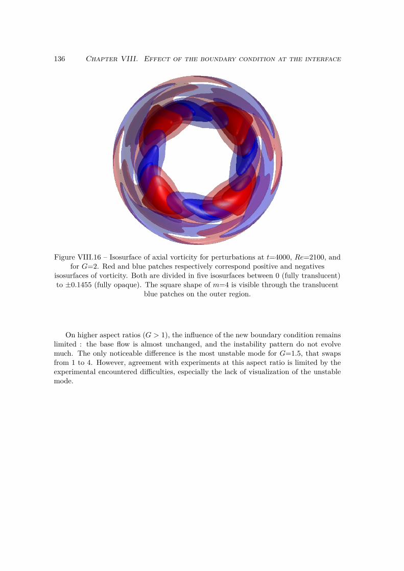
136 Chapter VIII. Effect of the boundary condition at the interface
Figure VIII.16 – Isosurface of axial vorticity for perturbations at t=4000, Re=2100, andfor G=2. Red and blue patches respectively correspond positive and negatives
isosurfaces of vorticity. Both are divided in five isosurfaces between 0 (fully translucent)to ±0.1455 (fully opaque). The square shape of m=4 is visible through the translucent
blue patches on the outer region.
On higher aspect ratios (G > 1), the influence of the new boundary condition remainslimited : the base flow is almost unchanged, and the instability pattern do not evolvemuch. The only noticeable difference is the most unstable mode for G=1.5, that swapsfrom 1 to 4. However, agreement with experiments at this aspect ratio is limited by theexperimental encountered difficulties, especially the lack of visualization of the unstablemode.

VIII.2 Hybrid modelling 137
Hybrid modelling
Robin condition at the interfaceAlthough it was evident that the frozen surface condition was not the solution to
mismatches, it convinced us to explore more deeply the evolution of the flow and itsinstability regarding the surface condition. The first limit to the frozen condition hadalready made us give up the hypothesis of mechanical vibrations. However, the radialvelocity forced to zero at the surface is too unrealistic to efficiently represent the flowin our experiment. Indeed, at the exception of some experiments with Kalliroscope, wenever observed uSr=0 in experiments. However, we suggested that uSr could be curb by afront of pollutant that may exist where the recirculation in the meridional plan dives fromthe surface to the disc. Thus, we needed to create a new boundary condition that wouldnot completely slow down uSr , but where we could tune this braking using one parameteronly. The idea was then to build this boundary condition as an interpolation functionbetween the free and the frozen conditions, and to study the influence of this parameteron the flow. For this part, we only used ROSE and thus, all equations and results arerelated to this code. We remind that the boundary conditions for the free surface were∂ur∂z = ωθ = 0 (eq.(V.5)), while for the frozen surface, we simply had ur = 0 which leadsto eq.(VIII.1) in ROSE. From these two conditions, we can write :
(1− κ)ωθ + κur = 0.
Where κ is an ad hoc tuning parameter, assumed uniform on the whole surface. Sinceωθ = ∂ur
∂z −∂uz∂r and uz=0 at the surface, this leads to :
(1− κ)∂ur∂z
+ κur = 0, (VIII.2)
which is a Robin condition on ur at the surface. In ROSE, this last condition is easyto apply to the perturbations. However, the base flow is computed in (ω,ψ,Γ) variables.In order to keep the second order accuracy on the spatial discretization, ur is expressedusing the relation between ur and ∂ψ/∂z :
ur = 1r
∂ψ
∂z,
the link between ωθ and the second derivative of ψ at the surface :
ωθ = ∂ur∂z
= 1r
∂2ψ
∂z2 ,
and the Taylor expansion at the second order of ψ :
ψ(z − δz) = ψ(z)− δz∂ψ
∂z+ δ2
z
2∂2ψ
∂z2 + o(δz3),
where δz is the vertical step of the mesh. Now, ∂ψ/∂z can be expressed as a functionof ψ and ωθ :
∂ψ
∂z= 1δz
(ψ(z)− ψ(z − δz)) + δz2 rωθ

138 Chapter VIII. Effect of the boundary condition at the interface
Finally, considering that in z=G, ψ=0, the discretized condition for the base flow is :
(1− κ)ωθ + κ
(δz2 ωθ −
1rδz
ψ(G− δz))
= 0
With equation (VIII.2), we see that for κ=0, the boundary condition is the same asthe free surface, while if κ=1, the boundary condition corresponds to the frozen surface.We checked the values of critical Reynolds number in both cases, for m=5, in order tovalidate our code. The results are reported in table VIII.5.
ROSE ROSE hybrid ROSE hybrid (hub)free surface (κ=0) 17006 17006 17082
frozen surface (κ=1) 10555 10555 10465
Table VIII.5 – Comparison of Rec values of m=5, for G=1/14, and the three variants ofROSE. The hub radius is 0.5, and the mesh size for this case 351×101. Other cases usethe standard 701×101 mesh. The presence of the hub is discussed at the end of the
section.
The results are very consistent with former ROSE computations with free and frozensurface conditions.
Parametric study on G=1/14Now that we are able to obtain the same thresholds for the two limit cases of κ, we
varied κ to see how Rec evolves between these extrema. The simulations were done forthree modes, from m=3 to m=5.
The first noticeable point is that the evolution of Rec regarding κ is not the gentlelinear slope that could have been expected. On the left side of figure VIII.17, the increaseof κ is followed by an increase of Rec (blue points). But after a certain value of κ, thecurves show a dramatic variation of the slope, resulting of an impressive drop of Rec.If we focus on m=5, this brutal alteration occurs for κ ≈0.79, and can be interpretedowing to figure VIII.18. Here, we can observe a discontinuity in the frequency of themode, regarding κ. This means, although azimuthal wave number is still m=5, that themost unstable mode is a second unstable branch (pink points), and that a point close toκ ≈0.79, Rec=26070 is actually a point of codimension 2. This point exists when, forgiven parameters, two eigenvalues become unstable in the same time.
For m=4, the point of codimension two is not as marked as for m=5 : the jump infrequencies in figure VIII.18 corresponds to κ=0.84, for which the slope of Rec seemsalmost continuous in figure VIII.17. The drop of Rec only happens for κ=0.88. The casem=3 also displays the same drop, but it occurs for κ between 0.95 and 1. No furtherinvestigation was performed in order to locate the point of codimension 2 of the modem=3 more precisely.
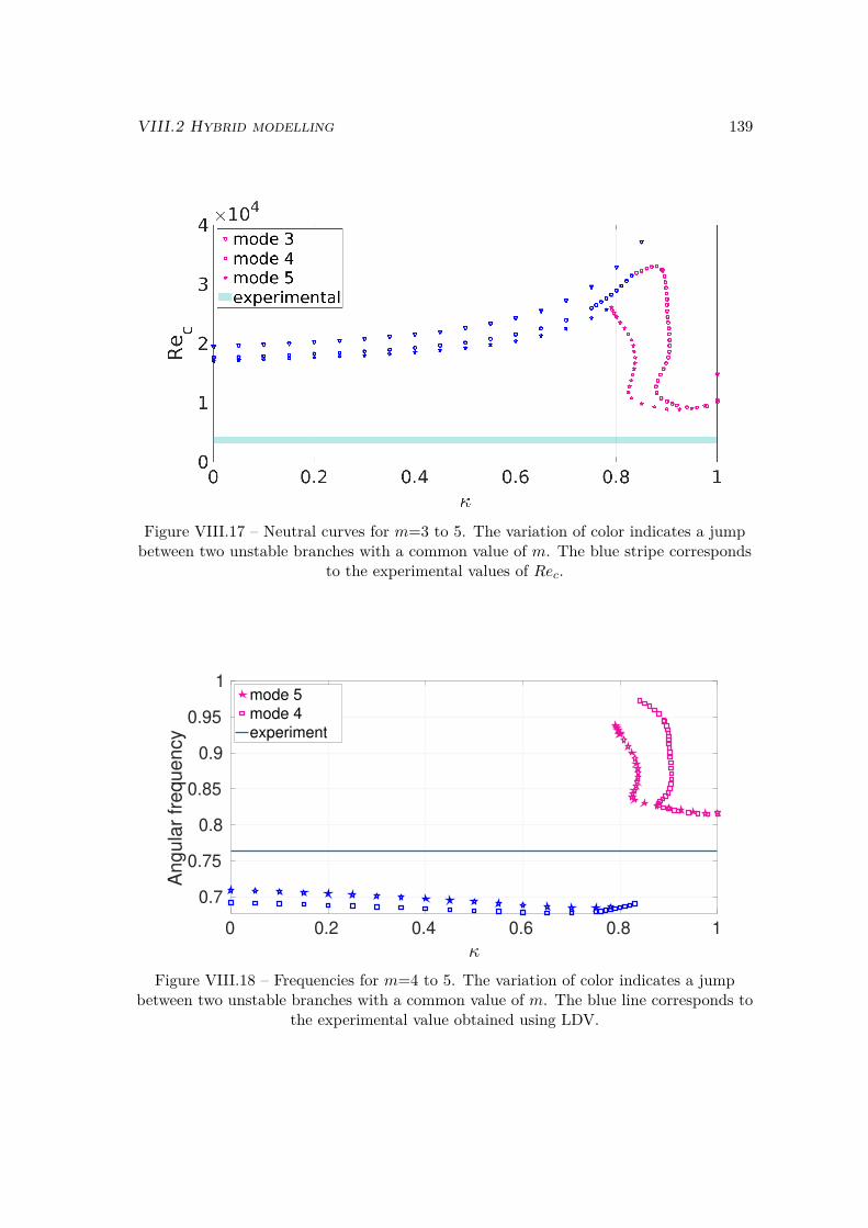
VIII.2 Hybrid modelling 139
Figure VIII.17 – Neutral curves for m=3 to 5. The variation of color indicates a jumpbetween two unstable branches with a common value of m. The blue stripe corresponds
to the experimental values of Rec.
0 0.2 0.4 0.6 0.8 1
0.7
0.75
0.8
0.85
0.9
0.95
1
Angula
r fr
equency
mode 5
mode 4
experiment
Figure VIII.18 – Frequencies for m=4 to 5. The variation of color indicates a jumpbetween two unstable branches with a common value of m. The blue line corresponds to
the experimental value obtained using LDV.

140 Chapter VIII. Effect of the boundary condition at the interface
The second important point concerns the supposed most "favourable" pair of parame-ters for which the gap with experimental value of Rec is smallest, Rec=8868 and κ=0.925 :although it matches the most unstable mode detected in experiments, this Rec value is still108.6% larger than the experimental one. The frequency does not help much to determinewhich branch corresponds to experiments, as the experimentally measured frequency hasalmost the same gap with frequencies for κ=0 and κ=1 (respectively 7.2% and 6.9%). Thegap on f for κ=0.925 is 7.4%. Any experimental imperfection, or measurement inaccu-racy can easily justify a mistake of 0.5%. However, from section Instability pattern at Recand Instability pattern in numerics, the visual aspects of vorticity pattern at the surfaceare known for both branches. It was already demonstrated that the frozen surface (κ=1)shares better qualitative visual with experiments than the free surface (κ=0). There-fore, one expects the pink branch to be more representative of the instability observed inexperiments than the blue branch.
Evolution of the base flow regarding κAlthough no couple of parameters seems to provide a close solution to experiments,
we still focus on the evolution of the base flow regarding κ. Especially, we were interestedin the length of the recirculation for κ=0.925. We see in figure VIII.19 that the minimumvalue of uz for κ=0.925 is located in r=0.806. We remind that in experiments, minimumvalue of uz is estimated close to r=0.85. The case κ=1 - equivalent to the frozen surface -remains the closer to experiments.
7 8 9 10 11 12 13 14
r
-0.05
0
0.05
0.1
uz
= 0
= 0.5
= 0.7
= 0.8
=0.925
= 1
Figure VIII.19 – uz profiles for various values of κ, in z=0.5G, at Re=18620 andG=1/14.
κ also has an effect on the overshoot of uθ. In figure VIII.19, we clearly see a monotonicdamping of the overshoot with the increase of κ. Finally, this overshoot completelyvanishes for κ between 0.7 and 0.8, which corresponds to the jump of the unstable branch.Note that uθ profiles for κ=0.925 and κ=1 are almost perfectly merged.

VIII.2 Hybrid modelling 141
0.5 0.6 0.7 0.8 0.9 1
r
0
0.2
0.4
0.6
0.8u
= 0
= 0.5
= 0.7
= 0.8
=0.925
= 1
Figure VIII.20 – uθ profiles for various values of κ, in z=0.5G, at Re=18620 andG=1/14.
G=0.25
As the actual behaviour of Rec with respect to κ was unexpected, a similar parametricstudy was performed for G=0.25, on a 401×101 grid. An equivalent drop of Rec, followedby an ascending slope could explain results for the frozen surface condition, while allowingthe existence of a most favourable case for an intermediate value of κ. However, this time,only a soft and almost monotonic increase of Rec regarding κ is observed, as shown infigure VIII.21.
The tiny decrease of Rec for m=3, for κ between 0.95 and 1 seems to share the be-haviour of the same mode for G=1/14. Thus, one can think that the jump of unstablebranch occurs only for m >2. But frequencies of the modes shows no discontinuities (seefigure VIII.22), and a closer look at eigenvalues for m=3 and κ=[0.9,1] confirms there isno second unstable branch (see fig. VIII.23).
While G=1/14 brings new elements for each new model of surface condition, G=0.25keeps being enigmatic.
G=2
We previously saw that, for this aspect ratio, experiments and numerics match prettywell, whether free or frozen conditions were used. The application of the Robin conditionto G=2 is therefore not performed for the sake of getting a better agreement, but to checkif a jump of unstable branch is also present for such aspect ratio. The grid used is 201×401.
Figures VIII.24a and VIII.24b show evolutions of Rec and f respectively. Both show
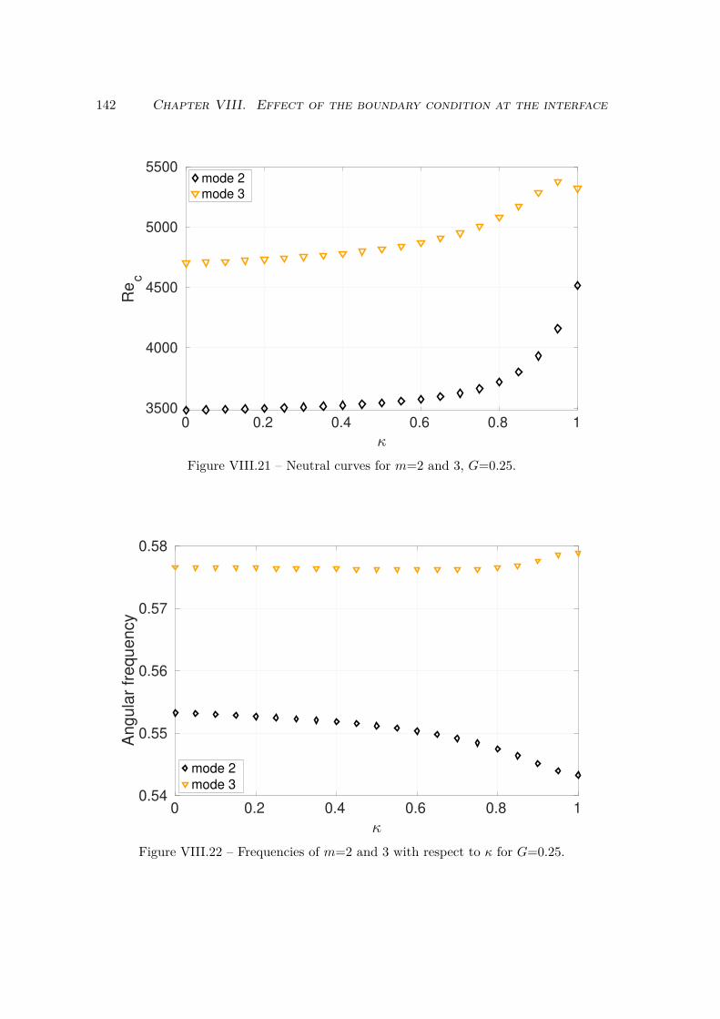
142 Chapter VIII. Effect of the boundary condition at the interface
0 0.2 0.4 0.6 0.8 1
3500
4000
4500
5000
5500
Re
c
mode 2
mode 3
Figure VIII.21 – Neutral curves for m=2 and 3, G=0.25.
0 0.2 0.4 0.6 0.8 10.54
0.55
0.56
0.57
0.58
An
gu
lar
fre
qu
en
cy
mode 2
mode 3
Figure VIII.22 – Frequencies of m=2 and 3 with respect to κ for G=0.25.

VIII.2 Hybrid modelling 143
-1 -0.5 0
( )
-3
-2.5
-2
-1.5
-1
-0.5
()
Figure VIII.23 – Evolution of eigenvalues of the mode m=3, for G=0.25 and Re=Rec.Three values of κ are superposed : 0.9 in blue, 0.95 in green, and 1 in orange. The red
spot circles the most unstable value for the three cases.
(a)
0 0.2 0.4 0.6 0.8 11910
1920
1930
1940
1950
1960
1970
1980
1990
Re
c
(b)
0 0.2 0.4 0.6 0.8 10.157
0.1575
0.158
0.1585
0.159
0.1595
0.16
0.1605
An
gu
lar
fre
qu
en
cy
Figure VIII.24 – Neutral curve (VIII.24a) and evolution of frequency (VIII.24b)regarding κ for m=4 and G=2.
an exponential-like increase of their respective slopes. However, their variations are veryrestricted : Rec evolves less than 4%, while variation of f is only 2%. Previous ob-servations of small differences in vorticity pattern between the free surface (κ=0) andthe frozen surface (κ=1) conditions, led us believe in the existence of a second unstablebranch. However this parametric study denies this possibility.
Conclusion on the Robin conditionThe hybrid model, initially built for a better understanding of the evolution of the
flow between free and frozen conditions, revealed a much more complex transition thanexpected. It highlighted the existence of a second unstable branch for large value of κ,which explains the difference in axial vorticity patterns at the surface. However, no valueof κ allowed for significant progress in the reduction of the discrepancy with experimental

144 Chapter VIII. Effect of the boundary condition at the interface
Rec and f , and the frozen surface still appears to be most "favourable" case.
Note that the computations for G=1/14 where done with a hub : it is only afterthat all the simulations required for the neutral curve VIII.17 were performed that theinfluence of the hub was tested on an other mode than m=5, and that we realized that itwas responsible for the swap of the most unstable mode. However, as the Robin conditionwas not convincing, and that simulations without hub would obviously not lower Rec, itwas deemed necessary to correct this part. According to results in table VIII.1, we canestimate that the only probable effect would be a small shift of Rec and f values, whichwould have lead to a slight vertical distortion of curves in figures VIII.17 and VIII.18.
Although it was learnt from smallest aspect ratios that the Robin condition was notrepresentative of the real surface, the parametric study was still performed for G=2.It confirms the almost stable behaviour of Rec and f for a given mode, whatever thecondition at the surface, and the absence of another unstable branch. This explains thatthe agreement between numerics and experiments is easier of obtain for higher aspectratios.

Chapter IX
Surface tension gradient as a bound-ary condition
145

146 Chapter IX. Surface tension gradient as a boundary condition
The mismatches reported in chapter VI do not seem to have a connection with dis-placements of the rotating disc, but appear to be partially cancelled by the applicationof the raw frozen surface condition in chapter VIII. The results are convincing enough toconsider that simulations with a free slip condition are not representative of the flow inour laboratory experiments. However, the simulations that show the best agreement withexperiments were performed with the frozen surface condition, which can hardly be ex-perimentally justified... The relative failure of the Robin condition to find an intermediatevalue of κ that would solve this paradox contrasts with the discovery of the second unsta-ble branch, that exists even for non completely frozen surface. This nuance is a tenuoushope for a surface boundary condition that could be compatible with experimental obser-vations of the surface, and that would give rise to the right unstable branch. Thereforethe exploration of the influence on the flow of the condition at the surface was pursuedwith a more complex model. Considering that the surface tension varies with the ran-dom deposition of ambient air pollution, a convection diffusion equation is used in ordermodelize the concentration of these pollutants at the interface. However, the difficultywas to close the model with a link between unknown concentrations of pollutants andthe velocity field. The sparkle came from the article [41], where the authors numericallyreproduced the experience in [38]. There, an insoluble surfactant was voluntarily addedonto the surface. This surfactant was clearly identified, and its concentration carefullycontrolled. More details on theses articles are given below.
In our case, we have no clue of the pollution type, nor its concentration. Indeed, it isnot in our ambition to know the precise chemical composition of the pollutants involved.Our objective was to build a model based on [41], but that would be independent of anychemical species. Such a model has to verify at least two empirical hypotheses :
• Only a small amount of pollutants is sufficient to reduce the Rec drop.
• The value of Rec is almost constant on an undetermined span of pollutants quantity.
The first point is easily understandable : even if we suspect pollutants to play the samerole as a surfactant, our experiment is not covered by dust, and the surface appears cleanalthough no vacuum is made around it. The second point comes from the reproducibilityof experiments. Indeed, the atmosphere is not controlled in experiments, and thus, thequantity of pollutants can not be considered as a constant for every experiments realized.Yet, for a given G, the value of Rec determined with LDV was almost invariant from oneexperiment to another.
Surface tension and surfactant
Surface tension is a phenomenon linked to microscopic interactions between moleculesat the surface of a liquid. Fluids adapt the shape of their surface in order to minimize thesurface area, and their energy. At the air-water interface, the cohesion forces (attractionof liquid particles between each other) are stronger than adhesion forces (attraction ofliquid particles by air particles). This leads to an elastic behaviour of the interface. Thesame competition happens on solid-liquid boundaries, and are responsible for the contact

IX.1 Surface tension and surfactant 147
angles, and thus for the shape of the interface.
Figure IX.1 – Water drops on a leaf keep a spherical shape thanks to surface tension,instead of spreading on the leaf.
Surface tension can be lowered by the addition of a surface-active compound, calledsurfactants. Figure IX.2 illustrates behaviour of surfactant regarding its concentration.The hypothesis we made was that pollutants act macroscopically like a small concentra-tion of surfactants, and thus, stay at the surface (only a negligible amount of pollutantis advected in the bulk). This hypothesis is reasonable as experiments are clean enoughto not see any pollutant cluster. Micelles are clusters of surfactant particles that createa macroscopic structure. They occur only under strong enough surfactant concentrationsand are found in the bulk of the fluid, not at the interface.
Measurement of surface tension can be done in many ways. Traditional methodsconsist in evaluating the force required to detach an object delicately pulled out of theimmobile surface of a liquid layer. This item can be a ring (De Noüy method), a needle(De Noüy-Padday method) or a plate (Wilhelmy method). Other solutions use drops, byevaluating the maximum length of the boundary between a drop and a vertical tube fromwhere it falls (pendant drop method). Despite all of these existent methods, no solutionexists to evaluate dynamically the evolution of the surface tension.
Water is known to be very sensitive and its surface tension is easily modified from theclassical value of 72.8 10−3N.m−1 (at 20°C). The surface tension influence was evaluatedexperimentally. As we were not able to guarantee the ideal value of surface tension, wechoose to heavily lower it with the addition of a small amount of surfactant (drop ofdishwashing liquid). No difference in Rec was found, and therefore, the role of surfacetension was initially neglected. Note that the experiment with dishwashing liquid wasdone with Kalliroscope.

148 Chapter IX. Surface tension gradient as a boundary condition
Figure IX.2 – For low concentration, surfactant are concentrated at the interface (left).With the increase of the concentration, surface is saturated, and surfactant are absorbed(middle). Once the fluid is saturated, surfactant particles gather themselves in micellarstructure (right). This means that the concentration of surfactant is above the critical
micellar concentration (CMC).
Bibliography
The aim of this complementary bibliography is not to provide an overview of studieson surfactants and colloids, but to introduce some papers that feed upcoming thoughts.In every articles, authors employ the Boussinesq-Scriven surface fluid model for a New-tonian gas/liquid interface so that the surface stress tensor Ss is
Ss = (σ + (κs − µs)∇s · us)1s + 2µsDs
where κs is the surface dilatational viscosity, µs is the surface shear viscosity, σ is theequilibrium surface tension, us is the surface velocity vector, ∇s is the surface gradientoperator, 1 is the tensor that projects any vector onto the surface, and
2Ds = ∇sus · 1s + 1s · (∇sus)T .
The first article considered here was published by Lopez and Chen in 1998 ([72]).The authors used an ad hoc closure model between surfactant concentration and surfacetension based on the tangent function :
σ − σi = − δπ
tan−1(βc− cici
)where σ and c are the dimensional surface tension and concentration, respectively,
while σi and ci are the reference surface tension and concentration, respectively. δis the saturation surface pressure, and β is a non-dimensional parameter, defined asβ=−πci∂σ/(δ∂c). This modelling allows for a study of the influence of the pollutantconcentration at the surface of a flow driven by a rotating disc, in a cylindrical cavity, i.e.the exact same configuration as ours, but with an aspect ratio G=2.5. The conclusion isthat even a small amount of contaminant can influence both interfacial and bulk flow.

IX.1 Surface tension and surfactant 149
In 2000, Lopez and Hirsa, considered an annular channel to study the coupling betweenthe bulk flow and an interface in the presence of an insoluble surfactant ([70]). This time,the autors used a closure equation based on the hyperbolic tangent :
σ = 1 + a1σc
tanh(a2(1− c))
where σ is the dimensionless surface tension, σc=66 mN.m−1 is a characteristic sur-face tension, and c is the dimensionless surfactant concentration. a1=6.3 and a2=6.2 aretwo parameters used to fit the model to experimental measurements with Hemicyanine.Among the profiles published in this article, those on the radial velocity at the surfacereveals that ur tends to zero everywhere along the surface while the surfactant concen-tration is increasing : authors wrote that “Marangoni stress makes the interface act likea no-slip condition“.
Using the same configuration as in [70], Hirsa et al. published in 2001 experimentalresults of velocity fields for various concentrations of K1 vitamin at the surface ([39]).This insoluble surfactant was used for its zero value surface shear viscosity µS on theconsidered range of concentration. In this article, the experimental approach is followedby a numerical comparison where another closure equation was used to link the pollutantconcentration and the surface tension. This closure equation was this time based on theexponential function :
σ(c) = a2 + a3c+ a4c2
1 + exp(a0a1 − a1c)+ a5 + a6c
2
1 + exp(a1c− a0a1)
where σ and c are respectively the dimensional surface tension and the dimensionedconcentration of surfactant at the interface. Parameters a0 to a1 are dimensional pa-rameters to fit the experimental data (see below, fig. IX.3). Results show a very goodagreements between numerics and experiments. This paper was followed by a second one,from the same authors, on the use of the annular channel flow to determine the surfaceshear viscosity µS ([71]).
Still using K1 vitamin monolayer, Vogel & al ([38]) studied macroscopic and micro-scopic patterns at the surface of a flow driven by a rotating disc located at the bottom ofa fixed cylindrical cavity, for G=0.25. Rec in presence of K1 vitamin is estimated between1900 and 2000, with an azimuthal wavenumber m=3, i.e. the same threshold than Lopezet al. in [37].
The previous article is at the origin of the publication [41], by Kwan and Shen. Thecore of the paper is a study of the mathematical background behind the experiment ofVogel et al., using the same closure equation as Hirsa et al. ([39]). The authors give theTaylor expansion of this model :
σ(c) ∼ 72.4− 4.2× 10⁻¹³c− 0.15c2 − 6.5× 10⁻¹¹c3 − 4.95× 10⁻¹⁰c4 − 3× 10⁻⁹c5 + ....

150 Chapter IX. Surface tension gradient as a boundary condition
Besides this equation, the main interest for us is in the two last pages, with the resultsof a simulation with the same closure model than [71]. For G=0.25 and c0=0.4 mg.m−2,Rec was estimated at 1050. With the free surface condition, this Rec was 3481, accordingto ROSE computation. Although not commented by the authors, and more than theRec drop, the most interesting result is the unstable mode predicted in their simulation :for c0=0.4 mg.m−2 the first one to growth is m=3, in agreement with[35] and our ownexperiments, while all our previous computations predicted m=2.
In a different configuration - a micro channel with super hydrophobic surface - Peaude-cerf et al., explain how pollutants can gradually change the boundary condition from freeslip to no slip ([73]) . The main interest of a micro channel is to create an air cushionbetween the wall and the liquid. As a consequence, the friction on the wall is so reducedthat it is almost a free slip. But in presence of pollutant, this slipping effect is cancelledand the drag can be even more important than in the case of the simple wall.
The last element of the bibliography was published in 2017, by Bandi et al.. In thispaper ([74]), authors demonstrated that for concentrations less than 15% of the criticalmicellar concentration (CMC), the flow is dominated by adsorbed surfactant. This means,that there is no diffusion of the surfactant inside the bulk for small concentration. TheCMC corresponds to the concentration of pollutant beyond which pollutant clusters (seefigure IX.2).
These articles reveal that for a small amount of surfactant, which could be atmosphericpollution, only the surface boundary condition has to be modified, compared to the idealpollutant-free surface. But this sole modification is sufficient to generate a heavy evolutionof the bulk flow. However, none of the previous authors explored the influence of thesurfactant, and, by extension, pollutant, on potential instability thresholds.
New boundary conditions in z = G
Since surface tension σ is no longer assumed constant, equations (IV.8) and (IV.10)are no longer valid. At the surface, the balance of surface force is :∫
Sn · SdA =
∫C
n · Ssdl (IX.1)
where S is the same stress tensor than in section Dynamic boundary conditions, Ssis the surface stress tensor and n is a normal vector to the surface. For Ss, we usea Boussinesq-Scriven model, where the surface dilatational viscosity κs and the surfaceshear viscosity µs are neglected. As a consequence, Ss is reduced to Ss = σ1. Using theStokes theorem (see appendix A), one can write :∫
Cn · Ssdl =
∫S
[∇sσ − σn(∇s · n)]dA. (IX.2)
Here, ∇s is the surface gradient operator, defined as ∇s = (1− n⊗ n) · ∇, since σ isonly defined at the interface. Under the flat surface hypothesis, we have n = ez, and thusσn(∇S · n) = 0. Besides, considering that S is an arbitrary surface, the surface stressbalance can be reduced to :

IX.1 Surface tension and surfactant 151
ez · S = ∇sσ
Therefore, the new boundary conditions at the surface are :∂ur∂z
= 1µ
∂σ
∂r
∂uθ∂z
= 1µr
∂σ
∂θ,
which can be respectively non-dimensionalized as :∂ur∂z
= 1Ca
∂σ
∂r∂uθ∂z
= 1Ca
1r
∂σ
∂θ.
Ca = µΩRσ0
is the capillary number, and σ0 is the reference surface tension. Note thatit is not required to apply the condition on ∂uθ/∂z to the base flow, as it is axisymmetric.The impermeability of the surface is conserved, and thus we keep the same condition onuz :
uz = 0
Closure equationThe main idea behind this model is the connection between the pollutants concentra-
tion c at the surface, and the surface tension σ. Thus, an equation that links these twoquantities has to be postulated in order to close the system. The equation used here isdirectly derived from [39] and [41].
There, the authors used the sophisticated model IX.1.1. We choose to start from theTaylor expansion IX.1.1 of this model, since its derivation is simpler and allows for aneasier implementation into ROSE. Actually, a closer look at the equation IX.1.1 revealsthat the c2 term is predominant. Therefore we only use this leading term of the Taylorexpansion, which comes down to :
σ = σ0(1− α
2σ0c2) (IX.5)
where α=0.3 is a dimensional parameter specific to the surfactant. Such models are bynature dedicated to one specific specie. In our experiment, no surfactant was added on thesurface and the pollution is not the result of only one pollutant. Therefore, the previousexpression needed to be modified in order not to have any α dependency. Consideringthe dimensionless form of equation (IX.5)
σ = 1− α
2σ0C2
0 c2, (IX.6)
where σ = σ/σ0, and c = c/C0, and

152 Chapter IX. Surface tension gradient as a boundary condition
Figure IX.3 – Comparison between modelization of σ(c) and experimental data for K1vitamin. Figure extracted from [71].
β = 1Ca
αC20
σ0. (IX.7)
Equation (IX.6) can be rewritten as
σ = 1− 12Caβc
2. (IX.8)
Combining (IX.8) and (IX.4) gives the boundary condition depending on c instead ofσ :
∂ur∂z
= −βc∂c∂r
∂uθ∂z
= −βcr
∂c
∂θ.
Convection-Diffusion equation at the surface
To compute the pollutant concentration, a convection-diffusion equation is added atthe surface. Since the amount of pollutant is supposed small enough (C0 CMC),pollutant is only advected along the surface and not into the bulk ([74]). The convection-diffusion equation is :
∂c
∂t= ∇ · (D∇c)−∇ · (vc) + F
Here, D is the diffusivity of the surfactant, v is the velocity field, and F representsthe volume sources. Since no chemical reaction is considered, F = 0, and D is assumedconstant. According to [75], since c is only defined at the surface, previous equation canbe rewritten as :

IX.1 Surface tension and surfactant 153
∂c
∂t+∇s · (vc) = D∆sc,
where ∇s is the surface operator defined previously, and ∆s = ∇s2 . Consideringonly the divergence part, and decomposing v into components along the surface, us andnormal to the surface (v · n)n, one can write :
∇s · (vc) = ∇s · (cus) +∇s · ((cv · n)n)
We remind that we made the hypothesis of a flat free surface, thus n = ez, andv · n = uz = 0 at the surface. As a consequence, the latest expression reduces to
∇s · (vc) = ∇s · (cus).
Finally the convection-diffusion equation can be simplified to :
∂c
∂t+∇s · (cus) = D∆sc,
and non-dimensionalized as :
∂c
∂t+∇s · (cus) = 1
Pe∆sc, (IX.9)
Pe is a Péclet number, defined here as Pe = ωR2
Ds . In the upcoming chapter, all vari-ables are non-dimensionalized. Therefore, for a better reading, the notation . is dropped.
As written in chapter II, β can be seen as a ratio between a Marangoni number andthe Péclet number. Indeed, the Marangoni number is not based on temperature, but onconcentration, and therefore, the thermal diffusivity is replaced by the replaced by the dif-fusion coefficient. According to equation (IX.6), (αC0) ∝ ∂σ
∂C , and thus,Ma = (αC0)RC0µDs .
Using the definition of Péclet given above, the result of Ma/Pe is exactly (IX.7).
Base flow
We saw in chapter V that fields were decomposed according to a complex ansatz. Theconcentration c is treated the same way : c(r,θ,t) = C(r)+ε<(c∗(r)eλt+imθ). For the baseflow, that is steady and axisymmetric, ∂.∂t = 0 and ∂.
∂θ = 0. Thus, the convection-diffusionequation for the base flow becomes:
1r
∂(rCur)∂r
− 1Pe
1r
∂
∂r(r∂C∂r
) = 0. (IX.10)
A new boundary condition also has to be implemented. We previously wrote that nochemical reaction was considered and that the global concentration is supposed to remainconstant, which translates to :
1π
∫ 2π
0
∫ 1
0c(r,θ,t)rdrdθ = 1.
For the base flow, this constraint resumes to :

154 Chapter IX. Surface tension gradient as a boundary condition
2∫ 1
0C(r)rdr = 1.
Numerically, this condition is implemented on the node at r=1 in the coupled systemof equations otherwise undetermined. In r = 0 :
∂C
∂r= 0 (IX.11)
according to the symmetry at the axis. Note that all integrals are approximated inROSE using a trapezoidal rule, coherent with the second order approximation.
Perturbation
The equation for the perturbations of c can be deduced by subtracting (IX.10) from(IX.9). This leads to
−λc∗ = 1r
(∂rCu∗r
∂r+ ∂rUrc
∗
∂r) + imUθc
∗
r− mCu∗θ
r− 1Pes
(∂2c∗
∂r2 + 1r
∂c∗
∂r− m2c∗
r2 ).
The boundary conditions for the perturbations are different from those applied to thebase flow. Here, two cases must be distinguished. The first one is m=0, and the secondis m >0.
• m=0The mode m=0 is an axisymmetric mode. Thus, an equivalent condition to (IX.11)must be imposed to perturbations :
∂c∗
∂r= 0 at r= 0.
Then, the conservation of the concentration still have to be respected. For theperturbations, the constraint on the concentration is no more equal to 1, but to 0.
∫ 1
0c∗(r)rdr = 0 at r= R.
• m>0For m >0, perturbations are no longer axisymmetric. The only solution to avoid asingularity at r=0 is to impose c∗(r=0)=0, while at r = 1, no mass flux crosses thewall. Thus, it yields ∂c∗
∂r = 0.
Boundary conditions for velocities on wall and discNow that we have determined the boundary condition for c, we must set the boundary
conditions on velocity components. On the wall and on the disc, they are unchanged fromchapter IV : impermeability and no-slip condition lead to the same equations than IV.5and IV.6 :

IX.1 Surface tension and surfactant 155
ur = uθ = uz = 0
and ur = uz = 0uθ = r.
Validity and Validation
Before we realize an in-depth study on the considered aspect ratios, we verified theimplementation in ROSE and the validity of the first order closure equation, with acomparison to [39] and [41].
0 0.5 1 1.5
cdim
(mg.m-2
)
62
64
66
68
70
72
74
(d
yn
.cm
-1)
Taylor Expansion 1st
order
Taylor Expansion 5th
order
Full law
Figure IX.4 – Comparison of the first order Taylor expansion model, to fifth orderTaylor expansion and complete model from [39], corresponding to figure IX.3.
One can see from figure IX.4 that 1st and 5th order Taylor expansions match perfectly.Therefore, there is no need to code such a high order in ROSE. However, the gap withthe complete closure equation quickly increases after c=1 mg.m−2. This correspond tothe beginning of the transition to a second plateau, where σ saturates to a lower value.The fact that our model does not capture this behaviour means that the value of σ inour computations remains close to σ0 even for very large values of c, (and thus of β). Asit will be seen in this chapter, the small variations of σ allowed by our model are alreadysufficient to highlight the influence of the condition at the interface.
We now validate this new version of ROSE. We compare first Ur(r) and C(r) profilesin z = G, computed on a 401 × 101 grid, to data from [41] (G=0.25, Re=1000). ThePéclet number is set to 1000, and β=0.663.

156 Chapter IX. Surface tension gradient as a boundary condition
0 0.2 0.4 0.6 0.8 1
r
-0.12
-0.1
-0.08
-0.06
-0.04
-0.02
0
0.02
ur
Kwan 2010
ROSE
0 0.2 0.4 0.6 0.8 1
r
0
0.5
1
1.5
C
ROSE
Kwan & Shen 2010
Figure IX.5 – Comparaison of baseflow radial velocity Ur (left) and concentration C(rigth) at the surface (z = G), for G=0.25,β=0.663 and Re=1000.
According to figure IX.5 the agreement is excellent on the base flow between ROSEand the DNS from [41]. Minor gaps appear, which can be attributed to inaccuracy of thedata from [41], as it was extracted directly on the graph.
For the same parameters, the authors report that the flow loses its stability aroundRec=1050, via a supercritical Hopf bifurcation. The primary instability at this value ofRe displays an azimuthal wavelength m=3. A computation with ROSE gave Rec=908.This represents a gap of 13.5% with [41]. Note that in this article, the authors used aDNS code based on a spectral method. They did not provide any explanation on howthey determined the value of Rec. They only indicated that "the base flow remains stableup to about Re=1050".
Effect of pollutant concentration
In the same way we explored the influence of κ on Rec for the Robin condition in theprevious chapter, we now perform a parametric study of Rec(β). For G=1/14, the resultswere highly positive. A soon as β was larger than 0.14, Rec drops below 3000; and staysclose to this value for β up to 5. Similarly to the Robin condition, two unstable branchescross at a codimension 2 point. The frequencies for β ≥2.5, are close to the experimentalvalue of f . More details were given in chapter II, and except for the comparison of baseflows and the verification of the selected value of the Péclet number made for G=1/14,the rest of this chapter is dedicated to the application of the pollutant model to G >1/14.
Discussion on the Péclet number
The Péclet number that appears in equation IX.9 is arbitrary set to 1000, followingthe value given in [71] and [41]. This number compares convection effects (r2ω) to dif-fusion (D). In water, D ≈ 10−5 cm2.s−1 at 298 K. For a rotation rate of 1 rpm inour smallest cavity, which represent the smallest value for convection, r2ω ≈0.2 cm2.s−1,and then Pe ≈2*104. As the minimum experimental value of Pe is twenty times largerthan the numerical one, one may question the validity of this approximation. Therefore,we computed the base flow for seven Péclet numbers, at Re=10000, for β=0.3 and for

IX.2 Effect of pollutant concentration 157
G=1/14. The results are exhibited in figures IX.6a and IX.6b.
(a)
0 0.2 0.4 0.6 0.8 1
-0.16
-0.14
-0.12
-0.1
-0.08
-0.06
-0.04
-0.02
0
Pe = 10
Pe = 50
Pe = 100
Pe = 500
Pe = 1000
Pe = 5000
Pe =10000
(b)
0 0.2 0.4 0.6 0.8 10
0.5
1
1.5
Pe = 10
Pe = 50
Pe = 100
Pe = 500
Pe = 1000
Pe = 5000
Pe =10000
Figure IX.6 – Influence of the Péclet number on Ur(r) (left) and C(r) (right) in z= G,for G=1/14, β=0.3 and Re=10000.
For Pe <1000, the variation in velocity profile (IX.6a) and in concentration profile(IX.6b) at the surface are obvious : the increase of Pe straightens the pollutant frontat r ≈0.82, and increases the radial velocity gradient ∂ur/∂r at the same radius. ForPe >1000, this evolution is not that marked, and profiles for Pe ≥5000 even merge.Differences between Pe=1000 and larger values are not signifiant, and therefore, thisapproximation on Pe appears coherent. Moreover, the high values of the Péclet numberimpose to increase the grid resolution to compensate the stronger gradients.
G=1/14
In chapter II, no direct comparison of the effect of β on the base flow with LDV profileswas made. Therefore, the influence of β on both ur and uθ is detailed in this section.
Figure IX.7a focuses on uθ. The effect of β is evident as soon as β ≥ 0.5. Indeed, theovershoot in r=[0.68,0.69] completely vanishes for such values. Actually, the overshoot isno longer present as soon as β ≈ 0.2. Despite the fact that this evolution came for lowvalues of β, ROSE base flow gets closer to LDV profile only for β ≥ 4.
This last observation is corroborated by figure IX.7b. In this figure, as in figureIX.7a, the curves for β=4 are very close to the frozen surface velocity profile and tothe experimental profile. The large gap between experimental points and simulations forr=[0.5,0.8] is probably caused by the imperfect verticality of the laser. If the two lasersbeams are not in the same vertical plan, the LDV device capture a projection of uθ. Sincethe amplitude of uθ is much larger than that of uz, even a small projection of uθ caninfluence uz measurement. This is coherent with the slope observed in experimental datain figures IX.7b.

158 Chapter IX. Surface tension gradient as a boundary condition
(a) uθ in z=0.8G
0.5 0.6 0.7 0.8 0.9 1
r
0
0.1
0.2
0.3
0.4
0.5
0.6
0.7
0.8
u
LDV
ROSE free surface
ROSE frozen surface
ROSE =0.1
ROSE =0.5
ROSE =2
ROSE =4
(b) uz in z=0.5G
0.5 0.6 0.7 0.8 0.9 1
r
-0.06
-0.04
-0.02
0
0.02
0.04
0.06
uz
LDV
ROSE free surface
ROSE frozen surface
ROSE =0.1
ROSE =0.5
ROSE =2
ROSE =4
Figure IX.7 – Comparison of ROSE base flow for four different values of β, with theLDV measurements introduced in previous chapters, for G=1/14 and Re=18620. Notethat the three different colors for uz LDV data belongs to three different experiments.

IX.2 Effect of pollutant concentration 159
G=0.25
For G=0.25, the focus is on m=2 and 3, since they are azimuthal wavenumbers forwhich mismatches between numerics and experiments were observed : ROSE predicts amost unstable mode m=2 at Rec=3481 while our experiments, in agreement with [37],exhibits a m=3 azimuthal wavenumber at Rec ≈2000. The application of the frozen sur-face condition did not solve this contradiction. However, we saw in figure IX.5 that forthe base flow, ROSE displayed a good agreement with [41], where authors numericallyreproduce experiments at G=0.25. Therefore we can expect our pollutant model to havea value of Rec closer to experiments.
First, the base flows for various β are compared with LDV profile in figure IX.8. Forβ as low as 0.1, the overshoot on uθ, which existed for the free surface condition, disap-pears. However, the best agreement between the base flow and the LDV profile is onlyobtained for β ≥ 1.85. After this value, the base flow does not evolve much, and is almostindistinguishable with the profile obtained for the frozen surface condition (figure IX.8a).Concerning the azimuthal velocity component, the fitting is obtained as soon as β ≥ 1.25.Above this value, the computed profiles are completely merged with the profil obtainedwith the frozen surface condition (figure IX.8b).
The results for Rec(β) are introduced in figure IX.9. One can see a behaviour close towhat was previously observed form=5 in the case G=1/14 : Rec curves for bothm=2 and3 present a cusp, followed by a drop of Rec. As commented previously, this correspondsto a jump to a second unstable branch, highlighted in figure IX.10 by a discontinuity inthe frequency of the most unstable mode. For m=2 this occurs at β=1.25, and at β=0.25for m=3. It is also for β=0.25 and Rec=4000 that m=3 become the most unstable modeand remains it up to β=0.75 and Rec=1000. Rec of both modes are then very close, upto β=1.6, where the gap is increasing. It is interesting to remind that in [37], the authorsnoted that a mode m=2 grew first when lower quality water was used : in figure IX.9 onemay suggest that this observation correspond to the interval β ∈ [1; 2] where m=2 is themost unstable mode. But this seems to be unlikely, since the results for G=1/14 tend toshow that velocity profiles from experiments performed with distilled water match withnumerics only for β >4 (see figure IX.7).
The most important feature of the figure IX.9 are represented by the gray triangles.This "buckle" delimits a range of parameters (β,Re), inside which the flow is unstable.For a given β - lets keep β=4 - one can see that for Re ∈ [0; 1334], the flow is stable.Then for Re ∈ [1334; 2793] the mode m=3 is unstable. However increasing Re stabilizethe flow up to Re=4614, where the mode m=2 becomes unstable. This evolution can beput in parallel to the experimental sequence displayed in figures VI.20a and VI.21 : inthis experiment, the mode m=3 was visible around Re=2150, before the flow restabilizesfor Re ≈3700 and becomes axisymmetric. It evolves to an ellipse for Re ≈4930, and thento a undefined pattern for Re ≈5240. The mode m=2 then grows for Re ≈5545. Thesesexperimental thresholds are not very accurate, but still, the similarities with the simula-tion are sticking. Moreover, the undefined pattern, kind of a mix between m=2 and m=3,could find the beginning of an explanation in the vicinity of the modes 2 and 3 for β=4

160 Chapter IX. Surface tension gradient as a boundary condition
(a) uθ in z=0.8G
0 0.2 0.4 0.6 0.8 1
r
0
0.1
0.2
0.3
0.4
0.5
u LDV
ROSE frozen surface
ROSE free surface
ROSE =0.1
ROSE =0.5
ROSE =1.25
ROSE =1.85
(b) uz in z=0.5G
0 0.2 0.4 0.6 0.8
r
-0.1
-0.05
0
0.05
0.1
uz
LDV
Free surface
Frozen surface
ROSE =0.1
ROSE =0.5
ROSE =1.25
ROSE =1.85
Figure IX.8 – Comparison of ROSE base flow for four different value of β, with the LDVmeasurements introduced in previous chapters, for G=0.25 and Re=1895.

IX.2 Effect of pollutant concentration 161
0 1 2 3 4 50
1000
2000
3000
4000
5000
6000
7000R
ec
Figure IX.9 – Neutral curves Rec(β) for modes m=2 (circles) and m=3 (triangles), inthe case G=0.25. The changing in the colors for a given mode represents the different
branches of each mode.
and Re ≈4900. Like for G=1/14, the critical Reynolds number of the most unstable modedoes not evolve much for β >5 : for β =5, Rec=1421, while for β=100, Rec=1832. Thisrepresents a variation of 29% of Rec for an increase of 1900% of β. Interestingly, and oncegain, like for G=1/14, the Rec value for β ≥100 agrees even better with the experimentalRec : the error with values reported in table VI.6 and in page 93 are between 2% and 13%.
For β ≥4.9 and Re >6500, another branch appears for m=3 (blue triangles). It isreported as a different branch, but note that it can be the continuation of the first one(in green), according to its frequency (see figure IX.10).
Discontinuities in frequencies are less marked than for G=1/14. For both modes thegap between the frequency for β=0 (free surface) and β=0.75 is less than 2%. Therefore,no experimental measurement can confirm which branch is actually growing in experi-ments, since the gap between their respective frequencies is of the same order of magnitudethan the experimental uncertainty.
G=1.5
We previously observed a variation in the most unstable mode between free and frozensurface conditions, from m=1 to 4 respectively. We expect to observe the same behaviourwith the increase of β. However, experiments shown many frequencies, and therefore, we

162 Chapter IX. Surface tension gradient as a boundary condition
0 1 2 3 4 50.5
0.55
0.6
0.65
0.7
0.75
0.8A
ng
ula
r fr
eq
ue
ncy
Figure IX.10 – Frequencies f(β) of modes m=2 and m=3, associated to curves in figureIX.9.
did not restrict our study to the lone m=1 and m=4, but we included all modes from 0to 5, in order to find a match with experimental data. Grid used here was 201×301.
As we anticipated, figure IX.12 reveals that the mode m=4 become more unstablethan m=1. However we did not forecast that this would happen for such a low β value :transition occurs between β=0 and β=0.05, and this does not evolve any more up to β=1.Therefore, we can expect the mode m=4 to be the first mode to growth in experiments.On the contrary to lower aspect ratio detailed previously, only two others modes presenta jump of unstable branch on the selected β span. Indeed modes m=2 and m=3 evolvequietly, without discontinuity. The axisymmetric mode m=0 jumps on a second unstablebranch between β=0.05 and β=0.1, while the transition form=1 only takes place betweenβ=0.8 and β=0.85. Above these values, Rec for m=1 is close to be perfectly constant,around 2600.
These jumps are emphasized in figure IX.12 by the discontinuity of the respective fre-quencies of these modes. Apart from that, figure IX.12 does not show the same tortuousfrequency curves than for lower G : for every modes from 0 to 5, frequencies are almostconstant, except when a jump of branch occurs. Figure IX.13 illustrates the switching ofeigenvalues for m=0.
The constant value of frequencies does not help much to find an agreement withexperimentally determined frequencies. We remind that Rec is only known to be above1820. Frequencies of oscillations occurring at Re=2180 and 2540 are m× f ≈0.48, which

IX.2 Effect of pollutant concentration 163
0 0.2 0.4 0.6 0.8 12000
2200
2400
2600
2800
3000
Re
c
mode 0
mode 1
mode 2
mode 3
mode 4
Figure IX.11 – Neutral curves Rec(β) for modes m=0 to m=1, in the case G=1.5.
0 0.2 0.4 0.6 0.8 1-0.2
-0.1
0
0.1
0.2
0.3
0.4
An
gu
lar
fre
qu
en
cy
mode 0
mode 1
mode 2
mode 3
mode 4
Figure IX.12 – Frequencies of modes 0 to 4, for G=1.5, at their respective Rec.

164 Chapter IX. Surface tension gradient as a boundary condition
-0.4 -0.3 -0.2 -0.1 0 0.1
( )
-0.4
-0.2
0
0.2
0.4
()
Figure IX.13 – Eigenvalues of m=0 at Re=Rec, for β=0.05 (in blue), and for β=0.15(orange), in the case G=1.5. For β=0.05, the most unstable eigenvalue has an imaginarypart =(λ)=±0.22, while for β=0.15, this eigenvalue becomes stable (<(λ) <0). A secondeigenvalue, with an imaginary part =(λ)=±0.34 becomes the most unstable. Red circles
highlight unstables eigenvalues.
does no match any of the frequencies in figure IX.12. We can notice that it is the onlyaspect ratio for which no frequency matching is observed. It is also the only aspect ratiowhere experiments of Rec findings were done in the small cavity. This set-up shows astrong presence of the main mode of vibration of the disc in measurements. Althoughthe stimulation of unstable modes by the disc rotation rate did not seem relevant, thepresence of non-negligible oscillation in velocity time series alters the threshold detectionand the evaluation of the frequency associated to Rec.
G=2
We already had a good agreement between experiments and numerics with the freesurface condition for G=2. The application of the frozen surface did not change the unsta-ble branch, and only increased the Rec from 1914 to 1987. Therefore, we only check, form=4, that Rec and f variations are negligible. Figure IX.14a confirms the Rec evolutionnotified for the frozen surface condition : we obtain the exact same values than the frozensurface condition.
According to figure IX.14b, the same conclusion can be applied to f , that only in-creases by 2% between β=0 and β=1. We can notice that both Rec and f are constantfor β ≥ 0.3. In any case, Rec and f are consistent with experimental measurements fromref. [35].

IX.2 Effect of pollutant concentration 165
(a)
0 0.2 0.4 0.6 0.8 11900
1920
1940
1960
1980
2000
Re
c
mode 4
(b)
0 0.2 0.4 0.6 0.8 10.157
0.1575
0.158
0.1585
0.159
0.1595
0.16
0.1605
An
gu
lar
fre
qu
en
cy
mode 4
Figure IX.14 – Neutral curve and evolution of frequency regarding β for m=4 and G=2.
Conclusion on the pollutant modelStarting from a surfactant model, we built a more generic model, not based on any
specific chemical specie. The main restriction of this model is the range of the controlparameter : its validity is probably limited to low concentrations of pollutant. However,this corresponds to the experimental condition we look to replicate.
The application of this model to G=1/14 gives four main results :
• The Rec of the most unstable mode, m=5 dropped below 3000 for β ≥ 0.15.
• Rec is almost constant whatever is the value of β above 0.15.
• The frequency is in better agreement with experimental measurements.
• Agreement on the base flow is better for β ≥4.
The application of this model to G=0.25, in order to check its range of application,also gives very convincing results, especially for β ≥ 2.08. Indeed, above this value, a newunstable branch has been discovered which has shed new light on our previous experi-ments for G=0.25. Although ROSE cannot be used to explore the non linear dynamics,the evolution observed in the experiment may be explained step by step with the neutralcurve IX.9. Moreover, the same asymptotic trend as for G=1/14 was observed in Rec forβ >5.
Regarding the largest aspect ratios, this model confirms the reduced influence of thesurface condition. Although we still notice a mode switching for G=1.5, from m=1 tom=4, both Rec and f have very restricted variations. Unfortunately, probable experi-mental issues do not allow us to conclude on any experimental match. Yet, experimentalagreement is excellent for G=2.
Globally, this model performs better than the free and frozen surface model : agree-ments between experiments and numerics for G=1/14 and G=0.25 are far better than

166 Chapter IX. Surface tension gradient as a boundary condition
they were, both with free and frozen model, while they remain excellent for G=2. Never-theless, it is still difficult to link the state of the surface to β, and thus to perform DNSwith the adequate value. The cost in time to perform the simulation is also increased.
Sensitivity to mixed conditions : a second glance on the frozeninterface condition
While we were working on the hybrid model, we experimented to apply a differentboundary condition on the base flow and on the perturbations, for the free and frozencases. The results obtained did not match any experimental results, and we only concludethat the most favourable combination of boundary condition for G=1/14 in order tolower Rec was to apply the frozen condition on the base flow and the free condition toperturbations. This set of boundary conditions is reported as "mixed condition". Theresults obtained using the most complex model including surface tension renewed theinterest for these previous numerical explorations. Results for G=1/14 have already beendiscussed in chapter II, and thus we mostly deal with aspect ratios from 0.25 to 2 in thissection. Still, it is reminded that for G=1/14, applying a frozen surface surface conditionto the base flow, and a free surface condition to perturbations led to a drop of Rec from17006 to 2776 for m=5, which is only 5.4% lower than the prediction of ROSE with thepollutant model (by comparison to Rec=2934, for β=5). This drop was also present form=4, with a final value of Rec equals to 2714, i.e. very close to m=5, which correspondsto observations with the pollutant model, although here m=4 is more unstable that m=5.
G=0.25
The frozen surface condition for G=0.25 was not satisfying, resulting in an increase ofRec. The most unstable mode was unchanged from simulation with free surface condition,and was m=2, which did not match the m=3 observed experimentally. As for G=1/14,we applied the mixed condition to G=0.25 : an initial calculation of the base flow with afrozen surface condition, followed by a computation of perturbations with the free surfacecondition, for both m=2 and m=3 azimuthal wave numbers. The results are shown intable IX.1.
m 2 3Rec 3625 1588f 0.540 0.620
Table IX.1 – Rec for m=2 and 3, andG=0.25, with mixed boundary
conditions.
m 2 3Rec 4293 1421f 0.548 0.625
Table IX.2 – Rec for m=2 and 3, andG=0.25, for β=5.
The first important observation concerns the most unstable mode : while the free, thefrozen, and the hybrid condition forecast thatm=2 grows first, the mixed condition is able
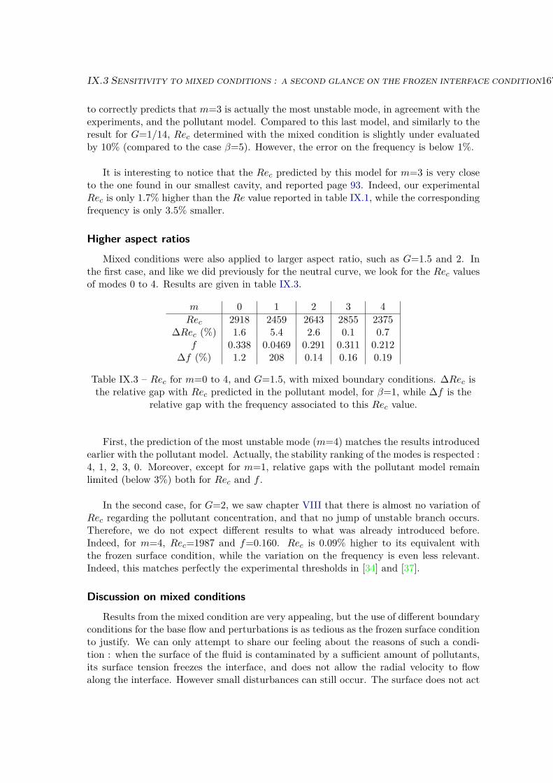
IX.3 Sensitivity to mixed conditions : a second glance on the frozen interface condition167
to correctly predicts that m=3 is actually the most unstable mode, in agreement with theexperiments, and the pollutant model. Compared to this last model, and similarly to theresult for G=1/14, Rec determined with the mixed condition is slightly under evaluatedby 10% (compared to the case β=5). However, the error on the frequency is below 1%.
It is interesting to notice that the Rec predicted by this model for m=3 is very closeto the one found in our smallest cavity, and reported page 93. Indeed, our experimentalRec is only 1.7% higher than the Re value reported in table IX.1, while the correspondingfrequency is only 3.5% smaller.
Higher aspect ratios
Mixed conditions were also applied to larger aspect ratio, such as G=1.5 and 2. Inthe first case, and like we did previously for the neutral curve, we look for the Rec valuesof modes 0 to 4. Results are given in table IX.3.
m 0 1 2 3 4Rec 2918 2459 2643 2855 2375
∆Rec (%) 1.6 5.4 2.6 0.1 0.7f 0.338 0.0469 0.291 0.311 0.212
∆f (%) 1.2 208 0.14 0.16 0.19
Table IX.3 – Rec for m=0 to 4, and G=1.5, with mixed boundary conditions. ∆Rec isthe relative gap with Rec predicted in the pollutant model, for β=1, while ∆f is the
relative gap with the frequency associated to this Rec value.
First, the prediction of the most unstable mode (m=4) matches the results introducedearlier with the pollutant model. Actually, the stability ranking of the modes is respected :4, 1, 2, 3, 0. Moreover, except for m=1, relative gaps with the pollutant model remainlimited (below 3%) both for Rec and f .
In the second case, for G=2, we saw chapter VIII that there is almost no variation ofRec regarding the pollutant concentration, and that no jump of unstable branch occurs.Therefore, we do not expect different results to what was already introduced before.Indeed, for m=4, Rec=1987 and f=0.160. Rec is 0.09% higher to its equivalent withthe frozen surface condition, while the variation on the frequency is even less relevant.Indeed, this matches perfectly the experimental thresholds in [34] and [37].
Discussion on mixed conditions
Results from the mixed condition are very appealing, but the use of different boundaryconditions for the base flow and perturbations is as tedious as the frozen surface conditionto justify. We can only attempt to share our feeling about the reasons of such a condi-tion : when the surface of the fluid is contaminated by a sufficient amount of pollutants,its surface tension freezes the interface, and does not allow the radial velocity to flowalong the interface. However small disturbances can still occur. The surface does not act

168 Chapter IX. Surface tension gradient as a boundary condition
like a rigid lid, but more like an elastic boundary, that accept small variations around anequilibrium state.
Right now, the segregation of boundary conditions can only be done in the linearstability analysis. However, modifications of the DNS code should allow for such im-plementation, and therefore, to obtain visualisations of vorticity patterns, to check thecoherence of such computed flows. However, eigenmodes computed with ROSE tend toget closer to the frozen unstable branch than to the free one, and one can have goodexpectations about upcoming 3D simulations.

Chapter X
Conclusion & outlooks
169

170 Chapter X. Conclusion & outlooks
Conclusion
The realisation of an experimental bench to undertake the study of a flow generatedby a rotating disc with a flat free surface initially brought more interrogations than an-swers. Indeed, a previous numerical study [42] had shown a very good agreement withformer experiments [40], especially on Rec and azimuthal wave number for G ≥ 1/14.But experiments in LIMSI’s cavity exhibit a primary instability for a Reynolds numbermuch lower than expected. The gap was non negligible : for G=1/14, experimental Recwas 75% smaller than predicted by the linear stability analysis.
As the agreement of numerical simulations with the IRPHE experiments was good(less than 5% gap), it was obvious that our bench had some flaw that forced instabilitygrowth. Various tests were run to identify this flaw : influence of the gap between thedisc and cavity wall, influence of viscosity, of markers, ..., without any result but theinconstant behaviour of Kalliroscope. We suggested that mechanical vibrations, from themotor, or bearings, may trigger instability prematurely. The decision to build a newexperimental set-up originates from such hypothesis. We intended to use electroactiveactuators to compensate for mechanical noise. The creation of the bench, and of its con-trol loop would required the expertise of GeePs laboratory, also involved in the project.In the long run, we expected to fully control this instability thanks to this demonstrator :avoid instability or select the first mode to grow.
Unfortunately, the analysis of vibrating modes of the disc did not indicate any match-ing with instability frequencies. Therefore, this hypothesis was quickly judged irrelevant.Moreover, forG=0.25, the experimental value ofRec did match with published results [37],where the same discrepancies between numerics and experiments were noticed. Again,we faced a deadlock.
Nevertheless, we did fully start afresh. All previous failures in the identification ofdiscrepancies causes delineate a path. Indeed, we gave a new interest to a single com-putation of the flow, using a boundary condition suggested in [69]. Although the Recbetween this simulation from ROSE and experiment still differ from 60%, the use of newtools highlighted unexpected conclusions. Indeed, DNS computation allows visualisationsof axial vorticity pattern that reveal to be closer to experiments snapshots. Moreover,the access to LDV device definitely confirms that previous simulations did not reproducethe right flow, and that previous agreements with experiments were serendipitous. Rightnow, the focus of the thesis slips from vibrations of the bottom of the cavity, to inability ofthe free surface condition to replicate in simulations the effective condition at the interface.
However, we were only at the beginning of the road : the first alternative to free sur-face condition, that consisted in freezing the radial velocity at the surface, did not provideany quantitative agreement neither for G=1/14, nor G=0.25. This last case seemed evenmore problematic, as even the predicted mode in simulations did not match the exper-imental one... Therefore, we experimented successive boundary conditions on G=1/14,while other aspect ratio were mostly used for validation.

X.1 Conclusion 171
To understand how the transition in the flow between the free and frozen surfacecondition happens, we introduced a simple model, built as a linear interpolation betweenthe two previous boundary conditions. This translates as a Robin condition on the radialvelocity at the interface, monitored by a new parameterkappa. Although the progress on the reduction of Rec was limited, this modelling allowsto discover a new unstable branch for a given mode. This new branch appeared in a betteragreement with experiments. Moreover, this branch already existed for κ <1, i.e. for anon-completely frozen surface, which was more coherent with experimental observations.We now had to find a way to catch this branch to a lower Reynolds.
After few unsuccessful tries to modify the Robin condition in order to lower the criticalReynolds number, the reading of articles on the influence of a Langmuir monolayer on aflow motivated to implement a much more complex model into our linear stability analysiscode. Under the hypothesis of low pollutant concentration at the surface, no pollutantpenetrates the bulk. Therefore, using a 2D convection-diffusion equation, we modelledthe variations of pollutant concentration at the interface. Then, a closure equation linkedthe surface tension to pollutants concentrations. We chose a simple approach, decoupledfrom any specific chemical species, with a quadratic dependence of the surface tension onthe concentration. The independence of the model regarding the nature of the pollutantwas a key point of the creation of this model : in experiments, we had no clue about theprecise chemical composition of the interface. Thus, in the model, the state of the surfaceis governed by a new control parameter, β. This closure equation proved sufficient for therange of values of β considered.
The results of this model went beyond our expectations. Firstly, we observed a mas-sive drop of Rec for a low β value. This Rec then showed an asymptotic behaviour up tothe limit of validity of β and even beyond. This plateau explains well the reproducibilityseen in experiments, although the laboratory atmosphere was not controlled. The corre-sponding value of Rec is 40% smaller than the experimental threshold, for G=1/14. Thefrequency of the eigenmode also better match LDV measurements.
The application of the model to G=0.25 has made possible to predict for the firsttime the mode m=3 as the most unstable. The neutral curve is even more tortuous thanfor G=1/14 : similarly to this case, the drop of Rec appears after the crossing of twounstable branches. However, and on the contrary to the case G=1/14, this new mostunstable branch does not seem to have an asymptotic behaviour for the highest β val-ues considered. Indeed this asymptotic behaviours was observed by a third branch, thatdefines a "bubble" of instability, and that may explain the evolution of the flow in theexperiments, while Re in increased.
The pollutant model did not only show motivating results. It also gave a new interestto a series of four simulations done one year before. Initially, they were performed toidentify the role of the frozen surface on Rec, whether this condition was applied to thebase flow or to perturbations. We found that the lowest Rec was obtained for a "frozen"base flow, whereas perturbations were computed with a free surface condition. However,at this time, this Rec was not judged relevant. Surprisingly it matches with the results

172 Chapter X. Conclusion & outlooks
of the pollutant model for sufficiently large β. Therefore, the mixed boundary conditionwas reconsidered : could it be a simple and time-saving solution to compute this flow ?Indeed, the agreements for G=1/14 are confirmed by the excellent results for G=0.25 :not only does the mixed condition model give a good agreement on Rec, but it is alsoable to predict m=3 as the most unstable mode.
Larger aspect ratios were also experimented, although our cavity is limited to G=1.5.Quickly we suggested that the surface condition has a very low impact on such G. Com-putations tends to confirm this. Despite the low variation of Rec and f , we still observedfor G=1.5 a switching of the most unstable mode with the pollutant model. This switchis also present in the mixed condition model, that gave astonishing agreement with resultsfrom the more complex model based on the concentration of a pollutant at the interface.
To conclude on our work in this thesis, we may simply say that we demonstratethat the standard free surface condition is not able to effectively represent the air-waterinterface. One suggested to change the fluid, since water is well-known for its sensitivecondition at the interface. Yet experiment proved that results were not that erratic.After sweeping through various models, we finally were able to propose a solution thatanswer the discrepancies observed between experiments and numerics that existed fora rotating flow with an air-water interface. Although this solution remains perfectible,it confirms that very small surface tension variations are at the origin of discrepanciesbetween numerics and experiments.

X.2 Outlooks 173
OutlooksAs for many research work, any single answer brings dozen of new interrogations. In-
deed, although we attempted to gather in this thesis the largest spectrum of investigationson the role of surface tension on the studied instability, there is much left to do.
In the direct continuation of this work, it would be interesting to implement thepollutant model and the mixed condition model into the DNS code. This would allowfor visualizing instability patterns, and to compare each others to experimental pictures.Both models also have to tested on other aspect ratios. Since publications are not legion,this means modifying the experimental set-up to study higher G values, to avoid opticalissue with LDV, and even to plan the realisation of PIV measurements.
About the large aspect ratios, experimental difficulties limited our field of analysis,although many possibilities are offered. Thanks to the effectiveness of the linear stabilityanalysis code, it would be interesting to draw the curve of Rec versus G, i.e. to extendthe figure 3. of [43] to larger values of G, and to determine for which aspect ratio theinfluence of the surface state vanishes.
Very small aspect ratios are also very complex to study experimentally, mostly be-cause of the uncertainty on the height the fluid. But such G values always display heavydiscrepancies between numerics and experiments. Therefore, a new glance at these aspectratios could be very interesting, especially for the validation of our models.
Another plain outlook is to find a connection between the abstract β parameter andthe effective concentration of pollutants. To do so, experiments with controlled concen-tration of surfactant are to be considered. With a strict experimental protocol, in orderto get initially a surface as clean as possible, and an accurate determination of Rec, onemay observe the variation of Rec regarding the surfactant concentration, and thus checkthe fitting with the neutral curve obtained with the pollutant model.
On the contrary, one may consider changing the fluid in experiments, for another one,less sensitive to surface tension gradient, such as silicon oil. Doing so should make itpossible to obtain experimental Rec values closer to those predict with the free surfacecondition.
Finally, we wonder whether the surface state still plays a role on the value of Recof the instability that occurs at high Froude number, with a heavy surface deformation.Implementing a model such as the pollutant based one represent a consequent work : theconvection-equation, although still applied to the surface only, is no longer 2D. Indeed,since the surface is no longer flat, normal vector is no longer merged with ez, but willdepend on both ez and er. In addition, the code has to track the surface deformation.This last modification was already done in [51].

174 Chapter X. Conclusion & outlooks

Appendix A
Stokes theorem
In this appendix we detailed the mathematical process to go from equation (IX.1) toequation (IX.2), using the Stokes theorem. We remind that this theorem writes :∫
CF · d` =
∫S
n · (∇∧ F)dS
where n is the normal vector so the surface S.
Along the contour C, d` = md`, where m is a normal vector to the contour C.Therefore, the equation above can be rewritten :∫
CF ·md` =
∫S
n · (∇∧ F)dS.
If we note F = f ∧ b, where b in an arbitrary constant vector, we obtain :∫C
(f ∧ b) ·md` =∫S
n · (∇∧ (f ∧ b))dS.
Using identities (f ∧ b) ·m = −b · (f ∧m) and ∇∧ (f ∧ b) = f(∇ · b)− b(∇ · f) + b ·∇f − f · ∇b = −b(∇ · f) + b · ∇f), the previous equation becomes :
b ·∫C
(f ∧m)d` = b ·∫S
[n(∇ · f)− (∇f) · n] dS.
Since b is arbitrary, this equation can be simplified to :∫C
(f ∧m)d` =∫S
[n(∇ · f)− (∇f) · n] dS.
In our case, we have f = σn, and since n ∧m = −s, we can write−∫Cσsd` =
∫S
[n∇ · (σn)−∇(σn) · n] dS
=∫S
[n∇σ · n + σn(∇ · n)−∇σ − σ(∇n) · n] dS.
Since ∇σ is necessary tangent to the surface S, we have ∇σ · n = 0. In addition,(∇σ) · n = 1/2∇(n · n) = 1/2∇(1) = 0 and thus we finally access to the desired result :
175

176 Appendix A. Stokes theorem
∫Cσsd` =
∫S
[∇σ − σn(∇ · n)] dS

Appendix B
Evaluation of the error
Experiments are always subject to a finite accuracy because of uncertainty on dimen-sions or measurements. Besides the errors made in the LDV measurements, that are hardto estimate because many factors are not quantified (such as gap to ideal horizontality,distance to zero, non ideal cylindricity and coaxiality of both cylinder wall, distance toideal zero ...) we can quantify the error made on the experimental Rec and G.
For G, only two variables are considered : the cavity radius R and the height of thefluid H. For R, tolerance are given in table B.1. H is evaluated with a graduated steelruler, in the middle of the cavity to prevent the meniscus on the wall to alter measurement.The rule is graduated every 0.5 mm and thus the error is included between 0 and 0.5 mm.For G=1/14, in the largest cavity, this leads to an uncertainty of 5%. The method tomeasure H may appear archaic and inaccurate, especially for very small G, however,regarding the gap between experiments and numerics reported in chapters II and VI, itwas not our priority to develop a method to obtain a better evaluation of H. Note thatin [37], cavity dimensions correspond to G, and therefore are filled up to the top. ForG=0.25, their cavity also have a 5% tolerance on H. If we note ∆G the variation of G,we have :
∆G = ∆(H
R
)= ∆H
R+ H∆R
R2
As we are interested in the relative variation ∆G/G, we can simplify the previousexpression as :
∆GG
= ∆HH
+ ∆RR
Thus, the final estimation of the relative error made on G is the sum of relative errorson R and H, and worth 5.1% in the largest cavity, and 5.3% in the smallest cavity.
In the same way, Re depends on R, Ω and ν. The uncertainty on Ω is given by theoscillations of the tension provided by the tachometer. According to table B.1, oscillationsremains limited, and the tension is known within ±1mV . As no rotation rate thresholdis below 1 rpm, maximum error on Ω is only 2.2%.
177
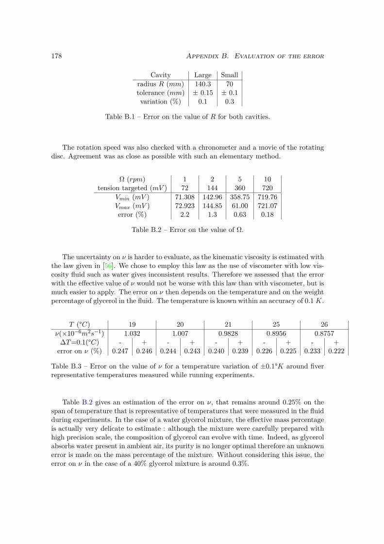
178 Appendix B. Evaluation of the error
Cavity Large Smallradius R (mm) 140.3 70tolerance (mm) ± 0.15 ± 0.1variation (%) 0.1 0.3
Table B.1 – Error on the value of R for both cavities.
The rotation speed was also checked with a chronometer and a movie of the rotatingdisc. Agreement was as close as possible with such an elementary method.
Ω (rpm) 1 2 5 10tension targeted (mV ) 72 144 360 720
Vmin (mV ) 71.308 142.96 358.75 719.76Vmax (mV ) 72.923 144.85 61.00 721.07error (%) 2.2 1.3 0.63 0.18
Table B.2 – Error on the value of Ω.
The uncertainty on ν is harder to evaluate, as the kinematic viscosity is estimated withthe law given in [56]. We chose to employ this law as the use of viscometer with low vis-cosity fluid such as water gives inconsistent results. Therefore we assessed that the errorwith the effective value of ν would not be worse with this law than with viscometer, but ismuch easier to apply. The error on ν then depends on the temperature and on the weightpercentage of glycerol in the fluid. The temperature is known within an accuracy of 0.1K.
T (°C) 19 20 21 25 26ν(×10−6m2s−1) 1.032 1.007 0.9828 0.8956 0.8757
∆T=0.1(°C) - + - + - + - + - +error on ν (%) 0.247 0.246 0.244 0.243 0.240 0.239 0.226 0.225 0.233 0.222
Table B.3 – Error on the value of ν for a temperature variation of ±0.1°K around fiverrepresentative temperatures measured while running experiments.
Table B.2 gives an estimation of the error on ν, that remains around 0.25% on thespan of temperature that is representative of temperatures that were measured in the fluidduring experiments. In the case of a water glycerol mixture, the effective mass percentageis actually very delicate to estimate : although the mixture were carefully prepared withhigh precision scale, the composition of glycerol can evolve with time. Indeed, as glycerolabsorbs water present in ambient air, its purity is no longer optimal therefore an unknownerror is made on the mass percentage of the mixture. Without considering this issue, theerror on ν in the case of a 40% glycerol mixture is around 0.3%.

179
As we did for the division earlier, we can demonstrate that ∆(R2Ω = 2∆R/R+∆Ω/Ω,and thus :
∆ReRe
= 2∆RR
+ ∆ΩΩ + ∆ν
ν
Finally, the relative error on Re values is around 2.7% in the largest cavity, and 3.1%in the smallest cavity. These errors are optimistic, but we can reasonably think thatexperimental Reynolds numbers are known with ≈ 5% accuracy.

180 Appendix B. Evaluation of the error

Appendix C
LDV corrections
This appendix is dedicated to details about the optical corrections applied to LDVmeasurement. [53]. Note that the notations used here do not correspond to the nomencla-ture. Indeed, optical standards were kept, such as λ for the wavelength, and n for opticalindices. Since corrections are not the same depending on whether the measurement ismade on uθ or uz, both configurations are considered below.
In the second case (uz measurement), the laser beams lie in the same meridionalplane, and normal vectors to interface are parallels. Thus Snell-Descartes laws give :nasin(θa/2) = ncsin(θc/2) = nwsin(θw/2) where the indices a, c & w stand for air, cavityand water, respectively. Starting from equation (III.1), and considering that θa/2 = θL isthe angle made by beams in the absence of interface crossing, we easily obtain :
fr2up
= 2sin(θa/2)λa
= 2sin(θw/2)λw
. (C.1)
with λi = f/(nic), where c is the speed of light in vacuum and i index is relative tothe medium crossed.
Here, crossing various media has no influence on the values of the measured velocity,and only the position of measurement is shifted. However in the first case (uθ measure-ment), curvature effect affects the measurement : since normal straight lines to inner andouter walls are no longer parallel, equation (C.1) does not hold any more. Therefore acorrection coefficient Cθ has to be applied.
Cθ = up,realup,measured
(C.2)
where up,measured is estimated relatively to θa/2, while up,real, should consider θw/2.Starting from equation (III.1), we can write :
up,measured = frλa2sin(θa/2) ,
up,real = frλw2sin(θw/2) . (C.3a)
181

182 Appendix C. LDV corrections
θa
θw
Figure C.1 – Illustration of effective path of laser beams (red plain lines) in the verticalconfiguration (uz measurement). Red doted lines are the hypothetical path of beams ifthere was only one medium. Black plain lines are inner and outer walls of the cavity.Dark blue and green doted lines are normals to the inner wall and the outer wall,respectively. The cyan plain line is the axis of symmetry. Angles are not to scale.
Thus, from equations (C.2) and (C.3a), it quickly comes :
Cθ = nasin(θa/2)nwsin(θw/2)
With these corrections, the LDV measurements give us instantaneous velocity signalin one point of the flow, through a selected time scope. The post-processing on thesesignals can return average and RMS velocities, or frequencies of oscillations that exist invelocity signals, owing to Fourier transform. An example of differences that exist in LDVmeasurements between corrected and uncorrected data is given in figure C.3.
The LDV device is able to detect particles for radius that are "outside" the cavity, asshown in figure C.3, which confirms the need for a correction. However, the theoreticalcorrection places the zero at r <1. This under-evaluation was also observed only purewater, and with both glass (see fig. VI.32) and plexiglass walls. Error is probably causedby inaccurate refraction indices, for fluids, cavity or both of them.

183
θwθa
Figure C.2 – Illustration of effective path of laser beams (red plain lines) in thehorizontal configuration (uθ measurement). The color code is the same as in figure C.1.
Note that normals cross at the center of the cavity.
0 0.2 0.4 0.6 0.8 1
r
0
0.1
0.2
0.3
0.4
0.5
u
Figure C.3 – Comparaison of corrected (blue) and raw (orange) uθ LDV profile, forG=0.25 and Re=1895. The fluid used was a 40% glycerol mixture, in the large plexiglas
cavity.

184 Appendix C. LDV corrections

Internet sources
• Figure .1 : https://svs.gsfc.nasa.gov/vis/a010000/a012500/a012550.
• Figure .2 : https://qph.fs.quoracdn.net/main-qimg-9c91ac489ef9f25bb14140897dd827a7.
• Figure .3 : https://thesis.library.caltech.edu/1143/.
• Figure .4 : http://www.earthscienceguy.com/2019/03/kelvin-helmholtz-clouds-caused-by-wind.html.
• Figure .6 : http://lgef.insa-lyon.fr/fr/content/materiaux-electro-actifs.
• Figure .7 : https://www.sciencedirect.com/science/article/pii/S0889974616304121.
• Figure I.7b : https://twitter.com/kevinmgill/status/948253930596712448.
• Figure III.4 : https://physics.stackexchange.com/questions/317051/michelson-interferometer-circular-fringes.
• Figure III.6 : https://www.compadre.org/advlabs/wiki/Taylor-Couette_Flow.
• Figure IV.1 : https://www.newscientist.com/article/dn14030-liquid-mirror-telescopes-are-a-reality-at-last/.
• Figure VII.6 : https://astropassion-jc.pagesperso-orange.fr/precession.html.
• Figure IX.1 : https://clairegogendeau.wixsite.com/tpe-bdc/la-tension-superficielle.
• Figure IX.2 : https://m.tau.ac.il/ phchlab/exp-tension-theory.html.
185

186 Appendix C. LDV corrections

Bibliography
[1] V. W. Ekman, “On the influence of the Earth’s rotation on the ocean-currents,”Arkiv. Mat. Astr. Fys., vol. 2, no. 11, pp. 1–52, 1905.
[2] T. von Kármán, “Über laminare und turbulente Reibung,” Z. Angew. Math. Mech.,vol. 1, pp. 233–252, 1921.
[3] R. J. Lingwood, “Absolute instability of the Ekman layer and related rotating flows,”J. Fluid Mech., vol. 331, pp. 405–428, 1997.
[4] G. K. Batchelor, “Note on a class of solutions of the Navier-Stokes equations repre-senting steady rotationally-symmetric flow,” Q. J. Mech. Appl. Math., vol. 4, pp. 29–41, 1951.
[5] K. Stewartson, “On the flow between two rotating coaxial disks,” Proc. Camb. Phil.Soc., vol. 49, pp. 333–341, 1953.
[6] H.-O. Kreiss and S. V. Parter, “On the swirling flow between rotating coaxial disks :Existence and nonuniqueness,” Comm. Pure Appl. Math., vol. 36, pp. 55 – 84, 011983.
[7] D. Peckham and S. Atkinson, Preliminary results of low speed wind tunnel tests ona gothic wing of aspect ratio 1.0. Royal Aircraft Establishment, 1957.
[8] N. Lambourne, D. Bryer, and A. R. C. (G.B.), The Bursting of Leading-edge Vortices:Some Observations and Discussion of the Phenomenon. Reports and memoranda /Aeronautical Research Council, H.M. Stationery Office, 1962.
[9] H. Vogel, “Experimentelle Ergebnisse über die laminare Strömung in einem Zylin-drischen gehause mit darin rotierender Scheibe.,” Tech. Rep., pp. Max–Planck Insti-tute, 1968.
[10] H. J. Lugt and H. J. Haussling, “Axisymmetric vortex breakdown in rotating fluidwithin a container,” J. Appl. Mech, vol. 49, pp. 921–923, 11 1982.
[11] M. P. Escudier, “Observations of the flow produced in a cylindrical container by arotating end wall,” Exp. Fluids, vol. 2, pp. 189–196, 1984.
[12] A. Spohn, M. Mory, and E. Hopfinger, “Observations of vortex breakdown in an opencylindrical container with a rotating bottom,” Exp. Fluids, vol. 14, pp. 70–77, 1993.
187

188 BIBLIOGRAPHY
[13] E. Serre, M. Schäfer, and P. Bontoux, Vortex breakdown in a cylinder with a freesurface, pp. 1125 – 1127. Oxford: Elsevier Science Ltd, 2003.
[14] E. Serre and P. Bontoux, “Vortex breakdown in a cylinder with a rotating bottomand a flat stress-free surface,” Int. J. Heat Fluid Flow, vol. 28, pp. 229–248, 2007.
[15] M. Piva and E. Meiburg, “Steady axisymmetric flow in an open cylindrical containerwith a partially rotating bottom wall,” Phys. Fluids, vol. 17, no. 6, p. 063603(12),2005.
[16] R. Iwatsu, “Numerical study of flows in a cylindrical container with rotating bottomand top flat free surface,” J. Phys. Soc. Jpn., vol. 74, pp. 333–344, 01 2005.
[17] H. Niino and N. Misawa, “An experimental and theoretical study of barotropic in-stability,” J. Atmos. Sci., vol. 41, no. 12, pp. 1992–2011, 1984.
[18] A. C. B. Aguiar, P. L. Read, R. D. Wordsworth, T. Salter, and Y. H. Yamazaki, “Alaboratory model of Saturn’s north polar hexagon,” Icarus, vol. 206, no. 2, pp. 755– 763, 2010.
[19] A. Y. Gelfgat, “Primary oscillatory instability in a rotating disk-cylinder systemwith aspect (height/radius) ratio varying from 0.1 to 1,” Fluid Dyn. Res., vol. 47,p. 035502(14), 2015.
[20] O. Daube and P. Le Quéré, “Numerical investigation of the first bifurcation for theflow in a rotor-stator cavity of radial aspect ratio 10,” Computers & Fluids, vol. 31,pp. 481–494, 2002.
[21] G. Gauthier, Étude expérimentale des instabilités de l’écoulement entre deux disques.PhD thesis, Université Paris XI, France, 1998.
[22] H. Goller and T. Ranov, “Unsteady rotating flow in a cylinder with a free surface,”J. Basic Eng., vol. 90, no. 4, pp. 445–452, 1968.
[23] A. Siginer and R. Knight, “Swirling free surface flow in cylindrical containers,” J.Eng. Math., vol. 27, no. 3, pp. 245–264, 1993.
[24] J. Mougel, D. Fabre, and L. Lacaze, “Waves in Newton’s bucket,” J. Fluid Mech.,vol. 783, pp. 211–250, 2015.
[25] G. H. Vatistas, “A note on liquid vortex sloshing and Kelvin’s equilibria,” J. FluidMech., vol. 217, pp. 241–248, 1990.
[26] G. H. Vatistas, J. Wang, and S. Lin, “Experiments on waves induced in the hollowcore of vortices,” Exp. Fluids, vol. 13, pp. 377–385, 1992.
[27] T. R. N. Jansson, M. P. Haspang, K. H. Jensen, P. Hersen, and T. Bohr, “Polygonson a rotating fluid surface,” Phys. Rev. Lett., vol. 96, p. 174502, 2006.
[28] T. Suzuki, M. Iima, and Y. Hayase, “Surface switching of rotating fluid in a cylinder,”Phys. Fluids, vol. 18, p. 101701(4), 2006.

BIBLIOGRAPHY 189
[29] Y. Tasaka and M. Iima, “Flow transitions in the surface switching of rotating fluid,”J. Fluid Mech., vol. 636, pp. 475–484, 2009.
[30] L. Tophøj, J. Mougel, T. Bohr, and D. Fabre, “Rotating polygon instability of aswirling free surface flow,” Phys. Rev. Lett., vol. 110, p. 194502, May 2013.
[31] J. Mougel, D. Fabre, L. Lacaze, and T. Bohr, “On the instabilities of a potentialvortex with a free surface,” J. Fluid Mech., vol. 824, pp. 230–264, 2017.
[32] J. M. Hyun, “Flow in an open tank with a free surface driven by the spinning bottom,”J. Fluids Eng., vol. 107, no. 4, pp. 495–499, 1985.
[33] R. Iwatsu, “Analysis of flows in a cylindrical container with rotating bottom and topunderformable free surface,” JSME Int. Journ., vol. 47, no. 3, pp. 549–556, 2004.
[34] D. L. Young, H. J. Sheen, and T. Y. Hwu, “Period-doubling route to chaos for aswirling flow in an open cylindrical container with a rotating disk,” Exp. Fluids,vol. 18, pp. 389–396, 1995.
[35] A. H. Hirsa, J. M. Lopez, and R. Miraghaie, “Symmetry breaking to a rotating wavein a lid-driven cylinder with a free surface: Experimental observation,” Phys. Fluids,vol. 14, no. 6, pp. 29–32, 2002.
[36] R. Miraghaie, J. M. Lopez, and A. H. Hirsa, “Flow induced patterning at the air–water interface,” Phys. Fluids, vol. 15, no. 6, pp. L45–L48, 2003.
[37] J. M. Lopez, F. Marques, A. H. Hirsa, and R. Miraghaie, “Symmetry breaking infree-surface cylinder flows,” J. Fluid Mech., vol. 502, pp. 99–126, 2004.
[38] M. J. Vogel, R. Miraghaie, J. M. Lopez, and A. H. Hirsa, “Flow-induced patterningof langmuir monolayers,” Langmuir, vol. 20, pp. 5651–4, 08 2004.
[39] A. H. Hirsa, J. M. Lopez, and R. Miraghaie, “Measurement and computation ofhydrodynamic coupling at an air/water interface with an insoluble monolayer,” J.Fluid Mech., vol. 443, pp. 271–292, 2001.
[40] S. Poncet and M. Chauve, “Shear-layer instability in a rotating system,” J. FlowVisual. Image Process., vol. 14, no. 1, pp. 85–105, 2007.
[41] Y. Kwan, J. Park, and J. Shen, “A mathematical and numerical study of incompress-ible flows with a surfactant monolayer,” Discrete Contin. Dyn. S., vol. 28, pp. 181–197, 2010.
[42] L. Kahouadji, Analyse de stabilité linéaire d’écoulements tournants en présence desurface libre. PhD thesis, Université Pierre et Marie Curie, Paris, France, October2011.
[43] L. Kahouadji, L. M. Witkowski, and P. Le Quéré, “Seuils de stabilité pour un écoule-ment à surface libre engendré dans une cavité cylindrique tournante à petit rapportde forme,” Mécanique et Industries, vol. 11, pp. 339–344, 2010.

190 BIBLIOGRAPHY
[44] S. J. Cogan, K. Ryan, and G. J. Sheard, “Symmetry breaking and instability mech-anisms in medium depth torsionally open cylinder flows,” J. Fluid Mech., vol. 672,pp. 521–544, 2011.
[45] N. Cousin-Rittemard, O. Daube, and P. Le Quéré, “Description des couches lim-ites des écoulements stationnaires interdisques en configuration rotor–stator,” C. R.Acad. Sci., Ser. II b, vol. 327, pp. 215–220, 1999.
[46] C. Nore, L. M. Witkowski, E. Foucault, J. Pécheux, O. Daube, and P. L. Quéré,“Competition between axisymmetric and three-dimensional patterns between exactlycounter-rotating disks,” Phys. Fluids, vol. 18, p. 054102, 2006.
[47] L. Martin Witkowski, I. Delbende, P. Le Quéré, and J. S. Walker, “Axisymmetricstability of the flow between two exactly counter-rotating disks with large aspectratio,” J. Fluid Mech., vol. 546, pp. 193–202, 2006.
[48] E. Pélissier, “Mesures et calculs de la déformation d’une surface libre engendrée parun disque en rotation,” Master’s thesis, Université Pierre et Marie Curie, France,2012.
[49] A. Faugaret, “Détermination expérimentale des seuils d’instabilité d’un écoulementengendré par un disque tournant en présence d’une surface libre,” Master’s thesis,Université Pierre et Marie Curie, France, 2013.
[50] A. Faugaret, “Étude des instabilités de l’écoulement engendré par un disque tournanten présence de surface libre : Confrontation expérimentale et numérique,” stage M2,Université Pierre et Marie Curie, France, 2014. 15 avril – 15 septembre.
[51] W. Yang, Études expérimentales et numériques d’écoulements tournants à surfacelibre déformable. PhD thesis, Université Pierre et Marie Curie, Paris, France, Décem-bre 2018.
[52] F. Moisy, T. Pasutto, and M. Rabaud, “Instability patterns between counter-rotatingdisks,” Nonlinear Process. Geophys., vol. 10, 05 2003.
[53] S. G. Huisman, D. P. van Gils, and C. Sun, “Applying laser Doppler anemometryinside a Taylor–Couette geometry using a ray-tracer to correct for curvature effects,”Eur. J. Mech. B/Fluids, vol. 36, pp. 115–119, 2012.
[54] K. Takamura, H. Fischer, and N. R. Morrow, “Physical properties of aqueous glycerolsolutions,” J. Petrol. Sci. Eng., vol. 98-99, pp. 50 – 60, 2012.
[55] G. P. Association, Physical Properties of Glycerine and Its Solutions. GlycerineProducers’ Association, 1963.
[56] N.-S. Cheng, “"formula for the viscosity of a glycerol-water mixture",” Ind. Eng.Chem. Res., vol. 47, pp. 3285–3288, 05 2008.
[57] D. Borrero-Echeverry, C. J. Crowley, and T. P. Riddick, “Rheoscopic fluids in apost-kalliroscope world,” Phys. Fluids, vol. 30, no. 8, p. 087103, 2018.

BIBLIOGRAPHY 191
[58] M. A. Dominguez-Lerma, G. Ahlers, and D. S. Cannell, “Effects of “kalliroscope”flow visualization particles on rotating couette-taylor flow,” Phys. Fluids, vol. 28,no. 4, pp. 1204–1206, 1985.
[59] P. Matisse and M. Gorman, “Neutrally buoyant anisotropic particles for flow visual-ization,” Phys. Fluids, vol. 27, no. 4, pp. 759–760, 1984.
[60] L. Kahouadji, B. C. Houchens, and L. M. Witkowski, “Thermocapillary instabilitiesin a laterally heated liquid bridge with end wall rotation,” Phys. Fluids, vol. 23,p. 104104(16), 2011.
[61] G. Ryskin and L. Leal, “Numerical solution of free-boundary problems in fluid me-chanics. part 1. the finite-difference technique,” J. Fluid Mech., vol. 148, pp. 1–17,1984.
[62] G. Ryskin and L. Leal, “Numerical solution of free-boundary problems in fluid me-chanics. part 2. buoyancy-driven motion of a gas bubble through a quiescent liquid.,”J. Fluid Mech., vol. 148, pp. 19–35, 1984.
[63] G. Ryskin and L. Leal, “Numerical solution of free-boundary problems in fluid me-chanics. part 3. bubble deformation in an axisymmetric straining flow,” J. FluidMech., vol. 148, pp. 37–43, 1984.
[64] L. N. Trefethen, A. E. Trefethen, S. C. Reddy, and T. A. Driscoll, “Hydrodynamicstability without eigenvalues,” Science, vol. 261, no. 5121, pp. 578–584, 1993.
[65] W. Yang, I. Delbende, Y. Fraigneau, and L. Martin Witkowski, “Large axisymmetricsurface deformation and dewetting in the flow above a rotating disk in a cylindricaltank: spin-up and permanent regimes,” Phys. Rev. Fluids, 2019. submitted.
[66] R. Bouffanais and D. Lo Jacono, “Transitional cylindrical swirling flow in presenceof a flat free surface,” Computers & Fluids, vol. 38, pp. 1651–1673, 2009.
[67] M. Le Bars and P. Le Gal, “Experimental analysis of the stratorotational instabilityin a cylindrical couette flow,” Phys. Rev. Lett., vol. 99, p. 064502, Aug 2007.
[68] N. Abcha, N. Latrache, F. Dumouchel, and I. Mutabazi, “Qualitative relation be-tween reflected light intensity by kalliroscope flakes and velocity field in the couette–taylor flow system,” Exp. Fluids, vol. 45, pp. 85–94, Jul 2008.
[69] A. Spohn and O. Daube, “Recirculating flows in a cylindrical tank,” in V Int. Conf.Computational Methods and Experimental Measurement (A. Sousa, C. A. Brebbia,and G. M. Carlomagno, eds.), (Montreal), pp. 155–166, Elsevier, July 1991.
[70] J. M. Lopez and A. H. Hirsa, “Surfactant-influenced gas–liquid interfaces: Nonlinearequation of state and finite surface viscosities,” J. Colloid Interface Sci., vol. 229,no. 2, pp. 575 – 583, 2000.
[71] A. H. Hirsa, J. M. Lopez, and R. Miraghaie, “Determination of surface shear viscosityvia deep-channel flow with inertia,” J. Fluid Mech., vol. 470, pp. 135–149, 2002.

[72] J. M. Lopez and J. Chen, “Coupling between a viscoelastic gas/liquid interface anda swirling vortex flow,” J. Fluids Eng., vol. 120, pp. 655–661, 12 1998.
[73] F. J. Peaudecerf, J. R. Landel, R. E. Goldstein, and P. Luzzatto-Fegiz, “Traces ofsurfactants can severely limit the drag reduction of superhydrophobic surfaces,” Proc.Natl. Acad. Sci, vol. 114, no. 28, pp. 7254–7259, 2017.
[74] M. M. Bandi, V. S. Akella, D. K. Singh, R. S. Singh, and S. Mandre, “Hydrodynamicsignatures of stationary Marangoni-driven surfactant transport,” Phys. Rev. Lett.,vol. 119, p. 264501, 2017.
[75] H. Stone, “A simple derivation of the time-dependent convective-diffusion equationfor surfactant transport along a deforming surface,” Phys. Fluids, vol. 2, pp. 111–112,1990.


Antoine FAUGARET 25 septembre 2020
Sujet : Influence de la condition à l’interface air-eau sur la stabilitéd’un écoulement tournant : exploration numérique et
experimentale.
Résumé : Notre étude porte sur la première instabilité qui apparait dans un écoulement engen-dré par un disque tournant au fond d’une cavité cylindrique fixe, avec une interface liquide-gaznon déformée. Grace à la double approche numérique et expérimentale, nous révélons un écartimportant sur le seuil d’apparition de cette instabilité. Après avoir supposé et infirmé que desvibrations d’origine mécanique puissent être responsables de ces écarts, notre étude s’est orientéesur l’influence de la condition limite à l’interface utilisée dans les simulations. Nous montronsque la condition de glissement libre ne permet pas de simuler le même écoulement que dansles expériences. Dans le but de réduire ces différences, nous explorons successivement plusieursmodélisations de cette interface. La prise en compte des variations de la tension de surface enfonction de la concentration d’un polluant à l’interface à notamment permis de réduire consid-érablement l’erreur commise sur le nombre de Reynolds critique, et de reproduire plus fidèlementl’écoulement dans les simulations.
Mots clés : Ecoulement tournant, tension de surface, simulation, DNS, analyse de stabilitélinéaire, condition limite à l’interface air-eau, expérimental, vibrations, LDV
Subject : Influence of air-water interface condition on rotating flowstability : experimental and numerical exploration.
Abstract: Our study focuses on the first instability that appears in a flow generated by a rotatingdisc placed at the bottom of a fixed cylindrical cavity, with a flat liquid-gas interface. Owing tothe dual numerical and experimental approach, we highlight a robust mismatch on the thresholdof this instability. After having assumed and later ruled out that mechanical vibrations could beresponsible for these mismatches, this investigation has focused on the boundary condition usedin simulations at the interface air-water and its influence on the flow. We show that the freeslip condition does not allow to simulate the same flow as in the experiments. Several models ofthis interface are explored in order to reduce the mismatches. In particular, taking into accountvariations in surface tension depending on the concentration of a pollutant at the interface resultsin a considerable reduction of the error on the critical Reynolds number, and to a more accuratereproduction of the flow in the simulations.
Keywords : Rotating flow, surface tension, simulation, DNS, linear stability analysis, boundarycondition at the air/water interface, experimental, vibrations, LDV