Senior Thesis in Mathematics

Infiniteness and LinearTemporal Logic:

Soundness, Completeness, & Decidability

Author:Eric Hayden Campbell

Advisor:Dr. Michael Greenberg

Submitted to Pomona College in Partial Fulfillmentof the Degree of Bachelor of Arts

April 12, 2017,Minor Revisions: July 13, 2017

Abstract

In this thesis, we present sound and complete axiomatic framework for LinearTemporal Logic over finite traces (LTLf ), as well as a decision procedure.This is founded on the work on LTL of [21, 14, 25, 24], and the specific workon LTLf in [8, 9, 4]. Our approach follows the least fixpoint method for LTLgiven in [21], using insights about finitude presented in [25, 24]. Finally, thecompleteness of LTLf extends the partial completeness proof for TemporalNetkat to a full completeness result.

Contents

1 Introduction 1

1.1 Syntax . . . . . . . . . . . . . . . . . . . . . . . . . . . . . . . 2

1.2 Classical Logic: Semantics . . . . . . . . . . . . . . . . . . . . 5

1.3 A Proof System . . . . . . . . . . . . . . . . . . . . . . . . . . 7

1.4 Soundness and Completeness . . . . . . . . . . . . . . . . . . . 9

2 Linear Temporal Logic 13

2.1 Background for Linear Temporal Logic . . . . . . . . . . . . . 16

2.1.1 Assumptions . . . . . . . . . . . . . . . . . . . . . . . . 16

2.1.2 Applications . . . . . . . . . . . . . . . . . . . . . . . . 17

2.2 Classical Formulation . . . . . . . . . . . . . . . . . . . . . . . 19

3 Linear Temporal Logic over finite traces 23

3.1 Syntax of LTLf . . . . . . . . . . . . . . . . . . . . . . . . . . 24

3.2 Semantics for LTLf . . . . . . . . . . . . . . . . . . . . . . . . 24

3.3 Axiomatization of LTLf . . . . . . . . . . . . . . . . . . . . . 30

3.4 Completeness for LTLf . . . . . . . . . . . . . . . . . . . . . . 33

3.5 A Decision Procedure for LTLf . . . . . . . . . . . . . . . . . 47

4 Related Work, Applications and Further Directions 59

4.1 Insensitivity to Infiniteness . . . . . . . . . . . . . . . . . . . . 59

4.2 Coinductive Completeness . . . . . . . . . . . . . . . . . . . . 61

4.3 An Extension to the Past . . . . . . . . . . . . . . . . . . . . . 62

4.4 Network Applications . . . . . . . . . . . . . . . . . . . . . . . 65

4.5 Further Directions . . . . . . . . . . . . . . . . . . . . . . . . 67

4.6 Conclusion . . . . . . . . . . . . . . . . . . . . . . . . . . . . . 68

A Auxiliary Proofs 75A.1 Semantics . . . . . . . . . . . . . . . . . . . . . . . . . . . . . 75A.2 Proof Theory . . . . . . . . . . . . . . . . . . . . . . . . . . . 76A.3 Completeness . . . . . . . . . . . . . . . . . . . . . . . . . . . 81A.4 Decidability . . . . . . . . . . . . . . . . . . . . . . . . . . . . 85A.5 Derived Rules in LTLf . . . . . . . . . . . . . . . . . . . . . . 91

Chapter 1

Introduction

Temporal logics give us ways to reason about how various objects changeover discrete time steps. Temporal reasoning is invaluable for escaping thefunctional model of program verification, where programs are modelled asfunctions and verifications are based on the input and output of those func-tions. However, sometimes we want to analyze the internal behaviour ofprograms independent of their output, and so an analysis of their correctnessunder this functional model leaves something to be desired.

As an example, consider the flight plans of two passengers Speedy andSleepy, both travelling from their homes in San Francisco to a conferencein New York. Speedy, a senior professor, is flying direct from SFO to JFK,whereas Sleepy, a student, is flying from SFO to PHX to DFW to JFK. If wea consider a function ports : Traveler → Port×Port that collects the first andlast airports for each traveler, we see that ports(Sleepy) = ports(Speedy) =(SFO, JFK). Our functional interpretation presents Speedy’s and Sleepy’stravel as equivalent, however we know that Sleepy probably spent less money,and had a more exhausting experience, whereas Speedy probably paid moremoney for their ticket, and had a more pleasant experience.

Temporal logic allows us to differentiate Speedy’s travel from Sleepy’stravel by asking questions like “if the traveler is at SFO, will they be in JFKnext?” which is true for Speedy and false for Sleepy. We can also specifyultimate correctness goals like “if the traveler is at SFO, will they ever endtheir journey in JFK?”.

Another use case for temporal logic is the class of functions with sideeffects. For example, database systems [6], operating systems [6], and MarsRovers [2, 3] are programs that begin running with little to no input, accept-

1

ing instead inputs during the run of the program, and and producing outputsbefore termination. So in these situations, a functional model, while provid-ing important and necessary information, is not sufficiently nuanced. Toformally verify their systems, then, the above authors use the most widely-used temporal logic, called Linear Temporal Logic, or LTL [28].

Conventionally, LTL’s model of time assumes the possibility of infinitetime. Recently, researchers have more closely considered a variant of LTL,called LTLf [8], that assumes a strictly finite model of time, analyzing boththe theoretical properties [9, 8] and applying it to network programming toreason about the history of a packet in a network [4].

Before we begin to study LTLf in earnest, we first need to understand howto formulate and study a logic. We understand [18] a logic to be comprised ofthree parts: a syntax, a semantics, and a theory i.e. an axiomatic framework.We will descibe these in more detail presently. Once we have the entirelogic specification, we can begin to prove certain properties about the logic.The important properties that we consider are soundness, completeness anddecidability.

Before we jump into reasoning about Temporal Logic (Sections 2 - 3q)we study the the syntax, semantics, axiomatic framework, soundness, andcompleteness of the simpler and more familiar context of Classical Logic.Once we complete that we will study the cannonical temporal logic, LTL,and its properties of soundness and completeness. Then, we will present themeat of the paper, a sound and complete axiomatic framing for LTLf and adecision procedure. We will conclude with an analysis of related work andfuture directions.

1.1 Syntax

Around the turn of the century, mathematicians and philosophers becameinvolved in self-study, attempting to discover what mathematical reasoningwas, and if it worked. Of course, this includes problems like “why does2 + 2 = 4 and not 5?” and “Does the set of all sets contain itself?”, but itreally attempts to solve a much more fundamental problem:

How do we know that our proofs prove what we think they do?

For some, this is a rather simple problem. A student will submit a proof,as part of a homework set, to an oracle. The oracle decides whether the

2

proof is correct, and adjusts the student’s grade accordingly. But this begsthe question! When a mathematician has a new proof, they have no oracleto turn to, so she will consult her colleagues, friends, family, and dog, whowill decide if they believe that the proof works. Then she will submit it to“the community”, which will then decide whether it believes the proof.

In studying proofs, it is futile to try and model this “belief” approachwhen analyzing proof in general. It similarly unwise to attempt to studyevery proof ever written and determine its correctness. To avoid absurdity,we need to come up with effective abstractions for proofs as well as theirtruth. So, we will first consider the even more fundamental question of Whatis a proof? Typically, a proof is an sequence of sentences designed to convicea reader of the truth of a statement. So, we need to abstract from specificsentences to generic sentences and define way to combine and maniplate theform of these sentences in a way that is universally convincing.

To abstract sentences, we need a set of symbols that define sets of thesesentences. Of course we can only represent a small subset of these sentences,but we can capture many of the important ones. We will call the set ofsymbols a syntax. The syntax we will start with in Definition 1.1 is theubiquitous Classical Propositional Logic [5, 18].

Definition 1.1 (Syntax for Classical Logic). A formula can be either avariable v from some set V, the symbol ⊥, pronounced “bot”, “bottom”, or“false”, or an implication, a → b, pronounced “a implies b”, where a and bare other formulae. We can define this syntax symbolically below:

a, b ::= v | ⊥ | a→ b

The set of formulae that can be generated by the set V and using the abovesyntax is CL(V), that is, every formula in CL(V) is v ∈ V, the symbol ⊥,or a→ b where a ∈ CL(V) and b ∈ CL(V).

This syntax allows us to abstractly represent sentences like “If Socratesis a man, then Socrates is mortal.” To do this, we specify the set V to be

V = {“Socrates is mortal”, “Socrates is a man”}

.Then we can abstractly represent the sentence as ”Socrates is a man”→

“Socrates is mortal”. Often, however, we don’t care about the content of the

3

sentences, so we will leave the set V unspecified and only consider arbitraryelements thereof.

This simple implication model seems like it might be limiting. How canwe represent that we believe a and b? What about if we believe that a holdsor b holds? Or what if we just think that b is false? To represent these kindsof sentences we will use syntactic sugar, which is a way of including moreoperators as a shorthand for more complicated combinations of symbols.

Definition 1.2 (Syntactic Sugar for Classical Logic).Negation “a doesn’t hold”

¬a , a→ ⊥Disjunction “a or b holds”

a ∨ b , ¬a→ b

Conjunction “a holds and b holds”

a ∧ b , ¬(¬a ∨ ¬b)Lets walk through an intuitive justification for each of these encodings.

Negation We want to express that a does not hold. If a doesn’t hold thatmeans we should get a contradiction whenever we try and claim a. Theimplication goes both ways, so we can encode ¬a as a→ ⊥.

Disjunction Here we want to express that a holds or b holds. Either a holdsor it doesn’t. If a does hold, then certainly “a or b” holds. If a doesn’t hold,then we say ¬a holds, and since ¬a→ b holds, b must hold and so “a or b”also holds. The same justification works if we swap the terms a and b, sowe can equivalently encode a ∨ b as ¬b→ a.

Conjunction Here we are simply using DeMorgan’s laws [10]. If a holdsand b holds, then neither ¬a nor ¬b holds. This goes both directions, so weencode a ∧ b as ¬(¬a ∨ ¬b).

Remark 1.3. Notice that using syntactic sugar is a compact way of speci-fying common behavior. For example if we were to represent a ∧ b in all itsunsugared glory, we would have to write

a ∧ b , (a→ (b→ ⊥))→ ⊥Remark 1.4. Our chosen basic syntax isn’t the only way of encoding Clas-sical logic. We could have also chosen to make ∧ and ¬ our simple operators,encoding instead a ∨ b , ¬(¬a ∧ ¬b) and a→ b , ¬a ∨ ¬b.

4

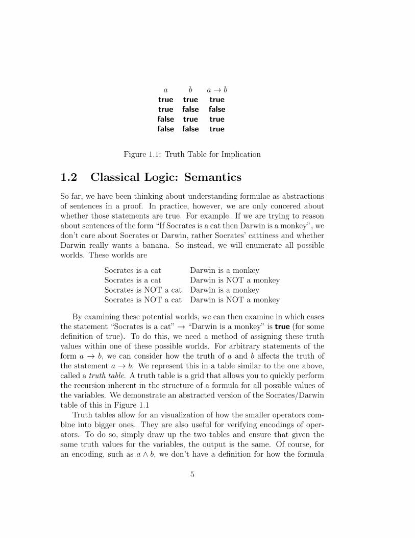
a b a→ btrue true truetrue false falsefalse true truefalse false true

Figure 1.1: Truth Table for Implication

1.2 Classical Logic: Semantics

So far, we have been thinking about understanding formulae as abstractionsof sentences in a proof. In practice, however, we are only concered aboutwhether those statements are true. For example. If we are trying to reasonabout sentences of the form “If Socrates is a cat then Darwin is a monkey”, wedon’t care about Socrates or Darwin, rather Socrates’ cattiness and whetherDarwin really wants a banana. So instead, we will enumerate all possibleworlds. These worlds are

Socrates is a cat Darwin is a monkeySocrates is a cat Darwin is NOT a monkeySocrates is NOT a cat Darwin is a monkeySocrates is NOT a cat Darwin is NOT a monkey

By examining these potential worlds, we can then examine in which casesthe statement “Socrates is a cat”→ “Darwin is a monkey” is true (for somedefinition of true). To do this, we need a method of assigning these truthvalues within one of these possible worlds. For arbitrary statements of theform a → b, we can consider how the truth of a and b affects the truth ofthe statement a→ b. We represent this in a table similar to the one above,called a truth table. A truth table is a grid that allows you to quickly performthe recursion inherent in the structure of a formula for all possible values ofthe variables. We demonstrate an abstracted version of the Socrates/Darwintable of this in Figure 1.1

Truth tables allow for an visualization of how the smaller operators com-bine into bigger ones. They are also useful for verifying encodings of oper-ators. To do so, simply draw up the two tables and ensure that given thesame truth values for the variables, the output is the same. Of course, foran encoding, such as a ∧ b, we don’t have a definition for how the formula

5

a b a ∧ btrue true truetrue false falsefalse true falsefalse false false

a b ¬b a→ ¬b ¬(a→ ¬b)true true false false truetrue false true true falsefalse true false true falsefalse false true true false

Figure 1.2: Verification of ∧ encoding

behaves. So we have to define how we want the operator to behave, and thenverify that our encoding behaves appropriately. This is done in Figure 1.2.Notice that the highlighted columns are exactly the same for the two tables.

While truth tables are useful in some situations, we often want to providea more general approach to reasoning about which possible world we are in.We use a valuation function to define a possible world.

Definition 1.5 (Valuation Function). A valuation function is defined to bea function η : V→ {true, false}

Now we can mathematically represent rows in the truth tables. For in-stance, if we have a function η such that η(“Socrates is a cat”) = true, thenwe only need to consider possible worlds where Darwin is and isn’t a monkey.Now, we can use this class of functions to build up meaning for our morecomplex operators. We will use the function valη to do this for ClassicalLogic.

Definition 1.6 (Valuation Function for Classical Logic). A valuation func-tion for Classical Logic, written valη : CL(V)→ {true, false}, is an extensionof a valuation fuction η, where CL(V) is the set of all syntactic terms in Clas-sical Logic over the domain V as defined in 1.1. The function valη is appliedto the terms in CL(V) as follows:

(⊥) valη(⊥) = false

(v) For v ∈ V, valη(v) = η(v)

(→) valη(a→ b) = true if valη(a) = false or valη(b) = true

Now that we have a functional interpetation, want to define a relation� pronounced “models” that will generalize the valuation function. We will

6

write F � a when we want to convey that given a valuation function forwhich a certain set of formulae F hold, a will certainly hold. This is a kindof metamathematical implication that allows us to say, “if I know that theformulae in F are true, then I also know a”. We define this formally belowin Definition 1.7

Definition 1.7 (The Models Relation for Classical Logic). Given a formulaa and a set of formulae F , we write F � a when for all η : CL(V) →{true, false}, if for all b ∈ F , valη(b) = true, then we can show that valη(a) =true.

We say that a formula a is a consequence of F , when F � a. If F = ∅,then we say that a is (universally) valid and write � a.

Example 1.8. Lets look at an example to understand how this works. Con-sider the set of formulae F = {a → b, a} and the formula a ∧ b. We wantto see if a ∧ b is a consequence of F . So consider an arbitrary valuationfunction η : CL(V), such that valη(a→ b) = true and valη(a) = true, and wewant to show that in this valuation function valη(a ∧ b) = true. So, we havethat valη(a) = false or valη(b) = true, the first case contradicts our otherassumption that valη(a) = true. So we know that valη(b) = true. Since botha and b are mapped to true, then we see that valη(a ∧ b) = true.

We have given a semantics for Classical Logic, and discussed several se-mantic models that allow us to understand what formulae (our abstractionof sentences) mean on an intuitive level. However, we still don’t know howabstractly reason about them independent of their semantic truth. We stillneed a solid way to construct proofs of formulae so that we can know whichmoves are allowable in proofs.

1.3 A Proof System

Now we leave the world of truth, and enter the world of proof. When weconsider a semantic interpretation of the formula, we wonder if its valuationreturns true or false. However, in the world of proof we create a set of axiomsand inference rules, and wonder if a formula can be derived by applicationand combination of these axioms and inference rules.

Axioms are formulae that we presume to hold. They are often so “ob-vious” or simple that any rational viewer should be easily able to ascertain

7

their correctness. Sometimes, this means doing complicated math! We rep-resent axioms and inference rules in the standard way [5]. For an arbitraryrule, we write

〈Premises〉〈Conclusion〉

(NameOfRule)

where the premises are a set of formulae and the conclusion is a single for-mula. By this notation, we means that the formula

∧p a Premises f implies the

Conclusion. there are no assumptions, the rule is called an axiom. Otherwise,it is an inference rule.

We will also define a relation · ` · ⊆ 2CL(V )×CL(V) pronounced “proves”.Writing F ` a means that according to a set of rules, a can be derived fromthe set of assumptions F . We will write ` for ∅ ` a.

The axioms, inference rules, and ` relation, allow us to reason about whatformulae are provable. Let’s see how these pieces fit together with respect toClassical Logic. First we will define the proof system for classical logic.

Definition 1.9 (Proof System for Classical Logic). Let the following axiomsand inference rules specify the allowable terms in the ` relation.

The axioms for Classical Logic are:

` a→ a (Id)

` a→ (b→ a) (Weak)

` (a→ (b→ c))→ ((a→ b)→ (a→ c)) (Distr)

` (¬b→ ¬a)→ (a→ b) (ContraPos)

The single inference rule for Classical Logic is

` a→ b ` a` b

(ModusPonens)

To better understand and believe these rules, let’s show their truth tables.For each of these rules to be sensible, we expect them to be universally valid,i.e. true in all possible worlds. This means that the column containing therule should be entirely true.

8

a a→ atrue truefalse false

Figure 1.3: Truth Table for Id

a b b→ a a→ (b→ a)true true true truetrue false true truefalse true false truefalse false true true

Figure 1.4: Truth Table for Weak

The most interesting case is when we consider ModusPonens rule. Thismeans that we do not consider all possible worlds, we only consider thoseworlds in which a is true and a→ b is true. So, in the truth table, we consideronly rows where a 7→ true and b 7→ true (Figure 1.7).

1.4 Soundness and Completeness

We have an axiomatic framework and a mathematical semantic interpretationof formulae in the logic; are they really talking about the same thing? Thatis, do our notions of proof and truth agree?

Informally, soundness is the claim the the axiomatic framework doesn’tallow us to prove claims that are not “true” in the intuitive semantic inter-pretation (whatever “true” means [26, 18]). This serves as a kind of sanitycheck; the rules we’ve defined to govern our system actually work. This iscritical for any axiomatic system. If the rules are not sound, then the systemcan derive formulae that are “false” in the model.

Once the rules are proven to be sound, we want to know something aboutwhat portion of the set of “true” claims our rules can derive. Completenesssays that the set of “true” claims is a subset of those things that the rulescan derive, meaning that, if a claim is “true”, then it can be proven by theaxiomatic framework. We define these more formally below:

9

a b c b→ c a→ b a→ c a→ (b→ c) (a→ b)→ (a→ c) Distrtrue true true true true true true true truetrue true false false true false false false truetrue false true true false true true true truetrue false false true false false true true truefalse true true true true true true true truefalse true false false true true true true truefalse false true true true true true true truefalse false true true true true true true true

Figure 1.5: Truth table for Distr Axiom

a b ¬a ¬b a→ b ¬a→ ¬b ContraPostrue true false false true true truetrue false false true false true truefalse true true false true false truefalse false true true true true true

Figure 1.6: Truth Table for ContraPos Axiom

Definition 1.10 (Soundness). A logic is called sound if for every F a set offormulae in the logic, and a a formula in the logic, F ` a implies F � a.

Definition 1.11 (Completeness). A logic is called complete if for F a set offormulae in the logic and a a formula in the logic, then F � a implies F ` a.

Soundness is a simple property at says that our proofs correspond toreality. It’s proof is a sensibility argument that amounts to showing that allof the axioms and inference rules are valid under the model, since every proofis based on some combination of these axioms and inference rules.

In general, it is a very bad if a proof system or logic is not sound, sincethat would allow you to prove things that are false. Since the proof systemis intended to be a formal way of evaluating whether something is true ornot (according to some set of rules) then it defeats the purpose if the systemis not sound.

In contrast, completeness makes a totality argument, saying that the cur-rent set of axioms can prove every true statement in the logic. This is notnecessary for a logic, and there are many interesting logics that are soundbut not complete, in which we can prove interesting things. For instance,

10

a b a→ b btrue true true truetrue false falsefalse true truefalse false true

Figure 1.7: Truth Table for the ModusPonens Inference rule

any system of logic or mathematics that has a notion of infinite arithmeticis not complete [15, 16]. So, this would imply that much of mathematics,including fields like Number Theory and Analysis, are incomplete. However,these are quite vibrant fields, in which mathematicians have proven and con-tinue to prove interesting and useful theorems. So completeness doesn’t sayanything about the “usefulness” or breadth of a system, it is only making aclaim about how tight the correspondence between the rules and the concreteinterpretation of the symbols.

Proving completeness is typically much harder than proving soundness.To do the latter, we simply need to show that the axioms and inference rulesare sensible with respect to some concrete model. To prove completeness,we need to consider an arbitrary formula that is true in our model and showthat there exists a proof of that formula.

Let’s start by showing that our choice of axioms are sensible, i.e. provingthat every axiom and inference rule is true under our semantic model.

Theorem 1.12 (Soundness of Classical Logic). Classical Logic is sound.

Proof. We already showed that each of the rules is valid! Examining thetruth tables presented in Section 1.3 demonstrates that each of the rules isvalid in all possible worlds. This is a combinatorial proof that enumeratesall possible inputs and outputs to valη over all η. 4

Theorem 1.13 (Completeness of Classical Logic). Classical Logic is com-plete.

Proof. Given a proposition a such that F � a, show that ` a. Let V ⊆ Vbe the set of variables in F . Consider an arbitrary η function, and let Sη ⊆CL(V) be

S =

{v, if v ∈ V, and η(v) = true

¬v, if v ∈ V, and η(v) = false

11

Notice now that for every s ∈ Sη, valη(s) = true. Let F ′ = {f ∨¬f | f ∈F}. Kleene [18] proves a lemma to show that for an arbitrary formula f ,then valη(f) = true if and only if S ` f . He also shows that for an arbitraryformula f , if for every η, if Sη ` f , then F ′ ` f .

Chaining these together, we can conclude that F ′ ` a. We can now showthat for every formula f , we have ` f ∨¬f , by desugaring the ∨ operator tosee ` ¬f → ¬f which it a tautology by Id. Since every element of F ′ is ofthe form f ∨ ¬f we can conclude that ` a. For more detail, see [18]. 4

12

Chapter 2

Linear Temporal Logic

A computer does exactly what a user or programmer tells it to do. Thisis a blessing and a curse, as being perfectly precise in the instructions onegives is a very difficult thing to do, and a programmer will often vociferatein anguish “That’s what I said, but not what I meant!” Since computers arefrustratingly pedantic, we must find a way to prove that programs do whatwe want them to do.

To verify the correctness of programs, computer scientists frequently useconstructive, classical, and first-order logic. These are often powerful toolsused to prove functional properties for programs that have clearly definedinputs and deliver an output on termination. Sometimes we want to verifyproperties of programs that are not related to the inputs and outputs and notdependent on termination; programs like operating systems [6], databases [6],or Java execution traces [27]. Linear Temporal Logic (LTL) gives us morepower to verify these types of programs.

LTL offers a way to ask questions about the execution of a program [28].For example, we can use Temporal Logic to examine the predicament of ourtravellers Sleepy and Speedy who want to get from LAX to JFK. If we treatSleepy’s flight plan to get from SFO to JFK as a program, we want to makesure that Sleepy eventually gets to JFK, that the final state of the programis JFK. If, for some reason, Sleepy has a criminal record in Texas, we canalso make sure that they never fly though DFW.

To formalize these kinds of statements in LTL, we will use that syntaxstandard to modal logics, adding the 2 (global), and # (next) operators, tothe standard classical logic operators.

13

Definition 2.1. For a set of variables V, with v ∈ V and a and b proposi-tions, this gives a minimal syntax

a, b ::= v | ⊥ | # a | a→ b | aW b

Define LTL(V) to be the set of formulae generated by the above syntaxover V. An arbitrary formula f ∈ LTL(V) is the symbol ⊥, a variable in V,of the form # a where a ∈ LTL(V), of the form a→ b where a, b ∈ LTL(V),or of the form aW b, where a, b ∈ LTL(V).

The statement a W b intuitively corresponds to the statement “a holdsuntil b holds, or a always does”, and # a corresponds to the statement “inthe next time step, a”. For example, to make sure that Sleepy avoids gettingarrested due to the warrant for their arrest in Dallas, we can make sure that(Sleepy at SFO) → ¬(Sleepy at DFW) W ⊥, i.e. if Sleepy is at SFO, thenSleepy won’t arrive at DFW until ⊥ holds. Since ⊥ will never hold, Sleepywill never be at DFW.

Extending this basic syntax, we get the standard classical logic encodingsfrom Definition 1.2 of ∧,∨,¬, and >. Further, we can define a couple ofpieces of temporal syntactic sugar. The “always a” operator, written as 2 a,says “now and for every in the future a”. The “ever” operator is written3 a, meaning that “at some point in the future, a.” Continuing with ourflight-plan example, it is now easy to determine whether Sleepy actually getsto JFK airport via the formula Sleepy at SFO → 3(Sleepy at JFK), whichmeans that Sleepy being in SFO means that they will eventually get to JFK.Of course, these are just intuitive justifications for these encodings, but wecan make these intuitions more concrete with a semantic interpretation ofthe model, using a Kripke Structure [19].

Definition 2.2. Let V be a set of variables. Define a Kripke structure K asan infinite sequence of valuation functions

K = (η1, η2, η3, . . .)

where ηi : V→ {true, false} is a function from variables to truth values. Wealso define the temporal valuation function Ki : LTL(V)→ {true, false}, forsome index i of this kripke structure K, to be

14

Ki(v) = ηi(v), for v ∈ V

Ki(⊥) = false

Ki(a→ b) = true iff Ki(a) = false, or Ki(b) = true

Ki(# a) = true, or Ki+1(a) = true

Ki(aW b) = true iff there exists k ≥ i such that Kk(b) = true,

and for i ≤ j ≤ k,Kj(a) = true,

or for every k ≥ i,Kk(a) = true.

We can now set up Sleepy’s travel plans using this formalism. We defineK = (η1, η2, η3, η4, . . .), where

η1(x) =

{true x = (Sleepy at SFO)

false otherwise

η2(x) =

{true x = (Sleepy at PHX)

false otherwise

η3(x) =

{true x = (Sleepy at PHL)

false otherwise

η4(x) =

{true x = (Sleepy at JFK)

false otherwise

ηi(x) = η4(x) ∀i > 4

So, then we can evaluate our correctness criterion, that

(Sleepy at SFO)→ 3(Sleepy at JFK).

We start at time step 1, since at every other time step i, it is the casethat ηi(Sleepy at SFO) = false. So, let’s evaluate K1(Sleepy at SFO →3(Sleepy at JFK)). By definition, this is true if K1(¬(Sleepy at SFO)) =true or K1(3(Sleepy at JFK) = true. We can simplify the first case toK1(Sleepy at SFO) = false, but, we know that η1(Sleepy at SFO) = true,so we conclude that K1(¬(Sleepy at SFO)) = false, so we must be in the

15

other case. Now, we can simplify K1(3(Sleepy at JFK)) = true to the newexpression K1(2¬(Sleepy at JFK)) = false. So, we must find some i ≥ 1such that Ki(Sleepy at JFK) = ηi(Sleepy at JFK) = true. This is true wheni = 4, so conclude that K1(3(Sleepy at SFO) = true, and ultimately thatK1(Sleepy at SFO→ 3(Sleepy at JFK)) = true.

Remark 2.3. So far, we have been referring to a “time step” without muchjustification for what that means. In this model, we mean a time step i tobe the world ηi.

Once we have a logic’s syntax and its mathematical semantics (as wedo now), we can consider the appropriate axiomatic framework, followed bysoundness and completeness results. But first, we will asses some of theassumptions made by LTL and show real-world examples of how it is used.

2.1 Background for Linear Temporal Logic

First we present the main assumptions of LTL, and then motivate their use-fulness with applications of LTL to the real world verification tools JavaPathfinder [27] and Eagle [2].

2.1.1 Assumptions

Let’s first address the assumptions being made in linear temporal logic. Thereare three: (1) time is discretizable, (2) there is always a “next time”, and(3) if a time step has a “next time” it is unique [21]. The sense of theseassumptions is not entirely apparent, so we will take some time to examineand justify each of them.

Time is discretizable Physics understands time as continuous, however,we have presented LTL with a discrete model of time. Why can we dothis? In day to day life, we already use a discrete model of time wherewe say that something occurs at time t if it happens between time t andtime t + 1. Computers take a similar approach, operating under a discretetime model [22]. Since LTL is most frequently used for verifying computerprograms, this assumption makes sense for LTL.

16

There is always a “next time” This is a fairly reasonable assumption,especially when we consider programs like operating systems, and databasesystems that ought to run indefinitely, and then when they are terminated,correctness is suddenly no longer an issue. In certain situations, however, wemay want to want to reason about the end of time. The assumption thatthere is always a next time is no longer viable. A simpler system forces timeto end, adding the assumption that “eventually, time ends.” This systemis called Linear Temporal Logic over finite traces 3, also known as (LTLf ).Another variant of this LTL that questions this assumption is called Past-time LTL, which in addition to introducing operators about the past, allowstime to either be finite or infinite.

Uniqueness Here we assume that every time step has a unique successor.With a human, macroscopic understanding of physical processes, it seemsobvious that in the next time step there are not two different valid worlds(represented as η-functions). This intuition holds for sequential processes,because there is one sequence of commands that are executed. However,the uniqueness assumption is often not sufficient for concurrent or parallelprocesses [23], as each thread/process has its own distinct successor. Whenwe throw away the uniqueness assumption, we get a logic called Linear Dy-namic Logic (LDL), which, while being extremely powerful, is not as popularas LTL. The uniqueness assumption permits a tractable, easy-to-use formal-ization.

Once we have these assumptions, one might wonder when these assump-tions are good ones to make and how powerful the system of LTL is underthese assumptions. The best way to assess the power of a logic is by example;so what follow are summaries of some of the theoretical properties and usesin model-checking software.

2.1.2 Applications

Now that we’ve examined the assumptions, it is useful to justify them byshowing they can be applied to real-world situations. What follows is adescription of LTL’s importance to hardware verification and of two distinctverification tools that use LTL.

17

Intel Hardware Verification LTL, along with its variant CTL (computa-tion tree logic), is an essential tool in hardware verification [20, 17, 11]. LTLhas been one of the major tools used by Intel [11], used to verify CPU designsfor the Intel Pentium 4 processor [30]. Specifically, they use LTL to verifythe correctness in the “pre-silicon” stage, i.e. to eliminate bugs in the designof the processor. Following the “pre-silicon” stage is, of course, the “silicon”stage, in which Intel uses standard test-driven bug-finding techniques. Theywere able to use LTL to verify floating-point properties and arithmetic [13]using a model-checking tool [13] based on LTL that was developed at Intel.

Java Pathfinder Java is an extremely well-known and popular language,and Java Pathfinder [27], a tool developed by the NASA Ames ResearchCenter, is the self-titled “swiss army knife of Java verification”. JPF is avirtual machine that runs automatic tests on your code, theoretically tryingall possible executions of the program to try and expose vulnerabilities.

Recently, an LTL extension called jpf-ltl was added to JavaPathfinder [27]. It allows for the user to specify various LTL formulae abouttheir Java program jpf-ltl will attempt to falsify the claim. Most in-terestingly, a user can specify conditions about sequential and concurrentprograms, referring to anything from method calls to program variables.

For example, a user could ensure that if you call a certain method, itbehaves properly. Let foo be the name a function that computes the actionf on its inputs. We want to know that f(x), happens eventually (after somelatency period). So we could ask jpf-ltl to verify the claim

∀x.2(foo(x)→ 3 f(x))

which says that it is always the case that, the effect of foo on x will eventuallyoccur. Or equivalently, that foo terminates.

Mars Rover Another project out of NASA Ames Laboratory is the Eagleverification tool used to verify event controllers in an experimental NASArover [2]. Eagle is based on the observation that the formulae 2F can beexpressed as maximal solution to the equation X = F ∧ #X and that 3Fis the minimal solution to the equation X = F ∨ #X. Using this notionof minimal and maximal fixpoints, the authors define further a semantics,calculus, and evaluation algorithm.

18

After its specification and implementation, Eagle was then applied totest a planetary rover controller called K9. The rover controller was anextensive multi-threaded shared-memory C++ application that needed tobe responsive to external stimuli. The verification tool, called X9 (since itexplores K9) generated test cases and produced an execution trace for thosecases that failed. The paper cites an error detected by X9 having to do withtemporally dependent processes terminating improperly. More specifically,for pairs of processes p1 and p2, where p2 depends on the completion of p1, X9detected a class of bugs caused by p2 trying to start before p1 had terminated.

These real-world examples demonstrate the usefulness of temporal logic ingeneral, but specifically the formal and operational models provided by LTL.They also justify assumptions that underlie LTL and begin to explain thewide acceptance and common usage of LTL.

2.2 Classical Formulation

This section will present the Classical formulation (semantics and proof the-ory) of LTL and a proof of soundness and completeness. The proof follows amodifed version of the Henkin-Hasenjaeger proof of LTL of completeness forclassical logic [21]. The first thing we need here is a set of axioms; the axiomsfor classical logic and those for predicate logic are remarkably similar.

Definition 2.4 (Proof System for LTL). Define the relation · ` · ⊆ 2LTL(V)×LTL(V) to be the formulae generated by the following axioms and inferencerules:

Axioms

` all tautologies in Classical Logic (Taut)

` ¬# a↔ #¬a (NegNextDistr)

` #(a→ b)→ # a→ # b (NextDistr)

` aW b→ b ∧ b ∨ a ∧ aW b (WkUntilUnroll)

Inference Rules

19

` a ` a→ b

` b(ModusPonens)

` a` # a

(Next)

` a→ b a→ # a

` a→ 2 b(Induction)

Definition 2.4 defines the set of axioms for LTL. The first is the Tautaxiom, in which we simply assume that anything that is a tautology in Clas-sical Logic (provable from no assumptions) is an axiom of LTL. The nextaxiom, NegNextDistr, simply states that (¬·) and (# ·) are distributive.Then AlwUnroll says that if you have an 2 a, then you get a now, and 2 ain the next time step. Then we have ModusPonens which is exactly thesame as in classical logic, followed by the Next rule which says that a proofof a in general, i.e. a proof of a’s validity, is sufficient to say that in the nexttime step a holds true, because valid formulae always hold. The final rule isInduction, which says that if ` a→ b and ` a→ # a then ` a→ 2 b.

As a sanity-check for the rules in Definition 2.4, we state the followingsoundness result (Theorem 2.8), which says that the proof rules above onlyadmit proofs of valid formulae.

Definition 2.5 (Valid). A formula a of LTL(V) is called valid in the tem-poral structure K for V, denoted �K a, if Ki(a) = > for every i ∈ N.

Definition 2.6 (Consequence). For a set of formula F ∈ LTL(V), we writeF � a, pronounced “a is a consequence of F”, if

∀K, (∀c ∈ F ,�K c) =⇒ �K b

Definition 2.7 (Universal Validity). A formula a is called universally validif a is a consequence the empty set of formulae. This is written ∅ � a, orequivalently � a.

Theorem 2.8 (Soundness). If F ` a, then F � a.

Proof Idea. Induction on the derivation of F ` a. 1 41For clarity, we use the 4 symbol to represent the end of a proof since the � symbol

forms part of the object of study.

20

Now we want to assess completeness for LTL. Completeness says that ifa formula a is a consequence of the set of formulae F , then, if we assumethe formulae in F , we can prove a. The proof relies on several importanttheorems and lemmata. We will start with a couple of deduction theorems forLTL, which will allow us to convert consequence and provability statementsof the form F ` a or F � a, to statements of the form ` b and � c.

Theorem 2.9 (Semantic Deduction). For F , a set of formulae, with a andb formulae, then F , a � b if and only if F � 2 a→ b.

Proof. The proof proceeds by induction on the size of F . 4Theorem 2.10 (Deduction). For F , a set of formulae, with a and b formu-lae, then F , a ` b if and only if F ` 2 a→ b.

Proof. Each direction is proved separately and directly. 4

These smaller results allow for us to convert the problem

F � a =⇒ F ` a

to a simpler one. We can let F = a1, a2, . . . an and simplify the problem to

` 2 a1 → 2a2 → · · ·2 an → a

=⇒ � 2 a1 → 2 a2 → · · ·2 an → a

In fact we can generalize this claim even further to

� b =⇒ ` b

This is a much more manageable claim to prove. Next, we will prove anunsatisfiability result that demonstrates how to bridge the gap between the� and the ` relations. Specifically, we will come up with a way to generate aformula b such that ` b in the theory implies b is satisfiable in the model. Wewill use the contrapositive of this result in the completeness proof. To provethis satisfiability theorem, we will introduce a positive-negative pair (PNP)structure.

The intuition behind the notation and terminology is that a PNP is apair of two sets, a positive set (F+), which only contains formulae that areprovable, and the negative set (F−), which only contains formulae whosenegations are provable. PNPs give us a way to separate sets of formulae intothose that we think are true and those that we think are false. We enforcewith a consistency property that allows us to turn our beliefs about truth toconclusions about provability. These are defined formally below

21

Definition 2.11 (Positive-Negative Pair). A Positive Negative Pair (PNP)is a pair of sets of formulae (F+,F−). For a PNP P , We define the literal

interpretation of P , P to be the formula:

P ,∧a∈F+

a ∧∧b∈F−

¬b

A PNP P is inconsistent if ` ¬P , and consistent otherwise. Let the setof all PNPs be PNP .

Now we can prove the Satisfiability Theorem (Theorem 2.12), which saysthat the literal interpretation of a consistent PNP is satisfiable in the model.Here we are relating a statement about provability (“a PNP P is consistent”)

to one about the the model (“there is a model Ki for which Ki(P) = true”).

Theorem 2.12 (Satisfiability for LTL). For P, a consistent PNP, the for-

mula P is satisfiable.

Proof idea. Evaluate the way that the PNPs change throughout time (defin-ing a transition function σ in the full proof) to ensure that each of the tem-poral operators (# and 2) behave appropriately. Then construct a Kripkestructure K based on the evolution of the PNP throughout time, and showthat K0(P) = true. 4

Theorem 2.13 (Completeness for LTL). For F a set of formulae, and a aformula, if F � a, then F ` a.

Proof Idea. Assume that F � a, where F = a1, . . . , an. Using Theorem 2.9,we get � 2 a1 → · · · → an → a. We can perform an analogous transformationon our desired result, using Theorem 2.10. So that we need to show

` 2 a1 → · · · → 2 an → a.

Broaden the claim so that for all formulae b, � b implies ` b. Let thePNP P = (∅, {b}). Notice that P ≡ ¬b. Then by the contrapositive ofTheorem 2.12, we see ` ¬¬b, which then by Taut derives ` b. 4

22

Chapter 3

Linear Temporal Logic overfinite traces

We present our main contribution: a presentation and axiomatization of Lin-ear Temporal Logic over finite traces (LTLf ), highlighting explicit differencesbetween itself and standard Linear Temporal Logic (LTL). Importantly, wederive soundness (Theorem 3.20), and Completeness (Theorem 3.43). Weconclude with a novel decision procedure and a corresponding proof thatsatisfiability is decidable (Theorem 3.58).

While the core syntax of LTLf will remain the same as that of LTL, weintroduce some new pieces of syntactic sugar, namely end, pronounced “end”,and a, pronounced “weak next a”. The symbol end means that there is nonext state, and a means either # a or end, so if a holds in every state, awill also be true in every state, whereas # a will be false in the final state.

We also adjust the semantics to assert that time will certainly end. In theunderlying model, we will still use Kripke structures from LTL to representthe evolution of the world through time. In our finite setting, we define afinite variant of these Kripke structures with exactly n states. When we’rein this nth and last state, and we try and make a statement like # a, whichasks to evaluate a in the n+1th state, then we immediately evaluate to false,without ever looking at how a evaluates.

Similarly, in the proof theory, we will include the axiom Finite, which is` 3 end, and says that eventually, time ends. When time ends, we want tomimic the behavior of the semantics, i.e. that trying to make a statement ofthe form # a is contradictory. To incorporate this behaviour, we also includethe axiom EndNextContra, ` end→ ¬# a, meaning that if we are in the

23

last state, # a is contradictory for all formulae a. Further, to compensate forthe end of time, we replace all instances of # a with a in the unrolling, step,and induction rules. Notice that, in LTL, the formula 3 end is unsatisfiable.

Finally, in the proofs of soundness, completeness, and decidability, we willuse a similar method to the proofs of those properties for LTL [21], takingspecial care to account for these changed assumptions.

3.1 Syntax of LTLf

The syntax for LTLf is th same as LTL’s (Definition 2.1).

a, b ::= # a | aW b | a→ b | ⊥ | v

Figure 3.1: Syntax for LTLf (V)

Our syntax subsumes that of Classical Logic (Chapter 1), namely the bi-nary implication operator→, the constant ⊥, and the ability to use variablesfrom the alphabet V. From each of these we can encode the more widelyrecognized operators, ∧, ∨, ¬, >, as presented in Definition 1.2.

We also have the temporal operators from LTL, the weak until operatorW , and the next operator #. Intuitively, a statement aW b can be thoughtof as “moving forward in time, a holds until b holds, or a always holds”.Similarly the statement # a can be thought of as “in the next time step aholds true”.

Recall from Section 2 that unary operators bind tighter than binary op-erators, so 2, #, and ¬ bind tighter than →, ∧, and ∨, and ∧ binds moretightly than ∨ which binds more tightly than→. As an example, the formula# a→ 2 d ∧ c is equivalent to (# a)→ ((2 d) ∧ (¬c)).

3.2 Semantics for LTLf

In LTL, the underlying model is an infinite Kripke structure [19], defined asan infinite tuple of functions that assign truth values to the variables. Incontrast, for LTLf , we use a finite version, forcing the underlying tuple tohave only finitely many functions.

24

Definition 3.1 (Finite Kripke Structure). A finite Kripke structure Kn isan n-tuple of functions

Kn = (η1, η2, . . . , ηn)

where ηi is a function ηi : V→ {true, false}.

To give a semantics to the formulae generated by the grammar, we firstdefine a function Kn

i interpreting a formula at time-step i, defined as a fix-point on the formula. Different from LTL, we need to handle what happensin the last state. In our finite setting, we make sure that any occurence of# a at the nth always give false, without ever looking at a.

Definition 3.2. Given a finite Kripke structure Kn = (η1, · · · , ηn), we definethe temporal valuation function Kn

i at state i as a fixpoint on its input:

Kni (v) = ηi(v)

Kni (⊥) = false

Kni (a→ b) =

true if Kn

i (a) = false

true if Kni (b) = true

false otherwise

Kni (# a) =

{Kni+1(a) if i < n

false otherwise

Kni (aW b) =

true if Kn

j (a) = true, for all i ≤ j ≤ n

true if there exists i ≤ k ≤ n, such that Knk (b) = true

and for every j such that i ≤ j < k,Kni (a) = true

false otherwise

Now prove a totality lemma, which says that in any function Kni , every

formula in LTLf (V) evaluates to true or false.

Lemma 3.3 (Totality). For every Kripke structure Kn, every i ∈ {1, . . . , n},and an arbitrary formula a, then Kn

i (a) = true or Kni (a) = false.

Proof. By structural induction on an arbitrary formula a (Lemma A.1). 4

25

Example 3.4. As an example, we will define and motivate couple of commonpieces of syntactic sugar [4, 21, 24]. Define

2 a , aW ⊥ (3.1)

3 a , ¬2¬a (3.2)

a U b , aW b ∧3 b (3.3)

a , ¬#¬a (3.4)

end , ¬#> (3.5)

Lets examine each of these new pieces of syntax in turn, examining whywe might want to use them.

(3.1) The statement 2 a can be interpreted as Kni (2 a) = true iff Kn

j (2 a) =true for all i ≤ j ≤ n. We encode this as (a W ⊥). This eliminatesthe second case, since for any i, Kn

i (⊥) = false. Considering the firstcase, we have Kn

j (a) = true for i ≤ j ≤ n, which is exactly when wewant Kn

i (2 a) to be true.

(3.2) The unary operator 3 a, pronounced “ever a” or “eventually a” couldbe built into the fix Kn

i , interpreted as “there exists a state i such thatKni (a) = true”. We can derive this algebraically.

Kni (¬2¬a) = true⇔ Kn

i (2¬a) = false

⇔ not for all j, i ≤ j ≤ n such that Knj (¬a) = true

⇔ exists j, i ≤ j ≤ n such that Knj (¬a) = false

⇔ exists j, i ≤ j ≤ n such that Knj (a) = true

(3.3) The formula a U b, pronounced “a until b” is equivalent to aW b exceptthat we enforce that b is true at some point, hence the conjunctive 3 b.

(3.4) The next piece of syntax a, pronounced “weak next” is a form ofnext (#) that has a valuation to true in the last state. We observethat Kn

i ( >) = true forall states i, and this is not the case for #. Theoperator behaves as expected for i < n. because of the double negationin the definition of . The interesting case coming when i = n, i.e.there is no next state. In the interpretation above, Kn

n(#>) = false,

26

so Knn( >) = Kn

n(¬#¬>) = true. In this way, the operator isend-agnostic, and will still be true when the world has ended.

(3.5) This also justifies the end sugar, which gives true exactly when i = n.To see this lets evaluate Kn

n(end).

Knn(end) = Kn

n(¬#>) = true iff Knn(#>) = false)

Since the only time Kni (#>) = false is when i = n, we know that

Knn(end) = true.

We have defined LTLf ’s evaluation scheme in a similar way to that ofLTL, paying close attention to the end behavior. To further explore thenuances of LTLf , we can compare the way that 2 a behaves in LTLf to howit behaves in LTL. In LTL, the statement 2 a means that in every singlestate now and in the future, a holds. Lets look at what happens when wewant to examine 2 a in the last state:

Lemma 3.5 (Always Convergence). Given a Kripke structure of length n,and a formula a of LTLf (V) then Kn

n(2 a) = Knn(a)

Proof. Immediate, by definition of the evaluation function (Lemma A.2). 4

This means that in the last state, given a formula a, if Knn(a) = true

then the formula a′ created by removing all of the 2 statements inside agives Kn

n(a′) = true. Then we only have to deal with #-statements (whichare false) and classical logic in the nth state.

With this denotational model of LTL over finite traces, we can definevalidity of a formula within the language LTLf (V). Notionally, this is whensome assignment of truth values holds for every formula.

Definition 3.6 (Valid). A formula a of LTLf (V) is called valid in the tem-poral structure Kn for V, denoted �Kn a, if Kn

i (a) = true for every i ∈ N.

Definition 3.7 (Consequence). For a set of formula false, we write F � a,“pronounced a is a consequence of false”, if

for all Kn, (for all c ∈ F �Kn b) =⇒ �Kn b

Definition 3.8 (Universal Validity). A formula a is called universally validif a is a consequence the empty set of formulae. This is written ∅ � a, orequivalently � a.

27

Remark 3.9. When we write Kn, we are not saying that n is an index to aninfinite Kripke structure K or a finite one Km with m ≥ n. Rather, n is thenumber of time-steps in the structure, and we cannot formulate it withoutthis n. It is helpful to think of n as an annotation that marks the structure’ssize.

Lets make a brief aside to consider an alternate notion of what it meansto be a “finite Kripke structure”. Instead of a finite list of valuations, wecould define it as a finite prefix of an infinite kripke structure, parameterizingon n.

Definition 3.10 (Truncated Kripke Structure). Let K be a kripke struc-ture K = (η1, η2, . . .) where the functions η are defined as above, and letn be a positive integer. Then a truncation of K is a finite tuple K[n] =[η1, η2, . . . , ηn].

The definitions of Validity, Consequence, and Universal Validity wouldthen mostly be syntactic translations from Kn to K[n] assuming a Kripkestructure K. However we need to modify consequence slightly:

Definition 3.11 (Consequence). Let F be a set of formulae, a a formula,and K be a Kripke structure such that for every trucation of K at timestepn ∈ N, and every formula b ∈ F , we can write �K[n] b. Then write F � a,pronounced a is a consequence of false, if �K[n] a.

These two semantic models, finite Kripke structures and truncated Kripkestructures, seem like they might have different consequences and differentproof mechanisms. However, it doesn’t matter which we choose, since theyare, in fact, equivalent.

Corollary 3.12. Given a finite Kripke structure Kn = (η1, η2, . . . , ηn) andan infinite Kripke structure K = (η′1, η

′2, η′3, . . .), such that ηi = η′i, �Kn a if

and only if �K[n] a.

Proof. By induction on the size of Kn (Lemma A.3). 4

Now lets prove a couple of important lemmata that will help us later.First, we prove that implication behaves appropriately, by proving a semanticversion of modus ponens.

Lemma 3.13 (Semantic Modus Ponens). For a given set of formulae F ,with a, b formulae, if F � a and F � a→ b, then F � b.

28

Proof. By unrolling the definitions (Lemma A.4). 4

Now, we demonstrate the power of the temporal operators. We show thatif you assume a, you will be able to show 2 a, and similarly, if you have aand #>, you can derive # a.

Lemma 3.14 (Assumption of Temporal Operators). For a set of formulaeF , then F ∪ {a,#>} � # a and F ∪ {a} � 2 a.

Proof. By definition; since F � a means a is a consequence of F , i.e. a holdsat all steps (Lemma A.5). 4

Corollary 3.15 (Always to Next). For a formula a, � (#> ∧2 a)→ # a.

Proof. Direct consequence of the proof of Lemma 3.14. 4

Corollary 3.16 (Next Assumption).

#> � ⊥

Proof. Vacuously true — no finite Kripke structure exists such thatKni (#>) =

true for all i ∈ {1, . . . , n} (Lemma A.6). 4

Notice that a consequence of Corollary 3.16 is that we can never assume# a for any a. We must bear this in mind when we formulate our axioms.In fact, it seems that when we assume a set of formulae F we are lifting the2 operator over the set and assuming the formulae in the set {2 a | a ∈ F}.Notice that this means that our idea of deduction for the � relation must beslightly different than we might usually imagine. Typically, we are able toshow that a � b if and only if � a→ b. However, Lemma 3.14 demonstratesthat we won’t get this result. In fact, the best we can do is a � b if and onlyif � (2 a)→ b as shown in Theorem 3.17.

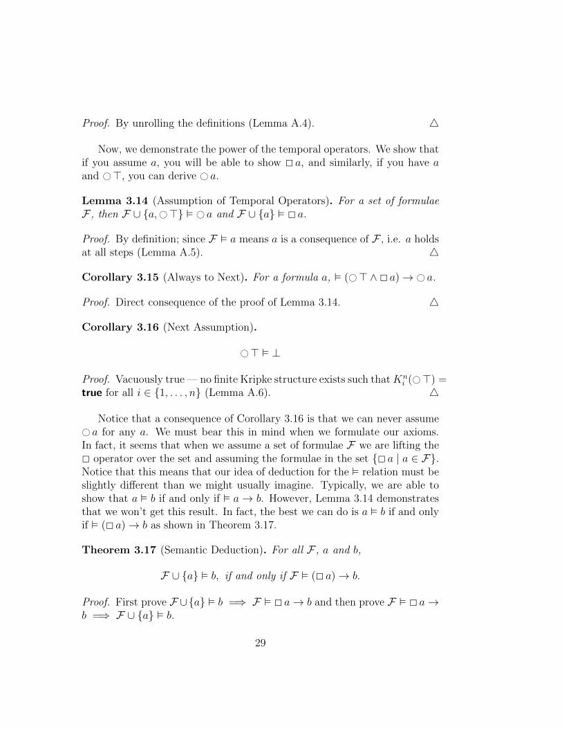
Theorem 3.17 (Semantic Deduction). For all F , a and b,

F ∪ {a} � b, if and only if F � (2 a)→ b.

Proof. First prove F ∪{a} � b =⇒ F � 2 a→ b and then prove F � 2 a→b =⇒ F ∪ {a} � b.

29

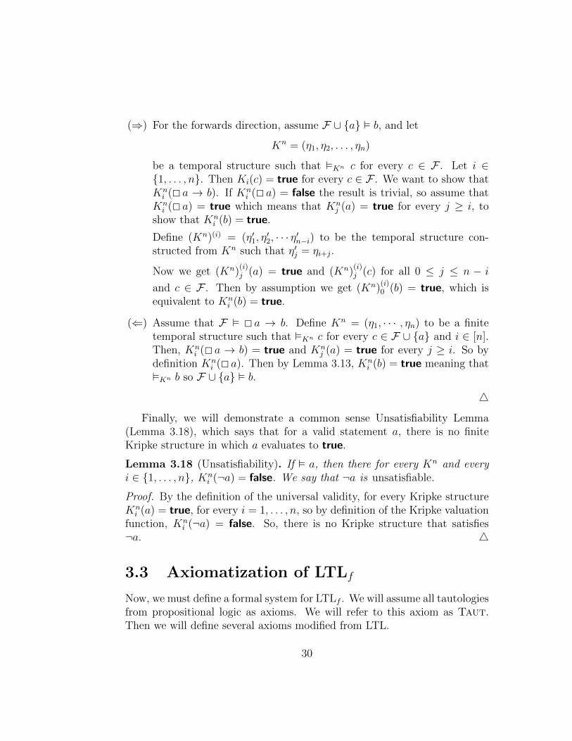
(⇒) For the forwards direction, assume F ∪ {a} � b, and let

Kn = (η1, η2, . . . , ηn)

be a temporal structure such that �Kn c for every c ∈ F . Let i ∈{1, . . . , n}. Then Ki(c) = true for every c ∈ F . We want to show thatKni (2 a → b). If Kn

i (2 a) = false the result is trivial, so assume thatKni (2 a) = true which means that Kn

j (a) = true for every j ≥ i, toshow that Kn

i (b) = true.

Define (Kn)(i) = (η′1, η′2, · · · η′n−i) to be the temporal structure con-

structed from Kn such that η′j = ηi+j.

Now we get (Kn)(i)j (a) = true and (Kn)

(i)j (c) for all 0 ≤ j ≤ n − i

and c ∈ F . Then by assumption we get (Kn)(i)0 (b) = true, which is

equivalent to Kni (b) = true.

(⇐) Assume that F � 2 a → b. Define Kn = (η1, · · · , ηn) to be a finitetemporal structure such that �Kn c for every c ∈ F ∪ {a} and i ∈ [n].Then, Kn

i (2 a → b) = true and Knj (a) = true for every j ≥ i. So by

definition Kni (2 a). Then by Lemma 3.13, Kn

i (b) = true meaning that�Kn b so F ∪ {a} � b.

4

Finally, we will demonstrate a common sense Unsatisfiability Lemma(Lemma 3.18), which says that for a valid statement a, there is no finiteKripke structure in which a evaluates to true.

Lemma 3.18 (Unsatisfiability). If � a, then there for every Kn and everyi ∈ {1, . . . , n}, Kn

i (¬a) = false. We say that ¬a is unsatisfiable.

Proof. By the definition of the universal validity, for every Kripke structureKni (a) = true, for every i = 1, . . . , n, so by definition of the Kripke valuation

function, Kni (¬a) = false. So, there is no Kripke structure that satisfies

¬a. 4

3.3 Axiomatization of LTLf

Now, we must define a formal system for LTLf . We will assume all tautologiesfrom propositional logic as axioms. We will refer to this axiom as Taut.Then we will define several axioms modified from LTL.

30

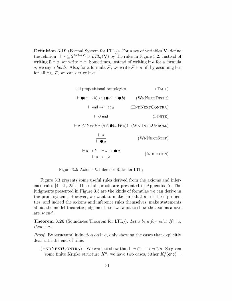
Definition 3.19 (Formal System for LTLf ). For a set of variables V, definethe relation · ` · ⊆ 2LTLf (V)×LTLf (V) by the rules in Figure 3.2. Instead ofwriting ∅ ` a, we write ` a. Sometimes, instead of writing ` a for a formulaa, we say a holds. Also, for a formula F , we write F ` a, if, by assuming ` cfor all c ∈ F , we can derive ` a.

all propositional tautologies (Taut)

` (a→ b)↔ ( a→ b) (WkNextDistr)

` end→ ¬# a (EndNextContra)

` 3 end (Finite)

` aW b↔ b ∨ (a ∧ (aW b)) (WkUntilUnroll)

` a` a

(WkNextStep)

` a→ b ` a→ a

` a→ 2 b(Induction)

Figure 3.2: Axioms & Inference Rules for LTLf

Figure 3.3 presents some useful rules derived from the axioms and infer-ence rules [4, 21, 25]. Their full proofs are presented in Appendix A. Thejudgments presented in Figure 3.3 are the kinds of formulae we can derive inthe proof system. However, we want to make sure that all of these proper-ties, and indeed the axioms and inference rules themselves, make statementsabout the model-theoretic judgement, i.e. we want to show the axioms aboveare sound.

Theorem 3.20 (Soundness Theorem for LTLf ). Let a be a formula. If ` a,then � a.

Proof. By structural induction on ` a, only showing the cases that explicitlydeal with the end of time:

(EndNextContra) We want to show that � ¬#> → ¬# a. So givensome finite Kripke structure Kn, we have two cases, either Kn

i (end) =

31

` # a→ ¬end NextNotEnd

` ¬(#> ∧#⊥) NextContraIsContra

` ¬# a↔ end ∨#¬a CommNegNext

` a↔ (# a ∨ end) NextWkNext

` (end ∨#(a→ b))↔ (# a→ # b) NextDistr

` > WkNextTop` a→ b

` # a→ # bNextMonotone

` 2 a↔ a ∧ 2 a AlwUnroll

` 3 a↔ a ∧#3 a EverUnroll

` (2 a ∧2 b)→ 2(a ∧ b) AlwaysAndDistr` a→ b

` 2 a→ 2 bAlwMonotone

` 2 a ∧3 b→ 3(b ∧ a) AlwaysEver

` 2 a→ 3(end ∧ a) AlwaysFinite

` (a U b)↔ b ∨ (a ∧#(aW b))) UntilUnroll

` ¬(a U b)↔ (¬b)W (¬ ∧ ¬b) NotUntil

` 2 a↔ ¬3¬a AlwaysEverDual

` c→ b ∨ (a ∧ c)` c→ (aW b)

WkUntilInduction

` 2 a→ aW b AlwaysWkUntil

Figure 3.3: Derived rules (proofs in Appendix A)

32

false and we’re done, or Kni (¬#>) = true and we need to show that

Kni (¬# a) = true. The only way that Kn

i (¬#>) could be false is ifi = n, so Kn

i (# a) = Knn(# a) = false. Then applying the definition

gives Kni (¬# a) = true.

(Finite) Assume we have a proof that ` 3 end. We want to show that� 3 end. We can desugar this to a form that the Kn

i functions willunderstand, namely � ¬2#>. Take an arbitrary function Kn

i andshow that Kn

i (¬((#>) W ⊥)) = true. Equivalently, we show thatKni (((#>) W ⊥)) = false. Since we know that Kn

k (⊥) = false for allpossible k, we must find an index j ∈ [i, n] such that Kn

j (#>) = false.Let j = n, then by definition Kn

j (#>) = Knn(#>) = false.

See Lemma A.7 for remaining cases.

4

Theorem 3.17 showed that for a set of formulae F , and formulae a, b wehave F ∪ {a} � b if and only if F � (2 a)→ b. We want to be able to showthe exact same thing, swapping the ` relation for the � relation.

This informs how we can perform deductive proofs in the logic. In Clas-sical logic, {a} ` b if and only if ` a → b. So, we prove statements of theform ` a → b by first proving the equivalent {a} ` b; we say “Assume ` a,and show ` b”. However in our proof system for LTLf , the judgement a ` bmeans ` (2 a)→ b which does not prove ` a→ b. Hence, we cannot derive` a→ b by saying “Assume ` a and show ` b”. See the proofs in Appendix Afor examples of how to resolve this trouble.

Theorem 3.21 (Deduction Theorem). Let a, b be formulae, F a set of for-mulae. F ∪ {a} ` b if and only if F ` 2 a→ b.

Proof. From left to right, by induction on the derivation of F ∪{a} ` b; fromright to left, by Taut, WkNext, and Induction (c.f. Theorem A.8). 4

3.4 Completeness for LTLf

We want to show completeness of LTLf , i.e. we want to show that ∀Kn,�Kn aimplies that ` a, for all terms a. That is, if something is valid in the model,we can prove it using our axioms.

33

Our proof largely follows the completeness proof for LTL [21], except wemake sure to both ensure the existence of a final state, and in constructingsatisfying timelines, we make sure to keep track of whether we are in a finalstate.

To show the existence of a proof for a formula a, we create a PNP basedon the negation of this formula. As in the proof of Theorem 2.13, this PNPshould be P = (∅, {a}). We will want to show that P is inconsistent, i.e.that we can derive ` ¬¬a, which is exactly ` a. However, we need to ensurethat our construction respects the finiteness assumption, so we will injectthe axiom Finite into the positive set of this PNP. Construct another PNPP = ({3 end}, {a}); and demonstrate it’s inconsistency. To do this, weuse a satisfiability theorem (Theorem 3.42) that says that consistent PNPshave satisfiable interpretations. We show P is unsatisfiable, to conclude thatit is inconsistent. This means that ` ¬P , so ` ¬(3¬#> ∧ ¬a), whichdemonstrates ` a using Taut.

The key point in this proof is the satisfiability theorem (Theorem 2.13)which says that every consistent PNP is satisfiable. To show this theoremwe will construct a large graph structure from a PNP P , called GP , thatwill step the PNP through time, examining all potential successors at eachtime step. Each node of the graph is a consistent PNP, we will use a closurefunction called τ and the step function called σ to create the edge set in thegraph.

We inductively define the function τ : LTLf (V) → 2LTLf (V) from a for-mula to a set of formulae, to be set of all subformulae of a given formula(taking # a as atomic). We can then lift this to sets of formulae and PNPsin the obvious way. For a given PNP Q, call τ(Q) the closure of Q. Forexample, we can consider a PNP Q0 = ({3 end,#>}, ∅), then τ(Q0) willcontain every recursive expansions of the formulae in Q0, we see this below:

τ(Q0) = {3 end,2¬end,¬end,¬#>,#>}

So, for a given PNP Q, we want to take all of the formula in τ(Q) andconstruct all sensible assignments of the subformulae in τ(Q) to the positiveor negative sets of a PNP. Specifically, extend the positive and negativesets of Q with elements of τ(Q) − FQ, where no formula is in both sets,to get a to get a new PNP Q∗. We say that Q∗ is a completion of Q.So, continuing the above example, one possible completion of Q0 is Q∗0 =({¬end,3 end,#>}, {⊥, end,2¬end}). We see that pos(Q0) ⊂ pos(Q∗0) and

34

Q∗0

Q1

QQQ2

Figure 3.4: An Example Proof Graph

since neg(Q0) = ∅, the same is true for the negative sets. Notice also thatthe two sets are distinct, and every element of τ(Q0) appears exactly once.

To get the successors of a PNP, we will step the PNP forward one step intime, and then take all of the completions at that step. This step functionis called σ. So now, we can to step this forward one place to get

σ(Q∗0) = ({>}, {2¬end})

Then we can find all consistent completions of σ(Q∗0), these will be thesuccessors of Q∗0. They are:

Q1 = ({>,¬end,#>}, {⊥, end,2¬end})Q2 = ({>, end}, {⊥,¬end,#>,2¬end})

These two PNPs, Q1 and Q2 correspond to the interesting successorstates, where time ends in Q1 but continues in Q2.

If we continue to build this tree by finding the consistent completions ofσ(Q1) and σ(Q2), we see that σ(Q2) has no consistent completions, whereasthe consistent completions of σ(Q1) are exactly the same as the consistentcompletions of σ(Q0). Then we can construct the graph, GQ∗

0shown in Fig-

ure 3.4. We can see the satisfying models in GQ∗0, either the next state is

the end of time Q0 to Q2, or you can take arbitrarily many steps, using anypath like π = Q0,Q1, . . . ,Q1,Q2. This path corresponds to a finite Kripkestructure K |π| = (η1, . . . , η|π| where ηi(v) = true if and only if v is in thepositive set of the ith node in π.

Notice in particular that GQ0∗ is finite. In general, the set of nodes in anarbitrary proof graph is finite, and for our original PNP P = ({3 end}, {a}),

35

we engage in a path-finding exercise1. We care about terminal paths. Aterminal path is one that ends in a node Z, such that #> ∈ Z (calleda terminal node). In our running example, Q2 is a terminal node, and isidentified with a double circle in GQ∗

0. So, all paths that end in Q2 are

terminal, i.e. all paths of the form Q0,Q1, . . .Q1︸ ︷︷ ︸0 or more

,Q2.

Some proofs for completeness of LTL [21, 24] try to find something calleda fulfilling or complete path, by which they mean that all temporal formulaein the path are realized in the path. In the finite setting, it is straightforwardto prove that terminal paths are exactly the fulfilling paths (Corollary 3.40).

Now, we know there exists a terminal path π = P1, P2, . . . , Pn. We createa Kripke structure Kn from this path as above. We then show that Kn

1 (a) =true, i.e. that a is satisfiable. So we can conclude that for every PNP Q, ifQ is consistent, then Q is satisfiable.

So how do we use the satisfiability result to prove the general completenessresult? We know that if a PNP is consistent, then it is satisfiable. We’vecreated this PNP P = ({3 end}, {a}), with the intent to show that � aimplies ` a. We know that ¬a is unsatisfiable since a is valid, so we knowthat P is inconsistent. This gives us a derivation of ` ¬(3 end ∧ ¬a), whichby some classical machinery gives ` a.

Now we proceed with this proof formally.

Preliminary Definitions and Lemmata

Before we can use the PNPs we defined in Definition 2.11, we need to provea lemma about the way that they behave.

Lemma 3.22 (PNPs are Well-Behaved). Let P = (F+,F−) be a consistentPNP, and a, b be formulae, then

1. F+ and F− are disjoint

2. Either (F+,F− ∪ {a}) or (F+ ∪ {a},F−) is a consistent PNP

3. ⊥ 6∈ F+

4. If, a, b, a→ b ∈ FP , then if a ∈ F− or b ∈ F+, a→ b ∈ F+, otherwisea→ b ∈ F−.

1Here we are using a loose definition of path where repetition and self-loops are al-lowed [21]. Some call this structure a walk [31]

36

5. If a→ b, a, b ∈ FP , then if a→ b ∈ F+, and a ∈ F+, then b ∈ F+.

Proof. See Lemma A.10. 4

We also want a way to reason about how a formula evolves over time.We will create a graph structure whose nodes are consistent PNPs, and theedges represent a potential step forward in time. To do this, we will definea “step” function σ that will mirror the way the Kn function steps throughthe lifetime of the temporal operators.

Definition 3.23 (Step Function). The step function, σ is inductively definedfor a PNP P = (F+,F−) as follows:

σ+1 (P) = {a | # a ∈ pos(P)}σ+2 (P) = {aW b | aW b ∈ pos(P) and b ∈ neg(P)}σ+3 (P) = {aW b | aW b ∈ pos(P),#> ∈ neg(P), and a ∈ pos(P)}σ−4 (P) = {a | # a ∈ neg(P)}σ−5 (P) = {aW b | aW b ∈ neg(P) and a ∈ pos(P) or b ∈ pos(P)}

Where σ(P) = (σ+1 (P) ∪ σ+

2 (P) ∪ σ+3 , σ

−4 (P) ∪ σ−5 (P)).

We call a formula f ∈ FP unresolved in a PNP P if f ∈ Fσ(P); otherwise,call f resolved.

Intuitively, applying σ to a function steps all formulae of the form # a toa, in their respective sets, and then for each statement like aW b, it assesseswhether we have seen as at every step until we see our first b. These actionscombine to provide a transformation on PNPs that morally represents takingone step forwards in time.

Example 3.24. Now, we can formally see the way that the σ function worksfor the node Q∗0 that we examined earlier. Recall the PNP:

Q∗0 = ({¬end,3 end,#>}, {⊥, end,2¬end}) .

Since our definitions are written in terms of the syntactic sugar, lets reducethe formulae in Q∗0 to only use the basic operators. Then, we rewrite Q∗0 as

Q∗0 = ({¬¬#>,¬((¬¬#>)W ⊥),#>}, {⊥,¬#>, (¬¬#>)W ⊥}) .

37

We compute:

σ(Q∗0) = ({>}, {(¬¬#>)W ⊥}) ≡ ({>}, {2¬end}).

Notice that #> is resolved, and (¬¬#>)W ⊥ is unresolved.

We want this σ-function to have a couple of essential properties, and the4-part definition facilitates a proof by cases. First of all, the σ function isintended to simulate the change in interesting formulae over a single timestep. In order for this representation to make sense, ` P must imply `# σ(P)) — unless we’re at the end of time, in which case we get ¬# a for all

formulae a. So, to encompass these two cases, we show that P → σ(P ).

Lemma 3.25 (Next-Step Implication). Let P be a PNP

` P → σ(P)

Proof. By cases on σi, ` P → c whe have c ∈ σ1(P) ∪ σ2(P), and ` P → ¬c when c ∈ σ3(P)∪σ4(P). The proposition follows directly from this andWkNextAndDistr. See Lemma A.9 for the case analysis.

4

Lemma 3.26 (Step Consistency). Let P be a consistent PNP. If ` P →¬end, then σ(P) is consistent.

Proof. First we show that ` P implies ` σ(P). So, assume ` P , and for

the sake of contradiction, assume ` ¬σ(P). Then, from WkNext we get

` ¬σ(P). Then, finally from NextWkNext we get ` end ∨ ¬ σ(P).

However, we know that ` P → ¬end, so we can just conclude ` σ(P). Then

by the contrapositive of Lemma 3.25, derive ` ¬P . We have a contradiction

with ` P , so conclude that ` σ(P).

So, if P is consistent, then we know that it is not the case that ` P . Wewant to show that σ(P) is consistent, so assume, for the sake of contradiction,

that ` ¬σ(P). Then by the contrapositive of ` P implies ` σ(P ) (shown in

the previous paragraph), we get ` ¬P , which contradicts the assumption ofP ’s consistency. Hence σ(P) is consistent. 4

38

Now that we have a way of stepping PNPs through timesteps, we want tobe able to examine all the pieces of a PNP to see how they interact with eachother. The tool we need to do this is the completion of a PNP. It allows usto break apart composite formulae into their atomic pieces and assign eachsubformula to the positive or negative set. This gives all of the informationabout how a PNP is consistent. We define the function τ to perform thisexamination of subformulae, formalize a notion of completion, and define thecomps function.

Definition 3.27 (Closure). Define the closure function τ : F → 2F as afixpoint on an input formula, that returns the set of subformula of the input:

τ(v) = v for v ∈ V

τ(⊥) = {⊥}τ(a→ b) = {a→ b} ∪ τ(a) ∪ τ(b)

τ(# a) = {# a}τ(aW b) = {aW b} ∪ τ(a) ∪ τ(b)

We can also lift the function τ over sets of formula, i.e. τ : 2F → 2F ,using the definition τ(F) =

⋃f∈F τ(f), and to apply over a PNP, where

τ(P) = τ(FP). The set τ(x) is called the closure of x.

Definition 3.28 (Extensions and Completions). A PNP Q is an extensionof another PNP P if pos(P) ⊆ pos(Q) and neg(P) ⊆ neg(Q). We say Qextends P . Q is a completion of P if τ(P) = pos(Q) ∪ neg(Q) and Q is anextension of P ; Q is called complete.

Definition 3.29 (Completion Function). Let F ∈ LTLf (V) be a set offormulae and let the function comps : 2LTLf (V) → 2PNP be defined as

comps(F) = {Q | τ(Q) = τ(F)}

We overload the definition of comps to also be a function comps : PNP →2PNP such that:

comps(P) = {Q | τ(Q) = τ(P) and Q extends P}

The completion of a PNP is an expansion of all of its subformulae thatcan be evaluated at the current time step, i.e. all of those formulae that arenot under a # operator. We want to be able to say something about theconsistency of the completions of a complete PNP. But which completionsare consistent?

39

Example 3.30. Given a PNP P = ({v1 → v2}, ∅), where v1 and v2 arevariables, we have four completions:

comps(P) = {P∗0 ,P∗1 ,P∗2 ,P∗3}P∗0 = ({v1 → v2, v1, v2}, ∅)P∗1 = ({v1 → v2, v1}, {v2})P∗2 = ({v1 → v2, v2}, {v1})P∗3 = ({v1 → v2}, {v1, v2})

All of these are consistent, except for P∗2 , the axiom Taut tells us that

the formula P∗2 ≡ v1 → v2 ∧ v2 ∧ ¬v1 is contradictory.

The previous example demonstrates that not all completions are consis-tent, but we’d really like it if at least one of the completions were consistent(Lemmata 3.31 and 3.33).

Lemma 3.31 (Consistent Closure Existence). Let F be a finite set of for-mulae, and let P∗1 , · · · P∗m be PNPs with FP∗

i= τ(F) for all i ∈ {1, . . . ,m}

such that the positive and negative sets are disjoint. Then, `∨mi=1 P∗i .

Proof. By induction on the number of formulae in F . Consider the base casewhere F = τ(F) = ∅. Then P∗ = (∅, ∅) so with FP∗ = τ(F), and P∗ ≡ >and the conclusion holds by Taut.

Now consider the case where τ(F) = {a1, . . . , ak}, for k ≥ 1. Since τ(f)only contains f and subterms of f , there is some maximal formula aj suchthat

aj 6∈ τ({a1, . . . , aj−1, aj+1, . . . , ak}).Let F ′ ≡ τ(F) − aj. Let P∗′1, . . . ,P∗′l, be the PNPs constructed from F ′.Then for each PNP P∗′i we construct two new PNPs, one by adding aj tothe positive set, and one by adding aj to the negative set. Let m = 2land the PNPs P∗1 , . . . ,P∗m be those PNPs constructed in this manner. Theinduction hypothesis is that `

∨li=1P∗

′i. So using the construction above,

and Lemma 3.22, we can conclude that `∨li=1(P∗

′ ∨ aj) ∨∨li=1(P∗

′ ∨ ¬aj).The result follows by Taut. 4

Example 3.32. Let F = {a ∧ ¬a}. Show that we can prove one of thePNPs constructed from its completeions. We can do this despite the factthat a ∧ ¬a is neither provable nor satisfiable. Calculate τ(F) to be

40

τ(F) = {a ∧ ¬a, a,¬a}

Let P∗i for i = 1, . . . ,m be the PNPs that can be constructed by par-

titioning τ(F). To show `∨mi=1 P∗i , we only need to show ` P∗i for some

i = 1, . . .m. We know there is some i such that P∗i = ({¬a}, {a, (a ∧ ¬a)}.Note that P∗i = ¬a ∧ ¬a ∧ ¬(a ∧ ¬a). So, by Taut, we can see that ` P∗i .

conclude `∨mi=1 P∗i .

Lemma 3.33 (Consistent Completion Existence). For P, a consistent PNP,and

` P →∨

Q∈comps(P)

Q

Proof. Let P1, . . . ,Pm be those PNPs with disjoint pos/neg sets such thatτ(P) = τ(Pi). Each one is either in comps(P), inconsistent, or not an exten-sion, for more detail see Lemma A.11. 4

Lemmata 3.31 and 3.33 allow us to construct the graph using σ and compsto create the edge relation. Because now we know that for all PNPs that dontrepresent the end of time, we can find a consistent successor (Lemmata 3.33and 3.26) that represents a next state (Lemma 3.25).

Definition 3.34. For a consistent and complete PNP P∗, define the proofgraph rooted at P∗, called GP∗ , to be the root P∗, and the successors GQ forevery consistent Q ∈ comps(P∗).

Corollary 3.35. For a consistent and complete PNP P∗, there are a finitenumber of vertices in GP∗.

Proof. Each node is a PNP. Specifically each PNP has a finite number ofchildren, because there are a finite number of completions via τ , and thereare a finite number of unique steps as the σ function consumes # operators,negativeW operators, and continuing positiveW operators. Since our initalformula is constrained to be finite, we can only have finitely many nodes. 4

Intuitively this graph GP represents the potential satisfying Kripke struc-tures of the original formulae in the root P , so we want to show that the tem-poral operators behave nicely on paths. So we will prove the following lemma,that looks suspiciously close to our original Semantics (Definition 3.2).

41

Lemma 3.36 (Temporal Operators On Paths). Let P be a consistent andcomplete PNP and P0,P1,P2, · · · an infinite path in GP , for i ∈ N and a aformula.

1. If # a ∈ FPi, then # a ∈ pos(Pi), if and only if a ∈ pos(Pi+1).

2. If aW b ∈ FPi: aW b ∈ pos(Pi), if and only if b ∈ pos(Pk), for some

k ≥ i, implies that for every j ∈ [i, k), a ∈ pos(Pj).

Proof.

1. Assume that # a ∈ FPi. If # a ∈ pos(Pi) then a ∈ pos(σ(Pi)) by the

definition of σ and the completeness of Pi. Then the definition of GPimplies a ∈ pos(Pi+1). Conversely, if # a 6∈ pos(Pi), it must be that# a ∈ neg(Pi). Then by the definition of σ and the completeness of Pi,a ∈ neg(σ(Pi)). Then a ∈ neg(Pi+1) and by the disjointness of positiveand negative sets (Lemma 3.22) we get a 6∈ pos(Pi+1).

2. We prove each direction separately.

(⇒) Assume a W b ∈ pos(Pi), to show that there exists k ≥ i suchthat for every j ∈ [i, k), a ∈ pos(Pj) and b ∈ pos(Pk).By Taut and WkUntilUnroll ` Pi → b or ` Pi → (a∧ (aWb)). If ` Pi → b, then we set k = i, and so vacuously a ∈ pos(Pj)for every j ∈ [i, i) = ∅ and b ∈ PiOtherwise, if ` Pi → a ∧ (a W b), then since a ∈ τ(a W b),we have a ∈ pos(Pi). We also know a W b ∈ pos(Pi+1) by thedefinition of σ. Continue inductively to see that either a ∈ pos(Pj)for all j ≥ i, or there is some k such that b ∈ pos(Pj) and for everyi ≤ j < k, a ∈ pos(Pj).

(⇐) Assume that a W b 6∈ pos(Pi). Since a W b ∈ FPiit must be

that a W b ∈ neg(Pi). Then by Taut and WkUntilUnroll,

` Pi → (¬b ∧ ¬a) or ` Pi → (¬b ∧ ¬ (aW b)).

If ` Pi → (¬b ∧ ¬a), then we have a, b ∈ neg(Pi) which showsthat neither is a ∈ pos(Pi) for all k ≥ i nor does there exist ak ≥ i where b ∈ pos(Pk) and a ∈ pos(Pj) for every i ≤ j < k.

Otherwise, we consider ` Pi → ¬b ∧ #¬(a W b). Consistencygives us that b ∈ neg(Pi) and the definition of σ tells us that

42

aW b ∈ neg(Pi+1), so we cannot set k = i. Continue inductivelyto conclude that b ∈ neg(Pi).

4

Some proofs using this method loosely refer to the proof graph structureas a tree [21], which is somewhat misleading since the graphs can have arbi-trarily large cycles. The graph in Figure 3.4 of the proof graph constructedfrom the formula #> already has a self-loop. However, for more compli-cated formulae, we can see more complicated graph structures. For exampleconsider the graph constructed from the formula 2((# a)∨ b), in Figure 3.5.There are many cycles in this graph, such as (Q3,Q4) and (Q4,Q6,Q5,Q7).

Now we can show that every node Q that is not the end of time has asuccessor.

Lemma 3.37 (All Nodes Have Successors). Let P be a consistent and com-plete PNP, and Q1, · · · ,Qn the nodes of GP .

`n∨i=1

Qi → n∨i=1

Qi

Proof. By Lemma 3.25 and Lemma 3.33 (c.f. Lemma A.11). 4

Reasoning about Paths

We want to find a path through this graph structure that we can use toconstruct a satisfying finite Kripke structure. When we’re at some nodeQ, it is connected to the consistent PNPs in comps(σ(Q)). If there are noconsistent completions, then we know we are at the end of time. So we canmaintain a path of consistent nodes, moving forwards in time with successivenode. However, so far, we don’t know that this path will end, or if it doeswhere we can find that end point. We have the axiom Finite which saysthat ` 3 end, so we can be pretty confident that at some point every pathwill end. Let’s call a path that does reach a node in which #> is in thenegative set a terminal path. In Figure 3.4, the terminal paths, were thosethat ended in Q2. In Figure 3.5, the red path is the chosen terminal path,but any path ending in one of the double-lined nodes is a terminal path.

Definition 3.38 (Terminal Path). Given a consistent and complete PNP P ,and a graph GP , a node Z ∈ V(GP) is called terminal when #> ∈ neg(Z).A path π is called terminal if it ends in a terminal node.

43

Q0

Q8 QOQ1Q6

Q3

Q5

Q4

Q7

OQQ2

Node ContentsQ0 ({3 end,2(# a ∨ b)}, ∅)Q1 ({b,>,# a ∨ b,¬# a, end,2(# a ∨ b)}, {⊥, a,#> ∨⊥,# a,#>,2¬end})Q2 ({a, b,>,# a ∨ b,¬# a, end,2(# a ∨ b)}, {⊥,#> ∨⊥,# a,#>,2¬end})Q3 ({# a ∨ b,#> ∨⊥,3 end,# a,#>,2(# a ∨ b)}, {⊥, b,¬# a, end,2¬end})Q4 ({b,# a ∨ b,¬# a, end,3 end,2(# a ∨ b)}, {⊥,#> ∨⊥,# a,#>,2¬end})Q5 ({b,# a ∨ b,#> ∨⊥,3 end,# a,#>,2(# a ∨ b)}, {⊥,¬# a, end,2¬end})Q6 ({b,# a ∨ b,#> ∨⊥,¬# a,3 end,#>,2(# a ∨ b)}, {⊥, end,# a,2¬end})Q7 ({a,>,# a ∨ b,#> ∨⊥,# a,#>,2(# a ∨ b)}, {⊥, b,¬# a, end,2¬end})Q8 ({a, b,>,# a ∨ b,#> ∨⊥,# a,#>,2(# a ∨ b)}, {⊥,¬# a, end,2¬end})Q9 ({a, b,>,# a ∨ b,#> ∨⊥,¬# a,#>,2(# a ∨ b)}, {⊥, end,# a,2¬end})Q10 ({>,# a ∨ b,#> ∨⊥,# a,#>,2(# a ∨ b)}, {⊥, a, b,¬# a, end,2¬end})Q11 ({b,>,# a ∨ b,#> ∨⊥,# a,#>,2(# a ∨ b)}, {⊥, a,¬# a, end,2¬end})Q12 ({b,>,# a ∨ b,#> ∨⊥,¬# a,#>,2(# a ∨ b)}, {⊥, a, end,# a,2¬end})

Figure 3.5: The graph for 2((# a) ∨ b), with many cycles

44

Other proofs for LTL [21, 24] search for a different kind of path, calleda fulfilling path which says that for every i ∈ N, if 2 a ∈ neg(Pi), thena ∈ ¬(P) for some j ≥ i. We are usingW instead of 2 as our basic operator,so we will define an analogous definition for paths containing aW b.

Definition 3.39 (Fulfilling Path). Consider a path π = P0,P1, . . . in a graphGP , where P is a consistent and complete PNP. A temporal formula c ∈ FPi

is called fulfilled in π when there exists a node Pj with j ≥ i such thatc 6∈ τ(σ(Pj)). When the π is clear from context, we can just say that c isfulfilled. If every temporal term in π is fulfilled, call π a fulfilling path.

In fact, in LTLf , we can demonstrate that every terminal path is a ful-filling path, thus greatly decreasing the proof obligation.

Lemma 3.40. Every terminal path is a fulfilling path.

Proof. In the terminal node, every as-yet unresolved temporal operator willbe resolved in the terminal node (c.f. Lemma A.12). 4

Since we’ve shown that every terminal path is fulfilling, we need onlyto show that there exists a terminal path. Unfortunately this is not truefor proof graphs in general, because they may me constructed without anyinformation about the end of time. For example, we can have a PNP Q =({2 a}, ∅), which will never know anything about end or #>, because #> 6∈τ(Q). To ensure that the tree structure knows about the end of time, wecan insert the axiom ` 3 end into the positive set of the root PNP. This willmake it so that every node is forced to consider whether to stick end into thepositive or negative set; Lemma 3.41 demonstrates that end will end up in apositive set somewhere in the graph.

Lemma 3.41 (Terminal Path Existence). Let P be a consistent and completePNP with 3 end ∈ pos(P). There is a terminal path in GP .

Proof. In fact, we only need to show that there exists a terminal node Zin the nodes of GP , because GP is connected by definition. We proceed byinduction on the size of GP .

In the base case, the graph is the singleton node P . The only way thata node has no successors is (by Lemma 3.26) when #> ∈ neg(P), and soZ ≡ P .

Now, assume that we have a nontrivial GP . Assume for the sake of con-tradiction that for every node Q of GP , #> ∈ pos(Q). Since 3 end ∈ pos(P),

45

and every path out of GP has #> ∈ pos(P), we know that for every node Qin GP , 2¬¬#> ∈ neg(Q).

Let Q1,Q2, . . . ,Qn be the nodes of GP . Then since ` Qi → #> for everyi = 1, . . . n, we conclude `

∨ni=1Qi → #>.

Recall that `∨ni=1 Qi →

∨ni=1 Qi (Lemma 3.37). Now we can use

Induction to conclude `∨ni=1 Qi → 2#>. We have that P is a node of GP ,

so P ∈ {Q1, · · · ,Qn}, so we know that ` P →∨ni=1 Qi, and consequently

` P → 2#>. However we assumed P → 3 end, i.e. ` P → ¬2#>,contradicting the assumption that every node Q of GP has #> ∈ pos(Q).Therefore, there exists a node Z such that #> ∈ neg(Z). 4

The Proof

Now we are finally in a position to prove the satisfiability result (Theo-rem 3.42) and use it to derive the completeness theorem (Theorem 3.43).

Theorem 3.42 (Satisfiability Theorem for LTLf ). For any consistent PNP

P, the formula P is satisfiable.

Proof. P ′ = ({3 end} ∪ pos(P), neg(P)) is a consistent PNP, P∗ is a com-pletion of P ′. And P0, P1, · · · , Pn a complete, finite, rooted path of length n(by Lemma 3.41) in GP∗. Define Kn = (η0, η1, · · · , ηn) by

ηi(v) = true if v ∈ F+i

ηi(v) = false otherwise

We want to show that Kn0 (P) = true. This is equivalent to showing that

Kn0 (P ′) = true, which is also equivalent to showing that Kn

0 (P0) = true.Proving this is hard, so we will generalize the hypothesis making it easier toprove. We will show that for PNP Pi, and f ∈ FPi

, then Kni (f) = true iff

f ∈ pos(Pi), and Kni (f) = false otherwise.

We proceed by induction on the derivation of an arbitrary formula f .Here show only the interesting cases corresponding to the operators → andW . For the full proof see Lemma A.14

(f = a→ b). Since Pi is a complete PNP, we have that a, b ∈ F+∪F−.The inductive hypothesis allows us to conclude that Kn

i (a) = false iff

46

a 6∈ F+i . It also allows the conclusion Kn

i (b) = true iff b ∈ F+i . Then,

Kni (a → b) = true if and only if Kn

i (a) = false or Kni (b) = true, we

can apply the inductive hypotheses to get a ∈ F−i or b ∈ F+i . Then by

Lemma 3.22, we can conclude that a→ b ∈ F+i .

(f = a W b). Here we dont need to break into cases, we can provethis directly. Kn

i (a W b) = true if and only if there exists k ∈ [i, n]such that for all j ∈ [i, k), Kn

j (a) = true and Knk (b) = true. using

the inductive hypothesis, we know this statement holds if and only ifthere exists k ∈ [i, n] such that for all j ∈ [i, k), a ∈ pos(Pj) andb ∈ pos(Pk). Then by Lemma 3.36 the previous statement holds if andonly if aW b ∈ pos(Pi).

4

Theorem 3.43 (Weak Completeness Theorem for LTLf ). Given a finite setof formulae F = a1, a2, · · · an and a formula b, if F � a, then F ` a.

Proof. First we prove the claim for F = ∅. If � a, then ¬a is not satisfiableby Theorem 3.18. Consequently the PNP (∅, {a}) is inconsistent by Theo-rem 3.42. By the definition of consistency, we get ` ¬¬a which gives ` ausing Taut. Let us now show that a proof of � a implies ` a is sufficient.

Let F = a1, · · · an for n > 0. We then have a1, · · · an � a. Then byTheorem 3.17 we have a1, · · · an−1 � 2 an → a. We can apply Theorem 3.17n− 1 more times to get � 2 a1 → · · · → 2 an → a, which, as proved above,gives ` 2 a1 → · · · → 2 an → a. Then by applying Theorem 3.21 n timeswe get F ` a. 4

3.5 A Decision Procedure for LTLf

In Section 3.2, we defined the terms valid and satisfiable with respect toformulae of LTLf . These are great as mathematical definitions and workwell when we can simply assume the validity or satisfiability of a formula.We now want a way to decide whether a formula is satisfiable, valid, orotherwise.

Now, how might we fix this? We need to come up with an algorithm todecide whether a given formula is satisfiable, valid, or unsatisfiable. This isequivalent to deciding whether, for a given formula, there exists a satisfying

47

Kn, every Kn is satisfying, or no Kn is satisfying, respectively. Notice thatif the negation of a formula is unsatisfiable, then that formula is valid, so ouralgorithm will only need to detect whether a given formula is satisfiable.

The decision procedure will look very much like a traversal of GP for aPNP P . The difference is that now we are not allowed to know anythingabout the consistency of a node, a central piece of knowledge in the con-tstruction of GP . If we knew whether a PNP P was consistent, we wouldthen know that P is satisfiable by soundness (Theorem 3.20). Instead, for agiven PNP, we will create successor nodes that are be implied by the currentnode, i.e. if some node Q evaluates to true, then one of its successors alsoevaluates to true. We will call our structure a tableau (Definition 3.46). Tomake a tableau, we are constructively exploring the potential truth values ofthe subformulae in a node Q to determine if it is satsifiable, whereas in theproof graph, we are assuming consistency of each node to prove satisfiability.We have no way of knowing anything about the consistency or satisfiabilityof a given node in an arbitrary tableau.

As an example, consider a node P with a → b ∈ pos(P). We want toperfom a case analysis on a and b, so we create 2 successors: a left successorwith ¬a in the positive set, and a right successor with b in the positive set.Critically, we remove a → b from the positive sets of the successors, sinceboth ` ¬a → (a → b) and ` b → (a ∨ b) by Taut. Thus, removing a → bhas the nice feature that |τ(P)| is decreasing.

The tricky case to consider, as we might expect, is what to do when#> ∈ neg(P). At this point we want to try and end time, so we willdefine a transformation on PNPs that removes all temporal information.For variables, implication and the ⊥ symbol we can just remove temporaloperators for any subformulae that may occur. However, for operators likeW and # we need to take some action.

As in the semantics and proof theory, if we are in the last state andsee a formula matching the pattern # a, we simply transform it into ⊥. Ifwe see a formula a W b, we will need to do some more work. Recall theWkUntilUnroll axiom which says that aW b↔ b∨ a∧ (aW b). Sincewe are at the end of time, the term (a W b) just becomes > and fallsaway, giving a ∨ b. Then since a and b might themselves contain temporaloperators, we will recursively continue the transformation on those formulae.This is defined formally as the drop function below:

48

Definition 3.44 (drop Function). Define drop : LTLf → LTLf below

drop(c) =

⊥ if c ≡ ⊥⊥ if c ≡ # av if v ∈ V

drop(a) ∨ drop(b) if c ≡ aW b

drop(a)→ drop(b) if c ≡ a→ b

We can lift drop to sets of formulae, setting

drop(F) ,⋃

c∈Form

drop(c).

Lemma 3.45. For every formula c and every finite Kripke structure Kn,

Knn(c) = Kn

n(drop(c))

Proof. Let c be an arbitrary formula, Kn an arbitrary Kripke structure. Showthat Kn

n(c) = Knn(c). By induction on the structure of c (c.f. Lemma A.15).

4

Now that we have a schema for dealing with syntactic operators, and away for dealing with the end of time, we can formally define our constructionof a tableau.

Definition 3.46 (Tableau). Given a PNP P we construct a tableau for P ,written TP . Let the PNP ({3 end}∪pos(P), neg(P)), be the root node of TP .For a given node Q in TP , construct its successors using one of the followingrules. If more than one rule is relevant, apply the one occuring earlier in thelist.

(⊥) If ⊥ ∈ pos(Q) or pos(Q) ∩ neg(Q) 6= ∅, there are no successors.

(→+) If a→ b ∈ pos(Q), the successors are:

• ((pos(Q)/{a→ b}) ∪ {b}, neg(Q)), and

• ((pos(Q)/{a→ b}), neg(Q) ∪ {a})

(→−) If a→ b ∈ neg(Q), the successor is:

49

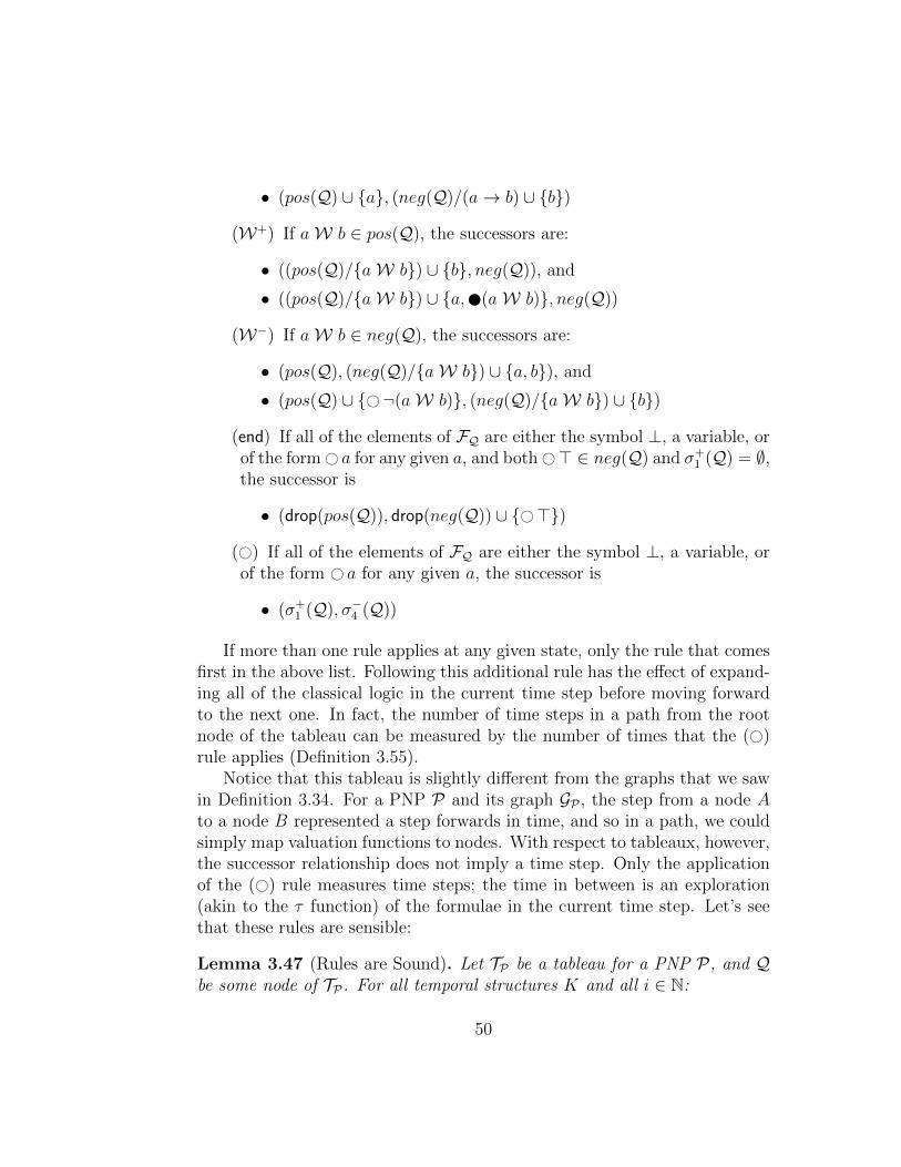
• (pos(Q) ∪ {a}, (neg(Q)/(a→ b) ∪ {b})

(W+) If aW b ∈ pos(Q), the successors are:

• ((pos(Q)/{aW b}) ∪ {b}, neg(Q)), and

• ((pos(Q)/{aW b}) ∪ {a, (aW b)}, neg(Q))

(W−) If aW b ∈ neg(Q), the successors are:

• (pos(Q), (neg(Q)/{aW b}) ∪ {a, b}), and

• (pos(Q) ∪ {#¬(aW b)}, (neg(Q)/{aW b}) ∪ {b})

(end) If all of the elements of FQ are either the symbol ⊥, a variable, orof the form# a for any given a, and both#> ∈ neg(Q) and σ+

1 (Q) = ∅,the successor is

• (drop(pos(Q)), drop(neg(Q)) ∪ {#>})

(#) If all of the elements of FQ are either the symbol ⊥, a variable, orof the form # a for any given a, the successor is

• (σ+1 (Q), σ−4 (Q))

If more than one rule applies at any given state, only the rule that comesfirst in the above list. Following this additional rule has the effect of expand-ing all of the classical logic in the current time step before moving forwardto the next one. In fact, the number of time steps in a path from the rootnode of the tableau can be measured by the number of times that the (#)rule applies (Definition 3.55).

Notice that this tableau is slightly different from the graphs that we sawin Definition 3.34. For a PNP P and its graph GP , the step from a node Ato a node B represented a step forwards in time, and so in a path, we couldsimply map valuation functions to nodes. With respect to tableaux, however,the successor relationship does not imply a time step. Only the applicationof the (#) rule measures time steps; the time in between is an exploration(akin to the τ function) of the formulae in the current time step. Let’s seethat these rules are sensible:

Lemma 3.47 (Rules are Sound). Let TP be a tableau for a PNP P, and Qbe some node of TP . For all temporal structures K and all i ∈ N:

50

a) If (#) does not apply, then Kni (Q) = Kn

i (Q′) for some successor Q′ ofQ.

b) If (#) applies, then Kni (Q) = Kn

i+1(Q′) for the successor Q′ of Q. Also,

Q′ is satisfiable only if Q is satsifiable.

Proof. By cases on the rule applied (c.f. Lemma A.16). 4

Similar to the proof of completeness (Theorem 3.43), we need to findsomething akin to a terminal path to construct a satsifable finite Kripkestructure. We define it slightly differently, because in the last state, we stillneed to examine those non-temporal conditions that hold in the final state.Define a terminating node, is a node in a tableau TP that has #> in thenegative set, or is a successor of a node Z that has #> in the negative set.For simplicity, we will simply continue to add #> to the negative sets of Z’ssuccessors.

Definition 3.48 (Terminating Node in a Tableau). A node Z is terminatingin a tableau TP if #> ∈ neg(Z), and every element in FZ/{#>} is ⊥ or avariable.

Definition 3.49 (Terminating Path). A terminating path in TP is a paththat ends in a terminating node with no successors.

Let’s look at a simple example of this construction. Most notably, con-sider the tableau constructed from the PNP ({3 end,2((# a)∨ b)}, ∅), whichis the same PNP as in the root node of the proof graph in Figure 3.5. InFigure 3.6 we observe a much larger graph, because eacu successor in truePrepresents only a single step of logical unfolding, but σ represents a wholetime step. Notice that there is a terminating path from node Q0 to node Q1,this is denoted by the the red path.

Definition 3.50 (Closed Nodes). A node Q in a tableau TP for a PNP P isclosed if:

(C1) The (⊥) rule applies to Q, or

(C2) All the successors of Q are closed, or

(C3) All terminating paths from Q have at least one closed node.

51

0

13 22

1

2

3

16

4

5

6

39

7

8

9

40

10

11

24 25

12

14

2627

15

1718

21

19

20

23

28

293031

32 36

33 34

35

37

47 48

38

41 42

45

43

44 46

49 50

5155

52 53

54

Node ContentsQ0 ({3 end,2(# a ∨ b)}, ∅)Q1 ({b}, {⊥,#>})Q2 ({a, b}, {⊥,#>})Q3 (∅, {¬2(# a ∨ b),2¬end})Q4 ({⊥}, {¬2(# a ∨ b)})Q5 ({3 end}, {¬2(# a ∨ b)})Q6 ({a}, {¬2(# a ∨ b),2¬end})Q7 ({⊥, a}, {¬2(# a ∨ b)})Q8 ({a,3 end}, {¬2(# a ∨ b)})Q9 ({a,2(# a ∨ b)}, {⊥,>})Q10 ({a}, {>,¬2(# a ∨ b)})Q11 ({# a ∨ b, 2(# a ∨ b)}, {2¬end})Q12 ({⊥}, {2¬end})Q13 ({2(# a ∨ b)}, {2¬end})Q14 ({# a ∨ b, 2(# a ∨ b)}, {⊥,2¬end})Q15 ({⊥}, {⊥,2¬end})Q16 ({2(# a ∨ b)}, {⊥,2¬end})Q17 ({# a,#3 end}, {⊥,#¬2(# a ∨ b)})Q18 ({# a}, {⊥,#> ∨⊥,#¬2(# a ∨ b)})Q19 ({# a}, {⊥,#¬2(# a ∨ b),2¬end})Q20 ({# a}, {⊥,#>,#¬2(# a ∨ b)})Q21 ({end,# a}, {⊥,#¬2(# a ∨ b)})Q22 ({⊥,2(# a ∨ b)}, ∅)Q23 ({⊥,# a}, {⊥,#¬2(# a ∨ b)})Q24 ({# a ∨ b}, {#¬2(# a ∨ b),2¬end})Q25 ({⊥,# a ∨ b}, {2¬end})Q26 ({# a ∨ b}, {⊥,#¬2(# a ∨ b),2¬end})Q27 ({⊥,# a ∨ b}, {⊥,2¬end})Q28 (∅, {¬# a,#¬2(# a ∨ b),2¬end})Q29 ({b}, {#¬2(# a ∨ b),2¬end})Q30 (∅, {⊥,¬# a,#¬2(# a ∨ b),2¬end})Q31 ({b}, {⊥,#¬2(# a ∨ b),2¬end})Q32 ({b,#3 end}, {⊥,#¬2(# a ∨ b)})Q33 ({b}, {⊥,#>,#¬2(# a ∨ b)})Q34 ({⊥, b}, {⊥,#¬2(# a ∨ b)})Q35 ({b, end}, {⊥,#¬2(# a ∨ b)})Q36 ({b}, {⊥,#> ∨⊥,#¬2(# a ∨ b)})Q37 ({a,# a ∨ b, 2(# a ∨ b)}, {⊥,2¬end})Q38 ({⊥, a}, {⊥,2¬end})Q39 ({a,2(# a ∨ b)}, {⊥,2¬end})Q40 ({⊥, a,2(# a ∨ b)}, {⊥})Q41 ({a,# a,#3 end}, {⊥,#¬2(# a ∨ b)})Q42 ({a,# a}, {⊥,#> ∨⊥,#¬2(# a ∨ b)})Q43 ({a,# a}, {⊥,#¬2(# a ∨ b),2¬end})Q44 ({a,# a}, {⊥,#>,#¬2(# a ∨ b)})Q45 ({a, end,# a}, {⊥,#¬2(# a ∨ b)})Q46 ({⊥, a,# a}, {⊥,#¬2(# a ∨ b)})Q47 ({a,# a ∨ b}, {⊥,#¬2(# a ∨ b),2¬end})Q48 ({⊥, a,# a ∨ b}, {⊥,2¬end})Q49 ({a}, {⊥,¬# a,#¬2(# a ∨ b),2¬end})Q50 ({a, b}, {⊥,#¬2(# a ∨ b),2¬end})Q51 ({a, b,#3 end}, {⊥,#¬2(# a ∨ b)})Q52 ({a, b}, {⊥,#>,#¬2(# a ∨ b)})Q53 ({⊥, a, b}, {⊥,#¬2(# a ∨ b)})Q54 ({a, b, end}, {⊥,#¬2(# a ∨ b)})Q55 ({a, b}, {⊥,#> ∨⊥,#¬2(# a ∨ b)})

Figure 3.6: The tableau constructed from the formula 2((# a) ∨ b)

52

In Figure 3.7 the tableau is unsuccessful because Q0 is closed. Which is aresult of Q8 and Q14 being closed. Q14 is closed because ⊥ is in the positiveset, and Q8 is closed because every successive node is also closed (somethingthat can be verified by carefully checking the tableau).

Definition 3.51 (Successful Tableau). For a PNP P , the tableau TP isunsuccessful when the root node is closed, otherwise, it is successful.

The tableau in Figure 3.6 is a good example of a successful tableau, sincethere is the red path from Q0 to Q1 that specifies a terminating path, whichcontains no closed nodes (Lemma 3.53). On the other hand, the tableauconstructed from 2#> in Figure 3.7 is closed, since all of the children ofQ0 = ({3 end,2#>}, ∅). This makes sense since the formula used to con-struct this PNP, 2#>, is not satisfiable, since it is indirect contradictionwith the axiom Finite.

Definition 3.52 (Tableau Path). For a tableau TP for a PNP P , a finiteKripke structure Kn, and a node Q in TP , we inductively define the pathπK

n(Q), where Qi represents the ith node in the path πK

n(Q).

1. Q0 = Q.

2. If Qi has no successor node, then Qi is the last node.

3. If there is only a single successor to Qi, call it Q′, let Qi+1 = Q

4. If Qi has two successor nodes Ql and Qr, then if Kcnt(i)(Ql) = true,set Qi+1 = Ql else set Qi+1 = Ql.

Lemma 3.53 (Tableau Paths Not Closed). Let Q be a node in a tableau

and Kn a finite Kripke structure such that Kn0 (Q) = true. Consider a path

πKn(Q) = Q0,Q1, . . . ,Qm, then

(a) πKn(Q) does not contain any closed node, and

(b) For every i = 0, . . . ,m, then Kncnt(i)(Qi) = true.

Proof. See Lemma A.17 for proof. 4

Lemma 3.54 (Terminating Path Existence). Every successful tableau TP fora PNP P contains a terminating path.

53

0

8 14

1

19

2

3

4

20

5

6

11 15

7

9 10

13

12

16

17

23 26

18

2122

25

24 27

Node ContentsQ0 ({3 end,2# a}, ∅)Q1 ({a}, {¬2# a,2¬end})Q2 ({⊥, a}, {¬2# a})Q3 ({a,3 end}, {¬2# a})Q4 ({a,2# a}, {⊥,>})Q5 ({a}, {>,¬2# a})Q6 ({ 2# a,# a}, {2¬end})Q7 ({⊥}, {2¬end})Q8 ({2# a}, {2¬end})Q9 ({# a,#3 end}, {⊥,#¬2# a})Q10 ({# a}, {⊥,#> ∨⊥,#¬2# a})Q11 ({# a}, {#¬2# a,2¬end})Q12 ({# a}, {⊥,#>,#¬2# a})Q13 ({end,# a}, {⊥,#¬2# a})Q14 ({⊥,2# a}, ∅)Q15 ({⊥,# a}, {2¬end})Q16 ({⊥,# a}, {⊥,#¬2# a})Q17 ({a, 2# a,# a}, {⊥,2¬end})Q18 ({⊥, a}, {⊥,2¬end})Q19 ({a,2# a}, {⊥,2¬end})Q20 ({⊥, a,2# a}, {⊥})Q21 ({a,# a,#3 end}, {⊥,#¬2# a})Q22 ({a,# a}, {⊥,#> ∨⊥,#¬2# a})Q23 ({a,# a}, {⊥,#¬2# a,2¬end})Q24 ({a,# a}, {⊥,#>,#¬2# a})Q25 ({a, end,# a}, {⊥,#¬2# a})Q26 ({⊥, a,# a}, {⊥,2¬end})Q27 ({⊥, a,# a}, {⊥,#¬2# a})

Figure 3.7: Unsuccessful Tableau evaluating the formula 2#>.

54

Proof. Let TP be a successful tableau for a PNP P . We need to find a pathto a non-closed terminating node that has no successors. We will simplypresent a way to construct a terminating path that is not closed. Let π0 =({3 end} ∪ pos(P), neg(P)). Then, note that π0 is not closed, since is onlynode is the root node of a successful tree.

Now consider the general case. Given an arbitrary πi = P0, . . . Pk that hasalready been defined, and no node in πi is closed. Hence, by the definition ofclosed, Pk as at least one successor that is not closed. Append one of thesesuccessors P ′ to πi to derive πi+1.

Continue until there are no more successors. Now we must demonstratethat the output of this procedure is terminating. Let Z be the final node.If Z is not terminating, then 2¬end must be in neg(Z) — and so Z hasa successor. Sincer Z is not closed, it has a successor that it not closed,contradicting the assumption that Z is final in the path. So, Z must beterminating. 4

We need to come up with a way to convert between the index of a pathin a tableau, and the index of an η-function in a Kripke structure. To dothis, we will use two functions, idx and cnt. These will be pseudo inverses,where cnt(idx(i)) = i but idx(cnt(i)) ≥ i. The intuition for this is that cntis counting the number of η functions, and idx gives the index of the nodein the path. We define these formally below:

Definition 3.55 (Indexing functions). Given a path π = P0, P1, P2, . . . in atableau, define the monotonic function

cntπ(i) = |{j < i | (#) applies to Pj}|

and

idxπ(i) = max{i ∈ N | cnt(i) = k}

We omit the π and just write cnt and idx when the path is obvious fromcontext.

We use these to define the translation bewteen paths and Kripke struc-tures.

Lemma 3.56 (Path Modeling). Given a rooted, finite, terminating path π =P0, P1, P2, . . . , Pn, in a tableau TP for some PNP P. If Kn is a temporal

55

structure such that for every v ∈ V and i ∈ N,

v ∈ pos(Pidx(i))⇒ ηi(v) = true

v ∈ neg(Pidx(i))⇒ ηi(v) = false,

then for every v ∈ V and i ∈ N,

a ∈ pos(Pi)⇒ Kcnt(i)(a) = true

a ∈ neg(Pi)⇒ Kcnt(i)(a) = false.

Proof. Let P be a PNP, and TP be a tableau. Let P0, P1, . . . , Pn be a ter-minating path such that P0 = P . Let Kn be defined such that for everyi ∈ {1, . . . , n} and variable v ∈ V,

v ∈ pos(Pidx(i))⇒ ηi(v) = true

v ∈ neg(Pidx(i))⇒ ηi(v) = false.

Consider an arbitrary node Pi for some i ∈ {1, . . . , n}, and a formulaa ∈ FPi

. Show that a ∈ pos(Pi) means that Kcnt(i)(a) = true and a ∈ neg(Pi)implies Kcnt(i)(a) = false. We will proceed by induction on the structure ofthe formula a, showing only the interesting cases, the remaining ones can beseen in the proof of Lemma A.18:

Case 1: (a ≡ b → c). Assume a ∈ pos(Pi). At the current “timeslice” we have the nodes Pi, . . . , Pidx(cnt(i)). Since node Pidx(cnt(i))+1

represents an application of (end) or (#), we know that at some indexi ≤ j < idx(cnt(i)), the rule (→+) is applied to a. By construction, itfollows that b ∈ neg(Pj+1) or c ∈ pos(Pj+1). The induction hypothesisgives that Kn

cnt(j)(A) = true, and that Kncnt(j)(A) = true. This gives us

Kncnt(j)(A) = true. Note that since i ≤ j < st(cnt(i)), we know that

cnt(j) = cnt(i), and so we conclude that Kncnt(i)(A) = true.

Assume, contrarily, that a ∈ neg(Pi). Consider the same “time slice”portion of the path as above, namely Pi, . . . , Pidx(cnt(i)). By the sameanalysis there must be some index i ≤ j ≤ idx(cnt(i)) such that (→−)is applied to a in Pj. This means that b ∈ pos(Pj+1) and c ∈ neg(Pj+1).The inductive hypothesis gives that Kn

cnt(j)(a) = true and Kncnt(j)(c) =

false. The definition of Kn and the fact that cnt(i) = cnt(j) meansthat Kn

cnt(j)(b→ c) = false.

56

Case 2: (a ≡ a W b). Let b W c ∈ pos(Pi), and as in previous sub-proofs, we know that there exists some j ∈ [i, idx(cnt(i))) at which the(W+) rule is applied to a in Pj. At this point, we know that either c ∈pos(Pj+1), or b∧ bW c ∈ pos(Pj+1). In the first case, we know by theinductive hypothesis that Kn

cnt(j)(c) = Kncnt(i)(c) = true and so we have

that Kncnt(i)(b W c) = true. Otherwise, b ∧ b W c ∈ pos(Pj+1). So,

by a similar argument, we know that Kncnt(i)(b) = true. We also know

that #¬bW c ∈ neg(Pidx(cnt(i))), and that ¬bW c ∈ neg(Pidx(cnt(i))+1).So there is some index k ∈ (idx(cnt(i)), idx(idx(cnt(i)+1))) ⊂ N, suchthat a ∈ pos(Pk).

Continue with this process iteratively until the end of the path. Oneof two outcomes will occur. Either for every k ≥ cnt(i), we see thatKnk (b) = true or there exists some k ≥ cnt(i) such that Kn

k (c) =true and for every j ∈ (cnt(i), k), Kn

j (b) = true. Either way, we canconclude that Kn(bW c) = true.

The proof is similar for bW c ∈ neg(Pi).

4

Lemma 3.57 (Tableau Satisfiability). A tableau TP is a successful tableau

for a PNP P if and only if P is satsifiable.

Proof. We prove each direction separately:

(⇒) Let TP be a tableau for a PNP P . Assume that P is satisfiable, to

show that TP is successful. Since P is satisfiable, there is some Kripkestructure Kn such that K0(P) = true. Then, Lemma 3.53 gives thatπK

n

P in TP does not contain any closed tableau node, and hence, theroot is not closed, and the tableau successful.

(⇐) Let P be a PNP, and assume that TP is successful. Let P0, P1, · · ·Pn bea terminating path in TP , whose existence was proven by Lemma 3.54.Let Kn be a temporal structure such that for every v ∈ V and i ∈ N,

v ∈ pos(Pst(i))⇒ ηi(v) = true

v ∈ neg(Pst(i))⇒ ηi(v) = false

57

Then Lemma 3.56 shows that

A ∈ pos(Pi)⇒ Kcnt(i)(A) = true

A ∈ neg(Pi)⇒ Kcnt(i)(A) = false

for all formulae A and i ∈ N. This gives us that Kcnt(0)(P0) = true,

which is exactly K0(P) = true, and so P is satisfiable.

4

Theorem 3.58 (Decidability of LTLf ). For every formula a of LTLf , thesatisfiability of a is decidable.

Proof. To test if a formula a of LTLf is satisfiable, we can create a PNP

for it P = ({a}, ∅). For an arbitrary Kn, note that Kn(P) = Kn(a). This

means that P is satsifiable exactly when a is satisfiable. Lemma 3.57 saysthat the tableau TP is successful if and only if there exists a Kn such thatKn

0 (P) = true. Since we can easily (via depth-first search) test whether TPis successful, we know whether it is decidable. 4

58

Chapter 4

Related Work, Applicationsand Further Directions

Now that we have seen the standard presentations of LTL and LTLf , we canlook at some extensions of the logics. First, we will consider a translationof LTLf to LTL and consider which formulae are equivalent in the two set-tings [7]. Then, we will consider a coinductive proof of completeness for LTLf(ours is inductive) [29]. Then we will add past time temporal operators toLTL. This so-called “past-time LTL” has been shown to be sound, complete,and decidable [24]. Then we will consider the application of Temporal Logicthat motivated this work in the first place, network programming [4], andconclude with some remarks about other temporal logics.

4.1 Insensitivity to Infiniteness

It is important to note that LTL and LTLf are in fact different logics [7], i.e.there are nontrivial formulae that are satisfiable in LTL and unsatisfiable inLTLf . The formula

3 a ∧2(a→ 3 b) ∧2(b→ 3 a) ∧2(¬a ∨ ¬b)is one such formula. So, when we are trying to decide the satisfiability offormulae in LTLf , it is insufficient to simply translate the formula to LTL andevaluate it there. Nonetheless, the line between LTL and LTLf is blurred [7].We can define a translation finite from LTLf terms to LTL terms that relieson the infinite replication of a variable done that denotes the end of time.We define it below.

59

Definition 4.1 (LTLf -LTL Translation). Given a formula f ∈ LTLf (V),translate f into LTL by introducting a fresh proposition done, such thatdone 6∈ V. Further, require that 3 done holds, that 2(done → # done), andthat all other propositions are false, i.e. that 2(done →

∧v1∈V ¬v1). Define

the function finite : LTLf (V)→ LTL(V ∪ {done}) by

finite(v) = v

finite(end) = # done

finite(¬a) = ¬finite(a)

finite(a→ b) = finite(a)→ finite(b)

finite(# a) = #(finite(a) ∧ ¬done)

finite(a U b) = finite(a) U (finite(a) ∧ ¬done)

Given a finite Kripke structure Kn = (η1, . . . , ηn), let

finite(Kn) = (η1, . . . , ηn, η⊥, η⊥, . . .),

where η⊥(done) = true and for every other formula c, η⊥(c) = false.

Now we define a formula a to be insensitive to infiniteness a is true inboth the finite and infinite setting under this translation, i.e.

�Kn a⇔�finite(Kn) a.

So, we can define a formula that must be true on Kn to determine if agiven formula a is insensitive to infiniteness.

Theorem 4.2 (Insensitivity to Infiniteness). A formula a ∈ LTLf (V) is in-sensitive to infiniteness if and only if the following LTL(V∪{done}) formulais valid:

(3 done ∧2(done → # done) ∧2(done →∧v∈V

¬v)→ (c↔ finite(c)))

Proof. See [7] for proof 4

Example 4.3. The formula 3¬a is sensitive to infiniteness. We can observethis simply by noting that 3¬a is satisfiable but not valid in LTLf . However,it is valid in our translated LTLf . For any finite Kripke structure and any i,we see that finite(Kn)i(3¬a) = true, because we know 3 done evaluates totrue, and that done→ ¬a evaluates to true.

60

Remark 4.4. Example 4.3 points out a philisophical difference betweenLTLf and this translation into LTL. In LTLf , once you reach the end oftime, there is nothing, it doesn’t make sense to ask if a formula is true or if itis false, because there is nothing to ask about. However, in these η⊥ states,all variables are false, so things still exist, but hang around as ghosts.

A colloquial example highlighting this distinction regards a soccer match.After the conclusion of the 90 minutes, two fans might make very similarproclamations two versions of the same question, fan A says is “I hope Dro-goba doesn’t score in the next few minutes!”, and fan B says “I hope Drogobadoesn’t score again in the game!” Both of these allow the fans to concludethat Drogoba in fact won’t score, but for fan A, it is because Drogoba is inthe locker room and not scoring points, where for fan B it is because thegame is over, and so of course, noone can score.

The authors of [7] are sure to stress that this is broadly insufficient formost practical purposes, and go on propose improved process modeling tech-niques for LTLf to make the logic more usable in model-checking. Theyprovide a decision procedure based on the Past-Time Model 4.3, which runsin EXPTIME and PSPACE.

This work makes it clear that a distinct decision procedure for LTLf isnecessary, as well as motivating the need for a sound and complete axioma-tization, to allow for proofs about increasingly useful logic.

4.2 Coinductive Completeness

The first soundness and completeness results for LTLf used a coinductiveaxiomatic framework [29]. They use a completely analogous semantics, butuse axioms and inference rules identified in Figure 4.1.

The main differences are the existence of the CoInduct and AlwSteprules. We have the same number of rules, but take a more natural approach,preferring to start at the beginning instead of at the end for our inductiveinference rules.

Theorem 4.5 (Coinductive Soundness). The coinductive proof theory issound.

Proof. Show all of the axioms and inference rules are valid [29] 4

61

all propositional tautologies (Taut)` (a→ b)→ ( a→ b) (NextDistr)

` ¬ a→ ¬a (NegNext)` aW b↔ (b ∨ a ∧ (aW b)) (WkUntilUnroll)

` a` a

(NextStep)

` a→ a

` a(CoInduct)

` a` 2 a

(AlwStep)

Figure 4.1: Coinductive proof system for LTLf

Theorem 4.6 (Coinductive Completeness). The coinductive proof theory iscomplete.

Proof Idea. Create a graph of all possible PNPs and the transitions betweenthem via a greatest fixpoint method. Prune away maximal connected com-ponents that do not contain satisfying paths [29]. 4

4.3 An Extension to the Past

Past-Time LTL [24] introduces past-time operators into LTL. In this modelof time, we still have a fixed starting point, and time only moves forwards,however we can now ask questions like “two states ago, did a always hold?”.The syntax is presented below, with the previous state operator P, and thebinary “back-to” operator B.

Definition 4.7 (Syntax for Past-Time LTL [24]). Let V be a set of variables,then we can define the syntax for past-time LTL as

a, b ::= v ∈ V | ⊥ | a→ b | (From Classical)

X a | a W b | (From LTL)

P a | a B b (Past-Time operators)

Note that we are using X to refer to the “next” operator, that we denotedas # in the previous section, and P to refer to the “last” operator, the past

62

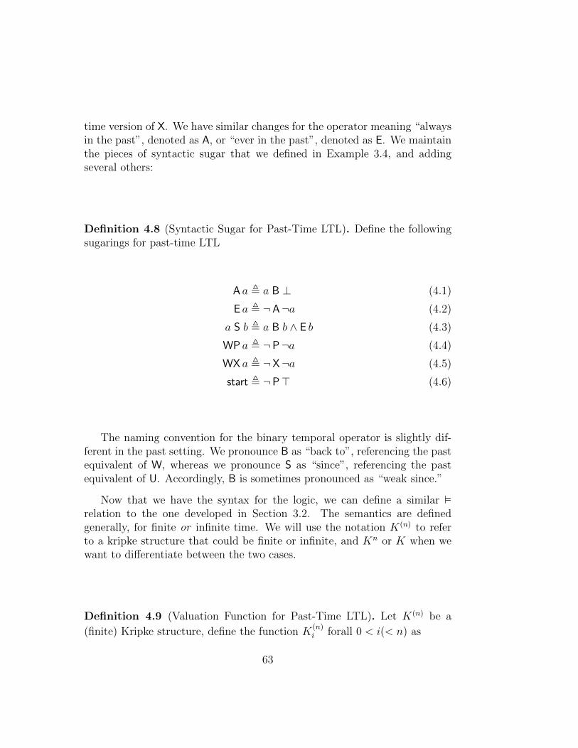
time version of X. We have similar changes for the operator meaning “alwaysin the past”, denoted as A, or “ever in the past”, denoted as E. We maintainthe pieces of syntactic sugar that we defined in Example 3.4, and addingseveral others:

Definition 4.8 (Syntactic Sugar for Past-Time LTL). Define the followingsugarings for past-time LTL

A a , a B ⊥ (4.1)

E a , ¬A¬a (4.2)

a S b , a B b ∧ E b (4.3)

WP a , ¬P¬a (4.4)

WX a , ¬X¬a (4.5)

start , ¬P> (4.6)

The naming convention for the binary temporal operator is slightly dif-ferent in the past setting. We pronounce B as “back to”, referencing the pastequivalent of W, whereas we pronounce S as “since”, referencing the pastequivalent of U. Accordingly, B is sometimes pronounced as “weak since.”

Now that we have the syntax for the logic, we can define a similar �relation to the one developed in Section 3.2. The semantics are definedgenerally, for finite or infinite time. We will use the notation K(n) to referto a kripke structure that could be finite or infinite, and Kn or K when wewant to differentiate between the two cases.

Definition 4.9 (Valuation Function for Past-Time LTL). Let K(n) be a

(finite) Kripke structure, define the function K(n)i forall 0 < i(< n) as

63

K(n)i (v) = ηi(v)

K(n)i (⊥) = false

K(n)i (a→ b) =

true if K

(n)i (a) = false

true if K(n)i (b) = true

false otherwise

K(n)i (X a) =

{Kni+1(a) if i < n

false otherwise

K(n)i (a W b) =

true if K

(n)j (a) = true, for all i ≤ j ≤ n

true if there exists i ≤ k ≤ n, such that K(n)k (b) = true

and for every j such that i ≤ j < k,K(n)i (a) = true

false otherwise

K(n)i (P a) =

{K

(n)i−1(a) if i > 0

⊥ otherwise

K(n)i (a B b) =

true if K

(n)j (a) = true, for all i ≥ j ≥ 0

true if there exists i ≥ k ≥ 0, such that K(n)k (b) = true

and for every j such that i ≥ j > k,K(n)i (a) = true

false otherwise

These semantics are unsurprising, the forward-time operators have theexact same interpretaton, and the past-time operators begin interpreted in acompletely analogous way. The last piece we need is the proof theory.

Definition 4.10 (Proof System for Past-Time LTL). The axioms for Past-Time LTL are:

64

P1 ` ¬P a↔ WP¬a F1 ` ¬X a↔ WX¬aP2 ` P a→ WP a F2 ` X a→ WX aP3 ` a→ WP X a F3 ` a→ WX P aP4 ` WP(a→ b)→ (WP a→ WP b) F4 ` WX(a→ b)→ (WP a→ WP b)P5 ` ¬E a↔ A¬a F5 ` ¬F a↔ G¬aP6 ` A(a→ b)↔ (A a→ A b) F6 ` G(a→ b)↔ (G a→ G b)P7 ` A a→ WP a F7 ` G a→ WX aP8 ` A(a→ WP a)→ (a→ A a) F8 ` G(a→ WX a)→ (a→ G a)P9 ` a S b↔ b ∨ [a ∧ P(a S b)] F9 ` a U b↔ b ∨ [a ∧ X(a U b)]P10 ` E start F10 ` a U b→ F b

And then we can define the three inference rules:

R1 For a propositional tautology p, ` p.R2 a→ b, a ` bR3 a ` G a ∧ A a

We can point out a clear difference between LTL and LTLf . One mightthing that the past-time axioms P1-10 would completely specify LTLf andthe forward-time axioms F1-10 would completely specify LTL. However, wenotice that the axiom P3 cannot even be stated in LTLf . This is a key axiomto use and leverage in certain proofs [25, 24]. Hence, our system, which omitsthis ability to transition between past and forward time, and forces a finitemodel of time presents a truly distinct sytem.

We see that Past-Time LTL is decidable, [24], and that completeness isa direct consequence of their decision procedure, which uses a greatest fixedpoint approach, as opposed to our least fixpoint approach.

Theorem 4.11 (Decidability). Satisfiability (and validity) in Past-TimeLTL are decidable.

Theorem 4.12 (Completeness). Past-Time LTL is complete.

4.4 Network Applications

With the rise of the Internet and the increasing interconnectedness of theglobal computational architecture, there is an increasing need for verifiablemethods of computing across multiple connected devices. Until quite re-cently [12], the main method of creating networks was to write hardware-specific code on each of the individual servers and switches and hope to

65

coordinate certain ideal properties of the network. This is extremely ardu-ous to make rigorous, and invariably, networks created this way are severelysucceptible to attackers, who can exploit this lack of rigor.

Netkat is the proposed solution to this problem [1], creates a unifiedtop-level language with an abstract hardware-agnostic representation of aswitch, allowing for formal, rigorous reasoning about network topologies,and forwarding strategies. This formal system is called Netkat, short forNetwork Kleene Algebra with Tests. The basis of the language is KleeneAlgebra (ka) used to model regular expressions. This is extended to KleeneAlgebra with Tests (kat), adding adds boolean comparison to the language,which adds axioms enabling network programming, creating Netkat.

The true innovation of Netkat is that it is a formal system that easilymodels network topology, allows for the programming of specific forwardingpolicies, and allows for axiomatic proofs regarding those policies. A problemhere is that these specifications become intractably large as the topologyincreases in size. The reason is this: as a network packet traverses thenetwork, it accumulates a packet history, which is a list of vectors, the headof which is the current state of the packet (destination, addresses, type,etc). Unfortunately Netkat policies can only ask questions about the currentstate, the head of this list. This is a less-than-efficient construction, since weare storing this packet history, but are unable to do anything with it.

Temporal Netkat [4], an extension of Netkat, leverages the packet his-tory to increase expressivity. To do this, Temporal Netkat adds LTLf tostandard Netkat. We have been primarly examining its expression for for-wards time; however, as we saw in Section 4.3, we can easily turn it aroundto express statements about the packet history. Importantly, we might askquestions such as “Has the packet ever been through a firewall?” or “Didthe packet just come from some secure switch x?”.

Temporal Netkat does have succeed in proving soundness and decid-ability properties. It is formulated use an equational theory instead of anaxiomatic framework. So their axioms are in the form a ≡ b. Notice that thisis effectively the same as saying ` a↔ b. They also prove a modified versionof Completeness for their equational theory. We present the LTLf portion ofthe axioms translated into our metatheoretical notation in Figure 4.2

Theorem 4.13 (Temporal Netkat Partial completeness). For two arbitraryformulae of Temporal Netkat, if [start; a] = [start; b], then start; a ≡ start; b

Now that we have a proof of completeness for LTLf , we can derive a proof

66

` # a ∧# b↔ #(a ∧ b) (ltl-last-dist-seq)` # a ∨# b↔ #(a ∨ b) (ltl-last-dist-plus)

` > (ltl-wlast-one)` a U b↔ b ∨ a ∧#(a U b) (ltl-since-unroll)

` ¬(a U b)↔ (¬b)W (¬a ∧ ¬b) (ltl-not-since)

` a→ a ∧ b` a→ 2 b

(ltl-induction)

` 2 a→ 3(end ∧ a) (ltl-finite)

Figure 4.2: LTLf Rules and axioms in Temporal Netkat

of completeness for Temporal Netkat.

Theorem 4.14 (Temporal Netkat Completeness). If [a] = [b] then a ≡ b.

Proof Idea. We have some formulae a and b, and we know that [a] = [b].This is translated to [a↔ b] = [true]. Now, the following table links theTemporal Netkat Axioms with equivalent LTLf axioms.

LTLf Rule Temporal Netkat AxiomNextAndDistr ltl-last-dist-seqNextOrDistr ltl-last-dist-plusWkNextTop ltl-wlast-oneUntilUnroll ltl-since-unrollNotUntil ltl-not-sinceInduction’ ltl-inductionAlwaysFinite ltl-finite

The above table shows the equivalent versions of all of the LTLf relatedTemporal Netkat Axioms. We can also show that our LTLf axioms canbe proved in Temporal Netkat. Hence, LTLf and the Temporal NetkatAxioms are equivalent. 4

4.5 Further Directions

We have shown soundness, completeness, and decidability for a finite versionof the infinite temporal logics. What if we look at other kinds of temporallogics? A close variant of LTL, known as Linear Dynamic Logic, or LDL, does

67

away with the assumption that every successor state is unique. It has alreadybeen studied in the finite setting [8], and it could be fairly straightforward toextend some of the observations and techniques made here to find soundnessand completeness results for this logic. Computation tree logic, or CTL forshort, is more complicated, in that it defines predicates in future temporaltimelines, it is possible that soundness and completeness results could befound for some hypothetical CTLf , or Finite Computation Tree Logic. Wemight also consider other temporal logics.

4.6 Conclusion

The main contribution of this work is a sound and complete proof theoryfor LTLf along with a decision procedure for satsifiability (Section 3). Theproof structures and basic procedures largely outline the work presented byKroger and Merz on Linear Temporal Logic [21], the general outline, graphconstruction and many of the definitions are largely based on their work.However, we have made several key additional contributions, aside from thetranslation to the finite setting. We formulated the system using the binaryweak until (· W ·) operator instead of the always (2 ·) operator, making ourpresentation slightly more general. We also have clarified many definitionsand presented proofs in a slightly more formal way, with the addition of thecomps function (Definition 3.29). Part of this is due to our presentation andsome of it is due to our formalism, and part of it is due to the fact that thefinite setting allows us to prove slightly simpler properties.

A further contribution is the insertion of the completeness and decid-ability results for LTLf into the Temporal Netkat framework (Section 4.4).This extends their partail completeness and decidability results that hingeon packet histories having a symbolically identified start point, allowing theauthors to derive general, compositional completeness and decidability re-sults.

Our secondary contributions are a introduction to metamathematical in-quiry intended for undergraduate mathematics students (Section 1), and asummary of the semantics, sound proof theory, and completeness propertiesfor LTL (Section 2). This is a slightly modified version of what is presented byKroger & Merz [21], again using the weak until operator instead of the alwaysoperator. We also present a summary of related results regarding LTLf , interms of related logics(Sections 4.2 and 4.3) and in terms of properties about

68

LTLf itself (Section 4.1).We expect that these results will encourage the use of LTLf more ap-

plication domains, and motivate further research into more efficient decisionprocedures.

69

70

Bibliography

[1] Anderson, C. J., Foster, N., Guha, A., Jeannin, J.-B., Kozen,D., Schlesinger, C., and Walker, D. Netkat: Semantic founda-tions for networks. In ACM SIGPLAN Notices (2014), vol. 49, ACM,pp. 113–126.

[2] Barringer, H., Goldberg, A., Havelund, K., and Sen, K. Pro-gram monitoring with ltl in eagle. In Parallel and Distributed ProcessingSymposium, 2004. Proceedings. 18th International (2004), IEEE, p. 264.

[3] Barringer, H., Groce, A., Havelund, K., and Smith, M. For-mal analysis of log files. Journal of aerospace computing, information,and communication 7, 11 (2010), 365–390.

[4] Beckett, R., Greenberg, M., and Walker, D. Temporal netkat.ACM SIGPLAN Notices SIGPLAN Not. 51, 6 (Feb 2016), 386401.

[5] Bornat, R. Proof and disproof in formal logic: an introduction forprogrammers. 2005.

[6] Cook, B., Koskinen, E., and Vardi, M. Temporal property ver-ification as a program analysis task. In International Conference onComputer Aided Verification (2011), Springer, pp. 333–348.

[7] De Giacomo, G., De Masellis, R., and Montali, M. Reasoningon ltl on finite traces: Insensitivity to infiniteness. In AAAI (2014),Citeseer, pp. 1027–1033.

[8] De Giacomo, G., and Vardi, M. Y. Linear temporal logic and lineardynamic logic on finite traces. In IJCAI’13 Proceedings of the Twenty-Third international joint conference on Artificial Intelligence (2013),Association for Computing Machinery, pp. 854–860.

71

[9] De Giacomo, G., and Vardi, M. Y. Synthesis for ltl and ldl onfinite traces. In Proc. of IJCAI (2015).

[10] De Morgan, A. Formal logic: or, the calculus of inference, necessaryand probable. Taylor and Walton, 1847.

[11] Fix, L. Fifteen years of formal property verification in intel. In 25Years of Model Checking. Springer, 2008, pp. 139–144.

[12] Foster, N., Harrison, R., Freedman, M. J., Monsanto, C.,Rexford, J., Story, A., and Walker, D. Frenetic: A networkprogramming language. In ACM Sigplan Notices (2011), vol. 46, ACM,pp. 279–291.

[13] Fraer, R., Kamhi, G., Ziv, B., Vardi, M., and Fix, L. Ef-ficient reachability computation both for verification and falsification.In Proceedings of International Conference on Computer-Aided De-sign,(CAV00).

[14] Giero, M. Weak completeness theorem for propositional linear timetemporal logic. Formalized Mathematics 20, 3 (2012), 227–234.

[15] Godel, K. Uber formal unentscheidbare satze der principia mathemat-ica und verwandter systeme i. Monatshefte fur mathematik und physik38, 1 (1931), 173–198.

[16] Godel, K. Some metamathematical results on completeness and con-sistency, on formally undecidable propositions of principia mathematicaand related systems i, and on completeness and consistency. From Fregeto Godel: A source book in mathematical logic 1931 (1962).

[17] Kern, C., and Greenstreet, M. R. Formal verification in hard-ware design: a survey. ACM Transactions on Design Automation ofElectronic Systems (TODAES) 4, 2 (1999), 123–193.

[18] Kleene, S. C. Introduction to metamathematics. 1952.

[19] Kripke, S. Semantical considerations of the modal logic.

[20] Kropf, T. Introduction to formal hardware verification. Springer Sci-ence & Business Media, 2013.

72

[21] Kroger, F., and Merz, S. Temporal logic and state systems.Springer, 2008.

[22] Lamport, L. Time, clocks, and the ordering of events in a distributedsystem. Communications of the ACM 21, 7 (1978), 558–565.

[23] Lamport, L. ”sometime” is sometimes ”not never”: On the temporallogic of programs. In Proceedings of the 7th ACM SIGPLAN-SIGACTSymposium on Principles of Programming Languages (New York, NY,USA, 1980), POPL ’80, ACM, pp. 174–185.

[24] Lichtenstein, O., Pnueli, A., and Zuck, L. The glory of the past.In Workshop on Logic of Programs (1985), Springer, pp. 196–218.

[25] Manna, Z., and Pnueli, A. The anchored version of the temporalframework. In Workshop/School/Symposium of the REX Project (Re-search and Education in Concurrent Systems) (1988), Springer, pp. 201–284.

[26] Nathanson, M. B. Desperately seeking mathematical truth. The BestWriting on Mathematics 2010 (2011), 13.

[27] Nguyen, A. C., and Khoo, S. C. Towards automation of ltl verifi-cation for java pathfinder.

[28] Pnueli, A. The temporal logic of programs. In Foundations of Com-puter Science, 1977., 18th Annual Symposium on (Oct 1977), pp. 46–57.

[29] Rosu, G. Finite-trace linear temporal logic: Coinductive completeness.In International Conference on Runtime Verification (2016), Springer,pp. 333–350.

[30] Schubert, T. High level formal verification of next-generation mi-croprocessors. In Proceedings of the 40th annual Design AutomationConference (2003), ACM, pp. 1–6.

[31] West, D. B., et al. Introduction to Graph Theory, vol. 2. Prenticehall Upper Saddle River, 2001.

73

74

Appendix A

Auxiliary Proofs

A.1 Semantics

Lemma A.1 (Totality). For every Kripke structure Kn, every i ∈ {1, . . . , n},and an arbitrary formula a, then Kn

i (a) = true or Kni (a) = false.

Proof. Let a ∈ LTLf (V), and Kn be a finite Kripke structure of length n.Let i ∈ {1, . . . , n}. It is easy to show by structural induction that Kn

i (a) isdefined. Hence, Kn

i is a total function on LTLf (V). 4

Lemma A.2 (Always Convergence). Given a Kripke structure of length n,and a formula a of LTLf (V) then Kn

n(2 a) = Knn(a)

Proof. Immediate, by definition of the evaluation function. Knn(2 a) = true

if and only if Knj (a) = true for all n ≤ j ≤ n. So j must be n. Since

Knn(2 a) = true if and only if Kn

n(a) = true, we can conclude that Knn(2 a) =

Knn(a). 4

Corollary A.3 (Finite is Truncated). Given a finite Kripke structure Kn =(η1, η2, · · · , ηn) and an infinite Kripke structure K = (η′1, η

′2, η′3, · · · ), such

that ηi = η′i, �Kn a if and only if �K[n] a.

Proof. We proceed by induction on the size of Kn. For the base case, letn = 1. Then K1 = (η1) and K[1] = [η1]. So it is clear that �Kn a if and onlyif �K[n] a.

Now consider a general n. Then Kn = (η1, η2 · · · , ηn), and K[n] =[η1, η2, · · · , ηn]. Create modified structures Ln−1 = (η2, · · · , ηn) and L =(η2, η3 · · · , ηn, · · · ). Then by the induction hypothesis we know that �Ln−1 a

75

if and only if �L[n−1] a. So for K[n]i(a) = Kni (a) for all a and 1 < i ≤ n. So

we need to consider the case that i = 1. We see that K[n]1(a) = Kn1 (a) by

definition and the inductive hypothesis. 4

Lemma A.4 (Semantic Modus Ponens). For a given set of formulae F , witha, b formulae, if F � a and F � a→ b, then F � b.

Proof. Let F be a given set of formulae, and let a and b formula. Assumethat (i) F � a and (ii) F � a ∧ b to show that F � b. Let Kn be a Kripkestructure in which F �Kn a, and F �Kn a → b. Let i ∈ {1, . . . , n}, to showKni (b) = true. By definition of �, we have Kn

i (a) = true (from (i)) and thateither Kn

i (a) = false or Kni (b) = true (from (ii)). If we are in the case where

Kni (b) = true, we are done; however the other case, wherein Kn

i (a) = false,is contradictory, since Kn

i (a) = true. So Kni (b) = true and F � b.

4

Lemma A.5 (Assumption of Temporal Operators). For a set of formulaeF , then F ∪ {a,#>} � # a and F ∪ {a} � 2 a.

Proof. Let Kn be a finite Kripke structure such that �Kn b for every b ∈ Fand i ∈ [n], including a. In otherwords, �Kn a for every i ∈ [n], which givesF � 2 a, and a specialization gives Kn

i+1(a) for i < n, meaning F � # a. Weknow that i 6= n by contradiction. If it were the case, then K(#>) = false,which contradicts the assumption. 4

Corollary A.6 (Next Assumption).

#> � ⊥

Proof. We want to show that for an arbitrary finite Kripke structure, Kn,such that Kn

i (#>) = true, we can derive Kni (⊥) = true. However, in fact,

the assumption fails, because Knn(#>) = false. The result follows. 4

A.2 Proof Theory

Theorem A.7 (Soundness Theorem for LTLf ). Let a be a formula and F aset of formulae. If ` a, then � a.

Proof. By structural induction on ` a:

76

(Taut) a is a propositional tautology. Following Theorem 2.2.1 inKroger-Merz [21], all propositional tautologies are valid. Their proofapplies for our syntax, replacing formulae mutatis mutandis.

(NextDistr) We want to show that � (a→ b)↔ ( a→ b). Showeach direction separately.

(→) Let Kn be an arbitrary finite Kripke Structure and i an arbitraryindex, to show that Kn

i ( (a → b) → ( a → b) = true. Thisbreaks down into two cases.

(Kni ( (a→ b)) = false) Immediate.

(Kni ( (a→ b)) = true) Now, we must show that Kn

i ( a → b) = true. Now, if i = n, then Kn

i ( b) = true (be-cause time has ended) and so Kn

i ( a → b) = true, andwe’re done. Otherwise, i 6= n, and so we can step the val-uation function to see Kn

i (#¬(a → b) = false, and againto see Kn

i+1(¬(a → b) = false) and once more to see thatKni+1(a→ b) = true). Now, we have two cases

(Kni+1(a) = false) Now we can add the ¬ constructor andsee that Kn

i+1(¬a) = true and again the # constructor toget Kn

i (#¬a) = true, and once more apply the ¬ rules,and add the sugar to get Kn

i ( a) = false. Finally wecann apply the → construction and get Kn

i ( a→ b).(Kn

i+1(b) = true) Add the ¬ constructor and its valuationto get Kn

i+1(¬b) = false, followed by the same for #, tosee Kn

i+1(#¬b) = false. Then, once more negation andthe syntactic sugar for weak next gives Kn

i ( b) = true,which allows the conclusion Kn

i ( a→ b) = true usingthe implication valuation rule.

(←) Let Kn be an an arbitrary finite Kripke structure, and i be anarbitrary index, to show that Kn

i (( a → b) → (a → b)) =true. If Kn

i ( a → b) = false, then we’re done. Otherwise,Kni ( a → b) = true and we must show that Kn

i ( (a → b)) =true. Now, we have two cases:

(Kni ( a) = false) We can desugar a to ¬#¬a. Then we can

step the valuation function forward to get Kni+1(a) = false.

Then we can see Kni+1(b) = true. Now using the implication

77

constructor we can see Kni+1(a→ b) = true, which again using

the weak next sugar lets us conclude Kni ( (a→ b) = true.

(Kni ( b) = true) If i = n we can immediately concludeKn

i ( (a→b)) = true. Otherwise, We use the weak next sugar to ato ¬#¬a, which gives Kn

i+1(b) = true. Then using the im-plication case for the valuation function , we can constructKni+1(a→ b) = true, which again using the weak next sugar,

lets us conclude that Kni ( a→ b) = T .

(EndNextContra) We want to show that � end → ¬# a. So givensome finite Kripke structure Kn and an arbitrary index i, we havetwo cases, either Kn

i (end) = false and we’re done, or Kni (end) =

Kni (¬#>) = true and we need to show that Kn

i (¬# a) = true. Theonly way that Kn

i (¬#>) could be false is if i = n, in which caseKni (# a) is also false. Then applying the negation case of the valua-

tion function gives Kni (¬# a) = true.

(Finite) Assume we have a proof that ` 3 end. We want to show that� 3 end. We can desugar this to a form that the Kn

i functions will un-derstand, namely � ¬((#>)W ⊥). Take an arbitrary function Kripkestructure Kn and an arbitrary index i, to show that Kn

i (¬((#>) W⊥)) = true. Equivalently, we show that Kn

i (((#>) W ⊥)) = false.Since we know that Kn

k (⊥) = false for all possible k, we must findan index j ∈ [i, n] such that Kn

j (#>) = false. Let j = n, then bydefinition Kn

j (#>) = Knn(#>) = false.

(WkUntilUnroll) We have derivation of ` (aW b)→ b∨a∧ (aWb). We must show that � (a W b) → b ∨ a ∧ (a W b), specifically,we must show that for an arbitrary finite Kripke structure Kn andarbitrary index i ∈ {1, . . . , n}, that Kn

i ((aW b)→ b∨a∧ (aW b)) =true. By definition, we can equivalently show that Kn

i (aW b) = false,or Kn

i (b ∨ a ∧ (a W b)) = true. Assume Kni (a W b) = true (since

otherwise we are done), and show that Kni (b ∨ a ∧ (a W b) = true.

So, we know that there exists some j ∈ [i, n] such that Knj (b) = true

and for all k ∈ [i, j), Knk (a) = true. There are two cases, j = i, or

j > i. If j = i, then we know that Kn(b) = true, and the resultfollows by definition. Otherwise, j > i, and so Kn

i (a) = true. Notealso that either Kn

i+1(aW b) = true, or i = n. If i = n we are done, soconsider the other case, which by using the next case of the valuation

78

function definition, and then the weak next syntactic sugar to createKni (#(a W b) = Kn

i ( (a W b) = true. Then, by the implication caseand the disjunctive syntactic sugar we can construct Kn

i (b∧a∨ (aWb) = true

(WkNextStep) We know that a ` a, so we need to show that a � a. Consider an arbitrary Kn such that Kn

i (a) = true for all i =1, . . . , n. We need to show that for an arbitrary Kn

i , Kni ( a) = true.

There are two cases, either i = n, or i < n. If i = n, then we needto show that Kn

n(#¬a) = false, which holds by definition. Otherwise,show that Kn

i (#¬a) = Kni+1(¬a) = false. Equivalently show that

Kni+1(a) = true, which we know from our construction of Kn.

(Induction) We assume that we have ` b → c and ` b → b. Theinduction hypothesis allows us to interpret these semantically, i.e. F �b→ c and F � b→ b. Let Kn be an arbitrary Kripke structure suchthat F �Kn (b → c) and F �Kn b → b. So if Kn

i (b) = false, we canuse the implication case of the valuation function to show Kn

i (b→ 2 c).So, assume that Kn

i (b) = true. Then, Kni (c) = true and Kn

i ( b) =true. We want to show Kn

i (2 b), i.e. for all i ≤ j ≤ n, Knj (2 b). When

i = j the result follows by assumption, and when j = n, the resultfollows by definition of the weak next case of the valuation function. Inevery other case (such that it exists), we can assume Kj−1( a) = true,and since j < n, we know Kn

j (a) = true by the definition of the weaknext sugar, and the negation and next cases of the valuation function.

4

Theorem A.8 (Deduction Theorem). Let a, b be formulae, F a set of for-mulae. F , a ` b if and only if F ` 2 a→ b.

Proof. Prove each direction separately.

(⇒) We assume that F , a ` b to show that F ` 2 a → b. Proceed bystructural induction on the derivation of b from F , a.

Case 1: Assume that b is an axiom, or b ∈ F . Then, F ` b andF ` 2 a→ b follows with Taut

Case 2: Assume that b ≡ a. Then we know from AlwaysUnroll,that ` 2 a→ (a∧ 2 a), which simplifies to ` 2 a→ a by Taut.Now, we can freely add more conditions and see that F ` 2 a→ a.

79

Case 3: Assume that b ≡ c is a conclusion of WkNextStep. So,we must also have F , a ` c. Then applying the induction hypoth-esis, we get F ` 2 a → c. Now we show that from these we canderive 2 a→ # c.

1. 2 a→ c shown so far

2. 2 a→ #> shown so far

3. (2 a→ c) WkNext, 1

4. 2 a→ c WkNextDistr, 3

5. 2 a→ a ∧ 2 a AlwUnroll

6. 2 a→ 2 a Taut, 5

7. 2 a→ c Taut, 6, 4

Case 4: Assume that b ≡ c → 2 d. Is a conclusion of Inductionwith premises c → d and c → c. Then we get the inductivehypotheses that F ` 2 a → (c → d) and F ` 2 a → (c → c).Then, we can derive 2 a → (c → 2 d) by Taut, WkNextAnd-Distr and Induction.

1. 2 a→ (c→ d) derivable

2. 2 a→ (c→ c) derivable

3. 2 a ∧ c→ d Taut, 1

4. 2 a ∧ c→ c Taut, 1

5. 2 a→ 2 a Taut,AlwUnroll

6. 2 a ∧ c→ 2 a ∧ c Taut, 4, 5

7. 2 a ∧ c→ (2 a ∧ c) WkNextAndDistr

8. 2 a ∧ c→ (2 a ∧ c) Taut, 6, 7

9. 2 a ∧ c→ 2 d Induction, 3, 8

10. 2 a→ c→ 2 d Taut, 9

(⇐) Assume that F ` 2 a→ b to show that F , a ` b. If F ` 2 a→ b, thenF , a ` 2 a → b. Then, since F , a ` a, we need to show F , a ` 2 a, ormore specifically that a ` 2 a. Then we get F , a ` b by Taut.

80

It remains to be shown that a ` 2 a. Assume a. Then by WkNextwe get a. Then by Taut we derive a → a. Then by Induction,we get a→ 2 a, and then finally by Taut, we get 2 a.

4

Lemma A.9 (Next-Step Implication). Let P be a PNP

` P → σ(P)

Proof. By cases on σi, ` P → c when c ∈ σ1(P)∪σ2(P), and ` P → ¬cwhen c ∈ σ3(P) ∪ σ4(P). The proposition follows directly from this and

WkNextAndDistr. In fact the cases will be for when c ∈ σ+/−i (P), for

each i = 1, 2, 3, 4, 5.

1. If c ∈ σ+1 (P), then # c ∈ pos(P), so P → c by Taut and P → c.

2. If c ∈ σ+2 (P) then c ≡ a W b ∈ pos(P), and b ∈ neg(P). So, `

P → ¬b ∧ a W b by Taut. Then, WkUntilUnroll proves P →¬b ∧ (b ∨ a ∨ aW b). Conclude that P → aW b holds by Taut.

3. If c ∈ σ+3 (P) then c ≡ a W b ∈ pos(P). We know that ` P → end, so

` P → σ(P) is apparent by CommNegNext.

4. If c ∈ σ−4 (P), then # c ∈ neg(P). We can say that ` P → ¬# c.We want to show that P implies ¬c, which is equivalent to ¬#¬¬c,which is then equivalent to ¬# c, by Taut. Hence ` P → ¬c.

5. If c ∈ σ−5 (P), then 2 c ∈ neg(P) and c ∈ pos(P), so ` P → (¬2 c∧ c),then by AlwUnroll, we get ` P → c∧(¬c∨#¬2 a). Then by Taut,we can simplify this to ` #2 c, and by NextWkNext, conclude` P → ¬2 c.

4

A.3 Completeness

Lemma A.10 (PNPs are Well-Behaved). Let P = (F+,F−) be a consistentPNP, and a, b be formulae, then

81

1. F+ and F− are disjoint

2. Either (F+,F− ∪ {a}) or (F+ ∪ {a},F−) is a consistent PNP

3. ⊥ 6∈ F+

4. If, a, b, a→ b ∈ FP , then if a ∈ F− or b ∈ F+, a→ b ∈ F+, otherwisea→ b ∈ F−.

5. If a→ b, a, b ∈ FP , then if a→ b ∈ F+, and a ∈ F+, then b ∈ F+.

Proof.

1. Assume F+ ∩ F− is nonempty, and pick some a ∈ F+ ∩ F−. The` P → a∧¬a, so conclude ` ¬P , which contradicts the consistency of` P .

2. If a ∈ F+ or a ∈ F− we have (F+∪{a},F−) = P , or (F+,F−∪{a}) =P and the assertion follows by the consistency of P . Otherwise, we as-sume for the sake of contradiction, that both pairs under considerationare inconsistent, which in turn gives ` ¬(P ∧a) and ` ¬(P ∧¬a). This

gives a contradiction since Taut gives ` ¬P . Hence at least one of thepairs must be consistent.

3. Assume ⊥ ∈ F+. Then ` P → ⊥ by Taut, which contradicts theconsistency of P , so ⊥ 6∈ F+.

4. Assume that a → b ∈ F+, but a 6∈ F− and b 6∈ F+. Since a, b ∈ FP ,a ∈ F+ and b ∈ F−. Then ` P → a ∧ ¬b ∧ (a→ b) which yield ` ¬Pby Taut. The contradiction demonstrates that a ∈ F− or a ∈ F+.To show the other direction, assume that a ∈ F− or b ∈ F+. Forthe sake of contradiction assume that a → b 6∈ F+ which means thata→ b ∈ F−. This gives ` P → ¬(a→ b) ∧ ¬a or ` P → ¬(a→ b) ∧ bwhich both give ` ¬P by Taut. Conclude a→ b ∈ F+.

5. Assume that b 6∈ F+. Then b ∈ F−, which gives ` P → a ∧ ¬b. Wealso see that ` P → (a → b). Then by Taut we get ` ¬P , whichproves that b ∈ F+ by contradiction to the consistency of P .

4

82

Lemma A.11 (Consistent Completion Existence). For P, a consistent PNP,and

` P →∨

Q∈comps(P)

Q

Proof. Let P be a consistent PNP, and let P1, · · · ,Pm be those PNPs withdisjoint positive and negative sets such that τ(P) = τ(Pi), for all i =1, . . . ,m. Let P ′1, · · · ,P ′n be those P ′i which are in comps(P). Without lossof generality, relabel P1, · · · ,Pm such that P ′j = Pi with i = 1, . . . ,m andj = 1, . . . , n.

Then, for m > i > n, either Pi is inconsistent, or pos(P) 6⊆ pos(Pi) and

neg(P) 6⊆ pos(Pi). In either case, we obtain ` P → ¬P ′i by Taut for every

i > n. From Lemma 3.31, we get that `∨mi=1 P ′i. Then we can eliminate the

bad cases, and get ` P →∨ni=1 P ′i. 4

Lemma A.12 (All Nodes Have Successors). Let P be a consistent and com-plete PNP, and Q1, · · · ,Qn the nodes of GP .

`n∨i=1

Qi → n∨i=1

Qi

Proof. From Lemma 3.25, we have ` Qi → σ(Qi) for each i = 1, · · ·n.Let Q′i1 , · · · ,Q

′im be the m completions of σ(Qi), by Lemma 3.33, we get

that ` σ(Qi) →∨nj=1Q′ij . Since by the definition of GP we have Q′ij ∈

{Qi, · · · ,Qm}, which in our proof system is represented by ` Q′ij →∨mk=1Qk

for each j ∈ [m]. Since each Q′ij , (a completion of σ(Qi)) implies anothernode in the tree, and σ(Qi) implies each of its completions, we can chain

these to get ` σ(Qi)→∨nk=1 Qk. Then, by WkNext and NextDistr, we

get ` σQi → ∨k+1 Qk, and we get the result ` Qi →

∨nk=1Qk for each

i ∈ [n]. The result follows by Taut. 4

Lemma A.13. Every terminal path is a fulfilling path.

Proof. Consider a terminal path π = P1,P2, · · · ,Pn,Z. Let S be the setof temporal formulae in π. Consider the terminal node Z. Either there areno temporal formulae in FZ , or there is at least one. In the first case, weare done, since every temporal formula has been fulfilled. So, consider thesecond case, where we have some set S ′ = FZ ∩ S of exactly the temporal

83

operators that haven’t been fulfilled by the last state. We will show thatthey are fulfilled by the final state. The elements of S ′ can either be of theform # a or of the form aW b, and can be either in the positive or negativesets. We will examine each of these cases:

Case 1 (# a ∈ FZ). This is trivial by definition of σ.

Case 2 (aW b ∈ FZ). Here we have two subcases:

Case 2a (a W b ∈ pos(Z)). Since Z is consistent, we have ` Z →b ∨ a ∧ (a W b) by WkUntilUnroll. Since we also have

` Z → end by definition of a terminal node, we get ` Z → b ∨ a.Since b, a ∈ τ(aW b), we know that b or a is in pos(Z), so aW bis fulfilled.

Case 2b (a W b ∈ neg(Z)). We know ` Z → ¬(a W b), which gives

` Z → ¬(b ∨ a ∧ (a W b))). Since we know ` Z → end, bythe definition of a terminal node, (a W b) becomes >. So we

have ` Z → ¬b ∨ a, or equivalently ` Z → ¬b ∧ ¬a. Since aand b are subformulae of a W b, and a W b ∈ neg(Z), then alsoa, b ∈ neg(Z). Hence aW b 6∈ τ(σ(Z)).

4

Theorem A.14 (Satisfiability Theorem for LTLf ). For any consistent PNP

P, the formula P is satisfiable.

Proof. P ′ = ({3 end} ∪ pos(P), neg(P)) is a consistent PNP, P∗ is a com-pletion of P ′. And P0, P1, · · · , Pn a complete, finite, rooted path of length n(by Lemma 3.41) in GP∗. Define Kn = (η0, η1, · · · , ηn) by

ηi(v) = true if v ∈ F+i

ηi(v) = false otherwise

We want to show that Kn0 (P) = true. This is equivalent to showing that

Kn0 (P ′) = true, which is also equivalent to showing that Kn

0 (P0) = true.Proving this is hard, so we will generalize the hypothesis making it easier toprove. We will show that for PNP Pi, and f ∈ FPi

, then Kni (f) = true iff

f ∈ pos(Pi), and Kni (f) = false otherwise.

We proceed by induction on the derivation of an arbitrary formula f :

84

(f = v ∈ V). This is proved by the definition of Kn.

(f = ⊥). By definition of Kni , Kn

i (⊥) = false and ⊥ 6∈ F+i by

Lemma 3.22.

(f = a→ b). Since Pi is a complete PNP, we have that a, b ∈ F+∪F−.The inductive hypothesis allows us to conclude that Kn

i (a) = false iffa 6∈ F+

i . It also allows the conclusion Kni (b) = true iff b ∈ F+

i . Then,Kni (a → b) = true if and only if Kn

i (a) = false or Kni (b) = true, we

can apply the inductive hypotheses to get a ∈ F−i or b ∈ F+i . Then by

Lemma 3.22, we can conclude that a→ b ∈ F+i .

(f = # a). Lets break this down into a proof of each direction.

(⇒) We want to show that if Kni (# a) = true, then # a ∈ F+. It

must be that i < n, So by the definition of Kni , we know that

Kni (# a) = true implies that Kn

i+1(a) = true. and so by the in-ductive hypothesis, we know that a ∈ F+

i+1. Then by Lemma 3.36,# a ∈ F+

i .

(⇐) Now lets show that if # a ∈ F+i , then Kn

i (# a) = true. We knowthat since # a ∈ F+

i , Pi is a consistent PNP, Lemma 3.36 meansthat a ∈ F+

i+1. Then by the induction hypothesis, Kni+1(a) = true,

so Kni (# a), by definition of Kn.

(f = a W b). Here we dont need to break into cases, we can provethis directly. Kn

i (a W b) = true if and only if there exists k ∈ [i, n]such that for all j ∈ [i, k), Kn

j (a) = true and Knk (b) = true. using

the inductive hypothesis, we know this statement holds if and only ifthere exists k ∈ [i, n] such that for all j ∈ [i, k), a ∈ pos(Pj) andb ∈ pos(Pk). Then by Lemma 3.36 the previous statement holds if andonly if aW b ∈ pos(Pi).

4

A.4 Decidability

Lemma A.15. For every formula c and every finite Kripke structure Kn,

Knn(c) = Kn

n(drop(c))

85

Proof. Let c be an arbitrary formula, Kn an arbitrary Kripke structure. Showthat Kn

n(c) = Knn(c). By induction on the structure of c:

Case 1: (c ≡ ⊥). Since drop(⊥) = ⊥, and clearly Knn(⊥) = Kn

n(⊥), theresult follows.

Case 2: (c ≡ v ∈ V). Since drop(v) = v, the result follows.

Case 3: (c ≡ a → b). By definition, drop(a → b) = drop(a) → drop(b).Again, by definition Kn

n(a → b) = true if and only if Knn(a) = false

or Knn(b) = true. We can also expand the definition for drop(a) →

drop(b) and see that Knn(drop(a) → drop(b)) = true if and only if

Knn(drop(a)) = false or Kn

n(drop(b)) = true. The inductive hypothesisgives that Kn

n(drop(a)) = Knn(a) and Kn

n(drop(b)) = Knn(b). So, We

have that Knn(drop(a)→ drop(b)) = true if and only if Kn

n(a) = false orKnn(b) = true. Which then implies Kn

n(drop(a) → drop(b) = Knn(a →

b).

Case 4: (c ≡ a W b). We have that drop(a W b) ≡ drop(a) ∨ drop(b).ConsiderKn

n(aW b); we know by Soundness and completeness that thisis equivalent to Kn

n(b ∨ a ∧ (aW b)). We also know that Knn( F ) =

true for any formula F . So we equivalently have to consider Knn(b∨a),

which is true when Knn(b) = true or Kn

n(a) = true. The inductivehypothesis is that Kn

n(b) = Knn(drop(b)) and Kn

n(a) = Knn(drop(a)).

This gives us that Knn(b ∨ a) = true if and only if Kn

n(drop(b)) = trueor Kn

n(drop(a)) = true. The by definition Knn(b ∨ a) = Kn

n(drop(a) ∨drop(b)) = Kn

n(drop(aW b).

4

Lemma A.16 (Rules are Sound). Let TP be a tableau for a PNP P, and Qbe some node of TP . For all temporal structures K and all i ∈ N:

a) If (#) does not apply, then Kni (Q) = Kn

i (Q′) for some successor Q′ ofQ.

b) If (#) applies, then Kni (Q) = Kn

i+1(Q′) for the successor Q′ of Q. Also,

Q′ is satisfiable only if Q is satsifiable.

Proof.

86

a) We will analyze each of the rules that could have applied, and showthat the property holds for each of them:

(⊥) If (⊥) applies to Q, then Q has no successor, and the propertyholds vacuously.

(→+) If (→+) applies to Q then there is some a → b ∈ pos(Q) thatis being acted on. In the left successor, Ql, we have b ∈ pos(Ql),and in the right successor, Qr, we have a ∈ ¬(Qr). We know thatKni (a → b) = true if and only if Kn

i (a) = false or Kni (b) = true.

Notice that Kni (Ql) = true if and only if Kn

i (a) = false and that

Knk (Qr) = true, if and only if Kn

i (b) = true. And so we have that

Kni (Q) = true if and only if Kn

i (Qr) = true or Kni (Qr) = true.

The result follows.

(→−) If (→−) applies to Q then there is some a → b ∈ pos(Q) thatis being acted on. For the single successor Q′, a ∈ pos(Q′) andb ∈ neg(Q′). Recall that Kn(a → b) = false if and only if bothKni (a) = true and Kn

i (b) = false. Since these are the only termsthat change from Q to Q′, we know that Kn

i (Q) = Kni (Q′).

(W+) If (W+) applies to Q, then there is some a W b ∈ pos(Q),and there are two successors, Ql and Qr. We know that b ∈Ql and a, (a W b) ∈ pos(Qr). Soundness, Completeness, andBackUnroll give that Kn

i (aW b) = true if and only if Kni (b) =

true orKni (a∧ (aW b)) = true. This implies thatKn

i (Q) = true

if and only if Kni (Ql) = true or Kn

i (Qr) = true. The resultfollows.

(W−) If (W−) applies to Q, then there is some a W b ∈ neg(Q).There are two succesors, Ql and Qr. By definition, a, b ∈ neg(Ql),#¬(a W b) ∈ pos(Qr). Then Soundness and Completeness giveus that Kn

i (a W b) = false, if and only if Kni (a ∧ b) = true or

Kni (#¬(aW b)) = false. This gives us that Kn

i (Q) = true if and

only if Kni (Ql) = true or Kn

i (Qr) = true. The result follows.

(end) If (end) applies to Q, then all of the elements of FQ are either thesymbol ⊥, a variable, or of the form # a. Also #> ∈ neg(Q) andσ+1 (Q) = ∅. Then Q′ = (drop(pos(Q)), drop(neg(Q)) ∪ {#>}).

There are no more positive temporal formulae, so we can considerKnn(Q′). By Lemma 3.45, Kn

n−1(Q) = Knn(Q′).

87

b) Let Q be a node in TP , and Q′ a successor of Q. Then we know thatevery formula in pos(Q) and neg(Q) is of the form # a. We also knowthat #⊥ 6∈ neg(Q). So for a given formula # a ∈ FQ, we know thatKni (# a) = Kn

i+1(a). Then we can conclude that Kni (Q) = Kn

i+1(Qi).

Assume that Q is satisfiable. Let Kn = (η0, η1, . . . , ηn−1) be a satisfy-

ing model. We know that Kn0 (Q) = true. We have just proven that

Kn1 (Q) = true. So if we let K ′n−1 = (η1, . . . , ηn−1), then it is clear that

K ′n−10 (Q) = true.

4

Lemma A.17 (Tableau Paths Not Closed). Let Q be a node in a tableau

and Kn a finite Kripke structure such that Kn0 (Q) = true. Consider a path

πKn(Q) = Q0,Q1, . . . ,Qm, then

(a) For every i = 0, . . . ,m, then Kncnt(i)(Qi) = true.

(b) πKn(Q) does not contain any closed node, and

Proof. Let Q be an arbitrary node in a tableau, with Kn a Kripke structuresuch that Kn is a finite kripke structure with Kn

0 (Q) = true. Consider apath πK

n(Q) = Q0,Q1, . . . ,Qm. Now show the desired properties

(a) Consider an arbitrary i ∈ {0, 1, . . . ,m}, to show that Kncnt(i)(Qi) =

true. We will do so inductively.

First we let i = 0 and see that since cnt(0) = 0, Q = Q0 and Kn0 (Q0) =

true, we are done.

Now consider the general case, where for every element Qj of the path

πK(Q) up to the current one, Qi,(i.e. j < i) has Kncnt(j)(Qj) = true.

We are considering the next element, Qi, and we want to show thatKncnt(i)(Qi) = true. We have two cases. If cnt(i− 1) = cnt(i), then we

know that Kncnt(i)(Qi−1) = true, and Lemma 3.47 gives Kn

cnt(i)(Qi) =

true. Otherwise cnt(i − 1) + 1 = cnt(i), and Q is the only successor.

Then by parts b) or c) of Lemma 3.47, we conclude that Kncnt(i)(Qi) =

true.

88

(b) We want to show that πKn(Q) has no closed node. Assume some Qi

in the path is closed according to one of the rules (C1), (C2), or (C3).We proceed by induction on the m = πK

n(Q).

(C1) If (⊥) applies to a node Qi, Kn(Qi) = false, which contradictspart (a).

(C2) Assume all the successors of Qi are closed, but the induction hy-pothesis gives that at least one of them (specifically Qi+1) is not,hence Qi is not closed.

(C3) Assume that all terminating paths of Qi have at least one closednode. Then for the successor of Qi in πK

n(Q), namely Qi+1, we

know that all terminating paths in the tableau, rooted at Qi+1,have at least one closed node. Hence, Qi+1 is closed. However,the induction hypothesis says that Qi+1 is not closed, and so theremust exist a terminating path rooted at Qi (in fact one such pathis πk(Q)).

4

Lemma A.18 (Path Modeling). Given a rooted, finite, terminating pathπ = P0, P1, P2, . . . , Pn, in a tableau TP for some PNP P. If Kn is a temporalstructure such that for every v ∈ V and i ∈ N,

v ∈ pos(Pidx(i))⇒ ηi(v) = true

v ∈ neg(Pidx(i))⇒ ηi(v) = false,

then for every v ∈ V and i ∈ N,

a ∈ pos(Pi)⇒ Kcnt(i)(a) = true

a ∈ neg(Pi)⇒ Kcnt(i)(a) = false.

Proof. Let P be a PNP, and TP be a tableau. Let P0, P1, . . . , Pn be a ter-minating path such that P0 = P . Let Kn be defined such that for everyi ∈ {1, . . . , n} and variable v ∈ V,

v ∈ pos(Pidx(i))⇒ ηi(v) = true

v ∈ neg(Pidx(i))⇒ ηi(v) = false.

89

Consider an arbitrary node Pi for some i ∈ {1, . . . , n}, and a formulaa ∈ FPi

. Show that a ∈ pos(Pi) means that Kcnt(i)(a) = true and a ∈ neg(Pi)implies Kcnt(i)(a) = false. We will proceed by induction on the structure ofthe formula a:

Case 1: (a ≡ v ∈ V). Assume a ∈ pos(Pi), then i ≤ idx(cnt(i)). Inthe construction of TP and the definitions of idx and cnt, note thatno variables are removed until idx(cnt(i)) + 1. So it must be that v ∈pos(Pidx(cnt(i))). Then the construction of Kn gives Kn

cnt(i)(a) = true.

Assume now that a ∈ neg(Pi). Again by definition, a ∈ neg(Pidx(cnt(i))),and so Kn

cnt(i)(a) = true.

Case 2: (a ≡ ⊥). If ⊥ ∈ pos(Pi), we must be in a contradictionsince we have assumed that Pi is not closed. So, the other optionis that ⊥ ∈ neg(Pi). By definition of any arbitrary valuation function,Knj (⊥) = false for every j ∈ {1, . . . , n}. So of course Kn

cnt(i)(⊥) = false.

Case 3: (a ≡ b → c). Assume a ∈ pos(Pi). At the current “timeslice” we have the nodes Pi, . . . , Pidx(cnt(i)). Since node Pidx(cnt(i))+1

represents an application of (end) or (#), we know that at some indexi ≤ j < idx(cnt(i)), the rule (→+) is applied to a. By construction, itfollows that b ∈ neg(Pj+1) or c ∈ pos(Pj+1). The induction hypothesisgives that Kn

cnt(j)(A) = true, and that Kncnt(j)(A) = true. This gives us

Kncnt(j)(A) = true. Note that since i ≤ j < st(cnt(i)), we know that

cnt(j) = cnt(i), and so we conclude that Kncnt(i)(A) = true.

Assume, contrarily, that a ∈ neg(Pi). Consider the same “time slice”portion of the path as above, namely Pi, . . . , Pidx(cnt(i)). By the sameanalysis there must be some index i ≤ j ≤ idx(cnt(i)) such that (→−)is applied to a in Pj. This means that b ∈ pos(Pj+1) and c ∈ neg(Pj+1).The inductive hypothesis gives that Kn

cnt(j)(a) = true and Kncnt(j)(c) =

false. The definition of Kn and the fact that cnt(i) = cnt(j) meansthat Kn

cnt(j)(b→ c) = false.

Case 4: (a ≡ # b). Without loss of generality, let # b ∈ pos(Pi). Weknow that # b ∈ pos(Pst(cnt(i))), by the construction of st, cnt, and TP .Then, by tableau construction, b ∈ FPst(cnt(i))+1). Note that Kn

cnt(i)(b) =

Kncnt(i)+1(b) = Kn

idx(idx(cnt(i))+1)(b). The inductive hypothesis gives that

Knidx(idx(cnt(i))+1)(b) = true, and so conclude that Kn

idx(idx(cnt(i))+1)(b)

90

Case 5: (a ≡ a W b). Let b W c ∈ pos(Pi), and as in previous sub-proofs, we know that there exists some j ∈ [i, idx(cnt(i))) at which the(W+) rule is applied to a in Pj. At this point, we know that either c ∈pos(Pj+1), or b∧ bW c ∈ pos(Pj+1). In the first case, we know by theinductive hypothesis that Kn

cnt(j)(c) = Kncnt(i)(c) = true and so we have

that Kncnt(i)(b W c) = true. Otherwise, b ∧ b W c ∈ pos(Pj+1). So,

by a similar argument, we know that Kncnt(i)(b) = true. We also know

that #¬bW c ∈ neg(Pidx(cnt(i))), and that ¬bW c ∈ neg(Pidx(cnt(i))+1).So there is some index k ∈ (idx(cnt(i)), idx(idx(cnt(i)+1))) ⊂ N, suchthat a ∈ pos(Pk).Continue with this process iteratively until the end of the path. Oneof two outcomes will occur. Either for every k ≥ cnt(i), we see thatKnk (b) = true or there exists some k ≥ cnt(i) such that Kn

k (c) =true and for every j ∈ (cnt(i), k), Kn

j (b) = true. Either way, we canconclude that Kn(bW c) = true.

The proof is similar for bW c ∈ neg(Pi).

4

A.5 Derived Rules in LTLf

Lemma A.19. The following rule can be derived from the rules in Defini-tion 3.19

` # a→ ¬end (NextNotEnd)

Proof. We can start with the Taut ` end∨¬end. Then applying the contra-positive of EndNextContra to end gives ` ¬# a ∨ ¬end, which desugarsto ` # a→ ¬end.

4

Lemma A.20. The following rule can be derived from the rules in Defini-tion 3.19

` ¬(#> ∧#⊥) (NextContraIsContra)

Proof. We know that ` >, so WkNextStep gives ` >. Then, by Taut,` end∨ >. We can desugar this to ` ¬#>∨¬#¬>, which by DeMorgan’slaws in Taut, gives ` ¬(#> ∧#⊥).

91

4

Lemma A.21. The following rule can be derived from the rules in Defini-tion 3.19

` ¬(¬# a ∧ ¬# a ∧ end (CommNegNextR)

Proof. We see, Taut and EndNextContra give ` ¬# a ∧#¬a ∧ end →¬#∧#¬a ∧ ¬#¬a→ ⊥. The result follows by Taut. 4

Lemma A.22. The following rule can be derived from the rules in Defini-tion 3.19

` ¬# a ∧#¬a→ end (CommNegNextR”)

Proof. We can write ` ¬# a ∧ #¬a → (end ∨ ¬end) ∧ ¬# a ∧ #¬a. Thenwe can distribute to get ` ¬# a ∧ #¬a → (end ∧ ¬# a ∧ #¬a) ∨ (¬end ∧¬# a ∧ #¬a). Then by CommNegNextR’ and Taut, we can conclude` ¬# a ∧#¬a→ (¬end ∧ ¬# a ∧#¬a) The result follows by Taut. 4

Lemma A.23. The following rule can be derived from the rules in Defini-tion 3.19

` ¬# a↔ end ∨#¬a (CommNegNext)

Proof. Consider each direction separately.

(→) We by Taut, we can see that ` ¬# a → ((¬# a ∧ #¬a) ∨ (¬# a ∧¬#¬a)). Then by CommNegNextR” and Taut we see ` ¬# a →(end ∨ ¬# a ∧ ¬#¬a). Then Taut gives ` ¬# a→ (end ∨ ¬(#¬a ∨# a)), so by Taut we can write ` ¬# a→ end ∨#¬a.

(←) Equivalently show ` (¬end ∧ a) ∨ ¬# a.

Taut gives ` (end ∨ ¬end) ∧ (# a ∧ ¬# a), from which we can see

` (end ∧# a) ∨ (end ∧ ¬# a) ∨ (¬end ∧# a) ∨ (¬end ∧ ¬# a)

Note that ` ¬end∧# a is a direct consequence of EndNextContra.So we now have

` (end ∧ ¬# a) ∨ (¬end ∧# a) ∨ (¬end ∧ ¬# a)

92

The forwards direction and Taut gives

` (¬end ∧# a) ∨ (¬# a)

We now leverage the fact from Taut that ` ¬#¬a ∨#¬a to see

` (¬end ∧# a ∧#¬a) ∨ (end ∧# a ∧ ¬#¬a) ∨ ¬# a

Desugaring # a ∧ #¬a to ¬(¬# a ∨ ¬#¬a), we can then apply theforwards direction to see that

` (¬end ∧ ¬(¬end ∨#¬a ∨ ¬#¬a)) ∨ (end ∧# a ∧ ¬#¬a) ∨ ¬# a

The leftmost disjunction is contradictory by Taut, so we can prove

` (end ∧# a ∧ ¬#¬a) ∨ ¬# a

4

Lemma A.24. The following rule can be derived from the rules in Defini-tion 3.19

` (# a→ # b)↔ #(a→ b) ∨ end (NextDistr)

Proof. First prove the following

` a ∧ ¬end→ # a (nextdistrlem)

We can see from Taut and CommNegNext that ` a∧¬end→ (end∨#¬¬a)∧¬end. Then Taut gives ` a∧¬end→ #¬¬a∧¬end. Then, twoapplications of CommNegNext give ` a∧¬end→ ¬¬# a∧¬end. Thennextdistrlem follows by double-negation elimination from Taut. X.

Now, consider each direction separately

(→) Taut gives ` (# a → # b) → end ∨ (¬# a ∨ # b) ∧ ¬end. Wecan distribute, using Taut, and get ` (# a → # b) → end ∨ (¬# a ∧¬end) ∨ (¬¬# b ∧ ¬end. Finally, we can apply CommNegNext toboth applicable disjunctive clauses, and get ` (# a → # b) → end ∨

93

(#¬a ∧ ¬end) ∨ ( b ∧ ¬end). Then we can factor the (¬end) out,and desugar the disjunction to implication, giving ` (# a → # b) →end ∨ (( a → b) ∧ ¬end). Then, using WkNextDistr, we get` (# a → # b) → end ∨ ( (a → b) ∧ ¬end). Then, nextdistrlemapplies to give ` # a → # b → end ∨ (#(a → b) ∧ ¬end). The resultfollows by Taut.

(←) Let φ = #(a→ b)∨end. We know by Taut that ` φ→ #(a→ b)∧end∨#(a→ b)∧¬end∨ end. We can simplify this formula using Tautand EndNextContra, and see that ` φ → #(a → b) ∧ ¬end ∨ end.Then we can apply nextdistrlem to get ` φ→ ¬end∧ (a→ b)∨end.Then WkNextDistr gives ` φ→ ¬end ∧ a→ b ∨ end. Now, weuse Taut to get ` φ→ (¬ a ∧ ¬end ∨ b ∧ ¬end ∨ end. Now we useCommNegNext 3 times to get ` φ→ (# a→ # b)∧¬end∨ end. Andnow, we can use EndNextContra to get ` φ→ (# a→ # b)∧¬end∨end∧ (¬# a) and finally, Taut gives ` φ→ (# a→ # b)∧¬end∨end∧(# a→ # b). Then Taut gives ` #(a→ b) ∨ end→ # a→ # b.

4

Lemma A.25. The following rule can be derived from the rules in Defini-tion 3.19

` a→ b

` # a→ # b(NextMonotone)

Proof. We know ` a → b, we want to show ` # a → # b. WkNextStepgives us ` (a→ b), to which we add a Taut to get ` (a→ b)∧end∨ (a→b) ∧ ¬end. We can apply EndNextContra and Taut to get

` (¬# a ∨# b) ∧ (a→ b) ∧ ¬end

Then CommNegNext turns (a → b) ∧ ¬end into #(a → b) ∧ ¬end.Then NextDistr gives ` (¬# a ∨ # b) ∧ (# a → # b), so we conclude` # a→ # b by Taut.

4

Lemma A.26. The following rule can be derived from the rules in Defini-tion 3.19

` a↔ (# a ∨ end) (NextWkNext)

94

Proof. We know from Taut, that ` a↔ a∧(end∨¬end). Then by Taut,CommNegNext, and Taut again, we get ` a↔ ( a∧end)∨ ¬a. Thenwe see that ` a∧ end∨#¬a→ end∨#¬a by Taut, and the converse byEndNextContra. Then, by Taut, conclude that ` a↔ (# a ∨ end).

4

Lemma A.27. The following rule can be derived from the rules in Defini-tion 3.19

` (a ∧ b)↔ a ∧ b (WkNextAndDistr)

Proof.

` (a→ b)

↔ (¬(a→ ¬b)) def.

↔ (¬(a→ ¬b)) ∧ end ∨ ¬#(a→ ¬b) ∧ ¬end Taut

↔ end ∨ ¬#(a→ ¬b) ∧ ¬end EndNextContra,Taut

↔ end ∨ ¬ (a→ ¬b) ∧ ¬end NextWkNext

↔ end ∨ ¬( a→ ¬b) ∧ ¬end WkNextDistr

↔ end ∨ ¬( a→ ¬ b) ∧ ¬end CommNegNext

↔ end ∨ ( a ∧ b) ∧ ¬end Taut

↔ a ∧ b ∧ end ∨ a ∧ b ∧ ¬end EndNextContra,Taut

↔ a ∧ b Taut

So conclude ` (a ∧ b)↔ ( a ∧ b)4

Lemma A.28. The following rule can be derived from the rules in Defini-tion 3.19

` 2 a↔ a ∧ 2 a (AlwUnroll)

Proof. Desugar the proposition to ` (a W ⊥) ↔ a ∧ (a W ⊥). ThenWkUntilUnroll gives ` aW ⊥↔ ⊥∨ (a ∧ (aW ⊥)). Then Taut letsyou cancel the disjunctive ⊥, so conclude ` aW ⊥↔ a ∧ (aW ⊥), whichresugars to ` 2 a↔ a ∧ 2 a. 4

95

Lemma A.29. The following rule can be derived from the rules in Defini-tion 3.19

` (2 a ∧ ¬end)↔ a ∧#2 a (AlwUnrollStep)

Proof. We know ` (2 a ∧ ¬end) ↔ (a ∧ 2 a) ∧ ¬end by AlwUnrolland Taut. Then NextWkNext gives ` (a ∧ 2 a ∧ ¬end) → a ∧ #2 a.Similarly, ` a ∧#2 a→ a ∧ 2 a ∧ ¬end follows from NextNotEnd andNextWkNext. This gives ` (2 a ∧ ¬end)↔ a ∧#2 a.

4

Lemma A.30. The following rule can be derived from the rules in Defini-tion 3.19

` (2 a ∧ end)→ a (AlwEnd)

Proof. AlwUnroll gives ` (2 a ∧ end) ↔ a ∧ 2 a. Then Taut gives` a ∧ 2 a→ a. Compose these to get ` (2 a ∧ end)→ a.

4

Lemma A.31. The following rule can be derived from the rules in Defini-tion 3.19

` 3 a↔ a ∨#3 a (EverUnroll)

Proof. By definition ` 3 a ↔ ¬2¬a. Then we can apply AlwUnrollwhich gives ` 3 a ↔ ¬(¬a ∧ 2¬a). Then Taut shows us that ` 3 a ↔a ∨#¬2¬a. Then again by definition, ` 3 a↔ a ∨#3 a. 4

Lemma A.32. The following rule can be derived from the rules in Defini-tion 3.19

` a→ b

` 2 a→ 2 b(AlwMonotone)

Proof. Assume ` a→ b, to show ` 2 a→ 2 b. Apply AlwUnroll one stepto get ` 2 a ↔ a ∧ 2 a. Then applying the assumption and Taut gives` 2 a → b ∧ 2 a. So we can conclude by Taut that ` 2 a → 2 a and` 2 a→ b, which allows us to derive ` 2 a→ 2 b via Induction.

4

96

Lemma A.33. The following rule can be derived from the rules in Defini-tion 3.19

` ¬(¬#> ∧# a) (EndNextContra’)

Proof. NextNotEnd says ` end → ¬# a. By DeMorgan’s laws in Taut,conclude ` ¬(end ∧# a).

4

Lemma A.34. The following rule can be derived from the rules in Defini-tion 3.19

` (end ∧3 a)→ a (EverEnd)

Proof. We know ` (end∧3 a)↔ ((end∧ a)∨ (end∧#3 a)) from EverUn-roll. Then since ` ¬(end ∧ #3 a) by EndNextContra’, conclude that` (end ∧3 a)↔ (end ∧ a). And finally ` (end ∧3 a)→ a by Taut.

4

Lemma A.35. The following rule can be derived from the rules in Defini-tion 3.19

` 2 a ∧2 b→ 2(a ∧ b) (AlwaysAndDistr)

Proof. The AlwUnroll and Taut rules give ` 2 a∧2 b→ a∧ b∧ 2 a∧ 2 b. Then apply WkNextAndDistr and Taut to get ` 2 a → (a ∧ b)and ` 2 a → (2 a ∧ 2 b). Then an application of Induction proves ourgoal, that ` 2 a→ 2(a ∧ b).

4

Lemma A.36. The following rule can be derived from the rules in Defini-tion 3.19

` 2 a ∧3 b→ 3(b ∧ a) (AlwaysEver)

Proof. Taut gives us that ` 2 a∧3 b↔ (2 a∧3 b)∧ (¬3(b∧a)∨3(b∧a)).Notice that ` 2 a ∧ ¬3(b ∧ a) ↔ 2((¬b ∨ ¬a) ∧ a) by AlwaysAndDistr,then Taut and AlwaysAndDistr lets us conclude that ` (2 a ∧ ¬3(b ∧a)) ↔ 2(¬b) ∧ 2 a. So, now we can say that ` 2 a ∧ 3 b ∧ ¬3(b ∧ a) ↔2 a ∧2(¬b) ∧3 b, which is contradictory by Taut.

Conclude that ` 2 a ∧3 b→ 3(b ∧ a)), by Taut.4

97

Lemma A.37. The following rule can be derived from the rules in Defini-tion 3.19

` 2 a→ 3(end ∧ a) (AlwaysFinite)

Proof. We know ` 2 a ↔ (2 a ∧ 3 end) by Finite and Taut. Then Al-waysEver and Taut give ` 2 a→ 3(end ∧ a). 4

Lemma A.38. The following rule can be derived from the rules in Defini-tion 3.19

` #(a ∨ b)↔ # a ∨# b (NextOrDistr)

Proof. We want to show ` #(a ∨ b) ↔ # a ∨ # b. We can desugar this to` #((¬a)→ b)↔ ¬# a→ # b.

(→) The rules NextDistr and NextNotEnd give ` #((¬a) → b) →¬end∧ (#(¬a)→ # b)). Then by Taut and CommNegNext, we get` #((¬a)→ b)→ (#¬a)→ # b

(←) We know that ` ¬# a → # b ↔ (¬# a → # b) ∧ (¬# a ∨ # a). Thenwe also see, by Taut, that ` ¬# a → # b → (¬# a → # b) ∧ (# b ∨# a) which lets us conclude by NextNotEnd and Taut ` (¬# a→# b)→ (¬# a→ # b) ∧ ¬end. Then CommNegNext and Taut give` (¬end ∧ (¬# a → # b)) → (#¬a → # b). Then by NextDistr wecan see ` (¬end ∧ (¬# a → # b)) → #(¬a → b) which ultimately letsus conclude that ` (# a ∨# b)→ #(a ∨ b).

4

Lemma A.39. The following rule can be derived from the rules in Defini-tion 3.19

` #(a ∧ b)↔ # a ∧# b (NextAndDistr)

Proof. We will phrase this in terms of distributivity over ∨. So we canrephrase the goal as ` #(¬(¬a ∨ ¬b)) ↔ ¬(¬# a ∨ ¬# b). We will proveeach case separately.

By NextNotEnd and Taut, we get ` #(¬(¬a ∨ ¬b)) ↔ #(¬(¬a ∨¬b)) ∧ ¬end. Then from CommNegNext and Taut, we see ` #(¬(¬a ∨

98

¬b))↔ ¬(#(¬a∨¬b))∧¬end Then by NegNextDistr, we get ` #(¬(¬a∨¬b))↔ ¬(#¬a ∨#¬b) ∧ ¬end And finally by CommNegNext, and Tautwe conclude that ` #(¬(¬a ∨ ¬b))↔ ¬(¬# a ∨ ¬# b) ∧ ¬end. Then finallyby NextNotEnd and Taut, we conclude ` #(a ∧ b)↔ # a ∧# b.

4

Lemma A.40. The following rule can be derived from the rules in Defini-tion 3.19

` > (WkNextTop)

Proof. Taut gives ` >. Then from WkNextStep, we get ` >. 4

Lemma A.41. The following rule can be derived from the rules in Defini-tion 3.19

` (a U b)↔ b ∨ (a ∧#(a U b)) (UntilUnroll)

Proof. We prove both directions simultaneously. We show (a U b)→ b∨ a∧#(a U b) using only “if and only if” implications.

Assume a U b, to show b ∨ a ∧ #(a U b). Desugar both the premise toget a W b ∧ 3 b. Apply WkUntilUnroll and EverUnroll to get thestatement (b∨a∧ (aW b))∧ (b∨#3 b). We can simplify this using Taut,and we see that b ∨ a ∧ (aW b) ∧#3 b.

We can introduce the tautology ¬end ∨ end to the right branch of the ∨,giving (b ∨ a ∧ (a W b) ∧ #3 b) ∧ (end ∨ ¬end). Expanding this, we cansee that end and #3 b result in a contradiction via NextNotEnd. So wesimply have b∨a∧ aW b∧#3 b∧¬end. Since ¬end, we note that can bereplaced with # (via CommNegNext). So we get b∨a∧#(aW b)∧#3 b.Then using NextAndDistr, we get b ∨ (a ∧#(aW b ∧3 b)).

4

Lemma A.42. The following rule can be derived from the rules in Defini-tion 3.19

` ¬(a U b)↔ (¬b)W (¬a ∧ ¬b) (NotUntil)

Proof. We will prove each direction separately.

99

(→) The UntilUnroll rule gives ` ¬(a U b)↔ ¬(b ∨ a ∧#(a U b). ThenTaut gives us ` ¬(a U b)↔ (¬b ∧ ¬a) ∨ (¬b ∧ ¬#(a U b)). Note thatTaut gives ` ¬(a U b)→ ¬b. This will be useful later. Consider eachcase separately:

Notice that we can immediately turn the (¬b∧¬a) into (¬b)W (¬a∧¬b) from WkUntilUnroll and Taut. So, we now have ` ¬(a Ub)↔ ((¬b)W (¬a ∧ ¬b)) ∨ (¬b ∧ ¬#(a U b)).We can apply CommNegNext to conclude that

` ¬(a U b)↔ ((¬b)W (¬a ∧ ¬b)) ∨ (¬b ∧#¬(a U b)) ∨ (¬b ∧ end).

Then EndNextContra gives ` ¬b∧end→ ¬b∧ 2¬b, which allowsus to conclude the following from AlwaysWkUntil and Taut:

` ¬(a U b)→ ((¬b)W (¬a ∧ ¬b)) ∨ (¬b ∧ end).

Further, we can show, by NextWkNext that ` ¬(a U b) ∧ (a ∨ b)→¬ ∧ (¬(a W b)), which by induction gives 2¬b, which in turn byAlwaysWkUntil and Taut derives ` ¬(a U b)→ (¬b)W (¬a∧¬b).

(←) WkUntilUnroll gives ` (¬b) W (¬b ∧ ¬b) ↔ (¬a ∧ ¬b) ∨ (¬b ∧ ((¬b)W (¬a ∧ ¬b))).We can introduce ¬(a U b) ∨ (a U b) to the first disjunct. However` a U b → a ∨ b, by WkUntilUnroll which is contradictory, soconclude

` (¬b)W (¬b ∧ ¬b)→ aW b ∨ (¬b ∧ ((¬b)W (¬a ∧ ¬b)))

Then Taut gives

` ((¬b)W (¬b∧¬b)∧ (a∨ b)→ (¬b∧ ((¬b)W (¬a∧¬b)∧ (a∨ b))),

to which we can apply Induction and conclude

` (¬b)W (¬b ∧ ¬b) ∧ (a ∨ b)→ 2¬b

Then, finally, we have

` (¬b)W (¬a ∧ ¬b)→ ¬(aW b) ∨2¬b

This is equivalent to the result by Taut, because ` ¬(aW b)∨2¬b↔¬(a U b) is a result of syntactic sugarings and Taut.

100

4

Lemma A.43 (Duality of 3 and 2). The following rules can be derived fromthe rules in Definition 3.19

` 2 a↔ ¬3¬a (AlwaysEverDual)

` 3 a↔ ¬2¬a (EverAlwaysDual)

Proof.

1. Desugar 3 a to ¬2¬a. Then the goal is 2 a↔ ¬¬2¬¬a. The nega-tions cancel by Taut, and the result follows.

2. By definition.

4

Lemma A.44. The following rule can be derived from the rules in Defini-tion 3.19

` a→ a ∧ b` a→ 2 b

(Induction’)

Proof. Assume ` a → a ∧ b. Taut breaks this down to ` a → a and` a→ b. Then we apply Induction and conclude ` a→ 2 b. 4

Lemma A.45. The following rule can be derived from the rules in Defini-tion 3.19

` 2 a→ aW b (AlwaysWkUntil)

Proof. We know from Taut that ` 2 a → ((a W b) ∨ ¬(a W b)), so if weshow that ` ¬(2 a ∧ ¬(aW b)), we can conclude that 2 a→ (aW b).

We know by AlwUnroll and WkUntilUnroll that

` 2 a→ a ∧ 2 a, and

` (¬aW b)→ (¬b ∧ ¬a ∨ ¬b ∧#¬(aW b))

Then, we can combine these two with Taut and NextWkNext to seethat

` (2 a ∧ ¬(aW b))→ 2 a ∧ ¬(aW b)

101

Then WkNextAndDistr gives ` (2 a∧¬(aW b))→ 2 a∧ ¬(aWb) and Taut admits ` (2 a ∧ ¬(a W b)) → (2 a ∧ ¬(a W b)). ThenInduction lets us conclude that

` (2 a ∧ ¬(aW b))→ 2(2 a ∧ ¬(aW b))

Then by AlwUnroll and Taut we have

` (2 a ∧ ¬(aW b))↔ 2(2 a ∧ ¬(aW b)).

Now, we from above that ` ¬(aW b)→ #¬(aW b), which by NextNo-tEnd gives ` ¬(a W b) →6 end. Then by AlwMonotone and Taut,conclude that

` 2(2 a ∧ ¬(aW b))→ 2¬end

which, by Taut shows ` ¬(2 a∧¬(aW b)), so conclude that ` 2 a→ aW b4

Lemma A.46. The following rule can be derived from the rules in Defini-tion 3.19

` c→ b ∨ (a ∧ c)` c→ aW b

(WkUntilInduction)

Proof. Let d , c ∧ ¬a W b. Recall the WkUntilUnroll, rule, whichsays that ` a W b → b ∧ [a ∧ (a W b)]. Its negation is ` ¬(a W b) →¬b ∧ [¬a ∨#¬(aW b)]. Then we can say ` d→ ¬b ∧ [¬a ∨ ¬(aW b)], byNextWkNext. Then because ` d → c, Taut gives that ` d → a ∧ c ∧¬b ∧ #¬(a W b). Note especially that ` d → a, and ` d → c. Hence,also, ` d→ c∧ ¬(aW b). Then using WkNextAndDistr, we see that` d → [c ∧ ¬(a W b)], which is, by definition, ` d → d. Since we have` d→ a and ` d→ d, conclude ` d→ 2 a by Induction.

We know ` d→ 2 a, so by AlwaysWkUntil, we get ` d→ aW b. Thisis equivalent to ` [c ∧ ¬(aW b)]→ aW b, which entails ` ¬(c ∧ ¬(aW b)).Then conclude ` c→ aW b via Taut. 4

Lemma A.47. The following rule can be derived from the rules in Defini-tion 3.19

` (aW b ∧2¬b)→ 2 a (WkUntilAlways)

102

Proof. WkUntilUnroll and AlwUnroll give ` (a W b) ∧ 2¬b) →(b ∨ a ∧ (a W b)) ∧ ¬b ∧ 2¬b. Then Taut and WkNextAndDistrgives ` (aW b)∧2¬b)→ b∨ (¬b∧a∧ (aW b∧¬b), and then Taut againgives ` (aW b ∨ ∧¬b)→ ⊥∨ a ∧ ((aW b) ∧ 2¬b). Then applying Tautand WkUntilInduction gives ` (a W b ∧ 2¬b) → a W ⊥, which is, bydefinition, exactly what we wanted to prove. 4

103