ISSN 0104-6632 Printed in Brazil

www.abeq.org.br/bjche Vol. 27, No. 01, pp. 41 - 62, January - March, 2010

*To whom correspondence should be addressed

Brazilian Journal of Chemical Engineering

INCLUDING DISSOLVED OXYGEN DYNAMICS INTO THE Bt δ-ENDOTOXINS

PRODUCTION PROCESS MODEL AND ITS APPLICATION TO PROCESS CONTROL

A. Amicarelli1*, F. di Sciascio1, J. M. Toibero1 and H. Alvarez2

1Instituto de Automática (INAUT), Universidad Nacional de San Juan,

Av. Libertador San Martín 1109 (Oeste), J5400ARL, San Juan, Argentina. E-mail: amicarelli@inaut.unsj.edu.ar

2Escuela de Procesos y Energía, Facultad de Minas, Grupo de Automática, Universidad Nacional de Colombia. E-mail: hdalvare@unalmed.edu.co

(Submitted: June 22, 2009 ; Revised: October 30, 2009 ; Accepted: October 30, 2009)

Abstract - This paper proposes a model to characterize the Dissolved Oxygen Dynamics (DO) for the Bacillus thuringiensis (Bt) δ-endotoxins production process. The objective of this work is to include this dynamics into a phenomenological model of the process in order to facilitate the biomass estimation from the knowledge of oxygen consumption; and for control purposes, by allowing the addition of a new control variable in order to favorably influence the bioprocess evolution. The mentioned DO model is based on first principles and parameter estimation and model verification are supported by real experimental data. Finally, a control strategy is designed based on this model with its corresponding asymptotic stability and robustness analysis. Keywords: Dissolved Oxygen Phenomenological Model; Batch Processes; Biotechnological Processes; Parameter Estimation; Dissolved Oxygen Control.

INTRODUCTION

Bioinsecticides are of great interest and importance on account of their low environmental impact and increasing production rate in the industry. Bacillus thuringiensis (Bt) is one of the microorganisms that is well known as a biological insecticide producer. Bt produces crystal proteins called δ-endotoxins, that present important toxic properties to combat some insects larvae. Many authors have reported extensive research on the various aspects of the δ-endotoxin production process. Indeed, most attention has been focused on the regulation mechanisms that ensure the efficient production of insecticidal proteins. Because Bacillus thuringiensis is an aerobic bacterium, it is then

reasonable to consider the level of dissolved oxygen present in the reactor as a key factor in the production of Bt - based bioinsecticides. Thus, inadequate levels of this substrate in the culture medium could result in microorganism inhibition or limitation. The work of Ghribi et al. (2007) clearly demonstrates the importance of dissolved oxygen and the control of this variable for Bt fermentation.

At present, advanced control techniques are based on reliable process models (Henson and Seborg, 1997). In general, bioreactor modeling is a difficult task that requires a significant amount of time and effort to properly understand the system and to identify its phenomenological model. Indeed, many aspects complicate the modeling of bioprocesses. For example: biochemical reactions in a fermentation

42 A. Amicarelli, F. di Sciascio, J. M. Toibero and H. Alvarez

Brazilian Journal of Chemical Engineering

process are highly nonlinear and depend on several inducing ambient parameters (e.g., temperature, pH, etc.); the metabolic processes of microorganisms are very complex and, generally, are not well understood (Wiechert, 2002; Hiroshi, 2002). The modeling task is further complicated because the fermentation duration is short and large differences arise among different fermentations having the same initial and operating conditions. Therefore, this partial understanding makes it difficult to design a reliable advanced controller. The model complexity depends on factors such as: the amount of fundamental knowledge; data requirements and availability for the model construction and validation; computational power requirements; and the intended use of the model. Some model uses are e.g.: to explain an observed behavior; to predict the system evolution; to include it as a part of the control system; to detect anomalies; and similar purposes (Bernard, 2001).

When controlling biotechnological processes that include aerobics microorganisms, the usual practice is to ensure an oxygen supply with an excess of the DO concentration with respect to the nominal DO concentration. Often a nutrient is a growth-limiting substrate and an agitator has to be used to continuously mix the liquid contents in order to minimize spatial gradients in substrate concentrations and cell density, and thereby improve bioreactor productivity. The agitation speed is chosen to render a proper mixing while avoiding excessive shear forces that may cause cells rupture (Henson, 2006).

In the last years, DO dynamics for biotechnological processes have been more frequently treated in the literature. A sample of this includes the works of Birol et al. (2002), where the model of the penicillin production process has been extended by including additional input variables such as agitation power and aeration rates. Nielsen et al. (2003) proposed an empirical correlation to represent the oxygen transfer coefficient for a bioreactor. In the work of Znad et al. (2004), DO dynamics were incorporated into the process model of gluconic acid using Aspergillus niger. Bandaiphet and Prasertsan (2006) studied the effects of aeration rate, agitation rate, type and size of the fermentor and its accessories on the volumetric oxygen transfer coefficient in the process of exopolysaccharide production from Enterobacter cloacae WD7. De Maré and Hagander (2006) presented a model describing the oxygen dynamics in an E. coli fed-batch culture. This continuous-time phenomenological model was not used for on-line control and the parameter estimation was made off-

line. Pereira et al. (2008) investigated the effects of agitation speed and the effect of dissolved oxygen concentration on red pigment and citrinin production by Monascus purpureus cultivated in liquid medium in a batch process. In the recent work of Ranjan and Gomes (2009) on a fed-batch model for methionine production, the DO dynamics were considered with control objectives. Furthermore, in Rayak and Gomes (2009) this model was used to generate the data for training a sequential adaptive network (SAN) in the absence of large experimental datasets. There are many reports that include DO dynamics modelling, though their application does not belong in the area of biotechnological processes (e.g. Lee et al., 1991; Gaudenta, 2001; Radwan et al. 2003; Donald Dean et al., 2004).

The level of dissolved oxygen in culture medium for δ-endotoxin of Bacillus thuringiensis production affects cell density as well as δ-endotoxin synthesis (Ghribi et al., 2007). For an efficient production of bioinsecticides, it is important to keep throughout the fermentation an optimal profile of dissolved oxygen concentration. This optimal trajectory control is greatly facilitated when a model of the underlying dynamics is available. In most Bt research articles, it is reported that dissolved oxygen concentration is controlled in such a way that it never reaches the minimal critical value for the microorganism growth. Data for critical oxygen concentration in Bt fermentations are available from Moraes and Santana (1981). High levels of dissolved oxygen concentrations promote the formation of O2 compounds toxic for Bt. In many instances, the oxygen partial pressure (OPP) is inhibitory for aerobic cultures if it goes beyond a certain threshold level (higher than approximately 1 bar). Besides, high OPP levels inhibit microbial growth and product formation (Onken and Liefke, 1989). On the other hand, as stated before, a low dissolved oxygen concentration (below the critical value for the microorganisms) produces an effect known as “oxygen limitation”. Therefore, it is apparent that high and low dissolved oxygen concentrations, as well as oxygen fluctuations, can be detrimental for protein expression (Konz et al., 1998).

The DO critical concentration (Cc) for most of the microorganisms ranges between 0.1 and 1 mg/l. These values are relatively low when compared with the O2 solubility in a dilute aqueous medium at 30°C, specifically, about 7.8 mg/l. O2 must be added continuously at a rate that follows closely the consumption rate. This is a fundamental factor in designing bioreactors for aerobic microorganism

Including Dissolved Oxygen Dynamics Into the Bt δ-EndotoxinsProduction Process Model 43

Brazilian Journal of Chemical Engineering Vol. 27, No. 01, pp. 41 - 62, January - March, 2010

culture, which must be capable of supplying O2 at suitable rates.

In the phenomenological based model for Bacillus thuringiensis proposed by Rivera et al. (1999) and modified by Atehortúa et al. (2006; 2007) the DO dynamics was not included. These works, nevertheless, point out the need of considering in future research the oxygen dynamics and its limiting effect on cell growth. In the present study, the oxygen concentration is assumed to be in excess, but it decreases to values that are even smaller than the critical one (10%) (Atehortúa et al., 2007). In some fermentations, DO can also be used for estimating the microorganism concentration in the medium if the O2 consumption is known (Amicarelli et al., 2006; di Sciascio and Amicarelli, 2008). In batch Bt fermentations, the dissolved oxygen demand is significant during the vegetative growth phase of microorganisms, but decreases during the sporulation phase. The works of Zhang et al. (2003) and Wu et al. (2002) show curves of dissolved oxygen concentration for fed-batch fermentation that have an evolution similar to the above mentioned ones. Douglas (1969) presents results of dissolved oxygen concentration for Bacillus thuringiensis. In the work of Wu et al. (2002), experimental results showed that the agitation speed has a significant effect on Bt production during the stationary phase.

With the final aim of performing on-line biomass estimation and process control design, a model is proposed based on first principles to characterize the Dissolved Oxygen (DO) dynamics for the Bacillus thuringiensis (Bt) δ-endotoxins production process. Both the parameters estimation and the model verification are based on real experimental data of fermentations. The benefits of including DO dynamics are: i) it facilitates the estimation of microorganism concentration in the culture medium from knowledge of the level of O2 consumption, this variable has been used for biomass estimation in previous publications (e.g., Leal et al., 1997; Silveira and Molina, 2005) and ii) it allows for incorporating a new control variable in order to favorably influence the bioprocess evolution. In the work of Rodrigues and Maciel Filho (1997), a deterministic and nonstructured mathematical model was used for the penicillin production process with the aim to perform control algorithms for the stabilization of the dissolved oxygen concentration. In the works of Oliveira et al. (2004) and Holenda et al. (2008), a DO model was used for process control.

The paper is organized as follows: next Section presents the microorganism’s characteristics and the model based on first principles, with the dynamics as

it actually appears in the model of Rivera et al. (1999) and Atehortúa et al. (2006, 2007). In the same Section, the DO dynamics for δ-endotoxins from the Bacillus thuringiensis production process are modeled and the parameters estimation is described. The subsequent Sections present the simulation results and model verification with experimental data, a dissolved oxygen control strategy based on the proposed model and, finally, a robustness analysis for this controller. Then, some conclusions of the work are stated.

MATERIALS AND METHODS Microorganism and Bioprocess Characteristics

Bt is an aerobic spore -former bacterium and, during sporulation, it also produces insecticidal crystal proteins known as δ-endotoxins. It has two stages in its life cycle: a first stage characterized by its vegetative growth, and a second stage called sporulation phase. When the vegetative growth finishes, the beginning of the sporulation phase is induced when the mean exhaustion point (substrate deficiency) has been reached. Normally the sporulation is accompanied by δ-endotoxin synthesis. After the sporulation, the process is completed with the cellular wall rupture (cellular lysis), and the consequent liberation of spores and crystals to the culture medium (Starzak and Bajpai, 1991; Aronson, 1993; Liu and Tzeng, 2000).

This research has been done with the same process and fermentation conditions used in Atehortúa et al. (2007). The microorganism used in this work was Bacillus thuringiensis serovar. kurstaki strain 172-0451 isolated in Colombia and stored in the culture collection of the Unidad de Biotecnología y Control Biológico (CIB), (Vallejo et al., 1999). The medium contained: MnSO4.H2O ( 10.03g L− ), CaCl2.2H20 ( 10.041g L− ), K2HPO4 ( 10.5 g L− ), (NH4)2SO4 ( 11g L− ), yeast extract ( 18 g L− ), MgSO4.7H2O ( 14g L− ) and glucose ( 18 g L− ). Other media used in this work (CIB-3X, CIB- 4X and CIB-5X) were 3, 4 and 5 times higher in glucose and yeast extract concentration than CIB-1, whereas the other components had the same concentration as CIB-1.

Growth experiments of the fermentation process with Bacillus thuringiensis were performed in a reactor with a nominal volume of 20 liters (Fig. 1). The fermentations were performed with an effective volume of 11 liters of cultivation medium. The bioreactor was inoculated to 10% (v/v) with the

44 A. Amicarelli, F. di Sciascio, J. M. Toibero and H. Alvarez

Brazilian Journal of Chemical Engineering

microorganism Bt culture. The added inocula, consisting of vegetative phase culture of 5 mL spore suspension with 1 × 107 UFC/mL (stored at –20°C). were used to inoculate a 500 mL flask containing 100 mL of CIB-1, and incubated with shaking at 250 rpm at 30 C during 13 h. Fifty milliliters of this culture was aseptically transferred to each one of two 2 L flasks containing 500 mL of CIB-1 and incubated as above for 5 h. The pH of the medium was adjusted to 7.0 with KOH before its heat sterilization. The culture contained 90% free spores and δ-endotoxins crystals at the time of harvest. Two different experiments were carried out: (1) Batch cultures to provide experimental data for model parameters estimation. Four batch cultures with different initial glucose concentrations (CIB 1, CIB-3X, CIB-4X and CIB-5X) were carried out; (2) IFBC-TCR to generate experimental data for model validation and fine tuning of parameters.

The temperature was kept around 30ºC by using an ON/OFF controller; whereas the pH was automatically controlled between 6.5 and 8.5 (limit values of the pH were maintained during process operations by a PID regulation controller). The air flow rate was set at 22 1[L min ]− and the agitation speed at 400 rpm. Manometric pressure in the reactor was set at 41,368 Pa by using a pressure controller. The readings of temperature, pH and dissolved oxygen were recorded by a data acquisition system

(using an Advantech® PCL card). Biomass quantification was done by the dry weight method (Dry cell weight DCWl = [final weight – initial weight] / volume of filtered microbial suspension) (Madigan et al., 2006). The glucose concentration was quantified with the reducing sugar method that uses the reagent dinitrosalicylic acid (Miller, 1959). The reagents used for the pH control were nitric acid (5N) and potassium hydroxide (2N). The foam formation was avoided by aggregating a sterile antifoam solution manually.

The Bacillus thuringiensis δ-endotoxin production is an aerobic operation, i.e., the cells require oxygen as a substrate to achieve cell growth and product formation (Ghribi et al., 2007). The duration of the batch fermentation is limited and depends on the initial conditions of the microorganism culture. All the fermentations were initialized with the same inocula and different substrate concentration conditions (Atehortúa et al., 2007). When the medium is inoculated, the biomass concentration increases at the expense of reducing the nutrients. The fermentation concludes when the glucose that limits Bt growth is consumed, or when 90% or more of cellular lysis has occurred. Without considering the latency period (the bioprocess dead time is not considered in this study), the duration of each experiment varies between 14 hours and 18 hours, approximately.

Figure 1: Scheme of the fermentation pilot plant of the Unidad de Biotecnología y Control Biológico de la

Corporación para Investigaciones Biológicas (CIB), headquartered in Medellín, Colombia.

Including Dissolved Oxygen Dynamics Into the Bt δ-EndotoxinsProduction Process Model 45

Brazilian Journal of Chemical Engineering Vol. 27, No. 01, pp. 41 - 62, January - March, 2010

As was said before, in this paper we improve the process model proposed by Rivera et al. (1999) and modified by Aterhortúa et al. (2006, 2007) by adding the dynamics of dissolved oxygen ( DO ). This is done with the aim of performing a later on-line biomass estimation and designing an adequate process controller. The extended batch model for growth and sporulation of Bacillus thuringiensies on which this work is based is described in Atehortúa et al. (2007). Equations for the model are: Vegetative Cells Balance

( )vs e v

dX (t) (t) k (t) k (t) X (t)dt

= μ − − (1)

Sporulated cells balance

ss v

dX (t) k (t)X (t)dt

= (2)

Total cells Balance

( )e vdX(t) (t) k (t) X (t)

dt= μ − (3)

Specific growth rate (Monod)

( )max

s

S(t)(t)K S(t)μ

μ =+

(4)

Substrate Balance

s vx/s

dS(t) (t) m X (t)dt Y

⎛ ⎞μ= − +⎜ ⎟

⎝ ⎠ (5)

where

Gs(S( t ) Ps)

Gs(S Ps)initial

1s smax

1smax

k (t) k1 e

k1 e

−

−

⎛ ⎞⎜ ⎟⎝ ⎠⎛ ⎞⎜ ⎟⎝ ⎠

= −+

+

e emax Ge(t Pe)

emax Ge(t Pe)initial

1k (t) k1 e

1k1 e

⎛ ⎞⎜ ⎟⎜ ⎟−⎝ ⎠⎛ ⎞⎜ ⎟⎜ ⎟−⎝ ⎠

= −+

+

(6)

smaxk maximum kinetic constant 1[h ]−

emaxk maximum cell death specific rate

1[h ]−

Gs gain constant of the sigmoid equation for spore formation rate

1[L g ]−

Ge gain constant of the sigmoid equation for cell death specific rate

1[h ]−

Ps position constant of the sigmoid equation for spore formation rate

1[g L ]−

Pe position constant of the sigmoid equation for death cell specific rate

[ ]h

initialS initial glucose concentration 1[g L ]−

initialt initial fermentation time [h]

In addition, the work of Atehortúa presents an extended model for growth and sporulation of Bacillus thuringiensies in an intermittent fed-batch culture with total cell retention (IFB - TCR). For notation, see Table 1.

Table 1: Variables in the model

Symbol Description S substrate concentration 1[g L ]− t time [h]

sX sporulated cells concentration 1[g L ]−

vX vegetative cells concentration 1[g L ]− X total cell concentration 1[g L ]− μ specific growth rate 1[h ]−

maxμ maximum specific growth rate 1[h ]−

sm maintenance constant 1

[gsubstrateh gcells ]−

sk kinetic constant representing the spore formation

1[h ]−

ek cell death specific rate 1[h ]−

X/SY growth yield 1

[gsubstrateh gcells ]−

sK saturation constant 1[g L ]−

Four batch cultures with different initial glucose

concentrations (8, 21, 32 and 40 g/L) were carried out to generate experimental data for model validation and parameter identification. In this context, four parameter sets guarantee a representative covering of an intermittent fed-batch culture (IFBC) with total cell retention (TCR) in the operation space, according to the work of Atehortúa et al. (2007) (see Table 2). Maximum glucose concentration in the medium ( maxS ) was used as the switching criteria among the estimated batch parameter sets.

46 A. Amicarelli, F. di Sciascio, J. M. Toibero and H. Alvarez

Brazilian Journal of Chemical Engineering

Table 2: Set of model parameters for batch and for the intermittent fed-batch culture with total cell retention of Bacillus thuringiensis subsp. Kurstaki

Smax < 10 g/L 10 g/L < Smax < 20 g/L 20 g/L < Smax < 32 g/L Smax > 32 g/L

1max [h ]−μ 0.8 0.7 0.65 0.58

1x/sY [g g ]− 0.7 0.58 0.37 0.5

1sK [g L ]− 0.5 2 3 4

1sm [g h g ]− 0.005 0.005 0.005 0.005

1smaxk [h ]− 0.5 0.5 0.5 0.5

1sG [g L ]− 1 1 1 1

1sP [g L ]− 1 1 1 1

1emaxk [h ]− 0.1 0.1 0.1 0.1

1Ge[h ]− 5 5 5 5

Pe[h] 4 4.7 4.9 6

Oxygen Dynamics Model Model Structure

In this section a first principles based model is developed for the dissolved oxygen dynamics. The mass balance is considered in the liquid phase for the Dissolved Oxygen ( DO ). The objective of this work is to incorporate the DO model into Aterhortúa’s model. Here, some experimental fermentations with different initial glucose concentrations (8, 21, 32 and 40 g/L) were used to estimate the model parameters. Then, four sets of parameters for the batch model were identified and validated by considering that each batch model covers a region of an intermittent fed-batch culture (IFBC) operation.

A perfect mixture inside the reactor is assumed (the reactor medium is homogeneous). Next, a model is proposed so that the aeration occurs under laminar flow conditions ( Re 3000≤ ). This is due to the presence of aerobic microorganisms which are “sensitive” to shear forces and to high hydrodynamic effects.

In batch fermentation, the mass balance for dissolved oxygen is written as follows:

( )( ) ( )DOd C tOTR OUR

dt= − (7)

where OTR is the Oxygen transfer rate from the air bubble to the liquid phase, and OUR is the oxygen uptake rate by microorganisms.

The batch fermentation duration is limited in time due to the initial substrate concentration and to the initial microorganism conditions. Upon inoculating the medium, the biomass concentration increases at the expense of nutrients, and when the substrate that limits the biomass growth is consumed, the batch ends.

Oxygen Generation Term

Depending on the efficiency of aeration, a part of the air flow rate into the reactor is dissolved in the culture medium trying to reach the oxygen saturation concentration in the liquid medium. This is represented in the model through a typical gradient term:

L DO DO*OTR k a (C C (t))= − (8)

In order to consider DO model based control, and

with the aim to use air inF (inlet air flow rate that enters the bioreactor) as control command, it is proposed to correlate the value of Lk a with the air flow rate entering the bioreactor: L 3 air inK Fk a = where Lk a is

the volumetric oxygen transfer coefficient 1h[ ]− . Other correlations using similar Lk a substitutions can be seen in Chen et al. (1980) and Bocken et al. (1989).

In (8), DOC is the dissolved oxygen concentration in the culture medium, 1[g L ]− , *

DOC the O2 saturation concentration ( DO concentration in equilibrium with the oxygen partial pressure of the gaseous phase) 1[g L ]− and air inF is the inlet air flow

rate that enters the bioreactor, in 1[L h ]− . It is important to mention that *

DOC is also a function of time, because the composition of the gas phase (in equilibrium with the liquid phase) varies with time. However, to simplify the model, the time dependency of *

DOC was not considered in the present formulation.

Agitation effects, i.e., agitation speed (N), on the mass transfer coefficient ( Lk a ) are not considered due

Including Dissolved Oxygen Dynamics Into the Bt δ-EndotoxinsProduction Process Model 47

Brazilian Journal of Chemical Engineering Vol. 27, No. 01, pp. 41 - 62, January - March, 2010

to a key operating condition of the bioreactor: constant agitation speed. Agitation speed was set as high as possible to obtain better mass transfer between air bubbles and liquid. Obviously, a natural limit to this speed is the shear forces caused during liquid agitation; thus, the 3K value is obtained from DO experimental data at the nominal agitation speed (N= 400 rpm).

At high cell concentrations, the DOC (t) value will be low because the oxygen that passes to the liquid phase is consumed and the system does not reach saturation ( )*

DO DOC (t) C< . The oxygen transfer must

be greater than the oxygen demand in order to prevent oxygen limitation. Oxygen Consumption Term

Unlike the common one-term model for oxygen consumption (e.g. Bandaiphet and Prasertsan, 2006), a two-term model is proposed here including a dynamic part for the consumption directly associated with biomass growth. In this way, DO reduction is directly connected to high oxygen consumption during fast biomass growth periods. Note that here the dissolved oxygen is treated as another substrate and, for this reason, two terms are proposed, one for cell consumption and another for cell maintenance.

( ) ( )1 2dX tOUR= K +K X t

dt (9)

where: X 1[g L ]− is the total cell concentration,

X/O2

k11 Y

K = , and 1k (dimensionless) is a constant for

microorganism growth and X/O2Y is the production

yield coefficient biomass/oxygen 22

2 X/O2

gcells k.KgO Y

⎡ ⎤=⎢ ⎥

⎣ ⎦

is the rate of use of DO by biomass, where k21h[ ]− is a

constant for oxygen consumption. Experimental Data Preprocessing

The collected data from the fermentations is a set of measurements of biomass concentration ( X ), substrate ( S ), and dissolved oxygen concentration ( DOC ). The data set was obtained with different sampling at different frequency, 1 per hour for biomass and glucose concentrations ( X was quantified by the cell dry weight method), and 10 per hour for DOC that was measured with a polarographic oxygen sensor (InPro 6000, Mettler Toledo, Switzerland). A sampling time T 1 / 10 hours=s was selected for DO based on signal

bandwidth considerations (by using Fourier frequency analysis).

All batch fermentations were performed for different initial substrate conditions (8, 21, 32 and 40 1[g L ]− ) and equal initial inoculate condition (0.645 1[g L ]− ). The O2 saturation concentration is *

DOC 0.00759= 1[g L ]− (corresponding to 100% oxygen saturation in

citrate buffer solutions at 30°C) (Zimeri and Tong, 1999), on the assumption that the other dissolved components do not affect significantly the oxygen solubility. The value of the air inlet flow was 1

air inF 1320 [L h ]−= . The density of the medium in the tank is regarded to be constant. The coefficient

X/O2Y is considered to be an integral part of the parameters 1K and 2K . The raw measurements of dissolved oxygen and biomass concentrations must be pre-processed before using them. The following subsections explain this preprocessing. In Table 3 the model equations for DO dynamics under batch and fed-batch operating conditions are presented. Table 3: Dissolved Oxygen Dynamics added to the available model for the batch system and for the intermittent fed-batch culture with total cell retention of Bacillus thuringiensis subsp. Kurstaki Culture type Proposed model for the dissolved oxygen

dynamics

Batch ( )( )( )

( ) ( )

* *DO3 air in DO DO

1 2

d(C (t)) K F C C tdt

dX tK K X t

dt

= −⎡ ⎤−⎢ ⎥⎣ ⎦

⎡ ⎤+⎢ ⎥

⎣ ⎦

Fed-batch ( )( )( )

( ) ( )

3 air in DO* DODO

1 2

K F C C td(C (t)) v V

dt dX tK K X t

dt

−

=

⎧ ⎫⎡ ⎤⎪ ⎪−⎢ ⎥⎣ ⎦⎪ ⎪⎨ ⎬⎪ ⎪⎡ ⎤

+⎪ ⎪⎢ ⎥⎣ ⎦⎩ ⎭

In order to represent the fed-batch mode, balance

terms associated with the reactor’s flow streams and the tangential filter’s flow streams appear (see Fig. 1). For this reason some additional assumptions are required. The assumptions in this work were: the culture density is maintained constant during the process; the substrate concentration is the same in all filter flow streams; the filter does not have mass accumulation; the culture volume remains constant during the fermentation process, except during filtration and pulse addition stages; the filter allows complete cell retention; the reactive inlet flow for controlling pH and foam formation were not taken into account. In fed-batch mode, there is a substrate feed feedF , but the

48 A. Amicarelli, F. di Sciascio, J. M. Toibero and H. Alvarez

Brazilian Journal of Chemical Engineering

magnitude of feed DOF C for inlet is small with respect to the mass transfer and reaction terms. Usually, the Lk a term is much greater that the dilution rate feedF / V . Hence, the fed-batch model can be simplified for this operation conditions as shown in Table 3. Filtering the Experimental Dissolved Oxygen Concentration

In the case of DOC (t) , the data collected directly from the process using a data acquisition system (Advantech® PCL card) are immersed in high frequency noise, easily identifiable and distinguishable in frequency with respect to the normal variation of the dissolved oxygen concentration. Therefore, the original signal DOC (t) is passed through a low-pass filter to remove the high frequencies. Figure 2 shows the measurements of dissolved oxygen concentration and the filtered dissolved oxygen concentration. The signal ( DO ) has been filtered with a low-pass filter with a 1/36 Hz corner frequency.

Filling Biomass Missing Data

The preprocessing of biomass concentration X(t) corresponds to the resolution of a missing data problem. As previously mentioned, the sample frequency for both measurement signals X(t) and

DOC (t) is different. Therefore, the biomass concentration data record must be increased to have the

same experimental data record length as the dissolved oxygen concentration (approximately from 18 to 180 samples). Note that, in a deterministic setting, this data augmentation task can be viewed as a curve-fitting or interpolation problem.

There are several alternatives to address this missing data problem, all based on nonlinear (generally nonparametric) regression techniques. In the present paper, Gaussian Process regression (Rasmussen et al., 2006) has been used as an imputation method for filling in the missing values. This approach has been proposed for biomass estimation in the Bt δ-endotoxins production process by di Sciascio and Amicarelli (2008). Alternatively, a method based on Neural Networks was described by Amicarelli et al. (2006).

If it is assumed that the data-generating model for biomass concentration measurements is the following:

k k kˆX(t ) X(t ) (t )= + ε (10)

Then, the purpose of performing the regression is

to identify the systematic component, i.e., the estimated biomass concentration X (without the observation error ε ), from among the noisy empirical observations (biomass measurements) X .

Figure 3 shows the completion of biomass missing data with Gaussian Process regression for two fermentations from a set of various representative fermentations (di Sciascio and Amicarelli, 2008).

0 5 10 15 200

1

2

3

4

5

6

7

8x 10

-3

Time[h]

Dis

solv

ed O

xyge

n C

once

ntra

tion

[g/l]

Original DaltaFiltered Signal

Time[h]

Dis

solv

edO

xyge

nC

once

ntra

tion

[g/l]

x 10-3

0

1

2

3

4

5

6

7

8

0 5 10 15 200 5 10 15 200

1

2

3

4

5

6

7

8x 10

-3

Time[h]

Dis

solv

ed O

xyge

n C

once

ntra

tion

[g/l]

Original DaltaFiltered Signal

Time[h]

Dis

solv

edO

xyge

nC

once

ntra

tion

[g/l]

x 10-3

0

1

2

3

4

5

6

7

8

0 5 10 15 20Time[h]

Dis

solv

edO

xyge

nC

once

ntra

tion

[g/l]

x 10-3

0

1

2

3

4

5

6

7

8

0 5 10 15 200

1

2

3

4

5

6

7

8

0

1

2

3

4

5

6

7

8

0 5 10 15 200 5 10 15 20

0 2 4 6 8 10 12 14 16 180

5

10

15

Time [h]

Bio

mas

s C

once

ntra

tion

[g/l]

0 2 4 6 8 10 12 14 16 180

5

10

15

Time [h]

Bio

mas

sC

once

ntra

tion

[g/l]

0 2 4 6 8 10 12 14 16 180

5

10

15

Time [h]

Bio

mas

s C

once

ntra

tion

[g/l]

0 2 4 6 8 10 12 14 16 180

5

10

15

Time [h]

Bio

mas

sC

once

ntra

tion

[g/l]

0 2 4 6 8 10 12 14 16 180

5

10

15

0 2 4 6 8 10 12 14 16 180 2 4 6 8 10 12 14 16 180

5

10

15

0

5

10

15

Time [h]

Bio

mas

sC

once

ntra

tion

[g/l]

Figure 2: Example of data preprocessing for a typical fermentation. The grey line represents the experimental oxygen concentration and the black line represents the filtered oxygen concentration. The oxygen is critical during a great part of the microorganism growth. The dissolved oxygen demand decreases when the sporulation starts and is critical in the vegetative phase.

Figure 3: Example of completion of biomass missing data for two different batch fermentations. The crosses represent the biomass concentration measurements X , the black dots represent the biomass estimated X , and the grey region depicts the 95% confidence interval for the estimations (±2 standard deviations).

Including Dissolved Oxygen Dynamics Into the Bt δ-EndotoxinsProduction Process Model 49

Brazilian Journal of Chemical Engineering Vol. 27, No. 01, pp. 41 - 62, January - March, 2010

Model Parameter Estimation

Once the DO dynamics model structure and the experimental data preprocessing have been presented, the next step is the estimation of the model parameters 1K , 2K , and 3K . The proposed continuous DO dynamics model for a batch system is:

( )( ) ( ) ( )DO1 2 3 air in DO* DO DO

dC (t) dX(t)K . K .X(t) K .F C C t C 0 ,X 0dt dt

⎧ ⎫= − − + −⎨ ⎬⎩ ⎭

(11)

where DOC (0) and X(0) are the initial values of DOC (t) and X(t) , respectively. The approximate discrete-time model of the DO continuous-time dynamic model (11) is: ( ) ( )DO k DO k 1 k k 1

1 2 k 3 air in DO* DO ks s

k s DO 0 DO 0

C (t ) C (t ) X(t ) X(t )K K X(t ) K F (C C (t ))

T Tt k T , 1 k N , C (t ) C (0) , X(t ) X(0)

− −⎧ ⎫− −⎪ ⎪= − ⋅ − ⋅ + ⋅ −⎨ ⎬⎪ ⎪= ⋅ ≤ ≤ = =⎩ ⎭

(12)

Where Ts is the sampling time. Now, operating algebraically with (12):

( ) ( )1DO* DO k DO* DO k 1 k k 1

3 air in s 3 air in s

2 sk

3 air in s

k s DO 0 DO 0

1 KC C (t ) C C (t ) X(t ) X(t )1 K F T 1 K F T

K T X(t )1 K F T

t k T , 1 k N, C (t ) C (0) , X(t ) X(0)

− −⎧ ⎫− = ⋅ − + ⋅ −⎪ ⎪+ ⋅ ⋅ + ⋅ ⋅⎪ ⎪⎪ ⎪⋅⎪ ⎪+ ⋅⎨ ⎬+ ⋅ ⋅⎪ ⎪⎪ ⎪

= ⋅ ≤ ≤ = =⎪ ⎪⎪ ⎪⎩ ⎭

(13)

The Equation (13) can be written compactly in the following form:

Tk 1 1 k 2 2 k 3 3 k ky (t ) (t ) (t ) (t ) (t )= θ ϕ + θ ϕ + θ ϕ =θ θ ϕ (14)

Equation (14) represents a discrete-time linearly parameterized model, where

*k DO kDOy(t ) C C (t )= −θ ,

* DO k 1DO1 k

k 2 k k k 1

3 k k

C C (t )(t )(t ) (t ) X(t ) X(t )

(t ) X(t )

−

−

−⎡ ⎤ϕ⎡ ⎤⎢ ⎥⎢ ⎥= ϕ = −⎢ ⎥⎢ ⎥⎢ ⎥⎢ ⎥ϕ⎣ ⎦ ⎣ ⎦

ϕ ,1

2 13 in S

2 S3

1K

K T K T

11 F⋅ ⋅

⋅

θ⎡ ⎤ ⎡ ⎤⎢ ⎥ ⎢ ⎥= θ = ⋅⎢ ⎥ ⎢ ⎥+⎢ ⎥θ ⎣ ⎦⎣ ⎦

θ (15)

A column vector θ featuring the unknown

parameters is the parameters vector, whereas ky(t )θ is the scalar output of the model (a known auxiliary signal directly related with DO kC (t ) ), k(t )ϕ is the regression vector also formed by known signals and whose components are called regressors (see, for example, the classic book by Ljung (1999).

It is assumed that the real system (the DO dynamics) responds to:

k k ky(t ) (t ) e(t )Τ0= +θ ϕ

Where 0θ is an unknown parameters vector (it is

an idealized abstraction that represents the “true” system parameters), and k(t )e is a zero mean Gaussian white noise sequence, with variance 2σ , that is, ke(t ) ~ 2(0, )σN (the symbol "~" means "distributed according to").

From a set of N input-output experimental data, sampled at equally-spaced time intervals Ts , it is possible to estimate the parameters vector θ and therefrom the physical parameters estimates 1K , 2K , and 3K (see Eq. (19)). In the least-squares framework, an estimate of θ can be obtained in closed form by (Ljung, 1999; Rencher and Schaalje, 2008):

50 A. Amicarelli, F. di Sciascio, J. M. Toibero and H. Alvarez

Brazilian Journal of Chemical Engineering

( )N 2

j jj 1

1N N

k k k kk 1 k 1

ˆ ˆy(t ) y(t )

(t ) (t ) (t ) y(t )

arg min=

−

= =

= − =

⎛ ⎞ ⎛ ⎞⎜ ⎟ ⎜ ⎟⎜ ⎟ ⎜ ⎟⎝ ⎠ ⎝ ⎠

∑

∑ ∑Τ

θθ θ

ϕ ϕ ϕ

(16)

( )N 2

k kk 1

1N

k kk 1

1ˆ ˆˆcov ( ) y(t ) y(t )N

(t ) (t )

=

−

=

⎛ ⎞≈ −⎜ ⎟⎜ ⎟

⎝ ⎠

⎛ ⎞⎜ ⎟⎜ ⎟⎝ ⎠

∑

∑ Τ

θ θ

ϕ ϕ

(17)

Provided that N is large enough, a Central Limit

Theorem holds, if the perturbation ( )e ⋅ is assumed Gaussian, then the estimated parameters vector θ is also approximately multivariate Gaussian (Ljung, 1999; Rencher and Schaalje, 2008), i.e.,

0ˆ ˆ~ N( ,cov( ))θ θ θ (18)

It is worth noting that θ is considered to be a

vector of random variables, because the parameters show a variability level caused by the stochastic nature of the experimental data, and because of the finite record lengths. Repeated experiments with the same data size render different values of the estimates; besides, these values are distributed according to an underlying Gaussian distribution.

The estimated parameters of the phenomenological model 1 2

T3ˆ ˆ ˆ ˆK K K= [ ]K are obtained directly from

(15):

2

113

213

1

1air in

KK K

.TsK1

F Ts.

⎡ ⎤θ⎢ ⎥

θ⎢ ⎥⎡ ⎤⎢ ⎥θ⎢ ⎥= ⎢ ⎥⎢ ⎥ θ⎢ ⎥⎢ ⎥⎣ ⎦ − θ⎢ ⎥⎢ ⎥θ⎣ ⎦

(19)

From (19), it is clear that K is a function of θ

and, consequently, is also a vector of random variables. It is known that the probability density function (or distribution function) provides the most complete information about random variables. Using (18) and (19), we are interested in estimating the empirical density distributions of K in order to assess the confidence intervals (CI) of the model. One way to do this is through the mean of Monte Carlo simulations techniques. First, enough samples

i (i) (i) (i) T1 2 3[ ]( ) θ θ θ=θ from the multivariate normal

distribution ˆ ˆ,cov ( ))θN ︵θ may be generated. Next, by applying (16) (basically a quotient of two Gaussian distributed random variables), the empirical density distributions of 1K , 2K , and 3K are obtained. From the practical point of view, these empirical distributions turn out to be very close to normal distribution (see Fig. 4). Finally, from these empirical density distributions, the confidence intervals for 1K , 2K , and 3K can be calculated in a straightforward manner.

Figure 4 shows the empirical density distributions of the physical model parameters 1K , 2K , and 3K obtained with Monte Carlo simulations, and the best Gaussian distribution fit to the data. Two Brief Remarks on the Estimation of the Parameter Probability Distributions

i) A statistical distribution constructed as the distribution of the ratio or quotient of random variables is a ratio distribution. The ratio distribution of two uncorrelated Gaussian distributed variables with zero mean is the Cauchy distribution. In our problem, 1K , 2K , and 3K have a ratio distribution of two correlated Gaussian distributed variables, with non-zero mean and different variances. Although Curtiss (1941) has stated that, for this general case, it is apparently impossible to evaluate the density in closed form. Marsaglia (1965) gives the exact closed form expression of the density in terms of the product of a Cauchy density distribution and a factor involving the normal density and integral. Most recently, Pham-Gia et al. (2006) gave the exact closed form expression of the ratio density distribution in terms of Hermite and confluent hypergeometric functions. However, Marsaglia and Pham-Gia’s explicit mathematical expressions are very complex; for this reason, we prefer to work with a more general and simple Monte Carlo method.

ii) The standard deviations iKσ , i 1,2,3= or, what

is equivalent, the confidence intervals, indicate the level of certainty in the model parameters. This means, the probability with which a repeated trial with a similar but independent data set would yield essentially the same parameter value. The distributions shown in Fig. 4 are consistent with the experimental data record lengths. Note from Eq. (18) that the standard deviations are proportional to the inverse square root of the sample size N , i.e., Ki i 1 / Nθσ ∝ σ ∝ , i 1,2,3,= . There are two possibilities to increase the length N of the experimental data (and, therefore, to reduce

iKσ , i 1,2,3= , because of the "inverse square root" relation between sample size N and standard deviations).

Including Dissolved Oxygen Dynamics Into the Bt δ-EndotoxinsProduction Process Model 51

Brazilian Journal of Chemical Engineering Vol. 27, No. 01, pp. 41 - 62, January - March, 2010

The first and obvious possibility depends on the feasibility of performing more experiments, i.e., it is necessary to collect more data from more fermentations. In the second possibility, several data resampling schemes to generate new data records or subsets of the experimental data can be used, such as, a resampling and bootstrapping techniques (see, for instance, Dunstan and Bitmead (2003), and references therein). In this framework, it is not assumed that the Central Limit Theorem holds and, therefore, (18) not is a valid assumption. This means that the estimated parameters vector θ is not approximated by a multivariate Gaussian

random vector. Instead, in a Bayesian setting, Eq. (18) may be considered to be a prior distribution and the posterior distribution can be estimated from the new enlarged data records. Finally, as done before, the empirical density distributions of K are estimated from the new distributions of θ and applying Eq. (19) again. Note that in this case the θ have an arbitrary probability distribution; hence, to obtain samples from θ is not simple as before (the Gaussian case). Now we need to use other statistical tools to do it, e.g., importance sampling, rejection sampling Markov Chain Monte Carlo methods and the like.

Fermentation 1 Fermentation 2

[ ]T -3ˆ = 1.597 0.561 1.045 10K , [ ]T -4= 2.376 1.437 1.187 10Kσ , T -3ˆ = 3.795 0.729 2.114 10⎡ ⎤⎣ ⎦K ,

T -4= 5.277 3.374 7.192 10K ⎡ ⎤⎣ ⎦σ ,-3 -3

11.12 10 K 2.07 10≤ ≤ , -4 -422.73 10 K 8.49 10≤ ≤ -3 -3

12.74 10 K 4.85 10≤ ≤ , -3 -320.06 10 K 1.40 10≤ ≤

-3 -330.68 10 K 3.55 10≤ ≤

-3 -330.8110 K 1.28 10≤ ≤

Fermentation 3 Fermentation 4

43 5ˆ = 4.502.10 4.630.10 3.369 T−− −⎡ ⎤

⎣ ⎦K , -4K = 5.230 3.848 3.137 T 10⎡ ⎤⎣ ⎦σ , T -4ˆ = 9.725 1.589 4.363 10⎡ ⎤⎣ ⎦K , 4

K = 1.832 0.596 1.436 T 10−⎡ ⎤⎣ ⎦σ-3 -3

13.74 10 K 5.26 10≤ ≤ , -420 K 8.14 10≤ ≤

-3 -310.6110 K 1.34 10≤ ≤ , -4

20.40 K 4.37 10≤ ≤ -4

30 K 9.65 10≤ ≤ -4 -4

30.68 10 K 1.76 10≤ ≤ Figure 4: The solid-line describes the empirical density distributions of the physical model parameters 1K , 2K , and 3K obtained with Monte Carlo simulations. The short dashed lines indicate the best Gaussian distribution fit to the data. The confidence interval of the parameters is approximated by i K i i Ki i

ˆ ˆmax (0,K 2 ) K K 2− σ ≤ ≤ + σ ( iK 0≥ , therefore,in

some cases an asymmetric CI in achieved).

52 A. Amicarelli, F. di Sciascio, J. M. Toibero and H. Alvarez

Brazilian Journal of Chemical Engineering

RESULTS AND DISCUSSION

A model for dissolved oxygen dynamics for δ-endotoxin production by the Bt process was presented in past sections. The foundations for preprocessing experimental data used in this work for conditioning the signals have also been explained. The identification theory employed for determining the model parameters was also presented. The model parameters determined are shown in Table 4. Four parameter sets guarantee a representative covering of an intermittent fed-batch culture (IFBC) with total cell retention (TCR) in the operation space according to the work of Aterhortúa et al. (2007). Maximum glucose concentration in the medium ( maxS ) operates as the switching criterion between the estimated batch parameter sets according to the developed model that incorporates these dynamics.

Four sets of parameters corresponding to the different substrate concentration conditions were

found. For the continuous and fed-batch model the four data sets and the parameters changes were used when the substrate concentration changed (continuity of batch models and covering power, respecting the operation region of intermittent fed-batch culture).

The approach obtained with the proposed model and the experimental verification can be observed in Figs. 5, 6, 7 and 8 for four fermentations that represent the behavior with different initial glucose concentrations. These figures present experimental data of DO concentration and the predicted DO concentration, using the model. From the figures, the acceptable performance between the prediction model and the real experimental data in batch experiments can be inferred. The model can be used in an intermittent fed-batch process by using the four data sets of batch models switched in accordance to the substrate concentration value, and in a batch process choosing a particular parameter set depending of the initial substrate condition.

Table 4: Parameter Estimation Summary

Parameter Fermentation 01

Smax > 32g / L Fermentation 02

20g / L < Smax < 32g / L Fermentation 0 3

10g / L < Smax < 20g / L Fermentation0 4 Smax < 10g / L

1K

1CD(K )

31.60 10−⋅ -3 -3

11.12 10 K 2.07 10≤ ≤

33.80 10−⋅ -3 -3

12.74 10 K 4.85 10≤ ≤

34.50 10−⋅ -3 -3

13.74 10 K 5.26 10≤ ≤

49.73 10−⋅ -3 -3

10.6110 K 1.34 10≤ ≤

2K

2CD(K )

-45.61 10⋅ -4 -4

22.73 10 K 8.49 10≤ ≤

-47.29 10⋅ -3 -3

20.06 10 K 1.40 10≤ ≤

-54.60 10⋅ -4

20 K 8.14 10≤ ≤

-41.59 10⋅ -4

20.40 K 4.37 10≤ ≤

3K

3CD(K )

-31.05 10⋅ -3 -3

30.8110 K 1.28 10≤ ≤

-32.11 10⋅ -3 -3

30.68 10 K 3.55 10≤ ≤

-43.37 10⋅ -4

30 K 9.65 10≤ ≤

-44.64 10⋅ -4 -4

30.68 10 K 1.76 10≤ ≤

0 2 4 6 8 10 12 140

1

2

3

4

5

6

7

x 10-3

Time [h]

DO

Con

cent

ratio

n [g

/l]

Fermentation 01

Experimental DataFiltered Experimental DataOutput Model

Time [h]

DO

Con

cent

ratio

n[g

/l]

x 10-3 Fermentation 01

0

1

2

3

4

5

6

7

0 2 4 6 8 10 12 140 2 4 6 8 10 12 140

1

2

3

4

5

6

7

x 10-3

Time [h]

DO

Con

cent

ratio

n [g

/l]

Fermentation 01

Experimental DataFiltered Experimental DataOutput Model

Time [h]

DO

Con

cent

ratio

n[g

/l]

x 10-3 Fermentation 01x 10-3 Fermentation 01

0

1

2

3

4

5

6

7

0

1

2

3

4

5

6

7

0 2 4 6 8 10 12 140 2 4 6 8 10 12 14

0 2 4 6 8 10 120

1

2

3

4

5

6

7x 10

-3

Time [h]

DO

Con

cent

ratio

n [g

/l]

Fermentation 02

Experimental DataFiltered Experimental DataModel Output

Time [h]

DO

Con

cent

ratio

n[g

/l]

0 2 4 6 8 10 120

1

2

3

4

5

6

7x 10-3 Fermentation 02

0 2 4 6 8 10 120

1

2

3

4

5

6

7x 10

-3

Time [h]

DO

Con

cent

ratio

n [g

/l]

Fermentation 02

Experimental DataFiltered Experimental DataModel Output

Time [h]

DO

Con

cent

ratio

n[g

/l]

0 2 4 6 8 10 120

1

2

3

4

5

6

7x 10-3 Fermentation 02

Time [h]

DO

Con

cent

ratio

n[g

/l]

0 2 4 6 8 10 120

1

2

3

4

5

6

7x 10-3 Fermentation 02

0 2 4 6 8 10 120 2 4 6 8 10 120

1

2

3

4

5

6

7

0

1

2

3

4

5

6

7x 10-3 Fermentation 02x 10-3 Fermentation 02

Figure 5: DOC experimental and model output for Fermentation 01. The solid line represents the estimated oxygen concentration attained by the model (model output), the grey line represents the experimental data of dissolved oxygen concentration and the dotted line represents the filtered experimental data of dissolved oxygen concentration.

Figure 6: DOC experimental and model output for Fermentation 02. The solid line represents the estimated oxygen concentration attained by the model (model output), the grey line represents the experimental data of dissolved oxygen concentration and the dotted line represents the filtered experimental data of dissolved oxygen concentration.

Including Dissolved Oxygen Dynamics Into the Bt δ-EndotoxinsProduction Process Model 53

Brazilian Journal of Chemical Engineering Vol. 27, No. 01, pp. 41 - 62, January - March, 2010

0 1 2 3 4 5 6 7 8 92

2.5

3

3.5

4

4.5

5

5.5

6

6.5

7x 10

-3

Time [h]

DO

Con

cent

ratio

n [g

/l]

Fermentation 03

Experimental DataFiltered Experimental DataModel Output

0 1 2 3 4 5 6 7 8 922.5

33.5

44.5

55.5

66.5

7

Time [h]

DO

Con

cent

ratio

n[g

/l]

x 10-3 Fermentation 03

0 1 2 3 4 5 6 7 8 92

2.5

3

3.5

4

4.5

5

5.5

6

6.5

7x 10

-3

Time [h]

DO

Con

cent

ratio

n [g

/l]

Fermentation 03

Experimental DataFiltered Experimental DataModel Output

0 1 2 3 4 5 6 7 8 922.5

33.5

44.5

55.5

66.5

7

Time [h]

DO

Con

cent

ratio

n[g

/l]

x 10-3 Fermentation 03

0 1 2 3 4 5 6 7 8 90 1 2 3 4 5 6 7 8 922.5

33.5

44.5

55.5

66.5

7

22.5

33.5

44.5

55.5

66.5

7

Time [h]

DO

Con

cent

ratio

n[g

/l]

x 10-3 Fermentation 03x 10-3 Fermentation 03

0 1 2 3 4 5 6 7

0

1

2

3

4

5

6

7x 10

-3

Time [h]

DO

Con

cent

ratio

n [g

/l]

Fermentation 04

Experimental DataFiltered Experimental DataModel Output

Time [h]

DO

Con

cent

ratio

n[g

/l]

0 1 2 3 4 5 6 70

1

2

3

4

5

6

7x 10-3 Fermentation 04

0 1 2 3 4 5 6 70

1

2

3

4

5

6

7x 10

-3

Time [h]

DO

Con

cent

ratio

n [g

/l]

Fermentation 04

Experimental DataFiltered Experimental DataModel Output

Time [h]

DO

Con

cent

ratio

n[g

/l]

0 1 2 3 4 5 6 70

1

2

3

4

5

6

7x 10-3 Fermentation 04

Time [h]

DO

Con

cent

ratio

n[g

/l]

0 1 2 3 4 5 6 70

1

2

3

4

5

6

7x 10-3 Fermentation 04

0 1 2 3 4 5 6 70

1

2

3

4

5

6

7

0 1 2 3 4 5 6 70 1 2 3 4 5 6 70

1

2

3

4

5

6

7

0

1

2

3

4

5

6

7x 10-3 Fermentation 04x 10-3 Fermentation 04

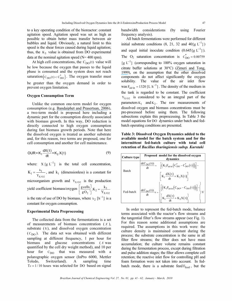
Figure 7: DOC experimental and model output for Fermentation 03. The solid line represents the estimated oxygen concentration attained by the model (model output), the grey line represents the experimental data of dissolved oxygen concentration and the dotted line represents the filtered experimental data of dissolved oxygen concentration.

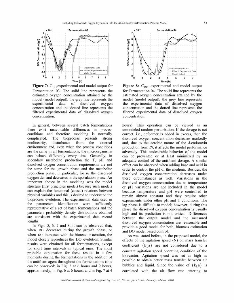
Figure 8: DOC experimental and model output for Fermentation 04. The solid line represents the estimated oxygen concentration attained by the model (model output), the grey line represents the experimental data of dissolved oxygen concentration and the dotted line represents the filtered experimental data of dissolved oxygen concentration.

In general, between several batch fermentations

there exist unavoidable differences in process conditions and therefore modeling is normally complicated. The bioprocess presents strong nonlinearity, disturbance from the external environment and, even when the process conditions are the same in all fermentations, the microorganisms can behave differently every time. Generally, in secondary metabolite production the T, pH and dissolved oxygen concentration requirements are not the same for the growth phase and the metabolite production phase; in particular, for Bt the dissolved oxygen demand decreases in the sporulation phase. An important choice in the modeling was the model structure (first principles model) because such models can explain the functional (causal) relations between physical variables and this is desired to understand the bioprocess evolution. The experimental data used in the parameters identification were sufficiently representative of a set of batch fermentations and the parameters probability density distributions obtained are consistent with the experimental data record lengths.

In Figs. 5, 6, 7 and 8, it can be observed that, when DO decreases during the growth phase, or when DO increases with the bioreactor aeration, the model closely reproduces the DO evolution. Similar results were obtained for all fermentations, except for short time intervals in typical ones. The most probable explanation for these results in a few moments during the fermentations is the addition of the antifoam agent throughout the fermentations (this can be observed: in Fig. 5 at 6 hours and 9 hours, approximately; in Fig. 6 at 6 hours; and in Fig. 7 at 4

hours). This operation can be viewed as an unmodeled random perturbation. If the dosage is not correct, i.e., defoamer is added in excess, then the dissolved oxygen concentration decreases markedly and, due to the aerobic nature of the δ-endotoxin production from Bt, it affects the model performance adversely. This undesirable behavior of the model can be prevented or at least minimized by an adequate control of the antifoam dosage. A similar effect can be observed when adding base and acid in order to control the pH of the medium. Besides, the dissolved oxygen concentration decreases under these circumstances as well. Variations in the dissolved oxygen concentration due to temperature or pH variations are not included in the model because temperature and pH were controlled to remain almost constant and they require other experiments under other pH and T conditions. The lag phase is difficult to model; however, during this phase the dissolved oxygen concentration is usually high and its prediction is not critical. Differences between the output model and the measured dissolved oxygen concentration are reasonable and provide a good model for both, biomass estimation and DO model based control.

As was stated before, in the proposed model, the effects of the agitation speed (N) on mass transfer coefficient ( )Lk a are not considered due to a constant agitation speed operating condition of the bioreactor. Agitation speed was set as high as possible to obtain better mass transfer between air bubbles and liquid. Since the value of ( )Lk a is correlated with the air flow rate entering to

54 A. Amicarelli, F. di Sciascio, J. M. Toibero and H. Alvarez

Brazilian Journal of Chemical Engineering

bioreactor ( )L 3 air ink a K F= to add a new control action for this process. Then, the proposed dynamics model can be used for the dissolved oxygen concentration control specifically for this process. The oxygen requirements of Bt differ at different fermentation stages but, by choosing an adequate temporal profile of the dissolved oxygen during the fermentation, the product formation can be achieved without wasting energy. In the next section, the dynamic model presented in this work is used to control the dissolved oxygen concentration in the fermentation process of Bt.

APPLICATION OF THE DISSOLVED OXYGEN MODEL TO IMPROVE THE

PROCESS CONTROL

The ability to control bioprocesses is of great interest, because it allows reduction of production costs and an increase of productivity while maintaining the products quality. According to the results obtained from the performed fermentations for the δ-endotoxin production of Bt, in some cases it may be observed that the dissolved oxygen concentration decreases to values that are below the critical one at 10% (Atehortúa et al., 2007), even when it is assumed that the air flow rate is in excess (See Fig. 9). With reference to Fig. 9, two important facts can be seen: firstly, the critical influence of oxygen in a great part of the microorganism growth (the vegetative phase), and secondly, the notable fall in the DO demand in the sporulation phase. This situation occurs in most of the fermentations and the limitations caused by oxygen have been detected under various operating conditions. In the case shown in Fig. 9, the airflow was set at 22 1Lmin−⎡ ⎤

⎣ ⎦ ,

assuming that this air flow rate is sufficient to maintain the oxygen in excess, or at least to put it in a range which is favorable to the process, i.e., above the critical concentration of dissolved oxygen reported for the microorganism (10% of the saturation concentration). The dissolved oxygen concentration in culture medium decays mostly during the early hours of the fermentation (first 5 to 7 hours of a 30 hour process) and in some cases it may decay even below its critical value. Consequently, the air flow was used as the manipulated variable in order to control the dissolved oxygen.

Ghribi et al. (2007) state that the level of dissolved oxygen in the fermentation of Bt affects the cell density and δ-endotoxin synthesis.

Therefore, by using appropriate dissolved oxygen profiles, the microorganism productivity can be improved. In this same paper, the authors postulate that, to achieve a high insecticide production, it is necessary to maintain the reactor aeration near to 60% or 70% of oxygen saturation during the first six hours of the fermentation (for a glucose initial concentration of 15 1g min−⎡ ⎤

⎣ ⎦ ). It can be noted that

the structure of the proposed reference is very important, i.e., the controller reference must change after the first few hours of fermentation (first 5 to 7 hr) since the dissolved oxygen requirements will be smaller at the sporulation phase. After these first hours, the percentage of oxygen saturation must approach 40% of oxygen saturation and should be maintained at this value until the end of fermentation, regardless of the carbon source used as substrate.

It is a well known fact that an elevated dissolved oxygen concentration increases the cell density, whereas the δ-endotoxin synthesis is reduced. This knowledge has great practical importance, since it is possible to produce proteins insecticides in large-scale while reducing production costs. On the other hand, the mentioned work of Gribi et al. (2007) provides relationships between the process oxygen requirement and the carbon source used as substrate. The authors report oxygen profiles for glucose-based substrates and also for other glycerol-based substrates.

In this paper, the fermentations were carried out with substrates based primarily on glucose; for this reason, the DO concentration is maintained as close as possible to the established benchmark value for this case. Summarizing, a high production of δ-endotoxin is assumed when a dissolved oxygen concentration of 60% of the oxygen saturation concentration in the culture medium is maintained during the first six hours of incubation, and a dissolved oxygen concentration of 40% of the oxygen saturation concentration until the end of the fermentation (Fig. 10 shows this dissolved oxygen profile). Next, the development of a DO controller that allows the process to follow this dissolved oxygen profile throughout the fermentation course (Amicarelli et al, 2008). The controller is based on the complete knowledge of the model process and illustrates the utility of the DO model proposed here.

First, the DO concentration error is defined as follows

refDO DO DOC (t) C (t) C (t)= − (20)

Including Dissolved Oxygen Dynamics Into the Bt δ-EndotoxinsProduction Process Model 55

Brazilian Journal of Chemical Engineering Vol. 27, No. 01, pp. 41 - 62, January - March, 2010

where refDOC (t) is considered as in Ghribi et al.

(2007) , with

DO DOdC (t) dC (t)dt dt

= − (21)

As the DO dynamics involves not only previous

DO values but also total biomass values according to

( )DO3 air in DO* DO

1 2

dC (t) K F (t) C C (t)dt

dX(t)K K X(t)dt

= − −

−

(22)

The following control action for the air flow rate

command is then proposed

( )DO

air in *3 DO

L DO 1 2

1F (t)K C C (t)

dX(t)K C (t) K K X(t)dt

=−

⎛ ⎞+ +⎜ ⎟⎝ ⎠

(23)

where LK is a positive design constant whose value was set to 2.76. The control action is specified in liters per hour. Its nominal value is equal to 1320

1[Lh ]− and the maximum admissible value is equal to 1800 1[Lh ]− . For this reason, a saturation function is included in the simulations with the aim to not exceed this maximum air flow rate value. Figure 11 shows this saturation.

2 4 6 8 10 12 14 16 180

20

40

60

80

100

Time [h]

DO

Per

cent

age

DO

[%]

Experimental Dissolved Oxygen Data - Bt Fermentations

Critical DO Concentration (Cc)

2 4 6 8 10 12 14 16 180

20

40

60

80

100

Time [h]

DO

Per

cent

age

DO

[%]

Experimental Dissolved Oxygen Data - Bt Fermentations

2 4 6 8 10 12 14 16 180

20

40

60

80

100

Time [h]

DO

Per

cent

age

DO

[%]

Experimental Dissolved Oxygen Data - Bt Fermentations

Critical DO Concentration (Cc)

2 4 6 8 10 12 14 16 180

20

40

60

80

100

2 4 6 8 10 12 14 16 182 4 6 8 10 12 14 16 180

20

40

60

80

100

0

20

40

60

80

100

Time [h]

DO

Per

cent

age

DO

[%]

Experimental Dissolved Oxygen Data - Bt Fermentations

Figure 9: Example of experimental results of dissolved oxygen concentration for some typical batchfermentations. The oxygen is critical during a part of microorganism growth. It can be observed that, in onefermentation, the dissolved oxygen percentages decreased to values even below that the corresponding dissolvedoxygen percentage of the critical dissolved oxygen concentration. The dissolved oxygen demand decreases whenthe sporulation starts (after the eight first hours) and is critical in the vegetative phase (the first 8 to 10 hours).

0 5 10 150

10

20

30

40

50

60

70

Time [h]

Dis

solv

ed O

xyge

n Pe

rcen

tage

s [%

]

Dissolved Oxygen Control fot Bt Fermentations

DO Percentages [%]DO Reference Profile

0 5 10 150

10

20

30

40

50

60

70

Time [h]

Dis

solv

edO

xyge

nPe

rcen

tage

s[%

]

Dissolved Oxygen Control fot Bt Fermentations

0 5 10 150

10

20

30

40

50

60

70

Time [h]

Dis

solv

ed O

xyge

n Pe

rcen

tage

s [%

]

Dissolved Oxygen Control fot Bt Fermentations

DO Percentages [%]DO Reference Profile

0 5 10 150

10

20

30

40

50

60

70

Time [h]

Dis

solv

edO

xyge

nPe

rcen

tage

s[%

]

Dissolved Oxygen Control fot Bt Fermentations

0 5 10 150

10

20

30

40

50

60

70

0 5 10 150 5 10 150

10

20

30

40

50

60

70

0

10

20

30

40

50

60

70

Time [h]

Dis

solv

edO

xyge

nPe

rcen

tage

s[%

]

Dissolved Oxygen Control fot Bt Fermentations

Time [h]

Dis

solv

edO

xyge

nPe

rcen

tage

s[%

]

Dissolved Oxygen Control fot Bt Fermentations

0 5 10 150

500

1000

1500

2000Control Action

Air

Flow

Rat

e [L

/h]

Time [h]0 5 10 150

500

1000

1500

2000Control Action

Air

Flow

Rat

e [L

/h]

Time [h]0 5 10 15

0

500

1000

1500

2000Control Action

Air

Flow

Rat

e [L

/h]

Time [h]0 5 10 150

500

1000

1500

2000Control Action

Air

Flow

Rat

e [L

/h]

Time [h]0 5 10 15

0

500

1000

1500

2000

0 5 10 150 5 10 150

500

1000

1500

2000

0

500

1000

1500

2000Control Action

Air

Flow

Rat

e [L

/h]

Time [h]

Figure 10: Controller Results: reference for oxygen percentage experimentally validated (solid line) and dissolved oxygen percentage (in dashed black line).

Figure 11: Control Action. The control action is specified in liters per hour, with a maximum admissible value equal to 1800 [L/h]. For this reason, a saturation function is included in the simulations with the aim to not exceed this maximum air flow rate value.

56 A. Amicarelli, F. di Sciascio, J. M. Toibero and H. Alvarez

Brazilian Journal of Chemical Engineering

The closed loop equation can be obtained by placing the control action (23) into the model (22),

DOL DO

dC (t) K C (t)dt

= (24)

Now, it is possible to prove the asymptotic

stability for the control system on the equilibrium point at the origin ( DOC (t) 0= ) by considering the following candidate Lyapunov function (Vidyasagar, 1993)

2DO

1 C (t)2

=V (25)

for which the derivative along the system’s trajectories is given by

DODO

2DODO L DO

d dC (t)C (t)dt dt

dC (t)C (t) K C (t) 0dt

= =

− = − <

V

(26)

In other words, when the control action (23) is

considered, the DO error (20) tends asymptotically to zero as the time tends to infinity. In spite of this proof of asymptotic stability for this control system, certain restrictions should be considered for the controller implementation: i) the air flow rate has a maximum physically plausible value (given by the valve used); ii) it is only possible to perform a DO control by increasing the DO concentration, but a decrease in the concentration value can be expected only due to the microorganisms’ consumption, to the addition of antifoam agents (or pH control agents), but not as a direct consequence of this control scheme.

Of particular importance for this process is the instant at which the sporulation begins. The online detection of this instant is advisable in order to perform the step change (from 60% to 40%) of the reference at the most opportune instant. This instant is reflected in the curve response with the highest negative slope (Fig. 10), so, the detection of this instant can be done at any time by taking into account the DO value and its time derivative. This way, the control of this process would be adaptable

instead of the fixed version constrained to the literature reference values. The correct detection in conjunction with an acceptable controller performance guarantees an improvement in the use of oxygen for the process, avoiding unnecessary air supply. Given an experimentally validated profile of dissolved oxygen, this nonlinear controller (Fig. 10) exhibits satisfactory performance due to the implicit knowledge of the dynamics model for the DO concentration.

In order to show how the addition of this controller affects the other process states, namely, the substrate concentration S, the total biomass concentration ( X ), the vegetative cell concentration ( Xv ) and the sporulated cell concentration ( Xs ), the specific growth rate equation (4) must be modified to reflect the dissolved oxygen limitation. Since the specific growth rate (μ ) as it appears in (4), only shows the substrate limitation. We, next, considered a model based on Monod equation for each limiting nutrient ( S and DOC ) as appears in Bailey & Ollis (1986):

( ) ( )DO

maxs d DO

S(t) C (t)(t)K S(t) K C (t)

⎛ ⎞μ = μ ⎜ ⎟⎜ ⎟+ +⎝ ⎠

(27)

Assuming that the values for maxμ and sK do not

change, it is possible to obtain a value for the parameter ( dK ) by using standard identification tool. This assumption is supported by the fact that, when the DO level is not critical, this new limiting factor must not affect the overall process behavior. But, under dissolved oxygen limitation, the process dynamics are affected. The results of such identification are shown in Fig. 12, presenting the time evolution of the rest of the process states when the DO is controlled as previously shown in Fig. 10. Finally for comparison, results are presented in Fig. 13 for the evolution in time of the same states under uncontrolled conditions (open loop), while the DO profile for this same situation is shown in Fig. 14. From these figures, one can note the permanent effect of the oxygen limitation, which appears approximately between 6 and 14hr of the experiment, on the total biomass concentration, making clear the importance of DO control in this bioprocess.

Including Dissolved Oxygen Dynamics Into the Bt δ-EndotoxinsProduction Process Model 57

Brazilian Journal of Chemical Engineering Vol. 27, No. 01, pp. 41 - 62, January - March, 2010

0 5 10 15 20 25 305

10

15

20

25

30

35

Time [h]

Subs

trate

Con

cent

ratio

n [g

/L]

00

12

0

2

4

6

8

10

12

Cel

l Con

cent

ratio

n [g

/L]

Substrate Concentration

Total Cell Concentration

Sporulated Cell Concentration

Vegetative Cell Concentration

Time [h]

Subs

trat

eC

once

ntra

tion

[g/L

]

0 5 10 15 20 25 305

10

15

20

25

30

35

0

2

4

6

8

10

12

Cel

lCon

cent

ratio

n[g

/L]

0 5 10 15 20 25 305

10

15

20

25

30

35

Time [h]

Subs

trate

Con

cent

ratio

n [g

/L]

00

12

0

2

4

6

8

10

12

Cel

l Con

cent

ratio

n [g

/L]

Substrate Concentration

Total Cell Concentration

Sporulated Cell Concentration

Vegetative Cell Concentration

Time [h]

Subs

trat

eC

once

ntra

tion

[g/L

]

0 5 10 15 20 25 305

10

15

20

25

30

35

0

2

4

6

8

10

12

0 5 10 15 20 25 300 5 10 15 20 25 305

10

15

20

25

30

35

5

10

15

20

25

30

35

0

2

4

6

8

10

12

0

2

4

6

8

10

12

2

4

6

8

10

12

Cel

lCon

cent

ratio

n[g

/L]

0

5

10

15

20

25

30

35

Subs

trate

Con

cent

ratio

n [g

/L]

00 5 10 15 20 25 300

2

4

6

8

10

12

Time [h]

Cel

l Con

cent

ratio

n [g

/L]

Substrate Concentration

Total Cell Concentration

Sporulated Cell Concentration

Vegetative Cell Concentration

Subs

trat

eC

once

ntra

tion

[g/L

]

0

5

10

15

20

25

30

35

0 5 10 15 20 25 30Time [h]

Cel

lCon

cent

ratio

n[g

/L]

0

2

4

6

8

10

12

0

5

10

15

20

25

30

35

Subs

trate

Con

cent

ratio

n [g

/L]

00 5 10 15 20 25 300

2

4

6

8

10

12

Time [h]

Cel

l Con

cent

ratio

n [g

/L]

Substrate Concentration

Total Cell Concentration

Sporulated Cell Concentration

Vegetative Cell Concentration

Subs

trat

eC

once

ntra

tion

[g/L

]

0

5

10

15

20

25

30

35

0 5 10 15 20 25 300

5

10

15

20

25

30

35

0

5

10

15

20

25

30

35

0 5 10 15 20 25 300 5 10 15 20 25 30Time [h]

Cel

lCon

cent

ratio

n[g

/L]

0

2

4

6

8

10

12

0

2

4

6

8

10

12

Figure 12: Bioprocess States Time Evolution under controlled conditions. The solid grey line represents the substrate concentration; the solid black line is the vegetative cell concentration; the black dashed line is the sporulated cell concentration; and the grey dashed line the total biomass concentration.

Figure 13: Bioprocess States Time Evolution with a fixed air flow rate of 750 [L/h]. The solid grey line represents the substrate concentration, the solid black line is the vegetative cell concentration, the black dashed line is the sporulated cell concentration and the grey dashed line the total biomass concentration.

0 5 10 15 20 25 300

20

40

60

80

100

Time [h]

Dis

solv

ed O

xyge

n Pe

rcen

tage

s [%

]

0 5 10 15 20 25 300

20

40

60

80

100

Time [h]

Dis

solv

edO

xyge

nPe

rcen

tage

s[%

]

0 5 10 15 20 25 300

20

40

60

80

100

Time [h]

Dis

solv

ed O

xyge

n Pe

rcen

tage

s [%

]

0 5 10 15 20 25 300

20

40

60

80

100

Time [h]

Dis

solv

ed O

xyge

n Pe

rcen

tage

s [%

]

0 5 10 15 20 25 300

20

40

60

80

100

Time [h]

Dis

solv

edO

xyge

nPe

rcen

tage

s[%

]

0 5 10 15 20 25 300

20

40

60

80

100

0 5 10 15 20 25 300 5 10 15 20 25 300

20

40

60

80

100

0

20

40

60

80

100

Time [h]

Dis

solv

edO

xyge

nPe

rcen

tage

s[%

]

Time [h]

Dis

solv

edO

xyge

nPe

rcen

tage

s[%

]

Figure 14: Dissolved Oxygen Profile in open- loop corresponding to a constant air flow rate of 750 [L/h].

For aerobic microbial cultures, sufficient oxygen

must be supplied during growth to satisfy the organism’s demand. The limitations caused by the lack of oxygen have been detected for this process under various operating conditions (even assuming that this air flow rate is sufficient to maintain the oxygen in excess). The proposed control strategy offers improvements in productivity with respect to the open-loop configuration (See Figs. 12 and 13). Furthermore, this controller prevents the possible inhibition caused by high oxygen levels that may occur with elevated air flow rates during the growth phase.

ROBUSTNESS ANALYSIS

In this Section, a robustness analysis was performed for the proposed dissolved oxygen controller. This controller is integrated with a biomass estimator in a closed loop, i.e., the robustness analysis is investigated

for errors introduced from both: biomass estimation and modeling errors.

Having proved the asymptotic stability for the control system on the equilibrium point at the origin ( DOC (t) 0= ), it is interesting to analyze the effects of the biomass estimation and modeling errors on the control errors and what happens with the control system stability in this context. The dissolved oxygen dynamics for batch mode are shown in Table 3.

Now, it is possible to write the proposed control law in terms of the estimated biomass concentration and the estimated model parameters 1 2

ˆ ˆK ,K and 3K as follows:

( )DO

air in *3 DO

L DO 1 2

1F (t)K C C (t)

ˆdX(t)ˆ ˆ ˆK C (t) K K X(t)dt

−=

−⎛ ⎞

+ +⎜ ⎟⎝ ⎠

(28)

58 A. Amicarelli, F. di Sciascio, J. M. Toibero and H. Alvarez

Brazilian Journal of Chemical Engineering

where X(t) is the estimated biomass concentration obtained with some estimator (Amicarelli et al, 2006; di Sciascio and Amicarelli, 2008). The closed loop equation can now be rewritten as:

DO 3L DO 1 2 1 2

3

ˆdC (t) K dX(t) dX(t)ˆ ˆ ˆK C (t) K K X(t) K K X(t)ˆdt dt dtK⎛ ⎞

= + + − −⎜ ⎟⎝ ⎠

(29)

The Lyapunov function (25) which proved the asymptotic stability was 2DOC (t) / 2=V , whose derivative

along the system’s trajectories is given by (26). Now, replacing (29) in (26):

DO 3 L DO 3 1 3 2 1 2ˆd dX(t) dX(t)ˆ ˆ ˆC (t) K ' K C (t) K ' K K ' K X(t) K K X(t)

dt dt dt⎡ ⎤

= − + + − −⎢ ⎥⎣ ⎦

V (30)

where 33

3

KK 'K

=

In order to satisfy the asymptotic stability condition, it must be guaranteed that the term 3 L DOK ' K C− is

bigger than 3 1 3 2 1 2ˆdX(t) dX(t)ˆ ˆ ˆK ' K K ' K X(t) K K X(t)dt dt

+ − − . Next, it follows that:

3 L DO 1 2 3 2 3 1ˆdX(t) dX(t)ˆ ˆ ˆK ' K C K K X(t) K ' K X(t) K ' K

dt dt> + − − (31)

Denoting the error associated with the estimated biomass as ˆX(t) X(t) X(t)= − ; and, consequently:

ˆdX(t) dX(t) dX(t)dt dt dt

= − . a maximum bound for the control error is given by

( ) ( ) ( )1DO 3 L 1 3 1 1 2 3 2 2

ˆdX(t) dX(t)ˆ ˆ ˆC (t) K ' K K K ' K K K X(t) K ' K K X(t)dt dt

−≤ + − + + − (32)

Furthermore, considering the triangle inequality,

( ) ( ) ( )

( ) ( ) ( )

13 L 1 3 1 1 2 3 2 2

13 L 1 3 1 1 2 3 2 2

ˆdX(t) dX(t)ˆ ˆ ˆK ' K K K' K K K X(t) K ' K K X(t)dt dt

ˆdX(t) dX(t)ˆ ˆ ˆK ' K K K' K K K X(t) K ' K K X(t)dt dt

−

−

+ − + + − ≤

⎛ ⎞≤ + − + + −⎜ ⎟⎜ ⎟

⎝ ⎠

(33)

the maximum bound for the control error can be rewritten as:

( ) ( ) ( )1DO 3 L 1 3 1 1 2 3 2 2

ˆdX(t) dX(t)ˆ ˆ ˆC (t) K ' K K K ' K K K X(t) K ' K K X(t)dt dt

− ⎛ ⎞≤ + − + + −⎜ ⎟⎜ ⎟

⎝ ⎠ (34)

Now, considering the control action (28), the DOC is bounded by (34) and the stability condition is maintained in the control system.

Now, if there are not biomass estimation errors X(t) , i.e., there are only model parametric errors, the expression for the bound is given by:

( ) ( ) ( )1DO 3 L 3 1 1 3 2 2

dX(t)ˆ ˆC (t) K ' K K ' K K K ' K K X(t)dt

− ⎛ ⎞≤ − + −⎜ ⎟⎝ ⎠

(35)

and, conversely, in absence of parametric errors, the bound is given by:

1DO L 1 2

dX(t)C (t) K K K X(t)dt

− ⎛ ⎞≤ +⎜ ⎟

⎝ ⎠ (36)

Including Dissolved Oxygen Dynamics Into the Bt δ-EndotoxinsProduction Process Model 59

Brazilian Journal of Chemical Engineering Vol. 27, No. 01, pp. 41 - 62, January - March, 2010

0 5 10 15 200

10

20

30

40

50

60

70

Time [h]

Dis

solv

ed O

xyge

n Pe

rcen

tage

s [%

]

DO considering estimation andparametric model errorDO Reference ProfileDO without considering errors

0 5 10 15 200

10

20

30

40

50

60

70

Time [h]

Dis

solv

edO

xyge

nPe

rcen

tage

s[%

]

0 5 10 15 200

10

20

30

40

50

60

70

Time [h]

Dis

solv

ed O

xyge

n Pe

rcen

tage

s [%

]

DO considering estimation andparametric model errorDO Reference ProfileDO without considering errors

0 5 10 15 200

10

20

30

40

50

60

70

Time [h]

Dis

solv

ed O

xyge

n Pe

rcen

tage

s [%

]

DO considering estimation andparametric model errorDO Reference ProfileDO without considering errors

0 5 10 15 200

10

20

30

40

50

60

70

Time [h]

Dis

solv

edO

xyge

nPe

rcen

tage

s[%

]

0 5 10 15 200

10

20

30

40

50

60

70

0 5 10 15 200 5 10 15 200

10

20

30

40

50

60

70

0

10

20

30

40

50

60

70

Time [h]

Dis

solv

edO

xyge

nPe

rcen

tage

s[%

]

0 5 10 15 20

-2

-1

0

1

2

3

4

5x 10-3

Time [h]

Con

trol E

rror

[g/L

]

Control error for the system without errors Control error with model parametric errorsand biomass estimation errorsControl error boundControl error bound

0 5 10 15 20

x 10-3

-2

-1

0

1

2

3

4

5

Time [h]

Con

trol

Erro

r[g/

L]

0 5 10 15 20-2

-1

0

1

2

3

4

5x 10-3

Time [h]

Con

trol E

rror

[g/L

]

Control error for the system without errors Control error with model parametric errorsand biomass estimation errorsControl error boundControl error bound

0 5 10 15 20-2

-1

0

1

2

3

4

5x 10-3

Time [h]

Con

trol E

rror

[g/L

]

Control error for the system without errors Control error with model parametric errorsand biomass estimation errorsControl error boundControl error bound

0 5 10 15 20

x 10-3

-2

-1

0

1

2

3

4

5

Time [h]

Con

trol

Erro

r[g/

L]

0 5 10 15 200 5 10 15 20

x 10-3

-2

-1

0

1

2

3

4

5

-2

-1

0

1

2

3

4

5

Time [h]

Con

trol

Erro

r[g/

L]

Figure 15: Dissolved Oxygen desired profile (solid black line); controlled output without errors (dash black line) and controlled output when considering both parametric model errors of 10% and estimation errors of 20% (solid gray line).

Figure 16: Control Error. The dash black line represents the control error for the system without errors and the gray line is the control error with the presence of model parametric errors of 10% and biomass estimation errors of 20%. The solid black lines represent the control error bound.

Equations (34), (35) and (36) give a bound for the

estimation errors or for the model parametric errors depending on the case. Note that, considering the control action (28), DOC is bounded by (34) in the most general case, preserving the control system stability condition.

Figure 15 shows an example of the performance of the dissolved oxygen controller in closed-loop with a biomass estimator; more specifically, it shows the controller output for 20% biomass estimation errors and for 10% model parametric errors. In Fig. 16 the control error is shown for both cases (with and without estimation and parametric model errors). Moreover, in this same figure one can observe the maximum bound for this situation according to (36).

Note that in Fig. 10 and Fig. 15 there appears a drop in the DO concentration below the critical dissolved oxygen level. This drop occurs due to the sudden reference change for the dissolved oxygen controller. The mentioned behavior can be reduced or eliminated with a smooth change in the reference profile. Furthermore, even when this occurs, the dissolved oxygen concentration is below the critical level during a short time period, which does not affect the microorganism concentration.

CONCLUSIONS

In this paper, an existing mathematical model of δ-

endotoxin production by Bacillus thuringiensis was augmented by incorporating a model of dissolved oxygen dynamics. A linearly parameterized model

based on first principles has been developed and compared with experimental data of real fermentations. The results presented in the previous section show that the model predicts quite satisfactory the dynamic behavior of dissolved oxygen concentration throughout the fermentation. Due to its inherent linearity assumption, the level of model complexity is fairly reduced. This complexity decrease can be determined from the available experimental data records and by balancing the trade-off between simplicity and goodness-of-fit. The proposed dissolved oxygen model allows improvement of the microorganism growth, the product formation and the process productivity. The DO dynamic model is based on unstructured and unsegregated descriptions of the cell population, which are the best selection for model-based controller design. It is clear that the microorganism growth is affected by dissolved oxygen concentration (below the 10% critical value).

It is important, then, that the model take into account these dynamics to control the dissolved oxygen limitation on cell growth. Furthermore, in this work a stable model reference controller is designed. Given an experimentally validated temporal profile of the dissolved oxygen during the fermentation, the controller can maintain the dissolved oxygen level at an optimum level for this process. The proposed nonlinear controller presents an adequate performance due to the implicit knowledge of the dynamic model for the DO concentration. A robustness analysis has been performed for the errors introduced by the biomass

60 A. Amicarelli, F. di Sciascio, J. M. Toibero and H. Alvarez

Brazilian Journal of Chemical Engineering

estimation and by modeling errors. Finally, this work provides three expressions to bound the control error under biomass estimation errors; model parametric errors; and for the case when both errors are present. Furthermore, considering the proposed control action it is demonstrated that the control error is ultimately bounded.

ACKNOWLEDGMENT The authors wish to thank the following persons

and organizations who contributed to the completion of this work, and without whom much of the information in this paper could not have been obtained. In particular, we wish to thank Paula Atehortúa and Dr. Sergio Orduz (Universidad Nacional de Colombia, Sede Medellín, and Corporación para Investigaciones Biológicas (CIB), Medellín, Colombia). This work was partially supported by Universidad Nacional de San Juan (UNSJ, Argentina), and by Consejo Nacional de Investigaciones Científicas y Técnicas (CONICET, Argentina).

REFERENCES

Amicarelli, A., di Sciascio, F., Álvarez, H. and Ortiz, O., Estimación de Biomasa en un proceso Batch: Aplicación a la producción de δ-endotoxinas de Bt. XXII Interamerican Congress of Chemical Engineering, Bs. As., Argentina (2006). (In Spanish).

Amicarelli, A., Toibero, J. M., Quintero O., di Sciascio F. and Carelli R., Estrategias de Control de Oxígeno Disuelto Aplicadas a la Fermentación Batch de Bt. XIII Congreso Latinoamericano de Control Automático, VI Congreso Venezolano de Automatización y Control. 25 al 28 de Noviembre Mérida, Venezuela (2008).

Amicarelli, A., Toibero, J. M. and di Sciascio F., Stable and Robust Dissolved Oxygen Control for the Fermentative Process of Bt δ-Endotoxin Production. XIII Reunión de Trabajo en Procesamiento de la Información y Control (RPIC), 16-18 September - Rosario, Argentina (2009).

Atehortúa, P., Álvarez, H., and Orduz, S., Comments on: “A Sporulation Kinetic Model for Batch Growth of B. thuringiensis”. The Canadian Journal of Chemical Engineering, v. 84, No. 3 (2006).

Aronson, A. I., The two faces of Bacillus thuringiensis: insecticidal proteins and post exponential survival. Molecular Microbiology, v. 7, pp. 489- 96 (1993).

Atehortúa, P., Alvarez, H. D. and Orduz, S., Modeling of Growth and Sporulation of Bacillus thuringiensis in an Intermittent Fed-batch Culture with Total Cell Retention. Bioprocess Biosystem Engineering. v. 30, pp. 447-456 (2007).

Bandaiphet, C. and Prasertsan, P., Effect of aeration and agitation rates and scale-up on oxygen transfer coefficient, kLa in exopolysaccharide production from Enterobacter cloacae WD7. Carbohydrate Polymers, v. 66. pp. 216-228 (2006).

Bailey, J. and Ollis, D. X., Biochemical Engineering Fundamentals. 2nd ed. McGraw-Hill, New York (1986).

Bernard, O., Mass Balance Modelling of Bioprocesses. Lectures given at the Summer School on Mathematical, Control Theory, Trieste, 3-28, September (2001).

Birol, G., Undey, C. and Cinar, A., A modular simulation package for fed-batch fermentation: penicillin production. Computers & Chemical Engineering, v. 26, pp. 1553-1565 (2002).

Bocken, S. M., Braae, M. and Dold, P. L., Dissolved Oxygen Control and Oxygen Utilization Rate Estimation: Extension of the Holmberg/Olsson Method. Wat. Sci. Tech., v. 21 (10-11), 1197-1208 (1989).

Chen, C. Y., Roth, J. A. and Eckenfelder, W. W. Jr., Response of Dissolved Oxygen to Changes in Influent Organic Loading to Activated Sludge Systems. Wat. Res., v. 14, pp. 1449-1457 (1980).

Curtiss, J. M., "On the Distribution of the Quotient of Two Chance Variables". The Annals of Mathematical Statistics, v. 12 (4), pp. 409-421 (1941).

de Maré, L. and Hagander, P., Parameter Estimation of a Model Describing the Oxygen Dynamics in a Fed-Batch E. Coli Cultivation. In Reglermöte, Stockholm, Sweden, May (2006).

di Sciascio, F. and Amicarelli, A. N., Biomass: Estimation in Batch Biotechnological Processes by Bayesian Gaussian Process Regression. Computers and Chemical Engineering v. 32, pp. 3264-3273 (2008).

Donald Dean, A., Roider, E. and Thomas G., S., Oxygen Sag Models for Multiorder Biochemical Oxygen Demands Reactions. Journal of Environmental Engineering, v. 130, Issue 7, pp. 784-791 (2004).

Including Dissolved Oxygen Dynamics Into the Bt δ-EndotoxinsProduction Process Model 61

Brazilian Journal of Chemical Engineering Vol. 27, No. 01, pp. 41 - 62, January - March, 2010

Douglas, W. R., Automatic Assessment of Respiration during Growth in Stirred Fermentors. Applied Microbiology, v. 18, No 3, pp. 438-443 (1969).

Dunstan, W. J. and Bitmead, R. R., Empirical estimation of parameter distributions in system identification. 13th IFAC Symposium on System Identification, Rotterdam, The Netherlands (2003).

Gaudenta, S., Dissolved Oxygen Balance Model for Neris. En: Nonlinear Analysis: Modelling and Control, v. 6, No 1, pp. 105-131 (2001).

Ghribi, D., Zouari, N., Trabelsi, H. and Jaoua, S., Improvement of Bacillus thuringiensis δ-endotoxin Production by Overcome of Carbon Catabolite Repression Through Adequate Control of Aeration. Enzyme and Microbial Technology, v. 40, pp. 614-622 (2007).

Henson, M. A. and Seborg D. E., Nonlinear Process Control. Prentice Hall (1997).

Henson, M. A., Biochemical Reactor Modeling and Control, Control Systems Magazine, IEEE v. 26, Issue 4, pp. 54-62, (2006).

Holenda B., Domokos E., Rédey Á. and Fazakas J., Dissolved oxygen control of the activated sludge wastewater treatment process using model predictive control. Computers and Chemical Engineering, v. 32, pp. 1270-1278 (2008).

Hiroshi, S., Metabolic Engineering - Integrating Methodologies of Molecular Breeding and Bioprocess Systems Engineering, Journal of Bioscience and Bioengineering, v. 94, No. 6, pp. 563-573 (2002).

Konz, J. O., King, J. and Cooney, C. L., Effects of Oxygen on Recombinant Protein Expresión, Biotechnology Progress. v. 14, pp. 393-409 (1998).

Leal, R. R., Butle, P., Lane, P. and Payne, P. A., Data fusion and artificial neural networks for biomass estimation. Science Measurement and Technology, IEEE Procedings, v. 144, Issue 2, pp. 69-72 (1997).

Lee, J., Wu, R., Cheung, Y., and Wong, P., Dissolved oxygen variation in marine fish culture Zone. Journal of Environmental Engineering, v. 117, No 6, pp. 799-815 (1991).

Liu, B. L. and Tzeng, Y. M., Caracterization study of the sporulation kinetics of Bacillus thuringiensis. Biotechnology Bioengineering, v. 68, pp. 11-17 (2000).

Ljung L., System Identification: Theory for the User. Second Edition, Prentice-Hall, Inc., Upper Saddle River, New Jersey (1999).

Madigan, M. T., Martinko, J. M. and Parker J., Brock Biology of Microorganisms. 11th edition, Prentice Hall (2006).

Marsaglia, G., "Ratios of Normal Variables and Ratios of Sums of Uniform Variables". Journal of the American Statistical Association, v. 60 (309), pp. 193-204. doi:10.2307/2283145 (1965).

Miller, G., Use of Dinitrosalicylic Acid Reagent for Determination of Reducing Sugar. Analytical Chemistry, v. 31 (3), pp. 426-428 (1959).

Moraes, I. and Santana, M., The influence of oxygen concentration on microbial insecticide production. Murray Moo-Young (Org.), Advances in Biotechnology, v. 1, pp. 75-79 (1981).

Nielsen, D., Daugulis, A. and McLellan, P., A Novel Method of Simulating Oxygen Mass Transfer in Two-Phase Partitioning Bioreactors, Biotechnology and bioengineering, v. 83, pp. 735-742 (2003).

Oliveira R., Simutis R. and Feyo de Azevedo V., Design of a stable adaptive controller for driving aerobic fermentation processes near maximum oxygen transfer capacity. Journal of Process Control, v. 14. pp. 617-626 (2004).

Onken, U. and Liefke, E., Effect of total and partial pressure (oxygen and carbon dioxide) on aerobic microbial processes. Advances in Biochemical Engineering/Biotechnology, Springer Berlin/ Heidelberg, v. 40, pp. 137-169 (1989).

Pham-Gia, T., Turkkan, N. and Marchand, E., "Density of the Ratio of Two Normal Random Variables and Applications". Communications in Statistics: Theory and Methods, v. 35 (9), pp. 1569-1591, Taylor & Francis (2006).

Pereira, D. G., Tonso, A. and Kilikian, B. V., “Effect of dissolved oxygen concentration on red pigment and citrinin production by Monascus purpureus ATCC 36928”. Braz. J. Chem. Eng., v. 25 (2), pp. 247-253 (2008).

Radwan, M., Willems, P., El Sadek, A. and Berlamont, J., Modelling of dissolved oxygen and biochemical oxygen demand in river water using a detailed and a simplified model. Intl. J. River Basin Management, v. 1, No. 2, pp. 97-103 (2003).

Rajib N. and Gomes, J., Sequential adaptive networks: An ensemble of neural networks for feed forward control of L-methionine production. Chemical Engineering Science, v. 64, No. 10, pp 2401-2412 (2009).

Ranjan, A. and Gomes, J., Simultaneous dissolved oxygen and glucose regulation in fed-batch methionine production using decoupled input–output linearizing control. Journal of Process Control, v. 19, No. 4, pp 664-677 (2009).

62 A. Amicarelli, F. di Sciascio, J. M. Toibero and H. Alvarez

Brazilian Journal of Chemical Engineering

Rasmussen, C. E., Christopher, K. I. and Williams, C. K. I., Gaussian Processes for Machine Learning. The MIT Press (2006).

Rencher, A. and Schaalje, G., Linear Models in Statistics. Second Edition, John Wiley & Sons, Inc., Hoboken, New Jersey, (2008).

Rivera, D., Margaritis, A. and De Lasa, H., A Sporulation Kinetic Model for Batch Growth of B. thuringiensies. The Canadian Journal of Chemical Engineering, v. 77, pp. 903-910 (1999).

Rodrigues, J. A. D. and Maciel Filho, R., Analysis of the Predictive DMC Controller Performance Applied to a Feed-Batch Bioreactor, Braz. J. Chem. Eng., v. 14 (4), pp. 353-358 (1997).

Silveira, M., and Molina, M., Indirect Estimation of Bacillus thuringiensis var. israelensis Biomass Concentration using oxygen balance data. Brazilian Journal of Chemical Engineering, v. 22, pp. 495-500 (2005).

Starzak, M. and Bajpai, R., A structured model for vegetative growth and sporulation in Bacillus thuringiensis. Applied Biochemistry /Biotechnology, v. 28/29, pp. 699-718 (1991).

Vallejo, F., González, A., Posada, A., Restrepo, A. and Orduz, S., Production of Bacillus thuringiensis subsp. Medellín by batch and fed-

batch culture. Biotechnology Tech., v. 13, pp. 279-281 (1999).

Vidyasagar, M., Nonlinear Systems Analysis. Prentice Hall, New York (1993).

Wiechert, W., Modeling and simulation: tools for metabolic engineering. Journal of Biotechnology, v. 94, pp. 37-63 (2002).

Wu, W., Hsu, Y., Ko, Y. and Yao L., Effect of shear stress on cultivation of Bacillus thuringiensis for thuringiensin production. Applied Microbiology/ Biotechnology, v. 58, pp. 175-177 (2002).

Zhang, Z., Szita, N., Boccazzi, P., Sinskey, A. J. and Jensen, K. F., Monitoring and Control of Cell Growth in fed-batch microbioreactors. 7th lnternational Conference on Miniaturized Chemical and Biochemical Analysis Systems, Squaw Valley, California USA (2003).

Zimeri, J. and Tong, C. H., Degradation Kinetics of (-)-Epigallocatechin Gallate as a Function of pH and Dissolved Oxygen in a Liquid Model System. Journal of Food Science, v. 64, No. 5, pp. 753-758 (1999).

Znad, H., Blažej, M., Báleš, V. and Markoš, J., A Kinetic Model for Gluconic Acid Production by Asphergillus Niger. Chemical Papers, v. 58 (1), pp. 23-28 (2004).