INAUGURAL – DISSERTATION zur Erlangung der DoktorwЭrde der ...
201
INAUGURAL – DISSERTATION zur Erlangung der Doktorwürde der Naturwissenschaftlich - Mathematischen Gesamtfakultät der Ruprecht - Karls - Universität Heidelberg vorgelegt von Dipl.-Phys. Maya Bräunlich aus Frankfurt a.M. Tag der mündlichen Prüfung : 18. Juli 2000
-
Upload
khangminh22 -
Category
Documents
-
view
1 -
download
0
Transcript of INAUGURAL – DISSERTATION zur Erlangung der DoktorwЭrde der ...

INAUGURAL – DISSERTATIONzur
Erlangung der Doktorwürdeder
Naturwissenschaftlich - MathematischenGesamtfakultät
derRuprecht - Karls - Universität
Heidelberg
vorgelegt vonDipl.-Phys. Maya Bräunlich
aus Frankfurt a.M.
Tag der mündlichen Prüfung : 18. Juli 2000

Untersuchung von atmosphärischem Kohlenmonoxid und Methan
anhand von Isotopenmessungen
Gutachter: Prof. Dr. Ulrich Platt
Prof Dr. Konrad Mauersberger

Dissertationsubmitted to the
Combined Faculties for the Natural Sciences and for Mathematicsof the Rupertus Carola University of
Heidelberg, Germanyfor the degree of
Doctor of Natural Sciences
Study of atmospheric carbon monoxide and methane
using isotopic analysis
presented by
Diplom-Physicist: Maya Bräunlich
born in : Frankfurt a.M.
Heidelberg, 18. July 2000
Referees: Prof. Dr. Ulrich Platt
Prof Dr. Konrad Mauersberger

Le présent n'est pas un passé en puissance,il est le moment du choix et de l'action.
Simone de Beauvoir
To Monique Cariot Edith and Walter Bräunlich
Untersuchung von atmosphärischem CO und CH4 anhand von Isotopen-
messungen Die Analyse von Isotophenverhältnissen ist ein weit verbreitetes Mittel
zur Erforschung von atmosphärischen Spurengasen. Wir haben sowohl das Verhält-
nis der stabilen Isotope δ13C und δD an atmosphärischem CH4, als auch δ13C ,
δ18O und die Konzentration von 14CO an atmosphärischem CO an der Station
Izaña, Tenerife, von 1996 bis 1999 gemessen. Die Genauigkeit der δD Messungen
erlaubte zum ersten mal einen Jahresgang von δD nachzuweisen. Die ausgeprägten
Jahresgänge in den Isotopensignalen von CH4 und CO ermöglichte Rückschlüsse auf
ihre Quellen und Senken. Starke Abweichungen mancher Proben von den mittleren
Jahresgängen konnten den wichtigen Quell-Regionen Nord Amerika und Europa, bzw
sauberen Luftmasen aus Afrika und dem Nordatlantik zugeordnet werden. Weiterhin
haben wir δ13C (CH4) und δD (CH4) an Firnluft Proben von zwei Antarktischen
Stationen gemessen. Mit Hilfe eines Firnluft-Di�usionsmodells konnten die δ13Cund δD Signale von atmosphärischem CH4 der letzten fünfzig Jahre rekonstruiert
werden. Parallel zu den steigenden CH4 Konzentrationen der letzten Jahrzehnte
wurde ein positiver δ13C Trend nachgewiesen, welcher den wachsenden Beitrag der
anthropogenen CH4 Quellen widerspiegelt. δD zeigt ein ausgeprägtes Minimum um
1975, verursacht durch das Ungleichgewicht zwischen den Quellen und Senken von
CH4. Dieser E�ekt konnte somit zum ersten mal auch für δD nachgewiesen werden.
Study of atmospheric CO and CH4 using isotopic analysis The analysis
of isotope ratios is widely used for the investigation of atmospheric trace gases. We
measured the stable isotopes δ13C and δD of atmospheric CH4 as well as δ13C ,
δ18O and the 14CO concentrations of atmospheric CO at Izaña, Tenerife, from 1996
to 1999. We report the �rst directly measured δD seasonality for atmospheric back-
ground CH4. The large seasonal cycles in mixing and isotopic ratios of CH4 and CO
enable inferences about the underlying source and sink processes. The large synoptic
scale variations occurring for these trace gases at Izaña made it possible to study
source regions such as North America, Europe, as well as background conditions over
the North Atlantic and Africa. We also measured δ13C and δD on �rn air samples
from two Antarctic sites. From these measurements the atmospheric trends of δ13Cand δD of CH4 over the past �fty years have been reconstructed with the help of a
�rn air di�usion model. We �nd that parallel to increasing CH4 mixing ratios δ13Cincreases, which is evidence for a growing contribution of the heavier anthropogenic
CH4 sources. For δD we �nd a period of decline previous to 1975, followed by a
gradual increase. This δD minimum is due to the non-equilibrium state between
CH4 and its sources and sinks and has for the �rst time been detected for δD.

2

Contents
1 Review of atmospheric CH4 and CO 9
1.1 Atmospheric CH4 and CO . . . . . . . . . . . . . . . . . . . . . . . . 9
1.2 The global CH4 budget . . . . . . . . . . . . . . . . . . . . . . . . . . 12
1.3 CH4 measurements . . . . . . . . . . . . . . . . . . . . . . . . . . . . 12
1.3.1 Atmospheric Trends . . . . . . . . . . . . . . . . . . . . . . . 14
1.3.2 Global distribution . . . . . . . . . . . . . . . . . . . . . . . . 16
1.4 Isotope studies . . . . . . . . . . . . . . . . . . . . . . . . . . . . . . 16
1.4.1 Æ-notation . . . . . . . . . . . . . . . . . . . . . . . . . . . . . 17
1.4.2 Kinetic Isotope E�ect (KIE) . . . . . . . . . . . . . . . . . . . 17
1.5 Isotope variations in CH4 . . . . . . . . . . . . . . . . . . . . . . . . 18
1.5.1 Atmospheric CH4 isotope data . . . . . . . . . . . . . . . . . 20
1.6 The global CO budget . . . . . . . . . . . . . . . . . . . . . . . . . . 21
1.7 CO measurements . . . . . . . . . . . . . . . . . . . . . . . . . . . . 21
1.7.1 Global distribution . . . . . . . . . . . . . . . . . . . . . . . . 23
1.7.2 Atmospheric trends . . . . . . . . . . . . . . . . . . . . . . . . 23
1.8 Isotope variations in CO . . . . . . . . . . . . . . . . . . . . . . . . . 23
1.8.1 Kinetic Isotope E�ect . . . . . . . . . . . . . . . . . . . . . . 26
1.8.2 Atmospheric 14CO . . . . . . . . . . . . . . . . . . . . . . . . 27
1.9 Scope of this thesis . . . . . . . . . . . . . . . . . . . . . . . . . . . . 30
2 Sampling and Measurement 33
2.1 Air sampling . . . . . . . . . . . . . . . . . . . . . . . . . . . . . . . 34
2.1.1 The compressor system . . . . . . . . . . . . . . . . . . . . . 34
2.1.2 High pressure sample cylinders . . . . . . . . . . . . . . . . . 35
2.1.3 Spot air sampling . . . . . . . . . . . . . . . . . . . . . . . . . 36
2.1.4 Continuous air sampling . . . . . . . . . . . . . . . . . . . . . 36
2.2 GC measurements . . . . . . . . . . . . . . . . . . . . . . . . . . . . 37
2.3 The extraction system . . . . . . . . . . . . . . . . . . . . . . . . . . 40
2.3.1 The CO and CO2 extraction system . . . . . . . . . . . . . . 40
3

4 CONTENTS
2.3.2 The CH4 extraction system . . . . . . . . . . . . . . . . . . . 43
2.3.3 The CH4 combustion system . . . . . . . . . . . . . . . . . . 44
2.4 The extraction procedure . . . . . . . . . . . . . . . . . . . . . . . . 44
2.4.1 Processing of the air sample . . . . . . . . . . . . . . . . . . . 45
2.4.2 Transfer of the CO derived CO2 sample . . . . . . . . . . . . 47
2.4.3 Transfer of the CO2 sample . . . . . . . . . . . . . . . . . . . 47
2.4.4 Transfer of the CH4 sample . . . . . . . . . . . . . . . . . . . 48
2.4.5 CH4 combustion . . . . . . . . . . . . . . . . . . . . . . . . . 49
2.5 Determination of CO mixing ratios . . . . . . . . . . . . . . . . . . . 50
2.5.1 Determination of the quantity of air . . . . . . . . . . . . . . 50
2.5.2 Volumetric determination of CO2 . . . . . . . . . . . . . . . . 51
2.5.3 CO yield calibration . . . . . . . . . . . . . . . . . . . . . . . 51
2.6 Isotope ratio mass spectrometry (IRMS) . . . . . . . . . . . . . . . . 53
2.6.1 δ13C and δ18O calibration of CO . . . . . . . . . . . . . . . . 54
2.6.2 δ13C calibration of CH4 . . . . . . . . . . . . . . . . . . . . . 59
2.7 Methane Isotopomer Spectrometer (MISOS) . . . . . . . . . . . . . . 62
2.7.1 Methane δD measurements . . . . . . . . . . . . . . . . . . . 62
2.7.2 δD calibration of CH4 . . . . . . . . . . . . . . . . . . . . . . 63
2.8 Accelerator Mass Spectrometry (AMS) . . . . . . . . . . . . . . . . . 64
2.8.1 Dilution . . . . . . . . . . . . . . . . . . . . . . . . . . . . . . 64
2.8.2 AMS measurements . . . . . . . . . . . . . . . . . . . . . . . 65
2.8.3 Derivation of the �nal 14CO data . . . . . . . . . . . . . . . . 66
2.9 Summary of the di�erent analytical precisions . . . . . . . . . . . . . 68
3 Seasonal cycles of atmospheric CH4 69
3.1 GAW station Izaña, Tenerife . . . . . . . . . . . . . . . . . . . . . . . 69
3.1.1 Air sampling . . . . . . . . . . . . . . . . . . . . . . . . . . . 70
3.1.2 Back trajectories . . . . . . . . . . . . . . . . . . . . . . . . . 71
3.2 Atmospheric CH4 and SF6 records at Izaña . . . . . . . . . . . . . . 73
3.2.1 Seasonal cycles and interannual variations . . . . . . . . . . . 73
3.2.2 Synoptic scales variations . . . . . . . . . . . . . . . . . . . . 76
3.3 Atmospheric Æ13C record at Izaña . . . . . . . . . . . . . . . . . . . . 83
3.3.1 Seasonal cycles and interannual variations . . . . . . . . . . . 83
3.3.2 Synoptic scale variations . . . . . . . . . . . . . . . . . . . . . 84
3.3.3 Calculation of the KIE . . . . . . . . . . . . . . . . . . . . . . 86
3.4 Atmospheric ÆD record at Izaña . . . . . . . . . . . . . . . . . . . . . 88
3.4.1 Seasonal cycles and interannual variations . . . . . . . . . . . 88

CONTENTS 5
3.4.2 Synoptic scale variations . . . . . . . . . . . . . . . . . . . . . 90
3.4.3 Calculation of the KIE . . . . . . . . . . . . . . . . . . . . . . 90
3.5 Comparison to model results . . . . . . . . . . . . . . . . . . . . . . 93
3.6 Conclusion . . . . . . . . . . . . . . . . . . . . . . . . . . . . . . . . . 97
4 Seasonal cycles of atmospheric CO 99
4.1 Atmospheric CO mixing ratios at Izaña . . . . . . . . . . . . . . . . 100
4.1.1 Seasonal cycles and interannual variations . . . . . . . . . . . 102
4.1.2 Comparison to NOAA/CMDL CO measurements . . . . . . . 102
4.1.3 Synoptic scale variations . . . . . . . . . . . . . . . . . . . . . 104
4.2 Atmospheric Æ18O record from Izaña . . . . . . . . . . . . . . . . . . 106
4.2.1 Seasonal cycles and interannual variations . . . . . . . . . . . 106
4.2.2 Synoptic scale variations . . . . . . . . . . . . . . . . . . . . . 110
4.3 Atmospheric Æ13C record from Izaña . . . . . . . . . . . . . . . . . . 111
4.3.1 Seasonal cycles and interannual variations . . . . . . . . . . . 111
4.3.2 Synoptic scale variations . . . . . . . . . . . . . . . . . . . . . 113
4.4 Atmospheric 14CO record from Izaña . . . . . . . . . . . . . . . . . . 113
4.4.1 Seasonal 14CO cycles and interannual variations . . . . . . . . 114
4.5 Comparison to model results . . . . . . . . . . . . . . . . . . . . . . 119
4.5.1 Mean seasonal cycle of CO mixing ratios . . . . . . . . . . . . 120
4.5.2 Mean seasonal cycles of δ13C and δ18O . . . . . . . . . . . . 123
4.6 Comparison to the Spitsbergen record . . . . . . . . . . . . . . . . . 128
4.7 The BERLIOZ campaign . . . . . . . . . . . . . . . . . . . . . . . . 130
4.8 Conclusion . . . . . . . . . . . . . . . . . . . . . . . . . . . . . . . . . 134
5 Antarctic �rn air records 137
5.1 Antarctic sampling sites . . . . . . . . . . . . . . . . . . . . . . . . . 138
5.2 Firn air measurements . . . . . . . . . . . . . . . . . . . . . . . . . . 140
5.2.1 Mixing ratios . . . . . . . . . . . . . . . . . . . . . . . . . . . 142
5.2.2 δ13C of CH4 in �rn air . . . . . . . . . . . . . . . . . . . . . . 143
5.2.3 δD of CH4 in �rn air . . . . . . . . . . . . . . . . . . . . . . . 146
5.3 Properties of �rn . . . . . . . . . . . . . . . . . . . . . . . . . . . . . 148
5.3.1 The �rn structure . . . . . . . . . . . . . . . . . . . . . . . . 148
5.3.2 Gravitation processes in �rn . . . . . . . . . . . . . . . . . . . 150
5.3.3 Di�usion processes in �rn . . . . . . . . . . . . . . . . . . . . 152
5.3.4 Thermal Di�usion in �rn . . . . . . . . . . . . . . . . . . . . 155
5.4 Firn air di�usion model . . . . . . . . . . . . . . . . . . . . . . . . . 156
5.4.1 Firn air age distribution . . . . . . . . . . . . . . . . . . . . . 157

6 CONTENTS
5.5 Past trends of atmospheric Æ13C and ÆD . . . . . . . . . . . . . . . . 160
5.5.1 Monte Carlo modeling . . . . . . . . . . . . . . . . . . . . . . 160
5.5.2 The positive Æ13C trend . . . . . . . . . . . . . . . . . . . . . 161
5.5.3 The observed minimum in the ÆD record . . . . . . . . . . . . 163
5.6 The e�ects of changing sources and sinks . . . . . . . . . . . . . . . . 164
5.6.1 Atmospheric model results . . . . . . . . . . . . . . . . . . . . 166
5.6.2 Discussion . . . . . . . . . . . . . . . . . . . . . . . . . . . . . 170
5.7 Conclusion . . . . . . . . . . . . . . . . . . . . . . . . . . . . . . . . . 172
Bibliography 174
Acknowledgements 195

List of acronyms
AEROCE : Atmospheric/Ocean Chemistry Experiment (Trajectory Archive)
AMS : Accelerator Mass Spectrometry
AVHRR : Advanced Very High Resolution Radiometer measurements
[Dywer & Gregoire, 1998]
BERLIOZ : BERlin-Ozone Experiment
BMBF : Bundesministerium für Bildung und Forschung
BOSCAGE-8 : 8-BOx SF6 CAlibrated Global Euler transport model [Marik, 1998]
CIR : Centre for Isotope Research
ECD : Electron Capture Detector
EDGARV2.0 : Emission Database for Global Atmospheric Research Version 2.0
[Olivier et al., 1999]
FID : Flame Ionization Detector
FIRETRACC : Firn Record of Trace Gases Relevant to Atmospheric
Chemical Change Over 100 Years
FFT : Fast Fourier Transformation
GAW : Global Atmospheric Watch station
GEIA : Global Emissions Inventory Activity [Guenther et al., 1995]
GC : Gas Chromatography
GWP : Global Warming Potential
HYSPLIT : HYbrid Single-Particle Lagrangian Integrated Trajectory program
IRMS : Isotope Ratio Mass Spectrometry
K : Kelvin
KIE : Kinetic Isotope E�ect
7

8 CONTENTS
MFC : Mass Flow Controller
MG : Messer-Griesheim
MIF : Mass independent fractionation
MISOS : Methane Isotopomer Spectrometer
MPI : Max Planck Institute Mainz
NH : Northern Hemisphere
NILU : Norwegian Institute for Air Research
NIWA : National Institute of Water and Atmospheric Research
NMHC : Nonmethane-Hydrocarbons
NOAA/CMDL : National Oceanic and Atmospheric Administration
Climate Monitoring and Diagnostics Laboratory
pmC : percent modern Carbon
SH : Southern Hemisphere
STE : Stratosphere-Troposphere Exchange
STP : Standard Temperature and Pressure
TC1 : Chemistry Module [Hein et al., 1997]
TDL : Tunable Diode Laser
TFS : Troposphären Forschungsschwerpunkt
UBA : Umwelt Bundesamt
VERA : Vienna Environmental Research Accelerator
V-PDB : Vienna PeDeBelimnite
V-SMOW : Vienna Standard Mean Ocean Water
Chapter 1
Review of atmospheric CH4 and
CO
Methane (CH4) and carbon monoxide (CO) are two important atmospheric trace
gases because of their large in�uence on atmospheric chemistry and, in the case of
CH4, its signi�cant impact on the earth's radiative budget. The cycles of these two
trace gases are closely linked via their common sink, the reaction with hydroxyl (OH)
radicals, and also because CH4 oxidation is an important source for CO.
For tropospheric background chemistry the increasing emissions and atmospheric
concentrations of CH4 and CO are of special importance. They lead to changes in
the concentrations of tropospheric ozone (O3), an important greenhouse gas, and in
the highly reactive OH radicals, which are responsible for the oxidation of several
trace gases. Thus large e�orts are made to understand the cycles of CO and CH4 and
to improve their budget calculations. For this purpose concentration measurements
are done on a global scale. Additional valuable information about the global CH4
and CO cycles can be gained through measurements of their isotopic composition.
1.1 Atmospheric CH4 and CO
Atmospheric methane is, after carbon dioxide, the second most important greenhouse
gas. The absorbtion properties of methane were �rst measured by John Tyndall in
1859, who discovered that water vapor, carbon dioxide and methane were trapping
infrared (terrestrial) radiation, while the most abundant atmospheric gases, nitrogen
and oxygen, were not. Meanwhile methane is responsible for nearly 20 % of the
current anthropogenic greenhouse forcing. Its direct contribution is estimated to
be 0.44 Wm�2, plus an additional 0.13 Wm�2 due to indirect, chemically induced
e�ects [Lelieveld et al., 1998]. On a per molecule basis CH4 has a much greater
9

10 CHAPTER 1. REVIEW OF ATMOSPHERIC CH4 AND CO
Global Warming Potential (GWP) than CO2 (GWP of � 56 for the next 20 years
[IPCC, 1996]).
CH4 plays a central role in tropospheric and stratospheric chemistry. In the
troposphere about 90% of CH4 destruction occurs via OH radicals, providing a
major sink for OH. Thus, CH4 has a signi�cant in�uence on the oxidizing capac-
ity of the atmosphere and hence on the lifetime of several other trace gases, such
as CO, non-methane hydrocarbons (NMHCs) and hydrochloro�uocarbons (HCFCs)
[Crutzen & Zimmermann, 1991], [Logan et al. 1981], [Prather, 1996], [Thompson,
1992]. The oxidation of CH4 by OH leads to the formation of formaldehyde (CH2O)
and CO. In environments with su�cient NOx it can also result in O3 (see Figure
1.1).
In the stratosphere CH4 acts as a sink for chlorine atoms and is therefore im-
portant in stratospheric ozone chemistry. Methane oxidation by OH is also a major
source of water vapor in the stratosphere. This in�uences the formation of polar
stratospheric clouds, which are involved in the formation of the arctic and antarctic
ozone hole.
Carbon monoxide is an important atmospheric trace gas and a major pollutant in
Figure 1.1: Atmospheric methane oxidation chain [Seinfeld & Pandis, 1998].

1.1. ATMOSPHERIC CH4 AND CO 11
O3
O1D O3P
low NOx high NOx
NMHC
CO
CH4
OH
HO2HO2
RO2
RO RO
NO
NO2
O3
NO
NO2
hν O2
hνM
O2
H2ONO
hν
Figure 1.2: Atmospheric CO oxidation chain.
industrialized areas. Although not a signi�cant greenhouse gas, CO plays a central
role in tropospheric chemistry via its reaction with the OH radical. In the back-
ground troposphere about 60% of the OH radicals react with CO, and most of the
rest with CH4 and its di�erent oxidation products. Thus increasing CO and CH4
concentrations could in�uence the tropospheric concentrations of OH and thus the
lifetime of several other trace gases that are removed by reaction with OH. Never-
theless, the reactions with CO and CH4 do not necessarily lead to the removal of
OH. For instance, in the presence of su�ciently large amounts of nitric oxide, the
oxidation of CO will lead to the formation of O3, without loss of the catalysts OH,
HO2, NO and NO2. The catalytic reaction chain is shown in Figure 1.1, the net
reaction is:
CO + 2O2 ! CO2 +O3 (1.1)
In contrast, in NO-poor (typically maritime) environments the oxidation of CO to
CO2 leads to ozone destruction, likewise without loss of OH and HO2 radicals (see
12 CHAPTER 1. REVIEW OF ATMOSPHERIC CH4 AND CO
also Figure 1.1). The net reaction being:
CO +O3 ! CO2 +O2 (1.2)
1.2 The global CH4 budget
Estimating the contribution of individual CH4 sources to the global budget often
relies on extrapolation of local �ux measurements to the global scale, resulting in
signi�cant (20-75% [Crutzen, 1995]) uncertainties in the individual source terms.
Recent estimates of the global methane budget are shown in Table 1.2 together with
their isotopic source signatures. The anthropogenic contribution to CH4 sources
(�410Tg yr�1) is more than twice the contribution of natural sources (�160Tg yr�1),
i.e. �70% [Lelieveld et al., 1998]. The most important natural CH4 sources are
wetlands in the tropics and at northern latitudes. Important anthropogenic sources
are coal mining, natural gas losses and land�lls. Large amounts of CH4 are also
released by biomass burning.
CH4 sources can be further distinguished by their di�erent production processes.
Nearly 70% of total CH4 sources is due to biogenic CH4 production by acetate fermen-
tation (e.g. the digestive tracs of cattles or termites) or CO2 reduction in strictly
anaerobic environments such as swamps, rice paddies, tundera and also land�lls.
Another �20% of total CH4 sources results from thermogenic production at high
temperatures by which most of the natural gas has been formed. Finally �10% of
total CH4 sources is formed by incomplete combustion of biomass or fossil fuels.
The global source strength is currently estimated at �600Tg yr�1 [Lelieveld et
al., 1998], derived from the atmospheric burden and estimates of the CH4 sink.
The largest CH4 sink is OH oxidation, while stratospheric removal accounts for less
than 10%. The small soil sink (�30Tg yr�1) is due to the consumption of CH4 by
methanotrophic bacteria in soils (see Table 1.2).
1.3 CH4 measurements
In 1948 the �rst measurements of atmospheric CH4 were published by Migenotte
[Migeotte, 1948] showing concentrations of about 2µmol/mol. In 1951 Glueckauf
regarded CH4 as a 'non-variable component of atmospheric air' and until the 1970s
methane was believed to be a stable gas in the Earth's atmosphere.

1.3. CH4 MEASUREMENTS 13
Sources Tg yr�1 a δ13C b δD c
[ 0=00 ]V-PDB [ 0=00 ]V-SMOW
coal mining and combustion 45�15
oil and gas related emissions 65�30
total fossil fuel related 110�45 �40� 7 �175� 10
methane hydrates 10�5
total 14CH4-free 120�40
wetlands 145�30 �60� 5 �322� 30
termites 20�20
oceans 10�5
wild ruminants 5�5
freshwaters 5�5
CH4 from sediments 5�5
total natural 190�70
land�lls 40�20 �50� 2 �293� 20
biomass burning 40�30 �24� 3 �30� 20d
�210 � 16e
domestic ruminants 80�20 �60� 5 �305� 9
animal waste 30�10
rice paddies 80�50 �63:5� 5 �323� 18
total agricultural 230�115
total sources 580�80 �53:5 � 2:6 �283� 13a[Lelieveld et al., 1998]
b[Stevens & Engelkemeir, 1988], [Rust, 1981], [Tyler et al., 1988],
[Quay et al., 1991], [Levin et al., 1993], [Stevens, 1993], [Wahlen, 1993],
[Tyler et al., 1994], [Wahlen et al., 1989], [Kuhlmann et al., 1998], [Zimov et al., 1997]
[Chanton et al., 1997], [Bergamaschi, 1997], [Quay et al., 1988]
c[Wassmann et al., 1992], [Burke et al., 1988], [Levin et al., 1993],[Wahlen et al., 1989],
[Bergamaschi, 1997], [Bergamaschi et al. 1998b], [Liptay et al., 1998],[Kuhlmann et al., 1998],
[Rice & Claypool, 1981], [Zimov et al., 1997],[Bergamaschi & Harris, 1995], [Bönisch, 1997]
d Wahlen, pers. communic. cited in [Bergamaschi et al., 1998a]
e[Snover et al., 1999]
Table 1.1: The budget of CH4, with source strengths and the isotopic composition of
CH4 sources. For the total source the Æ values of the mean atmospheric source are given
(bottom-up calculation, see equation 1.9).

14 CHAPTER 1. REVIEW OF ATMOSPHERIC CH4 AND CO
Sinks Tg yr�1 KIE(δ13C ) KIE(δD)
reaction with OH 510�50 1.0039�0:0004f 1.294�0:018e
in the troposphere 1.0054�0:0009a
bacterial oxidation in soils 30�15 1.021�0:005c 1.066g
1.25�0:07b
1.16�0:04f
reaction with OH, Cl and O1D 40�10 1.012d 1.19�0.02h
in the stratosphere 1.161g
total sink 580�80
mean average source �52:0 � 0:8 �274 � 10
a[Cantrell et al., 1990]b[Gierczak et al., 1997]c[King et al., 1989]
d[Brenninkmeijer et al., 1995]e[Saueressig, 1999]f [Snover & Quay, 1999]
g[Wahlen, 1993]h[Irion et al., 1996]
Table 1.2: Estimated sink strengths [Lelieveld et al., 1998] and kinetic isotope e�ects. The
derived Æ value of the mean sources are given (top-down calculation, see equation 1.10).
1.3.1 Atmospheric Trends
First hints for the rapid increase of CH4 concentrations in the atmosphere came
from the improvement of CH4 gas chromatographic measurements in the 1960s
and 1970s [Rasmussen & Khalil, 1981], from �rst global CH4 budget estimations
[Ehhalt & Volz, 1974] and from the �rst CH4 measurements of air extracted from po-
lar ice in 1973 [Robbins et al., 1973]. However, only in the 1980s direct atmospheric
observations established a signi�cant increase of CH4 mixing ratios [Dlugokencky et
al., 1994c]. In addition, ice core measurement established that atmospheric CH4 mix-
ing ratios have more than doubled since pre-industrial times [Chappellaz et al., 1990],
[Etheridge et al., 1992]. During the early 1990s the slowing down and temporary
cessation of growth rates has induced a wide scienti�c discussion about possible
reasons [Bekki et al., 1994], [Dlugokencky et al., 1994a], [Dlugokencky et al., 1994b],
[Hogan & Harriss, 1994], [Rudolph, 1994]. However, recent measurements clearly in-
dicate that atmospheric CH4 mixing ratios have not yet stabilized.
The causes of the large increase from the pre-industrial 730 nmol/mol to the
present 1720 nmol/mol shown in Figure 1.3 are not known in detail. Increasing
anthropogenic methane emissions from the industrial (e.g. fossil fuel sources and
land�lls) and agricultural sectors (e.g. rice paddies, ruminant animals and biomass
burning) are probably the main factors. In addition, the main sink for methane,

1.3. CH4 MEASUREMENTS 15
Figure 1.3: (a) Concentrations and (b) trends of methane over the last 1000 years. ppbv
stands for nmol/mol. Data of Rasmussen and Khalil [1984](+) and Etheridge et al. [1992](�)
are from ice core samples. NOAA/CMDL atmospheric data (Æ)[Khalil, 2000].
i.e. the reaction with OH, may have simultaneously decreased [Thompson, 1992 and
references therein].
Measurements made on the Vostoc ice core allowed the reconstruction of CH4
and CO2 concentrations over the last 420.000 years [Petit et al., 1999]. From this
time record it is obvious that the mixing ratios of these two greenhouse gases are
positively correlated with atmospheric temperature.
16 CHAPTER 1. REVIEW OF ATMOSPHERIC CH4 AND CO
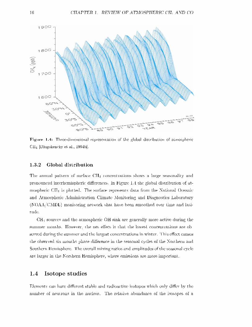
Figure 1.4: Three-dimensional representation of the global distribution of atmospheric
CH4 [Dlugokencky et al., 1994b].
1.3.2 Global distribution
The annual pattern of surface CH4 concentrations shows a large seasonality and
pronounced interhemispheric di�erences. In Figure 1.4 the global distribution of at-
mospheric CH4 is plotted. The surface represents data from the National Oceanic
and Atmospheric Administration Climate Monitoring and Diagnostics Laboratory
(NOAA/CMDL) monitoring network that have been smoothed over time and lati-
tude.
CH4 sources and the atmospheric OH sink are generally more active during the
summer months. However, the net e�ect is that the lowest concentrations are ob-
served during the summer and the largest concentrations in winter. This e�ect causes
the observed six months phase di�erence in the seasonal cycles of the Northern and
Southern Hemisphere. The overall mixing ratios and amplitudes of the seasonal cycle
are larger in the Northern Hemisphere, where emissions are more important.
1.4 Isotope studies
Elements can have di�erent stable and radioactive isotopes which only di�er by the
number of neutrons in the nucleus. The relative abundance of the isotopes of a

1.4. ISOTOPE STUDIES 17
Element Isotope rel. amount [% ] Standard Isotopic Material
Hydrogen H 99.985 V-SMOW
D 0.015
Carbon 12C 98.90 V-PDB13C 1.10
Oxygen 16O 99.762 V-SMOW
17O 0.038
18O 0.200
Table 1.3: Terrestrial abundance of Standard Isotopic Materials [Kaye, 1987].
trace gas can be measured with the help of mass spectometry and optical techniques
(sections 2.6 and 2.7). Isotopic substitution into a molecules leads to changes in the
reaction speed which a�ect both the atmospheric sink and the production pathways.
From observed variations in the isotope ratios of a trace gas information of the relative
strength of di�erent sources and sinks can be inferred, as well as transport processes
in�uencing its distribution [Kaye, 1987]. Trace gases emitted from a certain source
tend to carry a distinct isotopic composition that is representative for the source.
The isotopic composition of a source is often referred to as its isotopic �ngerprint.
1.4.1 Æ-notation
As isotopic variations are usually small, only relative deviations are measured and
reported in the Æ-notation. The Æ value is de�ned as the relative deviation of an
isotope ratio from an international standard ratio in 0=00,
Æ = [Rsample
Rstd� 1] � 1000 0=00 (1.3)
where Rsample and Rstd denote the isotope ratio of a sample and the correspond-
ing standard respectively [Coplen, 1994]. For example, for δ13C the R stands for
13C/12C. δ13C measurements are usually reported relative to the international stan-
dard V-PDB, which stands for 'Vienna Pee Dee Belemnite' [Craig, 1957], [Gon�-
antini, 1978]. Isotopic ratios of δ18O and δD are expressed relative to V-SMOW,
which stands for Vienna Standard Mean Ocean Water [Gon�antini, 1978]. In Table
1.4.1 the isotope ratios of these reference materials are listed.
1.4.2 Kinetic Isotope E�ect (KIE)
The �rst work on isotope fractionation processes was done by Bigeleisen et al. [1947],
Biegeleisen [1949] and Urey [1947]. During the formation and destruction of CH4 the

18 CHAPTER 1. REVIEW OF ATMOSPHERIC CH4 AND CO
original balance of its isotopes is disturbed by fractionation e�ects. These kinetic
isotope e�ects (KIE) arise because isotopes have di�erent energy levels (vibrational
and rotational) leading to di�erences in bond strength.
In the methane oxidation KIEs of both primary and secondary form occur. In
the primary isotope e�ect the deuterium atom is directly involved in the reaction
OH + CH4 ! H2O + CH3 (1.4)
OH + CH3D ! H2O + CH2D (1.5)
The fractionation of the sink process in equations 1.4 and 1.5 is given by the factor
� or KIE and is the ratio of the inverse lifetime k of the heavy isotopomer to that
of the light (rare) isotopomer:
�D = KIEDOH = kCH4=kCH3D (1.6)
The reaction of the deuterated form is about 30% slower than the normal form (due
to stronger, e.g. less reactive, C-D bonds compared to the C-H bonds). This results
in a KIEOH of 1.29 [Saueressig, 1999].
In the case of the secondary isotope e�ects, the isotopically labeled atoms are
remote from the reaction site and exert an e�ect only through the dependence of
the overall energy levels on mass. In this case, the isotopic e�ects are much smaller
(�0.5%).
OH +12 CH4 ! H2O +12 CH3 (1.7)
OH +13 CH4 ! H2O +13 CH4 (1.8)
The rate coe�cients of the wide range of observed isotope e�ects can be calculated
[Bigeleisen & Mayer, 1947]. However, this is di�cult, even at a 10% level, due to
di�culties in de�ning the exact energies of the transition state and e�ects of quantum
mechanical tunneling [Gellene, 1993].
1.5 Isotope variations in CH4
The isotopic composition of atmospheric methane can be used to better constrain the
large uncertainties in present CH4 budget estimations. Individual source types have
typical δ13C and δD isotopic signatures as illustrated in Figure 1.5, that re�ect di�er-
ent methane production processes. CH4 from biogenic (bacterial) methane formation
is highly depleted in δ13C . For CH4 from thermogenic formation fractionation pro-
cesses are important, whilst they are less important during incomplete combustion

1.5. ISOTOPE VARIATIONS IN CH4 19
of biomass or fossil fuels. The methane sinks also a�ect the isotopic composition
by inducing signi�cant changes via isotopic fractionation in the reaction with OH,
with O1D and Cl in the stratosphere [Saueressig, 1999] and the oxidation in soil.
As a result δ13C and δD re�ect changing source and sink contributions to the CH4
budget.
The fractionation of the sinks and the δ13C and δD measurements on atmospheric
methane can be used to determine the isotopic composition of the mean source
[Cantrell et al., 1990]:
Æsource =nXi=1
Qi
QÆi (bottom-up calculation) (1.9)
= Æatm + [fOH(1
KIEOH� 1) + fsoil(
1
KIEsoil� 1) + fstra(
1
KIE�
stra
� 1)]
�(1 +Æatmos
1000)� 1000 (top-down calculation) (1.10)
Æsource: Æ13C or ÆD of the mean source
Æi: Æ13C or ÆD of the source i
Æatm: Æ13C or ÆD value of the mean atmosphere
Qi: global source strength of source i
Q: global source strength of all methane sources
f : fraction of the global sink (of the sink OH, soil oxidation or net transport into
the stratosphere)
Table 1.2 lists the mean δ13C and δD sources which have been derived with equation
1.9 (bottom-up calculation) from the corresponding source strengths and source sig-
natures of the individual sources. Equation 1.10 (top-down calculation) is only valid
for an atmosphere at equilibrium. In Table 1.2 the mean sources from the top-down
calculations are given.
The 13C/12C content of atmospheric CH4 has been used to examine the bud-
get of atmospheric CH4 on both regional [Thom et al., 1993], [Lassey et al., 1993],
[Bergamaschi et al., 1998a] and global scales [Stevens & Engelkemeir, 1988], [Quay
et al., 1999], [Fung et al., 1991],[Hein et al., 1997]. The D/H content of CH4 is a po-
tential useful tracer for the atmospheric CH4 budget but is less well developed than
13C/12C [Bergamaschi et al., 1998a], [Quay et al., 1999], [Marik, 1998]. There are
fewer determinations of the δD composition of CH4, the hydrogen KIEs associated
with the CH4 sinks and the δD composition of the CH4 sources.
With equation 1.6 the expected average isotope fractionation in the troposphere
KIEavg can be calculated:
KIEavg = fOHKIEOH + fsoilKIEsoil (1.11)

20 CHAPTER 1. REVIEW OF ATMOSPHERIC CH4 AND CO
-100 -80 -60 -40 -20 0-400
-300
-200
-100
0
average source
wetlands
natural gas
ruminants
rice
biomassburning
present atmosphere
KIE
δδ δδD[‰
V-S
MO
W]
δδδδ13C [‰ V-PDB]
Figure 1.5: δD versus δ13C is plotted for di�erent methane source signatures (see Table
1.2) and the mean atmospheric methane values are shown together with the mean source.
The sink fractionation is indicated by the solid line.
with fOH and fsoil representing the fractional contribution of the OH sink and soil
sink respectively (fOH+fsoil = 1).
1.5.1 Atmospheric CH4 isotope data
Additional constraint on the global CH4 cycle have been obtained by isotope measure-
ments (14C, 13C, D), utilizing the fact that the individual sources bear typical isotopic
signatures (Figure 1.5). 14C measurements were mainly used to estimate the fraction
of fossil CH4 sources, such as losses during exploration and distribution of natural
gas or from coal mining [Lowe et al., 1988], [Quay et al., 1991], [Wahlen et al., 1989],
while δ13C measurements have been reported for a small number of global observa-
tional sites [Lowe et al., 1997], [Marik, 1998], [Quay et al., 1999]. Precise δD mea-
surements have so far been hampered by di�culties in sample preparation required
prior to isotope ratio mass spectrometry (IRMS) analysis [Marik, 1998]. As a princi-
1.6. THE GLOBAL CO BUDGET 21
pal alternative to IRMS, an optical technique has been developed by Bergamaschi et
al. [1994], allowing direct measurements on CH4 without conversion into H2. This
technique, originally used for studies of CH4 sources and sinks, has been further re-
�ned and now allows the investigation of the small variations expected in atmospheric
background CH4 (see section 3.2).
1.6 The global CO budget
CO is released at the surface by incomplete combustion associated with fossil fuels
and biomass burning. CO is also produced by the oxidation of CH4 and other hydro-
carbons such as isoprene. Sources of less importance include emission by vegetation
and microorganisms on the continents and by photochemical oxidation of dissolved
organic matter in the oceans. In Table 1.4 the global CO budget is given. The aver-
age atmospheric residence time of about 2 months, combined with an concentration
of the order of 100 nmol/mol, correspond to an annual global turnover of approxi-
matively 3000 Tg. However, the global budget of CO is not well de�ned, mainly due
to the wide variety of natural and anthropogenic sources. About 50% to 60% of the
CO emissions result from human activities, part of which is biomass burning, that
comprises perhaps a third of total sources. The amount of CO from non-methane
hydrocarbons is nearly as important as from CH4 oxidation and a major part of both
is also indirectly attributed to the anthropogenic source. The dominant sink for at-
mospheric CO is the oxidation by OH (90%), while the uptake by soils accounts for
the remaining 10%. The problem of constructing a reliable budget is further aggra-
vated by the relatively short atmospheric lifetime of CO of about 2 months, which
results in large concentration gradients and variations.
1.7 CO measurements
The �rst atmospheric CO measurements were made by Mignotte in 1949 in the
Swiss Alps. He assigned absorption lines in the 4.7 �m region of the solar spectrum
to atmospheric CO. In the 1960s gas chromatographic methods allowed to study
the �rst global distribution of CO [Robinson & Robins, 1970]. Since, measurements
of CO in the troposphere have been made at various locations around the world
[Seiler, 1974], [Seiler et al., 1984], [Brunke et al., 1990], [Khalil & Rasmussen, 1988]
and monitoring networks have been developed, the most extensive one being managed
since 1988 by NOAA/CMDL [Novelli et al., 1998a]. The �rst CO measurements from
space were done in 1981 aboard the spaces shuttle [Reichle et al., 1986]. Satellite

22 CHAPTER 1. REVIEW OF ATMOSPHERIC CH4 AND CO
Sources Tg yr�1 δ13C [ 0=00 ] δ18O [ 0=00 ] 14CO �17O[ 0=00 ]
V-PDB V-SMOW [pmC]
Fossil fuel combustion 300-550 �27:5a 23.5a;b;m 0.0 0.0l
Biomass burning 300-700 �21:3c � 16:3b;n � 115 0.0l
�24:5d � 18e
CH4 oxidation 400-1000 �52:6f � 0b;g � 125 0?
� 15e
NMHC oxidation 200-600 �32:2e � 0b;g � 110 0.0?
14.9e
Ozonolysis 80-100h 25-40l
Biogenic 60-160 � 110 0.0
Oceans 20-200 �13:5i � 110
Total sources 1800-2700
Sinks Tg yr�1 KIE(δ13C ) KIE(δ18O ) KIE(14CO) KIE(�17O)
CO + OH 1400-2600 1.006j;o 0:990j;o 1.010k 1.004o
Soil uptake 250-640
Loss to stratosphere � 100
Total sinks 2100-3000
a[Stevens & Krout, 1972]b[Brenninkmeijer, 1993]c[Conny et al., 1997]d[Conny, 1998]e[Stevens & Wagner, 1989]f [Quay et al., 1991]
Value based on CH4 δ13C of �47:2 0=00
and the fractionation in CH4 + OH of 5.4 0=00g[Brenninkmeijer & Röckmann, 1997]
h[Röckmann et al., 1998]i[Manning et al., 1997]jAt atmospheric pressurekInferred from the value for δ13C , assuming
mass dependent behavior.l[Röckmann & Brenninkmeijer, 1998b]m[Kato et al., 1999a]n[Kato et al., 1999b]o[Röckmann et al., 1998c]
Table 1.4: The tropospheric budget of CO, with source strengths and respective isotopic
composition and with the sink fractionation constants.

1.8. ISOTOPE VARIATIONS IN CO 23
measurements of CO promise true global scale coverage of its distribution.
1.7.1 Global distribution
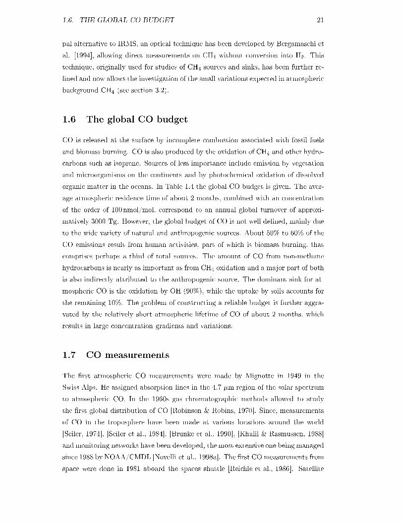
Figure 1.6 shows the large seasonality and pronounced interhemispheric di�erences
of CO mixing ratios which have been derived from the NOAA/CMDL data. As for
CH4 mixing ratios a phase shift of 6 months is observed for the seasonal cycles of
the Northern and Southern Hemisphere. The highest mixing ratios are observed in
the northern winter (� 210nmol/mol) and the lowest ones in the southern sum-
mer (� 40 nmol/mol). The interhemispheric gradient exhibits a strong seasonality
with maximum di�erences between the high latitudes of the northern and southern
hemispheres in February and March (� 170nmol/mol) and a minimum in July and
August (10 to 20 nmol/mol).
In areas of regional scale pollution, mixing ratios range from near background
levels to more than 500 nmol/mol. In urban environments or areas of biomass burning
CO levels may reach several µmol/mol.
1.7.2 Atmospheric trends
Ice core measurements from Greenland [Haan et al., 1996] indicate a signi�cant in-
crease of CO mixing ratios in the Northern Hemisphere during the last 200 years.
The observed increase is attributed to anthropogenic activities, mainly combustion
of fossil fuel. In contrast, CO mixing ratio derived from an Antarctic ice core for the
high Southern Hemisphere, revealed only small variations during the last 2000 years
[Haan & Raynaud, 1998].
For central Europe comparison of spectroscopic measurements of CO between the
early 1950s to mid-1980s suggest an average increase of �1 nmol/mol yr�1. After
the eruption of Mount Pinatubo in June 1991 a signi�cant anomaly was observed for
CO mixing ratios [Khalil & Rasmussen, 1994], [Novelli et al., 1994]. For the period
from 1990 through 1995 a decrease of CO mixing ratios of approximately 2 nmol/mol
yr�1 is reported by Novelli et al. [1998a].
1.8 Isotope variations in CO
For the isotopical analysis of CO four rare isotopes are available, 13C, 14C, 17O and18O. The major atmospheric sources exhibit clearly di�erent 13C/12C and 18O/16O
isotope ratios [Stevens & Krout, 1972], [Stevens & Wagner, 1989], [Brenninkmeijer,
1993]. In Figure 1.7 the δ13C and δ18O signatures of CO sources are plotted.

24 CHAPTER 1. REVIEW OF ATMOSPHERIC CH4 AND CO
Figure 1.6: Three-dimensional representation of the global distribution of atmospheric CO
[Novelli et al., 1998a].
The δ13C balance in atmospheric CO is largely in�uenced by CO from CH4
oxidation, which represents by far the most depleted source. Atmospheric CH4 is
already quite depleted, with an average δ13C of around �47 0=00 and the kinetic iso-
tope e�ect in the reaction of CH4 with OH of 3.9� 0.4 0=00 [Saueressig, 1999] further
reduces the δ13C of the resulting CO to values below �50 0=00. In contrast, all the
remaining major sources are in the δ13C range between �32 and �12 0=00 (see Table
1.4 for references). Technological sources have typical δ13C values around �27:5 0=00,
re�ecting the δ13C of combusted fuel, as usually no signi�cant isotope fractionation
occurs in high-temperature combustion processes. Similarly, CO from biomass burn-
ing is thought to have δ13C values close to the δ13C of burnt plant matter. Slightly
depleted compared to these sources is CO originating from the oxidation of natural
non-methane hydrocarbons.
The δ18O signatures are clearly not correlated with δ13C , thus providing a fur-
ther independent tracer. CO from technological sources has the most enriched δ18O ,
close to δ18O of atmospheric oxygen of 23.5 0=00. Measurements in plumes from large
cities showed a remarkably low δ18O variability [Brenninkmeijer & Röckmann, 1997],
[Stevens & Wagner, 1989], while δ18O values from individual automobiles show a
much wider spread (11 to 29 0=00) [Hu� & Thiemens, 1998], [Kato et al., 1999a], the

1.8. ISOTOPE VARIATIONS IN CO 25
-60 -50 -40 -30 -20 -10-10
-5
0
5
10
15
20
25
30
NMHC oxidation
fossil fuelcombustion
CH4 oxidation
biomassburning
atmosphere
KIE
(CO
+OH
)
δδ δδ18O
[‰V
-SM
OW
]
δδδδ13C [‰ V-PDB]
Figure 1.7: δ18O versus δ13C is plotted for di�erent CO source signatures (see Table 1.4
for error bars) together with the range of atmospheric CO data. The kinetic isotope e�ect
of the sink process is also indicated.
most common being again 23.5 0=00. For biomass burning, δ18O values of 18�1 0=00 are
reported by [Stevens & Wagner, 1989], while δ18O values varied from 10 to 26 0=00
during �aming and smoldering of plants [Kato et al., 1999b]. No direct measure-
ments are available for δ18O from the oxidation of NMHCs and CH4. Stevens and
Wagner [1989] inferred a value of 14.9 0=00 for oxidation of natural NMHCs, based
on observed CO - δ18O correlations at a rural site in Illinois. On the basis of at-
mospheric observations and simple budget considerations for CO and δ18O in the
Southern Hemisphere, Brenninkmeijer and Röckmann [1997] estimated the δ18O of
both CH4 and NMHC oxidation to be near 0 0=00.
Over the last years atmospheric observations of CO isotopes from several sta-
tions have been reported, e.g. from Scott Base (Antarctica) and Bearing Head (New
Zealand) [Brenninkmeijer, 1993], from Montauk Point (Long Island) [Mak & Kra,
1999], Alert and Spitsbergen [Röckmann, 1998a], Happo (Japan) [Kato et al., 2000]

26 CHAPTER 1. REVIEW OF ATMOSPHERIC CH4 AND CO
and Sonnblick (Austrian Alps) [Gros et al., 2000]. These measurements reveal pro-
nounced seasonal cycles both in δ13C and δ18O at all stations and a large, seasonally
varying, latitudinal gradient.
1.8.1 Kinetic Isotope E�ect
In order to relate atmospheric observations to the isotopic signatures of the indi-
vidual sources, the kinetic isotope e�ect (KIE) of the sinks has to be taken into
account. The KIE is de�ned as the ratio of reaction rate constants i.e., KIE(δ13C )
= k(12CO)/k(13CO), and KIE(δ18O )=k(C16O)/k(C18O), respectively (see also sec-
tion 1.4.2).
Measurements of the fractionation factor KIE for δ13C have been made by
Stevens et al. [1980], Smit et al. [1982] and Röckmann et al. [1998]. A modest frac-
tionation exists which declines with decreasing temperature. Already below 400 hPa
the isotopic e�ect reverses into an inverse e�ect, where 13CO reacts faster with OH
than 12CO. The overall fractionation in the troposphere is � 3 0=00. Measurements for
δ18O have also been made by Stevens et al. [1980] and Röckmann et al. [1998] and
Fig. 1
-60
-40
-20
0
20
40
60
80
100
120
-60 -40 -20 0 20 40 60 80 100 120
δδδδ18O (‰)
δδ δδ17O
(‰)
air- O2
mass dependentfractionation line(slope 0.52)meteoric wateroxygen in rock samples
air-CO2
V-SMOW
tropospheric O3
stratospheric O3
Oxygen fromAllende meteorite(slope 1)
slope 1stratospheric CO2 ∆∆∆∆17O
tropospheric CO
Figure 1.8: A three isotope diagram illustrating the concept of mass independent fractiona-
tion and the distribution of the oxygen isotopes in di�erent oxygen bearing compounds. Most
compounds on earth de�ne the terrestrial mass dependent fractionation line with slope �
0:52. A MIF process causes a deviation from this line [Röckmann & Brenninkmeijer, 1998b]
.

1.8. ISOTOPE VARIATIONS IN CO 27
show an inverse slight pressure dependent e�ect. A KIE value of �0.990 is represen-
tative for most of the troposphere. For the soil sink, KIE(δ13C )=1.0060�0.0009 and
KIE(δ18O )=1.014�0.002 have been determined [Bergamaschi et al., 2000c] (personal
communication C. Stevens therein).
Most fractionation processes depend on mass and therefore scale with the relative
mass di�erences of the di�erent isotopes (see section 1.4.2). In the case of oxygen
this leads to 17O/16O variations matching approximately half of the accompanying18O/16O variations, i.e.
Æ17O = 0:52 � Æ18O (1.12)
Almost all oxygen bearing substances (e.g. minerals, water, atmospheric oxygen
and tropospheric CO2) show Æ17O and Æ18O variations that de�ne a line with slope
�0.52 (see Figure 1.8). Any deviation from this mass dependent fractionation line is
a clear indicator for mass-independent isotope fractionation (MIF). Signi�cant MIF
had �rst been detected for meteoritic material. In the atmosphere MIF has been
found for O3 [Mauersberger, 1987], stratospheric CO2 [Thiemens et al., 1995], and
N2O [Cli� & Thiemens, 1997]. Æ17O(CO) measurements also established a mass-
independent isotope fractionation in atmospheric CO [Hodder et al., 1994]. For tro-
pospheric CO, two di�erent mechanism cause MIF. The reaction of O3 with un-
saturated hydrocarbons produces CO that inherits the relative strong MIF in O3
[Röckmann et al., 1998]. But the major source of MIF in atmospheric CO is the frac-
tionation in the removal reaction CO + OH = CO2 + H [Röckmann et al., 1998c].
At high northern latitudes an 17O excess of up to 7.5 0=00 was observed during summer.
In Figure 1.9 we have used a simple 1-box model to simulate the isotopic changes
of atmospheric CO during the CO + OH sink reaction. Air representative of the mid
latitude Northern hemisphere at 150 nmol/mol (δ13C =�27 0=00, δ18O =10 0=00) has
been used in these examples. The changes with and without the CH4 oxidation source
and an added fossil source are shown. CO mixing ratios take several months before
they approach the equilibrium (average OH levels of 106molec./cm3). This illustrates
the di�culty of interpreting isotope data without modeling. The typical meridional
transport times in the troposphere and seasonal changes in OH are comparable to
its chemical lifetime and the time of isotopic change.
1.8.2 Atmospheric 14CO
14CO is a natural atmospheric tracer occurring at concentration levels of 5 to 30
molec./cm3. The main source 1of atmospheric 14CO is the nuclear reaction [Libby,

28 CHAPTER 1. REVIEW OF ATMOSPHERIC CH4 AND CO
0 30 60 90 120 150 1800
50
100
150
CO+OH sinkCH4 source addedCH4 and fossil source added
CO
[ppb
]
days
0 30 60 90 120 150 180-50
-40
-30
-20
-10
days
δδ δδ13C
[‰V
-PD
B]
0 30 60 90 120 150 180
-20
-10
0
10
days
δδ δδ18O
[‰V
-SM
OW
]
0 30 60 90 120 150 1800
2
4
6
8
10
days
∆∆ ∆∆17O
0 30 60 90 120 150 1800
5
10
15
14C
O[m
olec
ules
cm-3
s-1]
OH sink only
with production
days
Figure 1.9: The changes in concentration and isotopic composition for CO in a given air
mass due to the e�ect of OH. Scenarios are shown without sources, including the meth-
ane oxidation source (assuming 106 OH cm�3 and 1780 nmol/mol CH4) and an additional
constant fossil source (of 1.2 nmol/mol per day, δ13C =�27 0=00, δ18O =15 0=00) respectively.
For 14CO scenario two scenarios are shown (OH sink only, additional constant source of
3�10�6 molecules s�1 cm�3).

1.8. ISOTOPE VARIATIONS IN CO 29
1946]:
14N + n!14 C + p (1.13)
14C +O2 !14 CO +O (1.14)
followed by the subsequent oxidation of the exited radiocarbon atom to 14CO (yield
about 95%) [McKay et al., 1963], [Pandow et al., 1960].
More than 75% of atmospheric 14CO is from the cosmogenic source. The cosmo-
genic production rate increases with increasing altitude up to about 16 km and then
decreases. The cosmogenic source is modulated by the solar wind plasma with a cycle
time of 11 years, while the Earth magnetic �eld provides a shielding and focusing to
the magnetic poles. These e�ects lead to an atmospheric source distribution with a
maximum production rate in the lowermost stratosphere and a varying total source
strength of �25% within 11 years [Lingenfelter & Flamm, 1963].
The smaller biogenic fraction of � 25% is recycled 14CO from biomass, released
into the atmosphere by CH4 oxidation, NMHC oxidation and biomass burning. The
relative contribution from these sources containing recycled 14CO can be estimated,
because they all have similar 14C/12C ratios of about 1.4�10�12, or 120% modern
carbon (pmC). Uncertainties in the magnitude of these sources are mitigated since
the 14C/12C ratio in atmospheric CO is generally between 400 and 900 pmC.
Apart from a small soil sink (about 10%), 14CO is removed from the atmosphere
via oxidation by OH. Thus atmospheric 14CO and CO share the same sinks, but have
very di�erent sources. The abundance of OH is highest in the tropics year-round and
shows a strong seasonal cycle in the middle and high latitudes. Given the distinct
source and sink distribution and the relatively fast rate constant for the CO+OH
reaction, 14CO measurements provide a unique tracer of OH abundance.
Weinstock et al. [1969] used the 14C data from McKay et al. [1963] to esti-
mate the atmospheric lifetime of CO. Volz et al. [1981] measured the �rst annual
14CO cycle for the mid northern latitudes and showed that it agreed with the ex-
isting OH distribution and seasonality. For this purpose they processed samples of
20.000 l to extract enough 14CO as 14CO2 for applying proportional beta counting.
The development of accelerator mass spectrometry for 14C (see section 2.8) enabled
Brenninkmeijer et al. [1992] to make routine 14C measurements in the southern
hemisphere, using 1 m3 air samples. They published 14CO measurements from New
Zealand and Germany exposing a large 14CO abundance di�erence, while also infer-
ring a rather small southern hemispheric latitudinal gradient. Various mechanisms,
like di�erences in production due to changes in solar activity, latitudinal gradients,
troposphere stratosphere exchange, and biogenic 14CO were not considered adequate

30 CHAPTER 1. REVIEW OF ATMOSPHERIC CH4 AND CO
to explain the large di�erence. They suggested higher southern hemisphere OH levels
as a possible explanation.
1.9 Scope of this thesis
In this study the stable isotope ratios 13C/12C and D/H of atmospheric CH4 were
measured as well as the 13C/12C, 18O/16O ratios and 14CO concentrations of at-
mospheric CO. In chapter 2 the further improvements of these measurements are
documented. This mainly involved changes of the CH4 extraction procedure, neces-
sary for the subsequent analysis of δ13C by mass spectrometry and δD by tunable
diode laser.
A major part of this thesis was the measurement of a three year record of the
isotopic composition of atmospheric CH4 (chapter 3) and CO (chapter 4) at the
background station Izaña, Tenerife. The large seasonal cycles in mixing and isotopic
ratios of CH4 and CO allowed to infer the impact of source and sink processes
on these trace gases. Thus the average kinetic isotope e�ect in the sink processes
of atmospheric methane could be deduced from the δ13C and δD records. The
measured δD seasonality is the �rst ever reported for atmospheric background CH4.
The comparison of the δ13C and δD records with results from an inverse CH4 model
study in which the isotope records of Izaña were included, allowed the quanti�cation
of the di�erent source contributions. Similarly the Izaña records for δ13C and δ18Oof CO were compared to an inverse CO model study from which the seasonal pattern
of the source and sink processes could be quanti�ed for Izaña. Finally, the large
synoptic scale variations occurring at Izaña made it possible to study source regions
such as North America, Europe and partly Africa, as well as maritime background
conditions of the North Atlantic.
Finally we compare the Izaña records to CO isotope measurements done at a
number of other stations, i.e Spitsbergen, a remote station at high northern latitude,
Schauinsland (Germany) and Sonnblick (Austria), which are representative for con-
tinental stations at mid latitudes. In contrast more polluted air masses have been
encountered at Kollumerwaard, The Netherlands, and during the BERLIOZ cam-
paign in summer 1998, for which CO, δ13C , δ18O and 14CO have been investigated.
In chapter 5 we present the measurement and interpretation of two Antarctic
�rn air records, which have been analyzed for methane and its stable isotopes. With
the help of a �rn air di�usion model the atmospheric trends of δ13C and δD of
atmospheric CH4 since the mid-20th century were reconstructed. In step with in-
creasing CH4 mixing ratios a positive δ13C trend was inferred re�ecting a shift in

1.9. SCOPE OF THIS THESIS 31
atmospheric source strength towards the heavier anthropogenic sources. For δD a
period of decline was observed previous to 1975, followed by a gradual increase also
towards the heavier anthropogenic sources. This is the �rst time the non-equilibrium
state between CH4 and its sources and sinks has not only been observed for δ13Cbut also for δD.

32 CHAPTER 1. REVIEW OF ATMOSPHERIC CH4 AND CO

Chapter 2
Sampling and Measurement
The sampling, extraction and subsequent analysis of CO and CH4 and their isotopic
composition require a high degree of accuracy in order to establish seasonal variations
and long-term trends. To measure the isotopic composition of atmospheric CO and
CH4 those gases have to be extracted from atmospheric air samples prior to their
analysis by mass spectrometry or by tunable diode laser spectroscopy. As this is a
very time consuming task it can only be done for selected samples. The ongoing
progress with continuous �ow GC-MS measurements will change this for selected
stable isotopes in the future, but cannot at present compete with our precision in
δD for example. Neither can GC-MS be used for 14CO measurements.
In this chapter we describe how ambient air samples are collected in high pres-
sure cylinders with a high purity compressor (see section 2.1.1 and 2.1.2) at various
stations for long-term observation and during short-term �eld campaigns (section 4.7
and 5). At the MPI a complete analysis of the air samples consists in a �rst step of
the measurement of CH4, CO2, N2O and SF6 mixing ratios by gas chromatography
(GC) (section 2.2). Subsequently the isotopic composition of CO2, CO and CH4 are
determined by mass spectrometry (section 2.3 and 2.6). Only δD of CH4 is measured
by tunable diode laser spectroscopy (section 2.7). For the analysis of 14CO we send
the samples to accelerator mass spectrometry facilities (section 2.8).
The process used for the measurement of CO mixing ratios and isotopic compo-
sitions has been previously documented in [Brenninkmeijer, 1993] and [Röckmann,
1998]. The measurement procedure for CH4 and its isotopes, δ13C and δD, includingimprovements that have been made during this thesis, are described here for the �rst
time.
33

34 CHAPTER 2. SAMPLING AND MEASUREMENT
2.1 Air sampling
Air samples of 500 to 1100 L (STP) are taken on a regular basis at several world-wide
stations (see Table 3.1) and the air samples are sent to the MPI for analysis. There air
samples are stored and shipped in high pressure cylinders. While atmospheric CH4
can be sampled and stored in appropriate cylinders without signi�cant contamination
[Marik, 1998] this is more di�cult for CO. Cylinders and compressors are known to
easily produce CO which contaminates the air samples. To ensure high quality air
sampling we use a modi�ed compressor system and high pressure aluminum cylinders
which will be described in the next subsections.
2.1.1 The compressor system
The compressor used is an oil-free three-stage-compressor (Rix Industries, Oakland,
CA, USA) which has been modi�ed according to Mak and Brenninkmeijer [1994].
The aim of these modi�cations is to suppress possible sources of CO contamination,
either due to leakage or the formation of CO during operation. Further modi�cations
consisted of the introduction of a drying unit (Drierite, anhydrous CaSO4, Hammond,
Ohio) to trap H2O both at the inlet and on the high pressure side of the compressor
system. Separate tests have shown that the drying agent neither a�ects CO and CH4
mixing ratios nor their isotopic composition.
Before sampling the compressor is �ushed by opening an additional vent valve
mounted on the high pressure side. Thereafter, the high pressure sample cylinder
is �lled twice to �5 bar and drained again. Thus contamination from remaining air
of previous air samples is reduced to less than 0.1%. Finally, cylinders are �lled to
120 bar at typical �ow rates of 15 lmin�1.
The modi�ed RIX compressors have been shown to produce less than 1 nmol=mol
CO in the sampled air [Mak & Brenninkmeijer, 1994a]. They are used at the di�erent
sampling stations and need little maintenance apart from regular exchange of the
Drierite. Nevertheless, after several years of regular air sampling some problems
may occur. Corrosion processes can be signi�cant at sampling stations with high
humidity and this can a�ect the valves. Also the sealing of the pistons gets less
e�ective due to wear and air on the high pressure side is lost. This results in longer
�lling times and may also lead to leakage into the �rst stage piston. To prevent these
problems, compressors are send to Mainz every 1 to 2 years for maintenance.
Another problem has been the air sampling at low temperatures. These prob-
lems were encountered during winter at the stations Mount Sonnblick, Austria, and
Happo, Japan. The compressors failed to start unless they were warmed before

2.1. AIR SAMPLING 35
CT CT CT
DT
1/2"
DTHPRBPR
C
V
1st STAGE
CP
P1
P3
P2
2nd STAGE 3rd STAGE MSMS
F
RVRVRV
Figure 2.1: The modi�ed three-stage RIX compressor. 1/2 inch: te�on inlet; BPR: Back
pressure regulator; C: Sample cylinder; CP: Cooling plates; CT: Cooling tubings; DT: Drying
trap; F: Glass �bre �lter; HPR: High pressure �lter; MS: Moisture separator; P1�3: Pressure
gauges (�uid dampened); RV: Pressure relief valve; V: Vent valve. [Röckmann, 1998a]
use. The compressor system used for the �rn air sampling in Antarctica was further
modi�ed (see Figure 5.2 in section 5.1).
2.1.2 High pressure sample cylinders
We use high pressure aluminum cylinders (4.7 liter: BOC Gases, UK; 5 and 10 liter:
Scott Marrin Inc., Riverside, CA, USA). Tests have shown that the cylinders only
insigni�cantly increase the CO mixing ratios of air samples (below 2ppb in two
months [Mak & Brenninkmeijer, 1994a]). Nevertheless single cylinders may still ex-
hibit a strong CO increase in mixing ratios accompanied with signi�cant changes in
the isotopic CO signal. This happened with one of the BOC cylinders �lled twice
in Izaña in 1996, which has not been used afterwards. In this case CO mixing ra-
tios increased by �20 nmol/mol and δ18O and δ13C values of CO were enhanced
by �5 0=00 and 1 0=00 to 2 0=00 respectively. The more than 80 remaining cylinders have
not exhibited such problems. Measurements of a large number (>60) of duplicate
samples have never shown signi�cant di�erences in the CO mixing ratios and isotopic
composition (see section 4.1). CH4 is much less sensitive to storage in cylinders and
air samples can be stored over several years without changes in the mixing ratio and
isotopic signal [Francey et al., 1999].

36 CHAPTER 2. SAMPLING AND MEASUREMENT
2.1.3 Spot air sampling
The compressor is usually kept in a laboratory or storage room at the sampling
stations. The air is pumped through a 1/2 inch PFA tube with the inlet mounted
on a sampling tower. To collect spot samples we pump air through the air inlet line
directly into high pressure cylinders. These air samples are representative for air
masses encountered during the 0.5 to 1 hour �lling time. In general spot samples are
taken biweekly at the stations listed in Table 3.1.
2.1.4 Continuous air sampling
Due to important synoptic scale variations occuring at Izaña, we decided to col-
lect 2-week time-integrated samples in addition to the biweekly spot samples. This
continuous sampling makes it possible to de�ne seasonal background signals repre-
sentative for the sampling station. The system for the continuous sampling at Izaña
has been set up by T. Röckmann and P. Bergamaschi in 1996 [Röckmann, 1998a].
The continuous sampling proceeds as follows. A diaphragm compressor (KNF
Neuberger, Freiburg, Germany) is used to continuously pump air at a �ow rate of
� 3 l min�1 and a pressure of � 3 bar through a drier (Perma Pure Inc, Toms River,
NJ, USA). The �rst part of the Perma Pure drier is heated to about 40 ÆC to prevent
condensation and to improve the drying e�ciency (achieved dew point: < -20 ÆC).
Only a small fraction of the air coming out of the drier is used for the samples while
the rest is redirected into the drier as counter-current purge gas (after expansion to
ambient pressure).
To monitor the quality of the sample storage process a sample fraction of 2x100
cm3min�1 were directed via two mass �ow controllers into two separate � 500 L
polyethylene coated aluminium bags. These sampling bags are suited for storage
of air and did not exhibit any signi�cant CO increase during tests. Nevertheless,
CO mixing ratios from continuous samples during summer 1998 were signi�cantly
higher than those from spot samples over the same period, suggesting contamination
problems. This will be further discussed in section 4 together with the data. Both
sampling bags are continuously �lled for one week and then replaced with two new
bags. Finally the air from two consecutive weeks is transferred via the compressor
into a high pressure cylinder (�nal �lling pressure is usually about 120 bar). This is
done for the two separate sets of sampling bags. We therefore end up with duplicate
air samples for every two week period.

2.2. GC MEASUREMENTS 37
2.2 GC measurements
Measurements of mixing ratios of di�erent gases were made using a HP 6890 GC
equipped with a �ame ionization detector (FID) and an electron capture detector
(ECD). The FID channel allows the measurement of CH4 and also CO2 after meth-
anization. The ECD channel is used for measurements of N2O and SF6. The sample
inlet is through an 8-port valve, allowing the fully automated measurement of up to
8 cylinders, controlled via HP Chemstation software.
Working reference gases are calibrated for CH4 (as well as for CO2 and N2O)
versus two calibration gases (NOAA-1 and NOAA-2) from the National Oceanic
and Atmospheric Administration Climate Monitoring and Diagnostics Laboratory
(NOAA/CMDL). In Table 2.1 their reported mixing ratios are given together with
their con�dence intervals. The results of the regular intercalibration between our
working reference gases MPI-1 to MPI-4 and these two calibration gases since De-
cember 1996 are also listed in Table 2.1 and are shown in more detail in Figures 2.2
and 2.3 for CH4 and CO2 respectively.
With measurements of mixing ratios extending over several years at our sampling
stations (see section 3 to 5), the long time stability of our GC reference gases is of
high importance. Without this long term trends in the atmospheric mixing ratios
CH4 CO2 N2O SF6 n
[nmol/mol] [mmol/mol] [nmol/mol] [pmol/mol]
NOAA-1 1781 � 18 365:50 � 0:4 312:4 � 3 3:595 � 0:02
NOAA-2 1815 � 3 362:95 � 0:06 312:6 � 3:1 4:042 � 0:02
MPI-1 1961:1 � 2:5 382:85 � 0:52 315:19 � 0:32 4:817 � 0:001 13
(Feb 97-Jul 98)
MPI-2 1974:6 � 1:1 376:02 � 0:29 310:32 � 0:29 5:968 � 0:132 23
(Jul 98-Mar 00)
MPI-3 1776:5 � 0:5 347:77 � 0:10 305:53 � 0:39 4:363 � 0:024 21
MPI-4 1846:0 � 0:5 373:29 � 0:08 320:25 � 0:38 4:203 � 0:000 19
(since Apr 98)
duplicates �0:78 �0:50 �0:26 �0:009 55
Table 2.1: NOAA/CMDL calibration standards, GC working reference gases and mean
deviation of duplicate continuous samples. The time periods during which the MPI standards
were used as working reference gases are given and n is the number of calibrations performed
against NOAA-2.

38 CHAPTER 2. SAMPLING AND MEASUREMENT
01.12.96 01.06.97 01.12.97 01.06.98 01.12.98 01.06.99 01.12.991962
1964
1966
1968
1970
1972
1974
1976
1978
1980
1982
MPI-2
CH
4[p
pb]
date
01.12.96 01.06.97 01.12.97 01.06.98 01.12.98 01.06.99 01.12.991946
1948
1950
1952
1954
1956
1958
1960
1962
1964
1966
MPI-1
01.12.96 01.06.97 01.12.97 01.06.98 01.12.98 01.06.99 01.12.991772
1774
1776
1778
1780
1782
1784
1786
1788
1790
1792
MPI-3
01.12.96 01.06.97 01.12.97 01.06.98 01.12.98 01.06.99 01.12.991838
1840
1842
1844
1846
1848
1850
1852
1854
1856
1858
MPI-4
Figure 2.2: CH4 working reference gas MPI-1 to MPI-4 versus NOAA-2.
cannot be established. Figures 2.2 and 2.3 show the CH4 and CO2 mixing ratios of
our working reference gases MPI-1 to 4 against the NOAA/CMDL standard NOAA-
2 over the last 4 years. An obvious, but weak temporal trend can be detected for
MPI-1 and 2 from Dec 96 to Dec 99 in CH4 mixing ratios of 8 and 4 nmol/mol
respectively. A strong decrease in CO2 for MPI-1 and MPI-2 of � 3µmol/mol wasobserved between Dec 96 and Jan 98.
The high precision of our SF6 GC-measurements of 0.01 pmol=mol is gained by
reprocessing the ECD chromatographs for selected samples. The calibration of our
SF6 measurements is made against a set of standards prepared at the University of
Heidelberg [Maiss et al., 1996]. In addition, most of the continuous samples were also
analyzed for SF6 at the Institut für Umweltphysik, Heidelberg, using a cryo-trapping
GC/ECD system [Maiss et al., 1996], with a precision of �0.02 pmol=mol.
The N2O GC-measurements su�er from the nonlinearity of the ECD detector
[Bräunlich, 1996]. Dilution tests starting from N2O mixing ratios close to atmo-

2.2. GC MEASUREMENTS 39
01.12.96 01.06.97 01.12.97 01.06.98 01.12.98 01.06.99 01.12.99
376
377
378
379
380
MPI-2
CO
2[p
pm]
date
01.12.96 01.06.97 01.12.97 01.06.98 01.12.98 01.06.99 01.12.99381
382
383
384
385
386
MPI-1
01.12.96 01.06.97 01.12.97 01.06.98 01.12.98 01.06.99 01.12.99345
346
347
348
349
350
MPI-3
01.12.96 01.06.97 01.12.97 01.06.98 01.12.98 01.06.99 01.12.99369
370
371
372
373
374
MPI-4
Figure 2.3: CO2 working reference gas MPI-1 to MPI-4 versus NOAA-2.
spheric values down to 10 nmol=mol established a correction factor for the GC in
Mainz of 20% of the di�erence between sample and standard. However, problems
with the ECD in 1998 make further correction of our N2O data necessary before
detailed studies of atmospheric trends can be done.
For the �nal reporting of the GC trace gas measurements we correct all mixing
ratios of air samples relative to the NOAA/CMDL calibration gas NOAA-2. Each
air samples is measured against our MPI working gas. We then use the mean of
working gas values measured against NOAA-2 previous and subsequent to the GC
analysis to calculate the �nal mixing ratio of the sample.
The precision of the GC system (for a single measurement series consisting of
about 10 injections) is approximately �1 nmol/mol for CH4, �0.2µmol/mol forCO2, �0.4 nmol/mol for N2O and �0.04 pmol/mol for SF6. The mean deviation
between the average values (usually from at least two di�erent measurement se-

40 CHAPTER 2. SAMPLING AND MEASUREMENT
ries on di�erent days) from 55 duplicate continuous samples was �0.8 nmol/mol for
CH4, �0.5µmol/mol for CO2, �0.3 nmol/mol for N2O and �0.009 pmol/mol for SF6.
These values re�ect the overall precision that is obtained during sampling, storing
and subsequent GC-analysis.
2.3 The extraction system
In 1996 a new sample preparation system was set up, which allows the successive
extraction of CO2, CO and CH4 for isotope analysis [Bergamaschi et al., 1998a].
During the research for this thesis, nearly 400 air samples have been processed on
this system. Improvements of the CH4 extraction and combustion system increased
the accuracy of stable isotope measurements of atmospheric CH4 (see section 2.3.3).
Figures 2.4 to 2.6 show the three parts of the extraction system, the CO and CO2
extraction section, the CH4 extraction section and the CH4 combustion section re-
spectively.
The CO section of the system is similar to that described in Brenninkmeijer [1993]
and Brenninkmeijer et al. [2000] and is based on the extraction technique developed
by Stevens and Krout [1972]. The main idea is to remove CO2 before oxidizing
CO to CO2 which is subsequently collected and analyzed by mass spectrometry.
The volumetric measurement of the collected CO2 also allows an absolute and very
precise measurement of the CO mixing ratio.
The CH4 extraction system has been designed to enable the pre-concentration
of the methane samples necessary for the direct δD analysis by tunable diode laser
spectroscopy [Bergamaschi et al., 1994](see section 2.7). In the CH4 combustion sys-
tem CH4 is combusted to CO2 with the help of a platinum catalyst. The derived
CO2 is then measured by mass spectrometry to infer the δ13C value of CH4.
2.3.1 The CO and CO2 extraction system
The air sample is introduced into the glass line at a �ow rate of 1.5 to 5 lmin�1
(STP) controlled by a thermal mass �ow controller (MFC, Hastings type HFC-202F).
A safety pressure relief valve designed by Brenninkmeijer and Bergamaschi [1998d] is
installed at the outlet of the MFC to protect the glass line from any unwanted build-
up of high pressure. Condensable compounds such as H2O, CO2, N2O and NMHCs
are removed from the air stream by cryogenic trapping. For this purpose two ultra-
e�cient metal Russian Doll traps (RDT) with a yield of more than 99.95% per RDT
for the removal of CO2 and N2O (overall yield >99.999) [Brenninkmeijer, 1991] are
connected in series with an U-tube between them. The RDT are stainless steel cylin-

2.3.THEEXTRACTIONSY
STEM
41
DP1VENT
SR
ZAG200°/850°
MFC
MFC
COT
DP
PIRPIR
PMST
PT
MANDF
BGMBV
HV RP1
CH4-line
CH4-line
SB1
RDT1
TPR
PT
H
CAG
SA
RDT2
Syn. air
A
HB
C
Figure2.4:TheCO
andCO2extra
ctionsystem
.A,BandCindica
tetheinlets
ofzero
-
air,
calibratio
ngas(CAG)andairsampleresp
ectively.
BGM:Bellow
gasmeter;
BV:Bu�er
volume;
COT:Collectio
ntra
p(glass
RDT);
DF:Drying�nger
containingP2 O
5 ;MAN:
Manometer;
DPandDP1:Diaphragmpump;HV:Highvacuumpump;MFC:Therm
alsen
-
sormass�ow
contro
llerwith
integ
rator;PIR:Pira
nivacuumgauge;PMST:Purgemolecu
lar
sievetra
p;PT:piezo
resistiveabsolute
pressu
retra
nsducer;
RDT:Cryogenicmeta
lRussia
n
Dolltra
pwith
therm
ocouplebased
heater
elements(H
);RP1:Rotary
pump;SA:Airsample
cylinder
with
pressu
rereg
ulator(PR);SB1:Samplebottle;
SR:Schütze
reacto
r;T:U-tu
be;
ZAG:Genera
torofzero
air(Ptcatalystheated
to200ÆC
(850ÆC
)forCO(CH4 )
freeair).

42 CHAPTER 2. SAMPLING AND MEASUREMENT
ders incorporating three concentric borosilicate glass �ber thimbles and metal bellow
tubes (Cajon) as inlet and outlet. When submerged in liquid nitrogen, sheathed
thermocouples, which are wrapped around the outlet bellows, are used as heater
elements, to prevent excessive cooling of the outlet valves. The U-tube makes it
possible to recover the trapped CO2 (and N2O) quantitatively from the �rst RDT.
Subsequently the sample air passes through a Schütze reactor (stainless steel
reactor of 1 l volume �lled with 0.8 l of Schütze reagent) in which the important
oxidation step from CO to CO2 takes place. Schütze reagent is I2O5 acidi�ed with
sul�ric acid on a silica gel support [Schütze, 1949] and allows the quantitative con-
version of CO into CO2. It is prepared according to [Smiley, 1965] by loading dry
silicagel with an aqueous solution of I2O5 (Merck). After drying, the white mate-
rial is impregnated with concentrated H2SO4 and �nally activated by driving out
the water under a �ow of synthetic air (MG, 5.0) at a temperature of near 220 ÆC.
Accurate temperature control is essential during the activation. The oxidation has
shown to be most e�cient when the �nal reagent is of a bright yellow color. The
exact oxidation mechanism is not known, but various iodic acids are assumed to be
active. It is imperative to keep the material dry because hydrolysis is rapid. The
Schütze reactor is sealed-o� with underpressure (� 10�2 hPa) when not in use. The
reagent granules rest on a glass �ber disc supported by a perforated stainless steel
disc. Glass wool at the inlet and outlet prevent the contamination of the extraction
line with dust from the reagent. The reactor is kept at room temperature.
The small quantity of CO derived CO2 is trapped at liquid nitrogen temperature
in a succeeding glass collection trap (COT) [Brenninkmeijer & Röckmann, 1996].
The CO2 glass collection trap di�ers in design from the metal traps and has only
two concentric glass �ber thimbles. This number has shown to be the optimum for
e�cient trapping and realizing of µmol quantities of CO2. It also has a heat exchange
section which reduces the consumption of liquid nitrogen and a subsequent U-tube
which facilitates the quantitative transfer of the CO2 from the trap. From here, the
air passes either through the diaphragm pump DP1 and the gasmeter when CH4
isotopes are not analyzed, or is pumped through the methane extraction section.
Pressure is held below 200 hPa within the entire system to prevent liquefaction of
O2.
After processing of the air sample, �rst the CO derived CO2 is transferred from
the glass COT through the U-tube into a drying �nger (containing P2O5). This
drying agent is very e�ective and does not lead to isotopic exchange of the oxygen
of the CO2, which is important for the isotopic analysis. The quantity of CO2
formed is measured volumetrically. The manometer consists of a volume isolated

2.3. THE EXTRACTION SYSTEM 43
PT
N2
N2
RP2
RP2
RP2
DP1
AK1
AK2
DP2
CO-linePT
PT
SB2
Figure 2.5: The extraction system for CH4. AK(1&2): Activated charcoals; DP(1&2):
Diaphragm pumps; N2: Nitrogen inlet; PT: Piezoresistive absolute pressure transducer;
RP2: Rotary pump; SB2: Sample bottle with septum.
glass valve [Brenninkmeijer & Louwers, 1985] and is equipped with a small piezo-
resistive absolute semiconductor pressure transducer (IGNS, Model 9401). The small
total volume of only 0.915 cm3 improves the pressure level and therefore the obtained
resolution. Finally the CO2 is transferred into a small sample bottle (SB1). A high
vacuum pump (HV, Pfei�er molecular drag pump) is used together with a rotary
pump (RP1) as a fore pump in order to reach pressure of less than 1 hPa prior to
the transfer of the CO derived CO2 sample.
2.3.2 The CH4 extraction system
After extracting CO, CH4 can be extracted by passing the air stream through the
CH4 extraction line (Figure 2.5). The main components of the CH4 extraction system
are two activated charcoal traps (AK1 and AK2), which allow the enrichment of CH4
from air samples by a factor of 1000.
The �rst trap AK1, which is kept at liquid nitrogen temperature (77 K), contains
277 g of granular activated charcoal which quantitatively absorbs CH4. Desorption of
CH4 from the activated charcoal trap is achieved by heating it to 100 ÆC. During the
desorbtion process the gases are directed through a second small activated charcoal
trap (AK2, 75 g) which is also kept at 77 K. Subsequent desorption of CH4 from

44 CHAPTER 2. SAMPLING AND MEASUREMENT
this small trap occurs rapidly at room temperature (see section 2.4.4). By using this
second charcoal trap a CH4 pre-concentration to about 3000 nmol/mol is attained.
The enriched CH4 sample is transferred with a N2 �ow from the second charcoal trap
into a sample bottle (SB2). This CH4 sample bottle has a volume of � 300 ml and
is equipped with a septum that allows the extraction of some gas for CH4 mixing
ratio measurements. Special care has been taken to ensure safety on the methane
extraction system. The Russian Doll Traps on the CO side as well as the activated
charcoals are cooled with liquid nitrogen for more than an hour. In case of leakage
this may lead to liqui�cation of air, which will boil o� rapidly when the liquid nitrogen
is removed. A safety pressure relief valve (RV), similar to the one at the inlet of the
CO line, has been installed at the outlet of the �rst activated charcoal. The second
activated charcoal is connected to PVC tubes via Cajons, which would disconnect in
case of high pressure.
2.3.3 The CH4 combustion system
One third of the pre-concentrated CH4 sample is introduced into a separate CH4
combustion line (Figure 2.6) via a MFC. Oxygen is admixed via another MFC and
the gas mixture is directed through a platinum catalyst heated to 800 ÆC (platinized
quartz wool, Shimadzu Europe, Duisburg, Germany) for the quantitative conversion
of CH4 into CO2:
CH4 + 2O2 ! CO2 + 2H2O (2.1)
The resulting H2O and CO2 are trapped in two subsequent glass RDTs, the �rst
held at 195 K (ethanol cooled with liquid nitrogen) and the second at 77 K. The
subsequent processing of the CH4 derived CO2 is the same as described above for
the CO derived CO2. In order to remove small amounts of CO arising from the
activated charcoal an additional trap, consisting of Schütze reagent and Ascarite,
was inserted into the inlet of the combustion line between the MFC and the catalyst.
This modi�cation was introduced in February 1998, and small δ13C corrections are
applied for all samples processed before this date (see section 2.6).
2.4 The extraction procedure
The extraction procedure for air samples depends on the trace gases that are ana-
lyzed. In this section we describe the full procedure to extract CO and CH4 from the
air sample. This procedure can also be used to extract CO2 and N2O for subsequent
analysis. In a �rst step samples are pumped through the CO and CH4 extraction
lines (section 2.4.1). After this the CO derived CO2 (section 2.4.2) and also CO2

2.4. THE EXTRACTION PROCEDURE 45
PI
HV
HV
BP2
BP2
PT
COT1
DF
N2
MAN
PT
PT
COT2
O2
Ptcat
800°
MFC SR / AS
MFC
CAG
SB2
SB3
Figure 2.6: The combustion system for CH4. CAG: Calibration gas; COT(1&2): Collection
traps (glass RDT); DF: Drying �nger containing P2O5; BP2: Diaphragm pump; HV: High
vacuum pump; MAN: Manometer; MFC: Thermal mass �ow controller; PI: Piezoresistive
absolute pressure transducer; Pt cat: Platinum catalyst; SB2: Sample bottle with septum;
SB3: Sample bottle; SR/AS: Schütze/ ascerite reagent.
and N2O (section 2.4.3) can be recovered and measured on the mass spectrometer.
To measure the stable CH4 isotopes, δ13C and δD, two further steps are necessary,
described in sections 2.4.4 and 2.4.5 respectively.
When not in use, the CO system is back-�ushed with laboratory air that has been
cleaned by pumping it through a large bed of purge molecular sieve trap (PMST).
This back-�ushing process removes the condensable compounds trapped in the Rus-
sian doll traps. The Schütze reagent is kept sealed-o� at 100 hPa. The CH4 extrac-
tion line is �lled with N2 and kept slightly overpressurized (� 1100 hPa) in order to
avoid the contamination of the activated charcoal. The CH4 combustion system is
kept evacuated with the Pt catalyst shut down and sealed-o�.
2.4.1 Processing of the air sample
The sample cylinder is �tted with a pressure regulator which is �ushed several times.
The sample cylinder is then connected to the extraction line. Back-�ushing is ter-

46 CHAPTER 2. SAMPLING AND MEASUREMENT
minated, the inlet valve closed and the CO line evacuated via the diaphragm pump
(Vacubrand, type MZ4, several extra o-rings were used for improved sealing). At
10 (hPa) the line is sealed-o� and the pressure is monitored to identify any leakage
of the CO line before processing sample air. Then the �rst metal RDT is submerged
in liquid nitrogen and 2 min later sample air is let into the line with an initial �ow
rate of 1.5 Lmin�1 and pumped away using the diaphragm pump again. The sys-
tem pressure is close to 50 mbar under those conditions. Then the second RDT is
cooled with liquid nitrogen and the system is �ushed for 6 min. The appropriate
trap heaters are switched on. Next, the air is shunted through the Schütze reactor
and the bypass is then closed. The entire line is now �ushed again for 10 min. This
procedure consumes 30 l of the sample air. Subsequently the collection trap is cooled,
and the heater activated. After one minute the glass �ber thimbles have reached low
enough temperatures and the collection commences. At this point the integrator of
the �ow controller is initialized, and the gas meter readings are recorded.
If methane is processed, then the CH4 extraction line (Figure 2.5) has previously
been evacuated via the rotary pump (RP1). This is done after connecting a new
sample bottle with a new septum. All 3-way valves are open during the evacuation
process of the entire CH4 line. After a minimum pumping time of 10 min the upper
part of the CH4 extraction line is sealed-o� while the second activated charcoal and
the sample bottle are still evacuated with the rotary pump. A leakage test is done by
checking if pressure stays constant in the upper part. Subsequently the �rst activated
charcoal is cooled with liquid nitrogen for 10 min before air processing through the
CH4 extraction line can start. After 2 min of collecting sample air on the CO line, the
sample cylinder is closed again and the collection glass COT is sealed-o� by closing
the valve behind the Schütze reactor and the one for the diaphragm pump (DP1).
The integrator of the �ow controller and the gas meter readings are again recorded.
The connection to the CH4 extraction line is now opened and pressure drops when
the air expands into the cooled activated charcoal (AK1). The valve behind the
Schütze reactor and the sample cylinder is opened again and the re-established air
stream increases the pressure in the line. Once it reaches 30 hPa the diaphragm
pump (DP1) it starts pumping the air away from behind the activated charcoal.
The �ow is increased to 5 Lmin�1 and all three heaters turned to maximum. The
pressure in the system increases to 200 hPa in the CO line and is signi�cantly lower
(110 hPa) after the sample air has passed the activated charcoal. The pressure is kept
as high as possible to maximize the residence time of CO molecules in the Schütze
reactor, but has to be low enough to prevent freezing out oxygen. Still 10-20 l (STP)
of air oxygen is trapped in the cooled activated charcoal under these conditions.
2.4. THE EXTRACTION PROCEDURE 47
In general samples with 350 to 800 l of air are processed, which results in collect-
ing times ranging from 1 to 3 h. During this time several readings of temperature,
pressure, gas meter and integrator values are made and the liquid nitrogen of the
di�erent collection traps is re�lled. The processing of sample air is stopped after a
de�nite amount of air has been processed or the pressure in the sample cylinder falls
below 5 hPA. The sample air �ow is then reduced with the mass �ow controller to
1.5 lmin�1 and stopped altogether after another minute. Pumping is also terminated
at that moment and all heaters are switched o�. The CO line is separated from the
CH4 extraction line by closing the valve between both systems. On the CH4 side
the activated charcoal is now pumped with the rotary pump (RP2) that �rst has to
be sealed from the lower part of the CH4 extraction line, where it has up to now
evacuated the second activated charcoal and the sample bottle.
2.4.2 Transfer of the CO derived CO2 sample
On the CO side, the valve at the inlet of the collection trap is closed, the bypass
opened and the Schütze reactor isolated. Next, the valve to the high vacuum pumping
stage is opened and the collection trap evacuated until pressure gets below 10�3 hPa
on the Pirani pressure sensor (for at least 8 min). Thereafter, the U-tube is sub-
merged in liquid nitrogen, its outlet valve closed and the large dewar surrounding
the collection trap removed. During 5 min the sample CO2 is distilled into the U-
tube. Next, the outlet valve is opened again and the U-tube evacuated for 8 min.
During this procedure the trapped CO2 on the two concentric glass �ber thimbles
of the collection trap is completely released. From the U-tube, the CO derived CO2
is distilled into a small �nger containing some P2O5 that removes traces of water.
From the drying tube the CO2 is transferred into the manometer. After establishing
pressure (typically 20 to 60 hPa) and temperature, the sample is trapped in a small
sample bottle for transfer to the mass spectrometer.
2.4.3 Transfer of the CO2 sample
For selected samples the CO2 trapped in the �rst Russian Doll trap is recovered for
isotopic analysis. This is done after the transfer of the CO derived CO2 sample is
�nished and the high vacuum pump (HV) can be used for the evacuation of the whole
CO extraction line. Due to the �ow resistance of the collection traps, it takes up to
10 min for pressure to drop below 4 hPa at the outlet of the �rst RDT. Once the
U-tube between the two RDTs is cooled with liquid nitrogen the Dewar is removed
from the �rst trap. During 35 min the transfer of CO2 and N2O can be observed by
�rst rising and than falling pressure levels at the outlet of the warming RDT1. We
48 CHAPTER 2. SAMPLING AND MEASUREMENT
continue to pump with the high vacuum pump at the end of the CO line. Before
H2O also starts to desorb, we seal-o� the U-tube by closing the valves at the in and
outlet. The trapped CO2 and N2O can subsequently be used for isotopic analysis.
2.4.4 Transfer of the CH4 sample
On the CH4 extraction line (Figure 2.5) the methane sample is now transferred from
the �rst activated charcoal AK1 to the second activated charcoal AK2. When the
pressure over AK1 has dropped below 1 hPa we start the transfer procedure. Any
leakage over AK2 and the sample bottle is checked by controlling the pressure in the
sealed-o� lower part of the extraction line. Next, AK2 is cooled with liquid nitrogen.
The dewar is removed from AK1 and during exactly 4 min the released gases from
the no longer cooled �rst activated charcoal are pumped away. This process increases
the pre-concentration of the CH4 sample once more.
Afterwards the outlet valve to the rotary pump (RP2) is closed and the two
charcoals are now linked via the 3-way valve. At the same time the valve at the
outlet of the second activated charcoal is opened so that the rotary pump is now
pumping the trapped air from AK1 through AK2. For the quantitative desorption
of the CH4 AK1 is heated to 100 ÆC for 1 h. Temperature is critical during this
time, as beyond 100 ÆC the activated charcoal produces CO2. However, even at
100 ÆC the charcoal releases considerably amounts of CO (1 to 2µmol/mol in the
�nal CH4 sample bottle, see section 2.6.2). After 1 h both activated charcoals are
�ushed for 10 min with N2 (MG, 5.0) which is introduced from behind AK1 while the
rotary pump at the outlet of AK2 is still pumping. This is done in order to transfer
the remaining CH4 from AK1 to AK2. Once the �ushing with N2 is stopped, the
activated charcoals are evacuated until the pressure is below 1 hPa before pumping
is stopped altogether. With the help of the lower 3-way valve we separate the upper
part of the extraction line and connect AK2 with the still closed sample bottle (SB2).
Similar to the procedure for AK1 we pump for exactly 3 min at the outlet of AK2
once the liquid nitrogen is removed from AK2. The pumping time of 4 and 3 min
for AK1 and AK2 respectively has been checked by taking small air samples from
behind the activated charcoals during those pumping processes and analyzing their
CH4 content. The desorbtion of CH4 only starts at least 30 sec after these pumping
times. After 3 min the pumping is stopped and the sample bottle opened. During
the following 10 min CH4 desorbs from AK2 (which is heated with an water-bath
at room-temperature) and expands into the 300 ml sample bottle. Subsequently a
N2 �ow is used to transfer remaining gases from AK2 into the sample bottle and to
store the sample sligthly overpressurized (� 1100 hPa). Pressure and temperature

2.4. THE EXTRACTION PROCEDURE 49
are recorded for yield calculation.
In order to desorb both activated charcoals completely before they are used for
new samples, we heat them for 1 h at 200 ÆC while they are �ushed with N2. They
cool down to room-temperature while still being �ushed and are then put under
overpressure.
2.4.5 CH4 combustion
Most of the samples are now transferred to the CH4 combustion line, where ap-
proximatively one third of the enriched CH4 sample is used for δ13C analysis. The
remaining gas is used for δD analysis by tunable diode laser spectroscopy (see sec-
tion 2.7). In case of low CH4 abundance this order is reversed, e.g. for the �rn
samples reported in chapter 5. In this case samples are �rst analyzed on the MISOS
system, recovered after the measurement procedure and then processed on the CH4
combustion line.
The platinum catalyst from the CH4 combustion line is heated to 800 ÆC and
evacuated with the high vacuum pump (HV) while the inlet valve of the reactor is
still closed. Once pressure stabilizes at less than 10�4 hPa this part of the system
is sealed-o�. Now the �rst part of the combustion line, from the sample bottle to
the closed inlet of the reactor, is evacuated with the HV pump. Mainly due to the
Schütze/ascarite trap which needs low amounts of humidity on the ascarite side,
pressure does not drop below 10�4 hPa. Once pressure stabilizes, we close the valve
towards the HV pump and the valve at the outlet of the mass �ow controller (MFC)
and open the sample bottle. Temperature and pressure between sample bottle and
MFC are again recorded. The valve at the inlet of the reactor is opened and the
�rst collection trap (COT1) is cooled down to 195 K (ethanol-bath with added liquid
nitrogen). We start with �ushing the combustion line with O2 (MG, 5.0) for 2 min.
For this purpose the valve at the outlet of the MFC on the O2-side is opened and the
mass �ow controller regulated to 100 sccm. The valve towards the diaphragm pump
(DP2) is opened once the pressure in the system is above 20 hPa. Now the second
collection trap (COT2) is cooled with liquid nitrogen and the system �ushed for an
additional 2 min in order to wait for the glass �ber thimbles on both collection traps
COT1 and COT2 to be cool enough for the caption of H2O and CO2.
The enriched methane sample is now added to the O2-stream by opening the
valve at the outlet of the corresponding MFC, which is also regulated to 100 sccm.
Traces of CO and CO2 are removed by the Schütze/ascarite trap (SR/AS) and only
the CH4 is quantitatively converted to CO2 in the Pt-catalyst-reactor. The valve
behind the MFC on the sample side is closed once su�cient CH4 has been processed

50 CHAPTER 2. SAMPLING AND MEASUREMENT
(app. 300 ml CO2). Pressure between sample bottle and MFC is again recorded (for
subsequent volumetric calculation of the CH4 mixing ratio of the original air sample
and thus the corresponding extraction yield). The system continuous to be �ushed
for another 2 min with O2. We switch from the diaphragm pump to the HV pump to
evacuate the system below 10�3 hPa. The reactor is then sealed-o� and the transfer
of the CH4 derived CO2 from the second collection trap to the �nal sample bottle
(SB3) is identical to the transfer of the CO derived CO2 described above in section
2.3.1. As typical sample sizes range from 280 to 350 ml CO2 the calibration volume
is with 1.0898 ml not as small as the corresponding calibration volume on the CO
side.
2.5 Determination of CO mixing ratios
The extraction of CO allows the calculation of the absolute CO mixing ratio of an air
sample. This calculation is based on the volume of CO derived CO2 that has been
recovered in the manometer and the volume of dry air processed. In this section,
we address both steps: the determination of the quantity of processed air and the
volumetric determination of the CO derived CO2. Finally we document the achieved
CO yields from calibration runs.
2.5.1 Determination of the quantity of air
The quantity of processed air is measured at the inlet of the extraction line with the
integrator of the mass �ow controller and at the outlet of the diaphragm pump DP1
with the gas meter. The quantity of air measured by the gas meter is equal to the
processed air,
(1) if there is no leak between the inlet of the line and the gas meter at the end of
the line,
(2) if there is no loss of air apart from the extracted trace gases and
(3) if we can correct for the expansion of air due to temperature changes.
The absence of leaks can be checked by observing the gas meter readings while the
diaphragm pump runs under vacuum. Concerning point (2), it turned out that 10 to
20 l of air are trapped in addition to CH4 on the �rst activated charcoal when samples
are processed through the whole extraction line. Because no systematic correction
for the amount of trapped air could be established, we rely for those air samples on
the integrating electronic mass �ow controller. Calibration of the MFC against a gas
burette led to a constant correction of +1%. In addition, the ratio between both
air quantity measurements have been recorded for samples which have only been

2.5. DETERMINATION OF CO MIXING RATIOS 51
processed on the CO line. It has remained constant at 1.004�0:004 (n=84) since
measurements started in 1996, thus no further correction is applied for the readings
of the MFC.
The integrating electronic mass �ow controller directly gives air quantities nor-
malized to STP, while gas meter readings are corrected afterwards for temperature
and pressure. Concerning problem (3), this has been analyzed in great detail for
another CO extraction line (ACO-line) which does not include a further CH4 extrac-
tion part and is otherwise identical to the one used during this thesis. Results are
documented in [Brenninkmeijer et al., 2000]. If the weight of the sample cylinders
is taken with an electronic balance before and after processing air on the ACO-line,
then the measurement of the amount of air processed is found to be linear and precise
within an 0.1% range. Similar tests on the BCO line have shown that results from
the integrating electronic mass �ow controller and an electronic balance were within
a 1% range.
2.5.2 Volumetric determination of CO2
More di�cult is the accurate determination of the small amount of the CO derived
and recovered CO2. For this the volume of the manometer, the pressure, and the
temperature have to be known accurately.
In the range from 0 to 200 hPA the electronic pressure transducer has a resolution
of 0.01 hPA (0.1 hPA in the atmospheric pressure range). The reading of the gauge is
regularly compared to the reading of an extremely stable atmospheric pressure gauge
(Paroscienti�c, Digiquartz 740) which has a resolution of 0.001 hPA. The standard
deviation for the di�erence in pressure readings over a period of one year amounts to
only 0.1 hPA and the linearity of the pressure sensor is better than 0.1%. The volume
of the manometer was established using a calibrated volume to be 903:0� 1 �l. The
largest random error is introduced by the temperature measurement, which is read
from an thermometer attached not far from the manometer. We discuss in the next
section how completely the small amount of CO derived CO2 is recovered for the
accurate determination of the CO content of the air sample.
2.5.3 CO yield calibration
CO calibration runs are done regularly (on average after every 4 samples), during
which isotopically known CO is injected into a �ow of zero air. The frequent calibra-
tion runs allow to establish the e�ect of the Schütze reagent on the oxygen isotopic
composition of the CO2 produced. The CO calibration results concerning δ13C and

52 CHAPTER 2. SAMPLING AND MEASUREMENT
δ18O will be discussed in detail in section 2.6.1. In addition to this isotopic in-
formation, the yield of a calibration run allows the quanti�cation of the amount of
recovered CO derived CO2 relative to the processed air. By injecting not only iso-
topically known CO, but also a known amount of CO, we expect to recover the same
amount as CO2 at the end of the extraction process.
It is essential that the zero air used for calibration runs is free of CO (in section
2.6.2 the same applies to CH4). The ultrapure zero air (Linde or Messer Griessheim)
used was found to have blank CO mixing ratios of up to 20 nmol=mol. Since these
quantities would add a signi�cant contamination to the �nal gas mixture, the zero
air was �rst directed through a heated reactor that contained Pt on aluminum-oxide
catalyst (Merck), operated at 200 ÆC. This puri�cation reduced the CO mixing ratios
to levels below 0.1 nmol=mol for �ow rates of 5 lmin�1. When only puri�ed zero air
is processed, one still recovers small amounts of condensables, presumably CO2 and
SO2. Those 0.5�0:3 �l of condensables are subtracted from the quantity obtained
from a normal air sample. For air samples containing 50 to 200 nmol=mol CO, of
which 400 l of air is processed, the uncertainty in the blank correction introduces an
uncertainty of 0.5 % to 0.1 % respectively.
During calibration runs, CO is not injected as pure CO gas, but as a mixture of
269�3 �mol=mol CO in nitrogen gas. The use of a reference gas mixture with such
high mixing ratio has the advantage that the �0.25 l of CO stored in one cylinder is
suitable for many sample preparations. On the other hand, it is of course crucial to
test the line with gas mixtures which have a CO mixing ratio close to ambient air.
Therefore, the reference gas mixture is diluted dynamically into a �ow of zero air with
the ratio of mass �ows adjusted so that the �nal mixture entering the extraction line
has a mixing ratio of about 200 nmol=mol. For this purpose an additional thermal
mass �ow controller (Hastings HFC-202A) is used on the reference gas side and
calibrated from time to time against a gas burette.
Based on 30 calibration runs on the BCO line since August 1998 with this cali-
bration mixture, the yield of the CO extraction system is 99.8�1:3 %. Before August
1998 the MFC for the reference gas has not been calibrated and yields were slightly
lower (99.3�2:1 %). Calibration runs done with the �rst Schütze reagent until July
1997 had an average yield of only 95:2 � 2:4 %. Air samples analyzed during this
period were corrected by +5%.
In Figure 2.7 the long term distribution for calibration runs are shown. The near
100 % yield of the calibration runs proves independently that the quantity of CO
can be determined with a precision of about 1 %.
The precision of our CO mixing ratios can also be inferred from measurements
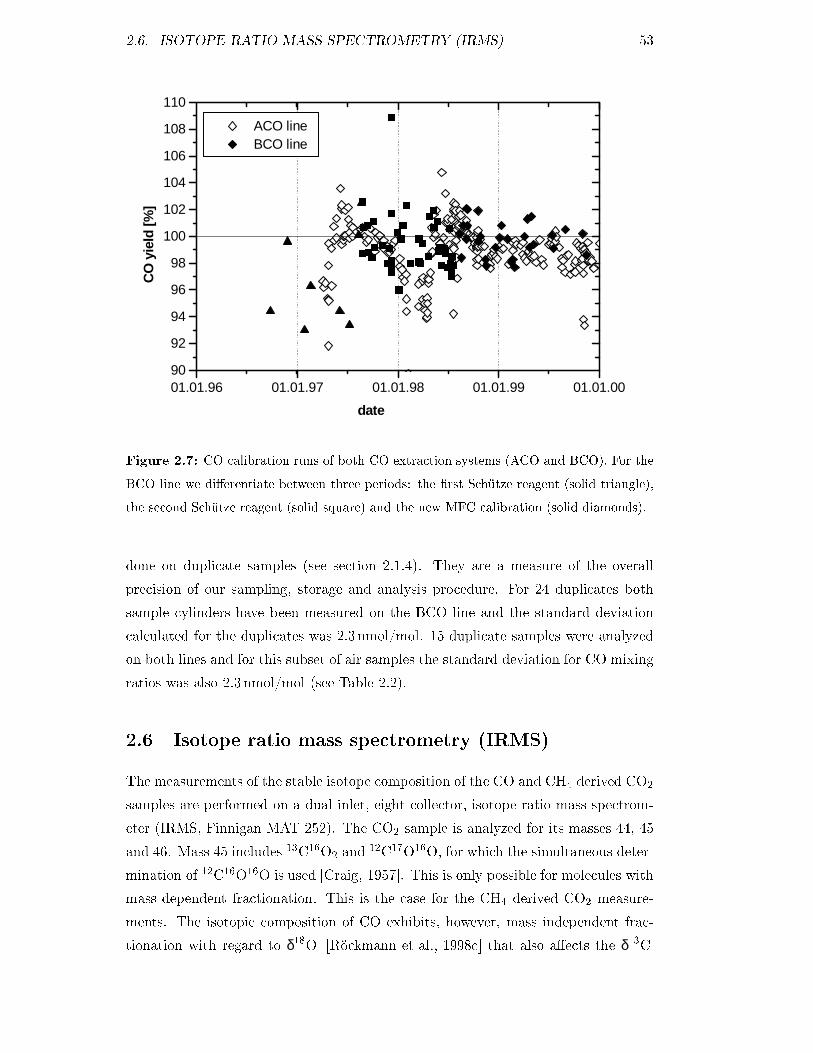
2.6. ISOTOPE RATIO MASS SPECTROMETRY (IRMS) 53
01.01.96 01.01.97 01.01.98 01.01.99 01.01.0090
92
94
96
98
100
102
104
106
108
110
ACO lineBCO line
date
CO
yiel
d[%
]
Figure 2.7: CO calibration runs of both CO extraction systems (ACO and BCO). For the
BCO line we di�erentiate between three periods: the �rst Schütze reagent (solid triangle),
the second Schütze reagent (solid square) and the new MFC calibration (solid diamonds).
done on duplicate samples (see section 2.1.4). They are a measure of the overall
precision of our sampling, storage and analysis procedure. For 24 duplicates both
sample cylinders have been measured on the BCO line and the standard deviation
calculated for the duplicates was 2.3 nmol/mol. 15 duplicate samples were analyzed
on both lines and for this subset of air samples the standard deviation for CO mixing
ratios was also 2.3 nmol/mol (see Table 2.2).
2.6 Isotope ratio mass spectrometry (IRMS)
The measurements of the stable isotope composition of the CO and CH4 derived CO2
samples are performed on a dual inlet, eight collector, isotope ratio mass spectrom-
eter (IRMS, Finnigan MAT 252). The CO2 sample is analyzed for its masses 44, 45
and 46. Mass 45 includes 13C16O2 and12C17O16O, for which the simultaneous deter-
mination of 12C16O16O is used [Craig, 1957]. This is only possible for molecules with
mass dependent fractionation. This is the case for the CH4 derived CO2 measure-
ments. The isotopic composition of CO exhibits, however, mass independent frac-
tionation with regard to δ18O [Röckmann et al., 1998c] that also a�ects the δ13C

54 CHAPTER 2. SAMPLING AND MEASUREMENT
IRMS measurements [Röckmann & Brenninkmeijer, 1998b](see section 1.8.1). For
the quantities of CO derived CO2 (down to 20 �l) the MS is equipped with two
microvolumes (for CO2 and O2). The CH4 derived CO2 samples of normally 200 to
500 �l are done by bellow measurements.
Our working standard (MG-CO2, Messer Griesheim ultrapure CO2) was calibra-
ted against NBS-19 and assigned a δ13C value of �42:465 0=00 V-PDB [Röckmann,
1998]. This value is close to the Æ value of atmospheric methane (� �47 0=00), where
precision has to be highest, and reasonably close to CO (�26 0=00 to �32 0=00). For
δ18O a value of �29:058 0=00 V-PDB has been assigned.
We regularly measured a separate aliquot of MG-CO2 gas (stored in glass vessels)
against the MG-CO2 working standard in order to check the long-term stability of
the MS measurements. This was usually done after �lling the standard side with
new reference gas and when CH4 derived CO2 samples were measured. Figure 2.8
shows that long-term drifts in δ13C for this aliquot were less than 0.01 0=00 and the 1�
standard deviation over the whole 3-year measurement period was �0.02 0=00 (n=140).
For δ18O the measurements exhibit a drift of less than 0.02 0=00 and the 1� standard
deviation has been �0.05 0=00. Deviations of more than 0.05 0=00 and 0.15 0=00 have been
measured for δ13C and δ18O respectively, when previous to the CO2 measurements
O2 or N2O measurements had been performed. In Figure 2.8 these samples were
labeled as outliers.
2.6.1 δ13C and δ18O calibration of CO
The calibration runs described in section 2.5.3 give information about the 13C/12C
ratio, which for δ13C of the formed CO2 should match that of the CO injected.
During the oxidation process from CO to CO2 discussed in section 2.3.1, solely one
oxygen atom is added to the CO molecule, while neither isotopic exchange occurs
for CO, nor for the formed CO2 [Stevens & Krout, 1972], [Brenninkmeijer, 1993],
[Brenninkmeijer & Röckmann, 1997]. Thus, by using CO of known isotopic compo-
sition, the e�ect of the oxidation can be corrected for δ18O . Figures 2.9 and 2.10
show the long-term development of δ13C and δ18O for the reference gas which has
been used on the two CO extraction systems ACO and BCO. In section 4 δ13C and
δ18O measurements of atmospheric CO are presented that have been measured on
both extraction lines. It is therefore essential that the �nal stable isotope CO data
is reported relative to a coherent reference scale. In addition, atmospheric samples
have also been divided for subsequent analysis on both lines. In the following two
sections we document the applied δ13C and δ18O correction that allow the direct
comparison of stable isotope CO measurements from both extraction lines.

2.6. ISOTOPE RATIO MASS SPECTROMETRY (IRMS) 55
-0.15
-0.10
-0.05
0.00
0.05
0.10
0.15
1. cal gas 2. cal gas 3. cal gasoutliers mean 1-σ
δδ δδ13C
[‰V
-PD
B]
01.01.97 01.01.98 01.01.99 01.01.00-0.2
-0.1
0.0
0.1
0.2
date
δδ δδ18O
[‰V
-SM
OW
]
Figure 2.8: Measurements of (a) δ13C and (b) δ18O of a MG-CO2 calibration gas aliquot
versus the MS working standard MG-CO2.
Corrections for δ13C CO measurements
Over the considered 3.5 year period from July 1996 to December 1999 the δ13C CO
calibration (Figure 2.9) have varied around �43:99 � 0:19 0=00 (n=84) and �44:01 �

56 CHAPTER 2. SAMPLING AND MEASUREMENT
0:22 0=00 (n=277) for the two CO extraction lines BCO and ACO respectively. Apart
from two periods (Aug 1997 to Feb 1998 and May 1998 to Aug 1998) the δ13Ccalibration of both extraction lines agree well within their error speci�cation.
01.01.96 01.01.97 01.01.98 01.01.99 01.01.00-45.0
-44.5
-44.0
-43.5
-43.0
-42.5
period 2
period 1
ACO lineBCO line
δδ δδ13C
[‰V
-PD
B]
date
Figure 2.9: δ13C calibration runs of both CO extraction systems (ACO and BCO). For
the BCO line we di�erentiate between: the �rst Schütze reagent (solid triangle), the second
Schütze reagent (solid square) and the new MFC calibration (solid diamonds). Period 1 and
2 indicate the time periods for which samples are corrected in δ13C .
For the �rst period (period 1 in Figure 2.9) the CO measurements of the BCO line
are considered to be 0.2 0=00 enriched compared to the average mean of �44 0=00. The
�nal δ13C values of atmospheric air samples measured in this period on the BCO
line are shifted by 0.2 0=00. For the ACO line a similar correction of 0.2 0=00 applies
for atmospheric air samples measured between May and August 1998 (period 2 in
Figure 2.9). δ13C calibration during this period have been too heavy compared to
the average mean. To which extend a shift in δ13C from calibration runs can be
directly translated to air samples is not clear. The calibration runs are more sensitive
to contamination because of the di�erences of nearly 20 0=00 in the δ13C value.
Direct intercomparison between both extraction lines by measuring stable CO iso-
topes on the same cylinder have only been carried out in periods directly after those
with di�erences in the calibration runs. In Table 2.2 they are listed (ACO+BCO) to-
gether with selected air samples from Izaña. This subset of 14 air samples consists of

2.6. ISOTOPE RATIO MASS SPECTROMETRY (IRMS) 57
CO δ13C δ18O n
[ nmol/mol ] [ 0=00 ] [ 0=00 ]
ACO + BCO 4.0 0.26 0.59 3
Duplicate ACO/BCO 2.1 0.17 0.44 14
Duplicate BCO/BCO 2.3 0.23 0.40 24
Table 2.2: Direct intercomparison of both CO extraction systems, ACO and BCO. Stan-
dard deviations are given for duplicate samples and for samples analyzed on both lines.
duplicate continuous samples of which one has been measured on the BCO extraction
system for the analysis of CO and CH4 isotopes while the second has been analyzed
on the ACO extraction system for CO isotopes only (duplicate ACO/BCO). With
the applied correction factors from above those samples agree within 0.17 0=00. We
compare the results from samples measured on both lines to duplicate samples only
measured on the BCO line (duplicate BCO/BCO).
Important changes on the BCO system have been the replacement of the original
Schütze reagent by a new batch in August 1997 and the readjustments of pumping
times in the extraction procedure. Previous to August 1997, the pumping after
the transfer from the collection trap to the U-tube was too short. Table 2.3 shows
how the CO yield, as well as the standard deviation for a single δ13C and δ18Omeasurement have improved subsequently.
CO yield δ13C δ18O n
[%] [ 0=00 ] [ 0=00 ]
1.Schütze 95.2�2:4 �44:07 � 0:28 �15:12 � 0:23 8
(until Jul 97)
2.Schütze 99.3�2:1 �43:92 � 0:19 �14:94 � 0:13 46
(Aug 97 - Aug 98)
MFC cal. 99.8�1:3 �44:06 � 0:13 �14:86 � 0:19 29
(since Aug 98)
Table 2.3: CO calibration runs of the BCO line. CO yield, δ13C and δ18O values are given
for the �rst Schütze, the second Schütze and for the additional calibration of the MFC.

58 CHAPTER 2. SAMPLING AND MEASUREMENT
Corrections for δ18O CO measurements
The isotopic analysis of air samples is performed on the CO derived CO2. Thus
regular δ18O calibration runs are essential in order to retrieve the original oxygen
isotopic composition of CO. With the help of the δ18O value of the CO which is used
in the calibration runs and the measured δ18O of the CO derived CO2, the δ18Ovalue of the Schütze reagent can be established. Subsequently the δ18O value of air
samples can be obtained by correcting for the added oxygen atom in the oxidation
process (see equation 2.4). First the reaction
CO + I2O5 ! CO2 (2.2)
leads to an equation for the Æ values [Brenninkmeijer, 1993]:
δCO + δI2O5= 2 � δCO2
(2.3)
with ÆCO : initial Æ value of CO;
ÆI2O5: Æ value of the Schütze reagent and
ÆCO2: Æ value of the CO derived CO2.
By using equation 2.3 for sample and standard we can �nally derive equation
2.4 which relates the initial δ18O value of the CO sample to the δ18O value of the
corresponding calibration run:
SAδCO = 2 �SA δCO2� (2 �CAL δCO2
�CAL δCO) (2.4)
with SAÆ : Æ value of the sample and
CALÆ : Æ value of the calibration gas.
The isotopic composition of the calibration gas (CALδCO) has been established
according to [Brenninkmeijer, 1993] and is given in Table 2.3. The δ18O value has
been con�rmed by independent measurements using the conversion of known CO2
to CO on activated charcoal [Röckmann, 1998a].
In Figure 2.10 the δ18O calibration values for the two extraction lines are shown.
The observed δ18O variation of the calibration gas can be signi�cant, because of
changes in the isotopic composition of the Schütze reagent. Equation 2.4 not only
allows the correction for direct intercomparison of δ18O values for samples measured
on di�erent extraction systems but also for statistical variation as well as long term
drifts of the two systems. For the CALδCO2used in equation 2.4, the moving average
over the previous and following 10 calibration runs is used in order to take into
account the long term drift and the uncertainty of the single measurement.
On the ACO extraction system the Schütze reagent was changed in April 1997
because the CO yield dropped signi�cantly (see Figure 2.7). After the exchange of

2.6. ISOTOPE RATIO MASS SPECTROMETRY (IRMS) 59
01.01.96 01.01.97 01.01.98 01.01.99 01.01.00
-16
-15
-14
-13
-12ACO lineBCO line
date
δδ δδ18O
[‰V
-SM
OW
]
Figure 2.10: δ18O calibration runs of both CO extraction systems (ACO and BCO). For
the BCO line we di�erentiate between: the �rst Schütze reagent (solid triangle), the second
Schütze reagent (solid square) and the new MFC calibration (solid diamonds).
the Schütze reagent the δ18O displayed a large drift towards heavier values. The
Schütze was therefore exchanged again in March 1998. The observed change in δ18Oshows that the isotopic composition of the Schütze reagent can vary from batch to
batch. The δ18O standard deviation calculated for duplicate samples processed on
the two extraction systems, ACO and BCO, is 0:44 0=00 (Table 2.2).
2.6.2 δ13C calibration of CH4
The performance of the CH4 extraction line was checked using the CH4 reference
gases EG-95 [Marik, 1998] and EG-96. Several dilutions of these gases in ultrapure
N2 were produced, resulting in �nal CH4 mixing ratios of �1000 to 4000 �mol=mol
(see Table 2.4).
The use of these high concentration reference gas mixtures has the advantage,
that the amount of CH4 stored in one individual cylinder is suitable for numerous
(�100) sample preparations. It is, however, crucial to test the line with gas mixtures
which have a CH4 concentration close to ambient air. Similar to the procedure with
the CO calibration runs (2.6.1) the reference gas mixture is diluted dynamically into a

60 CHAPTER 2. SAMPLING AND MEASUREMENT
EG95-V2 EG95-V3 EG96-V1
CH4 [ nmol/mol ] 834 1157 1171
δ13C [ 0=00 ]: �50:55 � 0:05 �50:48 � 0:10 �51:17 � 0:02
direct combustion (n=33) (n=6) (n=30)
(without Schütze)
δ13C [ 0=00 ]: �50:60 � 0:01 �50:58 � 0:02
direct combustion (n=8) (n=60)
(with Schütze)
δ13C [ 0=00 ]: �50:42 � 0:05
complete extraction (n=12)
(without Schütze)
δ13C [ 0=00 ]: �50:7 � 0:05 �50:54 � 0:03 �51:11 � 0:02
complete extraction (n=6) (n=12) (n=11)
(with Schütze)
δD [ 0=00 ]: �205:5 � 1:5 �204:7 � 1:7 �206:2 � 1:1
complete extraction (n=11) (n=9) (n=9)
δD [ 0=00 ]: �205:7 � 0:9
direct TDL (n=3)
Table 2.4: δ13C and δD calibration runs for di�erent CH4 reference gases with standard
deviations and the number of calibration runs (n).
�ow of zero air with the ratio of mass �ows adjusted so that the �nal mixture entering
the extraction line has a mixing ratio of about 2µmol/mol. Again, the ultrapure zeroair (Linde, Messer Griessheim) used was found to have blank CH4 mixing ratios of,
typically, several nmol/mol. Since these quantities added a signi�cant contamination
to the �nal gas mixture, the zero air was �rst directed through the Pt catalyst reactor,
that operated at 850 ÆC for CH4 calibration. This puri�cation reduced the CH4
mixing ratios to levels well below 1 nmol/mol, i.e. resulting in a �nal contamination
of less than 0.05%. In addition to these 'whole extractions' of the dynamically
diluted calibration gas mixtures, also direct injections of the EG95/96-Vx mixtures
into the combustion line were regularly performed ('direct combustion').
One important improvement in the δ13C measurements of methane has been the
introduction of a Schütze/Ascarite trap in the combustion line (section 2.3.2) in Au-
gust 98. Prior to this a signi�cant δ13C o�set between direct combustion runs and
whole extractions for δ13C of 0:12�0.07 0=00 was observed (see Table 2.4 and Figure

2.6. ISOTOPE RATIO MASS SPECTROMETRY (IRMS) 61
-51.4
-51.2
-51.0
-50.8
-50.6
-50.4
-50.2
-50.0
direct comb. EG-95 V1 (ohne Schütze) complete extraction EG-95 V1 (ohne Schütze)direct comb. EG-95 V2 (ohne Schütze) complete extraction EG-95 V2 (ohne Schütze)direct comb. EG-95 V2 (mit Schütze) complete extraction EG-95 V2 (mit Schütze)direct comb. EG-95 V3 (ohne Schütze)direct comb. EG-95 V3 (mit Schütze) complete extraction EG-95 V3 (mit Schütze)direct comb. EG-96 V1 (mit Schütze) complete extraction EG-96 V1 (mit Schütze)
Schütze/Ascerite trap
(b)
(a)
δδ δδ13C
[‰V
-PD
B]
01.01.97 01.01.98 01.01.99 01.01.00-214
-212
-210
-208
-206
-204
-202
-200
-198
EG-96 V1 direct TDL
δδ δδD[‰
V-S
MO
W]
date
Figure 2.11: δ13C and δD calibration runs for CH4 reference gases (as listed in Table 2.4).
2.11). This o�set was attributed to a small amount of CO produced in the activated
charcoal. Since the amount of contamination was obviously relatively constant, the
complete extractions showed nevertheless a rather good reproducibility (EG95-V2:
�50:41�0.04 0=00). After inserting the Schütze/ascarite trap, this o�set became sig-
ni�cantly smaller (0.03 - 0.04 0=00). Also the δ13C results for the direct combustion
runs shifted slightly and their precision signi�cantly improved, a behavior which is
not fully understood. The di�erence in δ13C of the whole extraction calibration was
applied to correct all δ13C data of samples processed without the trap. Although

62 CHAPTER 2. SAMPLING AND MEASUREMENT
the precision of the whole extraction calibration runs does not show a signi�cant
di�erence prior and after inserting the trap, we assume a larger uncertainty for
all samples processed prior to this modi�cation. We assign δ13C uncertainties of
�0.08 0=00 and � 0.04 0=00 for the samples prior and after inserting the trap respec-
tively. The mean deviation between measurements of duplicate continuous samples
changed from �0.041 0=00 to �0.026 0=00 after the trap has been inserted.
2.7 Methane Isotopomer Spectrometer (MISOS)
Tunable diode laser spectroscopy is usually employed in atmospheric sciences as
a highly selective and sensitive technique for in situ measurement of trace gases
[Reid & Labrie, 1978]. A new tunable diode laser based Methane ISOtopomer Spec-
trometer (MISOS) has been developed by Bergamaschi et al. [1994], which allows δDmeasurements of atmospheric methane. The instrument makes use of the di�erence
in the rotational-vibrational transitions and the corresponding infrared spectra for
the di�erent CH4 isotopomers.
Many small molecules in the atmosphere, such as methane, have sharp absorp-
tion lines from rotational-vibrational transitions. At low pressure, the linewidth is
limited by the Doppler shift of the individual molecules and the lines do not overlap.
By adjusting the diode laser temperature via its current, the laser output can be pro-
duced at a single frequency, which can be scanned continuously over bandwidths of
several cm�1 in the mid infrared region. Multipass absorption cells allow absorption
paths of � 100 m.
The development of the MISOS system and its application to δD measure-
ments of CH4 have been extensively documented in [Bergamaschi et al., 1994] and
[Saueressig, 1999]. In the following section we only brie�y summarize the main steps
of δD CH4 measurements. In section 2.7.2 the calibration of our reference gases for
atmospheric CH4 measurements reported in this thesis is documented.
2.7.1 Methane δD measurements
For the measurement of δD the absorption lines for 12CH4 and 12CH3D must have
approximately the same intensity. To compensate for the ratio of mixing ratios12CH3D=
12CH4 that is close to 6 � 10�4 the intensity of the 12CH3D line has to
be up to � 1500 times higher than that of the 12CH4 line. Therefore the line pair
chosen for δD measurements is at 3044.289 cm�1 and 3044.170 cm�1 for 12CH3D
and 12CH4 respectively.
The tunable diode laser is scanned over the spectral region of interest and the ab-

2.7. METHANE ISOTOPOMER SPECTROMETER (MISOS) 63
sorption spectra are recorded simultaneously for the sample and a working reference
gas. The low variation in the ratio of the isotopomers can only be separated when
the absorbtion of each species is high enough. Therefore the sample gas is intro-
duced into an evacuated multipass re�ection cell (White cell, volume 6.8 liter, base
length 1 m [Roths, 1992]), while the working reference gas is in a 1 m reference cell.
Optical path length of up to 126 m can be achieved and thus the minimum mixing
ratio of the pre-concentrated CH4 samples has to be � 1500µmol. The reference cellis put directly on top of the White cell, and both enclosed in a common, thermally
insulated housing. Measurements are made at 30 hPa total pressure and room tem-
perature. Multiple linear regression procedures are carried out online, comparing
the 12CH3D and the 12CH4 absorptions in the two optical channels. The precision
of individual δD measurements with the MISOS instrument may vary slightly and
individual errors are calculated for each measurement, considering the stability of
the instrument during the actual measurement series.
2.7.2 δD calibration of CH4
The working reference gas, CAL-3, was produced as a mixture of our reference gas
REF (99.995% CH4, δD = �164:4 0=00 V-SMOW) with pure (�99%) CH3D, resulting
in a �nal δD value of �84:5 0=00 V-SMOW. In order to scale δD deviations of samples
from the CAL-3 gas correctly, also the REF gas is measured within each measurement
series.
Since the δD of the CAL-3 gas is very close to the atmospheric samples, the po-
tential error in the scaling factor is almost negligible. The δD precision of the MISOS
instrument is �0:5 � �1 0=00, and the overall accuracy including sample preparation
is estimated to be around �1 0=00. The mean deviation between duplicate continuous
samples is �0.9 0=00. Note, however, that no international standards so far exist for
δD in CH4. Our δD scale is based on measurements of our standards REF, and
CAL-1 at the Bundesanstalt für Geowissenschaften und Rohsto�e, Hannover, using
CH4 combustion to CO2 and H2O, followed by reduction of H2O to H2 and sub-
sequent IRMS analysis on H2 [Bergamaschi et al., 1994] [Dumke et al., 1989]. The
calibration was against the IAEA water standards V-SMOW and V-SLAP. Since
this common procedure only calibrates the δD measurement on H2O and since in
particular the conversion of CH4 into H2O may be subject to some H2O contamina-
tion, signi�cant di�erences in the δD-CH4 scale among di�erent IRMS laboratories
may arise [Marik, 1998]. Thus some uncertainty remains about the absolute δD-CH4
scale, but the δD scale used for our MISOS measurements (including our previous
studies on CH4 sources and sinks) is considered to be internally consistent.

64 CHAPTER 2. SAMPLING AND MEASUREMENT
2.8 Accelerator Mass Spectrometry (AMS)
Accelerator Mass Spectrometry (AMS) is widely used for radiocarbon dating but can
also be used for the determination of the ultra-rare atmospheric trace gas 14CO. Part
of the European Project CO-OH-EUROPA has been the collaboration of three AMS
facilities for the regular analysis of atmospheric 14CO at several sampling stations
(see Table 3.1).
� Centre for Isotope Research (CIR), University of Groningen, Netherlands
� Vienna Environmental Research Accelerator (VERA), University of Vienna,
Austria
� University of Uppsala, Sweden
In addition some of the 14CO data shown in section 4 have been analyzed at AMS
facilities in Lower Hut, New Zealand and in Kiel (Leibniz Laboratory), Germany.
Following the conversion and extraction process, the CO derived CO2 sample is
recovered from the IRMS after the stable isotopic analysis. The samples are diluted
with 14C-free CO2 to increase the sample size to about 1 mg CO2 and subsequently
reduced to graphite. The graphite targets are then processed on the AMS. The
dilution of the samples is carried out at the MPI in Mainz, while the graphitization
is part of the 14CO measurement procedure of the AMS facilities. A short description
of the dilution procedure is given in the next section. Section 2.8.2 describes the main
features of the AMS facilities. Finally in section 2.8.3 we describe in detail how we
convert the pmC values of the di�erent AMS facilities into a consistent 14CO data
set reported in molecules cm�3 air at STP.
2.8.1 Dilution
The speci�c activity of atmospheric 14CO of up to 900 pmC is high compared to
the activity of �100 pmC usually encountered for radiocarbon dating (for which the
AMS facilities are optimized). For stratospheric samples even 14CO values of more
than 3000 pmC can be reached. Thus the dilution of the CO derived CO2 sample
by a factor of 5 to 30 with 14C-free CO2 is done previous to AMS analysis.
The CO derived CO2 samples of 10-100µl are often stored after the IRMS mea-
surement at low temperature. The dilution procedure is done on a separate dilution
line. We start the dilution process by drying each sample with P2O5 to remove H2O.
Subsequently the sample is transferred into a calibration volume (0.75 ml), sealed
and the exact pressure is recorded. The pressure is measured with a piezoresistive

2.8. ACCELERATOR MASS SPECTROMETRY (AMS) 65
pressure transducer and range between 30 and 200 hPa. Afterwards, the sample
is transferred back into its sample bottle. We then �ush the dilution line several
times with the CO2-free dilution gas MG-CO2. The next step consists of sealing
the MG-CO2 gas in the calibration volume at a pressure close to 900 hPa. Finally
we add this quantity of MG-CO2 gas to the sample. The mixture is subsequently
transferred into a break seal sample bottle in which the diluted sample is send to the
AMS facility.
The pressure ratios between the sample and the dilution gas in the calibration
volume is called the dilution factor � (see equation 2.5). Its accuracy will directly
determine the precision of the �nal 14CO concentration. Therefore the calibration of
the pressure transducer and its linearity over the whole pressure range of 10-1000 hPa
is important. We assume an error of 0.3-1% in the dilution process.
2.8.2 AMS measurements
Prior to the AMS analysis the CO2 samples are reduced to graphite. The reduction
takes place in an excess of puri�ed hydrogen, using Fe powder at typically 580 ÆC as
a catalyst:
(Fe; 580 ÆC)
CO2 + 2H2 $ C + 2H2O
The water from the reduction process is cryogenically trapped. The resulting carbon-
catalyst mixture is pressed into copper or aluminum target holders for the AMS
analysis, in which the 14C/C ratios of the graphite samples are measured [Wallace
et al., 1987], [Rom, 2000a].
The Accelerator Mass Spectrometry is basically a sequence of two large mass
spectrometers with an accelerator for the destruction of molecular isobars in between.
Thus the carbon isotopes 12C,13C and 14C are separated by their di�erent masses and
counted directly. There are several variations amongst the di�erent AMS systems
for 14C, but the main are [Rom et al., 1998] and [Wijma et al., 1998]:
� Negative-ion source: This produces isobars from 14N (as nitrogen does not
produce negative ions)
� (Van de Graa� or Pelletron) Tandem accelerator with an Ar gas stripper op-
erated at �+3 MV for 14C3+ (sometimes a foil stripper is used)
� High energy mass spectrometer
� Detector for the rare isotope

66 CHAPTER 2. SAMPLING AND MEASUREMENT
� Computer-control system with data acquisition
The pmCS value of the diluted CO2 sample we get from the AMS facilities is
measured relative to a solid IAEA standard material (C-6 sucrose, C-3 cellulose) and
is corrected for the accelerator blank. These corrections are speci�c to each AMS
facility and its graphitization procedure and vary among the di�erent accelerators.
2.8.3 Derivation of the �nal 14CO data
In order to obtain the 14CO concentrations, we need the 14C/12C ratio reported
from the AMS laboratories, the CO mixing ratio of the sampled air and the dilution
factor for the CO derived CO2 sample [Rom et al., 2000b]. This ratio is measured
relative to a standard with known 14C/12C ratio and is reported in percent Modern
Carbon (pmC). Because of its origin from archeological dating, a normalization to
δ13C =�25 0=00 is applied to correct for fractionation e�ects in the carbon isotope
composition. Because we are only interested in the 14C/12C ratio, this normalization
is, however, not meaningful in the case of atmospheric CO sample.
The �rst step is to converted the measured pmCS values to 14C/12C ratios.
Depending on the de�nition of pmC used by the di�erent accelerators, the activity
of the sample is either given relative to the present activity of the standard, or
relative to the "absolute" activity of the standard in 1950. This results in constant
or time-dependent pmC values respectively, because of the activity of the sample
decreasing in pace with the standard or relative to the absolute standard from 1950.
In equation 2.5 we use the �rst pmC de�nition and therefore correct for the time
elapsed since 1950.
For absolute atmospheric 14CO concentration at standard conditions (STP) �rst
the pmC value of the diluted sample has to be transformed into a non-δ13C -corrected
14C/12C ratio:
14RS(x; t) =pmCS
100�(1 + Æ13CS=1000)
2
(1� 25=1000)2�14 Rstd � e
��(t�1950)� e�(t�x) (2.5)
with 14RS(x; t) :14C/12C ratio of the diluted sample (sampled in year x and
analyzed in year t)
pmCS : speci�c activity of the diluted sample (from the AMS)
Æ13CS : δ13C value of the diluted sample
14Rstd = 1:189 �10�12 : 14C/12C ratio of an absolute international standard
� = ln2=5730 yr�1 : decay constant of 14C
The next step is to deduce the activity of the original, undiluted air sample
from the activity of the target. The dilution gas (pure CO2, Messer-Griesheim,

2.8. ACCELERATOR MASS SPECTROMETRY (AMS) 67
Mainz) was supposed to be free of radiocarbon. Blank tests of this gas have been
carried out at three of the AMS facilities and a pmC value of �0.5% was measured.
With equation 2.5 the resulting activity for the dilution gas (δ13C =�42:465 0=00) is14Rdil = 5:686�10�15. Thus the original conversion from the activity of the diluted
gas to the one of the original undiluted gas has changed from
14RCOs = 14RS � (�+ 1) to
14RCOs = (14RS �14 Rdil) � (�+ 1) +14 Rdil (2.6)
with 14RCOs :14C=12C ratio of the original (undiluted) air sample,
14Rdil :14C=12C ratio of the diluting gas (MG-CO2) and
� = pDil=pSam : dilution ratio (pressure ratio of the undiluted sample and the
dilution gas)
The �nal step is to obtain the 14CO concentration from the activity of the original
sample.
[14CO]s =14 RCOs � [CO]s �
[12CO]
[14CO] + [13CO]� L� (2.7)
with [14CO]s : �nal14CO concentration [molecules cm�3 (STP)],
[CO]s : CO mixing ratio of the original air sample [ nmol/mol ],
[12CO]�([14CO]+[13CO])�1 �= 0.989 : constant within 0.5 0=00 and
L� = 2:6868 �1010 cm�3: modi�ed Loschmidt constant.
We assume an overall uncertainty for the 14CO measurement of maximal 3%.
This includes errors arising from the dilution, the graphitization process and the
precision of the �nal AMS measurement of � 1% each.

68 CHAPTER 2. SAMPLING AND MEASUREMENT
2.9 Summary of the di�erent analytical precisions
The di�erent analytical procedures for measuring CO and CH4 mixing and isotope
ratios have been documented in this chapter. Table 2.5 gives an overview of the
numbers of samples processed during this thesis and the analytical precision we
attribute to each measurement.
CO mixing ratio �3 nmol/mol
δ13C �0.3 0=00
δ18O �0.4 0=00
n 370
CH4 mixing ratio �2 nmol/mol
δ13C �0.08 0=00 before Aug 1998
�0.04 0=00 after Aug 1998
δD �1 0=00
n 520
Table 2.5: Summary of the di�erent analytical precision of CO and CH4 mixing and isotope
ratios and the number of samples processed during this thesis (n).

Chapter 3
Seasonal cycles of atmospheric
CH4
In the following two chapters we report measurements of atmospheric CH4 and CO
mixing ratios and their isotopic composition at the baseline air Global Atmospheric
Watch (GAW) station Izaña. The measurements have been carried out as part of
the European 14CO-OH-Europe Project, for which mainly CO and its stable isotopes
together with 14CO have been investigated at several stations (listed in Table 3.1).
Sampling at Izaña started in late 1996 and nearly three annual cycles can now be
interpreted in terms of seasonal cycles, synoptic scale variability and consequences
for the methane and carbon monoxide budgets.
Here we report the �rst measured δD seasonality for atmospheric background
CH4, which was measured with the MISOS system. We also report measurements
of CH4 mixing ratios and δ13C at Izaña. To support the analysis also SF6 mixing
ratios are provided. Finally we summarize the results from an inverse model study by
Bergamaschi et al. [2000a] which uses our Izaña records together with δ13C records
from �ve other globally distributed stations.
3.1 GAW station Izaña, Tenerife
The Global Atmospheric Watch (GAW) station Izaña is located on Tenerife (28Æ N,
16Æ W), one of the Canary Islands, about 400 km west of the African coast. The
station complex is located on a mountain plateau at 2370 m above sea level (Figure
3.1). A characteristic meteorological feature is the existence of a trade wind inversion,
which usually shields the observatory from emissions on the island. Between January
1996 and October 1997, the station was above at least one inversion layer on 86%
of all nights [Schaefer, 1998]. During the summer months (June to August) this
69

70 CHAPTER 3. SEASONAL CYCLES OF ATMOSPHERIC CH4
country location altitude
[m a.s.l.]
sampling
period
Izaña Tenerife
Spain
28Æ N
16Æ W
2370 Mai 96- Spanish Meteoro-
logical Service
Mt. Sonnblick Austria 47Æ N
13Æ E
3106 Sep 96- Institute for Mete-
orology, Salzburg
Schauinsland Germany 48Æ N
8Æ E
1205 95 Umwelt Bundes-
amt Schauinsland
Kollumerwaard Netherlands 53Æ N
6Æ E
0 97- University of Gro-
ningen
Spitsbergen Norway 79Æ N
12Æ W
474 Mar 96- Norwegian In-
stitute for Air
Research
Alert Canada 82Æ N
62Æ W
210 Jul 96
-Dec 98
Atmospheric Envi-
ronment Service
Happo Japan 36Æ N
137Æ E
1840 Feb 97- University of
Tokyo
Kaashido Male 5Æ N
73.5Æ E
0 Sep 98 Kaashido Observ-
atory
Table 3.1: Sampling stations
percentage increased to 100%, while it is lowest during winter (73-96%). During
daytime the station may be subject to contamination from boundary layer air due to
local upslope winds and hence local trace gas sources. During nighttime, these local
wind systems are absent at the station and sampled air usually represents the free
troposphere. Air sampling was therefore restricted to nighttime (see section 3.1.1).
The dominant air �ow at the station is from western to north eastern directions, with
air masses mainly coming from the North Atlantic. Frequently, air masses arriving at
Izaña have crossed the North American continent. To a lesser extent also air masses
which passed Europe or the African continent are encountered [Schmitt et al., 1988]
[Schmitt & Volz-Thomas, 1997] (see section 3.2.2 for a detailed discussion).
3.1.1 Air sampling
The air inlet is installed on top of a tower next to the main station building, at a
height of 13 m above ground, and connected via 25 m 1/2 inch te�on (PFA) tubing
to the sampling equipment inside the building. In order to prevent condensation, the

3.1. GAW STATION IZAÑA, TENERIFE 71
Puerto dela CruzPuerto dela Cruz
Izana(2370 m)Izana(2370 m)
Santa Cruzde TenerifeSanta Cruzde Tenerife
Pico del Teide(3718 m)Pico del Teide(3718 m)
28°°18' N
16 29' W28 18' N16 29' W
°°
Orotava valley
La Laguna
0 5 10 km
Figure 3.1: Map of Tenerife with the location of the GAW Izaña observatory.
whole sampling line is heated 5-10 K above ambient temperature. For the �lling of
the air bags used for the 2-week continuous samples a clock-controlled valve restricts
the sampling to nighttime hours between 21:00 and 7:00 LT. As described in section
2.1.4 duplicate continuous samples are taken. This allows a quality control over the
whole analytical procedure, including air sampling, GC analysis and isotope mea-
surements. In addition to the continuous samples also spot samples are collected at
intervals of two weeks. Again sampling is restricted to nighttime hours. For a de-
tailed description of the sampling procedure see section 2.1.4. During the three-year
sampling period 128 continuous and 86 spot samples have been taken and analyzed.
3.1.2 Back trajectories
Back trajectories for air masses arriving at Izaña were obtained from the Atmo-
spheric/Ocean Chemistry Experiment (AEROCE) Trajectory Archive for the period
1991-1997. They are calculated on hypothetical isentropic surfaces, as described by

72 CHAPTER 3. SEASONAL CYCLES OF ATMOSPHERIC CH4
Figure 3.2: Isentropic �ow probability �elds for Izaña for 1991-1997 (January-December).
Residence time from all available trajectories were combined to calculate isoplethe maps.
Red areas represent 25%, yellow areas 50% and green areas 75% of the total time of all
trajectories. The applied geometrical correction factor compensates for the decrease of
the probabilities with increasing distance (which fall o� with the square of the distance)
[Schaefer, 1998].

3.2. ATMOSPHERIC CH4 AND SF6 RECORDS AT IZAÑA 73
Merrill [1994]. Individual trajectories are calculated for the four corners of a 1Æ x 1Æ
square around Izaña (the position of Izaña constitutes the center of the square), for
the 10 days prior to their arrival at Izaña. The divergence of the four single trajec-
tories can be regarded as a measure of the reliability of the individual calculations.
From 1998 onwards back trajectories were provided by the Spanish Meteorologi-
cal Service Tenerife. Further, we used the HYSPLIT 4.0 (HYbrid Single-Particle
Lagrangian Integrated Trajectory) program from NOAA to calculate 10-day back
trajectories. We compared the calculated trajectories of the three di�erent methods
and found a good agreement.
The origin of the di�erent air masses reaching Izaña during the year is summarized
in Figure 3.2. Based on the AEROCE database, Schäfer [1998] has evaluated the ori-
gin of air masses reaching Izaña in terms of isentropic �ow probability �elds. In �gure
3.2 the residence time from all available trajectories are used in order to calculate
isoplethe maps for Izaña for 1991-1997 (January-December). The monthly isentropic
�ow probability �elds are normalized by a geometrical factor which compensates for
the decrease of the raw probabilities with increasing distance [Merill, 1994]. It is
obvious that air masses from very di�erent origins reach the remote station Izaña.
Thus important source regions like Europe and North America, as well as very clean
maritime or African air can be characterized by our isotopic studies of CH4 and CO
in chapter 3 and 3 respectively.
3.2 Atmospheric CH4 and SF6 records at Izaña
3.2.1 Seasonal cycles and interannual variations
The atmospheric record of CH4 mixing ratio is shown in Figure 3.3. We plot
our 2-week-continuous and spot samples together with CH4 mixing ratios from the
NOAA/CMDL monitoring network. The �t curves applied to all three data sets
were calculated with a low pass convolution �lter of the form
f(t) = N � exp(�(t
�T)2) (3.1)
in the frequency domain by Fast Fourier Transformation (FFT). Before the �lter is
applied, the data are linear interpolated on daily basis for spot samples and on weekly
basis for continuous samples [Jöckel et al., 2000b]. N is a normalization constant, t
is time and �T the time window of the low pass �lter. Three time window widths
�T of 1 week, 2 weeks and 4 weeks were calculated for the spot samples. However,
the 2-week-interval of the continuous samples made it necessary to use a 4-week �lter
for those samples. For the direct comparison of the di�erent data sets we use the
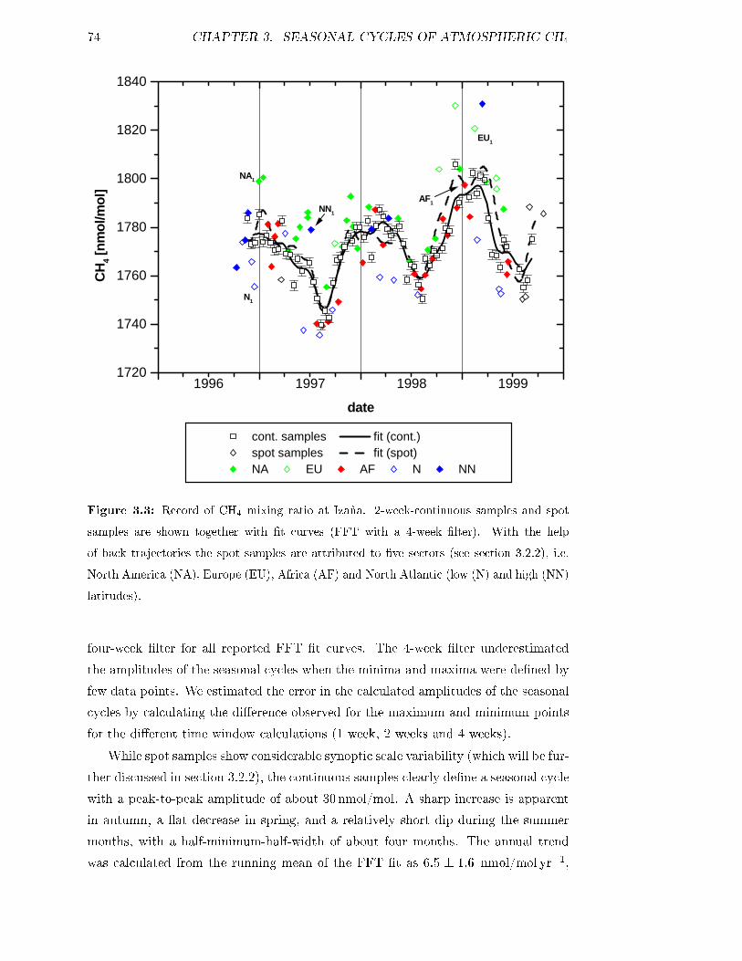
74 CHAPTER 3. SEASONAL CYCLES OF ATMOSPHERIC CH4
1996 1997 1998 19991720
1740
1760
1780
1800
1820
1840
N1
NN1
AF1
EU1
NA1
cont. samples fit (cont.)spot samples fit (spot)NA EU AF N NN
CH
4[n
mol
/mol
]
date
Figure 3.3: Record of CH4 mixing ratio at Izaña. 2-week-continuous samples and spot
samples are shown together with �t curves (FFT with a 4-week �lter). With the help
of back trajectories the spot samples are attributed to �ve sectors (see section 3.2.2), i.e.
North America (NA), Europe (EU), Africa (AF) and North Atlantic (low (N) and high (NN)
latitudes).
four-week �lter for all reported FFT �t curves. The 4-week �lter underestimated
the amplitudes of the seasonal cycles when the minima and maxima were de�ned by
few data points. We estimated the error in the calculated amplitudes of the seasonal
cycles by calculating the di�erence observed for the maximum and minimum points
for the di�erent time window calculations (1 week, 2 weeks and 4 weeks).
While spot samples show considerable synoptic scale variability (which will be fur-
ther discussed in section 3.2.2), the continuous samples clearly de�ne a seasonal cycle
with a peak-to-peak amplitude of about 30 nmol/mol. A sharp increase is apparent
in autumn, a �at decrease in spring, and a relatively short dip during the summer
months, with a half-minimum-half-width of about four months. The annual trend
was calculated from the running mean of the FFT �t as 6:5 � 1:6 nmol/mol yr�1,

3.2. ATMOSPHERIC CH4 AND SF6 RECORDS AT IZAÑA 75
1991 1992 1993 1994 1995 1996 1997 1998 19991700
1720
1740
1760
1780
1800
1820
1840
MPI spot samples fit MPI (spot)NOAA/CMDL data fit NOAA/CMDL
CH
4[n
mol
/mol
]
date
Figure 3.4: Records of CH4 mixing ratios at Izaña. MPI spot and 2-week-continuous
samples and measurements from the NOAA/CMDL monitoring network are plotted together
with �t curves (FFT with a 4-week �lter).
thus establishing a signi�cant CH4 increase over the observed period.
We compare our three year record of CH4 mixing ratios to measurements from
the NOAA/CMDL monitoring network starting at Izaña in 1991 [Dlugokencky et al.,
1994b]. Both data sets are shown in Figure 3.4 together with their respective FFT
�t curves (four-week �lter). Based on the FFT �t curves we note the general good
agreement between both data sets. Some discrepancies are nevertheless apparent
which re�ect the variability of CH4 mixing ratios due to the large synoptic scale
variations at Izaña occurring on time scales of less than 24 h.
Atmospheric SF6 mixing ratios at Izaña which are reported in Figure 3.5 show
a pronounced linear increase of 0.197�0:004 pmol/mol yr�1. SF6 is known to be a
virtually inert tracer of anthropogenic origin with a lifetime of about 2300 years.
Its mixing ratio exhibit a signi�cant North-South gradient and important enhance-
ments over industrialized sources regions such as North America or Europe [Maiss

76 CHAPTER 3. SEASONAL CYCLES OF ATMOSPHERIC CH4
1996 1997 1998 19993.8
3.9
4.0
4.1
4.2
4.3
4.4
4.5
4.6
NA1
NN1
AF1
N1
EU1
Lin. fit (cont.) m=0.197+/-0.004 pmol/mol yr-1
(R2=0.97, n=67)
cont. samples spot samplesNA EU AF N NN
SF 6
[pm
ol/m
ol]
date
Figure 3.5: Record of the SF6 mixing ratio at Izaña. 2-week-continuous samples and spot
samples are shown together with a linear �t through the continuous samples. The error
bars are the �0.02 pmol/mol precision of the GC measurements. With the help of back
trajectories the spot samples are attributed to �ve sectors (see section 3.2.2), i.e. North
America (NA), Europe (EU), Africa (AF) and North Atlantic (low (N) and high (NN)
latitudes).
& Brenninkmeijer, 1998] [Maiss & Levin, 1994]. The back trajectories indicate that
deviations from the linear �t towards higher values can in most cases directly be at-
tributed to air masses coming from North America or Europe. Similarly deviations
towards lower values are found for air masses from Africa or North Atlantic (see
Table 3.2).
3.2.2 Synoptic scales variations
Figure 3.3 shows that many of the spot samples deviate considerably from the mean
seasonal cycle of CH4 mixing ratios. There are several events, where the CH4 dif-
ference of subsequent samples (time interval usually � 2 weeks) is larger than the
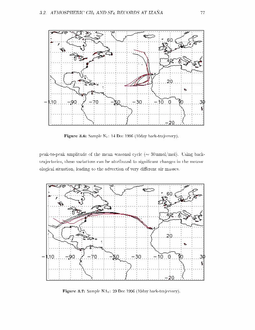
3.2. ATMOSPHERIC CH4 AND SF6 RECORDS AT IZAÑA 77
Figure 3.6: Sample N1: 14 Dec 1996 (10day back-trajectory).
peak-to-peak amplitude of the mean seasonal cycle (� 30 nmol/mol). Using back-
trajectories, these variations can be attributed to signi�cant changes in the meteor-
ological situation, leading to the advection of very di�erent air masses.
Figure 3.7: Sample NA1: 29 Dec 1996 (10day back-trajectory).

78 CHAPTER 3. SEASONAL CYCLES OF ATMOSPHERIC CH4
An instructive example are the samples taken on the 14 and 29 December 1996,
labeled as sample N1 and sample NA1 in Figure 3.3. The air collected by sample N1
circulated over the North Atlantic for 10 days without any contact with continental
source areas, thus representing clean marine air (see back-trajectory in �gure 3.6).
In contrast sample NA1 collects air originating from the North American continent
which was rapidly transported to Izaña. The back-trajectory shown in �gure 3.7
indicates that the transport time from the American East coast to Izaña was about
3 days. This in�uence from North America results in a CH4 mixing ratio in sample
NA1 which is 43 nmol/mol higher than in sample N1.
Back trajectories are used in the same way to determine the origin of air captured
in all spot samples taken between June 1996 and October 1999, with the exception
of six samples for which no back trajectories were available. Furthermore back tra-
jectories have been classi�ed into the �ve following areas of origin:
� North American continent (NA)
� Europe including Mediterranean area (EU)
� African continent (AF)
� North Atlantic (0Æ-50Æ N) (N)
� High latitude North Atlantic (50Æ-70Æ N)(NN).
In Figures 3.3 to 3.17 spot samples are plotted with di�erent symbols indicating
to which of the �ve groups they belong.
Similar to samples N1 and NA1 as examples for group N and NA typical samples
for the remaining three groups can be chosen. Two typical samples with air coming
mainly from Africa and Europe respectively were taken on the 10 January and the
15 February 1999. They are labeled AF1 and EU1 in Figure 3.3. In Figure 3.8
the corresponding back trajectory is shown for sample AF1. During the 10 day
period prior to their arrival at Izaña, these air masses have circulated over North
Africa. CH4 mixing ratios for this sample are � 25 nmol/mol lower than for sample
EU1. Here air masses have crossed vast regions of the European continent (see back
trajectories in �gure 3.9).
Trajectories coming from the North Atlantic are separated in two groups, N and
NN, in order to distinguish the very clean maritime air over the North Atlantic from
the considerably more polluted air masses at higher latitudes. Even if air masses
from the high latitude North Atlantic had no direct contact with source regions
before reaching Izaña, the remote high Northern Hemisphere is relatively well mixed
and thus highly a�ected by the continental source regions of North America, Europe
and Siberia. Sample NN1 taken on 7 July 1997 has been chosen as an typical example

3.2. ATMOSPHERIC CH4 AND SF6 RECORDS AT IZAÑA 79
Figure 3.8: Sample AF1: 10 Jan 1999 (10day back-trajectory).
Figure 3.9: Sample EU1: 15 Feb 1999 (10day back-trajectory).

80 CHAPTER 3. SEASONAL CYCLES OF ATMOSPHERIC CH4
Figure 3.10: Sample NN1: 7 July 1997 (10day back-trajectory).
for the high latitude North Atlantic. In �gure 3.10 the corresponding back trajectory
is shown. Air masses came directly from the high North (> 60Æ N) with less certain
origins before.
Clearly the assignment of spot samples to the �ve sectors with the help of back
trajectories is not always unambiguous. For example, all air masses classi�ed as
coming from North America must have crossed the Atlantic. We assigned trajectories
to the low North Atlantic (N) if they had nearly no contact with continental regions
within the 10 days prior to their arrival at Izaña. A complicating factor in the
classi�cation of these air masses is that they often reach Izaña after turning clockwise
around the station, thus touching the African coast. We still consider these samples
to be representative for group N, i.e. maritime air masses. A similar e�ect is seen
for samples attributed to the high latitude North Atlantic (group NN). These air
masses have partly traveled over Ireland or Spain, but are still considered to be
representative for the high latitude North Atlantic. Finally, air masses from the
African continent have partly also traveled over the European continent, mostly
Spain. Again we consider these samples to be representative for group AF.
If we look at the deviation of the CH4 mixing ratio of each of the spot samples
from the seasonal cycle derived from the continuous samples, a common pattern be-
comes apparent. Figure 3.3 shows, that spot samples of North American or European
origin and from the remote high Northern Hemisphere all have higher mixing ratios

3.2. ATMOSPHERIC CH4 AND SF6 RECORDS AT IZAÑA 81
�SF6 �CH4 �δ13C �δD n
[ pmol/mol ] [ nmol/mol ] [ 0=00 ] [ 0=00 ]
North America +0:04 � 0:03 +10:7� 6:2 �0:02� 0:10 �1:6 � 2:8 22
(NA)
Europa +0:08 � 0:03 +27:8� 8:3 �0:10� 0:04 �3:6 � 2:0 6
(EU)
Africa �0:02 � 0:03 �3:3� 7:2 +0:01� 0:06 �0:3 � 2:1 25
(AF)
North Atlantic �0:04 � 0:04 �14:8� 8:7 +0:04� 0:13 +0:8 � 1:2 16
(N)(0Æ- 50Æ N)
North Atlantic +0:02 � 0:05 +14:7 � 15:6 +0:01� 0:11 �2:5 � 2:9 8
(NN)(50Æ- 70Æ N)
Table 3.2: Residuals in mixing ratios of SF6 and CH4 together with the residuals of δ13C
and δD. The number n of samples attributed to each of the �ve groups is given.
than the mean seasonal trend. In contrast all samples from the low North Atlantic,
area N, have signi�cantly lower mixing ratios. In order to quantify the synoptic scale
variations we de�ne residuals (�CH4) as the di�erence between the measured mixing
ratio and the value of the �tted seasonal cycle.
Table 3.2 shows the clear relationship between the origin of air masses from
one of the �ve sectors and the corresponding residuals. The air masses from the
American continent, Europe and high latitude North Atlantic show signi�cant CH4
enhancements of 11:7�9:5 nmol/mol, 25:5�10:9nmol/mol and 17:4�12:3nmol/mol,
respectively. In contrast, air masses from Africa and from the North Atlantic show
CH4 depletions of �7:3� 4:7nmol/mol and �8:6� 8:6 nmol/mol.
These enhancements and depletions are directly linked to the source/sink strengths
above the respective regions. Assuming an average residence time of 1 to 3 days over
the source region and a mixing height of 1 to 12 km a CH4 residual of 10 nmol/mol
corresponds to a source strength of 0.1 to 3.3 mg CH4 m�2 h�1. This is in the range
of reported CH4 emission rates. For example, for the region of Fraserdale, Ontario,
Kuhlmann et al. [1998] estimated the CH4 �uxes to be 0.2 to 0.5 mg CH4 m�2 h�1.
While our calculation is only an illustrative estimate it shows the potential to derive
trace gas �uxes from the observed variability of mixing ratios. With the availability of
high resolution transport models it should be possible to substantially improve these
estimates. The observed variability of atmospheric mixing ratios at remote stations
could thus be used to infer integrated source �uxes [Engardt & Holmen, 1999].

82 CHAPTER 3. SEASONAL CYCLES OF ATMOSPHERIC CH4
-50 -40 -30 -20 -10 0 10 20 30 40 50-0.15
-0.10
-0.05
0.00
0.05
0.10
0.15
NN
EU
N
NA
AF
cont. samples spot samplesN NN EU NA AF
fit spot: m=0.0029+/-0.0003 (R2=0.66, n=68)
∆∆ ∆∆ SF 6[p
mol
/mol
]
∆∆∆∆CH4 [nmol/mol]
Figure 3.11: CH4 residuals vs. SF6 residuals. 2-week-continuous samples and spot samples
are shown together with the regression through the spot samples. The average values (�1�
range) for spot samples from North America (NA), Europe (EU), Africa (AF) and North
Atlantic (high (NN) and low (N) latitudes) are also indicated (according to Table 3.2).
Residuals for the SF6 mixing ratios can also directly be linked to the origin
of air masses (Table 3.2), similar to the CH4 residuals. Again, North America and
Europe act as sources of SF6, while air masses from the North Atlantic and Africa are
generally depleted, largely due to dilution. Figure 3.11 illustrates the generally very
high correlation between CH4 and SF6 residuals. Also shown in this �gure are the
ranges of the residuals for air masses from the above �ve regions, clearly illustrating

3.3. ATMOSPHERIC Æ13C RECORD AT IZAÑA 83
that the varying in�uence from these regions largely determine the overall �CH4-
�SF6 correlation.
In addition, however, it is important to note, that both CH4 and SF6 exhibit
strong latitudinal gradients at the latitude of Izaña. The varying latitudinal ori-
gin of di�erent air masses is therefore directly re�ected in highly correlated vari-
ations of both trace gases. With an average inter-hemispheric di�erence of �SF6
� 0:3 pmol/mol [Levin & Hesshaimer, 1996] and �CH4 � 90 nmol/mol (� 50 to
� 120 nmol/mol depending on season) [Dlugokencky et al., 1994c], the expected
slope is �SF6/�CH4 � 0:0033 (0.0025 to 0.0060) pmol/mol SF6/ nmol/mol CH4.
This is virtually identical to the slope obtained from the regression through the spot
samples (Figure 3.11), 0:0028 � 0:0003 pmol/mol SF6/ nmol/mol CH4 (R2 = 0:58,
n = 59).
Even though most of the samples from air masses coming from the African con-
tinent (sector AF) also have lower mixing ratios, there are 6 samples which have
higher mixing ratios than the mean annual cycle. These observations occur in late
winter between January and March for the years 1997 to 1999. Two di�erent scenar-
ios could explain these outliers. First, for three of those samples the corresponding
back trajectories show that air masses have also traveled over the European con-
tinent before crossing Africa on their way to Izaña. Second, the dry season with
maximum biomass burning in North Africa is exactly during this time period of
February/March [Hao & Liu, 1994]. This would explain enhanced CH4 levels, if
biomass burning events have been encountered by the air masses on their way to
Izaña. The question of biomass burning events will be addressed in section 4.2 when
we discuss the CO isotope measurements done on the same samples.
3.3 Atmospheric Æ13C record at Izaña
3.3.1 Seasonal cycles and interannual variations
The δ13C data are shown in Figure 3.12. As for CH4 mixing ratios, the continuous
samples de�ne the seasonality much clearer than the spot samples. The peak-to-peak
amplitude is � 0:2 0=00 and a small but signi�cant δ13C trend of 0:029�0:035 0=00 yr�1
was determined. A striking feature of the δ13C seasonality is that it is out of phase
with the CH4 mixing ratios, with the δ13C maximum occurring 1-2 months earlier
than the CH4 minimum. If the δ13C seasonality was driven predominantly by the
KIE of the sinks (i.e. mainly CH4 + OH), then a clear anti-correlation between
δ13C and CH4 would result. The di�erent phases of δ13C and CH4, however, clearly
indicate that in addition to the KIE of the sinks also the mixture of sources visible

84 CHAPTER 3. SEASONAL CYCLES OF ATMOSPHERIC CH4
1996 1997 1998 1999-47.6
-47.5
-47.4
-47.3
-47.2
-47.1
-47.0
NN1
AF1
EU1
N1
NA1
cont. samples fit (cont.)spot samples fit (spot)NA EU AF N NN
δδ δδ13C
[‰V
-PD
B]
date
Figure 3.12: Record of δ13C at Izaña. 2-week-continuous samples and spot samples are
shown together with �t curves (FFT with a 4-week �lter). With the help of back trajectories
the spot samples are attributed to �ve sectors: North America (NA), Europe (EU), Africa
(AF) and North Atlantic (low (N) and high (NN) latitudes).
at Izaña varies during the season. We return to this point in section 3.5.
3.3.2 Synoptic scale variations
We �rst investigate how the deviations in CH4 mixing ratios are linked to deviations
in the isotopic signature. Figure 3.13 shows the δ13C residuals versus CH4 residuals.
Most samples with negative CH4 residuals show a δ13C enrichment which is compat-
ible with the KIE=1.0039 of the CH4 + OH sink (or 1:005 � 0:001 of the combined
OH and soil sink)[Saueressig, 1999]. One single sample (sample N1), however, shows
a signi�cantly larger enrichment, which could be due to an additional in�uence from
the CH4 + Cl sink. Figure 3.6 shows that the air collected in December 1996 in this
sample circulated over the Atlantic for 10 days, where the Cl sink could have played
a signi�cant role. However, a very high contribution of the Cl sink of � 1=3 would

3.3. ATMOSPHERIC Æ13C RECORD AT IZAÑA 85
-40 -30 -20 -10 0 10 20 30 40 50-0.5
-0.4
-0.3
-0.2
-0.1
0.0
0.1
0.2
0.3
0.4
NA2
NA1
-70‰
-60‰
-50‰
-40‰
N1
KIE 3.9‰
KIE 12‰
cont. samples spot samplesNA EU AF N NN
∆∆ ∆∆δδ δδ13
C[‰
]
∆∆∆∆CH4 [nmol/mol]
Figure 3.13: δ13C residuals versus CH4 residuals. Mixing lines (dash-dotted) are shown
for admixture of CH4 with di�erent δ13C signatures and the kinetic isotope e�ects of the
sinks (Rayleigh process according equation 3.2).
be required to fully explain the δ13C -CH4 residual of this particular sample.
On the side of CH4 sources (i.e. positive CH4 residuals), a generally much larger
δ13C variability is apparent, directly indicating signi�cant di�erences in the δ13Csignatures of di�erent source areas. We depict the two samples which have large pos-
itive CH4 residuals (and for which also δD data are available), termed samples NA1
and NA2. Sample NA1 shows a relatively enriched δ13C signature of the admixing
source of around �40 0=00 V-PDB, while sample NA2 has a typical biogenic signature,
δ13C � �60 0=00 V-PDB. Both samples originate from the North American continent,
however from di�erent latitudes. Sample NA1 passed over the industrialized regions
of the United States and south eastern Canada and is likely to be mainly in�uenced
by anthropogenic sources, the mix of which may contain some non-biogenic sources,

86 CHAPTER 3. SEASONAL CYCLES OF ATMOSPHERIC CH4
such as e.g. natural gas or CH4 from coal mining. In contrast, sample NA2 (taken in
July 1997) passed over the Canadian wetlands, which during summertime represent
a large biogenic CH4 source, which is consistent with the derived δ13C � �60 0=00
V-PDB. This interpretation is also consistent with the δD residuals, shown in Figure
3.16.
3.3.3 Calculation of the KIE
Correlations between isotopic signatures and mixing ratios are widely used to ex-
tract information about the isotopic signatures of the sources or the kinetic isotope
e�ects (KIE) of the sinks. We consider a single well-mixed closed domain ("one-box
model"), with one source with a constant isotopic signature and one sink with a well-
de�ned, constant KIE. Isotopic signatures plotted versus inverse mixing ratio form
a straight line (approximated for small deviations around the annual mean value).
From the point of view of the sources this line represents the mixing line between
the atmospheric reservoir and the admixing source. From the point of view of the
sinks the line describes a Rayleigh distillation process. The intersection between the
regression line and the Æ-axis represents the Æ-signature of the source, and the slope
of the line is directly linked to the KIE. For small variations of the isotopic signature,
the Rayleigh equation can be approximated as:
δf � δi = [δi + 1000] � [1�1
KIE] � ln
cicf� [δi + 1000] � [1�
1
KIE] � [
cicf� 1] (3.2)
where Æ represents the isotopic signature, c the mixing ratio, and the indices i and
f indicate the initial and �nal values.
We already noted in section 3.3 that a clear phase shift between the δ13C cycle
and the CH4 mixing ratios is apparent. This phase shift is directly re�ected in a
strong deviation of the actual δ13C -1/CH4 correlation from a straight line, which
is most clearly seen when we look at the correlation between the corresponding �t
curves. This is illustrated in Figure 3.14 after subtraction of the (small) linear trends
in CH4 and δ13C .
The correlation between the δ13C and 1/CH4 forms a distorted ellipse. The rel-
atively large opening of the 'ellipse' is re�ected in the very poor correlation between
the individual data points, with correlation coe�cients of R2 = 0:28 (n=61) and
R2 = 0:10 (n=45) for the continuous and spot samples respectively. The opening of
the ellipse mainly re�ects the impact of the seasonality of CH4 sources, which causes
the observed phase shift between CH4 and δ13C . Furthermore, the spot samples
are more strongly in�uenced by synoptic scale variations linked to the advection of

3.3. ATMOSPHERIC Æ13C RECORD AT IZAÑA 87
0.550 0.555 0.560 0.565 0.570 0.575 0.580 0.585-47.7
-47.6
-47.5
-47.4
-47.3
-47.2
-47.1
-47.0
cont. samples FFT fit (cont. 1998)N NN EU NA AF
δδ δδ13C
detr
ende
d
1/CH4 detrended
Figure 3.14: δ13C -1/CH4 correlation for spot and 2-week-continuous samples. From the
CH4 and δ13C values a small linear trend has been subtracted. The plotted ellipse is based
on the FFT �t through continuous samples from 1998 which have also been detrended.
air masses which bear very di�erent δ13C signatures depending on the prevailing
sources/sinks. The source and sink e�ects have been discussed in section 3.2.2. For
sample N1 we considered a substantial in�uence of the Cl sink. Consequently the
correlation coe�cient of the spot samples is even poorer than that for the contin-
uous samples. However, when using the subset of continuous samples from 1998,
a distinctly higher correlation coe�cient of R2 = 0:41 (n=27) is calculated. This
might be due to the higher accuracy for these samples (�0:08 0=00 and �0:04 0=00 be-
fore and after August 1998, see section 2.6.2), but may also re�ect some interannual
variability. We plot through the continuous samples of 1998 the corresponding FFT
�t, which has previously also been detrended. Due to the interannual di�erences
occurring between 1996 and 1999 the subtraction of a linear �t for the data from
1998 leads to an ellipse which is not closed. The slope of the regression line through
this subset of samples corresponds to an apparent KIE of 1:009 � 0:003. This is

88 CHAPTER 3. SEASONAL CYCLES OF ATMOSPHERIC CH4
larger than the expected average isotope fractionation KIEavg:
KIEavg = fOHKIEOH + fsoilKIEsoil (3.3)
with fOH and fsoil representing the fractional contribution of the OH sink and soil sink
respectively (fOH+fsoil = 1). Inserting KIE13COH = 1:0039� 0:0002 [Saueressig, 1999],
KIE13Csoil = 1:022� 0:04 [Tyler, 1994] and fsoil = 0:06� 0:03 [Born et al., 1990] yields
KIE13Cavg = 1:005�0:001(1� uncertainties). The discrepancy to the measured apparent
KIE may indicate some in�uence of the CH4 + Cl sink, which is associated with an
extraordinarily large KIE of about 1.066 (at 298 K, slightly increasing with decreas-
ing temperature) [Crowley et al., 1999] [Saueressig et al., 1995] [Tyler et al., 1998].
Similar deviations between the apparent KIE and the KIE calculated from the com-
bined OH and soil sink were also observed in the extratropical SH, at the stations
Baring Head and Scott Base [Allen et al., 1999]. The CH4 and δ13C data from these
stations also showed a very pronounced elliptical phase behavior with the tilt of the
major axis being a good measure for the kinetic isotope e�ect [Allen et al., 1999].
At Izaña, however, the calculation of the average isotope fractionation KIEavg from
the δ13C -1/CH4 correlation has to be interpreted with some caution, in particular
in view of (1) the not fully consistent correlation patterns in 1997 and 1998, (2) the
very large distortion and opening of the 'ellipse' derived from the �t curves, and (3)
the in�uence of seasonally varying sources on the apparent KIE (see also section 3.5
and [Bergamaschi et al., 2000c]).
3.4 Atmospheric ÆD record at Izaña
3.4.1 Seasonal cycles and interannual variations
A signi�cant seasonal cycle is also evident for δD, which is shown in Figure 3.15.
The extremely high precision in our δD measurements has enabled us, to our knowl-
edge for the �rst time, to clearly establish a seasonal δD cycle at an atmospheric
background station. Marik [1998] has previously measured δD at the three sta-
tions Neumayer, Izaña, and Alert, using conventional sample preparation followed
by IRMS analysis (precision �5 0=00). His records for the 1991-1997 period show no
obvious seasonal cycle at any of these stations due to the relatively low precision
of the single measurements. However, after calculating monthly mean values over
the whole 1991-1997 period, seasonal cycles of 4 0=00 became apparent for Alert and
Neumayer, but not for Izaña. In contrast, the measurements presented here, clearly
establish a seasonal cycle at Izaña with a peak-to-peak amplitude of about 3.5 0=00.
The δD maximum in mid-August coincides with the minimum of CH4 mixing ratios.

3.4. ATMOSPHERIC ÆD RECORD AT IZAÑA 89
1996 1997 1998 1999-88
-86
-84
-82
-80
-78
-76
-74
AF1
EU1NN1
N1
NA1
cont. samples fit (cont.)spot samples fit (spot)NA EU AF N NN
δδ δδ D[‰
V-S
MO
W]
date
Figure 3.15: Record of δD at Izaña. 2-week-continuous samples and spot samples are shown
together with �t curves (FFT with a 4-week �lter). With the help of back trajectories the
spot samples are attributed to �ve sectors: North America (NA), Europe (EU), Africa (AF)
and North Atlantic (low (N) and high (NN) latitudes).
This suggests a, in contrast to δ13C , much closer link of the δD seasonality to the
KIE of the sinks, and a smaller in�uence of seasonal variations of the sources. This
will be discussed in the next section and compared to model results in section 3.5.
A small but signi�cant positive δD trend 0:21 � 0:49 0=00 yr�1 is discernible from the
FFT �t through the continuous samples.
In 1997 δD measurements were made regularly on spot and continuous samples.
The comparison of the two data sets with the help of the calculated FFT �ts shows
that the spot samples are slightly depleted compared to the continuous samples. Only
few samples (mostly from the North Atlantic and Africa) are enriched compared
to the background de�ned by the continuous samples. δD sources are very light
(� �260 0=00) compared to the atmospheric value of � �79 0=00. Thus we expect spot

90 CHAPTER 3. SEASONAL CYCLES OF ATMOSPHERIC CH4
samples which have recently been in�uenced by source regions prior to their arrival
at Izaña to have depleted δD values. Nevertheless, the extremely low δD values for
some samples in 1999 are not consistent with their corresponding CH4 mixing ratios.
In section 3.4.3 we show that even δD sources of less than �400 0=00 cannot account for
the measured δD values of less than �68 0=00. As δD measurements are very sensitive
to the exchange with H2O we cannot exclude that these spot samples in 1999 have
been contaminated. If the drying unit during the sampling process has started to be
less e�ective, this would mainly a�ect the corresponding δD measurements.
3.4.2 Synoptic scale variations
In Figure 3.16 δD residuals are plotted versus CH4 residuals in order to quantify the
synoptic scale variations occurring in the δD signals of the spot samples. Compared
to δ13C , δD residuals generally correlate much better with the CH4 residuals since
the typical δD signatures of atmospheric sources lead to a much smaller spread of
mixing lines. Sample 3 exhibits a derived δD signature of below �300 0=00 V-SMOW,
which is typical for biogenic sources. Sample 2 lies slightly above the �300 0=00 mixing
line, but considering the given error bars the di�erence is not signi�cant.
3.4.3 Calculation of the KIE
Figure 3.17 shows that a compact correlation exists between δD and 1/CH4. Con-
sidering the set of continuous samples, a R2 = 0:54 (n=54) is calculated. Thus 54%
of the variations in δD are explained by variations in 1/CH4. The plot of the de-
trended FFT �t curves (δD �t vs. inverse of CH4 �t) forms a very �at ellipse not
very di�erent from the regression line through the data. The δD data closely fol-
low the idealized relationship outlined above for the one-box model with one source
and one sink. The main underlying reason for this behavior is the large KIE of
1:294� 0:04 [Saueressig, 1999] associated with the CH4 + OH reaction, and the fact
that the majority of sources have δD values far away from atmospheric CH4. Typi-
cal δD values of (terrestrial) biogenic sources are around �350 to �280 0=00 V-SMOW
[Bergamaschi, 1997] [Bergamaschi et al. 1998b], [Levin et al., 1993], [Wahlen, 1993],
[Whiticar et al., 1986] and also CH4 from natural gas (even if thermogenic) has δDvalues signi�cantly depleted relative to atmospheric CH4 of around �150 to �280
0=00
V-SMOW [Schoell, 1980]. The only source for which δD are reported which are
enriched relative to atmospheric CH4 is biomass burning with δD values � �30 0=00
V-SMOW [Wahlen, 1993]. Recent measurements, however, yielded much more de-
pleted values of �233�2 0=00 for large scale laboratory combustion and �210� 16 0=00
for forest and pasture burning in the Brazilian Amazon [Snover et al., 1999].
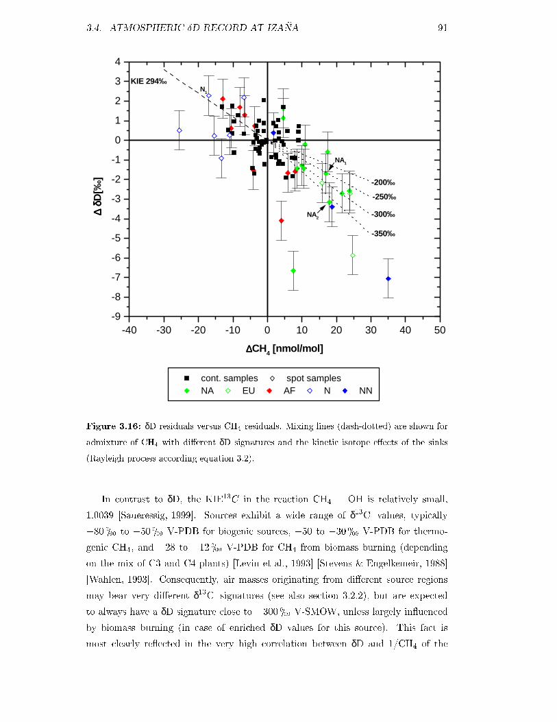
3.4. ATMOSPHERIC ÆD RECORD AT IZAÑA 91
-40 -30 -20 -10 0 10 20 30 40 50-9
-8
-7
-6
-5
-4
-3
-2
-1
0
1
2
3
4
NA2
NA1
N1
-350‰
-300‰
-250‰
-200‰
KIE 294‰
cont. samples spot samplesNA EU AF N NN
∆∆ ∆∆δδ δδD
[‰]
∆∆∆∆CH4 [nmol/mol]
Figure 3.16: δD residuals versus CH4 residuals. Mixing lines (dash-dotted) are shown for
admixture of CH4 with di�erent δD signatures and the kinetic isotope e�ects of the sinks
(Rayleigh process according equation 3.2).
In contrast to δD, the KIE13C in the reaction CH4 + OH is relatively small,
1.0039 [Saueressig, 1999]. Sources exhibit a wide range of δ13C values, typically
�80 0=00 to �50 0=00 V-PDB for biogenic sources, �50 to �30 0=00 V-PDB for thermo-
genic CH4, and �28 to �12 0=00 V-PDB for CH4 from biomass burning (depending
on the mix of C3 and C4 plants) [Levin et al., 1993] [Stevens & Engelkemeir, 1988]
[Wahlen, 1993]. Consequently, air masses originating from di�erent source regions
may bear very di�erent δ13C signatures (see also section 3.2.2), but are expected
to always have a δD signature close to �300 0=00 V-SMOW, unless largely in�uenced
by biomass burning (in case of enriched δD values for this source). This fact is
most clearly re�ected in the very high correlation between δD and 1/CH4 of the

92 CHAPTER 3. SEASONAL CYCLES OF ATMOSPHERIC CH4
0.550 0.555 0.560 0.565 0.570 0.575 0.580 0.585-90
-88
-86
-84
-82
-80
-78
-76
-74
Lin. fit cont m=0.271+/-0.034 (R2=0.54, n=54)
cont. samples FFT fit (cont. 1998)N NN EU NA AF
δδ δδ Dde
tren
ded
1/CH4 detrended
Figure 3.17: δD-1/CH4 correlation for spot and 2-week-continuous samples. From the
CH4 and δD values a small linear trend has been subtracted. The plotted ellipse is based
on the FFT �t through continuous samples from 1998 which have also been detrended.
spot samples (R2 = 0:74), compared to a correlation coe�cient of R2 = 0:10 for the
corresponding δ13C -1/CH4 correlation.
The compact δD-1/CH4 correlation de�nes the slope of the linear regression rel-
atively precisely. Using the regression through the continuous samples, we derive
an average KIE of 1:23 � 0:04. Since this value re�ects the seasonal (rather than
synoptic scale) δD variation, and mixing within the hemispheres occurs relatively
fast (time scale a few weeks to months), this estimate can be considered to be repre-
sentative at least for the Northern Hemisphere. In contrast, the value derived from
the regression through the spot samples may to a larger extent be in�uenced by the
source and sink areas relevant for Izaña, such as North America and Europe (CH4
sources) or the North Atlantic and Africa (CH4 sinks). The result of the regression
through the spot samples, KIEDavg = 1:24 � 0:03 is, however, virtually identical to

3.5. COMPARISON TO MODEL RESULTS 93
the result derived from the continuous samples.
3.5 Comparison to model results
In order to simulate the global distribution of CH4 mixing ratios, δ13C and δD, ourmeasurements from Izaña were used in a three-dimension inverse model by Berga-
maschi et al. [2000a]. This study used the �rst two years of our CH4 records
(1996 to 1998) together with data from a number of other sources. Observational
data for CH4 mixing ratios were taken from the NOAA/CMDL network (38 sta-
tions) [D. Dlugokencky, data retrieved from ftp:// ftp.cmdl.noaa.gov/ccg/CH4/].
For δ13C records from Scott Base (Antarctica), Baring Head (New Zealand)(data of
the National Institute of Water and Atmospheric Research (NIWA), New Zealand
[Lowe et al., 1999]), Pt. Barrow (Alaska), Olympic Peninsula (Washington) and
Mauna Loa (Hawai) [P. Quay, University of Washington, Seattle, data retrieved
from Carbon Dioxide Information Analysis Center, Oak Ridge, Tennessee, USA,
http://cdiac.esd.ornl.gov/ndps/quay.html] were used. For δD only the data from
Izaña was included.
The model setup is similar to the one used by Hein et al. [1997]. Atmospheric
transport is simulated with the TM2 model [Heimann, 1996], with a horizontal res-
olution of � 8Æ latitude by 10Æ longitude, and 9 layers in the vertical dimension.
Meteorological �elds (advection, and subgridscale vertical transport) are based on
12-hourly ECMWF (European Community Medium Range Weather Forecast) an-
alyzes for the year 1987. For the treatment of the isotopic composition the TM2
was con�gured for three tracers, representing the principal isotopomers of methane,
12CH4,13CH4,
12CH3D (with a mean abundance as listed in table 1.4.1 of 98.8%,
1.1%, and 0.06%, respectively).
The principal CH4 sources considered are swamps, bogs, rice paddies, domestic
animals (incl. animal waste), biomass burning (separated into forest and savanna
burning), land�ll sites, and fossil fuel related emissions (separated into coal, oil/gas,
and Siberian gas). The spatio-temporal emission patterns used for these sources were
as described by Hein et al. [1997], except for bogs and biomass burning, for which
the distributions of Fung et al. [1991] and [Hao & Liu, 1994] were used respectively.
Possible small δ13C calibration o�sets among the three δ13C laboratories were
treated as additional parameters to be optimized by the inversion. A posteriori
results for these calibration o�sets were, however, not signi�cantly di�erent from
zero. Together with Marik [1998] this was the �rst time δD measurements were
included for a better understanding of the methane budget.

94 CHAPTER 3. SEASONAL CYCLES OF ATMOSPHERIC CH4
Figure 3.18: Comparison of observational data with results from an inverse model
[Bergamaschi et al., 2000a]: (a) CH4 mixing ratios, (b) δ13C , and (c) δD. Model results are
given as monthly mean values (solid line) and standard deviation (1�) of daily model data
(shaded area). Observational data are detrended and their monthly mean values are shown
as black bars, with the error bars representing the 1� standard deviation from the �tted
curve.

3.5. COMPARISON TO MODEL RESULTS 95
Figure 3.18 shows the results from the inverse model along with the observa-
tional data from Izaña. Model data are given as monthly mean values (solid line)
�1� standard deviation of the daily data (shaded area). Observational data are
detrended and their monthly mean values are shown as black bars, with the error
bars representing the 1� standard deviation from the �tted curve (over the 2-year
record 1996 - 1998). Both spot and continuous samples were used in this case, with
a stronger weight on the continuous samples in the �t procedure (by a factor of
2; thus in this representation the mean seasonal cycle is mainly determined by the
continuous samples, but the given standard deviation by the spot samples). The
�gure shows the excellent agreement between inverse model and observational data
for CH4 mixing ratios, δ13C , and δD. Note that also the phase behavior of CH4,
δ13C , and δD is exactly reproduced by the model, i.e. a time lag of two months
between δ13C maximum and CH4 minimum, and a coincidence of δD maximum and
CH4 minimum.
Another output of the model was the calculation of the contribution of the indi-
vidual sources on the seasonal cycles. In Figure 3.19 this is shown for CH4 mixing
ratios, δ13C and δD. The seasonal CH4 cycles of the sources with assumed constant
emissions throughout the year (animals, waste, and fossil sources) are mainly in�u-
enced by the seasonality of the OH sink, while in particular CH4 from bogs, rice
paddies and biomass burning show a signi�cantly di�erent phase behavior, largely
determined by their emission seasonality. The sum of all individual sources is shown
in black (and equals the seasonal CH4 cycle shown in Figure 3.18). For δ13C and
δD the contribution of the individual sources is given in Figure 3.19 b and 3.19 c as:
[δj(t)� δavg ] � fj(t)� const (3.4)
with δj(t) representing the modeled isotopic signature of source j at the observa-
tional site at time t (as determined by the original isotopic signature of the emission
and the KIEs of the sinks during the transport to Izaña), δavg the annual mean value
of the total Æ at the station, fj(t) the relative contribution of source j (as determined
from modeled CH4 mixing ratios) and const an o�set chosen so that the integral over
(3.4) becomes zero. Again, the sum of the individual sources is shown in black. For
δ13C , the most prominent seasonal cycle is seen for bogs, with an overall amplitude
of about 50% of the total seasonal δ13C cycle. This large in�uence is mainly due
to the signi�cantly increasing CH4 mixing ratios from this source in autumn (Figure
3.18 a), combined with its relatively low δ13C (a posteriori δ13C = �64:2� 2:8 0=00).
As for CH4 mixing ratios, a signi�cant contribution to δ13C also arises from rice
paddies. In contrast to CH4, however, biomass burning exhibits a much more pro-
nounced in�uence, due to its very enriched δ13C values. This component has indeed

96 CHAPTER 3. SEASONAL CYCLES OF ATMOSPHERIC CH4
Figure 3.19: Contribution of the di�erent sources to the modeled seasonal cycles
[Bergamaschi et al., 2000a] of (a) CH4 mixing ratios, (b) δ13C , and (c) δD. The black
curves represent the sums of the individual sources and equal the seasonal cycles shown in
Figure 3.18. (d) δ13C enrichment of CH4 from the individual sources. (e) δD enrichment of
CH4 from the individual sources.

3.6. CONCLUSION 97
a signi�cant impact on the overall δ13C seasonality. Test runs performed with the
biomass burning source strength set to zero showed a δ13C maximum only one month
prior to the CH4 minimum. In contrast to δ13C , the relative in�uence of biomass
burning is much weaker on δD, while again bogs and rice paddies constitute the
two sources with the largest impact. The results shown in Figure 3.19 refer to an
inversion with an a posteriori δD value from biomass burning of �203 � 20 0=00. In
general, the behavior of the individual sources and the overall δD seasonal cycles
largely mirrors the behavior seen for CH4 mixing ratios.
Finally, in Figure 3.19 the isotopic enrichment in the CH4 of the individual sources
(corresponding to equation 4.1 in 4.5) can be seen, re�ecting the integrated in�uence
of the sinks (i.e. mainly OH) during the transport from the source areas to the
station (Figure 3.19). CH4 from savanna burning undergoes the strongest isotopic
enrichment on its way from the tropical emission regions (with high OH concentra-
tions) to Izaña. In contrast, CH4 from fossil sources and land�lls exhibit a relatively
week isotopic enrichment, since it encounters less OH during its transport from mid
latitudes of the northern hemisphere to Izaña. The largest seasonal cycle is evident
for bogs, with the emission peak in late summer constituting a source of fresh (i.e.
little enriched) CH4, which later undergoes signi�cant isotopic enrichment.
3.6 Conclusion
Izaña is located at 28Æ N, where trace gases, such as CH4 and SF6 exhibit large latitu-
dinal gradients. Furthermore, Izaña is directly in�uenced by sources from the North
American continent, and to a lesser extent by European sources. Consequently, at-
mospheric CH4 mixing ratios show considerable variability, with short term synoptic
scale variations often exceeding the mean seasonal cycle. In order to de�ne the mean
seasonal cycle, continuous air sampling proved to be very helpful, while exclusive spot
sampling at a 2-week frequency would provide an only fragmentary picture at this
station. Signi�cant seasonal cycles of δ13C and δD were detected, with peak-to-peak
amplitudes of 0.2 0=00 and 3.5 0=00, respectively. δ13C shows a signi�cant phase shift
with respect to CH4 mixing ratios, resulting in an 'elliptical' behavior in the phase
diagrams, attributed to a seasonally varying source mixture. In contrast, δD showed
a compact correlation with inverse CH4 mixing ratios, allowing an estimate of the
average KIE of atmospheric sinks of 1:23 � 0:04. This apparent KIE is consistent
with recent measurement of the KIE in the CH4 + OH reaction [Saueressig, 1999],
resulting in an average KIE of 1:28�0:01, when corrected for a small in�uence of the
soil sink. Application of an 3-D inverse model allowed an excellent reproduction of

98 CHAPTER 3. SEASONAL CYCLES OF ATMOSPHERIC CH4
observed mean seasonal cycles of CH4, δ13C , and δD, including their phase behavior.Thus the isotopic information (atmospheric records, source signatures, and kinetic
isotope e�ects of the sinks) can be regarded as consistent with our present knowledge
of the atmospheric CH4 cycle and its description in the model. Visualization of the
contribution of the individual sources showed the signi�cant in�uence of bogs and
rice paddies on CH4, δ13C , and δD at Izaña, and in addition a signi�cant in�uence
of biomass burning on δ13C . Observed short term variations of CH4 mixing ratios
could be clearly linked to changing synoptic situations, leading to the advection of
very di�erent air masses. Further evidence for the in�uence of transport on CH4
mixing ratios arose from the signi�cant correlation between CH4 and SF6 residuals.
The American continent and Europe act as signi�cant CH4 and SF6 sources, while
air masses from Africa and the North Atlantic usually showed depleted mixing ra-
tios of these trace gases. Isotope analysis helped to identify di�erent CH4 sources
such as the Canadian wetlands or the industrialized regions of the United States and
Southeastern Canada. At stations as Izaña, which are subject to direct in�uence
from sources and sinks, measurements of short term variations may be utilized to
infer integrated sources or sink strengths, when combined with high resolution at-
mospheric transport models with an exact model meteorology for the time period of
observations.

Chapter 4
Seasonal cycles of atmospheric CO
In this chapter we present the Izaña records of CO and its isotopes, δ13C , δ18Oand 14CO, from July 1996 to August 1999. These are the �rst long term records
of the isotopic composition of CO at subtropical latitudes. We infer seasonal cycles
as well as interannual variations of CO mixing and isotopic ratios for the three-year
period analyzed during this research period. Air masses sampled at Izaña have a
wide range of latitudinal and longitudinal origins (chapter 3). We therefore use
back-trajectories to discuss the large synoptic scale variations encountered for CO
and its isotopes. Most of the time clean tropospheric conditions are encountered at
the Izaña observatory.
The Izaña records of the stable CO isotopes, δ13C and δ18O , have been used
together with CO isotope records from four other globally distributed stations in an
inverse model study by Bergamaschi et al. [2000b]. Through optimization of the
agreement between modeled and measured mean annual CO mixing and isotopic
ratios, estimations of the CO budget as well as the isotopic signature of di�erent CO
sources have been improved. The main results of this study concerning the Izaña
records are summarized in section 4.5.
Finally we compare the Izaña records to CO isotope measurements done at a
number of other stations. At Spitsbergen, a remote station at high northern lat-
itude, CO isotope measurements have already started in 1995. We also use CO
isotopes records from UBA Schauinsland, Germany, and Sonnblick, Austria, which
are representative for continental stations at mid latitudes. In contrast more polluted
air masses have been encountered at Kollumerwaard, The Netherlands, and during
the BERLIOZ campaign in summer 1998, for which CO, δ13C , δ18O and 14CO have
been investigated.
99

100 CHAPTER 4. SEASONAL CYCLES OF ATMOSPHERIC CO
4.1 Atmospheric CO mixing ratios at Izaña
The meteorological situation of the Izaña station has been discussed in detail in the
previous chapter. Its location on the Island of Tenerife at 2370 m altitude allows the
sampling of air from the free troposphere, especially during night time when inversion
layers shield the observatory from the marine boundary layer and locally polluted air
masses from the island. We consider the seasonal cycles and annual trends derived
from our three-year record of atmospheric CO and its isotopes (section 4.1 to 4.4)
to be representative for the subtropical North Atlantic. The large synoptic scale
variations occurring in the spot sample measurements are classi�ed with the help
of their corresponding back-trajectories. We smooth the data sets for CO mixing
ratios, δ13C , δ18O and 14CO (based on the spot and 2-week-continuous samples)
by applying a low pass convolution �lter in the frequency domain (by Fast Fourier
Transformation (FFT)). Both the classi�cation of spot samples and the FFT �ts are
done in the same way as for CH4 in the previous chapter. The 3-year record of CO
mixing ratios measured on spot and continuous samples are shown in Figure 4.1.
The spot samples are attributed to �ve di�erent sectors as discussed in section 3.2.2,
e.g. the American continent, Europe, Africa and the North Atlantic (low and high
latitudes). A FFT �t with a �lter of four weeks (see equation 3.1) is applied to both
data sets of CO mixing ratios, e.g. our spot and continuous samples. With the help
of these �t curves we discuss the seasonal cycles and inter-annual trends observed
over the three years of our analysis. While both �ts display a similar picture for the
evolution of CO mixing ratios, some di�erences are also apparent.
Comparing the �ts through our spot and continuous samples it is remarkable
that, despite of the large degree of variability of the spot samples, the two �ts agree
very well from November 1996 to February 1998. Only during spring 1998 �t curves
di�er by 15 nmol/mol because of spot samples with very low CO mixing ratios while
no spot samples with higher mixing ratios than the continuous samples have been
encountered. Flasks sampled in June/July 1998 by the NOAA/CMDL network (dis-
cussed below) captured events of signi�cantly higher (� CO >30nmol/mol) CO
mixing ratios. This explains the consistently higher CO mixing ratios of the contin-
uous samples compared to our spot samples during this period.
From July to October 1998 a signi�cant contamination of the continuous samples
of up to 15 nmol/mol was observed. For these samples problems have occurred
during the transfer of the air sample from the bags into the cylinders (see section
2.1.4). In Figures 4.1 to 4.10 these contaminated continuous samples are labeled.
They are omitted in the calculation of FFT �t curves. In November 1998 the �lling

4.1. ATMOSPHERIC CO MIXING RATIOS AT IZAÑA 101
1996 1997 1998 199940
60
80
100
120
140
160
180
cont. samples fit cont. contaminatedspot samples fit spotNA EU AF N NN
CO
[nm
ol/m
ol]
date
Figure 4.1: Record of CO mixing ratio at Izaña. 2-week-continuous samples and spot
samples are shown together with �t curves (FFT with a 4-week �lter). With the help
of back trajectories the spot samples are attributed to �ve sectors: North America (NA),
Europe (EU), Africa (AF) and North Atlantic (low (N) and high (NN) latitudes).
procedure of the continuous samples has been checked and the agreement between
the �t curves calculated for spot and continuous samples is again very good. We
note that the motivation for taking continuous samples at Izaña was to enable us
to extract background values at this station which is known for its large synoptic
scale variations. The good agreement between background CO values derived from
continuous and spot samples with the help of the FFT �ts was unexpected. Thus
background CO mixing ratios representative for the subtropics can be inferred from
spot samples (taken biweekly) after an appropriated smoothing of the data. For
the following discussion of the seasonal cycles, synoptic scale variations and annual
trends we will refer to the FFT �t through our spot samples.

102 CHAPTER 4. SEASONAL CYCLES OF ATMOSPHERIC CO
4.1.1 Seasonal cycles and interannual variations
The seasonal cycle of CO mixing ratios with its minimum in late summer and its
maximum during winter/spring is mainly due to the seasonality of its main sink, i.e.
oxidation by OH. The high OH concentrations during summer reduce the lifetime of
CO to a few weeks compared to an average lifetime of two to three months during
winter.
For the three-year period of our study signi�cant interannual variations were
encountered. During the maximum in winter/spring 1997/1998 and the minimum
in late summer 1998 CO mixing ratios were above the corresponding values one
year earlier by 30 nmol/mol and 20 nmol/mol respectively. This strong increase in
CO mixing ratios is not maintained during the third seasonal cycle. The maximum
in late 1998 and early 1999 with around 130 nmol/mol and the minimum in late
summer 1999 with 70-80 nmol/mol are closer to the values before 1998. The cal-
culated trend of the CO mixing ratio for the period from June 1996 to June 1999
is +9.1�4:8 %=yr(derived from the running mean through the FFT �t). This very
high trend of the CO mixing ratio is mainly due to the huge increase between 1997
and 1998.
The strong interannual variations in the seasonal cycles are also re�ected in the
corresponding peak-to-peak amplitudes. The amplitudes of the seasonal cycles in
1996/1997 and 1997/1998 nearly increased by a factor of two, from � 35nmol/mol to
� 70 nmol/mol respectively. In the following section 4.2 we discuss possible scenarios
explaining the exceptionally high CO growth rates in 1998.
4.1.2 Comparison to NOAA/CMDL CO measurements
We compare our three year record of CO mixing ratios to measurements from the
NOAA/CMDL monitoring network starting at Izaña in 1991 [Novelli et al., 1998a].
Both data sets are shown in Figure 4.2 together with their respective FFT �t curves
(four-week �lter). Based on the FFT �t curves we note the general good agreement
between both data sets. Some discrepancies are nevertheless apparent which could
re�ect a di�erence in the reference scales as well as the natural variability of CO
mixing ratios due to the large synoptic scale variations at Izaña occurring on time
scales of less than 24 h. The MPI samples and the NOAA/CMDL samples have not
been collected at the same time. A direct inter-comparison between our spot samples
and the NOAA/CMDL �asks is therefore questionable even for the few occasions on
which they were both taken on the same day. During the winter/spring plateaus
di�erences between the two �ts are mainly due to the variability of mixing ratios of

4.1. ATMOSPHERIC CO MIXING RATIOS AT IZAÑA 103
1991 1992 1993 1994 1995 1996 1997 1998 199940
60
80
100
120
140
160
180
200
MPI spot samples FFT fit MPI spot samplesNOAA/CMDL data FFT fit NOAA/CMDL
CO
[nm
ol/m
ol]
date
Figure 4.2: Records of CO mixing ratios at Izaña. MPI spot samples and measurements
from the NOAA/CMDL monitoring network are plotted together with �t curves (FFT with
a 4-week �lter).
up to 40 nmol/mol seen in both data sets.
It is, however, apparent that for all four summer minima the NOAA/CMDL
�asks are on average lower. We compared the FFT �ts from both data sets for the
four summer periods between June and October (1996-1999). On average the FFT
�t through the NOAA/CMDL measurements lies 7.7%�3.8% below the �t through
the MPI data. Thus from this three year inter-comparison of CO mixing ratios no
systematic di�erence appears in the 100-170 nmol/mol range whereas there is a clear
di�erence in the 50-100 nmol/mol range. This con�rms results from two laboratory
inter-comparison organized by NOAA/CMDL in 1994 and 1999 [Novelli et al., 1994]
[Brenninkmeijer et al., 2000]. In this inter-comparison CO mixing ratios based on
relative measurements using NOAA/CMDL standards have been consistently lower
by 8.2% in the 50 nmol/mol range than absolute measurements of CO mixing ratios
at NIWA [Novelli et al., 1998a] and MPI [Brenninkmeijer et al., 2000]. The drift in

104 CHAPTER 4. SEASONAL CYCLES OF ATMOSPHERIC CO
the NOAA CO scale is discussed in Masari et al. [2000].
Novelli et al. [1998a] reported for the globally-averaged CO mixing ratio a de-
crease of approximately 2 nmol/mol yr�1 in the long term trend for the period from
1990 through 1995. The reasons for this decrease in mixing ratios in the background
atmosphere are not yet fully understood (see section 1.6). The period of decreasing
CO mixing ratios is also seen in the Izaña record shown in Figure 4.2. Thus the large
increase of CO mixing ratios in 1998 observed in our study has been exceptional for
the 1990s and marked a change in the previously decreasing growth rates.
4.1.3 Synoptic scale variations
The synoptic scale variations of the spot samples which have already been discussed
for the CH4 mixing ratios (section 3.2.2) are also signi�cant for CO. During all
three winters subsequently taken spot samples can di�er by more than 40 nmol/mol.
These large variations in CO mixing ratios often re�ect the impact of source regions,
as can be seen from the corresponding back-trajectories. We note, however, that the
latitudinal gradient in CO mixing ratios reaches its maximum during winter. This
e�ect is seen for two samples taken on the 12th and 24th of April in 1998 which di�er
by 40 nmol/mol. While the air of the �rst sample came from the high North Atlantic
(>60Æ N), air masses for the second traveled for several days between 20Æ and 40Æ
N. Their mixing ratios of 140 nmol/mol and 100 nmol/mol are close to background
values for their respective latitudinal origin (see Figure 1.6 in section 1.7.1).
As the latitudinal gradient in CO mixing ratios is smaller during summer, syn-
optic scale variations are less pronounced. Still mixing ratios of subsequent samples
can di�er by more than 10 nmol/mol. We note that samples of African or low North
Atlantic origin are far more frequent during the summer months (70% from sectors
AF and N during June-October for the years 1996-1998), than samples attributed
to the Northern sectors, e.g. NA, NN and EU. This pattern is con�rmed by the
statistical analysis of AEROCE back-trajectories for the years 1991 to 1997 done by
Schäfer [1997]. The main results of this study have been summarized in section 3.1.2.
Figure 3.2 shows that the in�uence from the North American continent on air masses
reaching Izaña is less important from June to October than for the winter and spring
months. Under most conditions the Izaña station is meteorologically separated from
Europe [Armerding et al., 1997]. Only during few episodes do we see the impact of
European emissions (mainly in winter/spring 1998/1999).
In order to quantify the synoptic scale variations we calculate the residuals (�
CO) of the spot samples. As de�ned in section 3.2.2 we calculate the di�erence
between measured mixing ratios and the value of the FFT �t curve (representing

4.1. ATMOSPHERIC CO MIXING RATIOS AT IZAÑA 105
-50 -40 -30 -20 -10 0 10 20 30 40 50-0.15
-0.10
-0.05
0.00
0.05
0.10
0.15
AF
NNN
NA
EU
fit spot m=0.0026+/-0.0004 (R2=0.34, n=71)
cont. samples contaminated spot samplesNA EU AF N NN
∆∆ ∆∆ SF 6
[pm
ol/m
ol]
∆∆∆∆CO [nmol/mol]
Figure 4.3: CO residuals versus SF6 residuals for spot and 2-week-continuous samples. A
linear �t through the spot samples is applied. The average values (�1� range) for samples
from North America (NA), Europe (EU), Africa (AF) and North Atlantic (low (N) and high
(NN) latitudes) are also indicated (according to Table 4.1).
the mean annual cycle) at the time of sampling. In table 4.1 the � values for CO
and SF6 mixing ratios are listed for spot samples from the di�erent sectors. The
residuals calculated for δ13C , δ18O and 14CO are also given and will be discussed
in the following sections. We plot the �SF6 against the �CO residuals in Figure 4.3
and a clear relationship between the origin of air masses from one of the �ve sectors
and the residuals is apparent.
The enhancements/depletions are directly linked to the source/sink strengths in
the respective sectors. As in the case of CH4 and SF6, North America and Europe
act as a CO source, while air masses from the North Atlantic (0Æ to 50Æ N) and
Africa are generally depleted, largely due to dilution and also to some extent due to
chemical destruction. The simpli�ed calculation of trace gas �uxes done in section

106 CHAPTER 4. SEASONAL CYCLES OF ATMOSPHERIC CO
� CO � δ13C � δ18O � 14CO � SF6 n
[ nmol/mol ] [ 0=00 ] [ 0=00 ] [molec./cm3 ] [ pmol/mol ]
NA +3:4� 6:8 +0:3� 0:5 +0:6 � 0:8 +0:6 � 1:0 +0:04� 0:03 22
EU +18:8 � 7:6 +0:4� 0:3 +2:2 � 0:7 +2:4 � 1:6 +0:08� 0:03 6
AF �2:6� 6:9 �0:2� 0:4 �0:4 � 1:0 �0:3 � 0:8 �0:02� 0:03 25
N �13:4 � 7:2 �0:5� 0:5 �1:8 � 1:0 �2:6 � 1:5 �0:04� 0:04 16
NN +10:1 � 8:7 +0:2� 0:5 +1:5 � 1:2 +2:7 � 1:3 +0:02� 0:05 8
Table 4.1: Residuals of CO mixing and isotopic ratios together with SF6 residuals for
spot samples. The average � values are given together with �1� standard deviations and
the number of samples n from North America (NA), Europe (EU), Africa (AF) and North
Atlantic (low (N) and high (NN) latitudes).
3.2.2 (average residence time of 1 to 3 days over the source region and a mixing
height of 1 to 12 km) gives for CO residuals of 10 nmol/mol a corresponding source
strength of 1.2 to 5.8 mgCOm�2 h�1.
Both e�ects, the in�uence of source regions of the North American and Euro-
pean continent and the latitudinal gradients for CO mixing ratios lead to the ob-
served correlation of CO and SF6 residuals. For the regression through the spot
samples (Figure 4.3) we obtain a slope of +0.0026�0.004 pmol/mol SF6 ( nmol/mol
CO)�1 (R2=0.34, n=34). With the extremely di�erent lifetimes of SF6 and CO it
is not surprising that the ratio between both interhemispheric gradients can vary
between 0.002 and 0.01 pmol/mol SF6 ( nmol/mol CO)�1 during winter and summer
respectively.
4.2 Atmospheric Æ18O record from Izaña
Three annual cycles of the isotopic composition of atmospheric CO have been mea-
sured at Izaña during this thesis. In Figure 4.4 the δ18O record is shown. Again
FFT �ts (with a 4-week �lter) are applied through the 2-week-continuous samples
and spot samples.
4.2.1 Seasonal cycles and interannual variations
For δ18O we observe a similar seasonal cycle as for the CO mixing ratios. The min-
ima and maxima during winter/spring and summer respectively are in phase with
the CO mixing ratios. The δ18O cycle is mainly driven by the OH seasonality and
the heavy technological source (δ18O value of +23.5 0=00 [Stevens & Krout, 1972] and
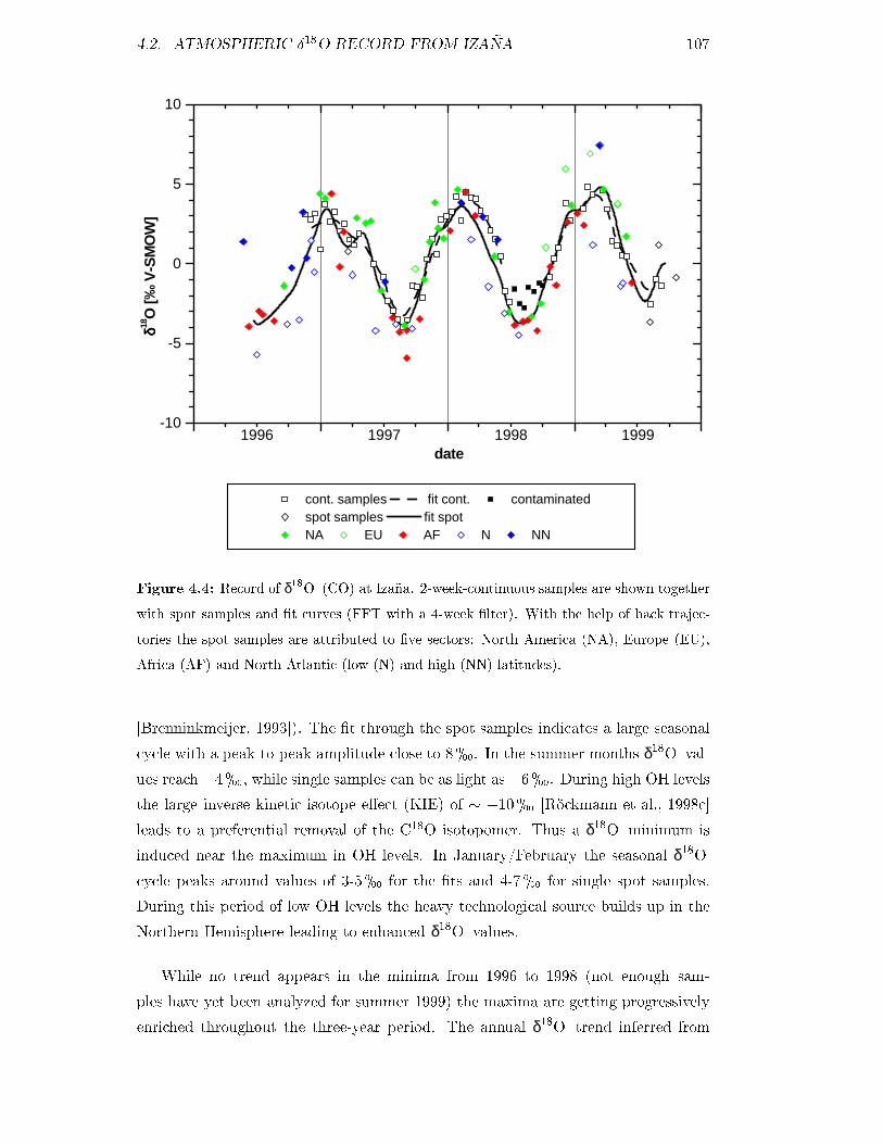
4.2. ATMOSPHERIC Æ18O RECORD FROM IZAÑA 107
1996 1997 1998 1999-10
-5
0
5
10
cont. samples fit cont. contaminatedspot samples fit spotNA EU AF N NN
δδ δδ18O
[‰V
-SM
OW
]
date
Figure 4.4: Record of δ18O (CO) at Izaña. 2-week-continuous samples are shown together
with spot samples and �t curves (FFT with a 4-week �lter). With the help of back trajec-
tories the spot samples are attributed to �ve sectors: North America (NA), Europe (EU),
Africa (AF) and North Atlantic (low (N) and high (NN) latitudes).
[Brenninkmeijer, 1993]). The �t through the spot samples indicates a large seasonal
cycle with a peak-to-peak amplitude close to 8 0=00. In the summer months δ18O val-
ues reach �4 0=00, while single samples can be as light as �6 0=00. During high OH levels
the large inverse kinetic isotope e�ect (KIE) of � �10 0=00 [Röckmann et al., 1998c]
leads to a preferential removal of the C18O isotopomer. Thus a δ18O minimum is
induced near the maximum in OH levels. In January/February the seasonal δ18Ocycle peaks around values of 3-5 0=00 for the �ts and 4-7 0=00 for single spot samples.
During this period of low OH levels the heavy technological source builds up in the
Northern Hemisphere leading to enhanced δ18O values.
While no trend appears in the minima from 1996 to 1998 (not enough sam-
ples have yet been analyzed for summer 1999) the maxima are getting progressively
enriched throughout the three-year period. The annual δ18O trend inferred from

108 CHAPTER 4. SEASONAL CYCLES OF ATMOSPHERIC CO
40 60 80 100 120 140 160 180-10
-8
-6
-4
-2
0
2
4
6
8
10
autumn
spring
winter
summer
cont. samples 96 spot samples 96 FFT fit (spot 96)cont. samples 97 spot samples 97 FFT fit (spot 97)cont. samples 98 spot samples 98 FFT fit (spot 98)cont. samples 99 spot samples 96 FFT fit (spot 99)
δδ δδ18
O[‰
V-S
MO
W]
CO [nmol/mol]
Figure 4.5: δ18O values for continuous and spot samples are plotted against CO mixing
ratios. The samples and calculated FFT �t curves (spot samples) are labeled for the four
di�erent years 1996 to 1999.
the FFT �t through the spot samples for the period of June 1996 to June 1999 is
+0.43�0:40 0=00 yr�1. No signi�cant di�erence between the �t curves through the
smooth record of continuous samples and the by far more scattered spot samples can
be observed in Figure 4.4. The contaminated continuous samples in summer 1998
(see previous section) are not included in the �t calculation.
In Figures 4.5 the δ18O values of the continuous and spot samples are plotted
against CO mixing ratios. We di�erentiate between samples of the four years 1996
to 1999 of our study. The FFT �t curve calculated for the spot samples is also shown
for the four di�erent years.
The apparent correlation between CO mixing ratios and δ18O underlines the

4.2. ATMOSPHERIC Æ18O RECORD FROM IZAÑA 109
similarity of the two seasonal cycles. Nevertheless, we observe an ellipsoid-shaped
curve for a given year. The transitions from winter to summer and summer to winter
are slightly di�erent. For a given CO mixing ratio, the corresponding δ18O values are
1 to 2 0=00 lower in spring than in autumn. This implies a small phase shift between
the two seasonal cycles, caused either by a seasonality of CO and δ18O sources or
sinks. In section 4.5 the underlying reason for this small phase shift between CO
and δ18O will be discussed together with results obtained by the inverse CO model
study [Bergamaschi et al., 2000b].
The other interesting feature in Figure 4.5 are the observed interannual di�er-
ences. It has already been apparent in the seasonal cycles shown in Figures 4.1 and
4.4 that CO mixing ratios and δ18O variations were very di�erent in 1998 compared
to 1997 and 1999. In Figure 4.5 the positive trend towards higher CO mixing ratios
from 1996 to 1998 can be seen, while values for 1999 are closer to those from 1997.
For δ18O this results in approximately 2 0=00 lower δ18O values for a given CO mix-
ing ratio in 1998 compared to 1997 or 1999. With the simple 1-box model presented
in section 1.6 we calculated the change in OH concentrations necessary for a 1 0=00
decrease in δ18O . Assuming OH concentration of 106molec./cm3, OH levels would
need to increase by 15% in order to explain the observed shift. With present inter-
annual OH variations supposedly of the order of � 0:5% [Krol et al., 1998] the more
than 2 0=00 lower δ18O values of 1998 relative to 1997 and 1999 can not be explained
by a change in the sink process. Thus an important change in CO sources is a more
likely explanation for our observations.
The most plausible explanation are the intense biomass burning events occurring
in late 1997 and early 1998 in the tropics [Levine, 1999]. The atmospheric disequilib-
rium caused by this sudden increase in source activity could explain why unusually
high CO mixing ratios have been measured up until the minimum of the seasonal
cycle in 1998. Even if the source signature of biomass burning is around +10 0=00,
high OH levels in the tropics would reduce the original high δ18O values due to the
inverse KIE of �10 0=00. Nevertheless, the same feature of lower δ18O values for a
given CO mixing ratio in 1998 have also been observed at higher latitudes (at the
Sonnblick observatory in Austria (47Æ N, 13Æ E) [Gros et al., 2000] and at Spitsber-
gen (79Æ N, 12Æ E) [Röckmann et al., manuscript in preparation]). Even intense
biomass burning events in the tropics cannot account for the observed increase of
nearly 30 nmol/mol in the CO mixing ratios at Spitsbergen during the summer min-
imum from 1997 to 1998 (see section 4.6). Thus also emissions from the biomass
burning source at higher latitudes (>30Æ N) which can signi�cantly �uctuate from
one year to the other [Dywer & Gregoire, 1998] should be considered.

110 CHAPTER 4. SEASONAL CYCLES OF ATMOSPHERIC CO
-40 -30 -20 -10 0 10 20 30 40-5
-4
-3
-2
-1
0
1
2
3
4
5
fit spot m=0.12+/-0.01 (R2=0.83, n=78)
cont. samples spot samples contaminatedNA EU AF N NN
∆∆ ∆∆ δδ δδ18
O[‰
V-S
MO
W]
∆∆∆∆CO [nmol/mol]
Figure 4.6: Residuals calculated for CO mixing ratios and δ18O for continuous and spot
samples are plotted together with respective linear �ts. With the help of back trajectories
the spot samples are attributed to �ve sectors: North America (NA), Europe (EU), Africa
(AF) and North Atlantic (low (N) and high (NN) latitudes).
4.2.2 Synoptic scale variations
Next, we address the signi�cant synoptic scale variations in δ18O that can exceed
2 0=00 during summer and 5 0=00 during winter/spring. The reason for the large vari-
ations during maximum δ18O values in January to March are similar to those al-
ready discussed for CO mixing ratios in the previous section. The latitudinal gra-
dient for δ18O is largest during this period (see Figure 4.16), with typical values
of 2 0=00 at low latitudes and � 8 0=00 at high latitudes of the Northern Hemisphere
[Bergamaschi et al., 2000b]. In Table 4.1 the �δ18O residuals for air samples from
the di�erent sectors are given and are plotted against �CO mixing ratio residuals in
Figure 4.6.

4.3. ATMOSPHERIC Æ13C RECORD FROM IZAÑA 111
Again a clear relationship exists between the origin of air masses from one of the
�ve sectors and the residuals. Air masses from low latitudes, e.g. low North Atlantic
(N) and Africa (AF), are considerably depleted by �1:8� 1:0 0=00 and �0:4 � 1:0 0=00
respectively. In contrast, air masses from the North (North American continent
(NA), Europe (EU) and the high North Atlantic (NN)) are signi�cantly enriched
by +0:6 � 0:8 0=00, +2:23 � 0:7 0=00 and +1:5 � 1:2 0=00 respectively. These enhance-
ments/depletions are directly linked to the source/sink strength in the respective
regions. The positive � δ18O residuals from Northern source regions are due to the
(dominating) heavy technological source. In contrast, in the tropical and subtropical
regions, apart from biomass burning, light sources dominate and are further depleted
in the OH sink process. For the regression through the spot samples we obtain a slope
of +0.121�0.006 0=00/ nmol/mol (R2=0.83, n=78). This is close to values calculated
from North hemispheric CO and δ18O gradients for summer (�20 nmol/mol, �3 0=00)
and winter (�60 nmol/mol, �6 0=00) of 0.15�0:02 0=00 ( nmol/mol)�1 and 0.1�0:2 0=00
( nmol/mol)�1 respectively. Thus for air masses of varying latitudinal origin the
strong latitudinal CO and δ18O gradients at the latitude of Izaña lead to highly
correlated variations of these tracers.
4.3 Atmospheric Æ13C record from Izaña
The main characteristics of the δ13C record shown in Figure 4.7 are the relatively
smooth records for continuous and spot samples compared to those from CO mixing
ratios and δ18O . On the other hand, large di�erences are observed for the position
of the summer minima over the 3-year period. We note that, despite of the good
agreement between the FFT �ts through the spot and continuous samples, the four
week �lter does not catch the sharp summer minima as well as desirable. For the
calculation of the seasonal δ13C amplitudes and trends we therefore use a FFT �t
with a 2-week �lter through the spot samples .
4.3.1 Seasonal cycles and interannual variations
As for CO and δ18O , the δ13C cycle is controlled by source and sink processes.
However, in contrast to the δ18O cycle where the dominant (technological) source
and the KIE of the OH sink are in phase, the two major contributions to the δ13Ccycle partly attenuate each other. On the source side the extremely depleted methane
oxidation source (� �52 0=00) leads to the sharp summer minima when its relative
contribution to CO levels is highest [Bergamaschi et al., 2000b]. On the sink side
the positive KIE (+2 0=00 at 500 hPa and +5 0=00 1000 hPa [Stevens et al., 1980]) forces

112 CHAPTER 4. SEASONAL CYCLES OF ATMOSPHERIC CO
1996 1997 1998 1999
-32
-30
-28
-26
-24
cont. samples fit cont. contaminatedspot samples fit spotNA EU AF N NN
δδ δδ13C
[‰V
-PD
B]
date
Figure 4.7: Record of δ13C (CO) at Izaña. 2-week-continuous samples are shown together
with spot samples and �ts (FFT with a 4-week �lter). With the help of back trajectories
the spot samples are attributed to �ve sectors: North America (NA), Europe (EU), Africa
(AF) and North Atlantic (low (N) and high (NN) latitudes).
δ13C towards higher values in spring/summer. These e�ects were best seen in 1997.
First, δ13C values seemed to stabilize in February/March around �27 0=00. Second, in
April/May a short positive dip of nearly 1 0=00 is apparent for both spot and continuous
samples. This is attributed to the positive KIE when OH levels start to rise in spring.
Third, the sharp decrease of more than 5 0=00 over the summer months led to minimum
values in September 1997 of less than �31 0=00. While the absolute contribution from
the very light methane oxidation source stays more or less constant over the year, its
relative contribution to CO mixing ratios increases signi�cantly during summer and
causes the sharp decrease in δ13C . Finally, during autumn and winter δ13C values
increase again by nearly 6 0=00 until they reach the winter/spring plateau of � �26 0=00.
During this time the enhanced atmospheric lifetime of CO (when OH levels decrease)

4.4. ATMOSPHERIC 14CO RECORD FROM IZAÑA 113
leads to a piling up of CO from the important sources of the Northern Hemisphere
which have δ13C signatures of close to �27 0=00.
For 1998, the situation is somewhat di�erent. During the �rst �ve months δ13Cvalues stabilized around �26 0=00 before they reached the summer minimum slightly
earlier and at 1:5 0=00 higher values than 1997. For 1999, not all samples are yet
analyzed but a huge seasonal cycle (comparable to the one in 1997) of more than
5 0=00 can already be seen. Thus large interannual variations with amplitudes of the
seasonal cycles varying from 5-6 0=00 in 1997 and 1999 to 3.5 0=00 in 1996 and 1998 have
been observed.
4.3.2 Synoptic scale variations
In contrast to CO mixing ratios and δ18O values, the synoptic variations for δ13Care less pronounced. Table 4.1 shows that, nevertheless, a small but signi�cant
relationship between the origin of air masses from di�erent sectors and the calculated
� δ13C residuals exists. Air masses from the American continent, Europe and
high Northern latitudes are generally enriched (by +0.3�0.5 0=00, +0.4�0.3 0=00 and
+0.2�0.5 0=00 respectively) compared to the mean annual cycle. While air masses
from the African continent and the low North Atlantic are depleted by �0:2�0.4 0=00
and �0:5�0.5 0=00 respectively.
Another interesting feature of the synoptic scale variations of δ13C is that they
are not smaller during the δ13C minimum in late summer than during the large
plateau in winter and spring. This stands in contrast to the results for CO and δ18O .
δ13C from combustion processes is close to �27 0=00. For spot samples in�uenced
by technological sources (e.g. from the North American or European sector) this
leads to stronger deviations from the summer background value of �32 0=00 to �30 0=00
than for winter/spring values that are already close to �27 0=00. In Figure 4.16 the
seasonal cycle of δ13C is plotted as a function of latitude (extracted from model
results [Bergamaschi et al., 2000b]). The �gure shows a small gradient of less than
2 0=00 for latitudes > 10Æ N from January to May compared to � 4 0=00 between July
and September.
4.4 Atmospheric 14CO record from Izaña
In this section we present the three year record of 14CO measurements for Izaña.
In Figure 4.8 spot samples (selected by sectors) and 2-week-continuous samples are
plotted together with their respective �t curves (FFT with a 4-week �lter).

114 CHAPTER 4. SEASONAL CYCLES OF ATMOSPHERIC CO
1996 1997 1998 19990
5
10
15
20
25
cont. samples fit cont. contaminatedspot samples fit spotNA EU AF N NN
14C
O[m
olec
.cm
-3(S
TP)]
date
Figure 4.8: Record of 14CO at Izaña. 2-week-continuous samples are shown together with
spot samples and �ts (FFT with 4-week �lter). With the help of back trajectories the spot
samples are attributed to �ve sectors: North America (NA), Europe (EU), Africa (AF) and
North Atlantic (low (N) and high (NN) latitudes).
4.4.1 Seasonal 14CO cycles and interannual variations
14CO displays a seasonal cycle similar to CO mixing ratios. The winter max-
ima in Februar/March increased from � 15molec./cm3 in 1997 to 17molec./cm3
and 18molec./cm3 in 1998 and 1999 respectively. The summer minima in Au-
gust/September varied between 7.5 and 9molec./cm3. While the continuous samples
show a smooth record with well de�ned seasonal cycles, the spot samples are sig-
ni�cantly more scattered. However, both data sets de�ne seasonal cycles with a
peak-to-peak amplitude of 8.9�0:8molec./cm3 .
From the �t through the continuous samples (no 14CO spot samples were mea-
sured during summer 1998) a small but signi�cant positive trend of +0.5�0:25molec.

4.4. ATMOSPHERIC 14CO RECORD FROM IZAÑA 115
0 1 2 30
1
2
3
4
5
Lin. fit spot samples: m=0.18+/-0.1 (R2=0.83, n=60)
Lin. fit cont. samples: m=0.16+/-0.1 (R2=0.83, n=46)
cont. samples contaminated spot samplesNA EU AF N NN
14C
O/14
CO
min
CO/COmin
Figure 4.9: Normalized 14CO concentrations are plotted against normalized CO mixing
ratios. Shown are 2-week continuous samples and spot samples (selected by sectors) together
with a linear �t through the spot samples.
cm�3 yr�1 is obtained for the period 1997 to mid 1999. We expect slightly increased14CO concentrations in 1998 due to a higher production rate of 14CO, which depends
on the solar cycle activity (Jöckel, personnal communication).
As already mentioned for the CO and δ18O records, continuous samples were
contaminated between July and October 1998. No correction for the 14CO concen-
tration is necessary, if the contamination was 14CO free. If the total added CO
(15-20 nmol/mol) was of biogenic origin (an increase of 10 nmol/mol from recycled
CO of biogenic origin leads only to a 0.38molec./cm3 increase in 14CO), then cor-
responding 14CO concentration would be at most 0.57 to 0.76molec./cm3 too high.
However, this only changes the calculation of the annual 14CO trend within the
range given above. The seasonal 14CO cycle is mainly controlled by the OH sink,
because the main source of 14CO is cosmogenic and hardly exhibits a seasonal cycle

116 CHAPTER 4. SEASONAL CYCLES OF ATMOSPHERIC CO
[Volz et al., 1981]. The common OH sink for CO and 14CO explains why these trace
gases are in phase over the whole period of our analysis. We therefore observe in
Figure 4.9 a compact correlation between CO mixing ratios and 14CO concentrations
for the continuous samples as well as for the spot samples. In order to compare the
amplitudes of the CO and 14CO cycles, we use normalized CO mixing ratios and
14CO concentrations in Figure 4.9. The normalization is obtained by dividing the
CO mixing ratio and 14CO concentration of each sample by the respective values of
the lowest sample, which are COmin=64nmol/mol and14CO min=5.48molec./cm
3
for the spot sample taken on the 6.9.1997. We obtain slopes of +1.8�0.1molec./cm3
( nmol/mol)�1 and +1.6�0.1molec./cm3 ( nmol/mol)�1 for the regression through
the spot and continuous samples respectively.
One may have expected in �rst instance a slope of 1molec./cm3 ( nmol/mol)�1,
if 14CO and CO exhibit a similar seasonal gradient due to their common OH sink.
However, the gradient is steeper for 14CO than for CO. A 10% change in CO corre-
sponds to a 16% to 18% change in 14CO. The explanation for the smaller decline in
CO relative to 14CO is that CO sources increase at the same time, while they stay
constant for 14CO. The 14CO to CO ratio depends only on the 14CO source (and the
Stratosphere-Troposphere Exchange (STE)) and the CO sources. Thus variations
of the 14CO source and the STE would only be seen in interannual variations of
the 14CO to CO ratio, whereas the CO sources induce a latitudinal gradient of the14CO to CO ratio. For 14CO measurements at high latitudes (Spitsbergen, 79Æ N,
12Æ E) a 14CO to CO ratio close to one has been found [Röckmann, 1998a]. At the
latitude of Izaña the relative contribution of the CH4 oxidation source to CO mixing
ratios is signi�cantly higher than at higher latitudes. This is especially true during
the summer minimum. Thus when the common sink, the oxidation by OH, starts
to decrease CO and 14CO levels during summer we still see a signi�cant contribu-
tion to CO mixing ratios from CH4 oxidation (which is also higher in this period
of enhanced OH levels). This explains why the amplitude of the seasonal cycle at
Izaña is higher for 14CO than for CO. Concerning the interannual variations of the14CO to CO ratio, we found no signi�cant di�erences between the four years of our
analysis. The annual variations of the 14CO cosmogenic source can be quanti�ed
[Jöckel et al., 1999], [Jöckel et al., 2000a], however, they are too small to be directly
seen in Figure 4.9. Interannual variations of the recycled 14CO source would also
only lead to small changes in 14CO (a 10 nmol/mol change in CO only yields the al-
ready mentioned 0.38molec./cm3 change in 14CO). Altogether, our 14CO data does
not suggest any important changes in total CO sources and STE during the years of
our study. This stands in contrast with the signi�cant interannual changes which we

4.4. ATMOSPHERIC 14CO RECORD FROM IZAÑA 117
-40 -30 -20 -10 0 10 20 30 40-10
-8
-6
-4
-2
0
2
4
6
8
10
fit spot (all) m=0.15+/-0.01 (R2=0.65, n=58)
fit spot (winter) m=0.15+/-0.02 (R2=0.70, n=58)
fit spot (summer) m=0.12+/-0.03 (R2=0.41, n=58)
cont. samples contaminated spot samplesNA EU AF N NN
∆∆ ∆∆14C
O[m
olec
.cm
-3(S
TP)]
∆∆∆∆ CO [nmol/mol]
Figure 4.10: Residuals of 14CO concentrations versus residuals of CO mixing ratios. Plot-
ted are 2-week continuous samples and spot samples (selected by sectors). Linear �ts through
all spot samples and for the subsets of summer and winter values are shown.
observed for δ18O at Izaña (see section 4.2).
Synoptic scale variations
For the spot samples, large synoptic scale variations occur in the 14CO concentration.
The reason for this has already been mentioned for CO mixing ratios and δ18O . De-
pending on the latitudinal origin of air masses reaching Izaña, corresponding 14CO
concentrations, as well as CO mixing ratios and δ18O , can vary signi�cantly. During
winter 14CO concentrations are, for example, 5-10molec./cm3 lower for spot samples
attributed to the low North Atlantic than for those from high latitudes. During sum-
mer this latitudinal gradient is still apparent, but with variations of 2-5molec./cm3
less pronounced.
In Figure 4.10 we plot residuals of 14CO concentrations against residuals of mixing

118 CHAPTER 4. SEASONAL CYCLES OF ATMOSPHERIC CO
0 30 60 900
5
10
15
20
25
30
winter max. 1997summer min. 1997winter max. 1998summer min. 1998
14C
O
latitude N
0 30 60 9060
80
100
120
140
160
180
200
latitude N
CO
[nm
ol/m
ol]
Figure 4.11: 14CO and CO measurements at stations of di�erent latitudinal location.
ratios for continuous and spot samples (see Table 4.1). If the deviations of 14CO
concentrations from the mean seasonal cycle are related to the varying latitudinal
origin of di�erent air masses, we should observe a correlation to �CO residuals. We
�nd a slope of +0:15 � 0:01molec./cm3 14CO (nmol/mol CO)�1 for the linear �t
through the spot samples (R2=0.65, n=58). As expected, spot samples from the low
North Atlantic and Africa (sectors N and AF) have low or negative �14CO and �CO
values, while positive �14CO and �CO values dominate for spot samples from higher
latitudes (sectors NN, NA and EU). With an average annual mean of �70 nmol/mol
for the latitudinal gradient of the North hemisphere [Novelli et al., 1998a], this would

4.5. COMPARISON TO MODEL RESULTS 119
result in a corresponding latitudinal 14CO gradient of 10.5�0.7molec./cm3 .
We compare this estimated 14CO gradient to 14CO measurements at stations
of di�erent latitudinal locations. In Figure 4.4.1 the 14CO and CO summer min-
ima and winter maxima in 1997 and 1998 are given for four di�erent stations,
i.e. Spitsbergen, Sonnblick, Izana (see Table 3.1) and Barbados (13Æ N, 53Æ W)
[Mak & Southon, 1998].
Clearly the latitudinal gradient for 14CO concentrations as well as CO mix-
ing ratios is less pronounced during summer than during winter. For CO mix-
ing ratios this has already been reported by [Novelli et al., 1998a] and for 14CO
by [Mak et al., 1994]. The correlation in Figure 4.4.1 is therefore higher for win-
ter samples (R2=0.70) than for summer samples (R2=0.41) and our derived North
hemispheric latitudinal 14CO gradient of�14CO =� 10:5molec./cm3 is in agreement
with the observed di�erence in 14CO concentrations of 11�1.5molec./cm3 between
Barbados and Spitsbergen during winter. We address the large interannual di�er-
ences in CO and 14CO between 1997 and 1998 at Izaña in section 4.6 where the
records of Spitsbergen and Izaña are compared over the three year period 1996 to
1999.
4.5 Comparison to model results
Records of CO mixing ratios and its stable isotopes can be used to infer the source
distribution of CO and its source strengths. CO mixing ratios have been simulated
with global chemistry transport models, [Brasseur et al., 1998] [Crutzen & Zimmer-
mann, 1991] and [Bergamaschi et al., 2000c], mostly based on CO data from the
globally distributed network of 49 NOAA/CMDL sites [Novelli et al., 1998a]. From
this CO budgets have been calculated which are partly summarized in Table 1.4 in
section 1.6.
The �rst two years of our three year record of CO mixing ratios and its stable
isotopes at Izaña have been used together with records from four other stations for an
inverse CO modeling study by Bergamaschi et al. [2000b]. The model setup of this
study is similar to the one described in section 3.5 for the inverse CH4 model study
[Bergamaschi et al., 2000a]. We report the main results from this study with regard
to the Izaña records presented in the previous section of this thesis. We note that
inverse modeling of CO and its isotopic composition is inherently di�cult because
of the short lifetime of CO and its strong coupling with OH.
With the inverse modeling technique source emissions are inferred from observed
mixing ratios. Thus information on source strengths are retrieved and the agreement

120 CHAPTER 4. SEASONAL CYCLES OF ATMOSPHERIC CO
between the model and observational data is optimized. The isotopic information is
included by treating the CO isotopomers, 13C and 18O, as independent tracers. This
allows the simultaneous optimization of modeled atmospheric mixing and isotope
ratios with respect to the measurements.
The three North Hemisphere stations on which the inverse model study was
based were part of the MPI sampling network listed in Table 3.1, i.e. δ13C and
δ18O data from Alert (82.5Æ N, 62.5Æ W; 210 masl) and Spitsbergen (78.9Æ N, 11.9Æ
W; 473 masl) were included together with the Izaña data. The Spitsbergen data
set is shown in Figure 4.17 in section 4.6 where we compare the two long term
records of Spitsbergen and Izaña. The data from the two Southern Hemisphere
stations, Baring Head (41.4Æ S, 174.9Æ E; 80 masl) and Scott Base (77.8Æ S, 167.5Æ
E; 200 masl), came from the National Institute of Water and Atmospheric Research
(NIWA). Thus the observational data of δ13C and δ18O which were used in the
inverse CO study came from globally distributed sites. As has been shown for Izaña,
they all exhibit pronounced seasonal cycles and together they de�ne large latitudinal
gradients [Bergamaschi et al., 2000b].
4.5.1 Mean seasonal cycle of CO mixing ratios
In Figure 4.12 the contribution of individual sources to atmospheric CO mixing ratios
is shown for Izaña. Plotted are also monthly mean values calculated for the period
1993-1995 from NOAA/CMDL CO mixing ratios at Izaña. The error bars indicate
�2 standard deviations. The time period 1993-1995 was chosen because of a previ-
ous inverse model study based on CO mixing ratios from the NOAA/CMDL network
[Bergamaschi et al., 2000c]. The shown seasonal amplitude of 45�15 nmol/mol to-
gether with CO mixing ratios varying between 50 and 160 nmol/mol cover the wide
range of seasonal cycles we measured for the period 1996-1999 shown in Figure 4.1.
The large seasonal CO cycle is driven by the OH cycle with maximum OH levels
during summer and minimum OH levels during winter. This directly in�uences the
lifetime of CO, which is 2-3 months in winter and only a few weeks in summer. The
e�ect of changing CO lifetimes due to changing OH levels is best seen in the contri-
bution of the technological source to atmospheric CO mixing ratios at Izaña. The
inverse model considers the technological source to be constant throughout the year,
with total emissions of 478Tg yr�1 (90% from the North hemisphere) (see Figure
4.13 for the latitudinal and seasonal distribution of CO sources and corresponding
references). However, while CO from technological sources accounts for more than
50 nmol/mol during winter, its contribution to atmospheric CO mixing ratios drops
to 10-20 nmol/mol during summer. The relative contribution of � 1=3 of the tech-

4.5. COMPARISON TO MODEL RESULTS 121
CO
[nm
ole/
mol
e]
100
200
50
150
0J JF M A A S O N DM J J
ocean
anthr. NMHC
terpenes
isoprene
bio. burn. >30 oN
trop. savanna burn.
trop. forest burn.
technological
CH4 oxidation
Figure 4.12: Contribution of individual sources to atmospheric CO mixing ratios at Izaña.
Observational data (symbols) are given as monthly mean values �2 standard deviations
[Bergamaschi et al., 2000b].
nological source to CO mixing ratios remains nearly constant throughout the year.
The in�uence of the CH4 oxidation on CO mixing ratios is very di�erent. With
assumed total emissions of 830Tg yr�1 (see section 1.6) the emissions in the North
Hemisphere are comparable to those from the technological source, but exhibit a
small seasonal cycle. The contribution to atmospheric CO mixing ratios remains
with 20�2nmol/mol nearly constant throughout the year. This results in a relative
contribution to CO mixing ratios which is much larger during summer (40%) than
winter (15%). The reason for the di�erent seasonal in�uence of the two important
CO sources, technological and CH4 oxidation, on CO mixing ratios is their di�erent
latitudinal source distribution. While the technological source has its maximum
between 20Æ N and 60Æ N, CH4 oxidation is most important in the tropics between
30Æ S and 30Æ N. Thus the discussed in�uence of seasonally changing OH levels and
CO lifetimes is by far more important for the technological source than for CH4
oxidation. The contribution of the remaining CO sources to CO mixing ratios at
Izaña will be discussed in more detail together with the isotopic composition of CO.

122 CHAPTER 4. SEASONAL CYCLES OF ATMOSPHERIC CO
Figure 4.13: Latitudinal and seasonal distribution of CO sources. (left) Percentage of
average annual emissions per 1Æ latitude band. (right) Percentage of total emissions per
month. Emissions in the SH (dashed line) and NH (dotted line) are indicated separately
[Bergamaschi et al., 2000c].

4.5. COMPARISON TO MODEL RESULTS 123
4.5.2 Mean seasonal cycles of δ13C and δ18O
The phase behavior of the mean seasonal cycles of CO mixing and isotope ratios
is summarized in Figure 4.5.2. The observed and simulated mixing ratios, δ18Oand δ13C of atmospheric CO at Izaña are shown. Observational data are given
as monthly mean values �2 standard deviations. Also given are the a priori and a
posteriori model simulations (shown as monthly mean values �2 standard deviations
of the daily model data).
The seasonal cycles of CO mixing ratios and δ18O are in phase. Both values
are highest from January to April and lowest from July to October. For δ13C the
plateau from January to May is even more pronounced while the minimum values are
reached slightly later in August and for a shorter time span. We note the di�erence
in the a priori and a posteriori results for δ13C . In order to reproduce the δ13Cvalues measured at Izaña and the other stations, the model increased the CO yield
from CH4 oxidation to 84%. Present estimates for the CO yield from CH4 oxidation
range from 0.7 to 0.94 [Kanakidou et al., 1999].
With the help of Figure 4.15 we discuss the driving forces of the mean annual
cycles observed at Izaña for δ13C and δ18O of atmospheric CO. The δ13C and δ18Odata given in Figure 4.15 are monthly mean values of the time period from mid-1996
to mid-1998, again with error bars corresponding to �2 standard deviations. This
inconsistency in time periods chosen for the monthly mean values of CO mixing ratios
(1993-1995) and its isotopic composition (1996-1998) could introduce a systematic
error. But the monthly mean values derived from the NOAA/CMDL Izaña record
for 1993-1995 do not di�er from those in 1996-1998. The latter have been shown
in Figure 4.1 where also the agreement between the NOAA/CMDL and our CO
mixing ratios was discussed (the systematically lower NOAA/CMDL values at levels
between 50 and 90 nmol/mol are taken into account by allowing the large range of
�2 standard deviations).
Before we discuss how the inverse model results help to understand the mean sea-
sonal cycles observed at Izaña, we de�ne the notation used in the inverse model and
plotted in Figure 4.15. Æ13Ci(x,t) and Æ18Oi(x,t) illustrate the isotopic enrichment
due to the sinks during transport. They are de�ned by the equation 4.1
Æi(x; t) = Æi(source) + �i(x; t) (4.1)
where Æi(source) is the source signature and �i(x; t) a model parameter which cal-
culates the isotopic e�ect due to removal of CO during transport (for each source
i). The total δ13C and δ18O signature in atmospheric sources is the average of the
Æ13Ci(x,t) and Æ18Oi(x,t) from the individual sources i (shown for Izaña in Figure

124 CHAPTER 4. SEASONAL CYCLES OF ATMOSPHERIC CO
CO
[ppb
]δ13
C [‰
V-P
DB
]δ18
O [‰
V-S
MO
W]
J JF M A A S O N DM J J
20
15
5
-5
-10
10
0
0
50
150
100
200
-30
-20
-25
-35
Figure 4.14: Observed and simulated mixing ratios, δ18O and δ13C of atmospheric CO
at Izaña. Observational data (symbols) are given as monthly mean values �2 standard
deviations. A posteriori model simulations are shown as monthly mean values (solid line)
�2 standard deviations of the daily model data (shaded area). A priori results are shown
as thin dash-dotted lines [Bergamaschi et al., 2000b].

4.5. COMPARISON TO MODEL RESULTS 125
-20
-25
-30
-35
-40
10
-10
-5
0
5
-20
-10
10
δ13C
[‰ V
-PD
B]
δ18O
[‰ V
-SM
OW
]
0
-30
-20
20
-10
10
0
-30
-40J JFM A
ocean
anthr. NMHC
terpenes
isoprene
bio. burn. >30 oN
trop. savanna burn.
trop. forest burn.
technological
CH4 oxidation
A SO NDM J J JFM A A SO NDM J J
-40
-60
-50
Figure 4.15: In�uence of individual sources at Izaña: (top, left) Æ13Ci(x,t) illustrates
the isotopic enrichment due to the sinks during transport; (top, right) visualization of the
in�uence of the individual sources on atmospheric δ13C . The optimized model results for
the monthly mean values are plotted (black solid line); (bottom, left and right) the same
for δ18O . Observational data (symbols) are given as monthly mean values �2 standard
deviations [Bergamaschi et al., 2000b].

126 CHAPTER 4. SEASONAL CYCLES OF ATMOSPHERIC CO
4.15), weighted with their relative contribution fi. In order to illustrate the in�u-
ence of the individual sources on the modeled δ13C and δ18O the inverse model also
allows to plot (solid line through the observational data)
[Æi(x; t)� Æmean]fi + Æmean] (4.2)
with
fi = �ici(x; t)=X
�ici(x; t) (4.3)
where Æmean represents the average δ13C or δ18O of the measurements at Izaña and
�i and ci(x; t) represent source strength and CO mixing ratios respectively.
We now discuss the mean seasonal cycles for δ13C and δ18O at Izaña, which were
calculated from the �rst 2-years of measurements shown in Figure 4.7 and Figure 4.4
respectively. This is done with the help of the inverse model results plotted in Fig-
ure 4.15. For δ13C this presentation illustrates the large in�uence of the seasonally
varying relative contribution of CO from CH4 oxidation on the seasonal δ13C cycle
at Izaña. The 5 0=00 decrease in δ13C values from May to August is nearly exclusively
due to the increasing relative contribution of CH4 oxidation when CO mixing ratios
decrease during the same period. We already noted that the absolute contribution
of CH4 oxidation is nearly constant throughout the year. The CO+OH sink reaction
does not induce important seasonal variation for δ13C through its kinetic isotope ef-
fect (KIE). While the KIE is responsible for the absolute value of Æ13Ci(x,t) for each
source (see equation 4.1 and Figure 4.15(top-left)), only sources with strong seasonal
varying source strengths, e.g. biomass burning, exhibit a isotopic enrichment with
a seasonal pattern. For CO from CH4 oxidation not only the absolute contribution
but also Æ13Ci(x,t) and Æ18Oi(x,t) remain almost constant throughout the year.
For the mean seasonal cycle of δ18O of atmospheric CO at Izaña we note the
dominant in�uence of the technological source. As discussed for the CO mixing
ratios, the emissions from technological sources are assumed constant throughout the
year. However, the isotope e�ect of the main CO sink, oxidation by OH, is opposite
in sign for δ18O (inverse isotope e�ect) and much more pronounced compared to
δ13C . Thus nearly 7 0=00 of the annual cycle of 9 0=00 is explained by the in�uence of
the technological source on the δ18O signal. This explains why the δ18O cycle is
highly correlated to the OH cycle and to the CO mixing ratios.
It is clear that the global distribution of the �ve sites used in the inverse study
de�ned large latitudinal gradients. These seasonal varying latitudinal gradients are
shown in Figure 4.16 for CO mixing ratios as well as for δ13C and δ18O .

4.5. COMPARISON TO MODEL RESULTS 127
Figure 4.16: Seasonal cycles in the free troposphere (vertical and zonal average) as function
of latitude: surface plots for (top) CO mixing ratios, (middle) δ13C , and (bottom) δ18O
[Bergamaschi et al., 2000b].

128 CHAPTER 4. SEASONAL CYCLES OF ATMOSPHERIC CO
4.6 Comparison to the Spitsbergen record
CO isotope measurements at Spitsbergen (79Æ N, 12Æ W) started in spring 1995 (see
Table 3.1). Since spring 1996 spot samples have been taken regularly by the Norwe-
gian Institute for Air Research (NILU) and sent for analysis to the MPI. In Figure
4.17 the CO mixing ratio and isotope record for Spitsbergen is shown and compared
to the Izaña record. We also plot a �t through data from the Sonnblick observatory
(47Æ N, 13Æ E), which represents the background values of this continental station
situated in the Austrian Alps [Gros et al., 2000]. Thus long term records are shown
for three stations which are representative for high latitudes, mid-latitudes (free tro-
posphere) and subtropical latitudes of the Northern Hemisphere respectively.
All three CO records exhibit the well known, strongly OH driven, seasonal cycle.
During the winter maxima strong di�erences between the Spitsbergen and the Izaña
record are apparent. In 1998 CO mixing ratios are nearly 70 nmol/mol higher in
Spitsbergen compared to Izaña, whereas the di�erence is less during winter 1998
(�30 nmol/mol). CO values for Sonnblick are lower but still comparable to those
from Spitsbergen during winter. Thus the strong increase in CO mixing ratios at
Izaña discussed in section 4.1 is not seen for the two stations at higher latitudes. The
summer minima at Izaña and Spitsbergen are very close for 1997 and 1998. This
re�ects the much smaller latitudinal CO gradient during the summer months (see
Figures 1.6 and 4.16). For Sonnblick CO levels were higher in summer 1997. Regional
sources can in�uence the low summer values at this continental station, nevertheless
in 1998 values were close to background values found at Izaña and Spitsbergen.
A similar pattern is seen for the 14CO concentrations at the three stations. The
latitudinal 14CO gradient of these three stations has already been discussed in section
4.4. As for CO mixing ratios, large interannual di�erences between 14CO concentra-
tions at Izaña and Spitsbergen are apparent for the winter months in 1997 and 1998.
Again the strong increase observed in the Izaña record for this period (see section
4.4) is not seen in the records from Spitsbergen and Sonnblick. Altogether Izaña
seemed to be more representative for lower latitudes from mid-1996 to mid-1997.
This would explain why CO and 14CO values at Izaña were comparable to measure-
ments at Barbados (see Figure 4.4.1) during this period. This is also con�rmed by
the stable isotopes records from both stations [Mak et al., 2000].
The δ13C records shown in Figure 4.17 for Izaña, Sonnblick and Spitsbergen
highlight the in�uence of the OH seasonality and the contribution of the CH4 ox-
idation on the seasonal δ13C cycle. Due to the pronounced seasonal CO cycle at
Spitsbergen the kinetic isotope e�ect in the CO + OH reaction leads to a signif-
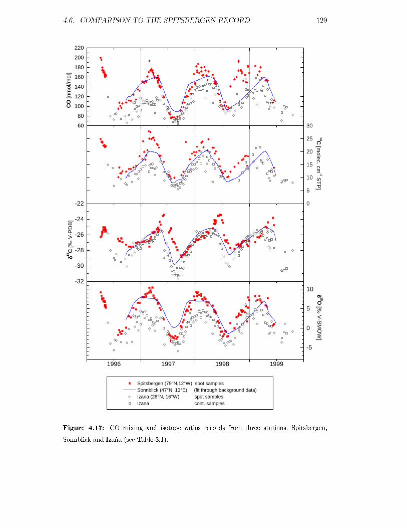
4.6. COMPARISON TO THE SPITSBERGEN RECORD 129
60
80
100
120
140
160
180
200
220
CO
[nm
ol/m
ol]
0
5
10
15
20
25
30
14C[m
olec.cm-3
ST
P]
-32
-30
-28
-26
-24
-22
δδ δδ13C
[‰V
-PD
B]
1996 1997 1998 1999
-5
0
5
10
Spitsbergen (79°N,12°W) spot samplesSonnblick (47°N, 13°E) (fit through background data)Izana (28°N, 16°W) spot samplesIzana cont. samples
δδ δδ18O
[‰V
-SM
OW
]
Figure 4.17: CO mixing and isotope ratios records from three stations, Spitsbergen,
Sonnblick and Izaña (see Table 3.1).
130 CHAPTER 4. SEASONAL CYCLES OF ATMOSPHERIC CO
icant phase shift between CO and δ13C of � 3months. During rising OH levels,
and therefore decreasing CO levels, the remaining CO gets progressively enriched
(KIE(δ13C ) of 1.004 to 1.005 in the lower troposphere [Stevens et al., 1980]). With
decreasing CO levels the contribution of the very light CH4 oxidation source gets
relatively more important and a sharp decrease in δ13C is observed from June to
October. This e�ect has already been discussed for the Izaña δ13C variations. The
considerably lower δ13C values during summer/autumn at Izaña compared to Spits-
bergen re�ect that CH4 oxidation is a relatively more important source at lower
latitudes. Bergamaschi et al. [2000b] calculated the contribution from CH4 oxida-
tion to total CO levels. During the summer months CH4 oxidation accounts only for
approximately 1/5 of CO mixing ratios at Spitsbergen, whereas it is 1/2 at Izaña (see
Figure 4.12). The δ13C signal at Sonnblick is between those from Spitsbergen and
Izaña, in accordance with the latitudinal gradient shown in Figure 4.16. Only during
the winter maximum is δ13C higher than at the other stations. This re�ects again
that regional sources from combustion processes with heavy δ13C source signatures
are more important at this continental station. Concerning the interannual variabil-
ity between 1997 and 1998 we note that in all three records the summer minimum
in 1997 was lower than in the previous and subsequent years. This e�ect is yet not
fully understood [Gros et al., 2000], [Röckmann, 1998a].
The δ18O cycles shown in Figure 4.17 re�ect the seasonality of the OH sink which
is enhanced by the CO source shift from isotopically light sources in summer towards
isotopically heavy combustion sources in winter. This leads to the strong latitudinal
gradient between the three δ18O records which is largest in winter. Again the higher
contribution of combustion sources during low CO concentrations in summer can be
seen for the continental station Sonnblick.
4.7 The BERLIOZ campaign
In July and August 1997 we have taken samples during the Berlin-Ozone Experi-
ment (BERLIOZ) in the surroundings of Berlin. The BERLIOZ campaign was part
of the BMBF-Project for tropospheric studies (TFS) in which Ozone and its pre-
cursors were studied [Becker et al., 1998]. We compare these measurements taken
in the continental boundary layer to long term measurements at two European sta-
tions, e.g. Kollumerwaard (Netherlands) and Umweltbundesamt (UBA) Schauins-
land (Germany). While the Kollumerwaard station is located in the boundary layer
a few km from the North See, the UBA station is located at the top of the Schau-
insland at 1205 ma:s:l:. With an elevation about 1000 m above the regional level

4.7. THE BERLIOZ CAMPAIGN 131
(e.g., the broad Rhine valley), it is usually above the ground level inversion layer
during night, but within the ground level boundary layer during day-time. Samples
are usually taken in the early morning when the night-time inversion still shields the
station from local emissions.
The BERLIOZ samples were collected at the Papsthum station (53Æ N, 13Æ E)
approximately 60 km northwest from Berlin. Between the 20th July and 6th August
1998 twenty high pressure aluminum cylinders (Scott Marin Inc., 5 l) were taken with
the compressor system described in section 2.1.1. The CO mixing and isotopic ratios
from the BERLIOZ samples are shown in Figure 4.18 together with the 1998 data
sets from the Kollumerwaard station (53Æ N, 6Æ E, 0 ma:s:l:) and the Schauinsland
station (48Æ N, 8Æ E, 1205 ma:s:l:)(see also Table 3.1). The FFT �ts through the
Izaña and Spitsbergen records are also shown which indicate the background signals
from high northern and subtropical latitudes.
The previously discussed seasonal cycles of CO and its isotopes are indicated by
the FFT �t curves. The CO mixing ratios at both monitoring stations are very scat-
tered, ranging from � 110 nmol/mol in summer to values as high as 220 nmol/mol
and 300 nmol/mol for Schauinsland and Kollumerwaard respectively. These large
variations make it di�cult to extract a distinct seasonal cycle. The BERLIOZ sam-
ples had CO mixing ratios ranging between 136 and 192 nmol/mol on the 20th/21th
July, while they reached background concentrations between the 3rd and 6th of Au-
gust (109 to 152 nmol/mol).
14CO measurements were much less a�ected by local and regional sources and
therefore distinct annual cycles are apparent for 1998 at both monitoring stations.
Most 14CO values lie within the �t curves for Izaña and Spitsbergen, indicating
that the seasonal cycles are mainly de�ned by the OH sink, i.e. the latitudinal
location of Kollumerwaard and Schauinsland. The BERLIOZ data vary between
8 and 11molec./cm3 and exhibit the same scatter as observed for the monitoring
stations during the summer minimum.
The δ13C signals of Kollumerwaard and Schauinsland exhibit a similar seasonal
cycle as discussed for Sonnblick in section 4.6. The scatter of the BERLIOZ data
is relatively high especially on the 20th/21th July. But apart from one outlier with
an extremely low δ13C signal of less than 30 0=00, the variability is within the range
of δ13C values observed at the monitoring stations during the same period. The
reasons for the up to 2 0=00 depleted value for the outlier sampled on the 21th July
at 2 p:m: are not yet clear. For samples from the boundary layer with high levels of
carbon containing compounds, such as formaldehyde, cross interference may occur
during the analysis.
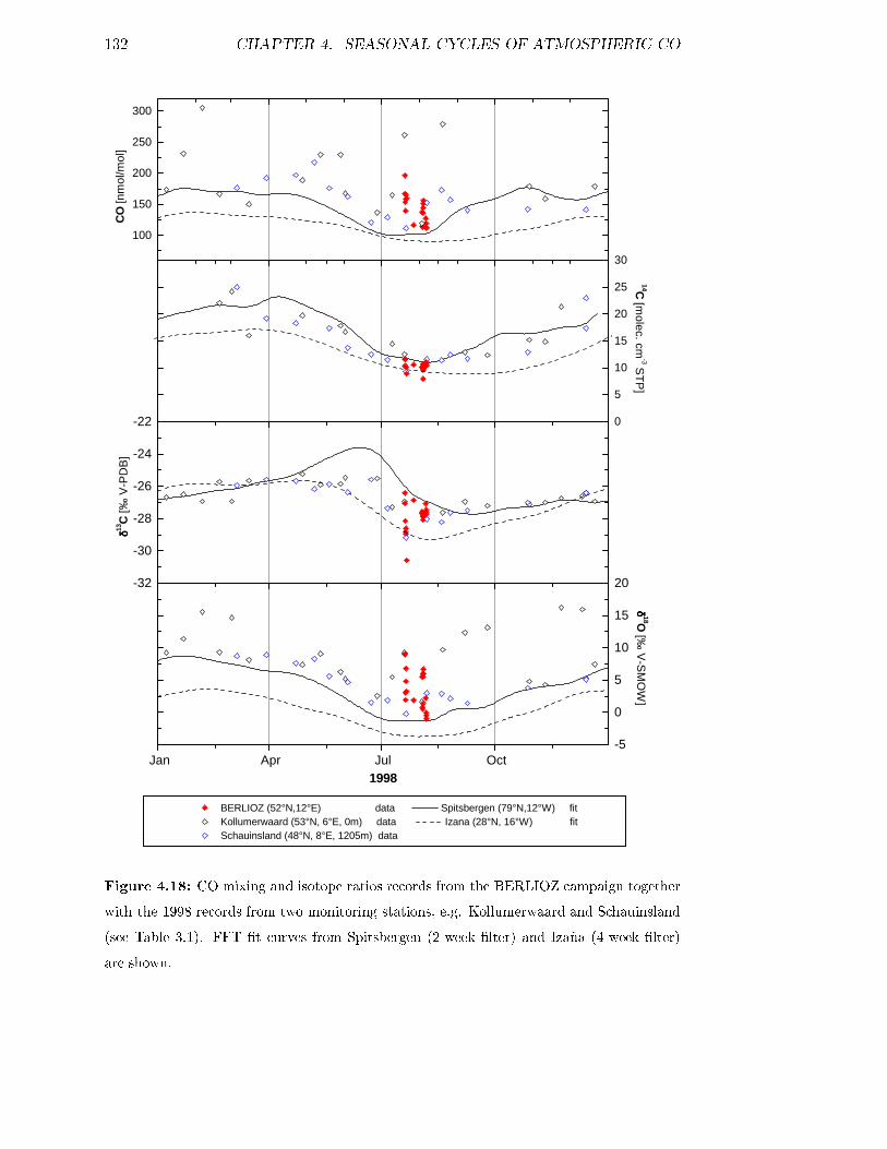
132 CHAPTER 4. SEASONAL CYCLES OF ATMOSPHERIC CO
100
150
200
250
300C
O[n
mol
/mol
]
0
5
10
15
20
25
30
14C[m
olec.cm-3
ST
P]
-32
-30
-28
-26
-24
-22
δδ δδ13C
[‰V
-PD
B]
Jan Apr Jul Oct-5
0
5
10
15
20
1998
BERLIOZ (52°N,12°E) data Spitsbergen (79°N,12°W) fitKollumerwaard (53°N, 6°E, 0m) data Izana (28°N, 16°W) fitSchauinsland (48°N, 8°E, 1205m) data
δδ δδ18O
[‰V
-SM
OW
]
Figure 4.18: CO mixing and isotope ratios records from the BERLIOZ campaign together
with the 1998 records from two monitoring stations, e.g. Kollumerwaard and Schauinsland
(see Table 3.1). FFT �t curves from Spitsbergen (2-week �lter) and Izaña (4-week �lter)
are shown.

4.7. THE BERLIOZ CAMPAIGN 133
0 1 2 3 4 5 6 7 8 9 10-5
0
5
10
15
20
25
Lin. fit BERLIOZ data
y = -2,28x+20.4(+/-2.2) (R2 =0.77, n=20)
1/[CO] (nmol/mol)-1
BERLIOZ dataKollumerwaard dataSchauinslanddata
δδ δδ18O
[‰V
-SM
OW
]
Figure 4.19: δ18O values are plotted against the inverse concentration for the BERLIOZ
data and for Kollumerwaard and Schauinsland data from 1998. A linear �t through the
BERLIOZ data is applied.
In Figure 4.19 we show how the variability of the δ18O signals at the moni-
toring stations as well as for the BERLIOZ samples can be explained by the con-
tribution of combustion sources. CO from combustion sources is enriched in 18O
and nearly matches the isotopic composition of atmospheric oxygen which has a Æ
value of 23.5 0=00. Because combustion is the only large source of enriched CO, CO
and δ18O values are correlated for samples a�ected by local combustion sources
[Brenninkmeijer & Röckmann, 1997]. By plotting δ18O values against the inverse
concentration, the intercept with the linear �t gives the δ18O value of unmodi�ed
CO from combustion processes (mainly tra�c). For the BERLIOZ data the ap-
134 CHAPTER 4. SEASONAL CYCLES OF ATMOSPHERIC CO
plied linear �t had an high correlation coe�cient of R2=0.77 and an intercept of
20.4�2:2 0=00. The Kollumerwaard and Schauinsland data all lie close to the dilution
line de�ned by the �t. This underlines that δ18O variations at continental stations,
which are in�uenced by local and regional sources, are mainly due to the admixing
of CO from combustion processes, which dominates the fractionation process of the
OH sink.
4.8 Conclusion
The seasonal cycles observed for CO mixing and isotopic ratios at Izaña are mainly
explained by the OH seasonality. While continuous samples were representative of
the background signal at the subtropical station Izaña, large variations occurred in
the measured CO, 14CO and δ18O values of spot samples. These short term synoptic
scale variations often exceeded the mean seasonal cycles. We showed with the help of
back trajectories that air masses from very di�erent origins reach the remote station
Izaña. Thus important source regions like Europe and North America, as well as
very clean maritime or African air were characterized by our isotopic study. For
some samples from the African continent biomass burning events were detected in
the CO and δ18O signals between January and March 1997 to 1999. The large range
of latitudinal origins of the air masses allowed to con�rm and estimate the large
latitudinal gradients occurring in the CO, 14CO, δ13C and δ18O signals at Izaña.
The �rst two years of our three year record of CO mixing ratios and its stable
isotopes at Izaña have been used together with records from four other stations for
an inverse CO modeling study by Bergamaschi et al. [2000b]. This made it possible
to quantify the seasonal variation in the contribution of CO sources which were
responsible for the small phase shift observed in the δ13C record relative to CO.
This is mainly due to the changing relative contribution of the CH4 oxidation source
to CO levels.
Through the comparison of our Izaña measurements to the Spitsbergen record
we could address the question of the large interannual di�erences seen at Izaña
between 1997 and 1999. While the measurements of CO and its isotopic composition
at Izaña resulted in values that were close to measurements at the tropical station
Barbados from mid-1996 to mid-1997, values in 1998 are more representative of higher
latitudes and thus the di�erence to the Spitsbergen record was less pronounced. This
explanation for the observed interannual variations mainly between 1997 and 1998
is further supported by our SF6 measurements at Izaña. Figure 3.5 shows that SF6
concentrations in 1997 where slightly lower compared to the interannual trend, while

4.8. CONCLUSION 135
they were on average slightly higher in 1998. This is especially true for the continuous
samples which are considered to be representative of the background signal at Izaña.
This is a further indication that in addition to large CO sources at the end of 1997,
which we attribute to a larger biomass burning source in this year, the large scale
meteorological situation also changed. Further analysis of back-trajectories, as has
been done by Schäfer [1997] for the period 1992 to 1997, should allow to distinguish
these two factors which in�uenced the Izaña record.
Finally long term records of CO and its isotopic composition from two continental
stations, Schauinsland and Kollumerwaard, were compared to measurements during
the BERLIOZ campaign in July/August 1998. While the observed 14CO and δ13Cvariations were comparable to those from high northern and subtropical latitudes and
de�ned a latitudinal gradient, the observed variations in CO and δ18O were much
larger at these continental sites and were explained by the in�uence of combustion
processes.

136 CHAPTER 4. SEASONAL CYCLES OF ATMOSPHERIC CO

Chapter 5
Antarctic �rn air records
Temporal trends of atmospheric trace gases represent a crucial information for the
understanding of their global budget. Using Antarctic �rn air the atmospheric trend
of methane isotopic ratios over much of the present century has been reconstructed.
High volume air samples were extracted at several depth levels at two sites in East
Antarctica. Methane concentrations and its 13C/12C and D/H ratio were deter-
mined by gas chromatography, mass spectrometry and infrared spectroscopy. A �rn
air transport model was applied to reconstruct past atmospheric trends in methane
and its isotopic composition. Also results from an atmospheric model are presented,
which explores changes in methane sources and OH sink compatible with our recon-
structed atmospheric trends.
Historical information about the isotopic ratios of CH4 in the atmosphere is
still limited. [Stevens & Engelkemeir, 1988] pioneered the investigation of atmo-
spheric δ13C trends in the northern and southern hemispheres. Since then other
attempts have been made for long-term monitoring of this signal at various sites
([Quay et al., 1996] [Lowe et al., 1999], and references therein), including δD Marik
[1998], thus providing some information over the last decade. The recent analysis of
the Cape Grim air archive and �rn air samples, collected at Law Dome in Antarctica,
have extended the history of δ13C to the last 20 years [Francey et al., 1999]. This
study showed an increase of �0.6 0=00 in δ13C since 1978, while the CH4 mixing ratio
increased by �200 nmol/mol. The authors concluded that global CH4 sources and
sinks probably remained constant since 1982, and that the trend observed in δ13Cre�ects the slower equilibration of isotopic signals in the atmosphere compared to
mixing ratios. Other historical information on CH4 isotopic trends is provided by
ice core measurements. The only such record to date, suggests an increase in δ13Cof �2 0=00 since pre-industrial times [Craig et al., 1988]. The authors interpreted this
in terms of a biomass burning source strength in the present-day CH4 budget, which
137

138 CHAPTER 5. ANTARCTIC FIRN AIR RECORDS
would amount to about 50Tg yr�1.
The present study is part of the European Project FIRETRACC (Firn Record
of Trace Gases Relevant to Atmospheric Chemical Change Over 100 Years) which
included several laboratories:
� CNRS Laboratoire de Glaciologie et G�eophysique de l�Environnement(LGGE),
France
� British Antarctic Survey (BAS), UK.
� School of Environmental Sciences, University of East Anglia, UK.
� Physics Institute , University of Bern, Switzerland.
� MPI, Mainz, Germany
We use air captured in Antarctic �rn (unconsolidated snow), spanning several
decades due to the time required for gas di�usion in this porous medium. The
advantage of �rn lies in the possibility of extracting much larger amounts of air
compared to ice-cores, which makes it possible to study with greater accuracy and
smaller risk of contamination the decadal to secular history of trace gases of low
abundance, including their isotopic composition. An additional rational for collecting
very high sample volumes was to allow measurements of 14CO with an abundance
of about 20 molecules per cm3 (STP) and other ultra rare atmospheric trace gases.
In this chapter we focus on measurement and modeling of CH4 mixing ratios
including its stable isotopes, 13C and D, from two drilling sites in Antarctica in order
to reconstruct their evolution in the atmosphere over the last 50 years. In a second
step these reconstructed trends are interpreted with the help of an atmospheric model
in terms of changing ratios of natural to anthropogenic methane sources over time.
Because of the high sensitivity of δD levels to changes in OH mixing ratios, this will
be done with regard to potential changes in the OH sink.
5.1 Antarctic sampling sites
The �rst drilling conducted by the British Antarctic Survey (BAS) took place in
Dronning Maud Land (DML) (77Æ S, 10Æ W; 2300 masl) in January 1998. The site
has a mean annual temperature of �38 ÆC and a relatively high snow accumulation
rate (60 kgm�2 yr�1) compared with the Antarctic plateau. Eighteen �rn air sam-
ples were taken starting from the surface to the �rn-ice transition zone at 73.5 m.
Similarly, in January 1999 drilling and �rn air sampling was conducted by BAS and

5.1. ANTARCTIC SAMPLING SITES 139
Figure 5.1: FIRETRACC drilling sites
site location T Acc Alt P depth
Dronning Maud Land 77Æ S, 10Æ W �38 60 2300 730 73.5
Dome C 75Æ S, 123Æ W �53 30 3240 655 99.5
Table 5.1: Location, annual mean surface temperature T ( ÆC), accumulation rate Acc
(kg cm�2 yr�1), altitude Alt (m), atmospheric pressure P (hPa) and depth (m) of the �rn-
ice transition at both Antarctic drilling sites.
the Laboratory of Glaciology and Geophysics of the Environment (LGGE) at Dome
Concordia (DC) (75Æ 06′ S, 123Æ 23′ E, 3233 masl). This is an extremely cold site
(�53 ÆC) with a low accumulation rate (30 kgm�2 yr�1), resulting in a deeper �rn-ice
transition (99 m) than DML. This time 20 air samples were taken down to 99.5 m.
In Figure 5.1 the location of the two drilling sites in East Antarctica is shown and
in Table 5.1 their climatic parameters are listed.

140 CHAPTER 5. ANTARCTIC FIRN AIR RECORDS
The sampling of �rn air was �rst documented by Schwander [1993]. Here we
describe a modi�ed set-up for the extraction of large �rn air samples of up to 1000 l.
Drilling progressed stepwise in intervals of 1 to 5 m. At each level the drill was
withdrawn and the hole sealed close to the bottom with a 5 m (DML) or 3 m (DC)
long in�atable rubber bladder. Two continuous, 105 meter long, 3/8 inch PFA tubes
passed through the bladder, connected the pumping system at the surface to the
bottom of the hole. Through one of those tubes, ending just below the aluminum
end cup of the bladder, air was drawn continuously at a high �ow rate (25 lmin�1) to
waste. The sample air itself was drawn at a lower �ow rate (15 lmin�1) via the other
tube, which ended about 10 cm lower. Both inlets were separated by a set of metal
ba�es. The function of these ba�es (originally devised by M. Bender, Princeton
University) is to prevent any possible contamination from the bladder material or
leakage past the seal from reaching the sample inlet at the very bottom of the hole.
The quality of the sampling was continuously monitored with an infrared CO2
analyzer (Li-Cor) attached to the sample air stream and calibrated with a standard
gas. Stable CO2 levels (at � 0.1µmol) were usually encountered after about 10 min
�ushing following in�ation of the bladder. Purging and �lling the di�erent types of
sample �asks at each depth level usually required about 2 hours and 1200 liters of
�rn air. The maximum di�erence in CO2 mixing ratio observed between the start
and the end of sampling was 1µmol at DC.
A high purity air extraction system was deployed consisting of a 2-stage metal
bellows pump (Parker) for �lling small cylinders, i.e. for LGGE 0.5 l CSIRO glass
�asks pressurized at 25 psi. Subsequently the air emerging from the metal bel-
low pump was fed into a three-stage, oil-free, modi�ed RIX SA3 piston compressor
[Mak & Brenninkmeijer, 1994a], which allowed the high volume air samples for the
MPI to be compressed to � 120 bars in 5 or 10 l aluminum cylinders (Scott Marrin).
See section 2.1 for a detailed description of the cylinders and compressor system
respectively.
5.2 Firn air measurements
The D measurements of CH4 presented here are the �rst from �rn air. For 13C we
report in addition to our analysis those from a second laboratory, LGGE.
The high volume samples allowed a wide range of trace gases to be analyzed. At
the MPI GC analysis for CO, CH4, CO2, N2O and SF6 was performed. Further,
mass spectrometry was applied after the extraction of CO2 and CO for 13C and 18O
isotope analysis. Analysis of the 14C content of CO, CH4 and CO2 were done by

5.2. FIRN AIR MEASUREMENTS 141
������������������������������
������������������������������
������������������������������
������������������������������
D
R
1/4
3/83/8
M
U.C.S
SNOW SURFACE
PS
Firn
140 mm Borehole
Baffle plate
Upper inlet
5 m longBladder
Seal
Bladderinflation
Lower inlet
Figure 5.2: Firn air sampling at Dronning Maud land and Dome C. D: 2-stage, 4-leads
diaphragm compressor for in�ation of the bladder; M: 2-stage, 2-leads metal bellows com-
pressor for the medican pressure ultra clean samples (U.C.S); P: modi�ed 3-stage RIX com-
pressor for the �lling of high volume sample cylinders (S); R: 3-section reel with 2�110 m
3/8 Inch PFA and 1�110 m 1/4 Inch for the bladder.
accelerator mass spectroscopy (AMS). In this chapter we mainly concentrate on CH4
and its isotopes, 13C and D.
At LGGE aliquots of �rn air were �rst used for the determination of CH4 and
CO2 by gas chromatography (Varian 3300). Working reference gases are calibrated
against the NOAA/CMDL scale at LGGE and the overall precision for the �rn air
samples is estimated to be �4 nmol/mol and �0.4µmol/mol respectively. Then,
13C/12C of CH4 was measured with a Finigan GC-Combustion interface coupled to
a Finnigan MAT 252 isotope-ratio mass spectrometer.

142 CHAPTER 5. ANTARCTIC FIRN AIR RECORDS
70
60
50
40
30
20
10
0
dept
h[m
]
1200 1300 1400 1500 1600 1700
DML
CH4
[nmol/mol]
320 330 340 350 360
CO2
[µmol/mol]
SF6
[pmol/mol]
100
80
60
40
20
0CH4 MPI dataCH4 LGGE data DC
dept
h[m
]
100
80
60
40
20
0
100
80
60
40
20
0
298 300 302 304 306 308 310 312 314N2O[nmol/mol]
100
80
60
40
20
0
0 1 2 3 4
100
80
60
40
20
0
Figure 5.3: CH4, CO2, N2O and SF6 mixing ratios of �rn air at DML and DC plotted
against depth.
5.2.1 Mixing ratios
The data for DML and DC in Figure 5.3 show the expected decrease in the mixing ra-
tios of CH4, CO2, N2O, CO and SF6 with depth. For CH4 the mixing ratios at DML
(January 1998) ranged from contemporary atmospheric levels of 1684�2 nmol/mol
at the surface to 1284�2 nmol/mol at the �rn-ice transition at 73.5 m. CH4 mix-

5.2. FIRN AIR MEASUREMENTS 143
ing ratios at DC (January 1999) were 1694�2 nmol/mol at the surface and went
down to 1218 �10 nmol/mol near the close-o� zone at 99.5 m. Thus a change in
concentrations of more than 400 nmol/mol has been observed, re�ecting the underly-
ing increase of methane concentration over time. The two ambient air measurements
from January 1998 and 1999 indicate an atmospheric increase of +0.6 %=yr for 1998,
in agreement with measurements from the NOAA/CMDL network.
At DC methane mixing ratios have been measured by both MPI and LGGE.
The two methane series agreed well within the uncertainty of the measurements (see
Figure 5.3). One notable exception are the samples taken at a depth of approxi-
mately 97 m, where the MPI results were signi�cantly higher than those of LGGE.
The di�erence was also observed for δ13C (CH4) and for CO2. The most plausible
explanation lies in the sequence of sampling, and in the di�culty of recovering �rn
air in the low open porosity close-o� region. The LGGE �asks were the �rst to be
�lled after in�ating the bladder and the MPI �asks followed. At this speci�c depth
level, the prolonged pumping may have created a route towards lower depths thus
�lling MPI �asks with shallower and therefore younger air. For this reason only the
LGGE results are considered at the DC depth of 97 m in the following discussion
and interpretation.
5.2.2 δ13C of CH4 in �rn air
For the further analysis of the �rn pro�les we also consider δ13C measurements which
have been carried out at LGGE. For Dronning Maud Land δ13C was measured on the
same high volume samples, while for Dome C the δ13C measurements from LGGE
were done on separate glass �asks.
The 13C analyses at LGGE were performed on a Finnigan MAT-252 mass spec-
trometer, coupled to a Finnigan GC / combustion interface in continuous �ow mode
(CF-IRMS). A custom pre-concentration unit was used to isolate CH4 from the ma-
jor air constituents. This unit included a sample loop of 150 ml, a Haysep D column
(20 cm length, 1/8 inch ID) held at �130 ÆC with a pentane-ice slush, and a 3 m
capillary focussing trap also held at �130 ÆC and identical to the main separation
column (GS-Q, 30 m length, 0.32 mm ID). After pre-concentration, methane was
separated from the residual trace gases on the capillary column, combusted to CO2
and injected with helium into the mass spectrometer for measurement of masses 44,
45 and 46. Isotopic calibration was performed against a pure CO2 working standard
with a 13C/12C ratio of �45:98�0.02 0=00 versus PDB, which is close to the carbon
isotopic ratio of methane in the atmosphere. This value was determined by inter-
calibration with the MPI standard and with other laboratories measuring methane

144 CHAPTER 5. ANTARCTIC FIRN AIR RECORDS
isotopes. Simultaneously with the �rn air measurements the external accuracy of the
CF-IRMS was determined by regularly analyzing a tank of atmospheric air sampled
at Baring Head, New Zealand, on 27 May 1997 by D. Lowe (National Institute of
Water and Atmospheric Research, NIWA), with a δ13C of �47:16�0.05 0=00 versus
PDB. The �rn air samples were each measured at least four times, using a sample
size of only 80 ml STP. The mean reproducibility on replicate �rn air samples and
the NIWA standard was �0.05 0=00.
For the international isotope standard NZCH [Brenninkmeijer, 1990] our mea-
surements gave a value of �47:13 0=00, close to the δ13C value of �47:12 0=00 based
on a laboratory intercomparison [Röckmann, 1998a]. The low abundance of CH4 in
the older �rn air samples necessitated the recovery of CH4 after the MISOS D/H
measurements for subsequent combustion, instead of splitting samples as is usually
done [Bergamaschi et al., 2000a]. The resulting measurement error in δ13C was es-
timated to be �0.08 0=00 for the DML data. The recovery was improved in 1999 and
the measurement error thus reduced to �0.04 0=00 for the DC data. Regarding the
LGGE measurements of the DML samples (Figure 5.4), made on residual air in the
MPI �asks, a +0.25 0=00 correction was applied, which takes into account a mass spec-
trometer non-linearity e�ect caused by peak intensity di�erences between standard
and sample on this set of measurements.
The δ13C values for DML and DC are shown in Figures 5.4 a and b respectively.
At the surface the δ13C values were �47 0=00 in January 1998 (DML) and January
1999 (DC). With increasing depth the �rn air methane was progressively depleted in
13C and reached �50 0=00 at the �rn-ice transition. The δ13C measurements of both
isotope laboratories are plotted together and a good agreement of approximately
0.02 0=00 can be observed between the LGGE and MPI pro�les. Only near the �rn-ice
transition of DC (Figure 5.4b) did the LGGE measurements become slightly lighter
relative to those of MPI, most probably due to the sampling artifact discussed in
section 5.2.1.
For DML (Figure 5.4a) the LGGE data are signi�cantly less scattered. The con-
tamination e�ects due to the recovery of the methane from the MISOS system, as
discussed above, might have been more important than expected. Both laborato-
ries did measure a signi�cant variation of nearly 0.3 0=00 in the top 10 m in the DC
record (Figure 5.4b), most probably re�ecting seasonal thermal fractionation of gas
isotopes in cold �rn compared to the relatively warm surface of the austral summer
[Severinghaus & Brook, 1999]. This phenomenon impacts the �rn composition only
over the upper 10-15 m and has no e�ect deeper down, provided that there was no
abrupt climate change at the surface over the time period covered by the �rn air

5.2. FIRN AIR MEASUREMENTS 145
100
80
60
40
20
0
-51 -50 -49 -48 -47
MPI data LGGE dataDML DC combined
(a) DML
δδδδ13C [‰ V-PDB)]
dept
h[m
]
100
80
60
40
20
0
-51 -50 -49 -48 -47
dept
h[m
]
(b) DC
δδδδ13C [‰ V-PDB)]
Figure 5.4: δ13C of CH4 in �rn air at (a) DML and (b) DC, measured by MPI and LGGE.
Error bars are 1� analytical precision and 1� scattering on replicate measurements for MPI
and LGGE respectively. Lines running through the data are �rn model results for the best
atmospheric δ13C scenarios (as a function of time in �gure 5.11) for DML, DC and the
combination of both sites (see section 5.5.1).

146 CHAPTER 5. ANTARCTIC FIRN AIR RECORDS
samples.
The measured total δ13C range of nearly 3 0=00 from top to bottom of the two
pro�les is very large compared to direct atmospheric measurements. For example, the
seasonal amplitude observed at a remote southern hemisphere station, Baring Head
(41Æ S, 175Æ E), is around 0.4 0=00 and the observed trend is smaller than 0.05 0=00 yr�1
[Lowe et al., 1994].
5.2.3 δD of CH4 in �rn air
The δDmeasurements are shown for DML and DC in Figures 5.5 a and b respectively.
The values obtained for ambient air samples were �70 0=00 at DML in January 1998
and as light as�80 0=00 at the �rn-ice transition at 73.5 m. For DC they were �72 0=00 in
January 1999 and reached �82 0=00 at 97.5 m. The δD measurement error including
sample preparation is estimated to be �1 0=00. The ambient air at DML and DC
was 2 to 3 0=00 enriched compared to the shallowest �rn air. Opposite to the δ13Csignal, thermal fractionation seems to be overwhelmed by the seasonality of the
atmospheric signal for δD propagating in the shallow �rn. As we will show later,
the �rn integrates seasonal variations after the �rst few meters. This means that the
recent annual average should be �74:3 0=00. The strong kinetic isotope fractionation
of nearly 300 0=00 in the CH4 + OH reaction drives a strong seasonal δD cycle which
reaches its maximum in May, when OH levels are beyond the summer maximum.
For January ambient air measurements for δD are expected to be close to the annual
mean value and not 2 to 3 0=00 enriched as observed. The measured di�erence between
the ambient air samples and the �rst �rn air samples is not expected and has no
explanation at the moment. The fact that coherent atmospheric scenarios from
DML and DC can be drawn from the �rn pro�les (section 5.5) suggests that there
was no signi�cant artifact in the �rn (supposedly temperature, chemical composition,
or density related) disturbing the δD signal, and that at least the relative trend in
δD is robust.
As for the δ13C variation, the observed δD range of �10 0=00 from top to bottom
is high compared to present atmospheric variations. For instance, a seasonal cycle of
4 0=00 in East Antarctica has been deduced for Neumayer Station (70Æ S, 8Æ W), after
calculating monthly mean values over a 6 year period [Marik, 1998] (see also section
3.2 for seasonal cycles and the atmospheric trend at Izaña)

5.2. FIRN AIR MEASUREMENTS 147
100
80
60
40
20
0
-85 -80 -75 -70
(a) DML
δδδδD [‰ V-SMOW]
dept
h[m
]
100
80
60
40
20
0
-85 -80 -75 -70
data DML DC combined
dept
h[m
]
(b) DC
δδδδD [‰ V-SMOW]
Figure 5.5: δD of CH4 in �rn air at (a) DML and (b) DC. Error bars are 1� analytical
precision. Lines running through the data are �rn model results for the best atmospheric
δD scenarios (which are shown as a function of time in �gure 5.12) for DML, DC and the
combination of both sites (see section 5.5.1).
148 CHAPTER 5. ANTARCTIC FIRN AIR RECORDS
5.3 Properties of �rn
Firn is a porous medium which results from the densi�cation of dry snow at the
surface of polar ice sheets and glaciers. Its structure is discussed in section 5.3.1. Firn
is permeable to gases and the di�usivity of these gases decreases with the increasing
density of the �rn with depth. Variations in atmospheric trace gas mixing ratios
occurring at the surface continuously propagate downwards by molecular di�usion
and are in�uenced by the e�ect of gravitation, which will be discussed in sections
5.3.3 and 5.3.2 respectively. During these processes the atmospheric variations are
attenuated by di�usive mixing. In general, light gases such as methane di�use faster
downwards whereas gravitational settling favors the accumulation of the heavier gases
in the deepest part of the �rn. These two main processes modify mixing ratios as
well as isotopic ratios.
5.3.1 The �rn structure
Figure 5.6 indicates the typical depth, density and age ranges for polar ice sheets
[Schwander, 1989]. The �rn layer at polar sites can be separated into four di�erent
zones that are relevant for the transport of gases through this permeable medium.
� The mixing zone:
In this snow-layer close to the surface (0 to 10-25 m depth) the air can be
mixed by winds, atmospheric pressure variations or thermal gradients. If strong
annual temperature gradients occur thermal di�usion e�ects can be impor-
tant [Leuenberger et al., 2000]. At the surface the density is typically around
300 kgm�3.
� The di�usion zone:
This zone covers most of the �rn layer (10-25 m to 60-110 m depth). It is
de�ned as the zone where transport through the open pores takes place until the
di�usion gets zero (the open porosity can still be non-zero). The transport of
gases in this zone is due to mass di�erences of the molecules (gravitation e�ect),
to the concentration gradient (di�usion e�ect) and the downward movement
of air created by the trapping of gas in the �rn close-o� zone.
� The non-di�usion zone:
Here the air begins to be trapped into bubbles and open pores and bubbles
coexist. The di�usion is already zero, while the open porosity is still non-
zero. The average gas age increases rapidly in this zone (up to 100 years),
because no dilution with younger air masses from above takes place any longer.

5.3. PROPERTIES OF FIRN 149
Figure 5.6: Diagram of the snow-ice transformation, indicating the typical depth, density
and age ranges for polar ice sheets [Schwander, 1989].
Nevertheless, the �rn air is even at this depth considerably younger than the
surrounding ice, which can be up to 2600 years old. The air in the remaining
open pores and the bubbles is transported downwards with the advection of
the ice layers.
� The close-o� zone (�rn-ice transition):
From this zone onwards all porosity is closed and the gas trapped in bubbles
is descending with the ice layers. This downward movement only depends on
the snow accumulation rate at the surface. The density of the ice at the close-
o� zone is close to 850 kgm�3 [Arnaud, 1997] (this value has changed since
[Schwander, 1989] in Figure 5.6).

150 CHAPTER 5. ANTARCTIC FIRN AIR RECORDS
The factors determining gas transport and mixing in the �rn are molecular weight,
the molecular di�usion coe�cients of the considered trace gas, pressure, temperature,
and the porosity and tortuosity pro�les of the �rn matrix. The �rn is characterized
by three pro�les that can be measured as a function of depth (z) and two climatic
parameters:
� the density pro�le �(z)
� the closed porosity pro�le �(z)
� the tortuosity pro�le (z)
� the mean annual surface temperature T
� the accumulation rate at the surface Acc
The porosity pro�le �(z) is closely linked to the density pro�le of the �rn:
�(z) = 1��(z)
�ice(5.1)
The e�ective di�usivity of a speci�c gas in the �rn will depend on the porosity pro�le
and on the molecular di�usivity of the pure gas in air. The tortuosity pro�le of the
�rn re�ects the in�uence of the �rn structure on the e�ective di�usion coe�cient
D(z) (in m2/s):
(z) =D(z)
Dm(5.2)
For this study the density pro�les of both drilling sites have been measured by the
BAS and a smoothed �t through these measurements has been used in the �rn
di�usion model discussed in section 5.4. In Figure 5.7 the density pro�les of both
sites are shown.
The open porosity pro�le can be directly measured [Arnaud, 1997]. In our study
we use the open porosity calculated by J.M. Barnola (personal communication).
Figure 5.7 also shows the open and total porosity pro�les of both sites.
5.3.2 Gravitation processes in �rn
The air in the open �rn pores is considered to be hydrostatic . Therefore the classic
results for an isotherm atmosphere can be applied to the air below the mixing zone
[Craig et al., 1988b]. The concentration of air in �rn is then given by the barometric
equation:
cair(z) = cair(0) � exp(�Mairgz
RT) (5.3)
z : depth (m)
Mair : molecular air mass (29�10�3 kgmole�1)

5.3. PROPERTIES OF FIRN 151
120
100
80
60
40
20
0
0 200 400 600 800
density (DML)density (DC)fit (DML)fir (DC)
density [kg/m -3]
dept
h[m
]
0.0 0.2 0.4 0.6 0.8 1.0
120
100
80
60
40
20
0
porosity
total porosity (DML)open porosity (DML)total porosity (DC)open porosity (DC)
dept
h[m
]
Figure 5.7: density pro�les for DML (dashed line) and DC (dotted line)
g : gravitation constant (9.81 ms�2)
R : perfect gas constant (8.314 Jmole�1K�1)
T : temperature (K)
Equation 5.3 allows to calculate the gravitational e�ect in �rn at depth z for two
gases with mass di�erence �M :
�(z) = �Mgz
RT� 1000 (5.4)
with � = 1000 � (R
R0� 1)
where R is the concentration ratio at a given depth and R0 is the atmospheric
concentration ratio of both gases. For isotopes � is the Æ value de�ned in section
1.4.1.
This theoretical value of the gravitation e�ect in �rn can be compared to mea-
surements shown in �gure 5.8. The depth pro�les for ÆO2/N2, Æ29N2, ÆAr/N2 and
Æ34O2 are plotted for DML (Rolf Neubert, personal communication). The fact that
N2, O2 and Ar exhibit no signi�cant temporal trend in the atmosphere is used to sep-
arate the gravitation e�ect from di�usion e�ects due to concentration gradients. The

152 CHAPTER 5. ANTARCTIC FIRN AIR RECORDS
measured Æ29N2 value of 0.33�0:008 0=00 at 71 m is close to the theoretical value of
0.35 0=00 (equation 5.4). The Æ34O2 value of 0.69�0:04 0=00 (measured at 71 m) directly
re�ects the factor of �M=2 between 32O2 and34O2.
We note that the observed changing concentration ratios between gases due to
gravitation e�ects in the �rn re�ect that the e�ective distance covered by a gas is
much longer than the depth at which the sample was taken. For the scale height
(z0 = RT=Mg) de�ned by equation 5.3 the calculated values for O2 and N2 are
6224 m and 5446 m respectively (T=235 K at DML). The mixing ratios of both gases
are, however, already attenuated at depths of less than 100 m. This phenomena of
increasing e�ective distances covered by gases with increasing depth of the �rn is
addressed in the next section.
Note that in Figure 5.8 all isotope ratios deviate signi�cantly from the theoretical
value between 0 m and 20 m. This is due to thermal di�usion e�ects in the mixing
zone of DML, which is discussed in section 5.3.4.
5.3.3 Di�usion processes in �rn
In the troposphere and stratosphere turbulent processes dominate mixing and trans-
port processes and molecular di�usion can be neglected. In contrast, the separation
of molecules by molecular di�usion can be observed in the higher atmospheric layers
above 80 km, i.e. the mesosphere. In this region temperature and pressure are low
enough and result in mean free paths of several cm. Here molecules of di�erent mass
separate and the very light molecules such as hydrogen are even lost to free space.
A similar e�ect of gas separation due to molecular di�usion can be observed in �rn.
For the discussion of di�usion e�ects in �rn we assume that we are in a Knudsen
regime (mean free path � radius of the molecules), where the di�usion is charac-
terized by a single di�usion coe�cient. The mean free paths of molecules in �rn
are in the range of 10�8 m, whereas the dimension of the pores is in the order of
10�4 m. This implies that molecules collide less frequently with the �rn structure
than between themselves.
In a �rst step the temperature and pressure dependence of di�usion coe�cients
are discussed. Bzowzki et al. [1990] calculated the di�usion coe�cient Dij for a
binary mixture of gases i and j:
Dij =3
8
s(mi +mj
mimj)kT
��
1
�2ij�
ij(T�
ij)(5.5)
mi: mass of molecule i
�ij : characteristic parameter of the inter-molecular potential (distance). For a

5.3. PROPERTIES OF FIRN 153
80
60
40
20
0
0 1 2 3 4
(a)
δδδδ O2/N2 [‰ vs WS]
dept
h[m
]
80
60
40
20
0
0 1 2 3 4 5
(c)
dept
h[m
]
δδδδ Ar/N2 [‰ vs WS]
80
60
40
20
0
0.00 0.10 0.20 0.30 0.40
(b)
dept
h[m
]
δδδδ 29N2 [‰ vs WS]
80
60
40
20
0
0.0 0.2 0.4 0.6 0.8
(d)de
pth
[m]
δδδδ 3402 [‰ vs WS]
Figure 5.8: Depth pro�les for ÆO2/N2, Æ29N2, ÆAr/N2 and Æ34O2 for DML. Æ values are
given relative to a working standard (WS) of the atmospheric isotope (Rolf Neubert, personal
communication).
potential energy equal to zero this corresponds to the distance between molecules
ij : collision integral of the di�usion
�
ij = ij=(��2ij): reduced collision integral
T �
ij = kT=�ij : reduced temperature
�ij : characteristic parameter of the inter-molecular potential (energy), represents
the maximum of attraction between the molecules
The collision integral of the di�usion ij is a function of temperature and of the
force between the molecules. To obtain the temperature and pressure dependence of

154 CHAPTER 5. ANTARCTIC FIRN AIR RECORDS
the di�usion coe�cient equation 5.5 can be transformed to:
D(T; P ) = DT0;P0 �P0P� (
T
T0)3=2
�(T �
0 )
�(T �)(5.6)
For the last term, �(T �
0 )=�(T �), the temperature dependence varies with the con-
sidered gas. For the overall temperature dependence Schwander et al. [1993] pro-
posed an exponent of 1.85 for all gases. For the temperature range relevant for �rn
air Trudinger et al. [1997] found that the exponent can vary between 1.8 and 1.95,
resulting in di�usion coe�cients which vary less than 1%. We therefore consider the
pressure and temperature dependence to be:
D(T; P ) = DT0;P0 �P0P� (T
T0)1:85 (5.7)
The equation 5.5 can also be used to calculate the di�usion coe�cients for gases
for which measurements are not yet available. In this case the di�usion in air is
calculated for a mixture of 21.2% of oxygen and 78.8% of nitrogen after Blancs law
[1908]:
1
Dgas=air=
0:788
Dgas=N2
+0:212
Dgas=O2
(5.8)
Finally equation 5.5 can be used to infer the di�usion coe�cients of isotopes:
D(M1)
D(M2)=
sM2(M1 +Mair)
M1(M2 +Mair)(5.9)
The ratio of di�usion coe�cients is in this case only mass dependent.
Table 5.2 lists the di�usion coe�cients calculated with equations 5.5 and 5.9 for
the gases which are used in this study. They are also given relative to the di�usion
coe�cient of CO2, which is the value used in the �rn air di�usion model in section
5.4.
For the �ux through �rn we neglect the thermal di�usion and only consider the
molecular di�usion and the discussed gravitational e�ect:
~j = ~jdiff +~jgrav = �D(Æc
Æz+Mgc
RT) (5.10)
~j : total �ux, sum of the �ux due to di�usion ~jdiff and gravitation ~jgrav
D : Di�usion coe�cient (m2 s�1)
In the �rn di�usion model from Rommelaere et al. [1997] (see section 5.4) equation
5.10 is solved with respect to conservation of the air and the considered trace gas in
the �rn.

5.3. PROPERTIES OF FIRN 155
gas mass di�usion coe�cient Dgas/DCO2
[10�3kg mol�1] [cm2 s�1]
CO2 44.01 0.1203 1
CH4 16.043 0.1702 1.415
SF6 146.056 0.0747 0.621
O2 31.9988 0.1596 1.326
N2 28.0135 0.1583 1.316
12CH4 16 0.1702 1.415
13CH4 17 0.1671 1.3889
CH3D 17 0.1671 1.388914N15N 29 0.1569 1.304
16N18N 34 0.1573 1.308
Table 5.2: Summary of di�usion coe�cients (calculated after equations 5.5 and 5.9 at
253 K and 1013 hPa). Also di�usion coe�cients relative to CO2 are given (values used in
the �rn air di�usion model in section 5.4).
5.3.4 Thermal Di�usion in �rn
Figures 5.8 shows a considerable thermal di�usion e�ect for �rn samples taken in
DML at depths of 1 m to 20 m. Between winter and summer temperature gradients
occur in the mixing zone. As mentioned in section 5.3.2 no molecular di�usion is ex-
pected for the considered gases because of lacking temporal concentration gradients.
However, the di�usion coe�cients are temperature dependent and therefore the dif-
ferent isotopes di�use with di�erent velocities. Usually this results in an enrichment
of heavy molecules in colder zones.
The impact of the thermal di�usion e�ect has also been detected for the DC
samples [M. Leuenberger, personal communication, 1999]. Because of the lower
temperature of DC compared to DML we even detected the thermal fractionation
in our δ13C pro�le in Figure 5.4. At depths of 1 m to 15 m at DC a deviation of
nearly 0.3 0=00 occurs. For δD we would expect an e�ect of the same range, because
mass di�erence and di�usion coe�cient are the same as for δ13C . However, a 0.3 0=00
shift is too small to be detected on our δD measurements for which reproducibility
is �1 0=00.
156 CHAPTER 5. ANTARCTIC FIRN AIR RECORDS
5.4 Firn air di�usion model
Schwander et al. [1993] developed the �rst model that accounted for the di�usion of
gases and an additional modi�cation due to gravitational e�ects for the interpretation
of �rn air measurements. Since, two other �rn di�usion models from Trudinger et
al. [1997] and Rommelaere et al. [1997] have been used in several �rn air studies,
e.g. [Etheridge et al., 1998] and [Arnaud, 1997].
We apply the �rn air transport model developed by Rommelaere et al. [1997] in
order to reconstruct the atmospheric history of the methane isotopic ratios from the
convoluted �rn air signals. The main assumptions in this model are that the climatic
parameters (temperature and accumulation rate) and �rn structural variables have
remain constant in time, and thus also the �rn di�usivity pro�le and depth of the
�rn-ice transition.
The main assumptions of the �rn di�usion model are in detail:
� Isotherm �rn
The model applies only to stable climatic conditions where temperature gradi-
ents are limited to the top �rn layer, i.e. the well-mixed zone. Otherwise the
�rn is considered to be constantly at the mean annual temperature of the site.
� Constant accumulation rate and �rn structure over the modeled period
The model is not valid during important climatic changes, which would mod-
ify the �rn structure and the accumulation rate. In our study we limit the
reconstructed atmospheric records to the last 50 years, where this assumption
is justi�ed.
� No direct air entraining with the downward movement of the �rn layer
The transport of gases takes place in a porous medium which moves downwards
and increases in density �(z). Nevertheless, the �rn layers do not entrain the
air in the open porosity unless they reach the close-o� zone. From here the air
is trapped in bubbles and moves downwards with the surrounding ice layers.
� E�ective di�usion coe�cient and tortuosity
The e�ective di�usion coe�cient is considered to be the product of the molec-
ular di�usion coe�cient and a tortuosity function, which is only determined by
the �rn structure. Once this tortuosity function is established for one molecule,
it can be used to calculate the e�ective di�usion coe�cient of any trace gas.
The pro�le of e�ective di�usivity is the main unknown in the model [Fabre, 1999].
We infer it, as proposed by Fabre et al. [1999], by calibration with a trace gas of well-

5.4. FIRN AIR DIFFUSION MODEL 157
known atmospheric evolution. Here we use the CO2 history, based on atmospheric
CO2 monitoring since 1958 [Keeling and Whorf, 1994] and ice core measurements
[Etheridge et al., 1996]. Once the e�ective di�usivity pro�le has been calibrated
for CO2 the mixing ratio of any trace gas in the atmosphere can be computed by
inversion techniques from its �rn pro�le, its molecular di�usivity and its mass as
described by Rommelaere et al. [1997]. This is true for all gases which do not react
with the surrounding snow or ice.
In order to validate the di�usivity pro�les for DML and DC, calibrated with CO2
measurements, we apply the �rn model to known atmospheric CH4 records. A �t
through atmospheric measurements from Palmer Station [NOAA/CMDL], starting
in 1978, and ice core measurements [Etheridge et al., 1992] is taken as input of the
�rn model (see Figure 5.9a). The model-generated DML and DC methane pro�les
are shown in Figure 5.9b together with our measurements. The agreement between
the data and the model reconstruction based on the CO2-calibration is excellent for
DML. For DC a di�erence of �10 nmol/mol is observed around 90 m, representing
less than the equivalence of one year of atmospheric evolution during industrial times.
The mixing ratio of 1240 nmol=mol from the deepest �rn air sample in DC could
not be reproduced by the �rn di�usion model, because density data suggest that
this level is below the close-o� zone, whereas the model requires open pores for the
reconstruction of �rn air mixing ratios. The large MPI air samples could not be �lled
at this depth, because of the limited amount of air which could be pumped from this
depth. Therefore, no δD and δ13C measurements from the MPI were available at
99 m and the corresponding δ13C measurement from LGGE has not been included
in the reconstruction of past atmospheric δ13C trends.
5.4.1 Firn air age distribution
The �rn air model allows the calculation of the age distribution of any trace gas as
a function of depth. This is shown in Figure 5.10 for CH4 and SF6 at DML and
DC. At both sites contemporary air was still contributing signi�cant to the �rn air
of the top 40 m, while the average gas age rapidly increased towards the close-o�
zone. The deeper close-o� (non-di�usive zone) at DC compared with DML resulted
in broader age distributions.
The age distribution can be very di�erent from site to site. In general, there is a
trade o� between high, "cold" sites with low accumulation rates and lower, "warmer"
sites, which tend to have higher accumulation rates. Cold sites will have a deep �rn-
ice transition zone and thus cover a broader time scale than warmer sites with a
more swallow close-o� zone. On the other hand higher accumulation rates will result

158 CHAPTER 5. ANTARCTIC FIRN AIR RECORDS
100
80
60
40
20
0
1100 1200 1300 1400 1500 1600 1700
MPI data (DML)MPI data (DC)LGGE data (DC)firn model (DML)firn model (DC)
(b)
CH4 [nmole/mole]
dept
h[m
]
1900 1920 1940 1960 1980 2000800
1000
1200
1400
1600
1800
Etheridge et al.[1992]Palmer Station[NOAA/CMDL]fit
(a)
Year
CH
4[n
mol
/mol
]
Figure 5.9: (a) Atmospheric methane mixing ratios since 1900 based on ice-core measure-
ments [Etheridge et al., 1992] and direct atmospheric measurements from Palmer Station
(64Æ S, 64Æ W) [NOAA/CMDL] starting in 1978. A �t through both data sets is applied.
(b) Measured CH4 mixing ratios are plotted against depth for DML and DC and compared
to �rn model results.

5.4. FIRN AIR DIFFUSION MODEL 159
1900 1920 1940 1960 1980 2000
0.00
0.01
0.02
0.03
0.04
0.05
(b)z0=40m
z0=71m
z0=74m
Year
G(z
,t)
0.00
0.05
0.10
0.15
(a)
z0=99m
z0=40m
z0=74m
G(z
,t)
Figure 5.10: (a) �rn air age distribution for CH4 at depth z0 for DC, plotted as the transfer
function G(z,t) (model output) for di�erent values of z0. (b) �rn air age distribution for
CH4 (continuous line) and SF6 (dotted line) at DML.
in a higher time resolution. For DC with an annual mean temperature of �53 ÆC the
�rn ice transition is 20 m deeper than at DML, which is 15Æ warmer. At the same
time the lower accumulation rate of DC results in age distributions which are larger
than in DML. Another characteristic of the �rn air age distribution concerns gases
of di�erent masses which are analyzed on the same sample, i.e. the same depth. At
a given depth, the age of a light molecule is less and its age distribution broader
compared to heavier gases. For DML the light CH4 molecule is nearly 20 years
160 CHAPTER 5. ANTARCTIC FIRN AIR RECORDS
younger than the heavier SF6, for which the downward di�usion of recent SF6 takes
considerably longer to dilute the old air at the bottom.
5.5 Past trends of atmospheric Æ13C and ÆD
In the case of isotopic ratios, the inversion technique with the �rn air model cannot
be readily applied because the comparatively high measurement errors in the iso-
topic composition are magni�ed by the model inversion and result in a reconstructed
isotopic history of considerably uncertainty. We have instead used a Monte Carlo
approach where scenarios of temporal trends in the isotopic composition of atmo-
spheric methane were tested against the �rn air pro�les with the di�usion model run
in forward mode.
Since the �rn model is linear with regard to mixing ratios, each isotopomer
(12CH4,13CH4 and CH3D), which was previously derived from a Æ value and the
CH4 concentration (equation 1.3), was calculated separately by the �rn model. Sub-
sequently the model results were recombined to give 13CH4/12CH4 and CH3D/
12CH4
ratios and the Æ values calculated, using again equation 1.3, and compared with the
measured Æ values. The di�usion coe�cient for methane and its isotopomers in air
was calculated after Bzowski et al. [1990].
5.5.1 Monte Carlo modeling
The atmospheric evolution (the �rn model input) was parameterized as a third-order
polynomial de�ned on the time interval 1950 to 1998 (DML) and 1999 (DC). Sensi-
tivity studies showed that atmospheric CH4 changes prior to 1950 hardly in�uenced
the reconstructed �rn air records at DML and DC.
The polynomial scenarios were set up with four free parameters: the Æ value and
yearly rate of change in 1950 and in 1999. 10.000 depth pro�les (the �rn model
output) for δ13C and δD were calculated with the �rn model for DML and for DC,
varying the polynomial coe�cients, i.e the four free parameters, at random within
the limits given in Table 5.3.
The resulting �rn model depth pro�le, which best reproduced the measurements,
de�nes the most likely reconstructed atmospheric CH4 isotopic evolution of the past
50 years. In order to obtain this best scenario we de�ne the error function
E =nXi=1
q(m(di)� �(di))2 �
��(di)P��(di)
(5.11)
where �(di) are the observations and m(di) the model results at depth d. The
measurement error ��(di) is introduced in order to give di�erent weights to mea-

5.5. PAST TRENDS OF ATMOSPHERIC Æ13C AND ÆD 161
Monte Carlo parameters parameter space best scenario envelope
δ13C (1950) [ 0=00 ] �52:0 to �46:0 �48:75 �0:5
δ13C (1950) [ 0=00 yr�1 ] �1 0.0 �0:1
δ13C (1999) [ 0=00 ] �47:1 to �46:9 �47:0 �0:05
δ13C (1999) [ 0=00 yr�1 ] �0:5 0.03 �0:02
δD (1950) [ 0=00 ] �85:0 to �50 �73:8 �3:9
δD (1950) [ 0=00 yr�1 ] �2 �0:58 �0:6
δD (1999) [ 0=00 ] �74:0 to �70:0 �72:2 �0:3
δD (1999) [ 0=00 yr�1 ] �2 +0.82 �0:16
Table 5.3: Range of free parameters and best scenarios used in Monte Carlo runs of the �rn
air di�usion model to get the best agreement between modeled and measured �rn pro�les.
surements done at LGGE and MPI, and for DML and DC. For δ13C the measure-
ment errors varied depending on the isotope laboratories and the year of analy-
sis (MPI(1998, DML)=�0.08 0=00, MPI(1999, DC)=�0.04 0=00, LGGE(DML, DC)=�
0.05 0=00). δD measurements had a reproducibility of �1 0=00 for both sites and were
only measured at MPI. The ambient air δD values at the surface were not used in the
Monte Carlo runs because they are clearly di�erent from the annual mean (section
5.2.3).
As there are no known methane sources in the remote high latitude southern
hemisphere and the tropospheric air is well mixed, the pro�les from DML and DC
should represent an identical history. We therefore combined the two sites and
performed a third Monte Carlo (MC) run (again with 10.000 parameter sets) using
identical free parameters for both locations, and tested against both pro�les.
5.5.2 The positive Æ13C trend
The reconstructed atmospheric evolution of δ13C is shown in Figure 5 for the three
Monte Carlo runs. The main common feature of the di�erent scenarios is the positive
trend in the δ13C signal over the last 50 years. Among the large range of parameters
considered (Table 5.3) the best de�ned scenario for each of the three MC runs all lie
within a much narrower range. For the scenario with the best �t to the combined
DML and DC measurements we calculate an error envelope de�ned by scenarios for
which the corresponding modeled depth pro�les were within a 0.3 0=00 range of each
measurement and for which the MC error (equation 5.11) was within 5% of the best
scenario. In Table 5.3 this best scenario is given together with its error envelope and

162 CHAPTER 5. ANTARCTIC FIRN AIR RECORDS
1950 1960 1970 1980 1990 2000-50.5
-50.0
-49.5
-49.0
-48.5
-48.0
-47.5
-47.0
-46.5
-50.5
-50.0
-49.5
-49.0
-48.5
-48.0
-47.5
-47.0
-46.5δ13
C[‰
V-P
DB
]
year
Figure 5.11: Atmospheric scenarios of δ13C evolution for the last 50 years, reproducing the
�rn air pro�les of DML and DC, based on Monte Carlo runs of a �rn air di�usion model. The
best scenario reproduces both �rn air pro�les. The thin solid lines represent error envelopes
around the best scenario (see text). In addition δ13C values from the Cape Grim Air
Archive (solid symbols) and other �rn measurements (open symbols) [Francey et al., 1999]
are shown.
it is also plotted in Figure 5.11. Here we plot su�cient envelope scenarios to de�ne
the outer limits of the error envelope. The calculated �rn pro�les corresponding to
the best scenarios for DC and DML are plotted with the measurements in Figure 5.4.
For the annual trends and for the absolute δ13C values the Monte Carlo approach
has constrained the initial range in the parameter space by at least a factor of 2.
The best scenarios generated separately for DML and DC have a very consistent
trend for δ13C of +0.04�0.01 0=00 yr�1 over the last 15 years, but di�er by nearly
1 0=00 in 1950. The best scenario for DC starts around �48:3�0.5 0=00 in 1950 and ends
after a positive trend over the last 50 years around �47:0�0.05 0=00 in 1999. Whereas
the best scenario for DML starts around �49:4�0.7 0=00 in 1950, but is in very good
5.5. PAST TRENDS OF ATMOSPHERIC Æ13C AND ÆD 163
agreement with the DC scenario from 1985 onwards. For the combined DC and
DML Monte Carlo run Figure 5.11 shows that the resulting atmospheric scenario
is very close to the already extracted best DC scenario. With more samples taken
in the deep DC �rn compared to DML, together with the improved measurement
error at the MPI in 1999, the scenarios are altogether better de�ned by the DC
measurements. The best DML scenario lies clearly outside the error envelope for
the combination of DML and DC, because it reproduces the DC data less precisely
at depths around 90 m (see Figure 5.4 b). An interesting feature is the turning
point observed in the modeled δ13C pro�le near the �rn-ice transition zone in DML
(75 m). Below 70 m e�ective di�usion is zero at DML and the �rn air age increases
dramatically over short distances. In this non-di�usion zone the atmospheric trend
towards lighter δ13C values is directly re�ected in the �rn pro�le.
In Etheridge et al. [1998] a detailed δ13C record, based on atmospheric methane
measurements from the Cape Grim Air Archive and data from Antarctic �rn air, was
published for the time period 1978 to 1993. While their overall trend is comparable to
our reconstructed trend over this period, there is a signi�cant o�set of nearly 0.4 0=00
between the two data sets. Their δ13C values have subsequently been linked with the
NZCH standard [Francey et al., 1999], which now allows a direct comparison with
our data. The two data sets now agree within their error speci�cation. From 1978
onwards, their observed mean trend over the last 17 years is +0.04 0=00 yr�1, which is
identical to our mean DC/DML positive δ13C trend of +0.04�0.01 0=00 yr�1 over the
same period. Thus the signi�cantly higher trend reported earlier by Stevens et al.
[1988], �+0.14 0=00 yr�1 from 1978 to 1988, is further questioned.
5.5.3 The observed minimum in the ÆD record
The past atmospheric evolution of δD is unknown. Even if D/H measurements are
di�cult, and have a measurement uncertainty of �1 0=00, δD can be reconstructed
with as much con�dence as δ13C from �rn air samples. Corrections for di�usion
and gravitation are basically mass dependent and therefore identical for both stable
isotopes. However, the δD variation from top to bottom in the �rn air were more
than 10 0=00. This makes the reconstruction of the past atmospheric δD evolution very
sensitive to its trend over the last few decades, as will be shown below.
Figure 5.12 shows the results for δD. The reconstructed scenarios start in 1950 at
values between �81 0=00 and �67 0=00. They show a clear minimum of between �83 0=00
and �79 0=00 in the 1970s and have strikingly similar slopes of 0.55�0.05 0=00/year
over the last two decades. Scenarios with lower starting values tend to have their
minima in the early 1980s at higher values. Even with a wide parameter range (Table

164 CHAPTER 5. ANTARCTIC FIRN AIR RECORDS
5.3), the best �ts through the DML and DC data, separately and combined, gave
a very coherent picture. Thus the Monte Carlo technique is able to constrain not
only the starting point signi�cantly, but also the present mean atmospheric value
of �72:2�0.3 0=00 and the δD trend over the recent decades. The envelope for the
combined scenarios was chosen in a way similar to that for the δ13C record. Again
the set of scenarios shown corresponds to modeled depth pro�les (see Figure 5.5)
which �tted each measurement within a 3 0=00 range and for which the associated
error was again within 5 % of the best scenario. As for δ13C , the modeled pro�les
for DML showed a change in trend towards enriched isotopic values in the non-
di�usive zone near the �rn-ice transition. This re�ects the atmospheric trend prior
to 1975.
Our δD reconstruction is so far unique and cannot be compared with any other
time series covering several years or decades. In terms of absolute values, and for
discussion of the methane budget (section below), the intercalibration in δD between
MPI and other laboratories measuring δD of CH4 must be addressed. The δD source
signatures considered by Marik [1998] and used here for the discussion, had to be
shifted by an o�set of +5.7 0=00. This factor has been established by comparing parallel
methane δD data sets at a remote station [Bergamaschi et al., 2000a].
5.6 The e�ects of changing sources and sinks
After reconstructing atmospheric scenarios the next step is to infer changes in the
methane sources and sinks that can explain these scenarios. In the following sec-
tion the two main features of the atmospheric records, the positive δ13C trend and
the observed minimum in the δD record, will �rst be qualitatively explained. The
changes in the isotopic composition of methane in a period of increasing mixing ra-
tios combined with the delay due to the atmospheric response time [Tans, 1997] lead
to complex connections, which are analyzed in detail using an atmospheric model.
The uninterrupted positive trend in δ13C (Figure 5.11) seems to suggest a shift
from light to heavier sources during recent decades. The present-day δ13C value of
about �47 0=00 [Quay et al., 1999] is not the weighted mean isotopic composition of
all sources because of the fractionation accompanying the sink processes (oxidation
with OH and Cl in the atmosphere and bacterial oxidation in soils). Estimation of
the isotopic composition of CH4, averaged over all sources, is based either on the
sum of methane sources weighted by their isotopic signatures (bottom-up) or on the
present atmospheric isotopic values taking into account relative contribution of the
sinks and their kinetic isotopic e�ect (KIE)(top-down).

5.6. THE EFFECTS OF CHANGING SOURCES AND SINKS 165
1950 1960 1970 1980 1990 2000-86
-84
-82
-80
-78
-76
-74
-72
-70
-68
-66
-86
-84
-82
-80
-78
-76
-74
-72
-70
-68
-66
δD[‰
V-S
MO
W]
year
Figure 5.12: Atmospheric scenarios of δD evolution for the last 50 years, reproducing the
�rn air pro�les of DML and DC, based on Monte Carlo runs of a �rn air di�usion model. The
best scenario reproduces both �rn air pro�les. The thin solid lines represent error envelopes
around the best scenario (see text).
Using source distributions from Lelieveld et al. [1998] and isotopic source signa-
tures listed in Table 1.2 (chapter 1), the �rst approach gives ÆS(13C)=�53:5�2.6 0=00
for the mean isotopic composition of the CH4 sources. The high error re�ects the
current uncertainties in the methane budget and in the measured isotopic compo-
sition of sources. The second approach gives a δ13C value for the mean source
of ÆS(13C) = �52:0�0.8 0=00. This calculation is based on a sink distribution from
Lelieveld et al. [1998], and KIEs for the OH sink (88 %, with mean OH mixing
ratios of 5�10�6 molecules/cm3), oxidation in soils (5 %) and for the stratosphere
(7 %) of 1.0039�0.0004 [Saueressig, 1999], 1.021�0.005 [King et al., 1989] and 1.012
[Brenninkmeijer et al., 1995] respectively (see Table 1.2). This second approach can

166 CHAPTER 5. ANTARCTIC FIRN AIR RECORDS
only be applied to an equilibrium state, as has been shown by Tans [1997]. In reality
the rising CH4 levels in the past have in�uenced the present atmospheric δ13C values
[Lassey et al., 2000]. During non-equilibrium states excess source methane leads to
a smaller di�erence between the atmospheric and the mean source value.
The non-equilibrium e�ect can be well identi�ed in the reconstructed δD signal.
The observed minimum in δD (Figure 5.12) is partly explained by the large di�erence
between the atmospheric value and the mean isotopic source composition. For an
identical sink and source distribution as above and isotopic source signatures from
Table 1.2 (chapter 1) bottom-up calculations lead to ÆS(D)=�283�130=00. With
an atmospheric global average of �79 0=00 (chapter 3 and our �rn measurements)
and the corresponding KIE factors for the sink processes (KIEDOH=1.294�0.018
[Saueressig, 1999], KIEDstratos=1.19�0.02 [Irion et al., 1996], and KIED
soil=1.066 [Wah-
len, 1993]), top-down calculations give a mean source signature of ÆS(D)=�274 �
10 0=00. Again the high error in the bottom-up calculation is due to current uncertain-
ties, not only in the methane budget but also in the measured isotopic composition
of sources. We note that the bottom-up calculation considers a steady-state situa-
tion, whereas the top-down calculation is a�ected by the far-from-equilibrium state
of the current atmosphere. Calculations by Marik [1998] show that, if CH4 sources
remained constant from now on, then atmospheric δD values would reach their equi-
librium state only after more than 20 years.
The non-equilibrium state between sources and sinks leads to the observed de-
creasing trend for δD between 1950 and the minimum around 1975. High CH4 growth
rates have led to excess source methane which is extremely depleted in δD relative to
the atmospheric value. After the stabilization and subsequent slowing down of the
CH4 growth rates at the beginning of the 1980s [Dlugokencky et al., 1994c], a strong
δD increase of +0.55�0.05 0=00 yr�1 is observed, clearly re�ecting the shift towards
the heavier atmospheric equilibrium values. The atmospheric model introduced in
the next section will take into account the non-equilibrium state of methane mixing
ratios and isotopes in the atmosphere.
5.6.1 Atmospheric model results
To quantify the constrains imposed on the methane budget by long-term atmo-
spheric records of methane mixing ratios and isotope ratios, including their sea-
sonal variations and annual trends, Marik designed an atmospheric eight-box model
(BOSCAGE-8) [Marik, 1998]. He uses our data set of δ13C and δD trends over the
past 50 years for new model runs with BOSCAGE-8 [Bräunlich et al., 2000b].
The modeled tracers are CH4 (including 13C and D) and SF6. The model has

5.6. THE EFFECTS OF CHANGING SOURCES AND SINKS 167
a time resolution of two weeks and SF6 measurements are used to calibrate the
inter-box exchange time. The CH4 source distribution and seasonality is taken from
[Hein et al., 1997], while the source signatures for δ13C and δD are taken within
the range given by present publications (see Table 1.2). The free parameters of the
model are the total emission of each source type. Changing sinks will be considered
by discussing two di�erent model runs: case A with OH levels kept constant at the
present value, and case B with decreasing OH levels in periods of growing CH4 and
CO mixing ratios. The sink KIE factors are taken with the values mentioned above.
The model outputs have to reproduce:
(1) the present atmospheric values for δ13C and δD from Neumayer station (70Æ S,
8Æ W) [Marik, 1998]
(2) methane mixing ratios since 1800 based on Antarctic ice-core records [Etheridge
et al. 1998]
(3) present-day atmospheric CH4 distribution based on the NOAA/CMDL monitor-
ing network.
In order to limit the range of scenarios tested in our simulation of long-term CH4
and isotopic trends in the high latitude Southern hemisphere, we consider two main
assumptions about the evolution of methane sources. First, they are divided into
two categories, natural and anthropogenic, with the natural source (wetlands and
30 % of the total biomass burning) kept constant over the last 200 years. Second,
the increasing anthropogenic source (rice paddies, ruminants, land�lls, fossil fuel,
and 70 % of the total biomass burning) is related to human population growth, as
suggested by Khalil & Rasmussen [1985]. This assumption will be discussed in more
detail together with the model results. In Table 5.4 the temporal scenarios since
pre-industrial times of methane source strengths (natural and anthropogenic) and
the mean δ13C and δD source signatures for the two cases A (OH constant) and
B (OH decreasing) are listed. The corresponding Antarctic δ13C and δD trends
calculated with the BOSCAGE-8 model are shown in Figure 5.13 together with the
best estimate from the �rn air measurements.
Until 1980 the assumption of an anthropogenic methane source strength pro-
portional to human population is in agreement with changing methane mixing ra-
tios over the past 200 years. After 1980, however, decreasing CH4-growth rates
[Dlugokencky et al., 1994c] make it necessary to decouple the two variables. There-
fore we lowered the annual increase of methane sources in 1983 from �+6.3Tg yr�1
(+1.3 %=yr) to �+1Tgyr�1 (+0.2 %) until 1991 and we kept it constant afterwards
for case A (constant OH). The decreasing OH levels until 1978 in case B result in a
slightly lower annual methane source increase before 1983 (+5Tg yr�1).

168 CHAPTER 5. ANTARCTIC FIRN AIR RECORDS
Case A Case B
OH constant OH decreasing
1800 1950 1999 1800 1950 1999
total source [ Tg yr�1 ]: 211 354 519 262 375 517
nat. sources 135 135 135 200 200 200
anth. sources 76 219 384 62 175 317
δ13C source [ 0=00 ] �55:9 �53:1 �52:0 �55:6 �53:4 �52:0
δD source [ 0=00 ] �274 �266 �262 �274 �267 �262
source signatures: δ13C δD δ13C δD
nat. sources �59:6 �286 �57:9 �281
anth. sources �49:3 �254 �48:3 �250
Table 5.4: Emission rates, mean δ13C and δD of natural and anthropogenic sources of
CH4 used as input to the BOSCAGE-8 atmospheric model. Results are given for two cases:
A (OH constant), and B (OH decreasing).
For δ13C the comparison of the modeled and �rn-based reconstructed evolution
of the atmospheric trend over the past 50 years is encouraging (see Figure 5.13a).
Both cases A and B fall within the envelope of scenarios given by the �rn model.
The positive δ13C trend corresponds to a calculated increase of the anthropogenic
methane source, which implies a positive trend in the mean δ13C source as listed
in Table 5.4). In contrast, the results for δD scenarios di�er signi�cantly from the
reconstructed atmospheric δD. For both cases A and B the calculated δD values
show a pronounced minimum around 1980, which happens later and is 1 to 3 0=00
lighter than the �rn air-derived δD scenario. As a consequence, the trend over the
last 20 years is stronger than reconstructed from the �rn pro�les (+0.7 instead of
0.55 0=00 yr�1). If real, the enhanced gradient over the last two decades would lead to
�rn pro�les depleted by more than 1 0=00 compared to our δD measurements at DML
and DC.
The main parameter which in�uences the position of the δD minimum, is the time
at which the growth of methane sources started to slow down. The response time
of atmospheric δD is nearly instantaneous when the source growth rate decreases,
because the sink processes gain over the sources and drive the atmosphere towards
its equilibrium value. This implies a shift in the δD trend from negative to positive
values, whereas the positive growth rate of mixing ratios only change in strength
from 1 %=yr to 0.2 %=yr. This makes mixing ratios less sensitive than the isotopic

5.6. THE EFFECTS OF CHANGING SOURCES AND SINKS 169
1950 1960 1970 1980 1990 2000-50.5
-50.0
-49.5
-49.0
-48.5
-48.0
-47.5
-47.0
-46.5
year
(a)δδ δδ13
C[‰
V-P
DB
]
1950 1960 1970 1980 1990 2000-86
-84
-82
-80
-78
-76
-74
-72
-70
-68
-66
Best scenario Envelope Case A Case B case C
(b)
year
δδ δδD[‰
V-S
MO
W]
Figure 5.13: (a) Comparison of three outputs (Case A-C) of the atmospheric methane
isotope model BOSCAGE-8 with the reconstructed best atmospheric δ13C scenario over
the last 50 years from DML and DC. In case A OH levels are kept constant over the last
200 years; in case B OH levels are linearly decreasing by 23 % from 1885 to 1978. In case
C the growth rate of methane sources is optimized to better �t the recent trend in mixing
ratios and isotopes. (b) Same for δD.

170 CHAPTER 5. ANTARCTIC FIRN AIR RECORDS
ratios to any change in the total methane source strength.
For the BOSCAGE-8 runs shown in Figures 5.13 (a) and (b) for δ13C and δD,respectively, the growth in the methane source was adapted in order to shift the mini-
mum towards 1975, while trends in mixing ratios and δ13C still had to be reproduced.
For this case C the other model parameters were kept unchanged compared to case
A. This approach implied for constant OH levels (case A), methane source strengths
that changed earlier and less abruptly. The growth rates are stepwise reduced from
1974 onwards (before 1974: 6.6Tg yr�1 (1.4 %); 1974-1981: 5Tg yr�1 (1 %); 1981-
1991: 1.6Tg yr�1; short period of decline from 1991 to 1994: from 526 to 519Tg) and
the methane source strength stays constant at 519 Tg yr�1 after 1994. This scenario
of total methane emissions (�gure 5.13, case C) best reproduces the observed atmo-
spheric mixing ratios and our reconstructed trends in δ13C and δD. Although the
δ13C trend for case C agrees with the �rn-based reconstruction, for δD the scenario
C (Figure 5.13b) still lies outside the uncertainty envelope of the �rn-based scenario.
The calculated δD minimum happens either �5 years too early or is 1-2 0=00 too light.
Another parameter in�uencing the δD minimum is, however, the fractionation
factor in the sink process. Sensitivity tests made with the BOSCAGE-8 model in
order to shift the minimum by about 1 0=00 towards heavier values, resulted in a
reduction of the mean tropospheric KIE factor from 1.27 to 1.22, a reduction of
the total sink contribution of OH from 88 % to 81 % towards the soil sink and a
reduction of the KIEOH from 1.294 to 1.250. For the mean δD source this would
result in a shift from �262 0=00 to �255 0=00, with δD source signatures being at the
lower end of their error speci�cation. The tests described above, although limited,
give some indications on the sensitivity of the model output to key parameters. Thus
additional work is needed before the best constraints on the methane budget from
our data set can be extracted.
5.6.2 Discussion
When assuming that OH levels remained unchanged over the last 200 years, only the
increasing anthropogenic source is responsible for growing methane mixing ratios and
the positive δ13C and δD trend towards a heavier equilibrium state in both isotopes.
Assuming a constant natural source of 135Tg yr�1, the ratio between natural and
anthropogenic sources has decreased since pre-industrial times from �1.8 to �0.4.
With the mean anthropogenic source being more than 10 0=00 enriched in δ13C relative
to the mean natural source, the global CH4 source would have become �4 0=00 heavier
in δ13C compared to 1800 and 2 0=00 heavier since 1950 (Table 5.4). This potential
2 0=00 shift is close to our reconstructed trend of 1.7�0.7 0=00. Thus even if for all these

5.6. THE EFFECTS OF CHANGING SOURCES AND SINKS 171
values the far-from-equilibrium state of the atmosphere is taken into account by the
model, the atmospheric δ13C trend still closely re�ects the underlying trend of the
mean methane source. The situation is di�erent for δD. Here the di�erence betweenmean anthropogenic and natural source is more than 30 0=00, making the present global
source up to 12 0=00 heavier in δD than compared to pre-industrial values. This time
the atmospheric shift in δD values is not comparable to the di�erences in the mean
sources, because of the already mentioned far-from-equilibrium state of the present
atmosphere. For the last 50 years the expected shift of 7 0=00 is less directly seen in
the reconstructed scenarios than for δ13C .
When assuming that the OH sink increased by 23% between 1885 and 1978
[Thompson & Cicerone, 1986; Marik, 1998] the CH4 increase since pre-industrial
times is due to a combination of increasing anthropogenic sources and a decreas-
ing sink. In addition, the ratio between natural and anthropogenic sources since
pre-industrial times becomes more important (from �3.2 to �0.6), in order to com-
pensate for the more important sink in pre-industrial times. As we still assume that
the natural and anthropogenic sources remained constant and proportional to human
population respectively, we need to compensate for the higher isotopic fractionation
in the past during elevated OH levels by shifting natural and anthropogenic sources
towards heavier values. δD is far more sensitive to changing OH levels than δ13C ,
because of the huge fractionation of �300 0=00 in this sink process. The mean anthro-
pogenic and natural δD source have thus both to be changed in the range of +5 0=00
in order to compensate for the increased sink.
Overall, our interpretation of the temporal trends deduced from the �rn air pro-
�les su�ers from several caveats:
(1) the lack of intercalibration between laboratories measuring methane isotopes on
sources and in the atmosphere (we note that this concerns the absolute δD and δ13Cvalues, but not the trends derived in this study),
(2) the large range of Æ values for the sources,
(3) the large uncertainties in the fractionation factors for the di�erent sinks,
(4) the limited number of free parameters (e.g. not including the strength of indi-
vidual sources, changing natural sources, etc.) tested in the BOSCAGE-8 model so
far.
Altogether, this makes it di�cult to quantify the evolution of individual methane
sources since pre-industrial times from the �rn air data alone. Concerning the OH
sink, the expected δD trends calculated by BOSCAGE-8 also su�er from the prob-
lems listed above. Even if δD is very sensitive to OH changes, we can not con�dently
di�erentiate between the two considered cases A and B with our �rn pro�les. Still,

172 CHAPTER 5. ANTARCTIC FIRN AIR RECORDS
any future attempt to produce a methane budget over the corresponding time period
should be tested against the temporal evolution of the three tracers now available:
the mixing ratio and the two stable isotopes.
5.7 Conclusion
Detailed �rn air measurements of the stable isotopes 13C and D in methane, together
with methane mixing ratios from two Antarctic sites, Dronning Maud Land and
Dome Concordia, allowed us to estimate the temporal evolution of these three signals
over the last approximately 50 years. They extend and complete existing records
of δ13C of CH4 and appear to be the �rst ever reported for past δD of CH4. A
Monte Carlo approach using a �rn di�usion model enables us to extract from the
�rn pro�les the most plausible scenarios of atmospheric trends. We found very similar
reconstructed trends for δ13C and δD for the two Antarctic sites, thus allowing us to
combine both �rn air pro�les and to increase the precision of the reconstruction. We
revealed a positive δ13C shift of 1.7�0.7 0=00 over the last 50 years, with a trend of
+0.04�0.01 0=00 yr�1 over the last 15 years. The latter trend compares very well with
previously published δ13C measurements based on the Cape Grim air archive and
Law Dome �rn air [Francey et al., 1999]. The reconstructed trends of δD revealed
a decrease until �1975 followed by a gradual increase of 0.55�0.05 0=00 yr�1 over
the last two decades. The δD minimum re�ects the non-equilibrium state between
atmospheric methane and its sources and sinks in a period of a changing budget.
We tested di�erent scenarios of a changing methane budget against our temporal
reconstruction with the help of an atmospheric eight-box model from Marik [1998].
Assuming constant sinks and natural sources over the last 200 years, and an increase
in the anthropogenic sources proportional to human population, the model repro-
duced reasonably well the temporal trend of methane and its stable isotopes until
1975. The minimum in our δD record at that time required a decrease in the growth
rate of methane emissions from 6.3Tg yr�1 to 5Tg yr�1 until 1981, with a further
drop afterwards to 1.6Tg yr�1 until 1991, before methane source strength stabilized
from 1994 onwards (after a short period of decline from 1991 to 1994). We also
assumed a change in the sink strength over the considered time period, mainly to
change the ratio between the isotopically lighter natural sources and the isotopically
heavier anthropogenic sources, which drives the equilibrium of δ13C and δD towards
heavier values.
Our present knowledge of the atmospheric CH4 cycle, including the isotopic in-
formation based on atmospheric records, source signatures and kinetic isotope e�ects
5.7. CONCLUSION 173
of the sinks, permitted us to reproduce our observed positive δ13C trend and the
main features of our �rn-based δD trend. Nevertheless, the di�erence in the calcu-
lated and observed δD record over the last two decades indicates that there may still
be some ambiguity in the actual KIE factors, the sink distribution and the applied
models. The importance of the methane isotope data from �rn air of the last 50
years presented here will increase with higher precision of the source signatures for
δD and of the fractionation factors of the sink process. The comparison with �rn
air measurements going further back in time together with a Northern hemisphere
record, de�ning an inter-hemispheric gradient, would also put important constraints
on the global methane budget. All this will considerably improve our knowledge of
changes in the atmospheric source and sink processes of methane that have caused
the large increase in methane mixing ratios since pre-industrial times.

174 CHAPTER 5. ANTARCTIC FIRN AIR RECORDS

Bibliography
[Allen et al., 1999] Allen, W., M. R. Manning, A. J. Gomez, D. C. Lowe and
K.R.Lassey, Modelling the variation of d13C in atmospheric methane: phase el-
lipses and the kinetic isotope e�ect, submitted to Global Biogeochem. Cycles, 1999.
[Anderson, 1996] Anderson, B. L., Modeling isotopic fraction in systems with multi-
ple sources and sinks with application to atmospheric CH4, Global Biogeochemical
Cycles, 10, No. 1, 191-196, 1996.
[Armerding et al., 1997] Armerding, W., F. J. Comes, H. J. Crawack, O. Forberich,
G. Gold, C. Ruger, M. Spiekermann, J. Walter, E. Cuevas, A. Redondas, R.
Schmitt and P. Matuska, Testing the daytime oxidizing capacity of the troposphere:
1994 OH �eld campaign at the Izana observatory, Tenerife, J. Geophys. Res., 102,
D9, 10,603-10,611, 1997.
[Arnaud, 1997] Arnaud, L., Modelisation de la transformation de la neige en glace
a la surface des calottes polaires; Etudes du transport des gaz dans ces milieux
poreux., Laboratoire de Glaciologie et Geophysique de l'Environnemen-CNRS,
1997.
[Bates et al., 1995] Bates, T. S., K. C. Kelly, J. E. Johnson and R. H. Gammon,
Regional and seasonal variations in the �ux of oceanic carbon monoxide to the
atmosphere, J. Geophys. Res., 100, 23.093-23.101, 1995.
[Becker et al., 1998] Becker, K. H., F. Fiedler, R. Winkler, D. Möller, V. A. Mohnen,
U. Platt, E. Reimer and A. Volz-Thomas, BERLIOZ-Operationsplan, Version 3.15,
Berlin, 1998.
[Bekki et al., 1994] Bekki, S., K.S. Law and J.A. Pyle, E�ect of ozone depletion on
atmospheric CH4 and CO concentrations, Nature, 371, 595-597, 1994.
[Bergamaschi et al., 1994] Bergamaschi, P., M. Schupp and G. W. Harris, High-
precision direct measurements of 13CH4/12CH4 and 12CH3D/12CH4 ratios in at-
175

176 BIBLIOGRAPHY
mospheric methane sources by means of a long-path tunable diode laser absorbtion
spectrometer, Applied Optics, 33� 7704-7716, 1994.
[Bergamaschi & Harris, 1995] Bergamaschi, P. & G.W. Harris, Measurements of sta-
ble isotope ratios (13CH4/12CH4; 12CH3D/12CH4) in land�ll methane using a tun-
able diode laser absorption spectrometer, Global Biogeochem. Cycles, 9, 4, 439-447,
1995.
[Bergamaschi, 1997] Bergamaschi, P., Seasonal variations of stable hydrogen and car-
bon isotope ratios in methane from Chinese rice paddy, J. Geophys. Res., 102, D21,
25 383-25 393, 1997.
[Bergamaschi et al., 1998a] Bergamaschi, P., C. A. M. Brenninkmeijer, M. Hahn,
T. Röckmann, D. H. Schar�e and P. J. Crutzen, Isotope analysis based source
identi�cation for atmospheric CH4 and CO across Russia using the Trans-Siberian
railroad, J. Geophys. Res., 103, 8227-8235, 1998.
[Bergamaschi et al. 1998b] Bergamaschi, P., C. Lubina, R. Königstedt, H. Fischer,
A. C. Veltcamp and O. Zwaagstra, Stable isotopic signatures (δ13C , δD) of meth-ane from European land�ll sites, J. Geophys. Res., 103, D7, 8251-8265, 1998.
[Bergamaschi et al., 2000c] Bergamaschi, P., R. Hein, M. Heimann and P. J.
Crutzen, Inverse modeling of the global CO cycle: 1. Inversion of atmospheric
mixing ratios, J. Geophys. Res.,105, D2, 1909-1927 , 2000.
[Bergamaschi et al., 2000b] Bergamaschi, P., R. Hein, C. A. M. Brenninkmeijer and
P. J. Crutzen, Inverse modeling of the global CO cycle: 2. Inversion of 13C/12C
and 18O/16O ratios, J. Geophys. Res., 105, D2, 1928-1946, 2000.
[Bergamaschi et al., 2000a] Bergamaschi, P., M. Bräunlich, T. Marik and C. A. M.
Brenninkmeijer, Measurements of CH4 and its carbon and hydogen isotopes at
Izaña, Tenerife - seasonal cycles and synoptic scale variations, J. Geophys. Res.,
105, D11, 14,531-14,546, 2000.
[Bigeleisen & Mayer, 1947] Bigeleisen, J. and M. G. Mayer, Calculation of equilib-
rium constants for isotopic exchange reactions, J. Chem. Phys., 15, 261-267, 1947.
[Bönisch, 1997] Bönisch, H., Aufbau einer teilautomatisierten Aufbereitungsappa-
ratur für Methan aus Heidelberger Luft, Diploma Thesis, Institut für Umwelt-
physik, Universität Heidelberg, 1997.
[Born et al., 1990] Born, M., H. Dürr and I. Levin, methane consumption in aerated
soils of the temperate zone, Tellus, 42, B, 2-8, 1990.

BIBLIOGRAPHY 177
[Bräunlich, 1996] Bräunlich, M., Gaschromatographische Messungen von atmos-
phaerischem N2O in Heidelberger Luft, Diploma Thesis, Institut für Umweltphysik,
Universität Heidelberg, 1996.
[Bräunlich et al., 2000a] Bräunlich, M., P. Bergamaschi and C. A. M. Brenninkmei-
jer, Isotopic composition of CO at Izana, tenerife, manuscript in preparation
[Bräunlich et al., 2000b] Bräunlich, M., O. Aballain, T.Marik, P. Jöckel, C. A.
M. Brenninkmeijer, J. Chapellaz, J.-M. Barnola, R. Mulvaney and W. Sturges,
Changes in the atmospheric methane budget over the last decades inferred from13C and D isotopic analysis of Antarctic �rn air, submitted to J. Geophys. Res,
2000.
[Brasseur et al., 1998] Brassuer, G. P., D. A. Hauglustaine, S. Walter, P. J. Rasch,
J.-F. Müller, C. Granier and X.X.Tie, MOZART: A Global chemical transport
model for ozone related chemical tracers,1, Model description, J. Geophys. Res.,
103, 28.265-28.289, 1998.
[Brasseur, 1999] Edited by Brasseur, G. P., J. J. Orlando and G.S.Tyndall, Atmo-
spheric Chemistry and Global Change, Oxford University Press, 1999.
[Brenninkmeijer & Louwers, 1985] Brenninkmeijer, C. A. M. and M. C. Louwers,
Vacuum actuated high-vacuum glass valve, Anal. Chem, 57, 960, 1985.
[Brenninkmeijer, 1990] Brenninkmeijer, C. A. M., A light carbonate standard for 13C
analysis of atmospheric methane, INS-R�913,1990.
[Brenninkmeijer, 1991] Brenninkmeijer, C. A. M., Robust, high e�ciency, high-
capacity cryogenic trap, Anal. Chem., 63, 1182-1184, 1991.
[Brenninkmeijer et al., 1992] Brenninkmeijer, C. A. M., M. R. Manning, D. C. Lowe,
R. J. Sparks, G. Wallace and A. Volz-Thomas, Interhemispheric asymmetry in OH
abundance inferred from measurements of atmospheric 14CO, Nature, 356, 50-54,
1992.
[Brenninkmeijer, 1993] Brenninkmeijer, C. A. M., Measurement of the abundance of14CO in the atmosphere and the 13C/12C and 18O/16O ratio of atmospheric CO,
with application in New-Zealand and Antarctica, J. Geophys. Res., 98, 10,595-
10,614, 1993.
[Brenninkmeijer et al., 1995] Brenninkmeijer, C.A.M., D.C. Lowe, M.R. Manning,
R.J. Sparks and P.F.J. van Velthoven, The 13C, 14C, and 18O isotopic composi-

178 BIBLIOGRAPHY
tion of CO, CH4, and CO2 in the higher southern latitudes lower stratosphere, J.
Geophys. Res., 100, D12, 26 163-26 172, 1995.
[Brenninkmeijer et al., 1996] Brenninkmeijer, C.A.M., R. Müller, P.J. Crutzen, D.C.
Lowe, M.R. Manning, R.J. Sparks and P.F.J. van Velthoven, A large 13CO de�cit
in the lower Antarctic stratosphere due to �ozone hole� chemistry: Part I, Obser-
vations, Geophys. Res. Lett., 26 163-26 172, 1996.
[Brenninkmeijer & Röckmann, 1996] Brenninkmeijer, C. A. M. and T. Röckmann,
Russian doll type cryogenic traps: Improved design and isotope separation e�ects,
Anal. Chem., 68, 3050-3053, 1996.
[Brenninkmeijer & Röckmann, 1997] Brenninkmeijer, C. A. M. and T. Röckmann,
Principal factors determining the 18O/16O ratio of atmospheric CO as derived from
observations in the southern hemispheric troposphere and lowermost stratosphere,
J. Geophys. Res., 102, 25477-25485, 1997.
[Brenninkmeijer & Bergamaschi, 1998] Brenninkmeijer, C. A. M. and P. Bergam-
aschi, A Safety Pressure Relief Valve for Glass Systems, Anal. Chem., 70, 1652-
1653, 1998.
[Brenninkmeijer et al., 2000] Brenninkmeijer, C. A. M., C. Koeppel, T. Röckmann,
D. S. Schar�e, M. Bräunlich and V. Gros, Absolute measurements of the abundance
of atmospheric carbon monoxide, J. Geophys. Res., in press, 2000.
[Brown, 1995] Brown, M., The singular value decompostion method applied to the
deduction of the emissions and the isotopic composition of atmospheric methane,
J. Geophys. Res., 100, 11,425-11,446, 1995.
[Brunke et al., 1990] Brunke, E. G., H. E. Scheel and W. Seiler, Trends of troposheric
CO, N2O and CH4 as observed at Cape Point, South Africa, Atmos. Environm.,
24A, No. 3, 585-595, 1990.
[Burke et al., 1988] Burke Jr., R.A., T.R. Barber and W.M. Sackett, Methane �ux
and stable hydrogen and carbon isotope composition of sedimentary methane from
the Florida Everglades, Global Biogeochem. Cycles, 2, 4, 329-340, 1988.
[Bzowski et al., 1990] Bzowski, J., J. Kestin, E. A. Mason and F. J. Uribe, Equilib-
rium and transport properties of gas mixtures at low density: Eleven polyatomic
gases and �ve noble gases, J. Phys. Chem. Ref. Data, 19, 5, 1179-1232, 1990.
[Cantrell et al., 1990] Cantrell, A.C., R.E. Shetter, A.H. McDaniel, J.G. Calvert,
J.A. Davidson, D.C. Lowe, S.C. Tyler, R.J. Cicerone and J.P.Greenberg, Carbon
BIBLIOGRAPHY 179
Kinetic Isotope E�ect in the Oxidation of Methane by the Hydroxyl Radical, J.
Geophys. Res., 95D, 22, 455-462, 1990.
[Chanton et al., 1997] Chanton, J.P., G.J. Whiting, N.E. Balir, C.W. Lindau and
P.K. Bollich, Methane emission from rice: Stable isotopes, diurnal variations, and
CO2 exchange, Global Biogeochem. Cycles, 11, 1, 15-27, 1997.
[Chappellaz et al., 1990] Chappellaz, J.A., J.M. Barnola, D. Raynaud, Y.S. Korotke-
vich and C. Lorius, Ice-core record of atmospheric methane over the past 160,000
years, Nature, 345, 127-131, 1990.
[Cli� & Thiemens, 1997] Cli�, S. S. and M. H. Thiemens, The 18O/16O and 17O/16O
ratios in atmospheric nitrous oxide: a mass-independent anomaly, Science, 278,
1774-1776, 1997.
[Conny et al., 1997] Conny, J. M., R. M. Verkouteren and L. A. Currie, Carbon 13
composition of tropospheric CO in Brazil: A model scenario during the biomass
burn season, J. Geophys. Res., 102, 10,683-10,693, 1997.
[Conny, 1998] Conny, J. M., The isotopic characterization of carbon monoxide in the
troposphere, Atmos. Environm., Atmos. Environm., 32, (14-15), 2669-2683, 1998.
[Coplen, 1994] Coplen, T. B., Reporting of stable hydrogen, carbon, and oxygen iso-
topic abundances, Pure & Appl. Chem., 66 No. 2, 273-276, 1994.
[Craig, 1954] Craig, H., Carbon 13 in plants and the relationships between 13 and
carbon 14 variations in nature, J. Geol., 62, 115-149, 1954.
[Craig, 1957] Craig, H., Isotopic standards for carbon and oxygen and correction
factors for mass-spectrometric analysis of carbon dioxide, Geochim. Cosmochim.
Acta, 12, 133-149, 1957.
[Craig et al., 1988] Craig, H., C. C. Chou, J. A. Welhan, C. M. Stevens and A.
Engelkemeir, The Isotopic Composition of Methane in Polar Ice Cores, Science,
242, 1535-1538, 1988.
[Craig et al., 1988b] Craig, H., Y. Horibe and T. Sowers, Gravitational separation of
gases and isotopes in polar ice caps., Sciences, 242, 1675-1678, 1988.
[Crowley et al., 1999] Crowley, J., G. Saueressig, P. Bergamaschi, H. Fischer and G.
W. Harris, Carbon kinetic isotope e�ect in the reaction CH4 +Cl: A relative rate
study using FTIR spectroscopy, J. Phys. Chem., 303, 268-274, 1999.

180 BIBLIOGRAPHY
[Crutzen & Zimmermann, 1991] Crutzen, P. J. and P. H. Zimmermann, The chang-
ing photochemistry in the troposphere, Tellus, 43(AB), 136-151, 1991.
[Crutzen, 1995] Crutzen, P. J., On the role of CH4 in atmospheric chemistry:
Sources, sinks and possible reductions in anthropogenic sources, Ambio, 24, 52-
55, 1995.
[Deines, 1980] Deines, P., The isotopic composition of reduced organic carbon, in
The Terrestrial Environment (ed. by A. P. Fritz and J. Fontes), Elsevier Scienti�c
Publishing Company, Amsterdam, 1980.
[DeMore, 1993] DeMore, W.B., Rate constant ratio for the reactions of OH with
CH3D and CH4, J. Phys. Chem., 97, 33, 8564-8566, 1993.
[Dlugokencky et al., 1994a] Dlugokencky, E.J., K.A. Masarie, P.M. Lang, P.P. Tans,
L.P. Steele and E.G. Nisbet, A dramatic decrease in the growth rate of atmospheric
methane in the northern hemisphere during 1992, Geophys. Res. Lett., 21, 1, 45-48,
1994.
[Dlugokencky et al., 1994b] Dlugokencky, E.J., P.M. Lang, K.A. Masarie and L.P.
Steele, Atmospheric methane mixing ratios � The NOAA/CMDL global cooperative
air sampling network, 1983-1993, http://cdiac.esd.ornl.gov/ftp/db1008, 1994.
[Dlugokencky et al., 1994c] Dlugokencky, E. J., P. P. Steele, P. M. Lang and K. A.
Masaire, The growth rate and distribution of atmospheric methane, J. Geophys.
Res., 99, 17,021-17,043, 1994.
[Dlugokencky et al., 1996] Dlugokencky, E.J., E.G. Dutton, P.C. Novelli, P.P. Tans,
K.A. Masarie, K.O. Lantz and S. Madronich, Changes in CH4 and CO growth
rates after the eruption of Mt. Pinatubo and their link with changes in tropical
tropospheric UV �ux, Geophys. Res. Lett., 23, 20, 2761-2764, 1996.
[Dumke et al., 1989] Dumke, I., E. Faber and J. Poggenburg, Determination of stable
carbon and hydrogen isotopes of light hydrocarbons, Anal. Chem, 61, 2149-2154,
1989.
[Dywer & Gregoire, 1998] Dywer, E. and J. M. Gregoire, A global analysis of vegeta-
tion �res using satellite images-spatial and temporal dynamics, Ambio, 27, 175-181,
1998.
[Ehhalt & Volz, 1974] Ehhalt, D. H. and A. Volz, Coupling of the CH4 with the H2
and CO cycle: Isotopic Evidence, 1974.

BIBLIOGRAPHY 181
[Engardt & Holmen, 1999] Engardt, M. and K. Holmen, Model simulations of an-
thropogenic CO2 transport to an Arctic monitoring station during winter, Tellus,
Ser. B, 44, 282-294, 1999.
[Etheridge et al., 1992] Etheridge, D.M., G.I. Pearman and P.J. Fraser, Changes
in tropospheric methane between 1841 and 1978 from a high accumulation-rate
Antarctic ice core, Tellus, 44B, 282-294, 1992.
[Etheridge et al., 1996] Etheridge, D. M., L. P. Steele, R. L. Langenfelds, R. J.
Francey, J.-M. Barnola and V. I. Morgan, Natural and anthropogenic changes
in atmospheric CO2 over the last 1000 years from air in Antarctic ice and �rn,
J. Geophys. Res.,, 101, NO. D2, 4115-4128, 1996.
[Etheridge et al., 1998] Etheridge, D. M., L. P. Steele, R. J. Francey and R. L. Lan-
genfelds, Atmospheric methane between 1000 AD and present: Evidence of antro-
pogenic emissions and climatic variability, J. Geophys. Res., 103, 15979-15993,
1998.
[Fabre, 1999] Fabre, A., J.-M. Barnola, L. Arnaud and J. Chappellaz, Determination
of gas di�usivities in polar �rns: comparison between experimental measurements
and inverse modelling, GRL, 27, NO. 4. 557-560, 2000.
[Francey et al., 1999] Francey, R. J., M. R. Manning, C. E. Allison, S. A. Coram,
D. M. Etheridge, R. L. Langenfelds, D. C. Lowe and L. P. Steele, A history of
δ13C in atmospheric CH4 from Cape Grim Air Archive and Antarctic �rn air,
J. Geophys. Res.,, 104, D19, 23,631-23,643, 1999.
[Fung et al., 1991] Fung, I., J. John, J. Lerner, E. Matthews, M. Prather, L.P. Stelle,
and P.J. Fraser, Three-dimensional model synthesis of the global methane cycle,
J. Geophys. Res.,, 94D, 11, 11,089-11,104, 1991.
[Games & Hayes, 1976] Games, L.M. & J.M. Hayes, On the mechanisms of CO2
and CH4 production in natural anaerobic environments, Environ. Biogeochem., 1,
51-73, 1976.
[Gellene, 1993] Gellene, G. I., Symmetry-dependent isotopic fractionation in the for-
mation of He2+, J. Phys. Chem., 97, 34-39, 1993.
[Gierczak et al., 1997] Gierczak, T., R.K. Talukdar, S.C. Herndon, G.L. Vaghjiani
and A.R. Ravishankara, Rate coe�cients for the reaction of hydroxyl radicals with
methane and deuterated methane, J. Phys. Chem., A, 101, 3125-3134, 1997.

182 BIBLIOGRAPHY
[Gon�antini, 1978] Gon�antini, R., Standards for stable isotope measurements in
natural compounds, Nature, 271, 534-536, 1978.
[Gros et al., 2000] Gros, V., M. Bräunlich, T. Röckmann, P. Jöckel, P. Bergamaschi,
C. A. M. Brenninkmeijer, W. Rom, W. Kutschera, A. Kaiser, H. E. Scheel, M.
Mandel, J. v. d. Plicht and G. Possnert, Detailed analysis of the isotopic com-
position of CO and characterization of the air masses arriving at Mt. Sonnblick
(Austrian Alps), submitted, 2000.
[Guenther et al., 1995] Guenther, A., C. N. Hewitt, D. Erickson, R. Fall, C. Geron,
T. Graedel, P. Harley, L. Klinger, M. Lerdau, W. A. McKay, T. Pierce, B. Scholes,
R. Steinbrecher, R. Tallamraju, J. Taylor and P. Zimmerman, A global model of
natural volatile organic compound emissions, JGR, 100, No. D5, 8873-8892, 1995.
[Haan et al., 1996] Haan, D., P. Martinerie and D. Raynaud, Ice core data of atmo-
spheric carbon monoxide over Antarctica and Greenland during the last 200 years,
Geophys. Res. Lett., 23, No. 17, 2235-2238, 1996.
[Haan & Raynaud, 1998] Haan, D. and D. Raynaud, Ice core record of CO variations
during the last two millenia: Atmospheric implications and chemical interactions
with the Greenland ice, Tellus, 50, Ser.B, 253-262, 1998.
[Hao & Liu, 1994] Hao, W. M. and M. H. Liu, Spatial and temporal distribution of
tropical biomass burning, Global Biogeochem. Cycles, 8, 4, 495-503, 1994.
[Hein et al., 1997] Hein, R., P.J. Crutzen and M. Heimann, An inverse modeling
approach to investigate the global atmospheric methane cycle, Global Biogeochem.
Cycles, 11, 1, 43-76, 1997.
[Heimann, 1996] Heimann, M., The global atmospheric tracer model TM2, Technical
Report No. 10,1996.
[Hodder et al., 1994] Hodder, P. S., C. A. M. Brenninkmeijer and M. H. Thiemens,
Mass independent fractionation in tropospheric carbon monoxide, ICOG proceed-
ings, US Geological Circulair 1107, 1994.
[Hogan & Harriss, 1994] Hogan, K.B. & R.C. Harriss, Comment on `A dramatic de-
crease in the growth rate of atmospheric methane in the Northern Hemisphere
during 1992' by E.J. Dlugokencky et al., Geophys. Res. Lett., 21, 22, 2445-2446,
1994.
[Hough, 1991] Hough, A. M., Developement of a Two-Dimensional Global Tropo-
spheric Model: Model Chemestry, J. Geophsys. Res., 96, No. D4, 7325-7362, 1991.

BIBLIOGRAPHY 183
[Houweling et al., 1998] Houweling, S., F. Dentener and J. Lelieveld, The impact of
nonmethane hyydrocarbon compounds on troposheric photochemistry, J. Geophys.
Res., 103, D9, 10673-10696, 1998.
[Hu� & Thiemens, 1998] Hu�, A. K. and M. H. Thiemens, 17O/16O and 18O/16O
isotope measurements of atmospheric carbon monoxide and its sources, Geophys.
Res. Lett., 25, 3509-3512, 1998.
[IPCC, 1995] IPCC (Intergovernmental Panel on Climate Change), Climate Change
1994: Radiative forcing of climate change and An evaluation of the IPCC IS93
emission scenarios., Cambridge University Press, 1995.
[Irion et al., 1996] Irion, F. W., E. J. MOyer, M. R. Gunson, C. P. Rinsland, Y. L.
Yung, H. A. Michelsen, R. J. Salawitch, A. Y. Chang, M. J. Newchurch, M. M.
Abbas, M. C. Abrams and R. Zander, Stratospheric observations of CH3D and
HDO from ATMOS infrared solar spectra: Enrichments of deuterium in methane
and implications for HD, Geophys. Res. Lett., 23, 2381-2384, 1996.
[Jöckel et al., 1999] Jöckel, P., M. G. Lawrence and C. A. M. Brenninkmeijer,
Simulations of cosmogenic 14CO using the three-dimensional atmospheric model
MATCH: E�ects of 14C production distribution and the solar cycle, J. Geophys.
Res., 104, 11,733-11,743, 1999.
[Jöckel et al., 2000a] Jöckel, P., C. A. M. Brenninkmeijer and M. G. Lawrence, The
atmospheric response time of cosmogenic 14CO to changes in solar activity, J.
Geophys. Res.,105, 6737-6744, 2000.
[Jöckel et al., 2000b] Jöckel, P., C. A. M. Brenninkmeijer, M. G. Lawrence and P.
Siegmund, Cross tropopause transport of solar proton event induced atmospheric14CO: Modeling and observations of the 1989 events, submitted, 2000.
[Kanakidou et al., 1999] Kanakidou, M., F. J. Dentener, G. P. Brasseur, T. K.
Berntsen, W. J. Collins, d. A. Hauglustaine, S. Houweling, I. S. A. Isaksen, M.
Krol, M. G. Lawrence, J.-F. Muller, N. Poisson, G. J. Roelofs, Y. Wang and W.
M. F. Wauben, 3-D global simulations of tropospheric CO distributions - results
of the GIM/IGAC intercomparison 1997 exercise, Global Change Science, 1, 1-3,
263-282, 1999.
[Kandilar & McRae, 1995] Kandilar, M. and G. J. McRae, Inversion of the global
methane cycle using chance constrained programming: methodology and results,
Chemosphere, 30, 1151-1170, 1995.
184 BIBLIOGRAPHY
[Kato et al., 1999a] Kato, S., H. Akimoto, M. Bräunlich, T. Röckmann and C. A. M.
Brenninkmeijer, Measurements of stable carbon and oxygen isotopic composition
of CO in automobile exhausts and ambient air from semi-urban Mainz, Germany,
Geochem. J., 33, 73-77, 1999.
[Kato et al., 1999b] Kato, S., H. Akimoto, T. Röckmann, M. Bräunlich and C. A.
M. Brenninkmeijer, Stable isotopic compositions of carbon monoxide from biomass
burning experiments, Atmosph. Environm., 33, 4357-4362, 1999.
[Kato et al., 2000] Kato, S., J. Kajii, H. Akimoto, M. Bräunlich, T. Röckmann and
C. A. M. Brenninkmeijer, Observed and modeled seasonal variation of 13C, 18O
and 14C of atmospheric CO at Happo, a remote site in Japan, and a comparison
with other records, J. Geophys. Res., 105, D7, 8891-8900, 2000.
[Kaye, 1987] Kaye, J. A., Mechanisms and Observations for Isotope Fractionation
of Molecular Species in Planetary Atmospheres, Reviews of Geophysics, 25 No.8,
1609-1658, 1987.
[Keeling and Whorf, 1994] Keeling, C. D. and T. P. Whorf, Atmospheric CO2
records drom sites in the SIO air sampling network, South Pole,, 1994.
[Khalil & Rasmussen, 1985] Khalil, M.A.K. & R.A. Rasmussen, Causes of increasing
atmospheric methane: depletion of hydroxyl radicals and the rise of emissions,
Atmos. Environ., 19, 3, 397-407, 1985.
[Khalil & Rasmussen, 1988] Khalil, M. A. K. and R. A. Rasmussen, Carbon monox-
ide in the earth's atmosphere: indications of a global increase, Nature, 332, 242-
245, 1988.
[Khalil & Rasmussen, 1994] Khalil, M. A. K. and R. A. Rasmussen, Global decrease
in atmospheric monoxide concentration, Nature, 370, 639-641, 1994.
[Khalil, 2000] Khalil, M. A. K., Atmospheric Methane: An Introduction, In: Atmo-
spheric Methane Its Role in the Global Environment, Springer, Heidelberg, 1-8,
2000.
[King et al., 1989] King, S.L., P.D. Quay and J.M. Lansdown, The 13C/12C kinetic
isotope e�ect for soil oxidation of methane at ambient atmospheric concentrations,
J. Geophys. Res., 94, D15, 18 273-18 277, 1989.
[Krol et al., 1998] Krol, M., P. J. v. Leeuwen and J. Lelieveld, Global OH trends
inferred from methylchloroform measurements, JGR, 103, 10,697-10,711, 1998.

BIBLIOGRAPHY 185
[Kuhlmann et al., 1998] Kuhlmann, A. J., D. E. J. Worthy, N. B. A. Trivett and I.
Levin, Methane emissions from a wetland region within the Hudson Bay Lowland:
An atmospheric approach, J. Geophys. Res, 103, D13, 16.009-16.016, 1998.
[Lassey et al., 1993] Lassey, K.R., D.C. Lowe, C.A.M. Brenninkmeijer and A.J.
Gomez, Atmospheric methane and its carbon isotpoes in the southern hemisphere:
Their time series and an instructive model, Chemosphere, 26, (1-4), 95-110, 1993.
[Lassey et al., 2000] Lassey, K. R., D. C. Lowe and M. R. Manning, The trend in
atmospheric methane δ13C and implications for isotopic constraints on the global
methane budget, Global Biogeochem. Cycles, 14, 1, 41, 2000.
[Lelieveld et al., 1998] J. Lelieveld, P. J. Crutzen and F. J. Dentener, Changing con-
centration, lifetimes and climate forcing of atmospheric methane, Tellus, 50B, 128-
150, 1998.
[Leuenberger et al., 2000] M. Leuenberger Thermal di�usion, submitted, 2000.
[Levin et al., 1993] Levin, I., P. Bergamaschi, H. Dörr and D. Trapp, Stable isotopic
signature of methane from major sources in Germany, Chemosphere, 26, 161-177,
1993.
[Levin & Hesshaimer, 1996] Levin, I. & V. Hesshaimer, Re�ning of atmospheric
transport model entries by the globally observed passive tracer distributions of85krypton and sulfur hexa�uoride (SF6), J. Geophys. Res., 101, D11, 16 745-16 755,
1996.
[Levin et al., 1999] Levin, I., H. Glatzel-Mattheier, T. Marik, M. Cuntz, M. Schmidt
and D. E. Worthy, Veri�cation of German methane emission inventories and their
recent changes based on atmospheric observations, J. Geophys. Res., 104, 26,125-
26,135, 1999.
[Levine, 1999] Levine, J. S., The 1997 �res in Klaimantan and Sumatra, Indonesia:
Gaseous and particulate emissions, Geophys. Res. Lett., 26, 815-818, 1999.
[Libby, 1946] Libby, W. F., Atmospheric Helium three and radiocarbon from cosmic
radiation, Phys. Rev., 69, 2, 671-672, 1946.
[Liptay et al., 1998] Liptay, K., J. Chanton, P. Cizepiel and B. Mosher, Use of stable
isotopes to determine methane oxidation in land�ll cover soils, J. Geophys. Res.,
103, 8243-8250, 1998.

186 BIBLIOGRAPHY
[Lingenfelter & Flamm, 1963] Lingenfelter, R. E. and E. J. Flamm, Production of
carbon 14 by solar �ares, J. Atmos. Scienc., 21, 134-140, 1963.
[Logan et al. 1981] Logan, J. A., M. J. Prather, S. C. Wofsy and M. B. McElroy,
Tropospheric chemistry: A global perspective, J. Geophys. Res., 86, 7210-7254,
1981.
[Lowe et al., 1988] Lowe, D. C., C. A. M. Brenninkmeijer, M. R. Manning, R. Sparks
and G. Wallace, Radiocarbon determination of atmospheric methane at Baring
Head, New Zealand, Nature, 332, 522-525, 1988.
[Lowe et al., 1994] Lowe, D.C., C.A.M. Brenninkmeijer, G.W. Brailsford, K.R.
Lassey and A.J. Gomez, Concentration and 13C records of atmospheric meth-
ane in New Zealand and Antarctica: Evidence for changes in methane sources,
J. Geophys. Res., 99, D8, 16,913-16,925, 1994.
[Lowe et al., 1997] Lowe, D.C., M.R. Manning, G.W. Brailsford and A.M. Bromley,
The 1991�1992 atmospheric methane anomaly: southern hemisphere 13C decrease
and growth rate �uctuations, Geophys. Res. Lett., 24, 8, 857-860, 1997.
[Lowe et al., 1999] Lowe, D. C., W. Allan, M. R. Manning, T. Bromley, G. Brails-
ford, D. Ferretti, A. Gomez, R. Knobben, R. Martin, Z. Mei and R. Moss, Ship-
board determinations of the distribution of 13C in atmospheric methane in the
Paci�c, J. Geophys. Res., 104, 26,125-26,135, 1999.
[Manning et al., 1997] Manning, M. R., C. A. M. Brenninkmeijer and W. Allan,
Atmospheric carbon monoxide budget of the southern hemisphere: Implications of13C/12C measurements, J. Geophys. Res., 102, D9, 10,673-10,682, 1997.
[Maiss & Levin, 1994] Maiss, M. and I. Levin, Global increase of SF6 observed in
the atmosphere, Geophys. Res. Lett., 21, 7, 569-572, 1994.
[Maiss et al., 1996] Maiss, M., L.P. Steele, R.J. Francey, P.J. Fraser, R.L. Langen-
felds, N.B.A. Trivett and I. Levin, Sulfur hexa�uoride � a powerful new atmo-
spheric tracer, Atmos. Environ., 30, 10/11, 1621-1629, 1996.
[Maiss & Brenninkmeijer, 1998] Maiss, M. and C. A. M. Brenninkmeijer, Atmo-
spheric SF6: trends, sources, and prospects, Environ. Sci.Technol., 32, 3077-3086,
1998.
[Marik, 1998] Marik, T., Atmospheric δ13C and δD Measurements to balance the
Global Methane Budget, Umweltphysik, 1998.

BIBLIOGRAPHY 187
[Mak & Brenninkmeijer, 1994a] Mak, J. E. and C. A. M. Brenninkmeijer, Com-
pressed air sample technology for isotopic analysis of atmospheric carbon monox-
ide, J. Atmos. Oceanic Technol., 11, 425-431, 1994.
[Mak et al., 1994] Mak, J. E., C. A. M. Brenninkmeijer and J. Tamaresis, Atmo-
spheric 14CO observations and their use for estimating carbon monoxide removal
rates, J. Geophys. Res., 99, 22915-22922, 1994.
[Mak & Southon, 1998] Mak, J. E. and J. R. Southon, Assessment of tropical OH
seasonality using atmospheric 14CO measurements from Barbados, Geophys. Res.
Lett., 25, 2801-2814, 1998.
[Mak & Kra, 1999] Mak, J. E. and G. Kra, The isotopic composition of carbon
monoxide at Montauk Point, Long Island, Chemosphere Glob. Change Sci., 1,
205-218, 1999.
[Mak et al., 2000] Mak, J. E., G. Kra, T. Sandomenico and M. Bräunlich, The sea-
sonal varying isotopic composition of the sources of carbon monoxide at Barbados,
West Indies, manuscript in preparation, 2000.
[Masari et al., 2000] in press
[Mauersberger, 1987] Mauersberger, K., Ozone isotope measurements in the strato-
sphere, Geophys. Res. Lett., 14, 80-83, 1987.
[McKay et al., 1963] McKay, C., M. Pandow and R. Wolfgang, On the chemistry of
natural radiocarbon, J. Geophys. Res., 68, 3929-31, 1963.
[Merill, 1994] Merill, J. T., Isentropic air�ow probability analysis, J. Geophys. Res.,
99, 25,881-25,889, 1994.
[Migeotte, 1948] Migeotte, M.V., Spectroscopic evidence of methane in the Earth's
atmosphere, Phys. Rev., 73, 519-520, 1948.
[Migeotte, 1949] Migotte, M., The fundamental band of carbon monoxide at 4.7m in
the solar spectrum, Phys. Rev., 75, 1108-1109, 1949.
[Migeotte & Neven, 1952] Migotte, M. and L. Neven, Recents progres dans l obser-
vation du spectra solaire a la station scienti�c du Jungfrauhoch, Soc. R. Sci. Liege,
12, 165-169, 1952.
[Novelli et al., 1994] Novelli, P. C., J. E. Collins, Jr., R. C. Myers, G. W. Sachse and
H. E. Scheel, Reevaluation of the NOAA/CMDL carbon monoxide reference scala

188 BIBLIOGRAPHY
and comparisons with CO reference gases at NASA-Langley and the Fraunhofer
Institut, J. Geophys. Res., 99, No. D6, 12,833-12,839, 1994.
[Novelli et al., 1998a] Novelli, P. C., K. A. Masarie and P. M. Lang, Distribution and
recent trends in carbon monoxide in the lower troposphere, J. Geophys. Res., 103,
19,015-19,033, 1998.
[Novelli et al., 1998b] Novelli, P. C., V. S. Connors, H. G. Reichle, B. E. Anderson,
C. A. M. Brenninkmeijer, E. G. Brunke, B. G. Dodderidge, V. W. J. H. Kirchho�,
K. S. Lam, K. A. Masarie, T. Matsuo, D. D. Parish, H. E. Scheel and L. P. Steele,
An internally consistent set of globally distributed atmospheric carbon monoxide
mixing ratios devoloped using results from an intercomparison of measurements, J.
Geophys. Res., 103, 19258-19293, 1998.
[Novelli, 1999] Novelli, P. C., CO in the atmosphere: measurements techniques and
related issues, Global Change Science, 1, 1-3, 115-126, 1999.
[Olivier et al., 1999] Olivier, J. G. J., J. P. J. Bloos, J. J. M. Berdowski, A. J. H.
Visschedijk and A. F. Bouwman, A 1990 global emission inventory of anthro-
pogenic sources of carbon monoxide on 1o x 1o development in the framework of
EDGAR/GEIA, Glob. Change Sci., 1, 1-3, 1-17, 1999.
[Pandow et al., 1960] Pandow, M., C. McKay and R. Wolfgang, The reaction of
atomic carbon with oxygen: Signi�cance for the natural radio-carbon cycle, J. In-
org. Nucl. Chem., 14, 153-158, 1960.
[Pernaton et al., 1996] Pernaton, E., A. Prinzhofer and F. Schneider, Reconsidera-
tion of methane isotope signature as a criterion for the genesis of natural gas -
In�uence of migration on isotopic signatures, REVUE DE L INSTITUT FRAN-
CAIS DU PETROLE, 51, (5), 635-651, 1996.
[Petit et al., 1999] Petit, J. R., J. Jouzel, D. Raynaud, N. I. Barkov, J.-M. Barnola,
I. Basile, M. Bender, J. Chappellaz, M. Davis, G. Delaygue, M. Delmotte, V. M.
Kotlyakov, M. Legrand, V. Y. Lipenkov, C. Lorius, L. Pépin, C. Ritz, E. Saltzman
and M. Stievenard, Climate and atmospheric history of the past 420,000 years from
the Vostok ice core, Antarctica, Nature, 399, 429-436, 1999.
[Prather, 1996] Prather, M. J., Time scales in atmospheric chemistry: Theory,
GWPs for CH4 and CO, and runaway growth, Geophys. Res. Lett., 23, 2597-2600,
1996.

BIBLIOGRAPHY 189
[Quay et al., 1988] Quay, P., S.L. King, J.M. Lansdown and D.O. Wilbur, Isotopic
composition of carbon in gases of biogenic origin, Global Biogeochem. Cycles, 2,
385-397, 1988.
[Quay et al., 1991] Quay, P.D., S.L. King, J. Stutsman, D.O. Wilbur, L.P. Steele, I.
Fung, R.H. Gammon, T.A. Brown, G.W. Farwell, P.M. Grootes and F.H. Schmidt,
Carbon isotopic composition of atmospheric CH4: fossile and biomass burning
source strengths, Global Biogeochem. Cycles, 5, 25-47, 1991.
[Quay et al., 1996] Quay, P. D., J. Stutsman and R. J. Francey, δ13C of atmospheric
CH4 at Cape Grim, 1991-1995, Baseline Atmospheric Program (Australia) 1991,
110-111, 1996.
[Quay et al., 1999] Quay, P. D., J. L. Stutsman, D. O. Wilbur, A. K. Snover, E. J.
Dlugokencky and T. A. Brown, The isotopic composition of atmsopheric methane,
Global Biogeochem. Cycles, 13, 2, 445-461, 1999.
[Rasmussen & Khalil, 1981] Rasmussen, R.A. & M.A.K. Khalil, Atmospheric meth-
ane (CH4): trends and seasonal cycles, J. Geophys. Res., 86, C10, 9826-9832,
1981.
[Reichle et al., 1986] Reichle, H. g., V. S. Connors, J. A. Holland, W. D. Hypers,
H. A. Wallio, J. C. Casas, B. B. Gormsen, M. S. Saylor and W. D. Hesketh,
Middle and Upper Tropospheric Carbon Monoxide Mixing Ratios as Measured by
Satellite-Borne Remote Sensor, JGR, 91, NO. D10, 10,865-10,887, 1986.
[Reid & Labrie, 1978] Reid, J. and D. Labrie, Second-harmonic detection with tun-
able diode lasers-comparison of experiment and theorie, Appl. Phys., B26, 203-210,
1981.
[Rice & Claypool, 1981] Rice, D.D. & G.E. Claypool, Generation, accumulation,
and resource potential of biogenic gases, Am. Assoc. Pet. Geol. Bull., 65, 5-25,
1981.
[Robinson & Robins, 1970] Robinson, E. and R. C. Robinson, Atmospheric back-
ground concentrations of carbon monoxide, Ann. N.Y. Acad. Sci., 174, 89-95, 1970.
[Robbins et al., 1973] Robbins, R. C., L. A. Cavanagh and L. J. Salas, Analysis of
ancient atmospheres, J. Geophys. Res., 78, 5.341-5.344, 1973.
[Röckmann, 1998a] Röckmann, T.,Measurement and interpretation of 13C, 14C, 17O
and 18O variations in atmospheric carbon monoxide, Thesis, Physics departement,
University of Heidelberg, 1998.

190 BIBLIOGRAPHY
[Röckmann & Brenninkmeijer, 1998b] Röckmann, T. and C. A. M. Brenninkmeijer,
The error in conventionally reported 13C/12C ratios of atmospheric CO due to
the presence of mass independent oxygen isotope enrichment, Geophys. Res. Lett.,
25, 3163-3166, 1998.
[Röckmann et al., 1998c] Röckmann, T., C. A. M. Brenninkmeijer, G. Saueressig,
P. Bergamaschi, J. Crowley, H. Fischer and P. J. Crutzen, Mass independent frac-
tionation of oxygen isotopes in atmospheric CO due to the reaction CO + OH,
Science, 281, 544-546, 1998.
[Röckmann et al., 1998] Röckmann, T., C. A. M. Brenninkmeijer, P. Neeb and P. J.
Crutzen, Ozonolysis of nonmethane hydrocarbons as a source of the observed mass
independent oxygen isotope enrichment in tropospheric CO, J. Geophys. Res., 103,
1463-1470, 1998.
[Rom et al., 1998] Rom, W., R. Golser, W. Kutschera, A. Priller, P. Steier and E.
Wild, AMS, Radiocarbon, 40, 1-2, 255, 1998.
[Rom, 2000a] Rom, W., 14C Accelerator Mass Spectronomy Applications in Archael-
ogy, Biomedicine and in Atmospheric Sciences, 2000.
[Rom et al., 2000b] Rom, W., C. A. M. Brenninkmeijer, M. Bräunlich, R. Golser,
M. Mandl, A. Kaiser, W. Kutschera, A. Priller, S. Puchegger, T. Röckmann and
P. Steier, A. detailed 2-year record of atmospheric 14CO in the temperate northern
hemisphere, Nucl.Instr.Meth.Phys.Res.B, in press, 2000.
[Rommelaere et al., 1997] Rommelaere, V., L. Arnaud and J.-M. Barnola, Recon-
structing recent atmospheric trace gas concentrations from polar �rn and bubbly
ice data by inverse methods, J. Geophys. Res., 102, 30,069-30,083, 1997.
[Roths, 1992] Roths, J., Entwicklung einer �ugtauglichen, laserspektroskopischen
Spurengassensors und dessen Einsatz bei der TROPOZ-II-Flugmesskampagne,
Johannes-Gutenberg-Universität, 1992.
[Rudolph & Ehhalt, 1981] Rudolph, J. and D. H. Ehhalt, measurements of C2-C5
hydocarbons over the north Atlantic, J. Geophys. Res., 86, C12, 11959-11964, 1981.
[Rudolph, 1994] Rudolph, J., Anomalous methane, Nature, 368, 19-20, 1994.
[Rudolph et al., 1997] Rudolph, J., D. C. Lowe, R. J. Martin and T. S. Clarkson, A
novel method for the compound speci�c determination of d13C in volatile organic
compounds at ppt levels in ambient air, Geophys. Res. Lett., 24, 659-662, 1997.

BIBLIOGRAPHY 191
[Rust, 1981] Rust, F., Ruminant methane (13C/12C) values: relation to atmospheric
methane, Science, 211, 1044-1046, 1981.
[Saueressig et al., 1995] Saueressig, G., P. Bergamaschi, J.N. Crowley, H. Fischer
and G.W. Harris, Carbon kinetic isotope e�ect in the reaction of CH4 with Cl
atoms, Geophys. Res. Lett., 22, 1225-1228, 1995.
[Saueressig, 1999] Saueressig, G., Bestimmung von Isotopentrennfaktoren in den at-
mosphärischen Methanabbaureaktionen, MPI Chemie, Abt. Luftchemie, 1999.
[Schütze, 1949] Schütze, M., 1949, Ein neues Oxidationsmittel für die quantitative
Überführung von Kohlenmonoxyd in Kohlendioxyd. Ein Beitrag zur Chemie des
Jodpentoxids, Ber. Dtsch. Chem. Ges, 77b, 484-487, 1949.
[Schaefer, 1998] Schaefer, H., Meterologische Analyse für Spurengasmessungen am
Observatorium Izana (Teneri�a) unter Verwendung von Rückwärtstrajektorien,
Physik, 1998.
[Schmitt et al., 1988] Schmitt, R., B. Schreiber and I. Levin, E�ects on Long-Range
Transport on Atmospheric Trace Constituents at the Baseline Station Tenerife
(Canary Island), Journal of Atmospheric Chemestry, 7, 335-351, 1988.
[Schmitt & Volz-Thomas, 1997] Schmitt, R. and A. Volz-Thomas, Climatology of
Ozone, PAN, CO, and NMHC in the Free Troposhere Over the Southern North
Atlantic, Jour. Atm. Chem., 28, 245-262, 1997.
[Schoell, 1980] Schoell, M., The hydrogen and carbon isotopic composition of meth-
ane from natural gases of various origins, Geochim. Cosmochim. Acta, 44, 649-661,
1980.
[Schwander, 1989] Schwander, J., The transformation of snow to ice and the occlu-
sion of gases, In: The Environmental Record in Glaciers and Ice Sheets, Report
of the Dahlem Workshop held in Berlin 1988, March 13-18, John Wiley and Sons,
Chichester, 51-67, 1989.
[Schwander et al., 1993] Schwander, J., J. M. Barnola, C. Andrie, M.Leuenberger,
A. Ludin, D.Raynaud and B. Stau�er, The age of the air and the ice at Summit,
Greenland, J. Geophys. Res., 98, 2831-2838, 1993.
[Seiler, 1974] Seiler, W., The cycle of atmospheric CO, Tellus, 26, 116/35, 1974.
[Seiler et al., 1984] Seiler, W., H. Giehl, E.-G. Bruncke and E. Halliday, The season-
ality of CO abundance in the Southern Hemisphere, Tellus, 36b, 219-231, 1984.
192 BIBLIOGRAPHY
[Seinfeld & Pandis, 1998] J. H. Seinfeld, S. N. Pandis Atmospheric Chemistry and
Physics, From Air Pollution to Climate Change, John Wiley & Sons, N.Y., 1998.
[Severinghaus & Brook, 1999] Severinghaus, J. P. and E. J. Brook, Abrupt climate
change at the end of the Last Glacial Period inferred from trapped air in polar ice,
Science, Science, 286, 930-934, 1999.
[Smiley, 1965] Smiley, W. G., Note on a reagent for oxidation of carbon monoxide,
Nucl. Sci. Abstr, 3, 391, 1965.
[Smit et al., 1982] Smit, H. G. J., A. Volz, D. H. Ehhalt and H. Knappe, The isotopic
fractionation during the oxidation of carbon monoxide by hydroxyl radicals and its
implications for the atmospheric CO-cycle, Stable Isotopes, 147-152, 1982.
[Snover & Quay, 1999] Snover, A. K. and P. D. Quay, Hydrogen and carbon kinetic
isotope e�ects during soil uptake of atmospheric methane, Global Biogeochem.
Cycles, 14, 1, 25-39, 2000.
[Snover et al., 1999] Snover, A. K., P. D. Quay and W. M. Hao, The D/H content of
methane emitted from biomass burning, Global Biogeochem. Cycles, 14, 1, 11-24,
2000.
[Stern & Kaufmann, 1996] Stern, D. I. and R. K. Kaufmann, Estimates of global
anthropogenic methane emissions 1860-1993, Chemosphere, 33, 159-176, 1996.
[Stevens & Krout, 1972] Stevens, C. M. and L. Krout, Method for the determina-
tion of the concentration and of the carbon and oxygen isotopic composition of
atmospheric carbon monoxide, International Journal of Mass Spectrometry and
Ion Physics, 8, 265-275, 1972.
[Stevens et al., 1980] Stevens, C. M., L. Kaplan, R. Gorse, S. Durkee, M. Compton,
S. Cohen and K. Bielling, The kinetic isotope e�ect for carbon and oxygen in the
reaction CO + OH, Int. J. Chem. Kinet., 12, 935-948, 1980.
[Stevens & Rust, 1982] Stevens, C. M. and F. E. Rust, The Carbon Isotopic Com-
position of Atmospheric Methane, J. Geophys. Res.,, 87, No. C7, 4879-4882, 1982.
[Stevens & Engelkemeir, 1988] Stevens, C.M. & A. Engelkemeir, Stable carbon iso-
topic composition of methane from some natural and anthropogenic sources, J.
Geophys. Res., 93, D1, 725-733, 1988.
[Stevens & Wagner, 1989] Stevens, C. M. and A. F. Wagner, The role of isotope
fractionation e�ects in atmospheric chemistry, Z. Naturforsch, 44a, 376 - 384,
1989.

BIBLIOGRAPHY 193
[Stevens, 1993] Stevens, C.M., �Isotopic abundances in the atmosphere and sources�,
in Atmospheric methane: sources, sinks and role in global change (ed. by M.A.K.
Khalil), Springer-Verlag, Berlin, 1993.
[Tans, 1997] Tans, P.P., A note on isotopic ratios and the global atmospheric methane
budget, Global Biogeochem. Cycles, 11, 1, 77-81, 1997.
[Thiemens et al., 1995] Thiemens, M. H., T. Jackson, E. C. Zipf, P. W. Erdman and
C. v. Egmond, Carbon dioxide and oxygen isotope anomalies in the mesosphere
and stratosphere, Science, 270, 969-972, 1995.
[Thom et al., 1993] Thom, M., R. Bosinger, M. Schmidt and I. Levin, The regional
budget of atmospheric methane os a highly populated area, Chemosphere, 26, 143-
160, 1993.
[Thompson & Cicerone, 1986] Thompson, A. M. and R. J. Cicerone, Atmospheric
CH4, CO and OH from 1860 to 1985, Nature, 321, 148-150, 1986.
[Thompson, 1992] Thompson, A. M., The oxidizing capacity of the Earth�s atmo-
sphere: probable past and future changes, Science, 256, 1157-1165, 1992.
[Trudinger et al., 1997] Trudinger, C. M., I. G. Enting, D. M. Etheridge, R. J.
Francey, V. A. Levchenko, L. P. Steele, D. Raynaud and L. Arnaud, Modeling
air mouvement and bubble trapping in �rn, J. Geophys. Res.,, 102, d6, 6747-6763,
1997.
[Tyler, 1986] Tyler, S.C., Stable carbon isotope ratios in atmospheric methane and
some of its sources, J. Geophys. Res., 91, D12, 13,232-13,238, 1986.
[Tyler et al., 1988] Tyler, S.C., P.R. Zimmerman, C. Cumberbatch, J.P. Greenberg,
C. Westberg and J.P.E.C. Darlington, Measurements and interpretation of δ13C of
methane from termites, rice paddies, and wetlands in Kenya, Global Biogeochem.
Cycles, 2, 4, 341-355, 1988.
[Tyler et al., 1994] Tyler, S.C., G.W. Brailsford, K. Yagi, K. Minami and R.J. Ci-
cerone, Seasonal variations in methane �ux and δ13CH4 values for rice paddies in
Japan and their implications, Global Biogeochem. Cycles, 8, 1, 1-12, 1994.
[Tyler, 1994] Tyler, S. C., P. M. Crill and G. W. Brailsford, 13C/12C Fractionation
of methane during oxidation in a temperate forested soil, Geochimica et Cosmo-
chemica Acta, 58, No. 6, 1625-1633, 1994.

194 BIBLIOGRAPHY
[Tyler et al., 1998] Tyler, S. C., H. O. Ajie, A. L. Rice, R. J. Cicerone and E. C.
Tuazon, Experimentally determined kinetic isotope e�ect in the reaction of CH4
with Cl: Implications for atmospheric CH4, EOS, Trans., 79, 45, F102, 1998.
[Urey, 1947] Urey, H. C., The Thermodynamic Properties of Isotopic Substances, J.
Chem. Soc., 562-581, 1947.
[Volz et al., 1981] Volz, A., D. H. Ehhalt and R. G. Derwent, Seasonal and latitudinal
variation of 14CO, and the tropospheric concentration of OH radicals, J. Geophys.
Res., 86, 5163-5171, 1981.
[Wahlen et al., 1989] Wahlen, M., N. Tanaka, R. Henry, B. Deck, J. Zeglen, J.S.
Vogel, J. Southon, A. Shemesh, R. Fairbanks and W. Broecker, Carbon-14 in
methane sources and in atmospheric methane: the contribution from fossil carbon,
Science, 245, 286-290, 1989.
[Wahlen, 1993] Wahlen, M., The global methane cycle, Annu. Rev. Earth Planet.
Sci., 21, 407-426, 1993.
[Wallace et al., 1987] Wallace, G., R. J. Sparks, D. C. Lowe and K. P. Pohl, The New
Zealand accelerator mass spectrometry facility, Nucl. Instr. Meth, 29(B), 124-128,
1987.
[Wassmann et al., 1992] Wassmann, R., U.G. Thein, M. Whiticar, H. Rennenberg,
W. Seiler and W.J. Junk, Methane emissions from the Amazon �oodplain: char-
acterization of production and transport, Global Biogeochem. Cycles, 6, 1, 3-13,
1992.
[Weinstock, 1969] Weinstock, B., Carbon monoxide: Residence time in the atmo-
sphere, Science, 166, 224-225, 1969.
[Whiticar et al., 1986] Whiticar, M.J., E. Faber and M. Schoell, Biogenic methane
formation in marine and freshwater environments: CO2 reduction vs. acetate fer-
mentation � Isotope evidence, Geochim. Cosmochim. Acta, 50, 693-709, 1986.
[Wijma et al., 1998] Wijma, S., J. v. d. Plicht, A. Zondervan and H. A. Been, The
AMS System, 1998.
[Zimov et al., 1997] Zimov, S.A., Y.V. Voropaev, I.P. Semiletov, S.P. Davidov, S.F.
Prosiannikov, F.S. Chapin III, M.C. Chapin, S. Trumbore and S. Tyler, North
Siberian lakes: A methane source fueled by Pleistocene carbon., Science, 277, 800-
802, 1997.

Acknowledgements
During the work on this thesis I bene�ted tremendously from the support, suggestions
and encouragement of many people. I like to especially acknowledge and thank my
supervisor Carl Brenninkmeijer for his continuous support, advice and for sharing
his great passion for science with us. I thank Prof. Paul Crutzen for making the
MPI for chemistry an exciting place to work at. Furthermore, I thank Prof. Ulrich
Platt for his guidance throughout this thesis and Prof. Konrad Mauersberger for
refereeing.
At the MPI I am especially indebted to the whole 'Brenninkmeijer group' for the
support and friendship I received over the last years: Thomas Röckmann, without
whom three years in the lab would have been only half as e�ective and much less fun;
Patrick Jöckel for his help with the modeling of the �rn data; Valerie Gros for her
patience and for our French connection; Manfred Maiss and Andreas Zahn for per-
suading me to come to Mainz in the �rst place; Wolfgang Hanewacker, Rolf Hofmann,
Claus Koeppel and Dieter Schar�e for keeping pace with the incredible amount of
samples and help with trouble of any kind; many thanks also go to Eva Oberländer,
Jan Kaiser, Jens Mühle, Shungo Kato, Denis Haan, Je� Johnson, Michael Hahn and
Harald Schäfer.
I have also greatly bene�ted from the collaboration with Peter Bergamaschi, who
guided my �rst steps measuring methane isotopes and whose modeling of global CO
and CH4 isotope data signi�cantly improved the understanding of the Izaña records.
I am also indebted to Thomas Marik for his help with the interpretation and mod-
eling of the �rn data, for the δD measurements (together with Peter) and for being
my LATEX guru. Many thanks go also to Gerd Saueressig for providing the CH4
fractionation factors. Doing research at at the MPI would be very di�erent without
the excellent support from the Glassbläserei, Werkstätten, Zeichenbüro, Bibliothek,
Verwaltung and Sekretariat. Finally I gratefully acknowledge �nancial support from
the Max Planck Gesellschaft through a HSP-II scholarship and from the European
Commission DG-XII through the FIRETRACC and CO-OH Europe projects.
My debts extend well beyond the MPI community. In particular I would like to
195

thank Jerome Chappellaz, Olivier Aballain, Jean-Marc Barnola, Adeline Fabre and
Laurent Arnaud from the LGGE in Grenoble for supplying the �rn di�usion model
and for more than one year of continuous discussion of the �rn data. Many thanks
go also to Robert Mulvaney from the British Antarctic Survey for his incredible �eld
work in QML and DomeC and William Sturges from the University of East Anglia
for his never-ending energy to keep the EU-project FIRETRACC on track.
I am also grateful for the cooperation of our partners in the EU-project CO-OH-
Europe: Pilar Ripodas, Emilio Cuevas, Pedro Carretero, Ramon Juega and Ramon
Ramon from the Spanish Meteorological Service for collecting the air samples and
for supplying the continuous CH4 and CO measurements as well as meteorological
data and back-trajectories; Rolf Neubert, Bert Kers, Harro Meijer and Hans van der
Plicht from the University of Groningen for providing the Kollumerwaard samples
and 14CO data; Frank Meinhardt and Rolf Graul from the UBA Schauinsland for
their continuous support; Michael Mandl from the Central Institute for Meteorology
and Geodynamics in Salzburg for taking the samples at the Sonnblick Observatory;
Werner Rom and Walter Kutschera from Vienna University for 14CO measurements;
the Norwegian Institute for Air Research Spitsbergen and the Norsk Polar Institute
for their support and Georg Possnert from the University of Uppsala also for 14CO
measurements.
Many thanks also to John Mak from the State University of New York at Stony
Brook for making the Barbados data available and many discussions. I would also
like to thank Andreas Volz-Thomas for organizing the Papsthum station during the
BERLIOZ campaign and Dirk Grossmann for his help with the sampling during this
time.
I would also like to thank my co-organizers Rolf von Kuhlmann, Ste� Meilinger,
Fritz Hanisch, Hermann Bange and Marc von Hobe of the airchemistry and bio-
geochemistry seminar. Life at the MPI would not have been the same without our
DonnerstagDiscussionGroup meetings and I thank all DDG presidents for keeping
it alive. Finally I also want to thank the women from the Frauenkommission in
Heidelberg and from the Lovelace Project in Mainz for providing the network which
made life in science much easier.
After ten years at university and more than twenty years of education altogether,
I would like to use this opportunity to thank all the teachers and friends who had
to deal with me on this long way. In particular I have to thank: Frau Höher for
her early support; Herr Wessling for saving my life twelve years ago and for de-
mystifying mathematics; Charlie Smith, without whom I would never have studied
Physics; Herr Lutter for his philosophical weekends at the Möhnesee; Prof. Malte
196

Faber for being a wonderful teacher and for his help and support; Prof. Sonntag for
the famous evenings with all the others in Mozartstr. 8.
And �nally I thank my parents for their love and support, my brother for showing
up in emergencies, Amai for two wonderful years at Boppstr. 14, the Kischka family
for always keeping their door wide open in Heidelberg and Daniel not only for his
courage to marry me.
197