In Vitro Methodology for Measuring Bioaccessible Cesium-137, Strontium-90, Lead, and Mercury...

IN VITRO METHODOLOGY FOR MEASURING BIOACCESSIBLE CESIUM-137,

STRONTIUM-90, LEAD, AND MERCURY ASSOCIATED WITH DIETARY OR

NON-DIETARY INGESTION

by

CHANG HO YU

A Dissertation submitted to the

Graduate School-New Brunswick

Rutgers, The State University of New Jersey

And

University of Medicine and Dentistry of New Jersey

in partial fulfillment of the requirements

for the degree of

Doctor of Philosophy

Graduate Program in Environmental Sciences and

Graduate School of Biomedical Sciences

written under the direction of Dr. Paul J. Lioy

and approved by

________________________

________________________

________________________

________________________

New Brunswick, New Jersey

October, 2005

2005

Chang Ho Yu

ALL RIGHTS RESERVED

ii

ABSTRACT OF THE DISSERTATION

In Vitro Methodology for Measuring Bioaccessible Cesium-137, Strontium-90, Lead, and

Mercury Associated with Dietary or Non-dietary Ingestion

By CHANG HO YU

Dissertation Director:

Paul J. Lioy, Ph. D.

A methodology to determine the bioaccessibility of heavy metals and low-level

radionuclides in soil has been developed to estimate the bioavailability of each toxicant in

the digestion system of mammalians. In this thesis, it is applied as a method for different

toxicants within matrices associated with dietary or non-dietary ingestion. Three specific

cases were tested to expand the application of the bioaccessibility method.

The bioaccessible radionuclides in radioactive-contaminated soils were measured

and compared with the soil hazard class. The bioaccessibility of cesium-137 ranged from

8.4 % to 31.2 % and 8.3 % to 38.8 % in gastric and intestinal fluid, respectively. The

level of strontium-90 ranged from 29.7 to 97.1 % and 17.8 to 71.0 % for gastric and

intestinal bioaccessibility, respectively. The comparison of bioaccessibility with levels of

soil radioactivity was proportionate between the bioaccessibility of strontium-90 in soil

with the level of strontium-90 in the soil; however, the relationship of the bioaccessibility

of cesium-137 in soil did not correspond to the level of cesium-137 in that soil.

Lead present in house dust was measured in gastric and intestinal fluid, and the

association of lead bioaccessibility with three size fractions of house dust (below 75 µm,

75-150 µm, and 150-250 µm) was explored. The bioaccessible lead in the house dust

iii

ranged from 52.4 % to 77.2 % and 4.9 % to 32.1 % for gastric and intestinal

bioaccessibility, respectively. The bioaccessibility of lead within the three size fractions

was not significantly different for the gastric bioaccessibility (p = 0.7019); however, the

intestinal bioaccessibility was significantly different among three particle size fractions (p

= 0.0067).

The bioaccessibility method was applied to simulate dietary ingestion of a

contaminant using realistic food matrices. Two approaches (direct measurement and mass

balance estimation) were adopted to report the bioaccessible mercury in the gastric and

intestinal phase. Mercury bioaccessibility for tuna steak ranged between 67.0 ~ 88.8 %

and 24.4 ~ 65.4 % in gastric and intestinal phase, respectively. The gastric

bioaccessibility of mercury in canned tuna ranged from 55.0 % to 74.0 %. The intestinal

bioaccessibility for canned tuna was estimated ranging from 12.7 % to 36.6 % by the

approach of mass balance estimation. This was the first known use of the bioaccessibility

method to examine cooked food bioaccessibility.

iv

Acknowledgement

There are many people to whom I owe a deep debt of gratitude. Even though this

work is credited to me, I have received a tremendous amount of support and help during

its’ progression. To those people I will always be grateful.

First, I have to thank my father and mother. Without their love and support I

couldn’t finish this work. I also must thank my wife, Enu-Hyeong Yi, a greater supporter

and sometimes a keen-edged outside observer for my research. Because she is also a Ph.

D. student in Electrical and Computer Engineering, her understanding for graduate

student life and difficulties allowed me make excuses for fast 5 years of studying.

I am always indebted to my advisor, Dr. Paul J. Lioy. He introduced me to this

dissertation topic, bioaccessibility of inorganics, and enabled me to finish the whole work

greatly. His continuing enthusiasm for the truth and confidence in me was a driving force

to keep this long-time project rolling forward. I always thank his support mentally and

financially. I also am grateful for the help and guidance of Dr. Clifford P. Weisel, Dr.

Natalie C. G. Freeman, and Dr. Junfeng (Jim) Zhang. They always encouraged me to

finish the dissertation writing nicely, and guided me to get back on the right track when I

headed into a wrong direction. Their dedication and efforts to my dissertation were

deserved. Special thanks to Dr. Joanna Burger for her help to use a nice mercury analyzer,

Dr. Lih-Ming Yiin for his support for lead analysis and mentoring as a predecessor of Dr.

Lioy’s student, and Dr. Alan H. Stern for his valuable comments about mercury.

Several individuals must be acknowledged for all of their technical expertise,

without which none of this research could ever be possible. I am indebted to Carl

v

Schopfer for his help of radionuclides sample analyses in soil matrix, Kristie Ellickson

for her help for the lead sample analyses in house dust matrix, and to Tara Shukla with

the mercury sample analyses in fish matrix. Each of you spent countless hours unselfishly

sharing your expertise with me.

The administrative staff at EOHSI has also been invaluable in helping me to

survive in the tons of paperwork. The financial and budget-related help was from Susan

Wund and Mary Doran. Special thanks to the following secretarial staff for their help

with every task: Ann Marie McCann-Roe, Teresa Boutillette, and Martha Rajaei.

Additionally I must thank the following dear friends and laboratory colleagues at

EOHSI for helping me keep my research through this process and for cheering me

whenever I encountered with an emergency: Kyung Hwa Jung, Jaymin Kwon, In Kyu

Han, Yuri Mun, Il Yang, Kunning Zhu, Jason Herrington, Lin Zhang, Chen Zhang, Maria

Perez, Xianlei Zhu, and Xiangmei Wu. And my former laboratory colleagues and

successful students of Dr. Lioy: Dr. Kristie Ellickson, Dr. Vito Ilacqua, and Dr. Paromita

Hore.

Finally, I have to acknowledge the funding agency for this dissertation work

possible. This work was funded in part by U.S. Department of Energy through CRESP

(Consortium for Risk Evaluation with Stakeholder Participation, grant # DE-FC01-

95EW55084) project, and U.S. Housing and Urban Development through ECSC

(Evaluating Dry Steam Cleaning in Reducing Contaminants in Carpets, grant #

NJLHH0111-02).

vi

Table of Contents

Abstract………………………………………………………………………….…. ii

Acknowledgement………………………………………………………………….. iv

Table of Contents…………………………………………………………………... vi

List of Tables………………………………………………………………………. xii

List of Figures and Illustrations……………………………………………………. xv

Chapter 1. Introduction…………………………………………………………….. 1

1.1. Human Exposure via Ingestion……………………………………………. 1

1.2. Susceptible Populations……………………………….…………………... 4

1.3. Bioavailability and Bioaccessibility……………………………………….. 7

1.4. Purpose of the Study………………………………………………………. 12

1.5. Hypotheses & Specific Aims……………………………….……………... 13

1.5.1. Hypotheses………………………………………………………….. 13

1.5.2. Specific Aims………………………………………….……………. 13

1.6. Objectives of Current Work……………………………………………….. 14

1.6.1. Bioaccessible Radionuclides in Soil…………..…………………...... 14

1.6.2. Bioaccessible Lead in House Dust……………..……….…………… 15

1.6.3. Bioaccessible Mercury in Fish………………………………………. 16

Chapter 2. Bioaccessible Radionuclides in SRS Soils……………………….…….. 17

2.1. Introduction…………………………………………………………..……. 17

2.2. Background………………………………………………..………............. 18

vii

2.2.1. Radionuclides (137Cs & 90Sr)………………………………………… 18

2.2.1.1. Radiation Units………………………………………………... 19

2.2.1.2. Ionizing Radiation……………………..……………………… 21

2.2.1.2.1. Alpha Particles………………………………...………… 21

2.2.1.2.2. Beta Particles……………………………………………. 21

2.2.1.2.3. Gamma Rays………………….......................................... 22

2.2.1.3. Cesium-137……………………….…………………………… 24

2.2.1.4. Strontium-90…………………………………………………... 25

2.2.2. Savannah River Site (SRS) and CRESP Involvement………………. 26

2.2.3. Crystal Ball………………………………………………………….. 29

2.3. Methods…………..…………………………………………...................... 30

2.3.1. Test Soils ………………………………………………..................... 30

2.3.2. Soil Preparation……………………………………………………… 33

2.3.2.1. Soil Drying…………………………………………………….. 34

2.3.2.2. Soil Sieving……………………………………………………. 34

2.3.3. Total Soil Dissolution for Radionuclide Analysis…………………... 35

2.3.4. Bioaccessibility Extraction………………………………………….. 36

2.3.4.1. Artificial Fluids Preparation…………………………………… 37

2.3.4.2. In Vitro Extraction…………………………………………….. 38

2.3.5. Cesium-137 Samples: Preparation & Measurement………………… 39

2.3.6. Strontium-90 Samples: Preparation & Measurement……………….. 40

2.3.7. Statistical Analyses………………………………………………….. 42

2.3.8. SRS vs ChNPP Area….……………………………………………... 43

viii

2.3.9. Exposure / Dose Calculations……………………………………….. 45

2.4. Results and Discussion…..……………………………………………........ 53

2.4.1. Bioaccessible Cesium-137 and Strontium-90 in Two Biofluids…….. 53

2.4.2. Bioaccessibility with Soil Hazard Class…………………………….. 54

2.4.3. Bioaccessibility with Soil Physico-chemical Characteristics……….. 57

2.4.4. Exposure / Dose Estimation…………………………………………. 64

Chapter 3. Bioaccessible Lead in Carpet House Dust……………………………… 75

3.1. Introduction………………………………………………………………... 75

3.2. Background………………………………………………………………... 78

3.2.1. Lead………………………………………………………………….. 78

3.2.2. IEUBK Model……………………………………………………….. 80

3.3. Methods……………………………………………………………………. 83

3.3.1. Test House Dusts……………………………………………............. 83

3.3.2. House Dust Preparation………………………................................... 83

3.3.3. Total House Dust Dissolution for Lead Analysis…………………… 84


3.3.4.1. Artificial Fluids Preparation…………………………………… 85

3.3.4.2. In Vitro Extraction…………………………………………….. 85

3.3.5. Analysis for Total and Bioaccessible Lead…………………………. 87


3.3.7. IEUBK Model Predictions…………………………………………... 88

3.4. Results and Discussion…..……………………………………………........ 90

ix

3.4.1. Bioaccessibility Test for Vacuumed House Dusts…………………... 90

3.4.2. Bioaccessibility / Recovery Test for Different Size Fractions………. 93

3.4.3. IEUBK Model Estimates of Dose Using Bioaccessible Lead………. 96

Chapter 4. Bioaccessible Mercury from Fish Consumption……………………….. 101

4.1. Introduction………………………………………………………………... 101

4.2. Background………………..………………………………………………. 103

4.2.1. Mercury……………………………………………………………… 103

4.2.2. Mercury Absorption…………………………………………………. 105

4.2.2.1. Elemental Mercury…………………………………………….. 105

4.2.2.2. Inorganic Mercury……………………………………………... 105

4.2.2.3. Organic Mercury………………………………………………. 106

4.2.2.4. Methylmercury in Tuna……………………………………….. 106

4.2.2.5. Digestion and Absorption of Food…………………………….. 107

4.3. Methods……………………………………………………………………. 109

4.3.1. Approach…………………………………………………………….. 109

4.3.2. Study Materials (Tuna Steak & Canned Tuna)……………………… 110

4.3.3. Synthetic Fluid Preparation………………………………………….. 110

4.3.4. Bioaccessibility Modifications………………………………………. 111

4.3.4.1. Pilot Study…………………………………………………….. 111

4.3.4.2. Changing Experimental Conditions…………………………… 112

4.3.4.3. Final Experimental Conditions…………………………..……. 113


x

4.3.6. Digestion for Total and Bioaccessible Mercury…………………….. 116

4.3.7. Mercury Analysis……………………………………………………. 116

4.3.8. Bioaccessibility Calculations………………………………………... 117


4.4. Results……………………………………………………………………... 120

4.4.1. Bioaccessibility / Recovery for Tuna Steak (Raw & Cooked)……… 120

4.4.2. Bioaccessibility / Recovery for Canned Tuna (Light & White)…….. 122

4.5. Discussion…………………………………………………………………. 124

4.5.1. Direct vs Directadj vs Mass Balance Bioaccessibility…………….…. 124

4.5.2. Bioaccessibility Differences by Biofluids and Preparation Methods.. 126

4.5.3. Bioaccessibility Mercury for Fish Matrix…………………………… 132

Chapter 5. Summary and Conclusions……………………………………………... 135

5.1. Bioaccessible Radionuclides in SRS Soils…………………….…………... 135

5.2. Bioaccessible Lead in Carpet House Dust.…………………….………….. 136

5.3. Bioaccessible Mercury from Fish Consumption…...………….…………... 137

5.4. Conclusions………………………………………………………………... 138

Chapter 6. Recommendations for Future Research………………………………… 140

Appendices 1. CRESP SOP-001 “Soil Drying”…….……………………………… 141

Appendices 2. CRESP SOP-002 “Preparation of Soil Sub-Fractions”……….……. 153

Appendices 3. CRESP SOP-003 “Bioaccessibility Assay”………………………... 167

xi

Appendices 4. CRESP SOP-004 “Acid Digestion of Soil or House Dust for Liquid

Scintillation Counting”……………………………...……………………………... 182

Appendices 5. Data for Bioaccessible Radionuclides (137Cs & 90Sr)……………… 193

5.1. Cesium-137…………………………...…………………………………… 193

5.1. Strontium-90………………...…………………………………………….. 196

Appendices 6. Data for Bioaccessible Lead…………….…………………………. 198

6.1. Three Particle Size Fractions……………………………………………… 198

6.2. Particle Size < 75 µm Fractions…………………………………………… 201

Appendices 7. Data for Bioaccessible Mercury…………….……………………… 203

7.1. Tuna Steak…………………………………………………………………. 203

7.2. Canned Tuna………………………………………………………………. 207

References………………………………………………………………………….. 211

Curriculum Vitae…………………………………………………..……………….. 223

xii

Lists of Tables

Table 1. The Bioaccessibility of Heavy Metals and Low-level Radionuclides from

Previous Studies……………………………………………………………………. 11

Table 2. Unit for Radiation and Radiation Dose in Radiological Science…………. 20

Table 3. SRS Soil Hazard Classification, Radionuclides Activity, and Sampled

Conditions………………………………………………………………………….. 32

Table 4. Standard Efficiencies of Sample Geometry for Cesium-137 Gamma

Spectroscopy.………………………………………………………………………. 40

Table 5. Shapiro-Wilk Normality Test for the Bioaccessibility of 137Cs and 90Sr

from Soil Samples……………………………………………….…………………. 43

Table 6. Comparison of Total Radioactivity between SRS Soils and Chernobyl

Areas…………………………………………………...…………………………... 45

Table 7. Two Radionuclides Ingestion / Inhalation Absorption Parameters for

Different Aged Groups……………………………………………………………... 49

Table 8. Age-specific Input Values for Exposure / Dose Estimations………..……. 51

Table 9. Age-specific Effective Dose Coefficients for Each Exposure Pathway….. 52

Table 10. Total Cesium-137 and Strontium-90 Concentration and Gastric /

Intestinal Bioaccessibility for Analyzed SRS Berm Soil Samples………………… 53

Table 11. Non-parametric Kruskal-Wallis ANOVA Test for Each Bioaccessibility

by Soil Class and Non-parametric Post Hoc Multiple Comparison Test…………... 57

Table 12. Soil Physico-chemical Characterization Data for SRS Seepage Basin /

Berm Soils……………………………………………………..…………………… 58

Table 13. The Spearman Rank-order Correlation Tests among Six Variables…….. 59

xiii


by Sampled Depth and Non-parametric Post Hoc Multiple Comparison Test…….. 60


by Sampled Location and Non-parametric Post Hoc Multiple Comparison Test….. 61

Table 16. The Spearman Rank-order Correlation Tests between Gastric / Intestinal

Bioaccessibility and Seven Variables…………………….…………….………….. 62

Table 17. The Age-specific Variables and Converted MCL for 137Cs and 90Sr

Respect to Each Age Group………………….…………………………………….. 65

Table 18. Potential Dose Estimates from Ingestion and Inhalation Pathways for

137Cs and 90Sr……………………………………………………….……………… 70

Table 19. Effective Dose Estimates for 137Cs from Short-term Exposure…………. 71

Table 20. Effective Dose Estimates for 90Sr from Short-term Exposure.………….. 72

Table 21. Effective Dose Estimates for 137Cs from Long-term Exposure…….…… 73

Table 22. Effective Dose Estimates for 90Sr from Long-term Exposure…………... 74

Table 23. The Mass Distribution by Particle Size Fraction for 5 House Dust

Samples…………………………………………………………………………….. 84

Table 24. Shapiro-Wilk Normality Test for the Bioaccessibility of Lead from

House Dust Samples……………………………………………………………….. 88

Table 25. The Bioaccessibility Test Used for 15 Vacuumed House Dust Samples.. 93

Table 26. The Bioaccessibility / Recovery of Vacuumed House Dust Samples for

Three Sub-fractions………………………………………………………………… 95

Table 27. Non-parametric Tests for Lead Bioaccessibility by Particle Size

Fractions (Kruskal-Wallis ANOVA Test & Post Hoc Multiple Comparison Test).. 96

xiv

Table 28. The Comparison of Actual Blood Lead Levels with Predicted Blood

Lead Levels for Each Home Environment…………………………………………. 98

Table 29. The Percentile and Confidence Intervals (95 %) Corresponding to 30 %

Intestinal Bioaccessibility………………………………………………………….. 100

Table 30. Serving Size of Fish and Volumes of Biofluids Used in Mercury

Bioaccessibility Experiments………………………………………………………. 114

Table 31. Shapiro-Wilk Normality Test for the Bioaccessibility of Mercury from

Tuna Samples………………………………………………………………………. 120

Table 32. Mercury Bioaccessibility / Recovery Data for Tuna Steak……………… 121

Table 33. Mercury Bioaccessibility / Recovery Data for Canned Tuna………...…. 123

Table 34. Non-parametric Tests for Gastric Bioaccessibility by Preparation Ways

(Kruskal-Wallis ANOVA Test & Post Hoc Multiple Comparison Test).…………. 130

Table 35. Non-parametric Tests for Intestinal Bioaccessibility by Preparation

Ways (Kruskal-Wallis ANOVA Test & Post Hoc Multiple Comparison Test).…... 131

xv

List of Figures and Illustrations

Figure 1. Schematic Diagram of Dose and Exposure by Oral Route………………. 4

Figure 2. Areas of the Savannah River Site………………………...……………… 27

Figure 3. Savannah River Site Soil Sample Locations…………………………...... 33

Figure 4. Soil Sieve Unit…………………………………………………………… 35

Figure 5. Sample Processing Unit for Hydrofluoric Acid Digestion………………. 36

Figure 6. Schematic Representation of the Bioaccessibility Procedure……………. 39

Figure 7. The Example of Crystal Ball™ Cesium-137 Potential Dose Estimates for

Pica Children on Class “A” Soil via Ingestion……………...……………………... 52

Figure 8. The Example of Crystal Ball™ Cesium-137 Total Dose Predictions for

Pica Children on Class “A” Soil during One-year Residence…………………..…. 52

Figure 9. The Comparison of Cesium-137 Bioaccessibility by Soil Class………… 56

Figure 10. The Comparison of Strontium-90 Bioaccessibility by Soil Class……… 56

Figure 11. The Change of Total Bioaccessible Percentage in Dust Matrix from

Default to Gastric Bioaccessibility and Intestinal Bioaccessibility………………... 89

Figure 12. The Set-up of IEUBK Model for Predictions of Blood Lead vs Media

Concentration………………………………………………………………………. 90

Figure 13. The Comparison of Bioaccessible Lead among Three Different Test

Matrices…………………………………………………………………...………... 92

Figure 14. The Comparison of IEUBK Model Predictions Using Gastric

Bioaccessibility, Intestinal Bioaccessibility, and Model Default Value.…………... 97

Figure 15. The Comparison of Mercury Bioaccessibility Methods (Direct vs

Directadj vs Mass Balance)…………………………………………………………. 126

xvi

Figure 16. The Comparison of Mercury Bioaccessibility(MB) by Different Fish

Preparation Methods……………………………………………………………….. 131

1

I. Introduction

1.1. Human Exposure via Ingestion

Human risk is generally defined as the probability (or likelihood) of a harmful

consequence as a function of a hazard and the actual or potential contact (exposure) with

the hazard. To evaluate the risk accurately, risk assessment is evolved with a four-step of

process: hazard identification, dose-response assessment, exposure assessment, and risk

characterization, which is followed by risk management (NAS, 1983). Of the four

processes associated with risk assessment, “exposure assessment provides both

qualitative and quantitative evaluation of contact with a hazardous material including

descriptions of the intensity, frequency, and duration of exposure. Often one evaluates the

rates at which a hazardous material crosses the boundary (chemical intake and uptake

rate), the route by which a hazardous material crosses the boundary (exposure route:

dermal, oral, or respiratory), and the resulting amount of the hazardous material that

actually crosses the boundary (a potential dose) and the amount absorbed (internal dose)”

(EPA, 1992, p. 5).

A hazardous material contacting the outer boundary of a human can yield an

exposure based on the concentration at the point of contact, which is called exposure

concentration at the contact of time (EPA, 1992). “Most of the time, a toxicant is present

in air, water, soil, or a product (e.g., food). It is then transported or carried to the point of

contact where exposure can be measured. Exposure over a period of time can be

represented by a time-dependent profile of the exposure concentration” (EPA, 1992, p. 6).

“The area under the curve of this profile is the magnitude of the exposure, in

concentration-time units (Lioy, 1990, p. 939):

2

2

1

( )t

t

E C t d t= ∫

Where E is the magnitude of exposure (e.g., µg/kg-day or mg/kg-day), C(t) is the

exposure concentration as a function of time, and dt is an increment of time from t1 to t2”.

“The process by which a chemical enters the body can be described in two steps:

contact to achieve exposure, which is followed by crossing a boundary to achieve a dose”

(EPA, 1992, p5). “There are two major processes by which a chemical can cross the

boundary from outside the body to inside the body. Intake (entry) involves physically

moving the chemical through an opening in the outer boundary (usually mouth or nose),

typically via breathing, eating, or drinking. Uptake (absorption) involves absorption of

the chemical through the skin, lung, or gastrointestinal (GI) tract” (EPA, 1992, p. 5-6).

“Dose, which can result from exposure, can be represented by the integration of

exposure time contact rate and modifiers that ultimately may lead to a biologically

effective dose (Lioy, 1990, p. 940):

0 0

( ) ( ) ( ) ( ) ( )t t

D D t dt f x g y h z C t dt = = ∫ ∫

For the above, D is an integrated dose at a target tissue or cell (mass or mass/body

weight); D(t) is a time-varying function for dose; f(x) is the contact rate (e.g., m3/time for

inhalation; mass/time for ingestion; area/time for dermal exposure); g(y) is a variable

dependent on the target organ or system, and the bioavailability that affects the extent of

absorption; and h(z) is a variable dependent on the nature of a contaminant’s assimilation,

the cell repair or damage, elimination, and metabolism”. Dose can be expressed in several

different ways, and will be dependent upon the location of the agent in the body and level

3

of interaction with system. “Potential (administered) dose is simply the amount of

chemical ingested, inhaled, or material applied to the skin. Applied (external) dose is the

amount of a chemical at the absorption barrier (skin, lung, and gastrointestinal tract). The

amount of chemical that has been absorbed and is available for interaction with

biologically significant receptors is called internal (absorbed or bioavailable) dose. Once

absorbed, the chemical can undergo metabolism, storage, excretion, or transport within

the body. The amount transported to an individual organ, tissue, or fluid of interest is

termed the delivered dose. Biologically effective dose, or the amount that actually

reaches cells, sites, or membranes where adverse health effects occur, may only be a part

of the delivered dose” (EPA, 1992, p. 7-9).

Based upon the preceding, knowledge of human exposure is necessary for

understanding the continuum of human contacts with environmental toxicants and other

hazardous materials that can result in a dose and potentially lead to a human health effect.

For the ingestion route of exposure, it is important to accurately estimate bioavailable

dose for use in risk characterizations. Since childhood non-dietary ingestion of soil or

house dust can be a critical exposure pathway for radionuclides (Simon, 1998) and heavy

metals (Clayton et al., 1999), the analysis of the bioavailability for the toxicants in soil

and dust should be done prior to assessing human risk. For dietary or non-dietary

ingestion, environmental toxics present in various media will pass to the body through the

oral route (intake process via the mouth), and will be processed within the digestive

system. Subsequently, dissolvable toxics are released in the stomach and can be absorbed

through the small intestine (uptake process via gastrointestinal tract). The toxicant

4

absorbed via the small intestine can be transported to target organs (e.g., liver, kidney,

brain…etc), and can lead to health effects.

The schematic diagram for ingestion related exposure is presented in Figure 1.

Oral bioaccessibility defined as the soluble fraction in the gastrointestinal tract part of the

digestive system. Oral bioavailability defined as the fractional potential dose that reaches

the bloodstream. Both oral bioaccessibility and bioavailability can affect the internal dose.

Figure 1. Schematic diagram of dose and exposure by oral route (Modified from EPA, 1992)

1.2. Susceptible Populations

In exposure assessment, attention is currently focused on susceptible populations.

The purpose is to better protect a vulnerable group of the general population. Lead

poisoning of young children is a classical example that can assist in understanding the

issues surrounding of susceptible populations (ATSDR, 1999). After the United States

phased out lead as an additive to gasoline, the dominant exposure pathway to lead has

been the ingestion of lead-contaminated soil and house dust contaminated with lead paint

or soil, or inhalation of smaller lead-contaminated particles (ATSDR, 1999). Young

children (aged from 2 to 6 years old) are more likely to be exposed by these routes

5

because of frequent hand-to-mouth activities (HUD, 1995). Therefore, focusing on young

children has been considered an effective way to minimize the public health impact of

lead.

Children are more vulnerable to exposure to environmental toxicants than adults.

This is due to the differences in child and adult behavior patterns, physiological

characteristics, and metabolism (EPA, 2003). “For example, children and adults divide

their time differently across locations (the amount of time spent indoors versus outdoors,

or the amount of time spent on the floor versus sitting in the chair), and across activities

(e.g., playing, crawling, and mouthing objects). In many instances, children’s behavior

patterns result in exposures that are greater than those of adults over time, or result in

exposures that adults do not experience at all” (EPA, 2003, p. 7).

“Children are physiologically different from adults, and have higher basal

(resting) metabolic rates. Combined with the fact that children grow rapidly and generally

are more active than adults, their higher metabolic rate means that they eat, drink, and

breathe more than adults in proportion to their body size. As a result, children may

receive a higher dose of an environmental contaminant than the adults living in the same

house. Since the nature and severity of adverse effects of environmental exposures are

closely related to the dose, higher doses translate into increased concern for adverse

effects” (EPA, 2003, p. 7-8).

“Finally, children and adults may also metabolize environmental agents

differently. In addition, children’s metabolic capacity (i.e., their ability to chemically

process environmental agents) can be less well-developed than that of adults. These

factors contribute to differences in the persistence of environmental agents in children

6

and adult bodies and the concentration of the agents in specific organs. Concern about

children’s environmental exposures arises when agents persist in the body for longer

periods of time or are associated with higher concentrations” (EPA, 2003, p. 8).

Women are exposed to environmental toxicants, and the differences derived by

activity patterns (spend more time in indoors than men), physiological characteristics

(more body fat than men), and specific events (pregnancy and nursing a baby) may lead

to more susceptibility than men (Hatch, 2000). For women of childbearing age, the risks

from exposure to environmental toxicants are greater when they are pregnant or breast-

feed children. During such times they can become a source of a toxicant, since the unborn

child or developing infants are exposed to environmental toxicants in the womb (in utero)

during pregnancy or by consuming milk while nursing (Jacobson et al., 1990, 1996).

For example, lead from the maternal skeleton is transferred across the placenta to

the fetus during the gestation. Additional lead exposure may occur during breast feeding.

This means that lead stored in the mother’s body from prior to conception can result in

exposure to fetus or nursing neonate (ATSDR, 1999). Fetus might be exposed to

radiation from the decay of radioactive strontium: from transfer of strontium across the

placenta or from proximity to radiation emitted from the maternal body (ATSDR, 2004).

Methylmercury exposure to childbearing women is another example. After a pregnant

mother is exposed to mercury, the child developing in utero can be exposed because of

mercury’s ability to cross the placenta and reach the fetal brain (EPA, 1997). Mercury in

the mother’s body will also enter the milk, and infants who are breast-fed can be exposed

to the toxicants from breast milk (EPA, 1997). The predominant source of mercury to

women is fish (e.g., swordfish and tuna) (EPA, 1997).

7

1.3. Bioavailability and Bioaccessibility

The study of the bioavailability of chemicals in various media began around 1980

and continues to be an important topic (Paustenbach, 2000). Ruby et al. (1999) defined

the appropriate terminology for the study of bioavailability / bioaccessibility:

Oral Bioavailability: The fraction of ingested dose that reaches the central (blood)

compartment from the gastrointestinal tract.

Oral Bioaccessibility: The fraction that is soluble in the gastrointestinal environment and

is available for absorption.

For several years, simple extraction methods were used to assess the degree of

metals dissolution in a simulated gastrointestinal tract environment (Davis et al., 1993;

Ruby et al., 1993, 1996). The predecessor of these systems was developed originally to

assess the bioavailability of iron from food, for studies of nutrition (Miller et al., 1981).

In these systems, various metal salts or soils containing metals were incubated in a low

pH solution for a period of time that was intended to mimic the residence time in the

stomach. The pH was then increased to near neutral, and incubation continued for a

period of time intended to mimic the residence time in the small intestine. Enzymes and

organic acids were added to simulate gastric and small intestinal fluid.

“Bioavailability studies are used to characterize the dose of a drug or toxicants

delivered to an animal or plant receptor. Such studies are also used in human exposure

assessment to prioritize remediation by identifying areas on a contaminated site where

toxicants, such as heavy metals, are highly available to humans upon ingestion”

(Ellickson et al., 2001, p. 128). “The two principal factors limiting quantification of the

8

oral bioavailability of a heavy metal by a mammalian system are 1) dissolution in the

gastrointestinal tract and 2) absorption through the intestine” (Ellickson et al., 2001, p.

128). “The dissolution of a metal depends on the characteristics of the contaminant itself,

the environmental matrix in which it is incorporated, and the composition of the GI

(gastrointestinal) fluid. Once dissolved in the GI fluid, intestinal absorption is limited by

the speciation of the metal (e.g., particle bound, free ion, complexation interactions with

food, exogenous chemicals, or GI components) and GI motility. Inherent in the definition

of oral bioavailability is the fact that a biological membrane (intestinal mucosa) has been

crossed. Bioaccessibility will be greater than bioavailability because the latter includes

membrane transport while the former does not” (Ellickson et al., 2001, p. 128).

“Several studies have measured the oral bioavailability of metals. These studies

incorporated various leaching and dissolution techniques (Ruby et al., 1996; Davis et al.,

1993), studies of soil type and structure (Davis et al., 1997), human feeding studies

(Gargas et al., 1994; Maddaloni et al., 1998) and animal experiments (Freeman et al.,

1992, 1996; Groen et al., 1994; Clapp et al., 1991). Studies have also been performed to

compare GI dissolution techniques with in vivo animal models (swine model - Rodriquez

et al., 1999; mouse model - Sheppard et al., 1995; rat, rabbit, and monkey models - Ruby

et al., 1996). However, no clear pharmacokinetic relationship has been established

between oral bioavailability and the dissolution of contaminants within the GI system

(bioaccessibility)” (Ellickson et al., 2001, p. 128-129).

The laboratories of EMAD-EOHSI (Division of Exposure Measurement and

Assessment in the Environmental and Occupational Health Sciences Institute) have

successfully developed a method for determining bioaccessibility of heavy metals (lead,

9

arsenic, chromium, and cadmium), and low-level radionuclides (cesium-137 and

strontium-90) in soil samples (Hamel et al., 1999; Ellickson et al., 2001). Bioaccessibility

and recovery data were obtained through the mass balance calculations for heavy metals

in each set of the sequential extraction procedures that represented the entire digestive

process. The basic mass balance and bioaccessibility / recovery equations for the

analyzed toxicant in system design are:

T T E E R RC W C V C W ε× = × + × +

where, CT = total contaminant concentration of experimental sample (ng/g)

WT = total weight of each sample administered in the experiment (g)

CE = contaminant concentration in extracted fluid (ng/mL)

VE = volume of extracted fluid (mL)

CR = contaminant concentration in re-captured filter (ng/g)

WR = net weight of re-captured filter (g)

ε = error term

(%) 100

( )(%) 100

E E

T T

E E R R

T T

C VBioaccessibilityC W

C V C WRecoveryC W

× = ×

×× + ×

= ××

Mass balance of each metal is established by the summation of maximal

extractable mass in the biofluids, re-captured mass on the filter (i.e., non-extractable

portion of the metal and any residual mass precipitated during the sequential extraction),

and an error term (e.g., metal loss during processing). If one assumes the error is

negligible, one can set up the bioaccessibility and recovery calculation formulae using the

above approach to obtain a mass balance. Bioaccessibility (%) is calculated from the

extracted mass divided by total mass and multiplying by 100. Recovery (%) is also

10

obtained from the summation of extractable mass and re-captured mass divided by total

mass and multiplying by 100.

“Results of oral bioavailability and bioaccessibility measurements vary according

to the method, the soil, and contaminant characteristics. Consequently, the importance of

validation process reviewed by Ruby et al. (1999) becomes self-evident” (Ellickson et al.,

2001 p. 129). Validation of the EMAD-EOHSI bioaccessibility method for arsenic,

chromium, nickel, cadmium, and lead in soil, as a function of the liquid-to-solid ratio,

was completed by Hamel et al. (1998). The authors determined that bioaccessibility of

metals in synthetic gastric juice was affected only slightly by changes in the liquid-to-

solid ratios in the range of 100:1 to 5,000:1 (mL/g). Two methods called mass-balance

and soil recapture were used to estimate the bioaccessibility of heavy metals (Pb, As, and

Cr) in soils (Hamel et al., 1999). The study concluded that the mass-balance technique

could be employed routinely to determine bioaccessibility of heavy metals in

contaminated soils and the result could be used as an estimate of human bioavailability.

The soil recapture technique provided a reasonable estimate of bioaccessibility in soils,

allowing for rapid prioritization of remediation sites or soils within a site. The

comparison of in vitro dissolution and in vivo rat feeding techniques for oral

bioavailability of soil contaminants (Pb and As) was conducted by Ellickson et al. (2001).

Their results showed that bioaccessibility was greater than bioavailability for both metals

in both gastrointestinal compartments. The published soil bioaccessibility method was

modified to measure the bioaccessible radionuclides (cesium-137 and strontium-90) in

contaminated soils (Ellickson et al., 2002). The physico-chemical characteristics were

investigated to explore the association with the bioaccessibility. For cesium-137, the

11

bioaccessibility was negatively correlated with clay content, while strontium-90 was

significantly correlated to calcium bioaccessibility (Ellickson et al., 2002).

The previous studies modified the bioaccessibility protocols and artificial fluids

composition to each study design. More detail information about the bioaccessibility

protocols and compositions for biofluids is provided in the appendices (CRESP SOP-003,

“Bioaccessibility Assay”). The results obtained from the previous EMAD-EOHSI

bioaccessibility experiments are summarized in Table 1. They showed the differences in

bioaccessibility among target environmental toxicants and soil samples. Significant

differences in bioaccessibility were found between the gastric and intestinal fluid

extractions for cesium-137 (Mann-Whitney U test; p = 0.031) and strontium-90 (Mann-

Whitney U test; p < 0.001) (Ellickson et al., 2002).

Table 1. The bioaccessibility of heavy metals and low-level radionuclides from previous EMAD-EOHSI studies

Bioaccessibility Sample Matrix

Gastric Fluid Intestinal Fluid Lead NIST 2710 Soil (<74µm) Residential Soil, NJ (<125µm) Bunker Hill Soil, ID (<125µm) Jersey City Slag, NJ (<125µm)

62 ± 1 %

69 % 70 ± 11 % 39 ± 14 %

ND

Arsenic NIST 2710 Soil (<74µm) Residential Soil, NJ (<125µm)

66 ± 8 % 41 ± 2 %

ND

Chromium Jersey City Slag, NJ (<125µm)

34 ± 14 %

ND

Cesium-137 (Low Radioactivity Soil) SRS* Soil (<250µm) LTR** Soil (<250µm)

10.6 ~ 22.0 % 6.3 ± 0.6 %

12.0 ~ 28.7 % 8.7 ± 1.9 %

Strontium-90 (Low Radioactivity Soil) SRS* Soil (<250µm)

60.1 ~ 95.2 %

40.6 ~ 59.3 %

*SRS: Savannah River Site (see the section of 2.2.2. and 2.3.1. for SRS) **LTR: Lower Three Runs samples in SRS (see the section of 2.3.1. for LTR) ND: not determined (Taken from Hamel et al., 1999 for heavy metals and Ellickson et al., 2002 for radionuclides)

12

1.4. Purpose of the Study

Evaluation of exposure and dose received from the non-dietary ingestion of

environmentally contaminated media (e.g., soil, house dust…etc) is an important

component of the characterization of exposure for risk assessments. The bioavailability of

specific contaminants has a key role in linking the exposure to the dose absorbed by the

human digestive system. Methods that evaluate bioavailability rather than methods that

use strong acid leaching procedures for total environmental toxicants levels, can achieve

a more accurate estimation of human risks associated with dietary or non-dietary

ingestion exposure. The number of human bioavailability studies is limited, and rely

primarily on the results from animal studies. Since animals are not necessarily equivalent,

physiologically or quantitatively to humans, the results from animal studies may not

appropriate for human risk characterizations. The soluble amount of contaminants

released in artificial human gastrointestinal fluids has been measured as an alternative to

bioavailability data to define the bioaccessible fraction of contaminants present in

environmental matrices (Ruby et al., 1996; Davis et al., 1997; Oliver et al., 1999).

Bioaccessibility can be employed as a predictor of bioavailability, and can be

incorporated within calculations of the exposure / dose for risk characterization.

Previously, the methodologies measuring bioaccessible heavy metals (Pb, As, Cr,

and Cd) and low-level radionuclides (137Cs and 90Sr) in various soil samples were

successfully developed in the EMAD-EOHSI laboratory (Hamel, 1998; Ellickson, 2001).

In the present thesis, the established bioaccessibility method is expanded to important,

but different types of pollutants and matrices to which human can be exposed: high-level

radionuclides from contaminated soils, lead from ingested house dust, and mercury from

13

consumed fish. In addition, the obtained bioaccessibility data were used to calculate

exposure / dose estimations.

1.5. Hypotheses & Specific Aims

1.5.1. Hypotheses

A. The bioaccessibility of cesium-137 and strontium-90 in radioactive SRS soils is

not equivalent among radioactive soil hazard classes.

B. The lead bioaccessibility for the size fraction of below 75 µm diameter in house

dust is less than 100 %, and lead bioaccessibility from smaller particles is greater

than from the total particles present in vacuumed house dust.

C. The mercury bioaccessibility is different among raw tuna steak, cooked tuna steak,

light canned tuna, and white canned tuna.

1.5.2. Specific aims

A. Evaluate the bioaccessibility of cesium-137 and strontium-90 present in high

radioactive-contaminated soils.

B. Quantify the bioaccessibility of lead in vacuumed house dust in residences.

C. Investigate the difference in bioaccessibility among three particle size fractions

(below 75 µm, 75-150 µm, and 150-250 µm).

D. Develop a bioaccessibility method for mercury found in fish used for human

consumption.

E. Investigate the bioaccessibility of mercury from tuna steak filet (cooked and

uncooked) and canned tuna (light and white).

14

1.6. Objectives of Current Work

1.6.1. Bioaccessible radionuclides in soil

Previous experiments were successfully conducted to quantify the bioaccessible

fraction of radionuclides for low-level radioactive contaminated soil collected at the DOE

(Department of Energy) Savannah River Site (SRS; see the section of 2.2.2.). In these

experiments (Ellickson et al., 2002), the method used to determine the bioaccessible

heavy metals (Hamel, 1998) was expanded to detect the concentration of radioactivity in

contaminated soil (e.g., SRS soil samples). For safety reasons, the method to measure

bioaccessible radionuclides developed by Ellickson et al. (2002) for radionuclides in low-

level radioactive contaminated soil, required additional protocols to further minimize

potential contact with radioactive soil and radiation hazard. All procedures and analyses

performed in the EMAD-EOHSI laboratories were approved by both the University-wide

(RWJMS/UMDNJ) and internal safety committee (CRESP SOP-001 “Soil Drying”,

CRESP SOP-002 “Preparation of Soil Sub-Fractions”, CRESP SOP-003

“Bioaccessibility Assay”, and CRESP SOP-004 “Acid Digestion of Soil or House Dust

for Liquid Scintillation Counting” in the appendices). Bioaccessible radionuclides found

in low-level and high-level radioactive contaminated soils were compared with the

radioactive soil hazard class (e.g., “A”, “B”, and “C”), and each was ranked as cesium-

137 and strontium-90 radiation hazard from high to low, respectively (see the section of

2.3.1. and Table 3). The levels of bioaccessible radionuclides present in different samples

were examined to identify changes in the bioaccessibility with soil sampled depth,

15

location, as well as soil physico-chemical characteristics (pH, SOM, CEC, and clay / sand

content).

1.6.2. Bioaccessible lead in house dust

As part of this thesis, a new method for quantifying bioaccessible lead levels was

developed specifically for vacuumed house dust. Since the ingestion of house dust is a

major route of children’s non-dietary lead exposure (Lanphear et al., 1996), data on the

bioaccessible fraction of lead present in dust matrices provide valuable information that

can improve residential exposure and dose estimations. The lead bioaccessibility method

for house dust was derived from the bioaccessibility method used for heavy metals in

contaminated soils (Ellickson et al., 2001). The target of the current study is the

bioaccessibility of lead in house dust. The justification is the presence of high-levels of

lead in the dust of homes that can yield high exposure, and the parallel concern about

exposure to lead after ingestion of residential dust by young children (EPA, 1995). The

study primarily tested house dust sieved below 75 µm diameter, but included sieving the

dust samples into three particle size fractions: below 75 µm, 75-150 µm, and 150-250 µm.

The goal was to identify the relationship between the sieved particle fractions (< 75 µm,

75-150 µm, and 150-250 µm) and the bioaccessibility of lead in both biofluids. The

acquired bioaccessibility data were applied into one of the current risk assessment models

(i.e., IEUBK model) to show the feasibility of future use of lead bioaccessibility in house

dust / soil as an alternative to default model parameters. In the IEUBK model, 30% of

lead in house dust / soil matrix is assumed to be absorbed through children’s

gastrointestinal tract.

16

1.6.3. Bioaccessible mercury in fish

Tuna steak and canned tuna (light and white) purchased from the supermarket

were used to determine the bioaccessibility of mercury associated with the dietary food

consumption. The tuna sample was selected for the study because tuna is often

environmentally contaminated with mercury, and tuna (including canned tuna product) is

one of the most frequently consumed fish species by much of the U.S. population (EPA,

1997). To determine the bioaccessibility of mercury in food, the techniques associated

with the soil-based method (Ellickson, 2001) were modified. The development of a

method for bioavailability of mercury in a food matrix was not simple. Food has different

components and variables to consider than soil or house dust, and mercury can be lost via

volatilization and coagulation to organic materials in the sample or condensation on the

walls during an experiment. Thus, two approaches (Hamel et al., 1999) were proposed to

estimate the bioaccessibility: 1) direct calculation of a mercury bioaccessibility by

measuring the mercury mass released in both biofluids; 2) indirectly estimate

bioaccessible mercury by calculating a mass balance for mercury in a simulated human

digestive system. Different food matrices (raw tuna filet, cooked tuna filet, light canned

tuna, and white canned tuna) were tested to evaluate the effect of food type on

bioaccessibility.

17

II. Bioaccessible Radionuclides in SRS Soils

2.1. Introduction

Ingestion of radioactively contaminated soil is a critical pathway for human

exposure to radionuclides that are relatively immobile in surface soils and the

environments (Simon, 1998). Childhood soil ingestion is an important route of exposure

to environmentally contaminated soils for young children whether directly, as inhaled

dust, or indirectly as a constituent of contaminated house dust (Thornton et al., 1990;

Clayton et al., 1999). Young children are more susceptible to high incidence of soil

ingestion than adults because of their greater hand-to-mouth activity (Hubal et al., 2001),

and are more likely susceptible to high exposures than infants since they are more active

(Hubal et al., 2001).

Both cesium-137 and strontium-90 are radionuclides of concern for exposure and

dose assessment, because of their long half-life (almost 30 years each) and biological

activity. Cesium-137 tends to behave in a similar manner to potassium (K), causing it to

distribute pervasively throughout body. Strontium-90 is chemically similar to calcium

(Ca), and is a bone-seeking element, which causes it to deposit in bones.

Risk assessments for inorganic contaminated soils have been primarily based on

total inorganic contaminant levels, however, the strong binding properties of inorganic

compounds in soil can reduce the oral bioavailability, or the fraction of inorganics to be

able to reach systemic circulation (Ruby et al., 1999). Since oral bioavailability is

dissolution-limited, we can estimate bioavailability using human gastrointestinal

dissolution model that measures bioaccessibility (Hamel et al., 1999). Current

bioaccessibility work has focused on measurements of stable metals, but some

18

radionuclide studies were completed by Ellickson et al. (2002). Bioaccessibility of 137Cs

and 90Sr was measured for low levels of radionuclides (42.2 ~ 85.4 pCi/g of 243/244Cm) in

contaminated SRS soils (Ellickson et al., 2002). This work presents the application of

bioaccessibility method for both measurements of low and high levels of radionuclides

(776 pCi/g of 243/244Cm) in radioactive-contaminated soils.

The bioaccessibility of cesium-137 and strontium-90 was evaluated using SRS

seepage / basin soils. SRS seepage / basin was a disposal area for mixed radionuclides

wastes (tritium, strontium-89/90, cesium-137…etc) throughout the operation of the

nuclear facilities (see the section of 2.2.2.). Three soils: high-level radioactive soils (class

“A”) and low-level radioactive soils (class “B” and “C”) were compared with

bioaccessibility determined for each radionuclide level in soil. The factors that control

impact on gastric and intestinal bioaccessibility were analyzed in SRS seepage / basin

experimented soil sets. Exposure and dose levels were estimated on three soil classes

with two exposure durations (short-term and long-term for two weeks and one year,

respectively) and four sub-groups (pica young children, young children, children, adults).

2.2. Background

2.2.1. Radionuclides (137Cs & 90Sr)

At the Savannah River Site, radioactive materials were released to the

environment during the processing of radiological waste created by the previous

operation of the nuclear reactors and support facilities at SRS. Airborne emissions and

liquid discharges were the main pathways to the environment (SRS, 2000). Through the

release of more than 100 different radioisotopes to SRS, radionuclides (unstable nuclide

19

capable of spontaneous transformation into other nuclides by changing its nuclear

configuration or energy level) have accumulated in SRS soils from various sources such

as the cooling water from reactors and atmospheric deposition from airborne effluents

(SRS, 2000). The magnitude of harmful properties of radionuclides is weighed in several

ways: its persistence, measured by half-life; its physicochemical properties (biological

affinity); and the type and energy of its emissions (ATSDR, 1999).

2.2.1.1. Radiation units

One curie (Ci = 37×109 Bq) of radioactive material will have 37 billion atomic

transformations (disintegrations) in one second. One becquerel (Bq) is the radiation

caused by one disintegration per second; this is equivalent to 27.0270 picocuries (pCi).

Picocuries are 1 million millionth of a curie (1×10-12 Ci) used in measuring the typically

small amount of radioactivity in air and water. EPA has established a Maximum

Contaminant Level (MCL) of 4 millirem per year for beta particle and photon

radioactivity from man-made radionuclides in drinking water. The average concentration

of cesium-137, which is assumed to yield 4 millirem per year, is 200 picocuries per liter

(pCi/L). Also the average concentration of strontium-90, equivalent to MCL level (4

mrem/year), is 8 pCi/L (EPA, 1993).

Gray (Gy) is the SI unit of measurement for absorbed dose. It relates to the

amount of energy actually absorbed in a material, and is used for any type of radiation

and material. The dose is the amount of energy deposited per unit of mass. One gray is

defined to be the dose of one joule (J) of energy absorbed per kilogram (kg) of matter, or

100 rad. Rad (radiation absorbed dose) is the metric unit of measuring radiation dose.

One rad is equal to a dose of 0.01 J/kg.

20

Sievert (Sv) is an SI unit for measuring the effective (equivalent) dose of radiation

received by a human or some other living organism. Various kinds of radiation have

different effects on living tissue, so a simple measurement of dose as energy received,

stated as grays or rads, does not give a clear indication of the probable biological effects

of the radiation. The equivalent dose, in sieverts, is equal to the actual dose, in grays,

multiplied by a quality factor that is larger for more dangerous forms of radiation. An

effective dose of one sievert requires one gray of beta or gamma radiation but only 0.05

gray of alpha radiation or 0.1 gray of neutron radiation. The sievert is a large unit, so

radiation doses are often measured in millisieverts (mSv). One sievert equals 100 rem.

Rem (radiation equivalent in man) is a unit used for measuring effective (equivalent)

dose of radiation received by a human.

Table 2. Unit for radiation and radiation dose in radiological science

Specification Unit Explanation

Radiation Ci Bq

Curie: 37 billion atomic disintegration per second Becquerel: one disintegration per second pCi = 10-12 Ci

Radiation Absorbed Dose

Gy Rad

Gray: dose of one joule of energy absorbed per kilogram (= 1 J/kg) Radiation absorbed dose: metric unit of measuring dose (= 0.01 J/kg)

Gy = 100 rad

Radiation Equivalent Dose

Sv Rem

Sievert: equivalent dose of radiation received by human or living organism (= 1 Gy for β/γ; 0.05 Gy for α; 0.01 Gy for neutron) Radiation equivalent in men: equivalent dose of radiation received by human

Sv = 100 rem mSv = 10-3 Sv

21

2.2.1.2. Ionizing radiation

2.2.1.2.1. Alpha particles1

Alpha particles are a type of ionizing radiation ejected by the nuclei of some

unstable atoms. They are large subatomic fragments consisting of 2 protons and 2

neutrons. Each is a relatively heavy, high-energy particle, with a positive charge of +2

from its two protons. Alpha particles have a velocity in air of approximately one-

twentieth the speed of light, depending upon the individual particle’s energy.

The health effects of alpha particles depend heavily upon how exposure takes

place. External exposure is of far less concern than internal exposure, because alpha

particles lack the energy to penetrate the outer dead layer of skin. However, if alpha

emitters have been inhaled, ingested, or absorbed into the blood stream, sensitive living

tissue can be exposed to alpha radiation. The resulting biological damage increases the

risk of cancer; in particular, alpha radiation is known to cause lung cancer in humans

when alpha emitters are inhaled.

2.2.1.2.2. Beta particles2

Beta particles are subatomic particles ejected from the nucleus of some

radioactive atoms. They are equivalent to electrons. The difference is that beta particles

originate in the nucleus and electrons originate outside the nucleus. Beta particles have an

electrical charge of –1, and a mass of 549 millionths of one atomic mass unit. While beta

particles are emitted by atoms that are radioactive, beta particles themselves are not

radioactive. It is their energy, in the form of speed that causes harm to living cells. When

transferred, this energy can break chemical bonds and form ions.

1 The text was excerpted from EPA website (http://www.epa.gov/radiation/understand/alpha.htm) 2 The text was excerpted from EPA website (http://www.epa.gov/radiation/understand/beta.htm)

22

Beta particle emission occurs when the ratio of neutrons to protons in the nucleus

is too high. There is an excess neutron transforms into a proton and an electron. The

proton stays in the nucleus and the electron is ejected energetically. Strontium-90 was the

major man-made beta emitter released in the environment. Fallout from atmospheric

nuclear testing from the 1950’s to the early 1970’s has spread strontium-90 worldwide.

Beta radiation can cause both acute and chronic health effects. Acute exposures

are uncommon. Chronic effects are much more concern. Chronic effects result from fairly

low-level exposures over a long period of time. They develop relatively slowly (5 to 30

years for example). The main chronic health effect from radiation is cancer. When taken

internally, beta emitters can cause tissue damage and increase the risk of cancer. The risk

of cancer increases with increasing dose.

A number of radionuclides, including 3H, 14C, 32P, 35S, 45Ca, 89Sr, 90Sr, and 90Y,

emit only beta radiation. Liquid scintillation counting systems are widely used for the

assay of low levels of beta-emitting radionuclides and can be used to quantify the above

radionuclides (ATSDR, 1999).

2.2.1.2.3. Gamma rays3

A gamma ray is a packet of electromagnetic energy, i.e., photon. Gamma photons

are the most energetic photons in the electromagnetic spectrum. Gamma rays (gamma

photons) are emitted from the nucleus of some unstable (radioactive) atoms. Gamma

radiation is very high-energy ionizing radiation. Gamma photons have about 10,000

times as much energy as the photons in the visible range of the electromagnetic spectrum.

Gamma photons have no mass and no electrical charge. They are pure electromagnetic

3 The text was excerpted from EPA website (http://www.epa.gov/radiation/understand/gamma.htm)

23

energy. Because of their high energy, gamma photons travel at the speed of light and can

cover hundreds to thousands of meters in air before spending their energy.

Gamma rays can pass through many kinds of materials, including human tissue.

Very dense materials, such as lead, are commonly used as shielding to slow or stop

gamma photons. Cesium-137 provides an example of radioactive decay by gamma

radiation. A neutron transforms to a photon and a beta particle. The additional photon

changes the atom to barium-137. The nucleus ejects the beta particle. However, the

nucleus still has too much energy and ejects a gamma photon (gamma radiation) to

become more stable.

Both direct (external) and internal exposures to gamma rays are of concern.

Gamma rays can travel much farther than alpha or beta particles and have enough energy

to pass entirely through the body, potentially exposing all organs. A large portion of

gamma radiation largely passes through the body without interacting with tissue –the

body is mostly empty space at the atomic level and gamma rays are vanishingly small in

size. By contrast, alpha and beta particles inside the body lose all their energy by

colliding with tissue and causing damage. Gamma rays do not directly ionize atoms in

tissue. Instead, they transfer energy to atomic particles such as electrons (which are

essentially the same size as beta particles). These energized particles then interact with

tissue to form ions, the indirect ionizations they cause generally occur farther into tissue.

For environmental samples containing radionuclides that emit gamma rays,

scintillation detectors (sodium iodide) and semiconductor detectors (germanium) are

commonly used. These detectors, along with the appropriate electronics, computers and

software, can be used to simultaneously identify and quantify a number of gamma-

24

emitting radionuclides. Germanium detectors have superior resolution and are more

suitable if more than a few radionuclides are present in the sample (ATSDR, 1999).

2.2.1.3. Cesium-137

The source of cesium-137 found in the SRS region comes from two major routes:

the atmospheric and liquid release of cesium-137 to the environment. The amount of each

released was 8.15×10-3 Ci/year and 8.81×10-2 Ci/year, respectively (SRS, 2000). The

management of radiological nuclear waste from nuclear reactors and support facilities

(separation facilities, tritium facilities, Savannah River Technology Center…etc)

contributed most of cesium-137 released to the SRS environments (SRS, 2000).

Cesium-137 undergoes radioactive decay with the emission of beta particles and

relatively strong gamma radiation (EPA, 2002). Cesium-137 decays to barium-137 (a

short-lived decay product, half-life of 2.6 minutes), that in turn decays to a non-

radioactive form of barium. The half-life of cesium-137 is 30.17 years. Because of the

chemical nature of cesium, it moves easily through the environment. This makes the

cleanup of cesium-137 difficult to achieve.

Everyone is exposed to very small amounts of cesium-137 present in soil and

water as a result of atmospheric fallout (EPA, 2002). People may also be externally

exposed to gamma radiation emitted by cesium-137 by walking on contaminated sites

and coming in contact with waste materials at contaminated sites. Also, people may

ingest cesium-137 that is present in food and water, or they may inhale it as dust. If

cesium-137 enters the body, it is distributed fairly uniformly throughout the body's soft

tissues, resulting in exposure of those tissues. Compared to some other radionuclides,

25

cesium-137 remains in the body for a relatively short time and is eliminated through the

urine.

Like all radionuclides, exposure to radiation from cesium-137 results in increased

risk of cancer (EPA, 2002). If exposures are very high, serious burns and even death can

result. The magnitude of the health risk depends on exposure conditions. These include

the strength of the source, length of exposure, distance from the source, and whether

there was shielding between you and the source (such as metal plating).

2.2.1.4. Strontium-90

The presence of strontium-90 at the SRS area resulted from atmospheric and

liquid release of radioactive materials to the environments. The amount of strontium-90

release was 3.89×10-3 Ci/year and 5.44×10-2 Ci/year for atmospheric and liquid release,

respectively (SRS, 2000). The management of radiological waste from reactors and

release of radioisotopes from separation processes contributed most of strontium-90

accumulated in SRS environments (SRS, 2000). Strontium-90 is considered a hazardous

constituent of nuclear wastes.

As strontium-90 decays, it releases beta radiation and forms yttrium-90 (90Y),

which in turn decays to stable zirconium (EPA, 2002). The half-life of strontium-90 is

29.1 years, and that of yttrium-90 is 64 hours. Strontium-90 emits moderate energy of

beta particles, and yttrium-90 emits very strong (energetic) beta particles. Strontium-90

can form many chemical compounds, including halides, oxides, and sulfides, and moves

easily through the environment.

Everyone is exposed to small amounts of strontium-90, since it is also widely

dispersed in the environment and the food chain (EPA, 2002). People may inhale trace

26

amounts of strontium-90 as a contaminant in dust. But, swallowing strontium-90 with

food or water is the primary pathway of intake. When people ingest strontium-90, about

70 ~ 80 % of it passes through the body. Virtually all of the remaining 20 to 30 % is

absorbed and deposited in the bone. About 1 % is distributed among the blood volume,

extracellular fluid, soft tissue, and surface of the bone, where it may stay and decay or be

excreted from the body.

Strontium-90 is chemically similar to calcium, and tends to deposit in bone and

blood-forming tissue (bone marrow). Thus, strontium-90 is referred to as a "bone seeker".

Strontium-90 deposited onto bone is linked to bone cancer, cancer of the soft tissue near

the bone, and leukemia (EPA, 2002). The risk of cancer increases with increased

exposure to strontium-90.

2.2.2. Savannah River Site (SRS) and CRESP Involvement

The Savannah River Site (SRS), a facility in the U.S. Department of Energy

(DOE) complex, encompasses approximately 310 square miles in South Carolina and is

adjacent to the Savannah River. The site was established by an agreement between the

U.S. Atomic Energy Commission (AEC) and Du Pont in 1950 to produce plutonium and

tritium for national defense and additional special nuclear materials for other government

uses and for civilian purposes. Production of these materials continued for about 40 years.

Du Pont operated the site until March 31, 1989 at which point Westinghouse Savannah

River Company (WSRC) became the prime operator. The WSRC is still the operator of

the currently named SRS. When the Cold War ended in 1991, DOE responded to

changing world conditions and national policies by refocusing its mission. The site’s

27

priorities shifted toward waste management, environmental restoration, technology

development and transfer, and economic development (SRS, 2000).

Figure 2. Areas of the Savannah River Site (Taken from SRS Environmental Report for 2000)

28

SRS was divided into several areas (Figure 2) to achieve the site mission 4 :

Reactor Materials Area, Reactor Areas, Heavy Water Reprocessing Area, Separation

Areas, Waste Management Areas, Administration Area, and Other Areas (SRS, 2000).

The reactor materials area (M-Area) is home to three analytical laboratories, various

offices, and the vendor treatment facility. This facility, which completed its operations in

1999, processed 670,000 gallons of mixed-waste (both radioactive and hazardous) sludge

into glass beads. The Reactor Areas (C, K, L, P, and R-Area) house the site’s five heavy

water reactors. All five reactors (C, K, L, P, and R-Reactor) are permanently shut down.

Facilities in C-Area, K-Area, and L-Area are being used to store heavy water. Heavy

water was used as a coolant and moderator in the SRS reactors. P-Area and R-Area are

shut down completely. The Heavy Water Reprocessing Area (D-Area) is no longer

conducting any nuclear-related operations. The Separation Areas (F and H-Area) include

the facilities for separating and purifying the waste products, storage of spent fuel for

processing, recycling tritium remaining after the decay from nuclear weapons reservoirs,

and waste treatment. The Waste Management Areas (E, F, H, S, and Z-Area) contain the

engineered concrete facilities for disposal of low-level radioactive solid waste (E-Area);

waste tanks farms consisting of large underground storage tanks that hold high-level

liquid radioactive waste resulting primarily from the reprocessing of spent nuclear fuel (F

and H-Area); and the defense waste processing facilities to immobilize the high-level

waste sludge and the precipitate by changing it into a solid glass waste form (S-Area).

The Administration Area (A-Area) contains DOE’s Savannah River Operation Office,

Westinghouse Savannah River Company’s (WSRC’s) administrative offices, Savannah

River Technology Center (SRTC), and the Savannah River Ecology Laboratory (SREL). 4 The text for areas of Savannah River Site was excerpted from SRS Report for 2000

29

Other Areas (B, N, TNX, and G-Area) include an engineering complex and some

administrative offices (B-Area); central shops (N-Area); multipurpose pilot plant campus

and research / development area (TNX-Area); and general area, not designated for

specific purposes (G-Area).

“The DOE, South Carolina Department of Health and Environmental

Conservation (SCDHEC) and the EPA have worked with local citizens to form a

Citizen’s Advisory Board to facilitate public participation in the SRS cleanup decisions.

In consideration of the involvement of the general public with risk assessment, the

Consortium for Risk Evaluation with Stake Holder Participation (CRESP) was

established. The CRESP is a national organization and was created to provide

information necessary for risk-based cleanup of contaminated sites. CRESP has worked

to fulfill its mission by improving the scientific and technical basis of environmental

management decisions leading to advance protective and cost-effective cleanup of the

nation’s nuclear weapons and to enhance stakeholder understanding of the national

nuclear production facility waste sites (http://www.cresp.org). In the work with SRS

seepage / basin soils, our association with CRESP allowed scientific work to be

conducted on soils with high relevancy to both current public health issues and general

soil-related cleanup goals” (Ellickson, 2001, p. 5-6).

2.2.3. Crystal Ball

Crystal Ball® v7.1 (Decisioneering Inc, Denver, CO) is a forecasting and risk

analysis program that works with a spreadsheet program, specifically Microsoft Excel®.

It runs with a built model that processes combinations of data, variables, formulas, and

functions in a spreadsheet. The forecasting procedure is performed with defining each

30

input value of a model by specific probability distribution and simulating the model with

generated numbers from assumed probability distribution. The Crystal Ball® program

includes 17 built-in pre-specified probability distributions (e.g., normal, lognormal,

uniform, binomial, exponential distribution…etc) and two sampling methods. The two

sampling methods are: Monte Carlo, randomly selects any valid value that are totally

independent from each assumption’s defined distribution, and Latin Hypercube,

randomly selects values, but spreads the random values evenly over each assumption’s

defined distribution.

The Crystal Ball® program repeats the calculations up to the desired iteration

numbers with randomly chosen values from the pre-specified distribution of variables.

Then it produces the results with distribution chart and percentiles. The simulation allows

us to predict the possible exposure / dose numbers for general population using given

scenarios with site-specific variables. Detailed model adaptation and calculation is

provided in the section of 2.3.9.

2.3. Methods

2.3.1. Test soils

“Several soils known to contain elevated levels of cesium-137 were collected

along the Lower Three Runs (LTR) in the SRS. The exact sampling sites were chosen as

a result of preliminary investigations on the sampling locations using a NOMAD

(Neutrino Oscillation Magnetic Detector) portable gamma counter (EG&G Corp,

Wellesley, MA). LTR samples were collected and indicated on Figure 3 as identifiers of

SB3 (Stinson Bridge), TC3 (Tabernacle Church), and DS1 (Donora Station). The LTR is

31

a stream discharging Par pond, which was a man-made cooling water pond that had a

history of contamination” (Ellickson, 2001, p. 38). The soils were of interest in the

previous bioaccessibility study on low-level radionuclides conducted by Ellickson (2001).

“Another soil was collected from the Savannah River Laboratory (SRL) seepage /

basin sites. The samples have been used to manage low-level radioactive waste disposal

by the SREL building from 1954 to 1982 (Figure 3). The laboratory’s waste was stored in

waste tanks until levels reached lower than 100 disintegrations per minute per milliliter

(dpm/mL) alpha or 50 dpm/mL for beta. Once waste met these criteria, the liquid was

sent to basin 1 via sewer line. There are no records of overflow out of the basins or

ground surface seepage. The wastewater was allowed to evaporate leaving behind

contaminated soils and sediments; however, SRS has found that the contamination did

not travel down vertically further than 2 feet. If radionuclide levels in the soils or

sediments ever exceeded federal regulatory standards, the waste was sent by tank truck to

the 200-F Area separations facility for disposal. Final remediation of the SRL seepage /

basin site started in February 2000. The contaminated soil and vegetation was sent to

Environcare of Utah, Inc., which is a low-level radioactive waste storage facility”

(Ellickson, 2001, p. 41).

The soil samples (Table 3) were acquired from seepage / basin soils at berm

locations-1/2/3/4, and depth profiles-1/2/3/4. “This was done at the time of the final

facility remediation investigation, which also included the work on the baseline risk

assessment, corrective measurement study, and feasibility study. CRESP investigators

were able to take the samples discussed in this thesis in parallel with samples collected

for afore mentioned SRS studies. All samples contained elevated levels of many

32

radionuclides including cesium-137, strontium-90, and curium-243/244; however, the

initial risk assessment for allowable levels of intake for CRESP researchers was driven

by the curium-243/244 content soils” (Ellickson, 2001, p. 41). SRS soil samples were

distinguished from the highest to lowest soil hazard class: class “A” (1berm1 and 1berm2

with 776 pCi/kg of 243/244Cm), class “B” (2berm1, 2berm2, 2berm3, 2berm4, 4berm1, and

4berm2 with 76.5 ~ 85.4 pCi/kg of 243/244Cm), and class “C” (1berm3, 3berm1, and

3berm2 with 42.2 pCi/kg of 243/244Cm). The soil class (“A”, “B”, and “C”) determination

relied upon the levels of radionuclides found in each soil for classifying the hazard class

of SRS seepage / basin samples. In addition, the accessibility of each soil set to people

was considered for the classification of soil hazard class. The berm soil samples were

characterized as sands, and had acidic pH, very low SOM contents and CEC.

Table 3. SRS soil hazard classification, radionuclides activity, and sampled conditions

Soil ID Class Mass (kg)

Cm-243/244 (pCi/g)

Cs-137 (pCi/g)

Sr-90 (pCi/g)

Depth (ft) Location

1Berm1 0.767 776 4660 265 0.0 – 0.5 1Berm2

A 0.758 0.5 – 1.0

1Berm3 C 1.095 44.3 1.0 – 2.0

Basin 1/2

2Berm1 0.989 76.5 144 119 0.0 – 0.5 2Berm2 1.097 0.5 – 1.0 2Berm3 1.028 4.76 1.0 – 2.0 2Berm4

B

1.172 2.0 – 3.0

Basin 2/3

3Berm1 1.180 42.2 81.7 14.6 0.0 – 0.5 3Berm2

C 1.214 0.5 – 1.0

Basin 3/4

4Berm1 1.328 85.4 36.2 2.71 0.0 – 0.5 4Berm2

B 1.374 0.5 – 1.0

Basin 4

33

Figure 3. Savannah River Site soil sample locations (Taken from Ellickson et al., Health Physics, 83(4):476-484, 2002)

2.3.2. Soil preparation

Each SRS soil set was transferred from the REHS (Rutgers Environmental Health

and Safety) to the EOHSI laboratory. From one set of soil samples, a small amount of soil

(approximately 50 g) was transferred to the soil jar; the remaining soil sample was

immediately returned to REHS. All procedures and analyses performed at the EMAD-

EOHSI laboratories were approved by both the University-wide (RWJMS/UMDNJ) and

internal safety committee (CRESP SOP-001 “Soil Drying”, CRESP SOP-002

“Preparation of Soil Sub-Fractions”, CRESP SOP-003 “Bioaccessibility Assay”, CRESP

SOP-004 “Total Soil Dissolution Procedure” in the appendices).

34

2.3.2.1. Soil drying

The SRS soil samples were oven dried using a Fisher Isotemp oven at the

temperature of 70 °C to obtain a constant weight. Then the samples were labeled and

stored in a desiccator. All soil drying experiments followed CRESP SOP-001 “Soil

Drying” (appendices 1).

2.3.2.2. Soil sieving

“An important factor contributing to the estimation of exposure from hand to

mouth activity is the quantity of soil that adheres to a child’s hand. Particle size has been

shown to be a very important factor affecting soil adherence variability on a child’s hands,

with soil adherence increasing as particle size decreased (Driver et al., 1989). Although

soils of particle size < 150 µm (1.4 mg/cm2) tend to adhere to the hand at the highest

percentage, the < 250 µm size incorporates particle size range capable of adhering to a

child’s hand. Driver et al. (1989) found that a significant drop off in soil adhesion for the

particle size region > 250 µm (0.95 mg/cm2). Based upon the above, the soil used in these

bioaccessibility studies were sieved to < 250 µm in diameter” (Ellickson, 2001, p. 46-47).

Radionuclide-contaminated soils were sieved in enclosed and disposable

containers to minimize radiation contamination. The sieve unit was fabricated with high-

density polyethylene sample jars and nylon sieve sheets of 250 µm cut-off size (Ellickson

et al., 2002 and Figure 4). The entire sieve unit was fixed with laboratory tape and placed

in a plastic bag for double containment and again sealed with tape. The whole unit was

inverted and placed on the sieve shaker and performed for 20 minutes within a glove box.

Dust was settled for one hour before removing the soil collection jar for storage. All soil

35

sieving experiments followed the CRESP SOP-002 “Preparation of Soil Sub-Fractions”

(appendices 2).

SoilCollection

Jar

Soil

Soil DryingJar

Sieve

SieveShaker

SieveAnchor

ModifiedJar

ModifiedLid

CentralUnit

Heat-Sealable

Bag

Static FreePlastic

Figure 4. Soil sieve unit (Taken from Ellickson et al., Health Physics, 83(4):476-484, 2002)

2.3.3. Total soil dissolution for radionuclide analysis

The total concentration of each radionuclide in a sample was obtained by

dissolution of the soil. Total radioactivity was used as the denominator to calculate the

bioaccessibility of the radionuclides in soil. The sample refluxed on a hot plate, and the

acid was prevented from volatilization (Ellickson et al., 2002 and Figure 5).

Approximately 1 g of soil was weighed into a Teflon™ sample container and 9 mL of 1:1

36

nitric acid (HNO3) was added to the solution. The acid-soil mixture was refluxed at 95 ±

5 °C for two hours. At the end of the reflux period, 10 mL of hydrogen peroxide (H2O2)

was added, and then 1.5 mL of hydrofluoric acid (HF) was also added to the container.

After the addition of hydrofluoric acid, the mixture was heated for another one hour at 95

± 5 °C. The samples were then decanted into polyethylene bottles containing 90 mL of

4 % boric acid (H3BO3) solution at the room temperature. It was allowed to stabilize in a

refrigerator for 3 days. The total soil dissolution experiments followed the CRESP SOP-

004 “Total Soil Dissolution Procedures” (appendices 4).

Teflon

Tube

Screw Top Teflon Container

Diagram of Sample Processing

Figure 5. Sample processing unit for hydrofluoric acid digestion (Taken from Ellickson et al., Health Physics, 83(4):476-484, 2002)

2.3.4. Bioaccessibility extraction

The in vitro bioaccessibility procedure was completed using the Ellickson et al.

(2002) modified version of the method developed for elemental inorganic bioaccessibility

(Ruby et al., 1992, 1993, and 1996). The assay consisted of a sequential extraction using

37

synthetic human saliva, gastric and intestinal fluids. Each step was completed at

physiological temperature (around 37 °C) and a mixing speed of 90 rpm. All

bioaccessibility extraction experiments followed the CRESP SOP-003 “Bioaccessibility

Assay” (appendices 3).

2.3.4.1. Artificial fluids preparation

The formula for preparation of artificial saliva was a modified version of the

Fusayama’s protocol (Fusayama et al., 1963). It included 0.004 M of calcium chloride

dihydrate (CaCl2⋅2H2O), 0.4 % (w/v) of mucin, 0.005 M of potassium chloride (KCl),

0.007 M of sodium chloride (NaCl), 0.004 M of sodium phosphate dibasic (Na2HPO4),

and 0.007 M of urea (H2NCONH2). Hypothiocyanite, used as an antimicrobial

component, and sodium benzonate (C7H5O2Na), a preservative, were excluded in the

artificial saliva because neither microbial activity nor long-term storage of the artificial

saliva was of concern in this experiment. The artificial saliva was stored at 4 °C.

The synthetic gastric fluid (Hamel, 1998) was prepared following the

recommendations of the U.S. Pharmacopoeia, which is utilized in drug dissolution studies

(U.S. Pharmacopoeia, 1990). The gastric fluid was prepared on the day of use as follows:

0.03 M of sodium chloride, 0.084 M of hydrochloric acid (HCl), and 0.32 % (w/v) of

pepsin.

The synthetic intestinal fluid analogue (Hamel, 1998) was modified from the U.S.

Pharmacopoeia formulation to yield a fluid with stronger solvent properties. The artificial

intestinal fluid was a 0.2 M sodium bicarbonate (NaHCO3) solution.

38

2.3.4.2. In vitro extraction

Triplicate soil samples were prepared for gastric and intestinal bioaccessibility

test. 0.5 g for class “B” & “C” soils and 0.05 g for class “A” soil were mixed with 8 mL

of the artificial saliva. This was followed by the addition of 100ml of gastric fluid. A pH

= 1.4 ± 0.2 was maintained throughout the extraction. Subsequently, the samples were

placed into a constant temperature water bath at 37 °C and allowed to shake for two hours

at 90 rpm. After the saliva-gastric incubation, the gastric samples were filtered using a

0.45 µm of pore sized cellulose nitrate filter in a polycarbonate 250 mL filter funnel

apparatus. The intestinal samples were adjusted to a pH of 6.5 by adding 100 mL of

intestinal juice, and then the intestinal samples were digested in the incubation process at

the same conditions. After the saliva-gastric+intestinal incubation, the intestinal samples

were also filtered using the gastric sample procedures. Following the sequential

gastrointestinal extraction, the residual soil mass was re-captured on the filter to

determine the mass of soil and radionuclides not released as bioaccessible radionuclides

from the soil. Bioaccessibility was calculated by dividing the concentrations in filtered

fluids by the total radionuclides concentrations found in the soil. The schematic diagram

(Ellickson et al., 2002 and Figure 6) shows the processes of in vitro extraction step by

step.

39

Figure 6. Schematic representation of the bioaccessibility procedure (Modified from Ellickson et al., Health Physics, 83(4):476-484, 2002)

2.3.5. Cesium-137 samples: preparation & measurement

After filtration, the gastric / intestinal extracts were stored in polyethylene bottles

and sealed with parafilm™. Total soil samples and re-captured soil samples were placed

into 2.5 mL of polyethylene liquid scintillation vials. No further preparation was

necessary prior to measurement of cesium-137 concentration. Cesium-137 was measured

directly by gamma counting using a 50 % relative efficiency High-Purity Germanium

Detector (GEM, EG&G/Ortec Inc., Gaithersburg, MD) with a Digital Gamma Ray

Spectrometer (DSPEC, EG&G/Ortec Inc., Gaithersburg, MD) at 661.52 keV. The activity

of a sample was determined using efficiency values obtained from spiked solutions for

each geometry of sample. The efficiency values (cps/dps) varied and were dependent

upon the bottle size and number of samples. Standard efficiency for each geometry of

40

sample was counted at least ten times, and reported in Table 4. The over-all efficiency

calculation was based on the average of these values. Samples were blank subtracted

when the method blank was greater than the MDA (Minimum Detection Activity; the

smallest amount of activity that can be quantified for comparison). The sample counts

were divided by the efficiency values for each sample type and the mass of soil using the

following:

Sample Bq/g = {(net countssample / tseconds) – (net countsmethod blank / tseconds)} / {εcesium-137 *

soil mass (g)}

Table 4. Standard efficiencies of sample geometry for cesium-137 gamma spectroscopy

Geometry Efficiency (cps/dps)

125 mL Nalgene Bottle – single sample 0.0150

250 mL Nalgene Bottle – single sample 0.0102

2.5 mL Liquid Scintillation Vial 0.0376

125 mL Nalgene Bottle – triple sample 0.0087

250 mL Nalgene Bottle – triple sample 0.0061

2.3.6. Strontium-90 samples: preparation & measurement

The 3M™ Empore™ Sr Rad Disk (3M Bioanalytical, St. Paul, MN) is a thin

membrane consisting of strontium selective particles held in a stable inert matrix of

polytetrafluoroethylene (PTFE) fibrils. The 3M™ Sr disk is a cost-effective alternative to

conventional radiochemical sample preparation methods that use wet chemistry or packed

columns. It has advantages of a quick separation time (within 20 minutes) in aqueous

samples and the elimination of time-consuming evaporation steps (at least 2 hours for

each batch sample). Thus, the 3M™ Sr disk was used for Sr separation by modifying the

41

method suggested by the supplier (Goheen, 1997). It was fabricated from a strontium

selective chelating ligand embedded in a Teflon™ matrix.

To prepare samples for analysis, 2 M nitric acid was added to 50 mL

gastrointestinal extract or HF acid digested solution. All gastrointestinal samples were

allowed to digest in nitric acid for about 48 hours. After the initial digestion, 5 mL of

hydrogen peroxide was added to the fluids to complete the digestion. The strontium-90

separation was conducted using a filtering manifold with 3 parallel 50 mL filter funnels.

The filter funnel was equipped with a 3M™ Empore™ Rad disk and a 45 µm Nylon filter

as a pre-filter. These filters were washed with 2 mL methanol (CH3OH) and 20 mL of 2

M HNO3, respectively. After 24 hours of digestion by hydrogen peroxide, the samples

were filtered through the disks using a mild vacuum (flow rate was less than 14 mL/min).

At the end of filtering, 20 mL of nitric acid (2 M) were applied to the filter funnel to

complete filtering and cleaning. The 3M™ Empore™ Rad disks were placed in low

potassium glass liquid scintillation vials containing 20 mL of Packard Ultra LLT liquid

scintillation cocktail. The Sr disks were then allowed to equilibrate for 30 days to ensure

equilibrium of yttrium-90 with strontium-90. This growth period (30 days) was

determined by the fact that Cherenkov counting, in conjunction with liquid scintillation,

has been used to detect strontium-90 by measuring the concentration of its progeny,

yttrium-90 in solution (ATSDR, 2004). After 30 days, all Sr disks were counted in a

Liquid Scintillation Analyzer (Tricarb 2770 TR/SL, Packard Bioscience at PerkinElmer

Life Sciences, Boston, MA) for 60 ~ 240 minutes each. The alpha / beta discriminator

value was 128 and the chosen channel for β was 15.0 ~ 2,000 keV. Minimum Detection

Activity (MDA) and Lower Limit of Detection (LLD; the smallest amount of activity that

42

can be detected for comparison) were calculated for each sample. The MDA calculation

was dependent on the relative counting time of blanks and samples. The samples were

calculated using efficiency values (εstrontium-90) resulting from the counts of spiked disks of

equal geometry to the sample containing 3M™ Empore™ Rad disks. All samples were

blank subtracted using the method blank, adjusted by the dilution factor using the original

sample weight divided by the strontium sample aliquot weight, and divided by the mass

of soil used in the procedure:

εstrontium-90 = {(CPMAlaboratory spike + CPMBlaboratory spike) – (CPMAlaboratory blank +

CPMBlaboratory blank)} / spike activityCPM

Sample Bq/g = [{(CPMAsample + CPMBsample) – (CPMAmethod blank + CPMBmethod blank)} /

{εstrontium-90 * 60seconds/minute} * dilution factor] / soil mass (g)

2.3.7. Statistical analyses

A normality test is a statistical process used to determine if a sample or any group

of data fits a standard normal distribution. Because many data analysis methods (e.g., t-

test, ANOVA, regression) depend on the assumption that data were sampled from a

Gaussian distribution. Non-parametric tests are often used in place of their parametric

counterparts when certain assumptions about the underlying population are questionable.

Normality tests were completed, and the results found that the cesium-137 data

sets for gastric bioaccessibility (Shapiro-Wilk test; p = 0.0022; N = 20) and intestinal

bioaccessibility (Shapiro-Wilk test; p < 0.0001; N = 19) were neither normally nor log-

normally distributed. Similarly strontium-90 for gastric bioaccessibility data was not

normally or log-normally distributed (Shapiro-Wilk test; p < 0.0001; N = 57). Although

intestinal bioaccessibility for strontium-90 data (Shapiro-Wilk test; p = 0.1541; N = 41)

43

were normally distributed, non-parametric statistics were also performed for these data.

All results were analyzed using the Wilcoxon-Mann-Whitney test and Spearman rank

correlations. All statistical analyses were conducted by using SAS® Program v9.1 (SAS

Institute Inc., Cary, NC) and SigmaStat® Program v3.11 (Systat Software Inc., Richmond,

CA).

Table 5. Shapiro-Wilk normality test for the bioaccessibility of cesium-137 and strontium-90 from soil samples

Radionuclides Tested Group Data No. Test Statistic p-value

Gastric Bioaccessibility 20 0.82682 0.0022 137Cs Intestinal Bioaccessibility 19 0.715262 <0.0001 Gastric Bioaccessibility 57 0.870437 <0.0001 90Sr

Intestinal Bioaccessibility 41 0.959748 0.1541*

A 6 0.903342 0.3941* B 8 0.977409 0.9490* 137Cs Intestinal Bioaccessibility

C 5 0.822224 0.1215*

A 9 0.890918 0.2039*

B 20 0.964359 0.6341* 90Sr Intestinal Bioaccessibility C 12 0.854429 0.0417

*Insufficient evidence to reject the assumption of normality

2.3.8. SRS vs ChNPP area

Exposure and dose were calculated for cesium-137 and strontium-90 based on

radionuclides concentrations on SRS soils to estimate the magnitude of impact of people

living around or visiting SRS. This estimation would not be realistic, considering the very

high level of radioactivity on tested soil (331 ~ 2.49 Bq/g for cesium-137 and 24.97 ~

1.48 Bq/g for strontium-90). However, if one assumes a worst possible scenario for the

general population, one can provide probable estimates of exposure / dose from contact

with the radiation. The levels of total radioactivity on SRS soils used in the following

exposure / dose models are similar to radioactivity present in the Chernobyl surface soil

44

located within Exclusion Zone, 30 km around the Chernobyl Nuclear Power Plant

(ChNPP). The radioactivity levels, after 10 years of accident, ranged from 0.07 to 400

Bq/g and from 0.09 to 100 Bq/g for cesium-137 and strontium-90, respectively, on

undisturbed sandy / peaty soils sampled 6 km distant from Chernobyl Nuclear Power

Plant at depth profile of 0 ~ 0.5 ft (Amano et al., 2003).

After the Chernobyl catastrophe on April 26, 1986, approximately 161,000

residents were evacuated from within a 30 km radius of ChNPP (2,800 km2) and later

relocated. Since then, the site has been declared an Exclusion Zone and strictly prohibited

public access up to date (http://www.chernobyl.info). However, at least 800, mostly older,

people have returned to their former villages in the Exclusion Zone, and the governments

(Ukraine, Belarus, Russian Federation) anticipates to resettle the evacuated families in

the Resettlement Zone (15 ~ 40 Ci/km2 of cesium-137) in 20 to 30 years later. From the

view of facts, the estimated exposure / dose levels on SRS soils can be successfully

translated into Chernobyl situation. Because people are not going to live in SRS area;

however, some people are living in the Chernobyl Exclusion Zone and more may move

back to the vicinity of Chernobyl regions in the near future. Thus, this exposure / dose

estimations can provide a worst possible scenario for people contacting with very high

level of radioactivity or current residents inside the Chernobyl Exclusion Zone facing

similar total radioactivity levels on surface soils.

SRS soils were classified as high-level (“A” soils) and low-level (“B” and “C”

soils). Similarly, mean (± S.D.) cesium-137 and strontium-90 activities at two Chernobyl-

contaminated field sites (Chistogalovka; 3.5 km from the Chernobyl reactor and

Polesskoye; 60 km SW of the Chernobyl reactor) in Ukraine (Malek et al., 2002) were

45

close to the high-level of radioactive SRS soil (class “A”) and low-level of radioactive

SRS soils (class “B” and “C”), respectively (Table 6). Thus, one can assume the exposure

/ dose estimates based on SRS soils can be smoothly applied for Chernobyl radioactive-

contaminated soils (e.g., Exclusion Zone for high level of class “”A and Resettlement

Zone for low level of class “B” and “C”). Following exposure / dose estimations can

allow us to evaluate the radiological health effects from long-lived radionuclides (about

30 years of half-life for 137Cs and 90Sr) deposited on the surface soil in or around the

ChNPP Exclusion Zone.

Table 6. Comparison of total radioactivity (mean ± S.D.) between SRS soils and Chernobyl areas

SRS Chernobyl Soil Class 137Cs (Bq/g) 90Sr (Bq/g) 137Cs (Bq/g) 90Sr (Bq/g) Radius

A 331 ± 363 24.97 ± 12.27 74 ± 17 36 ± 19 < 3.5 km B 2.49 ± 2.85 1.78 ± 1.72

C 6.36 ± 1.73 1.48 ± 1.40 15 ± 3 0.13 ± 0.03 < 60 km

2.3.9. Exposure / dose calculations

The exposure / dose estimates were calculated based on SRS soil sample results,

and the case for Chernobyl soils were also conducted using the results of SRS

experiments. Two radionuclides exposure scenarios were defined: one is visiting SRS or

ChNPP area for two weeks and the other is residing there for one year. The hypothetical

populations were placed into four specific categories: 2.5-year-old pica children, 2.5-

year-old children, 6.0-year-old children and adults. Because the risk of radioactivity in

soil via non-dietary soil ingestion was expected to increase based upon the magnitude of

age-specific soil ingestion rate. The soil ingestion rate would be highest for 2.5-year-old

children and the rate for 6-year-old was reduced by one fifth. Following age groups were

46

selected for the exposure / dose calculations: pica / young children (aged from 2 to 6),

older children (aged from 6 to 11), and adults.

To estimate the exposure and dose levels for SRS areas or a similar area around

the Chernobyl Exclusion Zone, we assumed the direct contact of radionuclides in soil by

the inhalation of re-suspended soils, ingestion of non-dietary soils, and external exposure

to radionuclides in soil through the penetration of radiation within the body. The dermal

route of exposure to radionuclides is not included in the exposure / dose estimations. The

radiation exposure through skin is considered as the external exposure, since the radiation

arises “external” the body. This situation is in contrast to the intake of radionuclides by

inhalation or ingestion, where the radiation is emitted inside the body (EPA, 1993). The

modes for external exposures are: 1) submersion in a contaminated atmospheric cloud,

i.e., air submersion, 2) immersion in contaminated water, i.e., water immersion, and 3)

exposure to contamination or in the ground, i.e., ground exposure (EPA, 1993). Thus, the

dermal route was replaced with the external exposure to radionuclides on or in the ground.

The other two external exposure modes, air submersion and water immersion, were not

considered in the estimations due to the lack of reasonable data for making such

estimations. However, at a minimum, they could increase the total exposure to

radionuclides.

In this model, an exposure was displayed as the ingested or inhaled radiation

(pCi) normalized with body weight (kg) over time (day) to represent the radiation energy

potentially affecting the organs or tissues within the body. Otherwise, a dose was

displayed as pathway specific-effective dose (mSv) over lifetime to provide an effective

dose that could lead to health effects within organs or tissues. Thus, considering the

47

concept of oral route related bioaccessibility / bioavailability (provided in Figure 1), the

exposure and resulting dose represent the potential dose and (biologically) effective dose,

respectively, associated with the schematic diagram of oral contact. This work relies on

predicted effective doses to compare the calculated doses with recommendations of

NCRP (National Commission of Radiological Protection and Measurements) for public

health.

Exposure, as a potential dose from ingestion and inhalation pathways, was

calculated using:

1,

1, ( )

p g s g

p h s l h

D C R W

D C f R W

−

−

= × ×

= ⋅ × ×

where, Dp,g is the potential dose per body weight over time via ingestion (pCi/kg-day)

Dp,h is the potential dose per body weight over time via inhalation (pCi/kg-day)

Cs is the radioactivity of each soil class (Bq/g)

Rg is the soil ingestion rate for age-specific group (mg/day)

Rh is the resuspended-soil breathing rate for age-specific group (m3/day)

W is the body weight for each exposure group (kg)

fl is the mass loading factor for radioactivity in air by soil resuspension (10-5 g/m3)

Mass loading factor (fl) is obtained from Anspaugh, et al. (1975). The authors

have suggested the use of 100 µg /m3 for predictive purposes. The choice of this value is

partly based upon measurements of particulate concentration in 1966 reported by

NAPCA (National Air Pollution Control Administration) for 30 non-urban locations.

Annual arithmetic averages of particulate matter varied from 9 to 79 µg/m3 with a mean

for all 30 locations of 38 µg/m3. In this work, a value of 10 µg /m3 (= 10-5 g/m3) was

chosen for mass loading factor (fl), which is the most typical of current levels in the air.

Total soil concentration, ingestion rate, and inhalation rate were used with an assumption

48

of a lognormal distribution; while body weight was assumed to have a normal

distribution in the exposure / dose estimations.

Dose, as a biologically effective dose from ingestion, inhalation, and external

exposure to SRS soils or ChNPP surface soils, was calculated using:

, ,

, ,

,

, , ,

{ ( )} ( )

e g p g g

e h p h h

e x s i s o x a s

t e g e h e x

D D B W d

D D W d

D C d t f t fD D D D

ε

ε

ε ρ

= × × × ×

= × × ×

= × × ⋅ + × ⋅ ×

= + +

where, De,g is the biologically effective dose via ingestion (mSv)

De,h is the biologically effective dose via inhalation (mSv)

De,x is the biologically effective dose via external exposure (mSv)

Dt is the total dose from radioactive-contaminated soil (mSv)

B is the intestinal bioaccessibility for each soil class (unitless)

d is the duration of exposure (14 or 365 days)

εg is the age-dependent effective dose coefficients from ingestion (Sv/Bq)

εh is the age-dependent effective dose coefficients from inhalation (Sv/Bq)

ti is the indoor time for age-specific group (hrs/day)

fs is the shielding effect of structure (unitless)

to is the outdoor time for age-specific group (hrs/day = 24 hrs/day – ti)

εx is the effective dose coefficients for external exposure to soil contaminated to

an infinite depth (Sv⋅m3/Bq-sec)

fa is the age-specific factor for εx (unitless)

ρs is the density of soil (kg/m3)

The sum of the effective doses obtained from ingestion, inhalation, and external

exposure pathways yielded a total dose, Dt (mSv). The ingestion and inhalation dose

coefficients for each exposure pathway (εg and εh; Sv/Bq) were obtained from ICRP

49

report (No. 67 and 71). These effective dose coefficients were derived from the age-

variable GI absorption fraction and the lung model (Fast, Moderate, and Slow) that was

related to the inhaled particle distribution and absorption in lungs. The dose coefficients

are calculated in the following process: 1) Exposure → Absorbed (Internal) Dose, 2)

Absorbed Dose → Committed Equivalent Dose (the time integral of the equivalent dose

rate in a particular tissue or organ that will be received by an individual following intake

of radioactive material into the body), 3) Committed Equivalent Dose → Committed

Effective Dose (the sum of the products of the committed organ or tissue equivalent

doses and the appropriate organ or tissue weighting factors). However, these parameters

were based on human data or results of animal experiments as soluble form of cesium

(e.g., 137CsCl) and strontium (e.g., SrCl2) or dietary strontium (cow milk). The

bioaccessibility obtained in the experiments conducted on each soil class was introduced

into effective dose calculations of ingestion. For inhalation dose estimates, there was no

information for solubility of re-suspended soil in human lung; therefore the ICRP default

values were used. Here are the parameter values for each radionuclide:

Table 7. Two radionuclides ingestion / inhalation absorption parameters for different aged groups

Age Absorption Type

3 months 1 year 5 years 10 years 15 years adults

137Cs GI absorption 1.00 1.00 1.00 1.00 1.00 1.00 90Sr GI absorption 0.60 0.45 0.30 0.35 0.40 0.30

137Cs F type absorption 1.00 1.00 1.00 1.00 1.00 1.00 90Sr M type absorption 0.20 0.10 0.10 0.10 0.10 0.10

(Taken from Annals of ICRP publication No. 67 and 71)

50

The effective dose coefficients for external exposure to soil contaminated to an

infinite depth (εx; Sv⋅m3/Bq-sec) were obtained from EPA Federal Guidance Report (No.

12). The tested SRS soils have four depth profiles (profile “1”: 0-0.5 ft, “2”: 0.5-1.0 ft,

“3”: 1.0-2.0 ft, and “4”: 2.0-3.0 ft); even the same hazard class has different depth

profiles. The guidance report provides several effective dose coefficients for the radiation

source from the surface, depth of 1 cm, depth of 5 cm, depth of 15 cm (≈ 0.5 ft), and

infinite depth. Therefore, to cover all depth-profiled SRS soils (0 ~ 3 ft), we selected

effective dose coefficients for exposure to soil contaminated to an infinite depth.

The coefficient, εx, was developed for the reference adult males (height: 179 cm

and weight 73 kg). However, these coefficients were not relevant for our hypothetical

young / older children groups. Thus, age adjustment factor (fa) was obtained from the

work of Petoussi et al. (1991). The author found the discrepancy was 40 % between the

organ dose for 8 weeks old baby and man, and recommends multiplying the fa for adults

by 1.5 for young children (aged < 2 year) to modify the coefficients for young children.

Young children are more vulnerable to the effect of external radiation due to the lower

height and closer to the radiation source for developing organs than modeled man.

Another adjustment of external exposure obtained from the contaminated soil was

the shielding effects (fs) provided by the structures, buildings, or vehicles in the radiation

field. Without the shielding effect, duration of dose will be 24 hours per day. This will

cause the external dose to be overestimated. Therefore, the shielding effect was adapted

to the calculation of duration, d, using the indoor time (hours/day) for each exposed

group obtained from EPA Exposure Handbook (1999). The outdoor time (hours/day) is

calculated by subtracting an indoor time from a total of 24 hours per day. The structure

51

shielding effect is assumed to reduce the fraction of 0.1 for external radiation by residing

in single house with basement of 1 or 2 walls fully exposed case. The reduction factor of

0.1 was obtained from Burson, et al. (1977).

Effective dose forecasts using the Crystal Ball® program required an assumed

distribution for each input value. We found that the intestinal bioaccessibility for most

radionuclides was normally distributed (Table 5), and assumed normal distributions for

the effective dose coefficients from ingestion (εg), inhalation (εh), and external exposure

to contaminated soil (εx). Body weight values, used in the exposure / dose estimation,

were averaged by age and race, and were obtained from the National Center for Health

Statistics Studies (EPA, 1999). Soil ingestion and inhalation rate, and indoor time for

each age-specific group were referred from the Exposure Factor Handbook (EPA, 1999).

The model input values and effective dose coefficients for each age-specific group are

provided in the Table 8 and 9, respectively. The calculations were repeated 10,000 times,

and reported the exposure / dose estimations at distribution percentiles of 50 % and 95 %

showing the central and maximum value for each estimation. Examples of Crystal Ball®

model runs are provided in Figure 7 and 8 for pica children on class “A” soil for the

ingestion exposure and total dose of one-year residence, respectively.

Table 8. Age-specific input values for exposure / dose estimations

Subgroups Ingestion Rate (mg/day)

Inhalation Rate (m3/day)

Body Weight (kg)

Indoor Time (hours/day)

Pica Children 500 6.8 14.3 20

2.5-Year Children 110 6.8 14.3 20

6.0-Year Children 22 10 22.6 19.6

Adults 20.4 15.2 72.8 21

52

Table 9. Age-dependent effective dose coefficients for each exposure pathway Ingestion Inhalation External Exposure

Subgroups 137Cs (Sv/Bq)

90Sr (Sv/Bq)

137Cs (Sv/Bq)

90Sr (Sv/Bq)

137Cs (Sv*m3/Bq-s)

90Sr (Sv*m3/Bq-s)

Pica Children 1.2×10-8 7.2×10-8 5.4×10-9 1.1×10-7 6.0×10-21 5.7×10-21

2.5-Year Children 1.2×10-8 7.2×10-8 5.4×10-9 1.1×10-7 6.0×10-21 5.7×10-21

6.0-Year Children 9.7×10-9 4.7×10-8 3.6×10-9 6.5×10-8 4.0×10-21 3.8×10-21

Adults 1.4×10-8 2.8×10-8 4.6×10-9 3.6×10-8 4.0×10-21 3.8×10-21

Figure 7. The example of Crystal Ball™ cesium-137 potential dose estimates for pica children on class “A” soil via ingestion

Figure 8. The example of Crystal Ball™ cesium-137 total dose predictions for pica children on class “A” soil during one-year residence

Statistics Value Trials 10000Mean 1.17E-1Median 1.15E-1S.D. 1.99E-2Skewness 0.52Kurtosis 3.54C.V. 0.17Minimum 6.09E-2Maximum 2.33E-1S.E. 1.99E-490 % 1.44E-195 % 1.52E-1

Statistics Value Trials 10000Mean 316.785Median 310.703S.D. 56.420Skewness 0.64Kurtosis 3.66C.V. 0.18Minimum 165.387Maximum 666.927S.E. 0.56490 % 390.30095 % 418.487

53

2.4. Results & Discussion 2.4.1. Bioaccessible cesium-137 and strontium-90 in two biofluids

Total radioactivity and gastric / intestinal bioaccessibility for radionuclides found

within each soil sample are reported in Table 10. Bioaccessibility and total radioactivity

levels for all 2Berm, 3Berm, and 4Berm soils were acquired from Ellickson (2001). Class

“A” soil (1berm1 and 1berm2) had much higher total radioactivity for both cesium-137

and strontium-90 than class “B” or “C” soil. The total radioactivity of each radionuclide

was utilized to calculate the bioaccessibility of each soil set and to complete the exposure

/ dose calculations. The percentage of bioaccessible cesium-137 and strontium-90 is

calculated from the concentration of soluble portion (Bq/g of soil added) dividing by the

total concentration of contaminant in that soil.

Table 10. Total cesium-137 and strontium-90 concentration (mean ± S.E.) and gastric / intestinal bioaccessibility (mean ± S.D.) for analyzed SRS berm soil samples

Cesium-137 Strontium-90 Bioaccessibility (%) Bioaccessibility (%) Soil ID Total Conc.

(Bq/g) Gastric Intestinal Total Conc.

(Bq/g) Gastric Intestinal

1Berm1 588.4±4.79 9.98±0.2 13.38±0.2 33.64±1.10 93.36±6.4 58.13±4.3

1Berm2 75.38±2.12 14.63±0.8 14.15±0.7 16.29±0.30 97.05±6.7 60.52±2.4

1Berm3 8.35±0.15 12.30±0.4 16.28±0.5 3.10±0.02 78.13±5.1 46.98±7.8

2Berm1 6.71±0.28 8.36±0.6 11.82±0.8 1.76±0.13 82.22±2.5 38.26±8.5

2Berm2 0.76±0.05 11.17±2.7 8.25±1.0 4.45±1.31 81.74±13.9 30.17±6.5

2Berm3 0.43±0.05 ND ND⋅ 3.12* 90.81±3.3 53.39±3.9

2Berm4 0.09±0.01 ND ND⋅ 1.07* 92.65±3.4 71.01±4.0

3Berm1 5.52±1.12 22.42±3.4 31.18±6.8 0.71±0.04 29.69±4.7 17.83±3.1

3Berm2 5.20±0.21 31.15±1.6 38.76±2.0 0.64±0.15 72.41±3.6 56.91±3.3

4Berm1 0.72±0.05 13.86±2.4 12.69±3.2 0.14±0.01 49.63±4.6 48.00±7.2

4Berm2 1.75±0.23 8.86±1.1 15.04±1.9 0.13±0.08 74.30±13.7 46.17±1.6 *Only one value was available for the analysis; bioaccessible cesium-137 for 2berm3 / 2berm4 soils was not included in the table due to the results of lower method detection limit

54

For cesium-137, most soil samples had higher intestinal bioaccessibility than

gastric bioaccessibility; however, a few soil samples (2Berm2 and 4Berm1) gave

different results. Most samples had gastric / intestinal bioaccessibility between 8.3 % and

16.3 %; although, 3Berm1 and 3Berm2 were relatively higher values and ranged between

22.4 % and 38.8 %. The difference between gastric and intestinal bioaccessibility was not

statistically significant (Wilcoxon two-sample test; two-sided; p = 0.1002).

The gastric / intestinal bioaccessibility of strontium-90 (Table 10) was quite

different than the cesium-137 bioaccessibility: gastric samples had higher bioaccessibility

than intestinal samples. Some samples (2Berm1 and 2Berm2) had gastric bioaccessibility

at least two times higher than intestinal bioaccessibility. The difference between gastric

and intestinal bioaccessibility for strontium-90 was statistically significant (Wilcoxon

two-sample test; two-sided; p = 0.0001).

2.4.2. Bioaccessibility with soil hazard class

Comparison of bioaccessible cesium-137 by soil hazard class (Figure 9) showed

the bioaccessibility in intestinal phase was slightly higher than in gastric phase for three

soil classes (difference of gastric and intestinal bioaccessibility ranging from 1.3 % to

6.7 %), and the gastric / intestinal bioaccessibility for class “C” soil (22.0 % ~ 28.7 %)

was higher than other soils (10.6 % ~ 13.8 %). The elevated level of bioaccessibility in

class “C” soil resulted from higher bioaccessibility of 3Berm1 and 3Berm2 (22.4 % ~

38.8 %). The comparison of bioaccessibility by soil hazard class (Figure 10) also yielded

distinctive differences in strontium-90 bioaccessibility. The magnitude of bioaccessible

strontium-90 for two biofluids was ordered as the soil hazard class “A”, “B”, and “C”.

The soil hazard classification was summarized in Table 3 for each soil sample set.

55

A non-parametric one-way analysis of variance between gastric and intestinal

bioaccessibility for cesium-137 and strontium-90 was tested with respect to the variable

of soil hazard class. The Kruskal-Wallis tests were conducted to compare each

bioaccessibility group by soil class, and the results are presented in Table 11. There were

statistically significant differences among three soil classes for all categories. Further,

non-parametric post hoc multiple comparison tests (Dunn’s method for unbalanced

sample subgroups; significance level of 0.05) were conducted to identify within group

differences. The bioaccessible cesium-137 was different (p < 0.05) between soil class “C”

and soil class “B”; however, the difference was not significant between soil class “C” and

soil class “A”. The levels of bioaccessible strontium-90 in the gastric samples were

different for each soil hazard class (p < 0.05); however, the difference between soil class

“B” and soil class “C” for bioaccessible strontium-90 in intestinal fluids was not

significant.

Soil hazard class with different levels of radioactivity affected the bioaccessibility

in both biofluids for cesium-137 and strontium-90. Thus, one can expect proportionally

higher risk from strontium-90 exposure for soil that has higher level of strontium-90

since the higher radioactivity soil was also more bioaccessible. In contrast,

bioaccessibility of cesium-137 for class “C” soil was more soluble than cesium-137

bioaccessibility for class “B” soil.

56

0.0

0.1

0.2

0.3

0.4

0.5

Class "A" Class "B" Class "C"

Bio

acce

ssib

le C

esiu

m-1

37

Gastric Solubility

Intestinal Solubility

Figure 9. The comparison of cesium-137 bioaccessibility by soil class

0.0

0.2

0.4

0.6

0.8

1.0

Class "A" Class "B" Class "C"

Bio

acce

ssib

le S

tron

tium

-90

Gastric Solubility

Intestinal Solubility

Figure 10. The comparison of strontium-90 bioaccessibility by soil class

57

Table 11. Non-parametric Kruskal-Wallis ANOVA test for each bioaccessibility by soil class and non-parametric post hoc multiple comparison test

Class No. Mean Score Significance Min. Med. Max. Grouping

C 6 15.33 0.101 0.176 0.312

A 6 11.33 0.088 0.123 0.157 Cesium-137 Gastric

B 8 6.25

Pr > χ2 (<0.0001)

0.063 0.091 0.139

A A A B B B

C 5 16.40 0.152 0.173 0.388

A 6 9.67 0.131 0.139 0.143 Cesium-137 Intestinal

B 8 6.25

Pr > χ2 (<0.0001)

0.066 0.124 0.179

A A A B B B

A 12 47.50 0.858 0.955 1.060 B 30 29.07 0.461 0.829 0.958 Strontium-90

Gastric C 15 14.07

Pr > χ2 (<0.0001)

0.246 0.715 0.831

A B C

A 9 32.78 0.532 0.608 0.632 B 20 18.30 0.233 0.453 0.755 Strontium-90

Intestinal C 12 16.67

Pr > χ2 (0.0035)

0.154 0.491 0.607

A B B B

*Different letters indicate significant differences (p < 0.05) by unbalanced Dunn’s multiple comparison test; the same letter indicates no difference between median ranks

2.4.3. Bioaccessibility with soil physico-chemical characteristics

The soil characteristic data for SRS seepage basin / berm soils are provided in

Table 12. The soil physico-chemical characteristic experiments were based on only 2/3/4-

berm soils, excluding 1berm soils (1berm-1/2/3) for those experiments, due to the safety

issue of very high radioactive 1berm soils (Table 3). The detailed analytical procedures

for measuring soil physico-chemical characteristics can be obtained from Ellickson

(2001). “The cation exchange capacity (CEC) of soil was measured by Southwest

Research Institute (SwRI, San Antonio, TX). The measurement method for CEC involves

the equilibration of an ammonium solution with the soil, the subsequent measurement of

absorbed ammonium ions, and the report of CEC as centimoles of ammonium per 100

grams of soil. The CEC data were not highly variable between these soils; however, it

58

decreased from the first berm soil (2berm1) to the final berm soil (4berm2). The CEC

values ranged from 5.06 meq/100g in 2berm1 to 0.64 meq/100g in 4berm2. The soil pH

was measured using the Corning pH meter with electrode (Model 430, Cole-Parmer,

Vernon Hills, IL) at EMAD-EOHSI laboratory. The soil pH values ranged from 3.86 in

3berm1 to 5.06 in 3berm2, and did not increase or decrease dependent on their sampling

location or depth. Soil organic matter was measured using the Walkley-Black method at

EMAD-EOHSI laboratory. The method uses chronic acid to measure the oxidizable

organic carbon in a soil. The SOM percentage was low overall, with values ranging from

4.1 % in 2berm2 to 0.3 % in 3berm2. The soil particle size determination was analyzed

using a sedigraph, which measured sedimentation of particles with an X-ray beam by

Southwest Research Institute. The silt+clay percentage was 0.96 % in 2berm1 and

decreased to 0.13 % in 4berm2. These values are very low, which places their textural

classification well in the sand region” (Ellickson, 2001, p. 43-46).

Table 12. Soil physico-chemical characterization data for SRS seepage basin / berm soils

Soil Identity 2berm1 2berm2 2berm3 2berm4 3berm1 3berm2 4berm1 4berm2

Cation Exchange Capacity

(meq/100g)

5.06 4.93 2.61 3.61 1.38 1.34 1.46 0.64

Soil pH 4.59 5.12 4.69 4.78 3.86 5.06 4.21 3.94

Soil Organic Matter (%) 3.9 4.1 3.0 0.6 0.8 0.3 0.8 0.8

Sand (%) 99.04 99.49 99.41 99.62 99.64 99.54 99.72 99.87

Silt+Clay (%) 0.96 0.51 0.58 0.38 0.36 0.46 0.27 0.13

Textural Class Sand Sand Sand Sand Sand Sand Sand Sand

* Taken from Ellickson, K. M. Ph. D. Dissertation, 2001.

59

A correlation analysis examines the relationship among two or more variables,

reported usually as a correlation coefficient. A correlation coefficient is a measure of the

linear association between two variables, and the significance is a measure of error

probability in the intensity of the association. A correlation coefficient is not a measure of

quantitative change of one variable with respect to another, while it can be used to

account for variability in one factor when accounting for the variability in another. A

Spearman rank test was completed to explore the relationships among several soil

physico-chemical characteristics: SOM (Soil Organic Matter content; %), CEC

(meq/100g), clay content (%), pH, and radioactivity of each soil set (Bq/g for cesium-137

and strontium-90). The resulting correlation coefficients and statistical significance

reported in Table 13 indicated that strontium-90 radioactivity, clay content, and CEC

were strongly correlated (positively) each other in that soil set.

Table 13. The Spearman rank-order correlation tests among six variables (total radioactivity of 137Cs / 90Sr, SOM, CEC, pH, and Clay) (N = 8)

137Cs 90Sr SOM CEC pH Clay

137Cs 1.00000 -0.14286 (0.7358)

0.14639 (0.7294)

-0.09524 (0.8225)

-0.33333 (0.4198)

0.14286 (0.7358)

90Sr 1.00000 0.65873 (0.0757)

0.80952 (0.0149)

0.57143 (0.1390)

0.83333 (0.0102)

SOM 1.00000 0.63434 (0.0912)

0.07319 (0.8633)

0.51235 (0.1942)

CEC 1.00000 0.42857 (0.2894)

0.73810 (0.0366)

pH 1.00000 0.54762 (0.1600)

Clay 1.00000

The results in Table 14 show a non-parametric one-way analysis of variance for

gastric and intestinal bioaccessibility for two target radionuclides by sampling depth. The

depth index (No. “1” ~ “4”) is proportional to the depth of sampled soil (see Table 3). A

60

statistical difference was found only for the category of intestinal bioaccessibility of

strontium-90. Further, a non-parametric multiple comparison test (Dunn’s method for

unbalanced sample subgroups, α = 0.05) was conducted for intestinal bioaccessibility of

strontium-90. Soil sampled depth “1” was different (p < 0.05) with other soil depths

(“2”,”3“, and “4”) for intestinal strontium-90 bioaccessibility. The gastric and intestinal

bioaccessibility for two radionuclides generally increased with the depth index of

sampled soil. This can be described by the effect of clay in the soils that can bind the

radionuclides and make it hard to dissolve in the human gastrointestinal system. Clay

contents in tested soil samples were usually decreasing with the depth index of soil

sampling.

Table 14. Non-parametric Kruskal-Wallis ANOVA test for each bioaccessibility by soil sampled depth and non-parametric post hoc multiple comparison test

Depth No. Mean Score Significance Min. Med. Max. Grouping

2 8 11.50 0.101 0.176 0.312 1 8 10.25 0.088 0.123 0.157 Cesium-137

Gastric 3 4 9.00

Pr > χ2 (0.7788)

0.063 0.091 0.139

3 4 13.25 0.152 0.173 0.388 2 8 10.00 0.131 0.139 0.143 Cesium-137

Intestinal 1 7 8.14

Pr > χ2 (0.3505)

0.066 0.124 0.179

4 4 44.50 0.876 0.941 0.947 2 21 31.81 0.604 0.853 1.060 3 9 29.56 0.715 0.831 0.947

Strontium-90 Gastric

1 23 23.52

Pr > χ2 (0.0856)

0.246 0.821 1.015

4 3 40.00 0.679 0.696 0.755 2 14 24.57 0.233 0.565 0.632 3 9 20.11 0.377 0.503 0.571

Strontium-90 Intestinal

1 15 14.40

Pr > χ2 (0.0039)

0.154 0.440 0.609

A A A A A B


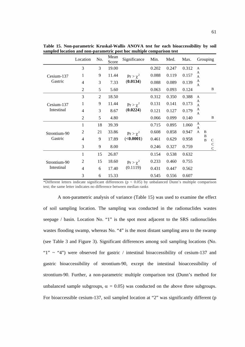
61

Table 15. Non-parametric Kruskal-Wallis ANOVA test for each bioaccessibility by soil sampled location and non-parametric post hoc multiple comparison test

Location No. Mean Score Significance Min. Med. Max. Grouping

3 3 19.00 0.202 0.247 0.312 1 9 11.44 0.088 0.119 0.157 4 3 7.33 0.088 0.089 0.139

Cesium-137 Gastric

2 5 5.60

Pr > χ2 (0.0134)

0.063 0.093 0.124

A A A A A B

3 2 18.50 0.312 0.350 0.388 1 9 11.44 0.131 0.141 0.173 4 3 8.67 0.121 0.127 0.179

Cesium-137 Intestinal

2 5 4.80

Pr > χ2 (0.0224)

0.066 0.099 0.140

A A A A A B

1 18 39.39 0.715 0.895 1.060 2 21 33.86 0.608 0.858 0.947 4 9 17.89 0.461 0.629 0.958

Strontium-90 Gastric

3 9 8.00

Pr > χ2 (<0.0001)

0.246 0.327 0.759

A A A B B B C C C

1 15 26.87 0.154 0.538 0.632 2 15 18.60 0.233 0.460 0.755 4 6 17.40 0.431 0.447 0.562

Strontium-90 Intestinal

3 6 15.33

Pr > χ2 (0.1119)

0.545 0.556 0.607


A non-parametric analysis of variance (Table 15) was used to examine the effect

of soil sampling location. The sampling was conducted in the radionuclides wastes

seepage / basin. Location No. “1” is the spot most adjacent to the SRS radionuclides

wastes flooding swamp, whereas No. “4” is the most distant sampling area to the swamp

(see Table 3 and Figure 3). Significant differences among soil sampling locations (No.

“1” ~ “4”) were observed for gastric / intestinal bioaccessibility of cesium-137 and

gastric bioaccessibility of strontium-90, except the intestinal bioaccessibility of

strontium-90. Further, a non-parametric multiple comparison test (Dunn’s method for

unbalanced sample subgroups, α = 0.05) was conducted on the above three subgroups.

For bioaccessible cesium-137, soil sampled location at “2” was significantly different (p

62

< 0.05) than the values obtained for the other sampling locations (“3”, “1”, and “4”).

However, the difference (p < 0.05) was found between sampled location “1-4”, “1-3”,

and “2-3” for gastric bioaccessibility of strontium-90. This analysis showed that a

variable such as soil sampling location could affect the bioaccessibility of two

radionuclides, and emphasized the importance of collecting site-specific data for risk

assessments.

Table 16. The Spearman rank-order correlation tests between gastric / intestinal bioaccessibility and seven variables (radioactivity, sampling depth, sampling location, SOM, CEC, pH, and Clay)

Radio-activity Depth Location SOM CEC pH Clay

137Cs Gastric

0.1286 (0.5890)

N=20

-0.0323 (0.8924)

N=20

-0.0383 (0.8727)

N=20

-0.4408 (0.1748)

N=11

-0.2569 (0.4457)

N=11

-0.1285 (0.7066)

N=11

-0.2752 (0.4127)

N=11

137Cs Intestinal

0.2022 (0.4064)

N=19

0.33040 (0.1671)

N=19

-0.1042 (0.6711)

N=19

-0.7553 (0.0115)

N=10

-0.5138 (0.1287)

N=10

-0.4159 (0.2319)

N=10

-0.2936 (0.4103)

N=10

90Sr Gastric

0.6320 (0.0001)

N=57

0.2888 (0.0294)

N=57

-0.6032 (0.0001)

N=57

0.2000 (0.2222)

N=39

0.3862 (0.0152)

N=39

0.5779 (0.0001)

N=39

0.4130 (0.0090)

N=39

90Sr Intestinal

0.2872 (0.0686)

N=41

0.4297 (0.0050)

N=41

-0.3613 (0.0203)

N=41

-0.5524 (0.0034)

N=26

-0.1637 (0.4241)

N=26

0.4104 (0.0373)

N=26

-0.0767 (0.7096)

N=26

Associations between bioaccessibility and other characteristic variables in the

tested soils were examined using a non-parametric Spearman statistical test (Table 16).

For gastric bioaccessible cesium-137, there were no significant associations with any of

the seven soil characteristic variables. For intestinal bioaccessible cesium-137, SOM

percentage in soil was the only factor correlated with the bioaccessibility (p = 0.0115),

and that was a negative correlation. Clay is a known absorbent for cesium-137 and causes

limited dissolution of cesium-137 in the extraction system (Ellickson et al., 2002). It was

expected that the clay factor would have the negative relationship between cesium-137

63

bioaccessibility and clay contents; but there was no significant correlation. The clay

content of each soil sample was minimal (below 1 %), therefore, the association between

clay content and bioaccessible cesium-137 was not found in these samples.

Conversely, both gastric and intestinal bioaccessible strontium-90 had statistically

significant associations with the following variables: sampling depth (p = 0.0294, 0.0050),

sampling location (p = 0.0001, 0.0203), and soil pH (p = 0.0001, 0.0373), respectively.

Since the soil distribution coefficient (Kd) increased with soil pH, it could be expected

that a negative association between strontium-90 bioaccessibility and soil pH would exist.

Increasing soil pH would cause cation extraction decrease, due to more binding of

strontium-90 with soil (Brady et al., 1995). However, correlation coefficient for the

bioaccessibility and soil pH for strontium-90 in seepage / basin soils was positive. A key

observation here is the positive correlations between total strontium-90 and bioaccessible

strontium-90 in gastric phase (coefficient of 0.6320; p = 0.0001) as well as soil pH

(coefficient of 0.57143; p = 0.1390). This result was associated with the relatively high

solubility of strontium-90 in gastric fluid (95.2 ~ 60.1 %) and therefore, shows little

variation with soil pH value. The index number (No. “1” ~ “4”) for soil sampling depth

and location was inversely correlated with the radioactivity of strontium-90 in soil. Total

radioactivity of strontium-90 was positively correlated with the bioaccessible strontium-

90 (coefficient of 0.36189; p = 0.0003). Therefore, the negative association of sampling

location with bioaccessible strontium-90 was associated with the higher radioactive soil.

However, a positive association between sampling depth and bioaccessible strontium-90

might be explained by the soil characteristics, especially the clay content in each soil. The

64

correlation between intestinal bioaccessibility of strontium-90 and clay contents was

negative (-0.0767), however, not significant (p = 0.7096).

2.4.4. Exposure / dose estimation

Two radionuclides exposure and dose estimations were completed on three soil

hazard classes for four hypothetical population groups by the duration of short-term and

long-term exposure. Three exposure pathways (ingestion of soil, inhalation of re-

suspended soil, and external radiation exposure from soil) were considered to estimate

exposure / dose predictions for each population group. Two exposures (ingestion and

inhalation) and three dose levels were projected along with each hypothetical group’s

physiological condition and scenario using the Monte Carlo simulation of Crystal Ball®

program.

The estimated exposure (potential dose) values for cesium-137 and strontium-90

from ingestion / inhalation pathways are presented in Table 18 for three soil classes and

four sub-groups. For each route of exposure, the median and 95 percentile for estimates

of potential dose to cesium-137 and strontium-90 are provided in the table. The potential

dose estimations are given as intake radiation (pCi) per body weight (kg) over time (day).

These estimated potential dose values for two radionuclides could be compared with the

allowable regulatory values. For example, EPA has established a Maximum Contaminant

Level (MCL) of 4 millirem per year from man-made radionuclides in drinking water. The

average concentration for equivalent cesium-137 is 200 picocuries per liter (pCi/L), and

the average concentration for equivalent strontium-90 is 8 pCi/L (EPA, 1993). Thus, the

MCL was converted to the same unit of calculated potential dose of ingestion (pCi/kg-

65

day) for two radionuclides, and provided in Table 17. For cesium-137, the potential dose

estimates surpassed the converted MCL for pica, 2.5, and 6 years old children on class

“A” soil; however, the other estimates were below the MCL. In case of strontium-90, the

potential dose estimates were above the converted MCL for pica and 2.5-year old

children on three soil classes as well as 6-year old children and adults on class “A” soil.

Table 17. The age-specific variables (dinking rate and body weight) and converted MCL for cesium-137 and strontium-90 respect to each age group

2.5-year-old Children

6.0-year-old Children Adults

Drinking* (L/day) 0.61 0.74 1.4

Weight* (kg) 14.3 22.6 72.8

Cesium-137 (pCi/kg-day) 8.53 6.55 3.85

Strontium-90 (pCi/kg-day) 0.34 0.26 0.15

*: Taken from U.S. EPA Exposure Factor Handbook, 1999

The result for estimated potential dose levels showed large differences among

class “A” soil and other soil classes (“B” and “C”). The ratio of potential dose for

cesium-137 ranged from 131 to 134 for soil class “A” / “B” and 51 to 52 for soil class

“A” / “C”, respectively. The ratio of soil class (“A” / “B” and “A” / “C”) for strontium-90

dropped to 13 and 17, respectively. The higher proportion of radionuclide potential dose

for pica and young children resulted from non-dietary ingestion rather than inhalation.

For pica children, especially the estimated potential doses were approximately five times

higher than non-pica children in the same age group (2.5 years old). The higher potential

dose values would be a result of children’s pica activity, yielding the differences in the

amount of soil ingested for pica children, 500 mg/day versus 2.5 years old non-pica

children, 110 mg/day. The elevated potential dose levels resulted from high radioactivity

66

of soil (soil hazard class of “A”), children’s specific activity (pica or hand-to-mouth), and

exposure pathway (non-dietary ingestion).

The biologically effective dose values were estimated based on the radioactivity

of each soil class, age-specific exposure variables, and durations. The predicted short-

term (two weeks duration) effective doses for cesium-137 and strontium-90 are presented

in Table 19 and 20, respectively. For each target radionuclide, the median and 95

percentile were provided for three major exposure pathways (ingestion, inhalation, and

external exposure) to the contaminated soil and subsequent total dose. The median and 95

percentile values were descriptive statistics and approached the maximum probable

values for radionuclides effective dose for age-specific groups, respectively. The

exposure duration was extended to one-year in residence (as a long-term exposure) for

Chernobyl residents, and the calculated effective dose estimates for cesium-137 and

strontium-90 are found in Table 21 and Table 22, respectively.

The NCRP, in considering the risks associated with low-level radiation exposures,

has recommended that there be some level of exposure below which no individual need

be concerned. This is called “Negligible Individual Dose” (NID). A value of 1.0 millirem

(0.01 mSv) in a year has been recommended as constituting a “boundary below which the

dose can be dismissed from consideration” (NCRP Report No. 116, 1993). Currently

NCRP recommends that “when the annual effective dose limit as a result of irradiation

attributable to a single site, the site operator should ensure that the annual exposure of the

maximally exposed individual, from all man-made exposure (excepting that individual’s

medical exposure), the dose should not exceed 1 mSv on a continuous basis” (NCRP

Report No. 116, 1993).

67

For short-term exposure to cesium-137 and strontium-90, the effective dose

estimates were below 0.01 mSv level - a negligible individual dose by the NCRP- with

the exception of pica children on class “A” soil for strontium-90. Due to the short

duration of two weeks, the cumulative amount of cesium-137 and strontium-90 was not

high enough to impact on the health of visitors.

The results for total dose calculated changed greatly for the example of long-term

exposure to these radionuclides. Total dose of cesium-137 and strontium-90 was nearly

26X higher than that of short-term exposure. For cesium-137, total doses of all sub-

groups on class “A” soil were over the 0.01 mSv level. Effective doses resulted from both

ingestion and external exposure contributed to exceed the level for pica / young children;

however, for older children and adults, effective dose from external exposure was enough

to surpass the level of 0.01 mSv. In the case of strontium-90, effective dose estimates for

pica children on three soil classes and young children on class “A” soil exceeded the

NCRP NID (0.01 mSv). It can be concluded that the effective dose for strontium-90 via

ingestion was a dominant exposure pathway, and yielded the total dose easily surpassed

the level of NCRP negligible individual dose.

Effective dose predictions were based on three hazard classes for radioactive-

contaminated soils with three exposure routes (ingestion, inhalation, and external

exposure) and two exposure scenarios (two week vacation and one year residence). The

effective dose contributed by each exposure pathway to total dose was different for each

exposed group and target radionuclide. For cesium-137, contribution of external radiation

to total dose was smaller than that of non-dietary soil ingestion for pica children (below

20 %) due to their very high amount of soil ingestion (500 mg per day). However,

68

contribution of external exposure to total dose was equal to or slightly larger than that of

ingestion to total dose for young children. The contribution of external exposure

outweighed the portion of non-dietary soil ingestion for older children and adults (over

70 %). For strontium-90, the contribution of ingestion to total dose was dominant for pica

/ young children (over 95 %), and reduced greatly for older children and adults (below

25 %). Due to high ingestion rate for pica and young children, non-dietary ingestion was

a primary exposure route for both radioactive contaminants. However, for older children

and adults, external radiation was a major exposure pathway from radioactive-

contaminated soil. The contribution of inhalation to total dose was very low (below 4 %

of contribution to total dose) for all exposure scenarios and soil classes.

Among four hypothetical population groups, pica children on class “A” soil were

a worst case for effective dose predictions. Their effective doses were close to the NCRP

acceptable dose limit (1 mSv) for public health. The NCRP considers 1 mSv dose as an

acceptable dose limit for continuous exposure to the public (NCRP, 1987, 1993). For

long-term exposure, there was a distinct gap between total doses associated with high-

level soil (class “A”) versus low-level soil (class “B” and “C”). The high-level

radionuclide effective doses were larger than the low-level effective doses by the

magnitude of 15 to 150X reflecting the high radiation emitted from class “A” soils. The

greater intestinal bioaccessibility contributed to the increased radiation dose for

strontium-90 as compared to cesium-137. For example, the total cesium-137 radiation in

class “A” soil was much higher, approximately 13 times, than the values for strontium-90.

However, the effective dose estimations for young children based upon class “A” soils

showed an opposite pattern: namely, the estimated effective doses calculated for

69

strontium-90 were two times higher than those of cesium-137. This was caused by the

much higher bioaccessibility of strontium-90 (59.3 % bioaccessible in intestinal phase)

versus cesium-137 (13.8 % of intestinal bioaccessibility) and the difference in effective

dose coefficient of 9.1*10-8 Sv/Bq for strontium-90 versus 1.1*10-8 Sv/Bq for cesium-

137 for young children.

Pica children and 2.5-year-old children, residing on highly radioactive-

contaminated sites such as Chernobyl Nuclear Power Plant Exclusion Zone and

Resettlement Zone at least one year, would be at higher risk of exposure to cesium-137

and strontium-90 than adults or older children. This would be their activities (i.e., hand-

to-mouth activity, more mobility than younger children) and potential higher possibilities

of soil ingestion. Further, the calculated risk to the general population (median value)

would be above the negligible dose (0.01 mSv) for cesium-137 as a result of exposure to

very high radioactive-contaminated soils (e.g., the surface soil of ChNPP Exclusion Zone)

for one year. Similarly pica children would be above the negligible dose established by

NCRP (0.01 mSv) for strontium-90, if they lived on the highly radioactive-contaminated

soils in the ChNPP Exclusion Zone or Resettlement Zone for one year.

70

Table 18. Potential dose estimates (50 % & 95 %) from ingestion and inhalation pathways for Cesium-137 and Strontium-90

Cesium-137 (pCi/kg-day) Strontium-90 (pCi/kg-day) Subgroup Soil

Class Ingestion Inhalation Ingestion Inhalation

A 310.703 418.487

4.24E-02 5.67E-02

23.508 31.415

3.19E-03 4.25E-03

B 2.337 3.113

3.18E-04 4.26E-04

1.668 2.227

2.27E-04 3.01E-04

Pica Children

C 5.953 7.992

8.12E-04 1.08E-03

1.390 1.860

1.89E-04 2.52E-04

A 68.361 92.297

4.22E-02 5.66E-02

5.147 6.943

3.19E-03 4.23E-03

B 0.515 0.687

3.17E-04 4.25E-04

0.365 0.491

2.26E-04 3.04E-04

2.5-Year Children

C 1.312 1.760

8.12E-04 1.09E-03

0.305 0.407

1.89E-04 2.53E-04

A 8.699 11.606

3.95E-02 5.28E-02

0.650 0.871

2.96E-03 3.94E-03

B 0.065 0.087

2.96E-04 3.93E-04

0.046 0.062

2.12E-04 2.82E-04

6.0-Year Children

C 0.166 0.221

7.57E-04 1.01E-03

0.039 0.052

1.76E-04 2.35E-04

A 2.495 3.310

1.86E-02 2.49E-02

0.188 0.250

1.39E-03 1.86E-03

B 0.019 0.025

1.40E-04 1.86E-04

0.013 0.018

9.95E-05 1.33E-04 Adults

C 0.048 0.064

3.57E-04 4.76E-04

0.011 0.015

8.31E-05 1.11E-04

*Bold means the ingestion estimate is above the EPA’s MCL (maximum contamination level) from man-made radionuclides in drinking water

71

Table 19. Effective dose estimates (50 % & 95 %) for cesium-137 from short-term exposure

Subgroup Soil Class

Ingestion (mSv)

Inhalation (mSv)

External (mSv)

Total (mSv)

A 3.47*10-3 4.79*10-3

1.69*10-6 2.24*10-6

9.64*10-4 1.21*10-3

4.44*10-3 5.85*10-3

B 2.25*10-5 3.09*10-5

1.26*10-8 1.67*10-8

7.23*10-6 9.11*10-6

2.98*10-5 3.90*10-5

Pica Children

C 1.39*10-4 1.92*10-4

3.23*10-8 4.31*10-8

1.84*10-5 2.32*10-5

1.57*10-4 2.13*10-4

A 7.62*10-4 1.06*10-3

1.69*10-6 2.24*10-6

9.62*10-4 1.20*10-3

1.73*10-3 2.17*10-3

B 4.96*10-6 6.83*10-6

1.27*10-8 1.69*10-8

7.23*10-6 9.05*10-6

1.22*10-5 1.53*10-5

2.5-Year Children

C 3.04*10-5 4.19*10-5

3.22*10-8 4.27*10-8

1.85*10-5 2.31*10-5

4.90*10-5 6.28*10-5

A 1.25*10-4 1.73*10-4

1.65*10-6 2.20*10-6

6.77*10-4 8.51*10-4

8.06*10-4 9.98*10-4

B 8.12*10-7 1.12*10-6

1.24*10-8 1.62*10-8

5.08*10-6 6.39*10-6

5.91*10-6 7.35*10-6

6.0-Year Children

C 4.98*10-6 6.91*10-6

3.17*10-8 4.18*10-8

1.30*10-5 1.64*10-5

1.81*10-5 2.25*10-5

A 1.67*10-4 2.30*10-4

3.21*10-6 4.25*10-6

5.44*10-4 6.88*10-4

7.16*10-4 8.89*10-4

B 1.09*10-6 1.50*10-6

2.40*10-8 3.18*10-8

4.09*10-6 5.11*10-6

5.21*10-6 6.43*10-6 Adults

C 6.66*10-6 9.18*10-6

6.15*10-8 8.15*10-8

1.04*10-5 1.31*10-5

1.72*10-5 2.14*10-5

72

Table 20. Effective dose estimates (50 % & 95 %) for strontium-90 from short-term exposure

Subgroup Soil Class

Ingestion (mSv)

Inhalation (mSv)

External (mSv)

Total (mSv)

A 9.31*10-3 1.24*10-2

2.59*10-6 3.41*10-6

6.81*10-5 8.55*10-5

9.38*10-3 1.25*10-2

B 5.34*10-4 7.14*10-4

1.84*10-7 2.42*10-7

4.86*10-6 6.05*10-6

5.39*10-4 7.19*10-4

Pica Children

C 3.77*10-4 5.03*10-4

1.53*10-7 2.02*10-7

4.03*10-6 5.04*10-6

3.81*10-4 5.08*10-4

A 2.04*10-3 2.73*10-3

2.58*10-6 3.42*10-6

6.78*10-5 8.53*10-5

2.11*10-3 2.81*10-3

B 1.18*10-4 1.56*10-4

1.84*10-7 2.45*10-7

4.84*10-6 6.08*10-6

1.23*10-4 1.62*10-4

2.5-Year Children

C 8.31*10-5 1.10*10-4

1.53*10-7 2.03*10-7

4.03*10-6 5.07*10-6

8.74*10-5 1.15*10-4

A 1.85*10-5 2.46*10-5

2.25*10-6 2.97*10-6

4.79*10-5 6.01*10-5

6.86*10-5 8.48*10-5

B 1.06*10-6 1.41*10-6

1.60*10-7 2.11*10-7

3.41*10-6 4.28*10-6

4.64*10-6 5.72*10-6

6.0-Year Children

C 7.49*10-7 9.94*10-7

1.33*10-7 1.76*10-7

2.85*10-6 3.56*10-6

3.74*10-6 4.60*10-6

A 1.46*10-5 1.95*10-5

1.89*10-6 2.50*10-6

3.83*10-5 4.80*10-5

5.50*10-5 6.76*10-5

B 8.40*10-7 1.12*10-6

1.35*10-7 1.79*10-7

2.74*10-6 3.44*10-6

3.72*10-6 4.59*10-6 Adults

C 5.93*10-7 7.91*10-7

1.12*10-7 1.48*10-7

2.28*10-6 2.87*10-6

3.00*10-6 3.70*10-6

*Bold number means the estimate is above the NCRP negligible annual dose level (0.01 mSv)

73

Table 21. Effective dose estimates (50 % & 95 %) for cesium-137 from long-term exposure

Subgroup Soil Class

Ingestion (mSv)

Inhalation (mSv)

External (mSv)

Total (mSv)

A 9.02*10-2 1.24*10-1

4.38*10-5 5.80*10-5

2.51*10-2 3.15*10-2

1.15*10-1 1.52*10-1

B 5.86*10-4 8.14*10-4

3.30*10-7 4.39*10-7

1.88*10-4 2.36*10-4

7.76*10-4 1.02*10-3

Pica Children

C 3.59*10-3 5.00*10-3

8.40*10-7 1.11*10-6

4.81*10-4 6.03*10-4

4.08*10-3 5.52*10-3

A 1.98*10-2 2.74*10-2

4.39*10-5 5.81*10-5

2.51*10-2 3.15*10-2

4.50*10-2 5.64*10-2

B 1.29*10-4 1.79*10-4

3.29*10-7 4.35*10-7

1.89*10-4 2.36*10-4

3.19*10-4 3.98*10-4

2.5-Year Children

C 7.90*10-4 1.10*10-3

8.43*10-7 1.12*10-6

4.82*10-4 6.01*10-4

1.28*10-3 1.65*10-3

A 3.24*10-3 4.48*10-3

4.30*10-5 5.73*10-5

1.77*10-2 2.22*10-2

2.10*10-2 2.61*10-2

B 2.11*10-5 2.90*10-5

3.22*10-7 4.26*10-7

1.32*10-4 1.66*10-4

1.54*10-4 1.92*10-4

6.0-Year Children

C 1.30*10-4 1.80*10-4

8.24*10-7 1.09*10-6

3.39*10-4 4.24*10-4

4.71*10-4 5.84*10-4

A 4.34*10-3 5.98*10-3

8.39*10-5 1.11*10-4

1.42*10-2 1.78*10-2

1.87*10-2 2.31*10-2

B 2.83*10-5 3.93*10-5

6.24*10-7 8.27*10-7

1.06*10-4 1.33*10-4

1.36*10-4 1.68*10-4 Adults

C 1.74*10-4 2.40*10-4

1.60*10-6 2.11*10-6

2.72*10-4 3.41*10-4

4.49*10-4 5.58*10-4


74

Table 22. Effective dose estimates (50 % & 95 %) for strontium-90 from long-term exposure

Subgroup Soil Class

Ingestion (mSv)

Inhalation (mSv)

External (mSv)

Total (mSv)

A 2.43*10-1 3.24*10-1

6.73*10-5 8.86*10-5

1.77*10-3 2.22*10-3

2.45*10-1 3.26*10-1

B 1.39*10-2 1.85*10-2

4.81*10-6 6.36*10-6

1.26*10-4 1.59*10-4

1.40*10-2 1.87*10-2

Pica Children

C 9.84*10-3 1.31*10-2

4.00*10-6 5.30*10-6

1.05*10-4 1.32*10-4

9.95*10-3 1.32*10-2

A 5.35*10-2 7.17*10-2

6.72*10-5 8.90*10-5

1.77*10-3 2.23*10-3

5.53*10-2 7.37*10-2

B 3.06*10-3 4.08*10-3

4.79*10-6 6.33*10-6

1.26*10-4 1.58*10-4

3.19*10-3 4.23*10-3

2.5-Year Children

C 2.16*10-3 2.86*10-3

3.99*10-6 5.29*10-6

1.05*10-4 1.32*10-4

2.27*10-3 2.99*10-3

A 4.82*10-4 6.41*10-4

5.85*10-5 7.72*10-5

1.25*10-3 1.57*10-3

1.80*10-3 2.20*10-3

B 2.77*10-5 3.69*10-5

4.17*10-6 5.55*10-6

8.93*10-5 1.12*10-4

1.21*10-4 1.49*10-4

6.0-Year Children

C 1.96*10-5 2.59*10-5

3.46*10-6 4.59*10-6

7.39*10-5 9.30*10-5

9.71*10-5 1.20*10-4

A 3.79*10-4 5.07*10-4

4.93*10-5 6.52*10-5

1.00*10-3 1.25*10-3

1.43*10-3 1.76*10-3

B 2.19*10-5 2.91*10-5

3.52*10-6 4.65*10-6

7.12*10-5 8.94*10-5

9.68*10-5 1.19*10-4 Adults

C 1.54*10-5 2.05*10-5

2.93*10-6 3.89*10-6

5.93*10-5 7.46*10-5

7.78*10-5 9.61*10-5


75

III. Bioaccessible Lead in Carpet House Dust

3.1. Introduction

House dust has been investigated to identify a proximate source of toxicants and

quantify levels of toxicants in an exposure pathway that can be used for the estimation of

human exposure in indoor residential settings (Lioy et al., 2002). Toxicants present in

house dust include semi-volatile and non-volatile pesticides, PAHs (polyaromatic

hydrocarbons), heavy metals, asbestos, and persistent organic compounds (Lioy et al.,

2002). The specific information has been obtained from measurements of total level of

each toxicant in house dust. The values were represented as dust loading (µg/ft2, µg/cm2)

or dust concentration (µg/g) collected by wipe and vacuum sampling (Lioy et al., 2002).

Since the ingestion of house dust can be a major route of children’s non-dietary exposure

to lead (Thornton et al., 1990), data on the bioaccessible fraction of toxicants, like lead,

present in house dust matrices can provide valuable new information on the exposure. It

should also be a better indicator of the dose available to an individual or population (e.g.,

young children) from house dust.

House dust contaminated with lead is currently a primary source of childhood

non-dietary exposure to lead in the United States (Lanphear ea al., 1996; Rhoads et al.,

1999). Hand-to-mouth activity is generally considered as the most important lead

exposure pathway for young children (EPA, 1995). It is well known that children are

especially vulnerable to the effects caused by lead exposure because their rapidly

developing nervous systems are particularly sensitive to lead (ATSDR, 1999). Moreover,

lead exposure to a fetus has been correlated with slow mental development and lower

intelligence later in life (ATSDR, 1999). Thus, exposure to lead can have a wide range of

76

effects on children’s development and behavior (EPA, 2001). Considering that after

exposure to small amounts of lead levels, children may appear inattentive, hyperactive,

and irritable. Children with high lead levels can have problems with learning and reading,

and hearing loss. At high levels, lead exposures can cause permanent brain damage and

even death.

A method for measuring bioaccessible lead in house dust used in this study was

derived from a bioaccessibility method developed for heavy metals present in

contaminated soils (Hamel et al., 1999; Ellickson et al., 2001). The laboratory of EMAD-

EOHSI has successfully developed the bioaccessibility method for heavy metals (Pb, As,

Cr, and Cd) and low-level radionuclides (137Cs and 90Sr) in various soil samples. The

method was modified for use with a different sample matrix (vacuumed house dust for in

vitro extraction). The target for the current study was bioaccessible lead in house dust,

and the levels were measured in both simulated gastric and intestinal fluids.

Based upon previous research, the levels of bioaccessible lead in vacuumed house

dust (sieved to < 75 µm) were expected to be different from lead levels obtained after

total extraction of lead from each sample (Ruby et al., 1992, 1993, 1996). Previous lead

dissolution studies showed a significant difference in bioaccessible lead levels at different

pH conditions for household dust (Oliver et al., 1999), soil (Ellickson et al., 2001; Ruby

et al., 1992, 1996; Oomen et al., 2002), and slagged aggregate (Davis et al., 1997). To

quantify the bioaccessible lead in artificially developed human fluids in the stomach and

small intestine, the bioaccessibility of lead was measured in simulated gastric and

intestinal fluids.

77

It was also expected that lead present in smaller particles had higher levels of

bioaccessibility than lead associated with larger dust particles. Barltrop and Meek (1979)

examined the relationship between lead particle size and absorption from the

gastrointestinal tract of rats, and found an inverse relationship between particle size and

lead absorption. Studies have shown that lead is generally more concentrated in the fine

fraction of dust (Duggan et al., 1985), and lead absorption into the body is inversely

related to particle size (Barltrop et al., 1979). Empirical evidence, however, has not

necessarily shown that collection and analysis of the lead content of a fine fraction of

dust (diameter sized below 250 µm) is a better predictor of children’s blood lead level

than total dust (EPA, 1995).

The size fraction of house dust that most readily adheres to a hand is less than 200

µm (Duggan et al., 1985) or 246 µm (Que Hee et al., 1985). Driver et al. (1989) dry-

sieved five soil types to obtain two size fractions of particles, one less than 250 µm and

the other less than 150 µm. The results showed that the finer soil particles adhere more

readily to hands than do coarse particles. Edwards et al. (1999) also demonstrated that

particles less than 100 µm adhere to hands longer than particles greater than 100 µm, and

Rodes et al. (2001) determined that particle size of dust that adheres best to the hand is

typically less than 40 µm. To link the bioaccessibility of lead with particle size fractions,

the bioaccessible lead in two biofluids and total lead in house dust was measured in three

particle size ranges: < 75 µm, 75-150 µm, and 150-250 µm.

78

3.2. Background

3.2.1. Lead

Lead is a naturally occurring bluish-gray metal found in small amounts in the

earth’s crust. Lead occurs naturally in the environment. However, most of the high levels

found throughout the environment come from human activities. Before leaded gasoline

was banned in the United States, most of the lead released into the environment came

from car exhaust. Other sources of lead released to the air include burning fuel, such as

coal or oil, industrial processes, and burning solid waste.

Once lead is released into the atmosphere, it may travel thousands of miles if the

lead is on small particles or if the lead compounds (e.g., organo lead vapors such as lead

alkyls) easily evaporate (ATSDR, 1999). Lead is removed from the air by rain and by

particles depositing to the ground or onto surface water. The release of lead to the air is

now lower than the ground of lead that has been deposited on / in the soil or dust

(ATSDR, 1999). Most of the lead found in inner city soils comes from both houses with

deteriorated paint containing lead and lead deposited in soil from automotive exhaust

emitted when gasoline contained lead (ATSDR, 1999). Higher levels of lead in soil can

be measured near roadways. This accumulation came from previous car exhaust

emissions. Once lead settles onto soil, it sticks to soil particles; however, it can be

redistributed slowly due to resuspension.

Lead can affect almost every organ and system in the human body (ATSDR,

1999). The most sensitive is the central nervous system, particularly in children. Lead

also damages kidneys and the reproductive system. The effects are the same whether it is

breathed or swallowed. At high levels, lead may decrease reaction time, cause weakness

79

in fingers, wrists, or ankles, and possibly affect the memory. Lead may also cause

anemia, a disorder of the blood, as well as damage the male reproductive system. The

connection between these effects and exposure to low levels of lead is uncertain (ATSDR,

1999).

Young children (< 6 years old) can be exposed to lead by eating lead-based paint

chips, chewing on objects painted with lead-based paint, or swallowing house dust or soil

that contains lead (ATSDR, 1999). A child who swallows large amounts of lead-

contaminated soil or dust may develop blood anemia, severe stomachache, muscle

weakness, and brain damage. Even at much lower levels of exposure, lead can affect a

child’s mental and physical growth. Unborn children can be exposed to lead through their

mothers (ATSDR, 1999). Lead can easily cross the placenta; therefore, exposure of

women to lead during pregnancy results in uptake by fetus. Prenatal exposure may be

related to postnatal mental retardation, impaired postnatal neurobehavioral development,

and reduced birth weight and gestational age (ATSDR, 1986).

Lead is ubiquitous in the urban environment, and has detrimental impacts on

human health. Elevated levels of lead are found in house dust; the source is mostly from

the tacked-in soil that is contaminated with lead (EPA, 1995). The ingestion of lead-

contaminated house dust by young children as a result of hand-to-mouth and object-to-

mouth behavior is recognized as an important pathway of lead exposure to children

(Lanphear et al., 1996; Rhoads et al, 1999). For these reasons, lead was chosen as the

target contaminant of concern to evaluate the bioaccessibility of a heavy metal in house

dust obtained from urban residences.

80

3.2.2. IEUBK model5

The Integrated Exposure Uptake Biokinetic Model for Lead in Children (IEUBK;

EPA, 2002) is used to predict blood lead concentrations (PbBs) for children exposed to

lead in their environment. The IEUBK model allows the user to input relevant absorption

parameters (e.g., the fraction of lead absorbed from soil / house dust) as well as intake

and exposure rates. Using these input values, the model estimates the potential

concentration of lead in the blood for a hypothetical child or population of children (6

months to 7 years of age). Measured lead concentration is not only an indication of

exposure, but also a widely-used index for discerning future health problems. The U.S.

EPA and U.S. Center for Disease Control (CDC) have determined that childhood PbB

concentrations at or above the 10 µg/dL are present risks to children’s health. The

IEUBK model calculates the probability that children’s PbB concentrations will exceed

10 µg/dL (or other user entered value). By varying the data entered into the model, the

user can evaluate how changes in environmental conditions may affect PbB levels in

exposed children.

The IEUBK model is designed to predict the probable PbB concentrations for

children between 6 months and 7 years of age who have been exposed to lead through

environmental media (air, water, soil, dust, and diet). The model has the following 4

functional components:

Exposure Component compares lead concentrations in environmental media with the

amount of lead entering a child’s body. The exposure component uses environmental

5 The text was excerpted from EPA website (http://www.epa.gov/superfund/programs/lead/ieubk.htm)

81

media-specific consumption rates and lead concentrations to estimate media-specific lead

intake rates.

Uptake Component compares lead intakes into the lungs or digestive tract with the

amount of lead absorbed into child’s blood.

Biokinetic Component shows the transfer of lead between blood and other body tissues,

or the elimination of the lead from the body altogether.

Probability Distribution Component shows the probability of certain outcome (e.g., a

PbB concentration greater than 10 µg/dL in an exposed child based on the parameters

used in the model).

The IEUBK model attempts to standardize exposure by assuming age-weighted

parameters for intake of food, water, soil, and dust. The model simulates continual

growth under constant exposure levels (on a year-to-year basis). The model also

simulates lead uptake, distribution within the body, and elimination of the body. It is

commonly thought that the IEUBK model can predict the average PbB level for an entire

community. This is misleading since many factors can vary between homes within a

single community. Instead of using community means for the environmental lead inputs,

it would be more accurate to apply the IEUBK model to individual homes or

homogeneous areas, then combine the results in order to find the mean for a

neighborhood or community. However, for individuals at risk, an individual estimate of

exposure and risk would be the appropriate approach.

The IEUBK model is intended to estimate a typical child’s long-term exposure to

lead in or out his / her residence;

82

• to provide an accurate estimate of the geometric average PbB concentrations for a

typical child aged from 6 months to 7 years

• to provide a basis for estimating the risk of elevated PbB concentrations for a

hypothetical child

• to predict likely changes in the risk of elevated PbB concentrations from exposure

to soil, dust, water, or air following concerted action to reduce such exposure

• to provide assistance in determining target cleanup levels at specific residential

sites for soil or dust containing high amounts of lead

• to provide assistance in estimating PbB levels associated with the lead

concentrations of soil or dust at undeveloped sites which may be developed at a

later date.

The site-specific risk assessments require information on soil and dust lead

concentrations for the particular location in question. Variables affecting any

consideration of lead exposure from soil and dust include: ingestion parameters for soil

and dust (e.g., how much soil or dust a typical child may ingest or inhale over a set of

period time); and the amount of lead that can be absorbed from the soil. These parameters

are quite sensitive, that is, changing one variable can significantly affect the results. The

IEUBK model is designed to facilitate calculating the elevated risk of PbB levels, and is

helpful in demonstrating how results may change when the user enters different

parameters. Overall, the IEUBK model is a tool for assessing PbB concentration in

children exposed to lead. Its advantage is that it considers the several different media

which children can come in contact with doing their days.

83

3.3. Methods

3.3.1. Test house dusts

All house dust samples were obtained from 50 homes participated in the ECSC

(Evaluation of Carpet Dry Steam Cleaning) project which was sponsored by U.S. HUD,

Department of Housing and Urban Development. The ECSC study was designed to

evaluate two different cleaning methods, HEPA vacuum only vs. HEPA vacuum + dry

steaming, for their effectiveness in removing lead and other toxicants from participant’s

carpets. Samples were taken, before and after each home was cleaned, and then the

samples were analyzed for lead and other materials in the house dust. Carpets were

located in typical northern New Jersey residences on the period of July 2003 to June 2004.

A participant had to have at least one child diagnosed with a blood lead level higher than

15 µg/dL, which had been reported to State Health Department from 2000 to 2002. Dust

samples were collected in dust mite allergen bag of HEPA vacuum cleaner (HEPA

Vacuum Cleaner Upright, Hoover, Newton, IA) from the carpets. All sampled vacuum

bags were shipped directly to EOHSI and stored in a cold room (constant temperature at

4°C and relative humidity at 35%) before the analysis.

3.3.2. House dust preparation

House dust vacuum samples collected from fifteen residences were sieved to

below the 75 µm-diameter fraction using the unit shown in Figure 4. This mass fraction

was used as the primary sample for conducting the lead bioaccessibility experiments. The

total lead and the lead that was bioaccessible in the gastric and intestinal fluids were

measured in all samples. Five of these house dust samples were also sieved into three

84

separate fractions (< 75 µm, < 150 µm, and < 250 µm). Further sieving tests for the < 150

µm and < 250 µm samples were conducted to determine the lead mass distribution by

particle size (Table 23) and to examine the lead bioaccessibility as a function of the

following particle size fractions: < 75 µm, 75-150 µm, and 150-250 µm. Analyses were

completed on each size fraction to determine which particle size fraction had the highest

amount of bioavailable lead. The dust sieving was conducted using the standard operation

procedures (CRESP SOP-002 “Preparation of Soil Sub-Fractions” in the appendices) that

currently employed by EMAD-EOHSI laboratory (Ellickson et al., 2002).

Table 23. The mass distribution by particle size fraction for 5 house dust samples Dust Size Fractions Home 001 Home 002 Home 004 Home 005 Home 006

< 75 µm 36.50 % 16.73 % 15.99 % 30.94 % 46.38 % 75-150 µm 31.87 % 27.71 % 16.27 % 34.72 % 23.37 %

150-250 µm 31.63 % 55.56 % 67.74 % 24.34 % 30.25 %

3.3.3. Total house dust dissolution for lead analysis

The total lead content in house dust was determined using microwave-assisted

digestion with atomic absorption analysis, and these data were used as the reference total

lead concentration in each dust sample. Subsequently, the total lead value was used as the

denominator in all calculations of bioaccessible fraction of lead in house dust. Two sub-

samples of house dust (0.2 g from each prepared dust sample) were transferred into 50

mL centrifuge tubes. Twenty millimeters of nitric acid (TraceMetal grade, lead < 0.1 ppb,

Fisher Scientific, Edison, NJ) and 10 mL of de-ionized water were added to each tube.

Samples were digested in microwave oven (CEM Corporation, Matthews, NC, USA)

with the three-step program (1st stage of 90 % power for 20 minutes, 2nd stage of 0 %

power for 20 minutes, and 3rd stage of 90 % power for 20 minutes). After processing in

85

the microwave oven, the samples were allowed to cool down in a hood, and then diluted

up to 45 mL.


The in vitro determinative of bioaccessible lead was conducted using the modified

version of the method (Hamel et al., 1999; Ellickson et al., 2001) developed for

measuring elemental bioaccessibility in soil (Ruby et al., 1992, 1993, 1996). The assay

consisted of sequential extractions using synthetic human saliva, gastric and intestinal

fluids. Each step was conducted at physiological temperature and mixing conditions. All

bioaccessibility extraction experiments followed the University-wide (RWJMS/UMDNJ)

approved standard operation procedures (CRESP SOP-003 “Bioaccessibility Assay” in

the appendices).

3.3.4.1. Artificial fluids preparation

The artificial saliva / gastric / intestinal fluids were prepared using the same

procedures as discussed previously for the soil radionuclides bioaccessibility study (see

the section of 2.3.4.1. for detailed information).

3.3.4.2. In vitro extraction

The amount of each house dust sample used in the lead bioaccessibility

experiment was based on soil / dust intake rate (0.135 g/day) for young children between

one and four years old. Lead dissolution in synthetic gastric juice was studied previously

by Hamel et al. (1998) who showed that the lead solubility was relatively consistent

within liquid-to-solid ratios of 100:1 to 5000:1 mL/g for simulated soil ingestion of 0.05

to 0.5 g. A 0.135 g of house dust sample as the amount of house dust ingested and 400:1

86

mL/g (50+4 mL / 0.135 g) liquid-to-solid ratio were used throughout the extraction

procedure.

Approximately 0.135 g sample of sieved house dust (triplicate samples for gastric

and intestinal, respectively) was mixed with 4 mL of the artificial saliva. This was

followed by the addition of 50 mL of gastric juice (pH = 1.4 ± 0.2 throughout the

extraction). Then, the samples were placed into a constant temperature water bath (MSB-

1122A-1 General Signal, Blue Island, IL) at 37 °C and shaken for two hours at 90 rpm.

After the saliva-gastric incubation, all samples were taken from the water bath.

Subsequently, the gastric samples were filtered using a 0.45 µm pore sized cellulose

nitrate filter in a polycarbonate 250 mL filter funnel apparatus. With the addition of 1 mL

of nitric acid the filtered aqueous gastric samples were preserved in polyethylene bottles.

Meanwhile the intestinal samples were adjusted to a pH 6.5 by adding 50 mL of intestinal

juice. The samples were incubated again in the water bath at the same conditions. After

the saliva-gastric+intestinal incubation, the intestinal samples were also filtered, and

preserved in polyethylene bottles with 2 mL of nitric acid. Following the sequential

gastrointestinal extraction, the house dust residue was captured on a filter. The residual

was used to determine the total recovery and obtain a mass balance of lead for gastric and

intestinal samples. The captured house dust residue samples followed the same

procedures of total lead analysis, i.e., 10 mL of nitric acid and 5 mL of de-ionized water,

before the digestion of microwave oven. The bioaccessible lead was obtained by dividing

the lead concentration of each filtered fluid with total lead concentration found in each

house dust sample. The schematic diagram (Figure 6) showed the processes of in vitro

extraction step by step (Ellickson et al., 2002).

87

3.3.5. Analysis for total and bioaccessible lead

The gastric and intestinal extracts were directly transferred into centrifuge tubes

from the polyethylene bottles, and diluted from 10 up to 100 times prior to lead analysis.

A 10 mL of microwave-digested total lead and house dust residue sample was decanted,

spun in Metpath tabletop centrifuge (906×g) for 10 min, and then diluted to properly be

within the range of calibration curve from 2.5 ppb to 25 ppb. A GFAA (Graphite Furnace

Atomic Absorption Spectrometer, Perkin Elmer Zeeman 4100ZL, Norwalk, CT) with a

detection limit of 2.5 ppb in solution was used to quantify the lead levels. The GFAA was

calibrated for each run with standards prepared in Optima grade acid (Fisher Scientific,

Edison, NJ). The National Institute of Standardized Testing (NIST, Gaithersburg, MD)

reference material 1643D (lead dissolved in water with a concentration of 18.15 ± 0.64

µg/L, density of the solution = 1.016 g/mL at 22 °C) was used for quality control at each

run of the GFAA analysis. Sample digestion blanks and NIST 2710 soil spikes were

included in all analytical runs. The allowable instrument error was ± 20 %, although most

of the quality control results were within ± 10 %.


The data for the bioaccessibility experiments were tested for normality using a

Shapiro-Wilk test for both the gastric and intestinal data (N = 45). The test for normality

was conducted on fifteen house dust samples sieved to < 75 µm, and five house dust

samples that were separated into particle size fractions of < 75 µm, 75-150 µm, and 150-

250 µm. The results in Table 24 showed that three out of four sets of experimented data

were not normally distributed. Therefore, further statistical analyses were completed

88

using non-parametric methods. All statistical analyses were conducted using SAS®

Program v9.1 (SAS Institute Inc., Cary, NC) and SigmaStat® Program v3.11 (Systat

Software Inc., Richmond, CA).

Table 24. Shapiro-Wilk normality test for the bioaccessibility of lead from house dust samples (N = 45)

Experiment Tested Group Test Statistic p-value

Gastric Bioaccessibility 0.900696 0.0010 15 Home Samples

Intestinal Bioaccessibility 0.767012 <0.0001 Gastric Bioaccessibility 0.965795 0.2025*

5 Home Samples Intestinal Bioaccessibility 0.910170 0.0020

*Insufficient evidence to reject the assumption of normality

3.4.7. IEUBK model predictions

The IEUBK model estimates the potential concentration of lead in the blood for a

hypothetical child or population of children (6 months to 7 years old) based upon typical

reference variables, including absorption parameters, intake and exposure rates (Lewis et

al., 1999). However, errors can occur due to assumptions made about lead bioavailability

as well as other variables. In this study, the bioaccessible fractions of lead in gastric and

intestinal fluids determined for house dust may be used to augment the default input

values used as determinants of GI/Bioavailability in the model.

Two parts of the IEUBK were modified to use the house-specific bioaccessibility

data as input data: The GI Values/Bioavailability Information option on the Parameter

Input menu allowed the user to make adjustments to the gastrointestinal absorption

coefficient to account for site-specific information on bioavailability. The Blood Pb vs

Media Concentration option on the Computation menu allowed the user to generate a

plot of the relationship between blood lead concentration and the exposure to lead in a

89

specific, user-selected, environmental medium (e.g., soil, dust, air, drinking water, or

diet).

Using the results from the lead bioaccessibility analyses, blood lead levels were

predicted by substituting the default absorption value with the values of bioaccessible

lead obtained from the house dust study. These values were 65 % for gastric

bioaccessible lead and 12 % for intestinal bioaccessible lead. The input parameters for

total lead levels in house dust were changed ranging from 209 mg/kg as the lowest lead

concentration of tested house dust to 1770 mg/kg as the highest concentration. Age of the

child was selected to be from 0 to 84 months. The model simulation was run 15 times

(maximum allowed by the program) to estimate the blood lead concentrations within a

population of children exposed to bioaccessible lead levels found in house dust (Figure

11 and Figure 12).

Figure 11. The change of total bioaccessible percentage in dust matrix from default (30 %) to gastric bioaccessibility (65 %) and intestinal bioaccessibility (12 %)

90

Figure 12. The set-up of IEUBK model for predictions of blood lead vs media concentration based on studied dust concentration from 209 mg/kg to 1770 mg/kg with 15 times of running for 0 to 7 years old children

3.4. Results & Discussion

3.4.1. Bioaccessibility test for vacuumed house dusts

Fifteen house dust samples (the sample size used for the analysis was satisfied

with the significance level, α=0.05 and power, β=0.8) were chosen from the ECSC study,

and analyzed for bioaccessible lead (Table 25). The lead that was soluble in gastric fluid

yielded bioaccessibility values that ranged from 52.4 % (Home 027) to 77.2 % (Home

009). Simulated gastric juice resulted in the highest level of bioaccessible lead because of

the strong acidity (pH = 1.4 ± 0.2 throughout the extraction) associated with the artificial

91

gastric juice. This strong acid solution is representative of a fasting child and maximum

lead that would be resulted from the house dust. This would provide an upper-bound

estimate of available lead and would apply to ingestion of small particles by children

several hours after food ingestion or under fasting conditions (Oomen et al., 2003). After

the gastric solution passed into the intestinal phase, the bioaccessibility was reduced, and

ranged from 4.9 % (Home 13) to 32.1 % (Home 10). The levels dropped abruptly below

gastric bioaccessibility values since the pH increased to 6.5 with the addition of NaHCO3

solution. Thus, part of the mobilized lead was removed from intestinal solution. The

difference between gastric bioaccessibility and intestinal bioaccessibility was statistically

significant (Wilcoxon two-sample test; two-sided; p < 0.0001). Such a pH-dependent

decrease in lead solubility (Figure 13) has been observed by previous lead

bioaccessibility tests on soil sets (Ellickson et al., 2001; Ruby et al., 1992, 1993, 1996;

Oomen et al., 2002), household dust samples (Oliver et al., 1999), and slagged aggregates

(Davis et al., 1997).

Based on studies that determined the lead solubility in soils, the lead

bioaccessibility appears to depend on chemistry (e.g., pH in the solution), particle size

distribution (Ruby et al., 1992), the mechanism of dissolution (Ruby et al., 1992), and the

geochemistry of the soils (Davis et al., 1997; Ruby et al., 1999). The sharp decrease in

lead bioaccessibility after passing the intestine may be due to one of three possibilities: 1)

readsorption of lead onto the dust particles (Ellickson et al., 2001; Ruby et al., 1992,

1996), 2) complexation by pepsin (Ellickson et al., 2001), or 3) chemical precipitation of

the lead caused by phosphate within the higher pH environment found in the intestinal

compartment (Ellickson et al., 2001; Ruby et al., 1992, 1996).

92

0%

20%

40%

60%

80%

100%

House Dust, Newark NIST 2710 Soil House Dust, PortPirie

Test Matrices

Bio

acce

ssib

ility

GastricIntestinal

Figure 13. The comparison of bioaccessible lead among three different test matrices *House dust, Newark (< 75µm; N=15), the current study results NIST 2710 Soil (< 74µm; N=3), certified soil matrix from Ellickson et al., 2001 House dust, Port Pirie (< 53µm; N=7), collected household dust in Australia study from Oliver et al., 1999

and conducted the in vitro extraction test for gastric / intestinal phase at pH 1.3 / 7.0, respectively

The lead bioaccessibility ranged from 52.4 % to 77.2 % for gastric extracts and

4.9 % to 32.1 % for intestinal extracts. This finding shows that bioaccessibility of

individual house dusts can be different. Current risk assessment models (e.g., the IEUBK

model adopted 30 % fraction of lead in house dust will be absorbed in the children’s

body) do not consider the variation of house dust bioaccessibility. The range of house-

specific bioaccessibility data found on these experiments can reduce the uncertainty in

dose estimations for children, but support the general use of 30 % lead absorption value

as a default in the IEUBK model.

93

Table 25. The bioaccessibility test used for 15 vacuumed house dust samples (mean±S.D.)

Home ID Total Pb Concentration (µg/g)

Gastric Bioaccessibility (%)

Intestinal Bioaccessibility (%)

001 1097 76.6±3.1 6.7±0.3

002 596 74.3±14.5 6.7±0.2

004 216 70.1±4.5 8.5±0.7

005 1125 68.9±0.5 17.8±0.7

006 358 71.3±3.5 7.3±1.1

007 1312 74.7±2.2 6.0±0.2

009 709 77.2±0.9 11.1±0.2

010 487 52.7±1.4 32.1±0.7

013 732 55.8±1.4 4.9±0.2

014 209 57.0±1.9 9.3±0.7

016 820 72.6±2.7 5.8±0.2

021 676 59.9±2.0 12.3±0.7

023 1770 55.1±2.1 6.4±0.2

027 813 52.4±1.1 28.8±2.1

029 541 53.7±0.3 17.7±0.9

Mean±S.D. 764.1±422.5 64.8±9.4 12.1±8.2

3.4.2. Bioaccessibility / recovery test for different size fractions Lead in house dust is generally considered to be more concentrated in the fine

fraction of dust and lead absorption into the body is inversely related to particle size

(EPA, 1995). However, data showing a relationship between lead absorption and particle

size is not strong. The in vitro lead bioaccessibility was determined for three particle size

94

fractions in five house dust samples. The analyses were designed to examine changes in

bioaccessible lead that would be associated with different particle size fractions.

Recovery tests were included as a part of the bioaccessibility procedures for artificial

fluids and three particle size fractions. The recovery tests were designed to establish that

the proposed extraction system does not lose much lead through the in vitro extraction

and to examine the behavior of dissolved lead in the extraction system. The

bioaccessibility / recovery results are provided in Table 26. The results for the recovery

tests conducted for each fluid showed that the in vitro extraction procedures did not lose

much lead during the sequential extractions.

The values obtained for gastric bioaccessible lead with each of the three particle

size fractions were not significantly different (Kruskal-Wallis test; p = 0.7019). However,

intestinal bioaccessibility obtained for each of three particle size fractions was

significantly different (Kruskal-Wallis test; p = 0.0067). Further, a non-parametric post

hoc multiple comparison test (Tukey’s method for balanced subgroups; α = 0.05) was

conducted to compare the intestinal bioaccessibility obtained for each fraction, and there

were statistical differences between the size fractions (Table 27).

95

Table 26. The bioaccessibility / recovery (mean±S.D.) of vacuumed house dust samples for three sub-fractions (< 75 µm, 75-150 µm, and 150-250 µm)

Home ID Gastric Bioaccessibility Recovery Intestinal

Bioaccessibility Recovery

<75µm 76.6±3.1 % 85.1±2.4 % 6.7±0.3 % 71.2±4.2 %

75-150µm 71.0±9.9 % 87.4±4.0 % 15.6±1.0 % 96.4±13.2 % 001

150-250µm 63.8±7.1 % 91.4±2.8 % 15.2±3.7 % 94.6±1.4 %

<75µm 74.3±14.5 % 84.6±13.3 % 6.7±0.2 % 117.3±12.6 %

75-150µm 68.5±4.2 % 83.3±4.1 % 8.8±0.6 % 115.9±7.9 % 002

150-250µm 71.2±11.0 % 82.4±8.6 % 4.7±1.0 % 96.8±10.6 %

<75µm 70.1±4.5 % 76.5±2.4 % 8.5±0.7 % 76.6±8.1 %

75-150µm 69.3±3.1 % 77.0±1.4 % 9.9±1.1 % 80.9±3.4 % 004

150-250µm 79.2±21.0 % 86.1±16.0 % 15.4±5.8 % 76.7±26.8 %

<75µm 68.9±0.5 % 75.4±4.3 % 17.8±0.7 % 98.7±3.7 %

75-150µm 85.9±7.2 % 87.7±5.5 % 27.2±4.9 % 121.8±11.1 % 005

150-250µm 90.9±7.2 % 84.4±4.6 % 26.8±4.6 % 118.9±1.8 %

<75µm 71.3±3.5 % 78.2±3.5 % 7.3±1.1 % 96.8±2.9 %

75-150µm 56.3±7.5 % 76.0±5.7 % 23.9±4.7 % 84.0±5.1 % 006

150-250µm 65.0±6.0 % 79.9±1.7 % 19.1±6.9 % 93.5±8.1 %

The bioaccessibility of particle size fraction sieved to < 75 µm was significantly

different (p < 0.05) from the values obtained for particle size fractions both the 75-150

µm and 150-250 µm. Larger particle size fractions, 75-150 µm and 150-250 µm, had

higher intestinal bioaccessibility than smaller particle size fraction (< 75 µm). The

difference in bioaccessibility obtained for each size fraction suggested that lead

dissolution in gastric fluid was not affected by the dust particle size, however lead

96

dissolution for each size fraction was influenced by contacting with the intestinal fluid.

This behavior seems to indicate that lead is dissolved uniformly in gastric fluid but can be

quickly re-adsorbed onto the surface of smaller dust particles after the addition of

artificial intestinal juice. The magnitude of adsorption of dissolved lead onto the dust

particles is inversely related to particle size, because smaller particles have larger surface

area at unit mass (EPA, 1995; Yiin et al., 2002).

Table 27. Non-parametric tests for lead bioaccessibility by particle size fractions (Kruskal-Wallis ANOVA test & post hoc multiple comparison test)

Matrix No. Mean Score p-value Min. Med. Max. Grouping

< 75 µm 15 24.600 0.577 0.719 0.848

75-150 µm 15 20.733 0.490 0.687 0.941 Gastric

150-250 µm 15 23.667

Pr < χ2 (0.7019)

0.561 0.689 1.001

< 75 µm 15 14.333 0.062 0.072 0.183

75-150 µm 15 28.467 0.081 0.157 0.319 Intestinal

150-250 µm 15 26.200

Pr < χ2 (0.0067)

0.038 0.141 0.320

A B B B

*Different letters indicate significant differences (p < 0.05) by balanced Tukey’s multiple comparison test; the same letter indicates no difference between median ranks.

Intestinal recovery data also supported the explanation that the larger difference

between gastric and intestinal bioaccessibility resulted from the absorption of dissolved

lead onto dust particles or chemical precipitation in the mixture caused by phosphates in a

high pH environment.

3.4.3. IEUBK model estimates of dose using bioaccessible lead

The IEUBK model predicted two levels of blood lead concentrations: one that

was based on gastric bioaccessible lead and the other was based upon intestinal

bioaccessibility of lead (Figure 14). It is believed that most lead is absorbed into the

upper part of the intestine (ATSDR, 1999); consequently the values obtained for

97

intestinal bioaccessible lead were more representative of the absorption fraction.

However, gastric bioaccessibility provided a maximum fraction of lead available within

the human gastrointestinal system. The IEUBK model predictions showed that blood lead

levels generally would not exceed the lower blood lead level of 11 µg/dL using intestinal

bioaccessibility (12 %) or default value (30 %) in the range of tested house dust

concentrations. However, the calculated values based on gastric bioaccessibility (65 %)

easily surpassed the level of 11 µg/dL.

House Dust Concentration (µg/g)

200 400 600 800 1000 1200 1400 1600 1800

Blo

od L

ead

Leve

l (µg

/dL)

0

5

10

15

20

25

30

35

Upper PbB

Median PbB

Lower PbB

GastricIntestinalDefault ValueUpper PbBMedian PbBLower PbB

Fig. 14. The comparison of IEUBK model predictions using gastric bioaccessibility (65 %), intestinal bioaccessibility (12 %), and model default value (30 %)

The IEUBK predictions, based on model default parameter of 30 % GI absorption,

generally did not yield blood lead levels above 11 µg/dL. This was inconsistency with

reported blood lead levels. The model predictions using the 30 % absorption were

expected to approach the reported blood lead levels ranged from 11 to 32 µg/dL; however,

98

the predictions could not reach the levels. Instead, using the gastric bioaccessibility value,

65% absorption, the predictions did yield values close to the median blood lead level of

19 µg/dL. The IEUBK model predictions were obtained using the arithmetic mean of

gastric and intestinal bioaccessibility of the house dust. However, the gastric / intestinal

bioaccessibility is site-specific (dust from each home), and each home and child has

different levels of total lead and blood lead, respectively. A comparison of actual blood

lead levels was made with predicted blood lead level obtained using the intestinal, gastric,

and default value of bioaccessibility (see Table 28). The predicted blood lead levels were

found to be below the actual blood lead levels; generally blood lead levels predicted by

gastric bioaccessibility had values that were more closely associated with children’s

blood lead levels.

Table 28. The comparison of actual blood lead levels with predicted blood lead levels for each home environment.

Bioaccessibility (%) Predicted PbB (µg/dL) Home ID Dust Conc.

(mg/kg) Intestinal Gastric

Actual PbB

(µg/dL) Intestinal Default Gastric

002 596 6.66 74.28 26 3.3 5.8 9.9 004 216 8.51 70.05 17 2.9 3.8 5.4 006 358 7.29 71.28 26 3.0 4.6 7.1 007 1312 6.00 74.66 11 4.0 9.2 16.4 009 709 11.11 77.16 21 4.1 6.4 11.3 013 732 4.87 55.82 14 3.2 6.5 9.4 014 209 9.29 57.03 32 2.9 3.7 4.8 016 820 5.75 72.63 14 3.5 7.0 12.0 027 813 28.75 52.36 21 6.8 6.9 9.7 029 541 17.68 53.74 16 4.4 5.6 7.7

This inconsistency may be derived from the difference between the time for each

child’s blood lead level measurements (at least 6 months or above) and the time at which

99

lead concentration was determined in the house dust from the carpets. A child might be

exposed to lead present in previous residences, different locations (e.g., windowsills or

window walls where house dust was contaminated with lead), different matrices (paint

chips, lead-painted toys), or doing some types of activities (e.g., ingesting lead-

contaminated paint chips). In addition, the home environment might be improved with

the vacuum cleaning of carpets or abatement of leaded paint inside the house after the

high blood lead levels was reported to State Health Department.

The default value for GI/Bioavailability (30 %) in the IEUBK model is considered

reasonable estimator for predicting the blood lead levels in a target population. It has

been supported somewhat by the results of the current bioaccessibility experiments for

house dust, but the range in values obtained from the bioaccessibility analyses should be

considered for future use in sensitivity analyses. The highest value of intestinal

bioaccessibility (32 %) is essentially equivalent to the default absorption value used by

the IEUBK model. A one sample median test was conducted to determine whether or not

a sample median differs significantly from a hypothesized value. The IEUBK model

default parameter, 30 % lead absorption from soil / dust, was assumed as a hypothesized

value. Then it was significantly different with the obtained intestinal bioaccessibility data

(Wilcoxon singed rank test; H0 = 0.3; p < 0.0001). The percentiles and confidence

intervals (95 %) corresponding to 30 % intestinal bioaccessibility were obtained (Table

29). The IEUBK model default value covers over 90 % of all intestinal bioaccessibility

values determined in our experiments, however, it still could not predict blood lead

values above 11 µg/dL which was seen in each child. Thus, based upon our work, the

default value used for IEUBK risk estimates is a reasonable estimator of absorption for

100

determining the blood lead levels in target populations, however the range of values in

sensitivity analyses should be expanded to including values up to 65 % in an effort to

account for underestimate due to the lack of site-specific in the future.

Table 29. The percentile and confidence intervals (95 %) corresponding to 30 % intestinal bioaccessibility

95% Confidence Limits Distribution Free Order Statistics

Quantile Estimate

Lower Upper LCL Rank UCL Rank Coverage

100% 0.3270 99% 0.3270 ⋅ ⋅ ⋅ ⋅ ⋅ 95% 0.3128 0.2939 0.3270 41 45 82.76 90% 0.2939 0.1801 0.3270 37 45 95.93 75% 0.1663 0.1103 0.2939 29 41 95.46 50% 0.0841 0.0660 0.1129 16 30 96.43 25% 0.0631 0.0568 0.0668 5 17 95.46 10% 0.0568 0.0463 0.0616 1 9 95.93 5% 0.0504 0.0463 0.0568 1 5 82.76 1% 0.0463 ⋅ ⋅ ⋅ ⋅ ⋅ 0% 0.0463

101

IV. Bioaccessible Mercury from Fish Consumption

4.1. Introduction

Mercury cycles in the environment as a result of natural and human

(anthropogenic) activities. The most common mercury compound present in biota is

methylmercury. Methylmercury is of particular concern because it accumulates in edible

fish tissue and can reach levels millions of times greater than surrounding water

concentrations (Watras et al., 1992). The health effects of low-level human exposure to

methylmercury include cardiovascular and immunological effects, and developmental

neurotoxicity (Jacobson et al., 1989, 1990, 1996; Sparks et al., 1994; ATSDR, 1999).

Populations that are sensitive to mercury are pregnant women, infants, and younger

children (EPA, 1997; FDA, 2001). Recently, U.S. Food and Drug Administration issued a

consumption advisory based on mercury which suggested that pregnant women and

women of childbearing age who may become pregnant should avoid eating four species

or species groups of saltwater fish: shark, swordfish, king mackerel, and tilefish (FDA,

2004).

Inorganic and metallic mercury have shown limited absorption in humans (15 %;

Rahola et al., 1973) and in rodents (20 ~ 25 %; Piotrowski et al., 1992). Organic mercury

is more easily absorbed with 95 % absorption measured in humans (Aberg et al., 1969).

The protective effect of selenium on mercury toxicity has been known for about a quarter

of a century ago (Satoh et al., 1985; Ganther et al., 1972; Berlin et al., 1978). Overall, the

past findings indicate that methylmercury bound to fish tissue is almost completely

absorbed after consumption (95 %; Miettinen et al., 1973). Animal data support this

finding (Berglund et al., 1971).

102

Understanding the driving factor of mercury bioavailability in fish is a key to

predicting the level of risk. It is also important to study environmentally contaminated

fish, the portion of the fish that is used for consumption, and the manner in which the fish

is prepared for consumption by humans (i.e., cooked). Considering that the bioavailable

portion of many metals is less than 100 % in the human gastrointestinal system, new data

of mercury bioaccessibility is valuable to the estimation of methylmercury risk in the

general population and important in establishing what type of the fish matrices (e.g., raw

tuna steak vs. cooked tuna steak) are more readily bioavailable. Towards this end, the

results from the development of a method are presented for estimating mercury

bioaccessibility in fish. The result was obtained specifically for mercury in a fish;

however, the method may be generalized for application to other food products or other

metals.

Considering that fish and seafood are important dietary sources of protein and can

contain relatively high level of mercury, bioaccessibility data on mercury for fish

products will give a better understanding of the mercury dose received by the sub-groups

of the population that consume fish. Similarly, bioaccessibility data on cooked filet and

canned tuna will be more relevant than levels in raw fish to assess the risk of exposure to

mercury when dealing with the consumption of the processed product. The current data

of mercury content in fish are based on the uncooked flesh of fish (FDA, 2001), but most

people eat fish after it is cooked in a variety of ways. Thus, a method that includes

cooked fish products is necessary to construct meaningful estimates of bioaccessibility.

Also this study is a first attempt to quantify the bioaccessible mercury from food matrices

to estimate the exposure / dose levels used for risk assessments.

103

4.2. Background

4.2.1. Mercury

Mercury is a naturally occurring element; however, human activities such as

burning coal and using mercury in manufacture have increased the amount of mercury

that is currently cycling in the atmosphere, soil, lakes, streams, and oceans (EPA, 1997).

According to the EPA National Emissions Inventory (1999), coal-fired electric power

plants are the largest source of anthropogenic mercury atmospheric emissions in the U.S.

Power plants account for about 40 % of the total U.S. anthropogenic mercury emissions.

Other large sources are industrial boilers (about 10 % of U.S. mercury emissions),

burning hazardous waste (about 5 %), and chlorine production (also about 5 %).

When mercury is deposited into the water, or runs off the ground into the water,

microorganisms convert it to methylmercury, a highly toxic form of mercury (EPA,

1997). Small organisms accumulate the mercury as they feed. The accumulation of

methylmercury is magnified as animals higher up the food chain eat those organisms. The

process known as bioaccumulation results in higher levels of mercury in the tissue of

organisms as predators move up the food chain. Fish that are higher in the food chain

(e.g., sharks and swordfish) have much higher mercury concentration than fish that are

lower on the food chain (EPA, 1997). Humans become exposed when they eat mercury-

contaminated fish.

The nervous system is affected by all forms of mercury (EPA, 1999). However,

methylmercury and metallic mercury vapors are more harmful than other forms, because

mercury in these forms can cross the blood-brain barrier. Exposure to high levels of

104

metallic, inorganic, or organic mercury can permanently damage the brain, kidneys, and a

developing fetus. Effects on brain functioning may result in irritability, shyness, tremors,

changes in vision or hearing, and memory problems (ATSDR, 1999). Short-term

exposure to high levels of metallic mercury vapors may cause effects including lung

damage, nausea, vomiting, diarrhea, increases in blood pressure or heart rate, skin rashes,

and eye irritation (ATSDR, 1999).

Very young children (< 6 months old) are more sensitive to effects caused by

mercury exposure than adults (EPA, 1997). Mercury in the mother's body can pass to a

fetus and may accumulate there. It can also pass to a nursing infant through breast milk.

Mercury's harmful effects to the fetus include brain damage, mental retardation,

incoordination, blindness, seizures, and inability to speak. Children poisoned by mercury

may develop problems in their nervous and digestive systems, and can also have kidney

damage. Since the developing fetus is highly sensitive to the effects of mercury, women

of childbearing age are the population of greatest concern (EPA, 1997). Children born to

women exposed to relatively high levels of mercury during pregnancy have exhibited a

variety of abnormalities, including delayed onset of walking and talking, reduced

neurological test scores, and delays and deficits in learning ability. In addition, there is

growing evidence that methylmercury exposure can have adverse cardiovascular effects

for adults, resulting in elevated blood pressure and incidence of heart attack (ATSDR,

1999).

Mercury is accumulated by the edible fish through biomagnification in the food

chain (EPA, 1997). The most important exposure route for mercury in the general

population is through dietary ingestion of fish (FDA, 2001). Mercury exposure to

105

pregnant women is at greater concern than exposure to others, due to mercury having

detrimental impacts on the health of developing fetus (FDA, 2001). Mercury was,

therefore chosen as a toxin of concern for this study.

4.2.2. Mercury absorption

4.2.2.1. Elemental mercury

Liquid metallic mercury is very poorly (less than 0.01 %) absorbed from the

gastrointestinal tract (Bornmann et al., 1970). The release of mercury vapor from liquid

elemental mercury in the gastrointestinal tract and the subsequent absorption of the

released vapor are limited by reaction of the mercury with sulfur to form mercuric sulfide

(Berlin, 1986).

4.2.2.2. Inorganic mercury

The absorption of mercuric mercury from the gastrointestinal tract has been

estimated at approximately 7 ~ 15 % in human volunteers following oral administration

of radiolabeled inorganic mercury. Rahola et al. (1973) examined mercury absorption and

elimination after oral administration of mercuric nitrate to five male and female

volunteers, and reported very low and variable rate of gastrointestinal absorption (8 to

25 %). Investigations (Miettinen, 1973) were carried out to determine the percentage of

absorption for protein-bound mercury using 203Hg-labeled compounds and the whole-

body counting technique. Eight subjects were fed 4 µCi to 8 µCi 203Hg in calf liver

protein and two subjects 4 µCi and 14 µCi 203Hg(NO3)2 in water solution. Within the first

4 to 5 days, 85 percent of the 203Hg was excreted, mostly in the feces (absorption of

15 %).

106

4.2.2.3. Organic mercury

Methylmercury is efficiently absorbed from the gastrointestinal tract.

Approximately 95 % of methylmercury in fish ingested by volunteers was absorbed from

the gastrointestinal tract. The oral intake of 2.6 µCi of methyl-mercuric nitrate 203Hg

(CH3203HgNO3) in aqueous solution by three volunteers and total body counting were

conducted (Aberg et al., 1969). The absorption from the gastrointestinal tract was almost

complete (over 95 %) and the dominant excretion route was via the feces. An organic

mercury absorption study (Miettinen, 1973) was conducted to estimate the absorption

percentage for protein-bound methylmercury. Fifteen subjects were fed 2 µCi Me203Hg in

fish muscle protein, then about six percent of the administered Me203Hg was excreted

mostly in feces (absorption of 94 %).

The mercury in experimental fish-meal (fish caught in polluted areas of Halifa

Bay, Israel; mercury concentration of 60.2 ppb) and commercial fish-meal (Milubar,

Mobile Post Oshrat, Israel; mercury concentration of 280.8 ppb) was approximately 93 ±

5 % and 75 ± 3 % bioavailable in rats, respectively (Yannai et al., 1993). Plant based

mercury (corn infused with 203Hg during the growth; mercury concentration of 14 ppb)

tends to be less bioavailable (51 ± 11 %) than meat based (fish) mercury in rats; and this

is explained by fiber in the plants (Yannai et al., 1993).

4.2.2.4. Methylmercury in tuna

Many studies have shown that almost all of the mercury in fish tissue is

methylmercury, and 90 % is a reasonable approximation of this proportion, which varies

somewhat among fish types and laboratories (Burger et al., 2005). Storelli et al. (2002)

reported a range of 77 ~ 100 % of the total mercury is methylmercury (average of

107

91.3 %) for albacore tuna (N = 127) and 75 ~ 100 % is methylmercury (average of 91 %)

for bluefin tuna (N = 161) from the Mediterranean Sea. Burger et al. (2004) measured the

methylmercury in light and white canned tuna sampled in New Jersey supermarket (N =

40), and reported that methylmercury was 83 ~ 89 % of the total mercury. Considering

only cans with total mercury > 0.1 ppm, the value was about 89 %.

4.2.2.5. Digestion and absorption of food6

Most food is initially consumed as large particles containing many

macromolecules, such as proteins and polysaccharides that are unable to cross the wall of

the gastrointestinal tract. Before ingested food can be absorbed, it must be dissolved and

broken down into much smaller molecules. This dissolution and breaking-down process

(digestion) is accomplished by the action of hydrochloric acid secreted by the stomach,

bile secreted by liver, and a variety of digestive enzymes that are released by the system’s

exocrine glands, a process termed secretion. The molecules produced by digestion then

moved from the lumen of the gastrointestinal tract across a layer of epithelial cells and

enter the blood or the lymph- absorption. While digestion, secretion and absorption are

taking place, contractions of smooth muscles in the gastrointestinal tract wall mix the

luminal contents with the various secretions and move them through the tract from mouth

to anus- motility.

Proteins are broken down to peptide fragments in the stomach by pepsin and in

the small intestine by trypsin and chymotrypsin, which are secreted by the pancreas

(Marieb, 1997). These fragments are further digested to free amino acids by

carboxypeptidase secreted by the pancreas and by aminopeptidase located in the luminal

epithelial membranes of the small intestine. These last two enzymes split off amino acids 6 The text was excerpted from “Essentials of Human Anatomy and Physiology, 5th Ed.” Marieb, 1997

108

from the carboxyl and amino ends of the peptide chains, respectively. The free amino

acids then undergo secondary active transport, coupled with sodium, across the intestinal

wall. Short chains of two or three amino acids are also actively absorbed. Protein

digestion and absorption are largely completed in the early portion of the small intestine.

Fat (most is in the form of triacylglycerols) digestion occurs almost entirely in the

small intestine (Marieb, 1997). The major digestive enzyme in this process is pancreatic

lipase, which catalyzes the splitting of bonds linking fatty acids to the first and third

carbon atoms of glycerol. This produces two free fatty acids and a monoglyceride as

products. The triacylglycerols entering the small intestine from the stomach are insoluble

in water and are aggregated into large lipid droplets. Since only the lipids at the surface

are accessible to the water-soluble lipase. At this point, digestion would proceed very

slowly without the solubilizing action of bile. Bile salts increase the rate of fat digestion

and absorption in two ways by 1) emulsification with preventing large lipid droplets from

aggregating into still larger ones and 2) combining with the fatty acids and

monoglycerides produced by lipase at the droplet surface to form very small, water-

soluble aggregates (micelles). In the absence of bile salts, the resulting lipid

emulsification and micelle formation, fat digestion and absorption would occur so slowly

that much ingested fat would pass to the large intestine and would be excreted in the

feces.

Carbohydrate composed of polysaccharides, disaccharides, and monosaccharides

(Marieb, 1997). About two thirds of this carbohydrate is the plant polysaccharide starch

and the remainder is mostly the disaccharides sucrose and lactose. Cellulose and certain

other complex polysaccharides found in vegetable matter cannot be broken down by the

109

enzymes in the small intestine. They are passed on to the large intestine, where they are

metabolized in bacteria. Starch is partially digested by salivary amylase in the upper part

of the stomach before the enzyme is destroyed by gastric acid, and digestion is continued

in the small intestine by pancreatic amylase. The products formed by the amylases, along

with ingested sucrose and lactose, are broken down into monosaccharides (glucose,

galactose, and lactose) by enzymes located in the plasma membranes of the small

intestinal epithelial cells. These monosaccharides are then transported across the

epithelium by facilitated diffusion, while glucose and galactose undergo secondary active

transport coupled to sodium.

The tested matrices (tuna steak and canned tuna) consist mostly of proteins, fats,

and water. For example, canned white tuna (drained 56 g) is composed of protein (15 g of

26.8 %), total fat (1.0 g of 1.8 %), total carbohydrate (0 g of 0.0 %), with the remainder

of the mass being water and minerals. The mechanism of food digestion facilitated with

enzymes and secretion fluids in human gastrointestinal tract is important in understanding

the behavior of bioavailable mercury in vitro extraction system.

4.3. Methods

4.3.1. Approach

The in vitro protocol for estimating human exposure to mercury in tuna products

developed for this work was adapted to our previous heavy metal bioaccessibility studies

in soils (Hamel et al., 1998, 1999; Ellickson et al., 2001, 2002), but with a different

procedure for recapturing the residual tuna tissues at the end of each sequential extraction.

The approach taken to recapturing tuna tissues included combining the non-extracted

110

portion of the mercury and any residual matter precipitated during the extraction. An

acid-digestion of the material in the recaptured tuna tissues was considered to be the

amount of mercury retained in the recaptured tuna tissues after sequential extraction by

the biofluids. The amount of mercury in the recaptured tuna was used for bioaccessibility

/ recovery calculation for the overall tuna extraction procedure.

4.3.2. Study materials (tuna steak & canned tuna)

Yellow-fin tuna (Thunnus Albacares) steak and commercial canned tuna (light

chunk tuna in water and white solid tuna in water) were purchased from a local grocery

store in New Brunswick, NJ. Analysis of tuna steak and canned tuna was conducted to

achieve two goals: environmentally contaminated fish and one of the most widely

consumed seafood (fresh tuna - 1.79 %, white canned tuna - 5.29 %, and light canned

tuna - 13.35 % of market share; FDA, 2001) in the United States. These particular species

were chosen because it has some of the highest mercury concentrations due to its

biomagnification and bioaccumulation. One pound of previously frozen tuna steak and

commercial tuna cans (light and white) were purchased on July 7, 2004 and returned to

the EOHSI laboratory where they were stored in a laboratory freezer at -10.7 °C.

4.3.3. Synthetic fluid preparation

The artificial saliva / gastric / intestinal fluids were prepared using the same

procedures as discussed previously for the soil radionuclides bioaccessibility study (see

the section of 2.3.4.1. for detailed information).

111

4.3.4. Method modifications

4.3.4.1. Pilot study

The measurement of bioaccessible mercury from human fish consumption was

tested at the laboratory of EMAD-EOHSI with the adaptation of bioaccessibility method

for heavy metals in soils. The first experiment to measure bioaccessible mercury from

raw tuna steak and cooked tuna steak was conducted to evaluate exposures to

childbearing-aged women who frequently consumed fish. The amount of tuna (232

g/meal) and artificial saliva / gastric / intestinal volumes used (0.6 L/day for saliva and 2

L/day for gastric and intestinal fluids) were obtained from Burger et al. (2000) and

Marieb (1997). Based on each of the above daily excretion of human fluids, artificial

saliva / gastric / intestinal fluids were determined to 10 mL, 50 mL, and 50 mL,

respectively. The amount of tuna (17.4 g) was calculated from the fish consumption (232

g/meal), multiplied by gastric fluid volume (50 mL), and divided by the gastric fluid

volume per one-meal (667 mL/meal).

The sequential extraction experiments were conducted to determine the

bioaccessibile mercury following the same experimental conditions previously conducted

to determine the bioaccessible radionuclides from a soil matrix. The bioaccessibility of

triple replicates for raw tuna steak were 8.47 ± 2.54 % and 8.35 ± 1.05 % for gastric and

intestinal samples, respectively. The ranges for cooked tuna steak were lower, between

1.34 ± 0.76 % and 0.92 ± 0.02 % in gastric and intestinal phase, respectively. The

averaged mass recovery for mercury was 60.1 % and 85 % for gastric and intestinal

sample, respectively. These bioaccessibility results are considerably lower than the

reported mercury bioavailability (i.e., 95 % in vivo; ATSDR, 1999).

112

One possible reason for the lower bioaccessibility values might be that the in vitro

extraction protocols were not sufficient to release bioaccessible mercury into simulated

gastrointestinal fluids (see the section of 4.2.2.5. for the digestion of food). Considering

much of mercury mass was still remained in the solid phase (recaptured tuna flesh on the

filter), more in vitro extraction procedures may be required.

4.3.4.2. Changing experimental conditions

In order to digest tuna samples more completely, a smaller mass of tuna was used,

and changes were made in volume of artificial fluids. The mass of tuna used for each

sequential extraction test was reduced to 4.46 gram of tuna steak, while the new volume

of artificial saliva and gastric fluid were 8 mL and 42 mL, respectively for the sequential

extraction test. The new amount of tuna used (4.46 g) was calculated from the fish

consumption (232 g/day- assuming one meal per day), multiplied by saliva+gastric fluid

volume (50 mL), and divided by the saliva+gastric fluid excretion volume per day (2,600

mL/day). The intestinal volume (50 mL) was not changed from previous values. To make

the tuna samples homogenous and reduce the size of the digestate, a laboratory blender

(7009G, Waring® Laboratory & Science, Torrington, CT) method was adopted. The food

particle size (< 2 mm) obtained by the blender represents the food mixtures right after

passing the human throat. The previously used polyethylene bottles were replaced with

Teflon® bottles to extract and store samples. The use of Teflon® bottle (FEP 500 mL

wide mouth, Nalgene Labware, Rochester, NY) was introduced into the sequential

extraction method to minimize the mercury loss via volatilization or sticking to the wall

of polyethylene bottles.

113

Using the revised method, the mercury bioaccessibility determined for tuna steak

was 88.5 ± 3.44 % and 31.0 ± 18.27 % for gastric and intestinal samples (N = 3),

respectively. Total recovery of mercury was 96.9 ± 5.69 % for gastric samples, and 48.2

± 18.38 % for intestinal samples. The bioaccessibility and recovery for intestinal samples

were not only lower, but also had much higher variability. The analysis for bioaccessible

mercury was conducted again to check the reliability of the method. The bioaccessible

mercury was 88.1 ± 9.36 % and 21.5 ± 13.87 % for gastric and intestinal samples (N= 3),

respectively. Total mercury recoveries for gastric and intestinal fluids were 96.3 ± 5.27 %

and 54.4 ± 23.83 %, respectively.

The bioaccessibility and recovery in intestinal phase were much lower than the

levels in gastric fluid. It was possible that mercury was lost during the sample storage or

mercury analysis. For example, EPA recommends that the analysis for low-levels

mercury should be conducted within one or two days to avoid mercury loss from

prepared samples (EPA, 2002). Otherwise the samples were acidified to pH 1.0 with

nitric acid and stored in the EOHSI cold room for 3 ~ 4 days prior to mercury analysis.

4.3.4.3. Final experimental conditions

Based upon the test runs for the tuna samples, the method measuring

bioaccessible mercury in a food matrix has been modified for the artificial human

biofluids. The final experimental condition is determined by changes in the amount of

tuna provided in each extraction test set and the volume of fluids added to each extraction

bottle. The reference and experimental values for serving size and volumes of biofluids

are reported in Table 30. These values were determined on the assumption that the

childbearing aged women eating tuna steaks at local restaurants. The amount of tuna

114

(2.92 g) was further reduced from previous tuna weight (4.46 g) due to the change of

serving size in reference value. This was expected to improve the digestion process by

increasing solid-to-liquid ratio. The experimental tuna weight was obtained from the

amount of fish (111 g/meal) consumed in a restaurant, multiplied by total volume of

artificial fluids (100 mL), and divided by maximal excretion of human biofluids per meal

(3,800 mL/meal = 7,600 mL/day ÷ 2). The sample preservation method was changed

from nitric acid to hydrochloric acid, and it was added in aqueous solution after filtering.

EPA Method 1631 Revision E (Mercury in Water by Oxidation, Purge, and Trap, and

Cold Vapor Atomic Fluorescence Spectrometry) recommends the use of either 5 mL/L of

pre-tested 12 N HCl or 5 mL/L of BrCl solution within 48 hours of sample collection to

preserve the sample. Acid-preserved or BrCl-preserved samples are stable for a period of

90 days. Therefore, 1 mL and 2 mL of HCl (Optima grade, Fisher Chemical, Fair Lawn,

NJ) were added to gastric and intestinal filtrate samples, respectively.

Table 30. Serving size of fish and volumes of biofluids used in mercury bioaccessibility experiments

Description Reference Value Used in Experiments Source

Serving Size 111 g/meal 2.92 g Burger et al., 2000

Saliva Fluid 0.6 ~ 1.5 L/day 8 mL Davenport, 1982

Gastric Fluid 3 ~ 3.5 L/day 46 mL Davenport, 1982

Intestinal Fluid 3.5 L/day 46 mL Vander, 1990


Tuna samples were analyzed for four experimental matrices (cooked tuna filet,

uncooked tuna filet, light canned tuna, and white canned tuna). Samples of cooked filet

were prepared by the following procedures: a portion of tuna was thawed, weighed, and

pan-fried in a frying pan with vegetable oils. After fully cooking the filet, it was cooled

115

and weighed again to record changes in total weight. No preliminary preparation steps

were taken for the uncooked tuna samples (i.e., raw tuna steak). Canned tuna samples

were opened and placed on a funnel with paper filter for at least 30 minutes to drain as

much water as possible.

The four different tuna samples were divided into pieces weighing 2.92 grams

each, and individually placed into a laboratory blender for processing with 8 mL of

artificial saliva. Each mixture (tuna sample + artificial saliva) was processed in the

blender for 2 ~ 3 minutes. After saliva+fish samples were completely mixed, 46 mL of

synthetic gastric juice was mixed into the Teflon® sample bottles. These samples were

shaken (125 cycles per minute) at 37 °C for two hours in a Constant General Bath,

(MSB-1122A-1 Water Bath, Blue M Electronic Co., Blue Island, IL). After the saliva-

gastric incubation, all samples were removed from the water bath.

Subsequently, 46 mL of intestinal juice was added to the intestinal samples, and

they were allowed to incubate again for another 2 hours at 37 °C with moderate shaking

(125 cycles/min). During the incubation of intestinal samples, the gastric samples were

filtered with a 0.45 µm diameter membrane filter. They were acidified by adding 1.0 mL

of Optima grade hydrochloric acid to preserve the samples and each was labeled as

“gastric liquid 1, 2 or 3”. The undigested semi-solid tuna tissue that remained on the

membrane filter was collected, weighed and labeled as “gastric solid 1, 2 or 3”.

After the saliva-gastric+intestinal incubation was completed, the intestinal

samples were removed from the water bath and filtered using the gastric sample filtering

procedure. Similarly, the intestinal samples were acidified by adding 2.0 mL of

hydrochloric acid to each fluid sample and labeled as “intestinal liquid 1, 2 or 3”. The

116

insoluble portion of intestinal bioaccessible samples were obtained and labeled as

“intestinal solid 1, 2 or 3”. All gastric and intestinal bioaccessibility samples were tightly

sealed and kept in the cold room at 4 °C for later mercury analysis.

4.3.6. Digestion for total and bioaccessible mercury

To determine the mercury levels in the experimented sample matrices (tuna steak,

white canned tuna, and light canned tuna), total mercury digestion was conducted prior to

each experiment. Duplicate tuna tissue samples (approximately 1.5 g each) were selected

from four experimental tuna samples, and these were digested using a microwave-

assisted digestion method (see the section of 4.3.7.) for total mercury. To quantify the

mercury levels in recaptured tuna tissue, it was digested with the same procedures used

for total mercury analysis. Aqueous extracted samples (5 mL) were concurrently digested

with the solid-phase tuna samples (tuna tissue and recaptured tuna tissue sample). The

acid-digestion of aqueous extracted samples was conducted to reduce the mercury in the

samples to an elemental form and prevent the generation of foams during the analytical

analysis by totally dissociating mercury from mercury-bound organics in the samples.

Four milliliter of Ultrex® II Ultrapure nitric acid (Reagent grade, J. T. Baker, Phillipsburg,

NJ) and 2 mL of de-ionized water were added into the mixture of each solid digestion

vessel. Two milliliter of Ultrex® II Ultrapure nitric acid was used for each liquid

digestion vessel.

4.3.7. Mercury analysis

Mercury was analyzed by EPA Method 7471A Cold Vapor Atomic Absorption

Spectrometry (Mercury in Solid or Semisolid Waste; EPA, 1994). This method is based

117

on the absorption of radiation at the 253.7 nm wavelength by mercury vapor. The

mercury is reduced to the elemental state and aerated from solution in a closed system.

The mercury vapor passes through a cell positioned in the light path of an atomic

absorption spectrophotometer. Absorbance is measured as a function of mercury

concentration. The method detection limit (MDL) is 0.2 ppb. The fish digestion

procedure was modified from EPA Method 3051: Microwave Assisted Acid Digestion of

Sediments, Sludges, Soils, and Oils (EPA, 1994).

Samples were digested in Ultrex® II Ultrapure nitric acid in a microwave oven

(MD 2000 CEM, Matthews, NY), using three-stage digestion protocol of ten minutes

each under 50, 100 and 150 (3.5, 7, and 10.6 kg/cm2) pounds per square inch at 70X

power. Digested samples were subsequently diluted in 25 mL of de-ionized water. All

laboratory equipment and containers were washed in 10 % HNO3 prior to each use. All

concentrations are expressed in parts per billion (ng/g) on a wet weight basis. Detection

limit was 0.2 ppb. All specimens were run in batches that included blanks, a standard

calibration curve, and spiked specimens. The accepted recoveries for spikes ranged from

85 % to 115 %; no batches were outside of these limits. Mercury was measured using a

cold vapor atomic absorption spectrometer (Lumex Mercury Analyzer RA-915+,

OhioLumex Co., Twinsburg, OH).

4.3.8. Bioaccessibility calculations

Two estimations of bioaccessible mercury were made in this study. The first was

the direct measurement of extracted mercury in two biofluids, and the second was the

estimation of bioaccessibility indirectly by obtaining the mass balance of mercury in the

system. Mercury concentrations obtained in the intestinal fluid for canned tuna were too

118

low (< 0.2 ppb) to reliably calculate bioaccessibility by the direct method for the

intestinal fluid.

The indirect estimation of bioaccessibility was previously used by Hamel et al.

(1999) as one of two novel methods, mass-balance and soil recapture, for estimating the

bioaccessibility of heavy metals in soils. The Hamel et al. (1999) study concluded that the

recaptured soil metal mass, obtained by the same way of indirect estimation for

bioaccessible mercury, was a valuable measurement since it greatly reduced analysis for

efficient processing of many soil samples and analysis of metals in each fluid; yet also

provided a reasonable estimate of bioaccessibility. It also allowed for calculating

bioaccessibility in a soil containing very low metal mass. Otherwise the analysis would

have resulted in non-detectable concentrations at the dilutions required in the synthetic

human fluid system. Therefore, the approach for estimating bioaccessibility indirectly by

mass balance was added to the conventional direct measurement of bioaccessibility for

canned tuna.

The direct measurement of bioaccessibility (BioaccessibilityD) was calculated by

multiplying the mercury concentration in the soluble portion of mercury (L-mercury) in

gastric or intestinal fluid by the volume of each fluid (around 54 and 100 ml for gastric

and intestinal samples, respectively), divided by the averaged total mercury concentration

(T-mercury) in tuna samples and the weight of tuna used in each experiment:

( ) ( )(% ) 100( ) ( )D

L m ercury ppb vo lum e m lB ioaccessib ilityT m ercury ppb w eigh t g

− ×= ×

− ×

The mass balance estimate of bioaccessibility (BioaccessibilityMB) was estimated

through the following approach. A bioaccessible percentage was estimated by subtracting

the ratio of recaptured mercury mass (S-mercury times approximately 3 g of weight for

119

recaptured filter) to total mercury mass (T-mercury times 2.92 g of weight for tuna) from

100 percent:

( ) ( )(% ) 100 100( ) ( )M B

S m ercury ppb w eight gBioaccessibilityT m ercury ppb w eight g

⎡ ⎤− ×= − ×⎢ ⎥− ×⎣ ⎦

The recovery of each set of gastric and intestinal sample was obtained from the

measured total mass, divided by total mercury in each set of samples:

[ ( ) ( ) ( ) ( )](%) 100( ) ( )

L mercury ppb volume ml S mercury ppb weight gRecoveryT mercury ppb weight g

− × + − ×= ×

− ×


To test for normality in the data, a Shapiro-Wilk test was completed on both the

gastric and intestinal data (N = 60). The direct measurements for intestinal

bioaccessibility were below the detection limit of 0.2 ppb, and they were not included in

the statistical analyses (N = 30). The result (Table 31) showed that direct measurements

of bioaccessibility (BioaccessibilityD) in two biofluids were normally distributed, while

mass balance estimates of bioaccessibility (BioaccessibilityMB) were not normally

distributed. Further statistical analyses (α = 0.05) were done with the parametric

approach for direct bioaccessibility estimates and non-parametric approach for mass

balance bioaccessibility estimates. All statistical analyses were provided by SAS®

Program v9.1 (SAS Institute Inc., Cary, NC) and SigmaStat® Program v3.11 (Systat

Software Inc., Richmond, CA).

120

Table 31. Shapiro-Wilk normality test for the bioaccessibility of mercury from tuna samples

Experiment Data No. Tested Group Test Statistic p-value

60 Gastric Bioaccessibility 0.984694 0.6541* Direct Measurement 30 Intestinal Bioaccessibility 0.767012 0.9129*

60 Gastric Bioaccessibility 0.944817 0.0089 Mass Balance Estimation 60 Intestinal Bioaccessibility 0.875299 <0.0001

60 Gastric Bioaccessibility 0.985059 0.6731* Recovery

60 Intestinal Bioaccessibility 0.965221 0.0849* *Insufficient evidence to reject the assumption of normality

4.4. Results

4.4.1. Bioaccessibility / recovery for tuna steak (raw & cooked)

The results obtained for bioaccessible mercury in tuna steak are reported in Table

32. The averaged total mercury levels (mean ± S.D.) found in raw and cooked tuna steak

were 688.4 ± 23.2 ppb and 1075 ± 90.9 ppb, respectively. Estimates of bioavailability

obtained from direct method ranged from 48.7 % to 76.4 % for the gastric

bioaccessibility of raw tuna steak. The gastric bioaccessibility for cooked tuna steak

ranged from 49.1 % to 70.9 %. These gastric bioaccessibility data represent the maximum

levels of mercury expected to be released in the human digestive system. After the

addition of artificial intestinal juice into the samples, the intestinal bioaccessibility of

mercury was measured in each sample. The intestinal bioaccessibility of mercury for raw

tuna steak ranged from 33.8 % to 51.9 %, while the values ranged from 22.1 % to 57.8 %

for cooked tuna steak. The difference between the gastric bioaccessibility and intestinal

bioaccessibility was statistically significant (N = 30, pooled t-test, p < 0.0001).

121

Table 32. Mercury bioaccessibility / recovery data for tuna steak (wet weight)

Test Matrix Fluid BioaccessibilityD (mean±S.D.)

BioaccessibilityMB (mean±S.D.)

Recovery (mean±S.D.)

Gastric 49.3±6.2 % 80.6±4.2 % 68.7±2.2 % Raw

Intestinal 39.2±3.7 % 41.7±14.8 % 97.6±18.1 % Gastric 59.9±3.0 % 82.6±4.4 % 77.3±4.1 %

1

Cook Intestinal 22.1±8.0 % 32.3±4.6 % 89.8±4.9 %

Gastric 68.3±7.1 % 91.4±1.5 % 77.0±8.5 % Raw


2

Cook Intestinal 49.0±1.9 % 66.7±2.5 % 82.3±3.2 %

Gastric 48.7±1.7 % 82.7±3.0 % 66.0±4.2 % Raw


3

Cook Intestinal 45.3±4.9 % 64.3±1.0 % 81.0±5.8 %

Gastric 76.4±7.9 % 86.1±2.5 % 90.2±6.7 % Raw


4

Cook Intestinal 57.8±7.7 % 68.1±2.5 % 89.6±8.2 %

Gastric 69.6±8.1 % 86.7±1.8 % 82.8±7.1 % Raw


5

Cook Intestinal 22.6±6.7 % 35.3±1.5 % 87.3±7.0 %

The mass balance method for calculating bioaccessibility was also used for the

tuna steak samples. The gastric bioaccessibility of mercury for raw tuna steak and cooked

tuna steak, using the mass balance method, ranged from 80.6 % to 91.4 % and 73.2 % to

85.6 %, respectively. The intestinal bioaccessibility of mercury for raw tuna steak ranged

from 41.7 % to 73.0 %, and the bioaccessibility of mercury for cooked tuna steak ranged

from 32.3 % to 68.1 %. Thus, bioaccessibility determined by the mass balance approach

was generally higher than the values obtained using the direct bioaccessibility approach.

The reason may be resulted from the fact that the mass balance estimation represents the

122

portion of total mercury theoretically achievable in the extraction system, while the direct

measurement only shows the portion of mercury remaining in the sample after the loss of

mercury during in vitro sequential extraction. The difference in bioaccessibility obtained

for the gastric and intestinal fluids by the mass balance method was also significant (N =

30, Wilcoxon two-sample test, p < 0.0001). The recovery test was completed to

determine if there were mercury losses during each experiment. Most recovery results

were above 70 %, ranging from 66.0 % to 97.6 % for tuna steak study.

4.4.2. Bioaccessibility / recovery for canned tuna (light & white)

The results of the mercury bioaccessibility experiment for canned tuna (light and

white) are reported in Table 33. The averaged total mercury levels (mean±S.D.) found in

light and white canned tuna were 52 ± 3.5 ppb and 231 ± 5.7 ppb, respectively. For the

direct method of calculating bioaccessibility, the gastric bioaccessibility for light canned

tuna ranged from 36.6 % to 66.7 %, while the gastric bioaccessibility for white canned

tuna ranged from 47.3 % to 65.7 %. The intestinal bioaccessibility, however, dropped to

9.4 % and 2.1 % for light and white tuna, respectively. The detection limit (0.2 ppb) is

equivalent to 40.7 % and 18.2 % of total extracted mercury in intestinal fluid for light and

white canned tuna, respectively. All intestinal bioaccessibility data were below the

method detection limit (< 0.2 ppb), thus these data are not included in further analyses.

The mass balance method for calculating bioaccessibility was also applied for

canned tuna matrices (light and white). The gastric bioaccessibility of mercury for light /

white canned tuna ranged from 70.5 % to 77.9 % and 72.1 % to 76.8 %, respectively. The

intestinal bioaccessibility of mercury ranged for 27.9 ~ 36.8 % and 12.7 ~ 21.0 % for

123

light / whit canned tuna, respectively. The recovery results were mostly above 70 %,

ranging from 61.8 to 93.8 %, and close to the tuna steak values. The difference in

mercury bioaccessibility obtained between gastric fluid and intestinal fluid was

significant (N = 30, Wilcoxon two-sample test, p < 0.0001).

Table 33. Mercury bioaccessibility / recovery data for canned tuna (wet weight)

Test Matrix Fluid BioaccessibilityD (mean±S.D.)

BioaccessibilityMB (mean±S.D.)

Recovery (mean±S.D.)

Gastric 52.5±5.6 % 77.9±3.7 % 74.6±9.1 % Light

Intestinal BDL 35.3±2.9 % 74.0±2.9 % Gastric 65.7±7.2 % 76.8±4.2 % 88.9±11.0 %

1

White Intestinal BDL 17.3±5.5 % 84.8±5.5 %

Gastric 50.3±8.1 % 71.1±2.5 % 79.2±9.2 % Light


2


Gastric 66.7±4.5 % 72.9±0.7 % 93.8±4.4 % Light


3


Gastric 36.6±7.4 % 70.5±2.7 % 66.1±7.9 % Light


4


Gastric 38.4±6.3 % 76.6±2.1 % 61.8±5.0 % Light


5


*BDL: below the detection limit (< 0.2 ppb) In an attempt to account for mercury losses prior to in vitro sequential extraction,

the level of mercury volatilized from canned tuna was measured using a simple mercury

emission test. Each of three canned solid white and chunk light tuna (6 oz.) were opened

124

and placed inside a chamber with a volume of 0.15 m3 at room temperature (18 ~ 22 °C).

It took 4 hours, after opening the lid of a can, to achieve an equilibrium status inside the

chamber. Background ambient air mercury level was subtracted from measured mercury

concentration (ng/m3). The average mercury concentrations found inside the chamber for

white and light canned tuna were 107 ng/m3 and 34 ng/m3, respectively. Thus, only a

small portion of the mercury (approximately 0.12 % and 0.18 % of total mercury for light

and white canned tuna, respectively, in 4 hours) was volatilized at room temperature. The

mercury volatilization occurred through the diffusion of mercury concentration gradient

inside of chamber without the movement of air current. The previous total mercury

analysis showed that the white canned tuna has higher mercury concentration (231 ng/g)

than light canned tuna (52 ng/g).

4.5. Discussion

4.5.1. Direct vs Directadj vs Mass Balance bioaccessibility

Two different approaches were proposed to estimate bioaccessible mercury levels

in artificial biofluids used to attempt to simulate fish consumption. One was derived from

the direct measurements of mercury in extracted biofluids. The other was indirectly

estimated by the subtraction of recaptured mercury from total mercury based on a mass

balance for mercury, assuming all extracted mercury remained stable and bioaccessible in

the bottle except the non-extracted mercury retained on the filter. This mass balance

estimation was additionally proposed because the direct measurement of bioaccessible

mercury provided very low levels of mercury especially for all canned tuna samples (0.1

~ 0.2 ppb) after intestinal extraction. The lower concentrations of mercury extracted in

125

intestinal fluids may be resulted from the lower concentrations of total mercury found in

canned tuna (52 ppb for light and 231 ppb for white tuna) versus tuna steak (688 ppb),

and the possible mercury loss in the intestinal phase via volatilization, or sticking to the

surface of experimental apparatus (filtering system, digestion bottle…etc). The mass

balance estimation provided relatively higher mercury concentrations for both tuna steak

and canned tuna samples (all above 2.0 ppb), and lower variations in triplicate samples

(mostly below 5 %).

All direct mercury bioaccessibility data determined by this research were lower

than those of mass balance bioaccessibility estimates for the two biofluids and all tested

matrices. That difference was supported by the recovery obtained for entire extraction

procedure (N = 60). The mercury recovery was 80.7 ± 8.3 % and 79.9 ± 8.3 % for tuna

steak and canned tuna, respectively. Thus, we adjusted the direct bioaccessibility (N =

60) for each sample by dividing the corresponding recovery (N = 60). For example, the

direct bioaccessibility for one sample of raw tuna steak (54.3 %) was divided by a

corresponding recovery (70.9 %) for the same sample. A new bioaccessibility (76.6% =

54.3 / 70.9) was generated, and the value was close to a mass balance estimate for the

same sample (83.4 %). This corrected bioaccessibility value (called directadj) should

compensate for the effects of mercury loss during the sample handling. The values of

adjusted direct bioaccessibility were much closer to the levels of mass balance estimated

bioaccessibility. However, directadj bioaccessibility values for canned tuna in the

intestinal phase were still lower than the values determined by the mass balance

estimation, due to very low concentrations of mercury in the intestinal fluid for canned

126

tuna. The graphical comparison among direct, directadj, and mass balance bioaccessibility

is illustrated in Figure 15.

The data obtained by the mass balance approach are appropriate for analyzing the

differences by fish preparation methods and gastrointestinal fluids; because they indicate

the maximum achievable levels of mercury in extracted biofluids and are much consistent

within the same test matrix. Thus, the discussion in following section is based only on the

mass balance estimation method.

Direct vs Directadj vs Mass Balance Bioaccessibility

0%

20%

40%

60%

80%

100%

Gastric Intestinal Gastric Intestinal Gastric Intestinal Gastric Intestinal

Raw Cooked Light White

Bio

acce

ssib

ility

(%)

DirectDirectadjMass Balance

Figure 15. The comparison of mercury bioaccessibility methods (Direct vs Directadj vs Mass Balance)

4.5.2. Bioaccessibility differences by biofluids and preparation methods

A higher bioaccessibility from gastric fluid was determined compared to intestinal

fluid in all tested sample sets. The difference was statistically significant (N = 30;

Wilcoxon two-sample test; p < 0.0001), and recovery for all experimental sample sets

127

showed the method recovered above 70 % of total mercury during the whole

experimental procedures.

In general, 95 % of methylmercury is absorbed in human gastrointestinal tracts

(Aberg et al., 1969; Miettinen, 1973). This value was also supported by several animal

tests (Yannai et al., 1993; Berglund et al., 1971; Charbonneau et al., 1976). However, our

finding was somewhat lower than the human / animal tests, especially due to the lower

bioaccessibility in the intestinal phase. Organic mercury comprises about 90 % of the

mercury in tuna tissue (Burger et al., 2005). The fraction of organic mercury and

inorganic mercury absorbed is 95 % and 7 %, respectively (Burger et al., 2005). Thus, the

total amount of mercury absorption is expected to be around 86 % from the fish. The

gastric bioaccessibility determined by mass balance approach was close to the previously

reported 86 percent. Therefore, the gastric bioaccessibility determined by mass balance

approach provided reliable levels to estimate in vitro bioaccessible mercury from two

tested tuna matrices (tuna steak and canned tuna). This suggests that the mercury in

gastric phase is dissociated from tuna muscles at the expected levels (86.2 of total

mercury as an absorption fraction in human gastrointestinal tract) due to gastric fluid’s

very strong acidity (pH = 1.4 ± 0.2) and physiological conditions (temp = 37 °C and

mixing at 90 rpm).

After the addition of intestinal juice, the acidity of intestinal sample was increased

to pH = 6.5. The bioaccessibility dropped significantly (p < 0.0001), to a range of 16.3 %

and 62.8 %. The decrease of bioaccessible mercury in intestinal phase was not expected

in the study, because more tissue-bound mercury would be dissolved in the intestinal

fluid with the completion of digestion process as the undigested tuna tissue in gastric

128

phase was transferred to the intestinal fluid. On explanation for the decline in

bioaccessible mercury in the intestinal phase, it may be 1) the transport mechanisms of

mercury in digestive fluid, and 2) biochemical interactions with proteins rich in the

experimental assay from tuna flesh (personal communication with Dr. Alan H. Stern).

The transport mechanism for mercury in biofluids is not dependent on solubility

only, especially for methylmercury. Due to organic mercury’s low water solubility (1.0

g/L at 21 °C as dimethylmercury), methylmercury is expected to be relatively lipid

soluble (NAS, 2000). The organic mercury absorbed across the small intestine can be

transported actively by the complexes of Hg-SH (monovalent or divalent mercury cations

+ sulfhydrl groups such as cysteine or glutathione due to its high affinity) through the

lumen of intestinal mucosa (NAS, 2000). The methylmercury cation can bind to the thiol

group of the amino acid cysteine, creating a chemical structure similar to that of the

essential amino acid methionine (Clarkson, 1995). In such a manner, methylmercury can

cross the blood-brain barrier "disguised" as an amino acid that is the basic form of

breakdown of proteins in biochemistry via a carrier-mediated system (i.e., transport is not

solely the result of methylmercury’s lipid solubility). Thus, some dissolved mercury

(ionized monovalent or divalent mercury in gastric phase) can bind very tightly with free

cysteine (most active one from sulfhydryl or thiol groups and abundant in the

gastrointestinal fluid with the result of tuna tissue digestion), and may re-adsorb into the

undigested tuna tissues with the condition of neutral pH.

Lawrence et al. (1999) showed that the dissolved monomethylmercury (filtration

passing) from environmentally contaminated sediments in digestive juice of deposit

feeding lugworm was decreased over time ranging from 13 % at 0.5 hour of residence

129

time to 6 % at 4 hours of residence time. The reduction of dissolved methylmercury over

time was 53.8 % for the lugworm study. To estimate how much of the dissolved mercury

would be adsorbed onto the tuna tissues from gastric fluid to intestinal fluid for this study,

the mercury reduction was calculated. The result (mean±S.D.) was 27.9 ± 13.6 % and

33.6 ± 21.3 % for raw and cooked tuna steak, respectively, and it was greater for light

and white canned tuna, 56.2 ± 3.2 % and 78.4 ± 3.9 %, respectively. The authors

concluded that the decrease in the amount of soluble methylmercury over time may be

due to partitioning and reabsorption of methylmercury to particles, coagulation of

colloidal material, or adsorption / precipitation of protein onto particulate matter rather

than decreased solubilizing power of the digestive fluid (Lawrence et al., 1999). Animal

studies also showed that the in vivo absorption of mercury in intestine was reduced by the

addition of dietary fibers (wheat bran, corn silage) with administered mercuric chloride

diets (Rowland et al., 1986; Yannai et al., 1993; Kimura et al., 2001). They explained the

effect of dietary fiber in lowering absorption of mercury by reducing gastrointestinal tract

residence time and by adsorption processes.

For this study, the undigested tuna tissues provided binding sites for mercury-

cysteine complexes similar to the role of fibers or sediments that adsorbed some

dissolved mercury in digestive fluids and consequently lowered the fraction of mercury

absorption in the experiment of in vitro and in vivo. Therefore, some portion of mercury

complexes, ranging from 23.7 % to 58.9 % of dissolved mercury in gastric fluid, could

have been adsorbed onto the surface of undigested tuna flesh, and couldn’t penetrate the

filter (pore sized of 0.45 µm) as a dissolved form; instead they came out as a part of

mercury mass precipitated on the recaptured filter. This explanation is supported by an

130

equivalent recovery percentage from gastric and intestinal samples for all four kinds of

tested tuna matrices.

The difference of bioaccessibility was also explored in four different tuna

matrices: raw tuna steak, cooked tuna steak, light canned tuna, and white canned tuna.

For gastric mass balance bioaccessibility (Table 34), there was a difference among four

test matrices (Kruskal-Wallis test; N = 15; p < 0.0001). A non-parametric post hoc

multiple comparison test (Tukey’s method for balanced subgroups, α = 0.05) was

conducted for gastric bioaccessibility by serving method. The test revealed a difference

(p < 0.05) between the tuna steak and canned tuna; however, the difference was not

significant either between raw and cooked tuna steak or between light and white canned

tuna. Therefore, the mercury bioaccessibility in the gastric phase of the human digestive

system is higher for tuna steak compared to canned tuna.

Table 34. Non-parametric tests for gastric bioaccessibility by preparation ways (Kruskal-Wallis ANOVA test and post hoc multiple comparison test)

Matrix No. Mean Score p-value Min. 25 % Med. 75 % Max. Grouping

Raw Steak 15 47.267 0.758 0.834 0.852 0.883 0.926

Cooked Steak 15 37.600 0.511 0.779 0.846 0.858 0.876

White Can 15 20.933 0.705 0.728 0.750 0.767 0.810

Light Can 15 16.200

Pr < χ2 (<0.0001)

0.675 0.716 0.736 0.758 0.819

A A A B B B

*Different letters indicate significant differences by balanced Tukey’s multiple comparison test; the same letter indicates no difference between median ranks

For intestinal mass balance mercury bioaccessibility (Table 35), there was a

difference among four tested matrices (Kruskal-Wallis test; N = 15; p < 0.0001). A non-

parametric post hoc multiple comparison test (Tukey’s method, α = 0.05) was conducted,

and it was found that white canned tuna was different (p < 0.05) from the other three

131

samples, and light canned tuna was significantly different (p < 0.05) with raw tuna steak;

however, the difference between tuna steaks (raw and cooked) was not significant.

Table 35. Non-parametric tests for intestinal bioaccessibility by preparation ways (Kruskal-Wallis ANOVA test and post hoc multiple comparison test)

Matrix No. Mean Score p-value Min. 25 % Med. 75 % Max. Grouping

Raw Steak 15 46.467 0.278 0.586 0.635 0.712 0.755 Cooked Steak 15 41.200 0.270 0.349 0.640 0.654 0.702

Light Can 15 26.267 0.229 0.290 0.332 0.366 0.386

White Can 15 8.067

Pr < χ2 (<0.0001)

0.115 0.129 0.157 0.183 0.235

A A A B B B C

*Different letters indicate significant differences by balanced Tukey’s multiple comparison test; the same letter indicates no difference between median ranks

The differences in bioaccessible fraction found for gastric or intestinal extraction

may have been affected by way the tuna was prepared (Figure 16). Greater decrease from

gastric to intestinal bioaccessibility was observed for canned tuna versus tuna steak.

Canned tuna sample had lower gastric bioaccessibility, which could provide more

adsorption capacity (i.e., undigested tuna tissue) for mercury dissolved in digestive fluids

than tuna steak.

Hg Bioaccessibility in Tuna

0%

20%

40%

60%

80%

100%

Raw Tuna Steak Cooked Tuna Steak Light Canned Tuna White Canned Tuna

Tuna Matrices

Bio

acce

sssi

bilit

y (M

B)

GastricIntestinal

Figure 16. The comparison of mercury bioaccessibilityMB by different fish preparation methods

132

4.5.3. Bioaccessible mercury for fish matrix

The soil-based bioaccessibility method was adapted for a fish matrix (tuna steak

and canned tuna) to estimate the exposure to mercury by human consumption, especially

for sub-population group such as childbearing aged women. Through the bioaccessibility

experiments for two types of tuna, we have achieved progress on the adaptation of our

bioaccessibility system for use in a different exposure pathway. However, the

bioaccessible mercury results were lower than general value of 95 % reported for

methylmercury absorption in human gastrointestinal system.

In the gastric phase, in vitro sequential extraction procedures provided relatively

comparable levels for bioaccessible mercury, using either an adjusted direct

bioaccessibility or a mass balance estimate of bioaccessibility. A bioaccessibility, at most,

of 85.5 % for mercury tightly bound to tuna muscle was determined for the sequential

extraction in gastric phase. The solubilizing power of gastric fluid (hydrochloric acid +

pepsin) dissociated the tissue-bound mercury from the tuna muscles and ionized it

(usually monovalent or divalent status) into gastric fluid. Mass balance estimation in

gastric phase was close to the expected levels of mercury bioavailability (86.2 %) from

usual tuna consumption.

Mercury bound to tuna tissue is dissolved almost completely in human

gastrointestinal tract, and then the dissolved mercury is absorbed through the lumen of

intestinal walls. For example, methylmercury is approximately 90 % of the total mercury

in tuna and is actively transported through wall of intestine as methylmercury-cysteine.

Inorganic mercury, which is approximately 10 % of the total mercury in tuna, is not

133

absorbed actively like methylmercury. Generally 95 % and 7 % of the total mercury is

absorbed through the human gastrointestinal tract as methylmercury and inorganic

mercury, respectively. Thus, the absorption mechanism of mercury in tuna is not only

dependent on solubility, but also active transport and biochemical complexes. The

proposed approach for bioaccessible mercury may underestimate the bioavailability of

mercury. Since the sequential extraction system is only based on solubility of mercury

that is bound to tuna tissue, and the artificial digestive fluid does not digest the tested

tuna matrix completely. The direct measurement data were lower than the mass balance

estimation data throughout all tested sample matrices, ranging from 50.0 % to 91.6 % of

the estimated bioaccessibility by mass balance. The proposed direct method for

calculating bioaccessibility was not appropriate, especially for low-level mercury samples

(e.g., canned tuna matrices).

In the intestinal phase, however, the methods for estimating bioaccessible

mercury either by direct measurement or mass balance estimation were not relevant for

determining mercury bioaccessibility in the extracts. All direct intestinal bioaccessibility

for canned tuna were below the method detection limit (0.2 ppb). There may be two

reasons for the lower bioaccessibility in intestinal fluid compared to gastric fluid. One is

the possible readsorption of mercury onto the undigested tuna tissues that remained in our

in vitro extraction system. The other is mercury loss during the sample preparation or

lower concentration of mercury in the sample tested.

The artificial intestinal juice used did not contain some enzymes that are

important components for breaking down of proteins and fats in human guts. Bile

secretion enzyme (bile salts) by liver can start to dissolve water-insoluble fats in food

134

matrix; pancreatic secretion enzyme (trypsin, chymotrypsin, carboxypeptidase) by

pancreas can finish digesting proteins to amino acids that are object to intestinal

absorption. The tested intestinal fluid was composed of only 0.2 M of sodium bicarbonate

to return the pH to neutral when mixed with saliva+gastric solution in test bottles. The

lack of enzymes in the prepared gastrointestinal fluids might cause the incomplete

digestion of tuna tissues in gastrointestinal system, not releasing all tissue-bound mercury

in artificial digestive fluids, and subsequently allow the readsorption of dissolved

mercury onto the undigested tuna tissues during the in vitro extraction system. Because

proteins are not completely digested in the human stomach, but rather the digestion

process requires the presence of pancreatic secretions in small intestines to be completed.

The in vitro method for measuring bioaccessible mercury from food matrix was

developed to estimate the mercury levels in simulated human gastrointestinal system.

Based upon the experiments, the gastric bioaccessibility obtained by mass balance

approach came close to the level of mercury absorption reported from in vivo

experiments (86.2 % by general knowledge); however, intestinal bioaccessibility,

physiologically more relevant for human absorption than gastric bioaccessibility, did not

reach the reported mercury absorption value. Analytical difficulties have been observed

when intestinal fluid is prepared for in vitro sequential extraction (Hamel, 1998). Thus, a

method, that only uses the levels of mercury in gastric fluid and the mass balance

approach for calculating bioaccessibility, is appropriate for estimating bioaccessible

mercury from food matrix at this time. This is actually a strong conclusion since the

method is simple, and can be used as a conservative screening tool for mercury and other

metals found in food matrices.

135

V. Summary and Conclusions

5.1. Bioaccessible Radionuclides in SRS Soils

A method to measure bioaccessibility has been successfully adapted for two

radionuclides (cesium-137 and strontium-90) for both low-level radioactive-contaminated

soils (class “B” and “C”) and high-level radioactive-contaminated soils (class “A”) from

the Savannah River Sites. The method development adopted several procedures (e.g.,

sample processing unit for hydrofluoric acid digestion, soil sieve unit, glove box, swipe

test) to minimize the radiation contamination for the radioactive soil experiments at the

EMAD-EOHSI laboratory.

For cesium-137 bioaccessibility estimates, the gastric bioaccessibility (8.9 ~

22.4 %) was lower than or equal to the levels of intestinal bioaccessibility (8.3 ~ 38.8 %).

However, the gastric bioaccessibility (29.7 ~ 97.1 %) was higher than intestinal

bioaccessibility for strontium-90 (17.8 ~ 60.5 %). The comparison of gastric and

intestinal bioaccessibility by soil hazard class showed that strontium-90 of class “A” soil

was more soluble than that of class “B” or “C” soil in simulated gastrointestinal tract (P <

0.05). The difference of bioaccessibility within soil class was also observed for cesium-

137, and the bioaccessibility of class “C” soil was higher than that of class “B” soil (p <

0.05). The sub-population group, children with pica activities, was predicted to be

potentially at the elevated risk of radiation exposure to cesium-137 and strontium-90 via

the non-dietary ingestion or external exposure to radioactive-contaminated soil such as

the surface soil of Chernobyl Nuclear Power Plant Exclusion Zone (< 30 km) or

Resettlement Zone (15 ~ 40 Ci/km2 of 137Cs). The values predicted to exceed the NCRP

136

negligible dose limit (0.01 mSv) for cesium-137 and strontium-90 when residing in the

ChNPP Exclusion Zone at least one year.

The in vitro bioaccessibility method for radionuclides in radioactive-contaminated

soils allows the estimation of radionuclides bioavailability is lower in cost and quicker to

perform than in vivo test. Further, it can be used safely to model human exposure / dose

from radionuclides-contaminated soils. The bioaccessibility measurements for

radionuclides contaminated soils can be used to improve risk prioritization of

contaminated sites as well as enhance risk assessments by increasing their accuracies.

5.2. Bioaccessible Lead in Carpet House Dust

The bioaccessibility method for lead in vacuumed house dust derived from the

method used for soils has been successfully streamlined to quantify the bioaccessible

fraction of lead in environmentally contaminated house dust. The method was optimized

for lead in house dust by a slight change in parameters (e.g., volume of artificial fluids

and amount of house dust used). Reliable values of bioaccessibility were obtained in both

gastric and intestinal fluids with overall good recoveries (above 70 %).

The gastric bioaccessibility for lead in house dust (sieved to below 75 µm-

diameter size) from an urban environment was significantly higher than the intestinal lead

bioaccessibility (p < 0.0001). This was due to the readsorption of dissolved lead onto the

surface of dust particles at a higher pH in the intestinal fluid. The level of intestinal

bioaccessibility was significantly different (p = 0.0067) among three dust particle size

fractions (< 75 µm, 75-150 µm, and 150-250 µm), but the gastric bioaccessibility was

equal for each size fraction (p = 0.7019).

137

The bioaccessibility data obtained for two biofluids (gastric and intestinal juice)

was applied to the IEUBK model, and provided a support for the 30 % absorption default

value used for dust bioavailability. However, since the model did not predict actual high

blood lead values in the children, sensitivity analyses should be expanded to include

absorption values up to 65 % to reduce the underestimation for site-specific lead on

individuals. The variability in bioaccessibility observed in these experiments could

contribute towards the uncertainty in estimations of blood lead concentrations for young

children from non-dietary ingestion of dust. In addition, the bioaccessibility method for

lead in house dust can be expanded to other toxicants present in house dust (e.g.,

cadmium, arsenic, copper…etc).

5.3. Bioaccessible Mercury from Fish Consumption

A method to measure bioaccessible mercury for fish matrix was developed based

on the current bioaccessibility method for soil. The mercury bioaccessibility study was

conducted for commercial tuna products (supermarket-purchased tuna steaks and canned

tunas). Two approaches, direct measurement and mass balance estimation, were used to

report the bioaccessible mercury from human fish consumption. Mass balance estimation

was relevant than direct measurement to calculate the bioaccessible mercury in sequential

extraction system, especially for low-level of mercury in canned tuna.

The mass balance bioaccessibility for gastric fluid ranged from 73.8 % to 85.5 %

for tuna. While for intestinal fluid, the bioaccessibility by mass balance estimation was

lower and ranged from 16.3 % to 61.8 %. Thus, the experiments concluded that the level

of mercury extracted by gastric fluid is more appropriate than intestinal fluid as an

138

indicator of bioaccessible mercury extracted from food matrix in simulated human

gastrointestinal system.

The study estimated the bioaccessible mercury obtained from various prepared

methods for tuna. The results showed that tuna steak (either cooked or uncooked) had

statistically higher bioaccessibility than canned tuna (light and white tuna) in both the

gastric and intestinal phase (p < 0.05). Additionally white canned tuna had lower

bioaccessibility than light canned tuna in the intestinal phase (p < 0.05).

The current method for measuring bioaccessible mercury from tuna consumption

has been modified, and a combination of using only the gastric fluid digestion results

with a mass balance approach for calculating bioaccessible contaminants provides a

reasonable screen tool for other elements found in food.

5.4. Conclusions

• The magnitude of strontium-90 bioaccessibility was proportional to the soil

hazard class (“A” > “B” ≥ “C”); however, the relation of cesium-137

bioaccessibility was not proportional to soil hazard class (“A” = “B” ≤ “C”).

• The dose predictions for cesium-137 and strontium-90 from the exposure to

radioactive-contaminated soil such as the surface soil of ChNPP Exclusion Zone

showed that the non-dietary ingestion was critical for pica / young children due to

their high soil ingestion amount; however, the external exposure by the

penetration of radiation was significant for older children / adults.

• The difference between gastric and intestinal bioaccessibility for lead in house

dust was significant (p < 0.0001), and explained by the readsorption onto the

139

residual house dust and / or precipitation of dissolved lead due to the increase of

pH from 1.4 to 6.5 in the intestinal phase.

• The levels of lead bioaccessibility for three particle size fractions in house dust

were not statistically different in the gastric phase (p = 0.7019), however they

were significantly different in the intestinal phase (p = 0.067).

• The intestinal bioaccessibility data supported the IEUBK default parameter

(30 %) as a reasonable estimator for children’s blood lead level predictions;

however, the gastric bioaccessibility could yield the model predictions close to the

reported blood lead levels (> 11 µg/dL), and may be useful for future use in

sensitivity analyses to reduce the underestimation of a child’s blood lead value.

• Direct measurements and mass balance estimations were tested to report the

mercury bioaccessibility from human fish consumption; the mass balance

approach was more relevant than direct measurement approach for representing

mercury levels in gastrointestinal tract, especially for low-level mercury samples

(i.e., canned tuna). However, the method is not used for field application.

140

VI. Recommendations for Future Research

Through the experiments for proposed bioaccessibility studies, we have modified

the current bioaccessibility method into various environmental media and toxicants that

are important to understand the estimation of exposure / dose by the pathway of dietary

or non-dietary ingestion in human gastrointestinal tracts. However, some research is still

required in the future. Here are some recommendations for future work:

First, the relationships between soil physico-chemical characteristics and

bioaccessibility of environmental radionuclides are not clear. Future studies for

investigating the soil physico-chemical factor(s) to determine the level of bioaccessibility

for radionuclides are necessary for risk assessments based on site-specific soil as well as

future soil remediation / prioritization processes.

Second, three possible mechanisms were mentioned in lead study to explain the

decreased lead levels in intestinal phase: readsorption of lead onto house dust particles,

complexation by pepsin, and chemical precipitation of the lead caused by phosphates in

higher pH environment. Future work is needed to explore the feasibility of each

mechanism in simulated gastrointestinal system to understand the behavior of dissolved

lead in the sequential extraction.

Third, the method for measuring bioaccessible mercury from food matrix was not

developed to relevantly report the mercury levels in tested fish samples. The method

should be reliable for various foods and comparable to in vivo study results. Future

studies are needed to develop the bioaccessibility method working for food matrices in

the simulated human digestive system for environmental toxicants.

141

Appendices 1. CRESP SOP-001 “Soil Drying” 1.0 Cover Page Author(s): Kristie Ellickson Date Robert Meeker Date Scott Petlick Date Mike Pollock Date

Carl Schopfer Principal Investigator(s): David Kosson, Ph.D. Date Paul Lioy, Ph.D. Date Robert Tata, Ph.D. Date Authoree: David Kosson, Ph.D. Date EOHSI Radiation Safety Committee Chair: Arthur Upton, M.D. Date

142

2.0 Experimental The traditional definition for a “dry soil” is one that has come to constant weight after being in an oven at a temperature between 100 and 110ºC. Soil samples dried to constant weight may provide more precise results, as some physical and physico-chemical properties of soil depend on water content. For example, pore size may vary with water content and may also affect metal availability in soil. If soils are dried to approximately the same water content (by means of constant weight analysis) this variable can be controlled. 2.1 Hypothesis A soil sample dried to constant weight will be apportioned more easily to smaller particle sizes. 2.2 Objectives Approximately 200 soil samples will be dried in preparation for sieving. Drying will be conducted in a vacuum dessicator or drying oven to a constant weight. Resultant samples will be stored in a vacuum dessicator until they can be processed further. 2.3 Experimental Design Samples will dried for a specified amount of time, weighed, dried for that same time, and then weighed again until scale measurement is constant. 2.4 Method Summary Soil samples are dried in either an oven or vacuum dessicator. The oven is used for gross drying, whereas the vacuum dessicator will be used for the final drying step. 2.5 Procedure Quality Objectives Soils will be dried to constant weight. This weight must be constant to the first decimal point. For example 100.1, 100.2, and 100.3 would be considered constant drying weights. 3.0 Radionuclides 3.1 Radionuclides present in the soils to be processed are from core samples of seepage

basins used to dispose of radioactive wastes over several decades. Other samples to be processed may include surface soil samples from areas thought to be radioactively contaminated. Also, background samples will be processed. (Background soils contain no known radionuclide contaminants other than that which may be naturally present.)

143

3.2 The EOHSI Radiation Safety committee will review radionuclide characterization data prior to releasing each sample. All samples, including background samples, are characterized for radionuclides prior to use.

3.3 The principal investigator prior to authorizing work with any sample shall consider

the possibility of the presence of other toxic contaminants, such as metals or organics. 3.4 Each principal investigator supervising persons using this procedure shall review the

known or suspected contents of each sample, the sample quantity and its physical form and may consult with members of the EOHSI Radiation Safety committee if desired.

3.5 The principal investigator shall discuss with the technician any hazards in the sample. 3.6 Technicians processing soils shall observe any quantity limits imposed by the EOHSI

Radiation Safety Committee and shall follow instructions regarding custodianship of samples and contaminant inventory.

4.0 List of Procedures This protocol includes one standard operating procedure, SOP-001, ”Soil Drying.” 4.1. Purpose Soil is dried in order to obtain an additional degree of control over an experiment. Drying allows soil to be processed with greater ease in its entirety. Drying soil is applicable to most applications, but will affect some biological, physical, and chemical characteristics. 4.2 Scope and Application 4.2.1 This procedure applies to experiments requiring constant weight dryness from soils

and sediments that are declared to be or which may be radioactive, or have been determined to require handling appropriate for radioactive hazards.

4.2.2 Approximately 200 samples will be dried using this method. Approximately 40 of

these will be samples containing substantial amounts of radioactive isotopes. One hundred fifty four of these samples will contain background or low-levels of radioactive contaminants.

4.2.3 This procedure is an approved “plug-in” procedure for CRESP personnel. 4.3 Summary Field-moist samples dried to constant weight. Constant weight will be obtained by the use of one or more of the following pieces of equipment: drying oven, vacuum oven, or vacuum desiccators.

144

4.4 Definitions 4.4.1 Glove Bag - a completely sealed, disposable, plastic containment apparatus with an

internal frame used to avoid release of dust, aerosols, or other contaminants to the laboratory.

4.4.2 Soil Drying Jar - A Wide Mouth Nalgenetm Jar used to dry the soil, and then

inverted directly into the sieving apparatus.

4.4.3 HEPA filter box - an apparatus containing two suction hoses which will be fitted into the wall of the glove box and uses a blower or fan to suction away any airborne contaminants from the glove box. The box contains a HEPA filter that traps soil particles.

4.5 Responsibilities 4.5.1 All technicians performing work under this protocol are responsible for following

all instructions as written. 4.5.2 The principal investigator supervises persons implementing this protocol. 4.5.3 The authoree, when not the principal investigator, approves the written protocol and

may provide instructions to the technician as appropriate. 4.5.4 EOHSI Radiation Safety Committee members may provide advice on protocols and

materials safety as requested. 4.5.5 Scott Petlick acts as Sample Manager. 4.5.6 The following people can provide on-the-job training (OJT) on this protocol. Kristie Ellickson – soil sieving (module OJT-002) Robert Meeker – soil sieving (module OJT-002) Michael Pollock– soil sieving (module OJT-002) Carl Schopfer - health physics surveys and instrumentation (module OJT-001) 4.6 Prerequisites All soil samples must be in 250ml Wide Mouth Nalgenetm Polypropylene Sample Jars before transfer. 4.7 Interferences

145

Interferences of concern are the cross contamination of soil samples. In order to eliminate this possibility, polypropylene bottles will not be reused and adhesives with low leaching characteristics will be used. 4.8 Materials 4.8.1 Parafilm M 4.8.2 1000ml Wide Mouth Nalgenetm Sample Jars, with lids 4.8.3 250ml Wide Mouth Nalgenetm Sample Bottles, with lids 4.8.4 Paper Towels or Kimwipes 4.8.5 laboratory tape 4.8.6 Sharpi magic marker 4.8.7 decontaminating detergent (Picoclean) 4.8.8 TORBAL* Flexible Glove Cabinet with Frame (Vertex# GC-2 VWR# 32980-

000) 4.8.9 Grade #1 Filter Paper 3.2cm diameter (Whatman # 1001-032, VWR# 28450-021) 4.8.10 Respirator with HEPA filter cartridge 4.8.11 Timer 4.8.12 personal safety equipment: elbow-length gloves, Tyvek laboratory coat, eye

protection Plastic Adhesive (3M Scotchtm Super Glue Gel)

4.9 Equipment 4.9.1 Drying Oven 4.9.2 Vacuum Oven 4.9.3 Vacuum Desiccator 4.9.4 Appropriate radiation survey instruments 4.9.5 PACE multi arm evac II fume extraction system with HEPA/Gas filtration

cartridge 4.10 Safety 4.10.1 All experiments will be carried out in compliance with safety recommendations

provided by the Radiation Safety Committee at Rutgers University, which is authorized by the Nuclear Regulatory Commission and the State of New Jersey (see reference 1.20.2.)

4.10.2 Samples will be stored at room temperature. Constant weight dried samples will

be stored in a vacuum desiccator. 4.10.3 Soil, which can be released as a dispersible dust or aerosol, represents a potential

inhalation hazard. The work being performed creates fine particles, which must be contained to avoid exposure to the worker and others in the vicinity.

146

4.10.4 Soil drying is accomplished with minimum disturbance to the media and any outflow is filtered where possible.

4.10.5 To contain the samples during sieving and sample transfers requires working in a

closed, HEPA-filtered chamber or glovebox. The entire assembly is placed in a fume hood.

4.10.6 Soil materials should be contained within and transferred between sealed vessels.

The drying takes place while shaking within a sealed assembly. Opening the assembly is done in a filtered environment, after settling has take place. Dust creation is minimized by not allowing the soil to dry completely. Static electricity is avoided by not using plastic bags as the primary containment. Double containment is used, such as a bottle within a bag, or sealing an assembly with plastic wrap within a filtered chamber.

4.10.7 Samples must be in closed containers when removed from the filtered enclosure or

fume hood. 4.10.8 The potential for radiation exposure from soils will be determined prior to starting

work. The quantities approved for use will generally be limited by the exposure potential such that exceeding regulatory limits will not be possible, or determined to be extremely unlikely.

4.10.9 Radiation dosimetry badges will be worn if necessary. 4.10.10 All samples are labeled with the sample identifier code and radiation hazard

class. A chain of custody form is kept with each container. (See reference 1.) 4.10.11 Protective eyeglasses, dust mask, long-sleeved laboratory coat, long pants, and

two pairs of disposable vinyl gloves (elbow length) will be worn when working with radioactive samples. Gloves are to be surveyed periodically during work, and when removed. Hands must be washed after gloves are removed.

4.10.12 Laboratory coats, safety glasses and other safety wear must remain in room 149.

Do not bring the items into the counting room (room 145.) 4.10.13 All items shall be surveyed for contamination before exiting the laboratory. 4.10.14 Bench surfaces shall be covered with disposable bench paper. 4.10.15 Survey the work area and the laboratory for radioactive contamination at the end

of each day. 4.10.16 Wastes are contained in closed containers for pick-up by REHS and disposed per

agreement with the Savannah River Site. (See references 2 and 3.)

147

The Drying Oven, Vacuum Oven, and Vacuum Desiccator will be equipped with traps to ensure that the sample will not be released to the laboratory environment as well as protect the vacuum pump. 4.11 Sample Collection, Handling, and Preservation Soil samples will be collected by the Department of Energy and will be stored at Rutgers Environmental Health and Safety Department’s Environmental Services Building. Samples are stored in 1-liter polyethylene bottles, wrapped in a polyethylene bag, and placed in Styrofoam coolers/shipping boxes. Samples will be requested by the researcher by completing a sample request form and samples will only be transported by REHS. A record of sample flow will be recorded with a chain of custody form that will be assigned to each soil sample (See reference 1.) 4.11.1 Quality Control Constant weight drying will be tested according to the procedures below. To eliminate cross contamination, the sample bottles and jars will not be reused rather disposed after a soil sample has been dried. Each sample will be dried to the same extent. Samples will be labeled with a batch number, the date of sieving, and the sample identification number in order to eliminate possible identification confusion. Finally, any balances used will be checked with a test weight prior to use. 4.11.2 Calibration Balances will be calibrated on an annual basis. This calibration will be checked by a test weight before use. 4.11.3 Calculations None 4.11.4 Procedure Read this entire document before beginning any work in this section. Note: When working with radioactive soils, keep materials and equipment away from the edge of the laboratory bench at all times. 4.11.4.1 Weigh a 1000ml Wide Mouth Nalgenetm sample jar and lid. 4.11.4.2 In order to transfer the soil in a closed environment, seal the lid of a 250ml wide

mouth Nalgenetm Sample bottle to the lid of a 1000ml wide mouth Nalgenetm sample jar with an epoxy adhesive. The top of the two lids should be bonded

148

facing away from one another and so the smaller (250ml) lid is in the center of the larger(1000ml) lid.

4.11.4.3 Once the epoxy adhesive has bonded, drill a 1/2” circle into the center of the two

lids. 4.11.4.4 Secure the larger lid onto a 1000ml Nalgenetm sample jar. 4.11.4.5 Invert the 1000ml jar, and screw the lid onto the 250ml wide mouth bottle. 4.11.4.6 Transfer approximately 100 grams or less of soil into the 1000ml Wide Mouth

Nalgenetm sample jar within a glove bag. This glove box must have a HEPA filter attached to capture dust.

Note: It may help to mark an approximate 100 gram point on the 1000ml sample jar. 4.11.4.7 After the transfer, turn on the HEPA vacuum for 1 minute. Note: While the HEPA vacuum is on, make sure the hood sash is down to operating

level, or lower. 4.11.4.8 Wipe the sample jar with a moistened paper towel. 4.11.4.9 Take a wipe of the sample jar before removing it from the glove box. Include the

inner accessible part of the lid, and measure the wipe with the appropriate survey equipment.

4.11.4.10 Weigh the 1000ml Wide Mouth Nalgenetm sample jar and soil, and calculate

the approximate soil weight by subtracting the soil and jar from the initial jar weight.

4.11.4.11 Once the soil has been weighed, remove the tops from the jars and place them

in the oven at 100°C -110°C to dry. 4.11.4.12 Shake the soil occasionally back and forth in order to allow the soil on the

bottom of the sample jar to dry as well. 4.11.4.13 When the soil appears dry (light in color, and a loosening of the texture), place

the soil on a balance and monitor stability of the weight. 4.11.4.14 If the weight decreases over time, the soil will need to be dried further. If the

soil is still quite humid, place the soil jar in the drying oven again at 100°C - 110°C.

4.11.4.15 If the weight of the soil remains unstable, a vacuum oven may be used to take

off the last portion of water from the soil. This final drying step can be

149

conducted using a vacuum oven with the following settings: temperature = 105°C and pressure = 15”Hg.

Note: Make sure temperature within the vacuum oven is maintained at or below 110°F. 4.11.4.16 Once the soil has dried by visual observation, test for constant weight. 4.11.4.17 To test for constant weight, place the soil sample(with lid secured) into the

vacuum desiccator for one day. 4.11.4.18 After one day weigh the soil. 4.11.4.19 Place the soil in the desiccator for another day (times may be changed, but must

remain consistent through constant weight testing) .

4.11.4.20 After the second time in the vacuum desiccator, weight the soil sample again. If it is the same as the previous weight, this sample is ready for use.

4.11.4.21 Store all dried samples in a vacuum desiccator. 4.11.5 Storage and containment 4.11.5.1 All samples will be stored in sealed polypropylene or polyethylene containers. 4.11.5.2 Polypropylene jars will then be placed inside Ziploc storage bags as a secondary

containment measure. 4.11.5.3 Samples will be stored in the dark, under conditions of reasonable humidity and

room temperature. 4.11.5.4 Dried samples will be stored within a vacuum desiccator. 4.11.6 Cleaning or disposal of glassware and equipment 4.11.6.1 All weighing papers, spatulas, soil sieve and catch basin that exhibit

radioactivity when measured with a radiation meter will be disposed of in a container marked “radioactive solid waste”.

4.11.6.2 Dispose of radioactive soils, which do not pass through the sieve in the container

for radioactive solid wastes. 4.11.6.3 Remove all other solid radioactive wastes to a container for radioactive wastes. 4.11.6.4 Rinse all non-contaminated equipment with 1% reagent grade nitric acid. Rinse

acid washed equipment into a Buchner funnel and Erlenmeyer flask (separate from the funnel and flask used for acid washed materials.

150

4.11.6.5 Follow the 1% acid rinse procedure with a deionized water rinse following step. 4.11.6.6 In the case of mixed waste (liquid with solid), a vacuum filtration apparatus will

be used to separate solid from liquid. The solids, contained on the filter will be disposed of as solid waste. The liquids, contained in the Erlenmeyer flask, will be disposed of in liquid waste (see 1.15.5).

4.11.6.7 Deionized rinse water should be stored and disposed of separately from the 1%

nitric acid rinse, or neutralized. 4.11.6.8 Remove the liquid radioactive wastes to a container for radioactive wastes (see

1.16.5) 4.11.6.9 After operations are completed, check all work surfaces, non-waste materials,

and the regular trash, with radiation probes to assure that no radioactivity is present outside of permitted storage and waste containers.

4.11.6.10 Check for contamination on all equipment and containers and record the survey

results before removal from the radioactive facility. Check the activity of the normal trash as well, to ensure that no radioactive waste has been placed there accidentally.

4.11.6.11 After all operations are completed, perform swipes on all work areas and count

in a scintillation counter. 4.11.7 Waste Minimization By enclosing the drying and transferring apparatus in a small, filtered environment, we will minimize the spread of contamination and, therefore, the amount of cleanup. In addition, it may be possible to use the waste soil for other experiments that do not need smaller, sieved fractions. 4.11.8 Waste Disposal Wastes generated by these procedures will include dry solid waste such as gloves, paper towels, dust-containment apparatus and unused soil. Liquid waste will include any aqueous waste generated for the purpose of dust minimization/collection and decontamination procedures. Acidic Liquid waste will include any acid rinse waste collected in an Erlenmeyer flask. All waste from these procedures will be collected in appropriate containers for transport to the Savannah River Site for disposal. 4.11.9 Accident Instructions 4.11.9.1 Prior to beginning work, discuss with the OJT trainers how to respond to

accidents. Accidents that might result in an unplanned external radiation

151

exposure or in any internal exposure (inhalation or ingestion) require immediate REHS notification. Review the instructions on pages 24, 25, 29 and 30 of reference 1.20.2.

4.11.9.2 Small, localized spills (with no personal contamination) will be handled by the

technician. Use a spray bottle with water to prevent the spilled material from drying out and becoming airborne. Use moist paper towels to cleanse the spill area with a blotting action to prevent the spread of radioactive material. Use decontaminating detergent to clean surfaces. Check for persistent contamination following cleaning. Contact REHS immediately (445-2550, or 5-2550 from laboratory phones) if the area cannot be decontaminated. Dispose of the contaminated cleaning materials in the radioactive waste. Report the lost material to the Sample Manager.

4.11.9.3 If there is personal contamination, remove contaminated clothing. Use a spray

bottle with water to prevent the spilled material from drying out and becoming airborne, and cover with damp paper towels. Wash contaminated skin with mild soap and water. Do not use abrasives. Limit contact with others to avoid spreading contamination into clean areas. Exit the immediate area of the spill, but do not leave the laboratory area until advised by REHS or Rutgers Police.

4.11.9.4 Contact REHS for assistance in cleaning large spills. 4.11.9.5 In the event of dispersal of radioactive material outside of the ventilated

enclosure, exit the laboratory immediately and contact REHS. Restrict access to area.

4.11.10 References 4.11.10.1 EOHSI/CRESP Radiation Safety Global Procedures Manual. 4.11.10.2 Rutgers University Radiation Safety Guide, 7th edition, 1989. 4.11.11 Attachments/Enclosures 4.11.11.1 REHS Radioisotope Disposal Form, DY 6/93 AF/disp. 4.11.11.2 Chain-of-Custody form 4.11.11.3 Waste Log 5.0 Training Task-specific training, laboratory and radiation safety training are required before this procedure is used to process soil samples. All training modules must be completed successfully before work may begin.

5.1 On-the-Job Training (SOP-001, Soil Sieving) is required.

152

5.1.1 The technician shall demonstrate to the OJT trainer familiarity and understanding of all written procedures and manuals.

5.1.2 The technician shall obtain adequate training on the use of all equipment and an

understanding of expected outcomes. 5.1.3 The technician shall demonstrate the ability to successfully operate the equipment

under normal conditions with typical samples, and to recognize abnormal situations. 5.1.4 The technician shall demonstrate proficiency by obtaining the desired product or

results while performing the procedure under the direction of the OJT trainer. 5.2 Safety training includes at a minimum, the following components: Rutgers or UMDNJ Laboratory Safety Training Right-to-Know Training Radiation Safety Training On-the-Job Training - Health Physics Surveys and Instrumentation 6.0 Facility 6.1 Location Work conducted under this procedure will be performed in room 149, EOHSI. 6.2 Major Equipment Fume hood. 6.3 Time Factors, Staffing, and Resources No critical issues. 7.0 Other Reviews A copy of this procedure has been provided to REHS. 8.0 References SOP-002, Soil Sieving, November 13, 1998. Editor - Klute, A Method of Soil Analysis Part I – Physical and Minerological Methods. Agronomy. No. 9. Part 1. 2nd Edition. Madison, Wisconsin. 1986.

153

2. CRESP SOP-002 “Preparation of Soil Sub-Fractions” 1.0 Cover Page Author(s): Kristie Ellickson Date Robert Meeker Date Scott Petlick Date Mike Pollock Date


154

2.0 Experimental Soil is sieved in order to obtain an additional degree of control over an experiment. Different particle sizes vary in biological activity, and in chemical and physical properties. For example, smaller particle sized fractions of a soil sample have higher surface area to volume ratio. Therefore, these fractions may have greater amounts of available or surface-bound contamination per unit mass. Sieving separates soil particles into different size ranges without mechanical grinding. 2.1 Hypothesis It is important to prepare soil and sediments to achieve a more uniform particle size distribution prior to experimentation. 2.2 Objectives Soils are separated to sizes appropriate for testing in a manner that will not alter bulk composition or structure of the component material. The methods described provide an efficient means to fractionate soil so as not to waste the limited amount of parent material. Fractionation and sample transfer is accomplished in such a way as to minimize the risk of exposing research personnel to airborne particles. In sieving, soil fractionation is accomplished without mechanical grinding. 2.3 Experimental Design The sieving process utilizes a stack of calibrated sieves that decrease in mesh size in a descending manner. By adding air-dried soil to the top of the stack and shaking for an appropriate amount of time, particles of various sizes are separated and collected. In addition, each sieve may be sprayed with water to minimize the creation of airborne particles, thereby minimizing the chance of exposure to workers. 2.4 Method Summary Soils are air-dried prior to sieving. Sieves of appropriate sizes are assembled in order of descending pore size. A sample of soil is added to the top of the sieve, the entire stack assembly sealed and then shaken for an appropriate amount of time. Moisture is added if necessary. The soil is allowed to settle. Soil fractions are collected individually from the bottom sieve, proceeding upward. Soils are stored in labeled polypropylene bottles. Disposal parts of the sieving apparatus are discarded as radioactive waste. Other parts will be decontaminated and surveyed prior to storage. 2.5 Procedure Quality Objectives Mechanical grinding of the soil is minimized when sieving to ensure only intact particles are used. Particle sizes may be verified by microscopic or light-scattering techniques if

155

necessary. Parts of the sieving apparatus are disposable; other parts will be decontaminated to minimize cross-contamination. 3.0 Radionuclides 3.1 Radionuclides present in the soils to be processed are from core samples of seepage

basins used to dispose of radioactive wastes over several decades. Other samples to be processed may include surface soil samples from areas thought to be radioactively contaminated. Also, background samples will be processed. (Background soils contain no known radionuclide contaminants other than that which may be naturally present.)

3.2 The Environmental and Occupational Health Sciences Institute Radiation safety

committee will review radionuclide characterization prior to releasing each sample. All samples, including background samples, are characterized for radionuclides prior to use.

3.3 The principle investigator prior to authorization work with any sample shall consider

the possibility of the presence of other toxic contaminants, such as metals or organics. 3.4 Each principle investigator supervising persons using the procedure shall review the

known or suspected contents of each sample, the sample quantity and its physical form and may consult with members of the Environmental and Occupational Health Sciences Institute Radiation Safety committee if desired.

3.5 The principle investigator shall discuss with the technician any hazards in the smaple. 3.6 Technicians processing the soils shall observe any quantity limits imposed by the

Environmental and Occupational Health Sciences Institute Radiation Safety committee and shall follow instructions regarding custodianship of samples and contaminant inventory.

4.0 List of Procedures 4.0.1 Before starting any work described in this procedure, the laboratory worker is

required to read all of this plug-in-procedure (PIP-002). 4.0.2 A prerequisite to this procedure is PIP-001, “Soil Drying”, which involves the

drying of the soil. 4.0.3 Included with this procedure is a procedure for sieving soils entitled “Preparation of

Soil Sub-fractions”. 4.1.1 Purpose Soil is sieved in order to obtain an additional degree of control over an experiment. Different particle sizes vary in biological activity, and in chemical and physical properties. For example, smaller particle sized fractions of a soil sample have higher surface area to volume ratio. These fractions may have greater amounts of available or

156

surface-bound contamination per unit mass. Sieving separates soil particles into different size ranges without aggressive mechanical grinding. 4.1.2 Scope and Application

4.1.2.1 This procedure applies to experiments requiring uniform particle sizes from soils and sediments that are declared to be or which may be radioactive, or have been determined to require handling appropriate for radioactive hazards.

4.1.2.2 Approximately 200 samples will be sieved using this method. Approximately 40

of these will be samples containing substantial amounts of radioactive isotopes. One hundred fifty four of these samples will contain background or low-levels of radioactive contaminants.

4.1.3 Summary Field-moist samples will be sieved to 2mm. Due to the lack of a viable procedure to clean sieves of radioactive material, all sieving will be performed on the same day and the sieve discarded after use. 4.1.4 Definitions 1.4.1 Sieve Mesh - a nylon mesh at the bottom containing holes of a singular and specific

size. The soil is agitated within it to allow the specific particle sizes to pass through the mesh openings and be collected in the collection bin.

1.4.2 Soil Collection Jar - A 500ml Wide Mouth Nalgene Sample Jar with modified lid to

be used to collect soil during sieving as well as store it for later use. 1.4.3 Modified Lid - A Wide Mouth Nalgene Sample Jar Lid where the inner diameter

inside the white indentation has been cut. 1.4.4 Modified Jar - A Wide Mouth Nalgene Jar with the bottom cut out to form a

cylinder. 1.4.5 Sieve Shaker - A motor, with a circular base into which fits the soil collection jar. A

small hole is located on either side of the circular base, where the fasteners from the sieve anchor fit.

1.4.6 Sieve Anchor - An “H-shaped” securing clamp with two large screws on either side

joined by a horizontal (with respect to the sieve lid) bar. Two slits are cut into the central horizontal bar, and are used to stabilize the sieve apparatus. Also, on either side of the horizontal bar are screws for tightening the circular shaped mount onto the top of the sieve lid.

157

1.4.7 Glove Bag - a completely sealed, disposable, plastic containment apparatus with an internal frame used to avoid release of dust, aerosols, or other contaminants to the laboratory.

1.4.8 Central Unit - The central part of the sieving apparatus containing: Nylon mesh

secured to a modified jar with a modified lid. 1.4.9 Soil Drying Jar - A Wide Mouth Nalgene Jar used to dry the soil, and then inverted

directly into the sieving apparatus.

1.4.10 HEPA filter box - an apparatus containing two suction hoses which will be fitted into the wall of the glove box and uses a blower or fan to suction away any airborne contaminants from the glove box. The box contains a HEPA filter that traps soil particles.

1.5 Responsibilities 1.5.1 All technicians performing work under this protocol are responsible for following

all instructions as written. 1.5.2 The principal investigator supervises persons implementing this protocol. 1.5.3 The authoree, when not the principal investigator, approves the written protocol and

may provide instructions to the technician as appropriate. 1.5.4 EOHSI Radiation Safety Committee members may provide advice on protocols and

materials safety as requested. 1.5.5 Scott Petlick acts as Sample Manager. 1.5.6 The following people can provide on-the-job training (OJT) on this protocol. Kristie Ellickson – soil sieving (module OJT-002) Robert Meeker – soil sieving (module OJT-002) Michael Pollock– soil sieving (module OJT-002) Carl Schopfer - health physics surveys and instrumentation (module OJT-001) 1.6 Prerequisites All soil samples must be dried prior to the start of any sieving operations according to PIP-001, “soil drying”. 1.7 Interferences As small particle dispersion is a concern with the sieving, water will be introduced to the sieving apparatus in order to eliminate dust. Other interferences of concern are the cross

158

contamination of soil samples. In order to eliminate this possibility, nylon mesh will be used instead of metal and these nylon sieves will not be used again for later samples. 1.8 Materials 1.8.1 Parafilm M 1.8.2 Large Ziploc Storage Bags 1.8.3 1000ml Wide Mouth Nalgene Sample Jars, with lids 1.8.4 500ml Wide Mouth Nalgene Sample Jars, with lids 1.8.5 Nylon Mesh opening size <250µm (McMaster-Carr #9318T16) 1.8.6 Nylon Mesh opening size <75µm (McMaster-Carr #9318T22) 1.8.7 Nylon Mesh opening size <2000µm (McMaster-Carr #9318T26) 1.8.8 Heat Sealable Plastic Bags (20.5 cm opening) (McMaster-Carr # 2062T44) 1.8.9 Paper Towels or Kimwipes 1.8.10 laboratory tape 1.8.11 Sharpi magic marker 1.8.12 plastic o-ring 11.5cm in diameter, Dash # 155 (McMaster-Carr # 9452K176) 1.8.13 Scissors 1.8.14 plastic spatulas 1.8.15 decontaminating detergent (Picoclean) 1.8.16 PACE Multi Arm Evac II Fume Extraction System with HEPA/Gas Filtration

Cartridge 1.8.17 Grade #1 Filter Paper 3.2cm diameter (Whatman # 1001-032, VWR# 28450-021) 1.8.18 Respirator with HEPA filter cartridge 1.8.19 Timer 1.8.20 appropriate radiation survey instruments 1.8.21 TORBAL* Flexible Glove Cabinet with Frame (Vertex# GC-2 VWR# 32980-

000) 1.8.22 personal safety equipment: elbow-length gloves, Tyvek laboratory coat, eye

protection 1.8.23 Sieve Shaker, CSC Scientific - Catalogue Number 18480 1.8.24 H-Shaped Anchor 1.8.2 Equipment 1.8.2.1 appropriate radiation survey instruments 1.8.2.2 glove box 1.8.2.3 H-Shaped Anchor 1.8.2.4 HEPA filter unit 1.8.2.5 personal safety equipment: gloves, laboratory coat, eye protection 1.8.2.6 Sieve Shaker, CSC Scientific - Catalogue Number 18480 1.9 Safety 1.9.1 All experiments will be carried out in compliance with safety recommendations

provided by the Radiation Safety Committee at Rutgers University, which is

159

authorized by the Nuclear Regulatory Commission and the State of New Jersey (see reference 1.20.2.)

1.9.2 Samples will be stored at room temperature in closed containers. 1.9.3 Soil, which can be released as a dispersible dust or aerosol, represents a potential


1.9.4 Soil drying is accomplished with minimum disturbance to the media and any

outflow is filtered where possible. 1.9.5 To contain the samples during sieving and sample transfers requires working in a

closed, HEPA-filtered chamber or glovebox. The entire assembly is placed in a fume hood.

1.9.6 Soil materials shall be contained within and transferred between sealed vessels. The

sieving takes place while shaking within a sealed assembly. Opening the assembly is done in a filtered environment, after settling has take place. Dust creation is minimized by not allowing the soil to dry completely. Static electricity is avoided by not using plastic bags as the primary containment. Double containment is used, such as a bottle within a bag, or sealing an assembly with plastic wrap within a filtered chamber.

1.9.7 Samples must be in closed containers when removed from the filtered enclosure or

fume hood. 1.9.8 The potential for radiation exposure from soils will be determined prior to starting


1.9.9 Radiation dosimetry badges will be worn if necessary. 1.9.10 All samples are labeled with the sample identifier code and radiation hazard class.

A chain of custody form is kept with each container. (See reference 1.) 1.9.11 Protective eyeglasses, dust mask, long-sleeved laboratory coat, long pants, and

two pairs of disposable vinyl gloves will be worn when working with radioactive samples. Gloves are to be surveyed periodically during work, and when removed. Hands must be washed after gloves are removed.

1.9.12 Laboratory coats, safety glasses and other safety wear must remain in room 149.

Do not bring the items into the counting room (room 145.) 1.9.13 All items shall be surveyed for contamination before exiting the laboratory.

160

1.9.14 Bench surfaces shall be covered with disposable bench paper. 1.9.15 Survey the work area and the laboratory for radioactive contamination at the end

of each day. 1.9.16 Wastes are contained in closed containers for pick-up by REHS and disposed per

agreement with the Savannah River Site. (See references 1 and 2) 1.10 Sample Collection, Handling, and Preservation Soil samples will be collected by the Department of Energy and will be stored at Rutgers Environmental Health and Safety Department’s Environmental Services Building. Samples are stored in 1-liter polyethylene bottles, wrapped in a polyethylene bag, and placed in styrofoam coolers/shipping boxes. Samples will be requested by the researcher by completing a sample request form and samples will only be transported by REHS. A record of sample flow will be recorded with a chain of custody form that will be assigned to each soil sample (See reference 1.) 1.11 Quality Control Nylon mesh will be used with the appropriate opening size. Nylon mesh is preferred over wire mesh to eliminate the possibility of metal leaching from a metal sieve. To eliminate cross contamination, the sieve mesh will not be reused rather disposed after a soil sample has been sieved. Samples will be dried to the same extent, and sieved for an equal amount of time (per the timer located on the sieving device). All samples will be sieved at the sieve shaker control rate of 1-3 (per the shaker control on the front of the sieve shaker), and once chosen this sieve rate will remain constant for all soil samples. Samples will be labeled with a batch number, the date of sieving, and the sample identification number in order to eliminate possible identification confusion. Finally, any balances used will be checked with a test weight prior to use. 1.12 Calibration Balances will be calibrated on an annual basis. This calibration will be checked by a test weight before use. The sieve shaker timer will be used during every sieving procedure to ensure equal sieving time. 1.13 Calculations None 1.14 Procedure Read this entire document before beginning any work in this section.

161

Note: When working with radioactive soils, keep materials and equipment away from the

edge of the laboratory bench at all times. 1.14.1 Soil must be dried to constant weight before sieving (See Soil Drying Procedure

SOP#001). 1.14.2 Set up the sieving apparatus according to the desired particle size. The situation

of each part of the sieve apparatus (from top to bottom) will follow this outline; soil drying jar, modified lid, desired particle size (250µm) Nylon mesh, modified central jar, modified bottom lid, and the soil collection jar.

1.14.3 Before assembly of the sieve apparatus put down an extra piece of bench paper,

which may be discarded after sieving. Note: Sieve apparatus will be assembled starting at the bottom collection jar to the top

soil drying jar. 1.14.4 Modify the lid of a 500ml Nalgenetm sample jar by cutting a hole into the top of

the lid just inside the white central indentation. 1.14.5 Secure this lid onto the jar, making the soil collection unit. 1.14.6 Modify the lid of this jar by cutting a hole into the top of the lid just inside the

white central indentation. 1.14.7 Cut out the bottom of the central jar to make the central sieve cylinder. 1.14.8 Drill a hole into the side of the central sieve cylinder, and secure a screw and a

nut into the hole surrounded by two Nylon washers. 1.14.9 Prepare the central unit by cutting a 6” x 6” piece of Nylon mesh from the desired

mesh size(250µm). 1.14.10 Place the Nylon mesh over the mouth of the central sieve cylinder, and secure it

with the modified lid of the jar. Make sure the sieve is tightly in place before continuing with the assembly of the sieve.

1.14.11 Once the sieve is in place, connect a conducting wire to the screw on the inside of

the central sieve cylinder so that it runs along the nylon mesh. 1.14.12 Place the central sieve unit on top of the soil collection unit. Secure this fitting

by placing an o-ring around the bottom of the central sieving unit, which will fit just inside of the white indentation on the soil collection unit.

1.14.13 Cut strips of Parafilm double the length of a Nalgenetm jar circumference.

162

1.14.14 Secure these two units with Parafilm strips and secure the Parafilm with

laboratory tape. 1.14.15 Work a heat sealable bag up over the soil collection unit and the central unit

leaving enough slack to enclose the upper soil drying jar as well. 1.14.16 Gather and twist the soil collection side end of the heat sealable bag and secure

with laboratory tape. 1.14.17 Invert the central and soil collection units together and place them on top of the

soil drying jar. 1.14.18 Secure the entire bottom unit to the soil drying jar with strips of Parafilm and

secure the Parafilm with strips of laboratory tape. 1.14.19 Pull the heat sealable bag up to enclose the entire sieving apparatus. 1.14.20 Gather and twist the top end of the heat sealable bag, and secure with laboratory

tape. Note: The grounding wire will exit the top of the heat sealable bag, and can be grounded

to the HEPA vacuum. 1.14.21 Turn on the HEPA vacuum for 1 minute before continuing work. 1.14.22 Wipe outside of the heat sealable bag with a moistened paper towel. 1.14.23 Do a swipe of the outside of the heat sealable bag and count with the appropriate

survey equipment. 1.14.24 Invert the entire enclosed apparatus and place onto the sieve shaker. 1.14.25 Place the h-shaped sieve anchor on top of the sieving apparatus, inserting the

top of the apparatus into the slots on the h-shaped sieve anchor. 1.14.26 Place the two fasteners on either of the sieve anchor in the holes on the bottom

of either side of the sieve shaker. 1.14.27 Secure this whole apparatus by tightly screwing down the knobs on either side of

the horizontal bar on the top of the sieve anchor. 1.14.28 One can assure that the screws are horizontal by making sure that the top two

screws, and the top bar, are horizontal with respect to the sieve lid. If the two top screws and the horizontal bar are not horizontal, the sieve may vibrate.

163

1.14.29 When the sieve is secure, and the top bar is parallel with the sieve, turn the sieve on.

1.14.30 The sieve will vibrate a little, but if it is too noisy the top screws need to be

tightened further. As one tightens the sieve screws, make sure to check the position of the horizontal bar and the top two screws with respect to the sieve lid keeping everything parallel.

1.14.30 Sieve soil for approximately fifteen minutes, at a shaking level no greater than 3.

The sieving time may change but should remain constant for each succeeding soil sample.

Note: The sieving apparatus should not run unattended, the technician must be present

during the whole sieving process. 1.14.31 Once the sieving time has expired, turn off sieve and wait for the vibration to

come to a full stop. 1.14.32 Unscrew and remove clamp. 1.14.34 Remove sieve apparatus from the sieve shaker. 1.14.35 Let sieving apparatus rest for one hour to allow dust to settle. 1.14.36 To remove the soil collection jar, carefully slide the heat sealable bag up the soil

collection jar until it can be removed. 1.14.37 Remove tape and Parafilm from around the bottom soil collection jar. 1.14.38 Invert top and central jar as a unit and set down. 1.14.39 Remove the nylon mesh from the central unit, and shake any remaining soil from

the central cylinder into the heat sealable bag. Place the central cylinder in a plastic bag until it can be rinsed for future use.

1.14.40 Carefully unscrew the lid of the soil collection jar. 1.14.41Place the lid into the heat sealable bag containing the soil drying jar. 1.14.42 Cap the soil collection jar. 1.14.43 Turn on the HEPA vacuum for 1 minute. 1.14.44 Now, dispose of the heat sealable bag (Nylon mesh and modified lid) into the

solid waste container.

164

1.14.45 Allow the sample container to sit so that dust can settle, then wipe around the outside of the jar with a moistened paper towel.

1.14.46 Take a swipe of the outside of the soil sample jar including the inner accessible

part of the lid. 1.14.47 Enclose the sample bottles with a large Ziploctm bag. 1.14.47 Measure activity of the soil sample, and mark the reading on the front of the wide

mouth Nalgenetm sample bottle. Specific counting methods will include a total gamma count of the bottle, and two prepared scintillation vials for gross alpha and beta.

1.14.49 Label sample bottle with sample identification number, activity of the sample,

date of sieving, and batch number. 1.14.50 Complete previous steps for all desired particle sizes. 1.15 Storage and containment 1.15.1 All samples will be stored in sealed polypropylene or polyethylene containers. 1.15.2 Polypropylene jars will then be placed inside Ziploctm storage bags as a secondary containment measure. 1.15.3 Samples will be stored in the dark, under conditions of reasonable humidity and room temperature. 1.16 Cleaning or disposal of glassware and equipment 1.16.1 All weighing papers, spatulas, soil sieve and catch basin that exhibit radioactivity

when measured with a radiation meter will be disposed of in a container marked “radioactive solid waste”.

1.16.2 Dispose of radioactive soils, which do not pass through the sieve in the container

for radioactive solid wastes. 1.16.3 Remove all other solid radioactive wastes to a container for radioactive wastes. 1.16.4 Rinse all non-contaminated equipment with DI water and acid washed materials

with 10% reagent grade nitric acid. 1.16.5 Remove the liquid radioactive wastes to a container for radioactive wastes.

165

1.16.6 After operations are completed, check all work surfaces, non-waste materials, and the regular trash, with radiation probes to assure that no radioactivity is present outside of permitted storage and waste containers.

1.16.7 Check for contamination on all equipment and containers and record the survey

results before removal from the radioactive facility. Check the activity of the normal trash as well, to ensure that no radioactive waste has been placed there accidentally.

1.16.8 After all operations are completed, perform swipes on all work areas and count in

a scintillation counter. 1.17 Waste Minimization By enclosing the sieving apparatus in a small, filtered environment, we will minimize the spread of contamination and, therefore, the amount of cleanup. In addition, it may be possible to use the waste soil for other experiments that do not need smaller, sieved fractions. 1.18 Waste Disposal Wastes generated by these procedures will include dry solid waste such as gloves, paper towels, dust-containment apparatus and unused soil. Liquid waste will include any aqueous waste generated for the purpose of dust minimization/collection and decontamination procedures. All waste from these procedures will be collected in appropriate containers for transport to the Savannah River Site for disposal. 1.19 Accident Instructions 1.19.1 Prior to beginning work, discuss with the OJT trainers how to respond to accidents. Accidents that might result in an unplanned external radiation exposure or in any internal exposure (inhalation or ingestion) require immediate REHS notification. Review the instructions on pages 24, 25, 29 and 30 of reference 1.20.2. 1.19.2 Small, localized spills (with no personal contamination) will be handled by the technician. Use a spray bottle with water to prevent the spilled material from drying out and becoming airborne. Use moist paper towels to cleanse the spill area with a blotting action to prevent the spread of radioactive material. Use decontaminating detergent to clean surfaces. Check for persistent contamination following cleaning. Contact REHS immediately (445-2550, or 5-2550 from laboratory phones) if the area cannot be decontaminated. Dispose of the contaminated cleaning materials in the radioactive waste. Report the lost material to the Sample Manager. 1.19.3 If there is personal contamination, remove contaminated clothing. Use a spray bottle with water to prevent the spilled material from drying out and becoming airborne, and cover with damp paper towels. Wash contaminated skin with mild soap and water.

166

Do not use abrasives. Limit contact with others to avoid spreading contamination into clean areas. Exit the immediate area of the spill, but do not leave the laboratory area until advised by REHS or Rutgers Police. 1.19.4 Contact REHS for assistance in cleaning large spills. 1.19.5 In the event of dispersal of radioactive material outside of the ventilated enclosure,

exit the laboratory immediately and contact REHS. Restrict access to area. 1.20 References 1.20.1 EOHSI/CRESP Radiation Safety Global Procedures Manual. 1.20.2 Rutgers University Radiation Safety Guide, 7th edition, 1989. 1.21 Attachments/Enclosures 1.21.1 REHS Radioisotope Disposal Form, DY 6/93 AF/disp. 1.21.2 Figure 1, Soil Shaker 1.21.3 Chain-of-Custody form 1.21.4 Waste Log

167

3. CRESP SOP-003 “Bioaccessibility Assay” 1.0 Cover Page Author(s): Kristie Ellickson Date Robert Meeker Date Scott Petlick Date Mike Pollock Date


168

2.0 Experimental Bioaccessibility is the amount of a contaminant that becomes dissolved in the gastrointestinal system, whereas bioavailability is the amount of a contaminant that actually crosses the intestinal wall to become an internal dose. The bioaccessibility assay is a method for the estimation of potential dose to a contaminant by mimicking the human gastrointestinal system. The specific exposure scenario of interest is inadvertent or purposeful ingestion of a contaminated soil. Two current methods involved in the assessment of potential dose by incidental soil ingestion are animal bioavailability models and microwave acid digestion procedures. The microwave digestion procedure, may not provide a reliable estimate of bioaccessibility or bioavailability as biological fluids (e.g. intestinal fluid) may solubilize only a small percentage of the total elements present in a soil. Animal models are more reliable and closer estimates, but are highly expensive and time consuming. Animal models, therefore, would be impractical as the main vehicle for determining the bioavailable fraction with the high number of DOE hazardous waste sites in the United States at present. The bioaccessibility procedure involves the introduction of a soil sample to physiologically based extraction fluids, in a sequential manner from saliva to gastric to intestinal fluid. This in vitro extraction then will be compared to assimilation values of an in vivo rat model, as a comparison of bioaccessibility and bioavailability. 2.1 Hypothesis Our hypotheses are: 1) the more closely the synthetic, in vitro, extractant mimics the extraction properties of the human digestive biological fluids, the more accurate will be the estimate of an internal dose; 2) performances can be evaluated by in vivo studies with a rat model and quantitative examination of a mass balance, calculation and dose estimates from model simulations for the in vitro and in vivo system; and 3) the concentration of the elements, present in the bioaccessible fraction obtained with a synthetic extraction system, will be a better indicator of contaminant ingestion from a contaminated soil because it represents the portion of the mass which can yield exposure, uptake and the internal dose to an individual. 2.2 Objectives Several surface soils will be processed through a bioaccessibility assay as a means to approximate the potential dose one may receive due to incidental ingestion of that soil. Gamma spectroscopy and liquid scintillation of the total soil and the extractant in each synthetic biofluid will measure radioactivity. If further alpha analysis is desired, isolation methods (wet chemical or electroplating) will be used and counted with alpha spectrometry. Experiments will include a quality control procedure including laboratory blanks, method blanks, lab controls, and method controls. The following elements and total counts analysis are of interest: cesium, uranium, gross alpha, gross beta, and all gamma emitters; however others may be incorporated into the design as the work progresses.

169

2.3 Experimental Design The dependent variable of interest is the percent bioaccessible, and the research question is to understand how various factors affect this value. Independent factors of interest are biological fluid components and their quantities, soil characteristics, specific elements and isotopes. It is important to understand both how closely the human gastrointestinal fluid can be practically mimicked, as well as the factors, which most affect bioaccessibility. For each unique sample, four replications will be run. The order of experimentation and analysis of these samples will be randomized by the assignment of a number to each sample with the key located only in the laboratory notebook. Sample order will be randomized both in the execution of the procedure and the instrumental analysis. Specific factors will be tested for significant influence on bioaccessibility using SPSS software. 2.4 Method Summary Soil preparation will involve the drying and sieving of the soil into one of the following particle sizes of <2000µm, <250µm, and <75µm (see PIP-001 “soil drying” and PIP-002 “preparation of soil sub-fractions”). The sample volumes that are to be analyzed are approximately 10ml fluid samples. Twelve of these samples may be processed through the bioaccessibility procedure in parallel, where four identical samples will be run as replicates. A 0.05g - 0.5g soil sample is weighed into a polyethylene Nalgene bottle. Approximately 208 milliliters of synthetic biological fluid is added sequentially to the bottle. An aliquot of the supernatant is taken from each step. This fluid sample is centrifuged, filtered to <0.45µm, and diluted to a suitable concentration. The remaining soil will be collected using vacuum filtration with a HEPA trap attached to the vacuum apparatus. The original soil sample will be counted before bioaccessibility analysis to provide a direct measurement of the total contaminant level. Gamma spectrometry and liquid scintillation will be used for all activity analyses. 2.5 Procedure Quality Objectives 2.5.1 Results of these procedures need to have adequate precision and accuracy to

distinguish differences between the affects of varying gastrointestinal fluid components, soil characteristics and other dependent variables. Method detection limits will be measured upon receiving soil samples in order to estimate the number of samples needed for sufficient statistical power.

2.5.2 Method control, laboratory control, method blanks and laboratory blanks will be run

in parallel to all experiments in order to detect matrix effects. Three replicates of each sample will also be run.

3.0 Radionuclides 3.1 Radionuclides present in the soils to be processed are from core samples of seepage

basins used to dispose of radioactive wastes over several decades. Other samples to

170

be processed may include surface soil samples from areas thought to be radioactively contaminated. Also, background samples will be processed. (Background soils contain no known radionuclide contaminants other than that which may be present naturally or from global deposition/contribution.)

3.2 The EOHSI Radiation Safety committee will review radionuclide characterization

data prior to releasing each sample. All samples, including background samples, are characterized for radionuclides prior to use.

3.3 The principal investigator, prior to authorizing work with any sample, shall consider

the possibility of the presence of other toxic contaminants, such as metals or organics. 3.4 Each principal investigator supervising persons using this procedure shall review the

known or suspected contents of each sample, the sample quantity and its physical form and may consult with members of the EOHSI Radiation Safety committee if desired.

3.5 The principal investigator shall discuss with the technician any hazards in the sample. 3.6 Technicians processing soils shall observe any quantity limits imposed by the EOHSI

Radiation Safety Committee and shall follow instructions regarding custodianship of samples and contaminant inventory.

4.0 List of Procedures 4.1 This protocol includes one standard operating procedure, SOP-003, ”Bioaccessibility

Assay.” 4.2 This protocol requires the procedures SOP-001 “Soil Drying” and SOP-002 “Soil

Sieving” for soil preparation. 4.1 Format The procedure SOP-003 follows a formal written procedure format. 4.1.1 Purpose The bioaccessibility is used to approximate the potential dose one would receive by the inadvertent or purposeful ingestion of contaminated soil. Of specific interest is the potential dose to radionuclides present in soil. The values resulting from this work will be compared to dose estimations obtained from computer models and animal models. 4.1.2 Scope This procedure applies to experiments requiring uniform particle sizes from soils and sediments that are declared to be or which may be radioactive, or have been determined to require handling appropriate for radioactive hazards.

171

Approximately 200 samples will be processed by this method. Approximately 40 of these will be samples containing substantial amounts of radioactive isotopes. One hundred fifty four of these samples will contain background or low-levels of radioactive contaminants. 4.1.3 Definitions 4.1.3.1 Glove Bag - a completely sealed, disposable, plastic containment apparatus with

an internal frame used to avoid release of dust, aerosols, or other contaminants to the laboratory.

4.1.3.2 HEPA filter box - an apparatus containing two suction hoses which will be fitted

into the wall of the glove box and uses a blower or fan to suction away any airborne contaminants from the glove box. The box contains a HEPA filter that traps soil particles.

4.1.4 Responsibilities 4.1.4.1 All technicians performing work under this protocol are responsible for following

all instructions as written. 4.1.4.2 The principal investigator supervises persons implementing this protocol. 4.1.4.3 The authoree, when not the principal investigator, approves the written protocol

and may provide instructions to the technician as appropriate. 4.1.4.4 EOHSI Radiation Safety Committee members may provide advice on protocols

and materials safety as requested. 4.1.4.5 Scott Petlick acts as Sample Manager. 4.1.4.6 The following people can provide on-the-job training (OJT) on this protocol. Kristie Ellickson – bioaccessibility assay (module OJT-002) Carl Schopfer - health physics surveys and instrumentation (module OJT-001) 4.1.5 Prerequisites All soil samples must be air-dried and sieved prior to this procedure. Worker must read entire Standard Operating Procedure before starting any laboratory work. 4.1.6 Interferences As small-particle dispersion is a concern with the weighing and transfer of soil, these actions will be conducted in a glove bag with a HEPA vacuum attached. Other

172

interferences of concern are the cross contamination of soil samples. In order to eliminate this possibility, sample bottles will not be reused. 4.1.7 Materials 4.1.7.1 250 ml Nalgene wide mouth plastic bottles (Fisher# 02-923-7) 4.1.7.2 Teflon coated spatula for weighing (Fisher# 21-401-50B) 4.1.7.3 Weigh paper 4” X 4” (Fisher# 09-898-12B) 4.1.7.4 Deionized water 4.1.7.5 NaCl (<2 ppm heavy metals) 4.1.7.6 NaHCO3 (<2 ppm heavy metals) 4.1.7.7 Pepsin, purified powder (Fisher# p53-100) 4.1.7.8 High purity HCl for trace metal analysis (Fisher# A508-500) 4.1.7.9 Glass volumetric flask, 1L 4.1.7.10 Glass volumetric flask, 100ml 4.1.7.11 0.1 - 2.5 ml Rainin automatic pipette 4.1.7.12 Wheaton 0.5 - 5.0 ml pipette 4.1.7.13 2-10ml adjustable pipette 4.1.7.14 Pipette tips for 2-10ml pipette (UMDNJ stockroom# 175680115P) 4.1.7.15 100ml reusable glass pipette and bulb 4.1.7.16 Rainin microliter pipette tips, RC-2500 (VWR# 53550-452) 4.1.7.17 Oxford 914 pipette tips (VWR# 53503-826) 4.1.7.18 Nalgene bottles, 30 ml (UMDNJ stockroom# 175680022P) 4.1.7.19 Parafilm M 4.1.7.20 Teflon-coated tweezers 4.1.7.21 Polystyrene screw top centrifuge tubes, Falcon 15ml conical (Fisher# 05-

527-90) 4.1.7.22 Appropriate Survey Instrument 4.1.7.23 Personal Safety Equipment: laboratory gloves, laboratory coat with long

sleeves, and eye protection. 4.1.7.24 Protective barrier for working with high activity levels (lead, or acrylic) 4.1.7.25 Glove bag with frame (Torbal* VWR# 32980-000) 4.1.7.26 Nalgene Analytical Test Filter Funnels (funnels are polypropylene and

filters are cellulose nitrate) (VWR# 28198-865) 4.1.7.27 Polypropylene propylene flask with angular tubulation (Fisher# 29417-

047) 4.1.7.28 Silicone No. 8 Stoppers 4.1.7.29 100 x 15mm Standard Petri Dishes 4.1.7.30 Retort Stand 4.1.7.31 Fixed Angle Clamps 4.1.7.32 Personal safety equipment: elbow length gloves, laboratory coat, eye

protection 4.1.7.33 Tygon Tubing 3603 4.1.8 Equipment

173

4.1.8.1 HEPA filter trap for the vacuum apparatus (Fisher #09-743-28), or Desiccant Vacuguard (Fisher #09-746B)

4.1.8.2 Sieve Shaker, CSC Scientific - Catalogue Number 18480 4.1.8.3 IEC Centra CL2 Centrifuge (capacity - 50ml samples) (Fisher #05-101-7) 4.1.8.4 Magni Whirl Constant Temperature Water Bath (Blue M) 4.1.8.5 Analytical microbalance 4.1.9 Safety 4.1.9.1 All experiments will be carried out in compliance with safety recommendations

provided by the Radiation Safety Committee at Rutgers University, which is authorized by the Nuclear Regulatory Commission and the State of New Jersey (see reference 1.20.2.)

4.1.9.2 Samples will be stored at room temperature. 4.1.9.3 Soil, which can be released as a dispersible dust or aerosol, represents a potential


4.1.9.5 To contain the samples during weighing and sample transfers requires working in

a closed, HEPA-filtered chamber or glovebox. The entire assembly is placed in a fume hood.

4.1.9.6 Samples must be in closed containers when removed from the filtered enclosure

or fume hood. 4.1.9.7 The potential for radiation exposure from soils will be determined prior to starting


4.1.9.8 Radiation dosimetry badges will be worn if necessary. 4.1.9.9 All samples are labeled with the sample identifier code and radiation hazard class.

A chain of custody form is kept with each container. (See reference 1.) 4.1.9.10 Protective eyeglasses, dust mask, long-sleeved laboratory coat, long pants, and

two pairs of disposable vinyl gloves will be worn when working with radioactive samples. Gloves are to be surveyed periodically during work, and when removed. Hands must be washed after gloves are removed.

4.1.9.11 Laboratory coats, safety glasses and other safety wear must remain in room 149.

Do not bring the items into the counting room (room 145.) 4.1.9.12 All items shall be surveyed for contamination before exiting the laboratory.

174

4.1.9.13 Bench surfaces shall be covered with disposable bench paper. 4.1.9.14 Survey the work area and the laboratory for radioactive contamination at the end

of each day. 4.1.9.15 Wastes are contained in closed containers for pick-up by REHS and disposed per

agreement with the Savannah River Site. (See references 2 and 3.) 4.1.10 Sample Collection, Handling, and Preservation Soil samples will be collected by the Department of Energy and will be stored at Rutgers Environmental Health and Safety Department’s Environmental Services Building. Samples are stored in 1-liter polyethylene bottles, wrapped in a polyethylene bag, and placed in styrofoam coolers/shipping boxes. Samples will be requested by the researcher by completing a sample request form and samples will only be transported by REHS. A record of sample flow will be recorded with a chain of custody form that will be assigned to each soil sample (See reference 1.) 4.1.11 Quality Control A NIST standard reference material will be used to maintain appropriate quality control. This material will be run in parallel to all experiments. Every experiment will also involve a method blank, and a method control, wherein a mixed gamma standard and Uranium and Thorium spike will be used to follow method recoveries and detect possible matrix interferences. Samples will be labeled with a batch number, the date of sieving, and the sample identification number in order to eliminate possible identification confusion. The pH and redox potential of each synthetic gastrointestinal fluid will be measured before the start of each experiment. Finally, any balances used will be checked with a test weight prior to use. 4.1.12 Calibration Balances will be calibrated on an annual basis. This calibration will be checked by a test weight before use. The sieve shaker timer will be used during every sieving procedure to ensure equal sieving time. The pH meter will be calibrated before each using using buffers of pH 4, 7, and 11. 4.1.13 Calculations The bioaccessibility of an element is calculated using the mass balance equation, which is outlined below. Mass refers to the mass can apply to the mass of a metal, radionuclide, or other analytes.

MB = MGJ + MIJ where MB = mass bioaccessible

175

MGJ = mass soluble in gastric fluid MIJ = mass soluble in intestinal fluid percent bioaccessible = (MGJ + MIJ)/MT where MT = total mass in soil

The mass in intestinal fluid cannot be measured directly, as the resulting fluid is a mixture of saliva, gastric, and intestinal fluids. The analysis of the intestinal fluid mixture without soil present, and the subsequent analysis of this same mixture with soil present measure this fraction. In this way the change in metal concentration from the addition of soil can be analyzed, which allows an indirect measurement of the influence of synthetic intestinal fluid on metal dissolution from soils. The mass soluble in the intestinal mixture with soil will be subtracted from the mass soluble in the intestinal mixture alone as an indirect measurement of the mass soluble in the intestinal mixture. The relationship is described below;

MIJ = Mijs - Mij where Mij = mass soluble in intestinal fluid, Mijs = mass soluble from intestinal mixture with soil present, and Mij = mass soluble from intestinal mixture with no soil present

The mass total can be measured by an EPA 3051 microwave digestion, or by the summation of the bioaccessible components including the concentration found in soil which is recovered at the end of the procedure. Another way of estimating bioaccessibility is the measurement of solubility ar one point in the system. For example, if the site of absorption is known well(ie. Upper jejunal for Hg) the solubility may be measured at the conditions of that section of intestine. In this way, the additon of the final Mijs and recovered soil mass will result in the total metal mass, and Mijs/MT are the bioaccessible fraction. 4.1.14 Procedure Preparation of Artificial Fluids

Artificial Saliva 1.14.1 Weigh 0.8g of CaCl2 •4H2O, 1.0g urea, 0.6g Na2HPO4, 0.4g KCl, 0.4g NaCl, 4g

mucin individually onto weigh paper. 1.14.2 Add the chemicals to a 1L volumetric flask, and dilute to volume. Artificial Gastric Fluid 1.14.3 Weigh 2.0g NaCl onto weigh paper. 1.14.4 Measure 7ml HCl into a graduated cylinder (or enough HCl to result in a pH=2

fluid). 1.14.5 Add these chemicals to a 1L volumetric flask and dilute up to 250ml volume. 1.14.6 Add 3.2 g pepsin to the flask directly before the assay is run, and then the

components are diluted up to a final volume of 1L. 1.14.7 Adjust the pH to 2 using HCl. Artificial Synthetic Intestinal Fluid 1.14.8 Add 16.8g NaHCO3 to a 1L volumetric flask and dilute up to volume. Soil Preparation 1.14.9 Dry and Sieve the soil according to The Drying and Sieving of Soil procedures

(SOP-001, and SOP-002).

176

Bioaccessibility Assay 1.14.10 Add 8 ml of synthetic saliva to the 250 ml Nalgene sample bottles. 1.14.11 Add 100 ml of synthetic gastric fluid to the Nalgene sample bottles. 1.14.12 Place the balance in the glove bag. 1.14.13 Place a folded piece of weigh paper in a petri dish, and place the petri dish on the

scale. 1.14.14 Using a Teflon coated spatula for transfer, weigh 0.05 - 0.5g of soil onto weigh

paper in the glove bag (which is located under a fume hood), and empty into the 250ml Nalgene wide mouth sample bottle containing synthetic saliva and gastric fluid.

1.14.15 Before removing sample bottles from the glove box, wipe the outside with a moist paper towel and secure rim with parafilm.

1.14.16 Check bottles for outside contamination by taking a wipe with small filter paper and counting the paper with Geiger counter or appropriate probe.

1.14.17 Place the samples in a water bath at 37°C and shake at approximately 125 cycles per minute for two hours.

1.14.18 Wipe the balance and soil sample bottle with a moist paper towel before removing from the glove bag.

1.14.19 Acid (1% nitric acid) rinse the Teflon coated spatula and the rinse with DI-water and dry, before removing from glove bag.

1.14.20 After processing in the water bath, remove sample bottles from the water bath and place into the glove bag.

1.14.21 Pipette a 10 ml aliquot from the supernatant of the samples and dispense into a 15ml conical centrifuge tube.

1.14.22 Replace lids onto the sample bottles and secured bottles with parafilm. 1.14.23 Centrifuge the 250ml sample bottles for 10 minutes until the soil has settled to

the bottom of the bottles. 1.14.24 Decant the liquid portion of the saliva and gastric fluid sample so the intestinal

fluid may be added to the saliva and gastric fluid alone (without soil). 1.14.25 Weigh each bottle, and an empty 250ml bottle to obtain total liquid remaining in

the bottle containing soil. 1.14.26 Secure the lid onto the soil-containing bottle with parafilm and store in a glove

box. 1.14.27 Add 100 ml of synthetic intestinal fluid to the Nalgene sample bottles containing

saliva, gastric, and intestinal fluid (without soil). Note: This may be done before hand to decrease time between sample processing. If so

pour the gastric fluid directly into bottles containing intestinal fluid. 1.14.28 Place the sample bottles once again into the water bath at 37°C for two hours to

shake at approximately 125 cycles per minute. 1.14.29 After the two hour processing period, remove sample bottles and place them in

the glove bag. 1.14.30 Pipette a 10 ml aliquot from the supernatant of each sample into a 15ml conical

centrifuge tube.

177

1.14.31 Add the saliva, gastric, and intestinal fluid to the bottles containing soil (making sure to transfer between the correct sample numbers)

1.14.32 Before placing the sample bottles back into the water bath, wipe down the outside with a moist paper towel.

1.14.33 Process the samples in the shaker bath at 125 cycles per minute for two hours at 37°C.

1.14.34 After processing, pipette a 10ml aliquot from the supernatant of the samples and dispense into a 15ml Conical screw top test tube.

Bioaccessibility Fluid Sample Preparation 1.14.35 Make sure the lids for the centrifuge tubes from the saliva-gastric, saliva-gastric-

intestinal, and saliva-gastric-intestinal-soil samples, are secured before centrifugation.

1.14.36 After lids are secured, wrap the lids with parafilm. 1.14.37 Wipe the centrifuge tubes with a moist paper towel before removing from the

glove bag. 1.14.23 Centrifuge 15ml Falcon tubes for 20 minutes at 3400 rpm. 1.14.38 After centrifugation and within a glove bag, press the samples through a

Whatman 0.45 syringe filter into a 30ml Nalgene sample bottle. 1.14.39 Between samples, rinse out the glass syringes with 1% nitric acid, and then DI

water. 1.14.40 Secure the lids on the sample bottles, and then wrap parafilm around the bottle

lid. Soil Collection Procedure 1.14.41 The remaining soil will be collected onto a cellulose nitrate filter using a vacuum

filtration apparatus (with HEPA filter trap or Desiccant Vacuguard attached, and within a glove bag).

1.14.42 Place a piece of Tygon R-3603 into a Nalgene Analytical Test Filter Funnel (250ml capacity).

1.14.43 Parafilm the filter funnel to a glass erlenmeyer flask (1000ml capacity), and attach a vacuum tube.

1.14.44 The vacuum apparatus “train” will be set up as follows 1. House vacuum, 2. Vacuum hose, 3. HEPA or Desiccant Vacuguard, 4. Vacuum hose, 5. Erlenmeyer Flask #2, 6. Vacuum hose, 7. Erlenmeyer Flask #1.

1.14.45 Clamp the entire apparatus to a retort stand using fixed angle clamps. 1.14.46 Secure the vacuum hose to the Erlenmeyer flask tube(#2) and to the house

vacuum, then turn the vacuum on. 1.14.47 Pour the remaining contents from the Nalgene wide mouth bottles into the

collection beaker, and allow filtering until the soil appears dry. 1.14.48 Rinse the filter with DI water to collect the total amount of soil remaining on the

rim of the collection beaker. 1.14.49 Remove the collection beaker from the connector and cellulose nitrate filter, and

place the filters flat into a 100 x 15mm petri dish. 1.14.50 Secure the petri dish with laboratory tape or parafilm. 1.14.51 Allow the filters to dry to constant weight in a vacuum dessicator. 4.1.15 Storage and containment

178

4.1.15.1 All samples will be stored in sealed polypropylene sample bottles or petri dishes. 4.1.15.2 Place polypropylene jars and the petri dishes inside a plastic bin with a cover as

a secondary containment measure. 4.1.15.3 Store samples in the dark, under conditions of reasonable humidity and room

temperature. 4.1.16 Cleanup or disposal of glassware and equipment 1.16.1 All weighing papers, spatulas, and polypropylene filtration equipment that exhibit

radioactivity when measured with a radiation meter will be disposed of in a container marked “radioactive solid waste”.

1.16.2 Remove all other solid radioactive wastes to a container for radioactive wastes. 1.16.3 The acid rinse waste will be kept separate from all deionized water rinse and

disposed separately. 1.16.4 Rinse all non-contaminated equipment with a 1% reagent grade nitric acid rinse

solution. Equipment will be rinsed into a vacuum filtration apparatus equipped with a Buchner funnel and a filter, where the liquid will empty into an Erlenmeyer flask. For safety precautions two Erlenmeyers will be placed in line to avoid contamination of the vacuum pump.

1.16.5 The acid wash will be followed by a deionized water rinse as per step 1.16.4. This water rinse should be emptied into a different Erlenmeyer flask than the rinse from step 1.16.4.

1.16.6 Remove the liquid (non-acidic) radioactive wastes to a container for radioactive wastes.

1.16.7 Remove the acidic liquid radioactive wastes to a separate waste container. 1.16.8 After operations are completed, check all work surfaces, non-waste materials, and

the regular trash, with radiation probes to assure that no radioactivity is present outside of permitted storage and waste containers.

1.16.9 Check for contamination on all equipment and containers and record the survey results before removal from the radioactive facility. Check the activity of the normal trash as well, to ensure that no radioactive waste has been placed there accidentally.

1.16.10 After all operations are completed, perform swipes on all work areas and count in a scintillation counter.

1.16.11 Before removing equipment and supplies from the glove bag, wipe these down with a moist paper towel.

4.1.17 Waste Minimization 1.17.1 The conservative estimates of solid wastes (given in Table 1), are based upon the

weights of samples, glassware, and materials that actually come in contact with the soil samples. The maximum estimates are approximate summations of the weights of all samples, glassware, and materials used in each procedure. As many of the wastes are very dilute, some samples may be decontaminated after use, and can be reused. In this case the following tables may represent overestimates of contaminant levels.

179

Table 1. Conservative and Maximum Estimates of Radioactive Solid Wastes per Soil Sample.

Procedure Conservative estimates of per sample waste (g)

Maximum estimate of per sample waste (g)

Bioaccessibility 130 1575* Maximum values for the generation of liquid radioactive waste have been estimated. These estimates have been made with the assumption that all liquid wastes will show signs of radioactivity. The synthetic biological fluids will dilute the radioactivity, thereby minimizing the total activity of the resulting waste. Table 2. Maximum Estimates for the generation of Liquid Radioactive Wastes.

Procedure Maximum estimate of per sample Waste (milliliters)

Bioaccessibility Assay 250ml** * refers to the actual sample, dilutions, and the cleaning of the microwave vessels. ** refers to the actual sample, dilutions, and the cleaning of the microwave vessels and

the filtering apparatus. 4.1.18 Waste Disposal 4.1.18.1 Wastes generated by these procedures will include dry solid waste such as

gloves, paper towels, dust-containment apparatus and unused soil. Liquid waste will include any aqueous waste generated for the purpose of dust minimization/collection and decontamination procedures. All waste from these procedures will be collected in appropriate containers for transport to the Savannah River Site for disposal.

4.1.19 Accident Instructions 4.1.19.1 Prior to beginning work, discuss with the OJT trainers how to respond to

accidents. Accidents that might result in an unplanned external radiation exposure or in any internal exposure (inhalation or ingestion) require immediate REHS notification. Review the instructions on pages 24, 25, 29 and 30 of reference 1.20.2.

4.1.19.2 Small, localized spills (with no personal contamination) will be handled by the

technician. Use a spray bottle with water to prevent the spilled material from drying out and becoming airborne. Use moist paper towels to cleanse the spill area with a blotting action to prevent the spread of radioactive material. Use decontaminating detergent to clean surfaces. Check for persistent contamination following cleaning. Contact REHS immediately (445-2550, or 5-2550 from laboratory phones) if the area cannot be decontaminated. Dispose of the contaminated cleaning materials in the radioactive waste. Report the lost material to the Sample Manager.

180

4.1.19.3 If there is personal contamination, remove contaminated clothing. Use a spray

bottle with water to prevent the spilled material from drying out and becoming airborne, and cover with damp paper towels. Wash contaminated skin with mild soap and water. Do not use abrasives. Limit contact with others to avoid spreading contamination into clean areas. Exit the immediate area of the spill, but do not leave the laboratory area until advised by REHS or Rutgers Police.

4.1.19.4 Contact REHS for assistance in cleaning large spills. 4.1.19.5 In the event of dispersal of radioactive material outside of the ventilated

enclosure, exit the laboratory immediately and contact REHS. Restrict access to area.

4.20 References 4.20.1 EOHSI/CRESP Radiation Safety Global Procedures Manual. 4.20.2 Rutgers University Radiation Safety Guide, 7th edition, 1989. 4.20.3 Hamel, S.C., Buckley, B., Lioy, P.J., “Bioaccessibility of Metals in Soils for

Different Liquid to Solid Ratios in Synthetic Gastric Fluid” Environmental Science and Technology Vol. 32. Pps. 358-362. 1998.

4.21 Attachments/Enclosures 1.21.1 REHS Radioisotope Disposal Form, DY 6/93 AF/disp. 1.21.2 Chain-of-Custody form 1.21.3 Waste Log 4.2.2 References and standardized procedures. 3-PIP-BIO, Bioaccessibility Assay is an approved “plug-in” procedure for use by CRESP personnel. PIP-001 “Soil Drying” and PIP-002 “Preparation of Soil Sub-Fractions” are needed to carry out this procedure. Kingston, H.M., Test for Evaluating Solid Waste, Physical methods, 3rd Edition; U.S. Environmental Protection Agency, Office of Solid Waste and Emergency Response. U.S Government Printing Office: Washington D.C. SW- 846-3051, (1986). 5.0 Training Task-specific training, laboratory and radiation safety training are required before this procedure is used to process soil samples. All training modules must be completed successfully before work may begin.

181

5.0.1 On-the-Job Training (SOP-003, Bioaccessibility Assay) is required. 5.0.2 The technician shall demonstrate to the OJT trainer familiarity and understanding of

all written procedures and manuals. 5.0.3 The technician shall obtain adequate training on the use of all equipment and an

understanding of expected outcomes. 5.0.4 The technician shall demonstrate the ability to successfully operate the equipment

under normal conditions with typical samples, and to recognize abnormal situations. 5.0.5 The technician shall demonstrate proficiency by obtaining the desired product or

results while performing the procedure under the direction of the OJT trainer. 5.0.6 Safety training includes at a minimum, the following components: Rutgers or UMDNJ Laboratory Safety Training Right-to-Know Training Radiation Safety Training On-the-Job Training - Health Physics Surveys and Instrumentation 6.0 Facility 6.0.1 All work using radioactive materials will be performed in room #149 in the

Environmental and Occupational Health Sciences Institute of the University of Medicine and Dentistry of New Jersey and Rutgers University in Piscataway, New Jersey.

6.0.2 Preparation of the synthetic fluids, which does not involve radioactive materials, will be performed in room # 360 of EOHSI (see 6.1).

6.1 Location Work conducted under this procedure will be performed in room 149, EOHSI. 6.2 Major Equipment Fume hood. 6.3 Time Factors, Staffing, and Resources No critical issues. 7.0 Other Reviews A copy of this procedure has been provided to REHS.

182

4. CRESP SOP-004 “Acid Digestion of Soil or House Dust for Liquid Scintillation Counting” 1.0 Cover Page Author(s): Kristie Ellickson Date Robert Meeker Date Scott Petlick Date Mike Pollock Date


183

2.0 List of Procedures This protocol includes one standard operating procedure, SOP-004, “Acid Digestion of Soil or House Dusts for Liquid Scintillation Counting.” 2.1 PURPOSE As soil will attenuate radioactive emissions, heavy metal or organic availability, these contaminants need to be released from the soil for accurate analysis. Depending on soil type and the age of contaminant, a nitric acid digestion can completely release some metals from the soil matrix into the liquid phase. A possible further step in the removal of radionuclides from a soil matrix is the complete dissolution of the soil matrix. This is carried out with the incorporation of hydrofluoric acid and hydrogen peroxide, providing the most accurate assessment of the non-volatile contaminants in the soil matrix. 2.2 SCOPE The resultant acid solution from this procedure can be used for any gross alpha or beta analysis. Analysis of specific radionuclides may require further chemical or electroplating techniques if interferences exist. When applicable, heavy metal analysis by such methods as ICP/MS or GFAA is also possible for long-lived isotopes or heavy metals. 2.3 DEFINITIONS or TERMINOLOGY 2.3.1 Environmental and Occupational Health Sciences Institute Hydrofluoric Acid

Policy (EOHSI HF policy) – a document, housed in the EOHSI, outlining specific daily and emergency procedures for dealing with HF. This document also contains health effect information and references.

2.3.2 Liquid Scintillation Counter - A type of particle or radiation counter that makes

use of a flash of light(scintillation) emitted by an excited atom falling back to its ground state after having been excited by a passing photon or particle. The liquid scintillation medium is used in connection with a photomultiplier tube, which produces a pulse of current for each scintillation.

2.3.3 Scintillator - A phosphor, a substance capable of luminescence, that releases its

energy after a short delay of 10-10 to 10-4 seconds. 2.3.4 Suspension - A mixture in which small liquid or solid particles are incorporated

into a liquid or a gas for a prolonged period of time relative to larger particles. 2.3.5 Leach - Extraction of soluble components of a solid mixture by percolating a

solvent through it. 2.3.6 Digestion - The process of adsorbing and incorporating materials into a medium.

A digestion is more aggressive than a leaching technique. 2.3.7 Digestate – The solution resulting from an acidic digest of a soil.

184

2.3.8 Matrix - The components of tissues, solution or coarser grained rocks into which a

material is embedded. It is generally considered the material that surrounds an analyte.

2.3.9 Sample Processing Container - A 30ml capacity Teflon container with a screw top

lid. The top of the container has been equipped with a Teflon tube fitting, and approximately 1 foot of Teflon tubing. This allows refluxing of the acid, so this method does not require the addition of acid during the digestion process.

2.4 RESPONSIBILITIES Carl Schopfer - leaching techniques, health physics surveys and instrumentation. Kristie Ellickson - leaching techniques and a portion of instrumentation work. Vito Ilacqua – Perform extractions of house dusts from the Tom’s River Cancer Cluster project, which are unrelated to CRESP work. Mr. Ilacqua will not be processing radioactive samples from CRESP. 2.5 PREREQUISITES Soil samples must be dried before use in these procedures. (see CRESP procedure entitled “Soil Drying”) Worker must read the entire protocol before starting any laboratory work. All workers involved with these procedures must have the proper training (outlined in the safety section). 2.6 INTERFERENCES Any particulate material will interfere with the counting results. Certain solvents may not be compatible with the liquid scintillation cocktail. Hydrofluoric acid must never be stored in glass containers. 2.7.0 STANDARDS, REAGENTS and MATERIALS 2.7.1 Trace Metal Nitric Acid, Fisher A509-500 2.7.2 Trace Metal Hydrofluoric Acid, Fisher A513-500 2.7.3 Hydrogen Peroxide, Fisher 50% Catalogue # H341-500 2.7.4 The appropriate mixed or single isotope standard for efficiency calculations 2.7.5 Deionized Water 2.7.6 Filter Paper - Whatman No. 41 or equivalent 2.7.7 Whatman GD/X 13 or Whatman Puradisc syringe filters 2.7.8 Funnel 2.7.9 Pipette or Volumetric measuring device 2.7.10 Teflon screw top sample jars, Savillex Co. Part #0201 2.7.11 Teflon tubing, McMaster-Carr 5239K14 2.7.12 Tube Fitting, McMaster-Carr 52195K56 2.7.13 Tap, McMaster-Carr 8322A62

185

2.7.14 HF Use Kit: • Calcium gluconate tubes • Heavy duty polyethylene bags for disposal of contaminated cleaning supplies. • Laminated Caution/Danger sign for HF use • 2 neoprene gloves (outer gloves), nitrile gloves (inner gloves) • Orange hazardous waste labels from REHS • HF Spill kit including: 3 Calcium Gluconate Gel tubes, 5 heavy duty polyethylene

bags, laminated caution/danger sign, 2 pair nitrile gloves (inner), hazardous waste labels, copy of EOHSI HF guideline, neoprene gloves(outer), absorbent cotton sheets, plastic tongs.

• Rubber Apron • Face Shield • Calcium carbonate decontamination solution • Laminated wallet sized card outlining HF medical procedures and safety. • Plastic tongs • Tyvek overalls and booties • Brightly colored stickers to place on samples containing (neutralized or not) HF. 2.8.0 EQUIPMENT or APPARATUS 2.8.1 Hot plate 2.8.2 Thermometer 2.8.3 Analytical Balance 2.8.4 Laboratory standing clamp 2.9 SAFETY General • All samples are labeled with the sample identifier code, radiation hazard class and a

chain of custody form. The labels shall indicate the presence of hydrofluoric acid. • Bench surfaces shall be covered with disposable bench paper. • Secondary containment is required for both radioactivity-contaminated samples and

samples containing HF and workstations where HF is used. Radioactivity Related • All experiments will be carried out in compliance with safety recommendations

provided by the Radiation Safety Committee at Rutgers University, which is authorized by the Nuclear Regulatory Commission and the State of New Jersey. Anyone conducting work with radionuclides must attend yearly radioactive training courses given by REHS.

• Soil represents a potential inhalation hazard, because it can be dispersed as a dust or

aerosol. The work must be performed with the proper containment to avoid exposure

186

to the worker and other in the vicinity. Dry soil will be handled in a glove bag within the fume hood. Liquid samples will be handled inside the fume hood.

• Radiation dosimetry badges will be worn if necessary. • The potential for radiation exposure from soils will be determined prior to starting


♦ All safety equipment, including gloves, laboratory coat, face shield and safety glasses

must be kept in room 149. Do not bring these items into the counting room.(room 145)

♦ All items shall be surveyed for contamination before exiting the laboratory ♦ Survey the work area and the laboratory for radioactive contamination at the end of

each day. ♦ Wastes are contained in closed containers for pick-up by REHS and disposed per

agreement with the Savannah River Site. Hydrofluoric Acid Related All hydrofluoric acid use will be done only if the Environmental and Occupational

Health Sciences Institute Hydrofluoric Acid Policy is followed, the worker is trained for work and had obtained prior approval.

Nitric and Hydrofluoric Acids are highly caustic agents. The worker must wear

elbow-length neoprene gloves (outer) (as per REHS glove chart), nitrile gloves(inner), a face shield, hard shoes, lab coat and long durable pants during the entire experiment. Hands must be washed after gloves are removed.

After working with HF the worker shall carry home with them: 1. Calcium Gluconate

Gel, 2. A laminated card outlining HF safety procedures (provided by Scott Petlick at EOHSI).

A HF kit shall be in place at the workstation before beginning any HF involved work.

This kit shall contain: HF spill kit, 3 Calcium Gluconate Gel tubes, 5 heavy-duty polyethylene bags, laminated Caution/Danger sign, 2 pairs of nitrile gloves (inner), 2 pairs neoprene gloves (outer), hazardous waste labels, plastic tongs, absorbent cotton sheet, copy of the EOHSI HF guideline. There should be one of these kits in the laboratory where work will be performed and in the Employee Health Clinic at EOHSI.

187

The buddy system must be used while working with hydrofluoric acid. When laboratory work is to be performed, make sure someone else knows when and where you will be working. As your work proceeds have them check on your progress personally every 30 minutes.

While working with hydrofluoric acid, post a sign on the laboratory door that states:

“Hydrofluoric Acid in Use.” Work with hydrofluoric acid can be performed only during normal business hours of

the EOHSI (Monday-Friday, 8:30 to 16:30). The technician’s/student’s primary supervisor or primary investigator shall be informed when HF work is in progress.

All HF work must be performed in the fume hood, with the sash at operating height.

Protective equipment will be donned before hydrofluoric acid is removed from the

storage area. Persons who have been working with HF during the day should carry a calcium

gluconate tube with them for the following 24 hours. In case a burn should become apparent at any time, apply the gel and seek medical attention immediately. If the worker must seek medical attention, they must bring the HF treatment card and the calcium gluconate card with them to the medical attendant.

2.10 COLLECTION, HANDLING, and PRESERVATION 2.10.1 Wet soil samples, once delivered from REHS will be stored in a locked cabinet. 2.10.2 Dried soil samples will be stored in a vacuum dessicator until the time of use. 2.10.3 Reagent or sample bottles containing hydrofluoric acid will be labeled upon

delivery (or manufacture) with a printed label reading: “Training Required for the use of this chemical. See EOHSI procedure #”.

2.10.4 Reagent or sample bottles must be securely capped when not actively transferring

materials. 2.11 QUALITY CONTROL The samples will be run in triplicate for proper replication. A spiked solution will be run as a method control. Method blanks will include the solution without the soil or spike present. Laboratory blanks will include the scintillation cocktail only. If necessary, a laboratory control will be run using a spiked liquid scintillation cocktail. The method should detect no less than 50 pCi per gram of dry soil. 2.12 CALIBRATION

188

All balances will be calibrated on a biannual basis, and checked with a known weight and bubble level, before use. 2.13 CALCULATIONS 1pCi = 0.037Bq The HF solutions will be neutralized with boric acid before further analysis or processing. The quantities of boric acid to HF are based on the chemical equation below: H3BO3 + 4HF HBF4 + H2O 1) 1.5ml HF is used per sample. 2) (1.5ml HF) * (1.13g/mlHF) * (20.01g/mole)-1 = 0.085moles

If we can neutralize 4moles of HF with 1 mole of H3BO3, we need a total of 0.021moles(or 1.31g) of H3BO3 (61.81g/mole).

3) So, we can add 100ml of a 4% boric acid solution to each prepared sample-this triples the amount of boric acid necessary to neutralize the HF.

3.0.0 PROCEDURE 3.0.1 Dry the soil in the sample processing container according to CRESP SOP-001. 3.0.2 If necessary, sieve the soil according to CRESP SOP-002 (Preparation of Soil

Sub-fractions) 3.0.3 Weigh 1gram of soil into the sample-processing container. Note: All work involving HF shall be performed in the fume hood. Double gloves shall

be worn when using HF. The outer neoprene gloves shall remain in the fume hood after use.

3.0.4 Once the samples have been dried to constant weight and weighed into the sample processing container (figure 1), add 9ml of a 1:1 HNO3 mixture (50% DI water) to each 1 gram soil sample.

3.0.5 Place a beaker of water on the hot plate and heat water to 95°C, and place the sample processing container in the beaker.

3.0.6 Secure the sample in the water bath with a laboratory stand clamp. 3.0.7 Reflux the acid solution in the sample processing container at 95°C ± 5°C for two

hours without letting the sample boil. Note: Maintain the acid levels in the bottle, do not let evaporate to dryness. 3.0.8 After the two hour time period, cool sample to room temperature. 3.0.9 Once the sample is cooled, add 0.5ml 30% hydrogen peroxide. 3.0.10 Note: Add the hydrogen peroxide very slowly so that there is no vigorous

effervescence. 3.0.11 Add hydrogen peroxide slowly until there is no more effervescence. You may

need to heat the solution in order for the effervescence to occur, however do not add hydrogen peroxide to hot digestate. Do not add more than 10 ml total of hydrogen peroxide total.

3.0.12 Cool digestate to room temperature in the fume hood.

189

3.0.13 Once cool, add 1.5ml of 50% hydrofluoric acid. 3.0.14 Heat digestate to 95°C ± 5°C for up to one hour. Condensation can be tested by

holding a pH strip at the top of the Teflon tube. 3.0.15 Complexation Reaction (to be used for all samples). 1 Fill a 125ml wide mouth polyethylene bottle with 100ml of a 4% boric acid solution. 2 Pour entire digestate into the sample bottle with the boric acid solution. 3 Mark the outside of the wide mouth sample bottle with a brightly colored sticker-to

advise others that the sample contained HF. 4 Secure the top of the wide mouth sample bottle with Parafilm, and place in a

refrigerator for 72 hours. 5 Double contain the vial in a larger wide mouth Nalgene jar, if storage outside the

refrigerator is required. 3.0.16 Counting Preparation 1 Add 18ml scintillation cocktail to scintillation vials. The Packard Ultima Gold A/B

liquid scintillation cocktail can be used, or Packard Ultima Gold LLT liquid scintillation cocktail if low background is necessary.

2 Add 2ml of the acid mixture to a syringe filter apparatus-with a 0.45µm polypropylene syringe filter in place.

3 Note: Use of either Whatman GD/X 13 or Whatman Puradisc syringe filters will work for all the leaching procedures. The first syringe filter type is more expensive, but requires less force by the technician.

4 Filter the sample into a liquid scintillation vial containing scintillation cocktail. 5 Count samples using the liquid scintillation counting procedure. 6 Gamma Spectra: These samples can be diluted and counted directly using the gamma

counter. In this case the samples would be diluted with water and placed into a plastic bottle with the appropriate geometry standards. Samples must be parafilmed and placed in a plastic zip-loc bag before placing onto the gamma counter detector.

7 To measure specific Sr-90, Ra-226 or Ra-228 activities the samples may be filtered using the appropriate 3M Empore Rad disk. The counting procedures for these disks are available from the 3M Company.

4.1 STORAGE and CONTAINMENT Dried soil samples will be contained in a vacuum dessicator.

Wet soils samples will be contained in a locked cabinet in room 149 in the EOHSI

building. All samples containing HF, or liquid samples with radioactivity, will be double

contained before storage. The double containment should be durable plastic (compatible with HF) and able to hold the entire volume of the samples.

4.2 WASTE MINIMIZATION Kim wipes will be used rather than paper towels as a way to reduce the mass of solid

waste.

190

Teflon sample processing containers will be washed and reused by refluxing with

10ml 50% reagent grade nitric acid. 4.3 WASTE DISPOSAL The residual acid will be collected into a common container, neutralized with sodium

bicarbonate or calcium carbonate and then disposed of as liquid radioactive waste. All solid wastes including gloves, sample containers, stir bars, etc. will be collected into a common solid radioactive waste container and disposed of as solid waste. All wastes will be collected in their appropriate containers for transport to Savannah River Site for disposal.

Segregate solid radioactive wastes from solid wastes that have HF contamination.

REHS will pickup HF containing waste as hazardous waste. The acidic liquid wastes

will be neutralized with sodium bicarbonate or calcium carbonate to reduce the level of hazard. Liquid waste should be placed in compatible bottles with a tight fitting cap.

Contaminated gloves, vials, towels and other disposable objects should be placed in

sturdy polyethylene bags. Hazardous waste labels should be filled in and applied to the containers or bags.

4.4 ACCIDENT INSTRUCTIONS 4.4.1. Radioactive Sample Considerations • Prior to beginning work, discuss with the OJT (On the Job Trainers) how to respond

to accidents. Accidents that might result in an unplanned external radiation exposure or in any internal exposure (inhalation or ingestion) require immediate REHS notification. Review the instructions on pages 24, 25, 29 and 30 of the EOHSI/CRESP Radiation Safety Global Procedures Manual.

• Small localized spills (with no personal contamination and assuming no HF has been

added to the sample at this time) will be handled by the technician. Use a spray bottle with water to prevent the spilled material from drying out and becoming airborne. Use moist paper towels to cleanse the spill area with a blotting action to prevent the spread of radioactive material. Use decontaminating detergent to clean surfaces (Sparkleen 1 or Picoclean). Check for persistent contamination following cleaning. Contact REHS immediately (445-2550, or 5-2550 from laboratory phones) if the area cannot be decontaminated. Dispose of the contaminated cleaning materials in the radioactive mixed waste. Report the lost material to the Sample Manager.

• If there is a spill of radionuclide contaminated soils, the worker shall use a spray

bottle with water to prevent the spilled material from drying out and becoming airborne, and cover with a damp paper towels.

191

• If spill is on glove, remove outer glove immediately, but leave it in the hood. Check

for contamination of the inner glove. Remove the inner glove and check for skin contamination. Dispose of contaminated gloves as hazardous material.

4.4.2 Hydrofluoric Acid Spill Considerations ♦ In general, HF will be neutralized with a basic compound on contaminated objects.

The rationale for this action is that the fluoride ion (F-) so formed, though toxic, has much less potential to cross the body barriers than HF does.

♦ If HF (1% or more) is spilled in any amount outside of a chemical hood, evacuate the

area close the doors, and post the area with a sign to prevent others from entering. The cleaning procedure may require the use of a respirator and the judgement is not to be made while breathing HF. If the ventilation system is not working, a 50-m3 room may reach OSHA PEL with the evaporation of only 125 mg of HF (approx. 0.25 mL of 50% solution)! A few milliliters of diluted 20% acid may be cleaned up by trained personnel at EOHSI. For larger spills or more concentrated acid call REHS. If the spill is on disposable objects, place them in a polyethylene bag without cleaning them up. Non-disposable objects should be washed in the hood with calcium carbonate solution before being washed with water.

♦ Spills on the workbench in the hood are best neutralized by slowly covering them

with dry sodium or calcium carbonate, bicarbonate or hydroxide, as available. The worker shall keep one of these powders or salts in the hood while working. To facilitate the process of picking up the salts you may carefully add some water to form slurry. This procedure is safe for dilute solutions (50% or less) and up to 20-30 mL. Dispose of the resulting salts as hazardous waste.

♦ For larger spills, up to 100 mL of dilute acid, in the hood use the spill kit included in

the HF spill kit. A new kit should be ordered afterwards as necessary. In the case of such spills of concentrated acid (50% or more) or for larger amounts of dilute solutions, contain the spill as best as you can, turn over the warning signal, close the hood and call REHS. These spills require trained personnel. (EOHSI HF Policy) All wastes from clean up of HF are regulated hazardous waste; if also radioactive it is considered a mixed waste.

♦ For localized well-defined personal contamination, neutralize clothing with Calcium

Gluconate Gel, remove clothing, rinse affected area on skin with water for 1 minute and then treat skin with Calcium Gluconate Gel. To treat the contaminated skin with Calcium Gluconate Gel: wash contaminated skin with mild soap and water and then apply gel liberally. Reapply for 10-15 minutes while seeking medical attention. Do not use abrasives when washing skin. Limit contact with others to avoid spreading contamination into clean areas. If there is a hazardous condition the worker shall exit the immediate area of the spill, but do not leave the laboratory area until advised by REHS or Rutgers Police.

192

♦ For non-localized spill, remove contaminated clothing, rinse skin with water for 1 minute and then treat contaminated skin with the Calcium Gluconate Gel.

♦ To check for workbench contamination, take a pH strip and wipe it across the area. A

low reading (pH of 1-4) could mean that there is still some residual contamination in the area of the spill. You may conclude that there is no contamination in the area if the pH is above 6.

♦ Contact REHS for assistance in cleaning large spills. ♦ In the event of dispersal of radioactive material outside of the ventilated enclosure,

exit the laboratory immediately and contact REHS. Restrict access to area. 5.0 REFERENCES EOHSI/CRESP Radiation Safety Global Procedures Manual. Rutgers University Radiation Safety Guide, 7th edition, 1989. Kingston, H.M. Test for Evaluating Solid Waste, Physical Methods, 3rd Edition; US Environmental Protection Agency, Office of Solid Waste and Emergency Response. US Government Printing Office: Washington DC SW-846-3051, (1986). Environmental and Occupational Health Sciences Institute Hydrofluoric Acid Policy 6.0 ATTACHMENTS/ENCLOSURES 1. Environmental and Occupational Health Sciences Institute Hydrofluoric Acid Policy 2. Figure 1: Schematic of the Sample Processing Container

193

5. Data for Bioaccessible Radionuclides (137Cs & 90Sr) 5.1. Cesium-137

Sample Weight (g)

Concentration (Bq/g)

Bioaccessibility (%)

Recovery (%)

1Berm1 Gas 1 0.2 59.1640 10.06 Gas 2 0.2 51.8844 8.82 Gas 3 0.2 65.0989 11.06 Soil 1 0.2 158.5107 37.00 Soil 2 0.2 249.0262 51.14 Soil 3 0.2 211.0695 46.94 Int 1 0.2 77.8546 13.23 Int 2 0.2 77.1764 13.12 Int 3 0.2 81.1098 13.79 Soil 1 0.2 176.3620 43.21 Soil 2 0.2 143.2791 37.47 Soil 3 0.2 232.7617 53.35



194

Sample Weight (g)



Recovery (%)

2Berm1 Gas 1 1.5860 0.4975 7.42 Gas 2 1.7904 0.6240 9.30 Soil 1 0.5694 4.1662 71.42 Soil 2 0.6277 4.7327 79.87 Soil 3 0.5601 4.2370 72.48 Int 1 1.7180 0.9396 14.01 Int 2 2.3465 0.6461 9.63 Soil 1 0.5841 4.5533 77.52 Soil 2 0.5295 4.1415 71.38 Soil 3 0.6107 4.1892 72.09

2Berm2 Gas 1 1.6241 0.0760 9.96 Gas 2 0.5232 0.0367 4.81 Gas 3 1.9148 0.0945 12.38 Soil 1 0.6325 0.4904 76.63 Soil 2 0.5557 0.3588 59.40 Soil 3 0.7266 0.5239 81.03 Int 1 1.5944 0.0757 9.92 Int 2 1.5944 0.0503 6.59 Soil 1 0.5145 0.5382 77.12 Soil 2 0.5736 0.5425 77.67

2Berm3 Gas 1 1.00 0.0273 6.33 Soil 1 0.198 0.3916 99.08 Soil 2 0.250 0.2881 74.60 Soil 3 0.218 0.3387 86.58 Int 1 1.7180 0.0590 14.01 Soil 1 0.2282 0.2912 82.84 Soil 2 0.2278 0.0019 14.41 Soil 3 0.2282 0.3721 101.98

3Berm1 Gas 1 0.4831 1.1771 21.31 Gas 2 1.5524 1.3617 24.66 Gas 3 1.5808 1.1149 20.19 Soil 1 0.5609 2.2092 60.19 Soil 2 0.5181 3.1143 76.58 Soil 3 0.5018 3.3111 80.14 Int 1 1.6460 1.7696 32.04 Soil 1 0.5335 2.7392 80.78 Soil 2 0.5712 3.6664 97.57 Soil 3 0.5494 3.4777 94.15

195

Sample Weight (g)



Recovery (%)

4Berm1 Gas 1 1.6403 0.0394 5.44 Gas 2 1.6403 0.1003 13.86 Soil 1 0.5512 0.4421 74.93 Soil 2 0.5395 0.3148 57.35 Soil 3 0.5496 0.3493 62.12 Int 1 1.7020 0.0918 12.69 Soil 1 0.5031 0.6055 96.33 Soil 2 0.5508 0.6149 97.63 Soil 3 0.6485 0.5751 92.13

4Berm2 Gas 1 0.5197 0.2253 12.90 Gas 2 1.5642 0.1559 8.93 Gas 3 2.0611 0.1537 8.80 Soil 1 0.6636 1.1684 75.70 Soil 2 0.6817 1.0396 68.32 Soil 3 0.7158 0.7576 52.18 Int 1 1.6973 0.2121 12.15 Int 2 1.6973 0.3131 17.93 Soil 1 0.6038 0.9173 64.66 Soil 2 0.5782 0.7918 57.48 Soil 3 0.5153 0.7943 57.62

196

5.2. Strontium-90 Sample Weight

(g) Concentration

(Bq/g) Bioaccessibility

(%) 1Berm1

Gas 1 0.20 32.8461 95.91% Gas 2 0.20 30.0162 87.64% Gas 3 0.20 35.5194 103.71% Int 1 0.20 21.1046 61.62% Int 2 0.20 18.3956 53.71% Int 3 0.20 20.9096 61.05%

1Berm2 Gas 1 0.2079 17.2776 106.05% Gas 2 0.2054 14.7164 90.33% Gas 3 0.2029 16.1460 99.10% Int 1 0.2037 9.4196 57.82% Int 2 0.2145 10.2064 62.64% Int 3 0.2086 10.2929 63.18%





197

Sample Weight (g)






4Berm2 Gas 1 0.5197 0.1376 105.49% Gas 2 0.5195 0.1081 82.86% Gas 3 0.5250 0.1128 86.46% Int 1 1.6973 0.0632 48.47% Int 2 1.6973 0.0572 43.87%

198

6. Data for Bioaccessible Lead 6.1. Three Particle Size Fractions

Extracts Recaptured Type Sample Weight (g) (ng/g) (mL) (ng/g) (mL)

Bioaccessibility(%)

Home 001 Gas 1 0.1334 2032 52.85 299.9 45 73.40 Gas 2 0.1342 2212 52.91 261.2 45 79.52 Gas 3 0.1351 2192 52.03 267.5 45 76.97 Int 1 0.1380 97.2 102.73 2252 45 6.60 Int 2 0.1377 93.0 103.08 2015 45 6.35

<75µm

Int 3 0.1321 98.0 103.48 2146 45 7.00 Gas 1 0.1387 1846 52.23 408.9 45 72.44 Gas 2 0.1366 1765 52.04 410.3 45 70.07 Gas 3 0.1348 1948 52.03 387.4 45 78.35 Int 1 0.1327 121.5 102.97 2850 45 9.82 Int 2 0.1394 134.0 103.42 2205 45 10.36

<150µm

Int 3 0.1383 129.8 103.31 2477 45 10.10 Gas 1 0.1318 1684 52.50 553 45 73.21 Gas 2 0.1280 1646 51.47 520.3 45 72.07 Gas 3 0.1298 1727 51.89 341.3 45 75.35 Int 1 0.1304 129.5 101.80 2258 45 11.03 Int 2 0.1363 137.0 102.71 2275 45 11.27

<250µm

Int 3 0.1376 154.5 103.42 2295 45 12.67 Home 002

Gas 1 0.1364 889 52.80 216.0 45 57.74 Gas 2 0.1377 1246 52.90 157.0 45 80.31 Gas 3 0.1397 1352 52.23 194.3 45 84.81 Int 1 0.1377 53.2 103.11 1783 45 6.68 Int 2 0.1322 52.1 104.16 1944 45 6.89

<75µm


<150µm


<250µm

Int 3 0.1354 68.4 101.01 2348 45 6.67

199

Extracts Recaptured Type Sample Weight

(g) (ng/g) (mL) (ng/g) (mL) Bioaccessibility

(%) Home 004

Gas 1 0.1422 379.7 52.61 60.5 45 64.92 Gas 2 0.1321 386.4 53.22 34.2 45 71.94 Gas 3 0.1349 403.3 53.04 33.3 45 73.28 Int 1 0.1360 23.0 103.61 419.9 45 8.10 Int 2 0.1347 26.1 104.32 403.2 45 9.34

<75µm

Int 3 0.1383 23.5 103.16 518 45 8.10 Gas 1 0.1355 402.0 53.29 54.2 45 68.38 Gas 2 0.1447 421.3 53.47 66.5 45 67.33 Gas 3 0.1409 436.9 52.51 59.7 45 70.42 Int 1 0.1383 30.8 102.69 532 45 9.89 Int 2 0.1365 27.2 103.25 493.5 45 8.90

<150µm


<250µm

Int 3 0.1324 31.1 104.41 322 45 10.22 Home 005

Gas 1 0.1395 2055 52.46 194.0 45 68.67 Gas 2 0.1312 1898 53.34 104.0 45 68.57 Gas 3 0.1376 2049 52.49 368.0 45 69.46 Int 1 0.1329 262.1 104.35 2723 45 18.29 Int 2 0.1347 248.7 103.55 2613 45 16.99

<75µm


<150µm


<250µm

Int 3 0.1375 267.3 104.13 3094 45 19.97

200

Extracts Recaptured Type Sample Weight (g) (ng/g) (mL) (ng/g) (mL)

Bioaccessibility(%)

Home 006 Gas 1 0.1394 639.0 52.67 77.8 45 67.51 Gas 2 0.1394 681.0 52.62 72.6 45 71.88 Gas 3 0.1310 668 52.20 73.8 45 74.43 Int 1 0.1335 39.0 102.93 911 45 8.41 Int 2 0.1383 35.0 102.34 977 45 7.24

<75µm


<150µm

Int 3 0.1380 55.6 104.37 822 45 12.17 Gas 1 0.1328 525.6 52.88 122.8 45 67.72 Gas 2 0.1315 522.4 53.26 86.0 45 68.46 Gas 3 0.1339 481 53.21 170.7 45 61.85 Int 1 0.1374 63.1 103.96 740 45 15.45 Int 2 0.1371 56.4 104.16 825 45 13.87

<250µm

Int 3 0.1322 50.8 102.85 658 45 12.79

201

6.2. Particle Size < 75 µm Fractions Type Sample Weight

(g) Volume

(mL) Concentration

(ng/g) Bioaccessibility

(%) Home 007

Gas 1 0.1361 52.21 2487 72.70 Gas 2 0.1367 51.56 2583 74.24 Gas 3 0.1341 52.19 2598 77.04 Int 1 0.1315 102.75 100.6 5.99 Int 2 0.1333 103.94 98.5 5.85

<75µm

Int 3 0.1315 104.48 101.7 6.16 Home 009


<75µm

Int 3 0.1390 103.61 104.9 11.02 Home 010


<75µm

Int 3 0.1371 104.62 205.4 32.21 Home 013


<75µm

Int 3 0.1321 104.50 42.8 4.63 Home 014


<75µm

Int 3 0.1387 103.83 27.8 9.97 Home 016


<75µm

Int 3 0.1386 105.06 64.6 5.97

202

Type Sample Weight (g)

Volume (mL)

Concentration (ng/g)

Bioaccessibility(%)

Home 021 Gas 1 0.1317 52.35 1043 61.30 Gas 2 0.1315 52.02 1038 60.71 Gas 3 0.1294 52.34 962 57.53 Int 1 0.1282 104.08 102.4 12.29 Int 2 0.1291 104.74 108.0 12.96

<75µm

Int 3 0.1348 102.96 102.4 11.56 Home 023


Int 3 0.1347 104.35 144.2 6.31 Home 027


<75µm

Int 3 0.1330 104.31 273.4 26.36 Home 029


<75µm

Int 3 0.1261 104.46 120.4 18.43

203

7. Data for Bioaccessible Mercury 7.1. Tuna Steak


Volume (mL)


Bioaccessibility / Recovery (%)

1st Tuna Steak Test Gas Liq 1 2.9800 56.34 19.5 54.34 Gas Liq 2 2.9200 55.99 15.0 42.39 Gas Liq 3 2.9400 56.85 18.0 51.30 Gas Sol 1 2.9800 40 8.4 16.62 Gas Sol 2 2.9200 40 12.0 24.23 Gas Sol 3 2.9400 40 8.6 17.24 Int Liq 1 2.9000 107.45 6.7 36.70 Int Liq 2 2.9400 106.97 7.0 37.54 Int Liq 3 2.9400 106.82 8.12 43.48 Int Sol 1 2.9000 40 21.0 42.69 Int Sol 2 2.9400 40 30.0 60.16

Raw Steak

Int Sol 3 2.9400 40 36.0 72.19 Gas Liq 1 2.9600 56.74 30.0 56.38 Gas Liq 2 2.9400 56.21 33.0 61.86 Gas Liq 3 2.8800 57.26 31.5 61.40 Gas Sol 1 2.9600 40 15.0 19.87 Gas Sol 2 2.9400 40 15.0 20.01 Gas Sol 3 2.8800 40 9.1 12.39 Int Liq 1 2.9000 107.37 3.9 14.23 Int Liq 2 2.9600 106.51 6.2 21.73 Int Liq 3 2.9500 105.85 8.6 30.25 Int Sol 1 2.9000 40 54.0 73.02 Int Sol 2 2.9600 40 49.0 64.92

Cooked Steak

Int Sol 3 2.9500 40 49.0 65.14 2nd Tuna Steak Test

Gas Liq 1 2.9400 56.06 23.8 69.39 Gas Liq 2 2.9700 56.22 21.0 60.78 Gas Liq 3 2.9600 54.45 26.6 74.82 Gas Sol 1 2.9400 40 3.9 8.11 Gas Sol 2 2.9700 40 3.6 7.41 Gas Sol 3 2.9600 40 5.0 10.33 Int Liq 1 3.0200 102.77 6.2 32.05 Int Liq 2 2.9700 102.08 6.2 32.37 Int Liq 3 2.9500 104.16 6.9 37.04 Int Sol 1 3.0200 40 18.0 36.45 Int Sol 2 2.9700 40 20.0 41.19

Raw Steak

Int Sol 3 2.9500 40 20.0 41.47

204


Volume (mL)




Cooked Steak

Int Sol 3 3.0000 40 27.0 34.95 3rd Tuna Steak Test


Raw Steak


Cooked Steak

Int Sol 3 2.9400 30 35.0 36.52

205


Volume (mL)



4th Tuna Steak Test Gas Liq 1 2.9300 55.92 25.2 68.71 Gas Liq 2 2.9300 55.60 28.0 75.90 Gas Liq 3 2.9300 56.23 30.8 84.44 Gas Sol 1 2.9300 20 17.0 16.58 Gas Sol 2 2.9300 20 12.0 11.70 Gas Sol 3 2.9300 25 11.0 13.41 Int Liq 1 2.9600 101.86 7.0 34.41 Int Liq 2 2.9400 103.04 7.8 39.25 Int Liq 3 2.9200 102.31 11.8 58.86 Int Sol 1 2.9600 20 27.0 26.06 Int Sol 2 2.9400 20 31.0 30.13

Raw Steak


Cooked Steak

Int Sol 3 2.9600 20 51.0 31.04 5th Tuna Steak Test


Raw Steak

Int Sol 3 2.9600 25 21.0 24.50

206


Volume (mL)




Cooked Steak

Int Sol 3 2.9400 30 79.0 65.27

207

7.2. Canned Tuna Type Sample Weight

(g) Volume

(mL) Concentration

(ng/g) Bioaccessibility / Recovery (%)

1st Canned Tuna Test Gas Liq 1 2.9500 55.01 1.5 55.23 Gas Liq 2 2.9200 55.38 1.5 56.17 Gas Liq 3 2.9700 56.52 1.3 46.11 Gas Sol 1 2.9500 35 1.0 22.82 Gas Sol 2 2.9200 35 1.1 25.36 Gas Sol 3 2.9700 35 0.8 18.13 Int Liq 1 2.9600 102.17 0.14 9.29 Int Liq 2 2.9200 101.33 0.14 9.34 Int Liq 3 2.9700 102.16 0.14 9.2 Int Sol 1 2.9600 35 2.7 61.40 Int Sol 2 2.9200 35 2.9 66.85

Yellow Can


White Can

Int Sol 3 2.9400 35 15.0 77.42 2nd Canned Tuna Test


Yellow Can

Int Sol 3 2.9225 20 5.1 67.12

208


Volume (mL)




White Can

Int Sol 3 2.9887 19 31.0 86.51 3rd Canned Tuna Test


Yellow Can


White Can

Int Sol 3 2.9887 19 32.0 88.19

209


Volume (mL)



4th Canned Tuna Test Gas Liq 1 2.9587 54.47 1.0 34.70 Gas Liq 2 2.9537 55.35 0.8 30.27 Gas Liq 3 2.9526 54.49 1.3 44.72 Gas Sol 1 2.9587 20 2.5 32.50 Gas Sol 2 2.9537 20 2.1 27.35 Gas Sol 3 2.9526 20 2.2 28.66 Int Liq 1 2.9606 102.17 0.14 9.29 Int Liq 2 2.9688 101.08 0.14 9.17 Int Liq 3 2.9422 102.30 0.14 9.36 Int Sol 1 2.9147 20 5.6 73.90 Int Sol 2 2.9143 20 5.7 75.23

Yellow Can


White Can

Int Sol 3 2.9453 20 26.0 76.54 5th Canned Tuna Test


Yellow Can

Int Sol 3 2.9347 20 4.8 62.91

210


Volume (mL)




White Can

Int Sol 3 2.9464 20 28.0 82.40

211

References 1. Aberg, B., Ekman, L., Falk, R., Greitz, U., Persson, G., and Snihs, O. S.

Metabolism of Methyl Mercury (203Hg) Compounds in Man. Archives of Environmental Health, Vol. 19, pp 478-484, 1969.

2. Akagi, H., Malm, O., Branches, F. J. P., Kinjo, Y., Kashima, Y., Guimaraes, J. R.

D., Oliveira, R. B., Haraguchi, K., Pfeiffer, W. C., Takizawa, Y, and Kato, H. Human Exposure to Mercury due to Gold Mining in the Tapajos River Basin, Amazon, Brazil: Speciation of Mercury in Human Hair, Blood and Urine. Water, Air, and Soil Pollution, Vol. 80, pp 85-94, 1995.

3. Amano. H., and Onuma, Y. Depth Profile of Long Lived Radionuclides in

Chernobyl Soils Sampled around 10 Years after the Accident, Journal of Radioanalytical and Nuclear Chemistry, Vol. 255, No. 1, pp 217-222, 2003.

4. Ambrecht, V., Jensen, J., Eden, S., and Stockbrugger, R. Assessment of Oro-

caecal Transit Times by Means of a Hydrogen (H2) Breath Test as Compared with Radiological Control Method. Scandinavian Journal of Gastroenterology, Vol. 21, pp 669-677, 1986.

5. Anspaugh, L. R., Shinn, J. H., Phelps, P. L., and Kennedy, N. C. Resuspension

and Redistribution of Plutonium in Soils, Health Physics, Vol. 29, pp 571-582, 1975.

6. Annals of the ICRP Publication 56, Age-dependent Doses to Members of the

Public from Intake of Radionuclides: Part 1. Vol. 20, No. 2, 1989. 7. Annals of the ICRP Publication 71, Age-dependent Doses to Members of the

Public from Intake of Radionuclides: Part 4 Inhalation Dose Coefficients, Vol. 25, No. 3/4, 1995.

8. Barltrop D. and Meek, F. Effect of Particle Size on the Lead Absorption form the

Gut. Archives of Environmental Health, July/August, 34(4) pp 280-285, 1979. 9. Berglund, F., Berlin, M., Birke, G., Cederlof, R., Von Euler, U., Friberg, L.,

Holmsteadt, B., and Johnson, E. Methylmercury in Fish: a Toxicological-Epidemiologic Evaluation of Risks (Report from an Expert Group). Nordisk Hygenisk Tidskrift. Suppl. 4, Stockholm, 1971.

10. Berlin, M. Interactions Between Selenium and Inorganic Mercury. Environmental

Health Perspectives, Vol. 25, pp 67-69, 1978. 11. Bornmann, G., Henke, G., Alfes, H., and Mollmann, H. Intestinal Absorption of

Metallic Mercury. Archives of Toxicology, Vol. 26, No. 3, pp 203-209, 1970.

212

12. Brady, N.C., and Weil, P.R. Elements of the Nature and Properties of Soils 11th Edition. Prentice Hall, Upper Saddle River, New Jersey, 1995.

13. Burger, J. Fishing and Risk along the Savannah River: Possible Intervention.

Journal of Toxicology and Environmental Health, Part A, Vol. 55, pp 405-419, 1998.

14. Burger, J., Stephens, W.L., Boring, C.S., Kuklinski, M., Gibbons, J.W., and

Gochfeld, M. Factors in Exposure Assessment: Ethnic and Socioeconomic Differences in Fishing and Consumption of Fish Caught along the Savannah River. Risk Analysis, Vol. 19, No. 3, pp 427~437, 1999.

15. Burger, J. Gender Differences in Meal Patterns: Role of Self-caught Fish and

Wild Game in Meat and Fish Diets. Environmental Research, Part A, Vol. 83, pp 140-149, 2000.

16. Burger, J., Gaines K. F., Boring C. S., Stephens, W. L., Snodgrass, J. J., and

Gochfeld, M. Mercury and Selenium in Fish from the Savannah River: Species, Tropic Level, and Locational Differences. Environmental Research, Part A, Vol. 87, pp 108-118, 2001.

17. Burger, J. and Gochfeld, M. Mercury in Canned Tuna: White versus Light and

Temporal Variation, Environmental Research, Vol. 96, pp 239-249, 2004. 18. Burger, J., Stern, A. H., and Gochfeld, M. Mercury in Commercial Fish:

Optimizing Individual Choices to Reduce Risk, Environmental Health Perspectives, Vol. 113, No. 3, pp 1-6, 2005.

19. Burson, Z. G. and Profio, A. E. Structure Shielding in Reactor Accidents, Health

Physics, Vol. 33, pp 287-299, 1977. 20. Charbonneau, S. M., Munro, I. C., Nera, E. A., Armstrong, F. A., Willes, R. F.,

Bryce, F., and Nelson, R. F. Chronic Toxicity of Methylmercury in the Adult Cat, Interim Report. Toxicology, Vol. 5, No. 3, pp 337-349, 1976.

21. Clapp, T. C., Umbreit, T. M., Meeker, R. J., Kosson, D. S., Gray, D., and Gallo,

M. A. Bioavailability of Lead and Chromium from Encapsulated Pigment Materials. Bulletin of Environmental Contamination and Toxicology, Vol. 46, No. 2, pp 271-275, 1991.

22. Clarkson, T. W. Environmental Contaminants in Food Chain, American Journal

of Clinical Nutrition, Vol. 61, No. 3, pp 682-686, 1995. 23. Clayton, C.A., Pellizzari, E.D., Whitmore, R.W., Perritt, R. L., and Quackenboss,

J. J. National Human Exposure Assessment Survey (NHEXAS): Distribution and Associations of Lead, Arsenic, and Volatile Organic Compounds in EPA Region

213

5. Journal of Exposure Analysis and Environmental Epidemiology, Vol. 9, No. 5, pp 381-392, 1999.

24. Crystal Ball 2000 User Manual. Decisoneering Denver, CO. 25. Cuvin-alalar, L. A. and Furness, R. W. Mercury and Selenium Interaction: A

Review. Ecotoxicology and Environmental Safety, Vol. 21, pp 348-364, 1991. 26. Davis, A., Drexler, J. W., Ruby, M. V., and Nicholson, A. Micromineralogy of

Mine Wastes in Relation to Lead Bioavailability, Butte, Montana. Environmental Science and Technology, Vol. 27, No. 7, pp 1415-1425, 1993.

27. Davis, A., Ruby, M. V., Goad P., Eberle, S., and Chryssoulis, S. Mass Balance on

Surface-Bound, Mineralogic, and Total Lead Concentrations as Related to Industrial Aggregate Bioaccessibility. Environmental Science and Technology, Vol. 31, No. 1, pp 31-37, 1997.

28. Driver, J. H., Konz, J. J., and Whitmyre, G. K. Soil Adherence to Human Skin,

Bulletin of Environmental Contamination and Toxicology, Vol. 43, pp 814-820, 1989.

29. Duggan, M. J. and Inskip, M. J. Childhood Exposure to Lead in Surface Dust,

Public Health Review, No. 13, pp 1-54, 1985. 30. Edwards, R. D. and Lioy, P. J. The EL Sampler: A Press Sampler for the

Quantitative Estimation of Dermal Exposure to Pesticides in Household Dust. Journal of Exposure Analysis and Environmental Epidemiology, Vol. 9, pp 521-529, 1999.

31. Ellickson, K. M., Meeker, R. J., Gallo, M. A., Buckley, B. T., and Lioy, P. J. Oral

Bioavailability of Lead and Arsenic from a NIST Standard References Soil Material. Archives of Environmental Contamination and Toxicology, Vol. 40, pp 128-135, 2001.

32. Ellickson, K.M. The Bioaccessibility of Selected Radionuclides and Heavy

Metals: An Investigation of Bioaccessibility, Bioavailability, and Natural Soil Characteristics. Ph. D. Dissertation, Rutgers and UMDNJ, May 2001.

33. Ellickson, K.M., Schopfer, C.J. and Lioy, P.J. The Bioaccessibility of Low Level

Radionuclides from Two Savannah River Site Soils. Health Physics, Vol. 83, No. 4, pp 476-484, October 2002.

34. Freeman, G. B., Johnson, J. M., Killinger, J. M., Liao, S. C., Feder, P. I., Davis, A.

O., Ruby, M. V., Chaney, R. L., Lovre, S. C., and Bergstrom, P. D. Relative Bioavailability of Lead from Mining Waste Soil in Rats. Fundamental and Applied Toxicology, Vol. 19, pp 388-398, 1992.

214

35. Freeman, G. B., Dill, J. A., Johnson, P. J., Parham, F., and Matthews, H. B.

Comparative Absorption of Lead from Contaminated Soil and Salts by Weanling Fisher 344 Rats. Fundamental and Applied Toxicology, Vol. 33, pp 109-119, 1996.

36. Fusayama, T., Katayori, T., and Nomoto, S. Corrosion of Gold and Amalgam

Placed in Contact with Each Other. Journal of Dental Research, Vol. 42, pp 1183-1197, 1963.

37. Ganther, H.E., Goudie, C., Sunde, M.L., Kopecky, M. J., Wagner, P., Oh, S., and

Hoekstra, W. G. Selenium Relation to Decreased Toxicity of Methylmercury Added to Diets Containing Tuna. Science, Vol. 175, pp 1122-1124, 1972.

38. Gargas, M. L., Norton, R. L., Harris, M. A., Paustenbach, D. J., and Finley, B. L.

Urinary Excretion of Chromium Following Ingestion of Chromite-ore Processing Residues in Humans: Implications for Biomonitoring. Risk Analysis, Vol. 14, No. 6, pp 1019-1024, 1994.

39. Gibaldi, M. Biopharmaceutics and Clinical Pharmacokinetics. 3rd Edition. Lea

and Febiger, Philadelphia, 1984. 40. Goheen, S. C. Method RP515, Rapid Determination of Radiostrontium Using

Empore™ Sr Rad Disks, DOE Methods for Evaluating Environmental and Waste Management Samples. Columbus, OH, Batelle Press, 1997.

41. Gallegos, G. Surveillance Monitoring of Soils for Radioactivity: Lawrence

Livermore National Laboratory 1976 to 1992. Health Physics, Vol. 69, No. 4, pp 487-493, October 1995.

42. Groen, K., Vaessen, H. A. M. G., Liest, J. J. G., De Boer, J. L. M., Van Ooik, T.,

Timmerman, A., and Vlug, R. F. Bioavailability of Inorganic Arsenic from Bog Ore-containing Soil in the Dog. Environmental Health Perspectives, Vol. 102, No. 2, pp 182-184, 1994.

43. Hamel, S. C., Buckley, B., and Lioy, P. J. Bioaccessibility of Metals in Soils for

Different Liquid to Solid Ratios in Synthetic Gastric Fluid. Environmental Science and Technology, Vol. 32, No. 3, pp 358-362, 1998.

44. Hamel, S. C. The Estimation of Bioaccessibility of Heavy Metals in Soils Using

Artificial Biofluids. Ph. D. Dissertation, Rutgers and UMDNJ, May 1998. 45. Hamel, S.C., Ellickson, K.M., and Lioy, P.J. The Estimation of the

Bioaccessibility of Heavy Metals in Soils Using Artificial Biofluids by Two Novel Methods: Mass-balance and Soil Recapture. Science of Total Environment, Vol. 243/244, pp 273-283, 1999.

215

46. Hatch, M. C. Centers Needed to Study Women’s Environmental Health.

Environmental Health Perspectives, Vol. 108, No. 1, A10-A11, January 2000. 47. Hubal, E.A.C., Sheldon, L.S., Burke, J.M., McCurdy, T. R., Berry, M. R., Rigas,

M. L., Zartarian, V. G., and Freeman, N. C. G. Children’s Exposure Assessment: A Review of Factors Influencing Children’s Exposure and the Data Available to Characterize and Assess that Exposure. Environmental Health Perspectives, Vol. 108, No. 6, pp 475-486, 2000.

48. Institute of Medicine (IOM). Seafood Safety. National Academy Press,

Washington D.C., 1991. 49. Institute of Medicine (IOM). Gender Differences in Susceptibility to

Environmental Factors: A Priority Assessment. National Academy Press, Washington D.C., 1998.

50. Jacobson, J.L., Humphrey, H.E.B., Jacobson, S.W., Schantz, S. L., Mullin, M. D.,

and Welch, R. Determinants of Polychlorinated Biphenyls (PCBs), Polybrominated Biphenyls (PBBs), and Dichlorodiphenyl Trichloroethane (DDT) Levels in the Sera of Young Children. American Journal of Public Health, Vol. 79, No. 10, pp 1410-1404, 1989.

51. Jacobson, J.L., Jacobson, S.W., and Humphrey, J.B. Effects of in Utero Exposure

to Polychlorinated Biphenyls and Related Contaminants on Cognitive Functioning in Young Children. Journal of Pediatrics, Vol. 116, No. 1, pp 38-45, 1990.

52. Jacobson, J.L., and Jacobson, S.W. Intellectual Impairment in Children Exposed

to Polychlorinated Biphenyls in Utero. New England Journal of Medicine, Vol. 335, No. 11, pp 783-789, 1996.

53. Kimura, Y., Nagata, Y., Bryant, C. W., and Buddington, R. K. Nondigestible

Oligosaccharides Do Not Increase Accumulation of Lipid Soluble Environmental Contaminants by Mice. Journal of Nutrition, Vol. 132, pp 80-87, 2002.

54. Landi, M. T., Consonni, D., Patterson, D. G. Jr., Needham, L. L., Lucier, G.,

Brambilla, P., Cazzaniga, M. A., Mocarelli, P., Pesatori, A. C., Bertazzi, P. A., Caporaso, N. E. 2,3,7,8-Tetrachlorodibenzo-p-dioxin Plasma Levels in Seveso 20 Years after the Accident. Environmental Health Perspectives. Vol. 106, No. 5, pp 273-277, 1998.

55. Lanphear, B. P., Weitzman, M., Winter, N. L., Eberly, S., Yakir, B., Tanner, M.,

Emond, M., and Matte, T. D. Lead-Contaminated House Dust and Urban Children’s Blood Lead Levels. American Journal of Public Health, Vol. 86, No. 10, pp 1416-1421, 1996.

216

56. Lewis, R. G., Fortune, C. R., Willis, R. D., Camann, D. E., and Antley, J. T. Distribution of Pesticides and Polycyclic Aromatic Hydrocarbons in House Dust as a Function of Particle Size. Environmental Health Perspectives, Vol. 107, No. 9, pp 721-726, 1999.

57. Lioy, P. J. Assessing total human exposure to contaminants. Environmental

Science and Technology, Vol. 24, No. 7, pp 938-945, 1990. 58. Lioy, P. J., Freeman, N. C. G., and Millette, J. R. Dust: A Metric for Use in

Residential and Building Exposure Assessment and Source Characterization. Environmental Health Perspectives, Vol. 110, No. 10, pp 969-983, 2002.

59. Maddaloni, M., LoIacono, N., Manton W., Blum, C., Drexler, J., and Graziano, J.

Bioavailability of Soilborne Lead in Adults, by Stable Isotope Dilution. Environmental Health Perspectives, Vol. 106. Suppl. 6, pp 1589-1594, 1998.

60. Malagelada, J. R., Longstreth, G. F., Summerskill, W.H. J., and Go, V. L. W.

Measurement of Gastric Functions During Digestion of Ordinary Solid Meals in Man. Gastroenterology, Vol. 70, No. 2, pp 203-210, 1976.

61. Malek, M. A., Hinton, T. G., and Webb, S. B. A comparison of 90Sr and 137Cs

Uptake in Plants via Three Pathways for Two Chernobyl-Contaminated Sites. Journal of Environmental Radioactivity, Vol. 58, pp 129-141, 2002.

62. Malmstrom, M., Sundquist, J., Johansson, S. E. Neighborhood Environment and

Self-reported Health Status: A Multilevel Analysis. American Journal of Public Health. Vol. 89, No. 8, pp 1181-1186, 1999.

63. Marieb, E. N. Essentials of Human Anatomy and Physiology, 5th Edition.

Benjamin/Cummings Publishing Company, 1997. 64. Mason, R. P., Lawson, N. M., Lawrence, A. L., Leaner, J. L., Lee, J. G., and Sheu,

G. R. Mercury in the Chesapeake Bay. Marine Chemistry. Vol. 65, pp 77-96, 1999.

65. Miettinen, J.K. Absorption and Elimination of Dietary (Hg2+) and Methylmercury

in Man. Mercury, Mercurial and Mercaptans, Chapter 13, Springfield, IL. Thomas, 1973.

66. Miller D.D., Schricker B.R., Rasmussen R.R., and Van Campen, D. An In Vitro

Method for Estimation of Iron Availability from Meals. The American Journal of Clinical Nutrition, Vol. 34, pp 2248-2256, 1981.

67. National Academy of Sciences. Risk Assessment in the Federal Government:

Managing the Process, National Research Council, National Academy Press, Washington D.C., 1983.

217

68. National Academy of Sciences. Toxicological Effects of Methylmercury,

Committee on the Toxicological Effects of Methylmercury, Board on Environmental Studies and Toxicology, National Research Council. National Academy Press, Washington D.C., 2000.

69. National Council on Radiation Protection and Measurements. NCRP Reports 93:

Ionizing Radiation Exposure of the Population of the United States. Bethesda, Maryland, 1987.

70. National Council on Radiation Protection and Measurements. NCRP Reports 115:

Risk Estimates for Radiation Protection. Bethesda, Maryland, 1993. 71. National Council on Radiation Protection and Measurements. NCRP Reports 116:

Limitation of Exposure to Ionizing Radiation. Bethesda, Maryland, 1993. 72. Navarro, M., Lopez, M. C., and Lopez, H. Microwave Dissolution for the

Determination of Hg in Fish by Cold Vapor Atomic Absorption Spectrometry. Analytica Chimica Acta, Vol. 257, No. 1, pp 155-158, 1992.

73. Olden, K. and Newbold, R. R. Women’s Health and the Environment in the 21st

Century. Environmental Health Perspectives, Vol. 108, Suppl. 5, pp 767-768, October 2000.

74. Oliver, D. P., McLaughlin, M. J., Naidu, R., Smith, L. H., Maynard, E. J., and

Calder, I. C. Measuring Pb Bioavailability from Household Dusts Using an In Vitro Model. Environmental Science and Technology, Vol. 33, No. 24, pp 4434-4439, 1999.

75. Oomen A.G., Hack A., Minekus M., Zeijdner, E., Cornelis, C., Schoeters, G.,

Verstrete, W., Van De Wille, T., Wragg, J., Romperberg, C. J. M., Sips, A. J. A. M., and Van Wilnen, J. H. Comparison of five In Vitro Digestion Models to Study the Bioaccessibility of Soil Contaminants, Environmental Science and Technology, Vol. 36, No. 15, pp 3226-3334, 2002.

76. Oomen, A. G., Rompelberg, J. M., Bruil, M. A., Dobble, C. J. G., Pereboom, D. P.

K. H., and Sips, A. J. A. M. Development of an In Vitro Digestion Model for Estimating the Bioaccessibility of Soil Contaminants. Archives of Environmental Contamination and Toxicology, Vol. 44, pp 281-287, 2003.

77. Paustenbach, D. J. The Practice of Exposure Assessment: A state-of-the-art

Review. Journal of Toxicology and Environmental Health, Part B, Vol. 3, pp 179-291, 2000.

218

78. Petoussi, N., Jacob, P., Zankl, M., and Saito, K. Organ Doses for Fetuses, Babies, children, and Adults from Environmental Gamma Rays. Radiation Protection Dosimetry, Vol. 37, pp 31-41, 1991.

79. Piotrowski, J.K., Szymanska, J.A., Skrypinska-Gawrysiak, M, Kotelo, J., and

Sporny, S. Intestinal Absorption of Mercury in Rat. Pharmacological Toxicology. Vol. 70, pp 53-55, 1992.

80. Que Hee, S. S., Peace, B., Clark, C. S., Boyle, J. R., Bornshein, R. L., and

Hammond, P. B. Evolution of Efficient Methods to Sample Lead Sources, such as House Dust and Hand Dust, in the Homes of Children. Environmental Research, Vol. 38, pp 77-95, 1985.

81. Rahola, T., Hattula, T., Korolainen, A., and Miettinen, J. K. Elimination of Free

and Protein-bound Ionic Mercury 203Hg2+ in Man. Annals of Clinical Research. Vol. 5, No. 4, pp 214-219, 1973.

82. Rhoads, G. G., Ettinger, A. S., Weisel, C. P., Buckley, T. J., Goldman, K. D.,

Adgate, J. L., and Lioy, P. J. The Effect of Dust Lead Control on Blood Lead in Toddlers: A Randomized Trial. Pediatrics, Vol. 103, pp 551-555, 1999.

83. Rodes, C. E., Newsome, J. R., Vanderpool, R. W., Antley, J. T., and Lewis, R. G.

Experimental Methodologies and Preliminary Transfer Factor Data for Estimation of Dermal Exposures to Particles. Journal of Exposure and Analysis and Environmental Epidemiology. Vol. 11, No. 2, pp 123-139, 2001.

84. Rodriguez, R. R., Basta, N. T., Casteel, S. W., and Pace, L. W. An In Vitro

Gastrointestinal Method to Estimate Bioavailable Arsenic in Contaminated Soils and Solid Media. Environmental Science and Technology, Vol. 33, No. 4, pp 642-649, 1999.

85. Rowland, I. R., Mallett, A. K., Flynn, J., and Hargreves, R. J. The Effect of

Various Dietary Fibers on Tissue Concentration and Chemical Form of Mercury after Methylmercury Exposure in Mice. Archives Toxicology, Vol. 59, No. 2, pp 94-98, 1986.

86. Ruby, M.V., Davis A., Kempton J. H., Drexler, J. W., and Bergstrom, P. D. Lead

Bioavailability: Dissolution Kinetics under Simulated Gastric Conditions. Environmental Science and Technology Vol. 26, pp1242-1248, 1992.

87. Ruby, M.V., Davis A., Link T. E., Schoof, R., Chaney, R. L., freeman, G. B., and

Bergstrom, P. Development of an In Vitro Screening Test to Evaluate the In Vivo Bioaccessibility of Ingested Mine-waste Lead. Environmental Science and Technology, Vol. 27, pp 2870-2877, 1993.

219

88. Ruby, M.V., Davis, A., Schoof, R., Eberle, S., and Sellstone, C. M. Estimation of Lead and Arsenic Bioavailability Using a Physiologically Based Extraction Test. Environmental Science and Technology, Vol. 30, No. 2, pp 422-430, 1996.

89. Ruby, M.V., Schoof, R., Brattin, W., Goldade, M., Post, G., Harnois, M., Mosby,

D. E., Casteel, S. W., Berti, W., Carpenter, M., Edwards, D., Cragin, D., and Chappell, W. Critical Review: Advances in Evaluating the Oral Bioavailability of Inorganics in Soil for Use in Human Health Risk Assessment. Environmental Science and Technology, Vol. 33, pp 3697-3705, 1999.

90. Savannah River Site. Environmental Report for 2000. Westinghouse Savannah

River Company, Aiken, South Carolina, 2000. 91. Savannah River Site. Environmental Data for 2000. Westinghouse Savannah

River Company, Aiken, South Carolina, 2000. 92. Satoh, H., Yasuda, N., and Shimai, S. Development of Reflexes in Neonatal Mice

Prenatally Exposed to Methylmercury and Selenite. Toxicology Letters, Vol. 25, pp 199-203, 1985.

93. Sheppard, S. C., Eveden, W. G., and Schwartz, W. J. Ingested Soil:

Bioavailability of Sorbed Lead, Cadmium, Cesium, Iodine, and Mercury. Journal of Environmental Quality, Vol. 24, pp 498-505, 1995.

94. Simon, S.L. Soil Ingestion by Humans: A Review of History, Data and Ecology

with Applications to Risk Assessment of Radioactively Contaminated Soils. Health Physics, Vol. 74, No. 6, pp 647-672, 1998.

95. Sparks, P., and Shepherd, R. Public Perceptions of the Potential Hazards

Associated with Food Production and Food Consumption: an Empirical Study. Risk Analysis, Vol. 14, pp 799-806, 1994.

96. Storelli, M. M., Stuffler, R. G., and Marcotrigiano, G. O. Total and

Methylmercury Residues in Tuna-fish from the Mediterranean Sea, Food Additives and Contaminants, Vol. 19, No. 8, pp 715-720, 2002.

97. Suzuki, T., Hongo T., Yoshnaga J., Imai, H., Nakazawa, M. Matsuo, M., and

Akagi, H. The Hair-organ Relationship in Mercury Concentration in Contemporary Japanese. Archives of Environmental Health, Vol. 48, No. 4, pp 221-229, 1993.

98. Thornton I., Davies D.J., Watt J.M., and Quinn, M. J. Lead Exposure in Young

Children from Dust and Soil in the United Kingdom. Environmental Health Perspectives, Vol. 89, pp 55-90, 1990.

220

99. U.S. Department of Housing and Urban Development. Guidelines for the Evaluation and Control of Lead-based Paint Hazard in Housing. HUD-1539-LBP, Washington D.C.: U.S. HUD, 1995.

100. U.S. Department of Health and Human Services, Agency for Toxic Substance and

Disease Registry. Toxicological Profile for Mercury. Atlanta, Georgia: U.S. DHHS-ATSDR, 1999.


Disease Registry. Toxicological Profile for Lead. Atlanta, Georgia: U.S. DHHS-ATSDR, 1999.


Disease Registry. Toxicological Profile for Ionizing Radiation. Atlanta, Georgia: U.S. DHHS-ATSDR, 1999.


Disease Registry. Toxicological Profile for Cesium. Atlanta, Georgia: U.S. DHHS-ATSDR, 2004.


Disease Registry. Toxicological Profile for Strontium. Atlanta, Georgia: U.S. DHHS-ATSDR, 2004.

105. U.S. Environmental Protection Agency. Limiting Values of Radionuclide Intake

and Air Concentration and Dose Conversion Factors for Inhalation, Submersion, and Ingestion. Federal Guidance Report, No. 11, September 1988.

106. U.S. Environmental Protection Agency. Guidelines for Exposure Assessment.

EPA/600/Z-92/001, U.S. EPA, May 1992. 107. U.S. Environmental Protection Agency. External Exposure to Radionuclides in

Air, Water, and Soil. Federal Guidance Report, No. 12, September 1993. 108. U.S. Environmental Protection Agency. Method 7471A, Revision 1: Mercury in

Solid or Semisolid Waste (Manual Cold-vapor Technique). U.S. EPA, September 1994.

109. U.S. Environmental Protection Agency. Method 1631, Revision 0: Microwave

Assisted Acid Digestion of Sediments, Sludges, Soils, and Oils. U.S. EPA, September 1994.

110. U.S. Environmental Protection Agency. Sampling House Dust for Lead -Basic

Concepts and Literature Review. EPA747R-95-007, Washington D.C.: U.S. EPA, 1995.

221

111. U.S. Environmental Protection Agency. Mercury Study Report to Congress Vol. 1-7. U.S. EPA, December 1997.

112. U.S. Environmental Protection Agency. Exposure Factors Handbook. Washington

D.C.: U.S. EPA, 1999. 113. U.S. Environmental Protection Agency. Protect Your Family from Lead in Your

Home. EPA747-K-99-001, Washington D.C.: U.S. EPA, 2001. 114. U.S. Environmental Protection Agency. User’s Guide for the Integrated Exposure

Uptake Biokintetic Model for Lead in Children (IEUBK) Windows® version. EPA 540-K-01-005, Washington D.C.: U.S. EPA, 2002.

115. U.S. Environmental Protection Agency. EPA Facts About Cesium-137. U.S. EPA,

July 2002. 116. U.S. Environmental Protection Agency. EPA Facts About Strontium-90. U.S.

EPA, July 2002. 117. U.S. Environmental Protection Agency. Method 1631, Revision E: Mercury in

Water by Oxidation, Purge and Trap, and Cold Vapor Atomic Fluorescence Spectrometry. U.S. EPA, August 2002.

118. U.S. Environmental Protection Agency. Children’s Environmental Exposures.

U.S. EPA, March 2003. 119. U.S. Food and Drug Administration. Mercury in Fish: Cause for Concern? U.S.

FDA, March 2001. 120. U.S. Pharmacopoeia. The United States Pharmacopoeia 22 Inc. U.S.

Pharmacopoeia Convention, Twinbroke Parkway, Rockville, Maryland, 1990. 121. Vander, A. J., Sherman, J. H., and Luciano, D. S. Human Physiology: The

Mechanism of Body Function, 7th Ed. McGraw Hill, New York, 1997. 122. Watras C.J., and Bloom N.S. Mercury and Methylmercury in Individual

Zooplankton for Bioaccessibility. Limnology Oceanography, Vol. 37, pp 1313-1318, 1992.

123. Wilson C. G., Parr G. D., Kennerley J. W., Taylor M. J., Davis, S. S., Hardy, J. G.,

and Rees, J. A. Pharmacokinetics and In Vivo Scintigraphic Monitoring of a Sustained Release Acetylsalicylic Acid Formulation. International Journal of Pharmacy, Vol. 18, pp 118, 1984.

222

124. Yannai, S., and Sachs, K.M. Absorption and Accumulation of Cadmium, Lead and Mercury from Foods by Rats. Food and Chemical Toxicology. Vol. 31, pp 351-355, 1993.

125. Yiin, L., Rhoades, G. G., Rich, D. Q., Zhang, J., Bai, Z., Adgate, J. L., Ashley, P.

J., and Lioy, P. J. Comparison of Techniques to Reduce Residential Lead Dust on Carpet and Upholstery: The New Jersey Assessment of Cleaning Techniques Trial. Environmental Health Perspectives, Vol. 110, No., 12, pp 1233-1237, 2002.

223

Curriculum Vitae

Chang Ho Yu

1997 B.S. Degree, Environmental Engineering, Youngnam University, Kyungsan, KOREA (R.O.K.)

2000 M.S. Degree, Environmental Engineering, Kyungpook National

University, Taegu, KOREA (R.O.K.) 2000-present Graduate Student, Exposure Assessment Option, Environmental Sciences,

Rutgers-The State University of New Jersey, New Brunswick/Piscataway, New Jersey & UMDNJ-University of Medicine and Dentistry of New Jersey, Piscataway, New Jersey

2000-2002 Research Assistant, CRESP (Consortium for Risk Evaluation with Stake-

holders Participation) Project. 2003-2004 Part-time Lecturer, Environmental Sciences, Rutgers-The State University

of New Jersey, “Principles of Air Pollution” (3 semesters) 2003-2005 Research Assistant, Community Help to Reduce Environmental Lead

Exposure Project. 2003-2005 Project Coordinator, ECSC (Evaluation of Dry Steam Cleaning in

Reducing Contaminants in Carpets) Project. 2001 Jo, W. and Yu, C. H. Public Bus and Taxicab Drivers’ Exposure to

Aromatic Work-time Volatile Organic Compounds. Environmental Research, Section (A)86, pp 66-72, 2001.

2005 Yu, C. H., Yiin, L., and Lioy, P. J. The Bioaccessibility of Lead (Pb) from

Vacuumed House Dust on Carpet in Urban Residences. Risk Analysis, In Press.

In Vitro Methodology for Measuring Bioaccessible Cesium-137, Strontium-90, Lead, and Mercury...

Documents

Transcript of In Vitro Methodology for Measuring Bioaccessible Cesium-137, Strontium-90, Lead, and Mercury...