Imran Khan's ex-wife suggests he can join 'The Kapil Sharma Show'
Upload
independentCategory
view
1download
0
1111
DETERMINANTSDETERMINANTSDETERMINANTSDETERMINANTS OFOFOFOF EXPORTEXPORTEXPORTEXPORT
(A(A(A(A CASECASECASECASE STUDYSTUDYSTUDYSTUDYOFOFOFOF PAKISTAN)PAKISTAN)PAKISTAN)PAKISTAN)
MUHAMMADMUHAMMADMUHAMMADMUHAMMAD IMRANIMRANIMRANIMRAN SABIRSABIRSABIRSABIR
FA11-M.SC.FA11-M.SC.FA11-M.SC.FA11-M.SC. (ECO)(ECO)(ECO)(ECO) 33-VHR33-VHR33-VHR33-VHR
SESSIONSESSIONSESSIONSESSION 2011-132011-132011-132011-13
MASTERMASTERMASTERMASTEROFOFOFOF SCIENCESCIENCESCIENCESCIENCE ININININ ECONOMICSECONOMICSECONOMICSECONOMICS
DEPARTMENTDEPARTMENTDEPARTMENTDEPARTMENTOFOFOFOFMANAGEMENTMANAGEMENTMANAGEMENTMANAGEMENTSCIENCESSCIENCESSCIENCESSCIENCES
COMSATSCOMSATSCOMSATSCOMSATS INSTITUTEINSTITUTEINSTITUTEINSTITUTEOFOFOFOF INFORMATIONINFORMATIONINFORMATIONINFORMATIONTECHNOLOGYTECHNOLOGYTECHNOLOGYTECHNOLOGYVEHARIVEHARIVEHARIVEHARI CAMPUSCAMPUSCAMPUSCAMPUS

2222
COMSATSCOMSATSCOMSATSCOMSATS INSTITUTEINSTITUTEINSTITUTEINSTITUTEOFOFOFOF INFORMATIONINFORMATIONINFORMATIONINFORMATIONTECHNOLOGYTECHNOLOGYTECHNOLOGYTECHNOLOGYVEHARIVEHARIVEHARIVEHARI CAMPUSCAMPUSCAMPUSCAMPUS
DETERMINANTSDETERMINANTSDETERMINANTSDETERMINANTS OFOFOFOF EXPORTEXPORTEXPORTEXPORT
(A(A(A(A CASECASECASECASE STUDYSTUDYSTUDYSTUDYOFOFOFOF PAKISTAN)PAKISTAN)PAKISTAN)PAKISTAN)
AAAA ThesisThesisThesisThesis SubmittedSubmittedSubmittedSubmitted inininin thethethethe PartialPartialPartialPartial FulfillmentFulfillmentFulfillmentFulfillment ofofofof thethethethe requirementsrequirementsrequirementsrequirements ofofofofthethethethe DegreeDegreeDegreeDegree ofofofof MasterMasterMasterMaster ofofofof ScienceScienceScienceScience inininin EconomicsEconomicsEconomicsEconomics
BY:BY:BY:BY:
MUHAMMADMUHAMMADMUHAMMADMUHAMMAD IMRANIMRANIMRANIMRAN SABIIRSABIIRSABIIRSABIIR
FA11-M.Sc.FA11-M.Sc.FA11-M.Sc.FA11-M.Sc. (ECO)(ECO)(ECO)(ECO) 033-VHR033-VHR033-VHR033-VHR
SESSIONSESSIONSESSIONSESSION 2011-132011-132011-132011-13
SUPERVISORS:SUPERVISORS:SUPERVISORS:SUPERVISORS:
MRS.MRS.MRS.MRS. FARRAHFARRAHFARRAHFARRAHYASMINYASMINYASMINYASMIN
MR.MR.MR.MR. AFAQAFAQAFAQAFAQMEHMOODMEHMOODMEHMOODMEHMOOD

3333
APPROVALAPPROVALAPPROVALAPPROVAL CERTIFICATECERTIFICATECERTIFICATECERTIFICATE
DETERMINANTSDETERMINANTSDETERMINANTSDETERMINANTS OFOFOFOF EXPORT:EXPORT:EXPORT:EXPORT:
AAAA CASECASECASECASE STUDYSTUDYSTUDYSTUDYOFOFOFOF PAKISTANPAKISTANPAKISTANPAKISTAN
SupervisorSupervisorSupervisorSupervisor 1:1:1:1: ________________________________________________________________________ SupervisorSupervisorSupervisorSupervisor 2:2:2:2: ____________________________________________________________________
Mrs.Mrs.Mrs.Mrs. FarrahFarrahFarrahFarrah YasminYasminYasminYasmin Mr.Mr.Mr.Mr. AfaqAfaqAfaqAfaqMehmoodMehmoodMehmoodMehmood
HeadHeadHeadHead ofofofof Department:Department:Department:Department: ________________________________________________________________
Mr.Mr.Mr.Mr. SyedSyedSyedSyed TouqeerTouqeerTouqeerTouqeer AhmadAhmadAhmadAhmad
ExternalExternalExternalExternal Supervisor:Supervisor:Supervisor:Supervisor: ____________________________________________________________________
Date:Date:Date:Date: _________________

4444
DECLARATIONDECLARATIONDECLARATIONDECLARATION
I, Muhammad Imran Sabir, Registration No., FA11, M.Sc. (Eco), 033-VHR,
in the Department of Management Sciences at The COMSATS, Vehari do here by
solemnly declare that the thesis entitle, ““““DeterminantsDeterminantsDeterminantsDeterminants ofofofof ExportExportExportExport :::: AAAA CaseCaseCaseCase StudyStudyStudyStudy ofofofof
PakistanPakistanPakistanPakistan”””” submitted by me in partial fulfillment of the requirement of M.Sc. in the
subject of Economics is my original work. I solemnly declare that this is my original
work and has not been submitted or published earlier and also shall not be submitted
in future. It shall also not be submitted to obtain any degree to any other university or
institution.
M.ImranM.ImranM.ImranM.Imran SabirSabirSabirSabir
CERTIFICATECERTIFICATECERTIFICATECERTIFICATE
The research entitled ““““DeterminantsDeterminantsDeterminantsDeterminants ofofofof Export:Export:Export:Export: AAAA CaseCaseCaseCase StudyStudyStudyStudy ofofofof PakistanPakistanPakistanPakistan””””
is conducted under my supervision and the thesis is submitted to COMSATS, Vehari
in the partial fulfillment of the requirement of the degree of Master of Economics with
my permission.
Mrs.Mrs.Mrs.Mrs. FarrahFarrahFarrahFarrah YasminYasminYasminYasmin

5555
DEDICATEDDEDICATEDDEDICATEDDEDICATED TOTOTOTO
ALMIGHTYALMIGHTYALMIGHTYALMIGHTY ALLAH,ALLAH,ALLAH,ALLAH,
HOLYHOLYHOLYHOLY PROPHETPROPHETPROPHETPROPHET (P.B.U.H),(P.B.U.H),(P.B.U.H),(P.B.U.H),
MR.MR.MR.MR. &&&&MRS.MRS.MRS.MRS. SABIRSABIRSABIRSABIR ALIALIALIALI JOIYAJOIYAJOIYAJOIYA (LATE),(LATE),(LATE),(LATE),
MYMYMYMYBROTHERSBROTHERSBROTHERSBROTHERS
&&&&
MYMYMYMYRESPECTEDRESPECTEDRESPECTEDRESPECTED TEACHERSTEACHERSTEACHERSTEACHERS

6666
ACKNOWLEDGEMENTACKNOWLEDGEMENTACKNOWLEDGEMENTACKNOWLEDGEMENT
All praises to Almighty Allah, who enables us to know about certain unknown
things in the universe and helps us to overcome a lot of difficulties. All respect for
Holy Prophet Muhammad (PBUH) who clearly mentioned the difference of right and
wrong path, to ensure the success in our lives.
I am deeply indebted and wish my utmost appreciation and gratitude to my
research supervisor Mrs. Farrah Yasmin for her encouragement, technical discussion,
inspiring guidance, remarkable suggestions, keen interest and constructive criticism
which enabled me to complete this research study.
I also express my thanks to honorable head of department Mr. Syed Touqeer
Ahmad and honorable Mr. Affaq Mehmood for providing me possible facilities for
the completion of this research work.
I cannot find proper words to express my heartiest gratitude to my Loving
Parents and Friends whose chain of prayers, cooperation have created incredible
impression in my life.
In the end, I am thankful to Almighty ALLAH who enabled me to complete
my research work. Alhamdulillah!
MuhammadMuhammadMuhammadMuhammad ImranImranImranImran SabirSabirSabirSabir

7777
AbstractAbstractAbstractAbstract
This study represent the estimates of the export on Gross Domestic
Product ,Exchange rate ,Foreign direct investment ,agriculture growth rate and
industry growth rate form the Pakistan last three decades. The Export is the
dependent variable on the other side the GDP, ER, FDI, AGRI and INDU are the
independent variables. The focus of the study is to find out empirical relationship
among variables, the data set on variables belongs to the period 1981 to 2010 and data
type is secondary. Econometric techniques like ADF, Johnson co integration, FM
OLS and impulse response function are applied for finding the required results. The
estimation result shows that GDP has the positive impact on the Export. When the
GDP increased the progress of a country and increased the production. While the
agriculture growth rate has negatively impact on the Export of the country .Industry
growth rate and foreign direct investment has significant result and when both of
these are increased the export increases. Exchange rate has positive coefficient that
shows when exchange rate increases, in other words domestic country currency
devalues which gives to raise in exports in the country.

8888
TableTableTableTable ofofofof ContentsContentsContentsContents
CHAPTER I.................................................................................................................................11
INTRODUCTION........................................................................................................................ 11
2 1.1 Background and context.............................................................................................11
1.2 Statement of problem................................................................................................ 14
1.3 Objective of the study................................................................................................ 14
1.4 Adopted Methodology................................................................................................ 14
1.5 Structure of the thesis:...............................................................................................15
3 CHAPTER II........................................................................................................................16
4 INTRODUCTION................................................................................................................ 16
5 2.1 Literature Review:...................................................................................................... 16
2.2 TABULAR LITERATURE FORM:...................................................................................... 20
3.1 THEORETICAL BACKGROUND...................................................................................... 26
3.2 Theoretical Basis...........................................................................................................26
CHAPTER IV...............................................................................................................................28
4.1 Methodology:...............................................................................................................28
4.2 Sources of the Variables...............................................................................................30
4.3 Variable description:.................................................................................................... 31
4.4 Gross domestic product (GDP).....................................................................................31
4.5 Exchange rate...............................................................................................................31
4.6 Foreign direct investment (FDI)....................................................................................32
4.7 Agriculture growth rate................................................................................................32
4.8 Industrial growth rate..................................................................................................33
4.9 Data description........................................................................................................... 33
4.10 Fact and figure of Pakistan.......................................................................................... 33
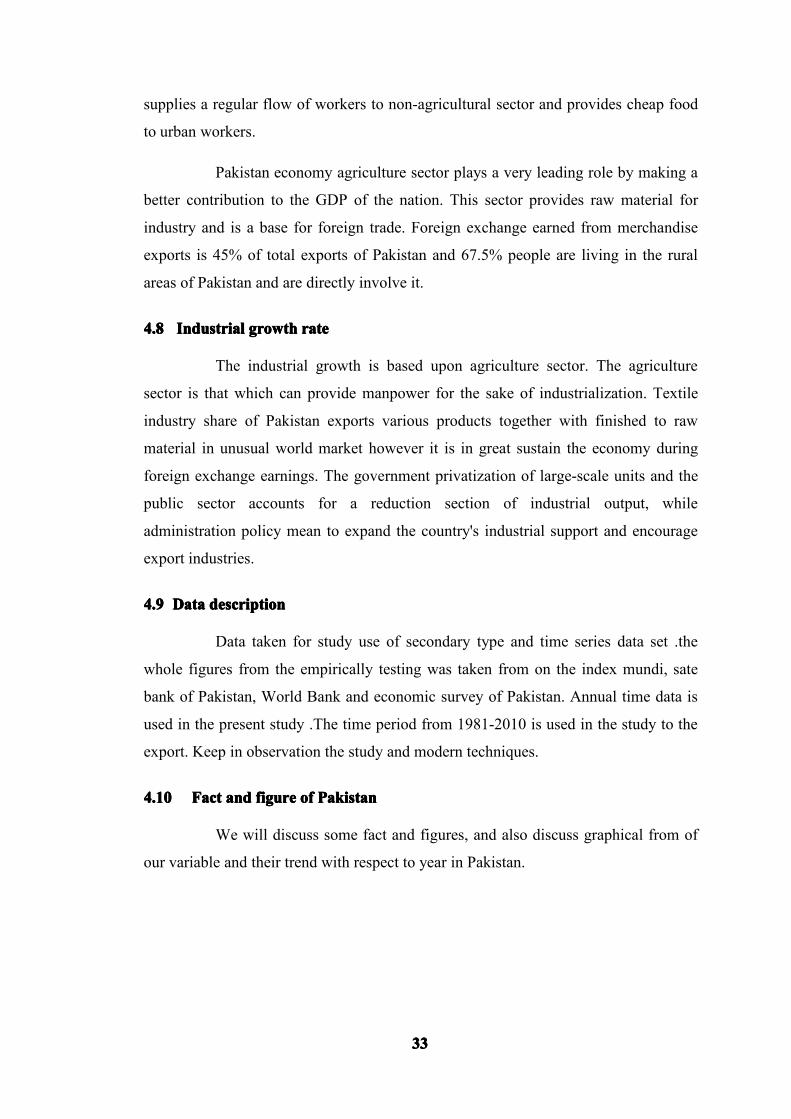
4.10.1 Export...............................................................................................................34
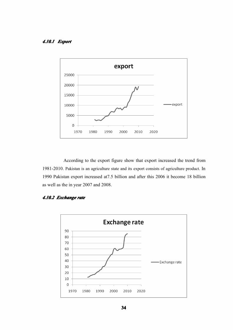
4.10.2 Exchange rate.......................................................................................................34
4.10.3 Foreign direct investment.................................................................................35
4.10.4 Gross dogmatic product (GDP)..............................................................................36
4.10.5 Agriculture growth rate.........................................................................................36
4.10.6 Industrial growth rate........................................................................................... 37
4.11 Statistical Techniques:.................................................................................................37

9999
6 CHAPTER V........................................................................................................................39
THE EMPIRICAL ANALYSIS........................................................................................................ 39
5.1 Unit Root Test...............................................................................................................39
5.1.1 Augmented Dickey Fuller Test (ADF) (table #3).................................................... 39
5.2 Johansen Co Integration:..............................................................................................40
5.3 VAR (vector auto regression)....................................................................................... 42
5.3.1 Impulse Response Analysis.......................................................................................42
5.3.2 Variance decomposition...........................................................................................50
5.4 Granger Causality Trace Tests...................................................................................... 52
5.4.1 HYPOTHESIS:.............................................................................................................52
5.5 Fully Modified Least Squares (FMOLS):........................................................................56
5.5.1 Result of FMOLS........................................................................................................56
7 CHAPTER: VI......................................................................................................................58
6.1 Conclusion:......................................................................................................................... 58
6.2 Policy implications:.......................................................................................................59
REFERENCES............................................................................................................................. 60

10101010
LISTLISTLISTLIST OFOFOFOF TABLESTABLESTABLESTABLES
TableTableTableTable No.No.No.No. NameNameNameName ofofofof TableTableTableTable PagePagePagePage No.No.No.No.
Table No.1 Literature Review Table 13
Table No.2 Data Source 23
Table No.3 Unit Root Test 32
Table No.4 Johansen co integration 34
Table No.5 Variance decomposition of the Export 44
Table No.6 Granger Causality Tests 47
Table No.7 FMOLS 49
LISTLISTLISTLIST OFOFOFOF FIGURESFIGURESFIGURESFIGURES
FigureFigureFigureFigure No.No.No.No. NameNameNameName ofofofof FigureFigureFigureFigure PagePagePagePage No.No.No.No.
Figure No. 1 Export 43
Figure No. 2 Exchange rate 34
Figure No. 3 FDI 35
Figure No. 4 GDP 36
Figure No. 5 Agriculture growth rate 36
Figure No. 6 Industrial growth rate 37

11111111
CHAPTERCHAPTERCHAPTERCHAPTER IIII
1111
INTRODUCTIONINTRODUCTIONINTRODUCTIONINTRODUCTION
2222 1.11.11.11.1 BackgroundBackgroundBackgroundBackground andandandand contextcontextcontextcontext
Exports are extensively believed to play a key role in the development
procedure of any economy. Access to the world market allows domestic firms to
attain economies of scale and consequently enhance their productivity. Being a strong
foundation of foreign exchange earnings, higher exports allow a country to meet its
expansion and development needs through import of assets goods and raw materials.
Exports lead to an improvement in economic efficiency by increasing the degree of
competition and exports also play vital role in reducing import export gap.
According to the classical economists and the modern liberal opinion the
trade is an engine of the economic expansion, which can process the economic
maturity. The export sector which can generate foreign reserve earning and increase
nation’s reserve of the country, the country export measure goods and services in
home market as well as the world market .In the long run, enhance the country export
show the development in the industrial sector which can causes the employment in the
country.
In Pakistan, the study of exports last few decades there were high
fluctuating result. Pakistan’s exports are less than its imports, which worsen its
position of trade. If we examine Pakistan history we find just two year in which

12121212
Pakistan enjoy trade surplus. First 1951-52 when the demand of Pakistan raw jute
goes up in international market, so Pakistan increased the export of raw jute. As the
result export of raw jute become the major source of foreign exchange earnings for
the Pakistan in this period. The second year in which Pakistan enjoy the trade surplus
was 1972-73 when concerned strategy of high tariff on luxury item and also
depreciated the Pakistani currency, it made Pakistani goods cheaper for foreigner and
export of Pakistan increased.
Pakistan most important exports are raw cottons, rice, leather, fabric
product, fisheries, vegetables, fruits, cement, sport goods and surgical instrument. If
export increase as contrast the import than nothing to split the being development in
the country , on the other side lower the export means that lower the foreign exchange
and low capacity of the purchasing power. Pakistan gets major part of the foreign
reserve from export.
In developing countries the expansion of the export base on the primary
goods, exports are very significant factor of the national economy which can measure
the goods and services in the world market. The stage of development process of
export used the indicator factor, so that balance of payment represented in the country,
if export greater than import than the balance of trade surplus.
The history of the growth various countries achieve the target of exports
through planning of industrial growth, quality of assurance attentive observation
change the global market and meeting changing their exportable surpluses.
The economic policy reflects three foremost elements. First one as money
demand and supply policy, second one government policy and third one is trade
policy. These three constituent correlates with each other. On the other side the trade
policy reflects the country which owing the other country.
According to report of Pakistan Bureau of Statistics¸ it is baring the
continuously trade deficit in the globalization that is terrible for Pakistan economy.
Pakistan government and economist should take step for this important matter. The
trade deficit of record at 21.27 billion dollar in country growth the negatively growth
rate at over the four percentage .On the other hand the country boost the import at
11.3 % in one year

13131313
[Pakistan Bureau of Statistics]
Domestic exports play very important role in the international market to
increase the domestic production as well as the economic growth and Pakistan
highest export relation is with the USA .The United state is single country which
can above the 27% export. If we compare economy of Pakistan with the
developing nation from the last 30 year than result that growth rate for 6% in this
time period.
The manufacturing sector is very significant of any countries to
increase exports normally base on the manufacturing goods. In Pakistan export
depend on the textile and semi-manufacturing goods and need to enhance
manufacturing segment. Above 75% of exports, manufacturing goods in Pakistan
(1974-2003) and after that real growth shows decline tendency in this export
sector.
Pakistan is an agricultural state and export raw material that fetches
low prices in global market and on the other side Pakistan imports heavy
machinery and petroleum product which have high prices in the international
market. The difference between the export and import prices is the major cause of
Pakistan trade deficit.
The classical economist David Ricardo, strong believer of promotion
of the export is the strong feature of the national growth. Obviously so that the
national asset is reflect in the foreign exchange which can promote the economy
of the country.
Development economics of the literature on trade got concerned
between import substitution and export promotion. Prebisch-Singer theorem
based on export theory, the big push theory and other similar thoughts argued
effectively that developing countries embark on a strategy of substituting imports
by domestic production of those goods.
Pakistan has immeasurable natural resources and foreign trade can
facilitate in utilization of natural resources in the best possible way. Trade
liberalization provides opportunity for foreigners to invest in this region. In this
way, new technologies are brought into the country with the help of other trading

14141414
nations. Exports are big source of foreign reserves, only possible due to foreign
trade.
1.21.21.21.2 StatementStatementStatementStatement ofofofof problemproblemproblemproblem
Exports are base for economy of developing nations such as Pakistan.
The new preparation always required to compete the whole world market, point
for which rays for this study focus on how export are significance for economy of
the developing nation like Pakistan. The required study on export execution is to
earn the foreign reserve and encourage growth in the economy. The study shows
clear picture of exports performance of Pakistan in last three decades.
Another object of this study how to the exports are effected towards
FDI, GDP, exchange rate, agriculture growth rate and industrial growth rate.
Pakistan suffering in trade deficit it the main cause the low demand for its export,
to enhance the export in the country.
1.31.31.31.3 ObjectiveObjectiveObjectiveObjective ofofofof thethethethe studystudystudystudy
This study will focus on macro economics variables that impact on exports
for Pakistan. The variable which are included in this study have directly impacts on
the exports;
1. To determine the relation between factor of exports variable.
2. How many the exports in effect by the exam of exchange rate?
3. What is impact of FDI on exports?
4. What is relationship between agriculture growth rate and
industry growth rate in terms of export?
We study all these suggestion in case of Pakistan
1.41.41.41.4 AdoptedAdoptedAdoptedAdopted MethodologyMethodologyMethodologyMethodology
In this study export is depended variable and exchange rate, GDP,
foreign direct investment, agriculture growth rate and industrial growth are used
as the independent variables. The study contains time series data of this variable
for the time period 1981–2010. Adopted secondary data for further empirical testing

15151515
has been taken from profile of Pakistan. In this study unit root test like ADF apply
to check the stationary of the variables and also apply Johnson co integration for
determine the relationship among the variables and impulse response. Granger
Causality trace test for the final estimation of the result of the study FMOLS test is
used.
1.51.51.51.5 StructureStructureStructureStructure ofofofof thethethethe thesis:thesis:thesis:thesis:
The study is divided into five sections. The background literature is in
chapter 2, chapter 3 explores the theoretical framework, chapter 4 illustrates data
and methodology, chapter 5 contains the empirical results and chapter 6 based on
the conclusion and Policy recommendations.

16161616
3333 CHAPTERCHAPTERCHAPTERCHAPTER IIIIIIII
4444 INTRODUCTIONINTRODUCTIONINTRODUCTIONINTRODUCTION
This chapter of the study based on the previous literature and empirical
work done on determinant of exports. The focal point of literature is Pakistan, which
already done on the export determinate and in this study also takes in the literature of
developing and developed nations on exports take that provide base to our study and
will help to generate required result.
5555 2.12.12.12.1 LiteratureLiteratureLiteratureLiterature Review:Review:Review:Review:
Siddique et al (2012) analyzed the determinants of export textile and
clothing sector of Pakistan .They found the result by using the variable of GDP, CPI
and ER .The type of data was secondary form (1971-2009). They used OLS technique
and co-integration. The result showed that world income was major factor of export
demand of cloth and textile sector, and other factor which can determine the export of
country was trade restriction. In this model the trade restrictions used as proxy
variables.
Hafeez (2011) estimated the determinants of export and it’s occurred result
by the adopted variable as GDP, exchange rate, and relative prices from (1980-
2010).He used the regression analysis and as well as the OLS technique. The data
used was secondary. The empirical result showed that GDP and relative price were
positively effect on the other side the export and exchange rate were negatively affect
each other .So the founded these result GDP has favorable effect on the export but
exchange rate has negatively impact on the export.

17171717
Najia Saqib and Irfan Sana(2010) described the exchange rate volatility
and its effect on Pakistan export and used the date time serious (1981-2010).They
used the variable export ,import ,reserve ,CPI and GDP deflator . Simple linear
regression model used and as well as tested the augmented dickey fuller and used the
Phillips Peron test. The consequence showed that increased the size of international
export connected develops the exchange rate. There were negatively relationship
between the exchange rate and export and showed the positively relation between the
export and import.
Ghafoor et al (2010) studied the determinant of mango export. They used
the primary data and selected the variables as education of the exporter, experience in
export business, average purchasing prices, average marking cost, average sale prices
and used the dummy variables as government policy. They used the regression
analysis as well as the OLS technique in this model. The empirically result showed
that as the variables use in the model effected the mango export on the other hand
government policy was to be known indicative variables.
Musleh, Ejaz and Tariq (2009) developed the determinants of export
performance (Evidence from firm level) and concluded the strategic result by using
the variable textiles, leather, agro, foods and fisheries .Each variable collected the data
in sub variable .They used sample approach total 180 firm were selected and used
statistical analysis and estimated the OLS technique .The empirical result showed that
in investment market the exports positively affected and explain the link between the
foreign owned firm much used the resource as compare the domestic used firm.
Siddiqui et al (2008) highlighted the strategic literature on impact on
export led growth hypotheses in Pakistan. Used the variables were GDP, export,
import and labor force. The date spanned over was from 1971-2005.They used the
regression analysis as well as the auto regressive in distributed lag model. The
empirical result showed that export, import and labor force have the positive effect on
the growth in short run as well as in long run. On the other hand the term of trade has
the negative affected on growth.
Muhammad Tariq Majeed and Eatazaz ahamad (2006) adopted the
determinants of export in developing countries and concluded the strategic result by
using the variables’ as FDI, GDP, indirect taxes national savings ,labor forces, real

18181818
exchange rate and official development assistance from (1970-2004). The nut shell of
this study showed that the export deals with the trade labialization but the developing
countries faced the fiscal deficit and trade deficit. The developing countries take place
of the agriculture export and enhance the industrial export. The exchange rate
unstable the problem in developing nation and another factor was increased the import.
Naeem and Hussain worked the determinants of export in the case of
Pakistan and concluded that deliberate result by used the variables of primary goods
export, semi manufacturing goods export and manufacturing goods exports which
can used the time series date from (1970-2006).They used the ADF test to converted
the data into the stationery and used the Johnson co integration test to discovered the
long run connection with the time serious data and also used OLS technique to
determinate the export in the country. The empirically result showed that if increased
the 1% of the primary goods of export than the export increase the 0.97% and if
increase the 1% of the semi manufacturing goods export increased the 0.99%. On the
same increment in manufacturing export the result indicated that change in export in
1% change.
Sandeep Kaur (2008) adopted the determinant of export service of USA
with its Asian partner and concluded the deliberate result by using the gravity
model ,the type of data was secondary (2000-2008) . The empirically result show that
USA had convergence in exports with three Asian countries Hong Kong, India and
Korea deviation with three Asian countries Japan, China and Singapore. There is a
large scope for export growth for Hong Kong, India and Korea. As these economies
especially India is one of the rising economy, USA’s export of s increase its growth
would be constant.
Yousaf, Hussain and Ahmad (2008) analyzed the impact of FDI (foreign
direct investment) with the circumstance of exports and imports on economic growth
of Pakistan. They acquired the time series data for their study which starts form
(1973 – 2004). They attain import and export demand as dependent variable and real
gross domestic product, foreign remittances, foreign direct investment and a dummy
variable for democracy and military rule era. They make import and export model
individually. They apply Augmented Dickey Fleur test for checking the stationary of
data. After that Johansen Juselius is applied for result the co-integration among
19191919
variables. They concluded that in the import model the relation of foreign direct
investment is positive in long and short term but in export model the foreign direct
investment has negative relation in short run but positive in long run.
Rano (2007) adopted that the determinants of import and export demand in
Nigerian nation. In this study imports and exports dependent variables while exchange
rate, income, imports capacity and level of reserves used as independent variables.
The sample period of this study starts from (1970 – 2004). There was simple linear
relationship between dependent variables and independent variables. The estimation
methods were used co integration and specification of an error correction model. He
concludes that exchange rate was better instrument for achieving the balance of
payment stability.
Khan (1994) examined that effect of devaluation on balance of trade and
balance of payment in case of Pakistan. They sample period of this study starts from
1983 and ends at 1993. By using conventional method they described effects of
devaluation on the external balance and export and import were demand functions. In
this paper they used quarterly data which shows that no optimistic effect on external
balance due to devaluation. They suggested that depreciation in currency improved
the balance of trade.

20202020
2.22.22.22.2 TABULARTABULARTABULARTABULAR LITERATURELITERATURELITERATURELITERATURE FORMFORMFORMFORM:
AuthorAuthorAuthorAuthor
namenamenamename
StatisticalStatisticalStatisticalStatistical
techniquetechniquetechniquetechnique
DependentDependentDependentDependent
variablevariablevariablevariable
IndependeIndependeIndependeIndepende
ntntntnt
variablesvariablesvariablesvariables
SampleSampleSampleSample
periodperiodperiodperiod
conclusionconclusionconclusionconclusion
2012 Sadique They used
OLS
technique
and co-
integration
Export GDP
Consumer
price index
Exchange
rate
s
1971-
2002
Thestatement ofresultshowed Theresultshowed thatworldincome wasmajor factorof exportdemand ofcloth andtextile sector,and otherfactor whichcandeterminethe export ofcountry wastraderestriction
2011 HafeezThe author
used the
regression
analysis and
as well as the
OLS
Export GDP
exchange
rate
relative
prices
1980-
2010
The foundedthese resultGDP hasfavorableeffect on theexport Buton the otherhandexchangerate hasnegativelyimpact onthe export.
2010 Ghafoor
, et, al
they used the
regression
analysis as
Mango
exportthe
variables
as
They
used the
primary
Empirically
result
showed that
TableTableTableTable 1111

21212121
well as the
OLS
technique in
this model
education
of the
exporter,
experience
in export
business,
average
purchasing
prices,
average
marking
cost,
average
sale prices
and they
used the
dummy
variables
as
governmen
t policy
data as the
variables use
in the model
affected the
mango
export on the
other hand
government
policy was to
be known
indicative
variables.
2010 Najia
Saqib
and
Irfana
Simple linear
regression
model used
and as well
as tested the
augmented
dickey fuller
and used the
Phillips
Peron test.
Export import ,res
erve ,CPI
and GDP
deflator
1981-
2010
The
consequence
showed that
increased the
size of
international
export
connected
develops the
exchange
rate. There
were

22222222
negatively
relationship
between the
exchange
rate and
export and
showed the
positively
affected
between the
export and
import.
2009 Musleh,
Ejaz and
Tariq
statistical
analysis and
estimated the
OLS
technique
Export textiles,
leather,
agro, foods
and
fisheries
They
used
sample
approach
total 180
firm
were
selected
and
used
statistica
l
analysis
The
empirical
result
showed that
in investment
market the
export a
positively
affected and
describes the
link between
the foreign
owned firms
much used
the resource
as compare
the domestic
used firm.
2008 Siddiqui They used Export GDP, 1971- The

23232323
, the
regression
analysis as
well as the
auto
regressive
distributed
lag model
import and
labor force
2005 empirical
result shows
that export,
import, and
labor force
have the
positive
effect on the
growth in
short run as
well as in
long run. On
the other
hand the
term of trade
has the
negative
effect on the
growth.
2008 Yousaf,
Hussain
and
Ahmad
Augmented
Dickey Fleur
(Unit Root
test)
Johansen
Juselius (for
finding the
co-
integration
Export and
import
demand
real gross
domestic
product,
foreign
remittance
s, foreign
direct
investment
dummy
variable
for
democracy
and
1974 -
2004
In import
model the
relation of
foreign direct
investment is
positive in
long and
short term
but in export
model the
foreign direct
investment
has negative

24242424
military
rule
relation in
short run but
positive in
long run.
2007
Rano Co
integration,
vector error
correction
model,
ordinary
least square
regression
model
Import
and export
Income,
import
capacity
and level
of reserves
1970 -
2004
Exchange
rate was the
better
instrument
for achieving
the balance
of payment
stability.
2006 Muham
mad
Tariq
Majeed
and
Eatazaz
ahamad
Export FDI, GDP,
indirect
taxes
national
savings ,la
bor forces,
real
exchange
rate and
official
developme
nt
assistance
from
the 75
countries
1970-
2004
The export
deals with
the trade
labialization
but the
developing
countries
faced the
fiscal deficit
and trade
deficit. The
developing
countries
take place of
the
agriculture
export and
enhance the
industrial
export

25252525
1994 Khan Johansenestimation,Marshall-Lernercondition
Exportdemand,importdemand,exportsupply,importsupply
GDP, realexchangerate
Quarterly datafrom1983to1993
Depreciation
in currency
improved the
balance of
trade.

26262626
CHAPTERCHAPTERCHAPTERCHAPTER IIIIIIIIIIII
3.13.13.13.1 THEORETICALTHEORETICALTHEORETICALTHEORETICAL BACKGROUNDBACKGROUNDBACKGROUNDBACKGROUND
This chapter of study is based on theoretical back ground. In this section
we discuss the theory that are related and define our study. Through this theory that
relate our study are helpful to understand our topic more briefly.
3.23.23.23.2 TheoreticalTheoreticalTheoreticalTheoretical BasisBasisBasisBasis
In 1817 David Ricardo presented the theory of comparative advantage.
The other name of this theory called the cost theory .The international trade concept
of comparative benefit most significant. According to Ricardo import and export
among the two countries happen due to difference in labor, labor skill, physical
wealth, nature reserve and technology crossways the countries.
Ricardo used the concept of comparative gain and opportunity cost in his
theory of global trade and stress on the point that the countries should produce that
goods in which it have relative advantage as well as the low opportunity cost. The
main theme of this theory is that the countries should in specialty in the product in
which they have comparative advantage.
If we make certain that, the Ricardian theory is in contrast of Pakistan than
improves his trade balance. Pakistan is the agriculture state and have the relative
advantage to produce the agriculture product rather than the industrial product, if
Pakistan gain the specialize the agriculture region than the production of the
agriculture goods increase in this way countries able to fulfill the domestic use and
also bright to the export a huge amount of agriculture of the foreign reserve. Pakistan
used the reserve on the imported goods like heavy equipment and enhances the term
of trade.

27272727
The Gravity model have to do trade among the two countries depend the
size of their economies, this model relate the distance and border of the countries. The
model was first used by Tinbergen in 1962. The world trade is record the relative size
of countries which can lessen the amount of pay for transport cost and communication
cost. The model of an economy direct has to do the volume of import and export, the
huge economy production the more goods and services so that these countries have
more to sell in export. The effect of distance in gravity model forecast that if increase
the distance 1% than the volume of trade diminishes at 0.7% to 1%, so we can say
that there are negative relationship among the trade and distance regarding this
model.1
Swedish Economists, Hecksher and Ohlin introduced a theory named as
Hecksher-Ohlin Model. Theory was concerned with the distribution of resources for
their best use and their prices among countries are the key elements of trade.
According to Heckscher–Ohlin model a country is predicated to export those goods
which are the intensive in abundant of dynamic of production. This model abundant
of factor of production caucuses for the gain for trade, so change the trade pattern
relatively price of goods and service has large effect on the distribution of income in
every country which can get the benefits from the trade on the owner of the factor but
on the other side get lose form trade on the owner of the limited factor of production.2
1 The model was first used by Tinbergen in 1962. The basic model for trade between two countries (iand j) takes the form of:
2 Ohlin, Bertil (1967). Interregional and International Trade.Harvard Economic Studies 39. Cambridge,MA: Harvard University Press

28282828
CHAPTERCHAPTERCHAPTERCHAPTER IVIVIVIV
DataDataDataData andandandandMethodologyMethodologyMethodologyMethodology
In this chapter, we will identify the model of the study and elaborate the
methodology that has been use to spot the export model in the case of Pakistan. We
will construct model and also focus on the statistical techniques as well as dimension
of study.
4.14.14.14.1 Methodology:Methodology:Methodology:Methodology:
In this section we express a structure of analysis to establish effect of the
different variable on export in case of Pakistan, which we get in our sample. The
countries export promotes have very important part play like liberalization of the
government system. On the other side the developing nation are facing two deficits
that is say, fiscal deficit and trade deficit. The debt crises make the great extent the
financial difficulty; so that in such financial problem the influence of foreign direct
investment is not sufficient.
The export execution of our country depend many factor and these issue
can be classified in term of demand and supply. The ability of the trading partner
which can usually indentified the GDP of these country ,however the political factor
play a very important role in this stage . The other side in supply feature which can
measure gross domestic product, wage rate, exchange rate and import input in the
country.

29292929
UINDUAGRIGDPFDIEREX ++++++= 54321 ααααααο
Where
EX = total export
ER= exchange rate
FDI = foreign direct investment
GDP= gross domestic product
AGRI= agriculture growth rate
INDU= industrial growth rare
αο = Constant
1α = Coefficient of ER
2α = Coefficient of FDI
3α = Coefficient of GDP
4α = Coefficient of AGRI
5α = Coefficient of INDUST
U = Error term

30303030
4.24.24.24.2 SourcesSourcesSourcesSources ofofofof thethethethe VariablesVariablesVariablesVariables
This graph includes the sources of all variables.
SerialSerialSerialSerial
no.no.no.no.variablevariablevariablevariable Variable.Variable.Variable.Variable. DataDataDataData source.source.source.source.
1 EXP Export Hand book of statistic
2 ER Exchange rateInternational monetary
fund (IMF)
3 FDI Foreign direct investment Hand book of statistic
4 GDP Gross domestic product Economy watch
5 AGRI Agriculture growth rate Hand book of statistic
6 INDUST Industrial growth rate Hand book of statistic
31313131
4.34.34.34.3 VariableVariableVariableVariable description:description:description:description:
Exports of the nation include those goods and services which domestic
country send excess amount of goods and services to the foreign countries and that is
good for the economy growth of the country and improve the balance of trade. If
exports of the nation increased than a country can earn huge amount of foreign
reserve. In 1990 Pakistan export increased 100% and reach 7.5 billion and after this
2006-7 it become 18 billion. In 2009-10 Pakistan has targeted to take export up to US
20 billion dollar and in April 2011 Pakistan export was US 25 billion dollar.
4.44.44.44.4 GrossGrossGrossGross domesticdomesticdomesticdomestic productproductproductproduct (GDP)(GDP)(GDP)(GDP)
The economic growth pilot to the increment in amount of goods and
services produced by and country over the period of time GDP impact the positively
on export. There are direct relationship of the above this variable, high level of GDP
show the cause of high level of export in the country. Therefore the empirically result
(Kumar, 1998) indentify the positive impact of GDP on export. The economic growth
is very important to an economy because it keeps an economy move the positively
dimension and society better off
4.54.54.54.5 ExchangeExchangeExchangeExchange raterateraterate
The exchange rate is factor due to fall the price in domestic market .In
international trade it can negatively influence on export owing to deprecation of
currency in domestic market. The empirically review (Sharma, 2000) describe the
positively effect on export of country. If exchange rate not fully stables the decrease
the international trade activities the exchange rate play the major role for determinant
of the trade balance. In 1982 Pakistan Rs was fixed to the pound but later on
government of General Zia-Ul-Haq take action and convert floating exchange rate.
And as the result Pakistan Rs devalue by 38.5% in1982-83 and many old industries
that established their ancestor have to face huge flow in import cost. In Zulfikar Ali
Buhtoo regime, rupee appreciation but later on despite raise in foreign aid the rupee
depreciated. And in 1980 Pakistan RS value against $ is 12.1 but due to continuously
decreasing the Rs value it reach in 2010 at 85.49 Rs per $.

32323232
4.64.64.64.6 ForeignForeignForeignForeign directdirectdirectdirect investmentinvestmentinvestmentinvestment (FDI)(FDI)(FDI)(FDI)
Foreign direct investment is the direct speculation into the country by a
company situated in a further country either by buying a company in a country or by
growing of accessible business in the country. Foreign direct investment is another
work collection invests which is passive in the other country such as bond, stock and
so on. It is source of investment in economic growth and lead to development it
benefits of both investing country and as well as the home country. The FDI also hurt
the local level of investment.
The empirically role of the FDI in export find the positively effect, the
main propose to the export oriented to promote the export. In case of Pakistan if
foreign direct investment done in the sector of oil, gas, financial, Telecommunication
and media sector than it prove beneficial for the Pakistan economy and promote the
export in Pakistan. Foreign direct investment play vital role to improve and expansion
china’s textile industry and it progress quickly and now china has comparative
advantage in textile industries.
Foreign direct investment increase the investment in the country and
establish new industry hence the production of the country increased as well as export
of the country and that improve the export volume so, it has a positive relationship
with the export . And foreign investor s has full freedom on inflow of capital and
investment. In 2006-7 the foreign direct investment in Pakistan reach 8.4 billion but in
2010 foreign direct investment in Pakistan fall by 34.6% due to political instability.
And in 1995 foreign direct investment in Pakistan was 442.4 million. But now
Pakistan ranked 85th in the list of more foreign direct investment countries
4.74.74.74.7 AgricultureAgricultureAgricultureAgriculture growthgrowthgrowthgrowth raterateraterate
Agriculture is life blood of our country. Agriculture is the largest division
of the financial activity and the stage a vital role in the economic development by
providing food, raw material and employment to a great proportion of the people. It is
the main stay of Pakistan’s economy. More than two third of Pakistan’s population
lives in rural areas and their livelihood continuously depends upon agriculture sector
and its activities. Agriculture in Pakistan is closely linked to rest of the country. It
33333333
supplies a regular flow of workers to non-agricultural sector and provides cheap food
to urban workers.
Pakistan economy agriculture sector plays a very leading role by making a
better contribution to the GDP of the nation. This sector provides raw material for
industry and is a base for foreign trade. Foreign exchange earned from merchandise
exports is 45% of total exports of Pakistan and 67.5% people are living in the rural
areas of Pakistan and are directly involve it.
4.84.84.84.8 IndustrialIndustrialIndustrialIndustrial growthgrowthgrowthgrowth raterateraterate
The industrial growth is based upon agriculture sector. The agriculture
sector is that which can provide manpower for the sake of industrialization. Textile
industry share of Pakistan exports various products together with finished to raw
material in unusual world market however it is in great sustain the economy during
foreign exchange earnings. The government privatization of large-scale units and the
public sector accounts for a reduction section of industrial output, while
administration policy mean to expand the country's industrial support and encourage
export industries.
4.94.94.94.9 DataDataDataData descriptiondescriptiondescriptiondescription
Data taken for study use of secondary type and time series data set .the
whole figures from the empirically testing was taken from on the index mundi, sate
bank of Pakistan, World Bank and economic survey of Pakistan. Annual time data is
used in the present study .The time period from 1981-2010 is used in the study to the
export. Keep in observation the study and modern techniques.
4.104.104.104.10 FactFactFactFact andandandand figurefigurefigurefigure ofofofof PakistanPakistanPakistanPakistan
We will discuss some fact and figures, and also discuss graphical from of
our variable and their trend with respect to year in Pakistan.
34343434
4.10.14.10.14.10.14.10.1 ExportExportExportExport
According to the export figure show that export increased the trend from
1981-2010. Pakistan is an agriculture state and its export consists of agriculture product. In
1990 Pakistan export increased at7.5 billion and after this 2006 it become 18 billion
as well as the in year 2007 and 2008.
4.10.24.10.24.10.24.10.2 ExchangeExchangeExchangeExchange raterateraterate

35353535
This figure represents the exchange rate of Pakistan from 1981 to 2010.
Pakistan’s currency is continuously decreasing against the dollar that was not good for
Pakistan economy. In 1985 to 1986 the slightly change of the exchange rate but in year
2007 to 2008 it can large change in exchange rate.
4.10.34.10.34.10.34.10.3 ForeignForeignForeignForeign directdirectdirectdirect investmentinvestmentinvestmentinvestment
Above figure of foreign direct investment is showing different trends of
data set. In 1983 foreign direct investment was on its lower point foreign direct
investment start increasing from 1990 and in 1995 foreign direct investment in
Pakistan was 1.5% of the GDP and it attain highest point in 2007 but after this due to
political instability foreign direct investment start decreasing again. But now Pakistan
ranked 85th in the list of more foreign direct investment countries.

36363636
4.10.44.10.44.10.44.10.4 GrossGrossGrossGross dogmaticdogmaticdogmaticdogmatic productproductproductproduct (GDP)(GDP)(GDP)(GDP)
The above figure is viewing the trends of GDP growth rate and graph is
showing mixed trends from 1980-2010. The facts and figures are not showing
consistent upward or nor consistent downward trend. In year 1992 to 1993 it can huge
decline the GDP in the country on the other side it can large increment in 2003 to
2004.
4.10.54.10.54.10.54.10.5 AgricultureAgricultureAgricultureAgriculture growthgrowthgrowthgrowth raterateraterate

37373737
The graph of Agriculture growth rate show that there are disparity heave
the years in 1983 to 1984 there are so much decline in this sector. After this it can
decline throw to 1991 .In 1992 the rate of growth incased but after this it can decline
the trend.
4.10.64.10.64.10.64.10.6 IndustrialIndustrialIndustrialIndustrial growthgrowthgrowthgrowth raterateraterate
The graph of industrial growth rate shows that there are slightly change
throw the year in 1981.It much important of the growth of the export in the country.
Industrial growth rate percentage increased in 2003 to 2004 much better rates for the
country after this growth rate decline.
4.114.114.114.11 StatisticalStatisticalStatisticalStatistical Techniques:Techniques:Techniques:Techniques:
In the present study the empirically investigate thorough analysis of the
variables using model. The focus of study is in the way of empirical analysis among
endogenous variable and exogenous variable by using modern econometric technique
and empirically data as well. According to requirement of the data and study, and
keeping in view the analysis. In primary test of study the Augmented Dickey-Fuller
(ADF) analysis is engaged to check the stationary property of data on these data types
real export, exchange rate, foreign direct investment, gross domestic product,
agriculture growth rate and industrial growth rate . These chains come into view to be
non- stationary in level shape.
It was necessary to observe co-integration association between variables
all the way through Johansen's (1998) unrestricted co-integration test to classify and

38383838
to illustrate the long term connection among variables. Now, co-integration
investigation is applied to explore any long-term equilibrium.
The Impulse response criteria is an upset to i-th variable not merely in a
straight line influences i-th variable nevertheless is as well broadcasts to all of further
endogenous variables all the way through the lag arrangement of VAR and Granger
Causality trace test .

39393939
6666 CHAPTERCHAPTERCHAPTERCHAPTER VVVV
THETHETHETHE EMPIRICALEMPIRICALEMPIRICALEMPIRICAL ANALYSISANALYSISANALYSISANALYSIS
In this chapter of study discuss the empirical set up by explanation of data
and econometrics techniques use for estimations and the required result. For the
purpose of estimations time series data is collected of 29 years from 1981-2010.
5.15.15.15.1 UnitUnitUnitUnit RootRootRootRoot TestTestTestTest
Unit Root Test The stationary property of the variables is checked by using
Augmented Dickey-Fuller (ADF) unit root test. To resolve the order integration of
time series, unit root test is practical on stage and as well as on first difference.
Stationary of all variables has been tested with intercept and trend. Results point to
the taking of the unit root hypothesis in the level, and then time series become
stationary in first difference.
VariablesVariablesVariablesVariables
AugmentedAugmentedAugmentedAugmented DickeyDickeyDickeyDickey
FullerFullerFullerFuller TestTestTestTest
AugmentedAugmentedAugmentedAugmented DickeyDickeyDickeyDickeyFullerFullerFullerFuller TestTestTestTest1111stststst DifferenceDifferenceDifferenceDifference
ConclusioConclusioConclusioConclusio
nnnnWithoutWithoutWithoutWithout
TrendTrendTrendTrend
WithWithWithWith
TrendTrendTrendTrend
WithoutWithoutWithoutWithout
TrendTrendTrendTrend
WithWithWithWith
TrendTrendTrendTrend
EXP 1.46 2.21 5.32* 3.50 1(1)
E.RATE 0.9 2.45 4.34* 4.4* 1(1)
FDI 3.25 4.36* 4.04* 4.32 1(0)
GDP 3.75* 3.67 7.18* 7.04* 1(0)
AGRI 1.26 1.99 5.17* 5.20* 1(0)
INDS 1.79 2.09 5.32* 5.28* 1(1)

40404040
5.1.15.1.15.1.15.1.1 AugmentedAugmentedAugmentedAugmented DickeyDickeyDickeyDickey FullerFullerFullerFuller TestTestTestTest (ADF)(ADF)(ADF)(ADF) (table(table(table(table #3)#3)#3)#3)
Note:Note:Note:Note: 1%, 5% and 10% critical standards for Augmented Dickey Fuller Test (ADF) level are 3.67, 2.96and 2.62 for without trend, on the other hand critical worth of with trend as 1%, 5% and 10 are 4.39,3.61 and 3.24 respectively. In first difference the critical value for Augment Dickey Fuller Test are 1%,5% and 10% for without trend are 3.68, 2.97 and 2.62, at the same time 1%, 5% and 10% criticalvalues with trend are 4.41, 3.62 and 3.24 respectively.
Augment Dickey Fuller Test result show that foreign direct investment
(FDI) and gross dogmatic product (GDP) both are stationery in level but on the other
side the Export, Exchange rate, Agriculture growth rate and industry growth rate these
variable non stationery when variable defend in level, by taking the first difference the
data become the stationery. . The null hypothesis of non stationary factor was clearly
discarded at the 5% level of significance and this suggest that all used variables are
integrated of order one.
5.25.25.25.2 JohansenJohansenJohansenJohansen CoCoCoCo Integration:Integration:Integration:Integration:
The Johansen approach can conclude the number of co-integrated vectors
for any pre-described number of non-stationary variables of the same order. This test
may be observed as a long run equilibrium relationship between the variables. The
objective of the Co-integration tests is to define the co-integration of a group of non –
stationary series. Engle and Granger (1987) introduced the concept of co-integration.
Toda and Philips (1993) have revealed that, when co-integration exists and it is
ignored, than it brings the model towards serious model misspecification. We use the
extreme likelihood technique of Johansen (1991, 1995).

41414141
TableTableTableTable 4444
(R=0 we not see this value we check the value of R1 if the value of R1 Eigen
(likelihood) value is greater than the critical value than we will reject the null
hypotheses Ho). And just we see the R1 value if this value is accepted than we not
move to the other R values.
If the values of trace statistics (based on likelihood ratio) and values of
max-Eigen values are greater than their critical values than we reject null hypothesis.
The Johansan co-integration test illustrate that, at R=0 the value of
likelihood ratio and max Eigen value are greater than their critical values so we not
found the long run co-integrating vector mean, thus we will reject null hypothesis. At
R ≤ 1 the t-statistics likelihood ratio and max Eigen value is also greater than the
critical value and prob. value so we reject the null hypothesis. At R ≤ 2 the results
shows that the t-statistics and Eigen value is greater than the critical value and prob.
value than we also reject the null hypothesis and shows there is no long run vector
mean, the economics behind the test is that there is no long run vector mean among
the variables. Moving towards R ≤ 3, interprets that there is long run co-integrating
vector mean exists so, we will accept null hypothesis here at R≤ 3. Johansan trace test
5.2.15.2.15.2.15.2.1 JohansenJohansenJohansenJohansen andandandand JuseliusJuseliusJuseliusJuselius (1990)(1990)(1990)(1990) MaximumMaximumMaximumMaximum LikelihoodLikelihoodLikelihoodLikelihood TestTestTestTest ForForForFor CoCoCoCo integrationintegrationintegrationintegration
NullNullNullNull
HypothesisHypothesisHypothesisHypothesis
TraceTraceTraceTrace StatisticStatisticStatisticStatistic
basedbasedbasedbased onononon
LikelihoodLikelihoodLikelihoodLikelihood
RationRationRationRation
CriticalCriticalCriticalCritical
ValueValueValueValue atatatat
5%*5%*5%*5%*
Prob.Prob.Prob.Prob.
Value*Value*Value*Value*
MaxMaxMaxMax
EigenEigenEigenEigen
ValueValueValueValue ****
CriticalCriticalCriticalCritical
ValueValueValueValue atatatat
5%*5%*5%*5%*
Prob.Prob.Prob.Prob.
ValueValueValueValue
atatatat ****
R=o 144.8431 95.75366 0.0000 52.47646 40.07757 0.0013
R≤1 92.36669 69.81889 0.0003 40.45454 33.87687 0.0071
R≤2 51.91214 47.85613 0.0198 29.26576 27.58434 0.0301
R≤3 22.64638 29.79707 0.2639 17.45986 21.13162 0.1514
R≤4 5.186520 15.49471 0.7887 4.847571 14.26460 0.7610
R≤5 0.338949 3.841466 0.5604 0.338949 3.841466 0.5604
42424242
indicates that there are three co-integration equations at the 0.05 level. In these
equations our null hypothesis is accepted. In our case three equations does not show
the co-integration, so that there is long run relation exist in our model. This mean here
we have found three integrated vector in this case this means co-integration is found
among the variables (GDP ,FDI, exchange rate ,agriculture growth rate and industrial
growth rate ) co-integrated among each other.
5.35.35.35.3 VARVARVARVAR (vector(vector(vector(vector autoautoautoauto regression)regression)regression)regression)
VAR is a statistical method that is used to find out the linear relationship
among variables in a time series. Christopher Sims (1980) first time introduced the
frame work of VAR in which present value is expressed as its own lagged value.
VAR is an important technique for forecasting, data description and policy analysis.
One important advantage of VAR is impulse response that shows a shock in one
variable would continue in future.
5.3.15.3.15.3.15.3.1 ImpulseImpulseImpulseImpulse ResponseResponseResponseResponse AnalysisAnalysisAnalysisAnalysis
Impulse response purpose were execute in order to illustrate the how a
shock in one variable would persist in the future period .the forecasting was made the
considering a trend period. This examination will portray the impulse response
function for the main endogenous variables of the model in the direction of exogenous
variables. We investigate the GDP, exchange rate, agriculture growth rate, industry
growth rate and foreign direct investment and used the dependent variable export
shock with all variables. The conditions that minimize the information criteria give
the optimal selection of lags. The smaller these value the better the model, after
running Chelosky test.

43434343
5.3.1.15.3.1.15.3.1.15.3.1.1 FigureFigureFigureFigure 1111:::: AAAA
We adopted the vector Auto regression (VAR) model to indentified the
impulse of variable under the Chelosky method on differenced series in the case of
Pakistan figure.1, graph (A) showed the response of export to the exchange rate. The
economics behind that export gives positive response to exchange rate when we give
shock to exchange rate toward the response of the export. In the start of the period the
export gave the negatively response toward the exchange rate and approximately at
4.5th lag export increase throws the 10th lags.
5.3.1.2Figure5.3.1.2Figure5.3.1.2Figure5.3.1.2Figure 1111 BBBB

44444444
Graph (B) shows the response of exchange rate what the shock is given to
export. Change in export effects on exchange rate. At the second leg the exchange rate
increase while it decline and reach at the 8.5th lag the exchange rate increase.
5.3.1.35.3.1.35.3.1.35.3.1.3 FigureFigureFigureFigure:::: 2222 AAAA
In figure, 2 graphs (A) illustrate for response of export toward the GDP in
the start of the diagram the export increase and it can positively response of the export
up to 10th lag. The economic behind this there are the positive relationship between
the gross domestic product and export as the increase of the export the GDP will also
increase.
5.3.1.45.3.1.45.3.1.45.3.1.4 FigureFigureFigureFigure 2222 BBBB

45454545
Figure 2, diagram (B) show that result of the GDP response the export in
the initiate of the 1st of the lag GDP show the positively reaction wile 3.3 lag period
the GDP show the negatively response. After this GDP showed the positive trend with
response to the export, and the end of the 9th lag the GDP show the negatively
reaction.
5.3.1.55.3.1.55.3.1.55.3.1.5 FigureFigureFigureFigure:::: 3333 AAAA
In figure, 3 graph (A) demonstrate for response of export toward the
agriculture in the first of the lag the export show the negatively response throw the
10th lag .It can show that there are negatively response of export response of the
agriculture in case of Pakistan.
5.3.1.65.3.1.65.3.1.65.3.1.6 FigureFigureFigureFigure 3333 BBBB
46464646
Figure 3, graph (B) show the response of the agriculture in the direction of
the export and it can show the negatively trend heave at the first lag on ward the 6.5th
lag and after this period of time it can show the negatively trend illustrate the
negatively response of agriculture toward the export.
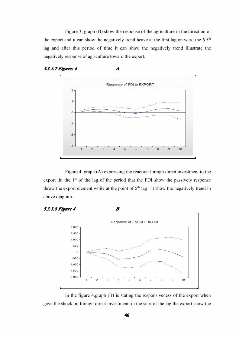
5.3.1.75.3.1.75.3.1.75.3.1.7 FigureFigureFigureFigure:::: 4444 AAAA
Figure.4, graph (A) expressing the reaction foreign direct investment to the
export .in the 1st of the lag of the period that the FDI show the passively response
throw the export element while at the point of 5th lag it show the negatively trend in
above diagram.
5.3.1.85.3.1.85.3.1.85.3.1.8 FigureFigureFigureFigure 4444 BBBB
In the figure 4.graph (B) is stating the responsiveness of the export when
gave the shock on foreign direct investment, in the start of the lag the export show the

47474747
negatively response to the foreign direct investment on the other hand at the 6.8th lag
the show the positively response and end of the 9th lag show the again negatively
response.
5.3.1.95.3.1.95.3.1.95.3.1.9 FigureFigureFigureFigure:::: 5555 AAAA
Figure.5, graph (A) showed the response of export toward the industrial
growth rate .The increased industrial growth have a positive relationship with the
export .In the first lag the export show the positively response and at the 4th lag it can
illustrate the negatively response of the export.
5.3.1.105.3.1.105.3.1.105.3.1.10 FigureFigureFigureFigure 5555 BBBB
Figure.5, graph (B) the response of the industry growth toward the export
in the start of the lag the industry growth rate show the positively response throw the
48484848
export and it can become the negatively at 5.5th lag than industry growth rate show the
positively growth rate in above diagram.
5.3.1.115.3.1.115.3.1.115.3.1.11 FigureFigureFigureFigure 6666 AAAA
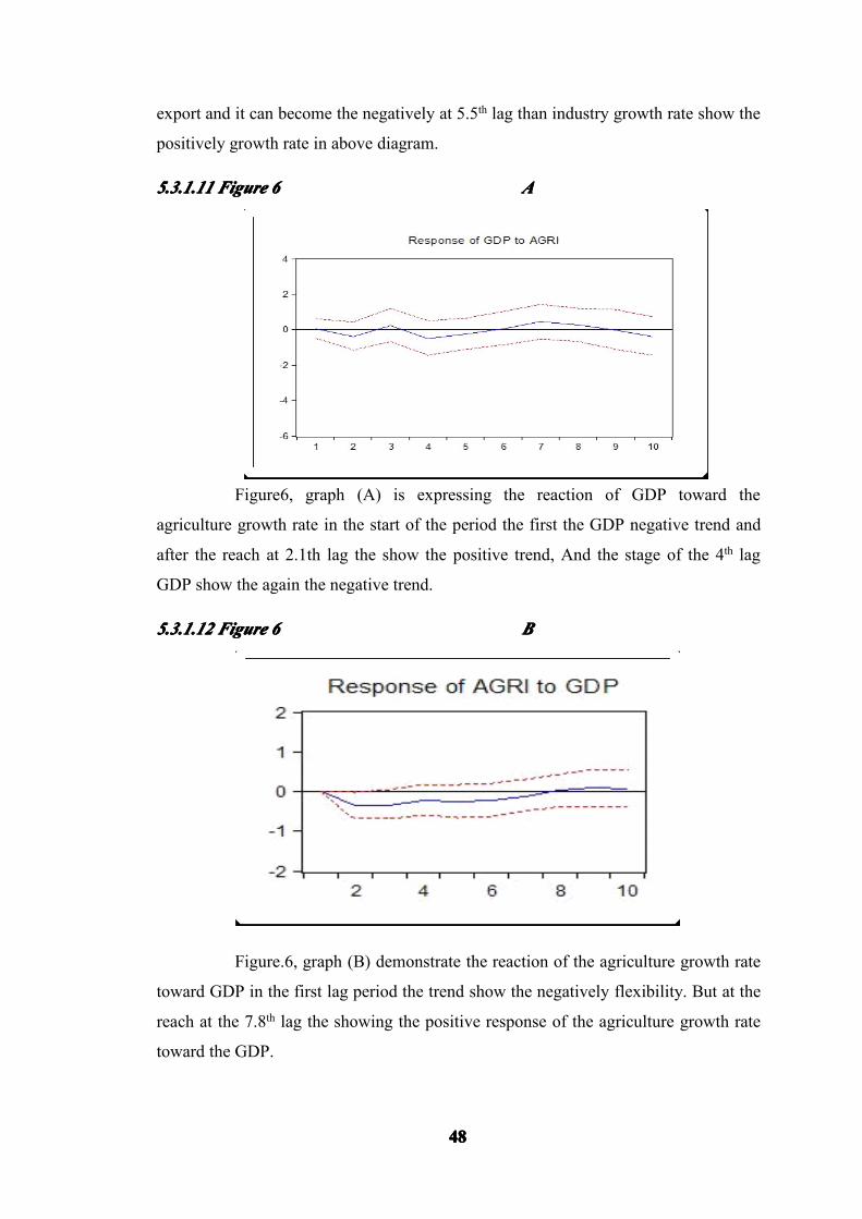
Figure6, graph (A) is expressing the reaction of GDP toward the
agriculture growth rate in the start of the period the first the GDP negative trend and
after the reach at 2.1th lag the show the positive trend, And the stage of the 4th lag
GDP show the again the negative trend.
5.3.1.125.3.1.125.3.1.125.3.1.12 FigureFigureFigureFigure 6666 BBBB
Figure.6, graph (B) demonstrate the reaction of the agriculture growth rate
toward GDP in the first lag period the trend show the negatively flexibility. But at the
reach at the 7.8th lag the showing the positive response of the agriculture growth rate
toward the GDP.

49494949
5.3.1.135.3.1.135.3.1.135.3.1.13 FigureFigureFigureFigure 7777 AAAA
Figure7, graph (A) showed the response of agriculture growth rate toward
the foreign direct investment start of the lag agriculture growth rate show the positive
response but at the 6.5th lag it show the decline throw the 9.8th lag and after this it
show the again positive response .
5.3.1.145.3.1.145.3.1.145.3.1.14 FigureFigureFigureFigure 7777 BBBB
Figure6, graph (B) show the response of foreign direct investment when
gave the shock of the agriculture growth rate in the start of the lag period foreign

50505050
direct investment show at equilibrium. While at the 3.2th lag it show the negative
response .In the 8th lag period the foreign direct investment at again equilibrium stage.
5.3.25.3.25.3.25.3.2 VarianceVarianceVarianceVariance decompositiondecompositiondecompositiondecomposition
Variance decomposition is an alternative technique of the impulse
response function for investigates the reaction of dependent variables due to the
effects of shocks by explanatory variables. This method explains that the size of
prediction error variance or any variable is described by innovations of each
independent variable is a system over the horizons. The shocks also affect the
variables in the system due to shocks explained by error variance. From the test, it can
be concluded that each time series describes the prevalence of its own values
5.3.2.15.3.2.15.3.2.15.3.2.1 EquationsEquationsEquationsEquations
titi
iti
iti
iti
iti
iti
tttttt
UINDAGRiFDIERGDP
ExpINDUAGRIFDIERGDPExp
γγγγγγ
γαααααα
++++++
+−−−−−=
−−−−−
−
1615141312
11615141312101
iiti
iti
iti
iti
iti
iti
tttttt
UINDAGRiFDIEREXPGDP
INDUAGRIFDIEREXPGDP
γγγγγγγ
αααααα
+++++++
−−−−−=
−−−−−− 262524232221
625242322202
iiti
iti
iti
iti
iti
iti
tttttt
UINDAGRiFDIEXPGDPER
INDUAGRIFDIEXPGDPER
γγγγγγγ
αααααα
+++++++
−−−−−=
−−−−−− 363534333231
635343332303
iiti
iti
iti
iti
iti
iti
tttttt
UINDAGRiEXPERGDPFDI
INDUAGRIEXPERGDPFDI
γγγγγγγ
αααααα
+++++++
−−−−−=
−−−−−− 464544434241
645444342404
iiti
iti
iti
iti
iti
iti
tttttt
UINDEXPFDIERGDPAGRI
INDUEXPFDIERGDPAGRI
γγγγγγγ
αααααα
+++++++
−−−−−=
−−−−−− 565554535251
655554352505
iiti
iti
iti
iti
iti
iti
tttttt
UEXPAGRiFDIERGDPINDU
EXPAGRIFDIERGDPINDU
γγγγγγγ
αααααα
+++++++
−−−−=
−−−−−− 666564636261
665664362606 _

51515151
5.3.2.25.3.2.25.3.2.25.3.2.2 VarianceVarianceVarianceVariance decompositiondecompositiondecompositiondecomposition ofofofof thethethethe ExportExportExportExport
TableTableTableTable 5:5:5:5:
PeriodPeriodPeriodPeriod S.ES.ES.ES.E EXPORTEXPORTEXPORTEXPORT ERERERER FDIFDIFDIFDI GDPGDPGDPGDP AGRIAGRIAGRIAGRI INDUSTINDUSTINDUSTINDUST
1626.2977 100.0000 0.000000 0.000000 0.000000 0.000000 0.000000
2835.2043 78.62365 7.499834 0.729687 7.257425 2.433289 3.456114
31185.891 79.03190 9.649420 2.217702 3.609339 3.633046 1.858590
41534.470 55.88635 12.79821 16.02820 7.613093 6.341640 1.332506
51843.233 52.16389 9.035586 19.41795 6.905222 11.35435 1.122998
62030.341 48.42665 7.470483 18.93498 9.420804 14.79612 0.950967
72191.545 51.09415 7.058332 16.68237 9.032442 15.30603 0.826673
82304.976 52.92941 6.381715 15.66923 9.804791 14.40692 0.807945
92424.067 56.42599 5.780018 14.17449 9.591176 13.20161 0.826719
102534.648 56.17709 5.402545 15.31452 9.941479 12.38110 0.783267
In the first of the period the export explains the 100% of its own forecast
error variance or Explain through its own innovative shocks. In second lag period the
exchange rate 7.4%, foreign direct investment 0.72%, gross domestic product 7.25%,
agriculture growth rate 2.43% and industrial growth rate show the 3.45% so the
according to the second time period here we conclude that the exchange rate is the
most significant .In the 10th time period the export explain the over the 56% error
variance or explain the its own innovative shocks. While the exchange rate 5.4%,
foreign direct investment 15.3%, gross domestic product 9.94%, agriculture growth
rate 12.38, and industrial growth rate show the 0.78% .Here the 10th lag period
foreign direct investment is the most significant.

52525252
5.45.45.45.4 GrangerGrangerGrangerGranger CausalityCausalityCausalityCausality TraceTraceTraceTrace TestsTestsTestsTests
Granger causality test is used to check that how one variable cause the
other variable in the short term and also in long term. If one variable cause the second
variable but in response second variable not cause the first variable it is known as
unidirectional causality. On the other hand both variables cause each other it is known
as bi directional causality.
• If F-statistics 4 or greater than 4 and probability value is 0.05 or less than 0.05,
than one variable cause the other variable.
• If F-statistics is 4 and probability value is 0.05, than one variable nearly
causing the other variable.
• If F-statistics is nearly 4 and probability value also near to 0.05, than one
variable weakly causing the other variable.
5.4.15.4.15.4.15.4.1 HYPOTHESIS:HYPOTHESIS:HYPOTHESIS:HYPOTHESIS:
1.1.1.1. Ho:Ho:Ho:Ho: GDP does not Granger Cause INDUST and vice versa.
Ha:Ha:Ha:Ha: GDP does Granger Cause INDUST and vice versa.
2. Ho:Ho:Ho:Ho: FDI does not Granger Cause INDUST and vice versa.
Ha:Ha:Ha:Ha: FDI does Granger Cause INDUST and vice versa.
3.3.3.3. Ho:Ho:Ho:Ho: EXPORT does not Granger Cause INDUST and vice versa.
Ha:Ha:Ha:Ha: EXPORT does Granger Cause INDUST and vice versa.
4. Ho:Ho:Ho:Ho: ER does not Granger Cause INDUST and vice versa.
Ha:Ha:Ha:Ha: ER does Granger Cause INDUST and vice versa.
5. Ho:Ho:Ho:Ho: AGRI does not Granger Cause INDUST and vice versa
Ha:Ha:Ha:Ha: AGRI does Granger Cause INDUST and vice versa.

53535353
6.6.6.6. Ho:Ho:Ho:Ho: FDI does not Granger Cause GDP and vice versa.
Ha:Ha:Ha:Ha: FDI does Granger Cause GDP and vice versa.
7. Ho:Ho:Ho:Ho: EXPORT does not Granger Cause GDP and vice versa.
Ha:Ha:Ha:Ha: EXPORT does Granger Cause GDP and vice versa.
8. Ho:Ho:Ho:Ho: ER does not Granger Cause GDP and vice versa.
Ha:Ha:Ha:Ha: ER does Granger Cause GDP and vice versa.
9. Ho:Ho:Ho:Ho: AGRI does not Granger Cause GDP and vice versa
Ha:Ha:Ha:Ha: AGRI does Granger Cause GDP and vice versa
10. Ho:Ho:Ho:Ho: EXPORT does not Granger Cause FDI and vice versa
Ha:Ha:Ha:Ha: EXPORT does Granger Cause FDI and vice versa
11. Ho:Ho:Ho:Ho: ER does not Granger Cause FDI and vice versa
Ha:Ha:Ha:Ha: ER does Granger Cause FDI and vice versa
12. Ho:Ho:Ho:Ho: AGRI does not Granger Cause FDI and vice versa
Ha:Ha:Ha:Ha: AGRI does Granger Cause FDI and vice versa
13. Ho:Ho:Ho:Ho: ER does not Granger Cause EXPORT and vice versa
Ha:Ha:Ha:Ha: ER does Granger Cause EXPORT and vice versa
14. Ho:Ho:Ho:Ho: AGRI does Granger Cause EXPORT and vice versa
Ha:Ha:Ha:Ha: AGRI does Granger Cause EXPORT and vice versa
15. Ho:Ho:Ho:Ho: AGRI does Granger Cause ER and vice versa
Ha:Ha:Ha:Ha: AGRI does Granger Cause ER and vice versa

54545454
5.4.1.15.4.1.15.4.1.15.4.1.1 PairPairPairPair wisewisewisewise GrangerGrangerGrangerGranger CausalityCausalityCausalityCausality TestsTestsTestsTests
TableTableTableTable 6666
Lags: 2
Null Hypothesis: Obs F-Statistic Prob.
GDP does not Granger Cause INDUST 28 1.31993 0.2866
INDUST does not Granger Cause GDP 3.27693 0.0560
FDI does not Granger Cause INDUST 28 0.43509 0.6524
INDUST does not Granger Cause FDI 2.87761 0.0767
EXPORT does not Granger Cause INDUST 28 0.53371 0.5935
INDUST does not Granger Cause EXPORT 1.88941 0.1739
ER does not Granger Cause INDUST 28 4.09409 0.0301
INDUST does not Granger Cause ER 2.01272 0.1565
AGRI does not Granger Cause INDUST 28 2.44891 0.1086
INDUST does not Granger Cause AGRI 0.21867 0.8052
FDI does not Granger Cause GDP 28 0.44243 0.6478
GDP does not Granger Cause FDI 2.10012 0.1453
EXPORT does not Granger Cause GDP 28 1.16711 0.3290
GDP does not Granger Cause EXPORT 5.58336 0.0106
ER does not Granger Cause GDP 28 1.31265 0.2885
GDP does not Granger Cause ER 0.15350 0.8586
AGRI does not Granger Cause GDP 28 1.12063 0.3432
GDP does not Granger Cause AGRI 2.80420 0.0813
EXPORT does not Granger Cause FDI 28 8.78015 0.0015
FDI does not Granger Cause EXPORT 4.01866 0.0319
ER does not Granger Cause FDI 28 4.28142 0.0263
FDI does not Granger Cause ER 9.29000 0.0011
AGRI does not Granger Cause FDI 28 4.40843 0.0240
FDI does not Granger Cause AGRI 0.12267 0.8851
ER does not Granger Cause EXPORT 28 8.19775 0.0021
EXPORT does not Granger Cause ER 4.73413 0.0190

55555555
AGRI does not Granger Cause EXPORT 28 3.60438 0.0435
EXPORT does not Granger Cause AGRI 1.45483 0.2541
AGRI does not Granger Cause ER 28 1.86517 0.1775
ER does not Granger Cause AGRI 1.75447 0.1954
We applied Granger Causality Trace Tests (1969) approach with lag
specification of 2 .In first observation GDP does not cause the industrial growth rate.
The values of F-statistics and probability helps us whether to reject Ho or not. Here F-
statistics value is less than 4 and probability value is greater than 0.05 so we will
accept Ho that means GDP does not cause the industrial growth and reject the Ha .On
the other side industrial growth rate cause the weakly on the GDP. In second
observation foreign direct investment does not granger cause industrial growth rate.
The value of F-statistics is less than 4 and probability value is greater than 0.05 so we
will accept Ho that means it is true that foreign direct investment does not cause the
industrial growth rate .On the other hand the industrial growth also does not cause the
foreign direct investment as F-statistics value is less than 4 and probability value is
greater than 0.05 and we are accept Ho and reject the Ha. In third observation export
does not granger cause the industrial growth rate? Here F-statistics is less than four
and probability value is greater than 0.05 so we accept the Ho and reject the Ha .while
on the other hand the industrial growth also does not cause the export because the
both F-statistic less than four and probability value greater than 0.05.So both the
variable does not cause.
In fourth observation exchange rate cause the industrial growth
rate .Because the value of the F-statistic greater than four and probability value less
than 0.05 so we accept the Ha and reject the Ho. While on the other hand industrial
growth rate does not granger cause the exchange rate for the reason that the value of
F-statistic (2.01272) that is less than four and value of the probability (0.1565) that is
greater than 0.05 so relation cause in the fourth observation is unidirectional
causality .In tenth observation export does granger cause the foreign direct
investment .F –statistic (8.78015) that is greater than four and value of the probability
(0.0015) that is less than 0.05 so in this case we reject the null hypothesis (Ho) and
accept the alternative hypothesis (Ha) .On the other way foreign direct investment
granger cause the export because the value of the F-statistic (4.01866) that is greater

56565656
than four and probability value (0.0319) less than 0.05 so we reject the Ho and accept
Ha.
5.55.55.55.5 FullyFullyFullyFully ModifiedModifiedModifiedModified LeastLeastLeastLeast SquaresSquaresSquaresSquares (FMOLS):(FMOLS):(FMOLS):(FMOLS):
FMOLS was introduced first time by Philips and Hansen in 1990 to
provide the estimation of co-integration regression .this method was used to the
circumstance parameter effect the asymptotic allocation of the OLS estimator. In
this why this method used to achieve the asymptotic and serial correlation effect the
test for the endogenous in regression that result from subsistence for co-integression.
5.5.15.5.15.5.15.5.1 ResultResultResultResult ofofofof FMOLSFMOLSFMOLSFMOLS
TableTableTableTable 7777 DependedDependedDependedDepended variable:variable:variable:variable: ExportExportExportExport
VariableVariableVariableVariable CoefficientCoefficientCoefficientCoefficient Std.Std.Std.Std. ErrorErrorErrorError t-Statistict-Statistict-Statistict-Statistic Prob.Prob.Prob.Prob.
ERERERER 329.2252 51.88908 6.344787 0.0000
FDIFDIFDIFDI 1451.736 279.5093 5.193874 0.0000
GDPGDPGDPGDP 221.7293 99.99314 2.217445 0.0372
AGRIAGRIAGRIAGRI -373.7161 183.5522 -2.036021 0.0540
INDUSTINDUSTINDUSTINDUST 629.4765 264.3619 2.381117 0.0263
CCCC -5471.624 10104.60 -0.541498 0.5936
TRENDTRENDTRENDTREND -536.9140 155.4418 -3.454115 0.0023
RRRR squaredsquaredsquaredsquared ==== 0.9698700.9698700.9698700.969870 Durbin-WatsonDurbin-WatsonDurbin-WatsonDurbin-Watson stat=1.633120stat=1.633120stat=1.633120stat=1.633120
We adopted fully Modified Least Squares (FMOLS) on choice of series
after this result show that these variables. The R-square shows significant subject of
the model because here R.2show the 0.969870 which show the endogenous
considerable depended on the endogenous variable. While on the other side Durban
Watson statistic are showing the minor problem of the autocorrelation. In addition the
economics behind above results is that if our exogenous variables stay constant at

57575757
zero than our value of export decline at 5471.62. while increase the one unit exchange
rate than our value of increase of export at 339.22 unit ,if GDP increase by one unit
according to the data set of the Pakistan and consequence the export will increase at
221.72 unit and if increase the one unit of foreign direct investment than our export
increase by 1451.76 unit while if increase the one unit of the agriculture growth rate
and our export decline at 337.71 unit ,at the same time as if increase the one unit of
the industry growth rate and increment at 629.47 unit in export in Pakistan.
.

58585858
7777 CHAPTER:CHAPTER:CHAPTER:CHAPTER: VIVIVIVI
6.16.16.16.1 Conclusion:Conclusion:Conclusion:Conclusion:
Export is a main source of the providing the foreign exchange to perform
the economic activity in the general and economic growth, so that export is the part of
the need of developing nation for the assets equipment. The fundamental principle of
this study was to find out relation between export and different variables in case of
Pakistan form 1981-2010 under time series data set type.
In this study through an econometrics analysis it has been made to exam
the association with different factors and exports performance of the country .Demand
of both developing and developed markets has positive effect of Pakistani exports .In
this way competitiveness of exports leads to increased the exports of Pakistan .
In economic growth the demand of the export performance positively
effect on the both developing and developed market in our study the main object to
assessment the behavior of the export in relation with GDP, exchange rate, agriculture
growth rate industry growth rate and foreign direct investment .As it verify when use
the non stationery time series data than it is not possible apply the econometric
technique, therefore the first step to apply the ADF test to confirm the stationery date.
Furthermore it finding that our date become stationery in first difference.
After the concern of ADF test to verify the co integration between the
variables, so on the basis of this outcome we find that the variable are co integrated
therefore the long run relationship exist in it.Finaly apply the FMOLS test to
indentified the relationship between the dependent variable either the positively affect
or negatively.
The estimation result shows that GDP has the positive impact on the
Export. When the GDP increased the progress of a country and increased the
production. While the agriculture growth rate has negatively impact on the Export of

59595959
the country .Industry growth rate and foreign direct investment has significant result
and when both of these are increased the export increases. Exchange rate has positive
coefficient that shows when exchange rate increased in other word domestic country
devalue that give raise to export in the country.
6.26.26.26.2 PolicyPolicyPolicyPolicy implications:implications:implications:implications:
The main object of the study to find that important in determinates of
export in Pakistan. The consequence of the GDP is significant with the positive sign
in explaining the export in Pakistan .High the production level mean to main source of
export growth.
The policy implication of the study as following;
� A stable or depreciate exchange rate policy has ensured in order
to enhance the export volume in the country.
� This study suggest that, to enhance the industry growth and
improve the productivity of regarding this sector because the industry sector is
the backbone of the export in country
� Study also suggests that, the foreign direct investment in export
oriented industry can be very important part play to boosting the export in the
country.
� In our country need to replace the agriculture export into to
industry export which can domination the stable price in the world market.

60606060
REFERENCESREFERENCESREFERENCESREFERENCES
DIN, M., GHANI, E., &MAHMOOD, T. (2009). Determinants of Export
Performance of Pakistan: The Pakistan Development Review, 227–240.
Funke M. and S. Holl (1992). “The Determinants of West German Exports of
Manufactures: An Integrated Demand and Supply Approach”, Weltwirtschaftliches
Archive, 128(3): 498-512.
Ghafoor, A.Mustafa, K., Zafar, & Mushtaq, (2010). DETERMINANTS OF MANGO
EXPORT FROM PAKISTAN. 105-119
Khattak, N. U., Hussain, & Hussain, A. (2010). Determinants of Exports in Pakistan:.
MPRA Paper No. 41988,
KAUR, S. (2011). Determinants of Export Services of USA with. Eurasian Journal of
Business and Economics 2011, 4 (8) , 101-117.
Khan, S. R. (1994). Devaluation and the Balance of Trade in Pakistan: A Policy
Analysis. Sustainable Development Policy Institute.
MAJEED, M.& AHMAD, E. (2006). Determinants of Exports in Developing
Countries. The Pakistan Development Review, 1265–1276
Rano, A. S. (2007). Imports-Exports Demand Functions and Balance of Payments
Stability in Nigeria: A Co-integration and Error Correction Modeling. Munich
Personal RePEc Archive, pp 1-26
Riedel, J., C. Hall and R. Grade (1984). “Determinants of Indian Exports Performance
inThe 1970s”, Weltwirtschaftliches Archive, 120(1): 40-63.
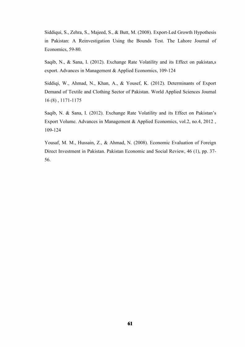
61616161
Siddiqui, S., Zehra, S., Majeed, S., & Butt, M. (2008). Export-Led Growth Hypothesis
in Pakistan: A Reinvestigation Using the Bounds Test. The Lahore Journal of
Economics, 59-80.
Saqib, N., & Sana, I. (2012). Exchange Rate Volatility and its Effect on pakistan,s
export. Advances in Management & Applied Economics, 109-124
Siddiqi, W., Ahmad, N., Khan, A., & Yousef, K. (2012). Determinants of Export
Demand of Textile and Clothing Sector of Pakistan. World Applied Sciences Journal
16 (8) , 1171-1175
Saqib, N. & Sana, I. (2012). Exchange Rate Volatility and its Effect on Pakistan’s
Export Volume. Advances in Management & Applied Economics, vol.2, no.4, 2012 ,
109-124
Yousaf, M. M., Hussain, Z., & Ahmad, N. (2008). Economic Evaluation of Foreign
Direct Investment in Pakistan. Pakistan Economic and Social Review, 46 (1), pp. 37-
56.
Copyright © 2022 FDOKUMEN