THEORETICAL ADVANCES

Improving acoustic vehicle classification by information fusion

Baofeng Guo • Mark S. Nixon • Thyagaraju Damarla

Received: 8 November 2009 / Accepted: 20 February 2011

� Springer-Verlag London Limited 2011

Abstract We present an information fusion approach for

ground vehicle classification based on the emitted acoustic

signal. Many acoustic factors can contribute to the classi-

fication accuracy of working ground vehicles. Classifica-

tion relying on a single feature set may lose some useful

information if its underlying sound production model is not

comprehensive. To improve classification accuracy, we

consider an information fusion diagram, in which various

aspects of an acoustic signature are taken into account and

emphasized separately by two different feature extraction

methods. The first set of features aims to represent internal

sound production, and a number of harmonic components

are extracted to characterize the factors related to the

vehicle’s resonance. The second set of features is extracted

based on a computationally effective discriminatory anal-

ysis, and a group of key frequency components are selected

by mutual information, accounting for the sound produc-

tion from the vehicle’s exterior parts. In correspondence

with this structure, we further put forward a modified

Bayesian fusion algorithm, which takes advantage of

matching each specific feature set with its favored classi-

fier. To assess the proposed approach, experiments are

carried out based on a data set containing acoustic signals

from different types of vehicles. Results indicate that the

fusion approach can effectively increase classification

accuracy compared to that achieved using each individual

features set alone. The Bayesian-based decision level

fusion is found to be improved than a feature level fusion

approach.

Keywords Pattern classification � Bayesian decision

fusion � Information fusion

1 Originality and contribution

This paper analyzes the characteristics of sound emission

for working ground vehicles, and discusses the classifica-

tion of vehicles’ type by information fusion. Novelties of

the work include: (1) general sounds of a working ground

vehicle are categorized as internal and exterior part,

respectively, based on their specific sound production

mechanisms; (2) a comprehensive sound production model

is presented, to give a full picture of the acoustic signature;

(3) two feature extraction schemes, a model-based har-

monic searching and a mutual information-based selection,

are applied to obtain the vehicle’s sound signature for

classification; (4) a modified Bayesian fusion algorithm is

proposed to match each specific feature set with its favored

classifier. This research jointly uses the finer-grained

spectrum information extracted by mutual information and

the coarse-grained spectrum information provided by the

harmonic features, leading to a novel ‘‘generative-dis-

criminative’’ classification paradigm.

B. Guo (&)

School of Automation, Hangzhou Dianzi University,

Xiasha Higher Education Park, Hangzhou

310018, Zhejiang, People’s Republic of China

e-mail: gbf@hdu.edu.cn

M. S. Nixon

School of Electronics and Computer Science,

University of Southampton, Southampton SO17 1BJ, UK

e-mail: msn@ecs.soton.ac.uk

T. Damarla

US Army Research Laboratory, 2800 Powdermill Road,

Adelphi, MD 20783-1197, USA

e-mail: rdamarla@arl.army.mil

123

Pattern Anal Applic

DOI 10.1007/s10044-011-0202-5

2 Introduction

Acoustic sensors, such as a microphone array, can collect

aeroacoustic signals (i.e., passive acoustic signals) to

identify the type and localize the position of a working

ground vehicle. Acoustic sensors can be used in sensor

networks for applications such as traffic monitoring and

surveillance [28]. They become more and more attractive

because they can be rapidly deployed and have low cost

[11]. In acoustic sensor processing, classification algo-

rithms play a critical role to identify the type of vehicle [9,

28], and help to improve the performance of localization

and tracking [10].

To effectively classify a working vehicle using its

acoustic emissions, defining appropriate features and

combining them effectively are major challenges. Ideal

acoustic features should characterize the intrinsic distinct-

ness among different types of vehicular sounds and should

be robust to interference. Feature extraction is also required

to reduce data dimensionality and meet the sensor net-

works’ real-time constraints, such as embedded processing

capacity, limited wireless communication bandwidth, as

well as to avoid the ‘‘curse of dimensionality’’ associated

with some classifiers. The commonly used features include

the moment measurements [28], the eigenvectors [31],

linear prediction coefficients [24], Mel frequency cepstral

coefficients [22], the levels of various harmonics [9, 16],

time-domain features [21]. Note that this is not a vastly

established field, despite the time over which it has been

approached.

The acoustic signal of a working vehicle is complicated.

It is well known that the vehicle’s sound may come from

multiple sources, not only exclusively from the engine but

also from exhaust, tires, gears, etc. Classification based on

one particular feature extraction is therefore likely to be

confined by its assumed sound production model, and can

only efficiently capture one of the many aspects of the

acoustic signature. Although it could be argued that this

model can target the major attributes and makes the

extracted features represent the most important acoustic

knowledge, given the intricate nature of the vehicles’

sounds it is still likely to lose information, especially when

the assumed model is not comprehensive. For example, in a

harmonics oscillator model it is difficult to represent those

non-harmonic elements, which can also contribute signifi-

cantly to the desired acoustic signature. This information

leakage could become even worse when the number of

model parameters is further restricted by other factors, such

as the dimensionality of the classifier’s input.

To handle the above problem, previous research in [8]

analyzed the vehicular noises from engine, tire, exhaust

and air turbulence. They used a vehicle profile vector,

consisting of three envelope shape components, estimates

of the vehicle engine RPM (rotations per minute) and the

number of cylinders, to cover these noises for classification

[8]. In this paper, we address this problem from the per-

spectives of joint ‘‘generative-discriminative’’ feature

extraction and information fusion. In detail, we first cate-

gorize the multiple vehicle noises into two groups based on

their resonant property, which leads to the subsequent

‘‘generative-discriminative’’ feature extraction and a fusion

framework. Apart from this methodology difference, the

applied feature extraction methods, where global and

detailed spectrum information can be obtained together, are

also different from previous research. The first set of fea-

tures we use is the amplitudes of a series of harmonics

components. This feature-set, characterizing the acoustic

factors related to the fundamental frequency of resonance,

has a clear physical origin and can be represented effec-

tively by a ‘‘generative’’ Gaussian model. The second set of

features are named as key frequency components, desig-

nated to reflect other minor (in the sense of sound loudness

or energy in some circumstances) but also important (in the

sense of discriminatory capability) acoustic characters,

such as tire friction noise, aerodynamic noise, etc. Because

of the compound origins of these features (e.g., involved

with the multiple sound production sources), they are better

extracted by a discriminative analysis to avoid modeling

each source of sound production separately. To search for

the key frequency components, mutual information (MI)

[14]), a metric based on the statistical dependence between

two random variables, is applied. Selection of the key

acoustic features by the mutual information can help to

retain those frequency components (in this research, we

mainly consider the frequency domain representation of a

vehicle’s acoustic signal) that contribute most to the dis-

criminatory information, meeting our goal of fusing

information for classification.

In association with this feature extraction, information

fusion is introduced to combine the acoustic knowledge

represented by the above two sets of features, as well as

their different underlying sound production. In this sense,

information fusion can be achieved not only by combining

different sources of data, such as in the traditional sensor

fusion, but also by different feature extraction or

‘‘experts’’, which can compensate the deficiency in model

assumptions or knowledge acquisitions. After applying a

feature level fusion method, an improved Bayesian-based

decision fusion approach is proposed to take advantage of

matching each specific feature-set with its preferred clas-

sifier. To assess the proposed method, experiments are

carried out based on an acoustic data set containing multi-

category vehicles’ sounds.

The rest of this paper is organized as follows. In Sect. 3,

we describe information fusion for acoustic vehicle clas-

sification. Next in Sect. 4, we discuss how to use mutual

Pattern Anal Applic

123

information to extract the key frequency components to

obtain the necessary new information for fusion. Subse-

quently, to combine the harmonic features and the key

frequency features, we design a feature level fusion

approach and propose a modified decision level fusion

approach in Sect. 5. Experimental results are presented in

Sect. 6. We end with conclusions and some future

proposals.

3 An information fusion diagram for acoustic vehicle

classification

It is known that the acoustic signal of a working vehicle is

made up of a number of individual elements. Research in

[8] summarized the vehicle noises into four components:

engine noise, tire noise, exhaust noise, and air turbulence

noise. In this research, we further categorize these noises

into two groups based on their sound production property.

First, the mechanical noises (e.g., the engine noise) and

airflow noises (e.g., the exhaust noise) originate from the

interior parts of a vehicle. The vibrations generated by

these internal excitations have to pass through the engine

compartment as well as the vehicle body. Therefore, con-

siderable acoustic resonance is generated during the pas-

sage, implying the harmonics can provide distinguishing

information regarding the vehicle’s structure and materials.

In this case, a vehicle or the engine compartment was

modeled as a harmonic oscillator, and its major excitation

source is the engine’s periodic firing. Correspondingly, the

received acoustic signal s(t) has been assumed as approx-

imately periodic sound, and thus can be decomposed into a

series of harmonics as follows [16, 17]:

sðtÞ ¼XM

k¼1

Ak cosðhkf0t þ /kÞ; ð1Þ

where f0 is the fundamental frequency, hk is an integer

indicating the k-th harmonic number, and /k is a phase

variable.

These harmonic features, i.e. the amplitudes of the

group of harmonics, characterize the engine and vehicle’s

natural frequency and its resonant properties. They are

effective for classification, not only with apparent physical

meaning but also outlining the envelope of the overall

spectrum of the received signal (i.e., represented by a

group of formants). Many classification algorithms that

have been developed in acoustic vehicle classification were

based on the harmonic features, and have achieved good

performance [9, 10, 16, 30].

However, it appears that that the harmonic features do

not encompass the tire friction noise and aerodynamic

noises. These two sources of noise basically originate from

the interaction between the vehicle’s exterior parts with

road surface or air. For example, the tire noise is generated

by the friction between the tires and road; the air turbu-

lence noise is caused by the interaction between a vehicle’s

body surface and air. Because of their particular positions

in sound production and their special vibration natures

(e.g., more surface concentrated or localized sound pro-

duction), the majority of the vibration energy will be

directly transmitted to the sensors (i.e., the microphones),

rather than by passing through the vehicle’s body. Thus,

the useful information embedded in these two elements

may not necessarily relate to the vehicle’s resonance (e.g.,

its fundamental frequency and its integral multipliers), and

carry much less resonant attributions to the type of vehicle.

This indicates that the harmonics are unable to capture the

useful distinguishing information conveyed by these two

elements.

Though tire friction and aerodynamic noises seem to be

the minor constituents of the overall vehicle’s sound, they

actually contain valuable acoustic signature, and some-

times could be important to vehicle classification. For

example, the acoustic signal of tire friction is heavily

influenced by the tires’ thread and rubber blocks, which are

the vehicle-dependent features; the air turbulence noise

reflects the aerodynamics of vehicles’ outer body, which

contains information regarding a vehicle’s profile. Obvi-

ously, all these factors are closely linked with the type of

vehicle and are important to classification. Moreover, there

is research showing that in some circumstances, they can

also have the greater impact on the overall sounds. For

example, the tire noise could be the main source of a

vehicle’s total noise when the running speed is above

50 km/h [8, 12]; with the increase of a vehicle’s speed, the

air turbulence noise can take a major portion in the overall

loudness [8]. Finally, because of their direct transmission

passage, these sounds will become particularly significant

when the vehicle is just passing by the sensors.

In the above arguments, we examined the different

natures of the tire friction noise and aerodynamic noises,

and contend that they cannot be effectively represented by

the harmonics alone. We also cite literature showing that

these noise elements, though in varying proportions of the

vehicle’s sound, indeed contain the distinguishing infor-

mation and could be an important fraction of the overall

loudness. Therefore, for a more effective acoustic vehicle

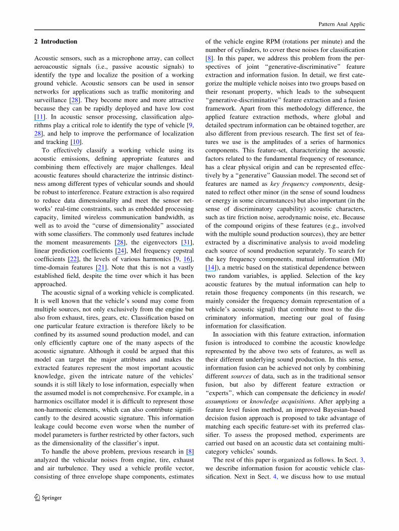
classification, we consider an information fusion diagram

to include more complete acoustic knowledge, illustrated

in Fig. 1.

This fusion diagram consists of multiple sound pro-

duction sources (see the left half of Fig. 1). By examining

the specific properties of each sound source, its contribu-

tion to the overall loudness, the stability of the received

signal and the application scenario of sensor networks, two

Pattern Anal Applic

123

corresponding branches of feature extraction are applied

(see the middle of Fig. 1). The upper branch of feature

extraction is based on the harmonic oscillator model,

accounting for the noise transferred through vehicle body

and exhaust system. The extracted harmonic feature vector

is called xh. The lower branch of feature extraction is

aiming at the remaining vehicle-dependent information,

mainly embedded in the tire friction noise, air turbulence

noise, etc. The corresponding features set is named as the

key frequency feature vector, xk.

The above feature extraction actually categorizes the

multiple sound sources into two parts, i.e., the resonance

derived and the non-resonance derived. This strategy is

different from previous research, e.g. [8], where multiple

noises were mentioned as well. The advantage of this

categorization is that new sources of information are added,

while the computational cost is controlled by grouping the

tire noise and the aerodynamic noise into one category,

based on their common non-resonant property. Compared

to the relatively stable engine excited noise, the tire noise

and the aerodynamic noise are more volatile. They are

heavily influenced by the vehicle’s distance to the sensors,

the vehicle’s velocity, road conditions, etc. For the purpose

of classification, it is difficult and also unnecessary to

extract them individually, which will consume the sensor

networks’ valuable resource and hinder real-time

implementation.

Based on this information fusion diagram, the output of

an acoustic signature consists of two parts, xh and xk,

respectively. To explore this structure, a natural approach

is by information fusion, where the fusion is actually car-

ried out by combining different sound excitation sources

(see the right part of Fig. 1), rather than different sensors’

outputs, as emphasized in the traditional fusion literature.

Based on our previous discussions, this fusion strategy is

reasonable for this application. Because the two sets of

features characterize the acoustic signal from different

facets, they are complementary to each other in the sense of

knowledge acquisition from different sound production’s

modeling. Fusing them, therefore, will provide more

knowledge about the desired acoustic signature for classi-

fication. Actually, this is the same principle or motivation

shared by the traditional sensor fusion or classifiers com-

bination, except that our fusion strategy compensates for

the deficiency in the model assumption but the sensor

fusion compensates the incompleteness in observation.

The methods on extracting the harmonic features xh can

be found in [16, 17]. Thus, the major problems remaining

in this fusion method are:

– how to select the key frequency features xk, which will

be discussed in the next section and

– how to develop a suitable fusion scheme, which will be

discussed in Sect. 5.

4 Extracting complementary features

for the harmonics-based vehicle classification

The lower branch of feature extraction in Fig. 1 is expected

to capture the vehicle-dependent information related to the

tire friction noise and the air turbulence noise. Some

research has studied the sound production model for sim-

ilar noises, for example by modeling the noise as a sto-

chastic component [2]. But the previous research basically

focused on synthesizing or reconstructing the noise, and a

satisfactory method for classification is not available.

Moreover, the targeted noises, i.e., tire friction noise and

air turbulence noise, are distinct in nature except both share

a non-resonant property. Naturally, we need two sets of

models to reconstruct them, which is disadvantageous in

the capacity-limited sensor networks. However, because

our goal is pattern classification, the information embedded

in these noises can be determined by discriminatory anal-

ysis. Also, by their non-resonant nature, this search can be

conveniently carried out in the residual non-harmonic part

xk

xh

Interior excitations

Exterior excitations

Engine

Tires Road friction transfer system

Air interaction transfer system

Non-harmonicfeatures

extraction

Harmonicfeatures

extraction

Featureassociation Classifier

ClassifierA

ClassifierB

Decisionfusion

or

Fig. 1 An information fusion diagram for acoustic vehicle classification

Pattern Anal Applic

123

of the acoustic signal to avoid information redundancy.

Thus, the new distinguishing information will naturally

differ from the harmonic features, leading to a meaningful

information fusion. Given that the applied discriminatory

analysis is generic and does not rely on a specific sound

production model, the useful information for classification

will be included automatically, regardless of whether it

arises from the tire friction or from the air turbulence.

In this research, we applied an effective feature

searching method based on mutual information (MI),

illustrated as follows (full details about this method can be

found in [14]):

1. The first component is chosen as:

X01 ¼ max

iI Xi; Yð Þ; ð2Þ

where X10 represents the result of maximization at step 1.

2. Then, the second component is chosen as:

X02 ¼ max

Xi 6¼X01

I Xi; Yð Þ � I Xi;X01

� �þ I Xi;X

01 jY

� �� �: ð3Þ

3. The remaining components are chosen in the same

way:

X0n ¼ max

Xi 6¼X0j

I Xi; Yð Þ �X

j

I Xi;X0j

� �"

þX

j

I Xi;X0j jY

� �#; ð4Þ

where X0j ; j ¼ 1; 2; . . .; n� 1 are the components

already selected. This search is repeated until the pre-

specified number, M, of components is reached.

The above strategy selects features sequentially, and so

avoids the problem of ‘‘combinatorial explosion’’. This

solution can also implicitly include other vehicle-depen-

dent factors probably omitted by the model, as long as their

representative features are detected with enough discrimi-

natory information.

It is known that to obtain essential features from the

original data (i.e., dimension reduction), two possible

routes are usually followed, i.e., feature extraction and

feature selection respectively. Among them, feature

extraction (in the context of dimension reduction) maps the

data from a high dimensional space to a low dimensional

space (subspace) by a linear or nonlinear transformation,

but feature selection finds a subset of the original attributes

by searching. In feature extraction, the typical linear

transformations are principal component analysis (PCA),

Fisher’s linear discriminant analysis (LDA), etc., and

nonlinear techniques include kernel PCA, manifold learn-

ing-based algorithms, etc. Recently, some novel feature

representations were proposed, such as geometric/

harmonic mean-based LDA [4, 27], manifold regularized

SIR (Sliced Inverse Regression) [5], spectral clustering/

embedding [23], etc. These methods are different from the

MI-based method that was used in this paper. In detail, the

dimension reduction methods introduced in [4, 5, 23, 27]

are in the category of feature extraction (i.e., features

transformation or mapping), but our MI-based strategy is a

feature selection method, specifically a feature filtering

approach. It is noticed that the geometric/harmonic mean-

based dimension reduction [27] discussed the Kullback-

Leibler (KL) divergence that is closely related to the metric

of the mutual information used in this paper. This implies

that the two approaches, though in different dimension

reduction groups and with distinct technical background

and implementation details (see [14]), may aim at opti-

mizing a similar criterion. However, this research prefers to

the feature selection in that it is important to retain the

original physical meaning of data (e.g., frequency loca-

tions) for further processing. This requirement becomes

difficult for feature extraction, where the linear or nonlin-

ear combination of many attributes makes it complicated to

reason the underlying sound production model. On the

other hand, the above MI-based feature selection finds the

most discriminating attributes straightforwardly, which can

be used to match different sound production sources,

making the following research on model refining easier.

Although we have shown that the key frequency com-

ponents selected by MI can effectively provide useful

discriminatory information, it is not recommended to

replace the harmonic feature extraction. This is because the

new features are extracted purely on the discriminatory

analysis, akin to a ‘‘black box’’. Without modeling each

specific physical nature, the captured features will tend to

include some unwanted components (like adding noise),

and the features’ effectiveness and invariability may be

reduced by these unforeseen additions. Meanwhile, due to

the volatile nature of the targeted noises, the amount of

information extracted by the new feature-set can be

checked, but its invariability is unsure. For example,

changes of velocity and road condition are very likely to

affect the selected results of the key frequency components.

Although this problem can be alleviated by considering a

more generally sampled population for training, it is

inevitable to increase the number of selected features. So,

the key frequency features should be better considered as a

supplemental constituent to the major harmonic features,

and a fusion approach should be applied to utilize both of

them. As long as this strategy is followed, the final per-

formance could be improved if the key frequency compo-

nents captured the new information, but will not degrade

significantly even if they failed (because the key frequency

components are assumed to be invariant for a given vehicle

Pattern Anal Applic

123

type traveling at a specific speed, on a known terrain, and

the stable harmonic features are still remained).

It is seen that both the feature vectors xh and xk are

calculated from the Fourier transform of the original

vehicle acoustic signals, so they are statistical dependent to

some extent. This dependency has been reduced by the

frequency normalization operation during the harmonic

extraction, also by the MI searching strategy particularly

designed to avoid searching for the harmonic locations.

The time-series of the original acoustic signals are sampled

at 1,024 points/s, and their corresponding data in Fourier

transform domain are cut to 351 dimensions, i.e., focusing

on the low frequency part. The feature extraction intro-

duced above further reduces the data dimensionality from

hundreds (351) to dozens (21), and therefore avoids the

‘‘curse of dimensionality’’ and makes the processing more

efficient. Moreover, during the dimension reduction, the

domain knowledge included by the sound production

model and discriminating analysis has been embedded into

the xh and xk implicitly, which may add extra a priori

information to benefit classification.

5 Fusing acoustic feature sets

After extracting the multiple feature sets, a natural way to

combine them for classification is by information fusion

[20]. Two possible fusion strategies that can be applied for

this task are feature level fusion and decision level fusion,

which are investigated as follows.

Apart from these fusion schemes, there are also other

ways to combine the two feature vectors. For example, one

may use the two feature sets in different steps of classifi-

cation, which essentially results in a kind of hierarchical

analysis [3]. The fundamental difference between the

hierarchical classification and the conventional fusion

schemes is that the former one usually partitions the output

space (i.e., the class labels) into a series of conceptual

subgroups. Without the output portioning, the hierarchical

analysis will reduce to the same processing similar to

decision level fusion since both of them analyze the dif-

ferent sources of information independently and combine

the results afterward. The hierarchical analysis usually will

produce a tree structure defining the relationships between

classes, which has been explored by our another ontology-

based fusion research [15].

5.1 Feature level fusion

Feature level fusion is a medium-level fusion strategy,

where several sets of features extracted from raw data are

directly combined for decision. Given the harmonic feature

vector represented by

xh ¼ X1h ;X

2h ; . . .;XL

h

� �;

where the superscripts represent different harmonic orders,

and the key frequency feature vector is represented as

xk ¼ X1k ;X

2k ; . . .;XJ

k

� �;

where the superscripts represent different key frequency

bins, one approach to feature level fusion can be simply

implemented by concatenating the two sets of features

together, and the fused feature vector is formed as follows:

xhk ¼ X1h ;X

2h ; . . .;XL

h ;X1k ;X

2k ; . . .;XJ

k

� �: ð5Þ

To determine whether fusing the two feature sets can

improve classification accuracy, the second assessment is

based on the feature vectors with the same dimensionality

as the harmonic feature vector’s, and the above fusion is

revised as:

x0hk ¼ X1h ;X

2h ; . . .;XI

h;X1k ;X

2k ; . . .;XJ

k

� �; ð6Þ

where I ? J = L, and L is the original dimensionality of

the harmonic feature vector. The fused feature vector now

has the same dimensionality as that of the harmonic feature

vector, but with the J higher order harmonics replaced by

the same number of key frequency components. In this

feature level fusion, since features from different extraction

methods are augmented directly, a proper normalization

should be applied to address the difference in the mea-

surement scale.

According to our previous discussion, the fused feature

vector tends to depict the acoustic signature more fully: the

ingredient from the harmonics part characterizes the major

engine noises and gives a global outline of the power

spectrum; the key frequency components reflect other

minor noises and provide some localized details of the

spectrum. From the point of view of multi-resolution rep-

resentation, the former part presents the coarse-grained

information, and the latter part gives the finer-grained

information.

The implementation of this feature level fusion is

straightforward. However, one major problem associated

with this fusion scheme is that the same classifier has to be

applied to the fused feature set, which means that the two

feature-sets will be classified by the same classification

algorithm. This is an unwanted consequence for this

application. According to the ‘‘No-free-lunch’’ theorem,

classification performance depends greatly on the charac-

teristics of the data to be classified [29], and there is no

single classifier that works best on all given data sets. In

this application, the two feature sets are based on different

model assumptions and have different utilities to represent

the acoustic signature. So it is quite likely that they have

their individually favored classifiers. To achieve better

Pattern Anal Applic

123

performance, decision level fusion was investigated

further.

Recently, a similar phenomenon has been observed by a

parallel research on image retrieval [32], where multiple

features from different views are extracted to represent an

object. Since the features in different views have their

specific statistical properties, the direct concatenation

(similar to the feature level fusion in this research) used in

the conventional spectral-embedding algorithms cannot

efficiently explore the information provided by the differ-

ent views. Therefore, a multiview spectral embedding

approach has been proposed, which can treat different

features in different ways. Though the multiview spectral

embedding discussed in [32] is a kind of clustering and

feature extraction method (different from the feature

selection framework required in this research), it indeed

echoes our above argument to further introduce the deci-

sion level fusion.

5.2 Decision level fusion

Decision level fusion is a high-level operation, where

separate intermediate decisions are drawn from each indi-

vidual feature set and then combined to reach a global

decision. To achieve better intermediate decisions in the

first place, it is necessary to find a suitable classifier for

each of the feature sets. In pattern classification, choosing a

suitable classifier for a given feature set is usually regarded

as more an art than a science. Without a priori knowledge,

it is difficult to find the relationship between the data to be

classified and the resulting performance of various

classifiers.

In this application, following prior experience in vehicle

classification [9, 10], we choose a multivariate Gaussian

classifier (MGC) for the harmonic features xh. Apart from

its previously proved performance, this choice also reflects

the fact that the physical model underlying the resonance

derived sound, i.e., the harmonics oscillator with additive

white noise, is relatively understandable, and a ‘‘genera-

tive’’ classifier is a reasonable option to match this data.

Moreover, the MGC algorithm is fast to implement and

particularly suited to use in sensor networks.

As mentioned before, the non-resonance-derived sound

involves the tire friction noise and the air turbulence noise.

The compound nature will made the single-nodal Gaussian

assumption unsuitable for modeling the feature vector xk.

Moreover, the proportions of the tire friction and the air

turbulence noise to the overall loudness are much more

unstable, which makes the multi-nodal Gaussian assump-

tion, such as the Gaussian mixture model, difficult to

implement (e.g., the changeable weights to the Gaussian

components). Therefore, it is better to consider a ‘‘dis-

criminative’’ classifier for this feature vector, consistent

with its feature extraction. Support vector machines

(SVMs) [6] have shown competitive performance with the

best available algorithms in many classification areas, so

were chosen as the classifiers for the key frequency fea-

tures vector xk.

Based on the knowledge available, we have chosen the

above classifiers for the two feature sets. To examine this

arrangement, we carryout tests and compare different

configuration results empirically, which are presented in

Table 7 of the next section. As mentioned earlier, the

reason of assigning MGC to the harmonic features and

SVM to the key frequency features is mainly based on the

model assumptions of sound production and feature gen-

eration. Considering the good performance achieved by

SVMs, one reasonable idea is to use the SVM for both

feature sets, or probably in a feature level fusion way.

However, our later experiments will suggest that applying

the same classifier to the two feature sets will result in

unsatisfactory outcome. For example, from Table 7, it is

shown that using SVM for the harmonic features produced

classification accuracy of 71.52%, which is lower than the

73.44% achieved by the MGC. On the other hand, using

MGC for the key frequency features got classification

accuracy of 66.10%, much poorer than the SVM’s 77.05%.

To avoid this mismatch of feature models with the applied

classifiers, one has to consider the decision level fusion.

The major worry regarding using decision level fusion is

the possible loss of discriminatory information during the

imperfect decision making and non-coincidently data

sampling [13]. However, the decision level fusion suffers

less from the potential ‘‘curse of dimensionality’’ [18], and

can achieve the good result as the same level as the feature

level fusion as long as the fusion rule is designed appro-

priately [13]. Indeed, the best fusion technique will depend

on the application and the data used [7]. In this research,

the decision level fusion is a better choice as evidenced by

the empirical results shown in Fig. 3 and Table 6, where

the classification accuracy of feature level fusion (using

SVM as the classifier) is significantly lower than the

accuracies achieved by the decision level fusion.

After applying the classifier MGC to the feature set xh

and the SVM to xk, two classification outputs are available.

To combine them to reach a global decision, an improved

Bayesian decision rule is proposed as follows.

5.2.1 A modified Bayesian decision fusion method

In the traditional Bayesian framework, there are several

approaches to combine probabilistic information. Let

xi; i ¼ 1; 2; . . .;N be N information sources (or different

feature sets in this research), and y the decision result,

according to the maximum a posteriori (MAP) criterion,

two usually used fusion methods are listed as follows [20]:

Pattern Anal Applic

123

p yjx1; x2; . . .; xNð Þ /YN

i¼1

p yjxið Þ; ð7Þ

and

p yjx1; x2; . . .; xNð Þ / p yð ÞYN

i¼1

p xijyð Þ: ð8Þ

It is known that both of the methods are based on

certain independence assumptions. However in our

application, the two feature sets are extracted from the

frequency response of the same acoustic signal, and the

independent assumption might not hold. So directly

applying the above fusion rules will result in

discrepancy from the expected MAP result. To obtain a

more accurate fusion, we propose the following improved

fusion criterion.

First, based on our application scenario, two information

sources, i.e., x1 and x2, are considered. According to the

Bayes rule, the posterior probability can be written as

follows:

p yjx1; x2ð Þ ¼ pðx1Þp yjx1ð Þp x2jy; x1ð Þp x1ð Þp x2jx1ð Þ : ð9Þ

For decision purposes, (9) can be simplified as:

argmaxy

p yjx1; x2ð Þ / p yjx1ð Þp x2jy; x1ð Þ; ð10Þ

and (10) reduces to (8) if x1 is independent of x2 given the

same prior p(y).

To implement the fusion rule in (10) without any

independence assumption, the conditional probabilities

p yjx1ð Þ and p x2jy; x1ð Þ are needed. Through our previous

discussion, the posterior p yjx1ð Þ can be obtained from the

SVM’s output (see Sect. 5.2.3 for details), and the likeli-

hood p x2jyð Þ can be conveniently obtained from the out-

puts of the MGC. Then a major problem is to estimate

p x2jy; x1ð Þ based on all available information, which can be

formulated as follows:

p x2jyð Þ; x1; x2f g ! p̂ x2jy; x1ð Þ; ð11Þ

where ? represents to estimate the conditional probability

p x2jy; x1ð Þ based on a set of information available, i.e., a

likelihood p x2jyð Þ and two extracted feature sets x1 and x2.

So for our specific application scenario, a more accurate

MAP decision rule can be re-written as:

argmaxy

p yjxh; xkð Þ / p yjxkð Þp xhjy; xkð Þ ð12Þ

where xh and xk represent the harmonic feature vector and

the key frequency feature vector, respectively.

To estimate p xhjy; xkð Þ, i.e., to implement (11), we

propose an approach based on a simple information-theo-

retical criterion, presented as follow.

5.2.2 Modulating the multi-dimensional Gaussian

distribution

Let xh be a L-dimensional harmonic feature vector, the

likelihood function will be:

pðxhjyÞ ¼1

ð2pÞL=2 Rj j1=2exp �1

2ðxh � lÞ>R�1ðxh � lÞ

� ;

ð13Þ

where l and R are the mean vector and the covariance

matrix, respectively.

Because the feature vector xh is not independent of xk,

the appearance of xk will reduce the uncertainty of xh. In

information theory, the uncertainty is often measured by

entropy. So to estimate p xhjy; xkð Þ from p xhjyð Þ, one con-

venient approach (based on the above basic concept in

information theory) is to reduce the entropy of xh by

including the knowledge of xk. It is known that the entropy

of xh (given its probability as in 13) [1] is:

� ¼ ln

ffiffiffiffiffiffiffiffiffiffiffiffiffiffiffiffiffiffiffið2peÞL Rj j

q� : ð14Þ

To reduce (14), we have to update or modulate the

determinant of the covariance matrix R based on the

knowledge available. Let the amount by which entropy is

reduced be represented by D:

D ¼ �� �� ¼ kD; ð15Þ

where the original entropy � is based on p xhjyð Þ, and the

updated entropy �� is based on p̂ xhjy; xkð Þ; D 2 ½0; 1� is a

normalized metric measuring how independent the xk is of

xh, and the constant k 2 Rþ controls the modulation depth

(i.e., the maximum reduction of entropy). Using (14) into

(15), we can find that the entropy reduction by D can by

carried out by modifying R as follows:

ln

ffiffiffiffiffiffiffiffiffiffiffiffiffiffiffiffiffiffiffið2peÞL Rj j

q� � ln

ffiffiffiffiffiffiffiffiffiffiffiffiffiffiffiffiffiffiffiffiffið2peÞL R�j j

q� ¼ kD

) ln

ffiffiffiffiffiffiffiffiRj jR�j j

s !¼ kD) R�j j ¼ e�2kD Rj j ð16Þ

where R� is the updated covariance matrix.

In our application, each feature component represents

the amplitude of a frequency bin in the frequency domain

representation of the acoustic signal, so the independence

indicator D can be intuitively estimated by calculating how

far xk is to xh, e.g., an averaged frequency distance d0

defined as follows:

d0 ¼ 1

LJ

XL

i¼1

XJ

j¼1

fXih� fXj

k

� �ð17Þ

where fXi represent the frequency location of the feature

component Xi; L and J are the dimensions of the two

Pattern Anal Applic

123

feature vectors xh and xk. Then, the normalized distance D

can be obtained by:

D ¼ d0=d0max: ð18Þ

According to the property of determinant: rAj j ¼ rn Aj j(n is the dimension of matrix A), the simplest approach to

update the covariance matrix in (16) can be implemented

as follows:

R� ¼ffiffiffiffiffiffiffiffiffiffiffie�2kDLp

R: ð19Þ

Thus, the conditional probability p xhjy; xkð Þ can be

estimated by modulating the covariance matrix R of

p xhjyð Þ according to the frequency distance between xk

and xh, i.e.,

p̂ xhjy; xkð Þ�N ðl;R�Þ; ð20Þ

where R� is modified as described in (19), based on the

independence knowledge between xk and xh as estimated in

(17) and (18).

5.2.3 Calibrating SVMs’ output to probability

After obtaining the conditional probability p̂ xhjy; xkð Þ from

the MGC’s output, to implement the fusion approach in

(12) we still need another posterior probability from the

SVM classifier, i.e., p yjxkð Þ. However, standard SVMs do

not provide posterior probability directly. To obtain the

posterior probability, a mapping method introduced in [25]

is used, where an additional sigmoid function is used to

approximate the necessary posterior probability. Specifi-

cally, the posterior probability is trained by a sigmoid

function:

p yjxð Þ � 1

1þ exp Af xð Þ þ Bð Þ; ð21Þ

where parameters A and B are found by minimizing the

following cross-entropy error function:

argminA;B

�XT

i¼1

ti log p yjxið Þð Þ þ 1� tið Þ log 1� p yjxið Þð Þ" #

;

ð22Þ

with ti ¼ yiþ12

. The details on the calculation of (22) can be

found in [19, 25].

Based on the above discussions, a new decision fusion

approach, tailor made for this application, is implemented

and summarized as the following steps:

– An SVM is used to draw a decision based on the key

frequency feature vector xk, and its output is calibrated

to a posterior probability p yjxkð Þ (see Sect. 5.2.3);

– A maximum likelihood classifier, i.e. MGC, is applied

to the harmonic feature vector xh, and based on its

output p xhjyð Þ, the necessary p xhjy; xkð Þ is estimated

using a simple information-theoretic rule (see Sect.

5.2.2); and

– An improved fusion rule, shown in (12), is then used to

achieve the final global decision.

Comparing with other Bayesian fusion rules, e.g., (7)

and (8), the proposed method does not need the indepen-

dence assumption, and is based on a more accurate MAP

criterion (see 12). Both research studies and the formula

(7), (8) show that it is significantly necessary for an

effective fusion that fused sources or features are inde-

pendent or approximately independent with each other.

However, in practice the independence cannot be observed

straightforwardly from the partitioned sources or features.

Once the independence assumption is not able to be veri-

fied easily, the proposed fusion scheme becomes a useful

alternative to the traditional Bayesian fusion rules. Mean-

while, benefiting from the specific characters of the

application data (e.g., the Multivariate Gaussian distribu-

tion for the harmonic features), its implementation is

simplified and avoid those more complicated Bayesian

methods, which make it more appealing to this application.

6 Experimental results

To assess the proposed information fusion approach,

experiments are carried out based on a multi-category

vehicles acoustic data set from US ARL [10]. The ARL data

set consists of recoded acoustic signals from five types of

ground vehicles, named as V1t, V2t, V3w, V4w, and V5w

(the subscript ‘t’ or ‘w’ denotes the tracked or wheeled

vehicles, respectively). These vehicles cover six running

cycles around a prearranged track separately, and the cor-

responding acoustic signals are recorded for the assessment.

To obtain a frequency domain representation, the Fou-

rier transform (FFT) is first applied to each second of the

acoustic data with a Hamming window, and the output of

the spectral data (a 351 dimensional frequency domain

vector x) is considered as one of the samples for these five

vehicles. Then feature extraction is carried out on the

sample x to get the two sets of features, i.e., the harmonic

feature vector xh and the key frequency feature vector xk

(see Sect. 4) Subsequently, these feature vectors are fed

into the classifier(s), and the final classification result will

be obtained from the fusion algorithms (see Sect. 5).

The type label and the total number of the (spectral) data

vectors for each vehicle are summarized in Table 1. A

‘‘run’’ corresponds to a vehicle moving a 360� circle

around the track and the sensors array, and a sample means

the FFT result at 1 s signal. Differences in the total num-

bers of the samples reflect the vehicles’ different moving

speeds.

Pattern Anal Applic

123

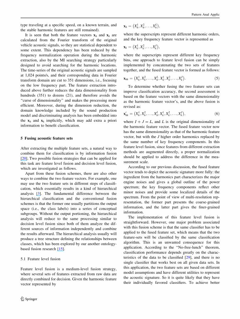
As we discussed in Sect. 5, the features to be fused came

from the harmonic extraction and mutual information

evaluation, respectively. The left column of Fig. 2 illus-

trates the 351 dimensional spectral vectors for the five

types of vehicles (corresponding to V1t - V5w, from top

to bottom). For each type of vehicle, 20 samples are

illustrated in Fig. 2, reflecting the variations at different

sampling times and different runs. The right column of

Fig. 2 shows the 21 dimensional harmonic features

extracted from the above spectral vectors for these five

vehicles. The amplitudes of these harmonics form a har-

monic feature vector xh.

From Fig. 2, it can be seen that the spectral responses of

the vehicles’ sounds are quite complex, consisting of many

formants that did not appear at the exact positions of the

integral multipliers of its fundamental frequency. There are

also large within-class variations in the features (see the

extracted harmonic features). As for the between-class

variations, there are many overlapped formants among the

five vehicles. For example, Fig. 2a and g has similar peaks

around frequency 50 and 100 Hz; Fig. 2g and i shows

similar frequency response between 1 and 50 Hz. This

evidence shows that vehicle noises are much more complex

than the previously assumed oscillator model, and it is

difficult to cover all of the acoustic characters using a single

feature set. To address the actually multiple excitations and

the complicated noises, we indeed need an improved model

shown in Fig. 1 and fusion approaches discussed in Sect. 5.

For accuracy assessment, half of the runs from each

vehicle (i.e., 3 runs from all 6 runs) were randomly chosen

Table 1 The number of runs and the total sample numbers for five

types of vehicles: tracked vehicles V1t and V2t; wheeled vehicles

V3w,V4w and V5w

Vehicle class Number

of runs

Total number

of samples

V1t 6 1,734

V2t 6 4,230

V3w 6 5,154

V4w 6 2,358

V5w 6 2,698

50 100 150 200 250 300 350

2468

101214

Frequency

Am

plitu

de

(a)

2 4 6 8 10 12 14 16 18 20

20406080

100

Harmonics order

Am

plitu

de

(b)

50 100 150 200 250 300 350

2468

10

Frequency

Am

plitu

de

(c)

2 4 6 8 10 12 14 16 18 20

20

40

60

Harmonics order

Am

plitu

de

(d)

50 100 150 200 250 300 350

5

10

15

Frequency

Am

plitu

de

(e)

2 4 6 8 10 12 14 16 18 20

20406080

100120140

Harmonics order

Am

plitu

de

(f)

50 100 150 200 250 300 350

2468

10

Frequency

Am

plitu

de

(g)

2 4 6 8 10 12 14 16 18 20

20

40

60

Harmonics order

Am

plitu

de

(h)

50 100 150 200 250 300 350

5

10

15

Frequency

Am

plitu

de

(i)

2 4 6 8 10 12 14 16 18 20

20406080

100120140

Harmonics order

Am

plitu

de

(j)

Fig. 2 Illustration of the spectrum (left column) and the harmonic features (right column) for the five vehicles V1t (top) - V5w (bottom),

respectively; 20 samples (depicted in different colors) are drawn for each vehicle (color figure online)

Pattern Anal Applic

123

to estimate the statistical parameters for feature extraction.

The remaining half forms the test set on which perfor-

mance was assessed. Next, feature extraction is carried out

based on the methods introduced in Sect. 5 Following the

results in [10], the harmonic number is chosen as 21. The

main reason to choose the harmonics number of 21 is to be

consistent with the previous studies [10]. However, we note

that there may be a minimum sufficient number for the

harmonics but that will depend on different applications.

As discussed previously, SVMs are chosen as the clas-

sifier for the key frequency feature vector. Because SVMs

are inherently binary (two-class) classifiers, ð 52Þ one-

against-one classifiers were used with subsequent majority

voting to give a multi-class result. The kernel function used

is an heterogeneous polynomial. The penalty parameter C

is tested between 10-3 and 105, and polynomial order is

tested from 1–10 by a twofold validation procedure using

only training data. The polynomial order 3 and C = 20

were finally found as the best values for this SVM, and

applied to the following testing stage. The training data set

is also used to estimate the means vector l and the

covariance matrix R for MGC.

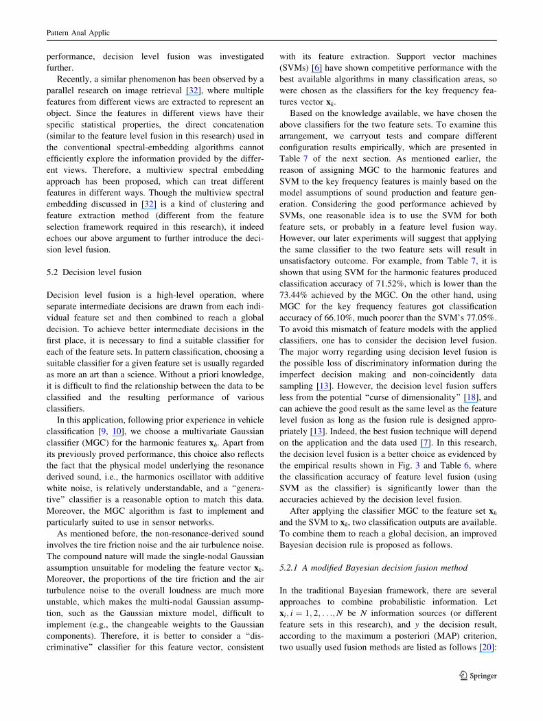
To avoid bias on random samplings of the training

‘‘runs’’, the testing was repeated 10 times. The 10 times

classification results based on each individual feature set

and the fusion approaches are shown in Fig. 3. The con-

catenated feature set in the feature level fusion has the

same dimensionality as that of the each individual feature

set (see 6). In this data set, each run consists of about 290 to

860 s of acoustic data depending on the vehicles’ different

running speeds. Tests are carried out based on each second

of the acoustic data (i.e., to classify the vehicles in each

second interval, which is useful for vehicle tracking) from

the three test runs, and the overall accuracies are summa-

rized from the above results for all five types of vehicles.

From Fig. 3, the following results are observed:

– For each individual feature set, the key frequency

feature set (the second column) achieved better clas-

sification accuracy than the harmonic feature set (the

first column). This supported our proposal to include

new acoustic characters (such as the tire friction noise

and air turbulence noise) for vehicle classification and

to use the mutual information for feature selection.

– The feature level fusion (the third column) is slightly

better, but very close to the best result from each

individual feature set. This phenomenon coincides with

the finding observed by previous fusion literature [26].

We will explain this phenomenon later, from the

perspective view of this application.

– The decision level fusion approaches (the fourth and

fifth column) achieved significant improvement com-

pared with those using each feature set individually,

and are also much better than the feature level fusion.

– The improvement of the modified decision fusion (the

fifth column) to the traditional decision fusion (the

fourth column) is found consistent in all of the 10 times

tests, but not very significant. As for the limited

improvement, two possible reasons are considered: (1)

because the key frequency components are selected to

be unrelated with the harmonic features in the first

place, the independence assumption is enhanced and

makes the subsequent uncertainty reduction (see 11)

less necessary and (2) the method to update the

Multivariate Gaussian function (e.g., to reduce the

uncertainty by entropy, see 16) is not very effective,

and a more suitable modulating method should be

considered in the future. However, the consistent

improvement archived by the new fusion rule is still

encouraging, showing potential to be applied to other

similar applications where it is not easy to ensure the

independence assumption.

The average numbers for the above 10 tests’ results are

summarized in Table 2, which further demonstrated the

effectiveness of the fusion methods.

In this multi-category vehicles data set, due to the

vehicles’ different running speeds, the numbers of the

testing samples for different vehicles vary greatly (see

Table 1). To better observe the performance, it is necessary

to show the individual classification results for each of the

1 2 3 4 5 6 7 8 9 1065

70

75

80

85

90

95

Number of tests

Cla

ssifi

catio

n ac

cura

cy (

%)

Harmonics featuresKey frequency featuresFeature−level fusionDecision−level fusionModified Bayesian fusion

Fig. 3 Comparison of

classification accuracy for the

different feature sets and fusion

methods; 10 times tests with

randomly chosen 3 runs for

training and the remaining 3

runs for testing; the accuracy is

the overall result for all 5 types

of vehicles

Pattern Anal Applic

123

vehicles. Two confusion matrices are therefore listed as

follows, corresponding to one of the reference methods

based on the harmonic features (Table 3) and one of the

decision fusion methods based on the modified Bayesian

rule (Table 4).

In Tables 3 and 4, each column of the matrix represents

the predicted type of vehicle class, while each row repre-

sents the actual class type of vehicle. It can be seen that in

the fusion approach (Table 4), the numbers of correct

labeling (i.e., the numbers in the leading diagonal of Table

4) is much higher than those in the method without fusion

(see the leading diagonal of Table 3), indicating the higher

detection accuracy achieved by the fusion method. At the

same time, the majority of the numbers of mislabeling in

the fusion approach is lower than the method without

fusion (i.e., in 17 from all other 20 non-leading diagonal

components), indicating less confusing between classes

after the fusion is carried out.

Another highlight of this research is to categorize vari-

ous acoustic signatures into two groups according to their

sound production property, instead of using them

separately. The effectiveness of this scheme can be

observed from Fig. 3 and Table 1, which show that using

two feature sets (i.e., the fusion methods) outperformed

those using them individually. To further confirm this, an

experiment is carried out by comparing the proposed fea-

ture grouping scheme with the existing harmonic features

under the same dimensionality. Results are listed in

Table 5, where the single feature-set contains 21 dimen-

sional harmonics and is classified by a maximum likeli-

hood classifier. The compound feature-set consists of 11

dimensional harmonics and 10 dimensional key frequency

bins, and is classified by SVM and maximum likelihood

classifier correspondingly. Table 5 shows that the classifi-

cation accuracies using the compound feature-set are better

than using the existing harmonics feature-set, confirming

the advantage of the proposed feature grouping scheme.

In addition to decision level fusion, we also implement a

feature level fusion scheme for comparison. The results are

illustrated in Fig. 3 and Table 1, where instead of directly

concatenating two feature sets together, the proposed

scheme keeps the dimensionality of the fused features as

the same as that of either feature set. This may reduce the

discriminability of the fused feature and, in turn, lower the

classification performance. Therefore, an extra experiment

is carried out to provide a comparison of the proposed

approach with those of concatenating two feature sets,

where both a trimmed concatenation (produces a

21-dimensional feature-set) and a direct concatenation

(produces a 42-dimensional feature-set) are considered.

Results are listed in Table 6, showing that the decision

level fusion is indeed superior to its counterparts in this

particular case. It is well known that fusion performance is

heavily influenced by the characteristics of the applied

Table 2 Mean classification accuracy of 10 times tests

Methods Average accuracy (%)

Harmonic feature set 73.44

Key frequency feature set 77.05

Feature-level fusion 77.34

Decision-level fusion 83.86

Modified Bayesian decision fusion 84.24

Table 3 Confusion matrix for the classification based on the har-

monic features

V1t V2t V3w V4w V5w

V1t 768 50 20 26 3

V2t 72 1,592 134 196 121

V3w 47 126 1,805 341 258

V4w 21 91 141 825 101

V5w 3 74 119 119 1,016

Table 4 Confusion matrix for the classification based on the modi-

fied Bayesian decision fusion

V1t V2t V3w V4w V5w

V1t 772 61 17 14 3

V2t 21 1,923 63 79 29

V3w 23 70 2,192 170 122

V4w 4 61 148 911 55

V5w 0 42 120 60 1,109

Table 5 Comparison of acoustic signatures extraction

Acoustic signatures Classification

accuracy (%)

Single feature-set (21-dimensional harmonics) 74.43

Compound feature-set (21-dimensional mixed,

ML classifier)

75.72

Compound feature-set (21-dimensional mixed,

SVM classifier)

79.56

Table 6 Comparison of feature level and decision level fusion

Fusion schemes Classification

accuracy (%)

Feature level fusion (21-dimensional feature-set) 79.56

Feature level fusion (42-dimensional feature-set) 83.32

Decision level fusion (two 21-dimensional feature-

sets)

86.06

Pattern Anal Applic

123

data, so the above conclusion should be carefully checked

when it is considered to be extended to other applications.

Finally, we examine the performance changes by

applying different classifiers to each of the feature sets.

Table 7 lists the average classification accuracy of

10 times tests based on the two classifiers, i.e., SVM and

MGC, for the harmonic features and the key frequency

features, respectively. It can be found that for the harmonic

features, the MGC is a better classifier than the SVM,

confirming the previous experience [9]. Meanwhile, for the

key frequency features, the SVM is a better classifier than

the MGC. This empirical comparison clearly supports the

‘‘No-free-lunch’’ claim: there is not a panacea classification

algorithm, which is best for all data sets.

The results in Table 7 not only verified our previous

classifiers arrangement but also can explain why the feature

level fusion did not work very well in this application (see

Table 2). Because each feature set has its individually

preferred classifier and the performance variations under

different classifiers are significant (see Table 7), the feature

level fusion, which has to use one classifier, cannot take

into account of both of them at the same time. So the

effectiveness of feature level fusion is offset by this con-

straint, making decision level fusion a more suitable choice

in this case.

Due to the difficulty of obtaining more vehicles’

acoustic data (e.g., including more tracked and wheeled

vehicles in a more complex scenario), currently we tested

our method at the ARL data set that we can access. Once

more challenging data (e.g., running more tracked vehicles

by our partner) is available, we will extend testing to the

new data set and probably amend new results in a future

correspondence.

7 Conclusions

In this paper, we developed an information fusion approach

for ground vehicle classification. The harmonic features,

based on the vehicle-body’s resonance assumption, and the

key frequency components, based on the vehicular exterior

parts’ non-resonance assumption, were extracted, respec-

tively, for information fusion. Especially, the features

extracted by mutual information added finer-grained

spectrum information to the coarse-grained spectrum

information provided by the harmonic features. Fusing

them can give a full picture of the desired acoustic signa-

ture, and produces an analogous multi-resolution repre-

sentation for classification. By breaking out the

independence constraint among the fused sources, a modi-

fied Bayesian decision fusion rule is also proposed, which

can better combine the classification results obtained from

the two feature-sets. Experiments were carried out to assess

the classification accuracies of the fusion approaches, based

on a multi-category vehicles acoustic data set. Results

showed that the classification accuracy has been improved

by the fusion approaches, especially by the decision level

fusion. To emphasize the major contributions of this

research, i.e., the comprehensive sound production model

and the supporting feature selection and fusion schemes, we

mainly tested the proposed method benchmarked on the

currently mature technology. Due to the scope of this

research, we have not further compared the proposed

scheme with other available algorithms, which will be

studied in future. Next research will address the new fea-

tures’ stability with regard to vehicles’ velocity changes,

and extend this approach to other more complicated data

sets (involving new sensors and vehicles deployment and

data acquisition), such as the acoustic signals with lower

SNR or simultaneous appearance of multiple vehicles.

Acknowledgments The Correspondence author is currently spon-

sored by Zhejiang Provincial ‘‘Qianjiang Rencai’’ Project of China

(Grant No. 2010R10011), and partially sponsored by National Natural

Science Foundation of China (Grant No. 61004119) and National

Basic Research Program of China (973 Program, Grant No.

2009CB320600 or No. 2009CB320602). The research was sponsored

by the US Army Research Laboratory and the UK Ministry of

Defence and was accomplished under Agreement Number W911NF-

06-3-0001. The views and conclusions contained in this document are

those of the author(s) and should not be interpreted as representing the

official policies, either expressed or implied, of the US Army

Research Laboratory, the US Government, the UK Ministry of

Defence or the UK Government. The US and UK Governments are

authorized to reproduce and distribute reprints for Government pur-

poses notwithstanding any copyright notation hereon.

References

1. Ahmed N, Gokhale D (1989) Entropy expressions and their

estimators for multivariate distributions. IEEE Trans Inf Theory

35(3):688–692

2. Amman S, Das M (2001) An efficient technique for modeling and

synthesis of automotive engine sounds. IEEE Trans Ind Electron

48(1):225–234

3. Bailey A, Harris C (1999) Using hierarchical classification to

exploit context in pattern classification for information fusion. In:

The second international conference on information fusion,

pp 1196–1203

4. Bian W, Tao D (2008) Harmonic mean for subspace selection. In:

Proceedings of 19th international conference on pattern recog-

nition, ICPR, pp 1–4

Table 7 Mean classification accuracy (%) of different classification

algorithms and feature sets

Harmonic features Key frequency features

MGC 73.44 66.10

SVM 71.52 77.05

Pattern Anal Applic

123

5. Bian W, Tao D (2009) Manifold regularization for sir with rate

root-n convergence. In: Bengio Y, Schuurmans D, Lafferty J,

Williams CKI, Culotta A (eds) Advances in neural information

processing systems, pp 117–125

6. Boser BE, Guyon IM, Vapnik VN (1992) A training algorithm for

optimal margin classifiers. In: Proceedings of the fifth annual

workshop on computational learning theory, pp 144–152

7. Busso C, Deng Z, Yildirim S, Bulut M, Lee CM, Kazemzadeh A,

Lee S, Neumann U, Narayanan S (2004) Analysis of emotion

recognition using facial expressions, speech and multimodal

information. In: Sixth international conference on multimodal

interfaces ICMI, pp 205–211

8. Cevher V, Chellappa R, McClellan JH (2007) Joint acoustic-

video fingerprinting of vehicles. In: ICASSP 2007, pp 745–752

9. Damarla T, Pham T, Lake D (2004) An algorithm for classifying

multiple targets using acoustic signature. In: Proceedings of SPIE

signal processing, sensor fusion and target recognition, pp 421–

427

10. Damarla T, Whipps G (2005) Multiple target tracking and clas-

sification improvement using data fusion at node level using

acoustic signals, vol 5796. In: Proceedings of SPIE unattended

ground sensor technologies and applications, pp 19–27

11. Duarte M, Hu YH (2004) Vehicle classification in distributed

sensor networks. J Parallel Distributed Comput 64:826–838

12. Forren J, Jaarsma D (1997) Traffic monitoring by tire noise. In:

Proceeding of IEEE conference on intelligent transportation

system, ITSC 97, pp 177–182

13. Gunatilaka A, Baertlein B (2001) Feature-level and decision-

level fusion of noncoincidently sampled sensors for land

mine detection. IEEE Trans Pattern Anal Machine Intell 23(6):

577–589

14. Guo B, Nixon M (2009) Gait feature subset selection by mutual

information. IEEE Trans Syst Man Cybern Part A 39(1):36–46

15. Guo B, Nixon MS, Damarla T (2009) Acoustic vehicle classifi-

cation by fusing with semantic annotation. In: Proceedings of

12th international conference on information fusion, FUSION

’09, pp 232–239

16. Lake D (1998) Harmonic phase coupling for battlefield acoustic

target identification. In: Proceedings of IEEE international con-

ference on acoustics, speech, and signal processing, pp 2049–

2052

17. Lake D (1998) Tracking fundamental frequency for synchronous

mechanical diagnostic signal processing. In: Proceedings of 9th

IEEE signal processing workshop on statistical signal and array

processing, pp 200–203

18. Lee CM, Narayanan S (2005) Toward detecting emotions in

spoken dialogs. IEEE Trans Speech Audio Process 13(2):293–

303

19. Lin HT, Lin CJ, Weng RC (2007) A note on Platt’s probabilistic

outputs for support vector machines. Machine Learn 68:267–276

20. Manyika J, Durrant-Whyte H (1994) Data fusion and sensor

management: a decentralized information-theoretic approach.

Ellis Horwood, New York

21. Mazarakis G, Avaritsiotis J (2007) Vehicle classification in sen-

sor networks using time-domain signal processing and neural

networks. Microprocess Microsyst 31:381–392

22. Munich M (2004) Bayesian subspace methods for acoustic sig-

nature recognition. In: Proceedings of the 12th European signal

processing conference, pp 1–4

23. Ng AY, Jordan MI, Weiss Y (2002) On spectral clustering:

analysis and an algorithm. In: Dietterich T, Becker S, Ghahra-

mani Z (eds) Advances in neural information processing systems

(NIPS), pp 1–4

24. Nooralahiyan AY, Kirby HR, McKeown D (1998) Vehicle

classification by acoustic signature. Math Comput Model

27(9–11):205–214

25. Platt J (2000) Advances in large margin classifiers, Chap. MIT

Press, Cambridge

26. Rao N (2001) On fusers that perform better than best sensor.

IEEE Trans Pattern Anal Machine Intell 23(8):904–909

27. Tao D, Li X, Wu X, Maybank SJ (2009) Geometric mean for

subspace selection. IEEE Trans Pattern Anal Machine Intell

31(2):260–274

28. Thomas D, Wilkins B (1972) The analysis of vehicle sounds for

recognition. Pattern Recogn 4(4):379–389

29. Walt C, Barnard E (2006) Data characteristics that determine

classifier performance. In: The sixteenth annual symposium of

the Pattern Recognition Association of South Africa, pp 160–165

30. Wu H, Mendel J (2007) Classification of battlefield ground

vehicles using acoustic features and fuzzy logic rule-based clas-

sifiers. IEEE Trans Fuzzy Syst 15(1):56–72

31. Wu H, Siegel M, Khosla P (1999) Vehicle sound signature rec-

ognition by frequency vector principal component analysis. IEEE

Trans Instrum Meas 48(5):1005–1009

32. Xia T, Tao D, Mei T, Zhang Y (2010) Multiview spectral

embedding. IEEE Trans Syst Man Cybern Part B Cybern

40(6):1438–1446

Author Biographies

Baofeng Guo received the

B.Eng. degree in electronic

engineering and the M.Eng.

degree in signal processing from

Xidian University, Xi’an, in

1995 and 1998, respectively,

and the Ph.D. degree in signal

processing from the Chinese

Academy of Sciences, Beijing,

in 2001, respectively. From

2002 to 2004, he was a

Research Assistant in the

Department of Computer Sci-

ence, University of Bristol, UK.

From 2004 to 2009, he was a

Research Fellow in the School of Electronics and Computer Science,

University of Southampton, Southampton, UK. Since 2009, he has

been with the School of Automation, Hangzhou Dianzi University,

Hangzhou, China. His current research interests are pattern recogni-

tion, information fusion, and image processing.

Mark S. Nixon is current a

Professor in computer vision

with the University of South-

ampton, Southampton, UK. His

team develops new techniques

for static and moving shape

extraction which have found

application in automatic face

and automatic gait recognition

and in medical image analysis.

His team were early workers in

face recognition, later came to

pioneer gait recognition and

more recently joined the pio-

neers of ear biometrics. Among

research contracts, he was Principal Investigator with John Carter on

the Defense Advanced Research Projects Agency supported project

Automatic Gait Recognition for Human ID at a Distance. He chaired

British Machine Vision Conference 98 and, with Josef Kittler, chaired

Pattern Anal Applic

123

the Audio Visual Biometric Person Authentication 2003. He was

Publications Chair for the International Conference on Pattern Rec-

ognition 2004 and the IEEE 7th International Conference on Face and

Gesture Recognition 2006. His vision book, cowritten with Alberto

Aguado, Feature Extraction and Image Processing was published in

2002 by Butterworth, and with Tieniu Tan and Rama Chellappa, his

new book Human ID based on Gait, which is part of the new Springer

Series on Biometrics, was published in 2005. His research interests

are in image processing and computer vision.

Thyagaraju Damarla received the B.Sc. degree (hons.) in mathe-

matics, the B.Tech. degree (hons.) in electronics and electrical

communication engineering, and the M.Tech. degree in controls and

computation engineering from the Indian Institute of Technology,

Kharagpur, India. He received Ph.D. in engineering from Boston

University, Boston, MA. He was an Assistant Professor in the

Electrical Engineering Department, University of Kentucky, Lexing-

ton, until 1994. He is currently an Electronics Engineer with the US

Army Research Laboratory, Adelphi, MD. His interests include signal

processing, automatic target detection and recognition algorithm

development, and neural networks.

Pattern Anal Applic

123