Implications of the “Status Quo” in Theoretical Trade Policy ...

23

Implications of the “Status Quo” in Theoretical Trade Policy Analyses ── Piecemeal Policy and the Stable Set Approach──

Noritsugu Nakanishi*†

Graduate School of Economics, Kobe University

Abstract

I argue that if the notion of the “status quo” is not incorporated appropriately in the models of trade policy issues, there may arise some theoretical/conceptual problems in interpreting the results derived from the models as the guidance for the implementation of trade policies. To clarify the point, I use concrete examples of theoretical analyses of trade policies both in the general equilibrium framework (the piecemeal tariff reforms and the optimal tariffs) and in the game-theoretic framework (the tariff negotiations). JEL Classification: F13, C71, C72.

Key words: Status Quo, Trade Policy, Piecemeal Policy, von Neumann-Morgenstern Stable Set

1　Introduction

What is the meaning of analyzing trade policy issues by making use of some theoretical or, almost equivalently, mathematical models ? A theoretical model of a trade policy issue is constructed so that it can appropriately represent the behavior of agents, who are concerned with the issue, and the functioning of related markets and/or other institutions: the model is supposed to reproduce the reality or, at least, the skeletal structure of the issue in reality. Instead of examining the real world itself, we examine the working of the model through mathematical calculation and logical deduction. Then, believing that there is a certain corre-spondence between the model and the state of affairs in reality, we identify the working of the model with that of the reality and, consequently, we think of the results obtained through cal-culation/deduction from the model as the guidance for the implementation of trade policies in the real world.

Although all that is a commonplace conduct of theoretical analysis in economics in gen-eral, it can be somewhat misleading when we apply it to trade policy issues in order to obtain

Received 15 January 2017, Accepted 25 January 2017* Address for correspondence: Graduate School of Economics, Kobe University, Rokkodai-cho 2-1,

Nada-ku, Kobe 657-8501, Japan. Email: [email protected].† This article is based on my Kojima Kiyoshi Prize Lecture at Kyoto Sangyo University (October 26,

2014). I wish to express my deep appreciation to all the (current and past) members of the Japan Society of International Economics for awarding me the Kojima Kiyoshi Prize 2014. My special thanks go to the late Professors Kiyoshi Kojima and Kiyoshi Ikemoto. I also thank Professor Taiji Furusawa, the editor of this journal, for his valuable comments.

The International Economy, Vol. 19, 2016

Implications of the “Status Quo” in Theoretical Trade Policy Analyses

24

some guiding implications for actual policies from the model. The problem is in the way how we understand the relationship between the reality and the model. In particular, the problem is associated with how we embed the roles of the “status quo” in the model and how we derive and interprete the implications of it. In this short article, I will argue this problem by showing concrete examples of theoretical analyses of trade policies in two different frameworks: the general equilibrium framework and the game-theoretic framework, those which I have been working on in my career.

In the general equilibrium framework, I compare the theory of piecemeal policy recom-mendation and the theory of optimal tariffs. Then, I discuss that the piecemeal policy argu-ment, which incorporates the notion of the status quo appropriately in the model, can provide a good theoretical guidance for the implementation of the policy and, in contrast, that the opti-mal tariff argument, which lacks the reference to the status quo, fails to be persuasive founda-tions of the implementation of the policy.

In turn, in the game-theoretic framework, I argue that the usual game models together with the Nash equilibrium as the solution concept grasp the real world phenomena as “matters of choice” by the players and, consequently, they by nature lack the reference to the status quo. Just because of this, I argue, there arise some legitimate questions that cannot be answered in a sound way within the usual game-theoretic framework. Further, in order to overcome these difficulties in the usual game-theoretic framework, I introduce an alternative framework—the stable set approach—that can incorporate the notion of the status quo appro-priately in theoretical models; to show how the stable set approach works well, I also give examples of the models of trade negotiations.

2 Trade Policy Analyses via the Comparative Statics Technique

The theory of piecemeal tariff reforms seeks what kind of (small) tariff changes can bring about an increase in the welfare of a country or countries. Similarly, the theory of optimal tariffs tries to characterize what kind of tariff rates can attain the maximum welfare of a country. Although both of the arguments can be analyzed within a single general equilibrium model by resorting the same comparative statics technique, their implications are quite different. And the difference between these two arguments depends on how we interprete the status quo and how we place its roles in the model.

The Base Model Let us consider a competitive world economy consisting of K countries and N+1 goods (numbered consecutively from 0 to N ). The world price vector is denoted by p= (p0, p1, ..., pN). Taking the zero-th good as the numéraire, the world price vector can be written as p/ (1, q) where p0 =1 and q/ (p1, ..., pN) is the price vector for the non-numéraire goods. Correspondingly, the tariff vector of country k is denoted by tk/(0, tk

1, ..., tkN). Then,

the domestic price vector of country k becomes pk/p+ tk.1) The behavior of the production sector of country k is represented intensively by the GDP function Gk(pk)/max{pkyk | yk!Yk}, where Yk is the production possibility set of country k and yk denotes production vector of

1) In this paper, we do not make use of explicit distinction between column vectors and row vectors. When we conduct matrix calculation, the readers should interprete the vector notation appropriately.

N. Nakanishi

25

country yk. In contrast, the behavior of the household sector is represented intensively by the expenditure function Ek(pk, uk)/min{pkxk | Uk(xk)$uk}, where Uk is the social utility function, xk is the consumption vector, and uk is the utility index of country k. We define Sk(p, tk,uk)/Gk(p+ tk)-Ek(p+ tk, uk). It is well-known that the partial derivative of Sk with respect to p generates the net-export function of the country: yk-xk =Sk

p(p, tk, uk)/∂Sk(p, tk, uk)/∂p and that Sk is decreasing in uk. For simplicity, we denote the net-export function for the non-

numéraire goods by Skq/∂Sk((1, q), tk, uk)/∂q. Let us define S(p, {tk}K

k=1, {uk}Kk =1)/

k=1K! Sk(p, tk, uk). Naturally, the partial derivative of S with respect to p yields the world net-

export function: we write Sp(·)/∂S(·)/∂p and Sq(·)/∂Sq(·)/∂q.2)

Let bk be the net transfer payment out of country k. Then, the world trading equilibrium can be described by the following system of equations:

pSkp((1, q), tk, uk)-bk =0, k=1, 2, ..., K, (1)

Sq((1, q),{tk}Kk=1, {uk}

Kk=1)=0, (2)

bk=0.k=1

K! (3)

Eq. (1) represents the budget constraints of the countries; Eq. (2) is the market clearing con-ditions for the non-numéraire goods; and Eq. (3) is the consistency requirement for the net transfer payments by the countries. Given the tariff vectors {tk}K

k=1 of all countries and the transfer payments {bk}K

k=1 of all countries but one, the utility levels {uk}Kk=1, the prices of the

non-numéraire goods q, and one of bks are determined endogenously.

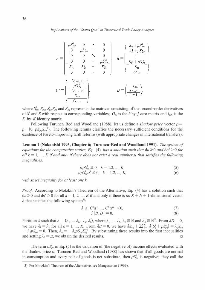
Piecemeal Tariff Reforms For technical ease, suppose that the tariff policy of country k is written as a function of policy parameter vk, that is, tk(vk). An increase in vk represents a prog-ress in the tariff policy. The derivative of tk(vk) with respect to vk is denoted by ak/ utk(vk)/uvk. Then, a piecemeal change in the tariff policy in country k can be represented by akdvk with dvk >0. By totally differentiating the system of equations Eq. (1) through Eq. (3), we obtain the following equation for the comparative statics analysis:

Adu+Bdq+ Ckakdvk+Ddb=0,k=1

K! (4)

where du=(du1, ..., duK), dq=(dq1, ..., dqN), db=(db1, ..., dbK). The matrices are defined as follows:

2) For the properties of the GDP function Gk, the expenditure function Ek, Sk, and S, see Woodland (1982).


26

where Skpu, Sk

qu, Skpq Sk

qq and Sqq represents the matrices consisting of the second-order derivatives of Sk and S with respect to corresponding variables; Oi,j is the i-by-j zero matrix and IKK is the K-by-K identity matrix.

Following Turunen-Red and Woodland (1988), let us define a shadow price vector t/p-(0, pSpqSqq

-1). The following lemma clarifies the necessary-sufficient conditions for the existence of Pareto-improving tariff reforms (with appropriate changes in international transfers):

Lemma 1 (Nakanishi 1993, Chapter 6; Turunen-Red and Woodland 1991). The system of equations for the comparative statics, Eq. (4), has a solution such that du&0 and dvk >0 for all k=1, ..., K if and only if there does not exist a real number n that satisfies the following inequalities:

ntSkpu#0, k=1,2, ..., K, (5)

ntSkpqa

k#0, k=1,2, ..., K, (6)

with strict inequality for at least one k.

Proof. According to Motzkin’s Theorem of the Alternative, Eq. (4) has a solution such that du&0 and dvk >0 for all k=1, 2, ..., K if and only if there is no K+N+1-dimensional vector m that satisfies the following system3):

m[A, C1a1, ..., CKaK] <0, (7) m[B, D]=0. (8)

Partition m such that m=(m1, ... λK , λq, λb), where λ1, ..., λK, λb!R and mq!RN. From mD=0, we have mk=mb for all k=1, ..., K. From mB=0, we have mSqq + k=1

K! m{Skq+pSk

pq}=mqSqq+mbpSpq=0. Then, mq =-mbpSpqSqq

-1. By substituting these results into the first inequalities and setting mb=n, we obtain the desired results. □

The term tSkpu in Eq. (5) is the valuation of (the negative of) income effects evaluated with

the shadow price t. Turunen-Red and Woodland (1988) has shown that if all goods are normal in consumption and every pair of goods is net-substitute, then tSk

pu is negative; they call the

3) For Motzkin’s Theorem of the Alternative, see Mangasarian (1969).

N. Nakanishi

27

condition tSkpu<0 the “Generalized Hatta Normarity” (GHN for short).4) If we assume the

GHN condition for all countries, then any positive real number can satisfy Eq. (5). Therefore, in order for Pareto-improving tariff reforms to exist, we must have tSk

pqak>0 for at least one

country. With these observations in hand, we can establish the following theorem:

Theorem1 (Nakanishi 1993, Chapter 6, Proposition 4). Suppose that the GHN condition is satisfied in all countries. Then, the following tariff reforms with appropriate changes in inter-national transfers can bring about a Pareto-improvement:

ak =[-S0qSqq-1]-[-Sk

0q(Skqq)

−1], k=1, 2, ..., K, (9)

where Sk0q is a submatrix of Sk

pp defined as follows:

Proof. It suffices to show that tSkpqa

k>0. From the definition of t, we have

tS pqk ak= pS pqk -pSpqSqq-1SqqkF Iak=p S pqk SqqkR W-1-SpqSqq-1F ISqqk ak

=p ONN

S0qk SqqkR W-1-S0qSqq-1U ZSqqk ak= S0qk SqqkR W-1-S0qSqq-1F ISqqk ak=akSqqk ak>0.

The last inequality follows from the positive semi-definiteness of Skqq. □

The tariff reform formula Eq. (9) consists of two parts: the first part [−S0qSqq-1] is common

to all countries and the second part [-Sk0q(Sk

qq)-1] is specific to country k. The first part can be

seen as the common target tariff index and the second part as the country specific tariff index. Therefore, Eq. (9) means that country k increases (decreases) the tariff rate on good i if the common target tariff index is higher (lower, respectively) than the country specific tariff index. Under certain conditions5), we can show that [-S0q Sqq

-1]=p+ l=1K! iltl for a certain

set of weights il>0 (l=1, 2, ..., K) with l=1K! il =1 calculated from the elements of the sub-

stitution matrices Skpp (k=1, 2, ..., K), and that [-Sk

0q(Skqq)

-1]=p+ tk for each k. In this case, we have ak= l=1

K! iltl-tk. Therefore, Eq. (9) represents such a tariff reform that changes the status quo tariff rate tk toward the average target rate l=1

K! iltl.

4) Hatta (1977a, b) have introduced and used the condition that the valuation of (the negative of) income effects evaluated with the world price p is negative, which is termed as the “Hatta Normarity.” Nakanishi (1993) has shown that the GHN condition can be seen as a stability condition for a dynamic adjustment process related to the system Eq. (1)-Eq. (3).

5) We say that non-numéraire goods are independent with each other (in country k) if the off-diagonal elements of submatix Sk

qq of the substitution matrix Skpp are zero (i.e., Sk

qq is a diagonal matrix). If non-numéraire goods are independent with each other in all countries, we obtain the desired results; see Nakanishi (1993, Chapter 6).


28

The Optimal Tariff To highlight the roles or implications of the status quo, let us turn to the optimal tariff argument; we consider the optimal tariff by country 1. By solving Eq. (4) for du1 with setting dvk=0 for k =2, 3, ..., K and dbk =0 for k =1, 2, ..., K, we obtain the expression for du1/dv1. Then, in general, the optimal tariff of country 1 can be derived by solving du1/dv1 =0. To be specific, let us consider a two-country two-good case. It is well-known that the optimal ad valorem tariff rate x* of country 1 is equal to the inverse of the price elasticity h of export supply by country 2: x*=1/h. In our context, we have h = q [S2

qq/S2q-S2

qu/S2u]. Similar to the piecemeal tariff reform ak in Eq. (9), the optimal tariff can be

calculated and expressed using the elements of the substitution matrices.

Discussion The piecemeal tariff reform ak in Eq. (9) and the optimal tariff rate x* are similar in that both of them are making use of the local information about the substitution matrices and derived by using a common comparative statics technique. However, they have quite different implications for the implementation of the policies, which depend on the roles of the status quo in the models. I discuss two related points: one is concerned with the availability/observability of relevant information for the implementation of the policies and the other is concerned with the usefulness of the theories. In deriving the piecemeal tariff reform, we do not require that the economy satisfies any particular conditions other than the general equilibrium conditions Eqs. (1)-(3). That is, the piecemeal tariff reform ak takes the status quo as it is. To calculate ak properly, we need the information about the local properties of the substitution matrices, which is considered to be observable and available in the status quo. Then, the tariff reform formula ak so calculated is always applicable to the real world as far as the world is in the general equilibrium. The theory of piecemeal tariff reforms provides the policy makers with a relevant guidance for the imple-mentation of the policy; in this sense, the theory can be said to be useful.

In contrast, the derivation of the optimal tariff requires an implicit assumption that, not only the economy satisfies the general equilibrium conditions Eq. (1)-(3), but also it is indeed in the optimal-tariff equilibrium. There is, however, no good reason to assume that the status quo in reality is in the optimal-tariff equilibrium. Even if we could calculate the price elasticity of export supply based on the local information about the substitution matrices observable and available in the status quo, the inverse of the calculated elasticity may fail to be the optimal rate. Further, even if the current tariff rate happens to be equal to the inverse of the price elasticity of export supply observed in the status quo, this does not guarantee that the current state of affairs is in the optimal-tariff equilibrium. The tariff rate calculated in accordance with the theory of optimal tariffs by using information available in the status quo may not be “opti-mal” at all. Since the theory of optimal tariffs fails to associate the predictions by the theory itself with the information available in the status quo, it cannot provide the policy makers with any relevant guidance for the implementation of the policy; the theory is useless (at least, to the policy makers).

One may argue that if the government of a country possesses adequate information about the global properties of functions Sk and S, in other words, if the government knows the whole structure of the economy, it can attain the optimal-tariff equilibrium. Yes, this is true. In this case, however, the government does not have to resort to the theory of optimal tariffs. Taking

N. Nakanishi

29

advantage of its knowledge about the whole economy, the government can set its tariff rate at the optimal level without the guidance (that the optimal rate is equal to the inverse of the price elasticity of export supply) provided by the theory. Although the theory is of no use in this case, still the status quo must turn out to be the optimal-tariff equilibrium. Then, by observing the information about the substitution matrices available in the status quo, we would find that the tariff rate set by the government is actually equal to the inverse of the price elasticity of export supply. However, this is merely a reconfirmation that the optimal-tariff equilibrium is indeed the optimal-tariff equilibrium.

If the economy is not in the optimal-tariff equilibrium, the theory of the optimal tariffs cannot be a sound foundation for the implementation of the policy. In turn, if we know that the economy is actually in the optimal-tariff equilibrium, the theory tells us nothing about what we should do, because we have already been able to achieve the optimal-tariff equilibrium. After all, the optimal tariff argument is a tautology that ignores the roles or implications of the status quo. Unlike the piecemeal policy argument, the optimal tariff argument cannot provide us with any theoretically sound guidance to the trade policy consideration.

3 Game Theoretical Consideration on Trade Policies

3.1 Relevant Question ?When we consider trade policy issues in some game-theoretic circumstances, the situation

becomes conceptually more problematic. To see the point, let us consider a real situation where two countries A and B are in conflict over the attitudes toward trade liberalization. Each country is contemplating whether to take a liberalist stance or to take a protectionist stance. We call this “real” situation as the Liberalist-Protectionist situation.

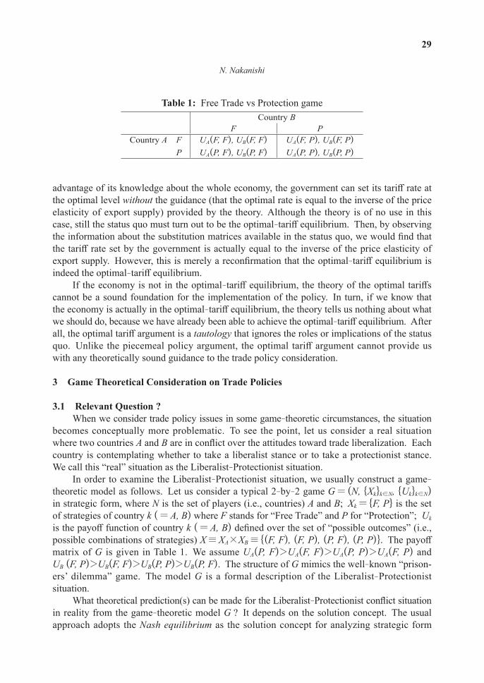
In order to examine the Liberalist-Protectionist situation, we usually construct a game-theoretic model as follows. Let us consider a typical 2-by-2 game G=(N, {Xk}k!N, {Uk}k!N) in strategic form, where N is the set of players (i.e., countries) A and B; Xk ={F, P} is the set of strategies of country k (=A, B) where F stands for “Free Trade” and P for “Protection”; Uk is the payoff function of country k (=A, B) defined over the set of “possible outcomes” (i.e., possible combinations of strategies) X/XA#XB/ {(F, F), (F, P), (P, F), (P, P)}. The payoff matrix of G is given in Table 1. We assume UA(P, F)>UA(F, F)>UA(P, P)>UA(F, P) and UB (F, P)>UB(F, F)>UB(P, P)>UB(P, F). The structure of G mimics the well-known “prison-ers’ dilemma” game. The model G is a formal description of the Liberalist-Protectionist situation.

What theoretical prediction(s) can be made for the Liberalist-Protectionist conflict situation in reality from the game-theoretic model G ? It depends on the solution concept. The usual approach adopts the Nash equilibrium as the solution concept for analyzing strategic form

Table 1: Free Trade vs Protection gameCountry B

F PCountry A F P

UA(F, F), UB(F, F)

UA(P, F), UB(P, F)

UA(F, P), UB(F, P)

UA(P, P), UB(P, P)


30

games. In other words, the players in games (i.e., countries in our context) are assumed to be such agents who make actual choices of their strategies if and only if the very combination of the chosen strategies constitutes the Nash equilibrium from which no player has an incentive to deviate unilaterally. As is well known, (P, P)!X is the unique Nash equilibrium of G—both countries choose to take the protectionist stances. That is, the game-theoretic model G together with the Nash equilibrium predicts the realization of the protectionist world in the model. It should be noted that the realization of (P, P) is the result of the countries’ choices of strategies. The game-theoretic model G with the Nash equilibrium grasps the Liberalist- Protectionist situation in reality as a “matter of choice” by the players. So far, so good.

When we construct a (game-theoretic) model of a situation in reality, we usually take for granted that there exists a certain correspondence between the model and the real situation. Accordingly, if we were to interprete the Liberalist-Protectionist situation in reality by using the game-theoretic model G with the Nash equilibrium as the solution concept, the reality itself must be in the Nash equilibrium. Why ? On one hand, we know that in the real situation, countries (i.e., players) have already taken certain stances; it is hard (though not impossible) to imagine a new-born country who is about to make its decision, but has done nothing yet. On the other hand, we also know that in the model, the players’ actual choices are possi-ble if and only if they constitute the Nash equilibrium. In other words, the players in the model will never choose non-equilibrium strategies. So, if the model G together with the Nash equilibrium has had captured appropriately the behavior of the players in reality and if we were to suppose that there exists a correspondence between the model and the reality, the reality must correspond to the prediction by the model—what the players actually do in the real world constitutes the Nash equilibrium.

What is the problem ? Recall that the Nash equilibrium is established after the players made their choices. When the players are facing the game G and contemplating—but have not decided—their strategies, nothing can happen (could have happened) in the model. In other words, there is no status quo on which the players’ decisions are based. The players’ choices of strategies in the model are made without any status quo. However, in the international trade policy scene in reality, countries have been involved in a certain situation where something has had been realized already. Then, we may well ask a following question, for example: [Q] “What will happen if country A is taking the liberalist stance while country B is taking the protectionist stance in the status quo ?” This question [Q] seems legitimate; indeed, it is. But, unfortunately, [Q] cannot be answered in a theoretically sound way as far as we stick to the Nash equilibrium of G. Because the Nash equilibrium players never choose non-equilibrium strategies, the presupposition “country A is taking the liberalist stance while country B is taking the protectionist stance” in [Q] is false. Logically, any conclusion, whether true or false, can be derived from a false presupposition.

One way to avoid the logical difficulty shown above is to simply deny to answer those questions like [Q] as “irrelevant” ones and take a position (of believing) that the status quo in reality always constitutes the Nash equilibrium. Of course, this kind of attitude toward the difficulty is not productive nor appropriate at all. I do not think that there is a good reason to assume that the status quo in reality is in the Nash equilibrium. The status quo, whatever it is, may have been established by a historical accident or by groundless choices or by others with no particular reasons. The status quo stands as it is. In order to answer such questions as [Q]

N. Nakanishi

31

in a theoretically sound way, we need an alternative framework that can provide the status quo with a legitimate position in theoretical models.

3.2 The Stable Set ApproachIn order to incorporate the notion of the “status quo” into theoretical models appropriately,

I shall adopt the framework of the Theory Of Social Situations (TOSS for short) developed by Greenberg (1990).6) One notable advantage of TOSS is that it can incorporate the notion of “negotiation” among players into the model in a very simple but powerful way, that is, by introducing the notion of the “inducement correspondence.” The inducement correspondence describes how players can change the current state of affairs (i.e., the status quo) to another state. Technically, given a status quo, the inducement correspondence specifies a subset (not a particular state) of the set of all possible states that can be attained through changes in the actions of some players (possibly, those of a single player) from the status quo.

Formally, let J/ (N, X, {Ui}i!N, m) be a game, where N is the set of players; X is the set of possible “outcomes”; Ui is the payoff function for player i defined on X; and m is the inducement correspondence. As explained above, the most important component of the model is the inducement correspondence m, which is a correspondence from the Cartesian product of the set 2N of all subsets of N and X to X, that is, m: 2N#X |→ X. Let us consider a non-empty coalition of players S1N and an outcome x!X. The inducement correspondence m maps the pair of S and x into a subset of X denoted by m(S, x).7) If y!m(S, x) for some y!X, it is interpreted as follows: given x as the status quo, the coalition S can change the state of the world from x to another y. It should be noted that no particular outcome is assigned as the status quo; but, any outcome in X can be a legitimate candidate for the status quo. It should also be noted that the definition of the inducement correspondence does not refer to the payoffs of the players at all. That is, the inducement correspondence only describes what the coalition S can do (not will do) when the status quo is given as x. Whether the coalition S will actually induce y!m(S, x) from the status quo x depends on the solution concept.

The solution concept I introduce here is an analog of the classical solution concept of the von Neumann-Morgenstern stable set (vN-M stable set), which had been developed as the solution concept for the characteristic function form games originally by von Neumann and Morgenstern (1944). Due to TOSS, we can now apply the notion of the vN-M stable set (at least, its spirit) to games in various forms. The vN-M stable set explains consistently not only why a particular outcome included in the vN-M stable set stay put once it has been established as a status quo, but also explains why outcomes excluded from the vN-M stable set cannot maintain their current positions.

If a subset K of X satisfies the following two stability requirements, K is said to be a von-Neumann-Morgenstern stable set (vN-M stable set) for J.

6) In a sense, this subsection is a brief introduction of TOSS. However, to make things as simple as possible, I do not utilize the framework of TOSS in its fully general form. In particular, it should be noted that the solution concept in TOSS, which is called the “stable standard of behavior,” is different from (though closely related to) the von Neumann-Morgenstern stable set that I will define later. A stable standard of behavior (if it exists) yields a corresponding von Neumann-Morgenstern stable set and, conversely, a von Neumann-Morgenstern stable set yields a corresponding stable standard of behavior. For formal relationship between them, see Greenberg (1990, Chapter 4).

7) It is possible to have m(S, x)=0/ for some pair of non-empty S1N and x!X.


32

Internal stability: If x!K, then there is no pair of an outcome y!K and a nonempty coalition S1N such that y!m(S, x) and Ui(y)>Ui(x) for all i!S.8)

External stability: If x!X\K, then there exists a pair of an outcome y!K and a nonempty coalition S1N such that y!m(S, x) and Ui(y)>Ui(x) for all i!S.

We simply say that “y dominates x” if, for x!X, there exists a pair of an outcome y!X and a non-empty coalition S1N such that Ui(y)>Ui(x) for all i!S.

Let us briefly examine the meanings of the internal and external stabilities. Let Z be a subset of the set of outcomes and suppose that each and every player believes that the out-comes in Z are persistent (“stable”) and that the outcomes outside of Z are not persistent (“unstable”). Take an outcome x!Z as a status quo. If there exists a coalition S of players that can make all the members of the coalition better-off by inducing another persistent out-come y!Z from x (i.e., Z violates the internal stability), then, since the members of that coali-tion S may want to replace the status quo x with new outcome y, the belief of all the players (including all the members of S) that “x is persistent” will be disproved. In turn, take an out-come xgZ as a status quo. If there does not exist a coalition S of players that can make all the members of the coalition better-off by inducing an outcome in Z (i.e., Z violates the exter-nal stability), then, since no coalition wants to replace the status quo x with another outcome, the status quo will remain unchanged and, thereby, the belief of all the players that “x is not persistent” will be disproved, again. Therefore, if a set Z in fact satisfies both the internal and the external stabilities (i.e., Z is a vN-M stable set), then the belief of all the players will never be disproved. In this sense, the vN-M stable set can be said to be self-consistent to the belief of the players.

3.3 Tariff NegotiationsIn order to show how the stable set approach vitally works in analyzing the trade policy

issues, I apply it to the problems of tariff negotiations with and without the rules of the World Trade Organization (WTO).9) The WTO rules prescribe the legitimate way of changing tariff rates (i.e., the concession rates) from the current tariff rates; in other words, under the WTO rules, each country cannot change its own tariff rate freely.

The Base Model Consider a standard two-country (countries 1 and 2), two-good (goods 1 and 2), competitive international trade model, in which country i imports good i. Let N= {1, 2} be the set of the countries. Xi/ {xi!R | -1<xi<t̄i} is the set of feasible ad valorem tariff rates (i.e., the set of strategies) of country i, where t̄i is the prohibitive tariff rate of country i.10) A negative tariff rate means an “import subsidy.” X/X1#X2 is the set of all feasible combinations of tariff rates. A typical element of X is denoted by x (or, by y, z, and so forth)

8) The term “coalition” simply means a subset of players; it does not necessarily imply that members of a coalition make some binding agreements or exercise certain monopoly power over other players.

9) This subsection is a simplified reproduction of Chapter 3 of Nakanishi (2010).10) It is possible to include the prohibitive tariff rate t̄i in the set of strategies; but, this makes the analysis

unnecessarily complicated. To concentrate on the essence of the argument, we exclude t̄i from the set of strategies.

N. Nakanishi

33

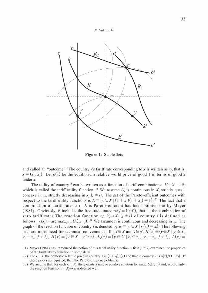
and called an “outcome.” The country i’s tariff rate corresponding to x is written as xi, that is, x= (x1, x2). Let p(x) be the equilibrium relative world price of good 1 in terms of good 2 under x.

The utility of country i can be written as a function of tariff combinations: Ui: X → R, which is called the tariff utility function.11) We assume Ui is continuous in X, strictly quasi-concave in xi, strictly decreasing in xj (j! i). The set of the Pareto-efficient outcomes with respect to the tariff utility functions is E/ {x!X | (1+x1)(1+x2)=1}.12) The fact that a combination of tariff rates x in E is Pareto-efficient has been pointed out by Mayer (1981). Obviously, E includes the free trade outcome f/ (0, 0), that is, the combination of zero tariff rates.The reaction function ri: Xj→Xi (j! i) of country i is defined as follows: ri(xj)/arg maxxi!Xi Ui(xi, xj).13) We assume ri is continuous and decreasing in xj. The graph of the reaction function of country i is denoted by Ri/{x!X | ri(xj)=xi}. The following sets are introduced for technical convenience: for x!X and i!N, Hi(x)/{y!X | yi$xi, y j =xj, j! i} , H(x)/{y !X | y $x} , Li(x)/{y !X |yi #xi , y j =xj, j! i} , L(x)/

11) Mayer (1981) has introduced the notion of this tariff utility function. Dixit (1987) examined the properties of the tariff utility function in some detail.

12) For x!X, the domestic relative price in country 1 is (1+x1)p(x) and that in country 2 is p(x)/(1+x2). If these prices are equated, then the Pareto-efficiency obtains.

13) We assume that, for each xj!Xj, there exists a unique positive solution for maxxi Ui(xi, xj) and, accordingly, the reaction function ri: Xj→Xi is defined well.

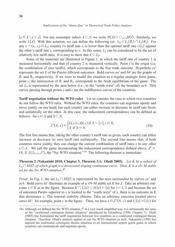
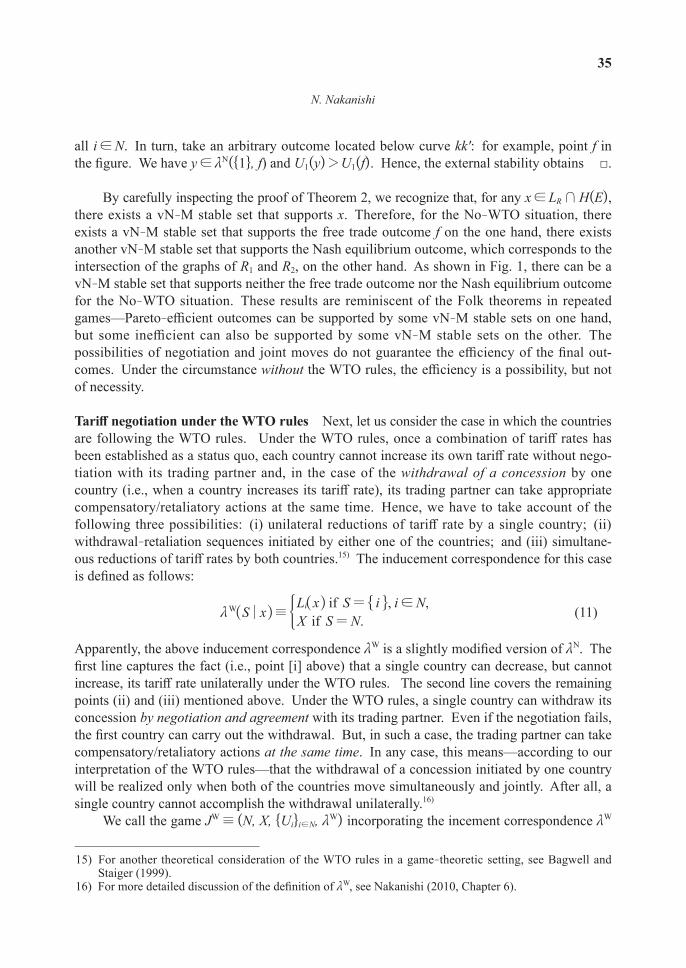
Figure 1: Stable Sets


34

{y!X | y#x}. For any nonempty subset A1X, we write H(A)/,x!AH(x). Similarly, we write L(A). With this notation, we can define the following set: LR/L1(R1)+L2(R2). For any x= (xi, xj)!LR, country i’s tariff rate xi is lower than the optimal tariff rate ri(xj) against the other’s tariff rate xj corresponding to x. In this sense, LR can be considered to be the set of relatively low tariff rates. It is easy to show that E1LR.

Some of the materials are illustrated in Figure 1, in which the tariff rate of country 1 is measured horizontally and that of country 2 is measured vertically. Point f is the origin (i.e, the combination of zero tariffs), which corresponds to the free trade outcome. Hyperbola ee′ represents the set E of the Pareto-efficient outcomes. Bold curves aa′ and bb′ are the graphs of R1 and R2, respectively. If we were to model the situation as a regular strategic form game, point c, the intersection of R1 and R2, corresponds to the Nash equilibrium of the game. The set LR is represented by the area below (i.e., to the “south-west” of) the boundary acb. Thin curves passing through points x and c are the indifference curves of the countries.

Tariff negotiation without the WTO rules Let us consider the case in which two countries do not follow the WTO rules. Without the WTO rules, the countries can negotiate openly and move jointly on one hand, but each country can either increase or decrease its tariff rate freely and unilaterally on the other. In this case, the inducement correspondence can be defined as follows: for x!X and S1N,

mN S, xR W/ Li xR W,Hi xR W if S= iF I, i!N,X if S=N.G (10)

The first line means that, taking the other country’s tariff rate as given, each country can either increase or decrease its own tariff rate unilaterally. The second line means that, if both countries move jointly, they can change the current combination of tariff rates x to any other y!X. We call the game incorporating the inducement correspondence defined above, JN/ (N, X, {Ui}i!N, mN), the “No-WTO situation.”14) The following theorem is immediate:

Theorem 2 (Nakanishi 2010, Chapter 3, Theorem 3.1; Oladi 2005). Let K be a subset of LR+H(E) of which graph is a downward-sloping continuous curve. Then, K is a vN-M stable set for the No-WTO situation JN.

Proof. In Fig. 1, the set LR+H(E) is represented by the area surrounded by curves ee′ and acb. Bold curve kk′ illustrates an example of a vN-M stable set K for J. Take an arbitrary out-come x!K as in the figure. Because K+Li(x),Hi(x)={x} for i=1, 2 and because the set of outcomes Pareto-superior to x is located to the “south-west” of x, there is no outcome in K that dominates x. The internal stability obtains. Take an arbitrary outcome located above curve kk′: for example, point c in the figure. Then, we have x!mN(N, c) and Ui(x)>Ui(c) for

14) Although we defined the No-WTO situation JN in a very much simplified way, it is intrinsically the same as the “coalitional contingent threats situation” introduced by Greenberg (1990, Chapter 7). Oladi (2005) has formulated the tariff negotiation between two countries as a coalitional contingent threats situation. Therefore, Oladi’s analysis applies to our No-WTO situation as well. Nakanishi (1999) has applied the coalitional contingent threats situation to an international export quota game in which countries can communicate and negotiate openly.

N. Nakanishi

35

all i!N. In turn, take an arbitrary outcome located below curve kk′: for example, point f in the figure. We have y!mN({1}, f) and U1(y)>U1(f). Hence, the external stability obtains □.

By carefully inspecting the proof of Theorem 2, we recognize that, for any x!LR+H(E), there exists a vN-M stable set that supports x. Therefore, for the No-WTO situation, there exists a vN-M stable set that supports the free trade outcome f on the one hand, there exists another vN-M stable set that supports the Nash equilibrium outcome, which corresponds to the intersection of the graphs of R1 and R2, on the other hand. As shown in Fig. 1, there can be a vN-M stable set that supports neither the free trade outcome nor the Nash equilibrium outcome for the No-WTO situation. These results are reminiscent of the Folk theorems in repeated games—Pareto-efficient outcomes can be supported by some vN-M stable sets on one hand, but some inefficient can also be supported by some vN-M stable sets on the other. The possibilities of negotiation and joint moves do not guarantee the efficiency of the final out-comes. Under the circumstance without the WTO rules, the efficiency is a possibility, but not of necessity.

Tariff negotiation under the WTO rules Next, let us consider the case in which the countries are following the WTO rules. Under the WTO rules, once a combination of tariff rates has been established as a status quo, each country cannot increase its own tariff rate without nego-tiation with its trading partner and, in the case of the withdrawal of a concession by one country (i.e., when a country increases its tariff rate), its trading partner can take appropriate compensatory/retaliatory actions at the same time. Hence, we have to take account of the following three possibilities: (i) unilateral reductions of tariff rate by a single country; (ii) withdrawal-retaliation sequences initiated by either one of the countries; and (iii) simultane-ous reductions of tariff rates by both countries.15) The inducement correspondence for this case is defined as follows:

mW S;xR W/ Li xR W if S= iF I, i!N,X if S=N.G (11)

Apparently, the above inducement correspondence mW is a slightly modified version of mN. The first line captures the fact (i.e., point [i] above) that a single country can decrease, but cannot increase, its tariff rate unilaterally under the WTO rules. The second line covers the remaining points (ii) and (iii) mentioned above. Under the WTO rules, a single country can withdraw its concession by negotiation and agreement with its trading partner. Even if the negotiation fails, the first country can carry out the withdrawal. But, in such a case, the trading partner can take compensatory/retaliatory actions at the same time. In any case, this means—according to our interpretation of the WTO rules—that the withdrawal of a concession initiated by one country will be realized only when both of the countries move simultaneously and jointly. After all, a single country cannot accomplish the withdrawal unilaterally.16)

We call the game JW/ (N, X, {Ui}i!N, mW) incorporating the incement correspondence mW

15) For another theoretical consideration of the WTO rules in a game-theoretic setting, see Bagwell and Staiger (1999).

16) For more detailed discussion of the definition of mW, see Nakanishi (2010, Chapter 6).


36

the “WTO situation.” On the surface, the WTO situation JW and the No-WTO situation JN differ only slightly—The difference appears only in the first lines in the definitions of the inducement correspondences mW and mN. These situations, however, generate quite different sets of the final outcomes.

Theorem 3 (Nakanishi 2010, Chapter 3, Theorem 3.2). The set E of the Pareto-efficient outcomes is a unique vN-M stable set for the WTO situation under mW.

Proof. The internal and external stabilities of E can be shown similar to Theorem 2. We only have to show the uniqueness. Let K be another vN-M stable set for JW. If x!E \ K, there must be an outcome y!mW({i}, x) such that Ui(y)>Ui(x) for some i!N. By the definition of mW, however, we have yi<xi and yj =xj (j! i) for all y!mW({i}, x), which implies Ui(y)<Ui(x). Therefore, we have E1K. On the other hand, if x!K\E, there exists an Pareto-efficient outcome z!E that Pareto-dominates x. By the external stability of K, there must exist another outcome in mW({i}, z)+K for some i!N that dominates z. But, it is not possible, either. Therefore, we have K1E. That is, E=K; the uniqueness obtains. □

The vN-M stable set for the WTO situation is characterized by full efficiency. Unlike the No-WTO situation, any inefficient tariff combination cannot be the final outcome. Only efficient outcomes are the candidates for the final outcome under the negotiation procedure with the WTO rules.

4 Remarks

In the previous section, I have argued that the usual game-theoretic framework with the Nash equilibrium as the solution concept fails to capture the roles or implications of the status quo. This should not be regarded as a criticism that the usual game-theoretic approach is useless or inappropriate in general. Whether a particular framework is suitable and/or appropriate to analyze a given problem depends on the nature of the problem. Take the duopoly market for example. We can easily imagine a situation where there is an oligopolistic market for a brand-

new commodity and firms have not made their decisions yet. In addition, we can imagine this kind of situations may arise repeatedly in the real world (though the players and markets con-cerned are different from situation to situation). In this kind of situation, nothing happens actually before the firms make their choices and, therefore, there is no status quo. Hence, the usual game-theoretic approach would be an appropriate framework for analyzing the oligopoly problems. In contrast, in the trade policy issues, it is hard to imagine that countries (i.e., play-ers) get involved in a brand-new situation where they have not made their decisions yet. In almost all cases, countries have already chosen their actions (whatever they are) and, therefore, a certain state of affairs has been established as the status quo. In spite of the apparent resem-blance between the oligopolistic problems and the trade policy issues in some game-theoretic circumstances, they require different analytical frameworks.

To incorporate the status quo in theoretical models, I have introduced the stable set approach. Although I do believe that the stable set approach can provide us with an appropriate framework for analyzing trade policy issues, it has its own weakness. First, similar to the

N. Nakanishi

37

classical von Neumann-Morgenstern stable set for characteristic function form games, the general (sufficient) conditions for the existence of the stable set have not been known yet; some games may have no stable set.17) Second, even if the stable sets were to exist for a certain problem, techniques of the mathematical optimization (such as the Lagrangean method, the dynamic programming, the optimal control, and others) do not play important roles in finding the stable sets. Often, we have to take heuristic approaches; the quest for the stable sets is of the trial-and-error nature.

References

Bagwell, K. and R.W. Staiger, 1999, An economic theory of GATT, American Economic Review 89 (1): 215-

247.Dixit, A., 1987, Strategic aspects of trade policy, in T.F. Bewley, ed., Advances in Economic Theory: Fifth

World Congress, Cambridge University Press.Greenberg, J., 1990, The Theory of Social Situations: An Alternative Game-Theoretic Approach, Cambridge:

Cambridge University Press.Hatta, T., 1977a, A theory of piecemeal policy recommendations, Review of Economic Studies 44: 1-21.Hatta, T., 1977b, A recommendation for a better tariff structure, Econometrica 45 (80): 1859-1869.Mangasarian, O.L., 1969, Nonlinear Programming, MacGraw-Hill.Mayer, W., 1981, Theoretical considerations on negotiated tariff adjustments, Oxford Economic Papers 33:

135-153.Nakanishi, N., 1993, Theoretical Analysis on Trade Liberalization―Stepwise and Piecemeal Policies and

Economic Welfare, Kobe University Publishing Association, Distributed by Yuhikaku Publishing Co. (in Japanese)

Nakanishi, N., 1999, Reexamination of the international export quota game through the theory of social situ-ations, Games and Economic Behavior 27: 132-152.

Nakanishi, N., 2010, Game-Theoretic Analysis of Trade Policies under Inter-dependent Circum-stances: Applications of the Theory of Social Situations and the Stable Set Approach, Minerva Shobo Publishing Co. (inJapanese)

Oladi, G., 2005, Stable tariffs and reataliations, Review of International Economics 13 (2): 205-215.Turunen-Red, A.H. and A.D. Woodland, 1988, On the multilateral transfer problem existence of Pareto

improving international transfers, Journal of International Economics 25: 249-269.Turunen-Red, A.H. and A.D. Woodland, 1991, Strict Pareto-improving multilateral reforms of tariffs, Econo-

metrica 59 (4): 1127-1152.Von Neumann, J. and O. Morgenstern, 1944, Theory of Games and Economic Behavior (2nd ed., 1947),

Princeton University Press.Woodland, A.D., 1982, International Trade and Resource Allocation, North-Holland.

17) In my own experience, most of “well-defined” problems admit the stable sets.

Implications of the “Status Quo” in Theoretical Trade Policy ...

Documents

Transcript of Implications of the “Status Quo” in Theoretical Trade Policy ...