ImpBench Revisited:An Extended Characterization of Implant-Processor

Benchmarks

Christos Strydis, Dhara Dave, Georgi N. Gaydadjiev

Computer Engineering Lab, Delft University of Technology,

P.O. Box 5031, 2600 GA Delft,The Netherlands

Phone:+31-(0)15-27-82326 E-mail: C.Strydis@tudelft.nl

Abstract—Implants are nowadays transforming rapidly fromrigid, custom-based devices with very narrow applications tohighly constrained albeit multifunctional embedded systems.These systems contain cores able to execute software programsso as to allow for increased application versatility. In responseto this trend, a new collection of benchmark programs forguiding the design of implant processors, ImpBench, has al-ready been proposed and characterized. The current paperexpands on this characterization study by employing a genetic-algorithm-based, design-space exploration framework. Throughthis framework, ImpBench components are evaluated in terms oftheir implications on implant-processor design. The benchmarksuite is also expanded by introducing one new benchmark andtwo new stressmarks based on existing ImpBench benchmarks.The stressmarks are proposed for achieving further speedupsin simulation times without polluting the processor-explorationprocess. Profiling results reveal that processor configurationsgenerated by the stressmarks follow with good fidelity - exceptfor some marked exceptions - ones generated by the aggregatedImpBench suite. Careful use of the stressmarks can seriouslyreduce simulation times up to x30, which is an impressive speedupand a good tradeoff between DSE speed and accuracy.

Index Terms—Implant, benchmark suite, stressmark, profiling,genetic algorithm, Pareto, kernel, power, energy.

I. INTRODUCTION

In 1971, Abdel Omran in his - now - classic article on

epidemiologic transition [1] has investigated the historical

demography of populations, theorizing about three distinct

periods of health transition: i) the era of pestilence and famine,

ii) the era of receding pandemics, and iii) the era of man-

made diseases. In the eve of the 21st century, Omran’s theory

has been verified as we are surely going through the third

era of man-made, non-communicable diseases, better known

as degenerative or chronic diseases. Characteristic of this

transition has been a general pattern shift from dominating

infectious diseases with very high mortality at younger ages,

to dominating chronic diseases and injury, with lower overall

mortality but peaks at older ages [2]. What makes chronic

diseases an issue of interest is the presence, in developed

countries, of a prevailing demographic trend of an ageing

population.

Not all countries have undergone this transition in the same

fashion, albeit developed countries are well into the transition

path described by Omran. Yet, Omran’s theory intended on

stressing the fact that, when progressing from high to low

mortality rates, all populations involve a shift in the causes

of death and disease. True enough, developing and, primarily,

developed countries are manifesting the effects predicted by

the theorized shift such as low fertility rates, population

growth, increased heart-disease and cancer rates. Given the

two latter trends, the healthcare sectors strive for policy and

institutional adaptation so as to safeguard the provision of

healthcare services.

In addition to policy and institutional adaptations and up-

dates, the healthcare sector has benefited from technological

advancements coming from the disciplines of medicine as

well as microelectronics. A technological niche of biomedical

engineering that has particularly contributed is implantable

microelectronic devices which act as a means to deal with

monitoring and/or treatment of chronic patients. With the

implantable pacemaker being the first and perhaps most well-

known implant type - 299,705 such devices have been regis-

tered in Europe alone, by the year 2003 [3] - the road is being

paved for numerous other applications [4]. An ever expanding

implant list already contains monitors of body temperature,

blood pressure or glucose concentration; also, intracardiac

defibrillators (ICDs) and functional electrical stimulators for

bladder control, for blurred eye cornea and so on.

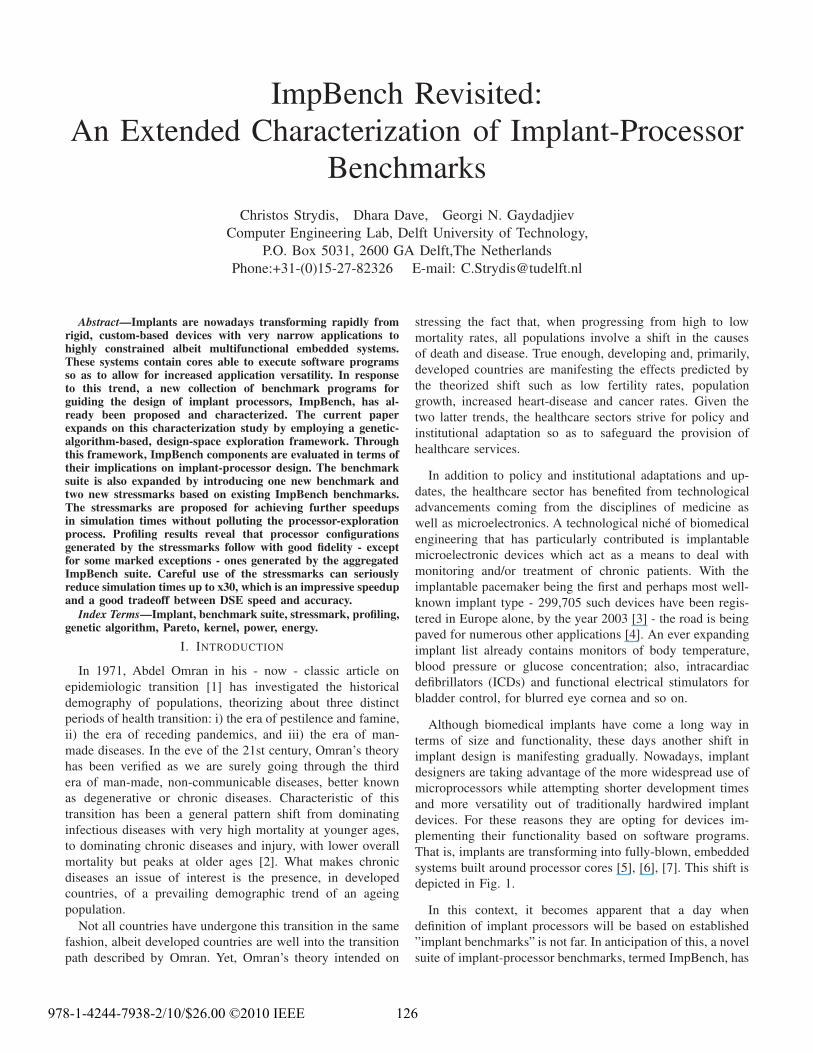
Although biomedical implants have come a long way in

terms of size and functionality, these days another shift in

implant design is manifesting gradually. Nowadays, implant

designers are taking advantage of the more widespread use of

microprocessors while attempting shorter development times

and more versatility out of traditionally hardwired implant

devices. For these reasons they are opting for devices im-

plementing their functionality based on software programs.

That is, implants are transforming into fully-blown, embedded

systems built around processor cores [5], [6], [7]. This shift is

depicted in Fig. 1.

In this context, it becomes apparent that a day when

definition of implant processors will be based on established

”implant benchmarks” is not far. In anticipation of this, a novel

suite of implant-processor benchmarks, termed ImpBench, has

978-1-4244-7938-2/10/$26.00 ©2010 IEEE 126

0%

20%

40%

60%

80%

100%

1994-1997 1998-2001 2002-2005

no core(s)

P/ C

FSM

Fig. 1. Implant-core architecture trends over time [8].

been previously proposed and characterized [9]1. Since its

release, it has been put to good use in exploring efficient

implant processors [10], [11] and in the work of others [12]. In

this paper, we primarily attempt to expand the original charac-

terization study with extensive, new results acquired through

use of ImpEDE, a genetic-algorithm-(GA)-based, design-space

exploration (DSE) framework [13]. Through using ImpEDE,

we effectively investigate the sensitivity of different processor

attributes (e.g. cache geometries) to the various benchmarks

in ImpBench. We also update the suite with a new benchmark

and two new, so-called ”stressmarks”, bringing ImpBench to

version 1.1. Concisely, this paper contributes in:

• Providing a novel and sound methodology, based on

GAs, of evaluating benchmark characteristics in terms of

resulting processor configurations;

• Identifying a representative (subset of) benchmark(s) for

substituting the whole suite in simulations, thus achieving

radically shorter DSE times;

• Updating the ImpBench suite to version 1.1 by proposing:

(a) a more sophisticated version of the DMU benchmark,

and (b) two derived stressmarks for enabling shorter

simulation times while biasing the exploration process

insignificantly or, at least, predictably; and

• Reporting/amending errata of the original work and giv-

ing further clarifications, where needed.

The rest of the paper is organized as follows: section II

gives an overview of previously proposed benchmark suites.

In section III, the details of the components of ImpBench

v1.1 are briefly reproduced. Section IV provides the details

of our selected profiling testbed for benchmark evaluation.

Section V presents, reflecting upon various metrics, the par-

ticular characteristics of each benchmark and its effect on the

processor properties under investigation. The stressmarks are

also introduced and evaluated. A summarizing discussion of

the results is included in VI while overall conclusions and

future work are discussed in section VII.

II. RELATED WORK

A large number of benchmark suites has already been

proposed for various application areas, making covering the

whole domain a far from trivial attempt. Instead, in this section

we briefly discuss well-known and freely available benchmark

suites, and mostly ones targeting the embedded domain, as is

our implant case. The latest SPEC benchmark suite, CPU2006

1Available online: http://sims.et.tudelft.nl/, under ”downloads”.

[14], targets general-purpose computers by providing pro-

grams and data divided into separate integer and floating-point

categories. MediaBench [15] is oriented towards increased-

ILP, multimedia- and communications-oriented embedded sys-

tems. The Embedded Microprocessor Benchmark Consortium

(EEMBC) [16] licenses ”algorithms” and ”applications” or-

ganized into benchmark suites targeting telecommunications,

networking, digital entertainment, Java, automotive/industrial,

consumer and office equipment products. It has also provided

a suite capable of energy monitoring in the processor. EEMBC

has also introduced a collection of benchmarks targeting mul-

ticore processors (MultiBench v1.0). MiBench [17] is another

proposed collection of benchmarks aimed at the embedded-

processor market. It features six distinct categories of bench-

marks: automotive, industrial, control, consumer devices and

telecommunications. MiBench bears many similarities with

EEMBC, however it is composed of freely available source

code. NetBench [18] has been introduced as a benchmark

suite for network processors. It contains programs representing

all levels of packet processing; from micro-level (close to

the link layer), to IP-level (close to the routing layer) and

to application-level programs. Network processors are also

targeted by CommBench [19], focused on the telecommu-

nications aspect. It contains eight, computationally intensive

kernels, four oriented towards packet-header processing and

four towards data-stream processing.

Compared with our own prior work [9], the new version

of the ImpBench suite introduces a more detailed variation

of the (originally described) DMU benchmark and two stress-

marks, that is, two benchmarks based on DMU and motion

and exhibiting worst-case execution (i.e. stress) behavior. A

further novelty of the current work is the employment of

a GA-based, DSE framework and analytic metrics in order

to characterize the old and new ImpBench benchmarks. In

effect, this paper extends the previous work in both terms

of content and methodology. To the best of our knowledge,

no benchmark suite has been published before to address the

rising family of biomedical-implant processors. What is more,

no characterization study has utilized GAs before to explore

the benchmark properties and their implications on the targeted

processor.

III. IMPBENCH V1.1 OVERVIEW

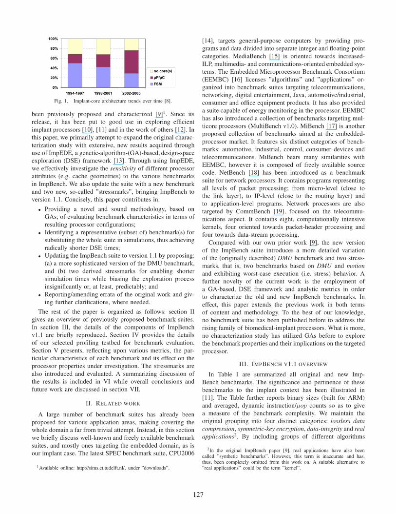
In Table I are summarized all original and new Imp-

Bench benchmarks. The significance and pertinence of these

benchmarks to the implant context has been illustrated in

[11]. The Table further reports binary sizes (built for ARM)

and averaged, dynamic instruction/µop counts so as to give

a measure of the benchmark complexity. We maintain the

original grouping into four distinct categories: lossless data

compression, symmetric-key encryption, data-integrity and real

applications2. By including groups of different algorithms

2In the original ImpBench paper [9], real applications have also beencalled ”synthetic benchmarks”. However, this term is inaccurate and has,thus, been completely omitted from this work on. A suitable alternative to”real applications” could be the term ”kernel”.

127

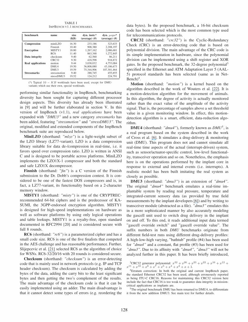
TABLE IIMPBENCH V1.1 BENCHMARKS.

benchmark name size dyn. instr.* dyn. µops*

(KB) (average) (#) (average) (#)

Compression miniLZO 16.30 233,186 323,633Finnish 10.40 908,380 2,208,197

Encryption MISTY1 18.80 1,267,162 2,086,681RC6 11.40 863,348 1,272,845

Data integrity checksum 9.40 62,560 86,211CRC32 9.30 418,598 918,872

Real applications motion 9.44 3,038,032 4,753,084DMU4 19.50 36,808,080 43,186,673DMU3 19.59 75,344,906 107,301,464

Stressmarks stressmotion 9.40 288,745 455,855stressDMU3 19.52 124,212 224,791

(*) Typical 10 − KB workloads have been used, except for DMU-variants which use their own, special workloads.

performing similar functionality in ImpBench, benchmarking

diversity has been sought for capturing different processor

design aspects. This diversity has already been illustrated

in [9] and will be further elaborated in section V. In this

version of ImpBench (v1.1), real applications have been

expanded with ”DMU3” and a new category stressmarks has

been added, featuring ”stressmotion” and ”stressDMU3”. The

original, modified and extended components of the ImpBench

benchmark suite are reproduced below.

MiniLZO (shorthand: ”mlzo”) is a light-weight subset of

the LZO library (LZ77-variant). LZO is a data compression

library suitable for data de-/compression in real-time, i.e. it

favors speed over compression ratio. LZO is written in ANSI

C and is designed to be portable across platforms. MiniLZO

implements the LZO1X-1 compressor and both the standard

and safe LZO1X decompressor.

Finnish (shorthand: ”fin”) is a C version of the Finnish

submission to the Dr. Dobb’s compression contest. It is con-

sidered to be one of the fastest DOS compressors and is, in

fact, a LZ77-variant, its functionality based on a 2-character

memory window.

MISTY1 (shorthand: ”misty”) is one of the CRYPTREC-

recommended 64-bit ciphers and is the predecessor of KA-

SUMI, the 3GPP-endorsed encryption algorithm. MISTY1

is designed for high-speed implementations on hardware as

well as software platforms by using only logical operations

and table lookups. MISTY1 is a royalty-free, open standard

documented in RFC2994 [20] and is considered secure with

full 8 rounds.

RC6 (shorthand: ”rc6”) is a parameterized cipher and has a

small code size. RC6 is one of the five finalists that competed

in the AES challenge and has reasonable performance. Further,

Slijepcevic et al. [21] selected RC6 as the algorithm of choice

for WSNs. RC6-32/20/16 with 20 rounds is considered secure.

Checksum (shorthand: ”checksum”) is an error-detecting

code that is mainly used in network protocols (e.g. IP and TCP

header checksum). The checksum is calculated by adding the

bytes of the data, adding the carry bits to the least significant

bytes and then getting the two’s complement of the results.

The main advantage of the checksum code is that it can be

easily implemented using an adder. The main disadvantage is

that it cannot detect some types of errors (e.g. reordering the

data bytes). In the proposed benchmark, a 16-bit checksum

code has been selected which is the most common type used

for telecommunications protocols.

CRC32 (shorthand: ”crc32”) is the Cyclic-Redundancy

Check (CRC) is an error-detecting code that is based on

polynomial division. The main advantage of the CRC code is

its simple implementation in hardware, since the polynomial

division can be implemented using a shift register and XOR

gates. In the proposed benchmark, the 32-degree polynomial3

specified in the Ethernet and ATM Adaptation Layer 5 (AAL-

5) protocol standards has been selected (same as in Net-

Bench)4.

Motion (shorthand: ”motion”) is a kernel based on the

algorithm described in the work of Wouters et al. [22]. It is

a motion-detection algorithm for the movement of animals.

In this algorithm, the degree of activity is actually monitored

rather than the exact value of the amplitude of the activity

signal. That is, the percentage of samples above a set threshold

value in a given monitoring window. In effect, this motion-

detection algorithm is a smart, efficient, data-reduction algo-

rithm.

DMU4 (shorthand: ”dmu4”), formerly known as DMU5, is

a real program based on the system described in the work

of Cross et al. [6]. It simulates a drug-delivery & monitoring

unit (DMU). This program does not and cannot simulate all

real-time time aspects of the actual (interrupt-driven) system,

such as sensor/actuator-specific control, low-level functional-

ity, transceiver operation and so on. Nonetheless, the emphasis

here is on the operations performed by the implant core in

response to external and internal events (i.e. interrupts). A

realistic model has been built imitating the real system as

closely as possible.

DMU3 (shorthand: ”dmu3”) is an extension of ”dmu4”.

The original ”dmu4” benchmark emulates a real-time im-

plantable system by reading real pressure, temperature and

integrated-current sensory data (as provided by true field

measurements by the implant developers [6]) and by writing to

transceiver module (abstracted as a file). ”dmu3” emulates this

in a more sophisticated manner by also accurately modeling

the gascell unit used to switch drug delivery in the implant

on and off. To this end, it reads additional input data termed

”gascell override switch” and ”gascell override value”. The

suffix numbers in both DMU benchmarks originate from

different field-test runs using different drug-delivery profiles:

A high-low-high varying, ”bathtub” profile (#4) has been used

for ”dmu4” and a constant, flat profile (#3) has been used for

”dmu3”. Due to its affinity with ”dmu4”, ”dmu3” will not be

analyzed further in this paper. It has been briefly introduced,

3CRC32 generator polynomial: x32 + x26 + x23 + x22 + x16 + x12 +

x11 + x10 + x8 + x7 + x5 + x4 + x2 + x+ 1.4Erratum correction: In both the original and current ImpBench paper,

the standard Ethernet CRC32 has been used, although erroneously reportedas being ITU-C CRC16. Reasons for maintaining this CRC32 version hereinclude the fact that CRC16 is too weak to guarantee data integrity in mission-critical applications as implants are.

5The original benchmark DMU has been renamed to DMU4, to differentiateit from the new addition DMU3. See main text for further details.

128

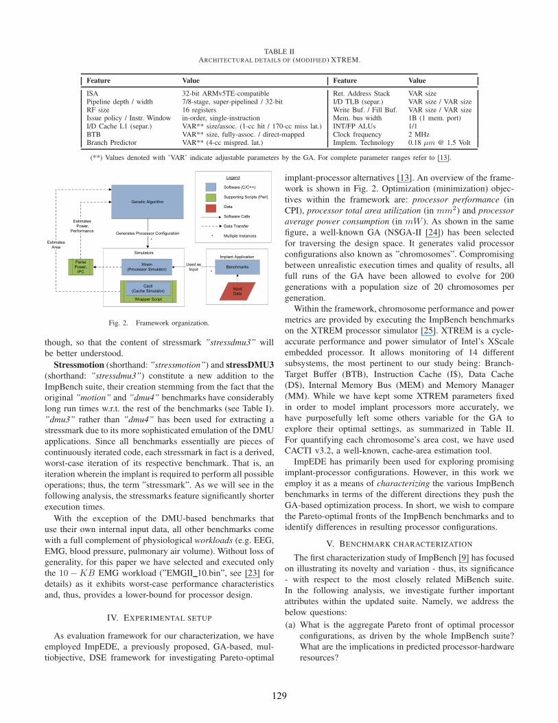
TABLE IIARCHITECTURAL DETAILS OF (MODIFIED) XTREM.

Feature Value Feature Value

ISA 32-bit ARMv5TE-compatible Ret. Address Stack VAR sizePipeline depth / width 7/8-stage, super-pipelined / 32-bit I/D TLB (separ.) VAR size / VAR sizeRF size 16 registers Write Buf. / Fill Buf. VAR size / VAR sizeIssue policy / Instr. Window in-order, single-instruction Mem. bus width 1B (1 mem. port)I/D Cache L1 (separ.) VAR** size/assoc. (1-cc hit / 170-cc miss lat.) INT/FP ALUs 1/1BTB VAR** size, fully-assoc. / direct-mapped Clock frequency 2 MHzBranch Predictor VAR** (4-cc mispred. lat.) Implem. Technology 0.18 µm @ 1.5 Volt

(**) Values denoted with ’VAR’ indicate adjustable parameters by the GA. For complete parameter ranges refer to [13].

Legend

Software (C/C++)

Supporting Scripts (Perl)

Data

Software Calls

Data Transfer

Multiple Instances*

Simulators

Xtrem(Processor Simulator)

Wrapper Script

Implant Application

Input Data

Benchmarks

Genetic Algorithm

Estimates Area

*

Generates Processor Configuration*

Used asInput

EstimatesPower,

Performance

Parse Power,

IPC

Cacti(Cache Simulator)

Fig. 2. Framework organization.

though, so that the content of stressmark ”stressdmu3” will

be better understood.

Stressmotion (shorthand: ”stressmotion”) and stressDMU3

(shorthand: ”stressdmu3”) constitute a new addition to the

ImpBench suite, their creation stemming from the fact that the

original ”motion” and ”dmu4” benchmarks have considerably

long run times w.r.t. the rest of the benchmarks (see Table I).

”dmu3” rather than ”dmu4” has been used for extracting a

stressmark due to its more sophisticated emulation of the DMU

applications. Since all benchmarks essentially are pieces of

continuously iterated code, each stressmark in fact is a derived,

worst-case iteration of its respective benchmark. That is, an

iteration wherein the implant is required to perform all possible

operations; thus, the term ”stressmark”. As we will see in the

following analysis, the stressmarks feature significantly shorter

execution times.

With the exception of the DMU-based benchmarks that

use their own internal input data, all other benchmarks come

with a full complement of physiological workloads (e.g. EEG,

EMG, blood pressure, pulmonary air volume). Without loss of

generality, for this paper we have selected and executed only

the 10 −KB EMG workload (”EMGII 10.bin”, see [23] for

details) as it exhibits worst-case performance characteristics

and, thus, provides a lower-bound for processor design.

IV. EXPERIMENTAL SETUP

As evaluation framework for our characterization, we have

employed ImpEDE, a previously proposed, GA-based, mul-

tiobjective, DSE framework for investigating Pareto-optimal

implant-processor alternatives [13]. An overview of the frame-

work is shown in Fig. 2. Optimization (minimization) objec-

tives within the framework are: processor performance (in

CPI), processor total area utilization (in mm2) and processor

average power consumption (in mW ). As shown in the same

figure, a well-known GA (NSGA-II [24]) has been selected

for traversing the design space. It generates valid processor

configurations also known as ”chromosomes”. Compromising

between unrealistic execution times and quality of results, all

full runs of the GA have been allowed to evolve for 200

generations with a population size of 20 chromosomes per

generation.

Within the framework, chromosome performance and power

metrics are provided by executing the ImpBench benchmarks

on the XTREM processor simulator [25]. XTREM is a cycle-

accurate performance and power simulator of Intel’s XScale

embedded processor. It allows monitoring of 14 different

subsystems, the most pertinent to our study being: Branch-

Target Buffer (BTB), Instruction Cache (I$), Data Cache

(D$), Internal Memory Bus (MEM) and Memory Manager

(MM). While we have kept some XTREM parameters fixed

in order to model implant processors more accurately, we

have purposefully left some others variable for the GA to

explore their optimal settings, as summarized in Table II.

For quantifying each chromosome’s area cost, we have used

CACTI v3.2, a well-known, cache-area estimation tool.

ImpEDE has primarily been used for exploring promising

implant-processor configurations. However, in this work we

employ it as a means of characterizing the various ImpBench

benchmarks in terms of the different directions they push the

GA-based optimization process. In short, we wish to compare

the Pareto-optimal fronts of the ImpBench benchmarks and to

identify differences in resulting processor configurations.

V. BENCHMARK CHARACTERIZATION

The first characterization study of ImpBench [9] has focused

on illustrating its novelty and variation - thus, its significance

- with respect to the most closely related MiBench suite.

In the following analysis, we investigate further important

attributes within the updated suite. Namely, we address the

below questions:

(a) What is the aggregate Pareto front of optimal processor

configurations, as driven by the whole ImpBench suite?

What are the implications in predicted processor-hardware

resources?

129

100

101

102

103

90

100

110

120

130

140

150

160

CPI

Pow

er

all

mlzo

fin

(a) CPI (-) – Power consumption, avg. (mW )

90 100 110 120 130 140 150 16010

−1

100

101

102

103

Power

Are

a

all

mlzo

fin

(b) Power consumption, avg. (mW ) – Area (mm2)

10−1

100

101

102

103

100

101

102

103

Area

CP

I

all

mlzo

fin

(c) Area (mm2) – CPI (-)

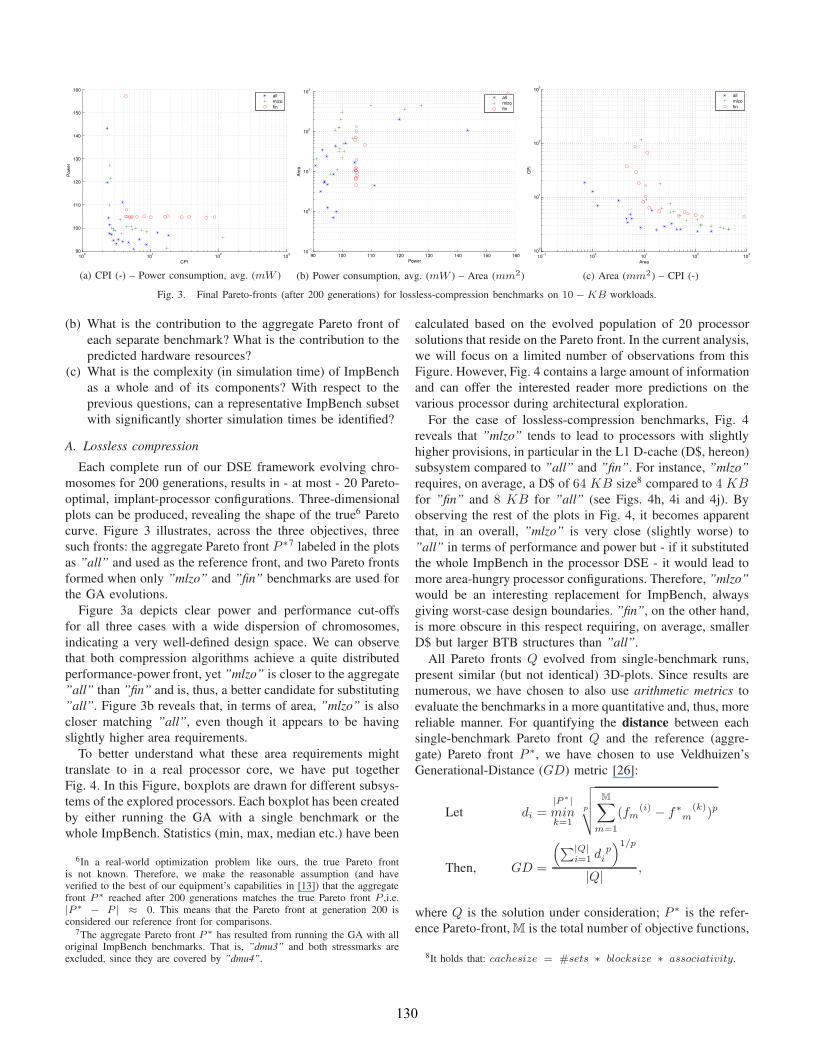
Fig. 3. Final Pareto-fronts (after 200 generations) for lossless-compression benchmarks on 10−KB workloads.

(b) What is the contribution to the aggregate Pareto front of

each separate benchmark? What is the contribution to the

predicted hardware resources?

(c) What is the complexity (in simulation time) of ImpBench

as a whole and of its components? With respect to the

previous questions, can a representative ImpBench subset

with significantly shorter simulation times be identified?

A. Lossless compression

Each complete run of our DSE framework evolving chro-

mosomes for 200 generations, results in - at most - 20 Pareto-

optimal, implant-processor configurations. Three-dimensional

plots can be produced, revealing the shape of the true6 Pareto

curve. Figure 3 illustrates, across the three objectives, three

such fronts: the aggregate Pareto front P ∗7 labeled in the plots

as ”all” and used as the reference front, and two Pareto fronts

formed when only ”mlzo” and ”fin” benchmarks are used for

the GA evolutions.

Figure 3a depicts clear power and performance cut-offs

for all three cases with a wide dispersion of chromosomes,

indicating a very well-defined design space. We can observe

that both compression algorithms achieve a quite distributed

performance-power front, yet ”mlzo” is closer to the aggregate

”all” than ”fin” and is, thus, a better candidate for substituting

”all”. Figure 3b reveals that, in terms of area, ”mlzo” is also

closer matching ”all”, even though it appears to be having

slightly higher area requirements.

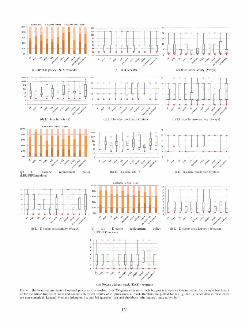
To better understand what these area requirements might

translate to in a real processor core, we have put together

Fig. 4. In this Figure, boxplots are drawn for different subsys-

tems of the explored processors. Each boxplot has been created

by either running the GA with a single benchmark or the

whole ImpBench. Statistics (min, max, median etc.) have been

6In a real-world optimization problem like ours, the true Pareto frontis not known. Therefore, we make the reasonable assumption (and haveverified to the best of our equipment’s capabilities in [13]) that the aggregatefront P ∗ reached after 200 generations matches the true Pareto front P ,i.e.|P ∗ − P | ≈ 0. This means that the Pareto front at generation 200 isconsidered our reference front for comparisons.

7The aggregate Pareto front P ∗ has resulted from running the GA with alloriginal ImpBench benchmarks. That is, ”dmu3” and both stressmarks areexcluded, since they are covered by ”dmu4”.

calculated based on the evolved population of 20 processor

solutions that reside on the Pareto front. In the current analysis,

we will focus on a limited number of observations from this

Figure. However, Fig. 4 contains a large amount of information

and can offer the interested reader more predictions on the

various processor during architectural exploration.

For the case of lossless-compression benchmarks, Fig. 4

reveals that ”mlzo” tends to lead to processors with slightly

higher provisions, in particular in the L1 D-cache (D$, hereon)

subsystem compared to ”all” and ”fin”. For instance, ”mlzo”

requires, on average, a D$ of 64 KB size8 compared to 4 KB

for ”fin” and 8 KB for ”all” (see Figs. 4h, 4i and 4j). By

observing the rest of the plots in Fig. 4, it becomes apparent

that, in an overall, ”mlzo” is very close (slightly worse) to

”all” in terms of performance and power but - if it substituted

the whole ImpBench in the processor DSE - it would lead to

more area-hungry processor configurations. Therefore, ”mlzo”

would be an interesting replacement for ImpBench, always

giving worst-case design boundaries. ”fin”, on the other hand,

is more obscure in this respect requiring, on average, smaller

D$ but larger BTB structures than ”all”.

All Pareto fronts Q evolved from single-benchmark runs,

present similar (but not identical) 3D-plots. Since results are

numerous, we have chosen to also use arithmetic metrics to

evaluate the benchmarks in a more quantitative and, thus, more

reliable manner. For quantifying the distance between each

single-benchmark Pareto front Q and the reference (aggre-

gate) Pareto front P ∗, we have chosen to use Veldhuizen’s

Generational-Distance (GD) metric [26]:

Let di =|P∗|

mink=1

p

√

√

√

√

M∑

m=1

(fm(i) − f∗

m(k))p

Then, GD =

(

∑|Q|i=1 d

pi

)1/p

|Q|,

where Q is the solution under consideration; P ∗ is the refer-

ence Pareto-front, M is the total number of objective functions,

8It holds that: cachesize = #sets ∗ blocksize ∗ associativity.

130

80%

100%

BIMODAL ALWAYS TAKEN ALWAYS NOT TAKEN

20%

40%

60%

0%

(a) BPRED policy (NT/T/bimodal)

16

32

48

64

80

96

112

128

144

(b) BTB sets (#)

0

8

16

24

32

40

(c) BTB associativity (#ways)

1

4

16

64

256

1024

4096

16384

(d) L1 I-cache sets (#)

0

8

16

24

32

40

(e) L1 I-cache block size (Bytes)

1

2

4

8

16

32

(f) L1 I-cache associativity (#ways)

80%

100%

RANDOM FIFO LRU

20%

40%

60%

0%

(g) L1 I-cache replacement policy(LRU/FIFO/random)

1

4

16

64

256

1024

4096

(h) L1 D-cache sets (#)

0

8

16

24

32

40

(i) L1 D-cache block size (Bytes)

1

2

4

8

16

32

(j) L1 D-cache associativity (#ways)

80%

100%

RANDOM FIFO LRU

20%

40%

60%

0%

(k) L1 D-cache replacement policy(LRU/FIFO/random)

0

2

4

6

8

10

12

14

16

18

(l) L1 D-cache miss latency (#c.cycles)

0

1

2

3

4

5

6

7

8

(m) Return-address stack (RAS) (#entries)

Fig. 4. Hardware requirements of optimal processors, as evolved over 200-generation runs. Each boxplot is a separate GA run either for a single benchmarkor for the whole ImpBench suite and contains statistical results of 20 processors, at most. Barchars are plotted for (a), (g) and (k) since data in these casesare non-numerical. Legend: Medians (triangle), 1st and 3rd quartiles (star and rhombus), min (square), max (x-symbol).

131

100

101

102

80

90

100

110

120

130

140

150

CPI

Pow

er

all

misty

rc6

(a) CPI (-) – Power consumption, avg. (mW )

80 90 100 110 120 130 140 15010

−1

100

101

102

103

Power

Are

a

all

misty

rc6

(b) Power consumption, avg. (mW ) – Area (mm2)

10−1

100

101

102

103

100

101

102

Area

CP

I

all

misty

rc6

(c) Area (mm2) – CPI (-)

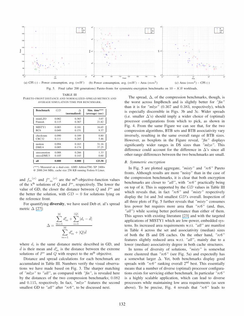
Fig. 5. Final (after 200 generations) Pareto-fronts for symmetric-encryption benchmarks on 10−KB workloads.

TABLE IIIPARETO-FRONT DISTANCE AND NORMALIZED-SPREAD METRICS AND

AVERAGE SIMULATION TIME PER BENCHMARK.

Benchmark GD ∆ Sim. time***

(normalized) (average) (sec)

miniLZO 0.082 0.383 3.07Finnish 0.115 0.367 21.82

MISTY1 0.083 0.181 16.65RC6 0.049 0.151 9.37

checksum 0.090 0.189 0.80CRC32 0.111 0.285 5.46

motion 0.094 0.163 31.16DMU4 0.085 0.174 37.25

stressmotion 0.088 0.266 1.33stressDMU3 0.105 0.143 0.60

all 0.000 0.000 125.58

(***) Measured on a dual-core, AMD Athlon(TM) XP 2400+@ 2000.244 MHz, cache size 256 KB running Fedora 8 Linux.

and fm(x) and f∗

m(x) are the mth-objective-function values

of the xth solutions of Q and P ∗, respectively. The lower the

value of GD, the closer the distance between Q and P ∗ and

the better the solution, with GD = 0 for solutions lying on

the reference front.

For quantifying diversity, we have used Deb et. al’s spread

metric ∆ [27]:

∆ =

M∑

m=1

dem +

|Q|∑

i=1

|di − d|

M∑

m=1

dem + |Q|d

where di is the same distance metric described in GD, and

d is their mean and dem is the distance between the extreme

solutions of P ∗ and Q with respect to the mth objective.

Distance and spread calculations for each benchmark are

accumulated in Table III. Numbers verify the visual observa-

tions we have made based on Fig. 3. The sharper matching

of ”mlzo” to ”all”, as compared with ”fin”, is revealed here

by the distances of the two compression benchmarks; 0.082and 0.115, respectively. In fact, ”mlzo” features the second

smallest GD to ”all” after ”rc6”, to be discussed next.

The spread, ∆, of the compression benchmarks, though, is

the worst across ImpBench and is slightly better for ”fin”

than it is for ”mlzo” (0.367 and 0.383, respectively), which

is especially discernible in Figs. 3b and 3c. Wider spreads

(i.e. smaller ∆’s) should imply a wider choice of (optimal)

processor configurations from which to pick, as shown in

Fig. 4. From the same Figure we can see that, for the two

compression algorithms, BTB sets and BTB associativity vary

inversely, resulting in the same overall range of BTB sizes.

However, as boxplots in the Figure reveal, ”fin” displays

significantly wider ranges in D$ sizes than ”mlzo”. This

difference could account for the difference in ∆’s since all

other range differences between the two benchmarks are small.

B. Symmetric encryption

In Fig. 5 are plotted aggregate, ”misty” and ”rc6” Pareto

fronts. Although results are more ”noisy” than in the case of

the compression benchmarks, it is clear that both encryption

benchmarks are closer to ”all”, with ”rc6” practically being

on top of it. This is supported by the GD values in Table III

which reveals that, in fact ”rc6” and ”misty” respectively

display the 1st and 3rd smallest GD’s overall. Inspection of

all three plots of Fig. 5 further reveals that ”misty” consumes

less power but requires more area than ”rc6” (and, thus,

”all”) while scoring better performance than either of them.

This agrees with existing literature [23] and with the targeted

applications of MISTY1 which are low-power, embedded sys-

tems. Its increased area requirements w.r.t. ”all” are manifest

in Table 4 across the set and associativity (median) sizes

of both the I$ and D$ caches. On the other hand, ”rc6”

features slightly reduced area w.r.t. ”all”, mainly due to a

lower (median) associativity degree in both cache structures.

In terms of diversity of solutions, ”misty” is somewhat

more clustered than ”rc6” (see Fig. 5a) and expectedly has

a somewhat larger ∆. Yet, both benchmarks display good

spreads with ”rc6” ranking overall 2nd best. This essentially

means that a number of diverse (optimal) processor configura-

tions exists for servicing either benchmark. In particular ”rc6”

is a highly scalable application, which can lead to diverse

processors while maintaining low area requirements (as seen

above). To be precise, Fig. 4 reveals that ”rc6” leads to

132

100

101

102

60

80

100

120

140

160

180

CPI

Po

we

r

all

checksum

crc32

(a) CPI (-) – Power consumption, avg. (mW )

60 80 100 120 140 160 18010

−1

100

101

102

103

104

Power

Are

a

all

checksum

crc32

(b) Power consumption, avg. (mW ) – Area (mm2)

10−1

100

101

102

103

104

100

101

102

Area

CP

I

all

checksum

crc32

(c) Area (mm2) – CPI (-)

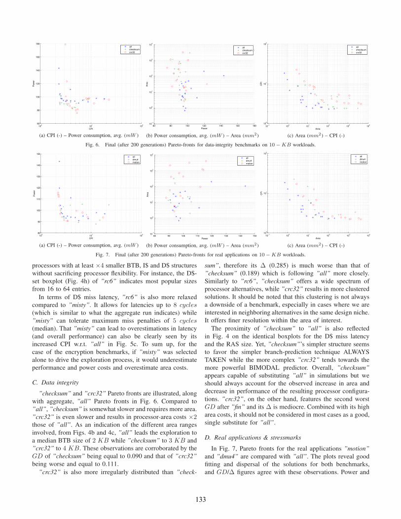
Fig. 6. Final (after 200 generations) Pareto-fronts for data-integrity benchmarks on 10−KB workloads.

100

101

102

80

90

100

110

120

130

140

150

CPI

Pow

er

all

dmu4

motion

(a) CPI (-) – Power consumption, avg. (mW )

80 90 100 110 120 130 140 15010

−1

100

101

102

103

104

Power

Are

a

all

dmu4

motion

(b) Power consumption, avg. (mW ) – Area (mm2)

10−1

100

101

102

103

104

100

101

102

Area

CP

I

all

dmu4

motion

(c) Area (mm2) – CPI (-)

Fig. 7. Final (after 200 generations) Pareto-fronts for real applications on 10−KB workloads.

processors with at least ×4 smaller BTB, I$ and D$ structures

without sacrificing processor flexibility. For instance, the D$-

set boxplot (Fig. 4h) of ”rc6” indicates most popular sizes

from 16 to 64 entries.

In terms of D$ miss latency, ”rc6” is also more relaxed

compared to ”misty”. It allows for latencies up to 8 cycles

(which is similar to what the aggregate run indicates) while

”misty” can tolerate maximum miss penalties of 5 cycles

(median). That ”misty” can lead to overestimations in latency

(and overall performance) can also be clearly seen by its

increased CPI w.r.t. ”all” in Fig. 5c. To sum up, for the

case of the encryption benchmarks, if ”misty” was selected

alone to drive the exploration process, it would underestimate

performance and power costs and overestimate area costs.

C. Data integrity

”checksum” and ”crc32” Pareto fronts are illustrated, along

with aggregate, ”all” Pareto fronts in Fig. 6. Compared to

”all”, ”checksum” is somewhat slower and requires more area.

”crc32” is even slower and results in processor-area costs ×2those of ”all”. As an indication of the different area ranges

involved, from Figs. 4b and 4c, ”all” leads the exploration to

a median BTB size of 2 KB while ”checksum” to 3 KB and

”crc32” to 4 KB. These observations are corroborated by the

GD of ”checksum” being equal to 0.090 and that of ”crc32”

being worse and equal to 0.111.

”crc32” is also more irregularly distributed than ”check-

sum”, therefore its ∆ (0.285) is much worse than that of

”checksum” (0.189) which is following ”all” more closely.

Similarly to ”rc6”, ”checksum” offers a wide spectrum of

processor alternatives, while ”crc32” results in more clustered

solutions. It should be noted that this clustering is not always

a downside of a benchmark, especially in cases where we are

interested in neighboring alternatives in the same design niche.

It offers finer resolution within the area of interest.

The proximity of ”checksum” to ”all” is also reflected

in Fig. 4 on the identical boxplots for the D$ miss latency

and the RAS size. Yet, ”checksum”’s simpler structure seems

to favor the simpler branch-prediction technique ALWAYS

TAKEN while the more complex ”crc32” tends towards the

more powerful BIMODAL predictor. Overall, ”checksum”

appears capable of substituting ”all” in simulations but we

should always account for the observed increase in area and

decrease in performance of the resulting processor configura-

tions. ”crc32”, on the other hand, features the second worst

GD after ”fin” and its ∆ is mediocre. Combined with its high

area costs, it should not be considered in most cases as a good,

single substitute for ”all”.

D. Real applications & stressmarks

In Fig. 7, Pareto fronts for the real applications ”motion”

and ”dmu4” are compared with ”all”. The plots reveal good

fitting and dispersal of the solutions for both benchmarks,

and GD/∆ figures agree with these observations. Power and

133

100

101

102

80

85

90

95

100

105

110

115

120

CPI

Pow

er

dmu4

motion

stressdmu3

stressmotion

(a) CPI (-) – Power consumption, avg. (mW )

80 85 90 95 100 105 110 115 12010

0

101

102

103

104

Power

Are

a

dmu4

motion

stressdmu3

stressmotion

(b) Power consumption, avg. (mW ) – Area (mm2)

100

101

102

103

104

100

101

102

Area

CP

I

dmu4

motion

stressdmu3

stressmotion

(c) Area (mm2) – CPI (-)

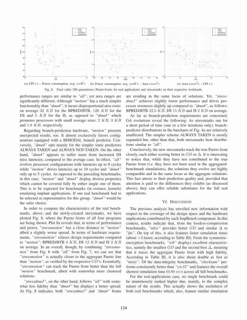
Fig. 8. Final (after 200 generations) Pareto-fronts for real applications and stressmarks on their respective workloads.

performance ranges are similar to ”all”, yet area ranges are

significantly different. Although ”motion” has a much simpler

functionality than ”dmu4”, it incurs disproportional area costs:

on average 32 KB for the BPRED/BTB, 120 KB for the

D$ and 5 KB for the I$, as opposed to ”dmu4” which

promotes processors with small average sizes: 2 KB, 3 KB

and 1.8 KB, respectively.

Regarding branch-prediction hardware, ”motion” presents

unexpected results, too. It almost exclusively favors config-

urations equipped with a BIMODAL branch predictor. Con-

versely, ”dmu4” opts mainly for the simpler static predictors

ALWAYS TAKEN and ALWAYS NOT-TAKEN. On the other

hand, ”dmu4” appears to suffer more from increased D$

miss latencies, compared to the average case. In effect, ”all”

evolves processor configurations with latencies up to 8 cycles

while ”motion” drives latencies up to 10 cycles and ”dmu4”

only up to 5 cycles. As opposed to the preceding benchmarks,

in this case, ”motion” and ”dmu4” display diverse properties

which cannot be covered fully by either single one of them.

This is to be expected for benchmarks (in essence, kernels)

emulating implant applications. If one real benchmark had to

be selected as representative for this group, ”dmu4” would be

the safer choice.

In order to compare the characteristics of the real bench-

marks, above, and the newly-created stressmarks, we have

plotted Fig. 8, where the Pareto fronts of all four programs

are being shown. Plot 8a reveals that, in terms of performance

and power, ”stressmotion” has a close distance to ”motion”

albeit a slightly worse spread. In terms of hardware require-

ments, ”stressmotion” relaxes design requirements compared

to ”motion”: BPRED/BTB 4 KB, D$ 12 KB and I$ 2 KB

on average. In an overall, though, by combining ”stressmo-

tion” from Fig. 8 with ”all” from Fig. 7, we can see that

”stressmotion” is actually closer to the aggregate Pareto line

than ”motion”, as verified by the respective GD’s. Essentially,

”stressmotion” can track the Pareto front better than the full

”motion” benchmark, albeit with somewhat more clustered

solutions.

”stressdmu3”, on the other hand, follows ”all” with some-

what less fidelity than ”dmu4” but displays a better spread.

As Fig. 8 indicates, both ”stressdmu3” and ”dmu4” fronts

are residing in the same locus of solutions. Yet, ”stress-

dmu3” achieves slightly lower performance and drives pro-

cessor resources slightly up compared to ”dmu4”, as follows:

BPRED/BTB 22.5 KB, D$ 15 KB and I$ 2 KB on average.

As far as branch-prediction requirements are concerned,

GA evolutions reveal the following: As stressmarks run for

a short period of time (one or a few iterations only), branch-

predictor distributions in the barcharts of Fig. 4a are relatively

unaffected. The simpler scheme ALWAYS TAKEN is mostly

expanded but, other than that, both stressmarks bear distribu-

tions similar to ”all”.

Conclusively, the new stressmarks track the true Pareto front

closely, each either scoring better in GD or ∆. It is interesting

to notice that, while they have not contributed to the true

Pareto front (i.e. they have not been used in the aggregated-

benchmark simulations), the solutions they evolve are highly

comparable and in the same locus as the aggregate solutions.

This fact attests to their prediction quality and, provided that

attention is paid to the differences they exhibit (as discussed

above), they can offer reliable substitutes for the full real

applications.

VI. DISCUSSION

The previous analysis has unveiled new information with

respect to the coverage of the design space and the hardware

implications contributed by each ImpBench component. In this

context, results indicate that, from the lossless-compression

benchmarks, ”mlzo” provides better GD and similar ∆ to

”fin”. On top of this, it also features faster simulation times

(about ×3 faster, according to Table III). From the symmetric-

encryption benchmarks, ”rc6” displays excellent characteris-

tics, namely the smallest GD and the second best ∆, meaning

that it traces the aggregate Pareto front with high fidelity.

According to Table III, it is also about double as fast as

”misty”. Of the data-integrity benchmarks, ”checksum” per-

forms consistently better than ”crc32” and features the overall

shortest simulation time (0.80 sec) across all full benchmarks.

For the real-applications case, no single benchmark could

be unanimously ranked higher due, mainly, to the complex

nature of the results. This actually shows the usefulness of

both real benchmarks which, also, feature similar simulation

134

times (and the largest in the whole suite). Last, analysis of the

new stressmarks has revealed that, although they display some

variability in predicted processor specifications w.r.t. the full

real applications, they both track the true Pareto front closely.

Careful use of the stressmarks can seriously reduce simulation

times up to ×30 (see Table III), which is an impressive

speedup and a good tradeoff between DSE speed and accuracy.

The above results indicate highest-ranking benchmarks

within the ImpBench suite, however this is not to say that

the poorest-performing ones are redundant. The findings of

the original analysis [9] indicate that each benchmark in

ImpBench exhibits diverse characteristics (e.g. µop mixes) and

should not be dropped from consideration when considering

implant-processor design. On the contrary, this study comes as

a complement and extension of the original ImpBench study.

VII. CONCLUSIONS

In view of more structured and educated implant proces-

sors in the years to come, we have carefully put together

ImpBench, a collection of benchmark programs and assorted

input datasets, able to capture the intrinsic of new implant

architectures under evaluation. In this paper, we have extended

the suite with an additional benchmark and two stressmarks.

The stressmarks proposed, feature fraction-of-the-original-

time execution times and, provided that their peculiarities are

taken into account by the designer, they can considerably en-

hance and speedup processor-profiling times. We have, further,

expanded our characterization analysis to include predictions

on actual implant-processor configurations resulting from the

use of this suite as a profiling basis. ImpBench is a dynamic

construct and, in the future, more benchmarks will be added,

subject to our ongoing research. Among others, we anticipate

simple DSP applications as potential candidates as well as

more real applications like the ”artificial pancreas”, a crucial

application nowadays for diabetic patients.

VIII. ACKNOWLEDGEMENTS

This work has been partially supported by the ICT Delft

Research Centre (DRC-ICT) of the Delft University of Tech-

nology. Many thanks are due to Erik de Vries and Eef Hartman

for their excellent technical support in setting up and operating

the DSE computer cluster. Without them, this work would not

have been possible.

REFERENCES

[1] A. Omran, “The epidemiological transition,” Milbank Memorial Fund

Quarterly, vol. 49, no. 4, pp. 509–538, 1971.[2] R. Beaglehole and R. Bonita, Public health at the crossroads: achieve-

ments and prospects, 2nd ed. Cambridge University Press, 2004.[3] H. Ector and P. Vardas, “Current use of pacemakers, implantable

cardioverter defibrillators, and resynchronization devices: data from theregistry of the european heart rhythm association,” European Heart

Journal Supplements, vol. 9, pp. 144–149, August 1988.[4] F. Nebeker, “Golden accomplishments in biomedical engineering,” in

IEEE Engineering in Medicine and Biology Magazine, vol. 21, Piscat-away, NJ, USA, May - June 2002, pp. 17–47.

[5] C. Liang, J. Chen, C. Chung, C. Cheng, and C. Wang, “An implantablebi-directional wireless transmission system for transcutaneous biologicalsignal recording,” Physiological Measurement, vol. 26, pp. 83–97,February 2005.

[6] P. Cross, R. Kunnemeyer, C. Bunt, D. Carnegie, and M. Rathbone,“Control, communication and monitoring of intravaginal drug deliveryin dairy cows,” in International Journal of Pharmaceuticals, vol. 282,10 September 2004, pp. 35–44.

[7] H. Lanmuller, E. Unger, M. Reichel, Z. Ashley, W. Mayr, and A. Tschak-ert, “Implantable stimulator for the conditioning of denervated musclesin rabbit,” in 8th Vienna International Workshop on Functional Electrical

Stimulation, Vienna, Austria, 10-13 September 2004.[8] C. Strydis, G. Gaydadjiev, and S. Vassiliadis, “Implantable microelec-

tronic devices: A comprehensive review,” Computer Engineering, DelftUniversity of Technology, CE-TR-2006-01, December 2006.

[9] C. Strydis, C. Kachris, and G. Gaydadjiev, “ImpBench - A novel bench-mark suite for biomedical, microelectronic implants,” in International

Conference on Embedded Computer Systems: Architectures, Modeling,

and Simulation (SAMOS08), 2008, pp. 21–24.[10] C. Strydis and G. N. Gaydadjiev, “Evaluating Various Branch-Prediction

Schemes for Biomedical-Implant Processors,” in Proceedings of the

20th IEEE International Conference on Application-specific Systems,

Architectures and Processors (ASAP’09), July 2009, pp. 169–176.[11] ——, “The Case for a Generic Implant Processor,” in 30th Annual

International Conference of the IEEE Engineering in Medicine and

Biology Society (EMBC’08), August 2008, pp. 3186–3191.[12] V. Guzma, S. Bhattacharyya, P. Kellomaki, and J. Takala, “An inte-

grated asip design flow for digital signal processing applications,” inFirst International Symposium on Applied Sciences on Biomedical and

Communication Technologies (ISABEL’08), October 2008, pp. 1 –5.[13] D. Dave, C. Strydis, and G. N. Gaydadjiev, “ImpEDE: A Multidimen-

sional, Design-Space Exploration Framework for Biomedical-ImplantProcessors,” in Proceedings of the 21th IEEE International Confer-

ence on Application-specific Systems, Architectures and Processors

(ASAP’10), July 7-9 2010.[14] “SPEC CPU2006,” http://www.spec.org/cpu2006/.[15] C. Lee, M. Potkonjak, and W. Mangione-Smith, “MediaBench: a tool for

evaluating and synthesizing multimedia and communications systems,”30th Annual IEEE/ACM International Symposium on Microarchitecture,pp. 330–335, 1-3 Dec 1997.

[16] “EEMBC,” http://www.eembc.com.[17] M. Guthaus, J. Ringenberg, D. Ernst, T. Austin, T. Mudge, and

R. Brown, “MiBench: A free, commercially representative embeddedbenchmark suite,” IEEE International Workshop on Workload Charac-

terization, pp. 3–14, 2 December 2001.[18] G. Memik, W. H. Mangione-Smith, and W. Hu, “NetBench: a bench-

marking suite for network processors,” in IEEE/ACM international

conference on Computer-aided design (ICCAD’01), Piscataway, NJ,USA, 2001, pp. 39–42.

[19] T. Wolf and M. Franklin, “CommBench-a telecommunications bench-mark for network processors,” in IEEE International Symposium on Per-

formance Analysis of Systems and Software (ISPASS’00), Washington,DC, USA, 2000, pp. 154–162.

[20] H. Ohta and M. Matsui, A Description of the MISTY1 Encryption

Algorithm, United States, 2000.[21] S. Slijepcevic, M. Potkonjak, V. Tsiatsis, S. Zimbeck, and M. Srivastava,

“On communication security in wireless ad-hoc sensor networks,” En-

abling Technologies: Infrastructure for Collaborative Enterprises (WET

ICE’02), pp. 139–144, 2002.[22] P. Wouters, M. D. Cooman, D. Lapadatu, and R. Puers, “A low

power multi-sensor interface for injectable microprocessor-based animalmonitoring system,” in Sensors and Actuators A: Physical, vol. 41-42,1994, pp. 198–206.

[23] C. Strydis, D. Zhu, and G. Gaydadjiev, “Profiling of symmetric encryp-tion algorithms for a novel biomedical-implant architecture,” in ACM

International Conference on Computing Frontiers (CF’08), Ischia, Italy,5-7 May 2008, pp. 231–240.

[24] K. Deb, A. Pratap, S. Agarwal, and T. Meyarivan, “A Fast ElitistMulti-Objective Genetic Algorithm: NSGA-II,” IEEE Transactions on

Evolutionary Computation, vol. 6, pp. 182–197, 2000.[25] G. Contreras, M. Martonosi, J. Peng, R. Ju, and G.-Y. Lueh, “XTREM:

A Power Simulator for the Intel XScale Core,” in LCTES’04, 2004, pp.115–125.

[26] D. A. V. Veldhuizen and G. B. Lamont, “Evolutionary computationand convergence to a pareto front,” in Proceedings of the 3rd Annual

Conference on Genetic Programming, 1998.[27] K. Deb, Multi-Objective Optimization Using Evolutionary Algorithms.

John Wiley & Sons, LTD, 2001.

135