Transactions of the ASABE

Vol. 51(1): 139-151 � 2008 American Society of Agricultural and Biological Engineers ISSN 0001-2351 139

IMPACTS OF LAND USE CHARACTERIZATION IN MODELING

HYDROLOGY AND SEDIMENTS FOR THE LUXAPALLILA

CREEK WATERSHED, ALABAMA AND MISSISSIPPI

J. N. Diaz‐Ramirez, V. J. Alarcon, Z. Duan, M. L. Tagert, W. H. McAnally, J. L. Martin, C. G. O'Hara

ABSTRACT. The Hydrological Simulation Program - Fortran (HSPF), interfaced with the Better Assessment ScienceIntegrating Point and Nonpoint (BASINS), was used to evaluate the impact of land use (as characterized by different landuse/land cover (LU/LC) datasets) on hydrology and sediment components of the Luxapallila Creek watershed. The 1,770 km2

watershed is located in Alabama and Mississippi. Simulation of the watershed processes were tested at the hillslope and atthe watershed outlet for the period between 1985 and 2003. Three LU/LC databases were used: the Geographic InformationRetrieval and Analysis System (GIRAS), the Moderate Resolution Imaging Spectroradiometer land cover product (MODISMOD12Q1), and the National Land Cover Dataset (NLCD). The two main land use categories revealed by the three LU/LCdatabases were forest and agricultural lands. Whereas forest cover mechanisms were the main source of water loss inhydrology simulation, agricultural land was the main source of sediment export in sediment modeling. Land use datasets ofcoarser spatial resolution (MODIS and GIRAS) produced larger HSPF estimations for sediment fraction values than landuse datasets identifying smaller percentages of those agricultural land cover classes (NLCD). Differences in agricultural landcharacterization among the land use datasets showed that sediment predictions were more sensitive than streamflowpredictions to the scale and resolution of land use datasets. Choosing the right land use dataset will impact the modeling ofsediments and, potentially, other water quality constituents that are related with agricultural activities.

Keywords. HSPF, Hydrology, Land use, Sediments, Watershed modeling.

and use is an important factor in watershed modeling,especially when water quality or environmental man‐agement is the focus of the modeling/ simulation ef‐fort. Loss of farmland to urban sprawl impacts the

environment in a variety of ways, including groundwater re‐charge, water pollution, and stormwater drainage (Engel et al.,2003). Some studies have identified a relationship between landuse and surface water quality. For example, Tong and Chen(2002) used a comprehensive approach to study this relationshipin a local watershed in the East Fork Little Miami River basin,Ohio, using the Better Assessment Science Integrating Pointand Nonpoint Sources (BASINS) software suite. Their study re‐vealed that there was a significant relationship between land useand in‐stream water quality, especially for nitrogen, phosphorus,and fecal coliform. It also revealed that BASINS is a very useful

Submitted for review in August 2007 as manuscript number SW 7156;approved for publication by the Soil & Water Division of ASABE inDecember 2007.

The authors are Jairo N. Diaz‐Ramirez, ASABE Member Engineer,Post‐Doctoral Associate, Department of Civil and EnvironmentalEngineering, and Vladimir J. Alarcon, Assistant Research Professor,GeoResources Institute, Mississippi State University, Mississippi State,Mississippi; Zhiyong Duan, Engineer, CDM, New Orleans, Louisiana;Mary Love Tagert, Assistant Research Professor, Water ResourcesResearch Institute, William McAnally, Associate Professor, and James L.Martin, Professor, Department of Civil and Environmental Engineering,and Charles G. O'Hara, Associate Research Professor, GeoResourcesInstitute, Mississippi State University, Mississippi State Mississippi.Corresponding author: Jairo N. Diaz‐Ramirez, Department of Civil andEnvironmental Engineering, Mississippi State University, P.O. Box 9546,Mississippi State, MS 39762; phone: 662‐325‐9885; fax: 662‐325‐7189;e‐mail: jd216@msstate.edu.

and reliable tool, capable of characterizing the flow and waterquality conditions for the study area under different watershedscales. Whitehead et al. (2002) applied steady‐state and dynam‐ic modeling studies to illustrate the impact on the water qualityof the River Kennet (U.K.) due to land use change. Their resultsshowed that there has been a significant shift in the nitrogen bal‐ance in the River Kennet system caused by nonpoint‐sourcepollution from agriculture and point‐source discharges.

BASINS is a multipurpose environmental analysis pro‐gram developed by the U.S. Environmental ProtectionAgency (USEPA, 2001). It integrates a geographic informa‐tion program (ArcView), national watershed and meteoro‐logical databases, and modeling simulation routines into onepackage (USEPA, 2001). BASINS provides an interface thatallows the user to manipulate and display geospatial data andinteract with point and nonpoint source pollution models ina GIS‐based environment.

The Hydrologic Simulation Program - Fortran (HSPF)model (Bicknell et al., 2001) computes the movement of wa‐ter through a complete hydrologic cycle (rainfall, evapotran‐spiration, runoff, infiltration, and flow through the ground)and the associated transport of constituents with that flow. Itrepresents a watershed as a collection of land segments andchannels (reaches). The land segments, either pervious or im‐pervious, are connected to channel reaches, which can func‐tion as either streams or reservoirs. Rainfall is computed overthe entire watershed and runs off land segments and reaches.Pervious land segments also store water in the plant canopy,on the surface, and in the soil, from which it can percolate intogroundwater or flow downslope as interflow. HSPF also com‐putes the transport and kinetics of multiple water quality con‐

L

140 TRANSACTIONS OF THE ASABE

stituents, including temperature, sediment, nutrients, andpesticides. As such, it presents a well designed package formodeling the hydrology and water quality of a watershed. Amore complete description of its features and capabilities canbe found in the HSPF user's manual (Bicknell et al., 2001).The version of HSPF that is packaged with Version 3.1 of BA‐SINS can be run in the Windows environment (in stand‐alonemode) and is called WinHSPF. In this article, WinHSPF andHSPF will be used interchangeably.

Employing different land use databases for simulating hy‐drological phenomena can produce different simulation re‐sults, affecting subsequent modeling and simulation ofrelated hydrological or water quality processes. For example,hydrograph estimations were sensitive to swapping alterna‐tive land cover maps (Endreny et al., 2003), showing effectsranging from 35% underestimation to 20% overestimationfor peak flows. McAnally et al. (2005) detected differencesin simulated values of total suspended sediments after usingtwo land use databases when modeling hydrological pro‐cesses for a watershed in Mississippi. Moglen and Beighley(2002) showed that temporal land use change (captured withtwo different land use maps) resulted in considerable peakdischarge changes throughout the Watts Branch watershed,Maryland. Anantharaj et al. (2006) showed that changes inland cover altered surface fluxes (particularly the latent heatfluxes) when simulating sea breeze in the gulf coast area us‐ing NASA's Moderate Resolution Imaging Spectroradiome‐ter (MODIS) and USGS land cover data. While severalstudies have focused on the sensitivity of flow rate simula‐tions to land use, not many have analyzed the sensitivity ofwater quality estimations (sediments, nutrients, dissolvedoxygen, biochemical oxygen demand) to land use data quali‐ty. Today's easy and fast access to updated land cover maps(e.g., MODIS) provides good opportunities to investigate theimpact of land use data in modeling and simulation of wa‐tershed processes.

This research explores the impact of agricultural lands, ascharacterized by different land use/land cover (LU/LC) data‐

sets, on simulation of watershed processes at hillslope scaleand at the watershed outlet of the Luxapallila Creek basin, lo‐cated in Alabama and Mississippi. Simulated values of flowand sediments are obtained after swapping three land use da‐tabases. The changes in simulated values are analyzed andcompared. BASINS and WinHSPF are used to perform thespatial and hydrological estimations. The MODIS land use/land cover data (MODIS MOD12Q1) provided by NASA, theGeographic Information Retrieval and Analysis System(GIRAS), and National Land Cover Data (NLCD) were usedin the analysis. Although the GIRAS land use dataset is notthe best‐quality land use map available, it is taken here as thebenchmark for comparison in illustrating how higher‐resolution data (NLCD) or more up‐to‐date data (MODIS)would impact BASINS/WinHSPF's flow and sediment es‐timations.

METHODOLOGYBASINS/WinHSPF was used to calculate rainfall‐runoff,

flow, and sediments for the Luxapallila Creek watershed. Thewatershed was initially modeled with a standard set of proce‐dures and data to provide a base set of results. The system wasthen modeled with improved LU/LC inputs, and the resultswere compared with the base conditions. The GIRAS,NLCD, and MODIS LU/LC databases were swapped to eval‐uate their effect on water balance and sediment components.For all model runs, the meteorological input data were thesame. Goodness‐of‐fit coefficients, residual analysis, andgraphical evaluation were used to assess the model results.

STUDY AREA

Luxapallila Creek is an upland, rural watershed in Ala‐bama and Mississippi (fig. 1). Near the outlet, the watershedhas a drainage area of 1,770 km2, an average basin slope of2%, and average annual precipitation of 1,379 mm recordedat the Millport 2E weather station (1982‐2004 period).

Figure 1. Location of the Luxapallila Creek watershed.

141Vol. 51(1): 139-151

LAND USE/LAND COVER DATAThree LU/LC databases were used in this research: BA‐

SINS GIRAS, NLCD, and NASA's MODIS MOD12Q1.Throughout this article, the MODIS MOD12Q1 dataset willbe named MODIS, for brevity.

The GIRAS LU/LC data, developed by USGS between1977 and 1980, are provided in geographic coordinate unitswith a resolution of 0.0001 decimal degrees (USEPA, 1994).The original land use/land cover digital data were convertedto ARC/INFO format by the USEPA. Although these datasetsare useful for environmental assessment of land use patternswith respect to water quality analysis, growth management,and other types of environmental impact assessment, theiruse is limited because they are not current (USEPA, 1994).

The 1992 NLCD set was produced by the Multi‐Resolution Land Characteristics Consortium (MRLC),which consists of several federal agencies. The 1992 NLCDdataset was derived from Landsat - Thematic Mapper (TM)satellite data at a 30 m resolution and exists for the entire U.S.(USGS, 2004). A 21‐class modified Anderson land coverclassification scheme was consistently applied to Landsat -TM scenes for the entire country using an unsupervised clus‐tering algorithm. The 1992 NLCD layer for the Mississippiregion was obtained in .tif format and clipped to the Luxapal‐lila watershed boundary. When the NLCD dataset was subset,an adequate buffer outside the watershed boundary was in‐cluded in the subset to provide flexibility if a different wa‐tershed delineation became necessary. BASINS requires thatthe LU/LC information be in a shapefile format; therefore,the subset raster files were converted to a polygon shapefileusing ArcGIS's “raster to feature” option of the Spatial Ana‐lyst extension. The “value” field in the image file, which rep‐

resents the LU/LC classification, was used to populate the“gridcode” field in the new shapefile. Finally, the resultantLU/LC shapefile was reprojected from Albers Conical EqualArea to Mississippi State Plane East.

The MODIS Land Cover product (MOD12Q1) is publiclyavailable in five types of land cover classifications with 1 kmspatial resolution. The data are provided by NASA in integer‐ized sinusoidal (ISIN) projection. For this research, MODIS'Land Cover Type 1, which includes 17 classes of land coverin the International Geosphere‐Biosphere Programme(IGBP) global vegetation classification scheme, was repro‐jected and reclassified to meet the needs of the HSPF modelfor Luxapallila Creek. The original MODIS LU/LC data‐cube (MOD12Q1.A2001001.h10v05.004.2004149203002.hdf) was obtained through NASA's Earth Observing SystemData Gateway website. The metadata file associated with thedata‐cube specifies a production date of 28 May 2004. Thereprojection of the data‐cube to the State Plane, MississippiEast coordinate system was performed using the MODIS Re‐projection Tool. During the reprojection phase, the originalHDF format was converted to GEOTIFF for easier input ofthe data layer into ArcView. Then, the area of interest (Luxa‐pallila watershed) was clipped using the BASINS shape‐fileboundaries for Luxapallila. The clipped land use polygonswere converted to shapefile format for introduction into BA‐SINS.

GIRAS, NLCD, and MODIS have different numbers ofland use classes and terminology. For introduction into HSPF,those different LU/LC classifications were consolidated intosix categories: forest land, urban or built‐up land, agriculturalland, barren land, water, and wetlands. Table 1 and figure 2show results of the LU/LC reclassification.

Table 1. Consolidation of GIRAS, NLCD, and MODIS LU/LC classification into HSPF land use classification.HSPF LUClassification

GIRAS LU/LCClassification

NLCD LU/LCClassification

MODIS LU/LCClassification

Forest land Deciduous forest landEvergreen forest landMixed forest land

Deciduous forestEvergreen forestMixed forest

Evergreen needleleaf forestEvergreen broadleaf forestDeciduous needleleaf forestDeciduous broadleaf forestMixed forestsWoody savannasClosed shrublandsOpen shrublands

Agricultural land Crop land and pastureOrchards, groves, vineyards, nurseries,

and ornamental horticultural areasConfined feeding operationsOther agricultural land

Pasture/hayRow cropsUrban/recreational grasses

SavannasGrasslandsCroplandsCropland/natural vegetation

mosaic

Urban or built‐up land ResidentialCommercial and servicesIndustrialTransportation, communications,

and utilitiesIndustrial and commercial complexesMixed urban or built‐up landOther urban or built‐up land

Low‐intensity residentialHigh‐intensity residential,

commercial, industrial, and transportation

Urban and built‐up

Wetlands Forested wetlandNonforested wetland

Woody wetlandsEmergent herbaceous wetlands

Permanent wetlands

Water Stream and canalsLakesReservoirs

Open water Water

Barren land Strip mines quarries and gravel pitsTransitional areas

Bare rock/sand/clayQuarries/strip mines/gravel pitsTransitional

Barren or sparsely vegetated

142 TRANSACTIONS OF THE ASABE

Figure 2. HSPF land use classification using NLCD, USGS‐GIRAS, and MODIS datasets.

BASINS/HSPF MODEL SETUPSpatial and climatic data, including topography, LU/LC,

soil properties, reach characteristics, and detailed meteoro‐logical data, were established using the BASINS/HSPF Arc‐View interface. The topographic data used in the model setupwas the U.S. Geological Survey (USGS) Digital ElevationModel (DEM). The DEM was used to delineate the watershedand subwatershed boundaries and generate the associatedstream network (digitized streams). All geoprocessing opera‐tions were performed using the toolkits provided by BA‐SINS. During this process, land use areas and topographicalparameters (overland plane slopes, streams slope and length,etc.) were summarized for export to HSPF's User Control In‐put file. HSPF also requires a tabular characterization ofstreams geometry (FTABLE) with relationships among area,volume, and flow in a river cross‐section. These relationshipsare calculated by BASINS using the DEM and Manning'sequation for steady uniform flow.

Daily rainfall data were obtained from the NationalWeather Service (NWS) for the Sulligent and Millport 2Egauging stations (fig. 3). Hourly precipitation recorded at theHaleyville station was used to disaggregate the above citedstations. Hourly potential evapotranspiration, air tempera‐ture, dew point, wind speed, solar radiation, evaporation, andcloud cover values were obtained from the Haleyville station.The weather database for the Haleyville station was down‐loaded through the BASINS ArcView interface.

BASINS' automatic delineation tool subdivided the Luxa‐pallila watershed into ten subwatersheds or hydrologic responseunits (HRUs). Consequently, the channel network was dividedinto ten reaches. After delineation, the initial (not calibrated)HSPF model for Luxapallila was generated from within BA‐SINS (fig. 4). The climatological database was processed inde‐pendently using the WDMUtil software (also part of theBASINS suite) and then incorporated into the watershed datamanagement file (.wdm) specific for Luxapallila.

HYDROLOGY CALIBRATION

The GIRAS land use dataset was used for flow calibration.Daily streamflow data, recorded at USGS gauging station

Figure 3. Location of Luxapallila water quality, streamflow, and weatherstations.

02443500 at the outlet of the watershed (fig. 3), wascompared to HSPF‐simulated streamflow at the same loca‐tion. Table 2 shows the minimum, maximum, and coefficientof variation (CV) values for selected time periods of observedflow data. Hydrologic calibration was performed for the

143Vol. 51(1): 139-151

Figure 4. Channel network conceptualized by HSPF.

Table 2. Statistical characteristic of observed flow data.

Period CVMaximum(m3 s‐1)

Minimum(m3 s‐1)

1 Jan. 1985 to 30 Sept. 2003 1.7 897.6 0.71 Jan. 1985 to 31 Dec. 1993 2.0 897.6 0.71 Jan. 1994 to 30 Sept. 2003 1.5 549.3 1.0

period 1 January 1985 to 31 December 1993 because duringthis period flow data showed the highest CV value and widestmax‐min range. Although an hourly time step was used formodel calibration, results of the HSPF streamflow were pre‐sented on a daily time step for comparison with the gaugingstation records. Flow calibration was performed by using aniterative procedure. Initial parameter values were chosenbased on EPA BASINS Technical Note 6 (USEPA, 2000) ac‐cording to the specific physiographic characteristics of Luxa‐pallila watershed. HSPF's flow calibration guides werefollowed (USEPA, 2004). These guides provide a sequentialstrategy for determining which parameters are adjusted forflow calibration. Flow calibration consisted of adjusting theparameters that govern water balance, seasonal flows, andstorm events.

In this research, the HSPF parameters adjusted during cal‐ibration were: lower zone nominal soil moisture storage(LZSN), infiltration capacity (INFILT), variable groundwa‐ter recession (KVARY), base groundwater recession(AGWRC), fraction of groundwater inflow to deep recharge(DEEPFR), fraction of remaining evapotranspiration frombaseflow (BASETP), fraction of remaining evapotranspira‐tion from active groundwater (AGWETP), interception stor‐age capacity (CEPSC), upper zone nominal soil moisturestorage (UZSN), Manning's for overland flow (NSUR), inter‐flow inflow parameter (INTFW), interflow recession param‐eter (IRC), and lower zone evapotranspiration parameter(LZETP).

HYDROLOGY VALIDATIONTo increase the confidence in model simulation findings,

a flow validation study was performed for the period 1 Janu‐ary 1994 to 30 September 2003. Statistical characteristics ofobserved flow data for this period are showed in table 2. Dur‐ing the validation period, the HSPF parameters were not ma‐nipulated. The land use dataset and watershed delineationwere the same as those used during the model calibration pe‐riod.

MODEL EVALUATION

The generation and analysis of model simulation scenar‐ios for watersheds (GenScn) software (Kittle et al., 2001) wasused for evaluation of the HSPF outputs. Visual evaluationwas performed using a scatterplot of observed and simulatedstreamflow data. The following numerical criteria were usedto evaluate observed data versus simulated data by HSPF: thecoefficient of determination (R2), the Nash‐Sutcliffe coeffi‐cient (NS), and the relative error.

The coefficient of determination (R2), which is the squareof Pearson's product‐moment correlation coefficient, repre‐sents the fraction of variability in y that can be explained bythe variability in x. It ranges from zero to one, with higher val‐ues indicating better agreement, and is given by:

2

5.0

1

2

5.0

1

2

12

)()(

))((

R

⎟⎟⎟

⎭

⎟⎟⎟

⎬

⎫

⎟⎟⎟

⎩

⎟⎟⎟

⎨

⎧

⎥⎥

⎦

⎤

⎪⎪

⎣

⎡−

⎥⎥

⎦

⎤

⎪⎪

⎣

⎡−

−−

=

∑∑

∑

==

=

n

jj

n

jj

n

jjj

SSOO

SSOO

(1)

where Oj is the observed streamflow at time step j, O is theaverage observed streamflow during the evaluation period, Sj

is the simulated streamflow at time step j, and S is the averagesimulated streamflow at time step j.

144 TRANSACTIONS OF THE ASABE

The Nash‐Sutcliffe coefficient (NS) (Nash and Sutcliffe,1970) represents the fraction of the variance in the measureddata explained by the model. The NS ranges from minus in‐finity to one. An NS value of one represents a perfect fit. TheNS coefficient is considered one of the best statistical criteriafor the evaluation of continuous‐hydrograph simulation pro‐grams (Engelmann et al., 2002; Legates and McCabe, 1999).The NS is given by the following equation:

∑

∑

=

=

−

−

−=n

jjj

n

jjj

OO

SO

1

2

1

2

)(

)(

1NS (2)

The relative error for long‐term continuous simulation isgiven by the following equation:

100*(%)Error 1

n

O

SOn

j j

jj∑=

−

= (3)

A positive value in equation 3 implies that (on average)the model underpredicted flow, whereas a negative value im‐plies overprediction of flow.

SEDIMENT CALIBRATION

HSPF's subroutines SEDMNT (production and removalof sediments) and SOLIDS (accumulation and removal ofsolids) simulate production/removal of sediments from per‐vious and impervious areas, respectively. In this research,only parameters from SEDMNT were adjusted during cal‐ibration due to the predominance of pervious areas in theLuxapallila Creek watershed.

Sediment calibration was performed for the period 1 Janu‐ary 1985 to 30 September 2003 following the BASINS/WinHSPF sediment calibration guide (USEPA, 2006). TheHSPF parameters included in the process were: managementpractice factor (SMPF), coefficient in the soil detachmentequation (KRER), exponent in the soil detachment equation(JRER), daily reduction in the detached sediment (AFFIX),fraction land surface protected from rainfall (COVER), at‐mospheric addition to sediment storage (NVSI), coefficientin soil matrix scour equation (KSER), exponent in soil matrixscour equation (JSER), coefficient in soil matrix scour equa‐tion (KGER), and exponent in soil matrix scour equation(JGER). Calibration was accomplished on an annual basis bycomparing simulated soil erosion rates to values reported inthe literature (table 3). The erosion rates found by Grace(2004), Hairston et al. (1990), and Larson et al. (1985) werefor nearly similar soil types as those found in the LuxapallilaCreek watershed. Sediment validation was not performed inthis project because of lack of observed data.

SENSITIVITY OF CONSTITUENTS TO LAND USE DATABASESWAPPING

As stated previously in this study, the initial simulationscenario was set up using the GIRAS land use database.Streamflow and sediment model calibrations were subse‐quently performed to provide a base set of results. Then, addi‐tional simulation scenarios were conducted using improvedland use datasets (NLCD and MODIS' MOD12Q1). The new

Table 3. Soil erosion rates observedin Alabama and elsewhere in the U.S.

Cover

Soil ErosionRate (ton

ha‐1 year‐1) Source

Undisturbed forest land (Alabama) 0.7 Grace, 2004Agricultural land (Alabama) 17.5 Hairston et al., 1990Cropland (Alabama, 1977) 11.2 to 31.1 Larson et al., 1985Natural (U.S.) 0.03 to 3.0 Morgan, 2005Cultivated (U.S.) 5.0 to 170.0 Morgan, 2005Barren (U.S.) 4.0 to 9.0 Morgan, 2005

simulation scenarios used the calibrated parameter values(obtained during calibration) and were run for streamflowand sediments. Simulated streamflow time‐series and totaloutflows of sediment (ROSED output in HSPF) werecompared to those calculated with the base conditions. Thiscomparison was performed at the watershed outlet.

Sensitivity of simulations under different land use datasetswas evaluated by calculating the mean, standard deviation,and coefficient of variation for each time series. Selected per‐centiles (5th, 25th, 50th, 75th, and 95th) were estimated foreach time series. Relative change analyses were also per‐formed using the GIRAS dataset as a base line:

100

changeRelative

×−

=

GIRAS

GIRASMODISorNLCD

tConstituen

tConstituentConstituen (4)

where Constituent is the simulated streamflow (FLOW) orsimulated sediment fraction (ROSED), and the subscripts de‐note which land use database was used to obtain the simu‐lated constituent.

When generating a new HSPF model run (from withinBASINS), the ArcView interface assigns “effective rainfallareas” according to the land use distribution specified by theland use database. Hence, the water balance in the watershedis affected by variations of land use acreage. To assess the ef‐fects of land use database swapping in the water balance atthe hillslope scale, relative changes on water balance compo‐nents per land use class were also assessed using equation 4.

RESULTSLAND USE DATABASE CHANGES

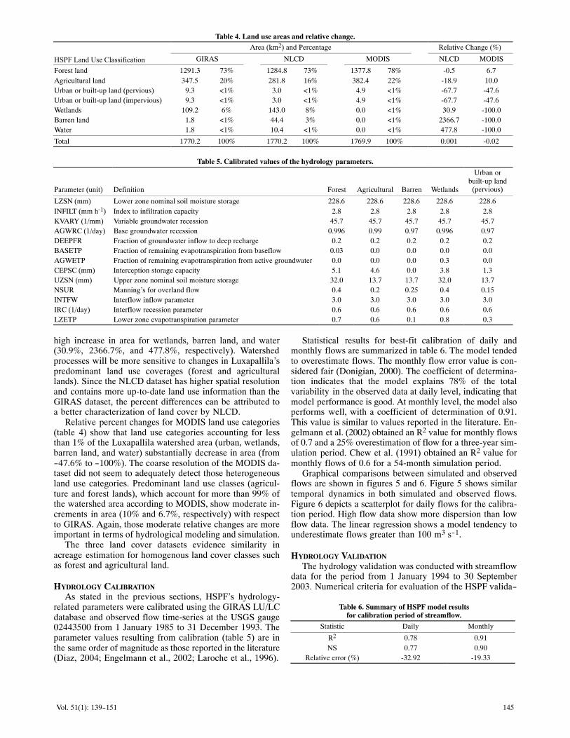
GIRAS' land use characterization of the Luxapallila wa‐tershed attributes more than 90% land coverage to forest andagricultural lands (73% and 20%, respectively), with otherland use categories (wetlands, urban, barren, etc.) accountingfor the remaining 7% (table 4). Although NLCD and MODISland use databases also show that more than 89% of the wa‐tershed is covered by forest and agricultural land, percent dif‐ferences exist in most land use classes, as shown in table 4.

Most NLCD land use categories decrease in area (table 4).Only wetlands, barren land, and water show increments.Table 4 shows that forest and agricultural lands present lowto moderate decreases in area (-0.5% and -18.9% respective‐ly) and a substantial decrease in urban areas (-67.7%). How‐ever, since urban areas account for less than 1% of theLuxapallila watershed area, this high relative change couldnot be expected to have big effects in the context of hydrolog‐ical modeling and simulation. The same can be said about the

145Vol. 51(1): 139-151

Table 4. Land use areas and relative change.

HSPF Land Use Classification

Area (km2) and Percentage Relative Change (%)

GIRAS NLCD MODIS NLCD MODIS

Forest land 1291.3 73% 1284.8 73% 1377.8 78% ‐0.5 6.7Agricultural land 347.5 20% 281.8 16% 382.4 22% ‐18.9 10.0Urban or built‐up land (pervious) 9.3 <1% 3.0 <1% 4.9 <1% ‐67.7 ‐47.6Urban or built‐up land (impervious) 9.3 <1% 3.0 <1% 4.9 <1% ‐67.7 ‐47.6Wetlands 109.2 6% 143.0 8% 0.0 <1% 30.9 ‐100.0Barren land 1.8 <1% 44.4 3% 0.0 <1% 2366.7 ‐100.0Water 1.8 <1% 10.4 <1% 0.0 <1% 477.8 ‐100.0

Total 1770.2 100% 1770.2 100% 1769.9 100% 0.001 ‐0.02

Table 5. Calibrated values of the hydrology parameters.

Parameter (unit) Definition Forest Agricultural Barren Wetlands

Urban orbuilt‐up land

(pervious)

LZSN (mm) Lower zone nominal soil moisture storage 228.6 228.6 228.6 228.6 228.6INFILT (mm h‐1) Index to infiltration capacity 2.8 2.8 2.8 2.8 2.8KVARY (1/mm) Variable groundwater recession 45.7 45.7 45.7 45.7 45.7AGWRC (1/day) Base groundwater recession 0.996 0.99 0.97 0.996 0.97DEEPFR Fraction of groundwater inflow to deep recharge 0.2 0.2 0.2 0.2 0.2BASETP Fraction of remaining evapotranspiration from baseflow 0.03 0.0 0.0 0.0 0.0AGWETP Fraction of remaining evapotranspiration from active groundwater 0.0 0.0 0.0 0.3 0.0CEPSC (mm) Interception storage capacity 5.1 4.6 0.0 3.8 1.3UZSN (mm) Upper zone nominal soil moisture storage 32.0 13.7 13.7 32.0 13.7NSUR Manning's for overland flow 0.4 0.2 0.25 0.4 0.15INTFW Interflow inflow parameter 3.0 3.0 3.0 3.0 3.0IRC (1/day) Interflow recession parameter 0.6 0.6 0.6 0.6 0.6LZETP Lower zone evapotranspiration parameter 0.7 0.6 0.1 0.8 0.3

high increase in area for wetlands, barren land, and water(30.9%, 2366.7%, and 477.8%, respectively). Watershedprocesses will be more sensitive to changes in Luxapallila'spredominant land use coverages (forest and agriculturallands). Since the NLCD dataset has higher spatial resolutionand contains more up‐to‐date land use information than theGIRAS dataset, the percent differences can be attributed toa better characterization of land cover by NLCD.

Relative percent changes for MODIS land use categories(table 4) show that land use categories accounting for lessthan 1% of the Luxapallila watershed area (urban, wetlands,barren land, and water) substantially decrease in area (from-47.6% to -100%). The coarse resolution of the MODIS da‐taset did not seem to adequately detect those heterogeneousland use categories. Predominant land use classes (agricul‐ture and forest lands), which account for more than 99% ofthe watershed area according to MODIS, show moderate in‐crements in area (10% and 6.7%, respectively) with respectto GIRAS. Again, those moderate relative changes are moreimportant in terms of hydrological modeling and simulation.

The three land cover datasets evidence similarity inacreage estimation for homogenous land cover classes suchas forest and agricultural land.

HYDROLOGY CALIBRATIONAs stated in the previous sections, HSPF's hydrology‐

related parameters were calibrated using the GIRAS LU/LCdatabase and observed flow time‐series at the USGS gauge02443500 from 1 January 1985 to 31 December 1993. Theparameter values resulting from calibration (table 5) are inthe same order of magnitude as those reported in the literature(Diaz, 2004; Engelmann et al., 2002; Laroche et al., 1996).

Statistical results for best‐fit calibration of daily andmonthly flows are summarized in table 6. The model tendedto overestimate flows. The monthly flow error value is con‐sidered fair (Donigian, 2000). The coefficient of determina‐tion indicates that the model explains 78% of the totalvariability in the observed data at daily level, indicating thatmodel performance is good. At monthly level, the model alsoperforms well, with a coefficient of determination of 0.91.This value is similar to values reported in the literature. En‐gelmann et al. (2002) obtained an R2 value for monthly flowsof 0.7 and a 25% overestimation of flow for a three‐year sim‐ulation period. Chew et al. (1991) obtained an R2 value formonthly flows of 0.6 for a 54‐month simulation period.

Graphical comparisons between simulated and observedflows are shown in figures 5 and 6. Figure 5 shows similartemporal dynamics in both simulated and observed flows.Figure 6 depicts a scatterplot for daily flows for the calibra‐tion period. High flow data show more dispersion than lowflow data. The linear regression shows a model tendency tounderestimate flows greater than 100 m3 s-1.

HYDROLOGY VALIDATION

The hydrology validation was conducted with streamflowdata for the period from 1 January 1994 to 30 September2003. Numerical criteria for evaluation of the HSPF valida-

Table 6. Summary of HSPF model resultsfor calibration period of streamflow.

Statistic Daily Monthly

R2 0.78 0.91NS 0.77 0.90

Relative error (%) ‐32.92 ‐19.33

146 TRANSACTIONS OF THE ASABE

0

1

10

100

1000

1 Jan.1985

16 May1986

28 Sept.1987

9 Feb.1989

24 June1990

6 Nov.1991

20 March1993

Time (date)

Simulated

Observed

Flo

w (

m3

s-1 )

Figure 5. Simulated and observed streamflows for the calibration period.

y = 1.11x - 2.70

R 2 = 0.78

0

100

200

300

400

500

600

700

800

900

1000

0 100 200 300 400 500 600 700 800 900 1000

1:1

Ob

serv

ed F

low

(m

3 s-

1 )

Simulated Flow (m3 s-1)

Figure 6. Scatterplot of observed versus simulated streamflows for the calibration period.

Table 7. Summary of HSPF model resultsfor validation period of streamflow.

Statistic Daily Monthly

R2 0.68 0.77NS 0.68 0.76

Relative error (%) ‐19.91 ‐13.83

tion results are included in table 7. In general, HSPF overesti‐mated streamflows during this period. Relative error valuescalculated in the validation period were smaller than errorvalues estimated for the calibration period. The HSPF perfor‐mance was fair on a daily basis, with NS and R2 values of68%. The agreement of the HSPF model at monthly levelswas good, with an R2 value of 77%.

Figure 7 shows similar temporal dynamics in both simu‐lated and observed flows. In figure 8, the daily HSPF model

simulation output is plotted against the observed streamflowfor the validation period. The HSPF model slightly overpre‐dicted flow values greater than 100 m3 s-1.

SEDIMENT CALIBRATIONTable 8 shows values of sediment‐related parameters that

were obtained during calibration. These values are in thesame order of magnitude as those reported in the literature(USEPA, 2006). Simulated annual sediment rates (ton ha-1)are reasonable as compared to observed values (table 9). Dif‐ferences could be, in part, a result of the variations in soiltypes between the Luxapallila watershed and the specificareas from which calibration data were taken. Soil erosionparameters related to wetland areas were adjusted to zero.

147Vol. 51(1): 139-151

0.1

1

10

100

1000

Simulated

Observed

1 Jan.1994

16 May1995

27 Sept.1996

9 Feb.1998

24 June1999

5 Nov.2000

20 March2002

Time (date)

2 Aug.2003

Flo

w (

m3

s-1 )

Figure 7. Simulated and observed streamflows for the validation period.

y = 0.94x + 2.73

R2 = 0.68

0

100

200

300

400

500

600

0 100 200 300 400 500 600

1:1

Ob

serv

ed F

low

(m

3 s-

1 )

Simulated Flow (m3 s-1)

Figure 8. Scatterplot of observed versus simulated streamflows for the validation period.

Table 8. Calibrated values of the sediment parameters.

Parameter (unit) Definition Forest Agricultural Barren Wetlands

Urban orbuilt‐up land

(pervious)

SMPF Management practice (P) factor from USLE 1 1 1 1 1KRER (complex) Coefficient in the soil detachment equation 0.35 0.75 0.4 0.0 0.35JRER Exponent in the soil detachment equation 2.0 2.0 2.0 2.0 2.0AFFIX (day) Daily reduction in the detached sediment 0.003 0.003 0.003 0.0 0.003COVER Fraction land surface protected from rainfall 0.9 0.6 0.0 1.0 0.6NVSI (kg/ha‐day) Atmospheric addition to sediment storage 0.0 0.0 0.0 0.0 0.0KSER (complex) Coefficient in soil matrix scour equation 1.5 10.0 10.0 0.0 4.0JSER Exponent in soil matrix scour equation 1.1 1.1 2.0 0.0 2.0KGER (complex) Coefficient in soil matrix scour equation 0.0 0.0 10.0 0.0 0.0JGER Exponent in soil matrix scour equation 0.0 0.0 2.2 0.0 0.0

148 TRANSACTIONS OF THE ASABE

Table 9. Comparison of simulated annual sediment rates withsoil erosion rates observed in Alabama and elsewhere in the U.S.

Cover

Soil Erosion Rate (ton ha‐1 year‐1)

Simulated Observed

Forest land 0.4 0.7Agricultural land 8.3 11.2‐31.1

Barren land 6.3 4.0‐9.0

Table 10. Components of average annual water balance frompervious and impervious areas (1 Jan. 1985 to 30 Sept. 2003).

Volume (km3) Relative Change (%)

Component GIRAS NLCD MODIS NLCD MODIS

Rainfall 46.59 46.37 46.63 ‐0.48 0.08

Actual evapo‐transpiration

26.46 26.42 26.46 ‐0.18 0.00

Total runoff 17.30 17.12 17.33 ‐1.02 0.20

Deep ground‐water

2.73 2.73 2.74 ‐0.10 0.26

Storage change 0.10 0.10 0.10 0.74 ‐3.04

SENSITIVITY EVALUATION AT THE HILLSLOPE SCALETable 10 shows a comparison of simulated annual water

budgets for the Luxapallila watershed. Relative changes fol‐low the same trend as changes in area in the predominant landuse classes (table 4). Rainfall, actual evapotranspiration, to‐tal runoff, and deep groundwater annual water volumeschange due to decreasing (NLCD) or increasing (MODIS)agricultural and forest land use areas. This is due to effectiverainfall areas assigned by BASINS/WinHSPF proportionallywith those predominant areas. Similar trend was estimated bythe model for actual evapotranspiration and total runoff com‐ponents. Actual evapotranspiration is the main mechanism ofwater loss in the Luxapallila watershed model (57%). Waterloss due to deep groundwater only represents 5.8%. Waterbalance components changed less than 3%.

The low relative change in percent values (table 10) is ex‐plained by the relatively small relative changes in forest andagriculture land cover areas among the GIRAS, NLCD, andMODIS databases. To explore further how the water loss isdistributed for each land use cover, the total water volumes(table 10) were partitioned into water losses per land covertype (table 11). Water losses due to forest cover representmore than 70% of total losses in each LU/LC database. Thismay also explain the insignificant change among LU/LC da‐tabases in water balance components in the LuxapallilaCreek model.

Table 12 shows annual sediment loads from selectedsources. In general, total soil erosion decreased 8.7% fromGIRAS to NLCD and increased 8.6% from GIRAS to MO‐DIS, primarily because the percentage of agricultural landwas smaller for the NLCD dataset and greater for the MODIS

Table 11. Percentage of annual water losses from each cover.

Database and HSPFLU Classification

ActualEvapotrans‐

pirationTotal

Runoff

DeepGround‐

water

GIRASForest 73.8 71.6 74.7Agriculture 19.0 20.9 18.6Wetlands 6.4 5.8 6.3Barren 0.1 0.1 0.0Urban or built‐up land

(pervious) 0.5 0.6 0.4(impervious) 0.2 1.1 0.0

NLCDForest 73.5 72.1 74.2Agriculture 15.4 17.1 15.2Wetlands 8.4 7.6 8.2Barren 2.4 2.7 2.2Urban or built‐up land

(pervious) 0.2 0.2 0.1(impervious) 0.1 0.3 0.0

MODISForest 78.7 76.2 79.3Agriculture 20.9 22.9 20.3Urban or built‐up land

(pervious) 0.2 0.3 0.4(impervious) 0.1 0.6 0.0

dataset, as compared to the GIRAS dataset. Agriculturalareas produced the highest sediment loads of any land useclass, contributing between 75% and 85% in each LU/LC da‐taset. This is consistent with results reported in the literature(Sonzogni et al., 1980; Laflen et al., 2004).

SENSITIVITY EVALUATION AT THE WATERSHED OUTLET

Figures 9 and 10 show scatterplots of simulated stream‐flow (FLOW) and total amount of sediment fraction con‐tained in outflow (ROSED). Both figures compare simulatedvalues using GIRAS versus NLCD and MODIS databases.Since streamflow does not show departure from the 1:1 line,simulated values of streamflow do not substantially changewhen land use databases are swapped. This is also shown intable 13, where descriptive statistics for streamflow (mean,standard deviation, and coefficient of variation) are almostidentical. Simulated ROSED values, however, show somevariance around the 1:1 line. Estimated ROSED values usingthe MODIS database are shown to be higher than those valuesestimated using GIRAS, while NLCD‐simulated ROSEDvalues tend to be smaller than GIRAS‐estimated values(fig.�10). Statistical indicators for ROSED (table 13) indicatethat NLCD land use produces ROSED values with highervariance than values generated using GIRAS and MODIS.Despite these differences, simulated ROSED values at the

Table 12. Annual sediment loads from selected sources.

HSPF LUClassification

GIRAS NLCD MODIS Relative Change (%)

Tons % Tons % Tons % NLCD MODIS

Forest 50,459.7 15 50,205.3 16 53,837.0 15 ‐0.50 6.69Agricultural 286,997.6 84 232,725.4 75 315,840.1 85 ‐18.91 10.05Urban (pervious) 1,926.9 <1 612.0 <1 1,009.9 <1 ‐68.24 ‐47.59Urban (impervious) 1,432.8 <1 455.1 <1 750.9 <1 ‐68.24 ‐47.59Wetlands 0.0 <1 0.0 <1 0.0 <1 ‐‐ ‐‐Barren 1,123.2 <1 28,133.7 9 0.0 <1 2,404.12 ‐100.00

Total 341,940.2 312,131.5 371,437.9 ‐8.72 8.63

149Vol. 51(1): 139-151

Flow Simulated Using GIRAS Land Use (m3 s-1)

Flo

w S

imu

late

d (

m3

s-1 )

Figure 9. Scatterplot of flow simulated using GIRAS versus NLCD and MODIS.

ROSED Simulated Using GIRAS Land Use (tons)

RO

SE

D S

imu

late

d (

ton

s)

Figure 10. Scatterplot of total amount of sediment fraction contained in outflow (ROSED) simulated using GIRAS versus NLCD and MODIS.

watershed outlet follow a similar trend as those calculated atthe hillslope scale, i.e., land use databases that identify morepresence of agricultural areas (MODIS and GIRAS) produceHSPF‐estimations of ROSED values bigger than land use da‐tabases that identify less presence of those land covers(NLCD).

Table 14 shows maximum, median, and minimum percentchanges for FLOW and ROSED after swapping land use da‐tabases. Again, the percent changes shown in this table arerelative to the simulated values of FLOW and ROSED withthe GIRAS database. Although the scatterplot for FLOW val‐ues does not show much variation from one database to the

Table 13. Evaluation of daily HSPF simulations usingGIRAS, NLCD and MODIS land uses in Luxapallila

Creek watershed (1 Jan. 1985 to 30 Sept. 2003).Constituent and Statistic GIRAS NLCD MODIS

StreamflowMean (m3 s‐1) 29.6 29.4 29.7SD (m3 s‐1) 43.5 43.4 43.4CV 1.5 1.5 1.5

Total outflows of sediments (ROSED)Mean (ton) 889.3 815.3 966.1SD (ton) 6,045.9 6,472.9 6,485.9CV 6.8 7.9 6.7

150 TRANSACTIONS OF THE ASABE

Table 14. Flow and total amount of sediment fraction containedin outflow (ROSED) effects of daily relative changes under

different LU/LC datasets (1 Jan. 1985 to 30 Sept. 2003).

Database ConstituentMaximum

(%)Minimum

(%)Median

(%)

NLCD FLOW 16.7 ‐1.1 0.8ROSED 100.0 ‐34.1 18.7

MODIS FLOW 22.3 ‐20.3 ‐0.7ROSED 100.0 ‐69.0 ‐9.7

Table 15. Daily total amount of sediment fraction (tons)contained in outflow (ROSED) at selected percentiles.

Database

Percentile

5th 25th 50th 75th 95th

GIRAS 0.0 0.06 2.5 38.0 2841.5NLCD 0.0 0.04 1.9 30.4 2349.2MODIS 0.0 0.05 2.5 40.5 3196.6

other, table 14 shows that relative differences range from-1.1% to 16.7% for NLCD and from -20.3% to 22.3% forMODIS. Median values of relative change are very low foreither database (less than ±1%). Despite these relativechange values for FLOW, the three time‐series are shown tohave significant differences. On the other hand, table 14shows that ROSED's maximum and minimum percentchanges are higher than ±34% for either database (reachingup to -69% for MODIS).

To further explore the differences produced in simulated sed‐iment (ROSED) values after swapping land use databases, se‐lected percentiles (calculated for each time‐series) are shown intable 15. Percentiles below the 75th show that there exist smallto moderate differences among predicted ROSED values whenswapping land use maps. The biggest dissimilarities are de‐tected for the upper quartile of the time series. This indicatesthat land use database swapping tended to generate more vari‐ability for high sediment loads. Since high sediment load gener‐ation is usually related with high streamflows, and thestreamflow calibration in this research shows that the model isless certain for high streamflow values, the model should be re‐fined for addressing this inconsistency.

CONCLUSIONSThis study evaluated the impact of three LU/LC datasets

on hydrology and sediment components of the HSPF modelfor the Luxapallila Creek watershed at the hillslope scale andthe watershed outlet. The HSPF model was successfullyadapted to model hydrological processes. The coefficient ofdetermination and the Nash‐Sutcliffe coefficient reachedvalues around 0.78 for daily streamflows after the hydrologi‐cal calibration process. Both coefficient values decreased forthe validation period (i.e., 0.68), but long‐term relative errorswere smaller. Although no sediment data were available forthe Luxapallila Creek watershed, annually integrated sedi‐ment values generated by the model compared reasonablywell, via calibration of sediment‐related parameter values, tosoil erosion rates found in the literature.

The comparison of land use datasets revealed that GIRAS,NLCD, and MODIS LU/LC classified more than 73% of thewatershed area as covered by forest and more than 16% cov-

ered by agricultural lands. Forest areas showed small changesamong databases. Larger percent differences in agriculturalareas were detected when comparing the NLCD and MODISdatasets to GIRAS (-8.9% and 10%, respectively). The data‐set with the lowest spatial resolution (MODIS) had the largestpercentage of agricultural land, while the dataset with thehighest spatial resolution (NLCD) estimated the least amountof agricultural land.

At hillslope scale, water balance components from forestareas (evapotranspiration, total runoff, and deep groundwa‐ter) accounted for between 70% and 80% of total water lossesin the Luxapallila model. Water losses from agriculturallands range around 20%; therefore, water losses in Luxapalli‐la are governed by the predominant land use covers (forestand agricultural lands). After swapping land use datasets, theHSPF model estimations did not show substantial changes inthe water balance components and streamflow for long peri‐ods (e.g., annual or total period). However, on a daily timestep, streamflow variations between 16.7% and -1.1% werecalculated when NLCD was used as input, compared to simu‐lations using GIRAS. Using the same base of comparison(GIRAS‐simulated streamflows), larger daily differences(22.3% and -20.3%) were calculated for MODIS.

Comparison of simulated annual sediment rates from for‐est, agriculture, and barren land covers are shown to be in thesame order of magnitude as those reported in the literature forthe region. At the hillslope scale, the LU/LC datasets gener‐ated noticeable differences in simulated values of total frac‐tion of sediments when swapping LU/LC datasets. Theanalysis shows that agricultural areas produce the highestsediment loads, contributing between 75% and 85% witheach LU/LC dataset. At the watershed outlet, the totalamount of sediment fraction contained in outflow values fol‐lows a similar trend as at the hillslope scale, i.e., land use da‐tasets that identify more presence of agricultural areas(MODIS and GIRAS) produce HSPF estimations of total sed‐iment fraction values bigger than land use databases thatidentify less presence of those land covers (NLCD). In thecase of hydrology simulation, forest cover mechanisms werethe main source of water losses, but in sediment modeling,agricultural land was the main source of sediment export(i.e., between 70% and 80% of total sediments).

Land use datasets of coarser spatial resolution (MODISand GIRAS) produced larger HSPF estimations for sedimentfraction values than land use datasets identifying smaller per‐centages of those agricultural land cover classes (NLCD).Thus, sediment predictions were more sensitive than stream‐flow predictions to the scale and resolution of land use data‐sets. These results are significant for the modeling ofwatershed processes in watersheds where agricultural landsare important. Choosing the right land use dataset will impactthe modeling of sediments and (potentially) other water qual‐ity constituents that are related with agricultural activities.

ACKNOWLEDGEMENTSThis work was supported by the NASA Science Mission

Directorate, Earth Science Division, Applied SciencesProgram as part of a Crosscutting Solutions contract toMississippi State University through Stennis Space Center.We would also like to thank the tutors of the ShackoulsTechnical Communication Program, Bagley College ofEngineering, Mississippi State University, for their time andeffort in reviewing the technical English of the manuscript.

151Vol. 51(1): 139-151

REFERENCESAnantharaj, V., P. J. Fitzpatrick, Y. Li, R. King, and E. Johnson.

2006. Influences of MODIS land use data on a gulf coast seabreeze simulation. In Proc. 10th Symposium on IntegratedObserving and Assimilation Systems for the Atmosphere,Oceans, and Land Surface (IOAS‐AOLS). Washington, D.C.:American Meteorological Society.

Bicknell, B. R., J. C. Imhoff, J. L. Kittle, T. H. Jobes, and A. S.Donigian. 2001. Hydrological simulation program - Fortran(HSPF) version 12: User's manual. Prepared for AQUA TERRAConsultants Mountain View, Cal., in cooperation with USGSWater Resources Discipline, Reston, Va., and U.S.Environmental Protection Agency, Athens, Ga.

Chew, C. R., L. W. Moore, and R. H. Smiths. 1991. Hydrologicalsimulation of Tennessee's North Reelfoot Creek watershed. Res.J. Water Pollution Control Fed. 63(10): 10‐16.

Diaz, J. N. 2004. Modeling sediment export potential of the RioCaonillas watershed. MS thesis. Puerto Rico: University ofPuerto Rico.

Donigian, A. S., Jr. 2000. HSPF training workshop handbook andCD: Lecture 19. Calibration and verification issues, slideL19‐22. Washington, D.C.: U.S. EPA, Office of Water, Office ofScience and Technology.

Endreny, T. A., C. Somerlot, and J. M. Hassett. 2003. Hydrographsensitivity to estimates of map impervious cover: A WinHSPFBASINS case study. Hydrol. Process. 17(5): 1019‐1034.

Engel, E. A., J. Choi, J. Harbor, and S. Pandey. 2003. Web‐basedDSS for hydrologic impact evaluation of small watershed landuse changes. Computers and Electronics in Agric. 39(3):241‐249.

Engelmann, C. J. K., A. D. Ward, A. D. Christy, and E. S. Bair.2002. Application of the BASINS database and NPSM modelon a small Ohio watershed. J. American Water Resources Assoc.38(1): 289‐300.

Grace, J. M. 2004. Soil erosion following forest operations in thesouthern piedmont of central Alabama. J. Soil and Water Cons.59(4): 160‐166.

Hairston, J., K. Edmisten, and J. LaPrade. 1990. Important waterquality and quantity issues facing Alabama agriculturalproducers. Auburn, Ala.: Auburn University, ExtensionEnvironmental Educational.

Kittle, J. L., R. Dusenbury, P. R. Hummel, P. B. Duda, and M. H.Gray. 2001. A tool for the generation and analysis of modelsimulation scenarios for watersheds (GenScn): User's manual forrelease 2.0. Washington, D.C.: U.S. Environmental ProtectionAgency, Office of Science and Technology and Office of Water.

Laflen, J. M., D. C. Flanagan, and B. A. Engel. 2004. Soil erosionand sediment yield prediction accuracy using WEPP. J.American Water Resources Assoc. 40(2): 289‐297.

Laroche, A., J. Gallichand, R. Lagacé, and A. Pesant. 1996.Simulating atrazine transport with HSPF in an agriculturalwatershed. J. Environ. Eng. 122(7): 622‐630.

Larson, W. E., F. J. Pierce, and R. H. Dowdy. 1985. Loss inlong‐term productivity from soil erosion in the United States. InSoil Erosion and Conservation, 262‐271. S. A. El‐Swaify, W. C.Moldenhauer, and A. Lo, eds. Ankeny, Iowa: Soil ConservationSociety of America.

Legates, D. R., and G. J. McCabe, Jr. 1999. Evaluating the use of“goodness‐of‐fit” measures in hydrologic and hydroclimaticmodel validation. Water Resources Res. 35(1): 233‐241.

McAnally, W. H., J. L. Martin, J. N. Diaz, Z. Duan, C. A. Mancilla,M. L. Tagert, C. O'Hara, and J. A. Ballweber. 2005.Assimilating remotely sensed data into hydrologic decisionsupport systems: BASINS evaluation. Mississippi State, Miss.:Mississippi State University, Department of Civil Engineeringand GeoResources Institute.

Moglen, G. E., and R. E. Beighley. 2002. Spatially explicithydrologic modeling of land use change. J. American WaterResources Assoc. 38(1): 241‐253.

Morgan, R. P. C. 2005. Soil Erosion and Conservation. Oxford,U.K.: Blackwell Science.

Nash, J. E., and J. V. Sutcliffe. 1970. River flow forecasting throughconceptual models: Part I. A discussion of principles. J.Hydrology 10(3): 282‐290.

Sonzogni, W. C., G. Chesters, D. R. Coote, D. N. Jeffs, J. C.Konrad, R. C. Ostry, and J. B. Robinson. 1980. Pollution fromland runoff. Environ. Sci. and Tech. 14(2): 148‐153.

Tong, S. T. Y., and W. Chen. 2002. Modeling the relationshipbetween land use and surface water quality. J. Environ. Mgmt.66(4): 377‐393.

USEPA. 1994. GIRAS land use/land cover data for theconterminous United States by quadrangles at scale 1:250,000.Washington, D.C.: U.S. Environmental Protection Agency,Office of Information Resources Management (OIRM).Available at:www.epa.gov/waterscience/basins/metadata/giras.htm. Accessed20 February 2004.

USEPA. 2000. EPA BASINS technical note 6: Estimatinghydrology and hydraulic parameters for HSPF.EPA‐823‐R00‐012. Washington, D.C.: U.S. EnvironmentalProtection Agency. Available at: www.epa.gov/waterscience/basins/docs/tecnote6.pdf. Accessed 24 February 2004.

USEPA. 2001. Better assessment science integrating point andnonpoint sources: BASINS version 3.0, user's manual. EPAPublication EPA‐823‐B‐01‐001. Washington, D.C.: U.S.Environmental Protection Agency, Office of Water.

USEPA. 2004. Training “flow validation tutorial”. Washington,D.C.: U.S. Environmental Protection Agency. Available at:www.epa.gov/waterscience/ftp/basins/training/tutorial/di.htm.Accessed 24 February 2004.

USEPA. 2006. EPA BASINS technical note 8: Sediment parameterand calibration guidance for HSPF. Washington, D.C.: U.S.Environmental Protection Agency. Available at:www.epa.gov/waterscience/basins/docs/tecnote8.pdf. Accessed6 March 2006.

USGS. 2004. The USGS Land Cover Institute (LCI): National landcover data. Washington, D.C.: U.S. Geological Survey.Available at: land cover.usgs.gov/prodescription.php. Accessed20 February 2004.

Whitehead, P. G., P. J. Johnes, and D. Butterfield. 2002.Steady‐state and dynamic modeling of nitrogen in the RiverKennet: Impacts of land use change since the 1930s. Sci. TotalEnviron. 282‐283: 417‐434.

152 TRANSACTIONS OF THE ASABE