Impact of the alignment between the strategic and operational levels of a manufacturing enterprise

International Journal of Production ResearchVol. 48, No. 4, 15 February 2010, 1195–1215

Impact of the alignment between the strategic and operational levels of

a manufacturing enterprise

Cesar Martinez-Olvera*

Department of Industrial Engineering, Tecnologico de Monterrey, Hermosillo, Sonora, Mexico

(Received 12 February 2008; final version received 26 September 2008)

In today’s economic environment, manufacturing organisations compete againsteach other as part of supply chains (SC). As both the SC strategic level andproduction floor operational level are interdependent, a misalignment betweenthem has a deep impact on the performance of the manufacturing organisation.For this reason, in this paper we develop an analytical expression of the impactsuch misalignment has on the manufacturing organisation performance,specifically, its demand fulfillment ability. The usefulness of the analyticalexpression is illustrated via the development, for the case of a local furniturecompany, of a system dynamics (SD) simulation model. The SD simulation modelis tested under different operational conditions, so the case study company canderive conclusions regarding actions to improve its demand fulfillment ability.

Keywords: capacity management; demand fulfillment; inventory management;manufacturing strategy; simulation

1. Introduction

According to Ismail and Sharifi (2006), competition among manufacturing enterprises isfought between supply chains (SC). In this scenario, competitiveness becomes somethingholistic (Duclos et al. 2003), as the satisfaction of the end customer is determined by theeffectiveness and efficiency of the SC as a whole (Terzi and Cavalieri 2004). This requireseach SC partner to realign their structural elements (Vernadat 2002), more specifically, itbecomes necessary for the alignment of activities, from the strategic level through to theoperational level (Angelides and Angerhofer 2006). Authors like Rao and Young (1994),Lamming et al. (2000), Huang et al. (2002), Jonsson and Mattsson (2003), Olhager (2003),Balogun et al. (2004), and Petersen et al. (2005) highlight the need for linking the strategiclevel (i.e., customer, demand issues) and the operational level (i.e., process flow, equipmenttechnology issues) of a manufacturing organisation, as it has been noticed that both thelevels are interdependent. In fact, the decisions taken at the strategic level have a deepimpact at the operational level (Son and Venkateswaran 2005), and the correct

*Email: [email protected]

ISSN 0020–7543 print/ISSN 1366–588X online

� 2010 Taylor & Francis

DOI: 10.1080/00207540802534723

http://www.informaworld.com

management of the operational level has a big impact on the efficiency of the strategic level

(Khoo and Yin 2003). So, even though strategic issues are important to achieve

responsiveness to market changes, they are not sufficient without achieving responsiveness

at the operational level (Zhang et al. 2006). In this paper we understand the strategic and

operational levels of a manufacturing organisation, in terms of the customer-product-

process resource (CPPR) framework proposed by Martinez-Olvera and Shunk (2006): the

strategic level of a manufacturing enterprise corresponds to the customer level of the

CPPR framework, while the operational level corresponds to the process level of the

CPPR framework.

1.1 Alignment relationships of the strategic – operational levels

Within the CPPR framework, the structural elements of an SC partner are referred as SC

structural elements: the customer, product, process, and resource attributes of

a manufacturing organisation that allows its representation from an SC standpoint.

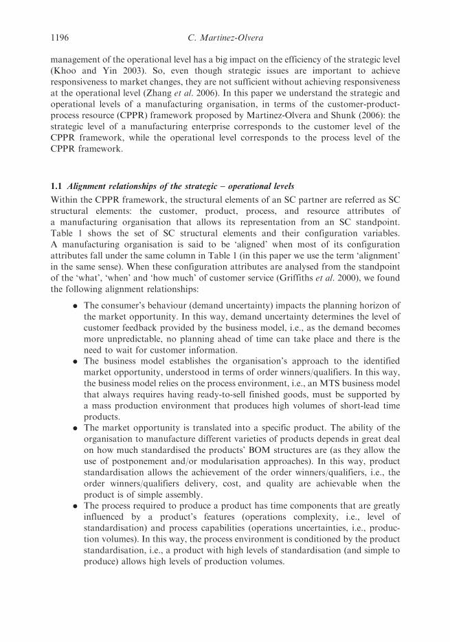
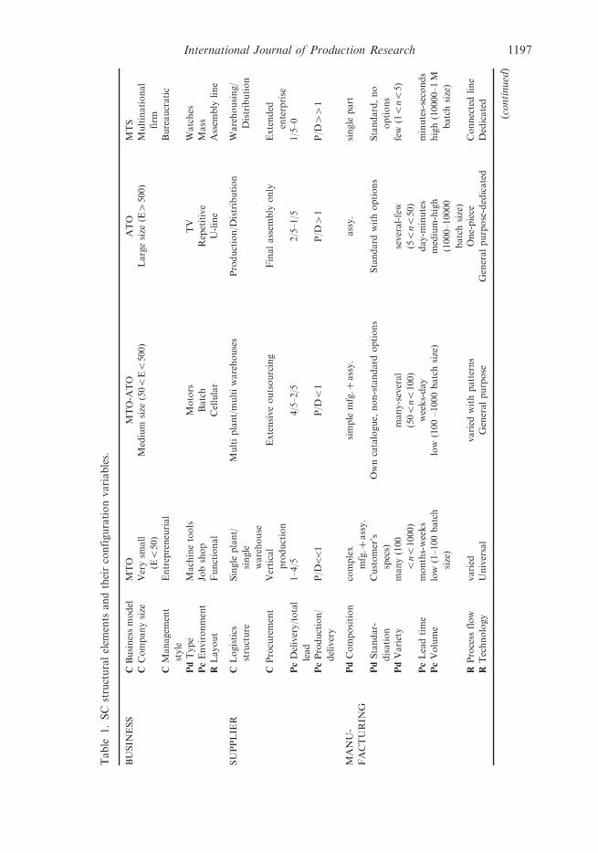
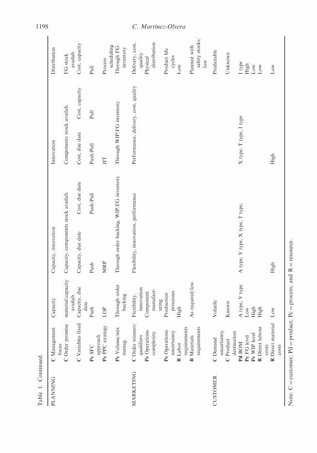
Table 1 shows the set of SC structural elements and their configuration variables.

A manufacturing organisation is said to be ‘aligned’ when most of its configuration

attributes fall under the same column in Table 1 (in this paper we use the term ‘alignment’

in the same sense). When these configuration attributes are analysed from the standpoint

of the ‘what’, ‘when’ and ‘how much’ of customer service (Griffiths et al. 2000), we found

the following alignment relationships:

. The consumer’s behaviour (demand uncertainty) impacts the planning horizon of

the market opportunity. In this way, demand uncertainty determines the level of

customer feedback provided by the business model, i.e., as the demand becomes

more unpredictable, no planning ahead of time can take place and there is the

need to wait for customer information.. The business model establishes the organisation’s approach to the identified

market opportunity, understood in terms of order winners/qualifiers. In this way,

the business model relies on the process environment, i.e., an MTS business model

that always requires having ready-to-sell finished goods, must be supported by

a mass production environment that produces high volumes of short-lead time

products.. The market opportunity is translated into a specific product. The ability of the

organisation to manufacture different varieties of products depends in great deal

on how much standardised the products’ BOM structures are (as they allow the

use of postponement and/or modularisation approaches). In this way, product

standardisation allows the achievement of the order winners/qualifiers, i.e., the

order winners/qualifiers delivery, cost, and quality are achievable when the

product is of simple assembly.. The process required to produce a product has time components that are greatly

influenced by a product’s features (operations complexity, i.e., level of

standardisation) and process capabilities (operations uncertainties, i.e., produc-

tion volumes). In this way, the process environment is conditioned by the product

standardisation, i.e., a product with high levels of standardisation (and simple to

produce) allows high levels of production volumes.

1196 C. Martinez-Olvera

Table

1.SC

structuralelem

ents

andtheirconfigurationvariables.

BUSIN

ESS

CBusinessmodel

MTO

MTO-A

TO

ATO

MTS

CCompanysize

Verysm

all

(E5

50)

Medium

size

(505E5500)

Largesize

(E4

500)

Multinational

firm

CManagem

ent

style

Entrepreneurial

Bureaucratic

PdType

Machinetools

Motors

TV

Watches

PcEnvironment

Jobshop

Batch

Repetitive

Mass

RLayout

Functional

Cellular

U-line

Assem

bly

line

SUPPLIE

RC

Logistics

structure

Single

plant/

single

warehouse

Multiplant/multiwarehouses

Production/D

istribution

Warehousing/

Distribution

CProcurement

Vertical

production

Extensiveoutsourcing

Finalassem

bly

only

Extended

enterprise

PcDelivery/total

lead

1–4/5

4/5–2/5

2/5–1/5

1/5–0

PcProduction/

delivery

P/D551

P/D

51

P/D

41

P/D

44

1

MANU-

FACTURIN

G

PdComposition

complex

mfg.þ

assy.

simple

mfg.þ

assy.

assy.

single

part

PdStandar-

disation

Customer’s

specs)

Owncatalogue,

non-standard

options

Standard

withoptions

Standard,no

options

PdVariety

many(100

5n5

1000)

many-several

(505

n5100)

several-few

(55n550)

few

(15

n5

5)

PcLeadtime

months-weeks

weeks-day

day-m

inutes

minutes-seconds

PcVolume

low

(1–100batch

size)

low

(100–1000batchsize)

medium-high

(1000–10000

batchsize)

high(10000–1M

batchsize)

RProcess

flow

varied

varied

withpatterns

One-piece

Connectedline

RTechnology

Universal

Generalpurpose

Generalpurpose-dedicated

Dedicated

(continued)

International Journal of Production Research 1197

Table

1.Continued.

PLANNIN

GC

Managem

ent

focus

Capacity

Capacity,innovation

Innovation

Distribution

COrder

promise

material/capacity

availab.

Capacity,components

stock

availab.

Components

stock

availab.

FG

stock

availab.

CVariablesfixed

Capacity,due

date

Capacity,duedate

Cost,duedate

Cost,duedate

Cost,capacity

Cost,capacity

PcSFC

approach

Push

Push

Push/Pull

Push/Pull

Pull

Pull

PcPPC

strategy

LOP

MRP

JIT

Process

scheduling

PcVolume/mix

manag.

Throughorder

backing

Throughorder

backing,WIP/FG

inventory

ThroughWIP/FG

inventory

ThroughFG

inventory

MARKETIN

GC

Order

winners/

qualifiers

Flexibility,

innovation

Flexibility,innovation,perform

ance

Perform

ance,delivery,cost,quality

Delivery,cost,

quality

PcOperations

complexity

Component

manufact-

uring

Physical

distribution

PcOperations

uncertainty

Production

processes

Product

life

cycles

RLabor

requirem

ents

High

Low

RMaterials

requirem

ents

Asrequired/low

Planned

with

safety

stocks/

low

CUSTOMER

CDem

and

uncertainty

Volatile

Predictable

CProduct

destination

Known

Unknown

PdBOM

Atype,

Vtype

Atype,

Vtype,

Xtype,

Ttype,

Xtype,

Ttype,

Itype

Itype

PcFG

level

Low

High

PcWIP

level

High

Low

RDirectlabour

costs

High

Low

RDirectmaterial

costs

Low

High

High

Low

Note:C¼customer;Pd¼product;Pc¼process;andR¼resource.


It must be noted that there are four recurrent configuration attributes present in

these within-and-among alignment conditions: demand uncertainty, business model,

product standardisation, and process environment flexibility. In the next section we use

these four configuration attributes to derive an analytical expression of the impact the

strategic-operational levels alignment have on the performance of the manufacturing

organisation. Section 3 illustrates the usefulness of the analytical expression via the

development of a simulation model, Section 4 shows the sensitivity analysis performed

over the proposed simulation model, and Section 5 closes with the conclusions and

future research.

2. Analytical expression of the alignment impact

According to Chen (2008), the performance of a manufacturing organisation can be

expressed in terms such as customer satisfaction, product quality, speed in completing

manufacturing orders, productivity, diversity of product line, flexibility in manufacturing

new products, etc. In this paper we use demand fulfilment – understood as the achievement

of the demanded volume – as it relates to the four configuration attributes of the previous

section:

. Demand uncertainty (U ); according to Safizadeh and Ritzman (1997),

when demand uncertainty is low, an MTS business model is recom-

mended. When demand uncertainty is high, an MTO business model is

recommended.. Business model (BM); according to (Gupta and Benjaafar 2004), in an MTS

business model production planning is made on forecast (rather than actual

orders), allowing to produce ahead of time, keep stock, and ship upon receipt

of orders. According to Buxey (2003), when using this business model, an

inventory-oriented level strategy should be used, where a steady production is

maintained and finished goods inventory is used to absorb ongoing

differences between output and sales. In the case of the MTO business

model, according to (Gupta and Benjaafar 2004), production planning is

made on actual orders (rather than on forecast), allowing elimination of

finished goods inventories. When using this business model, a capacity-

oriented chase strategy should be used (Buxey 2003), where the expected

demand is tracked and the corresponding capacity is computed, raising it or

lowering it accordingly.. Process environment flexibility (F); according to Safizadeh and Ritzman (1997),

when following a level strategy, a rigid continuous production line should be used.

When following a chase strategy, a flexible job shop should be used.. Product standardisation (S ); according to Miltenburg (1995), a continuous

production line uses special-purpose equipment – grouped around the

product – to profitably manufacture high-volumes of standardised products.

In the case of the of the job shop, it uses general-purpose equipment –

grouped around the process – to profitably manufacture low-volumes of

customised products.

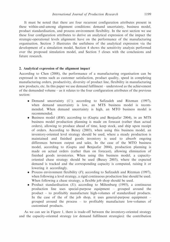
As we can see in Figure 1, there is trade-off between the inventory-oriented strategy

and the capacity-oriented strategy (or demand fulfilment strategies): the contribution


increase/decrease of one implies the contribution decrease/increase of the other. This can

be express in an analytical way:

. When uncertainty U is low (0), business model BM is MTS (0), standardisation

S is high (1), and flexibility F is low (0), demand is fulfilled 100% from inventory

(Equation (1)):

Inventory contribution to demand fulfilment

¼ D � ð1�U Þ � ð1� BMÞ �S � ð1� FÞ: ð1Þ

. When uncertainty U is high (1), business model BM is MTO (1), standardisation S

is low (0), and flexibility F is high (1), demand is fulfilled 100% from capacity

(Equation (2)):

Capacity contribution to demand fulfilment

¼ D �U �BM � ð1� S Þ �F: ð2Þ

In this way, demand fulfilment would be the sum of the contributions made by the

inventory-oriented and capacity-oriented strategies: for a totally aligned scenario (left or

right sides of Figure 1), demand will be fulfilled by a 100% inventory-oriented or 100%capacity-oriented strategy; for a misaligned scenario, demand will be fulfilled by

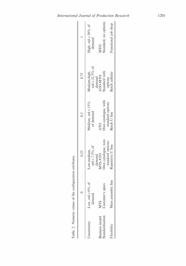
a combination of both strategies. Table 3 presents all the different combinations of limit

conditions (that is, the 0 s or 1 s in Table 2), for a demand level of 100 units. As we can see,

Equations (1) and (2) represent accurately the trade-off between the demand fulfilment

strategies. Note, when the demand fulfilment is equal to zero it means that even though

some level of production takes place, the achieved demand volume is really low – when

compared to the demanded volume – that it can be considered to be zero. For example, if

demand is equal to 100 units, there is high uncertainty in the demand (U¼ 1), the business

model used is MTO (BM¼ 1), the product is totally standardised (S¼ 1), and it uses

a functional job shop (F¼ 1). Here the high uncertainty of the demand requires waiting for

customer feedback (provided by the MTO business model). However, the totally

standardised product is characterised by using simple manufacturing and/or assembly

operations (that take a really short time). In this case, the functional job shop used would

affect the fulfilment of the 100 units, by presenting two obstacles to the flow of theprocess: (1) the set up times proper of the universal equipment used (very long compared

to the production run); and (2) the moving time from one operation to the next (as all the

equipment is grouped based on their functionality). In this way, the analytical expression

of the alignment impact cannot be taken as an estimator of the final values of the fulfilled

demand, but instead, as an indicator of the feasibility of the manufacturing organisation to

Inventory-orientedstrategy

Capacity-orientedstrategy

BM =0U=0

S =1 F=0

BM= 1U =1

S =0 F =1

Figure 1. Demand fulfilment relationships.


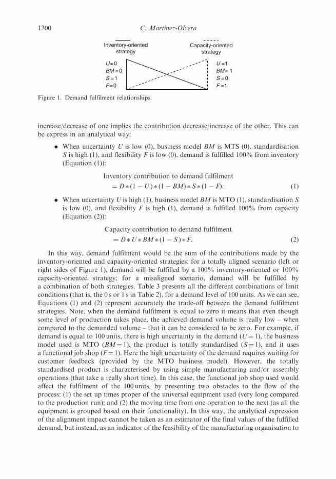
Table

2.Numeric

values

oftheconfigurationattributes.

00.25

0.5

0.75

1

Uncertainty

Low,std¼0%

of

dem

and

Low-m

edium,

std¼7.5%

of

dem

and

Medium,std¼15%

ofdem

and

Medium-high,

std¼22.5%

of

dem

and

High,std¼30%

of

dem

and

Businessmodel

MTS

MTS-A

TO

ATO

ATO-M

TO

MTO

Standardisation

Customer’sspecs

Owncatalogue,

non-

standard

options

Owncatalogue,

with

standard

options

Standard

with

options

Standard,nooptions

Flexibility

Mass

assem

bly

line

RepetitiveU

line

BatchU

line

Batchcellular

Functionaljobshop


Table

3.Resultsfordifferentcombinationsoflimitconditions.

Dem

andfulfilmentstrategy

100%

inventory-

oriented

100%

capacity-

oriented

D100

100

100

100

100

100

100

100

100

100

100

100

100

100

100

100

U0

10

00

11

10

00

11

10

1BM

00

10

01

00

11

01

10

11

S0

00

10

01

01

01

10

11

1F

00

00

10

01

01

10

11

11

Equation(1)result

00

0100

00

00

00

00

00

00

Equation(2)result

00

00

00

00

00

00

100

00

0


achieve the demanded volume (or demand fulfilment feasibility indicator): the closer thisindicator is to the demand volume, the more feasible it will be for the manufacturingorganisation to achieve the demanded volume.

Before proceeding to the next section, it must be noted that the customer service andthe demand fulfilment relationships (presented in the previous sections), are well-knownfacts – for production managers and industrial engineers – that have been reportedpreviously in the literature. What we consider to be an original contribution of this paperis taking these well-known facts of production engineering, and putting them in the formof the demand fulfilment feasibility indicator, an analytical expression that relates thedegree of alignment (between the structural and operational levels) with demandfulfilment. Martinez-Olvera (2008a), presented two similar demand fulfilment equationsthat only considered the uncertainty and business model configuration attributes. In ourproposal, we extend that work by including the standardisation and flexibilityconfiguration attributes. The next section presents the practical applications (andtherefore its usefulness) of the derived analytical expression.

3. Practical application of the demand fulfilment feasibility indicator

3.1 Case study

Company ABC is a local furniture company with a reputation for manufacturing highquality products. Within its production site, the plant-within-a-plant approach has beenfollowed, so manufacturing cells – using mostly general purpose equipment – have beenimplemented. Its catalogue has no more than 30 different products, and these can begrouped into three product families: (1) eight-seater plus dinner tables, (2) modularkitchens, and (3) semi-finished bedroom furniture (drawers, closets, etc.). For each of theproducts within a family, the typical batch size is kept within the range of a dozen (or less).In order to assure its success in the furniture industry, Company ABC has implementeda series of company-wide initiatives: the marketing department has established flexibilityand innovation as a top priority of Company ABC; the logistics department is required tohave products stocked in a ready-to-assembly condition and only assembles them to meetthe orders; the production department has implemented the one-piece flow principles, withthe idea of supporting the logistics demand of having ready-to-assembly products (becauseof this, the production site is performing in-house only simple manufacturing andassembly operations, and outsourcing the rest); the finance department has establishedthe policy of accepting orders from customers based only on the on-hand levels of ready-to-assembly components.

As a result of the implementation of the company-wide initiatives, Company ABC isfacing some unforeseen problems: the strategy of having products stocked in a ready-to-assemble condition (for a somewhat predictable market demand) is supported by onlyone product family of the catalogue (modular kitchens). However, the rest of the productfamilies do not support such strategy, but on the other hand, are ideal for the productionenvironment used by Company ABC (even though the distribution of the equipment onthe production floor is not the ideal). Also, this strategy would allow Company ABC toexcel in the areas of performance, delivery, cost, and quality, as the organisation focuseson the assembly part of the process, and accepts orders based only on the on-hand levels ofready-to-assembly components. However, the desired flexibility and innovation require-ments will be hard to achieve under these conditions.


The impact these policies have on Company ABC’s performance, can be evaluatedusing the following values (from Table 2):

. U¼ 0.25, for a somewhat predictable market demand.

. BM¼ 0.5, for having products stocked in a ready-to-assemble condition.

. S¼ 0.25, for the offered own catalogue – non-standard options.

. F¼ 0.75, for the use of manufacturing cells.

In this way, for a demand level of 100 units, the demand fulfilment feasibility indicatorshows a total value of 9.37 (meaning that Company ABC has a really hard time trying toachieve the demanded volume of 100 units):

Inventory contribution ¼ 100 � ð1� 0:25Þ � ð1� 0:5Þ � 0:25 � ð1� 0:75Þ ¼ 2:34

Capacity contribution ¼ 100 � 0:25 � 0:5 � ð1� 0:25Þ � 0:75 ¼ 7:03 ¼ 7:03

Total ¼ 9:37:

At this point, Company ABC needs to explore the possibility of making someadjustments to their policies, by migrating from their current alignment conditions to newones. This migration process implies either increasing or decreasing some of the businessmodel, standardisation, and/or flexibility values. Examples of such migration process canbe found in Martinez-Olvera and Shunk (2006) and Martinez-Olvera (2008b). Thequestion becomes then which values to increase/decrease and in what amount. Analternative to Company ABC having to answer these questions is the development ofa simulation model that guides its search for more advantageous alignment conditions.Some important business applications of simulation within SC scenarios are:

. Provide a means to evaluate the impact of policy changes and to answer ‘what if ?’and ‘what’s best?’ questions (Shah et al. 2004).

. Are useful for performance prediction (Towill 1996) and for representing timevarying behaviour (Venkateswaran and Son 2004).

. Is maybe the only approach for analysing the complex and comprehensivestrategic level issues that need to consider the tactical and operational levels,(Zhao et al. 2002).

In this paper we follow a similar approach to the one presented in Longo and Mirabelli(2008), where a discrete event simulation model (of a supply chain) is implemented and anapplication example is proposed for a better understanding of the simulation modelpotential. In our case, we use Equations (1) and (2) to develop a systems dynamics (SD)simulation model – SD is one of the four simulation types mentioned by Kleijnen (2005) –and use the situation of Company ABC as an application example. In case Company ABCwanted to use the simulation model as a decision making tool, then a design of experiment(DOE) or an analysis of variance (ANOVA) could be used to perform the statisticalanalysis of the output, as the result of the decision making process depends on howexperiments are planned and how experiments results are analysed.

3.2 Simulation model of the case study

Based on Equations (1) and (2), an SD simulation model was built using the simulationsoftware iThink (1996). An SD simulation model is a system thinking approach that is notdata driven, and that focuses on how the structure of a system and the policies taken affect


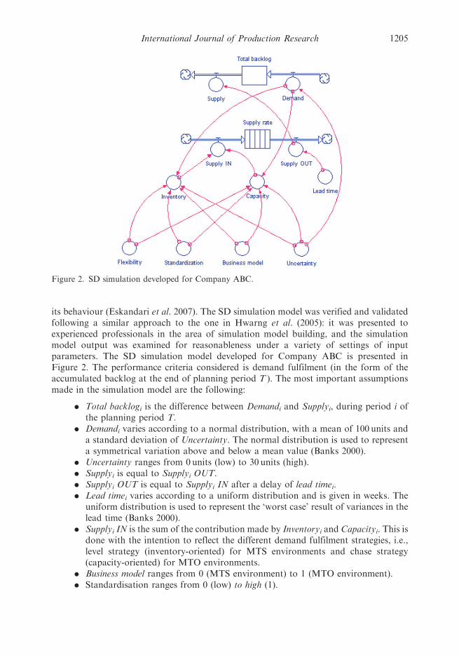
its behaviour (Eskandari et al. 2007). The SD simulation model was verified and validatedfollowing a similar approach to the one in Hwarng et al. (2005): it was presented toexperienced professionals in the area of simulation model building, and the simulationmodel output was examined for reasonableness under a variety of settings of inputparameters. The SD simulation model developed for Company ABC is presented inFigure 2. The performance criteria considered is demand fulfilment (in the form of theaccumulated backlog at the end of planning period T ). The most important assumptionsmade in the simulation model are the following:

. Total backlogi is the difference between Demandi and Supplyi, during period i ofthe planning period T.

. Demandi varies according to a normal distribution, with a mean of 100 units anda standard deviation of Uncertainty. The normal distribution is used to representa symmetrical variation above and below a mean value (Banks 2000).

. Uncertainty ranges from 0units (low) to 30 units (high).

. Supplyi is equal to Supplyi OUT.

. Supplyi OUT is equal to Supplyi IN after a delay of lead timei.

. Lead timei varies according to a uniform distribution and is given in weeks. Theuniform distribution is used to represent the ‘worst case’ result of variances in thelead time (Banks 2000).

. Supplyi IN is the sum of the contribution made by Inventoryi and Capacityi. This isdone with the intention to reflect the different demand fulfilment strategies, i.e.,level strategy (inventory-oriented) for MTS environments and chase strategy(capacity-oriented) for MTO environments.

. Business model ranges from 0 (MTS environment) to 1 (MTO environment).

. Standardisation ranges from 0 (low) to high (1).

Figure 2. SD simulation developed for Company ABC.


. Flexibility ranges from 0 (low) to high (1).

. Inventoryi is equal to Equation (1):

Demand � ð1�UncertaintyÞ � ð1� Business modelÞ

�Standardisation � ð1� FlexibilityÞ:

. Capacity Pi is equal to Equation (2):

Demand �Uncertainty �Business model

� ð1� StandardisationÞ �Flexibility:

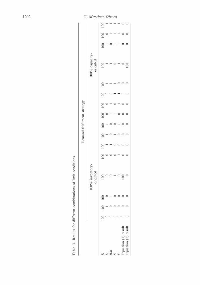
4. Sensitivity analysis

In order to study the effect of varying the level of demand uncertainty and lead time

variation, 1875 different scenarios were tested:

. Uncertainty levels of 0, 7.5, 15, 22.5, and 30. As it was stated previously, these

values represent the standard deviation (given in units) of the normal distribution

used to represent the demand variation.. Business model, Standardisation, and Flexibility levels of 0, 0.25, 0.5, 0.75, and 1

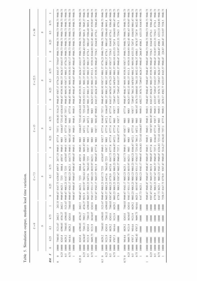
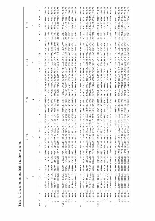
(see Table 2).. Lead time levels of uniform (1, 1), uniform (1, 3), and uniform (1, 5). In a uniform

distribution, values spread uniformly between a minimum and a maximum value.

In this way, uniform (1, 1) represent a low lead time variation (no variation),

uniform (1, 3) represent medium lead time variation (values spread between 1 and

3weeks), and uniform (1, 5) represent a high lead time variation (values spread

between 1 and 5weeks).

For a planning period T¼ 100 and 30 replications per scenario, confidence intervals of

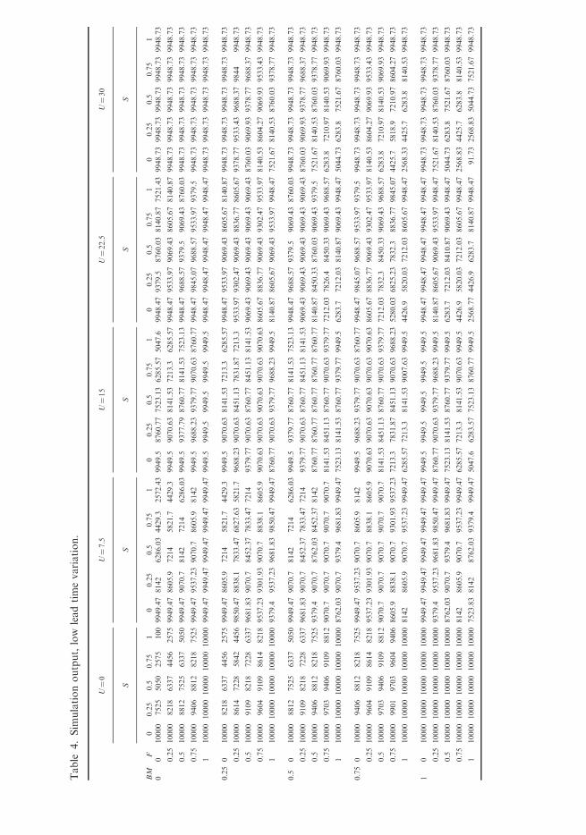
95% level were constructed. Tables 4–6 summarise the behaviour of the total

backlog values as standardisation, flexibility, and business model increases from 0 to 1,

uncertainty increases from 0 to 30, and lead time increases from low – uniform (1, 1) to

high – uniform (1, 5).

4.1 Standardisation increase

When using the scenarios with a standardisation level of zero as a comparison basis, an

analysis of Tables 4–6 reveals the same behaviour:

. Below the diagonal that goes from BM¼ 1, U¼ 0 to BM¼ 0, U¼ 1 (Figure 3), the

total backlog values decrease 76% of the time, remain the same 18% of the time,

and increase 6% of the time. These results are explained by the fact that the U,

BM and S values tend to the alignment conditions of a 100% inventory-oriented

demand fulfilment strategy (U¼ 0,BM¼ 0,S¼ 1).. Within the diagonal, the total backlog values decrease 24% of the time, remain

the same 52% of the time, and increase 24% of the time.


Table

4.Sim

ulationoutput,low

leadtimevariation.

U¼0

U¼7.5

U¼15

U¼22.5

U¼30

SS

SS

S

BM

F0

0.25

0.5

0.75

10

0.25

0.5

0.75

10

0.25

0.5

0.75

10

0.25

0.5

0.75

10

0.25

0.5

0.75

10

010000

7525

5050

2575

100

9949.47

8142

6286.03

4429.3

2572.43

9949.5

8760.77

7523.13

6285.57

5047.6

9948.47

9379.5

8760.03

8140.87

7521.43

9948.73

9948.73

9948.73

9948.73

9948.73

0.25

10000

8218

6337

4456

2575

9949.47

8605.9

7214

5821.7

4429.3

9949.5

9070.63

8141.53

7213.3

6285.57

9948.47

9533.97

9069.43

8605.67

8140.87

9948.73

9948.73

9948.73

9948.73

9948.73

0.5

10000

8812

7525

6337

5050

9949.47

9070.7

8142

7214

6286.03

9949.5

9377.79

8760.77

8141.53

7523.13

9948.47

9688.57

9379.5

9069.43

8760.03

9948.73

9948.73

9948.73

9948.73

9948.73

0.75

10000

9406

8812

8218

7525

9949.47

9537.23

9070.7

8605.9

8142

9949.5

9688.23

9379.77

9070.63

8760.77

9948.47

9845.07

9688.57

9533.97

9379.5

9948.73

9948.73

9948.73

9948.73

9948.73

110000

10000

10000

10000

10000

9949.47

9949.47

9949.47

9949.47

9949.47

9949.5

9949.5

9949.5

9949.5

9949.5

9948.47

9948.47

9948.47

9948.47

9948.47

9948.73

9948.73

9948.73

9948.73

9948.73

0.25

010000

8218

6337

4456

2575

9949.47

8605.9

7214

5821.7

4429.3

9949.5

9070.63

8141.53

7213.3

6285.57

9948.47

9533.97

9069.43

8605.67

8140.87

9948.73

9948.73

9948.73

9948.73

9948.73

0.25

10000

8614

7228

5842

4456

9850.47

8838.1

7833.47

6827.63

5821.7

9688.23

9070.63

8451.13

7831.87

7213.3

9533.97

9302.47

9069.43

8836.77

8605.67

9378.77

9533.43

9688.37

9844

9948.73

0.5

10000

9109

8218

7228

6337

9681.83

9070.7

8452.37

7833.47

7214

9379.77

9070.63

8760.77

8451.13

8141.53

9069.43

9069.43

9069.43

9069.43

9069.43

8760.03

9069.93

9378.77

9688.37

9948.73

0.75

10000

9604

9109

8614

8218

9537.23

9301.93

9070.7

8838.1

8605.9

9070.63

9070.63

9070.63

9070.63

9070.63

8605.67

8836.77

9069.43

9302.47

9533.97

8140.53

8604.27

9069.93

9533.43

9948.73

110000

10000

10000

10000

10000

9379.4

9537.23

9681.83

9850.47

9949.47

8760.77

9070.63

9379.77

9688.23

9949.5

8140.87

8605.67

9069.43

9533.97

9948.47

7521.67

8140.53

8760.03

9378.77

9948.73

0.5

010000

8812

7525

6337

5050

9949.47

9070.7

8142

7214

6286.03

9949.5

9379.77

8760.77

8141.53

7523.13

9948.47

9688.57

9379.5

9069.43

8760.03

9948.73

9948.73

9948.73

9948.73

9948.73

0.25

10000

9109

8218

7228

6337

9681.83

9070.7

8452.37

7833.47

7214

9379.77

9070.63

8760.77

8451.13

8141.53

9069.43

9069.43

9069.43

9069.43

9069.43

8760.03

9069.93

9378.77

9688.37

9948.73

0.5

10000

9406

8812

8218

7525

9379.4

9070.7

8762.03

8452.37

8142

8760.77

8760.77

8760.77

8760.77

8760.77

8140.87

8450.33

8760.03

9069.43

9379.5

7521.67

8140.53

8760.03

9378.77

9948.73

0.75

10000

9703

9406

9109

8812

9070.7

9070.7

9070.7

9070.7

9070.7

8141.53

8451.13

8760.77

9070.63

9379.77

7212.03

7826.4

8450.33

9069.43

9688.57

6283.8

7210.97

8140.53

9069.93

9948.73

110000

10000

10000

10000

10000

8762.03

9070.7

9379.4

9681.83

9949.47

7523.13

8141.53

8760.77

9379.77

9949.5

6283.7

7212.03

8140.87

9069.43

9948.47

5044.73

6283.8

7521.67

8760.03

9948.73

0.75

010000

9406

8812

8218

7525

9949.47

9537.23

9070.7

8605.9

8142

9949.5

9688.23

9379.77

9070.63

8760.77

9948.47

9845.07

9688.57

9533.97

9379.5

9948.73

9948.73

9948.73

9948.73

9948.73

0.25

10000

9604

9109

8614

8218

9537.23

9301.93

9070.7

8838.1

8605.9

9070.63

9070.63

9070.63

9070.63

9070.63

8605.67

8836.77

9069.43

9302.47

9533.97

8140.53

8604.27

9069.93

9533.43

9948.73

0.5

10000

9703

9406

9109

8812

9070.7

9070.7

9070.7

9070.7

9070.7

8141.53

8451.13

8760.77

9070.63

9379.77

7212.03

7832.3

8450.33

9069.43

9688.57

6283.8

7210.97

8140.53

9069.93

9948.73

0.75

10000

9901

9703

9604

9406

8605.9

8838.1

9070.7

9301.93

9537.23

7213.3

7831.87

8451.13

9070.63

9688.23

5280.03

6825.23

7832.3

8836.77

9845.07

4425.7

5818.9

7210.97

8604.27

9948.73

110000

10000

10000

10000

10000

8142

8605.9

9070.7

9537.23

9949.47

6285.57

7213.3

8141.53

9007.63

9949.5

4426.9

5820.03

7212.03

8605.67

9948.47

2568.33

4425.7

6283.8

8140.53

9948.73

10

10000

10000

10000

10000

10000

9949.47

9949.47

9949.47

9949.47

9949.47

9949.5

9949.5

9949.5

9949.5

9949.5

9948.47

9948.47

9948.47

9948.47

9948.47

9948.73

9948.73

9948.73

9948.73

9948.73

0.25

10000

10000

10000

10000

10000

9379.4

9537.23

9681.83

9850.47

9949.47

8760.77

9070.63

9379.77

9688.23

9949.5

8140.87

8605.67

9069.43

9533.97

9948.47

7521.67

8140.53

8760.03

9378.77

9948.73

0.5

10000

10000

10000

10000

10000

8762.03

9070.7

9379.4

9681.83

9949.47

7523.13

8141.53

8760.77

9379.77

9949.5

6283.7

7212.03

8410.87

9069.43

9948.47

5044.73

6283.8

7521.67

8760.03

9948.73

0.75

10000

10000

10000

10000

10000

8142

8605.9

9070.7

9537.23

9949.47

6285.57

7213.3

8141.53

9070.63

9949.5

4426.9

5820.03

7212.03

8605.67

9948.47

2568.83

4425.7

6283.8

8140.53

9948.73

110000

10000

10000

10000

10000

7523.83

8142

8762.03

9379.4

9949.47

5047.6

6283.57

7523.13

8760.77

9949.5

2568.77

4426.9

6283.7

8140.87

9948.47

91.73

2568.83

5044.73

7521.67

9948.73

Table

5.Sim

ulationoutput,medium

leadtimevariation.

U¼0

U¼7.5

U¼15

U¼22.5

U¼30

SS

SS

S

BM

F0

0.25

0.5

0.75

10

0.25

0.5

0.75

10

0.25

0.5

0.75

10

0.25

0.5

0.75

10

0.25

0.5

0.75

1

00

10000

7560.83

5121.67

2682.5

243.339949.478167.736338.074507.9

2677.339949.5

8777.4

7557.1

6336.835116.279948.479387.178776.238165.577554.679948.739948.739948.739948.739948.73

0.2510000

8243.8

6390.03

4536.27

2682.5

9949.478625.1

7253

5880.4

4507.9

9949.5

9083

8166.877251.636336.839948.479539.539081.378624.178165.579948.739948.739948.739948.739948.73

0.5

10000

8829.2

7560.83

6390.03

5121.679949.479083.238167.737253

6338.079949.5

9387.7

8777.4

8166.877557.1

9948.479691.939387.179081.378776.239948.739948.739948.739948.739948.73

0.7510000

9414.6

8829.2

8243.8

7560.839949.479543.179083.238625.1

8167.739949.5

9691.879387.7

9083

8777.4

9948.479846.379691.939539.539387.179948.739948.739948.739948.739948.73

11000010000

10000

10000

10000

9949.479949.479949.479949.479949.479949.5

9949.5

9949.5

9949.5

9949.5

9948.479948.479948.479948.479948.479948.739948.739948.739948.739948.73

0.250

10000

8243.8

6390.03

4536.27

2682.5

9949.478625.1

7253

5880.4

4507.9

9949.5

9083

8166.877251.636336.839948.479539.539081.378624.178165.579948.739948.739948.739948.739948.73

0.2510000

8634.07

7268.13

5902.2

4536.279851.9

8853.977863.636871.975880.4

9691.879083

8472.1

7861.5

7251.639539.539311.3

9081.378852.138624.179386.439539.079691.8

9845.379948.73

0.5

10000

9121.9

8243.8

7268.13

6390.039685.579083.238473.6

7863.637253

9387.7

9083

8777.4

8472.1

8166.879081.379081.379081.379081.379081.378776.1

9081.679386.439691.8

9948.73

0.7510000

9609.73

9121.9

8634.07

8243.8

9543.179311.179083.238853.978625.1

9083

9083

9083

9083

9083

8624.178852.139081.379311.3

9539.538164.938622.439081.679539.079948.73

11000010000

10000

10000

10000

9387.479543.179685.579851.9

9949.478777.4

9083

9387.7

9691.879949.5

8165.578624.179081.379539.539948.477554.5

8164.938776.1

9386.439948.73

0.5

010000

8829.2

7560.83

6390.03

5121.679949.479083.238167.737253

6338.079949.5

9387.7

8777.4

8166.877557.1

9948.479691.939387.179081.378776.239948.739948.739948.739948.739948.73

0.2510000

9121.9

8243.8

7268.13

6390.039685.579083.238473.6

7863.637253

9387.7

9083

8777.4

8472.1

8166.879081.379081.379081.379081.379081.378776.1

9081.679386.439691.8

9948.73

0.5

10000

9414.6

8829.2

8243.8

7560.839387.479083.238778.9

8473.6

8167.738777.4

8777.4

8777.4

8777.4

8777.4

8165.578470.878776.239081.379387.177554.5

8164.938776.1

9386.439948.73

0.7510000

9707.3

9414.6

9121.9

8829.2

9083.239083.239083.239083.239083.238166.878472.1

8777.4

9083

9387.7

7249.677861.338470.879081.379691.936333.337247.9

8164.939081.679948.73

11000010000

10000

10000

10000

8778.9

9083.239387.479685.579949.477557.1

8166.878777.4

9387.7

9949.5

6333.977249.678165.579081.379948.475110.976333.337554.5

8776.1

9948.73

0.750

10000

9414.6

8829.2

8243.8

7560.839949.479543.179083.238625.1

8167.739949.5

9691.879387.7

9083

8777.4

9948.479846.379691.939539.539387.179948.739948.739948.739948.739948.73

0.2510000

9609.73

9121.9

8634.07

8243.8

9543.179311.179083.238853.978625.1

9083

9083

9083

9083

9083

8624.178852.139081.379311.3

9539.538164.938622.439081.679539.079948.73

0.5

10000

9707.3

9414.6

9121.9

8829.2

9083.239083.239083.239083.239083.238166.878472.1

8777.4

9083

9387.7

7249.677861.338470.879081.379691.936333.337247.9

8164.939081.679948.73

0.7510000

9902.43

9707.3

9609.73

9414.6

8625.1

8853.979083.239311.179543.177251.637861.5

8472.1

9083

9691.875876.736868.037861.338852.139846.374500.3

5874.577247.9

8622.439948.73

11000010000

10000

10000

10000

8167.738625.1

9083.239543.179949.476336.837251.638166.879083

9949.5

4502.775876.737249.678624.179948.472668.474500.3

6333.338164.939948.73

10

1000010000

10000

10000

10000

9949.479949.479949.479949.479949.479949.5

9949.5

9949.5

9949.5

9949.5

9948.479948.479948.479948.479948.479948.739948.739948.739948.739948.73

0.251000010000

10000

10000

10000

9387.479543.179685.579851.9

9949.478777.4

9083

9387.879691.879949.5

8165.578624.179081.379539.539948.477554.5

8164.938776.1

9386.439948.73

0.5

1000010000

10000

10000

10000

8778.9

9083.239387.479685.579949.477557.1

8166.878777.4

9387.7

9949.5

6333.977249.678165.579081.379948.475110.976333.337554.5

8776.1

9948.73

0.751000010000

10000

10000

10000

8167.738625.1

9083.239543.179949.476336.837251.638166.879083

9949.5

4502.775876.737249.678624.179948.472668.474500.3

6333.338164.939948.73

11000010000

10000

10000

10000

7558.378167.738778.9

9387.479949.475116.276336.837557.1

8777.4

9949.5

2670.174502.776333.978165.579948.47

224.872668.475110.977554.5

9948.73

Table

6.Sim

ulationoutput,highleadtimevariation.

U¼0

U¼7.5

U¼15

U¼22.5

U¼30

SS

SS

S

BM

F0

0.25

0.5

0.75

10

0.25

0.5

0.75

10

0.25

0.5

0.75

10

0.25

0.5

0.75

10

0.25

0.5

0.75

1

00

10000.00

7587.50

5175.00

2762.50

350.009949.478187.006377.304567.032756.309949.508790.137583.036375.875168.509948.479393.278788.808184.677580.309948.739948.739948.739948.739948.73

0.2510000.00

8263.00

6429.50

4596.00

2762.509949.478639.477282.305924.604567.039949.509092.408186.137280.776375.879948.479543.879090.638638.408184.679948.739948.739948.739948.739948.73

0.5

10000.00

8842.00

7587.50

6429.50

5175.009949.479092.678187.007282.306377.309949.509393.838790.138186.137583.039948.479694.679393.279090.638788.809948.739948.739948.739948.739948.73

0.7510000.00

9421.00

8842.00

8263.00

7587.509949.479547.539092.678639.478187.009949.509694.679393.839092.408790.139948.479847.479694.679543.879393.279948.739948.739948.739948.739948.73

110000.0010000.0010000.0010000.0010000.009949.479949.479949.479949.479949.479949.509949.509949.509949.509949.509948.479948.479948.479948.479948.479948.739948.739948.739948.739948.73

0.250

10000.00

8263.00

6429.50

4596.00

2762.509949.478639.477282.305924.604567.039949.509092.408186.137280.776375.879948.479543.879090.638638.408184.679948.739948.739948.739948.739948.73

0.2510000.00

8649.00

7298.00

5947.00

4596.009852.978865.837886.306905.475924.609694.679092.408488.037884.107280.779543.879318.179090.638863.938638.409392.339543.339694.479846.439948.73

0.5

10000.00

9131.50

8263.00

7298.00

6429.509688.479092.678489.607886.307282.309393.839092.408790.138488.038186.139090.639090.639090.639090.639090.638788.539090.939392.339694.479948.73

0.7510000.00

9614.00

9131.50

8649.00

8263.009547.539318.079092.678865.838639.479092.409092.409092.409092.409092.408638.408863.939090.639318.179543.878183.938636.579090.939543.339948.73

110000.0010000.0010000.0010000.0010000.009393.609547.539688.479852.979949.478790.139092.409393.839694.679949.508184.678638.409090.639543.879948.477580.078183.938788.539392.339948.73

0.5

010000.00

8842.00

7587.50

6429.50

5175.009949.479092.678187.007282.306377.309949.509393.838790.138186.137583.039948.479694.679393.279090.638788.809948.739948.739948.739948.739948.73

0.2510000.00

9131.50

8263.00

7298.00

6429.509688.479092.678489.607886.307282.309393.839092.408790.138488.038186.139090.639090.639090.639090.639090.638788.539090.939392.339694.479948.73

0.5

10000.00

9421.00

8842.00

8263.00

7587.509393.609092.678791.708489.608187.008790.138790.138790.138790.138790.138184.678486.638788.809090.639393.277580.078183.938788.539392.339948.73

0.7510000.00

9710.50

9421.00

9131.50

8842.009092.679092.679092.679092.679092.678186.138488.038790.139092.409393.837278.677883.778486.639090.639694.676371.837276.738183.939090.939948.73

110000.0010000.0010000.0010000.0010000.008791.709092.679393.609688.479949.477583.038186.138790.139393.839949.506372.737278.678184.679090.639948.475162.506371.837580.078788.539948.73

0.750

10000.00

9421.00

8842.00

8263.00

7587.509949.479547.539092.678639.478187.009949.509694.679393.839092.408790.139948.479847.479694.679543.879393.279948.739948.739948.739948.739948.73

0.2510000.00

9614.00

9131.50

8649.00

8263.009547.539318.079092.678865.838639.479092.409092.409092.409092.409092.408638.408863.939090.639318.179543.878183.938636.579090.939543.339948.73

0.5

10000.00

9710.50

9421.00

9131.50

8842.009092.679092.679092.679092.679092.678186.138488.038790.139092.409393.837278.677883.778486.639090.639694.676371.837276.738183.939090.939949.73

0.7510000.00

9903.50

9710.50

9614.00

9421.008639.478865.839092.679318.079547.537280.777884.108488.039092.409694.675920.436901.137883.778863.939847.474558.405918.077276.738636.579948.73

110000.0010000.0010000.0010000.0010000.008187.008639.479092.679547.539949.476375.877280.778186.139092.409949.504561.205920.437278.678638.409948.472746.034558.406371.838183.939948.73

10

10000.0010000.0010000.0010000.0010000.009949.479949.479949.479949.479949.479949.509949.509949.509949.509949.509948.479948.479948.479948.479948.479948.739948.739948.739948.739948.73

0.2510000.0010000.0010000.0010000.0010000.009393.609547.539688.479852.979949.478790.139092.409393.839694.679949.508184.678638.409090.639543.879948.477580.078183.938788.539392.339948.73

0.5

10000.0010000.0010000.0010000.0010000.008791.709092.679393.609688.479949.477583.038186.138790.139393.839949.506372.737278.678184.679090.639948.475162.506371.837580.078788.539948.73

0.7510000.0010000.0010000.0010000.0010000.008187.008639.479092.679547.539949.476375.877280.778186.139092.409949.504561.205920.437278.678638.409948.472746.034558.406371.838183.939948.73

110000.0010000.0010000.0010000.0010000.007584.378187.008791.709393.609949.475168.506375.877583.038790.139949.502748.304561.206372.738184.679948.47

328.602746.035162.507580.079948.73

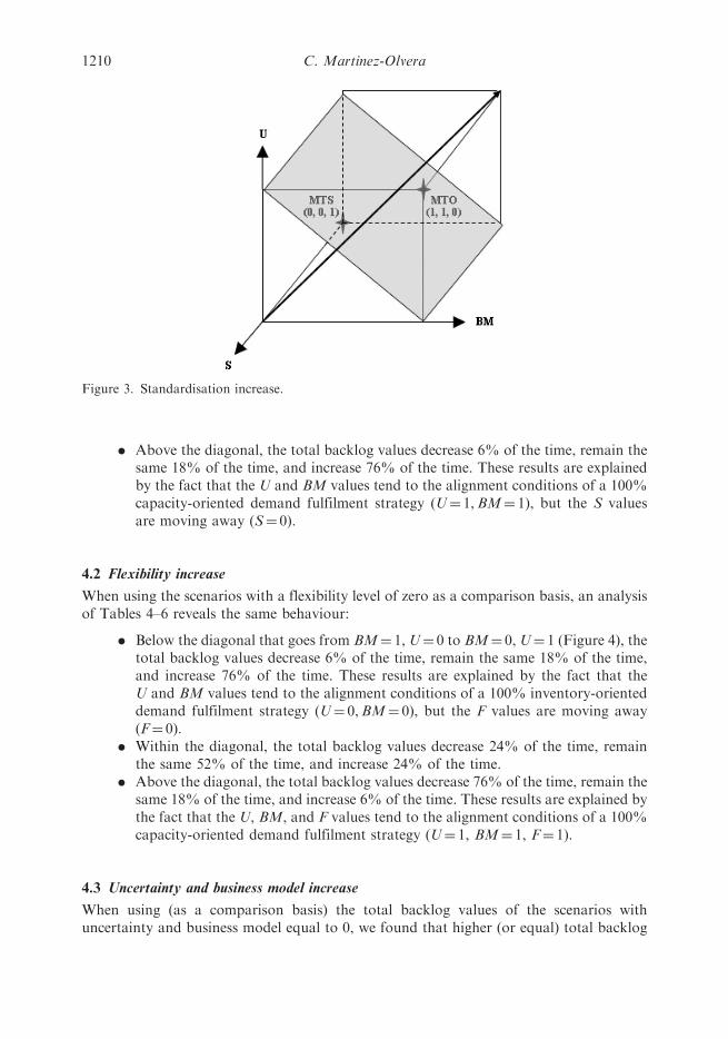
. Above the diagonal, the total backlog values decrease 6% of the time, remain thesame 18% of the time, and increase 76% of the time. These results are explainedby the fact that the U and BM values tend to the alignment conditions of a 100%capacity-oriented demand fulfilment strategy (U¼ 1,BM¼ 1), but the S valuesare moving away (S¼ 0).

4.2 Flexibility increase

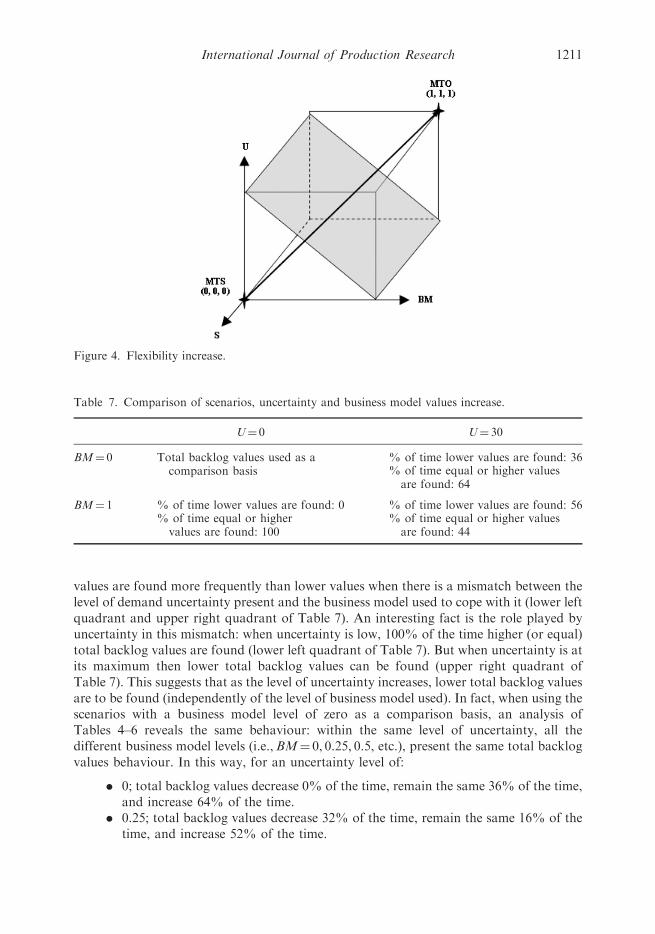
When using the scenarios with a flexibility level of zero as a comparison basis, an analysisof Tables 4–6 reveals the same behaviour:

. Below the diagonal that goes from BM¼ 1, U¼ 0 to BM¼ 0, U¼ 1 (Figure 4), thetotal backlog values decrease 6% of the time, remain the same 18% of the time,and increase 76% of the time. These results are explained by the fact that theU and BM values tend to the alignment conditions of a 100% inventory-orienteddemand fulfilment strategy (U¼ 0,BM¼ 0), but the F values are moving away(F¼ 0).

. Within the diagonal, the total backlog values decrease 24% of the time, remainthe same 52% of the time, and increase 24% of the time.

. Above the diagonal, the total backlog values decrease 76% of the time, remain thesame 18% of the time, and increase 6% of the time. These results are explained bythe fact that the U, BM, and F values tend to the alignment conditions of a 100%capacity-oriented demand fulfilment strategy (U¼ 1, BM¼ 1, F¼ 1).

4.3 Uncertainty and business model increase

When using (as a comparison basis) the total backlog values of the scenarios withuncertainty and business model equal to 0, we found that higher (or equal) total backlog

Figure 3. Standardisation increase.


values are found more frequently than lower values when there is a mismatch between thelevel of demand uncertainty present and the business model used to cope with it (lower leftquadrant and upper right quadrant of Table 7). An interesting fact is the role played byuncertainty in this mismatch: when uncertainty is low, 100% of the time higher (or equal)total backlog values are found (lower left quadrant of Table 7). But when uncertainty is atits maximum then lower total backlog values can be found (upper right quadrant ofTable 7). This suggests that as the level of uncertainty increases, lower total backlog valuesare to be found (independently of the level of business model used). In fact, when using thescenarios with a business model level of zero as a comparison basis, an analysis ofTables 4–6 reveals the same behaviour: within the same level of uncertainty, all thedifferent business model levels (i.e.,BM¼ 0, 0.25, 0.5, etc.), present the same total backlogvalues behaviour. In this way, for an uncertainty level of:

. 0; total backlog values decrease 0% of the time, remain the same 36% of the time,and increase 64% of the time.

. 0.25; total backlog values decrease 32% of the time, remain the same 16% of thetime, and increase 52% of the time.

Figure 4. Flexibility increase.

Table 7. Comparison of scenarios, uncertainty and business model values increase.

U¼ 0 U¼ 30

BM¼ 0 Total backlog values used as acomparison basis

% of time lower values are found: 36% of time equal or higher valuesare found: 64

BM¼ 1 % of time lower values are found: 0 % of time lower values are found: 56% of time equal or highervalues are found: 100

% of time equal or higher valuesare found: 44


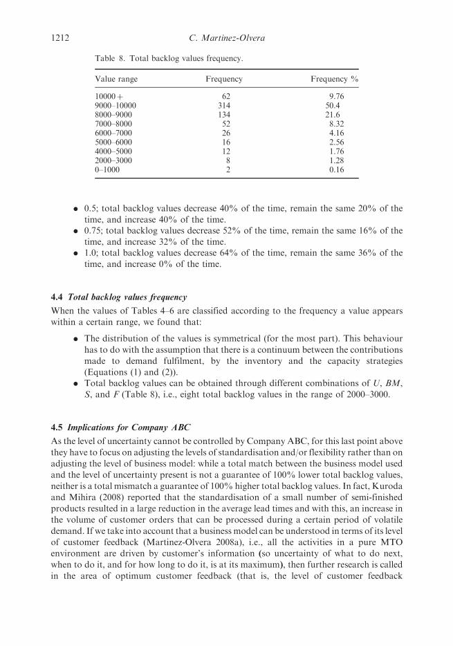
. 0.5; total backlog values decrease 40% of the time, remain the same 20% of the

time, and increase 40% of the time.. 0.75; total backlog values decrease 52% of the time, remain the same 16% of the

time, and increase 32% of the time.. 1.0; total backlog values decrease 64% of the time, remain the same 36% of the

time, and increase 0% of the time.

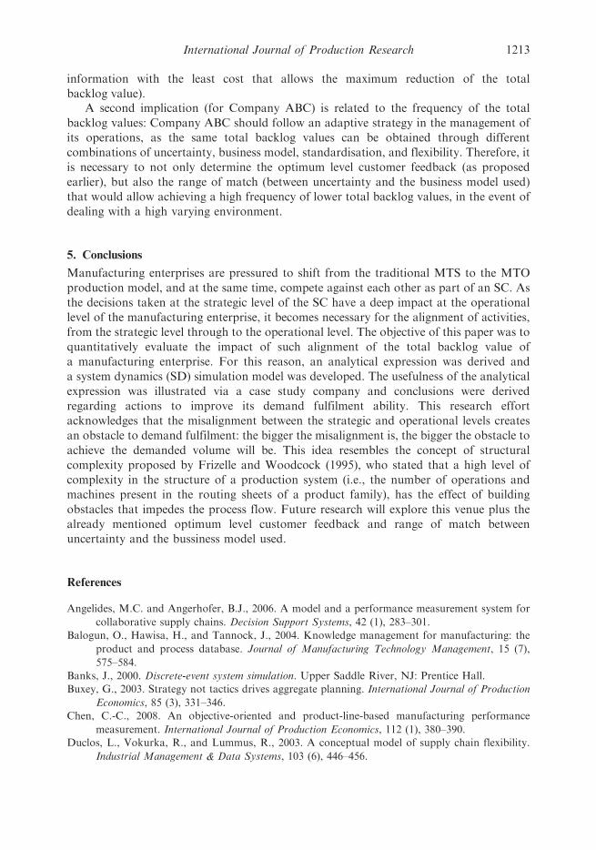
4.4 Total backlog values frequency

When the values of Tables 4–6 are classified according to the frequency a value appears

within a certain range, we found that:

. The distribution of the values is symmetrical (for the most part). This behaviour

has to do with the assumption that there is a continuum between the contributions

made to demand fulfilment, by the inventory and the capacity strategies

(Equations (1) and (2)).. Total backlog values can be obtained through different combinations of U, BM,

S, and F (Table 8), i.e., eight total backlog values in the range of 2000–3000.

4.5 Implications for Company ABC

As the level of uncertainty cannot be controlled by Company ABC, for this last point above

they have to focus on adjusting the levels of standardisation and/or flexibility rather than on

adjusting the level of business model: while a total match between the business model used

and the level of uncertainty present is not a guarantee of 100% lower total backlog values,

neither is a total mismatch a guarantee of 100% higher total backlog values. In fact, Kuroda

and Mihira (2008) reported that the standardisation of a small number of semi-finished

products resulted in a large reduction in the average lead times and with this, an increase in

the volume of customer orders that can be processed during a certain period of volatile

demand. If we take into account that a business model can be understood in terms of its level

of customer feedback (Martinez-Olvera 2008a), i.e., all the activities in a pure MTO

environment are driven by customer’s information (so uncertainty of what to do next,

when to do it, and for how long to do it, is at its maximum), then further research is called

in the area of optimum customer feedback (that is, the level of customer feedback

Table 8. Total backlog values frequency.

Value range Frequency Frequency %

10000þ 62 9.769000–10000 314 50.48000–9000 134 21.67000–8000 52 8.326000–7000 26 4.165000–6000 16 2.564000–5000 12 1.762000–3000 8 1.280–1000 2 0.16


information with the least cost that allows the maximum reduction of the total

backlog value).A second implication (for Company ABC) is related to the frequency of the total

backlog values: Company ABC should follow an adaptive strategy in the management of

its operations, as the same total backlog values can be obtained through different

combinations of uncertainty, business model, standardisation, and flexibility. Therefore, it

is necessary to not only determine the optimum level customer feedback (as proposed

earlier), but also the range of match (between uncertainty and the business model used)

that would allow achieving a high frequency of lower total backlog values, in the event of

dealing with a high varying environment.

5. Conclusions

Manufacturing enterprises are pressured to shift from the traditional MTS to the MTO

production model, and at the same time, compete against each other as part of an SC. As

the decisions taken at the strategic level of the SC have a deep impact at the operational

level of the manufacturing enterprise, it becomes necessary for the alignment of activities,

from the strategic level through to the operational level. The objective of this paper was to

quantitatively evaluate the impact of such alignment of the total backlog value of

a manufacturing enterprise. For this reason, an analytical expression was derived and

a system dynamics (SD) simulation model was developed. The usefulness of the analytical

expression was illustrated via a case study company and conclusions were derived

regarding actions to improve its demand fulfilment ability. This research effort

acknowledges that the misalignment between the strategic and operational levels creates

an obstacle to demand fulfilment: the bigger the misalignment is, the bigger the obstacle to

achieve the demanded volume will be. This idea resembles the concept of structural

complexity proposed by Frizelle and Woodcock (1995), who stated that a high level of

complexity in the structure of a production system (i.e., the number of operations and

machines present in the routing sheets of a product family), has the effect of building

obstacles that impedes the process flow. Future research will explore this venue plus the

already mentioned optimum level customer feedback and range of match between

uncertainty and the bussiness model used.

References

Angelides, M.C. and Angerhofer, B.J., 2006. A model and a performance measurement system for

collaborative supply chains. Decision Support Systems, 42 (1), 283–301.

Balogun, O., Hawisa, H., and Tannock, J., 2004. Knowledge management for manufacturing: the

product and process database. Journal of Manufacturing Technology Management, 15 (7),

575–584.

Banks, J., 2000. Discrete-event system simulation. Upper Saddle River, NJ: Prentice Hall.Buxey, G., 2003. Strategy not tactics drives aggregate planning. International Journal of Production

Economics, 85 (3), 331–346.Chen, C.-C., 2008. An objective-oriented and product-line-based manufacturing performance

measurement. International Journal of Production Economics, 112 (1), 380–390.Duclos, L., Vokurka, R., and Lummus, R., 2003. A conceptual model of supply chain flexibility.

Industrial Management & Data Systems, 103 (6), 446–456.


Eskandari, H., et al., 2007. Value chain analysis using hybrid simulation and AHP. International

Journal of Production Economics, 105 (2), 536–547.

Frizelle, G. and Woodcock, E., 1995. Measuring complexity as an aid to developing strategy.

International Journal of Operations & Production Management, 15 (5), 268–270.

Griffiths, J., James, R., and Kempson, J., 2000. Focusing customer demand through manufacturing

supply chains by the use of customer focused cells: an appraisal. International Journal of

Production Economics, 65 (1), 111–120.Gupta, D. and Benjaafar, S., 2004. Make-to-order, make-to-stock, or delay product differentiation?

A common framework for modeling and analysis. IIE Transactions, 36 (6), 529–546.Huang, S.H., Uppal, M., and Shi, J., 2002. A product driven approach to manufacturing supply

chain selection. Supply Chain Management, 7 (4), 189–199.Hwarng, H.B., et al., 2005. Modeling a complex supply chain: understanding the effect of simplified

assumptions. International Journal of Production Research, 43 (13), 2829–2872.Ismail, H.S. and Sharifi, H., 2006. A balanced approach to building agile supply chains. International

Journal of Physical Distribution & Logistics Management, 36 (6), 431–444.iThink, 1996. Analyst technical documentation (Software Manual). Hanover, NH: High Performance

Systems.Jonsson, P. and Mattsson, S.A., 2003. The implications of fit between planning environments and

manufacturing planning and control methods. International Journal of Operations &

Production Management, 23 (8), 872–900.Khoo, L.P. and Yin, X.F., 2003. An extended graph-based virtual clustering-enhanced approach

to supply chain optimization. International Journal of Advanced Manufacturing Technology, 22

(11–12), 836–847.

Kleijnen, J.P.C., 2005. Supply chain simulation tools and techniques: a survey. International Journal

of Simulation & Process Modelling, 1 (1/2), 82–89.

Kuroda, M. and Mihira, H., 2008. Strategic inventory holding to allow the estimation of earlier due

dates in make-to-order production. International Journal of Production Research, 46 (2),

495–508.Lamming, R., et al., 2000. An initial classification of supply networks. International Journal of

Operations & Production Management, 20 (6), 675–691.Longo, F. and Mirabelli, G., 2008. An advanced supply chain management tool based on modeling

and simulation. Computers & Industrial Engineering, 54 (3), 570–588.Martinez-Olvera, C. and Shunk, D., 2006. A comprehensive framework for the development of

a supply chain strategy. International Journal of Production Research, 44 (21), 4511–4528.Martinez-Olvera, C., 2008a. Impact of hybrid business models in the supply chain performance,

In: Supply chain: theory and applications (ISBN 978-3-902613-22-6). Vienna, Austria: I-Tech

Education and Publishing, 113–134.Martinez-Olvera, C., 2008b. Methodology for realignment of supply-chain structural. International

Journal of Production Economics, 114 (2), 714–722.Miltenburg, J., 1995. Manufacturing strategy: how to formulate and implement a winning plan.

Portland, OR: Productivity Press.Olhager, J., 2003. Strategic positioning of the order penetration point. International Journal of

Production Economics, 85 (3), 2335–2351.Petersen, K.J., Handfield, R.B., and Ragatz, G.L., 2005. Supplier integration into new product

development: coordinating product, process, and supply chain design. Journal of Operations

Management, 23 (3/4), 371–388.Rao, K. and Young, R.R., 1994. Global supply chains: factors influencing outsourcing of logistics

functions. International Journal of Physical Distribution & Logistics Management, 24 (6),

11–19.

Safizadeh, M.H. and Ritzman, L.P., 1997. Linking performance drivers in production planning and

inventory control to process choice. Journal of Operations Management, 15 (4), 389–403.


Shah, N., et al., 2004. A flexible and generic approach to dynamic modelling of supply chains.Journal of the Operational Research Society, 55 (8), 801–813.

Son, Y.J. and Venkateswaran, J., 2005. Hybrid system dynamic: discrete event simulation-basedarchitecture for hierarchical production planning. International Journal of Production

Research, 43 (20), 4397–4429.Terzi, S. and Cavalieri, S., 2004. Simulation in the supply chain context: a survey. Computers in

Industry, 53 (1), 3–16.

Towill, D.R., 1996. Time compression and supply chain management – a guided tour. Supply ChainManagement, 1 (1), 15–27.

Venkateswaran, J. and Son, Y.J., 2004. Impact of modelling approximations in supply chain

analysis – an experimental study. International Journal of Production Research, 42 (15),2971–2992.

Vernadat, F., 2002. UEML: towards a unified enterprise modeling language. International Journal of

Production Research, 40 (17), 4309–4321.Zhang, D.Z., et al., 2006. An agent-based approach for e-manufacturing and supply chain

integration. Computers & Industrial Engineering, 51 (2), 343–360.Zhao, Z.Y., Ball, M., and Chen, C.Y., (2002). A scalable supply chain infrastructure research test-bed.

Chapter 7, Scalable enterprise system: an introduction to recent advances. Springer.


Copyright of International Journal of Production Research is the property of Taylor & Francis Ltd and its

content may not be copied or emailed to multiple sites or posted to a listserv without the copyright holder's

express written permission. However, users may print, download, or email articles for individual use.

Impact of the alignment between the strategic and operational levels of a manufacturing enterprise

Documents

Transcript of Impact of the alignment between the strategic and operational levels of a manufacturing enterprise