PLEASE SCROLL DOWN FOR ARTICLE

This article was downloaded by: [Ribas, Rafael Perez]On: 29 April 2010Access details: Access Details: [subscription number 921315398]Publisher RoutledgeInforma Ltd Registered in England and Wales Registered Number: 1072954 Registered office: Mortimer House, 37-41 Mortimer Street, London W1T 3JH, UK

Journal of Development EffectivenessPublication details, including instructions for authors and subscription information:http://www.informaworld.com/smpp/title~content=t906200215

Impact evaluation of a rural conditional cash transfer programme onoutcomes beyond health and educationFabio Veras Soares a; Rafael Perez Ribas b;Guilherme Issamu Hirata a

a International Policy Centre for Inclusive Growth (IPC-IG), Brasília-DF, Brazil b Department ofEconomics, University of Illinois at Urbana-Champain, USA

Online publication date: 14 April 2010

To cite this Article Veras Soares, Fabio , Perez Ribas, Rafael andIssamu Hirata, Guilherme(2010) 'Impact evaluation of arural conditional cash transfer programme on outcomes beyond health and education', Journal of DevelopmentEffectiveness, 2: 1, 138 — 157To link to this Article: DOI: 10.1080/19439341003624433URL: http://dx.doi.org/10.1080/19439341003624433

Full terms and conditions of use: http://www.informaworld.com/terms-and-conditions-of-access.pdf

This article may be used for research, teaching and private study purposes. Any substantial orsystematic reproduction, re-distribution, re-selling, loan or sub-licensing, systematic supply ordistribution in any form to anyone is expressly forbidden.

The publisher does not give any warranty express or implied or make any representation that the contentswill be complete or accurate or up to date. The accuracy of any instructions, formulae and drug dosesshould be independently verified with primary sources. The publisher shall not be liable for any loss,actions, claims, proceedings, demand or costs or damages whatsoever or howsoever caused arising directlyor indirectly in connection with or arising out of the use of this material.

Impact evaluation of a rural conditional cash transfer programmeon outcomes beyond health and education

Fabio Veras Soaresa*, Rafael Perez Ribasb and Guilherme Issamu Hirataa

aInternational Policy Centre for Inclusive Growth (IPC-IG), Brasılia-DF, Brazil; bDepartment ofEconomics, University of Illinois at Urbana–Champain, USA

This paper presents impacts of the pilot conditional cash transfer programme inParaguay. The choice of outcomes of interest is based on the work developed by thefamily counselling component undertaken by social workers. Propensity score techni-ques are used to deal with the problem of non-random treatment assignment. Tekoporahas had a positive effect on investment in agriculture, savings, and on the possessionof identity card, but did not have much impact on access to credit and on socialparticipation. These results suggest that conditional cash transfer programmes canhave impacts that go beyond the usual impacts on consumption, and health andeducation outcomes.

Keywords: conditional cash transfers; impact evaluation; propensity score matching

1. Introduction

Conditional cash transfer (CCT) programmes in Latin America have been intensivelyevaluated with the aim of both to inform programme managers on achievements andpotential shortcomings and to attempt to gain political support for the programme. Theevaluations of PROGRESA in Mexico, Familias en Accion (FA) in Colombia, Bono deDesarrollo Humano (BDH) in Ecuador, and Red de Proteccion Social (RPS) in Nicaraguahave revealed important impacts on consumption, health and education outcomes.Furthermore, these evaluations have not found negative effects on adult labour supply,which is often a concern in programmes that increase unearned income. Most evaluationshave focused on the health and education indicators and to a lesser extent on consumptionand diet diversification,1 and not much attention has been paid to issues such as the impacton agricultural activity, savings and access to credit. These dimensions are especiallyrelevant in rural settings in which most small-scale or pilot CCT programmes are currentlybeing implemented.2

In this paper we evaluate the impacts of a Paraguayan pilot CCT programme calledTekopora on selected indicators that are not usually addressed in the evaluations of CCTprogrammes; namely, agricultural activity, access to credit, social participation and thepossession of identity cards. Tekopora’s rural setting and some features of its design makethese outcomes extremely relevant for the assessment of the effectiveness of the programme.

The programme started in 2005 in five districts (municipalities) of two departments(states). It aims to reduce extreme poverty through direct cash transfers to poor households

Journal of Development EffectivenessVol. 2, No. 1, March 2010, 138–157

*Corresponding author. Email: fabio.veras@ipc-undp.org

ISSN 1943-9342 print/ISSN 1943-9407 online# 2010 Taylor & FrancisDOI: 10.1080/19439341003624433http://www.informaworld.com

Downloaded By: [Ribas, Rafael Perez] At: 22:15 29 April 2010

with children, and to diminish future poverty by encouraging investments in human andsocial capital. Transfers are conditional on school attendance, regular visits to health centresand updating of immunisations. However, during the implementation of the pilot, condi-tionalities were not monitored.3

The programme also includes a family support component that consists of monthly visitsof young social workers (family guides) to beneficiary households.4 During these visits,social workers are required to give support to the beneficiary families in several dimensions:budget planning; raising awareness on the requirement to comply with conditionalities;helping family members to get their identification cards (civil registry); imparting somebasic notions on health, hygiene and healthy diet; and stimulating income-generatingactivities – sometimes organising cooperatives of beneficiaries – as well as consumptionfrom own production (vegetable gardens and livestock acquisition). These activities shouldreinforce the impact of the conditionalities as well as have an impact on their own, especiallyon the social capital and on the productive capacity of beneficiary households. Thiscomponent motivates the choice of some of outcomes evaluated in this paper.

Households are eligible for the programme if they fulfil the following conditions:presence of children under 15 years old or pregnant women; residence in priority areas forthe programme – namely, the poorest districts in the country according to the Index ofGeographical Prioritisation (IPG); and low Index of Quality of Life (ICV). The IPG ranks thepoorest districts in the country using a poverty map based on data from the 2002 census and2003 national household survey (Encuesta Permanente de Hogares [EPH]). It is basically aweighted average of monetary (40%) and non-monetary (60%) poverty indicators, the lattercomprised of unsatisfied basic needs indicators. The ICV is a non-monetary index calculatedthrough principal component analysis that summarises several dimensions of living condi-tions, such as access to public services, health, education, occupation, housing quality, andasset ownership. The ICV ranges from zero to 100 points; households with an ICV below40 points are eligible for the programme.5

Data used in the analysis come from an evaluation survey that took place betweenJanuary and April 2007 in the five districts where the pilot had already started and in twoother districts where the programme had not been initiated at the time of the survey. Inaddition, we used data from administrative records, which include the payment register, anddata from Ficha Hogar, a small questionnaire used to gather information for the selection ofbeneficiary households in the seven districts.

Experimental design is considered the best approach to estimate a valid counterfactual inan impact evaluation. For that reason experiments were adopted in the case of PROGRESA,RPS, and BDH. However, difficulties in the coordination between programme implementersand the evaluation team can spoil an experimental design. For instance, when there iswidespread contamination of both treated and control groups, one may have to adopt quasi-experimental methods to assess the impact of the programme.

We used a quasi-experimental strategy similar to the one adopted in the evaluation of FAundertaken by the Centre for the Evaluation of Development and Econometria (EDePo2004) since the criteria for treatment assignment in the case of Tekopora are observed (ICVand families with children). With regards to the adequacy of propensity score methods toevaluate CCT programmes, particularly those with geographical targeting, Diaz and Handa(2006) and Handa and Maluccio (2009) show that these methods are capable of reproducingthe experimental results for the cases of PROGRESA and RPS, respectively, even in a non-experimental setting.6

The evaluation of Tekopora shows positive impacts on investment in agriculturalinvestment, savings, and on possession of identification cards. These dimensions are

Journal of Development Effectiveness 139

Downloaded By: [Ribas, Rafael Perez] At: 22:15 29 April 2010

precisely those in which the social workers are supposed to work with the beneficiaryfamilies. Although we do not disentangle the combined effect of the cash transfer and ofthe other components of the programme, its design suggests that at least part of the impact isdue to the activities undertaken by the social workers.

The rest of this paper is organised as follows. Section 2 discusses the data, the choiceof a comparison group, and the evaluation strategy. Section 3 presents the results for theoutcomes of interest. Section 4 provides a discussion of the main results and our researchagenda regarding the evaluation of Tekopora.

2. Methodology

The major challenge of this evaluation was the lack of a proper baseline survey that couldinform us about the differences between beneficiaries and non-beneficiaries before theprogramme in key outcome indicators. In addition, the fact that the programme’s imple-mentation did not follow a randomised assignment requires that we use a quasi-experimentalstrategy to identify the impact of the programme.

2.1. Database

In the absence of a baseline, information on household characteristics before theprogramme comes from the Ficha Hogar database. The latter was the administrativeinstrument used during the district census to obtain the variables that determine pro-gramme eligibility according to the ICV score. The follow-up survey questionnaire wasmuch more detailed than the Ficha Hogar. In addition to all variables of the latter, thefollow-up survey gathered information on health and education outcomes, expenditures,food consumption, access to credit, investment in agricultural activities, and socialparticipation. As all households were interviewed following the same method overthe same period, there is no bias or systematic error in favour of a specific group inboth surveys

The pilot of Tekopora started in five districts: Buena Vista and Abaı in the departmentof Caazapa; and Santa Rosa del Aguaray, Lima and Union in the department of San Pedro. Inthis phase, the Ficha Hogar was fielded through a census that took place in the poorest areasof the selected districts, in addition to the poorest areas of another two districts – MoisesBertoni in the department of Caazapa, and Tucuati in the department of San Pedro – that didnot take part in the pilot.

Furthermore, potentially eligible households that did not reside in the poorest areasof the districts of the pilot or that had been skipped in the census process could also fillin the Ficha Hogar. In total, 7990 households were registered by the census and 1827 bydemand.

The first payment took place in Buena Vista in September 2005. By August 2006,the pilot covered 4324 beneficiary households in the five districts. The evaluationsurvey went to the field between January and April 2007 based on a sample of 1401households.

2.2. Comparison group

The comparison group in a quasi-experimental setting has to be as similar as possible to thetreated group. In the case of Tekopora, it was possible to identify two potential comparisongroups: non-beneficiaries who live in the two districts covered by the census (Ficha Hogar)but not by the pilot; and non-beneficiaries who live in the same districts as the beneficiaries.7

140 F.V. Soares et al.

Downloaded By: [Ribas, Rafael Perez] At: 22:15 29 April 2010

Both groups can be further classified into two subgroups: eligibles (ICV below 40), andineligibles (ICV equal or greater than 40).

Table 1 classifies untreated households in the seven districts according to the motivefor their exclusion from the programme. As one should expect, the largest group iscomprised of households in the non-pilot districts (39%). In these districts, more than90 per cent of the households with children had ICV lower than 40 (eligible households).It is worth mentioning that those two districts were meant to be in the pilot, but due tobudget restrictions, the programme could only afford five districts. In order to keep thegeographical balance of the pilot, one district from each department was excluded fromthe pilot.

The second largest group of untreated households consists of households in the pilotdistricts that were ‘overlooked’ by the programme (35%). In this case, about 66 per cent(542 of 708) were eligible for the programme. A possible reason for this administrativemistake refers to the change in the cut-off point of eligibility from 25 to 40 when theregistration process into the programme had already begun. Then potential beneficiarieswhose ICV was in this range were not invited to register for the programme.

The other reasons provided in Table 1 refer to: rejections by the community oversightcommittees, which double check the list of potential beneficiaries; and potential benefici-aries in settlements controlled by the landless movement who were waiting for permissionfrom their leaders to take part in the programme.

Our comparison group is comprised of households in districts out of the pilot andhouseholds overlooked by the programme in the pilot districts. The other groups wereexcluded from the evaluation because they were not treated due to specific reasons. Eventhough the existence of two different comparison groups would allow us to estimate two setsof impacts – namely, ‘between-district’ and ‘within-district’ impact – our estimates use onlythe composite comparison group.8 Nevertheless, when assessing the heterogeneity of theimpact we allow for the impact to differ by comparison group, which can give us an idea ofpotential externality effects of the programme.9

Notice that the districts excluded from the pilot are neither geographically concentratednor distinct from the pilot districts. Table 2 confirms that, in general, there is no largedifference between them.

Table 3 presents the differences among the treated, comparison and remaining house-holds registered in the Ficha Hogar. The comparison group showed a significantly bettersituation than the treatment group, but the former was on average worse than the otherregistered households. About 26 per cent of the comparison group had an ICV equal to or

Table 1. Reasons for not receiving treatment.

Eligible Ineligible

ICV,40 Percentage ICV.40 Percentage Total Percentage

District excluded from the pilot 1160 44.24 124 17.71 1284 38.65Overlooked 776 29.60 398 56.86 1174 35.34Rejected by selection committee 559 21.32 166 23.71 725 21.82Waiting for landless movementpermission

127 4.84 12 1.71 139 4.18

Total 2622 100.00 700 100.00 3322 100.00

Source: Ficha Hogar and payment register of Tekopora.

Journal of Development Effectiveness 141

Downloaded By: [Ribas, Rafael Perez] At: 22:15 29 April 2010

greater than 40, and therefore they were not eligible for the programme. However, thisgroup was included in the evaluation because there was an intention of comparinghouseholds on the limit of eligibility in order to implement a regression discontinuityanalysis.

2.3. Sampling strategy

As already mentioned, it was possible to classify the comparison group into four subgroups.These subgroups consist of eligible (ICV , 40) and ineligible (ICV � 40) householdsin districts where the programme was implemented and in districts where it was not. Tocalculate the follow-up survey sample, the population from Ficha Hogar was firstly classi-fied into five strata, which consist of the four comparison subgroups (the combination ofeligible and ineligible groups in pilot and non-pilot districts) and the group of eligible treatedhouseholds. A residual number of ineligible households that were occasionally treated bymistake, were excluded from the sample.

The number of observations in each stratum was calculated using the formula of samplesize for finite population, with a significance level of 0.05, a response rate of 0.8, and anacceptable error of 0.04 in the logarithm of ICV. Thus the samples of the five primary strataare representative of their respective population.

A second stratification was defined according to the area of residence (urban/rural)and the type of registration (census/demand). At this level, only the samples of rural and

Table 2. Socio-economic conditions of districts screened by the Ficha Hogar.

Districts in the pilot Districts out of the pilot Total

Mean ICV 27.56 29.87 29.39Per cent with ICV less than 25 52.72 46.57 47.84Per cent with ICV between 25 and 40 32.71 33.32 33.20Mean per-capita income (in Gs) 94,401.44 109,554.10 106,411.10Per cent of (monetarily) poora 82.10 81.08 81.29Per cent of (monetarily) extremely poor 69.41 70.09 69.95Number of observationsb 6320 1654 7974

aPoverty and extreme poverty lines come from the 2003 national household survey (EPH).bAll households with complete interview in the census.Source: Ficha Hogar.

Table 3. Socio-economic conditions of treated and untreated households.

Treated Untreated comparison Others Total

Mean ICV 22.93 32.27 33.23 28.74Per cent with ICV less than 25 66.08 35.90 39.00 49.31Per cent with ICV between 25 and 40 31.99 38.36 32.28 33.77Mean per-capita income (in Gs) 39,442.93 98,955.26 164,203.28 95,698.53Per cent of (monetarily) poora 94.90 80.48 70.57 83.19Per cent of (monetarily) extremely poor 87.71 67.95 58.59 73.03Number of observationsb 3726 2393 2946 9065

aPoverty and extreme poverty lines come from the 2003 national household survey (EPH).bAll households with complete interview in the census.Source: Ficha Hogar.

142 F.V. Soares et al.

Downloaded By: [Ribas, Rafael Perez] At: 22:15 29 April 2010

census-registered households are representative of their population. Since registrations bydemand only took place in pilot districts, the final sample was divided into 16 strata. Thenumber of observations in the final strata was given by the relative participation of theirpopulation in the primary stratum.

As mentioned before, we intended to apply regression discontinuity design to our data,for this reason we oversampled households with ICV close to 40 – the eligibility cut-offpoint.10 In practice, all households near this threshold were included in the sample withprobability one, except those in the primary stratum of untreated eligible households in thepilot districts (overlooked households).

After defining the probability of each household being in the sample, the selectionoccurred by simple random sampling. The response rate of the evaluation survey was78 per cent so that 1089 of 1401 households were interviewed.

2.4. The evaluation problem

The evaluation problem consists of estimating what would have happened to the outcomesof interest for the beneficiary families had they not received the benefit. As we cannotobserve the same beneficiary family in both states at the same time, we need to estimate acounterfactual. The comparison group discussed before provides this counterfactual. Belowwe discuss the assumptions required to identify the impact of the programme and in the nextsubsection we present a technique that we use to make the treated and comparison groups assimilar as possible.

There are two types of outcomes with regards to data availability: those that areobserved only after the programme (not covered in the Ficha Hogar), and those that areobserved before and after the programme. For this reason, two types of estimators wereadopted: the difference-in-differences (DD) estimator when baseline information exists,and the single difference (SD) estimator when the outcome is observed only after theimplementation.

Our parameter of interest is the average treatment effect on the treated (ATT)households, which is the expected difference between two outcomes – one with thetreatment and the other without the treatment – over the population participating in theprogramme.

To identify the ATT when both baseline and follow-up information are available, wecan apply the DD estimator (Heckman et al. 1997). The identification of the DD estimatorrequires the assumption that, conditioned on a set of observable characteristics, theaverage difference between treated and comparison groups would have followedthe same trend in the absence of the programme (Abadie 2005). However, when wedo not have baseline information and therefore have to rely on differences after theprogramme, we have to make an additional assumption, which basically says that theoutcome before the treatment was the same for both treated and untreated groups.Combined with the first assumption, the latter implies that selection into the programmeis completely based on observable variables and yields the SD estimator for the ATT. TheDD estimator is preferred over the SD estimator because it relies on weaker assumptionsand because it wipes the effect of constant unobserved idiosyncratic characteristics forboth groups out. We can only calculate the DD estimator when the outcome of interestis available in the baseline (Ficha Hogar); when this is not the case, we report the SDestimator.

Journal of Development Effectiveness 143

Downloaded By: [Ribas, Rafael Perez] At: 22:15 29 April 2010

2.5. Propensity score methods

The main challenge in calculating the above mentioned estimators is to guarantee thecorrect balance in the observed characteristics in order to avoid selectivity bias. Asshown by Rosembaum and Rubin (1983), we can rely on the propensity score (PS) tobalance the treated and comparison groups according to their observed characteristics ThePS is defined as the probability of receiving the transfer conditional on the observedcharacteristics:

pðX ðiÞÞ ¼ Pr½Dði; 1Þ ¼ 1jX ¼ X ðiÞ�

where Dði; tÞ ¼ d stands for household i’s status of beneficiary (d = 1) or non-beneficiary(d = 0) before (t = 0) or after (t = 1) the programme. This probability can be calculatedparametrically using, for instance, a logit model.

The balance property requires that the households in the treated and comparisongroups with similar PS have, on average, similar observed characteristics in the commonsupport:

E½X ðiÞ j pðX ðiÞÞ;Dði; 1Þ ¼ 1� ¼ E½X ðiÞj pðX ðiÞÞ;Dði; 1Þ ¼ 0�: (1)

The PS is then applied to estimate the impact through two techniques: propensity scorematching (PSM) and inverse probability weighted regression (IPW). The specific PSMtechnique that we implement is nearest-neighbour matching (NNM), in which webasically matched each treated observation with the closest comparison-group observa-tion in terms of PS (Dehejia and Wahba 2002). Formally, the ATT matching parameterunder DD can be defined following Blundell et al. (2001):

ATTM;DD ¼1

NT

X

i2TY1ðiÞ � Y1ðjÞ� �

� 1

NT

X

i2TY0ðiÞ � Y0ðjÞ� �

: (2)

where Y t(k) is the value of the outcome Y in period t = 0,1 for treated households (k = i) orits untreated nearest neighbour (k = j) unit. Equation (2) is estimated non-parametrically forall treated observations (i P T).11

In the IPW case, we weight the untreated observations in the regression analysisaccording to their propensity score. Then the observations with a high propensity score –that is, those more similar to the treated ones – will have a larger weight in the regressionanalysis (Wooldridge 2007). Following Hirano et al. (2003), the weight for estimating theATT effect can be represented as:12

!ATT ðDði; 1Þ;X ðiÞÞ ¼ Dði; 1Þ þ ð1� Dði; 1ÞÞ pðX ðiÞÞ1� pðX ðiÞÞ : (3)

In the analysis of individual outcomes, we combine the IPW estimator with theregression adjustment proposed by Rubin (1977), as suggested by Hirano and Imbens(2001). This is particularly important when estimating individual rather than householdoutcomes, since we can control not only for household characteristics that are includedin the propensity score, but also for individual characteristics, included in the regressionas covariates. Equation (4) stands for the DD estimator and Equation (5) for the SD one.

144 F.V. Soares et al.

Downloaded By: [Ribas, Rafael Perez] At: 22:15 29 April 2010

For household level outcomes, we calculate ‘clustered’ standard errors at the neighbour-hood level; for individual outcomes, we cluster the standard errors at the householdlevel.

Yit ¼ �þ �1 � treat þ �2 � timeþ �3 � treat � timeþX

j

�j Xjt þ "ij (4)

Yi ¼ �þ �1 � treat þX

j

�j Xj þ "i (5)

In the analysis of the results, we consider a result robust when it is both significantat the level of five per cent probability for one of those estimators and significant at leastat the level of 10 per cent for the other estimator. Imbens and Wooldridge (2009)actually recommend using a combination of methods like IPW, in which one combinesthe PS with regression analysis, rather than using only one technique like matching withthe PS.

2.6. Propensity score estimation

We basically use three approaches to estimate the propensity score through a logit regres-sion. The first one includes all the variables in the Ficha Hogar - 98 variables in total. Thesecond approach includes only the variables that were significant in the first estimation; thisprocedure reduces the number of variables to 24, but does not ensure the balance property. Inorder to satisfy this property, we looked for a more parsimonious specification includingvariables into the second approach. We ended up with a model with 78 variables, all of them,including the ICV, balanced in accordance with assumption (1). For each one of the variablesincluded in the estimation, the balance property was tested under the null hypothesis of nodifference in mean between treated and comparison groups, using observations in thecommon support.13 In this last model, we tested the differences between groups for fiveintervals of the PS, taking into consideration a confidence interval of 97.5 per cent.14

The balanced model includes, in addition to the ICV, several of its components indisaggregated form and other indicators derived from the Ficha Hogar. The set of observablevariables includes, for instance, demographic characteristics of the household, housingconditions, education of the household head and of his/her spouse, their occupations,household assets, monetary poverty and some interactions.

Figure 1 shows how the weight !ATTchanges the distribution of the ICV in the comparisongroup. In the panel on the left, with the unweighted distributions, the ICV is more negativelyskewed for the comparison group. The panel on the right shows how the weighting schemegiven by the PS changes the distribution of the comparison group so that it resembles thedistribution of the treatment group. The primary function of this weighting scheme is to makesure that the comparison group is as similar as possible to the treatment group in observeddimensions before the treatment. Indeed, for most of the baseline variables no significantdifference was found between groups after the PS weighting (see Appendix 1).

3. Results

In this section, we discuss the results of the impact of the programme on socio-economicindicators. Before showing them, it is important to have a brief overview of how the

Journal of Development Effectiveness 145

Downloaded By: [Ribas, Rafael Perez] At: 22:15 29 April 2010

programme was implemented. The perception of the beneficiaries on the programmeimplementation was captured by a specific module of the questionnaire of the evaluationsurvey. Conditionalities have not been monitored in the pilot of Tekopora; however,the family guides have apparently been effective in communicating the message aboutconditionalities to beneficiaries: only nine per cent either said they did not know theconditionalities of the programme or that they simply did not exist. About 85 per centof the beneficiaries correctly stated that attendance at school was a conditionality, while70 per cent mentioned regular visits to a health centre and 60 per cent the updating of theimmunisation card.

The great majority of beneficiaries have been visited at least once per month by thefamily guide. About 69 per cent of the beneficiaries think that the main activity of the familyguide was monitoring children’s school attendance, 46 per cent monitoring the healthcheckups, and 37 per cent checking the updating of the immunisation card. Moreover,36 per cent said that the family guides organised seminars and kept them informed aboutthe programme. About 24 per cent said that the guides monitored their purchases.

As mentioned before, we focus on more unusual outcomes instead of expected ones suchas school attendance, health indicators or food consumption.15 Our results refer to agricul-tural activities and labour supply, social participation, access to credit and savings andidentity cards. On the more common outcomes, we can briefly report that, on the onehand, school attendance for children aged seven to 15 years and visits to the health centrefor children up to five years old have been positively affected by the programme (Table 4).On the other hand, there was no impact on immunisation, per-capita consumption and per-capita food consumption.16

In the following sections, we present the average effects of the programme for thewhole treated group, as well as for specific groups like households in rural areas, different

0 10 20 30 40 50 60 70

ICV

TreatmentControl

not weighted

0 10 20 30 40 50 60 70

ICV

weighted

0

0.02

0.04

0.06

0

0.02

0.04

0.06

Figure 1. Kernel density of the ICV for the treated and comparison groups.

Source: Authors’ own elaboration based on Ficha Hogar.

146 F.V. Soares et al.

Downloaded By: [Ribas, Rafael Perez] At: 22:15 29 April 2010

comparison groups and the extremely poor, but only when the heterogeneity of the impact isrelevant.

3.1. Access to credit and savings

One of the potential impacts of a cash transfer is to relax the budget constraint of a householdby providing a regular and predictable transfer. This feature gives more choice to thehousehold on its consumption decisions, but also allows it to be more effectively cushionedagainst negative shocks (which can be frequent for extremely poor households). In order toevaluate how beneficiary households manage their budget, we assessed their access to creditfor consumption and savings as a result of the transfer through three indicators. Access tocredit is a dummy variable indicating whether the household had access to credit in the past12 months in grocery stores, with door-to-door salesman, in cooperatives or other salespoint. As for savings rate, it is defined as the difference between the logarithms of monthlyincome and expenditures following Deaton (1997). Finally, we have the proportion of foodpurchased on credit. Table 5 presents the main findings.

The impact analysis revealed no impact of the programme on increasing householdaccess to credit for consumption, even though the point estimates are positive for both IPWand NNM. In rural areas, the impact was not robust, but the point estimates were higher–between eight and 10 per cent – and significant for the NNM estimates. Similarly the NNMestimates for the moderate and extreme poor subgroups as well as for between groups revealpositive and significant impacts that are not confirmed by the IPW estimates.

The evaluation shows that beneficiary households saved 20 per cent more than thecomparison group. This positive effect is due to the impact on the treated in comparison withthe non-beneficiaries living in districts where the programme had not been implemented.One can observe in Table 5 that the between-district impact was 33 per cent while the within-district impact was only 4.25 per cent. Among extremely poor households, the saving rate forbeneficiary households was 20–26 per cent higher than for non-beneficiary households –whereas among the moderately poor, this impact was not robust. These results are consistentwith the point estimates for the food purchased on credit: extremely poor beneficiaryhouseholds had less purchase through debt than non-beneficiaries. On the contrary, positivesaving rate for the moderate poor could mean that they are now having access to this type

Table 4. Impact on schooling, health and consumption indicators (SD).

IPW S.E. NNM S.E. Obs.

School attendance 0.085*** 0.019 0.083*** 0.012 1523Proportion of updated vaccinations (above70% given child’s age protocol)

0.056** 0.048 -0.027 0.031 841

Visits to the health centre (whole sample):Zero per year -0.061** 0.025 – 840One or two per year -0.060* 0.031 – 840Three per year 0.010 0.007 – 840Four or five per year 0.038** 0.018 – 840Six and over per year 0.072** 0.033 – 840

Log of per-capita consumption 0.090 0.082 0.149*** 0.043 1045Log of per-capita food consumption 0.059 0.081 0.124*** 0.047 1043

Note: Results are not presented due to the inexistence of an ordered probability model with NNM. ***1% significant;**5% significant; *10% significant.Source: Authors’ estimation.

Journal of Development Effectiveness 147

Downloaded By: [Ribas, Rafael Perez] At: 22:15 29 April 2010

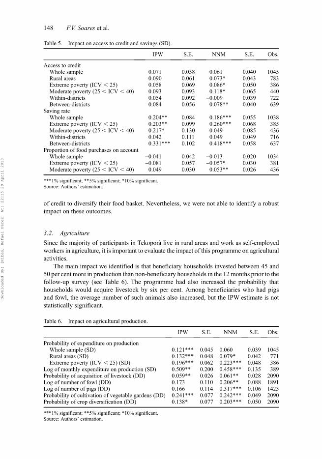
of credit to diversify their food basket. Nevertheless, we were not able to identify a robustimpact on these outcomes.

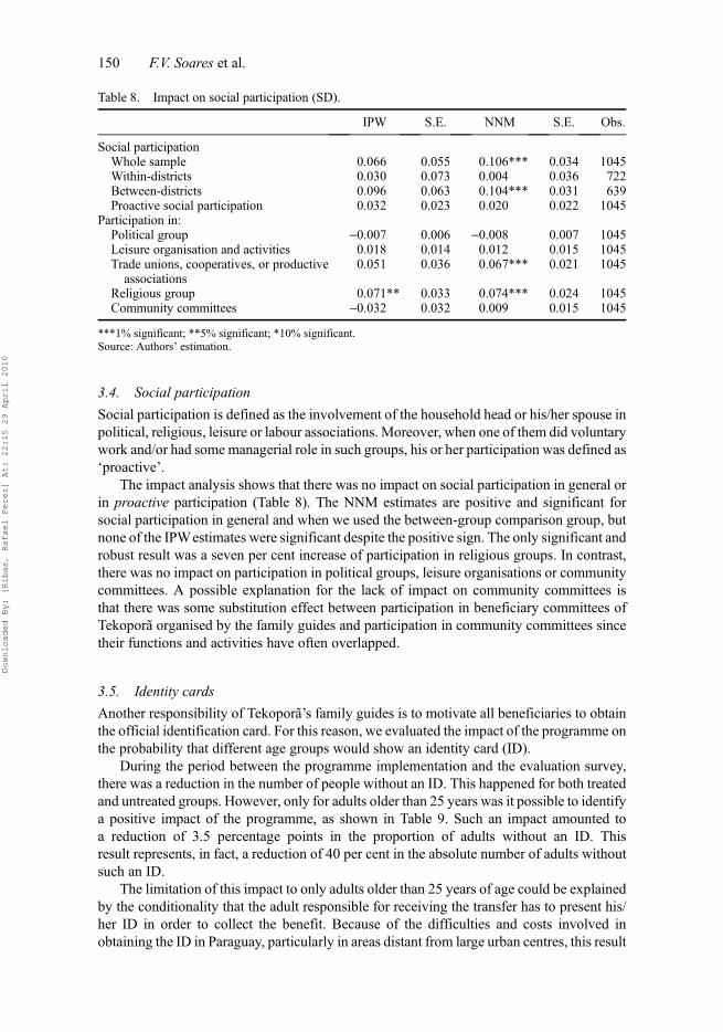
3.2. Agriculture

Since the majority of participants in Tekopora live in rural areas and work as self-employedworkers in agriculture, it is important to evaluate the impact of this programme on agriculturalactivities.

The main impact we identified is that beneficiary households invested between 45 and50 per cent more in production than non-beneficiary households in the 12 months prior to thefollow-up survey (see Table 6). The programme had also increased the probability thathouseholds would acquire livestock by six per cent. Among beneficiaries who had pigsand fowl, the average number of such animals also increased, but the IPW estimate is notstatistically significant.

Table 5. Impact on access to credit and savings (SD).

IPW S.E. NNM S.E. Obs.

Access to creditWhole sample 0.071 0.058 0.061 0.040 1045Rural areas 0.090 0.061 0.073* 0.043 783Extreme poverty (ICV , 25) 0.058 0.069 0.086* 0.050 386Moderate poverty (25 , ICV , 40) 0.093 0.093 0.118* 0.065 440Within-districts 0.054 0.092 -0.009 0.039 722Between-districts 0.084 0.056 0.078** 0.040 639

Saving rateWhole sample 0.204** 0.084 0.186*** 0.055 1038Extreme poverty (ICV , 25) 0.203** 0.099 0.260*** 0.068 385Moderate poverty (25 , ICV , 40) 0.217* 0.130 0.049 0.085 436Within-districts 0.042 0.111 0.049 0.049 716Between-districts 0.331*** 0.102 0.418*** 0.058 637

Proportion of food purchases on accountWhole sample -0.041 0.042 -0.013 0.020 1034Extreme poverty (ICV , 25) -0.081 0.057 -0.057* 0.030 381Moderate poverty (25 , ICV , 40) 0.049 0.030 0.053** 0.026 436

***1% significant; **5% significant; *10% significant.Source: Authors’ estimation.

Table 6. Impact on agricultural production.

IPW S.E. NNM S.E. Obs.

Probability of expenditure on productionWhole sample (SD) 0.121*** 0.045 0.060 0.039 1045Rural areas (SD) 0.132*** 0.048 0.079* 0.042 771Extreme poverty (ICV , 25) (SD) 0.196*** 0.062 0.223*** 0.048 386

Log of monthly expenditure on production (SD) 0.509** 0.200 0.458*** 0.135 389Probability of acquisition of livestock (DD) 0.059** 0.026 0.061** 0.028 2090Log of number of fowl (DD) 0.173 0.110 0.206** 0.088 1891Log of number of pigs (DD) 0.166 0.114 0.317*** 0.106 1423Probability of cultivation of vegetable gardens (DD) 0.241*** 0.077 0.242*** 0.049 2090Probability of crop diversification (DD) 0.138* 0.077 0.203*** 0.050 2090

***1% significant; **5% significant; *10% significant.Source: Authors’ estimation.

148 F.V. Soares et al.

Downloaded By: [Ribas, Rafael Perez] At: 22:15 29 April 2010

Particularly in rural areas and among extremely poor households, there was not only anexpansion in the amount invested in production but also an increase in the proportionof beneficiaries doing such investment. In rural areas this increase was between 8 and 13per cent, and among the extremely poor about 20 per cent.

Despite the overall decrease in both the cultivation of vegetable gardens (from 77% to65%) and in crop diversification (from 32% to 22%) for the entire sample between thebaseline and the follow-up survey, we identify positive impacts of the programme on theseindicators for treated households. That is, the programme effect took the form of dissuadingbeneficiary households from reducing their cultivation of vegetable gardens and reducingcrop diversification as much as the drastic way that the untreated households had done.

3.3. Labour supply

The impact on labour supply is one of the main concerns about cash transfer programmes.There is often a fear that transfers might cause dependency. For Tekopora, we assessed theimpact on the labour supply of the entire adult population and onmen and women separately,according to two definitions of ‘economic activity’. In the first definition, we included allpeople either working or looking for a job; and in the second definition, we added to the firstgroup temporary workers who were seasonally inactive at the time of the survey.

With regard to the first definition, Table 7 shows that we did not find a robust impact forthe whole sample – the IPWand the NNM estimates actually have different signs. For adultmen, both estimates were negative, but only the NNM estimate was statistically significant.For adult women, unlike the estimates for men, the impact was positive, but for bothdefinitions there were no significant impacts.

An explanation for the fact that the second definition yields a smaller negative pointestimate of the impact on beneficiary males than the first definition is that temporaryworkers, who usually work according to the seasonality of agriculture, might have refrainedfrom seeking casual jobs during their period of lay-off due to the receipt of the cash transfer.Using a qualitative approach, Guttandin (2007) corroborates this hypothesis by pointing outthat men participating in Tekopora could afford not to engage in casual work (changas) dueto the transfer. It is interesting to note that unlike the male labour supply, the point estimatesfor adult female labour supply actually decreases using the second definition. In any case,none of the definitions yield robust evidence of a negative impact of the programme on malelabour supply or positive for female labour supply.

Table 7. Impact on labour supply.

IPW S.E. NNM S.E. Obs.

Labour supply (without seasonal workers)Whole sample 0.022 0.033 -0.064** 0.025 5925Men -0.033 0.037 -0.101*** 0.024 3070Women 0.064 0.054 0.015 0.039 2855

Labour supply (with seasonal workers)Whole sample 0.028 0.032 -0.060** 0.026 5925Men -0.019 0.032 -0.097*** 0.023 3070Women 0.061 0.054 0.014 0.040 2855

***1% significant; **5% significant; *10% significant.Source: Authors’ estimation.

Journal of Development Effectiveness 149

Downloaded By: [Ribas, Rafael Perez] At: 22:15 29 April 2010

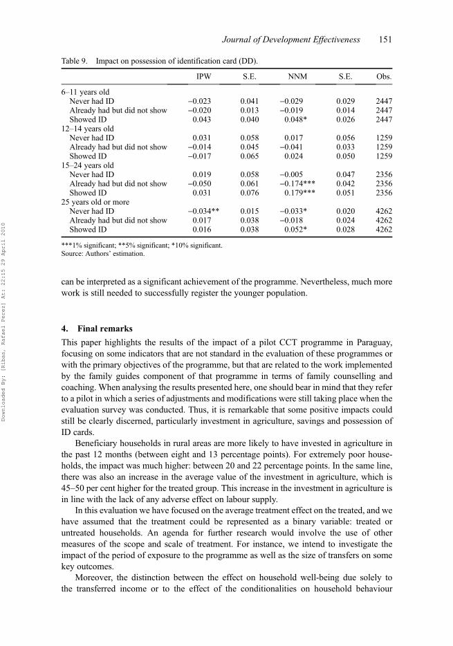
3.4. Social participation

Social participation is defined as the involvement of the household head or his/her spouse inpolitical, religious, leisure or labour associations. Moreover, when one of them did voluntarywork and/or had some managerial role in such groups, his or her participation was defined as‘proactive’.

The impact analysis shows that there was no impact on social participation in general orin proactive participation (Table 8). The NNM estimates are positive and significant forsocial participation in general and when we used the between-group comparison group, butnone of the IPWestimates were significant despite the positive sign. The only significant androbust result was a seven per cent increase of participation in religious groups. In contrast,there was no impact on participation in political groups, leisure organisations or communitycommittees. A possible explanation for the lack of impact on community committees isthat there was some substitution effect between participation in beneficiary committees ofTekopora organised by the family guides and participation in community committees sincetheir functions and activities have often overlapped.

3.5. Identity cards

Another responsibility of Tekopora’s family guides is to motivate all beneficiaries to obtainthe official identification card. For this reason, we evaluated the impact of the programme onthe probability that different age groups would show an identity card (ID).

During the period between the programme implementation and the evaluation survey,there was a reduction in the number of people without an ID. This happened for both treatedand untreated groups. However, only for adults older than 25 years was it possible to identifya positive impact of the programme, as shown in Table 9. Such an impact amounted toa reduction of 3.5 percentage points in the proportion of adults without an ID. Thisresult represents, in fact, a reduction of 40 per cent in the absolute number of adults withoutsuch an ID.

The limitation of this impact to only adults older than 25 years of age could be explainedby the conditionality that the adult responsible for receiving the transfer has to present his/her ID in order to collect the benefit. Because of the difficulties and costs involved inobtaining the ID in Paraguay, particularly in areas distant from large urban centres, this result

Table 8. Impact on social participation (SD).

IPW S.E. NNM S.E. Obs.

Social participationWhole sample 0.066 0.055 0.106*** 0.034 1045Within-districts 0.030 0.073 0.004 0.036 722Between-districts 0.096 0.063 0.104*** 0.031 639Proactive social participation 0.032 0.023 0.020 0.022 1045

Participation in:Political group -0.007 0.006 -0.008 0.007 1045Leisure organisation and activities 0.018 0.014 0.012 0.015 1045Trade unions, cooperatives, or productiveassociations

0.051 0.036 0.067*** 0.021 1045

Religious group 0.071** 0.033 0.074*** 0.024 1045Community committees -0.032 0.032 0.009 0.015 1045

***1% significant; **5% significant; *10% significant.Source: Authors’ estimation.

150 F.V. Soares et al.

Downloaded By: [Ribas, Rafael Perez] At: 22:15 29 April 2010

can be interpreted as a significant achievement of the programme. Nevertheless, much morework is still needed to successfully register the younger population.

4. Final remarks

This paper highlights the results of the impact of a pilot CCT programme in Paraguay,focusing on some indicators that are not standard in the evaluation of these programmes orwith the primary objectives of the programme, but that are related to the work implementedby the family guides component of that programme in terms of family counselling andcoaching. When analysing the results presented here, one should bear in mind that they referto a pilot in which a series of adjustments and modifications were still taking place when theevaluation survey was conducted. Thus, it is remarkable that some positive impacts couldstill be clearly discerned, particularly investment in agriculture, savings and possession ofID cards.

Beneficiary households in rural areas are more likely to have invested in agriculture inthe past 12 months (between eight and 13 percentage points). For extremely poor house-holds, the impact was much higher: between 20 and 22 percentage points. In the same line,there was also an increase in the average value of the investment in agriculture, which is45–50 per cent higher for the treated group. This increase in the investment in agriculture isin line with the lack of any adverse effect on labour supply.

In this evaluation we have focused on the average treatment effect on the treated, and wehave assumed that the treatment could be represented as a binary variable: treated oruntreated households. An agenda for further research would involve the use of othermeasures of the scope and scale of treatment. For instance, we intend to investigate theimpact of the period of exposure to the programme as well as the size of transfers on somekey outcomes.

Moreover, the distinction between the effect on household well-being due solely tothe transferred income or to the effect of the conditionalities on household behaviour

Table 9. Impact on possession of identification card (DD).

IPW S.E. NNM S.E. Obs.

6–11 years oldNever had ID -0.023 0.041 -0.029 0.029 2447Already had but did not show -0.020 0.013 -0.019 0.014 2447Showed ID 0.043 0.040 0.048* 0.026 2447

12–14 years oldNever had ID 0.031 0.058 0.017 0.056 1259Already had but did not show -0.014 0.045 -0.041 0.033 1259Showed ID -0.017 0.065 0.024 0.050 1259

15–24 years oldNever had ID 0.019 0.058 -0.005 0.047 2356Already had but did not show -0.050 0.061 -0.174*** 0.042 2356Showed ID 0.031 0.076 0.179*** 0.051 2356

25 years old or moreNever had ID -0.034** 0.015 -0.033* 0.020 4262Already had but did not show 0.017 0.038 -0.018 0.024 4262Showed ID 0.016 0.038 0.052* 0.028 4262

***1% significant; **5% significant; *10% significant.Source: Authors’ estimation.

Journal of Development Effectiveness 151

Downloaded By: [Ribas, Rafael Perez] At: 22:15 29 April 2010

requires a deeper investigation. Also requiring more research are the externalities of theprogramme. This research agenda would probably shed light on some of the key issues in theglobal debate about the effectiveness of CCT programmes and of their various components.

AcknowledgementsThe authors gratefully acknowledge the anonymous peer reviewer for comments and suggestions. Wewould like to thank the support and collaboration from Irene Ocampo (GTZ), Ofelia Insaurralde, JorgeCenturon, Pedro Gimenez, Dora Liz and Jorge Castillo from the Secretariat for Social Action (SAS) ofthe government of Paraguay throughout the evaluation project as well as the financial support fromGTZ Paraguay. We also would like to thank participants of the 3ie conference ‘Perspectives on ImpactEvaluation: Approaches to Assessing Development Effectiveness’ held in Cairo (March–April 2009)as well as anonymous peer reviewers for their suggestions and comments.

Notes1. For PROGRESA, see Behrman and Hoddinott (2005), Gertler (2004), Hoddinot et al. (2000) and

Parker and Skoufias (2000). For FA, see Attanasio andMesnard (2006), EDePo (2004), Attanasioet al. (2005). For BDH, see Schady and Araujo (2008). For RPS, seeMaluccio and Flores (2005).

2. Gertler et al. (2006) is one of the few papers to look at the impact of PROGRESA on productiveinvestments. They find a positive and significant impact of 2.5 percentual points on theprobability of beneficiary families to get involved in microenterprise.

3. The lack of monitoring in pilots or during the initial phase of programmes is not uncommon anddoes not prevent, at least in the short run, positive impacts on health and education outcomes. InEcuador, the conditionalities of the BDH were not monitored, but there have been positiveimpacts on school attendance. See Schady and Araujo (2006) for more details.

4. This component was largely inspired by the psychosocial support of the Puente Programmeimplemented in Chile.

5. Initially the programme intended to target only households with an ICV below 25 but, afterfailing to achieve the number of beneficiaries predicted by the poverty maps, the eligibilitythreshold was increased to 40 (Ribas et al. 2008). It is interesting to note that a similar problemhappened during the implementation of the first phase of PROGRESA, when there was aperception that some households were undeservedly excluded. To address this issue the cut-offpoint was revised upwards with the inclusion of new beneficiaries, the so-called ‘densificados’(Parker et al. 2008).

6. Note that our data, unlike Diaz and Handa’s (2006) and Handa and Maluccio’s (2010) non-experimental approach, come from the same instrument. Therefore, it is in line with the best-practices regarding the use of propensity score matching methods. Namely, the samequestionnaire, comparison group from the same socio-economic environment, and datacollected in the same period for both groups (Heckman et al. 1997).

7. The fact that some eligible households were forgotten was revealed to the managers of theprogramme, when the evaluation team was analysing the Ficha Hogar database.

8. See Ribas et al. (2009) for an analysis using the two comparison groups separately in order toidentify externality effects on the treated.

9. Externality effects would occur if the non-beneficiary (comparison) in the pilot was also affectedby the programme. In such a situation, the Single Unit Treatment Value Assumption – whichstates that the programme only affected treated observations – would be violated within the pilotdistricts. The impact of the programme on the treated could be estimated only with thecomparison group from non-pilot districts. By the same token, the difference in impact asmeasured by the two different comparison groups would offer an estimate of the externalityeffect. See Ribas et al. (2009) for more details.

10. This strategy was abandoned due to the lack of observations close to the threshold of eligibilityeven in the Ficha Hogar.

11. We implemented a modified version of Becker and Ichino (2002) STATAmodule that account forsampling weights. According to Abadie and Imbens (2008), matching standard errors should notbe bootstrapped.

152 F.V. Soares et al.

Downloaded By: [Ribas, Rafael Perez] At: 22:15 29 April 2010

12. In fact, we also have sampling weights. The final weight used in the regression analysis is thesampling weight multiplied by !ATT.

13. Because our focus is on the estimation of ATT, we define the common support as the propensityscore range for the treated. Any control observation with PS higher than the maximum or lowerthan the minimum of that range is dropped. We lost 4.3 per cent of the control group.

14. We implement these tests through Becker and Ichino (2002) STATA command. In the other twospecifications, 2.5 per cent and 2.8 per cent of the mean tests had rejected the null hypothesis ofequality of means. See Appendix 1.

15. For a summary of the impact of the programme on all outcomes evaluated, see Soares et al.(2008).

16. School attendance is a dummy variable indicating whether the child was attending classes duringthe month of the interview.

ReferencesAbadie, A., 2005. Semiparametric difference-in-difference estimators. Review of economic studies,

72(1), pp. 1–19.Abadie, A. and Imbens, G.W., 2008. On the failure of the bootstrap for matching estimators.

Econometrica, 76 (6), 1537–1558.Attanasio, O. and Mesnard, A., 2006. The impact of a conditional cash transfer programme on

consumption in Colombia. Fiscal studies, 27 (4), 421–442.Attanasio, O., Battistin, E., Fitzsimons, E., Mesnard, A. and Vera-Hernandez, M., 2005. How effective

are conditional cash transfers? Evidence from Colombia, IFS Briefing Note no. 54, IFS,University College London.

Becker, S.O. and Ichino, A., 2002. Estimation of average treatment effects based on propensity score.Stata journal, 2 (4), 358–377.

Behrman, J.R. and Hoddinott, J., 2005. Program evaluation with unobserved heterogeneity andselective implementation: the Mexican Progresa impact on child nutrition. Oxford bulletin ofeconomics and statistics, 67, 547–569.

Blundell, R., Costa Dias, M., Meghir, C. and Van Reenen, J., 2001. Evaluating the employment impactof a mandatory job search assistance programme. London: Institute of Fiscal Studies, UniversityCollege London, IFS Working Paper W01/20.

CEDP, 2004. Baseline report on the evaluation of Familias en Accion. London: Centre for theEvaluation of Development Policies, Institute of Fiscal Studies, IFS Report.

Deaton, A., 1997. The analysis of household surveys – a microenometric approach to developmentpolicy. Baltimore, MD: Johns Hopkins University Press, and Washington, DC: World Bank.

Dehejia, R.H. and Wahba, S., 2002. Propensity score-matching methods for nonexperimental causalstudies. Review of economics and statistics, 84 (1), 151–161.

Diaz, J.J. and Handa, S., 2006. An assessment of propensity score matching as nonexperimental impactestimator: evidence fromMexico’s PROGRESA programme. Journal of human resources, 41 (2),319–345.

Gertler, P., 2004. Do conditional cash transfer improve child health? Evidence from PROGRESA’scontrol randomizes experiment. American economic review, 94, 336–341.

Gertler, P., Martinez, S. and Rubio-Codina, M., 2006. Investing cash transfers to raise long-term livingstandards. Washington, DC: World Bank Policy Research, Working Paper 3994.

Guttandin, F. 2007. Pobreza campesina desde la perspectiva de las madres beneficiarias del programaTekopora. Asuncion: GTZ, UNFPA, and SAS.

Handa, S. and Mallucio, J.A., 2010. Matching the gold standard: comparing experimental and non-experimental evaluation techniques for a geographically targeted programme. Economic develop-ment and cultural change, 58, 415–447.

Heckman, J.J., Ichimura, H. and Todd, P.E., 1997. matching as an econometric evaluation estimator:evidence from evaluating a job training programme. Review of economic studies, 64 (4),605–654.

Hirano, K. and Imbens, G.W., 2001. Estimation of causal effects using propensity score weighting: anapplication to data on right heart characterization. Health services and outcomes research meth-odology, 2 (3–4), 1387–3741.

Hirano, K., Imbens, G.W. and Ridder, G., 2003. Efficient estimation of average treatment effects usingthe estimated propensity score. Econometrica, 71 (4), 1161–1189.

Journal of Development Effectiveness 153

Downloaded By: [Ribas, Rafael Perez] At: 22:15 29 April 2010

Hoddinot, et al., 2000. The impact of PROGRESA on consumption: a final report. Washington, DC:International Food Policy Research Institute.

Imbens, G. andWooldridge, J., 2009. Recent developments in the econometrics of program evaluation.Review of economic literature, 47 (1), 5–86.

Maluccio, J.A. and Flores, R., 2005. Impact evaluation of a conditional cash transfer program: theNicaraguan Red de Proteccion Social. Washington, DC; IFPRI, Research Report 141.

Parker, S.W. and Skoufias, E., 2000. The impact of PROGRESA on work, leisure and time allocation.Report submitted to PROGRESA. Washington, DC: IFPRI.

Parker, S.W., Rubalcava, L. and Teruel, G., 2008. Evaluating conditional schooling and healthprograms. In: T.P. Schultz and J. Strauss, eds. Handbook of development economics. vol. 4.Amsterdam: Elsevier, 3963–4035.

Ribas, R.P., Hirata, G.I. and Soares, F.V., 2008. Debating targeting methods for cash transfers:choosing between a multidimensional index and an income proxy for Paraguay’s Tekoporaprogramme. Brasılia: International Poverty Centre, IPC Evaluation Note 2.

Ribas, R.P., Soares, F.V., Silva, E. and Teixeira, C.G., 2009 Beyond cash: assessing externality andbehavioural change effects of a non-randomized CCT programme. Mimeo. Brasılia: IPC-IG.

Rosembaum, P. and Rubin, D.B., 1983. The central role of the propensity score in observational studiesfor causal effects. Biometrika, 70 (1), 41–55.

Rubin, D.B., 1977. Assignment to treatment group on the basis of a covariate. Journal of educationalstatistics, 2 (1), 1–26.

Schady, N. and Araujo, M.C., 2008. Cash transfers, conditions, school enrolment, and child work:evidence from a randomized experiment in Ecuador. Economıa, 8 (2), 131–154.

Soares, F.V., Ribas, R.P. and Hirata, G.I., 2008. Achievments and shortfalls of conditional cashtransfers: impact evaluation of Paraguay’s Tekopora programme. Brasılia: International PovertyCentre, IPC Evaluation Note 3.

Wooldridge, J.M., 2007. Inverse probability weighted estimation for general missing data problems.Journal of econometrics, 141 (2), 1281–1301.

154 F.V. Soares et al.

Downloaded By: [Ribas, Rafael Perez] At: 22:15 29 April 2010

Appendix1.

Differences

inhouseholdvariablesbefore

andaftertheweighting

process.

Unw

eigh

ted

Weigh

ted

treat

secomparison

set

comparison

set

ICV*

23.25

0.37

731

.37

0.45

0-1

3.81

22.21

0.27

42.23

ICVhealth

3.118

0.04

63.26

10.02

9-2

.63

3.22

10.02

6-1

.95

ICVeducation

3.73

10.09

74.47

70.09

2-5

.58

3.72

30.07

00.06

ICVocup

ation

0.31

20.02

90.511

0.02

9-4

.87

0.25

10.01

91.76

ICVho

using

8.75

90.19

811.65

0.21

0-1

0.02

8.111

0.14

52.65

ICVservices

4.68

70.13

57.51

00.15

2-1

3.90

4.41

50.10

01.62

ICVassets

1.00

50.10

22.18

60.08

9-8

.76

0.86

70.06

21.16

Rural(dum

my)*

0.88

00.01

80.69

30.01

77.47

0.90

00.011

-0.92

Caazapa

(dum

my)

*0.55

60.02

80.46

60.01

82.66

0.56

20.01

8-0

.18

Censo

(dum

my)

*0.76

20.02

40.92

20.01

0-6

.15

0.711

0.01

71.73

Interviewdate

91.73

5.52

966

.92

2.30

04.14

113.7

3.60

8-3

.33

Num

berof

children

under15

**3.29

80.10

22.72

40.06

34.80

3.24

90.06

60.41

Num

berof

children

6-14

years**

2.115

0.08

21.70

60.04

94.29

2.07

30.05

20.43

Num

berof

children

0-5year

**1.18

30.06

21.01

80.03

72.31

1.17

60.04

00.10

Num

berof

mem

bersin

thehh

**6.12

10.13

45.77

70.09

32.11

6.09

70.09

70.15

Headof

hhwithpartner(dum

my)

*0.84

40.02

00.84

10.01

40.11

0.84

00.01

40.17

Pregn

antwom

en(dum

my)

*0.06

40.01

40.07

90.01

0-0

.87

0.04

00.00

71.57

Elder

(dum

my)

*0.08

30.01

60.08

40.01

0-0

.03

0.09

70.011

-0.76

Num

berof

wom

en10

-59years

1.81

80.06

21.81

40.04

30.06

1.75

50.04

30.83

Wom

anhead

ofho

usehold(dum

my)

*0.25

40.02

50.20

20.01

51.80

0.26

30.01

6-0

.29

Headof

households

age*

43.02

0.75

443

.20

0.50

2-0

.19

44.96

0.49

2-2

.15

HeadhasID

card

(dum

my)

*0.86

60.01

90.80

60.01

52.49

0.85

70.01

30.41

Insalubrious

area

(dum

my)

*0.29

40.02

60.14

40.01

35.22

0.30

70.01

7-0

.40

Livein

aho

use(dum

my)

*0.33

60.02

70.54

90.01

8-6

.60

0.29

10.01

71.42

Owns

house(dum

my)

*0.88

00.01

80.90

40.011

-1.13

0.88

60.01

2-0

.27

Dirty

floo

r0.79

00.02

30.52

30.01

99.05

0.78

60.01

50.16

Thatchroof

0.51

70.02

80.40

80.01

83.24

0.58

70.01

8-2

.10

Woo

denwall

0.92

50.01

50.84

90.01

33.84

0.74

80.01

68.08

3or

morepeop

leperdo

rmitory(dum

my)

*0.54

70.02

80.39

10.01

84.68

0.58

90.01

8-1

.25

4or

morepeop

leperdo

rmitory(dum

my)

*0.19

50.02

20.10

30.011

3.68

0.18

00.01

40.56

Has

toilet(dum

my)

*0.04

20.011

0.13

70.01

3-5

.60

0.02

90.00

60.98

(con

tinu

ed)

Journal of Development Effectiveness 155

Downloaded By: [Ribas, Rafael Perez] At: 22:15 29 April 2010

App

endix1.

(Con

tinu

ed)

Unw

eigh

ted

Weigh

ted

treat

secomparison

set

comparison

set

Has

bath

0.39

40.02

80.48

80.01

9-2

.83

0.31

20.01

72.53

Water

pipedfrom

networkor

wells(dum

my)

*0.21

00.02

30.55

50.01

8-1

1.73

0.18

50.01

40.93

Water

conn

ection

outsidetheho

use(dum

my)

*0.26

10.02

50.15

10.01

33.91

0.31

30.01

7-1

.74

Has

electricity(dum

my)

*0.77

50.02

40.87

20.01

2-3

.65

0.72

70.01

71.68

Has

kitchen(dum

my)

*0.841

0.021

0.882

0.012

-1.71

0.87

20.01

2-1

.27

Has

teleph

one(dum

my)

*0.05

10.01

20.12

80.01

2-4

.37

0.04

90.00

80.13

Has

motorcycle

0.05

70.01

30.19

30.01

5-6

.99

0.08

10.01

0-1

.49

Has

laun

drymachine

(dum

my)

*0.07

10.01

40.21

00.01

5-6

.63

0.05

70.00

90.85

Has

refrigetator

(dum

my)

*0.25

40.02

50.49

00.01

9-7

.69

0.22

30.01

51.05

Yearsof

educationlost(upto

14years)**

1.24

70.06

50.98

50.04

23.37

1.18

60.04

80.75

Yearsof

educationlost(upto

24years)**

2.69

20.15

22.86

90.114

-0.93

2.74

50.111

-0.27

Headspeaks

guaranıandotherlang

uage

0.07

60.01

50.116

0.01

2-2

.09

0.09

30.011

-0.89

Spo

usespeaks

guaranıandotherlang

uage

(dum

my)

*0.08

60.01

60.09

90.011

-0.69

0.08

10.01

00.27

Heads

yearsof

education**

3.87

60.117

4.71

90.10

9-5

.28

3.76

10.08

20.80

Spo

uses

yearsof

education**

3.42

20.14

24.21

40.118

-4.29

3.44

00.09

0-0

.11

Num

berof

peop

lein

training

prog

rammes

*0.09

50.23

20.22

70.02

0-4

.25

0.06

80.01

21.04

Num

berof

sick

children

**0.72

40.07

50.63

50.04

41.02

0.71

20.05

20.12

Num

berof

chidrenwitho

utvaccinationcard

**0.26

20.03

00.23

40.01

60.82

0.22

70.01

80.99

Num

berof

sick

peop

le**

1.39

50.12

21.35

90.07

40.25

1.29

70.08

30.66

Som

eone

illwithhealth

care

(dum

my)

*0.31

30.02

60.37

00.01

8-1

.82

0.30

20.01

70.33

Allillmem

bershave

health

care

(dum

my)

0.19

70.02

20.26

30.01

6-2

.38

0.21

40.01

5-0

.61

Headisill(dum

my)

0.22

40.02

40.22

00.01

50.15

0.17

10.01

41.94

Spo

useisill(dum

my)

*0.23

60.02

40.23

40.01

60.07

0.19

00.01

51.63

Headisan

employ

ee(dum

my)

*0.08

30.01

60.113

0.01

2-1

.56

0.07

90.01

00.21

Headisaself-employed

(dum

my)

*0.690

0.026

0.665

0.017

0.78

0.746

0.016

-1.83

Headisano

n-remun

erated

worker(dum

my)

*0.20

70.02

30.17

70.01

41.11

0.16

00.01

41.77

Spo

useisan

employ

ee(dum

my)

0.01

80.00

70.03

60.00

7-1

.79

0.02

20.00

5-0

.38

Spo

useisaself-employ

ed(dum

my)

0.16

60.02

10.14

50.01

30.85

0.14

20.01

30.98

Spo

useisano

n-remun

erated

worker(dum

my)

*0.65

00.02

70.64

20.01

80.24

0.67

30.01

7-0

.72

Num

berof

children

who

work

0.23

60.03

50.112

0.01

43.30

0.16

90.01

81.72

Has

achildlabourer

(dum

my)

0.160

0.021

0.094

0.011

2.83

0.129

0.012

1.29

156 F.V. Soares et al.

Downloaded By: [Ribas, Rafael Perez] At: 22:15 29 April 2010

Num

berof

peop

leactive

inlabo

urmarket*

1.90

20.07

71.84

10.04

80.67

1.86

00.05

30.45

Has

avegetablegarden

(dum

my)

*0.77

50.02

40.77

10.01

60.12

0.79

10.01

5-0

.58

Has

land

forfarm

ing(dum

my)

*0.92

90.01

40.93

40.00

9-0

.28

0.93

10.00

9-0

.09

Has

sing

lecrop

cultivation(dum

my)*

0.25

40.02

50.25

20.01

60.08

0.24

20.01

60.40

Has

multiplecrop

scultivation(dum

my)

*0.35

30.02

70.28

50.01

72.14

0.33

20.01

70.65

Has

poultry(dum

my)

*0.88

30.01

80.89

70.011

-0.66

0.89

20.011

-0.42

Has

pigs

(dum

my)

0.66

60.02

70.65

70.01

80.29

0.62

50.01

81.28

Has

cows(dum

my)

*0.35

10.02

70.45

30.01

8-3

.12

0.411

0.01

8-1

.82

Has

horses

(dum

my)

*0.18

40.02

20.21

90.01

5-1

.34

0.13

00.01

22.12

Has

sheeps

(dum

my)

*0.66

60.02

60.65

60.17

60.29

0.62

50.01

81.28

Has

otheranim

als(dum

my)

0.016

0.007

0.025

0.006

-0.95

0.02

50.00

6-0

.98

Livein

thesameho

useformorethan

oneyear

(dum

my)

0.91

00.01

60.92

90.01

0-1

.00

0.96

30.00

7-3

.04

Livein

thesameho

usefor3yearsor

more(dum

my)

*0.77

10.02

40.81

60.01

4-1

.62

0.78

90.01

5-0

.67

Livein

thesameho

usefor5yearsor

more(dum

my)

*0.69

10.02

60.70

50.01

7-0

.44

0.72

00.01

7-0

.94

Livein

thesameho

usefor10

yearsor

more(dum

my)

0.44

90.02

80.52

20.01

9-2

.18

0.52

80.01

9-2

.34

Livein

thesameho

usefor20

yearsor

more(dum

my)

*0.21

30.02

30.22

90.01

6-0

.56

0.23

20.01

6-0

.68

percapitaincome*

3635

726

0872

877

2987

-9.21

3457

116

320.58

Mod

eratepo

or(dum

my)

*0.05

60.01

30.13

00.01

2-4

.14

0.05

50.00

80.05

Extremepo

or(dum

my)

*0.89

70.01

70.72

70.01

77.14

0.90

40.011

-0.36

Observation

s(com

mon

supp

ort)

401

974

401

974

*Variableincluded

inthefinalpropensity

scoremodel.

**Variableincluded

inthefinalpropensity

scoremodelthorughdummies.

Sou

rce:Ficha

Hog

ar.

Journal of Development Effectiveness 157

Downloaded By: [Ribas, Rafael Perez] At: 22:15 29 April 2010