MNRAS 492, 978–992 (2020) doi:10.1093/mnras/stz3519Advance Access publication 2019 December 16

I–Love–Q relations for realistic white dwarfs

Andrew J. Taylor,1 Kent Yagi2‹ and Phil L. Arras1

1Department of Astronomy, University of Virginia, Charlottesville, 22904, USA2Departmnet of Physics, University of Virginia, Charlottesville, 22904, USA

Accepted 2019 December 11. Received 2019 December 10; in original form 2019 November 8

ABSTRACTThe space-borne gravitational wave interferometer, Laser Interferometer Space Antenna, isexpected to detect signals from numerous binary white dwarfs. At small orbital separation,rapid rotation and large tidal bulges may allow for the stellar internal structure to be probedthrough such observations. Finite-size effects are encoded in quantities like the moment ofinertia (I), tidal Love number (Love), and quadrupole moment (Q). The universal relationsamong them (I–Love–Q relations) can be used to reduce the number of parameters in thegravitational-wave templates. We here study I–Love–Q relations for more realistic white dwarfmodels than used in previous studies. In particular, we extend previous works by including (i)differential rotation and (ii) internal temperature profiles taken from detailed stellar evolutioncalculations. We use the publicly available stellar evolution code MESA to generate coolingmodels of both low- and high-mass white dwarfs. We show that differential rotation causes theI–Q relation (and similarly the Love–Q relation) to deviate from that of constant rotation. Wealso find that the introduction of finite temperatures causes the white dwarf to move along thezero-temperature mass sequence of I–Q values, moving towards values that suggest a lowermass. We further find that after only a few Myr, high-mass white dwarfs are well describedby the zero-temperature model, suggesting that the relations with zero temperature may begood enough in most practical cases. Low-mass, He-core white dwarfs with thick hydrogenenvelopes may undergo long periods of H burning which sustain the stellar temperature andallow deviations from the I–Love–Q relations for longer times.

Key words: gravitational waves – white dwarfs.

1 IN T RO D U C T I O N

The Laser Interferometer Space Antenna (LISA) mission is slatedto launch in the 2030s, and it is expected that LISA will detectthousands of short-period white dwarf–white dwarf (WD–WD)binaries in the galaxy via their gravitational wave (GW) emission(Littenberg 2011). These binaries will be detected by fitting modelwaveforms to the observed GW data to infer relevant parameterssuch as orbital periods, chirp masses, and distances. The GWsignal of a WD–WD binary is given by a point-mass contributionand small corrections due to the finite size of the WDs. Thesesmall corrections may be measurable for binaries with sufficientlysmall separations (Shah, van der Sluys & Nelemans 2012; Shah &Nelemans 2014).

The leading-order finite-size correction to the GW signal comesfrom the transfer of angular momentum from the orbit to the spinsof the individual WDs by tidal friction. In the limit of strongtidal torques, the spins of the individual WDs may be nearly

� E-mail: ky5t@Virginia.EDU

synchronized to the spin frequency of the orbit well before merger(Iben, Tutukov & Fedorova 1998; Piro 2019). The strength of thiscorrection may be estimated by the small parameter (I1 + I2)/μa2

for perfect synchronization, where I1, 2 is the moment of inertia ofeach WD, μ is the reduced mass of the binary, and a is the semimajoraxis of the binary orbit (Benacquista 2011). Thus, the moment ofinertia of both WDs enter as parameters into the GW signal from abinary.

Higher order corrections to the GW signal appear due to thequadrupole moments of the individual stars themselves. As eachindividual star is distorted by tides and rotation, the orbital po-tential energy is changed, and this alters the relationship betweensemimajor axis and frequency away from the usual Keplerian one(Poisson 1998; Flanagan & Hinderer 2008; Benacquista 2011); thisis often referred to as the conservative effect. Additionally, as seenfrom a non-rotating frame, the quadrupoles raised on each star bytides vary over the orbit, leading to GW radiation emitted from theWDs themselves; this is often referred to as the non-conservativeor dissipative effect (Flanagan & Hinderer 2008). Though thecontributions from these effects to the GW signal are small, they arelikely to be measurable over the lifetime of LISA for systems with

C© 2019 The Author(s)Published by Oxford University Press on behalf of the Royal Astronomical Society

Dow

nloaded from https://academ

ic.oup.com/m

nras/article/492/1/978/5679150 by guest on 14 February 2022

I-Love-Q for realistic WDs 979

high signal-to-noise ratio, a low-mass (large-radius) primary, anda high-mass companion. Thus, we have that the moment of inertia(I), tidal Love number (Love), and rotational quadrupole moment(Q) of each WD enter as important parameters into the gravitationalwaveform for a double WD binary.

In the case of neutron stars (NSs), Yagi & Yunes (2013a, b)found that I, Love, and Q were related to each other in a waythat was independent of the assumed equation of state (EoS),which is currently poorly understood for NSs. These relationshipsformed the so-called ‘I–Love–Q relations’, and they serve to breakthe degeneracy between Q and other NS parameters, which inturn reduces the overall measurement uncertainties on the latter.Indeed, such universal relations, together with similar relations(Yagi & Yunes 2016, 2017), have been applied to GW170817 bythe LIGO/Virgo Collaborations (Abbott et al. 2018; Chatziioannou,Haster & Zimmerman 2018), which helped to improve our under-standing of nuclear physics by constraining the relation betweenpressure and density at supra-nuclear densities.

While different EoS prescriptions in the NS case may lead tosignificant differences in the mass–radius relation, the WD EoSis better understood. The EoS of the WD core is a degenerateelectron gas, allowing for arbitrarily relativistic electron velocity,and there are small corrections due to the electrostatic interaction ofthe electrons and ions, as well as due to finite temperature. Outsidethe degenerate core, there is a non-degenerate envelope composedof hydrogen and/or helium. The size of the envelope may be largerfor low-mass WDs, and for masses less than � 0.2 M�, residualnuclear burning in a thick hydrogen envelope may significantlyslow the WD’s cooling. The composition of the WD is determinedby post-main-sequence nuclear burning as well as binary masstransfer episodes. Low-mass WDs (M � 0.4 M�) are comprisedof a He core and H-rich envelope, while the bulk of the higher massWD will have a mixture of carbon and oxygen in the core, withthin shells of He and H outside. Element diffusion acts to allowheavy elements to sink down and light elements to rise up duringthe evolution, leading to the fractionated structure. The startingcentral temperature on the WD cooling track is determined by post-main-sequence He core burning and H/He shell burning. The finiteinitial core temperature, relative to the central Fermi energy, allowssome thermal pressure support, causing the WD to deviate fromthe zero-temperature solution. Thus, in the case of WDs, the I–Love–Q relations aim to relate relevant parameters of WDs to eachother across varying internal structure (such as varying composition,rotation profile, central temperature, age, etc.) as was accomplishedin the NS case.

In the case of binary WDs, it is I, Love, and Q that encode theeffects of the finite sizes of the WDs on to the gravitational waveform(unlike the binary NS case where it is the spin angular momentuminstead of I that is measurable). Boshkayev, Quevedo & Zhami(2017) first studied these I–Love–Q relations in the context of WDsand found that differences in WD compositions, and hence meanmass per electron and Coulomb interaction effects, did not affect therelationships between I, Love, and Q. Boshkayev & Quevedo (2018)further studied WDs with finite and uniform temperature, findingthat finite temperature effects did cause the relations to deviate fromthe zero-temperature result.

In this work, we further investigate these I–Love–Q relationsfor more realistic WD models. In particular, we consider twomain extensions: (i) differential rotation and (ii) self-consistenttemperature profiles.

As WDs in close binaries may be subject to strong tidal torquesand internal angular momentum redistribution mechanisms, their

rotational angular frequency profiles may be far from uniform.We study how this may affect the I–Love–Q relations for WDs.Yagi et al. (2014) have already studied these relations in thecontext of differentially rotating main-sequence stars (not compactobjects), and we build upon this work by studying how differentialrotation affects WD I–Love–Q relations.1 To do so, we solvefor the modification to interior structure using the Hartle–Thorneformalism (Hartle 1967; Hartle & Thorne 1968) in which wetreat the stellar rotation as a small perturbation. The results arecompared to the uniform rotation case (see Boshkayev et al. 2017).True differential rotation that occurs in the interiors of WDs isa complicated process; in this work, we assume a parametrizedmodel and investigate possible deviations from the usual I–Love–Qrelations that could occur.

Additionally, we will be studying the effects of finite temper-ature on WD I–Love–Q relations, extending the previous work(Boshkayev & Quevedo 2018) by using the publicly available MESA

code (Paxton et al. 2013) that evolves a star from the pre-mainsequence to the WD cooling track and allows for nuclear burning,as well as convective and radiative heat transport. We generate twoWD models, a low-mass He-core WD with mass M = 0.15 M� anda more massive C/O-core WD with mass M = 0.83 M� to test if theI–Love–Q relations hold in these two extremes. The use of MESA

models allows two improvements over the uniform temperatureused by Boshkayev & Quevedo (2018). First, the core temperatureis set by post-main-sequence burning and is not a free parameter.Second, while WD cores are nearly isothermal a few thermal timesafter formation, their envelopes have a steep outward tempera-ture gradient, and hence for low-mass WD with thick envelopesthe uniform temperature assumption may overestimate thermalsupport in the envelope. The finite temperature effects are mostpronounced in low-mass WD with thick H envelopes, which mayhave residual nuclear burning for Gyr which delays the cooling ofthe WD.

The Newtonian equations of inviscid fluid motion will be usedthroughout this paper, although occasional contact is made withresults for NSs, which used general relativity.

The remainder of the paper is organized as follows. In Section 2,we show how differential rotation alters the WD I–Love–Q relationscompared to that of constant rotation. In Section 3, we analysethe effects of finite temperature on the structure of WDs and howthe I–Love–Q relations are affected. Finally, Section 4 contains adiscussion of the results and the conclusions.

2 D I FFERENTI AL ROTATI ON

2.1 The background model

For the study of differential rotation in the present section (2), it isconvenient to employ simple models of zero-temperature WDs.The background model is constructed by solving the equationsof hydrostatic balance, interior mass, and the EoS. The EoS, orpressure–density relation, which is assumed here is P = Pe + Pc

+ PTF, where Pe is the pressure from degenerate electrons and Pc

is due to the electrostatic attraction among electrons and nuclei,and PTF is the correction due to non-uniform electron density ineach ion cell. The dominant contribution to the pressure is from the

1See also Bretz, Yagi & Yunes (2015) for the universal relations amongmultipole moments of differentially rotating Newtonian polytropes.

MNRAS 492, 978–992 (2020)

Dow

nloaded from https://academ

ic.oup.com/m

nras/article/492/1/978/5679150 by guest on 14 February 2022

980 A. J. Taylor, K. Yagi and P. L. Arras

degenerate electron gas (e.g. Shapiro & Teukolsky 1986):

Pe = mec2

8π2λ3e

[x(1 + x2

)1/2(

2

3x2 − 1

)+ ln

(x + (1 + x2)1/2

)],

(1)

where me is the mass of the electron, c is the speed of light,λe ≡ �/mec is the electron Compton wavelength, and x ≡ pF/mec� 1 for the non-relativistic case and x � 1 for the relativistic case.The Fermi momentum pF is related to the mass density ρ by

pF =(

3h3

8π

ρ

μemp

)1/3

, (2)

where μe is the mean mass per electron (μe = A/Z for a gas withone ion of mass Amp and charge +Ze) and mp is the mass of theproton. For stellar masses well above Jupiter’s mass, the Coulomband Thomas–Fermi corrections are a small perturbation, given by(see e.g. Salpeter 1961)

Pc + PTF = −mec2

λ3e

[αZ2/3

10π2

(4

9π

)1/3

x4

+ 162

175

(αZ2/3)2

9π2

(4

9π

)2/3x5

√1 + x2

], (3)

where α = 1/137 is the fine-structure constant. We see that theCoulomb correction is proportional to ρ4/3, while the degeneracypressure is proportional to ρ5/3, indicating that the Coulomb andThomas–Fermi corrections become smaller as WD central densityincreases.

In this section, the WD is assumed to be made of a singleion, and models with either 4He, 12C, or 16O will be given. Someresults are presented including PC + PTF while others ignore thesecorrections. The purpose of this section is not to perform an in-depth analysis of WD composition. Rather, the goal is to explorethe effect of differential rotation on WD models with different massand composition. Similarly, we choose to calculate WD parametersoutside of their physical mass ranges (C/O WDs do not exist belowroughly 0.45 M�) to show that the I–Love–Q relations hold forWDs even in these unphysical regimes.

2.2 Differential rotation profile

The equation of hydrostatic balance is given by

0 = −∇P − ρ∇� − ρ∇U, (4)

where P and ρ are the pressure and density, � is the gravitationalpotential, and U is the perturbing potential, here due to thecentrifugal force. For constant rotation, the perturbing potentialis given by

U = −1

2�2 2, (5)

where � is the spin frequency of the star, = rsin θ is thecylindrical radius, θ is the colatitude, and r is the spherical radius.The resulting centrifugal force is

Fc = −∇U = �2 � . (6)

We assume the following form for � = �( ) (see Komatsu,Eriguchi & Hachisu 1989):

�

�c= A2

A2 + 2. (7)

Here, �c is the central rotation frequency and A may be thought ofas a core radius of the rotation profile. The A → ∞ limit recoversconstant �, while small but non-zero A gives constant specificangular momentum j = � 2. Demanding that the centrifugal forcestill be of the same form

Fc = − dU

d= �2, (8)

gives the following potential for the differentially rotating case

U = −∫

0�2

c

(A2

A2 + 2

)2

d (9)

= −1

2�2

c

2

1 + 2/A2. (10)

Written in this form, it is clear that in the limit that A � , werecover the results of constant rotation. In Appendix A, the perturbedstructure equations are given including the effect of differentialrotation.

Since the chief purpose of this work is to aid in modelling grav-itational waveforms from WD binaries, we only consider leading-order contributions to I, Love, and Q in rotation. These termsappear in small corrections to the waveform, so spin correctionsto these terms are higher order and therefore negligible. Due tothis assumption, the moment of inertia is entirely a backgroundquantity, unaffected by (differential) rotation while the quadrupolemoment is proportional to spin squared. The tidal Love numberis also unaffected by rotation, which we explain in more detail inSection 2.4.

2.3 Choice of A and �c

The core radius for differential rotation is expressed as a dimension-less parameter As ≡ A/R, where R is the radius of the non-rotatingbackground star. Only a certain range of As is physically relevant;if As � 1, then nearly the entire star has constant-j rotation, andthe entire star has uniform rotation for As � 1, a case alreadystudied (see Boshkayev et al. 2017). Thus, any study of the effectsof differential rotation on the I–Love–Q relations need only concernitself with intermediate values of As. Models are presented over arange of As between 0.1 and 10 as well as for a range of WD centraldensities. We then calculated I, Q, and the tidal Love number foreach model using the perturbative approach given in Appendix A3.

As we now motivate, sequences of models with fixed J willbe used in order to study the variation of I and Q for differentAs. In previous works, it was natural to fix the spin frequency ofthe star at the breakup frequency

√GM/R3 as this demonstrated

the maximum possible effect of rotation. Here, however, the freeparameter is the central spin frequency �c, which is different fromthe spin frequency at the surface. We fix each WD’s value of J toa specified Jfixed by adjusting the value of �c. Each WD structurewas first computed using a test value of �c equal to

√GM/R3,

and its angular momentum J0 was calculated using the methods ofSection A3. The value of �c was then scaled down by a factor ofJfixed/J0, since J ∝ �c at leading order in spin. The model was thencomputed again using this new value of �c, and the parameters ofthis second iteration were recorded. Had we not chosen to fix J andinstead fixed �c, the sequences of I and Q would not be physicallymeaningful, e.g. for small As, most of the star would be rotatingslowly. By fixing J, we aim to compare similar stars to each other,rather than stars rotating at significantly different rates, and by doingso properly calibrate the effects of differential rotation.

MNRAS 492, 978–992 (2020)

Dow

nloaded from https://academ

ic.oup.com/m

nras/article/492/1/978/5679150 by guest on 14 February 2022

I-Love-Q for realistic WDs 981

2.4 The Love number

In Newtonian physics (but not in full general relativity – see Mora &Will 2004), the Love number represents the linear response of thestar to a perturbing potential, and is simply related to the quadrupolemoment. In the case of tides, the point mass gravity of star 2 givesrise to a quadrupole tidal potential acting on star 1

U2(�x1) = −Gm2r2

1

r32

P2(cos θ12). (11)

Here �x1 = (r1, θ1, φ1) are the coordinates inside star 1. The coordi-nates (r2, θ2, φ2) describe the position of the centre of mass of star2 as seen from the centre of mass of star 1. The angle θ12 is definedby cos(θ12) = �x1 · �x2/(r1r2). This tidal potential will cause densitychanges within star 1, causing the external potential to deviate fromthe point mass value through the quadrupole moment

Q1 = λ1m2R5

1

r32

, (12)

where λ1 is the quadrupolar Love number of star 1, a dimensionlessnumber mainly dependent on the central concentration. The case ofuniform rotation is similar. The quadrupolar centrifugal potentialis

U (�x1) = 1

3�2

1r21 P2(cos θ1). (13)

This potential has the same form as for tides, and so the Lovenumber, which is independent of any constants in U, must be thesame as for tides. The quadrupole moment is then only differentdue to the parameters in the forcing potential, and an extra factorof P2(0) = −1/2 for rotation axis perpendicular to the orbital plane,giving

Q1 = 1

6Gλ1�

21R

51 . (14)

Hence in the Newtonian case, there is a simple relationship betweenLove numbers and quadrupole moments, at least for uniformrotation, and it is not necessary to consider the full I–Love–Qrelations.

Different branches of physics and astronomy refer to differentquantities by the term ‘Love number’. Here the Love number isdefined by a ratio of response potential to forcing potential fora particular spherical harmonic component and evaluated at thesurface,

λ ≡ δ� (R)

U (R)(15)

(also see Appendix A3). In this work, the main perturbing potentialwe are dealing with is the centrifugal potential. However, in thechief application of this work (GWs from binary WDs), it is ratherthe tidal potential (and thus the tidal Love number) which is moreimportant (see Benacquista 2011). This is the ‘Love’ of the I–Love–Q relations, as it provides information about small corrections tothe background point-mass GW signal emitted by a binary system.

In Newtonian physics assuming constant rotation, the rotationalLove number λR and the tidal Love number λT are equivalent(Mora & Will 2004), and they are often used interchangeably. Thetidal Love number depends on the type of material being tidallydistorted; thus, WDs (which vary in polytropic index from 3/2 to3) vary in tidal Love number depending on their density profile.However, to leading order in spin, the tidal Love number does notdepend on the amount of rotation occurring inside the WD, so thereshould be no dependence of the tidal Love number on the amountof differential rotation occurring inside the WD.

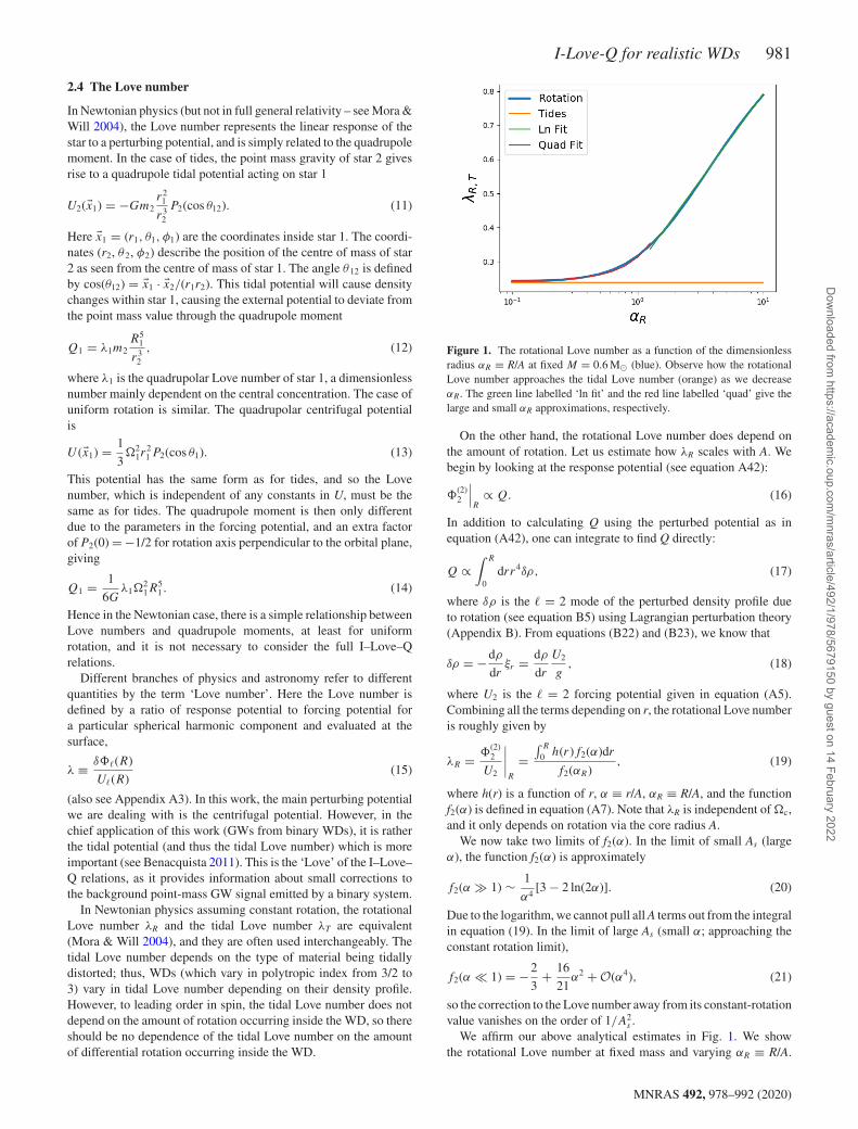
Figure 1. The rotational Love number as a function of the dimensionlessradius αR ≡ R/A at fixed M = 0.6 M� (blue). Observe how the rotationalLove number approaches the tidal Love number (orange) as we decreaseαR. The green line labelled ‘ln fit’ and the red line labelled ‘quad’ give thelarge and small αR approximations, respectively.

On the other hand, the rotational Love number does depend onthe amount of rotation. Let us estimate how λR scales with A. Webegin by looking at the response potential (see equation A42):

�(2)2

∣∣∣R

∝ Q. (16)

In addition to calculating Q using the perturbed potential as inequation (A42), one can integrate to find Q directly:

Q ∝∫ R

0drr4δρ, (17)

where δρ is the = 2 mode of the perturbed density profile dueto rotation (see equation B5) using Lagrangian perturbation theory(Appendix B). From equations (B22) and (B23), we know that

δρ = −dρ

drξr = dρ

dr

U2

g, (18)

where U2 is the = 2 forcing potential given in equation (A5).Combining all the terms depending on r, the rotational Love numberis roughly given by

λR = �(2)2

U2

∣∣∣∣R

=∫ R

0 h(r)f2(α)dr

f2(αR), (19)

where h(r) is a function of r, α ≡ r/A, αR ≡ R/A, and the functionf2(α) is defined in equation (A7). Note that λR is independent of �c,and it only depends on rotation via the core radius A.

We now take two limits of f2(α). In the limit of small As (largeα), the function f2(α) is approximately

f2(α � 1) ∼ 1

α4[3 − 2 ln(2α)]. (20)

Due to the logarithm, we cannot pull all A terms out from the integralin equation (19). In the limit of large As (small α; approaching theconstant rotation limit),

f2(α � 1) = −2

3+ 16

21α2 + O(α4), (21)

so the correction to the Love number away from its constant-rotationvalue vanishes on the order of 1/A2

s .We affirm our above analytical estimates in Fig. 1. We show

the rotational Love number at fixed mass and varying αR ≡ R/A.

MNRAS 492, 978–992 (2020)

Dow

nloaded from https://academ

ic.oup.com/m

nras/article/492/1/978/5679150 by guest on 14 February 2022

982 A. J. Taylor, K. Yagi and P. L. Arras

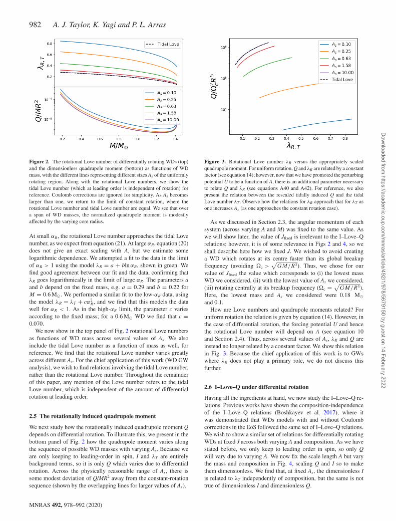
Figure 2. The rotational Love number of differentially rotating WDs (top)and the dimensionless quadrupole moment (bottom) as functions of WDmass, with the different lines representing different sizes As of the uniformlyrotating region. Along with the rotational Love numbers, we show thetidal Love number (which at leading order is independent of rotation) forreference. Coulomb corrections are ignored for simplicity. As As becomeslarger than one, we return to the limit of constant rotation, where therotational Love number and tidal Love number are equal. We see that overa span of WD masses, the normalized quadrupole moment is modestlyaffected by the varying core radius.

At small αR, the rotational Love number approaches the tidal Lovenumber, as we expect from equation (21). At large αR, equation (20)does not give an exact scaling with A, but we estimate somelogarithmic dependence. We attempted a fit to the data in the limitof αR > 1 using the model λR = a + bln αR, shown in green. Wefind good agreement between our fit and the data, confirming thatλR goes logarithmically in the limit of large αR. The parameters aand b depend on the fixed mass, e.g. a = 0.29 and b = 0.22 forM = 0.6 M�. We performed a similar fit to the low-αR data, usingthe model λR = λT + cα2

R , and we find that this models the datawell for αR < 1. As in the high-αR limit, the parameter c variesaccording to the fixed mass; for a 0.6 M� WD we find that c =0.070.

We now show in the top panel of Fig. 2 rotational Love numbersas functions of WD mass across several values of As. We alsoinclude the tidal Love number as a function of mass as well, forreference. We find that the rotational Love number varies greatlyacross different As. For the chief application of this work (WD GWanalysis), we wish to find relations involving the tidal Love number,rather than the rotational Love number. Throughout the remainderof this paper, any mention of the Love number refers to the tidalLove number, which is independent of the amount of differentialrotation at leading order.

2.5 The rotationally induced quadrupole moment

We next study how the rotationally induced quadrupole moment Qdepends on differential rotation. To illustrate this, we present in thebottom panel of Fig. 2 how the quadrupole moment varies alongthe sequence of possible WD masses with varying As. Because weare only keeping to leading-order in spin, I and λT are entirelybackground terms, so it is only Q which varies due to differentialrotation. Across the physically reasonable range of As, there issome modest deviation of Q/MR2 away from the constant-rotationsequence (shown by the overlapping lines for larger values of As).

Figure 3. Rotational Love number λR versus the appropriately scaledquadrupole moment. For uniform rotation, Q and λR are related by a constantfactor (see equation 14); however, now that we have promoted the perturbingpotential U to be a function of A, there is an additional parameter necessaryto relate Q and λR (see equations A40 and A42). For reference, we alsopresent the relation between the rescaled tidally induced Q and the tidalLove number λT. Observe how the relations for λR approach that for λT asone increases As (as one approaches the constant rotation case).

As we discussed in Section 2.3, the angular momentum of eachsystem (across varying A and M) was fixed to the same value. Aswe will show later, the value of Jfixed is irrelevant to the I–Love–Qrelations; however, it is of some relevance in Figs 2 and 4, so weshall describe here how we fixed J. We wished to avoid creatinga WD which rotates at its centre faster than its global breakupfrequency (avoiding �c >

√GM/R3). Thus, we chose for our

value of Jfixed the value which corresponds to (i) the lowest massWD we considered, (ii) with the lowest value of As we considered,(iii) rotating centrally at its breakup frequency (�c =

√GM/R3).

Here, the lowest mass and As we considered were 0.18 M�and 0.1.

How are Love numbers and quadrupole moments related? Foruniform rotation the relation is given by equation (14). However, inthe case of differential rotation, the forcing potential U and hencethe rotational Love number will depend on A (see equation 10and Section 2.4). Thus, across several values of As, λR and Q areinstead no longer related by a constant factor. We show this relationin Fig. 3. Because the chief application of this work is to GWswhere λR does not play a primary role, we do not discuss thisfurther.

2.6 I–Love–Q under differential rotation

Having all the ingredients at hand, we now study the I–Love–Q re-lations. Previous works have shown the composition-independenceof the I–Love–Q relations (Boshkayev et al. 2017), where itwas demonstrated that WDs models with and without Coulombcorrections in the EoS followed the same set of I–Love–Q relations.We wish to show a similar set of relations for differentially rotatingWDs at fixed J across both varying A and composition. As we havestated before, we only keep to leading order in spin, so only Qwill vary due to varying A. We now fix the scale length A but varythe mass and composition in Fig. 4, scaling Q and I so to makethem dimensionless. We find that, at fixed As, the dimensionless Iis related to λT independently of composition, but the same is nottrue of dimensionless I and dimensionless Q.

MNRAS 492, 978–992 (2020)

Dow

nloaded from https://academ

ic.oup.com/m

nras/article/492/1/978/5679150 by guest on 14 February 2022

I-Love-Q for realistic WDs 983

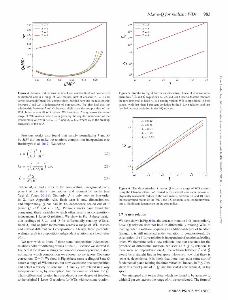
Figure 4. Normalized I versus the tidal Love number (top) and normalizedQ (bottom) across a range of WD masses, now at constant As = 1 andacross several different WD compositions. We find here that the relationshipbetween I and λT is independent of composition. We also find that therelationship between I and Q depends slightly on the composition of theWD chosen across all WD masses. We have fixed J = J0 across the entirerange of WD masses, where J0 is given by the angular momentum of thelowest mass WD with A/R = 10−3 and �c = �b, where �b is the breakupfrequency of the WD.

Previous works also found that simply normalizing I and Qby MR2 did not make the relations composition-independent (seeBoshkayev et al. 2017). We define

I ≡(

c2

G

)2I

M3, (22)

λT ≡ 1

3

(c2

GM/R

)5

λT , (23)

Q ≡ c2Q

J 2/M, (24)

where M, R, and I refer to the non-rotating, background com-ponent of the star’s mass, radius, and moment of inertia (seeYagi & Yunes 2013a). Similarly, J is only kept to first-orderin �c (see Appendix A3). Each term is now dimensionless,and importantly, Q has had its �c dependence scaled out of it(since Q ∼ �2

c and J ∼ �c). Previous works have found thatcomparing these variables to each other results in composition-independent I–Love–Q relations. We show in Fig. 5 these partic-ular scalings of I, λT, and Q for differentially rotating WDs atfixed As and angular momentum across a range of WD massesand several different WD compositions. Clearly, these particularscalings result in composition-independent relations at a fixed valueof As.

We now wish to know if these same composition-independentrelations hold for differing values of the As. Because we showed inFig. 5 that the above scalings are composition-independent, it doesnot matter which composition we choose, so we ignore Coulombcorrections (Z = 0). We show in Fig. 6 these same scalings of I and Qacross a range of WD masses, but now we choose one compositionand select a variety of core radii. I and λT are related in a wayindependent of As by assumption, but the same is not true for Q.Thus, differential rotation has introduced a new degree of freedomto the original I–Love–Q relations for WDs with constant rotation.

Figure 5. Similar to Fig. 4 but for an alternative choice of dimensionlessquantities I , λ, and Q (equations 22, 23, and 24). Observe that the relationsare now universal at fixed As = 1 among various WD compositions in bothpanels, with less than 1 per cent deviation in the I–Love relation and lessthat 0.4 per cent deviation in the I–Q relation.

Figure 6. The dimensionless I versus Q across a range of WD masses,using the Chandrasekhar EoS, varied across several core radii. Across allphysically reasonable values of the core radius (between 0.1 and 10 timesthe background radius of the WD), the I–Q relation is no longer universaldue to significant dependence on the core radius.

2.7 A new relation

We have shown in Fig. 6 that the constant-rotation I–Q (and similarlyLove–Q) relation does not hold in differentially rotating WDs toleading order in rotation, acquiring an additional degree of freedom(though it is still universal under variation in compositions). Byassumption, the I–Love relation is independent of rotation at leadingorder. We therefore seek a new relation, one that accounts for thepresence of differential rotation; we seek an I–Q–As relation. Ifthere were no dependence on As, the relation between I and Q

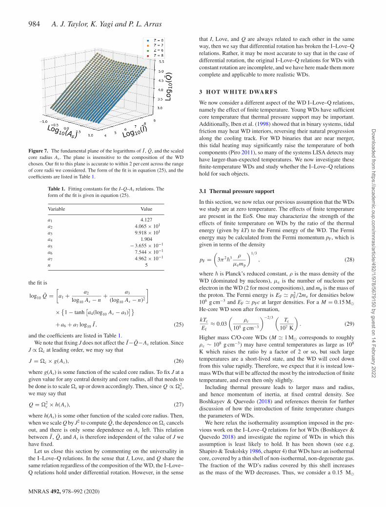
would be a straight line in log space. However, now that there issome As dependence, it is likely that there may exist some sort offundamental plane relating the three variables. Indeed, in Fig. 7 weshow this exact plane of I , Q, and the scaled core radius As in logspace.

We attempted a fit to the data, which we found to be accurate towithin 2 per cent across the range of As we considered. The form of

MNRAS 492, 978–992 (2020)

Dow

nloaded from https://academ

ic.oup.com/m

nras/article/492/1/978/5679150 by guest on 14 February 2022

984 A. J. Taylor, K. Yagi and P. L. Arras

Figure 7. The fundamental plane of the logarithms of I , Q, and the scaledcore radius As. The plane is insensitive to the composition of the WDchosen. Our fit to this plane is accurate to within 2 per cent across the rangeof core radii we considered. The form of the fit is in equation (25), and thecoefficients are listed in Table 1.

Table 1. Fitting constants for the I–Q–As relations. Theform of the fit is given in equation (25).

Variable Value

a1 4.127a2 4.065 × 101

a3 9.918 × 101

a4 1.904a5 − 3.655 × 10−1

a6 7.544 × 10−1

a7 4.962 × 10−1

n 5

the fit is

log10 Q =[a1 + a2

log10 As − n+ a3

(log10 As − n)2

]

×{1 − tanh

[a4(log10 As − a5)

]}+ a6 + a7 log10 I , (25)

and the coefficients are listed in Table 1.We note that fixing J does not affect the I−Q−As relation. Since

J ∝ �c at leading order, we may say that

J = �c × g(As), (26)

where g(As) is some function of the scaled core radius. To fix J at agiven value for any central density and core radius, all that needs tobe done is to scale �c up or down accordingly. Then, since Q ∝ �2

c ,we may say that

Q = �2c × h(As), (27)

where h(As) is some other function of the scaled core radius. Then,when we scale Q by J2 to compute Q, the dependence on �c cancelsout, and there is only some dependence on As left. This relationbetween I , Q, and As is therefore independent of the value of J wehave fixed.

Let us close this section by commenting on the universality inthe I–Love–Q relations. In the sense that I, Love, and Q share thesame relation regardless of the composition of the WD, the I–Love–Q relations hold under differential rotation. However, in the sense

that I, Love, and Q are always related to each other in the sameway, then we say that differential rotation has broken the I–Love–Qrelations. Rather, it may be most accurate to say that in the case ofdifferential rotation, the original I–Love–Q relations for WDs withconstant rotation are incomplete, and we have here made them morecomplete and applicable to more realistic WDs.

3 H OT W H I T E DWA R F S

We now consider a different aspect of the WD I–Love–Q relations,namely the effect of finite temperature. Young WDs have sufficientcore temperature that thermal pressure support may be important.Additionally, Iben et al. (1998) showed that in binary systems, tidalfriction may heat WD interiors, reversing their natural progressionalong the cooling track. For WD binaries that are near merger,this tidal heating may significantly raise the temperature of bothcomponents (Piro 2011), so many of the systems LISA detects mayhave larger-than-expected temperatures. We now investigate thesefinite-temperature WDs and study whether the I–Love–Q relationshold for such objects.

3.1 Thermal pressure support

In this section, we now relax our previous assumption that the WDswe study are at zero temperature. The effects of finite temperatureare present in the EoS. One may characterize the strength of theeffects of finite temperature on WDs by the ratio of the thermalenergy (given by kT) to the Fermi energy of the WD. The Fermienergy may be calculated from the Fermi momentum pF, which isgiven in terms of the density

pF =(

3π2�

3 ρ

μemp

)1/3

, (28)

where � is Planck’s reduced constant, ρ is the mass density of theWD (dominated by nucleons), μe is the number of nucleons perelectron in the WD (2 for most compositions), and mp is the mass ofthe proton. The Fermi energy is EF � p2

F/2me for densities below106 g cm−3 and EF � pFc at larger densities. For a M = 0.15 M�He-core WD soon after formation,

kTc

Ef≈ 0.03

(ρc

105 g cm−3

)−2/3 (Tc

107 K

). (29)

Higher mass C/O-core WDs (M � 1 M� corresponds to roughlyρc ∼ 108 g cm−3) may have central temperatures as large as 108

K which raises the ratio by a factor of 2 or so, but such largetemperatures are a short-lived state, and the WD will cool downfrom this value rapidly. Therefore, we expect that it is instead low-mass WDs that will be affected the most by the introduction of finitetemperature, and even then only slightly.

Including thermal pressure leads to larger mass and radius,and hence momentum of inertia, at fixed central density. SeeBoshkayev & Quevedo (2018) and references therein for furtherdiscussion of how the introduction of finite temperature changesthe parameters of WDs.

We here relax the isothermality assumption imposed in the pre-vious work on the I–Love–Q relations for hot WDs (Boshkayev &Quevedo 2018) and investigate the regime of WDs in which thisassumption is least likely to hold. It has been shown (see e.g.Shapiro & Teukolsky 1986, chapter 4) that WDs have an isothermalcore, covered by a thin shell of non-isothermal, non-degenerate gas.The fraction of the WD’s radius covered by this shell increasesas the mass of the WD decreases. Thus, we consider a 0.15 M�

MNRAS 492, 978–992 (2020)

Dow

nloaded from https://academ

ic.oup.com/m

nras/article/492/1/978/5679150 by guest on 14 February 2022

I-Love-Q for realistic WDs 985

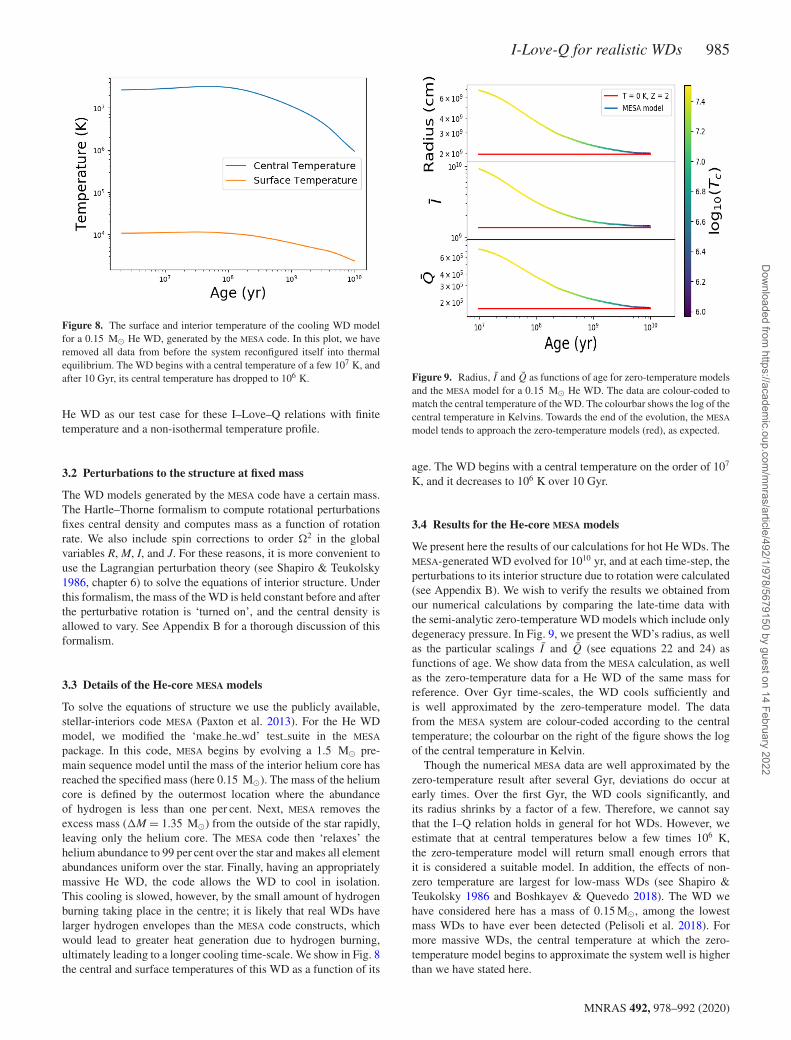
Figure 8. The surface and interior temperature of the cooling WD modelfor a 0.15 M� He WD, generated by the MESA code. In this plot, we haveremoved all data from before the system reconfigured itself into thermalequilibrium. The WD begins with a central temperature of a few 107 K, andafter 10 Gyr, its central temperature has dropped to 106 K.

He WD as our test case for these I–Love–Q relations with finitetemperature and a non-isothermal temperature profile.

3.2 Perturbations to the structure at fixed mass

The WD models generated by the MESA code have a certain mass.The Hartle–Thorne formalism to compute rotational perturbationsfixes central density and computes mass as a function of rotationrate. We also include spin corrections to order �2 in the globalvariables R, M, I, and J. For these reasons, it is more convenient touse the Lagrangian perturbation theory (see Shapiro & Teukolsky1986, chapter 6) to solve the equations of interior structure. Underthis formalism, the mass of the WD is held constant before and afterthe perturbative rotation is ‘turned on’, and the central density isallowed to vary. See Appendix B for a thorough discussion of thisformalism.

3.3 Details of the He-core MESA models

To solve the equations of structure we use the publicly available,stellar-interiors code MESA (Paxton et al. 2013). For the He WDmodel, we modified the ‘make he wd’ test suite in the MESA

package. In this code, MESA begins by evolving a 1.5 M� pre-main sequence model until the mass of the interior helium core hasreached the specified mass (here 0.15 M�). The mass of the heliumcore is defined by the outermost location where the abundanceof hydrogen is less than one per cent. Next, MESA removes theexcess mass (�M = 1.35 M�) from the outside of the star rapidly,leaving only the helium core. The MESA code then ‘relaxes’ thehelium abundance to 99 per cent over the star and makes all elementabundances uniform over the star. Finally, having an appropriatelymassive He WD, the code allows the WD to cool in isolation.This cooling is slowed, however, by the small amount of hydrogenburning taking place in the centre; it is likely that real WDs havelarger hydrogen envelopes than the MESA code constructs, whichwould lead to greater heat generation due to hydrogen burning,ultimately leading to a longer cooling time-scale. We show in Fig. 8the central and surface temperatures of this WD as a function of its

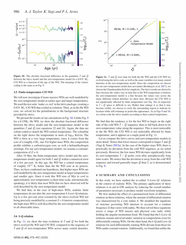
Figure 9. Radius, I and Q as functions of age for zero-temperature modelsand the MESA model for a 0.15 M� He WD. The data are colour-coded tomatch the central temperature of the WD. The colourbar shows the log of thecentral temperature in Kelvins. Towards the end of the evolution, the MESA

model tends to approach the zero-temperature models (red), as expected.

age. The WD begins with a central temperature on the order of 107

K, and it decreases to 106 K over 10 Gyr.

3.4 Results for the He-core MESA models

We present here the results of our calculations for hot He WDs. TheMESA-generated WD evolved for 1010 yr, and at each time-step, theperturbations to its interior structure due to rotation were calculated(see Appendix B). We wish to verify the results we obtained fromour numerical calculations by comparing the late-time data withthe semi-analytic zero-temperature WD models which include onlydegeneracy pressure. In Fig. 9, we present the WD’s radius, as wellas the particular scalings I and Q (see equations 22 and 24) asfunctions of age. We show data from the MESA calculation, as wellas the zero-temperature data for a He WD of the same mass forreference. Over Gyr time-scales, the WD cools sufficiently andis well approximated by the zero-temperature model. The datafrom the MESA system are colour-coded according to the centraltemperature; the colourbar on the right of the figure shows the logof the central temperature in Kelvin.

Though the numerical MESA data are well approximated by thezero-temperature result after several Gyr, deviations do occur atearly times. Over the first Gyr, the WD cools significantly, andits radius shrinks by a factor of a few. Therefore, we cannot saythat the I–Q relation holds in general for hot WDs. However, weestimate that at central temperatures below a few times 106 K,the zero-temperature model will return small enough errors thatit is considered a suitable model. In addition, the effects of non-zero temperature are largest for low-mass WDs (see Shapiro &Teukolsky 1986 and Boshkayev & Quevedo 2018). The WD wehave considered here has a mass of 0.15 M�, among the lowestmass WDs to have ever been detected (Pelisoli et al. 2018). Formore massive WDs, the central temperature at which the zero-temperature model begins to approximate the system well is higherthan we have stated here.

MNRAS 492, 978–992 (2020)

Dow

nloaded from https://academ

ic.oup.com/m

nras/article/492/1/978/5679150 by guest on 14 February 2022

986 A. J. Taylor, K. Yagi and P. L. Arras

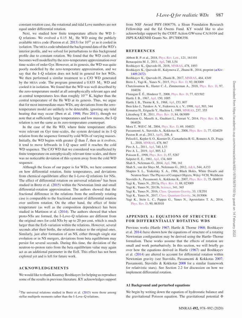
Figure 10. The absolute fractional difference in the quantities I and Q

between the MESA model and the zero-temperature model for a 0.835 M�C/O WD as a function of the age of the WD. The meaning of the colour-coding is the same as in Fig. 9.

3.5 Finite-temperature C/O WD

We will now investigate if more massive WDs are well modelled bythe zero-temperature model at earlier ages and larger temperatures.We used the test suite ‘make co wd’ in the MESA package, creating a0.835 M� C/O WD that cooled in isolation. Then, as in the He WDcase, we solved for the perturbations to the background structureprovided by MESA.

We present the results of our calculations in Fig. 10. Unlike Fig. 9for a 0.15M� He WD, we show the absolute fractional differencebetween the MESA model and the zero-temperature model in thequantities I and Q (see equations 22 and 24). Again, the data arecolour-coded to match the WD central temperature. The colourbaron the right shows the temperature in units of log10 Kelvin. TheWD is born at a very large temperature, since it comes from thecore of a roughly 4 M� star. For higher mass WDs, the compositionprofile exhibits a carbon/oxygen core, as well a helium/hydrogenenvelope. For our zero-temperature models, we assume a constant-composition of Z = 6.

After 10 Myr, the finite-temperature MESA model and the zero-temperature model agree for both I and Q within a numerical errorof a few per cent. At this age, the WD has a central temperatureof roughly 107.6 K, hotter than the He WD core at its genesis.Thus, we have confirmed our hypothesis, that higher mass WDs arewell modelled by the zero-temperature model at larger temperaturesand smaller ages. Since it took this WD tens of Myr to cool toapproximately zero temperature (a short time-scale, astronomicallyspeaking), it is likely that most WDs that we have observed will bewell described by the zero-temperature model.

We find that, in the case of high-mass WDs, realistic finitetemperatures do not alter the zero-temperature I–Love–Q relations.Up to a few per cent error (created by the MESA-evolved WD notbeing precisely modelled by a constant Z = 6 interior composition),the high-mass WD is well described by the zero-temperature modelin all observable times.

3.6 I–Q relation

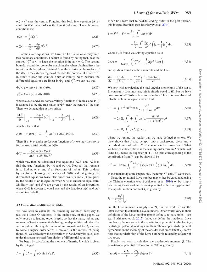
In Fig. 11, we show the time evolution of I and Q for both theMESA-evolved He WD and C/O WD, compared to the sequence ofI and Q of zero-temperature WDs across many central densities.

Figure 11. I and Q over time for both the He WD and the C/O WD weevolved using the MESA code, as well as the same variables over many centraldensities in the zero-temperature model. Since the composition we choosefor our zero-temperature model does not matter (Boshkayev et al. 2017), wechoose the Chandrasekhar EoS for simplicity. The MESA results are shown bylines because the values vary in time due to the WD temperature evolution;the zero-temperature model is a line because the values vary across themany different central densities we show here. Because the C/O WD isnot significantly affected by finite temperature (see Fig. 10), its trajectoryin I − Q space is difficult to see. Rather than enlarge it so that it maybecome visible, we choose to circle the surrounding region to indicate itslocation while still retaining its point-like appearance. As in Figs 9 and 10,we colour-code the MESA models according to their central temperature.

We find that the tendency is for the hot WD to begin on the rightside of the cold WD I − Q sequence, then to fall back down to itszero-temperature value along the sequence. This is most noticeablein the He WD; the C/O WD is not noticeably affected by finitetemperature, and it appears as a single point in Fig. 11.

Let us compare the MESA curves and zero-temperature models inmore detail. Notice that lower masses correspond to larger I and Q

(Yagi & Yunes 2013a). In the case of the higher mass WD, there ispractically no deviation from the cold WD sequence, as we notedpreviously. However, the low-mass WD deviates significantly fromits zero-temperature I − Q point, even after astrophysically longtime-scales. We notice that the deviation is away from the cold WDsequence and toward generally larger Q than I , as is demonstratedin Fig. 9.

4 SU M M A RY A N D C O N C L U S I O N S

In this work, we have studied the so-called ‘I–Love–Q’ relationsin the context of realistic WDs. The primary application of theserelations is to aid in GW analysis by reducing the overall numberof parameters necessary to produce model waveform templates.

We first studied the effect of a parametrized form of differentialrotation on these relations, where the amount of differential rotationwas characterized by a core radius A. We modified the equationsof structure governing WD interiors to account for a rotationfrequency � that varies with radius. We then solved these equationsacross a range of WD masses and physical core radii, whileholding the angular momentum fixed. We found that the I–Love–Qrelations remain universal under variation in compositions even fordifferentially rotating WDs. On the other hand, the I–Q and Love–Qrelations for such differentially rotating WDs deviate from those forWDs under constant rotation. Additionally, we found that unlike the

MNRAS 492, 978–992 (2020)

Dow

nloaded from https://academ

ic.oup.com/m

nras/article/492/1/978/5679150 by guest on 14 February 2022

I-Love-Q for realistic WDs 987

constant rotation case, the rotational and tidal Love numbers are notequal under differential rotation.

Next, we studied how finite temperature affects the WD I–Q relations. We evolved a 0.15 M� He WD using the publiclyavailable MESA code (Paxton et al. 2013) for 1010 yr as it cooled inisolation. The MESA code tabulated the background data of the WD’sinterior profile, and we solved for perturbations to this backgroundprofile due to constant rotation. We found that the WD cools andbecomes well modelled by the zero-temperature approximation overtime-scales of order Gyr. However, at its genesis, the WD was quitepoorly modelled by the zero-temperature approximation, and wesay that the I–Q relation does not hold in general for hot WDs.We then performed a similar treatment to a C/O WD generatedby the MESA code. The program generated a 0.835 M� WD andcooled it in isolation. We found that the WD was well described bythe zero-temperature model at all astrophysically relevant ages andat central temperatures less than roughly 107.6 K, higher than thecentral temperature of the He WD at its genesis. Thus, we arguethat for most intermediate-mass WDs, any deviations from the zero-temperature model are unlikely to be detectable, ignoring any tidalheating that may occur (Iben et al. 1998; Piro 2011), though wenote that at sufficiently large temperatures and low masses, the I–Qrelation is not the same as its zero-temperature counterpart.

In the case of the He WD, where finite temperature effectswere relevant on Gyr time-scales, the system deviated in its I–Qrelation from the sequence formed by cold WDs of varying masses.Initially, the WD begins with greater Q than I , then as it evolves,it tend to move leftwards in I–Q space until it reaches the coldWD sequence. The C/O WD that we considered was unaffected byfinite temperature on astrophysically relevant time-scales, and therewas no noticeable deviation of this system away from the cold WDsequence.

Although the focus of our paper is for WDs, we here commenton how differential rotation, finite temperatures, and deviationsfrom chemical equilibrium affect the I–Love–Q relations for NSs.The effect of differential rotation on universal relations2 has beenstudied in Bretz et al. (2015) within the Newtonian limit and smalldifferential-rotation approximation. The authors showed that thefractional difference in the relations from the uniformly rotatingcase is comparable to the fractional amount of differential rotationover uniform rotation. On the other hand, the effect of finitetemperature (as well as the composition dependence) has beenstudied in Martinon et al. (2014). The authors showed that whenproto-NSs are formed, the I–Love–Q relations are different fromthe original ones for cold NSs by up to 20 per cent, which is muchlarger than the EoS-variation within the relations. However, severalseconds after their births, the relations reduce to the original ones.Similarly, just after formation of an NS, either through single starevolution or in NS mergers, deviations from beta equilibrium maypersist for several seconds. During this time, the deviation of theneutron-to-proton ratio from the beta equilibrium value may againact as an additional parameter in the EoS. This effect has not beenexplored yet and is left for future work.

AC K N OW L E D G E M E N T S

We would like to thank Kuantay Boshkayev for helping us reproducesome of the results in previous literature. KY acknowledges support

2The universal relations studied in Bretz et al. (2015) were those amongstellar multipole moments rather than the I–Love–Q relations.

from NSF Award PHY-1806776, a Sloan Foundation ResearchFellowship and the Ed Owens Fund. KY would like to alsoacknowledge support by the COST Action GWverse CA16104 andJSPS KAKENHI Grants No. JP17H06358.

REFERENCES

Abbott B. P. et al., 2018, Phys. Rev. Lett., 121, 161101Benacquista M. J., 2011, ApJ, 740, L54Boshkayev K., Quevedo H., 2018, MNRAS, 478, 1893Boshkayev K., Quevedo H., Kalymova Z., Zhami B., 2014, preprint (arXiv:

1409.2472)Boshkayev K., Quevedo H., Zhami B., 2017, MNRAS, 464, 4349Bretz J., Yagi K., Yunes N., 2015, Phys. Rev. D, 92, 083009Chatziioannou K., Haster C.-J., Zimmerman A., 2018, Phys. Rev. D, 97,

104036Flanagan E. E., Hinderer T., 2008, Phys. Rev. D, 77, 021502Hartle J. B., 1967, ApJ, 150, 1005Hartle J. B., Thorne K. S., 1968, ApJ, 153, 807Iben Icko J., Tutukov A. V., Fedorova A. r. V., 1998, ApJ, 503, 344Komatsu H., Eriguchi Y., Hachisu I., 1989, MNRAS, 237, 355Littenberg T. B., 2011, Phys. Rev. D, 84, 063009Martinon G., Maselli A., Gualtieri L., Ferrari V., 2014, Phys. Rev. D, 90,

064026Mora T., Will C. M., 2004, Phys. Rev. D, 69, 104021Passamonti A., Stavridis A., Kokkotas K., 2008, Phys. Rev. D, 77, 024029Paxton B. et al., 2013, ApJS, 208, 4Pelisoli I., Kepler S. O., Koester D., Castanheira B. G., Romero A. D., Fraga

L., 2018, MNRAS, 478, 867Piro A. L., 2011, ApJ, 740, L53Piro A. L., 2019, ApJ, 885, L2Poisson E., 1998, Phys. Rev. D, 57, 5287Salpeter E. E., 1961, ApJ, 134, 669Shah S., Nelemans G., 2014, ApJ, 790, 161Shah S., van der Sluys M., Nelemans G., 2012, A&A, 544, A153Shapiro S. L., Teukolsky S. A., 1986, Black Holes, White Dwarfs and

Neutron Stars: The Physics of Compact Objects, Wiley-VCH, WeihheimStavridis A., Passamonti A., Kokkotas K., 2007, Phys. Rev. D, 75, 064019Yagi K., Yunes N., 2013a, Phys. Rev. D, 88, 023009Yagi K., Yunes N., 2013b, Science, 341, 365Yagi K., Yunes N., 2016, Class. Quantum Gravity, 33, 13LT01Yagi K., Yunes N., 2017, Class. Quantum Gravity, 34, 015006Yagi K., Stein L. C., Pappas G., Yunes N., Apostolatos T. A., 2014,

Phys. Rev. D, 90, 063010

A P P E N D I X A : EQUAT I O N S O F S T RU C T U R EFOR D I FFERENTI ALLY ROTATI NG WDS

Previous works (Hartle 1967; Hartle & Thorne 1968; Boshkayevet al. 2014) have shown how the equations of structure of a rotatingNewtonian configuration may be derived using the Hartle–Thorneformalism. These works assume that the effects of rotation aresmall and work perturbatively. In this section, we will briefly goover how the equations derived in Hartle (1967) and Boshkayevet al. (2014) are altered to account for differential rotation withinNewtonian gravity (see Stavridis, Passamonti & Kokkotas 2007;Passamonti, Stavridis & Kokkotas 2008 for a similar frameworkfor relativistic stars). See Section 2.2 for discussion on how weimplement differential rotation.

A1 Background and perturbed equations

We begin by writing down the equation of hydrostatic balance andthe gravitational Poisson equation. The gravitational potential �

MNRAS 492, 978–992 (2020)

Dow

nloaded from https://academ

ic.oup.com/m

nras/article/492/1/978/5679150 by guest on 14 February 2022

988 A. J. Taylor, K. Yagi and P. L. Arras

separates into its background contribution (order �0) and leading-order perturbations (order �2), additionally selecting out the =0 and = 2 spherical harmonic modes of the perturbation. Thus,each equation becomes three separate equations. The equation ofhydrostatic equilibrium becomes

�0c :

∫dP

ρ+ �(0) = const, (A1)

�2c, = 0 : ξ0

d�(0)

dr+ �

(2)0 + U0 = const(2), (A2)

�2c, = 2 : ξ2

d�(0)

dr+ �

(2)2 + U2 = 0, (A3)

where ξ is the perturbation to the radial coordinate r → r + ξ +O(�4

c). Here, we have denoted the order in �c by a superscriptand the spherical harmonic by a subscript. The expansion of U inspherical harmonics is not as simple as in the constant rotation case,so we calculate the = 0 and = 2 components here:

U0(r) = −1

2�2

cr2f0(α), (A4)

U2(r) = −1

2�2

cr2f2(α), (A5)

where α ≡ r/A, and the functions f0(α) and f2(α) are given by

f0(α) = 1

2

∫ π

0

sin2 θ

1 + α2 sin2 θP0(cos θ ) sin θdθ

= 1

α3

(α − Arcsinh(α)√

1 + α2

), (A6)

f2(α) = 5

4

∫ π

0

sin2 θ

1 + α2 sin2 θP2(cos θ ) sin θdθ

= 5

2α5

(3α − (3 + 2α2)Arcsinh(α)√

1 + α2

). (A7)

The gravitational Poisson equation, which states

∇2� = 4πGρ, (A8)

becomes

�0c : ∇2

r �(0) = 4πGρ, (A9)

�2c, = 0 : ξ0

d

dr∇2

r �(0) + ∇2

r �(2)0 = 0, (A10)

�2c, = 2 : ξ2

d

dr∇2

r �(0) + ∇2

r �(2)r − 6

r2�

(2)2 = 0. (A11)

We now define two new variables p∗0 and m∗

0 to simplify the aboveequations:

p∗0 ≡ ξ0

d�(0)

dr, (A12)

Gm∗0

r2≡ d�

(2)0

dr. (A13)

It can be shown that, when integrated from the centre to the surface,m∗

0 is the correction to the mass. See Boshkayev et al. (2014) fora more explicit discussion of these new variables (our m∗

0 is theirM(2)).

These six equations plus the definition of interior mass

dm

dr= 4πr2ρ (A14)

and the EoS (which is well known for WDs) are all that are necessaryto solve for the interior structure of a differentially rotating WD.The stellar mass for a non-rotating configuration M is determinedfrom M = m(R) with the stellar radius R determined by the conditionP(R) = 0.

Let us rewrite the above equations here for completeness. Thebackground equations are

dP

dr= −Gmρ

r2, (A15)

dm

dr= 4πr2ρ, (A16)

P = P (ρ). (A17)

The = 0 equations are

dp∗0

dr= −Gm∗

0

r2+ 1

2�2

c

(2rf0(α) + r2 df0(α)

dr

), (A18)

dm∗0

dr= 4πr2 dρ

dPp∗

0ρ. (A19)

The = 2 equations are a second-order ODE in terms of �(2)2 ,

which may be decomposed into two first-order ordinary differentialequation (ODEs) to be numerically integrated:

d�(2)2

dr≡ g

(2)2 , (A20)

dg(2)2

dr= −4πGρ

dρ

dP

(�

(2)2 − 1

2�2

cr2f2(α)

)

+ 6

r2�

(2)2 − 2

rg

(2)2 . (A21)

We had three equations from decomposing both equations (4) and(A8), and we added in the definition of mass and the EoS, totallingeight equations, yet here we only have six (the two = 2 equationsare really just one equation). What happened to the seventh andeighth equations? The ‘unused’ equations are equations (A3) and(A9), which we may use to solve for ξ 2 and �(0).

In the main part of this paper, we only kept to leading-order inspin, so the only perturbed variable we need is �

(2)2 , which is used

to calculate the quadrupole moment Q. However, in the interest ofbeing thorough, we include the equations for the = 0 variables(which tell us information about corrections to the mass, radius, andmoment of inertia) as well.

A2 Boundary conditions

It is important to have knowledge of how the above functions behaveat small r away from the centre of the star to have accurate initialconditions. For the background variables ρ, m, and P near r = 0,

ρ(r) = ρc (free parameter), (A22)

m(r) = 4

3πr3ρc, (A23)

P (r) = P (ρc), (A24)

where the central density ρc is a free parameter to be chosen.For the = 0 equations, we look at the leading-order terms in r in

equation (A18). It is not immediately clear what the leading-orderin r is for the first term, but the term in parenthesis is clearly of orderr (see equation A4). We assume that this is the lowest order in r forp∗

0 . This would imply that p∗0 ∼ r2 near the centre, which implies

MNRAS 492, 978–992 (2020)

Dow

nloaded from https://academ

ic.oup.com/m

nras/article/492/1/978/5679150 by guest on 14 February 2022

I-Love-Q for realistic WDs 989

m∗0 ∼ r5 near the centre. Plugging this back into equation (A18)

confirms that linear order is the lowest order in r. Thus, the initialconditions are

p∗0(r) = 1

3�2

cr2, (A25)

m∗0(r) = 4

15πρ

dρ

dP�2

cr5. (A26)

For the = 2 equations, we have two ODEs, so we clearly needtwo boundary conditions. The first is found by noting that, near thecentre, �

(2) ∝ r to keep the solution finite at r = 0. The second

boundary condition comes by matching the values obtained from theinterior with the values obtained from the exterior at the surface ofthe star. In the exterior region of the star, the potential �

(2) ∝ r− −1

in order to keep the solution finite at infinity. Now, because thedifferential equations are linear in �

(2)2 and g

(2)2 , we can say that

�(2)2 (r) = a(r) + b(r)�(0), (A27)

g(2)2 (r) = c(r) + d(r)�(0), (A28)

where a, b, c, and d are some arbitrary functions of radius, and �(0)is assumed to be the true value of �(2) near the centre of the star.Then, we demand that at the surface

d�(2)2

dr

∣∣∣∣r=R

= − + 1

R�

(2)2

∣∣∣r=R

= − 3

R�

(2)2

∣∣∣r=R

, (A29)

which tells us that

c(R) + d(R)�(0) = − 3

R(a(R) + b(R)�(0)) . (A30)

Then, if a, b, c, and d are known functions of r, we may then solvefor the true initial condition �(0)

�(0) = − c(R) + 3a(R)/R

d(R) + 3b(R)/R, (A31)

which may then be substituted into equations (A27) and (A28) tofind the true functions �

(2)2 (r) and g

(2)2 (r). Now all that remains

is to find a, b, c, and d as functions of radius. This is doneby carefully choosing two values of �(0) and integrating thedifferential equations twice. The functions a(r) and c(r) are givenby the results of an integration when �(0) is chosen to equal zero.Similarly, b(r) and d(r) are given by the results of an integrationwhen �(0) is chosen to equal one and the functions a(r) and c(r)are subtracted off.

A3 Calculating additional variables

We now seek to calculate the remaining variables necessary totest the I–Love–Q relations. In the main body of this paper, weonly kept up to leading order in spin, so that the mass, radius, andmoment of inertia were entirely background quantities; additionally,we considered the angular momentum proportional to �c and notto contain higher order terms. However, in the interest of beingthorough, we derive how the corrections to I and J may be calculatedunder this parametrized formulation of differential rotation.

We begin by calculating the moment of inertia, I, which is givenby the integral

I =∫

dI =∫

ρ(r sin θ )2dV . (A32)

It can be shown that to next-to-leading order in the perturbation,this integral becomes (see Boshkayev et al. 2014)

I = I (0) + I (2) = 8π

3

∫ R

0ρ(r)r4dr

− 8π

3

∫ R

0

dρ

drr4

(ξ0 − 1

5ξ2

)dr, (A33)

where ξ 2 is found via solving equation (A3)

ξ2(r) = − r2

Gm(r)

(�

(2)2 (r) − 1

2�2

cr2f2(α)

), (A34)

and dρ/dr is found via the chain rule and the EoS

dρ

dr= dρ

dP

dP

dr= −

(dP

dρ

)−1Gm(r)ρ(r)

r2. (A35)

We now wish to calculate the total angular momentum of the star J.In constantly rotating stars, this is simply equal to I�, but we havenow promoted � to be a function of radius. Thus, it is now absorbedinto the volume integral, and we find

J (1) =∫

ρr2 sin2 � �cA2

A2 + r2 sin2 θdV (A36)

= 2π�c

∫ R

0dr

∫ π

0ρr4dr

sin3 θ

1 + α2 sin2 θdθ (A37)

= 4π�c

∫ R

0ρr4f0(α)dr, (A38)

where we remind the reader that we have defined α ≡ r/A. Wehave shown that I may be split into a background piece and aperturbed piece of order �2

c . The same can be shown for J. Whatwe have calculated above is the leading-order term in J, which is oforder �1

c , hence the superscript (1). The term corresponding to thecontribution from I(2) can be shown to be

J (3) = −4π�c

∫ R

0

dρ

drr4

(ξ0f0(α) + 1

5ξ2f2(α)

)dr. (A39)

In the main body of this paper, only the terms I(0) and J(1) were used.Next, the rotational Love number may either be calculated using

the Clairaut equation (see Boshkayev et al. 2014) or by simplycalculating the ratio of the response potential to the forcing potential.The apsidal motion constant k2 is given by

k2 = 1

2

�(2)2

U2

∣∣∣∣R

, (A40)

and the Love number is simply λ = 2k2. In this work, we use thelatter method to calculate Love numbers. Other works vary in theirdefinition of the Love number (some define λ to have units – seee.g. Boshkayev et al. 2017); here, we define the rotational Lovenumber as the response in the gravitational potential to the forcingcentrifugal potential, making λ unitless. There appears to be generalagreement on the meaning of the apsidal motion constant k2, so wenote that our definition of the Love number is related by a factor oftwo to k2.

Finally, we wish to calculate the quadrupole moment Q. Thegravitational potential exterior to the WD is given by

�(r, θ ) = −GM

r+ GQ

r3P2(cos θ ). (A41)

MNRAS 492, 978–992 (2020)

Dow

nloaded from https://academ

ic.oup.com/m

nras/article/492/1/978/5679150 by guest on 14 February 2022

990 A. J. Taylor, K. Yagi and P. L. Arras

In how we have defined m∗0 (see equation A13), one can see that

equation (A41) may be solved for Q:

�(2)2

∣∣∣R

= GQ

R3→ Q = R3

G�

(2)2

∣∣∣R. (A42)

Using this sign convention, Q > 0 represents an oblate object, andQ < 0 represents a prolate object.

APPEN D IX B: EQU ILIBRIUM FLUIDC O N F I G U R AT I O N S I N W D S

In this section, we will derive formulae for the moment of inertia Iand the quadrupole moment Q of a perturbed fluid configuration. Incontrast to the Hartle–Thorne formalism, here we assume that themass (rather than the central density) is fixed after the perturbationis ‘turned on’.

We begin by assuming that the background (unperturbed) quanti-ties are known as functions of radius: pressure P, density ρ, sound-speed squared c2

s , Brunt–Vaisala frequency N2, and interior mass m.Now, due to some perturbing potential U, the fluid configurationexperiences small changes in these quantities away from theirbackground values. In general, for some arbitrary fluid variableB, the Eulerian perturbation δB is defined by

δB ≡ B(x, t) − B0(x, t), (B1)

where B0 is the background quantity. See section 6.2 of Shapiro &Teukolsky (1986), for a more thorough description of these pertur-bations.

Next, we express all relevant perturbed quantities in terms ofspherical harmonics:

δA =∑ ,m

δA m(r)Y m(θ, φ), (B2)

with A = (P, ρ, �, ξ r, ξ h, U). Here, ξ r is the radial perturbation, ξ h

is the horizontal perturbation, and � is the gravitational potential.One can show (e.g. Shapiro & Teukolsky 1986) that to conserve themass of the fluid element, the following relation must hold

δρ = −∇ · (ρξ ) . (B3)

We define the quadrupole moment via the gravitational potential �

of the fluid:

�(x) = −GM

r− GQ

r3P2(cos θ ) + O

(R4

r5

), (B4)

where G is the gravitational constant, M is the total mass of thefluid, r is the distance from the origin to the point at which thegravitational potential is being evaluated, and P2(x) is the = 2Legendre polynomial in x. One can then show that Q is given by

Q =√

4π

5

∫δρ20(r ′)(r ′)4dr ′, (B5)

where ρ20 is the ( , m) = (2, 0) mode of the density perturbation,using the language of spherical harmonics, rather than Legendrepolynomials.

Next, we wish to find the perturbation to the integral quantityI. In the absence of any perturbations, the moment of inertia isgiven by

I =∫ R

0ρ(x2 + y2)d3x. (B6)

Following the procedure of Shapiro & Teukolsky (1986), theperturbation to I using the Lagrangian treatment is given by

dI =∫

�(x2 + y2) × ρd3x (B7)

=∫

ρ(2xξx + 2yξy

)d3x (B8)

= 2∫

ρξ · (x x + y y) d3x, (B9)

where � represents a Lagrange perturbation. To simplify the abovedot product, we rewrite the radial perturbation as the sum of itsradial and horizontal piece:

ξ = ξr, mY m r + ξh, mr∇Y m. (B10)

One can show that the vector sum of x + y can be expressed as

x + y = r sin θ(

sin θ r + cos θ θ)

. (B11)

Then, using the orthogonality of the gradient of spherical harmon-ics,∫

(r∇Y m) · (r∇Y ′m′ ) d� = ( + 1)δ ′δmm′ , (B12)

one can show that the perturbation to I is given by

dI = 2∫

ρr3dr

[4

3

√π

(ξr,0(r) − 1√

5ξr,2(r)

)

− 4

√π

5ξh,2(r)

], (B13)

where only the = 0, 2 and m = 0 components survive theintegration. Here, we have dropped the m subscript, as it is zerofor all terms. Thus, we need to know ξ r, and ξ h, .

Now, for a fluid configuration exposed to some perturbingpotential (with no oscillatory response), the equation of hydrostaticbalance becomes (to leading-order in the perturbation)

0 = −∇δP − ∇ (δρ � + ρ δ�) − ρ∇U. (B14)

The gradient operator acts both on the radial piece in the sphericalharmonic expansion as well as the spherical harmonics themselves.Thus, we may split equation (B14) into a radial equation and ahorizontal equation. Each term in the radial equation carries aspherical harmonic, which we may cancel from each. Similarly, thehorizontal expression carries the gradient of a spherical harmonic,which is proportional to /r. We keep the /r and cancel the rest,leaving us with

0 = −dδP m

dr− gδρ m − ρ

(dδ�

dr+ dU m

dr

), (B15)

0 =

r[δP + ρ (δ� + U )] . (B16)

For = 0, the second equation tells us no information. Thus, wemust solve the equations of structure separately for the = 0 and = 2 cases.

B1 Solving the � = 2 case

We begin with the simpler = 2 case. We assume that all backgroundquantities (P, ρ, m(r), N2, c2) are known as functions of radius. Then,we have the three equations we discussed above (equations B3, B15,

MNRAS 492, 978–992 (2020)

Dow

nloaded from https://academ

ic.oup.com/m

nras/article/492/1/978/5679150 by guest on 14 February 2022

I-Love-Q for realistic WDs 991

and B16), as well as the EoS:

δρ = δP

c2+ ρ

N2

gξr , (B17)

where g is the interior gravity (equal to Gm(r)/r2), and we havecancelled the Y m from both sides and suppressed the m subscript.For the rest of this section, the m subscripts are implied on allperturbed quantities unless specifically stated otherwise. From thehorizontal hydrostatic equilibrium equation, we have that

δP

ρ= − (δ� + U ) . (B18)

We then substitute this into the EoS to find

δρ = − ρ

c2(δ� + U ) + ρ

N2

gξr , (B19)

which we may then plug into the radial hydrostatic equilibriumequation. Some cancellation occurs, and we are left with

0 = −N2

gρ − ρN2ξr . (B20)

In the above simplification, we have used the definition of N2:

N2 ≡ −g

(1

ρ

dρ

dr+ g

c2

). (B21)

Thus, in radiative regions (where N2 > 0), we have that

ξr = − δ� + U

g. (B22)

In convective regions, where N2 � 0, this relation does not holdexplicitly. Then, we may solve for δρ to yield

δρ = −dρ

drξr . (B23)

We now need to invoke a fourth equation: the gravitational Poissonequation:

∇2δ� = 4πGδρ (B24)

= 4πG

(dρ

dr

)(δ� + U

g

)(B25)

= 4πGρ

(1

c2+ N2

g2

)(δ� + U ) . (B26)

This is a self-consistent equation in terms of δ�, its derivatives, andknown quantities. Thus, with the proper boundary conditions, thismay be solved to find δ�, which tells us ξ r and then δρ and δP.Once all of these variables are known, we substitute back into themass-conservation equation to solve for ξ h:

ξh = r

( + 1)

(δρ

ρ+ dξr

dr+ 2ξr

r+ 1

ρ

dρ

drξr

). (B27)

The radial derivative of ξ r may be found by taking the derivative ofequation (B22) and carefully applying the chain rule. Since U is aknown quantity, all derivatives of terms in equation (B22) are knownexplicitly. All we need now are the proper boundary conditionsfor δ�. We refer the reader to the discussion in Appendix A2 onchoosing appropriate boundary conditions for �. The process issimilar: two different initial conditions near r = 0 are chosen forδ� in order to solve for the appropriate initial condition by matchingwith the values at the surface.

B2 Solving the � = 0 case

Next, we turn our attention to the = 0 case. From equation (B13),we see that we must also know the = 0 mode of ξ r to properlyintegrate to find the perturbations to I. The derivation above relieson the horizontal hydrostatic equilibrium equation (equation B16),which only applies in the case where �= 0. To solve for the = 0 case, we must start over, using only the radial hydrostaticequilibrium equation, the equation of mass-conservation, the EoS,and the gravitational Poisson equation. In the previous section,we also had the horizontal hydrostatic equilibrium equation. Thevariable ξ h is zero in the = 0 mode (see equation B27) to keep thenumber of equations and variables equal. We define a new variable

� ≡ δP

ρ+ δ� + U, (B28)

where as before, we have dropped the m subscripts (zero is assumedfor both here). We rewrite the four equations we have in terms ofthis new variable, as well as for clarity:

0 = − d

dr(ρ(� − δ� − U )) − gδρ − ρ

d

dr(δ� + U ), (B29)

0 = δρ + d

dr(ρξr ) , (B30)

δρ = ρ

c2(� − δ� − U ) + ρ

N2

gξr , (B31)

∇2δ� = 4πGδρ. (B32)

Substituting the EoS into the radial hydrostatic equilibrium equationand dividing by ρ, we find some cancellations, and we are left with

d�

dr= N2

(� − δ� − U

g− ξr

). (B33)

For �= 0, we have defined � = 0, so then also its derivative must bezero. This reduces to the equation for ξ r we found in equation (B22).Next, we substitute δρ from the EoS into the equation of constantmass to arrive at

dξr

dr= −ξr

(2

r− g

c2

)− � − δ� − U

c2. (B34)

Finally, we substitute δρ from the EoS into the gravitational Poissonequation to arrive at a single equation containing derivatives of δ�.For numerical integration, it is best to rewrite this second-orderODE as two first-order ODEs, which we list below:

dδ�

dr≡ δg, (B35)

dδg

dr= 4πGρ

(� − δ� − U

c2+ N2

gξr

)− 2

rδg. (B36)

We now have four first-order ODEs for our four variables. Wetherefore need four sets of boundary conditions in order to solve forthese entirely. Two of these boundary conditions are the restrictionswe have previously imposed on δ� and δg:

δg(r)∣∣∣r=R

= − 1

Rδ�(r)

∣∣∣r=R

, (B37)

δg(r)∣∣∣r∼0

= 0. (B38)

The next boundary condition comes by demanding that the surfaceof both the rotating and the non-rotating star have zero pressure,asserting that �P = 0 (the Lagrangian perturbation to P; see

MNRAS 492, 978–992 (2020)

Dow

nloaded from https://academ

ic.oup.com/m

nras/article/492/1/978/5679150 by guest on 14 February 2022

992 A. J. Taylor, K. Yagi and P. L. Arras

Shapiro & Teukolsky 1986, chapter 6). This gives us

�(r)∣∣∣r=R

= (g(r)ξr (r))∣∣∣r=R

+ δ�(r)∣∣∣r=R

+ U (r)∣∣∣r=R

. (B39)

For the fourth boundary condition, we look at the behaviour of ξ r(r)near the centre. Just as we needed δ� ∝ r for it to be finite nearthe centre, we can see that we need ξ r ∝ r for it to be finite near thecentre as well. Thus, we have our fourth boundary condition:

ξr (r)∣∣∣r∼0

= − r

3c2(�(r) − δ�(r))

∣∣∣r∼0

. (B40)

We now have four ODEs for four variables with four boundaryconditions on those variable, though these boundary conditions aregiven in terms of ‘free’ parameters: δ�(0), δ�(R), �(0), and �(R).How do we find the correct values of these free parameters? Weintegrate multiple times with different boundary conditions fromthe surface and from the centre, matching our values at some radiusin the middle. We begin by declaring (in a similar method to whatwe used in Appendix A2) that the four variables we study here areexclusively determined by these ‘free’ parameters:

δ�(r) = a1(r) + a2(r)δ�(0) + a3(r)�(0), (B41)

δg(r) = b1(r) + b2(r)δ�(0) + b3(r)�(0), (B42)

ξr (r) = c1(r) + c2(r)δ�(0) + c3(r)�(0), (B43)

�(r) = d1(r) + d2(r)δ�(0) + d3(r)�(0). (B44)

We may rewrite these four equations in terms of a matrix (notingthat ai through di are all functions of r):

⎛⎜⎜⎜⎜⎝

δ�

δg

ξr

�

⎞⎟⎟⎟⎟⎠ =

⎛⎜⎜⎜⎜⎝

a1 a2 a3

b1 b2 b3

c1 c2 c3

d1 d2 d3

⎞⎟⎟⎟⎟⎠

⎛⎜⎜⎝

1

δ�(0)

�(0)

⎞⎟⎟⎠ . (B45)

We may do the same for the ‘free’ parameters at the surface:

⎛⎜⎜⎜⎜⎝

δ�

δg

ξr

�

⎞⎟⎟⎟⎟⎠ =

⎛⎜⎜⎜⎜⎝

a′1 a′

2 a′3

b′1 b′

2 b′3

c′1 c′

2 c′3

d ′1 d ′

2 d ′3

⎞⎟⎟⎟⎟⎠

⎛⎜⎜⎝

1

δ�(R)

�(R)

⎞⎟⎟⎠ . (B46)

Now, these ‘free’ parameters are not truly free; they have true valuesthat are not able to be chosen, and we wish to find these true values.If the functions ai through d ′

i are known functions of r, then wesolve for these true values by matching at some radius in betweenthe centre and the surface, which we will call r1. Then, at r1, we

demand that⎛⎜⎜⎜⎜⎝

a1 a2 a3

b1 b2 b3

c1 c2 c3

d1 d2 d3

⎞⎟⎟⎟⎟⎠

⎛⎜⎜⎝

1

δ�(0)

�(0)

⎞⎟⎟⎠ =

⎛⎜⎜⎜⎜⎝

a′1 a′

2 a′3

b′1 b′

2 b′3

c′1 c′

2 c′3

d ′1 d ′

2 d ′3

⎞⎟⎟⎟⎟⎠

×

⎛⎜⎜⎝

1

δ�(R)

�(R)

⎞⎟⎟⎠ . (B47)

We have four equations for four unknowns, which we may alsoexpress as a matrix (where all quantities other than the ‘free’parameters are again evaluated at r = r1):⎛⎜⎜⎜⎜⎝

a′1 − a1

b′1 − b1

c′1 − c1

d ′1 − d1

⎞⎟⎟⎟⎟⎠ =

⎛⎜⎜⎜⎜⎝

a2 −a′2 a3 −a′

3

b2 −b′2 b3 −b′

3

c2 −c′2 c3 −c′

3

d2 −d ′2 d3 −d ′

3

⎞⎟⎟⎟⎟⎠

⎛⎜⎜⎜⎜⎝

δ�(0)

δ�(R)

�(0)

�(R)

⎞⎟⎟⎟⎟⎠ . (B48)

This matrix may be inverted, and thus the true values of the ‘free’parameters are solved, once ai through d ′

i are known functions of r.How do we find these functions of r? We integrate several times

with different choices of the boundary conditions. We choose tointegrate three times from the surface and three times from thecentre. In both cases (surface and centre) the choices of boundaryconditions are the same. We begin by choosing the tuple of boundaryconditions (δ�, �) = (0, 0). Then, the results of this integrationgive us

δ�1(r)(known) = a1(r), (B49)

which gives us the coefficient a1 (or a′1) as a function of radius. This

integration tells us all of the variables with subscript 1. For the nextintegration, we choose the boundary condition-tuple (δ�, �) = (0,1), giving us

δ�2(r)(known) = a1(r)(known) + a2(r), (B50)

which then tells us a2 (and similarly a′2 and all other variables with

subscript 2). Finally, we choose the third boundary condition-tuple(δ�, �) = (1, 0), which gives us

δ�3(r)(known) = a1(r)(known) + a3(r), (B51)

and we then know the rest of the coefficients ai through d ′i as

functions of radius. Thus, integrating the same set of differentialequations three times (at both the centre and the surface) gives us thecoefficients, which we use to solve for the true boundary conditionsvia equation (B48). Then, once the true boundary conditions areknown, the true values of all four perturbed variables may be foundusing either equations (B45) or (B46).

This paper has been typeset from a TEX/LATEX file prepared by the author.

MNRAS 492, 978–992 (2020)

Dow

nloaded from https://academ

ic.oup.com/m

nras/article/492/1/978/5679150 by guest on 14 February 2022