LOVE AND SEX

CHAPTER ONE

1.1 INTRODUCTION

Why do people get married? Love, Sex, Children, money. Why

do people get divorced? Probably for the same reasons,

while most people would, at most want to hear economist

have to say about the financial aspects of marriage,

economist have to say about the financial aspects of

marriage, everyone else) have taken it on economics is one

of many academic disciplines to weigh in particularly once

important change in marriage and divorce over the last

several decades began to grab national attention.-

In this chapter, we will illustrate the insights

offered by the economic approach to analysing marriage and

divorce. For Example, economists have studied whether

divorce. For example, economist have studied whether

divorce law affect the divorce rate. Before 1970, many U.S

states required both spouses to agree before a divorce

could take place; now, most states allows one spouse to

initiate a divorce unilaterally, under certain assumptions

that economist have spelled out the type of divorce law

would not actually affect the number of divorces, even

while it does affect the way that divorced couples share

resources.

Economist has tested this hypothesis and, to the

extent possible, the assumptions it rest on. Furthermore,

economist have shown that the type of divorce law affects

how married couples share resources, even if they do not

divorce, and extending the ideas further, it might even

influence how often they have sex.

In order to understand these ideas, we have to

develop a model of both marriage and divorce (or, in other

words, a model of that allows for changes over time in the

utility from marriage). In this chapter, we will set the

stage for this analysis with a brief discussion in section

1 of trends in marriage and divorce in the U.S. then, to

keep things simple we will discuss separately the gains

from marriage versus living together (in section 2) the

reasons why people marry (in section 3) the nature of

decision making within marriages (in section 4), and the

nature of the decisions to marry and to divorce (in

section 5).

Marriage versus cohabiting

What is the difference between shacking up and getting

hitched? Marriage is a contractual arrangement, with rules

determined by church or state. For examples, Jewish

weddings are not complete until the bride and groom sign

the ketubah, a marriage contract which spells out the

husband’s obligations to the wife during marriage,

conditions of inheritance upon his death, and obligations

regarding, the support in the event of divorce.

Brides in many cultures brought (or still brings)

dowries to their husbands, with religious or secular law

determining the disposition of the dowry in the event of

death or divorce. In other cultures, husbands must provide

a pride price to the bride or her father. With some

exception, non-marital relationships do not entail the

same contractual obligations, several aspects of marriage

as a contract are important.

First, marriage as a transaction may be costly in

terms of time, effort, and/or money to enter into and to

leave it implies that the utility from marriage must

exceeded the utility from being apart as well as the

cost involved in getting married, and possibly divorced as

well as the costs involved in getting married, and

possibly divorced (although we do not emphasize this in

the model of getting married which we develops later).

Second, divorce as the dissolutions of a contract

entails financial obligations between the spouses. For

example, one spouse may be required to pay income support

to the other and property acquired during the marriage (or

even before) must be split according to some rule, perhaps

depending on behaviour during the marriage.

There are a few motives for these financial

obligations associated with divorce. One is to provide

support for children issuing from the marriage, although

these rules affect childless couples as well. Another

motive is to punish certain types of behaviour which are

viewed as violating the contractual obligations of

marriage. An additional motive is to compensate spouses

for some types of investments in the marriage which are

undertaken with the belief that the marriage will last. We

will elaborate on the motives for these. Sharing rules, as

we outline the reasons why people marry and subsequently

divorce.

Third, the nature of the marriage contract has varied

greatly across religions, countries and time periods. The

Old Testament, for example, established a right of

husbands to unilaterally divorce their wives, for any

reason or no reason, although not without absolving all

financial.Jesus, in various gospels, recognized (though

disapproved of) divorce while the Roman Catholic Church

forbids it. Occasionally legal and/or religious divorce

law has changed in response to demands of influential

society members (e.g, Henry VII). We will discuss some

reasons why the legal regime governing marriage and

divorce has varied as the circumstances surrounding

marriage have shifted?

What are the gains from marriage?

At the outset, we listed several reasons: love, sex,

children and money why people might have married. Let’s

consider in turn how each of them affects and individuals

utility and moreover why the impact may depend on whether

the couple marries instead of just living together.

Love and sex

While love may be one of many splendored things, we will

model it as a simple gain in utility from your life with

another love may matter because you enjoy being the one

you love, and it may matter because it causes you to care

about the well being of the one you love. In other words,

love may be an argument of your utility function and it

may change your utility function by placing weight on the

utility of another person. Next, there is sex.

But sex any different from love from a modeling point

of view? They both require another, and the both offer

utility, given the right partner. Sex may complement love;

if emotional intimacy enhances sexual satisfaction.

However, there are other important characteristics of sex.

One which we will ignore in this chapter is that there is

a relatively well functioning market for sex (via

partition), but not one for love, since sex is an act but

love is an emotion which is difficult to transact. Another

characteristic of sex is that it involves certain risks.

it may be for the latter reason that sex is often

associated with marriage.

One risk of sex is diseases. Monogamy reduces the risk of

disease, but how does one insure monogamy?

First, both marriage and co habilitation increase

physical proximity and hence the ability to monitor the

partner.

Secondly marriage as a legal contract often specifies

penalties which raise the cost of adultery. For instance,

it may provide grounds for the other partner to end the

marriage or affect the distribution of income and property

after divorce. Another risk of sex is pregnancy. the risk

of pregnancy explains why sex within marriage may be

preferred to sex outside of marriage, Because the welfare

children, and so the welfare of parents who care about

their children, is enhanced by making marriage difficult

to end and by the financial obligation may be imposed for

children born out of wedlock as well) seen in this light

once can understand why the advert of effective

contraction in recent decades. By reducing the risk of

pregnancy resulting from sex has reduced the frequency of

marriage and increase the frequency of living together.

While condoms have been around for over millennia, the

introduction of the birth control pill has had a drastic

effect, especially after decisions in the late 1960s

allowed it to be distributed widely among unmarried women.

That is because it allows women to control their fertility

and women bear more of the costs of child bearing than men

do.

CHILDREN

Sex naturally brings us to talk about children. There are

a few reasons why people have kids besides the possibility

that they are an accidental by product of sex. One that

they feel a biological imperative, another is that the

enjoy kids. Those two reasons look the same in a simple

economic model. They are things that raise an individual's

utility. What makes kids interesting for our purposes is

that one kid are public, not private goods. In other

words, one kid provides utility to two parents, and the

utility one parent gets from spending time with the kid is

not diminished by the utility the other gets from spending

time with the kid as long as the parents live together. If

not, then kids are more like other private goods, for

example, spaghetti. If one person eats the spaghetti, the

other cannot.

Since kids cost about the same whether they live with

one parent or both, it is efficient, from this

perspective, for parents to live together. we will not

have a chance to say anything about the decision of

whether to have kids, although it may have some of the

same features as other types of marital decision, which we

will not discuss about, how many kids to have, and the

tradeoff between investing in child quantity (by having

more kids).

Whether they are assessing options for reforming

social security, contemplating changes to the tax code, or

trying to improve the well being of children, policy

makers require an accurate assessment of trends in

marriage, divorce and other living arrangements.

Historically, vital statistics data collected at the state

and local levels and consolidated by the national center

for health statistics (NCHS) provided the most complete

information on marriage and divorce rates.

These data were based on administrative record of

actual marriage and divorces that occurred in the

reporting jurisdictions. Prior 1996, the federal

government provided more financial support to state to

collect marriage and divorce data. In 1996, NCHS

discontinued funding for the collection of detailed

marriage and divorce data for a number of reasons. First,

there were resource constraints. By easing funding to

state for the collection of detailed marriage, divorce the

agency was able to redirect & 1.25million per year to

maintain birth and death data system. Second, there were

coverage and quality concerns. NCHS was not consistently

receiving data from all states. Similarly the quantity of

the data never rose to the level expected by NCHS or

researchers. Data reporting was often incomplete or of

uncertain reliability. States were facing staffing

shortages and internal funding issues, resulting in many

relegating the reporting and collection of marriage and

divorce data to a lower priority than birth and death

data.

Finally, the collection of marriage and divorce

information was an uneasy fit for an agency that focuses

on health statistics, few NCHS staff worked with marriage

and divorce data, thus, when the budget needed to be cut,

there were few advocates for the continuation of its

collection. In addition, staff argued that the data could

be captured in surveys, such as the national survey of

family growth, and in census data. As a result, the

quantity and quality of national, state and local

information on marriage and divorce deteriorated while

policy makers need for this information increased.

The administration for children and families and the

effect of the assistant secretary for planning and

evaluation, within the us department of health and human

services (DHHS) contracted with the Levin group and the

Urban institute to explore options for collecting marriage

and divorce information. This report examines the

feasibility and potential benefits of using existing

survey data sets to provide reliable, tike tamely

information. This report examines the feasibility and

potentials benefits of using existing survey data sets to

provide reliable, timely information on marriage and

divorce.

It assesses the ability of a variety of data sets to

produce marriage and divorce statistics of the national,

state and local levels. The main criterion is whether the

existing survey data sets provide or can be modified to

provide information on marriage and divorce rates, as was

possible using data collected under the vital statistics

system. Beyond their potential to provide information on

marriage and divorce rates, survey data sets can also

provide information on current marital status, alternative

living arrangements such as co habilitation and the

correlates of marriage, divorce and other living

arrangements.

To his report first describes criteria for evaluating

survey data sets on their ability to provide information

on marriage and divorce.

HISTORY OF ILE-OLUJI/OKEIGBO LOCAL GOVERNMENT

Ile-oluji/Okeigbo Local government council was created on

27th August 1991, with Ile-Oluji as the headquarters,

according to the federal government gazette No 34 Vol 78

of 21st October 1991.

Ile-Oluji/Okeigbo Local government by the administration

was carved out of the Old Ifesowopo local government by

the administration of General Ibrahim Babangida, it is

made up of Ile-Oluji/ Okeigbo and other villages,

farmsteads and hamlets. It is instructive to note that the

creation of Ile-Oluji/Okeigbo local government was made

possible largely by the persistent agitations of the

people of the Ile-Oluji, especially the Jegun – in-

council and influential community leaders. The local

Government is situated in the western part of Ondo state,

sharing boundries in the east with ondo and Ifedore Local

governments, and in the west by Osun state. The

provisional result of the 1991 national head count put the

population of the local government at 123, 397 with the

Yoruba being the predominant ethnic group.

There are also sprinkling of mainly farmers, while

subsistence crops include Yam, Cassava, Maize, Plantain,

Banana, fruits. Two third of the population are Christians

while Muslims and traditionalists are also to be found in

the hook and grannies of local government.

Apart from the major towns of Ile-Oluji and okeigbo there

are about 306 other villages and farmlands.

INDUSTRY/COMMERCE

Ile Oluji cocoa processing company limited is the most

prominent industrial outfit in the local government are

first Bank, Co-operative Bank, Owena Bank, UBA and

community Banks, Major hotels are Gboluji guest house,

Jossy international Hotel, Quiet Hotel, New Era, Valentine

Hotel.

VEGETATION

The local government lies within the tropical rainforest

belt. There is luxuriant vegetation because of high

humidity structures in the face of urbanization. Tropical,

the local government has a relatively high plain

punctuated by the rolling tableland of rocks structures.

The area has the loamy soil type, well drained and

fertile.

1.2 STATEMENT OF PROBLEM

This study was to determine the number of marriage and

divorce in Ile-Oluji/Okeigbo local government area.

1.3 AIMS AND OBJECTIVES

This project work have it aims and objective for

conducting the research which are as follows:

1. To study and determine the trend of marriage against

time in Ile-Oluji/Oke-Igbo local government for the

year under study using regression analysis.

2. To study and determine the trend of the divorce against

time in Ile-Oluji/ Okeigbo Local Government of the year

under study using regression analysis.

3. To study and determine the degree of relationship

between marriage divorce against time in

Ile-Oluji/Okeigbo local government using correlation

analysis.

1.4 SIGNIFICANCE OF THE STUDY

The finding of the study would provide understanding

of the factors that influence people for engaging in

marriage and divorce. The result is expected to help

the society as well as government to project the plan

for necessary future improvement.

1.5 SCOPE AND COVERAGE

This project work focus mainly on marriage and divorce for

the year 2005- 2014 in Ile Oluji/ Okeigbo local

government.

1.6 DEFINITION OF TERMS

Marriage: Can be defined as a socially acknowledge

and approved sexual union between two adults of

opposite sex.

Divorce; can be defined as the legal dissolution of a

marriage by a court or other competent body.

Sororate marriage: these occurs when a man marries

two sisters

Leviratic Marriage: It occurs when a man marries a

woman to raise children to the memory of his brother.

Ghost marriage: Occurs when a man provides the bride

price and the consort for another woman in other that

the children born will be hers.

Absolute divorce: The final ending of a marriage.

Both parties legally free to remarry

Alimony: it is a payment of support provided by one

spouse to the other\

Annulment: A marriage can be dissolved in a legal

proceeding in which the marriage is declared void, as

though it never took place. In the eye of the law,

the parties were never married.

Group marriage: this is where a group men will share

marital relations with a group of women

Condo nation: is the act of forgiving one’s spouse

who has committed an act of wrong doing that would

constitute a ground for divorce.

Polygamy: this is where a man can/may marry more than

one woman

Polyandry: This appears when a woman simultaneously

marries two or more men.

CHAPTER TWO

LITERATURE REVIEW

For better or for worse, an analysis of marriage and divorce

changes in Japan (BY BRYAN NICOL) Under the supervision of

professor Leslie Winston. “For better or for Worse?” analyzes

the changes in Japanese marriage and divorce culture in the

100 years surrounding the turn of the 20th century. In a

relatively short period of time, Japanese society underwent

fascinating transformation from having the world’s highest

recorded divorce rate in 1885, to one of the lowest in the

world only sixty years later.

First, I will analyze the pre – industrial and industrial era

culture in order to illustrate fully the social implications

of marriage and divorce and how they have change over time. I

follow this with an analysis of the theories that attempt to

explain divorce rate changes across these specific time

periods both of the theories that attempt to explain divorce

rate changes across these specific time periods, both of which

lasted for roughly 50 years since 1860 and saw distinct

changes in divorce rate trends.

Finally, comparisons will be made between the periods with

analysis regarding the changes in women’s well being with

respect to the marriage institution to show that the

implementation of a marriage and divorce system based on

cultural values foreign to the Japanese society inevitable led

to a decrease in Japanese women’s socio – economic well being.

The meiji period (1868-1912) of Japan, up until the passage of

the meiji Civil code in 1898, was characterized by a unique

feature. It was at this point in time that Japan had the

world’s highest divorce rate. Harald Fuess, in his book

divorce in Japan, offers statistical data that claims that the

divorce rate of Japan was not only the highest in the world

during the 1800s, but that the only country to see an

equivalent divorce trend was the united states almost a

country later (2004). Yet the reason for the drastic

difference is simply because the Japanese society as a whole

differed from its western counterparts on various cultural

aspects. A community based on the ideas of the i.e. a trial

marriage system, and a complete lack of codification of the

marriage institution all facilitated divorce during the meiji.

Period, which inevitably left Japanese brides with a greater

sense of socio – economic well being than the western form of

the institution did.

In order to understand how the institution impacted brides

during the meiji Era, it is important to analyze the marriage

and divorce decisions during the 1800s were made through the

i.e. defined as the societal, communal and familial based

relationships that even today is regarded with great

importance throughout Japan. There is a small, lineage based

community comprised of family within the same dwelling with

one another (Long 1990). Both Susan orpett long, in her book

family change and the life course in Japan, and Joy Hendry, in

marriage in changing Japan, agree that marriage was, during

this time, a cultural institution driven to perpetuate the

i.e. (Hendry 1981, Long 1990). For Pre- Industrial Japan, this

was achieved by means of the arranged marriage rather than a

love marriage primarily because a love marriage implies an

individual affair – rather than a community based decision –

whereas with an arranged marriage the entire family was

typically involved (Hendry 1981).

Furthermore, the marriage was not simply the union of two

individuals, but rather was considered to be the marriage

between two entire families (Long 1990). In the Meiji period

and in previous era, this inevitable gave rise to a trial

marriage system, wherein spouses were tested with one another

for a certain amount of time to ensure that a well suited

match was made.

The trial marriage system seems match to be Japan’s equivalent

to the dating system in America and Europe. Western style

courtship has only recently begun developing as a social norm

in Japan (Ritsuko 1990), so it can be said that dating as a

catalyst for marriage was completely non – existing in Pre –

industrial Japan. Trial marriage, however, may almost be

analogous. According to fuess, during the end of the 1800s,

nearly 50 percent of all marriage, ended in divorce, while

half of all divorce were realized within the first two years

marriage themselves were, in a sense, a form of dating,

coupled with cohabitation with a spouse and his on her family.

Interestingly, since there was a definitive lack of marriage

codification in the government, trial marriages, as well as

their subsequent divorces, became an easy and common affair.

The absence of a legalized form of marriage in the Japanese

culture during the 1800s, undoubtedly had a drastic impact on

the relative ease of divorce in comparison to America and

Europe. Fuess argues that cultural signals that a couple had

consumed its marriage were more dominant than actual legal

registration of the union itself, and, in fact, registration

of marriages was not even required by the government until

shortly before the beginning of the 20th century (Cornell 1990;

Fuess 2004). Rather, a young Japanese woman with blackened

teeth or a certain hair style could indicate that a marriage

had recently taken place, while in other instances it was the

birth of the first child that indicated the commencement of a

marriage (Cornell 1990; fuess 2014). There was some record of

marriage ceremonies taking place, but Fuess states that on a

whole, scholars at the time regarded these ceremonies as small

affairs, devoid of much religious, social, or legal meaning

(Fuess 2004)

Divorce proceedings seemed to be an equally simple matter in

pre – industrial Japan, as well. Joy, Hendry, for example,

refers to the ease with which a husband could divorce his

wife. Fuess concurs with Hendry stating that not only was the

mikudarihan the only required notice to complete a divorce,

but on a social scale. It was seen as mainly the husband’s

prerogative (Fuess 2004). Fuess also adds that in Japan’s

entire history, state institutions were involved in only a

very minute’s portion of total divorces (Fuess 2004). With

very little government interaction taking place within the

institution of marriage during the end of the 20th century,

marriage and divorce from a legal stand point could occur with

relative ease. These three factors – the lack of a legal

codification of marriage, the importance of the i.e. and the

trial marriage system – helped develop a society in which

divorce was both typical and frequent during the 1800s. Yet it

was not a system that was free from heavy criticism by both

not system that was free from heavy criticism by both scholars

of the time and today. Various European scholars at the time

claimed that Japan’s high divorce rate was highly indicative

of the inequality between the sexes and a lack of concern for

the overall institution of marriage itself, while some even

claimed that the high divorce rate was such a problem that it

prevented Japan from becoming a “modern society” (Fuess 2004,

141). Hendry claims, for example, that the ease with which a

husband could obtain a divorce from his wife reflects her

lowly social status as she had very limited options when

initiating divorce (Hendry 1981). While Fuess agrees that

there was indeed sexual inequality in terms of obtaining a

divorce, he points out that women were not as entirely

helpless as Hendry may indicate. Fuess sites evidence

indicating that a woman’s parents could coerce a husband into

providing a mikudarihan, or in extreme cases she had the

option of using a divorce temple as a mediator to settle

disputes (Fuess 2014). Fuess also quotes the scholar J.E de

becker who states that “the Japanese wife was not regarded so

seriously as at present by the house, when she was unfortunate

enough to incur the displeasure of her lord and his relative.

Seeming to imply that it was not entirely uncommon for a wife

to be divorced on whim (Fuess 2004:124). On the other hand,

Laurel Cornell in her essay “peas Becker and ant women and

divorce in pre-industrial Japan”. Argues that a wife was

actually an invaluable aspect to the i.e. while both de becker

and Hendry strongly argue that the high divorce rate is

clearly indicative of women’s powerlessness in Japan in the

1800s was a society culturally constructed in such a way that

divorce was not uncommon practice. As previously stated, 25%

of all marriages was expected to end within the first two

years of marriage (Fuess 2004), and it is entirely plausible

that with the trial marriage system in plausible that with the

trial marriage system in place it was more likely a mismatch

of spouses that led to a divorce rather than the malevolence

of the husband or his parents. This, however, should not

consider a universal truth. Inevitable there will be

individual cases in which a spouse of either sex desires to

procure a divorce and is unable to do so. Yet the Japanese

woman during the Meiji period seemed to be at a clear

disadvantage over her make cohort, which clearly indicates a

difference in social status.

During the meiji period, the frequency of divorce created a

social stigma towards divorces much different from that of

modern Japan. According to Fuess, the divorce was left with

two options remarriage or returning to her natal home.

Fuess states that there was no legal prohibition against

immediate remarriage for either sex (Fuess 2004). In fact,

recent divorces were expected to remarry quickly after

divorce, and according to Cornell most did she states that a

third of divorced women in one particular case study had

remarried within the first year of being divorced, implying

that even after divorce women in no way removed from the

marriage market (Cornell 1990). Although the Japanese woman’s

options after divorce were limited, the ability to return to

her family or to remarry implies that some level of her

economic well being remained stable, as either her family or

her new husband would presumably provide for their needs.

Thus, the argument that the high rate of divorce among

Japanese couples during this time period reflected a lack of

regard for the institution itself may not be entirely true.

Rather, the trial marriage system helped to ensure that an

agreeable match could be made between families and allowed for

a simple dissolution of mismatched marriages. This facilitated

a generally positive well-being for Japanese women

specifically in terms of this institution, since simple

divorce should not then, be so simply associated with a

relatively low state of well-being for Japanese women in the

pre – industrial era as many critics are willing to argue.

Surely the unequal access to initiating divorce represent

differences in the social status of women versus men, yet in

spite of this there does not seem to be any substantial or

valid argument that can attest to the fact that women’s socio-

economic well being in terms of marriage and divorce was not,

in fact, equal to that of men’s. Women who were divorced were

not subject to any social stigma, were not placed in economic

danger as they had the opportunity to return to their natal

home or to remarry immediately after divorce, and were not

removed from the marriage market since most divorces took

place within the first few years of marriage. Yet the heavy

criticism from foreign scholars on the various aspects

marriage and divorce in Japan did not go unheeded and

beginning in 1898 with the passage of the Meiji civil code,

the Japanese began to enter into a cultural transformation

that would span the next fifty years. Yet this was based on

arguments from foreign scholars regarding the status of women

and the marriage institution in Japan that may not have ever

been accurate. Traditionally the Japanese society based its

marriage and divorce values on a Confucianism doctrine, while

many of the foreign scholars were attempting to analyze and

critique the Japanese system of marriage and divorce from a

Judeo- Christians point of view. Despite the social inequality

between men and women in their ability to procure a divorce,

Japanese women of the 19th century maintained a theoretically

positive socio- economic well – being, and thus any changes in

the system in place had the potential to change this.

Regardless, by the end of the 20th century a variety of factors

were influencing Japan in such a way that an extraordinary

transformation would be seen almost immediately.

The Meiji civil code actually expanded the right to divorce to

the wife in addition to the husband. Various scholars claimed

that the passage of the code brought modernity and security to

the Japanese family and rejoiced in the immediate decline in

recorded divorce rate by nearly 50% (Fuess 2004). De becker

argued that the decline represented society’s rejection of

divorce which was caused, he believed, by the equality of men

and women in their ability to obtain a divorce (Fuess 2004).

Fuess, on the other hand, argues that there are actually two

periods of declination worthy of review. First is the extreme

decline that took place from 1898 to 1899 immediately

following the passage of the code, followed by a second and

more gradual decline from 1900 to 1940, both of which are

represented by figure I from Fuess’s Divorce in Japan found at

the end of this essay.

The first decline, fuess argues, is due in part to four

different possibilities from changes in marriage and divorce

practices, the adoption of a new registration for families,

statistical errors, or a combination of all three (Fuess

2004). One of the major problems with the statistics,

collected at the time is that they no longer recognized common

– law marriages as full marriages and thus their data

disappeared from the official records (Fuess 2004). The new

registration required by families would have much the same

effect, as the number of marriages recognized by legal

standards clearly would differ from those recognized purely by

social standards.

This first possibility listed above is perhaps more likely, to

explain the general downward trend in divorce rate that took

place over the following fifty years. The scholars in Meiji

Japan who had heavily critiqued society for its high divorce

rates had also been calling for a reformation of the marriage

ceremony, saying that the ease with which one could marry and

divorce detracted from the significance of the institution

itself (Fuess 2004). A complete renovation in the marriage

ceremony began to take place. Scholars and even the government

now wanted the ceremony to reflect religious principles and

the resulting ceremony became a grandiose affair that would

incorporate heavy influences from its Christian counterparts.

(Fuess 2004). Fuess quotes various scholars who comment on the

elaborateness of the affair, saying that previously one could

marry for a mere five yen, while after the transformation

marriages saw nearly unbelievable cost increases (Fuess 2004).

In either case, women who desired to procure a divorce during

Japan’s Industrial era inevitability saw an increase in the

social and economical opportunity costs for doing so, which

further restricted opportunities for the dissolution of

mismatched marriages. Thus while foreign scholars were

focusing so heavily on their fight to create “equality” for

Japanese women in terms of the law, they did not consider that

the ramifications of the implementation of a foreign value

system of marriage and divorce into Japan’s highly active

divorce culture. Women who found themselves in unhappy

marriages were now faced with two options to suffer through

the relationship or as Trucco writes, to be worse than “dead

to society”. Thus, the Meiji code, the foreign scholars and

the government had failed Japanese women.

Completely, creating a zero – sum game for those who, before

1898, could have divorced and entered into a new relationship.

CHAPTER THREE

3.0 RESEARCH METHODOLOGY AND STATISTICAL TOOLS

3.1 REASEARCH METHODOLOGY

It comprises definition of data, source of data, types of data,

method of data collection and limitation of data.

STATISTICAL TOOLS

It comprises definition of statistical tools to be used to

analyze this project. They are:

1. REGRESSION ANALYSIS

2. CORRELATION ANALYSIS

3. CO-EFFICIENT OF DETERMINATION

4. ANALYSIS OF VARIANCE (ANOVAs)

5. CHARTS AND DIAGRAMS

Data is information collected; collection is the act of

gathering things together. Therefore, data collection is the

act of gathering information together in order to draw

references from it.

More so, it’s refers to as the numerical description or

representation of things either in quantitative or qualitative

or both.

QUANTITATIVE DATA: Are those that can be described in numerical

form.

QUALITATIVE DATA: Are characteristics which cannot be described

in numerical form.

3.1 TYPES OF DATA

There are two types of data namely:

PRIMARY DATA: Are data that is collected for a specific purpose

and used for that specific purpose that is collected for. These

types of data are collected and published by the organization

that collected them.

3.1.1 MERIT OF PRIMARY DATA

It is completed because theory supply exact information needed.

Interpretations are give and more details. Errors which are

sometimes introduced in secondary data are omitted and such as

reliable.

3.1.2 DEMERITS OF PRIMARY DATA

It may be costly to collect.

It is very expensive.

There is usually large non-response.

3.1.3 SOURCES OF PRIMARY DATA

Census for instance, population census.

Scientific experiment

Sample survey e.g. an enquire on the health.

Administrative purpose e.g. records of births and deaths.

3.2 SECONDARY DATA: Are data which have been collected for

some other purpose by someone else and used for another

purpose. Most published statistical data are secondary data to

the user.

3.2.1 MERIT OF SECONDARY DATA

It allows for timely result

It is less expensive to collect

The information is quickly gathered.

3.2.2 DEMERIT OF SECONDARY DATA

It may be outdated.

It is less detail.

The sample size required might not be met.

The sources of data may not be known.

3.2.3 SOURCES OF SECONDARY DATA

Research organization.

Publication and annual abstract of statistics.

Administrative records e.g. school records, office

records.

Tertiary institutions e.g. Federal school of statistics,

Ibadan, primary schools, polytechnics, universities.

Media organization e.g. print and electronic.

3.3 INTERNAL AND EXTERNAL DATA

INTERNAL DATA: This is data collected within an organization

and used by the same organization.

EXTERNAL DATA: This is data collected by the organization

outside the organization outside the organization.

The day-to-day record of attendance in an organization is

internal data while data collected outside the organization say

on welfare package for workers is external data.

3.4 METHOD OF DATA COLLECTION

a) Personal interview or direct method

b) Postal questionnaire method

c) Observation method

d) Telephone interview

e) Electronic (internet) method of data collection

f) Documentary method

g) Reports

h) Result experiment

3.5 PROBLEM OF DATA COLLECTION

Since the data used in this project work is secondary some of

the problems encountered are those peculiar to data collection

through secondary sources.

However, some of the problems are:

1. Language barrier

2. Religion belief

3. Culture

4. Non-response

That I encountered are:

1. CALL BACK: There was the need for call backs. Before it was

possible to get the required document to extract the data

needed for this work.

2. BUREAUCRACY: The exercise was seen as a kind of probing

into the activities of the local government. This

necessitates the writing of letter to the zonal officer who

later rendered his assistance.

1.6 LIMITATION OF DATA COLLECTION

The quality of a statistical result depends on the quality

of the raw material for example the level of accuracy and good

result depend on the raw material which the measurable aspect

of things it does not usually give a complete solution to a

problem rather it only provides a basis for good judgment.

Hence, the scope of the data used for analysis is limited.

Also, as stated earlier, one of the demerits of secondary

data is that it is less accurate and secondary data is used in

this project, it therefore becomes necessary to advise all

those that like to use the work to employ some degree of

caution in analysis and interpretation there in.

1.7 CHARTS AND DIAGRAMS

Statistical data can be used or represented in chart,

diagram or graphs. This may be in form of component of bar

chart, simple bar chart, multiple bar chart and pie chart.

Chart and diagrams serves as a way of simplifying data for

easy and fast reading. It gives information at a glance. A

simple well constructed diagram that will be used in this work

for visual impression of the data.

SIMPLE BAR CHART

This is a diagrammatic presentation of series of

rectangular block erected at regular equidistance internal

along the axis (either horizontal or vertical) it can be used

to compare aggregate that is the whole magnitude, only one

variable can be shown with this diagram.

COMPONENT BAR CHART

It is a special bar chart in which each bar is sub divided into

component. On the other hand the bar of the component bar chart

could be referred to as block diagrams.

MULTIPLE BAR CHARTS

This is a chart where two or more bars are drawn together; it

is used to compare two or more variable. The bars are drawn

either horizontal or vertical.

1.8 REGRESSION ANALYSIS

This is a statistical process for estimating the

relationship among two variables.

Linear regression is an approach to model the relationship

between a scalar dependent variable “Y” and one or more

explanatory variables denoted “X”.

The case of one explanatory variable, it is called SIMPLE

LINEAR REGRESSION. For more than on explanatory variable, it is

called MULTIPLE LINEAR REGRESSIONS.

Also simple linear regression is the least squares

estimator of a linear regression model with a single

explanatory variable. In the words, simple linear regression

fits a straight line through the set of N points in such a way

that makes the sum of squared residual of the model (that is,

vertical distance between the points of the data set and the

fitted line) as small as possible.

The relationship could be shown in a scatter diagram on

which a line of best fit (trend & regression) can be drawn.

The line of best fit can be drawn using an equation known

as regression equation, that shown the nature of the

relationship between the two variable. This will be used to

show the relationship between ADMISSION & GRADUATION.

1.8.1 REGRESSION EQUATION

This is the equation of the regression line. It gives the

linear regression between two variables. If the values of one

variable using this equation:

Y=a + b(x)

Where: Y is dependent variable

X is independent variable

A is the point slope of the line

B is the slope of the line

1.8.2 HOW TO OBTAIN “a” & “b” FROM GENERAL EQUATION

The parameter “a” and “b” could be obtained by using the

general equation Y= a + bί + eί

Where “a” and “b” are constant and “e” is the error margin

and the equation is regression equation of “Y” on “X” in the

least square method approach we week for “a” and “b” that

minimize the sum of square error of prediction.

Y= a + b(xί) + eί

Make eί the subject of the formula

eί = ( yί - a - b(xί))

Sum of the square error

e∑ ί 2 = ( yί - a - b(xί))2

Differentiate by function with respect to “a” and hold “b” has

constant

δ e∑ ί 2 = 2 ( y∑ ί - a - b(xί)) x-1= 0

δa

= -2 ( y∑ ί – a – b(xί)) = 0

Divide both sides by -2

= ( y∑ ί – a – b(xί)) = 0

= y∑ ί - na - b x∑ ί = 0

= y∑ ί = na + b x∑ ί …………………………….. (i)

Similarly e∑ ί = ( y∑ ί - a - b(xί)) sum of the square error

differentiate by function of function with respect to “b” and

hold “a” has constant.

δ e∑ ί 2 = 2 ( y∑ ί – a – b(xί)) x-1= 0

δa

= -2 x∑ ί ( yί – a – b(xί)) = 0

Divided both sides by -2

x∑ ί ( yί - a - b(xί)) = 0

x∑ ί yί - a x∑ ί – b x∑ ί2 = 0

x∑ ί yί = a x∑ ί – b x∑ ί2 …………………….(ii)

Multiply equation (i) by x∑ ί and equation (ii) by n

x∑ ί yί = na x∑ ί – b( x∑ ί2) …………………….(iii)

n x∑ ί yί = na x∑ ί – nb( x∑ ί2) …………………….(iv)

Then subtract equation (ii) from (iv)

i.e. n x∑ ί yί – x∑ ί y∑ ί = na x∑ ί – na x + nb x∑ ∑ ί2 – b( x∑ ί)2

nb x∑ ί2 – b( x∑ ί)2 = n x∑ ί yί – x∑ ί y∑ ί

b(n x∑ ί2 – b( x∑ ί)2) = n x∑ ί yί – x∑ ί y∑ ί

Divide both side by (n x∑ ί2 – b( x∑ ί)2)

b = n xy – x y∑ ∑ ∑

n x∑ 2 – ( x)∑ 2

To obtain “a” from equation (i)

i.e. nb y∑ ί ≤ na + b x∑ ί

Make na the subject of the formula

i.e. na = y∑ ί – b x∑ ί

Divide both sides by n

na = y∑ ί – b x∑ ί

n n

where i.e.

Y = y∑ X = x∑

n n

Therefore a= y – b(x)

1.9 CORRELATION

Correlation is the study of the degree to the strength of

the relationship between two variables. When two variables are

involved, the correlation is said to be simple.

1.9.1 INTERPRETATION OF CORRELATION

1. POSITIVE CORRELATION: As X increase and the regression line

slope upward from the left right.

2. NEGATIVE CORRELATION: As X increase Y decrease or vice-versa

and the regression line slopes downward from the left to

right.

3. NO CORRELATION: If there is no definite pattern in the

direction of the variable.

Perfect positive correlation Perfect

negative correlation

Positive correlation Negative

correlation

1.9.2 CORRELATION CO-EFFICIENT OR PRODUCT MOMENT

CORRELATION “r”

The formula for computing the correlation Co-efficient is given

by:

r = n xy – ( x)( y)∑ ∑ ∑

√ (n∑x2−∑ (x )2 )¿¿

1.9.3 INTERPRETATION OF CORRELATION CO-EFFICIENT

“r” must always lie between –1 and +1 (–1 ≤ r ≤ +1)

1. When r = 1 there is a perfect positive linear

relationship.

2. When r = –1 there is a perfect negative linear

relationship.

3. When 0.5 < r < 1 there is a strong positive linear

relationship.

4. When –1 < r < –0.5 there is a strong negative linear

relationship.

5. When 0 < r < 0.5 there is a weak positive linear

relationship.

6. When 0.5 < r < 0 there is a weak negative linear

relationship

7. When r = 0 there is no linear correlation.

1.9.4 CO-EFFICIENT OF DETERMINATION (R²)

It shows how much of the dependent variable can be

explained by the independent variable. It is an increasing and

usually denoted by R². It values ranges between 0 and 1 i.e. 0

≤ R² ≤ 1.

R² can be computed directly from the result obtained for

the product moment correlation of (y) on (x) with that of

regression Co-efficient of (x) on (y).

R² = (n∑xy−∑x∑yn∑x²−(∑x)²) (n∑xy−(∑x)(∑y)

n∑y2−(∑y)² )1.10 TEST OF HYPOTHESIS ABOUT SIMPLE REGRESSION AND CORRELATION

The regression co-efficient “b” is an estimate of

population regression co-efficient “b”. it has become customary

to use the sample estimate “b” to test the hypothesis about the

population or to estimate for population regression co-

efficient “b”.

The commonest significant test is the one that test whether “b”

is significant different from zero or not. The normal analysis

of variance table (ANOVAs TABLE) for simple linear regression

is below.

ANOVA TABLE

Source of

variation

Sum of

square

(SS)

Degree of

freedom(D.F

)

Mean

square

(MSS)

Fcal or

Fratio

Between

treatment

S.S.R K – 1 MSR =

SSR

1

F =

MSR

MSE

Within

treatment

S.S.E N – K MSE =

SSE

2

Total

variation

S.S.T N–1

Procedure: we assume that the terms are normally distributed so

that the above hypothesis can be tested by using the Fratio test,

when the test for linearity between X and Y is true, the ratio;

The hypothesis is given by

H0: a = b = 0 [there is no linearity between admission (x) and

graduation (y)]

H1: a ≠ b ≠ 0 [there is linearity between admission (x) and

graduation (y)]

Has an F-distribution with I, and n – 1 degree of freedom.

The sum of square are given by sum of square total (S.S.T)

SST = y² - ( y)²∑ ∑

n

Sum of square regression that is between the treatment (S.S.R)

S.S.R = b [∑xy− (∑x ) (∑y )n ]

Sum of square error that is within the treatments (S.S.E)

S.S.E = S.S.T – S.S.R

3.11 STEPS FOR TESTING HYPOTHESIS

1. State the hypothesis

H0: The null hypothesis

H1: The alternative hypothesis

2. State your critical region

e.g. [Fα, Fv1, Fv2]

3. DECISION RULE: The decisions to accept or reject (H0) null

hypothesis based on the test statistics. Hence, we reject H0:

if the test statistics calculated value is greater than test

statistics tabulated and vice versa.

4. State your test statistics

e.g. F = MSR

MSE

5. CONCLUSION: compare your computed statistics with your

tabulated statistics write your conclusion based on your

decision.

1.10.1 TEST OF HYPOTHESIS: This is referred to as the

statistical procedure to determine, whether or not a hypothesis

is acceptable.

a) HYPOTHESIS: This is known as a statistical claim about a

population, which has not been claimed to be true.

b) NULL HYPOTHESIS: Any hypothesis which states that there is

no difference between hypothesis value and sample result, it is

donated by H0.

c) ALTERNATIVE HYPOTHESIS: Any hypothesis which differs from

the null hypothesis, in order word, it is the hypothesis that

claims the null hypothesis untrue and it is the donated by H1.

d) LEVEL OF HYPOTHESIS: This is the minimum probability with

which the risk of type 1 error can be taken. It is denoted α.

It is implies the confidence level for example 5% level of

significance to 95% confidence interval.

e) TYPE 1 ERROR: This is the error of rejecting the null

hypothesis (H0) when it ought to be accepted.

f) TYPE 2 ERROR: This is the error of accepting the null

hypothesis (H0) when it ought to be rejected.

g) DEGREE OF FREEDOM: The degree of freedom of a statistics

is given by the sample size minus the number (K) of a

population parameter. Which must be estimated from sample

observation i.e. D.F = n – k when n is sample size.

h) TEST OF STATISTICS: This is the statistics computed from

the sample data to which a decision whether or not the null

hypothesis is should be rejected is made. The statistics has

distribution that depends on the nature of the data.

i) CRITICAL REGION: All possible value that tests statistics

can assume are divided into two group or region by a certain

pre-determine value number called the critical value. The set

of all possible value of the test statistics that lie to one

side of the critical value that are to other side of the

critical value constitute the acceptance region.

j) DECISION RULE: The decisions to accept or reject (H0) null

hypothesis based on the test statistics. Hence, we reject H0:

if the test statistics calculated value is greater than test

statistics tabulated and vice versa.

FORECAST

In any statistical investigation prediction is very important

to be made by possess. Present situation to project for future

event, in the light of this prediction will be made on the

admission and discharged of student in Ojoo High school,

Akinyele Ibadan from (2004-2013).

1.11 TEST OF HYPOTHESIS ABOUT SIMPLE CORRELATION CO-EFFICIENT

In this project we also wish to test the correlation co-

efficient and the procedure for testing this hypothesis is

given as, it follows:

I. State the null hypothesis H0 and an appropriate

alternative hypothesis H1.

II. Using the sampling distribution of an appropriate test

statistics, determine a critical region of size X, where Y is

specified.

III. Computed the value of the test statistics from sample data

IV. Data whether to reject the null hypothesis or to accept

and whether to reserve the judgment.

V. The test statistics to use is t- statistics and is given

as:

T = r √ n−21−r²

CHAPTER FOUR

ANALYSIS OF DATA

Presentation of data on marriage and divorce in

Ile-Oluji/Okeigbo Local Government

YEAR MARRIAGE DIVORCE

2005 36 4

2006 66 7

2007 42 5

2008 26 8

2009 79 13

2010 40 8

2011 34 6

2012 58 5

2013 62 10

2014 82 15

SOURCE: ILE – OLUJI/ OKEIGBO LOCAL GOVERNMENT

REGRESSION ANALYSIS OF MARRIAGE ON TIME

X Y XY X2 Y2

1. 36 36 1 1296

2. 66 132 4 4356

3. 42 126 9 1764

4. 26 104 16 676

5. 79 395 25 6241

6. 40 240 36 1600

7. 34 238 49 1156

8. 58 464 64 3364

9. 62 558 81 3844

10. 82 820 100 6724

55 525 3113 385 31021

X = Time passage

Y= Number of marriage

Regression analysis of marriage and time:

Where regression line = Y = a + bx

b=nεxy−εxεynεx2−¿¿

b=10 (3113)−(55)(525)

10(385 )−¿¿

= 31130−288753850−3025

=2255825

= 2.733

b = 2.733

a = y⃛−bx⃛

a = 525−(2.733 )10

5510

= 52.5 – (2.733) 5.5

= 52.5 – 15.0315

= 37.4685

Recall that Y = a + bx

Therefore Y = 37.4685 + 2.733x

Interpretation; The regression equation shows that for every

increase in time there will be an increase of 3 in the number

of marriage while in the absence of time there will be 37

marriage.

TEST FOR LINEARITY OF REGRESSION OF MARRIAGE ON TIME

HO : There is no linearity

H1: There is linearity

Critical Region F0.05 (V1V2)

Where V1 = K- 1 = 2-1 -1

V2 = N –K = 10-2 = 8

COMPUTATION

SST = εy2−¿¿

= 31021 - ¿¿

= 31021−27562510

= 31021 – 27562.5

= 3,458.5

SST = 3, 458.5

SSA = b(εxy−εxεyn )

= 2.733(3113−(55) (525 )

10 )= 2.733 (3113−

2887510

)

= 2.733 (3113 – 2887.5)

= 2.733 (225.5)

= 616.2915 ≈616.3

SSA = 616.3

SSE = SST – SSA

= 3,458.5 – 616.3

= 2842.2

SSE = 2842.2

SOURCE DEGREE OF

FREEDOM

SUM OF

SQUARE

MEAN OF SUM

OF SQUARE

FRATION

REGRESSION

ERROR

1

8

616.3

2842.2

616.3

355.3

1.73

TOTAL 3458.5

Fcal = 1.73

Critical region

F0.05 (1,8) = 5.32

Ftab= 5.32

Decision Rule: Accept Ho if Fcal < Ftab otherwise reject.

Conclusion: Since Fcal (1.73) < Ftab (5.32) we accept Ho and

conclude that there is no linearity between marriage and time

in Ile-Oluji/Okeigbo Local government.

CORRELATION ANALYSIS OF MARRIAGE AND TIME

X= Passage of time

Y= Marriage

r = nεxy−εxεy√¿¿¿

r = 10(3113)−(55)(525)√¿¿¿

= r = 31130−28875√(3850−3025 )(310210−275625)

= 2255

√(825) (34585 )

= 2255√28532625

= 22555341.6

= 0.42

r = 0.42

There is week positive correlation between marriage and time

in Ile – Oluji/Okeigbo local government.

COEFFICIENT OF DETERMINATION

= R2 × 100%

= (0.42)2 × 100%

= 0.1764 × 100%

= 17.64% ≈18 %

= 18%

18% of variation in marriage can be explained by time while

82% can be explained by other factors.

TEST FOR THE SIGNIFICANCE OF CORRELATION

Ho : P = 0 (correlation is not significant)

H1 : P ≠ 0 (correlation is significant)

Critical Region

Ttab= T α/2 V, Where V = n-2 = 10-8 =8

= T0.05/2, 8

= T0.025, 8 = ± 2.306

Ttab = ± 2.306

COMPUTATION

t = r√n−2√1−r2

= 0.42√10−2√1−(0.42)2

= 0.42√8√1−0.1764

= 0.42(2.83)

√0.8236

= 1.18860.9075

= 1.3098 ≈1.31

Tcal = 1.31

Decision Rule: Accept Ho if Tcal < Ttab otherwise reject.

Conclusion: Since Tcal (1.31) < Ttab (±2.306) we therefore accept

Ho and conclude that the correlation between marriage and time

is not significant.

REGRESSION ANALYSIS OF DIVORCE ON TIME

X Y XY X2 Y2

1. 4 4 1 16

2. 7 14 4 49

3. 5 15 9 25

4. 8 32 16 64

5. 13 65 25 169

6. 8 48 36 64

7. 6 42 49 36

8. 5 40 64 25

9. 10 90 81 100

10. 15 150 100 225

55 81 500 385 773

X = Time passage

Y= Number of divorce

Regression analysis of divorce and time:



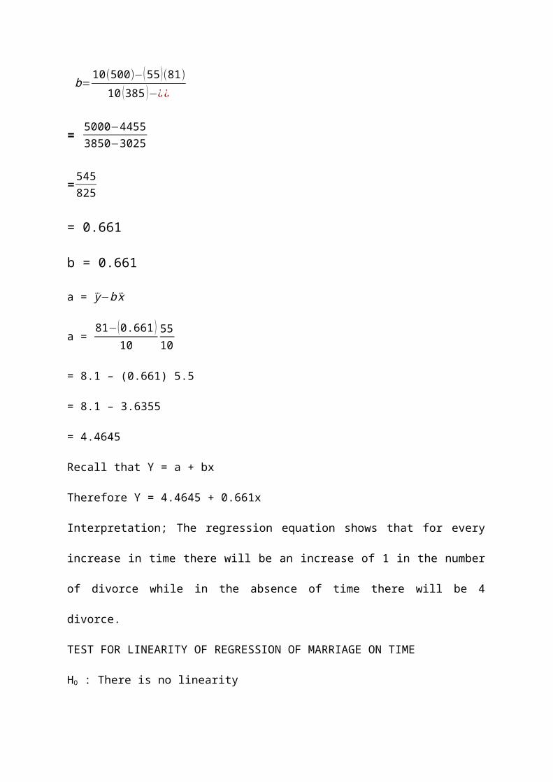
b=10(500)−(55)(81)

10 (385 )−¿¿

= 5000−44553850−3025

=545825

= 0.661

b = 0.661

a = y⃛−bx⃛

a = 81−(0.661 )10

5510

= 8.1 – (0.661) 5.5

= 8.1 – 3.6355

= 4.4645


Therefore Y = 4.4645 + 0.661x


increase in time there will be an increase of 1 in the number

of divorce while in the absence of time there will be 4

divorce.





Where V1 = K- 1 = 2-1 -1

V2 = N –K = 10-2 = 8

COMPUTATION

SST = εy2−¿¿

= 773 - ¿¿

= 773−656110

= 773-656.11

= 116.9

SST = 116.9


= 0.661(500−(55) (81)10 )

= 0.661 (500−445510

)

= 0.661 (500 – 445.5)

= 0.661 (54.5)

= 36.0245

SSA = 36.0245

SSE = SST – SSA

= 116.9– 36.0245

= 80.8755

SSE = 80.8755

SOURCE DEGREE OF

FREEDOM

SUM OF

SQUARE

MEAN OF SUM

OF SQUARE

FRATION

REGRESSION

ERROR

1

8

36.0245

80.8755

36.0245

10.1094

3.5635

TOTAL 116.9

Fcal = 3.5635

Critical region

F0.05 (1,8) = 5.32

Ftab= 5.32


Conclusion: Since Fcal (3.5635) < Ftab (5.32) we accept Ho and

conclude that there is no linearity between divorce and time

in Ile-Oluji/Okeigbo Local government.

CORRELATION ANALYSIS OF DIVORCE AND TIME

X= Passage of time

Y= Divorce


r = 10(500)−(55 )(8)√¿¿¿

= r = 5000−4455√(3850−3025 )(7730−6561 )

= 545

√(825) (1169)

= 545√964425

= 545982.05

= 0.55

r = 0.55

There is weak positive correlation between divorce and time in

Ile – Oluji/Okeigbo local government.


= R2 × 100%

= (0.55)2 × 100%

= 0.3025 × 100%

= 30.25%

= 30%

30% of variation in divorce can be explained by time while 70%

can be explained by other factors.




Critical Region

Ttab= T α/2 V, Where V = n-2 = 10-8 =8

= T0.05/2, 8

= T0.025, 8 = ± 2.306

Ttab = ± 2.306

COMPUTATION

t = r√n−2√1−r2

= 0.55√10−2√1−(0.55)2

= 0.55√8√1−0.3025

= 0.55(2.828)

√0.6975

= 1.55540.8352

= 1.8623 ≈1.86

Tcal = 1.86


Conclusion: Since Tcal (1.86) < Ttab (±2.306) we therefore accept

Ho and conclude that the correlation between divorce and time

is not significant.

REGRESSION ANALYSIS OF DIVORCE ON TIME

X Y XY X2 Y2

36 4 144 1296 16

66 7 462 4356 49

42 5 210 1764 25

26 8 208 676 64

79 13 1027 6241 169

40 8 320 1600 64

34 6 204 1156 36

58 5 290 8364 25

62 10 620 3844 100

82 15 1230 6724 225

525 81 4,715 31,021 773

X = Marriage

Y= Divorce



b=10(4715)−(525 )(81)

10 (31021 )−¿¿

= 47150−42525310210−275625

= 462534585

= 0.1337

b = 0.1337

a = y⃛−bx⃛

a = 81−(0.1337 )10

52510

= 8.1 – (0.1337) 52.5

= 8.1 – 7.02

= 1.08


Therefore Y = 1.08 + 0.1337x


increase in marriage there will be no increase of in the

number of divorce while in the absence of marriage there will

be 1 divorce.





Where V1 = K- 1 = 2-1 -1

V2 = N –K = 10-2 = 8

COMPUTATION

SST = εy2−¿¿

= 773 - ¿¿

= 773−656110

= 773-656.11

= 116.9

SST = 116.9


= 0.1337(4715−(525 ) (81)

10 )= 0.1337 (4715−

4252510

)

= 0.1337 (4715 – 4252.5)

= 0.1337 (462.5)

= 61.836 - 61.84

SSA = 61.836

SSE = SST – SSA

= 116.9– 61.836

= 55.064

SSE = 55.064

SOURCE DEGREE OF

FREEDOM

SUM OF

SQUARE

MEAN OF SUM

OF SQUARE

FRATION

REGRESSION

ERROR

1

8

61.836

55.064

61.836

6.883

8.984

TOTAL 116.9

Fcal = 8.984

Critical region

F0.05 (1,8) = 5.32

Ftab= 5.32


Conclusion: Since Fcal (8.984) < Ftab (5.32) we reject Ho and

conclude that there is no linearity between marriage and

divorce Ile-Oluji/Okeigbo Local government.

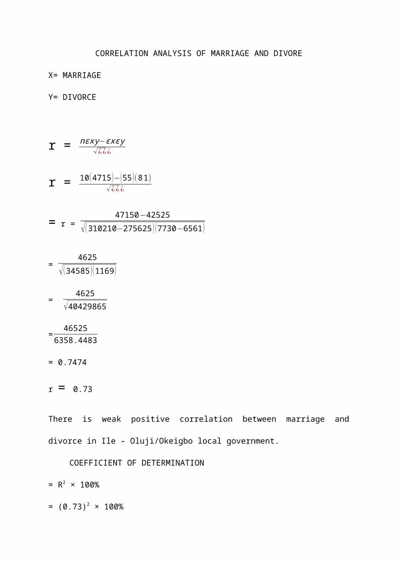
CORRELATION ANALYSIS OF MARRIAGE AND DIVORE

X= MARRIAGE

Y= DIVORCE


r = 10(4715)−(55)(81)√¿¿¿

= r = 47150−42525√(310210−275625 ) (7730−6561)

= 4625

√(34585 )(1169)

= 4625√40429865

= 465256358.4483

= 0.7474

r = 0.73

There is weak positive correlation between marriage and

divorce in Ile – Oluji/Okeigbo local government.


= R2 × 100%

= (0.73)2 × 100%

= 0.5329 × 100%

= 53.29%

= 53%

53% of variation in divorce can be explained by marriage while

47% can be explained by other factors.




Critical Region

Ttab= T α/2 V, Where V = n-2 = 10-8 =8

= T0.05/2, 8

= T0.025, 8 = ± 2.306

Ttab = ± 2.306

COMPUTATION

t = r√n−2√1−r2

= 0.73√10−2√1−(0.73)2

= 0.73√8√1−0.5329

= 0.73(2.828)

√0.4671

= 2.06440.6834

= 3.0208 ≈3.02

Tcal = 3.02


Conclusion: Since Tcal (3.02) < Ttab (±2.306) we therefore reject

Ho and conclude that the correlation between marriage and

divorce is significant.

LOVE AND SEX

Documents

Transcript of LOVE AND SEX