ikayex Software Tools - Cambridge University Press
183
-
Upload
khangminh22 -
Category
Documents
-
view
0 -
download
0
Transcript of ikayex Software Tools - Cambridge University Press

� �
QED�
Static� Dynamic� Stability
andNonlinear Analysis
ofSolids and Structures
ikayex Software Tools� �

ii
Copyright Notice
No part of this publication may be reproduced without prior written consent fromikayex Software Tools�Copyright�c� ���� � ����ikayex Software Tools�This manual describesDiSPtool ver ���� GenMesh ver ���� NonStaD ver ���� PloMeshl ver ���� QED ver ����Simplex ver ���� StaDyn ver ���� released January �����
Software License Agreement
The essence of this agreement is that ikayex Software Tools grants the purchasera single license for the use of the accompanying software�The software may be used at more than one location and by more than one
person provided there is no possibility that it is being used by two or more peoplesimultaneously�
Disclaimer
ikayex Software Tools makes no warranties as to the contents of this manual orthe accompanying software� Although every e�ort has been made to insure that themanual is accurate and the software reliable ikayex Software Tools cannot beheld responsible for any damages su�ered from use of this product�
ikayex Software Tools
Lafayette� Indiana �����

Contents
Table of Contents iv
� QED the Computer Laboratory �
��� Overview of QED � � � � � � � � � � � � � � � � � � � � � � � � � � � � �
� Model Building with GenMesh �
��� Types of Structures Considered � � � � � � � � � � � � � � � � � � � � ���� Structure Data File � � � � � � � � � � � � � � � � � � � � � � � � � � � ����� Rectangular Mesh � � � � � � � � � � � � � � � � � � � � � � � � � � � � ���� Compound Meshes � � � � � � � � � � � � � � � � � � � � � � � � � � � ����� Circular Plate with Pressure � � � � � � � � � � � � � � � � � � � � � � ����� Arbitrary Meshes � � � � � � � � � � � � � � � � � � � � � � � � � � � � ���� Complex Structure � � � � � � � � � � � � � � � � � � � � � � � � � � � ���� Extruded Meshes � � � � � � � � � � � � � � � � � � � � � � � � � � � � � ��� Solid Meshes � � � � � � � � � � � � � � � � � � � � � � � � � � � � � � � ������ Some Hints � � � � � � � � � � � � � � � � � � � � � � � � � � � � � � � �
� Basic StaDyn Tutorials ��
��� Static Example � � � � � � � � � � � � � � � � � � � � � � � � � � � � � ����� Static Analysis of Trusses and Frames � � � � � � � � � � � � � � � � � ����� Static Analysis of Plates � � � � � � � � � � � � � � � � � � � � � � � � ���� Complex Structure � � � � � � � � � � � � � � � � � � � � � � � � � � � ����� Some Hints � � � � � � � � � � � � � � � � � � � � � � � � � � � � � � � ���
� Advanced StaDyn Analyses ���
�� Stability Analysis � � � � � � � � � � � � � � � � � � � � � � � � � � � � �� �� Vibration Analysis � � � � � � � � � � � � � � � � � � � � � � � � � � � ��� �� Forced Frequency Response � � � � � � � � � � � � � � � � � � � � � � �� � Transient Response � � � � � � � � � � � � � � � � � � � � � � � � � � � ���
� Nonlinear Analyses with NonStaD and Simplex ���
��� Large De�ection Analysis of a Beam � � � � � � � � � � � � � � � � � � � ���� Structural Instability � � � � � � � � � � � � � � � � � � � � � � � � � � ��
iii

iv Contents
��� Elastic�Plastic Behavior using Simplex � � � � � � � � � � � � � � � � � ���
� Utilities ���
��� PlotMesh � � � � � � � � � � � � � � � � � � � � � � � � � � � � � � � � � ������ FormGen � � � � � � � � � � � � � � � � � � � � � � � � � � � � � � � � � ������ DiSPtool � � � � � � � � � � � � � � � � � � � � � � � � � � � � � � � � � ����� GSview and GhostScript � � � � � � � � � � � � � � � � � � � � � � � � �� ��� Automating Running in Batch Mode � � � � � � � � � � � � � � � � � � ���
References ���
Index ���

Chapter �
QED the Computer Laboratory
The QED program is a Visual Simulation Tool for Analysis� Its intent is to provide aninteractive simulation environment for understanding a variety of problems in solidand structural mechanics� This chapter gives an overview of QED the underlyingmechanics and programs plus some introductory tutorials on static and dynamicstress analysis� The purpose is not to provide a tutorial on running QED � thisis provided in the richly documented text Guided Explorations in the Mechanics of
Structures ����� rather it is a set of tutorials on running the underlying supportingexecutables associated with the QED package� It is not necessary to understand theseprograms in order to run QED however knowing the material in this manual willenrich the use of QED�
��� Overview of QED
An experiment by its nature is a single realization � a single geometry materialor load case� multiple test cases and examples are just not economically feasible�But engineers being introduced to something new need to see other examples aswell as variations on the given examples� For instance in the stress analysis of asymmetrically notched specimen some logical questions to ask are
� What if the notches are bigger or smaller�� What if there is one instead of two notches�� What if the notches are closer or further apart�� What if the material is changed�� What if instead of a notch there is a hole�� What if the clamped boundary has some elasticity�
These questions are too cumbersome and expensive to answer experimentally but arevery appropriate for a simulation program� Furthermore a very important role of atest engineer is to be able to distinguish those aspects of an experiment that have
�

� Chapter �� QED the Computer Laboratory
a signi�cant deleterious e�ect from those that are insigni�cant� This can come onlythrough experience and here too the program can help to accelerate the process ofaccumulating experience�What is missing in the traditional laboratory is the iterative stage in both analysis
and testing that all engineers go through � the process of asking the �What�Ifs�doing parameter sensitivity studies and re�designing the experiment� Having a �ex�ible sophisticated model running simultaneously on the computer to counterpointthe experiment can profoundly a�ect the engineers� perception of both theory andexperiment� The interplay of both establish an interesting and exciting dynamic�As envisioned the modeling program runs simultaneously with the experiment andbecomes a resource to be interacted with and tested against the experiment�
QED: a computer laboratory
Models
➤
➤
➤
➤
➤
➤
frame
cylinder
open
hole
notch
solid
geometrybcsloadsmesh
GenMesh:
Analysis
➤
➤
➤
➤
➤
➤
linear static
linear vibration
linear transient
buckling
nonlinear incremental
nonlinear transient
StaDyn/NonStaD/Simplex:
➤
Views
➤
➤
➤
➤
➤
➤
contours
shapes
tractions
time traces
movies
distributions
The �gure above shows a schematic of the functional parts of the program� Itsdesign is such that it isolates the user from having to cope with the full�blown �ex�ibility of the underlying enabling programs and presents each problem in terms of alimited �but richly adaptable� number of choices and combinations�The process of �nite element analysis can be broken down into three separate
stages� These are presented as independent modules in QED� The pre�processingstage allows the model geometry to be de�ned the boundary conditions imposed theloads applied and the mesh generated� In the second stage the analytical solution isobtained� Choices as to the type of solution required and the parameters best suitedto guide the procedure are made� In the post�processing stage results are displayedin a variety of ways� Contour plots of nodal results the deformed shape free bodydiagrams and time history traces are available� The following sections provide fullerexplanation of these three analysis steps�The design philosophy of QED is to make each module very speci�c but �exible�
This is important as it helps to �x focus on the signi�cant aspects of behavior� Eachproblem has a template of properties therefore the user need only focus on what they

���� Overview of QED �
want to change�Solution techniques are separated from the model building to emphasize the inde�
pendent general nature of the analysis� Whether static or transient model solutionsare sought that do not depend on the type of structure or model geometry considered�In the post�processing general tools are provided which demonstrate the behavior
of di�erent characteristics� Knowing which is best suited to a particular problem isvital and having all available but being taught which are most appropriate or e�ectiveto communicate the desired information is very valuable to a deep understanding aproblem�As shown in the following chapters the underlying programs can be menu driven
but their operation under QED is by way of driver or script �les� Script �les That isQED creates the script �les to execute GenMesh and StaDynNonStaD� The name ofthe script �les are
StaDyn�NonStaD�Simplex� instad� inpost� inps
GenMesh� inmesh� inmesh�� insdf
In this way the programs can operate as separate executable programs�The description of the structure and its material properties is kept in a separate
�le referred to as the Structure DataFile� This will have the name qed�sdf� Creatingthis �le and inputting it properly is a crucial step in the analysis� As the data �le isread in numerous types of checks are performed on it so as to con�rm that it was readproperly� It is also echoed back into the �le ��StaDyn�LOG�� or ��NonStaD�LOG�� ifdesired�
For Starters
There is no installation procedure per se in getting QED up and running � just amatter of copying it from the CD disk onto your hard disk� If you are not familiarwith the process do the following�Open a command prompt window �this is sometimes called an MS�DOS prompt
window� o� the start�accessories menu or by typing �cmd� in the run window�The properties of the command window can be adjusted by left clicking on the topbar and selecting properties�Go to the root directory �assuming you are not already there and assuming you
are on the C drive� by
C� cd�
�Do not type the C��� Make a working directory� Later you can place the programsin your favorite directories but for now type
C� mkdir qed
C� cd qed
� Version ����� January ����

Chapter �� QED the Computer Laboratory
Now place the CD in the CD drive and �assuming it is drive D�� type
C� copy d����
Typing the dir command gives some of the contents of the disk as
STADYN �EXE NONSTAD �EXE QED �EXE
GENMESH �EXE STRIP �EXE
PLOTMESH�EXE
These programs will be explained in due course but to check that all the copying wentas it should type
C� stadyn
You should get the opening menu� If so choose
Note that within STADYN all interaction through the keyboard requires a carriagereturn or ENTER to complete the entry� Having pressed return exit by typing
Now run QED by typing
C� qed
and the opening graphical screen should appear� If it does not then press �q� to quit�Go to �settings� o� the control panel and change the number of colors to ���� Thisshould cure the problem� Note that while most interaction with QED is through thekeyboard a carriage return is not required unless data is being entered�
Setup and Interaction Keys
QED launches GenMesh StaDynNonStadSimplex and so on as separate executableprograms� Therefore QED needs to know where to �nd these programs� The defaultlocation in is the
C��qed
directory but this can be changed through the �fth line of the ��qed�cfg�� �le� Thefull contents of this �le are

���� Overview of QED �
��� ��Max memory
��� �� ��Max lines � pts
� � ��size font
� ��animate pause �
c��qed
�� �� � �E� ��xyz rots
� � � � � � � � � � ��subs
� ��grav
�� DATE� ������ TIME� ����
end
The third line can be used to adjust the size of the QED window and the size of thefonts� both numbers are percentages�Generally interaction is through the keyboard� When input in the form of num�
bers is required the input is terminated with a carriage return�Some keys are available at most stages these are
h help remindersm mesh display toggle on�o�o change orientation of axesq quit the current operations show�render the current operationt tags toggle on�o�w write a PS �le of zoomed image
The help reminders are somewhat context sensitive�A few pointers on running QED
� It is strongly recommended that QED be launched from the COMMAND win�dow and not from EXPLORER�
� All interaction with QED is via the highlighted keys or the leftmost symbol�number�letter� on the menus�
� The size of the window and of the fonts are changed by editing the third line inthe �le ��qed�cfg��� These numbers are percentages� the �rst number is thepercentage of the full screen occupied by the QED window�
� If the initial screen is black use settings of the CONTROL PANEL to changethe number of colors and�or resolution�
� PS �les of contours can be obtained by pressing �w� in the zoom window�Parameters for the PS contours are changed by editing the �le ��stadyn�ctr���To set up GhostView as the PostScript viewer type SETUP�
� Version ����� January ����

� Chapter �� QED the Computer Laboratory
� TRACE data �les are obtained by zooming on the window� the data is storedin the �le ��qed�dyn���
� For problems with a large number of elements it may be necessary to changethe dynamically allocated memory sizes in ��stadyn�cfg�� ��nonstad�cfg��and ��genmesh�cfg���
� The symptom that a supporting �EXE program did not run is that the win�dow pops up and closes immediately� If this happens look in the appropriate����log�� �le�
Being productive with QED
QED is set up so as to remember the complete state of a procedure whether itis creating a model or doing an analysis� The relevant information is stored inthe ������cfg�� �les such as ��frame�cfg�� ��solid�cfg�� and ��anal�cfg���These get over�written as changes are made therefore to archive a particular framesay copy ��frame�cfg�� to a new name� When this particular frame is requiredagain then just copy the �le back to ��frame�cfg��� It is important to note thatthis must be done while QED is not running�There are two facilities for recording the graphics results fromQED� The simplest is
to cut and paste the screen into Paint and then use Paint�s capability to manipulateand print the image� Suppose it is desired to print a copy of the contours then onthe QED top bar menu click Edit�Select All then click Edit�Copy� Launch Paint
from Start�Accessories and click Edit�Paste� The resulting �les can be stored ina variety of bitmap formats including ������bmp�� and ������jpg���The support for vector graphics is through PostScript� QED produces strictly
ASCII �les which are easily edited with any text editor if needed� Grey scale images�such as for photoelastic or Moir�e fringe patterns� are included via the image function�

Chapter �
Model Building with GenMesh
When structural problems are large it is essential to have an automatic scheme forthe generation of an input data �le� this not only removes the drudgery of making the�le but more importantly it helps ensure its integrity� The purpose of this chapteris to show how the program GenMesh �GENerate a MESH� can be used to createstructure data�les for use by StaDynNonStaDSimplex�The design of StaDynNonStaD is such that a frame and a meshed plate have very
much in common � primarily the nodes have exactly the same number of degrees offreedom� Thus any generic mesh can be easily made to represent either of these twostructural types� Indeed both can be combined to form a complex mesh� The Simplexmeshes are quite di�erent since they only have translational degrees of freedom andcannot �at present� be combined with StaDynNonStaD meshes�When manipulating complex �or compound meshes� it is essential to avoid having
to deal directly with node numbers or element numbers� GenMesh uses the idea ofgroups and tags to keep track of special collections of nodes and elements respectively�These are usually speci�ed at the time of making the component meshes and thecomplex mesh then inherits them� Operations such as specifying material propertiesor specifying boundaries for attachment become easier and most important becomeindependent of the mesh density�The main capabilities of GenMesh involve generating meshes and performing the
following executive functions
� Create Generic ��D Shapes� Create Arbitrary ��D Meshes� Create ��D Structures� Create ��D Solids� Re�Map Mesh� Re�connect Mesh� Merge two Meshes� Make Structure DataFile
�

� Chapter �� Model Building with GenMesh
Unlike frame elements plate elements are approximate and therefore many ele�ments are required to accurately model a given region� Some of the generic meshesavailable are
��D Plane shapes ��D StructuresQuadrilateral block Dome w�out stringersTwo to One reduction General w�out stringersGeneric Cut�out Space FrameGeneric Notch Space TrussArbitrary shape
The same mesh can be used for a linear analysis by StaDyn or for a nonlinearanalysis by NonStaD� The solid element meshes can be analyzed only by Simplex�
���� Types of Structures Considered �
��� Types of Structures Considered
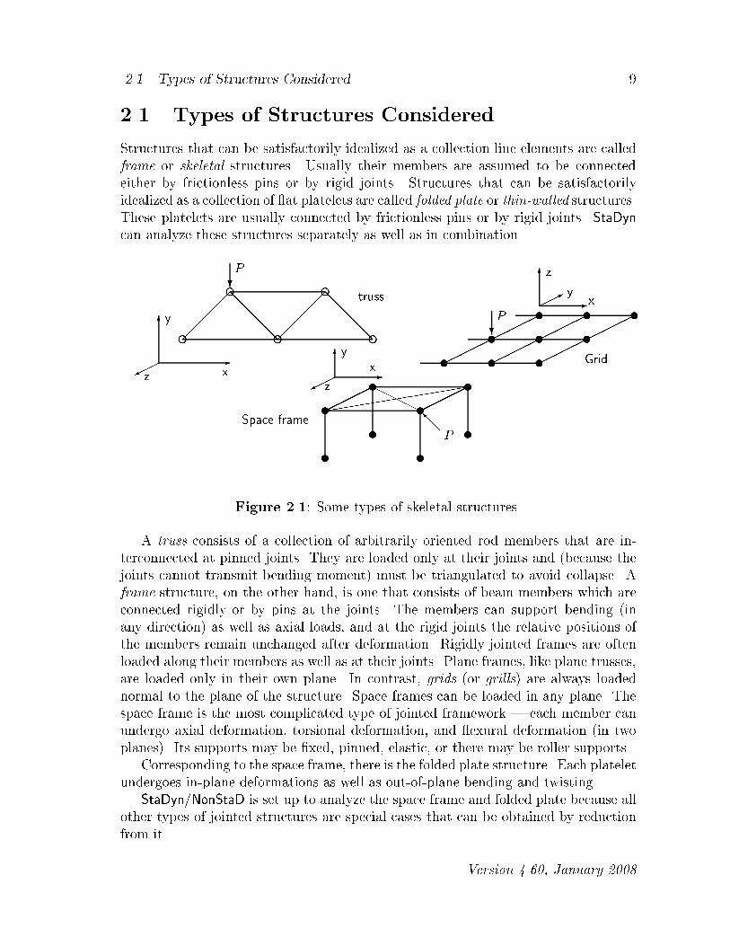
Structures that can be satisfactorily idealized as a collection line elements are calledframe or skeletal structures� Usually their members are assumed to be connectedeither by frictionless pins or by rigid joints� Structures that can be satisfactorilyidealized as a collection of �at platelets are called folded plate or thin�walled structures�These platelets are usually connected by frictionless pins or by rigid joints� StaDyncan analyze these structures separately as well as in combination�
�
�
��� x
y
z
�
�
��� xy
z
��
���
xy
z
����
���
�
����
����
e e e
e etruss
�P
����
����
��������
����
����
u u u
uu u
u u u
Grid
�P
����
����
u u
u u
u u
u u
��������
����HHHHSpace frame ��I
P
Figure �� Some types of skeletal structures�
A truss consists of a collection of arbitrarily oriented rod members that are in�terconnected at pinned joints� They are loaded only at their joints and �because thejoints cannot transmit bending moment� must be triangulated to avoid collapse� Aframe structure on the other hand is one that consists of beam members which areconnected rigidly or by pins at the joints� The members can support bending �inany direction� as well as axial loads and at the rigid joints the relative positions ofthe members remain unchanged after deformation� Rigidly jointed frames are oftenloaded along their members as well as at their joints� Plane frames like plane trussesare loaded only in their own plane� In contrast grids �or grills� are always loadednormal to the plane of the structure� Space frames can be loaded in any plane� Thespace frame is the most complicated type of jointed framework � each member canundergo axial deformation torsional deformation and �exural deformation �in twoplanes�� Its supports may be �xed pinned elastic or there may be roller supports�Corresponding to the space frame there is the folded plate structure� Each platelet
undergoes in�plane deformations as well as out�of�plane bending and twisting�StaDynNonStaD is set up to analyze the space frame and folded plate because all
other types of jointed structures are special cases that can be obtained by reductionfrom it�
� Version ����� January ����

�� Chapter �� Model Building with GenMesh
folded plate
Figure �� A folded plate structure�
The number of possible displacement components at each node is known as thenodal degree of freedom �DoF�� the nodal degree of freedom for di�erent structuraltypes is shown in the following table
Structure Dimension u v w �x �y �z Type �
Rod ��Dp
��Beam ��D
p p��
Shaft ��Dp
��Truss ��D
p p��
Frame�membrane ��Dp p p
��Grill�P late ��D
p p p��
Truss ��Dp p p
��Frame�FoldedP late ��D
p p p p p p��
GeneralStructure ��Dp p p p p p
��Solid ��D
p p p���
From this table it is clear how the frame structure and folded plate structure sharecommon types of degrees of freedom� This essentially is what allows them to becombined together to form complex structures�
A Note on the Elements Used
Since StaDynNonStaD is designed to analyze thin�walled ��D structures comprisinga mixture of frame and plate sub�structures then it simpli�es the implementationwhen both structural types are modeled in a compatible way� This section brie�ydescribes the elements used � more general treatments of the �nite element method

���� Types of Structures Considered ��
can be found in References �� � �� ��� and aspects speci�c to framed structuresare developed in References �� �� ��� and aspects speci�c to StaDynNonStaD inReferences ��� ���� Three�noded triangular elements were chosen primarily becausethey can be conveniently mapped to form irregular shapes� Furthermore we consideronly thin plate �exural theory �Kirchho� plates� and the corresponding slender beamtheory �Bernoulli�Euler��A ��D frame member has six DoF at each node
fug fu� v� w� �x� �y �zg
In local coordinates this has three behaviors� There is a rod action with axial dis�placement and force
fug fug � F �x� EA�u
�x
There are two beam actions� the bending moment and shear force� The correspondingnodal degrees of freedom are the rotation �z�x� �or the slope of the de�ection curveat the node� and the vertical displacement v�x��
fug fv� �zg � M�x� EI��v
�x�� V �x� �EI �
�v
�x�
There is also a bending about the y�axis� Finally there is a twisting about the axis
fug f�xg � T �x� GJ��z�x
where EA EI and GJ are the axial bending and torsional sti�nesses respectively�E and G are the Young�s and shear modulus respectively� and A I and J are thearea moment of inertia and polar moment of inertia respectively� Full details onthe matrix implementation for frame structures can be found in Reference �����A ��D plate supports both in�plane �membrane� and out�of�plane ��exural� ac�
tions� The in�plane behavior of the plate is analogous to that of a plane ��D frame�Thus at each node we want the DoF to be
fug fu� v� �zg
The usual constant strain triangle �CST� element has only the two displacementsin its formulation� The element implemented in StaDyn is taken from the paper byBergan and Felippa ���� This is a nine�noded triangular element which is shown tohave superior in�plane performance over the CST� But more importantly from ourperspective is that it correctly implements the drilling DoF ��z� and therefore makesit suitable for a ��D incorporation� The �rotation� implemented is actually that takenfrom continuum mechanics
�z �
���v
�x� �u
�y�
� Version ����� January ����

�� Chapter �� Model Building with GenMesh
Coding for the element is given in Reference ����The strains are obtained by di�erentiation of the displacements
�xx �!u
�x� �yy
�!v
�y� �xy
�!u
�y"�!v
�x
The material behavior is represented �for the plane stress case� by�����
�xx�yy�xy
�����
E
�� ��
�� � � �� � �� � ��� ����
�������
�xx�yy�xy
�����
where � is Poison�s ratio�The out�of�plane behavior is analogous to that of a plane ��D grid� That is we
want an element that has at each node the degrees of freedom
fug fw� �x� �ygThe rotations are related to the de�ection by
�x �w
�y� �y ��w
�x
In local coordinates the three�noded triangle has a total of � degrees of freedom�This element now called the Discrete Kirchho� Triangular �DKT� element was �rstintroduced by Stricklin Haisler Tisdale and Gunderson in ���� ����� It has beenwidely researched and documented as being one of the more e#cient �exural elements�see Batoz Bathe and Ho � ��� Code for the element is given in References �� ���The curvatures are obtained by di�erentiation of the displacement
�xx ��w
�x�� �yy
��w
�y�� �xy
��w
�x�y
The material behavior is represented �for the plane stress case� by�����
Mxx
Myy
Mxy
�����
Eh�
����� ���
�� � � �� � �� � ��� ����
�������
�xx�yy�xy
�����
where h is the plate thickness�In this manner each node whether it is associated with a frame or a plate element
has the requisite six DoF and all resolved components of applied loading will besupported�The ��D solids are modelled using Hex�� elements� This has �� nodes and each
node has the DoFfug fu� v� wgT
Formulations for its use are given in a number of texts two of which are references ����� This element performs well even when used to construct shells�

���� Structure Data File ��
��� Structure Data File
The description of the structure and its material properties is kept in a separate �lereferred to as the Structure DataFile� Creating this �le and inputting it properly is acrucial step in the analysis�This section describes the �elds for the structure data�le�
Structure DataFile Format
The input data�le can be in free format with blanks or commas used as separators�Any editor or word processor can be used to make changes to a �le but make sure tostore the new �le as strict ASCII �les without any hidden word�processing symbols�Note that the data input is arranged in groups and that each group must have
the word END or end as its last line� This acts as an additional data checker�
Header Group
TITLE
IGLOBAL
IFLAG� IFLAG� IFLAG� IFLAG�
end
TITLE Short title �up to � characters� describing the mesh or problem�
IGLOBal Global problem reduction��integer���D �� rod �� beam �� shaft��D �� truss�cable �� frame�membrane �� grill�plate��D �� truss�cable �� frame�folded�plate �� general��D ��� solid plane strain ��� solid general
IFLAG Echo �ags for the input� � on � o�� connectivity � material � numbering loads
Connectivities Group
The number of lines is equal to NEL� Every element must have an input for it althoughthey do not have to be input in strict sequential order� However the nodes fortriangular elements must be input counter�clockwise�
NEL
ELM TYP NPI NPJ NPK
� � � � �
� � � � �
end
� Version ����� January ����

� Chapter �� Model Building with GenMesh
NEL Number of elementsELM The unique number assigned to each element�TYP The type of element� �integer�
� truss � cable � frame triangle �� solid�NPI The number of the �� node on the element� �integer�NPJ The number of the �� node on the element� �integer�NPK The number of the �� node on the element� �integer�
For truss or frame members set NPK�NPJ� For solids NP� ranges from � to ���
Material Tags Group
The number of lines is equal to NMAT� Every element must have a material numberor tag� however it is possible to specify overlaying numbers� For example to makeElement � di�erent from Elements ��� and ���� say specify � � �� followed by � � ��
NMAT
ELM� ELM� �
� � �
� � �
end
NMAT Number of element material lines� �integer�ELM� First element of this material� �integer�ELM� Last element of this material� �integer�� Material number tag number or sub�structure number� �integer�
Coordinates Group
The number of lines input must equal NNP� The lines do not have to be input in strictorder from � to NNP but every node must be on a separate line�
NNP
NODE XORD YORD ZORD
� � � �
� � � �
end
NNP Number of nodal pointsNODE The unique number assigned to each node�XORD x�coordinate of the node point�YORD y�coordinate of the node point�ZORD z�coordinate of the node point�
���� Structure Data File ��
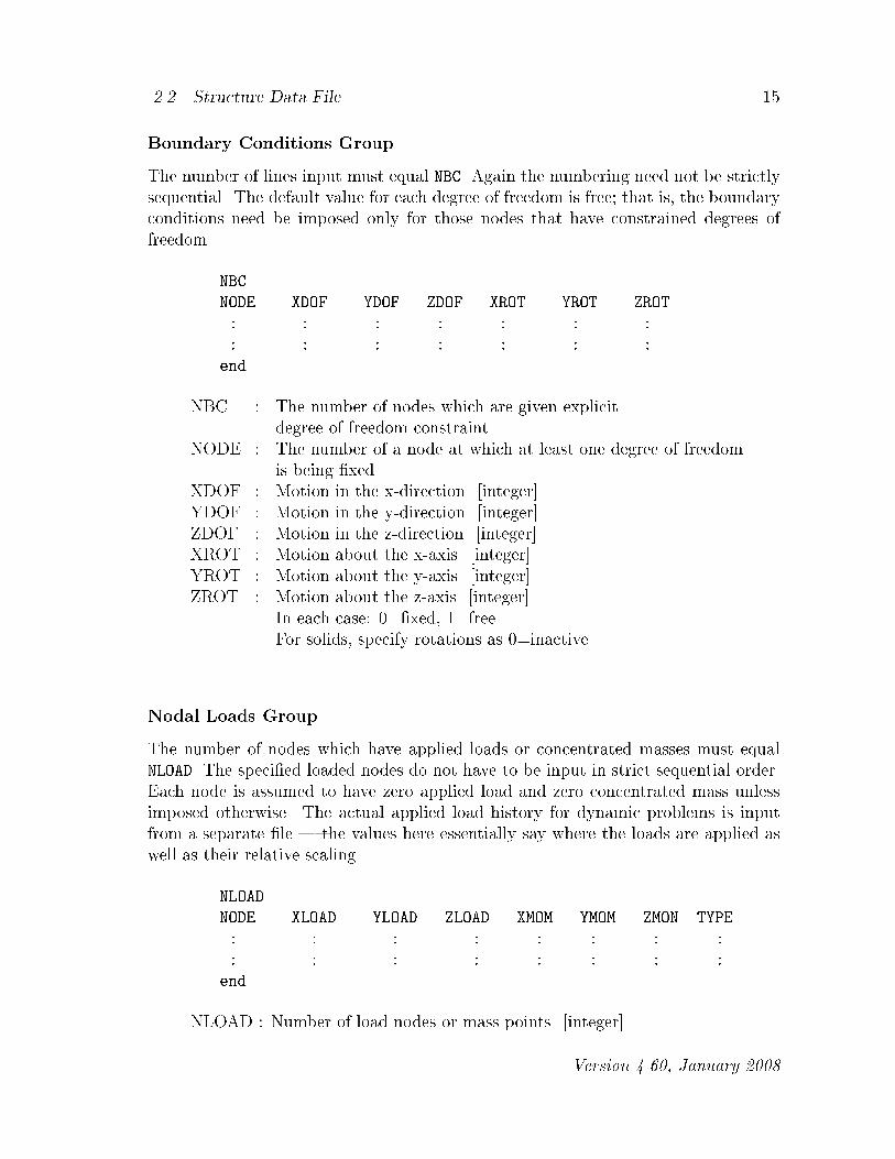
Boundary Conditions Group
The number of lines input must equal NBC� Again the numbering need not be strictlysequential� The default value for each degree of freedom is free� that is the boundaryconditions need be imposed only for those nodes that have constrained degrees offreedom�
NBC
NODE XDOF YDOF ZDOF XROT YROT ZROT
� � � � � � �
� � � � � � �
end
NBC The number of nodes which are given explicitdegree of freedom constraint�
NODE The number of a node at which at least one degree of freedomis being �xed�
XDOF Motion in the x�direction� �integer�YDOF Motion in the y�direction� �integer�ZDOF Motion in the z�direction� �integer�XROT Motion about the x�axis� �integer�YROT Motion about the y�axis� �integer�ZROT Motion about the z�axis� �integer�
In each case � �xed � free�For solids specify rotations as � inactive�
Nodal Loads Group
The number of nodes which have applied loads or concentrated masses must equalNLOAD� The speci�ed loaded nodes do not have to be input in strict sequential order�Each node is assumed to have zero applied load and zero concentrated mass unlessimposed otherwise� The actual applied load history for dynamic problems is inputfrom a separate �le � the values here essentially say where the loads are applied aswell as their relative scaling�
NLOAD
NODE XLOAD YLOAD ZLOAD XMOM YMOM ZMON TYPE
� � � � � � � �
� � � � � � � �
end
NLOAD Number of load nodes or mass points� �integer�
� Version ����� January ����

�� Chapter �� Model Building with GenMesh
NODE The unique number assigned to each node� �integer�XLOAD Force applied in the x�direction at the node� �real�YLOAD Force applied in the y�direction at the node� �real�ZLOAD Force applied in the z�direction at the node� �real�XMOM Moment applied about the x�axis at the node� �real�YMOM Moment applied about the y�axis at the node� �real�ZMOM Moment applied about the z�axis at the node� �real�TYPE Additional load feature� �real�
TYPE � �� Concentrated mass of value TYPE at the node� TYPE �� Second force distribution� For solids specify moments as ����
Element Material Properties Group
The number of lines is equal to MATYPE� There must be a type speci�ed for eachmaterial tag� The input format is identical for both the plate and frame elementsalthough a couple of the entries have slightly di�erent interpretations� The framevalues are indicated in parenthesis�
MATYPE
Mat� E G A Rho Gama Ix Iy Iz ��truss
Mat� E G A Rho Gama Ix Iy Iz ��cable
Mat� E G A Rho Gama Ix Iy Iz ��frame
Mat� E G h Rho Gama Ip Ia Ib ��plate
Mat� E G Rho ��solid
Mat� C Alf Rho ��rubber
� � � � � � � � �
� � � � � � � � �
end
MATYPE Number of element materials� �integer�Mat� Material number� �integer�E Young�s modulus of the material� �real�G Shear modulus of the material� �real�A Cross�sectional area of the frame elements� �realh Thickness of the plate element� �real�Rho The density of the element �input as W�g�� �real�Gama Sti�ness modi�er� �real�
cable !Fo �EAframe orientation of principal axesplate � � plane stressplate � � � plane strain
Ix Frame polar moment of area about x�axis� �real�

���� Structure Data File ��
Iy Frame second moment of area about y�axis� �real�Iz Frame second moment of area about z�axis� �real�Ip Bending second moment of area for plate� �real�
Ip h���� uniform plateIa In�plane drilling parameter �� ���� �real�Ib In�plane drilling parameter � ���� �real�C��Alf Mooney�Rivlin �C�� ��� ��C��� C�� �C���� �real�
Specials Group
This group is a mechanism to allow the input of special global properties� In thepresent formulation damping is applied to all members equally and is made propor�tional to their mass and�or sti�ness matrices�The number of lines input must equal NSP�
NSP
CODE C� C� C�
� � � �
� � � �
end
NSP Number of linesCODE Unique code number for each special attribute� �integer�
���� damping � C � �c�����M � " �c�����K ����� gravity $g c�$ex " c�$ey " c�$ez
���� shear e�ect rod c��qGIx�EAL�� beam c���EIz�GAL
�
�� � plasticity �Y c�� ET c��� �� reduced integration c� �� c� �� c� �� �� � �Hex�� � full��
C� First constant �real�C� Second constant �real�C� Third constant �real�
Examples of Structure DataFiles
The following example is for a simple in�plane plate structure as shown in Fig�ure ����a��
ex�ps��� �element plate ��header
��
� � � �
end
��element
� � � �
� Version ����� January ����

�� Chapter �� Model Building with GenMesh
� � � �
� � � �
� � � �
� � �
� � � �
� � � �
� � �
end
� ��material �s
� �
end
��node
� � � �
� �� � �
� �� �� �
� � �� �
�� �� �
� �� � �
� �� �� �
�� �� �
end
� ��boundary condns
�
� �
� �
� �
end
� ��applied loads
� �� � � � � � � �
� �� � � � � � �
end
� ��� of materials
� ��e� ��e� �� �� e�� � � �� �
end
��specials
end
This is the input �le for a simple plate problem and a copy of it is on the disk as��ex ps����� Note that this data is inputted in free format with blank spaces usedonly as separators� In general the �le can be documented by adding comments onthe remainder of a line � a convention followed in all the examples is that commentsare separated from the required numbers by double colons but otherwise there isnothing special about the double colons� For this particular example the customary

���� Structure Data File ��
units are used � StaDynNonStaD however will handle any set of units as long asthey are consistent� This mesh corresponds to one quarter of a plate with a uniformstress of ���� psi applied at both ends�
�
�
���
��������
���
���
��
��������
���
�����
u
u
u
u
u
u
u
u
Plate
m� m� m�
m� m� m�
m� m�
���
���
���
���
�
�
��
�
��
� ������
������
u
utruss
m�
m�
m�
��� ���
��������������������������������������������������
ee����������������������������������������������
��
Figure �� Some simple structures� �a� EX PS�� an eight element plate��b� EX FS�� a three element truss�
Notice how the boundary conditions are imposed Node � is �xed in all directionsbut Node � and Node � are free to move in the x�direction and not in any of the otherdirections� That is they are on horizontal rollers� Likewise Node is on verticalrollers� The imposition of a stress corresponds to a distributed applied loading� thiselement has an edge shape function similar to that of a beam hence the consistentload moments are
P� �
��otL "
�
�� ����� �� � ���� P�
T� "�
���tL� "
��
��� ����� �� �� � ��� �T�
where � is the drilling parameter as appears in the material line� Imposing thesemoments is only necessary when the mesh is relatively coarse� generally speaking thelumped approximation will be adequate�Note that there must be entries in each group� Thus even if there are no loads
say there must be at least one line indicating so� This is illustrated in the lines forthe Specials Group� While seemingly unnecessary this helps the input checker tobe more accurate and therefore useful�The following example is for a simple ��D truss structure as shown in Figure ����b�
and a copy of it is on the disk as ��ex fs�����
ex�fs��� Balfour pp���� ��header
��
� � � �
end
� ��element
� � � � �
� Version ����� January ����

�� Chapter �� Model Building with GenMesh
� � � � �
� � � � �
end
� ��material �
� � �
end
� ��node
� � � �
� �� �� �
� �� � �
end
� ��boundary conditions
�
� �
end
� ��applied loads � mass
� �e� �e� � � � � �
end
� ��material props
� �e� �e� �e�� � � �� �� ��
end
��specials
end
For this particular example the units are in metric � StaDynNonStaDSimplex willhandle any set of units as long as they are consistent� Notice how the boundaryconditions are imposed Node � is �xed in all directions but Node � is free to movein the x�direction and not in any of the others� That is Node � is on rollers�The structure data�les for both the plate and truss are almost identical � the
only di�erences are in the element number the speci�cs of the material propertiesand the repeated third connectivity� Consequently it is very easy to construct astructure that contains both types of elements�
Checking the Input
This tutorial shows how to use some of the built�in diagnostics of StaDynNonStaDto help ensure that the structure data�le is correct�To run the program simply type
C� stadyn
Note that stadyn is the name of the executable version� The menu will appear andyou then just respond to the questions� Since you want to input the structure data�lechoose

���� Structure Data File ��
�
and you are asked for the data �lename� Type
ex�ps��
If StaDyn has read the data correctly it will acknowledge so and then present themain menu again� To quit choose
In the working directory there is a newly created �le called ��stadyn�log��� It is anASCII �le so peruse it by typing
C� type StaDyn�log
It is a long �le so it may be preferable to pipe to MORE� There appears to be a bigjumble of numbers and symbols such as
�� StaDyn version ���� June ��
�� DATE� ������� TIME� ����
�� MAXimum storage � �
�� MAXimum elements �
�� MAXimum nodes �
�� MAXimum force incs� �
�� ITERmax � ��
�� rtol � ��E��
�� ALLOCATION succeeded
� ��MAIN
ex�ps��
�
�� HEADER GROUP
�� Title � ex�ps�� �element plate
�� Problem type � ��
�
This �le is actually a record or log of the session just completed� There are twotypes of lines in this �le� The lines that have double colons ���� are generally theinputs given to StaDyn� What follows the colons are brief descriptions of what wastyped or where it was typed� The other lines that begin with double ats ���� areStaDyn�s information or answers as responses� It gives extra insight into its workingsthat can be very useful when trying to backtrack to nail a problem� In this particularcase it can be used to judge if all the structural data was read as intended� If StaDyndetects inconsistencies in the input data it will �ag them and by looking through thislog �le it is possible to determine approximately where the inconsistency occurred�
� Version ����� January ����

�� Chapter �� Model Building with GenMesh
Look further through the �le and see the manner in which the structural data isechoed� The single most common source of errors for a �nite element analysis is inthe data input� You should attempt to become familiar with this �le because it canbe an immensely useful tool for checking the integrity of the data input�The data�le can also be visually checked by running it through the plotting utility
PlotMesh by simply typing
C� plotmesh
By pressing the active keys various forms of the data�le will be presented�

���� Rectangular Mesh ��
��� Rectangular Mesh
Unlike frame elements plate elements are approximate and therefore very many ele�ments are usually required to accurately model a given region� The purpose of thisintroductory tutorial is to mesh a rectangular region�
Getting Started
GenMesh is designed to run as a console �or command window� program under thevarious �avors of MS Windows� Note that all instructions are case insensitive� we willvary the case only to help make the instructions clearer�To run the program type �at the �C prompt��
C� genmesh
�note the name of the executable�� You are given the opening menu
MAIN menu�
� Quit
�create�
�� Create Generic ��D Shapes
��� Create Generic ��D Solid Shapes
�� Create Arbitrary ��D Mesh
�� Create Arbitrary ��D Shapes
�� Create ��D Structures
�manipulate�
� Re�Map
�� Re�Mesh
�� Merge two Meshes
�realize�
� Make Structure DataFile
��
�services�
�� Write PostScript Plot File
���� Ikayex help
SELECT ���
Quit by typing
There are two �les worth looking at� The �rst is the log �le ��genmesh�log��
�� GenMesh version ���� April ��
�� DATE� ������� TIME� �����
� Version ����� January ����

� Chapter �� Model Building with GenMesh
�� MaxElem request�
�� Maxes � � � � � � �
�� ALLOCATION succeeded
��MAIN
�� GenMesh OK� exited from MAIN
The second is ��genmesh�cfg��� This is the con�guration �le and has in it
��MaxElem
�� �� ��pos X Y
�� ��pen�thick
� � � �� ��rotX Y Z shrink
�� �� �� ��cap X Y size
� ��mesh type
�� DATE� ������� TIME� �����
end
This allows the run time setting of the dimensions of the arrays� The other settings arethe parameters for making a PostScript drawing of the mesh� If a memory allocationfailure occurs this is the place to make the adjustments�
Making the Mesh
We will now run GenMesh to generate a �le containing the same information as inthe �le ��ex ps����� Type
C� genmesh
to get the opening menu� We wish to mesh a simple plate so choose
�
and you are asked to give the mesh �le a new name or keep the default one
SAVE new mesh as�
�return ��GMesh�MSH ��New Name
Choose a new name
�
m�
and the program responds with the choice of generic shapes
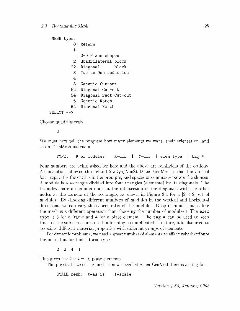
���� Rectangular Mesh ��
MESH types�
� Return
��
� ��D Plane shapes
�� Quadrilateral block
��� Diagonal block
�� Two to One reduction
��
� Generic Cut�out
�� Diagonal Cut�out
�� Diagonal rect Cut�out
�� Generic Notch
��� Diagonal Notch
SELECT ���
Choose quadrilaterals
�
We must now tell the program how many elements we want their orientation andso on� GenMesh instructs
TYPE� � of modules X�dir � Y�dir � elem type � tag �
Four numbers are being asked for here and the above are reminders of the options�A convention followed throughout StaDynNonStaD and GenMesh is that the verticalbar j separates the entries in the prompts and spaces or commas separate the choices�A module is a rectangle divided into four triangles �elements� by its diagonals� Thetriangles share a common node at the intersection of the diagonals with the othernodes at the corners of the rectangle as shown in Figure �� for a �� � �� set ofmodules� By choosing di�erent numbers of modules in the vertical and horizontaldirections we can vary the aspect ratio of the module� �Keep in mind that scalingthe mesh is a di�erent operation than choosing the number of modules�� The elemtype is � for a frame and for a plate element� The tag � can be used to keeptrack of the sub�structures used in forming a complicated structure it is also used toassociate di�erent material properties with di�erent groups of elements�For dynamic problems we need a great number of elements to e�ectively distribute
the mass but for this tutorial type
� � � �
This gives �� �� �� plate elements�The physical size of the mesh is now speci�ed when GenMesh begins asking for
SCALE mesh� �as�is ��scale
� Version ����� January ����

�� Chapter �� Model Building with GenMesh
�
�
���
�������
��������������
��������
������
��������������
�������
t
t
t
t
t
t
t
t
t
t t
t t
Plate
l� l� l�
l�� l�� l��
l� l�
l� l�
l�l� l�
Figure �� A ��� �� set of modules�
We will scale it now so type
�
which leads to
NE NW SW SE
TYPE� x� � y� � x� � y� � x� � y� � x� � y�
These correspond to the coordinates of four corners � �x�� y�� is the coordinate of thenortheast corner �x�� y�� the northwest corner and so on around in an anti�clockwisefashion� Note that it is at this point that the mesh may be con�gured to any foursided shape� it may be stretched out squashed or sheared� For our case type
�� �� � �� � � �� �
This makes it a square plate with �� units on the side� GenMesh responds withinformation that NEW mesh in� m�� Back at the main menu quit by typing
Look through the mesh �le and you will see
Quads
��
end
�� ��ELEMENT GROUP
� � � � �
� � � � �
�
�
���� Rectangular Mesh ��
The structure of the �le is there plus the connectivities and coordinates� At this stagethis is a generic mesh meaning that it could be used for in�plane loading bending or��D folded plates� Or it could be used to attach to another generic shape to make amore complex mesh involving plates and frames�
Adding Properties
To make the generic mesh into a structure data�le we need to add properties� Inparticular we need to state the type of material the boundary conditions and theloads� The generic meshes have a default state inferred from the construction process�This section allows changes to be made to this state�Initiate GenMesh
C� genmesh
and from the main menu select
to add properties� We are going to read in our generic mesh add properties to itand store it under a new name� First you are asked to give the mesh �le a new nameor keep the default one
SAVE new mesh as�
�return ��GMesh�MSH ��New Name
Choose to change the name
�
You are asked for the new name
TYPE� NEW�filename ���
respond
rect�sdf
Next you are asked for the input �lename
TYPE� IN�filename ���
Respond
m�
You are now given a summary of the mesh as
� Version ����� January ����

�� Chapter �� Model Building with GenMesh
� Matls
�� Nodes
BCs
Forces
materials
SPcls
� boundary groups
and the change properties menu�
� return
�� Header group
�� Matl tag group
�� BCs group
��� Loads group �new�
��� Loads group �overlap�
� Material group
�� Specials group
At this stage pick those properties to be changed or to be speci�ed� Start with thetitle
�
and you are asked
TYPE� Title ���
In response type
rect�sdf� square plate
This is the title of the problem not the �lename� The program then asks for theproblem type
GLOBAL types�
��D� ���rod ���beam ���shaft
��D� ���truss�cable ���frame�in�plane ���grill�plate
��D� ���truss�membrane ���frame�folded plate
TYPE� Global type ���
Since we are interested in ��D in�plane behavior choose
��
The four echo �ags are asked for next

���� Rectangular Mesh ��
TYPE� � flags
We will eventually have a large number of elements for the dynamic problem so wedon�t want to �ll our disk with all this information� But �rst time through with anew mesh it is a good idea to echo all the information so type
� � � �
Next select information about the substructure tags
�
and you are given
CHOOSE material types�
�return
��re�tag by groups
��create single tagged group
��re�tag by element
The �rst of these �that is making no change� will simply associate the materialnumbers with the tag number thus all elements tagged � say will have materialproperties ��� The other three options allow the re�tagging of the elements� Forsimplicity choose default material numbers
Specify the boundary conditions�
�
The program gives the options
BOUNDARY condns�
CHOOSE� �continue
��node range �sequential�
��node range �bc info�
��node group �bc info�
��cylinder �volume �
�nearest �single �
��interrogate �bc info�
The interrogate option is for reminders of the boundary information �although havingPlotMesh running simultaneously is a better option�� Options � and � take theirinformation from the boundary nodal information automatically stored at the bottomof each generated mesh �le� Since we only have a couple of boundary conditions inputby the boundary information range sequence hence type
� Version ����� January ����

�� Chapter �� Model Building with GenMesh
�
The node and boundary condition are speci�ed in response to
TYPE� ��fixed� ��free�
Node� � Node� � xdof � ydof � zdof � Xrot � Yrot � Zrot
Type
�� �
corresponding to the �xed boundary condition at the left side� When specifying theboundary conditions it is possible to specify a range of nodes� the sequence in therange is obtained from the bottom of the mesh �le� For plane meshes the nodes goin a counter clockwise fashion� The boundary condition menu is recurring so thatmany boundary conditions may be input� Note that ranges can overlap� Move on bytyping
The applied force data is speci�ed next in response to
��
The other load option would be used to add some new loads to an existing loadsystem�
APPLIED LOADS�
CHOOSE� �return
��nodal load �sequence�
��nodal load �bc info �
��nodal load �bc group info �
��nodal load �nearest xyz �
��cylinder load �volume�
���equal force to tagged surface
���uniform pressure to tagged surface
� �traction distribution
���traction distribution from file
��interrogate
There is a single applied force so type
�
Give its location in response to

���� Rectangular Mesh ��
TYPE�
Node� � Node� � Px � Py � Pz � Tx � Ty � Tz � cmass
and put it at Node �
�� � � � � � �
Just as for the boundary condition input this would be a recurring request if thereare more than one applied force� Note that while the force history will be speci�edelsewhere this �le must say where it is applied� Thus the entry ��� above could beused as a scaling factor� Indeed multiple force sources could be inputted but theywill all act as scalings on the applied load history� In this way distributed and vectorloads can be applied� Note also that this is the place where concentrated masses�separate from the distributed mass of the elements� are input�Next input the material information�
and receive the request
INPUT� � of different Materials
There is only one material
�
You are given a reminder of the appropriate format for the material data
INPUT�
� � E � G � t�A� � Rho � PLN�gama� � Ip�Ix� � Ia�Iy� � Ib�Iz�
In response let the material be nominally aluminum under plane stress conditions
� ��e� ��e� �� �� e�� � � �� �
The last two numbers are associated with the in�plane behavior of the plate element� generally they should always be speci�ed as above� This would be a recurringsequence if there is more than one material�We do not want to specify any special material properties so quit
After this you are now put back at the main menu� To exit GenMesh type
It would be a good idea at this stage to check the structure data�le by running itthrough StaDyn�
� Version ����� January ����

�� Chapter �� Model Building with GenMesh
��� Compound Meshes
The purpose of this tutorial is to show how GenMesh can be used to create a meshcomposed of a number of generic shape meshes� The particular mesh is shown inFigure ��� and is comprised of three di�erent meshes a �� � � quadrilateral a module two�to�one transition and a block with a circular hole�
Figure �� Compound mesh comprising three di�erent mesh types�
There are two reasons why a compound mesh might be formed� The �rst is that theobject is composed of two di�erent generic shapes for example rectangle and circular�each of these are best meshed in their natural coordinates� The other is that di�erentportions of the structure are composed of di�erent element types� In connectingdi�erent meshes together some transition elements are sometimes required� we willdemonstrate the use of these�
Making the Generic Meshes
The script �le for the quadrilateral is
C� genmesh
� ��MAIN
�
m�
� ��MESH
� � � � ��nxmod�nymod�el�tag
� ����scale
� � � �
��MAIN
Scaling is done so this is of size �� �� The script �le for the transition mesh isC� genmesh
� ��MAIN
�
m�

���� Compound Meshes ��
� ��MESH
� � � ��nxmod�el�tag
� ����scale
� �� �� �
��MAIN
This is scaled to size �� ���� Use PlotMesh to view this mesh� it is the same as inthe center section of Figure ��� but is horizontal�We will go through the mesh with a hole a little more in detail� Initiate the
program as usual and select the circular hole option
C� genmesh
� ��MAIN
�
m�
��MESH
We must now declare how many modules comprising the mesh
INPUT� � of modules Hoop � Radial � elem � tag �
Many of the generic meshes are basically the same the di�erences lie in their bound�aries�In specifying the modules we do not consider either the boundary modules or the
center fans since these require special �x�ups for the di�erent cases� Because the holeis inherently symmetrical choose a number of hoop modules that is divisible by ��Respond
�� � � �
You are now asked
INPUT� Rmin � exponent � �hollow ��full
The �rst is the inside radius while the second allows variation of the spacing of themodules in the radial direction� For example it might be good to put a higherconcentration of modules near the inside edge of the hole� this would be achieved byspecifying the exponent less than unity� For now choose
�� �
This gives equi�spaced modules between �� and ���� The outer boundary is currentlycircular but we can map it to a straight side�
MAP straight boundary� �as�is ��map
Choose to map
� Version ����� January ����

� Chapter �� Model Building with GenMesh
�
and you are asked for
NE N
TYPE� x��y� x��y�
We just want a square outer boundary so type
� � �
Meshes that are mapped may have elements with poor aspect ratio� it is good practicein those situations to smooth or balance the element shapes� In response to
INPUT� � of smooth cycles � type ���area���coord�
reply
because for the moment we want to see what an unsmoothed mesh looks like� Wealso do not want to scale the mesh so respond
As each of these generic meshes are being made it is advisable to use the utilityPlotMesh to survey the results� In particular you need to note the boundary nodenumbers�
Aligning Meshes
There are a variety of ways that generic meshes can be combined� some of the schemesare based on the information about their boundary nodes� �This information is storedat the end of each mesh �le�� Thus the process could be made highly automatedfor some problems� StaDynNonStaD and GenMesh are designed for analyzing gen�eral three�dimensional structures and therefore the schemes implemented for mergingmeshes must also work in those general cases� The basic idea is to �rst align the sub�structures as if they are to be physically welded and then attach the nearest nodes�
We will use M� as the reference mesh place M� rotated next to it and �nally alignM�� The two driver �les are
C� genmesh
�
m�b

���� Compound Meshes ��
m�
�
�
���
Sometimes a little iteration is needed in order to fully predict �in the ��D cases� wherethe rotations and translations will leave the new mesh� Again this is a case were theuse of a script �le can help considerably�The mesh with the hole need only be translated
C� genmesh
�
m�b
m�
�
��� ��
Merging Meshes
We will �rst combine M� and M�b� Initiate GenMesh and choose the merge option
C� genmesh
�
�
m��
You are now asked to
TYPE� infileNAME�� ���
It makes a di�erence which mesh is given �rst because that is the one to which thesecond is subservient� Respond
m�
Similarly for the second �lename
TYPE� infileNAME�� ���
Respond
� Version ����� January ����

�� Chapter �� Model Building with GenMesh
m�b
A brief summary of the two meshes is displayed� Now you are asked about how thetwo meshes are to be attached
CONNECTion modes� MODEL�� ��� MODEL��
�continue
��node to node
��group to surface
��intersecting surfaces
INPUT� mode
Note that Model � is attached to Model �� The most basic form of attachment is ��where essentially the two plates are stitch together node by node� The simplest is�� where any close nodes are automatically connected� We will use the second modefor illustrative purposes�
�
and you are asked about the attachment nodes
INPUT� group � � � of nodes � release as BC �none ��all ��interior
��� � all�
The group referred to is the group of boundary nodes at the bottom of the mesh�le� When two meshes are joined what were formerly boundaries now could becomeinterior regions� We therefore may wish to release them and not consider them asboundaries �or special collections of nodes� anymore� Since boundary nodal groupsusually overlay at a common node Options � and � allow distinguishing between thetwo situations� The sequence of attaching is counter�clockwise for the �rst meshand clockwise for the second� Before getting to this stage it is good practice to usePlotMesh to explore the generic meshes� In particular that program can determinethe boundary nodes�The appropriate information is
� �
The attaching is a recurring menu� Since we do not want to attach any more segmentsthen to quit type
Use PlotMesh to look at this mesh and note the boundary nodes�We now wish to merge this new mesh with M�b� The procedure is the same as what
was just done� To be di�erent we will show the use of the third mode of attachment�

���� Compound Meshes ��
C� genmesh
� ��MAIN
�
m���
m��
m�b
�
�� �
��MAIN
The only item of interest here is the �proximity� number� this can be made large orsmall depending on the density �or coarseness� of the nodal points� The resultingmesh is shown in Figure ���� An important point to note about the mesh �le is howthe through the use of the tags the identity of the individual sub�structure meshesis retained� This is re�ected in the di�erent colors used in PlotMesh�
Mesh Smoothing
An obvious feature of Figure ��� is that the elements are not in a smooth proportion�This is noticeable in the transition from the coarse rectangular mesh as well as in thetransition of the radial mesh to the rectangular outer boundary� This is a commonoccurrence in mesh generation however some of the obvious irregularities can �andshould� be removed and GenMesh has a menu option that does that� Note howeverthat this will work only for ��D plane meshes in other words this would be usefulbefore assemblage to the ��D structure�
Figure �� Compound mesh with smoothing�
Initiate GenMesh and choose the Re�Map option
C� genmesh
� Version ����� January ����

�� Chapter �� Model Building with GenMesh
��MAIN
�
m���b
m���
The following small menu of the various re�mappings is presented
CHOOSE mapping�
�move on
��scale
��position �rot � trans�
��move single nodes
�change boundary groups
��smooth
���extra smooth
���wrap around shape
This allows various ways to map or distort a global mesh� We just want to smoothso choose
�
You are asked about smoothing
INPUT� � of smooth cycles � type ���area���coord�
Choose
�� �
What smoothing does is replace the position of every node with the average position�with a weighting based on area or coordinate� of all the nodes of its immediateneighbors� All the nodes belonging to the boundary nodal groups are una�ected thusleaving the outer shape of the mesh intact� �Note that if a frame mesh is to besmoothed then the type based on coordinates should be used�� The number chosen isthe number of passes taken � between � and �� passes is usually adequate but checkin the LOG �le to see how rapidly the norm is converging� Quit by typing
The mesh now looks like Figure ���� There is some improvement but obviously thebad e�ects of incompatible meshes cannot be entirely eliminated� When smoothinga mesh additional biasing can be obtained by moving individual nodes to a desiredlocation and then specifying it as a boundary node� In this way the surroundingnodes will adjust appropriately� A much better mesh is obtained by making theuniform section � modules deep�

���� Circular Plate with Pressure ��
��� Circular Plate with Pressure
The purpose of this tutorial is to show how GenMesh can be used to mesh circularregions� In particular we will run it to generate a �le containing the same informationas in the �le ��ex ps���� that will be used for the circular plate for �exural tutorials�
Making the Mesh
Run the program and select the Generic Shapes
C� genmesh
�
�
m�
The program responds with the choice of generic shapes choose the �generic cut�out�option
We must now input how many modules comprising the mesh
TYPE� � of modules Hoop � radial � elem � tag �
Many of the generic meshes are basically the same the di�erences lie in their bound�aries�
Figure �� Solid circular hole representing a circular plate�
In specifying the modules we do not consider the center fan since this requiresspecial �x�ups� Respond
�� � � �
� Version ����� January ����

� Chapter �� Model Building with GenMesh
You are now asked
INPUT� Rmin � exponent � �hollow ��full
The �rst is the inside radius even though it is a solid plate� The radius referred tohere is that of the solid fan at the center� it is not possible to carry the module ideadown to a point� The second input allows variation of the spacing of the modules�For example it might be good to put a higher concentration of modules near theinside edge of the hole� this would be achieved by specifying the exponent less thanunity� Respond
�� � �
This will give equi�spaced modules between ��� and ���� We do not want to map theouter boundary of the mesh to a rectangle or smooth the interior node distributiontherefore type
Only the generic dimensions of the total mesh has been speci�ed but it is possibleat this stage to change it in response to
SCALE mesh� �as�is ��scale
We will scale it such that it is �� in radius�
�
which leads to
NE NW SW SE
INPUT� x� � y� � x� � y� � x� � y� � x� � y�
These correspond to the coordinates of four corners � �x�� y�� is the coordinate of thenortheast corner �x�� y�� the northwest corner and so on around in an anti�clockwisefashion� Note that it is at this point that the mesh may be con�gured to any foursided shape� It may be stretched out squashed or sheared� in fact the circle couldbe transformed into an ellipse� For our case type
�� �� � �� � � �� �
and quit
You are now informed that the mesh is in P�� Display it with PlotMesh it shouldlook like Figure ����

���� Circular Plate with Pressure �
Adding Properties
To make the generic mesh into a structure data�le we need to add properties� Thatis we need to state the type of material the boundary conditions and the loads� Wehave already done this in a previous tutorial hence the following will dwell only onthe signi�cantly di�erent parts�Initiate GenMesh and from the main menu select the Make Structure DataFile
option�
C� genmesh
�
m�
m�
You are now given a summary of the mesh as
� Matls
�� Nodes
BCs
Forces
materials
SPcls
� boundary groups
The series of questions to be answered are the same as the earlier tutorial so wewill just give the responses�
�
circ�msh� circular plate uniform pressure
��
We will specify the boundary conditions next�
�
�
�
corresponding to the �xed boundary condition all around the outside� This was madeconvenient by realizing that the outer boundary nodes are in group � � note that thisis a consequence of having used the generic mesh generator to produce the mesh inthe �rst instance� The boundary condition menu is recurring so that many boundaryconditions may be input� Note also that ranges can overlap�The applied force data is to be speci�ed next
� Version ����� January ����

� Chapter �� Model Building with GenMesh
��
and we are given the options
APPLIED LOADS�
CHOOSE� �return
��nodal load �sequence�
��nodal load �bc info �
��nodal load �bc group info �
���nodal load �bc group info � ���� ends�
���node traction �bc group� ���� ends�
��nodal load �nearest xyz�
��cylinder �volume�
��cylinder resultant �volume�
���equal force to tagged surface
���uniform pressure to tagged surface
����uniform load to tagged frame
����uniform pressure to Hex� surface
� �traction distribution
� ��traction distn �coords in file�
���traction distribution from file
��interrogate
We will use the idea of the tagged element to distribute the pressure over the elements�
��
and you are asked for
TYPE� tag � � pressure
Although there is only one element tag in this model it can be imagined that thistag idea is a way of isolating particular sub�structures for application of the pressure�For example this can be used to isolate the outer skin of an aircraft wing� Respond
� ��
Note that an applied pressure is treated di�erently than applied point forces � a pres�sure acting on a surface produces tractions normal to the surface� The components ofthe forces are computed automatically and will then be distributed among the nodesof the each element� This is a lumped formulation the slightly more accurate �forcoarse meshes anyway� consistent method is not as clean to implement here since itrequires knowledge of the plate bending shape functions�The applied loads menu is a recurring one that allows multiple loads to be added
but we will quit here
���� Circular Plate with Pressure �
The material properties are speci�ed by
�
� ��e� ��e� �� �� e�� � ���e�� �� �
The third last number computes the plate moment of inertia for a uniform plate as
Ip h�
�� ��
�� ������� ����
Note however that for arbitrary complex plates �with interior reinforcement forexample� an e�ective Ip can be used that is not related to the thickness as above�We have all our properties speci�ed so quit
Survey ��m��� and make sure the properties have been installed as expected�
Minimizing the Bandwidth
When forming the mesh no consideration is given to reducing the bandwidth� Thereason for this is that in all likelihood the mesh will be combined with another andconsequently its bandedness properties would be destroyed� The �nal step in themesh creation is the reduction of the bandwidth�Before we reduce the bandwidth it is instructive to �rst send the �le through
StaDyn� Initiate it read in the mesh ��m��� and quit�
C� stadyn
�
m�
This does two things �rst it checks that the mesh is readable by StaDyn the sec�ond thing it does is compute the bandwidth� This is displayed as ���� � ���� inthe stadyn�log �le� The computational cost for analysis with this mesh would bevery large� Also given is the pro�le storage value� this says that the actual storagerequirements is currently ����� or ��% of the bandwidth storage� It is this numberthat we should concentrate on reducing� Keep in mind however that in doing itsreduction GenMesh does not take the degrees of freedom into account and thus thespeci�c numbers will di�er between GenMesh and StaDyn�To reduce the bandwidth run GenMesh and select the Re�mesh option
� Version ����� January ����

Chapter �� Model Building with GenMesh
C� genmesh
�
�
m�
m�
You are now given the re�meshing menu
CHOOSE� �return
��
��remesh plate
��remesh frame
��add frame member
�
��reduce bandwidth
���mesh of only boundary elements
���separate elements
���form cohesive surface
���remove snags
�
Choose
�
and you are asked
CHOOSE� �return ��reduce ��update
Choose reduce
�
and you are informed that
INITIAL band � ��
STORAGE �� ��� ��� of NB
INPUT� wavefront center x � y � z
The initial band is di�erent from that reported by StaDyn because the present pro�gram does not take the number of degrees of freedom per node into account� theconsequences of this are negligible� Nor does it take the boundary conditions intoaccount� The simple scheme for bandwidth reduction is that of the wavefront thatis the nodes are numbered based on their relative distance from some point �thewavefront center�� Try

���� Circular Plate with Pressure �
and you are told that
INITIAL BAND � ��
FINAL BAND � ��
INITL STORAGE �� ��� ��� of NB
FINAL STORAGE � �� �� �� of NB
CHOOSE� �return ��reduce ��update
Note that while the bandwidth was reduced the pro�le storage was increased� Try
�
��
and you get an even smaller bandwidth
INITIAL BAND � ��
FINAL BAND � ��
INITL STORAGE �� ��� ��� of NB
FINAL STORAGE ���� ��� ��� of NB
CHOOSE� �return ��reduce ��update
This is a case where relative to the original we have reduction in both bandwidthand pro�le storage� You could experiment more but we will save it and quit�
�
If you now run ��m��� through StaDyn you will see that the storage requirements aredisplayed as ����� ���� and a pro�le storage value that is currently ����� or � % ofthe bandwidth storage�All the original node numbers have been changed so you should use PlotMesh to
familiarize yourself with the new numbers�
� Version ����� January ����

� Chapter �� Model Building with GenMesh
��� Arbitrary Meshes
The purpose of this tutorial is to show how the GenMesh program can be used to meshregions where the boundaries are speci�ed in an arbitrary fashion� In particular wewill redo the earlier problem of the circular hole in the rectangular block�
Boundary Information
We will need to input data that describes the boundary control points� These arethen connected to form segments� the numbering sequence is such that the area tobe meshed is on the left hand side� This takes the form
� of control points
node Xord Yord
� � �
� � �
end
� of segments
�st node �nd node connection type
� � �
� � �
end
The connection type speci�es the geometric shape of the segment� The currentimplemented forms are
straight line � �
inside semi�circle � �
outside semi�circle � ��
bezier curve � �
circular arc � �
Mesh Generation
Run the program
C� genmesh
�
�
a�
and in response to
TYPE� � of control points
�

���� Arbitrary Meshes �
We now input the location of these points
INPUT� point � � x� � y�
This will cycle through the six points�
�
� ���
� ��� �
� �
�� �
� ��� �
We now input the segment connections and the style of their connection� There aresix segments
TYPE� � of segments
�
TYPE� seg� � point�� � point�� � style
This will cycle through the six points�
� � � �
� � � �
� � � �
� � � �
� �
� � �
end
Each segment or overlapping segments can be divided and these will form the bound�ary edges of the elements�
INPUT� �st seg � �nd seg � � of divsns � to end�
This is a recurring menu type
� � �
� �
� � �
� ��
This will give the same number of modules around the hole and at the left and rightends as in our earlier tutorial� A �nal piece of information is asked for
� Version ����� January ����

� Chapter �� Model Building with GenMesh
INPUT� maxelements attempted � �
This subroutine is a situation were we do not know the �nal number of elements inadvance� This input allows you to set an upper limit on the number of elementsformed� Actually if the program is having di#culty forming a mesh it is a good ideato set this number very and view the partial mesh formed� this will give you an ideaof what is being attempted and how you might adjust the input �le to correct for it�Choose
�
The program proceeds periodically echoing its attempts at connecting nodes�The �rst mesh created is rather crude the better mesh is obtained by performing asmoothing operation�
INPUT� � of smooth cycles � type ���area ��coord�
Typically �ve to twelve smoothing cycles are adequate� Type
�� �
Finally we need to tag the mesh
INPUT� elem type � tag �
Give the information and quit�
� �
Now survey the mesh A� using the utility PlotMesh� The smoothed mesh shouldlook like Figure ���� A judicious use of boundary divisions segments can signi�cantlyimprove the smoothness of the mesh�Note that it is essential that these arbitrary meshes be sent through the bandwidth
reduction option�

���� Complex Structure �
Figure � Arbitrary mesh�
��� Complex Structure
Thin�walled structures are usually reinforced by the addition of stringers� these longslender members are added to give additional bending resistance� The thin�wall ismodeled using plate elements and the stringers are modeled using frame elements�Thus we have a structure composed of both types of elements�The purpose of this tutorial is to show how GenMesh can be used to create such
a mesh� in fact it is the �le ��ex cs���� to be used in a later tutorial�
Making the Generic Meshes
We want to make two generic meshes a � � � quadrilateral and a frame mesh thatwill surround it� The script �le for the quadrilateral is
C� genmesh
� ��MAIN
�
m�
� ��MESH
� � � � ��nxmod�nymod�el�tag
� ����scale
� � � �
��MAIN
Scaling is done so this is of size � � ��The simplest way to make the frame is to �rst create a three element mesh such
as the following
frame
��
� Version ����� January ����
�� Chapter �� Model Building with GenMesh
end
� ��ELEMENT GROUP
� � � � �
� � � � �
� � � � �
end
� ��material �s
� � �
end
� ��NODE GROUP
� � � �
� �� � �
� �� �� �
� � �� �
end
end
end
end
end
Call the mesh ��m���� Alternatively a one module frame can be created and theextraneous lines removed� We will convert the frame into twelve elements using theRe�Mesh capability of GenMesh� The responses are
C� genmesh
� ��MAIN
�
m�
m�
�
� � � ��nel� nel� mul
��MAIN
As each of these generic meshes are being made it is advisable to use the utilityPlotMesh to survey the results� In particular you need to note the boundary nodegroups of mesh ��m����

���� Complex Structure ��
Merging Meshes
Generic meshes can be combined based on the information about their boundarynodes or can be combined based on a node by node basis� We will use the formerapproach�Initiate GenMesh and choose the merge option
C� genmesh
�
�
m�
m�
m�
A brief summary of the two meshes is displayed� Now you are asked about how thetwo meshes are to be attached
CONNECTed modes� MODEL�� ��� MODEL��
�continue
��node to node
��group to surface
��intersecting surfaces
INPUT� mode
The most basic form of attachment is �� where essentially the two structures arestitched together node by node� This is generally a tedious menu option to respondto but is the preferred scheme when the response �le itself is generated automatically�The simplest is the third one and we will use this form of attachment since the twomeshes are already aligned
�
We will not release any boundary nodes �that is they will remain as boundaries whichmay prove useful for applying loads say� Respond
��
and quit
The new mesh is in m� use PlotMesh to look at it and note the boundary nodes� Inparticular note the di�erent color around the boundary� A more dramatic con�rma�tion can be obtained by changing ��mesh ��� �In this manner any number of stringers can be attached to the plate� In deed
if each is given a separate segment number then each can also be given separateproperties�
� Version ����� January ����

�� Chapter �� Model Building with GenMesh
Adding Properties
To make the generic structure into a structure data�le we need to add properties�That is we need to state the type of material the boundary conditions and theloads�Initiate GenMesh and from the main menu select the Make Structure DataFile
option�
C� genmesh
�
m
m�
You are now given a summary of the mesh as
� Matls
�� Nodes
BCs
Forces
materials
SPcls
� boundary groups
The series of questions to be answered are the same as an earlier tutorial so wewill just give the responses�
�
ex�cs��� thin�walled shear beam
��
� � � �
Boundary conditions are speci�ed next�
�
�
�
corresponding to a �xed boundary condition at the left side� The boundary conditionmenu is recurring so that many boundary conditions may be input� Note that rangescan overlap�There is a vertical point force to be applied at Node � so type
��
�
�

���� Complex Structure ��
Finally input the material properties�
�
� ��e� ��e� �� �� e�� � ���e�� �� �
� ��e� ��e� �� �� e�� � ����� ��� ���
There are no special properties so �nish by typing
Survey ��ex cs���� and compare with ��m �� to make sure the properties have beeninstalled as expected�
� Version ����� January ����

� Chapter �� Model Building with GenMesh
��� Extruded Meshes
There is a class of ��D meshes that can be viewed as a particular cross�section inthe x � y plane that is extruded in the z�direction� A circular cylinder is a simpleexample the cross�section shape is a circle and the cylinder is formed by moving this�as a generating surface� along the z�axis� By adding a mapping function the varietyof shapes can be increased substantially� GenMesh has two such generic meshes onewhich can be considered as a generalized cylinder and the other as a generalized dome�the essential di�erence between the two is that the latter is closed at one end�These ��D structures are usually thin�walled with stringers or sti�eners added for
extra support� These are rather complex modules with a signi�cant amount of datainput� our �rst tutorials therefore will concentrate on the meaning of the input termsby creating a triangular box beam with a half�cylinder attached� The last tutorialconsiders creating a thin�walled structure that resembles a multi�sparred wing�
Thin�walled Reinforced Structure
This structure will be constructed in three stages� First will be the folded platestructure comprising the shell followed by a frame structure of similar proportions�The �nal stage will consist of merging the two structures� Unlike the generic meshesof the previous sections the meshes created here are physical from the beginning�
��������v
v v
v
n�
n� n�
n�XXXXXXX
�������
vv
v
v
vv
n�
n� n�
n� n�n�
Figure �� Cross�section of extruded structures�
I� Folded Plate Structure
The structure will look like that of Figure ���� It will have four control points threeto de�ne the triangle and a fourth to de�ne the curved surface�Run the program and choose the name for the mesh as ��m���
C� genmesh
�
�
m�

���� Extruded Meshes ��
and you are given the mesh types
MESH types�
� return
�� ��D Extruded shapes ��
�� Dome �closed ended�
���
��� diag �closed ended� no stringer
��
�� General �open ended� two�planes
��� �open ended� no stringer
��� diag �open ended� no stringer
�� ��D Frame shapes ��
� General Rect �open ended� two�planes
�� ��D Arbitrary
�
We will look at the diagonal open�ended shape without stringers
��
The �rst series of information is to allow characterization of the cross�section in thex� y plane� We are asked for the number of control points and their coordinates
TYPE� � of control points
Input four control points
�
Now input the coordinates of each point
front back
Type� point � � x��y��z� � x��y��z�
This gives information about two planes �front and back� and the extrusion will bedone between the two� Note that the two planes need not be parallel� For now makethe control points in both planes the same
� � � � � � �
� �� � � �� � �
� ��� �� � ��� �� �
� �� �� � �� �� �
This sets the length of the extrusion as �� Thus unlike the generic meshes thesemeshes are physical from the beginning� in fact the control points can be used tolocate the sub�structure for attachment to other sub�structures�Next is information about the shape of the structure�
� Version ����� January ����

�� Chapter �� Model Building with GenMesh
SEGment styles� ��line �� ��bezier ��arc
TYPE� � of connected segments
In a complex structure with many control points there are a variety of ways thatthe points can be attached to each other� Each connection forms a segment and eachsegment can be of a di�erent style� The style of connection speci�es the geometricshape of the segment� The current implemented forms are
straight line � �
bezier curve � �
circular arc � �
Both the Bezier and arc actually require three control points to form it We willconnect Points � � and with an arc Points �&� Points �& and Points &� withstraight lines for a total of �ve segments� Thus respond
Now input which control points are connected and some of the attributes
TYPE� point�� � point�� � � divs � style � plate tag
A segment is not necessarily a single plate element and the � divs allows speci�cationof the number of modules connecting the two control points� Note that multipleconnections can be made to the control points� Respond
� � � �
� � � � �
� � � � �
� � � �
� � �
This gives the �at faces modules across and the curved surfaces � each� Eachplated segment will have a di�erent tag for easy identi�cation�The �nal piece of information to be speci�ed deals with how the cross�section is
extruded in the z�direction
Z�EXTRUSION
TYPE� � z�modules
This is the number of modules in the extruded direction� Put �� modules in thez�direction
�
Exit the program by typing
Now survey the mesh m� using the utility PlotMesh� change the orientation by pressingu�U and v�V� The mesh should look like Figure �����a��
GenMesh has the ability to produce the PostScript �le necessary to make hardcopy version of the mesh �les in this form� a later tutorial shows how it is done�

���� Extruded Meshes �� . .
�a� �b�
Figure ��� Extruded structures� �a� Folded plate� �b� Frame�
II� Extruded Frame Structure
We will make a frame structure of similar shape to the folded plate structure justconstructed� A merging of the two structures will then produce a reinforced thin�walled structure�Run the program and choose the name for the mesh as ��m���
C� genmesh
�
�
m�
and from the menu of mesh types
MESH types�
� return
�� ��D Extruded shapes ��
�� Dome �closed ended�
���
��� diag �closed ended� no stringer
��
�� General �open ended� two�planes
��� �open ended� no stringer
��� diag �open ended� no stringer
�� ��D Frame shapes ��
� General Rect �open ended� two�planes
�� ��D Arbitrary
�
choose the general rectangle with two planes�
� Version ����� January ����

�� Chapter �� Model Building with GenMesh
The �rst series of information is to allow characterization of the cross�section in thex� y plane� First is the number of control points
TYPE� � of control points
�
Then the coordinates and the joint tag
front back
Type� point � � x��y��z� � x��y��z� � joint tag
This gives information in two planes �front and back� and the extrusion will be donebetween the two� Note that the two planes need not be parallel� Control pointsact as joints and therefore it is useful to be able to associate a lengthwise �in thez�direction� property with them that is di�erent from other members� For now makeboth cross�sections the same and give each joint a di�erent property�
� � � � � � � ��
� �� � � �� � � ��
� ��� �� � ��� �� � ��
� �� �� � �� �� � ��
This sets the length of the frame structure as �� The tags are set di�erent from theplated structure in anticipation of merging the two meshes� Again unlike the genericmeshes these meshes are physical from the beginning� in fact the control points canbe used to locate the sub�structure for attachment to other sub�structures�In a complex structure with many control points there are a variety of points
that can be attached to each other� Each connection forms a segment� the choice ofconnections are
SEGment styles� ��line �� ��bezier ��arc
TYPE� � of connected segments � � z�divs � z�rate
Both the Bezier and arc actually require three control points we will connect Points �� and with an arc� The remaining two numbers gives the number of elements in thez direction and the rate at which transverse members are added respectively� Thusrespond
� �
Now input which control points are connected and some of the attributes
TYPE� point�� � point�� � � divs � style � t�tag � l�tag � rate

���� Extruded Meshes ��
A segment is not necessarily a single element and the � divs allows speci�cation ofthe number of elements connecting the two control points� The style of connectionspeci�es the geometric shape of the segment� The current implemented forms are
straight line � �
bezier curve � �
circular arc � �
The tags are for the transverse and lengthwise members the rate is the rate atwhich lengthwise members are added along the segment� As a result there willbe lengthwise members associated with the joints and also a set of intermediatelengthwise members� Note that multiple connections can be made to the controlpoints� Make the discretization similar the folded plate hence respond
� � � � �� �
� � � � � ��
� � � � � ��
� � � � �� �
� � � � �� �
This gives the straight segments elements across and the curved segments � each�The �at and curved faces of the frame structure will have an intermediate lengthwisemember� Note that if GenMesh has di#culty placing the intermediate members thenit will not place any for that segment�Exit the program by typing
and survey the mesh ��m��� using the utility PlotMesh� the mesh should look likeFigure �����b��
III� Merging the Meshes
We will combine ��m��� with ��m��� to produce a thin�walled structure reinforcedby frame members�Initiate GenMesh and choose the merge option
C� genmesh
�
�
m��
You are now asked to
TYPE� infileNAME�� ���
� Version ����� January ����

�� Chapter �� Model Building with GenMesh
It makes a di�erence �for some of the merge options� which mesh is given �rst becausethat is the one to which the second is subservient� Respond
m�
Similarly for the second �lename
TYPE� infileNAME�� ���
Respond
m�
A brief summary of the two meshes is displayed� The mode of how the two meshesare to be attached must be decided
CONNECTion modes� MODEL�� ��� MODEL��
�continue
��node to node
��group to surface
��intersecting surfaces
INPUT� mode
Note that Model � is attached to Model �� The most basic form of attachment is ��where essentially the two structure are stitched together node by node� The simplestis �� where any close nodes are automatically connected� We will use the third mode
�
and you are asked about the attachment nodes
Intersecting Sections�
INPUT� proximity � release as BC �none ��all ��interior
The �proximity� number is the radius of a sphere and all nodes found inside this sphereare collapsed into a single node� It can be speci�ed large or small depending on thedensity �or coarseness� of the nodal points� generally it is speci�ed at about ����� ofthe smallest element size� In the present case care was taken to ensure that manyof the nodes coordinates of the frame coincided with those of the folded plate andhence a very small proximity can be used� When two meshes are joined what wereformerly boundaries now could become interior regions� We therefore may wish torelease them and not consider them as boundaries �or special collections of nodes�anymore� In the present case we will keep all former boundaries� Choose
��
Quit by typing
An important point to note about the mesh �le is how through the use of the tagsthe identity of the individual sub�structure meshes is retained� This is re�ected inthe di�erent colors used in PlotMesh�

���� Extruded Meshes ��
Reinforced Structures
GenMeshhas the option to create reinforced structures directly� The inputs to theseare more involved than in the foregoing so generally the approached of creatingreinforced structures by merging separately created folded�plate and frame structuresis preferable�Two examples are illustrated a �at plate and a two�sparred wing�
I� Reinforced Plate
Run the program and name the mesh as m�
C� genmesh
�
�
m�
From the menu of mesh types
MESH types�
� return
� ��D Extruded shapes
�� Dome �closed ended�
��
��� diag �closed ended� no stringer
��
�� General �open ended� two�planes
��� �open ended� no stringer
��� diag �open ended� no stringer
� ��D Frame shapes
� General Rect �open ended� two�planes
�� ��D Arbitrary
��
choose the general open�ended shape
�
The �rst series of information is to allow characterization of the cross�section in thex� y plane in terms of the control points and their coordinates�
TYPE� � of control points
There are only two control points
� Version ����� January ����

�� Chapter �� Model Building with GenMesh
�
Now input the coordinates and the tag
�front� �back�
Type� point � � x��y��z� � x��y��z� � joint tag
This gives information about two planes �front and back� and the extrusion will bedone between the two� Note that the two planes need not be parallel� Most controlpoints act as joints and therefore it is useful to be able to associate a lengthwise �inthe z�direction� sti�ener with them� For now we will make both sti�eners the same
� � � � � � �� ��
� �� � � �� � �� ��
This sets the width of the plate as �� and its length as ��� Thus unlike thegeneric meshes these meshes are physical from the beginning� in fact the controlpoints can be used to locate the sub�structure for attachment to other sub�structures�In a complex structure with many control points there are a variety of points that
can be attached to each other� Each connection forms a segment� for our plate thereis only one segment hence in response to
SEGment styles� ��line �� ��bezier ��arc
TYPE� � of connected segments
respond
�
Now input which control points are connected and some of the attributes
TYPE� point�� � point�� � � divs � style � plate tag
A segment is not necessarily a single plate element and the � divs allows speci�cationof the number of modules connecting the two control points� The style of connectionspeci�es the geometric shape of the segment� The current implemented forms are
straight line � �
bezier curve � �
circular arc � �
Note that the last two of these actually require three control points� this will bedemonstrated in the next tutorial� We are interested in a �at plate so respond
� � � �

���� Extruded Meshes ��
This gives the plate modules across and all plate elements will be tagged as �Between the control points there may be additional sti�ening elements coinciding
with the boundaries of the element modules� The reinforcers can be transverse andlengthwise� The attributes of these are being asked for in
INPUT� trans tag � length tag � length divs rate
The lengthwise reinforcers must coincide with module boundaries hence the last itemjust speci�es how often they are realized� We will make both sti�eners look di�erentand put the lengthwise ones at every second module
�� �� �
If there were multiple segments then both sets of input would be input for eachsegment allowing each segment to be di�erent�The �nal piece of information to be speci�ed deals with how the cross�section is
extruded in the z�direction
Z�EXTRUSION
TYPE� � z�modules � trans rate
The �rst is the number of modules in that direction and the second is the rate atwhich the transverse sti�eners are placed� Again the maximum rate is to place themat every module that is a rate of �� We will put �� modules in the z�direction andplace the sti�eners at every third module
�� �
Exit the program by typing
Survey the mesh ��m��� using the utility PlotMesh change the orientation by press�ing u�U and v�V� The exploded version of the mesh should look like Figure �����
GenMesh has the ability to produce the PostScript �le necessary to make hardcopy version of the mesh �les is this form� the next small tutorial shows how it isdone�Run the program and choose the Write PostScript option
C� genmesh
�
A PostScript �le will be generated and we have the choice as to how to store it
SAVE new file as�
�return ��GMesh�PS ��NEW name
� Version ����� January ����
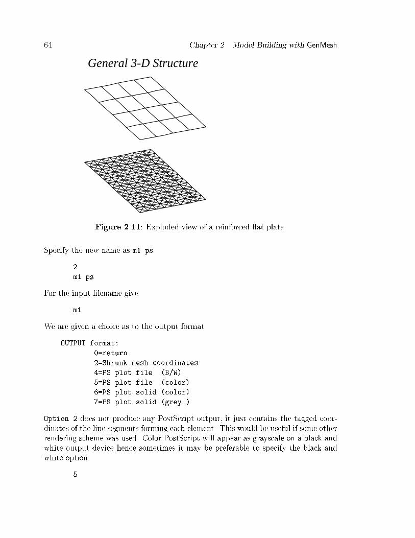
� Chapter �� Model Building with GenMesh
General 3-D Structure
Figure ��� Exploded view of a reinforced �at plate�
Specify the new name as m��ps
�
m��ps
For the input �lename give
m�
We are given a choice as to the output format
OUTPUT format�
�return
��Shrunk mesh coordinates
��PS plot file �B�W�
�PS plot file �color�
��PS plot solid �color�
��PS plot solid �grey �
Option � does not produce any PostScript output it just contains the tagged coor�dinates of the line segments forming each element� This would be useful if some otherrendering scheme was used� Color PostScript will appear as grayscale on a black andwhite output device hence sometimes it may be preferable to specify the black andwhite option�

���� Extruded Meshes ��
We can manipulate the image through the following menu
CHANGE default�
�Write PS file
��Position mesh
��Change orientation
��Move tagged surfaces
��Position or change title
�Change pen
For ��D meshes it is usually necessary to arrange the perspective so as to get a goodview� We will tilt the plate about the x and y axes
�
� � ��
The last item the shrinkage shrinks each element about its centroid� this is a wayof ensuring that there are no missing elements� An alternative way of viewing acomposite mesh is to move the tagged surfaces apart� This is very useful especiallyfor thinned�walled reinforced structures�
�
We will separate the plate elements �tagged �� from the remaining frame elements
INPUT� tag� � Xmove � Ymove � ends�
� � ���
Notice in this case we are dealing with page coordinates� This is a recurring menu somany of the surfaces can be moved� Finally the title �as read from the mesh headergroup� can be changed and repositioned�
�
Flat Plate
� �� ��
The PostScript �le can now be written and we can exit the program
The PostScript �le is named ��m��ps�� and this can be sent to a PostScript printeror displayed on a screen by use of an interpreter such as Ghostscript�In order to render the �gure it is necessary to also specify other information
such as the pen thickness� This information is kept in the ��genmesh�cfg�� �le� Itsformat is
� Version ����� January ����

�� Chapter �� Model Building with GenMesh
elem� max �
posn� X Y
pens� thickness
Rotn� X Y Z shrink
caps� X Y size
type� mesh type
Generally once these are set it should not be necessary to adjust them again�
II� Two Spar Wing
The second example is of a multi�spar wing� The cross�section control points areshown in Figure ����b��Run the program and choose the open�ended z�extrusion option�
C� genmesh
�
�
m�
�
The �rst series of information is to allow characterization of the cross�section in thex� y planes� There are six control points the input information is
�
� � � � � � � ��
� ��� �� � ��� �� � ��
� �� �� � �� �� � ��
� ��� �� � ��� �� � ��
� �� � � �� � ��
� ��� �� � ��� �� � ��
We could have used the second group of coordinates to give the wing a taper� howeverthis will be left to a separate tutorial that demonstrates how ��D meshes can beremapped� Typing lots of numbers like this can be very tedious and prone to error itis understood that all these numbers would be typed initially in a driver �response��le and GenMesh actually run in batch mode�In a complex structure with many control points there are a variety of points that
can be attached to each other� Each connection forms a segment� we now connectthese control points to form our wing cross�section�
SEGment styles� ��line �� ��bezier ��arc
TYPE� � of connected segments
We will make � segments� The information to be typed is

���� Extruded Meshes ��
TYPE� point�� � point�� � � divs � style � t�tag � l�tag � rate
TYPE� trans tag � length tag � length divs rate
� � � � �
� �� �
� � � � �
�� � �
� � � � �
�� � �
� � � �
�� �� �
� � � �
�� � �
� � � � �
�� �� �
� � � �
�� �� �
� � � � �
�� �� �
Note that the segments connecting points ���� form a Bezier curve�The �nal piece of information to be speci�ed deals with how the cross�section is
extruded in the z�direction
Z�EXTRUSION
TYPE� � z�modules � trans rate
We will make the mesh �� modules long and place the transverse sti�eners �ribs� atevery second module
�� �
Note that the rate number should divide evenly into the total number of modules�Quit the program
We will now show how a ��D mesh such as the wing can be further modi�ed byscaling� The physical dimensions have already been set where this option is useful isin tapering the extrusion�
C� genmesh
�
� Version ����� January ����

�� Chapter �� Model Building with GenMesh
Figure ��� Two�spar wing�
m�
m�
�
�
We will taper the wing in the x� z planform and the y � z depth�
�
A reminder of the format is given
SCALE wrt Z
�x
� x���������� x�
� �
x�����������x�����z
TYPE� x� � x� � x� � x� �� � �
The hint numbers will leave the mesh unchanged� We will give a slight taper as
� �� � ��
For the y � z plane we get

���� Extruded Meshes ��
SCALE wrt Z
�y
� y���������� y�
� �
y�����������y�����z
TYPE� y� � y� � y� � y� �� � �
Again we will give a slight taper
� �� � ��
Finally for the z � z plane
SCALE wrt Z
�z
z���������� z�
� �
z�����������z�����z
�
TYPE� z� � z� � z� � z� �� ��
Note the hint values in this case these are the ones we will use
�� � � ��
It is worth experimenting with these to see the various ways the extrusion can bemanipulated� For example by making the �rst line ��� �� � �� a swept�backwing can be generated� Quit the program
Now survey the mesh ��m��� using the utility PlotMesh� The exploded versionof the mesh should look like Figure �����
� Version ����� January ����

�� Chapter �� Model Building with GenMesh
�� Solid Meshes
The purpose of this tutorial is to show how GenMesh can be used to mesh solid regions�In particular we will run it to generate a �le containing the same information as inthe �le ��ex ep���� that will be used for the elastic�plastic tutorial�
Making the Mesh
Run the program and select the Solid Shapes
C� genmesh
��
�
m�
The program responds with the choice of shapes
MESH types�
� Return
� ��D Block shapes
��� Tet � elem block
��� Hex� � elem block
��� Hex�� � elem block
�
�� Tet � elem Cut�out
�� Hex� cylinder
�� Hex�� cylinder
� Hex�� cyl in rect
��� Hex�� notch
SELECT ���
Choose the Hex �� element block
��
We must now tell the program how many elements we want
TYPE� � of modules X�dir � Y�dir � Z�dir � tag �
Keep in mind that scaling the mesh is a di�erent operation than choosing the numberof modules� The tag � can be used to keep track of the sub�structures used informing a compound mesh it is also used to associate di�erent material propertieswith di�erent groups of elements� Respond
� � � �

��� Solid Meshes ��
You are now asked
TYPE� X�dim � Y�dim � Z�dim
This is the scaling on the mesh� Respond
� �� �
Back at the main menu choose to Quit with
Use PlotMesh to view the mesh�
Adding Properties
To make the generic mesh into a structure data�le we need to add properties� Thatis we need to state the type of material the boundary conditions and the loads� Wehave already done this in a previous tutorial hence the following will dwell only onthe signi�cantly di�erent parts�Initiate GenMesh and from the main menu select the Make Structure DataFile
option�
C� genmesh
�
m�
m�
You are now given a summary of the mesh as
� Matls
�� Nodes
BCs
Loads
matls
spcls
boundary groups
The series of questions to be answered are the same as the earlier tutorials so wewill just give the responses� We will specify the boundary conditions as �xed on oneend by isolating a thin disk of volume
�
�
��� ��
�
� Version ����� January ����
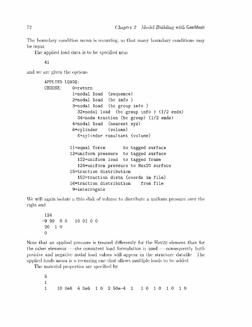
�� Chapter �� Model Building with GenMesh
The boundary condition menu is recurring so that many boundary conditions maybe input�The applied load data is to be speci�ed next
��
and we are given the options
APPLIED LOADS�
CHOOSE� �return
��nodal load �sequence�
��nodal load �bc info �
��nodal load �bc group info �
���nodal load �bc group info � ���� ends�
���node traction �bc group� ���� ends�
��nodal load �nearest xyz�
��cylinder �volume�
��cylinder resultant �volume�
���equal force to tagged surface
���uniform pressure to tagged surface
����uniform load to tagged frame
����uniform pressure to Hex� surface
� �traction distribution
� ��traction distn �coords in file�
���traction distribution from file
��interrogate
We will again isolate a thin disk of volume to distribute a uniform pressure over theright end�
���
����� ���
� ��
Note that an applied pressure is treated di�erently for the Hex�� element than forthe other elements � the consistent load formulation is used � consequently bothpositive and negative nodal load values will appear in the structure data�le� Theapplied loads menu is a recurring one that allows multiple loads to be added�The material properties are speci�ed by
�
� ��e� ��e� �� �� e�� � �� �� �� ��

��� Solid Meshes ��
The elastic�plastic material properties are speci�ed as part of the Specials group�Choose
�
to be given the recurring input
TYPE� Code � c� � c� � c� � to end�
We will also specify full integration on the element matrices� Thus respond
���� �e� � e�
��� � � �
Exit the properties section with
Back at the main menu we will choose to reduce the bandwidth with
�
�
m�
m�
�
�
��
�
Survey ��m��� and make sure the properties have been installed as expected� Thisshould be identical to the �le ��ex ep���� on the disk� Also use PlotMesh to viewthe mesh�
� Version ����� January ����

� Chapter �� Model Building with GenMesh
��� Some Hints
The following are some hints that may prove useful
� Once the procedures for the problem have been established convert them intoa driver �script� �le and use the program in batch mode�
� Whenever possible use the boundary nodal groups and element tags to realizethe structure data�le� This will make the driver �les independent of the meshdensity and therefore more versatile�
� When smoothing a mesh additional biasing can be achieved by moving indi�vidual nodes to a desired location and then specifying it as a boundary node�In this way the surrounding nodes will adjust appropriately�
� When making a compound mesh it is best to leave the property speci�cationuntil the second to last operation and the node re�numbering until the verylast operation�
� For very large and complex meshes make each sub�structure complete and self�contained including its absolute positioning� In this way the assembling is doneas the �nal stage�

Chapter �
Basic StaDyn Tutorials
This chapter is a collection of short tutorials for running StaDyn� It is advisable the�rst time through that all the tutorials be completed and that all the instructionsbe followed strictly� This is because some of the later tutorials make reference backto the earlier ones�The program StaDyn �STAtic and DYNamic analysis� is capable of doing the
static and dynamic analysis of ��D structures formed from a combination of framemembers and folded plates� Its main capabilities involve determining the memberdisplacements and loads and structural reactions for
� Static loading� Stability analysis� Vibration analysis� Forced frequency loading� Applied transient load history
The tutorials in this and the next chapter cover examples from each of these� Theprogram is menu driven in such a way that its functioning is apparent� This facilitatesearly understanding of it but can be somewhat intrusive after familiarity has beendeveloped� It will be shown however that it is possible to execute the programwithout these menus and thus speed all operations�As StaDyn proceeds it creates a number of �les among which are
stadyn�cfg stadyn�stf stadyn�dis
stadyn�log stadyn�mas stadyn�snp
stadyn�out stadyn�cms
stadyn�dyn stadyn�geo
stadyn�lod
The LOG �le echoes all the input responses as well as having some extra informationthat might prove useful during post analysis of the results� The OUT �le is the usual
��

�� Chapter �� Basic StaDyn Tutorials
location for StaDyn output� The second column of �les are associated with varioussystem matrices such as the sti�ness matrix and the mass matrix � these are left ondisk in case they may be of value for some other purpose� They are in binary form�The last column of �les are output �les� They too are in binary form for compactnessbut can be read for further post�processing�Regularly have a look in the StaDyn�LOG because there is much information to
be found there� Although this information is probably of no direct interest now it isgood planning to get used to interpreting this �le in anticipation of more complicatedproblems�

���� Static Example ��
��� Static Example
StaDyn is designed to run as a console �or command window� program under thevarious �avors of MS Windows� Note that all instructions are case insensitive� we willvary the case only to help make the instructions clearer� The class of static problemssolved by StaDyn is h
�KE� " ��KG�ifug ��fPg" ��fGg
where �i are various scale factors and fGg is the gravity load vector�
Getting Started
To run the program type �at the �C prompt��
C� stadyn
�note the name of the executable�� The opening menu is
MAIN menu�
� Quit
�� Read in structure DataFile
�� Form system matrices
�� Static loading
�� Forced frequency loading
� Transient loading
�� Eigen Analysis
�� PostScript plot files
� System services
���� Ikayex information
SELECT���
Quit by typing
There are two �les worth looking at� The �rst is the log �le StaDyn�LOG� use thelist utility to peruse it� It contains
�� StaDyn version ���� June ��
�� DATE� ������ TIME� �����
� Version ����� January ����

�� Chapter �� Basic StaDyn Tutorials
�� MAXimum storage � �
�� MAXimum elements �
�� MAXimum nodes �
�� MAXimum force incs� �
�� ITERmax � ��
�� rtol � ��E��
�� ALLOCATION succeeded
��MAIN
�� StaDyn OK� ended from MAIN
The second is StaDyn�CFG� This is the con�guration �le and has in it
� ��MaxStorage
��MaxNode
��MaxElem
� ��MaxForce
� ��ilump
�� ��itermax
��E�� ��rtol
�� DATE� ������ TIME� �����
This �le allows changing the run time settings of the dimensions of the arrays� If youget a memory allocation failure this is the place to make the adjustments�
A Static Analysis
Since we know the data in the �le EX PS�� to be correct we will use it to do a simplestatic analysis� Run StaDyn and read the structure DataFile
C� stadyn
�
ex�ps��
Before we can obtain the static solution we must �rst form the system matrices�Select
�
and you are given the choices
FORM System Matrices� sub�menu
��� �K�E� �static �
���
��� �K�G�
��� �K�E���K�G� �buckling�

���� Static Example ��
� � �M�
��� �K�E���M� �dynamic�
��� �K�E���K�G���M� �all�
Select
��
and make the choice
CHOOSE STIFFness storage�
�DEFault ��MEMory only��
��BINary �prof� ��StaDyn�STF ��
��ASCii �prof� ��StaDyn�OUT ��
��ASCii �NxB� ��StaDyn�OUT ��
��BINary �NxB� ��named ��
�DEFault � load ��StaDyn�OUT ��
���BINary �prof�locn� ��named ��
Since this is the �rst example echo the sti�ness matrix to StaDyn�OUT just to seewhat it looks like�
�
Since the loads were already read from EX PS�� we can now obtain a static solutionby typing
�
and there are two problem types
STATIC Problems� sub�menu
��� Distributed loadings
��� Pre�stress dP
��� Pre�stress P
��� All�node loadings
In the �rst the loads speci�ed in the structure data�le are the applied loads whilein the second those loads are interpreted as pre�loading on the structure� Choose
��
Each major capability of StaDyn is divided into two parts the analysis and thepost�processing� The �rst determines the nodal degrees of freedom in the global co�ordinates while the second allows post�processing of them to give strains or contoursand so on � basically member or local level information� Thus in response to
� Version ����� January ����

�� Chapter �� Basic StaDyn Tutorials
CHOOSE� �return ��analysis ��post�analysis
choose
�
since this is the �rst time through� Sometimes it is convenient to have unit loads inthe structure data�le and to use the analysis stage to scale the loads� In response to
INPUT scales� load � gravity
type
�� �
After echoing some information on the screen you are back to
CHOOSE� �return ��analysis ��post�analysis
Quit and get out of StaDyn by typing
That is all there is to it'The output can now be surveyed by viewing the ASCII �le StaDyn�OUT� This �le
is fairly well documented so there is little di#culty in interpreting it� The maximumdisplacement occurs at Node � with
� ��E�� � � � � �
Note that some of the nodes can have a rotation� this is a consequence of the type ofin�plane element implemented � it has three degrees of freedom at each node twodisplacements and one rotation� In the present case the rotations are zero indicatingthat the element arrangement satis�es the patch test�Also have a look in the StaDyn�LOG �le to see the type of information it contains�
Using Script Files
Actually the main reason for doing this simple example is to introduce a featureof StaDyn that underlies its design philosophy� One of the advantages of echoinginformation to the LOG �le is that it allows the creation of a driver or script �le� Ifyou are not familiar with this idea then perform the following little tutorial� Make acopy of the log �le by
C� copy stadyn�log instatic

���� Static Example ��
Now use an editor to edit instatic� The only editing you need do is remove blanklines and lines beginning with ��� What is left is the same collection of responses ason the previous page but now it is documented� After you exit your editor all youneed do to run the example of this section is
C� stadyn � instatic
Go ahead do it� The screen will scroll and everything is done automatically for you�After a while you will �nd yourself doing the same operations repeatedly� Then
you can make script �les for each of them� More important the script �le is a recordof how you processed the data� In a week a month or � months if you need toreconstruct what you did it is all there� The idea is that the script �le approachallows the user a greater variety of inputs and gives greater control of the program�quite complicated sequences of instructions can be pieced together to give very �necontrol over your data manipulations� It also allows the program to be used in batchmode and thereby blend in with your other programs more productively� This is thecommunication method used by QED�To further encourage use of script �les a small utility is provided on the disk for
stripping away the extra lines from the LOG �le� To run it simply type
C� strip � stadyn�log � instatic
� Version ����� January ����
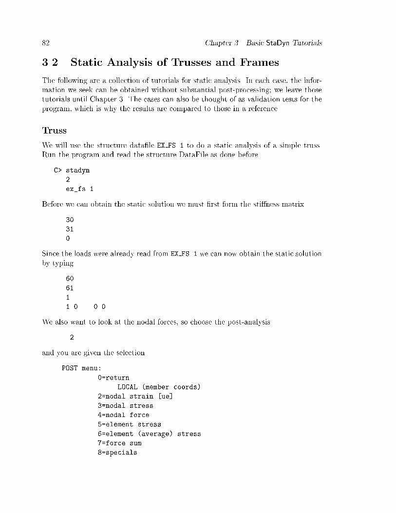
�� Chapter �� Basic StaDyn Tutorials
��� Static Analysis of Trusses and Frames
The following are a collection of tutorials for static analysis� In each case the infor�mation we seek can be obtained without substantial post�processing� we leave thosetutorials until Chapter �� The cases can also be thought of as validation tests for theprogram which is why the results are compared to those in a reference�
Truss
We will use the structure data�le EX FS�� to do a static analysis of a simple truss�Run the program and read the structure DataFile as done before
C� stadyn
�
ex�fs��
Before we can obtain the static solution we must �rst form the sti�ness matrix
�
��
Since the loads were already read from EX FS�� we can now obtain the static solutionby typing
�
��
�
�� �
We also want to look at the nodal forces so choose the post�analysis
�
and you are given the selection
POST menu�
�return
LOCAL �member coords�
��nodal strain �ue�
��nodal stress
��nodal force
�element stress
��element �average� stress
��force sum
�specials

���� Static Analysis of Trusses and Frames ��
GLOBAL
���Global displacement
���Global loads
���Global assembled DoF loads
� �Global assembled nodal loads
CONTOURs
���store displacement data
���store strain data
���store stress data
frames
���store displacement data
� �store strain data
���store stress data
�� �� select FRAMEs only ��
�� �� select PLATEs only ��
Select the Global loads and quit StaDyn by typing
��
The output can now be surveyed by viewing the ASCII �le StaDyn�OUT� This �leis fairly well documented so there is little di#culty in interpreting it� Reference ���gives for the displacement of Node �
Node �� u� �� �mm v� �����mm w� �mm
whereas the program gives
� �� ���E�� �������E�� � �������
These two sets agree� It is also worth noting that the nodal forces for Node � exactlyadd up to the applied forces
� � � � � � � �������
� � � � � � �������
sum �� �� � �������
Also have a look in the StaDyn�LOG to see the information it contains� It isgood planning to get used to interpreting this �le in anticipation of more complicatedproblems�
� Version ����� January ����

� Chapter �� Basic StaDyn Tutorials
Frame analysis
The following example is for a simple plane frame structure� It is speci�ed as planeby setting IGLOBAL��� and made of frame elements by letting TYPE���
ex�fs��� Balfour pp���� ��HEADER GROUP
��
� � � �
end
� ��ELEMENT GROUP
� � � � �
� � � � �
end
� ��material �s
� � �
end
� ��NODE GROUP
� � � �
� � �� �
� �� �� �
end
� ��boundary condns
� �
� �
end
� ��applied loads
� � � � � � ���e� �
� � �e� �� �e� � � � �e� �
end
� ��material props
� �e� �e� �e�� � � �� �� �� e��
end
��SPECIALs GROUP
end
A copy of this is on the disk as EX FS���
Run the program and read the structure data�le as before
C� stadyn
�
ex�fs��
Before we can obtain the static solution we must �rst form the system matrices

���� Static Analysis of Trusses and Frames ��
�
��
Since the loads were already read from EX FS�� we can now obtain the static solutionby typing
�
��
�
�� �
We also want to look at the nodal forces so choose the post�analysis and quit
�
��
The displacements and rotation at Node � as given by Reference ��� are
u� ����mm v� �����mm zrot� � ��e�� rad
while those from the program are
� �������E�� ������E�� ������� � �����E��
Both sets of numbers agree quite well� Here it is worth noting that the internal nodalmoments cancel to give a resultant of zero at Node ��Make a script �le for this problem by typing
C� strip � stadyn�log � instatic
We will use this for the following tutorials�
Grillage Analysis
The following example is for a simple grill structure and a copy of it is on the disk asEX FS���
ex�fs��� Balfour pp���� ��HEADER GROUP
��
� � � �
end
� ��ELEMENT GROUP
� � � � �
� Version ����� January ����

�� Chapter �� Basic StaDyn Tutorials
� � � � �
� � � � �
end
� ��material �s
� � �
end
� ��NODE GROUP
� �� ��� �
� �� � �
� � � �
� �� ��� �
end
� ��boundary condns
�
�
�
end
� ��applied loads
� � � ����e� � � ��e� � �
end
� ��material props
� � e� �e� �e�� � � �e�� e�� e��
end
��SPECIALs GROUP
end
Since this is a grill problem then IGLOBAL���� The other point of interest is that theload is distributed and this is converted into e�ective concentrated loads by
P� P� �
�qoL � T� �T� � �
��qoL
�
where qo is the uniformly distributed load on Member �� Note that since Node � is�xed there are no applied loads there�Once INSTATIC has been changed to re�ect the new input �lename the problem
can now be run simply by typing
C� stadyn � instatic
The displacement and rotations at Node � as given by Reference ��� are
z� ������mm xrot� ������e�� rad yrot� ����e�� rad
and those of the program
� � � �������E�� �������E�� � ����E�� ���
Note that internal nodal forces in the z�direction are generated�

���� Static Analysis of Trusses and Frames ��
��D Analysis
As another static example StaDyn is demonstrated on a three�dimensional problemspeci�ed by taking IGLOBAL���� All members are made of the same stock� A copy ofit is on the disk as EX FS���
ex�fs��� Balfour pp��� ��HEADER GROUP
��
� � � �
end
� ��ELEMENT GROUP
� � � � �
� � � � �
� � � � �
end
� ��material �s
� � �
� � �
end
� ��NODE GROUP
� � � �
� �� � �
� �� ��� �
� �� ��� ���
end
� ��boundary conditions
�
end
� ��applied loads
� ��e� � � � � � �
end
� ��material props
� ��e� e� �e�� � � ����e�� ����e�� ����e��
� ��e� e� �e�� � �� ����e�� ����e�� ����e��
end
��SPECIALs GROUP
end
Another point of interest is that the orientation of the last member is rotated ��o�Run the program as before preferably using the script �le� The displacements
and rotations at Node as given by Reference ��� are
u� ��� v� ���� w� ���� Rx� �� �e�� Ry� �� � Rz� ��
The values from the program are
� Version ����� January ����

�� Chapter �� Basic StaDyn Tutorials
� ������ �� ��� ����� � ������E�� � ���� �����
The digits are in close agreement but the orders of magnitude are o� for the rotations�This is due to the fact that the reference uses a combination of kN and mm for itsdimensions�
Gravity Loading
As a �nal static example StaDyn�s ability to compute gravity loading will be demon�strated� To make it more interesting we will seek to �nd the total mass of thestructure plus the location of the center of mass� For simplicity all members aremade of the same stock nominally of aluminum� A copy of the structure data�le ison the disk as EX FS� �
ex�fs� gravity ��HEADER GROUP
��
� � � �
end
� ��ELEMENT GROUP
� � � � �
� � � � �
� � � � �
� � � �
end
� ��material props
� � �
� � �
end
��NODE GROUP
� � � �
� � �� �
� �� �� �
� �� �� ��
� ��� �
end
� ��boundary conditions
end
� ��applied loads
� � � � � � � �
end
� ��material props
� �e� �e� �� �� e�� � �� �� ��

���� Static Analysis of Trusses and Frames ��
� �e� �e� �� �e�� � �� �� ��
end
� ��SPECIALs GROUP
��� � ��� �
end
The structure itself is comprised of members � to � Member is a massless rigidsupport that will act e�ectively as the weigh scale� Three components of gravity maybe speci�ed right now it is assumed to be acting in the vertical �y� direction� thisinformation is speci�ed in the SPECIALS category with a CODE����� Normally avalue such as ���in�s� would be speci�ed when interested in weight loading but nowwe want the mass so unity is used� Also note that there are no applied loads �otherthan gravity��Run the program and form the sti�ness matrix as usual
C� stadyn
�
ex�fs�
�
��
Gravity acts on the mass and forms a load vector with components at every translationdegree of freedom� That is it appears as a load vector similar to fPg� Now we arein a position to solve the static problem�
�
��
�
� ��
�
��
All the information we require can the obtained from the global information for theconnection between Member � and the structure at Node �� Hence quit by typing
For veri�cation purposes the displacements and rotations at Node � are given as
� ��� E�� ��� E�� ��� E� ��� E�� � ���� E��
The information we seek is given in the GLOBAL nodal forces row for Element at Node �� The force and moments at this point are
� Version ����� January ����

�� Chapter �� Basic StaDyn Tutorials
Fy � �� E�� Mx � ���� E�� Mz � ��� E��
The mass is given as
M W�g Fy�g ������� ����
The xc and zc centroids can be calculated as
xc Mz
Fy
����
���� �� � zc
�Mx
Fy
����
���� ���
Repeating the process but this time with the gravity vector in the x direction saywill allow the other coordinate of the centroid to be determined�This completes the static introduction� These examples were devised mainly to
give a simple means of accessing the way StaDyn does things� All the examples aresuch that you can verify them by hand or go to the source of the reference to getmore details� Redo these examples and try some of the other features not explicitlymentioned�

���� Static Analysis of Plates ��
��� Static Analysis of Plates
We will do two examples for the analysis of plates� The �rst is a static analysiswhere we look at the de�ections and moments in a plate in �exure� The second is anexample of a stress concentration in a bar with a hole�
Plate in Flexure
The �le EX PS�� describes a �at circular plate� The loading corresponds to a uniformpressure as computed in GenMesh� Thus the distributed load is implemented in itslumped form� Run StaDyn and read the data as before
C� stadyn
�
ex�ps��
You are informed that the size is ���� � ����� this is fairly large so we will do theminimum of echoing� Before we can obtain the static solution we must �rst form thesti�ness matrix� Select
�
��
The assembly stage for �exural and in�plane elements is signi�cantly more time con�suming than for the frame elements so ellipses are shown in order to give an idea ofhow much time it will take� Since the loads were already read from EX PS�� we cannow obtain a solution by typing
�
��
Each major capability is divided into two parts the analysis and the post�processing�The �rst determines the nodal degrees of freedom while the second allows post�processing of them to give strains or contours and so on� Thus in response to
CHOOSE� �return ��analysis ��post�analysis
choose
�
since this is the �rst time through� Although EX PS�� contains the loads sometimesit may be convenient to scale them� this is done next
INPUT scales� load � gravity
� Version ����� January ����

�� Chapter �� Basic StaDyn Tutorials
Input
�� �
and after echoing some information on the screen you are back to
CHOOSE� �return ��analysis ��post�analysis
Choose the post analysis
�
You are now asked to choose the form of nodal output
CHOOSE output�
POST menu�
�return
LOCAL �member coords�
��nodal strain �ue�
��nodal stress
��nodal force
�element stress
��element �average� stress
��force sum
�specials
GLOBAL
���Global displacement
���Global loads
� �Global assembled DoF loads
���Global assembled nodal loads
CONTOURs
���store displacement data
���store strain data
���store stress data
frames
���store displacement data
� �store strain data
���store stress data
�� �� select FRAMEs only ��
�� �� select PLATEs only ��
By default the displacements are stored as part of the analysis for the post analysiswe want the moments �or bending stress� so choose
�

���� Static Analysis of Plates ��
To quit type
The output can now be surveyed by viewing the ASCII �le StaDyn�OUT� This �leis fairly well documented so there is little di#culty in interpreting it� The maximumdisplacement occurs at Node �� and is
� � � ������� �����E� ����E�� �
Theory ��� � � gives that the maximum displacement at the center is
w�r� pa�
� D��� �r
a���� � D � Eh�
����� ���
For our parameters with � ��� and D ���� this becomes
w�r� ����� ��� �ra����
This gives a nice comparison a di�erence of little more than �%�
The computed �stress� moments at the center �Node ��� and at the edge �Node ���are given in the �le captioned as
NODAL STRESS averages�
Node� Sxx Syy Sxy Mxx Myy Mxy
� � � � ����� ����� ���� �E��
� � � � ������ ������ ������E��
The theoretical values �� ��� for the moments are
Mr�r� pa�
����� " ��� �r
a���� " ��� � Mt�r�
pa�
����� " ��� �r
a���� " ����
This gives at the center and at the boundary respectively
Mr Mt ����� � Mr ���� � Mt �����
Again we get a nice comparison especially at the center� We expect the values atthe boundary to be o� because we are replacing a circular boundary with a polygon�Improved results can be obtained by making a �ner mesh �����
� Version ����� January ����

� Chapter �� Basic StaDyn Tutorials
In�Plane Loading
The �le EX PS�� describes a bar with a hole in it� The full bar is modeled althoughbecause of symmetry it would be feasible to model only one�quarter of it� In thistutorial we will look at the e�ects of stress concentrations�Run StaDyn and read the data as before
C� stadyn
�
ex�ps��
You are informed that the size is ������ ����� this is fairly large which is typical ofproblems involving stress concentrations� Form the sti�ness matrix and do the staticanalysis
�
��
�
��
�
�� �
After echoing some information on the screen you are back to
CHOOSE� �return ��analysis ��post�analysis
Now choose the post analysis
�
You are now asked to choose the form of nodal output
POST menu�
�return
LOCAL �member coords�
��nodal strain �ue�
��nodal stress
��nodal force
��element stress
��force sum
GLOBAL
���Global displacement
���Global loads
CONTOURs
���store displacement data
���store strain data
���store stress data

���� Static Analysis of Plates ��
We want the stresses so choose
�
To quit type
The output can now be surveyed by viewing the ASCII �le StaDyn�OUT� This �leis fairly well documented so there is little di#culty in interpreting it� The maximumstress occurs at Node ��� and the corresponding line is
NODAL STRESS averages�
Node� Sxx Syy Sxy Mxx Myy Mxy
� � � �� ������ � ��� � � �
From a handbook on stress concentration factors �� � we get that the SCF should be
SCF ��
This compares with the above value of
SCF �����
������ ��
This type of di�erence is typical�
� Version ����� January ����

�� Chapter �� Basic StaDyn Tutorials
��� Complex Structure
We end these introductory tutorials with an example of a complex structure� thatis a structure which contains both frame and plate elements� The structure itself issimple being just a cantilevered shear beam lying in the x � y plane with a singlevertical applied load�The mesh is given in EX CS�� and was created as one of the tutorials in the
previous chapter� Notice that we specify the global type as being IGLOBAL��� thatis the shear beam will behave essentially as a plane frame� Remember however thatif in doubt about the global type then just specify it as its most general form thatis as IGLOBAL����
Analysis
Run StaDyn read the structure data�le form the sti�ness matrix and do the analysis
C� stadyn
�
ex�cs��
�
��
�
��
�
�� �
After echoing some information on the screen you are back to
CHOOSE� �return ��analysis ��post�analysis
Quit the program
The output can now be surveyed by viewing the ASCII �le StaDyn�OUT� This �leis fairly well documented so there is little di#culty in interpreting it� The maximumdisplacement occurs at Node � and is
�� ���E�� ����� �E�� � � � �������E��
An energy approach to this problem where the center panel is treated as having aconstant shear �ow ���� gives the maximum displacement at the load point as
v Pc
�EA"
PL�
�EAc�"
PL
Gtc ���� " ��� " ����� ���� �����

���� Complex Structure ��
There is a di�erence indicating that the actual structure is sti�er than that assumedin the simple theory� If on the other hand we instead treat the structure as a beamin bending then the tip de�ection is given by
v PL�
�EI
����� ��� ��� � �� ������ ��� ��
��
This relatively small value indicates that the shear deformation is a signi�cant portionof the total deformation�
We will look at the stresses to see if that clari�es the assumptions� Run StaDynand read the data as before
C� stadyn
�
ex�cs��
Choose the post analysis and look at the element stresses
�
��
�
�
���
To quit type
Look at the output in StaDyn�OUT it is clear that the shear stress is the dominantstress giving for example in Element ��
�� ����� �� ��� �� �
The shear stress in the elementary theory is given as
� P
ct
����
� �� ����
From this it is clear that the stringers are supporting a signi�cant part of the load�
� Version ����� January ����

�� Chapter �� Basic StaDyn Tutorials
PostScript Contours
Sometimes the full behavior of a structure is not apparent by looking at individualnumbers at individual nodes� Plotting the data as a contour plot can often help andthis tutorial shows the type of support given by StaDyn for accomplishing this�We will assume that this is the �rst time through the analysis� run StaDyn read
the structure data�le form the sti�ness matrix and do the analysis�
C� stadyn
�
ex�cs��
�
��
�
��
�
�� �
After echoing some information on the screen you are back to
CHOOSE� �return ��analysis ��post�analysis
Choose the post analysis
�
You are now asked to choose the form of nodal output we want to look at the contoursof displacement so choose
��
This stores the response data in the �le StaDyn�OUT� however it is the contour modulethat will now post�process it� We get to that menu o� the main menu by
�
�
p��ps
where we elected to name the �le� The contour menu is
CONTOURs�
� Quit
��RENDER PS file��
�� Deformed shape
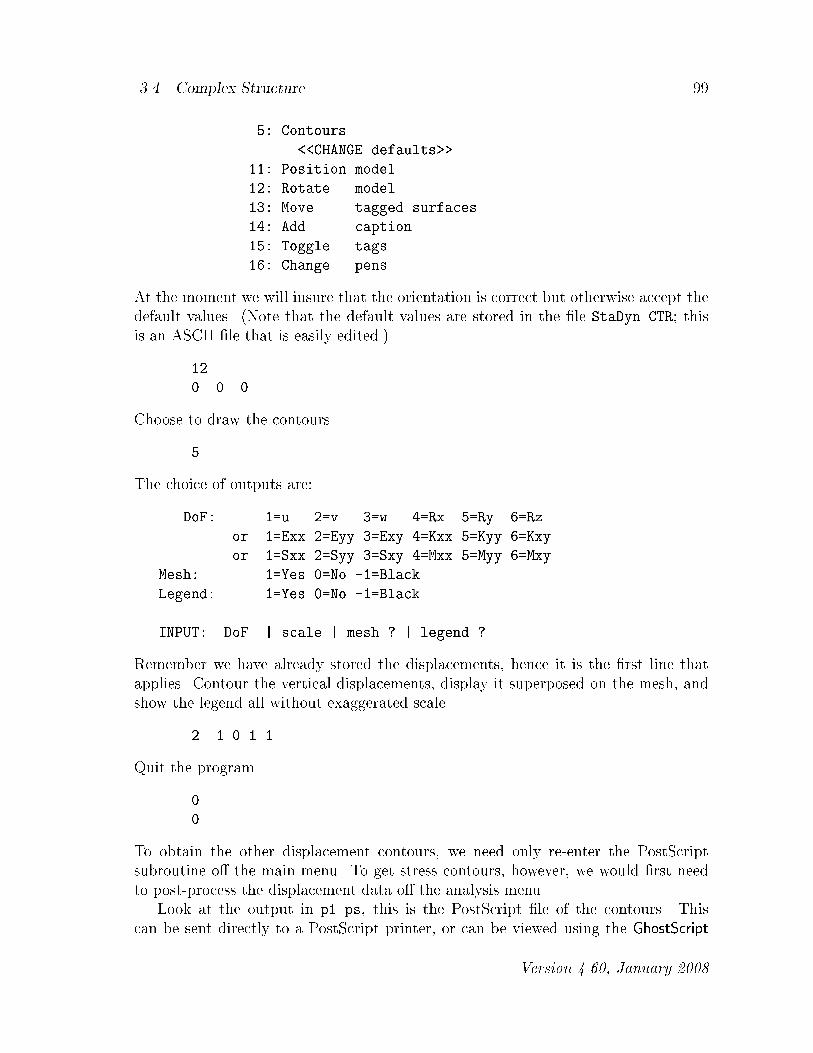
���� Complex Structure ��
� Contours
��CHANGE defaults��
��� Position model
��� Rotate model
��� Move tagged surfaces
��� Add caption
� � Toggle tags
��� Change pens
At the moment we will insure that the orientation is correct but otherwise accept thedefault values� �Note that the default values are stored in the �le StaDyn�CTR� thisis an ASCII �le that is easily edited��
��
Choose to draw the contours�
The choice of outputs are
DoF� ��u ��v ��w ��Rx �Ry ��Rz
or ��Exx ��Eyy ��Exy ��Kxx �Kyy ��Kxy
or ��Sxx ��Syy ��Sxy ��Mxx �Myy ��Mxy
Mesh� ��Yes �No ���Black
Legend� ��Yes �No ���Black
INPUT� DoF � scale � mesh � � legend �
Remember we have already stored the displacements hence it is the �rst line thatapplies� Contour the vertical displacements display it superposed on the mesh andshow the legend all without exaggerated scale
� �� � �
Quit the program
To obtain the other displacement contours we need only re�enter the PostScriptsubroutine o� the main menu� To get stress contours however we would �rst needto post�process the displacement data o� the analysis menu�Look at the output in p��ps this is the PostScript �le of the contours� This
can be sent directly to a PostScript printer or can be viewed using the GhostScript
� Version ����� January ����

��� Chapter �� Basic StaDyn Tutorials
.882E-04
.265E-03
.441E-03
.617E-03
.794E-03
.970E-03
.115E-02
.132E-02
.150E-02
.168E-02 StaDyn
.207E+03
.396E+03
.584E+03
.773E+03
.962E+03
.115E+04
.134E+04
.153E+04
.172E+04
.190E+04 StaDyn
Figure �� Contours of vertical de�ection and shear stress�
program� The �le will produce color contours as shown in Figure ���� It is clear thatslightly more deformation occurs at the lower right edge where the load is applied�Make a script �le for the postprocessing and look at the stresses� As shown in
Figure ����b� the shear stress distribution is highly non�uniform� Also look at thebending stress �xx�The con�guration for the contour plots is stored in the �le StaDyn�CTR� This has
the organization
��geometry
��position X Y
��pen thickness mesh� contour
��rotations X Y Z
��caption positions X Y and size
��modes mass
��sub�structure flags
Sometimes it may be more convenient to make the adjustment through this �le ratherthan through the program�

���� Some Hints ���
��� Some Hints
StaDyn is a complex program so it is di#cult to give tutorials that cover all of itsfeatures� Additional advanced tutorials are given in the next chapter but the bestapproach to using it usefully is to start with the examples given modify them �slightlyat �rst� until you are studying the problems of interest to you� Experiment'The following are some hints that may prove useful
� Once the procedures for the problem have been established convert them intoa script �les and use it in batch mode�
� Whenever possible use the boundary condition lines and the global�type vari�able to remove unnecessary degrees of freedom� This will reduce the size of thesystem of equations to be solved and improve performance�
� The input structure �le is the source of all that StaDyn can do so generally itis required that this �le be read in before any of the processing functions canbe used�
One feature of StaDyn of note is that it is fairly open meaning that you can accessmany of the system matrices� When there is a problem you may consider looking atthe system matrices directly�
� Version ����� January ����

��� Chapter �� Basic StaDyn Tutorials

Chapter �
Advanced StaDyn Analyses
In addition to static analyses StaDyn is designed to perform dynamic �transientvibration forced frequency� and stability �buckling� analyses� This chapter presentsa few tutorials that cover the basics of these analyses�Obtaining the buckling loads and buckled mode shapes for a ��D structure is
an eigenvalue problem similar to �nding the vibration natural frequencies and modeshapes� In fact once the appropriate matrices are established StaDyn treats the twoproblems almost identically� The number of modes possible is equal to the numberof free degrees of freedom in the system� But usually it is the lower loads andfrequencies of most interest therefore it is prudent to keep the system size small�However to get accurate lower loads �or frequencies� it is necessary to introducemore degrees of freedom �and thus be required to evaluate the higher loads also��As an approximate rule of thumb a system size N gives about N�� good values ofbuckling load� This must be treated with caution since it depends on the locationof the nodes and also if the mode shapes themselves are of interest� StaDyn givesa choice of using the Jacob rotations or the sub�space iteration schemes to solve theeigenvalue problem� the latter is the appropriate one for large systems�A di�erent set of issues arise when the applied loading is transient� here the equa�
tions of motion must be integrated step by step� StaDyn uses the implicit Newmarkintegration scheme for this because it is an unconditionally stable algorithm�
���
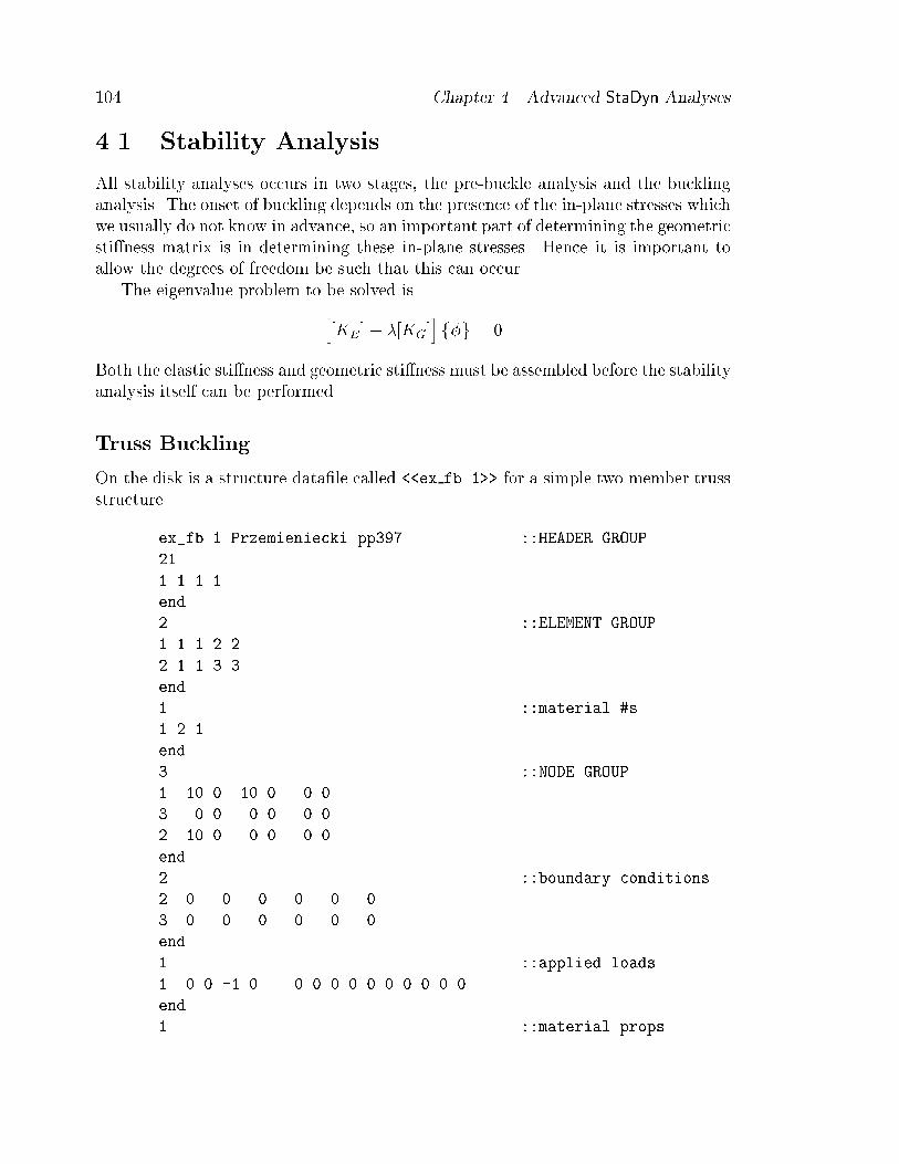
�� Chapter �� Advanced StaDyn Analyses
��� Stability Analysis
All stability analyses occurs in two stages the pre�buckle analysis and the bucklinganalysis� The onset of buckling depends on the presence of the in�plane stresses whichwe usually do not know in advance so an important part of determining the geometricsti�ness matrix is in determining these in�plane stresses� Hence it is important toallow the degrees of freedom be such that this can occur�The eigenvalue problem to be solved is
h�KE�� ��KG�
if�g �
Both the elastic sti�ness and geometric sti�ness must be assembled before the stabilityanalysis itself can be performed�
Truss Buckling
On the disk is a structure data�le called ��ex fb���� for a simple two member trussstructure�
ex�fb�� Przemieniecki pp��� ��HEADER GROUP
��
� � � �
end
� ��ELEMENT GROUP
� � � � �
� � � � �
end
� ��material �s
� � �
end
� ��NODE GROUP
� �� �� �
� � � �
� �� � �
end
� ��boundary conditions
�
�
end
� ��applied loads
� � ��� � � � � �
end
� ��material props

���� Stability Analysis ���
� �e� �e� �� �e�� � �� �� ��
end
��SPECIALs GROUP
end
The material is nominally aluminum and its properties are given in customary units�Both the sti�ness and geometric matrices must be assembled before the stability
analysis itself can be performed� Do this by typing
C� stadyn
�
ex�fb��
�
to be presented with the system matrices choices
FORM System Matrices� sub�menu
��� �K�E� �static�
���
��� �K�G�
��� �K�E���K�G� �buckling�
� � �M �
��� �K�E���M � �dynamic�
��� �K�E���K�G���M� �all�
Choose
��
In response to the storage options
CHOOSE storage�
�DEFault BINary �prof� ��StaDyn�GEO��
��ASCii �prof� ��StaDyn�OUT��
��ASCii �NxB� ��StaDyn�OUT��
��BINary �NxB� ��named ��
�DEFault � load ��StaDyn�OUT��
���BINary �prof�locn� ��named ��
choose
Note that in order to establish the geometric matrix it is �rst necessary for StaDynto solve the corresponding static problem for the press loads� There are two mainsources of pre�stress that from fPg speci�ed in the SDF and that from gravity�Both of these can be scaled separately thus the required input
� Version ����� January ����

��� Chapter �� Advanced StaDyn Analyses
�� �K�G� � s�� �K�G�P�� � s�� �K�G�G��
INPUT scales� load � gravity
Choose
�� �
Solving the statics problems is accomplished automatically and the material that isechoed to the screen is consistent with this� The required information for determiningthe stresses for use in the stability analysis is stored in the �le ��stadyn�dis���Back at the main menu select the eigenanalysis
�
StaDyn does two types of eigenvalue problems� vibration and stability and has imple�mented two eigensolvers� Jacobi rotations and Sub�space iterations� The sub�menuchoices are
EIGENvalue Problems� sub�menu
��� Vibration w� Jacobi
��� Vibration w� Sub�space
��� Buckling w� Jacobi
��� Buckling w� Sub�space
Jacobi rotations are very robust and give all the eigenvalues� Unfortunately it is alsocomputationally very expensive and generally should not be used for systems largerthan ���� Sub�space iteration is appropriate for large problems but has di#cultieswith very small problems� The present problem is only of size �� � �� so Jacobirotations is a good choice� Choose
��
Each major capability of StaDyn is divided into two parts the analysis and thepost�processing� The �rst determines the nodal degrees of freedom while the secondallows post�processing of them to give strains or contours and so on� Thus in responseto
CHOOSE� �return ��analysis ��post�analysis
choose
�
since this is the �rst time through� For large problems a good deal of informationwould now be echoed to the screen� lines to watch are

���� Stability Analysis ���
D�NORM� � Rotns � �
� of sweeps �
Finding eigenvalues is an iterative process and these can be used to monitor the rateof convergence� Note that StaDyn will automatically quit after �� sweeps� For thisproblem we get normal convergence after only � sweep� about � sweeps is typical forlarger problems� It should be realized that even if convergence has not occurred theeigenvalues and eigenvectors may be of acceptable quality�Finally we are asked again
CHOOSE� �return ��analysis ��post�analysis
For this exercise we are only interested in the �rst two buckling loads and thisinformation is automatically stored in ��stadyn�out�� as part of the analysis sowe could opt to quit the program now� However we will proceed to obtain theeigenvectors also� Choose
�
This can also be re�entered starting from the beginning as long as the �le ��stadyn�snp��has not been altered� This would be used if the various mode shapes for exampleare to be accessed� The post�processing menu is
MODAL storage�
�return � � to end�
� of modes � ��modal values
� � ��mode shapes
� � ��modal vectors
�
mode � � ���store contour data
The di�erence between mode shape and modal vector is that the former already hasthe boundary conditions factored in� This is a recurring prompt so if desired allthe information can be stored� The last option would be used if the results are tobe piped into a modal analysis post�processor� This option also wants the number ofmodes to be reported� It can be from one to the system size� If a number outsidethis range is given then the program takes the appropriate allowable limit� For thisexercise we are only interested in the �rst two buckling loads so select the �rst twomodal values
� �
and we are again given the output menu� Choose
� Version ����� January ����

��� Chapter �� Advanced StaDyn Analyses
and to quit the program type
The output can now be surveyed by viewing the ASCII text �le ��stadyn�out���The modal results are formatted similarly to a static analysis� Reference ���� showsthat the �rst buckling load should be
Pcrit �p�� ��
EA �����EA
The output from StaDyn gives the critical loads as
������E�� ��������E��
which is very close to the theory� The very high second value indicates that there isno second buckling mode� It must be realized that this truss buckling is not the sameas would occur if a frame member has pinned joints� this latter occurrence requiresa bending action� It can be said however that for a given geometry the column orframe buckling is more likely to occur �rst�
Frame Buckling
As a second example consider the simple frame described in the structure �le ��ex fb�����this corresponds to an inverted L�frame �xed at its two ends�
ex�fb�� Eisley pp��� ��HEADER GROUP
��
� � � �
end
� ��ELEMENT GROUP
� � � � �
� � � � �
� � � � �
� � �
� � �
� � � � �
end
� ��material �s
� � �
end
� ��NODE GROUP
� � � �
� � � �

���� Stability Analysis ���
� � �� �
� � �� �
� �� �
� � �� �
� �� �� �
end
� ��boundary condns
�
�
end
� ��applied loads
� �� � � � � � �
� ��� � � � � �
end
� ��material props
� ��� e� ��� �e� ��e�� �e�� �� e�� �����e�� �����e��
end
��SPECIALs GROUP
end
This problem is stated in metric �SI� units with the material being aluminum� Thisis used as an example problem in Reference ���� but beware that the material wasinadvertently stated as being steel�Run the program as before with no echoing
C� stadyn
�
ex�fb��
�
��
�
�
��
�
Since the system size is larger ���� than the last example more Jacobi iterations arerequired� Store only the �rst three mode shapes
�
� �
Now exit the program by typing
� Version ����� January ����

��� Chapter �� Advanced StaDyn Analyses
Scan through the output �le ��stadyn�out�� to see the results� Reference ����shows that the �rst eigenvalue and corresponding x displacements are
Pcrit �����
� ��
� � ��
� ��
������
� �������� �������� ��
The buckling loads �eigenvalues� from the program are
��� � ��� ��� ���
Again the complete physical interpretation of the modal vectors is given in a formatidentical to that of the static output� Picking o� the values corresponding to theabove gives
node u v rotz
�� � � �
�� ���� ��� E�� ���
�� � � �����E�� �����
�� ���� �����E�� ���
� ������E� ��� E�� � ��
�� � ����E�� ���E�� ����
�� � � �
If these values are normalized with respect to the displacement at Node � then it isseen that they correspond with the above�Experiment with reversing the sign of the loads and note that StaDyn still obtains
the correct buckling load� This is important in complex structures where it is notobvious �from a cursory glance� which members are in compression�
Stability of Plates
We will �nish the stability tutorials with an example of determining the stability ofplates� The �le ��ex pb�x��� models a rectangular plate �aspect ratio ��� withclamped edges but free to expand laterally�

���� Stability Analysis ���
All stability analysis occurs in two stages the pre�buckle analysis and the bucklinganalysis� The onset of buckling depends on the presence of the in�plane �membrane�stresses which we usually do not know in advance so an important part of determiningthe geometric sti�ness matrix is in determining these in�plane stresses� Hence it isimportant to allow the degrees of freedom be such that this can occur� Consequentlyalthough the boundary conditions are referred to as being �clamped� note that infact they are allowed to move in the in�plane direction in such a way that only a �xxstress is generated� Note also that we set IGLOBAL����Run StaDyn read in the structure data�le and form the sti�ness matrices
C� stadyn
�
ex�pb�x�
�
��
�
Back at the main menu select the eigenanalysis
�
StaDyn does two types of eigenvalue problems� vibration and stability and has imple�mented two eigensolvers� Jacobi rotations and Sub�space iterations� The sub�menuchoices are
EIGENvalue Problems� sub�menu
��� Vibration w� Jacobi
��� Vibration w� Sub�space
��� Buckling w� Jacobi
��� Buckling w� Sub�space
Jacobi rotations are very robust and give all the eigenvalues� Unfortunately it is alsocomputationally very expensive and generally should not be used for systems largerthan ���� Sub�space iteration is appropriate for large problems but has di#cultieswith very small problems� Plate problems are large �especially when a convergencestudy must be done� so sub�space iterations is the appropriate choice� Choose
��
Each major capability is divided into two parts the analysis and the post�processing� The �rst determines the nodal degrees of freedom while the second allowspost�processing of them to give strains or contours and so on� Thus in response to
CHOOSE� �return ��analysis ��post�analysis
� Version ����� January ����

��� Chapter �� Advanced StaDyn Analyses
choose
�
since this is the �rst time through� Unlike the Jacobi rotation solver subspace itera�tion scheme need not solve for all the eigenvalues� Thus in response to
INPUT� � of modes of interest
���
choose
�
This will compute the �rst �lowest� ten eigenvalues� Note that internally StaDynactually solves for about twice that number so as to ensure that the vector space isappropriately covered�A good deal of information is now echoed to the screen some of which may be
recognized as coming from the Jacobi rotations� Note that StaDyn will automaticallyquit after �� iterations �a number that can be changed in the StaDyn�CFG �le�� Itshould be realized that even if full convergence has not occurred the eigenvalues andeigenvectors may be of acceptable quality this can be judged by looking at the qualitynumber�Quit the program by typing
The buckling loads are stored in StaDyn�OUT as part of the analysis�The output can now be surveyed by viewing the ASCII �le ��stadyn�out��� It
contains
EIGENvalues�
N lambda �load�
� ��� �
� �� ���
� ������
� �
Theory ���� gives the lowest buckling load for a rectangular plate with aspect ratioa�b � as
�crh �����D
a� �� ��
The di�erence in the factor of ���� is due to the fact that ���� psi was the appliedin�plane load� The comparison is reasonable considering the number of elements used�
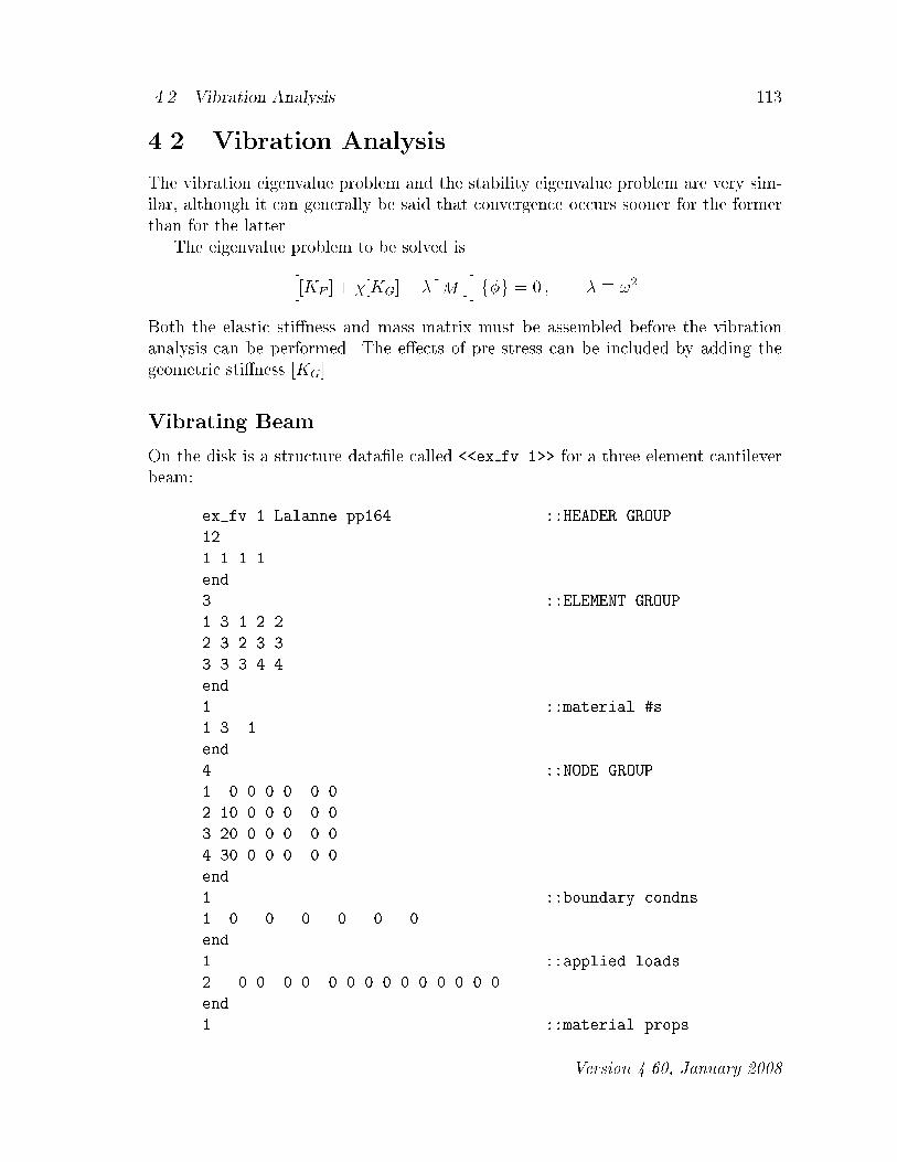
���� Vibration Analysis ���
��� Vibration Analysis
The vibration eigenvalue problem and the stability eigenvalue problem are very sim�ilar although it can generally be said that convergence occurs sooner for the formerthan for the latter�The eigenvalue problem to be solved is
h�KE� " ��KG�� �dM c
if�g � � � � ��
Both the elastic sti�ness and mass matrix must be assembled before the vibrationanalysis can be performed� The e�ects of pre�stress can be included by adding thegeometric sti�ness �KG��
Vibrating Beam
On the disk is a structure data�le called ��ex fv���� for a three element cantileverbeam
ex�fv�� Lalanne pp���� ��HEADER GROUP
��
� � � �
end
� ��ELEMENT GROUP
� � � � �
� � � � �
� � � � �
end
� ��material �s
� � �
end
� ��NODE GROUP
� � � �
� �� � �
� �� � �
� �� � �
end
� ��boundary condns
�
end
� ��applied loads
� � � � � � � �
end
� ��material props
� Version ����� January ����

�� Chapter �� Advanced StaDyn Analyses
� ��e� ��e� ��� �� e�� � � � ��
end
��SPECIALs GROUP
end
There is nothing special to note about this �le except perhaps that while it is notnecessary to have any applied loads in vibration analyses it is nonetheless necessaryto have some corresponding entries in the input data �le� The material is nominallyaluminum and its properties are given in customary units� The units for the densityare
� ���� ���� lb � s�in�This is di�erent from the weight per unit volume by the gravitational constant� Thatis � W ��g where W � is the weight per unit volume�Both the sti�ness and mass matrices must be assembled before the analysis itself
can be performed� Do this by typing
C� stadyn
�
ex�fv��
�
to be presented with the system matrices choices
FORM System Matrices� sub�menu
��� �K�E� �static�
���
��� �K�G�
��� �K�E���K�G� �buckling�
� � �M �
��� �K�E���M � �dynamic�
��� �K�E���K�G���M� �all�
To do a dynamic analysis we also need the mass matrix� Choose
��
�
�
This will echo the sti�ness and mass matrices into the ��stadyn�out�� �le�Vibration problems are eigenvalue problems so choose
�
StaDyn does two types of eigenvalue problems� vibration and stability and has imple�mented two eigensolvers� Jacobi rotations and Sub�space iterations� The sub�menuchoices are

���� Vibration Analysis ���
EIGENvalue Problems� sub�menu
��� Vibration w� Jacobi
��� Vibration w� Sub�space
��� Buckling w� Jacobi
��� Buckling w� Sub�space
Jacobi rotations are very robust and give all the eigenvalues� Unfortunately it is alsocomputationally very expensive and generally should not be used for systems largerthan ���� Sub�space iterations on the other hand can solve the partial eigenvalueproblem� that is it can solve for the lowest m eigenvalues where m� N � Since theseare the ones of most interest in structural analysis it makes sub�space very attractive�It is the one that we will choose later for the plate problems for now choose
��
Again each major capability is divided into two parts the analysis and the post�processing� The �rst determines the eigenvalues and nodal degrees of freedom whilethe second allows post�processing of them to give contours and so on� Thus inresponse to
CHOOSE� �return ��analysis ��post�analysis
choose
�
since this is the �rst time through� All vibration analyses can include the e�ects ofpre�stress as a scaling on the geometric sti�ness matrix� We will ignore these hencein response to
INPUT pre�stress scale� scale X �K�G!
type
�
The program now performs the complete analysis� A good deal of information isnow echoed to the screen� an interesting quantity to keep your eye on is the DIFF
NORM �nding eigenvalues is an iterative process and this quantity conveys an ideaof the rate of convergence� It should be realized that even if convergence has notoccurred the eigenvalues and eigenvectors may be of acceptable quality� Thus the�nal echoing of information is an assessment of the quality of the eigenvectors�Finally we are asked
CHOOSE� �return ��analysis ��post�analysis
To access the eigenvector results we must post process the binary �les� Choose
� Version ����� January ����

��� Chapter �� Advanced StaDyn Analyses
�
and you are given the storage menu
MODAL storage�
�return � � to end�
� of modes � ��modal values
� � ��mode shapes
� � ��modal vectors
�
mode � � ���store contour data
The di�erence between the mode shapes and the modal vectors is that the former hasthe boundary conditions already factored in� This is a recurring prompt so if desiredall the information can be stored� The last option would be used if the results areto be piped into a plotting analysis post�processor� This option also wants the modenumber to be reported� It can be from one to the system size� For this exercise weare interested in all the eigenvalues and eigenvectors so choose
� �
The information is now stored in ��stadyn�out�� and we are given again the outputmenu� We could re�enter the post analysis either now �or re�enter later� because thecomplete information is also stored in binary form in the �le ��stadyn�snp��� Thiswould be used if the various mode shapes for example are to be accessed� We willjust quit
Scan through the �le ��stadyn�out�� to see the results� The �rst portion of itcontains the sti�ness matrix written in band storage form and the mass matrix writtenin diagonal �lumped� form� The resonant frequencies according to Reference ���� are
�� ����
L�
sEI
�A ���� r�s � ��
����
L�
sEI
�A ����� r�s
and these compare to the program values of
EIGENvalues�
N omega �r�s� freq �Hz�
� ��� ����� real
� �� ��� ����� real
� ���� �� �� � real
� ����� ������ real
������ ������� real
� ������ ���� real

���� Vibration Analysis ���
Clearly the results are not fully converged� The complete physical interpretation ofthe modal vectors is given in the �le in a format identical to that of the static output�The reference also gives the modal vectors �in the format fv� �� g� as
�� f� � ������ � ��� � � ����� � �� � � �����g�� f� � ������ � ����� � ������ � ����� � ����� g
On the face of it these do not compare with the results from StaDyn� Howeverif these results are normalized with respect to the �rst entry then both sets agreeremarkably well� The di�erence lies in how the results are normalized the one chosenin the program is based on the mass matrix�A point worth mentioning in regards to dynamic problems is that after a structure
input data�le has been created it can be cumbersome to modify it to increase thenumber of elements �this would be required in order to improve the quality of theresults�� This is such a recurring need that the program GenMesh has a remeshingfeature built in� The tutorial on transient responses demonstrates how this is used�
Frame Vibration
As a second example consider the simple frame described in the structure �le ��ex fv����
ex�fv�� Lalanne pp���� ��HEADER GROUP
��
� � � �
end
� ��ELEMENT GROUP
� � � � �
� � � � �
end
� ��material �s
� � �
� � �
end
� ��NODE GROUP
� � � �
� �� � �
� ���� ���� �
end
� ��boundary conditions
�
�
end
� ��applied loads
� Version ����� January ����

��� Chapter �� Advanced StaDyn Analyses
� �� � � � � � �
end
� ��material props
� ��e� e� ��e�� � � �� �� ��e��
� ��e� � e� ��e�� �� � �� �� ��e��
end
��SPECIALs GROUP
end
This problem is stated in metric �MKS� units and corresponds to an aluminum beamconnected to a steel beam at a �o angle�
Make a driver �script� �le using the STRIP utility on the LOG �le of the previ�ous tutorial and call it ��invibn�� say� Now change the name of the input �le to��ex fv���� and run the problem as
C� stadyn � invibn
Scan through the output �le ��stadyn�out�� to see the results� The sti�nessmatrix written in band storage form is the same as given in Reference ���� but themass matrix written is di�erent� the reason is that the reference uses the consistentmass matrix�
The reference also shows that the three eigenvalues and eigenvectors are
�� ���� �� f������ � ������ � �g�� ���� �� f����� � ����� � �g�� ���� �� f�� �� � ����� � �g
The eigenvalues from the program are
�� ������
�� �����
�� ��� ��
Again the complete physical interpretation of the modal vectors is given further onin the �le in a format identical to that of the static output�
Spring Mass System
As a �nal example we depart a little from the continuous systems considered aboveand look at a discrete spring�mass system� This is only to demonstrate that StaDyncan handle concentrated inertias� The structure data �le is ��ex fv���� and consistsof three masses and three springs in a collinear arrangement�

���� Vibration Analysis ���
ex�fv�� Meirovitz pp�� � ��HEADER GROUP
��
� � � �
end
� ��ELEMENT GROUP
� � � � �
� � � � �
� � � � �
end
� ��material �s
� � �
� � �
end
� ��NODE GROUP
� � � �
� �� � �
� �� � �
� �� � �
end
� ��boundary conds
�
end
� ��applied loads
� � � � � � � ��
� � � � � � � ��
� � � � � � � ��
end
� ��material props
� ��e� �e� �� � � � � �
� ��e� �e� �� � � � � �
end
��SPECIALs GROUP
end
Note that the density is given as zero but concentrated masses are stated as the lastentries on the applied loads line� The units are mass units that is weight�gravity�Further since there are only axial degrees of freedom then IGLOBAL����Run this as above using the script �le and compare the results as given in Refer�
ence ����
�� ��� � �� f����� � ����� � �����g�� ���� � �� f����� � ��� � � ��� ��g�� ���� � �� f����� � ������ � ����g
� Version ����� January ����

��� Chapter �� Advanced StaDyn Analyses
The eigenvalues from the program are
�� �����
�� ������
�� ���
This reference further shows that the eigenvectors when normalized according to thescheme of StaDyn are
�� f����� � ����� � �����g�� f����� � ����� � ������g�� f���� � ������ � �����g
These are the same as reported by StaDyn�
Flexural Vibrations of Plates
In this tutorial we show the use of sub�space iteration as the means for solving theeigenvalue problem� This is the generally preferred scheme for large problems�We will look at the vibrations of a circular plate as described in the data�le
��ex ps����� Run StaDyn read the structure data�le and form the sti�ness andmass matrices as before
C� stadyn
�
ex�ps��
�
��
Vibration problems are eigenvalue problems so choose
�
and o� the sub�menu choices
EIGENvalue Problems� sub�menu
��� Vibration w� Jacobi
��� Vibration w� Sub�space
��� Buckling w� Jacobi
��� Buckling w� Sub�space
choose
��

���� Vibration Analysis ���
Jacobi rotations are very robust and give all the eigenvalues� Unfortunately it is alsocomputationally very expensive and generally should not be used for systems largerthan ���� Sub�space iterations on the other hand can solve the partial eigenvalueproblem� that is it can solve for the lowest M eigenvalues where M � N � Sincethese are the ones of most interest in structural analysis it makes sub�space veryattractive�Each major analysis capability is divided into two parts the analysis and the
post�processing� The �rst determines the nodal degrees of freedom while the secondallows post�processing of them to give strains or contours and so on� Thus in responseto
CHOOSE� �return ��analysis ��post�analysis
choose
�
since this is the �rst time through� All vibration analyses can include the e�ects ofpre�stress as a scaling on the geometric sti�ness matrix� We will ignore these hencein response to
INPUT pre�stress scale� scale X �K�G!
type
�
When using sub�space iterations it is necessary to choose the number of modesof interest�
INPUT� � of modes of interest
Internally StaDyn will automatically increase the number by about ten to ensure thatthe vector subspace is adequately spanned� Choose
�
A good deal of information is now echoed to the screen� part of the reason for this isthat Jacobi rotations are also performed as part of the sub�space iteration scheme� Anumber to keep your eye on is
TRIGGER rtolv� �
This says which eigenvalue failed the convergence test� Generally convergence occursfrom the lowest upward and this can be used to monitor the rate of convergence�When this number passes our selected number of modes the iteration quits� If thisdoes not happen then StaDyn will automatically quit after �� iterations �this number
� Version ����� January ����

��� Chapter �� Advanced StaDyn Analyses
can be changed in the stadyn�cfg�� �le�� For this problem we get normal convergenceafter about �� iterations� this is typical� It should be realized that even if convergencehas not occurred the eigenvalues and eigenvectors may be of acceptable quality� Thusthe �nal echoing of information is an assessment of the quality of the eigenvectors�Finally we are asked
CHOOSE� �return ��analysis ��post�analysis
The eigenvalues are automatically stored as part of the analysis but to access theeigenvectors we must post�process the binary �les� Choose
�
and you are given the storage menu
MODAL storage�
�return � � to end�
� of modes � ��modal values
� � ��mode shapes
� � ��modal vectors
�
mode � � ���store contour data
For this exercise we are only interested in the eigenvalues but choose the modeshapes anyway
� �
The information is now stored in ��stadyn�out�� and we are given the storage menuagain� We could ask for more data to be stored but for now we will just quit
The output can now be surveyed by viewing the ASCII �le ��stadyn�out��� Itcontains
EIGENvalues�
N omega �r�s� freq �Hz�
� ����� ������ real
� ����� ����� real
� ����� ����� real
� ������ ������� real
������ ������� real
� ������ ������ real
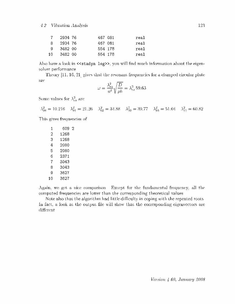
���� Vibration Analysis ���
� ������� ����� real
������� ����� real
� ���� ���� real
� ���� ���� real
Also have a look in ��stadyn�log�� you will �nd much information about the eigen�solver performance�Theory ��� �� ��� gives that the resonant frequencies for a clamped circular plate
are
� ��rsa�
sD
�h ��rs ����
Some values for ��rs are
���� ����� ��
�� ���� ��
�� � �� ��
�� ���� ��
�� ��� ��
�� ����
This gives frequencies of
� ����
� ����
� ����
� ��
��
� �����
� ����
����
� �����
� �����
Again we get a nice comparison� Except for the fundamental frequency all thecomputed frequencies are lower than the corresponding theoretical values�Note also that the algorithm had little di#culty in coping with the repeated roots�
In fact a look at the output �le will show that the corresponding eigenvectors aredi�erent�
� Version ����� January ����
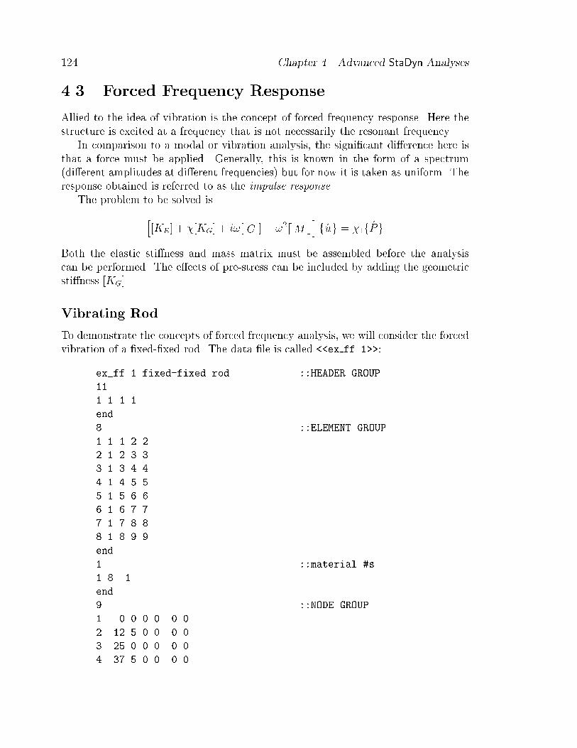
�� Chapter �� Advanced StaDyn Analyses
��� Forced Frequency Response
Allied to the idea of vibration is the concept of forced frequency response� Here thestructure is excited at a frequency that is not necessarily the resonant frequency�In comparison to a modal or vibration analysis the signi�cant di�erence here is
that a force must be applied� Generally this is known in the form of a spectrum�di�erent amplitudes at di�erent frequencies� but for now it is taken as uniform� Theresponse obtained is referred to as the impulse response�
The problem to be solved is
h�KE� " ��KG� " i�� C �� ��dM c
if$ug ��f $Pg
Both the elastic sti�ness and mass matrix must be assembled before the analysiscan be performed� The e�ects of pre�stress can be included by adding the geometricsti�ness �KG��
Vibrating Rod
To demonstrate the concepts of forced frequency analysis we will consider the forcedvibration of a �xed��xed rod� The data �le is called ��ex ff����
ex�ff�� fixed�fixed rod ��HEADER GROUP
��
� � � �
end
��ELEMENT GROUP
� � � � �
� � � � �
� � � � �
� � �
� � �
� � � � �
� � �
� � �
end
� ��material �s
� �
end
� ��NODE GROUP
� � � �
� ��� � �
� � � � �
� ��� � �

���� Forced Frequency Response ���
� � �
� ��� � �
� � � � �
�� � �
� �� � �
end
� ��boundary condns
�
�
end
� ��applied loads
�� � � � � � �
end
� ��material props
� ��e� ��e� �� �� e�� � � � �
end
� ��SPECIALs GROUP
��� ��e��
end
Note that the rod has a small amount of mass proportional damping as speci�edthrough the specials code ������ Also note that the load is applied at the centerof the rod�Run the program read in the structural data�le and form the sti�ness and mass
matrices by typing
C� stadyn
�
ex�ff��
�
��
Choose the forced frequency analysis
�
which leads to the menu choices
FORCED Frequency Problems� sub�menu
��� Distributed loadings "P!
��� Pre�stress "dP!
� Version ����� January ����

��� Chapter �� Advanced StaDyn Analyses
In the �rst of these the loads speci�ed in the input �le are made oscillatory whereas inthe second they form the pre�stress and the oscillatory load is a point load separatelyspeci�ed� We will choose the distributed loading analysis
��
�
Although the loads are speci�ed in the structure data�le sometimes it is useful to beable to specify a scale on the distribution� in response to
INPUT load scale� scale X "P!
type
��
Now input the frequency range information
INPUT� freq� �Hz� � d�freq �Hz� � � of incs
It is a practice of StaDyn that a vertical bar j separates multiple �elds that must beentered� So this wants three numbers the �rst being the beginning of the frequencyrange then the spacing of the frequencies and ending with the total number offrequencies to be tested� Note that these frequencies are to be given in Hz� For nowchoose
� �� ��
This gives ��� samples over a frequency range of ���� Hz� Be careful when lookingat freely supported structures that the initial frequency is not speci�ed as identicallyzero since then the system is singular� The next information required is the form ofthe output� The choices are
CHOOSE output�
�return
��Re�Im nodal displacements
��Mag nodal displacements
��norm of all displacement
An interesting thing about the normalized displacements is that in the vicinity of aresonance they approach the eigenvectors� For now choose
�
since the norm gives a global picture of the dynamic behavior� Exit the program bytyping

���� Forced Frequency Response ���
Look through the �le ��stadyn�dyn�� �not ��stadyn�out��� and see three un�labeled columns in the form
freq �Hz� displacement norm log� disp norm�
Notice where the maxima occur � this is in the vicinity of a resonance� A moreprecise value can be determined by re�running the example but having narrowed thefrequency down to the band of interest� There is no header in the �le because it isintended to be displayed by a program such as DiSPtool�For the above parameters the resonances are expected at ����
f �N
L
sEA
�A ��N k�rad�s N kHz
where N is the resonance number� Thus counting and identifying the resonances forthis problem will be easy�Now scan ��stadyn�dyn�� and see that the peaks appear close to
� � �
It is obviously missing some resonances� In fact it is picking up every other one� Nowchange the location of the force to Node � and re�run the program� �This is whereusing the script �le can save a lot of time�� When this is done it will be seen that thepeaks occur at
� � � � �
Again it is missing some peaks� Experiment with other locations� What this isshowing is that where the force is applied will determine what modes play a role inthe response� That is not all modes may be signi�cant for a given type of loading�Try putting a force at every node� contrary to expectation not all modes are excited'Now try alternating the directions of the forces�
� Version ����� January ����
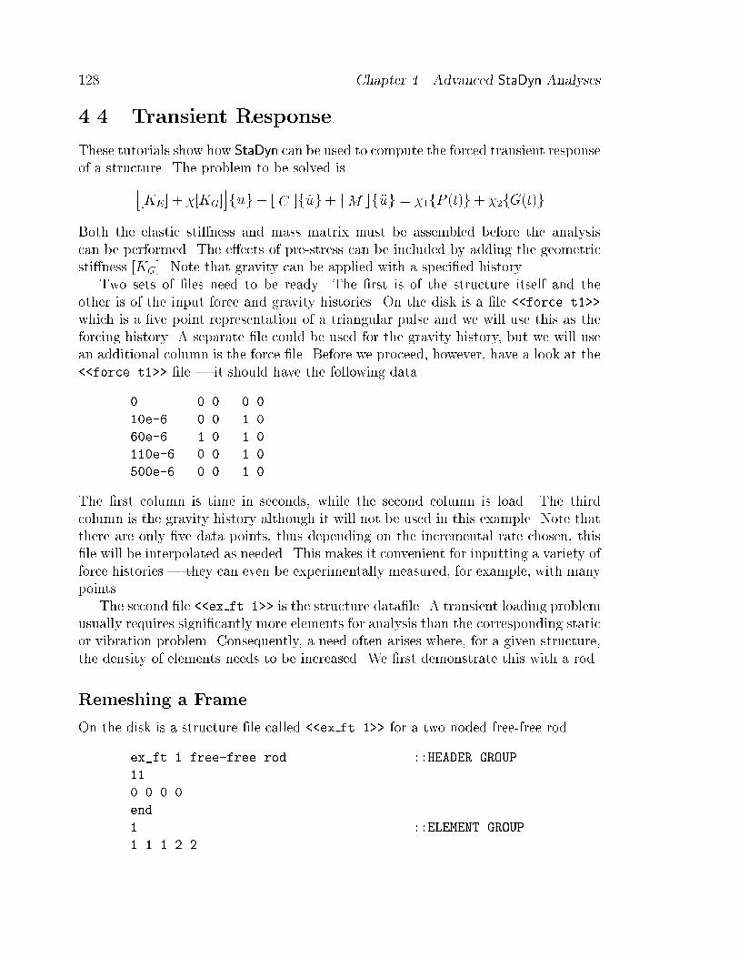
��� Chapter �� Advanced StaDyn Analyses
��� Transient Response
These tutorials show how StaDyn can be used to compute the forced transient responseof a structure� The problem to be solved ish
�KE� " ��KG�ifug" � C �f (ug" dM cf)ug ��fP �t�g" ��fG�t�g
Both the elastic sti�ness and mass matrix must be assembled before the analysiscan be performed� The e�ects of pre�stress can be included by adding the geometricsti�ness �KG�� Note that gravity can be applied with a speci�ed history�Two sets of �les need to be ready� The �rst is of the structure itself and the
other is of the input force and gravity histories� On the disk is a �le ��force�t���which is a �ve point representation of a triangular pulse and we will use this as theforcing history� A separate �le could be used for the gravity history but we will usean additional column is the force �le� Before we proceed however have a look at the��force�t��� �le � it should have the following data
� �
�e�� � ��
�e�� �� ��
��e�� � ��
e�� � ��
The �rst column is time in seconds while the second column is load� The thirdcolumn is the gravity history although it will not be used in this example� Note thatthere are only �ve data points thus depending on the incremental rate chosen this�le will be interpolated as needed� This makes it convenient for inputting a variety offorce histories � they can even be experimentally measured for example with manypoints�The second �le ��ex ft���� is the structure data�le� A transient loading problem
usually requires signi�cantly more elements for analysis than the corresponding staticor vibration problem� Consequently a need often arises where for a given structurethe density of elements needs to be increased� We �rst demonstrate this with a rod�
Remeshing a Frame
On the disk is a structure �le called ��ex ft���� for a two noded free�free rod�
ex�ft�� free�free rod ��HEADER GROUP
��
end
� ��ELEMENT GROUP
� � � � �

���� Transient Response ���
end
� ��material �s
� � �
end
� ��NODE GROUP
� � � �
� � � �
end
��boundary conditions
end
� ��applied loads
� �� � � � � � �
end
� ��material props
� ��e� ��e� �� �� e�� � �� �� ��
end
� ��SPECIALs GROUP
��� � � �
end
There are no boundary conditions for this problem but we must still include thesection that speci�es boundaries� hence the null group for the boundary conditions�Note that while the force history itself will be speci�ed elsewhere this �le must saywhere it is applied� Thus the entry ��� above could be used as a scaling factor�Indeed multiple forces could be inputted and they will all act as scalings on theapplied load history� In this way distributed and vector loads can be applied� Keepin mind however that each of these forces will have the same time history� Note thatthe rod has no damping but a small amount of mass and�or sti�ness proportionaldamping could be speci�ed through the specials code ������It is obvious that it is not possible to perform wave propagation studies with only
a single element� Hence the purpose of this tutorial is to show how the programGenMesh can be used to remesh a structure to the required number of elements�The interface of GenMesh is very similar to that of StaDyn so run it as
C� genmesh
We wish to remesh the inputted structure so choose
�
and you are asked for the new name and old name respond
�
ex�ft��
ex�ft��
� Version ����� January ����

��� Chapter �� Advanced StaDyn Analyses
which leads to the re�mesh menu
CHOOSE� �return
��
��remesh plate
��remesh frame
��add frame member
�
��reduce bandwidth
�
Choose to remesh a frame
�
The program wants to know how the structure is to be remeshed�
MULT factors�
INPUT� elm� � elm� � mult factor � to end�
It is looking for a range of elements and their corresponding multiplication factor�It is possible to overlap these ranges and thus save some typing� We have only oneelement so type
� � �
This has divided the original element into ���� Exit the program by typing
Look through the �le ��ex ft����� It is seen that indeed it has made ��� elements�however notice that the last element has connectivity
� � �� � �
While the program has remeshed the structure it has not numbered the nodes inany optimum fashion � the original numbering is left intact� This can be usefulsometimes but generally it means that the bandwidth has become unacceptablylarge and the nodes must be renumbered�
We will now repeat the procedure from the beginning and this time also renumberall the nodes�

���� Transient Response ���
C� genmesh
�
�
ex�ft��
ex�ft��
�
� � �
We now want to renumber the nodes�
�
�
Notice that the initial bandwidth is ���� We are using the wavefront method whichbasically renumbers based on the proximity of nodes to each other� This is determinedrelative to the focus point so in response to
INPUT wavefront center� x � y � z
respond
��
Note that the bandwidth is reduced to �� Also keep in mind that the renumberingis based on nodal number �not on the number of degrees of freedom of the reducedsystem� and so the bandwidth numbers may appear di�erent from that obtained whenusing StaDyn�Since the �le is acceptable to us update it and exit
�
Now look at ��ex ft���� to see that the connectivity of the last element is
� � � �� ��
This is what we wanted�
Impact of a Rod
Run StaDyn read in the structure data�le and form the sti�ness and mass matrices
� Version ����� January ����

��� Chapter �� Advanced StaDyn Analyses
C� stadyn
�
ex�ft��
�
��
With both the sti�ness and mass matrices formed the transient analysis can bechosen
This leads to the sub�menu
TRANSient Problems� submenu
�� Distributed loadings "P!�"G!
�� Multiple ��
�� Pre�stress �� "dP!
�� Moving ��
�� All�node ��
We wish to use the loads speci�ed in the structure data�le as the distribution oftransient applied loads hence choose
�
There are two stages to the transient analysis a �rst time analysis when all thebasic data is generated and a post�processing stage when the snapshots are analyzed��Snapshots are complete records of the nodal displacements at a particular instantthey are needed to obtain the member loads and element stresses�� Right now wejust want to solve the problem so in response to
CHOOSE� �return ��analysis ��post�analysis
choose
�
Sometimes it is convenient to have unit loads in the structure data�le or a loadhistory that is normalized somehow and to use the analysis stage to scale the loads�In response to
INPUT scales� load � gravity
type

���� Transient Response ���
� �
At this stage we must input information about the time integration parameters
TYPE� time inc � � of incs � print count � snap count
The equations of motion are integrated incrementally in time� The program wants toknow the time increment and how many of them� There is no hard and fast rule forthis especially since the algorithm implemented is unconditionally stable� it is bestto experiment� Since the time step may be �ner than what is necessary for displayof the results the print count allows the output rate to be varied� Snapshots arenecessary for the post�processing of the results to obtain stresses and strains� this isstored in binary form� For now we will not bother with snapshots so choose
�e�� � � �
For dynamic problems it is not feasible to output the results for every nodebecause there is just too many of them and ����% of the information would probablynot be used� So StaDyn allows selection of a limited number of nodes as output
CHOOSE nodal output�
TYPE� node � � DoF � rate ���accn� � to end�
Since each node can have up to six degrees of freedom �� displacements and � ro�tations� and up to � rates �displacement velocity and acceleration� it is easy tosee how the amount of information can mushroom� For now just select the velocityof Nodes � �� and ��� as output� Velocities are usually good quantities to choosebecause they are related more directly to the loads�
� � �
� � �
�� � �
This is a recurring menu allowing the nodes to be chosen randomly� Now the snapshotinformation
CHOOSE snapshot output� �none
��partial disp
��full disp
��Full disp� vel� acc
For now choose
The �nal piece of information required is about the force history
� Version ����� January ����

�� Chapter �� Advanced StaDyn Analyses
�� get "P! load history
�� TYPE� Load�Filename ���
Respond
force�t�
The �le is then parsed for the appropriate columns
�� INPUT� Time col � load col � � cols
Respond
� � �
Similar input is required for gravity
�� get "Grav! load history
�� TYPE� Load�Filename ���
Give the responses
force�t�
� � �
The program now proceeds on its way periodically echoing some information tothe screen� Finally back at the menu exit by typing
The results are located in the �le ��stadyn�dyn�� and are stored as
time P�load G�load resp � resp � ����
and in the present case it will have �ve columns� Note that the force is the linearlyinterpolated force� The times traces of these responses are shown in Figure ��� Thesenumbers are best viewed using the utility program DiSPtool�From the theory for the impact of rods ��� it can be established that the relation�
ship between force and velocity is
(u �PcoEA
���P
where co qEA��A ������ in�s is the wave speed� For the current maximum load
this gives a maximum velocity of �� in�s� This is close to that given by the programas ������ which occurs at ���s�
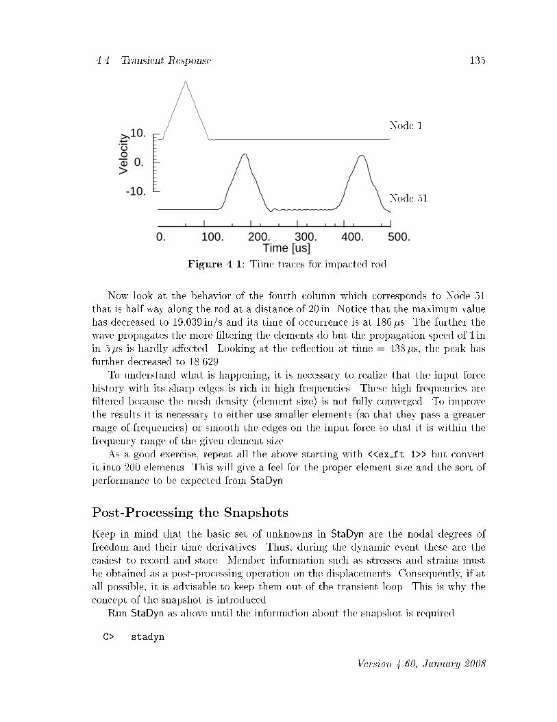
���� Transient Response ���
0. 100. 200. 300. 400. 500.Time [us]
-10.
0.
10.V
eloc
ityNode �
Node ��
Figure �� Time traces for impacted rod�
Now look at the behavior of the fourth column which corresponds to Node ��that is half way along the rod at a distance of �� in� Notice that the maximum valuehas decreased to ����� in�s and its time of occurrence is at ����s� The further thewave propagates the more �ltering the elements do but the propagation speed of � inin ��s is hardly a�ected� Looking at the re�ection at time ���s the peak hasfurther decreased to �������To understand what is happening it is necessary to realize that the input force
history with its sharp edges is rich in high frequencies� These high frequencies are�ltered because the mesh density �element size� is not fully converged� To improvethe results it is necessary to either use smaller elements �so that they pass a greaterrange of frequencies� or smooth the edges on the input force so that it is within thefrequency range of the given element size�As a good exercise repeat all the above starting with ��ex ft���� but convert
it into ��� elements� This will give a feel for the proper element size and the sort ofperformance to be expected from StaDyn�
Post�Processing the Snapshots
Keep in mind that the basic set of unknowns in StaDyn are the nodal degrees offreedom and their time derivatives� Thus during the dynamic event these are theeasiest to record and store� Member information such as stresses and strains mustbe obtained as a post�processing operation on the displacements� Consequently if atall possible it is advisable to keep them out of the transient loop� This is why theconcept of the snapshot is introduced�Run StaDyn as above until the information about the snapshot is required�
C� stadyn
� Version ����� January ����
��� Chapter �� Advanced StaDyn Analyses
�
ex�ft��
�
��
�
�
� �
�e�� � � �
� � �
� � �
�� � �
CHOOSE snapshot� �none ��partial ��full
Now select a partial snapshot
�
Since it is only a partial snapshot the program wants to know what nodes are involved
TYPE� node � � to end�
This is a recurring prompt therefore many unconnected nodes can be chosen� Keepin mind however that determining member values requires knowledge of all nodesassociated with an element� StaDyn insures that the appropriate nodes are includedfor the element of interest� In the present case we will only look at one node near thecenter of the rod so choose
�
The rest of the responses are the same as before
force�t�
� � �
force�t�
� � �

���� Transient Response ���
The output for the partial snapshot is in ��stadyn�out��� It is in ASCII textform so look at it� The data is stored as node number followed by the three dis�placements and three rotations� The beginning of each snapshot contains the timeand the number of elements stored� Note that there is duplication of the nodes� thisoccurs because the information stored is based on the triangular elements� Thus eachgroup of three lines represent the element completely� Parenthetically the record forthe full snapshot would be stored in ��stadyn�snp��� it is in BINARY form so youcannot look at it without re�running StaDyn�This snapshot information can now be converted to member loads and so on by
re�running StaDyn in post�analysis mode� That is
C� stadyn
�
ex�ft��
�
Now choose the post�analysis for partial snap shots
�
�
We have a choice of the type of output
OUTPUT�
�return
��displacement
��nodal strain �ue�
��nodal stress
��crack
�element stress
��force sum
��plate��
���displacement
���nodal strain �ue�
���nodal stress
��frame��
� �displacement
���nodal strain �ue�
���nodal stress �F�A M�I�
Choose the nodal stresses
��
� Version ����� January ����

��� Chapter �� Advanced StaDyn Analyses
The �nal piece of information we give is the particular node of interest
INPUT� node �
�
The program will search through the snapshots to locate the nodal data it will thencheck to insure that they belong to the same member� Exit the program by typing
The member stresses are stored in the �le ��stadyn�dyn�� in the form of sevencolumns
time F�x�A F�y�A F�z�A M�x�I�x M�y�I�y M�z�I�z
The �rst is time the next three are stresses and the last three are bending likestresses �the actual stress is obtained by multiplying by the appropriate distancefrom the neutral axis�� The maximum stress is ������� and it occurs at ����s� Thecomplete history is best viewed using the utility program DiSPtool�Wave propagation is a complicated subject and it puts great demand on the
program and the user� The above tutorial was to show the basic functioning of StaDynand does not indicate its full potential� It is recommended to consult References ��� ��� for more examples that can be tested against StaDyn�
In�Plane Impact of a Long Plate
In this tutorial we look at wave propagation in a ��D in�plane plate� The plateresembles somewhat a beam but because it is modeled two�dimensionally it willexhibit the evolution of waveguide types of behaviors� Only one half of the plate ismodeled since there is a line of symmetry at the left face�Run StaDyn read in the structure data�le form the sti�ness and mass matrices�
C� stadyn
�
ex�pt��
�
��
With both the sti�ness and mass matrices formed the transient analysis option canbe chosen from the main menu�

���� Transient Response ���
�
�
� �
Now input the parameters for the time integration and the nodal outputs
�e�� �� � �
� � �
�� � �
��� � �
This will store the velocities at every ��s and the snapshots at every ���s� We willdemonstrate the use of snapshots for obtaining contour plots of the stresses� So inresponse to
CHOOSE snapshot output� �none ��partial ��full
choose full snapshots
�
The last set of information required concerns the force and gravity histories
force�t�
� � �
force�t�
� � �
The program �gures out how much data is in the force �le and interpolates as neededbased on the time increment�The nodal velocity results are located in the �le ��stadyn�dyn�� and are stored
as
Time P�load G�load resp� resp� resp� ����
By scanning this �le some of the maximum velocities occur at
�
��e�� � ����� �� �� ������
�
���E�� ����� � ���� ������
�
��E�� �� ���� ������ �� ����
�
� Version ����� January ����

� � Chapter �� Advanced StaDyn Analyses
It is interesting how over time all monitored nodes tend to the same behavior�As a good exercise repeat the above but use more modules in the modeling and
try di�erent step sizes� This will give a feel for the proper element size and the sortof performance to be expected from StaDyn�We will now demonstrate how the snapshots can be post�processed to obtain
contours of stress� Recall that we already have stored the full snapshots� to accessthis information type
c� stadyn
�
ex�pt��
�
�
until the information about the snapshot is required
CHOOSE snapshot� �none
��partial disp
��full disp
��full disp� vel� acc
We stored the full snapshots hence
�
Now we will retrieve a particular snapshot
CHOOSE snapshot�
�return
��which snap
���all snaps at one node
���all snaps at all nodes
���rate at �
The �� option allows a single node to be monitored across all snapshots this is used forgenerating time traces� Here we will look at a single snapshot� Choose the eleventhsnapshot �i�e� time at ����s�
��
and after you see the counter you are launched into the Post menu
POST menu�
�return
LOCAL �member coords�

���� Transient Response � �
��nodal strain �ue�
��nodal stress
��nodal force
��element stress
��force sum
�specials
GLOBAL
���Global displacement
���Global loads
���Global assembled DoF loads
� �Global assembled nodal loads
CONTOURs
���store displacement data
���store strain data
���store stress data
frames
���store displacement data
� �store strain data
���store stress data
�� �� select FRAMEs only ��
�� �� select F�PLATEs only ��
This is almost identical to the Post menu for static problems� We want to see thestresses so select
��
Quit this menu and go to the PostScript output o� the main menu�
�
�
p��ps
At this sage we are given the contours menu
CONTOURs�
� Quit
��RENDER PS file��
�� Deformed shape
� Contours
��CHANGE defaults��
��� Position model
��� Rotate model
� Version ����� January ����

� � Chapter �� Advanced StaDyn Analyses
��� Move tagged surfaces
��� Add caption
� � Toggle tags
��� Change pens
The menu is divided into two parts the top renders the PS �le while the bottomallows changing the defaults for the drawing parameters� We will change the penthicknesses
��
and the choices are
INPUT pens� mesh � contour
current� �� �
���
Make the mesh lines thinner
�
Now choose to render the contours
to be given the DoF menu
DoF� ��u ��v ��w ��Rx �Ry ��Rz
or ��Exx ��Eyy ��Exy ��Kxx �Kyy ��Kxy
or ��Sxx ��Syy ��Sxy ��Mxx �Myy ��Mxy
Mesh� ��Yes �No ���Black
Legend� ��Yes �No ���Black
INPUT� DoF � scale � mesh � � legend �
Of interest now are the x�direction stresses since they relate to the bending stressesin beams� Choose this component and quit
� �� � �
Before we look at the contours it is worth pointing out that to access the othercomponents of stress for this snapshot it is only necessary to enter the PostScript�les menu option� If however a di�erent snapshot is desired then all of the aboveprocedure needs to be redone�
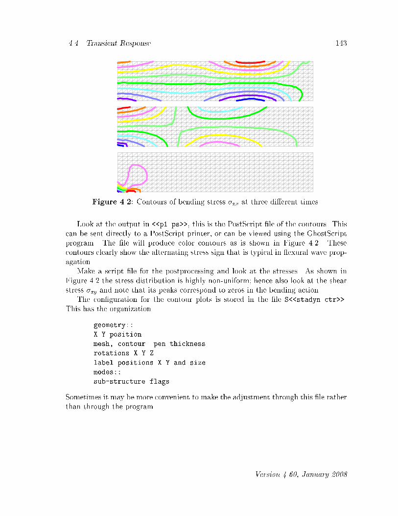
���� Transient Response � �
Figure �� Contours of bending stress �xx at three di�erent times�
Look at the output in ��p��ps�� this is the PostScript �le of the contours� Thiscan be sent directly to a PostScript printer or can be viewed using the GhostScriptprogram� The �le will produce color contours as is shown in Figure ��� Thesecontours clearly show the alternating stress sign that is typical in �exural wave prop�agation�Make a script �le for the postprocessing and look at the stresses� As shown in
Figure �� the stress distribution is highly non�uniform� hence also look at the shearstress �xy and note that its peaks correspond to zeros in the bending action�The con�guration for the contour plots is stored in the �le S��stadyn�ctr���
This has the organization
geometry��
X Y position
mesh� contour pen thickness
rotations X Y Z
label positions X Y and size
modes��
sub�structure flags
Sometimes it may be more convenient to make the adjustment through this �le ratherthan through the program�
� Version ����� January ����

� Chapter �� Advanced StaDyn Analyses
Chapter �
Nonlinear Analyses with NonStaD and
Simplex
NonStaD �NONlinear STAtic and Dynamic analysis� is designed to perform nonlinearstatic and dynamic analyses of thin�walled structures whereas Simplex does the samefor ��D solids� This chapter presents a few tutorials that cover the basics of thesenonlinear analyses� Note that both the computational cost and computer resourcesincreases substantially for these types of problems�The main nonlinear capabilities of NonStaD�Simplex involve determining the mem�
ber displacements and loads and structural reactions for
� Static incremental analysis� Dynamic implicit incremental analysis� Dynamic explicit incremental analysis
Simplex has the additional capability of nonlinear constitutive relations in the formof plasticity and rubber elasticity� The programs are menu driven in much the sameway as for StaDyn� indeed as they proceed they create a number of �les which sharethe same names �and internal format� as for StaDyn� The primary �les are
nonstad�cfg stadyn�stf stadyn�dis
nonstad�log stadyn�mas stadyn�snp
stadyn�out stadyn�mat
stadyn�dyn stadyn�geo
stadyn�mon stadyn�lod
The �LOG �le echoes all the input responses as well as having some extra informationthat might prove useful during post analysis of the results� The �DYN and �OUT �lesare the usual locations for NonStaD�Simplex output� there is the additional output �le��stadyn�mon� that contains monitored information �such as vibration eigenvalues�that are very useful in nonlinear analyses� The second column of �les are associated
� �

� � Chapter �� Nonlinear Analyses with NonStaD and Simplex
with various system matrices such as the sti�ness matrix and the mass matrix �these are left on disk in case they may be of value for some other purpose� They arein binary form� The last column of �les are output �les� They too are in binary formfor compactness but can be read for further post�processing�Regularly have a look in the ��stadyn�log�� because it contains lots of additional
information about the functioning of NonStaD and Simplex�

���� Large Deection Analysis of a Beam � �
��� Large De�ection Analysis of a Beam
This tutorial considers the large de�ection of a cantilevered beam subjected to atransverse load� Elementary linear beam theory would indicate only a transversede�ection but such a situation would generate enormous axial forces in the beam� Thenonlinear analysis accounts for these axial loads correctly in an incremental�iterativemanner�
Getting Started with NonStaD
NonStaD is designed to run as a console program under MS Windows� Note thatall instructions are case insensitive� we will vary the case only to help make theinstructions clearer�To run the program type �at the �C prompt��
C� nonstad
�note the name of the executable�� to be given the opening menu
MAIN menu�
� Quit
�� Read in structure DataFile
��Elastic��
��� Static Incremental Analysis �full NR�
��� Incremental Time Analysis �imp�NR�
���� �� �� Analysis �imp�NR�
�� Incremental CoRot Wave Analysis �exp�
��� �� �� Wave Analysis �exp�
�� Cohesive ��
��� Incremental CoRot cohesive �exp�
��� Incremental CoRot cohesive �exp�init�
��Elastic�Plastic��
���� Incremental Time Mult�loads �imp�NR�
�� Incremental CoRot Wave Analysis �exp�
��� �� �� Mult�loads �exp�
�� Extras ��
�� PostScript plot files
� System services
���� Ikayex information
The biggest di�erence in comparison to the linear analyses of StaDyn is the absenceof the option to form the system matrices� in nonlinear analyses the system matriceschange during the analyses and are therefore part of the particular analyses� Quit bytyping
� Version ����� January ����

� � Chapter �� Nonlinear Analyses with NonStaD and Simplex
There are two �les worth looking at� The �rst is the log �le ��nonstad�log���use the list utility to peruse it� It contains
�� NonStaD version ���� August ��
�� DATE� � ���� TIME� �����
�� MAXimum storage �
�� MAXimum elements � �
�� MAXimum nodes � �
�� MAXimum force incs� �
�� ITERmax � ��
�� rtol � ��E��
�� ALLOCATION succeeded
��MAIN
�� NonStaD OK� ended from MAIN
The second is ��nonstad�cfg��� This is the con�guration �le and has in it
��MaxStorage
� ��MaxNode
� ��MaxElem
� ��MaxForce
� ��ilump
�� ��itermax
��E�� ��rtol
�� DATE� � ���� TIME� �����
This allows the run time setting of the dimensions of the arrays� If a memory alloca�tion failure occurs this is the place to make the adjustments�
Incremental�Iterative Solution
The element formulation for the linear static analysis of a beam is exact irrespective ofthe element size� This is not true for a nonlinear analysis� The one element structuredata�le for our beam is in the �le ��ex fn���� and contains
ex�fn��� doyle pp��� ��HEADER GROUP
��
� � � �
end
� ��ELEMENT GROUP
� � � � �
end

���� Large Deection Analysis of a Beam � �
� ��matl distn
� � �
end
� ��NODE GROUP
� � � �
� �� � �
end
� ��boundary condns
�
end
� ��applied loads
� � �� � � � � �
end
� ��matl props
� �e� �e� �� �� e�� �����e� �����e� ���e�
end
��SPECIALs GROUP
end
It is cantilevered at one end and has a transverse load at the other� The Remesh
capability of GenMesh was used to convert this into a model with ten elements whichis called ��ex fn�����
NonStaD�s nonlinear solvers use a combination of multiple load increments plusNewton�Raphson equilibrium iterations at each increment� This tutorial shows asimple example�Run NonStad and read the structure data�le
C� nonstad
�
ex�fn��
The choices for implicit nonlinear analyses are
��� Static Incremental Analysis �full NR�
��� Incremental Time Analysis �imp�NR�
���� �� �� Mult�loads �imp�NR�
The second of these uses a pseudo�time for static problems� We will choose the �rstoption to do an analysis
��
�
The information required is the load level plus the number of increments�
� Version ����� January ����

��� Chapter �� Nonlinear Analyses with NonStaD and Simplex
TYPE� force max � � of incs � max � inc � follower ��N���Y�
We will load to ��� using �ve increments� If NonStaD has di#culty converging it willdivide the load increment� the maximum number of increments is set to prevent anin�nite loop� Finally unlike a linear analysis the load in a large de�ection problemcan either keep its original direction or follow the deforming shape of the structure�We will keep the load pointing in the same direction�
� � �
The algorithm has a number of parameters to control the radius of convergence� twoof the parameters are
�� u � u � beta�du K � K�E � gamma�K�G
INPUT� beta � gamma
Input
�� ��
The Newton�Raphson iterations use a tolerance criterion for convergence however toprevent locking it is good to set a reasonable upper limit on the maximum numberof iterations� In response to
INPUT� iter max � tolerance ����e� �
input
�e��
Finally we need to choose the nodal outputs�
CHOOSE nodal output�
TYPE� node � � DoF � to end�
We will monitor the end �load� point
�� �
�� �
�� �
Quit the program
The results are in the �le ��stadyn�dyn��� The �nal line gives
�� � ����� ����� ���� � �
This is a large de�ection� The last column in the output is the number of iterationsat that load step� In general as the increment is increased so too do the number ofiterations� It is di#cult to know in advance the right balance between load incrementsversus number of iterations�
���� Large Deection Analysis of a Beam ���
Pseudo�Time Incremental Analysis
Because nonlinear static problems require a series of load steps then we can thinkof these increments as occurring over time� We will repeat the previous problem byapplying a load history from the force �le ��force����� with the following data
� �
� �
The �rst column is time in seconds while the second column is load� The time scaleis so slow that inertia e�ects are negligible� Note that there are only three datapoints thus depending on the incremental rate chosen this �le will be interpolatedas needed� This makes it convenient for inputting a variety of forces � they can evenbe experimentally measured for example with many points�Run NonStaD as before
C� nonstad
�
ex�fn��
The transient implicit option is chosen
��
There are two stages to the transient analysis a �rst time analysis when all the basicdata is generated and a post�processing stage when the snapshots are analyzed��Snapshots are complete records of the nodal displacements at a particular instantthey are needed to obtain the member loads�� Right now we just want to solve theproblem so in response to
CHOOSE� �return ��analysis ��post�analysis
choose
�
You are now asked for
TYPE� time inc � � of incs � print count � snap count
The equations of motion are integrated incrementally in time� The program wants toknow the time increment and how many of them� There is no hard and fast rule forthis especially since the algorithm implemented is unconditionally stable� it is bestto experiment� Since the time step may be �ner than what is necessary for displayof the results the print count allows the output rate to be varied� Snapshots arenecessary for the post�processing of the results to obtain moments and forces� Thiscan be stored in binary form and used later to obtain the forces and moments� Fornow we will not bother with snapshots so choose
� Version ����� January ����

��� Chapter �� Nonlinear Analyses with NonStaD and Simplex
� �� �
For the parameters
�� u � u � beta�du K � K�E � gamma�K�G
INPUT� beta � gamma � ramp
input
�� ��
The ramp modi�es beta so that the full increment of displacement is not applied untilthe ramp integer number� this is particularly useful for problems �such as beams�where the initial linear de�ections are large� The Newton�Raphson iterations use atolerance criterion for convergence however to prevent locking it is good to set areasonable upper limit on the maximum number of iterations� In response to
�� algor ��full N�R ��mod N�R
INPUT� algor � iter max � tolerance ����e� �
input
� �e��
For dynamic problems it is not feasible to output the results for every nodebecause there is just too many of them and ����% of the information would probablynot be used� So StaDyn allows you to select a limited number of nodes as output
CHOOSE nodal output�
TYPE� node � � DoF � rate ���accn� � to end�
Since each node can have up to six degrees of freedom �� displacements and � rota�tions� and up to � rates �displacement velocity and acceleration� it is easy see howthe amount of information can mushroom� We will monitor the displacements of theend �load� point
�� �
�� �
�� �
This is a recurring menu where the nodes �and DoF� can be chosen in any preferredsequence� The next information required is
�� Eigen type� �none ��� ��subspace
INPUT Eigen� type � rate � � vectors � scale � � �

���� Large Deection Analysis of a Beam ���
A characteristic of nonlinear problems is that the sti�ness can change with load�Indeed the sti�ness can go to zero resulting in a structurally unstable condition� Aunique feature of NonStaD is that it can monitor the changing sti�ness by reportingthe vibration eigenvalues� This will be explored in the next tutorial for now input
� �
The �nal piece of information required is the force history
TYPE� Force�Filename ���
To which respond
force���
The �le is then parsed for the appropriate columns
�� INPUT� Time col � Force col � � cols
Respond
� � �
The force histories can be scaled by
�� "P! � "Grav! � �rd �
TYPE force scales� P� � P� � P� � P�
We will simply choose
�� � � �
The program now proceeds on its way periodically echoing some numbers to thescreen� Finally you are given the menu again so exit by typing
The results are located in the �le ��stadyn�dyn�� and is stored as
time load�� ��� resp�� resp�� ���� iter hist�� ����
and in the present case it will have nine columns� Note that the force is the linearlyinterpolated force�
��� �� � ����� ������ ���� � �� � �
These are almost identical to the results for the previous tutorial�
� Version ����� January ����

�� Chapter �� Nonlinear Analyses with NonStaD and Simplex
��� Structural Instability
It is a characteristic of nonlinear systems that the structural sti�ness can changeunder load� This is investigated here�We consider a plate of dimensions ��� �� �� in�� made of aluminum and loaded
uniformly along the east edge� Such a load causes only an inplane uniform �xx stress�We will apply the load smoothly to a level above the �rst buckling load to see whathappens� More details on the problem can be found in Reference �����The mesh �le is called ��ex pn���� and the load is in �le ��force���p��� The
shape of the history is shown in Figure ����a� as P �t��
0 2500 5000 7500 10000 12500
Time [µs]
eigenvalues load history
P �t�
�a�
0 5000 10000 15000 20000
Time [µs]
w�
Q�t�
w�� w�
u
�b�
Figure �� Axially loaded plate� �a� Eigenvalue behavior against load� �b� Dis�placements after critical load and transverse ping applied�
Changing Eigenvalues
Run NonStaD as for the pseudo�time problem
C� nonstad
�
ex�pn��
��
�
When asked for
TYPE� time inc � � of incs � print count � snap count
respond

���� Structural Instability ���
e�� � � � �
We will do this problem on a time scale where inertia e�ects are signi�cant� Set thealgorithm parameters as
� �
� �e��
We wish to monitor both the in�plane and out�of�plane behavior so in responseto
CHOOSE nodal output�
TYPE� node � � DoF � rate ���accn� � to end�
select
�� �
�� �
��� �
��� �
This monitors the displacement at the loaded edge and the out�of�plane behaviorat the three quarter points along the centerline� The next monitoring informationrequired is
�� Eigen type� �none ��� ��subspace
INPUT Eigen� type � rate � � vectors � scale � � �
A unique feature of NonStaD is that it can monitor the changing sti�ness by reportingthe vibration eigenvalues� This is the main point to be explored in the this tutorial�The TYPE�� option chooses vector iteration which reports only the lowest eigenvaluewhile the TYPE�� option chooses subspace iteration which reports the ten lowesteigenvalues� In both cases the eigenvalues are stored in the �le ��stadyn�mon���The remaining option refer to the number of vectors �mode shapes� to be recorded�These are relevant here so choose
� � �� ��
The �nal piece of information required is the force history
�� get "P! history�
TYPE� Force�Filename ���
Respond with the name and relevant column information
force���p
� � �
� Version ����� January ����

��� Chapter �� Nonlinear Analyses with NonStaD and Simplex
The force histories must now be scaled
�� "P! � "Grav! � �rd �
TYPE force scales� P� � P� � P� � P�
For dynamic problems there are three contributions to the total magnitude of anapplied load� First there is the scale set in the structure data�le second there is thescale set in the history �le and third is the scale that can be set here� The history�le has a maximum magnitude of ���� and a linear buckling analysis gave a lowesteigenvalue of ��� ��� hence to load the plate beyond its �rst buckling load input
��� � � �
The negative sign makes the load compressive� The scales on P� and P� refer toadditional loads � we consider this in the next example�The program now proceeds on its way periodically echoing numbers to the screen�
some of these numbers may be recognized as those from a vibration eigenanalysis asdiscussed in Chapter � Finally exit the program by typing
The response results are located in the �le ��stadyn�dyn�� and are stored as
time load�� load�� ���� resp�� resp�� ���� iter hist�� ���
and in the present case it will have �� columns� The �nal line is
��� E�� ���� ���� ����E�� � � � ����
Note that the only displacement is the in�plane displacement of the loaded edge� Theinteresting results are in the ��stadyn�mon�� �le which gives the vibration eigenval�ues� These are shown plotted in Figure����a�� The results indicate three points ofinterest� First as the load changes so do the vibrational characteristics� Since themass is not changing then we conclude the sti�ness is changing� Second the modeinterchanges� Third it is possible for the eigenvalue to become negative� This meansthat the frequency �
p� becomes complex which in turn says that the system is
unstable� However the displacements do not indicate the large displacements usuallyassociated with an instability� This point is taken up in the next example�
Initiating the Instability
Because a structure becomes unstable does not mean that it will actually exhibit theinstability in terms of a large displacement or a bifurcation� an agent is necessary� Inthis tutorial we will make the structure unstable just as in the previous tutorial thenwe will apply a short duration �ping� transverse loading to initiate the bifurcationbehavior�We need to change ��ex pn���� in two ways� First append to the load lines

���� Structural Instability ���
��� � ��
and change the total number of loads to � ��boundary loads� This indicates thata transverse point load is applied at the center of the plate� the history will be readin as the third force history �the second is gravity if present�� The second change isthat damping must be added so as to settle the vibrations in a reasonable time�
� ��SPECIALs GROUP
��� e�� � �
end
The resulting �le is labelled ��ex pn��b�� on the disk� The ping history is given inthe �le ��ping���p�� and is shown in Figure ����b� as Q�t��Run NonStaD similarly to the previous tutorial
C� nonstad
�
ex�pn��b
��
�
e�� �� �
�� ��
� �e��
�� �
�� �
��� �
��� �
� � �� ��
force���p
� � �
The only di�erence is that another force �lename must be inputted and the responseis monitored over a longer period of time�
�� get "P��! history�
TYPE� Force�Filename ���
Input
ping���p
� � �
The third force can have a spatial distribution speci�ed within the structure �le oras a combination of the vibration eigenvectors� A nonzero scale on P� in
� Version ����� January ����

��� Chapter �� Nonlinear Analyses with NonStaD and Simplex
�� "P! � "Grav! � �rd �
TYPE force scales� P� � P� � P� � P�
would construct a third force whose spatial distribution is a combination of the �rsttwo vibration mode shapes when � � �� We will simply choose
���� � ��e�� �
A nonzero scale on P� would construct a second force whose spatial distribution is acombination of the �rst two current vibration mode shapes�The program now proceeds on its way periodically echoing numbers to the screen�
Finally exit the program by typing
The response results are located in the �le ��stadyn�dyn�� and the �nal line is
���� E�� �� ��� � E�� �� � E�� �� � E�� �����E��
���� � ����� ������� ���� �
Use the utility DiSPtool to view these results� Note that there are displacements at allthe nodes� The complete histories are shown in Figure ����b�� note that the transversedisplacements begin only after the application of the ping� Furthermore although thetransverse load is symmetric �point load at the center� and the geometry is symmetricthe motion of the plate is nonsymmetric as witnessed by the w� and w� displacementhistories being slightly di�erent� It is also interesting to note the �nal eigenvaluesgiven in the �le ��stadyn�mon�� �these are shown plotted in Figure����b� as thefull circles�� they are all positive showing that the plate has found a new equilibriumposition� The �nal de�ected shape is a ���� mode as expected from buckling theory�
Dynamic Instability� follower loads
This tutorial solves a nonlinear dynamic problem using the explicit integration scheme�The particular problem considered is the type of instability occurring under followerloads� More details of the problem can be found in Reference �����We will use a beam similar to that of ��ex fn���� but modi�ed for damping�
That is the specials section becomes
� ��SPECIALs GROUP
��� e�� � �
��� �� � �
end
The ����� code indicates that all loads are follower loads� The resulting �le islabelled ��ex fn� �� on the disk�Run NonStaD as before but choose the explicit time integration option
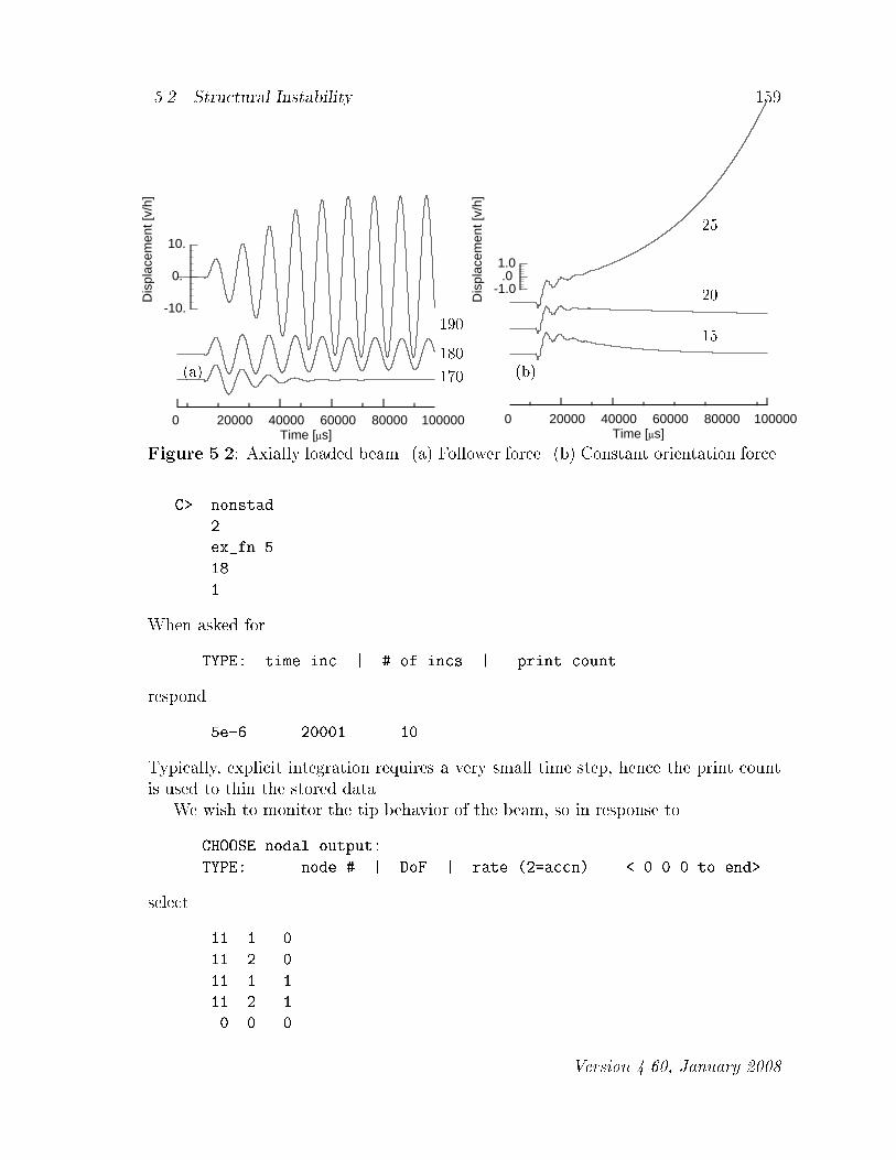
���� Structural Instability ���
0 20000 40000 60000 80000 100000Time [µs]
-10.
0.
10.
Dis
plac
emen
t [v/
h]
���
���
����a�
0 20000 40000 60000 80000 100000Time [µs]
-1.0.0
1.0
Dis
plac
emen
t [v/
h]
�
��
�
�b�
Figure �� Axially loaded beam� �a� Follower force� �b� Constant orientation force�
C� nonstad
�
ex�fn�
�
�
When asked for
TYPE� time inc � � of incs � print count
respond
e�� �� �
Typically explicit integration requires a very small time step hence the print countis used to thin the stored data�We wish to monitor the tip behavior of the beam so in response to
CHOOSE nodal output�
TYPE� node � � DoF � rate ���accn� � to end�
select
�� �
�� �
�� � �
�� � �
� Version ����� January ����
��� Chapter �� Nonlinear Analyses with NonStaD and Simplex
The type and rate of storing the snapshots is selectable
�� SNAPshot type� �none ��partial ��full
�� CHOOSE � type � count
Choose
� �
The �nal piece of information required are the force histories primary gravity andadditional� Respond
force���p
� � �
force���p
� � �
� �
ping���p
� � �
The ping load is placed at the beam center
�� TYPE� x y z � DoF � P�scale
� ��
The force histories can be scaled
�� "P! � "Grav! � �rd �
TYPE force scales� P� � P� � P� � P�
Input
���� � �� �
The negative sign makes the primary load compressive and the �le ��force���p��already is scaled to �����The program now proceeds on its way periodically echoing some numbers to the
screen� Finally you are given the menu again so exit by typing
The results are located in the �le StaDyn�DYN and is stored as
time load�� load�� load�� resp�� resp�� ���� hist�� ���
and in the present case it will have �� columns� Use the utility DiSPtool to viewthese results and they should look like those in Figure ����a�� For reference the �nalline is

���� Structural Instability ���
�� ���� � � ����E�� ��������E�� �����E�
��� �� �� � �
which indicates a relatively small displacement�Now repeat the run but having changed the load scales to
TYPE force scales� P� � P� � P� � P�
���� � �� �
The �nal line is
�� ���� � � ��������E�� ������� �������
��� �� �� � �
indicating a much larger displacement as shown in Figure ����a��By way of contrast repeat the run having set the follower load o��
� ��SPECIALs GROUP
��� e�� � �
��� � � �
end
The results are shown in Figure ����b�� First note that the load to cause the instabilityis considerably lower than the case of the follower load� Second the characteristicof the instability is di�erent in that for this latter case the displacement increasesmonotonically whereas for the follower load case it does so while oscillating� This isthe di�erence between a static instability and a dynamic instability�
� Version ����� January ����

��� Chapter �� Nonlinear Analyses with NonStaD and Simplex
��� Elastic�Plastic Behavior using Simplex
Simplex is designed to run as a console program under MS Windows� Note that all in�structions are case insensitive� we will vary the case only to help make the instructionsclearer� This tutorial will demonstrate it ability to model elastic�plastic behavior�
Getting Started
To run the program type �at the �C prompt��
C� simplex
�note the name of the executable�� to be given the opening menu
MAIN menu�
� Quit
�� Read in structure DataFile
��linear analyses��
�� Form system matrices
�� Static loading
� Transient loading
�� Eigenalysis
��imposed large deformation��
�� Incremental ��D
��nonlinear elastic� elastic�plastic��
�� Incremental ��D
��heat conduction��
� Quasi static
�
�� PostScript plot files
���� Ikayex information
One di�erence in comparison to NonStaD is that Simplex has a full implementation ofthe linear analyses including the option to form the system matrices� Quit by typing
There are two �les worth looking at� The �rst is the log �le ��simplex�log���use the list utility to peruse it� It contains
�� Simplex version ����� January ��
�� DATE� ����� TIME� � ���
�� MAXimum storage �
�� MAXimum elements � �
�� MAXimum nodes � �

���� Elastic�Plastic Behavior using Simplex ���
�� MAXimum force incs� � �
�� ITERmax � ��
�� rtol � ��E��
�� ALLOCATION succeeded
��MAIN
�� Simplex OK� ended from MAIN
The second is ��simplex�cfg��� This is the con�guration �le and has in it
��MaxStorage
� ��MaxNode
� ��MaxElem
� � ��MaxForce
� ��ilump
�� ��itermax
��E�� ��rtol
�� DATE� ����� TIME� � � �
This allows the run time setting of the dimensions of the arrays� If a memory alloca�tion failure occurs this is the place to make the adjustments�
Uniaxial Loading�Unloading Behavior
We consider a bar of dimensions ��� � �� � �� in�� made of aluminum and loadeduniformly at one end� Such a load generates essentially a uniaxial state of stress �xx�We will apply the load history smoothly to a level above yield then unload and reloadto above yield again�The mesh �le is called ��ex ep���� and is the same as generated in Section ����
the load history is speci�ed in �le ��force� �p�� and contains
� ��
� ��
�� ���
�� �
� �
�� �
�� ���
� ���
This will be interpolated as needed�Run Simplex as for the pseudo�time problem using NonStaD
C� simplex
� Version ����� January ����

�� Chapter �� Nonlinear Analyses with NonStaD and Simplex
.00 .01 .02 .03
strain-20.
-10.
0.
10.
20.
30.
40.
50..
➤
Figure �� Stress�strain behavior of axially loaded bar�
�
ex�ep��
�
This accesses the nonlinear analyses menu
��� Incremental Static E ��D TL
��� Incremental dynamic E ��D TL
���� �� �� E ��D TL mult
��� Incremental dynamic E ��D EXP
���� �� �� gen ��D EXP
� � Incremental Static Rubber ��D TL
��� Incremental Static E�P ��D TL
The designations TL refer to the implicit Total Lagrangian and explicit Central Dif�ference schemes respectively� Choose the elastic�plastic analysis
��
�
When asked for
INPUT� time inc � � of incs � print count � snap count
respond
�� �� � �
For the parameters
�� u � u � beta�du K � K�E � gamma�K�G
INPUT� beta � gamma � ramp

���� Elastic�Plastic Behavior using Simplex ���
input
�� ��
The ramp modi�es beta so that the full increment of displacement is not applied untilthe ramp integer number� this is particularly useful for problems �such as beams�where the initial linear de�ections are large� The Newton�Raphson iterations use atolerance criterion for convergence however to prevent locking it is good to set areasonable upper limit on the maximum number of iterations� In response to
�� algor� ��full N�R ��mod N�R
INPUT� algor � iter max � tolerance ����e� �
input
� � �e��
Most of the information we require will come from the post�processing but thistime through the analysis we will monitor some node behaviors to con�rm the correctsolution of the problem� In response to
CHOOSE nodal output�
TYPE� node � � DoF � to end�
choose
�� �
�� �
�� �
This monitors the displacements midway along the bar� The next monitoring infor�mation required is
�� Eigen types� �none ��� ��subspace
INPUT Eigen� type � rate � � vectors � scale � � �
A unique feature of NonStaD and Simplex is that they can monitor the changingsti�ness by reporting the vibration eigenvalues� This will not be explored in the thistutorial so type
�
During the formation of the mass matrix the option is given to store it we willchoose not to store it with
� Version ����� January ����

��� Chapter �� Nonlinear Analyses with NonStaD and Simplex
The �nal information required are the load histories�
�� get "P! history�
TYPE� Load�Filename ���
Respond with the name and relevant column information
force� �p
� � �
Then the gravity history
�� get "Grav! history�
TYPE� Load�Filename ���
Respond with
force� �p
� � �
The load histories must now be scaled
�� "P! � "Grav! � �rd �
TYPE force scales� P� � P� � P� � P�
For dynamic problems there are three contributions to the total magnitude of anapplied load� First there is the scale set in the structure data�le second there is thescale set in the history �le and third is the scale that can be set here� The history�le has a nominal value of order ��� and yielding is expected at �xx �Y ����� psi�Since � psi was applied at then end then we will scale the loads as
� � � �
The negative sign makes the load compressive�The program now proceeds on its way periodically echoing numbers to the screen�
Finally exit the program by typing
The response results are located in the �le ��stadyn�dyn�� and are stored as
time load�� load�� load�� resp�� resp�� ���� iter hist�� ���
and in the present case it will have �� columns� The �nal line is
�� �� � � �� � �������E�� �����E�� ����
Note that the axial displacement corresponds to an axial strain of about �xx ��������� ����in�in � ��% and is therefore well into the yield region of �Y �Y �E ��������e� ��%�

���� Elastic�Plastic Behavior using Simplex ���
Post�processing the Results
All the displacement data is stored in the snapshot �le ��stadyn�snp�� quantitiessuch as stress plastic strain and so on must be obtained by post�processing thesesnapshots�Run Simplex to get to the elastic�plastic post�processing menu
C� simplex
�
ex�ep��
�
��
�
The snapshots can be interrogated individually or a sequence
CHOOSE snapshot�
�return
��which snap
���all snaps
We will look at traces so choose
��
and get the menu
CHOOSE output�
�return
�movie�
����node displacement
����store displacement data
��Hex���
��x�displacement history
����displacement
��x�Lagrange strain history
����element strain IP
����element strain N
����nodal strain average
����element strain special
���nodal strain special
��x�Kirchhoff stress history
����element stress IP
����element stress N
����nodal stress average
� Version ����� January ����

��� Chapter �� Nonlinear Analyses with NonStaD and Simplex
����element stress special
���nodal stress special
��x�Cauchy stress history
����element stress IP
����element stress N
����nodal stress average
����element stress special
���nodal stress special
� �force history
��x�Plastic strain history
����element all IP
����element strain N
����nodal strain average
���nodal strain special
����nodal all average
Choose to store all the stress and strains at the particular Node �� and quit
���
��
The results are in the �le ��stadyn�dyn�� in the format
time Exx Eyy ���� SKxx SKyy ���� SCxx SCyy ���� EPxx EPyy ����
where SK are the Kirchho� stresses and SC the Cauchy stresses� The last line contains
�� ������E�� ��� ������� ��� ������� ��� ��� E�� ���
The complete stress�strain response is shown in Figure ����

Chapter �
Utilities
Since it is cumbersome for a single program such as QED to do all that is required�analysis postprocessing model generation plotting editing documentation of re�sults and so on� the design decision was taken to shift some of these functions ontoexternal programs� An obvious example of this is the fact that GenMesh and StaDynare executable programs separate from QED itself� Thus the user potentially hasthe option of substituting their own favorite programs for the ones provided�This chapter reviews some of the additional utilities provided as part of the QED
package�
���

��� Chapter �� Utilities
��� PlotMesh
There is a need for visual veri�cation of the input data and this is what PlotMeshprovides� It is not a graphics environment for data input but a simple means ofvisually verifying and interrogating the structure input data�le� It works on the same�les that is used as input to StaDynNonStaDSimplex as well as the intermediatemeshes generated by GenMesh�To run this utility simply type
C� plotmesh
The input �le must adhere to the conventions of StaDynNonStaDSimplex� after allit is its input �le that is being checked� Interaction is through the keyboard generallyby pressing the highlighted key� When input in the form of numbers is required theinput is terminated with a carriage return� To read in a �le press
and type the �lename
filename
Once the structure is displayed then various keys can be used to enhance theinformation� The help key
h
displays the various active keys� This is a toggle switch which means it is turned o�by pressing it a second time�After PlotMesh reads in the structure data�le it makes a best guess as to how to
display the mesh on the screen� If it is too large or too small use the magni�cation tosize appropriately� If white bands appear across the screen then this is an indicationthat the scales are too large� The structural information is displayed through the useof the three cursor switches
a�A b�B c�C
These check the numbering of the nodes �triangle Apexes� Boundaries and theelement Centroids respectively� The nearest node to any point can be found by�pressing nx� and inputting the coordinates�There are the refresh and home keys
r�R
Refresh means the screen is redrawn as is and R means the initial settings are re�established �except for any scalings�� All of the keys can be used in combination ifso desired� The program is exited by pressing the

���� PlotMesh ���
q
key�Meshes can also be viewed three�dimensionally by pressing
d
for a ��D animated rotation� The keys
x�X y�Y z�Z
animate the rotation about these three axes� Incremental rotation of the structure isobtained by pressing the keys
u�U v�V w�W
Finally the �size allows the display to show the di�erence between plate and frameelements�The size of the PlotMesh window can be changed by editing the second line of the
con�guration �le ��plotmesh�cfg�� �while Plotmesh is not running��
� Version ����� January ����

��� Chapter �� Utilities
��� FormGen
There is not a general graphical user interface for running GenMesh� Further thestandard models produced by QED �while varied and �exible� are only a subset ofthose produced by GenMesh� The program FormGen �FORM GENerator� was writtento be the interface for GenMesh� This program is now part of the QED program itselfand is accessed o� the �Create Models� menu as the ��General� option�The interface motif for FormGen is that of forms the information required by
GenMesh for its model building is laid out as �elds to be entered in a form� There aresix forms
Plane ��D models
Arbitrary ��D Models
Thin�wall ��D Structures
Frame ��D Structures
Merge Models
Render Structure DataFile
The information for each form is stored in the �le ��fgen�cfg�� so that each workingform is easily recreated�When the form is completed it is converted into script �les �either ��inmesh��
or ��insdf��� and the model rendered by running GenMesh in batch mode in thebackground� The produced model can then be viewed using PlotMesh� If the �nalname of the model is given as ��qed�sdf�� then it can be used directly for analysisby QED�All interaction is via the keyboard generally by pressing the �rst uppercase letter
key or the number�letter before the colon� When input in the form of numbers isrequired the input is terminated with a carriage return�If a particular form is not general enough for the model at hand� for example the
��D frame has more than �� control points a simple way to overcome the limitationis to edit and amplify the generated script �le� That is use the forms to produce a�complete� reduced model then directly modify the produced script �le�s� to includethe additional aspects� The model is then rendered by typing
genmesh � inmesh

���� DiSPtool ���
��� DiSPtool
Many of the results produced by StaDynNonStaD are in the form of columns ofnumbers against time� There is a need for visual interpretation of these numbers aswell as for further manipulation� This is what DiSPtool �DIgital Signal ProcessingTOOL� provides�Interaction is through the keyboard generally by pressing the highlighted key�
When input in the form of numbers is required the input is terminated with a carriagereturn�To run this program type
C� disptool
to be given the opening menu
Quit
Time Domain Input�
One�Channel
Two�Channel
Freq Domain Input�
One�Channel
Two�Channel
View Multiple Columns
Time Domain Input takes one or two channels of time dependent data and doesvarious transforms on them including smoothing windowing and Fourier transforms�It can also generate particular histories that can be used� for example as input forcehistories� A reminder of the available keys is given at the bottom of the screen�
Freq Domain Input takes one or two channels of frequency dependent data anddoes various transforms on them including windowing and Inverse Fourier transforms�A reminder of the available keys is given at the bottom of the screen�
View Multiple Columns reads a �le with up to �� columns of data determinesautomatically how many columns and displays the columns in various ways� Areminder of the available keys is given at the bottom of the screen�In each case a window can be zoomed by pressing the window number ���� or
� and a second �le can be superposed by �pressing i�� Also selected columns canbe stored by �pressing s��Re�reading of a �le �and re�doing the various manipulations� can be forced by
�pressing R�� This is useful if the �le was updated�The program is exited by pressing the
q
key�
� Version ����� January ����

�� Chapter �� Utilities
��� GSview and GhostScript
Both StaDynNonStaD and GenMesh provide some support for producing �gure andplots in PostScript� GSview is the utility through which these can be viewed on thescreen or rendered as hard copy by a printer�
GSview is a graphical interface for Ghostscript under MS�Windows� Ghostscriptis an interpreter for the PostScript page description language used by laser printers�For documents following the Adobe PostScript Document Structuring ConventionsGSview allows selected pages to be viewed or printed� It supports an impressive listof printers� Some of its features include� view pages in arbitrary order �Next Previous Goto�� selectable display resolution depth alpha� single button zoom� print selected pages using Ghostscript page o�set can be applied� extract selected pages to another �le� copy display bitmap to clipboard� graphically select and show bounding box for EPS �le� display PDF �les�The complete GhostView package is included on the disk as a possible way to
support graphical visualization of the meshes and the contours� It is also used toview the manual� The package contains
setup�exe MS�Windows installation program
gsview�zip
wizunz���dll MS�Windows Info�ZIP unzip utility
gs��ini�zip
gs��w���zip MS�Windows Win�� Aladdin Ghostscript
gs��fn��zip Aladdin Ghostscript fonts�
Installing the package is simple it just requires typing SETUP and a wizard controlsthe rest� Con�guration of GSview will occur the �rst time it is run�The latest version of GSview should be available from
ftp��ftp�cs�wisc�edu�ghost�rjl�gsview*�zipA World Wide Web home page for Ghostscript Ghostview and GSview is at
http��www�cs�wisc�edu� ghost�GSview uses Ghostscript to display the contents of the PostScript �les� Ghostscript iswritten and owned by Aladdin Enterprises� Aladdin Ghostscript comes with a licencethat is more restrictive than the GNU Licence� in particular it restricts the distribu�tion of Aladdin Ghostscript in commercial contexts� Please see the �le PUBLIC thataccompanies Aladdin Ghostscript for more details�
���� Automating Running in Batch Mode ���
��� Automating Running in Batch Mode
The stand�alone executables in the QED package can be run in batch mode� Indeedthis is how QED itself interacts with them� When tasks have to be repeated with onlyslight changes in parameters then it can be very bene�cial to automate the process�This esction describes how this might be done�Assume an executive program �written in Fortran or MatLab� can produce the
changed scripts then the following is some code that can automatically run the exe�cutables�
subroutine do�batch�ibat�
character� commnd�exe�locn
exe�locn� c��qed
ilent�lentrim�exe�locn�
if �ibat �eq� ��� then
commnd�exe�locn���ilent��� �genmesh � inmesh
elseif �ibat �eq� ��� then
commnd�exe�locn���ilent��� �genmesh � insdf
elseif �ibat �eq� ��� then
commnd�exe�locn���ilent��� �stadyn � instad
elseif �ibat �eq� ��� then
commnd�exe�locn���ilent��� �stadyn � inpost
endif
call syscom�commnd�
return
end
c
subroutine syscom�commnd�
c different OS s will have slightly different
c system command syntex
use msflib
character���� commnd
logical�� success
success�systemqq�commnd�
c call system�commnd�
return
end
c
c
� Version ����� January ����

���
References
�� Balfour� J�A�D�� Computer Analysis of Structural Frameworks� Nichols� New York�
��� �
�� Bathe� K��J�� Finite Element Procedures in Engineering Analysis� Prentice�Hall� En�
glewood Cli�s� NJ� ����� ��E ��� �
�� Bathe� K��J�� Finite Element Procedures in Engineering Analysis� Prentice�Hall� En�
glewood Cli�s� NJ� �����
�� Batoz� J�L�� Bathe� K�J� and Ho� L�W�� �A Study of Three�Node Triangular Plate
Bending Elements�� International Journal for Numerical Methods in Engineering� ���
pp� ���������� �����
� Batoz� J�L�� �An Explicit Formulation for an E�cient Triangular Plate�Bending El�
ement�� International Journal for Numerical Methods in Engineering� ��� pp� �����
����� �����
� Bergan� P�G� and Felippa� C�A�� �A Triangular Membrane Element with Rota�
tional Degrees of Freedom�� Computer Methods in Applied Mechanics and Engineering�
��� pp� �� �� ����
�� Cook� R�D�� Malkus� D�S� and Plesha� M�E�� Concepts and Applications of Finite
Element Analysis� ��E� Wiley � Sons� New York� �����
�� Dhondt� G�� The Finite Element Method for Three�Dimensional Thermomechanical
Applications� Wiley � Sons� Chichester� England� �����
�� Doyle� J�F�� Wave Propagation in Structures� Springer�Verlag� New York� ����� ��E
�����
��� Doyle� J�F�� Static and Dynamic Analysis of Structures� Kluwer� The Netherlands�
�����
��� Doyle� J�F�� Nonlinear Analysis of Thin�walled Structures� Statics� Dynamics� and
Stability� Springer�Verlag� New York� �����
��� Doyle� J�F�� Guided Explorations in the Mechanics of Structures� a modern course
on principles and methods of solution� Class Notes� Purdue University� �����
��� Eisley� J�G�� Mechanics of Elastic Structures� Prentice�Hall� Englewood Cli�s� NJ�
�����
��� Gra�� K�F�� Wave Motion in Elastic Solids� Ohio State University Press� Columbus�
����
���

��� References
�� Lalanne� M�� Berthier� P� and Der Hagopian� J�� Mechanical Vibrations for
Engineers� Wiley � Sons� New York� �����
� � Leissa� A�W�� Vibration of Plates� NASA SP�� �� �� ��
��� Martin� H�C�� Introduction to Matrix Methods of Structural Analysis� McGraw�Hill�
New York� �� �
��� Meirovitch� L�� Elements of Vibration Analysis� McGraw�Hill� ��� �
��� Przemieniecki� J�S�� Theory of Matrix Structural Analysis� Dover� New York� ����
��� Redwood� M�� Mechanical Waveguides� Pergamon Press� New York� �� ��
��� Soedel� W�� Vibrations of Shells and Plates� Marcel Dekker� New York� �����
��� Stricklin� J�A� Haisler� E�E�� Tisdale� P�R� and Gunderson� R�� �A Rapidly
Converging Triangular Plate Element�� AAIA Journal� ����� pp� �������� �� ��
��� Timoshenko� S�P� and Gere� J�M�� Theory of Elastic Stability� McGraw�Hill� New
York� �� ��
��� Timoshenko� S�P� and Woinowsky�Krieger� S�� Theory of Plates and Shells�
McGraw�Hill� New York� �� ��
�� Weaver� W� and Gere� J�M�� Matrix Analysis of Framed Structures� Van Nostrand�
New York� �����
� � Yang� T�Y�� Finite Element Structural Analysis� Prentice�Hall� Englewood Cli�s� NJ�
��� �

Index
Adding properties ��� ��� ��� ��
Applied loads ��
Arbitrary mesh ��
Arbitrary meshes ��
Bandwidth reduction ��� ���
Batch mode ���
Boundary conditions ��
Buckling ���
Circular plate �
Compound mesh ��� �� �
Concentrated mass ��
Conguration le ���
Connection types ��
Contours �� ���
Damping ���� ���
Degree of Freedom ��
Distributed loads �
Eigenanalysis ���
Elements ��
Extruded sections ��
Filtering ���
Finite element method �
Folded�plates ��
Forced frequency ���
Frame
Frames ��� ��� ���� ���
Gravity ��
Grid
Grills ��
Holes �
Impact ���
Log le ��
Lumped loads �
Material properties ��
Merging meshes ��� �
Model building �
Model making ���
Ping load ���� ���
Plates ��� �� �� ���
Plotting columns ���
Post�processing ��� ���
PostScript �� ��� �� ���
Reinforced structures ��
Remeshing ��� ���� ��
Scaling ��
Script les ��
Second load ���
Signal generation ���
Smoothing meshes ��
Snapshot ���� ���
Snapshots ���� ���
Solids ��
Specials properties ��� �
Stability ���
Statics ��
Structure datale ��
Structure DataFile �
Sub�space iterations ���
System matrices ��� ���� ���
Transforms ���
Transient problems ���
Truss � ��� ���
Types of structures
Vibrations ���
Viewing meshes ���
Waveguides ���
���