GOVERNMENT ARTS COLLEGE (AUTONOMOUS) COIMBATORE – 18

STUDY MATERIALS

CLASS:I M.Com

SEMESTER : II

SUBJECT : FINANCIAL MANAGEMENT

SUBJECT CODE : 18MCO23C

FACULTY : Dr. P.KANCHANA DEVI

18MCO23C-UNIT-3

Capitalisation-Over and Under Capitalisation-Causes, Evils and Remedies. Theories of Capital Structure- Net

Income approach-Net operating Income approach-MM Hypothesis-Factors determining capital structure-

Leverages-Financial and Operating leverages-EBIT and EPS analyses.

……………………………………………………………………………………………………………………………………………….

CAPITALISATION,CAPITAL STRUCTURE,FINANCIAL STRUCTURE

Capitalisation is a quantitative aspect of the financial planning of an enterprise, capital

structure is concerned with the qualitative aspect. Capitalisation refers to the total amount of

securities issued by a company while capital structure refers to the kind of securities and the

proportionate amount that make up capitalisation. Financial structure refers to all the financial

resources marshalled by the firm ,short as well as long –term ,and all forms of debt and equity.

Capital and Capitalisation

The term capital refers to the total investment of a company in money, tangible and

intangible assets. It is the total wealth of a company . The term Capitalisation is used only in

relation to companies and not in relation to partner ship firms or sole- proprietary organisations.

Capitalisation refers to the par value of securities i.e. share, debenture &reserves.

Over Capitalisation-It refers to that state of affairs where earning of a company do not justify the amount of capital invested in its business.

Under Capitalisation-It occurs when a companies actual capitalisation is lower than its proper capitalisation as warranted by its earning capacity.

Fair Capitalisation-It is neither over capitalisation nor under capitalisation.

The term capital structure refers to the relationship between the various long –term forms

of financing such as debenture ,preference share capital and equity share capital .Financing the

firm’s asset is a very crucial problem in every business and as a general rule there should be a

proper mix of debt and equity capital in financing the firms assets. The use of long term fixed

interest bearing debt and preference share capital along with equity share is called financial

leverage or trading on equity.

Capital gearing means the ratio between the various types of securities in the capital

structure of the company .A company is said to be in high gear ,when it has a proportionately

higher/large issue of debentures and preference shares for raising the long term resources ,whereas

low-gear stands for a proportionately large issue of equity shares.

Capital Structure Theory

The capital structure of a company refers to a combination of the long-term finances used

by the firm. The theory of capital structure is closely related to the firm’s cost of capital. The

decision regarding the capital structure or the financial leverage or the financing is based on the

objective of achieving the maximization of shareholders wealth. To design capital structure, we

should consider the following two propositions:

(i) Wealth maximization is attained.

(ii) Best approximation to the optimal capital structure.

Factors Determining Capital Structure

(1) Minimization of Risk :

(a) Capital structure must be consistent with business risk.

(b) It should result in a certain level of financial risk.

(2) Control : It should reflect the management’s philosophy of control over the firm.

(3) Flexibility : It refers to the ability of the firm to meet the requirements of the changing

situations.

(4) Profitability : It should be profitable from the equity shareholders point of view.

(5) Solvency : The use of excessive debt may threaten the solvency of the company.

(6)Financial leverage or Trading on equity.

(7) Cost of capital.

(8) Nature and size of the firm.

Process of Capital Structure Decisions

Capital Budgeting Decision

↓

Long-term sources of funds

↓

Capital Structure Decision

↓

Debt-Equity

↓

Effect on Cost of Capital

↓

Value of the Firm

THEORIES OF CAPITAL STRUCTURE:

Equity and debt capital are the two major sources of long-term funds for a firm. The

theories of capital structure suggest the proportion of equity and debt in the capital structure.

Assumptions

(i) There are only two sources of funds, i.e., the equity and the debt, having a fixed interest.

(ii) The total assets of the firm are given and there would be no change in the investment decisions

of the firm.

(iii) EBIT (Earnings Before Interest & Tax)/NOP (Net Operating Profits) of the firm are given and is expected to remain constant.

(iv) Retention Ratio is NIL, i.e., total profits are distributed as dividends. [100% dividend pay-out

ratio]

(v) The firm has a given business risk which is not affected by the financing decision.

(vi) There is no corporate or personal taxes.

(vii) The investors have the same subjective probability distribtuion of expected operating profits of the firm.

(viii) The capital structure can be altered without incurring transaction costs.

In discussing the theories of capital structure, we will consider the following notations :

E = Market value of the Equity

D = Market value of the Debt

V = Market value of the Firm = E +D

I = Total Interest Payments

T = Tax Rate

EBIT/NOP = Earnings before Interest and Tax/Net Operating Profit

PAT = Profit After Tax

D0 = Dividend at time 0 (i.e. now)

D1 = Expected dividend at the end of Year 1.

Po = Current Market Price per share

P1 = Expected Market Price per share at the end of Year 1.

Different Theories of Capital Structure

(1) Net Income (NI) approach

(2) Net Operating Income (NOI) Approach

(3) Traditional Approach

(4) Modigliani-Miller Model

(a) without taxes

(b) with taxes.

Net Income Approach

As suggested by David Durand, this theory states that there is a relationship between the Capital Structure and the value of the firm.

Assumptions

(1) Total Capital requirement of the firm are given and remain constant

(2) Kd < Ke

(3) Kd and Ke are constant

(4) Ko decreases with the increase in leverage.

Example

Firm A Firm B

Earnings Before Interest and Tax (EBIT)

Interest (I)

Equity Earnings (Ee)

Cost of Equity (Ke)

Cost of Debt (Kd)

Market Value of Equity (E)= Ee

Ke

Market Value of Debt (D) I

Kd

Total Value of the Firm [E+D]

Overall cost of capital (K0) EBIT

E + D

2,00,000 2,00,000

- 50,000

2,00,000 1,50,000

12% 12%

10% 10%

16,66,667 12,50,000

NIL 5,00,000

16,66,667

17,50,000

12% 11.43%

Net Operating Income (NOI) Approach

According to David Durand, under NOI approach, the total value of the firm will not be

affected by the composition of capital structure.

Assumptions

(1) K0 and Kd are constant.

(2) Ke will change with the degree of leverage.

(3) There is no tax.

Example

A firm has an EBIT of 5,00,000 and belongs to a risk class of 10%. What is the cost of

Equity if it employs 6% debt to the extent of 30%, 40% or 50% of the total capital fund of . 2.5

Crores debt.

Solution

30% 40% 50%

Debt ( ) 6,00,000 8,00,000 10,00,000

Equity ( ) 4,00,000 12,00,000 10,00,000

EBIT ( .) 5,00,00 5,00,000 5,00,000

Ko 10% 10% 10%

Value of the Firm (V) (

(EBIT/Ko)

) 50,00,000 50,00,000 50,00,000

Value of Equity (E) ( .)

(V–D)

44,00,000 42,00,000 40,00,000

Interest @ 6% ( ) 36,000 48,000 60,000

Net Profit (EBIT–Int.) ( ) 4,64,000 4,52,000 4,40,000

Ke (NP/E) 10.545% 10.76% 11%

Traditional Approach :

It takes a mid-way between the NI approach and the NOI approach

Assumptions

(i) The value of the firm increases with the increase in financial leverage, upto a certain limit only.

(ii) Kd is assumed to be less than Ke.

Modigliani – Miller (MM) Hypothesis

The Modigliani – Miller hypothesis is identical with the Net Operating Income approach.

Modigliani and Miller argued that, in the absence of taxes the cost of capital and the value of the

firm are not affected by the changes in capital structure. In other words, capital structure decisions

are irrelevant and value of the firm is independent of debt – equity mix.

Basic Propositions

M - M Hypothesis can be explained in terms of two propositions of Modigliani and Miller.

They are :

i. The overall cost of capital (KO) and the value of the firm are independent of the capital

structure. The total market value of the firm is given by capitalising the expected net

operating income by the rate appropriate for that risk class.

ii. The financial risk increases with more debt content in the capital structure. As a result

cost of equity (Ke) increases in a manner to offset exactly the low – cost advantage of

debt. Hence, overall cost of capital remains the same.

Assumptions of the MM Approach

1. There is a perfect capital market. Capital markets are perfect when

i) investors are free to buy and sell securities,

ii) they can borrow funds without restriction at the same terms as the firms do,

iii) they behave rationally,

iv) they are well informed, and

v) there are no transaction costs.

2. Firms can be classified into homogeneous risk classes. All the firms in the same risk class will

have the same degree of financial risk.

3. All investors have the same expectation of a firm’s net operating income (EBIT).

4. The dividend payout ratio is 100%, which means there are no retained earnings.

LEVERAGE

The concept of leverage has its origin in science. It means influence of one force over

another. Since financial items are inter-related, change in one, causes change in profit. In the

context of financial management, the term ‘leverage’ means sensitiveness of one financial variable

to change in another. The measure of this sensitiveness is expressed as a ratio and is called degree

of leverage. Algebraically, the leverage may be defined as, %Change in one variable

Leverage = % Change in one variable

% Change in some other variable

CONCEPT AND NATURE OF LEVERAGES OPERATING RISK AND FINANCIAL RISK AND COMBINED LEVERAGE :

The concept of leverage has its origin in science. It means influence of one force over

another. Since financial items are inter-related, change in one, causes change in profit. In the

context of financial management, the term ‘leverage’ means sensitiveness of one financial variable

to change in another. The measure of this sensitiveness is expressed as a ratio and is called degree

of leverage.

Measures of Leverage

To understand the concept of leverage, it is imperative to understand the three measures of

leverage

(i) Operating Leverage

(ii) Financial Leverage

Iiil Combined Leverage

In explaining the concept of leverage, the following symbols and relationship shall be used :

Number of units produced and sold = Q

Sale Price per unit = S

Total Sale Value or Total Revenue = SQ

Variable Cost per unit = V

Total Variable Cost = VQ

Total Contribution = Total Revenue – Total Variable Cost Number

= SQ – VQ

= Q (S–V)

Contribution per unit= Total Contribution

Units sold

= Q()S − V

Q

=S-V=C

Earning before Interest and Tax = EBIT

= Total Contribution – Fixed Cost

If, Fixed Cost = F

Then, EBIT = Q (S – V) – F

= CQ – F. ( Here, CQ denotes contribution)

Operating Leverage

It is important to know how the operating leverage is measured, but equally essential is to understand its nature in financial analysis.

Operating leverage reflects the impact of change in sales on the level of operating profits of the

firm.

The significance of DOL may be interpreted as follows :

- Other things remaining constant, higher the DOL, higher will be the change in EBIT for same

change in number of units sold in, if firm A has higher DOL than firm B, profits of firm A will

increase at faster rate than that of firm B for same increase in demand.

This however works both ways and so losses of firm A will increase at faster rate than that

of firm B for same fall in demand. This means higher the DOL, more is the risk.

- DOL is high where contribution is high.

-There is an unique DOL for each level of output.

Operating Leverage examines the effect of the change in the quantity produced on the EBIT

of the Company and is measured by calculating the degree of operating leverage (DOL)The degree

of operating leverage is therefore ratio between proportionate change in EBIT and corresponding

proportionate change in Q.

DOL= CQ

CQ-F

= Contribution

EBIT

Financial Leverage

The Financial leverage may be defined as a % increase in EPS associated with a given

percentage increase in the level of EBIT. Financial leverage emerges as a result of fixed financial

charge against the operating profits of the firm. The fixed financial charge appears in case the

funds requirement of the firm is partly financed by the debt financing. By using this relatively

cheaper source of finance, in the debt financing, the firm is able to magnify the effect of change in

EBIT on the level of EPS. The significance of DFL may be interpreted as follows :

- Other things remaining constant, higher the DFL, higher will be the change in EPS for same

change in EBIT. In other words, if firm K has higher DFL than firm L, EPS of firm k increases at

faster rate than that of firm L for same increase in EBIT. However, EPS of firm

K falls at a faster rate than that of firm K for same fall in EBIT. This means, higher the

DFL more is the risk.

-Higher the interest burden, higher is the DFL, which means more a firm borrows more is its risk.

- Since DFL depends on interest burden, it indicates risk inherent in a particular capital mix, and

hence the name financial leverage.

There is an unique DFL for each amount of EBIT.

While operating leverage measures the change in the EBIT of a company to a particular

change in the output, the financial leverage measures the effect of the change in EBIT on the EPS

of the company.

Thus the degree of financial leverage (DFL) is ratio between proportionate change in EPS

and proportionate change in EBIT.

EPS= ()E()BIT− I I − T − D

N

Where I = Interest

t = Tax rate

D = Preference Dividend

N = No of equity shares.

DFL= EPS / EPS

EBIT / EBIT

Substituting the value of EPS above, we have

DFL= EBIT (1− t )

()E()BIT − I I − t − D

If there is no preference share capital,

DFL= EBIT

EBIT − I

= Earning before interest and tax

Earning after interest

EBIT-I=Profit Before Tax (PBT)

Combined Leverage

The operating leverage explains the business risk of the firm whereas the financial leverage

deals with the financial risk of the firm. But a firm has to look into the overall risk or total risk of

the firm, which is business risk plus the financial risk.

One can draw the following general conclusion about DCL.

- Other things remaining constant, higher the DCL, higher will be the change in EPS for same change in Q (Demand).

-Higher the DCL, more is the overall risk, and higher the fixed cost and interest burden lower is

the earning after interest, and higher is the DCL.

-There is an unique DCL, for each level of Q.

A combination of the operating and financial leverages is the total or combination leverage.

The operating leverage causes a magnified effect of the change in sales level on the EBIT

level and if the financial leverage combined simultaneously, then the change in EBIT will, in turn,

have a magnified effect on the EPS. A firm will have wide fluctuations in the EPS for even a small

change in the sales level. Thus effect of change in sales level on the EPS is known as combined

leverage.

Thus Degree of Combined leverage may be calculated as follows :

DOL= Contribution

EBIT

DFL= EBIT

EBIT − I

= Earning before interest and tax

Earning after interest

DCL= Contribution

EBIT

= C

Example

EBIT EBIT − I EBIT − I

Calculate the degree of operating leverage (DOL), degree of financial leverage (DFL) and the

degree of combined leverage (DCL) for the following firms and interpret the results.

Firm K Firm L Firm M

1. Output (Units) 60,000 15,000 1,00,000

2. Fixed costs ( ) 7,000 14,000 1,500

3. Variable cost per unit ( ) 0.20 1.50 0 .02

4. Interest on borrowed funds ( ) 4,000 8,000 —

5. Selling price per unit ( ) 0.60

Solution :

5.00 0.10

Output (Units)

Firm K Firm L Firm M

60,000 15,000 1,00,000

Selling Price per unit ( ) 0.60 5.00 0.10

Variable Cost per unit 0.20 1.50 0.02

Contribution per unit ( ) 0.40 3.50 0.08

Total Contribution

24,000 52,500 8,000

(Unit × Contribution per unit)

Less : Fixed Costs 7,000 14,000 1,500

EBIT 17,000 38,500 6,500

Less : Interest 4,000 8,000 —

Profit before Tax (P.B.T.)

Degree of Operating Leverage

13,000 30,500 6,500

DOL= Contribution 24000 52500 8000

EBIT 17000 38000 6500

Degree of Financial Leverage

=1.41

= 1.38

= 1.23

EBIT E I − I DFL= B T

17000 38500 6500

13000 30500 6500

=1.31 = 1.26 = 1.00

Degree of Combined Leverage

DCL = C

EBIT − I

24000

13000

52500

30500

8000

6500

= 1.85 = 1.72 = 1.23

Interpretation :

High operating leverage combined with high financial leverage represents risky situation.

Low operating leverage combined with low financial leverage will constitute an ideal situation.

Therefore, firm M is less risky because it has low fixed cost and low interest and consequently low

combined leverage.

The selected financial data for A, B and C companies for the year ended March, 2009 are

as follows : A B C

Variable expenses as a % Sales 66.67 75 50

Interest 200 300 1,000

Degree of Operating leverage 5 : 1 6 : 1 2 : 1

Degree of Financial leverage 3 : 1 4 : 1 2 : 1

Income tax rate 50% 50% 50%

Prepare Income Statements for A, B and C companies

Solution :

The information regarding the operating leverage and financial leverage may be interpreted

as follows–For Company A, the DFL is 3 : 1 (i.e., EBIT : PBT) and it means that out of EBIT of 3,

the PBT is 1 and the remaining 2 is the interest component. Or, in other words, the EBIT : Interest

is 3 : 2. Similarly, for the operating leverage of 6 : 1 (i.e., Contribution- EBIT) for Company B, it

means that out of Contribution of 6, the EBIT is 1 and the balance 5 is fixed costs. In other words,

the Fixed costs : EBIT is 5 : 1. This information may be used to draw the statement of sales and

profit for all the three firms as follows:

Statement of Operating Profit and Sales

Particulars A B C

Financial leverage = (EBIT/PBT) = 3 : 1 4 : 1 2 : 1

or, EBIT/Interest 3 : 2 4 : 3 2 : 1

Interest 200 300 1,000

EBIT 200×3/2 300×4/3 1,000×2/1

= 300 = 400 = 2,000

Operating leverage = (Cont./EBIT) = 5 : 1 6 : 1 2 : 1

i.e., Fixed Exp./EBIT = 4 : 1 5 : 1 1 : 1

Variable Exp. to Sales 66.67% 75% 50%

Contribution to Sales 33.33% 25% 50%

Fixed costs 300×4/1 400×5/1 2,000×1/1

= 1,200 = 2,000 = 2,000

Contribution = (Fixed cost + EBIT) 1,500 2,400 4,000

Sales 4,500 9,600 8,000

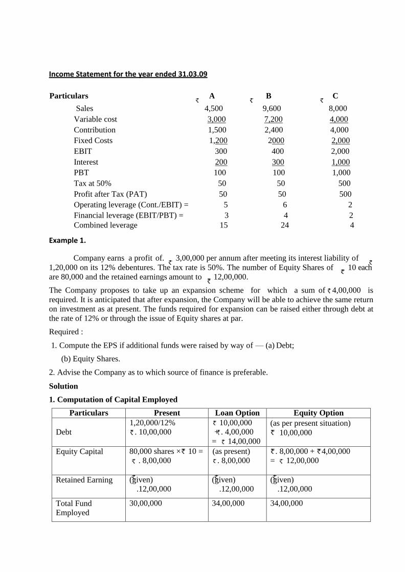
Income Statement for the year ended 31.03.09

Particulars A B C

Sales 4,500 9,600 8,000

Variable cost 3,000 7,200 4,000

Contribution 1,500 2,400 4,000

Fixed Costs 1,200 2000 2,000

EBIT 300 400 2,000

Interest 200 300 1,000

PBT 100 100 1,000

Tax at 50% 50 50 500

Profit after Tax (PAT) 50 50 500

Operating leverage (Cont./EBIT) = 5 6 2

Financial leverage (EBIT/PBT) = 3 4 2

Combined leverage 15 24 4

Example 1.

Company earns a profit of. 3,00,000 per annum after meeting its interest liability of

1,20,000 on its 12% debentures. The tax rate is 50%. The number of Equity Shares of 10 each

are 80,000 and the retained earnings amount to 12,00,000.

The Company proposes to take up an expansion scheme for which a sum of 4,00,000 is

required. It is anticipated that after expansion, the Company will be able to achieve the same return

on investment as at present. The funds required for expansion can be raised either through debt at

the rate of 12% or through the issue of Equity shares at par.

Required :

1. Compute the EPS if additional funds were raised by way of — (a) Debt;

(b) Equity Shares.

2. Advise the Company as to which source of finance is preferable.

Solution

1. Computation of Capital Employed

Particulars Present Loan Option Equity Option

Debt

1,20,000/12% . 10,00,000

10,00,000 + . 4,00,000

= 14,00,000

(as per present situation)

10,00,000

Equity Capital 80,000 shares × 10 = . 8,00,000

(as present) . 8,00,000

. 8,00,000 + 4,00,000 = 12,00,000

Retained Earning (given) .12,00,000

(given) .12,00,000

(given) .12,00,000

Total Fund Employed

30,00,000 34,00,000 34,00,000

2. Computation of EPS

Present EBIT = (3,00,000 + 1,20,000) = 4,20,000 for Capital Employed of 30,00,000.

So, Return on Capital Employed = 4,20,00 / . 30,00,000 = 14%.

Revised EBIT after introducing additional funds = . 34,00,000 × 14% = 4,76,000.

Particulars Present Loan Option Equity Option

EBIT at 14% 4,20,000 4,76,000 4,76,000

Less : Interest on Loans 1,20,000 1,68,000 1,20,000

EBIT 3,00,000 3,08,000 3,56,000

Less : Tax at 50% 1,50,000 1,54,000 1,78,000

EAT 1,50,000 1,54,000 1,78,000

Number of Equity Shares (given) = 80,000

EPS = EAT÷No. of ES 1.875 80,000 1,20,000

1.925 1.483

Conclusion : EPS is maximum under Debt Funding Option and is hence preferable.

Leverage Effect : Use of Debt Funds and Financial Leverage will have a favourable effect only if

ROCE > Interest rate. ROCE is 14% and Interest Rate is 12%. So, use of debt will have favourable

impact on EPS and ROE. This is called at “Trading on Equity” or “Gearing” Effect.