IES Transport Measures to Reduce Emissions in Hyderabad, India

RITES Ltd.

June 2004

IES TRANSPORT MEASURES TO REDUCE EMISSIONS IN

HYDERABAD, INDIA

TABLE OF CONTENTS

Table of Contents List of Tables List of Figures List of Annexures

Chapter 1 Introduction 1.1 Objective and Scope of the Study

Chapter 2 Study Methodology

2.1 Methodology 2.2 Collections and Preparation of Database for the Study 2.3 Transport Demand Modelling 2.4 Transport Demand Forecasting 2.5 Business-As-Usual (BAU) Scenario 2.6 Formulation of Policy Options 2.7 Estimation of Vehicular Emissions 2.8 Block Cost Estimates

Chapter 3 Existing Transport System in Hyderabad 3.1 Study Area 3.2 Primary Traffic & Travel Surveys 3.3 Traffic & Travel Characteristics 3.4 Vehicle Emission Surveys and Characteristics 3.5 Existing Bus Transport

Chapter 4 Transport Demand Modeling and Forecasting

4.1 Transportation Study Process 4.2 Trip Generation 4.3 Trip Generation and Attraction Models 4.4 Trip Distribution 4.5 Trip Distribution – Gravity Model 4.6 Gravity Model Formulation 4.7 Gravity Model – Calibration Process 4.8 Modal Split 4.9 Trip Assignment

4.10 Assignment Procedure

Chapter 5 Scenarios for more Effective Public Transit Service 5.1 Introduction 5.2 Business-as-Usual Scenario (BAU)

5.3 More effective bus transit service scenarios 5.4 MMTS Scenario 5.5 Vehicular Emissions 5.6 Broad Cost Estimates for More Effective Public Transit

Services Chapter 6 Traffic Management and Measures to Improve Traffic

Flow 6.1 Role on Traffic Management Measures 6.2 Traffic Management Corridors 6.3 Traffic Scenario on Traffic Management Scenario Corridors 6.4 Scenarios for Traffic Management And Measures to Improve

Traffic Flow 6.5 Business As Usual Scenario (BAU) 6.6 Flyover Scenario 6.7 GEP Scenario 6.8 Broad Cost Estimates for Traffic Management Measures

Chapter 7 Vehicle Technology / Training Measures Related to 2-

Stroke Vehicles 7.1 Introduction

7.2 Opinion & Technology Distribution Survey 7.3 Driving Habits of Two-Wheelers & Auto Rickshaw Drivers 7.4 Maintenance & Operation (M&O) Training Programs 7.5 Emission Reductions due to M&O Training Programs 7.6 Cost for M&O Training Programs 7.7 Evaluation

Chapter 8 Conclusions and Recommendations

8.1 Conclusions 8.2 Recommendations

LIST OF TABLES

Table No Title Table 3.1 Components of Different Districts in HUDA Area Table 3.2 Components of HUDA Area Table 3.3 Hyderabad Population Growth Table 3.4 Total Number of Vehicles Registered/on road in HUDA Table 3.5 Growth of Vehicles between 1993 and 2002 in HUDA Table 3.6 Peak Hour Approach Volume Table 3.7 Distribution of Major Road Network as per ROW Table 3.8 Distribution of Major Road Network as per Carriageway

Width Table 3.9 Distribution of Road Length by Peak Period Journey Speed Table 3.10 Peak hour Traffic Signal Time Table 3.11 Peak Hour Parking Accumulation Table 3.12 Pedestrian Volume Table 3.13 Distribution of Households According to Size Table 3.14 Number of Vehicle Owning Households by Type Table 3.15 Distribution of Households by Number of Cars Owned Table 3.16 Distribution of Households by Number of Scooters/Motor

Cycles Owned Table 3.17 Distribution of Individuals by Occupation Table 3.18 Distribution of Individuals by Education Table 3.19 Distribution of Households According to Monthly Household

Income Table 3.20 Distribution of Households According to Monthly Expenditure

on Transport Table 3.21 Modal Split - 2003 (Including Walk) Table 3.22 Modal Split - 2003 (Excluding Walk) Table 3.23 Modal Split - 2003 (Motorized Trips) Table 3.24 Purpose Wise Distribution of Trips - 2003 Table 3.25 Distribution of Trips by Total Travel Time Table 3.26 Sampling Locations along with the Sampling Date Table 3.27 RPM and TSPM (µg/m3) Concentrations in the Study Area Table 3.28 SO2 (µg/m3) Concentrations in the Study Area Table 3.29 NOx (µg/m3) Concentrations in the Study Area Table 3.30 Hourly CO (ppm) Concentrations in the Study Area Table 3.31 Hourly HC (ppm) Concentrations in the Study Area Table 3.32 Air Quality Exposure Index (AQEI) and Air Quality Categories

in the Study Area Table 3.33 Financial Status of APSRTC-Hyderabad City Region (Rs. in

million) Table 3.34 Total Tax Per Bus Per Year (2000-2001)

Table 4.1 Trip Production Models Attempted Table 4.2 Trip Attraction Models Attempted Table 4.3 Selected Trip Generation Sub-Models For Home Based One-

Way Work Trips Table 4.4 Selected Trip Generation Sub-Models For Home Based One-

Way Education Trips Table 4.5 Selected Trip Generation Sub-Models For Home Based One-

Way Other Trips Table 4.6 Calibrated Gravity Model Parameters

Table No Title Table 4.7 MNL Results For Households With No Access To Private

Vehicles Table 4.8 MNL Results For Households With Access To 2 – Wheelers Table 4.9 MNL Results For Households With Access To Cars Table 4.10 Calculated Mode Choice Elasticity Based On Reported

Average Time And Cost And Assumed Uncertainty Of 10 Minutes

Table 4.11 Types Of Roads And Their Capacities Table 4.12 Free Flow Speeds

Table 4.13 PCU Conversion Factors

Table 4.14 Comparison of Ground Counts And Assigned Trips Table 5.1 Modal Split for BAU Entire Study Area Table 5.2 Mode wise Daily Vehicle Kilometers – 2003 (BAU) for Entire

Study Area Table 5.3 Mode wise Daily Vehicle Kilometers – 2011 (BAU) for Entire

Study Area Table 5.4 Mode wise Daily Vehicle Kilometers – 2021 (BAU) for Entire

Study Area Table 5.5 Modal Split for More Effective Bus Transit Services for Entire

Study Area Table 5.6 Mode wise Vehicle Kilometers – 2011 (More Effective Bus

Transit Service Scenario) – Entire Study Area Table 5.7 Mode wise Vehicle Kilometers – 2021 (More Effective Bus

Transit Service Scenario) – Entire Study Area Table 5.8 Modal Split for MMTS Scenario Table 5.9 Mode wise daily Vehicle Kilometers – 2003, 2011 & 2021 Table 5.10 Speeds in kmph for Various Modes – MMTS Scenario Table 5.11 Estimated Daily Emissions for Study Area – BAU Table 5.12 Estimated Daily Emissions for BAU Scenario for Nine Major

Corridors Table 5.13 Daily Emissions With More Effective Bus Transit Scenario :

Entire Study Area Table 5.14 Estimated Emissions with More Effective Bus Transit

Scenario: Nine Major Corridors Table 5.15 Daily Emissions in MMTS Scenario Table 5.16 Reduction in Emissions for Various Scenarios Table 5.17 Broad Cost Estimates for More Effective Bus Transit Services

Sanatnagar – Nalgonda X Road Corridor Table 5.18 Broad Cost Estimates for More Effective Bus Transit Services

Panjugutta – Secunderabad Road Corridor Table 5.19 Cost Estimate for More Effective Public Transit Services

Total HUDA Area

Table 6.1 Sectionwise Peak Hour Traffic (Erragadda to Nalgonda ‘X’ Road) – 2000

Table 6.2 Sectionwise Peak Hour Traffic (Panjagutta to Secunderabad) – 2003

Table 6.3 Peak Hour Traffic Composition (Erragadda to Nalgonda X Roads Corridor) – 2003

Table No Title Table 6.4 Peak Hour Traffic Composition (Panjagutta to Secunderabad

Corridor) – 2003 Table 6.5 V/C Ratios – 2003 Table 6.6 Expected Traffic Speeds (kmph) for BAU and Flyover

Scenario (Sanatnagar to Nalgonda ‘X’ road corridor) Table 6.7 Emissions: Sanatnagar To Nalgonda ‘X’ Road BAU Scenario Table 6.8 Emissions: Sanatnagar To Nalgonda ‘X’ Road Flyover

Scenario Table 6.9 Reduction In Emissions Flyover From Sanatnagar To

Nalgonda ‘X’ Road Over BAU Scenario Table 6.10 Expected Traffic Speeds (kmph) for Removal of Side Friction

Scenario (Sanatnagar to Nalgonda ‘X’ road & Panjagutta to Secunderabad corridors)

Table 6.11 Emissions From GEP Scenario: Sanatnagar To Nalgonda 'X' Road (NH-9) – Identified Corridor-I

Table 6.12 Reduction In Emissions-GEP Scenario Sanatnagar To Nalgonda 'X' Road (NH-9) - Identified Corridor-I

Table 6.13 Emissions From GEP Scenario: Panjagutta To Secunderabad – Identified Corridor-II

Table 6.14 Reduction In Emissions-GEP Scenario Over BAU Scenario Panjagutta To Secunderabad – Identified Corridor-II

Table 6.15 Expected Traffic Speeds (kmph) for Providing and for effective utilization of Footpath Scenario (Sanatnagar to Nalgonda ‘X’ road & Panjagutta to Secunderabad corridor)

Table 6.16 Emissions from Separation of Vulnerable Road Users: Sanatnagar To Nalgonda 'X' Road (NH-9) - Identified Corridor-I

Table 6.17 Reduction In Emissions From Separation Of Vulnerable Road Users (Compared to BAU Scenario): Sanatnagar To Nalgonda 'X' Road (NH-9)

Table 6.18 Emissions From Separation Of Vulnerable Road Users: Panjagutta To Secunderabad

Table 6.19 Reduction In Emissions From Separation Of Vulnerable Road Users (Compared to BAU Scenario): Panjagutta To Secunderabad - Identified Corridor-II

Table 6.20 Synchronisation of Traffic Signals Erragadda to Maitrivanam Section & Ameerpet to KCP Section - Corridor No. 1

Table 6.21 Expected Traffic Speeds (Kmph) For Synchronization Of Traffic Signals And Junction Improvement Scenario (Sanatnagar To Nalgonda ‘X’ Road Corridor)

Table 6.22 Signal Coordination Scenario Emissions Table 6.23 Reduction in Emissions Due To Signal Coordination as

Compared to BAU Scenario Table 6.24 Broad Cost Estimates for Traffic Management Measures

Sanatnagar to Nalgonda ‘X’ Road Corridor

Table No Title Table 6.25 Broad Cost Estimates for Traffic Management Measures

Panjugutta to Secunderabad Corridor Table 7.1 Daily Emissions for BAU for 2 and 3 Wheelers Table 7.2 Daily Emissions (in Tons) after M&O Training Programs for 2-

Stroke Vehicles Table 7.3 Reduction in Daily Emissions due to M&O Training Programs

for 2-Stroke Vehicles Table 7.4 Cost Estimates for M&O Training Program Table 7.5 Cost Effectiveness of M&O Training Programs

LIST OF FIGURES

Figure 2.1 Methodology Adopted for the Study

Figure 3.1 Study Area Figure 3.2 Turning Movement Count Survey Locations Figure 3.3 Signal Time Survey Locations Figure 3.4 Parking Survey Locations Figure 3.5 Pedestrian Survey Locations Figure 3.6 Traffic Analysis Zonal Map of HUDA Figure 3.7 Ambient Air Quality Monitoring Stations Figure 4.1 Development of Trip Generation Models Figure 4.2 Distribution of HHS According to Vehicle Ownership and

Income Figure 4.3 Calibration of Gravity Model Figure 4.4 Mean Trip Length Frequency Distribution (Work Trips) Figure 4.5 Mean Trip Length Frequency Distribution (Education Trips) Figure 4.6 Mean Trip Length Frequency Distribution (Other Trips) Figure 4.7 Mean Trip Length Frequency Distribution (Total Trips) Figure 4.8 Conditional Multinomial Logit Model Design Figure 5.1 Layout of Exclusive Bus Lane for 6-Lane Divided

Carriageway Figure 5.2 Layout of Exclusive Bus Lane for 4-Lane Divided

Carriageway Figure 5.3 MMTS Corridors Figure 6.1 Demo Traffic Corridors Figure 6.2 Proposed Flyover on Demo Corridor

LIST OF ANNEXURES

Annexure 3.1 c Traffic Analysis Zones Annexure 3.2 Zone- wise Population Distribution Annexure 3.3 Zone-wise Employment Distribution Annexure 3.4 Zone-wise Distribution of Household Sample Size Annexure 3.5 Household Travel Survey by RITES for USEPA Annexure 3.6 Household Characteristics Annexure 3.7 Stated Preference Survey for Analysis of Various Transport Measures to

Reduce Vehicular Emissions in Hyderabad Annexure 3.8 Temperature (0c)and Wind Speed Levels in the Study Area Annexure 3.9 Average (24 hrly) SPM & RPM Concentrations in the Study Area Annexure 3.10 Average (24 hrly) SO2 & NOx Concentrations in the Study Area Annexure 3.11 Hourly CO & HC (ppm) Concentrations in the Study Area Annexure 3.12 National Ambient Air Quality Standards (NAAQAS) Annexure 3.13 Hyderabad City Region Bus Operations and Performance Characteristics Annexure 3.14 Comparative Fare Structure for Urban/Town Services of Various STUs Annexure 3.15 Comparative Statement of Motor Vehicle Tax for Stage Carriages (as on

March 2001) Annexure 4.1 Zone Wise Daily Trip Productions & Attractions (2003) –

Including/Excluding Walk Annexure 4.2 Daily Trip Productions & Attractions (Including Walk) Annexure 4.3 Daily Trip Productions & Attractions (Excluding Walk) Annexure 7.1 Two-Wheeler User’s Opinion Survey Annexure 7.2 Driving Habits of Two Wheelers and Autorickshaw Operators

CHAPTER - 1

INTRODUCTION 1.1 OBJECTIVE AND SCOPE OF THE STUDY 1.1.1 Hyderabad is one of the fastest growing centers of urban development in

India. This growth has also brought with it air quality and congestion problems. For a number of reasons, motorized two wheelers, auto rickshaws and private passenger cars, have displaced trip making which has been more traditionally accomplished by public transport and bicycle.

1.1.2 Traffic congestion, the predominance of two-stroke vehicles in the traffic mix

and inability of public (bus) transport to attract significant ridership have all been blamed for the severe air quality problems in Hyderabad especially the prevalence of Respirable Particulate Matter (PM10) as well as rapidly growing emissions of Greenhouse Gases (GHGs). The objective of this study is to carryout an analysis of policies to address these important areas of concern in Hyderabad’s transport sector. The scope of work for this study has the following three components:

(a) Scenario for more effective bus transit service. (b) Traffic management and measures to improve traffic flow. (c) Technology/Training measures relating to two-stroke vehicles.

1.1.3 However RITES has identified 3 more corridors in addition to the GEP Corridor (ESI Hospital to Khairatabad Junction, Length=4.6km) as a part of the study component on “Traffic Management & Measures to Improve Traffic Flow” (please refer to Figure 3.1 for details of study area). The corridors are: (i) Erragadda junction to ESI Hospital (NH-9), L=0.9km (ii) Khairatabad junction to Nalgonda ‘X’ roads (NH-9) via Nampelly Public

Garden and MJ Market, L=7.1km (iii) Panjagutta junction to Secunderabad Retifile bus station via Green

lands and Begumpet road, L=8.05km 1.1.4 However, the above (i) and (ii) corridors are extensions of the GEP Corridor.

Hence, the total selected corridors effectively are two. i.e., (a) Erragadda to Nalgonda ‘X’ road (b) Panjagutta to Secunderabad Retifile bus station

1.1.5 These analyses have been done as a part of the Integrated Environment

Strategies (IES) program being carried out by the Environment Protection Training & Research Institute (EPTRI) of Hyderabad with funding from USAID and USEPA.

1.1.6 USEPA has commissioned M/s ICF Consulting for carrying out this analyses, which, in turn engaged the services of RITES Ltd to accomplish these tasks.

CHAPTER - 2

STUDY METHODOLOGY

2.1 METHODOLOGY 2.1.1 Methodology adopted for the study is presented in Figure 2.1. Broadly, the

identified methodology comprises the following stages: i) Collection and Preparation of Database for the Study ii) Transport Demand Modeling iii) Transport Demand Forecasting iv) Business-as-Usual Scenario v) Formulation of Policy Scenario vi) Estimation of Vehicular Emissions vii) Block Cost Estimates viii) Evaluation of Policy Scenarios

2.1.2 The above stages are described briefly in the following paragraphs. More

details are given in the following Chapters.

2.2 COLLECTIONS AND PREPARATION OF DATABASE FOR THE STUDY

2.2.1 As a part of the study, various previous data/reports/maps were collected from various agencies and reviewed to assess the existing traffic scenario in Hyderabad. Secondary data such as population, employment, road network map, vehicle registration details, school enrollment and land use details were collected from various agencies viz., Census Department, Labour Office, Bureau of Economics and Statistics, HUDA, MCH, Department of School and College Education, Commercial Tax office and Industrial Department.

2.2.2 Following Primary Traffic and Travel surveys were also carried out to assess

the traffic and travel characteristics of the commuter traffic in study area. (a) Turning Movement Traffic Volume Count Survey along with Vehicle

Survey Occupancy at major junctions (29 locations) (b) Road Network Inventory Survey (c) Speed and Delay Survey (d) Traffic Signal Time Survey (e) Parking Survey (f) Pedestrian Survey (g) Passenger’s Opinion Survey (Public and Private modes) (h) Driving Habits of Two wheeler & Auto Rickshaw drivers (i) Household Travel Survey (Activity Diary & Stated Preference)

2.2.3 A special survey carried out as a part of this study was Stated Preference

survey of household travelers. The objective of this survey were to assess trade-offs among time, cost and reliability by commuters, develop performance goals to improve the existing bus transport system, and assess individual’s willingness to pay towards newer transport services.

2.2.4 Here it may be mentioned that the data collected from Household Travel Surveys and other surveys conducted as a part of project “Hyderabad Mass Rapid Transit System” has also been used to supplement the data collection exercise as a part of this study. The data collected was then analyzed to give traffic and travel characteristics for the year 2003.

2.3 TRANSPORT DEMAND MODELLING 2.3.1 In the present study, we have used in-house developed transport demand

modeling software. The 4-Step Transportation Study Process consists of development of formulae or models, enabling future travel demand to be forecasted and alternative strategies for handling this demand. In the present study, an attempt has been made to develop operational models. The normal and easily available planning variables at zonal levels such as population, employment, number of workers residing, number of students residing and student enrollment, etc. collected as a part of household survey and secondary data collected have been made use of in transport analysis. The study area has been divided into 129 Traffic Analysis Zones for the purpose.

2.3.2 Trip Generation: The first of the sub-models in the conventional study

process is that which predicts the number of trips starting and finishing in each zone. For the present study the regression analysis technique has been adopted for the development of trip generation sub models for home based one-way trips for various purposes. Attempts have been made to develop simple equations using normally available variables, which can be forecasted with reasonable degree of accuracy.

As part of this stage about 25 trip production models were developed for various purposes (work, education, others and total trips) with independent variables such as population, number (no.) of workers residing, no. of students residing, no. of cars, no. of 2 wheelers, average monthly income, accessibility rating (represented by no. of bus routes connecting a zone to other parts of the study area with assigned ratings of, 1(least connected), 2(medium connected) and 3(highly connected)), zone- wise no. of households, average household size and distance from CBD. Among the models developed it was found that zone wise no. of workers residing and no. of cars & no. of 2 wheelers are the most significant in estimating one-way work trips produced from each zone. For the models developed for one-way education trips produced from each zone, highly significant variable was no. of students residing in each zone. The one-way other purpose trips produced from each zone are most significantly related to zonal population and distance from CBD. 13 trip attraction models were developed for work, education and

other purposes by relating the purpose wise trips attracted to zone with independent variables such as zone wise employment, student enrollment, distance from CBD, accessibility rating and population. One-way work trips attracted to a zone were found to be statistically most significant to the zone wise employment. Zone wise student enrollment is significant in estimating one-way education trips attracted to a zone. Employment and accessibility rating were found to be most significant in estimating one-way other purpose trips attracted to each zone.

Accordingly the most significant trip production and attraction models were used along with projected values of the selected independent variables for 2011 and 2021 for estimating future zone-wise trip productions and attractions.

2.3.3 Trip Distribution: Trip distribution or inter-zonal transfers, is that part of transportation planning process which relates a given number of travel origins for every zone of the study area, to a given number of travel destinations located within the other zones of the study area. The gravity model with negative exponential deterrence function has been used in this study. The Gravity model has been validated by comparing the simulated and observed trip length frequency distributions for various trip purposes. The model thus developed has then been used to work out trip distribution for the years 2011 and 2021 for work, education and other trips with inputs of future zone-wise trip productions and attractions.

2.3.4 Modal Split: A total of 27000 choice set data points were collected as a part

of Stated Preference (SP) household survey and separate models were developed for respondents who had no access to any individual vehicle, those who had access to 2- Wheelers and those had access to cars. A multinomial logit model was developed to examine empirically how travelers trade-off among the attributes of price, time and reliability. The results from SP survey data analysis indicate that travelers are relatively more sensitive to time and reliability, and relatively less sensitive to cost. For all the groups reliability is relatively more important criteria than time. Among all groups, buses suffer from an image problem in Hyderabad and vehicle owners showed an inherent preferences for their own vehicle over buses.

In Business-as-Usual scenario it has been worked out that there will be substantial reduction in modal shares of bus and private vehicles, where as modal share of auto rickshaws would increase quite significantly. Based on the results obtained from modal split model, the modal shares for horizon years were derived for BAU and policy options.

2.3.5 Trip Assignment: Trip assignment is the process of allocating a given set of

trip interchanges to a specific transportation system and is generally used to estimate the volume of travel on various links of the system to simulate present conditions and to use the same for horizon years. Capacity Restraint Assignment Technique has been followed in this study.

The models developed were calibrated to synthesize the present day travel pattern and also validated by checking the assigned flows on various links with the ground counts after applying correction factors to account for additional trips that have not been taken care of in transport demand forecast exercise.

2.4 TRANSPORT DEMAND FORECASTING 2.4.1 For estimating the transport demand for the horizon years 2011 & 2021,

various model parameters (viz., Population, Employment, No. of workers residing, No. of Students Residing, Student Enrollment, etc) were projected for the year 2011 & 2021 and were inputted in the developed models as explained above to estimate the travel demand for future.

2.4.2 Zone wise population and employment were projected as per the Master Plan

for Hyderabad for 2020. The zone wise total no of vehicles were estimated based upon the income levels of households in each zone as estimated from household surveys. These households were classified into different vehicle owning groups. From this, zone wise total no of vehicles were derived. Income level of household was projected based on the Net State Domestic Product growth rates upto the years 2011 & 2021.

2.4.3 After forecasting the independent variables, zone wise future trip productions

and attractions were obtained by using the selected models for various purposes. Then the future trip production and attractions were distributed by using the trip distribution model developed. The modal split and trip assignment for BAU & policy options are explained in the following paragraphs.

2.5 BUSINESS-AS-USUAL (BAU) SCENARIO 2.5.1 The data collected from APSRTC and RTO office, indicates that there is

decline in the no. of passengers carried per bus and there is very heavy increase in the registration of 2-wheelers, cars and auto rickshaws. Heavy traffic of 2-wheelers, cars and auto rickshaws will reduce the bus speeds and further deteriorate the reliability of the bus. If such trend continues there will be increase in traffic congestion, which will lead to higher travel times. As the usage of private vehicles and Auto rickshaws increases, there will be increase in the vehicle kilometers traveled, which in turn will increase the vehicular emissions.

2.5.2 Under such a situation there will be increase in the headway for the buses. As

the no. of 2-wheelers and cars usage increases in future, there will not be enough supply for parking of the vehicles, which will result in increased parking cost and parking time. By considering these conditions, modal split for the years 2011 & 2021 were obtained from the modal split model developed. These trips were assigned on to future road network as given in Master Plan for Hyderabad - 2020 to derive the mode wise VKTs for the years 2011 & 2021 for BAU scenario. Average hourly volume and traffic speeds for private

and public modes were estimated for the years 2011&2021. With these speeds the assignment procedure was repeated again till the speeds on the road network were stabilized. After 5 such iterations, speeds on the road network were stabilized. Trip Distribution process was repeated by using the stabilized speeds to obtain the modified OD matrices. By applying the Modal Split model results, mode wise OD matrices were derived. These matrices were then assigned on to their respective networks to derive the VKT. This process has been carried out for the years 2011 & 2021.

2.6 FORMULATION OF POLICY OPTIONS 2.6.1 In Business-as-Usual (BAU) situation the vehicle kilometers traveled will grow

heavily, which will increase the pollution levels enormously. In order to address this problem 3 policy options were formulated. They are as follows: (a) Scenario for more effective public transit service (b) Traffic management and measures to improve traffic flow (c) Vehicle Technology/Training Measures related to two-stroke vehicles

2.6.2 Scenario for More Effective Public Transit Service: In this scenario following two options were tested i) More Effective Bus Transit Scenario ii) Multi Modal Commuter Transit System (MMTS)

i) More Effective Bus Transit Scenario This scenario was considered for the total study area i.e., HUDA and Nine major corridors including the two identified corridors for Traffic Management Scenario for the horizon years 2011&2021.

By providing dedicated bus lanes, properly designed bus stop/bays, priority for buses at signals, bus route rationalization, etc will have direct impact on speeds of bus, which in turn will increase the reliability of bus & reduce the travel time. The modified purpose wise OD matrices derived in BAU scenario were used to obtain the mode wise OD matrices by using the modal split model results. The modal split for the years 2011&2021 was worked out using the developed Multinomial Logit Model. After this, the mode wise trips obtained were assigned on to future road network to determine the Vehicle Kilometers Traveled by all modes for the year 2011&2021. Average hourly volume and traffic speeds for private and public modes were estimated for the years 2011&2021.

ii) MMTS Scenario Ministry of Railways, Government of India and Government of Andhra Pradesh are jointly developing Multi-Modal Commuter Transport Services in the twin cities of Hyderabad and Secunderabad for facilitating suburban commuter transportation. This is being done by upgrading the existing railway infrastructure along the two railway corridors. In this scenario, number of passenger trips that will shift to MMTS from various modes as against BAU scenario were assessed based on transport demand model by including the rail corridors in the transport network. When full MMTS is operational, the

number of vehicle kilometers of other modes would be reduced. The mode wise vehicle kilometers were then estimated for 2003, 2011 and 2021.

2.6.3 Traffic Management and Measures to Improve Traffic Flow: Various

Traffic Management measures have been proposed for improvement in traffic flow along the two identified corridors viz., Sanath Nagar to Nalgonda X Roads and Punjagutta to Secunderabad. A total of two scenarios have been developed for the these corridors as mentioned below: i) Flyover Scenario ii) GEP Scenario

i) Flyover Scenario A flyover of length about 12km is proposed on the first corridor from Sanathnagar to Nalgonda ‘X’ road with suitable number of up & down ramps. Accordingly road network with stabilized speeds was updated by adding flyover network. With this updated network, by using trip distribution model purpose-wise, OD matrices were derived and then mode wise OD matrices were obtained by applying the modal split model results. Then the traffic was assigned on to the updated network. Mode wise Vehicle kilometers Traveled (VKT) and traffic speeds were estimated for the flyover corridor for the years 2011 & 2021. This then has been compared with BAU scenario for the years 2011 & 2021.

ii) GEP Scenario In GEP Scenario the following measures have been considered for the two identified corridors: • Reduction of Side friction • Provision of Foot path • Synchronization of Traffic Signals along with junction improvements to

reduce intersection delays 2.6.4 Reduction of Side Friction: The zig-zag parking, on-street parking,

encroachments and presence of hawkers significantly reduce the effective carriageway width of roads. The provision of Guardrails, Signboards, and carriageway edge lines would result in increased road capacity as well as average speed. Speed-flow relationship was developed for base year for speeds on links with parameters such as traffic flow, side friction and link length for roads of various widths. By using this relationship, the traffic speeds in improved situation were calculated.

2.6.5 Provision of Footpath: The intermixing of vehicles and pedestrian

movements in the absence of footpaths results in reduced speeds and increase in number of accidents. The provision of footpaths and pedestrian crossings and traffic enforcement can reduce these conflicts to a great extent and increase the average speed of road traffic.

Speed-flow relationship was developed with availability or non-availability of footpath for the base year. This relationship was then used in estimating the speeds in improved situation.

2.6.6 Synchronisation of Traffic Signals along with Junction Improvements to

reduce Intersection delays: Signal coordination is one of the important measures in traffic management system. In this study, signal coordination exercise has been done by using TRANSYT 11 developed by TRL, UK. Signal coordination has positive impact on improving the traffic speeds. The junction improvements like signal coordination along with proper signages, zebra crossings, stop lines, removal of encroachments, provision of channelisers for free left traffic movement etc.. increases intersection capacity and reduces delays at the intersections. A total of 2 sections, comprising four junctions in each section of Sanath Nagar to Nalgonda X Road Corridor were coordinated. The corridor from Punjagutta to Secunderabad was excluded in this scenario because of presence of many flyovers, rotaries and non-signalized intersections. The analysis shows that there can be significant reduction in delays on the Sanath Nagar to Nalgonda X road corridor due to signal coordination when compared with BAU scenario. Expected traffic speeds were then worked out on this corridor with this scenario.

2.6.7 Vehicle Technology/Training Measures related to two-stroke vehicles: In

Hyderabad most of motorized auto rickshaws and 2-wheelers are powered by 2-stroke engines. These engines operate at relatively low compression ratios, do not burn fuels completely and burn a mix of gasoline and lubricating oil. These result in high CO2, hydrocarbon, CO and high particulate matter emissions. Poor maintenance levels of these vehicles leads to higher emissions. In order to reduce operation costs some of the operators adulterate the fuels, which exacerbates the emissions and engines degradation.

Emission levels of the 2-stroke vehicles can be reduced by better vehicle

maintenance and operations. Consultants have held meeting with officials of The Energy Research Institute (TERI), New Delhi to discuss about vehicle maintenance/training measures. During the discussions it was revealed that there could be better results by training the 2-wheeler and auto-rickshaw operators in good maintenance and operations practices. The discussions with these officials also revealed that due to better vehicle maintenance /training, emissions can be reduced by 10% to 20%. In our study, we have assumed that a conservative reduction of 10% in emissions due to better vehicle maintenance/training for car and 2-wheelers.

The penetration rate of the training is assumed to be 5% of 2-wheelers by

2011 and 8% by 2021. Similarly, a conservative estimates of penetration rates of 8% by 2011 and 15% by 2021 of 3-wheeler for the training programmes has been assumed.

2.7 ESTIMATION OF VEHICULAR EMISSIONS 2.7.1 The IVE (International Vehicle Emissions) Model developed jointly by

University of California, Riverside, College of Engineering – center for Environmental Research and Technology (CE-CERT), Global Sustainable

Systems Research (GSSR) and the International Sustainable Systems Research Center (ISSRC) has been used for estimation of emissions for BAU and policy options scenarios. The input data for running IVE model are mode wise vehicle kilometers traveled, vehicle startups, average speeds, altitude, humidity, temperature, mode wise driving style distribution, soak time distribution, fuel characteristics, etc. Mode wise driving style distribution, soak time distributions and mode wise vehicle technology distribution were taken to be the same as the Pune Vehicle Activity Study (India) carried out by CE-CERT.

2.7.2 IVE model was then run for BAU, More Effective Public Transit scenario and

Traffic Management and Measures to Improve Traffic Flow scenarios as discussed above to estimate the vehicular emissions for the years 2003, 2011 & 2021.

2.7.3 For vehicle/technology training measures, overall reduction in emissions has

been worked at assuming a certain level of reduction in existing in 2-stroke vehicles and their penetration rates for the years 2011 and 2021.

2.8 BLOCK COST ESTIMATES

Considering the proposed improvement measures for the various options, quantities have been estimated. Then the corridor wise preliminary cost estimates for the proposed improvement schemes have been worked out on the basis of the unit rates as prevalent in the region for such works. Similarly, assuming training cost per participant for the training programmes and target groups, cost of these training programmes has been worked out.

CHAPTER - 3

EXISTING TRANSPORT SYSTEM IN HYDERABAD 3.1 STUDY AREA 3.1.1 The study area is under jurisdiction of Hyderabad Urban Development

Authority (HUDA) and Secundrabad Cantonment Board. The total jurisdiction of HUDA is 1864.87 sqkm. The study area is shown in Figure 3.1. The Hyderabad Urban Development Area (HUDA) includes the Hyderabad District (excluding its parts falling in Secunderabad Cantonment Board area), substantial parts of Ranga Reddy District and a small portion of Medak District. The components of different districts in terms of area are as shown in Table 3.1.

Table 3.1

Components of Different Districts in HUDA Area District Total Area of

Distt. In sqkm Approx. area in HUDA jurisdiction in sqkm

Approx. % of area of total district

Hyderabad 217 173 80 Ranga Reddy 7493 1526 20 Medak 9699 166 2

Total 1865 100 Source: Draft Master Plan for Hyderabad Metropolitan Area-2020

3.1.2 The Jurisdiction of HUDA may also be considered as the Hyderabad

Metropolitan Area (HMA) if we add the small but significant Secunderabad Cantonment Area which is not part of HUDA area. The Secunderabad Cantonment Board is another 40.17 sq. km, making the Hyderabad Metro Area nearly 1905.04 sq. km.

3.1.3 The main components of HUDA area are shown in Table. 3.2.

Table 3.2

Components of HUDA Area S.No Components Area in sq.

km/Percentage Population-

2001 1. MCH 172.6(9%) 3632586 2. 10 Municipalities 418.58(22%) 1717617 3. Sec.bad Cantt.Board (SCB) NOT

PART OF HUDA 40.17(2%) 207258

4. Osmania University (OU), 13 Outgrowths (OG) & 4 Census Towns (CT) in HUA

146.82(8%) 194319

Sub Total for Hyderabad Urban Agglomeration (HUA)

778.17(41%) 5751780

S.No Components Area in Sqkm/Percentage

Population-2001

5. Other Parts of HUDA area namely Ghatkesar, Medchal and various rural areas not falling in HUA

1126.87(59%) 600000

Total HUDA area (taking in to account the SCB area)

1905.4 6383033

Total HUDA area (excluding the SCB area)

1864.87 6150000

Note: Sec.bad Cantonment Board is not part of HUDA area. Source: Draft Master Plan for Hyderabad Metropolitan Area-2020

3.1.4 The Hyderabad city population growth trend is shown in Table 3.3. During the

past 30 years, Hyderabad Metropolitan Area population has increased at about 4% p.a. It is expected to grow at the same rate for the next 20 years. As per Master Plan, the population for HUDA is expected to be 13.64 million in 2021.

Table 3.3

Hyderabad Population Growth Population (in ‘000) S.

No. Year

Urban Agglomeration HMA 1. 1971 1796 2093 2. 1981 2546 2994 3. 1991 4344 4667 4. 2001 5752 6383 5 2011* 9055

NATIONAL HIGH WAYS

MCH BOUNDARY

HUDA AREA BOUNDARY

RAILWAY NETWORK

LEGEND

Population (in ‘000) S. No.

Year Urban Agglomeration HMA

6. 2021* 13644 *Projected figures Source: Draft Master Plan for Hyderabad Metropolitan Area-2020

3.1.5 The total number of vehicles registered/on Road in HUDA area up to March,

2002 is given in Table 3.4.

Table 3.4 Total Number of Vehicles Registered/on road in HUDA

S.No

Type of Vehicle Hyderabad Dist.,

Ranga Reddy

Dist (RR)

Medak Dist.

Total HUDA Area=HYD+75%R

R+25%MEDAK 1 Private Stage Carriages 56 7 6 63 2 Goods Vehicles including TTs 40112 9809 3292 48292 3 Contract Carriages 876 200 314 1105 4 Taxi Cabs 4334 1486 331 5531 5 Auto Rickshaws 68493 2402 3098 71069 6 Private Service Vehicles 1125 379 66 1426 7 School Buses 590 248 47 788 8 Omni Buses 9014 1702 576 10435 9 Car & Jeeps 165764 24415 2559 184715

10 Two Wheelers 929768 242199 52364 1124508 Total 1220132 282847 62653 1447932

Source: Draft Master Plan for Hyderabad Metropolitan Area-2020

3.1.6 The percentage share and growth of vehicles in HUDA between 1993 & 2002 are given in Table 3.5.

Table 3.5

Growth of Vehicles between 1993 and 2002 in HUDA S.No

Categories 1993 2002 1993-2002 increase (%)

1 Buses 3836(0.66) 12391(0.86) 223.02 2 Auto rickshaws 23874(4.08) 71069(4.91) 197.68 3 Cars & Jeeps 66793(11.41) 184715(12.76) 176.55 4 Two Wheeler 467225(79.78) 1124508(77.06) 140.68 5 Goods Vehicles 16473(2.81) 48292(3.34) 193.16 6 Taxi Cabs 5333(0.91) 5531(0.38) 3.71 7 Pvt. Service Vehicles 2110(0.36) 1426(0.10) -32.42 Total 585644(100) 1447932(100) 147.24

Source: Draft Master Plan for Hyderabad Metropolitan Area-2020

3.1.7 The percentage of two-wheelers in total number of motor vehicles in Hyderabad is one of the highest in the country. It may be seen that almost all vehicles have increased significantly in the period 1993-2002. However, increase in buses is largely in inter-city or chartered bus operations. The growth of city buses has been minimal. But the high growth in personalized modes of transport and auto rickshaws has very much increased traffic on roads of Hyderabad.

3.2 PRIMARY TRAFFIC & TRAVEL SURVEYS 3.2.1 The following Primary Traffic and Travel surveys were carried out to assess

the traffic and travel characteristics of the commuter traffic in study area as a part of this study and the Hyderabad MRTS study: (j) Turning Movement Traffic Volume Count Survey along with Vehicle

Survey Occupancy at major junctions (29 locations) (k) Road Network Inventory Survey (l) Speed and Delay Survey (m) Traffic Signal Time Survey (n) Parking Survey (o) Pedestrian Survey (p) Passenger’s Opinion Survey (Public and Private modes) (q) Driver Habits of Two wheeler & Auto Rickshaw drivers (r) Household Travel Survey (Activity Diary & Stated Preference)

3.2.2 The data collected through the above field surveys has been analyzed to assess the present traffic and travel characteristics of the commuters in the study area. The detailed analyses of the surveys have been presented in the following paragraphs.

3.3 TRAFFIC & TRAVEL CHARACTERISTICS 3.3.1 Junction Approach Traffic Volume: Turning Movement Traffic Volume

Count Survey along with vehicle occupancy was carried out at total 29 major junctions, during peak period i.e., 8-12AM and 4-8PM on a typical weekday. The traffic data collected at each location was analyzed to assess the traffic flow characteristics. The survey locations are shown in Figure 3.2. The approach peak hour volume of traffic at survey locations is given in Table 3.6.

Table 3.6

Peak Hour Approach Volume Morning Peak Evening Peak S.

No JUNCTION NAME

Vehicles PCUs Vehicles PCUs 1 Erragadda Junction 11736 8799 8856 7294 2 ESI Junction 9523 7864 8999 7390 3 S.R.Nagar Junction 11399 8771 11124 8548 4 Maitrivanam Junction 10696 8207 11833 9109 5 Ameerpet Junction 9389 8330 12603 10249 6 Panjagutta Junction 16745 12751 17529 13072 7 Saifabad New Police Station Junction 14966 11598 14393 11978 8 Ravindra Bharathi Junction 15261 12519 14888 12017 9 Police Control Room Junction 17140 14090 16880 13094

10 L.B.Stadium Junction 12085 10635 12016 10420 11 A-1 Junction 14050 11861 16350 13395 12 Lata Talkies Junction 14365 11417 15632 12276 13 Goshamahal Junction 11982 9015 15717 12068 14 M.J.Market Junction 17860 13536 18915 14384

Morning Peak Evening Peak S. No

JUNCTION NAME Vehicles PCUs Vehicles PCUs

15 Putli Bowli Junction 7933 6631 10083 8066 16 Ranga Mahal Junction 11388 8819 10652 8743 17 Chadarghat Junction 23220 17820 25408 24565 18 Naigara Junction 12917 8980 13366 10345 19 Nalgonda ‘X’ Road Junction 13470 11013 11927 11233 20 Secunderabad Retifile Junction 8068 6430 6952 5909 21 Sangeet Cinema Junction 6946 5269 5822 4877 22 East Maradpally Junction 6819 5044 5986 4553 23 YMCA Junction 7284 6340 7797 6652 24 Hari Hara Kala Bhawan Junction 5591 4813 3617 3027 25 Plaza Junction 14565 11431 14397 11798 26 Parade Grounds Junction 8852 6265 8113 6435 27 NTR Junction 14275 10573 11714 9886 28 Green Lands Junction 18784 13548 21502 16028 29 Rajeev Gandhi Statue Junction 13005 9525 12847 9704

Source: RITES Primary Survey, 2003

It can be observed from above table that the maximum traffic is observed at Chaderghat junction with peak hour approach volume of 25408 vehicles (24565 PCUs).

3.3.2 Road Network Inventory Survey: The Road Network Inventory survey was

carried out along all arterial and sub-arterials roads in the study area as a part of Detailed Project Report (DPR) for Hyderabad MRTS Study in April 2003. The data collected as part of this survey included cross-sectional details such as Carriageway Width, ROW, footpath, median etc. The network comprised a total length of about 419 km.

3.3.2.1 The distribution of Road Network as per ROW is presented in Table 3.7. It

can be observed that that about 99% of road length has ROW less than 40m, which indicates that roads cannot be widened significantly to accommodate the growing traffic of personalized and IPT modes.

Table 3.7

Distribution of Major Road Network as per ROW ROW (M) Length (KM) Percentage

<20 174.50 41.66 20-30 240.80 57.48 30-40 0.00 0.00 >40 3.60 0.86

TOTAL 418.90 100.00 3.3.2.2 The distribution of the road network as per carriageway width is presented in

Table 3.8. It can be observed that about 40% roads are between 2-4 lanes and 60% roads are more than 4 lanes.

Table 3.8

Distribution of Major Road Network as per Carriageway Width Carriage way width (m) Length (KM) Percentage

>=2 and <4 lanes 171.20 40.87 >=4 & <= 6 lane 244.94 58.47

> 6 lane 2.76 0.66

TOTAL 418.90 100.00 3.3.3 Speed & Delay Survey: Speed & Delay Survey was conducted in a study

area as a part of Detailed Project Report (DPR) for Hyderabad MRTS Study in April 2003 using the Moving Car/ Test Car method during peak period. The results of the surveys with respect to the journey speeds are presented in the Table 3.9. It can be observed that more than half of the road length has speed below 20kmph. Average peak hour traffic speed is observed to be about 21kmph.

Table 3.9

Distribution of Road Length by Peak Period Journey Speed Traffic Stream S.No Journey Speed

(Km/hr) Road Length (Km.) Percentage (%) 1 < 10 1.48 0.35 2 10 – 20 221.56 52.89 3 20 – 30 151.28 36.11 4 30 – 40 37.76 9.01 6 >40 6.82 1.63 Total 418.90 100.00

3.3.4 Traffic Signal Time Survey: Traffic Signal Time survey was carried out at 25

major junctions of the two identified corridors of the study area for traffic management scenario. The survey was carried out during peak period on a typical weekday. Delays at these junctions were also noted down. The survey locations haven been shown in Figure 3.3. The peak hour cycle times for junctions are shown in Table 3.10.

Table 3.10

Peak hour Traffic Signal Time S.No NAME OF THE JUNCTION Peak Hour Cycle Time (Sec)

1 Erragadda Junction 75 2 E.S.I. Junction 80 3 S.R.Nagar Junction 127 4 Maitrivanam Junction 109 5 Ameerpet Junction 113 6 Panjagutta Junction 72 7 Khairtabad Junction 122 8 Saifabad New Police Station 88 9 Ravindra Bharathi 94

10 Control Room 104 11 L.B.Stadium Un Signalized 12 A - 1 Junction 76 13 Lata Takies 78 14 Goshamahal 59 15 M.J.Market 130 16 Putti Bowli Junction 59 17 Rangamahal 78 18 Chadharghat Junction 116 19 Niagara Junction Un Signalized

S.No NAME OF THE JUNCTION Peak Hour Cycle Time (Sec) 20 Nalgonda X Roads 65 21 Secbad Retifile Signals are not functioning 22 Sangeet Junction 100 23 East MarredPally Un Signalized 24 Y.M.C.A Un Signalized 25 Hari Hara KalaBhavan 127 26 Plaza Junction Un Signalized 27 Padade Grounds Junction 127 28 N.T.R.Junction 123 29 Green Lands Junction 57 30 Rajeev Gandhi Statue Un Signalized

3.3.5 Parking Accumulation Survey: Parking Accumulation survey was carried

out on the two identified corridors of study area for traffic management scenario. The survey was carried out for 12 hours on a typical weekday (10 am to 10 pm). The survey locations are shown in Figure 3.4. In the analysis, section wise parking accumulation has been established. The peak hour parking accumulation on major stretches are shown in Table 3.11. It is observed that most of the road stretches have high parking of two-wheelers, cars and auto-rickshaws.

Figure 3.3

Figure 3.4

Table 3.11

Peak Hour Parking Accumulation Parking Accumulation S.

No Location Direction Name of Section 2w Car Auto

Rick. Cycle Total ECS

Fantoosh to R.S. Fashion 39 5 4 7 20 R.S.Fashion to Hotal Abhilasha 25 16 14 14 39 1

Ameerpet to Shalimar Hotal Abhilasha to Shalimar 70 16 19 12 55

Swadesi Khadi Bhandar to Gopi Photo Studio 48 24 4 13 43

Gopi Studio to Chandana Bros 97 24 38 18 90 2 Shalimar to Ameerpet Chandana Bros to Shalimar 25 14 16 8 38

Mayuri Marg to Begumpet Airport 20 10 6 16 24 3

Mayur Marg to Begampet Air Port

Begumpet Airport to Mayuri Marg 42 22 14 12 49

3.3.6 Pedestrian Count Survey: Pedestrian Count survey was carried out at 6

locations on demo corridors of the study area. The survey was carried out for 12 hours on a typical weekday (8 am to 8 pm). The survey locations have been shown in Figure 3.5. The daily and peak hour pedestrian volumes at the survey locations are presented in Table 3.12. The analysis indicates quite high pedestrian traffic at these locations. The Peak Hour cross pedestrian traffic is highest at the Panjagutta Junction and M.J. Market Junction.

Table 3.12

Pedestrian Volume Daily Pedestrian

Volume Peak Hour Pedestrian

Volume S.No

Location

Along Across Along Across 1 Erragadda Junction 5524 5948 706 725 2 S.R.Nagar Junction 5160 7367 597 895 3 Ameerpet Junction 7969 8341 937 939 4 Panjagutta Junction 6283 7609 962 1125 5 M.J.Market Junction 8412 7350 1091 956 6 Khairatabad Junction 8648 5910 1402 908

3.3.7 Household Travel Survey - Hyderabad MRTS & Activity Diary Surveys 3.3.7.1 Zoning: The objective of the survey was to collect the socio-economic

characteristics of the Households and individual trip information and Activity Diary of the individuals from the household survey. The study area was divided into 129 zones. These 129 zones consist of MCH area, 10 Municipalities and remaining area of Hyderabad Urban Development Authority (HUDA) area. The division of the zones was carried out to obtain the zones with homogenous population. The traffic analysis zone map is shown in Figure 3.6. The list of traffic zones is presented in Annexure 3.1. The zone- wise land use parameters (population & employment) for base year 2003 and horizon years 2011 and 2021 have been estimated based on HUDA master plan and presented in Annexures 3.2 & 3.3.

Figure 3.5

3.3.7.2 Sample Size: A household travel survey for 5500 household samples was

collected as a part of Detailed Project Report (DPR) study for Hyderabad MRTS in April-May 2003. In addition to this about 1500 household surveys were carried out to get the information of Activity Diary of the individuals in the study area. 5500 samples of MRTS study have also been used for the analyses. Thus a total sample of about 7000 households has been made use of from all the traffic zones by random sampling basis. Stratification of the sample was done to cover various income groups. The zone wise distribution of sample size is given in Annexure 3.4.

3.3.7.3 Survey Format: The survey format covered the socio-economic profile of the

household providing details like Household size, Education Levels, Income, Vehicle Ownership, the individual trip information of the members of the household, which provides the details of all the trips performed on the previous day, by the household members and their complete activities performed. The survey format of Activity Diary survey is enclosed in Annexure 3.5.

3.3.7.4 Training Of Enumerators: The enumerators with minimum graduate

qualification were selected and were trained in-house by ICF and RITES experts to carryout the survey. Pilot survey was then carried out to obtain the response from the households and minor modifications were later incorporated in the proforma, based on the pilot survey. The pilot survey also helped in the training of the enumerators.

3.3.7.5 Field Survey: The survey was carried out after 6 PM on weekdays and

during daytime on weekends so that the head of the household and other members were available.

3.3.7.6 Output/Results: The following outputs are derived from the analysis of the

Household and Activity Diary surveys: zone wise distribution of the Households according to Household size, Household income and Vehicle Ownership, zone wise distribution of the individuals by their occupation, education and expenditure on transport, distribution of trips by mode and purpose, trip length frequency distribution by time.

Distribution Of Household By Size Distribution of households according to its family size is presented in Table.

3.13. The table indicates that only 2.08% of the households have 1 or 2 members. Majority of households (86%) have 3 to 6 persons per households. The average household size is 4.8.

Table 3.13

Distribution of Households According to Size S. No. Household by Size Number of HH Percentage

1 Up to 2 144 2.08 2 3 - 4 3374 48.78 3 5 - 6 2572 37.18 4 7 - 8 732 10.58 5 >8 95 1.37

Total 6917 100.00 Distribution of Household by Vehicle Ownership

Distribution of households owning motorized vehicles is presented in Tables 3.14 to 3.16. Table 3.14 indicates that 61% of households own two wheelers, 2% own car, and 10% households having both car and two wheelers, whereas 27% households have no motorized vehicle. Table 3.15 indicates in that only about 10% households have 1 car or more. However, Table 3.16 indicates that about 71% of households have one or more scooters/motor cycles.

Table 3.14

Number of Vehicle Owning Households by Type S No Type of Vehicle Number of Household

Owning Vehicle Percentage

1 Car 144 2.08 2 Scooter/M.Cycle 4227 61.11 3 Car & Scooter/M.Cycle 687 9.93 4 No Vehicles 1859 26.88

Total 6917 100.00

Table 3.15 Distribution of Households by Number of Cars Owned

S. No. No of Cars Owned Number of Sampled HH Percentage

1 No Car 6243 90.26 2 1 622 8.99 3 2 40 0.58 4 3+ 12 0.17

Total 6917 100.00

Table 3.16 Distribution of Households by Number of Scooters/Motor Cycles Owned

S. No.

No. of Scooters/ M. Cycles Owned Number of Sampled HH Percentage

1 0 2022 29.23 2 1 3935 56.89 3 2 791 11.44 4 3 133 1.92 5 4+ 36 0.52

Total 6917 100.0

Distribution of Individuals by Occupation Distribution of individuals of sampled households according to their occupation is presented in Table 3.17. It is observed that a little over 32% of individuals are engaged in Government Service, Private Service & Business. Interestingly the number of students is also accounted for by similar percentages.

Table 3.17

Distribution of Individuals by Occupation S.

No. Occupation Number of Individuals in Sampled Households Percentage

1 Govt. Service 2146 6.49 2 Pvt. Service 4759 14.39 3 Business 3937 11.90 4 Student 10376 31.37 5 House Wife 8421 25.46 6 Retired 1112 3.36 7 Unemployed 878 2.65 8 Others 1452 4.39 Total 33081 100.00

Distribution of Individuals by Education Distribution of individuals of sampled households according to their education is presented in Table 3.18. Graduates and post-graduates account for nearly 28% of the individuals. About 7% are illiterates.

Table 3.18

Distribution of Individuals by Education S.

No. Education Number of Individuals in Sampled Households Percentage

1 Below 10 th. Class 9612 29.06 2 10 th. Class 6503 19.66 3 Intermediate 5335 16.13 4 Graduate 7740 23.40 5 Post Graduate 1567 4.74 6 Illiterate 2149 6.50 7 Others 175 0.53 Total 33081 100.00

Distribution of Households by Monthly Household Income Distribution of Households according to monthly Income ranges is presented in Table 3.19. It is observed that about 44% of households have monthly income less that Rs. 5000 and another 34% have income between Rs. 5000-10,000 per month. The percentage of Household having monthly income more than Rs. 20,000 are only 4%. Average household income per month in the study area has been observed to be Rs. 7300.

Table 3.19 Distribution of Households According to Monthly Household Income S. No. Income Group Number of Sampled Households Percentage

1 < Rs. 5000 3039 43.94 2 Rs. 5000 - 10000 2337 33.79 3 Rs. 10000 - 15000 892 12.90 4 Rs. 15000 - 20000 335 4.84 5 > Rs. 20000 314 4.54 Total 6917 100.00

Distribution of Households by Monthly Expenditure on Transport Table 3.20 gives the distribution of the Households according to monthly expenditure on Transport. The table indicates that about 38% of Households spend less than Rs. 500 per month on transport and over 34% have monthly expenditure on transport ranging between Rs. 500-1000. Only 5% of Households are having more than Rs. 2000 expenditure per month on transport. Average monthly expenditure on transport per household is Rs. 835, which is more than 11% of the average household income.

Table 3.20

Distribution of Households According to Monthly Expenditure on Transport S.

No. Expenditure on

Transport Number of Sampled Households Percentage

1 Up to Rs. 500 2654 38.37 2 Rs. 500 - 750 932 13.47 3 Rs. 750 - 1000 1401 20.25 4 Rs. 1000 - 1250 530 7.66 5 Rs. 1250 - 1500 602 8.70 6 Rs. 1500 - 2000 409 5.91 7 > Rs. 2000 389 5.62 Total 6917 100.00

Distribution of Trips by Mode of Travel

Distribution of trips according to mode of travel is given in Tables 3.21 to 3.23. It is observed that 30% of the trips are walk trips. 31% the trips are performed by 2 Wheelers and 28% performed by bus. Trips performed by rail and cycle rickshaw are only 0.4%, where as trips performed by auto rickshaws, shared Auto and 7-Seaters are nearly 6%. Per capita trip rate for the base year 2003 is observed to be 1.203 including walk trips. If walk trips are excluded, share of two-wheelers in total demand goes upto 44% while the share of bus system becomes 40%. Per capita trip rate is observed to be 0.840 excluding walk trips.

Table 3.21 Modal Split - 2003 (Including Walk)

S.No. Mode No. Of Trips Percentage 1 Walk 2473970 30.21 2 Cycle 241003 2.94 3 2 Wheeler 2541161 31.03 4 Car 176605 2.16 5 Auto (3 seater) 412181 5.03 6 7 Seater 54578 0.67 7 Bus 2257244 27.57 8 Rail 18000 0.22 9 Cycle Rickshaw 13569 0.17 TOTAL 8188311 100.00

Table 3.22 Modal Split - 2003 (Excluding Walk)

S.No. Mode No. Of Trips Percentage 1 Cycle 241003 4.22 2 2 Wheeler 2541161 44.47 3 Car 176605 3.09 4 Auto (3 seater) 412181 7.21 5 7 Seater 54578 0.96 6 Bus 2257244 39.50 7 Rail 18000 0.31 8 Cycle Rickshaw 13569 0.24

TOTAL 5714341 100

Table 3.23 Modal Split - 2003 (Motorised Trips)

S.No. Mode No. Of Trips Percentage 1 2 Wheeler 2541161 46.54 2 Car 176605 3.23 3 Auto (3 seater) 412181 7.55 4 7 Seater 54578 1.00 5 Bus 2257244 41.34 6 Rail 18000 0.33 Total 5459769 100

Purpose wise Distribution of Trips Table 3.24 gives the purpose wise distribution of the trips. It is observed from the table that about 26% of the trips are performed for work and business purpose together, where as 19% trips are education and 7% for other purpose trips which includes shopping, social, health and recreation. 49% of total trips are return trips.

Table 3.24 Purpose Wise Distribution Of Trips - 2003

S. No. Purpose No. Of Trips Percentage 1 Work 2091356 25.54 2 Education 1541409 18.82 3 Others 547615 6.69

4 Return 4007931 48.95 TOTAL 8188311 100.00

Distribution of Trips by Total Travel Time

Distribution of trips according to Total Travel Time is given in Table 3.25. It is observed that about 65% trips are having travel time less than 30 min, however 27% of the trips are having travel time between 30 min-60 min, where as 8% of the trips are having travel time more than 60 min.

Table 3.25 Distribution of Trips by Total Travel Time

S. No. Travel Time (min) No.of Trips (Sampled) Percentage 1 0 - 15 14118 35.80 2 15 - 30 11638 29.51 3 30 - 45 6754 17.12 4 45 - 60 4036 10.23 5 60 - 75 1599 4.05 6 75 - 90 861 2.18 7 90 - 105 229 0.58 8 105 - 120 163 0.41 9 > 120 43 0.11 Total 39441 100.00

Other Household Characteristics

As a part of Activity Survey, other household characteristics were also collected and the results are given in Annexure 3.6.

3.3.8 Household Travel Survey-Stated Preference Survey Stated Preference (SP) survey was carried out to know the modal preferences of respondents. About 3500 household surveys were carried out to get the inherent modal preferences of the individual spread over the study area. The total 3500 samples were drawn from all the traffic zones by random sampling basis. Stratification of the sample was done to cover various income groups. The survey format covered the socio-economic profile of the household providing details like Household size, Education Levels, Income, Vehicle Ownership, the trip information of Head of the Household or regular trip Maker of the household and also SP survey choice sets (10 choices sets each) with improved modes and existing modes. The survey format of SP survey is enclosed in Annexure 3.7. The SP survey results have been used to assess the share of different modes in future for various policy options. The results are presented in later chapters of this report.

3.4 VEHICLE EMISISON SURVEYS AND CHARACTERISTICS 3.4.1 The present study has attempted to generate air quality data for a few

pollutants viz., Respirable Particulate Matter (RSPM or PM10), Total Suspended Particulate Matter (TSPM), Sulphur dioxide (SO2), Oxides of Nitrogen (NOx), Carbon monoxide (CO), and Hydrocarbons (HC) along with

atmospheric temperature and wind velocity along the two identified corridors of the study area for Traffic Management scenario.

3.4.2 Vehicular Emission Surveys 3.4.2.1 The vehicular emissions survey was carried out in the following demo

corridors: a) Sanathnagar/Erragada junction to Nalgonda X-Road (NH-9). b) Panjagutta junction to Secunderabad Retifile bus station via Green Lands

road, Begumpet road, S.P. Road, Hari Hara Kalabhavan. 3.4.2.2 The vehicular emissions monitoring was carried out in following locations (5

Junctions & 6 Mid Blocks) during typical working day continuously from 6 am to next day 6 am (24 hours) along with atmospheric temperature and wind speed measurements. In mid blocks sections, survey was carried out at one side/median of the road depending upon the site conditions. The ambient air quality monitoring stations are shown in Figure 3.7. The sampling locations along with the sampling date are shown in Table 3.26.

Table 3.26

Sampling Locations along with the Sampling Date Station Code Sampling Location Sampling Date

A Ravindra Bharathi Junction 03.03.03-04.03.2003B Ameerpet Junction 03.03.03-04.03.2003C Rajeev Gandhi Junction 04.03.03-05.03.2003D NTR/Rasoolpura Junction 04.03.03-05.03.2003E Sangeet Theatre Junction 05.03.03-06.03.2003F Nalgonda X Roads Junction 05.03.03-06.03.2003G Mid point of Hari Hara Kala Bhavan and Parade

Ground Fly Over 06.03.03-07.03.2003

H Chaderghat (Mid point) 06.03.03-07.03.2003I Erragada near Gokul Theatre (Mid point) 07.03.03-08.03.2003J Panjagutta near NIMS Hospital (Mid point) 07.03.03-08.03.2003K MJ Market near Care Hospital (Mid point) 07.03.03-08.03.2003

3.4.3 Air Quality Monitoring 3.4.3.1 Respirable Dust Samplers (ENVIROTECH-APM 460) were used for

monitoring. Monitoring was carried out on 24 hourly basis. RSPM was collected on Glass Fibre Filter Paper (Whatman) on 8 hourly intervals, while gaseous sampling (APM 411) was carried out for every 4 hours by drawing air at a flow rate of 0.5-0.6 LPM. CO was monitored with CO analyzer (NEOTOX-XL) and Hydrocarbons were monitored using portable GC analyzer (FOX BORO – OVA 128) at 1-hour interval. Temperature and Wind Speed were recorded using thermometer and anemometer respectively on hourly basis.

3.4.3.2 Particulate matter was determined gravimetrically. SO2 was determined by

West and Geake method and NOx was determined by Jacob-Hoccheiser method. TSPM, RSPM, SO2 and NOx were reported in µg/m3 at normalized temperature and pressure. CO and HC are reported in PPM.

3.4.4 Air Quality Exposure Index (AQEI) 3.4.4.1 For assessing the ambient air quality (AAQ) status, Air Quality Exposure

Index (AQEI) concept has been used. Among the various air quality indices, Oak Ridge- Air Quality Index (ORAQI) is found most useful in depicting ambient air quality parameters (SPM, SO2 and NOx) into a single value, as it clearly defines the AAQ status and also meets the criteria of uniform AQI, suggested by Thom and Off (1975). QRAQI is calculated using the equation:

ORAQI = (a ∑ Ci/Si)b

Where a and b are constants, Ci is monitored/predicted concentration of pollutant ‘i’ and S is National Air Quality Standard for pollutant i.

The constants a and b are estimated as a = 39.02 and b = 0.967, with the assumption that AQI 10 corresponds to back ground concentration levels of SPM, SO2 and NOx and AQI 100 corresponds to the pollutant concentration equal to the permissible standards. The above equation for three pollutants is

ORAQI = (39.02 ∑ Ci/Si) 0.967 The descriptor category are given below:

ORAQI Category

<20 Excellent 20-39 Good 40-59 Fair 60-79 Poor 80-99 Bad >100 Dangerous

3.4.5 Ambient Air Quality 3.4.5.1 Temperature and Wind Speed: The hourly recorded atmospheric and wind

speed during the study period at various locations is given in Annexure 3.8 respectively. The temperatures were in the range between 20.6 0C and 36.1 0C and the wind speed values were between 0.3kmph and 9.6kmph. The values recorded at different locations are more or less in the same range.

3.4.5.2 Particulate Matter: The 8 hourly observed TSPM and RPM values in the

study area at different monitoring stations are shown in Table 3.27. Maximum and minimum values of TSPM are 1061 µg/m3 and 344 µg/m3. Maximum values were observed at Sangeet Cinema Hall junction during 6-14 hrs, and minimum value at Chaderghat during 22-6 hrs. The maximum and minimum concentrations of RPM were 665 µg/m3 and 54 µg/m3, maximum value was observed at MJ market during 6-14 hrs and minimum value at Rajeev Gandhi junction during 22-6 hrs.

Table 3.27

RSPM and TSPM (µg/m3) Concentrations in the Study Area RSPM (µg/m3) TSPM (µg/m3)

Time Sample Code

Sampling Station

6-14 14-22 22-6 6-14 14-22 22-6 A Ravindra Bharati Junction 167 119 279 396 417 636 B Ameerpet Junction 242 143 152 445 293 403 C Rajeev Gandhi Junction 123 123 54 381 768 190 D NTR/Rasoolpura Junction 178 169 189 469 404 468 E Sangeet Theatre Junction 329 368 183 1061 871 444 F Nalgonda X Roads 112 268 225 558 646 754 G Harihara Kala Bhavan 169 235 224 463 550 372 H Chaderghat RUB 335 193 101 945 634 344 I Erragadda Junction 211 358 232 372 1057 369 J Punjagutta Junction 307 229 109 1126 759 785 K MJ Market Junction 665 387 594 1027 533 767

The variations in the average concentrations of SPM and RSPM for different locations are depicted in Annexure 3.9. The concentrations were observed to be high when compared to National Ambient Air Quality (NAAQ) Standards of TSPM 200 µg/m3 and RSPM 100 µg/m3 for commercial area respectively. Observed high levels reflect the base line conditions of surrounding area activities of study area.

3.4.5.3 Gaseous Pollutants: The 4 hourly values of SO2 and NOx are given in

Tables 3.28 to 3.29 respectively. The SO2 concentrations were in the range of 9.6 µg/m3 to 69.5 µg/m3, while NOx values are found to be in the range between 19.5 µg/m3 and 216.3 µg/m3. Maximum values of SO2 and NOx were observed at Chaderghat during 10-14 hrs, while minimum values of SO2 and NOx were observed at Ameerpet and MJ market during 22-2 hrs respectively.

The average Values of SO2 and NOx are shown in Annexure 3.10 respectively. The average values of SO2 and NOx are well below the prescribed standards of 80 µg/m3 for commercial area except at Chaderghat where the NOx value has exceeded the standard.

Table 3.28

SO2 (µg/m3) Concentrations in the Study Area Time Station

Code Sampling Station

6-10 10-14 14-18 18-22 22-2 2-6 A Ravindra Bharati Junction 26.0 44.7 35.0 22.5 13.6 17.0 B Ameerpet Junction 44.1 45.3 25.1 30.9 9.6 11.3 C Rajeev Gandhi Junction 14.8 38.9 48.7 28.6 14.8 15.9 D NTR/Rasoolpura Junction 18.8 26.8 32.0 25.7 9.6 15.9 E Sangeet Theatre Junction 18.2 24.0 21.1 18.8 13.6 21.7 F Nalgonda X Roads 36.6 21.1 22.8 38.9 12.5 18.2 G Harihara Kala Bhavan 21.7 14.2 29.2 18.8 11.3 31.5 H Chaderghat Rub 33.8 69.5 40.7 36.6 18.8 22.8 I Erragadda Junction 14.8 49.4 36.8 12.3 24.9 29.3 J Punjagutta Junction 44.1 11.9 25.1 22.8 13.0 14.8 K MJ Market Junction 21.1 11.3 13.6 18.8 13.0 18.2

Table 3.29

NOx (µg/m3) Concentrations in the Study Area Time Station

Code Sampling Station

6-10 10-14 14-18 18-22 22-2 2-6 A Ravindra Bharati Junction 62.2 124.1 97.6 50.1 35.0 34.3 B Ameerpet Junction 81.4 91.7 60.1 98.3 30.5 26.1 C Rajeev Gandhi Junction 53.9 71.1 81.4 59.1 29.1 31.2 D NTR/Rasoolpura Junction 52.2 75.2 95.5 94.2 29.1 35.0 E Sangeet Theatre Junction 51.5 49.8 39.5 58.4 24.7 56.3 F Nalgonda X Roads 125.1 57.7 79.0 65.3 20.2 45.7 G Harihara Kala Bhavan 43.6 23.0 79.0 64.2 29.1 74.2 H Chaderghat Rub 105.5 216.3 114.5 116.5 34.3 48.4 I Erragadda Junction 21.3 159.6 89.4 34.3 69.4 76.1 J Punjagutta Junction 104.8 23.6 59.4 60.8 29.1 25.7 K MJ Market Junction 40.2 21.2 35.1 39.5 19.5 34.3

The hourly CO and HC values are given in Tables 3.30 & 3.31 respectively. The CO values were in the range between 1.0 ppm and 17.7 ppm. Maximum values are observed at Ravindra Bharathi junction during 17:00 hrs and also at Rajeev Gandhi junction during 18:00 hrs. Minimum values are observed at NTR junction at 1:00 hr. The maximum hourly values of CO are observed to be high than compared to the standard of 3.5 ppm (on 1 hrly basis).

Table 3.30

Hourly CO (ppm) Concentrations in the Study Area Station

Code/Time A B C D E F G H I J K

6.00 6.0 2.0 3.5 1.5 3.2 3.2 1.5 4.0 2.0 2.6 3.3 7.00 4.3 2.8 5.2 2.2 2.7 3.8 2.7 8.2 2.8 2.3 5.7 8.00 8.2 3.5 6.3 5.5 7.0 4.0 3.0 13.7 3.5 3.8 9.3 9.00 11.5 7.0 10.3 11.8 12.3 8.8 13.0 15.0 7.0 12.2 9.2

10.00 14.7 3.5 10.7 16.5 14.5 11.0 14.0 17.2 3.5 13.2 10.0 11.00 13.8 3.7 12.7 15.5 13.3 10.3 13.7 15.8 3.7 14.0 10.3 12.00 12.8 4.8 13.0 8.2 15.0 15.8 13.5 11.7 4.8 12.3 6.0 13.00 11.5 4.0 13.7 2.8 5.7 11.3 7.8 9.5 4.0 3.7 2.8 14.00 10.7 2.8 12.7 4.8 3.0 9.2 3.5 12.5 2.8 2.3 3.2 15.00 13.0 2.3 13.0 4.0 4.5 7.8 3.2 14.2 2.3 4.2 4.2 16.00 12.2 3.3 13.0 4.7 6.7 7.5 9.8 12.0 3.3 6.8 4.0 17.00 17.7 7.2 18.3 14.0 13.8 13.0 15.0 12.8 7.2 12.7 6.3 18.00 19.5 5.8 17.7 13.0 16.2 11.0 13.8 20.2 5.8 13.2 8.8 19.00 20.5 6.7 20.0 13.5 15.2 14.3 11.7 23.5 6.7 12.8 9.8 20.00 16.8 3.8 15.3 12.3 15.3 14.7 4.7 17.3 3.8 13.3 9.8 21.00 8.0 4.7 11.0 7.3 6.0 15.7 4.2 13.2 4.7 7.8 5.8 22.00 3.2 1.8 9.0 3.2 2.7 11.8 3.3 9.7 1.8 2.6 3.7 23.00 2.8 2.2 3.2 1.7 2.5 14.2 4.0 7.2 2.2 2.3 3.5 24.00 2.5 2.2 2.3 1.2 2.2 13.3 3.8 4.7 2.2 2.3 2.3 1.00 3.2 1.3 2.7 1.0 1.5 6.7 4.7 3.7 1.3 1.3 2.2 2.00 3.3 1.3 2.0 1.6 1.2 3.0 3.0 2.7 1.3 1.8 1.0 3.00 1.5 1.5 2.7 1.6 1.2 1.5 2.8 2.8 1.5 2.0 1.0 4.00 2.0 1.3 3.8 1.6 1.5 3.1 1.3 2.8 1.3 2.5 1.2 5.00 3.0 2.3 2.6 1.7 3.3 3.6 2.0 4.0 2.3 2.4 3.9

Table 3.31

Hourly HC (ppm) Concentrations in the Study Area Station

Code/Time A B C D E F G H I J K

6.00 4.2 6.0 1.5 4.0 4.5 4.0 1.7 3.5 2.7 4.0 2.5 7.00 2.2 11.7 2.5 5.3 11.0 6.0 6.0 3.3 2.7 4.7 3.7 8.00 3.7 12.3 2.5 7.2 11.8 10.3 5.7 4.3 3.5 4.5 6.3 9.00 12.7 13.0 5.7 14.2 13.2 16.7 10.2 14.5 7.0 9.7 12.5

10.00 10.2 14.0 8.7 12.3 13.0 22.3 13.0 10.8 5.3 12.0 11.0 11.00 13.7 14.7 13.7 14.0 12.0 13.0 13.8 14.0 6.0 14.2 5.2 12.00 11.8 16.2 16.0 7.5 12.3 12.0 11.0 9.0 3.0 8.2 3.8 13.00 3.7 17.2 17.7 4.0 11.7 13.3 10.3 7.7 4.2 2.3 2.5 14.00 3.5 17.0 13.3 6.5 9.7 20.7 7.5 6.2 5.0 1.3 2.5 15.00 2.3 17.3 17.7 17.7 14.3 18.0 13.5 13.7 1.3 2.5 3.7

Station Code/Time

A B C D E F G H I J K

16.00 8.0 16.2 15.0 14.5 15.0 15.7 19.0 16.5 2.5 6.0 7.0 17.00 13.2 19.3 13.0 11.8 13.0 21.0 20.3 14.2 8.5 12.2 15.2 18.00 13.5 20.0 10.3 8.8 13.5 20.3 15.8 14.2 6.5 12.8 11.5 19.00 15.7 19.3 13.0 13.8 14.2 20.7 9.5 11.0 4.8 12.2 13.5 20.00 9.5 12.3 16.0 7.5 12.0 15.7 3.7 6.7 4.3 9.2 8.2 21.00 7.3 8.5 17.3 3.5 14.3 13.5 3.5 6.5 4.3 3.0 3.5 22.00 4.2 4.0 3.2 2.8 4.3 6.8 5.0 5.5 4.2 3.3 3.3 23.00 1.7 3.5 2.5 2.2 2.8 3.8 3.7 4.3 2.3 3.2 1.8 24.00 2.0 3.3 1.3 3.0 1.3 2.5 3.7 4.7 5.0 2.3 1.5 1.00 1.5 2.0 1.3 1.5 1.5 4.2 4.0 2.5 3.2 1.5 1.3 2.00 1.5 1.3 1.5 1.5 1.7 3.0 6.0 2.0 2.5 1.5 1.5 3.00 1.7 1.8 2.2 1.7 1.5 2.2 3.8 1.7 2.2 1.5 1.7 4.00 1.8 2.2 2.2 1.7 1.5 4.7 1.5 1.8 1.7 2.8 1.3 5.00 3.6 3.3 1.7 2.6 4.3 4.1 2.6 1.7 3.0 3.6 3.3

The HC concentrations were in the range between 1.3 ppm and 22.3 ppm with maximum value observed at Nalgonda X Roads junction during 10:00 hrs and with minimum value at Rajeev Gandhi junction during 24: 00 hrs to 1:00 hr. There are no prescribed standards for HC in the Indian context. The average values of CO and HC are shown in Annexure 3.11.

3.4.5.4 Ambient Air Quality Indices: There is a need to provide accurate, timely

and understandable information about air quality status in the region. Awareness of the daily level of air pollution is often important to those who suffer from illness, which are aggravated or caused by air pollution, as well as to the general public. A typical air pollution index is an interpretive technique, which transforms complex data on measured atmospheric pollutant concentrations into a single number or set of numbers in order to make the data more understandable.

An air quality standard predicts the maximum permissible limit for a particular pollutant to be present in the air so as not to cause any severe health and other damages. When two or more pollutants are present in air in significant amounts, the cumulative effect is observed. The AQEI gives an over all picture of air quality. The AQEI for TSPM, SO2, and NOx with respect to commercial standards of Central Pollution Control Board (CPCB) for all the 11 sampling locations are presented in Table 3.32.

Table 3.32

Air Quality Exposure Index (AQEI) and Air Quality Categories in the Study Area 24 hourly Avg. Conc.

(µg/m3) Station Code

Sampling Station

TSPM SO2 NOx

AQEI Category

A Ravindra Bharati Junction 295 27 67 103 Dangerous B Ameerpet Junction 201 28 129 112 Dangerous C Rajeev Gandhi Junction 346 27 54 104 Dangerous D NTR/Rasoolpura Junction 268 22 64 91 Bad E Sangeet Theatre Junction 499 20 47 125 Dangerous

24 hourly Avg. Conc. (µg/m3)

Station Code

Sampling Station

TSPM SO2 NOx

AQEI Category

F Nalgonda X Roads 451 25 66 127 Dangerous G Harihara Kala Bhavan 253 21 52 83 Bad H Chaderghat RUB 431 37 89 139 Dangerous I Erragadda Junction 332 35 75 101 Dangerous J Punjagutta Junction 675 30 51 159 Dangerous K MJ Market Junction 227 16 32 66 Poor

MJ market junction was observed to be having poor air quality while Hari Hara Kala Bhavan and NTR junction fall under bad air quality category and rest of the sampling locations were observed to be highly polluted and fall under dangerous category. The high air quality indices in the sampling locations reflect that the population residing in these areas are exposed to higher pollution levels which are bound to escalate in near future due to ever expanding population growth and related activities such as transport and growing commerce.

Hence, it is clear that most of the localities in Hyderabad are experiencing the air pollution stress and the trend is likely to worsen in near future if proper control measures are not implemented.

The National Ambient Air Quality (NAAQ) standards are presented in Annexure 3.12.

3.5 EXISITING BUS TRANSPORT INTRODUCTION 3.5.1 Introduction 3.5.1.1 APSRTC (Andhra Pradesh State Road Transport Corporation) is the largest

bus transport corporation in India. APSRTC finds its place in Guinness Book of World Records as the largest transport undertaking in the world with about 20,000 buses and 1.20 lakh employees. APSRTC bus services carrying large number of commuters both at urban and moffusil levels.

3.5.1.2 The existing public transport in Hyderabad mainly comprises bus system.

The bus services are being exclusively operated by the State run APSRTC. The modal share by the bus transit system in Hyderabad at present is about 40% of total vehicular transport demand. Ideally modal share should be more in favour of public transport for the city of size of Hyderabad. This shows that a large proportion of demand is being met by personalized and intermediate modes of transport, which is resulting in increased road congestion and higher emissions. The total bus fleet size in Hyderabad was 2605 in the year 2001-02 with 874 bus routes.

3.5.1.3 The total number of bus stops in Hyderabad City Region are about 1850. The

number of bus depots in Hyderabad City Region are 21 viz., Barkatpura, Faluknama, HCU, Mehdipatnam, Musheerabad, Rajendranagar, Diksukhnagar, Hayatnagar, Ibrahimpatnam, Midhani, Uppal, Contonment,

Hakimpet, Kushiguda, Ranigunj-I, Ranigunj-II, BHEL, Jeedimetla, Kutkatpally, Medchal and Miyapur Depots.

3.5.2 Hyderabad City Region Bus Operating Characteristics 3.5.2.1 The various operating characteristics of city bus system for Hyderabad City

Region are given in Annexure 3.13. It is apparent from the Annexure that bus fleet has been increasing steadily over the last 6 years. However, a disturbing fact is the reduction in number of passengers carried per day. Number of passengers carried per bus per day has decreased from 1500 in 1996-97 to 1180 in 2001-02. This indicates a 20% decrease in per bus productivity in last 6 years. Load factor has also decreased from 75% to 59% during this period although daily bus utilization has been more or less the same (about 240 km/day). The decreasing patronage of the available bus system indicates growing usage of motorized two wheelers and auto rickshaws ( 3 and 7 seaters). Incidentally whereas 3-seater auto rickshaw run as taxis, the 7 seater auto rickshaws run as stage carriage vehicles (illegally). Increased popularity of two wheelers and auto rickshaws is due to their lower operating costs, higher frequency/availability and door-to-door services. These vehicles instead of becoming complimentary have become competitors to the bus system. Due to mounting losses in city bus services, APSRTC has not been able to augment its fleet substantially. Passenger comfort level in buses has also declined. These factors have also contributed to proliferation and use of personalized and intermediate modes of transport. Higher use of two wheelers and auto rickshaws is leading to higher levels of vehicular pollution in the city. Higher average age of buses (about 7 years) is also contributing to the increased emission levels.

3.5.2.2 The large number of routes have come up due to popular demand for

operation of public bus system in various interior areas and also because of urban sprawl. This has resulted in two drawbacks. Firstly the bus system has become a ‘destination oriented’ system in low frequencies and poor quality of service. At the same time, buses have also to ply on narrow roads that are more suitable for operation of mini buses, auto rickshaws etc. that should act as feeders to buses. The buses, accordingly, compete with their feeder system. The congested roads increase the travel time of buses reducing their productivity and attractiveness. This is also resulting in 7-seater auto rickshaws competing with bus system on wide roads, where generally buses only should ply.

3.5.3 Fare Structure 3.5.3.1 The bus fare structure of APSRTC and other major State Transport

Undertakings (STUs) in India are presented in Annexure 3.14. This table indicates that fare rates are higher in Hyderabad than many of the other city bus services in India. This is specially so in the case of short distance travel. In this case, auto rickshaws compete favorably with buses in respect of fare structure. The auto rickshaws, because of the additional advantage of higher frequency and door-to-door service gain an edge over buses. With higher fares, commuters find two wheelers and auto rickshaws attractive. These modes, apart from lower operating costs / fares, offer better accessibility and

reduce travel time. With bus routing structure becoming more destination oriented than direction oriented, travel time of bus passengers is increasing. All these factors induce bus passengers to shift to other modes.

3.5.3.2 In 1994, APSRTC introduced metro liner and metro express buses with

better facilities and slightly higher fares than ordinary buses to capture the two and three wheeler users. They could achieve the objective and successfully captured a part of the two-wheeler traffic.

3.5.4 Bus Passes Scenario In Hyderabad City Region 3.5.4.1 Financial burden, due to concessional fares and free passes as announced

by the government, becomes inevitable to STUs. APSRTC also has to bear financial loss due to a large number of concessional passes and free passes.

3.5.4.2 The glance of bus passes in Hyderabad City Region (HCR) is given below:

• No of bus pass counters - 17 • Types of Passes Issued - 27 •

(Mainly Student pass (General), APSRTC employees pass, Student Route pass, Special Student General Bus Pass, Dist. Route Pass, Setwin Trainees bus pass, Greater Hyderabad Student Pass, General Commuter bus pass, Season ticket bus pass, NGOs Pass, Free pass for below 12 years, Girls free pass up to 10th class or up to 18 years, Physically Handicapped pass, Freedom fighters pass, Journalist, Special Privilege pass especially to CM/VVIP security staff). • Avg. no. of bus pass issues per month - 3.27 Lakh • Avg. no. of passes in Circulation per month - 5.05 Lakh • Amount Realised per month (Avg) - 8.00 Cr • Loss due to concessions on bus passes (Avg) per month- Rs.5.00 Cr

3.5.5 Financials Of The City Region 3.5.5.1 The following table shows a snapshot of the financials of APSRTC-

Hyderabad City Region for the last seven years are shown in Table 3.33.

Table 3.33 Financial Status of APSRTC-Hyderabad City Region (Rs. in million)

Year 1995-96 1996-97 1997-98 1998-99 1999-00 2000-01 2001-02REVENUE (Up to Feb’02)

Traffic Revenue 1652.980 1922.577 2216.606 2328.007 2613.040 2842.843 2458.264Hired Revenue 0.00 0.00 0.00 0.00 0.566 74.164 178.125 Other Revenue 26.383 21.887 35.218 35.725 36.882 44.476 44.825

1679.363 1944.464 2251.824 2363.732 2650.488 2961.483 2681.214EXPENDITURE Personnel Cost 811.667 875.587 1075.951 1183.719 1331.259 1357.699 1127.791Workshop Maintenance

80.580 94.663 99.860 94.367 112.105 104.687 84.911

Fuel Cost 304.330 351.172 434.832 455.788 594.743 752.780 690.254

Year 1995-96 1996-97 1997-98 1998-99 1999-00 2000-01 2001-02Tyres & Tubes 69.950 87.763 84.436 71.572 69.755 64.740 49.796 Stores & Lubricants 59.550 68.116 70.340 68.256 72.697 65.906 56.208 MV Taxes 199.992 285.738 330.928 347.760 390.485 423.950 335.360 Depreciation 150.704 155.475 136.881 128.482 130.731 118.543 132.544 Miscellaneous 31.125 43.250 42.452 48.041 47.790 48.779 54.988 Hire Charges 0.00 0.00 0.00 0.00 0.757 117.665 277.837 Suspense 0.00 0.00 0.00 0.00 14.236 30.167 19.314 R.O. Overheads 23.887 35.210 4.022 2.739 21.229 18.057 32.680 Z.O. Overheads 28.933 28.479 38.185 41.644 42.274 39.616 43.297 H.O. Overheads 43.308 28.278 23.601 92.491 6.343 147.777 191.423

1756.252 1983.311 2341.488 2534.859 2834.404 3193.918 3096.403LOSS -76.889 -38.847 -89.664 -171.127 -183.916 -23.2435 -415.189

Source: Ferguson & Co. Study Report, June 2002. 3.5.5.2 It can be observed from above table that the over the period of time, the

expenditure has been increasing faster than the revenue, leading to increase in loss. The losses are less than the loss due to the concessional passes. If Government were to compensate APSRTC for the loss in revenues due to concessional passes, then the Hyderabad City Region Bus System could have made some profits .

3.5.6 Motor Vehicle Tax Structure For Stage Carriages In India 3.5.6.1 The comparative motor vehicle tax structure of major cities have been

presented in Annexure 3.15. It is observed that in Karnataka, the taxes are 3% of the passenger revenue for city operation and 6% of the passenger revenue for rural operation against 10% and 12.5% respectively in Andhra Pradesh.

3.5.6.2 The total taxes and motor vehicle (M.V) Tax &permit fees per bus held per

year for various major state transport undertakings during 2000-2001 are presented in Table 3.34.

Table 3.34

Total Tax Per Bus Per Year (2000-2001) Total Taxes S.

No Name of the STU Rs. in

million Ps./Km

M.V.Tax and Permit fees per bus held per year (Rs)

Total Tax per bus held per year (Rs)

1 APSRTC 3687.6 169 192737 194639 2 MSRTC 3687.8 205 5188 218060 3 KnSRTC 330.8 67 80760 80760 4 BEST 265.6 109 4915 77449 5 CN-I&II 50.0 24 21485 21602 6 BMTC 77.0 45 34019 34019 7 DTC 240.2 65 6776 55485

Source: Association of State Transport Undertakings: Profile&Performance 2000-01,

3.5.6.3 It is observed from above table that the taxes in Andhdra Pradesh are very high as compared to other STUs except Maharasta. In 2000-2001, APSRTC paid an annual tax of about Rs. 1.94 lakh per bus per year. The APSRTC is paying tax about Rs. 470 per bus per day.

3.5.7 Motor Vehicle Taxes 3.5.7.1 The motor vehicle taxes of other modes are as follows:

• 2-Wheelers: 9% of cost of vehicle. It is about Rs. 300 per year • Car: 9% of cost of vehicle. It is about Rs. 3000 per year • 3-seater auto Rickshaw: Rs. 100 per quarter i.e., Rs. 400 per year • 7-seater auto Rickshaw: Rs. 200 per seat per quarter i.e., Rs.1200 per

quarter i.e., Rs. 4800 per year 3.5.7.2 A recent study carried out by ASCI (Administrative Staff College of India),

Hyderabad has indicated that a passenger traveling by a three wheeler 3-seater auto pays less than 1paise(ps) per trip as road tax, a seven seater auto pays 4 ps and a bus passenger pays 48ps as road tax per trip. A scooterist pays 19ps per trip and a car owner pays about 45ps per trip. Hence the passenger traveling by buses pays more taxes than a richer passenger traveling by a two or three wheeler. This lop sided taxation has resulted in 3-seater and 7-seater autos offering services some times at less than bus fares. It has resulted in two-wheeler travel becoming cheaper than bus travel and hence significant increase in two-wheeler population.

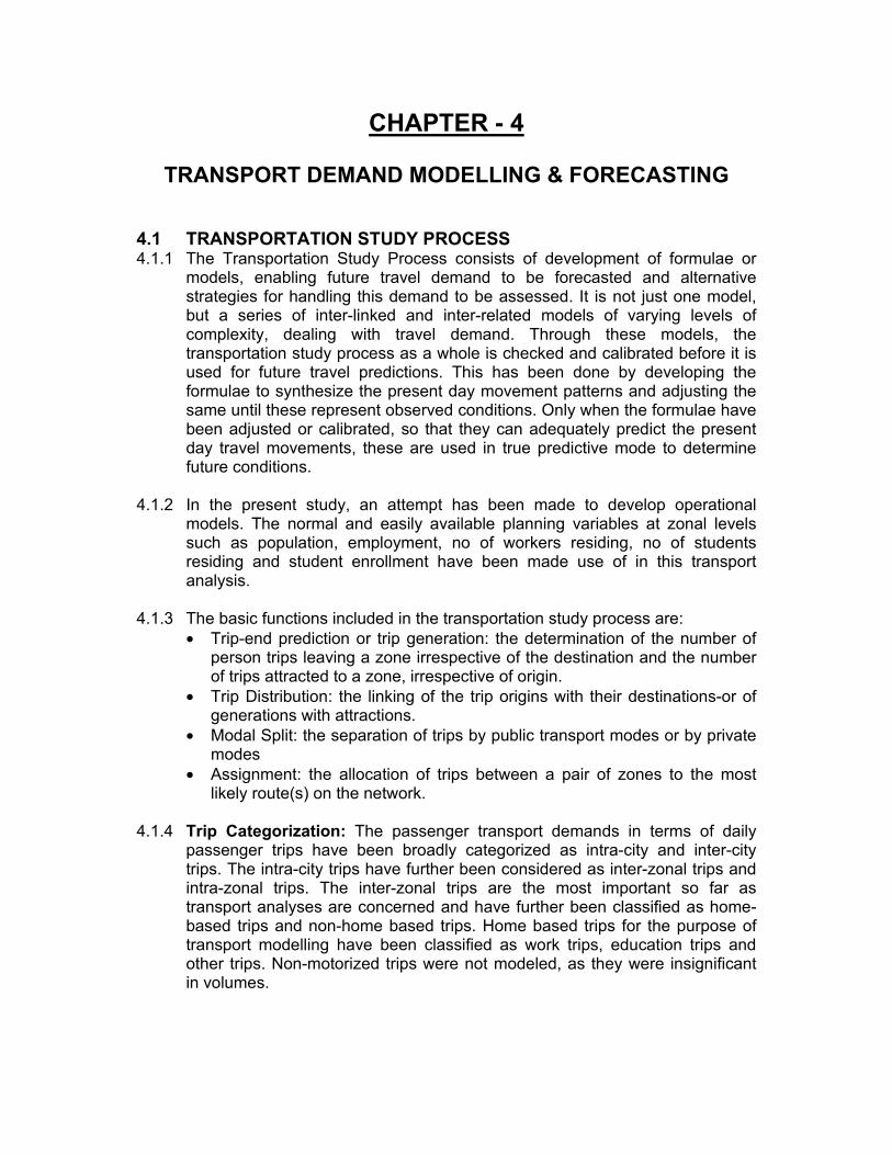
CHAPTER - 4

TRANSPORT DEMAND MODELLING & FORECASTING 4.1 TRANSPORTATION STUDY PROCESS 4.1.1 The Transportation Study Process consists of development of formulae or

models, enabling future travel demand to be forecasted and alternative strategies for handling this demand to be assessed. It is not just one model, but a series of inter-linked and inter-related models of varying levels of complexity, dealing with travel demand. Through these models, the transportation study process as a whole is checked and calibrated before it is used for future travel predictions. This has been done by developing the formulae to synthesize the present day movement patterns and adjusting the same until these represent observed conditions. Only when the formulae have been adjusted or calibrated, so that they can adequately predict the present day travel movements, these are used in true predictive mode to determine future conditions.

4.1.2 In the present study, an attempt has been made to develop operational

models. The normal and easily available planning variables at zonal levels such as population, employment, no of workers residing, no of students residing and student enrollment have been made use of in this transport analysis.

4.1.3 The basic functions included in the transportation study process are:

• Trip-end prediction or trip generation: the determination of the number of person trips leaving a zone irrespective of the destination and the number of trips attracted to a zone, irrespective of origin.

• Trip Distribution: the linking of the trip origins with their destinations-or of generations with attractions.

• Modal Split: the separation of trips by public transport modes or by private modes

• Assignment: the allocation of trips between a pair of zones to the most likely route(s) on the network.

4.1.4 Trip Categorization: The passenger transport demands in terms of daily

passenger trips have been broadly categorized as intra-city and inter-city trips. The intra-city trips have further been considered as inter-zonal trips and intra-zonal trips. The inter-zonal trips are the most important so far as transport analyses are concerned and have further been classified as home-based trips and non-home based trips. Home based trips for the purpose of transport modelling have been classified as work trips, education trips and other trips. Non-motorized trips were not modeled, as they were insignificant in volumes.

4.1.5 The non-home based trips and inter-city trips, which, do not form a significant proportion of total transport demand, are not being modeled. The proportion of non-home based trips was about 4.5% of total home-based trips as observed in base year (2003) for Hyderabad.

4.2 TRIP GENERATION 4.2.1 The first of the sub-models in the conventional study process is that which

predicts the number of trips starting and finishing in each zone. The techniques developed attempt to utilize the observed relationships between travel characteristics and the urban environment and are based on the assumption that trip making is a function of three basic factors: • The land use pattern and development in the study area • The socio-economic characteristics of the trip making population of the

study area • The nature, extent and capabilities of the transportation system in the

study area 4.2.2 Mathematically can be expressed as:

Trips Generated = Function (Socio-economic, locational, etc. variables) 4.2.3 Various techniques for developing trip generation models are available and

notable among these include: • Regression analysis • Category Analysis

4.2.4 In most of the studies conducted so far, generally least square regression

analysis technique has been used to develop trip generation models. For the purpose of present study the regression analysis technique has been adopted for the development of trip generation sub models for home based trips for various purposes. Attempts have been made to develop simple equations using normally available variables, which can be forecasted with reasonable degree of accuracy. Methodology adopted for developing trip generation models is presented in Figure 4.1.

4.2.5 A typical regression analysis trip generation model might be:

G = a1x1 + a2x2 + …………. + akxk + a0 Where G = Number of trips per zone for a specified purpose. a0, a1, a2, ….., ak = Coefficients determined by regression analysis. x0, x1, x2, ….., xk = Zonal planning input factors (Independent variables).

4.3 TRIP GENERATION & ATTRACTION MODELS 4.3.1 A number of trip production and attraction models for inter-zonal trips (both

motorized and non-motorized) were attempted. The trip production models / trip attraction models were developed relating zone-wise trips produced/trips attracted with a various independent variables. These production models are

SECONDARY DATA, REPORTS AND DOCUMENTS

HOUSEHOLD TRAVEL SURVEYS

TRAFFIC ANALYSIS ZONE WISE INPUT PARAMETERS VIZ.,

POPULATION/EMPLOYMENT /NO OF STUDENTS

RESIDING/NO OF WORKERS

RESIDING/TOTAL NO OF VEHICLES, ETC

TAZ WISE BASE YEAR (2003) PURPOSE WISE TRIP PRODUCTIONS /

ATTRACTIONS

REGRESSED FOR TRIP PRODUCTION /

ATTRACTION MODELS FOR VARIOUS INDEPENDENT

VARIABLES

SELECTION OF MOST SIGNIFICANT TRIP

PRODUCTION / TRIP ATTRACTION MODELS

FOR VARIOUS PURPOSES

INPUT PARAMETERS

PROJECTED FOR FUTURE

TAZ WISE FUTURE TRIP PRODUCTIONS / ATTRACTIONS

PURPOSE WISE

Figure 4.1 Development of Trip Generation Models

presented in Table 4.1 and attraction models are presented in Table 4.2. These tables also give the statistical significance of all variables tested. Models were built separately for work, education, other purpose trips and total trips. Models developed also include combination of the some independent variables. Zone wise trip productions and attractions for the year 2003 are presented in Annexure 4.1.

Tabl

e 4.

1 Tr

ip P

rodu

ctio

n M

odel

s A

ttem

pted

SI

No

TRIP

PU

RPO

SE

POPU

LATI

ON

N

O O

F W

OR

KER

S R

ESID

ING

NO

. OF

STU

DEN

TS

RES

IDIN

G

NO

OF

CAR

S N

O O

F 2

WH

EELE

RS

TOTA

L VE

HIC

LES

AVG

. M

ON

THLY

IN

CO

ME

AC

CES

SIB

ILI

TY

RA

TIN

G

ZON

E W

ISE

NO

O

F H

Hs

AVG

. HH

SI

ZE

DIS

TAN

CE

FRO

M C

BD

IN

TER

CEP

T R

SQ

UAR

EF

- VA

LUE

STA

ND

ARD

ER

RO

R

1 W

OR

K 0.

2854

(1

2.90

) -

- -

- 0.

041

(0.0

43)

- -

- -

- 70

6.57

0.

92

692

3150

.8

2 W

OR

K 0.

294

(37.

327)

-

- -

- -

- -

- -

- 68

1.95

0.

92

1393

31

40.7

3 W

OR

K -

0.86

22

(38.

61)

- -

- -

- -

- -

- 12

83.5

8 0.

92

1491

30

44.4

6

4 W

OR

K

- 0.

7355

(1

4.24

) -

- -

0.20

6(2

.708

) -

- -

- -

1242

.97

0.93

78

6.36

2971

.27

5 W

OR

K -

0.86

2 (3

8.41

) -

- -

- - 0

.002

(-0.0

3)

- -

- -

1306

0.

92

739.

6530

56.5

1

6 W

OR

K -

0.69

7 (1

2.76

) -

-0.1

25(-0

.66)

0.32

7(3

.34)

-

- -

- -

- 11

12.3

5 0.

93

536.

811

2939

.68

7 W

OR

K -

0.75

(1

4.64

) -

- -

0.18

7(2

.47)

-

723.

44

(2.2

50)

- -

- -1

97.0

1 0.

93

542.

9129

24.3

8 W

OR

K -

0.70

7 (1

3.21

) -

-0.2

2(-1

.17)

0.33

(3

.45)

-

- 84

3.72

(2

.64)

-

- -

-595

.16

0.93

42

3.62

2871

.75

9 W

OR

K -

0.86

6 (3

9.30

) -

- -

- -0

.039

(-0.4

6)

840.

433

(2.5

4)

- -

- -7

6.39

9 0.

92

516.

5 29

92.5

4

10

ED

UC

ATI

ON

0.

2341

(2

3.29

) -

- -

- -

- -

- -

- -4

03.8

0.

81

542.

6 40

02.8

9

11

ED

UC

ATI

ON

-

- 0.

6805

(2

2.32

) -

- -

- -

- -

- 63

6.36

0.

8 49

8.61

4141

.4

12

ED

UC

ATI

ON

0.

2342

(2

3.2)

-

- -

- -

- 0.0

169

(-0.1

54)

- -

- -

-262

.03

0.81

26

9.27

4018

.3

13

ED

UC

ATI

ON

-

- 0.

6808

(2

2.29

9)

- -

- 0.

085

(0.7

54)

- -

- -

- 96.

15

0.78

24

8.7

4148

.4

14

OTH

ER

S

0.06

27

(8.7

5)

- -

- -

- -

- -

- -

935.

9 0.

38

76.5

6 28

54.8

15

OTH

ER

S

0.06

27

(8.7

1)

- -

- -

- - 0

.006

(-0.0

75)

- -

- -

986.

68

0.38

37

.98

2866

.1

16

OTH

ER

S

0.08

(3

.99)

-

- -

- -0

.083

(-0.9

269)

- -

- -

- 88

8.14

0.

38

38.6

7 28

56.4

17

OTH

ER

S

0.05

01

(2.2

4)

- -

- 0.5

865

(-3.2

4)0.

1546

(1.3

3)

- -

344.

34

(1.1

00)

- -

- 11

6.64

0.

43

23.1

5 27

67

18

OTH

ER

S

0.05

05

(2.1

9)

- -

- 0.

064

(0.5

596)

- -

- -

- -

954.

64

0.38

38

.233

2862

.61

SI

No

TRIP

PU

RPO

SE

POPU

LATI

ON

N

O O

F W

OR

KER

S R

ESID

ING

NO

. OF

STU

DEN

TS

RES

IDIN

G

NO

OF

CAR

S N

O O

F 2

WH

EELE

RS

TOTA

L VE

HIC

LES

AVG

. M

ON

THLY

IN

CO

ME

AC

CES

SIB

ILI

TY

RA

TIN

G

ZON

E W

ISE

NO

O

F H

Hs

AVG

. HH

SI

ZE

DIS

TAN

CE

FRO

M C

BD

IN

TER

CEP

T R

SQ

UAR

EF

- VA

LUE

STA

ND

ARD

ER

RO

R

19

OTH

ER

S

0.06

36

(8.7

84)

- -

- -

- -

- -

- 36

.022

(0

.901

7)

540.

603

0.38

38

.633

2856

.97

20

TOTA

L TR

IPS

0.

0573

(1

1.88

) -

- -

- 0.

08

(0.3

86)

- -

- -

- 46

2.06

0.

9 58

5.6

658.

08

21

TOTA

L TR

IPS

-

0.75

5 (4

.69)

0.

682

(5.2

2)

- -

0.52

6(3

.078

) -

- -

- -

2319

.01

0.91

42

3.72

6632

.53

22

TOTA

L TR

IPS

0.

5978

(1

2.48

) -

- -

- -0

.157

(-0.0

75)

- 20

36.5

9(2

.74)

-

- -

-289

4.61

0.

91

413.

0867

09.6

23

TOTA

L TR

IPS

0.

5913

(3

4.33

) -

- -

- -

- -

- -

- 12

14.0

5 0.

9 11

78.9

6857

.78

24

TOTA

L TR

IPS

-

- -

- -

- -

- 53

6.23

9 (1

4.89

) -

- 36

52.8

0.

64

221.

7613

270.

4

25 N

O O

F TR

IPS

P

ER

HH

-

- -

- -

- -

- -

0.33

84(1

.872

9)-

1.37

48

0.03

3.

5 0.

847

Not

e: (V

alue

s ab

ove

repr

esen

t Co-

effic

ents

for t

he P

aram

eter

s)

(Val

ues

in b

rack

etsa

repr

esen

t "t"

stat

istic

s of

the

para

met

ers)

Tabl

e 4.

2 Tr

ip A

ttrac

tion

Mod

els

Atte

mpt

ed

TRIP

PU

RPO

SE

EMPL

OYM

ENT

STU

DEN

T EN

RO

LLM

ENT

POPU

LATI

ON

DIS

TAN

CE

FRO

M C

BD

(K

M)

AC

CES

SIB

ILI

TY R

ATI

NG

INTE

RC

EPT

R S

QU

AR

E F

- VA

LUE

STA

ND

AR

D

ERR

OR

1 W

OR

K

0.40

8 (2

.841

) -

- -

- 10

074.

477

0.05

9 8.

07

2035

8.45

2 W

OR

K 0.

4457

(3

.300

) -

- -1

143.

62

(-4.

32)

- 20

541.

83

0.18

1 13

.936

8 19

074.

339

3 W

OR

K -

- -

-108

8.26

7(-3

.968

) -

2670

1.23

6 0.

1103

15

.75

1980

3.41

4 ED

UC

ATIO

N

- 0.

419

(10.

023)

-

- -

4975

.195

0.

441

100.

4688

10

700.

46

5 ED

UC

ATIO

N

(EXC

LUD

ING

W

ALK

) -

0.82

59

(9.8

7)

- -

- 92

2.03

0.

44

97.5

8 94

74

6 O

THE

RS

0.

0599

(1

.824

6)

- -

- -

3344

.34

0.02

55

3.32

9 46

52.8

49

7 O

THER

S

- -

- -1

59.5

8 (-2

.505

) -

5783

.21

0.04

7 6.

275

4601

.15

8 O

THE

RS

0.

019

(0.5

19)

- 0.

03

(2.2

6)

-138

.57

(2.1

86)

- 36

80.6

45

0.11

3 5.

338

4473

.075

9 O

THER

S

- -

0.03

4 (3

.026

) -1

33.2

4 (-2

.136

) -

3723

.514

4 0.

111

7.91

8 44

60.1

10

OTH

ER

S

0.06

5 (2

.032

) -

- -1

67.7

06

(-2.6

59)

- 48

79.3

3 0.

077

5.28

45

45.4

5

11

OTH

ER

S

0.06

1 (1

.91)

-

- -8

1.47

2 (-1

.057

) 11

54.2

11

(1.9

08)

1884

.56

0.10

3 4.

808

4498

.51

12

OTH

ER

S

0.05

8 (1

.823

) -

- -

1529

.17

(3.1

20)

422.

388

0.09

5 6.

647

4500

.62

13

TOTA

L TR

IPS

0.

374

(1.8

43)

2.34

5 (9

.23)

-

9502

.6

0.44

1 49

.64

2820

0 N

ote:

(V

alue

s ab

ove

repr

esen

t Co-

effic

ents

for t

he P

aram

eter

s)

(V

alue

s in

bra

cket

s re

pres

ent "

t" s

tatis

tics

of th

e pa

ram

eter

s)

4.3.2 Various trip production models for one-way work trips were developed relating zone wise work trips produced with following independent variables:

i). Population ii). Total number of vehicles (no of cars & 2 wheelers combined), iii). No of workers residing in the zone iv). Average household monthly income v). No of cars vi). No of 2 wheelers vii). Accessibility rating (represented by no of bus routes connecting to a

zone to other parts of the study area with assigned ratings –1(least connected), 2 (medium connected) and 3(highly connected))

4.3.3 It was observed from all the models tested that the variables No of Workers

Residing in the zone and zone wise Total no of cars and 2 wheelers are highly significant in estimating one-way work trips produced from a zone.

4.3.4 Attraction models for one-way work trips attracted to a zone were related to

independent variables i). Employment ii). Distance from CBD

4.3.5 From the models developed it was found that zone wise employment is the

most significant in estimating the one-way work trips attracted to a zone. 4.3.6 The selected statistical significant models for one-way work trips produced/

attracted from / to a zone by all modes are presented in Table 4.3.

Table 4.3 Selected Trip Generation Sub-Models For Home Based One-Way Work Trips

Dependent Variable

Independent Variable Constant Term

Co-efficient

R2 Value

Work Trips Produced No of Workers Residing 1242.97 0.7355

(14.24) 0.9258

No. of Cars and 2 Wheelers - 0.206 (2.708)

Work Trips Attracted Employment 10074.48 0.408

(2.841) 0.059

4.3.7 One-way education trips produced from a zone were related to following

independent variables: Population

i). of students residing ii). Average Household Monthly Income

4.3.8 From all the variables tested it was found that no of students residing in zone

is the most significance in estimating education trips produced from a zone. 4.3.9 One-way education trips attracted to a zone were related to zone wise student

enrollment. Student enrollment is found to be most statistically significant in estimating the education trips attracted to a zone.

4.3.10 The selected statistical significant models for one-way education trips

produced / attracted from / to a zone by different modes are given in Table 4.4.

Table 4.4 Selected Trip Generation Sub-Models For Home Based One-Way

Education Trips Dependent

Variable Independent Variable Constant

Term Co-efficient R2

Value Education Trips Produced

No of Students Residing 636.36 0.6805

(22.32) 0.7969

Education Trips Attracted Student Enrollment 4975.195 0.419

(10.023) 0.441

4.3.11 Trip production model for one-way other purpose trips from a zone were

related with following independent variables: i). Population ii). Average Household Monthly Income iii). No of Cars iv). No of 2 wheelers v). Accessibility Rating vi). Distance from CBD

4.3.12 Of all the models developed it was observed that the combination of Zone

wise population and Distance from CBD are the most significant in estimating Other purpose trips produced from the zone.

4.3.13 One-way other purpose trips attracted to a zone were related with following

independent variables i). Employment ii). Accessibility Rating iii). Distance from CBD iv). Population

4.3.14 From the models developed it was observed that zone wise employment and

Accessibility Rating were statistically most significant in estimating other purpose trips attracted to a zone.

4.3.15 The most significant models considered for one-way home based other

purpose trips produced / attracted from / to a zone are presented in Table 4.5. Table 4.5

Selected Trip Generation Sub-Models For Home Based One-Way Other Trips

Dependent Variable

Independent Variable Constant Term

Co-efficient R2 Value

Population 540.603 0.0636 (8.784) 0.3703 Other Trips

Produced

Distance from CBD - 36.022 (0.9017)

Employment 422.388 0.058 (1.823) 0.095 Other Trips

Attracted

Accessibility Rating - 1529.17 (3.12)

4.3.16 Future population, employment were derived from Master Plan for

Hyderabad-2020. For estimating zone wise total no of vehicles for base year, total no of households were distributed according to the vehicle ownership viz., no vehicle owning, 1 vehicle owning, 2 vehicles owning, 3 vehicles owning, 4 vehicle owning and 5 & more vehicle owning households as obtained from household survey. Zone wise households were also classified according to household monthly income as obtained from household survey. Zone wise no of households in each income group were classified into various vehicle ownership groups. From this total no of vehicles in each zone were derived. Figure 4.2 shows the relationship between HH Income and HH vehicle ownership. Based on yearly growth rate of State Domestic Product it is observed that there is linear trend when extrapolated gives the growth rate as follows

Year By Linear Trend (p.a) Adopted (p.a) 2011 15% 10% 2021 25% 12%

4.3.17 Assuming Inflation Rate of 4% the net Income may grow at the rate of 6% up

to 2011 and 8% thereon. Above procedure is repeated to obtain the total no of vehicles zone wise for the years 2011 & 2021 after classifying the households according to income and by using the relationship between household income and vehicle ownership.

4.3.18 Total daily home-based inter-zonal motorized trips expected to be produced /

attracted in the study in the years 2011 & 2021 are 7,706,332 and 11,833,056 against 5,459,769 trips in the year 2003. Considering the selected trip production / attraction models and projected parameters for the selected independent variables, zone wise trip productions and attractions for the years 2011 and 2021 were derived, which are presented as Annexures 4.2 and 4.3.

4.4 TRIP DISTRIBUTION 4.4.1 Trip distribution or inter-zonal transfers, is that part of transportation planning

process which relates a given number of travel origins for every zone of the study area, to a given number of travel destinations located within the other

Fig 4.2 DISTRIBUTION OF HHS ACCORDING TO VEHICLE OWNERSHIP AND INCOME

0.0010.0020.0030.0040.0050.0060.0070.0080.0090.00

0-20

00

2000

-500

0

5000

-100

00

1000

0-15

000

1500

0-20

000

2000

0-30

000

>300

00INCOME

% O

F H

OU

SEH

OLD

S

NO VEHICLEOWNING HHS (%)1 2W OWNINGHHS(%)2 & MORE 2WOWNING HHS (%)1 CAROWNINGHHs(%)2 AND MORE CARSOWNING HHs(%)CAR & 2W OWNINGHHS(%)

zones of the study area. It is not necessarily concerned with the mode of travel used for neither a given trip nor the routes, which could be taken to complete this trip. Rather it is concerned with establishing links between a number of zones for which trip generation calculations have primarily been made. In other words, the output of trip generation sub-models becomes the input for trip distribution model.

4.4.2 Various mathematical procedures have been developed and used for this

purpose and these tend to fall in two main groups as under: • Analogous or Growth Factor methods in which growth factors are applied

to present day travel inter-zonal movements. • Synthetic or inter-area travel formulae in which as attempt is made to

understand the casual relationship behind patterns of movement, by assuming them to be similar to certain laws of physical behavior. Once understood, these casual relationships are projected into future and the appropriate travel pattern is synthesized.

4.4.3 Despite the diversity of formulation used in the various mathematical

procedures developed, the underlying principle in all trip distribution models is the same. “ Travel between any two points will increase with attraction for such travel, but decreases as the resistance to travel increases. ”

4.5 TRIP DISTRIBUTION: GRAVITY MODEL 4.5.1 The gravity model is the most widely used synthetic method of trip distribution,

because it is simple to understand and apply, and is well documented. For any given trip purpose, the generalized relationship is more usually expressed as Tij = K Pi Aj F(Cij) Where Tij = Trips from zone i to j K = A constant Pi = Total number of trips produced from zone i Aj = Total number of trips attracted to zone j F(Cij) is the deterrence or trip decay function and is based on the generalized cost of the journey from zones i to j.

4.5.2 The deterrence function is usually in one of the three basic forms: A power function F(Cij) = Cij

– α An exponential function F(Cij) = e – αc

ij A gamma function attributed to J.C. Tanner F(Cij) = e – αc

ij– βc

ij Where α & β are impedance parameters.

4.5.3 It has been found that power function is more appropriate to longer distances,

basically for inter-urban trips. The exponential function has been used in many studies and has been found to be particularly appropriate in short-distance intra-urban trips. The tanner function, which is the combination of power and exponential function, offers the opportunity to combine the advantages of each of these functions.

4.5.4 The constant K in the general formula is effectively two balancing constants a

and b combined together, one each for correcting the number of generations and attractions. Thus

K = ai bj Where Pi = ai Ej Tij Aj = bj Ei Tij The determination of each of the constants in the distribution model is known as calibration.

4.5.5 For the purposes of analyses in this study, the exponential forM (e- αc

ij) impedance function has been utilized to have comparisons with earlier studies carried out for Hyderabad. The Cij values, which should normally be based on generalized cost, have been taken only in terms of travel time for different modes due to non-availability of required data. Travel time matrices have been computed and “skim trees” built representing shortest travel paths between each pair of zones taking the congestion into consideration.

4.6 GRAVITY MODEL FORMULATION 4.6.1 For the purpose of distribution of home based trips, the formulation of gravity

model used is as under: Tij

n = Pin Aj

n exp(-an Cijm) / Ej Aj

n exp(-an Cij

m) Where Tij

n = The number of trips produced in zone i and attracted to zone j for nth purpose

Pin = The total number of trips produced in zone i for nth purpose

Ajn = The total number of trips attracted in zone j for nth purpose

an = Parameter calibrated for base year for nth purpose Cij

m = Travel time between pair of zones i & j by mode m 4.7 GRAVITY MODEL – CALIBRATION PROCESS 4.7.1 The sequence of activities involved in the calibration of Gravity Model is

shown in Figure 4.3. Only the home based motorized trips for different purposes (work, education and other), were simulated for comparison with the observed flows.

4.7.2 The calibrated values of Gravity Model Parameters for home-based trips for

various purposes are presented in Table 4.6. Calibration process includes comparison of observed and simulated mean trip lengths as well as shapes of the trip length frequency distribution.

4.7.3 The observed trip length frequency distributions for different purposes (work,

education and other) were obtained from the 2003 travel survey data. For simulated trip length frequency distributions, the parameter values (negative exponential) were varied until the simulated and observed trip length frequency distributions for each purpose exhibited the following: • The shape and position of both curves were relatively close to each other

when compared visually • The difference between mean trip lengths was within +/- 3%.

4.7.4 The calibration procedure developed by Bureau of Public Roads was used

which adjusts the measure of attraction used in the Gravity Model. 25 such iterations of trip attraction balancing procedure were carried out for each trip purpose separately.

Table 4.6

Calibrated Gravity Model Parameters Trip Purpose Parameter Value Mean Trip Length (min)

Work 0.040378 38.85

Education 0.04672 37.34 Others 0.05963 34.07 Total 0.04342 37.95

Figure 4.3

Calibration of Gravity Model

LAND USE ESTIMATES

ESTIMATION OF PRODUCTION & ATTRACTION TRIP ENDS BY TYPE

INTER-ZONAL SKIM TREES

ASSUME INITIAL TRAVEL TIME FUNCTIONS

CALCULATE Tij MATRIX

CALCULATE BALANCED ATTRACTIONS

CALCULATE TijS WITH BALANCED ATTRACTIONS

CALCULATE TRIP LENGTH FREQUENCY DISTRIBUTIONS

COMPARE SIMULATED AND OBSERVED TRIP LENGTH DISTRIBUTIONS

NEW TRAVEL TIME FUNCTION

CALIBRATED PARAMETER

TRAVEL TIME FUNCTION FOR TRIP TYPE

FIG - 4.4 MEAN TRIP LENGTH FREQUENCY DISTRIBUTION (WORK TRIPS)

02468

101214

2.5 32.5 62.5 92.5 123 153

MEAN TRIP LENGTH (MIN)

FREQ

UEN

CY

observedmodelled

FIG - 4.5 MEAN TRIP LENGTH FREQUENCY DISTRIBUTION (EDUCATION TRIPS)

02468

10121416

2.5 37.5 72.5 108 143 178

MEAN TRIP LENGTH (MIN)

FREQ

UEN

CY

OBSRVEDMODELLED

4.7.5 Comparison of observed and simulated trip length frequency distributions for work, education and other trip purposes as well as for all trips (aggregated) are presented in Figures 4.4 to 4.7.

4.7.6 A further check on the quality of calibration is made when the total (as

opposed to one purpose) base year (2003) synthesized flows are assigned to the road network. At this stage, although the synthesized flows correspond with observed flows, it is reasonable to expect a significant proportion of corridor flows, i.e., groups of more or less parallel roads, across a screen line or cordon to correspond within a reasonable limit, depending on the actual link flow level. This process is called validation of the model. This has been explained in paragraph 4.11.10.

FIG - 4.6 MEAN TRIP LENGTH FREQUENCY DISTRIBUTION (OTHER TRIPS)

0

5

10

15

20

2.5 27.5 52.5 77.5 103 128

MEAN TRIP LENGTH (MIN)

FREQ

UEN

CY

OBSRVEDMODELLED

FIG - 4.7 MEAN TRIP LENGTH FREQUENCY DISTRIBUTION (TOTAL TRIPS)

02468

101214

2.5 32.5 62.5 92.5 123 153

MEAN TRIP LENGTH (MIN)

FREQ

UEN

CY

OBSERVEDMODELLED

4.7.7 Purpose wise trip distribution, for years 2011 & 2021, was then carried out by

using the trip distribution model developed as above by inputting the zone wise future trip productions and attractions as obtained from trip generation stage.

4.8 MODAL SPLIT 4.8.1 The modal split for home-based trips (all purposes) as observed in the base

year (2003) was 39.81% by Public transport (Bus & Rail) modes and 60.19% by other modes (Fast and slow). The observed mode split in the base year has already been given in Table 3.22. Public transport share in Hyderabad has historically been strong, but public transport predominance has been slipping in recent years. The relatively low mode share of 3-seater and 7-seater auto rickshaws masks large impacts on the urban system. These auto rickshaws are powered by 2-stroke engines, and therefore are high emitters of hydrocarbons and particulate matter. More over their size, number and aggressive driving style of auto rickshaw operators increase the congestion and hinder speed and reliability of other modes particularly buses. If the pattern observed in other developing country cities of South and East Asia is to believed, Hyderabad may face a vicious cycle of decline in bus services over the next several years with poor reliability and decreasing speeds leading to decrease in ridership as travelers switch to 2-wheelers and auto-rickshaws.

4.8.2 Recent indicators form APSRTC, which operates bus services in HUDA area,

suggest that cycle of decline may come sooner than later. It is observed that there is substantial decrease in load factors and increase in loss per revenue kilometer. To reverse such trends is a critical policy question. The historic response by the policy makers in Andhra Pradesh has been to lower fares. The presumption behind such a policy is that people are more sensitive to price than to time or reliability. Purpose of this study was to examine empirically how travelers trade-off among the attributes of price, time and reliability.

4.8.3 A Stated Preference (SP) survey was designed and administered in HUDA to

investigate the air quality impacts of policy measures that influence Vehicle Kilometers Traveled (VKT) and mode shares, such as More Effective Bus Transit System.

4.8.4 The Revealed Preference (RP) survey data captures observed or reported

actual behavior, where as SP survey data presents observed or expressed in response to hypothetical scenarios (“experimental”). In SP survey data we can have attribute levels beyond the Revealed Preference survey data. Collection of RP data and analysis would be expensive and time consuming.

4.8.5 The Stated Preference (SP) survey designed included 3 attribute levels: Price,

Time and Reliability. For simplicity in implementation, the SP survey was carried out only for Journey to Work and Journey to Education Trips. The survey was designed for 40 different combinations of questions in comparison of base mode cost, travel time and reliability with improved modes. 10 SP choice sets were presented to each respondent.

4.8.6 Wording of the questions was straightforward, except for the question on

reliability. During the pilot phase, a number of potential wording structures were experimented with. The initial wording list varied with frequency in week that a certain amount of wait could be expected:

Attribute level 1: once in a week you need to wait 10 minutes or longer for the bus/ auto rickshaw Attribute level 2: 3 times per week you need to wait 10 minutes or longer for the bus/ auto rickshaw Attribute level 3:You need to wait 10 minutes or longer for the bus/ auto rickshaw virtually every time

4.8.7 Pilot survey revealed that a great deal of respondent confused with this

wording. It was concluded that use of two numerical indicators would be too confusing. To over come this, it was decided to set up the SP choices with script that established a posted timetable. All the respondents were read the following statement prior to beginning to make SP choices: “ For the buses that ply the streets of Hyderabad, suppose we were able to post schedules of all bus routes at the bus stop you most normally use for the trip you told us about, For autos, suppose that we were able to organise the services sufficiently such that auto rickshaw drivers were assigned specific routes and times, and those times were also posted at the location where you most normally would catch an auto-rickshaw for the trip you just told us about…..”. The reliability question were posed as follows: Attribute level 1:Vehicle never leaves more than 1 minute after posted schedule time Attribute level 2: Vehicle never leaves more than 10 minute later than posted schedule time Attribute level 3:Vehicle never leaves more than 20 minute later than posted schedule time

4.8.8 In this respect, the reliability questions were tested for response to level of

uncertainty (in minutes) in departure time. Pilot testing of this wording showed that the respondents easily understood it.

4.8.9 Levels for the other attributes to be tested – price and time – as well as

methodology to derive them were determined through pilot tests. In order to remain consistent with well-understood best practices in SP, the attribute levels that were presented to the respondents were based on the characteristics of journey to work they told us about. The interview begins with a conventional travel diary for the previous day (collected only for one working or independent school age household member, selected at random). Final attribute levels used for cost were: 1 rupee less than respondent paid, same as respondent paid and 2 rupees more than respondent paid. Final attribute levels used for time were: 10 minutes less than respondent’s reported travel time, same as respondent’s reported travel time and 15 minutes more than respondent' reported travel time.

4.8.10 On the basis of 2700 predominantly household interviews, a total of 27000

choice set data points were collected. The approach for logit model is as follows: The attribute values of hypothetical travel alternatives were related to the response obtained. Yi = f(Xi , β)

The objective was to determine an appropriate functional form for “f” and value for “β”. The response was characterized as a rating response. For rating responses, simple linear regression models were used Yi = logit(p) = log(p/(1-p)) = β0 + Σβi Xi +εi The response variable Yi is discrete while the independent variable Xi can be either discrete or continuous. The utility of hypothetical travel alternative is composed of an observable component (Vi) and an error (εI). Ui = Vi +εi = Σβi Xi +εI If an alternative “M” is chosen to an alternative “K” then

UM > UK VM+ εM> VK+ εK VM+VK>εM - εK

Thus, choice design is dependent on both observable components and error residuals. Conditional logit model used to model multinomial traveler’s choices in transportation modeling and shown in Figure 4.8.

Figure4.8 Conditional Multinomial Logit Model Design

Choice probabilities are pi = exp(Yi)/ Σ exp(Ys) = exp(Xiβ)/Σ exp(Xsβ) Model Elasticites are eii = (δpi/δXik)*( Xik/pi)

eii = βi Xik(1-pi)

Choice

Based on Vehicle Ownership

Car No Vehicle2-Wheeler

Bus OtherCar BusOther 7-Seater Auto Rick.

Bus Other 2-Wheeler

4.8.11 SP data was analysed using multinomial logit estimation with Multinomial Discrete Choice (MDC) procedure of Statistical Analysis Software (SAS) package. Separate models were run for respondents who indicated that they had no access to any individual vehicle, those who indicated that they had access to 2- Wheelers and those who indicated that they had access to a car. The model results are presented in Table 4.7 to 4.9.

Table 4.7

MNL Results For Households With No Access To Private Vehicles Parameter Estimate t- Value

Cost -0.113 -27.78 Time -0.0198 -21.38 Reliability -0.0425 -23.88 Constant – 7-seater -0.3124 -5.46 Constant – Bus -0.1824 -3.24

Table 4.8

MNL Results For Households With Access To 2 – Wheelers Parameter Estimate t- Value

Cost -0.022 -6.24 Time -0.0333 -22.1 Reliability -0.0634 -29.21 Constant – 7-seater -0.5892 -17.6 Constant – Bus -0.3125 -10.7

Table 4.9

MNL Results For Households With Access To Cars Parameter Estimate t- Value

Cost -0.009759 -0.6 Time -0.0102 -1.87 Reliability -0.0506 -6.04 Constant – 7-seater -1.0884 -8.48 Constant – Bus -0.6896 -6.55

4.8.12 Average cost of the commute was determined as Rs.7.90 for no-vehicle

owners, Rs.11.20 for 2-wheeler owners and Rs.23.90 for car owners. Average travel time values are worked out as 36.6 minutes for no-vehicle owners, 30.9 minutes for 2-wheeler owners and 35.5 minutes for car owners. Based on these averages, and assuming the midpoint of the reliability range we asked about (10 minutes of uncertainty), we have calculated mode choice elasticity’s as shown in Table 4.10.

Table 4.10 Calculated Mode Choice Elasticity’s Based On Reported Average Time And

Cost And Assumed Uncertainty Of 10 Minutes Parameter Respondents

with access to no vehicle

Respondents with access to

2-wheeler

Respondents with access to car

Cost -0.78 -0.19 -0.18* Time -0.62 -0.92 -0.29* Uncertainty (Inverse of Reliability)

-0.34 -0.53 -0.42

*-Insignificant at the 95% confidence level.

4.8.13 The results show that time, cost and reliability are important for households with access to no vehicles or access to 2- wheelers. The results are less straightforward for households with cars, where the co-efficient for cost and time, while in the proper direction, are not significant. That the cost co-efficient for these households is minuscule is expected: in India, households with cars tend to be fairly wealthy, and therefore price insensitive to alternative transport modes. Of more interest is the relationship between the time and reliability co-efficient for car-owning households. The time co-efficient is insignificant at the 95% confidence level, but significant at the 90% confidence level. One would expect time to be as important as reliability. The results indicate, however, that car-owning respondents seem to place premium on reliability.

4.8.14 The results obtained from the MNL model were utilized in estimating horizon

years modal split in BAU scenario and in Policy options, which is presented in detail in subsequent chapters.

4.9 TRIP ASSIGNMENT 4.9.1 Trip assignment is the process of allocating a given set of trip interchanges to

a specific transportation system and is generally used to estimate the volume of travel on various links of the system to simulate present conditions and to use the same for horizon year. The process requires as input a complete description of either the proposed or existing transportation system, and a matrix of inter-zonal trip movements. The output of the process is an estimate of the trips on each link of the transportation system, although the more sophisticated assignment techniques also include directional turning movements at intersections.

4.9.2 The Purposes of trip assignment are broadly:

• To assess the deficiencies of the existing transportation system by assigning estimated future trips on to the existing system.

• To evaluate the effects of limited improvements and extensions to the existing transportation system by assigning estimated future trips to the network, which includes these improvements.

• To develop construction priorities by assigning estimated future trips for intermediate years to the transportation system proposed for these years

• To test alternative transportation system proposals by systematic and readily acceptable procedures.

• To provide design hour volumes and turning movements. 4.9.3 The major alternative procedures which have been developed to assign

estimated future trips to a transportation system include: • All or nothing assignments • Diversion curve assignments • Capacity restraint assignments

4.9.4 The choice of assignment procedure to be adopted in any particular

transportation study depends largely on the purposes of that study and the degree of sophistication required in the output.

4.10 ASSIGNMENT PROCEDURE 4.10.1 Development of Road Network: For the purpose of trip assignment, the

urban area road network is broken down into links and nodes. For this study, all roads with ROW of 18m and above have been considered. A link is defined as the one-way part of the route between two intersections and depending upon the assignment technique to be used, detailed information concerning the length, speed and/or travel time etc. is coded and stored in the computer. Nodes are of two types – zone centroid and intersection identified by a numeric code, which is applied systematically whilst links are identified by node number at each end of the link.

4.10.2 Capacity Restraint Assignment Technique has been followed in this study. In

the capacity restrained method of assignment, private (car & 2 wheeler) and public (Bus & Auto / 7-seater) transport trip matrices are loaded to their respective networks, using an incremental assignment method. The trip matrices are assigned to the shortest paths generated successively after assignment of each 10% increment of the matrices. The incremental assignment proceeds by updating the link speeds for both private and public transport networks, using the speed flow relationships of the links until 100% if the two matrices are assigned.

4.10.3 The assignment is largely controlled by the paths, which are built by the shortest path algorithm through the network. In this present method of capacity constrained assignment, there is simultaneous building of shortest paths for the two networks, and rules adopted were: • The paths were not allowed to be built through the zone centroids, other

than the origin and the destination end. 4.10.4 Capacity of the Road System: Three types of roads have been considered

in the network. The type of the road and their capacities are presented in Table 4.11.

Table 4.11

Types Of Roads And Their Capacities SI No. Road Type Capacity in PCU’s

1 2- Lane 2000 2 4-Lane 4000 3 6-Lane 6000

4.10.5 Speed Flow Relationship

In addition to the capacity values, the speed flow relationships of the three types of links are required for modifying the speeds for each incremental loading. A mathematical model representing the graphical form was developed for each link type. These mathematical models as developed are as follow:

2 – lane divided: S = Sf (1.0-0.578(V/C)3.0)

4 – lane divided:

S = Sf (1.0-0.636(V/C)2.7)

6 – lane divided: S = Sf (1.0-0.605(V/C)2.5) Where S = Speed in kmph Sf = Free Flow Speed in kmph V = Assigned volume in PCU’s C = Capacity of Road link in PCU’s The initial free flow speeds taken for the assignment of public and private modes are summarized in Table 4.12

Table 4.12

Free Flow Speeds Free Flow Speed in KMPH Mode

2-Lane 4-Lane 6-Lane Public

Transport 15 20 25

Private Transport 30 35 40 4.10.6 PCU Conversion Factors

The results from the incremental assignment, which is in terms of person trips, have to be converted to PCU’s for updating the link speeds. As the occupancy level of the private modes are drastically different from the road-based public transport modes, separate passenger to PCU conversion factors were derived for the two types of travel. For this purpose, the city was divided into three regions each one having different mix of traffic characteristics. The factors used for the three regions are given in Table 4.13

Table 4.13 PCU Conversion Factors

PCU Conversion Factor Region Pub.

Vehicles Goods Vehicles

MCH Core Area 0.415010 0.067579 1.2045 10 Municipalities 0.360208 0.067108 1.2393 HUDA 0.398979 0.067010 1.2814

The roads are used by goods vehicles and other slow moving vehicles simultaneously. Thus the capacity comparison and speed modifications must take these vehicles into account. Thus, after the person trips are converted to vehicles in terms of PCUs, the goods vehicle factors are used to boost up the value to incorporate the goods and the slow moving vehicles.

4.10.7 Minimum Link Speed In the assignment process the link speeds get modified by appropriate modes of speed flow relationships. As the volume-capacity ratio increases towards 1.0 the link speed decreases quickly to a residual value of about 10 to 15 kmph. In case of further loading of the link (which is possible in absence of alternate path) beyond volume-capacity ratio of 1.0, the speeds may get negative. Thus to control the speed to a non-negative residual value, the lowest bound for public and private mode speeds is taken as 5.0 and 10.0 kmph respectively.

4.10.8 The assigned home-based trips were increased to the extent of 5% for taking into account the non-home based trips (not modelled). The intra-zonal trips were added in the same proportion to the base year trips in future.

4.10.9 The base year assigned trips were then compared with the ground counts of

10-selected arterial links to establish the validity of models, as stated earlier. Correction factors were applied to account for the trips of empty vehicles, car taxis, government vehicles and floating population intra-city trips. The assignment model developed was utilized in trip assignment for the BAU and other policy options to derive the vehicle kilometers traveled.

Table 4.14

Comparison of Ground Counts And Assigned Trips SI

No. Link Actual

(Vehicles) From Model

(Vehicle) 1 S.R. Nagar – Maitrivanam 90,204 75,867 2 Maitrivanam – Ameerpet 1,11,726 1,00,180 3 Lakdika Pool – Ravindra Bharati 1,52,960 1,73,473 4 L.B. Stadium – A1 Junction 1,01,863 92,987 5 Lata Talkies – Gosha Mahal 1,26,909 1,31,682

6 Chadarghat – Naiagara 1,17,346 1,29,028 7 Naiagara – Nalgonda X Road 1,50,801 1,45,728 8 NTR Junction – Paradise 73,395 68,592 9 Plaza – Harihara Kala Bhavan 65,601 83,181 10 East Marredpally – Sangeet Cinema 76,996 72,792

4.10.10The intercity trips upto the horizon years 2011 and 2021 have been projected

with a growth rate of 3% and 2% p.a., respectively, from base year (2003) trips and have been added to the road network.

4.10.11Feedback Loops

i) BAU Scenario: The initial speed on assignment was stabilised after 5 iterations. With new speeds, the modified origin-destination matrices have been worked out at Trips Distribution stage. The mode wise OD matrices have then been assigned on the public and private network to obtain the vehicle kilometers traveled.

ii) More Effective Bus Transit Services Scenario: The OD matrix

derived after stabilising the speeds in BAU scenario was used to derive the mode wise OD matrices by applying the modal split model results and these matrices were assigned on the pubic and private networks to derive the vehicle kilometers traveled.

iii) Flyover Scenario: the flyover network was included in the road

network with stabilised speed. With this updated network, purpose- wise OD matrices were derived by using the trip distribution model and then mode- wise OD matrices were obtained by applying the modal split model results to derive the mode- wise OD matrices. The mode- wise OD matrices so developed were then assigned on to the updated network by using capacity restraint assignment.

CHAPTER - 5

SCENARIOS FOR MORE EFFECTIVE PUBLIC TRANSIT SERVICE

5.1 INTRODUCTION 5.1.1 Public transport system should be the soul of a city. The presence of a good

public transport system can deliver better environmental conditions, faster speeds of travel, better mobility and economic growth.

5.1.2 Characteristics of existing bus transport system for Hyderabad has already

been described in Chapter-3. Share of buses in city transport demand has also been described in Chapter –3. Briefly, the bus transport system has been declining and use of two wheelers and three wheelers has been growing due to a variety of reasons. Study of operation of buses on city roads indicates no special facilities for the system. There are no bus lanes or dedicated busways. Proper busbays are not available at most of the major bus stops. There is no preferential treatment given to buses in signal timing at junctions. These factors also make bus travel slower and unattractive for passengers.

5.2 BUSINESS-AS-USUAL (BAU) SCENARIO 5.2.1 If the prevailing scenario continues in future as well, it will have serious

repercussions on the transport system of Hyderabad. BAU scenario will lead to the following; (i) Further decline in bus ridership (ii) Increase in use of personalised vehicles such as motorized two

wheelers and IPT modes such as auto rickshaws (iii) Increase in traffic congestion on roads (iv) Further decline in speeds of bus system which will lead to high travel

time (v) Higher vehicle km by two wheelers, cars and auto rickshaws (vi) Increase in emissions from motor vehicles (vii) Decline in quality of life, including health effects

5.2.2 The above BAU scenario have been constructed upto the year 2021.

Transport demand modeling exercise has been carried out to estimate transport demand that would be satisfied by various modes of transport such as motorised two wheelers, cars, auto rickshaws, buses and non-motorised transport upto the year 2021 for BAU scenario, using the calibrated and validated transport demand models as explained in Chapter - 4.

5.2.3 Modal Split for the Horizon Years 2011 & 2021

Given the poor bus services and very marginal increase in fleet size of buses as observed from past trends, it has been assumed that the existing headway of 12 minute for buses will increase to 18 minutes in the year 2011 (i.e., 50%

more than existing condition) and to 24 minutes in the year 2021 (double of the base year).

5.2.4 In Business As Usual (BAU) scenario the following assumptions have also been considered: a) The parking time & cost for 2-wheelers will be increased to 3 minutes &

Rs. 5 in year 2011 and 7 minutes & Rs 8 in the year 2021. b) The parking time & cost for cars will be increased by 5 minutes & Rs.5 in

the year 2011 and 9 minutes & Rs.10, respectively in the year 2021.

5.2.5 From the SP survey data multinomial logit model was used to derive logit parameters for travel time, travel cost and reliability. From the base year survey the travel time and travel cost of each mode were worked out. Then these parameters were used in the MNL model to work out the modal split for the base year and a variation in modal split is observed in comparison with modal split obtained from household survey.

5.2.6 For future, the revised input parameters of travel time and travel cost were

taken as per the scenarios and variation in modal split obtained was incorporated in the base year modal split to obtain the modal split for years 2011 & 2021. Modal split for years 2003, 2011& 2021 is presented in Table 5.1.

Table 5.1

Modal Split For BAU For Entire Study Area 2003 2011 2021

SI No Mode No of Trips Percentage No of Trips Percentage No of Trips Percentage1 Bus 2275244 41.67 2852225 37.01 3703651 31.302 Car 176605 3.23 213474 2.77 285170 2.413 2 Wheeler 2541161 46.54 3061846 39.73 3905991 33.014 Auto Rick 466759 8.55 1579089 20.49 3937940 33.28 Total 5459769 100.00 7706634 100.00 11832752 100.00

5.2.7 Thus it can be seen from the above tables that share of trips to be satisfied by

bus transport will decline to 31% by the year 2021 for BAU scenario. In BAU scenario the parking supply will not meet parking demand of private vehicles. The cost and time for parking the private vehicles will increase, which will reduce the usage of private vehicles. This will result in substantial higher use of three wheelers.

5.2.8 Traffic Speeds have their impact on vehicular emissions. For the year 2003,

traffic speeds as observed from the field surveys have been used. For the study area as a whole, traffic speeds for various modes have been estimated from the transport demand exercise for the year 2011 and 2021 for BAU and policy scenarios. For individual corridors, speed-flow relationships have been developed from the primary traffic surveys conducted for the year 2003. The mathematical model, as explained in chapter-4 of this report, has been used to estimate speeds.

5.2.9 For individual corridors, average hourly traffic volumes have been worked from the trip assignment for the BAU and policy scenarios for the year 2011 and 2021. Then, considering the projected traffic volumes and capacity of the road corridors, traffic speed for private and public modes have been estimated for the year 2011 and 2021 for BAU and policy scenarios. These average traffic speeds have been indicated in the following paragraphs for various scenarios.

5.2.10 BAU Scenario As mentioned earlier, all home-based trips (work, education and other

purposes) along with inter-city trips were assigned on to the base year network through capacity restrained assignment procedure. Passenger trips obtained from assignment were converted into vehicular trips by using average occupancy factors of vehicles observed in the traffic survey. The mode-wise daily vehicle kilometers for 2003 and horizon years are given in Table 5.2 to 5.4. Speeds for various modes for this scenario for the years 2003, 2011 and 2021 is also presented the tables.

Table 5.2

Mode-Wise Daily Vehicle Kilometers– 2003 (BAU) For Entire Study Area S

No Mode Speed

(Kmph) Inter-Zonal Intra-Zonal Inter-City Total

1 Bus 15.0 539128 4000 152000 695128 2 Auto Rick 20.0 4412710 71000 16000 4499710 3 Car 23.0 2032863 6000 503000 2541863 4 2-Wheeler 23.0 12702337 428000 426000 13556337 Total 19687038 509000 1097000 21293038

Table 5.3

Mode-Wise Daily Vehicle Kilometers – 2011 (BAU) For Entire Study Area S

No Mode Speed

(Kmph) Inter-Zonal Intra-Zonal Inter-City Total

1 Bus 12 714862 6008 220769 941639 2 Auto Rick 12 5710938 89957 140592 5941487 3 Car 20 2872985 7602 637101 3517688 4 2-Wheeler 20 22192865 541726 539053 23273644 Total 31491650 645293 1537515 33674458

Table 5.4

Mode-Wise Daily Vehicle Kilometers – 2021 (BAU) For Entire Study Area S

No Mode Speed

(Kmph) Inter-Zonal Intra-Zonal Inter-City Total

1 Bus 8 946893 7324 269116 1223333 2 Auto Rick 8 14518379 109658 171381 14799418 3 Car 15 4065493 9267 776622 4851382 4 2-Wheeler 15 29069309 660361 657102 30386772 Total 48600074 786610 1874221 51260905

5.2.11 From the above tables, it can be seen that that vehicle kilometers from the

year 2003 increases by about 2 to 3 times in the year 2021 due to increase in

the share of autos and also the overall increase in vehicular kilometers as estimated population and employment will increase by more than two times in 18 years. Speed of various modes will also decrease by about 35% to 60% during the next 18 years for BAU scenario due to increase in vehicle kilometers traveled.

5.3 MORE EFFECTIVE BUS TRANSIT SERVICE SCENARIOS 5.3.1 Alternative Scenarios: On the basis of analysis of problems plaguing the bus

system, the following alternative options have been considered to achieve a more effective bus service, which will result in lower emissions.

5.3.2 Making Bus System Faster: There are many road corridors in Hyderabad

where a large number of buses ply. If bus travel can be made faster on these corridors, this will induce/shift passengers from other transport modes. The bus system can be made faster by adopting the following measures:

• Exclusive bus lanes/ways on certain corridors • Provision of adequate and well designed bus stops • Priority for buses at traffic signals • Improving road surface on trunk routes

5.3.3 Exclusive Bus lane Scenario: The scenario is considered for entire study

area horizon years of 2011 and 2021. In Hyderabad there are mainly three types of vehicle streams: private fast mode (Car, 2-wheeler, auto), public mode (bus) and non-motorised modes (slow moving) on roads. However, slow moving traffic is small percentage of total traffic on Hyderabad roads, except in a few areas. These traffic streams generally intermingle with each other and thereby hamper the smooth traffic flow and cause congestion, delays and accidents etc. By segregating these public and private mode streams by restricting them to operate in their lanes will have direct impact on improving the overall traffic speeds. It has been proposed to provide 2-lanes for Exclusive Bus Lanes (one lane each for each direction), which in turn will reduce the number of lanes available for other (private vehicles). The typical sketch of Exclusive Bus lanes for 4-lane and 6-lane divided carriageway is presented in Figures 5.1 & 5.2.

5.3.4 Bus Route Rationalisation: The present bus system is predominantly

destination oriented. This means lower frequencies and higher travel time for most of the passengers. This scenario has also considered direction oriented bus system on major arteries of Hyderabad. High frequency of buses will be provided on the major corridors. Feeder system to this high frequency direction oriented bus system will also need to be provided in the form of mini buses, auto rickshaws, etc. Facilities for parking mini buses, auto rickshaws, two wheelers, cycles and cycle rickshaws can also be provided at (or adjacent to) major bus stops on the high frequency bus system.

Figure 5.1 Figure 5.2

5.3.5 Impact of More Effective Bus Transit Services: Due to exclusive bus lane,

the public transport speed has been assumed as 23 kmph and there will be a reduction of 37% travel time in public transport due to above improved bus transit service scenario. However, travel time for private vehicles i.e., Scooter and car will be increased by 5 minutes and 9 minutes for the car, 3 minutes and 6 minutes for Scooter for the years 2011 & 2021, respectively. The increase in travel time & travel cost of private vehicles is to account for parking as explained earlier. The Multinomial Logit Model has been developed and used to work out the modal split for the year 2011 & 2021 and results are given in Table 5.5. In this policy option it has been assumed that the modal split for auto is same for the years 2003, 2011 & 2021.

Table 5.5

Modal Split For More Effective Bus Transit Services For Entire Study Area

2011 2021 SI No Mode No of Trips Percentage No of Trips Percentage

1 Bus 4432856 57.52 7394287 62.492 Car 204226 2.65 270970 2.293 2 Wheeler 2491555 32.33 3280039 27.724 Auto Rick. 577997 7.50 887456 7.50

Total 7706634 100 11832752 100 Modal Split has been worked out and then mode wise trips were again assigned onto the network by Capacity Restraint Method. Vehicle kilometers for this Scenario have been worked out for the Years 2011 & 2021 for the entire study area and are presented in Table 5.6 and 5.7. Speed for various modes for the years 2011& 2021 is also presented in the tables.

Table 5.6

Mode-Wise Daily Vehicle Kilometers – 2011

(More Effective Bus Transit Service Scenario) – Entire Study Area S No Mode Speed

(Kmph) Inter-Zonal Intra-Zonal Inter-City Total

1 Bus 20 1111979 6008 220769 1338756 2 Auto Rick 17 2155983 89957 140592 2386532 3 Car 17 2734930 7602 637101 3379633 4 2-Wheeler 17 18058625 541726 539053 19139404 Total 24061517 645293 1537515 26244325

Table 5.7 Mode-Wise Daily Vehicle Kilometers – 2021

(More Efefctive Bus Transit Service Scenario) – Entire Study Area S

No Mode Speed

(Kmph) Inter-Zonal Intra-Zonal Inter-City Total

1 Bus 18 1907372 7324 269116 2183812 2 Auto Rick. 15 3657640 109658 171381 3938679 3 Car 15 3801673 9267 776622 4587562 4 2-Wheeler 15 24162187 660361 657102 25479650 Total 33528872 786610 1874221 36189703

Similarly, Vehicle Kilometers have been worked out for nine major corridors in study area including the two identified corridors of the study area for traffic management and are presented in subsequent paragraphs.

5.4 MMTS SCENARIO 5.4.1 Ministry of Railways and Government of Andhra Pradesh are jointly

developing Multi-modal commuter transport services in the twin cities of Hyderabad and Secunderabad with the objective of providing clean, fast, efficient, regular, reliable and affordable suburban commuter transportation to Hyderabad Urban Agglomeration and its neighbourhood. This is being done by upgrading the existing railway infrastructure along these corridors. In our study this scenario has been considered independently i.e. stand-alone scenario.

5.4.2 In Phase-I of the plan, the sections Falakuma-Secunderabad (Length=14km)

and Secunderabad-Hyderabad-Lingampalli (Length = 33) are being covered in two streams. The corridors are shown in Figure 5.3. At present Secunderabd-Hyderabad-Lingampalli section has already started functioning. In this section, 6 existing stations have been utilized and 11 new stations added to cover important locations of the city. On Falaknuma-Secunderbad section, the existing 11 stations will be covered. The inter station distance on Falakuma-Secunderabad and Secunderabad-Hyderabad-Lingampalli sections are 1.3km and 1.9km respectively.

5.4.3 In this scenario a stand alone MMTS has been considered. Number of

passenger trips that will be shifted to MMTS from various modes has been assessed based on transport demand model as explained earlier. When full MMTS is operational, the number of vehicle kilometers of other modes will be reduced. The following assumptions have been made for working out the demand on MMTS;

• The frequency of MMTS system would be 20 min.

• 15 min. time has been considered for interchanging between MMTS system and bus.

5.4.4 It is estimated that MMTS will carry 111045 passengers in 2011 and 236544

passengers in 2021. Thus, considering its services presently MMTS will not attract a significant number of passengers from other modes. The modal split for this scenario is presented in Table 5.8.

LEGEND NATIONAL HIGH WAYS

MCH BOUNDARY

HUDA AREA BOUNDARY

RAILWAY NETWORK

MMTS CORRIDORS

Table 5.8 Modal Spilt For MMTS Scenario

2003 2011 2021 SI No Mode No of Trips Percentage No of Trips Percentage No of Trips Percentage

1 Bus 2263307 41.45 2809815 36.46 3623171 30.622 Car 174547 3.20 210664 2.73 281808 2.383 2 Wheeler 2532347 46.38 3019411 39.18 3838972 32.444 Auto Rick. 465901 8.53 1555699 20.19 3852257 32.565 MMTS 23667 0.43 111045 1.44 236544 2.00 Total 5459769 100.00 7706634 100.00 11832752 100.00

5.4.5 The mode wise vehicle kilometers estimated for 2003,2011 and 2021 for MMTS scenario has been presented in Table 5.9. It is seen that MMTS will increase VKT by 4.6% by 2011and by 6% in 2021 over the BAU scenario. It may be due to increase in trip length. Thus, in its present form MMTS will not be very effective in reducing traffic from roads. Speed of various modes for the MMTS scenario for the years 2003, 2011 and 2021 is also presented in the Table 5.10.

Table 5.9

Mode-Wise Daily Vehicle Kilometers – 2003, 2011 & 2021 (MMTS Scenario)

S No Mode 2003-VKT 2011-VKT 2021-VKT 1 Bus 690900 972262 1285568 2 Auto Rick 4496449 6195115 15759569 3 Car 2522052 3732751 5194543 4 2-Wheeler 13441916 24423488 32311370 Total 21151317 35323616 54551049

Table 5.10

Speeds In Kmph For Various Modes – MMTS Scenario S No Mode 2003 2011 2021

1 Bus 15.00 13 9 2 Auto Rick 20.00 13 9 3 Car 23.00 21 16 4 2-Wheeler 23.00 21 16

5.5 VEHICULAR EMISSIONS 5.5.1 The Vehicular Emissions have been estimated by IVE Model. The IVE

(International Vehicle Emissions) Model developed by ‘’College of Engineering-Center for Environmental Research and Technology (CE-CERT), University of California, Riverside” has been used for this purpose. Due to lack of availability of field data, the following assumptions has been made to run IVE model. • In location file, mode wise driving style distribution and soak time

distribution are same as Pune Vehicle Activity Study conducted by CE-CERT.

• The following average number of vehicle startups per day per vehicle in entire study area has been assumed based on field observations

Car - 3.5, Two-wheeler - 3.5, Auto - 7.2, Bus – 7.2. • The average number of vehicle startups per day per vehicle on selected

corridors have been taken as follows: Car – 2, Two-wheeler – 3, Auto – 5, Bus – 4.

In fleet file, mode wise vehicle technology distribution has been assumed as same as Pune Vehicle Activity Study.

5.5.2 BAU SCENARIO

The vehicular emissions as estimated by IVE Model for 2001,2003,2011 and 2021 for the study area and nine major corridors in Hyderabad city have been presented in the following Tables 5.11 to 5.12, respectively. Emissions for 2001 have been back calculated.

Table 5.11

Estimated Daily Emissions For Study Area: BAU EMISSIONS IN METRIC TONNES PER DAY Y

EAR

VKT/day

CO NOX SOX PM CO2 N20 CH4 2001 16851248 503.27 27.72 0.40 5.00 2314.71 0.02 24.15 2003 21293038 630.15 34.22 0.50 6.27 2916.00 0.03 30.41 2011 33674458 1206.65 58.58 0.9 12.18 5144.47 0.04 61.21 2021 51260905 3044.78 128.17 2.08 32.54 11237.75 0.1 171.31

Table 5.12

Estimated Emissions For BAU Scenario For Nine Major Corridors EMISSIONS IN TONNES PER DAY YEAR VKT

CO NOX SOX PM CO2 N20 CH4 Corridor-I : Patanchervu to Sanatnagar (NH-9) (Length=17.45 km)

2001 272820 5.83 0.47 0.00 0.06 38.66 0.00 0.27 2003 357640 8.19 0.58 0.00 0.09 49.76 0.00 0.40 2011 697118 19.81 0.85 0.0 0.22 82.48 0.00 1.14 2021 1109836 55.25 1.88 0.05 0.66 201.34 0.00 3.62

Corridor No-II : Sanatnagar to Nalgonda 'X' Road (NH-9) (Length=11.5 km) 2001 1327949 36.30 2.18 0.05 0.38 198.40 0.00 1.82 2003 1546722 43.97 2.45 0.05 0.46 225.92 0.00 2.25 2011 1777942 75.36 3.39 0.05 0.87 313.13 0.00 4.48 2021 2825044 246.45 8.63 0.18 3.04 910.39 0.00 16.46

Corridor No-III : Nalgonda 'X' Road to Hayatnagar (NH-9) (Length=16.5 km) 2001 382232 9.91 0.79 0.00 0.12 59.51 0.00 0.54 2003 467533 12.54 0.87 0.00 0.15 69.32 0.00 0.69 2011 663376 21.33 0.96 0.01 0.25 90.19 0.00 1.26

EMISSIONS IN TONNES PER DAY YEAR VKT CO NOX SOX PM CO2 N20 CH4

2021 1026962 52.09 1.77 0.05 0.62 188.64 0.00 3.41 Corridor No-IV : Panjagutta to Secunderabad (Length=7.6 km)

2001 588778 18.23 1.01 0.01 0.17 94.66 0.00 0.86 2003 641933 20.36 1.08 0.01 0.19 101.88 0.00 0.97 2011 676655 26.05 0.96 0.01 0.25 91.68 0.00 1.39 2021 919585 51.14 1.62 0.02 0.57 158.35 0.00 3.17

Corridor No-V : MG Bus Station to Ghatkesar (Length=28.5 km)

2001 451039 8.50 0.71 0.00 0.09 58.45 0.00 0.38 2003 648621 13.26 0.99 0.00 0.14 85.09 0.00 0.63 2011 1281932 38.86 1.68 0.04 0.44 173.81 0.00 2.29 2021 1683883 88.73 3.10 0.06 1.10 339.30 0.00 5.96

Corridor No-VI : Medchal to Shamshabad (NH-7) (Length=50 km) 2001 1953133 43.49 2.80 0.04 0.54 260.71 0.00 2.48 2003 2365874 54.28 3.29 0.05 0.66 313.34 0.00 3.10 2011 2904924 92.02 4.47 0.09 1.13 442.37 0.00 5.71 2021 4579861 250.22 18.97 0.19 3.16 993.26 0.00 17.04

Corridor No-VII : Secunderabad to Charminar via RTC 'X' Road (Length=7.6 km) 2001 587684 18.05 1.06 0.00 0.18 80.14 0.00 0.89 2003 705399 22.77 1.21 0.00 0.23 96.32 0.00 1.15 2011 1388286 99.94 4.54 0.08 1.16 434.29 0.00 5.95 2021 1797897 165.41 5.64 0.12 1.99 581.49 0.00 10.83

Corridor No-VIII : Kachiguda to Tolichowki via Mehidipatnam (Length=9.96 km) 2001 361545 11.13 0.43 0.00 0.11 44.26 0.00 0.59 2003 437127 13.67 0.54 0.00 0.14 53.73 0.00 0.73 2011 535194 16.55 0.70 0.00 0.18 63.56 0.00 0.96 2021 605900 39.55 1.32 0.01 0.47 135.33 0.00 2.58

Corridor No-IX : Nalgonda 'X' Road to Turka Yamjal (Nagarjuna Sagar State Highway) (Length=22.11km) 2001 177282 3.94 0.41 0.00 0.04 36.87 0.00 0.18 2003 241534 5.64 0.49 0.00 0.06 44.66 0.00 0.27 2011 530274 17.45 0.81 0.00 0.20 78.81 0.00 1.06 2021 805638 38.43 1.33 0.02 0.46 143.90 0.00 2.55

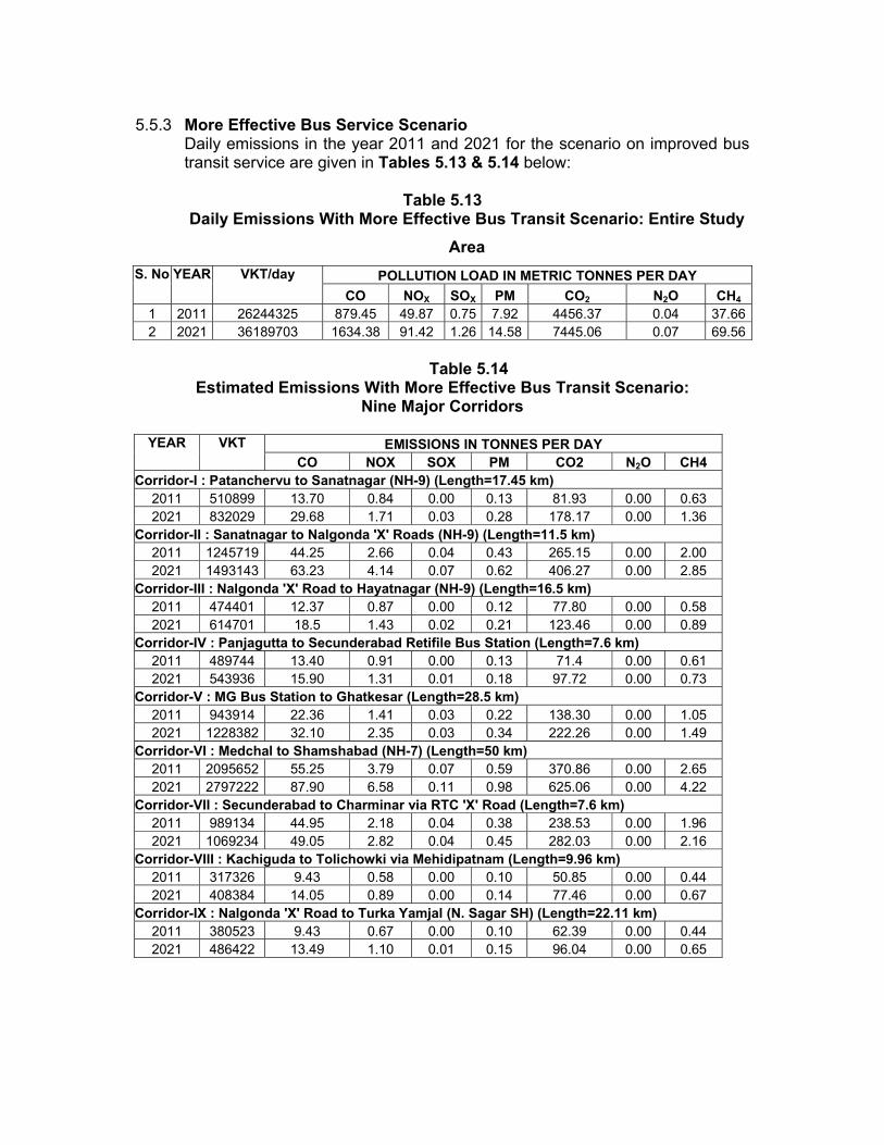
5.5.3 More Effective Bus Service Scenario Daily emissions in the year 2011 and 2021 for the scenario on improved bus transit service are given in Tables 5.13 & 5.14 below:

Table 5.13

Daily Emissions With More Effective Bus Transit Scenario: Entire Study Area

POLLUTION LOAD IN METRIC TONNES PER DAY S. No YEAR VKT/day CO NOX SOX PM CO2 N2O CH4

1 2011 26244325 879.45 49.87 0.75 7.92 4456.37 0.04 37.662 2021 36189703 1634.38 91.42 1.26 14.58 7445.06 0.07 69.56

Table 5.14

Estimated Emissions With More Effective Bus Transit Scenario: Nine Major Corridors

EMISSIONS IN TONNES PER DAY YEAR VKT

CO NOX SOX PM CO2 N2O CH4 Corridor-I : Patanchervu to Sanatnagar (NH-9) (Length=17.45 km)

2011 510899 13.70 0.84 0.00 0.13 81.93 0.00 0.63 2021 832029 29.68 1.71 0.03 0.28 178.17 0.00 1.36

Corridor-II : Sanatnagar to Nalgonda 'X' Roads (NH-9) (Length=11.5 km) 2011 1245719 44.25 2.66 0.04 0.43 265.15 0.00 2.00 2021 1493143 63.23 4.14 0.07 0.62 406.27 0.00 2.85

Corridor-III : Nalgonda 'X' Road to Hayatnagar (NH-9) (Length=16.5 km) 2011 474401 12.37 0.87 0.00 0.12 77.80 0.00 0.58 2021 614701 18.5 1.43 0.02 0.21 123.46 0.00 0.89

Corridor-IV : Panjagutta to Secunderabad Retifile Bus Station (Length=7.6 km) 2011 489744 13.40 0.91 0.00 0.13 71.4 0.00 0.61 2021 543936 15.90 1.31 0.01 0.18 97.72 0.00 0.73

Corridor-V : MG Bus Station to Ghatkesar (Length=28.5 km) 2011 943914 22.36 1.41 0.03 0.22 138.30 0.00 1.05 2021 1228382 32.10 2.35 0.03 0.34 222.26 0.00 1.49

Corridor-VI : Medchal to Shamshabad (NH-7) (Length=50 km) 2011 2095652 55.25 3.79 0.07 0.59 370.86 0.00 2.65 2021 2797222 87.90 6.58 0.11 0.98 625.06 0.00 4.22

Corridor-VII : Secunderabad to Charminar via RTC 'X' Road (Length=7.6 km) 2011 989134 44.95 2.18 0.04 0.38 238.53 0.00 1.96 2021 1069234 49.05 2.82 0.04 0.45 282.03 0.00 2.16

Corridor-VIII : Kachiguda to Tolichowki via Mehidipatnam (Length=9.96 km) 2011 317326 9.43 0.58 0.00 0.10 50.85 0.00 0.44 2021 408384 14.05 0.89 0.00 0.14 77.46 0.00 0.67

Corridor-IX : Nalgonda 'X' Road to Turka Yamjal (N. Sagar SH) (Length=22.11 km) 2011 380523 9.43 0.67 0.00 0.10 62.39 0.00 0.44 2021 486422 13.49 1.10 0.01 0.15 96.04 0.00 0.65

5.5.4 Multi-Modal Transport System (MMTS) Scenario Daily emissions in the year 2011 and 2021 for the MMTS scenario is given in Tables 5.15 below:

Table 5.15 Daily Emissions In MMTS Scenario

POLLUTION LOAD IN TONNES PER DAY YEAR

VKT/DAY

CO NOX SOX PM CO2 N20 CH4 2003 21151317 627.94 34.05 0.50 6.25 2896.94 0.03 30.31 2011 35323616 1190.58 56.64 0.89 11.88 5034.41 0.04 60.17 2021 54551050 2943.27 114.46 1.89 31.04 10089.88 0.07 165.33

5.5.5 Summary of Percentage Reduction In Emissions The reduction in quantity & percentage of pollution reduction due to

implementation of various scenarios are shown in following Tables 5.16. Table 5.16

Reduction In Emissions For Various Scenarios Reduction Due To More Effective Bus Transit Scenario In Entire Study Area (In Tonnes)

YEAR CO NOX SOX PM CO2 N2O CH4

2011 327.20

(27) 8.71 (15)

0.15 (17)

4.26 (35)

688.05 (13)

0.00 (0)

23.55 (38)

2021 1410.40

(46) 36.75 (29)

0.82 (39)

17.96 (55)

3792.69 (34)

0.03 (30)

101.75 (59)

REDUCTION DUE TO MORE EFFECTIVE BUS TRANSIT SCENARIO IN MAJOR NINE CORRIDORS

Corridor No : I YEAR CO NOX SOX PM CO2 N2O CH4

2011 6.11 (31)

0.01 (1)

0.00 (-)

0.09 (41)

0.55 (1)

0.00 (-)

0.51 (45)

2021 25.57 (46)

0.17 (9)

0.02 (40)

0.38 (58)

23.17 (12)

0.00 (-)

2.26 (62)

Corridor No : II

2011 31.11 (41)

0.73 (22)

0.01 (20)

0.44 (50)

47.98 (15)

0.00 (-)

2.48 (55)

2021 183.22

(74) 4.49 (52)

0.11 (61)

2.42 (80)

504.12 (55)

0.00 (-)

13.61 (83)

Corridor No : III

2011 8.96 (42)

0.09 (9)

0.01 (100)

0.13 (52)

12.39 (14)

0.00 (-)

0.68 (54)

2021 33.59 (64)

0.34 (19)

003 (60)

0.41 (66)

65.18 (35)

0.00 (-)

2.52 (74)

Corridor No : IV

2011 12.65 (49)

0.05 (5)

0.01 (100)

0.12 (48)

20.28 (22)

0.00 (-)

0.78 (56)

2021 35.24 (69)

0.31 (19)

0.01 (50)

0.39 (68)

60.63 (38)

0.00 (-)

2.44 (77)

Corridor No : V

2011 16.50 (42)

0.27 (16)

0.01 (25)

0.22 (50)

35.51 (20)

0.00 (-)

1.24 (54)

2021 56.63 (64)

0.75 (24)

0.03 (50)

0.76 (69)

117.04 (34)

0.00 (-)

4.47 (75)

Corridor No : VI

2011 36.77 (40)

0.68 (15)

0.02 (22)

0.54 (48)

71.50 (16)

0.00 (-)

3.06 (54)

2021 162.32

(65) 2.39 (27)

0.08 (42)

2.18 (69)

368.20 (37)

0.00 (-)

12.82 (75)

Corridor No : VII

2011 54.99 (55)

2.36 (52)

0.04 (50)

0.78 (67)

195.77 (45)

0.00 (-)

3.99 (67)

2021 116.36

(70) 2.82 (50)

0.08 (67)

1.54 (77)

299.46 (51)

0.00 (-)

8.67 (80)

Corridor No : VIII

2011 7.12 (43)

0.12 (170

0.00 (-)

0.08 (44)

12.71 (20)

0.00 (-)

0.52 (54)

2021 25.5 (64)

0.43 (33)

0.01 (100)

0.33 (70)

57.87 (43)

0.00 (-)

1.91 (74)

Corridor No : IX

2011 8.02 (46)

0.14 (17)

0.00 (-)

0.10 (50)

16.42 (21)

0.00 (-)

0.62 (58)

2021 24.94 (65)

0.23 (17)

0.01 (50)

0.31 (67)

47.86 (33)

0.00 (-)

1.90 (75)

Reduction Due to MMTS Scenario in Study Area

2003 2.21

(0.35) 0.17

(0.50) 0 (-)

0.02 (0.32)

19.06 (0.65)

0 (-)

0.1 (0.33)

2011 16.07 (1.33)

1.94 (3.31)

0.01 (1.11)

0.30 (2.46)

110.01 (2.14)

0.00 (-)

1.04 (1.70)

2021 101.51 (3.33)

13.71 (10.70)

0.19 (9.13)

1.50 (4.61)

1147.87 (10.21)

0.03 (30.00)

5.98 (3.49)

Note: figures in braces indicate the percentage reduction. From above table it can be observed that there are significant reductions in all

pollutants for all scenarios. 5.6 BROAD COST ESTIMATES FOR MORE EFFECTIVE PUBLIC

TRANSIT SERVICES 5.6.1 Broad cost estimates for implementation of most effective public transit

services as identified were prepared based on the unit rates of the items as prevalent in the study area as per 2003 price levels and are presented in Tables 5.17 to 5.19. Cost estimate for MMTS has been taken from Municipal Corporation of Hyderabad.

Table 5.17 Broad Cost Estimates for More Effective Bus Transit Services

Sanatnagar-Nalgonda 'X' Road Corridor

SI No Item Units Quantity Unit Rate

(Rs) Amount (Rs) (in millions)

1 More Effective Bus Transit Service

(I) Bus Lane markings Sq.m 2400 550 1.320 (ii) Construction of Busbays Each 17 300,000 5.100 (iii) Traffic Signs Each 200 3,000 0.600 (iv) Overhead Signs Each 6 180,000 1.080 (v) Pavement Markings Km 24 15,000 0.360

Total 8.46 Contingencies @ 5% Rs 0.423

Project Management Consultancy(PMC) @ 10% Rs 0.846

Supervision Cost @ 5% Rs 0.423

GRAND TOTAL Rs 10.152

Approx.

Rs 10 Millions

Table 5.18 Broad Cost Estimates for More Effective Bus Transit Services

Panjugutta to Secunderabad Corridor SI No Item Units Quantity Unit Rate

(Rs) Amount (Rs) (in

millions) (1) More Effective Bus Transit Service (I) Bus Lane markings sqm 1600 550 0.880 (ii) Construction of Bus bays Each 12 300,000 3.600 (iii) Traffic Signs Each 130 3,000 0.390 (iv) Overhead Signs Each 4 180,000 0.720 (v) Pavement Markings Km 16 15,000 0.240

Total 5.83 Contingencies @ 5% Rs 0.292

Project Management Consultancy(PMC) @ 10% Rs 0.583

Supervision Cost @ 5% Rs 0.292

GRAND TOTAL Rs 6.996

Approx. Rs 7 Millions

Table 5.19 Cost Estimates for More Effective Public Transit Services

Total HUDA area

SI No Item Units Quantity Unit Rate

(Rs) Amount (Rs) ( in millions)

(I) More Effective Bus Transit Service

(I) Bus Lane markings Sq.m 190000 550 104.500 (ii) Construction of Busbays Each 1500 300,000 450.000 (iii) Traffic Signs Each 3000 3,000 9.000 (iv) Overhead Signs Each 190 180,000 34.200 (v) Pavement Markings Km 1900 15,000 28.500 Sub Total 626.200 (II) MMTS - Construction Cost 1500.000

Total Rs 2126.200 Contingencies @ 5% Rs 106.310

Project Management Consultancy (PMC) @ 10% Rs 212.620

Supervision Cost @ 5% Rs 106.310

GRAND TOTAL Rs 2551.440

Approx. Rs 2551 Millions

CHAPTER - 6

TRAFFIC MANAGEMENT AND MEASURES TO IMPROVE TRAFFIC FLOW

6.1 ROLE OF TRAFFIC MANAGEMENT MEASURES 6.1.1 It has been the experience of many traffic & transport planners that most

transportation plans rarely progress beyond the drawing board for lack of financial resources and other related constraints. In many urban areas, socio-economic constraints, hutments, ribbon developments, etc. are serious impediments to further development, even if the problem of funds is overcome. Provision of new urban transport infrastructure is both long-term and capital intensive, and resources are simply not available at a scale that matches the escalating demand.

6.1.2 The only recourse open to the traffic manager, therefore is the option of

optimising the existing facilities to provide improved accessibility and mobility at a satisfactory level of safety and comfort to most of the road users. This can be achieved after studying and evaluating the problems in the light of sound and tested traffic management techniques, which are essentially low-cost, easily implementable and flexible. These are short-term solutions, primarily intended to reduce the intensity of inconvenience caused by congestion and the multiplicity of the modes of transport traversing in the common space. They may not offer a permanent solution, yet they lend themselves to some time saving relief, to a point where the administration may launch a long-term solution.

6.1.3 The fundamental approach in traffic management measures is to retain as

much as possible the existing pattern of streets but to alter the pattern of traffic movement on these, so that the most efficient use is made of the system. In doing so, minor alterations to street furniture are inevitable, and are part of management measures.

6.1.4 The aim of Traffic Management lies in achieving the best use and extension of

facilities & services available through use of low-cost solutions. Some of these could be regulations only, which may not cost anything. For this purpose, the greatest emphasis is placed on: (i) Rationalisation of the use of urban transport facilities; particularly road

space. (ii) Provision of better access through cost-effective improvements and

extensions of road networks. (iii) Traffic Management by adopting measures like one-way streets,

pedestrian friendly policies, signals, junction design & improvements, tidal flow, and better facilities for bicycles.

(iv) Improvement of the standards and viability of public transport and giving better access to public transport priority measures like bus lanes, etc.

(v) Strengthening of urban transport institutions including technical assistance and training.

6.2 TRAFFIC MANAGEMENT CORRIDORS 6.2.1 RITES has identified 3 more corridors in addition to the GEP Corridor (ESI

Hospital to Khairatabad Junction, Length=4.6km) as a part of the study. Only GEP corridors were to be considered as per terms of reference of the study. The corridors are: (iv) Erragadda junction to ESI Hospital (NH-9), L=0.9km (v) Khairatabad junction to Nalgonda ‘X’ roads (NH-9) via Nampelly Public

Garden and MJ Market, L=7.1km (vi) Panjagutta junction to Sec.bad Retifile bus station via Green lands and

Begumpet road, L=8.05km

6.2.2 However, the above (iv) and (v) corridors are extensions of the GEP corridor. Hence, the total selected/identified corridors effectively are two i.e., a) Erragadda to Nalgonda ‘X’ Road Corridor b) Panjagutta to Secunderabad Corridor

6.2.3 The two corridors are shown in Figure 6.1. 6.3 TRAFFIC SCENARIO ON TRAFFIC MANAGEMENT SCENARIO

CORRIDORS 6.3.1 Erragadda to Nalgonda ‘X’ Road Corridor

This identified corridor abuts densely populated commercial complexes, administrative and corporate offices. This corridor lies on NH-9 and connects Mumbai in the North and Vijayawada in the Southeast. The length of NH-9 in this section is about 12 km. The ROW on this corridor varies from 14m to 36m but at assembly and police control room the ROW is more than 40m. The peak hour approach volumes of the junctions falling under this corridor have been described in Chapter 3 of this report. The mid block peak hour traffic on the corridor varies from 4260 pcus to 10680 pcus. The section- wise peak hour traffic is presented in Table 6.1.

Table 6.1

Section-wise Peak Hour Traffic (Erragadda to Nalgonda ‘X’ Road) - 2003 Name of the Section Peak Hour (PCUs)

Erragada to E.S.I. 7593 E.S.I to S.R.Nagar 6510 S.R.Nagar to Maitrivanam 6060 Maitrivanam to Ameerpet 7249 Ameerpet to Panjagutta 7491 Panjagutta to Khairtabad 7436 Khairatabad to Saifabad New Police Station 8401 Lakidikapool to Ravindra Bharati 9303 Ravindra Bharati to Control Room 10679 Control Room to L.B.Stadium 10063

Name of the Section Peak Hour (PCUs) L.B. Stadium to A1-Junction 8047 A1-Junction to Lata Takies 9396 Lata Takis to Goshamahal 8700 Goshamahal to M.J.Market 9619 M.J.Market to PutliBowli 4256 Putlibowli to Rangamahal 5251 Rangamahal to Chadarghat 7641 Chadarghat to Naigara 8257 Naigara to Nalgonda X Road 7573

Sanatnagar/Erragadda

ESI

Panjagutta

Khairatabad

Nampelli

M.J.Market

Chaderghat Nalgonda ‘X’ Road

Begumpet

Greenlands

S.P.Road

Hari Hara Kala Bhawan

Secunderabad

Sanatnagar/Erragadda to ESI Corridor

ESI to Khairatabad Corridor

Khairatabad to Nalgonda ‘X’ Rd Corridor

Panjagutta to Secunderabad Corridor

Fig 6.1 DEMO TRAFFIC CORRIDORS

6.3.2 Panjagutta to Secunderabad Corridor

This corridor passes through densely populated commercial complex and corporate offices. In this corridor one ROB, Begumpet and three flyovers, Begumpet Airport, Paradise and Hariharakala Bhawan exist. The length of this corridor is about 8 km. The ROW on this corridor varies from 18m to 38m. The peak hour approach volumes of the junctions falling under this corridor have been described in Chapter 3 of this report. The mid block peak hour traffic on the corridor various from 4000 PCUs to 14850pcus.The section wise peak hour traffic is presented in Table 6.2.

Table 6.2 Section-wise Peak Hour Traffic (Panjagutta to Secunderabad) - 2003

Name of the Section Peak Hour (PCUs) Panjagutta to Rajeev Gandhi Statue 6237 Rajeev Gandhi Statue to Greenlands 9846 Greenlands to N.T.R. Junction 14848 N.T.R. Junction to Paradise 5061 Paradise Road to Plaza 4898 Plaza to Hariharakala Bhavan 4697 Hariharakala Bhavan to YMCA 3977 YMCA to East Maredpally 6108 East Maredpally to Sangeet Cinema 5230 Sangeet Cinema to Secandrabad Rethifile Bus Terminus 5049

6.3.3 Peak Hour Traffic Composition The average peak hour traffic composition on the two corridors is presented in

Tables 6.3 & 6.4. Table 6.3

Peak Hour Traffic Composition (Erragadda to Nalgonda X Roads Corridor) - 2003

S No Type of Vehicle Numbers Percentage 1 Bus 398 3.92 2 Goods 87 0.86 3 Cars 1427 14.07 4 2-Wheelr 5356 52.80 5 3-Seater Auto 1789 17.64 6 7-Seater Auto 350 3.45 7 Slow Moving Vehicles 729 7.19 8 Others 8 0.08

Table 6.4 Peak Hour Traffic Composition (Punjagutta to Secunderabad Corridor) -

2003 S No Type of Vehicle Numbers Percentage

1 Bus 293 3.57 2 Goods 91 1.11 3 Cars 1949 23.76 4 2-Wheelr 4283 52.22 5 3-Seater Auto 1170 14.26 6 7-Seater Auto 13 0.16 7 Slow Moving Vehicles 397 4.84

S No Type of Vehicle Numbers Percentage 8 Others 6 0.07

It is observed from above table that car traffic composition is significantly high on Panjagutta to Secunderabad corridor compared to Erragadda to Nalgonda ‘X’ road corridor.

6.3.4 Volume – Capacity (V/C) ratio The estimated V/C ratios on selected corridors are shown in Table 6.5.

Table 6.5

V/C Ratios - 2003 S. No. Name of the Section V/C Ratio Erragadda to ESI Corridor

1 Erragada to E.S.I. 1.7 2 E.S.I to S.R.Nagar 1.5 3 S.R.Nagar to Maitrivanam 0.7 4 Maitrivanam to Ameerpet 1.1 5 Ameerpet to Panjagutta 1.1 6 Panjagutta to Khairtabad 1.1 7 Khairatabad to Saifabad New Police Station 1.3 8 Lakidikapool to Ravindra Bharati 1.4 9 Ravindra Bharati to Control Room 1.0

10 Control Room to L.B.Stadium 1.1 11 L.B. Stadium to A1-Junction 1.2 12 A1-Junction to Lata Takies 2.1 13 Lata Takis to Goshamahal 1.0 14 Goshamahal to M.J.Market 1.1 15 M.J.Market to PutliBowli 1.0 16 Putlibowli to Rangamahal 1.2 17 Rangamahal to Chadarghat 1.7 18 Chadarghat to Naigara 1.3 19 Naigara to Nalgonda X Road 1.7

Panjagutta to Secunderabad corridor 1 Panjagutta to RajeevGandhi Statue 0.9 2 RajeevGandhi Statue to Greenlands 1.1 3 Greenlands to N.T.R. Junction 1.7 4 N.T.R. Junction to Paradise 0.8 5 Paradise Road to Plaza 0.6 6 Plaza to HariharakalaBhavan 0.5 7 Hariharakala Bhavan to YMCA 0.5 8 YMCA to East Maredpally 1.4 9 East Maredpally to Sangeet Cinema 0.8

10 Sangeet Cinema to Secandrabad Rethifile Bus Terminus 0.8 It is observed from above table that in many of the road sections, V/C value exceeds 1.

6.4 SCENARIOS FOR TRAFFIC MANAGEMENT AND MEASURES TO

IMPROVE TRAFFIC FLOW 6.4.1 The various Traffic Management measures have been proposed for

improvement in traffic flow along identified corridors. These measures are readily implementable. Various models were developed to estimate the impact of speed with various traffic measures. A total of three scenarios have been developed for the identified corridors as mentioned below;

1. Business As Usual Scenario (BAU) 2. Flyover Scenario 3. GEP Scenario

The above scenarios have been evaluated on the basis of various developed models.

6.5 BUSINESS AS USUAL SCENARIO (BAU) 6.5.1 The scenario has considered for the study area i.e., HUDA and the traffic

management for the base year 2003 and horizon years of 2011 and 2021. The traffic volumes in the study area and on the nine major corridors including two identified corridors for traffic management scenario were obtained by transport demand modeling as explained in Chapter 4 & 5. Accordingly, Vehicle Kilometer Traveled (VKT) has been estimated for the two corridors. The estimated vehicular emissions in this scenario have already been presented in chapter on scenarios for more effective public transit service.

6.6 FLYOVER SCENARIO 6.6.1 In this scenario, a flyover of length about 12km has been proposed from

Sanatnagar to Nalgonda ‘X’ Road identified corridor with suitable number of up & down ramps. The location of proposed flyover is shown in Figure 6.2. Accordingly road network was updated with increased speed of public and private modes due to inclusion of flyover. Speeds for BAU and Flyover scenario were estimated from speed-flow relationship as discussed in Chapter-4 and given in Table 6.6. Accordingly Vehicle Kilometer Traveled (VKT) has been estimated. The estimated vehicular emissions are presented in Tables 6.7 and 6.8 for BAU and Flyover scenario respectively. Reduction in pollution quantity loads and percentage reduction is mentioned in Table 6.9

Sanatnagar

Fig 6.2 PROPOSED FLYOVER ON DEMO CORRIDOR

Proposed Flyover

Legend

Nalgonda ‘X’ Road

Table 6.6

Expected Traffic Speeds (kmph) for BAU and Flyover Scenario ( Sanatnagar to Nalgonda ‘X’ road corridor)

2011 2021 MODE 2003 BAU FLYOVER BAU FLYOVER Car 23 18.10 38.50 10.00 31.50 2-w 23 18.10 38.50 10.00 31.50 Bus 15 10.30 21.40 5.00 17.50 Auto 20 10.30 21.40 5.00 17.50

Table 6.7

Emissions: Sanatnagar To Nalgonda ‘X’ Road BAU Scenario EMISSIONS PER DAY IN TONNES S. No YEAR VKT CO NOX SOX PM CO2 N2O CH4

1 2011 1777942 75.36 3.39 0.05 0.87 313.13 0.00 4.48 2 2021 2825044 246.45 8.63 0.18 3.04 910.39 0.00 16.46

Table 6.8

Emissions: Sanatnagar To Nalgonda ‘X’ Road Flyover Scenario EMISSIONS PER DAY IN TONNES S. No YEAR VKT CO NOX SOX PM CO2 N2O CH4

1 2011 2831374 75.23 3.26 0.05 0.80 292.84 0.00 4.12 2 2021 4443724 213.04 7.16 0.14 2.46 734.91 0.00 13.59

Table 6.9

Reduction In Emissions Flyover From Sanatnagar To Nalgonda ‘X’ Road Over BAU Scenario EMISSIONS PER DAY IN TONNES S. No YEAR CO NOX SOX PM CO2 N2O CH4

1 2011 0.13 (0.20)

0.13 (3.80)

0.00 (-)

0.07 (8.00)

20.29 (6.50)

0.00 (-)

0.36 (8.00)

2 2021 33.41 (13.60)

1.47 (17.00)

0.04 (22.20)

0.58 (19.10)

175.48 (19.30)

0.00 (-)

2.87 (17.40)

Note: figures in braces indicate percentage reduction 6.6.2 It can be observed that VKT increases considerably on the corridor. Although

reduction in emissions is expected to be small but there is a reasonable reduction for the year 2021.

6.7 GEP SCENARIO 6.7.1 Reduction of Side Friction

The zig-zag parking, on-street parking, encroachments and presence of hawkers significantly reduce the effective carriageway width of roads. These factors directly affect the capacity of road. Besides these, on-street and unplanned parking reduces the degree of maneuverability and decreases the average journey speed. The provision of on-street parking on road sections with wider carriageway and banning of on-street parking on sections with smaller carriageway would result in increase in road capacity as well as

average speed. Accordingly Vehicle Kilometer Traveled (VKT) has been estimated. Speeds for BAU and GEP scenario for the two corridors for the year 2011 & 2021 are given in Table 6.10. The vehicular emissions and corresponding percentage reductions in this scenario are presented in Tables 6.11 to 6.14.

Table 6.10 Expected Traffic Speeds (kmph) for Removal of Side Friction Scenario

(Sanatnagar to Nalgonda ‘X’ road & Panjagutta to Secunderabad corridors)

2011 2021

MODE BAU Removal of Side

Friction BAU Removal of Side

Friction

S.nagar-Nalgonda

P.gutta-Sec.bad

S.nagar-Nalgonda

P.gutta-Sec.bad

S.nagar-Nalgonda

P.gutta-Sec.bad

S.nagar-Nalgonda

P.gutta-Sec.bad

CAR 18.10 18.97 19.30 19.60 10.00 17.19 16.60 18.10 2W 18.10 18.97 19.30 19.60 10.00 17.19 16.60 18.10 BUS 10.30 15.72 16.70 17.00 5.00 9.99 14.00 15.50 AUTO 10.30 15.72 16.70 17.00 5.00 9.99 14.00 15.50

Table 6.11 Emissions From GEP Scenario:

Sanatnagar To Nalgonda 'X' Road (NH-9) - Identified Corridor-I EMISSIONS PER DAY IN TONNES S. No YEAR VKT CO NOX SOX PM CO2 N2O CH4

1 2011 1777942 60.39 2.36 0.04 0.64 232.14 0.00 3.37 2 2021 2825044 121.16 3.71 0.08 1.32 399.29 0.00 7.35

Table 6.12 Reduction In Emissions-GEP Scenario

Sanatnagar To Nalgonda 'X' Road (NH-9) - Identified Corridor-I EMISSIONS PER DAY IN TONNES S. No YEAR VKT

CO NOX SOX PM CO2 N2O CH4

1 2011 - 14.97 (20)

1.03 (30)

0.01 (20)

0.23 (26)

80.99 (26)

0.00 (-)

1.11 (25)

2 2021 - 125.29

(51) 4.92 (57)

0.10 (56)

1.72 (57)

511.10 (56)

0.00 (-)

9.11 (55)

Note: figures in braces indicate percentage reduction

Table 6.13 Emissions From GEP Scenario:

Panjagutta To Secunderabad - Identified Corridor-II EMISSIONS PER DAY IN TONNES S. No YEAR VKT

CO NOX SOX PM CO2 N2O CH4 1 2011 676655 25.10 0.92 0.01 0.24 86.69 0.00 1.33 2 2021 919585 41.46 1.20 0.02 0.43 120.04 0.00 2.42

Table 6.14 Reduction In Emissions-GEP Scenario Over BAU Scenario

Panjagutta To Secunderabad - Identified Corridor-II EMISSIONS PER DAY IN TONNES S. No YEAR VKT

CO NOX SOX PM CO2 N2O CH4

1 2011 - 0.95 (4)

0.04 (4)

0.00 (-)

0.01 (4)

4.99 (5)

0.00 (-)

0.06 (4)

2 2021 - 9.68 (19)

0.42 (26)

0.00 (-)

0.14 (25)

38.31 (24)

0.00 (-)

0.75 (24)

Note: figures in braces indicate percentage reduction Here it can be seen that emissions are substantially reduced due to traffic management improvements under GEP scenario. All pollutants are reduced considerably.

6.7.2 Separation of Vulnerable Road Users (Provision of Footpath) The intermixing of vehicles and pedestrians in the absence of footpaths results in reduced speeds and increase in number of accidents. The provision of footpaths and pedestrian crossings can reduce these conflicts to a great extent, which results in increase of the average speed. Accordingly Vehicle Kilometer Traveled (VKT) has been estimated. Speeds for BAU and separation for vulnerable road users scenario for the two corridors for the years 2011 and 2021 are given in Table 6.15. The vehicular emissions and corresponding percentage reductions in this scenario are presented in Tables 6.16 to 6.19.

Table 6.15 Expected Traffic Speeds (kmph) for Providing and for effective utilization of Footpath

Scenario 2011 2021

MODE BAU Foot Path Scenario BAU Foot Path Scenario

S.nagar-Nalgonda

P.gutta-Sec.bad

S.nagar-Nalgonda

P.gutta-Sec.bad

S.nagar-Nalgonda

P.gutta-Sec.bad

S.nagar-Nalgonda

P.gutta-Sec.bad

CAR 18.10 18.97 18.95 19.38 10.00 17.19 15.63 17.52 2W 18.10 18.97 18.95 19.38 10.00 17.19 15.63 17.52 BUS 10.30 15.72 16.64 17.16 5.00 9.99 12.58 14.89 AUTO 10.30 15.72 16.64 17.16 5.00 9.99 12.58 14.89

Table 6.16 Emissions From Separation Of Vulnerable Road Users: Sanatnagar To

Nalgonda 'X' Road (NH-9) - Identified Corridor-I EMISSIONS PER DAY IN TONNES

S. No YEAR VKT CO NOX SOX PM CO2 N2O CH4 1 2011 1777942 61.02 2.39 0.04 0.64 235.19 0.00 3.40 2 2021 2825044 129.75 4.03 0.08 1.43 434.90 0.00 7.95

Table 6.17

Reduction In Emissions From Separation of Vulnerable Road Users(Compared to BAU Scenario) Sanatnagar To Nalgonda 'X' Road (NH-9)

EMISSIONS PER DAY IN TONNES S. No YEAR VKT CO NOX SOX PM CO2 N2O CH4

1 2011 - 14.34 (19)

1.00 (29)

0.01 (20)

0.23 (26)

77.94 (25)

0.00 (-)

1.08 (24)

2 2021 - 116.70 (47)

4.60 (53)

0.10 (56)

1.61 (53)

475.49 (52)

0.00 (-)

8.51 (52)

Note: figures in braces indicate percentage reduction

Table 6.18 Emissions From Separation of Vulnerable Road Users: Panjagutta To

Secunderabad EMISSIONS PER DAY IN TONNES

S. No YEAR VKT CO NOX SOX PM CO2 N2O CH4 1 2011 676655 25.11 0.91 0.01 0.24 86.67 0.00 1.33 2 2021 919585 42.51 1.24 0.02 0.44 124.46 0.00 2.50

Table 6.19

Reduction In Emissions From Separation of Vulnerable Road Users(Compared to BAU Scenario) Panjagutta To Secunderabad- Identified Corridor II

EMISSIONS PER DAY IN TONNES S. No YEAR VKT CO NOX SOX PM CO2 N2O CH4

1 2011 - 0.94 (4)

0.05 (5)

0.00 (-)

0.01 (4)

5.01 (50

0.00 (-)

0.06 (4)

2 2021 - 8.63 (17)

0.38 (23)

0.00 (-)

0.13 (23)

33.89 (21)

0.00 (-)

0.67 (21)

Note: figures in braces indicate percentage reduction The above tables indicate that this low cost traffic improvement measure can bring out substantial reduction across all pollutants.

6.7.3 Synchronization Of Traffic Signals Along With Junction Improvements To Reduce Intersection Delays Signal coordination is one of the important measures in traffic management system. In this study, signal coordination exercise was done by TRANSYT 11 version (Traffic Network Study Tool) developed by TRL, UK. Junction Improvement measures also have positive impact on the average speeds. The junction improvements such as proper signages, zebra crossings, stop lines, removal of encroachments, provision of channelisers for free left traffic movement etc. increase intersection capacity and reduce delays at the intersections. These measures when implemented shall result in improved speeds along the corridor. The increase in speed has been directly computed from reduction in delays expected after implementation of the measures. The instances of frequent acceleration and de-acceleration will also be reduced due to the synchronized/smooth traffic movement. A total of 8 junctions have been coordinated in corridor No. 1 from Sanatnagar to Nalgonda Crossroad. The second identified corridor from Panjagutta to Secunderabad has not been considered for the scenario as this corridor has many flyovers, roundabouts and un-signalized junctions. The expected speeds on various sections by junctions signal coordination vis-à-vis isolated control for this corridor No. 1 is shown in the Table 6.20. These tables shows that signal coordinating offers improved traffic flow on the identified corridors. On the basis of improved traffic speeds, the above signal coordinated two sections, average speeds on the existing corridor from Sanatnagar to Nalgonda X Crossroad haven been worked out for 2003, 2011 and 2021 and presented in Table 6.21. Expected emissions with this scenario are given in Table 6.22. Table 6.23 shows that this option can bring substantial reduction in emission levels.

Table 6.20

Synchronisation of Traffic Signals Erragadda to Maitrivanam Section: Corridor No. 1

Name of the Junction

Node

Link No Mean Delay Time (Sec) Mean Journey Speed (kmph)

Erragadda 1 11 10 12 12 62 18 13 667 57 14 64 73

8

ESI 2 15 229 22 16 156 54 17 4 26 18 46 44

9.9

Sanjeev Reddy Nagar 3 19 109 34 20 268 82 21 419 69 22 305 89 23 75 41 24 556 66

6.5

22

Name of the Junction

Node

Link No Mean Delay Time (Sec) Mean Journey Speed (kmph)

25 202 50 26 231 58 Maitrivanam 4 27 44 34 28 1 1 29 58 63 30 1 1 33 55 74

17.3

Ameerpet to KCP Section: Identified Corridor No. 1

Mean Delay Time (Sec) Mean Journey Speed (kmph)

Name of the Junction Node Link No

Isolated Coordination Isolated CoordinationAmeerpet 101 101 8 11 102 71 49 103 71 70 104 91 46 105 58 64 106 84 63 107 60 49

11.9

Shalimar 102 201 14 12 202 38 25 203 124 64 204 60 44

16

Panjagutta 103 301 36 28 302 19 31 303 15 18 304 34 30

17.4

KCP 104 401 23 21 402 46 32 403 120 80 404 73 48

17.7

19.5

Table 6.21 Expected Traffic Speeds (Kmph) For Synchronization Of Traffic Signals And Junction Improvement Scenario (Sanatnagar To Nalgonda ‘X’ Road Corridor) Mode 2003 2011 2021

Car 30 23.50 13.00 2-w 30 23.50 13.00 Bus 20 13.40 6.50 Auto 25 13.40 6.50

Table 6.22 Signal Coordination Scenario Emissions

EMISSIONS PER DAY IN TONNES S. No YEAR VKT CO NOX SOX PM CO2 N2O CH4

1 2003 1546722 37.03 1.93 0.04 0.39 173.38 - 1.88 2 2011 1777942 61.54 2.67 0.04 0.70 241.62 - 3.61 3 2021 2825044 196.17 6.75 0.14 2.39 701.47 - 12.95

Table 6.23 Emissions Reduction Due To Signal Coordination as Compared to BAU

Scenario EMISSIONS PER DAY IN TONNES

S. No YEAR CO NOX SOX PM CO2 N2O CH4

1 2003 6.94 (15.78)

0.52 (21.22)

0.01 (20.00)

0.07 (15.22)

52.54 (23.26)

0.00 (-)

0.37 (16.44)

2 2011 13.82 (18.00)

0.72 (21.00)

0.01 (20.00)

0.17 (20.00)

71.51 (23.00)

0.00 (-)

0.87 (19.00)

3 2021 50.28 (20.00)

1.88 (22.00)

0.04 (22.00)

0.65 (21.00)

208.92 (23.00)

0.00 (-)

3.51 (21.00)

Note: figures in braces indicate percentage reduction 6.8 BROAD COST ESTIMATES FOR TRAFFIC MANAGEMENT

MEASURES 6.8.1 The preliminary cost estimates for the proposed improvement schemes have

been worked out for identified corridors on the basis of the unit rates as prevalent in the region for such works as per 2003 price level. The rates for signal installation and lane marking, etc. are obtained from the signal manufactures and from various studies done by the consultants The cost estimates are presented in Table 6.24 to 6.25.

Table 6.24 Broad Cost Estimates for Traffic Management Measures

Sanatnagar to Nalgonda ‘X’ Road Corridor SI No Item Units Quantity Unit Rate

(Rs) Amount (Rs) (in millions)

(A) Flyover Construction Km 16 140,000,000 2240.000 (B) Construction of Footpath Sq.m 4000 650 2.600

(C ) Synchronisation of Signals & Junction Improvements

(i) Junction Improvements Each 21 500,000 10.500

(ii) Street Furniture (Road Markings & Traffic Signs) Each 21 50,000 1.050

(iii) Signal Coordination of existing signals about 10 junctions (Cost of cables, soft & hard cutting and hardware upgradation etc)

Lump sum 2.000

Sub Total 13.550

(D) Side friction Removal (i) Construction of Guard Rails m 24000 1,100 26.400 (ii) Traffic Sign Boards Each 100 3,000 0.300

(iii) Carriageway edge lane marking with Thermoplastic paint Sq.m 7200 550 3.960

(iv) Cost of mini bollards, studs, reflectors etc Km 24 50,000 1.200

(v) Overhead Signs Each 12 180,000 2.160 Sub Total 34.02

Total Rs 2290.17

Contingencies @ 5% Rs 114.509

Project Management Consultancy (PMC) @ 10% Rs 229.017

Supervision Cost @ 5% Rs 114.509

GRAND TOTAL Rs 2748.204

Approx.

Rs 2750 Millions

Table 6.25 Broad Cost Estimates for Traffic Management Measures

Panjugutta to Secunderabad Corridor SI No Item Units Quantity Unit Rate

(Rs) Amount (Rs) ( in millions)

(A) Construction of Footpath Sq.m 6000 650 3.900 (B) Side friction Removal (i) Construction of Guard Rails m 16000 1100 17.600 (ii) Traffic Sign Boards Each 60 3,000 0.180

(iii) Carriageway edge lane marking with Thermoplastic paint Sq.m 4800 550

2.640 (iv) Junction Improvements Each 12 500,000 6.000

(v) Street Furniture with Thermoplastic paint Each 12 50,000

(vi) Overhead Signs Each 8 180,000 1.440

(vii) Cost of mini bollards, studs, reflectors etc Km 16 50,000 0.800

Sub Total 28.660 Total Rs 32.560 Contingencies @ 5% Rs 1.628

Project Management Consultancy (PMC) @ 10% Rs 3.256

Supervision Cost @ 5% Rs 1.628 GRAND TOTAL Rs 39.072

Approx.

Rs 40 Millions

CHAPTER – 7

VEHICLE TECHNOLOGY / TRAINING MEASURES RELATED TO TWO-STROKE VEHICLES

7.1 INTRODUCTION 7.1.1 Vehicular air pollution is common in growing metropolitan areas in India;

where about more than half of all vehicles are two and three wheel vehicles with two stroke engines. Hyderabad has a large number of 2-wheelers, many of which are powered by 2- stroke engines. All 3-wheelers in Hyderabad have 2-stroke engines. These engines operate at relatively low compression ratios (resulting in high CO2 emissions), do not burn their fuels completely (resulting in high gaseous and particulate hydrocarbon and carbon monoxide emissions) and burn a mix of petrol and lubricating oil (which, if not properly proportioned, can result in high particulate emissions). In addition, the motor fuels are often blended with lesser quality fuels or otherwise adulterated in order to save cost, which further increases emission levels. As a result, 2 stroke two or three wheelers in Hyderabad contribute quite disproportionately to air quality problems. In addition, the drivers of two wheelers and auto rickshaws also add to the air pollution with their inconsistence driver habits.

7.1.2 The technology for four stroke vehicles is gaining ground in India. However,

the people owning old technology vehicles may not be in a position to spend more money for better technology. The switch over will be gradual and phase out depends upon policy interventions/incentives provided by the Government.

7.1.3 The performance of any vehicle deteriorates gradually over time but regular

inspection and maintenance can improve performance and keep emissions under control.

7.1.4 Large scale ban on gasoline powered two-stroke engine vehicles would be

extremely difficult. However, emissions can be reduced significantly through other measures. The immediate and simple solution is to use the correct type and concentration of lubricant and to carry out regular maintenance. These measures would significantly reduce emissions from two stroke engines while saving drivers money and ultimately improving air quality. Promoting these “win-win” measures requires building public awareness by disseminating information on the health impacts of emissions. Partnerships among government, industry and the public will be crucial to bring about the correct driving, proper vehicle maintenance and changes required to achieve air quality goals. Fine particulate matter has been shown in studies in a number of cities around the world to have serious health effects, including premature mortality, respiratory symptoms, exacerbation of asthma and changes in lung function. Vehicle emissions of fine particles are particularly harmful because they occur near ground level, close to where people live and work.

7.1.5 Two stroke engines typically have a lower fuel efficiency than four stroke engines, with as much as 15-40 percent of the fuel-air mixture escaping from the engine through the exhaust port. These ‘scavenging losses’ contain a high level of unburned gasoline and lubricant, which increases emissions of hydrocarbons and organic lead (if leaded gasoline is used). The factors affecting vehicular emissions are poor vehicle maintenance, the misuse of lubricant, adulteration of gasoline, and lack of catalytic converters. These exacerbate two stroke engine harmful emissions. Both the quantity and quality of lubricant used affect the level of hydrocarbon and particulate emissions from two stroke engines.

7.2 OPINION & TECHNOLOGY DISTRIBUTION SURVEYS To assess the present vehicle technology distribution and opinion of two/

three wheeler passengers, limited surveys were carried out at petrol pumps and bus stops on the two identified corridors as a part of this study. About 4,399 samples were collected. Out of which 891 were IPT, 1,428 were 2-wheelers, 89 were cars and 1,991 were bus transport passengers. The survey proforma was designed after discussions with stake holders and covered information such as vehicle owner ship, fuel options, type of engine (2/4 stroke), Trip Length (km), Travel time, Make, Model, Year of manufacturing, Mileage (km/lit), Type of Lubricant, Average km. traveled per day, vehicle service frequency, pollution check up, measures to control pollution etc. The data was compiled and analyzed. The major findings of this survey have been presented in Annexure 7.1. It has been observed that about 80% of 2-wheelers have 2-stroke engines and all 3-wheelers (3 & 7 seater) have two stroke engines.

7.3 DRIVING HABITS OF TWO-WHEELERS AND AUTO RICKSHAW

OPERATORS To assess the driving style of two and three wheeler drivers, reconnaissance

survey was carried out at a few Intersections on selected corridors of the study area. The major observations of the survey are posted in Annexure 7.2. Improper driving habits of people have been observed during this survey.

7.4 MAINTENANCE & OPERATION (M&O) TRAINING PROGRAMS 7.4.1 Emission loads of these 2 stroke vehicles can be reduced by better vehicle

maintenance and operations. But most of the drivers of these vehicles are ignorant of these practices. Some may be aware about the benefits of such measures but generally do not know how to practice them. Therefore conducting maintenance and operation training programs for drivers of these vehicles can help in spreading awareness in reducing emissions. Better maintenance practices will include better engine tuning, using better lubricants etc. Better operations of the vehicle will include improved driving styles such as driving at steady speed instead of driving very fast and very slow by changing gears frequently, switching off the engine at signalized junctions, not constantly keeping the foot on the gear etc.

7.4.2 These training programs could be organized by targeting various groups such

as office goers, 3-wheeler operators associations etc. Non-Governmental Organizations such as Lions Club, Rotary Club etc along with Government organizations such as HUDA, Municipal Corporation of Hyderabad, Andhra Pradesh State Pollution Control Board may be included in this exercise of training drivers of 2-stroke vehicles. Awareness of better vehicle maintenance and operation programs can be further spread through television, radio and by placing small captions in prime time on TV. Help of print media can also be taken in this regard.

7.5 EMISSION REDUCTIONS DUE TO M&O TRAINING PROGRAMS 7.5.1 Discussions have been held with The Energy Research Institute (TERI)

officials regarding the extent of emissions reductions through these measures. Although no hard data is available on the potential of reduction of emissions for these M&O training programs, the discussions have revealed that these measures can reduce emission levels by 10% to 30%. However on a conservative side, reduction of emissions by 10% over BAU scenario for 2-stroke vehicles has been assumed in this study.

7.5.2 All the vehicle owners cannot be trained, as everybody may not have time or

inclination to join these training programs. Moreover, resources may not be available to train all the drivers. Therefore, only a part of existing 2-stroke engine vehicle operators can be called under this programs. Penetration rate of 5% for 2-stroke two wheeler drivers by 2011 and additional 8% by 2021 for the training programs has been assumed. It may be easier to bring in 3-wheeler drivers to these training programs through their unions/associations. Therefore a penetration rate of about 8% of 2-stroke three wheeler drivers by 2011 and additional 12% by 2021 for these training programs has been assumed.

7.5.3 Assuming above reduction in emissions in 2-stroke vehicles and their

penetration rates, over all reduction in emissions has been worked out for the year 2011 and 2021 and is presented in following paragraphs.

7.5.4 The estimated daily vehicle kilometers and emissions in BAU scenario for two

wheeler and three wheelers for 2001, 2003,2011 and 2021 have already been presented in Chapter-5.The daily emissions for BAU scenario for two and three wheelers for 2011 and 2021 are presented in Table. 7.1.

Table 7.1

Daily Emissions for BAU for 2 and 3 wheelers

EMISSIONS PER DAY IN TONES

YEAR DIALY VKT

CO NOX SOX PM CO2 N20 CH4 TOTAL 2011 29215131 1055.9 12.00 0.41 9.58 1628.18 0.0 59.18 2765.252021 45186190 2692.33 30.19 1.09 27.22 4262.66 0.01 166.79 7180.29

As discussed in Chapter-5, modal split (motorized trips) for 3-wheelers is expected to be 20% and 33% in 2011 and 2021 for BAU scenario. The total daily VKT for 2 and 3-wheelers are expected to be 88% of total VKT of all vehicles by 2021 for BAU scenario. Daily emissions for 2 and 3 wheelers are expected to be 49% of total emissions from all vehicles for BAU scenario by 2021. Further, from 2 and 3 wheelers, the daily PM10 and CO2 emissions are estimated as 84% and 38% respectively of total emissions for BAU scenario in 2021. This shows that 2 and 3 wheelers are expected to be the major contributors to vehicular emissions in Hyderabad.

7.5.5 The daily emissions after implementation of M&O training program for 2-stroke vehicles are presented in Table 7.2. The reduction in daily emissions due to M&O training programs is presented in Table 7.3 after using the assumed share of 2-stroke two wheelers and penetration rates of users of 2-stroke vehicles.

Table 7.2

Daily Emissions (in Tons) after M&O Training Programs for 2-Stroke Vehicles

Year CO NOX SOX PM CO2 N20 CH4 TOTAL 2011 1049.92 11.93 0.41 9.52 1618.80 0.00 58.81 2749.402021 2648.90 29.71 1.07 26.75 4192.65 0.01 163.90 7062.99

Table 7.3

Reduction in Daily Emissions due to M & O Training Programs for 2-Stroke Vehicles

REDUCTION IN EMISSIONS PER DAY IN TONNES

YEAR CO NOX SOX PM CO2 N20 CH4 TOTAL 2011 5.98 0.07 0.00 0.06 9.38 0.00 0.37 15.852021 43.43 0.48 0.02 0.47 70.01 0.00 2.89 117.30

The above emission reductions through M & O training programs are for the years 2011 and 2021 only. Corresponding reductions can also be accounted for other years up to the year 2021.

7.6 COST FOR M&O TRAINING PROGRAMS

The training programs cost primarily includes cost of course material, remuneration to experts, arrangements for classroom etc. and publicity through radio, TV and newspapers. For estimating number of drivers it has been assumed that the average distances traveled by 2 and 3 wheelers per day are 24 and 95 km respectively. Assuming training cost per person as Rs. 50, cost of M & O training programs for 2-stroke vehicles operators is estimated as Rs. 2.19 millions by 2011 and Rs. 8.14 millions by 2021 as shown in Table 7.4.

Table 7.4 Cost Estimates for M & O Training Programs

Trained Drivers by

2011 2021 Cumulative)

2-stroke 2-wheelers

38789 131676

3-wheelers 5003 31157 ning Cost (Rs in

Million) 2.19 8.14

7.7 EVALUATION

Considering the emissions reduction due to M & O training programs and cost for the training programs, cost effectiveness of this programs has been estimated. Emission reduction due to these programs will not be for a single day but for the future as well. It has been assumed that penetration rate of trainees would be equally distributed in various years up to 2011 and 2021. The emission reduction per rupee invested in these programs has then been worked out up to 2011 and 2021. The cost effectiveness of these programs is given in Table 7.5. The table indicates that 10kg and 38kg of emissions are expected to be reduced by per rupee invested in these programs cumulatively up to year 2011 and 2021, respectively. This indicates these programs are significantly cost effective. A TERI study has indicated that damage (health) cost of harmful emissions per kg is Rs. 32(updated to present price level). Considering this value, cumulative damage (health) cost is estimated as Rs. 314 by 2011 and Rs. 1213 by 2021 against the investment of one rupee. Therefore these training programs can be considered highly cost effective.

Table 7.5 Cost Effectiveness of M & O Training Programs

Item 2011 2021

Annual reduction in emissions (in tones) due to M & O training programs for 2-stroke vehicles

5389 39882

Cost of M & O training programs (Rs) 2189638 8141634 Emission reduction in kg per rupee invested in training programs in year 2011 and 2021

2.46 4.89

Cumulative reduction in emissions in kg per rupee invested in M & O training programs

9.81 37.9

CHAPTER - 8

CONCLUSIONS AND RECOMMENDATIONS 8.1 CONCLUSIONS 8.1.1 Hyderabad is one of the fastest growing centers of urban development in India

with population of 68.04 lakhs (in HUDA area, including Secunderabad Cantonment Area) in 2003 and is expected to grow upto136.4 lakhs by 2021.

8.1.2 Of the total registered vehicles in 2002 in Hyderabad, about 28% were 2-

wheelers. Auto rickshaws (3 and 7 seaters) numbered a high figure of 71,000. Two wheelers account for about 45% of total daily trips made (exclusive of walk trips). 3 wheelers account for another 8%. These statistics indicate the importance of these modes.

8.1.3 In comparison, bus transport service operated by state-owned APSRTC,

caters to less than 40% of total trips (exclusive of walk trips). Rail transport serves negligible transport demand. Productivity of bus transport is declining.

8.1.4 At present, 30% of total daily trips are made by walk. However facilities for

pedestrians are inadequate. 8.1.5 Per capita rate is worked out as 1.203 (including walk trips) and 0.84

(excluding walk trips) in the year 2003. A total of 8.2 millions trips per day were made including walk trips.

8.1.6 The peak hour approach traffic volumes on certain intersections of the road

network are in the range of 10,000 PCUs to 25,000 PCUs. Some of the road sections cater to traffic more than their capacities can handle.

8.1.7 At most of the locations along the identified two road corridors, emission

levels exceed the permissible levels. If the usage of private vehicles and auto rickshaws continues to grow, the situation will further worsen.

8.1.8 The situation is further compounded by the fact that most of the 2 wheelers

have 2 stroke engines. All the 3 wheelers have 2 stroke engines. These vehicles are more polluting.

8.1.9 If the present trend continues there would be further decline in bus ridership,

increase in vehicle kilometres traveled by 2-wheelers and auto rickshaws. This would further reduce traffic speeds and increase vehicular emissions. (Business As Usual Scenario).

8.1.10 The Stated Preference Survey indicates that travelers are more sensitive to

time and reliability and relatively less sensitive to cost.

8.1.11 Trip generations are found to be significantly related to number of workers residing, number of 2 wheelers and cars, number of students residing, population in a zone and distance from CBD from a zone for different trip purposes. Trip attractions are observed to be significantly related to zone wise employment, student enrolment and accessibility rating.

8.1.12 In BAU scenario, the share of the buses is expected to fall from 42% in total

motorized trips in 2003 to 31% by 2021 and of 3 wheelers is expected to increase from 9% in 2003 to 33% by 2021.

8.1.13 Daily Vehicle Kilometres Traveled (VKT) has been estimated at about 21

million for 2003. This figure is estimated to go up to about 51 million by 2021 i.e. about 2.4 times for the BAU scenario.

8.1.14 Enormous increase in VKT in BAU scenario will lead to reduction in travel

speeds on roads. The daily emissions are expected to increase by more than 4 times in 2021.

8.1.15 The problem can be addressed by implementing the following policy options:

i) More Effective Public Transit Services ii) Traffic Management and Measures to Improve Traffic Flow iii) Technology / Training Measures related to 2-Stroke Vehicles

8.1.16 The bus system can be made faster and more reliable by providing exclusive

bus lanes, provision of adequate and well-designed bus bays, bus route rationalization, high frequency buses, etc.

8.1.17 If more effective bus transit services are provided, the modal share of bus

travel would increase from 42% in 2003 to 62% in 2021. The total daily VKT will decrease by about 15 million in 2021 as against BAU scenario for the study area. Reduction in daily emission levels of CO would be about 1410 Metric Tones, CO2 – 3792 Metric Tones and Particulate Matter – 18 Metric Tones in 2021 as compared with BAU scenario for the study area. Particulate matter will be reduced by 55% and CO2 by 34% by 2021 over the BAU scenario. Similarly significant reduction in emissions are expected on the major road corridors.

8.1.18 More effective bus transit system is estimated to cost Rs 626 million for the

entire study area. 8.1.19 Multi-Modal Transit Services being implemented by upgrading the existing two

rail corridors would increase the VKT in 2021 by about 3.3 million over the BAU scenario. This is expected to reduce daily emission levels of CO by 101 Metric Tones, CO2 by 1148 Metric Tones and Particulate Matter by 1.5 Metric Tones when compared with BAU. MMTS is estimated to cost Rs 1,500 million.

8.1.20 A long flyover of length 12km with appropriate number of ramps on Sanath Nagar to Nalgonda X Road Corridor can reduce the daily emission levels in 2021 by about 14% to 22% for various pollutants even with substantial increase in VKT when compared with BAU scenario. This flyover is estimated to cost Rs. 2240million.

8.1.21 On the two identified corridors i.e., Sanath Nagar to Nalgonda X Road and

Punjagutta to Secunderabad, traffic management measures such as removal of on-street parking, encroachments and hawkers (removal of side frictions) can increase the traffic speeds substantially. It is estimated that these measures can reduce emission levels of various pollutants by 51% to 57% for the first corridor and by 19% to 26% for the second corridor in 2021 when compared with BAU scenario. Cost of these measures is estimated as Rs 34 million for the first corridor and Rs 28.7 million for the second corridor.

8.1.22 Segregation of vulnerable road users (provision of foot paths and related

facilities) on the two identified corridors i.e., Sanath Nagar to Nalgonda X Road and Punjagutta to Secunderabad can increase traffic speeds on these corridors. It is estimated that the emission levels of various pollutants can be reduced when using these measures by 17% to 56% in 2021 on these corridors in comparison with BAU scenario. Cost of these measures is estimated as Rs 2.6 million for the first corridor and Rs 3.9 million for the second corridor.

8.1.23 Synchronization of signals on the Sanatha Nagar to Nalgonda X Road

corridor can reduce the delays and increase the traffic speeds. These measures along with intersection improvements on the corridor can reduce emissions levels of various pollutants in 2021 by 20% to 23% over BAU scenario. Cost of these measures is estimated as Rs 13.6 million for this corridor.

8.1.24 About 80% of all 2 wheelers are estimated to have 2 stroke engines. All 3 wheelers have 2 stroke engines.

8.1.25 Emissions can also be reduced by proper training of drivers of 2-stroke engine

vehicles (2 wheelers and 3 wheelers) in vehicle maintenance and operations. On a conservative estimate, these measures can reduce emissions by 10%.

8.1.26 Penetration rate of 5% by 2011 and 8% by 2021 for 2 wheelers and 8% and

12% respectively for 3 wheelers for these M& O training programs is considered reasonable.

8.1.27 Cost of the M & O training programs is estimated to be Rs 2.19 million by

2011 and additional Rs 8.14 million by 2021. 8.1.28 It is estimated that these M & O training programs can reduce emissions by

38 kg cumulatively by 2021 per one rupee invested, which indicates superior cost effectiveness of these training programs

8.2 RECOMMENDATIONS 8.2.1 Improved bus transit can attract traffic from modes such as 2 and 3 wheelers

and cars and can reduce vehicular emissions significantly. Therefore, more effective bus transit services should be provided in Hyderabad.

8.2.2 Traffic management and measures such as removal of side friction,

segregation of vehicular and pedestrian traffic and synchronization of traffic signals should be implemented on all the corridors wherever they are feasible. These measures do not cost much and are very effective in reducing vehicular emission levels.

8.2.3 Although long flyovers with numerous ramps attract higher traffic as compared

to BAU scenario, they can still reduce emissions. However, construction of flyovers should be carefully planned keeping in view the issue of sustainable development.

8.2.4 Training programs and publicity for better maintenance of vehicle and proper

driving habits for 2-stroke vehicle drivers should be carried out regularly

ANNEXURES

Annexure 3.1 TRAFFIC ANALYSIS ZONES

Zone No Zone Name Zone No Zone Name 1 Charminar 50 Sithaphal mandi 2 Darulshifa 51 Ramnagar 3 Yakutpura 52 Nallakunta 4 Sultan Shahi 53 Kachiguda 5 Shamsher Gunj 54 Kachiguda quarters 6 Shahali banda 55 Amberpet 7 High court 56 Golnaka 8 Qilwat Palace 57 Mettuguda 9 Syed ali chabutra 58 Osmania university

10 Jahanuma 59 Ramanthapur 11 Petla burz 60 Begumpet 12 Chandulal baradari 61 Prakash nagar 13 Zoo park 62 Ramgopalpet 14 Old malakpet 63 Patny 15 Chanchal Guda 64 Monda market 16 Rain bazar 65 Secunderabad rlw. Station17 Uppu guda 66 Nehru nagar 18 Chandrayan gutta 67 Subhash nagar 19 Musaram bagh 68 Malkajgiri 20 Malakpet colony 69 Bowenpally 21 Indira Seva Sadan 70 Mudfort 22 Ibrahim Bagh 71 Bolaram 23 Jubilee Hills colony 72 Thirumalagiri 24 Golconda Fort 73 A.O.C.Gate 25 Erragadda 74 Himayath sagar 26 Banjara Hills 75 Peeram cheruvu 27 S.D.Hospital 76 Bandlaguda 28 Mehdipatnam 77 Rajendra nagar 29 Karwan 78 Katedan 30 Sanathnagar 79 Chintala kunta 31 S.R.Nagar 80 Nadergul 32 Panjagutta 81 Karman ghat 33 Erramanzil 82 L.B.Nagar 34 Vijaynagar colony 83 Gaddi Annaram 35 Dhoolpet 84 Dilsukh nagar 36 Ziaguda 85 Nagole 37 Nampally 86 Mansoorabad 38 Mallepally 87 Hathiguda 39 Goshamahal 88 Kuntloor 40 Secratariat 89 Vanasthalipuram 41 Public gardens 90 Amberpet kalan 42 Mozamjahi market 91 Ramchandrapuram 43 Afzal Gunj 92 Narsingi 44 Indira park 93 Tellapur 45 Himayath nagar 94 Patancheruvu

Zone No Zone Name Zone No Zone Name 46 Sultan bazar 95 Kondapur 47 Bhoi guda 96 Sherlimgampalli 48 Kavadi guda 97 Hafisguda 49 Ashok nagar 98 Madhapur 99 Manikonda 115 Kapra 100 Kaithapur 116 Cherlapally 101 Moosapet 117 Nacharam 102 Gajula ramaram 118 Shamirpet 103 Hydernagar 119 Cheryala 104 Kukatpally 120 Keesara 105 Dindigul 121 Boduppal 106 Srirangaram 122 Ghatkesar 107 Dhoolapally 123 Pocharam 108 Jeedimetla 124 Uppal 109 Medchal 125 Survey of India 110 Yamjal 126 Ankushapur 111 Poodur 127 Shamshabad 112 Alwal 128 Watte Nagulapally 113 Yapral 129 Maheshwaram 114 R.K.Puram

Annexure 3.2 ZONEWISE POPULATION DISTRIBUTION

ZONE NO. 2003 2011 2021 1 39833 42984 47281 2 39591 43745 49876 3 36703 38928 41750 4 60337 66595 75998 5 47290 52675 60978 6 29218 31659 35059 7 38008 39394 41132 8 61228 63021 65272 9 35232 37303 40144

10 66563 72274 79492 11 30475 31585 32967 12 40479 43874 48076 13 100235 108641 119044 14 40400 45599 53603 15 29905 33703 39540 16 51436 54599 58632 17 126302 140307 161792 18 166045 184841 213732 19 45702 51584 60639 20 89039 100324 117657 21 123872 131353 141031 22 48735 150236 50785 23 73275 115465 177260 24 136187 156878 187218 25 106983 167013 255907 26 181717 256498 384069 27 53168 57213 62451 28 87200 96892 111818 29 92684 104529 122621 30 42052 55162 74974 31 58300 76210 103089 32 31407 41125 55772 33 43926 54782 70915 34 42721 45951 50128 35 87001 97504 113633 36 37794 42472 49667 37 21682 25628 28217 38 38672 41675 45722 39 103772 111697 122316 40 17442 21303 27090 41 49521 53524 58862 42 21350 22762 24520 43 20197 21725 23764 44 56230 61806 70418 45 74359 78500 83641 46 37088 39925 43730 47 40745 43973 48370 48 35450 38655 43510

ZONE NO. 2003 2011 2021 49 53380 58139 65497 50 126748 133800 143042 51 125014 136137 153234 52 47916 52311 59104 53 60179 64079 69298 54 55913 62757 73300 55 82993 91634 104971 56 83010 91703 105120 57 108766 115374 123610 58 39490 61789 107569 59 39330 57680 79938 60 56031 70477 92222 61 15604 20611 28181 62 6188 8087 10956 63 7461 9722 13136 64 25200 27228 30030 65 24875 27110 30047 66 17228 18717 20559 67 30643 33198 36364 68 52626 73442 92899 69 27091 31476 38366 70 38194 43985 52475 71 57570 68899 87433 72 35660 41627 50795 73 41279 47539 56715 74 71731 135115 264925 75 13649 30338 59483 76 14187 21369 41899 77 118976 188200 426563 78 50361 78799 137182 79 59458 83123 133895 80 68394 103014 201983 81 31546 50729 92952 82 16257 26142 47900 83 23223 35104 61184 84 10827 17410 31901 85 23658 38212 67268 86 42848 68903 126252 87 40414 64990 119082 88 16773 28789 56449 89 77943 125340 229662 90 31594 47587 93305 91 107211 126410 591213 92 21060 31718 62192 93 31519 57274 88817 94 19004 35309 69231 95 26786 52719 98503 96 25033 52627 99912 97 40464 85068 161501 98 61988 123004 208571

ZONE NO. 2003 2011 2021 99 55822 127708 218139

100 84660 115895 191286 101 37894 51875 85620 102 119895 132604 253129 103 42769 58549 96636 104 25393 28421 53790 105 22292 34889 68407 106 25169 37908 74331 107 23343 51887 101737 108 81758 90425 172612 109 12315 18550 36372 110 80841 124078 208630 111 45450 68457 134226 112 78793 116152 188508 113 50231 77097 129634 114 134436 189419 245109 115 73944 123841 230195 116 79269 131555 239935 117 145202 238062 425671 118 22349 44210 86686 119 21351 36697 71955 120 52376 93547 183421 121 13879 23452 43993 122 18138 33811 66293 123 4827 9203 18047 124 29941 49272 72008 125 39732 65383 95554 126 44239 74454 145987 127 21500 45203 88633 128 36810 55443 108706 129 39282 58230 137333

Total 6804741 9055184 13643431

Annexure 3.3 ZONEWISE EMPLOYMENT DISTRIBUTION

ZONE NO. 2003 2011 2021 1 12516 14741 18977 2 8827 10461 13500 3 27205 28406 40321 4 14377 15304 22941 5 10300 11502 18960 6 10891 12001 16165 7 9631 11338 14152 8 8058 9694 12482 9 7117 8757 10332

10 9390 11021 14621 11 4854 5670 7414 12 16374 20483 25546 13 33852 40621 58263 14 7897 9534 11604 15 5714 6527 8648 16 9374 11123 14158 17 20952 25319 34513 18 35884 41518 68351 19 11554 13634 17770 20 20145 24869 30636 21 22506 28986 40803 22 36900 43327 68486 23 12445 14801 23961 24 14543 16141 26402 25 37579 41548 63922 26 65087 76524 114473 27 7316 8955 11285 28 19060 22322 28360 29 24540 30847 39858 30 41956 50130 64679 31 15354 17978 27852 32 14796 16417 21392 33 8844 10477 13623 34 10280 12542 16022 35 16208 19675 26977 36 7911 9548 11642 37 7923 9560 11605 38 12383 14099 18154 39 32437 40858 53496 40 10418 12047 15381 41 23109 28022 32817 42 8847 10480 12793 43 6745 7556 9788 44 12036 14960 18486 45 28954 35646 45267 46 12694 15146 18688 47 10654 12282 15596

ZONE NO. 2003 2011 2021 48 9598 11229 15161 49 7863 9500 12139 50 30475 40569 52368 51 40138 51611 66413 52 21846 25333 37591 53 29129 32573 47657 54 21430 25349 37964 55 13098 16385 20006 56 19451 23199 35305 57 27441 29574 46445 58 6715 8357 10399 59 6122 6935 9707 60 7218 9251 11861 61 5452 6463 9744 62 3952 7380 4923 63 2844 3086 4870 64 5824 7472 8510 65 23934 26363 33656 66 3256 4078 4936 67 4793 5609 7436 68 11470 13096 18604 69 4550 6210 7166 70 3894 7753 9696 71 9381 11012 15188 72 5859 7507 9328 73 6582 8361 10828 74 16171 30754 77048 75 2084 4240 7100 76 3374 4196 5331 77 30027 53576 103336 78 6967 13285 21974 79 17234 34062 54270 80 8279 19639 32227 81 4740 6810 11431 82 3600 4420 5764 83 5141 6794 8020 84 2420 2800 3916 85 4236 6111 10131 86 8114 10538 17350 87 9169 17388 27779 88 5126 10541 16849 89 10449 16957 28480 90 4573 7443 12598 91 44697 68868 138235 92 5194 9589 14765 93 6136 16493 29824 94 71235 123909 267829 95 7815 9203 15187 96 8614 10248 13486 97 11054 20488 32759

ZONE NO. 2003 2011 2021 98 12596 16089 27114 99 12412 22178 36636

100 15889 32129 51618 101 7550 9188 12421 102 19912 21128 35005 103 8283 9918 13273 104 5338 6990 8176 105 4060 7483 14840 106 10909 28494 62102 107 31785 75436 155783 108 12415 14868 19989 109 7016 8657 9937 110 13009 30934 60901 111 13883 35265 52605 112 16960 20674 33565 113 17757 45673 71299 114 27469 28169 46754 115 9263 17862 29620 116 30925 40860 62810 117 26848 37884 61866 118 64680 144536 337323 119 19712 56969 84937 120 16950 47812 75665 121 9573 24827 41144 122 28858 47608 88661 123 2642 5203 7875 124 7087 8727 11292 125 7766 9921 16304 126 10330 15984 26093 127 13531 31048 70293 128 5940 17337 27737 129 10370 21661 34607

Total 1936922 2807515 4503000

Annexure 3.4 Zone Wise Distribution of Household Sample Size

Zone Number

No. of Samples

Zone Number

No. of Samples

Zone Number

No. of Samples

1 50 46 26 91 61 2 78 47 76 92 19 3 41 48 38 93 27 4 68 49 81 94 22 5 51 50 119 95 54 6 32 51 118 96 20 7 44 52 78 97 43 8 87 53 91 98 36 9 40 54 36 99 31

10 56 55 92 100 80 11 39 56 45 101 36 12 50 57 135 102 117 13 70 58 32 103 40 14 24 59 50 104 26 15 25 60 62 105 20 16 80 61 14 106 24 17 67 62 19 107 20 18 178 63 16 108 71 19 64 64 44 109 37 20 97 65 27 110 75 21 122 66 61 111 42 22 51 67 25 112 80 23 56 68 111 113 60 24 92 69 26 114 128 25 107 70 49 115 46 26 82 71 54 116 78 27 41 72 41 117 93 28 82 73 31 118 20 29 91 74 64 119 20 30 33 75 12 120 47 31 64 76 13 121 13 32 61 77 128 122 36 33 46 78 39 123 4 34 62 79 39 124 41 35 92 80 49 125 23 36 48 81 25 126 40 37 28 82 26 127 14 38 74 83 98 128 34 39 127 84 49 129 37 40 20 85 21 Grand Total 6917 41 48 86 36 42 21 87 25 43 26 88 18 44 39 89 99 45 88 90 22

Ann

exur

e 3.

5 A

CTI

VITY

AN

D T

RA

VEL

DA

IRY

FOR

AN

ALY

SIS

OF

VAR

IOU

S TR

AN

SPO

RT

MEA

SUR

ES T

O R

EDU

CE

VEH

ICU

LAR

EM

ISSI

ON

S IN

HYD

ERA

BA

D

HO

USE

HO

LD T

RA

VEL

SUR

VEY

BY

RIT

ES F

OR

USE

PA

Lo

catio

n / C

olon

y N

ame:

D

ay:

Dat

e:

Loca

lity

Nam

e / N

o.

Nam

e of

Sur

veyo

r:

War

d N

o:

Nam

e of

Sup

ervi

sor:

Tr

affic

Zon

e N

o:

Nam

e of

Per

son

bein

g In

terv

iew

ed

Form

No:

A

ddre

ss:

How

man

y pe

ople

live

with

you

in y

our h

ouse

hold

? __

____

____

____

____

____

__

Prim

ary

Act

ivity

or e

mpl

oym

ent m

ight

incl

ude:

Em

ploy

men

t, H

ouse

Wife

, Stu

dent

, and

Pen

sion

er e

tc.

Se

ctio

n 1:

Hou

seho

ld D

emog

raph

ic In

form

atio

n M

embe

r N

o.

Nam

e &

Rel

atio

n to

H

ead

of

Hou

seho

ld

Sex

(M/F

) Ag

eEd

ucat

ion

Driv

er's

Li

cens

e?Pr

imar

y Ac

tivity

/Em

ploy

men

t M

onth

ly

Inco

me

(Rs.

)

Mon

thly

E

xpen

ditu

re o

n Tr

ansp

ort (

Rs.

)

Ty

pe o

f O

rgan

izat

ion/

Bus

ines

s Ty

pe o

f Ac

tivity

/Job

Loca

tion

1

2

3

4

5

6

7

8

T

otal

for h

ouse

Hol

d S

ectio

n 2.

Hou

seho

ld V

ehic

le C

hara

cter

istic

s

Vehi

cle

#1

Vehi

cle

#2

Vehi

cle

#3

Vehi

cle

#4

Vehi

cle

#5

Vehi

cle

#6

VEH

ICLE

TYP

E

(car

, mot

orcy

cle,

sco

oter

, bic

ycle

, etc

.)

VEH

ICLE

MA

KE

& E

NG

INE

TYPE

(2

/4 S

trok

e)

VEH

ICLE

MO

DEL

FU

EL T

YPE

(Pet

rol,

dies

el, L

PG

, CN

G, e

tc.)

VEH

ICLE

USA

GE

(d

ays

per w

eek

vehi

cle

used

)

VEH

ICLE

USA

GE

(S

ingl

e (n

on-r

etur

n) tr

ips

per d

ay v

ehic

le

used

)

VEH

ICLE

AN

NU

AL

MIL

EAG

E

(Mile

age

accu

mul

ated

per

day

)

VEH

ICLE

AN

NU

AL

MIL

EAG

E

(mile

age

accu

mul

ated

per

day

)

VEH

ICLE

MIL

EAG

E (T

otal

veh

icle

life

time)

For

mot

oriz

ed 2

-whe

eler

s an

d 3-

whe

eler

s (m

otor

cycl

es,

scoo

ters

, au

to-ri

cksh

aws)

ple

ase

also

incl

ude

engi

ne-c

ycle

typ

e (2

-stro

ke o

r 4-

stro

ke e

ngin

e).

A ve

hicl

e ge

nera

lly h

as a

2-s

troke

eng

ine

if th

e lu

bric

atin

g oi

l is

mix

ed d

irect

ly w

ith th

e fu

el. I

f no

lube

oil

is m

ixed

in th

e fu

el ta

nk, t

he v

ehic

le is

gen

eral

ly a

4-

stro

ke e

ngin

e.

Did

the

wea

ther

or a

ny o

ther

fact

ors

affe

ct w

hat y

ou d

id, h

ow y

ou tr

avel

ed, o

r how

you

did

an

activ

ity y

este

rday

?___

____

____

__

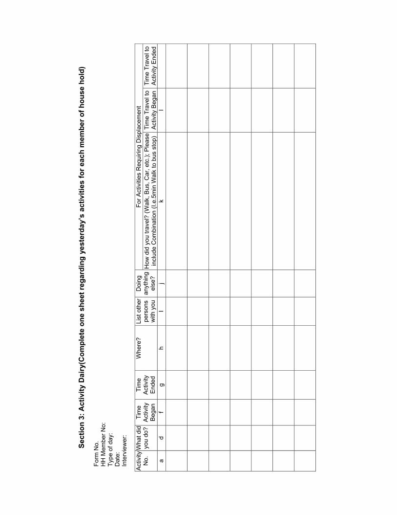
Se

ctio

n 3:

Act

ivity

Dai

ry(C

ompl

ete

one

shee

t reg

ardi

ng y

este

rday

’s a

ctiv

ities

for e

ach

mem

ber o

f hou

se h

old)

Fo

rm N

o.

HH

Mem

ber N

o:

Ty

pe o

f day

:

Dat

e:

Inte

rvie

wer

:

Fo

r Act

iviti

es R

equi

ring

Dis

plac

emen

t A

ctiv

ity

No.

W

hat d

id

you

do?

Tim

e A

ctiv

ity

Beg

an

Tim

e A

ctiv

ity

End

ed

Whe

re?

List

oth

er

pers

ons

with

you

Doi

ng

anyt

hing

el

se?

How

did

you

trav

el?

(Wal

k, B

us, C

ar, e

tc.);

Ple

ase

incl

ude

Com

bina

tion

(I.e.

5min

Wal

k to

bus

sto

p)

Tim

e Tr

avel

to

Activ

ity B

egan

Tim

e Tr

avel

to

Activ

ity E

nded

a d

f g

h I

j k

l

Sect

ion

4: T

rave

l Dai

ry (f

or tr

avel

rela

ted

activ

ities

onl

y fr

om p

revi

ous

page

)

Form

No.

H

H M

embe

r No.

: Ty

pe o

f Day

: D

ate:

In

terv

iew

er:

1s

t Seg

men

t 2n

d S

egm

ent

3rd

Seg

men

t 4t

h S

egm

ent

Act

ivity

N

o.

Tour

pu

rpos

e M

ode

Wai

t tim

e Tr

avel

tim

e C

ost

Tran

sfer

lo

catio

n be

twee

n 1s

t& 2

nd

Seg

men

t

Mod

eW

ait t

ime

Trav

el ti

me

Cos

tTr

ansf

er

loca

tion

betw

een

2nd

& 3

rd

Seg

men

t

Mod

e W

ait t

ime

Trav

el ti

me

Cos

t Tr

ansf

er

loca

tion

betw

een

3rd

& 4t

h S

egm

ent

Mod

eW

ait t

ime

Trav

el ti

me

Cos

t

N

ow, I

wou

ld li

ke to

ask

you

som

e qu

estio

ns a

bout

fuel

usa

ge a

nd a

pplia

nce

usag

e in

you

r hou

seho

ld.

Se

ctio

n 5:

Oth

er H

ouse

hold

Cha

ract

eris

tics

1.

List

tota

l hou

seho

ld fu

el c

onsu

mpt

ion

per m

onth

by

fuel

type

: Fu

el T

ype

Con

sum

ptio

n LP

G (c

ylin

der)

C

harc

oal(K

g.)

K

eros

ene

(litre

)

Oth

er*

2.

Li

st to

tal h

ouse

hold

ele

ctric

ity /

pow

er c

onsu

mpt

ion

(wat

ts /

units

) per

mon

th :

3.

List

tota

l hou

seho

ld s

pend

ing

is R

upee

s on

ele

ctric

ity a

nd fu

els

per m

onth

(oth

er th

an s

pend

ing

on tr

ansp

orta

tion)

:

Ener

gy T

ype

Rup

ees

LPG

(cyl

inde

r)

Cha

rcoa

l(Kg.

)

Ker

osen

e (li

tre)

O

ther

*

4. In

dica

te w

hich

of t

he fo

llow

ing

are

used

on

a fr

eque

nt b

asis

in y

our

hou

seho

ld:

Ye

s/N

o Te

levi

sion

Ref

riger

ator

Air

Con

ditio

ner

C

ompu

ter

M

icro

wav

e O

ven

W

ater

Coo

ler

Ann

exur

e 3.

6 H

ouse

hold

Cha

ract

eris

tics

Ta

ble

1 U

sage

Of L

PG

Si

No

Des

crip

tion

No

Of H

ouse

sPe

rcen

tage

1 YE

S

1241

89

.54

2 N

O

145

10.4

6 TO

TAL

1386

10

0

Ta

ble

2 U

sage

Of C

harc

oal

Si

No

Des

crip

tion

No

Of H

ouse

sPe

rcen

tage

1YE

S

49

3.54

2

NO

13

37

96.4

6 TO

TAL

1386

10

0

Ta

ble

3 U

sage

Of K

eros

ene

Si

No

Des

crip

tion

No

Of H

ouse

sPe

rcen

tage

1YE

S

206

14.8

6 2

NO

11

80

85.1

4 TO

TAL

1386

10

0

Tabl

e 4

Usa

ge O

f Ele

ctric

ity

Si

No

Des

crip

tion

No

Of H

ouse

sPe

rcen

tage

1YE

S

1323

95

.45

2N

O

63

4.55

TO

TAL

1386

10

0

Tabl

e 5

Usa

ge O

f Tel

evis

ion

Si

No

Des

crip

tion

No

Of H

ouse

sPe

rcen

tage

1YE

S

1327

95

.74

2N

O

59

4.26

TO

TAL

1386

10

0

Tabl

e 6

Usa

ge O

f Ref

riger

ator

Si

N

o D

escr

iptio

n N

o O

f Hou

ses

Perc

enta

ge

1YE

S

768

55.4

1 2

NO

61

8 44

.59

TOTA

L 13

86

100

Ta

ble

7 U

sage

Of A

ir co

nditi

oner

Si

N

o D

escr

iptio

n N

o O

f Hou

ses

Perc

enta

ge

1YE

S

64

4.62

2

NO

13

22

95.3

8

TOTA

L 13

86

100

Tabl

e 8

Usa

ge O

f Com

pute

r Si

N

o D

escr

iptio

nN

o O

f Hou

ses

Perc

enta

ge

1Y

ES

10

9 7.

86

2N

O

1277

92

.14

TOTA

L 13

86

100

Ta

ble

9 U

sage

Of M

icro

wav

e Si

N

o D

escr

iptio

nN

o O

f Hou

ses

Perc

enta

ge

1Y

ES

23

1.

66

2N

O

1363

98

.34

TOTA

L 13

86

100

Ann

exur

e 3.

7 St

ated

Pre

fere

nce

Surv

ey F

or A

naly

sis

Of V

ario

us T

rans

port

Mea

sure

s To

Red

uce

Vehi

cula

r Em

issi

ons

In H

yder

abad

Hou

seho

ld T

rave

l Sur

vey

by R

ITES

for U

SEPA

Lo

catio

n / C

olon

y N

ame:

D

ay: D

ate

: Lo

calit

y N

ame

/ No.

N

ame

of S

urve

yor:

W

ard

No:

N

ame

of S

uper

viso

r:

Traf

fic Z

one

No:

N

ame

of P

erso

n be

ing

Inte

rvie

wed

Fo

rm N

o:

Add

ress

: H

ow m

any

peop

le li

ve w

ith y

ou in

you

r hou

seho

ld?_

____

____

____

____

____

___

Prim

ary

Act

ivity

or e

mpl

oym

ent m

ight

incl

ude:

Em

ploy

men

t, H

ouse

Wife

, Stu

dent

, and

Pen

sion

er, e

tc.

Se

ctio

n 1:

Hou

seho

ld D

emog

raph

ic In

form

atio

n M

embe

r N

o.

Nam

e &

Rel

atio

n to

H

ead

of

Hou

seho

ld

Sex

(M

/F)

Age

E

duca

tion

Driv

er's

Li

cens

e?

Prim

ary

Activ

ity /E

mpl

oym

ent

Mon

thly

In

com

e (R

s.)

Mon

thly

Exp

endi

ture

on

Tra

nspo

rt (R

s.)

Type

of

Org

aniz

atio

n/B

usin

ess

Type

of A

ctiv

ity

/Job

Lo

catio

n

1

2

3

4

5

6

7

8

9

10

To

tal f

or h

ouse

Hol

d

Sect

ion

2: H

ouse

hold

Veh

icle

Cha

ract

eris

tics

Ve

hicl

e #1

Ve

hicl

e #2

Ve

hicl

e #3

Ve

hicl

e #4

Ve

hicl

e #5

Ve

hicl

e #6

VE

HIC

LE T

YPE

(car

, mot

orcy

cle,

sco

oter

, bic

ycle

, et

c.)

VEH

ICLE

MA

KE

& E

NG

INE

TYPE

(2/4

Str

oke)

VE

HIC

LE M

OD

EL

FUE

L TY

PE

(Pet

rol,

dies

el, L

PG

, CN

G, e

tc.)

VEH

ICLE

USA

GE

(day

s pe

r wee

k ve

hicl

e us

ed)

V VE

HIC

LE U

SAG

E (S

ingl

e (n

on-r

etur

n) tr

ips

per

day

vehi

cle

used

)

VEH

ICLE

AN

NU

AL

MIL

EAG

E (M

ileag

e ac

cum

ulat

ed

per d

ay)

VEH

ICLE

AN

NU

AL

MIL

EAG

E (m

ileag

e ac

cum

ulat

ed

per d

ay)

VEH

ICLE

MIL

EAG

E (to

tal v

ehic

le li

fetim

e)

For

mot

oriz

ed 2

-whe

eler

s an

d 3-

whe

eler

s (m

otor

cycl

es, s

coot

ers,

aut

o-ric

ksha

ws)

ple

ase

also

incl

ude

engi

ne-c

ycle

type

(2-

stro

ke o

r 4-

stro

ke e

ngin

e). A

ve

hicl

e ge

nera

lly h

as a

2-s

troke

eng

ine

if th

e lu

bric

atin

g oi

l is

mix

ed d

irect

ly w

ith th

e fu

el. I

f no

lube

oil

is m

ixed

in th

e fu

el ta

nk, t

he v

ehic

le is

gen

eral

ly a

4-

stro

ke e

ngin

e.

Sect

ion

3: T

rip In

form

atio

n C

olle

ct D

ata

on Y

este

rday

’s m

orni

ng tr

ip c

hara

cter

istic

s on

ly fo

r the

resp

onde

nt a

nsw

erin

g th

e SP

Que

stio

ns)

Now

I w

ould

like

to a

sk y

ou fo

r so

me

info

rmat

ion

on y

our

com

mut

e (tr

avel

from

hom

e to

wor

k) Y

este

rday

. Ple

ase

incl

ude

all t

rip e

lem

ents

, for

ex

ampl

e, w

alki

ng to

the

bus

stop

, bus

tran

sfer

, wal

king

to/fr

om a

par

king

spo

t to

your

inte

nded

des

tinat

ion,

wal

king

bet

wee

n tw

o st

ores

on

the

sam

e sh

oppi

ng s

tree

t, et

c.

Wha

t was

you

r tot

al tr

avel

tim

e (in

min

ute)

for t

he m

orni

ng c

omm

ute

trip

that

you

took

yes

terd

ay?

____

____

____

_ H

ow m

uch

did

it co

st y

ou in

tota

l (in

rupe

es) f

or th

e m

orni

ng c

omm

ute

trip

that

you

took

Yes

terd

ay?

____

____

___

Wha

t w

as t

he p

rimar

y m

ode

you

took

(C

ar, 2

-whe

eler

, bus

, wal

king

, 3-s

eate

r au

to-r

icks

haw

, 7-s

eate

r au

to-r

icks

haw

, bic

ycle

, or

othe

r) f

or t

he

mor

ning

com

mut

e tr

ip th

at y

ou to

ok Y

este

rday

? __

____

____

____

____

__

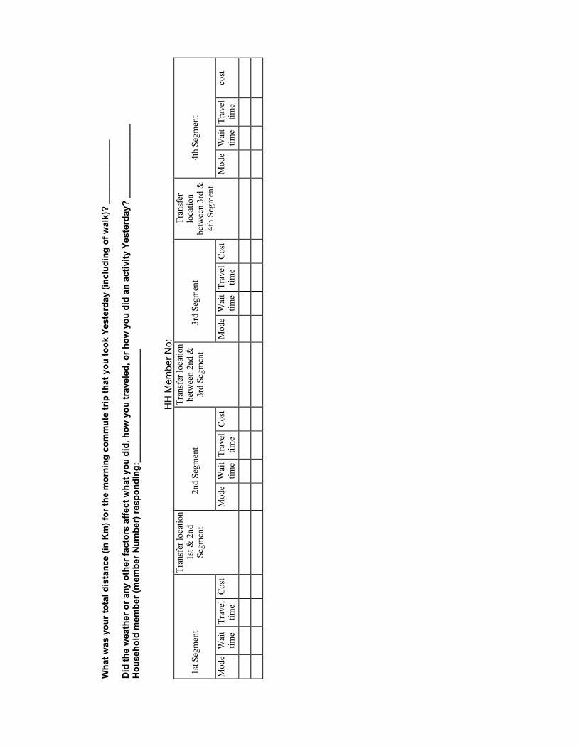
W

hat w

as y

our t

otal

dis

tanc

e (in

Km

) for

the

mor

ning

com

mut

e tr

ip th

at y

ou to

ok Y

este

rday

(inc

ludi

ng o

f wal

k)?

____

____

____

_ D

id th

e w

eath

er o

r any

oth

er fa

ctor

s af

fect

wha

t you

did

, how

you

trav

eled

, or h

ow y

ou d

id a

n ac

tivity

Yes

terd

ay?

____

____

____

___

Hou

seho

ld m

embe

r (m

embe

r Num

ber)

resp

ondi

ng:_

____

____

____

____

____

__

H

H M

embe

r No:

1st S

egm

ent

Tr

ansf

er lo

catio

n 1s

t & 2

nd

Segm

ent

2nd

Segm

ent

Tr

ansf

er lo

catio

n be

twee

n 2n

d &

3r

d Se

gmen

t 3r

d Se

gmen

t

Tr

ansf

er

loca

tion

betw

een

3rd

&

4th

Segm

ent

4th

Segm

ent

Mod

e W

ait

time

Trav

el

time

Cos

t

Mod

eW

ait

time

Trav

el

time

Cos

t

Mod

eW

ait

time

Trav

el

time

Cos

t

Mod

eW

ait

time

Trav

el

time

cost

Annexure 3.8 Temperature (0C) Levels in the Study Area

Station Code /Time

A B C D E F G H I J K

6.00 24.2 24.2 22.6 22.6 23.8 23.8 21.0 21.0 25.5 25.5 25.5 7.00 26.5 26.5 24.7 24.7 24.0 24.0 23.2 23.2 24.6 24.6 24.6 8.00 27.0 27.0 27.6 27.6 27.5 27.5 24.6 24.6 26.7 26.7 26.7 9.00 29.0 29.0 27.9 27.9 27.8 27.8 29.7 29.7 29.2 29.2 29.2 10.00 32.0 32.0 32.5 32.5 32.6 32.6 33.5 33.5 30.0 30.0 30.0 11.00 33.5 33.5 33.8 33.8 33.9 33.9 35.3 35.3 32.2 32.2 32.2 12.00 34.8 34.8 34.3 34.3 34.7 34.7 35.3 35.3 34.1 34.1 34.1 13.00 35.6 35.6 35.4 35.4 35.2 35.2 35.8 35.8 34.8 34.8 34.8 14.00 35.2 35.2 35.6 35.6 35.7 35.7 35.7 35.7 35.4 35.4 35.4 15.00 35.0 35.0 34.9 34.9 34.9 34.9 36.1 36.1 34.5 34.5 34.5 16.00 33.6 33.6 33.1 33.1 33.2 33.2 35.4 35.4 33.2 33.2 33.2 17.00 32.9 32.9 31.7 31.7 31.8 31.8 33.2 33.2 32.8 32.8 32.8 18.00 32.6 32.6 30.8 30.8 30.6 30.6 31.8 31.8 31.7 31.7 31.7 19.00 31.4 31.4 28.7 28.7 28.6 28.6 30.9 30.9 31.2 31.2 31.2 20.00 30.3 30.3 26.1 26.1 26.0 26.0 30.1 30.1 30.4 30.4 30.4 21.00 29.4 29.4 23.5 23.5 23.6 23.6 29.8 29.8 26.7 26.7 26.7 22.00 28.6 28.6 21.3 21.3 21.2 21.2 26.9 26.9 25.0 25.0 25.0 23.00 27.5 27.5 21.1 21.1 21.0 21.0 26.5 26.5 23.2 23.2 23.2 24.00 25.8 25.8 21.9 21.9 21.0 21.0 26.4 26.4 22.1 22.1 22.1 1.00 23.1 23.1 21.5 21.5 21.5 21.5 26.5 26.5 21.7 21.7 21.7 2.00 22.8 22.8 20.6 20.6 21.6 21.6 26.3 26.3 20.6 20.6 20.6 3.00 22.7 22.7 20.3 20.3 21.0 21.0 26.1 26.1 21.4 21.4 21.4 4.00 22.9 22.9 21.2 21.2 21.2 21.2 26.1 26.1 22.4 22.4 22.4 5.00 23.7 23.7 22.2 22.2 22.2 22.2 25.5 25.5 22.3 22.3 22.3

Wind Speed (KMPH) in the Study Area

Station Code /Time

A B C D E F G H I J K

6.00 4.2 4.8 6.2 4.8 4.2 5.3 7.3 7.3 3.3 4.8 4.3 7.00 3.6 3.8 6.8 6.6 4.8 6.0 8.1 6.3 3.8 5.6 4.6 8.00 1.8 2.6 4.2 3.2 5.2 4.0 6.3 4.2 4.2 5.8 6.2 9.00 1.6 1.9 3.1 2.8 3.1 2.0 4.8 3.6 6.1 2.1 3.2 10.00 1.3 1.9 2.6 2.9 3.6 2.3 2.2 2.5 5.4 2.0 2.1 11.00 1.1 1.2 2.2 2.7 2.8 2.5 1.8 2.0 4.8 1.5 1.1 12.00 1.2 0.8 1.3 3.9 1.3 3.6 1.2 1.0 3.3 1.3 1.3 13.00 0.8 0.9 1.0 3.7 0.8 2.3 1.1 0.9 1.1 1.1 0.3 14.00 2.1 1.5 0.8 3.1 0.9 2.2 0.9 0.8 1.1 0.9 1.2 15.00 2.6 1.9 0.9 3.0 1.1 2.0 0.6 2.2 0.8 3.6 3.3 16.00 7.1 6.8 2.1 3.0 3.3 0.7 0.3 3.9 2.7 4.1 4.2 17.00 7.5 7.0 6.3 2.8 8.4 5.0 1.8 4.6 5.5 6.8 7.2 18.00 8.6 8.9 8.1 4.4 7.6 8.8 4.3 8.2 9.6 7.5 8.1 19.00 4.9 5.1 9.2 9.5 6.5 7.0 6.6 7.1 8.7 8.8 9.6 20.00 4.6 4.1 5.3 8.1 7.1 4.2 8.8 5.5 9.2 4.2 4.7 21.00 2.2 2.0 3.4 6.2 4.8 2.6 5.4 4.3 6.1 2.6 3.1 22.00 2.9 3.2 2.6 4.6 2.1 1.8 2.9 2.8 7.2 2.2 2.0 23.00 1.3 1.1 2.8 2.7 1.3 1.2 1.4 1.2 4.8 1.0 1.1 24.00 1.1 0.9 1.0 1.1 0.9 0.4 1.0 1.0 2.2 1.8 1.2 1.00 0.8 0.7 0.8 0.9 0.8 0.2 0.7 0.9 1.2 0.8 0.5 2.00 0.5 0.6 0.7 0.7 0.9 0.2 0.6 0.8 0.9 1.1 1.0 3.00 1.6 1.8 0.3 1.1 1.4 0.5 1.3 0.9 0.6 0.9 0.5 4.00 3.4 3.7 1.4 2.6 2.9 6.0 3.8 1.9 1.9 2.6 2.4 5.00 5.9 6.7 5.7 3.6 3.7 8.1 4.4 4.6 2.8 3.2 3.1

Average (24 hrly) SPM Concentrations in the Study Area

0

100

200

300

400

500

600

700

800

A B C D E F G H I J KSites

Con

c. (µ

g/m

3 )

AVG SPM

SPM Std. 200 µg/m3

Average (24 hrly) RPM Concentrations in the Study Area

0

100

200

300

400

500

600

A B C D E F G H I J K

Sites

Con

c. (µ

g/m

3 )

AVG RPM

RPM Std. 100 µg/m3

Annexure 3.9

Average (24 hrly) SO2 Concentrations in the Study Area

0

10

20

30

40

50

60

70

80

90

A B C D E F G H I J KSites

Con

c. (µ

g/m

3 )

AVG SO2

Average (24 hrly) NOx Concentrations in the Study Area

0

20

40

60

80

100

120

A B C D E F G H I J KSites

Con

c. (µ

g/m

3 )

AVG NOx

NOx Std. 80 µg/m3

SO2 Std 80 µg/m3

Annexure 3.10

Hourly CO (PPM) Concentrations in the Study Area

0123456789

101112

A B C D E F G H I J KSites

Con

c (P

PM)

Avg CO

CO Std 3 5 PPM

Hourly HC (PPM) Concentrations in the Study Area

0

2

4

6

8

10

12

14

A B C D E F G H I J K

Sites

Con

c. (P

PM)

Avg HC

Annexure 3.11

Annexure 3.12 National Ambient Air Quality Standards (NAAQS)

Sensitive of Area

Industrial Area

Residential, Rural &

Other areasTesting Method

Annual Average* 15 µg/m3 80 µg/m3 60 µg/m3 Improved West and

Geake Method Sulphur Dioxide (SO2) 24 hours** 30 µg/m3 120 µg/m3 80 µg/m3 Ultraviolet Fluorescence

Annual* 15 µg/m3 80 µg/m3 60 µg/m3 Modified Jacob & Hochheiser (Na - Arsenite ) Method Oxides of

Nitrogen (NOx) 24 hours** 30 µg/m3 120 µg/m3 80 µg/m3 Gas Phase

Chemiluminescence Suspended Particulate

Matter (SPM)

Annual 24 hours**

70 µg/m3 100 µg/m3

360 µg/m3 500 µg/m3

140µg/m3 200µg/m3

High volume sampling. (Average flow rate not less than 1.1m3/min).

Respirable Particulate

Matter (RPM), (size less than

10 µm)

Annual * 24 hours**

50 µg/m3

75 µg/m3120 µg/m3 150 µg/m3

60 µg/m3 100µg/m3

Respirable particulate matter sampler

Lead (Pb) Annual* 24 hours**

0.50µg/m3

0.75µg/m31.0 µg/m3 1.5 µg/m3

0.75µg/m3 1.00µg/m3

ASS Method after sampling using EPM 2000 or equivalent Filter paper

Carbon Monoxide (CO)

8 hours** 1hour

1.0 mg/m3

2.0 mg/m35.0 mg/m3

10.0 mg/m3 2.0 mg/m3 4.0 mg/m3

Non dispersive infra red Spectroscopy

*Annual Arithmetic mean of minimum 104 measurements in a year taken twice a week 24 hourly at uniform interval. **24 hourly/8 hourly values should be met 98% of the time in a year. However, 2% of the time, it may exceed but not on two consecutive days. NOTE: 1. National Ambient Air Quality Standard: The levels of air quality with an adequate margin of safety, to protect the public health, vegetation and property. 2. Whenever and wherever two consecutive values exceeds the limit specified above for the respective category, it would be considered adequate reason to institute regular / continuous monitoring and further investigations.

Annexure 3.13 Hyderabad City Region Bus Operations and Performance Characteristics

S.No

Parameters 1996-1997

1997-1998

1998-1999

1999-2000

2000- 2001

2001- 2002

2002-2003*

1 No. of Depots 19 19 19 21 21 21 21

2 No.of Bus stations 12 12 12 12 16 16 18

3 No.of passenger

shelters

700 720 740 800 864 1004 1239

4 No. of Employees at

Hyderabad Branch

(H.C.R)

15162 15342 15676 16160 15729 16095 16203

5 No.of Buses (Avg.

Held)

2122 2217 2328 2425 2480 2605 2600

6 No.of Schedules (As

on last day)

1969 2066 2163 2253 2306 2421 2414

7 No.of Trips a Day 27808 29027 30488 31536 31803 34694 14455

8 Km.covered a day 504877 536784 559153 597470 602740 606956 643686

9 Avg.annual OR or %

Load factor

75 69 70 63 58 59 61

10 Avg. annual EPK in

Rs (P&L annual

account)

10.55 11.49 11.58 12.48 13.47 13.18 13.86

11 Avg. annual CPK in

Rs (P&L annual

account)

11.19 12.19 12.65 13.19 14.62 15.35 15.37#

12 Avg.Fleet age (kms

in million)

0 0 0 0.697 0.611 0.609 0.643

13 Total Revenue (Rs.

In million) (as per

P&L)

1944.47 2251.82 2363.74 2729.26 2961.48 2919.64 1365.02

14 Total subsidy

given(in million)

69.490 113.136 85.242 92.330 104.541 108.611 -

15 Total subsidy

received from

Govt(in million)

69.490 113.136 85.242 92.330 104.541 108.611 -

16 Profit (Loss)(in

million)

-118.528 -137.456 -218.79 -156.09 -241.47 -415.19 -86.231#

17 Profit & Loss Paise -64 -70 -107 -71 -106 -206 -110#

S.No

Parameters 1996-1997

1997-1998

1998-1999

1999-2000

2000- 2001

2001- 2002

2002-2003*

per Km

18 Vehicle utilisation(

kms)

238 242 240 246 243 233 247

19 Fleet Utilisation (%) 98.68 99.68 98.71 99.71 99.68 97.31 99.46

20 Breakdown rate (Per

10,000km)

0.35 0.35 0.28 0.22 0.46 0.32 0.42

21 Accident rate (per

1,00,000 km)

0.17 0.13 0.14 0.12 0.08 0.10 -

22 Fuel consumption

(Total)

39339860 41463825 42647197 45442767 44475858 37752609

-

23 HSD KMPL 4.73 4.79 4.86 4.87 4.80 4.86 4.85

24 LUB KMPL 1459 1596 1806 1890 1813 1965 1993

25 Average Tire life 1.63 1.68 1.67 1.75 1.93 2.03 2.09

26 Staff per bus 7.48 7.26 7.21 7.09 7.29 6.68 7.11

27 No. of Passengers

carried per day on

Avg(in Lakhs)

3.177 3.054 3.253 3.050 2.872 3.068 -

Source: APSRTC, Hyderabad City Region

* Up to Aug. 2002

# Up to July 2002

Abbreviations:

OR-Occupancy Rate

HCR-Hyderabad City Region

EPK-Earning Per Km

CPK-Cost per Km

P&L- Profit & Loss

HSD-Diesel

LUB-Lubricant Engine Oil

Annexure 3.14 Comparative Fare Structure For Urban/Town Services Of

Various STUs

Fare Structure per Passenger Km S.No

Name of STUs Type of Service Distance

(KM) Fare (Rs)

Ordinary 2 2.50 4 3.00 6 3.50 8 4.00 10 4.50 12 5.00 14 5.50 16 6.00 18 6.50 20 7.00 22 7.50 24 8.00 26 8.50 28 9.00 30 9.50 32 10.00 34 10.50 36 11.00 38 11.50 40 12.00

Suburban The above fares applicable to City/Town services Express 50 Ps more per passenger over the fare applicable to

City Ordinary services Metro/City Express

Rs. 3.50 for first stage of 2 kms and 50 Ps. for every subsequent stage of 2 kms thereafter.

Metro Liner 2 5.00 4 5.50 6 6.00 8 6.50 10 7.00 12 8.00 14 9.00 16 10.00 18 11.00 20 11.50 22 12.50 24 13.00 26 14.00 28 14.50 30 15.50 32 16.00

1 APSRTC (Andhra Pradesh State Road Transport Corporation)

34 16.50

Fare Structure per Passenger Km S.No

Name of STUs Type of Service Distance

(KM) Fare (Rs)

36 17.00 38 17.50 40 18.00

Ordinary Dist (in Kms)

Ordinary Fare

Limited Fare

A/C Fare Point to Point Fare

3 3.0 3.5 11.0 5.0 5 4.0 4.5 15.0 6.0 7 5.0 6.0 19.0 7.0 10 6.0 7.0 23.0 8.0 15 9.0 10.0 27.0 9.0 20 10.0 11.0 31.0 10.0 25 11.0 13.0 35.0 12.0 30 12.0 14.0 39.0 13.0 35 13.0 16.0 43.0 14.0

2 BEST (Brihan Mumbai Electric Supply & Transport Undertaking)

>35 Rs. 2.00 for every additional 5km or part

thereof

Rs. 4.00& Rs. 2.00 for every additional 5km or

part thereof in respectively for A/C &

Point to Point Ordinary 4 2.0

4-8 5.0 8-12 7.0

3 DTC (Delhi Transport Corporation)

>12 10.0 Ordinary Kms City

Services Sub-Urban

Ordinary Express Ordinary Exress 2 1.0 2.0 2.5 3.0 4 2.0 2.5 3.5 4.0 6 3.0 3.5 4.0 4.5 8 3.0 3.5 4.5 5.0 10 3.5 4.0 5.0 5.5 12 3.5 4.0 5.5 6.0 14 3.5 4.0 6.0 6.5 16 4.0 4.5 6.5 7.0 18 4.0 4.5 6.5 7.0 20 4.0 4.5 7.0 7.5 22 4.5 5.0 7.0 7.5 24 4.5 5.0 7.5 8.0 26 5.0 5.0 7.5 8.0 28 5.0 5.5 8.0 8.5 30 5.5 5.5 8.0 8.5

4 BMTC (Bangalore Metropolitan Transport Corporation)

32 5.5 6.0

Fare Structure per Passenger Km S.No

Name of STUs Type of Service Distance

(KM) Fare (Rs)

34 6.0 6.5 36 6.0 6.5 38 6.5 7.0 40 6.5 7.0 42 7.0 7.5 44 7.0 7.5 46 7.5 8.0

Pushpak Upto 3 3.0 4-8 5.0 9 7.0 10-16 8.0 17-19 9.0 20-25 10.0

Ordinary 6 2.0 8 2.5 12 2.8 16 3.0 18 3.3

5 South Bengal STC

22 3.8 Ordinary 3 3.0

6 4.0 9 5.0 12 6.0 15 7.0 18 8.0 21 9.0 24 10.0 27 11.0

6 Navi Mumbai MT (Navi Mumbai Municipal Transport)

30 12.0 Ordinary 2 1.5

4 1.8 6 2.0 8 2.3 10 2.3 12 2.8 14 3.0 16 3.3 18 3.3 20 3.5 22 3.8

7 Tamil Nadu

24 4.0

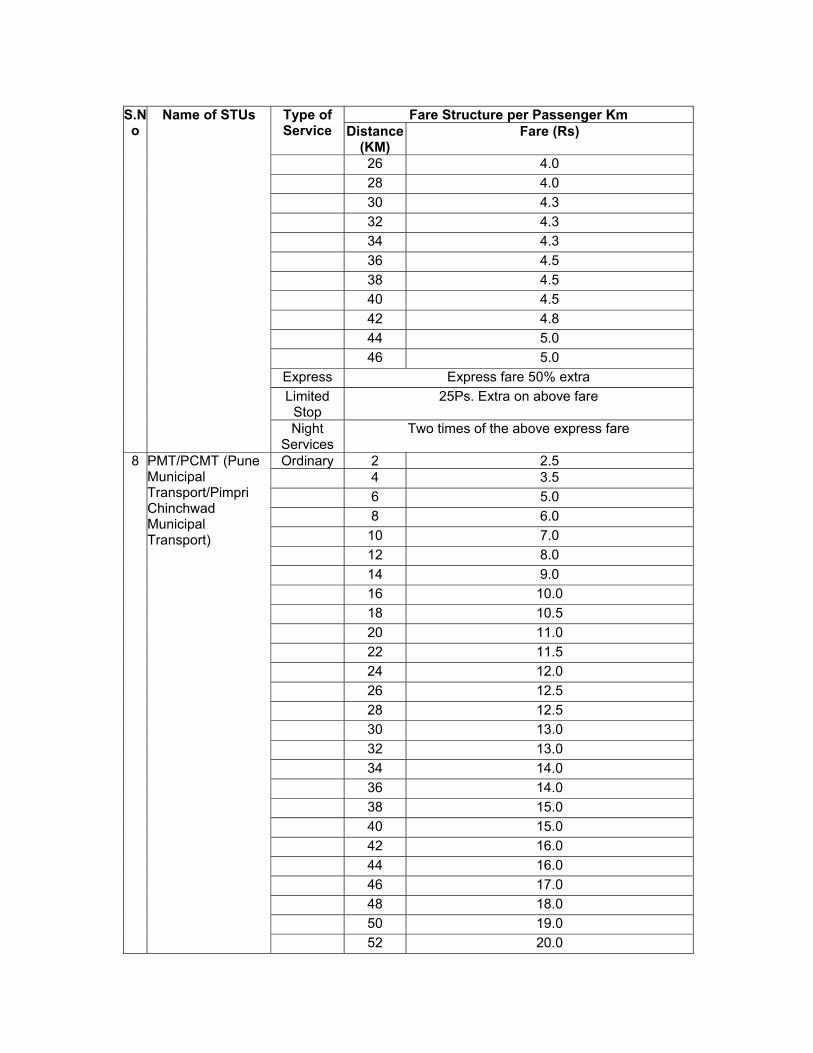
Fare Structure per Passenger Km S.No

Name of STUs Type of Service Distance

(KM) Fare (Rs)

26 4.0 28 4.0 30 4.3 32 4.3 34 4.3 36 4.5 38 4.5 40 4.5 42 4.8 44 5.0 46 5.0

Express Express fare 50% extra Limited

Stop 25Ps. Extra on above fare

Night Services

Two times of the above express fare

Ordinary 2 2.5 4 3.5 6 5.0 8 6.0 10 7.0 12 8.0 14 9.0 16 10.0 18 10.5 20 11.0 22 11.5 24 12.0 26 12.5 28 12.5 30 13.0 32 13.0 34 14.0 36 14.0 38 15.0 40 15.0 42 16.0 44 16.0 46 17.0 48 18.0 50 19.0

8 PMT/PCMT (Pune Municipal Transport/Pimpri Chinchwad Municipal Transport)

52 20.0

Fare Structure per Passenger Km S.No

Name of STUs Type of Service Distance

(KM) Fare (Rs)

54 21.0 56 22.0 58 23.0 60 24.0

Ordinary 4.0 3.0 8.0 3.5 12.0 4.0 16.0 4.5

9 CSTC (Calcutta State Transport Corporation)

20.0 5.0 Source: Association of State Transport Undertakings: Profile & Performance 2000-01,

Ann

exur

e 3.

15

CO

MPA

RA

TIVE

STA

TEM

ENT

OF

MO

TOR

VEH

ICLE

TA

X FO

R S

TAG

E C

AR

RIA

GES

(as

on M

arch

200

1)

W

EST

BEN

GA

L M

AH

AR

AST

RA

(M

SRTC

&

BES

T)

KA

RN

ATA

KA

K

ERA

LA

(KSR

TC)

TAM

ILN

AD

UD

ELH

I (D

TC)

AN

DH

RA

PR

AD

ESH

(APS

RTC

)

CST

C

NB

TC

(a) R

s.71

/- pe

r se

at p

er a

nnum

an

d R

s.18

/- pe

r st

ande

e pe

r ye

ar. A

nnua

l R

ate

of M

V T

ax

com

es to

Rs.

40

68

(a) K

nSTR

C &

B

MTC

: Rur

al

=6%

on

Traf

fic

reve

nue;

City

=

3% o

n Tr

affic

re

venu

e

(a) C

ity /

Ord

inar

y:

Rs.

400

/-+

per s

eat f

or

a qu

arte

r

(a) C

NI-I

&II:

City

Ser

vice

s:

Rs.

60/

- per

se

at a

nd

auth

oriz

ed

stan

dee

per

quar

ter

Ann

ual T

ax R

s.

1951

/- fo

r firs

t 18

pass

enge

r +R

s.

280/

- for

eve

ry

addi

tiona

l pa

ssen

ger t

he b

us

is a

llow

ed to

car

ry

cond

ucto

r and

dr

iver

exc

lude

d fro

m th

e nu

mbe

r lic

ense

d to

car

ry.

(1) O

rdin

ary:

Sla

b If

the

dist

ance

co

vere

d by

the

bus

per d

ay

(a)

Doe

s no

t exc

eed

100k

m- R

s. 1

91

Per

qua

rter p

er s

eat (

b) E

xcee

ds

100k

ms,

but

doe

s no

t exc

eed

160k

m- R

s. 2

67 P

er q

uarte

r per

se

at ©

Exc

eeds

160

kms,

but

doe

s no

t exc

eed

240k

m-R

s. 3

42 P

er

quar

ter p

er s

eat (

d) E

xcee

ds

240k

m b

ut d

oes

not e

xcee

d 32

0km

- Rs.

401

Per

qua

rter p

er

seat

(e) E

xcee

ds 3

20km

-Rs.

438

P

er q

uarte

r per

sea

t

(a) C

ity &

M

ofus

sil:T

he G

ovt.

of W

est B

enga

l has

ex

empt

ed to

tally

all

Sta

te C

arria

ges

buse

s be

long

ing

to

CS

TC fr

om

paym

ent o

f M

.V.T

ax fr

om th

eir

resp

ectiv

e da

tes

or

regi

stra

tion

(a) S

eatin

g C

apac

ity (5

0+1)

-R

s.79

9 pe

r Yea

r(b)

Sea

ting

Cap

acity

(40+

1)-

Rs.

699

per Y

ear©

S

eatin

g C

apac

ity(3

7+1)

-R

s.66

9 pe

r Yea

r(d)

Sea

ting

Cap

acity

(30+

1)-R

s.

580p

er Y

ear(

e)

Sea

ting

Cap

acity

(20+

1)-R

s.

431

per Y

ear

(b) F

or b

uses

pl

ying

sol

ely

with

in

mun

icip

al

limits

, onl

y 2/

3rd

of a

nnua

l tax

as

wor

ked

out

abov

e ne

ed b

e pa

id

(b) N

WK

nRTC

: R

ural

= 8

% o

n Tr

affic

reve

nue;

C

ity=

5% o

n Tr

affic

reve

nue

(b) F

ast

Pas

/Exp

ress

: Rs.

460

/- pe

r sea

t for

a

quar

ter

(b) O

ther

s: (1

) M

ofus

sil -

Rs.

45

0/-

seat

/qua

rter

(2) T

own

- Rs.

30

2.50

se

at/q

uarte

r (3

) Spa

re -

Rs.

33

7.50

se

at/q

uarte

r (4

) Gha

t - R

s.

50/-

seat

/qua

rter

(2

) Exp

ress

:(a) D

oes

not e

xcee

d 32

0km

-Rs.

504

Per q

uarte

r per

se

at(b

) Exc

eed

320

km-R

s.65

6 P

er

quar

ter p

er s

eat

(b) I

nter

-Sta

te

Ope

ratio

n: In

cas

e of

Inte

r-Sta

te

Ope

ratio

n, ra

tes

of

taxa

tion

paid

by

CS

TC to

the

Bih

ar

Gov

t. as

follo

ws;

R

oad

Tax-

@R

s.

375/

- per

bus

per

m

onth

& a

dditi

onal

M

.V.T

ax-@

Rs.

16

64/-

per b

us p

er

mon

th

©

For

bus

es

plyi

ng w

ith in

B

omba

y C

ity

Cor

pora

tion

limits

a w

heel

tax

@ R

s. 2

60/-

per

bus

per a

nnum

ha

s to

be

paid

to

the

Mun

icip

al

Cor

pora

tion

©

R

eser

ve/S

pare

bus

: Rs

25/-

per s

eat

for a

qua

rter

© S

pare

Veh

icle

s: R

s. 1

44/-

for

ever

y pa

ssen

ger w

hich

the

vehi

cle

is p

erm

itted

to c

arry

(d) B

us h

avin

g se

atin

g ca

paci

ty

49+2

2 st

ande

es

may

MV

Tax

per

ye

ar R

s. 2

937/

-

(d

) S

tand

ees:

R

s. 1

00/-

for

quar

ter

Sou

rce:

Ass

ocia

tion

of S

tate

Tra

nspo

rt U

nder

taki

ngs:

Pro

file

& P

erfo

rman

ce 2

000-

01.

Abb

revi

atio

ns:

MS

TRC

-Mah

aras

tra S

tate

Roa

d Tr

ansp

ort C

orpo

ratio

n B

ES

T-B

rihan

Mum

bai E

lect

ric S

uppl

y &

Tra

nspo

rt U

nder

taki

ng

KSR

TC-K

eral

a St

ate

Roa

d Tr

ansp

ort C

orpo

ratio

n D

TC- D

elhi

Tra

nspo

rt C

orpo

ratio

n AP

SRTC

-And

hra

Pra

desh

Sta

te R

oad

Tran

spor

t Cor

pora

tion

KnS

RTC

-Kar

nata

ka S

tate

Roa

d Tr

ansp

ort C

orpo

ratio

n B

MTC

-Ban

galo

re M

etro

polit

an T

rans

port

Cor

pora

tion

NW

KnR

TC-N

orth

Wes

t Kar

nata

ka R

oad

Tran

spor

t Cor

pora

tion

CN

I-I&

II-M

etro

polit

an T

rans

port

Cor

p.Lt

d(C

henn

ai D

iv I&

II)

CS

TC-C

alcu

tta S

tate

Tra

nspo

rt C

orpo

ratio

n N

BS

TC-N

orth

Ben

gal S

tate

Tra

nspo

rt C

orpo

ratio

n

Annexure 4.1 Zone Wise Daily Trip Productions & Attractions (2003) - Including Walk

TRIP PRODUCTIONS TRIP ATTRACTIONS ZONE NO. WORK EDUCATION OTHERS WORK EDUCATION OTHERS

1 13142 15581 4336 75462 29101 16565 2 11750 9739 2858 18230 5718 2435 3 10734 7098 3982 11057 7252 2106 4 18304 13898 10508 5271 8144 9090 5 12897 11139 1172 4109 6418 781 6 13122 15571 3674 7580 7147 2269 7 14275 7739 2064 17865 11227 2410 8 19399 16368 5001 4450 7407 3924 9 8808 11806 2061 3316 3716 2716

10 16015 20269 6006 10046 20224 3540 11 11629 5881 3743 9156 4365 2687 12 14194 8236 1227 6238 3591 1477 13 26712 15604 11901 14194 9415 8728 14 14124 4598 4927 7176 5096 2151 15 10875 6920 1483 3988 1847 736 16 15837 13174 561 3720 4892 280 17 38312 30312 6315 11123 16321 3119 18 59290 39755 7882 45699 24759 5294 19 14674 8101 7490 22188 16038 5400 20 27564 12295 4759 23086 18261 3757 21 35361 34933 9644 30368 39717 8268 22 10522 4246 2215 6498 2536 1975 23 22916 14429 2829 16889 8425 1242 24 38549 18852 8160 27106 12989 8474 25 28175 24296 4696 19858 11539 7197 26 51108 36911 3245 34198 19754 2276 27 13152 8675 3918 16894 10631 4767 28 25260 8566 4393 60347 53007 8887 29 24345 19647 6193 8373 8774 4604 30 16403 5368 4175 14891 5987 4202 31 26023 10692 2622 55147 33205 6620 32 11392 6814 852 34490 9879 419 33 14914 7151 3882 35434 7942 6473 34 11679 8606 2305 10398 13783 1570 35 28353 15342 4078 10210 7123 2202 36 12017 7141 174 7832 2986 174 37 19445 19273 2925 51182 40494 4660 38 7941 5775 412 6620 7357 1084 39 35338 24133 8102 35286 11019 10017 40 4774 6426 2020 24697 11277 1614 41 13882 10774 5387 62652 39437 15442 42 6312 4641 743 5251 2382 1137 43 7389 5254 2299 24105 4412 2492 44 12291 12905 1844 7734 4734 922 45 31043 18590 2707 69752 88641 9436 46 24725 10302 11126 74866 44261 20007 47 10392 8025 514 15256 6604 1658

TRIP PRODUCTIONS TRIP ATTRACTIONS ZONE NO. WORK EDUCATION OTHERS WORK EDUCATION OTHERS 48 11008 6530 1306 6004 2607 1494 49 15651 10480 3913 10800 10193 3719 50 38645 36242 17821 15756 18656 16286 51 37889 33432 10536 33103 28945 8615 52 11743 10798 4049 17537 14414 5321 53 19032 13671 3753 26209 34560 2684 54 16293 13701 4443 6363 4066 2962 55 19681 17824 4456 14379 10965 4431 56 25411 23717 2372 8299 11041 2033 57 29525 25283 14423 37232 32585 9655 58 11552 16656 4836 17342 27582 5418 59 10135 9379 3328 7966 11389 4161 60 22792 9877 5128 35171 14062 5577 61 4176 4176 659 2925 2544 659 62 1392 3017 0 6614 5071 361 63 1892 2417 105 3173 3065 702 64 9712 5775 1181 11036 3415 3490 65 17526 6784 4334 169571 78795 33933 66 5743 2960 2131 8401 12815 1071 67 9946 5107 3763 2616 1906 1873 68 15885 13400 4755 12644 8688 4846 69 2007 1003 201 6891 3348 671 70 12288 6808 2325 7186 4438 901 71 15252 12889 6230 8899 13269 3411 72 12303 6419 3744 1531 4551 1605 73 13112 10198 8013 5571 3089 3642 74 22226 8689 4243 13109 7632 2252 75 5783 1851 1388 1552 1619 1337 76 5573 1773 2027 1719 3166 1013 77 37466 27701 9566 27280 18483 5999 78 18024 11662 10602 10255 7689 10736 79 14951 11474 4520 17328 5553 4537 80 20914 13848 10457 18543 13280 6262 81 7960 5897 1179 3129 1948 884 82 4589 4982 1180 11297 7104 7824 83 5920 6375 1265 2844 2325 300 84 3733 3033 3127 38656 57869 15054 85 6795 4782 1762 6869 3928 3323 86 13419 12242 8475 4534 5415 3061 87 9547 4455 10183 4825 2120 6297 88 5920 1579 3552 2763 395 2174 89 25451 25451 19884 12044 18378 15886 90 6319 8517 6319 1509 2473 2473 91 36647 33528 8577 29210 24227 1229 92 6845 4475 0 2347 2171 180 93 10346 8180 962 4480 5774 722 94 6848 5136 1712 11717 3177 2458 95 6383 6487 1779 2275 5117 1965 96 6069 3287 2781 3500 134 2276

TRIP PRODUCTIONS TRIP ATTRACTIONS ZONE NO. WORK EDUCATION OTHERS WORK EDUCATION OTHERS 97 12835 11965 4786 5404 7202 4351 98 18352 12234 2447 23009 9030 2659 99 18875 4418 1606 5792 2008 0

100 23407 18813 5907 6502 6344 1313 101 10379 5793 7241 6509 2869 6975 102 34830 36169 7368 13106 19817 5371 103 13871 7398 6011 6063 2081 5506 104 11479 7131 174 40485 20244 6683 105 6130 9195 557 4276 3809 1076 106 8303 4670 519 704 578 0 107 7225 3335 2779 862 834 557 108 22684 16777 6616 14472 5798 6147 109 3289 3568 1679 4281 4397 1199 110 21470 13364 5258 6314 5546 4942 111 10575 13950 2250 1938 3601 2025 112 21059 25791 6625 11673 18875 4895 113 12275 17373 944 4364 12264 378 114 40905 38909 9228 10152 23934 7163 115 22997 13798 4599 5734 7788 4304 116 27621 19761 3368 47427 13607 4493 117 43244 37970 12305 25074 33012 12171 118 6417 7523 2213 3037 4204 1106 119 5132 4517 2053 3546 4138 1096 120 19296 9272 3508 9421 1422 1253 121 3036 4771 651 3557 5693 651 122 8493 1296 432 4878 2021 0 123 1536 439 0 728 0 0 124 10547 7655 2041 12328 6985 1373 125 7946 6863 3973 1445 2528 1445 126 14504 10153 5077 3626 6527 4593 127 7976 347 1040 7995 2077 1040 128 10382 1133 378 6622 9545 577 129 10611 9256 7224 4744 6763 7224

TOTAL 2091356 1541409 547615 2091356 1541409 547615

Annexure 4.2 Daily Trip Productions (Including Walk)

2011 2021 ZONE NO. WORK EDUCATION OTHERS WORK EDUCATION OTHERS

1 13702 15131 3431 17488 16579 3704 2 16365 11765 3467 21555 13325 3857 3 12913 12848 3185 16132 13733 3364 4 21783 19439 4980 28507 22094 5578 5 19018 12497 4138 24801 14367 4666 6 11695 8367 2756 14474 9197 2972 7 13958 10142 3191 16711 10561 3301

2011 2021 ZONE NO. WORK EDUCATION OTHERS WORK EDUCATION OTHERS

8 22133 15498 4724 27557 16028 4867 9 13328 9049 3177 16159 9690 3358

10 22232 17045 5399 27453 18684 5858 11 14070 8726 2718 17156 9080 2805 12 14483 10551 3557 18210 11501 3824 13 34393 33207 7695 42649 36327 8357 14 15646 10635 3597 19959 12391 4106 15 13011 9621 2872 16656 11177 3242 16 20803 11854 4210 26161 12682 4466 17 43125 37860 9729 54990 43560 11094 18 64704 44697 12626 83737 51584 14463 19 20381 12368 4261 26708 14428 4836 20 31025 15858 7145 40853 18488 8247 21 45311 26489 9178 55680 28393 9793 22 36275 15559 10415 15705 5681 4090 23 39555 24076 8149 65287 36621 12078 24 36393 31945 10758 48409 38000 12688 25 48841 32285 11391 80052 49130 17044 26 76646 47446 17010 124531 70727 25123 27 14161 13290 4276 17228 14449 4608 28 28616 13945 6867 37555 15996 7815 29 28096 22319 7371 37076 26072 8522 30 20108 7807 4277 29078 10382 5537 31 29393 13252 5568 43012 17702 7277 32 16227 10174 3289 23544 13571 4220 33 20388 9861 4097 28487 12577 5123 34 14632 7960 3524 18731 8626 3789 35 30021 20049 6874 39816 23260 7900 36 13234 8707 3398 17252 10074 3855 37 11453 4593 2207 13960 4993 2371 38 15129 10989 3264 19310 11994 3520 39 35092 25254 7746 44333 27594 8421 40 8484 6397 1956 11264 7961 2324 41 15747 9637 3945 19618 10535 4284 42 9064 6404 2061 10732 6849 2172 43 7609 4278 2019 9072 4620 2148 44 13294 13338 4544 16980 15108 5091 45 30862 16522 5582 38442 17563 5908 46 13047 14631 3157 15632 15965 3399 47 17560 8575 3482 22467 9369 3761 48 13296 8788 3108 16884 9812 3416 49 20852 9290 4335 27618 10385 4802 50 43010 37905 9231 54023 40480 9818 51 38014 35404 9343 49132 39770 10430 52 16051 5413 3964 20684 6033 4396 53 24744 12549 4717 31531 13519 5049 54 18233 17167 4669 23348 19944 5339 55 21125 18197 6561 27949 20753 7409 56 27171 30257 6575 34585 34590 7428

2011 2021 ZONE NO. WORK EDUCATION OTHERS WORK EDUCATION OTHERS 57 37301 26410 8131 46902 28249 8654 58 21362 17479 4711 38140 29957 7622 59 19638 15289 4485 29403 20944 5901 60 26871 12990 5215 38106 16801 6598 61 5504 6850 2008 7672 9133 2489 62 4544 2872 1211 5880 3665 1393 63 5131 2549 1327 6750 3221 1544 64 10300 6579 2429 13023 7190 2606 65 10159 5263 2457 12429 5765 2643 66 13649 4034 1959 18793 4369 2076 67 11216 5635 2892 13449 6112 3093 68 25465 12748 5536 35787 15956 6773 69 10109 9620 2838 13395 11587 3276 70 15877 9420 3602 21078 11115 4142 71 20825 15361 5439 28853 19322 6617 72 17002 7670 3548 22996 9219 4131 73 16365 10551 3852 21513 12464 4436 74 40193 34870 9710 82461 67759 17966 75 12368 6236 2866 24455 11616 4720 76 9216 3015 2308 17931 5301 3613 77 53109 42905 12918 125034 96439 28078 78 24728 13271 5977 45319 22631 9690 79 20388 17565 6171 34957 27905 9399 80 32689 24521 7561 67190 47468 13855 81 14727 10252 4163 27759 18256 6848 82 9935 6946 2540 17424 12197 3923 83 11516 8269 3074 20003 13940 4732 84 9903 3172 1939 16350 5283 2860 85 9365 6331 3396 16510 10660 5243 86 20472 20385 5341 39456 36822 8988 87 16964 12036 5178 32394 21523 8618 88 9944 4071 3020 19574 7371 4779 89 37170 27817 9041 71013 50440 15675 90 14234 14327 4239 28624 27480 7147 91 34257 25433 9444 161175 116608 39005 92 9696 7723 3014 18803 14531 4952 93 16379 11902 4927 26773 18107 6933 94 9672 11306 3578 18749 21556 5735 95 16312 9855 4458 30247 17861 7369 96 14630 11440 4524 28269 21146 7531 97 28780 19342 6575 57148 36148 11436 98 29773 23437 8748 53794 39299 14190 99 42843 25036 9191 78847 42313 14942

100 33022 26675 8356 57860 43613 13150 101 12829 8492 4152 21692 13602 6298 102 43532 29312 9503 86323 55376 17167 103 20138 10015 4769 34896 16116 7190 104 12525 10541 2733 22791 19381 4345 105 8966 9447 3576 17315 17911 5707

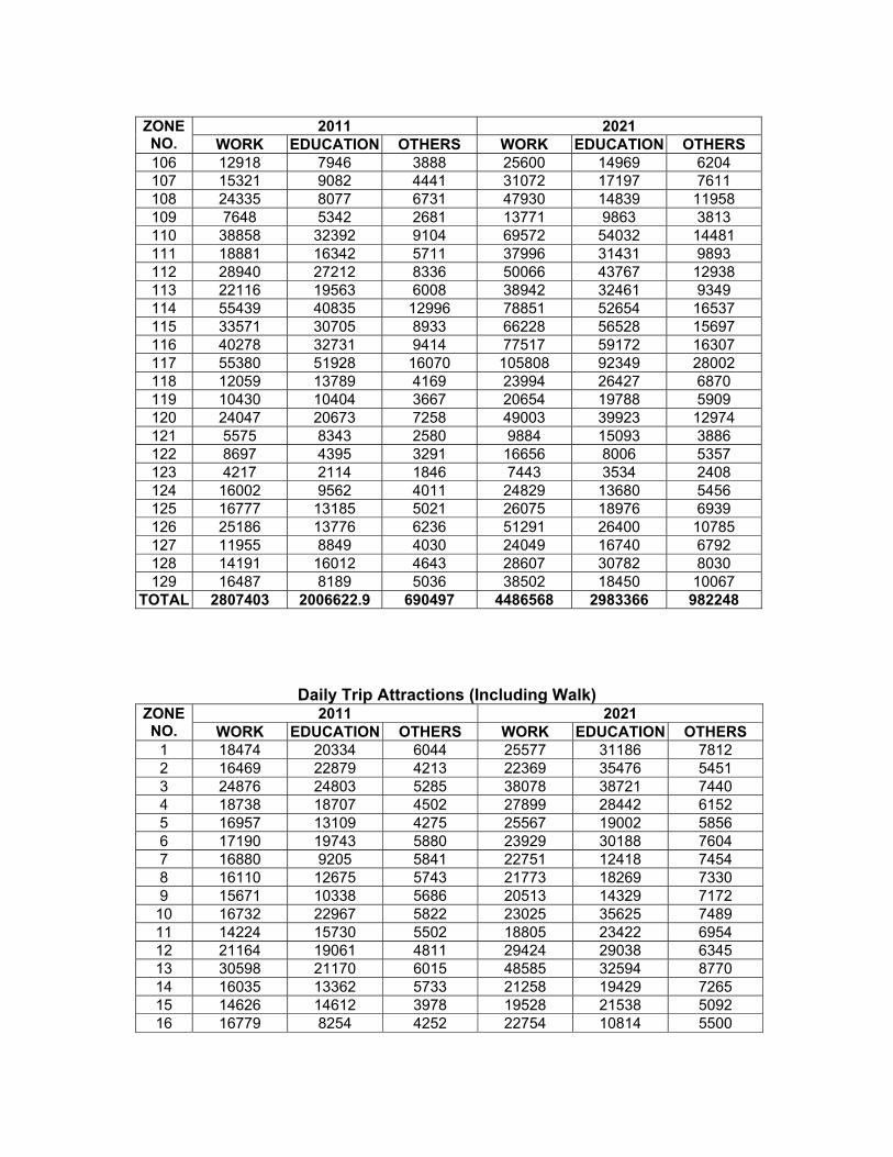
2011 2021 ZONE NO. WORK EDUCATION OTHERS WORK EDUCATION OTHERS 106 12918 7946 3888 25600 14969 6204 107 15321 9082 4441 31072 17197 7611 108 24335 8077 6731 47930 14839 11958 109 7648 5342 2681 13771 9863 3813 110 38858 32392 9104 69572 54032 14481 111 18881 16342 5711 37996 31431 9893 112 28940 27212 8336 50066 43767 12938 113 22116 19563 6008 38942 32461 9349 114 55439 40835 12996 78851 52654 16537 115 33571 30705 8933 66228 56528 15697 116 40278 32731 9414 77517 59172 16307 117 55380 51928 16070 105808 92349 28002 118 12059 13789 4169 23994 26427 6870 119 10430 10404 3667 20654 19788 5909 120 24047 20673 7258 49003 39923 12974 121 5575 8343 2580 9884 15093 3886 122 8697 4395 3291 16656 8006 5357 123 4217 2114 1846 7443 3534 2408 124 16002 9562 4011 24829 13680 5456 125 16777 13185 5021 26075 18976 6939 126 25186 13776 6236 51291 26400 10785 127 11955 8849 4030 24049 16740 6792 128 14191 16012 4643 28607 30782 8030 129 16487 8189 5036 38502 18450 10067

TOTAL 2807403 2006622.9 690497 4486568 2983366 982248

Daily Trip Attractions (Including Walk) 2011 2021 ZONE

NO. WORK EDUCATION OTHERS WORK EDUCATION OTHERS 1 18474 20334 6044 25577 31186 7812 2 16469 22879 4213 22369 35476 5451 3 24876 24803 5285 38078 38721 7440 4 18738 18707 4502 27899 28442 6152 5 16957 13109 4275 25567 19002 5856 6 17190 19743 5880 23929 30188 7604 7 16880 9205 5841 22751 12418 7454 8 16110 12675 5743 21773 18269 7330 9 15671 10338 5686 20513 14329 7172

10 16732 22967 5822 23025 35625 7489 11 14224 15730 5502 18805 23422 6954 12 21164 19061 4811 29424 29038 6345 13 30598 21170 6015 48585 32594 8770 14 16035 13362 5733 21258 19429 7265 15 14626 14612 3978 19528 21538 5092 16 16779 8254 4252 22754 10814 5500

2011 2021 ZONE NO. WORK EDUCATION OTHERS WORK EDUCATION OTHERS 17 23430 17629 5101 34675 26623 7009 18 31018 13373 6069 54494 19448 9519 19 17956 9813 5978 24870 13446 7723 20 23219 64966 6650 32406 106444 8676 21 25147 30926 6896 38360 49046 9431 22 31865 9834 6177 54573 13480 9528 23 18503 16176 4472 28496 24174 6227 24 19130 38612 4552 29925 62007 6408 25 31033 37332 7646 51900 59847 11145 26 47418 23687 8162 81507 36839 12938 27 15764 5466 5699 21071 6114 7242 28 22025 34874 6497 31072 55701 8508 29 26020 15403 5431 37806 22869 7406 30 35053 27897 8159 52343 43938 11201 31 19991 39258 6238 30774 63094 8470 32 19259 18274 6145 26991 27713 7991 33 16477 38411 5789 22441 61666 7416 34 17444 44138 4337 23846 71324 5639 35 20785 22286 4763 30263 34476 6451 36 16042 19127 4158 21281 29149 5313 37 16047 43815 5735 21259 70779 7266 38 18173 36548 4430 25095 58526 5796 39 30709 10376 6029 45795 14392 8417 40 17212 5466 5883 23481 6114 7545 41 24696 17641 6838 33700 26644 8839 42 16478 14638 5789 21956 21579 7353 43 15109 16993 5615 20194 25551 7131 44 18577 10521 4482 25289 14636 5820 45 28268 75252 7294 40974 123787 9762 46 18664 42295 6069 25408 68216 7790 47 17322 12486 5898 23596 17951 7562 48 16829 25746 4259 23342 40309 5575 49 16019 26481 4155 21572 41550 5350 50 30574 45134 6012 45133 73003 8334 51 35746 50345 6672 53358 81790 9374 52 23436 21442 6678 36478 33055 9193 53 26828 34103 7110 42374 54402 9938 54 23443 5466 6679 36697 6114 9220 55 19244 37041 4567 26180 59357 5934 56 22436 5934 4974 35139 6902 7068 57 25423 9630 5356 41665 13136 7894 58 15484 17867 5663 20553 27025 7177 59 14817 9435 4001 20148 12808 5170 60 15902 30631 5716 21409 48547 7284 61 14596 6678 3974 20170 8159 5172 62 15026 6276 5604 17346 7481 6770 63 13014 7419 5347 17315 9406 6766 64 15069 6894 4034 19446 8522 5082 65 23919 66692 6738 34174 109355 8900

2011 2021 ZONE NO. WORK EDUCATION OTHERS WORK EDUCATION OTHERS 66 13479 25339 3831 17354 39626 4817 67 14196 18870 3923 18818 28718 5002 68 17703 14628 4370 25358 21562 5829 69 14478 9763 3958 18660 13360 4982 70 15200 5513 4051 20141 6193 5170 71 16727 12430 4246 23358 17857 5576 72 15086 11659 4036 19926 16557 5142 73 15485 11001 4087 20804 15447 5253 74 25976 5466 5426 59588 6114 10163 75 13555 6999 3841 18621 8700 4977 76 13534 5466 3839 17585 6114 4845 77 36667 5828 6790 74984 6725 12113 78 17792 5466 4382 27333 6114 6080 79 27525 5466 5623 46247 6114 8474 80 20769 5466 4761 33336 6114 6839 81 14759 9572 3994 21158 13037 5298 82 13639 7286 5428 17839 9183 6833 83 14751 14695 3993 19159 21675 5044 84 12880 26577 5331 16756 41714 6695 85 14431 5466 3953 20395 6114 5202 86 16506 5466 4217 24624 6114 5737 87 19714 5466 4627 30732 6114 6509 88 16507 5466 4218 24330 6114 5699 89 19513 10057 4601 31143 13856 6562 90 15056 5466 4032 21841 6114 5384 91 43831 7926 9280 95424 10263 16655 92 16060 11245 4160 23110 15859 5546 93 19295 5648 4573 31929 6421 6662 94 69616 5804 10993 171323 6684 24308 95 15880 5466 4137 23357 6114 5576 96 16369 8824 4200 22360 11776 5450 97 21166 5466 4812 33649 6114 6879 98 19105 8578 4549 30343 11360 6461 99 21959 5466 4913 35920 6114 7167

100 26620 5466 5508 44694 6114 8277 101 15873 6048 4136 21737 7095 5372 102 21466 5466 4851 34964 6114 7046 103 16215 6409 4180 22237 7705 5434 104 14843 17130 5581 19251 25781 7012 105 15074 5466 4034 23154 6114 5551 106 24916 5466 5291 50835 6114 9055 107 46908 5466 8097 105700 6114 16001 108 18534 5466 4476 26169 6114 5933 109 15624 5481 4104 20282 6138 5188 110 26060 5466 5436 50130 6114 8965 111 28089 5466 5696 45272 6114 8350 112 21254 7594 4823 34121 9705 6939 113 32965 5466 6317 56221 6114 9737 114 24765 13751 5271 41844 20084 7917

2011 2021 ZONE NO. WORK EDUCATION OTHERS WORK EDUCATION OTHERS 115 19937 6052 4655 31810 7101 6646 116 30710 5466 6029 51250 6114 9107 117 29316 15533 5852 50695 23119 9037 118 79279 5466 12253 212025 6114 29461 119 38256 5466 6992 64208 6114 10749 120 33967 5466 6445 58777 6114 10061 121 23199 5466 5071 38560 6114 7501 122 33871 7913 6432 66390 10225 11025 123 14006 6185 3898 19075 7329 5034 124 15657 7281 4119 21076 9175 5287 125 16217 5466 4181 24011 6114 5659 126 19056 5466 4542 29745 6114 6385 127 26113 5719 5443 55631 6542 9662 128 19691 5466 4624 30708 6113 6507 129 21716 5629 4883 34731 6390 7012

TOTAL 2807568 2006623 690497 4502983 2983366 982248

Annexure 4.3

Daily Trip Productions (Excluding Walk) 2011 2021 ZONE

NO. WORK EDUCATION OTHERS WORK EDUCATION OTHERS 1 9591 10591 2402 12242 11606 2593 2 11456 8236 2427 15089 9328 2700 3 9039 8994 2230 11292 9613 2355 4 15248 13607 3486 19955 15466 3905 5 13313 8748 2897 17361 10057 3266 6 8187 5857 1929 10132 6438 2080 7 9771 7100 2234 11698 7393 2310 8 15493 10848 3307 19290 11220 3407 9 9330 6334 2224 11311 6783 2350

10 15562 11932 3779 19217 13079 4100 11 9849 6108 1903 12009 6356 1964 12 10138 7386 2490 12747 8051 2677 13 24075 23245 5387 29854 25429 5850 14 10952 7445 2518 13971 8673 2874 15 9108 6735 2010 11659 7824 2270 16 14562 8298 2947 18313 8878 3126 17 30188 26502 6810 38493 30492 7766 18 45293 31288 8838 58616 36109 10124 19 14267 8658 2983 18696 10099 3385 20 21718 11101 5002 28597 12941 5773

2011 2021 ZONE NO. WORK EDUCATION OTHERS WORK EDUCATION OTHERS 21 31718 18542 6425 38976 19875 6855 22 25393 10891 7291 10994 3977 2863 23 27689 16853 5704 45701 25635 8455 24 25475 22362 7531 33886 26600 8881 25 34189 22600 7974 56036 34391 11931 26 53652 33212 11907 87172 49509 17586 27 9913 9303 2993 12060 10114 3226 28 20031 9762 4807 26289 11197 5471 29 19667 15623 5160 25953 18250 5965 30 14076 5465 2994 20355 7268 3876 31 20575 9277 3898 30108 12391 5094 32 11359 7122 2302 16481 9500 2954 33 14272 6903 2868 19941 8804 3586 34 10242 5572 2467 13112 6038 2652 35 21015 14034 4812 27871 16282 5530 36 9264 6095 2379 12076 7052 2699 37 8017 3215 1545 9772 3495 1660 38 10590 7692 2285 13517 8396 2464 39 24564 17677 5422 31033 19316 5894 40 5939 4478 1369 7885 5573 1626 41 11023 6746 2762 13733 7374 2999 42 6345 4483 1443 7512 4794 1520 43 5326 2994 1413 6350 3234 1504 44 9306 9337 3181 11886 10576 3564 45 21603 11566 3907 26909 12294 4136 46 9133 10242 2210 10942 11175 2379 47 12292 6003 2437 15727 6559 2633 48 9307 6152 2176 11819 6869 2391 49 14596 6503 3035 19333 7270 3362 50 30107 26534 6462 37816 28336 6873 51 26610 24783 6540 34392 27839 7301 52 11236 3789 2775 14479 4223 3077 53 17321 8784 3302 22072 9463 3534 54 12763 12017 3268 16344 13961 3737 55 14788 12738 4593 19564 14527 5186 56 19020 21180 4603 24210 24213 5199 57 26111 18487 5692 32831 19775 6058 58 14953 12235 3298 26698 20970 5335 59 13747 10703 3140 20582 14661 4130 60 18810 9093 3651 26674 11761 4619 61 3853 4795 1406 5370 6393 1742 62 3181 2010 848 4116 2565 975 63 3592 1784 929 4725 2254 1081 64 7210 4605 1700 9116 5033 1825 65 7111 3684 1720 8700 4035 1850 66 9554 2824 1371 13155 3058 1453 67 7851 3944 2024 9414 4278 2165 68 17826 8923 3875 25051 11169 4741 69 7076 6734 1987 9377 8111 2293

2011 2021 ZONE NO. WORK EDUCATION OTHERS WORK EDUCATION OTHERS 70 11114 6594 2521 14755 7781 2899 71 14578 10752 3807 20197 13525 4632 72 11901 5369 2484 16097 6453 2892 73 11456 7385 2696 15059 8725 3105 74 28135 24409 6797 57723 47432 12576 75 8658 4365 2006 17119 8131 3304 76 6451 2111 1616 12552 3711 2529 77 37176 30033 9043 87524 67508 19655 78 17310 9289 4184 31723 15842 6783 79 14272 12295 4320 24470 19534 6580 80 22882 17165 5293 47033 33228 9698 81 10309 7177 2914 19431 12779 4794 82 6955 4862 1778 12197 8538 2746 83 8061 5788 2152 14002 9758 3312 84 6932 2221 1357 11445 3698 2002 85 6556 4431 2377 11557 7462 3670 86 14330 14269 3739 27619 25775 6291 87 11875 8425 3625 22676 15066 6033 88 6961 2850 2114 13702 5160 3345 89 26019 19472 6329 49709 35308 10972 90 9964 10029 2967 20037 19236 5003 91 23980 17803 6611 112823 81626 27304 92 6787 5406 2110 13162 10172 3466 93 11465 8331 3449 18741 12675 4853 94 6770 7914 2505 13124 15089 4015 95 11418 6899 3121 21173 12503 5158 96 10241 8008 3167 19788 14802 5272 97 20146 13539 4603 40004 25304 8005 98 20841 16406 6124 37656 27509 9933 99 29990 17525 6434 55193 29619 10459

100 23115 18672 5849 40502 30529 9205 101 8980 5944 2906 15184 9521 4409 102 30472 20519 6652 60426 38763 12017 103 14097 7010 3338 24427 11281 5033 104 8768 7378 1913 15954 13567 3042 105 6276 6613 2503 12121 12537 3995 106 9043 5562 2722 17920 10478 4343 107 10725 6358 3109 21750 12038 5328 108 17035 5654 4712 33551 10388 8370 109 5354 3739 1877 9640 6904 2669 110 27201 22675 6373 48700 37822 10137 111 13217 11439 3998 26597 22002 6925 112 20258 19049 5835 35046 30637 9056 113 15481 13694 4206 27259 22722 6544 114 38807 28585 9097 55196 36858 11576 115 23500 21494 6253 46360 39570 10988 116 28195 22912 6590 54262 41420 11415 117 38766 36349 11249 74066 64644 19601 118 8441 9653 2918 16796 18499 4809

2011 2021 ZONE NO. WORK EDUCATION OTHERS WORK EDUCATION OTHERS 119 7301 7283 2567 14458 13852 4136 120 16833 14471 5081 34302 27946 9082 121 3903 5840 1806 6919 10565 2720 122 6088 3077 2304 11659 5604 3750 123 2952 1480 1292 5210 2474 1686 124 11201 6693 2808 17380 9576 3819 125 11744 9230 3515 18253 13283 4858 126 17630 9643 4365 35904 18480 7550 127 8369 6195 2821 16834 11718 4754 128 9934 11208 3250 20025 21548 5621 129 11541 5733 3525 26951 12915 7047

TOTAL 1965182 1404636 483348 3140598 2088356 687574

Daily Trip Attractions (Excluding Walk)

2011 2021 ZONE NO. WORK EDUCATION OTHERS WORK EDUCATION OTHERS

1 12932 14234 4231 17904 21830 5468 2 11528 16015 2949 15658 24833 3816 3 17413 17362 3700 26655 27105 5208 4 13117 13095 3151 19529 19909 4306 5 11870 9176 2993 17897 13301 4099 6 12033 13820 4116 16750 21132 5323 7 11816 6444 4089 15926 8693 5218 8 11277 8873 4020 15241 12788 5131 9 10970 7237 3980 14359 10030 5020

10 11712 16077 4075 16118 24938 5242 11 9957 11011 3851 13164 16395 4868 12 14815 13343 3368 20597 20327 4442 13 21419 14819 4211 34010 22816 6139 14 11225 9353 4013 14881 13600 5086 15 10238 10228 2785 13670 15077 3564 16 11745 5778 2976 15928 7570 3850 17 16401 12340 3571 24273 18636 4906 18 21713 9361 4248 38146 13614 6663 19 12569 6869 4185 17409 9412 5406 20 16253 45476 4655 22684 74511 6073 21 17603 21648 4827 26852 34332 6602 22 22306 6884 4324 38201 9436 6670 23 12952 11323 3130 19947 16922 4359 24 13391 27028 3186 20948 43405 4486 25 21723 26132 5352 36330 41893 7802 26 33193 16581 5713 57055 25787 9057 27 11035 3826 3989 14750 4280 5069 28 15418 24412 4548 21750 38991 5956 29 18214 10782 3802 26464 16008 5184 30 24537 19528 5711 36640 30757 7841 31 13994 27481 4367 21542 44166 5929

2011 2021 ZONE NO. WORK EDUCATION OTHERS WORK EDUCATION OTHERS 32 13481 12792 4302 18894 19399 5594 33 11534 26888 4052 15709 43166 5191 34 12211 30897 3036 16692 49927 3947 35 14550 15600 3334 21184 24133 4516 36 11229 13389 2911 14897 20404 3719 37 11233 30671 4015 14881 49545 5086 38 12721 25584 3101 17567 40968 4057 39 21496 7263 4220 32057 10074 5892 40 12048 3826 4118 16437 4280 5282 41 17287 12349 4787 23590 18651 6187 42 11535 10247 4052 15369 15105 5147 43 10576 11895 3931 14136 17886 4992 44 13004 7365 3137 17702 10245 4074 45 19788 52676 5106 28682 86651 6833 46 13065 29607 4248 17786 47751 5453 47 12125 8740 4129 16517 12566 5293 48 11780 18022 2981 16339 28216 3903 49 11213 18537 2909 15100 29085 3745 50 21402 31594 4208 31593 51102 5834 51 25022 35242 4670 37351 57253 6562 52 16405 15009 4675 25535 23139 6435 53 18780 23872 4977 29662 38081 6957 54 16410 3826 4675 25688 4280 6454 55 13471 25929 3197 18326 41550 4154 56 15705 4154 3482 24597 4831 4948 57 17796 6741 3749 29166 9195 5526 58 10839 12507 3964 14387 18918 5024 59 10372 6605 2801 14104 8966 3619 60 11131 21442 4001 14986 33983 5099 61 10217 4675 2782 14119 5711 3620 62 10518 4393 3923 12142 5237 4739 63 9110 5193 3743 12121 6584 4736 64 10548 4826 2824 13612 5965 3557 65 16743 46684 4717 23922 76549 6230 66 9435 17737 2682 12148 27738 3372 67 9937 13209 2746 13173 20103 3501 68 12392 10240 3059 17751 15093 4080 69 10135 6834 2771 13062 9352 3487 70 10640 3859 2836 14099 4335 3619 71 11709 8701 2972 16351 12500 3903 72 10560 8161 2825 13948 11590 3599 73 10840 7701 2861 14563 10813 3677 74 18183 3826 3798 41712 4280 7114 75 9489 4899 2689 13035 6090 3484 76 9474 3826 2687 12310 4280 3392 77 25667 4080 4753 52489 4708 8479 78 12454 3826 3067 19133 4280 4256 79 19268 3826 3936 32373 4280 5932 80 14538 3826 3333 23335 4280 4787

2011 2021 ZONE NO. WORK EDUCATION OTHERS WORK EDUCATION OTHERS 81 10331 6700 2796 14811 9126 3709 82 9547 5100 3800 12487 6428 4783 83 10326 10287 2795 13411 15173 3531 84 9016 18604 3732 11729 29200 4687 85 10102 3826 2767 14277 4280 3641 86 11554 3826 2952 17237 4280 4016 87 13800 3826 3239 21512 4280 4556 88 11555 3826 2953 17031 4280 3989 89 13659 7040 3221 21800 9699 4593 90 10539 3826 2822 15289 4280 3769 91 30682 5548 6496 66797 7184 11659 92 11242 7872 2912 16177 11101 3882 93 13507 3954 3201 22350 4495 4663 94 48731 4063 7695 119926 4679 17016 95 11116 3826 2896 16350 4280 3903 96 11458 6177 2940 15652 8243 3815 97 14816 3826 3368 23554 4280 4815 98 13374 6005 3184 21240 7952 4523 99 15371 3826 3439 25144 4280 5017

100 18634 3826 3856 31286 4280 5794 101 11111 4234 2895 15216 4967 3760 102 15026 3826 3396 24475 4280 4932 103 11351 4486 2926 15566 5394 3804 104 10390 11991 3907 13476 18047 4908 105 10552 3826 2824 16208 4280 3886 106 17441 3826 3704 35585 4280 6339 107 32836 3826 5668 73990 4280 11201 108 12974 3826 3133 18318 4280 4153 109 10937 3837 2873 14197 4297 3632 110 18242 3826 3805 35091 4280 6276 111 19662 3826 3987 31690 4280 5845 112 14878 5316 3376 23885 6794 4857 113 23076 3826 4422 39355 4280 6816 114 17336 9626 3690 29291 14059 5542 115 13956 4236 3259 22267 4971 4652 116 21497 3826 4220 35875 4280 6375 117 20521 10873 4096 35487 16183 6326 118 55495 3826 8577 148418 4280 20623 119 26779 3826 4894 44946 4280 7524 120 23777 3826 4512 41144 4280 7043 121 16239 3826 3550 26992 4280 5251 122 23710 5539 4502 46473 7158 7718 123 9804 4330 2729 13353 5130 3524 124 10960 5097 2883 14753 6423 3701 125 11352 3826 2927 16808 4280 3961 126 13339 3826 3179 20822 4280 4470 127 18279 4003 3810 38942 4579 6763 128 13784 3826 3237 21496 4279 4555 129 15201 3940 3418 24312 4473 4908

2011 2021 ZONE NO. WORK EDUCATION OTHERS WORK EDUCATION OTHERS

TOTAL 1965298 1404636 483347.9 3152088 2088356 687574

Annexure 7.1

(1) TWO-WHEELER USERS’ OPINION SURVEY

The information collected from two wheeler users at petrol pumps are presented in the following tables.

Share of Two/Four Stroke Vehicles

Engine Type Sample %

2-stroke 1143 804-stroke 285 20

Grand Total 1428 100

Type of Two wheeler Models on Road

S.No

Model/Year Sample %

1 <=1990 133 9.3 2 1991-1995 202 14.1 3 >1995 & <=2000 762 53.4 4 >2000 331 23.2 Total 1428 100.0

Average Two Wheeler Fuel Mileage

Engine Type Avg. Mileage (km/Lt) 2-Stroke 44 4-Stroke 54

Average 50

Average Distance Traveled by Two Wheeler per day

Engine Type Avg. Km Traveled Per Day (km)

2-Stroke 234-Stroke 25

Average 24

Two wheeler passengers’ opinion to control pollution in the Hyderabad Measures to control Pollution*

1 2 3 4 5 6 7 8 9 10 11 Grand Total Total 124 325 102 150 127 119 111 85 125 77 83 1428 % 9 23 7 11 9 8 8 6 9 5 6 100

1-Ban on old vehicles, 2- Avoid use of mixed oil, 3- Ban on use of kerosene as a fuel, 4-plantation of trees, 5- Regular vehicle maintenance 6- Regular Clean and Green program, 7-Ban on 2-stroke vehicles, 8- Use of Gas vehicles, 9-Implementation of Metro, 10-Exclusive lanes, 11- Segregation of Fast & slow moving vehicles

(2) AUTO (3&7-SEATER) DRIVERS/PASSENGERS’ OPINION SURVEY The information collected from Auto (3&7-seater) drivers/passenger’s at petrol pumps are

presented in the following tables.

No. of 3&7-seater Autos

SEATERTYPE Sample %3-seater 868 977-seater 23 3

Grand Total 891 100

Type of auto models on road S.No Model/Year 3-Seater 7-Seater Total % 1 <=1990 15 0 15 1.7 2 1991-1995 115 1 116 13.0 3 >1995 & <=2000 548 18 566 63.5 4 >2000 190 4 194 21.8 Total 868 23 891 100.0

Auto Mileage

3-seater 7-seater Avg. Mileage (km/Lt) Avg. Mileage 31 22 26

Average Distance Traveled by Auto per day

SEATERTYPE Average Distance Traveled per day (km)

3-seater 91 7-seater 98

Average 95

Number of autos having Pollution Under Control Certificate (PUC)

SEATERTYPE PUC-YES PUC-NO Grand Total 3-seater 792 76 868 7-seater 23 0 23

Grand Total 815 76 891 % 91 9 100

Auto passengers’ opinion to attract bus transport from Pvt. Modes

SEATERTYPE More

FrequencyLess Fare Grand Total

3-seater 687 181 868 7-seater 15 8 23

Grand Total 702 189 891 % 79 21 100

Auto Passengers’ opinion for choosing auto SEATERTYPE 1 2 3 4 5 6 Grand

Total 3-seater 345 89 154 123 93 64 868 7-seater 3 2 2 10 2 4 23

Grand Total 348 91 156 133 95 68 891 % 39 10 18 15 11 8 100

1-Convinience, 2-Low Cost, 3-Safety, 4-Comfort, 5- Compulsory, 6- Others

Auto Passengers’ opinion to control pollution in the Hyderabad

SEATER TYPE

1 2 3 4 5 6 7 8 9 10 11 Grand Total

3-seater 364 68 43 158 53 7 26 17 20 95 17 8687-seater 2 1 1 6 1 1 1 9 1 23

Grand Total

366 69 44 164 54 8 26 17 21 104 18 891

% 41 8 5 18 6 1 3 2 2 12 2 100

1-Ban on old vehicles, 2- Avoid use of mixed oil, 3- Ban on use of kerosene as a fuel, 4-plantation of trees, 5- Regular maintenance 6- Regular Clean and Green program, 7-Ban on 2-stroke vehicles, 8- Use of Gas vehicles, 9-Implementation of Metro, 10-Exclusive lanes, 11- Segregation of Fast & slow moving vehicles

(3) CAR USERS’ OPINION SURVEY The information collected from Car users at petrol pumps are presented in the following

tables.

Type of Car models on road S.No Model/Year Sample % 1 <=1990 3 3.7 2 1991-1995 10 11.2 3 >1995 & <=2000 67 75.3 4 >2000 9 10.1 Total 89 100.0

Average Car Mileage

Avg. mileage (km/lit)

Car Avg. Mileage 12

Average Distance Traveled by Car per day

Average Distance Traveled per day (km) Car 55

No. of Cars having Pollution Under Control Certificate (PUC)

Car PUC-YES PUC-NO Grand Total

Total 88 1 89 % 99 1 100

Car Passengers ‘ Opinion to attract Bus Transport from Pvt. Modes

More

FrequencyLess Fare Grand Total

Total 60 29 89 % 67 33 100

Auto Passengers’ opinion for choosing own mode

Reasons 1 2 3 4 5 6 Grand Total

Total 46 11 8 17 3 4 89% 52 12 9 19 3 4 100

1-Convinience, 2-Low Cost, 3-Safety, 4-Comfort, 5- Compulsory, 6- Others

Car Passengers’ opinion to control pollution in the Hyderabad.

Measures to Control

Pollution

1 2 3 4 5 6 8 9 Grand Total

Total 18 6 1 29 8 7 3 17 89% 20 7 1 33 9 8 3 19 100

1-Ban on old vehicles, 2- Avoid use of mixed oil, 3- Ban on use of kerosene as a fuel, 4-plantation of trees, 5- Regular vehicle maintenance 6- Regular Clean and Green program, 7-Ban on 2-stroke vehicles, 8- Use of Gas vehicles, 9-Implementation of Metro

(4) BUS PASSENGERS’ OPINION SURVEY The information collected from Bus passengers at bus stops are presented in the following

tables.

Bus passengers’ opinion for choosing bus mode Reasons for

Choosing Mode

Pass Holder

Convenience Low Fare

Safety Comfort Reliability Others Grand Total

Sample 851 388 345 214 138 24 31 1991% 43 19 17 11 7 1 2 100

Bus Passengers’ opinion to attract bus transport from Pvt. Modes

Measures for attracting Bus from Pvt. Modes

More Frequency Less Fare Grand Total

Sample 1435 556 1991 % 72 28 100

Bus Passengers’ opinion to control pollution in the Hyderabad

Measures to control Pollution* 1 2 3 4 5 6 7 8 9 10 11 Grand Total

Sample 88 177 198 65 128 286 372 150 400 57 70 1991 % 4 9 10 3 6 14 19 8 20 3 4 100

1-Ban on old vehicles, 2- Avoid use of mixed oil, 3- Ban on use of kerosene as a fuel, 4-plantation of trees, 5- Regular vehicle maintenance 6- Regular Clean and Green program, 7-Ban on 2-stroke vehicles, 8- Use of Gas vehicles, 9-Implementation of Metro, 10-Exclusive lanes, 11- Segregation of Fast & slow moving vehicles

Annexure 7.2 DRIVING HABITS OF TWO WHEELERS & AUTO RICKSHAW OPERATORS Observations were made at few intersections during peak as well as non-peak hours. The following Intersections were observed during the reconnaissance survey:

1. The Ameerpet Cross Roads Intersection 2. The Srinagar Colony T Junction 3. The Panjagutta Cross Roads Intersection 4. The Green lands Rotary

The problems associated with these intersections are of two categories:

• Those arising due to improper Intersection/Signal cycle design and inadequate signboards to discipline the drivers

• Those associated with poor driving habits and lack of traffic awareness.

At intersection numbers 1 and 2 of above, it was observed that the right turning traffic was blocking the free straight moving traffic during peak hours. This is so because the green light for the right turn has a longer time cycle. Similarly at these junctions the straight and right turning traffic blocks the free left turn traffic leading to unnecessary congestion at these points. During non-peak hours, the 2 and 3 wheeler drivers do not follow the traffic signals and signals are violated even during peak hours leading to chaos on some occasions. These observations are valid even for the 4 wheelers and city transport buses. The 3-wheeler drivers lacked knowledge about the proper use of gears. They changed the gears too quickly while starting from rest at the intersections, resulting in inadequate speeds. This leads to obstruction for the faster moving vehicles, which are behind the 3-wheelers. Many vehicles do not switch off their engines even when stoppage time is quite high. This idling stage adds to emissions problem. Another common problem associated with the drivers concerns the wrong choice of lanes while waiting at the intersections. Drivers maneuvering their vehicles from the straight or left turn lane to take a right turn is a common sight. Majority of the drivers are ignorant about the rules of using a rotary. They take a right turn from the median end instead of going around the rotary purpose. This leads to obstruction of the traffic within the rotary. This is observed in particular at the Green Lands rotary. Improper tuning of the engine leads to a condition where the drivers are found to accelerate their vehicles continuously at the intersections. The drivers are so habituated to this practice that even the four stroke vehicle drivers, whose engines are well tuned, are found to indulge in it frequently.

The drivers are very often ignorant about the traffic rules and signal cycles. The amber light, one of the important components of the signal cycle is absent at most of the signals. This has been done because the drivers did not know the significance of the amber light and hence continued to cross the stop line even on amber.