IEEE paper on Motion detection using MATLAB

IEEE TRANSACTIONS ON CIRCUITS AND SYSTEMS FOR VIDEO TECHNOLOGY, VOL. 22, NO. 5, MAY 2012 683

A Linear Dynamical System Framework forSalient Motion Detection

Viswanath Gopalakrishnan, Deepu Rajan, and Yiqun Hu

Abstract—Detection of salient motion in a video involvesdetermining which motion is attended to by the human visualsystem in the presence of background motion that consists ofcomplex visuals that are constantly changing. Salient motionis marked by its predictability compared to the more complexunpredictable motion of the background such as fluttering ofleaves, ripples in water, dispersion of smoke, and others. Weintroduce a novel approach to detect salient motion based onthe concept of “observability” from the output pixels, when thevideo sequence is represented as a linear dynamical system.The group of output pixels with maximum saliency is furtherused to model the holistic dynamics of the salient region. Thepixel saliency map is bolstered by two region-based saliencymaps, which are computed based on the similarity of dynamicsof the different spatiotemporal patches in the video with thesalient region dynamics, in a global as well as a local sense. Theresulting algorithm is tested on a set of challenging sequences andcompared to state-of-the-art methods to showcase its superiorperformance on grounds of its computational efficiency andability to detect salient motion.

Index Terms—Linear dynamical systems, observability, videosaliency.

I. Introduction

THE PROBLEM of identifying salient regions in imageshas received much attention over the past few years [24],

[13]. There has been significant progress showing encouragingresults that could be quantified, thanks to datasets with groundtruth containing salient objects. The approaches mainly involvethe identification of “rare” features in an image that potentiallycontribute to visual saliency. However, when detecting saliencyin videos, it is important to consider the inherent temporalinformation in addition to the spatial features in a singleframe. This leads us to the notion of “motion saliency,” whichcould be the primary factor that contributes to the overallsaliency in videos. The detection of salient motion in videosfinds applications in object tracking and surveillance [28],

Manuscript received December 22, 2010; revised May 9, 2011 and Septem-ber 1, 2011; accepted September 22, 2011. Date of publication November 22,2011; date of current version May 1, 2012. This work was supported in partby the Media Development Authority, Singapore, under Grant NRF2008IDM-IDM004-032. This paper was recommended by Associate Editor J. Luo.

V. Gopalakrishnan and D. Rajan are with the Center for Multime-dia and Network Technology, School of Computer Engineering, NanyangTechnological University, 639798, Singapore (e-mail: [email protected];[email protected]).

Y. Hu is with the School of Computer Science and Software Engi-neering, University of Western Australia, Crawley 6009, Australia (e-mail:[email protected]).

Color versions of one or more of the figures in this paper are availableonline at http://ieeexplore.ieee.org.

Digital Object Identifier 10.1109/TCSVT.2011.2177177

[25], video retargeting [19], and activity recognition [21]. Forexample, surveillance and tracking applications are aided bythe information on “what to follow,” while video retargetingapplications can use the knowledge of salient motion to resizevideo frames with minimum distortion.

One of the early approaches for salient motion detectioninvolved background modeling. In [18], a Kalman filter-basedapproach is used for background estimation and foregrounddetection, with the assumption of a static camera. The differ-ence between the estimated pixel value and the actual pixelvalue is higher for foreground objects compared to the illumi-nation changes in the background. The background subtractionmodel discussed in [20] models each pixel as a mixture ofGaussians. The model is updated regularly and evaluated todetermine which of the Gaussians are sampled from the back-ground process. In [7], the probability density of the intensityvalue of a pixel is estimated using nonparametric methods tomodel the recent changes in the background. The pixels withlow probability in the new frame are considered as part of theforeground object. Background modeling techniques require alearning process that could be difficult when foreground ob-jects occupy a large part of the frame or when the backgroundvisual models vary rapidly as in outdoor sequences.

Optical flow vectors have also been utilized to detect salientmotion. In [23], Wixson defined salient motion in a video asthe consistent motion of a surveillance target as opposed to thedistracting nonconsistent motion like oscillation of vegetationin the background. The saliency of each pixel is based onthe straight line distance that it travels by considering theframe-to-frame optical flow. The assumption of straight linemotion of foreground objects is too restrictive. Mittal et al.[16] utilized optical flow along with intensity information todifferentiate between foreground and background. A hybridkernel-based density estimation method in which the band-width of the kernel is a function of the sample point, andthe estimation point is used to address the uncertainties in theoptical flow feature. Once the density approximation is built, aclassification method is designed to threshold the probabilityof the new observation to decide whether it belongs to theforeground or background. In [3], consistently moving objectsare detected as a group of pixels after compensating for thecamera motion. The descriptors based on color and motionare used to characterize the “moving pixels” and pixels withconstant photometry and motion are clustered using a mean-shift filtering algorithm and a method for automatic kernelbandwidth selection.

1051-8215/$26.00 c© 2011 IEEE

684 IEEE TRANSACTIONS ON CIRCUITS AND SYSTEMS FOR VIDEO TECHNOLOGY, VOL. 22, NO. 5, MAY 2012

Some researchers have approached the foreground salientmotion detection problem by representing the video sequenceas autoregressive (AR) models since AR models approximatethe dynamic characteristics of the background well. Monnetet al. [17] used an online AR model to predict the dynamicbackground and detection of salient motion that is performedby comparing the prediction with actual observation. Similarto the dynamic texture (DT) model proposed in [6], [17] usedthe most recent “k” frames in the video sequence to constructa predictive model that captures the most important variationsusing the subspace analysis of the signal. The differencesin the structural appearance and the motion characteristicsof the predicted and observed signal are used to detect theforeground from the background. In [27], the continuouslychanging background is predicted using an AR model forDTs and the foreground objects are detected as outliers to thismodel. The method evaluates the initial state vector when thereare no foreground objects in the scene and iteratively estimatesthe current state vector given the current observation. Theforeground mask image is formed by estimating a weightingfactor for every output in the formulation for minimizationof the error of observed output and predicted output. Theassumption of availability of “background only” scenes is adrawback of the methods discussed in [17] and [27].

More recent methods for detecting spatiotemporal saliencyinclude the methods proposed by [10], [12], and [14]. In [12],Liu et al. proposed an information-theoretic method in whichthe spatial saliency and temporal saliency of a patch in the spa-tiotemporal volume is calculated separately. They combine thespatial and temporal saliency maps to produce an information-saliency map. The combination is based on the conditionalprobability information with spatial and temporal contexts. In[10], the phase spectrum of the 2-D quaternion Fourier trans-form of a pixel is used to obtain the spatiotemporal saliencymap, when each pixel is represented as a quaternion composedof intensity, color, and motion feature. Mahadevan et al. [14]proposed a novel method for spatiotemporal saliency based onbiologically motivated discriminant center-surround saliencyhypothesis. They used the DT model [6] to represent naturalscene dynamics, and Kullback–Leibler divergence between DTmodels of center and surround windows is used to evaluatethe saliency of a particular location. Though the algorithmperforms well on a variety of complex video sequences, theaccuracy of the algorithm is dependent on the size of thecenter and surround windows. Large foreground objects maynot display good discriminant center-surround saliency in thismethod. The computational cost of [14] is also large. It isnotable that [14] has done a quantitative analysis with otherstate-of-the-art methods by manually annotating the regionsof salient motion over a reasonable number of natural videosequences and by evaluating the algorithms on this groundtruth. We use the same dataset and ground truth to compareour method with other methods.

In the proposed method, the sequence of frames in a videois represented as a multi-input multi-output (MIMO) ARstate-space model. We explore the relationship between theoutput of the model and the states of the model to evaluatethe relevance of every output pixel. The dynamics of the

salient region is modeled by analyzing the spatiotemporalpatch around the most relevant set of output pixels within alinear dynamical system framework. A distance measure [15]is used to compare the AR model around the most relevantspatiotemporal patch with other models. The proposed methoddoes not require any kind of explicit background modeling.The contributions in this paper are twofold.

1) We introduce the novel concept of evaluating thesaliency of the output pixels in a video frame byexploring its relationships to the hidden states when thevideo sequence is represented as a MIMO state-spacemodel. The concept of “observability” from the outputpixels is shown to provide a good clue to the salientmotion in natural videos.

2) The dynamics of salient region is modeled by fitting aDT model to the spatiotemporal patch having maximumpixel saliency. This model is further used for compari-son with the other patch models in the spatiotemporalvolume to compute the region-based saliency maps. Thefinal saliency map is computed from the pixel saliencymaps and the region-based saliency maps.

This paper is organized as follows. Section II reviews thetheory of DTs, observability of a state-space model, and non-Euclidian distance measures for AR processes. Section IIIdiscusses the computation of pixel saliency map by first estab-lishing the relationship between the observability of the lineardynamical system and salient motion in a video. The methodof computing saliency map by evaluating observability fromdifferent outputs is further elaborated in Section III. Section IVdetails a local and global approach to the computation ofregion-based saliency maps based on salient region dynamics.Section V presents the experimental results, which containsubjective as well as objective evaluations and comparisonswith other state-of-the-art methods. Finally, conclusions aregiven in Section VI.

A shorter version of this paper was presented at theAsian Conference on Computer Vision held in Queenstown,New Zealand, in November 2010 [9]. The shorter versiononly discussed the computation of pixel saliency map which isincluded in Section III. The computation of the region-basedsaliency map discussed in Section IV is a novel contributionin this paper. The experiments section in the proposed paper ismore elaborate detailing the improvement in the performanceof the algorithm on different stages. The performance compar-ison for different patch sizes used in computation of region-based saliency maps is also added in the experiments section.The final performance of the algorithm is improved comparedto the conference version. This paper also includes an intuitiveexplanation for the quantitative evaluation of observability fordiscrete-time time-invariant systems.

II. State-Space Representation

In this section, we present a review of: 1) the state-spacerepresentation of natural video sequences; 2) the conceptof observability of state-space models that originated fromcontrol systems theory; and 3) the non-Euclidian distancemeasures between AR processes.

GOPALAKRISHNAN et al.: A LINEAR DYNAMICAL SYSTEM FRAMEWORK 685

A. DTs as Linear Dynamical Systems

In [6], Doretto et al. proposed a state-space model known asDTs, in which the frames in a video sequence are representedas the output of a linear dynamical system. The output of themodel at time t is the lexicographically ordered frame vectorobserved at time t, y(t) ∈ Rm, which is the result of a hiddenstate Markov process driven by a Gaussian observation inputnoise. The state-space model can be represented as

x(t + 1) = Ax(t) + v(t)

y(t) = Cx(t) + w(t) (1)

where A ∈ Rn×n is the state transition matrix that describeshow the state vector x(t) ∈ Rn evolves. v(t) is the inputGaussian observation noise, which is an independent andidentically distributed realization from the density, N (0, Q),where Q ∈ Rn×n is the covariance matrix of the zero-meanGaussian process. w(t) is the output observation noise sampledfrom N (0, R), where R ∈ Rm×m is the covariance matrix.The m × n appearance matrix C relates the current stateto the observed output. The system identification problemproposed by [6] estimates the matrices A, C, Q, and R fromthe measurements y(1), y(2), . . . , y(τ).

Let Yτ1 = [y(1), y(2), . . . , y(τ)] ∈ R

m×τ and Xτ1 =

[x(1), x(2), . . . , x(τ)] ∈ Rn×τ be the matrices stacked withobserved output vectors and the hidden state vectors, re-spectively. The subscripts and the superscripts indicate thefirst and the last time instants, respectively, in the outputor state space. If the SVD decomposition of the stacked-up output observation vectors is given by Yτ

1 = U�V , thenC(τ) and Xτ

1 can be estimated as C(τ) = U and Xτ1 = �V

[14], where C(τ) is the estimate of the appearance matrixC using τ observations. The state transition matrix at timeτ, A(τ), is determined as the unique solution to the linearproblem A(τ)= argminA

∥∥Xτ2 − AXτ−1

1

∥∥F

, where ‖.‖F is theFrobenius norm. The variance of state estimates is furtherused to estimate the input noise covariance matrix Q. Whena video sequence is modeled as a linear dynamical system,it captures the holistic representation of motion in the scene.The appearance component of the scene is encoded into thematrix Yτ

1 while the motion component is encoded into thestate sequence [4]. Further, the columns of C(τ) consists ofthe principal components of the video sequence during t = 1to τ and the output at time τ, y(τ), is the linear combination ofcolumns of C(τ) weighted by the appropriate state estimatesfrom the vector x(τ).

B. Observability of a State-Space Model

Observability of a state-space model measures how well theinternal states of a system can be inferred from the knowledgeof its outputs. Consider the following more generic form of(1):

x(t + 1) = Ax(t) + Bu(t)

y(t) = Cx(t) + Du(t). (2)

Formally, the state-space model in (2) is said to be observableif any unknown initial state x(0) can be uniquely determinedfrom the knowledge of output y(t) together with the knowledge

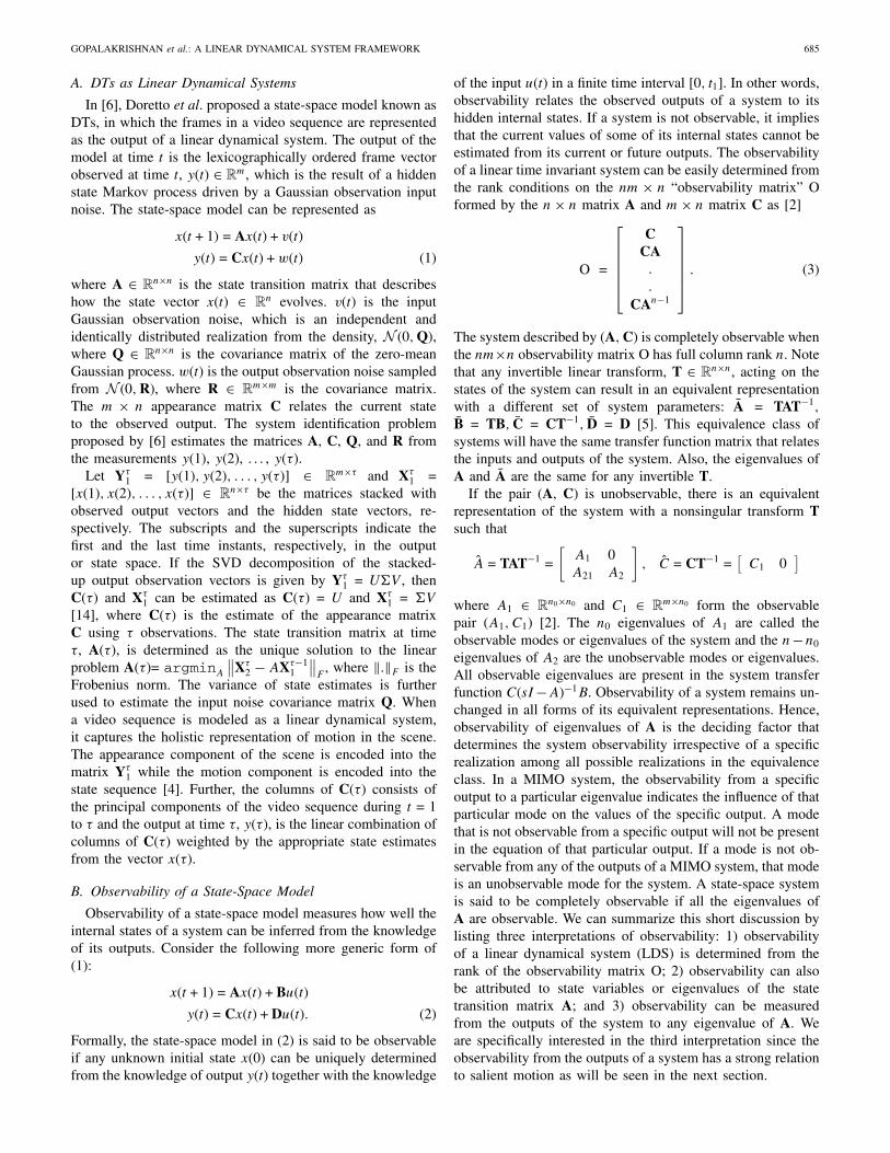
of the input u(t) in a finite time interval [0, t1]. In other words,observability relates the observed outputs of a system to itshidden internal states. If a system is not observable, it impliesthat the current values of some of its internal states cannot beestimated from its current or future outputs. The observabilityof a linear time invariant system can be easily determined fromthe rank conditions on the nm × n “observability matrix” Oformed by the n × n matrix A and m × n matrix C as [2]

O =

⎡⎢⎢⎢⎢⎣

CCA.

.

CAn−1

⎤⎥⎥⎥⎥⎦ . (3)

The system described by (A, C) is completely observable whenthe nm×n observability matrix O has full column rank n. Notethat any invertible linear transform, T ∈ Rn×n, acting on thestates of the system can result in an equivalent representationwith a different set of system parameters: A = TAT−1,

B = TB, C = CT−1, D = D [5]. This equivalence class ofsystems will have the same transfer function matrix that relatesthe inputs and outputs of the system. Also, the eigenvalues ofA and A are the same for any invertible T.

If the pair (A, C) is unobservable, there is an equivalentrepresentation of the system with a nonsingular transform Tsuch that

A = TAT−1 =

[A1 0A21 A2

], C = CT−1 =

[C1 0

]

where A1 ∈ Rn0×n0 and C1 ∈ Rm×n0 form the observablepair (A1, C1) [2]. The n0 eigenvalues of A1 are called theobservable modes or eigenvalues of the system and the n−n0

eigenvalues of A2 are the unobservable modes or eigenvalues.All observable eigenvalues are present in the system transferfunction C(sI −A)−1B. Observability of a system remains un-changed in all forms of its equivalent representations. Hence,observability of eigenvalues of A is the deciding factor thatdetermines the system observability irrespective of a specificrealization among all possible realizations in the equivalenceclass. In a MIMO system, the observability from a specificoutput to a particular eigenvalue indicates the influence of thatparticular mode on the values of the specific output. A modethat is not observable from a specific output will not be presentin the equation of that particular output. If a mode is not ob-servable from any of the outputs of a MIMO system, that modeis an unobservable mode for the system. A state-space systemis said to be completely observable if all the eigenvalues ofA are observable. We can summarize this short discussion bylisting three interpretations of observability: 1) observabilityof a linear dynamical system (LDS) is determined from therank of the observability matrix O; 2) observability can alsobe attributed to state variables or eigenvalues of the statetransition matrix A; and 3) observability can be measuredfrom the outputs of the system to any eigenvalue of A. Weare specifically interested in the third interpretation since theobservability from the outputs of a system has a strong relationto salient motion as will be seen in the next section.


Fig. 1. Video sequences with different dynamic backgrounds. (a) Jumpsequence with smoke. (b) Ocean sequence with waves. (c) Skiing sequencewith snow.

C. Distance Between AR Models

The DT models are AR in its nature and, consequently, thedistance between two different DTs is not Euclidean. In [15],the distance measure between two stable AR models M1 oforder n1 and having poles at αi and M2 of order n2 and havingpoles at βj is shown to be

d(M1, M2)2 = ln

∏n1i=1

∏n2j=1 |1 − α∗

i βj|2∏n1i,j=1(1 − α∗

i αj)∏n2

i,j=1(1 − β∗i βj)

(4)

where α∗i and β∗

i are complex conjugates of αi and βi. Thepoles of the DT model are the eigenvalues of the statetransition matrix A [2].

III. Pixel Saliency Map Using Observability

from Output Pixels

We represent the video sequence as a linear dynamicalsystem that can be described by the state-space equationsof (2). Consider the video sequences with various dynamicbackgrounds shown in Fig. 1. The Jump sequence in Fig. 1(a)has smoke-filled environment as the background, while theOcean sequence in Fig. 1(b) has waves in the sea as thedynamic background. The snowfall and the snow thrown outfrom the skiing gear is the complex dynamic background forthe Skiing video sequence in Fig. 1(c).

For the human visual system, the salient or foregroundmotion in these three different scenarios are the cyclist jump-ing, the people walking, and the movement of the skiers,respectively. This inference is made in the presence of complexand dynamic backgrounds in all the three cases. The salientmotion is considered as one that is more “predictable” fora human observer compared to the relatively unpredictablebackgrounds. For example, the smoke moving in the back-ground of the Jump sequence has haphazard motion, whilethe Cyclist has a regular motion. Similarly, the movement ofskiers is more robust and predictable compared to the snowfalland the motion of snow thrown out while skiing. Thoughwaves in Fig. 1(b) are less complex in its motion, the motionrelated to people walking becomes relatively simpler comparedto the motion of the waves. Thus, we attach the notion of

“predictability” or “regularity” to salient motion. It is lessrestrictive than the notion of linear motion as in [23] and itcan handle various kinds of motion. Also, we intend to focusonly on the relative predictability of different motions.

As explained in Section II-A, the DT model represents ascene of τ frames in a holistic manner using the state-spaceframework where the matrix C is the appearance matrix whichencodes the visual appearance of the texture and the states x(t)encode the motion of the entire sequence [4]. The observabilityfrom a specific pixel in output y(t) is a measure of inferencethat can be made on the values of the state variables, which area holistic characterization of the motion in the video sequence.Pixels belonging to complex unpredictable backgrounds willhave less observability to state variables compared to pixelsbelonging to regions of simple predictable motions. This isdue to the fact that we are modeling the video sequence overa period of time (τ frames), and the motion components be-longing to complex unpredictable regions are hard to estimatefrom its holistic characterization. Pixels belonging to staticregions will have zero observability as they do not contributeto the inference of any motion and hence the inference of statevariables. Hence, observability from a pixel computed underthe framework in (2) can be taken as a clue for the importanceof the pixel with regards to how much influence it holds indescribing the holistic motion of the scene.

A. Quantitative Measure for Observability

In Section II-B, we reviewed the basic definition of observ-ability and a simple rank-based method to evaluate whethera system is observable or not. However, such methods onlyhelp to make a binary decision on the observability of asystem and do not provide any insight into the observabilityfrom different outputs to the eigenvalues of state transitionmatrix A. Recall that observability is evaluated with respect toeigenvalues of A since it is invariant under various equivalentsystem representations. In [22], Tarokh discussed a simpleand computationally efficient method to evaluate a measureof observability for the ith eigenvalue λi of the state transitionmatrix A for continuous-time, time-invariant systems as

moi = |δi| [e∗i CT Cei]

12 (5)

where ei is the right eigenvector of the transition matrix Acorresponding to λi and δi is calculated as

|δi| = |n∏

j=1,i�=j

(λi − λj)|. (6)

It can be further concluded from (5) that the angle betweena specific row of output matrix C and the right eigenvector ei isa measure of observability from the respective output. If all therow vectors of the output matrix C are orthogonal to the righteigenvector ei, that specific λi will have zero observability[22]. We are particularly interested in the contribution of anyeigenvalue λi to a specific output which can be interpreted asthe visibility of that eigenvalue from the specific output. In ourmethod, every output corresponds to a pixel p in the outputframe since y(t) is the output frame lexicographically ordered


Fig. 2. Example showing the generation of final saliency map with sustainedobservability. (a) 12th frame of Cyclists video. (b) and (c) Saliency maps s1and s2 computed using frame buffers with frames 1–21 and 2–22. (d) Finalsaliency map.

as the m × 1 vector. Hence, we evaluate the observabilitymeasure from a pixel p to λi as

mpi = C[p] × ei

where C[p] is the pth row of C. An intuitive explanation forthe equation of mpi for discrete-time time-invariant systems isgiven in Appendix A. The total observability from output p,denoted by mp, is calculated as the sum of its observabilitymeasures to all the eigenvalues of A as

mp =n∑

i=1

mpi.

We evaluate the observability from all the pixels in theoutput in a similar fashion and normalize the values between0 and 1 to obtain the pixel saliency map.

B. Sustained Observability

The observability measure evaluated for pixels in the outputvector provides a good clue for salient motion. However, inthis process, some other pixels in the dynamic background canalso possess some observability as can be seen in the Cyclistsvideo sequence whose 12th frame is shown in Fig. 2(a).Fig. 2(b) and (c) shows the saliency maps for adjacent framebuffers wherein some part of the dynamic background alsoacquires observability. The idea of sustained observability isto lock on to points of consistent salient motion irrespectiveof the potential errors that would have happened due to thesuboptimal system modeling using [6] for a single buffer.Pixels having “sustained observability” are those that maintainhigh observability over successive saliency maps computed foradjacent frame buffers. Fig. 3 shows two such buffers each oflength q—the first buffer is from frame 1 to frame q and thesecond is from frame 2 to frame q + 1.

The DT models are evaluated for the adjacent buffersresulting in saliency maps s1 and s2. The final saliency map iscomputed by multiplying the two maps and normalizing it to[0, 1]. Thus, we give more saliency to those pixels that hold theobservability across the adjacent models. As seen in Fig. 2,although different regions in the dynamic background showsome saliency in individual binary saliency maps s1 and s2,the final saliency map in Fig. 2(d) correctly identifies pointsthat show high observability consistently.

Fig. 3. Sustained observability calculated over adjacent video buffers. s1 ands2 are saliency maps computed using DT models from frames 1 to q and 2to q + 1.

IV. Region-Based Saliency Map Using Salient

Patch Dynamics

The pixel saliency map computed in Section III evaluatesthe importance of each pixel in inferring the holistic dynamicsof the scene. However, the interior of large homogeneoussalient objects that occupy a majority of the pixels in theframe can appear to be relatively static over the frame buffer.Consequently, they will be marked as less salient due to theirapparent lesser involvement in the holistic dynamics of thescene. This drawback of the pixel saliency map is addressedby computing region-based saliency maps. In the proposedmethod, “regions” correspond to spatiotemporal patches offixed size selected from the spatiotemporal volume of theframe buffer. The dynamics of different regions are comparedwith the dynamics of the most salient region/patch, which canbe inferred from the pixel saliency map. However, the dynam-ics of the most salient region hold very specific informationof the region dynamics and may not always generalize well tothe dynamics of the salient object as a whole. Hence, we alsocompare the dynamics of different regions to the dynamicsof the whole of spatiotemporal volume (frame buffer). Thiscan be considered as a combination of local and globalapproaches in deciding region saliency. Finally, to compare thedynamics of different models, we rely on a distance measuresimilar to the one discussed in (4). The following sectionsdiscuss the computation of region-based saliency maps indetail.

A. Pole Analysis for Comparison of Region Dynamics

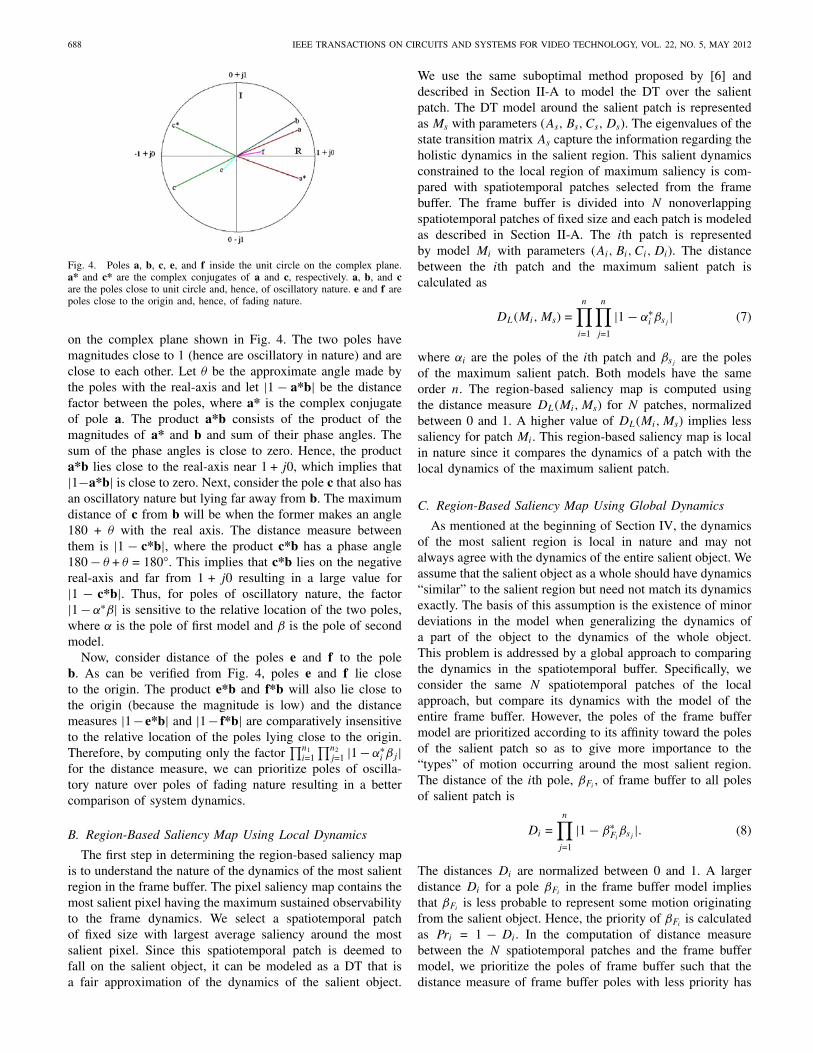
According to (4), the distance between two AR modelscontains knowledge of the poles of the two models. In theproposed method, we intend to compare the dynamics of twodifferent models which are encoded into their respective statetransition matrices. Therefore, their dynamics are reflected inthe eigenvalues (poles) of the respective matrices. The stablepoles of the LDS lie inside the unit circle in the complexplane. In [26], Yuan et al. showed that in a DT synthesisprocess, the poles that lie near to the unit circle influence theoutput with its “oscillatory” nature while the influence of polesthat lie close to origin “fades” away as time progresses. Theyconclude that poles of “oscillatory” nature (close to the unitcircle) contribute to a more accurate modeling of the DT. Thus,in order to compare system dynamics, we need a distancemeasure that prioritizes poles that are oscillatory in nature overpoles of fading nature. We formulate such a distance measureby considering the numerator of (4).

To analyze this in detail, consider the simple case ofcomparing the dynamics of two models with poles a and b


Fig. 4. Poles a, b, c, e, and f inside the unit circle on the complex plane.a* and c* are the complex conjugates of a and c, respectively. a, b, and care the poles close to unit circle and, hence, of oscillatory nature. e and f arepoles close to the origin and, hence, of fading nature.

on the complex plane shown in Fig. 4. The two poles havemagnitudes close to 1 (hence are oscillatory in nature) and areclose to each other. Let θ be the approximate angle made bythe poles with the real-axis and let |1 − a*b| be the distancefactor between the poles, where a* is the complex conjugateof pole a. The product a*b consists of the product of themagnitudes of a* and b and sum of their phase angles. Thesum of the phase angles is close to zero. Hence, the producta*b lies close to the real-axis near 1 + j0, which implies that|1−a*b| is close to zero. Next, consider the pole c that also hasan oscillatory nature but lying far away from b. The maximumdistance of c from b will be when the former makes an angle180 + θ with the real axis. The distance measure betweenthem is |1 − c*b|, where the product c*b has a phase angle180 − θ + θ = 180°. This implies that c*b lies on the negativereal-axis and far from 1 + j0 resulting in a large value for|1 − c*b|. Thus, for poles of oscillatory nature, the factor|1 − α∗β| is sensitive to the relative location of the two poles,where α is the pole of first model and β is the pole of secondmodel.

Now, consider distance of the poles e and f to the poleb. As can be verified from Fig. 4, poles e and f lie closeto the origin. The product e*b and f*b will also lie close tothe origin (because the magnitude is low) and the distancemeasures |1−e*b| and |1− f*b| are comparatively insensitiveto the relative location of the poles lying close to the origin.Therefore, by computing only the factor

∏n1i=1

∏n2j=1 |1 − α∗

i βj|for the distance measure, we can prioritize poles of oscilla-tory nature over poles of fading nature resulting in a bettercomparison of system dynamics.

B. Region-Based Saliency Map Using Local Dynamics

The first step in determining the region-based saliency mapis to understand the nature of the dynamics of the most salientregion in the frame buffer. The pixel saliency map contains themost salient pixel having the maximum sustained observabilityto the frame dynamics. We select a spatiotemporal patchof fixed size with largest average saliency around the mostsalient pixel. Since this spatiotemporal patch is deemed tofall on the salient object, it can be modeled as a DT that isa fair approximation of the dynamics of the salient object.

We use the same suboptimal method proposed by [6] anddescribed in Section II-A to model the DT over the salientpatch. The DT model around the salient patch is representedas Ms with parameters (As, Bs, Cs, Ds). The eigenvalues of thestate transition matrix As capture the information regarding theholistic dynamics in the salient region. This salient dynamicsconstrained to the local region of maximum saliency is com-pared with spatiotemporal patches selected from the framebuffer. The frame buffer is divided into N nonoverlappingspatiotemporal patches of fixed size and each patch is modeledas described in Section II-A. The ith patch is representedby model Mi with parameters (Ai, Bi, Ci, Di). The distancebetween the ith patch and the maximum salient patch iscalculated as

DL(Mi, Ms) =n∏

i=1

n∏j=1

|1 − α∗i βsj

| (7)

where αi are the poles of the ith patch and βsjare the poles

of the maximum salient patch. Both models have the sameorder n. The region-based saliency map is computed usingthe distance measure DL(Mi, Ms) for N patches, normalizedbetween 0 and 1. A higher value of DL(Mi, Ms) implies lesssaliency for patch Mi. This region-based saliency map is localin nature since it compares the dynamics of a patch with thelocal dynamics of the maximum salient patch.

C. Region-Based Saliency Map Using Global Dynamics

As mentioned at the beginning of Section IV, the dynamicsof the most salient region is local in nature and may notalways agree with the dynamics of the entire salient object. Weassume that the salient object as a whole should have dynamics“similar” to the salient region but need not match its dynamicsexactly. The basis of this assumption is the existence of minordeviations in the model when generalizing the dynamics ofa part of the object to the dynamics of the whole object.This problem is addressed by a global approach to comparingthe dynamics in the spatiotemporal buffer. Specifically, weconsider the same N spatiotemporal patches of the localapproach, but compare its dynamics with the model of theentire frame buffer. However, the poles of the frame buffermodel are prioritized according to its affinity toward the polesof the salient patch so as to give more importance to the“types” of motion occurring around the most salient region.The distance of the ith pole, βFi

, of frame buffer to all polesof salient patch is

Di =n∏

j=1

|1 − β∗Fi

βsj|. (8)

The distances Di are normalized between 0 and 1. A largerdistance Di for a pole βFi

in the frame buffer model impliesthat βFi

is less probable to represent some motion originatingfrom the salient object. Hence, the priority of βFi

is calculatedas Pri = 1 − Di. In the computation of distance measurebetween the N spatiotemporal patches and the frame buffermodel, we prioritize the poles of frame buffer such that thedistance measure of frame buffer poles with less priority has


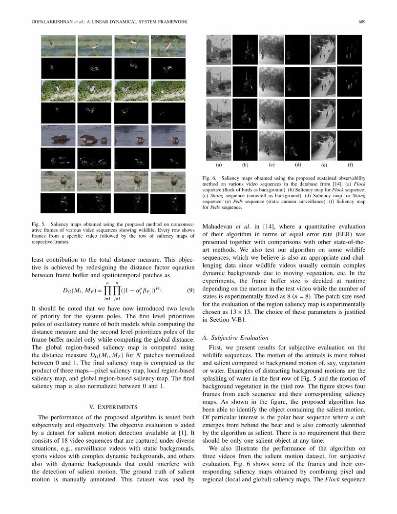
Fig. 5. Saliency maps obtained using the proposed method on nonconsec-utive frames of various video sequences showing wildlife. Every row showsframes from a specific video followed by the row of saliency maps ofrespective frames.

least contribution to the total distance measure. This objec-tive is achieved by redesigning the distance factor equationbetween frame buffer and spatiotemporal patches as

DG(Mi, MF ) =n∏

i=1

n∏j=1

(|1 − α∗i βFj

|)Prj . (9)

It should be noted that we have now introduced two levelsof priority for the system poles. The first level prioritizespoles of oscillatory nature of both models while computing thedistance measure and the second level prioritizes poles of theframe buffer model only while computing the global distance.The global region-based saliency map is computed usingthe distance measure DG(Mi, MF ) for N patches normalizedbetween 0 and 1. The final saliency map is computed as theproduct of three maps—pixel saliency map, local region-basedsaliency map, and global region-based saliency map. The finalsaliency map is also normalized between 0 and 1.

V. Experiments

The performance of the proposed algorithm is tested bothsubjectively and objectively. The objective evaluation is aidedby a dataset for salient motion detection available at [1]. Itconsists of 18 video sequences that are captured under diversesituations, e.g., surveillance videos with static backgrounds,sports videos with complex dynamic backgrounds, and othersalso with dynamic backgrounds that could interfere withthe detection of salient motion. The ground truth of salientmotion is manually annotated. This dataset was used by

Fig. 6. Saliency maps obtained using the proposed sustained observabilitymethod on various video sequences in the database from [14]. (a) Flocksequence (flock of birds as background). (b) Saliency map for Flock sequence.(c) Skiing sequence (snowfall as background). (d) Saliency map for Skiingsequence. (e) Peds sequence (static camera surveillance). (f) Saliency mapfor Peds sequence.

Mahadevan et al. in [14], where a quantitative evaluationof their algorithm in terms of equal error rate (EER) waspresented together with comparisons with other state-of-the-art methods. We also test our algorithm on some wildlifesequences, which we believe is also an appropriate and chal-lenging data since wildlife videos usually contain complexdynamic backgrounds due to moving vegetation, etc. In theexperiments, the frame buffer size is decided at runtimedepending on the motion in the test video while the number ofstates is experimentally fixed as 8 (n = 8). The patch size usedfor the evaluation of the region saliency map is experimentallychosen as 13 × 13. The choice of these parameters is justifiedin Section V-B1.

A. Subjective Evaluation

First, we present results for subjective evaluation on thewildlife sequences. The motion of the animals is more robustand salient compared to background motion of, say, vegetationor water. Examples of distracting background motions are thesplashing of water in the first row of Fig. 5 and the motion ofbackground vegetation in the third row. The figure shows fourframes from each sequence and their corresponding saliencymaps. As shown in the figure, the proposed algorithm hasbeen able to identify the object containing the salient motion.Of particular interest is the polar bear sequence where a cubemerges from behind the bear and is also correctly identifiedby the algorithm as salient. There is no requirement that thereshould be only one salient object at any time.

We also illustrate the performance of the algorithm onthree videos from the salient motion dataset, for subjectiveevaluation. Fig. 6 shows some of the frames and their cor-responding saliency maps obtained by combining pixel andregional (local and global) saliency maps. The Flock sequence


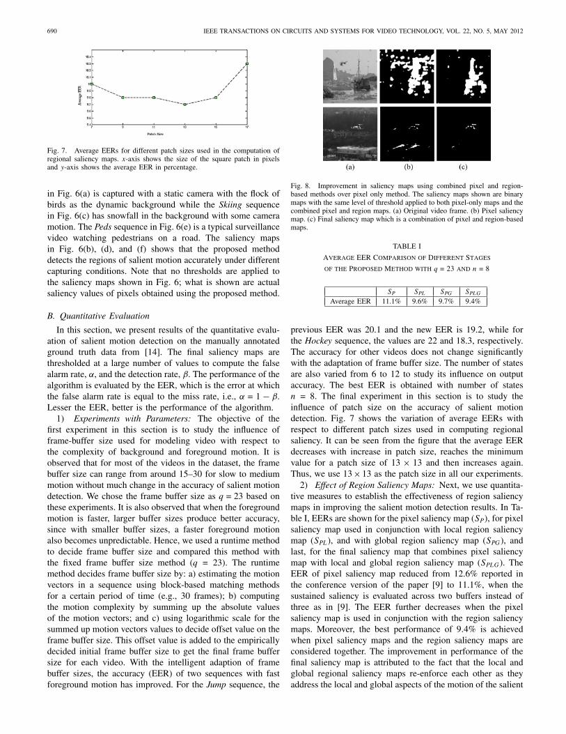
Fig. 7. Average EERs for different patch sizes used in the computation ofregional saliency maps. x-axis shows the size of the square patch in pixelsand y-axis shows the average EER in percentage.

in Fig. 6(a) is captured with a static camera with the flock ofbirds as the dynamic background while the Skiing sequencein Fig. 6(c) has snowfall in the background with some cameramotion. The Peds sequence in Fig. 6(e) is a typical surveillancevideo watching pedestrians on a road. The saliency mapsin Fig. 6(b), (d), and (f) shows that the proposed methoddetects the regions of salient motion accurately under differentcapturing conditions. Note that no thresholds are applied tothe saliency maps shown in Fig. 6; what is shown are actualsaliency values of pixels obtained using the proposed method.

B. Quantitative Evaluation

In this section, we present results of the quantitative evalu-ation of salient motion detection on the manually annotatedground truth data from [14]. The final saliency maps arethresholded at a large number of values to compute the falsealarm rate, α, and the detection rate, β. The performance of thealgorithm is evaluated by the EER, which is the error at whichthe false alarm rate is equal to the miss rate, i.e., α = 1 − β.Lesser the EER, better is the performance of the algorithm.

1) Experiments with Parameters: The objective of thefirst experiment in this section is to study the influence offrame-buffer size used for modeling video with respect tothe complexity of background and foreground motion. It isobserved that for most of the videos in the dataset, the framebuffer size can range from around 15–30 for slow to mediummotion without much change in the accuracy of salient motiondetection. We chose the frame buffer size as q = 23 based onthese experiments. It is also observed that when the foregroundmotion is faster, larger buffer sizes produce better accuracy,since with smaller buffer sizes, a faster foreground motionalso becomes unpredictable. Hence, we used a runtime methodto decide frame buffer size and compared this method withthe fixed frame buffer size method (q = 23). The runtimemethod decides frame buffer size by: a) estimating the motionvectors in a sequence using block-based matching methodsfor a certain period of time (e.g., 30 frames); b) computingthe motion complexity by summing up the absolute valuesof the motion vectors; and c) using logarithmic scale for thesummed up motion vectors values to decide offset value on theframe buffer size. This offset value is added to the empiricallydecided initial frame buffer size to get the final frame buffersize for each video. With the intelligent adaption of framebuffer sizes, the accuracy (EER) of two sequences with fastforeground motion has improved. For the Jump sequence, the

Fig. 8. Improvement in saliency maps using combined pixel and region-based methods over pixel only method. The saliency maps shown are binarymaps with the same level of threshold applied to both pixel-only maps and thecombined pixel and region maps. (a) Original video frame. (b) Pixel saliencymap. (c) Final saliency map which is a combination of pixel and region-basedmaps.

TABLE I

Average EER Comparison of Different Stages

of the Proposed Method with q = 23 and n = 8

SP SPL SPG SPLG

Average EER 11.1% 9.6% 9.7% 9.4%

previous EER was 20.1 and the new EER is 19.2, while forthe Hockey sequence, the values are 22 and 18.3, respectively.The accuracy for other videos does not change significantlywith the adaptation of frame buffer size. The number of statesare also varied from 6 to 12 to study its influence on outputaccuracy. The best EER is obtained with number of statesn = 8. The final experiment in this section is to study theinfluence of patch size on the accuracy of salient motiondetection. Fig. 7 shows the variation of average EERs withrespect to different patch sizes used in computing regionalsaliency. It can be seen from the figure that the average EERdecreases with increase in patch size, reaches the minimumvalue for a patch size of 13 × 13 and then increases again.Thus, we use 13×13 as the patch size in all our experiments.

2) Effect of Region Saliency Maps: Next, we use quantita-tive measures to establish the effectiveness of region saliencymaps in improving the salient motion detection results. In Ta-ble I, EERs are shown for the pixel saliency map (SP ), for pixelsaliency map used in conjunction with local region saliencymap (SPL), and with global region saliency map (SPG), andlast, for the final saliency map that combines pixel saliencymap with local and global region saliency map (SPLG). TheEER of pixel saliency map reduced from 12.6% reported inthe conference version of the paper [9] to 11.1%, when thesustained saliency is evaluated across two buffers instead ofthree as in [9]. The EER further decreases when the pixelsaliency map is used in conjunction with the region saliencymaps. Moreover, the best performance of 9.4% is achievedwhen pixel saliency maps and the region saliency maps areconsidered together. The improvement in performance of thefinal saliency map is attributed to the fact that the local andglobal regional saliency maps re-enforce each other as theyaddress the local and global aspects of the motion of the salient


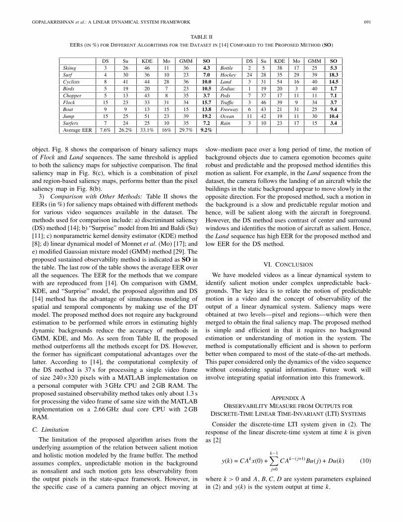
TABLE II

EERs (in %) for Different Algorithms for the Dataset in [14] Compared to the Proposed Method (SO)

DS Su KDE Mo GMM SO DS Su KDE Mo GMM SOSkiing 3 26 46 11 36 4.3 Bottle 2 5 38 17 25 5.3Surf 4 30 36 10 23 7.0 Hockey 24 28 35 29 39 18.3Cyclists 8 41 44 28 36 10.0 Land 3 31 54 16 40 14.5Birds 5 19 20 7 23 10.5 Zodiac 1 19 20 3 40 1.7Chopper 5 13 43 8 35 3.7 Peds 7 37 17 11 11 7.1Flock 15 23 33 31 34 15.7 Traffic 3 46 39 9 34 3.7Boat 9 9 13 15 15 13.8 Freeway 6 43 21 31 25 9.4Jump 15 25 51 23 39 19.2 Ocean 11 42 19 11 30 10.4Surfers 7 24 25 10 35 7.2 Rain 3 10 23 17 15 3.4Average EER 7.6% 26.2% 33.1% 16% 29.7% 9.2%

object. Fig. 8 shows the comparison of binary saliency mapsof Flock and Land sequences. The same threshold is appliedto both the saliency maps for subjective comparison. The finalsaliency map in Fig. 8(c), which is a combination of pixeland region-based saliency maps, performs better than the pixelsaliency map in Fig. 8(b).

3) Comparison with Other Methods: Table II shows theEERs (in %) for saliency maps obtained with different methodsfor various video sequences available in the dataset. Themethods used for comparison include: a) discriminant saliency(DS) method [14]; b) “Surprise” model from Itti and Baldi (Su)[11]; c) nonparametric kernel density estimator (KDE) method[8]; d) linear dynamical model of Monnet et al. (Mo) [17]; ande) modified Gaussian mixture model (GMM) method [29]. Theproposed sustained observability method is indicated as SO inthe table. The last row of the table shows the average EER overall the sequences. The EER for the methods that we comparewith are reproduced from [14]. On comparison with GMM,KDE, and “Surprise” model, the proposed algorithm and DS[14] method has the advantage of simultaneous modeling ofspatial and temporal components by making use of the DTmodel. The proposed method does not require any backgroundestimation to be performed while errors in estimating highlydynamic backgrounds reduce the accuracy of methods inGMM, KDE, and Mo. As seen from Table II, the proposedmethod outperforms all the methods except for DS. However,the former has significant computational advantages over thelatter. According to [14], the computational complexity ofthe DS method is 37 s for processing a single video frameof size 240×320 pixels with a MATLAB implementation ona personal computer with 3 GHz CPU and 2 GB RAM. Theproposed sustained observability method takes only about 1.3 sfor processing the video frame of same size with the MATLABimplementation on a 2.66 GHz dual core CPU with 2 GBRAM.

C. Limitation

The limitation of the proposed algorithm arises from theunderlying assumption of the relation between salient motionand holistic motion modeled by the frame buffer. The methodassumes complex, unpredictable motion in the backgroundas nonsalient and such motion gets less observability fromthe output pixels in the state-space framework. However, inthe specific case of a camera panning an object moving at

slow–medium pace over a long period of time, the motion ofbackground objects due to camera egomotion becomes quiterobust and predictable and the proposed method identifies thismotion as salient. For example, in the Land sequence from thedataset, the camera follows the landing of an aircraft while thebuildings in the static background appear to move slowly in theopposite direction. For the proposed method, such a motion inthe background is a slow and predictable regular motion andhence, will be salient along with the aircraft in foreground.However, the DS method uses contrast of center and surroundwindows and identifies the motion of aircraft as salient. Hence,the Land sequence has high EER for the proposed method andlow EER for the DS method.

VI. Conclusion

We have modeled videos as a linear dynamical system toidentify salient motion under complex unpredictable back-grounds. The key idea is to relate the notion of predictablemotion in a video and the concept of observability of theoutput of a linear dynamical system. Saliency maps wereobtained at two levels—pixel and regions—which were thenmerged to obtain the final saliency map. The proposed methodis simple and efficient in that it requires no backgroundestimation or understanding of motion in the system. Themethod is computationally efficient and is shown to performbetter when compared to most of the state-of-the-art methods.This paper considered only the dynamics of the video sequencewithout considering spatial information. Future work willinvolve integrating spatial information into this framework.

Appendix A

Observability Measure from Outputs for

Discrete-Time Linear Time-Invariant (LTI) Systems

Consider the discrete-time LTI system given in (2). Theresponse of the linear discrete-time system at time k is givenas [2]

y(k) = CAkx(0) +k−1∑j=0

CAk−(j+1)Bu(j) + Du(k) (10)

where k > 0 and A, B, C, D are system parameters explainedin (2) and y(k) is the system output at time k.


It can be seen from (10) that the relation between eigen-values of matrix A and output y(k) is governed by the factorsCAr, where r is some integer value between 1 and k. Theeigen decomposition of the square matrix A is given asQ ∧ Q−1, where ∧ = diag(λ1, λ2, . . . , λn). The matrix A andAr can be represented as

∑i=ni=1 λi.qif

Ti and

∑i=ni=1(λi)r.qif

Ti ,

respectively, where λi is the ith eigenvalue, qi and fi the ithcolumns of matrices Q and Q−1, respectively. Hence, CAr =C

∑i=ni=1(λi)r.qif

Ti =

∑i=ni=1(λi)r.(Cqi)fT

i . Thus, the vector (Cqi)becomes the crucial factor in deciding the presence of (λi) inthe multidimensional output equation. If a specific row, say p,of C is orthogonal or near orthogonal to qi, the estimate thatcan be made about λi from the pth output in the vector y(k)will be poor. Hence, the angle between the rows of C and thevector ei is chosen as the measure of the observability fromoutput pixels to the eigenvalue λi.

References

[1] Statistical Visual Computing Laboratory. Background Subtraction inDynamic Scenes [Online]. Available: http://www.svcl.ucsd.edu/projects/background−subtraction

[2] P. J. Antsaklis and A. N. Michel, Linear Systems. New York: McGraw-Hill, 1997.

[3] A. Bugeau and P. Perez, “Detection and segmentation of moving objectsin complex scenes,” Comput. Vision Image Understand., vol. 113, no.4, pp. 459–476, Apr. 2009.

[4] A. B. Chan and N. Vasconcelos, “Probabilistic kernels for the classifica-tion of auto-regressive visual processes,” in Proc. IEEE Conf. Comput.Vision Patt. Recog., Jun. 2005, pp. 846–851.

[5] C.-T. Chen, Linear System Theory and Design. New York: Oxford Univ.Press, 1998.

[6] G. Doretto, A. Chiuso, Y. N. Wu, and S. Soatto, “Dynamic textures,”Int. J. Comput. Vision, vol. 51, no. 2, pp. 91–109, Feb. 2003.

[7] A. M. Elgammal, D. Harwood, and L. S. Davis, “Non-parametric modelfor background subtraction,” in Proc. Eur. Conf. Comput. Vision, 2000,pp. 751–767.

[8] A. M. Elgammal, R. Duraiswami, D. Harwood, and L. S. Davis, “Back-ground and foreground modeling using nonparametric kernel densityestimation for visual surveillance,” Proc. IEEE, vol. 90, no. 7, pp. 1151–1163, Jul. 2002.

[9] V. Gopalakrishnan, Y. Hu, and D. Rajan, “Sustained observability forsalient motion detection,” in Proc. Asian Conf. Comput. Vision, Nov.2010, pp. 732–743.

[10] C. Guo, Q. Ma, and L. Zhang, “Spatio-temporal saliency detection usingphase spectrum of quaternion Fourier transform,” in Proc. IEEE Conf.Comput. Vision Patt. Recog., Jun. 2008, pp. 1–8.

[11] L. Itti and P. Baldi, “A principled approach to detecting surprising eventsin video,” in Proc. IEEE Conf. Comput. Vision Patt. Recog., Jun. 2005,pp. 631–637.

[12] C. Liu, P. C. Yuen, and G. Qiu, “Object motion detection usinginformation theoretic spatio-temporal saliency,” Patt. Recog., vol. 42,no. 11, pp. 2897–2906, Nov. 2009.

[13] T. Liu, J. Sun, N. Zheng, X. Tang, and H. Y. Shum, “Learning to detecta salient object,” in Proc. IEEE Conf. Comput. Vision Patt. Recog., Jun.2007, pp. 1–8.

[14] V. Mahadevan and N. Vasconcelos, “Spatiotemporal saliency in dynamicscenes,” IEEE Trans. Patt. Anal. Mach. Intell., vol. 32, no. 1, pp. 171–177, Jan. 2010.

[15] R. J. Martin, “A metric for ARMA processes,” IEEE Trans. SignalProcess., vol. 48, no. 4, pp. 1164–1170, Apr. 2000.

[16] A. Mittal and N. Paragios, “Motion-based background subtraction usingadaptive kernel density estimation,” in Proc. IEEE Conf. Comput. VisionPatt. Recog., Jun.–Jul. 2004, pp. 302–309.

[17] A. Monnet, A. Mittal, N. Paragios, and V. Ramesh, “Background mod-eling and subtraction of dynamic scenes,” in Proc. Int. Conf. Comput.Vision, 2003, pp. 1305–1312.

[18] C. Ridder, O. Munkelt, and H. Kirchner, “Adaptive background esti-mation and foreground detection using Kalman-filtering,” in Proc. Int.Conf. Recent Adv. Mechatron., 1995, pp. 193–199.

[19] M. Rubinstein, A. Shamir, and S. Avidan, “Improved seam carvingfor video retargeting,” ACM Trans. Graphics, vol. 27, no. 3, pp. 1–9,2008.

[20] C. Stauffer and W. Grimson, “Adaptive background mixture models forreal-time tracking,” in Proc. IEEE Conf. Comput. Vision Patt. Recog.,Jun. 1999, pp. 2246–2252.

[21] C. Stauffer and W. E. L. Grimson, “Learning patterns of activity usingreal-time tracking,” IEEE Trans. Patt. Anal. Mach. Intell., vol. 22, no.8, pp. 747–757, Aug. 2000.

[22] M. Tarokh, “Measures for controllability, observability and fixed modes,”IEEE Trans. Automat. Contr., vol. 37, no. 8, pp. 1268–1273, Aug.1992.

[23] L. E. Wixson, “Detecting salient motion by accumulating directionally-consistent flow,” IEEE Trans. Patt. Analy. Mach. Intell., vol. 22, no. 8,pp. 774–780, Aug. 2000.

[24] X. Hou and L. Zhang, “Saliency detection: A spectral residual approach,”in Proc. IEEE Conf. Comput. Vision Patt. Recog., Jun. 2007, pp. 1–8.

[25] A. Yilmaz, O. Javed, and M. Shah, “Object tracking: A survey,” ACMComput. Surveys, vol. 38, no. 4, p. 13, 2006.

[26] L. Yuan and H. Y. Shum, “Synthesizing dynamic texture with closed-loop linear dynamic system,” in Proc. Eur. Conf. Comput. Vision, 2004,pp. 603–616.

[27] J. Zhong and S. Sclaroff, “Segmenting foreground objects from adynamic textured background via a robust Kalman filter,” in Proc. Int.Conf. Comput. Vision, 2003, pp. 44–50.

[28] J. Zhu, Y. Lao, and Y. F. Zheng, “Object tracking in structured environ-ments for video surveillance applications,” IEEE Trans. Circuits Syst.Video Technol., vol. 20, no. 2, pp. 223–235, Feb. 2010.

[29] Z. Zivkovic, “Improved adaptive Gaussian mixture model forbackground subtraction,” in Proc. Int. Conf. Patt. Recog., 2004,pp. 28–31.

Viswanath Gopalakrishnan received the B.Tech.degree in electronics and communication engineer-ing from Regional Engineering College, Calicut(now National Institute of Technology Calicut),India, in 2001. Currently, he is pursuing the Ph.D.degree from the School of Computer Engineering,Nanyang Technological University, Singapore.

Deepu Rajan received the B.E. degree in electronicsand communication engineering from the Birla Insti-tute of Technology, Ranchi, India, the M.S. degreein electrical engineering from Clemson University,Clemson, SC, and the Ph.D. degree from the IndianInstitute of Technology Bombay, Mumbai, India.

He is currently an Associate Professor with theSchool of Computer Engineering, Nanyang Techno-logical University, Singapore. His current researchinterests include computer vision and multimediasignal processing.

Yiqun Hu received the B.S. degree in computerscience from Xiamen University, Xiamen, China, in2002, and the Ph.D. degree in computer engineeringfrom Nanyang Technological University, Singapore,in 2008.

He is currently a Research Assistant Professor withthe University of Western Australia, Perth, Australia.

IEEE paper on Motion detection using MATLAB

Documents

Transcript of IEEE paper on Motion detection using MATLAB