LBS Research Online

Neil BurgessComputational methodology for modelling the dynamics of statistical arbitrageThesis

This version is available in the LBS Research Online repository: https://lbsresearch.london.edu/id/eprint/2394/

Burgess, Neil

(2000)

Computational methodology for modelling the dynamics of statistical arbitrage.

Doctoral thesis, University of London: London Business School.

DOI: https://doi.org/10.35065/NTMJ7398

Users may download and/or print one copy of any article(s) in LBS Research Online for purposes ofresearch and/or private study. Further distribution of the material, or use for any commercial gain, isnot permitted.

A Computational Methodology

for Modelling the Dynamics of

Statistical Arbitrage

Andrew Neil Burgess

Decision Technology Centre

Department of Decision Sciences

A thesis submitted to the University of London

for the degree of Doctor of Philosophy

UNIVERSITY OF LONDON

LONDON BUSiNESS SCHOOL

October 1999

BIB!..

LONDON

UNW

To my parents, Arnold and Carol.

© A. N. Burgess, 1999

Acknowledgements

Thanks to my supervisor, Paul Refenes, for bringing me to LBS, keeping me in bread and

water, helping me with ideas and generally making the whole thing possible!

Thanks to past and present colleagues at the Neuroforecasting UmtlDecision Technology

Centre. Especially Yves Bentz, Peter Bolland, Jeny Connor, Stefania Pandelidaki, Neville

Towers and Peter Schreiner; for discussions, hard work (not all the time), company and six

good years. Also all the ex-CRLers who showed that even a real job can still be fun.

Thanks to the visitors to the LBS group, Fernando and Paul, for good times and hard work in

London, Helsinki and Melbourne.

Thanks for the people who helped keep it real, especially to Pratap Sondhi for ideas and

support when he was at Citibank at the beginning; the other sponsors of the Neuroforecasting

Club and then the Decision Technology Centre; Botha and Denck down in S.A. for trusting me

to build a trading system; and David and Andrew for all their efforts on behalf of New

Sciences.

Also to the guys who first decided to hold NIPS workshops at ski resorts; and to the regulars at

NNCM/CF conferences; John Moody, Andreas Weigend, Hal White, Yaser Abu-Mostafa,

Andrew Lo and Blake LeBaron in particular for their enthusiasm and inspiration.

Finally, my love and thanks to Deborah, who had to put up with me whilst I was writing up -

and whose photographs of chromosomes had to compete for computer time with my equity

curves.

3

Abstract

Recent years have seen the emergence of a multi-disciplinary research area known as

"Computational Finance". In many cases the data generating processes of financial and other

economic time-series are at best imperfectly understood. By allowing restrictive assumptions

about price dynamics to be relaxed, recent advances in computational modelling techniques

offer the possibility to discover new "patterns" in market activity.

This thesis describes an integrated "statistical arbitrage" framework for identifying, modelling

and exploiting small but consistent regularities in asset price dynamics. The methodology

developed in the thesis combines the flexibility of emerging techniques such as neural networks

and genetic algorithms with the rigour and diagnostic techniques which are provided by

established modelling tools from the fields of statistics, econometrics and time-series

forecasting.

The modelling methodology which is described in the thesis consists of three main parts. The

first part is concerned with constructing combinations of time-series which contain a significant

predictable component, and is a generalisation of the econometric concept of cointegration. The

second part of the methodology is concerned with building predictive models of the mispricing

dynamics and consists of low-bias estimation procedures which combine elements of neural and

statistical modelling. The third part of the methodology controls the risks posed by model

selection and performance instability through actively encouraging diversification across a

"portfolio of models". A novel population-based algorithm for joint optimisation of a set of

trading strategies is presented, which is inspired both by genetic and evolutionary algorithms

and by modern portfolio theory.

Throughout the thesis the performance and properties of the algorithms are validated by means

of experimental evaluation on synthetic data sets with known characteristics. The effectiveness

of the methodology is demonstrated by extensive empirical analysis of real data sets, in

particular daily closing prices of FTSE 100 stocks and international equity indices.

4

Table of Contents

ACKNOWLEDGEMENTS .3

ABSTRACT ...................................................................................................................................... 4

TABLEOF CONTENTS ................................................................................................................. 5

iNTRODUCTION: A METHODOLOGY FOR STATISTICAL ARBITRAGE........................... 7

1. INTRODUCTION............................................................................................................................8

1.1 Scope....................................................................................................................................81 .2 Motivation ............................................................................................................................9

1.3 Thesis Overview..................................................................................................................12

1.4 Contributions......................................................................................................................14

1.5 Organisation.......................................................................................................................16

1.6 Summary.............................................................................................................................19

2. BACKGROUND............................................................................................................................20

2.1 StatisticalArbitrage............................................................................................................20

2.2 Recent Advances in Computational Modelling....................................................................282.3 Applications of Low-bias Modelling in Computational Finance ..........................................64

2.4 Summary.............................................................................................................................73

3. ASSESSMENT OF EXISTING METHODS.......................................................................................... 74

3.1 Potential for Model-based Statisti ca/Arbitrage..................................................................74

3.2 Methodological Gaps..........................................................................................................82

3.3 Summary.............................................................................................................................89

4. OVERVIEW OF PROPOSED METHODOLOGY...................................................................................90

4.1 Overview ofModelling Framework.....................................................................................90

4.2 Part I: A Cointegration Framework for Statistical Arbitrage...............................................92

4.3 Part II: Forecasting the Mispricing Dynamics using Neural Networks................................98

4.4 Part III: Diversifying Risk by Combining a Portfolio ofModels........................................106

4.5 Summary...........................................................................................................................111

PART I: A COIINTEGBATION FRAMEWORK FOR STATISTICAL ARBITRAGE ............ 112

5. METHODOLOGY FOR CONSTRUCTING STATISTICAL MISPRICINGS ...............................................113

5.1 Description of Cointegration Methodology.......................................................................113

5.2 Extension to Time-varying Relationships..........................................................................127

5.3 Extension to High-dimensional Problems..........................................................................134

5.4 Summary...........................................................................................................................139

6. TESTING FOR POTENTIAL PREDICTABILITY................................................................................140

6.1 Description ofPredictabilily Tests....................................................................................1406.2 Monte-Carlo Evaluation of Predictability Test Power.......................................................1466.3 Bias-Correction of Predictability Tests.............................................................................159

6.4 Evidence for Potential Predictability in Statistical Mispricings.........................................164

6.5 Summary...........................................................................................................................167

7. EMPIRICAL EVALUATION OF IMPUCIT STATISTICAL ARBITRAGE MODELS ...................................169

7.1 Implicit StatisticalArbitrage Strategies and Trading Ru/es............................................... 169

5

7.2 Empirical Results for F7'SE 100 Equity Prices . 1727.3 Empirical Results for Equity Market Indices.....................................................................181

7.4 Summary...........................................................................................................................189

PART II: FORECASTING THE MISPRICING DYNAMICS USING NEURAL NETWORKS..............................................................................................................190

8. Low-BIAs FORECASTING IN HIGHLY STOCHASTIC ENVIRONMENTS ...............................................1928.1 General Formulation of the Model Estimation Problem....................................................1928.2 Estimating Predictive Models in Investment Finance ........................................................194

8.3 An Equivalent Kernels perspective on Neural Network learning .......................................199

8.4 Summary...........................................................................................................................209

9. MODEL-FREE VARIABLE SELECTION ..........................................................................................2119.1 Statistical methodology for model-free variable selection.................................................211

9.2 Implementation of Variable Selection Methodology..........................................................217

9.3 Evaluation of Variable Selection Test Power by Monte Carlo Simulation..........................221

9.4 Investigation ofModel Bias using Monte Carlo Simulation...............................................226

9.5 Summary...........................................................................................................................230

10. STATISTICAL METHODOLOGY FOR NEURAL NETWORK MODEL ESTIMATION .............................23210.1 Frameworkfor Optimising the Bias-Variance Tradeoff in Neural Networks....................232

10.2 Algorithms for Neural Network Model Estimation...........................................................240

10.3 Experimental Validation of Neural Model Estimation Procedures...................................248

10.4 Summary.........................................................................................................................252

11. EMPIRICAL EVALUATION OF CONDITIONAL STATISTICAL ARBITRAGE MODELS .........................25311.1 Conditional Statistical Arbitrage Models........................................................................253

11.2 Application of Variable Selection Methodology to FTSE 100 Data .................................257

11.3 Empirical Results of Conditional Statistical Arbitrage Models........................................263

11.4 Summary.........................................................................................................................278

PART ifi: DIVERSIFYING RISK BY COMBINING A PORTFOLIO OF STATISTICALARBITRAGEMODELS..............................................................................................................280

12.A "PORTFOLIO OF MODELS" APPROACH TO STATISTICAL ARBITRAGE ......................................28112.1 Model Selection in Noisy and Nonstationary Environments.............................................281

12.2 Controlling Model Selection Risk by Combining Models.................................................287

12.3 Empirical Results for F7'SE 100 models..........................................................................291

12.4 Summary.........................................................................................................................297

13.A POPULATION-BASED ALGORITHM FOR JOINT OPTIMISATION OF TRADING MODELS ................29913.1 Risk-averse Optimisation ................................................................................................299

13.2 Controlled Evaluation ofPopulation-basedAlgorithm....................................................315

13.3 Empirical Evaluation on Equity Index Data....................................................................322

13.4 Summary.........................................................................................................................327

CONCLUSIONSAND BIBLIOGRAPHY..................................................................................329

14. CONCLUSIONS .................................................................................................................. 330

BIBLIOGRAPHY ...................................................................................................................... 335

6

Introduction: A Methodology for Statistical Arbitrage

This part of the thesis introduces the concept of statistical arbitrage and examines the issues

which will be developed in the rest of the thesis. Chapter 1 consists of a brief introduction

which outlines the scope, motivation and organisation of the thesis as well as summarising the

major contributions which it makes to the current state of the art. Chapter 2 describes the

recent advances in computational modelling and computational finance which provide the

background to the thesis. Chapter 3 describes the opportunities for statistical arbitrage which

are presented by the advances in modelling methodology, assessing the strengths and

weaknesses of existing modelling methods and highlighting the outstanding issues which the

methodology presented in the thesis is designed to address. Finally Chapter 4 presents an

overview of the methodology and a "route map" to the rest of the thesis.

7

1. Introduction

1.1 Scope

Recent years have seen the emergence of a multi-disciplinary research area known as

"Computational Finance", driven on the one hand by advances in computing power, data

availability and computational modelling methods, and on the other by the competitive and

continually evolving nature of the financial markets. Whilst the competitive drive to achieve

high profitability at low levels of risk creates a demand for improved models of market

dynamics, the improvements in hardware, software, data and methodology create a fertile

platform for developing the supply of such "market beating" models.

In this thesis we investigate the opportunities that are presented by specific modelling tools

from the field of machine learning, namely neural networks and genetic algorithms, and exploit

these in the context of a specific area of investment finance, namely statistical arbitrage. The

thesis develops a methodological framework for exploiting these recent advances in

computational modelling as a means of identif'ing and forecasting predictable components in

the dynamics of combinations of asset prices. The resulting models present opportunities for

identifying statistically under- and over-priced assets, extending the traditional "riskiess"

arbitrage framework to encompass empirical as well as theoretical relationships between assets.

The thesis contributes to the state of the art by enhancing specific aspects of modelling

methodology and developing tools, such as variable and model selection algorithms, which

support the modelling and forecasting of noisy and nonstationary time series. It applies these

tools within the context of a modelling framework inspired by techniques from statistics,

econometrics, and time-series modelling. The starting point of the modelling framework is the

econometric concept of "cointegration". The machine learning techniques are employed to relax

the requirements and assumptions of cointegration modelling and hence open up the possibility

of improving the extent to which future innovations in the time-series can be both forecasted

and exploited.

The thesis is cross-disciplinary in nature, taking ideas from statistics and machine learning and

presenting a synthesis of these ideas in the form of novel methodologies for performing

modelling and forecasting in noisy and nonstationary environments. As such it is likely to be of

interest to statisticians, econometricians, operational researchers, computer scientists and

8

members of the machine learning community. The methodologies developed will be of

particular interest to researchers and practitioners of time-series forecasting, computational

finance and quantitative marketing. The methodologies derived provide insights into both the

opportunities and obstacles which are presented by the use of advanced modelling techniques in

investment finance and other application domains with similar properties. Throughout the

thesis the performance and properties of the algorithms are validated by means of experimental

evaluation on synthetic data sets with known characteristics. Further support for the

effectiveness of the algorithms is provided by extensive empirical analysis of real data sets, in

particular daily closing prices for equity of the companies which constituted the FTSE 100

index during the period 1997-1999.

1.2 Motivation

The philosophy espoused in this thesis is that recent improvements in computational modelling

techniques open up new opportunities to identify and model regularities in asset price

dynamics. The exploitation of the predictive information provided by such models is referred to

as "statistical arbitrage", reflecting the fact that it can be considered as an example of a

broader class of "arbitrage" strategies in which systematic components in asset price dynamics

are exploited by market participants known as "arbitrageurs".

There is a competitive "arms race" between arbitrageurs, which causes the opportunities

provided by theoretically-motivated "riskless" strategies to be both self-limiting and restricted

to relatively privileged market players who are geared to trade quickly, at low cost, and with

sufficient financial leverage to make the exercise worthwhile. In contrast, "statistical arbitrage"

opportunities, which are based on empirical regularities with no direct theoretical underpinning,

are likely to be both more persistent and more prevalent in financial markets. More persistent

because risk-free arbitrage opportunities are rapidly eliminated by market activity. More

prevalent because in principle they may occur between any set of assets rather than solely in

cases where a suitable risk-free hedging strategy can be implemented.

Due to the highly competitive nature of financial markets, there is an ongoing debate about

whether markets are so "efficient" that no predictable components can possibly exist. The

position taken in this thesis is that whilst there is no a priori reason why regularities in asset

price dynamics should not exist it is likely that any easily identifiable effects will soon be

eliminated or "arbitraged away" in the very process of being exploited. However, by looking at

9

the markets from new angles and using new tools it may be possible to identify new

opportunities in the form of previously undiscovered "patterns" in market activity.

It is this perspective that motivates this thesis, in aiming to harness recent developments in

computational modelling to the task of financial forecasting. In particular the thesis explores

the exciting opportunities which are offered by so-called "machine learning" methods such as

Neural Networks and Genetic Algorithms.

Neural Networks (NNs) are computational models inspired by the learning mechanisms of the

human brain; the fundamental concept of neural networks is that they "learn by example".

Typically a neural network is presented a set of "training examples" each of which matches a

stimulus, or input pattern, to a desired response, or output pattern. The original, untrained,

neural network, when presented with an example stimulus, will generate a random response. A

so-called "learning algorithm" is then applied, in order to calculate the error, or difference

between desired and actual output, and then to adjust the internal network parameters in such a

way that this error is reduced. Eventually the network will converge to a stable configuration

which represents the learned solution to the problem represented by the training examples.

From a modelling perspective, the novelty of NNs lies in their ability to model arbitrary input-

output relationships with few (if any) a priori restrictive assumptions about the specific nature

of the relationship.

Genetic Algorithms (GAs) are computational models inspired by the mechanisms of evolution

and natural selection. A genetic algorithm is a means by which a population of, initially

random, candidate solutions to a problem is evolved towards better and better solutions. Each

new generation of solutions is derived from the previous "parent" generation by mechanisms

such as cross-breeding and mutation. In each generation the "parents" are selected according to

their "fitness"; the fittest solutions will thus have an increased representation in the new

generation and advantageous traits will be propagated through the population. From a

modelling perspective, the novelty of GAs lies in the fact that they impose few restrictions on

the nature of the "fitness function" which determines the optimisation criteria.

With any new modelling methodology, a clear understanding of the strengths and weaknesses of

the methodology is critical in deciding how it should be applied to a particular problem domain,

and indeed whether or not it is suitable for application in that domain. Whilst the strengths of

the new techniques have been extensively demonstrated in other problem domains, attempts to

apply them in the financial domain have been largely unsuccessful.

10

A major motivation for applying the new techniques in financial forecasting is that the data

generating processes of financial and other economic time-series are at best imperfectly

understood. By allowing the restrictive assumptions of more established time-series modelling

techniques to be relaxed, the flexibility of the emerging techniques offers the possibility of

improving forecasting ability and identifying opportunities which would otherwise be

overlooked. However, in order to facilitate the successful uptake of the new techniques in this

important application area it is first necessary to provide modelling tools which overcome the

obstacles posed by the inherent properties of the financial domain - such as a typically large

stochastic component ("noise") in observed data and a tendency for the underlying relationships

to be time-varying (nonstationary) in nature. These difficulties are exacerbated by weaknesses

in the methodology which supports the emerging techniques, which to a large extent lacks the

diagnostic tools and modelling frameworks which are an essential component of more

traditional time-series modelling approaches.

The objective of this thesis is therefore to identify and exploit the opportunities which are

offered by the strengths of the emerging modelling techniques, whilst at the same time

minimising the effect of their weaknesses, through the development of an integrated modelling

framework which places the new methods in partnership with, and in the context of, established

statistical techniques. The methodology should include tools for the identification of statistical

mispricings in sets of asset prices, modelling the predictable component in the mispricing

dynamics, and exploiting the predictive forecasts through a suitable asset allocation strategy.

The task of identifying and exploiting statistical arbitrage opportunities in the financial markets

can be considered one of the purest and most challenging tests of a predictive modelling

methodology, whilst at the same time being of huge practical significance. The highly

competitive nature of financial markets means that any predictable component in asset price

dynamics is likely to be very small, accounting for no more than a few percentage points of the

total variability in the asset prices. Furthermore, the performance of a statistical arbitrage

strategy is related solely to the predictive ability of the underlying model, as the taking of

offsetting long and short positions in the market eliminates the (favourable) performance

contamination which is caused by any tendency for prices to drift upwards over time. The

potential rewards of a successful statistical arbitrage methodology are nevertheless enormous:

as Figure 1.1 illustrates, even an ability to predict only 1% of daily asset price variability can

provide a source of consistent profits at acceptably low levels of risk.

11

100%

41

2

;-.\i.

16191,98 1504198 1507196 1&'10,98 1501199 lWOI99 16197199

Figure 1.1: Illustration of the potential of statistical arbitrage strategies. The chart shows the accumulated

return of holding the FTSE 100 index over the period 16th January 1998 - 17th August 1999, together

with the returns of two strategies based on (idealised) predictive models constructed in such a way as to

explain 0% and 1% of the variability of the FTSE (i.e. with R2 statistics of 0% and 1%). Transaction

costs are not included.

1.3 Thesis Overview

The prime contribution of this thesis is the development of a computational methodology for

modelling and exploiting the dynamics of statistical arbitrage. A preview of the methodology

developed in this thesis is presented in schematic form in Figure 1.2. The methodology consists

of three main stages which are (i) constructing time-series of statistical mispricings, (ii)

forecasting the mispricing dynamics, and (iii) exploiting the forecasts through a statistical

arbitrage asset allocation strategy. These three strands correspond to the modelling phases of

intelligent pre-processing, predictive modelling, and risk-averse decision-making.

The three components are intimately linked to each other, in each case the methodology has

been arrived at following a process of reviewing the research literature in appropriate fields.

assessing the strengths and weaknesses of existing methods, and developing tools and

techniques for addressing the methodological gaps thus identified. In each phase, certain

assumptions of more traditional modelling approaches are relaxed in a manner aimed at

maximising predictive ability and reducing particular sources of forecasting error. The focus of

the methodological developments is a consequence of the relaxation of these assumptions, the

objective being to develop tools which support model development under the new, relaxed,

assumptions.

12

te-seso?' _Predictability testa Jc.statiStimis:cisi Cointeration framework

Model-free variable selection

IMethodology for

i.;::ncamica EJ_Biag-variance optimisation

statisticalarbitrage _____________________________

Neural model estimation

/tforectg\ StaLrbtrading rules

4 Joint optimisation of populatioll

Figure 1.2: Schematic breakdown of the methodology presented in this thesis, representing a

computational methodology for forecasting the dynamics of statistical arbitrage. Each of the three phases

aims to reduce forecasting enors by relaxing certain underlying assumptions of more traditional

forecasting techniques.

The first component of the methodology uses the econometric concept of cointegration as a

means of creating time-series of statistical "mispricings" which can form the basis of statistical

arbitrage models. The objective of this phase is to identify particular combinations of assets

such that the combined time-series exhibits a significant predictable component, and is

furthennore uncorrelated from underlying movements in the market as a whole.

The second component of the methodology is concerned with modelling the dynamics of the

mispricing process whereby statistical mispncings tend to be reduced through an "error

correction" effect. As in the first phase, the approach aims to improve forecasting ability by

relaxing certain underlying assumptions, in this case the usual assumptions of linearity and

independence are relaxed to allow for both direct nonlinear dependencies and indirect nonlinear

interaction effects. In order to support this approach, methodology is developed to support the

model-free identification of exogenous influences as a means of variable selection. Further

methodology is developed which aims to optiniise the bias-variance tradeoff by means of

neural network model estimation algorithms which combine elements of neural and statistical

modelling.

The third and final component of the methodology has the objective of controlling the effects of

both model and asset risk through the use of model combination techniques. The fact that the

fi ure performance of models cannot be known for certain is used to motivate firstly a

"portfolio of models" approach, and secondly a population-based algorithm which encourages

diversification between the information sets upon which individual models are based.

13

Earlier versions of the methodology described in this thesis formed the basis of the modelling

work in equity and fixed-income markets which was conducted in the ESPRIT project "High-

frequency Arbitrage Trading", (HAT) and have been described in Burgess (1995c, 1997, 1998,

1998b) and Burgess and Refenes (1995, 1996).

1.4 Contributions

In addition to the development of the modelling framework as a whole, the thesis also

contributes to the state of the art in a number of different ways.

Literature review and evaluation: the thesis presents a detailed review of techniques for

modelling and forecasting noisy and nonstationary time-series, and evaluates their strengths and

weaknesses in the context of financial forecasting.

Development of novel modelling algorithms: the thesis presents novel developments and

algorithms which address the methodological gaps identified in the development of the

statistical arbitrage framework. Subdivided by the stage of the overall framework to which they

refer, the major developments are:

Stage 1

generalisation of the concept of cointegration to include statistical mispncing between

sets of asset prices; use of cointegration framework for constructing statistical

mispricings; extensions to deal with time-varying relationships and high-dimensional

datasets;

development of novel variance ratio tests for potential predictability in cointegration

residuals; evaluation of empirical distribution of these tests using monte-carlo

simulations; corrections for bias induced by sample-size, dimensionality, and stepwise

selection;

development of novel "implicit statistical arbitrage" rules for trading mean-reversion in

combinations of asset prices.

14

Stage 2

development of statistical tests for selecting the subset of variables which should be

used as the input variables to a neural network model. The methodology is based upon

non-parametric statistical tests and is related to neural networks by means of an

"equivalent kernels" perspective;

• novel statistical methodology for neural model estimation, encompassing both variable

and architecture selection, based upon degrees of freedom calculation for neural

networks and analysis of variance testing; monte-carlo comparative analysis of the

effect of noise and spurious variables on constructive, deconstnictive and

regularisation-based neural estimation algorithms;

. formulation of "conditional statistical arbitrage models", based on mispncing-

correction models (MCMs) which are a generalisation of traditional error-correction

models (ECMs), and which have the ability to capture both nonlinear dependencies and

interaction effects in the mispricing dynamics.

Stage 3

• novel analysis of the risks involved in the model selection process, in particular

selection risk, criterion risk, and the inefficiency of multi-stage optimisation

procedures;

• development of the "portfolio of models" approach, based upon a synthesis of

evolutionary and genetic optimisation and portfolio theory, which is a novel model

combination procedure that explicitly incorporates the trade-off between the two

objectives of profit maximisation and risk minimisation;

• development of a population-based algorithm for joint optimisation both of models

within a portfolio, and of model components within a compound model; novel approach

in which fitness of models is conditioned upon remainder of population in order to

actively encourage diversification within the portfolio of models.

Simulations and real-world applications: The accuracy and value of the methodology presented

in the thesis are rigorously validated in artificial simulations using data with known properties.

The methodologies are also applied to real-world data sets, in particular the daily closing prices

15

of FTSE 100 stocks over the period 1997-1999, and are shown to result in significant

opportunities for statistical arbitrage. Specific real-world experiments include:

• evaluation of implicit statistical arbitrage models for FTSE 100 constituents;

• evaluation of adaptive statistical arbitrage models for Gennan Dax and French Cac

stock market indices;

• evaluation of conditional statistical arbitrage models for FTSE 100 constituents;

• evaluation of "portfolio of models" approach to trading statistical arbitrage models of

FTSE 100 constituents;

. evaluation of population-based algorithm for joint optimisation of a portfolio of equity

index models.

In general, the methodology and ideas presented in the thesis serve to place machine learning

techniques in the context of established techniques in statistics, econometrics and engineering

control, and to demonstrate the synergies which can be achieved by combining elements from

these traditionally disparate areas. The methodologies which are described serve to broaden the

range of problems which can successffihly be addressed, by harnessing together the "best" ideas

from a number of fields.

1 .5 Organisation

The thesis is divided into five parts.

The first part of the thesis consists of a brief introduction, followed by an extensive review and

analysis of computational modelling techniques from a statistical arbitrage perspective and an

outline of the methodological developments described in the remainder of the thesis. The

subsequent three parts of the thesis describe the three components which together comprise our

methodology for statistical arbitrage: Part I describes the cointegration framework which is

used to identify and constrnct statistical mispricings, Part II describes the neural network

methodology which is used to forecast the mispricing dynamics, and Part III describes the use

of model combination approaches as a means of diversifying both model and asset risk. The

final part consists of our conclusions and bibliography.

16

The organisation of the chapters within the thesis is given below.

Introduction:

Chapter 1 consists of a brief introduction which outlines the scope, motivation and

organisation of the thesis as well as summarising the main contributions which it

makes to the state of the art.

Chapter 2 presents a review of recent developments in computational modelling which

are relevant to statistical arbitrage modelling, particularly concentrating on particular

aspects of time-series modelling, econometrics, machine learning and computational

finance.

Chapter 3 assesses the opportunities for statistical arbitrage which are presented by the

advances in computational modelling, assessing the strengths and weaknesses of

existing modelling techniques and highlighting the outstanding issues which the

methodology in the thesis is designed to address.

Chapter 4 presents an overview of our methodology, and a "route map" to the rest of

the thesis.

Part I: A Cointegration Framework for Statistical Arbitrage

Chapter 5 introduces the cointegration framework which is used to generate potential

statistical mispricings, and describes extensions for dealing with time-varying and

high-dimensional cases.

Chapter 6 describes a range of predictability tests which are designed to identify

potential predictability in the mispricing time-series. Novel tests based upon the

variance ratio approach are described and evaluated against standard tests by means of

Monte-Carlo simulation.

Chapter 7 describes an empirical evaluation of the first part of the framework, in the

form of a test of a set of "implicit statistical arbitrage" models - so-called because

there is no explicit forecasting model at this stage. The high-dimensional version of the

methodology is evaluated with respect to models of the daily closing prices of FTSE

17

100 stocks and the adaptive version of the methodology is evaluated on the French

CAC 40 and Gennan DAX 30 stock market indices.

Part II: Forecasting the Mispricing Dynamics using Neural Networks.

Chapter 8 examines the factors which contribute to forecasting error and charactenses

Neural Networks as a "low bias" modelling methodology. An "equivalent kernels"

perspective is used to highlight the similarities between neural modelling and recent

developments in non-parametric statistics.

Chapter 9 describes a methodology in which non-parametric statistical tests are used to

pre-select the variables which should be included in the neural modelling procedure.

The tests are capable of identifying both nonlinear dependencies and interaction effects

and thus avoid discarding variables which would be rejected by standard linear tests.

Chapter 10 describes a statistical methodology for automatically optimising the

specification of neural network forecasting models. The basic approach combines

aspects of both variable selection and architecture selection, is based on the

significance tests of the previous chapter and is used as the basis of both constructive

and deconstructive algorithms.

Chapter 11 describes an empirical evaluation of the first two stages of the methodology

used in combination. The neural model estimation algorithms are used to generate

conditional statistical arbitrage models in which both exogenous and time-series effects

can be captured without being explicitly prespecified by the modeller. The resulting

models are evaluated on daily closing price data for the constituents of the FTSE 100

index.

Part III: Diversifying Risk by Combining a Portfolio of Statistical Arbitrage Models

Chapter 12 describes a "portfolio of models" approach which avoids the need for

model selection and thus reduces the risk of relying on a single model. The

methodology is evaluated by applying it to the set of conditional statistical arbitrage

models from Chapter 11.

18

Chapter 13 describes a population-based algorithm which explicitly encourages

decorrelation within the portfolio of models, thus generating a set of complementaty

models and enhancing the opportunities for risk-diversification.

Conclusions and Bibliography

Chapter 14 describes the conclusions of the thesis and discusses avenues for future

developments.

A list of references is included following the conclusions in Chapter 14.

1.6 Summary

In this chapter we have presented a brief introduction which outlines the scope, motivation and

organisation of the thesis as well as summarising the major contributions which it makes to the

current state of the art. In the following chapter we present the background to the

methodological developments which are described in the thesis, introducing the concept of

statistical arbitrage and describing the recent advances in computational modelling and

computational finance which provide the background to the thesis.

19

2. Background

In this chapter we present the background to our methodology. The first section develops the

concept of "statistical arbitrage" as a means of motivating the use of predictive modelling in

investment finance and outlines the modelling challenges which are involved. The second

section reviews the recent developments in computational modelling which form the basis of

our methodology for statistical arbitrage. The third section reviews other applications of these

techniques in the area of computational finance.

2.1 Statistical Arbitrage

In this section we develop the concept of "statistical arbitrage" as a generalisation of more

traditional "riskless" arbitrage which motivates the use of predictive modelling within

investment finance. We first review the basic concepts of traditional "riskiess" arbitrage, in

which relationships between financial asset prices are theoretically motivated, noting that

practical implementation of arbitrage strategies will necessarily lead to at least a small amount

of risk-taking. We then extend the arbitrage concept to cover the more general situation of

"statistical arbitrage", which attempts to exploit small but consistent regularities in asset price

dynamics through the use of a suitable framework for predictive modelling, and outline the

requirements that such a framework should fulfil.

2.1 .1 The Arbitrage Perspective

As mentioned in the motivation section, the philosophy espoused in this thesis is that recent

improvements in computational modelling techniques open up new opportunities in financial

forecasting, and that this is particularly the case in the area of "arbitrage" - namely identifying

and exploiting regularities or "patterns" in asset price dynamics1.

The view that market prices do not automatically reflect all currently available information,

but do so only to the extent to which this information is firstly recognised, and secondly acted

upon by participants in the markets might be termed the "relative efficiency" hypothesis. In

cases where regularities in market prices can be identified, they will attract the attention of

1 see Weisweiller (1986) and Wong (1993) for overviews of arbitrage strategies

20

speculators, in this case more properly termed "arbitrageurs". Arbitrage acts as an error-

correction, or negative feedback, effect in that the buying and selling activity of arbitrageurs

will tend to eliminate (or "arbitrage away") the very regularities (or "arbitrage opportunities")

which the arbitrageur is attempting to exploit.

Consider the hypothetical case where the price of a given asset is known to rise on a particular

day of the week, say Friday. Arbitrageurs would then tend to buy the asset on Thursdays (thus

raising the price) and "lock in" a profit by selling at the close of business on Fridays (thus

lowering the price), with the net effect being to move some of Friday's price rise to Thursday.

However, the cleverest amongst the arbitrageurs would spot this new opportunity and tend to

buy earlier, on Wednesdays, and the process would continue until no one single day would

exhibit a significant tendency for price rises.

Thus the competitive essence of financial markets entails that predictable regularities in asset

price dynamics are difficult to identiQ,T, and in fact it is largely the action of arbitrageurs (in the

broadest sense) that ensures that market prices are as "efficient" as they are at reflecting all

available information. In a general sense, market efficiency can be seen to equate to market

(almost-)unpredictability. The fact that arbitrageurs can be considered as living "at the

margins" of the markets explains the motivation behind the continual search for new arbitrage

opportunities.

The ideal arbitrage strategy is one which generates positive profits, at zero risk, and requires

zero financing. Perhaps surprisingly, such opportunities do exist in financial markets, even if

never quite in the ideal form. The following section describes the general structure of strategies

for "riskless arbitrage" and provides a particular example of such a strategy in the case of the

UK equity market.

2.1.2 Riskless Arbitrage

The basic concept of riskless arbitrage is very simple: if the future cash-flows of an asset can

be replicated by a combination of other assets then the price of fonning the replicating portfolio

should be approximately the same as the price of the original asset. More specifically, in an

efficient market there will exist no riskiess arbitrage opportunities which allow traders to obtain

profits by buying and selling equivalent assets at prices that differ by more than the

21

"transaction costs" involved in making the trades. Thus the no-arbitrage condition can be

represented in a general form as:

payoff(X - SA(X1 )) <TransactionCost (2.1)

where X is an arbitrary asset (or combination of assets), SA(X1 ) is a "synthetic asset" which

is constructed to replicate the payoff of X and TransactionCosi represents the net costs

involved in constructing (buying) the synthetic asset and selling the "underlying" X (or vice

versa). This general relationship forms the basis of the "no-arbitrage" pricing approach used in

the pricing of financial "derivatives" such as options, forwards and futures 2; the key idea being

that the price of the derivative can be obtained by calculating the cost of the appropriate

replicating portfolio (or "synthetic asset" in our terminology). We refer to the deviation

- SA(X) as the mispricing between the two (sets oD assets.

Although differing significantly in detail, there is a common structure to all riskless arbitrage

strategies. Riskless arbitrage strategies can be broken down into the following three

components:

• construction of fair-price relationships between assets (through theoretical derivation of

riskless hedging (replication) portfolio);

identification of specific arbitrage opportunities (when prices deviate from fair price

relationship);

implementation of appropriate "lock in" transactions (buy the underpriced asset(s), sell

the overpriced asset(s)).

A specific example of riskless arbitrage is index arbitrage in the UK equities market. Index

arbitrage (see for example Hull (1993)) occurs between the equities constituting a particular

market index, and the associated futures contract on the index itself. Typically the futures

contract F will be defined so as to pay a value equal to the level of the index at some future

"expiration date" T. Denoting the current (spot) stock prices as s;, the no-arbitrage

relationship, specialising the general case in Eqn. (2.1), is given by:

2 see Hull (1993) for a good introduction to derivative securities and standard no-arbitrage relationships

22

- <Cost (2.2)

where w, is the weight of stock i in determining the market index, r is the riskfree interest rate,

and q, is the dividend rate for stock i. In the context of Eqn. (2.1) the weighted combination of

constituent equities can be considered as the synthetic asset which replicates the index futures

contract.

The strategy based on Eqn. (2.2.) involves monitoring the so-called "basis"

F - w.s;e_Tt) , which represents the deviation from the fair-price relationship. When

the basis exceeds the transaction costs of a particular trader, the arbitrageur can "lock in" a

riskless profit by selling the (overpriced) futures contract F and buying the (underpriced)

combination of constituent equities. In the converse case, where the negative value of the basis

exceeds the transaction costs, the arbitrageur would buy the futures contract and sell the

combination of equities.

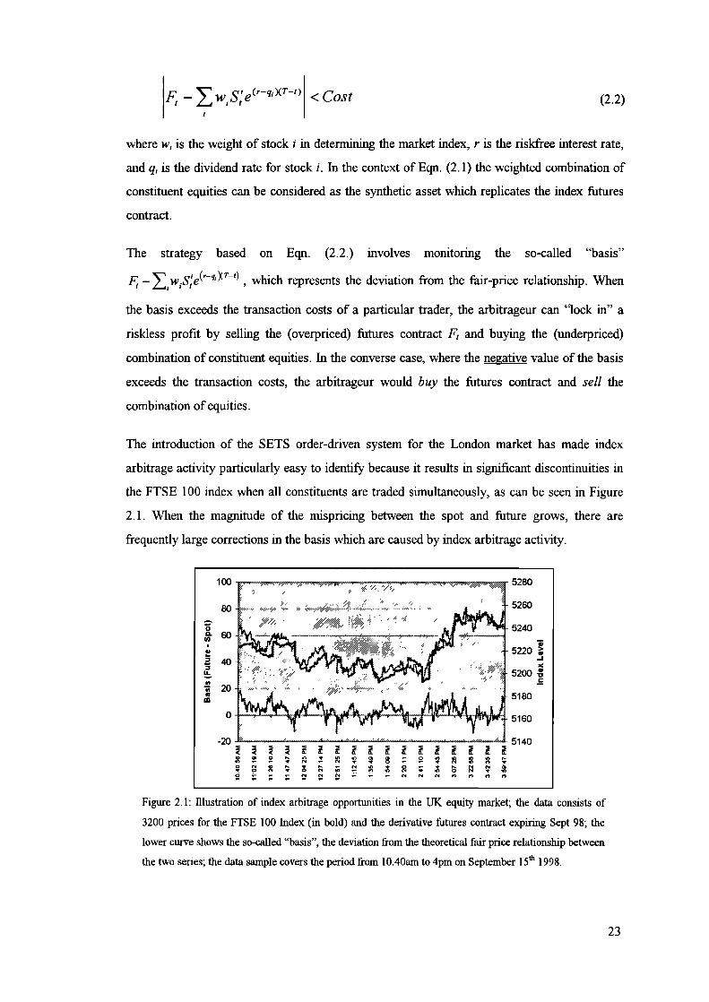
The introduction of the SETS order-driven system for the London market has made index

arbitrage activity particularly easy to identifi because it results in significant discontinuities in

the FTSE 100 index when all constituents are traded simultaneously, as can be seen in Figure

2.1. When the magnitude of the mispricing between the spot and future grows, there are

frequently large corrections in the basis which are caused by index arbitrage activity.

Figure 2.1: illustration of index arbitrage opportunities in the UK equity market; the data consists of

3200 prices for the FTSE 100 Index (in bold) and the derivative futures contract expiring Sept 98; the

lower curve shows the so-called "basis", the deviation from the theoretical fair price relationship between

the two series; the data sample covers the period from 1040am to 4pm on September 15th 1998.

23

Riskless (or near-riskiess) arbitrage is clearly an important subject in its own nght, and many

complex arbitrage relationships exist, particularly with the recent growth of financial

derivatives such as options, futures, swaps and exotic options. However such strategies are

inherently self-limiting - as competition amongst arbitrageurs grows, the magnitude and

duration of mispricings decreases. As the profits available through arbitrage decrease, the

amount of capital employed in order to achieve significant profits must increase. Furthermore

only the arbitrageurs who are geared to trade very rapidly and at low transaction costs will be

in a position to achieve arbitrage profits. For both of these reasons large banks and other

privileged financial institutions tend to dominate arbitrage activity.

In practice, even arbitrage which is technically "riskiess" will still involve a certain level of

risk. This risk is introduced by numerous factors: uncertain future dividend rates q; market

volatility during the short time required to carry out the lock-in trades (slippage); failure to

"fill" all legs of the trade, thus leaving a residual "unhedged" risk. A very important source of

risk in arbitrage activity is "basis risk" caused by fluctuations in the difference between spot

and futures prices prior to the expiration date.

"Basis risk" is indeed a source of risk, particularly when Exchange regulations or internal

accounting practices require that positions be regularly "marked to market" at current prices.

However, it is also a source of opportunity in that favourable fluctuations may move the basis

beyond the fair price value (i.e. from positive to negative, or vice versa) and thus allow an

arbitrageur to realise higher profits by reversing the trade at some point prior to expiration.

Thus practical arbitrage strategies are much more complex than may at first appear. In fact,

the majority of arbitrage strategies are at least implicitly reliant on the statistical properties of

the "mispricing" or deviation from the fair price relationship. From this perspective the

attraction of index arbitrage strategies lies in a favourable property of the mispricing dynamics

- namely a tendency for the basis risk to "mean revert" or fluctuate around a stable level. In the

following section we describe how this recognition, that practical arbitrage strategies both

involve risk and rely upon favourable statistical properties of the mispricing dynamics, leads to

a more general class of arbitrage strategies, namely "statistical arbitrage".

24

2.1.3 Elements of Statistical Arbitrage

The discussion above shows that from a statistical perspective, the mispricing time-series can

be considered as a "synthetic asset" which exhibits strong mean-reversion, and hence a certain

degree of potentially predictable behaviour. The premise of so-called "statistical arbitrage" (see

for example Wong (1993)) is that, in many cases, statistical regularities in combinations of

asset prices can be exploited as the basis of profitable trading strategies, irrespective of the

presence or absence of a theoretical thir-price relationship between the set of assets involved.

Whilst clearly subject to a higher degree of risk than "true" arbitrage strategies, such statistical

arbitrage opportunities are likely to be both more persistent and more prevalent in financial

markets. More persistent because risk-free arbitrage opportunities are rapidly eliminated by

market activity. More prevalent because in principle they may occur between any set of assets

rather than solely in cases where a suitable risk-free hedging strategy can be implemented. An

example of a set of assets which present possible opportunities for statistical arbitrage are

shown in Figure 2.2 below.

Figure 2.2: ifiustration of potential statistical arbitrage opportunities in the UK equity market; the chart

shows equity prices for Standard Chartered and HSBC, sampled on an hourly basis from August 20th to

September30th, 1998.

Comparing the illustration of potential statistical arbitrage opportunities in Figure 2.2, to the

riskless arbitrage opportunities shown in Figure 2.1, there is clearly a marked similarity. In

both cases the two prices "move together" in the long term, with temporary deviations from the

long term correlation which exhibit a strong mean-reversion pattern. Note however that in the

"statistical arbitrage" case the magnitude of the deviations is greater (around +1- 10% as

25

opposed to <0.5%) and so is the time-period over which the price corrections occur (days or

weeks as opposed to seconds or minutes).

From this perspective, we consider statistical arbitrage as a generalised case of riskiess

arbitrage in which the relative returns, payoff (x - sA(x)), are no longer completely

hedged (i.e. immunised) against the underlying sources of economic uncertainty (or "risk

factors") which drive asset price movements in general. Given a set of economic variables,

assets or portfolios of assets which correspond to risk factors F = ,..., i,, } we can

quantify the extent to which risk is introduced to the "statistical mispncing" portfolio

- SA(X , w) in terms of the set of sensitivities S = , Sn, } where

d E[payoff(X - SA1 (X, w))]

= dFand w are the parameters which define the synthetic asset.

Thus in the case of riskless arbitrage, the future relative return, payoff(X - SA(X , w)), is

dependent purely on the magnitude of the mispricing X - SA(X , w) and the sensitivity to all

risk factors is zero, i.e. V. : s, = 0.

In a case where an appropriate set of risk factors can be pre-deflned, perhaps the most natural

approach to developing statistical arbitrage strategies is to introduce risk in a controlled manner

through specifying a desired set of factor sensitivities s. This is the approach taken in Burgess

(1996), in which the "risk factors" common to a set of money-market futures contracts are

statistically determined through the use of Principal Component Analysis (PCA) [Jolliffe,

1986] of the returns (price changes) in the different contracts. The synthetic asset

SA(X,, w, F, s) is then defined as the combination of assets which, together with a particular

asset (or portfolio) X exhibits a specified risk profile s with respect to the set of risk factors

F. In the case of Burgess (1996) the risk factors are defined by the principal components of the

set of asset returns and the sensitivity profiles are of the form = 1, V: s, = 0, i.e. portfolios

defined to have unit exposure to a selected factor j whilst immunised to all other factors (a

"factor bet" on factorj).

However, whilst this approach is sufficient to control the degree of risk exposure which is

introduced into the deviation time-series, it does not directly support the identification of

mispricing time-series which contain mean-reverting or other (potentially nonlinear)

26

deterministic components in their dynamics. l'his is because a low (or otherwise controlled)

exposure to risk factors does not in itself imply the presence of a non-random component in the

dynamics. For instance, Burgess (1996) reports a situation where the third principle component

portfolio (j=3) shows evidence of being predictable with respect to nonlinear but not linear

techniques and the first two principle component portfolios (1= 1,2) show no evidence of either

mean-reversion or other non-random behaviour.

In comparison to the "explicit factor modelling" approach described above, the methodology

described in this thesis is based upon an alternative approach to the construction of synthetic

assets. In this approach, the introduction of risk is treated not from a risk factor perspective but

instead in an aggregate manner in which it is the "tracking error" between the asset or portfolio

X, and the synthetic asset SA(X , w) which is of concern. The parameters of the synthetic

asset are taken to be those, w, which minimise the variance of the price deviation series, i.e.

w =argminvar(x, _SA,(X,w)).

In the limiting case of perfect tracking, where var(Xt - SA (X, w e )) = 0, then the factor

exposures (to any set of factors) are also known for certain in that they must all be zero, i.e.

V 1 :s, = 0. In the more general case, where var(Xt - SA(X, w*))> 0, the factor

sensitivities s, are only implicitly defined in that the minimisation of residual price variance

(with respect to the synthetic asset parameters w) will tend to minimise the aggregate

exposure to the risk factors, without imposing any specific constraints upon permissible values

of the individual sensitivities. As discussed in Chapter 5, this additional flexibility has the

advantage of encouraging exposure to those risk factors (be they market wide or specific to an

individual asset) which contain a non-random (or more specifically, mean-reverting)

component. Furthermore, as we discuss in Chapter 3, a suitable set of econometric tools, upon

which to base a methodology for identifring models of this type, already exist in the form of

tools for modelling cointegration relationships within sets of time-series.

Thus in an analogous manner to that in which nskless arbitrage strategies were earlier

decomposed into three components, the three components required for statistical arbitrage

models can be considered as:

27

• construction of statistical fair-price relationships between assets such that the

deviations or "statistical mispricings" have a potentially predictable component

(through time-series analysis of historical asset price movements);

identification of statistical arbitrage opportunities (forecasting of changes in

combinations of asset prices);

implementation of appropriate trading strategy (buy assets which are forecasted to

outperform, sell assets which are forecasted to underperform).

These three components correspond to the three stages of our statistical arbitrage methodology,

which will be described in detail in the later parts of the thesis. The statistical arbitrage

equivalent of the no-arbitrage condition in Eqn. (2.1) can be expressed as:

E[payoff(X, - <TransactionCost

(2.3)

where E[ ] is the expectation operator. In the context of Eqn (2.3), the challenge for

computational modelling becomes clear: firstly, given an asset (or portfolio) X to identify an

appropriate combination of assets to form the corresponding statistical hedge, or "synthetic

asset", SA(X); secondly to create models capable of predicting the changes in the "statistical

mispricing" between the two portfolios, E[payoff(X - SA(X))]; thirdly to construct a

trading strategy which is capable of exploiting the predictive information in a manner which

overcomes the transaction costs. These three tasks correspond both to the general requirements

listed above and also to the three stages of our methodology for statistical arbitrage. Before

moving on in the rest of the thesis to describe the details of the methodology, the remainder of

this chapter presents a review of recent advances in computational modelling which form the

basis upon which our methodology has been developed.

2.2 Recent Advances in Computational Modelling

In this section we review the recent advances in computational modelling which comprise the

platform upon which our statistical arbitrage methodology is based. The review brings together

various strands of work from a number of academic disciplines, including time series

forecasting, statistical modelling, econometrics, machine learning and computational finance.

28

2.2.1 Time Series Representation

In this section we review alternative methods for representing and modelling time-series.

Perhaps the two key complications in modelling financial time-series are the inherent properties

of "noise" and "nonstationarity" and to a large extent these properties are determined by the

choice of time-series representation which is adopted. In recognition of the importance which

the choice of problem representation can have in detennining the likely success of any

subsequent modelling or forecasting procedure, researchers in forecasting and econometrics

have developed a number of modelling frameworks which are designed to exploit time-series

with different types of characteristics.

The choice of target or "dependent" variable is perhaps the single most important decision in

the entire modelling process. We can consider any random variable Yt as being the result of a

data-generating process which is partially deterministic and partially stochastic:

yt =g(z)+s(v)

(2.4)

where the deterministic component is a function 'g' of the vector of influential variables

= {zi , z2 ,.. . ,z, } and the stochastic component is drawn from a distribution 'c'

which may vary as a function of variables V = ,v2 ,... Under the assumptions

that the stochastic term is homoskedastic and normally distributed with zero mean and variance

the data-generating process reduces to:

= g(z1)+N(O,o)

(2.5)

The choice as the target or "dependent" variable implicitly limits the maximum possible

performance of a forecasting procedure to the proportion of the variance of y, which is due to

the deterministic and hence potentially predictable component:

E[(f(x,)_yl)21 cr=_

(2.6)

2 2R2(y,,f(x))=1— 21 2

E[(g(zi)_P,) +0 y E[(g(zi)_P,) ]^,

where the performance measure R 2 (y1 ,f(x)) is the proportion of variance (correctly)

absorbed by the model and n is the "noise content" of the time-series. Note that the degree to

29

which the inequality can approach the equality is dependent on how closely the forecasting

model f(x) approximates the true detenmnistic component g(z1 ) - an issue which is returned

to later in this review.

In many forecasting applications, the issue of representation is overlooked, largely because the

target series is often taken for granted. However in an application such as statistical arbitrage

there are many possible combinations of assets which could be used as target series, and

identifying combinations of time-series with the greatest possible potentially predictable

component is a key objective of the first stage of our statistical arbitrage methodology.

The second key property which is determined by the adopted representation is that of

"nonstationarity", or time-variation in the statistical properties. At some level, all forecasting

techniques are utterly reliant on the assumption that the future will be related to the past. This

assumption is typically phrased as one of stationarity, or stability of the statistical properties

of the system over time. Some common technical conditions for stationarity of a single time-

series are presented below:

E[y]= i.t

(Cl)

E[ (y, - .t)2 I = =

(C.2)

=y(r) r= 1,2 (C.3)

pdf( y , y+2, Yt+3, •.. ) = pdf( yt^-i, yt^,+2, y+^3, ... ) (C.4)

Conditions (C.1-C.3) relate in turn to stationarity of the mean, variance and auto-covariances

of the series. The fourth condition for "strict stationarity" requires that the entire joint

distribution of a sequence of observations be independent of the reference time from which they

are taken. A fuller treatment of these issues can be found in any time-series forecasting

textbook, for instance (Harvey, 1993).

The observation that successful application of statistical modelling tools is often dependent

upon the assumption of stationarity is easily illustrated; consider a time-series which exhibits

non-stationarity in mean, i.e. violates condition (C.1), as shown in Figure 2.3. Within an

autoregressive modelling framework, where lagged values of the series are used as the basis for

future forecasts, not only would forecasting involve the model being queried in a region where

30

/ / /

Tmie(t

it had seen no previous examples, but it would also be expected to give a previously unseen

response.

Figure 2.3: An example time-series which shows non-stationarity in mean; the left hand chart shows the

time series yt; the right hand chart illustrates the fact that the idealised probability distributions differ

during the in-sample and out-of-sample periods.

In the more general case, most types of model are more suited to tasks of interpolation (queries

within the range of past data) rather than extrapolation (queries outside the range of known

data) and thus the effect of nonstationarity is to cause a degradation in the perfonnance of the

associated model. The most common solution to the problems posed by nonstationarity is to

attempt to transform the representation of the data to achieve weak stationarity (Spanos, 1986),

i.e. satisfaction of(C.1) and (C.2).

Figure 2.4 illustrates different classes of time-series from the viewpoint of the transformations

that are required to achieve stationarity.

Tun(U

7.z

> .... /

d44fThi (t)

Figure 24: Time-series with different characteristics, particularly with regard to stationarity: (top left)

stationary time-series; (top right) trend-stationary time-series; (bottom left) integrated time-series;

(bottom left) cointegrated time-series

A stationary series, such as that shown in the top-left chart of Figure 2.4, is a suitable

candidate for direct inclusion as either a dependent or independent variable in a forecasting

model without creating a risk of extrapolation.

31

The chart in the top-right of Figure 2.4 is an example of a "trend stationary" variable, that is it

is stationary around a known trend which is a deterministic function of time. A stationary

representation of such a variable can be obtained by "de-trending" the variable relative to the

known deterministic trend

Series such as that in the bottom left chart of Figure 2.4 are known as "integrated series"

because they can be viewed as the integration (sum) of a stationary time-series. If the first-

differences (iy, = - y) of the series are stationary then the series is integrated of order

1, i.e. y - 1(1) and may also be referred to as being "difference stationary". From this

perspective, a stationary time-series is referred to as being integrated of order zero, or 1(0). In

recent years there has been a growing recognition that time-series may be neither completely

stationary, i.e. 1(0), nor completely nonstationary, i.e. 1(1), but instead may be fractionally

integrated, i.e. most typically 1(d) where 0<d<l (Granger and Joyeux, 1980).

The two series in the bottom-right chart of Figure 2.4 represent a so-called "cointegrated set"

of variables. The concept of cointegration, initially proposed over 15 years ago by Granger

(1983), has attracted much interest in recent years. As the name suggests, it is closely related to

the concept of integration but refers to a relationship between a number of time-series rather

than a property of an individual time-series. If two or more time-series are integrated of order d

and yet a linear combination of the time-series exists which is integrated of order b < d, then

the time-series are said to be cointegrated of order d, b; following the terminology of Harvey

(1993), the vector Yt CI( d,b) if

all components of Yt are 1(d); and

there exists a non-null vector, a, such that aTy is I(d-b) with b > 0

A wide range of methods have been proposed both for estimating the "cointegrating vector" a

including Ordinary Least Squares (OLS) regression [Engle (1993), (Engle and Granger,

1987)], Augmented Least Squares (with leads and lagged terms, possibly nonlinear), (Stock,

1987), Canonical Cointegration (Park, 1989), Principal Components [Stock and Watson

(1989); Phillips and Ouliaris (1988)], Three-Step estimation (Engle and Yoo, 1991), and

Differenced Vector Auto-Regression (Johansen, 1988, 1991). The most popular method of

testing for cointegration (see Section 2.2.2) is that introduced by Granger (1983) and is based

upon the concept of a "comtegrating regression". In this approach a particular time-series (the

32

"target series") y0 is regressed upon the remainder of the set of time-series (the "cointegrating

series") y1, , . . .

= a + fi1y1, + 132y2.......+f3y,7 + d

(2.7)

if the series are cointegrated then the "deviation" term c4 will be a stationary variable. The

usual motivation for this approach is that stationary time-series tend to have smaller variance

than nonstationary time-series; thus the OLS regression procedure of minimising the variance

of the residuals will tend to maxiniise the probability of identifying any cointegration between

the set of time-series. As a means of creating combinations of time-series which are statistically

"well behaved", the concept of cointegration will serve as an important motivation for the first

part of our statistical arbitrage methodology.

The class into which a time-series or set of time-series fall, whether stationary, mean-

nonstationary (integrated), or cointegrated, has important implications both for the modelling

approach which should be adopted and the nature of any potentially predictable components

that the time-series may contain. Having characterised different types of time-series by the

transformations which must be performed upon them to attain stationarity, we discuss in the

next section a range of statistical tests which serve one of two purposes: firstly to identify the

type of the time-series (stationary, nonstationary, cointegrated) and secondly, having

established the type of the time-series, to identify the presence of any potentially predictable

component in the time-series dynamics.

2.2.2 Time-series Identification

In this section we consider four main categories of time-series identification tests, based on the

type of behaviour which they are intended to identify, namely autoregressive tests, unit root

tests, variance ratio tests and cointegration tests. Autoregressive tests are designed to be

applied to stationary time-series, and are designed to distinguish time-series which contain a

predictable component from time-series which are pure noise. Unit root tests are designed to

differentiate between stationary and non-stationary (integrated) time-series. Variance ratio tests

are designed to distinguish random walk time-series from non-random walks. Cointegration

tests are designed to identify whether a set of mean-nonstationary time-series contain one or

more linear combinations which are themselves stationary (i.e. cointegration of order 1,1.)

33

Identification of Autoregressive Dynamics

The first set of tests are based on the short-term dynamics of the time-series and are derived

from the Auto-Correlation Function (ACF), otherwise known as the correlogram:

—)(y —Y)/[T—(k+l)]f-k+1

4 — T(yt j2/[]

Autocorrelations significantly different to zero indicate that future values of the time-series are

significantly related to past values, and hence the presence of a predictable component in the

time-series dynamics. The auto-correlation function and the related Partial Auto-Correlation

Function (PACF) form the basis of standard techniques such as ARMA and ARIMA

modelling. So-called 'portmanteau' tests such as those of Box and Pierce (1970) and Lyung

and Box (1978) are designed to test the joint null hypothesis: H0 :, = r2 =...= = 0,

against the general alternative H1 : not all r = 0. Box-Pierce-Lyung portmanteau tests are

often used as tests for non-random components, particularly as diagnostic tests applied to the

residual errors of a regression or time-series model. In the context of statistical arbitrage

modelling, such diagnostic tests for autoregressive behaviour in a time-series may play a useful

role in identifying a potentially predictable component in the dynamics of the statistical

mispricing.

Identification of Deterministic Trends

In the case of time-series with a known detenninistic trend, the standard procedure is to "de-

trend" the variable by subtracting the deterministic trend and build forecasting models based

upon the stationary variable which is thus created. Detrending of variables can also be achieved

by including a suitable time-trend within a regression (Frisch and Waugh, 1933). However, if

the time-trend is not deterministic but is actually stochastic (such as a random walk) it is likely

to appear to be (spuriously) significant [Nelson and Kang (1984), Phillips (1986)] and

furthermore will induce apparent penodicity in the de-trended series (Nelson and Kang, 1981).

In practice, even financial time-series which appear to contain a trend are generally treated as

stochastically trending (i.e. integrated) variables in order to avoid the risk of inducing spurious

periodicity. For similar reasons, the deterministic detrending approach is not considered further

in this thesis.

(2.8)

34

Tests for Stationarity

Stationarity tests are used to differentiate between integrated, (mean-)nonstationaiy, time-series

and stationary time-series. The most common such test is the Dickey-Fuller test which is

performed by regressing the one-step-ahead-values of a time-series on the current value:

= a + /' +

(2.9)

If the estimated coefficient fi is not significantly less than one, then the null hypothesis of

nonstationarity is not rejected and the time-series should be transformed by differencing before

being modelled. The fact that the null hypothesis of nonstationarity implies a /3 of one is the

reason why this test is often referred to as a "unit root" test. The regression may be extended by

including autoregressive terms which absorb any short-term dynamics in the differenced series,

the differenced form of this Augmented-Dickey-Fuller or ADF test thus involves the following

regression:

p-i- = Ay = a + f3y + fl3 Ay +6 (2.10)

j=1

and nonstationarity is rejected only if the /3 coefficient is significantly less than zero. The test-

statistic which is used for the DF or ADF test in this form is the t-statistic associated with the

/3 coefficient. Under the null hypothesis of nonstationarity the t-statistic follows a non-

standard distribution which was first studied by Dickey (1976) and Fuller (1976), and is

tabulated in Fuller (1976). Alternative stationarity tests have been proposed, for example by

Philips (1987), Phillips and Perron (1988) and Hall (1989), but the available evidence suggests

that these do not improve upon the original tests [Schwert (1989), Pantula (1991)].

Even in cases where nonstationarity can be rejected, as is sometimes the case in some financial

time-series, it is still common to difference the data before modelling. This serves two

purposes, firstly the quantity of interest is more often returns (price changes) of financial assets

as opposed to the price levels, secondly it serves to reduce the level of autocorrelation in the

resulting time-series, thus more closely approximating the assumption of independent

identically distributed (i.i.d.) errors upon which test diagnostics are predicated, thereby

reducing the danger of achieving spurious results.

35

Additionally, the DF and ADF tests can be considered as tests for a particular type of

predictable component in the dynamics of a time-series. This is made clear from the form of

Eqn (2.10): if the fi coefficient is significantly negative then this implies a significantly

negative relationship between future changes and current levels, indicative of a significant

mean-reversion component in the time-series.

Tests for Deviation from Random Walk Behaviour

Whilst the "unit root" tests are intended to distinguish between stationary and nonstationary

time-series, another family of tests are designed to identifi the situation where a time-series

deviates from a particular type of nonstationary dynamics in which increments in the time-

series are completely uncorrelated:

= +

(2.11)

So-called variance ratio tests follow from the fact that the variance of the innovations in such a

"random walk" series is a linear function of the period over which the increments are measured.

A simple intuition for this property is presented in Figure 2.5 below.

PerfectTrend:

PerfectReversion:

Random:

Pricer

Time

Price-r

Time50/50 mix of trend + reversion

Variance1-period 2-period

r2 (r+r)2= 4 r2

r2 (r-r)2= 0

r22r2

Figure 2.5: The relationship between variance and time for a simple diffusion process: in the limiting

case where all steps are in the same direction the variance of the series will grow as a function of time-

squared, at the other extreme of pure-reversion the variance of the series will be independent of time

(and close to zero). A random diffusion will be a weighted combination of both behaviours and will

exhibit variance which grows linearly with time.

The linear growth of variance as a function of the increment period has been used as the basis

of statistical tests for deviations from random walk behaviour by a number of authors since Lo

and McKinley (1988) and Cochrane (1988).

36

q-1 2( -

j=1 q(2.13)

The variance ratio statistic can be defined as the norinalised ratio of long term variance

(calculated over period t) to single-period variance and is thus:

-

VR( r)- - n2

(2.12)

As with autocorrelation statistics, the variance ratio statistics can be viewed collectively, thus

forming the "variance ratio function" or VRF of the time-series. A positive gradient to the

variance ratio function (VRF) indicates positive autocorrelation and hence trending behaviour;

conversely a negative gradient to the VRF indicates negative autocorrelations and mean-

reverting or cyclical behaviour. Figure 2.6 shows example time-series with different

characteristics, together with their associated VRFs.

...... Tiundrç..

fr 4

—u--Random Wo •• ..•

• . . ..

S .4 .4

vSTime

.2 _• . —4-- -.TendIrig

—I- —a-- Random Weli

• -a- Mean Re,rti,

a ---$---

Period

Figure 2.6: Example time-series with different characteristics (left), and their VRFs or variance ratio

functions (right). For the random walk, variance grows linearly with the period t and hence the VRF

remains close to one; for a trending series the variance grows at a greater than linear rate and so the VRF

rises above one as the period over which the differences are calculated increases; for the mean-reverting

series the converse is true: the variance grows sublinearly and hence the VRF falls below one.

The rationale for testing for deviations from random walk behaviour is that such deviations are

indications of a potentially predictable component in the dynamics of a time-series. Lo and

MacKinley (1988) showed that a particular form of the variance ratio statistic is essentially

equivalent to a linear combination of autocorrelation coefficients:

where are the autocorrelation coefficients calculated according to Eqn (2.8). Lo and

MacKinley (1989) used Monte Carlo simulation to investigate the finite sample performance of

37

the variance ratio against different alternative hypotheses and concluded that it is more

powerful than either the Dickey-Fuller or Box-Pierce tests in two of the three cases considered

and equally powerful in the third case. Faust (1992) noted that the VR statistic can be

considered as a specific example of a class of "filter variance ratio" statistics which consist of

linear combinations of autocorrelation coefficients and that such statistics can be shown to be

optimal tests for a wide class of time-series dynamics. Chow and Denning (1993) examined the

perfonnance of a multiple variance ratio test using Monte-Carlo simulations and found that the

test is as reliable as the Dickey-Fuller and Phillips-Perron unit root tests when testing a random

walk against an autoregressive AR(1) alternative, whilst being more powerful when testing

against two nonstationary alternatives which contain a predictable component.

As a powerful means of identifying deviations from random behaviour, variance ratio tests are

an important inspiration behind our methodology for testing for potentially predictable

behaviour in the dynamics of statistical mispricing time-series.

Tests for Cointegration

As noted in the previous section, cointegration is a property of a set of time-series which are

individually nonstationary (integrated) but which contain one or more stationaly components.

The implications of cointegration for statistical arbitrage modelling are twofold. The first of

these is that the presence of cointegration in a set of asset prices implies the existence of a long

run relationship between the assets which could be considered as the statistical equivalent of a

"fair price" relationship; deviations from this relationship could then be considered as

"statistical mispricings". The second major implication of cointegration is the presence of a

significant predictable component in the time-series dynamics - it already having been noted

above that the property of stationarity implies a mean-reverting component in the dynamics of a

time-series.

As noted in Section 2.2.1, the most popular form of cointegration testing is that introduced by

Granger (1983) and is based upon the concept of a "cointegrating regression". In this approach

a "target" time-series y is regressed upon the "cointegrating series" y , . . . y,.. The

presence (or absence) of cointegration is detected by testing the deviation term d which is

represented by the residual errors of the cointegrating regression:

d, =y0 —[a+fl1 y11 +/.i2y2 ......+/Jy]=aTy (2.14)

38

If the set of variables y = {y0,1 , 1, y , . . , y } are cointegrated then statistical tests will

indicate that d is stationary and the parameter vector a = (1,_a,_fl1,_fl2,...,_p) is

referred to as the cointegrating vector.

In order to correct for spurious mean-reversion which is induced by the cointegrating regression

itself, the stationarity tests used in the identification of cointegrating relationships are modified

versions of standard tests for stationarity. Many different cointegration tests have been

proposed in the econometric literature, for example Dickey-Fuller and Augmented Dickey-

Fuller (Said and Dickey, 1984), Cointegrating Regression Durbin Watson (Engle and Granger,

1987), adjusted ADF (Phillips, 1987), spurious regressors (Park, Ouliaris and Choi, 1988),

maximum likelihood (Johansen and Juselius, 1990). These tests reflect both the variety of

estimation methods which have been proposed, and also minor variations in the null and

alternative hypotheses between which the tests are designed to distinguish.

An early comparison of a range of cointegration tests was conducted by Engle and Granger

(1987) who recommend two tests in particular the Dickey-Fuller (DF) and the Cointegrating

Regression Durbin Watson (CRDW'). Further comparisons of cointegration tests are contained

in Gregory (1991) and Hargreaves (1 994b), the latter conducting a Monte-Carlo comparison of

different estimation methods/cointegration tests and concluding that no one technique can be

said to dominate the others.

Standard tests for cointegration make a "hard" distinction between stationary and nonstationary

processes, with a null hypothesis of no cointegration (nonstationarity) and an alternative

hypothesis of full cointegration (stationanty) 3 . As noted in the previous section, there is now a

growing recognition that time-series may be neither completely stationary nor completely

nonstationary but instead may be fractionally integrated (Granger and Joyeux, 1980); in the

multi-variate case this perspective has led to the development of so-called fractional

cointegration models [Baillie and Bollerslev (1994); Dueker and Startz (1995)] with the

objective of identifying linear combinations which have a lower (and potentially fractional)

degree of integration than any of the (also potentially fractionally integrated) original series.

Harris and hider (1994) reverse the standard test procedure by using a null hypothesis of cointegration and an

alternative hypothesis of no cointegration. However they still maintain the hard distinction between cointegrated

and non-cointegrated, stationary and nonstationary, series.

39

Whilst the hard distinction between stationary and nonstationary series may be useful when the

primary objective is descriptive, it is less appropriate from our predictive modelling

perspective, when the objective is to forecast the time-series. From our perspective of aiming to

exploit general deterministic components in asset price dynamics, an important motivation for a

multi-variate approach is that whilst a set of time-series might appear to be true random walks

and hence unpredictable on an individual basis, a suitable combination of the time-series may

contain a stationary (or other non-random) component - even if in combination with a

nonstationary (random) component. This issue is returned to in Chapter 3 as it constitutes an

important aspect of our methodology for statistical arbitrage.

Having reviewed in this section a number of families of tests which are designed to distinguish

between different types of dynamics and to identify the presence of potentially predictable

components, we move on, in the following section, to consider techniques for capturing the

predictability in appropriate time-series models and hence making forecasts of future dynamics.

2.2.3 Statistical Forecasting and Model Selection

In the previous sections we have reviewed the division of time-series into different classes

according to their stationarity characteristics (stationary, nonstationaiy/integrated,

cointegrated), tests to distinguish between these different classes, and tests to identify the

presence of potentially predictable components in the time-series dynamics (autoregressive,

mean reversion, deviations from random walk). In this section we move on to consider both the

modelling methods which aim to capture the predictable component of the dynamics, and the

model selection techniques which are used to identify the "best" model from amongst various

alternative model specifications.

Smoothing Methods

The most basic family of forecasting procedures are the so-called smoothing methods such as

the Exponentially Weighted Moving Average (EWMA), a simple ad-hoc technique which

forecasts future values through a recurrence relation:

9t+rt = f = ay + (1— (2.15)

40

i.e. at time 't' the forecasted future values Y+ r (over all forecast horizons z) are simply equal

to a weighted sum ft of the most recent observation Yt and the previous forecast ft_I. The

name arises because it is easy to show that the recurrence relation in Eqn (2.15) is equivalent to

constructing an exponentially weighted average of past observations. Originally an ad-hoc

procedure, the EWrvLA was shown by Muth (1960) to provide optimal forecasts (in the

minimum mean-squared-error sense) when the underlying time-series is a random walk

contaminated with stationaly noise. The model deals with time-variation in the level of the

series by constructing an adaptive estimate of the "local mean" which is updated with each new

observation. Holt (1957) and Winters (1960) generalised this exponential smoothing approach

to more complex models containing components relating to trend and seasonality. Discussions

of the optimality of these approaches, together with further generalisations, are provided by

Theil and Wage (1964) and Nerlove and Wage (1964).

A different approach, but which leads to almost identical models, is due to Brown (1963), who

suggested the use of discounted least squares, in which the increased relevance of more-recent

observations is explicitly taken into account through the use of an exponentially-weighted

decay function. This approach leads to a recurrence relation for updating estimates of both

intercept and slope which correspond to a "local trend". Further generalisations are discussed

in Brown (1963) and more recent papers, of which a review is provided by Gardner (1985).

In the case of these smoothing techniques, it is common for parameters such as the smoothing

parameter a in Eqn. (2.15) to be pre-specifled according to an a priori belief regarding the

underlying properties of the time-series. Alternatively a small number of plausible alternatives

may be compared, and the "best" model selected on the basis of one or more metrics of

forecasting accuracy such as (one-step ahead) mean-squared-error (MSE), mean-squared

percentage error (MSPE), mean-absolute error (MAE) or mean-absolute-percentage error

(MAPE). Definitions and discussions of such metrics can be found in any forecasting text, for

example in Chapter 12 of Diebold (1998).

Modelling stationary time-series

The classic approach to modelling stationary time-series is based on the recognition that any

stationary stochastic time series can be approximated by a combination of so-called auto-

regressive (AR) and moving-average (MA) processes, i.e. so-called ARMA processes of the

form:

41

y =u+ q51 y , + (2.16)i - i p j=1 q

A model with p>O, q—O includes only lagged values of the dependent variable as explanatory

variables and is known as a pure auto-regressive model, denoted AR(p). A model with p 0,

q>0, includes only past innovation terms as explanatory variables and is referred to as a pure

moving-average model, MA(q). The general case is known as an auto-regressive moving-

average model, and denoted ARTVIA(p,q).

This approach developed initially from the work of E. Slutsky (1927) and G.U. Yule (1921). It

was shown by Mann and Wald (1943) that pure AR models can be correctly estimated using

standard OLS regression. For pure MA or mixed (ARMA) models, more sophisticated methods

are required which are based upon nonlinear least squares estimation (Box and Jenkins, 1970)

or maximum likelihood methods (Newbold, 1974). A detailed discussion and improved

procedures can be found in any standard time-series or econometric text, for instance Harvey

(1993) or Greene (1993). ARMA modelling can be extended to allow for exogenous variables,

when it becomes known as ARMAX [Hatanaka (1975), Wallis (1977)].

Model selection for ARMA models is sometimes based upon diagnostic tests for (residual)

structure such as the Box-Pierce and Box-Ljung statistics, and statistical tests of variable

significance such as t-statistics, model restriction F-statistics, and stepwise regression

procedures. More common however is the use of statistical model selection criteria within a

modelling framework such as the Box-Jenkins framework discussed below.

Multivariate forms of ARMA models also exist, with the vector autoregression or VAR model

being particularly popular due to the difficulties in estimating multivariate models with moving-

average terms. VAR models have been studied extensively since being first popularised by

Sims (1980).

Modelling nonstationary time-series

The most common approach to modelling difference-stationary time-series is the ARIMA

modelling framework of Box and Jenkins (1970). This framework deals with nonstationary

time-series by repeatedly differencing the data until the resulting series is stationary, thus

identifying the "order of integration" within the data. ARMA modelling is then applied to the

42

stationary variable thus obtained. Data with degree of integration 1(1) need only be differenced

a single time and the resulting ARIMA(p,1,q) model has the form:

= ,u+ q$,Ay 1 + + e

(2.17)z=lp j lq

Box and Jenkins included the ARIMA modelling process within an integrated framework for

model identification. This framework uses model selection criteria to choose between

alternative specifications of ARIMA models with varying numbers of AR and MA terms p and

q respectively.

Statistical model selection criteria are based on a recognition of the fact that the insample fit of

a model will automatically improve when additional terms are added to a model, even in the

case where the additional terms have no real forecasting ability. This effect is a purely

mechanical consequence of adding free parameters into a model and is sometimes referred to as

"overfitting" or "data mining" 4. The objective of the model selection criteria is to adjust for

these spurious effects and thus allow a fair comparison between models of different complexity.

The criteria work by adjusting the insample goodness of fit by a penalty term based upon the

number of "degrees of freedom" (or free parameters) in the model. The basic "adjusted R2"

measure is a standard tool of regression modelling which is designed to allow comparison

between models with different numbers of explanatory variables. More sophisticated criteria

such as the AIC introduced by Akaike (l974b) and the BIC of Schwartz (1978) apply

increasingly severe penalties to model complexity.

Discussions of the relative pros and cons of different selection criteria can be found in many

places, including pages 85-91 of (Diebold, 1998), and chapter 17 of (Efron and Tibshirani,

1993). In particular the more heavily penalising BIC has the property of consistency (i.e. can

be shown to select the correct model in the asymptotic linüt, as the sample size n —* cc) and

the AIC has the property of asymptotic efficiency (will select models with performance which

converges towards the optimal performance at least as rapidly as any other criterion, as sample

size increases). Diebold (1998) notes that when the selection criteria differ as to the optimal

"Overfitting effects become increasingly important as model complexity grows, as is discussed in the following

section on "low bias" modelling approaches. Note that "data mining" in its more usual sense refers to the

identification of meaningful, rather than spurious, relationships between a set of variables.

43

model, many authors recommend use of the more parsimonious model selected by BIC, and

that this approach is supported by empirical comparisons such as that conducted by Engle and

Brown (1986).

Model selection issues play an important role in both the second and third parts of our

methodology, which are concerned with the estimation of forecasting models and the

diversification of model risk respectively, and hence are discussed more extensively later in the

thesis.

Modelling cointegrated time-series

A useful corollary of the existence of cointegration in a given set of variables y is provided by

the "Granger Representation Theorem" [Granger, (1983), Engle and Granger (1987)]. The

important implication of this theorem is that the presence of cointegration between a set of

variables motivates the use of Error-Correction Models (ECMs) [Sargan, 1964] of the form:

= /1+ Ø014v0 + ci$,iAv -2.d +e (2.18)k1..n j=1. Pk

where d is the (stationary) cointegration residual calculated according to Eqn. (2.14).

The motivation behind the ECM in Eqn (2.18) is to capture the autoregressive dynamics

of AY0,, the lagged cross-correlations between Ay0, and changes in the cointegrating variables

Ay,, and also the mean-reverting or "error-correcting" effect induced by the

cointegration residual d.

The key idea of the ECM is that the cointegration residual represents a misalignment within the

set of time-series and that the cointegrating effect will act so as to reduce this misalignment.

Thus the current sign and magnitude of the cointegration residual contain predictive

information about changes in the individual time-series. This two-step procedure, of estimating

the long-run or cointegration model, and then the ECM which governs the dynamics by which

the long-run relationship is restored, is due to Engle and Granger (1987). Multivariate forms of

the ECM are known as Vector Error-Correction Models (VECMs).

44

State Space Form and Adaptive Models

State space representations of ARMA and ARIMA models were first developed by Harrison

and Stevens (1971, 1976) and were based upon the workings of the Kalman Filter [Kalman

(1960), Kalman and Bucy (1961)] developed by control engineers interested in recursive

methods for multi-sensor systems such as tracking systems or servo-controls. In the engineering

context, the number of quantities to be estimated was generally small and the quantity of data

generally large. Various developments in maximum likelihood estimation and model selection

methodology were required in order to adapt the techniques to statistical and econometric

modelling. A review of these developments is contained in section 2.1.3 of Harvey (1989).

The recursive nature of state space models was used by Brown et al (1975) in their

development of "cusum" test statistics to check for nonstationarity in the form of unstable

regression parameters over time. A link between ARIMA and state-space modelling was also

provided by Akaike (1974) who showed that any ARIMA process could be expressed in state-

space fonn. A development of this approach was used by Harvey and Philips (1979) as the

basis of a methodology for estimating ARIMA models using exact maximum likelihood

methods, as opposed to the approximate methods which had previously been used. Standard

OLS regression turns out to be a special case of a more general adaptive model which allows

for different types of time-varying regression parameters, see for example (Duncan and Horn,

1972) or section 4.5 of (Harvey, 1993).

Volatility Modelling

Whilst the majority of the models discussed in this section have been concerned with estimating

the expected value, or conditional first moment, of a time-series, much recent effort has been

devoted to modelling the conditional variance, or second moment, of time-series. There are

now a whole family of models based on the Auto-Regressive Conditional Heteroskedasticity

(ARCI-1) model of Engle (1982) which is an ARIMA-like methodology for modelling the

squared innovations in a time-series. Generalisations of this model include the Generalised

Auto-Regressive Conditional Heteroskedasticity model (GARCH), of Bollerslev (1986), which

allows moving-average terms in the squared innovation regression, the (G)ARCH-in-Mean

models of Engle, Lilien and Robins (1987), and the EGARCH framework of Nelson (1991).

In the previous sections we have reviewed methods from time-series modelling, statistics and

econometrics regarding the representation, identification and modelling of stochastic time-

45

series. The modelling methods in these fields typically impose restrictive assumptions or

"biases", such as linearity and the lack of interaction effects, concerning the functional form of

the underlying data generating process. In the following section we review recent developments

in the field of machine learning, and neural networks in particular, from the perspective of the

potential which they offer for "low bias" modelling of financial time-series dynamics.

2.2.4 Low-Bias Modelling

In cases where the restrictive assumptions of traditional techniques are not completely correct,

the use of flexible modelling techniques may allow more accurate forecasting models to be built

by relaxing these underlying assumptions in a controlled manner. In this section we review the

recent emergence of computationally intensive and data intensive modelling techniques which

dispense with the traditional assumptions of linearity and independence and can be seen as

flexible developments of regression modelling.

Researchers in the fields of nonparametnc statistics and machine learning have recently

proposed a number of generalisations of traditional statistical methods for classification and

regression analysis. Such techniques include the generalised additive models of Hastie and

Tibshirani (1990), projection pursuit regression (Friedman and Stuetzle, 1981), classification

and regression trees (Breiman et al., 1984), multivariate adaptive regression spline models

(Friedman, 1991), interaction splines (Wahba, 1990) and non-parametric regression techniques

(Haerdle, 1990). In practice, the most widely studied and applied class of flexible

computational models is that referred to as "neural networks", a review of which is presented

below.

Neural networks

The idea of computational modelling using "neural networks" has existed since the earliest days

of computing, with pioneering research on computing using neural-like networks carried out by

McCulloch and Pitts (1943) and on learning through synaptic modification by Hebb (1949).

The area attracted much interest throughout the 1950's and 1960's, with important early work

by Minsky (1954, 1959) and the invention of the perceptron, a simplified forerunner of today's

neural networks, by Rosenblatt (1959, 1962). This interest declined, however, following a

mathematical demonstration of inherent limitations in perceptron-like models (Minsky and

Papert, 1969); for instance, the self-learning systems of the time were shown to be incapable of

46

1

X 1 X2 X€j.I Xd

learning a simple logical "exclusive or" (XOR) relationship. This identification of seemingly

insuperable technical obstacles had a significant dampening effect on the whole field.

There was a resurgence of interest in the field in the late 1980's following the discovery

(Rumelhart et al, 1986) of a more powerful learning rule which overcame the obstacles posed

by Minsky and Papert. This "generalised delta rule", was essentially a gradient descent

algorithm which, through the use of the chain rule of derivatives, allowed the use of neural

networks with more than one layer of adjustable parameters. In the wake of this development it

arose that similar learning rules had been developed independently by a number of earlier

researchers including Werbos (1974) and Parker (1985).

Figure 2.7 illustrates the method by which the response of a neural network is generated by

performing a so-called "forward pass":

};=A(n)zi+w)

j=IIf

= g4,)= 1/(1+exp(—a))

.5 4 .3 .2 .1 0 1 2 3 4 5

a1 = ^ wj

Figure 2.7: Generating a response from the neural network involves transmitting the input stimulus

through a first "layer" of weights before being combined in a summation and passed through a nonlinear

transform (generally sigmoidal) to obtain the activation levels of the "hidden units". These are then

modulated by a second layer of weights and combined to provide the network response.

The first "layer" of weights consists of parameters which determine the locations, projection

direction and slope of the basis functions. The second "layer" of weights consists of the

parameters which determine the manner in which the basis functions are combined. The

expression for the network response as a whole is given by the equation:

= wg( wx + w) + w))3:IM i1d

(2.19)

47

E=(]—YJkLc

X 1X2 X1 Xd

The "hidden unit" transformation g is typically sigmoidal. The output transformation is

linear for real-valued regression and sigmoidal for 0-1 classification problems. The neural

network models described in this thesis are intended for regression-type problems and all

employ linear output units.

The parameters or "weights" of the network are obtained by minimising a measure of the

network error" over a given training sample. The key phase of the learning process is the

reverse pass" in which errors are attributed to the various components of the network. Figure

2.8 illustrates this process in the most common case, where the "error function" is Mean-

Squared Error (MSE) 5 and is identical to the Ordinary Least Squares (OLS) of statistics.

dE= ökZj

.i!&± (i' _Y).tz(1_zj)-' dY dz da *

1dw'

Figure 2.8: Calculating the ezror derivative for the gradient descent learning procedure involves a so-

called "reverse pass". The chain rule of derivatives is used to propagate the error from the output of the

network back through the various sets of parameters. The process can be viewed as one of allocating the

"blame" for the error to the various components of the network.

The purpose of the reverse pass is to calculate the gradient of the error function with respect to

the parameter set. After presenting each pattern in the sample, the average value of the error-

use of MSE (or OLS) leads to the interpretation of the network response as a "conditional mean". The

iterative nature of the learning procedure means that it is straightforward to replace the MSE cost function with

any differentiable function. For instance in the case of an Absolute Deviation cost function, the network response

is interpretable as a "conditional median" (see Burgess, 1 995c)

48

dE

t=1..T "'

(2.20)

derivative is calculated and the parameters updated according to an iterative gradient descent

procedure6:

Where the step-size parameter i is the "learning rate" of the network.

Such a network is essentially a non-linear non-parametric regression model which consists of a

linear combination of flexible basis functions. Multi-layer networks of this type, sometimes

referred to as "multi-layer perceptrons" (MLPs), have been shown to be universal

approximators in that a sufficiently large neural network can approximate arbitrarily closely

any deterministic relationship between the input and output variables (Hornik et a!., 1989).

Whilst this flexibility is generally considered advantageous, it was only gradually that the

dangers of overfitting were recognised. Overfitting arises because with a finite learning set the

neural network may correctly learn the examples from the training data but not necessarily

generalise this performance to out-of-sample data. In the worst case, the network may have

sufficient learning capacity to match the training examples in an arbitrary manner, leaving the

response to previously unseen input patterns effectively random.

The solution to the problem of overfitting is to constrain the neural network in such a way that

the fit to non-training points is "reasonable", in other words to optimise the tradeoff between

restrictive assumptions on the one hand and excessive flexibility on the other. A variety of

methods have been proposed for controlling overfitting and thus dealing with the "bias/variance

dilemma" (Geman et al, 1992). Weight decay (Hinton, 1987, 1989) and similar

"regularisation" techniques7 add an additional term to the cost function which penalises high

absolute values of the parameters and hence, indirectly, high curvature of the network response

function. In this case the update procedure shown above is modified to:

6 Clearly any nonlinear optimisation procedure can be used to fmd the optimal parameter values. The simple

iterative gradient descent is illustrated here for historical reasons.

For a review of regularization techniques see Bishop (1995), pp. 338-353

49

BIBLLONDON

UNIV.

( dEAw=(-7i: -j--)_r.w (2.21)

r=1..T

The additional "weight decay" term penalises large connection weights and ensures that the

network function is smooth. Weight decay can be considered as analogous to statistical "ridge

regression" (Hoer! and Kennard, 1970a,b) and, as for many smoothing techniques

(Titterrngton, 1985), can also be interpreted in a Bayesian context (MacKay, 1992) - in this

case implying a gaussian prior distribution for the network weights. More recent weight decay

variants (Moody and Rognvaldsson, 1997) use a modified penalty term which is directly related

to the curvature of the estimated network function.

An alternative approach to dealing with over-fitting is that of "early stopping" [e.g. Morgan

and Bourlard (1990), Weigend et al, (1990)]. In this case the training data is divided into an

estimation (training) set and a "validation" set. The parameters are estimated using only the

training data but during this process the error on the validation data is also tracked. Whilst the

validation error is decreasing, the network is deemed to be learning useful patterns and

relationships within the data and the learning process is allowed to continue. When the

validation error starts to increase the network is deemed to be over-fitting the specific

characteristics of the training set and the learning process is terminated.

A final group of techniques for dealing with overfitting aim to limit the learning capacity of the

network by means of model selection, i.e. identifying an appropriate network architecture.

Architecture selection procedures can be divided into pruning algorithms, which start with a

complex network and systematically remove unnecessary components, and constructive

algorithms which start with simple networks and add components as necessary. Examples of

pruning algorithms are two-stage pruning (Sietsma and Dow, 1991), Optimal Brain Damage

(Le Cun, et a!, 1990), and Optimal Brain Surgeon (Hassibi and Stork, 1993). Examples of

constructive algorithms are the tiling algorithm (Mezard and Nadal, 1989), the upstart

algorithm (Frean, 1990), Cascade Correlation (Fahiman and Lebiere, 1990) and the CLS

procedure (Refenes and Vithlam, 1991). Recent surveys of constructive and pruning techniques

for neural networks are presented by Kwok and Yeung (1995), Anders and Korn (1996) and

Renner (1999).

Many "flavours" of neural network have been developed. By far the most commonly used is the

multi-layer perceptron (MLP) based on the backpropagation algorithm of Rumeihart et al

(1986); other influential developments have included the Seif-Organising Feature Map of

50

Kohonen (1982), Radial Basis Function networks [Broomhead and Lowe (1988), Moody and

Darken (1989), Poggio and Girosi (1990)] and various forms of temporal or "recurrent" neural

networks [Elinan (1990), Werbos (1990), Connor et al, (1994)]. In recent years the statistical

properties of neural networks have become increasingly well-understood with important

reference works due to Bishop (1995), Amari (1995) and Ripley (1994, 1996).

Decomposition of forecasting error

In order to motivate the use of flexible modelling techniques such as neural networks, let us

consider the task of modelling and forecasting a random variable y, = g(z 1 ) + e(v)

which is the result of a data-generating process which is partially deterministic and partially

stochastic as defined in Eqn. (2.4). The fundamental modelling task is to approximate the

deterministic component of the time-series as closely as possible through the construction of a

model:

•9 =f(x)

(2.22)

This model estimation problem can be broken down into two subproblems, namely variable

selection, and model specfi cation. Variable selection is the problem of identifying the optimal

set of explanatory variables X, whilst model specification is the problem of identifying the

optimal function of those variables, f . In the context of neural network modelling, the model

specification problem consists of defining the "architecture" of the neural network, and is

referred to as architecture selection.

The advantages and disadvantages of flexible modelling techniques can be highlighted by

considering the various steps of the modelling procedure in the light of the way in which they

influence the forecasting accuracy of a model; in particular we now present a breakdown of the

various components of the model error which are a result of the assumptions and restrictions

imposed during the modelling process.

Variable selection: selection of the "information set" upon which the model is based introduces

a "missing variables" component m(z, , x) to the model error which corresponds to the

difference between the true function g(z,) and the estimator g; (x 1) which is "optimal", but

only with respect to the restricted information set x:

51

m(z,x1)=g(z)—g;(x1) (2.23)

Architecture selection: imposing a particular parametrisation or functional form on a model

necessarily introduces a second component to the model error. This so-called "model bias" can

be defined as the difference between the optimal model f* ( *) given the parametrisation,

and the optimal model g; (xe) given the restricted information set:

b(f,x,) =g(x)— f*(9*)

(2.24)

Sample selection: estimating the parameters of the model with respect to a particular finite

sample will create a third component of the model error. This "sampling error" is also referred

to as "model variance" and can be defined as the difference between the asymptotically optimal

estimator f (x,, e') and the empirically optimised estimator f(x , 0):

v(f,x,,t9)=f'(x,,9')_f(x,,9)

(2.25)

We can now relate these quantities to the overall expected loss (in terms of mean-squared error)

ofthe model = f(xt,O):

E[(y,_p,)2]=E[(f(x,,8)+v(f,x,,O)+b(f,x,)+m(z,,x,)+s(v,),_f(x,,8))2](2.26)

= E[v(f,x,,O)2]+E[b(f,x,)2]+E[m(z,,x,)2]+E[s(v,),2]

Where the result is obtained under the assumption that the four sources of error are all

independent, thus allowing the cross-terms within the expectation to disappear. A more

extensive discussion of this breakdown of model error and the connection to performance

nonstationarity is presented in Burgess (1998).

The first two terms of Eqn. (2.26) comprise the well known "bias-variance tradeoff': model

variance is high for flexible functions and low for more restricted model families; conversely

model bias is low for flexible functions and high for more-restricted function classes. We can

perhaps summarise the potential, and the risks, of flexible computational modelling techniques

in the form of the bias-variance trade-off curve in Figure 2.9.

52

-Bias

- - - -Variance

Combined

C0

.0

C0

C.)I-

PI-

w

F

Complexity

Figure 2.9: illustration of the "bias variance trade-oft" in idealised form. The chart illustrates how

adding (appropriate) complexity to a model will reduce the error component which is due to model bias,

but at the price of increasing the error component which is due to model variance. The minimal error, and

hence optimal perfonnance, will lie at a particular level of complexity which achieves the best balance of

bias against variance.

The figure illustrates the fact that adding flexibility to a model will tend to reduce the error

which is due to model bias (provided the additional flexibility is represented in a manner which

is appropriate) but increase the error which is due to model variance. Due to the fact that there

is typically a diminishing return from marginal increases in model complexity, the optimal

model performance will lie at a complexity level which balances the marginal impact of model

bias and model variance. In cases where linear models lie to the left of the optimal trade-off, the

additional flexibility of techniques such as neural networks offers the o pportunity of reducing

the error and thus improving forecasting performance. On the other hand, the danger of using

the emerging methods lies in the fact that beyond the optimal trade-off the reduction in model

bias is more than offset by the increase in model variance, leading to an increase in the overall

error and a decrease in forecasting performance.

With an understanding of the manner in which different factors, such as variable selection,

model specification and the use of finite samples, contribute to the overall modelling error,

there has grown an understanding that for many practical problems a single model, however

powerful, may not be the optimal solution. Motivated from this perspective, the following

section presents a review of methods for improving forecasting ability by combining

computational models.

53

2.2.5 Model Combination

In this section we first review the early development of techniques for combining forecasts

which were primarily motivated by the desire to exploit the availability of models and forecasts

from different sources. Secondly we review the recent development of automated procedures

for model combination which have been developed by the machine learning community in an

attempt to improve the bias-variance trade-off and thus better exploit the opportunities

presented by the use of flexible computational models. We then reconcile these two strands of

development from the perspective of the break-down of model error which was presented in the

previous section.

Combining Time-series Models

The fact that forecasting performance can be improved by combining a number of models was

first demonstrated in the forecasting literature by Barnard (1963) who compared the

performance of Box-Jenkins and exponential smoothing models and found that, although Box-

Jenkins out-performed the smoothing method, the best performance was actually obtained by

taking an average of the forecasts provided by the two methods. This finding was seized upon

by Bates and Granger (1969) who investigated weighted combinations of forecasts, an idea

independently proposed by Nelson (1972), and shown to result in significant performance

improvement by Newbold and Granger (1974) who applied the methodology to 80 different

time-series. The original purely pragmatic motivation for combining forecasts was soon

complemented by a Bayesian perspective [Zellner, (1971); Geisel, (1974)], leading to a

framework for combining information from different sources (Bunn, 1975) motivated in part by

methods for aggregating the opinions of different experts (Morris, 1974).

Amongst a large literature on this subject, Winider and Makridakis (1983) provided further

empirical evidence for the success of combining methods in a large scale study of 1001 time-

series. Bunn (1989) noted the increasing popularity brought about by improvements in

computer software, and Granger (1989) reviewed the state of the art, emphasizing in particular

the fact that model combination will onl y result in superior forecasts either if the individual

models are suboptimal, or if there is a difference in the information sets (explanatory variables)

upon which they are based.

54

Procedures for Model Combination

The merits of model combination approaches have also been discovered by the machine

learning community, with a number of automated procedures being developed in the last

decade. These algorithms for model combination can be divided into two broad groups:

ensemble algorithms and modular algorithms.

Perhaps the simplest ensemble algorithm is "bootstrap aggregation" or bagging (Breiinan,

1996) in which a set of models are generated from a single dataset by resampling the data using

bootstrap techniques (Efron and Tibshirani, 1993) and estimating individual models for each

sample thus obtained. Similar resampling concepts underlie the ensemble learning of Hansen

and Salamon (1990) and Krogh and Vedeisby (1995) amongst others. A more sophisticated

approach which is designed for classification problems is the boosting algorithm [Schapire,

(1990), Freund (1990)] in which additional models are based on selected examples which are

incorrectly classified by the existing set of models. Forecasts may be based either on voting or

weighting methods.

Modular algorithms consist of a set of specialised models in combination with some form of

method for selecting the appropriate model at a given point in time, generally in the form of

combination weights for the individual forecasts. Examples of the modular approach are the

"mixture of experts" model (Jacobs et al, 1991) and "stacked generalisation" (Wolpert, 1992).

A mixture of experts model is illustrated in Figure 2.10.

Forecast: EM( y I s)

y1 (x)1 y(z) g1(x)1 g1(z)

Expert Expert Gating

1 k Network

netInput vector x

Figure 2.10: illustration of a "mixture of experts" model. The "expert" models learn to specialise in

different subspaces of the input domain. The "gating" network learns to identify conditions under which

each expert performs best, generating combination weights for the forecasts of the individual modules.

55

A mixture-of-experts model is a combination of simpler models together with a "gating"

network. The role of the gating network is to identify which of the simpler models, the

"experts", is most appropriate to respond to the current input pattern. Estimation of the

parameters of the mixture of experts model as a whole is rather complex, involving a

combination of "supervised" learning by the individual experts, together with "unsupervised"

learning by the gating network in order to allocate the examples to different experts. The basis

of the estimation procedure is the Expectation Maximisation (EM) algorithm of Dempster et

a!. (1977). Convergence of this algorithm for the mixture of experts framework has been shown

by Jordan and Xu (1995).

The fact that model combination only adds value in the case of models whose errors are at least

partially decorrelated was noted by Krogh and Vedelsby (1995) (a view widely understood by

the forecasting community even before Granger's review paper in 1989) with a significant

impact upon subsequent developments. An extensive review of model combination approaches

for neural networks in presented in the collection of papers edited by Sharkey (1999).

Analysis of Model Combination

The two strands of development shown above can be reconciled with each other from the

perspective of the break-down of forecasting error which is presented in Eqn. (2.26). Whilst,

the machine learning literature is primarily concerned with optimising the trade-off between

bias and variance, the forecasting literature makes it clear that it is at least as important to

diversify the infonnation set upon which a final forecast is made. Consider the simple example

of combining two models.

Model 1: y, = f1(x,,9)+v1(f,x,,G)+b1(f,x)+m1(z,,x,)+(v,), (2.27)

Model2: y, =f2(x,,9)^v2(f,x,®+b2(f,x,)+m2(z1,x,)^(v,),

Then the expected loss of the combined model is given by:

E[(y, _9)2] E{(y, _{wfj(11,e)+(1_w)f2(11,o)})2]

(2.28)

+ b1 (f,x) +ni1 (z,,x1 ) +e1 (v)} 121

=]

Defining o = E[v 1 (f,x,® 2 ],o 2 = E[v2(f,x,8)2], etc. this simplifies to:

56

E[( y, - s, )2]

= w2 o 1 + (1— w) 2 O 2 + 2w(l - w)po-1cr2

+ w2 o 1 +(l— w)2 2 +2w(l— W)PB cTBI O B2 (2.29)

+ w2 o 1 + ( 1— w) 2 M,2 + 2w(1 - W)PMcTMIcTM2

+

In the case where the two models are identical, then = PB = PM = 1 and the expected loss

(MSE) reduces to the single-model case shown in Eqn. (2.26). Combining resampled models

within the same family reduces the average loss by the extent to which the model variances are

uncorrelated (p1, < 1), but has no effect on errors due to model bias (p i), missing variables

(PM =1), and the inherent stochastic term. Combining models from different functional families,

but based on the same set of variables/representations, may reduce errors due to model bias

(p8 <1), but not those related to missing variables (PM =1).

In the context of traditional forecasting models, the model estimation procedures are based

upon analytic solutions and thus insensitive to heuristic parameters. Additionally the use of

linear models will tend to mean that the use of resampling techniques will add little value: the

underlying bias of linearity is still present in each model and the effect of averaging across

resampled data sets will be similar to estimating a single model from the entire dataset (no new

data is created by resampling).

In the machine learning context, however, the combination algorithms are concerned with

models which are both nonlinear and subject to instability in the estimation procedure. From

this perspective the use of resampling techniques may add value by reducing unnecessary

sources of additional bias and variance which are induced by the heuristic aspects of the model

estimation procedures.

In the light of the review and analysis presented in this and the previous section, it is clear that

recent developments in machine learning have a great deal of potential to offer in applications

of time-series forecasting, particularly in the form of flexible modelling techniques which are

not dependent on strong assumptions regarding the nature of the underlying data-generating

processes of financial time-series. A certain amount of the danger which is posed by the

potentially high variance of neural networks and related models, can perhaps be controlled both

by the regularisation techniques discussed in the previous section and the model combination

techniques discussed above. The next section presents a review of further exciting possibilities

57

which are presented by developments in machine learning in the form of advanced methods for

model optimisation.

2.2.6 Advanced Optimisation

In this section we review the development of recent techniques for advanced optumsation.

These techniques have been developed largely within the machine learning community and, as

yet, have been relatively little applied to problems in the financial domain. However the

flexibility of the techniques and the ability which they offer to broaden the scope of the

modelling process suggests that they offer exciting opportunities in this, as in other, fields.

Firstly we review the emergence of evolutionary optimisation algorithms such as "Genetic

Algorithms". Secondly we review the development of techniques to perform "Reinforcement

Learning".

Evolutionary Optimisation

Evolutionary optmiisation algorithms are search algorithms inspired by the mechanisms of

natural selection and "survival of the fittest". The first work in this field was performed during

the mid-60 '5 with the introduction of the concept of "genetic algorithms" [Holland (1975),

Goldberg (1989)]. More recent reference works are provided by Mitchell (1996) and

Michalewicz (1996).

The basic operation of a genetic algorithm (GA) is illustrated in Figure 2.11 below. An initial

population of candidate solutions is iteratively evolved through selective pressure over a

number of cycles or "generations". The stages of each cycle are (i) decoding of each candidate

from the genetic representation, (ii) evaluation of the "fitness" of each candidate solution, (iii)

selection of suitable "parent" solutions for the next generation, (iv) creation of the next

generation by combining the genetic information contained in the parents through a process of

"reproduction".

58

Genotype (encoding)

Decodin ,/" "\Production

OBJECTIVE = "OPTIMISATION"

Phenotype (thing) Parents

Population of candidate solutions

Figure 2.11: Schematic overview of a genetic algorithm. In the population cycle, successful genetic

configurations create individuals which survive to contribute to the genetic mix of the subsequent

generation.

Conceptually, the three novel aspects of GAs compared to more traditional algorithms can be

thought of as the use of optimisation by iterative selection, the use of genetic search and other

stochastic search mechanisms, and the maintenance of a population of candidate solutions.

Although these three strands are usually intimately linked within a single algorithm, they

nevertheless represent different motivations for the use of such algorithms and hence are

reviewed independently below.

Optimisation by iterative selection

Evolutionary algorithms such as GAs can be considered as optimisation algorithms which

operate through the iterative application of selective pressure. In each generation, the "parents"

are selected according to their "fitness"; the fittest solutions will thus have an increased

representation in the new generation and advantageous traits will be propagated through the

population.

Much of the motivation behind the early development of genetic algorithms in particular was

the fact that they provide a "robust" or general purpose mechanism for optiniisation (Goldberg,

1989). From this perspective the objective of the algorithm is to find a single "best" solution,

with the fitness function playing the role of the traditional "objective" function which is to be

optimised. In such cases, the attraction of evolutionary algorithms lies in the fact that, in

principle, they impose no requirements regarding the availability of gradient infonnation,

continuity of the fitness function, uni-modality of the fitness function, convexity of the feasible

59

region, and similar constraints imposed by traditional optiniisation approaches. It is primarily

in this context that GAs and other evolutionary optimisation procedures are increasingly being

used to solve complex real-world problems [Davis (1991), Winter et al (1995)].

Genetic and stochastic search

Genetic search can essentially be considered as a particular form of stochastic search procedure

in which new solutions are derived from existing solutions by the use of "reproductive

operators" such as "cross-over" and "mutation". Mutation involves introducing minor

variations upon existing solutions, and, together with a selection procedure, provides a basis for

"hillclimbing" towards improved solutions. Cross-over involves the combination of genetic

material from two or more parents and provides a basis for more significant improvements

through the concentration of independently-evolved advantageous traits. The efficiency of

genetic search mechanisms is based upon the fact that evaluating an individual provides

information about the fitness of the "building blocks" or subsets of parameters which it

contains, and hence indirectly about the likely fitness of other individuals which contain these

various building blocks. This is referred to by Holland (1975) as implicit parallelism.

For genetic algorithms with binary encodings, the incidence of a particular schema (pattern of

Os, is and "don't cares") in the population has been shown to be exponentially related to the

relative fitness of individuals containing that particular pattern. More recent analyses, however,

have shown that simple algorithms are strongly dependent upon the choice of a problem

representation which contains suitable building blocks [Thierens and Goldberg, (1993),

Thierens (1995)].

A significant problem with genetic search is that of "genetic drift" (De Jong, 1975) in which

diversity in the population is lost prior to identification of the optimal solution. This tendency,

sometimes known as "premature convergence", can be combated by methods which attempt to

maintain diversity in the population; such methods include crowding (De Jong, 1975), sharing

(Holland, 1975), deterministic crowding (Mahfoud, 1995) and dynamic niche sharing (Miller

and Shaw, 1996).

As with neural networks, much of the recent work in the field has tended to abstract away from

the biological inspiration of the earlier algorithms. In the use of an essentially stochastic search

mechanism, evolutionary algorithms bear many similarities to another powerful search

technique: simulated annealing, which are examined by Davis (1987). More recently, Baluja

60

(1997) has presented evidence that modified algorithms which maintain explicit population-

based search statistics will outperform standard GAs over a wide range of optimisation tasks.

Similarly, Juels and Wattenberg (1996) show that for many simple optimisation tasks, the use

of reproductive operators such as crossover and mutation is unnecessary and adds no

performance improvement over simpler stochastic hill-climbing algorithms. In recent years,

researchers in the field have started to focus more on the practical issues which arise from real-

world applications, with interesting work on such issues as dealing with situations where the

fitness function evaluation itself is contaminated by noise (Miller and Goldberg, 1996), hybrid

combinations of genetic algorithms and simple hiliclimbing techniques (Lobo and Goldberg,

1997) and identif'ing the optimal population size for a particular problem (Hank et al, 1997).

An engineering-style methodology for the use of genetic algorithms in real-world problems has

recently begun to emerge (Goldberg, 1998, 1999).

Population-based algorithms

The fact that evolutionary algorithms work on a population of candidate solutions in parallel,

has a number of important implications which are often overlooked. Most often the generation

of a population of solutions is viewed as "a means to an end", the "end" in this case being the

optimisation of potentially multi-model functions for which traditional algorithms are likely to

converge only to a local optimum (Deb, 1989). In this context, the "niching" strategies of

Mahfoud (1995) and Miller and Shaw (1996) are primarily intended as means to subdivide the

population and so help avoid premature convergence to a single fit individual which represents

only a pçg optimum.

More excitingly, the generation of a population of solutions can be viewed as an end in itself

One important area where this is the case is in multi-objective optimisation where a variety of

conflicting objectives must be balanced against each other. In this context evolutionary

algorithms can be used to generate populations which represent sets of "Pareto-optimal"

solutions [Horn, Nafpliotis and Goldberg (1994), Srinivas and Deb (1995)]. A "pareto

optimal" or "non-dominated" solution is one which does not lose, on all criteria, to any single

individual (see Section 13.1.2). The connection between pareto-optimality and diversity in

natural evolution is illustrated by the diversity of traits which reflect the individual "ecological

niche" of each species, as illustrated in Figure 2.12 below.

61

Fast

Gazelle

eth

codile

Sneaky

is

Tiger

Good at hiding

Figure 2.12: Pareto-optimality: natural species adapt to specialise in different ecological niches which can

be considered to be particular combinations of ability, measured against a number of different "fitness"

criteria. Species achieve the ultimate objective of survival, not necessarily by all trying to grow the

largest teeth, but by competing for scarce resources according to their own abilities. The use of

population-based algorithms offers similar possibilities to solve underlying problems by means of a

diverse set of strategies.

In the case of multi-objective optimisation the generation of a set of Pareto optimal solutions

avoids the need to prespecif' a somewhat arbitraiy tradeoff, thus leaving the final selection

decision to a later stage, at which time other less quantitative features may be taken into

account.

The generation of a population of candidate solutions also creates the potential for competitive

or co-operative interaction between individuals within the population. This feature is a central

aspect of the "classifier systems" first introduced by Holland and Reitman (1978) and more

recently studied in the context of niching algorithms [Horn, Goldberg and Deb (1994), Horn

and Goldberg (1996)]. Alternatively, from the perspective of optimising forecasting models or

trading strategies, it opens up the possibility of avoiding model selection as such and instead

exploiting an approach based on combining the population of candidate solutions [Burgess,

(1997); Opitz and Shavlik (1999)].

From the review above it can be seen that evolutionary algorithms offer useful insights and

exciting potential both for general purpose optiniisation and also for optimisation of an entire

population of complementary models. Another development from the field of machine learning

which offers interesting possibilities for advanced optimisation in financial modelling is that of

"reinforcement learning", a brief review of which is presented below.

62

Reinforcement Learning

Reinforcement learning (RL) is a machine learning approach to the optimisation of multi-period

decision making. The foundations of RL are based upon the work of Bellman (1957) who

developed the concept of a Markovian or state-dependent decision and formulated the

"principle of optimality". The principle of optimality states that the value of taking a particular

action in a given state is equal to the immediate payoff of the action plus the expected future

value of the new state which is arrived at by taking the action. Mathematically this can be

expressed as:

max E[r(a, ․ )+Q(a1+i,s1+3]

(2.30)

where a is the action taken at time t, s is the current "state" at time t, r(a, s) is the

immediate payoff function of taking action a when in state s, and Q(a, s) is the overall

value of taking action a when in state s when future consequences are also taken into

account.

The recursive expression of the principle of optimality provided in Eqn. (2.30) forms the basis

of the "dynamic programming" (DP) approach to solving multi-period decision problems

(Bellman, 1957). Given the state-transition probabilities and a defined payoff function, DP

methods solve the decision problem by working backwards from a known terminal date and

recursively constructing the value function contingent on the agent following an optimal

sequence of decisions from that point. The limitations of DP methods are that payoff function,

state-transition probabilities and terminal date must all be known a priori.

Within the machine learning community, the limitations of exact DP methods inspired the

development of approximate "reinforcement learning" (RL) methods for estimating the value

function Q(a, s) based on observed sequences of payoffs. Particularly important

developments in this area included temporal difference learning (Sutton, 1988) and Q-leaming

(Watkins, 1989). Temporal difference learning is a learning method which iteratively updates

an estimate of the reward function r(at , s ) based upon the differences between estimated and

observed payoffs. Q-learning extends temporal-difference learning to the case of dynamic

programming, introducing the "future consequences" component and thus estimating the total

value function Q(a, ․ ).

63

Reinforcement learning techniques, largely based on Q-learning, have recently achieved success

in fields as disparate as playing backgammon (Tesauro, 1992) and improving the perfonnance

of elevators (Cntes and Barto, 1996). From the perspective of financial modelling, RL offers a

systematic framework for optimising trading systems in terms of the actual trading

performance or "payoff' which they produce, rather than in terms of statistical measures of

performance accuracy which may not necessarily translate directly into trading performance

[Moody eta!, (1998), Towers and Burgess, (1999b)].

In this section we have reviewed recent developments in advanced optimisation techniques

based upon the concepts of evolutionary optimisation and reinforcement learning. Together

with previous sections this comprises an extensive review of a number of strands of

developments in time-series and financial modelling upon which our methodology for statistical

arbitrage is based. In the following section, we present a further review of the field of

"Computational Finance" in which we consider specific developments and applications of

computational modelling techniques to problems in investment finance.

2.3 Applications of Low-bias Modelling in Computational Finance

In the first section of this chapter we described the concept of statistical arbitrage, noting that

the competitive activity of arbitrageurs will tend to ensure that market dynamics are almost

entirely unpredictable, but there is no necessary reason that price regularities should not be

discovered by looking at the market from angles and using tools. This perspective

echoes that expressed by Lo and MacKinley (1999):

"...Jlnancial markets are predictable to some degree, but far from being a

symptom of inefficiency or irrationality, predictability is the oil that

lubricates the gears of capitalism.

Many other researchers and practitioners share this perspective also. Recent years have seen

the emergence and rapid growth of a multi-disciplinary field known as "Computational

Finance", driven on the one hand by advances in computing power, data availability and

computational modelling methods, and on the other by the competitive and continually evolving

8 Qute taken from the Introduction of"A Non-Random Walk down Wall Street", Lo and MacKinley (1999), emphasis in original.

64

nature of the financial markets. Many of the more important recent advances in modelling

methodology were reviewed in the previous section. In the remainder of this section we review

recent attempts to apply these methods to meet the particular challenges posed by applications

in investment finance.

The field of Computational Finance brings together researchers and practitioners with a wide

range of interests, both in tenns of the modelling methodologies employed and the application

areas addressed. In the review below we particularly focus on the specific developments which

provide the methodological basis for, and insights behind, the framework for statistical

arbitrage modelling which is presented in the remainder of the thesis.

Overview

The remainder of the thesis presents a methodological framework for exploiting recent

advances in computational modelling as a means of identifying and forecasting predictable

components in the dynamics of combinations of asset prices. From a practical perspective the

thesis can be seen as an attempt to reconcile the capabilities of the modelling techniques with

the challenges posed by the inherent characteristics of financial forecasting problems. In the

remainder of this section we consider other attempts to achieve this reconciliation, reviewing

firstly the issues raised in terms of methodological shortcomings and secondly the issues raised

by the particular requirements of financial applications.

Methodological Issues

In considering the most significant challenges which are posed by adapting flexible modelling

techniques such as neural networks to forecasting in the financial and economic domains,

Moody (1995), highlighted the two problems of noise and nonstationarity. The low signal to

noise ratios of economic and financial time-series leads to two separate trade-offs. The "bias-

variance" trade-off ensures that whilst traditional methods may tend to suffer from high model

bias, sample size effects will lead to model variance problems if the underlying modelling

assumptions are relaxed too far. The "noise/nonstationarity" trade-off entails that any attempt

to reduce sample size effects by using more distant historical data will lead to "nonstationarity"

in the general sense of performance degradation over time. The nonstationanty issue arises

firstly due to evolution in the dynamics of the financial markets over time and secondly due to

"missing variables" effects. Similarly, contrasting financial data to the more well-behaved

65

nature of most problems in the engineering and scientific domains, Abu-Mostafa (1990, 1993,

1995) charactensed financial forecasting as a domain where the success target was "5 0% +

rather than the "100% - s" of engineering applications. Refenes, Burgess and Bentz (1997)

review the development of neural network methodology in financial engineering, emphasising

both the importance of methodological developments such as model and variable selection

algorithms and also the importance of problem formulation and data representation in

maximising the extent to which the potential of the modelling methodology is realised.

Optimising the Bias-Variance trade-off through Low-bias Models

Inspired by the success of neural networks and other low-bias models in the domains of pattern

recognition and engineering, many researchers felt that such techniques also presented the

solution to the "apparent" unpredictability of financial markets.

In particular, early experiments to exploit this potential were inspired by the demonstrated

ability of neural networks to model deterministically-chaotic time-series (Lapedes and Farber,

1987), i.e. time series with non-linear dynamics and apparently random or "chaotic" behaviour.

This success led to unrealistically optimistic expectations that dynamics of financial markets,

seemingly random according to traditional approaches, would turn out to be largely or wholly

deterministic from a non-linear perspective. The results from early studies were mixed, with

some showing positive levels of predictability [Dutta and Shashi (1988), Schoenenberg (1990),

Bosarge (1991), Refenes (1992)] and others failing to detect evidence of significant market

inefficiency (White, 1988). The assumption of deterministically non-linear dynamics led to a

common tendency to use large networks, resulting in heavy overfitting of the data; a notable

exception being the statistical/econometric approach of White (1988).

However, an increased understanding of the stochastic nature of financial time-series led to the

development of a range of techniques for controlling model complexity and optiniising the bias-

variance trade-off. Weigend et al (1992) applied a weight-decay variant known as weight-

elimination and achieved significant out-of-sample forecasting ability for foreign exchange

markets. Moody and Utans (1992) adopted a model selection methodology based on variable

pruning and found positive results in predicting corporate bond ratings. Recognising the

challenges posed by the combination of noise and nonstationarity, Abu-Mostafa (1990, 1993,

1995) suggested the incorporation of prior knowledge as a model bias, in the form of "hints" or

assumed invariances of the target domain. More appropriate performance metrics for financial

66

forecasting, to replace the simple mean-squared-error criterion which had been commonly used

previously, were presented in Chapter 5 of Refenes (1995).

The acknowledgement of a significant stochastic element in financial time-series led researchers

to turn to traditional statistical and econometric models. Links between neural networks and

econometrics were made by White (1991), and neural-network based statistical tests for

neglected nonlinearity were presented by Lee et a! (1993). Traditional AR]vIA modelling was

generalised to the non-linear case to give so-called error-feedback [Burgess and Bunn, (1994),

Burgess and Refenes, (1999)] or "NARMA" modelling (Connor et al.,1994); in addition

Connor et al considered the effects of the heavy-tailed noise distributions which are common in

financial time-series. Variable and architecture selection methods for neural networks, based on

nonparametric statistical tests, were developed by Burgess (1995).

The primary justification for applying neural networks to financial forecasting tasks is the

potential presence of non-linear relationships, be they "direct" non-linearities in the relationship

between the dependent and a particular independent variable, or indirect non-linearities caused

by non-independence in the effects of two or more variables, i.e. so-called "interaction" or

"conditional" effects. In this context statistical tests of the significance of a neural network

model, such as the "neglected non-linearity" test of White (1989), or performance comparisons

between linear and neural network models [eg. Meier et al (1993), Steiner and Wittkemper

(1995), Burgess (1996), Steurer and Ha.nn (1996)] can be considered as indirect tests for such

relationships. This approach, of using a neural network as a stronger test than a linear model,

was made explicit by Bentz et al (1996) in the context of testing for cyclicality in stock prices

when considered relative to the market index. Explicit tests for non-linear effects are generally

of two kinds, firstly by visual analysis of low-dimensional cross-sections of the estimated

network function [Bilge and Refenes (1993), Grudnitski and Do (1995), Refenes et al (1995)],

secondly by non-parametric statistical tests for low dimensional non-linear relationships

[Burgess (1995)]; the two approaches were combined in Bentz et al (1996).

The global approach of testing for non-linearities via the performance of the neural network

model as a whole, and the local approach of testing for non-linear effects between specific

variables can be combined in a model selection methodology which attempts to optiniise overall

performance by testing the statistical significance of individual relationships. Variable pnming

algorithms operate by removing those variables which do not contribute usefully to the model;

the best example is "sensitivity based pruning" [Utans and Moody (1991), Moody and Utans

(1992)], with a development (Burgess and Refenes, 1995, 1996) which uses a statistical test

67

based on the approximate number of degrees of freedom which are related to each variable.

Weight pruning techniques operate more indirectly by eliminating insignificant weights from

the network, although methods such as Optimal Brain Surgeon (Hassibi and Stork, 1993) have

not been extensively used in financial forecasting; a similar effect may be obtained by using

regularisation techniques such as the weight elimination of Weigend et al (1992) or the more-

principled smoothing regularizers of Moody and Rognvaldsson (1997). An alternative to

pruning is the more parsimonious "constructive" approach in which a minimal linear model is

enhanced in a stepwise fashion in order to eliminate regularities in the residual error; an

example of this approach is the "Neural Additive Model" of Burgess (1995b) which is inspired

by the non-statistical "Cascade correlation" algorithm of Fahlman and Lebiere (1990). More

recently, significant steps have been taken to generalise statistical modelling methodology to the

nonlinear nonparainetric models represented by neural networks and other low-bias modelling

techniques. These include the development of neural estimation methods which are robust to

non-gaussian noise distributions, outliers and influence points (Bolland, 1998) and neural

model identification procedures (Zapranis and Refenes, 1999).

Optimising the Noise/Nonstationarity trade-off through Adaptive Models

Nonstationary or time-vaiying relationships in financial time-series can be caused either by

model misspecification or by true time-variation. This issue is studied extensively by Bentz

(1997, 1999) in the context of factor models of asset price returns. The causes and implications

of performance degradation due to underlying nonstationarities are studied by Burgess (1998,

l998b). Nonstationarity due to model misspecification arises primarily through the violation of

modelling assumptions, such as assuming that a relationship is independent of exogenous

factors when in fact there is a nonlinear dependency or interaction effect. The effects of such

nonstationarity can best be mitigated through the use of flexible low-bias models in

combination with appropriate model and variable selection procedures such as those referred to

above.

The second main approach to dealing with model instability is the use of adaptive models. In

this case the adaptive model is considered as a local lineansation in time of a more complex

underlying relationship. The simplest adaptive method for estimating regression models is the

"rolling window" method which has been employed by many authors, including Moody and Wu

(1994), Burgess and Refenes (1995, 1996), and Rehfuss et al (1996).

68

A more elegant approach than the rolling window is the use of recursive estimation procedures

based on the Kalman filter, which has the advantage of being equivalent to an exponentially

decaying weighting of the observations. Bolland and Connor (1996), embedded a non-linear

multivariate autoregressive (NMAR) model of exchange rates within a state-space

representation which captured the no-arbitrage relationships between the different exchange

rates; the neural network which embodied the NMAR model was used to forecast short-term

price movements in the underlying "base" rates. Connor, Bolland and Lajbcygier (1997) used a

Kalman filter to model intraday changes in the term structure of interest rates. Niranjan (1997)

embedded a radial-basis-function neural network within an "Extended Kalman Filter" (Candy,

1986) in order to track the price of options contracts. Bentz and Connor (1997) used a Kalman

filter to estimate conditional "factor sensitivities", i.e. the relationships between asset price

movements and fundamental economic factors, as they evolve over time. Burgess (1997)

describes an "adaptive cointegration" framework in which the equilibrium relationship between

a set of assets is allowed to evolve over time, with the cointegrating vector being estimated

using a "time-varying parameter" model.

Recursive estimation techniques have the effect of implicitly discounting past observations

using an exponential decay function over time and have the advantage of being computationally

efficient. With the increased availability of computing power, researchers have started to

consider alternative time-discounting functions. Refenes et al (1994, 1997) consider more

general time-discounting or "credibility" functions which consist of parametrised decay terms;

these are implemented by adding an explicit discount term to the cost function, as a means of

optimising the "noise/nonstationarity trade-off' during model estimation.

Application Issues

Many of the early attempts to apply neural network techniques to financial modellrng failed to

recognise either that financial time-series are generally nonstationary in mean (random walk) or

that this causes complications in both the modelling process and the analysis of the model

forecasts [Bergerson and Wunsch (1991), Refenes (1992), Tiam (1993)]. Since these early

experiments, the majority of authors have transformed the target data series in order to obtain

stationarity, the two most common approaches are to define a "trading signal" [Bosarge

(1991), Refenes and Azema-Barac (1994), Refenes and Zaidi (1995)], typically a binary

buy/sell signal, in which case the problem becomes essentially one of classification (up-moves

versus down-moves) or to use the more traditional approach of differencing the time-series and

69

hence trying to forecast asset returns rather than asset prices [White (1988), Weigend et al

(1992), Steiner and Wittkemper (1995)].

In conjunction with these methodological developments, came a more subtle and intelligent

application of the emerging techniques, largely brought about by cross-disciplinary interaction

with statisticians, econometncians and financial economists. The common trend of these new

applications was that they attempted to exploit indirect inefficiencies in the markets, rather

than trying to forecast directly observed price movements as had the earlier studies.

One strand of this development consists of applications to option pricing, in which the objective

is to forecast derived properties of a conditional probability distribution. Hutchison et a! (1994)

applied neural network techniques to the problem of pricing options through approximating the

non-linear pricing function to exploit minor inaccuracies in the traditional "Black Scholes"

model (Black and Scholes, 1973). This approach was extended by Lajbcygier et al. (1996) to

cover the "modified Black" option-pricing model of Black (1976). In contrast, Gonzalez-

Miranda (1993) adopted the indirect approach of using neural networks to forecast changes in

the "implied volatility" of the Spanish stock market, which in turn drives changes in option

prices; this approach was extended by Gonzalez-Miranda and Burgess, (1997).

A second strand of applications are concerned with forecasting returns of derived assets or

combinations of assets, the motivation for this approach being that dynamics which are not

directly observable by market participants are less likely to be completely efficient (i.e.

unpredictable). As a topic of central importance to our statistical arbitrage methodology, this

use of what may be considered "intelligent pre-processing" as a means of enhancing the

predictable component in asset dynamics is reviewed further below.

Enhancing Predictability through Intelligent Pre-processing

In many cases the volatility in asset returns is largely due to movements which are market-wide

or even world-wide in nature rather than specific characteristics of the particular asset;

consequently there is a risk that this "market noise" will overshadow any predictable

component of asset returns. A number of authors have recently suggested approaches which

attempt to reduce this effect by suitably transforming the financial time-series.

A number of authors have employed multivariate modelling techniques to identify statistically

interesting combinations of assets. Lo and MacKinley (1995) used canonical correlation as a

70

tool for identifying maximally predictable linear combinations of asset prices, conditioned upon

a particular infonnation set. Bentz et al (1996) employed a modelling framework in which

prices and returns were viewed relative to the market as a whole; this "de-trending" was found

to remove typically 80% of the volatility of asset returns, a finding consistent with the Capital

Asset Pricing Model (CAPM) [Sharpe, 1964] of finance theory. This approach is extended to

multi-variate "factor models" in Bentz (1997, 1999).

In contrast to the studies above, which included "exogenous" variables which were not in all

cases tradable assets, other authors have used multivariate methods which are concerned solely

with relationships within sets of asset prices. Burgess and Refenes (1995, 1996) used a

cointegration framework in which FTSE returns were calculated relative to a portfolio of

international equity indices, with the weightings of the portfolio given by the coefficients of a

cointegrating regression. Steurer and Hann (1996) also adopted a cointegration framework,

modelling exchange rates as short-term fluctuations around an "equilibrium" level dictated by

monetary and financial fundamentals. This type of approach in general is charactensed as

"statistical arbitrage" in Burgess (1996) where a principle components analysis was used to

create a eurodollar portfolio which was insulated from shifts and tilts in the yield curve and

optimally exposed to the third, "flex" component; the returns of this portfolio were found to be

partly predictable using neural network methodology but not by linear techniques. The

"statistical arbitrage" perspective was applied to the options prices and implied volatilities of

equity market indices by Bolland and Burgess (1997). Back and Weigend (1998) applied

"Independent Component Analysis" to stock price returns in the Japanese equity market in an

attempt to isolate the driving mechanisms behind market movements.

Model Risk and other Implementation Issues

The use of a predictive model as the basis of trading decisions necessarily introduces an

additional source of risk to the investment process as a whole. Nonstationarities, such as

"regime shifts" in the underlying data generating process create a risk that model performance

will degrade and entail that fixture model performance must of necessity include an element of

uncertainty (Burgess, 1998, 1998b). This risk is exacerbated by the fact that sampling error in

model selection criteria will create an upward bias in the expected performance of the selected

model. This selection bias may lead to spuriously "significant" results and is sometimes

referred to as "data snooping" [Lo and MacKinley, (1990), White (1997), Sullivan et al

(1998)].

71

One response to potential regime-shifts in the data-generating process is to attempt to learn to

distinguish between the different regimes. Weigend and Mangeas (1995, 1996) considered the

case of "multi-stationary" time-series where the dynamics oscillate between a number of

different regimes; the approach employed was based on the "mixture of experts" model of

Jacobs et al (1991). An extension of this approach to the task of modelling probability

distributions of asset returns was presented by Weigend and Sin (1998).

Where the nonstationarity is more significant, for instance when the different regimes are not

distinguishable and/or are changing through time, a more robust approach is to combine

independent models. Refenes, Bentz and Burgess (1994) suggested that an appropriate

framework for weighting independent trading models is provided by portfolio optimisation

theory (Markowitz, 1952, 1959). Markovitz mean-variance optimisation takes into account the

correlations between the profit and loss patterns of assets and thus encourages effective

diversification of risk. Rehfuss et a! (1996) motivated a "committee" approach where the

model forecasts were combined according to a fixed weighting, noting that the most robust

approach is to assign an equal weight to each model. In Burgess (1997) we suggested that

ideally it is appropriate to jointly optimise the models to be combined, rather than doing so on

an individual basis, and that this should be done in such a manner as to minimise the

correlations between the profits and losses of the different models. This approach forms the

motivation for the methodology winch is described in Part III of the thesis.

A further body of recent work has acknowledged the importance of the decision making

component of the investment strategy as of equal importance to the predictive modelling itself

(Towers and Burgess, 1998). Predictive information is of little use if it is inefficiently

translated into trading decisions, or leads to profits winch are no larger than the transaction

costs winch are incurred in the process of trading. One approach is to directly employ a (risk

adjusted) profit-maximization criterion during the learning process, either in the context of

neural network learning, [Choey and Weigend, (1997), Bengio (1997)] or in the more formal

setting of reinforcement learning [Moody and Wu, (1997), Moody et al (1998), Moody and

Saffell (1999)]. The optimisation of trading strategies for a given forecasting model has been

investigated by Towers and Burgess (1998, 1 999a) using a modified form of reinforcement

learning. Joint optimisation of predictive model and decision policy has been studied by Towers

and Burgess (1999b) and developed further by Towers (1999).

72

2.4 Summary

In this chapter we have presented the background to our methodology. We have discussed the

concept of "statistical arbitrage" as a generalisation of traditional "riskless" arbitrage strategies

and shown how it can be used to motivate the use of predictive modelling in investment finance.

We have outlined the elements which comprise a statistical arbitrage strategy and noted the

challenges which they pose to modelling methodology. We have reviewed the state of the art in

computational modelling, examining relevant techniques from fields such as econometrics,

machine learning and time-series modelling. Finally, we have presented an overview of recent

developments in the application of flexible computational modelling procedures to problems

involving financial forecasting and trading. In the following chapter, we consider these

developments from the specific perspective of statistical arbitrage, outlining the opportunities

which they provide and also the weaknesses which they expose in the form of "methodological

gaps" which remain to be addressed as part of our methodology for statistical arbitrage.

73

3. Assessment of Existing Methods

In this chapter, we assess the advances in computational modelling which were reviewed in the

previous chapter, from the perspective of statistical arbitrage. In the first section we assess the

strengths and weaknesses of the various techniques and identify the opportunity which they

provide for the creation of a model-based approach to statistical arbitrage. In the second section

we evaluate the requirements of such an approach, identifying the "methodological gaps" which

are exposed in the current literature.

3.1 Potential for Model-based Statistical Arbitrage

A common theme which emerges from our review of Computational Finance is that the

predictability of financial time-series is to some extent a function of the data-representation

adopted. In particular a number of authors use multivariate techniques to create combinations

of time-series, generally as a preliminary step to performing predictive modelling itself. Such

methods include factor models (Jacobs and Levy, 1988), canonical correlation (Lo and

MacKinley, 1995), relative prices (Bentz et al, 1996), principle-components analysis (Burgess,

1996), cointegration [Burgess and Refenes, (1995, 1996); Steurer and Hann (1996)] and

independent components analysis (Back and Weigend, 1998).

Such methods can be motivated from two perspectives; on a purely practical basis the

combinations thus created represent time-series which are not directly tradable in the

marketplace, and hence are less likely to have had any predictable component "arbitraged

away"; a second motivation is that the combinations can be seen as a means of improving the

signal to noise ratio of the data, and thus enhancing the predictable component in the data. This

second view can be seen as a consequence of modem asset pricing models such as the capital

asset pricing model (CAPM) of Sharpe (1964) and the "arbitrage pricing theory" (APT)t of

Ross (1976). Essentially these pricing models take the form:

AY1 = a1 +fl,M'f +/31Af1^....+/3,,Af,11 + (3.1)

Infactitmaybemoreapproprialetorefertothe

Ross pricing model as the "no-arbitrage pricing theoiy" as the basis of the approach is that predictable components of asset returns

should be "aebitraged-away" using a methodology such as our own, thus the residual price changes should be based only on

fundamental sources of risk in the global economy.

74

In the CAPM model, nO and the systematic component of asset price dynamics Ay is solely

attributed to the link with market movements AMkt 1 . In the APT model, and so-called "multi-

factor" versions of CAPM, there may be a number of additional market-wide risk factors if11.

The essence of modem portfolio theory is that in well-diversified portfolios, the net effect of the

asset specific risks is small and thus the major drivers of portfolio performance are the

underlying risk factors, AMkt 1 and 4f1 . From this perspective appropriately constructed

combinations of assets will "hedge" most of the market-wide risks and thus enhance any

predictable component which may exist in the asset specific components .

As a powerful means of testing for deviations from random-walk behaviour, the variance ratio

tests described in Section 2.2.2 provide a valuable tool for identifying predictable components

in asset price dynamics. Figure 3.1 below shows the results of calculating the variance ratio

functions for two equity market indices, namely the German Dax 30 index and the French Cac

40 index. In addition the figure shows the variance ratio of the "relative" price series

constructed by dividing the level of the Cac 40 by the level of the Dax 30.

Figure 3.1: The Variance Ratio profile of the Dax and Cac indices individually and in relative terms.

The x-axis is the period over which asset returns are calculated (in days), the y-axis is the nonnalised

variance of the returns.

The figure shows that the returns calculated over n-day periods have lower variance than n

times the variance of one-day returns. l'his implies a certain degree of mean-reversion in all

three of the price series (displayed as a tendency for short term volatility to cancel out over the

longer term). Further motivation for our statistical arbitrage perspective is provided by the fact

that the variance ratio for the relative price series deviates further from the random walk

profile than do those of either of the individual series.

75

In viewing the French and German stock market indices from a global perspective, it seems

plausible that the exposure of the two indices to "market wide" risk factors is quite similar and

that the fluctuations in "relative price" will be driven by the country-specific aspects of the

dynamics. Whilst the variance ratio profiles in Figure 3.1 provide qualitative evidence for a

predictable component in the relative price dynamics, time-series identification tests such as

those described in Section 2.2.2 can help to provide quantitative evidence. Table 3.1 presents

the result of applying some predictability tests to the relative Cac/Dax price series. In addition

to the DF unit-root test and two variance ratio statistics, the table presents a further "cyclicity"

test based upon the performance of a simple "implicit statistical arbitrage" trading rule.

Although the Dicky-Fuller test fails to reject the null hypothesis that the time-series is

nonstationaly ('t'-statistic of 2.34 against a 10% critical value of 2.84), the more powerful

"Variance Ratio" tests strongly reject the random walk hypothesis.

Test Test Statistic p-value Conclusion

Dicky-Fuller

2.34 > 0.10

fail to reject random walk

10-period VR

0.754 0.04

mean-reverting effect

100-period VR

0.295 0.01

strong mean-reversion

Sharpe (CycSO) 1.15 0.009 tradable statistical arbitrage

Table 3.1: The Dicky-Fuller test fails to reject the null hypothesis that the CacfDax relative price is

nonstationary; in contrast, the more general Variance Ratio tests indicate the presence of a mean-

reverting component in the price dynamics, and the opportunities for statistical arbitrage are confinned

by the performance of a simple trading rule

As the table also indicates, the presence of mean-reverting or "cyclical" effects can be turned

into profitable statistical arbitrage through the use of a simple technical trading rule (details of

similar "implicit statistical arbitrage rules" are presented in Chapters 4 and 7).

As the "relative price" approach is limited to the bivariate case, multivariate techniques may

offer a broader range of potential statistical arbitrage opportunities. From this perspective,

techniques such as cointegration analysis offer a natural generalisation of the relative price

approach. Figure 3.2 shows the results of estimating a cointegrating regression between the UK

FTSE 100 index and a combination of international equity indices.

76

3500- —Ftse

3000 -- —Portfolio

2500 -

2000

150006-Jun-8819-Oct-89 03-Mar-91 1 5-Jul-92 27-Nov-93

Figure 3.2: Equilibrium re1ations1ip between the level of the UK FTSE 100 index and a portfolio

constructed from a weighted combination of international equity market indices, over the period 6th j

1988 to 17th November 1993. The combination weights are estimated by means of a cointegrating

regression as described in Section 2.2.2.

The figure illustrates that the effect of estimating the cointegrating regression is to construct a

combination of the other indices which can be considered as a "portfolio" which closely

matches the movements of the FTSE over time. However whilst the price of the combined

portfolio both begins and ends the estimation period close to the level of the FTSE, there are

substantial short-term deviations between the two "assets". In retrospect these deviations can

be thought of as potential opportunities for statistical arbitrage.

The most straightforward way to exploit statistical arbitrage opportunities in the form of

temporary deviations (or "mispricings") between assets that are correlated (or "cointegrated")

in the long term would simply be to buy the underpriced asset and sell the overpriced asset

whenever a sufficiently large mispricing occurs. However such an approach incurs

unquantified risks in that short term dynamics and exogenous factors may be acting to increase

the deviation, leading to short term loses or "draw downs" before the longer term relationship is

restored. A more principled approach is to use the "mispricing" information as the basis of a

predictive model of the relative returns on the two assets.

Using the traditional (linear) time-series models which were described in Section 2.2.3 would

implicitly assume that the underlying data-generating process of the mispricing time-series is

linear in nature. As there is no reason for making such an assumption it is preferable, in

principle at least, to employ more flexible modelling procedures such as the low-bias neural

estimation techniques reviewed in Section 2.2.4. A particular motivation for the use of low-bias

models is that they can capture direct nonlinear dependencies such as threshold or saturation

effects, as well as interaction effects in which the values of other factors may modulate the

77

effect of the current statistical mispricing. From a statistical arbitrage perspective, the use of

low-bias models can be motivated by a desire to identify oppothmities which would be

overlooked or misinterpreted by more traditional modelling techniques. Figure 3.3 illustrates

this insight that opportunities which are overlooked by linear modelling techniques may be

correctly identified by more flexible methods.

Expected returnif (Xc Sli.p0.7

Net Effect-__.

if(XeS2) _-- --

p=o.3 (Underpnced)

- - - - - - Cointegration- - Residual- S

(Orpriced)

Figure 3.3: An example of a situation in which flexible nonlinear models would identify an opportunity

which is invisible to linear modelling techniques. Whereas the linear model can only identify an average-

case effect which is too weak to be exploited, the nonlinear model can in principle identify the significant

"conditional effects" which prevail under the two different regimes SI and S2.

In this particular case, evidence for the potential advantages to be gained from the use of low-

bias modelling techniques is presented in Table 3.2. The table presents the performance of a

simple buy-sell rule based upon predictive models of the relative performance of the FTSE

index and the cointegrating portfolio illustrated in Figure 3.2. The general functional form of

the models is:

A(F — P) =f(d,A(F—P)_5,z;e)+s,,, (3.2)

where it(F - is the 5-day relative return of buying the FTSE and selling the cointegrating

portfolio and d is the statistical mispricing represented by the deviation between the two

series. The lagged relative price change A(F - P) 1 is included as a means of capturing

short-term autoregressive dynamics in the mispricing series, ; is a vector of exogenous

variables and 0 is the vector of model parameters. The table presents results both for linear

models estimated using OLS regression, and for neural "multi-layer perceptron" models (Eqn.

2.19) estimated using gradient descent. Further details of the models are provided in (Burgess

and Refenes, 1995, 1996).

78

Model Model type Variable Predictive Cumulative Directional Sharpe

Number Selection? Coff elation Return Ability Ratio

I Linear No 0.15 8.28% 54% 0.36

2 Nonlinear No 0.21 23.2% 59% 1.02

3 Linear Yes 0.30 26.8% 58% 1.20

4 Nonlinear Yes 0.34 46.1% 63% 2.16

5 Nonlinear (MAD) Yes 0.30 45.4% 65% 2.05

Combined N/A N/A N/A 45.5% 72% (of 66%) 3.74

Table 3.2: Specification and performance of predictive models for relative returns of FTSE index versus

cointegrating portfolio of international indices. To account for in-sample biases, performance measures

are reported for a separate out-of-sample period of 500 days, trading performance metrics are based

upon a simple buy/sell rule.

In all cases the linear model is outperformed by the nonlinear model with otherwise identical

specification, providing evidence for the presence of nonlinear relationships within the data.

Models 1 and 2 contain 12 explanatory variables in total, based upon a set of economic factors

recommended by expert advice. Models 3-5 were based upon a reduced set of 3 variables, of

which the cointegration residual d was one, identified by a nonparametric screening procedure

described in Burgess and Refenes (1995, 1996). The improved results for the parsimonious

models thus obtained highlight the fact that variable selection can have a more significant

impact on the results even than the assumed functional form of the model.

Model 5 is a modification of Model 4 but with the standard OLS error-criterion replaced with a

Mean-Absolute Deviation (MAD) measure (see Burgess 1 995c for details), resulting in an

estimator of conditional median returns rather than the usual conditional expectation (mean).

The final row of the table refers to a simple combination of Models 4 and 5 where a modified

trading rule is adopted which only takes a position in the market when the two models are in

agreement as to the expected sign of the (relative) return. The improved reliability in this case

is an example of the potential benefits which can accrue from the use of model combination

techniques.

It should be noted that the performance of the models reported in Table 3.2 is based upon the

use of a naïve trading rule which exploits the predictive information in a very crude manner.

For instance the rule is sensitive only to the sign of the forecasted relative returns and does not

take into account in any way the magnitude of the forecasts. On the one hand this may result in

lost opportunities if particularly favourable circumstances are exploited no more aggressively

79

than are marginal situations. On the other hand it may involve conducting unnecessary

transactions. A more sophisticated, reinforcement learning system based on the techniques

described in Section 2.2.6 may for instance learn to avoid incurring high transaction costs in

the situation where a marginal forecast fluctuates between positive and negative without ever

indicating any significant opportunities for statistical arbitrage.

Whilst the results in Table 3.2 represent only a particular set of assets during a particular

period, they do serve to illustrate the potential benefits which can be obtained by combining

both low-bias modelling and variable selection within a statistical arbitrage context. The final

major observation which arises from the literature review concerns the potential benefits to be

obtained by the use of model combination techniques such as those reviewed in Section 2.2.5.

Whilst the use of model combination techniques will not necessarily improve the expected level

of performance, it does have the potential to improve the reliability with which this level of

performance can be attained. This is particularly important in the case of statistical arbitrage

models where the basic reliability of the models is low (or alternatively the "model risk" is

high) due to inherently low degrees of predictability and also to modelling issues such as

overfitting, nonstationarity and data snooping. In this context, Figure 3.4 illustrates the

potential which model combination techniques offer for improving the risk-adjusted

performance of the statistical arbitrage modelling strategy as a whole.

. I

lndi'iidual Model

Combination of 4models

Combination of 252 models2 I5. I

nsk oicjaIive :

____

Future Performance

Figure 3.4: An illustration of the potential for improved reliability which is made possible by the use of

model combination. Whilst the expected level of performance is not necessarily increased, the variability

in performance may be much reduced and hence the risk-adjusted performance can be improved

significantly.

80

It is perhaps in this area that the evolutionary optimisation procedures which were reviewed in

Section 2.2.6 have the most to offer. Unlike traditional optimisation procedures, the population-

based nature of the algorithms ofibrs the possibility of optimising an entire set of models that

could form the basis of a well-diversified portfolio and thus greatly reduce the risks that are

inherent in relying on any single model. The nonstationary nature of trading strategy

performance bears a strong analogy to the case of naturally evolved species which survive

tenuously in narrow and fragile ecological niches, such as the case of the dodo illustrated in

Figure 3.5.

Figure 3.5: illustration of an analogy between natural species living in fragile ecological niches, and

trading strategies which are subject to "model breakdown". The ecological niche (fitness) of the dada

was destroyed when its hidden island was discovered by man, compared to the earlier situation

illustrated in Figure 2.12. A similar fragility may be expected in the case of market-beating trading

strategies.

In this section, we have presented an overview of the opportunities for model-based statistical

arbitrage which are offered by the current state of the art in computational modelling. In

summary, a suitable framework should address the following three issues:

• multivariate analysis to identif' combinations of assets which exhibit statistical

Ihir-price relationships, deviations from which can be considered as statistical

mispricings:

• low-bias predictive modelling to capture the unknown characteristics of the

mispricing dynamics;

• model combination and trading rule implementation to exploit the opportunities

offered by the predictive information whilst simultaneously controlling the level of

risk which is incurred inso doing.

81

In the following section we consider the methodological requirements of such a framework,

highlighting the particular areas in which existing methodology falls short of these

requirements. The methodological gaps thus identified form the motivation for the novel

developments which are described in the remaining chapters of the thesis.

3.2 Methodological Gaps

In this section we evaluate the state of the art in computational modelling in order to identify to

what extent it provides the methodology capable of realising the statistical arbitrage

opportunities outlined in Section 3.1. The objective of this section is to highlight the specific

weaknesses of existing methodology which provided the motivation for developing the novel

tools and techniques which are described in the remainder of the thesis.

We divide our analysis into four parts. The first part discusses the need for an overall

framework for developing statistical arbitrage models. The remaining three parts address the

three components within the framework, namely identifying statistical mispricings, modelling

the mispricing dynamics and exploiting the predictive information.

3.2.1 Modelling Framework

From the perspective of statistical arbitrage, the primary weakness of existing methodology is

the lack of an integrated modelling framework which addresses the three modelling stages of

intelligent pre-processing, predictive modelling, and decision implementation. This is a crucial

failing because the practical advantage to be gained from any one of these stages is highly

dependent upon the other two aspects: "statistical mispricings" are only useful if they are in

some sense predictable, and "predictive information" is only useful if it can be successfully

exploited. Conversely, the trading strategy is dependent upon the quality of the predictive

infonnation and the predictive model is reliant upon the (continuing) properties of the

mispricing dynamics.

A number of methodologies do address two of these modelling stages at the same time, at least

to some extent, and some of the more recent techniques offer the potential to deal with all three

simultaneously. Table 3.3 presents an overview of candidate methodologies to form the basis of

an integrated statistical arbitrage framework, together with an assessment of the extent to

82

which the different methodologies either currently do address, or have the potential to address,

the issues of concern to each of the three stages.

Stage 1: Stage 2: Stage 3:Data representation Modelling the Exploiting

mispricing predictivethnamics intur,ndtinll

Technical analysis (chartists Graphical Implicit Tradiiiii signalsARIMA modelling Univariale. Time-series Ii(Box-Jenkins) - stationarily dynamics

Portfolio theory (Markowitt Asset Allocation

Cointegration Multivariate. Error-correction '•stationarity, mean- modelsreversion

Neural networks (PCAIICA networks) Nonlinear Reinforcementdynamics learning

Evolutionary algorithms maybe maybe general purpose(Population-based) livbrid model) lwbrid model) optiiflisatlon

Table 3.3: Evaluation of different modelling methodologies in temis of suitability as the basis of a

statistical arbitrage framework Shadings are used to distinguish between beneficial and detrimental

characteristics.

The first three rows of Table 3.3 represent what might be considered "established" techniques.

Whilst the technical analysis methods used by market practitioners known as "chartists" can be

considered to address all three stages of the modelling process, they have severe limitations

from a statistical arbitrage perspective. The representation of financial data as time-series

graphs is primarily suited to univariate analysis, the simple extension to bivariate "relative

prices" is possible but clearly offers limited possibilities compared to true multivariate analysis.

Similarly, technical analysis approaches are limited in that they contain no explicit forecasting

models, instead relying on the generation of simple "buy/sell" signals.

Moving on to the other "established" methods, time-series modelling techniques such as Box-

Jenkins address the issue of data-representation only as a subsidiary component of the

modelling itself, and fail to address the decision making stage at all. Meanwhile portfolio theory

will generate an asset allocation based upon forecasted risks and returns, but makes no

suggestions how the estimates are obtained.

The bottom three rows of Table 3.3 represent what we consider "emerging" techniques, from

the perspective of financial forecasting at least. Thus cointegration can be considered as an

alternative method of dealing with pre-processing issues, and can also be used as the basis of

error-correction models. In principle, neural network modelling has the potential to address all

83

three stages of the modelling process. However, the majority of NN development has focused

on predictive modelling through the use of so-called "supervised networks" of the type

reviewed in Section 2.2.4. Evolutionary algorithms also provide a potential solution to all

stages of the modelling process, particularly when used in combination with other techniques

(so-called "hybrid models"). They are most naturally positioned, however, at the third stage of

the methodology due to their ability to perform general-purpose optimisation.

The conclusion of this evaluation is that at the current state of the art no one methodology is

inherently suited to dealing with all three stages of the modelling process, although both neural

networks and evolutionary algorithms have perhaps the potential to do so in future. Thus the

first "methodological gap" which we address in this thesis is the development of an integrated

modelling procedure which, by combining suitable techniques within a suitable framework, will

address all three stages of the modelling process from a statistical arbitrage perspective.

3.2.2 Identifying Statistical Mispricings

In considering the first stage of the modelling process, the main failing existing of current

methodology is the lack of an approach which explicitly supports the identification of statistical

mispricings within sets of asset prices. From the perspective described in Section 2.1, the

overall objective of the first of the three components of a statistical arbitrage strategy was

noted as "construction of statistical fair-price relationships between assets such that the

"mispricings" have a predictable component (through time-series analysis of historical asset

price movements)" with the corresponding modelling challenge being stated as: "given an asset

(or portfolio) X, to identify an appropriate combination of assets to form the corresponding

statistical hedge, or "synthetic asset ", sA(x,)"

The primary objective of the methodology at this stage is to construct statistical mispncings

which contain a potentially predictable component. A secondary requirement is the existence of

tests to identify whether the deterministic component of the dynamics is statistically significant

(rather than simply an artefact of the construction procedure). A final requirement is that the

mispncings generated are amenable to statistical arbitrage trading. Table 3.4 presents an

overview of candidate methodologies for constructing statistical mispncings:

84

Induces Enhances Predictability Known Statisticalstationarity Predictability tests distribution arbitrage

________________ intcrpretationARIMA +ACF YES short-tcrni YES

dynamics

Cointegration YES YES stationarity > YES YES+ incan-reversionunit root tests ________________

Cointegration YES YES dia1itii' trLnt Iii YES+ VRtests riiidiiii .jIh

ICA/PCA Some Not dircctiv Some •ti Maybe___________ components ___________

Table 3.4: Evaluation of different modelling methodologies in tcnn ot thr eonstrucung statistu.al

mispricings and testing for potential predictability in the resulting time-series. Shadings are used to

distinguish between beneficial and detrimental characteristics.

The disadvantage of standard time-series modelling approaches such as Box-Jenkins ARIMA

modelling are that the pre-processing is univariate and hence not specifically designed to

identify predictable components amongst combinations of assets. Cointegration is a

multivariate technique and has the dual advantages of enhancing predictability by identifying

mean-reverting components whilst providing a natural statistical arbitrage interpretation in the

creation of balanced sets of "hedged" portfolios which can be traded against each other. A

disadvantage, however, is the low-power of standard "unit root" cointegration tests at detecting

predictable components, as illustrated in Table 3.1. This weakness of cointegration

methodology may in principle be overcome by replacing the unit root tests with more powerful

tests based on concepts such as the variance ratio, however the distribution of statistics for

such tests is not known and certainly would be expected to be nonstandard due to biases

induced by the cointegrating regression.

A final possibility would be toploy a methodology based upon multivariate methods such as

principal components analysis (PCA) or independent components analysis (ICA). Whilst these

methods do not explicitly induce either stationarity or predictability, a natural advantage of

these approaches is that the components would be decorrelated and hence suitable candidates

for a well-diversified statistical arbitrage strategy. Again, it is likely that suitable test statistics

would suffer from nonstandard distributions.

Thus the second methodological gap identified in this analysis can be stated as the need to

combine multivariate analysis techniques with predictability testing procedures in a manner

85

issues:

Regression

RidgeregressionStepwise

Arbitraryfunction

form

111(1st bespecified

inns! be

musi he

Modelinteraction

effects

lutist bespecilied

flhiisl l)e

must be

Neural automatic autonlaticRegression

which is aimed at explicitly creating and testing for predictable components in relative asset

price dynamics.

3.2.3 Modelling the Mispricing Dynamics

The objective of the second, predictive modelling, stage of the modelling process was stated in

Section 2.1 as: "to create models capable of predicting the changes in the "statistical

mispricing" between the two portfolios, E[payoff(X, - ".

Thus the primaiy objective of the methodology at this stage is to maxinñse the extent to which

the potentially predictable component in the mispricing dynamics can be captured within an

appropriate predictive model. As discussed in Section 2.4, and reinforced by the results in

Table 3.1, the main issues are to firstly identify the appropriate explanatory variables, secondly

to identify the functional form of the model and thirdly to minimise the disruption to the model

which is due to finite sample effects. Table 3.5 presents an overview of candidate modelling

methodologies evaluated according to criteria derived from the need to address these underlying

Variableselection

mncthiidiiIomanual(I-tests)

iIiul)liCit

F-tests

nuanual(ini1tmentiat

Model NoiseIdentification tolerance

niunual Fair(diagnostics) _____________

implicit Good

automatic Fair/Good

cross-validation L(P1

Regularised NN automatic automatic implicit cross-validation Fair

Cascade automatic automatic umianual aumtoinatk ' "

Correlation

Table 3.5: Evaluation of different modelling methodologies in terms of suitability for modclling and

forecasting the mispricing dynamics. Shadings are used to distinguish between beneficial and

detrimental characteristics.

Table 3.5 indicates that the main weaknesses of traditional regression based approaches to

predictive modelling lie in the underlying assumption that the (usually linear) functional form

has been correctly specified. This is a particularly significant drawback in the case of

86

predicting the dynamics of financial markets because any predictable components may be

missed entirely by such "high-bias" models. On the other hand, the strengths of traditional

methods lie in the availability of diagnostic statistics and modelling procedures which support

tasks such as model identification and variable selection. A further advantage of traditional

statistical methods is the relatively low complexity of the resulting models and hence a

tolerance to "sampling effects" or model variance.

Conversely, low-bias models such as neural regression techniques have the significant

advantage of requiring veiy few a priori assumptions about the underlying functional form of

the data-generating process. However this advantage is substantially negated by the lack of

statistically principled procedures for variable selection and model identification, although

some basis for the development of such techniques does exist in the form of regula.risation

techniques such as weight decay, and architecture selection procedures such as "cascade

correlation".

Thus the conclusion of this analysis is that an important methodological gap currently exists

between the "high-bias/low-variance" techniques of traditional statistical modelling, which are

relatively resistant to small sample effects but heavily dependent upon correct model

specification, and the "low-bias/high-variance" techniques of neural networks and other

nonparametnc techniques. The "semi-parametric" nature of neural networks offers an

important opportunity to create smooth yet flexible models of multivariate relationships.

However, for the limited sample sizes and high noise levels which are available in financial

modelling this opportunity is only likely to be realised if suitable neural model estimation

procedures are in place.

3.2.4 Exploiting the Predictive Information

It was noted in Sections 2.1 and 3.1 that the objective of the third stage of the modelling

process is to exploit the opportunities offered by the predictive information which is the product

of the previous two stages. This exploitation requires that the predictive information be used as

the basis of a trading strategy, or more-generally an asset—allocation strategy9, which returns

We use the term "asset allocation" strategy to refer to the overall process by which capital is allocated to the

various assets in the universe, this may be the net result of a number of different trading strategies.

87

Portfolio TheoiyModel Selection/

ModelCombination

Population-based

significantly positive profits (after transaction costs) whilst simultaneously controlling the risks

which are a consequence both of asset price dynamics in general and the specific statistical

arbitrage models in particular. Table 3.6, below, presents an overview of candidate

methodologies for implementing a model-based asset allocation strategy with these underlying

objectives:

Profit Control ofMaximisation Asset riskYES YLS

YES ma',bc

indirectl indirectly

YES in principle

Control of I Control ofI i i'I It .iiist liii ( sr.

if.

in principle . indirectly

in principle

in principle

Reinforcement

YES I YES

masbe

in principle

Table 3.6: Evaluation of different modelling methodologics in tcrins 01 suitability for exploiting

predictive information within a statistical arbitrage strategy. Shadings are used to distinguish between

beneficial and detrimental characteristics.

Table 3.6 indicates that in many ways this third stage of the modelling process is the one least

well served by existing methodology. Portfolio theory is well suited to dealing with the aspect

of asset allocation which is related to the risk/return characteristics of the market, but provides

little support for dealing with model related issues.

Model selection techniques can identif' the "best" model and hence provide an alternative

method of profit maximisation. So-called "backtesting", or simulating the historical trading

perfonnance of the strategy allows transaction costs and market risk to be accounted for as part

of the selection criteria but provides no protection against "data snooping" effects or "model

breakdown" caused by nonstationarities in the underlying relationships.

Model combination strategies are intended to control "model risk" in the form of forecasting

errors, but are not naturally suitable for the dual task of maximising return whilst

simultaneously minimising risk. Furthermore the analysis in Section 2.2.5 highlights the often-

overlooked fact that model risk is reduced only in cases where the various models are

decorrelated.

In contrast, the two emerging techniques of population-based algorithms and reinforcement

learning offer important potential for the optimisation of model-based decision-making, but

88

further developments are required before this potential can be fully realised. Reinforcement

learning techniques perhaps form an ideal basis for optiinising risk-adjusted return in a manner

which also accounts for market imperfectations such as transaction cost. Finally population-

based algorithms can be seen as general purpose optimisation techniques and hence in principle

can account for all factors simultaneously; furthennore the joint optimisation of an entire

population of models would in principle allow for explicit decorrelation of asset risk and model

risk between different models, allowing both of these sources of risk to be effectively

diversified.

In conclusion, sizeable weaknesses in existing methodology come to light when we consider the

issue of optimising the after-costs risk-adjusted return of model-based trading strategies. The

most basic requirement is the identification of suitable trading strategies to effectively exploit

the predictable component of misyncing dynamics. A second objective would be a method of

effectively diversifying risk across a number of statistical arbitrage models. A more ambitious

objective would be to recognise the interdependence of the modelling stages, and develop

methodology for actively encouraging the diversification of model risk.

3.3 Summary

In this chapter we have presented an overview of the opportunities for model-based statistical

arbitrage which are offered by the current state of the art in computational modelling. In

particular we have highlighted a number of "methodological gaps" or weaknesses in existing

modelling techniques. Chapter 4 contains an outline of the modelling framework which forms

our response to these issues, presenting an overview of our methodology for statistical arbitrage

and providing a "route map" to the remaining chapters of the thesis.

89

4. Overview of Proposed Methodology

In this chapter we present a brief overview of our statistical arbitrage methodology and provide

a "route map" to the specific developments and experiments which are described in the

remaining chapters of the thesis. In Section 4.1 we present a summaiy of the overall

methodology, whilst in the following sections we summarise the contents of the remaining parts

of the thesis. The methodology is based upon the background issues and techniques in Chapter

2 and the assessment of existing techniques in Chapter 3. The novel tools and techniques which

are described in the thesis are intended to address the gaps in existing methodology which are

identified in the analysis presented in the second part of Chapter 3.

4.1 Overview of Modelling Framework

The overall objective of our methodology is to provide a modelling framework for identifying

and exploiting particular types of regularities in the dynamics of asset prices, namely

opportunities for "statistical arbitrage". By analogy with traditional risidess arbitrage

strategies, our statistical arbitrage strategies involve three stages:

• identification of statistical fair-price relationships between assets such that the deviations

from the relationships can be considered "statistical mispricings" which exhibit a small but

consistent regularity (deterministic component) in their dynamics

construction of predictive models which capture as much as possible of the deterministic

component in the mispncing dynamics

implementation of appropriate trading strategies which exploit the predictive information

by buying assets (or combinations of assets) which are forecasted to outperform, and

selling assets (or combinations of assets) which are forecasted to underperform.

From a methodological perspective, each of these three stages requires a focus on different

aspects of the modelling process, pre-processing at stage 1, predictive modelling at stage 2, and

model implementation or decision-making at stage 3. Although these tasks are intimately linked

they can nevertheless be considered as raising different underlying modelling issues and our

methodology is divided into three parts to address these three sets of issues. An overview of our

methodology for statistical arbitrage modelling is shown in Figure 4.1 below:

90

PART I: Pre-processing

Construction of Testing tbr Implementation ofStatistical Potential Implicit StatisticalMispncings Predictability Arbitrage Strategies

1 Chaplvr 5 I Chapter (Chapter )

PART II: Predictive ModellingModel-free Estimation of Implementation ofVariable Low-bias Conditional StatisticalSelection Forecasting Arbitrage Strategies

modelsi( hipier . ' I ff hqaI,& l'i ' (Chapter 11)

PART III: ImnlementationJoint Optinusutionof Components within Combination in aModels and Models Portfolio of Modelswithin Population

fClwphw 13) fhlpter 12,

Figure 4.1: An overview of the methodolog y lbr statistical arbitrage which is described and evaluated in

the remainder of the thesis. The methdology is divided into three parts which address the issues involved

in pre-processing, predictive modelling and model implementation.

Part I focuses on the issue of pre-processing, which in our case consists of constructing and

identif'ing combinations of time-series which contain a predictable component which can be

exploited in a statistical arbitrage context. This part of the methodology is divided into three

components. The first component is concerned with constructing statistical mispricings

(Chapter 5) and is based upon the econometric concept of cointegration, with extensions to the

standard methodology to deal with time-varying parameters and high-dimensional datasets. The

second component is concerned with testing for potentially predictable components (Chapter 6)

in the mispricing dynamics and employs standard tests for autoregressive, mean-reverting and

non-random walk dynamics as well as introducing novel tests based upon the shape of the

variance ratio function of the time-series. The third component is concerned with the case of

implicit statistical arbitrage strategies (Chapter 7) where the typically mean-reverting nature of

the mispricing dynamics can be exploited directly, without the need for an explicit forecasting

model.

Part II deals with the issues involved in predictive modelling of the mispricing dynamics in the

situation where few assumptions can be made about the underlying data-generating process, the

amount of data available is small, and the noise content of the data is vely high (Chapter 8).

91

This part of the methodology is also divided into three components. A methodology for model-

free variable selection (Chapter 9) is intended to distinguish which variables from a set of

candidates should be included in the modelling procedure proper, and is based upon methods

from non-parametric statistics. The actual estimation of low-bias forecasting models (Chapter

10) is performed through novel algorithms which balance the flexibility of neural networks

with the noise-tolerance and diagnostic procedures of statistical regression. The third

component of the methodology consists of applying the modelling procedures in the form of

conditional statistical arbitrage stategies (Chapter 11).

Part III addresses the implementation issues which arise in the context of applying predictive

models to risk-averse decision making in general and statistical arbitrage trading in particular.

This part of the methodology is divided into two components. A portfolio of models

methodology (Chapter 12) is proposed as a means of diversifiing both model risk and asset

risk, and can be seen as a synthesis of portfolio theory and model combination. The final

component is a population-based algorithm which performs joint optimisation (Chapter 13) of

the models in a portfolio in order to promote explicit decorrelation between the different models

and thus increase the advantages which accrue from risk diversification.

4.2 Part I: A Cointegration Framework for Statistical Arbitrage

The objective of the first part of our methodology is to support the pre-processing of financial

time-series in a manner which allows the construction and identification of combinations of

assets which contain a predictable component which can be exploited in a statistical arbitrage

context. Such combinations are referred to throughout the thesis as (statistical) mispricings.

Construction of Statistical Mispricings

The approach which we take is essentially an extension of the concept of relative value and is

motivated by the view that asset prices are both more amenable to statistical arbitrage and

potentially more predictable when viewed in combined rather than individual tenns.

Appropriately constructed combinations of prices will be largely independent of market-wide

sources of risk and will instead highlight the asset specific aspects of the price dynamics. Such

combinations of assets are amenable to statistical arbitrage because they represent

opportunities to exploit predictable components in asset specific price dynamics in a manner

which is (statistically) independent of changes in the level of the market as a whole, or other

92

market-wide sources of risk. Furthermore, as the asset-specific component of the dynamics is

not directly observable by market participants, but only in combination with market-wide

effects, it is plausible that regularities in the dynamics may exist from this perspective which

have not yet been "arbitraged away" by market participants.

The methodology which we describe in this thesis is a generalisation of relative value modelling

which is inspired by the econometric concept of "cointegration" (see section 2.2.1-3). This

represents a major advance over the standard pairs trading approach described in Section 2.1.3

because it allows the modelling of relationships between more than two assets. Where pairs

trading relies on the existence of naturally similar pairs of assets, the basis of our approach is

to construct synthetic pairs from a combination of assets.

The advantages of the multivariate approach can clearly be seen in the artificial example shown

in Figure 4.2. In the left hand figure, the price of asset X fluctuates around a "fair price" which

is determined neither by asset Y alone, nor asset Z alone, but rather by the linear combination

O.2Y+1 .4Z. The implications of this relationship are shown in the relative value charts in the

right hand figure. Pairs trading strategies based on X/Y and X/Z would result in losses due to

persistent trends in the relative prices. In contrast, the multivanate relationship XI(O.2Y+l .4Z)

remains stable and could be used as the basis of a profitable strategy.

Figure 4.2: An illustration of the advantage of multivariate strategies over simple "pairs trading". In this

artificial example the price of asset X fluctuates around a stable "fair price" equal to O.2Y + 1 .4Z,

offering opportunities for statistical arbitrage which are by no means apparent from either of the bivariate

perspectives offered by X/Y and X/Z.

The relevance of cointegration lies in the fact that the parameters / can be optiniised from

historical prices using a "cointegrating regression" (Granger, 1983). Using this approach the

"fair price" relationship is constructed by regressing the historical price of Ton the historical

prices of a set of "constituent" assets C:

93

E[T] = SA(T) = (4.1)C, €C

where the /3; coefficients are estimated using the regression procedure. The synthetic asset can

be considered an optimal statistical hedge in that the OLS procedure ensures that the deviation

between the two price series is minimal in a mean-squared-error sense. Given an estimated fair

price relationship of the form shown in Eqn (4.1) the "statistical mispricing" is defined as the

deviation from the fair price relationship, i.e. the difference between the target and synthetic

assets:

M = T- J37C,

(4.2)

c, €c

In the simplest case where the asset universe is small and the optimal "constituent weights" /3;

are assumed constant over time then standard OLS regression can be used to estimate the fair

price relationship. As these situations are more the exception than the norm we develop two

extensions to the basic methodology. The first extension uses adaptive modelling techniques to

allow the constituent weights /3; to vary slowly over time, in this way allowing the model to

capture any long term drift which may occur in the fair price relationship between the assets:

M = -

(4.3)

C1cC

The second extension is intended to deal with the case where the asset universe is large and

employs stepwise regression techniques. Starting with the asset price itself, i.e.

C(o) = 0, M° = i;, the set of constituent assets is constructed step by step. At each step

the set of constituents is extended by including the variable which is most highly correlated

with the current mispricing:

C(k + 1) = C(k) u arg max E[M2 - (M - j3c )2]

(4.4)C A -C(k)

Testing for Potential Predictability

The next component of the methodology involves testing for the presence of a potentially

predictable component in the mispricing dynamics. Unfortunately it is not easy to find

examples of strictly cointegrated relationships in financial asset prices, and even the

94

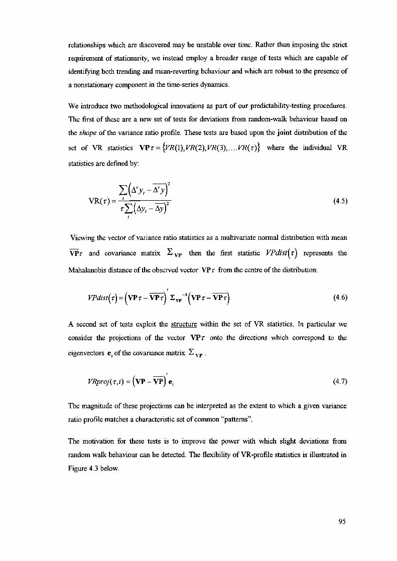
relationships which are discovered may be unstable over time. Rather than imposing the strict

requirement of stationanty, we instead empioy a broader range of tests which are capable of

identifying both trending and mean-reverting behaviour and which are robust to the presence of

a nonstationaly component in the time-series dynamics.

We introduce two methodological innovations as part of our predictability-testing procedures.

The first of these are a new set of tests for deviations from random-walk behaviour based on

the shape of the variance ratio profile. These tests are based upon the joint distribution of the

set of yR statistics VPr = {vR(1),vR(2),vR(3).....VR(r)} where the individual VR

statistics are defined by:

(ry _)2

vR( r)-- ? (Aye - (4.5)

Viewing the vector of variance ratio statistics as a multivariate normal distribution with mean

\TPr and covanance matrix vi' then the first statistic VPdist(r) represents the

Mahalanobis distance of the observed vector VPr from the centre of the distribution:

VPdist(r) = (VIPZ. - i) -'(vr - (4.6)

A second set of tests exploit the structure within the set of VR statistics. hi particular we

consider the projections of the vector VPr onto the directions which correspond to the

eigenvectors e. of the covanance matrix

VRproj('r,i) = (v - 'vr) e. (4.7)

The magnitude of these projections can be interpreted as the extent to which a given variance

ratio profile matches a characteristic set of common "patterns".

The motivation for these tests is to improve the power with which slight deviations from

random walk behaviour can be detected. The flexibility of VR-profile statistics is illustrated in

Figure 4.3 below.

95

0

VR(t)

ACF tests(churl-k, indrnwnks)

• trending

ineiui-rere,ting

VR.profile(t1e'iati mix iIosL%(uhinhsarI

behaviour)r(lIidolfl-1I'aIk Unit-root tests

slaliunury(long tern,

nIewv-revg.'r.cwn/

Random-walkprofile

Error-correctionprofile

Period ('r)

Figure 4.3: An illustration of the flexilbility of variance ratio profile statistics. Whilst tests based on the

autocorrelation function (ACF) are mainly designed to identify short-tenn dynamics and unit-root tests

are designed to distinguish between two specific types of long-tenn dynamics, tests based on the entire

variance ratio profile are sensitive to general deviations from random-walk behaviour, whether short-term

or long-term effects.

Tests based on the autocorrelation function (ACF) are most appropriate at detecting short-term

effects such as such as momentum or short-tenn correction effects. In contrast, unit-root tests

and standard variance ratio tests are most appropriate for observing long term effects, such as

distinguishing between stationary and nonstationaiy behaviour. Tests based on the overall

shape of the variance ratio profile are capable of recognising specific combinations of short-

term and long-term dynamics which are particularly amenable to statistical arbitrage.

The second innovation in our methodology for predictability testing is the application of both

the standard tests and the new tests in the context of multi-variate modelling. Except in the case

of unit root tests, which are used in cointegration modelling, the other tests are generally used

in a univariate setting rather than being applied to the results of a prelimmaiy multivariate

transformation. In order to apply the tests in a multi-variate setting it is necessary to correct for

the biases which are induced by the construction procedure which is used to create the

statistical mispricing time-series' 0. We achieve this by deriving appropriate empirical

'°For instance, the use of regression will induce a certain amount of spurious mean-reversion in the residuals

which may incorrectly lead to the rejection of random walk behaviour even when no true predictable component

is present (see Section 6.3).

96

distributions of the test statistics by the use of Monte-Carlo simulations. As well as correcting

for the biases induced by the algorithm itself, this approach has the additional advantage of

automatically taking sample size effects into account, rather than relying on asymptotic

behaviour.

Implicit Statistical Arbitrage Strategies

In cases where the mispncing dynamics contain a substantial mean-reverting component, we

have devised a set of "implicit statistical arbitrage" (ISA) trading strategies which are designed

to exploit the mean-reversion effect without the need for an explicit forecasting model.

The underlying assumption of the ISA strategies is that future price changes will be such as

will tend (on average) to reduce the mispncing between the target asset and the combination of

constituent assets. Thus over a period of time strategies based on selling the overpriced

(combination of) asset(s) and buying the underpnced (set of) asset(s) should realise positive

profits.

The ISA strategies operate by viewing the statistical mispncing M as a single portfolio

consisting of the assets ,c1 , .. . , c } with weightings {i,_fl1 ,—J32 '.f3nC }

respectively, where n is the number of constituent assets. Thus buying the target asset T and

selling the synthetic asset SA( T) = /3 C, is thought of as the single action of buying the

mispricing M. Similarly selling the target asset and buying the synthetic asset is thought of as

selling the mispricing M.

The ISA strategies are implemented by means of parametnsed trading rules which define a

desired holding in the mispricing portfolio as a function of the current level of the mispricing:

posn(M,k,h) = - j1..h

h (4.8)

Note the minus sign which indicates that the position taken should be opposite in sign to the

current mispricing. The parameter h can be thought of a as "holding period" which is used to

smooth the output of the trading rule and reduce the number of transactions which are

generated. The parameter k defines the sensitivity of the trading rule to the actual magnitude of

the mispncing as opposed to simply the sign of the mispncing, as shown in Figure 4.4 below:

97

C0

ii00.

k=O

k=O.33

• k1

4 ................................................................3

2

0

1 101 201 301 1

-1 -0.8 -0.6 -0.4 -0.2 0 0.2 0.4 0.6 0.

Mispricing M

Figure 4.4: The relationship between the level of the statistical mispncing M and the output of the

implicit statistical arbitrage trading rule posn(M, k, 1) for different values of the sensitivity parameter k.

The ability of ISA strategies to exploit mean-reverting behaviour is illustrated in Figure 4.5

which shows the results of applying the strategy to a synthetic time-series with a moderate

degree of mean-reversion:

4 .......................................! ............................. I

1 101 1 301 401 501k__________________

Figure 4.5: Results of applying the ISA strategy to an artifical time-series which exhibits moderate mean-

reversion. The left hand chart shows the time-series itself. The centre chart shows the output of the ISA

rule (with different levels of k). The right hand chart shows the accumulated profit and loss, or "equity

curves" for the three cases.

4.3 Part II: Forecasting the Mispricing Dynamics using Neural

Networks

The objective of the second part of our methodology is to support the building of predictive

models of the mispricing dynamics. The methodology aims to maximise the extent to which the

deterministic, and hence potentially predictable, component of the mispricing dynamics can be

actually captured in forecasting models and then exploited as the basis of practical statistical

arbitrage trading strategies.

98

Model-free Variable Selection

A key factor in the success of the modelling process is the accuracy of the infonnation set upon

which the model is conditioned. This fact is highlighted in the breakdown of model error in

Section 2.2.4, where the "missing variables" term is shown to be one of the three components

which inflate the model error over and above the inherent stochastic component of the data.

Thus the first aspect of our procedure for building forecasting models is a methodology for

"model-free" variable selection. The term mode/free reflects the intention that the methodology

should be sensitive to a wide range of relationships, rather than being predicated upon the

assumption of a particular functional form. The variable selection methodology is intended for

use in situations where the small size of the available data sample, together with the large

stochastic component in the data, precludes the inclusion of all of the variables in the model

building procedure proper. The flexibility of the variable selection procedure is vital in order to

avoid imposing a hidden bias on the subsequent stages of modelling.

In order to achieve this flexibility, our variable selection methodology is based upon techniques

from nonparametric statistics, and in particular nonparametric regression. The approach

which we take is to regress the dependent variable upon nonlinear projections of the original

variables to produce submodels of the form:

y = a + (4.9)

Where the basis functions b, () are chosen in such a way that in combination they can

approximate a wide range of functional relationships. Under the null hypothesis that

independent variable is unrelated to y, it is known that the F-ratio of the model should

follow an F-distribution with p degrees of freedom in the numerator and n-(p+1) in the

denominator, i.e.:

2

1( ^ l) Y[a^ O1b,(x)

Fp,n(p+l) (4.10)

99

The tests can also be used to test for interaction effects between variables; to do so the basis

functions act as a nonlinear projection of the subset of the original variables which is being

tested. In the two dimensional case the submodels are of the form:

y =a + 9,b I (xf ,xk ) +

(4.11)

The variable selection algorithm consists of "screening" all the low-dimensional combinations

of the candidate variables by constructing and testing appropriate submodels. Flexibility is

achieved in the first place by using basis fimctions which are known to be capable of closely

reproducing a wide range of relationships, and secondly by using a range of different basis

functions. Suitable basis functions include polynomials in xj , "bin smoothers" and "radial

basis functions" as well as the linear (identity) case and the more-flexible models offered by

neural estimation methods. An example of a "bin-smoother" applied to nonlinear relationship is

shown in Figure 4.6 below.

t5• ••• •.

• A

• S. S...S• •.: • • .S

. . S z.• •• I4 ':. I

-1.5 , -1. .t .5 0. • * 1 • 1.5

-0.5 .-

• • •• •.

-1 . .••

________________________ -1.5

Figure 4.6: An example of a non-linear relationship which may be identified by means of a bin smoother

(3 bins in the example) but which exhibits zero correlation and hence would be missed by a linear test.

The basis functions used in the bin-smoother consist of indicator values which take the value 1

if an observation is in a particular region of input space, or "bin", and 0 otherwise. If the mean

value of the dependent variable y varies substantially from one bin to another, the associated F-

test will indicate the presence of a statistically significant relationship which may be missed by

a linear test.

Estimation of Low-bias Forecasting Models

Having performed any necessary variable selection, the next task is to approximate the

deterministic component of the mispricing dynamics in the form of a predictive model. The

estimation procedure should optimise the complexity trade-off between bias and variance,

100

whilst at the same time incorporating underlying modelling assumptions which ensure that the

complexity is allocated in an appropriate manner. The methodology which we have developed

avoids the problem of excessive bias by using flexible neural network models and avoids

excessive estimation variance by using statistical significance testing to control the

specification of the neural network models.

As discussed above, perhaps the most important modelling assumptions relate to the choice of

variables to include within the model. If the model is lacking important explanatory variables

then it cannot capture the associated deterministic component of the mispricing dynamics,

irrespective of the flexibility of the functional form of the model. Likewise the incorporation of

irrelevant "noise variables" can only ever decrease model performance, irrespective of the

methodology which is used to control model variance (see Section 10.1). For these reasons

variable selection, in the sense of the allocation of model complexity to each of the explanatory

variables, is treated as an integral part of our neural model estimation procedures.

Existing algorithms for automatic neural network specification can be considered as belonging

to four main classes, namely: (i) early-stopping of learning through the use of (cross-)

validation, (ii) regularisation approaches; (iii) constructive algorithms and (iv) deconstructive

or "pruning" algorithms. For our purposes the first of these can be eliminated in that

tennination of learning when the network is not even in a local optimum invalidates the use of

hessian-based statistical diagnostics such as the degrees of freedom absorbed by the model (the

first order conditions used to derive the degrees of freedom measure no longer hold). Our

methodology encompasses, to some extent, each of the other three classes of algorithm. It

differs from existing methods in three main ways.

• our methodology is statistical in nature and provides diagnostics which avoid the need to

lay aside large fractions of the dataset for use in determining hyperparameters such as

training time, regularisation coefficients and number of hidden units.

our methodology views the modelling process from a data-centred rather than a

parameter-centred viewpoint. Rather than viewing the neural network in terms of the

individual weights which it contains, we adopt a nonparametnc perspective based upon the

"equivalent kernels" which describe the sensitivity of the estimated model to each

observation in the learning set. The estimated model as a whole is considered from the

perspective of the degrees of freedom which it absorbs and the amount of variance which

they explain.

101

our methodology treats the allocation of model complexity as being of equal importance as

the optimisation of the level of complexity; thus variable selection and architecture

selection are considered as inter-related aspects of the overall model specification.

Within this general perspective our methodology supports three alternative model estimation

algorithms. The three algorithms share a basic testing methodology in which the statistical

significance of model components is calculated by comparing the degrees of freedom which

they absorb with the additional explanatory power which they provide. The basic selection

criterion which we use might be tenned a "change of model" F-test" and is of the form:

(Ya)2(YbV S/Mf (4.12)= pss / n - df'

The first algorithm might be considered as a "benchmark" as it is simply based on the concept

of controlling the degrees of freedom within a model by varying the degree of regularisation

which is used during the estimation procedure. The "pseudo-constructive" form of the

algorithm starts with a heavy regula.risation term, and successively relaxes the regularisation

whilst the additional degrees of freedom thus created are deemed to be statistically significant.

The "pseudo-deconstructive" form of the algorithm starts with a low degree of regula.risation

which is successively increased whilst the degrees of freedom thus removed from the model are

shown to be insign/1cant.

The second algorithm is based upon a "constructive" approach which starts with a null model

which is successively enhanced by the addition of components to the model. The additional

components are selected on the basis of partial F-tests for significant low-dimensional

relationships in the residual errors of the current model. The tests for residual structure are

based upon the nonparametnc tests provided by the model-free variable selection methodology.

The algorithm combines the tasks of variable and architecture selection in that the additional

complexity which is added to the model is conditioned only upon the particular input subspace

(set of independent variables) within which residual structure has been identified.

sometimes referred to as a "partial" F-test in that only a part of the entire model is being tested for statistical

significance

102

The third algorithm within our (partial-)F testing methodology is based upon a

"deconstructive" approach. The algorithm starts with an overparametrised architecture which

is successively refined by iteratively removing variables which are found to provide statistically

insignificant contributions to the overall model. This approach can be seen as complementary

to the constructive approach in that the two algorithms approach the bias-variance tradeoff

from opposite directions. As with the constructive algorithm, the deconstructive algorithm also

provides an integrated approach to the two tasks of complexity control and variable selection.

Conditional Statistical Arbitrage Strategies

Our conditional statistical arbitrage strategies are a mechanism for exploiting the predictive

information which is contained in forecasting models of asset price dynamics. Rather than

being concerned with changes in individual asset prices, as would be the case in a standard

ECM (see Section 2.2.3), our models are concerned with changes in the prices of the

combinations of assets which define statistical mispricings. The general form of our

"mispricing correction models" or MCMs is:

- flI CI = = + s1 (4.13)C, EC

where M is the deviation from the statistical fair price relationship, or "statistical

mispricing", AAf represents a set of lagged changes in the mispricing, and Z,, represents a

selected set of exogenous variables which either directly influence the mispricing dynamics or

serve to modulate the mispncing-correction effect.

The "conditional statistical arbitrage" (CSA) trading rules which are designed to exploit the

predictions of the MCMs take a similar form to the implicit statistical arbitrage (ISA) rules

from Part I of the methodology. As in the case of the implicit rules, the CSA rules define the

position which should be taken in terms of the portfolio which corresponds to the statistical

mispricing M, namely a portfolio with assets , , C2 , ..., } and relative weightings

,-fi2 '-/ }. The difference in this case is that the position to be taken is defined as a

function of the MCM forecast E[LVvt], rather than of the level of mispricing M:

103

_[Jk

posn(E[&VI,],k,h)= f=L.h

h(4.14)

As in the case of the ISA rules, h and k represent smoothing and sensitivity parameters

respectively. The relationship is a positive one because the implicitly negative relationship

between the level of the mispncing and expected future changes in the mispncing is now

absorbed in the forecasting model.

We can define a taxonomy of statistical arbitrage strategies based upon different functional

forms of mispricing correction model and thus the types of behaviour that they are designed to

accommodate. Such a taxonomy is presented in Table 4.1 below:

Strategy Mispricing Correction Model Properties

(implicit or explicit)

riskless E[Mf1] = —M

implicit E[M4'1] —M

adaptive E[M4',] L - M

time-series E1IM'1] = a + - M)+fl,M'I1

imposition offair priceat expiry

strong reversion

time-variation inreversion level

momentum plus otherdynamics

conditional E[M4'] = f(L, - M, , ivw, , , z) threshold effects,- exogenous variables

Table 4.1: A taxonomy of statistical arbitrage strategies, based upon the assumed form of the mispricmg

correction model (MCM). The MCM may be implicit, as in the first three rows, or explicit, as in the

time-series and conditional models.

The taxonomy highlights the conceptual progression from riskiess strategies to implicit

statistical arbitrage strategies and then to conditional statistical arbitrage strategies. Riskless

strategies are based upon the expectation that the mispncing will be eliminated totally, at the

expiration date if not sooner. Implicit statistical arbitrage strategies exploit mean-reversion

tendencies in the mispricing dynamics, be they with respect to a fixed or time-varying reversion

level. Conditional statistical arbitrage strategies involve the construction of an explicit model to

exploit more general regularities in the mispricing dynamics.

104

The advantage of employing conditional statistical arbitrage strategies based upon flexible

forecasting models is that other detenninistic components of the dynamics can be accounted

for, in addition to the basic tendency of mean-reversion. By capturing these additional

components in the forecasting model it may be possible both to decrease risk and increase

profitability. A decrease in risk may occur because otherwise unfavourable effects, such as a

short-term momentum acting to temporarily increase the mispricing, can be accounted for in

the model forecasts. An increase in profits may occur because the overall accuracy of the

forecasting model will improve due to capturing a larger part of the deterministic component in

the underlying dynamics.

The advantage of employing conditional statistical arbitrage strategies in cases where the

mispricing dynamics are other than straightforwardly mean-reverting is illustrated in Figure

4.7. The figure compares the performance of a number of alternative statistical arbitrage

strategies applied to an artificial time-series with the data-generating process:

iW, =aiW,... - (p+rz,)M, +

(4.15)

The parameters a, fi and y were chosen such that the linear mean-reversion component,

- ,ÔM,, accounted for approximately 1% of the total variance of the time-series, the

momentum term, a further 1% and a modulated term, - j'Z, M,, a further 2% of

the total variance, in the form of an interaction effect with a (randomly generated) exogenous

variable Z,.

Figure 4.7: Comparison of the performance of different statistical arbitrage strategies when applied to an

artificial time-series with the data-generating process in Eqn. (4.15). The left hand chart shows the time-

series itself. The right hand side shows the cumulative profit and loss curves for three alternative models:

an implicit model, a linear time-series model, and a full conditional modeL

105

The figure clearly shows the perfonnance improvement which is attained by the models which

more-accurately capture the deterministic component of the time-series dynamics. The implicit

model only captures the mean-reversion effect which accounts for 1% of the total variability in

the time-series. Whilst generally profitable, the implicit strategy suffers from severe

drawdowns during the periods where the time-series exhibits short term trends away from the

equilibrium (for example around periods 300, 400 and 450). The linear time-series model

captures both the linear component of the mean-reversion together with the short-term

momentum effect, accounting in total for 2% of the total variability. The improved accuracy of

the time-series model leads to higher profits and less severe drawdowns than are achieved by

the implicit model. Finally, the conditional model also captures the modulation of the mean-

reversion effect with respect to the exogenous variable, accounting for 4% of the variability in

all and achieving substantially higher profits and lower drawdowns than either of the more

limited models.

4.4 Part Ill: Diversifying Risk by Combining a Portfolio of Models

The objective of the third part of our methodology is to support the diversification of model

risk. The methodology aims to reduce the risks which are inherent in the modelling process

itself, thus increasing the likelihood of achieving successful statistical arbitrage strategies.

Combination in a portfolio of models

Irrespective of the statistical rigour of the modelling process, the future performance of

forecasting models in general, or statistical arbitrage models in particular, will necessarily be

uncertain. The fact that model selection criteria are evaluated with respect to a particular finite

sample will cause sampling error. This in turn means that the model which is apparently

optimal, according to the model selection criteria, will not necessarily be optimal in future.

Furthermore this risk is much increased when the noise content of the data is high and/or the

performance may be unstable over time due to the presence of nonstationarities in the

underlying data-generating process.

The effect of using small and/or noisy samples is that the sampling error on any insample

performance estimate will necessarily be large. Similarly, the effect of any time-variation in the

underlying data-generating process will be to increase the variability of future performance,

given a particular level of insample performance. This serves to increase the model selection

106

risk, and reduce the probability that the optimal insample model will also perform optimally

during an out-of-sample period. The model selection risks which arise from the use of finite,

noisy and possibly nonstationaiy datasets are illustrated in Figure 4.8 below:

Performance

'I

Key

- Meaaured performance

Poulble figure performanceallowing for variance

- - - Pouible future performanceallowing for variance andnonatationarity

Model : Pousible location of modelwith beat fuure performance

Figure 4.8: Distribution of the possible future perfonnance of a set of models, allowing for both sampling

error in the performance statistic and the possible effects of nonstationarity.

Note that, whilst the effects of variance are equally likely to be positive as negative, time-

variation or "nonstationarity" is more likely to lead to performance degradation than to an

improvement.

Additional complications to the model selection procedure are caused by "criterion risk" and

"selection bias". Criterion risk arises in the case where the metric which is used for model

selection is not the same as the metric by which future performance will be evaluated. Selection

bias, or "data-snooping", arises because the measured performance of a selected model will be

positively biased with respect to the true expectation of future perfonnance, due to the fact

that:

max(1u) + E[J^ E[max(p +

ej]^ max() + max()

(4.16)

where ç is the Ini insample performance of model i and c, represents the sampling error of

the performance measure. The selection bias is caused by the discrepancy between the first

expression, which represents the true expectation of future performance, and the second

expression, which is the measured insample performance (after correcting for any other biases).

The third expression indicates that the maximum selection bias is detennined by the sample

variability of the performance metric.

The problems posed by model selection risk are not addressed by standard modelling

procedures. The model combination techniques discussed in Section 2.2.5 are intended not to

107

reduce model risk as such but rather to improve model performance, in the sense of

minimising forecasting error. In finance however, there is an explicit requirement to take into

account not only performance (or expected return) but also risk (or uncertainty in the level of

return), with the ultimate measure of utility being some form of "risk-adjusted return".

The methodology which we propose to deal with this issue is an adaptation of the model

combination approach in the context of modem portfolio theory (Markowitz, 1952). The core

inspiration of Markowitz portfolio theory is that a suitable combination (portfolio) of assets

may achieve a higlier level of risk-adjusted return than any individual asset, due to the ability to

diversify risk through a combination of less than perfectly correlated assets. The basis of our

model combination methodology is to adapt the Markowitz framework by substituting the

profits and losses of statistical arbitrage models in place of the returns on individual assets, i.e.

to create a "portfolio of models".

Given a set of models m = {m1 (01), m2 (02),..., m,,,,, (0,,)), (uncertain) performance estimates

=[E[r1 ] E[r2] E[r2]]Tand covariance matrix VM = E{[ei 2 1T[

2

Then the portfolio of models is given by:

= wMImI (4.17)

and the optimal vector of weights is that which maximises risk-adjusted performance:

*WM = arg m {wMTrM -

2TM WMVMWM}

w(4.18)

As in the case of standard portfolio optimisation, the risk-tolerance parameter TM embodies

the desired trade-off between increased expected perfonnance and decreased levels of risk.

Joint optimisation of components within models, and models within a population

The final component of our methodology is designed to address two important issues which in

fact are facets of the same underlying problem. The first issue is the so-called "forecasting

bottleneck" which arises when the performance of a trading rule is conditioned upon the output

of a forecasting model. The second issue is that of successful diversification of model risk

within the context of the "portfolio of models" approach.

108

The underly ing issue in both cases is the potential inefficiency which is caused by the use of

indirect optimisation, by which we mean optimising a model, or a model component, with

respect to criteiia which are different to those by which the ultimate performance of a model

will be judged. This risk is illustrated in Figure 4.9 below.

0.a

---------4

l..oss due It) UC ol0 rnu1ti-stag apprsueh 4 .

•in

to...

1:: : •• N'Iidel ihL.en

0 - • ai.i.tirdin to0 Stage I criteria

• 4.a.

0 -

0 0.2 0.4 0.6 0.8

Performance according to Stage I Criteria

Figure 4.9: illustration of the potential inefficiency which arises through the use of different criteria at

different stages of the modelling process, or when the criteria used during model construction are

different to those by which actual performance is measured.

In the figure, the model selected according to the criteria of Stage 1 is significantly less than

optimal at Stage 2 even though the criteria at each stage are 90% correlated, clearly

highlighting the potential inefficiency of indirect optimisation. In this thesis we refer to this

potential inefficiency, and source of additional uncertainty, as "criterion risk".

The criterion risk which arises in the context of the "forecasting bottleneck" is that the

forecasting model which is optimal with respect to the statistical criteria used during the

modelling procedure will not necessarily lead to the optimal performance when used in

conjunction with a trading strategy which is optimised independently. In particular a model

which has the most accurate forecasts may not lead to the optimal trading performance if the

volatility of the forecasts leads to large numbers of transactions being performed and the

profitability being eroded by transaction costs.

In the case of diversifring model risk using a portfolio of models approach, the criterion risk is

that models which appear attractive in terms of their individual risk-adjusted performance may

not necessarily add value to an existing portfolio of models. In particular, models which are

highly correlated with other models will offer little opportunity for risk-diversification. This is a

109

-0.59

-0

common problem because the use of model selection criteria which view models on an

individual basis will tend to select models which have advantageous, yet similar,

characteristics. In the context of genetic algorithms and similar population-based algorithms

this phenomenon is sometimes referred to as "premature convergence".

The final part of our methodology is a population-based algorithm which is intended to

mitigate the potential inefficiencies which are discussed above. The key elements of the

specification of each of the three components of a statistical arbitrage model (mispricing model,

forecasting model and trading rule) are grouped together as a set of "meta-parameters". The

"fitness" of the set of meta-parameters is evaluated in terms of the actual trading performance

of the overall model, thus serving to avoid the criterion risk which would arise from separate

optimisation of the different model components. This process can be seen as avoiding the

forecasting bottleneck by allowing feedback from the trading perfonnance to be passed back to

the other model components, thus closing the modelling "loop" (see Figure 4.1) and allowing

joint optimisation of all model components with respect to a single set of criteria.

Criterion risk due to the evaluation of models on an individual basis is controlled by means of

"conditional fitness" measures which evaluate models in the context of the broader set of

models. The conditional fitness is defined as the marginal utility of the model, i.e. the

improvement in the performance of the population as a whole which is caused by adding the

model to an existing portfolio of models. An example of a conditional fitness measure is

presented in Figure 4.10.

0.59

0.31

0.00

-0.31

Fitness Improvement1.00

0.951 00% .0.950.81 . 0.81

90% : 0.59

40% .. o.i20%

0.00

-0.31

-0.59

).81

Figure 4.10: illustration of the added value that a new model provides to an existing portfolio, according

to a standard measure of risk-adjusted return. The correlation between the returns of the model and those

of a pre-existing portfolio is displayed as a function of the angle (pcos(0)) with correlation of 1 at zero

degrees from vertical, 0 correlation at +1- 90° and -1 correlation at 180°. The expected risk and return of

the new model are equal to those of the existing portfolio

110

The figure clearly shows demonstrates that, irrespective of the fact that the expected return and

risk of the new model are identical to those of the existing portfolio, the added-value which the

new model represents is heavily dependent on the extent to which it is decorrelated with the

existing portfolio. This demonstrates how, in the context of trading a portfolio of statistical

arbitrage models, the conditional fitness approach employed in our population-based algorithm

explicitly accounts for the correlations between models and thus actively encourages the

creation of a diversified set of models.

4.5 Summary

In this chapter we have outlined our modelling framework and summarised the three main

components of our methodology. The following three parts of the thesis present the details of

the methodology, together with evaluations of the modelling procedures with respect to both

artificial simulations and real-world problems.

111

Part I: A Cointegration Framework for Statistical Arbitrage

In this part of the thesis we describe the first of the three parts of our methodology for

statistical arbitrage modelling. This consists of a framework for constructing combinations of

time-series which contain a potentially predictable component. An overview of the methodology

described in this part of the thesis is presented in Section 4.2.

Chapter 5 describes a framework for modelling combined asset prices, which is inspired by the

econometric concept of cointegration. The cointegration framework is used to generate

potential statistical mispricings, by performing stochastic detrending of asset prices with

respect to other, related, asset prices. The objective of this pre-processing is to generate

combinations of time-series which are largely immunised against market-wide uncertainties and

which enhance the potentially predictable components of asset price dynamics. The basic

methodology is extended to time-varying relationships and also to high-dimensional problems

where the number of assets is numbered in the tens or hundreds.

Chapter 6 describes a range of tests which are designed to identif r potential predictability in the

mispricing time-series. The tests include standard autocorrelation tests, cointegration tests for

stationanty, and variance ratio tests for deviations from random walk behaviour as well as

novel tests based upon the shape of the variance ratio profile as a whole. The strengths and

weaknesses of the various tests are examined under controlled circumstances using Monte-

Carlo simulations. Modifications of the predictability tests are presented which correct for the

bias induced by the construction procedure. The final section of the chapter contains the results

of applying the tests to combinations of FTSE 100 equity prices.

Chapter 7 describes a set of "implicit statistical arbitrage" (ISA) trading strategies which are

designed to directly exploit any mean-reverting component in the mispricing dynamics,

bypassing the intermediate stage of constructing an explicit forecasting model. The underlying

assumption of the ISA strategies is that future price changes will be such as will tend (on

average) to reduce the mispricing between a given "target" asset and the associated "synthetic

asset". The ISA rules are used to perform an empirical evaluation of the statistical mispricing

methodology. The high-dimensional version of the niispricing construction methodology is

evaluated with respect to models of the daily closing prices of FTSE 100 stocks; the adaptive

version of the methodology is evaluated on the French CAC 40 and German DAX 30 stock

market indices.

112

5. Methodology for Constructing Statistical Mispricings

This chapter describes the methodology which we use to construct combinations of asset prices

which represent statistical mispncmgs. Section 5.1 describes the basic cointegration framework

which is used to generate the mispricing time-series. The methodology operates by performing

stochastic detrending of related asset prices in order to partially immunise against market-wide

sources of uncertainty, or "risk factors", thus enhancing the potentially predictable asset

specific components of the dynamics. The following two sections present extensions of the

basic methodology. In Section 5.2, an adaptive filtering methodology is presented which is used

to remove nonstationaly components from mispncing time-series in order to qualify them for

use as the basis of statistical arbitrage models. Section 5.3 describes a stepwise approach

which extends the basic methodology to the case of high-dimensional problems where the

number of assets is numbered in tens or hundreds, as is typically the case in modelling the

constituents of indices such as the CAC, DAX, FTSE and Dow Jones.

5.1 Description of Cointegration Methodology

In this section we describe the basic cointegration framework which we use to generate

combinations of time-series which represent statistical mispricings. Whilst the econometric

methods used in cointegration modelling form the base upon which our methodology has been

developed, we apply and further develop these tools according to a rather different perspective

than the traditional one.

Cointegration testing (see Section 2.2.2) in particular is often seen as an end in itself, with the

objective of testing an economic hypothesis regarding the presence or absence of an equilibrium

relationship between a set of economic variables. This stage may or may not be followed by the

construction of an Error-Correction Model (ECM, see Section 2.2.3) in order to establish the

dynamics of the mechanism by which short-term deviations are corrected towards the long-term

equilibrium.

In our methodology the use of tools from comtegration modelling is seen as a "means to an

end", with the "end" being the creation of successful statistical arbitrage trading strategies.

From this perspective the cointegration framework is a useful starting point, but one in which

the underlying modelling assumptions and restrictions are overly strict. Whilst the object of

cointegration testing is to identify combinations of time-series which are stationary, our

statistical arbitrage modelling is concerned with the more general case of combinations of time-

113

series which simply contain a predictable component. This generalisation of the cointegration

framework is both necessaiy and useful because the requirement for strict stationarity is over-

restrictive and would cause many potential opportunities for statistical arbitrage to be

overlooked.

Our use of cointegration methods to construct statistical mispncings can be thought of as a

principled extension of the relative value strategies, such as "pairs trading", which are used by

some market practitioners. Before describing the details of our mispncing construction

methodology we first provide a more formal motivation for the use of a relative value approach

to modelling asset price dynamics.

Relative Value Modelling

In order to motivate the use of modelling techniques in which prices are viewed in relative (or

combined) rather than absolute (or individual) terms, we refer back to Section 2.2.1 and note

that any random variable y can be considered as being the result of a data-generating process

which is partially deterministic and partially stochastic:

= g(z) +

(5.1)

where g(z,) is the deterministic component of the time-series and (v) is the stochastic

component. Considering that the purpose of modelling the data-generating process is to

construct an estimator 5) = f(x) we note that the maximum possible predictive ability

(according to the R2 metric of proportion of variance explained) is limited by the proportion of

the variance of Yt which is due to the deterministic component:

21E[(g(z,)_/i,) j

R2CV,,f(;))^ E[(g(z,)_,)2]+E[s(v,)2]

In many forecasting applications, this issue is overlooked, largely because the target series is

often predetermined. However in an application such as statistical arbitrage there are many

possible combinations of assets which could be used as target series, and thus the construction

of time series with significant deterministic components is a key component of our

methodology.

(5.2)

114

The primary motivation for adopting a "combined price" approach is based upon the

recognition that much of the "noise" or stochastic component in asset returns is common to

many assets. This viewpoint forms the basis of traditional asset pricing models such as CAPM

(Capital Asset Pricing Model) and the APT (Arbitrage Pricing Theory). Essentially these

pricing models take the form:

Ay, = a, +fl,AMkt, +s, (5.3)

This general formulation, which is discussed in Section 3.1, relates changes in asset prices

'y to sources of systematic risk (changes in the market, Mfkt,, and in other economic "risk

factors", Af, ) together with an idiosyncratic asset specific component e,.

If markets are more efficient at discounting major sources of economic uncertainty than asset

specific risks, then the proportion of the variance of market-wide risk factors which is due to a

deterministic and hence potentially predictable component (dF) will be lower than the

deterministic component in idiosyncratic effects (d1). The overall level of potential

predictability of a time-series will lie somewhere between the two values depending upon the

extent to which the dynamics are influenced by the two types of effect:

R 2 (Ayj( , f )^wFdF +(1-wF )dI (5.4)

where .9 represents the forecasting model, R2 the proportion of variance correctly forecasted

by the model, and WF the proportion of the dynamics which are caused by market-wide risk

factors. For instance, if dF = 1% and d1 = 5%, an asset with market-wide exposure of

WF = 0.75 would have a potentially predictable component equivalent to

0.75 x 1% + 0.25 x 5% = 2% of its total variance. In contrast, a price series with lower exposure

to market-wide factors, say WF = 0.25, might contain a potentially predictable component

equivalent to 0.25 x 1% + 0.75 x 5% = 4% or a 100% increase on the first case.

This distinction between the dynamics which are due to market-wide risk factors and the asset

specific component of price dynamics provides a strong motivation for believing that the

returns of appropriate combinations of asset prices may be potentially more predictable than

the raw (individual) returns. Consider a portfolio consisting of a long (bought) position in an

asset y1 and a short (sold) position in an asset y 2 . If the asset price dynamics in each case

115

follow a data-generating process of the form shown in Eqn. (5.3) then the combined returns

Lyit - Ay2 are given by:

4y1,, —Ay2 , =(a1 —a2)

+(fi )g,ji + (i. ' -fi2.1)4f1.,+_+(fi1. fi2,)4f.,

(5.5)

- 62.1)

If the factor exposures are similar, i.e. fl,,, then the proportion of variance which is

caused by market-wide thctors will be correspondingly reduced and the potential predictability

correspondingly increased. This effect is illustrated in Figure 5.1 below.

100%

90%

80% DSSv'70% •Asset y

60%

50%

40S'

30"

20

10or

.,er M. seI - .ariarrce inar,etfactors variance

Figure 5.1: illustration of advantages of modelling within a combined price framework: whilst the

individual assets Yl and Y2 are primarily influenced by changes in market-wide risk factors, the price-

changes of the "synthetic asset" Y1-Y2 are largely ünmunised from such effects and magnify the effect of

stock-specific factors which are more likely to contain systematic (and hence potentially predictable)

components.

Thus the motivation for a relative value approach is that asset prices viewed in relative (i.e.

combined) rather than absolute (i.e. individual) tenns are both more amenable to statistical

arbitrage and potentially more predictable. The analysis above demonstrates that, in principle,

appropriately constructed combinations of prices can be largely immunised against market-

wide sources of risk and will instead highlight the asset specific aspects of the price dynamics.

Such combinations of assets are amenable to statistical arbitrage because they represent

opportunities to exploit predictable components in asset specific price dynamics in a manner

which is (statistically) independent of changes in the level of the market as a whole, or other

market-wide sources of uncertainty. Furthermore, as the asset-specific component of the

dynamics is not directly observable by market participants it is plausible that regularities in the

dynamics may exist from this perspective which have not yet been "arbitraged away" by

market participants.

116

This analysis helps to explain the popularity of relative value strategies amongst hedge funds,

proprietary trading desks and other "risk arbitrageurs". In its simplest form this approach is

called "pairs trading" and consists of trend and reversion analysis of a graph of relative prices,

with the assets X and Y being selected either on the basis of intuition, economic fundamentals,

long term correlations or simply past experience. Opportunities for pairs trading in this simple

form, however, are reliant upon the existence of naturally similar pairs of assets and thus are

very limited. We describe below the details of our methodology in which cointegration

techniques are used to create a wider range of opportunities, by constructing synthetic "pairs"

in the form of appropriate combinations of two or more assets.

Construction of Statistical Mispricings

In an analogy to the no-arbitrage relationships upon which riskless arbitrage strategies are

based, the objective of our methodology is to identify combinations of assets which represent

statistical "fair price" relationships upon which to base "statistical arbitrage" strategies.

More specifically, given an asset universe UA and a particular "target asset", T E UA, our

objective is to create a "synthetic asset" SA(T) such that the value of the synthetic asset can be

considered a statistical "fair price" for the target asset:

= SA(T)

(5.6)

Furthermore the fair price relationship in Eqn (5.6) should be such that deviations from the

relationship can be considered as "statistical mispricings":

M = 7 —SA(T)

(5.7)

where the dynamics of the mispricing time-series M contain a predictable component which

can be exploited as the basis of a statistical arbitrage trading strategy.

Our methodology for constructing statistical mispricings is based upon the use of cointegration

techniques to estimate the fair price relationships. A "cointegrating regression" (Granger,

1983) is used to estimate a linear combination of assets which exhibits the maximum possible

long-term correlation with the target asset T. The coefficients of the linear combination are

estimated by regressing the historical price of T on the historical prices of a set of

"constituent" assets C c UA - T:

117

SA(T) = s.t. {} = argmin - flICUJCC t=ln C,eC

and the "comtegratmg vector" f3 = ' ]' of constituent weights is given by:

1OLS = (Cr C)' Ct (5.9)

where C is the n = C by n matrix of historical prices of the constituents and

t =•..

is the vector of histoncal prices of the target asset.

The synthetic asset can be considered an optimal statistical hedge, conditioned upon the set of

constituent assets C, in that the standard properties of the OLS procedure used in regression

ensure both that the synthetic asset will be an unbiased estimator for the target asset, i.e.

E[1] = SA(T), and also that the deviation between the two price series will be minimal in a

mean-squared-error sense.

We formally define a "synthetic asset model" as a triple: Sit = {T € UA ; C - {T};/3 E n}

where UA is the asset universe, T E UA is the "target asset", C c UA - { T} is the set of

"constituent assets" and /1 E id is the vector of constituent weights. Given such a model, we

can derive the time-series which represents the associated statistical mispricing:

= - (5.10)C,EC

The statistical mispricing M can be considered as a composite portfolio consisting of the

assets {i ,C, ,C2 ,..., c) with weightings {i,_fl, ,-, . . . ,-p,, } respectively. The price of

this portfolio represents the excess value of the target asset T, relative to the linear

combination of assets SA(T) 1 = /3, C,, and can be thought of as a "stochastically

detrended" version of the original asset price 7 (i.e. detrended with respect to observed time-

series which are generated by (at least partially) stochastic processes rather than with respect to

a deterministic function of time).

(5.8)

118

In this context the set of constituent assets C can be considered as acting as proxies for the

unobserved risk factors which act as common stochastic trends in market prices. In maximising

the correlation between the target asset and the synthetic asset the construction procedure

cannot (by definition) account for the "asset specific" components of price dynamics, but must

instead indirectly maximise the sensitivities to common sources of economic risk. In the context

of Eqn (5.5) the effect of the construction procedure is to artificially create a pair of assets (the

target asset 1 and the synthetic asset SA(T)) which have similar exposures to the underlying

(but not necessarily directly observable) risk factors which drive the asset price dynamics.

Example

We now illustrate the manner in which the cointegrating regression acts to "cancel out" the

exposure to underlying risk-factors and thus enhance the relative magnitude of the asset

specific component of the price dynamics. Consider a set of three assets, each following a two-

factor version of the data-generating process shown in Eqn (5.3). Price changes within the set

of three assets are driven by a total of five factors, two common risk factors fj and J and three

asset specific components , e, and 63 , Furthermore fi and f2 are assumed to follow random

walk processes whilst the dynamics of the asset specific factors contain a mean-reverting

component.

The factor exposures of the three assets X, Y and Z are assumed to be as shown in Table 5.1:

Asset fi f2 ci s2 c3

X 1 1

1

0

0

Y 1 0.5

0

1

0

Z 0.5 1

0

0

1

Table 5.1: Price sensitivity of three assets X, Y and Z to changes in common risk factors f, andJ and

asset specific effects ei, e, and e.

Thus the dynamics of the system are given by:

4t = 1 = 1,2 r N(0,1)

= —O.l6 + j 1,2,3 N(0,0.25)

= + 4f2 + L\6

= 4fj + °. 4f2t +

AZ = 0.54f + 412.t +

(5.11)

119

1.5

1

0.5

0

.0.5

-1

.15

-2

101 201 301 41

A realisation of the asset prices generated by the system is shown in Figure 5.2 below. Note the

broad similarity between the price movements of the three assets.

i2I31 41

Figure 5.2: Realisation of three simulated asset price series which are driven by two underlying common

factors in addition to asset-specific components.

In the case of the realisation shown in Figure 5.2, a cointegrating regression of X on Y and Z

gives the estimated fair price relationship:

X, = O.632Y + 0.703Z1 + M (5.12)

The estimated relationship differs slightly from the theoretically optimal

X = 2/3 J + 2/3 Z + M,, due to sampling error. The resulting statistical mispricing time-

series M1 is shown in Figure 5.3 below. Unlike the nonstationary asset prices X, Y and Z, the

mispricing can clearly be seen to be mean-reverting.

Figure 5.3: Mispricing time-series from the fair price relationship I, = 0.632Y, + 0.703Z, + M

where the time-series for X, Y and Z are as shown in Figure 5.2.

The mean-reverting nature of the mispricing time-series, compared to the close to random walk

behaviour of the original time-series X, Y and Z, is highlighted by the variance ratio profiles

shown in Figure 5.3. Whilst the variance ratio for all three original assets remains close to

unity in each case, the variance ratio of the mispricing falls substantially below one as the

120

period over which the differences are calculated increases. This indicates that the volatility

which is present in the short-term dynamics is not reflected in the long term volatility, thus

providing evidence for a substantial mean-reverting component in the dynamics of the linear

combination x1 - (o.632Y + O.7O3Z).

I111213i4i61fl91

Period

Figure 5.4: Variance ratio profiles for the three time-series X, Y and Z (depicted in Figure 5.2) and the

mispricing time-series Mis, = x, - (o.632Y, + 0.703Z,)

In attempting to replicate the "target" time-series X the cointegrating regression procedure

creates the "synthetic asset" 0.6321' + O.703Z which has similar exposures to the common

factorsf, and 12. Thus in the mispricing time-series x, - (o.632iç + 0.703Z,) the net exposure

to the common factors is close to zero, allowing the mean-reverting asset specific effects 61, 62,

and 63 to dominate the mispricing dynamics. This "statistical hedging" of the common risk

fictors is quantified in Table 5.2, below, which reports the proportion of the variance of each

time-series which is associated with each of the sources of uncertainty:

X V Z Mis

Ii 46.1% 64.2% 16.8% 0.2%

12 41.5% 10.1% 67.8% 0.0%

11.5% 0.2% 0.0% 54.5%

0.5% 25.1% 0.1% 23.7%

63 0.4% 0.4% 15.3% 21.6%

Total 100.0% 100.0% 100.0% 100.0%

Table 5.2: Sensitivity of price changes of the original time-series X, Y and Z and the "mispricing" time-

series x, - (o.632 + o.7o3z,). The table entries show the proportion of the variance of each time-

series which is associated with changes in common risk factorsf, and 12 and asset specific effects Si. S2,

and e.

121

This demonstrates the fact that the use of cointegrating regression can immunise against

common stochastic trends which are not observed directly but instead proxied by the observed

asset prices. Whilst the variance of changes in the original time-series X, Y and Z is primarily

(70-90%) associated with the common risk factors f' and f, the effect of these factors on the

"mispricing" is minimal (0.2%). Conversely the effect of the asset specific factors is greatly

magnified in the mispncing time-series, growing from l0%-30% in the original time-series to

99.8% in the linear combination.

By magnifying the component of the dynamics which is associated with asset specific effects,

we would expect to magnify the predictable component which is present in the asset specific

effects but not in the common factors. This effect can be quantified by considering the Dickey-

Fuller statistics obtained from simple error-correction models (ECMs) of the time-series

dynamics:

DF(s) = from regression As = a - fls + (5.13)

The details of the estimated ECMs are presented in Table 5.3. The results confirm that the

predictable component in the asset specific dynamics is masked by the common risk factors in

the original time-series but is almost as strongly present in the mispricing time-series as in the

underlying, but also unobserved, asset specific dynamics themselves. The magnitude of the

deterministic component in the mispricing is 3.9%, which is comparable to the 4.8%, 6.2% and

4.0% in the true asset specific dynamics, and a negligible amount in the case of the original

time-series X, Y and Z.

Factor/Asset j 63 ______________ M

estimated 0.014 -0.001 0.096 0.124 0.079 -0.001 -0.000 -0.001 0.077

std. erroro 0.008 0.001 0.020 0.022 0.018 0.002 0.003 0.001 0.018

DF(s,) 1.631 -0.580 4.908 5.644 4.454 -0.452 -0.004 -0.591 4.398

R2 0.5% 0% 4.8% 6.2% 4.0% 0% 0% 0% 3.9%

Table 5.3: Details of simple Error Correction Models estimated to quantif' the mean-reverting

component in both the unobserved factors and the observed time-series. Values in bold correspond to

cases where the estimated mean-reversion coefficient fi is significant at the 0.1% level. The rows in the

table are: estimated reversion parameter fi; standard error of estimate; associated DF statistic

(approximately equivalent to the 't'-statistic in a standard regression); proportion of variance explained

by model (R2)

122

Discussion

The major objective of this stage of our methodology is to construct combinations of time-

series which are both decorrelated with major sources of economic risk and contain a

detenrnnistic (and hence potentially predictable) component in the dynamics. The first

objective, of decorrelation with major risk-factors, is desirable in order to aid diversification,

both within a set of statistical arbitrage strategies, and also between the statistical arbitrage

strategies as a whole and other sources of investment income. The second objective simply

recognises the fact that the magnitude of the deterministic component represents the maximum

possible performance of the statistical arbitrage strategies (which can only be reduced by

imperfections in the subsequent stages of predictive modelling and decision rule

implementation).

We have shown above that, under the assumption that the asset specific components of price

dynamics are more predictable than those which are due to market-wide risk factors, these two

objectives can be jointly achieved by using cointegrating regression to perform stochastic

detrending of time-series. However other methods exist which could also be used for this

purpose, and indeed which would also fit within our overall statistical arbitrage framework.

Given a particular asset y 1 there are two main methods for identifying appropriate assets

with similar exposures to market-wide risk factors. The "indirect approach" of relative value

modelling, has been described above; the other approach is to build explicit "factor models" of

the form shown in Eqn (5.3). From a statistical arbitrage perspective, the price sensitivity or

"exposure" /3,, of each asset y. to each "risk factor" {M j } can be used as the basis for

creating combinations of assets which have low net exposure to the major risk factors whilst

enhancing the asset specific components of the price dynamics.

The standard approach to estimating explicit factor models is to postulate a set of financial and

economic variables as the risk factors and to use regression-based techniques to estimate the

sensitivity coefficients /3, (e.g. the sensitivity of a particular stock to, say, long term interest

rates). Evidence for mean-reverting dynamics in the residuals of factor models was reported by

Jacobs and Levy (1988). However, the task of constructing such models is a difficult problem

in itself, and the interested reader is directed to a recent extensive study by Bentz (1999).

A second approach to factor-modelling is to perform multivariate analysis of asset price returns

and reconstruct the unobserved risk factors as linear combinations of observed asset returns.

123

The technique of "principal components analysis" (PCA) is a natural tool in this case as it

generates sequences of linear combinations (factors) which account for the greatest possible

amount of the total variance, subject to the constraint of being orthogonal to the previous

factors in the sequence. In an earlier paper (Burgess, 1995) we described an application of this

approach to modelling statistical arbitrage in the eurodollar money markets. In this case over

98% of the variability in 12 futures contracts was found to be due to two factors representing a

"shift" and a "tilt" in the yield curvet. Further applications of PCA to statistical arbitrage

modelling are described in Schreiner (1997); Towers (1998); Tjangdjaja et al (1998) and

Towers and Burgess (1998).

A generalisation of PCA which has recently attracted much attention in engineering disciplines

is so-called "independent components analysis" (ICA) using algorithms developed for the blind

separation of signals [Bell and Sejnowski, (1995), Amari et al (1996)]. In ICA the

orthogonality condition of PCA is strengthened to one of complete statistical independence,

thus taking into account higher moments. Whilst ICA techniques offer exciting potential in

computational finance, particularly in that they account not only for expectations ("returns")

but also for variances ("risk"), applications in this domain are still rare [Moody and Wu

(1997b), Back and Weigend (1998)].

Whilst these factor modelling approaches offer interesting possibilities for statistical arbitrage,

the relative value approach based upon cointegration has important practical advantages. The

most important of these is that the cointegration models can be conditioned upon the choice of a

particular target asset and (relatively small) set of constituent assets, whereas in PCA for

example, evely asset will be included in every factor. Thus the cointegration approach is both

more manageable, in terms of the number of assets which are traded in a given model, and

more intuitively understandable. For instance the "statistical mispncings" generated by the

cointegration methodology can be associated with the particular target asset upon which they

are conditioned; representing a "sophisticated relative value" perspective on the current price of

the target asset. This perspective forms the basis of a set of advanced analytics products which

we are currently developing in conjunction with Reuters.

The "yield curve" is a term used to describe the market interest rate (or "yield") as a function of the time

period; a shift in the yield curve can be interpreted as an across the board change in interest rates; a tilt in the

yield curve reflects a relative change in long- versus short-term interest rates.

124

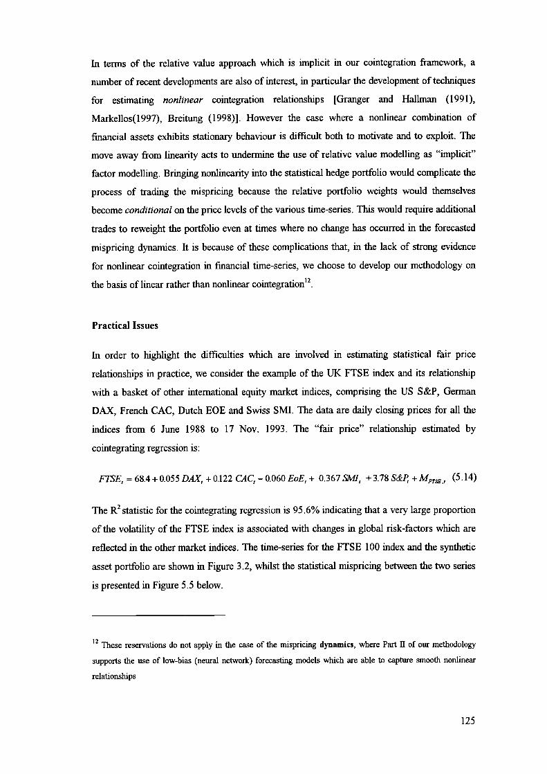
In terms of the relative value approach which is implicit in our cointegration framework, a

number of recent developments are also of interest, in particular the development of techniques

for estimating nonlinear cointegration relationships [Granger and Hallnian (1991),

Markellos(1997), Breitung (1998)]. However the case where a nonlinear combination of

financial assets exhibits stationary behaviour is difficult both to motivate and to exploit. The

move away from linearity acts to undermine the use of relative value modelling as "implicit"

factor modelling. Bringing nonlinearity into the statistical hedge portfolio would complicate the

process of trading the mispricing because the relative portfolio weights would themselves

become conditional on the price levels of the various time-series. This would require additional

trades to reweight the portfolio even at times where no change has occurred in the forecasted

mispricing dynamics. It is because of these complications that, in the lack of strong evidence

for nonlinear cointegration in financial time-series, we choose to develop our methodology on

the basis of linear rather than nonlinear cointegration12.

Practical Issues

In order to highlight the difficulties which are involved in estimating statistical fair price

relationships in practice, we consider the example of the UK FTSE index and its relationship

with a basket of other international equity market indices, comprising the US S&P, German

DAX, French CAC, Dutch EOE and Swiss SM!. The data are daily closing prices for all the

indices from 6 June 1988 to 17 Nov. 1993. The "fair price" relationship estimated by

cointegrating regression is:

FTSE, = 68.4 + 0.055 DAX, + 0.122 CAC, - 0.060 EoE, + 0.367 5M1, + 3.78 S&P, + MFT , (5.14)

The R2 statistic for the cointegrating regression is 95.6% indicating that a very large proportion

of the volatility of the FTSE index is associated with changes in global risk-factors which are

reflected in the other market indices. The time-series for the FTSE 100 index and the synthetic

asset portfolio are shown in Figure 3.2, whilst the statistical mispricing between the two series

is presented in Figure 5.5 below.

12 These reservations do not apply in the case of the mispricing dynamics, where Part II of our methodology

supports the use of low-bias (neural network) forecasting models which are able to capture smooth nonlinear

relationships

125

250 T

-350 -

Jun-88 Jun-89 Jun-90 Jun-91 Jun-92 Jun-93

Figure 5.5: Statistical mispricing between the FISE 100 index and a weighted portfolio of international

equity market indices, over the period 6th June 1988 to 17th November 1993.

The chart shows that the mispricing oscillates around a mean value of zero with an apparently

high degree of mean-reversion. The largest mispncing is that which follows the UK currency

crisis in the late summer of 1992. During this period, the exit of the UK from the Exchange

Rate Mechanism (ERM) led initially to a heavy fall in the FTSE relative to the other indices;

however, after a few weeks the FTSE had returned approximately to its fair price level relative

to the other markets. This sequence of events clearly represented a substantial opportunity for

statistical arbitrage had it been predicted in advance. Furthermore, the DF statistic for the

mispricing series is 3.5 which is significant at the 0.01 level, indicating that the mean-reversion

is not merely an artefact of the estimation procedure but instead represents a significant

cointegration between the set of market indices. The error-correction effect is relatively weak in

this case, with the mean-reversion component found to account for only around 1% of the

variance of the mispricing dynamics.

The major practical complication which arises when applying the mispricing construction

methodology is that the estimated fair price relationship may be unstable over time. Such

instability may be due either to true time-variation in the cointegrating vector, or by errors in

the estimation procedure. The implication is that in-sample significance of the cointegrating

relationship is not sufficient to guarantee that the future mispricing will be mean-reverting.

Whilst it is not generally possible to predict changes in the fair price relationship, it is possible

to adapt to the changes after they become manifest in the observed data. Thus in section 5.2 we

describe an extension of the basic methodology in which an adaptive modelling procedure is

used to track changes in the fair price relationship between a set of assets.

Instability in the estimation procedure itself is most likely to be caused by the presence of neai-

collinearity in the set of constituent asset prices. This danger is heightened when the number of

regressors is large because the number of cross-correlations is 0(N2) in the number of

regressors. In order to address this issue, Section 5.3 describes a stepwise procedure to select

126

appropriate subsets of the asset universe as constituent assets, thus extending our basic

methodology to the case where the size of the asset universe is numbered in tens or hundreds.

A further precaution against instability would fall into the category of biased and/or

constrained estimation procedures, and would consist of replacing the standard OLS regression

with a regularised or "ridge" regression. In this case a diagonal term is added to the covanance

matrix in order to artificially deflate the covariances and reduce the estimation variance which

is caused by near-collinearity. In this "regularised least squares" (RLS) case the cointegrating

vector is no longer given by Eqn (5.9) but instead by the modified expression:

1RLS =(c'c+21) 1 ct

(5.15)

As noted above, other biases or constraints could be imposed upon the mispricing construction

procedure, for example a natural constraint may be to disallow negative coefficients in the

cointegrating vector as these would correspond to short positions in the synthetic asset. This

may serve to further reduce instability, but is actually more likely to be imposed for practical

reasons if it is felt that it eases interpretation of the fair price relationships. Further discussion

of these modifications is beyond the scope of this thesis, but preliminary developments and

results are presented elsewhere (Burgess, 1999).

5.2 Extension to Time-varying Relationships

The basic methodology for constructing statistical mispricings assumes that the underlying

cointegrating relationship is itself stable through time. There is, however, every reason to

believe that the market's opinion as to what constitutes a "fair price" of one asset relative to

another will change over time, with changes in the surrounding economic and political climate,

and in market sentiment. For instance, in the Intertemporal Capital Asset Pricing Model

(ICAPM) of Merton (1973), shifts in the risk premia attached to the underlying sources of

financial and economic uncertainty will cause shifts in asset prices. In cases where the fair

price relationship between a set of assets describes a less than perfect hedge against the

underlying risk factors such price shifts will act as shocks to the statistical mispricing and thus

lead to time-variation in the coefficients of the underlying fair price relationship.

The implication of this is that even models which have worked well in the past are liable to

"break down", i.e. suffer performance degradation due to nonstationarity in the model

parameters. In modelling terms, such nonstationarity could arise either because of unobserved

127

components which although present in the true equilibrium relationship are not included in the

model or alternatively because the true constituent weightings are time-varying (perhaps due to

the influence of conditioning factors).

In this section we describe an extension to the methodology in which parameter nonstationarity

can be controlled by means of adaptive modelling techniques. The methodology is based on

exponential smoothing techniques in the simplest case and on a state-space implementation of

time-varying regression in the more general case. The purpose of these extensions is to allow

the constituent weightings to evolve slowly according to a "random walk parameter" model.

The random walk time-varying parameter model which is analogous to the cointegrating

regression given in Eqn. (5.8) is:

= +M,

C, €c

where

(5.16)

+17 77 N(O, o)

The important difference between Eqn (5.16) and Eqn (5.8) is that the parameter vector

= [p1., p2.1 ...

]T is now conditioned upon time to reflect the fact that the parameters are

no longer assumed constant but instead follow a random walk process.

In this extended model, deviations from the fair price relationship are considered as being only

partially due to statistical mispncings. Instead some of the deviation will be considered as being

due to errors in the parameter estimates, which will be updated accordingly. The extent to

which deviations are associated with the mispncing M and parameter errors will be

determined by the assumed variance of each of these two sources of innovation in the

dynamics.

Exponential Smoothing of the Reversion Level

The simplest implementation of our adaptive modelling can be considered as a restriction of the

more general model in which only the offset term a is allowed to have non-zero variance. In

this case the model can be simplified to:

128

0.8

0.6

0.4

0.2

0

-0.2

0.8

0.6

0.4

0.2

0

-0.2

-0.4

= fi,C1 , +a, +M,C EC

0aa, = a,.1 + - M,10M

(5.17)

The constituent weightings are estimated in a one-off regression procedure as in the basic

methodology, but a certain amount of the deviation is absorbed in the time-varying "constant"

term a,. If the assumed variance of the offset term is small relative to that of the mispncing,

i.e. °a /°M <<1, then a, will be fairly stable, and will only adjust if the deviations remain

consistently of one sign for a long period. The value of a, can be considered as a time-varying

reversion level which reflects changes in outside factors which are not included in the fair price

relationship. In particular this "exponential smoothing" approach can be viewed as a means of

gradually absorbing any nonstationarities which are asset specific rather than caused by

common stochastic trends in the set of asset prices.

This ability to absorb nonstationary components in the mispricing dynamics is illustrated in

Figure 5.6 below. The figure illustrates a case where the observed deviation from the fair price

relationship is affected by two asset specific events, a step change at period 100 and a gradual

decline between period 200 and period 300.

1.2

—Observed Dedation

•'Tp e Rewrsion Lewl

—Estimated Rewrsion

-0.4 .i ..................... .......-.-..-*-----.""-* ......-1 101 201 301

Figure 5.6: illustration of the absorbtion of nonstationarity in the mispricing dynamics by a model with

time-varying reversion level a, as defined in Eqn (5.15). In the case illustrated, the sensitivity ratio

= 0.05.

129

The upper figure clearly illustrates the manner in which the adaptive reversion level serves to

compensate for the nonstationanty in the observed deviation series. Although the step change at

period 100 is initially treated as a component of the mispricing, its persistence leads to it being

gradually absorbed within the time-varying reversion level. After this adjustment, the estimated

mispricing again becomes close to the true mispricing (lower figure). Similarly, the gradual

decay between period 200 and period 300 causes a temporary tendency for the estimated

mispncing to over-state the true case but again, with time, this nonstationarity is absorbed and

the estimated mispricing regains its accuracy.

State-space Formulation of Adaptive Regression

The more general case of our adaptive modelling methodology is where the fair price

relationship is estimated using time-varying parameter regression in which not only the

constant term a but also the constituent weights fl, are allowed to vary over time. This

formulation, which corresponds to that shown in Eqn. (5.14), is more appropriate than the

simpler "exponential smoothing" case when it is the factor exposures to the common stochastic

trends which vary with time, as opposed to asset specific price shocks.

The time-varying parameter model can be expressed in state space form and optimised using

Kalman filter methodology. In this case the "state" of the model consists of the parameter

vector = [a1,, ,t 2,1 fi] (which may or may not be supplemented by a constant term).

The current parameter estimates are compared to the observed value of the target asset by

means of the so-called "measurement equation":

T=Cj,+i, £y-N(0,o)

(5.18)

The parameter estimates (states) are then updated according to the "transition equation":

= TJ3, 1 + 1, 11, . N(O,R,)

(5.19)

In the simple random walk parameter model the state transition matrix T is the identity matrix

I, the state (parameter) covariance matrix is assumed to be diagonal

R = [o cr ... o and the model can be seen to correspond to the formulation in Eqn.

(5.16). Generalisations of this model can be constructed which allow for trends, reversion and

other deterministic components in the parameter values. The detailed formulation of these more

130

TWTe(t)

general models can be found in any advanced time-series text, such as Harvey (1993). Such

models are beyond the scope of this thesis but are discussed extensively by Connor and Bentz

(1997) in the context of estimating explicit factor models of asset price dynamics.

Example

We demonstrate the filtering methodology using a simulated cointegration relationship with

time-varying parameters and the following data-generating process:

[a,ly1 =[1 x1][]+d

where a +1 = a + N(pa , o), fi = /3 + N(p,

(5.20)

The dynamics of the "target" series Yt are governed by a reversion towards the current

"equilibrium value" y = + /3x, whilst the "constituent asset" x 1 follows a random walk:

Ay =— ri +N(p,o)

= N(1u1,a)(5.21)

A realisation of the system is illustrated in Figure 5.7 below. The parameters of the system are

as follows: xo=yo=1, = 0.05%, =0.03%, cr=y=0.7%, c,=0, fio=1, a=O.Ol%, r0.

CYa=0.1%, ag=0.1%. Finally the mean reversion parameter p = 0.1 (i.e. the stationary

component has an autoregressive root of 0.9). Knowing the values for cz and we also plot Yt

against the trne y.

ø*t,'.,:::: :&. "r'

Figure 5.7: Realisation of a system exhibiting dynamic cointegration; the left hand chart shows that the

deviation between the series is nonstationary, leading us to fail to reject the null h)pothesis of no

cointegration. The right hand chart shows, however, that the series yt actually exhibits a strong

cointegration with x when the time-varying cointegrating vector is taken into account.

131

The state-space form of the adaptive modelling methodology was employed to estimate the

time-varying cointegration vector. We measure the success of the filter in two ways: firstly by

the correlation between deviations from the true "equilibrium" y, = [i x, j] and those from

the estimated filter p = [i and secondly by the significance of the reversion effect

which is implied by the filtered deviation series. This can be tested by examining a modified

DF-statistic based upon the regression:

Ed = +

(5.22)

Our "Dynamic Dickey-Fuller" (DDF) test then consists of examining the strength of the

reversion effect: the significance of the mean-reverting effect is indicated by the degree to

which the 't' statistic of the y coefficient is significantly negative; the magnitude of the mean-

reverting component (as a proportion of the total variance) is quantified by the R 2 statistic of

the regression.

However, we camiot apply the difference operator directly to the deviation time-series compute

the dependent variable for the regression in Eqn. (5.22). This is because the time-varying

parameters will absorb some of the nonstationarity in d and create spurious mean-reversion in

the deviation time series. Instead we use a difference operator in which the cointegration vector

is held constant for the period over which the difference is computed:

= d*t+i - d, = - (â + - [, - (â + I3r X r )] (5.23)

A benchmark level of performance was established by applying the DDF test to the true

mispricing series. The regression equation in this case was found to be

= —0.07d, + N(0, 0.0196 2 ) with a 't' statistic of -12.4. The effect of the assumed balance

between parameter (state) noise and observation noise was then evaluated by varying the

sensitivity ratio = . Sample results for the case S =i0 are shown in Figure 5.8:

132

••,• •••0•

Qj

012

L..

Figure 5.8: The results recovered by the adaptive methodology for the case of sensitivity ratio S:1103; the

left hand chart shows the estimated series of deviations which is clearly stationary and represents a

suitable candidate as a predictive input variable to a forecasting model. The right-hand chart shows the

scatterplot between the true deviation and that recovered by the adaptive methodology, in this case the

correlation between the two series was found to be 0.696

Table 5.4 below reports the results of varying the sensitivity ratio of the filter from l00 and

10'. Also shown in the table are comparable figures for the ideal (true) model and for a

nonadaptive standard regression.

LoglO(S)

(regression)

-10-5-4-3-2

0

Cone! DDF

0.238 -5.24

0.238 -5.24

0.696 -10.71

0.758 -12.44

0.663 -12.42

0.507 -11.13

0.309 -7.35

0.150 -4.03

0.097 -2.99

Ideal 1.000 -12.41

Table 5.4: Perfonnance of adaptive methodology at extracting the deviations from dynamic relative

equilibrium of the time series in Figure 5.7. Performance figures are reported for models with different

levels of sensitivity S as well as for the true deviations and a nonadaptive model. Correl is correlation

coefficient between estimated and true deviations; DDF is the Dynamic Dickey Fuller statistic.

The results demonstrate that the filtering methodology is capable of extracting a good

approximation to the true deviations. The maximum correlation between estimated and true

deviations is just over 75% for a model with a sensitivity S This model also has a DDF

statistic which is very close to that obtained using the true deviations. The table also indicates

that although a certain level of adaptation can improve over the static model, too much

adaptation becomes counterproductive. In fact, in this instance, both the correlation and DDF

133

figures for over-sensitive models are worse than the comparable figures for the nonadaptive

model.

5.3 Extension to High-dimensional Problems

Although the concepts which underlie cointegration analysis are equally valid for systems with

tens or hundreds of variables as they are for systems with a handful of variables, in practice

cointegration methods are generally used for low dimensional problems. For instance the

review and analysis of comtegration methods in Hargreaves (1994) includes a Monte-Carlo

analysis of performance for a four dimensional problem, whilst noting that this is an

improvement on previous studies in which the problem dimension was only two. In contrast,

the asset universe under consideration for statistical arbitrage opportunities is generally of the

order of tens (40 constituents of the French Cac 40 index, 30 constituents of the Gennan Dax

or Italian Mib indices) or even hundreds (100 constituents of the UK FTSE, 300 of the

Eurotop, 500 of the US S&P index etc.).

In this section we describe a practical extension of the mispricing construction methodology to

the high-dimensional case where the size of the asset universe is of the order of tens or

hundreds. In order to reduce the dimensionality of the problem we identify relationships

between relatively small subsets of the data. There remains the problem of identifying the most

appropriate subsets to form the basis of the statistical arbitrage models. In order to ensure a

reasonable span of the entire space, we take each asset in turn as the dependent variable of a

cointegrating regression. To identify the most appropriate sub space for the cointegrating vector

we replace the standard "enter all variables" regression procedure with a "stepwise" regression.

In this approach, cointegrating variables are added sequentially to the model. At each stage the

variable added to the model is that which is most significantly correlated to the current

mispricing and hence, when added to the model, will result in the largest possible reduction in

the residual variance.

An economic interpretation of the stepwise methodology is that the first asset selected to

cointegrate with the target asset will be the one which has the most similar exposure to the

market-wide risk factors which dominate the price variance of the target asset. However the

second selected asset will be the one which is most correlated with the residual exposures

which remain after the target asset has already been stochastically detrended with respect to the

first selected asset.

134

Starting with the asset price itself, i.e. c(o) =0, M° = 1, the set of constituent assets is

constructed step by step. The fonn of the synthetic asset models which are generated by the

stepwise procedure is as follows. Let M be the mispricing generated by the model at stage

k, i.e. where the target asset is cointegrated with the first k variables selected from the asset

universe C(k) c: UA:

M = II ; -

fl(k)cJ

C. EC(k)(5.24)

Then the model for stage k + 1 is generated by first identifying the currently-excluded variable

which accounts for the greatest amount of the variance of the current niispncing:

C(k + 1) = C(k) u arg max E[M2 - (M - p,c, )2]

(5.25)Cj EUA-C(k)

Having extended the set of constituents, the full set of beta parameters are re-estimated in order

to account for the effects of cross-correlations between the explanatory variables.

The procedure will continue until either a prespecified maximum number of cointegrating

assets have been added to the model, or there are no statistically significant relationships

between the current residual (synthetic asset) and the variables remaining outside the model. As

in standard stepwise regression modelling, the significance test which is used is a partial-F test

of variable significance which relates the reduction in the variance to the additional degree of

freedom which is added to the model13.

As noted in Section 5.1, our cointegrating-regression approach shares with explicit factor

methods the general idea of detrending the asset prices relative to common stochastic trends. A

key difference in our approach, and particularly in this stepwise methodology, is that the risk

factors are implicitly determined with respect to each target asset on an individual basis. For

instance, in the case of a bank stock which is primarily sensitive to economic growth, market

risk, interest rate risk and investor sentiment, the selected group of cointegrating assets will

13 Similar F-tests of statistical significance underly the variable selection and neural estimation procedures in

Part II of the thesis, and are discussed in detail in Chapters 9 and 10.

135

consist of individual assets which, in a suitable linear combination, have similar exposure to

these underlying factors. In the case of a major retailer with significant export business the

selected assets may include other retailers, stocks which are sensitive to exchange rates, and

stocks of companies which have similar export markets. Thus rather than tiying to identify a

single set of factors which represent all stocks approximately equally, the stepwise

methodology implicitly allows the risk factors to be adjusted according to the particular

characteristics of the target asset under consideration.

Example

We now illustrate the operation of the stepwise methodology for synthetic asset construction

with respect to the particular example of daily closing prices of the constituents of the FTSE

100 index.

The objective of the methodology is to construct the synthetic assets which represent the

mispricings of the individual equities. This is performed by taking each asset in turn and using

the stepwise regression procedure to sequentially identify the five most suitable assets 14 in each

case. The general form of the resulting mispricing models is:

= - (=1 W 1 +

(5.26)

where M 1 is the statistical mispricing (synthetic asset) for stock s at time t; is the actual

stock price of asset S at time t; is the price of the i'th constituent asset selected for

target asset s and w ç , is the associated weighting parameter.

The data consists of daily closing prices from 13th June 1996 to 13th May 1998 and is divided

into an insample period of 400 days and an out-of-sample period of 100 days. After eliminating

assets for which a continuous history was unavailable (mainly due to mergers) we were left

with 94 assets including the index itself. The table below shows the specification of the first 10

14 Note that these will not necessarily (and in fact very rarely) be the five assets which are most correlated with

the target asset. Afier the first stage it is the correlation with the residual mispricing which is important, and

only at the first stage will this be equivalent the target asset itself.

136

synthetic assets, listing first the target asset and then the constituents, together with their

weightings, in reverse order of selection.

Number .Taret Const .itiWtl .Constit2 .Wt2Constit3 .Wt3Constit4 .Wt4Constit5Wt5ConstantI FTSE SCTN 0.916 RTR 0.414 REED 0.82 III 1.878 LLOY 2.72 633.7112 ABF Id -0.084 CW 0.315 GUS -0.16 WLMS -0.362 PRU 0.527 334.9753 ALLD PSON 0.197 STAN -0.043 SFW -0.407 WLY 0.121 SBRY 0.382 290.6944 ANL SFW 0.199 BT 0.564 BSY -0.092 WLMS -0.27 LGEN 1.497 13.3215 ASSD REED -0.034 ICI 0.031 BAY -0.05 BSY -0.05 TSCO 0.246 87.1926 AVZ RR -0.375 CPG 0.177 ORA 0.272 BASS 0.149 ULVR 0.944 -253.1247 BA SEBE 0.16 PSON 0.175 RTR -0203 WLY 0.303 BARC 0.101 -87.88 BAA BASS -0.085 WLMS 0.287 CCM 0.252 RR -0.515 HSBAx 0.1 341.5429 BARC Id 0.208 ORA -1.154 REED -0.624 SMIN 0.746 BSCT 2.429 117.82210 BASS SFW 0.241 EMI 0.148 GM 0.225 RIO -0.289 SCTN 0.846 151.271

Table 5.5: A selection of synthetic assets which represent statistical mispricings of FUSE 100

constituent stocks. In each case the constituent assets are listed in reverse order of selection and the

parameter values are those which apply when all five constituent assets are included in the model

As an example, consider the 10th listed asset, BASS, representing Bass Plc., the breweiy group.

The associated synthetic asset model is given by:

024lP5,, + 0.148P1,

M 551 = P, - + 0.225P, - (5.27)

+ °•846SCTN, +151.271

In the order selected, the constituent assets are SCTN (Scottish and Newcastle - another

breweiy group), RIO (Rio unto Plc - Mining and Natural Resources), GAA (Granada - TV

and entertainment), EMI (music), and SFW (Safeway supermarket group). The choice of a

brewery as the first selected constituent is unsurprising as we would expect the two stocks are

sensitive to similar economic fictors. The final three stocks have probably been selected on the

basis of a shared sensitivity to the UK economy as a whole and the luxury/entertainment side in

particular. Perhaps the only surprising choice, in this case, is that of Rio Tinto. However, note

that the coefficient in this case is negative (-0.289) indicating that (net of the effect of the other

constituents) fctors to which the Bass share price responds positively tend to have a negative

impact on Rio Tinto, and vice versa.

Whilst we have singled out one model in particular, a similar explanation could be produced

for each of the other models. These relationships are not always obvious: they may for instance

relate to a company's financial setup rather than its industrial sector, and may also be

complicated, as in the case of Bass/Rio Tinto, by the presence of negative coefficients.

However, in all cases there is at least an implicit relationship in the fict that the share price

movements of the companies have been found to be sufficiently related as to select out the five

particular stocks from a choice of 93 possible assets.

137

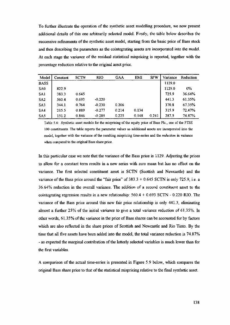
To further illustrate the operation of the synthetic asset modelling procedure, we now present

additional details of this one arbitrarily selected model. Firstly, the table below describes the

successive refinements of the synthetic asset model, starting from the basic price of Bass stock

and then describing the parameters as the cointegrating assets are incorporated into the model.

At each stage the variance of the residual statistical mispricing is reported, together th the

percentage reduction relative to the original asset price.

ModelBASSSAOSAlSA2SA3SA45A5

Constant SCTN RIO GAA EMI SFW [Variance Reduction

822.9383.3560.4

344.1215.5151.2

1129.01129.0

0.645 725.9

0.693 -0.220 441.3

0.764 -0.230 0.206 370.8

0.889 -0.277 0.214 0.134 315.9

0.846 -0.289 0.225 0.148 0.241 287.5

0%36.64%61.35%67.35%

72.47%74.87%

Table 5.6: Synthetic asset models for the mispricmg of the equity price of Bass Plc., one of the FTSE

100 constituents. The table reports the parameter values as additional assets are incorporated into the

model, together with the variance of the resulting mispricing time-series and the reduction in variance

when compared to the original Bass share price.

In this particular case we note that the variance of the Bass price is 1129. Adjusting the prices

to allow for a constant term results in a new series with zero mean but has no effect on the

variance. The first selected constituent asset is SCTN (Scottish and Newcastle) and the

variance of the Bass price around the "fair price" of 383.3 + 0.645 SCTN is only 725.9, i.e. a

3 6.64% reduction in the overall variance. The addition of a second constituent asset to the

cointegrating regression results in a new relationship: 560.4 + 0.693 SCTN - 0.220 RIO. The

variance of the Bass price around this new fair price relationship is only 441.3, eliminating

almost a further 25% of the initial variance to give a total variance reduction of 6 1.35%. In

other words, 61.35% of the variance in the price of Bass shares can be accounted for by factors

which are also reflected in the share prices of Scottish and Newcastle and Rio Tinto. By the

time that all five assets have been added into the model, the total variance reduction is 74.87%

- as expected the marginal contribution of the latterly selected variables is much lower than for

the first variables.

A comparison of the actual time-series is presented in Figure 5.9 below, which compares the

original Bass share price to that of the statistical mispricing relative to the final synthetic asset.

138

period110

90

70

50

30

10

-10

-30

-50

-70

- 1200

1000

800

-600

400

200

600

Estimation Period

_._T_SA5 - BAJ

Figure 5.9: Time-series of the share price of Bass Plc (right hand axis) and the associated statistical

mispricing series (left hand axis) which represents the deviation relative to a "synthetic asset" composed

of a combination of five other share prices. The first 400 observations were used to estimate the

cointegration relationship. During this period the synthetic asset has a 74.87% lower variance than the

original Bass share price. The fmal 100 observations are "out of sample".

The mispricing is clearly much more stable than the underlying share price. This fact is

emphasised during the "out of sample" period, during which the Bass share price trends up to

new levels whereas the statistical mispricing remains relatively stable and maintains a high

degree of mean-reversion. This supports the hypothesis that the mispncing is largely

immunised from the unpredictable sources of market risk which dominate the changes in the

original share price, and is instead more representative of stock specific factors which are lower

in variance and yet may contain a substantial component which is potentially predictable.

5.4 Summary

In this chapter we have described our cointegration framework for constructing synthetic

assets in the form of statistical mispricings of underlying asset prices relative to appropriately

constructed "synthetic assets". The synthetic assets consist of linear combinations of other

asset price series and are constructed by methodology based on the concept of a "cointegrating

regression", with extensions to the time-varying and high-dimensional cases. The intention

behind this pre-processing is to generate combinations of time-series which are largely

immunised against market-wide uncertainties and which enhance the potentially predictable

components of asset price dynamics.

In the following chapter we discuss the next component of the methodology, namely a broad

range of tests which are designed to identify the presence of a potentially predictable

component in the mispricing dynamics.

139

6. Testing for Potential Predictability

This chapter describes the tests which we have developed for the purpose of identifying

potentially predictable components in the dynamics of the statistical mispricrng time-series.

These tests include tests for short-term effects, which are based on the autocorrelation function

of the time-series, tests for stationarity in the form of cointegration "unit root" tests, and tests

for general deviations from random walk behaviour which are based upon the variance ratio

function of the time-series. We also introduce novel tests based upon the shape of the variance

ratio profile as a whole. The tests themselves are described in Section 6.1. The strengths and

weaknesses of the various tests can be defined in terms of their relative size and power in

distinguishing between the null hypothesis of purely stochastic dynamics (random walk

behaviour) and various alternative hypotheses which correspond to different types of partially

deterministic dynamics. Section 6.2 presents the results of an examination of the properties of

the various tests. The analysis was conducted under controlled circumstances using Monte-

Carlo simulations of a range of data-generating processes which represent plausible alternative

hypotheses. Section 6.3 presents modifications of the predictability tests which correct for the

bias induced by the construction procedure. Section 6.4 presents the results of applying the

tests to statistical mispricings generated from combinations of FTSE 100 equity prices.

6.1 Description of Predictability Tests

Having created a time-series which represents a statistical mispricing between a set of assets,

the next stage of our methodology involves testing the time-series for the presence of a

potentially predictable component in the mispricing dynamics. Given that our mispricing

construction procedure is based upon cointegration modelling techniques, the natural choice

would be to use cointegration tests such as unit root tests (see Section 2.2.2) in order to detect

the presence of a mean-reverting "error-correction" effect. Unfortunately it is not easy to find

examples of statistically significant cointegration relationships in financial asset prices.

Typically, even combinations of asset prices which contain a stationary component will be

contaminated by the presence of a nonstationary component. In such cases, the cointegration

tests will tend to fail to reject the null hypothesis of nonstationarity in spite of the fact that a

potentially predictable mean-reverting component is present in the dynamics of the time-series.

The reason why standard cointegration tests will in some cases fail to identify potential

opportunities for statistical arbitrage is simple: it is not the purpose for which the tests are

140

designed. Whilst the object of cointegration testing is to identify combinations of time-series

which are stationary, statistical arbitrage modelling is concerned with the more general case of

combinations of time-series which contain a stationary component, or indeed any other

deterministic component. Rather than imposing the strict requirement of stationarity, we instead

empioy a broader range of tests which are capable of identifying both trending and mean-

reverting behaviour and which are also robust to the presence of a nonstationary component in

the time-series dynamics.

The following subsections define the set of tests which we employ to identify predictable

components in noisy time-series. The tests include autocorrelation tests for short-term

dynamics, unit root tests for stationarity, and variance ratio tests for the presence of mean-

reversion. We introduce a fourth set of novel tests which are based upon the shape of the

variance ratio profile as a whole and which are intended to identify general deviations from

unpredictable (random walk) behaviour. The power of these tests against a range of alternative

hypotheses will be tested in the following section using a Monte-Carlo simulation.

6.1.1 Autocorrelation tests for short-term dynamics

The individual autocorrelation statistics which collectively comprise the autocorrelation

function (ACF) of a time-series are very sensitive to noise. To compensate for this weakness, it

is common to instead employ "portmanteau" statistics which are joint tests of a set of

individual correlation coefficients. In particular, we base our benchmark test for the presence of

autocorrelation effects in the mispricing time-series on the Box-Lyung test (see also Section

2.2.2) which quantifies the absolute magnitudes of the relationships in the short-term dynamics

of the time-series.

Q-BL statistic

The Box-Pierce Q statistic consists of the (unweighted) sum of the squares of the first p

components of the sample correlogram. The Q statistic is corrunonly used to test whether a

series is white noise and is asymptotically distributed as chi-squared with p degrees of freedom.

The Box-Lyung statistic (Q-BL) is a modification which is known to have better finite sample

properties, and is defined by:

141

= T(T+2) k=1

T—k (6.1)

Where T is the sample size, or length of the time-series and rk is the k'th autocorrelation

coefficient as defined in Eqn. (2.8). The exact specification of the Q-BL statistic will depend on

the parameter p which detemiines the number of autocorrelation coefficients to combine in the

summation.

6.1.2 Unit root tests for Stationarity

To represent the stationarity tests of cointegration analysis (see Section 2.2.2), we take the two

standard tests which are recommended by Engle and Granger (1987), namely the Dickey-Fuller

(DF) test and the Cointegrating Regression Durbin-Watson (CRDW). These are defined as

follows:

DF statistic

Calculating the DF statistic involves regressing changes in the series Ay = - on the

actual level of y itself. The test statistic is the 't' statistic of the regression beta:

Ay1 = a+I y +e (6.2)

If the 't' statistic indicates a beta value which is significantly less than zero then the series is

stationary. Under the null hypothesis of nonstationarity the DF statistic follows a non-standard

distribution which is tabulated in Fuller (1976).

CRDW statistic

The CRDW statistic is calculated as for the standard Durbin-Watson test for autocorrelated

regression residuals:

(yf -yf-l)2

CRDW= (6.3)

142

If y and Yt-i are independent and zero mean then the variance of their sum will equal the

of their variances and the DW or CRDW statistic will be within sampling error of the value

two. Perfect negative correlation gives a statistic close to 4 and perfect positive correlation a

value close to zero. Under the null hypothesis of a random walk the CRDW follows a

nonstandard distribution with values very close to zero (i.e. high positive autocorrelation).

6.1.3 Variance Ratio tests for mean-reversion

The variance ratio function is defined as the normalised ratio of long term variance (calculated

over period t) to single-period variance and is thus:

(iy, _-)2

vR( v)- - (6.4)

If the increments to the series are uncorrelated then the ratio will be close to 1. It can be shown

that suitably expressed VR statistics are equivalent to weighted sums of actual (rather than

squared - as in Section 6.1.1) autocorrelation coefficients (see Eqn. (2.13)). VR(r)> 1

indicates higher long-term variance than would be expected given the short-term variance, and

hence that the net effect over timescale r is of positive autocorrelation or trending behaviour.

VR( ) <1 indicates lower long-term variance than would be expected, given the short term

variance, and hence that the net effect over the period is of negative autocorrelation or mean-

reverting behaviour.

The conmon use of the YR statistic is to test for the presence of a significant mean-reverting

component in the dynamics of the time-series when viewed over a particular time-scale, i.e.

VR(r) <1 - d (where d represents a critical value based upon the required significance level).

6.1.4 Variance Profile tests for deviations from random walk behaviour

As noted above, the standard form of the YR statistics requires the specification of a timescale

r. Furthermore, such statistics can be adversely affected by short term effects in the dynamics.

For instance a short-term positive autocorrelation (trending behaviour) combined with longer-

term negative autocorrelation (mean-reversion) may lead to a YR statistic close to 1, and hence

143

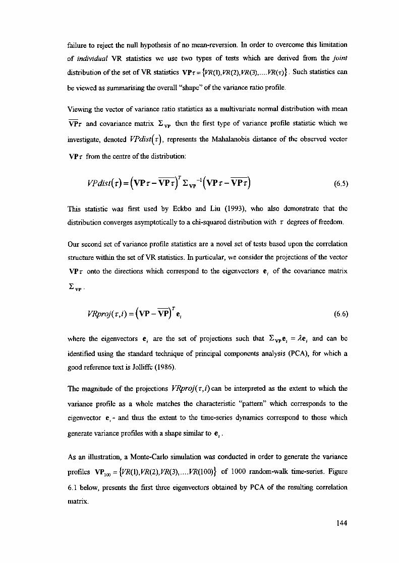
failure to reject the null hypothesis of no mean-reversion. In order to overcome this limitation

of individual YR statistics we use two types of tests which are derived from the joint

distribution of the set of YR statistics VPr= {VR(1),VR(2),J'R(3).....VR(r)). Such statistics can

be viewed as sunimarising the overall "shape" of the variance ratio profile.

Viewing the vector of variance ratio statistics as a multivariate normal distribution with mean

VPr and covariance matrix then the first type of variance profile statistic which we

investigate, denoted VPdist(r), represents the Mahalanobis distance of the observed vector

VP r from the centre of the distribution:

VPdist(r) = (vp vp ) T '(vp v) (6.5)

This statistic was first used by Eckbo and Liu (1993), who also demonstrate that the

distribution converges asymptotically to a chi-squared distribution with z degrees of freedom.

Our second set of variance profile statistics are a novel set of tests based upon the correlation

structure within the set of YR statistics. In particular, we consider the projections of the vector

VP r onto the directions which correspond to the eigenvectors e 1 of the covanance matrix

vP.

VRproj(v,i) ..(yp_Fp)Te (6.6)

where the eigenvectors e 1 are the set of projections such that ,e, = )te and can be

identified using the standard technique of principal components analysis (PCA), for which a

good reference text is Jolliffe (1986).

The magnitude of the projections VRproj(z,i) can be interpreted as the extent to which the

variance profile as a whole matches the characteristic "pattern" which corresponds to the

eigenvector e - and thus the extent to the time-series dynamics correspond to those which

generate variance profiles with a shape similar to e,.

As an illustration, a Monte-Carlo simulation was conducted in order to generate the variance

profiles VP1 = {vR(1),vR(2),vR(3).....VR(100)} of 1000 random-walk time-series. Figure

6.1 below, presents the first three eigenvectors obtained by PCA of the resulting correlation

matrix.

144

Figure 6.1: The first three eigenvectors (principal components) of the correlation matrix of the 100-period

variance profile, estimated under the null hypothesis of no predictable component (random walk

behaviour). The eigenvectors represent the common structure which is found in deviations from the

average variance profile.

For instance, the magnitude of the projection on the first eigenvector represents the extent to

which a variance profile exhibits a global shift upwards. Positive projections on this

eigenvector will correspond to positive autocorrelation (increasing VP) in the relatively short-

term dynamics, followed by zero autocorrelation (flat VP) in the medium and long-term

dynamics. Conversely, negative projections on this eigenvector will correspond to negative

autocorrelation in the short-term dynamics, and zero autocorrelation in the medium and long

term dynamics.

Interpreting the second component in a similar manner, we note that positive projections

correspond to short term reversion (low VR) and longer-term trending behaviour (increasing

VR). The third component represents a very short term trend, followed by a weaker medium

term reversion and a weaker still long term trend.

The PCA of the 100-period variance ratio profile VP also indicated that for random walk

series approximately 80% of the total variability is captured by the first principal component

(corresponding to projections onto the first eigenvector). The fct that such a high proportion

of the variance in a set of 100 metrics can be represented by a single statistic indicates a high

degree of structure within the correlation matrix of the different VR( z) statistics. Figure 6.2

below shows the scree plot of variance explained by each principal component, together with

cumulative variance for the first 'n' components.

145

- Elgenvalue I

-.-- CumulativeEigenvalues

100%

80%

60%

40%

20%

0%

1 2 3 4 5 6 7 8 9 10

Figure 6.2: Scree plot showing the variance accounted for by the first ten principal components of the

variance ratio profile VP evaluated over 1000 realisations of random walk time-series. The fact that

the first few components account for almost all the variance indicates a high degree of correlation

between the various VR(r) statistics.

Table 6.1, below, reports the actual and cumulative figures for the proportion of variance

explained by each principal component:

Principal Component Number 1 2 3 4 5 6 7 8 9 10

Variance Explained 81.6% 12.4% 3.6% 1.2% 0.5% 0.3% 0.1% 0.1% 0.1% 0.0%

Cumulative Variance 81.6% 94.0% 97.6% 98.8% 99.3% 99.6% 99.7% 99.8% 99.9% 99.9%

Table 6.1: Variance Explained by the principal components of the Variance Ratio profile VP

The first five components account for over 99% of the total variability in the 100-period

profile. A similar analysis of the 25-period variance ratio profile was found to produce similar

results, except that the overall time-scale is shorter and the "frequency" of the components is

correspondingly higher. Given that five components are sufficient in each case to account for

99% of the total variability in the VR profile, and that the different length profiles may be

sensitive to different dynamic effects, it was decided to include test statistics derived from each

of the first 5 components of both the 25-period and 100-period variance profiles within our

subsequent Monte-Carlo experiments.

6.2 Monte-Carlo Evaluation of Predictability Test Power

This section presents an analysis of the various predictability tests which were described in the

previous section. The usefulness of the predictability tests lies in their ability to distinguish

between different classes of time-series dynamics. In particular, this ability can be quantified

146

VR25

Variance Ratio 25

VR5 0

Variance Ratio 50

([y y]-4y) /75(Ay _)2

/

([y

VR75

Variance Ratio 75

VR100

Variance Ratio 100

by analysing the size and power of the tests in differentiating between the null hypothesis of

random-walk dynamics and different alternative hypotheses which correspond to different

types of partially deterministic dynamics.

The set of statistics included in our analysis are listed in Table 6.2 below:

Statistic Type Parameter Equation

Q5 Q (Box Lyung) 5 s r

Ql0 Q(BoxLyung) 10

DF Dickey-Fuller none

CRDW Durbin-Watson none

T(T+2)jk=1

T(T+2) T—k

/3/sefi from regression Ay = a + /3y + e.

(yt —yt_1)2CRDW=

VR1 0

Variance Ratio 10([y

_y_1O]_)2/10(4yf _)2

f t

([y _Yt25]_AY)/25(4yt_)2

t t

([y _Y5O]_AY)/50(4v_)2

t t

VP25d Variance Profile 25(distance)

VP100d Variance Profile 100(distance)

(v2, -25)

(v' - vi )

-1 (vi -

VP25c1..5 Variance Profile 25 i1...5(projection) (v25 - "25) e1

VP100c1..5 Variance Profile 100 i1..5(projection) (v100 - v 100 ) e1

Table 6.2: Predictability tests selected for analysis in the Monte Carlo simulations

The approach which we take to compare the various tests is to fix the size of the tests (false

positive rate, a) and then compare their power with respect to different alternative hypotheses

147

(l-, the false negative rate). This tradeoff between the size and power of a test is illustrated in

Figure 6.3 below.

Distribution of

Distribution of test tt ,tstitic given

statistic given H, HA: 1¼

size

•• I"'-I

True value ()

acceptance

Figure 6.3: TradeotTbetween size and power of a test The size ofthe test is a, the probability of a Type I

error or "false positive" (the alternative is falsely accepted). The power of the test is (1-f), where J is the

probability of a Type U error or "false negative" (the alternative is thisely rejected).

The first stage of the process is to generate the empirical null hypothesis distribution of the

various test statistics, i.e. in the case where the dynamics are completely stochastic:

yt = yt_l + e 6 N(0,o.2)

or alternatively: (6.7)

=

For this purpose, 1000 simulations of random-walk time-series were performed, each of length

1000 observations. The "acceptance region" for each of the test statistics was identified by

selecting critical values such that the false positive rate on the empirical sample corresponded

to the required size of the test. These ranges were then validated with respect to a second

simulation of 1000 random walk series in order to allow a comparison to be made between the

nominal and actual sizes (false positive rates) of the tests, as presented in Table 6.3 below.

Nominal DF CRDW Q5 Q10 VRIO VR25 VR5O VR75 VRIOO VPIDOd VP25d

1% 1.6% 1.3% 0.8% 0.9% 0.9% 0.9% 1.2% 1.0% 1.6% 5.9% 1.3%

5% 4.5% 3.9% 4.0% 5.2% 3.6% 6.0% 4.7% 4.4% 5.6% 18.8% 4.5%

10% 9.1% 8.0% 9.8% 8.8% 9.9% 12.2% 9.1% 9.2% 10.4% 26.5% 10.6%

Nominal VPIOOcI VPIOOc2 VPIOOc3 VPI0Oc4 VPIOOc5 VP25c1 VP25c2 VP25c3 VP25c4 VP25c5

1% 1.2% 1.0% 1.1% 1.6% 2.0% 0.8% 1.3% 1.4% 1.8% 1.0%

5% 4.4% 4.7% 5.3% 6.0% 7.3% 3.7% 6.6% 4.9% 5.8% 4.9%

10% 8.7% 9.4% 9.9% 12.4% 12.4% 9.8% 10.4% 10.4% 10.9% 12.3%

Table 6.3: Nominal size of predictability tests versus actual size on a calibration set of 1000 random

walk time-series

148

On the whole the validation results confirm that the actual size of the tests is close to the 1%,

5% and 10% nominal levels selected for the experiment. The only significant deviation from the

nominal levels was found for the VP100d statistic with false positive rates of (5.9%, 18.8%

and 26.5%) instead of the nominal {1%, 5% and 10%)'.

6.2.1 Specification of Alternative Hypotheses for Simulation Experiments

The power of the tests was then evaluated against a range of alternative hypotheses in which

the corresponding time-series dynamics contain a deterministic and hence potentially

predictable component in combination with a (much larger) stochastic component. Two simple

forms of deterministic component are considered, namely reversion and momentum. To

generalise the reversion component, however, from the case of standard "mean reversion" or

stationarity, we also allow for a degree of random-walk drift in the reversion level (which can

be compensated for adaptive modelling methods such as that in Section 5.2). Thus the data-

generating processes are of the form:

Ay =(1—w)As +wAn +A,n

where:

= —rs_ + Ct N(0,a) (6.8)

An = N(0,o)

isint = a(yt_i -

In all, simulation experiments were conducted to test the power of the predictability tests

against 10 different parametrisations of the system defined in Eqn. (6.8). The parameters of the

different experiments are specified in the Table 6.4 below.

15 Whilst the VPIOOd statistic suffers from a certain degree of instability, the corresponding eigenvector

projections YPIOOcI . .5 are close to the nominal size. Hence the source of the instability appears to be the later

projections which only account for a tiny proportion of the overall variance of the YR profile. As the

Mahalanobis distance metric effectively attaches an equal weight to each projection it would appear to be a

dangerous metric to use in unadjusted form.

149

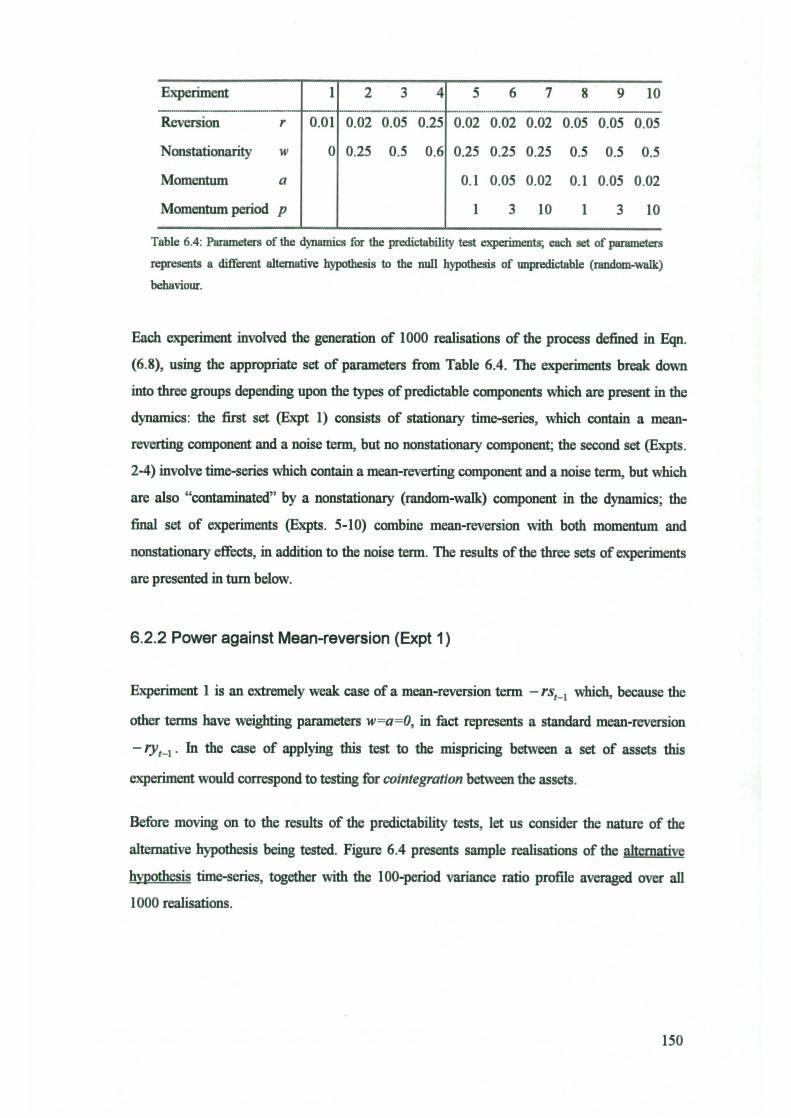
Experiment_..1.__1 ........ f--

....7_.__8

Reversion r

0.01 0.02 0.05 0

0.02 0.02 0.02 0.05 0.05 0.05

Nonstationarity

0 0.25 0.5

0.25 0.25 0.25 0.5 0.5 0.5

Momentum a

0.1 0.05 0.02 0.1 0.05 0.02

Momentum period p

1 3 10 1 3 10

Table 6.4: Parameters of the dynamics for the predictability test experiments; each set of parameters

represents a different alternative hypothesis to the null hypothesis of unpredictable (random-walk)

behaviour.

Each experiment involved the generation of 1000 realisations of the process defined in Eqn.

(6.8), using the appropriate set of parameters from Table 6.4. The experiments break down

into three groups depending upon the types of predictable components which are present in the

dynamics: the first set (Expt 1) consists of stationaiy time-series, which contain a mean-

reverting component and a noise tenn, but no nonstationaiy component; the second set (Expts.

2-4) involve time-series which contain a mean-reverting component and a noise tenn, but which

are also "contaminated" by a nonstationary (random-walk) component in the dynamics; the

final set of experiments (Expts. 5-10) combine mean-reversion with both momentum and

nonstationaiy effects, in addition to the noise term. The results of the three sets of experiments

are presented in turn below.

6.2.2 Power against Mean-reversion (Expt 1)

Experiment 1 is an extremely weak case of a mean-reversion term - rs ..1 which, because the

other terms have weighting parameters w=a=O, in fact represents a standard mean-reversion

- 'y-1. hi the case of applying this test to the mispricing between a set of assets this

experiment would correspond to testing for cointegration between the assets.

Before moving on to the results of the predictability tests, let us consider the nature of the

alternative hypothesis being tested. Figure 6.4 presents sample realisations of the alternative

hypothesis time-series, together with the 100-period variance ratio profile averaged over all

1000 realisations.

150

1 11 Z U ii U U

Figure 6.4: Rea]isations of time-series which exhibit mean-reversion (left) and the vatiance ratio profile

averaged over 1000 such series (right). For a truly stationary process the variance ratio will tend to zero

as the period over which the increments are calculated increases.

The mean-reversion term can clearly be seen to induce a smooth downward slope in the

variance ratio profile. In fact the variance ratio of a stationary process will asymptotically

trend towards zero as the length of the period r approaches infinity. One interpretation of this

type of variance ratio profile is that the mean-reversion causes a tendency for short-term

volatility in the series to partly cancel out, leading to longer term volatility being lower than

would be expected from the short-term volatility.

The power of the various tests is presented in Figure 6.5 and Table 6.5 below for the three

cases where the nominal size (expected false positive rate) of each test is 1%, 5% and 10%.

100%

90%

80%

70%

80%

50%

40%

30%

20%

10%

0%It) - C1 () It)

0U- U) 0

Ix IxIxIx Ix->>>>

C.)

Figure 6.5: illustration of the power of the predictability tests against the alternative hypothesis of

uncontaminated mean-reversion. The sets of bars represent false positive rates of 1%, 5% and 10%.

Size DF CRDW Q5 Q10 VRIO VR25 VR5O VR75 VRIOO VPIOOd VP25d

1% 14.3% 11.4% 0.7% 1.3% 2.5% 3.4% 2.9% 2.7% 3.3% 4.5% 2.4%5% 45.3% 45.1% 4.5% 5.1% 8.1% 12.8% 13.3% 15.0% 15.8% 17.0% 6.2%10% 65.5% 67.1% 9.3% 10.1% 16.4% 21.2% 24.1% 27.5% 29.4% 24.7% 13.1%

Size VPIOOcI VPIOOc2 VPIOOc3 VPIOOc4 VPIOOc5 VP25cI VP25c2 VP25c3 VP25c4 VP25c51% 3.7% 1.3% 0.8% 1.2% 1.0% 2.1% 2.0% 1.1% 1.8% 0.9%5% 13.6% 5.5% 4.2% 6.7% 6.2% 8.9% 9.0% 5.1% 7.1% 5.1%

10% 23.8% 12.9% 9.9% 14.0% 12.9% 17.6% 13.2% 12.9% 14.6% 10.0%

Table 6.5: Power of the different predictability tests to detect deviations from random walk behaviour in

the form of pure mean-reversion, uncontaminated by either nonstationary drift tenn or momentum.

151

Cases in which the power of a test is greater than the size of the test indicate that the test has a

positive ability to identify the deviation from random walk behaviour. Clearly, the standard

stationarity tests are the most successful in this first experiment which corresponds to the

standard cointegration hypothesis for which these tests are designed. Next in power come the

longer-period variance ratio tests VR75 and YR1 00 which detect the lower than expected long

temi variance which is due to the mean-reverting nature of the series. None of the YR

projections are particularly powerful but the highest power is shown by the first principal

components (VP 1 OOc 1, VP25c1) reflecting the fact that the mean-reversion induces a global

downward shift in the variance ratio profile.

6.2.3 Power against Nonstationary Reversion (Expts. 2-4)

Experiments 2 to 4 represent a contaminated form of mean-reversion in which the random walk

term wAne is assigned a nonzero weight and hence introduces a nonstationary drift in the

reversion level of the series. As this term degrades the effect of the reversion term, a

compensating increase in the reversion level r is employed to maintain an approximately

equivalent level of overall predictability.

The average variance ratio profiles for the three experiments are presented in Figure 6.6; the

reversion term induces a negative slope in the VR profile as in Experiment 1. The

nonstationaly component, however, serves to maintain the long-term variance and hence induce

a curvature in the YR profile. In the case of Experiment 4, the reversion is at its strongest,

giving a high negative slope at the beginning of the profile, but so is the degree of

nonstationarity, causing the profile to flatten out fairly rapidly so that the slope is almost zero

beyond the 30-period YR.

152

1 2

0

SIU

0.8

0.7

0.6 1•

0.5

Expt2 :•.•:..•.•...:.

- - Expt3

31 41 1 71

Period

Figure 6.6: The average variance ratio profiles of the simulated time-series used in experiments 2,3 and

4: mean-reversion contaminated by a nonstationaiy drift component. Whilst the mean-reverting

component causes a decay in the short-tenn variance, the addition of a nonstationaiy (random walk) term

prevents the longer term variance ratio from approaching zero.

Realisations of the data-generating processes for experiments 2 and 4 are presented in Figure

6.7. The data-generating process for experiment 3 has properties midway between the two.

'm,

Time ii)

' I J'\ ?'j,.i, .,0

Time lj

Figure 6.7: Realisations of the data-generating process used in the Monte-Carlo simulations for

predictability test experiments 2 (left) and 4 (right)

The power of the different tests against the contaminated reversion processes is shown in the

figure below. For the sake of brevity, only the figures for the test of size 10% are presented.

Figure 6.8: illustration of the power of the predictability tests against the alternative hypotheses of

experiments 2,3 and 4-mean-reversion which is contaminated by a low level of nonstationary drift. The

size (false positive rate) of the tests is 10%.

153

The overall picture is already very different to the simple case of the pure stationary time-series

in Experiment 1. A number of the other tests are now comparable or even superior in power to

the standard DF and CRDW tests. The detailed results are presented in Table 6.6 below.

DF CRDW Q5 Q10 VR1O VR25 VR5O VR75 VR100 VP100d VP25d

Expt2 75.0% 74.9% 11.2% 17.1% 25.6% 40.3% 47.6% 54.9% 59.5% 23.9% 16.1%

Expt3 29.8% 29.4% 20.8% 29.3% 39.5% 51.1% 49.4% 49.9% 47.9% 23.5% 17.4%

Expt4 22.2% 21.9% 62.5% 73.3% 84.5% 69.3% 49.2% 39.7% 35.5% 35.1% 25.8%

VP100c1 VP100c2 VP100c3 VP100c4 VP100c5 VP25c1 VP25c2 VP25c3 VP25c4 VP25c5

Expt2 49.5% 12.2% 11.1% 12.4% 15.1% 29.9% 13.8% 15.1% 17.7% 13.1%

Expt3 50.8% 8.5% 8.5% 10.0% 9.5% 43.5% 15.1% 13.0% 14.3% 12.2%

Expt4 58.8% 50.0% 19.8% 9.9% 7.5% 82.8% 17.9% 9.0% 10.4% 11.1%

Table 6.6: Power of the different predictability tests to detect deviations from random walk behaviour in

the form of mean-reversion which is contaminated by a nonstationary drift term. For the sake of brevity,

the power statistics are presented only for the case where the nominal size of the tests is 10%

Of the various tests, the stationarity tests (DF and CRDW) are most severely degraded by the

presence of a nonstationary component. In Expt. 2, this component only has weight 0.25

(accounting for only 1/1 6th of the short-term variance) and these tests remain the most powerful

of the set of tests under consideration, but by a much reduced margin than in the purely

stationary case of Expt 1. The other tests which perform relatively well in this case are the

long-period yR statistics and the first components of the VR profiles.

As the amount of nonstationarity increases (w =0.5 in Expt. 3 and w =0.6 in Expt 4) the

stationarity tests and long-period VR tests lose power at the expense of the Q tests and the

short-period VR tests. Whilst the nonstationary component degrades the power of the long-

period tests, the increased level of mean-reversion (which is included to maintain the overall

predictability at approximately the same level as the previous experiments) has the effect of

inducing stronger short-term correlations which are detected by the Q and short-period YR

statistics. The most consistent perfonnance is shown by the medium term VRSO statistic and

the first component of the 100-period profile, YP100c1.

6.2.4 Power against a combination of Momentum and Reversion (Expts. 5-10)

Experiments 5 to 10 represent a more complex, yet extremely plausible, form of dynamics in

which a relatively short-term trend or momentum term is combined with an underlying

reversion. Three different strengths of momentum are considered over different periods: a

relatively strong momentum based on single period changes, a weaker momentum over 3-period

154

changes and a weaker still momentum over 10-period returns. The adjustment of the strength of

the effect to the length of the period is to compensate for the higher variance over longer

periods and maintain the overall level of potential predictability approximately constant. This

avoids the two extremes of veiy weak predictability which is almost impossible to detect and,

on the other hand, very strong predictability which is almost impossible to fail to detect -

neither of which cases would provide much useful information about the relative strengths of

the various predictability tests. The three momentum specifications are explored in the context

of two combinations of reversion with nonstationary drift.

Firstly, the set of experiments 5-7 consider a combination of reversion with different period

momentum effects when the level of nonstationarity is relatively low (w=0.25). The variance

ratio profiles are shown in Figure 6.9.

1.2

1.1

0.9

0.8

0.7

0.6

0.5'

1 11 21 31 41 51 61 71 81 91

Period

Figure 6.9: The variance ratio profiles for experiments 5,6 and 7: longer-term mean-reversion combined

with short-term momentum and contaminated by a low-level of nonstationary drift, for short periods the

variance ratio is above 1 reflecting the positive autocorrelation or momentum effect; for longer time-

periods the ratio drops below I reflecting the effect of the mean reversion component.

The figure clearly indicates the increased short-term variance which is caused by the

momentum term. The point at which the profile attains a maximum can be seen to depend on

the period over which the momentum term operates. The power of the predictability tests in the

case of these alternative hypotheses is summarised in Figure 6.10 below.

155

100%

80%706050%40%30%20%10%

0%UIt) 0 81 ON

> > > > - a.U > > a. a.>>>>>> > > > >

• Expt8DExpt7

Figure 6.10: illustration of the power of the predictability tests against the alternative hypotheses of

experiments 5, 6 and 7 - mean-reversion which is contaminated by a moderate level of nonstationaty

drift. The size (false positive rate) of the tests is 10%, figures above 10% indicate a positive ability to

detect the predictable component in the data-generating process above and beyond that which would be

due to chance alone.

Again the picture is a mixed one; although the stationarity tests perform reasonably well, they

are in no case the best performing tests, and in Expt. 7 in particular they are only half as

powerful as the best of the tests. The detailed performance figures are shown in Table 6.7

below.

DF CRDW Q5 Ql0 VRIO VR25 VR5O VR75 VRIOO VPIOOd VP25d

Expt5 62.2% 62.1% 60.4% 42.3% 39.3% 9.6% 21.1% 32.1% 39.4% 9.8% 52.8%

Expt6 50.4% 50.6% 60.6% 52.7% 62.9% 23.0% 10.3% 16.9% 25.7% 57.6% 39.8%

Expt7 43.1% 43.9% 14.4% 22.8% 37.1% 30.3% 10.0% 11.5% 16.3% 65.5% 20.9%

VPI OOcl VPI 00c2 VPI 00c3 VPI 00c4 VPI 00c5 VP25cI VP25c2 VP25c3 VP25c4 VP25c5

Expt5 10.3% 12.0% 12.4% 14.5% 15.9% 33.8% 84.0% 41.7% 40.8% 15.1%

Expt6 18.7% 18.2% 17.4% 47.5% 55.0% 53.8% 61.3% 30.2% 19.9% 22.7%

Expt7 26.1% 30.7% 60.6% 79.3% 47.9% 33.4% 15.2% 16.7% 26.6% 24.6%

Table 6.7: Power of the different predictability tests to detect deviations from random walk behaviour in

the form of a combination of mean-reversion with short-term momentum effects, contaminated by a low

level of nonstationary drift.

The majority of the information appears to be contained in the relatively short term

relationships, as reflected by the fact that, on balance, the Q5 test outperfonns the Ql0 and the

VR1O outperforms the longer-period measures. Amongst the variance profile projections, the

second principal component of the 25-period VR profile is the highest performing test in

Experiment 5 and the second best test in Experiment 6. The third and fourth components of the

longer 100-period VR profile are the most powerful tests against the lower frequency

momentum exhibited by the time-series in Experiment 8.

156

Finally, the last set of experiments (numbers 8-10) consider the case where reversion and

momentum are combined with a moderately large degree of nonstationarity (w=0.5). The

average case VR profiles are illustrated in Figure 6.11.

.Expt8- - Ext

0.8

0.7

0.6

0.5i11 21 31 41 51 61 71 81 91

Period

Figure 6.11: Averaged variance ratio profiles from experiments 8,9 and 10: longer-tenn mean-reversion

combined with short-tenn momentum and contaminated by a moderate level of nonstationazy drift, note

that the higher level of nonstationarity means the longer-tenn variance ratios remain higher than is the

case in Figure 6.9.

In each case the profiles indicate the three characteristic features: short-term variance increased

by momentum effect, medium term variance decreased by reversion and long term variance

stabilised by a nonstationary component. The power of the tests is presented graphically in

Figure 6.12.

Figure 6.12: illustration of the power of the predictability tests against the alternative hypotheses of

experiments 8, 9 and 10 - mean-reversion which is contaminated by a moderate level of nonstationaiy

drift. The corresponding size (false positive rate) of the tests is 10%

These experiments depart from the assumptions of stationarity in two ways: firstly in the

presence of a momentum eftbct and secondly because the reversion level itself suffers from a

moderate degree of nonstationarity. It is clear that the more traditional tests (of either the

stationarity, variance ratio or correlation type) are not veiy well suited to identifying

157

predictable components under these circumstances, in spite of the fact that the underlying

dynamics are simple enough to be represented by only 4 parameters. It is here that the various

projections of the yR profile come into their own - each capable of detecting a different set of

deviations from random walk behaviour. The actual perfonnance figures are presented in Table

6.8.

DF CRDW Q5 Q10 VRIO VR25 VR5O VR75 VR100 VP100d VP25d

Expt8 20.7% 21.0% 55.9% 37.0% 28.0% 12.3% 17.9% 23.4% 22.1% 38.8% 51.4%

Expt9 16.7% 15.2% 50.7% 39.6% 50.0% 14.7% 10.3% 14.2% 16.0% 63.6% 35.2%

ExptlO 14.1% 13.4% 11.0% 14.8% 26.7% 21.6% 9.3% 8.6% 10.8% 71.5% 17.0%

VP100c1 VPIOOc2 VP100c3 VP100c4 VP100c5 VP25cI VP25c2 VP25c3 VP25c4 VP25c5

Expt8 9.6% 31.0% 24.1% 19.3% 22.4% 24.8% 84.2% 43.3% 42.7% 14.0%

Expt9 19.1% 26.8% 21.0% 58.5% 45.1% 42.5% 59.5% 28.5% 21.7% 22.3%

ExptlO 27.4% 53.7% 44.4% 86.2% 42.7% 25.1% 13.1% 14.2% 25.4% 22.6%

Table 6.8: Power of the different predictability tests to detect deviations from random walk behaviour in

the form of a combination of mean-reversion with short-term momentum effects, contaminated by a

moderate level of nonstationaly drift

The performance of the stationarity tests is very weak, only slightly above the 10% of false

positives which would be expected from random-walk time-series. On the other hand some of

the VR projections appear to be very well suited to identifying this type of potentially

predictable behaviour. For instance, in Experiment 10, VR100c4 has a power of 86.2%

compared to only 14.1% for DF, 14.8% for Q10 and 26.7% for VR1O. Even in the case of

Experiment 8 where Q5 performs moderately well with a power of 55.9%, this is significantly

outperformed by the 84.2% of the variance profile projection VP25c2.

6.2.5 Discussion

On the whole, the results presented above highlight the dangers of relying on standard tests for

predictability in time-series when the underlying dynamics do not match the implicit

assumptions of the tests being used. On the other hand, the projections of the variance ratio

profile provide a powerful method of identifying a wide variety of deviations from random-

walk behaviour.

Table 6.9 presents the most significant correlations between the test statistics, averaged across

the whole set of experiments.

158

OF CRDW Qstat5 Qstatl0 VR1O VR5O VP100d VP100c1 VP25d VP25c1

DF

CROW

Qstat5

Qstatl0

VR1O

VR5O

VPIOOd

VP1 ODd

VP25d

VP25c1

1

-0.974

0.008

-0.013

0.130

0.372

0.089

0.354

-0.064

0.093

1

0.000

0.012

-0.110

-0.374

-0.094

-0.351

0.070

-0.075

1

0.890

I

0.302

0.112 1

0.050 -0.011 0.588 1

0.086

0.117 0.180 0.192

I

0.154

0.058 0.746 0.941

0.279

I

0.258

0.207 0.121 -0.044

0.175

0.035

1

0.012 -0.166 0.700 0.446

0.165

0.562 0.222

Table 6.9: Correlations between the predictability test statistics, calculated across all simulated time-

series from the whole set often experiments.

The two stationarity/comtegration tests, the DF and CRDW statistics, are (negatively)

correlated to a very high degree (0.974) as might indeed be expected given that they are

designed for the same purpose. The two portmanteau statistics (Qstat5, Qstatlo) are also

relatively highly correlated (coefficient of 0.890) which suggests that the addition of squared

autocorrelation statistics 6 through 10 adds relatively little information to the first five. The

variance ratio tests VR1 0 and VR5O are also correlated, although at a lower level of 0.588.

Interestingly, the variance ratio statistics are not highly correlated with either the stationarity

tests (DF and CRDW) or the autocorrelation tests (Q5 and Qi 0), conflnning that they do

contain information which cannot be provided by either of these more commonly used families

of tests.

The variance ratio distance statistics (VP2Sd, VP 1 OOd) are largely uncorrelated both with each

other and with the other tests. This is likely to be due to the fact that by weighting deviations by

the inverse of the associated eigenvalue, they are highly sensitive to any deviation at all on the

higher order principal axes. Combined with the uninspiring performance of these tests in the

various Monte-Carlo experiments, this suggests that these particular tests are perhaps the least

useful of all of those considered.

Of the variance ratio projections, only the first principal components turn out to be

substantially correlated with any of the standard tests. Not only are they correlated with each

other (0.562), but also with the basic variance ratio statistics and, in the case ofVPlOOcl, the

stationarity tests DF and CRDW. From this we can take two main messages: the first principal

components of the variance ratio profiles are perhaps the best tests overall, and the subsequent

159

principal components can be used to identify classes of potentially predictable dynamics which

are likely to be completely missed by standard predictability tests - be they stationarity tests,

autocorrelation tests or even variance ratio tests.

6.3 Bias-Correction of Predictability Tests

In addition to the introduction of novel predictability tests based upon the joint distribution of

the variance ratio profile, the second major innovation in our methodology for predictability

testing is the application of both the standard tests and the new tests in the context of

multivanate modelling.

Except in the case of unit root tests, which are used in cointegration modelling, the other tests

are generally used in a univariate setting rather than being applied to the results of a

preliminary multivanate transformation. In order to apply the tests in a multivariate setting it is

necessary to correct for the biases which are induced by the construction procedure that is used

to create the statistical mispricing time-series. In particular, the problem with using the tests in

conjunction with a cointegration methodology is that the residuals of a cointegrating regression

(even when the variables are random walks) will not behave entirely as a random walk - for

instance, they are forced, by construction, to be zero mean. More importantly, the regression

induces a certain amount of spurious "mean-reversion" in the residuals and the impact of this

on the distribution of the test statistics must be corrected if they are to detect piy deterministic

components rather than spurious artefacts of the construction methodology itself. A further

complication arises in the case of the extended stepwise methodology for use in high-

dimensional problems, because the "selection bias" inherent in choosing the best m out of n>

m regressors must also be accounted for.

This bias in the tests is effectively due to the fact that the acceptance regions and critical values

for the test statistics are based implicitly on the assumption of a null hypothesis of random-

walk behaviour. In our case the test statistics are applied to time-series which are the result of

the preliminary mispricing construction procedure and so the random walk null hypothesis is no

longer appropriate. In order to account for the biases introduced by the construction procedure,

the appropriate null hypothesis would be that the series is the result of regressing one random

walk upon a set of random walks. The distribution of the test statistics may be quite different

under this corrected null hypotheses, and using the incorrect null hypothesis may result in false

160

0

0•

04

03

02

01

ii 21 •• . .

rejections of the null in favour of an assumed alternative that the time-series contains a

significant predictable component.

Our solution to this problem is to derive the empirical distribution of the test statistics under the

corrected null hypothesis, by the use of Monte-Carlo simulations. Given the experimental

parameters such as the length of the time-series, the number of regressors, etc. the empirical

distribution of the test statistic is generated by creating many realisations of random walk

processes and calculating the value of the test statistic in each case. As well as correcting for

the biases induced by the algorithm itself, this approach has the additional advantage of

automatically taking into account the appropriate sample size, rather than relying on

asymptotic behaviour.

In particular, we focus on the bias induced in the variance ratio profile when considering time-

series that are the result of regressing random walks upon each other, rather than in the case

where the time-series is itself a simple random walk. The size of the induced bias is a function

of the number of regressors used to construct the synthetic asset, the size of the asset universe

from which the regressors were selected, and the length (sample size) of the time-series.

Number of Regressors

To illustrate the sensitivity of the variance ratio profile we present one dimensional slices

through the design space by varying each of the parameters in turn. Figure 6.13 illustrates

effect of varying the number of regressors.

CI rereoss

2 regfessors

4 regressors

rerecsos

I'3 rereors

32 re2reowc5

84 erasscrs

128 regressoro

Figure 6.13: Illustration of the bias induced in the variance ratio profile of the residuals obtained by

regressing a random walk on a varying number of other random walk series. The variance ratio declines

substantially below 1, which might erroneously be taken to indicate the presence of mean-reversion but is

in fact merely a bias induced by the regression procedure. Results presented are calculated over 10000

Monte-Carlo simulations with a sample size of 500 in each case.

161

00

&

0

121 of

4

O3

In the case of 0 regressors, the behaviour of the series is as we would expect from a random

walk - namely an average variance ratio profile with a constant value of one. However, this

result is gpy obtained in the case where 0 regressors are used. In all other cases we notice a

distinct bias induced in the variance ratio profile. This bias takes the form of a decline in the

variance ratio profile which has a similar appearance to the profile produced by time-series

which contain a mean-reverting component. However in these cases, the apparent mean-

reversion is a completely spurious artefhct of the regression procedure and an even more

extreme deviation from the random walk profile would be required to indicate the presence of a

mean-reverting component.

Selection of Regressors

A further bias is caused by the use of a stepwise procedure, as the candidate variables which

are selected from the pool of available regressors will tend to be precisely those which induce

the greatest bias in the variance ratio profile. The effect of keeping the number of selected

regressors constant, but varying the size of the pool of variables from which they are selected,

is illustrated in Figure 6.14.

1 11 21 31 41 51 61 71 81 91

Period over which variance is calculated

Figure 6.14: illustration of the induced bias as a function of the size of the pool of variables from which

the regressors are selected. The profiles correspond to selecting a single regressor from a pooi of 'n'

candidate variables, with 'n' ranging from Ito 64. The sample size is 500 observations and each curve is

calculated as an average over 10000 Monte-Carlo simulations.

The figure clearly illustrates that an additional bias is induced by the fhct that the regressors

were selected from a larger set of candidate variables. This is a prime example of the dangers

posed by selection bias, or "data snooping" (see Section 12.1.2).

—1 outof 1

"1outof 2

I out of 4

1 out of 8

—1 out ofi

—1 out of 3

—. 1 out of6

162

1 11 21 31 41 51 61 71 81 91

•0

C D•1- 0o0

C

2

oIvz

>

I

0.8

0.6

0.4

0.2

0

In this particular case, where the sample size is 500 and the number of selected regressors is 1,

the number of candidate regressors has a large impact on the size of the induced bias. Where

only a single potential regressor is available the average value for the 100-period variance ratio

is around 0.86 - a relatively small deviation from the 1.00 expected if the series were a pure

random walk. On the other hand, where the single regressor is selected from a pool of 64

candidates, the 100-period variance ratio is only 0.4 - a much more substantial bias. These

results clearly indicate that the size of the asset universe should be taken into account when

testing for potential predictability in the dynamics of mispncing time-series which were

constructed using the stepwise version of our methodology.

Sample Size

The final factor which determines the size of the bias which is induced by the construction

procedure is the sample size. Figure 6.15 illustrates the average variance ratio profiles for the

residuals of regressing a random walk on a set of 8 regressors, where each regressor is also a

random walk.

Period over WhiCh variance is calculated

Sample size = 500

"SampIe size = 1000Sample size = 2000

Sample size 5000

Figure 6.15: ifiustration of the induced bias as a function of sample size. The profiles correspond to using

8 regressors in sample sizes ranging from 500 to 5000 observations. Each curie is calculated as an

average over 10000 Monte-Carlo simulations.

These results clearly demonstrate that the magnitude of the bias is inversely related to the

sample size, thus indicating a greater ability of the preliminary regression procedure to

"overfit" the observed data when the sample size is small. The bias induced in the large sample

case (sample size = 5000) is relatively small, with the 10-period variance ratio taking an

average value of 0.81, compared to the small-sample case (sample size = 500) where the bias

induced is such that the 100-period variance ratio takes an average value of only 0.23.

163

Two-dimensional sensitivity: Joint effect of Sample Size and Number of Regressors

The results presented above should be considered as one-dimensional slices through the three-

dimensional space defined by (number of regressors, size of regressor pool, sample size). By

performing an appropriate simulation, we can measure (and correct) the biases which are

introduced by two or more of these factors jointly. Table 6.10 presents the average VR(50)

statistics obtained by jpjtly varying both the number of regressors and the sample size.

500 1000 2000 5000

0 1.00

1.00

1.00

1.00

1 0.91

0.96

0.97

0.99

2 0.81

0.89

0.95 0.98

3 0.71

0.84

0.91

0.964 0.62 0.78 0.88 0.958 0.39 0.59 0.76 0.89

16 0.19 0.37 0.58 0.80

32 0.10 0.18

0.36 0.64

0.05 0.09

0.18 0.430.03 0.05 0.09 0.22

Table 6.10: The average value of the VR(50) statistic as a function of the sample size (columns) and

number of regressors used in the mispricing construction procedure (rows).

These results clearly demonstrate the fact that the bias induced by the regression procedure

increases with the number of regressors and decreases with the length of the time-series

(sample size).

Summary

The results reported above clearly demonstrate that variance ratio profiles which are generated

from regression residuals behave very differently from those of true random walks. The

induced bias grows with the number of regressors and also, in the stepwise procedure, with the

number of candidate variables from which the variables were selected. The size of the bias is

less when the sample size is large and greater when the sample size is small. When testing for

predictability in mispncing dynamics it is important to use test statistics which correct for the

induced bias. In particular, this correction, will reduce the risk of concluding that a time-senes

contains a predictable component when the deviation from the random walk profile is caused

by the construction procedure itself rather than a systematic component in the actual dynamics.

Our solution to this problem is to generate the appropriate empirical distributions of our test

statistics prior to performing the modelling procedure itself and such that the experimental

164

parameters (number of regressors, size of the pool form which the regressors are chosen, and

sample size) match those which will be used in the modelling procedure. This approach is

rather computationally intensive, given that the number of simulations required is of the order

of 1 000s or 1 0000s depending on the accuracy required, but is quite within the capabilities of

standard PCs. In principle, the use of such empirical distributions is very flexible as it allows

for further modification of the null hypothesis data-generating process should it be so desired.

An example of such a modification would be to take into account conditional volatility effects

through the use of the GARCH processes discussed in Section 2.2.3 rather than the standard

homoskedastic (constant variance) random walks discussed above.

6.4 Evidence for Potential Predictability in Statistical Mispricings

In this section we illustrate the use of the bias-corrected predictability tests, and the variance

profile tests in particular, with respect to the models described in Section 5.3. These models

represent statistical mispricings of the daily closing prices of the equities which constitute the

FTSE 100 index and, as described in Section 5.3, were constructed using the stepwise

regression methodology with a maximum of five constituent assets in each model.

In order to calculate the appropriate distributions for the variance ratio profile statistics we

apply the bias correction procedure described in Section 6.3. This consists of performing a

Monte Carlo simulation under the null hypothesis of regressing random walk variables on other

random walks (i.e. no predictable component). This procedure automatically accounts for the

impact of (a) the mean-reversion induced by the regression itself, and (b) the selection bias

introduced by the use of the stepwise procedure.

The empirical distribution was calculated from 1000 simulations, in each case the parameters

of the simulation match those of the subsequent statistical arbitrage modelling: that is, a 400

period realisation of a random walk is regressed upon 5 similarly generated series, selected

sequentially from a set of 93 such series, using a forward stepwise selection procedure, and the

variance ratio profile calculated from the residuals of the regression 16 . The variance ratio is

16 Clearly it would be straightforward to repeat the procedure for other experimental parameters: sample size,

number of variables etc, but as noted in section 6.3 the huge number of possible combinations leads towards

recalibrating for particular experiments rather than attempting to tabulate the entire distribution.

165

calculated for returns varying from one period up to fifty periods. Note however, that by

construction the value of VR( 1) can only take the value 1.

Given the average profile and covanance matrix of the profile under the null hypothesis of

random walk behaviour, we then tested the residuals of the actual statistical arbitrage models

for significant deviations from these profiles. Some examples of the variance profiles for the

mispricing models are presented in Figure 6.16.

Figure 6.16: Selected variance ratio profiles for statistical mispricings obtained through stepwise

regression of each target asset on five related assets from the FFSE 100 universe

The tests employed were the two types of variance ratio profile statistics described in Section

6.1 and analysed in Section 6.2, namely the Mahalanobis distance of the observed profile from

the average profile under the null hypothesis (VPd) and the projection of this difference onto

the first five eigenvectors VPc1.VPc5.

The results of the bias-corrected predictability tests are shown in Tables 6.11-6.13 below. The

nominal size of the tests is 1% in Table 6.11, 5% in Table 6.12 and 10% in Table 6.13. The

nominal test sizes are based upon the assumption that the tests statistics follow normal

distributions, in order to account for deviations from this assumption we present results both

for the calibration sample itself, for a second similar but independent "Test" sample, and for

the mispricing models. For the variance profile projections, we use eigenvectors derived from

both the correlation and the covariance matrix of the variance profile; statistics derived from

the covariance matrix arc indicated by a (v).

166

VPd VPC(v)1 VPc(v)2 VPc(v)3 VPc(v)4 VPc(v)5 VPc1 VPc2 VPc3 VPc4 VPc5

Cal 1.8% 1.6% 1.4% 1.4% 0.9% 1.4% 1.7% 1.1% 1.7% 1.5% 1.2%

Test 4.3% 1.2% 0.9% 1.8% 1.3% 1.2% 1.3% 0.9% 1.3% 1.3% 1.6%

Model 36.2% 8.5% 1.1% 2.1% 3.2% 3.2% 8.5% 4.3% 3.2% 4.3% 8.5%

Table 6.11: Comparison of VR tests for random-walk simulations and actual mispricings, nominal size

oftest= 1%

VPd VPc(v)1 VPc(v)2 VPc(v)3 VPc(v)4 VPc(v)5 VPcI VPc2 VPc3 VPc4 VPc5

Cal 6.6% 4.5% 5.1% 4.8% 5.2% 6.0% 4.7% 5.8% 4.0% 4.1% 4.8%

Test 9.9% 3.9% 5.5% 4.6% 4.8% 5.4% 4.1% 4.2% 4.3% 5.6% 6.2%

Model 53.2% 11.7% 8.5% 7.4% 12.8% 11.7% 11.7% 9.6% 8.5% 14.9% 13.8%

Table 6.12: Comparison of VR tests for random-walk simulations and actual mispricings, nominal size

of test = 5%

VPd VPc(v)1 VPc(v)2 VPc(v)3 VPc(v)4 VPc(v)5 VPc1 VPc2 VPc3 VPc4 VPc5

Cal 11.7% 8.7% 9.8% 9.5% 10.6% 10.5% 8.3% 10.0% 8.4% 9.4% 9.7%

Test 14.5% 8.2% 10.5% 9.3% 10.9% 10.7% 7.5% 10.1% 8.5% 12.1% 10.4%

Model 59.6% 20.2% 13.8% 14.9% 18.1% 18.1% 19.1% 14.9% 16.0% 19.1% 23.4%

Table 6.13: Comparison of VR tests for random-walk simulations and actual mispricings, nominal size

of test = 10%

The tests indicate that the mispncings of the statistical arbitrage models deviate significantly

from the behaviour of the random data - providing evidence of potentially predictable

deviations from randomness. Table 6.14 below shows 'z' tests for significant deviations in the

mean scores of the observed mispncings when compared to the random validation sample:

VPd VPc(v)1 VPc(v)2 VPc(v)3 VPc(v)4 VPc(v)5 VPcI VPc2 VPc3 VPc4 VPc5

AveTest 50.99 -0.01 -0.01 0.00 0.01 0.00 -0.15 0.03 0.10 0.08 -0.07

VarTest 135.19 0.22 0.04 0.01 0.01 0.00 33.57 5.56 2.72 1.57 0.83

AveModel 70.79 -0.23 0.01 0.07 -0.03 -0.03 -2.34 0.32 1.02 -0.65 0.61

VarModel 676.34 0.41 0.04 0.02 0.01 0.00 62.67 7.45 3.83 1.86 1.06

z stat 7.3 -3.2 0.5 4.0 -4.1 -5.0 -2.6 1.0 4.4 -5.0 6.3

p-value 0.0000 0.0012 0.6116 0.0001 0.0000 0.0000 0.0089 0.3282 0.0000 0.0000 0.0000

Table 6.14: Comparison of mean values of the various VR tests for random-walk simulations and actual

mispricings

167

The presence of significant deviations in the mean test statistics of the mispricing models,

compared to those of the simulated random walk series, reinforces the findings that the actual

mispricings deviate significantly from random behaviour and supports the hypothesis that there

may be potentially predictable components in the dynamics of the statistical mispncings.

6.5 Summary

In this chapter we have described the tests which we have developed for the purpose of

identifying potentially predictable components in the dynamics of the statistical mispricing

time-series, including both standard predictability tests and novel tests based upon the joint

distribution of the variance ratio profile of the time-series. Extensive simulations against a

range of alternative hypotheses provided evidence that these tests can outperform standard tests

in cases where the dynamics combine short-term trending behaviour (momentum) with longer

term reversion effects and suffer from a degree of nonstationary contamination. The biases

which are induced by applying both the standard and the novel tests in a multivariate setting

have been identified, and quantified by means of Monte Carlo simulations. Finally the bias-

corrected statistics have been applied to a set of mispricing models for FTSE 100 equity prices

and found to provide statistically significant evidence that the average mispricing dynamics

contain statistically significant deviations from random behaviour.

In the following chapter we present a set of specialised trading rules which are designed to

directly exploit any mean-reverting component in the mispricing dynamics, without the need for

an explicit forecasting model of the mispricing dynamics.

168

7. Empirical Evaluation of Implicit Statistical Arbitrage Models

In this chapter we describe a set of "implicit statistical arbitrage" (ISA) trading strategies

which are designed to directly exploit any mean-reverting component in the mispricing

dynamics, bypassing the intermediate stage of constructing an explicit forecasting model. The

ISA trading rules are defined in Section 7.1. In the following two sections, the ISA rules are

used to perform an empirical evaluation of the statistical mispricing methodology. The high-

dimensional version of the mispncing construction methodology is evaluated on FTSE 100

equity prices in Section 7.2 and the adaptive version of the methodology is evaluated on a pair

of European equity indices in Section 7.3.

7.1 Implicit Statistical Arbitrage Strategies and Trading Rules

In this section we describe a set of "implicit statistical arbitrage" (ISA) trading strategies, so-

called because the trading rules upon which they are based rely implicitly on the mean-

reverting behaviour of the mispncing time-series. An example of such a trading rule was given

in Eqn. (4.8). Given a mispricing model of the form shown in Eqn. (5.10), the underlying

assumption of the ISA strategies is that future price changes will be such as will tend (on

average) to reduce the mispricing between the target asset and the combination of constituent

assets. Thus the ISA strategies act by exploiting what might be considered a "mispricing

correction effect", and will realise profits in cases where the mean-reversion component in the

mispricing dynamics is sufficiently large to overcome the transaction costs which are

associated with following the strategy.

The ISA strategies are implemented by parametnsed trading rules which define the sign and

magnitude of the currently desired holding in the mispricin portfolio, which consists of the set

of assets {i , c1 , C2 ,..., c } in the proportions {i,_p1 ,-fl2 , . . . ,-fl, } respectively. The

basic strategy defines the desired holding according to the trading rule:

ISA(.M',,k) = _ sign(!vIt_3 )ivt_ (7.1)

The negative sign indicates that the mispricing should be bought when it is negative, and sold

when it is positive. The sensitivity parameter k allows the magnitude of the holding to vary as a

function of the size of the current mispricing. With k=0 the function is a step function, and the

entire holding is always invested in the mispricing portfolio (whether bought "long", or sold

169

"short"). With k>O the size of the portfolio will be increased if the magnitude of the mispricing

increases, and decreased if the magnitude of the mispricing decreases; the exact nature of this

scaling will depend upon the value k and is illustrated for selected values in Figure 4.4.

As discussed in Towers and Burgess (1998a) and Towers (1999), the perfonnance of the basic

ISA rule in Eqn. (7.1) can be highly sensitive to the level of transaction costs. Fluctuations in

the mispricing can lead to similar fluctuations in the desired holding, thus generating frequent

transactions and potentially undermining otherwise profitable strategies by incurring high levels

of transaction costs. Thus we define generalisations of the basic rule which are designed to

reduce the trading activity by smoothing the trading signal:

ISA(M1 ,k,h) =

(7.2a)h-i

ISA(M , k, O, = (1— 9)ISA(M, , k) + GISA(M1 , k, ® (7.2b)

The modified rules offer some control over the performance of the trading strategy net of costs.

This can be achieved by choosing smoothing parameters which optimise the tradeoff between

exploiting the predictive information (which is implicit in the level of the mispncing) on the one

hand, and incurring transaction costs through over-frequent trading on the other. Thus

increasing either the moving-average parameter h (in Eqn. 7.2a) or the exponential smoothing

parameter 8 will tend to reduce the level of transaction costs, but also the accuracy of the

smoothed trading signal. In a manner analogous to the bias-variance tradeoff of model

estimation, the imposition of a low level of smoothing ("regularisation tenn") may increase the

overall performance due to a more-than-offsetting reduction in transaction costs ("model

variance").

The "return" made by the ISA rule during a given period t to r+l is deemed to be:

Ml,-cfrJSA(M,,k),I (7.3)ISARET(M,,T,,SA(T),,k), =ISA(M,,k),

T ^SA(T),

i.e. the current portfolio holding, multiplied by the change in the portfolio value, scaled by the

total (rather than net) value of the holdings, and then adjusted to account for transaction costs

incurred as a result of changes in the trading signal. Thus the first term on the right hand side

of Eqn (7.3) corresponds to the proportional change in the mispricing relative to the total size

of the absolute holdings in the mispricing portfolio, i.e. the value of the target asset plus the

170

value of the corresponding synthetic asset. The transaction cost is approximated as a

proportion c of the change in the desired holding, note that c represents one half of the "bid-ask

spread" in that changing from a position of +1 to one of-i will incur costs of 2c.

The cumulative profit from period i to period n is simply given by:

ISAPROF(M,,T,,SA(T),,k) = ISARET(M,,1,SA(T),,k), (7.4)I-i.,,

i.e. no compounding of profits and losses is generally taken into account (although such a

measure can clearly easily be defined).

An important performance metric which accounts not only for the level of profitability, but also

the associated level of variability in profits (risk), is the Sharpe Ratio (Sharpe, 1966). This

measure of risk-adjusted return is the ratio of the mean return to the standard deviation of

returns. The Sharpe Ratio is commonly used by market practitioners as a means of quantifying

the amount of profitability per unit of risk 17. The Sharpe Ratios for our statistical arbitrage

strategies are calculated as the ratio of the mean profitability of a trading strategy to the

standard deviation of the profits of the strategy:

ISASR(M,,7,SA(T),,k), =

-- ISARET(M1,7,SA(T),,k),n

--IISARET(M,, 7,&4(T),,k) ------ ISARET(M,,n -1 [,,, n 1

The ability of the ISA trading mles to effectively exploit a mean-reverting component in

mispncing dynamics is illustrated in Figure 7.1. which shows the cumulative profit curves

(ISAPROF as defined in Eqn. (7.4)) for the statistical mispncing model of Bass Plc. which

served as an example of the stepwise construction methodology in Section 5.3.

17 The Sharpe Ratio scales with the square root of the number of periods n. To aid comparison between strategies

it is often annualised by multiplying by .Jppy / n where ppy is the number of trading periods in a year.

(7.5)

171

- k=1. theta=0. c=0k=1, theta=0.5,c=0.0025

k=1. theta =0, c=0.0025k=0, theta=0. c=0.0025

'1

0% 1 -,- - -.-- - . - -

-10%"1 101 201 301 401 501

Figure 7.1: Cumulative equity curves for ISA strategies applied to statistical mispricing of Bass Plc. The

first 400 observations correspond to the estimation period, whilst the final 100 observations represent a

subsequent "out of sample" period. The corresponding mispricing time-series is illustrated in Figure 5.9.

The equity curves clearly demonstrate the sensitivity of the performance not only to the

assumed level of transaction costs, c, but also to the parameters of the trading rule, which in

this case are the sensitivity parameter k and the exponential smoothina parameter 9 of the rule

inEqn(7.2b).

In the following section we apply the ISA trading rules to a more extensive set of statistical

mispricing models of FTSE 100 stocks.

7.2 Empirical Results for FTSE 100 Equity Prices

In this section we present an empirical evaluation of the implicit statistical arbitrage strategies

applied to statistical mispricings between the equities which comprise the FTSE 100 index. The

data consists of daily closing prices between 13th June 1996 and 5th October 1998. The 600

observations are divided into a 400 day "insample" period which is used to estimate the

statistical mispricing models, and a subsequent 200 day "out-of-sample" period which is used

to present an unbiased estimate of the generalisation performance of the models. After

removing the assets for which continuous data samples were not available, the number of assets

in the sample was 89 constituents plus the index itself.

172

Construction of the synthetic assets using the stepwise cointegration methodology

Due to the large size of the asset universe, the stepwise variant of the construction methodology

(Section 5.3) was used to generate the synthetic asset models. Each asset in turn was taken as

the "target" asset, and the number of constituent assets n varied from 0 to 4 (the case n=0

corresponding to the raw asset price). The mispricmg models are thus of the form:

M55 =- (:

WSj PC(iS( +

(7.6)

In total, this procedure resulted in the creation of 90*5 = 450 synthetic asset models, each

representing a candidate for trading through the use of an implicit statistical arbitrage trading

rule.

Correlation of trading performance with predictability test statistics

The first experiment was to investigate the correlation between the various predictability tests

described in Chapter 6 and the performance of the ISA trading rules. A summary of the

correlations which are exhibited between the insample profitability (ISAPROF defined by

Eqn. (7.4)) and the predictability test statistics of the 450 mispricing time-series (also evaluated

only on the insample period) is presented in Table 7.1. The ISA rule used was the basic rule

(Eqn. (7.1) with k = 1.

n OF DW Q5

0 -73% 69% -11%

1 -13% 8% -4%

2 -16% 11% 4%

3 -7% 6% 9%

4 -11% 9% 12%

Overall -16% 14% 2%

Q10 VR5 VR1O VR15 VR2O VR25 VP25d VP25c1 VP25c2 VP25c3 ISASR(IS)

-3% -24% -30% -29% -27% -25% -17% -28% 20% -13% 95%

4% -35% -28% -29% -30% -29% 0% -30% 26% 23% 60%

11% -24% -23% -28% -31% -32% 11% -29% 12% 9% 60%

18% -39% -35% -34% -34% -32% 17% -36% 32% 15% 42%

12% -38% -33% -30% -32% -35% 10% -34% 30% 21% 34%

6% -53% -55% -60% -62% -63% 4% -62% 25% 11% 82%

Table 7.1: Correlation between in-sample predictability test statistics applied to the statistical

mispricings, and the rn-sample profitability (ISAPROF) of the associated ISA trading rules.

The statistics most correlated with the trading profitability are the variance ratio statistics

(negative correlation with profits indicates that VR statistics tend to indicate iiih profits)

and the first variance profile projection, VP25c1. The risk-adjusted measure of insample

profits, ISASR as defined in Eqn. (7.5), is found to be highly, but not perfectly, correlated with

the cumulative profits ISAPROF indicating that the strategies vary in both return and risk.

173

It is interesting to note the extent to which the correlations between the test statistics and

trading performance will generalise to future trading performance. Table 7.2 presents the

correlations between the insample predictability test statistics and the out-of-sample

profitability:

n DF DW Q5 Q10 VRS VR10 VR15 VR2O VR25 VP25d VP25c VP25c VP25c ISAPROF ISASR1 2 3 (IS) (IS)

0 -13% 13% 11% 12% 12% 7% 1% -5% -8% -3% -1% 3% -26% 5% 5%

1 11% -10% 4% 13% -12% -20% -26% -27% -26% 10% -25% -22% -1% 3% 24%

2 11% -11% 0% 9% -7% -15% -21% -20% -18% 19% -19% -16% -1% 8% 28%

3 6% -2% -3% -1% -1% -5% -10% -10% -8% 12% -8% -5% -9% 25% 34%

4 3% -1% -4% -7% -3% -3% -4% -3% -3% 9% -3% -2% -5% 3% 20%

Overall 3% -2% 1% 4% -16% -22% -27% -29% -30% 9% -27% -25% -8% 28% 38%

Table 7.2: Correlation between in-sample predictability test statistics applied to the FTSE mispricings,

and the out-of-sample profitability. The rightmost columns show the correlation between the insample

and out-of-sample profitability of the ISA rules themselves.

The correlations here show a similar pattern to those in Table 7.1, but are approximately

halved in magnitude. This degradation suggests that the profitability of the ISA strategies is

unstable over time - a fact which is confirmed in the rightmost columns by the relatively low

level of correlation between insample and out-of-sample profits. Note also that the raw

insample profit, ISAPROF(IS), generalises less well to out-of-sample profit (correlation of

28%) than does the risk-adjusted insample profit, ISASR(IS) (correlation to out-of-sample

profit = 38%) suggesting that the best indicator of continued profitability is the consistency of

the in-sample performance rather than the mere magnitude of profits.

Trading performance and model selection

The second experiment was to investigate the trading performance of the models, and in

particular the effect of model selection. From each set of 90 models, the 10 best models were

selected according to each of four criteria: the VR2O and VP25c1 statistics and the insample

profitability in both raw and risk-adjusted form (ISAPROF and ISASR). The average out-of-

sample profitability of the selected sets of models is shown in Table 7.3.

174

ii All models ISAPROF(IS) ISASR(IS) VR2O VP25c1

0 -1% 4% 3% -1% -3%

1 5% 10% 10% 16% 15%

2 6% 6% 10% 12% 11%

3 8% 11% 16% 13% 16%

4 8% 8% 11% 10% 8%

Table 7.3: Trading performance of the FTSE ISA models. The first column corresponds to the number of

constituent assets included in the specification of the synthetic asset models. The second column

corresponds to the average profitability of all 90 models (with no selection criterion) during the 200-day

out-of-sample period. The remaining four columns show the performance of the top ten models of each

specification, selected by the different criteria.

The first main result is that the statistical mispricing models (n>0), which are based on

transformed prices, significantly outperform the models which are based on raw asset prices.

For the 90 models with n=0, the mean performance is -0.9% and the standard deviation of

performance is 8.9%; for the 360 models with n>0, the mean performance is 6.8% and the

standard deviation is 10.0%. The z-statistic for the difference between the two sample means

evaluates to 7.104, with a p-value of 6.11 E- 13, indicating that the out-of-sample performance

gain from using the stochastic detrending procedure is highly statistically significant.

The second main result is that, in almost all cases, the subsets of models identified by the

selection criteria outperform the baseline for each specification. Table 7.4 presents an analysis

of the performance increases from using model selection:

Profits Sharpe Ratio

ISAPROF ISASR VR2O VP25c1 ISAPROF ISASR VR2O VP25c1

Max 34.8% 32.6% 32.6% 32.6% 3.69 3.69 3.69 3.69

Mm -25.6% -11.2% -1.9% -25.6% -0.93 -0.93 -0.18 -0.93

Median 7.1% 11.5% 10.6% 11.6% 0.65 1.22 1.10 1.30

Average 8.7% 11.8% 12.9% 12.5% 0.84 1.20 1.35 1.36

Gain 2.0% 5.0% 6.2% 5.8% 0.07 0.43 0.58 0.60

z-stat 0.95 3.17 4.68 3.45 0.41 2.69 4.26 3.98

Table 7.4: Out-of-sample performance analysis of the sets of implicit statistical arbitrage models

selected by different criteria.

175

In all four cases the model perfonnance is increased above the baseline of 6.8% (average

across all 360 synthetic assets with number of constituents n>0). In all cases except that of

using the insample profit as the selection criterion, the increase in average perfonnance is

indicated as being statistically significant. A similar improvement in shown in the risk-adjusted

figures which are presented in the form of annualised Sharpe ratios.

Diversification across the set of models

Whilst the above results show that positive profits can be achieved from the application of the

ISA rules to the FTSE mispricings, they do not appear to be very impressive, particularly in

risk-adjusted terms. A general rule of thumb amongst practitioners when evaluating Sharpe

Ratio statistics for trading models, is that (annualised) values of below 1 are uninteresting,

between 1 and 2 indicates that a model shows promise, but only values of 2 or more are

considered noteworthy. In contrast, the average performance of the selected sets of ISA models

is only just over 1, and even then this is before transaction costs are taken into account.

However, this rather pessimistic view overlooks the advantages which can be obtained through

diversification. Just as traditional portfolio optiniisation can benefit from risk-diversification

across a number of different underlying assets, so model-based trading can benefit through

diversification across a number of models. This issue is in fact central to Part III of our

methodology, which presents the "portfolio of models" approach to risk diversification amongst

trading models.

As a preliminary indication of the advantages of model combination in a trading context, we

arbitrarily select the set of models chosen by the VR2O criteria and divide the nominal capital

equally across all 40 models. Table 7.5 presents the performance of the combined set of

models.

Overall Return Profitable Periods Sharpe Ratio

Partl 7.6% 61% 4.64

Part2 5.3% 57% 2.67

Overall 12.9% 59% 3.56

Table 7.5: Out-of-sample performance analysis of the combined set of 40 models which were selected

by the VR2O criterion. (with zero transaction costs). The results are presented both for the 200-day out-

of-sample period as a whole and also broken down into two equal parts.

176

The overall Sharpe Ratio is improved by almost a factor of three through diversif'ing across

the set of 40 models. As the mean return is unchanged, this improvement must be due to a

reduction in the risk (standard deviation of returns), relative to that of the individual models.

Figure 7.2 presents the equity curve for the combined set of models:

14%

12%

10%

8%

6%

4%

2%

0%0

100

2j

Figure 7.2: Equity curve of cumulative profits and losses for combined portfolio of ISA models of the

FTSE 100 constituents, over the 200-day out-of-sample period.

The equity curve is quite smooth, reflecting a low level of risk in the combined set of models.

The period of relatively weak performance corresponded to a period of excessive market

volatility (May-October 1998) but is also in part due to a certain degree of instability in the

performance of the statistical arbitrage models. Within our methodology we propose two main

ways of controlling the effects of such performance nonstationarity, the first is to deal with the

nonstationarity at the parameter level by means of the adaptive cointegration methodology

which was described in Section 5.2 and which is illustrated in Section 7.3; the second method is

to deal with the nonstationarity at the model level through the population-based model selection

and combination methodology which is described in Part III of the thesis.

From Sections 2.2.5 and 2.2.6 we note that the potential gain through risk diversification is

crucially dependent upon the correlations between the models which are being combined.

Figure 7.3 illustrates the effective diversification within the set of models, in the form of a PCA

of the model returns:

177

Figure 7.3: Illustration of diversification within a set of 40 implicit statistical arbitrage models. The chart

shows the percentage of the total variance which is explained by the principal components of the profits

and losses of the 40 models, in comparison to an equivalent analysis of the raw equity prices.

The set of statistical arbitrage models is substantially more diversified than the set of

underlying equity prices. In the original asset prices, there is a clear break after the first

principal component, which accounts for over 25% of the variance in the entire set of 90

models. Within the set of models, the strongest component is much less dominant and there are

a further 6 factors which each account for over 5% of the total variance. This result provides

support for our approach of inducing a certain degree of diversity in the pool of models, by

using each asset in turn as the "target" of the mispricing construction procedure. Nevertheless,

the diversification is less complete than might be desired. This is a necessary consequence of

using a model selection criterion which considers models in isolation, an issue which serves as

a major motivation for the population-based methodology which is described in Part III of the

thesis.

Trading Rule Implementation and Transaction Costs

In this section we discuss the impact of transactions costs and other trading parameters. Table

7.6 extends the results in Table 7.5 to take into account the impact of transaction costs on the

perfonnance of the combined set of models. The first two levels of c (0.1% and 0.25%)

represent plausible costs for large institutions whereas the third level (0.5%) is the lowest

figure that could be expected for an individual investor.

178

6.2%

4.4%

10.6%

4.0%

3.1%

7.1%

0.4%

1.0%

1.4%

C = 0.1%

Parti

Part2

Overall

C = 0.25%

Parti

Part2

Overall

c0.5%

Parti

Part2

Overall

59% 3.77

57% 2.24

58% 2.93

57% 2.46

55% 1.59

56% 1.98

47% 0.24

54% 0.51

51% 0.39

Overall Return Profitable Periods Sharpe Ratio

Table 7.6: Out-of-sample analysis of the impact of transaction costs on the performance of the combined

set of models selected by the VR2O criterion; these results extend the zero-cost case for which results

were presented in Table 7.5.

The results show that the effect of transaction costs on model profitability is very significant,

both in terms of the magnitude of the profits and on the annualised Sharpe Ratio. It is clear that

the market participants best placed to benefit from statistical arbitrage models of this type are

market-makers and other large players who benefit from relatively low transaction costs. Even

in these cases the absolute levels of profitability may appear low. However, in principle, these

strategies can either be leveraged, in which case profitability is multiplied by the leverage

factor, and/or overlayed on an underlying market long position, in which case the performance

would be added to the market return. As such it is the consistency of the profits which is of

paramount importance, and according to the Sharpe Ratio benchmark the results above remain

promising, even after moderate levels of transaction costs.

The final aspect of this evaluation concerns the effect of the trading parameters in the ISA

rules. In general, the implementation of the trading strategy is of at least comparable

importance to the informational advantage upon which the strategy is based [see for instance

Towers and Burgess (1998)]. This is an issue to which we return in Part III of the thesis, as it

provides a motivation for the joint optimisation of mispricing/predictive model and trading

strategy. Table 7.7 presents a simple sensitivity analysis of the average performance of the

individual models with respect to the parameters of the modified trading rule in Eqn. (7.2a).

179

Rulel Rule2 Rule3 Rule4 Rule5

Power(k) 1 1 1 0.5 2

Period(h) 1 1 5 1 1

Cost (c) 0 0.10% 0.10% 0.10% 0.10%

Total Return 12.9% 10.6% 10.9% 11.1% 9.8%

Sharpe Ratio 1.35 1.10 1.11 0.96 1.27

Profitable Periods 51.7% 49.9% 50.1% 50.7% 47.8%

Predictive Correlation 0.142 0.142 0.139 0.124 0.156

Table 7.7: Sensitivity analysis of the average performance of the individual models to the parameters of

the implicit statistical arbitrage trading nile ISAI:M,, k, h)

Firstly, note that the analysis is conducted as an average across the 40 individual models and

thus the advantages of diversification are not reflected in the proportion of profitable periods or

the risk-adjusted return.

Of the five cases presented in Table 7.7, Rule 1 was used previously to generate the results in

Table 7.5, whilst Rule 2 corresponds to the first case in Table 7.6 and forms the basis of the

other three parameterisations. In Rule 3 the holding period parameter h is increased from 1 to

5. The resulting smoothing of the trading signal causes fewer transaction costs to be incurred,

but at the price of a slight reduction in the average predictive correlation between the trading

signal and the price changes in the mispncing. In this case the net effect is a marginal increase

in profitability. In Rule 4 the trading signal is set to vary with the square root of the magnitude

of the mispncing, which increases profitability but disproportionally increases the risk, as

indicated in the reduced average Sharpe Ratio of 0.96. In Rule 5 the trading signal varies with

the square of the mispricing, leading to an increase in the average Sharpe Ratio. The increased

predictive correlation between the signals generated by this nonlinear rule and the returns on

the mispricing portfolios suggests that the mispricing dynamics may contain a nonlinear

component.

Summary

In this section we have presented an empirical evaluation of the stepwise extension of the

mispricing construction methodology in the high-dimensional case of a set of assets consisting

of the FTSE index and 89 of its constituents. The mispricing models were evaluated in the

context of implicit statistical arbitrage strategies which aim to exploit the presence of a mean-

reverting component in the mispncing dynamics.

180

The predictability tests which were found to be most hig1y correlated with insainpie model

profitability were the variance ratio statistics and the first component of the variance profile.

Out-of-sample profitability was also correlated with these statistics but most of all with the

insample risk-adjusted profitability in the form of the Sharpe Ratio metric.

Using either of these measures as the basis of a model selection process was found to

significantly increase the average profitability of the models. Combining a set of models was

found to result in an almost three-fold improvement in risk-adjusted performance, achieved

through the diversification of model risk.

Transaction cost levels were found to be very important, with meaningful levels of profitability

obtained at institutional cost levels (0.1%, 0.25% one way) but negligible profitability obtained

at cost levels closer to those charged to individual investors (0.5% one way). The profitability

is also sensitive to the form of the ISA trading rules, with small changes in the parameters

leading to performance increases or decreases of up to around 10% of total profitability.

In the following section we present a further empirical evaluation of the mispricing construction

methodology where the adaptive modelling techniques of Section 5.2 are applied to the

relationship between the Gennan DAX 30 and French CAC 40 equity market indices.

7.3 Empirical Results for Equity Market Indices

In this section we present an empirical evaluation of the adaptive version of the mispricing

construction methodology which was described in Section 5.2. We apply the methodology to

the task of identifying statistical arbitrage opportunities in the joint price dynamics of two

European equity market indices. The specific data upon which the evaluation is based consists

of the daily closing levels of the French CAC 40 index and the German DAX 30 index between

August 1988 and August 1996. A simple relative value analysis of these two series was

presented in Section 3.1.

In this case we first motivate the use of the adaptive modelling approach by demonstrating

evidence of parameter instability in the basic cointegration model between the two indices. The

statistical mispricing between the two indices can be constructed by means of a cointegrating

regression as described in Section 5.1. The fair price relationship obtained by regressing the

level of the CAC index on the level of the DAX between August 1988 and August 1990 is

given by:

181

('AC1 = 0.888 DAX, + 388 + M, (7.7)

This statistical mispricing of the CAC, relative to the DAX is then given by the deviation from

the fair price relationship:

M, = CAC, —0.888 (DAX, + 388)

(7.8)

We can plot the price of the CAC against the "fair price" of 0.888 times the price of the DAX

plus 388 points, as shown in Figure 7.4 below:

Figure 7.4: The French Cac index and its "fair price" versus the German Dax over the period August

1988 to August 1990

As discussed in Section 6.3, the cointegrating regression will induce a bias in the mispricing

dynamics during the insample period. l'his bias manifests itself in the form of a spurious mean-

reversion component that in turn will induce a bias in the apparent profitability of implicit

statistical arbitrage strategies which are applied to the mispricing time-series. In order to obtain

an unbiased evaluation of the effectiveness of the statistical arbitrage model between the

indices, we calculate the perfonnance of a simple ISA trading rule (with k0), when applied to

subsequent, out-of-sample data. Table 7.8 summarises this trading performance; the table

consists of six entries representing yearly periods from August to August together with a final

entry for the period as a whole.

Period I 90-91 91-92 92-93 93-94 94-95 95-96 I 90-96

Total Return I 11.3% 22.4% 17.7% 7.1% -4.2% -7.2% I 47.2%

Sharpe Ratio I

0.72 1.78 1.18 0.53 0.25 -0.56 11.30

Table 7.8: Out-of-sample perfomiance of a basic ISA(k0) model applied to the mispricing between the

CAC and DAX indices. Total Return is calculated according to Eqn. (7.4), and the Sharpe Ratio using

the annualised form of Eqn (7.5)

182

200

100

0-100

-200

-300

-400

-500

-700

In this simple analysis the model continues to perform well for the first few years but then

exhibits a substantial degradation in performance. A possible cause of this degradation is that

the model is based on the assumption that the parameters of the fair price relationship are

stable. There is, however, every reason to believe that the market's opinion as to what

constitutes a "fair price" of one asset to another will change over time. This risk is even greater

in the case where the assets are stock market indices from different countries, where there may

be many "hidden variables" which influence the perceived fair price relationship but which are

not explicitly included in the model. Thus even statistical arbitrage models which have worked

well in the past are liable to "break down". The fact that this has indeed happened in this case

can be seen from the plot of the extended price series which is presented in Figure 7.5.

2000

2100L.!.SIS.DSX_+_sse_J

2400

2200 +

2000 -j-

1000

1100

1400

1200

Figure 7.5: Extended price series for the CAC and (rescaled) DAX indices over both the insample and

out-of-sample periods; the figure demonstrates the presence of a fair price relationship which

subsequently breaks down as the two markets drift apart.

From early 1994 the two series begin to diverge and, contrary to the cointegration hypothesis,

do not move back into line with each other. Whatever relationship was present truly has

"broken down". The effect of this nonstationarity on the statistical mispricing and the

cumulative profits of the ISA trading rule is illustrated in Figure 7.6.

:

r1

-

Figure 7.6: The statistical mispricing (left) between the CAC and DAX indices remains stable for a

number of years but then begins to "drift"; the degradation in model performance is seen in the equity

curve (right) for an ISA trading rule which implicitly relies upon mean reversion in the mispricing.

183

The breakdown of the original relationship between the two series appears to occur somewhere

in early 1994 and is manifested both in the gradual downward drift of the mispricing and the

losses incurred by the associated ISA trading rule. However, an examination of the mispricing

series in Figure 7.6 also suggests that the relationship has not disappeared completely but

instead persists in a modified form. There appears to be a regularity in the mispricing dynamics

in the form of a mean-reversion around the downward drift, a type of "channel" effect. In fact

the persistence of a mean-reverting component can easily be confirmed by analysing the

variance ratio of the mispncing time-series (which in this case is very siniilar to that used as an

example in Figure 3.1). As discussed in Section 5.2, the motivation for using an adaptive

modelling technique in such a case is that it enables at least part of the nonstationary

component of the dynamics to be captured within the model parameters, thus maximising the

predictive information contained in the filtered mispricing.

The "model nonstationanty" phenomenon has been noted for other financial time series. For

instance, in modelling the FTSE against a basket of international equity indices (Burgess and

Refenes (1996)) we adjusted for a changing relationship by periodically recalculating the

coefficients of the cointegrating regression using a "rolling window" approach. Bruce, Connor

and Martin (1996) use a more sophisticated approach which is robust to both level and trend

shifts and find that it significantly improves the stability of a cointegrating relationship between

the FTSE and the U.S. S&P index. Bentz (1999) provides an extensive study of similar effects

in explicit factor models.

Both the "rolling window" and the "trend/level shift" approaches create discontinuities in the

beta parameters of the fair price relationship. These discontinuities might affect the accuracy of

any subsequent modelling procedure, by changing the semantics of the underlying synthetic

asset price. They may also require additional transactions to be performed in order to rebalance

the portfolio to reflect the new weightings. To avoid these complications, we use the adaptive

modelling methodology of Section 5.2 to allow the cointegration to evolve smoothly according

to a "random walk parameter" model of the form shown below:

=dEc

where

(7.9)

= At1 ii —N(O, cr)

184

This is a state-space model in which the states are the cointegration coefficients /3,. and which

can easily be implemented within the framework of a standard Kalman filter. The scale

parameters o detennine the rate at which the coefficients may evolve through time; in the

special case of V, : o = 0 the model collapses to a (fixed coefficient) regression model.

Further discussion of the random walk parameter model and related models can be found in

(Harvey, 1993).

In this case the CAC is the "target asset", 1, and the two constituent assets are the DAX and

the constant term. The adaptivity of the model is specified through a single scale parameter

crt _____

q = 2 / 2 = 2 / 2 which controls the rate at which the parameters are allowed to°M / °Cac M I Cac

vary, simplifying the more general case presented in Eqn. (5.19).

There is a slight complication in calculating the returns of the ISA trading strategies in the case

of a mispricing model which is itself adaptive. Changes in the mispncing will partially be due

to changes in the weightings of the mispricing portfolio rather than being purely attributable to

changes in the prices of the assets. To compensate for this effect it is necessary to apply a

similar correction to that used for calculating the Dynamic Dickey-Fuller (DDF) statistics in

Section 5.2. As changes in the portfolio are implemented only at the end of the trading period,

the actual return is determined by taking into account changes in the values of the assets but

not changes in the estimated fair price coefficients; this corrected measure is given by:

= M 1+1 - M = [Cact+i - (& + f3Dax^i )] - [ac - (& + /3tDax1 )] (7.10)

The (corrected) performance of the ISA strategy applied to the adaptive mispncing model is

presented in Table 7.9; in order to illustrate the effect of varying the degree of adaptivity of the

model, the performance is reported over a range of different values of the scale parameter q.

Period 90-91 91-92 92-93 93-94 94-95 95-96 90-96

q=O 11.3% 22.4% 17.7% 7.1% -4.2% -7.2% 47.2%

q=2.5e-6 12.9% 11.3% 20.9% 11.1% 0.3% 3.2% 59.8%

q=1.6e-4 15.4% 7.9% 19.4% 5.4% 13.6% 9.9% 71.5%

q0.O1024 23.3% -5.5% -16.9% 9.7% 14.6% 13.7% 38.9%

Table 7.9: Performance of implicit statistical arbitrage model for Dax-Cac indices as a function of the

parameter sensitivity q (Note: q = 0 is equivalent to fixed model)

185

Even with a low level of sensitivity (q=2 .5e-6) the model adjusts sufficiently to be marginally

profitable even when the original relationship breaks down in early 1994. With a moderate

level of sensitivity (q=1 .6e-4) the system performance is consistent across all periods, with the

least profitable period being the one in which the major adjustment is made. When the

sensitivity is high (q=0.0 1024) the system becomes unstable and performs less well than even

the fixed parameter model.

The performance of the system can be confirmed statistically by referring to the DDF statistics

for different levels of sensitivity q which are presented in Table 7.10.

Sensitivity (q) DDF-statistic

0 -1.022

2.5e-06 -2.454

1 .6e-04 -3.170

0.01024 -2.695

Table 7.10: Significance tests for reversion in the residuals of the adaptive mispricing models between

the Dax and Can indices. The table reports the DDF statistic as a function of the degree of adaptivity (q)

Note the similar pattern of results to the simulated example in Section 5.2, albeit with a smaller

underlying degree of mean reversion. In this case, the R 2 figures of the DDF regressions are

between 0.5% and 1%, corresponding to a predictive correlation in the range of 0.07 to 0.10.

With this low degree of predictability, it is clear that many other factors influence the German

and French stock markets in addition to the mispricing correction effect which exists between

the two.

The specific effect of the adaptive modelling can be seen in the model parameters, the

cointegration residual, and the performance of the "implicit" trading models. Noting that q=0 is

the fixed parameter case which has already been discussed, the results for the low sensitivity

case of q=2.5e-6 are shown in Figure 7.7a and Figure 7.7b:

0.5 Beta ax.

0.4 Alpha03

Iii

N

Figure 7.7a: Scaled parameters for the adaptive Dax-Cac relationship with low sensitivity (q2.5e6)

186

200. 70%

Figure 7Th: Filtered mispricing (left) and associated equity curve (right) for Dax-Cac model with low

sensitivity (q=2.5e6)

Figure 7.7a shows that the drifting apart of the two indices is reflected by a gradual change in

the beta parameter which represents the equilibrium ratio between the two indices. Figure 7.7b

shows that this adjustment is reflected in the statistical mispricing, which also initially drifts

downwards but eventually compensates for the change in the system and reverts to a

fluctuation around zero. In comparison to the fixed parameter model, the right hand chart

shows that adaptive model suffers greatly reduced losses during the period in which the

nonstationarity occurs and, in terms of the year-on-year results presented in Table 7.9, is at

least marginally profitable in each period.

With an increased sensitivity, q=l .6e-4, more of the nonstationaiy component is absorbed by

the parameters of the cointegration (synthetic asset) model. Once the changing parameters are

taken into account, the mispricing no longer drifts away from zero and the system is

consistently profitable, even during the periods in which the nonstationarity is strongest. The

associated curves are presented in Figure 7.8.

10% ...

:V'Figure 7.8: Cointegration parameters (left), filtered mispricing (centre), and ISA equity curve (right) for

Dax-Cac model with moderate sensitivity (q=l.6e-4)

This level of sensitivity represents the optimal bias-variance tradeoff for this particular case.

The parameters adapt rapidly enough to capture the drift in the underlying relationship, without

being so sensitive as to become overly contaminated by the underlying noise in the time-series.

187

:

100

.100

50%

-10%

-20%

The effect of this is that the ISA model remains profitable even during the period where the

parameters of the underlying fair price relationship are changing most rapidly. Both the

profitability (Table 7.9) and statistical significance of the mean-reversion effect (Table 7.10)

are maximum at this moderate level of adaptability.

At higher levels of sensitivity the system becomes unstable due to the effect of noise. Too much

of the relative volatility of the two series is absorbed by the parameters of the fair price model.

The residual "mispricing" thus becomes less meaningful - statistically the DDF statistic

becomes less significant - and the performance falls away. The corresponding curves are shown

in Figure 7.9.

Figure 7.9: Cointegration parameters (left), filtered mispricing (cenire), and ISA equity curve (right) for

Dax-Cac model with moderate sensitivity (q:0.0 1024)

Summary

In this section we have conducted an empirical evaluation of the adaptive variant of the

mispncing construction methodology. The consistent profitability of an associated implicit

statistical arbitrage (ISA) trading rule demonstrates the ability of the methodology to

compensate for a smooth evolution (weak nonstationarity) in the parameters of the underlying

fair price relationship.

The results indicate that a statistically significant but time-vazying relationship exists between

the French CAC 40 and the German DAX 30 equity market indices, and that this relationship

can be exploited by a similar implicit statistical arbitrage approach as was applied successfully

to the mispricing models of FTSE 100 constituents in the previous section. Furthermore the

general pattern of the results is similar in nature to that which was exhibited by the controlled

simulation experiment presented in Section 5.2, with the results improving along with increased

adaptivity up to a certain point, but then degrading beyond that point.

188

The main difference between the actual model and the earlier simulation is that the relationship

between the equity indices is relatively weak - only accounting for between 0.5% and 1% of the

variability in the relative levels of the two markets. In spite of the fact that the mean-reversion

is relatively slight, with a moderate degree of adaptivity the model is able to generate consistent

profits over a number of years and hence appears to offer real opportunities for statistical

arbitrage.

7.4 Summary

In this chapter we have described a set of "implicit statistical arbitrage" (ISA) trading

strategies which are designed to exploit any mean-reverting component in the dynamics of the

mispncing time-series which are constructed using the cointegration framework of Chapter 5.

Two sets of results are presented in order to support the economic significance of the

opportunities provided by the ISA strategies.

The first set of results concern mispricing models of the daily closing prices of FTSE 100

constituents and were created using the stepwise extension to the basic mispncing construction

methodology. Whilst the results were found to be sensitive to model selection criteria,

transaction costs and trading rules parameters, a set of 40 combined models, selected on the

basis of their variance ratio statistics, produced an out-of-sample, market-neutral, unleveraged

return of 12.9% (before costs) over a 200 day out-of-sample period.

The second set of results are based on a time-varying fair price relationship between the French

CAC and Gennan DAX stock market indices, which was estimated using the adaptive variant

of our mispricing construction methodology. A model with a moderate degree of adaptivity was

found to be able to capture the time-variation of the relationship in the parameters of the fair

price model and produce consistently positive returns over a six year out-of-sample period.

The implicit statistical arbitrage models are designed to exploit simple mean-reverting

components in mispricing dynamics. In cases where the true mispricing dynamics are more

complex, the ISA strategies will be at best inefficient at exploiting the deterministic component

of the dynamics. Part II of the thesis describes the second part of our methodology, which aims

to support the construction of explicit forecasting models which are capable of exploiting a

wide range of potentially predictable behaviour in the dynamics of statistical mispricing time-

series.

189

Part II: Forecasting the Mispricing Dynamics using Neural Networks

In this part of the thesis we describe the second of the three parts of our methodology for

statistical arbitrage modelling. This consists of algorithms, tools and procedures for supporting

the construction of predictive models of the dynamics of statistical mispricrng time-series. The

methodology is designed to address the particularly hard problems that arise in the context of

building predictive models in investment finance. An overview of the methodology described in

this part of the thesis is contained in Section 4.3.

Chapter 8 provides the motivation and general framework for our predictive modelling

methodology. It firstly presents a general formulation of the model estimation process before

moving on to discuss the particularly hard nature of the problems which arise in the case of

building predictive models of asset price dynamics. These problems include high noise, low

degree of prior knowledge, small sample sizes and potential time-variation (nonstationarity) in

the underlying data-generating processes. An "equivalent kernels" perspective is used to

highlight the similarities between neural modelling and recent developments in non-parametric

statistics. This in turn motivates the use of neural estimation methods in conjunction with

statistical testing procedures as a means of achieving both flexibility and parsimony in an

attempt to overcome the "bias-variance dilemma".

Chapter 9 describes our methodology for model-free variable selection, which is based upon

methods from non-parametric statistics and is intended to distinguish which variables from the

information set should be included in the modelling procedure proper. The purpose of this "pre-

selection" stage is to reduce the complexity, and hence variance, of the modelling process as a

whole. The flexibility of the tests provides an important role in retaining the largest possible

amount of relevant information upon which to condition the forecasting models. In particular,

the tests are capable of identifying both nonlinear dependencies and interaction effects and thus

avoid discarding variables which would be passed over by standard linear methods.

Chapter 10 describes our methodology for the actual estimation of low-bias forecasting models.

This task is perfonned through novel algorithms which balance the flexibility of neural

networks with the noise-tolerance and diagnostic procedures of statistical regression.

Statistical testing and selection procedures are employed within a rigorous modelling

framework which automatically optiniises the specification of the neural network. Our

integrated approach to the model estimation problem combines the two aspects of variable

190

selection and architecture selection, within a common framework based upon the statistical

significance tests which are developed in Chapter 9. Within this common framework we

describe three alternative algorithms which aim to optimise both variable selection and model

complexity using the constructive, deconstructive and regularisation-based approaches to

model building.

Chapter 11 describes an empirical evaluation of the methodology from Part I and Part II of the

thesis used in combination. The model-free variable selection procedures and neural model

estimation algorithms are applied to the problem of forecasting the dynamics of the statistical

mispncings generated by the first part of our methodology. The objective of this exercise is to

generate conditional statistical arbitrage (CSA) models in which nonlinearities, interaction

effects and time-series effects can all be captured and exploited without being explicitly

prespecified by the modeller. An empirical evaluation is presented of a set of CSA models

which are based upon statistical mispricings between the constituent stocks of the FTSE 100

index.

191

8. Low-bias forecasting in highly stochastic environments

This chapter describes our methodology for building predictive models of the mispricing

dynamics. Section 8.1 describes a general formulation of the model estimation process in terms

of the different elements which are involved, namely variable selection, model specification,

parameter estimation and model selection. Section 8.2 then highlights the particularly hard

nature of the problem posed by building predictive models of asset price dynamics, which is

due to a combination of the highly stochastic nature of financial time-series, the lack of a

theoretical basis upon which to formulate modelling assumptions, the high model variance

caused by small sample sizes and the performance instabilities caused by time-variation in the

underlying data-generating processes. Section 8.3 describes an "equivalent kernels" perspective

which is used to highlight the similarities between neural modelling and recent developments in

non-parametric statistics. This perspective emphasises the "data driven" nature of neural

estimation and provides the basic statistical tools which underpin the model-free variable

selection procedure and neural estimation procedures described in the subsequent chapters.

8.1 General Formulation of the Model Estimation Problem

The second stage of our methodology is concerned with modelling the predictable component of

mispricing dynamics. Where the implicit statistical arbitrage models of Chapter 7 can exploit

only the purely mean-reverting component of mispricing dynamics, the objective of the

methodology described in this section is to capture and exploit as much as possible of the

detenmnistic component in the mispricing dynamics. This task is essentially one of identifying

models of the form:

E[M.f]= f(M,LvvI 1 ,z)

(8.1)

These explicit models of the mispricing dynamics produce estimates of the expected (mean)

innovation in the mispricing, conditioned upon the information contained in the level of the

mispricing (Me ), past innovations in the mispricing time-series (M,.,), and other variables

(Zr ) which are either predictive of the mispricing innovations directly, or serve to modulate the

information contained in other variables. Forecasting models of the form shown in Eqn. (8.1)

comprise the basis of the conditional statistical arbitrage (CSA) strategies which are

described and evaluated in Chapter 11.

192

The task of building such forecasting models can be considered as an instance of the general

model estimation Droblem, which consists of constructing estimators of the fonn:

E[yI ] = $ = m{S(X I,f);6(D,L);x}

(8.2)

where the forecast 9 is the value produced by the model m with specification S, parameters

9, and input vector x,.

The model estimation problem can be decomposed into the following elements:

1) selection of the information set I

2) model specification

a) variable selection (X c I)

b) specification of parametensed functional form f(9)

3) parameter estimation

a) selection of data sample (D)

b) application of learning algorithm, to estimate parameters 0 = L(D)

4) diagnostic testing (reformulate model and return to (2))

5) model selection (repeat process from (2) onwards and then select the best model)

It is important to recognise that every single one of these stages can make a crucial impact on

the success or failure of the modelling process as a whole. In a general sense, the assumptions

and restrictions made at each stage will jointly comprise the bias of the model and the effect to

which they are jointly affected by the particular data sample D will comprise the variance of

the model.

Both the assumptions which comprise model bias and the sampling effects which comprise

model variance may be either explicit (as in the case of the specification of a particular

functional form), or implicit (such as choosing the set of variables after first examining the

data itself). Section 2.2.4 contains a discussion of the explicit manner in which the different

components of the modelling process introduce sources of forecasting error over and above the

inherent stochastic component of the system. Furthermore, the fact that these decisions are not

generally considered jointly, but rather sequentially, will introduce additional sources of bias

and variance into the modelling process as a whole (the recognition of this fact plays an

193

important motivation for the methodology described in Part III of the thesis, and Chapter 13 in

particular).

Whilst both bias and variance are unavoidable consequences of imperfect knowledge combined

with empirical inference, and hence are issues common to a wide range of computational

modelling problems, their importance is vastly magnified in the case of building predictive

models of asset price dynamics. The properties of asset price dynamics which cause the

modelling process to so often fail in the case of financial forecasting are discussed in the

following section.

8.2 Estimating Predictive Models in Investment Finance

This section highlights the particularly difficult nature of the problems which are posed by

model bias and model variance in the case of financial forecasting. A simple illustration serves

to demonstrate the severity of the test which the task of estimating predictive models in

investment finance poses to a modelling methodology.

Consider an idealised view of the performance of a forecasting model, in which the expected

level of model performance, Pm,, is given by:

P, =E[R2]=:d(1_b)_v (8.3)

where we define E[R2] as the expected performance, measured in terms of the proportion of

the variance in the dependent variable which is correctly forecasted by the model, d ^ 0 as the

deterministic proportion of the dynamics of the dependent variable (and hence the performance

of a perfect model), b ^ 0 as the idealised model bias (which represents the general effect of

incorrect modelling assumptions leading to a possibly imperfect ability to capture the

underlying deterministic component) and v ^ 0 as the idealised model variance (which

represents any degradation in performance which is caused by estimating model parameters

using finite and noisy samples). For real problems, the model variance can be quantified in

terms of the "degrees of freedom" in a model (Hastie and Tibshirani, 1990) which can be

interpreted as the number of "free" parameters which are estimated from the data (see Sections

8.3 and 9.1). The bias of a real model is dependent on the specific modelling assumptions (e.g.

a particular parametrisation of the model) and the true nature of the underlying relationships -

which in real-world problems is generally unknown. An empirical example of quantifying

194

model bias in controlled experiments (where the underlying relationships are pre-specified) is

presented in Section 9.4.

Returning to the idealised case, let us consider three broadly representative problems in the

form of statistical regression analysis applied to a business modelling problem, a neural

network applied to a pattern recognition problem, and an unimown methodology applied to a

financial forecasting problem. As a perspective which synthesises the approaches of Akaike

(1973), Haerdle (1990), Hastie and Tibshirani (1990), Moody (1992) and Amari and Murata

(1993) for a wide range of model classes, we define the idealised model variance as being equal

to the product of the noise content (i - d) of the dependent variable and the ratio of an

idealised measure of model complexity (following Moody (1992) we refer to this as the

"effective number of parameters" (p,ff )) to the sample size n:

v=(l—d)- (8.4)

In general, the effect of using flexible modelling techniques such as neural networks is to

reduce the level of model bias b but at the price of an increase in model complexity and hence

the "eflbctive number of parameters" p. In order to illustrate the sensitivity of the expected

perfonnance to the tradeoff between these two quantities, Table 8.1 below, presents a number

of hypothetical scenarios in which assumed values of the problem and the model characteristics

are used to calculate the expected performance by substitution in Eqns. (8.3) and (8.4):

Problem Deterministic Sample Model T3pe Complexity Model ExpectedComponent Size (n) (p1,) Bias Perfonnance(d) (b) ______

Business 70% 100 linear model 5 20% 54.5%Modelling 70% 100 neural network 20 5% 60.5%

70% 100 parametric 7 10% 60.9%Pattern 95% 1 million linear model 10 20% 76.0%Recognition 95% 1 million neural network 100000 5% 89.8%

95% 1 million parametric 20 15% 80.7%Financial 5% 400 linear model 5 80% -0.2%Forecasting 5% 400 NN/naive 20 5% 0.0%

5% 400 NN/possible? 16 5% 1.0%5% 400 parametric/naïve 10 53% 0.0%5% 400 parametric/possible? 10 33% 1.0%

Table 8.1: Expected perfonnance as a function of hypothetical model and problem characteristics for a

number of scenarios which are intended to be representative of applying different modelling approaches

to problems in three different problem domains.

195

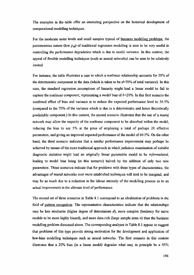
The examples in the table offer an interesting perspective on the historical development of

computational modelling techniques.

For the moderate noise levels and small samples typical of business modelling problems, the

parsimonious nature (low pejy) of traditional regression modelling is seen to be very useful in

controlling the performance degradation which is due to model variance. In this context, the

appeal of flexible modelling techniques (such as neural networks) can be seen to be relatively

limited.

For instance, the table illustrates a case in which a nonlinear relationship accounts for 20% of

the deterministic component in the data (which is taken to be d=70% of total variance). In this

case, the standard regression assumptions of linearity might lead a linear model to fail to

capture the nonlinear component, representing a model bias of b20%. In this first scenario the

combined effect of bias and variance is to reduce the expected performance level to 54.5%

(compared to the 70% of the variance which is due to a deterministic and hence theoretically

predictable component.) In this context, the second scenario illustrates that the use of a neural

network may allow the majority of the nonlinear component to be absorbed within the model,

reducing the bias to say 5% at the price of employing a total of perhaps 20 effective

parameters, and giving an improved expected performance of the model of 60.5%. On the other

hand, the third scenario indicates that a similar performance improvement may perhaps be

achieved by means of the more traditional approach in which judicious examination of suitable

diagnostic statistics might lead an originally linear parametric model to be reformulated,

leading to model bias being (in this scenario) halved by the addition of only two new

parameters. These scenarios indicate that for problems with these types of characteristics, the

advantages of neural networks over more established techniques will tend to be marginal, and

may be as much due to a reduction in the labour intensity of the modelling process as to an

actual improvement in the ultimate level of performance.

The second set of three scenarios in Table 8.1 correspond to an idealisation of problems in the

field of pattern recognition. The representative characteristics indicate that the relationships

may be less stochastic (higher degree of determinism d), more complex (tendency for naïve

models to be more highly biased), and more data-rich (large sample sizes n) than the business

modelling problem discussed above. The corresponding analyses in Table 8.1 appear to suggest

that problems of this type provide strong motivation for the development and application of

low-bias modelling techniques such as neural networks. The first scenario in this context

illustrates that a 20% bias (in a linear model) degrades what may in principle be a 95%

196

performance level (based on deterministic content) down to an expected level of only 76%. In

this context, the following scenario indicates that the additional flexibility of a neural network

model (reduction in bias from b=20% for the linear case to b=5%) compensates many times

over for additional model complexity (p=lOOOOO), giving an improved performance of 89.8%.

The relative importance of bias-reduction over variance-control in this context is illustrated in

the third scenario, which indicates that the diagnostic testing/reparametrisation approach may

also lead to perfonnance improvements over an initial model, but typically not of quite the

same scale as those achieved by the truly low-bias neural network approach.

However, whilst both regression modelling and neural networks represent natural and useful

solutions to the bias-variance tradeoff given the types of problems that they were designed to

solve, the final set of scenarios indicate that the situation is very different for problems

involving financial forecasting - in today's markets at least. Under the assumption that easily

detectable linear components of asset price dynamics have already been largely "arbitraged

away" it is plausible that naively parametrised linear models can be considered highly-biased

with respect to any detennirnstic component in asset price dynamics. Meanwhile the increased

number of parameters in even relatively parsimonious neural networks will tend to negate the

effect of any bias reduction through an associated increase in variance. The performance

improvement between the two scenarios, neural network (pe2O) and neural network (p=l6),

suggests that the specification of the neural model may play a key role in determining whether a

positive level of performance can be achieved. The final two scenarios likewise suggest that for

a problem with characteristics typical of the financial forecasting domain, a parametric model

will only be expected to achieve positive performance if the underlying modelling assumptions

are not greatly dissimilar to the actual nature of the underlying relationships.

Furthermore the discussion above neglects the effect of model selection bias or "data snooping"

(see Section 12.1.2). This is the bias which is introduced by repeatedly "tweaking" or

reformulating a model, selecting the formulation which leads to the greatest (apparent) level of

performance, and taking this as a measure of expected future performance. The magnitude of

the upward bias depends on the number of models investigated, the model variance, and the

correlation between the models (choosing between 20 identical models will induce no selection

bias). To illustrate this effect, we performed a simple Monte Carlo analysis based on the

expected value of the maximum of a set of n trials, and discovered that choosing between 10

uncorrelated values will induce a bias of approximately 1.6 times the individual variance, 100

models 2.5 times variance and 1000 models 3.1 times variance.

197

In our idealised business modelling example, model selection bias can be considered relatively

insignificant because the "performance signal to noise" ratio (of expected performance to

model variance) is approximately 45. In the pattern recognition case the equivalent ratio is

almost 200 and the deleterious effects of selection bias are again likely to be more than offset

by the potential for bias reduction which is achieved by considering alternative

parameterisations or formulations of the estimator. In contrast, the situation in financial

forecasting is that model variance is approximately comparable in magnitude to the

deterministic component in the data and hence "data snooping" represents a very real risk -

typically leading to the creation of models with an apparent, but in fact totally spurious,

predictive ability.

Thus neither traditional statistical methodology nor the emerging flexible modelling techniques

of machine learning are ideally suited to the particular nature of problems in investment

finance. The inherent weaknesses of the two "families" of modelling tools, in the context of

financial forecasting, forms the primary motivation for all three parts of our modelling

methodology, but this second, predictive modelling, part in particular.

The pre-processing methods in Part I are intended to look at prices from the novel perspective

of statistical mispricing, aiming to maximise the predictable component d and to enable the

possibility of forecasting the dynamics of the mispricing time-series. The model combination

methods in Part III are intended to control the risks which are posed by selection bias and

model instability and thus enable exploitation of the potential informational advantage provided

by the predictive models. However, the modelling procedures described in the subsequent

chapters of this part of the thesis form the core of our methodology as they are used to actually

construct the forecasting models themselves.

From a methodological perspective, the objective of the modelling algorithms is to capture the

maximum possible amount of the predictable component in the mispricing dynamics. This

involves mininiising model bias by building only appropriate assumptions into the models,

whilst simultaneously controlling the effects of model variance, by keeping the effective

number of parameters in the models sufficiently low. The basis of our attempted solution to this

problem is a synthesis of statistical and neural modelling techniques, which aims to exploit the

flexibility of neural models whilst ensuring that this flexibility is employed in a controlled and

appropriate manner. The medium through which this synthesis has been achieved is a particular

perspective, from which neural networks and traditional statistical models are viewed as being

based on a similar, fundamentally data-centred, approach to modelling. The "equivalent

198

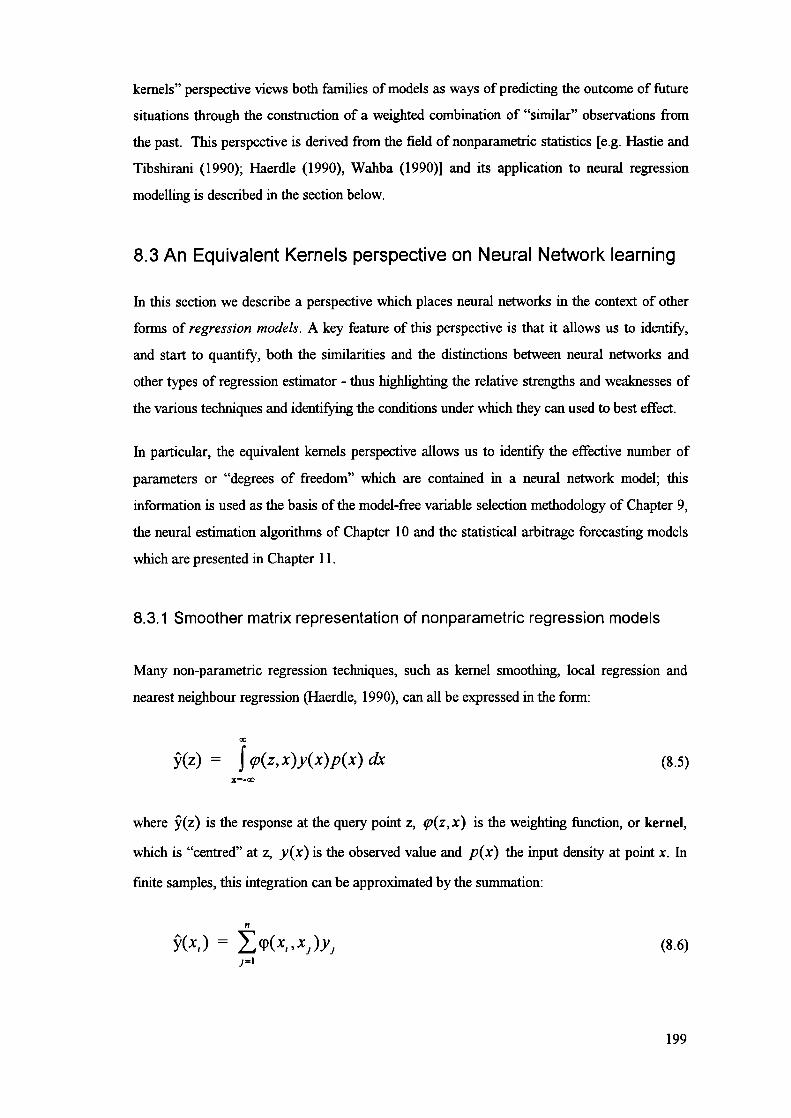
kernels" perspective views both families of models as ways of predicting the outcome of future

situations through the construction of a weighted combination of "similar" observations from

the past. This perspective is derived from the field of nonparametric statistics [e.g. Hastie and

Tibshirarn (1990); Haerdle (1990), Wahba (1990)] and its application to neural regression

modelling is described in the section below.

8.3 An Equivalent Kernels perspective on Neural Network learning

In this section we describe a perspective which places neural networks in the context of other

forms of regression models. A key feature of this perspective is that it allows us to identify,

and start to quantify, both the similarities and the distinctions between neural networks and

other types of regression estimator - thus highlighting the relative strengths and weaknesses of

the various techniques and identifying the conditions under which they can used to best effect.

In particular, the equivalent kernels perspective allows us to identify the effective number of

parameters or "degrees of freedom" which are contained in a neural network model; this

information is used as the basis of the model-free variable selection methodology of Chapter 9,

the neural estimation algorithms of Chapter 10 and the statistical arbitrage forecasting models

which are presented in Chapter Il.

8.3.1 Smoother matrix representation of nonparametric regression models

Many non-parametric regression techniques, such as kernel smoothing, local regression and

nearest neighbour regression (Haerdle, 1990), can all be expressed in the form:

(z) = Jço(z,x)y(x)p(x) dx (8.5)

where (z) is the response at the query point z, (z, x) is the weighting function, or kernel,

which is "centred" at z, y(x) is the observed value and p(x) the input density at point x. In

finite samples, this integration can be approximated by the summation:

= p(x,,x)y3 (8.6)

199

Thus the response at each point x 1 is a weighted average of the observed target values across

the entire dataset. The complete set of weighting kernels comprise the smoother matrix S:

(p(x1,x) (p(x1,x2)

(p(x1,x,,) y1

= (p(x2,x1) p(x2,x2)

y2(8.7)

.9,, (p(x,,,x1)

ç(x,,,x,,) y,,

Which can be expressed in matrix notation as:

= Sy (8.8)

Smoother matrices provide a natural representation for non-parametric statistical models. The

simplest example of a smoother matrix is that of a "look up table":

10...0

01

SL=. (8.9)

0 ......1

In this case the smoother matrix is the identity matrix and the "fitted value" or response at

point x, is simply the corresponding observed value y. Another model with a simple

smoother-matrix representation is the sample mean:

1/n 1/n •• 1/n

1/n 1/nSA,=

(8.10)

1/n ......1/n

The smoother matrix in this case reflects the fact that the fitted value is an equally weighted

combination of all of the observed values y., irrespective of the corresponding input values x,.

The smoother matrix S can be used as the basis of many useful statistical diagnostics. For

instance, because the model is expressed in terms of the influence of each observation on the

response at each sample point, it is possible to identify those observations which dominate the

model prediction at a particular point. An in-depth study of this, and related, issues regarding

extreme observations in both input-space (influence points) and output space (outliers) is

200

presented in (Bolland, 1998). It is also possible to calculate the model bias and variance at each

sample point [see (I-Iaerdle, 1990) for details of this process in the context of nonparametric

regression].

The key measure in which we are interested is the "degrees of freedom" which are absorbed

by the model. The degrees of freedom measure summarises the extent to which the reduction in

insample mean-squared error (MSE) is merely due to the fact that the observed values are used

both to estimate the model fit and to calculate the MSE, as opposed to the capture of true

structure within the data.

Consider the two examples of the look-up table and the sample mean. In the case of the look-up

table, the fitted value is identical to the observed value and so the (insample) residuals are all

zero. However this does not (necessarily) reflect any generalisation ability in the model, but

merely the fact that all of the degrees of freedom in the original data are absorbed by the model.

In contrast, the residual errors around the sample mean will typically be non-zero, reflecting

the fact that only one degree of freedom has been absorbed.

Depending upon the assumptions which are made about the nature of the model, a number of

slightly different expressions can be used to relate the structure of the smoother matrix S to the

degrees of freedom dofs; however in the case of fitting using ordinary least squares (OLS) they

all turn out [see pp 52-55 of(Flastie and Tibshirani, 1990)] to be equivalent to:

dof5 = S 11 = trace(S)

(8.11)i=Ln

It is straightforward to confirm that in the case of the look-up table SLUT, this measure equals

the number of observations 'n', and that for the sample mean S 1 absorbs a single degree

of freedom.

Perhaps the initial lack of a similar degrees of freedom measure for neural networks has been

one of the largest obstacles to the development of statistical significance tests and diagnostics

equivalent to those used in regression modelling. Somewhat paradoxically, this weakness has

had the advantage of stimulating the development of alternative approaches to model validation

and selection, such as cross-validation, bootstrapping and out-of-sample testing. However, it

has probably also reduced the credibility of the emerging modelling techniques and hindered

their uptake within the statistical modelling community. More importantly, the lack of

statistical significance measures that can be applied on an insample basis reduces the

201

effectiveness of neural modelling in situations where only small samples of noisy data are

available. In such cases, leaving data aside for purposes of selection or validation may

seriously degrade the quality of the model fit itself.

However, in recent years the nonparametric approach to estiinatrng the degrees of freedom in a

model has been generalised to include both simple parametric models and neural networks. The

following two sections review these extensions and discuss their implicaitons, firstly in the case

of standard "linear in the parameters" approaches such as OLS regression, and secondly to

more flexible neural network models.

8.3.2 Equivalent kernels for parametric models

If the smoother matrix representation and degrees of freedom measure were only applicable to

nonparametric models then they would still be very useful and important tools. However, the

same concepts can be extended to traditional parametric regression models through the

perspective of "equivalent kernels". Whereas in the nonparametric case the "kernels" which

comprise the smoother matrix are explicitly specified, in the case of parametric models the

smoother matrix is implicitly defined by the combination of parameterisation and estimation

procedure.

Consider a model of the form:

$(x,)= W;1k(Xj)

(8.12)k=1..m

i.e. a weighted combination of some arbitrary transformations of the input variables. Note that

the vast majority of statistical models, including many neural network formulations, can be

represented in such an "additive" form. The crucial feature of the model is that although the

basis functions dk are described with respect to the vector of independent variables x, the

parameters w are detennined, through the estimation procedure, with respect to the set of

observed values y1 . In particular, the effect on the model estimates of a perturbation or

contamination of a particular observation is given by the chain rule of derivatives:

-4k(x,)- (8.13)k=1 m k=1 m 4' âv

202

1S21-mi

0.10.060.060.040.02

0.002.004006

0.140.120.1

13

i.e. the effect on the fitted value 5(x1) of perturbing the observed values can be defined in

terms of the changes which are caused in the weights by which the (predefined) basis fimctions

are combined. By comparison with Eqn. (8.6) we note that this partial derivative is directly

equivalent to the elements which comprise the kernel flmctions (p(X1 ,x1 ). Hence we obtain

the so-called "equivalent kernels" and the smoother matrix for the parametric model is defined

by:

4(x) c(x) •• 4(xi)4'2 4'fl

4(x2 ) (x2)

S

(8.14)

This formulation allows us to compare on equal terms models with different parametric

representations and even parametric models with models which are not explicitly parameterised

(i.e. non-parametric models). Examples of equivalent kernels for different classes of parametric

and non-parametric models are given by (Hastie and Tibshirani, 1990) whilst a treatment for

Radial Basis Function (RBF) networks is presented in (Lowe, 1995).

For models with low-dimensional input-space, the equivalent kernels can be visualised by

plotting the kernel weightings as a flmction of the input vector x. Figure 8.1 illustrates

equivalent kernels from simple fixed-basis regression models with different types of basis

function:

0.05

Figure 8.1: Examples of equivalent kernels for sünple regression models. The kernels show the

"influence" fwictions of the models, sampled at different points in input space. The models are, from left

to right: linear regression, superposition of two sigmoid functions, and superposition of two gaussians.

Note the rigid stnicture of the linear model as opposed to the localised and more flexible kernels from

the non-linear models.

203

The equivalent kernels illustrate the sensitivity of the model 5(x ) at a given point x, to the

observed values at all other points in the estimation set. For the linear case (on the left) the

kernel labelled S2 1 indicates that the response at the mean x-value will be an equally weighted

combination of all observations, i.e. the sample mean. In contrast, equivalent kernel Si

corresponds to the mimimum x-value, the kernel weights are greatest at nearby observations

and decline linearly as a function of distance. In fact, a defining feature of linear models is that

the equivalent kernel is always a hyper-plane in input-space, with the orientation and slope of

the kernel depending on the direction and distance from the sampled point to the centre of the

input distribution.

The equivalent kernels for the two nonlinear models appear veiy different to the linear case, in

that the kernels are more highly localised and vary in shape depending upon the point in input

space at which they are sampled. This effect is most noticeable for the equivalent kernels

sampled at the centre of the input space (labelled S2 1 in each case). Unlike the linear case, the

response at the mean x-value will not necessarily equal the (global) sample mean.

This difference between the linear and nonlinear models is actually slightly misleading, as all

three models are of the additive form defined in Eqn. (8.12). The transformation by the

nonlinear basis functions changes the notions of "distance", and "locality" to reflect the

similarity of the transformed values as opposed to the original x-values, causing the equivalent

kernels to appear nonlinear when viewed in the original space

If the transformed values better reflect the inherent "similarity" of two observations, then the

use of a transformation should be expected to improve the accuracy of the estimated model.

The estimation method itself, however, is blind to the origin of the variables and thus, for a

predefined set of transformations, the smoother matrix follows the properties of linear

regression in that it is both symmetric and idempotent. An important consequence of this is that

the number of degrees of freedom absorbed by such an additive model is equal to the number of

transformed variables m.

8.3.3 Equivalent kernels for neural networks

The ability to estimate equivalent kernels, and to calculate the number of degrees of freedom

which are absorbed by the model, depends on the use of both fixed basis functions and on

standard Ordinary Least Squares (OLS) estimation. This is typically the case in parametric

204

models and even for some neural networks (such as some forms of RBF networks). However,

for a neural network with more than one layer of adjustable weights, the basis functions

themselves are parameterised (rather than fixed) and thus become dependent on the training

data. Consequently the equivalent kernels are also data-dependent, and the problem of finding

the equivalent kernels becomes non-linear. Similar complications arise in the case where the

estimation procedure itself is biased by the use of a regularisation procedure such as ridge

regression or the equivalent "weight decay" approach to neural estimation (see Section 2.2.4).

The solution to this problem is found in the work of Bolland (1998), following earlier work by

Moody (1992) and Burgess (1995). Moody (1992) was the first to note that not all parameters

in a neural network should be viewed as absorbing a full "degree of freedom". In his

terminology, the number of effective parameters, Peff, may be less than the actual number of

parameters contained in the neural network model. The equivalent kernels perspective on neural

networks was first investigated in Burgess (1995) using an empirical perturbation-based

methodology. Bolland (1998) built on both the equivalent kernels perspective of Burgess

(1995) and the analytic approach of Moody (1992), presenting an analytic approximation to

the degrees of freedom in a neural network and extending this perspective in the context of

general loss functions other than OLS, as reviewed below.

Analytic approximation of the smoother matrix for neural networks

From Eqn (8.14) we note that the elements of S correspond to the partial derivatives of the

fitted model at each point with respect to each observed value. Expanding the derivatives in

tenns of the model parameters, in this case the vector of neural network weights

w=[w1 W2 ... Wm] we obtain:

=c99 9Wk = (

V 9 T êw

k-i. mk Y1(8.15)

which corresponds to Eqn. (8.13) for the fixed basis function models discussed above. Taking

a first-order Taylor expansion of the loss function of the perturbed model about the original

model we obtain:

205

VL(y+dy,X,w)= VL(y,X,w)

+ VV,L(y,X, w)dy + VVL(y,X,w)dw (8.16)

Assuming that both the original set, w, and perturbed set, w - w of weights minimise the

empirical loss function L, then VL(y,X,w) = 0, and VL(y + dy,X,w) = 0. Thus,

neglecting higher order terms, we obtain the change in the network weights which is due to a

perturbation in the observed values:

dw = (vv L(y,X, ))' VVL(y,X, w)dy (8.17)

The first term on the right-hand side, the second derivative of the loss function with respect to

the model parameters, is known as the Hessian of the model. Substituting for dw into Eqn

(8.15) and expressing the result in matrix form gives:

s = (vj)T(vv L(y,X,w)) ' L(y,X,w) (8.18)

However for loss functions where the error component is quadratic, L = 1/2 (y - )2,

then

even in the presence of a regularisation term, we have VVL(y,X, w) = —Vj), and so the

smoother matrix is:

s =(8.19)

A final simplification is sometimes used in which the full Hessian V W

L(y, X, w) is

replaced by a more-stable linearised approximation (v9)(v.p)T giving the expression:

s = (vJ)T[(vc)(v..c)T]_l(v5)

(8.20)

As before the number of degrees of freedom in the network are given by

doff = ES,, = trace(S).

206

04

'4

3

_______ 'Ilh _____h. l,.. -t-'I-. ..1 .1L

Simulation results

Figure 8.2 shows examples of equivalent kernels from a univariate neural network trained to

reproduce the first two periods of a sine-wave, sampled at 41 points evenly spaced between 0

and 4it.

Figure 8.2: Equivalent Kernels for a univariate neural network trained to reproduce Sin(x); from left to

right, the three figures represent the kernels for x = 0,; and 2,t. The neural network consisted of a

single hidden-layer of four sigmoid units, a shortcut connection from input to output, and a linear output

unit, trained using the standard backpropagation learning algorithm (see Section 2.2.4)

The trained network was found to absorb 8.2 degrees of freedom, compared to the 14 potential

degrees of freedom represented by the parameters, and the 6 degrees of freedom for an

equivalent model with fixed transfer functions. This confirms (a) that the network is not

completely utilising its potential capacity, as suggested by Moody (1992); and (b) that

perturbations in the training data are partially accommodated by adjustments to the basis

function themselves.

We can also investigate the eficts of model regularisation on the ability of the network to

reproduce the target function, the number of degrees of freedom absorbed by the network, and

the kernel functions themselves. Using standard quadratic weight decay, we minimise a loss

function of the form:

1 2L = - (y, - + r w

j-1..m(8.21)

Selected results from this analysis are presented in Figure 8.3, below.

207

* — - a &.z. - WI

91

I R-d.4

I

Figure 8.3: Analysis of urnvariate network trained to reproduce a sine wave. The left-hand chart presents

a comparison of the network function (with r=O) and the function reconstructed from the estimated

kernels; the right-hand chart demonstrates the effect of the weight decay factor, r, on both network

performance (R2) and capacity (degrees of freedom).

The results in the figure indicate that the estimated kernel function reproduces the actual

network function very closely, indicating that the estimated equivalent kernels are also highly

accurate. Increasing the amount of weight decay serves to reduce the degrees of freedom of the

model, and in this noise-free example, the performance of the model is seen to degrade

accordingly.

It is in multidimensional problems, however, that the real power of neural networks as

parsimonious yet flexible function estimators is demonstrated. This power lies in the fact that

the shape of the kernels can vary in different regions of the input space. As an illustration,

kernels from a 2-dimensional model are shown in Figure 8.4 below.

The figure clearly illustrates the changing shape of the kernel functions in different parts of the

input space. The first kernel, generated at (-4/7, -4/7), exhibits a ridge-like structure, albeit

with some curvature. The second kernel, generated at (0,0), is a broad hummock with negative

sensitivity to points near the corners. The third kernel, generated for (2/7, 6/7), shows a distinct

curvature which echoes the ring shape of the original function.

These results demonstrate that the equivalent kernel functions of the neural network vary

significantly in different regions of the input space, not just in terms of "spread" but also

regarding the overall shape of the kernels. This supports the view that the representational

power of neural networks arises from an ability to parsimoniously exploit the degrees of

freedom within the model, in a way which is in some sense optimally related to local properties

of the data itself, rather than according to some external global parameterisation such as the

"bandwidth" parameters used in the kernel smoothing techniques of nonparametric statistics.

208

Y•• .-..-• ..

I

•t--.

6543

0

-2

E°:

iL't1i3.:::.. -2' -I,f

Figure 8.4: Equivalent Kernels for a neural network estimator of the function = + 3o(x2 + - 03)2]

sampled on a regular 15 by 15 grid running between plus and minus one. This function was

approximated using a 2-8-1 network with sigmoidal hidden units and a linear output unit.

8.4 Summary

In this chapter we have noted that estimating forecasting models of the mispricing dynamics

can be seen as a particular case of the general model estimation problem. A simple analysis of

the effect of model bias and variance on the expected level of forecasting ability highlights the

particularly difficult nature of financial forecasting problems. We suggest that these difficulties

may be alleviated by developing methodology which represents a synthesis of statistical and

neural modelling techniques, aiming to exploit the flexibility of neural models whilst ensuring

that this flexibility is employed in a controlled and appropriate manner.

209

The ability to transform neural network regression models into an equivalent kernel

representation raises the possibility of harnessing the whole battery of statistical methods which

have been developed for non-parametric techniques: model selection procedures, prediction

interval estimation, calculation of degrees of freedom, and statistical significance testing

amongst others. The recent work of a number of authors has a similar underlying theme.

Reference has already been made to the work of Moody (1992), Amari (1995) and Bolland

(1998), in addition Williams et al (1995) describe an equivalent kernel approach to estimating

error bars for RBF networks with a single layer of adjustable weights.

Most importantly for our purposes, the equivalent kernel perspective allows the modelling

process to be viewed as an explicit trade-off between the variance which is exvlained and the

number of degrees of freedom which are absorbed by a model. In the following chapters we

develop model-free variable selection and neural estimation procedures which are based upon

the tradeoff between these two fundamental properties of regression estimators.

210

9. Model-free variable selection

This chapter describes our methodology for model-free variable selection, by which we indicate

the intention that the methodology should be sensitive to a wide range of relationships, rather

than being predicated upon the assumption of a particular functional form. Section 9.1

describes the statistical significance tests which we use as the basis of the methodology. These

tests exploit the equivalent kernels perspective, in which all regression estimators can be seen

as ways of predicting the outcome of future situations through the implicit construction of a

weighted combination of "similar" observations from the past. In particular, the significance

testing methods are based upon the "F-ratio" of the amount of variance which is absorbed by a

model, and the degrees of freedom which are employed in so doing. Section 9.2 describes the

implementation of our methodology, in which a diverse set of basis functions are employed in

order to screen data for a wide range of potentially predictable components. Section 9.3

describes a Monte Carlo evaluation of the statistical power of the variable selection tests

against alternative hypotheses which contain only a small deterministic component and hence

are close to the null hypothesis of no predictable component. The power of the tests is

evaluated in two contexts, firstly in terms of the ability to detect any predictable component in

the data, secondly to detect explicitly nonlinear relationships. Section 9.4 contains the results

of a second Monte Carlo experiment to quantify the model bias which is imposed by the use of

each particular family of basis functions.

9.1 Statistical methodology for model-free variable selection

In this section we describe the basis of our methodology for model-free variable selection. The

objective of this stage of the modelling process is to identify the subset of variables X I

which should be used as the basis of the model estimation process. The reason for this pre-

selection may simply be that it is infeasible to include all of the variables in the model

estimation proper, perhaps because the resulting model would have too many parameters to

estimate from the available data. Alternatively, the preliminary filtering process may be

intended simply to reduce the number of variables with the intention of reducing the complexity

of the estimated model and hence the error which is due to model variance.

The aim of the methodology is to be "model free" in the sense that it should be sensitive to a

wide range of relationships, rather than only those which follow a particular functional form.

The flexibility of the variable selection procedure is vital in order to avoid imposing a hidden

211

on the subsequent stages of modelling by removing deterministic components in the data

simply because they are invisible to the variable selection procedure. In order to achieve this

flexibility, our variable selection methodology is based upon techniques from nonparametric

statistics, and in particular nonparametric regression. Specifically, we regress the dependent

variable upon a wide range of transformations of the variables and test for significant

relationships by analysing the so-called "F-ratio" of the variance explained by the model to the

degrees of freedom that it contains.

Linear Relationships

In order to motivate the use of a flexible variable selection methodology, let us first consider

the problems which would arise by using standard linear methodology at this stage of the

modelling process.

The standard linear regression model takes the form:

y. = a + /31 x11 + /32 x21 +. . .+/3X, 1 +6. (9.1)

Variable selection in this case is relatively straightforward, because the effect of each variable

xj is associated with a single parameter /3,. Under the null hypothesis that is unrelated to

y then the so-called 't'-statistic fl3 /se is known to follow a standard 't' distribution with

n - (m + 1) degrees of freedom, where n is the number of observations and m is the number of

variables in the model. A less precise measure of (linear) variable significance is based on the

(Pearson) correlation coefficient

1

- —(x - x)(y1 —y)

- cr,

XY -

(x, - 2 - )2 - a

in , in

Unlike the measures based on the regression coefficients the correlation coefficient ignores

any cross-correlations between the various x, 's. However, because it has the advantage of

being easy to compute for large numbers of variables, it is often used as a "pre-screening" tool

to reduce the number of variables to a manageable level before moving on to the more

computationally and data intensive phase of model estimation proper.

(9.2)

212

The additional complexity of nonlinear models entails that the variable selection process is

both more important and more dJjk'ult to perform - at least without imposing substantial

biases to the modelling procedure as a whole. A general nonlinear model with m regressors can

be broken down into submodels which relate to sub spaces ranging from one-dimensional up to

the entire space:

y= >2f,(x,)^ fjJ,k(xj,xf,xk)+.....+f(x.....Xm)+ (9.3)i1.mJ=1.J i=1..mj=1.ik=1..J

In the linear case the higher tenns do not exist, as can easily be seen in the case of the second-

order term:

f, 1 (x 1 ,x1 ) =f1(x1)+f(x)

f3x, +/3x (9.4)

Therefore, the properties of independence and linearity vastly simplify the nature of the

variable selection problem. Unfortunately, applying a linear test, such as the correlation

coefficient p,, in a situation where nonlinear relationships may exist is highly dangerous as it

will fail to detect either higher order "interaction" effects such as f,, (x, ,x) or univariate

relationships f,(x1 ) which do not contain a significant linear component. Thus, in order to

avoid discarding potentially invaluable infonnation, we have developed an alternative "model

free" variable selection procedure which relaxes the bias towards purely linear relationships

and is capable of identifying a wide range of nonlinear and interaction effects.

Basic Methodology

The approach which we take is to regress the dependent variable upon nonlinear projections of

the original variables to produce submodels of the form:

y=a+ (9.5)

j1..m

Where the basis fi4nctions b3 (x,) are chosen in such a way that in combination they can

approximate a wide range of functional relationships, with properties similar to those which are

believed to exist in the true mispncing dynamics (i.e. smooth functions of low-dimension and

high noise content). The fundamental test for a statistically significant relationship is that the

213

amount of variance explained by the model should be large, relative to the number of free

parameters. p, which were fitted to the data. Under the null hypothesis that x, is unrelated to

y, it is known that the F-ratio of the model should follow an F-distribution with p degrees of

freedom in the numerator and n-(p+1) in the denominator, i.e.:

P ,=1..n )=lm[[a+ 9)bj(xl)]-YJ

2 -, 11p,n—(p+1) (9.6)

193b (x1)jJ

n - (p + 1) iLn j=I.,n

The tests can also be used to test for interaction effects between variables; to do so the basis

functions act as a nonlinear projection of the subset of the original variables which is being

tested. In the two dimensional case the submodels are of the form:

y=a+

(9.7)

k=1..m

The variable selection algorithm consists of "screening" all the low-dimensional combinations

of the candidate variables, constructing appropriate submodels, and testing for evidence of a

significant deterministic component in the target series when it is conditioned on the particular

submodel. As the number of combinations grows exponentially with the dimensionality, the

maximum feasible cardinality of the sub space will typically be either 2 or 3. Clearly this

imposes a bias on the modelling procedure as a whole. Given the underlying assumption,

however, that the predictable component is primarily contained in low-dimensional subspaces,

it is hoped that the bias will be more than offset by the simultaneous reduction in model-

variance which results from reducing the input space used by the model estimation procedure.

OLS procedure

In the simplest case the model parameters 9, are estimated using ordinary-least-squares (OLS)

regression, where the cost function with respect to which the parameters are optimised is

simply the mean-squared error:

n( [ m2

1"

E0 y, -a+9b1(x,)L

=) 2(9.8)

214

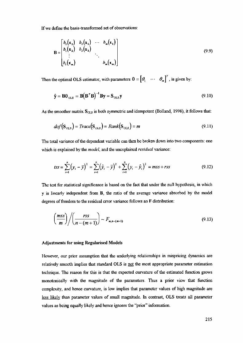
If we define the basis-transformed set of observations:

b1 (x j) b2 (x 1 ) bm(Xi)

B= b1 (x 2 ) b2(x2)

b i (X m ) b(X)

Then the optimal OLS estimator, with parameters 8 =

= B80 = B(BTB) 1 By = S0y

(9.9)

is given by:

(9.10)

As the smoother matrix SOLS is both symmetric and idempotent (Bolland, 1998), it follows that:

dof (S OLS ) = Trace(S QLS ) = Rank(S OLS ) = m

(9.11)

The total variance of the dependent variable can then be broken down into two components: one

which is explained by the model, and the unexplained residual variance:

tss=(y1 _)2 _)2 +E(y, .)2

=mss+rss

(9.12)

The test for statistical significance is based on the fact that under the null hypothesis, in which

y is linearly independent from B, the ratio of the average variance absorbed by the model

degrees of freedom to the residual error variance follows an F distribution:

) /1 rss

m / n—(m+1))(9.13)

Adjustments for using Regularised Models

However, our prior assumption that the underlying relationships in mispricing dynamics are

relatively smooth implies that standard OLS is the most appropriate parameter estimation

technique. The reason for this is that the expected curvature of the estimated function grows

monotomcally with the magnitude of the parameters. Thus a prior view that function

complexity, and hence curvature, is low implies that parameter values of high magnitude are

lesslikely than parameter values of small magnitude. In contrast, OLS treats all parameter

values as being equally likely and hence ignores the "prior" infonnation.

215

The solution to this discrepancy is to use an appropriate regularisation technique, which biases

the estimation procedure in such a way as to reflect the prior assumptions. In this case we use

"ridge regression" (Hoerl and Kennard, 1970) which is equivalent to assuming a prior

distribution for the parameters t9, which is gaussian and centred on zero. The optimal

regularised parameters will depend on the degree of regularisation r, producing the estimator:

=BO = B(B T B+rI)By=S o y (9.14)

An important feature of ridge regression is that, relative to standard OLS, the number of

degrees offreedom absorbed by the model is reduced:

dof(S G) = Trace(S G ) ^ m

(9.15)

and the F-test for statistical significance is adjusted appropriately:

(mss ___________rss

dof (S G)J/[ fl - [ dof (S G ) +1])(9.16)

Adjustments for using Neural Networks with adaptive basis functions

As discussed in Section 8.3, the basis functions, or rather the "equivalent kernels", for neural

network models are not predetermined, but instead are themselves estimated from the data. The

purpose of the neural network learning algorithm is to determine the parameters which

minimise the "cost function" E:

I- m

= minE = min —(y _NN(x,,e) 2 +rO (9.17)e [2n

1=1 ' j=1 ]

Where the r term represents a "weight decay" or regularisation term which controls model

smoothness in a manner similar to the ridge regression used for the fixed basis-function models.

From Section 8.3.3, the degrees of freedom absorbed by the neural network model are given by:

s = v NN(x,e)T[v9v8E] 1

V 9 NN(x,e) (9.18)

216

and the test for significance is based on the degrees of freedom obtained from the smoother

matrix:

mss ___________rss

trace(S )J/[n - [trace(S) +1]]ace(),n—(e(}1) (9.19)

9.2 Implementation of Variable Selection Methodology

The main issue in implementing the variable selection methodology is the specification of the

basis functions b3 (x1 ). In avoid to avoid imposing any strong biases at this preliminary stage

of the modelling procedure we employ a range of different model types, from untransformed

linear models, through fixed basis-function models to neural network models. The particular

parameterisations which we implement within our procedure are defined in Table 9.1 below.

Model Type Specification Number of

Parameters

nd + 1LinearL(xi,x2,...,x) = a

1=1

Polynomial

1=0

11= 0 =0

Bin- B(xl,x2,...,xd) - nd

smoother • nd rank(xd)

flJ1 if(idl)^

....1,.4 1 flM' d1 Ø otherwise

RBF nd' +1'

Network L.=1

MLP (nd+2)c+1M(x1,x2.....x,)=a+/ b,+w,,x1j

Network :=1 j=i I

Table 9.1: Specification of the different families of basis function which are implemented within the

variable selection methodology, nd is the dimensionality of the input subspace; c indicates the relative

level of complexity of the model.

Figure 9.1 presents examples of the basis functions generated by the five families of model.

217

- L -P2

-PLH________ .-B1

-

- 1 E 'EFigure 9.1: Univariate examples of the basis Ilinctions generated by each of the model families; from top-

left to bottom-right the models are linear (L), polynomial (P), bin-smoother (B), Radial Basis Function

(R) and Multi-layer perceptron (M).

The linear models (model type L) are of the standard linear regression form and are based on

the assumptions of linearity and independence between variables.

The polynomial models (model type P) can be considered a generalisation of the linear model

to allow for particular types of nonlinearity and interaction effects. Note that the ft000 term

is equivalent to the constant term a of the other formulations and that the polynomial model

with complexity c=l is equivalent to the linear model.

The bin-smoother models (or regressograms (Haerdle, 1990)) represent localised sets of basis

functions which are piece-wise constant indicator variables. The input space is divided into a

set of nd-dimensional boxes or "bins" and the indicator variable for the bin in which an

observation fulls is set to 1, whilst the other indicator variables are set to 0. The bin-smoother

model is capable of representing both nonlinear and interaction effects but unfortunately the

number of parameters scales exponentially in the number of input-dimensions. An additional

problem of the bin-smoother is the lack of smoothness of the estimated function, which is

discontinuous at the boundaries of the bins.

The Radial Basis Function models (model type R) are similar to the bin-smoothers in that the

basis functions are centred at particular points in the input space, but diffbr in that they have a

smooth (gaussian) response which decays gradually with the distance from the centre. The

number of parameters again scales exponentially with the input-space dimensionality.

218

The MLP Network models (model type M) are of the type of neural network known as "multi-

layer perceptrons", and can be considered as summations of projective basis functions which

have sigmoidal responses along arbitrary projections of the original input space. The particular

flexibility of these models derives from the fact that the basis functions themselves are

parameterised (by the projection "weights" w) and estimated from the data itself, rather than

being prespecified as in the cases of the other models. In neural network terminology the

number of basis functions c is often referred to as the number of "hidden neurons" in the

network. A further important advantage of the neural network models is the parsimonious

scaling behaviour, with the number of parameters being only linear in the input-space

dimensionality nd.

Statistical variable significance tests

Within the general framework of the statistical significance tests described in Section 9.1, we

have implemented four specific types of variable significance tests. These differ in the manner

in which the estimators are applied and in the component of the deterministic relationship which

is under scrutiny.

The first two types of test are simply aimed at detecting any deterministic component in the

data. The basic test in this case is a single-estimator test in which a given type of estimator is

applied to the data and tested for statistical significance. The second type of test recognises that

in a preliminary "filtering" stage it is preferable to err on the side of caution before concluding

that a variable should be eliminated from the analysis. Thus we define a joint test in which all

five types of estimator are applied to the data, with the most si gnificant of the findings taken

into account before deciding to eliminate a particular variable.

Note that by explicitly taking the maximum of a set of statistics, this approach introduces a

"data snooping" effect in which the relationships will tend to seem more significant than they

actually are, and in this case our results indicate that the false positive rate is approximately

double the nominal size of the test18 . If necessary, this bias could be explicitly corrected by

18 The exact magnitude of the effect will depend upon the correlation between the individual p-values derived

from the five different types of estimator (eg. taking the maximum of 5 identical tests would not produce a data

snooping effect)

219

constructing a Monte-Carlo distribution for the test statistic, as described for the predictability

tests in Part I of the thesis.

The remaining tests reflect the fact that, in some cases, the presence of nonlinear structure may

be of particular importance, either because it may influence the type of estimator which will be

employed in the modelling process proper, or, as in the case of many financial time-series,

because there is an underlying assumption that the linear component of any relationships will

already have been "arbitraged away" by market participants. Thus whilst the basic tests treat

linear and nonlinear components alike, we define modified test procedures in order to explicitly

identify nonlinear structure over and above any linear component. The test then becomes a

partial F-test in which the variance explained and degrees of freedom absorbed by the nonlinear

models are compared to the equivalent figures for the linear estimator. The F-test is then

conducted in terms of the additional variance which is explained by the nonlinear model, and

the additional degrees of freedom which are required in order to do so.

Empirical evaluation of variable selection properties through Monte Carlo simulation

The empirical properties of the variable selection methodology were tested by means of

extensive Monte-Carlo simulations. The objective of the evaluation was twofold: firstly to

quantify the ability to detect significant deterministic components and secondly to quantify the

bias of the different model types in terms of the extent to which they fail to represent the

underlying relationship in a manner which generalises to additional out-of-sample data.

In order to evaluate the flexibility of the variable selection procedure, a range of alternative

hypotheses are investigated, corresponding to the functional forms of the five different model

families specified in Table 9.1. Thus, in conducting a given simulation run, the detenninistic

component of the target data is constructed by taking a model of the appropriate class,

g e {L,P,B,R,M}, drawing the parameters at random from a (normal) distribution, and

applying the model thus generated to random input-vectors (x, , 1,2,.. . , x,,.,,) drawn from a

multivariate nonnal distribution.

The target data is then constructed from a weighted combination of the (nonnalised)

deterministic component ,X,2,. .. , x,,,,) and a stochastic component drawn from a

standard nonnal distribution. The resulting generating equation is given by:

220

g(x, 1 ,..., x, ,,,) — n-'g(x11,..., 9 20=

r2 + . J(i - d) N(0,l)

[g(x,i,..., x,,,.)_n_1 g(x,1,...,i-i,,

The parameter d controls the degree of determim.... with d= 1 the relationship is purely

deterministic; with d=O the relationship is purely stochastic; for 0 <d < 1 the relationship is

such that a fraction d of the variance of y is deterministic and fraction (1-d) is stochastic.

The results of the Monte Carlo experiments are described in the following two sections. Section

9.3 describes the results of the evaluation of the statistical power of the variable selection tests.

Section 9.4 describes the result of the evaluation of the bias of the families of estimator.

9.3 Evaluation of Variable Selection Test Power by Monte Carlo

Simulation

The effectiveness of the variable selection methodology was evaluated in terms of the power of

the tests, i.e. the probability that they will correctly identify the presence of a deterministic

component in the data. The flexibility of the tests was investigated by considering the five

different "alternative hypotheses" which are represented by the five families of model which are

presented in Table 9.1. In order to investigate the sensitivity to noise, three cases were

considered in which the magnitude of the predictable component was set to d=3 3%, 10% and

3.3%. The input dimensionality (nd) was set to two, reflecting both the prior assumption of low

dimensional relationships and a recognition of the poor scaling properties of some of the model

families (R, B and P).

For each predictability level, 100 realisations of each of the five model types were used to

generate a target time-series, and for each such time-series an estimator was constructed from

each of the different model families. The total number of models estimated was thus 3*5*5*100

= 7500. The length of each time-series was chosen to be 400 observations as being

representative of the typical sample-size available for modelling asset prices on a daily basis.

Single-estimator Tests

Table 9.2 presents a summary of the results of the basic form of the variable selection

methodology, i.e. single-estimator tests in which a given type of estimator is applied to the data

and the F-ratio of the model is tested for statistical significance.

221

Target Model Ty

Linear (L)

Bin-smoother (B)

Polynomial (P)

Estimator Model Type

d L B P R M

0.33 100% 100%

100% 100% 100%

0.1 99% 95%

96% 99% 99%

0.033 55% 22%

36% 48% 54%

0.33 67% 100%

96% 99% 100%

0.1 22% 99%

46% 64% 56%

0.033 4% 46%

6% 14% 11%

0.33 96% 89%

100% 100% 100%

0.1 79% 45%

93% 86% 92%

0.033 25% 8%

42% 33% 36%

RBF (R)

MLP (M)

Average

Overall

0.33 95%

0.1 83%

0.033 38%

0.33 98%

0.1 82%

0.033 29%

0.33 91%

0.1 73%

0.033 30%

100% 100% 100% 100%

81% 99% 100% 96%

29% 44% 59% 50%

98% 100% 100% 100%

82% 94% 95% 96%

29% 23% 36% 38%

97% 99% 100% 100%

80% 86% 89% 88%

27% 30% 38% 38%

65% 68% 72% 76% 75%

Table 9.2: Power of the variable significance tests at different levels of predictability d', broken down

by type of basis function used in the estimator, and also the nature of the underlying relationship. The

nominal size or "false positive rate" of the F-test for model significance is 1%, indicating that in the

absence of any true detection capability the test would be expected to indicate a significant result in I

case out of 100.

When the deterministic component represents 33% of the total variance (d=0.33) the majority

of the tests are 100% effective. The only substantial deviation from this pattern is the 67%

obtained by the linear estimator when the deterministic relationship is generated by a

smoother model - highlighting the differences in the underlying assumptions of these two

families of model.

When the potential predictability level falls to 10% the power of the tests is degraded somewhat

and a clustering of the results begins to appear. The relatively inflexible linear estimator is the

most affected, with an average power of only 73%, being sensitive only to the linear

component in any deterministic relationship. The smooth nonlinear estimators {P, R, M}

exhibit power of 85%+ with respect to each other but are much less efficient at detecting the

222

relationships generated by bin-smoother models. Similarly, the bin-smoother is 99% effective at

detecting relationships of the corresponding type, but only 45-82% effective at detecting

smooth nonlinear relationships.

In the third scenario, where the potentially predictable component represents only 0.03 3 of the

total variance of the target series, the power of the tests drops off noticeably. The three clusters

{L}, {P, R, M} and {B} are still apparent, but the average power of the estimators across all

types of relationship is roughly comparable. The most powerful tests overall are the neural

network fmilies R and M.

On a general level the results indicate that, for sample sizes in the order of a few hundred

observations, it is relatively easy to detect significant relationships when they account for as

much as 0.33 of the total variance of the target time-series. When the magnitude of the

predictable component is of the order of 0.10 it is still possible to identify relationships with

95% plus effectiveness, but typically gy when the nature of the estimator closely reflects that

of the underlying relationship. In cases where the predictable component is of the order of

0.03 3 the situation is much more difficult, with an average identification rate of only around

30%.

Joint Tests and the effect of the Significance Level

Table 9.3 presents the results of the joint tests which are conducted by applying all five types

of estimator to the data, and taking the most siamficant statistic as an indicator of the presence

of a deterministic relationship. The table also presents the results of increasing the test

sensitivity in another manner, by increasing the significance level (p-value) which represents

the acceptable "fulse positive" rate of the test.

d p-value L B P R M

0.33 0.01 100% 100% 100% 100% 100%

0.1 0.01 99% 99% 95% 100% 97%

0.05 100% 100% 100% 100% 100%

0.033 0.01 61% 48% 51% 67% 49%

0.05 82% 75% 74% 86% 73%

0.1 91% 82% 85% 92% 86%

Table 9.3: Power of the joint variable significance test in which all five estimators are used and the

most significant result taken Each column corresponds to a different type of underlying relationship.

(alternative hypothesis) The table also shows the effect of relaxing the significance requirement by

increasing the size (false positive rate) of the test.

223

As expected, the joint test is substantially more powerful than the single-estimator tests,

particularly for the lower levels of predictability. In the case d=0.33 there is no need to

increase the p-value as all relationships are detected successfully even at p = 0.01. At d=0. 10,

relaxing the p-value from 0.01 to 0.05 marginally improves the results from the already quite

impressive 95% plus to the maximum possible 100%. In the high noise case, d=0.033, relaxing

the p-value from 0.01 to 0.05 increases the detection rate from the range 48%-67% depending

on the nature of the relationship, to a range of 73% to 86%. A further relaxation to p=O.lO

improves the detection rate slightly, to a range of 82%-92%, but at this point the marginal

improvements appear unjustified by the increase in false positives which they would cause.

Explicit detection of nonlinear structure

Table 9.4 presents the power of the tests when applied in the context of detecting explicitly

nonlinear structure which is over and above any linear component. As noted in Section 9.2, this

test is in the form of a partial F-test which relates the additional variance which is explained by

the nonlinear model to the additional degrees of freedom which it contains.

d

0.33

0.1

0.033

0.33

0.1

0.033

0.33

0.1

0.033

0.33

0.1

0.033

0.33

0.1

0.033

Nature of relationship

Linear (L)

Bin-smoother (B)

Polynomial (P)

RBF (R)

MLP(M)

B P R

0% 0% 1%

0% 2% 3%

0% 2% 4%

100% 89% 99%

97% 38% 68%

54% 13% 26%

7% 100% 60%

7% 80% 42%

5% 31% 21%

26% 72% 83%

12% 52% 64%

5% 27% 40%

41% 89% 94%

20% 45% 68%

10% 13% 30%

M I Joint

2% 2%

6% 7%

7% 11%

97% 100%

53% 97%

17% 58%

90% 100%

59% 82%

24% 41%

76% 84%

59% 70%

31% 47%

97% 99%

74% 81%

22% 38%

Table 9.4: Power of the variable significance tests to explicitly identiij additional nonlinear structure

over and above any linear component Column 'd' indicates the magnitude of the deterministic

component of the data Columns B, P. R and M indicate the power of the single-estimator tests. The

fmal colunm indicates the power of the joint test based upon the most significant of the four estimators.

224

The results indicate that the ability to detect nonlinear structure varies widely depending on (a)

the nature of the underlying relationship (b) the type of estimator used and (c) the magnitude of

the predictable component.

When the underlying relationship is linear, any indication of nonlinearity is a "false positive"

and gives an indication of the true size of the test. In practice the figures range from 0 to 11 out

of the sample of 100, thus demonstrating that the actual size of the test can be much larger

than the nominal size of 1%. In the worst case, for the joint statistic, the size of the test is

inflated by the "data snooping" effect. A secondaiy pattern is the general trend for the false

positive rate to increase as the magnitude of the predictable component d decreases, indicating

that at low levels of predictability it is particularly difficult to distinguish between linear and

nonlinear effects.

When the underlying relationship is generated by a bin-smoother model, the detection of

nonlinear components is particularly high. The most effective case is the correctly specified one

in which the estimator is also a bin-smoother, with detection rates of 100%, 97% and 54% for

d values of 0.33, 0.1 and 0.033 respectively. The neural network model types R and M perform

only slightly worse and the polynomial model is least effective at detecting this type of

relationship. For the polynomial relationship the well-specified model performs best with rates

of 100%, 80% and 31%, the neural network models perform moderately, and the bin-smoother

is particularly ineffective. These results suggest that the underlying biases of the polynomial

and bin-smoother models are particularly incompatible, and that where they do coincide in

detecting structure the most likely reason is that they have both identified a significant linear

relationship in the data.

Finally, in the case of general, smooth, nonlinear relationships the two types of neural network

model perform similarly well, and substantially better than both the polynomial and, least

effective of all, the bin-smoother. Finally the overall detection rate is highest for the "Joint"

statistic; as mentioned above, however, this improved performance does come at the price of a

slight increase in the corresponding false positive rate.

Conclusion

The conclusion of this analysis is that the F-test methodology can serve as a suitable tool for

detecting both general relationships and also explicitly nonlinear relationships. The "detection

rate" varies greatly as a function of the magnitude of the deterministic component, from

225

generally close to 100% when the potentially predictable component accounts for a third of the

total variance (d=0.33), reducing to around 90% at d=0.1 and around 40% at d=O.033. This

suggests that for datasets of a typical size of a few hundred observations then the practical limit

of effectiveness for forecasting models is when the potentially predictable component accounts

for somewhere around this figure of 0.03 3 of the total variance, i.e. a signal to noise ratio of

approximately 1/33. Furthermore, in cases close to this borderline it may be preferable to

increase the p-value in acknowledgement of the uncertainty in the variable selection procedure,

and to err on the side of caution even at the price of risking the inclusion of insignificant

variables in the model estimation procedure proper.

9.4 Investigation of Model Bias using Monte Carlo Simulation

The results of the simulation experiments described in the previous section, to evaluate the

power of the variable selection methodology, can also be used to provide valuable information

regarding the relative biases of the different types of estimator.

The results in the previous section are primarily concerned with the detection of statistically

significant relationships, rather than the extent to which the estimator which is produced as a

means to this end accurately represents the underlying relationship. While this issue is more

appropriate to the model estimation stage proper, as described in Chapter 10, it is in any case

useful to understand the properties of the different families of estimator. In particular the

ability of the different types of estimator to accurately capture low-dimensional components of

the underlying relationship may have particular relevance to the design and implementation of a

constructive approach to neural model estimation. The reason for this is that the objective of a

constructive algorithm is to represent the broader relationship as an additive combination of a

number of simpler submodels, and clearly the properties of the individual submodels will

influence the overall performance of the algorithm.

The basis of our approach to predictive modelling is to jointly optimise the bias-variance

tradeoff by the use of appropriate assumptions and modelling procedures. Furthermore, we

have shown that the model variance is intimately linked to the concept of model complexity, in

particular as represented by the degrees of freedom which are absorbed by the model. There is

no general method of estimating model bias, however, because this is conditional both on the

form of the estimator and on the form of the (unknown) generating process (see also Section

8.2). From this perspective the Monte-Carlo experiments, across a range of both underlying

226

generators (alternative hypotheses) and types of estimator, present a valuable source of

information in assessing the bias properties of the estimators under modelling conditions which

are close to those which might be expected in practice.

However, given that in these controlled experiments we either know or can calculate both the

magnitude of the deterministic component and the performance degradation due to model

variance, we can define the effective model bias as the value of b which equates the observed

performance with the expected performance (as defined by the relationship in Eqn. (8.3). The

effective model bias is the average proportion of the predictable variance which is left

uncaptured due to discrepancies between the true model and the assumed form of the estimator.

biaseff E[1R 2 actuai [ i - rss/ 1__________ tss=

- R2eocaj] = E[1 -

d -

1— 5')/ '1= E[1 - ouwnp!e ouwnpk

d—'7'n

(9.21)

For instance a model with an empirical out-of-sample R 2 of 5%, in a case where the target data

is known to contain a potentially predictable component equivalent to 10% of the total data

variance, would have a bias of 1-0.05/0.1 = 50%. Note from the equation that the magnitude of

the deterministic component must first be adjusted for model variance effects based on the

model degrees of freedom m relative to the sample size n, before the effective model bias can be

computed.

Table 9.5 below presents a summary of the results of the analysis of effective bias for the five

different model types which are listed in Table 9.1. The table shows the average degrees of

freedom of the estimated models, the generalisation performance in terms of out-of-sample R2,

and the resulting bias. Target time-series are generated according to the procedure described in

Section 9.2, with two input variables (nd = 2). In all cases except the linear model, the

complexity parameter c is chosen in order to produce models with approximately 10 degrees of

freedom.

The results are particularly interesting when compared with Table 9.2. For instance, for

generators of type R and d=0.33, Table 9.2 reports a 95% detection rate for the linear

estimator (L), however the corresponding generalisation performance is only 20.1% compared

to the ideal benchmark of 33%. This behaviour is not as paradoxical as it might at first appear.

227

2.97 7.68 9.78 6.22 4.1

2.97 7.68 9.77 6.22 5A

2.97 7.68 9.78 6.22 5.1

2.97 7.68 9.77 6.22 5.€

2.97 7.68 9.77 6.22 5.E

L

B

P

R

M

d=0.033

Average

2.9% 1.1% 1.0% 2.2% 2.7% 0% 12% 0% 0% 0%

0.1% 1.8% -1.7% 0.2% 0.3% 75% 0% 77% 48% 49%

1.0% -0.7% 0.8% 0.6% 1.2% 46% 60% 1% 32% 24%

1.6% 0.4% 0.8% 2.2% 2.1% 27% 30% 0% 0% 0%

1.3% 0.4% -0.3% 1.3% 1.5% 35% 26% 31% 11% 8%

40% 30% 19% 22% 16%

The interpretation of this result is that in 95% of cases, the underlying relationship contains a

significant linear component but that this linear component only accounts for approximately

two-thirds of the total predictable component. In essence, the underlying biases of the linear

estimator may mean that although it can detect the presence of a predictable component, it is

not, in general, able to represent or model this component with any great accuracy. In this

particular case we can consult the table to note that in the case of a linear estimator versus

RBF generator, the effective bias turns out to be 37%.

Estimator Dot. Estimator Generalisation Estimator Bias

Target L B P R M L B P R M L B P R M

d=0.33

L 2.97 7.68 9.78 6.22 4.80 32.8% 22.9% 31.5% 31.1% 32.5% 0% 25% 0% 2% 0%

B 2.97 7.68 9.77 6.22 10.69 5.2% 31.5% 9.1% 11.9% 16.3% 82% 0% 65% 59% 42%

P 2.97 7.68 9.78 6.22 8.58 14.5% 7.6% 31.1% 17.2% 24.2% 53% 71% 0% 43% 20%

R 2.97 7.68 9.77 6.22 8.64 20.1% 18.5% 31.0% 32.1% 29.6% 37% 38% 0% 0% 3%

M 2.97 7.68 9.77 6.22 7.72 18.3% 19.7% 23.0% 24.3% 27.7% 42% 34% 22% 21% 9%

d=0.10

L 2.97 7.68 9.78 6.22 4.64 9.6% 6.0% 7.9% 8.8% 9.4% 0% 22% 0% 0% 0%

B 2.97 7.68 9.77 6.22 8.41 1.2% 8.5% 0.7% 2.8% 3.2% 80% 0% 68% 56% 47%

P 2.97 7.68 9.78 6.22 6.64 4.0% 1.2% 7.6% 4.3% 5.8% 51% 68% 0% 40% 24%

R 2.97 7.68 9.77 6.22 6.92 5.8% 4.5% 7.6% 9.0% 8.0% 34% 36% 0% 0% 2%

M 2.97 7.68 9.77 6.22 6.61 5.1% 4.7% 4.9% 6.4% 7.0% 40% 32% 25% 18% 11%

Table 9.5: Analysis of degrees of freedom, out-of-sample generalisation, and effective model bias.

Values are calculated as averages over 100 Monte Carlo runs, each with sample sizes of 400 and 1000

observations for estimation and generalisation set respectively. The parameter d indicates the magnitude

of the deterministic component.

Remaining with the same underlying generator, we can further see that the bin-smoother model

(B) has a very similar level of effective bias (38%) to the linear model, corresponding to an

average generalisation ability of only 18.5% and a correction for the slight increase in the

average degrees of freedom, and therefore model variance, which are associated with the bin-

smoother model. Meanwhile, the three smooth nonlinear estimators of types P (polynomial), R

228

(RBF) and M (MLP) achieve close-to-optimal generalisation performance of 31.0%, 32.1%

and 29.6%, indicating biases of 0%, 0% and 3% respectively.

In general, the effective bias results are very similar at all three levels of predictability, a

finding which is in contrast to the variable significance tests which are adversely affected by

higher levels of noise. As expected, the linear model (L) tends to suffer from quite high bias.

This supports the view that whilst many of the models may contain a linear component, they

also contain nonlinear and interaction effects which cannot be adequately captured by the

highly-biased model. The bin-smoother (B) also suffers from relatively high bias, but in this

case the effect is symmetric in that the other model types suffer from large biases when the

underlying model type is a bin-smoother. This result emphasises the different underlying

assumptions of smoothly changing functions on the one-hand and piecewise-constant but

globally-discontinuous functions on the other hand.

The three model types {P, R, M} which represent smooth nonlinear relationships suffer from

only mild bias with respect to each other. Amongst the three, the MLP model appears to be

most flexible, even in the worst case suffering only a 24% bias. On the whole it appears that all

three of these estimators can perform relatively well across a wide range of underlying

generators of the deterministic component.

The bias figures for the MLP estimator, when correctl y specified (i.e. applied to models

generated from the same family), tend to be higher than might have been expected. The reason

for this is the use of a regularisation term in our model estimation procedure, which introduces

an additional bias in the estimator. In all models except type M the effect of the regularisation

is independent of the degree of predictability and can thus be fine-tuned in advance to give

models of the desired complexity. The adaptive basis functions used by the MLP neural

network cause the degrees of freedom to vary substantially such that neural network model

tends to employ more degrees of freedom when the deterministic component is larger and/or

more complex. This adaptability means that the regulansation parameter is harder to fine-tune

than for the fixed basis function models, creating the risk of a minor bias being introduced even

when the model is otherwise well-specified.

Finally, the relatively low R2 figures achieved in the d0.033 case emphasise that at this low

level of predictability, model variance becomes a significant influence on the results. A simple

calculation suggests that in this scenario, even a completely unbiased model would have zero

expected out-of-sample R2 if the model complexity was as low as 0.03 3/400 = 13 parameters.

229

This reinforces the fact that at low levels of potential predictability even the most principled of

modelling approaches will be at the very limit of its effectiveness.

Conclusion

In comparison to the analysis in the previous section, the ability of the models to accurately

represent the underlying relationship is clearly seen to be lower than their ability simply to

detect the presence of a relationship, particularly in the case where the magnitude of the

predictable component is low relative to that of the noise component. For small data sets of a

few hundred observations, the effect of model variance alone will negate the predictive ability

of moderately complex models (10-20 parameters) if the magnitude of the predictable

component is much less than 5% of the total variance.

Defining "effective bias" as the average percentage of the predictable variance which is left

uncaptured due to the assumed model being of a different family to the true relationship, we

note that across the five model classes, both the linear model (L) and the bin-smoother (B) have

biases of around 50% whilst the three smooth nonlinear model classes (P, R, M) are closer to

25%. This supports the view that in a case where the underlying relationship is of unknown

form the best performance is likely to be achieved by using a smooth nonlinear estimator.

9.5 Summary

In this chapter we have described our statistical methodology for model-free variable selection.

The empirical evaluation of the methodology suggests that under realistic modelling conditions

the methodology is capable of identifying the presence of a wide range of potentially

predictable components in the underlying data-generating process. However at the low signal-

to-noise ratios which we expect to see in financial data it is easier to detect the presence of a

deterministic component than it is to capture the form of the corresponding functional

relationship. Both model bias and model variance will have a major impact on the average

generalisation ability of a model and thus both flexibility and parsimony are important

properties in an estimator.

In the following chapter we describe a development of the statistical testing methodology of this

chapter to the problem of low-bias model estimation in the context of small and highly noisy

230

data samples. The methodology is based upon the flexibility of neural network estimation,

coupled with the parsimony which is provided by the use of statistical significance tests.

231

10. Statistical Methodology for Neural Network Model

Estimation

This chapter describes our methodology for the estimation of low-bias forecasting models. This

task is pei-fonned through novel algorithms which balance the flexibility of neural networks

with the noise-tolerance and diagnostic procedures of statistical modelling. Section 10.1

extends the statistical perspective of the previous chapters to form the basis of a rigorous

modelling framework within which to automatically optimise the specification of neural

network models. Within this framework we develop an integrated approach to the model

estimation problem which combines the two tasks of variable selection and architecture

selection. Section 10.2 describes three specific algorithms which share the underlying statistical

methodology but approach the model estimation task from the different perspectives afforded

by the constructive, deconstructive and regularisation-based approaches. Section 10.3 presents

an experimental validation of the properties of the three algorithms under controlled

circumstances. The results demonstrate the ability of the algorithms to estimate neural models

with significant generalisation ability even when operating under conditions of high noise, small

sample size and the presence of spurious variables.

10.1 Framework for Optimising the Bias-Variance Tradeoff in

Neural Networks

Having performed any necessary variable selection, the next task is to approximate the

detenrnnistic component of the data in the form of a predictive model. Within this section we

describe a statistical framework for neural network model estimation. The objective of our

estimation procedures is to generate models which are neither too low in complexity (overly

biased) nor too high in complexity (overly susceptible to variance) whilst simultaneously

ensuring that the complexity is exploited in an appropriate manner. The essence of our

methodology is to avoid the problem of excessive bias by using flexible neural network models

and avoid excessive estimation variance by using statistical significance testing to control the

specification of the neural network models.

Within the general formulation of the model estimation process which was presented in Section

8.1, the first stage, that of preselecting the information set upon which to condition the model,

is addressed by the model-free variable selection methodology described in Chapter 9. The

232

methodology described in this chapter is designed to jointly address the second, third and fourth

stages of the process, namely model specification, parameter estimation and diagnostic testing.

Whilst certain aspects of the fifth stage (model selection) are also addressed in this chapter, a

more general discussion and proposed solution to the issues involved in model selection is

presented in Part III of the thesis.

Bias-variance tradeoff

In Section 8.2 we presented an idealised discussion of the particular difficulties which arise in

the case of estimating financial forecasting models. We can consider the performance of a

model in terms of the proportion of variance of the data which is captured in the model in a

manner which will generalise to future observations. The maximum expected performance of a

forecasting model was defined (Eqn (8.3)) in terms of the proportional magnitude (d) of the

deterministic component of the data, the bias (b) which is imposed upon the modelling

procedure in the form of incorrect modelling assumptions, and the variance (v) which is caused

by sampling error.

P, =E[R2]=d(1_b)_v (10.1)

The equivalent kernels perspective of section 8.3 allows us to quantify the model variance

which is induced by the parameter estimation process in tenns of the "effective number of

parameters" pt in the model as a ratio of the sample size n.

v=(1_d) '- (10.2)

This definition of model variance allows us to define the "effective bias" of the estimator as the

value b which equates the actual generalisation ability of the model to the expected

performance given the known level of predictability d, "degrees of freedom" Peff, and sample

size n. The simulation experiments of Section 9.4 indicate that under realistic circumstances,

and averaging over a wide range of data-generating processes, the average level of "effective

bias" is likely to be of the order of 25% for smooth nonlinear models and around 50% for less

flexible models. The results in Section 8.4 also highlight the difficulty of the task of achieving

positive generalisation ability in cases where the sample size is small (in this case 400

233

9%

8%

7%

.5 6%U

5%

4%

3%aa

2%0

1%

0%

r..........-- .

observations) and the data is highly noisy (detenninistic component of the data accounting for

33%, 10% and 3.3% of the data variance).

The basis of our model estimation framework is to explicitly optimise the tradeoff between

model bias and model variance by varying the complexity of the model. Increasing the effective

number of parameters will increase model variance in a linear manner, but reduce model bias

in a nonlinear manner with an decreasing marginal effect as the effective number of parameters

grows. This phenomenon is illustrated in Figure 10.1 below, which illustrates in idealised form,

the growth in both model variance and the ability to capture the structural component of the

data, as the degrees of freedom in the model increase:

1 11 21 31

Mod. I Corn pI.x Ity (d.gr... of fr..dom)

Figure 10.1: Idealised illustration of the manner m which additional model degrees of freedom are

allocated between the structural component hi the data and idiosyncratic noise effects (model variance).

Initially the degrees of freedom are used to capture the major structural components of the data.

Additional degrees of freedom will be of decreasing marginal benefit up to the point where the

modelled structural component equates to the entire deterministic component of the data (5% in

the example).

The decreasing marginal effect of additional model flexibility has important practical

consequences for model estimation in high-noise problem domains such as financial

forecasting. Whilst the additional degrees of freedom will always improve the model fit to the

particular estimation sample, the same is not true of the generalisation ability of the model

when applied to additional observations. The reason for this is that the extent to which the

model flexibility is used to capture idiosyncratic noise within the data sample will necessarily

reduce the apparent error of the model on the sample itself, but will actually serve to increase

the model error with respect to another sample. A well-known result in nonparametric statistics

234

tells us that whilst the insample errors are reduced by an amount equal to the model variance,

the expected out-of-sample error is increased by the same amount, i.e.

EJN,,,4(y 9)2] = g21 - (1 O.3a)

[( -

= amu2 Ii + (10.3b)

where °UE2 is the actual noise content of the data. A detailed derivation and discussion of

these results is contained in Chapters 5 and 6 of Hastie and Tibshirani (1990); for the

equivalent analysis for neural network modelling see for example Amari (1995).

The tradeoff between bias and variance is the basis of almost all statistical model selection

criteria. For instance the purpose of the "adjusted R 2" measure in regression analysis (e.g.

Weisberg, 1985) is to subtract the component of the insample performance which is simply due

to model variance, thus allowing models to be compared in terms of an unbiased measure of

insample performance. When the objective of the modelling procedure is to optimise the

expected generalisation performance, it can be seen from Eqns. (l0.3a,b) that it is appropriate

to penalise model variance twice, which is the approach implicit in measures such as the

Akaike Information Criterion (AIC) [Akaike, 1973, l974b], the Generalised Prediction Error

(GPE) [Moody, 1992], and the Network Information Criterion (NIC) [Murata et al, 1993]. The

motivation for this double penalisation is illustrated in the comparison of insample model fit

and generalisation performance which is shown in Figure 10.2 below.

14%

12% fit (l.1.,Cniptej

10% ..•C,bser'eJ fit eroeb,attc.

8%

8%a! 4%

2%

0%

. .2%

.4%11 21

Model Complexity (degree, of freedom)

Figure 10.2: illustration of the comparison between rnsample model fit and generalisation ability for a

model with bias/variance properties corresponding to those shown in Figure 10.1. The insample fit

equals the structural component captured by the model plus the model variance; the out-of-sample

generalisation ability equals the structural component minus the model variance.

235

However, these "variance correction" criteria are not strictly suitable for use within the

modelling process because they fail to take into account the effect of sampling error on the

selection criterion itself As discussed in Section 8.2 this drawback is not critical in cases where

the sample size is large and/or noise content is low, and hence has almost entirely been

overlooked in the neural network literature - perhaps because in such cases the added-value of

the variance correction itself is probably questionable. In contrast, standard statistical

procedures such as stepwise regression tend to adopt an approach which at least partially

accounts for the unsuitability of model selection criteria for use within the model estimation

process.

The solution to the problem of sampling error in the model selection criteria is simply to take

into account the probability distribution of the test statistics, and to test not only for a "high

enough" value but instead for a statistically significant value. Thus whilst the adjusted-R2

correction is equivalent to requiring a performance increase over and above model variance

(Afit> .2 Ap), and AIC is equivalent to requiring the increase in the structural component to

be greater than the increase in model variance (4/It > 2a2 zp), the partial F-testing

methodology of stepwise regression requires that the increase in fit be statistically significant.

Afit > F1t(a)

0•APeffAp,n-p ff (10.4)

From this perspective the F-ratios of 1 and 2 required by adjusted R 2 and AIC respectively

correspond to low levels of statistical significance. For example, with 1 additional degree of

freedom in the model and 100 residual degrees of freedom, the adjusted R2 threshold of 1

corresponds to a significance level for the standard F 1,100 distribution of 0.32, the AIC threshold

of 2 corresponds to a significance level of 0.16 and the actual threshold required for

significance at the 0.01 level would be 6.89.

Thus whilst the standard model selection criteria remain appropriate in the case of one-off

selection, they are not suitable for use in the repeated testing involved in the model estimation

process, which consists of an iterative process of specification/parameter estimation/diagnostic

testing/reformulation. The low significance levels implicit in such methods will tend to

exacerbate any "data snooping"/selection biases which are inherent in the model construction

process and tend to result in spuriously overparameterised models. This recognition may well

account for the fact that the more-parsimonious Bayesian or Schartz Information Criterion

236

(B/SIC) has been found to produce superior empirical performance to the AIC (see Diebold,

(1998), page 91), in spite of the fact that AIC is theoretically an asymptotically efficient

cnterion.

In the context of the small sample sizes and high noise levels of financial forecasting the effects

of model variance can be particularly debilitating, particularly when exacerbated by data-

snooping effects. For this reason we base our methodology for neural model estimation upon a

similar partial-F testing approach as that used in stepwise regression and in the "neglected

nonlinearity" tests of Lee et al (1993). This methodology can also be viewed as a natural

extension of the F-ratio approach which we use as the basis of the model-free variable

significance tests which are described in Chapter 9. Preliminary versions of this methodology

have been reported in Burgess (1995, 1998) and Burgess and Pandelidaki (1996, 1998).

Variable Selection and allocation of model complexity

It is rarely recognised that the allocation of complexity within a model plays an equally

important role as the optiniisation of the overall level of complexity. In particular, the level of

performance achievable by a neural network or any other model will be heavily dependent upon

the choice of explanatory (input) variables within the model and the allocation of degrees of

freedom to the different variables.

The complexity of the model is determined by a combination of two factors, namely the

parametensation of the model, referred to as the neural network "architecture", and the

parameter estimation process. In particular, we focus on projective basis function networks of

the form:

M(x1 , x2 , .. . , x) = a + thnh(b + wiixiJ

(10.5)

The maximum degrees of freedom within such a model is equal to the number of free

parameters (nd + 2)c +1, however the effective number of parameters is reduced from this

maximum by the inclusion of a "weight decay" or regularisation term in the parameter

estimation procedure, which modifies the basic mean-squared error criterion to give a loss

function of the form:

237

L = ! (y, - $(x, ))2 +

r (10.6)

An illustration of the effect of varying the weight decay parameter, r, on the effective degrees

of freedom in a neural network is presented in Figure 8.3. However, this approach is a global

approach to optimising model complexity which fails to take into account any local variations

in the reliability or complexity of the relationships between the input variables and the

dependent variable. The allocation of model complexity can be thought of as a "second

dimension" to the model optimisation process, as illustrated in Figure 10.3.

Model Error

Bias-variance tradeoff formodel which incorporatesinappropelate auwnptiona

Bias-variance tradeoff forstandard parametrisation

Bias-vanance tradeoff formodel which incorporatesappropriate assumptions

Complexity

due to bias Optimal complexity frp.g rordue tovanance

Figure 10.3: illustration of the multi-dimensional nature of the model optimisation problem. Whilst

optimising the bias-variance tradeoff IS a central element in model estimation, the assumptions which are

embodied within the modelling process are equally important in that they detennine whether the degrees

of freedom are efficiently allocated within the model.

Figure 10.3 illustrates that the overall "baseline" perfonnance of a model can be degraded by

imposing inappropriate assumptions, such as that all variables are equally important. Similarly

the overall performance can be improved (model error decreased) by imposing appropriate

assumptions, such as that relationships are both smooth and relatively low dimensional.

Within our methodology we treat variable selection as an important element of the modelling

process which is placed on an equal footing with the optimisation of model complexity. It is

clear that incorrectly omitting variables will entail that a model will be unable to capture that

238

0.10.090.08

0.07

0.080.050.04

0.030.02

0.010

• . -0• Nob. -1o NCS. -3DNa. 6

part of the predictable component of the target series dynamics which is conditioned on the

omitted variable. What is less obvious is that the inclusion of spurious or nuisance variables,

which are unrelated to the target time-series, can also have a significant effect on model

performance by increasing the amount of model variance and thus degrading model

performance. As such nuisance variables contribute nothing to the representational ability of

the model, their elimination represents a "free lunch" (Wolpert, 1992) in the sense of reducing

model variance at no cost in terms of model bias.

In particular, the regularisation-based approach to optimising model complexity is found to be

an inefficient method of allocating degrees of freedom in the case where some of the input

variables are merely spurious "noise" variables which have no relationship to the dependent

variable. Figure 10.4 illustrates the results of a Monte-Carlo simulation experiment in which a

varying number of spurious variables are included in the modelling process. The underlying

data generating process is 90% stochastic noise and 10% deterministic, being generated from a

univariate neural network with three hidden units.

0. •) 9 ' ci 0 a ai .,- .t -. 0 .. 0 0 0

82

Figure 10.4: Generalisation ability as a function of the number of noise variables, neural architecture

specification and the degree of regularisation. The underlying model is a univariate neural network with

three hidden units and accounts for 10% of the total variance. The notation Dx Ry corresponds to the

median performance of the neural network with x hidden units, and regularisation level y, averaged over

100 Monte-Carlo realisations, each consisting of 400 observations insample, and 1000 out-of-sample.

In these results, the absence of regularisation (cases where R=0) can be considered as a failure

to incorporate the appropriate assumption that the estimated relationships should be smooth. In

these cases the model performance is heavily degraded by model variance even in the case

where there are no noise variables. With R=0.0Ol the variance is controlled and the optimal

performance is achieved by the correctly specified model with 3 hidden units, however the

performance is still heavily degraded when spurious variables are present. It appears that in

239

order to compensate for the presence of noise variables on this global basis (i.e. not through

explicit variable selection) it is necessary to impose substantial bias to the model both in the

form of regularisation and in the form of underparameterisation. For instance, the optimal

generalisation perfonnance in the presence of 6 noise variables is achieved by models with only

one hidden unit instead of the correct specification of three. Very high levels of regularisation

can be seen to over-penalise complexity with the associated models becoming insensitive to the

number of hidden units D and clearly capturing only the linear component of the relationship.

These results motivate the use of algorithms which can perform the joint tasks of variable

selection and complexity optiniisation in a localised manner, with an explicit allocation of

complexity to different input variables. In the following section we describe three alternative

algorithms for neural network estimation which are designed for use in situations where

spurious variables may be present, sample sizes are small and the magnitude of the predictable

component is low.

10.2 Algorithms for Neural Network Model Estimation

In this section we present three algorithms which provide alternative methods for optimising the

bias-variance tradeoff in neural estimation. Although equally applicable to cases where the

deterministic component dominates the noise term, the algorithms are specifically designed for

the context where spurious variables may be present and the magnitude of the predictable

component in the data is relatively low (accounting for between 0 and 25% of the variance of

the target variable).

Within this general perspective our methodology supports three alternative model estimation

algorithms. The three algorithms share a basic testing methodology in which the statistical

significance of model components is calculated by comparing the degrees of freedom which

they absorb with the additional explanatory power which they provide. The basic selection

criterion which we use is a partial F-test of the form:

(y-9o)

dfA-dfB SS/Mf(10.7)

- RSS / n - dfV=(n-1)—dfB

where 9a is the estimator which consists of the set of components A and Yb is the estimator

which consists of the set of components B. The test compares the ratio of the variance per

240

degree of freedom which is explained by the set of components {f :f, E A - B) to the

average residual variance (adjusted for both variance and degrees of freedom which are

absorbed by the model). Under the null hypothesis that component f1 is irrelevant then the

statistic I follows an F-distribution with df degrees of freedom on the numerator and

n - df, degrees of freedom on the denominator.

This F-testing approach is the basis of conunon statistical tools such as "stepwise regression"

(e.g. Weisberg, 1985). It has a similar motivation to the econometric tests for neglected

nonlinearity used by Lee et a! (1993) for selecting the number of hidden units in a neural

network. The partial F-testing approach was first applied to neural network variable selection

by (Burgess, 1995) where a heuristic method was used to estimate the number of degrees of

freedom associated with each input variable. In the algorithms described below the degrees of

freedom for a neural network model are calculated from the smoother matrix according to the

methods described in Chapter 8.

The partial F-testing methodology can be used to optimise the bias-variance tradeoff by

approaching the optimal level of complexity either from below or from above. Methods which

approach the optimal complexity from below are referred to the neural network literature as

"constructive" approaches in that they can be viewed as gradually building-up or

"constructing" a model. By analogy, we choose to refer to the alternative approach, of

searching for the optimal complexity from above, as the "deconstructive" approach. The

constructive and deconstructive approaches to the optimisation of model complexity are

illustrated in Figure 10.5 below.

0

Cirnstrucive De-xiistrutive

Algcuithm A1zunthm

Model Complexity (degrees 01 freedom) Model Complesity (degree, ol freedore)

Figure 10.5: The constructive and deconstructive upproichc to optimising model complexity. The

constructive approach starts with a null model which is successively enhanced whilst the additional

components are found to be statistically sign(/icant. The deconstructive approach stalls with an over-

complex model which is successively refmed by removing components which are found to be statistically

insign(flcant.

241

We now describe our three algoritluns for automated neural model estimation. The first

algorithm is based upon the use of a regularisation term to control global model complexity.

The algorithm can be used in a "pseudo constructive" manner by using a high initial level of

regularisation which is then relaxed in order to add model complexity. The "pseudo

deconstructive" version of the algorithm uses an initially low degree of regularisation which is

increased in order to remove complexity from the model. We refer to the algorithm as pseudo

(de)constructive because although the model complexity will vary in terms of the degrees of

freedom in the model, the actual parametensation of the model remains constant throughout.

The other two algorithms combine the use of regulansation with the explicit addition and

subtraction of model components. In particular these algorithms combine the tasks of

complexity optimisation and variable selection. The first is a constructive algorithm which

operates by adding model components, whilst the second is a deconstructive algorithm which

operates by removing model components. In all cases the model estimation procedure is guided

by the use of statistical significance tests based upon the partial-F test of Eqn. (10.7).

Detailed descriptions and discussions of the three algorithms are presented below.

Algorithm 1: Complexity control using regularisation

The first algorithm is simply based on the concept of controlling the degrees of freedom within

a model by varying the degree of regularisation which is used during the estimation procedure.

This approach derives its inspiration from early work on "weight decay" (Hinton, 1987) and

"weight elimination" (Weigend et a!, 1990) in neural networks and the vast body of statistical

literature on smoothing and regularisation (Titterington, 1985).

The algorithm combines the use of regularisation, in order to control the model complexity,

with the partial-F testing methodology to determine whether the increased model complexity is

exploited in a statistically significant manner. The "pseudo-constructive" form of the algorithm

starts with a heavy regularisation term, and successively relaxes the regularisation whilst the

additional degrees of freedom thus created are deemed to be statistically sign y'Icant. The

"pseudo-deconstructive" form of the algorithm starts with a low degree of regularisation which

is successively increased whilst the degrees of freedom thus removed from the model are shown

to be insignflcant.

242

The algorithm might be considered a "global" algorithm in that all input variables are

considered on an equal basis and any "variable selection" which might occur will be on an

implicit basis, through competition for the degrees of freedom which are available to the model

as a whole.

The model architecture is fixed, but the flexibility of the model is varied by changing the

regularisation term. In the "pseudo-constructive" version of this algorithm, illustrated in Figure

10.6 below, the regularisation term is initially very strong, giving a model with low complexity.

The regularisation term is then successively relaxed and the model re-estimated. This process is

continued until an insignificant value for the change of model F-test indicates that the

additional complexity is no longer justified.

initialise: bestmss= O,bestmdof = O,rss= __j. E (y _ y)2 rdof =n-1

For(r = rm ; r> rm,n; r = r/ratio)

train network: °NN = thnE = min[_(Yi - NN(x1 ,o))2 + r$

calculate smoother mairix: S = V9NN(X,O)[V9V9E,.]'V9NN(x,O)

calculate degrees of freedom: mdof = trace(S NN ) - bestmdof

calculate variance explained: mss = [ (

y, - - (y, - NN(x1, o))2 ]- bestmss

calculate partial-F: F = mss/mdof/

/ rss/rdof

if (partial-F> then update model:

bestmss = mss,bestmdof = mdof

rss= __!_j _g)2 —mss,rdof = n—(mss+I)Next 1=1

Figure 10.6: Details of the regularisation-based algorithm for neural model estimation.

A typical value for the acceptance threshold Fi would be 4.0 - equating to a significance

level (false positive rate) of approximately 1%.

The alternative "pseudo-deconstructive" version of this algorithm is obtained by reversing the

direction of the search in "complexity space", i.e. the regularisation term is initially very small,

giving a model with maximal complexity for the specified architecture, and then gradually

243

increased until the change of model F-test indicates a statistically significant reduction in

perfonnance.

The key feature of this algorithm is that it allows the complexity of the model to be

(approximately) matched to the complexity of the underlying data-generating process.

Additional complexity is only accepted in the model if it is justified by a statistically

significant improvement in the amount of variance explained by the model, with the statistical

test used being a partial F-test. The major disadvantage of this approach is the lack of explicit

variable selection; in cases where spurious explanatory variables are included in the model

then at least some of the degrees of freedom will be allocated to these variables, increasing

model variance without improving the representational ability of the model, and thus leading to

unnecessaiy performance degradation. A discussion of this phenomenon was contained in the

previous section following the results of the simulation experiment which are shown in Figure

10.4.

Algorithm 2: Constructive Algorithm using Residual Testing: Neural Additive Model

Our second algorithm employs a "constructive" approach to optimising both model complexity

and variable selection. The algorithm starts with a null model which is successively enhanced

by the addition of components to the model. This approach is based upon the "cascade

correlation" algorithm of Fahiman and Lebiere (1990) but improves upon the earlier method by

firstly using the principled methodology of the previous section to identify whether the residual

structure is statistically significant, and secondly by only adding model complexity on a local

rather than on a global basis. In other words, when additional complexity is included within the

model, it is conditioned only upon the particular input subspace (set of independent variables)

within which residual structure has been identified. In this way the algorithm combines the two

tasks of variable selection and model specification.

The constructive algorithm starts with a null model which is successively enhanced by the

addition of potentially-nonlinear components to the model. The additional components are

selected on the basis of partial F-tests for significant low-dimensional relationships in the

residual errors of the current model, as described in the model-free variable selection

methodology in Chapter 9. The details of the constructive algorithm are presented in Figure

10.7.

244

Initialise nuilmodel: °NN = c,'v':, = y, r:s = —j- (y, - ,rdof = n-iRepeat:

Fm= 0

For each subspace: x = x,(J x,(...)))

estimate submodel of residual errors:

= minE 1 . = min[_((yi -P,)-NN(x,.,,e))2 +r O•]

calculate partial F:

mdof = trace(S TEST)

mss = ( -

- E ( y - 9,)- NNx.,,OTE$T))2

F mss/mdof/

= /rss/rdof

if ( F> F) then Fm = ' 'test' °REF = 8TEST

Next

if (F > F0.) then supplement model and continue:

0(n*1) = mm ENN = min1_E(y - NN(x 1 ,0 Li O REF)) + rENN9 Ln

V 1 :9, =NN(x1,O')),rss= (y -9j)2 , rdof = n_[trace(S))+1]1=1

else terminate: finished = TRUE

Until (finished= TRUE)

Figure 10.7: Details of the constructive algorithm for neural model estimation

The dual advantages of this algorithm are that additional complexity is only included in the

model when explicit structure is identified in the residual errors of the existing model, and that

the allocation of this additional complexity is targeted at the particular input sub space in which

the structure has been identified. This may be considered a "local" form of variable selection in

that variables are included in the model not on a global basis, but on the basis of particular

relationships which may exist only within the particular regions of the sub space in which they

have been identified.

The disadvantage of the algorithm lies in the fact that computational issues result in its

limitation to relatively low-order interaction effects. The residual testing algorithm requires that

the variable selection methodology be applied to all the low-dimensional combinations of the

candidate variables. As the number of combinations grows exponentially with the

dimensionality, the maximum feasible cardinality of the subspaces tested will typically be only

either 2 or 3. In cases where the predictable components are primarily contained in 1Q

dimensional subspaces, the resulting bias on the modelling procedure as a whole will be more

than offset by a reduction in model variance. This is achieved by targeting the allocation of

245

model complexity, rather than simply spreading degrees of freedom over the entire input space.

In cases where higher-order effects occur, however, the constructive algorithm will fail to

accurately model these relationships (although it will be able to model their low-dimensional

projections) resulting in a performance degradation due to excessive model bias.

Algorithm 3: Deconstructive Algorithm using Variable Elimination

The third algorithm within our (partial-)F testing methodology is based upon a

"deconstructive" approach. The algorithm starts with an overparametrised architecture which

is successively refined by iteratively removing variables which are found to provide statistically

insignificant contributions to the overall model. This approach can be seen as complementary

to the constructive approach in that the two algorithms approach the bias-variance tradeoff

from the opposite extremes. As with the constructive algorithm, the deconstructive algorithm

also provides an integrated approach to the two tasks of complexity control and variable

selection. The details of the deconstructive algorithm for neural model estimation are presented

in Figure 10.8 below.

Initialise: = 0

Repeat:train network: O, = minE NN = min[_(Y —NN(x—xd,O))'

.,..]rss = (Y, - NN(X - x.,..,wua,O))2 ,rdof n _[frace(S,)+ 1],F,, =

-1

For each variable: x cx -

train reduced network:= minE fi = min[_(y - NN(z_[x... x],O)) + r o]

calculate reduction in degrees of freedont mdof = trace(S ) - trace(S NNI)

calculate reduction in variance explained:

mss = [ (

y - NN(x - x - ± (y - NN(x -

calculate partial-F: = mss/mdo///df

if ( F,,, < F,,,,,,) then Fm = Xref =

Next

if(F,, then remove variable and continue: = U x,., finished = FALSE

else tenninate: finished = TRUE

Until (finished TRUE)

Figure 10.8: Details of the deconstructive algorithm for neural model estimation

246

The deconstructive algorithm starts with an overparametrised architecture which is capable of

modelling arbitrary nonlinear and interaction effects on a global basis. This architecture is

successively refined by removing variables which are found to provide statistically insignificant

contributions to the overall model. This process continues until the removal of any further

variables is found to result in a significant performance degradation

The methodology used can be considered as a refinement of the variable selection procedure of

Moody and Utans (1992), Burgess (1995) and Refenes et al (1997). For computational

reasons, the previous approaches used an approximation of the reduced model by simply

retaining the enhanced model but holding the "removed" variable to a constant average value.

This approximation relies upon an assumption of independence between the input variables in

that it does not allow for redundant information in the removed variable which is also provided

by one or more other variables in the model. In contrast our new methodology involves

estimating each reduced model in order to fairly evaluate the "added value" which is provided

by each variable, conditioned upon the other variables contained in the model.

Additionally, in Moody and Utans (1992) and Refenes et al (1997) the quantity obtained is

better considered a "metric" of model sensitivity rather than a "statistic" which has a known

distribution and hence can be tested for statistical significance. The approach of Burgess

(1995) represents an advance in that it relates the variance explained to a (heuristic) estimate of

degrees of freedom in an approximation of a (partial-) F statistic. In contrast the F-test used in

our new methodology can be considered a true F-test in that both the estimates of variance

explained and degrees of freedom absorbed are obtained using the methods which are described

in Chapter 8 and which are motivated by the "equivalent kernel" perspective of neural networks

as a form of nonparametric statistical estimator.

The underlying biases of the deconstructive algorithm differ from those of the constructive

algorithm in that variables are selected on a global rather than local basis. Rather than

decomposing the input space into merely additive components, the deconstructive algorithm

estimates a single component which allows high-dimensional interactions between any and all

selected variables. Thus the algorithm approaches the bias-variance tradeoff from the opposite

direction to the constructive algorithm not only in terms of the quantitative degrees of freedom

in the model but also in terms of the conceptual "model space" which is under consideration.

The computational complexity of the algorithm is lower than in the case of the constructive

algorithm, as at each stage only v reduced models need be estimated, where v is the remaining

247

number of variables in the model. The approach is still computationally rather expensive

however, as the total number of models which may be estimated during the procedure is 0(v2).

Summary

In this section we have described three alternative algorithms for neural model estimation. The

following section presents an empirical evaluation of the capabilities of the algorithms, paying

particular attention to their ability to control the effect of model degradation due to the presence

of spurious variables.

10.3 Experimental Validation of Neural Model Estimation

Procedures

In this section we perform an experimental validation of the neural estimation algorithms of the

previous section. Two experiments are described, the first being to investigate the performance

degradation caused by the inclusion of spurious variables in the set of explanatory variables,

and in particular the extent to which the three algorithms provide protection against this

degradation. The aim of the second experiment was to hold the number of noise variables

constant, whilst varying the dimensionality of the underlying data-generating process in order

to investigate the ability of the three algorithms to model relationships which consist, at least in

part, of high dimensional interaction effects.

Experiment 1: Effect of spurious variables

The results are obtained through Monte-Carlo simulations with 100 realisations of each

particular scenario. The deterministic component of the data is generated by a univariate neural

network model with three hidden units and the data is constructed such that this deterministic

component accounts for 10% of the variance of the target variable. The size of the insample

(estimation) dataset is 400 observations - sufficiently small that model variance will be

expected to have a significant effect on performance. Table 10.1 presents the average

generalisation ability of the models constructed using each of our three neural estimation

algorithms; benchmark performance figures are provided in terms of a neural network with

three-hidden units and no regularisation.

248

Noise = 0 Noise = I Noise = 3 Noise = 6

Benchmark 6.38% 4.86% -0.16% -6.53%

Regularisation- 8.83% 7.68% 4.74% 2.81%

based (0.22%) (0.22%) (0.22%) (0.24%)

Constructive 8.95% 9.00% 8.93% 8.65%

(0.23%) (0.26%) (0.31%) (0.32%)

Deconstructive 8.32% 8.29% 7.37% 7.27%

(0.22%) (0.22%) (0.28%) (0.38%)

Table 10.1: Generalisation performance of the automated neural selection algorithms as a function of

the number of noise variables included in the estimation procedure. Results represent out-of-sample R2

over 100 Monte-Carlo realisations of the data; standard errors are presented in brackets below the

corresponding performance statistics.

The results are also presented graphically in Figure 10.9 below:

Figure 10.9: Performance of the automated neural specification algorithms, in tenns of out-of-sample R2,

as a function of the number of noise variables included in the estimation procedure. The magnitude of the

underlying detenninistic component is 10%.

The results clearly indicate the effectiveness of the neural estimation algorithms at minimising

the effect of the spurious variables. Only marginal degradation is seen in the case of the

constructive algorithm, demonstrating the low size and high power of the F-tests for residual

structure upon which the models are based. The deconstructive algorithm suffers a slightly

greater degradation due to fact that the underlying bias of this approach is to favour more

complex models. In contrast to the constructive and deconstructive algorithms, which are based

on the statistical significance testing methodology of Chapter 9, the regularisation-based

algorithm performs noticeably less well in the presence of spurious noise variables. This is

249

Theoretical Max

Regulansation-

based

Constructive

Deco nstru ctive

because the underlying modelling bias of the regularisation approach is that all parameters and

hence variables are to be treated equally, which in this case is incorrect. The algorithm does at

least prevent the catastrophic performance degradation which is seen in the benchmark

unregularised models, and performs comparably to the other two approaches in the case where

only 0 or 1 noise variables are present.

Experiment 2: Effect of increasing the model dimensionality

The objective of the second experiment is to compare the ability of the different algorithms to

model relationships which at least partly consist of interaction effects between two or more

variables. The experiment consists of a set of Monte-Carlo simulations in which the

deterministic component is generated by an arbitrary non-linear relationship in the form of a

neural network with 3 hidden units. The dimensionality of the relationship (number of non-

noise variables) is varied between 1 and 5, with the number of noise variables being held

constant at one.

The results of the experiment are presented in Table 10.2 below. The figures reported consist

of average generalisation ability over 100 realisations of the data; the size of the estimation and

generalisation sets are 400 observations and 1000 observations respectively.

Numberof 1+lnoise 2+lnoise 3+lnojse 4+lnoise

Variables

8.75% 7.50%

6.25% 5.00%

7.68% 6.45%

5.21% 3.55%

(0.22%) (0.44%) (0.46%) (0.65%)

9.00% 5.85% 4.50% 2.41%

(0.26%) (0.59%) (0.57%) (0.60%)

8.29% 6.56% 5.43% 4.80%

(0.22%) (0.43%) (0.49%) (0.37%)

Table 10.2: Generalisation (out-of-sample) perfonnance of the automated neural estimation algorithms,

in tenns of out-of-sample R2, as a function of the underlying dimensionality of the deterministic

component (number of non-noise variables). The number of noise variables is held constant at one. The

magnitude of the underlying deterministic component is 10%, the size of the estimation set is 400

observations and the size of the out-of-sample set is 1000 observations.

250

The results illustrate that model perfonnance reduces as the dimensionality (and complexity) of

the data generating process increases. A significant component of this performance degradation

is due to unavoidable effects of model variance. This is illustrated in the table in the form of the

"Theoretical Max" figures which represent the theoretically achievable (average case)

performance given the deterministic component of the data (10%) and the model variance

(sampling error) which is due to the underlying complexity of the data-generating process

(DGP).

The results reflect the different biases of the three algorithms, and in particular they highlight

the effect of increasing the dimensionality of the underlying DGP. The constructive algorithm

performs well whilst the underlying dimensionality corresponds to that of the residual tests (1

in this case) but degrades rapidly beyond that point. In contrast, the deconstructive algorithm is

comparatively robust to the increasing dimensionality because its variable selection procedure

is capable of identifying structure involving arbitrarily high-order interaction effects between

the variables. The regularisation-based algorithm performs relatively inefficiently in most cases

but is better able to model the high-dimensional structure than is the constructive algorithm.

Conclusion

The experiments in this section have demonstrated the key properties of the three algorithms.

The results of the first experiment demonstrate that all three algorithms are capable of

extracting significant deterministic components even in the situation where a high proportion of

the input variables are nuisance variables, i.e. completely unrelated to the target variable. This

is in contrast to the benchmark performance using a simple OLS cost function and no

variable/architecture selection where the presence of noise variables greatly degrades, or even

eliminates, the ability to extract a predictable component from the data. The regularisation-

based algorithm employs a global approach to complexity optimisation which provides a

limited degree of robustness to noise. In contrast, both the constructive and deconstructive

algorithms are veiy robust to the presence of noise variables which are almost always excluded

by the explicit variable selection procedures which they employ.

The second experiment highlights the effect of increasing the dimensionality of the deterministic

component. The constructive algorithm is demonstrated to perform best in situations where the

detenninistic component is of low dimensionalily, commensurate with the cardinality of the

subspaces which are searched by the residual testing procedure. The deconstructive algorithm

251

avoids this bias and is capable of modelling the high-order interaction effects within the data,

outperfonning the constructive algorithm in high-dimensional cases. The regularisation-control

algorithm can be considered a "poor relation" in that its inability to explicitly differentiate

between noise and non-noise variables creates a general tendency to underperform both the

constructive and deconstnictive algorithms.

10.4 Summary

In this chapter we have described our methodology for neural model estimation. The statistical

perspective of the previous chapters is extended to form the basis of a rigorous modelling

framework within which to automatically optimise the specification of neural network models.

Three neural estimation algorithms have been described which in each case integrate the two

tasks of variable selection and model specification. The three algorithms approach the model

estimation task from the different perspectives afforded by the constructive, deconstructive and

regularisation-based approaches. An experimental validation of the properties of the algorithms

demonstrates the ability to estimate neural models with significant generalisation ability even

when operating under conditions of high noise, small sample size and the presence of spurious

variables.

It should be emphasised that the scenarios under which the algorithms have been evaluated

represent almost the extreme limits of feasibility for predictive models, in which model variance

alone will tend to almost negate any predictive capability. The results in Table 10.1

demonstrate that the use of naïve models can lead to catastrophic generalisation performance in

these circumstances, thus motivating the use of statistically well-principled estimation

procedures. Under more benign circwnstances it might be expected that the performance

improvements over simpler "non-statistical" approaches would be smaller, although potentially

very valuable depending on the nature of the application and the manner in which the predictive

information is exploited.

In the following chapter we describe the application of the low-bias neural modelling

methodology to the task of estimating forecasting models for innovations in statistical

mispricing time-series. These models are used to implement advanced statistical arbitrage

strategies in which trading decisions are conditioned upon the level of mispncing, the recent

dynamics of the mispricing time-series and other variables which contain predictive information

concerning future changes in the mispncing.

252

11. Empirical Evaluation of Conditional Statistical Arbitrage

Models

In this chapter we describe an empirical evaluation of the first two stages of our methodology

used in combination. The model-free variable selection procedures and neural model estimation

algorithms are applied to the problem of forecasting the dynamics of the statistical mispncings

generated by the first part of our methodology. Section 11.1 provides a brief description of the

Conditional Statistical Arbitrage (CSA) trading strategies which provide a mechanism for

exploiting the predictive information contained in the neural network forecasting models. The

remainder of this chapter then describes an empirical evaluation of the methodology in the

context of statistical mispncing models between the stocks which constitute the FTSE 100

index. Section 11.2 describes the results of the variable selection procedure for the FTSE 100

models. Section 11.3 presents an empirical evaluation of a set of CSA strategies which are

based upon neural network forecasting models of the mispricing dynamics.

11.1 Conditional Statistical Arbitrage Models

In this section we define a set of "conditional statistical arbitrage" (CSA) strategies which

generate trading signals conditioned upon the output of forecasting models. The objective of the

CSA strategies is to efficiently exploit any deterministic component of the mispncing dynamics

which has been captured in an appropriate forecasting model. Unlike the implicit (ISA)

strategies of Chapter 7, the CSA strategies make no assumptions about the nature of the

mispncing dynamics, but rather are based upon the assumption that the future changes in the

niispricing will be correlated with the output of the forecasting model.

Given a statistical mispncing model M = - /9 C (Eqn. (5.10)) we first use the low-decbias modelling methodology of Chapters 9 and 10 to estimate "mispncing correction models"

(MCMs) which are of the general form:

/31CJci cC =M1, (11.1)

dec

253

The MCM in Eqn. (11.1) can be considered as a novel modification of the standard error-

correction models (ECMs) which were described in Section 2.2.3. Rather than being concerned

with changes in individual asset prices, as would be the case of a standard ECM, our models

are concerned with changes in the combined prices of the sets of assets which define statistical

niispncings. The use of the general notation as opposed to a particular functional form,

reflects the fact that the MCMs are estimated using the low-bias neural model estimation

procedures which are described in Chapter 10. The specific choice of lagged terms M'I and

exogenous variables Z is performed by means of the model-free variable selection

methodology which is described in Chapter 9. Conditional strategies based on MCMs of the

form in Eqn. (11.1) can be related to riskless arbitrage and implicit statistical arbitrage by

means of the taxonomy of arbitrage strategies which is presented in Table 4.1.

Our CSA trading rules for exploiting the predictions of the MCMs take a similar form to the

implicit statistical arbitrage (ISA) rules from Part I of the methodology. As in the case of the

implicit rules, the CSA rules define the position which should be taken in terms of the portfolio

which corresponds to the statistical mispricing M. The basic CSA treading rule defines the

desired position in the mispricing portfolio as a function of the MCM forecast:

GSA (E[AIvI ], k) 1 = sign(E[is.iw, ])E[&iw', ]k

(11.2)

where k is a parameter which determines the sensitivity of the trading position to the magnitude

of the forecasted return, E[Mf 1 ]. In contrast to the equivalent ISA rule (Eqn. (7.1)) the

implicitly negative relationship between the level of the mispncing and expected future changes

in the mispricing is now absorbed in the forecasting model. As in the case of the ISA strategies,

we can define generalisations of the basic CSA rule which are designed to reduce the trading

activity (and hence trading costs). This is achieved by smoothing the trading signal using either

a moving-average or an exponential moving average with parameters h and 0 respectively:

GSA (E[A1v1], k,h) =

GSA (E[EilvI], k) (11 .3a)

GSA (E[M], k, 0) = (1 - e)csA (E[M1 ], k) + 0CSA(E[M I ], k, 0) (1 1.3b)

The advantage of employing conditional statistical arbitrage strategies based upon flexible,

low-bias, forecasting models is that, in addition to the basic tendency of mean-reversion, more

254

04

1• 0.2

•

•• -0.2

-0.3

' .•

• .

_70.2 0.7

•••

C

-28

general deterministic components of the dynamics can be captured in the forecasting model and

thus exploited by the trading strategy. In particular, the use of neural network methodology

makes it possible to automatically model both direct nonlinearities and also interaction effects

without having to specif' such effects in advance. Whilst it is of course possible to capture

nonlinear effects using parametric statistical techniques, this is only the case if either an

examination of the data, or some associated theory, suggests an appropriate parameterisation

which contains the desired effect as a component of the model. In practice, the high level of

noise in asset returns means that predictable components are very difficult to detect without the

use of principled methodology such as that described in the previous chapters.

Figures 11.1 and 11.2 illustrate the types of relationships which we would hope to be able to

capture through the use of flexible modelling techniques, but not necessarily through

parametric methods. Figure 11.1 presents two smooth nonlinear relationships which contain

negligible linear components. In each case a nonlinear model can capture a significant

component of the overall variance of the data which the linear technique fails to detect.

r--•• .- . . P

.......• • • .il_• • ••

• -c:w . •

-03

Explanatoly Variable (X)

Figure 11.1: illustration of smooth nonlinear relationships which can be captured by low-bias neural

forecasting models

Figure 11.2 contains an example of a multivariate interaction effect in which the influence of

independent variable x on dependent variable y is modulated by the value of a third variable z.

•03. •' •

I : • •..Explanatory Variable (X)

Explanatory Variable (X)

Figure 11.2: illustration of a multivariate interaction effect.

255

By capturing these additional components in the forecasting model it may be possible both to

decrease risk and increase profitability. A decrease in risk may occur because otherwise

unfavourable effects such as a short-term momentum acting to temporarily increase the

mispncing are now accounted for in the model forecasts. An increase in profits may occur

because the overall accuracy of the forecasting model will improve due to capturing a larger

part of the deterministic component in the underlying dynamics. The advantage of employing

conditional statistical arbitrage strategies in cases where the mispncing dynamics are other than

straightforwardly mean-reverting was illustrated in Figure 4.8 which compared the

perfonnance of a number of alternative statistical arbitrage models applied to an artificial time-

series containing a momentum term and a conditional or modulated mean-reversion effect.

The CSA strategies are ultimately dependent upon the predictive ability of the associated

forecasting models. This sensitivity is illustrated in Table 11.1 below. The table presents a

summary of the performance of the basic CSA strategy (with k=l) as a function of the

predictive correlation between the actual returns y and the forecasted returns 5).

correl(y,.9) R 2 (y5)) Directional Annualised Annualised SharpeCorrectness profit risk Ratio

0.05 0.25% 51.5% 11.8% 16.1% 0.738

(0.2%) (0.7%) (0.1%) (0.047)

0.1 1% 53.1% 26.0% 16.2% 1.605

(0.1%) (0.8%) (0.1%) (0.048)

0.15 2.25% 54.8% 38.9% 16.3% 2.393

(0.1%) (0.7%) (0.1%) (0.045)

0.2 4% 56.4% 51.4% 16.3% 3.142

(0.2%) (0.8%) (0.1%) (0.050)

0.25 6.25% 58.0% 64.4% 16.5% 3.904

(0.2%) (0.8%) (0.1%) (0.047)

0.3 9% 59.6% 76.4% 16.7% 4.579

(0.1%) (0.6%) (0.1%) (0.035)

0.35 12.25% 61.2% 89.3% 16.9% 5.282

(0.1%) (0.7%) (0.1%) (0.039)

0.4 16% 63.0% 101.4% 17.1% 5.915

(0.1%) (0.7%) (0.1%) (0.038)

0.45 20.25% 64.7% 114.1% 17.4% 6.570

(0.1%) (0.6%) (0.1%) (0.032)

0.5 25% 66.5% 127.4% 17.6% 7.231

(0.1%) (0.6%) (0.1%) (0.036)

Table 11.1: Sensitivity of the Conditional Statistical Arbitrage (CSA) strategy performance to the

predictive correlation between the actual returns y and the forecasted returns 5) . Standard errors are

presented in brackets underneath the associated perfonnance metrics. The data in constructed such that

the standard deviation of the underlying time-series is 1% per day, the trading signal is nonnalised to

have an average magnitude of 1. Transaction costs are not included.

256

The table demonstrates that only relatively low levels of predictive ability are required in order

to achieve economically meaningful performance. For instance, a predictive correlation of 0.2

will produce on average a strategy with an annualised Sharpe Ratio of approximately 3.1. As

this corresponds to capturing a detennirnstic component equivalent to only 4% of the total

variance in asset returns, it is quite plausible that such levels of performance might be

achievable in reality.

In the remainder of this chapter we present an empirical evaluation of the first two parts of our

methodology used in combination, in the form of a set of CSA strategies which are based upon

neural network forecasting models. The forecasting models are trained to predict the changes in

the statistical mispncings between the daily closing prices of the FTSE 100 constituents.

11.2 Application of Variable Selection Methodology to FTSE 100

Data

In this section, we describe an application of the model free variable-selection methodology of

Chapter 9, to the statistical mispricings between the constituent stocks of the FTSE 100 index.

An evaluation of these mispricing models, in the context of implicit statistical arbitrage

strategies was presented in Chapter 7. The data consists of daily closing prices between 1 3th

June 1996 and 5th October 1998. The 600 observations are divided into a 400 day "insample"

period which is used to estimate the statistical mispricing models, and a subsequent 200 day

"out-of-sample" period which is used to present an unbiased estimate of the generalisation

performance of the models. After removing the assets for which continuous data samples were

not available, the number of assets in the sample was 89 constituents plus the index itself.

The mispricing models of FTSE stocks which were presented in Chapter 7 were of the form:

=- (: WSj PC(, St +

(11.4)

where M, is the statistical mispricing for stock s at time t; P is price of asset s at time t;

is the price of the i'th constituent asset selected for target asset s and w3 , is the

associated weighting parameter. In the remainder of this chapter we evaluate the more

sophisticated "Conditional Statistical Arbitrage" strategies on the set of 90 mispricings which

257

result from each asset in the universe being compared to an associated synthetic asset

consisting of three constituent assets (i.e. n=3 in Eqn (11.4)).

The set of candidate variables for the forecasting models can be divided into two subgroups:

time-series variables which are derived from the mispricing itself, and candidate exogenous

variables. The pre-processing involved in creating these two sets of variables is described in

turn below, before moving on to the testing methodology and the empirical results of the

variable selection procedure.

Representation of the mispricing time-series

In order to correct the mispncing time-series for any nonstationary components which may

arise due to asset specific factors we apply the adaptive modelling methodology of Section 5.2.

Whilst the full time-varying regression version of the filtering methodology could be applied in

this case we choose instead to use the simpler exponential smoothing version of the

methodology. In the exponential smoothing approach the relative weightings of the assets

within the mispricing portfolio remain constant, thus simplifying the evaluation of the trading

performance of the CSA strategies.

The effect of the exponential smoothing version of the adaptive modelling methodology is to

create transformed versions of the mispricing time-series which represent the differences

between the original (static) mispricing and an exponentially-smoothed "reversion level" which

absorbs the nonstationary component in the mispricing dynamics. The resulting transformation

of the mispricing depends upon the choice of smoothing constant a and is given by:

AM =M _EMA(M,a)1

EM4(M, a) = aM' +(1—a)EMA(M, cx) 1 (11.5)

where EMA(M, a) 0 =0

This representation allows the mispricmg innovations to be sampled at different frequencies;

AE ispecial cases mclude the mispncmg itself Li 0 1V1 1 = ivi and the first-difference

zM1 = M - M11 = Ml,. Exponential decay is a natural representation of (near) random

walk time-series as it enjoys certain optimality properties, see for example Brown (1963). In

this case the exponentially-smoothed transformation represents an optimal estimation of the

location of the "fair price" of the mispricing time-series, under the assumption of different

258

levels of contamination by a non-stationary drift which is caused by asset specific shocks to the

mispncmg time-series. With a high-value of the smoothing parameter a the transfonnation

can also be viewed as a measure of the momentum of the series. Optimising the smoothing

parameter a at this stage would impose an additional bias on the subsequent forecasting stage

of the methodology. Therefore we choose instead to include three transformations of each series

as candidate variables for our model-free variable selection methodology, with a = 0.01, 0.3

and 0.9 corresponding to low, moderate and high frequency indicators respectively. An

example of the result of the exponential smoothing is shown in Figure 11.3 for the case

A 3MF.lt , i.e. the mispricing of the index itself with a smoothing parameter of 0.3.

1210 ::Mispriclng .8 —transformed, alphaO.3

f\ /V

-6 ...................................................................... Ou..of sample

Figure 11.3: illustration of the adaptive filtering methodology. The figure shows the mispricing

M,, = FTSE, -(1961+1033 LLOY, +1.100 WLY +0.377 ici,) and the transfonned version of the

series with smoothing parameter a =0. 3. The scale on the x-axis is measured in days.

Candidate Exogenous Variables and Transformations

In addition to the (transformed) mispricing itself, it is plausible that other, exogenous, factors

may influence the mispricing dynamics and as such represent predictive variables which will

improve model performance. A set of candidate exogenous variables were transfonned into

changes in the time-series, which may differentially affect the prices of underlying assets and

thus account in part for the dynamics of the mispricings also, and measures of the recent

volatility of these same exogenous factors, which may be expected to modulate the

relationships which drive the mispncing dynamics.

The set of exogenous variables, which were considered as candidate variables by the model-

free variable selection methodology, comprised a mixture of equity indices, bond indices,

commodity indices and exchange rates as listed in Table 11.2 below. The variables represent

259

both "direct" factors, which may differently affect the prices of different assets, and "context"

factors which may interact with or modulate the mispricing correction effect in some way.

Equity indices: FTSE 100 (UK) FTSE

S&P 500 (US) S&P

Dax 30 (Germany) Dax

Bond price indices: Datastream 10-year bond price index (UK) UKlOyr

Datastream 2-year bond-price index (UK) UK2yr

Commodities: Goldman Sacks Precious metals index GSPM

GS Industrial metals index GS1N

Oil price (Brent) LCR

Exchange rates: Sterling index STER

UK pound to US dollar USD

UK pound to German mark DEM

Table 11.2: Exogenous variables included in the variable selection procedure for the low-bias

forecasting models of the mispricing dynamics

Each variable was subjected to the five transformations listed in Table 11.3 to give 55

variables in all.

Differences Daily change

5-day change

20-day change

Volatilities 5 day variance in log(price)

20 day variance in log(price)

Table 11.3: List of transformations which were applied to the exogenous variables prior to use in the

variable selection procedure for the low-bias forecasting models of the mispricing dynamics

Methodology

The variable selection methodology of Chapter 9 was employed to identify the candidate

variables which may act as predictive indicators for each individual mispricing time-series.

The polynomial class of models (specification P from Table 9.1) were selected for the simple

reason that the degrees of freedom can be trivially partitioned into direct (umvariate) and

interaction (multivariate) effects on the basis of the number of variables which are assigned

260

non-zero powers within each polynomial term. Reflecting our underlying modelling bias

towards relatively low-order and low-dimensional relationships the maximum degree of

polynomial was taken as 3, and the maximum dimensionality of the model-free variable

selection test (of the form given in Eqn. (9.13)) was 2, giving nine degrees of freedom in all. In

each case, the dependent variable which is regressed onto the (transformed) candidate variables

is the one-day-ahead percentage change in the mispricing defined by the left-hand-side of

Eqn. (11.1).

Partly for practical reasons and partly to control the risks of "data snooping", a filtering

procedure was used in order to determine which combinations of variables should be tested:

firstly, all 58 candidate variables were tested on a umvanate basis, and then bivanate tests

were conducted between each individually signifIcant variable and all other variables. Thus a

(fairly typical) case with 4 variables being identified as umvariately significant would result in

4*57 = 228 bivariate tests being performed.

The critical values chosen for the F-tests were 4.0 in the univariate case and 7.0 in the bivariate

case. After correcting for data-snooping/repeated sampling effects (but not for redundancy of

information across multiple variables) these critical values represent a significance level of

approximately 1%.

Empirical Results

A summary of the results of the variable selection procedure is presented below. Firstly, with

respect to the filtered mispricing series themselves, the number of times each variable was

indicated as significant is shown in Table 11.4:

i 01 M i 3 M N9M

Direct 82 17 15

Indirect 0 3 4

Total 82 20 19

Table 11.4: Frequency of selection of the mispricing transformations, either as direct relationships with

futhre changes in the mispricing or as indirect or interaction effects involving a third variable. Indirect

relationships are only reported in cases where no direct relationship is indicated.

Amongst the transformed mispricings, the low-frequency measure A M, which is closely

related to the untransformed variable, is indicated as significant in 82 out of 90 cases. This

261

Total

18

30

16

I

I

6

3

3

10

4

8

100

suggests a common feature of mean-reversion amongst the mispricrng time-series. A significant

part of these apparent relationships, however, will be a spurious artefact of the mispricing

construction procedure. In the case of this indicator the only truly valid test will be the out-of-

sample performance of the forecasting models. In contrast, the two higher-frequency

transformations are each only selected with respect to about one-quarter of the synthetic assets.

These variables will tend to correspond to relatively short short-term (momentum) effects in the

mispricing time-series.

With regard to the exogenous variables, the number of times which each variable was selected

on the basis of a significant univariate relationship is presented in Table 11.5:

FTSE

s&P

Dax

UKlOyr

UK2yr

GSPM

GSI N

LCR

STER

USD

DEM

Total

Daily Change 5-day change 20-day change 5-day vol.

8

7

1

2

26

4

0

0

7

7

I

I

0

1

0

0

0

I

0

0

3

I

2

0

I

0

0

2

0

0

0

2

7

2

0

1

4

0

0

0

6

1

0

1

62

24

4

9

20-day vol

0

0

0

0

0

0

0

1

0

0

0

I

Table 11.5: Number of times which each exogenous variable was selected on the basis of containing a

significant univariate relationship with one-day-ahead changes in the mispricing

Unsurprisingly, the most commonly selected subset of variables are the recent changes in

equity markets. Perhaps more surprising is that the US stock market, represented here by the

broad S&P 500 index, is more commonly identified as a predictive indicator of changes in

mispricings than is the UK market, in the form of the FTSE 100 index. Amongst the other

variables, the commodities and exchange rates are selected on an infrequent basis and the two

bond-price indices only once each. Amongst the different transformations, the daily changes are

selected almost twice as often as all four other transformations combined.

Table 11.6 presents the number of times which each variable was selected on the basis of a

significant indication of an interaction effect, when tested jointly with a variable previously

262

Total

37

23

24

20

9

21

19

11

12

16

11

203

indicated significant on a univariate basis. The figures do not include variables which also

tested as significant during the univariate analysis.

FTSE

s&P

Dax

UKlOyr

UK2yr

GSPM

GSIN

LCR

STER

USD

DEM

Total

Daily Change

3

2

3

5

2

5

1

2

2

2

28

5-day change

12

4

2

4

2

7

4

2

1

3

I

42

20-day change

9

7

9

5

2

3

2

3

4

4

2

50

5-day vol

6

7

4

4

3

6

4

3

2

4

3

46

20-day vol.

7

3

6

2

0

4

4

2

3

3

3

37

Table 11.6: Number of times which each exogenous variable was selected on the basis of containing a

significant indirect or interaction effect with respect to one-day-ahead changes in the mispricing

In this case the picture is much less clear than with the direct relationships. Some preference is

shown for equity market variables and, amongst the transformations, 20-day changes and 5-day

volatilities. Over the set of 90 synthetic assets, the total number of selected variables was thus

121 (mispricings) + 100 (direct exogenous) + 203 (indirect exogenous) = 424, an average of

4.7 per model.

11.3 Empirical Results of Conditional Statistical Arbitrage Models

In this section we describe the results of applying the three neural estimation algorithms of

Chapter 10 to each of the 90 statistical mispncings, a total of 270 models in all. The

performance of the models is analysed below from a number of perspectives. Firstly the

average performance of the individual models is evaluated; secondly a number of specific

models with representative properties are analysed in more detail; thirdly the collective

performance of the models is considered, as a function firstly of the different algonthms which

were used to generate the models and secondly in the context of applying a number of different

model selection criteria; finally the paper-trading perfonnance of the models is evaluated, with

particular emphasis being placed on the effect of transactions costs.

263

The data used for the analysis is the same as was used for the implicit statistical arbitrage

models of Section 7.2 and consists of an in-sample set of 400 daily observations, covering the

period 22" May 1996 to 16th December 1997, and an out-of-sample set of 200 observations,

covering the period 17th December 1997 to 5th October 1998; to provide a context for the

analysis, the performance of the FTSE 100 index during this period is illustrated in Figure 11.4

6500.In-sample penod

Out.of.sample period:

5000

5500.

5000•

4500

4000:

3500L....-.._-I ................................

Figure 11.4: Perfonnance of the FTSE 100 index during the period covered by the data used for the

modelling and evaluation of the Conditional Statistical Arbitrage (CSA) models.

Average Performance of the individual models

The average performance of the individual models, from a statistical perspective, is presented

in Table 11.7, below. The first set of statistics correspond to in-sample measures of model

significance which are used as the basis of the model selection criteria discussed in more detail

below. The second set of measures correspond to the out-of-sample properties of the

forecasting models.

VP25cI

Maximum -0.04

Median -2.06

Minimum -3.02

Average -2.00

MSS MDOF F

140.99 35.37 14.41

20.50 2.57 6.63

0.00 0.00 0.00

25.88 4.41 6.62

R2Direction Correl

0.29 59.2% 0.27

0.04 51.3% 0.10

0.00 43.3% -0.13

0.05 51.3% 0.11

R' NonStat

0.06 3.43

-0.04 0.06

-3.41 0.00

-0.09 0.10

Table 11.7: Summary of the insample characteristics and out-of-sample performance across the set of

90*3=270 individual models. The statistics reported are VP25c1: projection onto the first principle

component of the 25-period variance profile; MSS = (insample) variance explained by forecasting

model; MDOF = degrees of freedom absorbed by forecasting model; F = F-ratio of forecasting model;

R2 = insample variance explained, adjusted for degrees of freedom; Direction = proportion of out-of-

sample periods in which sign(forecast)sign(actual); Correl = out-of-sample correlation between

forecasted and actual returns; R 1-MSE/VAR = variance explained (out-of-sample); and a measure

of model degradation due to nonstationarity, NonStat = (Correl)2-R2.

264

HI H2

1 101

100 200

From this perspective, the performance of the models is not particularly promising. During the

in-sample period the average proportion of variance explained (R 2) is only 5%. Model

complexity varies between zero (in cases where the architecture selection algorithms fail to

identify any significant structure) and 35.37, although the figures for average model degrees of

freedom (MDOF) of 4.41 and median value of 2.57 suggest that the majority of models are

relatively simple. The average F-statistic of 6.62 is highly significant, although it is not entirely

clear how much of this is due to the spurious mean-reversion which is an artifact induced by

the mispncing construction procedure.

The out-of-sample statistics appear to be equally uninspiring, with the average directional

ability only 51.3% and predictive correlation of 0.11. Furthermore, the average out-of-sample

R2 of -0.09 indicates that the average mean-squared error of the models is larger than the

variance of the target variable - suggesting a negative forecasting ability. Any deviation

between R2 (variance explained) and the squared correlation coefficient is indicative of

nonstationarity in either the mean forecasted return or the mean actual return (or both). From

the table we see that, on average, this effect corresponds to 10% of the variance of the target

series, more than eliminating the forecasting ability of the models from the perspective of

"variance explained".

However, the true value of the forecasting models lies in the profitability (or otherwise) of the

trading systems derived from them. Table 11.8 presents the out-of-sample performance of the

basic CSA rule in Eqn (11.1) averaged across all 270 models.

Start obs:

End obs:

Proportion of profitable models:

Maximum SR:

Median SR:

Minimum SR:

Average SR:

Overall QI Q2

1 1 51

200 50 100

80.4% 72.2% 69.3% 76.7% 71.1%

3.93 5.88 5.07 5.25 4.52

0.86 1.29 1.03 0.97 0.58

-1.68 -3.29 -3.49 -2.92 -3.25

0.85 1.37 0.93 1.02 0.76

Table 11.8: Summary of the average paper-trading performance across the set of 90*3=270 individual

models. The out-of-sample period of 200 observations is broken down into two halves, HI and H2, with

the first half being further subdivided into two quarters QI and Q2. The performance metric reported in

each case is a version of risk-adjusted return in the form of a Sharpe Ratio and represents the

(aimualised) mean return divided by the standard deviation of return.

265

From this perspective, the forecasting model performance is much more promising. Although

the performance of most models is not significant on an individual basis (average SR = 0.85),

an approximate19 't'-test for the mean performance indicates that the overall results are highly

significant ('t'-stat = 0 . 85*sqrt(270) = 13.97). Whilst the risk-adjusted performance, SR0.85

is not particularly high (an approximate benchmark amongst practitioners is that a Sharpe

Ratio above 2 is considered "good" and 3 or 4 is excellent) the results are at least evidence of

positive performance by the forecasting models.

Having established a baseline level of performance, a number of important questions follow.

On the positive side are the extent to which the performance may be improved by employing

both model selection and model combination, whilst on the negative side are the potential

performance degradation caused by nonstationarity and the impact of transaction costs.

Furthermore, there is the technical issue of explaining the fact that the mean level of

profitability is positive even though the mean out-of-sample R2 is negative.

Before going on to consider these various issues in detail, we can make some initial

observations based on Table 11.8. The superior performance of Qi to Q2 and Hi to H2

provides evidence that the average model quality is degraded over time. This suggests that

performance improvements of almost a factor of 2 (Ql/H2=l.8) may be achievable simply by

controlling the effects of nonstationarity, for instance by periodically re-estimating the models.

Secondly, the wide spread of performance across the individual models (from 5.88 to -3.49)

suggests the potential for further improvements, if the performance is in some way correlated

with a suitable model selection criterion.

Effect of mean-nonstationarity on trading performance

An important corollary of the use of the CSA trading rules is that they provide a certain degree

of robustness to nonstationarity in the mean of the target variable. Whilst the mispncing

construction process guarantees that the insample drift in the mispricing will be very close to

zero, no such guarantee applies during the out-of-sample period. In fact, nonstationarity in

the mean value of the mispncing innovations can be caused by a number of factors, including

test is only approximate because it assumes independence between the models; however a significance

level of 0.1% ('t'-stat3) would only require (3/0 . 85)2=12 independent models from the entire set of 270.

266

cases where the mean-reversion in the mispricing is completel y spurious, is subject to a degree

of nonstationary contamination, or suffers from a breakdown or "structural change" in the

underlying relationship. This risk is confirmed by the performance statistics in Table 11.7

above, indicating that the average magnitude of this effect is equivalent to 10% of the variance

of the mispricing.

The source of this robustness can be shown (Burgess, 1 999b) to be due to the fact that the

mean trading strategy return is actually unaffected by such a nonstationarity (intuitively this is

due to the fact that the out-of-sample bias will sometimes have a negative effect on trading

performance, and sometimes a compensating positive effect). Provided that the predictive

correlation remains positive, then the expected trading performance will also be positive. The

nonstationarity will, however, increase the variability of returns and hence degrade the risk-

adjusted performance, as well as the measured R2 during the out-of-sample period.

This phenomenon underlies the fact that the trading models, which from table 6 have an

average out-of-sample correlation of 0.11, achieve positive trading perfonnance in spite of the

fact that the average out-of-sample R2 is negative. This finding has important practical

implications for building forecasting models within a statistical arbitrage context2° and is

illustrated in the Figure 11.5 below:

Correl=0.2,R=4%.SR=3.29

-Correl=0.2Shift= 0.5.R"-21%.SR=2.87CorreI0.2Shift = 1R=-8B%.SR=2.25Correl=0.2.Shift 3.R 2 896%.SR1 02

-• .

Figure 11.5: Robustness of the CSA strategy to mean-nonstationarity in the mispricing innovations. An

out-of-sample bias in the mean value of the mispricing innovations may make the out-of-sampleR2 figure

negative but the trading performance will remain positive provided the predictive correlation does so

also. The increased variability (risk) results in a corresponding reduction in the Sharpe Ratio.

20 Primarily it suggests that the value of optimising "variance explained" (or squared error) is appropriate more

because of the monotonic relationship between in-sample correlation and insainpie R 2 than because "variance

explained" is important in itself.

267

Illustrative Examples of Forecasting Model Performance

Before moving on to consider the collective perfbrmance of the forecasting models in a

portfolio content, it is interesting to consider particular examples of models whose

performance in some way typifies certain properties of the set of models as a whole. In

particular we present below examples of models with consistently positive performance, with

nonstationarv performance, with performance which is robust to nonstationarity in the target

mean, and with performance which is highly sensitive to the level of transaction costs.

Consistently profitable model

Figure 11.6 illustrates the out-of-sample equity curve of a consistently profitable model,

created using the deconstructive version of the neural estimation procedure, and based on the

mispricing of Smiths Industries against Rolls Royce, Rank Group and BSKyB. The

characteristics of the model are reported in Table 11.9 (model ref = 228). The exogenous

variables selected for the model (by the procedure described in Section 11.2) were daily

changes and 20-day volatility of the FTSE index.

90%_...........................................................................................................- .

-10%

17/12.97 170298 17.04.96 17.0698 17,08,98

Figure 11.6: Example of a consistently profitable model, created using the deconstructive neural

estimation algorithm and based upon the mispricing between Smiths Industries, and a combination of

Rolls Royce, Rank Group and BSkyB.

Model with nonstationary performance

Figure 11.7 presents the out-of-sample equity curve of Model 127 (see Table 11.9) whose

performance undergoes a breakdown due to nonstationarity in the underlying relationships. The

model was created using the constructive algorithm and based on the statistical mispricing

between Lloyds TSB Group and a combination of the FTSE index, Allied Domecxi and

268

Rentokil. No exogenous variables were selected for this particular forecasting model which was

thus solely based upon the mispricing dynamics.

Figure 11.7: Example of a model which exhibits performance breakdown, created using the constructive

neural estimation algorithm and based upon the mispricing of Lloyds TSB against the FTSE index,

Allied Domecq and Rentokil.

Model which is profitable in spite of a negative R2

Figure 11.8 shows the out-of-sample equity curve for Model 83 which is consistently profitable

in spite of a negative R2 during the out-of-sample period. The model was created using the

regularised version of the neural estimation methodology and is based upon the mispricing of

Diageo against Next, Granada Group and Safeway. The exogenous variables selected for

inclusion in the forecasting model were 5-day changes in the FFSE index plus 5-day volatilities

in both the DEM exchange rate and the S&P 500 index.

Figure 11.8: The performance of the iegularised forecasting model for the nuspricing of Diageo against

Next, Granada and Safeway. The model is consistently profitable in spite of a negative R2 of -69% during

the out-of-sample period. The correlation between the forecasts and the actual relative returns, however,

is 0.15 - demonstrating that profitability is determined by correlation rather than R2.

269

Model which is highly sensitive to transaction costs

The final example, Model 235, which is highly sensitive to the assumed level of transaction

costs, is illustrated in Figure 11.9, and is based on the mispricing of Severn and Trent Water

against the National Grid, Orange and P&O, with the forecasting model created using the

constructive algorithm. Exogenous fctors selected for inclusion in the model were 5-day

changes in the VFSE and Dax indices, and i-day changes in the S&P and Dax indices.

Figure 11.9: The perfonnance of the forecasting model for the mispricing of Severn and Trent Water

against the National Grid Group, Orange and P&O. The model is profitable on a zero cost basis but

consistently loses money when the transaction cost spread of 50 basis points (0.5%) is accounted for.

This suggests that the magnitude of the mispncings with respect to this particular fair price relationship

is too low to exploit profitably - at least using a trading rule of this type.

The performance statistics and other characteristics of the four models are described in Table

11.9.

Model Algorithm Mispriclng MDOF F

228 D 76 12.04 5.31

127 C 43 2.55 9.82

83 R 28 18.84 4.83

235 C 79 2.09 6.63

H1/Obp H2(Obp HlISObp H2150bp Direction Corral

R2

4.38 3.39 2.96 2.31 53.8% 0.236 3.5%

2.78 -1.64 1.22 -1.84 45.4% 0.030 -7.8%

2.64 2.92 1.66 2.31 50.8% 0.153 -68.8%

2.61 1.35 -1.71 -1.63 58.3% 0.112 1.2%

Table 11.9: Summaiy of the characteristics of the four models presented above. The first set of table

entries describe the forecasting model and are 'Model': model reference number; 'Algorithm':

Ddeconstructive, C=constructive, R=regularised; 'Mispricing': reference to model used to generate the

mispricings; degrees of freedom (MDOF) and F-ratio (F); the second set of figures present the Sharpe

Ratio of the out-of-sample trading perfonnance, divided between Hi and H2 and with costs at 0 and 50

basis points; the final set of values are the out-of-sample statistical performance metrics: 'Direction' =

proportion of periods in which sign(forecast)sign(actual); 'Correl' = correlation between actual and

forecasted change in mispricing; 'R2' =1- MSE/VAR(actual)

270

Collective Performance of models created using different algorithms

When considering a set of models, for instance the set of forecasting models generated using a

particular algorithm, measures of the average performance of individual models are of limited

interest because they do not account for the relative correlations between the performance of

the models within the set. Instead, the appropriate method for evaluating a set of models is to

evaluate the combined performance of the entire set, thus taking into account the extent to

which the strengths and weaknesses of the individual models will compensate for each other. In

this section we employ a very simple approach to model combination, in which the notional

capital is simply divided equally amongst the set of models. This "equal weighting" approach is

the one which is most robust to sampling errors in the estimation of the cross-correlations of

the various models. More sophisticated approaches to model combination, and the various

issues involved in jointly optmiising a set of models, are discussed in Part 3 of the thesis.

Table 11.10 presents the collective performance statistics of the sets of 90 models generated by

each of the three neural estimation algorithms; the performance of a set of linear forecasting

models is provided as a benchmark.

Algorithm Sharpe Ratio Hi H2 Profitable HI H2 Return HI H2 StDev Hi H2

Linear 3.26 3.79 3.53 58% 60% 56% 28.2% 8.0% 20.2% 8.7% 2.1% 5.7%

Constructive I 4.63 4.32 5.03 I 60% 60% 61% I 19.4% 6.8% 12.6% I 4.2% 1.6% 2.5%

Regulansed 4.68 5.21 4.72 63% 67% 58% 19.9% 7.4% 12.5% 4.3% 1.4% 2.6%

Deconstructive 5.14 5.52 5.24 63% 65% 61% 22.5% 8.4% 14.1% 4.4% 1.5% 2.7%

Table 11.10: Suniinary of the collective performance of the sets of 90 models generated by each of the

three different neural network forecasting algorithms, together with benchmark figures for linear

regression forecasting models. The performance statistics reported are annualised 'Sharpe ratio'; the

proportion of trading periods which generated positive return across the portfolio as a whole; and first

and second moments of the portfolio returns. Figures are presented across the out-of-sample period as a

whole, and also broken down into two equal halves HI and H2.

On the whole the results are broadly comparable across the different algorithms, with the

deconstructive algorithm slightly outperforming in risk-adjusted terms. The linear models

achieve the highest total return but this is mainly due to the second period only and at a high

cost in terms of increased risk. On a risk-adjusted basis the low-bias models outperform the

linear models by a ratio of approximately 1.5, a result which is consistent across both sub-

periods.

271

The annualised Sharpe Ratios of the collective sets of models represent a substantial

improvement over the performance of the individual models (e.g. SR=5. 14 for the set of

models created using the Deconstructive algorithm, as opposed to SR0.85 for the average

across the individual models), this improvement reflects the advantages of diversifying across a

large set of models. The combined sets of models achieve profits of approximately 20% -

although this is before transactions costs have been accounted fbr. The equity curves for the

first half of the out-of-sample period are shown in Figure 11.10, below:

- - •Constmcti6%

Rag.ed

5% -Deconstniti

4%

11

21 31 41 51

61 71 81 91-1%

Figure 11.10: Equity curves for the collective perfonnance of the sets of 90 models generated by each of

the three different neural network forecasting algorithms, and linear regression forecasting models. The

chart shows only the first half of the out-of-sample penod during the second half the performance of the

linear models in particular becomes substantially more volatile.

The chart illustrates the strong correlation between the performance of the different sets of

models. This suggests that, to a large extent, the models are exploiting the same information in

the mispricing time-series and that the added-value of the more sophisticated low-bias models is

relatively small - at least in non-risk-adjusted terms. This result may be considered a positive

one in that it highlights the value of our modelling framework as a whole, and also a negative

one in that it reinforces the view that, in the case of modelling highly noisy time-series at least,

the use of neural network methods cannot be considered a "magic bullet" that achieves

significant results in cases where other modelling approaches fail dismally.

In spite of these provisos, the deconstructive methodology in particular appears to add

significant value in a risk-adjusted sense - achieving higher returns, and in a smoother manner

than the linear model in particular but also the two other low-bias modelling algorithms. This

result is consistent with the simulation results of Section 4.4 in which the deconstructive

272

algorithm was found most robustly able to model nonlinear and interaction effects whilst being

substantially resistant to the presence of spurious variables.

The effect of applying different model selection criteria

Whilst the performance of the different algorithms is broadly similar, we have already seen that

the performance varies widely across the individual models within each set. l'his motivates the

use of model selection criteria to attempt to distinguish between the good and bad models and

to improve performance by including only a subset of the models within the final portfolio.

Table 11.11 presents the results of applying a range of model selection criteria. The first is

simply the projection of the (25-period) variance ratio profile of the mispricing onto the first

principal component - i.e. an indication of the strength of the mean-reversion in the mispricing

time-series. The other four model selection criteria are based upon the in-samile fit of the

model, penalised according to the degrees of freedom. In order of increasing penalty they are:

adjusted R2, Akaike Information Criterion (AIC), Bayesian (or Swartz) Information Criterion

(BIC/SIC) and F-ratio. In each case the model subset was chosen by ordering the models

according to the selection criterion and then choosing a cutoff point at an appropriate

discontinuity. In each case the resulting set of models consists of approximately 50 models

chosen from the entire set of 270.

Criterion Sharpe Ratio Hi H2 Profitable Hi H2 Return Hi H2 StDev Hi H2

Var Profile 2.89 4.42 1.92 59% 63% 55% 18.3% 11.2% 7.2% 6.3% 2.5% 3.7%

Adjusted R

AIC

BICISIC

F-ratio

None

3.27 4.89 2.571 57% 63% 50%I 17.3% 8.9% 8.4%I 5.3% 1.8% 3.3%

3.i5 4.51 2.59 59% 62% 55% 16.0% 7.8% 8.2% 5.1% 1.7% 3.2%

3.59 5.49 2.57 63% 68% 58% 17.8% 10.1% 7.7% 5.0% 1.8% 3.0%

3.88 6.23 2.961 58% 64% 52%I 18.1% 9.4% 8.7%l 4.7% 1.5% 2.9%

3.92 5.23 3.451 60% 64% 55%I 14.2% 6.4% 7.8%I 3.6% 1.2% 2.3%

Table 11.11: Summary of the collective performance of the subsets of the 270 models which were

selected by different model selection criteria. The performance statistics reported are 'Sharpe ratio' of

expected return to std. dev. of returns; the proportion of profitable trading periods; cumulative portfolio

return and standard deviation of returns

Compared to the benchmark of simply including all 270 models, it appears that little is to be

gained by making use of a model selection criterion. The variance ratio projection performs

particularly badly, suggesting that it is not so much the degree of mean-reversion in the

273

mispricing which determines model performance, but rather how well this is captured in the

forecasting models themselves, possibly in conjunction with exogenous variables. Secondly, for

all of the criteria the performance is lower during the second half of the out-of-sample period

than during the first half, providing further evidence of performance nonstationarity amongst

the models.

Amongst the complexity-penalising measures of insample model fit, there is a marked

relationship between portfolio performance and the severity of the complexity penalty. The

BIC penalises each degree of freedom by log(n) observations - in this case 5.99, whilst for the

F-ratio the penalty for each additional degree of freedom is the F-ratio of the current model

(Table 11.7 indicates that on average F=6.62). The selected portfolios for these two criteria

significantly outperform the less-heavily penalised Adjusted R 2 and AIC, with the (most heavily

penalised of all) F-ratio achieving the best perfonnance. The implication of this is that in the

content of highly noisy data with potentially unstable relationships, it is appropriate to penalise

model complexity very highly when selecting amongst alternative models.

A final remark regarding these results is that although the BIC/SIC and F-ratio significantly

outperform the benchmark ("None") criterion during the first half of the out-of-sample period,

an increased level of performance degradation results in a relative underperformance during the

second half ofthe period. This can also be seen in the equity curves for selected sets of models,

shown in Figure 11.11 below:

3%

15% Prof iIe

15% ____ - - - F-ratio

M,ne14% ,N, /1AsJs'\ /

J__JJ •

' J V V V ,• .,,.-J1O3

4,

Figure 11.11: Equity curves for the collective out-of-sample perfonnance of the models subsets selected

by the variance ratio profile and F-ratio criteria, compared to the benchmark set of all 270 models.

The degradation in performance during the third quarter corresponds to the Russia/Brazil crisis

of August 1998. Except for this period, the smoothest performance is shown by the set of

274

models selected using the F-ratio criterion. This result indicates that there is a tradeoff between

the short-term improvement in performance which can be achieved by an appropriate model

selection criterion and the reduced robustness to performance nonstationarity due to the partial

loss of diversification which is incurred by rejecting some of the models. In practical terms, it

suggests that model selection should not be a "one-off' event, but be an ongoing process which

is capable of responding to either temporary or permanent model breakdown. This and related

issues regarding the joint optimisation of models within a portfolio are discussed in more detail

in Part III of the thesis.

The impact of transaction costs

The example in Figure 11.9 demonstrates that a model may have significant predictive ability

in a statistical sense yet achieve consistently negative profits once transaction costs are

accounted for. Table 11.12 presents the proportion of the 270 models which achieve positive

out-of-sample profits for different assumed levels of transaction costs.

Full period I QI Q2 I HI H2

Obp

1 Obp

2Obp

3Obp

4Obp

5Obp

75bp

IOObp

80.4% 72.2% 69.3% 76.7% 71.1%

75.6% 66.7% 65.9% 73.3% 68.5%

71.5% 62.2% 64.1% 69.6% 65.6%

67.4% 60.4% 62.6% 64.4% 59.3%

64.1% 56.3% 60.0% 60.7% 53.3%

59.3% 54.4% 56.7% 57.4% 50.0%

48.9% 46.3% 49.6% 47.0% 43.3%

38.1% 39.6% 35.9% 31.1% 37.8%

Table 11.12: Proportion of mdividual models which achieve positive out-of-sample profits, as a function

of the assumed level of transaction costs

The level of transaction costs is thus a major determinant of model profitability. The

highlighted row of figures corresponds to bid-ask costs of 50 basis points (0.5%) which is a

slightly higher value than would apply to a typical institutional trader (who is not a market

maker). At this level the proportion of profitable models (over the entire out-of-sample period)

has fallen from 80.4% at zero costs to only 59.3%; during the second half of the period the

degradation is proportionally worse: from 71.1% to only 5 0.0%.

275

This result may suggest that the models are of little value to anyone except a market maker,

with the inherent infonnational advantage being negated by market frictions. However, the

impact of transaction costs may be reduced by the use of appropriate trading rules and model

selection criteria. The trading rule issue concerns the trade-off between exploiting the available

information whilst minimising losses due to transaction costs and is studied in more detail by

Towers and Burgess (1998, 1999) and Towers (1999). The model selection issue relates to the

consistency, or more correctly "persistence", in model performance and is explored below.

The examples in Figure 11.6-11.9 suggest that the profitability (or otherwise) of models

contains a certain degree of persistence, and that this applies almost equally strongly even after

transaction costs are accounted for. If this property of persistence in model performance

generalises to the model set as a whole then we might expect to be able to identify subsets of

models which are consistently profitable even after costs. In fact rather than identifying models

with almost-certain good performance, it is more likely that we might identify the models with

almost-certain bad performance, and improve the overall performance by excluding these from

the model set. This is because while model performance may degrade through nonstationarity it

is much less likely to suddenly improve.

In order to select models with positive performance after transaction costs it is necessary to set

aside the first part of the out-of-sample period as a "selection period". Based on the (j)ost

transaction cost) performance during this period, it is possible to estimate the statistical

significance of the model performance against the null hypothesis of zero profitability:

-_______ Jjj'cost=c ( 1. )

(l(j2 crp

i=1n

where P is the (post-cost) profit achieved during period i. The results of applying this

performance related selection criterion to the set of 270 forecasting models are presented in

Table 11.13 below. The selected model set contains all models where the confidence level of

positive performance is 85% or more, based on the performance during the first quarter (50

observations) of the out-of-sample period. The resulting portfolio consisted of 26 models.

276

Sharpe RatIo 1Prob1eQi Q2 Q3 Q4 Q2-4 Iai Q2 Q3 Q4 Q24

Cost = ObpSelected models 13.65 4.82 2.71 5.24 4.25 80% 60% 56% 64% 60%

All models 7.42 3.96 0.62 5.60 3.52 72% 56% 50% 60% 55%

Cost = SObp

Selected models 10.02 2.26 0.85 3.70 2.45 76% 56% 48% 62% 55%

All models -0.26 -0.49 -2.76 2.52 0.13 52% 48% 44% 52% 48%

Table 11.13: Performance (in tenns of both Sharpe Ratio and the proportion of profitable periods) of

model portfolio selected on the basis of QI performance after accounting for transaction costs of 5Obp

(0.5%). First quarter figures for selected models are in italics to reflect the fact that they are in a sense

insample results and so cannot be fairly compared to the benchmark during this period

Whilst the transaction costs almost eliminate the profitability of the all-model benchmark

during quarters 2-4 of the out-of-sample period, the selected portfolio remains consistently

profitable during all three sub-periods. This indicates that the (post-transaction-cost)

performance of the individual models is sufficiently persistent to allow a meaningful filtering of

the models. Note that the reduced performance during quarter three (Q3) corresponds to the

period of abnormal market dynamics caused by the Russia/Brazil crises and that the improved

performance in Q4 corresponds to the period during which the markets returned somewhat to

normality. In spite of the turbulence the portfolio of selected models remains profitable during

this period (after costs) albeit with a reduced risk-adjusted perfonnance which is reflected by

the lower Sharpe Ratio. The equity curves for the selected models against the benchmark all-

model set, are presented in Figure 11.12 below.

QI

Q2 Q3

Q4

-...-

-All models - -Au, no costs -SeIect(QD85/) -SIQ1). no costs

Figure 11.12: Cumulative profits of the selected-set of models, using the performance-based criterion,

against the all-model benchmark. Profits are shown both gross, and net of round-trip costs of 50 basis

points (0.5%). Note that Qi performance contains an upward bias in the case of the selected set of

models as it was used as the evaluation period on the basis of which the model selection was perfonned.

45%

40%

35%

30%i

25%

20%

15%

10%

5%

0%

-5%

-10%

277

Summary

In this section we have described the results of applying the model-free variable selection

methodology of Chapter 9 and the low-bias modelling methodology of Chapter 10 to the

problem of forecasting the price-dynamics of statistical mispricings amongst constituents of the

FTSE 100 index. On an individual basis, the models are marginally profitable with an average

annualised Sharpe Ratio of only 0.85

In contrast to the individual performance of the models, the collective performance of the entire

portfolio of models benefits greatly through risk diversification, with a Sharpe Ratio of 4.88 for

the portfolio consisting of all 270 low-bias forecasting models. The deconstructive version of

the neural estimation methodology produces the most consistent risk-adjusted performance,

corresponding to a 50% improvement over a set of linear models. The application of various

statistical model selection criteria produced some evidence of short-term improvement in

performance, for those criteria which most heavily penalise additional model complexity, but at

the price of reduced diversification.

In a realistic evaluation, it was found that the positive information content in the models is

largely negated by the cost of the transactions which are generated. However by setting aside

the first part of the out-of-sample period to use as the basis of a performance related selection

criterion, a subset of models was identified which achieved consistently profitable performance,

even after costs, during the remainder of the out-of-sample period.

11.4 Summary

In this chapter we have described an empirical evaluation of the first two stages of our

methodology used in combination. The model-free variable selection procedures of Chapter 9

and neural model estimation algorithms of Chapter 10 are used to forecast innovations in the

statistical mispricings between FTSE 100 constituents. These forecasts are used as the basis of

a set of "conditional statistical arbitrage" (CSA) strategies and found to be capable of

generating consistently positive out-of-sample profits, even after realistic levels of transaction

costs are accounted for.

The results obtained in this chapter demonstrate that the methodology of previous chapters can

be successfully applied to the problem of forecasting the dynamics of statistical arbitrage. They

278

also highlight the importance of a number of issues related to model selection and combination,

particularly in the presence of transaction costs and where the ultimate performance metric is

different to that used during the model estimation process. These issues are developed in Part

III of the thesis.

279

Part III: Diversifying Risk by Combining a Portfolio of Statistical

Arbitrage Models

In this part of the thesis we describe the third part of our statistical arbitrage methodology. This

addresses the implementation issues which arise in the context of applying predictive models to

risk-averse decision-making in general and statistical arbitrage in particular. The methodology

aims to reduce the risks which are inherent in the modelling process itself, thus increasing the

extent to which the predictive information is efficiently exploited and increasing the likelihood

of achieving successful statistical arbitrage strategies.

Chapter 12 describes our methodology for diversifying model risk. This is achieved through the

use of model combination techniques which take into account the two equally important

objectives of maximising return and minimising risk. Furthermore, the methodology emphasises

the importance of using selection criteria which are as similar as possible to the ultimate

performance measure (i.e. after-costs trading performance) rather than the traditional statistical

criteria based upon forecasting accuracy alone. The traditional approach to model combination

is used in conjunction with the risk-averse optiniisation techniques of modern portfolio theory

in order to achieve a "portfolio of models" approach. This approach is evaluated with respect

to the conditional statistical arbitrage models described in the previous part of the thesis.

Chapter 13 represents a less developed solution to a much more ambitious task, namely that of

integrating all stages of the modelling process in a single optimisation procedure. The objective

of this approach is to reduce, and ultimately eliminate, the various inefficiencies which arise

through the use of "multi-stage" approaches to modelling; for instance, when pre-processing,

predictive modelling, and trading rule implementation as treated as separate rather than inter-

dependent tasks. This chapter describes a population-based algorithm in which an entire set of

models is generated in the context of a "joint" optimisation procedure. Through the use of

optimisation criteria in which individual models are evaluated in terms of the added-value they

provide to an existing portfolio, the algorithm actively encourages diversification and hence

maxiinises the consequent opportunities for risk-reduction. The approach is evaluated with

respect to both artificial and real-world problems.

280

12. A "Portfolio of Models" Approach to Statistical Arbitrage

This chapter describes our "portfolio of models" methodology for diversifying the individual

risks of the statistical arbitrage models. The basis of the methodology is a synthesis of the

model combination approach with modem portfolio theory (Markowitz, 1952, 1959), thus

creating a methodology which simultaneously optumses both risk and return within the context

of trading a set of statistical arbitrage models. Section 12.1 discusses the risks which are

involved in the use of model selection techniques which are aimed at identifying a single "best"

model, and also the manner in which these risks are much increased by the noisy and

nonstationary nature of asset price dynamics. Section 12.2 discusses how these risks can be

much reduced by the use of model combination techniques and describes our "portfolio of

models" algorithm for optimising the after-costs risk-adjusted return of a set of statistical

arbitrage models. Section 12.3 describes the application of the portfolio of models methodology

to the set of conditional statistical arbitrage models which were described in Chapter 11.

12.1 Model Selection in Noisy and Nonstationary Environments

Irrespective of the statistical rigour of the modelling process, the future performance of

forecasting models in general, or statistical arbitrage models in particular, will necessarily be

uncertain. The fact that model selection criteria are evaluated with respect to a particular finite

sample will cause sampling error. This in turn means that the model which is apparently

optimal, according to the model selection criteria, will not necessarily be optimal in future.

Furthermore this risk is much increased when the noise content of the data is high and/or the

performance may be unstable over time due to the presence of nonstationarities in the

underlying data-generating process.

In this section we consider the issue of model selection and present an analysis of the risks

which are induced by the model selection process.

12.1.1 Model Selection

Given a set of forecasting models F = {jj (' , e1 ), f2 ('2 ' 0 2)' ... ' f,r, (i,,,, , 0,,,, )} and perfonnance

metric p, = M(f (x,o ), y1 , z,) then the problem of model selection is simply to select the

model f * which achieves the highest value of the performance metric:

281

f =j s.t. p, = max(pj ,p2 ,...,pnm ) (12.1)

Performance criteria which are commonly used for model selection are referred to as model

selection criteria and fall into three main categories: measures of (insample) model fit,

measures of out-of-sample (statistical) performance and application-specific performance

measures. Before discussing the complications which can arise during the model selection

process, we briefly review the most common model-selection criteria.

Selection criteria based upon Model fit

A natural measure of model quality is the extent to which the model correctly represents the

available (insample) data. Criteria based upon this approach (see Section 2.2.3) vaiy primarily

in the extent to which they penalise the number of degrees of freedom which are required in

order to achieve the observed fit; the motivation for penalising complexity is to optimise the

bias-variance tradeoff by avoiding "overfitting". In order of the seventy of the complexity

penalty, model selection criteria within this class include R 2, adjusted R2, C, or Akaike

Information Criterion (AJC), Bayesian or Schwarz Information Criterion (BIC or SIC) and F-

ratio. These criteria can all be expressed as functions of two measures: the amount of insample

variance which is captured by the model, and the number of degrees of freedom absorbed by

the model. The evaluation in Chapter 11 suggests that statistical arbitrage models selected on

the basis of criteria which heavily penalise additional complexity (degrees of freedom), such as

BIC or F-ratio, tend to be superior to those selected using the less severe penalties.

Selection criteria based upon out-of-sample (statistical) performance

The second "family" of model selection approaches is that which relies in some sense on out-

of-sample testing. The simplest form of this approach is simple "validation" in which the model

is selected which perfonns best on a particular out-of-sample set. This method is commonly

used in the "early stopping" approach to neural network learning (see Section 2.2.4). A more

computationally intensive form of this approach is "k-fold cross validation", in which the data

set is divided into k subsamples and the performance on each subsample is estimated with

respect to the model optimised on all other subsamples. The extreme of this approach is full

"leave one out" cross-validation (Wahba and Wold, 1975). A related but distinct approach is

the use of "bootstrap" resampling (Efron and Tibshirani, 1993) of the data to obtain unbiased

estimates of prediction error.

282

Selection criteria based upon application-related criteria

In general, statistical measures of model fit or forecasting performance will only be indirectly

related to the ultimate objective of the wider decision making problem as a whole. l'his

suggests the possibility of performing model selection based upon appliccition-specific

measures of performance. In the context of model-based trading systems, such criteria are

concerned with the profitability of the trading signals which are generated by the system. The

simplest such measure is the cumulative trading profit, measured over a particular, preferably

out-of-sample, period. More commonly, the performance of the system is evaluated in terms of

a metric which takes into account both the profitability, or expected return, and the variability

of the returns, or risk. As noted in Section 7.1, a measure which is commonly used by

practitioners is the Sharpe Ratio (SR) of average (excess) return divided by standard deviation

of returns:

N

SR(f,y) = 11s()Ay =

(12.2)INE

- 11s(f1)AYtJ]

Where the "trading signal" s(f) indicates the exposure or "position taken" in asset y at time

t given the forecasted price change f . The Sharpe Ratio may be expressed in single-period

form, in which case N=l, or "annualised" by setting N equal to the number of trading periods

per year (approximately 250 for daily observations). Another common measure is the Risk-

Adjusted Return (RAR) from Markovitz (1952, 1959) mean-variance portfolio theory:

RAR(f,y, r) = Nf_-J

(12.3)

Where T can be viewed as a "risk appetite" or tolerance parameter. A survey of performance

metrics for trading systems is presented in (Refenes, 1995).

12.1.2 Model Selection Risk

In situations where the performance metrics are both perfectly accurate and perfectly stable

over time, then model selection poses relatively few risks and the main issue is simply one of

choosing the appropriate selection criterion. From our perspective, however, all of the criteria

283

Model Selection Q.034iRisk \

ModelSelectionRisk

= 0.219

listed in the previous section have two features in common which serve to make the distinctions

between them relatively unimportant. Firstly, given a finite data set, they may select the wrong

model; secondly, this risk is much increased when the noise content is high and/or model

performance may be unstable over time due to the presence of nonstationarities in the

underlying data-generating process.

Model selection risk due to sampling variance

In order to appreciate the primary source of model selection risk it is sufficient to consider that

the use of finite, noisy datasets will induce sampling error not only in the estimated model, but

also in the performance metric itself. Thus the "ideal" model selection task of Eqn. (12.1) is

transformed into the finite sample case:

1 = 1, s.t. p, +6 = max(pi +e11 , p2 +6j2,...,p, +6i,nm)

=j s.t. r, =max(r1,r2,...,r,)(12.4)

where is the insample variation of performance metric M applied to model i. Where such

sampling error is present, there is a possibility that a suboptimal model will be selected, i.e.

r = max( , r2 , . . ., r,,,,) but p, <max(p , ,. . . , p,,j. Figure 12.1 illustrates that when the

base level of performance is relatively low, this risk is greatly exacerbated:

=

9 9 9 9 9 0 0 0 0 0 0 0 9 0 0 0 0 0 0 0 0 0 0 -

Figure 12.1: illustration of the link between model selection risk and the base level of performance; in

the first case model I has an expected performance (R 2) of 2% and model 2 1%; based on a sample of

size 100 the chance of incorrectly selecting model 2 is 0.385; in the second case, model I has expected

perfonnance of 80% and model 2 of 40%, the risk of selecting the wrong model is only 0.033

The figure highlights the fact that "model selection risk" is related to the sampling error of the

performance metric, and is thus greatest either when the sample size is small and/or the noise

content of the data is high. Whilst the use of finite samples of noisy data is a sufficient cause of

model selection risk, a number of other factors may increase the risk by inducing additional

284

bias and/or variance into the model selection procedure. A number of these contributory factors

are considered below.

Use of finite out-of-sample period

Model selection risk is increased when the objective is to identif' the model which will

generalise best, not in an asymptotic sense, but during a particular finite out-of-sample period.

In this case the out-of-sample perfonnance, as well as the insample performance, is subject to

sampling error. This will approximately double the risk that the selected model will perform

suboptimally during a particular out-of-sample period.

The effect of performance nonstationarity

The effect of any time-variation in the underlying data-generating process will be to contribute

to the increase the variability of future performance, given a particular level of insample

performance. This exacerbates the effect described above, further reducing the probability that

the optimal insample model will also perform optimally during an out-of-sample period.

Performance nonstationarity will also tend to induce a bias in the value of the model selection

criterion being more likely to lead to a reduction in performance than to an improvement. The

model selection risks which arise from the use of finite, noisy and nonstationary datasets were

illustrated in Figure 4.9.

Selection bias or "Data snooping"

Even assuming that no other biases are present in the model selection criterion, it is easy to

demonstrate that the measured performance of the selected model will be positively biased with

respect to the true expectation of future performance.

If represents the sampling variation of perfonnance metric M applied to model I and the

optimal model f *

is selected according to Eqn. (12.4) then it is clear that:

max(t.ç)+ E[e,] ^ E[max(,u, + ^ max()+ max() (12.5)

As noted in Section 4.4, whilst the expected future perfonnance of model i is given by the fexpression in Eqn. (12.5), the measured performance of the selected model is given by the

285

second expression and will generally represent an inflated expectation of future performance.

This discrepancy has been referred to throughout the thesis by the terms "selection bias" and

"data snooping".

Criterion Risk

We also noted in Section 4.4. that a final source of risk during model selection is similar to the

effect of performance nonstationarity, in that it may represent either an additional bias, or an

additional source of variability, or both. This is the choice of selection criterion.

In the case where the metric M5 (, (x 1 , e. ), y. , which is used for model selection is not

the same metric M5 (j (x , e, ), y, ,z,) which will be used for the ultimate evaluation, then

there is no guarantee that the model which is selected according to criterion M5 will be the

same as that which would have been selected according to the true criterion ME. This can

occur when, typically for convenience, a statistical criterion such as R2 is used to select

between models, but an application-related performance measure such as Sharpe Ratio is used

to evaluate the final models.

A more general form of this criterion risk is when the selection procedure is being applied to

only a single component of a more complex system, such as selecting between synthetic assets

before constructing appropriate forecasting models, or selecting between forecasting models

independently of their associated trading rules. As with the use of statistical model selection

criteria, simplifications of this type are typically a consequence of methodological limitations

and will be discussed in more detail in Chapter 13.

Summary

Irrespective of the statistical rigour of the modelling process, the future performance of

forecasting models in general, or statistical arbitrage models in particular, will necessarily be

uncertain. The fact that model selection criteria are evaluated with respect to a particular finite

sample will cause sampling error. This in turn means that a model which is apparently optimal,

according to the model selection criteria, will not necessarily be optimal in future. Furthermore

this risk is much increased when the noise content of the data is high and/or the performance

286

may be unstable over time due to the presence of nonstationarities in the underlying data-

generating process.

In the following section we describe a portfolio of models approach which reduces model

selection risk through the use of appropriate model combination techniques.

12.2 Controlling Model Selection Risk by Combining Models

From the discussion in the previous section we can see that performance statistics should be

considered to be samples from noisy distributions - i.e. as being indicative rather than

definitive of future performance. The implication of this is that unless we are in the fortunate

position of being able to define a small set of models of which one is known to be correct, then

model selection, as such, is both a highly biased and a highly risky methodology to adopt. Our

solution to this problem is use model combination as a means of avoiding the risks which are

inherent in selecting any single "best" model.

Consider the simple "risk averse" objective of maximising the probability of achieving positive

performance. The expected performance of a combination C = wM1 + (1— w)M2 is given by:

Ic = E[R2 (C)] = wp1 + (1 - w)p2 (12.6)

However the standard deviation of the combined performance depends not only on the

individual standard deviations a, but also on the correlation p between the performance of

the two models.

= SD[R 2 (C)] = .jw2o + w 2 cr + 2w(l - w)p o °2 (12.7)

Figure 12.2 illustrates that the probability of achieving positive combined performance is a

nonlinear function of w with an optimal value which tends to lie between the two extremes. In

general, the advantages of model combination will depend upon the expected performance of

the individual models, the risk which is associated with each performance estimate, and the

correlation structure of the perfonnance risks across the set of models. This recognition forms

the basis of the "portfolio of models" approach which is described below.

287

w-1 0.8 w0.6 w0.4 w0.2 w=0Weight assIgned to model I

0.920.91

.5 0.90.89

•0.88

o 0.87

- 0.862 0.852 flR4a-

0.83

--Corr

---Corr-0.9

Corr-0.8

-*-Corr = 0.6

-I-Corr - 0.5

-4—Corr-0.4

--Corr - 0.3

---Corr-0.2

Corr-0.1

Figure 12.2: Figure illustrating the probability that a combination of two models will achieve positive

future performance; the sampled R 2 of both models is 1%, estimated over a sample of size 100;

combining the two models reduces the variability in the overall performance and increases the probability

that future performance will be positive.

The Portfolio of models approach

Given a pre-existing set of forecasting models F = {j (x 1 ,o )f2 (x2 ,O 2) ... ' f,,.,(' ,o )},

and (uncertain) performance estimates r1 = M(f1 (x ,e ), y. , z1 ) + , the task of model

combination can be viewed as one of identifying suitable combination weights w which

optimise the expected (risk-adjusted) performance of the combined set of models:

wS = argrnax E[M(wiri + 2•2+...+nmi•mn)]

(12.8)

Typical constraints are that the weights should be non-negative and sum to one. The optimal

combination of weights for a given set of models will depend upon the nature of the

performance metric (which is now considered the "objective function" of the optimisation

procedure), the set of performance estimates and the covanance structure of the performance

uncertainties.

Fortunately, whilst it is not in general possible to optimise Eqn. (12.8) for arbitrary risk-

adjusted objective functions, an ideal starting point for the case of trading strategies already

exists in the form of the mean-variance approach to portfolio optimisation (Markowitz, 1952).

The core inspiration of Markowitz portfolio theory is that an investor's risk-adjusted

perfonnance can be increased by combining a set of investments in a suitable portfolio:

P=>w1X, (12.9)

288

1 T-11

cr, = -r, )r -t=T-n

(12.1 ib)

where the X, 's represent the individual assets within the portfolio and the w, are the

"portfolio weights". Assuming the returns on each individual asset X, are normally distributed

with mean r, and standard deviation o , the vector of optimal portfolio weights is given by:

w = arrnax{ w1r1 - o,p, }

(12.10)

=argrnax {wTr_wTVw}

where T is a "risk appetite" parameter, w = , w 2 ,. . . , w } T

is the vector of portfolio

weights, r = {rj , r2 ,... , r,, } T

the vector of expected returns and V the covanance matrix of

the returns. In practice, the elements of r and V are estimated from the first and second

moments of historical returns over a particular time window T - n.....T - 1:

!

(12.1 la)t=T-n

The basis of our model combination methodology is to adapt the Markowitz framework by

substituting models in place of individual assets, i.e. to create a "portfolio of models".

Given a set of models m = {mi(Oi),m2(02),...,mnm(Onm)}. performance estimates

r,,f [iE] E{]11T

and covariance matrix vM=E{[

the portfolio of models is given by a weighted linear combination of the individual models:

= wMJmI (12.12)

and the optimal vector of weights is that which maximises risk-adjusted performance:

W M = argrnax {wMTr -

2TM wMVMwM}

(12.13)

289

as with standard portfolio optimisation, the risk-tolerance parameter TM embodies the desired

trade-off between increased expected performance and increased levels of risk.

The general "portfolio of models" framework could in principle be applied to situations where

the concepts of "risk" and "return" are very different from those involved in portfolio

investment. In this case the interpretation of the trade-off in Eqn. (12.13) is simply one between

the expected level of performance and the variability in performance, with performance being

defined in an application-specific manner. In the case of our statistical arbitrage methodology,

however, there is a natural mapping between the traditional concepts of risk and return, as they

relate to individual assets, and the risks and returns generated by the trading strategies which

are based upon forecasting models of mispricing dynamics.

In the case of creating a portfolio of statistical arbitrage models, each model consists of three

sub-models or components. The first component, which is constructed using the methodology

described in Part I of the thesis and forms the basis of the model, is the specification of the

statistical mispncing between the value of the target asset T(i) and a weighted

combination of "constituent" assets C(i,j):

= '3T(,),t Ii,j'C(i,j),r (12.14)

The second component of each statistical arbitrage model is the mispricing correction model

which is created using the tools described in Part II of the thesis and which is used to forecast

the expected innovation in the mispricing time-series:

E[M4,] = 3 'i,t-k z,, ,o)

(12.15)

The third and final component of the model is the decision rule which transforms the forecasts

into trading signals:

= d,(](M ,1 ,oj),q)

(12.16)

A particular class of trading rules for statistical arbitrage models have been described in

Chapter 11. These "conditional statistical arbitrage" (CSA) rules transform the forecasted

innovation in the mispricing time-series into a trading signal (here denoted s,) which indicates

the desired holding in the mispricing portfolio. In general, the choice of a suitable trading rule

290

with which to exploit predictive information is of comparable importance to the methodology

which is used to generate the information (Towers and Burgess, 1998). A particular motivation

for the portfolio of models approach is that it allows the performance of all three model

components (statistical mispricing, predictive model and decision rule) to be jointly evaluated.

This forms the basis of the population-based algorithm which is described in Chapter 13 and

which is one approach to overcoming the "forecasting bottleneck". An alternative

"reinforcement learning" methodology for performing joint optimisation of predictive models

and trading rules is described in Towers and Burgess (1 999b) and Towers (1999).

An important advantage of the portfolio of models approach is that the performance of the

individual models can be represented in a manner which accounts for transaction costs. For

instance, the performance estimates can allow for a proportional level of transaction costs tc:

r1 1 = SLVVI, - 1cs, - (12.17)

The relative weights of the models within the combined portfolio are then obtained by

constructing the vector of expected model returns r and covanance matrix of model returns

VM and solving for the maximum risk-adjusted return of the portfolio as a whole:

RAR(PM ) = maxrMw - W T VMW subject to = 1; w ^ 0 (12.18)

The final section in this chapter describes an empirical evaluation of the portfolio of models

methodology, applied to the CSA models between FTSE 100 constituents which were described

in Chapter 11.

12.3 Empirical Results for FTSE 100 models

In this section, we perform an empirical evaluation of the portfolio of models methodology

which is described above. We compare the different approaches of model selection, simple

model combination and "portfolio of models" combination in the context of the CSA models of

FTSE 100 mispricings which were described in Chapter 11.

291

12.3.1 Evaluation of Model Selection Risk

In this section we present results, based upon the statistical arbitrage models of FTSE

constituents, which illustrate the dangers of a "hard" model selection approach in a context

where noise, nonstationarity and finite data impose significant bias and variance in the model

selection criteria.

Selection of "incorrect" models

From amongst the set of 270 CSA models which were evaluated in Chapter 11, Table 12.1

presents an analysis of the performance of the models that are identified as the "best" models

according to a range of different model selection criteria.

Model SR SR(Q1) SR(Q2) lSRwc SRwc(Q1) SRwc(Q2) Direction Correl R

89

137

148

13

109

127

89

137

148

13

109

127

239

73

72

175

75

72

240

79

91

120

71

77

240

79

91

120

71

77

37

95

59

79

37

95

59

79

SelectionCriterion

VRprof

F-ratio

SIC

AIC

R2(adj)

SR(Q1)

SRwc(Q1)

8 97

8 97

156 66

97 66

97 66

43 74

43 74

203 204

203 204

86 237

74 249

74 249

138 63

138 63

Table 12.1: Performance of the "best" models which were identified by different model selection

criteria. Each column indicates the perfonnance rankings (out of 270) of the models which rank highest

according to a range of different selection criteria. The model selection criteria are Variance ratio

projection, F-ratio, SIC, AIC and adjusted R2 of the forecasting model, Sharpe Ratio of trading

performance during first 50 out-of-sample observations (wc = with costs at 50bps). Performance

measures are Sharpe Ratio (overall, first 50, next 50) at zero and 50bps costs, Directional Correctness,

predictive correlation, and (out-of-sample) R2

The results emphasise the danger of employing a hard model selection approach. Out of all

seven criteria, only the variance ratio profile and F-ratio select a model whose performance is

ranked even in the top 20, and then only according to 2 of the 9 measures. The average ranking

of the selected models, across all selection criteria and all performance measures is 102/270 -

only slightly better than a purely random selection.

292

Correlation of rankings between Model Selection criteria and out-of-sample performance

Table 12.2 presents a broader view of the accuracy of the rankings generated by the model

selection criteria, in the form of the rank-correlations between the in-sample selection criteria

and the out-of-sample performance metrics.

SR SR(Q1) SR(Q2) ISRwc SRwc(Q1) SRwc(Q2) IDirection Correl R'

0.141

0.146

0.113

0.053

0.037

1.000

0.903

SelectionCriterion

Vrprof

F-ratio

SIC

AIC

R2(adj)

SR(Q1)

SRwc(Q1)

0.064

0.084

0.064

-0.027

-0.032

0.446

0.395

0.102 0.117

0.079 0.121

0.046 0.074

0.026 -0.156

0.021 -0.189

0.187 0.415

0.193 0.565

0.173

0.154

0.096

-0.071

-0.097

0.903

1.000

0.134

0.143

0.108

-0.020

-0.040

0.132

0.244

0.074 0.235 -0.129

0.050 0.199 -0.114

0.043 0.175 -0.173

-0.050 -0.018 -0.473

-0.033 -0.041 -0.471

0.198 0.395 0.293

0.170 0.360 0.298

Table 12.2: Rank correlations between the model selection criteria (rows), and the different out-of-

sample perfonnance measures (columns). Values in italics are biased due to overlapping evaluation

periods.

The low levels of correlation in Table 12.2 emphasise the difficulty of performing model

selection. The variance ratio profile, F-ratio and SIC are more positively correlated with the

performance measures than are the AIC and adjusted R2 criteria. The actual trading

performance during the first quarter of the out-of-sample period is the most highly correlated

criterion with respect to subsequent trading performance, especially in the "with costs" form,

however note that only the Q2 correlations are meaningful in this case because the overlap with

Ql induces a bias in both the Qi and overall figures.

12.3.2 Evaluation of Model Combination

The advantages to be gained from model combination are highlighted in the results shown in

Table 12.3, which compares the average individual performance of the models to the collective

performance of two combined sets of models. The first set consists of an equally weighted

combination of all 270 models; the second set contains only those selected models whose

performance during Ql is statistically significant at the 0.15 level. (i.e. the final set of models

evaluated in Chapter 11).

293

Average ofindividual models

Combination

(All models)

Selected models

Average ofIndividual models

Combination

(All models)

Selected models

ost Sharpe ratio Profitable

QI Q2 Q3 Q4 Q2-4 QI Q2 Q3 Q4 Q2-4

Obp 1.37 0.93 0.39 1.21 0.69 52% 51% 50% 52% 51%

72% 56% 50% 60% 55%

80% 60% 56% 64% 60%

44% 45% 45% 47% 46%

52% 48% 44% 52% 48%

76% 56% 48% 62% 55%

Obp

7.42 3.96 0.62 5.60 3

Obp

13.65 4.82 2.71 5.24 4

5Obp

0.10 -0.06 -0.59 0.47 -0

5Obp -0.26 -0.49 -2.76 2.52 0.1

5Obp

10.02 2.26 0.85 3.7

Table 12.3: Comparison of performance of models on an individual basis, in a fully-inclusive

combination and in a selected combination of models. The performance statistics quoted are the

annualised Sharpe Ratio and the percentage of profitable periods. QI figures for "selected models" are

upwardly biased through being used as part of the selection process itself

The results represent an extension of those presented in Table 11.13, and clearly indicate the

performance improvement which is achieved through diversifying the performance risk across

the entire set of models. The inclusion of transactions costs at 50 basis points (0.5%) creates a

sufficient downward bias in performance that the simple (equally weighted) model combination

strategy is no longer successful. However, a subset selection criterion based on performance

during the first subpenod achieves consistently profitable performance. This criterion exploits

the persistence in risk-adjusted performance which was noted in the results of Table 12.2

above.

Additional results which demonstrate the improvement in performance which can be achieved

through simple model combination methods are presented in Sections 7.2 and 11.3, concerning

the ISA and CSA models respectively.

12.3.3 Evaluation of Portfolio of Models Approach

The results in this section were obtained by using the "portfolio of models" approach of

Section 12.2 to optimise the combination weights of the FTSE 100 statistical arbitrage models.

The portfolio of models approach can be thought of as a more sophisticated approach to model

combination which is specifically designed for the case of combining trading models.

294

The methodology employed is as described in Section 12.2. The models to be combined consist

of the 270 models which were generated in the experiments described in Section 11.3. For

reasons of computational tractability the portfolio was constructed from a subset of these

models, consisting of the 100 models which achieved the highest (risk-adjusted) perfonnance

during the first out-of-sample subpenod of 50 days. The portfolio of models was optimised

with respect to risk-adjusted return on an annualised basis; the risk-tolerance parameter T was

set to a realistic level of 20 (thus equating a risky expected perfonnance of 20% p.a. with

standard deviation 10% to a risk-free return of20(1/20)*l02=l5%).

The portfolio optimisation was performed on the basis of the first 50 out-of-sample

observations and the resulting portfolio of models evaluated for a further 50 observations.

After this period the portfolio was re-optimised to take into account systematic changes in the

performance of individual models over time. The performance of the resulting portfolio of

models is summarised in Table 12.4 below.

Costs = 0 bp Costs = 5Obp

Q2 Q3 Q4 Q2-4 Q2 Q3 Q4 Q2-4

Return 40.3% 30.6% 97.8% 56.2% 12.2% 6.5% 64.9% 27.9%

Risk 6.3% 7.6% 12.6% 9.4% 6.3% 7.6% 12.6% 9.3%

RAR (T=20) 38.3% 27.8% 89.9% 51.9% 10.2% 3.6% 57.0% 23.5%

S.R. 6.424 4.033 7.767 6.009 1.946 0.856 5.168 2.993

Table 12.4: Performance of portfolio of models; the statistics reported are (annualised) return and risk

(of the portfolio as a whole), mean-variance Risk-Adjusted Return (with risk tolerance parameter T=20)

and Sharpe Ratio. Portfolio is optiniised with respect to transactions costs, and evaluated at both

zero and 50 basis points transactions costs.

In comparison to the equivalent figures in Table 12.3, these results indicate that significant

performance improvements, in risk-adjusted tenns, can be achieved through combining the

models within a portfolio. This improvement extends even to the selected subset of models and

is due to the fact that the portfolio of models takes into account the covariance structure of the

model returns whereas this was neglected in the previous equally-weighted approach.

Figure 12.3 presents the equity curves for the cumulative return of the portfolio of models

under two different levels of assumed transaction cost.

295

Figure 12.3: Cumulative profit and loss for portfolio of models. Portfolio optimisation is performed

assuming zero transaction costs, and perfonnance evaluation is conducted considering the two "extreme"

scenarios of bid-ask spread =0 and 50 basis points. Note that Qi perfonnance is effectively insample as

it is used to estimate the expected returns and covanances of model returns. Perfonnance estimates and

portfolio weights are then updated after 100 and 150 periods.

Although the performance is veiy satisthctory when evaluated in the zero transaction cost case

in which the portfolio of models was optimised, there is a substantial degradation when

transactions costs are accounted for at the (rather high) level of 50 basis points. Particularly

during the central part of the out-of-sample period, which corresponds to the Russia/Emerging

markets crisis of late Summer 1998, the incorporation of these costs is seen to almost

completely eliminate the overall profitability of the models. Note however that even during this

period the portfblio of models remains marginally profitable and that perfonnance improves

substantially when the markets returned to more normal conditions towards the end of the out-

of-sample period.

This negative impact of transactions costs may partly be caused by criterion risk, namely that

the model weightings were selected under the assumption of transaction costs and may not

necessarily remain optimal in the case of non-zero costs. In order to investigate this possibility

the portfolio of models was re-evaluated in the context where the estimated returns upon which

the portfolio weightings are based are pre-adjusted to take into account the effect of transaction

costs at the 50 basis point level. The revised results in this case are presented in Table 12.5

and Figure 12.4.

296

Costs = Obp Costs = 5Obp

Q2 Q3 Q4 Q2-4 Q2 Q3 Q4 Q2-4

Return 38.7% 25.2% 95.6% 53.1% 16.0% 6.5% 89.6% 30.7%

Risk 6.3% 6.9% 12.3% 9.1% 6.3% 7.0% 12.3% 9.0%

RAR (T20) 36.7% 22.8% 88.1% 49.1% 14.1% 4.0% 62.1% 26.6%

SR. 6.177 3.630 7.794 5.871 2.564 0.923 5.670 3.398

Table 12.5: Performance of portfolio of models optimised transaction costs are accounted for, risk

and return measures are all annualised the portfolio of models is optinused with respect to transactions

costs at 50 basis points, and evaluated at both zero and 5Obp transaction cost levels

5045C7

40

35C.

30%

25

20

1 5

1 QCy,•

5C.

0%

1 51 101 151

Figure 12.4: Cumulative profit and loss for portfolio of models. Portfolio optimisation is performed

assuming transaction costs of 50 basis points, and performance evaluation is conducted considering the

two scenarios of bid-ask spread =0 and 50 basis points. The performance estimates and portfolio weights

are updated after 100 and 150 periods.

Although slightly degraded in the zero-costs case, the revised Q2-4 results are significantly

improved, by a factor of approximately 10% across both measures of risk-adjusted return,

under the 50 basis point scenario. This provides evidence that criterion risk can have a

significant influence on the overall performance and that it is best to optimise the portfolio of

models under circumstances similar to those ñi which they will be evaluated.

12.4 Summary

The use of model selection is extremely hazardous in the case of statistical arbitrage trading

strategies due to the high level of uncertainty which is attached to future trading performance.

An empirical evaluation of a set of FTSE 100 statistical arbitrage models has been used to

highlight the fact that model risk can be much reduced through the use of even simple model

combination strategies. The more sophisticated "portfolio of models" approach improves

297

performance further by allowing the correlation structure of the model performances to be

exploited, and has the additional advantage of being applicable on an "after costs" basis.

298

13. A Population-based Algorithm for Joint Optimisation of

Trading Models

The previous chapter describes a framework for employing statistical arbitrage models within a

"portfolio of models" context. In this chapter we investigate the mechanisms by which the risk-

adjusted performance of a set of models is improved through the process of risk-

diversification. Section 13.1 examines the circumstances which allow for successful risk

diversification amongst a set of models and describes a population-based algorithm which has

the objective of improving risk-diversification by performing joint optiniisation of sets of

models, rather than by optiniising the models on an individual basis and leaving the

diversification opportunities largely to chance. Section 13.2 illustrates the advantages of our

methodology by a set of controlled simulations. Finally, Section 13.3 presents empirical results

of applying the algorithm to generate diverse sets of statistical arbitrage models.

13.1 Risk-averse Optimisation

Given that a set of statistical arbitrage models will be applied within the context of a "portfolio

of models", it is also preferable to generate, optimise and select models within this context.

The motivation for such an approach is to minimise the effect of what we have referred to as

"criterion risk": the fact that a model, set of models, trading system or whatever, which is

optimal with respect to a particular selection or performance criterion will not necessarily be

optimal with respect to a different criterion. Therefore under ideal circumstances, to minimise

this risk, all parameters of a model would be optimised with respect to the ultimate

performance criterion.

13.1.1 The Potential Inefficiency of Indirect Optimisation

V/bile this ideal is not generally feasible to achieve, it is nevertheless true that standard

modelling approaches tend to deviate further from it than is strictly necessary. The algorithm

described later in this section attempts to reduce this discrepancy in the case of generating sets

of statistical arbitrage trading models which will be employed within a portfolio of models

context.

299

Section 12.2.1 briefly touched on the issue of "criterion risk", noting that the model and

parameters f, (0 ) which maximise a particular criterion M1 will not necessarily maximise

an alternative criterion M2 . This criterion risk can be quantified as:

CR(MI ,M2 ,j,o)= naéxM2[f(o)] - M2[f MV (OMI)]^ o

where fMr(0M1) = argmaxM1[f(0)](13.1)

I.e

In general, the construction and use of predictive models is a multi-stage process. Although the

details may differ depending on the precise methodology adopted, the general phases might be

considered to be: selection of the target series, variable selection, specification and estimation

of the forecasting model, model selection and combination, decision rule implementation. Each

of these stages involves a number of decisions, choices, inferences or optimisations regarding

issues such as: the underlying assumptions, parameter specification/estimation, selection

between alternatives etc.

Whilst ultimately based upon its practical utility, this standard "divide and conquer" approach

is nevertheless dangerous in that it introduces a number of inefficiencies to the model search

process. In particular the selections and optimisations performed at previous stages will impose

limitations on the options available at later stages. The modelling process can be thought of as

a multi-stage filter with each stage reducing the range of possible models, until ultimately a

single model or combination of models has been defined in its entirety. This perspective is

illustrated schematically in Figure 13.1.

Initial set of possible models

Stage 1: _____________ ___________

eg. specification t Possible modelsremaining afterstage 1

Stage2:eg. parameter estimation

Possible modelsremaining afterstage 2

Stage 3:Possible modelseg. decision rule optimisationremaining afterstage 3

Stage 4: 1eg. selection

• Final model

Figure 13.1: Schematic of the model-building process as a multi-stage filter; the wide range of possible

models is reduced at each stage until the complete model emerges from the final selection stage.

300

Due to the nature of model development, it is generally infeasible to use the same criteria at all

stages of the model-building process. For instance, the ultimate objective may be trading

perfonnance, but this can only be evaluated in the context of both a predictive model and a

decision rule. Thus, whilst trading performance can be used as a criterion at the later stage of

optimising the decision rule itself, estimation of the model parameters, and particularly

selection of the target variable, are tasks which must be performed befbre the decision rule is

known and hence must be performed using alternative criteria. Figure 13.2 illustrates the

"forecasting bottleneck" (Moody et a!, 1998) which can arise in the context of combining a

predictive model with a trading rule:

Figure 13.2: ifiustration of the "forecasting bottleneck"; separate optimisation of the forecasting system

and trading rule means that potentially useful infomation is ignored in each case; in particular the

forecasts generated by the model are optimised by a different criterion than the trading rule and will for

instance fail to take into account transaction costs and other market frictions; similarly the information in

the input series which represent the current environment are only transmitted to the trading rule in the

form of a single forecast, thus losing much information which is potentially important at later stages.

The population-based algorithm which we develop in this chapter represents an attempt to

overcome this limitation of multi-stage approaches by cflbctively "closing the loop" in Figure

13.2. This perspective is reflected in Figure 4.1 which prevents an overview of our

methodology, the basis of our approach is to "jointly optimise" the model components by both

evaluating and optimising the entire set of components within a model in terms of the ultimate

performance criterion.

301

Our statistical arbitrage models consist of three components which are generated sequentially:

the "fair price model" M,, = T(,t - ffiIjPC(I.)).I (see Chapter 5) which generates the time-

series of statistical mispricmgs; the "forecasting model" E[&1W,] = j, (, , , .0)

(see Chapter 11) which predicts the future dynamics of the mispricing; and the "statistical

arbitrage trading rule" s,, = ( s4lk,;(,e),qI) (see Chapters 7 and 11) which

translates the predictions into a trading signal. The modelling methodology as a whole also

contains a fourth stage, namely the combination of the individual models within a portfolio.

Thus we potentially suffer from three major sources of criterion risk.

• the criterion for optimising the model weightings within the portfolio

• the criterion for optiimsing/selecting the individual models within the portfolio

• the "intermediate" criteria for optimising the various components of each model

The general weaknesses of multi-step and individual optiniisation of models as opposed to the

joint optimisation of the set of models as a whole are discussed in Burgess (1 999c). In the

particular context of combining a set of statistical arbitrage trading models, the crucial

difference between the two approaches is that by optimising models on an individual basis we

may undennine the potential advantages which are due to risk diversification across the

population of models.

Intriguingly, due to the discrepancy between the criteria used at different stages, the danger of

inefficiency at the portfolio level is exacerbated by the degree of efficiency with which

individual models are optimised. The primary danger is that if the set of models "converge"

towards the single model which is optimal on an individual basis then the opportunities for

risk-diversification within the portfolio are correspondingly restricted. In the limit, where the

"convergence" is complete, and all models are identical, then there is no possibility at all of

benefiting from risk-diversification across the set of models.

13.1.2 Pareto Optimality, Diversity and Decorrelation

Having discussed the particular dangers which are posed by the use of multi-stage modelling

procedures and identified the need for a framework for performing joint optimisation, we now

consider the issues which are subsumed in the concept of "diversification" and the

302

circumstances under which a diversification strategy can be successfully applied to the task of

risk-averse optimisation.

In particular we consider below the issues of "Pareto Optiniality", in which different candidate

models or solutions may be optimal under different conditions, "Diversity" as represented by a

set of such Pareto-optimal solutions, and "decorrelation" as a fundamental aspect of the time-

series analogue of Pareto-optimality. From this perspective we note that successful

diversification amongst a portfolio of trading models is dependent upon the models being at

least partially decorrelated from each other.

Optimisation

The problem of optimisation can generally be considered one of selecting the parameters 9

which maximise (or minimise) the value of some optimisation criterion, often referred to as a

"fitness function" F or "utility function" U.

Given a set of candidate solutions C = {c1 , C2 , . . . , c }, the problem of optimisation can be

considered equivalent to that of producing a preference relationship or ordering >- amongst the

candidates such that u(c01 ) >. u(c02 ) >-. .. . u(c0 ). The optimal solution is then simply the

candidate which is first in the ordering C0 . Particularly in the case of multi-objective

optimisation (nf> 1), however, it may not be possible to produce such a total ordering because

there may be candidates for which neither u(q) - u(c) nor u(c1) . u(c1). In such a situation it

may be the case that no single optimal solution exists and the concept of optimality has to be

broadened to that of "Pareto optimality" as discussed below.

Pareto Optimality

In order to illustrate the concept of Pareto-optimality, consider utility functions of the form:

U(Ck:8= 9k) -f,(xI(9k),yI)

(13.2)

In this formulation, the fitness of a candidate solution Ck with parameters 9= 9k is defined

in terms of the partial fitness f, which is conferred by possession of each attribute i and which

303

will in general depend on both the degree x, (9k) to wlich the solution possesses the attribute

and the influence of external circumstances iv which determine the "value" f of the attribute.

In the case of single-objective optimisation (i.e. where nf= 1) the task of ordering the candidate

solutions is relatively straightforward, and in many cases can be perfonned even when the true

fitness or "utility" function U is unknown. Provided that the utility is both monotonic in the

attribute, d1 > d2 U(ci1 ) >.- u(d2), and independent of external circumstances,

V: u(d, = U(d), then candidates can be ordered purely on the basis of the extent to which

they possess the single desired attribute. In fact, even in the case where the utility function

contains a stochastic or unknown component which is due to exogenous (external) factors ,

only the weak assumption of linear separability [u(d, ) = U(d) + u(y4] is required in order

to still allow the candidates to be ranked with respect to d alone, as the monotonicity

assumption implies that d, > d2 = u(d1 ) + u(v) - u(d2 ) + u(v).

In contrast, the problem of choosing between candidate solutions which represent alternative

trade-offs between more than one desirable attributes is much less tractable. This difficulty is

illustrated in Table 13.1 which illustrates the possible situations which arise when comparing

candidate solutions on the basis of two desirable properties x 1 and x2.

xl(9A)> xl(9B) xl(9A)= xl(8B) xl(9A)< xl(9B)

x2(8A) > x2(9B)

MA

MA

7

x2(9A) = x2(9B)

MA indifferent

MB

x2 (8A ) <

7

MB

MB

Table 13.1: Choosing the optimal model from two alternatives in the case of dual-objective

optimisation; unless the relative values of the properties are known in advance, with certainty, then it

may not be possible to choose between the two alternatives.

In situations (indicated by '?') in which circumstances exist in which either candidate may be

superior, the candidates are said to be "non-dominated" by each other. When extended to the

full set of candidate solutions, any candidate which is not dominated by any other candidate is

said to be a "Pareto Optimal" solution. Formally, (again under the assumptions of

304

N

IAttribute 1 Attribute 1

N

I

monotonicity and independence) a candidate solution CA : e = 9A qualifies as Pareto-Optimal

if:

—13 B .V J .XJ (9B ) ^ x3 (e)

(13.3)

i.e. there is no other solution which is at least as good on all attributes, and strictly superior on

at least onet.

Figure 13.3 provides an illustration of the concept of Pareto-optimality in a 2-attribute setting:

Figure 13.3: illustration of Pareto-optimality in a 2-attribute optimisation problem. On the left the Pareto-

optimal set is {A, B, C1}, and on the right {A, B, C2}.

On the left, candidate A is optimal with respect to the first attribute, and candidate B optimal

with respect to the second attribute. However, model Cl is also Pareto-optimal because neither

A nor B dominates Cl by being simultaneously superior on ii attributes. Model D is

dominated by both A and Cl and under the monotomcity assumption cannot be optimal under

any circumstances. In the similar example on the right the Pareto-optimal set is {A, B, C2},

although candidate C2 could only be optimal if the fitness function were nonlinear in the

attribute values.

Diversification

A principled motivation for the strategy of diversification arises from a conjunction of two

factors. The first requirement is that the mapping from parameters to attributes must impose

or equivalently V B: : x (9A) > x (), the candidate outperforms all others on at least one attribute

305

Overall Fitness: Plan View

Parameter I

restrictions on the combinations of attributes which are realisable within an individual solution;

i.e. even when the search within "parameter space" is unrestricted, the search within "attribute

space" may be subject to unavoidable constraints. The second consideration is that the utility of

the achieved solution must be subject to an element of uncertainty or risk, i.e. the function

which relates the attributes of the solution to actual utility must contain either unknown

parameters or a random component due to outside influences.

In order to illustrate these issues, and thereby the potential advantages which accrue from the

use of diversification as a strategy, consider the following example. In this example the

candidate models are represented by two real-valued parameters: i.e. 9= {9 9 }2 which

map onto two attributes x 1 (e , e' ), x2 (e , e2 ) such that the utility of a solution is a linear

combination of the attributes:

F(Oj,02)=f1x1(01,82)+f2x2(01,02)

=fi/(1+3[1_o1]2 +41-02]) +f2/(l+5[2_01] +3[2 —02])(13.4)

The utility of a given solution will depend on the unknown attribute values f and 12. Figure

13.4 illustrates the "fitness landscape" as a function of the parameter values, in the case where

f =12 =1.

Overall Fitness - 3d view

0.2 .:j: Paramstsr2

- -r.i '-

Par.m.tsri__ -

Figure 13.4: Mapping between parameters and overall fitness in the case where f f2l Note that

due to the nonlinear mapping between parameters and attributes, the fitness fimction (which is linear in

the attributes) is also nonlinear in the parameters.

In general, the constants f3 and 12 which represent the relative desirability between the

different attributes, are not simply "unknown" but instead are dependent on exogenous

306

variables. In the context of natural selection and the evolution of life on earth, this dependence

on external factors goes some way towards explaining the existence of "ecological mches" in

which species evolve so as to exploit different sets of environmental conditions. In the context

of risk-averse optimisation, the variability is typically of a probabilistic rather than

geographical nature and the attribute values are seen as being drawn from probability

distributions p(j1) and p(f2) respectively. It is this uncertainty in the value of a solution that

we refer to as "risk", and it is within this context that we now motivate the use of

diversification as a strategy for the control and reduction of risk.

In the context of risk-averse optimisation, the fitness function which is used to choose between

alternative candidates will be a function both of the expected utility E[U(x(9))] and the utility

risk U(x(e), v) - E[U(x(8))]. In the simplest case of quadratic optimisation, for instance,

the objective is to maximise the expected utility whilst simultaneously minimising the variance

of the utility risk:

F(x(9), ) = E[U(x(8))] - E{[U(x(8). ) - E[U(x(8))]]2 } (13.5)

where T is a "risk tolerance" parameter which controls the trade-off between the two quantities.

With minor modifications, the quadratic formulation encompasses a wide range of problems,

from statistical parameter estimation (in which the objective is to minimise squared prediction

risk), to portfolio construction (where the objective is to maxumse the expected asset returns

whilst penalising risk or volatility of returns).

Within this setting, the advantage of model combination strategies is that they allow

diversification across different desirable attributes, thus reducing the overall level of

uncertainty, whilst maintaining the expected level of performance. Furthermore, by performing

optimisation at the combination or "population" level the range of achievable attribute

combinations is guaranteed to increase, because:

xwJcx(e)c (13.6)j=Ln

307

and therefore the optimal fitness of the population will be at least as great as that of the optimal

single model, which in turn will be at least as great as that of parameter-level combinations of

individual models:

mfx(wei)] ^ rnaxFx(8)] < maxF{>wjx(Gi)]

(13.7)

An everyday analogy would be to say that whilst the best generalist may perform better than a

team of generalists, the best results of all are likely to be achieved by a team of complementary

specialists.

From a modelling perspective, the advantages of model combination arise from the fact that it

may not be possible to construct a single set of parameters which represents a close to optimal

tradeoff between the different aftributes. By combining models, the tradeoff between attributes

can avoid the constraints which are otherwise imposed by the parameter-attribute mapping. For

this reason the risk-sensitive fitness of a population as a whole may greatly exceed that of the

optimal individual within the population. Furthermore, the models which are most likely to add

value at population level are most likely to be the non dominated or Pareto-optimal models, as

these represent the boundaries of the attribute values which can be achieved by individual

models and hence open up the space of possible solutions which can be achieved by attribute-

level interpolation. This effect is illustrated in Figure 13.5.

NI A Set of Pareto-cIimi1 indivi&iale/between A and B

Accessible regim of attribute egsce

Attribute I

• Set of Paretoop&na1 eoinblnations

and B)

\Acce,ilhk regIonal attribute psc.ifor cwnbinjtl..n. of medeki

Figure 13.5: The advantage of model combination: through allowing interpolation between models at the

attribute level, the range of potential solutions is larger than for individual models.

Time series Diversification: Decorrelation

Unfortunately, in time-series problems, the underlying "attributes" themselves are typically not

observed directly, but rather indirectly through the impact they have upon the observed time-

308

series. The desirable attributes of statistical arbitrage models are conceptually of the fonn:

"ability to exploit mean-reversion/trending behaviour between assets/markets X/Y and Z",

"reliance on normal market conditions", "sensitivity to emerging markets crisis", and hence are

difficult, if not impossible, to measure directly.

The solution to this dilemma is simply to recognise that although models cannot be compared

directly at the attribute level, the net effect of the model attributes can be evaluated indirectly

through the observed time-series of profits and losses. In particular the similarity of two models

can be assessed through the correlation of the returns which they generate. Consider a general

fitness function in which the profits and losses of a statistical arbitrage model are determined

by the sensitivity to an arbitrary number of unknown factors:

r(9) =::( + e )x (e)

(13.8)

Where r(0) is the return of the model with parameters 9; x. (9) is the extent to which the

model is sensitive to factor j; f1 is the expected value of factor f and is the stochastic

component associated with factorj at time t.

Assuming that the factors are independent of each other, then the correlation between the

returns of two models A and B is given by:

- cov(r(OA),,r(OJ)) - E[eJ2xf(OA)xJ(OJ)] oxJ(OA)xJ(OB)

_________________ JEF .I€, ____________ (13.9)A,B)_

sd(r(OA ) )sd(r(03 )) - sd(r(OA ))sd(r(OJ)) = IxJ (oA ) 2 fxJ(oB)2J€F

where = E[e] is the variance or risk associated with each factorj.

Thus the correlation will depend upon the similarity of the attributes xJ(OA) and x, (SB)

of the

two models. In the extreme case where the sensitivities of one model are identical (within a

scaling constant) to those of the other model, then x (OB) = 1o, (9) and the returns of the

models will be perfectly correlated.

oJ2xJ(O4)kxJ(O4) koxJ(OA)2p(A,B) = _________________________ jr = k = Ii jfk >0 (13.10)

/y xJ(g)2 /2((o))2 = I xj (9) 2 IkI/xj (0) 2 Iki k <0Jeff JeF JeF

309

Thus, the time-series equivalent of preferring to combine solutions which are individually

Pareto-optimal is to create a combination of models which differ in their (hidden) sensitivities

to the underlying factors which generate the profitability of the models. The degree to which

two models A and B differ is identified by the extent to which the correlation of their historical

profits and losses is less than perfect, i.e. d(A, B) = 1 - p(A, B).

In this section we have examined the underlying issues which determine the extent to which a

model combination strategy can successfully be used to diversify risk. In the following

subsection we use the insights gained from this analysis to develop a population-based

algorithm for joint optinusation of a complementary set of models.

13.1.3 A Population-based Algorithm

In this section we describe the population-based algorithm for joint-optiinisation of a set of

statistical arbitrage models. The key features of the algorithm are:

joint optimisation of components within each model through the use of "meta

parameters"

. forced decorrelation of models through conditional fitness measures

joint optimisation of the risk-adjusted performance of the "portfolio of models" as a

whole

Joint Optimisation

In Section 13. 1.1 we highlighted the dangers posed by so-called "criterion risk", namely that by

optiniising model parameters with respect to a "fitness" criterion which is different to the true

utility function, an additional source of bias is introduced to the modelling procedure. This risk

is exacerbated when a number of components within a model are optimised sequentially.

If we denote a model and its components as m = (c1 (o ), c2 (02 ), . . . , c,. (o ,,,)), the

optimisation criteria at each stage i as M, and the true "utility" or ultimate performance

metric as U, then the optimal model according to the multi-stage approach is given by:

310

mMS.e_1)J (13.11)

The key danger of this approach is that a set of models will converge to the single optimal

solution, thus reducing diversity and unnecessarily restricting the parameter space which is

explored by the search procedure. In the evolutionary optiniisation community this problem is

known as "premature convergence". Furthermore, a model which appears optimal when viewed

in isolation will not necessarily be that which has the greatest marginal utility when added to an

existing portfolio of models.

Within our population-based algorithm we reduce the "convergence" tendency by means of a

hierarchical approach in which a set of meta-parameters 4) = (4) c c o)

are not conditioned on the previous modelling stages but rather form part of a single high-level

model specification. The remaining parameters 0 n 4) are then optimised according to the

standard sequential procedures, but conditioned upon the values of the meta-parameters 4):

mH(4)) = max M1(0 1I$1),max M2(0 2l0 i,4)2),...,max M (0 I0 i .....(13.12)02r4,

By partitioning the parameter space in this manner, we reduce the dependency both on the

indirect optimisation criteria M1 .. . M,, and on the parameter estimation at previous stages,

which is replaced by a joint dependency upon the meta-parameters 4). The key advantage of

this approach is that the utility of the model specification at meta-paraineter level can be

evaluated as a whole using "conditional" fitness measures which take into account not only the

performance of the individual model but also its relationship to the performance of the existing

portfolio of models.

Conditional Fitness

Given a candidate model rn" (4k), the standard approach to optimisation would be to compare

the fitness of the model to that of the current optimal model, supplanting the existing model in

the case where the fitness of the new model exceeds that of the existing solution. The weakness

of this approach is that it overlooks any potential advantages which may be obtained through

model combination. In the context of a population-based approach, the true choice is not

311

between the new and a single old model, but rather whether the new model can add value to

the existing population of models 1' (4,). In other words, does the new model

have a positive marginal utility:

mu[mH(4)k)] = U[(,pmH(4i))L)mH(4ic)] - U[U m' ()] ( 13.13)

JEP

This expression forms the basis for our solution to the problem of jointly optimising a

population of models. In the particular case of optiniising the risk-adjusted performance of a

weighted combination of statistical arbitrage models, the marginal utility of model m is given

by:

=—.Iwr +mu[m"(4m)] d 1 1 r 2

ciwm (1_W)r]_4Wam +(1_w) 2 a +2W(1_W))amaPPm]} (13.14)

where rm , o-, are the expected return and risk of model m; rp , o- are the expected return and

risk of the existing portfolio of models and p,,, is the correlation of returns between the new

model and the existing portfolio. Solving for w in Eqn. (13.14) gives the optimal combined

portfolio with:

T— (rm _ r)+(o 0•m0pPmp)

w=+ o-p -

(13.15)

A positive value for w in Eqn (13. 15) indicates that the risk-adjusted performance of the

portfolio as a whole should be improved by the addition of the new model m. All other factors

being equal, a new model can be assigned a positive weight for any of three reasons: (a) a

higher expected return than the current portfolio (r,, - r > 0); (b) a lower level of risk than the

current portfolio (a,. - > o), or (c) a less than perfect correlation with the existing portfolio

(pmi' <i).

This analysis highlights the fact that the value of a model cannot be correctly evaluated

independently of the existing set of portfolios: whilst rm and o can be computed

independently, the correlation p,,,,, can only be calculated in the context of the existing

portfolio P. Whilst it may seem that correlation plays a less important role than the individual

levels of risk and return, this is often far from being the case. Figure 13.6 illustrates the size of

312

the "niche" w and the marginal utility mu in the case where a new model has equal levels of

expected return and risk to the existing portfolio.

Size of Niche1.00

0.95100% .0.950.81 60% . .0.81

0.59 60% . 0.59

A.

0.31 . . 0.31• 20%

:00..

-0.81 • ..

-095 ..................-095

Fitness improvement1.00

0.95100% .0.95

0.81 60% .0.81

0.59 60% . . 0.59

0.31 . 40%

.0.3120%

0.00 0.00

-0.31 .• . -0.31

-059 -059

-0.81 .. . -0.81-095

Figure 13.6: The marginal utility of a new model as a function of the correlation of its returns with

those of a pre-existing portfolio. The correlation is displayed as a fimction of the angle (p=cos(0))

with correlation of 1 at zero degrees from vertical, 0 correlation at +1- 900 and -1 correlation at 1800.

The figure on the left indicates the optimal weight w for the new model, whilst the figure on the right

indicates the proportional increase in overall utility relative to the old portfolio. The other parameters

are rm = = 10%, 0m = o, = 10%. The assumed level of risk tolerance, T, is 20.

The figure on the left displays the optimal weighting assigned to the new model, which may be

considered as the size of the "ecological niche" which is available for the new model. in this

case the fact that the levels of risk and return are equal to those of the existing portfolio creates

a symmetry in which the optimal weighting is always 50%. However the actual added value of

the new model varies widely as a function of the correlation. At a correlation of +1 the new

combination is completely equivalent to the old portfolio and there is zero added value, at the

other extreme, a correlation of-i allows the risk of the old portfolio to be completely cancelled

out with a consequent fitness improvement from 10(l0 2)/20) = 5 for the old portfolio to 10 for

the new combination, or a 100% improvement in relative tenns.

Algorithm

We now describe a population-based optimisation algorithm for maximising the combined

utility of a set of models. In our case the set of models will represent a portfolio of statistical

arbitrage models, although the methodology is equally applicable to other optimisation

problems in which the fitness fimction is risk-averse or contains trade-offs with unknown

parameters.

313

The key feature of the algorithm is that the maximisation is performed jointly on the entire set

of models, and is performed with respect to the fitness of the population P = U,1 ,m'' ()

as a whole rather than in terms of the fitness of individual models within the population. The

key innovation which allows the optimisation to be performed in this manner is the combination

of a meta-parameter representation with the use of conditional fitness functions. The meta-

parameters $ capture the key features of the individual models in a reduced search-space,

whilst the conditional fitness measures cf[m" (+k , = u[ (4)] - u[P] ensure

that the evaluation of new models is performed in a manner which accurately represents the

added value which they provide to the existing portfolio. The complete algorithm is presented

below:

Initialise population: V.=1: 4 = O,f, = 0

For each population cycleGenerate candidate modelsFor each candidate

Generate meta-parameters

V,. 1 nc : 4,,, = h g(P) + (1— h)randvec( )

For each model component k = 1. .ncOptimise parameters

= +i,k U maxJktk(O,kO,l.....,O1k_1,4Lk)

Calculate conditional fitness of model

cj[m( j ,)J= U[PUm(01)]_U[P]

Next modelUpdate Population

P = sP,C = Um(0i)cfi..np+ncJi=np+1..np+nc

Next cycle

Figure 13.7: Details of the population-based algorithm for joint optimisation of a set of models

The application independent details of the algorithm consist of the "heredity" factor 'h', the

generation function 'g', and the survival function 's'. The heredity factor h determines the

extent to which new candidates are derived from existing members of the population as

opposed to random exploration of the meta-paralneter space. For instance, the generation

function for new meta-parameters, 'g', may act by combining the parameters of a number of

314

"parent" models, in which case the algorithm may be considered a "genetic algorithm" and the

term (1-h) is the "mutation rate". The survival function 's' governs the manner in which the

population base at cycle t+ 1 is derived from the previous population at time t together with the

new candidates. One method is to hold the population size np constant, in which case 's' will

act by replacing old members of the population with new candidates which have higher

marginal utility with respect to the remainder of the population. Alternatively, we can allow the

population to grow and shrink naturally as new candidates with positive marginal utility are

discovered, incorporated into the population, and in some cases render existing models

obsolete.

The application dependent aspects of the algorithm will include the utility function U the

model parametrisation m = (c1 (o ). c2 (02),..., c,,, (o,,j), the set of meta-parameters 4), and the

optimisation criteria for the individual model components Mk.

Summary

In this section we have described the framework for a population-based algorithm for risk-

averse optiniisation. In the following sections we investigate the properties of the algorithm,

firstly with respect to a controlled experiment using simulated data, and secondly as a means of

generating a diverse portfolio of statistical arbitrage models.

13.2 Controlled Evaluation of Population-based Algorithm

In this section we describe an experiment to verify the properties of the population-based

algorithm. The experiment is based upon controlled simulations in which the model parameters

determine the sensitivity to a number of underlying "factors". In turn, the factor sensitivities

determine a time-series of "returns" which are a linear combination of the returns of the

underlying factors. Some factors have a positive expectation and hence represent systematic

opportunities for generating profits, other factors have zero expectation and merely represent

additional sources of model-dependent risk.

An important aspect of the experiment is that there is no single combination of parameters

which results in an optimal set of factor sensitivities. The performance of the population-based

algorithm is compared both to optimising a single model via stochastic hill-climbing, and to a

315

"naïve" population-based algorithm in which fitness is evaluated on an individual rather than

conditional basis.

13.2.1 Description of controlled experiment

The basis of the controlled simulations is an abstracted form of the general problem of

optiniising systems for "model based" trading. The objective is to maximise the quadratic

utility of risky returns which are computed as a linear combination of model attributes x (0)

and factor returns f3 (tv):

r(O, yI) = N(p,o)

(13.16)j=1..i

We partition the "risk factors" f1 (1) into a set which represent potential sources of excess

returns, i.e. u3=1 .1 > 0, and a second set which merely represent sources of additional

uncertainty, i.e. = 0. Attributes x =1., (0) represent the extent to which the model

has successfully captured potential sources of excess return, whilst attributes x 1 ,,.1 (0)

represent the exposure to the additional risks which are associated with trading a particular set

of assets, estimating a particular model, etc. The final link in the chain between parameter

values 9 and model fitness F(0) is the parameter attribute mapping. For ease of visualisation

we use an abstracted representation in which attributes are represented by two-dimensional

gaussians with "centre" (c1. , c2,) and "spread" s1.

Experimental Parameters

The parameters used for the simulation experiments are reported in Table 13.2.

Factor Return Risk Co-ordinates Spread

3.. ..............................-.. ................................................................................................................................1 1.0 0.5 (0.25, 0.25) 0.25

2 0.8 0.5 (0.25, 0.75) 0.25

3 0.7 0.5 (0.75, 0.75) 0.25

4 0.6 0.5 (0.75, 0.25) 0.25

5..29 0.0 1.0 ({0.l, 0.3, 0.5, 0.7, 0.9), 0.2

{0.l, 0.3, 0.5, 0.7, 0.9))

Table 13.2: The parameters of the risky factors which detennine model profits in the simulation experiments

The risk tolerance parameter T was set to 2. The overall risk and return of a model depend on

the combination of attributes (factor exposures) and the risk and return associated with each

individual factor. The set of attributes for model (0.5, 0.5) is shown in Figure 13.8.

316

lull'..'U'.'

0 0 0 0Theta I

16

1,6

1.4

1,2

1•

06

- ..

Figure 13.8: Attributes for model (0.5, 0.5). The first four columns represent the extent to which the

model embodies the four factors which are responsible for generating positive expected returns. The

following 25 columns represent the extent to which the model is influenced by each of the 25 noise

factors, which are arranged in an even grid over the parameter space. The fmal three columns show the

combined effect of the attributes in the form of expected return, risk, and risk-adjusted return.

The model with parameters (0.5, 0.5) lies mid-way between all four sources of positive returns

and at the centre of noise factor N13; it has an expected return of 0.42, total risk of 1.62, and

a risk-adjusted return of 0.42-(1/2)1.62 = -0.40.

Even in this relatively simple example, the nonlinearity in the parameter-attribute mapping

creates a situation where, viewed from parameter space, the fitness fimction is both highly

nonlinear and multimodal. The mapping between model parameters and risk-adjusted return is

presented in Figure 13.9 below. A grid search indicates that the optimal (individual) model

coincides with the centre of the strongest positive return factor at location (0.25, 0.25) and has

an expected return of 1.03, risk of 1.82 and risk-adjusted return of 0. 12.

4071-0.05-0.1 0 '/

I -O.2--O.05 RAR -o o,.l-O.35--O.2 -o:f

•U-O.5--O.35-0.35

:1 0.10 0.3

'.4 7

4',72 'Figure 13.9: Risk-adjusted return as a function of the two model parameters; superior models lie in

regions around the centre of each return-generating factor.

317

We verify the advantages of the portfolio of models approach by comparing its results to those

achieved by a standard "stochastic hill climbing" algorithm used to optimise a single model.

The importance of using conditional fitness measures is highlighted by comparing the results of

the population based algorithm in two cases.

In each case, the general form of the population-based algorithm is as described in Figure 13.7.

In the first case, P0, the fitness measure used is an individual measure of risk-adjusted return

and the inner-loop of the algorithm operates as shown in Figure 13.10:

a(cand)Generate candidate model: 1 = ran dO; G(c) = rand 0

2I("-c . ) +(e -C24 I

Calculate factor exposures: x" = e

Calculate individualfitness: f(cand) = p - I a24cand)2

Updatepopulation: 3m(k)J,:f(cand) > f(k) then replace model k with new model

Figure 13.10: Details of the population-based algorithm P0, in which fitness is evaluated on an individual

basis.

In contrast, the second version of the population-based algorithm, P1, uses conditional fitness

measures which are based upon the marginal increase in the utility of the population as a

whole. The fitness of the population is defined by the solution to the following quadratic

programming problem:

F(P)=maxp1

/ m(j)€Pw ixy)) - wxy)J

/ m(J)EP (13.17)

subject to L w 1 = 1; w 1 ^ 0i

and the inner loop of algorithm Pt operates as shown in Figure 13.11:

9(cand) - randOGenerate candidate model: i - ' 2 = rand 0-

Calculate factor exposures: x" = e

Calculateconditionalfitness: cf" max F(P - {m(k)}u {cand})_ F(P)

Updatepopulation: if cf > 0 then replace model k with new model

Figure 13.11: Details of population-based algorithm Pt, where fitness is evaluated in the context of the

current portfolio.

318

0.96

1.77

0.08

0.96

1.77

0.08

0.91

1.83

0.00

0.96

1.77

0.08

0.97

1.77

0.08

0.91

1.83

0.00

0.96

1.77

0.07

0.94

1.69

0.10

0.89

1.72

0.03

0.94

1.75

0.06

0.93

1.65

0.10

0.87

1.68

0.03

0.94

1.76

0.05

0.91

1.61

0.11

0.86

1.62

0.05

0.96

1.77

0.08

0.96

1.77

0.08

0.91

1.83

0.00

0.56

1.40 -0.14

0.75

0.44

0.52

0.73

0.62

0.42

0.62

1.59 -0.18

0.82

0.41

0.61

0.80

0.54

0.53

0.65

1.59 -0.14

0.82

0.36

0.64

0.80

0.54

0.53

0.67

1.55 -0.11

0.84

0.38

0.65

0.82

0.66

0.49

The following subsection presents the results of the simulation experiment.

13.2.2 Discussion of Empirical Results

Table 13.3 presents a summary of the performance of the final portfolio of models produced by

each of the two algorithms, as a function of the population size.

Population Size

Algorithm PU

(individual fitness)

I

4

9

16

25

Algorithm P1

(conditional fitness)

1

4

9

16

25

Return Risk RAR Port Port Port OS Port OS Port OS Port(mdiv) (mdiv) (mdiv) Return Risk RAR Return Risk RAR

Table 13.3: Performance Analysis of the portfolios of models produced by the two algorithms as a

function of population size. Algorithm P0 uses a fitness measure based solely on the performance of an

individual model. Algorithm P1 uses a fitness measure which is based on "value added" to the existing

portfolio.

The optimisation was conducted with respect to a 1000 observation "in-sample" realisation of

the time-series of returns r(O, v) and evaluated with respect to a further 1000 observations in

an "out-of-sample" set. The same sequence of 1000 candidate models was used for each

experiment, and in each case the rate of improvement had slowed almost to zero by this time.

Note that the performance with population size 1 is equivalent to that of a traditional single-

solution "hill climbing" approach.

With algorithm P0, there is little benefit from diversification, due to the population converging

towards the optimal individual model. The results for algorithm P1 are very different. Viewed

on an individual basis the quality of the models apparently deteriorates with larger population

size, but the improvement in portfolio performance indicates that the reduced individual return

is simply the price of achieving a diversified portfolio of models, with the net result being to

319

optimise the risk-adjusted return of the portfolio as a whole. Note that in this case the bulk of

the diversification can be achieved with only four models, although larger populations create

some additional opportunities for diversif'ing away the noise" factors.

Learning trajectories

Figure 13.12 compares the trajectories of portfolio return, risk and risk-adjusted return for the

two algorithms P0 and P1 (population size=16).

i.e .. ...................................

-l-Ris-I 4-

.

Figure 13.12: Evolution of portfolio risk and return in the case of algorithm P0 on the left (individual

fitness) and P1 on the right (conditional fitness) The nonlinear time-axis indicates the decreasing rate at

which interesting new models are discovered by the random search procedure.

In the early stages of the procedure, new models are discovered which increase the portfolio

return through higher individual returns and also reduce the risk through improved

diversification. However, a by-product of the convergence of algorithm P0 towards the

individually optimal model, is an eventual of population diversity and an associated

increase in portfolio risk. The "catastrophe" around time 285 corresponds to the loss of the last

model which is not in the "cluster" around the individual optimum. In contrast, the conditional

fitness measure used in the joint optimisation algorithm P1 recognises the value of diversity and

is seen to ensure a monotonic improvement in the true performance measure of portfblio risk-

adjusted return.

Portfolio composition

Figure 13.13 presents the composition of the population which is maintained by the different

algorithms at various stages of the optimisation procedure.

320

o•.. asi

::ocJ:.:::.cbEH

0 0.2 04 0.6 0.6 1

06

04

02

•.:::o

::[

_____

::t• •G

;20;

60 ...•H

Figure 13.13: Evolution of portfolio composition for the two algorithms. Figures on the left hand side

correspond to Algorithm P0 and on the right Algorithm P1. The top row is after 10 candidates have been

evaluated; the second row is after 30 candidates; the final row is on termination of the algorithms after

1000 candidates. For each sphere, the x-coordinate equals the value of the first model parameter 01, the

y-coordinate is the second parameter 02, and the size of the sphere is the weight allocated to the model

within the portfolio.

Initially the composition of the portfolios is similar. In the case of algorithm P0 there is a clear

convergence to a single optimal model, whilst in algorithm P1 the conditional fitness measure

leads to only a localised convergence towards each of the sources of (risk-bearing) return.

Summary

In this section we have demonstrated that the use of a population-based approach is not

sufficient in itself to guarantee that the potential advantages of diversification are realised in

practice. In contrast the joint optimisation algorithm actively encourages diversity by

evaluating models in terms of the added-value which they provide to the existing portfolio. The

321

following section demonstrates the application of the algorithm to the real-world problem of

jointly optiniising a portfolio of statistical arbitrage models.

13.3 Empirical Evaluation on Equity Index Data

In this section we describe the empirical results which were obtained as a result of applying the

population-based optimisation algorithm of Section 13.2 to the task of generating a portfolio of

statistical arbitrage models based on mispricings between a set of international equity indices.

13.3.1 Joint Optimisation of a portfolio of Statistical Arbitrage Models

The purpose of the joint optimisation is to optimise the risk-adjusted return of the entire

portfolio. 1 = I is the size of the portfolio, r = [E(ri ) E(r2 ) ... the vector of

expected returns, V the (np x np) covariance matrix of model returns, w = [, w2 •.. w,c,]T

the portfolio weights and T the risk-appetite parameter, then the optimal weights and expected

risk-adjusted return of the portfolio are given by:

RAR(P) = maxrw - wVw subject to w1 = 1; w ^ 0 (13.18)

and the "conditional fitness" or marginal utility of a candidate model is simply the increase in

risk-adjusted return which is obtained by adding the model to the current portfolio:

mu(cand) = RAR(P u cand) - RAR(P)

(13.19)

In this manner the "fitness" of a candidate model takes into account not only the expected

return (in r), and risk of the model (diagonal elements of V) but also the correlations

between the various models (off-diagonal elements of V). Straightforward modifications of the

algorithm can be used to optimise alternative measures of risk-adjusted return such as the

Sharpe Ratio.

Generation of Candidate Models

The components within each model are jointly optimised with respect to the conditional fitness

measure (marginal utility) at the level of a set of "meta-parameters". The meta-parameters are

322

considered as a high-level 'loint specification" of the model, from which the remaining

parameters then follow as a natural consequence of the estimation procedure and the sample

data. The objective of this approach is to reduce the dimensionality of the joint optimisation

process whilst minimising the criterion risk which would otherwise arise through the use of

"multi-stage" optimisation procedures.

Table 13.4 describes the general form of the three components which comprise a statistical

arbitrage model, defining both the meta-parameters and (standard) parameters which apply at

each stage:

Component General Form Meta- ParametersParameters

Statistical M1, = - fl1.f.tC(I.i).f T(i), C(i,j)Mispncmg

(Chapter 5) = +

Forecasting Model E[Mf11 ]= ],j,z1, 0,

(Chapter 10)

Trading Strategy ISA(M, , k), = - si(Mk k

(Chapters 7, 11)1.

(+smoothingCSA(E[LM, ], k) = sign(E[M4', ]E[M1I 11 parameters h, 8)

Table 13.4: Composition of an individual statistical arbitrage model: the meta-parameters are optimised at

portfolio level and determine the high-level specification of the model components, in contrast the remaining

parameters are estimated from the data and conditioned upon the values of the mets-parameters.

13.3.2 Results for Portfolio of Equity Index Models

In this section, we describe the results of applying the population-based algorithm to the

problem of jointly optimising a portfolio of statistical arbitrage models based on mispricings

between the following set of international equity indices:

Dow Jones Industrial Average, Standard and Poors 500 Index (US)

FTSE 100 (UK)

DAX 30 (Gennany)

CAC 40 (France)

SM! (Switzerland)

IBEX (Spain)

323

OM.X (Sweden)

Hang Seng (Hong Kong)

Nikkei 225 (Japan)

The data used in the experiment were daily closing prices for the period 1' August 1988 to 8th

October 1997. From the total of 2419 observations the first 1419 were used for estimation of

the parameters of the statistical arbitrage models, the following 500 observations (9th

December 1993 9 November 1995) were used to perform model selection within the context

of the population based optimisation procedure, and the final 500 observations (1 0th November

1995 8 October 1997) were withheld for an out-of-sample evaluation.

The population-based algorithm was applied to jointly optimise a set of 10 models, each

consisting of three components. For the first component, the adaptive form of the statistical

mispncing methodology was used, with meta-parameters specifying the target asset, the set of

constituent assets, and the degree of adaptivity. The second component consisted of either a

linear or neural forecasting model with meta-parameters specifying the functional form of the

model together with the explanatory variables (statistical mispricing together with selected

lagged innovations in the mispricing). The third group of meta-parameters specify the

sensitivity parameter k and the holding-period h for the moving-average form of the CSA

trading rule.

Table 13.5 summarises the out-of-sample performance of the individual models within the

population, together with two portfolios, one formed from a weighted (WtAv) and the other an

unweighted average (SimAv) of the individual models.

Out-sample (1-250) Out-sample (251-500)Directional Ability Sharpe Ratio Total Profit Directional Ability Sharpe Ratio Total Profit

WtAv 51.2% 1.79 13.3 52.0% 0.58 8.8SimAv 49.2% 1.60 11.8 49.6% 0.29 4.7

Modell 46.4% -0.31 -4.5 47.6% -0.51 -8.4Model2 52.4% 3.18 20.4 50.8% 2.17 41.4Model3 50.4% 0.57 6.8 55.6% 2.86 39.6Model4 50.8% 0.79 21.2 49.6% 0.28 11.6Model5 54.8% 1.04 19.8 47.6% -0.52 -33.8ModeI6 55.2% 2.08 38.8 51.2% 0.35 15.9Model7 51.6% -0.01 -0.1 53.6% 0.00 0.0Model8 46.4% -1.11 -26.3 48.0% -0.30 -10.1Model9 45.6% -0.06 -0.6 43.6% -1.53 -59.5

ModellO 53.2% 2.15 42.8 55.2% 1.96 50.3

Table 13.5: Performance of a portfolio of statistical arbitrage models of international equity indices

created using the population-based algoritlun the results are subdivided into two equal periods.

324

The wide diversity of the performance of the individual models highlights the high level of risk

which is inherent in attempting to choose a single "best" model. The two portfolios constructed

by combining the individual models, whether by the weighted average resulting from mean-

variance optimisation or a simple unwei&hted average, both have a similar level of performance

- less profitable than the best models, but a long way from making the losses of the worst

models, and significantly positive over the out-of-sample period as a whole. The equity curves

for the weighted combination of models, together with the individually best- and worst-

performing models are presented in Figure 13.14.

Figure 13.14: Perfonnance of statistical arbitrage models for international equity indices

Notice the increased level of risk exhibited by the combined portfolio in the second half of the

out-of-sample period. In practice however, it is unlikely that a single set of models would be

traded in unchanged form for a period of two years. Thus whilst the experiment serves to

demonstrate the frasibility, in principle, of using the population-based algorithm to generate a

set of trading models, it is a rather crude analysis which neglects the potential for leveraged

trading, de-selection of underperforming models, periodic refreshing of the portfolio and many

other enhancements that would be open to a potential trader of such a system.

In practice statistical arbitrage between international equity markets is conducted not on the

spot market index levels themselves, but through the futures markets. Moreover, the different

opening and closing times of the different markets mean that the most meaningful way of

analysing index futures strategies is through the use of synchronised intra-day observations.

The following subsection presents results of applying the population-based algorithm in such a

context.

325

13.3.3 Results for Portfolio of Intraday Equity Index Future Models

In this subsection we present the results from an application of the population-based

methodology to the task of jointly optinusrng a portfolio of intraday statistical arbitrage

models between an international set of equity index futures. In particular, the index futures

were the September 1998 contracts on the FTSE 100, Dax 30, Cac 40, S&P 500 and Mib 30

and the July 1998 contract on the Swiss market index. The data consists of hourly samples

taken live from a Reuters data-feed from 9am to 5pm daily during the period 15/5/98 through

to 20/7/97, giving a total of 364 observations.

A population of 10 models was jointly optimised using the first 264 observations and evaluated

on the remaining 100 out-of-sample observations. Due to the relatively small sample size, the

models used were of the implicit statistical arbitrage type which aims to exploit the mean-

reverting component of the mispricing dynamics. The meta-parameters which define each

model thus consist of the target asset, the set of constituent assets, the adaptivity parameter for

the weights of the fair price relationship, and the trading rule parameters. The performance of

both the individual models and unweighted and weighted combinations is shown in Table 13.6.,

net of transaction costs of 10 basis points.

Weighting Profit S.R. Direction

Model! 0.004 -0.84% -2.91 47.5%

Model2 0.055 -0.18% -0.61 46.5%

Model3 0.177 1.14% 4.11 55.4%

Model4 0.084 2.06% 6.71 58.4%

Model5 0.177 1.76% 5.63 53.5%

Model6 0.114 -0.57% -2.39 45.5%

Model7 0.219 0.90% 3.73 51.5%

Model8 0.038 1.22% 5.00 54.5%

Model9 0.110 1.78% 6.10 53.5%

ModellO 0.021 0.69% 2.55 51.5%

Best - 2.06% 6.71 58.4%

Worst - -0.84% -2.91 45.5%

Comb - 0.80% 3.60 53.5%

CombWt - 1.06% 4.57 53.5%

Table 13.6: Performance analysis of a portfolio of intraday statistical arbitrage models based on a set of

international equity index futures. Transaction costs of 10 basis points are included. "Comb" is the

performance of an equally weighted combination and "CombWt" a weighted combination of the models.

326

The table demonstrates a wide spread of performance figures across the individual models.

Note also that the model which is allocated the highest weight based on in-sample performance

(Model 7) is far from the best during the out-of-sample evaluation. This indicates the danger

of using a weighted combination scheme rather than the simpler equally-weighted combination,

even though in this case the weighted combination outperforms overall. Even this relatively

simple set of models show useful promise, with the annualised Sharpe Ratio of 4.57 for the

weighted portfolio suggesting that the performance is consistent enough to justify a moderate

degree of leverage.

13.4 Summary

In this chapter we have described an ambitious approach to the task of creating model-based

trading strategies. This approach aims to avoid the risks and inefficiencies which result from

the separate optimisation of components within a model, and models within a population.

In our population-based approach, models are jointly optmiised by the use of conditional fitness

measures which quantify the marginal utility or added value which a model provides to the

current population. As opposed to the traditional method of evaluating models on an individual

basis, this approach actively encourages the generation of a set of well-diversified and hence

complementary models. Furthermore, in an attempt to overcome the problem of criterion risk,

or the "forecasting bottleneck", the components within each model are also jointly optimised

with respect to the marginal utility at the level of a set of "meta-parameters" which can be

considered as a high-level specification of the model.

The properties of the algorithm have been verified using controlled simulation, in which the

joint optimisation approach was demonstrated to outperform a similar population-based

algorithm using a more traditional fitness measure. The algorithm has been applied to the real-

world task of optimising a set of statistical arbitrage models within the "portfolio of models"

context described in Chapter 12. Whilst many further improvements are envisaged, even these

preliminary results demonstrate the potential to generate profitable strategies at levels of risk

which are made tolerable through the strategy of diversification across a portfolio of models.

This chapter concludes the detailed exposition of our methodology for statistical arbitrage

modelling which has formed the subject of Parts I , II and III of the thesis, and which follows

the overview that was presented in the introductory part of the thesis. The remainder of the

thesis presents a summary of our main conclusions, including an evaluation of the contribution

327

which our current methodology makes to the state of the art, suggestions for future extensions

and refinements of the methodology, and the scope of possible practical applications of our

work both in statistical arbitrage specifically and in the broader context of investment finance

in general.

328

Conclusions and Bibliography

In this final part of the thesis we present a summary of our main conclusions and a

bibliography. Chapter 14 presents the main conclusions of the thesis and discusses directions

for further work; it contains an evaluation of the contribution which our current methodology

makes to the state of the art, suggestions for future extensions and refinements of the

methodology, and a discussion of the scope of possible practical applications of our work both

in statistical arbitrage specifically and in the broader context of investment finance in general.

329

14. Conclusions

In this thesis we have proposed and developed an integrated framework which enables the use

of recent advances in computational modelling as a means of exploiting small but consistent

regularities in asset price dynamics. We adopt a holistic perspective in which our methodology

is based on an extensive analysis of the obstacles which arise in financial forecasting and the

maimer in which they influence the effectiveness of the modelling process as a whole. We have

addressed the weaknesses of existing methodology by combining computational modelling

techniques from a number of different fields. Within our methodological framework we apply

the different techniques only to the parts of the modelling process for which they are inherently

suitable, thus maximising the strengths of the various techniques whilst mininusing the effect of

their weaknesses.

Within our integrated modelling framework, we have developed specific tools and techniques

which represent significant advances upon the existing state of the art. We have consistently

exploited the flexibility which is offered by emerging modelling techniques such as neural

networks and genetic algorithms whilst ensuring that this flexibility is employed in an

appropriate manner. This has been achieved by placing the emerging modelling techniques in

the context of, and in partnership with, the methodological rigour and diagnostic techniques

which are provided by established modelling tools from the fields of statistics, econometrics

and time-series forecasting.

In particular, we have developed extensions of the econometric methodology of cointegration

which are suitable for use in cases where the parameters of the underlying relationship are

time-varying and for cases where the number of time-series involved in the analysis in

numbered is tens or hundreds rather than units. We have developed novel tests for identifying

deterministic components in time-series behaviour which are based upon the joint distribution

of a set of variance ratio statistics. We have demonstrated, through controlled simulations, that

our new tests are sensitive to a wider range of deviations from random behaviour than are

standard predictability tests. By means of a computationally intensive approach based upon

Monte-Carlo simulation, we have generalised the applicability of both our new tests and

existing predictability tests to the case where the time-series under analysis represents the result

of a cointegration-based pre-processing procedure. The advantage of the simulation-based

approach is that the actual empirical distribution of the test statistics can be determined under

equivalent experimental parameters to those which are present in a given analysis, thus

330

accounting for any artefacts which are induced by the pre-proces sing stage, automatically

adjusting for sample size effects and avoiding any inefficiencies which would be incurred

through the use of incorrect theoretical assumptions.

Through the use of an "equivalent kernels" perspective taken from nonparametric statistics, we

have achieved a synthesis which includes both traditional parametric regression modelling and

neural network learning. In particular, this approach allows us to compute the "degrees of

freedom" which are contained in a neural network model and use this as the basis of a variety

of statistical significance tests for neural network models and components within such models.

We have developed three variant algorithms for neural model estimation which combine the

low-bias of neural modelling techniques with the low-variance of statistical modelling

procedures. Through controlled simulations, we have verified the properties of the algorithms

and demonstrated that such a combined approach is vital in the case of modelling highly noisy

time-series in which few a priori assumptions can be made about the nature of the underlying

data-generating process.

We have generalised the model combination approaches of statistical forecasting in order to

achieve diversification, and hence reduction, of the model risk which applies in the case of

trading model-based strategies. Our "portfolio of models" approach extends the ensemble

approach to forecasting with ideas from portfolio theory in order to provide a means of

maximising the expected returns whilst simultaneously mininiising the level of risk of a

combined set of trading strategies as a whole. We have built upon this approach in order to

develop a population-based algorithm, which exploits the particular strengths of genetic (and

evolutionary optimisation) algorithms as a means of jointly optimising the whole set of models

within a population. We have demonstrated, through the use of controlled simulations, that this

approach can overcome the criterion risk which arises in cases where complex models are

optimised in multiple stages and on an individual rather than collective basis. In particular, the

population-based algorithm can be used to generate a portfolio of complementary models by

actively encouraging diversification within the population and thus maximising the benefits

which can be achieved through the portfolio approach.

We have applied these various methodological developments from a particular perspective

which we refer to as "statistical arbitrage". We consider statistical arbitrage as a generalisation

of traditional "riskless" arbitrage strategies which are based on predefined relationships

between financial assets, typically between derivative instruments such as options and futures

contracts and the "underlying" assets upon which the derivatives are based. From our statistical

331

arbitrage perspective, we apply our extended cointegration methodology to identify statistical

"fair price" relationships between sets of related asset prices. Just as deviations from

theoretical no-arbitrage relationships are considered "mispricings" which represent potential

opportunities for nskless arbitrage, we likewise consider deviations from the analogous

statistical fair-price relationships as potential opportunities for statistical arbitrage, and refer to

them as "statistical mispricings".

We have demonstrated that our methodology is applicable to real-world problems by

performing extensive experimental evaluations from the statistical arbitrage perspective. This

approach can, perhaps, be considered the purest method of evaluating the added-value which is

provided by a computational modelling approach to investment finance. This is because the

profits and losses of the resulting models are almost entirely independent of the underlying

movements in the market as a whole and instead reflect only the informational advantage, if

any, which is provided by the models themselves. Furthermore, the significance of the resulting

performance can be evaluated not only from a statistical perspective but also from a practical

perspective in which the economic advantages of the models can be assessed after factors such

as transaction costs have been taken into account. In principle, the risk and return of our

strategies can either be multiplied through leverage (up or down) and/or overlayed as a market-

timing component on top of a more traditional trading strategy. Thus the benefits of our

approach are potentially of value to active fund managers in general, as well as arbitrageurs

and hedge funds in particular.

From this perspective, the results of our empirical evaluations can be taken as being highly

promising whilst at the same time not conclusive. The results are highly promising because

they indicate that significant levels of profitability can be achieved, at acceptable levels of risk,

even after transaction costs have been taken into account. At the same time we believe that the

results are not conclusive because the true tests of a trading methodology cannot be evaluated

in a research environment using historical data but must ultimately be performed in a true

trading environment using real prices, real trading costs and real trading infrastructure. Having

made this caveat, we do believe that our experimental results demonstrate significant potential.

Our first set of extensive experiments were based upon an implicit assumption of mean-

reverting behaviour in the time-series dynamics of statistical mispricings between daily closing

prices of FTSE 100 constituents. During a 200 day out-of-sample period, a set of these

"implicit statistical arbitrage" strategies produced a backtested performance of between 7 and

10%, assuming typical institutional levels of transaction costs, with the corresponding Sharpe

332

Ratios of between 2 and 3 demonstrating a high degree of consistency within this performance.

More advanced "conditional statistical arbitrage" strategies based upon low-bias neural models

of the mispncing dynamics achieved a collective annualised out-of-sample performance of 21%

return and 2.45 Sharpe Ratio even at a moderately high level of transaction costs (0.5%). This

annualised out-of-sample performance was further improved to 26.6% return and 3.40 Sharpe

Ratio by means of the "portfolio of models" approach. Additional experimental results of

statistical arbitrage models between international equity market indices indicate that the

methodology has real potential in these cases also.

Whilst beyond the scope of this thesis itself, certain additional evaluations and developments of

the methodology have been made in the commercial world itself. The original inspiration for

our methodology arose from collaborative projects between the Computational Finance Group

of the Decision Technology Centre (formerly Neuroforecasting Unit) at London Business

School and a number of financial institutions. An earlier version of the methodology formed the

basis of the modelling work conducted in the ESPRIT research project "1-ugh frequency

Arbitrage Trading" (HAT), with favourable live performance evaluations carried out by the

two banks in the consortium, one bank evaluating models within the equity and equity

derivatives markets and the other evaluating models within the fixed-income (and derivatives)

markets. Additional developments of the methodology currently form the basis of commercial

negotiations between an LBS spin-off company and a major financial information services

company and data vendor.

In terms of further methodological developments we believe that our work raises many avenues

for future research. In particular we have highlighted the important role played by the different

sources of potential error during the modelling process, especially in the context of the high

noise content and temporal instability (nonstationarity) of predictive relationships between asset

prices. We believe that further analysis of the issues raised in the thesis will lead to

developments concerning the identification of appropriate modelling biases for financial

markets, and methods for controlling the sources of model error which are represented by

model variance, data snooping, performance nonstationarity and criterion risk.

We believe that there is significant potential to develop the specific methodology described in

this thesis, both in the context of statistical arbitrage modelling and also extensions to other

modelling domains. Furthermore, our modelling framework as a whole should be considered as

inclusive rather than exclusive. We have referred within the body of the thesis to the fact that

our cointegration based approach for constructmg statistical mlspricmgs could be replaced or

333

combined with other multivariate approaches such as principal components analysis, factor

analysis and independent components analysis. Furthermore the linear fair price relationships,

to which we restrict ourselves for reasons of implementational convenience, could nevertheless

be extended to the nonlinear cases enabled by recent advances in these modelling techniques.

Similarly, the low-bias neural modelling methodology in the second stage of our framework

could be either extended to include, or indeed be replaced by, related low-bias approaches from

nonparametric statistics or machine learning. It is our belief that given appropriate underlying

modelling assumptions the achievable level of perfonnance will be limited more by the

informational content of the data itself than by the differences between alternative modelling

techniques. However, it would certainly be interesting to quantify the extent to which this is

true, and also the circumstances under which techniques such as projection pursuit, smoothing

splines and support vector machines will indeed achieve similar results to our synthesis of

neural and statistical techniques.

It is at the final stage of our methodology that perhaps the largest questions remain, and the

greatest potential for future development. Assuming that cases exist where financial asset price

data can be preprocessed into a form which contains significant deterministic components, and

predictive models can be estimated of the resulting time-series dynamics, then the most

interesting and important question arises in the form of "how can this advantage best be

exploited ?" We believe that we have made important first steps in this direction, in particular

though our recognition of the inter-related nature of the various stages of the modelling process

and our integration of these stages in the joint optimisation procedure of our population-based

algorithm.

Perhaps a productive route towards future advances may be to adopt a similar philosophy to

that which underlies this thesis, namely to identify the important problems which established

techniques have been developed to solve, and then also to identify the manner in which overly

restrictive assumptions of these techniques can be relaxed, through the appropriate application

of the continual developments in computational hardware, software, data availability and

modelling methodology. Another fruitful route may be to identify the important but previously

unanswerable (and hence generally unasked) questions which these developments now make it

possible to answer. If the financial markets can be thought of as an artificial ecology, then we

believe that computational analogies with natural evolution, neural recognition and

reinforcement learning, which have achieved such amazing results in the natural ecology, have

an equivalent potential in finance which we are only just beginning to realise.

334

Bibliography

Abu-Mostafa, Y. S., 1990, Learning from hints in neural networks, Journal of Complexity, 6, 192-198

Abu-Mostafa, Y. S., 1993, A method for learning from hints, in S. Hanson et a! (eds), Advances inNeural Information Processing Systems 5, Morgan Kaufinann, San Diego, 73-80

Abu-Mostafa, Y. S., 1995, Financial market applications of learning from hints, in A. N. Refenes(ed), Neural Networks in the Capital Markets, John Wiley and Sons Ltd., Chichester, 22 1-232

Akaike, H., 1973, Infonnation theoiy and an extension of the maximum likelihood principle, inSecond International Symposium on Information Theory (ed. B. N. Petrov and F. Czaki), AkademiaiKiado, Budapest, 267-81.

Akaike, H., 1974, Markovian representation of stochastic processes and its application to the analysisof autoregressive moving average processes, Annals of the Institute ofStatist. Math., 26, 363-387

Akaike, H., 1 974b, A New Look at the Statistical Model Identification, IEEE Transactions onAutomatic Control, AC-19, 716-723.

Amari, S., 1995, Learning and statistical inference, in The Handbook of Brain Theory and NeuralNetworks, M. A. Arbib (Ed.), MIT Press: Cambridge, MA, pp. 522-6

Amari, S., Cichocki, A., and Yang, H. H., 1996, A new learning algorithm for blind signalseparation, in Touretzky, D. S., et a! (Eds.) Advances in Neural Information Processing Systems 8,MIT Press, Cambridge MA, 757-763.

Amari, S., and Murata, N., 1993, Statistical theoiy of learning curves under entropic loss, NeuralComputation, 5:140-153.

Anders, U. and Korn, 0., 1996, Model selection in Neural Networks, ZEW Discussion Paper 96-21.

Anderson, J. A., and Rosenfeld, E., (eds.), 1988, Neurocomputing: Foundations of Research,Cambridge, Ma: MIT Press

Back, A. D., and Weigend, A. S., 1998, Discovering structure in finance using independentcomponent analysis, in A-P. N. Refenes et a! (Eds.) Decision Technologies for ComputationalFinance, Kiuwer Academic Publishers, Dordrecht., 309-3 22.

Baillie, R 1., and Bollerslev, T., 1994, Cointegration, Fractional Cointegration, and Exchange RateDynamics, Journal of Finance, 49, 73 7-745.

Baluja, S., 1997, Genetic Algorithms and Explicit Search Statistics, in Mozer M. C., et al (Eds.)Advances in Neural Information Processing Systems 9, MIT Press, Cambridge MA., 319-325.

Barnard, G. A., 1963, New methods of quality control, Journal of the Royal Statistical Society A, 126,255-9

Bates, J. M. and Granger, C. W. J., 1969, The combination of forecasts, Operations ResearchQuarterly, 20, 3 19-25

Bell, A., and Sejnowski, T., 1995, An information-maximisation approach to blind separation andblind deconvolution. Neural Computation, 7(6), 1129-1159.

Bellman, R E., 1957, Dynamic Programming, Princeton University Press, Princeton, NJ.

335

Bengio, Y., 1997, Training a neural network with a financial criterion rather than a predictioncriterion, in Weigend et a! (eds) Decision Technologies for Financial Engineering, World-Scientific,Singapore, 36-48.

Bentz, Y., 1997, Factor models in equity investment management: a review, Working Paper, DecisionTechnology Centre, London Business School.

Bentz, Y., 1999, Identing and modelling conditional factor sensitivities: an application to equityinvestment management, Unpublished PhD Thesis, London Business School.

Bentz, Y., and Connor, J. 1., 1998, Unconstrained and constrained time-vaiying factor sensitivities inequity investment management, in A-P. N. Refenes et a! (Eds.) Decision Technologies forComputational Finance, Kiuwer Academic Publishers, Dordrecht., 291-308.

Bentz, Y., Refenes, A. N. and De Laulanie, J-F., 1996, Modelling the performance of investmentstrategies, concepts, tools and examples, in Refenes et al (eds), Neural Networks in FinancialEngineering, World Scientific, Singapore, 24 1-258

Bergerson K., and Wunsch D. C., 1991, A commodity trading model based on a neural network-expert system hybrid, Proc. IEEE International Conference on Neural Networks, 1991, 1289-1293,reprinted in (Tnppi and Turban, 1993)

Bilge, U., and Refenes A. N., Application of sensitivity analysis techniques to neural network bondforecasting, Proc. First International Workshop on Neural Networks in the Capital Markets,November 18-19, 1993, London Business School

Bishop, C. M., 1995, Neural networks for Pattern Recognition, Clarendon Press, Oxford

Black, F., 1976, The pricing of commodity contracts, Journal of Financial Economics, 3, 167-179

Black, F., and Scholes, M., 1973, The pricing of options and corporate liabilities, Journal of PoliticalEconomy, 81, 637-654

Bolland, P. J., 1998, Robust neural estimation and diagnostics, Unpublished PhD Thesis, LondonBusiness School.

Bolland, P. J., and Burgess, A. N., 1997, Forecasting volatility mispricing, in Weigend et al (eds)Decision Technologies for Financial Engineering, World-Scientific, Singapore, 214-224.

Bolland, P. J., and Connor, J. T., 1996, Identification of FX arbitrage opportunities with a non-linearmultivariate Kalman filter, in Refenes et al (eds), Neural Networks in Financial Engineering, WorldScientific, Singapore, 122-13 4

Bollerslev, T., 1986, Generalised autoregressive conditional heteroskedasticity, Journal ofEconometrics, 31, 307-328.

Bosarge, W. E., 1991, Adaptive processes to exploit the nonlinear structure of financial markets,Presented at the Santa Fe Institute of Complexity Conference: Neural Networks and PatternRecognition in Forecasting Financial Markets, Februaiy 15, 1991, reprinted in (Trippi and Turban,1993)

Box, G. E. P. and Jenkins, G. M., 1970, Time Series Analysis: Forecasting and Control, SanFrancisco: Holden-Day, (revised edn, 1976)

Box, G. E. P. and Pierce, D. A., 1970, Distribution of residual autocorrelations in autoregressive-integrated moving average time series models. Journal of the American Statistical Association., 70,1509-26.

336

Breiman, L., Friedman, J. H., Olshen, R. A., and Stone C. J., 1984, Classification and RegressionTrees, Wadsworth and Brooks/Cole, Monterey.

Breinian, L., 1996, Bagging predictors, Machine Learning, 24, 123-140

Breitung, J., 1998, Nonparanietric tests for nonlinear cointegration, in A-P. N. Refenes et a! (Eds.)Decision Technologies for Computational Finance, Kiuwer Academic Publishers, Dordrecht., 109-123.

Broomhead, D. S., and Lowe, D., 1988, Multivariable functional interpolation and athptive networks.Complex Systems, 2, 321-355

Brown, R. G., 1963, Smoothing, Forecasting and Predi ction, Prentice-Hall, Englewood Cliffs, NJ.

Brown, R. L., Durbin, J. and Evans, J. M., 1975, Techniques for testing the constancy of regressionrelationships over time (with thscussion), Journal of the Royal Statistical Society, series B, 37, 149-192.

Bruce, A., Connor, J. T. and Martin, R D., 1996, Prediction with robustness towards outliers, trends,and level shifts, in Refenes et a! (eds), Neural Networks in Financial Engineering, Singapore: WorldScientific

Bunn, D. W., 1975, A Bayesian approach to the linear combination of forecasts, OperationalResearch Quarterly, 26, 325-9.

Bunn, D. W., 1989, Forecasting with more than one model, Journal of Forecasting, 8, 161-166.

Burgess, A. N., 1995, Non-linear model identification and statistical significance tests and theirapplication to financial modelling, in lEE Proceedings of the 4th International Conference onArtificial Neural Networks, Cambridge, 312-317

Burgess A. N, I 995b, Methodologies for neural network systems", Proc. Neural Networks inMarketing, London, Dec 13, 1995

Burgess, A. N., 1995c, Robust financial modelling by combining neural network estimators of meanand median, Proc. Applied Decision Technologies, UNICOM Seminars, Brunel University, London,UK

Burgess, A. N., 1996, Statistical yield curve arbitrage in eurodollar futures using neural networks, inRefenes et al (eds), Neural Networks in Financial Engineering, World Scientific, Singapore, 98-110

Burgess, A. N., 1997, Asset allocation across european equity indices using a portfolio of dynamiccointegration models, in Weigend et al (eds) Decision Technologies for Financial Engineering,World-Scientific, Singapore, 276-288.

Burgess, A. N., 1998, A Computational Intelligence methodology for forecasting noisy, nonstationarytime-series, Working Paper, Decision Technology Centre, London Business School.

Burgess, A. N., l998b, Controlling nonstationarity in statistical arbitrage using a portfolio ofcointegration models, in A-P. N. Refenes et al (Eds.) Decision Technologies for ComputationalFinance, Kiuwer Academic Publishers, Dordrecht., 89-107.

Burgess, A. N., 1999, Using regularisation to improve the stability of statistical fair pricerelationships, Working Paper, Decision Technology Centre, London Business School.

337

Burgess, A. N., 1999b, Analysis of the expected profitability of statistical arbitrage trading strategiesin the presence of mean-nonstationarity, Working Paper, Decision Technology Centre, LondonBusiness School.

Burgess, A. N., 1999c, Multi-stage versus joint optimisation of composite models, Working Paper,Decision Technology Centre, London Business School.

Burgess A.N. and Bunn, D.W., 1994, The Use of Error Feedback Terms in Neural Network Modellingof Financial Time Series", Proc. NNCM 1994, Pasadena, November 16-18 1994

Burgess, A. N., and Pandelidaki, S., 1996, Etude comparative des reseaux de neurones et de laregression logistique pour identifier les opportunities de ventes croisees, Recherche et Applications enMarketing

Burgess, A. N., and Pandelidaki, S., 1998, A Statistical Methodology for Specifying Neural NetworkModels, in Aurileille J-M and Deissenberg C., (eds) Bio-Mimetic Approaches in ManagementScience, Kiuwer Academic Publishers, 139-152.

Burgess, A. N. and Refenes, A. N., 1995, Principled variable selection for neural network applicationsin financial time series, Proc Quantitative Models for Asset Management, London, 1995

Burgess, A. N. and Refenes, A. N., 1996, Modelling non-linear cointegration in international equityindex futures, in Refenes et al (eds), Neural Networks in Financial Engineering, World Scientific,Singapore, 50-63

Burgess, A. N., and Refenes, A. N., 1999, Modelling non-linear moving-average processes usingneural networks with error feedback: An application to implied volatility forecasting, SignalProcessing, 74, 89-99

Candy, J. V., 1986, Signal processing: The model-based approach, McGraw-Hill, New York.

Choey, M., and Weigend, A. S., 1997, Nonlinear trading models through Sharpe Ratio Maximization,in Weigend et al (eds) Decision Technologies for Financial Engineering, World-Scientific,Singapore, 3-22.

Chow, K. V., and Denning, K. C., 1993, A simple multiple variance ratio test, Journal ofEconometrics, vol 58, no 3, 385-401

Cochrane, J. H., 1988, How Big is the Random Walk in GNP?, Journal of Political Economy, vol 96,no. 5, 893-920

Connor, J. T., Martin, R D., and Atlas, L. E., 1994, Recurrent neural networks and robust time seriesprediction, IEEE Transactions on Neural Networks, March 1994, 240-254

Connor, J. T., Bolland, P. J., and Lajbcygier, P., 1997, Intraday modelling of the term structure ofinterest rates, in Weigend et al (eds) Decision Technologies for Financial Engineering, World-Scientific, Singapore, 225-232.

Crites, R H., and Barto, A. G., 1996, Improving elevator performance using reinforcement learning,in Touretzky, D. S., et a! (Eds.) Advances in Neural Information Processing Systems 8, MIT Press,Cambridge MA, 430-436.

Davis, L., (Ed.), 1987, Genetic algorithms and simulated annealing, Pitman, London.

Davis, L., (Ed.), 1991, Handbook ofgenetic algorithms, Van Nostrand Reinhold, New York.

338

Deb, K., 1989, Genetic algorithms in multimodal function optimization, Masters Thesis and TCGAReport No. 89002, University of Alabama, Tuscaloosa, AL.

De Jong, K. A., 1975, An analysis of the behaviour of a class of genetic adaptive systems. DissertationAbstracts International, 36 (10), 5140B.

Dempster, A. P., Laird, N. M, and Rubin, D. E., 1977, Maximum likelihood from incomplete data viathe EM algorithm, Journal of the Royal Statistical Society B., 39, 1-38.

Dickey, D. A., 1976, Estimation and Hypothesis Testing in Nonstationary Time Series, Ph.D.dissertation, Iowa State University, Ames.

Dickey, D. A. and Fuller, W. A., 1979, Distribution of the estimators for autoregressive time-serieswith a unit root, Journal of the American Statistical Association, 74, 427-43 1.

Diebold, F. X., 1998, Elements of Forecasting, South-Western College Publishing, Cincinnati, Ohio

Dueker, M., and Startz, R., 1995, Maximum Likelihood Estimation of Fractional Cointegration wiithan Application to the Short End of the Yield Curve, Working paper, October 1995, University ofWashington.

Duncan, D. B. and Horn, S. D., 1972, Linear dynamic recursive estimation from the viewpoint ofregression analysis, Journal of the American Statistical Association, 67, 815-821

Dutta, S., and Shashi, S., 1988, Bond rating: A non-conservative application of neural networks, inProc. ICNN-88 San Diego, 24-27 July 1988, Vol. II, 443-450

Eckbo, B. E., and Liu, J., 1993, Temporary Components of Stock Prices: New Umvariate Results,Journal of Financial and Quantitative Analysis, Vol. 28, NO. 2, 161-176

Efron, B., and Tibshirarn, R. J., 1993, An Introduction to the Bootstrap, Chapman and Hall, NewYork.

Elman, J. L., 1990, "Finding Structure in Time" Cognitive Science, 14

Engle, R. F., 1982, Autoregressive conditional heteroskedasticity with estimates of the variance of theUK inflation, Econometrica, 50, 987-1007.

Engle, R. F., and Brown, S. J., 1986, Model Selection for Forecasting, Applied Mathematics andComputation, 20, 3 13-327

Engle, R F. and Granger, C. W. J., 1987, Cointegration and error-correction: representation,estimation and testing, Econometrica, 55, 251-276

Engle, R. F., Lilien, D. M. and Robins, R. P., 1987, Estimating time-vaiying risk premia in the termstructure: the ARCH-M model, Econometrica, 55, 391-407.

Engle, R. F., and Yoo, 5., 1989, A Survey of Cointegration, mimeo, San Diego: University ofCalifornia

Engle, R. F and Yoo, S., 1991, "Cointegrated economic time series: an overview with new results", pp237-66 in R.F Engle and C W J Granger (eds) Long-Run Economic Relationships; Oxford UniversityPress

Fahlman, S. E. and Lebiere, C., 1990, The cascade-correlation learning algorithm, in D. S. Touretsky(ed.), Advances in Neural Information Processing Systems 2, Morgan Kaufmann, San Mateo, CA,525-532

339

Faust, J., 1992, When are variance ratio tests for serial dependence optimal?, Econometrica, Vol. 60,No. 5, 1215-1226.

Frean, M, 1990, The upstart algorithm: a method for constructing and training feedforward neuralnetworks. Neural Computation 2 (2), 198-209

Freund, Y., 1990, Boosting a Weak Learning Algorithm by Majority, Proceedings of the ThirdWorkshop on Computational Learning Theory, Morgan-Kaufmann, 202-2 16

Friedman, J.H. and Stuetzle, W., 1981. Projection pursuit regression. Journal of the AmericanStatistical Association. Vol. 76, pp. 817-823.

Friedman, J.H., 1991. Multivariate Adaptive Regression Splines (with discussion). Annals ofStatistics. Vol 19, nuni. 1, pp. 1-141.

Fnsch, R and Waugh, F. V., Partial time regressions as compared with individual trends.Econometrica, 1, 387-401

Fuller, W. A., 1976, Introduction to Statistical Time Series, New York: Wiley.

Gardner, E. S., 1985, Exponential smoothing: The state of the art (with discussion), Journal ofForecasting, 4, 1-38.

Geisel, M. S., 1974, Bayesian comparison of simple macroeconomic models, Money, Credit andBanking, (1974), 751-72

Geman, S., Bienenstock, E., and Dorsat, R., 1992, Neural networks and the bias/variance dilemma,Neural Computation 4(1), 1-58

Goldberg, D. E., 1989, Genetic algorithms in search, optimization and machine learning, Addison-Wesley, Reading MA.

Goldberg, D. E., 1998, From Genetic and Evolutionary Optimization to the Design of ConceptualMachines, I11iGAL Report No. 98008, University of Illinois.

Goldberg, D. E., 1999, Genetic and Evolutionary Algorithms in the Real World, I11iGAL Report No.99013, University of Illinois.

Gonzalez-Miranda, F., 1993, Modelling implied volatilities using neural networks, presented at FirstInternational Workshop on Neural Networks in the Capital Markets, November 18-19, 1993, London

Gonzalez-Miranda, F., and Burgess, A. N., 1997, Modelling market volatilities: the Neural NetworkPerspective, European Journal of Finance, Vol. 3, No., 2, 137-1257.

Granger, C. W. J., 1983, Cointegrated variables and error-correcting models, UCSD DiscussionPaper.

Granger, C. W. J., 1989, Combining Forecasts - Twenty Years Later, Journal of Forecasting, 8, 167-173.

Granger, C. W. J., and Joyeux, R, 1980, An Introduction to Long-Memory Models and FractionalDifferencing, Journal of Time Series Analysis, 1, 15-39.

Granger, C. W. J., and Hallman, 1991, Nonlinear Transformations of Integrated Time-Series, Journalof Time Series Analysis, 12:207-224.

Greene, W. H., 1993, Econometric Analysis, Prentice-Hall, New Jersey.

340

Gregory A. W., 1991, Testing for cointegration in linear quadratic models, ntimeo, Dept ofEconomics, Queen's University, Ontario

Grudnitski, G. and Do, A. Q., 1995, Important factors in neural networks' forecasts of gold futuresprices, in Refenes (1995), 163-173

Haerdle, W., 1990. Applied nonparametric regression. Cambridge University Press.

Hall, A., 1989, Testing for a unit root in the presence of moving average errors, Biometrika, 76, 49-56.

Hansen L., K., and Salainon, P., 1990, Neural network ensambles, IEEE Transactions on PatternAnalysis and Machine Intelligence, 12(10), 993-1001

Hargreaves, C. P., 1994, Nonstationary Time Series Analysis and Cointegration, Oxford UniversityPress

Hargreaves, C. P., 1 994b, "A Review of Methods of Estimating Cointegrating Relationships", inNonstationary Time Series Analysis and Cointegration, Oxford University Press (Ed. C. P.Hargreaves), pp. 87-13 1

Hank, 0., Cantu-Paz, E., Goldberg, D. E., and Miller, B. L., 1997, The Gambler's Ruin Problem,Genetic Algorithms and the Sizing of Populations, Proceedings of the 1997 IEEE Conference onEvolutionary Computation, IEEE Press, New York, 7-12.

Harris D. and Inder B, 1994, "A test of the null hypothesis of cointegration", pp 133-152 inNonstationary Time Series Analysis and Cointegration, Oxford University Press (Ed. C. P.Hargreaves)

Harrison, P. J. and Stevens C. F., 1971, A Bayesian approach to short-term forecasting, OperationalResearch Quarterly, 22, 341-362

Harrison P. J. and Stevens, C. F., 1976, Bayesian forecasting, Journal of the Royal StatisticalSociety, series B, 38, 205-247.

Harvey, A. C., 1989, Forecasting, Structural Time Series Models and the Kalman Filter, CambridgeUniversity Press, Cambridge.

Harvey, A. C., 1993, Time Series Models, second edition, Harvester Wheatsheaf, London.

Harvey, A. C. and Phillips, G. D. A., 1979, Maximum likelihood estimation of regression models withautoregressive moving average disturbances, Biometrika, 66, 49-58.

Hassibi, B. and Stork, D. G., 1993, Second order derivatives for network pruning: Optimal BrainSurgeon, Advances in Neural Information Processing Systems 5, Morgan Kaufmann, 164-17 1

Hastie, T.J. and Tibshirani, R.J., 1990. GeneralisedAdditive Models. Chapman and Hall, London.

Hatanaka, M., 1975, On the global identification of the dynamic simultaneous equations model withstationary disturbances, international Economic Review, 16, 545-554

Hebb, D. 0., 1949, The organization of behaviour, New York: Wiley.

Hinton, G., E., 1987. Learning translation invariant recognition in massively parallel networks. In J.W. de Bakker, A. J. Nijman and P. C. Treleaven (eds.), Proceedings PARLE Conference on ParallelArchitectures and Languages Europe, pp. 1-13. Berlin: Springer-Verlag.

341

Hinton, G. E., 1989. Connectionist learning procedures. Artificial Intelligence 40, 185-234.

Hoer!, A. E., and Kennard, R. W., 1970a, Ridge regression: Biased estimation for nonorthogonalproblems, Technomefrics 12, 55-67

Hoer!, A. E., and Kennard, R. W., 1 970b, Ridge regression: Application to nonorthogonal problems,Technometrics 12, 69-82

Holland, J. H., 1975, Adaptation in natural and artificial systems, University of Michigan Press, AnnArbor, Mi.

Holland, J. H., and Reitman, J. S., 1978, Cognitive systems based on adaptive algorithms, InWaterman D. A., and Hayes-Roth, F. (Eds.), Pattern directed inference systems, Academic Press,New York, 313-329.

Holt, C. C., 1957, Forecasting seasonals and trends by exponentially weighted moving averages, ONRResearch Memorandum No 52, Carnegie Institute of Technology.

Horn, J., Goldberg, D. E., and Deb, K., 1994, Implicit Niching in a Learning Classifier System:Nature's Way. Evolutionary Computation, 2(1), 37-66.

Horn, J., and Goldberg, D. E., 1996, Natural Niching for Evolving Cooperative Classifiers, in Koza, J.R. et al(Eds.), Genetic Programming: Proceedings of the First Annual Conference 1996. MIT Press,Cambridge MA.

Horn, J., Naf,liotis, N., and Goldberg, D. E., 1994, A Niched Pareto Genetic Algorithm forMultiobjective Optimization, Proceedings of the First IEEE Conference on EvolutionaryComputation, IEEE Press, Piscataway, NJ.

Hornik, K., Stinchcombe, M. and White. H., 1989, Multilayer feedlorward networks are universalapproximators, Neural Networks 2 (5), 359-366

Hull, J. C., 1993, Options, Futures and other derivative securities, Prentice-Hall

Hutchinson, J., Lo, A. and Poggio, T., A non-parametric approach to pricing and hedging derivativesecurities via learning networks, Journal of Finance, XLJX:3 (July 1994).

Jacobs, B. I., and Levy, K. N., 1988, Disentangling Equity Return Regularities: New Insights andInvestment Opportunities, Financial Analysts Journal, May-June 1988, 18-43.

Jacobs, R. A., Jordan, M. I., Nowlan, S. J. and Hinton, G. E., 1991, Adaptive mixtures of localexperts, Neural Computation, 3, 79-87

Johansen, S., 1988, Statistical analysis of cointegration vectors, Journal of Economic Dynamics andControl, 12, 131-154.

Johansen, 5., 1991, "Estimation and hypothesis testing of cointegration vectors in gaussian vectorautoregressive models", Econometrica, Vol 59, pp 1551-81

Johansen, S. and Juselius, K., 1990, Maximum likelihood estimation and inference of cointegration -with applications to the demand for money, Oxford Bulletin of Economics and Statistics, 52, 169-210

Jolliffe, I. T., 1986, Principal Component Analysis, Springer-Verlag, New York.

Jordan, M. I. and Xu, L., 1995, Convergence results for the EM approach to mixtures of expertsarchitectures, Neural networks, 8(9), 1409-143!.

342

Juels, A., and Wattenberg, M., 1996, Stochastic Hillclimbing as a Baseline Method for EvaluatingGenetic Algorithms, in Touretzky, D. S., et a! (Eds.) Advances in Neural Information ProcessingSystems 8, MIT Press, Cambridge MA, 430-436.

Kalman, R. E., 1960, A new approach to linear filtering and prediction problems, Journal of BasicEngineering, Transactions ASME, Series D, 82, 35-45.

Kalman, R E. and Bucy R S., 1961, New results in linear filtering and prediction theoiy, Journal ofBasic Engineering, Transactions ASME, Series D, 83, 95-108

Kohonen, T., 1982, Self-organized formation of topologically correct feature maps. BiologicalCybernetics 43, 59-69. Reprinted in Anderson and Rosenfeld (1988)

Krogh, A., and Vedeisby, J., 1995, Neural network ensembles, cross-validation and active learning, inG. Tesauro et al (eds), Advances in Neural Information Processing Systems 7 MIT press, Cambridge,Ma., 23 1-238

Kwok T-Y., and Yeung, D-Y., 1995, Constructive neural networks for regression problems: A survey,Technical Report HKUST-CS95-43, Hong Kong University of Science and Technology.

Lajbcygier, P., Boek, C., Palaniswami, M. and Flitman, A., 1996, Neural network pricing of all-ordinaries SPI options on futures, in Refenes Ct al. (eds), Neural Networks in Financial Engineering,World Scientific, Singapore, 64-77

Lapedes A. and Farber, R., 1987, Nonlinear signal processing using neural networks, Proc. IEEEConference on Neural Information Processing Systems - Natural and Synthetic

Le Cun, Y., Denker, J. S., and Solla, S. A., 1990, Optimal brain damage. In D. S. Touretzky (Ed.)Advances in Neural Information Processing Systems 2, 598-605. San Mateo, CA: Morgan Kaufmann

Lee, T-H., White, H. and Granger, C. W. J., 1993, Testing for neglected nonlinearity in time seriesmodels, Journal of Econometrics, 56, 269-290

Lo A. W. and MacKinlay A. C., 1988, Stock Market Prices Do Not Follow Random Walks: Evidencefrom a Simple Specification Test, The Review of Financial Studies, 1988, Vol 1, No. 1, pp. 4 1-66

Lo A. W. and MacKinley A. C., 1989, The size and power of the variance ratio test in finite samples:A Monte Carlo Investigation, Journal of Econometrics, 40, 203-238.

Lo, A. W. and MacKinlay, A. C., 1990, Data-Snooping Biases in Tests of Financial Asset PricingModels, Review ofFinancial Studies,Vol.3, No.3

Lo, A. W., and MacKinley, A. C., 1995, Maximising predictability in the stock and bond markets,Working Paper No. 5027, National Bureau of Economic Research

Lo, A. W., and MacKinley, A. C., 1999, A Non-Random Walk down Wall Street, Princeton UniversityPress.

Lobo, F. G., and Goldberg, D. E., 1997, Decision making in a hybrid genetic algorithm, in Back, T.(ed.), Proc. Of the IEEE Conference on Evolutionary Computation, pp. 121-125. New York: IEEEPress.

Lowe, D., 1995, On the use of nonlocal and non positive definite basis functions in radial basisfunction networks, Proceedings of the Fourth lEE Conference on Art/icial Neural Networks, pp. 206-211

343

Lyung, G. M. and Box, G. E. P., 1978, On a measure of lack of fit in time series models. Biometrika,65, 297-304.

MacKay, D. J. C., 1992. A practical Bayesian framework for backpropagation networks. NeuralComputation 4 (3), 448-472

Mahfoud, S. W., 1995, Niching Methods for Genetic Algorithms, PhD Thesis, University of Illinois.

Maim, H. B., and Wald, A., 1943, On the statistical treatment of linear stochastic differenceequations, Econometrica, 11, 173-220.

Markellos, R. N., 1997, Nonlinear Equilibrium Dynamics, Working Paper 97/6, Department ofEconomics, Loughborough University, UK.

Markowitz, H. M., 1952, Portfolio Selection, Journal of Finance, 7, 77-9 1.

Markowitz, H. M., 1959, Portfolio Selection: Efficient Diversfication of Investments. John Wiley andSons, New York.

McCulloch, W. S., and Pius, W., 1943, A logical calculus of the ideas immanent in nervous activity,Bulletin ofMathematical Biophysics, 5, 115-133

Meier, D. C., Pfeifer, R., Demostene, R. and Scheier C., 1993, Is mean-reversion on stock indices alinear artifact ?, Proc. First International Workshop on Neural Networks in the Capital Markets,November 18-19, 1993, London Business School

Merton, R. C., 1973, An Intertemporal Capital Asset Pricing Model, Econometrica, 41, 867-887.

Mezard, M., and J. P. Nadal, 1989, Learning in feedlorward layered networks: The tiling algorithm.Journal of Physics, A 22, 2191-2203

Michalewicz, Z., 1996, Genetic Algorithms + Data Structures = Evolution Programs (third edition),Springer-Verlag.

Miller, B. L., and Goldberg, D. E., 1996, Optimal Sampling for Genetic Algoritluns, in ArtJIcialNeural Networks in Engineering (ANNIE) '96, Vol. 6, pp. 29 1-298, New York, ASME Press.

Miller, B. L., and Shaw, M. J., 1996, Genetic Algorithms with Dynamic Niche Sharing forMultimodel Function Optimization, Proceedings of the IEEE Conference on EvolutionaryComputation, IEEE Press, Piscataway NJ, 786-791.

Minsky, M., 1954, Neural nets and the brain-model problem, Unpublished doctoral thesis. PrincetonUniversity.

Minsky, M., 1959, Some methods of artificial intelligence and heuristic programming. InMechanisation of thought processes: Proceedings of a symposium held at the National PhysicalLaboratory, November 1958. Vol 1. pp. 3-28

Minsky, M., and Papert, S., 1969, Perceptrons, Cambridge, MA: MIT Press

Mitchell, M., 1996, An Introduction to Genetic Algorithms, MIT Press, Cambridge MA.

Moody J. E., and Darken C. J., 1989, Fast learning in networks of locally-tuned processing units,Neural Computation, 1 (2), 28 1-294

344

Moody J. E, 1992, The effective number of parameters: an analysis of generalisation andregularization in nonlinear learning systems, in J. E. Moody, S. J. Hanson and R P. Lipmann (eds),Advances in Neural Information Processing Systems 4, 847-5 4, Morgan Kaufmann, San Mateo, US

Moody, J. E., 1995, Economic forecasting: challenges and neural network solutions, keynote talkpresented at the International Symposium on Artificial Neural Networks, Hsinchu, Taiwan, December1995. (ftp: neural.cse.ogi.edulpub/neural/papers)

Moody, J. E., and Rognvaldsson, T. S., 1997, Smoothing regularizers for projective basis functionnetworks, in Mozer et al (eds) Advances in Neural Information Processing Systems 9, MIT press,Cambridge, Mass., 585-591

Moody, J. E., and Saffell, M., 1999, Minimizing Downside Risk via Stochastic DynamicProgramming, to appear in Y. S. Abu-Mostafa et al (Eds.) Computational Finance - Proceedings ofthe Sixth International Conference, Leonard N. Stern School of Business, January 1999.

Moody, J. E., and Utans, J., 1992, Principled architecture selection for neural networks: Applicationto corporate bond rating prediction, in J. E. Moody, S. J. Hanson and R. P. Lipmann (eds), Advancesin Neural Information Processing Systems 4, Morgan Kaufiuiann Publishers, San Mateo, CA, 683-690

Moody, J. E., and Wu, L., 1994, Statistical analysis and forecasting of high frequency foreignexchange rates, Proc. Neural Networks in the Capital Markets, Pasadena, November 16-18, 1994

Moody, J. E., and Wu, L., 1997, Optimization of trading systems and portfolios, in Weigend et al(eds) Decision Technologies for Financial Engineering, World-Scientific, Singapore, 23-35.

Moody, J. E., and Wu, L., 199Th, What is the "true price"? - state space models for high-frequencyFX data, in Weigend et al (eds) Decision Technologies for Financial Engineering, World-Scientific,Singapore, 346-358.

Moody, J. E., Wu, L., Liao, Y., and Saffell, M., 1998, Performance Functions and ReinforcementLearning for Trading Systems and Portfolios, Journal of Forecasting, Vol. 17, 441-470.

Morgan, N., and Bourlard, H., 1990, Generalisation and Parameter Estimation in Feedforward Nets:Some Experiments" in Advances in Neural Information Processing Systems 2, D. Touretzky, ed., pp.630-637. San Mateo, CA: Morgan Kaufmann.

Morris, P. A., 1974, Decision analysis expert use, Management Science, 20, 1233-41.

Murata, N., Yoshizawa, S., and Amari, S., 1993, Learning curves, model selection and complexity ofneural networks, in Hanson et al (eds) Advances in Neural Information Processing Systems 5, MorganKaufmann, San Mateo, CA.

Muth, J. F., 1960, Optimal properties of exponentially weighted forecasts, Journal of the AmericanStatisticalAssociation, 55, 299-305

Nelson, C. R., 1972, The prediction performance of the FRB-MIT-PENN model of the US economy,American Economic Review, 62, 902-9 17

Nelson, C. R. and Kang, H., 1981, Spurious periodicity in inappropriately detrended series.Econometrica, 49, 741-751

Nelson, C. R and Kang, H., 1984, Pitfalls in the use of time as an explanatory variable. Journal ofBusiness and Economic Statistics, 2, 73-82

Nelson, D., 1991, Conditional heteroskedasticity in asset returns: A new approach, Econometrica,59(2), 347-370.

345

Nerlove, M. and Wage, S., 1964, On the optimality of adaptive forecasting, Management Science, 10,207-224.

Newbold, P., 1974, The exact likelihood function for a mixed autoregressive moving average process,Biometrika, 61, 423-426.

Newbold, P., and Granger, C. W. J., 1974, Experience with forecasting univariate time-series and thecombination of forecasts, Journal of the Royal Statistical Society A, 137, 131-47.

Niranjan, M., 1997, Sequential tracking in pricing financial options using model-based and neuralnetwork approaches, in Mozer et a! (eds) Advances in Neural Information Processing Systems 9, MITpress, Cambridge, Mass., 960-966.

Opitz D., and Shavlik, J., 1999, A Genetic Algonthni Approach for Creating Neural NetworkEnsembles, in Sharkey, A. J. C. (Ed.), Combining ArtifIcial Neural Networks, Springer-Verlag,London., 79-99.

Pantula, S, 1991, Asymptotic distributions of unit-root tests when the process is nearly stationaiy,Journal of Business and Economic Statistics, 9, 63-7 1

Park J. Y., 1989, "Canonical cointegrating regressions", Econometrica, Vol. 60, pp 119-143

Park J. Y., Ouliaris S., and Choi B., 1988, "Spurious Regressions and Tests for Cointegration",mimeo, Cornell University

Parker, D. B., 1985, Learning logic. Technical Report TR-47, Cambridge, MA.: MIT Center forResearch in Computational Economics and Management Science.

Phillips, P. C. B., 1986, Understanding spurious regressions in econometrics. Journal ofEconometrics, 33, 3 11-340.

Phillips, P. C. B., 1987, Time series regression with a unit root, Econometrica, 55, 277-302.

Phillips P. C. B. and Ouliaris 5., 1988, "Testing for cointegration using Principal ComponentsMethods", Journal of Economic Dynamics and Control, Vol 12, pp 105-30

Phillips, P. C. B. and Ouliaris S., 1990, Asymptotic properties of residual based tests forcointegration, Econometrica, 58, 165-193.

Phillips, P. C. B. and Perron, 1988, Testing for a unit root in time series regression, Biomefrika, 75,335-346

Poggio T., and Girosi, F, 1990, Regularisation algorithms for learning that are equivalent tomultilayer networks, Science 247, 978-982

Refenes, A. N., 1992, Constructive learning and its application to currency exchange rate prediction,in (Trippi and Turban, 1993)

Refenes, A. N., 1995, (ed) Neural Networks in the Capital Markets, John Wiley and Sons Ltd.,Chichester.

Refenes A. N., and Azema-Barac, M., 1994, Neural network applications in financial assetmanagement, Neural Computing and Applications, 2, 13-39.

Refenes, A. N., Bentz, Y., Bunn, D. W., Burgess, A. N., and Zapranis, A. D., 1994, Backpropagationwith discounted least squares and its application to financial time-series modelling, Proc. NeuralNetworks in the Capital Markets, Pasadena, November 16-18, 1994.

346

Refenes, A. N., Bentz, Y., Bunn, D. W., Burgess, A. N., and Zapranis, A. D., 1997, Backpropagationwith discounted least squares and its application to financial time-series modelling, Neurocomputing,Vol. 14, No. 2, 123-13 8.

Refenes, A. N., Bentz, Y. and Burgess, N., 1994, Neural networks in investment management,Journal of Communications and Finance, 8, April 95-101

Refenes, A. N., Burgess A. N., Bentz, Y., 1997, Neural Networks in Financial Engineering: a study inMethodology, IEEE Transaction on Neural Networks, Vol. 8, No. 6, 1222-1267.

Refenes A.N., and Vithiani S., 1991, Constructive learning by specialisation. In Proc. ICANN-1991,Helsinki, Finland.

Refenes, A. N., Zapranis, A. D. and Francis, G., 1995, Modelling stock returns in the framework ofAPT: A comparative study with regression models, in (ed.) Refenes (1995), 101-125

Refenes, A. N., and Zaidi, A., 1995, Managing exchange-rate prediction strategies with neuralnetworks, in (Refenes, 1995), 213-219

Rehfuss, S., Wu, L., and Moody, J. E., 1996, Trading using committees: A comparative study, inRefenes et a! (eds), Neural Networks in Financial Engineering, World Scientific, Singapore, 612-621.

Renner, R. S., 1999, Improving Generalisation of Constructive Neural Networks using Ensembles,PhD Thesis, Florida State University.

Ripley, B.D., 1994, Neural networks and related methods for classification, Journal of the RoyalStatistical Society, B, 56, No 3, 409-456.

Ripley, B. D., 1996, Pattern Recognition and Neural Networks, Cambridge University Press, England.

Rosenblatt, F., 1959, Two theorems of statistical separability in the perceptron, In Mechanisation ofthought processes. Proceedings of a symposium held at the National Physical Laboratory, November1958. Vol 1. 421-456

Rosenblatt, F., 1962, Principles of neurodynamics,. New York: Spartan.

Ross, S. A., 1976, The Arbitrage Pricing Theoiy of Capital Asset Pricing, Journal of EconomicTheory, 13, 341-360

Rumeihart, D., E., Hinton, G. E., and Williams R., J., 1986. Learning internal representations byerror propagation. In D. E. Ruineihart, J. L. McClelland and the PDP Research Group (Eds.), ParallelDistributed Processing: Explorations in the Microstructure of Cognition, Volume 1 :Foundations, pp3 18-362. Cambridge MA: MIT Press.

Said, S.E., and Dickey D. A., 1984, Testing for unit roots in autoregressive moving-average models ofunknown orders, Biometrika, Vol. 71, pp 599-607

Sargan, J. D. 1964, Wages and prices in the United Kingdom: A study in econometric methodology,in Econometric Analysis for National Economic Planning, P. E. Hart et al (Eds.), London:Butterworth.

Sargan, J. D. and Bhargava, A., 1983, Testing residuals from least squares regression for beinggenerated by the Gaussian random walk, Econometrica, 51, 15 3-174

Schapire, R. E, 1990, The strength of weak learnability, Machine Learning, 5(2), 197-227

347

Schoenenberg, E., 1990, Stock price prediction using neural networks: A project report,Neurocomputing, 2, 17-27

Schreiner, P., 1998, Statistical Arbitrage in Euromark Futures using Intraday Data, unpublishedM.Sc. Thesis, Department of Mathematics, King's College London.

Schwarz, G., 1978, Estimating the Dimension of a Model, Annals of Statistics, 6, 461-464.

Schwert, G. W., 1989, Tests for unit roots: A Monte Carlo investigation, Journal of Business andEconomic Statistics, 7, 147-160.

Sharkey, A. J. C., 1999, Combining Artificial Neural Networks, Springer-Verlag, London.

Sharpe, W. F., 1964, Capital Asset Prices: A Theoiy of Market Equilibrium, Journal of Finance, 19,425-442.

Sharpe, W. F., 1966, Mutual Fund Performance, Journal of Business, Januaiy 1966, 119-138.

Sietsma, J., and Dow, it F. J., 1991, Creating artificial neural networks that generalize, NeuralNetworks, 4, 67-79.

Sims, C., 1980, Macroeconomics and reality, Econometrica, 48, 1-48.

Slutsky, E., 1927 , The summation of random causes as the source of cyclic processes. Econometrica,5, 105-146

Spanos, A., 1986, Statistical Foundations of Econometric Modelling, Cambridge: CambridgeUniversity Press

Snnivas, N., and Deb, K., 1995, Multiobjective Optimization Using Nondominated Sorting in GeneticAlgorithms, Evolutionary Computation, 2(3), 221-248.

Steiner, M., and Wittkemper, H-G., 1995, Neural networks as an alternative stock market model, in(Refenes, 1995), 137-147.

Steurer, E., and Hann, T. H., 1996, Exchange rate forecasting comparison: neural networks, machinelearning and linear models, in Refenes et al (eds), Neural Networks in Financial Engineering, WorldScientific, Singapore, 113-121

Stock, J. H., 1987, "Asymptotic properties of least squares estimators of cointegrating vectors",Econometrica, Vol. 55, pp 1035-56

Stock, J. H. and Watson, M., 1988, Testing for common trends, Journal of the American StatisticalAssociation, 83, 1097-1107.

Stock J. H. and Watson M., 1989, A simple MLE of cointegrating vectors in higher order integratedsystems, Technical Working Paper No. 83, National Bureau of Economic Research

Sullivan, it, Tiimnennan, A., and White, H., 1998, Data-Snooping, Technical Trading RulePerformance, and the Bootstrap, UCSD Working Paper, 97-31.

Sutton, it S., 1988, Learning to predict by the method of temporal differences, Machine Learning, 3,9-44.

Tesauro, G. J., 1992, Practical issues in temporal difference learning, Machine Learning, 8 (3/4), 257-277.

348

Theil, H. and Wage, S., 1964, Some observations on adaptive forecasting, Management Science, 10,198-206.

Thierens, D., and Goldberg, D. E., 1993, Mixing in genetic algorithms, Proceedings of the FifthInternational Conference on Genetic Algorithms, 38-45.

Thierens, D., 1995, Analysis and design of genetic algorithms, Unpublished doctoral dissertation,Catholic University of Leuven, Leuven.

Tiam, L.C., 1993, Hybrid technologies for far east markets, Proc. First International Workshop onNeural Networks in the Capital Markets, London, November 18-19, 1993

Tittenngton, D. M., 1985, Common Structure of Smoothing Techniques in Statistics, InternationalStatistical Review, 53, 2, pp. 141-170

Tjangdjaja, J., Lajbcygier, P., and Burgess, N., Statistical Arbitrage Using Principal ComponentAnalysis For Term Structure of Interest Rates, in Xu, L. et a! (Eds.), Intelligent Data Engineering andLearning, Springer-Verlag, Singapore, 43-53.

Towers, N., 1998, Statistical Fixed Income Arbitrage, Deliverable Report D4.6, ESPRIT project"High performance Arbitrage detection and Trading" (HAT), Decision Technology Centre, LondonBusiness School.

Towers, N., 1999, Joint optimisation of decision policies and forecasting models, Working Paper,Decision Technology Centre, London Business School.

Towers, N., and Burgess, A. N., 1998, Optimisation of Trading Strategies using ParanietrisedDecision Rules, in Xu, L. et a! (Eds.), Intelligent Data Engineering and Learning, Springer-Verlag,Singapore, 163-170.

Towers, N., and Burgess, A. N., 1999a, Implementing trading strategies for forecasting models,Proceedings Computational Finance 1999, (in press).

Towers, N., and Burgess, A. N., 1999b, A framework for applying Reinforcement Learning toInvestment Finance, Machine Learning, accepted for review March 1999.

Trippi, R. R., and Turban, E., 1993, Neural networks in finance and investing, Probus Publishing,Chicago

Utans, J, and Moody, J. E., 1991, Selecting neural network architectures via the prediction risk:Application to corporate bond rating prediction, in Proc. of the First International Conference onArtificial Intelligence Applications on Wall Street, IEEE Computer Society Press, Los Alainitos, CA.

Wahba, G., 1990, Spline Models for Observational Data. Society for Industrial and AppliedMathematics, Philadelphia.

Wahba, G., and Wold, S., 1975, A completely automatic French curve: fitting spline functions bycross-validation, Communications in Statistics, Series A, 4, 4-17.

Watkins, C., 1989, Learning from delayed rewards, PhD Thesis, Cambridge University.

Wallis, K. F., 1977, Multiple time series analysis and the final form of econometric models,Econometrica, 45, 1481-1497

Weigend A. S., Hubennan B. A. and Rumeihart, D. E., 1990, Predicting the Future: A ConnectiomstApproach, International Journal of Neural Systems 1, 193-209

349

Weigend A. S., Hubennan B. A. and Rumelhart, D. E., 1992, Predicting sunspots and exchange rateswith connectionist networks, in Nonlinear modelling and forecasting, Eds. Casdagli M. and EubankS., Addison-Wesley

Weigend, A. S., and Mangeas, M., 1995, Nonlinear gated experts for time series: Discovering regimesand avoiding overfitting. Technical Report CU-CS-725-94, Computer Science Department, Universityof Colorado at Boulder, ftp://ftp.cs.colorado.edu/pub/Time-SerieslMyPapers/experts.ps

Weigend A. S., and Mangeas, M., 1996, Analysis and prediction of multi-stationary time series, inRefenes et al (eds), Neural Networks in Financial Engineering, World Scientific, Singapore, 597-611

Weigend, A. S., and Ski, S., 1998, Predicting Daily Probability Distributions of S&P500 Returns,Working Paper IS-98-23/S-98-36, Leonard N. Stern School of Business.

Weisberg 5, 1985, Applied Linear Regression, Wiley, New York, USA

Weisweiller, R, 1986, Arbitrage, Wiley, New York, USA.

Werbos, P. J., 1974, Beyond regression: new tools for prediction and analysis in the behaviouralsciences. Ph.D. Thesis, Harvard University, Boston, MA.

Werbos P.J., 1990, Backpropagation through time: What it does and how to do it, Proc IEEE, Vol 78,No. 10, Oct 1990.

White, H., 1988, Economic prediction using neural networks: The case of IBM daily stock returns,Proc. IEEE International Conference on Neural Networks, July 1988, reprinted in (Trippi andTurban, 1993)

White, H., 1989, An additional hidden unit test for neglected nonlinearity in multilayer feedforwardnetworks, in Proc. of the International Joint Conference on Neural Networks, Washington DC (IEEEpress, New York, NY) H 451-455

White, H., 1991, Nonparametric estimation of conditional quantiles using neural networks, Proc.Twenty-Second Symposium on the Interface, New-York, Springer-Verlag, 190-199

White, H., 1997, A Reality Check for Data Snooping, San diego, NRDA Technical Report 97-0 1.

Williams, C. K. I., Qazaz, C., Bishop, C.M., and Zhu, H., 1995, On the relationship between bayesianerror bars and the input data density, Proceedings of the Fourth lEE Conference on Artificial NeuralNetworks, pp. 160-165.

Winider, R. C., and Makridakis, 5., 1983, The combination of forecasts, Journal of the RoyalStatistical Society A, 146, 150-57

Winter, G., Periaux, J., Galan, M., and Cuesta, P., (eds.), 1995, Genetic algorithms in engineeringand computer science, John Wiley and Sons, Chichester.

Winters, P. R, 1960, Forecasting sales by exponentially weighted moving averages, ManagementScience, 6, 324-342

Wolpert, D. H., 1992, Stacked generalisation, Neural Networks, 5(2), 241-259

Wong, M. A., 1993, Fixed-Income Arbitrage, John Wiley and Sons, mc: New York.

Yule, G.U., 1921, On the time-correlation problem with special reference to the variate-differencecorrelation method. Journal of the Royal Statistical Society, 84, July, 497-526

350

Zapranis, A., and Refenes, A. N., 1999, Principles of Neural Model Identfication, Selection andAdequacy, Springer, London.

Zeilner, A., 1971, An Introduction to Bayesian Inference in Econometrics, John Wiley, New York

351

n