
id/eprint/2402/ - LBS Research Online
222
LBS Research Online Carolina Minio Paluello UK closed-end fund discount Thesis This version is available in the LBS Research Online repository: Minio Paluello, Carolina (1998) UK closed-end fund discount. Doctoral thesis, University of London: London Business School. DOI: https://doi.org/10.35065/EQBN7021 Users may download and/or print one copy of any article(s) in LBS Research Online for purposes of research and/or private study. Further distribution of the material, or use for any commercial gain, is not permitted.
-
Upload
khangminh22 -
Category
Documents
-
view
2 -
download
0
Transcript of id/eprint/2402/ - LBS Research Online

LBS Research Online
Carolina Minio PaluelloUK closed-end fund discountThesis
This version is available in the LBS Research Online repository: https://lbsresearch.london.edu/id/eprint/2402/
Minio Paluello, Carolina
(1998)
UK closed-end fund discount.
Doctoral thesis, University of London: London Business School.
DOI: https://doi.org/10.35065/EQBN7021
Users may download and/or print one copy of any article(s) in LBS Research Online for purposes ofresearch and/or private study. Further distribution of the material, or use for any commercial gain, isnot permitted.

The UK Closed-End Fund Discount
Carolina Minio Paluello
London Business School
Submitted in partial fulfilmentof the requirements for the degree of
Doctor of Philosophy
April 1998
(toMD%LJ

Al nonno

Acknowledgments
Above all, I would like to extend my sincere thanks to Elroy Dimson whose endlessencouragement, thoughtful supervision, tireless enthusiasm and valuable insightsprovided me with the inspiration to complete this work.
In addition, Richard Brealey, Michael Theobald, Edwin Elton, Martin Gruber, MichaelRockinger, Ann Van Ackere, Walter Torous, Anthony Neuberger, Ian Cooper, MikeStaunton, Massoud Mussavian, Narayan Naik, Sabrina Kwan, Sam Wylie, HamishBuchan and participants at the Doctoral Colloquium of the European FinanceAssociation (Milan, 1995), the Inquire Conference (Leeds, 1997) and the EuropeanFinance Association (Vienna, 1997) deserve special thanks for their useful commentsand contributions.
I would like to mention James Rath and Ruth Bromnick of the Association ofInvestment Trust Companies, Charles Cade of Merrill Lynch, Hamish Buchan ofNatWest Securities, Michael Oliver of Lloyds Investment Managers and Lewis Aaronof SBC Warburg for providing me with background information and data on theindustry.
Aberforth Partners provided important information on the issuance of "C" Shares,relating to the Aberforth Split Level Trust plc and the Aberforth Smaller CompaniesTrust plc. Special thanks are due FIM Treasury and the Inland Revenue forinformation pertinent to the regulatory structure of the Open-ended InvestmentCompanies and the soon to be introduced Individual Savings Account, respectively.
ABN AMRO Hoare Govett provided data on the Hoare Govett Smaller CompaniesIndex, which is compiled by Elroy Dimson and Paul Marsh of the London BusinessSchool. Mark Makepeace of FTSE International provided data on the Growth andValue Indexes. Furthermore, Jane Arkie of Price Waterhouse provided me with adviceon the tax treatment of investment trusts and life insurance companies. Russell Lloydand Jonathan Eaton were instrumental in providing me with support for the databasesof the London Business School, that were utilised throughout the work.
My thanks goes to Edward Jones, Salomon Brothers and Steve Hardy of ZephyrAssociates for providing financial support during the course of my studies. Finally, Iwould like to thank Julian for his support and patience during my PhD.
3

The UK Closed-End Fund Discount
Abstract
A closed-end fund, referred to as an investment trust in the UK, is a collectiveinvestment company that typically holds other publicly traded securities. These fundsare characterized by one of the most puzzling anomalies in finance - the existence andbehaviour of the discount to net asset value (NAy). This study attempts to describeand characterise the discount on UK closed-end funds.
First we describe the industry and extensively review the literature on closed-end funddiscounts. Second, we revisit one of the traditional theories of the discount -managerial performance - which claims that discounts reflect the perception ofmanagement ability to outperform relative to a passive portfolio. We define the valueadded by active management using two methodologies - Gruber's (1996)unconstrained multi-index regression and Sharpe's (1992) returns-based style analysisregression'. We show that discounts weakly reflect past performance, but do not seemto predict future managerial performance.
Analysis of the time-series behaviour of closed-end fund discounts shows thatdiscounts are highly autocorrelated in their levels but not in their first differences.Nevertheless, we find weak evidence of price reversal. We also show that discountshave a tendency to revert to their mean and fluctuate around it within a certain range.Furthermore, there is strong evidence of discounts moving together.
An attempt is made to explain at least part of the largely idiosyncratic movements inthe discount. Our model of the discount generating process measures the sensitivity ofthe changes in the discount to factors that measure the influence of the market, size,sentiment, mean-reversion, manager, past performance and reversal. We find thatthese seven factors explain, on average, 35 percent of monthly changes in the discount.
Finally, we investigate the behaviour of UK closed-end funds at the time of the IPO, ofseasoned equity offerings (rights and "C" share issues) and of open-ending. We findthat (i) share prices tend to decline after the IPO, (ii) funds tend to disappear afterperiods of poor NAV performance and (iii) funds with good past share price and NAVperformance tend to have rights and "C" share issues.
M.J. Gruber (1996), Another Puzzle: The Growth in Actively Managed Mutual Funds. Journal of Finance and W.F. Sharpe(1992), Asset Allocation: Management Style and Performance Measurement. Journal of Portfolio Management
4

Table of Contents
Table of Contents
LISTOF TABLES ........................................................................................................................... 8
LISTOF FIGURES ........................................................................................................................ 10
CHAPTER1 ................................................................................................................................... 11
INTRODUCTION.............................................................................................................................11
CHAPTER2 ................................................................................................................................... 15
INVESTMENTAND UNIT TRUST REGULATIONS ...............................................................................15
1. Introduction.......................................................................................................................15
2. The Investment Trust Discount...........................................................................................18
3. Ownership..........................................................................................................................20
4. Capital Structure................................................................................................................21
5. Buying and Selling Shares and Units..................................................................................26
6. Charges..............................................................................................................................27
7. Promotion.........................................................................................................................28
8. Lfe of a fund.....................................................................................................................29
9. Freedom to invest...............................................................................................................29
10. Taxation...........................................................................................................................30
11. Saving Schemes and Personal Equity Plans......................................................................32
12. Open-Ended Investment Companies.................................................................................33
13. Conclusion.......................................................................................................................34
CHAPTER3 ................................................................................................................................... 35
THECLOSED-END FuND PUZZLE: A LITERATURE REVIEW..............................................................35
1. Introduction.......................................................................................................................35
2. Theoretical Principles and Performance of Closed-End Fund Shares.................................36
3. Tax-Timing Option Values.................................................................................................44
4. Limited Rationality - Investor Sentiment.............................................................................47
5. The Efficiency of the Closed-End Fund Market..................................................................55
6. Conclusion.........................................................................................................................62
5

Table of Contents
CHAPTER4 ................................................................................................................................... 64
MEASURINGCLOSED-END FUND DIscouNTs AND RETURNS ...........................................................64
I. Introduction.......................................................................................................................64
2. Methodological Issues........................................................................................................64
3. Sample Sizes and Time Periods..........................................................................................69
4. Investment Trust Databases................................................................................................70
5. Summary............................................................................................................................78
CHAPTERS ................................................................................................................................... 79
THECLOSED-END FUND DiscouNT AND PERFORMANCE PERSISTENCE ...........................................79
1. lntroduction.......................................................................................................................79
2. Literature Review..............................................................................................................82
3. Managerial Performance ...................................................................................................86
4. Empirical Results.............................................................................................................JO]
5. Conclusion.......................................................................................................................113
CLLAPTER6 ................................................................................................................................. 116
TIME-SERIEs BEHAVIOUR OFUK CLOSED-END FUND DISCOUNTS ................................................. 116
1. Introduction .....................................................................................................................116
2. Data Description..............................................................................................................116
3. Summary Statistics...........................................................................................................120
4. Autocorrelation of the discount........................................................................................123
5. Stat,onarilv......................................................................................................................125
6. Cointegration....................................................................................................................134
7.Seasonalitv in the discount................................................................................................139
8. Conclusion.......................................................................................................................139
CHAPTER 7................................................................................................................................. 141
MODELOF THE DiscouNT GENERATING PROCESS ........................................................................141
1. Introduction .....................................................................................................................141
2. The Model........................................................................................................................141
3. Data Description..............................................................................................................143
4. Methodology....................................................................................................................147
5. Empirical Results.............................................................................................................151
6. Robustness of Testing Procedure......................................................................................157
6

Table of Contents
7. Sensitivity Analysis...........................................................................................................159
8. Conclusion.......................................................................................................................169
APPENDIX: THE MULTI-FACTOR REGRESSION FOR THE INDIViDUAL FUNDS .....................................171
CHAPTER8 ................................................................................................................................. 180
OPPORTUNITIESFOR FUTURE RESEARCH ......................................................................................180
1. Introduction.....................................................................................................................180
2. Initial Public Offering......................................................................................................180
3. Open-Ending....................................................................................................................186
4. Seasoned Equity Issues: Rights and "C" Share Issues.....................................................195
S. Management Group..........................................................................................................202
6. Conclusion.......................................................................................................................204
CHAPTER9 ................................................................................................................................. 206
CONCLUSION..............................................................................................................................206
REFERENCES ............................................................................................................................. 212
7

List of Tables
List of Tables
TABLE2.1. CATEGORIES OF UK CLOSED -END FuNDS - MARCH 1997.................................................17
TABLE 2.2. CATEGORIES OF UNIT TRUSTS THAT ARE MEMBERS OF THE AUTIF - JUNE 1997...............18
TABLE 5.1. CORRELATION BETWEEN DiscouNTs AND SUBSEQUENT PRICE AND NAV RETURNS ..........90
TABLE5.2. INDEXES DESCRIPTION .................................................................................................... 95
TABLE 5.3. THE IN- AND OUT-oF SAMPLE R-SQUARED FROM THE TWO METHODOLOGIES ....................99
TABLE5.4. MANAGERIALPERFORMANCE PERSISTENCE ...................................................................104
TABLE5.5. SHAREPRICEPERFORMANCE PERSISTENCE ....................................................................107
TABLE 5.6. MANAGERIAL PERFORMANCE OF THE Top- AND BorroM-DiscouNT PowrpoLlos...........109
TABLE 5.7. DISCOUNT OF THE Top- AND BorroM NAV Rn-uiu PoR1JoLios................................110
TABLE5.8. ABSOLUTE DISCOUNT AND RESIDUAL RISK ....................................................................112
TABLE6.1. UK CLOSED-END FUNDS - MARCH 1997 .......................................................................118
TABLE 6.2. AVERAGE DISCOUNT AND CLOSED-END FUNDS' VOLATILITY.........................................121
TABLE6.3. CORRELATION OF DiscouNT Aui CHANGES............................................................122
TABLE6.4. AUTOCORRELATION OF THE CATEGORIES' DISCOUNT......................................................124
TABLE 6.5. AUTOCORRELATION OF THE INTERNATIONAL GENERAL CATEGORY DISCOUNT.................125
TABLE6.6. REGRESSION 1 RESULTS................................................................................................132
T..U3LE 6.7. REGRESSION 2 RESULTS................................................................................................134
TABLE 6.8. CORRELOGRAM OF CATEGORY DISCOUNTS' FIRST DIFFERENCES .................................... 135
TABLE 6.9. COINTEGRATION BETWEEN THE FUND AND THE CATEGORY DISCOUNT ...........................137
TABLE 6.10. COINTEGRATION BETWEEN THE DISCOUNTS OF THE DIFEtRENT CATEGORIES ................138
TABLE6.11. DISCOUNTFIRSTDIFFERENCES....................................................................................139
TABLE7.1. VARIABLES DESCRIPTION..............................................................................................146
TABLE 7.2. CORRELOGRAM OF THE INDEPENDENT VARIABLES IN THE MULTI-FACTOR REGRESSION 147
TABLE 7.3. THE MULTI-FACTOR REGRESSION USING THE FAMA-FRENCH FACTORS ............................149
TABLE7.4. MULTI-FACTOR REGRESSION - AITC CATEGORIES.......................................................152
TABLE7.5. MULTI-FACTOR REGRESSION - MANAGEMENT GROUPS.................................................156
TABLE7.6. MULTI-FACTOR REGRESSION - FULL HISTORY FUNDS....................................................158
TABLE 7.7. MULTI-FACTOR REGRESSION INTRODUCING THE FOREIGN MARKET INDEX.....................160
TABLE 7.8. MULTI-FACTOR REGRESSION USING DIFFERENT MEASURES OF PAST PERFORMANCE .........163
8

List of Tables
TABLE 7.9. MULTI-FACTOR REGRESSION USING MANAGERIAL PERFORMANCE ...............................165
TABLE 7.10. MULTI-FACTOR REGRESSION BASED ON NON-JANUARY MONTHS - ALL CATEGORIES. ... 167
TABLE 7.11. STANDARD DEVIATION OF THE RESIDUALS FROM THE MULTI-FACTOR REGRESSION.......168
TABLEAl. MULTI-FACTOR REGRESSIONS.......................................................................................171
TABLE 8.1. SH PRICE AND NAV BUY-AND-HOLD RETuIs BEFORE OPEN-ENDING.....................190
TABLE 8.2. CuMui&TIvE MANAGERIAL Rrus BEFORE OPEN-ENDING.........................................194
TABLE 8.3. SH PRICE AND NAV BUY-AND-HOLD RETus BEFORE THE IssuE........................... 199
TABLE8.4. DISCOUNT OF MANAGEMENT GROUPS...........................................................................203
9

List of Figures
List of Figures
FIGURE 2.1. UK INVESTMENT TRUST INDUSTRY - AVERAGE DiscouNT 1970-97 ................................19
FIGuRE 6.1. AVERAGE MEAN-REVERSION OF THE TOP AND BOTTOM DECILE PORTFOLIO ......................131
FIoui 8.1. BUY-AND-HOLD SH PRICE RETURNS AFTER THE INITIAL PUBLIC OFFERING ...............184
FIGURE 8.2. AVERAGE DISCoIJNT BEFORE OPEN-ENDING ..................................................................188
FIGURE 8.3. SHARE PRICE BUY-AND-HOLD RETURNS BEFORE OPEN-ENDING .....................................189
FIGURE 8.4. NAV BUY-AND-HOLD RFTuis BEFORE OPEN-ENDING ................................................191
FIGURE 8.5. AVERAGE CUMULATIVE MANAGERIAL PERFORMANCE ....................................................193
FIGi.iRE 8.6. AVERAGE DISCOUNT BEFORE THE RIGHTS IssuE ............................................................197
FIGURE 8.7. SHARE PRICE BUY-AND-HOLD RETURNs BEFORE THE RIGHTS Issui ................................198
FIGURE 8.8. NAV BUY-AND-HOLD RETURNS BEFORE THE RIGHTS IssuE........................................... 198
FIGURE 8.9. AVERAGE DISCOUNT BEFORE THE "C" SHi IssuE .......................................................200
FIGuRE 8.10. SHi PRICE BUY-AND-HOLD RETURNS BEFORE THE "C" SHARE ISsUE .........................201
FIGuRE 8.11. NAV BUY-AND-HOLD RETuRNs BEFORE THE "C" SHARE IssuE ...................................201
10

Chapter 1: Introduction
Chapter 1
Introduction
A closed-end fund, referred to as an investment trust in the 1.5K, is a collective
investment company that typically holds other publicly traded securities. Its purpose is
to provide investors with two services - diversification and management. The closed-
end fund is so-called because its capitalization is fixed, or "closed", which implies that
the share supply is inelastic. Thus, the price is a function of the supply and demand for
the shares trading on the market and has no direct link with the value of the assets
corresponding to each share. To liquidate their holding, investors must sell their shares
to other investors. An important characteristic that makes these securities unique is
that they provide contemporaneous and observable market-based rates of returns for
both stocks and underlying asset portfolios. Net asset value (NAV) is defined as the
market value of the securities held less the liabilities, all divided by the number of
shares outstanding. For many funds, the value of the portfolio is known with
considerable accuracy since the component assets are quoted on the stock market.
However, closed-end funds typically trade at a substantial discount to the underlying
value of their holdings, the NAV of the fund.
Closed-end funds are characterized by one of the most puzzling anomalies in finance -
the existence and behaviour of the discount to NAy. Closed-end fund shares are
issued at up to a 10 percent premium to NAV. This premium represents the
underwriting fees and start-up costs. Subsequently, within a matter of months, the
11

Chapter 1: Introduction
shares trade at a discount, which persists and fluctuates according to a mean-reverting
pattern. Upon termination (liquidation or 'open-ending') of the fund, the share price
rises and the discount disappears.
This study focuses on the world's largest market for closed-end finds, the London
Stock Exchange, and extends research previously carried out on the US market.
Chapter 2 investigates the regulations associated with the UK investment and unit trust
industries. Chapter 3 is a review of the literature and draws a comparison between the
behaviour of the discount in the US and the UK markets. Despite some differences in
leverage, taxation and ownership structure, the behaviour of UK discounts is in many
respects similar to that in the US. Many theories suggest an explanation for the
existence and behaviour of the discount, but since none solve all parts of the anomaly,
some scholars have found it necessary to resort to models of investor irrationality.
Chapter 4 describes some methodological issues relevant to the definition of the
closed-end fund discount and the computation of total returns. We compare different
definitions and discuss some choices for measuring the average discount for a category
or group of funds. We also define measures of total returns for share prices, indexes
and NAVs. The Chapter also reviews the databases available for analysing the
discount of the UK investment trust industry.
Chapter 5 revisits one of the traditional theories for the existence of the discount -
managerial performance. The conjecture that discounts reflect the quality of the
management has been investigated in the past but the results were inconclusive.
However, in these studies managerial performance is defined as the raw return on the
fund's NAy, whereas we measure the manager's quality after adjusting for factor
exposure. The value added by active management is defined using two methodologies:
unconstrained multi-index regression and returns-based style analysis. The results
contradict Gruber's (1996) evidence of managerial performance persistence in the US
mutual fund industry. We find no performance persistence in the UK closed-end fund
market. In terms of the pricing of these funds, we find no share price performance
12

Chapter 1: Introduction
persistence. On the contrary, there is weak evidence of price reversal. Gruber (1996)
argues that expectations of managerial performance should be incorporated in the price
of closed-end funds. However, we find no evidence that discounts predict managerial
performance. Finally, we investigate the relationship between a fund's residual risk
and its discount. If there is a cost to arbitrage, the greater the difficulty to hedge, the
larger the discount. We find evidence supporting this hypothesis and confirm Pontiff's
(1996) results.
Chapter 6 analyses the time series behaviour of the discount in terms of
autocorrelation, stationarity, mean-reversion and cointegration. The idea is to identify
the factors that might drive the model of the discount generating process analysed in
Chapter 7. The results show that discounts are highly autocorrelated in their levels but
not in their first differences. Nevertheless, we find weak evidence of price reversal.
The analysis also shows that UK closed-end funds have a tendency to return to their
mean and fluctuate around it within a certain range. Furthermore, there is strong
evidence of the UK closed-end fund discounts moving together. Based on these
results we identify two attributes that are likely to be significant in the model of the
discount generating process analysed in the following chapter: (i) discounts move
together and (ii) discounts are characterised by some degree of reversal.
Chapter 7 extends the analysis of the time-series behaviour of closed-end fund
discounts and attempts to develop a model of the discount generating process. Based
on the results of Pontiff (1997), we first take into account market risk, small firm risk,
and sentiment risk. An attempt is made to explain at least part of the largely
idiosyncratic movements in the discount by introducing additional factors. We
investigate the importance of mean-reversion, manager, past performance and price
reversal measures. The results show that this extended palette of factors can explain
approximately 35 percent of the changes in the discount.
13

Chapter 1: Introduction
Chapter 8 presents opportunities for future research. We investigate the performance
of UK closed-end funds at the time they are issued and when they are terminated
(open-ending). The results show that the price decline during the first years of trading
is higher than for industrial IPOs, but bears some similarities. The evidence tends to
suggest that the same IPO puzzle pertains to closed-end funds as to industrial
companies. The second part of the chapter focuses on the departures of funds from
the industry. The funds that disappear seems to be characterised by a poor market
adjusted NAV performance during the 5 years before the termination of the fund.
Finally, we investigate seasoned equity offerings. We find that funds with good past
share price and NAV performance tend to have rights and "C" share issues. The
evidence suggests that new money flows to well managed funds. Chapter 9 concludes.
14

Chapter 2: Investment and Unit Trust Regulations
Chapter 2
Investment And Unit Trust Regulations
1. Introduction
An investment trust is a company whose operations are similar to those of any business
corporation. It is different only because its corporate business consists largely of
investing its funds in the securities of other corporations' and managing these
investment holdings for income and profit. An important characteristic that makes
investment trusts unique is that they provide contemporaneous and observable market-
based rates of return for both stocks and underlying asset portfolios. The investment
trust is referred to in the US as a closed-end fund because its capitalisation is fixed, or
"closed"2, which implies that the supply of investment trust shares is inelastic. Thus,
the price is a function of the supply and demand for the shares trading on the market
and has no direct link with the value of the assets corresponding to each share. The
fixed size of the fund makes it easier for managers to make long term commitments.
Investors have access to independent boards of directors and the company's activities
are governed by Company Law and Stock Exchange regulations. In contrast, unit
Brickley. Manaster. Schallheim (1991) report for their sample of funds that, on average, nearly 80percent of the funds' assets consisted of actively traded equities with reliable market prices.
2 The capital structure can be modified by approval of the existing shareholders. Secondary issuesmay occur and in the UK closed-end fund market we report approximately 110 rights issues over theperiod 1980-1997. Burch and Weiss Hanley (1996) show that, based on a sample of 85 US closed-end
15

Chapter 2: Investment and Unit Trust Regulations
trusts, referred to in the US as an open-end funds or, more commonly, mutual funds,
are characterised by the continual selling and redeeming of their units at or near net
asset value3 (NAV) and this at the request of any unitholder. Therefore, the trusts
have a variable capitalisation. Unitholders have a share in the collective rights of the
fund's assets and an independent trustee acts on their behalf to supervise the manager
of the portfolio. The unit trust is regulated according to rules laid down by the
Security and Investment Board (SIB) and other regulating organisations.
Since the launch of the first investment trust by Foreign & Colonial in 1868, the British
closed-end fund industry has grown considerably. Over the past decade, capital has
been raised for investments in specialized areas or for special purposes, rather than for
traditional, internationally diversified funds 4. Currently there are around 360 funds,
with a total market capitalisation of over £47 billion. Each of the funds is allocated to
one of the 20 categories described in Table 2.1. The investment trusts are typically
members of the Association of Investment Trust Companies (AITC) which was formed
in 1932 to protect and promote such funds. In 1997 approximately 87 percent of the
funds were members of the AJTC.
fund rights offers issued between 1985 and 1994. managers tend to time rights offers to coincide withperiods of high demand and when funds trade at a premium.
NAV is defined as the market value of the securities held less the liabilities, all divided by thenumber of shares outstanding.
The removal of British exchange control restrictions in 1979 and the globalisation of world stockmarkets made it easier for investors to acquire overseas securities without having to invest throughclosed-end funds. Subsequently, during the period of reorganization of the early 1980s, manyinvestment trust managers concluded that investors needed more specialisation.
For simplicity we describe the category mnemonics excluding the first two digits 'IT' which refer tothe 'Investment Trust' sector (i.e. ITINGN is the full mnemonic of the International Generalcategory).
16

Mnin
INGN
INCG
INIG
UKGN
UKCG
UKIG
HIGH
CLOS
SMCO
FARE
FEJP
JAPN
EURO
PANE
PROP
COMM
EMRG
vrwrSPLIT
Number £bn
17
93
25
45
4
14
13
24
13
11
16
33
14
06
8
04
43
39
II
10
29
23
6
15
16
II
20
18
3
09
4
02
3
05
33
30
25
51
62
30
365
47,3
Chapter 2: Investment and Unit Trust Regulations
Table 2.1. Categories of UK Closed-End Funds - March 1997
Categoty
I International General
2 International Capital Growth
3 International Income Growth
4 UK General
5 UK Capital Growth
6 UK Income Growth
7 High Income
8 Closed-End Funds
9 Smaller Companies
10 North America
II Far East cxcludmg Japan
12 Far East including Japan
13 Japan
14 Continental Europe
15 Pan Europe
16 Property
17 Commodity & Energy
18 Emerging Markets
19 Venture & Development
20 Split Capital Trusts
Total
Invesunent policy
.800 in any one geographical ares
<80% in any one geographical area. Policy to accentuate capital growth
80% in any one geographical area Policy to accentuate income growth
>80°. in UK-mpigered companies
> 80% in UK-registered companies Policy to accentuate capital growth
> 80% in UK-registered conçanies Policy to accentuate income growth800 0 in equities and convertibles Yield 25°o above FTSE All-Share
'. 80% in investment trusts and other closed-end investment companies
'. 50° invested in the shares of analler and medium sized companies
80°c of their assets in North Amenca
80°. of their assets in Far East securities, with eitcepuon of Japan
>80°. in Far East secunties but less than 80% in Japan
80°c of their assets in Japan800 . of their assets in Continental Europe
800 0 in Europe (including UK) with at least 4000 in Continental Europe
800 . o(their assets in listed Property shares
> 800 0 of their assets in listed Commodity & Energy shares
80°, of their assets in emerging markets
A significant portion invested in the secunties of unquoted companies
Funds with a fixed winding-up date and more than one class of equity capital
Sources: NatWest Securities (January 1997) and London Business School Risk Measurement Service (January-March 1997).
In contrast, the total market capitalisation of UK unit trusts is approximately £150
billion. Unit trusts are typically members of the Association of Unit Trusts and
Investment Funds (AUTIF). Each of the funds is allocated to one of 24 categories
listed in Table 2.2. As a comparison, discussions with representatives from Credit
Lyonnais Laing have indicated that the total market capitalisation of the US closed-end
and mutual fund industry is approximately £10 billion and £2,300 billion, respectively.
The popularity of unit trusts is related to the fact that they are relatively simple for the
small investor to understand, they are easy to buy and sell, and from the management's
point of view, they are straightforward to promote and profitable to run. Investment
trusts share none of these advantages. They are more complex to understand, there are
severe restrictions on how they can be promoted, and before the introduction of the
savings schemes in 1984, they were much more difficult to buy and sell. But, these are
not the only comparisons that matter and the following sections will show some of the
17

163
86
ISO
77
107
23
49
9
174
39
38
20
96
39
80
125
131
II
0
84
14
30
42
1612
273
151
21 6
90
60
31
30
05
17.5
1.2
25
14
64
23
89
67
160
03
02
10
00
06
02
150.9
Chapter 2: Investment and Unit Trust Regulations
advantages of the investment trust companies. The chapter focuses on UK investment
trusts, but differences are drawn with the equivalent US closed-end ftinds.6
Table 2.2. Categories of Unit Trusts that are Members of the AUTIF - June 1997
Calapoey
Inumaneec policy Number £bum
I 15K O,owth & Income
2 UK Equity noun.
3 UKOroa-th
4 15K Smaller Compamuen
5 UKGiIt.andFix.dlnteeeet
6 UKEqwty&Binmdn
UK Equity & Bond. Inomne
8 lnannalmoemsl Equity lncmne
9 Iniornational Growth
10 linoniabonal Emx.d lideenet
II Intmnatmmmai Equity & Bond
12 Global Emorging Market.
13 Japan
14 Far East Isidudiig Japan
IS Far East Excludmngiapan
16 North Amenca
17 Europe
IS CommoditydiEnetey
19 Properly
20 Inventhimit Trust Units
21 FundofFwids
22 Index Bear Funds
23 Money Market
24 Poneom
Total
>30% in UK eqwb. Yield between SOb 110% o(FTSE All-Share. Policy to pruade both ammo end capital gowth
>80% in UK Iqulum Yield >1 10% c(FrSE Afl-Shaie
>80% in UK equine. Policy to um.itu.tecaprel peowth
>80% in UK iniwbin mended in the PTSE Smell Cup Index
80% in UK fixed marer oermtieo, including piles and UK corpotut. fixed mterer mcunlmm
>80% in the UK, but> 80%ui .thUK fixed ud.entn.cImb.orm UK oqwb. Yield impto 120% o(FTSEAJI-Sh.
>80% in the UK. but <80% mx indior UK fixed mntmiet uscuflhl. or in UK ewa. Yield upto 120% o(FTSE AJI-Sh
>80% in oquulum from ill over the world. Yie&d>II0% ofFrSE World Index
>80% in equin, from all over the world. Policy to accentuate capital growth
>30% in fixed eanmna. from afl over the world
>80% in utber mpub. or fixed miafer nemmnbee from all over the world
-. 80% chrecdy or indirectly in moinging market.
>80% in Jspamone mama,
>80% am For Eadmo e*0mnb.. but> 80% in Jatinmiese .cwthoa
>80% in For Eastien .ermnaee. excluding Japan
>80% in North Ainmica equinin
>80% in European aecunnee. but> 80% in UK eawmntie.
>80% in eammodity or mangy maim..
>80% in flnaiaaal or proportynoruna.
Inveet only ii uwortnmmlt trust cinmipamuin
Lzw.t only in other iuthonsed tout trust ecltmo.
Deagnad to umveriely track the pmfcemance of an mdex by using denveluvea
>80% in money market unOummit.
Available for use in amunt irust permonal pamnion plan echeme
Source: AUTIF (1997).
2. The Investment Trust Discount
One important characteristic that sets investment trusts apart from other collective
investment schemes is the mismatching between the trusts' share prices and the value
of their underlying investments; thus, the trusts' share prices trade at a discount or
premium to NAy. Investors therefore, potentially have two ways of making money:
from any increase in the value of the underlying investments, and from any narrowing
of the discount.
6 The paper is compiled by reviewing published material (Arnaud (1983), Masey (1988), Draper(1989), Anderson and Born (1992), AITC Complete Guide to Investment Trusts (1997), AUTIF UnitTrusts User's Handbook (1997)), soliciting publications from investment organisations (CreditLyonnais Laing Investment Trust Yearbook 1997) and trade orgamsations and by interviewing severalinvestment trust professionals. In this connection I wish to thank Lewis Aaron (Warburg), Hamish
18

-10%
-15%
-20%
-25%
-30%
-35%
-40%
Chapter 2: Investment and Unit Trust Regulations
The history of the UK investment trust discount and premium mirrors the popularity of
these funds. In the I 960s, when investment trusts were still popular with private
investors, the average discount fluctuated around 10 percent. However, by the middle
of the 1970s, private as well as institutional investors lost interest in such funds and the
average discount widened to nearly 50 percent. The bull market of the I 980s and the
introduction of new classes of shares, savings schemes and PEPs, renewed interest in
investment trusts. By the end of 1993, the average discount had gradually narrowed to
approximately 5 percent, but in the last few years the trend seems to have been
reverting, as illustrated in Figure 2.1.
Figure 2.1. UK Investment Trust Industry - Average Discount 1970-97
The average discount of UK investment trusts increased dramatically during the first half of the I 970s. Sincethen it has declined from more than 40 percent to less than 10 percent today. The industiy discount is expressedas the logarithm of the average ratio of Share Price to NAV (see Equation (4.4)).
Discount
T
I I I I I I
70 71 72 73 74 75 76 77 78 79 80 81 82 83 84 85 86 87 88 89 90 91 92 93 94 95 96 97
Source: Author's calculations using data from Dalastream
The causes of the discount have been widely discussed: the discounted cost of
management fees, the gearing of the trusts, valuation problems and many other
possible explanations have all been suggested. The existence of substantial discounts
Buchan (NatWest Securities), James Rath (AITC) and Michael Oliver (Hill Samuel InvestmentManagers).
19

Chapter 2: Investment and Unit Trust Regulations
together with legal and fiscal constraints have resulted in a relative decline of the
investment trust industry. Despite the recent reversion of the trend, the reduction in
private sector shareholdings is sometimes suggested as a cause of the discount since a
rationale for the existence of investment trusts is the provision of diversification at low
cost.
3. Ownership
Investment trusts continued to be popular with private investors right up until the
beginning of the 1970s. But competition from alternative forms of investments made it
increasingly difficult to persuade private investors to put their money at risk in the
stock market. At the same time, large institutional investors - insurance companies and
pension finds - became interested in the expertise that investment trusts could provide
to manage this new influx of funds coming from the private sector. The investment
trusts largely switched their promotional efforts from individual investors to the
institutions. The launch of the first split capital trust in 1965, began a short-lived
attempt at revitalising the entire investment trust industry but, by the middle the 1 970s,
investment trusts were deserted by private as well as institutional investors. This lack
of popularity made the average discounts to NAV increase to nearly 50 percent and led
to a number of takeover bids.
The ownership structure of investment trusts has changed considerably over the years.
In 1964 individuals held almost 60 percent of the trusts but, 20 years later, their stake
was less than 25 percent (Draper (1989)). On the other hand, over the same period of
time, pension fund holdings grew from almost zero to more than a quarter of the value
of the trusts7. The increase in the proportion of institutional shareholders - in 1990, 70
' The Finance Act of 1980 exempted approved investment trusts from tax on capital gains. Thechanges made it more profitable for pension funds, which are zero-bracket shareholders, to invest inthe shares of investment trusts.
20

Chapter 2: Investment and Unit Trust Regulations
to 75 percent of the investment trusts' shares were owned by institutions - has resulted
in pressure on the trusts to perform. Despite the large presence of pension funds, the
natural owners of investment trust shares are life insurance companies. Their trading in
shares through investment trusts has the advantage that, since 1980, any capital gains
realised within the trust is tax exempt 8 . Thus the tax shield tends to offset the costs of
the fund's management.
Institutional ownership has, however, began to decrease and individual investors are
now more present in the investment trust industry, particularly after the introduction of
savings schemes in 1984; in 1997 institutional ownership of investment trusts stood at
approximately 65 percent (Credit Lyonnais Laing Investment Trust Yearbook (1997)).
The diversification of assets provided by the investment trusts has become less
interesting for institutional shareholders who can perform this function for themselves.
Pension funds are gradually selling their shares in the 'general' investment trusts and
concentrating their holdings in the more specialised ones 9. In contrast, life insurance
companies are stuck with their holdings to avoid large capital gains tax liabilities.
4. Capital Structure
In addition to reorganising a trust's holdings, some investment trust managers devised
new ways of investing in the trusts. Different classes of investment are now available:
S Life insurance companies have a veiy distinct reason for holding investment trusts. Investmenttrusts are tax exempt on capital gains realised within the fund. In contrast, life insurance companiesare subject to unrealised capital gains liabilities. Investment gains are taxed in different waysaccording to the category of business to which they are allocated - either life assurance, pension orhealth insurance business. For the pension business, the policy holders are tax-exempt, but theinsurance company is still taxed on any trading profits which it derived from pension relatedtransactions and gains are taxed whether they are realised or unrealised. For the amounts allocated tothe life assurance category, sales of equity holdings and properties are taxed on realised capital gains.Gilt holdings, on the other hand, are taxed on both realised and unrealised capital gains (gains aremeasured using one of the two authorised accounting methods, mark-to-market or accruals). Thehealth insurance business is taxed only on realised gains (see Arkle (1997)).
21

Chapter 2: Investment and Unit Trust Regulations
ordinary shares, ordinary highly geared shares (shares in a company with a wind-up
date designed to give shareholders a highly geared return both in terms of capital and
income), income shares (shares that are entitled to the surplus income after expenses
and after the income requirement of any prior charge has been met), capital shares
(shares that are entitled to the surplus assets on wind-up after repayment of other share
classes), zero dividend preference shares (shares that have a pre-determined rate of
capital growth), stepped preference shares (shares with a pre-determined growth in
both income and capital), warrants and convertibles.
During the last decade, several investment trust managers have attempted to reduce the
discount on their existing trusts by converting them into split capital trusts which offer
two (income and capital shares) and sometimes more (stepped and zero-dividend
preference shares) classes of shares.
4.1. Borrowings
As they are generally forbidden by statute or by-law to sell senior securities'°, unit
trusts offer a single class of investment; only investment trusts make important use of
leverage through their own capital structures 11 . Gearing increases the holdings of an
investment trust. However, the risk of highly geared shares is larger as borrowing
boosts NAVs in rising markets but depresses them when markets fall. To protect the
interests of shareholders there are restrictions on the amount of capital that a company
may borrow, but the majority of trusts operate with very low levels of gearing and the
limits in leverage have rarely been reached. A factor that dissuades investment trust
managers from introducing or increasing the level of gearing is their implicit
If pension funds require exposure to a specific market (e.g. to the Far East) but have no stock-selection capacity and no desire to appoint specialist managers for each asset sub-category. there aremanagerial advantages to invest in specialised funds.
10 UK unit trusts are generally prohibited from borrowing money, which implies that unitholders'
interests valy directly with the value of their proportionate part of the fund, subject only toadjustments of the bid or offer calculations.
22

Chapter 2: Investment and Unit Trust Regulations
commitment towards shareholders to increase or at least maintain dividend payments.
The additional debt financed dividend income is insufficient, at least initially, to pay the
interest on borrowings and dividends on ordinary shares may have to be reduced. A
solution to this problem was Scottish Mortgage's introduction of the first stepped
interest debenture stocks in October 1982. These offer an increasing rate of interest -
the rate starts low and is stepped up annually until it reaches a pre-determined
maximum. Pension funds, more than private investors, are interested in this increasing
yield.
Another class of debenture is the equity linked loan stock. A number of investment
trusts, such as British Assets and Scottish American, issued a loan stock designed to
perform in line with an equity index such as the FTSE All Share index. The loan stock
is guaranteed to perform in line with the index in terms of the running yield and final
redemption. In 1993, Hoare Govett launched a new investment trust designed to
match the performance of their Smaller Companies Index.
Gearing through foreign currency loans is a way of managing the foreign exchange risk
related to overseas holdings. If the investment trust wants to match its foreign assets
with foreign liabilities, without increasing the trust's gearing, it can take a back-to-back
loan (the foreign loans are matched by UK deposits) or it can hedge by means of
forward contracts. Unit trusts, on the other hand, are restricted to back-to-back loans,
as the only method for managing foreign exchange risk exposure.
4.2. Dual purpose funds
The most common split capital trusts are capitalised with two types of claims, income
and capital shares, and usually have a fixed termination date. Income shares receive all
dividend and interest income generated by the entire portfolio of securities held by the
fund as it accrues and have a predetermined redemption price when the fund
In contrast, US closed-end funds are not allowed to borrow.
23

Chapter 2: Investment and Unit Trust Regulations
terminates. All realised capital gains are reinvested in the find. Upon termination,
income shareholders receive the minimum of either their stated redemption price or the
value of the remaining assets of the fund. Capital shareholders then have a residual
claim on the terminal value of the trust's portfolio. Some of the income shares have a
right to part of the capital growth, but most of the capital shares have no entitlement to
a share in the income. The split level concept had immediate attraction for income
seekers and high-rate tax payers. In fact, a possible reason for the existence of
investment trusts is to intermediate investment income' 2 among investors in different
tax brackets' 3 ; the most extreme form being the 'split-capital trusts"4.
Despite the advantages of these trusts, the structure of the early split trusts has proved
to be less than ideal in practice. Capital shares start trading at very high discounts
during the years following the initial public offering (IPO). This progressively narrows
as the winding-up date approaches. Over the long term, however, the performance of
these shares has been outstanding. The income shares have turned out to be less
attractive. In the early years following the [P0, the price of the income shares tends to
rise above their redemption value as the stream of dividend income increases. As the
winding-up date approaches, the shares fall back again because they are to be repaid at
their initial subscription price or par' 5 . Income shares, however, can perform very well
12 Idiosyncratic bankruptcy risk might deter individual firms from collectively achieving the optimalamount of gearing in relation to the tax system. The investment trust, by diversiIring this risk, cangear more cheaply than its portfolio constituents. For the funds, debentures are priced at yields onlyslightly higher than UK government bonds.
D Both tax-exempt pension funds and high-rate tax payers hold substantial proportions of investmenttrust shares.
14 Intermediation also explains some PEP-based structures: income units in a PEPs and capital gainsusing up each person's annual allowance.
The discount or premium on capital shares is computed by comparing the capital share price to theNAy. Most income shares have fixed redemption values over their lives; only a few havearrangements where they share in a portion of the capital growth over time. The net assetsattributable to this class correspond to the estimated final redemption value. The overall split capital
24

Chapter 2: Investment and Unit Trust Regulations
if interest rates fall and they have important defensive qualities. In declining markets
they fall less sharply than investment trust shares as a whole and much less than their
capital share counterparts'6 . Emerson (1994) provides a generalised formula for
pricing split-level investment trusts.
Split capital trusts are effectively a way of introducing an element of gearing without
borrowing any money. Capital shareholders have a residual claim on the value of the
trust at the winding-up date, after the income shareholders have been repaid. An
additional element of gearing is often introduced by issuing a greater number of income
shares than capital shares. The introduction in 1987 of two more classes of shares,
stepped and zero-dividend preference shares, resulted from the need to further increase
the gearing level of the trust.
4.3. Preference shares
Some investment trusts issue preference shares. They are designed to offer a low risk
investment and are usually the first class of shares to be repaid whenever the fund is
wound up. The income on the shares is fixed when they are first issued. In most cases
the income or the yield is higher than the income paid on ordinary shares. In May
1987, River & Mercantile launched the first stepped preference share. This class of
shares offers dividends which rise at a predetermined rate, together with a fixed
redemption value which is paid when the trust is wound up. In September 1987,
Scottish National went one step further and introduced the zero-dividend preference
share. This share offers a fixed capital return in the form of a redemption value, paid
when the trust is wound up. Zero-dividend preference shares have no entitlement to
dividends.
trust discount is computed by summing the market capitalisations of all classes of shares andcomparing it to the sum of the net assets attributable to each class.
16 The elimination, in March 1988, of differential taxing of capital gains and income had a strongimpact on income and capital shares. Income shares rose strongly, as income became as 'taxattractive' as capital profit, whereas discounts on capital shares widened.
25

Chapter 2: Investment and Unit Trust Regulations
4.4. Warrants
Warrants are long term traded options and give the right to buy shares at some time in
the future at a price fixed when the warrants are first issued. They are essentially call
options. Warrants do not form part of the company's issued share capital and they are
usually not entitled to dividends until exercised (a recent exception to the rule is the
"subscription share" which has all the features of a conventional warrant, but also pays
dividends). In November 1997 there were around 140 investment trust warrant issues
in the market. Most investment trusts include warrants with their share capital when
they are first launched. Typically an investor might be offered one warrant for every
five shares. Most warrants are "free" and are intended to compensate for any
downward move in the share price from that paid at launch. Investors can sell
warrants once they are traded in their own right, separate from the shares. Warrants
can also easily be repurchased.
5. Buying and Selling Shares and Units
The investment trust' 7 differentiates itself from the unit trust by the trading of the
shares after the initial offering. The investment trust's shares are traded on organised
exchanges, like those of any other company. Thus, when an investor buys shares in
this fund, he must generally buy them from an existing holder and not from the
manager or its agents as is the rule in unit trusts. The investor does not have the right
to ask the investment trust to redeem or sell more of his or her shares.
17 Section 842 of the Income and Corporate Taxes Act 1988 defines an 'investment trust' as follows:
- The company is resident in the UK- The company's income is derived wholly or mainly from shares or securities- No holding in a company, other than an investment trust or a company which would qualify as
an investment trust but is not quoted on the London Stock Exchange, represents more than 15percent by value of the investing company's investments
- The ordinaiy shares are quoted on the London Stock Exchange- The distribution as dividends of capital gains arising from the realisation of investments is
prohibited- The company does not retain in respect of any accounting period more than 15 percent of the
income it derives from shares and securities.
26

Chapter 2: Investment and Unit Trust Regulations
Units trusts are usually bought or sold directly from the managers and this has been a
determinant factor behind their success. In contrast, investment trust shares used to be
bought through stockbrokers. However, the introduction of savings schemes allows
small investors to deal directly with managers. Investors can either invest a lump sum
or make monthly payments at very low rates of commission. A disadvantage is that
most managers only offer this facility once a month, and not always on their fill range
of investment trusts.
6. Charges
The costs associated with acquiring investment trust shares are lower than those of unit
trusts. Unit trust managers set an initial charge of either 5 or 5.25 percent when units
are bought' 8 . However, the bid/offer spread is often larger than that. The calculation
is strictly controlled by the Department of Trade and Industry (DTI), and in theory can
go as high as 12 percent 19. In the case of investment trusts, there is no initial
management charge when shares are bought and the bid/offer spread is normally
around 2 percent. The dealing costs involved in buying or selling through the
investment trust management company can be as low as 0.2 percent, whereas a
stockbroker normally charges 1.65 percent 20 . On a purchase there is also a stamp duty
of 0.5 percent. Considering the management charges and bid/offer spread as a whole,
the cost associated with buying and selling investment trust shares can be less than 4
18 The annual charge will be deducted before the investment income is distributed to unitholders. butthe initial charge will normally be part of the buying price.
19 The published spread is normally between 5 and 7 percent. but the managers are free to fix theirprices anywhere within the permitted spread. An investor might have to buy the units when prices arebeing fixed in relation to the offer price, and sell them when they are being fixed on the bid - thespread can in theory become as high as 12 percent. On the other hand, if the investor buys the unitswhen prices are being fixed in relation to the bid price and sell them when they are being fixed at theoffer, the spread can in theory disappear.
27

Chapter 2: Investment and Unit Trust Regulations
percent of the original investment, and never above 8 percent. With unit trusts21, the
equivalent costs can be as high as 13 percent22.
Unit trust managers take a stated fee for managing unitholders' money. All saving
measures that they achieve will increase their own profit. Conversely, it costs the
unitholder no more if a trust is managed expensively, but the management organisation
suffers financially. When an investment trust is able to save money, any savings are
usually for the benefit of its shareholders.
7. Promotion
Investment trusts are not allowed to advertise as readily as unit trusts There are strict
legal rules governing the promotion of company shares which apply to all companies
including investment trnsts. Companies are not permitted to promote their own
shares unless they produce a fi.ill-scale prospectus, and clearly no investment trust can
afford to do this each time it wants to promote itself. This is one of the major reasons
why investment trusts may be neglected by the investment community. The problem
has been reduced by the introduction, in 1984, of investment trust savings schemes,
20 Stockbrokers usually have minimum charges of £25 or more, which increases the costs of smalltransactions.
In the US. some open-end companies, known as no-load funds, sell their shares by mail to theinvestors. Since no salesperson is involved, there is no sales commission (load) and the shares aresold at the Net Asset Price. Others, known as load-funds, offer shares through brokers or other sellingorganisations, which add a percentage load charge to the Net Asset Value, and a portion of theinvestor's equity is removed as the "load" at the beginning of the contract. The load charge isgenerally about 8 percent of the sale price. It is possible, but much less usual to buy units directlyfrom existing unitholders. In the US. the term "Unit Trust" is used in a more limited sense to refer toa fixed unit trust, a company with a portfolio that is fixed for the life of the fund.
22 Recently, the UK has turned to no-load unit trusts (e.g. Virgin and Legal & General index funds).Typically the bid/offer spread of no-load funds is 0.7 percent and if the fund is expanding, there issingle pricing. For some no-load trusts there are back-end fees, but they usually decrease the longeryou hold onto the units (e.g. M&G: the back-end fees are 5 percent if you sell the units within 1 year,4 percent if you sell them within 2 years etc.. and there are no back-end fees after 5 years).
The promotion of investment trusts is restricted by the Prevention of Fraud Act as an advertisementstimulates demand but the supply of shares by the fund is fixed.
28

Chapter 2: Investment and Unit Trust Regulations
which have been actively promoted by certain management groups. But even these
schemes cannot be advertised as aggressively as unit trusts.
8. Life of a fund
Investment trust companies do not usually have a fixed life. They stay in existence
until there is a liquidation, merger, takeover or conversion into a unit trust. Exceptions
to this general rule are the split-level trusts, which usually have a life fixed at the time
of formation, and the companies formed with a limited life 24 . Unit trusts have a stated
life, but most trust deeds are often drawn up in such a way as to require positive action
by the unitholders to terminate the trust.
9. Freedom to invest
Investment trusts must derive most of their income from shares or securities. Beyond
that they are relatively free in the choice of investment. Unit trust are governed by
their trust deed, which lays down very specific guidelines for investment management.
They are restricted to investments in securities quoted on recognised stock exchanges
and there are strict limitations on the proportions that may be invested in unlisted
securities. Unit trusts' freedom to invest is reduced by further restrictions - they must
maintain a minimum level of diversification and no single investment can account for
more than 7.5 percent of any unit trust, or more than 10 percent of any one class of
share. This contrasts with investment trusts, which can invest up to 15 percent of their
assets in any one security, except for unit trusts.
24 Limited-life trusts, introduced at the end of the 1 970s, have a provision requiring shareholders tovote at regular intervals on a resolution instructing the board to wind-up the company. The idea is tolimit the discount to NAy. If the discount gets too large, shareholders have the opportunity to wind-up the fund - they are repaid at NAV but bear the risk of not being able to realise the full value of theportfolio. Limited life imposes investment inhibitions, particularly with regard to new borrowingsand to less marketable and unlisted securities. In 1997, approximately 40 percent of investment trustshad a wind-up option.
29

Chapter 2: Investment and Unit Trust Regulations
10. Taxation
The investment revenue account must be divided into two streams: franked and
unfranked income. The franked stream consists of income net of UK corporation tax -
ordinary and preference dividends received from companies in the UK. The franked
stream, while not taxable, is shown gross in the accounts of a trust, with a provision
made for the amount of tax credit on the dividend received by the trust. If the franked
income is greater than the dividends the trust pays to its shareholders, the balance of
franked income is carried forward and set against dividends in the following year. The
unfranked stream represents all other income - dividends from overseas, interests on
debentures, loan stocks, money in deposits and commissions - and is subject to UK
corporation tax within the investment trust25 . Unit trust are not usually subject to
corporation tax.
Investment trusts cannot retain more than 15 percent of dividends received. If the
dividend they can distribute to their shareholders is lower than the desired level, they
are prevented from selling part of their holdings to boost the dividend payout.
Investment trusts are not allowed to distribute capital gains, but must retain them for
reinvestment26 . Capital Gains Tax on investment trusts was reduced to 10 percent in
25 It is theoretically possible for an investment trust company to have no UK tax liability on itsrevenues, If all the franked stream is paid out in dividends, the tax credit attached to the dividendincome received will exactly match the tax credits attributable to the dividends paid. Furthermore inthe unfranked stream, it is possible to construct a UK tax liability that exactly matches thewithholding tax on foreign dividends. Nevertheless, it would probably be a poor investment policy foran investment trust to regard tax avoidance as essential rather than desirable.
26 Under the US tax system, closed-end funds are required to distribute to shareholders 90% ofrealised gains in a given year to qualify for exclusion from corporation tax. Closed-end fundsdistribute two types of dividends - the income dividend and the capital gains dividend. Shareholderswill be taxed according to the type of dividend received; the income dividend is taxed as ordinaryincome and the capital gains dividend is taxed at the long-term capital gains rate. Before 1986, thecapital gains rate was lower than the highest tax rate on ordinary income. The 1986 Tax Reformeliminated the favourable tax treatment on capital gains by making capital gains income taxable asordinary income. In addition, there was no longer a difference between long- and short-term capitalgains tax rates. Federal regulations require closed-end funds that elect to retain their beneficial taxstatus to return all dividend income to shareholders every year. Closed-end flmds typically pay
30

Chapter 2: Investment and Unit Trust Regulations
1977 and removed completely in 1980. Therefore, investment trust managers can turn
over their portfolios without incurring any Capital Gains Tax liability27.
Investment trust shareholders and unitholders are liable to capital gains tax in exactly
the same way as for any other investment 28 . However, many investors need never pay
the tax. All capital gains are now inflation adjusted29 and there is an annual capital
gains tax exemption - £6,300 for the 1996/97 tax year (the threshold in increased to
£6,500 for 1997/98). The UK taxation treatment of dividend and interest distributed
by investment trusts is exactly the same as that for an equivalent holding in any other
type of company30 . Shareholders receive dividends net of basic rate tax with a tax
credit to cover the amount of tax deducted3 ' and debtholders receive interest less
income tax at the basic rate.
dividends quarterly or semi-annually. The US taxation of income received from UK investment trustsis complicated by the different regulations on capital gains. US investors are subject to capital gainsdividend tax related to the capital gains realised within the investment trust, despite the fact that theydo not receive such income as UK trusts are not allowed to distribute capital gains.
British closed-end finds have never distributed capital gains, but from 1965 to 1980. they weredirectly subject to Capital Gains Tax. Thus realisation of accrued capital gains had an adverse effecton the NAy. Unlike the case in the US. this also affected zero-tax bracket shareholders such aspension finds who collectively hold a substantial proportion of investment trusts' shares.
28 Capital gains are taxed at the investor's marginal rate of income tax - 20 percent, 24 percent (23percent in 1997/98) or 40 percent
29 The Inland Revenue has published monthly indexation tables, based on the Retail Price Index, sinceMarch 1982 - they indicate the amount of gains permitted without incurring Capital Gains Tax. Forindexation purposes, shares bought before March 1982 are treated as if they had been bought at thattime.
° The March 1988 Budget eliminated the differential taxing of capital gains and income.
31 When a company makes a distribution, it is required to make a payment of advance corporation tax(ACT). As from April 6, 1994 the tax amounts to 20/80 of the distribution - i.e. 20 percent of the sumof the dividend and the tax. The ACT paid can be offset against the ultimate corporation tax liabilityon profits for the same accounting period, but the amount set cannot exceed 20 percent of taxableprofits. Any ACT unrelieved can be carried back six years or forward indefinitely, or it can besurrendered to a subsidiaiy company. Income from share dividends is taxed at the basic rate of 20percent and a higher rate of 40 percent. Resident shareholders are entitled to a tax credit ondistributions received, which as from April 6, 1994 is equivalent to the ACT paid by the company - arate of ACT relief of 20 percent, reduced from 25 percent. As with the dividend from any other UK
31

Chapter 2: Investment and Unit Trust Regulations
11. Saving Schemes and Personal Equity Plans
For the small private investor the most important innovation has been the introduction
of investment trust savings schemes in 1984. The schemes are very similar to the
regular savings schemes offered by most unit trusts. They allow a lump sum
investment - the minimum is usually as low as £250 - or a regular amount each month -
the minimum is usually £25 - in the investment trust of your choice at a very low rate
of commission. The only disadvantage is that, in most savings schemes, money can be
invested only once a month32, but by pooling all the purchases and putting a bulk order
through one stockbroker, the investment trust manager can negotiate very low rates of
commission. Regular savings have the additional feature of pound-cost averaging -
more shares are bought for the same cash investment when share prices are lower.
Personal Equity Plans (PEPs) were introduced by the Government in 1986 to
encourage private individuals to invest in the UK stock market. The attraction of a
PEP is that all dividend income and capital gains from a PEP investment are entirely
free of tax33 . The maximum amount that may be invested in a general PEP is £6,000 in
each tax year. As a result of the changes in the March 1992 Budget, it became
possible to invest the whole of this amount in a qualifjing investment trust.
Nevertheless, PEPs can be costly to manage and they are of particular interest to
higher rate taxpayers.
company, the total amount of the dividend and the credit is included in the shareholder's income fortax purposes. The tax credit covers basic-rate tax only, so higher taxpayers have to pay a further 20percent. Non-tax payers can reclaim the tax credit on dividends. The 1997 Budget Reformannounced that, taking effect in April 1999, the tax credit would be further reduced from 20 to 10percent and that repayable tax credits would disappear almost entirely.
32 Regular monthly payments and lump sums are invested on a particular day of the month. Largerlump sums (usually above £1,000) are invested the first day after they are cleared.
Eveiy PEP receives income from its investments net of basic-rate tax. The Government permitsreclaim of this tax and the amount is reinvested in the PEP.
32

Chapter 2: Investment and Unit Trust Regulations
However, the scenario is due to change after the launch of the new Individual Savings
Accounts (ISAs) in April 1999, which are to replace the PEPs. PEPs will lose their
tax-free investment status - the tax on dividends reclaim will be removed - and PEP
investors will be able to transfer their PEPs into the ISA within the overall investment
limit. The Consultative Document of the Inland Revenue (December 1997) describes
the proposal for the new Individual Savings Account34.
12. Open-Ended Investment Companies
The open-ended investment companies (OEICS), introduced at the beginning of 1997,
are a hybrid between unit trusts and investments trusts. This new type of flind is
already common in other European countries such as Ireland and Luxembourg.
Unlike investment trusts, their structure ensures that they can consistently trade at a
price which is equal to the value of the underlying portfolio, the NA y. The manager
issues shares (and redeems them) at this value. OEICS are open-ended vehicles (the
size of the find is constantly expanding or contracting) and are regulated according to
the rules laid down by the SIB and other regulating organisations. Unlike most unit
trusts, OEICS are 'single-priced' - buyers and sellers deal at the same price, there is no
bid/offer spread. OEICS are companies and are not overseen by trustees charged with
representing investors' interests. Instead, an independent depositary, usually a bank,
represents the interest of shareholders. OEICS have boards, though potentially not as
independent as those that run investment trusts. Their shares may optionally be listed
on the stock exchange.
The Government's proposal for the new Individual Savings Account is: (i) investors will be able toinvest up to an annual limit of £5,000. The overall limit of £50,000, suggested when the ISAs wereannounced, is expected to be abandoned, (ii) as in the case of a PEP, investors will be entitled toexemption from income and capital gains tax on their investments. In addition, a 10 percent taxcredit will be paid on dividends from UK equities within the account for the first 5 years of thescheme, (iii) withdrawals may be made from the account at any time without loss of tax relief.
33

Chapter 2: Investment and Unit Trust Regulations
The OEICS have been introduced mainly because, unlike investment and unit trusts,
they can be sold to investors all over Europe. This new type of fund has also some
advantages for investors - they offer different classes of shares, typically in different
currencies and make it easier and cheaper for investors to switch between sub-funds
grouped under one umbrella.
13. Conclusion
Closed-end funds have existed in the UK as a distinct category for more than a
century. Over time the number of investment trust companies has gradually increased,
albeit with some setbacks. The 1 980s witnessed a period of unprecedented innovation.
A wide range of new funds came into existence, covering different investment
objectives, geographical regions and capital structures. At the same time, the
regulatory environment became increasingly complex. There is a greater need than
ever before to have a clear, research based, understanding of the functioning of the
investment trust industry.
34

Chapter 3: The Closed-End Fund Puzzle. A Literature Review
Chapter 3
The Closed-End Fund Puzzle: a Literature Review35
1. Introduction
Closed-end funds, referred to in the UK as investment trusts, are characterised by one
of the most puzzling anomalies in finance: the closed-end fund discount. Empirical
research has shown that shares in US funds are issued at up to a 10 percent premium
to net asset value (NAy). This premium represents the underwriting fees and start-up
costs. Subsequently, within a matter of months, the shares trade at a discount 36, which
persists and fluctuates according to a mean-reverting pattern.
Upon termination (liquidation or 'open-ending') of the fund, share price rises and
discounts disappear (Brauer (1984), Brickley and Schallheim (1985)). Several theories
of the pricing of closed-end funds attempt to make sense of the discount within the
framework provided by the efficient market hypothesis but none can account for the
aforementioned peculiarities. Agency costs, such as managerial performance and the
present value of management fees, cannot account for the fluctuations in discount.
'The Closed-End Fund Puzzle: A Literature Review' to be published in "Security MarketImperfections in World Wide Equity Markets", Cambridge University Press, 1998 (forthcoming), eds.W.T. Ziemba and D.M. Keim.
36 For a sample of 64 closed-end funds that went public from 1985-1987, Weiss (1989) shows thatwithin 24 weeks of trading, US stock funds trade at a significant average discount of 10 percent. Thecumulative index-adjusted return reaches -23.2 percent after 120 days.
35

Chapter 3: The Closed-End Fund Puzzle. A Literature Review
Similarly, the assertion that NAVs are incorrectly calculated (as a result of letter stocks
and tax liabilities relating to unrealised capital gains) cannot explain the price rise at
open-ending. Additionally, some published studies have shown that discount based
trading strategies can prove profitable when high discount shares are bought and low
discount shares are sold (Thompson (1978), Pontiff(1995)). Thus the issue of closed-
end fund shares may well represent a possible violation of the efficient market
hypothesis.
A theory that encompasses some aspects of the puzzle is the limited rationality model
of Lee, Shleifer and Thaler (1991). The irrationality of individual investors, the most
prominent holders of closed-end fund shares in the US, places an additional risk on the
assets they trade. The misperceptions of these investors translate into optimistic or
pessimistic overreactions. Furthermore, there is evidence that discounts are correlated
with the prices of other securities (such as small stocks), affected by the same investor
sentiment. However, the limited-rationality theory is inconsistent with empirical
evidence of the UK closed-end fund market largely dominated by institutional
ownership. This chapter reviews most of the theories attempting to explain the
existence and behaviour of the discount on closed-end funds.
2. Theoretical Principles and Performance of Closed-End Fund
Shares
Several standard theories of the pricing of closed-end funds attempt to explain the
discount within the framework provided by the efficient market hypothesis. The
existence of agency costs, tax liabilities and ifliquid assets have been put forward as
possible explanations for the discount, but none of these, even when considered
together, can account for the closed-end fund anomaly.
36

Chapter 3: The Closed-End Fund Puzzle. A Literature Review
2.1. Agency costs
Agency costs - management fees and management performance - are a possible
explanation of the closed-end fund discount if expenses are considered too high or if
future portfolio management is expected to be below par. There are, however, several
problems with this theory. Positive agency costs imply that funds should never be
issued at a premium as long as no-load open-end funds37 charging comparable fees
exist. Furthermore, the agency costs theory neither accounts for the wide cross-
sectional and periodic fluctuations in the discounts, nor for why some closed-end funds
trade at a premium. An additional drawback of this theory is that it cannot explain why
rational investors buy into closed-end funds that are issued at a premium, since they are
aware of the likelihood of the fund subsequently trading at a discount.
2.1.1. Management fees
The agency costs theory claims that the discount on closed-end funds is a consequence
of investors anticipating possible managerial dissipation and capitalizing future
management fees. However, Malkiel (1977) finds no correlation between US
discounts and management expenses38 . Furthermore, the theory predicts that when
long term interest rates fall, the present value of future management fees should rise
and discounts increase. Lee, Shleifer and Thaler (1991), however, show that changes
in discounts are not correlated with unanticipated changes in the term structure.
Open-end funds, referred to in the UK as unit trusts, are characterized by the continual selling andredeeming of their units at or near NAV and this at the request of any unitholder. Therefore, thesetrusts have a variable capitalisation. The open-end fund units not being traded implies that theirmanagers are not priced by the market. In the US. some open-end companies, known as no-loadfunds, sell their shares by mail. Since no salesperson is involved, there is no sales commission (load)and the shares are sold at NAy.
38 Turnover is also suggested as a possible explanation for the discount. While limited portfolioreallocations may be required to maintain diversification, some closed-end fund managers do a largeamount of unnecessaiy portfolio shifting. Malkiel (1977) finds no correlation between discounts andturnover.
37

Chapter 3: The Closed-End Fund Puzzle. A Literature Review
Ammer (1990) shows, with both a simplified static and dynamic version of a new
analytical arbitrage based framework, that expenses and yields account for a level of
the discount that is typical of UK investment trusts. However, this framework fails to
explain most of the time-series, cross-sectional, and international variations in discount.
Kumar and Noronha (1992) re-examine the role of expenses by developing a present
value model. Using a larger sample and a different specification of the expense
variable from the one used by Malkiel (1977), they find that discounts are related to
expenses39.
2.1.2. Management performance
The agency cost theory predicts that if the fund pays more than the 'fair value' for
managerial expertise, its shares should sell at a discount or earn an abnormally low
return on investment, and vice versa. Thompson (1978) does not support this
hypothesis. He observes that over long time periods many funds sell at a discount and
simultaneously earn, on a before-tax basis, greater rates of return than can be justified
by the two-parameter CAPM40 . This we shall term the performance theory of closed-
end fund discounts.
Malkiel (1977) defines the expense variable using: EXPJ, = expenses, INA . Kumar and Noronha(1992) propose the alternative specification: EXP2, = expenses, / (dividends, + expensesj
40 The two-factor CAPM is an asset pricing model which implies that, in equilibrium, the expectedreturn on an asset is
E('r) - E(r) + 4 (E(rM) - E(r)) where
E(r) = expected return on assetjE(r) = expected return on a security that has zero-beta with the market (which is
riskless in the portfolio Al)E(rM) = expected return on the market portfolio
4 = systematic risk, Cov(r r,)/Var (rAt)
Thompson (1978) estimates the systematic risk, b, regressing past asset returns on past marketreturns. The benchmark returns are taken to be those given by the restricted borrowing and lendingCAPM and defined as
= d0 +
38

Chapter 3: The Closed-End Fund Puzzle. A Literature Review
Agency costs do not seem to explain much of the cross-sectional variation in the
discount. Malkiel (1977) finds no significant relationship between future fund
performance and discount levels41 . Roenfeldt and Tuttle (1973) find, in a very small
sample, marginal support for a contemporaneous relationship. Assuming rational
expectations, the performance theory predicts that large discounts reflect poor future
NAV performance. However, Lee, Shleifer, and Thaler (1990) do not support the
hypothesis. They find that assets of funds trading at large discounts tend to
outperform those with smaller discounts. Furthermore, Pontiff (1995) shows that the
ability to predict future discounts based on current discounts is almost entirely
attributable to the ability to forecast stock returns as opposed to NAV returns. But
Chay (1992), calculating the net managerial performance 42, shows that funds selling at
discounts underperform funds selling at premiums. Thus, his findings tend to support
the hypothesis that discounts reflect market expectations of fund manager future
performance. However, in Chapter 5 we show that also using a definition of
managerial performance that adjusts for the fund's effective asset exposure, discounts
do not seem to reflect future managerial performance.
Deaves and Krinsky (1994) suggest a possible reconciliation of the conflicting findings
on closed-end funds. They investigate the puzzling evidence that managerial
where d0, d, are market determined parameters which describe ex-post the average relationshipbetween systematic risk and realised returns. The values are taken from Fama and MacBeth (1973).The residuals are
j,i =r,-(d0,+d1b3)
and the time series average of the e is the estimated a, the abnormal performance.
41 Malkiel assumes that either short- or long-run past performance might serve as a useful proxy forexpected future performance. In order to measure the perfonnance of managers NAVs are usedrather than market prices of the fund shares. The intercept a from the Ordinary Least Squaresregression of excess returns is used as a measure of risk-adjusted performance;
?,-rp =a+/3(rmtrF)
42 Chay defines 'Net managerial performance' as gross managerial performance less expenses chargedby managers.
39

Chapter 3: The Closed-End Fund Puzzle. A Literature Review
contribution and discounts are not negatively related. They show that it is possible to
explain some of the findings without abandoning market efficiency. The model has its
foundations in the principle of rationality amongst investors and shows that it is not
necessary for the relationship between managerial contribution (which is simply the
difference between managerial performance and managerial fees) and discounts to be
monotone. They argue that it is possible to imagine that, as managerial contribution
declines, the discount narrows if investors attach an increased probability to open-
ending, which by definition moves the price towards the NA V43.
2.1.3. Agency problems
Agency theory focuses on the relationship between the principal (the shareholder of the
trust) and the agent (the manager). Agency problems emerge when conflicts of
interests between agents and principals affect the operations of the company.
Draper (1989) investigates the UK fund management market and finds that UK
investment trusts are rarely managed 'in-house' but rather contract out their
management to groups of specialists. These lucrative contracts act as an incentive to
managers to impede shareholder asset realisation, as a result of open-ending.
Consequently, shareholders may be forced to bear substantial costs because of the
difficulty of displacing management and liquidating their holdings. To some extent, US
data supports this hypothesis". Evidence from the UK is less satisfactory. The very
low levels of liquidation and open-ending costs revealed by Draper's study suggest that
far more trusts could profitably have been liquidated with beneficial effects for the
shareholders of the trust. However, he also shows that investment trust managers
The Japan Fund Inc., the first major US fund to invest in Japan. traded as a closed-end fund untilAugust 14, 1987 when it was open ended. From the beginning of 1986 to the end of 1987, theshareholders earned 188 percent return, which includes the 19 October 1987 crash (Ziemba andSchwartz (1992)).
Infonnal discussions with US closed-end fund managers revealed the existence of attempts to resistany open-ending pressure from the shareholders.
40

Chapter 3: The Closed-End Fund Puzzle. A Literature Review
receive considerably higher fees on open-ending and consequently it would be in their
interest to open-end.
Additional evidence supporting agency problems is suggested by Barclay, Holderness
and Pontiff (1993). They find that there is a stable and significant cross-sectional
relationship between discounts and the concentration of ownership. The greater the
managerial stock ownership in the closed-end fund, the larger the discounts to NAy.
The average discount for funds with blockholders is 14 percent, whereas the average
discount for funds without blockholders is only 4 percent. The idea is that
blockholders receive private benefits that do not accrue to other shareholders and,
therefore, tend to veto open-ending proposals to preserve these benefits.
2.2. Miscalculation of NAY
Explanations of the discount, consistent with market efficiency and frictionless capital
markets, emphasise the notion that NAV may be overestimated. Tax liabilities relating
to unrealised capital gains and restricted stocks are considered as possible causes of
this miscalculation. However, this theory is neither consistent with the existence of
premiums to NAV nor with the empirical regularity of price rises at 'open-ending'45.
2.2.1. Tax liabilities related to unrealised capital appreciation
In the US the regulations governing closed-end funds and the tax system are such that
the funds must distribute 90 percent of realised gains to qualify for exclusion from
corporation tax. Therefore, shareholders receive two streams of dividends: the income
dividend and the capital gains dividend. If a closed-end fund is characterised by large
unrealised capital gains, this implies that shareholders will be liable for capital gains
The term "open-ending" (referred to in the UK as "unitisation") refers to a set of techniques thatforce a closed-end fund's share price to NAV: converting the find to an open-ended fund, mergingthe fund with an open-ended fund, and liquidating the fund's assets and distributing the proceeds tothe shareholders.
41

Chapter 3: The Closed-End Fund Puzzle. A Literature Review
taxes and the theory suggests that this might explain part of the discount on closed-end
funds46 . However, Malkiel (1977) finds, under fairly generous assumptions, that tax
liabilities can account for a discount of no more than 6 percent. Furthermore, the tax
liabilities theory implies that, upon open-ending, NAV should decrease. Lee, Shleifer
and Thaler (1990) show the opposite - upon liquidation prices rise to the NA y. In
Chapter 8 we confirm this pattern for the UK market.
Fredman and Scott (1991) argue that discounts may partially be caused by capital gains
liabilities and suggest that if portfolio performance has been good and capital gains
liabilities are large, then discounts follow suit. However, Pontiff (1995) provides
evidence that past NAV returns, net of market return, are more strongly related to
current discounts than simple NAV returns, which is inconsistent with our capital gains
arguments since capital gains are computed using unadjusted returns.
The theory of capital gains tax liabilities predicts that when stocks do well, closed-end
funds should accrue unrealised capital gains, and the discount should in general widen,
if turnover rates on fund assets are constant. However, Lee, Shleifer and Thaler (1991)
find that the correlation between returns on the market and changes in discounts is
about zero.
2.2.2. Restricted shares
Bookkeeping procedures can potentially lead to a fund manager either under- or
overestimating the fund's NAy. Reporting restricted shares47 (letter stocks) at the
same price as publicly traded common stocks can overstate the NA y. Malkiel (1977)
46 However. UK regulations are different. The trusts are not allowed to distribute any capital gainsand the shareholder's revenue is the income dividend with a tax credit attached. Unless they sell theirshares, they will not be liable to any capital gains tax.
Restricted or 'letter' stocks are like common stock except that they must be held for investment andcannot be sold for a prespecified period of time. These stocks are unregistered and highly illiqwdwhich implies that the market price of these stocks is not a fair indication of their liquidation value.
42

Chapter 3: The Closed-End Fund Puzzle. A Literature Review
finds, over the period 1969-74, a significant relationship between the discount and the
variable measuring the proportion of the portfolio in restricted stock. However, Lee,
Shleifer and Thaler (1990) show that restricted holdings cannot explain much of the
closed-end fund puzzle as most of the funds hold little letter stock and still sell at a
discount. More importantly, if restricted stocks were overvalued, the NAV should
drop down upon open-ending to the fund's price. Instead, as previously mentioned,
evidence shows that the share price in fact rises.
2.2.3. Liquidity
Seltzer (1989) argues that discounts can be accounted for by the mispricing of illiquid
securities in the portfolio. He suggests that these securities are likely to be overvalued
because of the difficulty to determine their fair market value. The importance of
liquidity in terms of explaining stock returns is demonstrated by Datar, Naik and
Radcliffe (1993). The liquidity argument is a possible explanation for the discounts.
However, investors might be willing to pay higher management fees for holding the
liquid shares of investment trusts that invest in less liquid securities, such as small
capitalisation stocks. Therefore, the importance of illiquid assets is difficult to
measure.
2.3. Other possible explanations for the discount
2.3.1. Sales effort
Pratt (1966) and Malkiel and Firstenberg (1978) suggest that closed-end investment
companies, when compared to open-end funds, sell at a discount primarily because of a
lack of sales effort and public understanding. Malkiel (1977) and Anderson (1984)
support this hypothesis and argue that brokers prefer to sell different securities from
closed-end fund shares because of lower commissions on the former48 . Furthermore,
Malkiel argues that 'investors usually do not buy investment funds', but it is the public who is soldfluid shares by brokers or other salesmen.
43

Chapter 3: The Closed-End Fund Puzzle. A Literature Review
Anderson (1984) shows that after the reduction of commission fees in 1975, which in
all probability reduced sales efforts, US discounts increased.
2.3.2. Holdings of foreign stocks
Some closed-end funds, referred to as country funds, invest exclusively in foreign
securities. The existence of restrictions on direct foreign investment is suggested as a
possible explanation for their trading, at certain times, at a premium. Bonser-Neal,
Brauer, Neal and Wheatley (1990) test whether a relationship exists between
announcements of changes in investment restrictions and changes in the price to NAV
ratios. Using weekly data from 1981 to 1989, they find that four out of five country
funds examined experience a significant decrease in the ratios following the
announcement of a liberalisation of investment restrictions. However, German and
Spanish funds, which invest in completely open markets, have sold at large premiums
in the 1980s, sometimes at levels above 100 percent. Furthermore, Malkiel (1977)
finds no significant relationship between discounts and holdings of foreign stocks49.
3. Tax-Timing Option Values
A number of papers have attempted to justif,r the discount of investment trusts by the
effect of the tax liabilities associated with unrealised capital gains. But, Tax Code
legislation may have an additional implication related to the tax-timing argument.
Constantinides (1983, 1984) investigates the influence of taxes on security returns.
The ownership of stocks confers upon the investor a timing option as taxes on capital
gains and losses are levied based on realisation and not accrual. He argues that the
As an interesting aside, Chang, Eun, and Kolodny (1995) investigate the potential for closed-endcountzy funds to provide international diversification. They show that funds exhibit significantexposure to the US market and behave more like US securities than do their underlying assets. Thisevidence supports Bailey and Lim's (1992) findings that these funds are poor substitutes for directholdings of foreign securities. However, Chang et al. argue that closed-end country funds provide USinvestors with substantial diversification benefits. In particular. emerging markets country funds suchas Brazil. Mexico, and Taiwan are shown to play a unique role in expanding the investmentopportunity set.
44

Chapter 3: The Closed-End Fund Puzzle. A Literature Review
optimal tax-trading strategy is to realise capital losses immediately and defer capital
gains until a forced liquidation. Constantinides also shows that, compared with a
suboptimal policy of never voluntarily realising capital losses, the optimal tax-trading
strategy would generate a tax-timing option value that constitutes 3 to 19 percent of
the position in the stock. Constantinides' results can be relevant for solving the
discount anomaly if we consider Merton's (1973) option pricing theorem which states
that for all options, including tax-timing options, a portfolio of options is more flexible
than an option on the corresponding portfolio.
3.1. Models
Brickley, Manaster and Schallheim (1991) and Chang-Soo Kim (1994) suggest an
explanation of the discount on closed-end funds based on the above mentioned papers.
Both find evidence consistent with the hypothesis that the investment trust discount is
partly driven by the fact that, by holding shares of a closed-end fund, investors lose
valuable tax-trading opportunities associated with the idiosyncratic movements of the
individual security prices in the portfolio. Brickley et al. (1991) show that, cross-
sectionally, discounts are positively correlated with the average variance of the
constituent assets in the fund and that in time-series the value of the discounts varies
countercyclically50.
Kim (1994) uses the state-preference framework to develop a one-period 'horizon'
model for discounts on closed-end funds. The model predicts that high correlations
among assets will result in low discounts 5 ' and that funds with more volatile securities
will show greater discounts than funds with less volatile securities in their portfolios52
° Discounts appear to increase during stock market declines and decrease during stock marketincreases. These findings are consistent with Schwert's (1989) results showing that the variances ofstocks tend to increase during business downturns.
In the extreme case where all assets are perfectly correlated, there are no discounts as the value of aportfolio of options on underlying securities is equal to the value of an option on the portfoliocomposed of the same underlying securities. For example, bond funds should have lower discounts
45
Chapter 3: The Closed-End Fund Puzzle. A Literature Review
3.2. Empirical evidence
Evidence from the US closed-end fund market tend to support the tax-timing option
argument. The 1986 Tax Reform eliminated the favourable tax treatment on capital
gains by making capital gains income taxable as ordinary income and made the long-
and short-term capital gains tax rates equal. The end of the 'restart option' 53 implied
that the tax law became less disadvantageous to closed-end funds. Consistent with this
prediction, the number of closed-end funds increased dramatically after 1986.
However, De Long, Bradford and Shleifer (1992) show that the discount on US
closed-end funds progressively widened between 1985 and 1990. The UK investment
trust market does not provide much stronger evidence supporting the tax-timing
argument. The 'restart option' was effectively55 eliminated in 1985 and the average
discount progressively narrowed from 20 percent in 1985 to 5 percent in 1990.
However, the lack of statistical tests and the dramatic increase of the discount
thereafter suggest that the tax-timing argument cannot explain, alone, the closed-end
fund anomaly.
than diversified funds since changes in the general level of interest rates affect the price of variousbonds in a similar way. From 1979 to 1988, the average discount on diversified funds and bond fundswas respectively 6.9 and 4.9 percent.
Brickley et al. (1991) find a similar result. However, they do not consider correlations betweenassets.
" Constantinides (1984) investigates the 'restart option' based on the fact that short-term capitalgains and losses used to be taxed at a higher rate. The restart strategy consist of recognizing all lossesshort term and all gains long term. The theory suggests that taxable investors should realise longterm gains in high variance stocks in order to realise potential future losses short term.
In March 1983, 45 closed-end fluids operated in the US, with total assets of $6.9 billion. In 1991,the number had jumped to 270, with total assets of $60 billion. Kim (1994) tests the hypothesis thatthe average number of closed-end funds before 1986 is equal to the average number after 1986. Themeans are respectively 55.2 and 152.7. The hypothesis of equal means is rejected.
In the UK, the differential taxation between long term and short term capital gains was effectivelyeliminated in 1985. In 1982 the tax rates were made equal, but it was not until 1985 that indexationof short term capital gains was introduced.
46

Chapter 3: The Closed-End Fund Puzzle. A Literature Review
The tax-timing option and investor sentiment explanations are not mutually exclusive
and both factors may contribute to the discount. The investor sentiment hypothesis
does not appear to explain the cross-sectional findings that relate the discount to the
variance of constituent assets within a given year. Additionally, however, the tax-
timing hypothesis cannot account for funds selling at a premium 56. However, the
introduction of more complicated capital structures such as zero-dividend securities
which generate a tax-free capital gains and income producing securities that can be
held by UK investors free of income tax within a Personal Equity Plan, is particularly
interesting because it allows the tax-timing argument to be consistent with both
premiums and discounts to NAy.
3.3. Relevance of the tax-timing option
Seyhun and Skinner (1994) show the relevance of the tax-timing option in terms of the
extent to which investors' transactions are motivated by Tax Code incentives. The
results tend to indicate that investors' trades are consistent with simple tax-reduction
strategies such as realising losses short term and deferring gains, but not with the
restart option suggested by Constantinides. Seyhun and Skinner estimate that in a
given year only a small fraction (5 to 7 percent) of investors trade to reduce their tax
payments and that the large majority (90 percent) buy and hold stocks. Overall, their
results show that taxes are important to investors, but not to the extent that they
continually adjust their portfolios to minimise the present value of their net tax
payments.
4. Limited Rationality - Investor Sentiment
The failure of the standard theories to explain the anomalous behaviour of the discount
on closed-end funds casts doubts on the rationality of the market. Furthermore,
56 The tax option argument fails to account for the coexistence of open-end and closed-end finds, asthe former are equally subject to the tax-timing option penalty, but sell at NAy.
47

Chapter 3: The Closed-End Fund Puzzle. A Literature Review
premiums seem to occur at times of great investor enthusiasm about stocks in general,
such as the late 1920s or mid 1980s, or times of investor enthusiasm about particular
securities, such as country stocks. In addition to high volatility, some country funds
have also experienced violent fluctuations that cannot be related to the state of the
foreign market. An anecdotal example is the behaviour of the discount in the US of
the Germany fund. During the winter of 1989-90, after the fall of the Berlin Wall, the
typical discount of 10 percent turned into a premium of 100 percent. This dramatic
rise was attributed to speculations about investment opportunities in Germany. For a
long time after this episode, the Germany fund traded at a premium. What made the
behaviour most puzzling is that it seemed to have carried a cross-border contagion.
Other country funds (Austria, First Iberia, Italy, Swiss, Malaysia, Thai and Taiwan)
experienced, over the same period, dramatic but short-lived increases (decreases) in the
premium (discount).
Zweig (1973) is the first to have suggested that discounts might reflect the
expectations of individual investors. Weiss (1 989) supports this conjecture and
shows that individual investors, as opposed to institutional investors, own a larger
stake in closed-end funds. Lee, Shleifer, and Thaler (1991) build on this evidence and
speculate that the discount movements reflect the differential sentiment of individual
investors since these investors hold and trade a preponderance of closed-end fund
shares but are not as important an ownership group in the assets of the funds' portfolio.
4.1. Investor sentiment model
De Long, Shleifer, Summers, Waldmann (1990) and Lee, Shleifer, and Thaler (1991)
have explored one possible explanation of the closed-end fund puzzle based on a model
of noise traders, an argument clearly inconsistent with the efficient market hypothesis.
Weiss (1989) compares and contrasts the relative level of institutional ownership for closed-endfund IPOs and a control sample of 59 equity IPOs, Institutional ownership of equity is significantlyhigher for the control sample of IPOs than for closed-end funds, respectively 21.82 percent and 3.50
48

Chapter 3: The Closed-End Fund Puzzle. A Literature Review
The argument is that discounts on closed-end funds reflect changes in investor
sentiment rather than changes in each fund management. They suggest the existence of
two kinds of investors, the rational and the irrational (noise) traders. The former have
unbiased expectations whereas the latter make systematic forecasting errors. Two
important assumptions are made: rational investors are risk averse and have finite
horizons. The intuition driving this model is that the fluctuations in the noise trader
sentiment are unpredictable. This new source of risk deters rational investors from
attempting aggressive arbitrage strategies. The evidence that funds, on average, sell at
a discount does not rely on the average pessimism of noise traders, but stems
completely from the risk aversion of rational investors that are willing to buy closed-
end fund shares only if they are compensated for the noise trader risk, which means
buying the fund at a discount.
Like fundamental risk, noise trader risk will be priced at equilibrium because the
fluctuations in the same noise trader sentiment affect many assets and are correlated
across noise traders, which implies that the risk that these fluctuations create cannot be
diversified. As a result, assets subject to noise trader risk will earn a higher expected
return than assets not subjected to such risk. Therefore, relative to their fundamental
values, these assets will be underpriced. The returns earned by Thompson's (1978)
portfolio strategies are earned at the expense of being exposed to the investor
sentiment. Pontiff (1995) provides weak evidence supporting the hypothesis that funds
with larger discounts are exposed to greater investor sentiment risk.
The implications derived from the investor sentiment theory are supported by US
empirical findings: discounts on various funds move together, 58 new funds get started
percent after the first quarter following the offering (the disparity of levels persists throughout the firstthree quarters).
58 Lee, Shleifer, Thaler (1991) show that the average pairwise correlation of annual changes indiscounts among domestic stock funds is 0.389 over the period 1965-1985.
lBt.LONOIL
UNIV

Chapter 3: The Closed-End Fund Puzzle. A Literature Review
when seasoned funds sell at a premium or at a small discount 59, and discounts are
correlated with prices of other securities, such as small stocks, that are affected by the
same investor sentiment. Furthermore, Weiss and Seyhun's (1994) show that, because
of the possibility of shifts in investor sentiment60, short sellers earn significant abnormal
returns only during the IPO period where price declines are fairly certain.
4.2. Discount and small firms effect
Evidence of individual investors specialising in holding small stocks justifies the Lee,
Shleifer and Thaler (1991) conjecture that the investor clientele argument explains both
the behaviour of the discount on closed-end funds and the 'small stock effect' 61 . Their
results support the theory because discounts tend to narrow when small stocks perform
well and vice versa. However, Chen, Kan and Miller (1993) challenge the sentiment
theory by questioning the link between discounts and small firms. They argue that the
time period tested and not institutional ownership matters for the results previously
found. Chopra, Lee, Shleifer and Thaler (1993) respond by providing additional tests
of the robustness of the relationship between the discounts and clientele ownership.
Following these results, Chen, Kan and Miller point out that the covariation between
closed-end fund discounts and size-based returns is no more than a trivial 4 percent62.
Summing up, the key issues in this debate are the statistical and economic significance
Levis and Thomas (1994) show that UK investment trust IPOs are subject to 'hot' issue periods,implying that they tend to occur when there is a marked narrowing in the discounts of seasoned trusts.
60 The shift is most noticeable in the case of the Spain fund in September 1987 when many shortsellers lost money because they were caught in a 'short squeeze' and were unable to obtain additionalshares after being forced to close their positions. A 'short squeeze' occurs when shorted shares arecalled back from the short seller by the owner's broker.
61 Small capitalisation stocks are shown to earn returns different from large capitalisation stocks.
62 In their regression for the critical small-firm size group of decile 1, Chopra, Lee, Shleifer, andThaler (1993) report a R-squared of 3.5 percent - smaller than the upper bound of 4 percentdetermined by Chen, Kan and Miller. However, they claim that the low R 2 is misleading because thedependent variable is effectively a change in the discount, which is purged of marker return, while theindependent variable, docile 1, contains the market return. Correcting for this bias the R 2 rise to 6.9percent.
50

Chapter 3: The Closed-End Fund Puzzle. A Literature Review
of the correlation between changes in the discounts on closed-end funds and excess
returns on small stocks, as measured by incremental R-squared. Chopra, Lee, Shleifer
and Thaler argue that, with an R-squared of about 7 to 9 percent, the investor
sentiment index explains small firm excess returns at least as well as "fundamental"
APT factors63.
The investor sentiment and this contemporaneous correlation between closed-end fund
discounts and small firm returns have been further investigated by Swaminathan
(1994a)64 . He recognises that any (mean-reverting) small investor sentiment should
not only affect current stock prices but also forecast future stock returns. 65 The idea is
that small investors' optimism pushes current stock prices above fundamentals, causing
current returns to be high. Then as these temporary deviations are corrected, stock
prices fall and revert to fundamentals. This in turn causes future returns to be low. The
empirical tests produce reliable evidence that discounts forecast small firm returns
better than they forecast large firm returns and that their forecasting power is
independent of the movements tracked by other forecasting variables, such as the
dividend yield, the default spread and the term spread66.
63 Lee et al. show that the five 'fundamental' factors used by Chen, Roll and Ross together explain12.5 percent of time series variation in small firm monthly excess returns. Adding the change in thevalue-weighted discount increases R2 to 17.9 percent.
64 Swaminathan (1994b) develops a noisy rational expectations model of closed-end fund discountswith perfectly infonned large investors and imperfectly informed small investors.
65 This is strictly true only if the small investor sentiment is stationaiy and mean-reverting. However,it is hard to imagine a sentiment that is non-stationaiy and yet behaves, for instance, like a randomwalk.
The default spread is a measure of the default risk premium in the economy and is defined as thedifference between the yield on a portfolio of low grade corporate bonds and the yield on a portfolio ofhigh grade corporate bonds. The term spread is a measure of the term risk premium in the economyand is defined as the difference between the yield on a portfolio of high grade bonds and the shortterm interest rates.
51

Chapter 3: The Closed-End Fund Puzzle. A Literature Review
Barber (1994) provides further evidence which supports the investor sentiment
hypothesis. He documents several empirical facts which are consistent with the
hypothesis that noise trading drives the time-series variation of the premium of Primes
and Scores67. Barber (1994) shows that Primes and Scores are predominantly traded
by individual investors, that the levels and changes of their premiums are correlated
across trusts and, finally, that changes in the premium of Primes and Scores are
correlated with the changes in the discount of closed-end funds as well as with small
firm returns. However, during 1995-96 US small stocks did well while discounts
remained high.
4.3. Discount and net redemption
Malkiel (1977) and Lee, Shleifer and Thaler (1991) provide additional evidence that
lends further support to the view that changes in closed-end fund discounts reflect
changes in individual investor sentiment. They show that discounts tend to increase
with net redemption68 from open-end funds, although the regression coefficient was
not significant. This suggests that open-end fund investors, which are mainly
individuals, are affected by the same investor sentiment. Furthermore, discounts do
not seem to be highly correlated with measures of fundamental risk, 69 which implies
67 Primes and Scores are derivative securities created by Americus Trust. Amencus offered investorsthe opportunity to tender common stock of select DOW 30 companies in exchange for a Prime and aScore. A Prime entitles an investor to all cash distributions on the stock and a pre-set capita gainsportion, fixed by a termination claim. A Score entitles an investor to the stock's capital appreciationabove the specified termination claim. Despite the fact that a combined Prime and Score guaranteesan investor the same cash flows as holding the underlying common stock, Prime and Scores trade, onaverage, at a 1 percent premium over the price of the underlying common stock.
Net redemption is defined as the number of units redeemed in excess of the number of new unitsissued.
69 Chen, Roll and Ross (1986) present a number of macroeconomics variables that affect stock returns
in time-series regressions and expected returns in cross-section regressions. They interpret thevariables to be risk factors. The variables include 'innovation' in: industrial production, risk premiaon bonds, the term structure of interest rates, and expected inflation.
52

Chapter 3: The Closed-End Fund Puzzle. A Literature Review
that this sentiment index is not a proxy for macroeconomics factors previously
identified in the literature.
4.4. The marketing of closed-end funds
The fact that closed-end funds are characterised by a substantial price decline after the
floatation cannot explain the behaviour of investors who buy in the first place. Weiss
Hanley, Lee and Seguin (1995) attempt to explain this anomaly examining the
aftermarket transactions for closed-end fund IPOs. They show that most closed-end
fund trading in the first weeks is seller-initiated 70, that there is evidence of intense price
stabilisation and finally that a significantly higher proportion of the sells (buys) over the
first 30 days are initiated by large (small) traders. These findings tend to suggest that
closed-end fund IPOs are sold by professionals to less informed (irrational) investors.
This 'marketing' hypothesis is consistent with US evidence of only small investors
holding these shares in the long-run.
4.5. Investor sentiment in the international markets
Lee, Shleifer and Thaler (1991) speculate that the discount movements reflect
individual investors' sentiment. However, using closed-end funds whose NAV are
determined in the same market as the share prices (domestic funds), does not capture
all the market-wide sentiment. Bodurtha, Kim and Lee (1992) investigate an extended
form of the investor sentiment hypothesis using closed-end country funds. They find
that stock prices of country funds co-move with US market returns, but changes in
their NAV do not. Bodurtha et al. also show that premiums on country funds tend to
move together, but not with domestic closed-end funds premiums.
The investor sentiment hypothesis finds interesting support in the international market.
Empirical evidence on the behaviour of country funds shows that discounts can be used
70 Short-selling is not allowed during the first weeks of trading. Therefore, Weiss et al. relate this
selling pressure with the presence of "flippers" - investors who buy IPO shares during the pre-issueperiod and immediately resell them in the aftermarket.
53

Chapter 3: The Closed-End Fund Puzzle. A Literature Review
to predict the future prices of the funds, but not of the underlying assets. This suggests
that fund prices are driven by factors other than the assets' values. Moreover, this
predictability seems linked to changes in world-wide and American stock returns, and
not to changes in individual countries.
4. 6. Limits to the investor sentiment hypothesis
The investor sentiment hypothesis provides an interesting explanation of the four-part
discount puzzle. However, some papers do not seem to confirm it. Abraham, Elan
and Marcus (1993) examine the sentiment hypothesis using the comparative
performance of bond versus stock funds. They find that discounts on bond funds
exhibit a systematic risk (the beta of the discount) almost as large as that on stock
funds, despite the fact that bond funds hold assets whose values are far less subject to
fluctuations of individual investors' sentiment. Furthermore, despite the similar level of
systematic risk, bond funds on average do not trade at discounts.
Even more contradictory is Ammer's (1990) evidence. The limited rationality theory is
grounded on the evidence that individual investors own the largest stake of US closed-
end funds. However, despite the fact that British investment trusts go through periods
of discount and premium similar in most respect to US funds 71 , their clientele is, and
has been over the last decade, almost entirely institutional (70 to 75 percent in 1990)72.
Despite this inconsistency, Levis and Thomas (1995) show that UK closed-end fund
IPOs are subject to 'hot' issue periods - IPOs tend to occur when there is a marked
narrowing in the discounts of seasoned trusts - which is related to the implications of
the De Long Ct al (1990) noise trader model. UK closed-end fund IPOs disclose an
aftermarket performance similar to that observed for industrial IPOs. When compared
71 The characteristics of UK fund discounts are veiy similar to those reported for American data,although discounts have been generally larger in the UK.
72 The 1989-1990 Warburg Securities Investment Trust Manual reports that only 7 out of 102 fundshave more than 50 percent of their shares registered to individuals.
54

Chapter 3: The Closed-End Fund Puzzle. A Literature Review
to US funds, the results show that the long-run underperformance is smaller. Larger
institutional ownership in the UK is suggested as a possible explanation.
The noise trading hypothesis is met with considerable scepticism by financial
economists and more research is undoubtedly required. However, no existing theories
of asset pricing are able to explain the empirical results documented by Lee, Shleifer
and Thaler (1991).
5. The Efficiency of the Closed-End Fund Market
Several US studies show that abnormal returns can be earned by following simple
trading strategies based on the level of recent movements of the discount. However,
there is still doubt that the existence and behaviour of discounts is evidence of
persistent mispricing of assets resulting from market inefficiencies 73 . With respect to
open-ending, the behaviour of closed-end funds is generally rational and the market for
closed-end fund shares seems efficient. If these traits characterise closed-end funds in
general, then the persistent discounts at which most funds sell must have a rational
explanation in an efficient market.
Closed-end fund prices diverge consistently from NAV but there seems to be little
opportunity for arbitrage. To some extent, it is possible to buy shares of a fund trading
at a discount and sell short its portfolio. But the costs of only partial proceeds from a
short sale and the risk of an increase in the discount result in a loss to an investor with
a short horizon. A possible alternative to 'buy and hold' arbitrage for eliminating the
discount is taking over the fund. However, this approach would tend to be resisted by
" In most cases tests of market inefficiency are tests of the joint hypothesis; market inefficiency(generally referring to semi-strong form of efficiency), and two-parameter equilibrium model of assetpricing
55

Chapter 3: The Closed-End Fund Puzzle. A Literature Review
find managers and shareholders have an incentive not to tender unless the bid is at
NAV (Grossman and Hart (1980)), which would leave no profit for the bidder.
5.1. Inefficiency
Several studies have tested various strategies for investing in closed-end finds using
buy-and-hold rules, filter rules, rules based on 'open-ending' information, and rules
exploiting discounts and expenses data. Often these rules appear to generate abnormal
returns and, therefore, contradict the efficient market hypothesis. However, the
contribution of mismeasured normal return benchmarks to such results is still unclear.
5.1.1. Abnormal returns
One of the most influential papers is Thompson (1978). He documents the empirical
regularity that US closed-end funds trading at a discount (premium) accrue positive
(negative) abnormal returns. Annual strategies based on this finding yield, over the
period 1940 to 1975, abnormal risk-adjusted return of about 4 percent. These results
suggest that high discounts tend to represent some sort of underpricing and that the
market is inefficient as it does not recognise this 74. Thompson is careful to emphasise
that it is not possible to identify the extent to which his result reflect capital market
inefficiency as opposed to deficiencies in the method of adjusting prices for risk, 75 but
confirmatory evidence from an earlier study by Zweig(1973) suggests a very real
inefficiency76 . Furthermore, Anderson (1986) reports evidence that abnormal returns
could be earned by the use of filter rules involving the purchase of the shares of US
Thompson tests relatively simple discount based trading rules ('premium', 'discount-equal weights','discount weighted') which he observes are unlikely to have used all of the information contained inthe discounts, and finds that positive abnormal returns can be earned using theses rules.
Thompson argues that the abnormal returns are likely to be due to inadequacies of the asset pricingmodel and not to market inefficiency since the data on closed-end fund discounts were widelyavailable over the entire period and extensively discussed in the professional press.
76 Zweig demonstrates the existence of sufficient forecasting properties in the investor's expectations.
56

Chapter 3: The Closed-End Fund Puzzle. A Literature Review
closed-end funds of which the discount had widened and the sale of the shares of those
companies of which the discounts had narrowed.
Evidence from UK investment trusts is both less comprehensive and less compelling.
The investment performance study of Guy (1978) suggests that trusts do not
outperform the market after suitable allowance for risk. However, Cheng, Copeland,
O'Hanlon (1994) test for evidence that abnormal returns can be earned by holding
investment trust shares in accordance with a simple discount based strategy. The
results are not strong enough to infer that positive abnormal returns are available to
round trip trading strategies, but very substantial returns would be available to a
strategy of selling one's existing holding of low discount investment trusts and
replacing it by high discount investment trusts77 . The availability of such returns
suggests the possibility of market inefficiency. The paper identifies positive and
negative abnormal returns as being associated respectively with high and low discount
investment trusts. Cheng et al. confirm Brickley, Manaster and Schallheim's (1991)
finding that US discounts tend to narrow as the market rises and widen as it declines78.
This empirical regularity might suggest the existence of some overreaction in the
pricing of investment trust shares.
5.1.2. AbnormaL returns during the reorganisation of the funds
A number of papers document the earning of positive abnormal returns by the holders
of US closed-end funds which reorganise to allow shareholders to obtain the market
value of the fund's assets. Brauer (1984) notes that a strategy of buying shares upon
the announcement and holding them for three months would have been rewarded with
abnormal returns. Brickley and Schallheim (1985) demonstrate this more rigorously
" Returns are computed using monthly prices of investment trust shares, without adjusting for thebid-offer spread. However, the typical spread on UK investment trusts is lower than 2 percent.
Brauer and Chang (1990) show that US closed-end funds display the typical size-related Januaiyeffect, while their NAVs do not. The return of large fund share portfolios over the first four weeks of
57

Chapter 3: The Closed-End Fund Puzzle. A Literature Review
and examine the possibility of exploiting the announcement of reorganisations, by
investing on the last day of the month in which the announcement is made and holding
until the fund is reorganised. The result of the strategy was a 15.3 percent average
abnormal return although after adjustments for transaction costs and liquidity
premiums during a liquidation, abnormal return are small. The existence of abnormal
returns after the announcement of 'open-ending' is inconsistent with the joint
hypothesis of market efficiency and that the market model is the correct return
benchmark for funds undertaking reorganisations. It is possible for the market model
not to capture the risks of whether or not the reorganisation will take place, the costs
of reorganisation and the uncertainty about the true NAy. Consequently, the market
prices these risks to yield higher expected returns than those given by the benchmark.
The initial response to the announcement suggests that investors in closed-end funds
are rational and awake to profit opportunities. Despite the evidence, neither study is
able to determine whether the closed-end fund market is really inefficient or the market
model is not the appropriate benchmark.
Brauer (1988) investigates further the returns earned during the restructuring of a
closed-end fund, focusing on the valuation effects of the potential for 'open-ending'.
The paper suggests a trading strategy based on the identification of likely candidates
for open-ending which is based on both the size of the discount and the management
expense ratio. Therefore, US closed-end funds' discounts contain information in the
sense that they can be used in a model that predicts open-ending activity to construct
portfolios that earn returns exceeding those predicted by the two-factor capital asset
pricing model as well as those earned by a discount-only strategy investigated by
Thompson (1988).
the year exceeds the average four-week rate of return over the rest of the year by 3.41 percent.Portfolios of small fund shares earn almost twice this differential, 6.67 percent.
58

Chapter 3: The Closed-End Fund Puzzle. A Literature Review
5.1.3. Predictability
Fraser and Power (1991) find significant autocorrelation in the excess returns of UK
investment trust fund shares, which tend to suggest the predictability of these
returns79. Pontiff(1995) provides further evidence showing that US discounts have an
economically strong ability to predict returns. However, this relationship remains
puzzling and cannot be explained by factors that affect expected returns, such as
multifactor risk exposure, bid-offer spreads, dividends and varying risk exposure.
Pontiff attributes the correlation between fund discounts and future returns to
discount-mean reversion, not to anticipated future performance. He finds that funds
with 20 percent discount have expected 12-month returns that are 6 percent greater
than non discounted funds.
5.1.4. Over-supply argument
An additional explanation for the inefficiencies in the UK investment trust market is the
over-supply argument suggested by Arnaud (1983). He argues that the market is
segmented and dominated by institutions that distort the prices 80 . The idea is that,
consistent with the empirical evidence of the steady stream of sales by individual
investors in particular over the period 1965 to 1985, institutions are prepared to buy
the investment trust shares but can, to a large extent, influence the price in terms of the
discount at which they are willing to buy.
Whiting (1984) finds evidence of the ability to trade profitably in UK investment trust shares usingmodels based on discount levels. In forecasting and trading rules tests, the AR(1) model applied tothe raw series gives the most consistent improvement upon the random walk model.
80 The ownership structure of the UK funds has changed considerably over the years. In 1964individuals held almost 60 percent of the trusts but the stake was not larger than 25 percent in 1984.The increase in the proportion of institutional shareholders - 70 to 75 percent in 1990 - has, however,began to revert and individual investors are now more active, particularly since the introduction of thesaving schemes in 1984.
59

Chapter 3: The Closed-End Fund Puzzle. A Literature Review
5.1.5. Arbitrage
The level of inefficiency in the closed-end fund market can be measured by the
presence of arbitrageurs. Weiss (1989) and Peavy (1990) document the gradual
decline in the value of the shares over the first 100 trading days. If this gradual decline
in value reflects market inefficiency, then investors possibly could take advantage of
the mispricing by short selling the securities. Weiss and Seyhun (1994) investigates the
profitability of arbitrage and provide evidence of closed-end fund pricing inefficiency
during the initial public offering (IPO). They show that short sellers are interested in
funds trading at a premium, but their profitability is limited to the first months of the
1P08 ' - on average, short sellers earn significant abnormal return of 21 percent after
150 trading days.
Discounts persist because arbitrage 82 is costly and, therefore, not always profitable.
Pontiff (1996) identifies factors that influence the arbitrage profitability and shows that
cross-sectionally, the magnitude of discounts is most severe in closed-end funds that
holds portfolios with high idiosyncratic risk, in funds with the lowest dividend yield83,
and in funds with the highest bid-offer spread. In time series, the average magnitude of
discounts is shown to increase when interest rates increases - interest rates being an
opportunity cost since arbitrageurs do not enjoy full access to short-sale proceeds.
81 Short sellers are unable to take advantage immediately of the overpricing in closed-end fund IPOssince physical delivery of the securities does not occur until after the distribution is completed (at least7 to 10 days later). Incentives to sell short investment trust IPOs are large, but Lee, Shleifer andThaler (1991) report conversations with traders who say that they find it very difficult to execute shortsales of closed-end fund IPOs.
82 investment trusts trade at a discount to NA y, an apparent arbitrage profit can be realised byshorting the fund's portfolio and holding the fund's shares. However. if the discount stays relativelyconstant over the investment horizon, the arbitrageurs make no profit. Furthermore, the exactportfolio composition is not known at every instant. In the UK, the Association of Investment TrustCompanies (AITC) publishes monthly each fluid's exposure, but not the detailed list of all sharesheld.
83 Dividends are a benefit for the arbitrageur, since for funds with similar discounts, trading the fluidwith the higher dividend yield will result in larger expected returns.
60

Chapter 3: The Closed-End Fund Puzzle. A Literature Review
5.2. Efficiency
The US evidence indicating the existence of profitable decision rules from investing in
closed-end funds, together with a failure to explain the discount, has turned market
inefficiency into the only possible explanation for the existence of the discount.
Therefore, if the closed-end fund market is inefficient, then the share price is expected
to respond slowly to new information. However, Brauer (1984) and Draper (1989)
provide strong evidence supporting the efficient market hypothesis.
5.2.1. Price reaction to open-ending announcements
Brauer (1984) investigates the rationality and the informational efficiency of the
market for closed-end fund shares in the US by examining 'open-ending' events that
force the share price to its NAy. The paper reports that most of the positive abnormal
returns associated with open-ending is exhausted by the end of the announcement
month. This rapid market reaction suggests that the market for closed-end funds is
generally efficient84.
Draper (1989) investigates the UK investment trust industry and finds that share prices
react rapidly to the announcement of takeovers, unitisations and liquidations. He
shows that by the end of the announcement month all the information about the
unitisation has been incorporated in the price and no significant rise occurs thereafter85
The study shows that the adjustments to the announcement of open-ending, as
compared to Brauer's (1984) results for US closed-end funds, appear to be more
concentrated and completed more rapidly.
Brauer also reports that high discount companies and companies with low management expenseratios (expense ratios being a proxy for managerial resistance to open-ending) were more likely toopen-end.
No statistically significant increase in returns occur after details of the liquidation or unitisationbecome public. This suggests that investors were able to make accurate estimates of the value of theportfolio.
61

Chapter 3: The Closed-End Fund Puzzle. A Literature Review
Draper (1989) provides an additional test of market efficiency comparing investment
trust market prices at the time of the announcement of open-ending (liquidating the
fund's assets) with the value of the trust's asset at the actual open-ending, adjusting for
transaction costs. On average, the difference between the announcement price and the
NAV of the liquidated trust was very small. The difference was somewhat larger for
the unitisation announcement (transforming the investment trust into a unit trust), but
attempts to derive a profitable decision rule were unsuccessful. These results show
that investing in unitising trusts from the day of the announcement to the end of the
unitisation yielded significant returns only if calculated using simply market prices.
Draper demonstrates that considering, instead, asking prices adjusted for transaction
costs this would reduce abnormal returns to levels not even approaching those found
by Brickely and Schallheim (1985).
6. Conclusion
This literature review has attempted to show the breadth of empirical evidence on the
closed-end fund puzzle, which has been presented over the last 20 years. Most
emphasis has been placed on the behaviour of US funds but some research has centred
on experience within the UK market. The research has presented evidence on the
puzzle from a number of perspectives, suggesting a variety of plausible explanations.
Several theories of the pricing of closed-end funds attempt to make sense of the
discount within the framework provided by the efficient market hypothesis, but none
can account for all parts of the puzzle - investors buy closed-end fund IPO shares
despite evidence of a substantial price decline within the first few months, discounts
vary cross-sectionally and fluctuate according to a mean-reverting pattern.
Agency costs (management performance and management fees) cannot account for the
fluctuations in the discounts. The conjecture that NAVs are undervalued (as a result of
letter stocks and tax liabilities related to unrealised capital gains) cannot explain the
62

Chapter 3: The Closed-End Fund Puzzle. A Literature Review
price rise at open-ending. The tax-timing option hypothesis attempts to explain the
closed-end fund discount in terms of the loss of valuable tax-trading opportunities
associated with idiosyncratic movements of the individual shares. The theory,
however, is inconsistent with evidence that investors' trades are not motivated by tax
incentives. Finally, the investor sentiment theory is extensively reviewed because of its
ability to explain some parts of the puzzle.
Several studies have shown that discount-based strategies can prove profitable.
However, it is not clear that the existence and behaviour of discounts is evidence of
persistent mispricing of assets resulting from market inefficiency. Closed-end fund
prices react rapidly to the announcement of open-ending and there is no evidence of
profitable arbitrage (except during the IPO months when the price decline is
substantial).
In the following chapters we have attempted to extend the analysis that, to date, has
primarily focused on the US closed-end fund industry. We first revisit one of the
traditional theories for explaining the discount - managerial performance. The
conjecture that discounts reflect the quality of the management has been investigated in
the past but the results were inconclusive. However, they defined managerial
performance as the total return on the fund's NAV whereas we introduce a measure of
managerial performance that adjusts for the fund's effective asset exposure. Second,
we describe the time-series behaviour of UK closed-end funds in terms of
autocorrelation, stationarity, mean-reversion and cointegration. Finally, we attempt to
model the discount generating process.
63

Chapter 4: Measuring Closed-End Fund Discounts and Returns
Chapter 4
Measuring Closed-End Fund Discounts and Returns
1. Introduction
This chapter describes some methodological issues relevant to the definition of the
closed-end fund discount and the computation of total returns. In the following
section, we compare different definitions and discuss some choices for measuring the
average discount for a category or group of funds. We also define measures of total
returns for share prices, indexes and NAVs. In Section 3 we explain the sample sizes
and the time periods for each chapter of the study. Section 4 reviews the databases
available for analysing the discount of the UK investment trust industry. Section 5
summarises.
2. Methodological Issues
2.1. The closed-end fund discount
This subsection presents the definition of the closed-end fund discount used in our
analysis. We also define the measure of average discount for a category of funds.
2.1.1. Definition of the discount
The discount on a closed-end fund is conventionally calculated as the difference
between the share price and NAV divided by the NAy.
64

Chapter 4: Measuring Closed-End Fund Discounts and Returns
d =(P-NAV) NAV,)
(4.1)
where P and NA Vt are the share price and the NAV per share of the closed-end fund,
respectively. However, following Pontiff (1995) we prefer to define the discount, d,,
as a logarithmic difference,
d1in (P NAV)
(4.2)
We use the log price to NAV ratio measure because it allows one to interpret changes
in the discount as returns. Equation (4.5) below shows the equality. The definition of
the discount as the logarithm of the price to NAV ratio implies that when this measure
decreases, it corresponds to an increase in the level of the discount86.
2.1.2. Average discount of a category or group of funds
Measuring the average discount of a category as the average of the funds' discount,
where the discount is defined by Equation (4.2), corresponds to the logarithm of the
geometric mean of the price to NAV ratio. Equation (4.3) shows the relationship.
= -1n (P1/NAVe) = - [ in (Pi NAVi)+in (P2/NA V2)+...... .+in (Pn/NAVn)]n i_I n
= -. in {Pi/NAVi P2/NA1'2 .Pn/NAVn)
= in /Pi/NA Vi • P2/NA V2 sPr17%TA
(4.3)
This would not be, however, the normal way of computing the average discount for a
group of funds. Equation (4.4) defines the average discount, , of a category or
86 Pontiff (1995), page 344, points out that the conclusions of his paper are unaffected if the discountis defined as in Equation (4.1). Preliminary testing on our data shows that this is also the case for theUK.
65

Chapter 4: Measuring Closed-End Fund Discounts and Returns
group of funds as the logarithm of the equally-weighted average of the price to NAV
ratios,
th=ln IPi.z/NA7z.t]z=1 (4.4)
where n is the number of funds in a category87. It would be incorrect to use Equation
(43)88• Bodie, Kane and Marcus (1996), page 67, show that the geometric mean is
less than the average mean, implying that c/. Since most funds trade at a
discount, Isi > IdI, which corresponds to a more substantial discount using Equation
(4.3). Therefore, the geometric mean makes the discount on an equally-weighted
portfolio look more extreme than the correct formula (4.4).
2.1.3. Discount first difference
The definition of the discount as described in Equation (4.2) implies that, if there are
no dividends, changes in the discount are equivalent to the difference between the
share price return and the NAV return:
1d - d1-d1
= in (Prices) - in (NAV,) - [in (Price 1 j) - in (NAV,.1)]
- Rpr,ce t - RNA V t (4.5)
where Rpr,ce: is the continuously compounded return on share price and RNAV, is the
continuously compounded return on the NAV. And if there are dividends,
87 When we measure the average discount of the entire UK investment trust industiy, n is the totalnumber of funds trading at time 1.
88 Lee, Shleifer and Thaler (1991) construct an index of discounts based on the definition of thediscount described in Equation (4.1). They, therefore, do not have the problem of averaging logratios.
66

Chapter 4: Measuring Closed-End Fund Discounts and Returns
LldgRp ce , RNAv.t ± d1 d1 (4.6)
where d1 = In (Price1 + Div1 ) / (NA V, + Div1 ). For investment trusts (though not
necessarily for companies), Divf is small compared to both NA V and Prices . it
follows that the last two terms in Equation (4.6) are of negligible magnitude compared
to the first two terms.
2.1.4. Absolute value of the discount for a group of funds
In this thesis we also explore the relationship between discounts and funds' residual
risk9°. We use the absolute value of the discount, defined as follows
IdtI —I ln (Pr/NA Vz)I
(4.7)
We define the average absolute value of the discount for a group of funds as the
logarithm of I plus the equally-weighted average of the absolute value of price to NAV
ratio minus 1.
I dtl ln { i+--I P,.r NAJ,, - ii }
(4.8)
where n is the number of funds in the group.
2.2. Total returns
This section defines total returns for closed-end fund share prices, indexes and NAVs.
We discuss the computation and the choice of the measure of income growth.
89 The average value for Div / Price across all years and trusts in our database is 2.4 percent; theaverage value for Div/ NAVE is even lower than this.
° This research is reported in Section 4.4 of Chapter 5.
67

Chapter 4: Measuring Closed-End Fund Discounts and Returns
2.2.1. Price returns
Following Fama and French (1998), we define monthly share price total returns as the
sum of the monthly share price capital growth and one-twelfth of the fund's annual
dividend yield
R Price).: = in [(P ,, P . . j) + 1 12 DY , f-I Iln[(P i.t ± I 12 . (div ,1 j P11)j
= in [(P ., — Div , ) P , (4.9)
where P ,. is the share price of fund j at time t, DY. .j is the annual dividend yield
measured at time i-i and div1, -i is the value of the expected annual dividend. We
approximate the dividend paid by the fund at time t, Div . . by one-twelfth of the
expected annual dividend.
We show in Section 3.2 of Chapter 5 that, as compared to using the actual dividend
payments and information on ex-dividend dates, this approximation has a negligible
impact on our empirical results. The Fama and French definition of returns does,
however, enable us to use the same formula for share returns as for index returns, as
we demonstrate in the next section.
2.2.2. NAY returns
We define monthly NAV total returns as the sum of the monthly NAV capital growth
and one-twelfth of the fund's annual dividend yield. Based on the evidence that the
share price usually differs from the NAy, we adjust the dividend yield as follows:
R NAVj,: = in [(NAV, NAVJ, i-i) + 1/12 (DY J, P , ,/NAV , -)) I= in [(NAVJ. /NAV1 j) + 1/12 (div 3, NAVJ. :-i)]
= in [ (NAV , + Div a. ) / NAV . i] (4.10)
68

Chapter 4: Measuring Closed-End Fund Discounts and Returns
where NA V1, is the net asset value of fund j at time t, DY , j is the annual dividend
yield measured at time i-i and div , ,j is the value of the expected annual dividend.
Given that the dividends from the shares in the portfolios are not distributed at the
same time, we approximate the dividend paid by the portfolio in month 1, Div , , by
one-twelfth of the expected annual dividend paid by the fund. The closed-end fund
dividend is paid out of the portfolio's income, after deducting expenses 91 . This
measure of total NAV return is, therefore, net of expenses.
2.2.3. Index returns
We define monthly index total returns as the sum of the monthly index capital growth
and one-twelfth of the index's annual dividend yield.
R Index, = in / (Index,, Index, -j) + 1 12 DY,. i I- in[((Index,, Index,, 1) + I 12 . (div ,, Index,,.1)]
= ln[(Index,, + Div,, ,) /Index,,,.j]
(4.11)
where Index,, is the value of index i at time 1, DY , ,-j is the annual dividend yield
measured at time 1-i and diva, is the value of the expected annual dividend. We
approximate the dividend paid by the index in month 1, Diva,,, by one-twelfth of the
expected annual dividend.
3. Sample Sizes and Time Periods
The UK closed-end fund industry consists of approximately 360 funds, with a total
market capitalisation of over £47 billion. Each of the funds is allocated to one of the
20 categories described in Table 2.1. This study investigates almost the entire UK
investment trust industry, with the exception of funds that invest in unquoted securities
By law at least 85 percent of the dividend received from the holdings must be paid out. Dividendsare paid out of income, not out of capital. Since 1996 UK closed-end funds are allowed to allocatemanagement expenses and borrowing costs between income and capital.
69

Chapter 4: Measuring Closed-End Fund Discounts and Returns
(Venture & Development), specialist funds (Commodity & Energy and Property),
Emerging Market funds and Split Capital Trusts - this leaves us with fifteen categories
with a total number of funds of 244. Table 6.1 details the funds and their management.
In Chapter 5 we extend the sample to include 94 dead funds - the overall sample
covers 338 different funds. In Chapter 7 we exclude the funds for which we have less
than 18 months of data (42 funds were issued between July 1995 and December 1996).
The overall sample includes 202 funds. Finally, in Chapter 8 the sample covers 172
IPOs, 94 open-ended funds, 33 rights issues and 37 "C" share issues.
For most of this study we investigate the behaviour of UK closed-end fund discounts
over the period January 1980 to December 1996. The exception is Chapter 7 where
the time period starts in January 1981. This interval was chosen because most of the
data was available since 198192. For Chapter 6, for which an additional quarter of
data was available, we consider the interval from January 1980 to March 1997.
4. Investment Trust Databases
This section describes the sources of data available for the analysis of the UK
investment trust industry.
4.1. Association of Investment Trust Companies (AITC)
The AITC's members are required to provide monthly93 valuations of the net asset
value of their trust. The actual net asset values must be calculated using AITC
formulations. The AITC collects the net asset values from all the investment trusts and
92 We have subsequently acquired data that would allow us to go back to 1980 but, because this is notlikely to change the results, we delay using it to future research.
Venture capital trusts usually do not reveal net asset values more than twice a year because it isdifficult to value their unquoted assets.
70

Chapter 4: Measuring Closed-End Fund Discounts and Returns
publishes them 6 working days after the end of the month. 94 The AITC database, run
by NatWest Securities Ltd., includes monthly values since 1963. Total returns (capital
and income) are also calculated.
Since 1984, the AITC has published annually the "Directory" 95 of the investment trusts
that are members of the Association. The Directory includes information on the funds'
investment policy, trust managers, capital structure, shareholder details, portfolio
profile, share price performance and historical records.
The AITC also publishes the "Monthly Information Service" including monthly data on
each fund's portfolio exposure, NAy, share price, discount, gearing, total returns,
management, PEP status, saving schemes, dividend payment date and winding-up
options.
4.2. NatWest Securities Ltd.
NatWest Securities Ltd. produces daily values of investment trusts, since 1987. The
database includes:
- Prices
- Market values
- Net asset values (NAVs)
- Dividends: the database includes the value of the dividends paid by the investment
trusts, but total returns are not calculated. For recent periods, the database
provides the ex-date as well as the announcement day of the dividend.
In the UK there are some trusts that reveal their NAVs daily and weekly, but most do so monthly.In the US, NAVs of closed-end funds are published weekly.
Since 1996, the AITC directoiy of investment trusts is published in the AITC publication"Complete Guide to Investment Trusts".
71

Chapter 4: Measuring Closed-End Fund Discounts and Returns
- Shareholdings : shareholdings larger than 3 percent are listed. These values are
published monthly, but they are updated more frequently.
- P/E ratios
- Convertible shares ('C' sharesf
- Buy/Sell recommendations
- Volume
Every fund member of the AITC reveals its NAV monthly, or sometimes more
frequently. During the period between the announcement of the exact value of the
portfolio, NAVs are estimated. NatWest Securities estimates daily NAYs using the
following model:
1) The year-end balance sheet characterises the capital structure and the portfolio
holdings of the trust.
2) Holdings larger than 2 percent are listed and updated according to the individual
share price.
3) The remaining holdings are allocated to different groups according to the
exposure to a geographical area and to a particular sector. The value of each
group is updated by the relevant industry share index. These estimates are
adjusted as soon as new information is revealed. The percentage difference is
used as a constant adjustment factor (B-factor) that transforms the estimated
value into the actual value. If the difference between the estimated value and the
actual value is larger than 2 percent, the model is re-estimated (the geographical
and sector exposures are re-calculated).
See Chapter 8 for a description of "C" shares.
72
Chapter 4: Measuring Closed-End Fund Discounts and Returns
4) NAVs are estimated five times a day 97. The daily estimates that are stored in the
database correspond to a value calculated overnight (when New York has also
closed) and all indexes become available. Extel consolidates all information on
the trust and this value is stored on the database.
5) The estimated net asset values are adjusted using a different procedure from the
one described in the next subsection for Datastream. In the NatWest database,
the change or "jump" occurs when the actual value becomes available. The
current estimate is replaced by the actual value, but the previous estimated
values are not modified. Net asset values are given undiluted and diluted
(assuming that warrants are exercised).
6) Prior charges are valued at par.
Since 1992, NatWest has published the semi-annual Investment Trust A-Z. This
provides very detailed summary statistics for each of the UK investment trusts. It also
issues regularly the "Sector Update".
NatWest Securities also calculates an Inertia Scenario. The value added by the
manager is calculated by comparing the value of the investment trust's portfolio to the
value of an "inertia portfolio" - where the proportions of investment are assumed to be
constant over time. However, this approach is limited in terms of the breakdown of
' 7.30 am., 9.30 a.m., 11.30 a.m.. 1.30 p.m. and 4.30 p.m.
Originally, prior charges used to be valued also at market value. Because of the insignificantdifference between the two procedures, market value estimation has been dropped.
73

Chapter 4: Measuring Closed-End Fund Discounts and Returns
the portfolio's investments, as only five indexes are used to proxy the relevant
exposure99.
4.3. SBC Warburg
SBC Warburg's database includes 900 closed-end funds (of which 300 are
investment trusts) and starts in 1988. The database includes price, market values,
NAVs, volume (data on volumes of trading is available since 1994), shareholdings,
dividends and Buy/Sell recommendations (IBES is used when Warburg's forecasts are
not available).
SBC Warburg publishes annually the "Private Investor Guide" including a detailed
description of each category of investment trust companies. It also issues weekly
information and data on all international closed-end funds - not only UK traded funds -
including share price, NAy, discount, portfolio exposure, gearing, dividends and
warrants.
NAVs are estimated as follows
1) The AITC reveals the holdings at the beginning of the month and NAVs are
calculated.
2) NAVs are estimated over the month taking into account the exposure to the
market and sector.
3) Until very recently, the database did not adjust for any difference between the
estimated value and the actual value published at the end of each month.
The Inertia Scenario procedure is similar to Sharpe's (1992) returns-based style analysis describedin Chapter 5. Both methodologies measure managerial performance after adjusting for factorexposure.
74

Chapter 4: Measuring Closed-End Fund Discounts and Returns
Warburg has now introduced a 'Smooth Routine' which is such that, once the
actual holding are revealed by the AITC, the difference between the estimated
and actual value is computed and adjusted backward, pro rata (1/N, where N is
the number of trading days), over the previous month.
4) NAVs are diluted for warrants and convertibles, where appropriate. When the
warrants are 'in the money', both market capitalisations and net assets reflect the
amounts based on the diluted number of shares. However, if the warrants are
'out of the money', only total market capitalisation is adjusted by the market
capitalisation of the warrants.
4.4. Datastream
Datastream provides daily data from 1970. The database includes prices, market
values, NAVs, dividends and asset performance (index figures showing the current
asset value as a percentage of the asset value at a specific base date). Values are
available with prior charges deducted both at par and at market value.
Datastream estimates daily NAVs as follows:
I) The portfolios, as published in the latest accounts, are arranged in industry
groups and the value of each group is updated daily by the relevant industry
share index. The subdivision of the portfolio and the application of group share
indices is taken to the most detailed level that is considered practical for both
UK and overseas investments. Approximately 230 daily share indices are used
in these calculations. Additionally, the largest investments of a trust (usually 1
percent or over) are updated according to the individual share price. All new
information available is added to the model to recalculate the estimated NAV
°° Bond funds exists in the US but not in the UK.
75

Chapter 4: Measuring Closed-End Fund Discounts and Returns
and the backward adjustments are made (past estimates are changed when the
model is recalculated using actual values101).
2) Information on any asset values is taken into account: (i) monthly AITC
publications, (ii) monthly news letters sent by fund managers, and (iii) daily
NAVs reported by fund managers through the Regulatory News Service (RNS),
a wire service of the London Stock Exchange.
3) All convertibles are treated as if fully converted.
4) Asset values are calculated on the basis of deducting prior charges both at par
(NAVP), and at market value (NAVM). These are taken as official list middle
prices of the previous day.
5) Asset vales are not diluted for outstanding warrant issues. (NAVD - net asset
values diluted - calculates NAVs assuming that the warrants are exercised.
These have been available since early 1995).
Datastream also compiles daily information on NAVs for a consortium of six brokers
- ABN AMIRO, BZW Securities, Credit Lyonnais Laing, HSBC James Capel, SBC
Warburg Securities and UBS Limited.
4.5. Other sources of data
Most of the financial institutions dealing with the investment trusts have their
research group and issue regular information on the sector. We review some of the
most extensive sources of data.
101 Backward adjustment does not account for the fact that the actual NAV is unknown during theperiods prior to the publication of this value. Therefore, for research purposes, it is not appropriate toreplace past estimates. The NatWest database avoids this problem by leaving past estimatesunchanged.
76

Chapter 4: Measuring Closed-End Fund Discounts and Returns
Credit Lyonnais Laing annually publishes the "Investment Trust Yearbook". The
publication includes details of the investment trust companies, the management
groups and provides an extensive analysis of the sector performance.
The Closed-End Fund team of West Merchant publishes the "Monthly List" which
includes prices, returns, asset allocation, and risk statistics for all international closed-
end funds. Additionally, it issues weekly and monthly publications reviewing the
industry.
The Investment Trust Research Group at Merrill Lynch publishes the "Investment
Trust Quarterly" reviewing the changes and prospects of the industry as a whole, as
well as individual funds.
And finally, ABN AMRO Hoare Govett regularly publishes information on the UK
investment trust industry.
4.6. Conclusion
The comparison of the three databases - NatWest Securities, SBC Warburg and
Datastream - shows that SBC Warburg provides extensive information on the
international closed-end fund industry. The database is useful when investigating the
behaviour of funds listed on different exchanges. On the other hand, NatWest
Securities is a particularly extensive source of data for the UK investment trust
industry, which is the market that our study focuses on. Datastream provides
extensive data on all UK traded funds since 1970. It also includes most of the funds
that disappeared. This study uses Datastream because it is an accurate and publicly
available source of data.
77

Chapter 4: Measuring Closed-End Fund Discounts and Returns
5. Summary
This chapter describes some issues relevant to the definition of the closed-end fttnd
discount and returns. We also describe the sample size and time periods for each part
of the thesis. Finally, we review the databases available for analysing the UK closed-
end fund industry.
78

Chapter 5: The Closed-End Fund Discount and Performance Persistence
Chapter 5
The Closed-End Fund Discount And
Performance Persistence'°2
1. Introduction
As explained in Chapter 2, a closed-end fund is a collective investment company that
typically holds other publicly traded securities. Its purpose is to provide investors with
two services - diversification and management. The closed-end fund is so-called
because its capitalisation is fixed, or "closed", which implies that the share supply is
inelastic. Thus, the price is a function of the supply and demand for the shares trading
on the market and has no direct link with the value of the assets corresponding to each
share. To liquidate their holding, investors must sell their shares to other investors.
An important characteristic that makes these securities unique is that they provide
contemporaneous and observable market-based rates of returns for both stocks and
underlying asset portfolios.
102 A predecessor to this chapter was presented at the Doctoral Colloquium, European FinanceAssociation, Milan 1995. This research was also presented at the Inquire Conference, Leeds 1997 andat the European Finance Association, Vienna 1997. The research was funded by Edward Jones,Salomon Brothers' scholarship from London Business School and received the StyIeADVISOR prize,1997. For useful comments, I thank Edwin Elton, Martin Gruber. Michael Rockinger, Dick Brealey,Sam Wylie, Sabrina Kwan, Hamish Buchan and my supervisor Elroy Dimson.
79

Chapter 5: The Closed-End Fund Discount and Performance Persistence
Net asset value (NAV) is defined as the market value of the securities held less the
liabilities, all divided by the number of shares outstanding. For many funds the value of
the portfolio is known with considerable accuracy since the component assets are
quoted on the stock market. However, closed-end funds typically trade at a substantial
discount to the underlying value of their holdings, the NAV of the fund. The discount
is not constant, and varies considerably over time, as illustrated in Figure 2.1.
The history of the UK closed-end fund discount and premium mirrors the popularity of
these funds. In the 1 960s, when closed-end funds were still popular with private
investors, the discount used to fluctuate around 10 percent. By the middle of the
1970s, private as well as institutional investors lost interest in such funds and the
discount widened to 40 percent. The bull market of the 1 980s and the introduction of
new classes of shares, savings schemes and Personal Equity Plans'°3 , renewed interest
in the closed-end fund industry. By the end of 1992 the average discount had
gradually narrowed to 5 percent but the trend seems now to be reversing.
In addition to high volatility, some country funds have also experienced violent
fluctuations that cannot be related to the state of the foreign market. An anecdotal
example is the behaviour of the discount of the Germany Fund in the US. During the
winter of 1989-90, after the fall of the Berlin Wall, the Germany Fund, which typically
traded at a discount, moved to a premium of over 100 percent. This dramatic rise was
attributed to speculation on the part of investors looking at new investment
opportunities in Germany. For a long time after this episode, the Germany Fund
traded at a premium. What made the behaviour even more intriguing was that it
103 Saving schemes, introduced in 1984. allow for a lump sum investment or a regular amount eachmonth - the minimum amounts are usually as low as £250 (approximately $400) for a lump sum and£25 ($40) on a monthly basis - at low rates of commission. Personal Equity Plans (PEPs) wereintroduced by the Government in 1986 to encourage private investment in the UK stock market. Theattraction is that income and capital gains from a PEP investment (maximum of £6,000(approximately $10,000) per tax-payer per year) are entirely tax free.
80

Chapter 5: The Closed-End Fund Discount and Performance Persistence
seemed to carry a cross-border contagion and other country funds (Austria, First
Iberian, Italy, Swiss, Malaysia, Thai and Taiwan) experienced dramatic but short-lived
increases (decreases) in the premium (discount). The fluctuation of these discounts,
over time as well as across funds, is difficult to explain.
Large fluctuations over time in the average discount are not the only characteristic of
closed-end funds. The level of discount also differs considerably from one fund to
another and this chapter aims to explain at least part of this difference. Section 2 of
this chapter reviews key elements of the literature on closed-end funds, drawing on the
survey presented earlier in Chapter 3. Several theories have attempted to explain the
existence of the discount - agency costs (managerial performance and the present value
of management fees) and miscalculation of the NAV (illiquid assets and tax liabilities
related to unrealized capital gains) - but none has been able to provide a full
explanation. As a result, the literature abandoned the efficient market framework and
introduced investor irrationality. Individuals, who are the major shareholders of US
funds, are identified as irrational investors who trade on 'sentiment', in contrast to
institutions that behave rationally. However, this approach is inconsistent with the
empirical evidence of persistent discounts for UK closed-end funds, which are
dominated by institutional owners rather than private.
Section 3 revisits the managerial performance theory - discounts and premiums reflect
the perception of managerial ability to perform relative to a passive investment strategy
- rectifying some of the weaknesses of the traditional definition of managerial
performance. The literature usually defines management performance as the NAV
return. Consistent with Pontiff's (1995) findings for the US market, we find that the
predictive power of the discount relates mostly to predicting future share price rather
than future NAV returns. Failure to observe a relation between discounts and future
NAV returns implies either that the relationship does not exist or that the power of the
test is too low to detect it. However, managerial performance should be measured
81

Chapter 5: The Closed-End Fund Discount and Performance Persistence
after adjusting for factor exposure. To define the value added by active management
we use two methodologies - unconstrained and constrained multi-index regression.
Section 4 shows the results. The analysis does not confirm Gruber's (1996) results
and finds no persistence in managerial performance. In terms of the pricing of the
funds, we also find that share price returns exhibit no performance persistence. On the
contrary, there is weak evidence of price reversal. Gruber (1996) suggests that
because closed-end funds are traded companies, the price should incorporate the
expectations of managerial performance. The results provide no support for this
conjecture. Discounts weakly reflect past performance, but do not seem to predict
managerial performance. We therefore find no support for the conjecture, believed to
be true by practitioners, that discounts reflect the quality of the management.
Empirical evidence shows that closed-end funds systematically trade at a price which
differs from NAY. If there is a cost to arbitrage, the greater the difficulty to hedge the
exposure, the larger the mispricing. Pontiff (1996) shows that funds with larger
unhedgeable risk trade at higher discounts. Using our sample of British funds we
estimate the funds' residual risk and confirm Pontiff's (1996) results. The higher the
basis risk, the larger the discount. Section 5 concludes the paper.
2. Literature Review
Closed-end funds are characterized by one of the most puzzling anomalies in finance -
the existence and behaviour of the discount. Closed-end fund shares are issued at up
to a 10 percent premium to net asset value. This premium represents the underwriting
fees and start-up costs. Subsequently, often within a matter of months, shares trade at
a discount. Upon termination (liquidation or 'open-ending') of the fund, the share
price rises and the discount disappears. This section reviews some key elements of the
literature on US and UK closed-end funds, drawing on the survey presented in Chapter
3.
82

Chapter 5: The Closed-End Fund Discount and Performance Persistence
2.1. US studies
The mutual fund industry is divided into open- and closed-end funds. The latter suffer
from a number of restrictions in terms of tax and regulatory status. Closed-end funds
are required to distribute 90 percent of realized capital gains to qualify for exclusion
from corporation tax. Like open-end funds, they are not allowed to leverage.
However, closed-end funds have been a popular vehicle for enabling investors to gain
exposure to specialized portfolios, often with a focus on foreign or illiquid assets.
Several theories of the pricing of closed-end funds attempt to make sense of the
discount within the framework provided by the efficient market hypothesis, but none
can explain all parts of the puzzle. Two essential classes of explanation are
miscalculation of the NAV and the existence of agency costs. The NAV may be
misestimated because of tax liabilities related to unrealized capital gains or because of
illiquidity of the funds' holdings. Under fairly generous assumptions, Malkiel (1977)
finds that tax liabilities can account for a discount of no more than 6 percent.
Furthermore, the evidence that price rises upon open-ending (Brauer (1984), Brickley
and Schallheim (1985)) does not support the hypothesis that NAV is overestimated.
The agency cost theory claims that the discount is a consequence of investors
anticipating managerial dissipation and capitalizing future management fees. Malkiel
(1977), however, finds no correlation between discounts and management expenses.
The performance hypothesis suggested by Boudreaux (1973) claims that discounts
reflect the expectation of future managerial performance. However, Malkiel (1977),
Lee, Shleifer and Thaler (1991) and Pontiff (1995) find no significant relationship
between discounts and future NAV performance. Roenfeldt and Tuttle (1973) find
only a weak relationship in contemporaneous performance.
The most severe difficulty that the above mentioned explanations face is coping with
the original issue of closed-end funds. Such funds start out priced some 10 percent
above NAV; but within 24 weeks of trading Weiss (1989) shows that US stock funds
83
Chapter 5: The Closed-End Fund Discount and Performance Persistence
can be expected to trade at a significant average discount of 10 percent (also see Peavy
(1990)). Given the likelihood that they will sell below NAV in the near future, it is
difficult to see why any investor, whose decisions are motivated by rational factors
rather than by irrational sentiment, would hold such assets. The initial public offering
of closed-end fund shares may well require modification, or even suspension, of the
efficient market hypothesis.
A theory that responds to some aspects of the puzzle is the limited rationality model of
De Long, Shleifer, Summers and Waldmann (1990). They assert that the irrationality
of individual investors, the most prominent holders of closed-end fund shares in the
US, places an additional risk on the assets they trade. The misperceptions of these
investors translate into optimistic or pessimistic overreactions. Like fundamental risk,
noise trader risk will be priced at equilibrium because fluctuations in individual investor
sentiment are correlated across investors, implying that this additional risk cannot be
diversified. Furthermore, Lee, Shleifer and Thaler (1991) show that discounts are
correlated with the price of other securities, such as small stocks, which are affected by
the same investor sentiment.
2.2. UK studies
Compared to their American counterparts, UK closed-end funds, known as investment
trusts, have a number of advantages. Other than the obligation to distribute at least 85
percent of the dividends received from their holdings, they benefit from considerable
flexibility. UK closed-end funds are allowed to borrow and many of them make use of
this opportunity to leverage their portfolios. Capital gains cannot be distributed and
are therefore reinvested in the fund, but capital gains have been exempt from corporate
taxation since 1980.
Numerous researchers have investigated the closed-end fund discount, in particular in
relation to the US market. Despite some differences in leverage, taxation and
84

Chapter 5: The Closed-End Fund Discount and Performance Persistence
ownership structure, the behaviour of UK discounts is in many respects similar to the
US. Many theories suggest an explanation for the existence and behaviour of the
discount, but since none solve all parts of the anomaly, some scholars have found it
necessary to resort to models of investor irrationality.
The limited rationality theory is based on the observation that (in the US) individual
investors own the largest proportion of closed-end fund shares. UK closed-end funds
have gone through periods of discount and premium, similar in most respects to US
funds. However, Ammer (1990) argues that the investor sentiment hypothesis does
not hold when applied to the UK market. The UK clientele is, and has been over the
last decade, almost entirely institutional (70 to 75 percent in I 990)'°. Despite this
inconsistency, Levis and Thomas (1995) show that UK closed-end fund iPOs are
subject to 'hot' issue periods - IPOs tend to occur when there is a marked narrowing in
the discounts of seasoned trusts - which is related to the implications of the De Long et
al (1990) noise trader model. UK closed-end fund IPOs disclose an aftermarket
performance similar to that observed for general equity IPOs. When compared to US
funds, the results show that the long-term underperformance is smaller. Larger
institutional ownership in the UK is suggested as a possible explanation for that
difference.
Draper (1989) investigates the UK closed-end fund industry and finds that share prices
react rapidly to the announcement of takeovers, open-ending and liquidation. He
shows that by the end of the announcement month all the information about the open-
ending has been incorporated in the price and no significant rise occurs thereafter.
Compared to Brauer's (1984) results for US closed-end funds, prices in the UK market
seem to react more rapidly to the announcement of open-ending. Furthermore, Draper
demonstrates that significant returns are earned investing in open-ending funds at the
!04 S.G. Warburg (1990) reports that by the end of the 1980s, 93 per cent of funds had the majority oftheir shares registered to institutions.
85

Chapter 5: The Closed-End Fund Discount and Performance Persistence
time of the announcement only if using mid-market prices. Substituting ask prices
adjusted for transaction costs reduces abnormal returns to levels not even approaching
those found by Brickley and Schallheim (1985). With respect to open-ending, the
behaviour of investment trusts is generally rational and the market for closed-end fund
shares seems efficient. If these traits characterise closed-end funds in general, then the
persistent discounts at which most funds sell demand a careful search for a rational
explanation.
This chapter revisits one of the traditional theories - managerial performance. The
theory predicts that if the fund pays more than the "fair value" for managerial
expertise, its shares should sell at a discount or earn an abnormally low return on
investment, and vice versa. Previous studies did not find any conclusive results.
However, they defined managerial performance as the total return on the fund's NAV
whereas we introduce a measure of managerial performance that adjusts for the fund's
effective asset exposure.
3. Managerial Performance'°5
One of the first academic papers to suggest a relationship between discounts and future
managerial performance is Boudreaux (1973). He argues that the persistent
divergence of the price from NAV is consistent with market efficiency and depends on
future portfolio alterations. The price can be expected to equate to (or to diverge by a
constant proportion of) its NAV only if the market believes that the fund manager
would never alter the holdings of the portfolio. Discounts and premiums reflect the
perception of managerial ability to perform relative to a passive investment strategy.
105 thank Professor Martin Gruber for suggesting the investigation of the relationship betweenmanagerial performance and closed-end fund discounts.
86

Chapter 5: The Closed-End Fund Discount and Perfonnance Persistence
The quality of mutual fund management has been investigated in the literature largely
in relation to stock-picking or market-timing ability. Chevalier and Ellison (1996)
extend the research and show that managerial characteristics - age and average SAT
score of his/her undergraduate institution - can predict future returns. Based on the
assumption that some managers are simply better than others, this chapter tests the
hypothesis that discounts reflect investor expectations of future managerial
performance - funds trade at a smaller discount (or even at a premium) if the market
anticipates good managerial performance. Ammer (1990) reports that casual readings
of British closed-end fund managers' trade publications suggest that this view is
prevalent among practitioners in the 1JK106.
The evidence presented by Malkiel (1977), Lee, Shleifer and Thaler (1991) and Pontiff
(1995), as well as the results from the analysis described in section 3.2, all contradict
the managerial performance theory. No significant positive correlation is found
between discounts - defined as the logarithmic price to NAV ratio - and future
managerial performance, when the performance is measured by the NAV return.
We therefore need a definition of performance that can capture the ability of the
manager to select the "right" stocks. The idea is that if a fund is exposed to a market
which is doing well, this does not imply that the manager is necessarily good. The
manager outperforms only if he does better than this particular market. We introduce
a multi-index model to adjust for the fund's effective asset exposure, and thereby
obtain a more refined measure of managerial performance.
3.1. Data description
There are around 360 UK closed-end funds, with a total market capitalization of over
£47 billion. Each of the funds is allocated to one of the 20 categories described in
106 Discussions with closed-end fund market-makers and analysts reveal that they believe the discountis related to managerial perfonnance.
87

Chapter 5: The Closed-End Fund Discount and Performance Persistence
Table 2.1. The UK investment trusts represent more than 15 percent of all securities
listed on the London Stock Exchange and approximately 4.5 percent of the total
market capitalization. Closed-end funds, referred to as investment trusts in the UK,
are typically members of the Association of Investment Trust Companies (AITC). The
AITC provides monthly information on the performance of each of its member trusts.
For all UK closed-end funds Datastream provides share price and undiluted NAV with
prior charges valued at par'°7 . Discounts and returns are computed for the period
January 1980 to December 1996. See Section 2 of Chapter 4 for the definition of the
discount and index, share price and NAV monthly returns.
In the sample investigated in this study, approximately 30 percent of the funds die.
Elton, Gruber and Blake (1996b) estimate the size of survivorship bias in measures of
mutual fund performance, and show that the relevance of fund characteristics can be
misinterpreted by the failure to account for the bias. Many studies have investigated
new methodologies to measure performance, but few have been concerned with bias in
the data. The problem of funds disappearing because of poor performance may result
in evidence of performance persistence when there is none. Our analysis avoids the
survivorship bias and includes the 94 funds that disappeared during the period 1980-
96; 56 as a result of a merger or bid, 34 unitised (open-ended) and 4 liquidated. These
correspond to the funds that Datastream classifies as "dead" funds and for which it
keeps a back history. Our analysis investigates almost the entire UK investment trust
industry, with the exception of funds that invest in unquoted securities (Venture &
107 NAV is defined as the market value of total assets less all prior charges values at their par or assetvalue, all divided by the number of shares in issue. Prior charges are defined as including alldebentures, all loans and short term loans and overdrafts that are to be used for investment purposes,reciprocal foreign currency loans, currency facilities to the extent that they are drawn down, index-linked securities, all types of preference or preferred capital and the income shares of split capitaltrusts. None of these prior charges are treated as current liabilities even if they are short-term andwould so appear in a published balance sheet. Originally, prior charges used to be valued also atmarket value. Because of the insignificant difference between the two procedures, market valueestimation has been dropped.
88

Chapter 5: The Closed-End Fund Discount and Performance Persistence
Development), specialist funds (Commodity & Energy and Property), Emerging
Market funds and Split Capital Trusts - fifteen categories with a total number of funds
of 244. Including the 94 dead funds, the overall sample covers 338 different funds.
Table 6.1 details the funds and their management.
3.2. Predictive power of discounts
Based on our sample of fourteen closed-end fund categories, we compute the category
discount autocorrelogram over the period from January 1980 to March 1997. The
results, which are presented in detail in Chapter 6, show a very high autocorrelation.
Using monthly data, the average first-order autocorrelation is about 0.93 and decays to
0.64 for the twelfth-order autocorrelation. This persistence implies that current
discounts contain information about future discounts. For a fund with average
autocorrelation, the first order autoregressive process can explain 86.5 percent (the
square of 0.93) of the discount variation. The question now is to determine whether
this predictive power of the discount levels can explain either future share price
returns, NAV returns, or both.
One of the traditional theories of the discount claims that discounts reflect future
managerial performance. The literature usually defines this performance as the return
on NAy. The analysis of the correlation between discounts and future returns
measures the predictive power of discounts and tests the hypothesis that:
H0 : p=O
(5.1)
H1 : p -> 0
where p is the correlation coefficient between discounts and subsequent NAV returns.
The Pearson correlation coefficient measures the correlation between discounts and
returns computed over the following one-month to one-year periods. The returns are
based on non-overlapping observations. The bid/offer spread and thin trading may
induce a negative autocorrelation between discounts and share price returns, both
89

Chapter 5: The Closed-End Fund Discount and Performance Persistence
computed for the same time I share price. To adjust for this bias we measure the
autocorrelation with a one-month gap between discounts and returns. Returns are
measured over one-month to one-year periods, with non-overlapping observations.
Table 5.1 shows the average correlation for the 338-fund sample and the
corresponding t-statistics'° 8 . Returns are continuously compounded.
Table 5.1. Correlation between Discounts and Subsequent Price and NAV Returns
The correlation between discounts and subsequent price and NAV total returns is computed for each of the 338closed-end funds. Discounts are defmed as D, = In (F, NA [1,). Returns are measured over one-month to one-year periods, with non-overlapping observations. The results are the equally-weighted average correlationcoefficient across the 338 funds. We also report the t-statistic for the correlation coefficient. To avoid thenegative autocorrelation induced by the bid/offer spread and thin trading, we introduce a one-month gap betweenmeasuring discounts and returns. We use data from January 1980 to December 1996.
Measure of return I month 3 months 6 months 12 months
Pnce return Correlation -0.17 -0.22 -0.24 -0.38t-statistic -2.43 -1.81 -1.38 -1.57
NAV return Correlation -0.05 -0.05 -0.07 -0.26t-statjstic -0.67 -0.44 -0.41 -1.04
Number of obs. 204 68
34 17
The results show that large discounts (low ratios of share price to NAV) tend to be
associated with high price and NAV returns. The negative correlation is stronger using
share price returns. However, with the exception of the correlation between discounts
and one-month price returns, the t-statistics show that the correlation coefficients are
not significant'°9.
108 The t-statistic for the correlation coefficient is measured as follows:
t = r. I N —2 I .I 1— rx. y2 where r. y is the correlation coefficient between discounts andreturns. N is the number of observations.
109 Total share price returns are measured using one-twelfth of the expected annual dividend as anapproximation for the dividends (see Section 2 of Chapter 4). To determine whether ourapproximation for the dividends affects the results of our study, we replicate the methodology formeasuring the correlation between discounts and subsequent share price returns using actual dividendpayments and information on ex-dividend dates. Based on our sample of International GeneralcategoTy funds, we find an average correlation between discounts and subsequent one-month share
90

Chapter 5: The Closed-End Fund Discount and Performance Persistence
The predictability of share price returns is related to the evidence that discounts are
mean-reverting: share price tends to increase when discounts are very large (see
Chapter 6). The possibility of trading on past share price information might suggest
that the pricing of closed-end fund shares is inefficient. On the other hand, Brauer
(1984) and Draper (1989) both provide strong evidence that share prices react very
quickly to new information. Therefore, it is reasonable to argue that since investors
are fully aware of discounts, the apparent abnormal performance may be a condition of
equilibrium.
Turning to the managerial performance hypothesis, we can examine whether smaller
discounts are associated with higher NAV returns. Our empirical results show a slight
(though non-significant) negative correlation between discounts and subsequent NAV
returns. In other words, smaller discounts (high share price to NAV ratio) are nQ.t
associated with future high NAV returns. Consistent with Malkiel (1977) and Pontiff
(1995), this analysis contradicts the manageria' performance hypothesis because it finds
no evidence of positive correlation between discounts and NAV returns. Such results
explain why so few studies have looked at managerial performance. However, the
non-rejection of the null hypothesis implies either that the relationship does not exist or
that discounts can predict future performance but the power of the test is too low to
detect it. The objective of this chapter is to revisit the managerial performance theory
and explain those results by rectifjing the weaknesses of the traditional definition of
managerial performance.
price returns of-0. 14 (-0.12). In brackets we report the corresponding values using our approximationfor dividends. For three-, six-month and twelve-month share price returns we find -0.17 (-0.20), -0.22(-0.26) and -0.32 (-0.38) respectively. The results tend to suggest that using the approximation fordividends does not affect the conclusions of our study. The correlation coefficients using the twodefinitions for the dividends are very similar and none is significant.
91

Chapter 5: The Closed-End Fund Discount and Performance Persistence
3.3. Methodology
This section defines managerial performance using two different methodologies - the
unconstrained and the constrained multi-index regression. Both measure managerial
performance after adjusting for the fund's effective asset exposure - NAV returns"0
are regressed on a set of indexes - over the period 1987-1996. The first approach
follows Gruber (1996) and defines performance as the intercept, the alpha, of a multi-
index unconstrained regression. The Gruber approach defines fund exposures based
on the asset mix over the entire analysis period. Since this does not allow for the find
to change exposure over time, we replicate the results using a rolling window
methodology and compare the adjusted R-squared. The alternative approach is
Sharpe's (1992) returns-based style analysis, in which factor loadings are constrained
to be non-negative and sum to unity 111 . The unconstrained and constrained regressions
provide measures of managerial performance. We compare the different
methodologies and investigate the relationship between discounts and future
managerial performance. We also test for the existence of performance persistence.
3.3.1. Unconstrained multi-index model
The methodology of running a multi-index unconstrained regression to adjust for the
risk of the fund, follows Elton, Gruber and Blake (1996a) and Gruber (1996). They
investigate the persistence of risk-adjusted mutual fund performance identifying four
factors: the local equity market index (in their case, the S&P 500), a size index, a bond
index and an index which measures the performance of capital versus income-growth
stocks. The last factor is introduced because of the importance of the market-to-book
ratio in explaining returns (Fama and French, 1993). Elton, Gruber and Blake (1996a)
110 NAV returns, rather than share price returns, are used to measure managerial performance becausethey are not affected by the fluctuations of the discount.
The usefulness of the constrained regression approach depends on the choice of the independentvariables. It is important that such indexes be exhaustive and have returns that differ as much aspossible.
92
Chapter 5: The Closed-End Fund Discount and Performance Persistence
define the performance of US mutual fi.ind managers as the intercept of this four-index
regression" 2 In our research we introduce two types of factors - market and style
indexes, the first measuring geographical risk and the second the sensitivity to size,
value and debt index movements"3.
Following Gruber (1996) we define one-, two- and three-year managerial performance
as the alpha from one-, two- and three-year multi-index regression, respectively. We
use weekly returns. The results from this approach are then compared to those
obtained using a three-year rolling window.
Following Sharpe's (1992) returns-based style analysis we use monthly data and define
managerial performance at time t - referred to as selection return - as the difference
between the NAV return at time t and the return on a passive portfolio with the same
style as the fund. The fund's style is estimated using returns from months 1-36 to 1-1.
The advantage of the rolling methodology is that it allows for changing in the fund's
exposure over time.
The alpha from a seven-factor model. The definition of managerial performance as
the alpha from a multi-index unconstrained regression follows Gruber (1996). The
risk-adjusted performance of the funds is measured using a seven-factor model. The
first four factors are categorised thus: two base indexes representing the weekly
returns of the FT/S&P World index, and the FTSE 100 index, and two market indexes
representing the weekly returns of the two geographical markets which most closely
112 The excess return of the fluids (open-end fluids sell at NAV) is regressed on the excess return ofthe S&P500, the difference in return between a small-cap and large-cap portfolio, the difference inreturn between a growth and value stock portfolio, and the excess return of a bond index.
" 3Dimson and Marsh (1983) show that the estimation of risk measures can be affected by thintrading. The London Business School Risk Measurement Service (Januaiy-March 1997) indicatesthat UK-listed closed-end finds do not suffer from liquidity problems - the value-weighted tradingfrequency for the entire industzy is 0.41 days (Ic, on average, closed-end find shares are traded severaltimes per day).
93

Chapter 5: The Closed-End Fund Discount and Performance Persistence
reflect the investment objectives of the trust 114 Most of these funds have a significant
exposure to the UK market. This gives rise to three style indexes measuring the size
effect, the market-to-book effect and the debt premium 115 . The intercept, a1, from
regressing NAV excess returns on the market and style indexes, measures the
contribution of the manager to the performance of the fund.
RNA I - RF, = a + flj (R World, I - RF:) ± /37 (Ru t - Rh ,) + fi;) (RM p0).! - Rh')1(J) 3
+ /35 (R . : - RL.,) + /36 (RG, : - R,,) + /37 (RD.( - R,-, ) ± t (5.2)
where /3 is the coefficient measuring the sensitivity of each factor. RNAV. J is the weekly
NAV total return for fund j and RM.10) represents the factor return on the 1th
geographical market that is appropriate for fundj. Index returns include dividends and
are sterling denominated" 6 . All indexes are described in Table 5.2. Using weekly
data, we measure managerial performance over one-, two- and three-year periods. The
aiphas are computed starting from the beginning of each calendar year.
114 The AITC's monthly publications give a breakdown of exposures, fixed interest and cash versusinvestments in different equity markets, for each of its members. Based on the 30th June 1996monthly report, we choose the largest holdings to determine those two markets. The factors aredefined from the following market price indexes: MSCI Europe excluding UK, S&P 500 composite,Nikkei 500, MSCI Pacific Basin excluding Japan, Milan Banca Commerciale Italiana, MSCI France,MSCI Spain and DAX 100 price index.
The UK size effect is measured as the difference between the return on the Extended Hoare GovettSmaller Companies index and the return on the FTSE 100 index. The FTSE 100 is used as a proxy forthe return on large companies. The UK market-to-book effect is measured as the difference betweenthe return on the FTSE 350 Growth index and the return on the FFSE 350 Value index. The UK debtpremium is the difference between the return on the FFA Government All Stock index and theInterbank 1 month middle rate.
116 The returns are sterling denominated and include the impact of appreciation/depreciation of theforeign currency relative to the sterling.
94

Chapter 5: The Closed-End Fund Discount and Performance Persistence
Table 5.2. Indexes Description
Type of Index Symbol Definition Source
Base Indexes I. Rwo FT S&P World Index Datastream2. RUK FTSE 100 Index Datastream
Market Indexes 3.4.
5.
67.
8.
9.
10.
R8R,
R, Et
RE,,
R11
RF
R5
R.omu.iy
S&P 500 composite IndexNikkei 500 Index
MSCI Pacific Basin excluding Japan IndexMSCI Europe excluding UK Index
Milan Banca Commerciale Italiana IndexMSCI France Index
MSCI Spain IndexDAX 100 Index
DatastreamDatastream
Datastream
DatastreamDatastream
Datastream
DatastreamDatastream
Style Indexes 11. R0 FTA Government All Stocks Index Datastream12. RF UK Interbank I month (middle rate) Datastream13. RL Extended Hoare Govett Smaller Companies Index Dimson-Marsh (1997)14. R0 FTSE 350 Growth Index FT-SE International15. Rv FTSE 350 Value Index FT-SE International
Nine-factor model: three-year rolling window. The three-year rolling window
methodology uses the same indexes as in Equation (5.2), but no intercept is allowed
and factors are expressed as single indexes. Managerial performance - referred to as
selection return - is defined as the difference between the fund NAV return and the
return on a passive portfolio whose style is estimated using the fund's previous three
years of data. Equations (5.3) and (5.4) describe the two-stage procedure.
RNAVJI = /3j . R World. + /32. ,RUK.t + ± qi * f, RMI,I + fl Rs + gj (5.3)1=3 k= n+I
Sz = RNAVJZ - [b 1 R World, t + b2 RUK: + . b, t RM,: + Rsk.t] (5.4)1=3 k=n+1
where n = 4. /3,. is the coefficient measuring the exposure of fund i and b,, the estimate
computed from Equation (5.3) using data from month t-36 to t-1. S is month 1
selection return. RWAVJ,( is the monthly NAV total return for fund j, at time 1. RMI,Z
95

Chapter 5: The Closed-End Fund Discount and Performance Persistence
represents the factor return on the th geographical market, for month 1. 0, is a binary
variable determining the markets that are appropriate for fund j. For the nine-factor
model q5 = 1 for two of the eight geographical markets and 0 for the other six markets.
Rsk.( represents the factor return on the style index, for month t. Index returns
include dividends and are sterling denominated. All factors are described in Table 5.2.
Managerial performance is the sum of monthly selection returns over one-, two- and
three-year periods. The rolling window methodology requires three years of data to
estimate the first monthly selection return. In order to increase the coverage of the
research, we back-fill the estimates of selection returns. We use data from month 1+36
to 1±1 to compute month I performance. Post-1990 data are therefore employed to
calculate out-of-sample selection returns for 1987- 1989117.
Fifteen-factor model: three-year rolling window. Since the beginning of the I 980s,
the investment trust industry has introduced many new fund categories which makes it
difficult to monitor each trust's classification over time. The two previous
methodologies - the alpha from a seven-factor model and the rolling window approach
using nine indexes - both define fund exposure using a regression based on an asset
mix held at a particular period of time. The choice of the two geographical markets
used to reflect the fund's exposure might result in a less-than-adequate model, as the
two chosen market indexes may not capture the fund's true asset allocation. To adjust
for this potential drawback we replicate the three-year rolling window unconstrained
regression using a more extensive palette of indexes. Equations (5.3) and (5.4)
measure the selection returns. For the fifteen-factor model, n = 10. The binary
variable, ,, is 1 for all market indexes. Index returns include dividends and are sterling
denominated. The fifteen factors are described in Table 5.2.
Note that the 1987-89 back-filling procedure does not have any impact on the findings of thisresearch. The conclusions from the returns-based style analysis are unchanged if we exclude the first36 monthly rankings corresponding to the back-filling estimation of selection returns.
96

Chapter 5: The Closed-End Fund Discount and Performance Persistence
3.3.2. Constrained methodology: returns-based style analysis
The unconstrained regression approach potentially suffers from two drawbacks. First
it makes use of estimated factor loadings, /3,, which can be inappropriate as measures
of subsequent portfolio exposures. For example, the estimated /3, may be negative,
despite the fact that short sales of market exposure are unusual in the closed-end fund
industry. Second, if the unconstrained approach defines the fund exposure based on
the asset mix held at a particular period of time, it might fail to capture the true risk
attributes of the funds that change exposure over time.
Returns-based style analysis, originally suggested by Sharpe (1992), is an alternative
approach for measuring the value added through active management. This technique
has been widely adopted by both researchers and investment professionals" 8. Sharpe
uses quadratic programming to determine a fund's effective exposures to the major
asset classes. The coefficients representing each exposure are constrained to lie
between 0 and 100 percent, and the sum of the effective exposures should be 100
percent. Equations (5.3) and (5.4) describe the constrained regression where selection
returns are measured using the entire palette of fifteen indexes and n 10.119 The
binary variable, 0,, is 1 for all market indexes. Index returns include dividends and are
sterling denominated. All factors are described in Table 5.2. As for the other two
rolling window methodologies we back-fill the estimates of selection returns for the
118 thank Steve Hardy of Zephyr Associates, Inc. for making StyleAD VISOR available at the LondonBusiness School.
119 The rolling window methodologies using the entire palette of indexes allow for the fund to changeexposure over time. lithe manager, at time t, modifies the portfolio's holdings and the fund becomesexposed to a market, e.g. US. that outperforms in the following periods, the manager will receivecredit for this successful rotation. At time t, the NAV returns are not adjusted for the performance ofthe US market because the factor loading corresponding to the S&P500, estimated using the returnsfrom month t-36 to i-i, is zero. In the following periods this factor loading will gradually reflect theexposure to the US market.
97

Chapter 5: The Closed-End Fund Discount and Performance Persistence
first three-years of data. Using data from month 1+36 to 1±1 to compute month 1
performance'20.
The in-sample R-squared from this constrained regression procedure is bound to be
lower than the corresponding value for unconstrained regression with the same
indexes. However, the constrained coefficients may conform more closely to the
investment policy of the funds. By imposing constraints on the coefficients, the out-of-
sample fit may be improved.
3.4. The explanatory power of the different methodologies
The unconstrained and constrained multi-index methodologies provide a measure of
managerial performance after adjusting for the fund's exposure. The importance of
managerial performance estimates depends on the quality of the approach. This
section compares the different methodologies in terms of in- and out-of-sample R-
squared.
The seven-factor model, following Gruber's (1996) methodology, defines managerial
performance as the alpha from a regression covering one-, two- or three-year periods.
The quality of the approach can be measured by the in-sample R-squared. For the
comparison with the three-year rolling window methodologies, we use the R-squared
from the three-year regression. On the other hand, the rolling window methodologies
use three years of data to determine the factor loadings and estimate managerial
performance for the following period. The quality of these methodologies can be
measured by the in- and out-of-sample R-squared' 21 . The R-squared from the
unconstrained regression is adjusted for degrees of freedom.
120 In section 4 below we consider the results including and excluding the back-filling period.
121 The out-of-sample R-squared is defined as = 1— Var(Error) I Var(Assez) where Error is theselection return and Asset is the fund's NAV return.
98

Chapter 5: The Closed-End Fund Discount and Performance Persistence
The constraints that quadratic programming impose on the coefficients of the return-
based style analysis are such that conventional tests of statistical significance cannot be
used to evaluate the coefficients of the model. The overall quality of the approach,
however, can be measured by the out-of-sample R-squared. Table 5.3 shows the in-
and out-of-sample R-squared for each AITC fund category using the four
methodologies. The results include the funds that disappeared during the period 1987-
96; as noted earlier, 34 funds were unitised (open-ended), 56 were subject to a bid or
merge and 4 were liquidated.
Table 5.3. The In- and Out-of Sample R-squared from the Unconstrained and Constrained Methodologies
Panels A and B show the in- and out-of-sample R-squared, respectively. Columns labelled Uncon 7 represent theR-squared for Gruber's (1996) seven-factor model, Uncon 9 for the rolling window unconstrained nine-factormodel, Uncon 15 for the rolling window unconstrained approach using fifteen indexes and Constr 15 for thereturns-base style analysis using fifteen indexes. The adjusted R-squared for the unconstrained methodologies arereported alongside. For each category of funds we define the R-squared as the equally-weighted average of the R-squared from the individual regressions. The three-year rolling window regressions use 36 months of data. Onthe other hand, Gruber's three-year unconstrained regression uses 144 weekly observations. The sample includes338 closed-end funds over the period 1987-96.
Panel A In-sample R-squared Panel B Out-of-sample R.squared
Category Uncon 7 Uncon 9 Uncon 15 Constr 15 Uncon 9 Uncon 15 Comic 15
R2AdjR2R2 AdjR2R2 Ad3R2R2 R2
International General
082
081
085
081
092
0 86
083
038
035 o sg
International Capital Growth o 66
0 65 o 78
071
088
0 80
0 74
021 o 20
053
International Income Growth o 74
0 73
0.84
0 79
091
085 o 80
041 o 49
057
UK General o 79
078
0 90
0 86
092 o 87 o 87
044
040
0 66
UK Capital Growth o 67
o 65
0 74
0 66
0 84
0 73
O 66
0 27
027
051
UK Income Growth
0 87
087
0 94
0 92
O 95
092
0 93
064
059
0 74
Smaller Companies
067
065
0 86
081
0 90
0 83
081
0 28
0 22
058
North America o 54
052
0 67
0 57
0 79
0 65 o 43
0 22
0 14 o 40
Japan
058
056
0 73
O 65
0 87
0 79
065
004
0.14
039
Closed-End Funds
0 49 o 47
0 76 o 69
0 83
0 72 o 74 o 29
021
059
High Income
0 70
0 69 o 84 o 79
0 88 o go 0 79
035 o 20 o 49
Continental Pan Europe 057
055
066
0 56
0 77
O 62 o 63
0 07
001
037
Far Ea excluding Japan 040
031
061
0 49
0 76
0 60
0 49 o 02
010
029
Far Ea including Japan 0 62
0 57
0.78
071
091
0 85 o 72
010
0 20
043
Umtised
0 68
0 63
0 82
0 77
0 89
0 82
0 79 o 47
0 42 o 54
Bid Merged
o 49
041
0 69
060
0 78
064
0 59 o 02
004
0 43
Liquidated
040
032
064
0 54
071
052
0 54
018
0 00
040
MI categorIes
0.63 0.60 0.77 0.70 0.85 0.76 0.71 0.26 0.23 0.50
99

Chapter 5: The Closed-End Fund Discount and Performance Persistence
The in-sample adjusted R-squared for the unconstrained methodologies increases with
the number of indexes. As can be seen at the foot of Panel A, the overall sample
average for the nine-factor model is 0.70 and the corresponding value for the fifteen-
index model is 0.76. The seven-factor model uses the excess returns and style indexes
expressed as differences. Compared to the nine-factor model that uses the same
indexes, the in-sample fit is lower. The adjusted R-squared is 0.60. The average in-
sample R-squared for the fifteen-indexes constrained methodology is 0.71, lower than
the equivalent value for the fifteen-factor unconstrained model' 22 . The result is
consistent with Sharpe's (1992) observation that imposing constraints on the
coefficients inevitably reduces the in-sample fit. However, as Sharpe points out, the
rolling window procedure needs to be compared in terms of the out-of-sample R-
squared.
Comparison of the two unconstrained approaches in Panel B shows that the nine-factor
model does slightly better with out-of-sample data than the fifteen-factor model; the
out-of-sample R-squared are 0.26 and 0.23, respectively. The nine-factor regression
can be considered as a partially constrained approach where the loadings, /3', on six
market indexes are set equal to zero. This suggests that no important variable was
omitted when we prespecified two of the geographical markets. The scope for
improving out-of-sample R-squared by imposing restrictions is flilfilled if we introduce
appropriate constraints. The interesting result, however, is that the constrained
approach does much better out-of-sample than the unconstrained regressions. The R-
squared of the returns-based style analysis is 0.50. Our conclusion is that the
22 For our sample of 338 UK closed-end funds, we find that the Sharpe's (1992) return-based styleanalysis methodology has an average R-squared of 0.71 - 70 per cent of the funds have an R-squaredabove 0.75 and 90 per cent have an R-squared higher than 0.50. The results show that the fifteen-factor constrained model provides satisfactory estimates of asset mix for a very large sample of closed-end funds. Our results are consistent with Fung and Hsieh (1997). They run Sharpe's (1992) styleregression for 3,327 open-end US mutual funds and find that 47 per cent of the funds have an R-squared above 0.75 and 92 per cent have an R-squared higher than 0.50.
100

Chapter 5: The Closed-End Fund Discount and Performance Persistence
constrained approach defines a superior performance benchmark for our analysis. The
other two rolling window unconstrained methodologies do not provide equally good
out-of-sample performance benchmarks.
The constrained approach needs now to be compared to Gruber's (1996) seven-factor
model. The returns-based style analysis, as discussed earlier, does not suffer from
some of the disadvantages of the unconstrained approach. The constrained regression
restricts the factor loadings to be non-negative and, with its rolling window estimation,
allows for the fund to change its exposure over time. However, the rolling window
approach is less efficient in the sense that the relationship between NAV returns and
factor returns is measured using a smaller number of observations. The seven-factor
model is a simple methodology but it has an important drawback. The fact that
managerial performance is defined as the intercept of the multi-index regression implies
that the performance is measured with in-sample data. The approach does not capture
the investor's expected returns since the measure of performance is not known until
after the end of the research period. In the next section we present the results from
Gruber' s (1996) seven-factor regression alongside those from the return-based style
analysis.
4. Empirical Results
Open-ended mutual funds are not traded companies but, instead, their size expands or
contracts depending on investor demand. As a result, their price is equal to their
NAy. Gruber (1996) suggests that because of this structure, the management of open-
end funds is not priced, and he finds evidence of performance persistence in the US
mutual fund industry. He shows that managers who have in the past been "good", tend
also to outperform in the future, and investors can earn superior returns by investing in
a portfolio of "well" managed funds. On the other hand, closed-end fund shares, fixed
in number and traded, are systematically priced at a value which differs from NAy.
Gruber (1996) argues that because the expectations of managerial performance are
101

Chapter 5: The Closed-End Fund Discount and Performance Persistence
likely to be reflected in the share price, investors are unable to trade on the evidence of
managerial performance persistence.
We define managerial performance using the two methodologies presented in the
previous section: returns-based style analysis and the unconstrained seven-factor
model. In contrast with Gruber's (1996) results, we find no evidence of managerial
performance persistence in the UK closed-end fund market. In terms of the pricing of
the funds, we also find no performance persistence in share price returns. Following
Gruber's (1996) argument, if the expectations of managerial performance are
incorporated in the fund's share price, discounts should reflect future managerial
performance - well managed funds ought to trade at a smaller discount. The results
provide no support for this hypothesis. Discounts do not seem to predict managerial
performance.
Finally, we investigate the relationship between the fund's residual risk, measured by
the variance of selection returns, and the discount. in the context of derivative
hedging, the larger the basis risk, the less efficient is the arbitrage in driving prices
towards fundamental values. The same principle may be applied in relation to closed-
end funds. When basis risk is large, closed-end funds are priced as though there is an
implied cost of arbitrage. The greater the difficulty of hedging, the larger the discount.
We find evidence suggesting that higher residual risk portfolios are indeed associated
with larger discounts.
4.1. Managerial performance persistence
Studies of performance persistence aim to determine whether investors would do
better by choosing some funds rather than others. The literature has a strong focus on
mutual funds. Gruber (1996) confirms the results of Hendricks, Pate! and Zeckhauser
(1993) and Goetzmann and Ibbotson (1994). All find evidence of persistence in
mutual fund performance over relatively short horizons (one to three years). On the
102

Chapter 5: The Closed-End Fund Discount and Performance Persistence
other hand, Grinblatt and Titman (1992) and Elton, Gruber, Das and Hlavha (1993)
suggest the existence of persistence over periods of five to ten years into the future.
Evidence of fund performance persistence is very extensive, but Carhart (1997) argues
that persistence of returns can be attributed mainly to the difference in expenses
charged. Much of the remaining persistence is driven by the one-year momentum
effect of Jegadeesh and Titman (1993) and the consistent underperformance of worst-
return mutual funds.
Using our sample of UK closed-end funds, we test the hypothesis of managerial
performance persistence. Returns-based style analysis and Gruber's (1996) seven-
factor model are used to define managerial performance. Equation (4.10) defines
NAV total returns. The fund's dividend yield is added to NAV capital returns to
obtain a measure net of management fees. Funds are ranked on the level of past
performance and allocated to deciles. Past performance is measured over one-, two-
and three-year periods. The risk-adjusted returns of the ten portfolios are then
computed over the following one-year period, referred to as the performance period'.
Table 5.4 shows the results with non-overlapping observations. The table also shows
the difference between deciles and whether these differences are statistically significant
- we use the Spearman rank correlation and t-tests. The Spearman rank correlation is
a nonparametric test measuring the correlation between the ranks of the deciles and
their average return over the subsequent performance period. To test the difference in
means between top and bottom deciles (and quintiles), we calculate the t-statistic under
the null hypothesis that the means are equal.
As explained in Chapter 4, one of the drawbacks of the Datastream database is the way that NAVis calculated. Every fund member of the AITC reveals its NAV monthly, or sometimes morefrequently. During the period preceding the next announcement, the NAVs are estimated. Once thevalues are revealed, Datastream uses the new information to adjust past estimates. In order to avoidany bias introduced by this backward re-adjustment, we leave a one-month lag between the selectionand the performance period.
103

Chapter 5: The Closed-End Fund Discount and Performance Persistence
Table 5.4. Managerial Performance Persistence
The risk-adjusted returns for the selection and the performance periods are measured using the returns-based styleanalysis approach and the unconstrained seven-factor model. Funds are ranked on past performance, measuredover the selection period, and allocated to deciles at the beginning of each calendar year. The portfolios' returns -the equally-weighted average of the funds' risk-adjusted returns - are measured over the following one-yearperformance period. The results from the performance period are based on non-overlapping observations.Percentage selection and performance returns are measured with a month interval. Column Constrained 15represents the annualised percentage cumulative selection returns using Sharpe's (1992) constrainedmethodology. The selection returns of each decile are cumulated over one-, two- and three-year performanceperiods. Column Unconstrained 7 shows the abnormal return from Gruber's (1996) unconstrained seven-factormodel. For each decile we compute the performance period one-, two- and three-year alpha. Spearman rankcorrelation coefficients are also computed between the value of each decile's average performance and its rank.The sample includes 338 UK closed-end funds over the period 1987-1996. Significance levels are denoted by** (1% level ), ** (5% level) and * (10% level).
Panel A: Average Performance
Decile of NAV paforrraince 1-year performance based on 1 -year performance based on 1-year performance based on
ot selection period prenous I-year performance prenou.s 2-year performance prmaous 3-year pafornaince
Constrained 15 Unconstrained 7 Constrained Ii Unconstrained 7 Constrained IS Unconstrained 7
1 (Highest performance) -0.3
3.2
0.0
1.7 -4.4
1.92
1.5
1.1
2.0
2.1
1.2
3.53
0.9
1.0
1.3
3.7
0.7
1.14
0.8
1.3
1.3
2.2
2.4
1.4S
0.9
0.3
1.1
1.2
1.4
1.46
0.0 -0.2
1.6
2.8
1.1 -0.67
0.7
1.8
0.3
1.3
2.4
1.58 0.2 -2.2 0.2 0.9 -0.5 -1.49 -0.2 0.0 0.0 0.3 1.3 0.5
IO(Lowestperfonnance) -0.3 -1.1 -0.9 -1.0 -1.8 0.0
Panel B: Rank Correlation Test and Diferences in Performance
Spearman Rank Coefficient 0.41 0.71 ' 0.58 * 0.72 as -0.07 0.70
Top-Bottomdecile -0.02 4.26 0.88 2.78 -2.60 1.95Top-l3ottomqumtile 0.84 2.70 1.44 2.29 -1.34 2.47
The unconstrained multi-index approach might suggest the existence of performance
persistence - the rank correlation coefficients for one-, two- and three year periods are
all significant at the 5 percent level. The methodology cannot, however, provide a
positive result in terms of the differences in the abnormal return of the top and bottom
performing groups. Returns-based style analysis reveals no evidence of performance
persistence. Neither the rank correlation coefficients nor the t-statistics for the test of
04

Chapter 5: The Closed-End Fund Discount and Performance Persistence
the difference in selection returns of top and bottom performing groups are
significant 124 . Top performing funds do not seem to outperform in the following
period. We also measure performance persistence using equal length selection and
performance periods (these results are available on request from the author) - on this
basis, the conclusions are unchanged from those presented here using a one-year
performance period.
The unconstrained methodology suffers severe look-ahead bias: an investor could not
devise a portfolio strategy that generates this level of performance until after the
sample period has ended. In particular, the methodology is based on the assumption
that the asset mix is fixed. This could potentially fail to capture the risk attributes of
the funds that change exposure over time and explain at least part of the difference in
results between the two methodologies. The comparison of the two methodologies
tends to suggest that the weak evidence of performance persistence using the seven-
factor unconstrained regression reflects drawbacks in this approach. We conclude that
there is no performance persistence in the UK closed-end fund market.
The weak evidence of performance persistence using the unconstrained seven-factor
model is, of course, consistent with Gruber's (1996) finding of performance
persistence in the US mutual fund industry. However, our UK evidence is much
weaker and is not supported by the results from the returns-based style analysis
methodology. A possible explanation for the different results in the two markets might
be related to fees. We examine performance persistence after deduction of fees, while
Gruber's (1996) study relates to gross, rather than net, performance. If good
managers charge more, gross NAV persistence could disappear with our measure. On
the other hand, if there is no NAV persistence, cross-sectional variation in the level of
fees could induce the appearance of performance persistence.
124 Out of nine measures, one is significant at the 10 percent level, as would be expected by chance.
105

Chapter 5: The Closed-End Fund Discount and Performance Persistence
4.2. Share price performance persistence
Investors cannot buy or sell the fund shares at the NAV because closed-end funds
systematically trade at a price which differs from NAy. The next step is to investigate
share price performance persistence. Jegadeesh and Titman (1993) show that relative
strength strategies - buying past winners and selling past losers - generate significant
profits when returns are measured over three- to twelve-month periods. On the other
hand, the contrarian literature shows that buying past losers and selling past winners
earns abnormal returns over very short intervals (one week to one month, Jegadeesh
(1990)).
Funds are ranked on the level of past performance, measured by total share price
return, and allocated to deciles. Past performance is computed over one-, two- and
three-year periods, referred to as the selection periods. The share price performance of
the ten portfolios is then computed over the following one-, two- and three-year
periods, referred to as performance periods. Selection and performance returns are
measured with one month intervals to adjust for negative autocorrelation created by
the bid/offer spread and thin trading. Table 5.5 shows no evidence of share price
performance persistence.
Our evidence provides no support for the Jegadeesh-Titman momentum hypothesis.
Past winners do not seem to do better than past losers' 25 . On the contrary,
performance measured over two and three years is characterized by a negative and
significant rank correlation coefficient - past winners tend to do worse than past losers.
When past performance is measured over two-year periods, the t-test tends to suggest
that the difference between top and bottom deciles is statistically significant. The
results are consistent with the evidence of price reversal discussed in Chapter 6.
I 25 The results for six-month periods (available from the author) also show no momentum in shareprice returns.
106

Chapter 5: The Closed-End Fund Discount and Performance Persistence
Table 5.5. Share Price Performance Persistence
Funds are ranked on past share price performance, measured over one-, two- and three-year selection penods, andallocated to deciles at the beginning of each calendar year. The portfolios' return - the equally-weighted averageof the funds' share price performance - are measured over the following one-year performance period. The resultsfrom the performance period are based on non-overlapping observations. Percentage selection and performancereturns are measured with a month interval. Spearinan rank correlation coefficients are also computed betweenthe value of each decile's average performance and its rank. The sample includes 338 UK closed-end funds overthe period 1987-1996. Significance levels are denoted by *5* (1% level), ** (5% level) and * (10% level).
Panel A: Average Share Price Performance
Decile of share pnce perfomiance 1-year pcifonrance based on 1-year peifoneance based on 1-year peifonnance based on
owe selection ponod prevIous I-year paforiusnce previous 2-year perfornnce previous 3-year pafoneance
1 (Highest performance)
12.15
9.78
7.272
13.94
8.86
7.823
11.89
11.29
12.154
13.67
12.17
11.935
11.67
13.27
12.856
11.57
13.00
9.627
12.07
13.86
10.818 13.96 10.81 10.509 15.21 17.22 13.67
1O(Lowestperformance) 17.81 17.87 16.21
Panel B: Rank Correlation Test and Diferences in Performance
SpearmanRankCoefficient -0.47 -0.79 -0.65 **
Top-Bouomdecile -5.65 -9.09 * -8.94Top-Bottomquintile -3.47 -8.23 ** -7.39
4.3. Discount as a predictor of managerial performance
The managerial performance theory suggests that discounts reflect the perception of
managerial ability to perform relative to a passive investment strategy. In this section
we revisit the hypothesis using a definition of managerial performance adjusted for the
fund's asset exposure. The relationship between discounts and future managerial
performance is investigated using the same ranking methodology. At the beginning of
each calendar year, the 338 funds are allocated to deciles based on the level of their
discounts. The performance of each decile is measured using both returns-based style
analysis and the unconstrained seven-factor model. The portfolios are an equally-
weighted average of the funds' performance. The hypothesis that discounts reflect
107

Chapter 5: The Closed-End Fund Discount and Performance Persistence
future managerial performance implies that the small-discount portfolio (Decile 1)
should earn a higher NAV return. Measuring two-and three-year performance of the
portfolios constructed based on the discount level at the beginning of each calendar
year, uses overlapping observations. To overcome the problem when interpreting the
average results from the rankings we use non-overlapping sub-periods. For the two-
year performance we test the relationship using, first, the odd rankings and then we
repeat the procedure using even rankings. The table reports the average of the two
series. For the three-year performance the results are the average of three series. The
Spearman rank correlation coefficient and the test of the difference in risk-adjusted
returns between the top and bottom deciles measures that relationship. Table 5.6
shows the results.
The unconstrained multi-index regression provides no support for the managerial
performance theory that discounts reflect the expectations of future managerial
performance. Neither the rank correlation coefficients nor the test for the difference in
performance between top and bottom groups tend to suggest a positive and significant
relationship between discounts and future managerial performance. The return-based
style analysis approach confirms these results. There is no evidence that small
discounts (high price to NAV ratios) are an indication of good future management
performance126.
126 The results are unchanged if we exclude the first 36 monthly rankings corresponding to the back-filled estimations of selection returns.
108

Chapter 5: The Closed-End Fund Discount and Performance Persistence
Table 5.6. Average Managerial Performance of the Top- and Bottom-Discount Portfolios.
Funds are ranked on the level of the discount and allocated, at the beginning of each calendar year, to deciles.The perfonnance of the ten portfolios is measured using returns-based style analysis and the unconstrained seven-factor model. Column Constrained 15 represents the annualised percentage cumulative selection returns using theconstrained methodology. For each decile, percentage selection returns are cumulated over one-, two- and three-year periods. Column Unconstrained 7 represents the aimualised percentage abnormal return from Gruber's(1996) unconstrained seven-factor model. For each dedile we compute the one-, two- and three-year alpha. Toavoid the problem of overlapping observations when measuring performance over periods longer than one year,we create non-overlapping sub-series. For performance measured over two- and three-year periods, the tablereports the average of two and three sub-series, respectively. Spearman rank correlation coefficients are alsocomputed between the value of each decile's average performance and its rank. The sample includes 338 15Kclosed-end funds over the period 1987-1996. Significance levels are denoted by *5* (1% level), (5% level)and (10% level).
Panel A: Average Managerial Performance
Decile of discount 1-year performance 2-year performance 3-year performance
based on discount based on discount based on discount
Constrained IS Unnemunmed 7 Constrained IS Unonnamed 7 Cotneauted 15 Utistjamed 7
1 (Largest premium) -1.0 0.4 -1.3 0.0 -0.7 0.32 -1.6 -1.5 -0.9 -0.2 0.5 -0.93 -0.3 -0.2 0.0 0.5 1.0 1.24 -1.1 0.6 -0.5 1.6 -0.3 0.55 1.3 0.8 1.6 1.9 1.5 1.26 2.0 0.3 1.0 0.8 1.2 0.57 0.4 1.0 1.4 1.0 1.4 0.58 0.9 1.1 1.0 2.1 1.1 2.19 0.1 2.1 0.8 1.8 1.0 0.710 (Largest discount) -2.7 -0.7 0.5 0.8 2.1 0.0
Panel B: Rank Correlation Test and Diferences in Performance
Spearman Rank Coefficient -0.18 -0.42 -0.58 * -0.58 * -0.73 -0.33
Top- Bottom decile 1.63 1.09 -1.74 -0.85 -2.81 * -0.33Top-Bottom quintile -0.04 -1.28 -1.73 * -1.43 -1.66 -1.00
Largest premium / smallest discount
On the other hand when funds are ranked on pasi managerial performance, measured
over one, two and three years, and allocated to deciles, the bottom performing
portfolios tend to be characterised by larger discounts (low ratios of price to NA y). If
the manager has performed poorly in the past, the fund will trade at a larger discount.
The evidence, however, is not very strong, in particular when the performance is
measured over one-year periods. Table 5.7 shows the results. The analysis of the
109

Chapter 5: The Closed-End Fund Discount and Performance Persistence
relationship between discounts and managerial performance suggests that price weakly
reflects past performance, but incorporates no expectations of future performance.
Table 5.7. Average Discount of the Top- and Bottom NAV Return Portfolios.
Funds are ranked on the level of past managerial performance, measured over one-, two- and three-year periods,and allocated to deciles at the beginning of each calendar year. The table shows the percentage discount of eachdecile. The discounts are the logarithm of an equally-weighted average of the funds' price to NA y ratios.Spearman rank correlation coefficients are also computed between the value of each decile's average discount andits rank. The sample includes 338 UK closed-end funds over the period 1987-1996. Significance levels aredenoted by (1% level), ** (5% level) and * (10% level).
Panel A: Average Discount
Decile of NAV performance Discount based on Discount based on Discount based onover selection period I-year performance 2-year performance 3-year performance
Cczslrsined 15 U,sUained 7 Couiitruined 15 Untzmed 7 CcisUained 15 Unccsau,ned 7
I (Highest performance) -13.8 -12.5 -11.1 -12.0 -11.3 -10.92 -12.4 -12.9 -12.5 -10.9 -9.3 -11.13 -10.9 -12.1 -9.3 -12.4 -10.2 -11.64 -13.4 -14.7 -11.6 -13.7 -10.4 -11.45 -12.5 -14.9 -13.0 -14.7 -11.3 -11.86 -13.7 -14.2 -11.3 -14.8 -10.4 -13.27 -13.2 -14.9 -12.8 -12.4 -12.0 -13.48 -14.7 -13.8 -12.3 -15.4 -11.0 -14.79 -12.7 -14.8 -11.6 -18.3 -13.0 -16.4l0(Lowestperformance) -16.3 -20.2 -15.7 -19.5 -15.3 -23.4
Panel B: Rank Correlation Test and Diferences in Discount
Spearman Rank Coefficient 0.44 0.73 ** 0.54 * 0.92 ** 0.70 ** 0.99
Top - Bottom decile 2.51 7.69 4.67 753 * 3.99 12.46 **Top - Bottom quintile 1.38 S 4.82 1.86 9.44 3.83 5* 8.88
4.4. Residual risk and cost of arbitrage
Empirical evidence shows that closed-end funds systematically trade at a share price
that differs from NAy. If there is a cost to arbitrage, the difficulty of hedging
determines the arbitrage profitability and the magnitude of the mispricing. Pontiff
(1996) shows that, in the US closed-end fund market, the share price is more likely to
deviate from NAV for funds that are characterised by higher specific risk. He
measures the unhedgeable risk by the volatility of the residuals from regressing NAV
returns on a set of assets.
110

Chapter 5: The Closed-End Fund Discount and Performance Persistence
Returns-based style analysis defines selection returns as the difference between the
fund NAV return and the return on a passive portfolio with the same style of the fund.
We measure the fund's residual risk as the volatility of the selection returns. If there is
a cost to arbitrage, the fund's price can be expected to deviate from the sum of the
NAV and the "correct" discount. Therefore, if it is difficult to hedge - the residual risk
is high - we can expect more extreme discounts. That is, when the price is too high,
arbitrage fails to push closed-end prices to the appropriate levels.
Using the returns-based style analysis approach we rank the funds on residual risk
measured over one-, two- and three-year periods and construct ten portfolios. Funds
are ranked at the beginning of each calendar year. The absolute value of each decile's
discount' 27 is then computed as at the start of the following year. Table 5.8 (Panel A)
shows the results. Both the rank correlation coefficients and the test for the difference
in residual risk between top and bottom groups tend to suggest that high-residual risk
portfolios are associated with large discounts. The higher the residual risk, the higher
is the absolute value of the discount. The results confirm Pontiff's (1996) evidence.
127 The absolute value of the discount is defined as I dtl = I ln (Pt/NA Vt) , where P and NAV,
are the share price and the net asset value of the closed-end fund, respectively. As discussed inChapter 4, the average discount of the decile is the logaritlun of 1 plus the equally-weighted averageof the absolute value of the price to NAV ratio minus 1.
111

Chapter 5: The Closed-End Fund Discount and Performance Persistence
Table 5.8. Absolute Discount and Residual Risk
Panel A: Funds are ranked on the level of residual risk, measured by the monthly selection return standarddeviation, and allocated to deciles at the beginning of each calendar year. Decile 1 corresponds to the highestresidual risk. The volatility of the selection returns is measured over one-, two- and three-year periods. The tableshows the percentage absolute value of each decile's discount. The average discount of the decile is the logarithmof 1 plus the equally-weighted average of the absolute value of the price to NAV ratio minus 1. Panel B: Fundsare ranked on the level of the discount absolute value and allocated to deciles at the beginning of each calendaryear. Decile 1 corresponds to the largest discount absolute value. The residual risk, defmed as the selectionreturn standard deviation, of the ten portfolios is measured over one-, two- and three-year periods. The portfoliosare the equally-weighted average of the funds' residual risk. Panel B shows the results expressed as thepercentage of selection return volatilities. To avoid the problem of overlapping observations when measuringselection returns over penods longer than one year, we create non-overlappmg sub-series. For selection returnsmeasured over two- and three-year periods, the table reports the average of two and three sub-series, respectively.The table reports the results from the test of the difference between the top and bottom deciles alongside theSpearman rank correlation coefficients. The sample includes 338 UK closed-end funds over the period 1987-1996. Significance levels are denoted by (1% level), (5% level) and * (10% level).
Panel A: Deciles based on Residual risk
1 (High) 14.1 13.8 12.02 12.8 12.8 11.93 12.5 12.1 11.74 14.7 12.6 13.25 11.9 12.8 11.26 12.4 11.4 10.07 12.4 10.6 10.48 12.3 11.9 10.59 11.6 11.4 11.0
10(Low) 12.2 11.6 11.4
Panel B: Deciles based on Discount
R,idoa1n,km RidniIn,ku, Ruidua1rukin
following I y.nr following 2yezn following 3yeini
3.10 2.90 2.83
2.49 2.45 2.31
1.83 1.71 1.67
1.82 1.90 1.95
1.81 1.72 1.70
1.98 1.97 2.05
1.91 1.94 1.91
1.94 1.94 1.83
2.00 2.05 1.94
2.17 2.17 2.27
Decile of Dcowit bed øn Dcount bed on Dgcow,t b.ed on
ranking variable l-yru nik 2-yren. n,k 3-yearres nsk
Panel C: Rank Correlation Test and Differences in Discount and Residual Risk
Spearman Rank Coeff. 0.78 5*5 0.72 ** 0.62 * 0.07 0.04 0.22
Top - Bottom decile 1.87 ** 2.23 ** 0.57 0.93 0.72 ** 0.56Top - Bottom quintile 1.47 * 1.92 0.74 0.71 5* 0.56 * 0.47 *
The level of funds' residual risk tends to be relatively stable (Dimson and Marsh
(1983)), so we would expect the relationship between residual risk and discount to be
persistent over time. To check this, we look at using the discount as a predictor of
subsequent levels of residual risk. Ranking the funds on the absolute value of the
discount and measuring the residual risk of the deciles shows the same relationship
between funds' risk and their discount. Large-discount portfolios are associated with
112

Chapter 5: The Closed-End Fund Discount and Performance Persistence
high residual risk. Table 5.8 (Panel B) shows the results for residual risk measured
over one-, two- and three-year periods. The results show that the relationship between
discounts and future residual risk is not as strong as between discounts and past
residual risk, in particular in terms of the rank correlation coefficient. This suggests
that discounts tend to reflect past rather than future unhedgeable risk.
5. Conclusion
This chapter revisits one of the traditional theories of the discount - managerial
performance - which claims that discounts reflect the perception of management ability
to perform relative to a passive portfolio. The fact that discounts do not seem to be
positively correlated to future NAV returns may explain why so few studies have
looked at managerial performance. However, prior tests have focused on raw
estimates of NAV returns, and have limited power. The literature implies either that
the relationship between discounts and managerial performance does not exist, or that
the power of tests based on NAV returns is too low.
The objective of this chapter was to rectify the weakness of using the return on NAV
as the definition of managerial performance. We measure performance after adjusting
for the risk and factor exposures of the fund. To define the value added by active
management we use two methodologies - the unconstrained and the constrained multi-
index regression. The first approach follows Gruber (1996) and defines performance
as the intercept of a multi-index unconstrained regression. Within the unconstrained
framework we also use a three-year rolling window to measure monthly abnormal
returns. The unconstrained methodology defines fund exposures based on the asset
mix held at a particular period of time. Choosing the set of indexes which most closely
reflect the investment policy of the trust does not allow for the fund to change
exposure over time. Therefore, we replicate the results from the rolling window
methodology using the entire palette of indexes and compare the adjusted R-squared.
The alternative approach is Sharpe's (1992) returns-based style analysis, in which
113

Chapter 5: The Closed-End Fund Discount and Performance Persistence
factor loadings are constrained to be non-negative and add to unity. The
unconstrained and constrained regressions provide measures of managerial
performance. The comparison of the different methodologies shows that the
constrained approach does much better out-of-sample than the rolling window
unconstrained regressions. We define managerial performance using Gruber's (1996)
seven-factor model and Sharpe's (1992) returns-based style analysis.
Using our sample of UK closed-end funds, we find weak evidence of performance
persistence using the seven-factor unconstrained regression. This is consistent with
Gruber's (1996) conclusion in his Presidential Address on performance persistence in
the US mutual fund industry. However, our evidence is much weaker, and is not
supported by the results from the returns-based style analysis. The comparison of the
two methodologies tends to suggest that the weak evidence of persistence using the
seven-factor model results from drawbacks in the unconstrained regression approach.
Consequently, we conclude that there is no performance persistence in the UK closed-
end fund market.
Closed-end funds are systematically priced at a value that differs from NAy. In terms
of their pricing, we find no evidence of share price performance persistence. On the
contrary, there is evidence of price reversal. Gruber (1996) argues that the price of
closed-end funds should incorporate the expectations of managerial performance. We
find that discounts weakly reflect past performance, but do not seem to predict
performance. The results tend to suggest that practitioners might be wrong in
believing that discounts reflect future managerial performance.
Finally we test the hypothesis that a fund's residual risk affects the discount. Pontiff
(1996) shows that funds with large unhedgeable risk trade at higher discounts. We
confirm his results, defining residual risk as the variance of selection returns. The
greater the difficulty of hedging - as measured by each fund's residual risk - the higher
114

Chapter 5: The Closed-End Fund Discount and Performance Persistence
the discount. This relationship also holds when we use discounts as a predictor of
residual risk in subsequent test periods.
115

Chapter 6: Time-Series Behaviour of UK Closed-End Funds
Chapter 6
Time-Series Behaviour of UK Closed-End Fund Discounts
1. Introduction
This chapter investigates the time-series behaviour of UK closed-end fund discounts
and extends research previously carried out for the US market. We attempt to
characterise the discounts in terms of autocorrelation, stationarity, mean-reversion and
cointegration. The idea is to identify the factors that might drive the model of the
discount generating process to be analysed in Chapter 7.
The analysis shows that discounts are highly autocorrelated in their levels but not in
their first differences. Nevertheless, we find weak evidence of price reversal. We also
show that UK closed-end fund discounts have a tendency to revert to their mean and
fluctuate around it within a certain range. Furthermore, there is strong evidence of UK
closed-end fund discounts moving together.
2. Data Description
For the entire UK closed-end fund industry, Datastream provides share price and
undiluted NAV with prior charges valued at par. Discounts are computed using
monthly data from January 1980 to March 1997. See Section 2 of Chapter 4 for the
definition of the discount.
116

Chapter 6: Time-Series Behaviour of UK Closed-End Funds
We investigate almost the entire UK investment trust industry, with the exception of
funds that invest in unquoted securities (Venture & Development), specialist funds
(Commodity & Energy and Property), Emerging Market funds and Split Capital
trusts' 28 . The fourteen categories' under investigation cover 244 funds. Table 2.1
describes the categories and Table 6.1 below details the individual funds. Some of the
results are based on the International General category (general investment trust
companies with less than 80 percent of their assets invested in any geographical area).
Although there are only 17 funds in this category, they are major players in the
sector130.
128 This study does not investigate in detail the Split Capital Trusts categoiy. Nevertheless, some of
the funds are included in other categories; in our 244-fund sample, 17 of the finds are also SplitCapital Trusts (see Section 4 of Chapter 2 for the computation of discountlpremium on Split Capitalfunds).
' Because of their small number and similarity to the funds in the Continental Europe categoiy, weinclude the three funds of the Pan Europe categoly in the Continental Europe category.
13080 per cent of the International General funds are included in the ETSE-All share index, whereasonly 40 per cent of all the investment trusts are part of the index. Furthermore, the International fundsrepresent 10 per cent of the number of investment trusts included in the index, but 28 per cent interms of market capitalisation.
117

Independent
Henderson Investors
Bnu Private
Ethnburgh Fund Managers
Kleinwort Beceon
Foreign&Colonial
I-Independent
Bathe Gifford
Independent
Stewat Ivory
MatinCinne
Bathe Gsffied
Rotlacinld It)
Henderson Investors
Morgan Grenfrll
Banr Pnvate
Ivo,y&Sune
Commercial Union
Edinburgh Fund Mantgeis
Henderson Investors
Gamnom
Fuwbtay
Funbury
Rerting
Govett (JoInt)
Henderson Investors
Henderson Investors
Juprter
IGeutwort Bernon
Bathe Gifibod
Murray Jolnatone
Morgan Grenfett
Slewal Ivory
Rothoctuld (J) Captal
Henderson Investors
Cazenove FlaidManageinent
Scottish Value
Ivory&Sime
Fleming
Mismy .tolnistone
Mutin Curie
Independent
Independent
Enbwgh Ftuid Managers
Foreign&Colorual
Foreign&Colonial
Fuwbiny
Fuwbury
Fleming
FP
Govett (Joint)
Grninnu FbgM
3'
Eànbwgh Fund Managers
Mercury
Independent
Independent
ICE
Fidelity
Fleming
Ivocy&.Sune
Kleinwort Benson
IGeuiwoet Benson
Legal&Gencral
Scottish Value
M&G
PictetUK
Sdun
Abtoist
Scottish Value
E&nburgh Fund Managets
Foreign&Colcanal
Fleming
LUT
Ivory&S&me
Henderson Inventors
M&G
M&.G
Kieurwcet Benson
Morgan Grenshll
Murray Johngone
Perpetual
Prolific
Sthm
Guirauss Flight
Heriderscm lrwesto,s
OLIM
Chapter 6: Time-Series Behaviour of UK Closed-End Funds
Table 6.1. UK Closed-End Funds - March 1997
The table details the funds in each A1TC categoly and their management group. An asterisk indicates a split-capital fund.
Funds Managcnan Group Funds Management Group
I latemikoal Go.sral
Alliance Trust
Ba*ers trw Truet
BingTnbrsse
Bntish Invlruet
Brunner IrwTst
Foreign & Colorist
Law Debenflas
Majedie toys
Mid Wynd Intl
Peenaral Assets
Scottish American
Scottish Eastern
Scottish Mortgage
Scottish mvSeccmd Alliance
Value ReaIijahonT
Wutan mv Co
2 InternatIonal Capital Growth
Ano & Overseas
Bans Strattcm
Bntish Enre Seis
Ccatvnercial Union Env
Dimedin Wisidwide
Electiic & General
Erhsh & Scottish
FuwbrayTeclmology
Fuwtsny Wwd Phami.
Flening verseas
Govett Globel Smoca
Greenfrtw
Henderson Technology
Juster International GreenKleuiwort Overseas
Moolts InvTnnt
MorraySnialler Mitts
Overseas mv
Ptsenigan lilemabonal
R Captal Partiers
TRTectmology
Updown mv
WnTngs & Value
3 lateiwatlssal Iac. Growth
Bntish Assets
Fleming Woridwide
Murray Intemabornl
Seconties Tnnt O(SCcdand
4 UKG.eral
Albany mv Tnat
British & American It
Etnburgh IiwTnat
Foreign& Colornal Pep liwTst
• Foreign&ColorialSpcUbls
Ftnsbwy Growth Tat
Fuwburylnnt
Fleming Clavethowe
• Friends Provident Ethical
• GartScotland
Govett Slrstec
• Ginmess Fhght Extra Income
lnvTstGuernsey
• Jister Split
Malvern Uk Index Tit
Mercury Keystone
Wetsh Induatnal It
5 (1K Capital Growth
Asset Management mv Co
Broadgate It
Fidelity Spc Values
Flennng Enterprise
Ivory& Sune Ins Trust
Kleinwort Endowment
KIeut2Nd Endowment
Legal & General Recovery
Life Othces Oppa
M&GRecovenj
Pictet Bntish trw Co
SdtJOdeT Uk Growth
Taverners Trust
Undervalued Assets
6 UKIncsrneCvowIh
Dusecbn Inc Growth
Foreign & Colormal Income Growth
• flenxnglncome&Captal
• Gertincee British Income & Growth
UT Income Growth
Investors Captal
Lowland len
• M&GEqraty
• M&G Income
Merchants Trust
Morgan Grenfell Eqtnty Income
Murray Inecene
Perpetual Income &. Growth
Prolific Income
Sdimder Income Gw
Temple Bar
TRCityOfLorn
Vaiue&Inconne
118

Chapter 6: Time-Series Behaviour of UK Closed-End Funds
Table 6.1. UK Closed-End Funds - March 1997 (Cont'd)
Funds Management Group Funds anagasicait Group
7 111gb Income
Abttust Convertible Income
Abfluat Higb income
Bzw Canvettible
Cainigonn Biálding Societies
City Merdaiul High Yield
Dartmocr lnvTst
Geared Incense Trust
aaagow Income
Govett High Income
Henderson Highland
Invesco Cosweitble
Glint Convertible
Shom lomme
TR High Income
8 Claned-E.d Funds
Benfield & Rca
Capital Geannglst
Exeter Preferred Capital
IrwTst OflnvTnLsts
London & StLawrencc
New City & Commercial
Scottish Value
Worldlrust Fund
9 Smaller Companies
3t SntQuotedCosTnst
Aberforth Smaller assipailes
Aberforth Split Level
Amicable Smaller Exits
Beacon mv Trust
Disseàn Smaller Con
Eaglet lxiv T
Eitnbwgh Smcos It
Fcweign& Colonial Smaller Con
F)ening fleiehng
Fleming Mercantile
Fleming Smaller Con
Framhngtcm 1000 Smcoa
Garanore Miao Index
Gartmore Smaller Con
Group Tiust
Henderson Sota
Herald lnv Tot
Hill Sanujel Uk Eireg
Hone Gcwett Ssncca
HoareGovett 1000 Id,c
IvcsyI Susie UK Discovexy
Ivoiy& &metik Smaller Con
Intl Biotechnology
Invesco Eng& liii
kwesco Enteransc
Klemwort Smaller Co
Uods Smaller Conipenles
Mcedniaro Uk Smco
Moorgate Iiw
Abtiust
Abte
Barelas Gobal
Cuxogonsi (JP)
INVESCO Pnvate Portfolio
Exeter Asset Maiugemeia
Broker Financial Services
Glasgow investment Managers
Govett (John)
Hendemon Investors
INVEScO
OLIM
Glasgow Investment Managris
Hendenion Irwegoni
Ron Brothers
Cizenove Fund Maisogemetd
Exeter Asaet Management
Jiqatef
Independent
INVESCO
Scottish Value
Lazsd Freres
3i
Abetfoith
Abetforth
Scottish Amicable
Rutherford
Ecbnbixgh Fund Managers
Rtgherford
E&nbwgh Fund Managers
Foreign&Colmaal
Fleming
Fleming
Fleming
Frunhngton
Gartinore
Gartinore
Lagal&General Ventures
Henderson Investors
Herald
Hill Samuel
Bioncmte
Broadgate
Ivo,y&Sime
lvo,y&Sime
Rothectald
INVEScO
INVEScO
IGeinwo,t Benson
Hill Samuel
Mormnsaro
Martin Come
Smaller CompanIes (Cs.td)
Moc,pte Smeller Cos Income
Misty Enteipnse
Netwect Smaller Coo
Perpetini UK Smc
Pilot InvTa
Saiecen Value Tot.
Shires Smaller Con
Smaller Companies It
StJ,n&cw Tnstt
The Knox DArcyTst
Threginoiton Pteferced income
T)woginoitonTniot
Ta Smaller Companies
10 North Am.rlca
American OpporTa
American Trust
Caimaiban General lay
Foreign & Cokxeal US Smeller Con
Fleming Ainencan
Goveti Amer Smcoa
Healthcare Reform Tnt.
No,tli Atlantic Smcon
Renaissance US Ow & Inc
Second Lonckm Anaxican
US Smaller Companies
Far Ead ezdudlng Japan
Abtnial Anan Smcoa
Abintot Emerging Aea
Abtnise New Dawn
Abtxust New Thai
AitsimohanOppa
Ethnlxegh Dragon Tot
Eckntssgh New Tiger
Echntogh Java
Fidelity Asian Values
First Philippine
Owthicre EmrgPaafic
Govefi A.uan Smcen
Hainkeon SntAaan
Invesco AsiaTnat
Invesai Korea
Korea Asta Fund
Korea Etrope Fund
NewZealwal mv
Pacific Assets
Pacific Horizon
Scottish Onesdal Sincon
Scottish A2an
Seliroder A.eaPaafic
Sdiroder Korea Fund
Siusi Selective Growth
Singapore Seodaq Fund
Taiwan 1mw Tnt
Tea Flardatiota lnv.Tat
TRPacsfic
Martin Ccene
Marray Jolaistone
Peipetiarl
Ridherford
SFM
Glasgow Investment Managers
Abtiust
Maim Come
Knox DArcy
Scottish Value
Fraisilingion
Henderson Investors
Hambro (JO)
Edinbiegli Final Managers
Maxwell Meighen & Associates
Foremgn&Colonaal
Fleming
Govett (John)HealthRefcem Pariners Inc
Haznbro(J 0)
Reinmosaitce Cstai Group Inc
Hanmlxecht I Quit
Wellington
Abttust
Abinist
Abliust
AbiruLot
Ingot Capital
Ecbnbwgls Fund Managers
Edinbuagh Fund Managers
E&nbwgjs Fulal Managers
Fidelity
Jiqater
Geilmcue
Govett (John)
Hambron
INVESCO
INVESCO
Korea Ann
Exeter Asset Management
Ivcey&Sinie
BaiujeGixd
Stewart Ivory
Minrsyiohnstone
Sthm
Sdsm
Management Intonational (Guensecy
Gayest (John) (Jersey)
iiqater
Regard (UK)
Henderson Investors
119

Chapter 6: Time-Series Behaviour of UK Closed-End Funds
Table 6.1. IlK Closed-End Funds - March 1997 (Cont'd)
Funds Managanont Group Funds Managanont Group
12 Far Ead l.clvngJapa. 14 C.11iieutaI Eursp.
Mu Hcolthcere Uoyd Geoige Abtrtist Europeni Index Abtiust
Fareign & Colcaval Pacific eign&CoIornl Cciainental Meets Ivcoy&.Sune
Fleming Far Eastern Fleming Eixopean Assets Tot Ivo,y.tSune
Govett Onetsal Govett (John) Fineign & Colc,aal Etrotnist Foceign&ColcioaI
Martin Cinne Pacific Martin Ciune Fmugn & Colonel Geiman Foreign&ColonaI
TR Far East Income Henderson liweasors Fidelity Eur Values Fidelity
FiM Ireland MB
13 Japan Fleming ConS Europe flenung
Allantis Japan Growth MeMo Fleming Eu, fledge fleming
Basilar thffiepan Baillie Giffoid Gaxunure European Gertinoie
BaThe Shin Nippon Baillie Giffoid Genturi lnv.Tst Hill Samuel
Enburgh Japan E&zthurgh Fond Managers Geman Smaller Coo Hill Samuel
Fidelity Japanese Values Fidelity • Henderson Ewonnart Henderson Irwestom
Flenunglapamse fleming Maim Cume Ear Martin Curne
C,eslmcre Select Japanese Gartmce Macmy Etropeam Murray Jclmstone
CT Japan LCT NatWest Irish Smoos Casetmore
1ff k Japan Smcun Henderson Investors Paribas Fronds lnv Parties
Inveaco Japan Day INVESCO Second Maiket 1mw Co Lonthard Odier
Irwesoru Tokyo Tnst INVESCO TR European Growth Henderson Investors
IF fledgeling Japan Jardine fleming Voyagew Ear Sn,co Voyager Irtenieboini
JFJapasuOtc
leMon fleming
Martin Cwne Japan
Martin Curne 15 Pan Europe
Perpetual Japanese
Perpetual European Smaller Con
Tiunton
Sdaroder Japan Growth
Sduuder Kleinwcil Chaster
Kleinwcwt Beitson
Merony Ear Petit. Mercury
Source: NatWest Securities (January 1997).
3. Summary Statistics
As illustrated in Figure 2.1, the discount on UK closed-end funds gradually narrowed
from an average of 33.5 percent at the beginning of the 1980s to approximately 5
percent in 1994. The trend then started to reverse and the average discount is
currently around 13 percent. Panel A of Table 6.2 shows the average discount of the
244-fund sample over the period 1980 to 1997, measured both as an equally-weighted
and market value weighted average. The trend for the market value weighted average
discount shows a similar narrowing during the period 1980-1994 to the equally-
weighted measure. For most years, the market value weighted average discount is
larger than the equally-weighted value. The results suggest that large funds tend to be
characterised by higher discounts.
120

Chapter 6: Time-Series Behaviour of UK Closed-End Funds
Table 6.2. Average Discount and Closed-End Funds' Volatility
Panel A shows the percentage average discount of the 244-fund sample over the period 1980-1997. The equally-weighted average discount is defmed as the logarithm of the equally-weighted average price to NAV ratios. Themarket value weighted discount is the logarithm of the market value weighted average price to NAV ratios.Discounts are measured at the beginning of each calendar year. Panel B shows the annualised monthly volatilities(standard deviations) of discount changes, share price total returns and NAV total returns. Monthly volatilities are
measured over one-year periods and then annualised (by multiplying by Excess volatility is measured asthe ratio of the variance of share price returns to the variance of NAV returns, minus 1. The results in Panel Bare the percentage average for the 244-fund sample. We use monthly data from January 1980 to December 1997.
Panel A : Average Discount
Equally-weighted MV weightedaverage discount average discount
1980 -33.52 -37.371981 -25.29 -27.951982 -29.90 -33.251983 -27.40 -29.971984 -23.84 -26.721985 -23.83 -27.231986 -21.57 -24.421987 -18.89 -20.641988 -20.34 -25.421989 -18.92 -22.161990 -11.82 -15.101991 -13.46 -13.691992 -11.16 -11.131993 -12.38 -11.591994 -5.15 -5.531995 -6.96 -6.851996 -9.61 -8.581997 -11.72 -12.17
Average -18.10 -19.99
Panel B : Annualised monthly volatility
Discount Price NAV Excesschanges total return total return volatility
13.29 23.42 17.74 74.26
14.54 24.62 18.91 69.43
15.62 19.54 13.96 96.13
15.71 17.32 13.24 70.96
13.10 22.71 16.28 94.56
13.98 17.71 13.92 61.87
16.83 18.97 14.01 83.40
20.51 44.44 39.12 29.05
13.62 17.75 13.82 65.08
12.82 19.30 14.27 82.96
15.99 24.39 20.31 44.22
15.03 22.86 16.54 91.09
16.12 24.96 21.97 29.13
13.11 17.66 13.29 76.65
13.16 18.34 15.11 47.32
10.38 14.67 11.60 59.90
10.83 13.95 12.04 34.12
11.96 18.49 17.22 15.36
14.26 21.17 16.85 57.84
In conjunction with the general decline in the average level of discounts, the volatility
of discount first differences slightly decreased, in particular during the I 990s. Panel B
of Table 6.2 shows the annualised monthly volatility (standard deviation) of discount
first differences measured over one-year periods. Panel B also describes the annualised
monthly volatility of share price and NAV total returns. Our measure of excess
volatility - the ratio of the variance of share price returns to the variance of NAV
returns - indicates that, on average, the variance of UK closed-end fund returns is 58
percent greater than the variance of portfolio returns. The evidence is consistent with
Pontiff's (1997) analysis. He shows that US closed-end fund monthly returns are 64
percent more volatile than their assets.
121

Chapter 6: Time-Series Behaviour of UK Closed-End Funds
A characterisation of the degree of price reversal in the closed-end fund market is the
average correlation of discount annual first differences. For each fund in our sample
we calculate the annual changes in the discount. We then measure the correlation
between discount changes over consecutive periods as follows:
correlation, = p ( Lldisc ,-i / ; zidisc 1+1)
(6.1)
where zldisc, 1 , is the annual change in the discount from January of year 1-1 to January
of year t and zldisc ,,,+j is the annual change in the discount from January of year t to
January of year 1+1. Table 6.3 shows the correlation coefficients as well as the value
of the I statistics based on our 244-fund sample.
Table 6.3. Correlation of Discount Annual Changes
Discount annual first differences are computed for each of the 244 funds in our sample. Discounts are measuredat the beginning of each calendar year over the period January 1980 to December 1997. The correlation betweendiscounts annual changes is then computed for consecutive periods. The time t correlation coefficient correspondsto the correlation between the annual changes from January of year 1-1 to January of year t and annual changesfrom January of year t to January of year t+i. In brackets are the values of the t-statistics for the correlationcoefficients.
Year Correlation t-statistic
19801981 -0.22
(-3.62)1982 -0.48
(-8.69)1983 -0.27
(-4.43)1984 -0.10
(-1.60)1985
0.04
(0.62)1986 -0.12
(-1.94)1987 -0.46
(-8.22)1988 -0.54
(-10.10)1989 -0.10
(-1.52)1990 -0.41
(-7.03)1991 -0.10
(-1.63)1992 -0.25
(-4.02)1993 -0.39
(-6.71)1994
-0.28
(-4.58)1995 -0.16
(-2.56)1996 -0.17
(-2.76)1997 -0.10
(-1.53)
Average -0.24 (-4.14)
122

Chapter 6: Time-Series Behaviour of UK Closed-End Funds
The results show that discount annual changes are, on average, negatively correlated
over the sample - the correlation coefficient of -0.24 is significant at the 1 percent
level'31.
4. Autocorrelation of the discount
The autocorrelation analysis is the first step in characterising the behaviour of the
discount. We start by investigating the autocorrelation process of the average discount
of each category. Discounts are expressed as levels. Panel A of Table 6.4 shows the
average results for all fourteen categories. Using monthly data, the average first-order
autocorrelation is about 0.93 and decays to 0.64 for the twelfth-order autocorrelation.
The t-statistics'32 for all-order autocorrelation coefficients in discount levels are highly
significant. The results show that current discount levels contain information about
future discounts. The first-order autoregressive process can explain 86.5 percent of
the discount variation for a fund with average autocorrelation.
Evidence that discounts are highly autocorrelated in their levels is not very surprising.
Discounts tend not to change considerably from one period to the next. What is more
important is to investigate the behaviour of discount first differences. Panel B of Table
6.4 shows the result of the first- to twelfth-order autocorrelation. The first order
autocorrelation coefficient is characterised by a negative coefficient, -0.18, which is
significant at the 1 percent level. Monthly changes in the discount can explain, on
average, 3.2 percent of the variance of changes during the following month. However,
the coefficients are insignificant for all higher order autocorrelations in discount first
differences.
131 The average t-statistic of the correlation coefficients is also significant at the 1 per cent level (t-statistic value of -4.30).
' 32 The t-statistic for the autocorrelation coefficient is measured as follows:
t = r / N-2 / ¶fi—rx.y where r.is the correlation coefficient, xis the discount at timetandy is the discount at time t-j, wherej = ito 12. N is the number of observations.
123

Chapter 6: Time-Series Behaviour of UK Closed-End Funds
Table 6.4. Autocorrelation of the categories' discount
The table shows the average first- to twelfth-order autocorrelation of discount levels (Panel A) and discount first-differences (Panel B). The t-statjstjcs of the autocorrelation coefficients are shown in brackets. The results arethe average for all fourteen categories. We use monthly data from January 1980 to March 1997.
Panel A: Autocorrelation in Levels
Imcmth 2months 3mmiths 4mmuhs 5months 6months lmonths 8months 9months l0months 11 months l2mcmths
Average 093 089 085 082 080 077 075 072 070 068 065 064(36 50) (27 57) (23 02) (20 61) (19 05) (1741) (16 14) (15 03) (14 03) (13 13) (12 19) (II 78)
Panel B: Autocorrelation in First Differences
Imonth 2months 3mca,ths 4months Smonths 6mc,nths 7months 8 months 9mcmths lOmontha Ilmcmths I2mcmths
Average -018 -004 -009 -003 004 -002 002 -001 -003 003 -008 -001(-2 68) (-0 53) (-1 23) (-0 39) (0 64) (-0 25) (031) (-0 17) (-0 39) (0 44) (-1 12) (-0 20)
Table 6.4 describes the average autocorrelation of the fourteen categories' discount.
Table 6.5 details the results for the International General category. Panels A and B
show the autocorrelation of the category's discount in terms of levels and first
differences, respectively. As a comparison, we show the average autocon-elation in
levels and first differences, respectively, of the individual funds in the category. The
results show that average autocorrelation of the individual funds' discount levels is
slightly lower than the corresponding values for the category's discount. This tends to
indicate that the average discount of the category is less volatile than the individual
funds. In contrast, the comparison of the first order autocorrelation in the discount
first differences shows a higher negative correlation when we average the results from
the 18 individual funds than when we consider the average discount of the category.
The results might suggest that the evidence of price reversal is weaker when we
consider the discount as an average for the category.
124

Chapter 6: Time-Series Behaviour of UK Closed-End Funds
Table 6.5: Autocorrelation of the International General category discount
The table shows the first- to twelfth-order autocorrelation of discount levels (Panel A) and discount first-differences (Panel B) for the International General category. The t-statistics of the autocorrelation coefficients areshown in brackets. The rows labelled 'Category discount' show the results for the discount of the InternationalGeneral category. The rows labelled 'Average individual funds' represent the average autocorrelation from the 18individual funds in the International General category. We use monthly data from January 1980 to March 1997.
Panel A: Autocorrelation in LevelsI month 2 months 3 months 4 mcnths 5 months 6 months 7 months 8 months 9 months 10 months I I months 12 months
097 096 094 093 092 091 091 089 088 088 089 088(60 94) (47 1%) (39 31) (35 78) (34 31) (32.24) (30 58) (28 39) (27 15) (26 81) (27 17) (26 98)
AvsrignIOdIIthl*IfiNk 090 086 082 079 077 075 076 075 076 076 073 075(30 33) (23 78) (20 12) (18 12) (1' 32) (16 23) (Is 65) (Is 05) (1687) (16 87) (IS 30) (lb 12)
Panel B: Autocorrelation in First DifferencesI month 2 months 3 months 4 months 5 months 6 months 7 months 8 months 9 months I 0 months II months 12 months
C.t.onjh.on.nt -018 001 -012 -010 006 00! 010 -006 -013 -006 003 006-(261) (Oil) 4179) -(I 50) (091) (010) (140) -(088) 4(80) -(082) (045) (087)
Avn18C in&whi.I furn -0 27 -0 04 -0 07 -O 05 0 03 -0 04 0 08 -006 0 02 -0 02 -0 05 0 074394) 4059) -40 98) -(0 63) (042) 4060) (I 08) 4084) (031) -(0 27) 4071) (093)
5. Stationarity
A series is said to be stationary if it tends to revert to its mean and fluctuate around it
within a certain range. The literature tends to suggest that discounts are stationary.
Pontiff (1995) argues that discounts can reasonably be expected to remain stationary
over long periods but not necessarily over short intervals' 33 . The results are similar to
those reported by Ammer (1990) who concludes that the aggregate discount of British
closed-end funds is stationary.
However, if the discounts follow a mean-reverting process or if there is a trend to their
mean, then the assumption of stationarity is no longer valid. Several papers suggest
that discounts have a tendency to return towards the levels predicted by fundamentals —
discounts are mean-reverting. Thompson (1978) and Pontiff (1995) argue that trading
strategies based on the level of discount accrue abnormal returns. The results are less
133 Pontiff (1995) conducts an augmented Dickey-Fuller test on 49 funds with more than 25 months ofdata. For 53 per cent of the funds the test rejects a unit root at the 10 per cent significance level.
125

Chapter 6: Time-Series Behaviour of UK Closed-End Funds
compelling for the UK market but Cheng, Copeland and O'Hanlon (1994) interpret the
evidence as an apparent rejection of the semi-strong form of market efficiency.
In this section we investigate the processes generating the discount. We test whether
discounts on UK closed-end funds follow a random walk or are a stationary process.
The analysis of the speed of adjustment gives insights to the mean-reverting pattern.
The results show that for more than 60 percent of the funds, the discount follows a
mean-reverting process. The average speed of adjustment for the fourteen categories
is 0.17.
5.1. The unit root test
The problem of testing the hypothesis that 13=1 in the first order autoregressive
equation of the form X = p + /3 X, -- is called testing for "unit roots". The
characterisation of the discount behaviour as being a random walk process - existence
of a unit root - implies that regular shocks have a permanent effect on the level of the
time series. The hypothesis and the specifications of the test are the following:
d 1. u - fld, 11 +
(6.2)
where d 1, is the level of the discount at time I on fundj.
H: 13 = 1 the discount follows a random walk (existence of a unit root)
H, : /31 < 1 the discount is stationary'34
The existence of a unit root is measured using an augmented Dickey-Fuller test.
Dickey and Fuller (1979, 1981) show that the conventional least square estimate of /3
is not distributed around one under the hypothesis of a random walk (the true value of
For each of the 244 funds in our sample, the estimated values of the 13 lie in the positive interval10,11. We, therefore, restrict the analysis to test whether 0 ^ fi ^ 1.
126

Chapter 6: Time-Series Behaviour of UK Closed-End Funds
/1 is one), but rather around a value less than one. The introduction of the lagged first
difference terms accommodate for higher-order autoregressive moving average
processes in . A convenient reformulation of the model allows the testing of the
hypothesis that /lequals zero'35.
z1d, =d ,3 -d,.1,3,u-t- + E, + (6.3)
To carry on the test, they derive an appropriate set of critical values. For a level of
significance of 5 percent and a sample size larger than 100 observations, the critical
value of the t-statistic from Dickey-Fufler's tables is -3.12.
For a model with a time trend, represented in Equation (6.4) by the term y 1, the unit
root null hypothesis implies that both yand /1' are equal to zero.
J d,. - - d 1,1 = p + rt+
d,, ± (6.4)
where 0, = - fJ and /1*
= ± Ph - 1h=I
For a level of significance of 5 percent and a sample size larger than 100 observations,
the critical value of the F-ratio from Dickey-Fuller is 6.25 while the corresponding F
value from the standard F-tables is 3.00136.
135 To define the appropriate number of lagged first difference tenns in the augmented Dickey-Fullermodel, we increase the lag terms until the residuals from the regression, n, are white noise. Weconsider the value of the Durbin-Watson, but the choice of the correct model is based on the valuesfrom an Autoregressive Integrated Moving Average (ARIMA) procedure.
136 The F-ratio is calculated as follows: F = [(R - R) /q]/[(1 - R) I(n - k)]
where, Ruc = unconditioned R-squared , detennined from the complete regressionRc = conditioned R-squared, determined from the regression where the two
coefficients, and ', are constrained to be equal to zeroq =setofconstraints=2k = number of regressors, including the intercept.
127

Chapter 6: Tune-Senes Behaviour of UK Closed-End Funds
5.2. Mean-reverting process
The distinction between a random walk and a stationary series is dependent upon the
value of /3. If the coefficient is not significantly different from 1, the series is said to
follow a random walk. However, the definition of stationarity is based on stronger
assumptions. A stochastic process is said to be weakly stationary if neither the mean,
nor the autocovariances depend on the date I (the series has a constant mean and
variance - one of the implications is that /3 is equal to 0). If the value of /3 is lower than
I, it is important to consider whether the value of the coefficient is close to 0 or lies
somewhere between 0 and 1. If 0 </3< 1 the process is mean-reverting.
We assume that the discounts follow a mean-reverting process of the general form:
Modell: L1d 1 r= 9(-dj).1t+oz1z (6.5)
where d r-I is the discount level at time 1-1, 9 is the speed of adjustment (measure of the
degree of mean-reversion to the long run mean discount), ic is the long run
equilibrium discount, a is the volatility of the stochastic process and zlz is the
increment to a standard Brownian motion 137. If 0 < e < 1, the process is mean-
reverting. If 0 is equal to 1 and the long run equilibrium discount is constant, the
process is stationary. The test of mean-reversion considers the following trend to the
mean.
Model2: zld, = 0(K**+q$td J)z1t+azlz (6.6)
A standard Brownian motion or Gauss-Wiener process { zt, t E [0. )} is a stochastic process inwhich the increment dz is distributed as £i/, where s is the standard normal random variable (withmean 0 and variance 1). The increment to the standard Brownian motion is normally distributed withmean 0 and variance dt.
128

Chapter 6: Time-Series Behaviour of UK Closed-End Funds
where K** is the long run equilibrium discount at time zero and is the drift of the
stochastic process.
Using monthly values of the average discount of the categories, as defined by the
AJTC classification, we estimate the regressions based on Model 1 and Model 2 for
which zlt 1:
Regression I: d = /3o+ J31 d 1 , - (6.7)
Using Model 1 and Regression 1, and equating coefficients, we can demonstrate that
0 = 1 - 1O1 and ,c=fit/(l-flL).
Regression 2: d = 13o + 13i d -i + 132 t + E (6.8)
Using Model 2 and Regression 2, and equating coefficients, we can demonstrate that 0
= 1- fi,, ,c* * = /Jo"(l-fii) and 0 = /32 (1-/Jj). 138
If the discounts follow a mean-reverting process, then the /3 coefficient estimated in
the two regressions should be significantly greater than zero and less than one. The
existence of a trend to the mean would imply the /32 coefficient estimated in Regression
2 to be significantly different from zero. Alternatively, if the process generating the
discount is stationary, Iii ought to be close to zero and K* to be constant.
Estimating Regression 2 based on Model 2, for which it = 1, we can demonstrate that equating thecoefficients:
ModeI2: dd=d,-d, = O(,c**+ q-d,) +d = O*+O^(1O,A1t,+et
Regression2: dtI3o+3dLl+t32t+ct
1-t9 = /3i -* 0=1-fl,O irc**=flo **po/a.fl,)
= 132 -4 = p2/a- 13')
129

Chapter 6: Time-Series Behaviour of UK Closed-End Funds
5.3. Mean-reversion in the behaviour of small/large-discount portfolios.
The performance of small and large-discount portfolios is a first indication of the
importance of mean-reversion in the discounts. We rank the 244 funds according to the
level of their discount and construct two portfolios, defined as small and large-discount
portfolios, containing the top and bottom decile, respectively. The portfolios' discount,
defined as the logarithm of the equally-weighted average of the price to NAV ratios, is
then measured over a one-year period. The ranking is repeated every six months, at the
beginning of January and July. Portfolios are constructed one month after the ranking.
Of the 244 funds in our sample, 172 were launched after January 1980. The results
from the ranking are therefore affected by the premiums at which the funds are issued.
Figure 6.1 shows the tendency for discounts to revert to their mean - the discount of
the small-discount portfolio tends to increase whereas the discount of the large-
discount portfolio tends to decrease. The plot representing the arbitrage portfolio, long
in the large-discount decile and short in the small-discount decile, shows a significant
decrease in the absolute value of the difference between the long and the short position.
On average the arbitrage portfolio moves from a discount of 66 percent to 42
percent'39 . The result tends to suggest that discounts are mean-reverting and that there
is the potential for generating positive returns. However, risk adjustments and
transaction costs would potentially reduce the gain considerably.
139 The average result from all the rankings show that the discount of the bottom decile increases by11 percentage points and the corresponding value for the top decile decreases by 13 percentage points.However, the decrease of the small discount portfolio partly reflects the fact that new funds arelaunched at a premium of up to 10 per cent to NA y, which moves to a discount within a short period.
130

Discount
20%
10%
0%
-10%
-20%
-30%
-40%
-50%
-60%
-70%
Chapter 6: Time-Series Behaviour of UK Closed-End Funds
Figure 6.1. Average mean-reversion of the top and bottom decile portfolio
The top and bottom decile of closed-end funds ranked on the level of their discounts are allocated to the small-and large-discount portfolios, respectively. The portfolios' discount, delmed as the logarithm of the equally-weighted average of price to NAV ratios, is then measured over a one-year period. The sample of 244 UKclosed-end funds is ranked evely six months, at the beginning of January and July. Portfolios are constructed onemonth after the ranking. The figure represents the average from the 35 rankings of the portfolios' discountmeasured over one-year periods. We use weekly data from January 1980 to March 1997.
1 3 5 7 9 11 13 15 17 19 21 23 25 27 29 31 33 35 37 39 41 43 45 47 49 51
weeks
5. 4. Results
Using the models described in Regression 1 and 2, we attempt to characterise the
behaviour of UK closed-end fund discounts. We test whether the process is stationary,
follows a random walk or is mean-reverting. The results are based on the average
discount of the categories defined by the AITC classification. For each category we
define the discount as the logarithm of the average price to NAY ratios.
Table 6.6 shows the results of Regression 1, defined in Equation (6.7), where we
regress the levels of the category discount on the lag terms. We find an average
adjusted R-squared of 86.9 percent and a long-run equilibrium monthly discount of
14.1 percent. The speed of adjustment coefficient, e, is very close to zero (0.08). This
suggests that the process is non stationary and that the mean-reversion speed is very
low. The average coefficient of the lag term, 0.92, is highly significant and close to
one. In order to determine whether the value is significantly lower than I - and thus,
reject the unit root hypothesis - we refer to the Dickey-Fuller test described in
131

International General
International Capital Growth
International Income Growth
UK General
UK Capital Growth
UK Income Growth
High Income
Closed-End Fund
Smaller Companies
North America
Far East including Japan
Far East excluding Japan
Japan
Continental Europe
Average
Chapter 6: Time-Series Behaviour of UK Closed-End Funds
Equation (6.3). The results show that for most categories we cannot reject the null
hypothesis of a unit root - the lag coefficient 3 is not significantly greater than zero.
The t-statistics are lower than the critical value of -3.12. The average t-statistic for all
categories is -2.47. The results of a regression model without a time trend tend to
suggest that the category discount follows a random walk.
Table 6.6. Regression I Results
The table shows the results from Regression 1, described in Equation (6.7) for the discount of 14 categories ofUK closed-end funds. The t-statistic of the coefficients are shown in brackets. The augmented Dickey-Fullertest, as defined by Equation (6.3) is used to determine if the lag coefficient fl is greater than zero. The criticalvalue for the t-statistic is -3.12. We use monthly data from January 1980 to March 1997.
Rcgresaion 1 Unit Roca Test
Acustcd Oba Intercept Lag Speed of Long run Lag t-statisticR-squared adjustment cquilibnum
(%) 13o 8=l—l5 Ks=r3o/(l_I3,)
948
206 -001 097
0 03 -0 167 -00338 -2 13(-I 62) (60 94)
901
206 -001 093 o oi -O 195 -0 0654 -302
(-2 64) (43 20)
94 0
206 -001 096
004 -0164 -00239 -148(-1 57) (56 59)
943
206 -001 096
004 -0 154 -00359 -2 17(-1 64) (58 32)
87 5
206 -001 093
0 07 -0 156 -00399 -1 67(-2 IS) (37 85)
962
206
000 097
0 03 -0100 -0 0223 -172(-1 17) (7224)
81 7
206
000 090
0 10 -0 024 -00982 -330(-090) (3031)
92 0
206 -4)01 096
004 -0 147 -0 0448 -227(-I 49) (48 49)
928
206 -001 096
004 -0 166 -00361 -1 89(-2 04) (51 29)
777
206 -003 087
0 13 -0198 -0 1303 -401(-3 66) (26 73)
87 6
206 -001 093
0 07 -0 172 -00585 -228(-2 48) (38 04)
65 1
139 -003 079
021 -0117 -0 1852 -3 18(-3 89) (16 29)
76 8
206 -002 088
012 -0 139 -00791 -220(-3 08) (26 10)
85 0
206 -001 091
009 -0 148 -00881 -3 29(-2 78) (34 05)
869 201 -001 0.92 008 -0.141 -00673 -2.47(-2.22) (42.89)
132

Chapter 6: Time-Series Behaviour of UK Closed-End Funds
However, the behaviour of the discount, as illustrated in Figure 2.1, would suggest the
existence of a time trend. Table 6.7 shows the results of Regression 2, defined in
Equation (6.8), where we regress the discount on the lag coefficient and a trend. The
average t-statistic of the trend coefficient, 2.88, is significant at the 1 percent level.
The average adjusted R-squared, 87.3 percent, is higher than the result for Regression
1. The results tend to suggest that the introduction of a time trend is a better
representation of the behaviour of the discount.
Table 6.7 shows that /3, the average lag coefficient, is lower than the result based on
Regression 1. This suggests that we are moving away from the value of 1, which
corresponds to a random walk. However, we need the Dickey-Fuller test described in
Equation (6.4) to decide whether we can reject the unit root hypothesis. The results
show that the joint hypothesis of y and /1* being equal to zero is rejected for seven
categories - International General, International Capital Growth, UK Capital Growth
Smaller Companies, North America, Far East including Japan and Far East excluding
Japan. The results show that for 50 percent of the categories under investigation'40
(representing 60 percent of the sample funds), we reject the unit root hypothesis in
favor of stationarity. However, as discussed previously, the definition of stationarity is
based on stronger assumptions. If 0 < < I the process is mean-reverting.
Regression 2 is characterised by an average lag coefficient of 0.83. The regression
model with a time trend tends to suggest that for the majority of funds, more than 60
percent, the discount is a mean-reverting process. The average speed of adjustment
for the fourteen categories is 0.17. The long-run equilibrium monthly discount at time
zero, 1980, is 26.0 percent.
140 The augmented Dickey-Fuller test on the discount of individual funds results in rejecting the unitroot hypothesis for approximately 65 per cent of the funds.
133

0 19
000130 .03303
000022 -01696 7146
025
000092 -03043
000022 -02413 12396
0 12
006141 -03326
000011 .00788 2722
0 IS
000118 .03018
000016 .01331 6113
0 29
000151 -0 3274 000033 -02201 8731
0 II
006150 -0 2934 000014 .00952 3405
oil 000033 -00584
000003 .01054 5201
006 000184 -03298
000004 -00394 1878
oil 000077
-02357
000022 -02740 13125
030 000061 .0 2865
000022 .02740 13.125
023
000122 -03121
000028 .02316 11907
021 000031 .0 1392
000004 -01928 6279
0 IS
000032 -0 1725 000063 .00933 3250
0 13
000065 -02192
000007 -01120 5095
Chapter 6: Time-Series Behaviour of UK Closed-End Funds
The analysis shows that UK closed-end funds have a tendency to return to their mean
and fluctuate around it within a certain range. The results are consistent with the
evidence reported in Figure 6.1.
Table 6.7 Regression 2 Results
The table shows the results from Regression 2, described in Equation (6.8) for the discount of 14 categories ofUK closed-end funds. The t-statistic of the coefficients is shown in brackets. The augmented Dickey-Fuller test,as defmed by Equation (6.4) is used to determine if the lag coefficient is greater than zero. The critical valuefor the F-ratio is 6.25. We use monthly data from January 1980 to March 1997.
Raprcisicm 2 j Unit Root Tait
Ad1usted Otis Intereept Leg Trend Speed of Rate o(dn6 Lcmg nut Trend Lag F-rioR.squared at1s0nent eqtnlilutwn
(96) -- , p, 0 =I- • = Pt / ti-Pt) a' = Pt ( I-p1 ) y t
lntg,nationaI Genial 95 I
huemananul Ca.toi Growth 91 0
huta,nabeuisl lice... Growth 94 2
UK Genwal
94 6
UK Capital Growth 888
UK Inn. Growth 964
Higit Inca..,. 81 7
.4Eu4 Food 920
SmaIIe Cutnp.ni.. 93 0
Nerd, Amance 795
Fir Out indudiag Japan 885
Fur Ouzt anduding Japan 65 6
Japan 768
Co,dinootul Europe 85 2
206 -006 081 000025(.430) (1886) (402)
206 .008 075 000023(-328) (1661) (463)
206 .004 088 000018(.3 20) (24 93) (2 87)
206 -005 085 000018(-3 74) (22 64) (3 42)
206 .010 071 000044(-5 47) (14 21) (504)
206 -004 086 000022(-3 36) (22 30) (3 20)
206 -001 089 000004(-I 14) (2764) (081)
206 .002 094 000011(-206) (4370) (153)
206 .003 089 000069(.3 14) (26 61) (255)
206 -009 070 000024(.5 63) (14.28) (4 38)
206 -007 077 000028(.477) (1729) (415)
139 -003 079 000087(-3 25) (16 25) (0 72)
206 .002 087 000004(-2 68) (23 02) (086)
206 .003 087 000009(-321) (25 19) (207)
Average 87.3 201 .0.05 0.83 000017 0.17 0.00100 -0.2696 0.00015 .0.1616 7.169(4.66) (2234) (288)
6. Cointegration
Discounts are characterized by large fluctuations over time and across funds. The
remaining question is to investigate whether discounts tend to move together. The
correlogram of the changes in the discount is a first indication of the co-movement
level. Based on the funds in the International General category, we find an average
134

Chapter 6: Time-Series Behaviour of UK Closed-End Funds
correlation of 0.30 between the changes in the discount of all pairs of funds' 41 . The
result suggests that changes in the discount of a fund are correlated with the changes in
the other funds' discounts. Table 6.8 shows the results of the correlation between
changes in the discount of the different categories. The correlogram shows high
correlation.
Table 6.8 Correlograin of Category Discounts' First Differences
The table shows the correlograin of the category discounts' first differences. We delme the discount of thecategory as the logarithm of the equally-weighted average price to NAV ratios. For all pairs of AITC categorieswe compute the correlation between the discount changes. We use monthly data from January 1980 to March1997.
INCG 1MG UKGN UKCG UKIG HIGH CLOS SM(X) NTRk FHIP FARE MPH EURO
INGN
0.80 0.73 0.27 0.10 0.68
0.17 -0.01
0.54
0.59
0.55
0.27
0.44
0.49
0.60 0.27 0.18 0.56
0.07
0.06
0.51
0.47
0.50
0.27
0.44
0.52
INTO
0.12 0.01 0.57
0.09
0.00
0.41
0.52
0.43
0.11
0.33
0.38
UKGN
0.20 0.35
0.13
0.11
0.34
0.14 -0.01
0.05 -0.10
0.07
UKCG
0.20
0.12
0.08
0.20
0.00
0.01 -0.09 -0.08 -0.06
UXIG
0.25 -0.01
0.55
0.36
0.28
0.05
0.22
0.24
HIGH
0.03
0.11
0.12
0.04
0.02
0.00 -0.07
cl-Os 0.02
0.13
0.03
0.24
0.05
0.05
SMCO
0.35
0.26
0.05
0.20
0.31
NflLk
0.50
0.35
0.42
0.33
FEJP
0.33
0.57
0.39
FARE
0.35
0.39
IAPN
0.44
A more robust specification of the co-movement in the discount changes of different
funds is provided by a cointegration test. The theory of cointegration developed by
Engle and Granger (1987) addresses the issue of integrating short-run dynamics with
long-run equilibria. If two variables are said to be cointegrated, it implies that there is
a long-run relationship between their trends and, therefore, they do not drift too far
apart from each other over time. Engle and Granger suggest estimating, by ordinary
least squares, the following regression equation:
141 For the funds in the International General category we compute the correlogram of discount firstdifferences - for all pairs of funds in the category we calculate the correlation between the discountchanges. 0.30 is the equally-weighted average of all correlation coefficients.
135

(6.10)
Chapter 6: Time-Series Behaviour of UK Closed-End Funds
d,, - çod,^u 1(6.9)
where d , , and d,, correspond to the level of discount of fund j and i, respectively.
The augmented Dickey-Fuller test described in Equation (6.2) is then applied to the
estimated residuals, ü .
H0 : /1 = 1 No cointegration (existence of a unit root)
H 1 : I /31 < 1 Cointegration of the discounts
A convenient reformulation of the model allows us to test the hypothesis that /3* equals
zero
p-I
Au, =u-u,, = PU:i+ (6.11)
where 6, = - /3,, and /3* = /3,, - 1h=l
Based on Dickey-Fuller's tables, the critical value of the t-statistic for the lag
coefficient is -3.12 (level of significance of 5 percent and a sample size larger than 100
observations). If the null hypothesis of a unit root is rejected, the discounts are taken
to be cointegrated.
Table 6.9 shows the result of the cointegration test based on the funds in the
International General category. For each fund in the category, we measure the
cointegration between the fund and the average discount of the category, where we
exclude from the average the fund of interest. In Equation (6.9), j corresponds to the
fund discount and / to the category discount. As expected from a correct specification
of the augmented Dickey-Fuller model, the residuals in Equation (6.11) are white
noise. The average Durbin-Watson value is very close to 2. The t-statistic for the lag
136

Chapter 6: Time-Series Behaviour of UK Closed-End Funds
coefficient /1 is, on average, larger than the critical value of -3. 12, suggesting that the
coefficient is significantly different from zero. For 70 percent of the funds we reject
the null hypothesis of a unit root. The results show that the discounts of funds in the
same category tend to be cointegrated. Similar results are obtained for other
categories but for reasons of space they are not reported here.
Table 6.9 Comtegration between the Fund and the Category Discount - International General category
The table shows the result of the cointegration test based on the funds in the International General category. Foreach fund in the category, we measure the cointegration between the fund, d, j, and the average discount of thecategory, d,,3 , where we exclude the fund of interest. We use the augmented Dickey-Fuller test on the residualsfrom Equation (6.9). Equation (6.11) describes the model. The table reports the estimated value of the lagcoefficient, Jl and the t-statistic. If we reject the null hypothesis of a unit root, the discount are taken to becointegrated. The critical value for the t-statistic is -3.12. We use monthly data from January 1980 to March1997.
Obs Durbin-Watson Lag coefficient t-statistic
p.
The Alliance Trust PLC 207 2.00 -0.175 -3.00The Bankers Investment Trust PLC 207 2.08 -0.351 -5.31Baring Tribune Investment Trust PLC 207 2.03 -0.198 -3.57British Investment Trust 207 2.01 -0.267 -4.31The Brunner Investment Trust PLC 207 2.03 -0.245 -4.65Foreign & Colonial Investment Trust PLC 207 2.01 -0.226 -4.20The Law Debenture Corporation PLC 207 2.04 -0.173 -3.74Majedie Investment PLC 138 2.04 -0.359 -5.45Mid Wynd International Investment Trust PLC 189 1.89 -0.186 -4.44Personal Assets Trust PLC 164 2.04 -0.100 -2.61Premium Trust 19 1.96 -0.576 -2.56The Scottish American Investment Company PLC 207 2.03 -0.100 -2.16The Scottish Eastern Investment Trust PLC 207 2.06 -0.121 -2.67The Scottish Mortgage and Trust PLC 207 2.00 -0.403 -5.65Scottish Investment Trust PLC 207 2.01 -0.158 -3.61The Second Alliance Trust PLC 207 1.98 -0.180 -3.30Witan Investment Company PLC 207 2.24 -0.264 -5.57
Average 188 2.03 -0.24 -3.93
The evidence that the discounts of funds in the same category tend to move together
leads to the question of whether the average discounts of the different categories are
cointegrated. We define the category discount as the logarithm of the average price to
NAV ratios. For each pair of combinations, we apply the augmented Dickey-Fuller
test. In Equation (6.9), j and i correspond to the discount of category j and i,
respectively. In Table 6.10 we report the t-statistic for the lag coefficient fl . A value
137

Chapter 6: Time-Series Behaviour of UK Closed-End Funds
larger than the critical -3.12 suggests that the discounts of the two categories are
cointegrated.
Table 6.10 : Cointegration between the Discounts of the Different Categories
The table shows the result of the cointegration between the discounts of the different categories. We define thecategory discount as the logarithm of the average price to NAV ratios. For each pair of combinations, we applythe augmented Dickey-Fuller t.est on the residuals from Equation (6.9). Equation (6.11) describes the model. Thetable reports the t-statistic for the estimated lag coefficient 3'. If we reject the null hypothesis of a unit root, thediscount are taken to be cointegrated. The critical value for the t-statistic is -3.12. We use monthl y data fromJanuary 1980 to March 1997. The categories are described by their abbreviated mnemonics: International General(INGN), International Capital Growth (INCG), International Income Growth (INIG), UK General (UKGN), UKCapital Growth (UKCG), UK Income Growth (UKIG), High Income (HIGH), Closed-End Funds (CLOS), SmallerCompanies (SMCO), North America (NTHA), Far East including Japan (FEJP), Far East excluding Japan(FARE), Japan (JAPN) and Continental Europe (EURO).
INCX3 INIG UKGN UKCG UKIG HIGH CLOS SM(X) NTHA FEJP FARE JAPN EURO
INGN
I -3.3311 -3.2511 -5.3211 -5.6811 -3.961
IN
I -3.9411 -5.2611 .5.2111 -4.671
INIG
I -3.1811 -4.55 11 -3.361
UKGN
I -6.30!! .5.031
UKcG
I -5.811
UKIG
HIGH
cLOS
SMO
NTHA
FEJP
FARE
JAPN
-2.33 -2.65 -2.23 I -4.2211 -3.461 -1.91 -2.04 -2.35
-3.09 I -3.751 -2.71 I -4.9211 -3.901 -2.92 -2.84 -3.09
-1.73 -1.87 -3.07 I -4.291 -2.84 -1.81 -1.45 -2.86
-2.27 -2.67 I -4.3011 -5.1711 -3.631 -2.48 -1.97 -2.16-1.60 -2.16 I -4.811! -6.391 -2.39 -1.43 -1.80 -1.92
-1.81 -1.89 I -3.901! -4.7211 -3.541 -1.91 -1.74 -2.10
I -3.3111 -3.5711 -3.5111 -3.831 -1.92 -2.52 I -3.451-2.56 -2.86 -2.74 I -3.19! -2.59 I -4.03j
I -5.721 -2.58 -1.50 -1.98 -2.20
I -5.0711 -3.7211 -3.8711 -4.611
-2.82 -2.05 -1.77
I -3.1511 -3.641
-2.12
The results show that there is strong evidence of cointegration within the International
(International General, International Capital Growth and International Income Growth)
and UK (UK General, UK Capital Growth and UK Income Growth) categories. The t-
statistics are all larger than the critical value, in particular within the UK categories.
On average, the International and UK categories show evidence of cointegration with
more than half of the total number of categories. An interesting result is the
cointegration pattern of the North America category. The average discount seems to
move together with almost all the other categories. The Closed-End Fund, Far East
excluding Japan and Continental Europe categories show little evidence of
cointegration, but the one category that seems to stand alone is the Japan category.
The discount seems to move only with the North America and Far East excluding
138

Chapter 6: Time-Series Behaviour of UK Closed-End Funds
Japan categories. The overall results show strong evidence of the UK closed-end ftind
discounts moving together.
7. Seasonality in the discount
This last section investigates the behaviour of the discount over periods of months. In
particular we are concerned with whether the changes in the discount during the month
of January are significantly different from the rest of the year. Table 6.11 shows the
percentage average discount changes over each month. The results show that, on
average, the discount decreases (the logarithm of the price to NAV ratio increases)
during the month of January. However, the average first differences are not
significantly different from the rest of the year. The results tend to suggest that the
behaviour of the discount is not characterised by the January effect.
Table 6.11: Discount First Differences
For each fund we measure the changes in the discount during the different months. The table shows the averagediscount first differences based on our sample of 244 funds. The results are shown as percentage values. Column[Al is the average of the non-January months. Column [Bj-[A] is the difference between the changes during themonth of January and the average value for the other months. Levels of significance for the test of the differencesbetween the two means are denoted by *** (1% level), (5% level) and * (10% level).
Febtu.ry March Apnl May Sane July August Septenb.r OctobeT Noan,nber D.o.nbar Nus-Jan Jarnusy[Af IBI [al-f Al
DiausmtFtr.tDff.ranc.s(%) -03) -039 -026 -0)6 -0)6 -0)6 036 -058 009 -051 -024 -02) 00) 023
8. Conclusion
The time-series analysis of UK closed-end finds shows interesting results. Discounts
are highly autocorrelated in their levels but not in their first differences. Nevertheless,
we find weak evidence of price reversal. The analysis also shows that UK closed-end
funds have a tendency to return to their mean and fluctuate around it within a certain
range. Furthermore, there is strong evidence of the UK closed-end fund discounts
moving together.
139

Chapter 6: Time-Series Behaviour of UK Closed-End Funds
Based on these results we identif' two factors that are likely to be significant in the
model of the discount generating process analysed in the next chapter: (i) discounts
move together and (ii) discounts are characterised by some degree of time-series
reversal.
Finally, we find no evidence of seasonality in the behaviour of the discount. Changes
in the discount during the month of January are not significantly different from the
other months.
140

Chapter 7: Model of the Discount Generating Process
Chapter 7
Model of the Discount Generating Process
1. Introduction
This chapter investigates the time-series behaviour of closed-end fund discounts and
attempts to identify the factors that might affect the changes in the level of the
discount. Based on the results of Pontiff (1997), we first take into account market
risk, small firm risk, book-to-market risk and the risk that affects other closed-end
funds. An attempt is made to explain at least part of the largely idiosyncratic
movements in the discount by introducing additional factors. We investigate the
importance of measures of mean-reversion (where the mean is the average discount of
the category), price reversal, past performance and management. Finally, we consider
the sensitivity to the local market factor and to different measures of past performance.
2. The Model
Pontiff (1997) shows that US closed-end fund monthly returns are 64 percent more
volatile than their assets - the variance of UK closed-end fund returns is 58 percent
greater than the variance of its portfolio returns (see Chapter 6). Pontiff argues that 15
percent of this excess volatility can be explained by market risk, small firm risk, book-
to-market risk and the risk that affects other closed-end funds. Based on these
observations, this chapter investigates the time-series behaviour of UK closed-end fund
141

Chapter 7: Model of the Discount Generating Process
discounts and attempts to identi& the factors that might affect the changes in the level
of the discount.
The importance of market risk, book-to-market-risk and small firm risk in explaining
cross-sectional differences in stock returns is discussed in Fama and French (1993).
Pontiff (1997) adds a fourth factor to these three risk measures, which is based on the
results of Lee, Shleifer and Thaler (1991) that closed-end funds are subject to
systematic "investor sentiment risk". Pontiff (1997) defines this sentiment measure as
the return of a portfolio that is long in the closed-end fund shares and short in the
underlying. Equation (4.5) shows that it corresponds to an index of changes in closed-
end fund discounts. The cointegration analysis in Chapter 6 shows that discounts tend
to move together and that the relationship is particularly strong within each category of
fund. Therefore, for each category, we measure sentiment as the return on an equally-
weighted index of changes in discounts, where we include all the funds in a category,
with the exception of the fund under investigation.
Several papers suggest that discounts follow a mean-reverting process. Thompson
(1978) and Pontiff (1995) argue that trading strategies based on the level of discount
accrue abnormal returns. The results are less compelling for the UK market but
Cheng, Copeland and O'Hanlon (1994) interpret the evidence as an apparent rejection
of the semi-strong form of market efficiency. Chapter 6 shows the importance of
mean-reversion for UK closed-end fund discounts. A model that attempts to describe
the time-series behaviour of the discounts must, therefore, account for this pattern. If
a fund is trading at a large/small discount compared to the average discount of the
category, we would expect the discount to decrease/increase and revert towards this
mean. We measure the category discount as the logarithm of the equally-weighted
price to NAV ratios of all the funds in the category, excluding the fund of interest.
The mean-reversion factor is defined as the difference between the category and the
fund's past discount.
142

Chapter 7: Model of the Discount Generating Process
The cointegration analysis discussed in Chapter 6 shows that the fund's discount is
affected by the behaviour of its category discount. However, the AITC categories
might not be the only relevant classification. The conjecture is that management brand
might influence the discounts of the funds under the same management. Therefore, for
each management group, we measure the "manager" effect as the returns on an
equally-weighted index of changes in the discount, where we include all the funds in
the management group with the exception of the fund under investigation.
The results in Chapter 5 tend to suggest that discounts weakly reflect past
performance. In order to capture more of the idiosyncratic changes in the discount, we
introduce a past performance factor. We define past performance as the fund's NAY
return' 42 in excess of the category's NAY performance.
The analysis of the time-series behaviour of UK closed-end fund discounts also
suggests the existence of weak negative autocorrelation both when discount changes
are measured over one-month and one-year periods (see Section 4 and Section 3 of
Chapter 6, respectively). The evidence suggests that the model of the discount
generating process might need an additional factor capturing this price reversal effect.
We refer to this measure as the "reversal" factor.
3. Data Description
For the entire UK closed-end fund industry, Datastream provides share price and
undiluted NAY with prior charges valued at par. Discounts and returns are computed
142 The fund performance is computed using the NAV because the share price is affected byfluctuations in the discount.
143

Chapter 7: Model of the Discount Generating Process
using monthly data from January 1981 to December 1 996'. See Section 2 of Chapter
4 for the definition of the discount and index, share price and NAV monthly returns.
We investigate almost the entire UK investment trust industry, with the exception of
funds that invest in unquoted securities (Venture & Development), specialist funds
(Commodity & Energy and Property), Emerging Market finds, Split Capital trusts and
dead funds'. The fourteen categories' 45 under investigation cover 244 funds. We
exclude the funds for which we have less than 18 months of data (42 funds were issued
between July 1995 and December 1996). The overall sample includes 202 funds,
Table 2. 1 describes the categories. Table 6.1 details the individual funds and their
management groups
We define the factors as follows. The market is the difference between the return on
the FTSE 100 index and the risk-free rate. The small firm risk measure is the
difference between the return on the Extended Hoare Govett Smaller Companies index
and the return on the FTSE 100 index'. Similarly, the market-to-book risk measure
is defined as the difference between the return on the FTSE 350 Growth index and the
FTSE 350 Value index.
The "sentiment" factor is measured using an equally-weighted index of changes in
discounts, where we include all the funds in a category except the fund of interest'47
143 This interval was chosen because most of the data was available since 1981. We have acquired
data that would allow us to go back to 1980 but, because this is not likely to change the results, wedelay it to future research.
The sample excludes dead funds because of some data limitations.
" Because of their small number and similarity to the funds in the Continental Europe category, weinclude the three funds of the Pan Europe category in the Continental Europe category.
' The FTSE 100 is used as a proxy for the return on large companies.
The category discount is defined as the logarithm of the equally-weighted average price to NAVratio. This sentiment measure excludes the funds during their first six month of trading. We
144

Chapter 7: Model of the Discount Generating Process
The mean-reversion factor is defined as the difference between the category and the
find discount. The equally-weighted average discount of the category is computed
excluding the fund of interest.
We define the "manager" factor as the equally-weighted index of changes in the
discount, where we include all the funds in the management group except the fund of
interest' 48 . We investigate the importance of the management brand for all groups
managing at least 3 closed-end funds - 26 management groups managing a total
number of 172 funds. The remaining 72 funds (independent managers and one- or
two-fund managers) are grouped into "large", "middle" and "small" size funds under
management. In this way, every closed-end fund has a house-average discount as an
independent variable'49.
The past performance factor is defined as the difference between the fund NAV return
and the equally-weighted average NAV return of the category, where we exclude the
fund of interest' 50 . We refer to this measure as excess NAV returns. Past performance
is measured over one-month periods to avoid the problem of overlapping observations.
Finally, we define the "reversal" factor as the change in the discount during the
previous period. All factors are described in Table 7.1 below.
eliminate, therefore, the influence of premiums that correspond to underwriting fees and start-upcosts.
' The management group discount is defined as the logarithm of the equally-weighted average priceto NAV ratio. This measure excludes the funds during their first six months of trading in order toeliminate the influence of premiums that correspond to underwriting fees and start-up costs.
Given this procedure, our results will underestimate the impact of management on the discount.
'5° The equally-weighted average NAV return of the category is computed if there are at least threefunds trading in that category.
145

Factors Symbols
Main Study
Market R-R1,
Size R5-R
Market-to-Book R0 -
Sentiment D1- DLII
Mean-reversion D11 - d,1.1
Manager DM h. t - DMh. 1.1
Reversal d1 - d 1.2
NAV Performance RNAVJII - RNAvLI.I
Sensitivity Analysis
Local Market RL t Rw1
Chapter 7: Model of the Discount Generating Process
Table 7.1. Variables Description
The fund discount is defined as = In (P, NA Vi). The category discount is the logarithm of the equally-weightedaverage of the price to NAy ratio where we exclude the fund of interest. Index and NAV returns are expressed astotal returns and are continuously compounded. Managerial returns are defined using returns-based styleanalysis.. The Extended Hoare Govett Smaller Companies index is taken from Dimson-Marsh (1997). FUSEInternational computes FTSE 350 Value and Growth indexes. All other indexes and closed-end fund share pricesand NAVs are donloaded from Datastreain. The upper panel describes the factors used in the main study. Thelower panel shows the variables used in the sensitivity analysis (Section 7).
NAV Performance RaflkNAV ,.RM. J(.I - RM,(mu ut-I
Definition of components of each factor
R- RL FUSE 100 index
RF Risk free rate - UK 1 month Libor
R5 Extended Hoare Govett Smaller Companies index
=
FUSE 100 index
FUSE 350 Groh index
Rv FUSE 350 Value index
Discount of the AITC category i. excluding fund
d, (.1 Discount of fundj in preceding time period
DMS Discount of the management group h, excluding fiindj
d 1-2 Discount of fundj in period before last
RNAVJ NAV return offundj
RNAV NAV return of the category i. excluding fund j
RWd MSCI World index= R S&P 500 index
= RF.E,e MSCI Pacific Basin excluding Japan index- MSCI Japan index
R5., MSCI Europe excluding UK index
RankNAV . I Rank offündj NAV return relative to its category i
Managerial return of fund j
RM.uuII u Managerial return of the category i, excluding fund
Consistent with the evidence illustrated in Table 6.8, the sentiment and the manager
factors are not independent - the average correlation between the changes in the
discount of the AITC category and the changes in the discount of the management
group is 0.65. We therefore orthogonalise the manager factor by regressing the
manager factor on the sentiment factor. The residuals from this simple regression are
used as our measure of manager risk. Table 7.2 shows the average correlogram based
on the 202-fund sample. The table shows that by orthogonalising the manager factor
we have reduced the problem of collinearity between the independent variables.
146

Chapter 7: Model of the Discount Generating Process
Table 7.2. Correlogram of the Independent Variables in the Multi-Factor Regression
The table shows the correlation between the independent variables of the multi-factor regression described inEquation (7.4). We report the average correlation for the 202 funds and the corresponding t-statistics51.
Factor 2 Factor 3 Factor 4 Factor 5 Factor 6 Factor 7
Size Sentiment Mean- Manager NAV Reversalreversion Performance
Factor I Market -0.32 (-4.80) 0.16 (2.26) 0.00 (0.05) 0.10 (1.35) 0.00 (-0.01) -0.04 (-0.58)
Factor2 Size 0.15 (2.12) -0.01 (-0.17) 0.08 (1.13) -0.01 (-0.17) 0.10 (1.42)
Factor 3 Sentiment -0.09 (-1.22) 0.00 (0.00) -0.04 (-0.54) -0.04 (-0.56)
Factor 4 Mean-reversion 0.03 (0.48) 0.20 (2.93) -0.27 (-3.94)
FactorS Manager 0.03 (0.35) 0.00 (-0.03)
Factor 6 NAV Performance -0.26 (-3.83)
The significance test shows that most correlation coefficients are nonsignificant.
However, we find that some factors are slightly correlated. This is important when we
interpret the results in this chapter.
4. Methodology
We begin our methodology section by investigating the importance of Fama-French
type factors in explaining returns and discount changes for UK closed-end funds. The
results show that the factors explain closed-end fund share price and NAV returns, but
not discount changes. We then introduce additional factors for the analysis of the
discounts.
4.1. Fama -French regression
Fama and French (1993) show the importance of market risk, small firm and book-to-
market risk in explaining cross-sectional differences in stock returns. Equations (7.1)
and (7.2) test the significance of these three factors in relation to share price and NAV
' The t-statistics for the correlation coefficient is measured as follows:
t = rx. . .[ N —2 / J 1— rx. y 2 where rx. y is the correlation coefficient between discounts andreturns. N = 202 observations.
147

Chapter 7: Model of the Discount Generating Process
returns of UK closed-end finds, respectively. Equation (7.3) investigates discount first
differences.
Rpr,ce,r /3o+ /3I(RuKt-RF) + f32('Rs,-RL) ± /33 (RG,t -Rv.t) +6 j, g (7.1)
R NAV( =/3O±/3J(RuK(-RF.) ±fi2(Rs t RL.C) +/33(RG f RV)+e J t (7.2)
= 13o+ flj(Rt-R) + I32 (Rs.t-RL.) ± f33(RG-R)+e J f (7.3)
Table 7.3 shows the results based on the sample of 202 finds and using data from
January 1987 to December 1996 (the FTSE 350 Growth and the FTSE 350 Value
index are computed starting from January 1987). All variables are described in Table
7.1.
Following Pontiff (1997), we test the significance of the estimated coefficient, /1 based
on the following null hypotheses:
(1) H0: ;i;
/3k,i= 0
(2) H0: = 0
where /3 is factor k estimated coefficient from the regression for find . I k, is the t-
statistic of the estimated coefficient /1 . n is the number of finds in a group or
category. If we test the significance of the factor based on the entire sample of funds,
n is equal to 202152.
152 In Table 7.6, reported later in this chapter, we test the robustness of the testing procedure
148

Chapter 7: Model of the Discount Generating Process
Table 7.3. The Multi-Factor Regression Using the Fama-French factors
The multi-factor regressions described in Equations (7.1), (7.2) and (7.3) measure the sensitivity of the sharepnce returns, NAV returns and discount first differences, respectively, to the market, size and market-to-bookfactors. The regressions are estimated over the period January 1987 to December 1996 (the FTSE 350 Growthand Value index are available since January 1987). The sample covers 202 funds. The number of observations isthe average number of monthly data available for the funds in each category. The coefficient is the equally-weighted average of the estimated coefficients from the 202 regressions. In parentheses, we show the t-statisticfor Ho: mean coefficient = 0 (the t-statistic is computed as the average coefficient divided by its cross-sectionalstandard error). In braces, we show the t-statistic for Ho: mean t-statistic = 0 (the t-statistic is computed as theaverage t-statistic divided by its cross-sectional standard error).
Factor 1 Factor 2 Factor 3
Adjusted Obs Intercept Market Size Market-to-BookR-squared (°o) (RUK - R) (R - RL) (Rv - RU)
PRICE Retuns 47.09
NAVRetuns 60.55
DISCOUNT Changes 6.32
78 0.00 0.97 0.61 -0.02(7.24) (37.85) (27.27) (-0.75)
(12.51} (21.89) (23.59) (1.37)
78 0.00 0.91 0.49 -0.01(11.63) (42.57) (21.40) (-0.78)
(16.79) (18.59) (17.41) (1.03)
78 0.00 0.07 0.12 -0.02(-5.28) (2.96) (6.40) (-0.66)(-3.85) (6.90) (9.14) (1.58)
The market, size and market-to-book factors explain both share price and NAV total
returns. The results are particularly significant for NAV returns because NAVs are not
affected by changes in the discount (the adjusted R-squared is 60.5 percent). The
coefficient is the equally-weighted average of the estimated coefficients from the 202
regressions. We report in round brackets the t-statistic for the null hypothesis that the
mean of the coefficients is equal to zero (the t-statistic is the average coefficient
divided by its standard error across the 202 regressions). The t-statistic for the null
hypothesis that the mean of the t-statistics is equal to zero is shown in braces (the t-
statistic is computed as the mean t-statistic divided by its standard error across the 202
regressions).
The results show that the market and size factors are highly significant in explaining
share price and NAV returns, whereas the market-to-book factor does not seem to
have much power. In contrast, changes in the discount are much less sensitive to Fama
149

Chapter 7: Model of the Discount Generating Process
and French-type (FF-type) factors (the average adjusted R-squared is 6.3 percent).
The market and in particular the size factors appear to be significant in explaining
changes in the discount. However, consistent with Pontiff (1997), we find that the
market-to-book factor does not seem to have any explanatory power. Consequently,
we exclude this factor from our analysis'53.
4.2. Multi-Factor Regression
It is not surprising to find that for the discount, essentially an arbitrage portfolio,
factors other than the FF-type must be included. We investigate the importance of
measures of sentiment, mean-reversion, management, past performance and price
reversal.
Equation (7.4) describes the time-series behaviour of the discount. NAV and index
returns are both expressed as total returns. All variables are described in Table 7.1.
z1d . = Dummy J k+J3o+/3J (RuK ( - RF) +fl2(Rsf-RL,)
+fi3 (V ,, - D ,,t1)+fi4(D,fJ
+fl5 (D Mh.f -DMh(1 ) + fi(R NAVJ.:. I -R NA y s. f—I)
+,87 -d1,) +SJ,1 (7.4)
Ii for k=lto6monthsafterthelPOwhere Dummy j. k = 1 0 elsewhere
Closed-end funds typically trade at a substantial discount to NAV which fluctuates
over time. The model of the discount generating process attempts to explain this
behaviour. However, closed-end funds are characterised by a significant price decline
' The market-to-book index computed by FFSE-International is available only since 1987. Given itsinsignificance in terms of explaining the changes in the discount, we decided to exclude the factor andextend the analysis back to 1981.
150

Chapter 7: Model of the Discount Generating Process
during the first months of trading. The funds are issued at up to a 10 percent premium
representing underwriting fees and start-up costs. Subsequently, within a matter of
months, the shares trade at a discount (see Chapter 8). In order to adjust for the
behaviour of the discount during the first months of trading, we introduce a dummy
variable, Dummy k, that takes value 1 during the first six months of trading and 0 in
the following months.
5. Empirical Results
The extent and the diversity of the UK closed-end fund industry makes it difficult to
analyse all funds as if they were an homogeneous group. Consequently, we need to
measure the behaviour of each fund relative to its category, as defined by the AITC
classification. We also analyse the importance of the management group.
The multi-factor regression methodology measures the sensitivity of the changes in the
discount to the market, size, sentiment, mean reversion, manager, past performance
and reversal factors.
5.1. The multi-factor regression
The multi-factor regression methodology described in Equation (7.4) measures the
sensitivity of the changes in the discount to the market, size, sentiment, mean
reversion, manager, past performance and reversal factor. Table 7.4 shows the
average results for the AITC categories (Table Al in the Appendix describes the
results of the multi-factor regression for the individual funds in the categories). The
results for the entire sample of 202 funds are described at the end of the table.
151

b,00n.Iuo,aI CipOal Growth 4053
kitontoctonal (oboe Growth 44.19
UK Onion) 27 60
UK Cipitol Growth 3223
UK mown. (koo0h 32 23
HiØt (oCowe 2707
CIoicd-EndFtm 1483
S.naJIoConini.s 2640
North Ainorow 400)
For Liii ocludoi.g Jipni 3030
Far Liii indud,ng Jipni 43 13
Jipam 5465
CniLmcnlni Euripe 37 86
34.73
Factor 2 Factor 3
Factor 4
Factor S
Sno Santunail
Mmmgurc.ai
004
083
0)7
0(3(I 4))
(27 12)
(627)
(3 28)(Ill)
(II 33)
((048)
(293)
004
090
023
017(108)
(12 08)
((0 24)
(2 20)(137)
(908)
(1400)
(424)
005
0 61
008
0 II(I 94) (62))
(689)
(4 29)(I 95) (595)
((068)
(607)
004
055
0 (6
024(0 63)
(478)
(606)
(29))((82)
(3)6)
(1251)
(290)
0 (9
044
032
045(I 88)
(243)
(335)
(3 97)(2.29)
(110)
(73))
(300)
004
069
0 (7
0 14(0.92)
(II 42) (7 n) (364)
(073)
(5)5)
(98))
(303)
.008
0.55
0 32
022(-0 80)
(657)
(692)
(I 65)
(-0 IS)
(70))
(12 93)
(266)
003
0))
0 (8 -0 10(033)
(0941
(255)
(-0 59)(026)
(1.13)
(433)
(-001)
002
0 74
020
o (9(06))
(13 86)
(7 24)
(3 28)(08))
(1166)
(14 97)
(4)))
0 (4
070
0 27 -0 01(( 03)
(7 38)
(2 76)
(-0 06)(024)
(470)
(IS 37)
((94)
0 IS
065
030
043(222)
(756)
(783)
(354)(IS))
(702)
(967)
(395)
003
075
032
022(080)
(969)
(248)
(2 24)(116)
(516)
((9 76)
(23))
.006
08)
038
0 (2(-I 33)
(2007)
(406)
(I 22)(-I 52)
(768)
(661)
(I 99)
003
073
0.24
oil(090)
((0 69)
((0%)
(I 99)(139)
(782)
(14 16)
(211)
0.04
0.70
0.24
0.20(2.77)
(29.14)
((9.23)
(7.77)(3.45)
(30.07)
(37.65)
(Ii.I4)
Factor -
Rovoam)
.013(.4 85)(-454)
-007(-282)(-3 50)
.0 (8(-3 30)(-343)
-008(-2 24)(-204)
.005(.0 94)(.089)
.010(-2 58)(.3 26)
.009(-2 51)(-2 81)
.008(-202)(-I 42)
.01)(-4 68)(.449)
.006(-1 30)(-2 28)
.0(3
(.4 45)(.480)
.002(-0 13)(-I 98)
.0 10(-2 56)(.2 73)
-0.09(.3.03)(-3 40)
-0.09(11.11)(.11.61)
Chapter 7: Model of the Discount Generating Process
Table 7.4. Multi-Factor Regression - AITC Categories.
The multi-factor regression described in Equation (7.4) measures the sensitivity of the first differences in thediscount to the market, size, sentiment, mean-reversion, manager, past performance and reversal factor. Theregression is estimated over the period Februaiy 1981 to December 1996. The sample covers 202 funds. Thenumber of observations is the average number of monthly data available for the funds in each category. For eachAITC category, we define the coefficients as the equally-weighted average of the estimated coefficients from theregressions. In parentheses. we show the t-statistic for Ho: mean coefficient = 0 (the t-statistic is computed as theaverage coefficient divided by its cross-sectional standard error). In braces, we show the t-statistic for Ho: meant-statistic = 0 (the t-statistic is computed as the average t-statistic divided by its cross-sectional standard error).At the bottom of the table we report the results based on the entire sample of 202 funds.
Factor I
Auowd Obo bflor8 Di.mny M6o0R.4)uowd (56)
bttoniouonaiGatorai 4670 (78 .000 000 000(004)(0.34)
00)(033)(033)
006(114)((.23)
-009(-I 42)(-I 06)
0 14(114)((02)
-004(-I 07)(-006)
.009(-I 23)(-I 19)
-001(0 12)(0(4)
002(055)(045)
006(088)(117)
013(252)(279)
021(I 87)(328)
.003(.0 6))(-04))
000(004)(063)
0.02(1.37)((.68)
(-I 00) (019)( .16)) (012)
(37 -000 000(.008) (030)(-I 39) (010)
191 000 -00)((56) (-068)(163) (.063)
132 -000 000(-0 22) (048)(-019) (I 05)
38 -000 002(-055) (in)(.086) (214)
(39 -000 -000(-0 29) (-0 32)(.000) (-054)
69 -000 00)(.039) (077)(-069) (lOS)
99 -00) 000(-I (0) (009)(-I 46) (064)
105 -000 002(-0 45) (3 73)(.068) (382)
mIS .00) -001(-0 92) (-0 66)(-069) (-009)
63 -000 000.064) (004)
(-086) (048)
IS) 00) 00)(084) (037)(004) (062)
85 .000 002(.0 (3) (202)(-042) (345)
(08 .000 001(-082) (0985(.064) (I 09)
III 0.00 1.11(-1.64) (2.83)(2.01) (303)
F.ct 6
NAyPaftoinniam
030(597)(518)
0 IS(34))(495)
035(5 87)(973)
0 II(3 65)(406)
0 II(258)(3)8)
021(2.54)(344)
00)(0(3)(020)
-aol(-0 32)(-003)
0(6(247)(354)
026(242)(236)
0)5(3 55)(362)
0 (2(208)(336)
025(604)(537)
0 (9(248)(412)
0.17(9.71)(12.63)
For each category of fund, we present the equally-weighted average of the estimated
coefficients from the regressions. In round brackets we report the t-statistic for the
152

Chapter 7: Model of the Discount Generating Process
null hypothesis that the mean of the coefficients is equal to zero (the t-statistic is the
average coefficient divided by its cross-sectional standard error). The t-statistic for the
null hypothesis that the mean of the t-statistics is equal to zero is shown in braces (the
t-statistic is computed as the mean t-statistic divided by its cross-sectional standard
error). t values may be more informative than the estimated coefficients if the standard
error of the coefficients vary. The results are shown for each category of funds and for
the entire sample of 202 funds.
Consistent with Pontiff (1997), the size factor appears to be significant in explaining
the changes in the discount. The mean coefficient for the entire sample (0.04) is
significant at the 1 percent level. The dummy is also significant at a similar level. In
contrast, the market factor does not seem to have any significant explanatory power.
The analysis of the sentiment risk, as defined by the changes in the category discount,
shows that changes in the discount are largely driven by the behaviour of the category.
The results show that an increase in the discount of the category is associated with an
increase in the discount of the fund. Based on the entire sample, the average sensitivity
to the sentiment factor is 0.7. The t-statistic for the mean coefficient is highly
significant (t-value of 29.76). The equivalent result using t-values is characterised by a
lower t-statistic, but always highly significant (t-value of 20.07). With the exception
of UK Capital Growth and Closed-End Funds categories, the t-statistic for both the
mean coefficient and the mean t values are significant at the 1 percent level for all
categories. The result is consistent with the evidence of cointegration discussed in
Chapter 6.
The mean-reversion factor is also very significant in explaining the changes in the
discount. The larger the difference between the category and the fund discount, the
larger the price correction towards the mean. If the fund trades at a larger discount
than the average for the category, the fund discount tends to decrease (implying that
153

Chapter 7: Model of the Discount Generating Process
the logarithm of the price to NAV ratio increases). Based on the entire sample, the
average estimated coefficient for the mean-reversion factor (0.24) is significant at the 1
percent level.
The results for the manager factor show that an increase in the discount of the
management group (the average discount of the funds managed by the same group) is
associated with an increase in the discount of the fund. Based on the entire sample, the
sensitivity to the "brand" of the management group is 0.24. Both the t-statistic for the
mean coefficient and the mean t-values are significant at the 1 percent level. The
results suggest that the performance of the other funds under the same management
affect the discount of the fund.
The orthogonalisation procedure makes it impossible to compare the significance of
the manager factor with the sentiment factor. For that, we need to run the multi-factor
regression with the factors taken one at the time. We find that the sentiment factor has
a higher explanatory power than the manager factor. The results tend to suggest that
the discounts are more sensitive to their AITC category, rather than to their
management group. The results is, however, not surprising, given that our measure of
the house-average discount is likely to underestimate the importance of the
management on the discount.
Past performance, defined as the difference between the fund NAV return and the
equally-weighted average NAV return of the category, where we exclude the fund of
interest, has some explanatory power for most of the categories (the exceptions are the
High Income and Closed-End Funds categories). An increase in our measure of excess
past performance is associated with an increase in the logarithm of the price to NAV
ratio (corresponding to a decrease in the level of the discount - see Section 2 of
Chapter 4). This implies that if the performance of the fund during the previous month
had been good relative to its peers in the category, its discount will tend to decrease.
154

Chapter 7: Model of the Discount Generating Process
Based on the entire sample, the average slope for the past performance factor is 0.17.
The t-statistic for the mean coefficient is significant at the 1 percent level (9.71). The
results using t-values are characterised by an even higher t-statistic (12.63).
The analysis of the reversal factor shows that an increase in the discount during the
previous month is associated with a decrease in the discount in the following period.
The estimated coefficient using the entire sample is -0.09. The results based on the
entire sample of 202 funds are significant at the 1 percent level.
This model of the discount generating process seems to capture a significant fraction of
the changes in the discount. The adjusted R-squared is higher than 40 percent for the
International General, International Capital Growth, International Income Growth,
North America, Far East including Japan and Japan categories. The seven factors
explain, on average, 34.7 percent of the changes in the discount, whereas the value-
weighted average adjusted R-squared is 37.9 percent.
5.2. The management group
The results from the multi-factor regressions have shown the importance of the
manager factors in explaining changes in the discount. The analysis has measured the
sensitivity to this factor for the entire sample and for all AITC categories. This section
investigates whether for some management groups the manager factor is more
significant. The idea is to identi1y the groups for which the "management brand" has a
stronger effect on the discount of the funds under management. Table 7.5 shows the
results (the management groups are sorted by the value of the estimated coefficient for
the manager factor).
155

F1d4
rewita,
0.24(25$)(527)
0 II(485)(646)
0 15(705)(371)
0 1712)5)(309)
013(4 54)(8 58)
046(373)(607)
020(608)(961)
023(262)(904)
0 16(2.63)(2.65)
0 19(4.5$)
(1471)
022(47))(IS 35)
034(680)(9 3))
027(228)(766)
0 19(3 17)(942)
020(603)
(1305)
036(230)(265)
020(543)(803)
Fad 5
059(256)
(14.91)
043(264)(382)
041(2 19)(225)
04)(094)(044)
037(4 75)(456)
034(286)(4)0)
030(2 16)(311)
025(289)(623)
025(4 IS)(376)
024(246)(5.46)
024(304)(3 54)
0 2)(121)(102)
020(260)(338)
0 17(26(5)(296)
0 17(283)(2.87)
0 17(190)(18$)
0 14(2.82)(2.47)
-002(.0 10)(-003)
-015(.095)( .4 76)
.002(.0 40)(-I 0))
008(4 20)(2 14)
-0 14(.4 57)(-4 46)
.008(-(26)(-I 82)
-0 16(-5%)(-3 II)
-0 10(.248)(-2.27)
-0 19(-265)(-242)
.010(-225)( .2. 22)
.010(-247)(.280)
.006(-4 03)(-358)
.007(-I 13)(-2 Il)
-4) 16(-5 521
(-II 09)
-008(-2.45)(-2.36)
-0 15(.1.51)(.1.31)
-001(-2.00)(.180)
Chapter 7: Model of the Discount Generating Process
Table 7.5. Multi-Factor Regression - Management Groups.
The multi-factor regression described in Equation (7.4) measures the sensitivity of the first differences in thediscount to the market, size, sentiment, mean-reversion, manager, past performance and reversal factors. Theregression is estimated over the period Februaiy 1981 to December 1996. The number of observations is theaverage nwnber of monthly data available for the funds in each category. For each management group, we definethe coefficients as the equally-weighted average of the estimated coefficients from the regressions. Inparentheses, we show the t-statistic for Ho: mean coefficient = 0 (the t-statistic is computed as the averagecoefficient divided by its cross-sectional standard error). In braces, we show the t-statistic for Ho: mean t-statistic= 0 (the t-statistic is computed as the average t-statistic divided by its cross-sectional standard error). The samplecovers 26 management groups. Management groups are sorted by the level of the estimated coefficient for themanager factor.
Fsd I
Managers (soiled by Mjied 00. frdarc.1 Dimuny Msokanimated fact 5) R..qied
M&G 53.23 54 000 007 .001
Edmiugh Fond Managers 34.32
KletnwortBenscn 31.2
Fimbury 2886
Flesnuig 37.20
Gov60 (John) 4300
Foreign&Colonial 3914
Ivory&Sune 32.34
Glasgow lnve08nont Mana 3333
Mirray Johnstcme 3824
Henderson Invegois 34 60
Abirust 3099
Martin Cirne 3705
Mcrgan GrifeIl 36 14
Exetar Asa Management 2530
Sohroder 2648
BailheGtftd 4863
(122) (251) (.007)(112) (333) (.026)
12$ .000 002 008(.060) (138) (19$)(.090) (083) (068)
142 000 000 0)0(062) (039) (1.28)(-035) (044) (099)
130 002 -002 .017(100) ( . 1 76) (.4 29)(077) (-I 89) (.1 69)
157 .000 000 005(.078) (070) (130)(.074) (077) (121)
78 .003 001 009(.2 16) (065) 1237)(-2.92) (047) (2.54)
137 001 001 0)0(116) (098) (223)(041) (I 0)) (373)
139 -00) 002 -00)(-I 27) (136) (.0 II)(-09)) (160) (119)
82 -001 002 -0)8(-269) (099) (-) II)(-360) (lOS) (.106)
147 .000 .001 001(-I 01) (-045) (017)(.007) ( .05)) (091)
140 000 00) 000(125) (14$) (Oil)(090) (183) (048)
65 -00) 001 014(.2.37) (09)) (2 12)(-227) (087) (234)
133 000 000 00)(lOt) (-007) (0.20)(065) (03)) (084)
147 .001 00) -00)(-I 43) (190) (.0 06)(-167) (162) (056)
70 001 .004 .926(0 55) (.0 62) (-I 10)(036) ( .0 13) (-I 15)
38 002 003 0.04(239) (149) (073)(174) (1)3) (067)
162 .000 00) -004(.0 30) (052) (-0 56)(.041) (067) (.0.13)
Fana-2 F.d3
&ze Si,Iim.rt
0.03
034
(0 12)
(062)
(.0)2)
(049)
000
055
( .0 0))
(556)(60) (406)
001
067
(008)
(4 20)
(0.18)
(324)
0 IS
I 02
(840)
(34))
(243)
(349)
005
071
(167)
(1234)
(148)
(628)
Oil
036
(083)
(2)2)
(042)
(245)
.001
067
(-0 IS)
(820)
(039)
(397)
005
078
(080)
(832)(61) (502)
001
060
(007)
(8 16)
(023)
(783)
001
093
(035)
(898)
(.021)
(356)
004
070
(123)
(II 07)
(093)
(76))
000
072
(.001) (573)
(063)
(430)
003
071
(096)
(892)
(037)
(509)
002
068
(I 02)
(1072)
(080)
(3 14)
.03)
043
(.7 53)
(385)
(-10 12)
(373)
0 12
062
(065)
(5.54)
(0 II)
(2.65)
.004
090
(-I 46)
(38)
(.156)
(720)
Faa 6
NAyPerlbinic,
.005(-022)(003)
023(448)(4.55)
020(24 63)(1041)
004(023)(131)
027(5 38)(544)
-001(-OIl)(04$)
0 14(2 10)(245)
-002(-0 10)(070)
.00)(.004)(.024)
0 I?(2 17)(2.31)
0 12(I 48)(345)
035(433)(612)
029(556)(447)
038(166$)(264)
-004(.072)(.036)
000(004)(04))
028(458)(5 13)
156

Chapter 7: Model of the Discount Generating Process
Table 7.5. Multi-Factor Regression - Management Groups (Cont'd).
Fatter) Fader2 Fader3 F,der4 Faan5 Faaer6 F.tter7
Managers (sorted by Med *a batrcej0 Dtmany Merker & S6latnheiO Mt- M.isg NAy Revasa,)esnmated factorS) R-.qisd Pstfo,n.nc.
Garlmore 2903 95 .000 000 .0.18 -008 062 0)0 0(2 098 .017
(-0 61) (060) (-2.14) (-I 00) (524) (515) (086) (0 78) (-2 60)( .023) (084) (-131) (.061) (321) (30)) (I 76) (194) (-296)
FhuiSasnuel 36.33 7) .001 004 002 007 082 024 OIl 018 .007
(-I 54) (2 25) (015) (117) (1035) (848) (244) (463) (-6 02)
(.1.14) (2.23) (023) ((24) (989) (642) (246) (265) (.534)
Fidebty 59.22 24 .001 .003 013 -011 076 034 006 038 .0)!
(-077) (.072) (051) (-062) (3618) (151) (227) (300) (.073)(-0 75) (.052) (044) (-0 36) (243) ((66) (162) (275) (-I 07)
ScottishValue 2571 37 001 003 0(2 014 004 040 006 .004 .02!
((066) (208) (133) (581) (019) (338) (072) (-061) (.452)(671) (249) ((87) (329) (041) (375) (015) (.067) (.453)
Perpetual 4671 39 00) 00) .004 .005 068 0(3 003 069 004
(15 10) (067) (.037) (-0 14) (192) (649) (0 20) (148) (029)(413) (031) (.044) (-024) (123) (4952) (004) (368) (-0 (0)
Rutherford 2631 35 -001 002 001 -003 091 0(9 003 002 .026(-I 38) (470) (005) (-0 81) (345) (305) (044) (007) (-4 (6)(-I 97) (2.12) (.043) (.055) (244) (835) (030) (001) (.640)
INVESCO 3082 77 -000 001 003 001 073 037 003 028 .005(-I 00) (069) (0 30) (007) (678) (352) (0 (5) (2.00) (.2 01)(-I 02) (043) (.040) (.064) (596) (965) (025) (2.14) (-123)
Jupiter 1678 61 -001 000 -003 004 101 027 .002 0(3 003(-I IS) (000) (.0 20) (026) ((0 45) ((707) (-0.31) (082) (060)(.09)) (-024) (005) (02)) (562) (840) (.041) ((09) (075)
S(cwartivcry 3719 58 00) 00! 008 .005 081 037 .009 03) .0(9(056) (342) (2.5)) (.2.16) ((7 37) (237) (-160) (2.21) (-3 19)(-059) (220) ((24) (-2.62) (298) (2.21) (-I 85) ((36) (.603)
For fifteen management groups - M&G, Edinburgh Fund Managers, Kieinworth
Benson, Fleming, Govett, Foreign & Colonial, Ivory&Sime, Glasgow Investment
Managers, Murray Johnstone, Henderson Investors, Martin Currie, Morgan Grenfell,
Exeter Asset Management, Baillie Gifford and Hill Samuel - we find a significant
estimated slope for the manager factor. Both the t-statistic for the mean coefficient
and the mean t-value are significant at the 5 percent level. The results suggest that for
these management groups the performance of the "manager" has a stronger impact on
the discount of the funds under management.
6. Robustness of Testing Procedure
We analyse the robustness of the testing procedure by focusing on the 72 funds that
have a full history of 191 months of observations. We use three different testing
procedures. The first two - the t-statistic for the null hypothesis that the mean of the
coefficients is equal to zero and the t-statistic for the null hypothesis that the mean of
157

Chapter 7: Model of the Discount Generating Process
the t-statistics is equal to zero - are described in the previous sections. We report the
values in parentheses and in braces, respectively. The third testing procedure is the
average of the t-statistics in each of the single-trust regressions. This measure is
reported in square brackets. Table 7.6 below presents the equally-weighted average of
the estimated coefficients from the 72 regressions, alongside the results of the testing
procedures.
A comparison with the results based on the entire sample of 202 funds (end of Table
7.4) shows that the full-history sample is characterised by a higher average adjusted R -
squared, 37.4 percent. It is not surprising to find that, using funds with a full history,
the model of the discount generating process improves. However, based on a smaller
cross-section of funds, the t-values from the first two testing procedures tend to be
lower. Nevertheless, our conclusions are unaffected and all factors with the exception
of the market are still significant.
Table 7.6. Multi-Factor Regression - Full history funds.
The multi-factor regression described in Equation (7.4) measures the sensitivity of the first differences in thediscount to the market, size, sentiment, mean-reversion, manager, past perfonnance and reversal factor. Theregression is estimated over the period February 1981 to December 1996. The sample covers the 72 funds with afull history of 191 observations. We defme the coefficients as the equally-weighted average of the estimatedcoefficients from the regressions. In parentheses, we show the t-statistic for Ho: mean coefficient = 0 (the t-statistic is computed as the average coefficient divided by its cross-sectional standard error). In braces, we showthe t-statistic for Ho: mean t-statistic = 0 (the t-statistic is computed as the average t-statistic divided by its cross-sectional standard error. In square brackets, we report the average t-statistic.
Fact 1 Fact 2 Fact 3 Fact 4 Facto 5 Fact 6 Fact 7
AdjustedR-squared (°.)
Average 3736
Obs Intercept Dumy Market Size Sentiment Mean- Manager NAV Reversalreversion Performance
191 000 000 002 003 067 014 020 024 -013(-007) (-1 35) (122) (202) (22 iS) (1557) (929) (1249) (-11 09)(-107) (-099) (148) (197) (1754) (2501) (986) (1298) (-1096)1-022] 1-0 101 1047] [033J 17241 13271 1191] 1196] [-2 17]
The third testing method, the average t-statistic, understates the significance of the
factors. However, with the exception of size, we still find that all factors are
characterised by an average t-statistic which is higher than the critical 10 percent level
of significance. For the sentiment and mean-reversion factors, the results are
158

Chapter 7: Model of the Discount Generating Process
significant at the 1 percent level. The results indicate that sentiment, mean-reversion,
manager, past performance and reversal are indeed significant factors in explaining
changes in the discount.
7. Sensitivity Analysis
This section analyses the sensitivity of the model of the discount generating process to
different variables. First, we introduce a factor measuring the exposure to the market
where the assets are invested, referred to as the local or 'home' market. Then we
investigate different definitions of past performance - past NAV returns, rank and
managerial performance - and compare them to our measure of excess NAV returns.
Finally, we test whether the results from the multi-factor regressions are related to
some seasonality in the behaviour of the discount.
7.1. The local market factor
Some of the categories contain funds that invest the majority of their assets in single
geographical areas other than the UK market. It is therefore interesting to introduce
an additional factor measuring the sensitivity to this market, where most of the
underlying assets are traded. We refer to this market as the local or 'home' market.
Equation (7.5) describes the multi-factor regression:
- d3, = Dummy , k + 13o bfl (&ocal. R World.:) /32 (R UK, t Rç. )
+133 (Rs t -. RL() + fi4(D,1-D,j)+fl5(D,,j-d,.j)
+ 136 (D Mh.tDMh.,l)+/i7(R NAVJ,t-J -RNA'1.:l)
+fig (d 1 - d1, t-2) + . (7.5)
Ii for k=lto6monthsafterthelPOwhere Dummy , k
= 0 elsewhere
159

F E. sxcIuui9JI 31 22 63
5637 83
CnILu,eutalEwq,e 3728 108
Fact I
I—'
Mrk
.023(.2 12)(-267)
0 02(0 30)(0 (3)
0 01(031)(0 37)
.002(-I (0)(.0 61)
F.ct 2
UK
0 07(0 75)(I 54)
0 (0((31)(I 9))
.0 03(-0 73)(0 36)
000(.0 02)(068)
F.t3 Fc14
S,z Sent,mnil
058(47))(422)
064(720)(694)
083(22 (9)(702)
0 75(10 23)(778)
0 (0(0 79)(0)))
0.12(I 76)((62)
-0 08(.1 22)(-I 42)
004(I 05)(I 52)
Ft 5
M..n.nfl'"
0 27(2 58)
(1183)
030(6 87)(939)
042(4 59)(682)
0.23(10 90)(1464)
Fct6 Ftor7 F.ctnS
M.zger NAV ReversalPerfoonsace
002 025 .006(0 (3) (268) (.1 22)(202) (271) (-236)
044 015 -0)3(367) (253) (-327)(413) (33)) (-4 17)
0(4 022 -009(I 53) (468) (-2 39)(275) (407) (.282)
0)0 0(9 .0.09(191) (2.51) (-306)(211) (409) (.346)
Mjued 06. bftrcej* DwnmyR-iqued
NnthA,nenn 4057 ((5 .001 .000(.091) (.003)(.044) (021)
.0.00 .0 00(-0 48) (.0 05)(.070) (.055)
000 002(032) (240)(-002) (369)
.000 002( .069) ((37)( .052) ((48)
Chapter 7: Model of the Discount Generating Process
and ob is a binary variable = I for a number of categories - North America, Far East
excluding Japan, Japan and Continental Europe. Table 7.7 shows the results.
For these four categories, more than 80 percent of the funds' assets are invested in the
'home' market. The introduction of the local market factor increases the adjusted R-
squared for all categories with the exception of Continental Europe. However, the
estimated coefficient of the local market factor is not significantly different from zero
(with the exception of the North America category). Furthermore, for most categories
the estimated coefficient for the local market is lower than for the UK market.
Table 7.7. Multi-Factor Regression Introducing the Foreign Market Index.
The multi-factor regression described in Equation (7.5) measures the sensitivity of the first differences in thediscount to the local market, the UK market, size, sentiment, mean-reversion, manager, past perfonnance andreversal factor. The local market measure is defined as the S&P 500 index for the North America categoly, theMSCI Pacific Basin excluding Japan index for the Far East excluding Japan category, the MSCI Japan index forthe Japan category and the MSCI Europe excluding UK index for the Continental Europe category. Theregression is estimated over the period February 1981 to December 1996. The number of observations is theaverage number of monthly data available for the funds in each category. For each category, we define thecoefficients as the equally-weighted average of the estimated coefficients from the regressions. In parentheses,we show the t-statistic for Ho: mean coefficient = 0 (the t-statistic is computed as the average coefficient dividedby its cross-sectional standard error). In braces, we show the t-statistic for Ho: mean t-statistic = 0 (the t-statisticis computed as the average t-statistic divided by its cross-sectional standard error).
Despite the insignificance of both the local market and the UK market factors, the
evidence tends to suggest that closed-end funds act more like securities of the market
where they are traded, the UK market, rather than of the market where their assets are
invested. The result is consistent with Chang, Eun and Kolodny's (1995) evidence that
160

Chapter 7: Model of the Discount Generating Process
US traded closed-end funds exhibit significant exposure to the US market and act more
like US securities than do their underlying assets.
7.2. Past performance based on NAV returns
The multi-factor regression described in Equation (7.4) attempts to explain the
behaviour of the discount using excess NAV returns as a measure of past performance.
In this section we investigate different definitions of past performance - raw NAV
returns and the rank. In Equation (7.4) we substitute the past performance factor,
factor six, with the alternative measures. The two measures are defined as R NM! ,
for the raw returns and Rank NAIl :-!. Carego for the rank of the past NAV return of the
fund relative to the performance of the other funds in the same category. Performance
measures are computed over one-month periods to avoid the problem of overlapping
observations.
Table 7.8 reports the results using the three different measures of past performance.
The first measure is excess NAV returns, defined as the difference between NAV
returns for ffindj and the average NAV returns of the category where we exclude the
fund of interest (Panel A). The results are repeated from Table 7.4. The second
measure is past NAV return (Panel B). The third measure is the rank of the fund's
NAV return relative to the NAV performance of the other funds in the category (Panel
C). Following Rockinger (1995) we attribute a rank of I to the highest NAV return in
the category.
Table 7.8 shows the result of the multi-factor regression for the International General
category' 54 . The comparison of the three measures shows that excess NAV returns
154 We report the results for the category that represents the major player in the sector. 40 percent ofthe UK investment trust companies are included in the FTSE All-Share index, whereas 80 percent ofthe funds in the International General category are part of the index. Furthermore, the InternationalGeneral category represents 10 percent of the number of funds included in the index, but 28 percent interms of market capitalisation.
161

Chapter 7: Model of the Discount Generating Process
(Panel A) is characterised by the highest adjusted R-squared (46.70 percent). The
average sensitivity to the excess NAV returns factor, 0.30, is significant at the I
percent level. Panel B shows that the multi-factor regression using past NAV returns
as a measure of past performance is characterised by a lower estimated coefficient
(0.04). The t-statistics for both the mean coefficient and the mean t values are
significant at the 1 percent level. However, the t-statistics are lower than the
corresponding values for the excess NAV returns. The measure of past rank (Panel C)
is characterised by an R-squared higher than using past NAV returns (46.07 percent),
but lower than using excess NAV returns. The estimated coefficient is significant at
the 1 percent level' 55 . For brevity, we report only the results for the International
General category. However, the results are similar across all categories.
The analysis shows that excess NAV returns is the most important performance
measure explaining changes in the discount. The results tend to suggest that the
performance relative to the peers in the group is more significant than past NAV
returns. Furthermore, we find that excess NAV returns is better than the rank. The
evidence contradicts Rockinger's (1995) claim that the rank is the most relevant
performance measure.
The results of the multi-factor regression introducing one- and two-month lags
between changes in the discount and past performance (excess NAV performance
measured over one-month periods) show that the past performance factor becomes
msignificant'56.
' The difference in sign of coefficient for the past rank factor is due to the fact that the highest NAVreturn is given a rank of 1, the lowest value.156 The results are available from the author.
162

Chapter 7: Model of the Discount Generating Process
Table 7.8. Multi-Factor Regression Using different measures of past performance based on NAV returns -
International General category (INGN).
The multi-factor regression described in Equation (7.4) measures the sensitivity of the first differences in thediscount to the market, size, sentiment, mean-reversion, manager, past performance and reversal factors. Thetable shows the results using two different measures of past monthly NAV performance. Panel A shows theresults using NAV returns as a measure of past performance. Panel B shows the results using the rank of pastNAV returns. The regression is estimated over the period February 1981 to December 1996. The number ofobservations is the average number of monthly data available for the funds in the International General category.For the International General category (INGN), we define the coefficients as the equally-weighted average of theestimated coefficients from the regressions. In parentheses, we show the t-statistic for Ho: mean coefficient = 0(the t-statistic is computed as the average coefficient divided by its cross-sectional standard error). In braces, weshow the t-statistic for Ho: mean t-statistic = 0 (the t-statistic is computed as the average t-statistic divided by itscross-sectional standard error).
Panel A Past Excess NAV Retuntt
I Faeter 2 Faster 3 Faster 4 Facter S Faster 6 Facter 7
A4teted Obs Intercept Dtmuny Market Sias 5e,6iment Mean- Manager Past Perfermance ReversalR-squared (%) rcwra1 Excess NAy rettrn
buernationaiGenerai 4670 178 -000 000 000 004 083 017 015 030 .0I3(-I 00) (019) (004) (141) (27 12) (6 27) (328) (597) (.4 85)(-I 61) (012) (034) (III) (II 33) (1048) (293) (588) (-454)
Panel B Past NAy Returns
Facter I Faster 2 Fader 3 Fader 4 Fader 5 Facter a Fader 7
Mtated Ota Intercept Dtnnsny Market Si Sennmeil Mean- Manager Past PerIamance ReversalR-squarcd (.) reversion NAy retirn
bsternaIicctaIGenerI 4553 178 -000 000 -001 001 082 0)8 015 004 -014(-I 26) (025) (.0 28) (035) (2488) (653) (331) (242) (-5 12)(-2 02) (014) (-0 02) (009) (10 75) (II II) (302) (2.21) (-4 94)
A4tatedR.squared (•.)
biteriataonal General 4607
Panel C Past Rank
Factcr I Factci- 2 Fader 3 Facter 4
Otis Intercept Dimuny Market 517e Sentiment Mean-reversion
178 000 000 -000 004 083 018(119) (0 06) (-0 02) (133) (25 69) (639)(153) (-005) (031) (103) (II 09) (1Q70)
Fscter5 Fader 6 Fac5n-7
Manager Past Petfanisnce ReversalNAV Rank
015 -000 -013(331) (-551) (-5 16)(300) (-571) (-482)
7.3. Past performance based on managerial performance
The relationship between changes in the discount and past performance has used a
measure of performance based on NAV returns. However, in Chapter 5 we discuss the
evidence that discounts do not reflect performance when performance is measured
using NAV returns. Instead, we introduce a definition of managerial performance that
adjusts for the fund's asset exposures - Sharpe's (1992) returns-based style analysis.
The results had shown a weak relationship between discounts and past managerial
performance when the performance is measured over two- and three- year periods.
163

Chapter 7: Model of the Discount Generating Process
Consequently, we use the multi-factor regression model described in section 4.2. to
test whether past managerial performance is more significant in explaining the
discount's first differences. In Equation (7.4) we substitute the past NAV performance
factor, factor six, with a measure of managerial performance. We define excess
managerial returns, R Managerialj. z-1 - R Manager:als. i-i. as the difference between the fund
managerial performance and the average managerial performance of the category,
where we exclude the fund of interest. Past managerial performance is measured over
one-month periods.
The returns-based style analysis methodology calculates the monthly values of
managerial performance starting from February 1987. The regressions are, therefore,
estimated over the period February 1987 to December 1996. Table 7.9 shows the
results of the multi-factor regressions. Panel A uses excess managerial returns whereas
Panel B is based on excess NAV returns. The estimated coefficient for both measures
of past performance, excess managerial returns and NAV returns, is positive and
significant. Based on the value of the t-statistics, we reject both null hypotheses that
the average coefficient is equal to zero and that the average t-statistic is equal to zero.
Nevertheless, the value of the t-statistics and the average adjusted R-squared are
higher when the multi-factor regression is estimated using NAV returns rather than
managerial returns'57.
The results are consistent across all categories of funds. The results for categories other than theInternational General are available from the author.
164

Chapter 7: Model of the Discount Generating Process
Table 7.9. Multi-Factor Regression Using Past Performance Measures based on Managerial Perfonnance and
NAV Returns - International General category (INGN).
The multi-factor regression described in Equation (7.4) measures the sensitivity of the first differences in thediscount to the market, size, sentiment, mean-reversion, past performance, manager and reversal factors. Panel Ashows the results using as a measure of past performance the difference between managerial performance of fundj and the average managerial performance of the category, where we exclude the fund of interest. We refer to thismeasure as excess managerial performance. Monthly managerial performance is defined using Sharpe's (1992)returns-based style analysis. Panel B shows the results using excess NAV returns as a measure of pastperformance. The regression is estimated over the period February 1987 to December 1996 for all 17 funds in theInternational General category. The number of observations is the average number of monthly data available forthe funds in the International General category. The coefficient is the equall y-weighted average of the estimatedcoefficient from the 17 regressions. In parentheses, we show the t-statistic for Ho: mean coefficient 0 (the t-statistic is computed as the average coefficient divided by its cross-sectional standard error). In braces, we showthe t-statistic for Ho: mean t-statistic = 0 (the t-statistic is computed as the average t-statistic divided by its cross-sectional standard error).
Panel A Past Managerial Performance
Factor 1 Factor 2 Factor 3 Factor 4 Factor 5 Factor 6 Factor 7
Acustcd Obs Intercept Dummy Market Size Sentiment Mean- Manager Managenal ReversalR-squared (¼) reversion Performance
IntcmationalGeneral 4225 115 000 000 000 003 080 017 013 021 -017(-0 92) (0 77) (0 04) (I 08) (16 55) (6 67) (2 68) (340) (-5 27)(-1 33) (0 62) (0 56) (0 76) {i 116) (946) (2 05) (339) (-5 19)
Panel B: Past NAV Performance
Factor I Factor 2 Factor 3 Factor 4 Factor 5 Factor 6 Factor 7
Acbusted Oba Intercept Dummy Market Size Sentiment Mean- Manager NAy ReversalR-aquared (¼) reversion Performance
IntemationalGeneral 4324 115 000 000 000 003 081 017 013 029 -016(-0.96) (063) (0 09) (114) (16 62) (652) (262) (481) (-4 80)(-1 36) (051) (06)) (077) (II 69) (938) (197) (430) (-473)
7.4. Seasonality in the behaviour of the discount
The multi-factor regression methodology shows that changes in the discount are
sensitive to the sentiment, mean-reversion, manager, past performance, and reversal
factors. This section extends the analysis to investigate whether these results are
related to some seasonality in the behaviour of the discount.
Several hypotheses have been suggested to explain the January seasonal effect in stock
returns. The most popular is the year-end tax-loss selling hypothesis (see Keim
(1988)) - investors sell securities that have experienced recent price decline in order to
offset short-term capital loss against a taxable income. After the tax year-end the
165

Chapter 7: Model of the Discount Generating Process
selling pressure disappears and the prices rebound. Keim (1983) shows that daily
abnormal returns in January are greater than in non-January months and that the
negative relation between abnormal returns and size is particularly pronounced in
January. It is therefore important to evaluate the extent to which the "January effect"
is responsible for the results of the previous sections.
We isolate the January effect by estimating the multi-factor regression described in
Equation (7.6). We introduce a dummy variable, Dummy2, which is equal to one for
the month of January and zero for the other months.
zid .1 = - d . .j = Dummy! , k +Dummy2 k ± ho
+/jJ (RUK.t - RF.L) +/32(Rs:-RL) +/33(D,1-D,j)
- d1 , 1) +/Jc (D Mh.Z - DAIh c-I)
+f36 (R NAV3. c-I - R NA y ,, 1-I) + i87 (d1. , - d3 c-2) + S). 1 (7.6)
Ii for k=lto6monthsafterthelPOwhere Dummy! ,,, k
= , 0 elsewhere
11 for k = Januaiy monthand Dummy2 k
= 0 elsewhere
Table 7.10 shows the results for the ten categories. For six categories - International
Capital Growth, UK General, UK Income Growth, Smaller Companies, Japan and
Continental Europe - the introduction of the dummy variable, Dummy2, increases the
adjusted R-squared. However, overall, the estimated coefficients are affected only
marginally and the relationship between the changes in the discount and the factors is
not modified. The significance of the sentiment, mean-reversion, manager, past
performance and reversal factors is not a January effect. Consistent with Section 7 of
Chapter 6, we find no evidence of seasonality in the behaviour of the discount. The
166

Chapter 7: Model of the Discount Generating Process
result is not surprising, given that the discount is an arbitrage portfolio and that a
January effect in returns ought not to show up in a long-short portfolio.
Table 7.10. Multi-Factor Regression Based on Non-January Months - All Categories.
The multi-factor regression described in Equation (7.6) measures the sensitivity of the first differences in thediscount to the market, size, sentiment, mean-reversion, manager, past performance and reversal factor. Themulti-factor regression is estimated introducing a dummy variable, Dummy2, which is equal to one for the monthof January and zero elsewhere. The regression is estimated over the period February 1981 to December 1996.The sample covers ten AITC categories. We have excluded the UK Capital Growth, High Income, Closed-EndFunds and Far East excluding Japan categories given the short history of data for most of the funds in thesecategories. The number of observations is the average number of monthly data available for the funds in eachcategory. For each of the ten AITC categories, we defme the coefficients as the equally-weighted average of theestimated coefficients from the regressions. In parentheses, we show the t-statistic for Ho: mean coefficient = 0(the t-statistic is computed as the average coefficient divided by its cross-sectional standard error). In braces, weshow the t-statistic for Ho: mean t-statistic = 0 (the t-statistic is computed as the average t-statistic divided by itscross-sectional standard error).
Fict I Ft 2 It3 Ft4 Fict S Ptor 6 7
Au*.d 00. b$ercept DinniyI Dwnmy 2 MwkoI Sizo SorliownI 64840- M84gCT NAY koverniR-.qowed (%) VeTwI Psi fo,m.ncs
bIan.Uou,a) G.n.s.I 4658 169 (.0 00) 002 (-0 00) 001 005 083 0 IS 014 029 .0 (3
(-I 0)) (I 45) (-0 77) (026) (147) (IS $2) (6 IS) (321) (540) (-5 (9)(-I 50) (130) (001) (0 59) (I 1$) (II 09) (949) (270) (512) (.4 76)
btansil,osis) CipUal Growth 4192 (30 (.0 90) 000 090 001 004 090 023 0 17 0 (3 .007(-0 53) (037) (049) (029) (090) (II 36) (577) (I 58) (2.33) (-2.25)(-147) (060) (076) (0.37) (129) (904) (1261) (375) (413) (-286)
blen84JcsIa) b,cowe Growth 43 73 ISO 0 00 0 04 (4 00) 0 05 005 0 58 0 09 0 17 038 -0 IS(103) (339) (-0 28) (I 05) (266) (572) (8 21) (458) (530) (-3 17)(1(2) (3)8) (445) (114) (279) (560) (1444) (639) (763) (.335)
UKGene, 2222 (28 (400) 001 401 408 006 053 915 025 0 17 408(.0 (2) (064) (-I 91) (.1 32) (I 22) (469) (595) (300) (376) (.2 37)(002) (103) (-Iii) (494) (233) (526) (II 68) (207) (4.16) (.209)
UK Incows Growth 32.71 (32 000 001 000 .004 003 069 017 014 021 .0 II(435) (090) (067) (-I 2$) (061) (1258) (749) (346) (220) (-2 92)(.41) (086) (41$) (428) (059) (606) (906) (30)) (306) (-352)
SsnnU.iCounps.mes 2758 101 (-000) 002 000 00) 001 074 0(9 01$ 017 .010(-0 70) (285) (10(1 (032) (022) (1336) (735) (299) (2 84) (.4.25)(-086) (3(9) (062) (030) (056) ((2.09) (1355) (395) (386) (.4.11)
N06hAmsnca 3557 110 -00) 00) 000 006 0)3 070 028 -002 025 .005(491) (058) (025) (086) (095) (732) (282) (.0 II) (230) (-I (6)(.42) (073) (4(5) (12$) (0(7) (484) ((994) (234) (249) (.2 (0)
FEusiu,ngisn 4352 (46 001 001 001 020 00) 074 034 023 OIl .00)(082) (061) (164) (192) (013) ((0 21) (278) (260) (186) (.011)(-0 07) (061) (154) (3)4) (072) (5(8) (13.54) (2(6) (334) (.1 88)
iapsn 5570 53 000 002 000 .003 .008 083 0.42 013 024 .009(0)8) (2 (3) (416) (-057) (-I 25) (22 59) (4 (0) ((25) (482) (-2 12)(002) (3)7) (-069) (044) (-(34) (756) (64)) (224) (463) (.254)
Co0U1&s!851 Etrop. 3875 (06 000 002 000 002 005 074 024 009 0 (9 409(-072) ((40) (-079) (048) (I 54) (96)) (998) ((74) (245) (-344)(-0 55) ((57) (-037) (055) ((70) (765) ((268) (200) (405) (-364)
Nevertheless, there may be some seasonality in the risk. For each month, we measure
the standard deviation of the residuals, e,, from the multi-factor regression described
167

[D HAl
033
.005
046
053 -o
029
044
.006
.0 30
0 02
.033
0.22
Chapter 7: Model of the Discount Generating Process
in Equation (7.6). Table 7.11 shows the average result for all categories' 58 . For five
categories, International General, International Income Growth, UK General, UK
Income Growth and Smaller Companies, the average standard deviation of the
residuals for the month of January is significantly larger than the corresponding value
for the non January months. Columns [A] and [B] show the results. The last row of
Table 7.11 reports, for each month, the average standard deviation of the residuals
across the entire sample. The results show that the variability of the residuals during
the month of January is greater than for other months - the difference is significant at
the 1 percent level.
Table 7.11. Standard Deviation of the Residuals from the Multi-Factor Regression.
For each month, we measure the standard deviation of the residuals from the multi-factor regression described inEquation (7.6). The table reports the average variability of the residuals for the different categories. The resultsare shown as percentage values. Column [A] is the average standard deviation for non-January months. ColumnFBI-LA] is the difference between the variability of the residuals during the month of January and the averagevalue for the other months. Levels of significance for the test of the differences between the two means aredenoted by (1% level ), *5 (5% level) and a (10% level).
I,*enauoul Geneoul
b*en86ionul Ciptul Growth
blenwOonul Owen, Growth
(1K Gonevul
UK Income Growth
Sneller Coenpeme,
No,lb Ainencu
Fur Eu tncludingJspon
CettinetOul Europe
Avuruge
Febnlay MemO April Msy June July Aug88 September Odeber November December NenJne ienuay
IAI IBJ
222 244 233 233 229 394 233 265 251 237 247 233 264
268 329 230 269 275 262 248 279 273 253 288 269 264
239 260 238 3.05 275 206 233 205 248 230 234 239 285
294 337 325 326 367 330 333 350 308 346 288 324 371
254 259 244 250 264 280 243 246 261 249 237 253 282
369 354 303 285 383 276 336 354 344 346 320 329 373
325 287 297 249 426 339 390 273 445 353 432 345 339
280 345 358 324 303 363 350 353 393 436 287 343 350
330 283 286 270 258 284 277 303 345 298 250 288 290
348 342 343 294 332 323 357 343 334 379 325 336 325
3.08 3.20 2.93 2.77 3.16 2.88 2.91 3.09 3.05 3.09 2.82 3.00 3.21
This study of seasonality reports negative results - there is no indication of seasonality
in the level of the discounts. Despite evidence of statistical significance of the residual
volatility, the economic magnitude is not significant (it represents only an increase
relative to the average of a few percentage points).
158 We have excluded the UK Capital Growth, High Income, Closed-End Funds and Far Eastexcluding Japan categories given the short histoiy of data for most of the funds in these categories.
168

Chapter 7: Model of the Discount Generating Process
8. Conclusion
This chapter investigates at first the importance of Fama-French type factors in
explaining returns and discount changes for UK closed-end funds. The results show
that the factors explain closed-end fund share price and NAV returns, but not
discounts changes. We then introduce additional factors in order to explain at least
part of the largely idiosyncratic movements in the discount. We investigate the
importance of measures of sentiment, mean-reversion, manager, past performance and
price reversal.
The multi-factor regression methodology measures the sensitivity of the changes in the
discount to the market, size, sentiment, mean-reversion, manager, past performance
and reversal factors. This model of the discount generating process seems to capture a
significant fraction of the changes in the discount. The seven factors explain, on
average, 35 percent of the changes in the discount. The adjusted R-squared is higher
than 40 percent for the International General, International Capital Growth,
International Income Growth, North America, Far East including Japan and Japan
categories. Changes in the discount are particularly sensitive to the sentiment and
mean-reversion factors.
Within the framework of the model, we investigate whether for some management
groups the manager factor is more significant. The idea is to identif,' the groups for
which the "management brand" has a stronger effect on the discount of the funds under
management. We find that for fifteen management groups - M&G, Edinburgh Fund
Managers, Kleinworth Benson, Fleming, Govett, Foreign & Colonial, Ivory&Sime,
Glasgow Investment Managers, Murray Johnstone, Henderson Investors, Martin
Currie, Morgan Grenfell, Exeter Asset Management, Baillie Gifford and Hill Samuel -
the estimated slope is significantly different from zero.
169

Chapter 7: Model of the Discount Generating Process
We then analyse the sensitivity of the model to different variables. First, we introduce
a factor measuring the exposure to the market where the assets are invested, referred
to as the local or 'home' market. Despite the evidence that both the UK market and
the home market factors are insignificant, the results tend to suggest that closed-end
funds act more like securities of the market where they are traded, the UK market,
rather than of the market where their assets are invested. We also investigate different
definitions of past performance - past NAV returns, rank and managerial performance -
and compare them to our measure of excess NAV returns. We find that the measure
of excess NAV returns has the highest power in terms of explaining changes in the
discount. Finally, we test whether the results from the multi-factor regressions are
related to some seasonality in the behaviour of the discount. We find evidence of
abnormal variability of residuals during the month of January. Nevertheless, the results
of the regression, estimated introducing a dummy variable for the January months, are
not significantly different.
170

Chapter 7: Model of the Discount Generating Process. Appendix
Appendix:
The multi-factor regression for the individual funds
Table Al: Multi-Factor Regressions.
The multi-factor regression described in Equation (7.4) measures the sensitivity of the first differences in thediscount to the market, size, sentiment, mean-reversion, manager, past performance and reversal factor. Theregression is estimated over the period Februaxy 1981 to December 1996. The table shows the results for the 202funds in our sample. The number of observations is the number of monthly data available for the funds. Wereport the estimated coefficients and, in round brackets, the t-statistics. At the end we report the average for theentire sample. The parameter is the equally-weighted average of the estimated coefficients from the 202regressions. In parentheses, we show the t-statistic for Ho: mean coefficient = 0 (the t-statistic is computed as theaverage coefficient divided by its cross-sectional standard error). In braces, we show the t-statistic for Ho: meant-statistic = 0 (the t-statistic is computed as the average t-statistic divided by its cross-sectional standard enor).
Fado 1 Fuglor 2 Fecim 3 Fictor 4 F1c8,c 3 Feci.o 6 Fector 7
Adjeeted Obe bitcept Dummy Mackm Size Sentiment Mum- Manager NAV RevumiR-.quer.d (to) rereniloul Pertoniumce
I.Ieu..tjonaI General
AllianceTnact 5693 191 000 -00! 006 005 096 024 .001 016 .005(.2 56) (.036) ((83) (102) (13 30) (440) (-0 12) (I 06) (-0 56)
B.kmujnvTn.t 3831 191 00! -00! 002 000 072 015 022 035 -027(265) (.0 34) (0 38) (005) (8 14) (3 48) (1.87) (I 90) (-4 40)
BanngTnb,me 4889 191 000 -005 012 009 076 010 038 037 -026(-(87) (.20!) (30!) (154) (878) (243) (263) (224) (-442)
BnlijhbivTru,t 4419 191 -00! 000 -016 011 074 028 040 019 -005(.3 81) (-0 06) (-4 43) (1.93) (871) (560) (401) (I 30) (-0 81)
BnueietlnvT,t 4353 191 000 000 003 010 084 016 -003 0(6 -014(-I 07) (-0 13) (092) ((74) (943) (338) (-0 31) (I.! I) (-2.39)
Fcemgn&Colmual 6279 191 000 000 003 -002 093 008 020 012 -033(087) (-02!) (III) (-0 50) ((2 49) (2 28) (3 (4) (098) (.7 0!)
LawDebenture 2582 191 00! -004 -0(4 021 048 005 018 028 -0(8(205) (-I 27) (-2 79) (4 18) (432) (209) (096) (I 58) (-I 20)
M.,,bebwe 4302 134 -003 -004 -012 004 095 047 031 005 006(.5 40) (-2 57) (.2.58) (060) (660) (621) (157) (029) (074)
McdWudbit1 2934 185 001 004 -026 -004 088 012 -007 034 002(I 88) (224) (-400) (-0 40) (573) (306) (-0 57) (387) (031)
PeracnalAe,et, 2684 (60 001 010 0(5 027 084 015 019 061 4(8(206) (3 60) (I 80) (1 96) (3.33) (3 84) (I 03) (375) (-I CX))
SccttcehAnu.ncen 5506 74 000 00! 0,13 000 084 006 -006 059 -018(-I 16) (094) (289) (-0 09) (605) (093) (-I 63) (367) (-2 00)
Sco(lijhEtmn 5480 19! -00! -00! 002 -014 088 019 0(5 052 -011(.2 62) (.0 30) (0.65) (-2.73) (II 70) (401) (1.90) (3.70) (-I 97)
SconiehMortgage 6630 191 000 00! 005 002 099 030 OIl 028 -017(-(.84) (044) (I 53) (033) (13 79) (469) (205) (2.56) (.5 55)
Sccttcehlnv 4515 191 000 000 -001 -006 089 009 -0(0 015 .014(-I 37) (016) (-0.14) (-1.11) (10 87) (280) (.0.75) (095) (-2.42)
Seccmd Aflawce 5258 191 000 .0 02 004 009 0.76 0 (2 046 039 .0 10(044) (-0 97) (123) ((90) (11.46) (302) (430) (260) (-I 89)
W.06ibivCo 53.65 191 -001 003 006 -0(2 082 019 0.02 -005 -015(-3 93) (I 54) (I 83) (-230) (II 30) (447) (021) (.042) (-2.93)
171

191 000 -003 017 007 043 008 013 025 .031(-0 53) (-I 08) (3 83) (I 06) (5 62) (240) (I 73) (2 II) (-5 06)
191 000 002 003 -001 086 007 009 042 .017(096) (073) (074) (-0 20) (12 50) (235) (I 77) (304) (-3 40)
191 000 -002 009 003 048 012 024 026 -005(I 77) (-I II) (249) (0.49) (759) (337) (288) (200) (-073)
191 000 -008 -024 032 039 014 018 004 -0(0(034) (-2.03) (-3 55) (2 96) (247) (352) (I 52) (0.18) (-I 31)
191 000 002 014 005 0.04 005 046 OIl -030(-095) (065) (363) (080) (0.44) (254) (519) (101) (49!)
Chapter 7: Model of the Discount Generating Process. Appendix
AdP-squared (%)
I.t..t(o..I Capital Growth
Aitg(o&Ovs. 4383
Baring Strattart 4485
Bnnsh Empue Sac, 12.84
Comn,eiaal Umou Eaw 5868
Dunedin Worldwide 4669
Electric & Gactacal 43 00
ngheh&Snetliah 50(8
Finsbunj Ward Niacin 2817
flanungOvunes, 5702
Govett Global Smear 5778
GTeacIfriar 43 19
JupintlOrn 747
lOacnwart Ovaries, 3781
Mark, btv Treat 4963
Murray Smaller Mkt, 5046
Ovaries, I,tv 3630
Pflmadona 27 59
Ptaimipn bid 3421
Pit Capital Partner, 3276
Tr Tedmolegy 2449
Updown 6w 5800
I.taraatle.sI liens,. Growth
BnO,b Astor, 3735
Mwmy bit! 38.64
SecneniissT,tSctl 3768
UK General
AlbesyliwTnort 2892
Edinburgh 6w Treat 33 30
Ob.
Table Al. Multi-Factor Regressions (Cont'd).
191
000 000 017 -001 064 0(6(-240) (022) (481) (.0 23) (793) (368)
119 -001 000 017 036 044 030(-292) (013) (341) (4.63) (309) (429)
191
001 -002 013 -005 058 0(7(205) (-037) (1.61) (.0 42) (3 19) (383)
56 -001 005 -016 -024 2(0 017(-I 76) (I 98) (-I 05) (.1 50) (7 06) (320)
191
000 -002 003 007 076 OIl(-0 93) (-0 93) (093) (I 37) (10 36) (278)
191
000 000 012 002 078 016(-000) (.0 09) (300) (027) (874) (357)
191
000 001 0(3 005 099 033(-0(2) (024) (308) (069) (1001) (537)
20
007 -005 -0(9 013 (60 032(I 63) (-I 49) (-0 24) (0 22) (I 81) (I 48)
191 -001 000 010 -008 091 019(-2 46) (001) (2.53) (-I 20) (10 33) (387)
32 -002 001 019 0(2 096 035(.2.2!) (049) (082) (0.53) (2 36) (228)
191
000 00! -037 007 114 0(9((56) (024) (-643) (082) (899) (449)
47
001 -001 -006 -040 075 029(I 88) (-0 46) (-0 33) (-I 82) (I 92) (263)
191
000 -001 013 00! 070 025(-206) (-0 40) (3 25) (023) (770) (4 73)
(9'
0.00 000 002 .003 085 0(0(-044) (-0 (9) (046) (-052) (1091) (270)
191
000 005 005 -002 114 OIl(I 64) (I 64) (I 06) (-0 32) (10 91) (2 80)
191
000 000 000 007 081 010(029) (009) (-004) (096) (796) (2 59)
78 -002 005 -008 00" 113 025(-260) (I 08) (-0 62) (046) (3 58) (3 03)
79 -001 001 003 -006 080 052(-1 61) (029) (026) (-0 4!) (2 74) (3 85)
l0l -001 -00! 052 017 040 009(-I 79) (-0 29) (5 (8) (I 35) (I 63) (I 97)
SI
00! -001 -007 -0.05 III 021(141) (-087) (.039) (-030) (374) (176)
191
001 -006 -056 000 020 020(371) (-2.26) (-(204) (006) (199) (637)
0 16
035 -014(282)
(2.86) (-2.35)
023
018 -017((59)
(087) (-20!)
006
005 000(040)
(033) (-005)
070
047 021(229)
(222) (215)
0 33
012 -018(393)
(119) (-322)
029
0(3 .019(243)
(108) (-321)
005
021 -CII(070)
(I 73) (-I 94)
1.30 -033 005(I 37)
(-060) (0(9)
063
040 -016(600)
(361) (-200)
022
0(4 007(080)
(046) (0 33)
031
015 014(I 86)
(1 23) (224)
0 II -019 003(076)
(-0 54) (0 22)
0 30
021 -004(3 IS)
(141) (-070)
0 22
025 -017(396)
(2 42) (-304)
0 16
024 -010(2.35)
(272) (-(82)
0 8
042 -0(2(2 21)
(435) (-186)
.004
057 019(-052)
(245) (152)
-021
0(3 .000(-0 92)
(061) (-060)
-022
015 -009(-0 63)
(101) (-095)
000
003 -020(001)
(013) (-144)
00! -010 -017(0 17)
(-I 01) (-320)
Factar I F.curr 2 FactorS Factor 4 Factor 5 Factor 6 Factor 7
bitarcept Dumnay Macbet Sr72 Sentunest Mist- Mactiger NAV R.vsr,alreveller, P.r*rms,c.
172

Chapter 7: Model of the Discount Generating Process. Appendix
Table Al. Multi-Factor Regressions (Cont'd).
P.c8,r I F&68 2 ftctoT 3 F. 4 FactorS Factor 6 Factor 7
Aait64 Ob. b.tc.pt Daoizny Mackit Sirs Ssntamsrt Maw- Mwasr NAY Rsw,a1R-.quat.d (96) t1iIon Pxcnwcs
UK Giueral (Costd)
F&CPepInvT.t 2862 50 004 -001 -4)07 015 077 036 010 -098 .01'(2 64) (.0 90) (-0 49) (I 25) (2 93) (2 65) (045) (-0 24) (-I 26)
F&CSpcUliliPkg.Utz 4025 41 -001 004 033 003 054 016 124 012 -013(-I 69) (I 78) (I 52) (0)3) (I II) (203) (279) (050) (-0 7))
FinsbwyGrothlit 3249 183 000 -002 -023 013 059 016 000 0)9 00(-0 '5) (-0 51) (-4 17) (I 42) (1 30) (3 89) (005) (I 8)) (093)
Fuc,bwyTrut 259) 188 000 000 -010 018 088 004 -006 026 OIl(073) (-0 20) (-I 48) (I 78) (563) (I 73) (-0 64) (242) (I 73)
FlemuigGawrhoise 2962 191 000 003 00) 011 032 004 039 025 -028(087) (094) (0 II) (151) (32)) (132) (404) (266) (-428)
FmdiPritPkgEllu 1923 36 00) 002 008 -037 ISO 024 028 0)0 014(I 59) (I 47) (040) (-I 66) (275) (1 95) (063) (034) (075)
Cb.tSortland 4876 64 000 005 -038 -0.35 120 0)2 0)8 040 -026(032) (3 27) (-3 88) (-2.86) (486) (3 25) (0 98) (I 33) (-2 5.4)
GovettS6acec 2438 191 -00) 003 OIl -003 050 025 007 030 -007(-309) (101) (200) (-03)) (400) (406) (118) (348) (-098)
bivT,tGuwtoey 1039 179 000 -00) -0)8 005 0)5 0)7 0)6 -009 -005(-003) (-0 26) (-I 87) (0.33) (073) (3 96) (059) (-0 59) (-0 65)
M.1acnUkbtde7iTpt 1448 76 00) -002 009 008 006 0)2 -004 029 -019(208) (-I 36) (ISO) (114) (052) (229) (-031) (209) (-I 66)
M.rouyKeyitooe 1648 191 000 000 0)2 023 030 009 006 029 -013(070) (002) (239) (3 16) (271) (245) (042) (240) (-I 88)
Wtl,hlnduithallt 1582 91 -007 -003 -058 -039 -004 038 062 -0)8 003(-3 43) (-0 52) (-2 00) (-I 03) (-0 06) (4 27) (I 21) (-0 78) (029)
UK Capital Gr.1k
AautMwi.g.macitlnvCo 869 25 .001 006 -001. 0)7 136 OIl 035 OIl -009(-I 17) (220) (-0 12) (034) (2 06) (0 90) (048) (035) (-0 3-4)
Broadgatelt 4755 52 000 001 -041 078 -037 010 024 021 -005(-0 82) (043) (-I 89) (355) (-I 27) (I 07) (072) (077) (-0 32)
FidslitySpcV&ue. 3746 25 -003 00! 060 -044 074 078 002 015 0)9(-3 3)) (057) (175) (-I 18) (I 45) (322) (010) (042) (077)
I&SIgi.Tnot 2992 42 -002 002 -045 029 069 OIl 025 02) 005(-I 66) (131) (.236) (124) (I 96) (155) (068) (070) (032)
IQonw1 Endowment 24 43 52 001 001 0 20 035 -O 10 0 18 I 03 021 020(121) (057) (116) (190) (-050) (218) (290) (130) (143)
Klmn2NdEndowms,g1614 36 000 000 034 -014 099 0)0 090 020 001(047) (-015) (114) (-042) (177) (098) (1)9) (078) (003)
L&GReooeiy 5067 24 -005 000 067 032 004 033 062 033 .022(-3 84) (003) (263) (I 34) (0 II) (297) (I 45) (075) (-I 05)
M&GRscovacy 5009 56 000 0)0 016 0.3) -021 0)5 082 017 -0.22(006) (342) (098) (1 78) (-I 24) (260) (532) (077) (-I 96)
SdirodgrUkOrowtji 1856 33 005 -001 00) 014 064 09) 0)0 -033 -098(207) (-0 6)) (005) (044) (I 23) (230) (0 83) (.0 73) (-0.30)
Und.ryalu.dAawt. 3882 32 001 000 029 012 062 042 019 012 -026(I 55) (035) (I 87) (060) (237) (I 98) (I 0)) (049) (-I 50)
UK lace.. Greeth
Dwied*nbtGioth 4181 19) 000 000 -002 007 074 017 0)9 049 -0)6(-I 23) (-0 04) (-0 34) (I 06) (830) (3 42) (2 03) (3 54) (.2 66)
FlmuIn.&Cap 938 37 000 -00) 006 022 09) 0)9 -006 027 -003(OIl) (-077) (046) (142) (239) (202) (-017) (058) (-02!)
Gt06tt.I&G 1645 33 001 -002 -033 018 051 002 03) -026 019(118) (-I 40) (-1.99) (087) (I 42) (0 16) (085) (-0 47) (098)
bivtiCap 3347 191 000 -00) 003 005 072 010 005 044 -0)9(-0 43) (-0 38) (070) (063) (1.4)) (2 16) (069) (343) (-280)
173

004 -007 -001(022) (-0 43) (-0 IS)
036 -026 018(465) (-073) (177)
035 021 -019(382) (I 50) (-3 25)
016 035 -022(066) (084) (-177)
008 009 -020(I 40) (0 59) (-3 33)
029 096 -003(052) (205) (-016)
-008 026 -029(-063) (213) (.5 II)
000 023 -023(004) (I 70) (-3 77)
010 011 -010(072) (I 29) (-I 34)
102 036 -004(199) (094) (-024)
014 067 -008(044) (221) (-044)
073 006 -010(160) (023) (-086)
008 -014 .011(108) (.087) (-083)
021 -014 -013(1.53) (-089) (-1.13)
-079 -025 -003(-2 14) (-I 24) (-022)
016 -023 -010(I 43) (-I 32) (-I 08)
013 -050 019(046) (-I IS) (094)
019 030 -013(064) (119) (-107)
022 -014 -033(I 73) (-0 60) (-3 30)
034 015 -015(I 25) (069) (-I 37)
030 -014 007(136) (-098) (096)
024 -004 -010(195) (-025) (-078)
016 009 013(1.17) (1 01) (-2.41)
-069 .001 -019(-1.95) (-007) (-I 14)
-0.14 -007 -010(-I 09) (-0.31) (-0.49)
-046 010 -001(-I 49) (055) (-004)
014(366)
033(352)
0 12(304)
031(2 88)
0 18(3 72)
0 IS(147)
0 IS(3 58)
0 4(335)
0 13(377)
034(2 35)
045(2 53)
0 34(321)
0 17(211)
025(3 39)
061(480)
0 20(3 81)
053(2 85)
029(3 34)
023(304)
0 12(2 26)
003(I 29)
0 14(2 65)
001(099)
034(254)
0 13(114)
043(406)
Chapter 7: Model of the Discount Generating Process. Appendix
Aeuctcd
OhsR-equar.d (96)
UK Isco.. Gruwtb (Cc.('d)
LowIe.idbiv 973
191
M&O Inconie Pk&UIul, 5636
SI
Merchanto Treat 47 78
191
Mre.rEqtaty Inc 2627
60
Murreybicoine 5132
191
Probficbicoine 1800
26
Temple Bar 42 52
191
TratyofLcndon 3645
191
VeIue&Incoin. 1381
184
HI. lacoem
Abirroit Convertible It 35 29
41
AbutHeghlnccene 2311
33
Bzw Convertible 25 64
SI
C,tyMrclrHrgh yld 1372
66
Dactinoor hr Tat 2987
79
Goared hicome Trust 3077
68
Olnigow lawn, 34 26
I00
Oarett High Income 1859
36
Handorarm Highland 27 69
SI
Share. hncon.e Tat. 35 18
95
TrHaghbacome 2363
84
Cued-Lad Fuadu
Capital GeoinigT.t 461
191
Exeter Prefoiy.d Cap 2649
58
London&StLaarniace 366
191
NewCity&Coinl 2351
47
Scottish Value 484
42
WcddTraatFwid 2586
64
Table Al. Multi-Factor Regressions (Cont'd).
001 -003 -008 028 018(290) (-073) (-I IS) (262) (131)
000 004 -018 -025 090(I 06) (184) (-I 67) (-2.25) (366)
000 000 008 002 076(-I 71) (-0 12) (2 31) (031) (939)
-001 002 -013 002 060(-2.32) (090) (-1 55) (0 II) (2 19)
000 -001 -002 -007 099(082) (-0 48) (-0 54) (-I 25) (II 50)
000 -002 -005 -0.14 0.59(-0 13) (-1 10) (.0 14) (-0 52) (119)
000 001 012 -004 061(-I 94) (041) (308) (-0 73) (7 54)
000 003 006 .007 072(0 52) (I 09) (I 59) (-1 16) (8 17)
000 -001 008 021 044(-040) (-039) (125) (I 88) (278)
000 004 000 -081 103(013) (146) (-001) (-240) (ISO)
-002 -001 -003 020 033(-I 73) (-069) (-0 12) (083) (086)
002 -003 015 -046 077(239) (-I 20) (I 21) (-2 13) (2 99)
-001 000 005 -014 055(-144) (018) (051) (-116) (316)
004 -007 -071 -040 021(3 35) (-2 36) (-4 SI) (-2.01) (079)
002 000 -010 013 021(322) (012) (-077) (070) (101)
-001 007 .029 017 046(-I 53) (3 13) (-3 30) (I 52) (3 18)
-004 002 -OIl -020 094(-2 81) (0 66) (-0 50) (-076) (250)
-002 006 -001 016 041(-3 17) (2 50) (.005) (I 30) (2 36)
-001 000 014 023 066(-221) (-009) (I 38) (181) (424)
-001 004 .010 020 045(-1.65) (201) (-092) (156) (296)
000 -008 017 032 015(066) (-I 10) (149) (164) (119)
-002 008 -015 -028 055(-302) (402) (-I 00) (-1 70) (1,52)
000 -003 -003 -004 004(.013) (-057) (-0 48) (-034) (0.91)
-002 -0.01 -019 000 022(-2.39) (-0 54) (-0 96) (-002) (046)
001 002 016 020 -024(085) (102) (1.36) (132) (.089)
-001 000 000 -002 -008(-I 87) (0 12) (-0 03) (-0 13) (-053)
Factor I Factor 2 FactorS Factor 4 FactorS Factor 6 Factor -
bitercept Dwnmy Maatst Size Sentiment Mean- Manager NAV RnceraalPerfannance
174

060(4 12)
031(I 43)
079(2 67)
117(346)
038(049)
060(516)
I 21(3 73)
090(277)
091(7 18)
073(5 28)
049(4 43)
085(336)
1 21(547)
067(104)
048(2 81)
043(I 23)
081(401)
I 30(246)
099(3 91)
075(I 48)
096(I 43)
0.99(357)
110(4 39)
0 59(2 49)
085(500)
080(3 34)
037(240)
oil(2 67)
008(I 50)
0 42(343)
0 56(3 84)
0 32(I 65)
007(2.01)
0.14(I 93)
007(061)
0 13(293)
022(3 73)
0 07(2 10)
009(I 45)
030(262)
023(I 53)
010(3 IS)
0 10(2 02)
009(2 53)
032(I 60)
041(3 63)
0.30(I 49)
082(275)
013(3 79)
0 10(3 30)
008(2 49)
0 12(336)
0.23(334)
004(167)
Chapter 7: Model of the Discount Generating Process. Appendix
Table Al. Multi-Factor Regressions (Cont'd).
Factor I Factor 2 Factor 3 Factor 4 Factor S Factoi- 6 Factor 7
Mju,tad Ohs Intercept Dummy Maziuit Size SenSuient Mean- Manager NAy RevenaiR-.quared (34) rovuimmi Perfurmanc,
S.all.r Cep..i
31 Sm Qucted Cm Tnist
2391
191
Abcrfceth Smom 960
71
AberthSpl
34.29
53
Amicable Smaller E, 3841
57
Bancea InvTrcet
1448
29
Dunedin Smaller Cm 21 23
191
Eaglet InvT,t
2833
II
Edinburgh Smoce It
13.93
41
F&C Smaller Ca, 44 15
191
Plenung dgeluig 3362
178
fleming MmcneWe 2799
191
lismuig Smaller Con 2843
76
Frvnluigkm 1000 Smoos 4986
52
GerliflOTe Miero hidmi 24 30
24
Guibaore Smaller Co. 1668
191
Group Truot 766
Ito
Hosderimi Sbata 1909
'33
Herald bivT,t
3330
34
Hosre Govitl Smco, 4964
48
Hcsre OovetO 1000 ld
1979
25
l&S Uk Disuiwmy 4823
20
I&S Uk Smaller Cc, 14 96
89
Ineneco Eng & bill
21 84
191
bwcv Entnrpuoe 1636
191
Klmnwmt Smaller Cc, 1794
191
LJa5do Smcc, Pk&Unitz
3296
57
Mootgale bro 4 19
191
000 -004 -009 -013
(-0 IS) (-I 03) (-I 57) (-I 53)
000 002 -008 -016
(030) (I 05) (-071) (-I 16)
003 007 019 -006
(264) (231) (125) (-033)
-001 004 -009 015
(-I 14) (I 28) (-0 58) (072)
-003 002 036 -002
(-2.01) (049) (105) (-006)
000 002 -003 002
(Ill) (092) (-073) (025)
-001 003 -016 003
(-I 55) (I 97) (-I 02) (0 1$)
-001 000 007 -028
(-I 07) (-004) (041) (-1.61)
000 000 002 023
(064) (016) (046) (312)
000 000 -013 009
(013) (006) (-2 52) (I 08)
-001 002 014 006
(-186) (061) (329) (096)
000 000 032 003
(-I 17) (-001) (251) (033)
-001 -001 017 003
(-I 71) (-055) (124) (023)
000 000 -046 -043
(027) (018) (-I 17) (-I 38)
000 -002 -011 003
(-003) (-0 57) (-I 71) (030)
-002 -004 017 033
(-I 62) (-I 05) (I 23) (I 50)
000 002 004 022
(016) (I 05) (055) (209)
000 001 0.35 003
(036) (048) (113) (013)
003 002 -031 020
(331) (120) (-230) (155)
001 004 015 -012
(093) (237) (047) (-0 46)
-003 004 -030 003
(-2.11) (135) (-075) (0 II)
001 010 015 013
(134) (314) (145) (080)
000 002 -009 -016
(-0 78) (043) (-I 01) (-I 08)
000 004 -007 -004
(-0 72) (067) (-0 83) (-0 26)
001 003 -021 -030
(177) (071) (-3 34) (-2.96)
000 003 -018 -003
(082) (2.50) (-I 64) (-0.25)
000 -002 -002 011
(058) (-056) (-028) (128)
002 041 -021
(0 II) (296) (-3 14)
Oil 045 -015
(031) (216) (-I 27)
-096 030 -027
(-225) (076) (-2 15)
065 -008 -001
(I 39) (-0 23) (-0 10)
004 -032 -038
(0 13) (-I 48) (-I 65)
022 047 -007
(222) (306) (-103)
013 -007 -024
(066) (-027) (-151)
-010 OIl -OIl
(-0 30) (044) (.0 62)
043 043 -013
(5 12) (380) (-203)
025 045 000
(194) (411) (002)
028 023 .014
(282) (223) (-210)
042 -010 -028
(141) (-037) (-233)
030 -017 -016
(I 43) (-084) (-147)
-079 -059 -037
(-I 69) (-I 40) (-I )
033 029 -010
(323) (I 97) (-I 42)
000 021 000
(001) (113) (-000)
046 017 007
(201) (092) (080)
084 051 -006
(099) (154) (-035)
041 -056 007
(116) (-243) (052)
031 -012 -015
(073) (-0 23) (-0 49)
081 -099 -009
(I 33) (-2 49) (-0 41)
020 007 -011
(III) (040) (-I 43)
-007 084 007
(-000) (5.25) (I 01)
011 053 004
(124) (437) (060)
-008 022 0.03
(-0 52) (1 59) (044)
003 OIl .005
(0.25) (023) (-0 41)
002 021 -0.03
(017) (129) (-042)
175

Chapter 7: Model of the Discount Generating Process. Appendix
Table Al. Multi-Factor Regressions (Cont'd).
Factor I Factor 2 Factor) Far 4 FactorS Factor 6 Factor 7
lntcept Dununy Market Size Sentiment Men.- Manager NAV Revere.)rev.ra, Perfamn
Adjusted
ObsR-.quared (96)
S.IIer Cawp..ius (Cent'd)
Moorgw Sawn. Inc 1) 79
66
Muniy Entarpnse 13 86
163
N.rwent Smallar Cc, 2468
64
Perpetual LJkSmoce 2396
36
PiicthivTet 3670
36
SarsoenV.IueT,t 4770
33
Shire, Smaller Cm 3055
52
SmcCoinpaii,eIt. 2928
73
StAndrewTnrst 1827
191
Thro9m Pf Inc 3365
38
Throgmorton Trust 2988
191
Tr Smaller Ccinpmum 3406
191
Narth America
AnienawOpporTet 3063
87
Amencus Trust 4493
191
MnenawT,t'B 4521
191
Cmiathan Gmieril biv 2277
2)
F&CUsSm.11erCze 3471
47
Fleming American 4236
191
GovettAmer.Smcc, 5877
54
Ninth Atlantic Saws. 30 16
191
Us SmaIIa Coinpens..
5032 64
Per 1est ezcludi.g Japs.
Abtnmt New Dawn 47 IS
78
A1,tiust New Thai 2083
83
AustziliusOpp. 2669
Ill
Edinbwgh Drigcm Trt
41 52
110
000 001 -002 -001 089(-041) (061) (-012) (.006) (305)
-002 004 000 007 120(-2 II) (093) (003) (032) (281)
000 002 018 020 051(-041) (115) (130) (I 27) (188)
001 003 007 03) 033(0 51) (070) (040) (I 61) (0 99)
000 002 -018 .009 114(-0 01) (058) (-0 80) (-0 40) (283)
000 .002 051 028 013(041) (-I 31) (263) (132) (037)
000 000 -039 -036 069(.0 80) (020) (-279) (-2.38) (2 79)
000 000 037 023 102(.053) (003) (250) (137) (374)
000 -001 -009 003 061(I 25) (-0 25) (-I 99) (039) (550)
002 007 -010 010 -025(I 71) (273) (-0 33) (033) (-0 50)
-001 001 039 -007 049(-3 33) (0 18) (5 32) (-0 57) (2 54)
000 000 021 -004 069(-0 61) (012) (446) (.0 55) (525)
000 002 -0)6 046 098(-0 09) (082) (-0 90) (2 06) (3 95)
000 003 -001 -019 068(014) (110) (-0 19) (-269) (tO 19)
000 00) -004 -013 072(-0 87) (0 50) (-0 75) (-I 64) (10 34)
-OIl -007 -022 079 048(-2 33) (-I 53) (-0 17) (094) (063)
001 006 024 -043 048(133) (285) (122) (-199) (244)
000 -003 001 -007 065(068) (-078) (0.24) (-081) (857)
00) -005 001 -006 125(I 02) (-2.09) (0 08) (-0 32) (700)
000 -010 044 039 027(-I 20) (-2 00) (5 40) (3 04) (2 42)
-001 00) 0.28 048 084(-117) (066) (192) (296) (489)
-002 005 008 007 09)(-3 59) (I 38) (0.63) (053) (5 IS)
-002 -003 031 024 042(-I 61) (-I 06) (I 80) (I 28) (I 76)
000 -001 023 018 023(-0 41) (-2.2)) (269) (131) (233)
00) 011 015 -009 067(1 93) (2 08) (1 06) (-0 56) (3 98)
005 -002 038 -032(095) (-004) (081) (-2 62)
0)4 071 002 009(347) (263) (0 18) (I 00)
021 029 014 -028(2 02) (I 09) (044) (-2 22)
OIl -014 110 024(1 42) (-1 13) (I 91) (1(7)
012 -009 066 -01'(I 26) (-0 49) (I 80) (-0 95)
035 074 012 -003(241) (177) (040) (-024)
004 036 035 -013(067) (327) (134) (-104)
024 004 025 000(265) (026) (131) (-002)
009 025 020 -002(2 88) (226) (I 37) (-0 24)
065 012 -019 -027(3 83) (0 29) (-0 75) (-I 45)
025 017 -004 -00'(4 97) (072) (-0 26) (-0 92)
004 039 02) -030(ISO) (305) ('37) (.475)
020 036 -0)5 009(261) (III) (-072) (087)
0)6 015 013 -018(328) (143) (096) (-3 16)
0)9 015 011 -018(342) (169) (086) (-3 16)
101 -166 087 020(2 89) (-0 72) (I 46) (072)
028 004 -011 -004(252) (015) (-042) (-027)
009 069 043 -012(25)) (523) (373) (-200)
042 025 0)4 -001(2 77) (099) (085) (-0 06)
008 017 040 -009(2 71) (I 02) (434) (-1.41)
007 -028 051 -025(158) (-066) (191) (-2.21)
050 024 027 -005(4 06) (I 73) (1 32) (-0 45)
0)8 -007 009 -007(20)) (-038) (071) (-063)
032 -0.24 005 -007(403) (-147) (077) (-070)
040 003 006 -022(471) (009) (036) (-274)
176
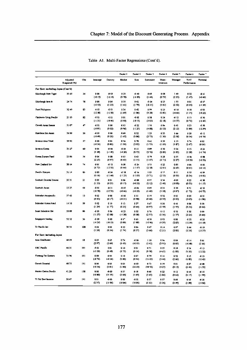
1 49
032 -011(235)
(147) (.060)
155
00) -017(2 52)
(005) (-I 39)
-0 10
0)8 -003(-0 64)
(115) (-023)
-012
013 -030(-057)
(071) (-246)
045
0.23 -030(2 12)
(189) (-239)
166
020 -0)2(2 55)
(054) (-070)
119
074 002(I 87)
(247) (009)
026
0)5 -024(I 05)
(I 38) (-I 74)
035 -006 -006(227)
(-0 35) (-0 55)
005
006 002(0 43)
(065) (-0 II)
oil
0)0 -009(0 50)
(054) (-092)
-001
022 -030(-003)
(055) (-I IS)
029
031 -010(087)
(173) (-073)
00!
003 -051(005)
(005) (-184)
041
006 0.10(I 95)
(0.3)) (066)
0 53
030 009(157)
(22)) (060)
081 -035 -020(205)
(-2 39) (-I IS)
097
044 -0)9(283)
(231) (-227)
004 -014 06)(005)
(-048) (216)
0 IS
014 -013(1 80)
(I 50) (-2.22)
032
015 -013(260)
(ISO) (-243)
001
027 -006(0 13)
(246) (-1.53)
0)2
014 -015(062)
(Ill) (-199)
0.66
014 -020(349)
(1.98) (-306)
Chapter 7: Model of the Discount Generatmg Process. Appendix
Adjueted
Oh.R-.quar.d (94)
Far East: uxeluding Japan (Cont'd)
Edinburgh Nam Tigur 35 65
34
EdutburaJt Jam It 24 74
78
Fits) Philppsne 3249
83
Gar800te Extug.Pun6c 21 03
82
GoettAaanSmco, 5107
47
Kambro. Sm Asian 5699
26
biv.co Asia Trout 3992
17
bivmor Korea 3)27
60
Korea Europe Fund 2386
54
NewZealandlnv 2014
74
PnciSc Horizon 3114
86
Scotbsh Onental Smcos 22 3)
21
ScottiehAsian 1525
64
Sdiroder Asiupain6c 37 43
13
Sduode, Korea Fund 1410
59
Siam Sdectiw Ow 2089 so
Singapore Smq 5232
36
Tr Punfic mv 30 54
108
Far East: i.dudiag Japan
AaraHeslthune 4009
18
F&CPaafic 4631
191
fleming Fur Enuturn 5196
'9'
Goc.tt Onmitul 48 73
'9'
Martin Corn. Paa6c 41.20
138
TrFurEastlnunn. 3047
19)
Table Al. Multi-Factor Regressions (Cont'd).
000 -003 025 -040
069
008(-0 IS) (-1.14) (078) (-I 09)
(I 44)
(079)
000 004 035 042 -004
025(-0 53) (I 23) (I 61) (I 79)
(-0 II)
(3 01)
.005 -005 034 042
099
0 23(-238) (-I 58) (1 69) (I 80)
(3 28)
(282)
.001 -001 001 -002
058
024(-I 21) (-046) (010) (-0)5)
(3 03)
(2 18)
-001 000 015 -022
110
006(-08)) (002) (096) (-1.25)
(408)
(0 53)
-001 000 069 032
I 25
033(-049) (021) (165) (088)
(273)
(I 30)
000 001 056 078
06)
039(-0 24) (082) (I 50) (205)
(I 53)
(I 09)
001 -004 -004 015
089
0 30(I 28) (-I 43) (-0 20) (0 73)
(276)
(289)
001 008 0)5 043
0 79
028(225) (097) (043) (115)
(I 47)
(271)
00! -012 008 -026
0 53
0 22(I 72) (-253) (044) (-I 47)
(2 IS)
(281)
000 -004 -018 -0)6
I 03
01'(016) (-I 66) (-I 23) (-103)
(5 71)
(2 II)
003 001 006 -OCR
097
054(122) (025) (0)7) (-023)
(2 12)
(I 40)
001 .011 -015 .006
049
031(.0 78) (-2 70) (-0 66) (.025)
(I 40)
(318)
002 000 -010 03)
0 19
032(043) (017) (-031) (098)
(040)
(0 59)
002 010 013 027
067
030(129) (177) (055) (064)
(097)
(2 58)
-001 006 -025 002
076
0 12(-I 27) (2 08) (-I 28) (008)
(2 57)
(2 30)
.009 000 01' 063 -0 51
093(-4 24) (-0 13) (060) (I 98)
(-096)
(4 59)
001 001 022 006
047
0 14(126) (034) (174) (037)
(366)
(221)
005 005 074 -006 110 096(297) (269) (143) (-015) (242) (391)
-001 001 010 001 071 025(-320) (048) (I 73) (0 14) (958) (465)
000 -001 0)0 007 079 014(-0 76) (-0 34) (200) (094) (II 02) (3 46)
000 005 005 -003 073 019(-0 31) (I SI) (I 00) (-0 33) (10 50) (4 23)
000 -003 027 0.18 060 022(-0 8)) (-I 19) (3 64) (I 69) (5 65) (3 84)
001 -005 000 -001 057 017(2 37) (-I 06) (-0 04) (-005) (5 32) (3 36)
Factor I Factor 2 Factor 3 Factor 4 Facto, Facto, 6 Factor"
hitaccept Dwnnty Market Size S.ohment Mean- Maunger NAV Revermirevarmini Porkemsnce
177

Chapter 7: Model of the Discount Generating Process. Appendix
Table Al. Multi-Factor Regressions (Cont'd).
A44u,tad Gore bitreriept Duninry Market Size Sentiment Mean- ManageT NAV ReaurualR-.quured (56) tsout Permance
J.pa.
BmllieOiffiip.n
51 49
183
Barth, Shin Nippout
6386
137
Edinburgh iepan It
4938
53
Fidelity Jspseese Vutlem 75 47
33
Rearing Jepenese
SI 09
191
Go Japan I,w
3116
191
Htr hp.i Smoos
6811
38
hivesco Jupun Iy
3266
29
lnwsse Tokyo Trust
6730
17
if Redgeling Jan 5723
152
if Jupuni Otc
2624
82
Merlin Cume Jepan
8311
IS
p_ —
6958
41
Sohroder Japan Ow
3845
29
ConUnestal Europe
Abliust Ene lik
3028
SI
Continental Asseta
48 7
133
European Asset, Tot. 33 17
155
F&C Eurotnist
37 54
191
F&C Garm.r
1878
191
fidelity Em Vuluen 6472
28
Faint Ireland
2616
80
Fleming CzedEurope
43 92
191
Fleming Eur fledge 33 59
79
Gortmore European
31 07
191
Gsetinotu huh Smoos
2808
IS
Gunman jnvTot. 3624
SI
000 002 001 -003 076(131) (099) (024) (-030) (II 77)
-002 001 015 001 090(-343) (032) (225) (010) (1062)
-001 003 012 016 079(-I 95) (016) (063) (077) (5 IS)
000 001 004 013 080(-0 46) (079) (0 26) (067) (5 26)
000 003 002 -010 059(047) (076) (040) (-I 09) (968)
001 -001 012 008 060(I 42) (-0.19) (I 35) (058) (665)
003 003 -017 -029 077(274) (I 60) (-1 Ii) (-I 19) (431)
000 002 -023 .028 074(-037) (085) (-084) (-101) (291)
001 000 022 -025 112(112) (-0 03) (077) (-I 40) (426)
-001 002 010 000 078(-3 12) (100) (144) (000) (965)
-003 or -034 029 068(-266) (278) (-I 51) (104) (284)
003 002 -030 00' 092(I 94) (I 92) (-I 08) (025) (3 49)
001 -001 -015 -042 104(0 84) (-0 37) (-I 01) (-2 64) (903)
-001 000 -001 -057 079(-0 93) (002) (-0 01) (-2 58) (3 89)
000 002 013 007 063(-024) (129) (109) (057) (312)
-001 003 .006 -029 124(-2 75) (I 46) (-0 78) (-260) (9 29)
000 001 02' 015 062(029) (070) (3 58) (I 47) (5 24)
003 -003 010 007 080(3 57) (-0 73) (I 55) (073) (7 60)
-001 001 005 -012 025(-I 48) (0 20) (067) (-I 14) (249)
001 -010 -026 -001 075(096) (-359) (-097) (-006) (199)
-003 003 015 013 038(.3 IS) (131) (112) (08!) (160)
000 000 .006 008 07!(041) (-005) (-I 32) (114) (1003)
000 003 -003 013 080(068) (I 44) (-0 27) (097) (3 95)
000 -001 -016 002 072(I 53) (-0 30) (-2 68) (0 Il) (741)
-002 002 -049 -041 -007(-235) (133) (-137) (-137) (-0.17)
-002 000 017 007 070(-2 96) (027) (I 83) (0.62) (3 93)
024 020 018 004(456) (161) (178) (073)
030 030 035 -008(431) (174) (280) (-I 17)
037 05) 043 -008(2 29) (I 08) (2 06) (-0 69)
002 010 043 -030(0 16) (0 79) (I 54) (-2 87)
005 06 021 -023(242) (4 97) (2 39) (-4 20)
OIl 017 018 -028(287) (066) (136) (438)
080 002 022 -001(3 I 9) (006) (1 00) (-060)
062 -013 -017 009(3 02) (-0 24) (-0 46) (-047)
098 -031 028 -016(191) (-I 26) (143) (-069)
036 006 044 -008(4 74) (024) (4.61) (-I 34)
03! -056 028 -002(400) (-093) (151) (-0 15)
103 071 OIS 029(3 46) (I 78) (049) (I SI)
015 020 021 -016(I 37) (1 22) (I 09) (-I 43)
-004 -003 032 .020(-0 26) (-0 32) (I 50) (-I IS)
031 -012 044 -010(290) (-108) (153) (-091)
026 023 -009 -006(4 24) (I 50) (-0 56) (-0 87)
016 025 -005 -007(3 4.4) (I 80) (-0 39) (-096)
023 002 038 -013(399) (0 17) (332) (-2.02)
013 023 012 -026(3 04) (I 61) (119) (-3 60)
023 004 057 -021(III) (017) (209) (-128)
036 002 017 -012(345) (007) (136) (-108)
003 052 026 -008(163) (503) (2 88) (-I SI)
031 001 040 -005(3 40) (0 04) (I 80) (-0 50)
019 015 031 007(415) (144) (283) (100)
015 065 009 -04!(159) (110) (038) (-I 72)
030 010 017 -008(3 38) (I 27) (I 33) (-080)
178

Chapter 7: Model of the Discount Generating Process. Appendix
Table Al. Multi-Factor Regressions (Cont'd).
Factor I Factor 2 F. 3 Factor 4 FactorS Factor 6 Factor 7
Obo
bitorcept Dummy Mackit Size Santonmit Mean- Maneper NAV Revoreilnvflai Perfirmana
Amtadk-.quersd (34)
Custlacalal Esrupe (Contd)
Gmm.iSmaI1Cas 3980
76
Hid.Eirotr Pkg 2284
53
MaitnWneEw 4534
SI
MuTT.y Europ.i 3991
84
Pana Freidi 6w 5365
118
SeorndMsrbtlnvCo 4717
145
Tr European Growth 3826
75
Average 34.73 III
-003 006 006 017(-I 64) (I 56) (050) (121)
001 OIl 000 010(146) (312) (0.02) (046)
001 004 013 001(112) (198) (lOS) (006)
000 -005 013 018(-0 78) (-238) (112) (I 27)
000 -001 -001 024(0 14) (-0 27) (-0.16) (230)
-001 006 -012 -005(-I 77) (2 67) (-I 52) (-0 43)
001 -003 006 009(I 78) (-I 90) (0 52) (0 bo)
0.00 0.01 0.02 0.04(-1.90) (2.83) (1.37) (2.77)1-2.) (3.53) (1.61) (3.45)
097 020 018 024 -000(4 74) (200) (1 74) (I 26) (-0 72)
106 044 017 -092 025(3 27) (4 12) (040) (-I 91) (I 70)
096 038 016 049 -016(4 22) (3 57) (065) (I 57) (-I 67)
088 031 013 -000 -009(4 13) (3 63) (0 89) (-0 36) (-0 89)
103 018 009 023 -024(793) (266) (049) (240) (-331)
095 027 -031 056 003(671) (443) (-167) (454) (040)
094 021 -042 030 -001(470) (284) (-I 63) (I 88) (-0 07)
0.70 0.24 0.20 0.17 -0.09(29.76) (19.23) (7.77) (9.71) (-10.40)(20.07) (37.65) (11.16) (1263) (-11.61)
179

Chapter 8: Opportunities for Future Research
Chapter 8
Opportunities for Future Research
1. Introduction
This chapter presents some of the main opportunities for future research on closed-end
funds. First, we attempt to characterise the behaviour of UK closed-end funds at the
time of the initial public offering (IPO), of seasoned equity offerings (rights and "C"
share issues) and of open-ending. We find evidence that the share price tends to
decline after the 1PO and the decline is particularly strong during the first ten months
of trading. Second, we show that the performance of our sample of "dead" funds
indicates that funds disappear after periods of poor NAY performance. At open-
ending, we find evidence that the share price increases towards NAY. Third, we
investigate seasoned equity offerings. We find that funds with good share price and
NAY performance tend to have rights and "C" share issues. The evidence suggest that
new money flows to well managed funds. Finally, we introduce some analysis relative
to the management group and investigate whether some management groups are better
than others.
2. Initial Public Offering
The underpricing of IPOs has been widely documented in the literature and appears to
be a short-run phenomenon. Ritter (1991) investigates the long-run performance
during the first three years of public listing. Ritter shows that issuing firms during
180

Chapter 8: Opportunities for Future Research
1975-84 substantially underperform a sample of matching firms. The
underperformance seems to be worse for companies that went public in high-volume
years. The evidence tends to suggest that IPO markets are subject to fads and that
issuing firms take advantage of these "windows of opportunity". The results are
consistent with the argument of Lee, Shleifer, and Thaler (1991) that closed-end funds
are issued more frequently in periods of low discounts.
Levis (1993) and Spiess and Aifieck-Graves (1995) analyse the long-run performance
of UK and US IPOs, respectively. They confirm Ritter's (1991) results. Levis and
Thomas (1995) further investigate the UK market and focus on the price performance
of closed-end finds. This chapter revisits the long-run performance of closed-end
funds listed on the London Stock Exchange and attempts to put into perspective the
"anomalous" price behaviour after the IPO. The price decline after the IPO is referred
to in Lee, Shleifer and Thaler (1990) as one of the closed-end fund's anomalies. We
believe, however, that the long-run underperformance of closed-end funds is similar to
the underperformance of industrial IPOs, and need not be regarded as a separate
anomaly.
2.1. Data and methodology
Blume and Stambaugh (1983) show that the bid-offer effect creates an upward bias to
computed single-period returns for individual stocks. Consequently, long term
cumulative performance measures suffer from a conceptual drawback as cumulating
single-period returns over long intervals implicitly amounts to rebalancing to equal
weight each month' 59 . Cumulative abnormal returns can be misleading measures of the
economic magnitude of performance. The bid-offer bias can be reduced by instead
computing the returns on a buy-and-hold portfolio. Conrad and Kaul (1993) and
' Many empirical studies compute portfolio returns as the arithmetic average of the returns on theindividual stocks. Since the arithmetic average implies rebalancing to equal weight each period (eachconstituent is given equal dollar exposure), this calculation gives the return on a rebalanced portfolio.
181

(8.1)
(8.2)
(8.3)
Chapter 8: Opportunities for Future Research
Canina, Michaely, Thaler and Womack (1998) measure the extent of the bias from
cumulating single-period returns over long periods rather than using the buy-and-hold
methodology.
We measure the share price buy-and-hold returns from the time of the IPO, s = 0, to
the first t months of trading, where t = 1 to 60. Abnormal returns are computed using
the market index (FTSE 100 index) where we assume a beta of 1. The sample consists
of 172 funds issued after 1980. Datastream provides price data for all of them. We
define the adjusted buy-and-hold returns, ar 5,, of fundj from period s to period 1 as
ar1,5, = R ,,,,, - I
where
PJ.t—PJ,SR,5,
rj,s
It - IsI S, =
Is
where s = 0, the time of the IPO and I corresponds to the number of months after the
IPO. I = 1 to 60 months. P, , and L are the fundj share price and the index value at I
months after the IPO, respectively. The mean cross-sectional market adjusted return,
AR , is defined as follows:
AR 5, = -- ar,,3, (8.4)
where n = 172 funds issued after 1980.
However, the computed return on the rebalanced portfolio is biased by the average of the bid-offer biasin the individual returns.
182

Chapter 8: Opportunities for Future Research
Modern portfolio theory assumes that realised returns are lognormally distributed. By
the central limit theorem, Cumulative Abnormal Returns (CARs) are approximately
normally distributed. However, buy-and hold returns are not normally distributed,
especially when measured over long periods. Following Dimson and Marsh (1986),
we evaluate their statistical significance using the measure
Ust = rsc lsr
(8.5)
where rr = loge (1 + R,r) and 1st = loge (1 + Ii). .kj,st is the equally weighted average
of over all n finds. The variance of this performance measure is estimated from
the single-period abnormal performance, are. t+l = ars,t+ i - ar 5. and it is equal to
Var (ar 5, ) = TVar('ar, 1+,) (8.6)
where T = t-s+1 is the length of the holding period over which performance is
measured. The variance of the single-period abnormal return, ar,. ^ , is estimated
from data for the second month of trading. The statistical significance of the buy-and
hold returns is estimated based on the following statistic
zst = us: .I.(ars, )
(8.7)
where the z51 statistic is a Student-t distribution with 1-s degrees of freedom.
However, when measuring long-horizon abnormal security returns, conclusions require
extreme caution. Kothari and Warner (1997) show that tests for long-horizon
performance around firm-specific events are severely mis-specified. Using a sample of
randomly selected securities and simulated random event dates, they find rejection
frequencies, using parametric tests, at times exceeding 30 percent, when the level of
183
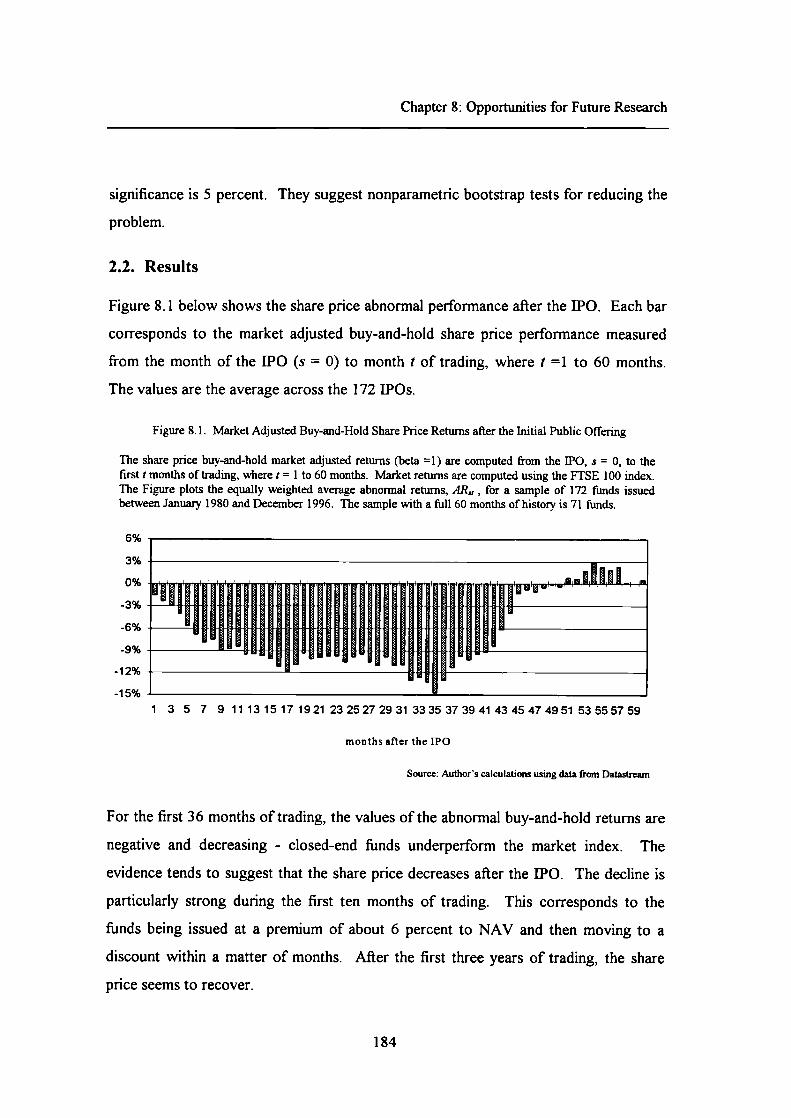
Chapter 8: Opportunities for Future Research
significance is 5 percent. They suggest nonparametric bootstrap tests for reducing the
problem.
2.2. Results
Figure 8.1 below shows the share price abnormal performance after the [P0. Each bar
corresponds to the market adjusted buy-and-hold share price performance measured
from the month of the [PU (s = 0) to month I of trading, where 1 =1 to 60 months.
The values are the average across the 172 iPOs.
Figure 8.1. Market Adjusted Buy-and-Hold Share Price Returns after the Initial Public Offering
The share price buy-and-hold market adjusted returns (beta = 1) are computed from the IPO, s = 0, to thefirst t months of trading, where t = 1 to 60 months. Market returns are computed using the FI'SE 100 index.The Figure plots the equally weighted average abnormal returns, AR,,, for a sample of 172 funds issuedbetween January 1980 and December 1996. The sample with a full 60 months of history is 71 funds.
6%
3%
0%
-3%
-6%
-9%
-12%
-15%1 3 5 7 9 11131517192123252729313335373941434547495153555759
months after the IPO
Source: Author's caIcuations using data from Datastream
For the first 36 months of trading, the values of the abnormal buy-and-hold returns are
negative and decreasing - closed-end funds underperform the market index. The
evidence tends to suggest that the share price decreases after the [P0. The decline is
particularly strong during the first ten months of trading. This corresponds to the
funds being issued at a premium of about 6 percent to NAV and then moving to a
discount within a matter of months. After the first three years of trading, the share
price seems to recover.
184

Chapter 8: Opportunities for Future Research
We find a negative and significant market adjusted buy-and-hold return of -8.8 percent
from the IPO to the end of the tenth month of trading. The abnormal performance is
significant at the 10 percent level (t-statistic of -1.9). 160 However, buy-and-hold
returns measured from the IPO to month 1, where 1 = 11 to 60 months of trading are
not significantly different from zero. The results tend to suggest that the evidence of
share price decline after the IPO is particularly strong over the first year of trading.
An interesting question is to determine whether this underperformance during the first
three years of trading is particular to closed-end funds or if it has some similarities with
industrial iPOs. Levis (1993) uses a sample of 712 UK industrial IPOs during the
period 1980-88. He finds cumulative average adjusted returns over 12, 24 and 36
months of +1.57 percent (0.85), -5.2 percent (-1.92) and -11.38 percent (-2.95),
respectively. We report the value of the t-statistic for the cumulative returns in
brackets. The cumulative performance is measured during the 36 months following the
first month of trading. With our sample of 172 closed-end funds we find buy-and-hold
adjusted returns over 12, 24 and 36 months of -9.5 percent (-1.67), - 10.5 percent
(-1. 17) and -13 percent (-1.12), respectively. Again, we report the value of the
t-statistic for the buy-and-hold returns in brackets. The abnormal performance is
measured relative to the first month of trading. It appears from this analysis that the
share price behaviour of closed-end fund IPOs may be similar to industrial IPOs, with
the difference that closed-end funds are characterised by a stronger decline. However,
the buy-and-hold returns computed for the closed-end fund industry are not
significantly different from zero when measured over the first 12, 24 and 36 months of
trading. Furthermore, the underlying assets in closed-end funds are typically listed
securities for which we know the market value. The prices of closed-end funds move
° The results are similar to Levis and Thomas (1995) who find, for a sample of 105 closed-end fundIPOs during the period 1984-92. a market adjusted cumulative return of -8.48 percent after 200trading days.
185

Chapter 8: Opportunities for Future Research
to a discount within a matter of months, reflecting the importance of management fees.
On the other hand, the market value of the net assets of an industrial company is more
difficult to estimate and this may mitigate the long-run underperformance (see Neal
and Wheatley (1998).
2.3. Limitations and scope for future research
In this preliminary study we do not consider the impact of dividends and adjust returns
only using the FTSE 100 index. In future research we can rectify these weaknesses
and introduce other indexes to adjust for factor exposures. The conjecture is that even
by taking into account the factors described in Chapter 7, we would still find negative
returns following the IPO. However, we believe that if we adjust for the performance
of industrial IPOs, we might find that the negative returns disappear. The idea is to
create a 'month of seasoning' index, as in Ibbotson (1975), where for each period we
would measure the performance of industrial IPOs with a certain age. Furthermore,
future research could also attempt to measure any arbitrage profitability during the first
months of trading.
3. Open-Ending
The UK closed-end fund industry has gone through intense changes and restructuring.
According to NatWest Securities (1997), 250 new funds were issued between 1980-
1996, with a total market capitalisation of £9.4 billion. On the other hand, there have
been several departures from the industry. Datastream provides data for 94 funds that
disappeared between 1980-1996. The following study investigates the performance of
these funds during the months preceding their disappearance'61 . Takeovers,
liquidations and unitisations are referred to as open-ending.
161 For a fimd undergoing restructuring, the Formula Asset Value (FAV) is calculated by taking NAVless x % representing the difference between the NAV and the likely realisable value of the underlyinginvestments.
186

Chapter 8: Opportunities for Future Research
3.1. Takeover, liquidation and unitisation.
A number of investment trusts, including most of the Split Capital Trusts, have fixed
dates on which they are to be wound-up but any investment trust can seek shareholder
approval for a winding up at any time. The discount to NAV on these trusts narrows
as the winding-up date approaches. Upon winding-up, domestic shareholders can end
up with potential capital gains tax liabilities. In these instances, a rollover vehicle is
typically made available.
Another method of eliminating the discount is to transform the investment trust into a
unit trust' 62 - the price of units reflecting the value of the underlying investments.
Investors exchanging investment trust shares for units are not liable for any capital
gains tax until they sells the units. Partial unitisation is a newer variation. Investors
are given the choice of opting for a unit trust or for continuing with a smaller
investment trust.
Finally, and particularly during periods of large discounts, closed-end funds have been
the target of raiders'63 (such as hedge funds), seeking to realise assets that have been
undervalued by the market.
3.2. The discount of open-ended funds
The first characterisation of the funds that have disappeared is to measure their average
discount during the last five years of trading. We define the average discount as the
logarithm of the mean price to NAV ratios (see Section 2 of Chapter 4) across the 94
"dead" funds. Figure 8.2 shows the results. The funds seem to have traded at a large
162 Unitisation involves the repayment of existing debentures, loan stocks, foreign currency loans andpreference shares and financing these repayments requires the sale of a vaiying proportion of theassets of the company.
163 Big City institutions have also attempted to use the voting power of their stake in the investmenttrust shares to persuade the management to come up with schemes for eliminating the discount.
187

Chapter 8: Opportunities for Future Research
discount - an average of 20 percent - during the last years of trading. The discount
disappears when the fund is open-ended, but share prices react long before that.
During the last year of trading the discount gradually moves towards zero, particularly
during the last 6 months of trading.
Figure 8.2. Average Discount before Open-Ending.
The average discount during the 60 months preceding open-ending is measured as the logarithm of theaverage price to NAV ratios across the 94 funds that disappeared during the period from January 1980 toDecember 1996. The dotted line corresponds to the average discount for the investment trust industr y at s =-60 to-I.
0%
-5%
-10%
-15%
-20% t_ .- - - - - - - - - - --25%
-60 -57 -54 -51 -48 -45 -42 -39 -36 -33 -30 -27 -24 -21 -18 -15 -12 -9 -6 -3months to open-ending
Source: Author's calculations using data from Datastream
The comparison of the average discount of the funds that disappeared and the average
discount for the investment trust industry (dotted line) tends to suggest that "dead"
funds did not trade at a substantially larger discount. Instead, the results show that,
consistent with the evidence presented in subsequent sections, open-ended funds are
characterised by a poor NAV performance.
3.3. Share price performance of open-ended funds
The behaviour of the funds that open-ended must also be characterised in terms of their
share price performance during the month before open-ending. We measure the
performance using the buy-and-hold methodology described by Equations (8.1) to
(8.4). Market adjusted buy-and-hold returns are measured from period s to period 1,
where I = 0 is the month of open-ending and s = -60 to -1 corresponds to the months
188

Chapter 8: Opportunities for Future Research
preceding the event. The significance of the buy-and-hold returns is measured using
the statistic described in Equations (8.5) to (8.7), where the variance of the single-
period buy-and-hold returns is evaluated using data for the month preceding the event.
Figure 8.3. Market Adjusted Share Price Buy-and-Hold Returns before Open-Ending.
The adjusted buy-and hold share price returns are computed from month .c, where s = -60 to -1, to open-ending (t = 0). The buy-and hold returns are adjusted using the FTSE 100 index, assuming a beta of I. Theresults are the equally-weighted average for the 94 funds that open-ended during the period January 1980 toDecember 1996.
16%
14%
12%
10%
8%
6%
4%
2%
0%
-2%-60 -57 -54 -51 -48 -45 -42 -39 -36 -33 -30 -27 -24 -21 -18 -15 -12 -9 -6 -3
months to open-ending
Source: Authors calculations using data from Datastream
Figure 8.3 shows the abnormal share price performance of the funds that open-ended.
Each bar corresponds to the market adjusted buy-and-hold share price performance
measured from month s, where s = -60 to -1, to open-ending (I = 0). The values are
the equally-weighted average across 94 funds that open-ended between January 1980
and December 1996. Table 8.1 reports t-values for the buy-and-hold returns.
The positive adjusted buy-and-hold returns show that, on average, closed-end funds
that are terminated outperform the index. The results for the last two years of trading
tend to suggest that share prices react to the likelihood of open-ending and rise
towards NAy. During the three months of trading the abnormal performance
decreases, suggesting that all the information about open-ending has already been
incorporated in the price. However, Table 8.1 shows that the abnormal share price
189

Chapter 8: Opportunities for Future Research
performance during the month preceding open-ending is not significantly different from
zero.
Table 8.1. Market Adjusted Share Price and NAV Buy-and-Hold Returns Before Open-Ending.
The adjusted buy-and hold share price and NAV returns are computed from month s, where s = -60 to -I, toopen-ending (t = 0). The buy-and hold returns are adjusted using the FTSE 100 index, assuming a beta of I.The results are the equally-weighted average for the 94 funds that open-ended during the period January 1980to December 1996. t-statistics are computed using the measure described in Equations (8.5) to (8.7).Significance levels are denoted by 5*5 (1% level), (5% level) and (10% level).
Share Price Returns
NAV Returns
Months to Adjusted t-statistic
Adjusted t-statisticOpen-Ending Return (%)
Return (%)
-1 -1.37 (-0.55) -0.57 (-1.40)
-6 11.34 (1.66) -0.95 (-1.52)-12 12.20 (1.19) -3.08 (-1.58)
-18 5.73 (0.44) -8.20 (-2.10) **
-24 7.09 (0.44) -10.02 (-2.31)
-30 15.26 (0.77) -8.52 (-3.40)-36 9.77 (0.43) -12.71 (-3.88)
-42 8.82 (0.34) -14.46 (-3.79)
-48 6.11 (0.20) -15.30 (-1.66) *
-54 7.42 (0.22) -17.84 (-1.73)
-60 3.84 (0.10) -13.34 (-1.52)
3.4. NAV performance of open-ended funds
The previous section shows open-ended funds cannot be characterised by share price
returns significantly different from zero. However, their behaviour must also be
analysed in terms of their NAV performance. We measure the performance using the
buy-and-hold methodology described by Equations (8.1) to (8.4) in Section 2, where
we replace fund share prices with NAY. Market adjusted buy-and-hold returns are
measured from period s to period t, where I = 0 is the month of open-ending and s =
-60 to -1 corresponds to the months preceding the event. The significance of the buy-
and-hold returns is measured using the statistic described in Equations (8.5) to (8.7),
where the variance of the single-period buy-and-hold returns is evaluated using data
for the month preceding the event.
190

Chapter 8: Opportunities for Future Research
Figure 8.4 shows abnormal NAV performance of the funds that open-ended. Each bar
corresponds to the market adjusted buy-and-hold NAV performance measured from
month s, where s = -60 to -1, to open-ending (I = 0). The values are the equally-
weighted average across 94 funds that open-ended between January 1980 and
December 1996. Table 8.1 above reports the t-values for the returns. The results tend
to indicate that closed-end funds that are terminated are characterised by a very poor
performance of the underlying assets relative to the market.
Figure 8.4. Market Adjusted NAV Buy-and-Hold Returns Before Open-Ending.
The adjusted buy-and hold NAV returns are computed from months, where s = -60 to -1, to open-ending (r =0). The buy-and hold returns are adjusted using the FTSE 100 index, assuming a beta of I. The results arethe equally-weighted average for the 94 funds that open-ended during the period January 1980 to December1996.
months to epen-ending
0%
-5%
-10%
-15%
-20%
-25%
-60 -57 -54 -51 -48 -45 -42 -39 -36 -33 -30 -27 -24 -21 -18 -15 -12 -9 -6 -3
Source: Author's calculations using data from Datastream
The negative adjusted buy-and hold returns suggest that the NAV underperformed the
market index for the five years before open-ending. The underperformance is
significant at the 1 percent level for s = -42 to -30 and at the 5 percent level for s = -30
to -18. During the last year of trading, the underperformance is not significantly
different from zero, indicating that the funds have a neutral performance relative to the
market index. The evidence suggests that the funds tend to behave like a passive
portfolio, probably as a result of having been put into restructuring.
191

Chapter 8: Opportunities for Future Research
3.5. Managerial performance of open-ended funds
Finally, we investigate the performance of the manager during the critical months
before the termination of the fund. Managerial performance is measured using returns-
based style analysis. The value added by active management is computed after
adjusting for the funds' effective asset exposure. Equations (5.3) and (5.4) describe
the computation of monthly selection returns. Managerial performance is measured
using NAV returns. The fund j cumulative selection returns to month T, csr ,. , is
computed as follows.
'çTcsr1r - L1=0 S,
where T= -1 to -36. The mean cross-sectional cumulative selection return, CSR , is
calculated:
1CSR =
csr
where n = 94 funds that open-ended between January 1980 and December 1996. The
statistical significance of the CSR r is evaluated using the t-statistic:
CSRT-.[A1=
-.IT Vary (8.10)
where N is the number of observations in month T and Varr is the cross-sectional
variance of the adjusted returns in month T. Figure 8.5 shows the returns cumulated
over the 36 months preceding the open-ending. We cumulate the monthly abnormal
returns from month Tto open-ending, where T -ito -36. Table 8.2 reports the t-
statistics for the returns.
(8.8)
(8.9)
192

2%
0%
-2%
-4%
-6%
-8%
-10%
-12%
-14%
-16%
-18%
Chapter 8: Opportunities for Future Research
Figure 85. Average Cumulative Managerial Performance.
The selection returns are cumulated from the month of open-ending to T months preceding the event, where T = -1to -36. The Figure plots the mean cross-sectional cumulative selection return. Managerial performance ismeasured using returns-based style anal ysis. The results are the equally-weighted average for the 94 fluids thatopen-ended during the penod January 1980 to December 1996.
Source: Author's calculations using data from Datastream
The results tend to suggest that managers, on average, underperform the passive
portfolio before open-ending. The selection returns cumulated over the last two years
of trading, -14.6 percent, are significant at the 1 percent level. However, consistent
with the NAV performance, we find that managers do not seem to do any 'stock
picking' during the last year of trading, but rather act as passive mangers.
193

Chapter 8: Opportunities for Future Research
Table 8.2. Cumulative Managerial Returns Before Open-Ending.
The selection returns are cumulated from the month of open-ending to T months preceding the event, whereT -ito -36. The table reports the mean cross-sectional cumulative selection return. Managerial performanceis measured usmg returns-based style analysis. The results are the equally-weighted average for the 94 fundsthat open-ended during the period January 1980 to December 1996. The computation of the t-statistics isdescribed in Equation (8.10). Significance levels are denoted by (1% level), (5% level) and*(10% level).
Managerial Performance
Months to Cumulative t-statisticOpen-Ending Returns (%)
-1 -0.37 (-0.24)
-2 -0.51 (-0.23)
-3 0.68 (0.24)
-4 0.49 (0.14)
-5 0.06 (0.01)
-6 -1.00 (-0.24)
-7 -1.30 (-0.38)
-8 -1.85 (-0.49)-9 -1.88 (-0.48)
-10 -2.37 (-0.60)
-11 -2.26 (-0.53)
-12 -3.74 (4)87)
-13 -3.51 (-0.84)
-14 -8.12 (-1.66)
-15 -8.22 (-2.17)
-16 -8.88 (-2.28)
-17 -8.75 (-2.34)
-18 -8.74 (-2.67)
Months to Cumulative t-statisticOpen-Ending Returns (%)
-19 -9.14 (-2.55)
-20 -11.51 (-3.54) •*.
-21 -11.29 (-3.80) ..
-22 -12.24 (-3.65)
-23 -11.77 (-3.67) •*.
-24 -14.64 (-4.14) •a*
-25 -15.45 (440) •'
-26 -15.30 (404) *..
-27 -15.79 (-3.82) *a.-28 -13.92 (-3.50)
-29 -14.34 (449) e.*
-30 -14.64 (-3.68)
-31 -11.72 (-3.14)
-32 -2.50 (-1.36)
-33 -1.69 (-1.13)
-34 -1.77 (-0.72)
-35 -0.23 (-0.11)
-36 0.01 (0.01)
3.6. Limitations and scope for improvements
As discussed earlier, this preliminary study does not account for dividends and adjust
returns only using the FTSE 100 index. In future research we can rectif' these
weaknesses and compare the performance of these funds to both their peers in the
AJTC category and to the industry overall. Furthermore, we could analyse the factors
and obstacles leading to open-ending.
194

Chapter 8: Opportunities for Future Research
The results show that during the last months of trading, funds that open-ended tend to
be neutral relative to the market. Future research could investigate further the reasons
for the termination of funds. We would attempt to distinguish between poor
management and the presence of the fund in an unpopular sector - thus analysing the
contribution of management versus the contribution of the sector. The study would
therefore compare relative performance to benchmark performance. Future research
could also attempt to identify the benchmark that managers actually aim to beat when
they are in a critical position (ie before and during a period of restructuring).
4. Seasoned Equity Issues: Rights and "C" Share Issues
Given the fact that open-end funds are bought and sold at NAV and thus management
ability may not be priced, Gruber (1996) argues that past performance tends to predict
future performance. Evidence that flows of new money into and out of mutual funds
follow the predictions of future performance suggests that investors recognise this
relationship. In contrast, the "closed" structure of closed-end funds ought to induce
the level of discounts to reflect past performance and eventually predict future
performance. Chapter 5 shows that discounts weakly reflect past managerial
performance, but incorporates no expectations of future performance. However,
Gruber' s (1996) argument that new money flows to better managed funds could be
tested for closed-end funds in terms of rights issues and "C" shares'64.
In the next sections we characterise the behaviour of the funds that had a rights or a
"C" share issue in terms of their discount, adjusted share price and NAV performance
during the months preceding the event.
' The additional capital raised by the issue of "C" shares is accounted for as a distinct pool of assetswithin the fund until the conversion date. The effect of this is that the NAV of the existing portfoliowill be unaffected by the introduction of the additional capital and the "C" shares will have anattributable NAV based solely on the net additional capital raised by their issue. "C" shares will beconverted into new ordinary shares (or income and capital shares) at or before the conversion dateaccording to a conversion ratio. The conversion takes place after most of the capital raised has beenfully invested.
195

Chapter 8: Opportunities for Future Research
4.1. Methodology
We measure share price and NAV performance using the buy-and-hold methodology
described by Equations (8.1) to (8.4). Market adjusted buy-and-hold returns are
measured from period s to period 1, where I = 0 is the month of open-ending and s
-60 to -1 corresponds to the months preceding the event. The significance of the buy-
and-hold returns is measured using the statistic described in Equations (8.5) to (8.7),
where the variance of the single-period buy-and-hold returns is evaluated using data
for the month preceding the event.
The average discount during the 60 months preceding the rights or the "C" share issue
is measured as the logarithm of the average price to NAV ratios (see Section 2 of
Chapter 4) across the funds that had the issue during the period from January 1980 to
December 1996.
4.2. Rights Issues
The average discount for the 22 funds (33 rights issues) during the 60 months
preceding the event is described in Figure 8.6. We also plot (dotted line) the average
discount for the investment trust industry at s = -60 to -1. The results show that
during the 60 months before the rights issue the funds are characterised, on average, by
a smaller discount than the industry. In particular, the funds tend to trade at a premium
during the 9 month leading to the rights issues. The evidence is consistent with Burch
and Weiss Hanley (1996). Based on a sample of 85 US closed-end fund rights offers
issued between 1985 and 1994, they find that managers time rights issues to coincide
with periods of low discounts.
196

Chapter 8: Opportunities for Future Research
Figure 8.6. Average Discount before the Rights Issue.
The average discount during the 60 months preceding the rights issue is measured as the logarithm of theaverage price to NAy ratios across the 22 funds (33 rights issues) that had an issue during the penod fromJanuary 1980 to December 1996. The dotted line corresponds to the average discount for the investment trustindustry at s = -60 to -1.
5%
0%-57
:. .
-25% -- - -
-30%months to rights issue
Source: Author's cacuIations using data from Datastrearn
Figure 8.7 shows the abnormal share price performance of the funds that had a rights
issue. Each bar corresponds to the market adjusted buy-and-hold share price
performance measured from month s, where s = -60 to -1, to the rights issue (/ = 0).
The values are the equally-weighted average across the 22 funds (33 right issues).
Panel A of Table 8.3 reports t-values for the buy-and-hold returns.
The positive adjusted buy-and-hold returns show that, on average, the funds that had a
rights issue tend to outperform the market index during the 60 months leading to the
event. Panel A of Table 8.3 shows that the buy-and-hold returns are significant at the
10 percent level for s = -24 to -12.
197

Chapter 8: Opportunities for Future Research
Figure 8.7. Market Adjusted Share Price Buy-and-Hold Returns before the Rights Issue.
The adjusted buy-and hold share price returns are computed from month s, where s = -60 to -1, to the rightsissue (t = 0). The buy-and hold returns are adjusted using the FTSE 100 index, assuming a beta of 1. Theresults are the equally-weighted average for the 22 funds (33 rights issues) that had an issue during the periodfrom Januaxy 1980 to December 1996.
48%
38%
28%
18%
8%
-2%-60 -57 -54 -51 -48 -45 -42 -39 -36 -33 -30 -27 -24 -21 -18 -15 -12 -9 -6 -3
months to rights issue
Source: Author's calculations using data from Datastream
The evidence is similar for the NAV buy-and-hold returns. Figure 8.8 shows the
results. The average value of the outperformance tends to be lower for the NAV
returns. Nevertheless, Panel A of Table 8.3 shows that the adjusted NAV buy-and-
hold returns are more significant.
Figure 8.8. Market Adjusted NAV Buy-and-Hold Returns before the Rights Issue.
The adjusted buy-and hold NAV returns are computed from month s, where s = -60 to -1, to the rights issue (t= 0). The buy-and hold returns are adjusted using the FTSE 100 index, assuming a beta of I. The results arethe equally-weighted average for the 22 funds (33 rightS issues) that had an issue during the period fromJanuary 1980 to December 1996.
25%
20%
15%
10%
5%
0%-60 -57 -54 -51 -48 -45 -42 -39 -36 -33 -30 -27 -24 -21 -18 -15 -12 -9 -6 -3
months to rights issue
Source: Author's calculations using data from Datastrcam
198

-6
-12-18
-24
-30-36-42
-48
-54
-60
-0.14
6.08
26.12
38.7537.20
23.88
16.81
42.25
30.32
21.20
29.98
0.56
2.84
10.917.57
22.5811.29
4.05
13.79
11.04
12.517.17
-0.48
7.79
21.26
28.8226.55
33.30
54.49
80.29
71.70
6449
55.79
1.16
6.81
17.59
23.33
23.5629.00
42.05
52.0639.62
40.41
38.45
(-0.31)
(1.85)
(3.15)(3.22)
(2.58)
(2.75)(3.66)
(4.35)
(3.72)
(3.21)
(2.45)
(-0.07)(0.89)
(2.24)(2.46)"
(1.96)'
(1.13)(0.68)
(1.41)
(0.88)
(0.55)
(0.65)
(0.56)(1.03)
(2.43)"(2.93)'"(3.06)
(1.37)(0.42)
(1.21)
(0.83)
(0.81)
(0.40)
(0.85)(1.87)
(3.05)(3.07)
(2.69)
(2.82)(3.38)
(3.51)
(2.59)(2.48)"
(2.04) -
Chapter 8: Opportunities for Future Research
The results tend to suggest that the funds that have a rights issue are characterised by a
good share price and NAV performance during the two years preceding the event.
Table 8.3. Market Adjusted Share Price and NAV Buy-and-Hold Returns Before the Issue.
The adjusted buy-and hold share price and NAV returns are computed from month s, where s = -60 to -I, to therights or "C" share issue (t = 0). The buy-and hold returns are adjusted using the FTSE 100 index, assuming abeta of 1. Panel A shows the results for rights issues. The values are the equally-weighted average for the 22funds (33 rights issues) that had an issue during the period from January 1980 to December 1996. Panel Bshows the results for "C" share issues. The values are the equally-weighted average across the 32 funds (37"C" share issues) that had an issue during the period from January 1980 to December 1996. t-statistics arecomputed using the measure described in Equations (8.5) to (8.7). Significance levels are denoted by(1% level), ** (5% level) and * (10% level).
Panel A: Rights Issues Panel B: "C" Share Issues
Share Price NAV Share Price NAV
Months Adjusted t-stat Mjusted t-stat Adjusted t-stat Adjusted t-stalto Issue Return (%) Return (%) Return (00) Return (0 o)
4.3. "C" Share Issues
The average discount for the 32 funds (37 "C" share issues) during the 60 months
preceding the event is described in Figure 8.9. We also plot (dotted line) the average
discount for the investment trust industry at s =-60 to -1. The results show that during
the 2 years before the "C" share issue the funds are characterised, on average, by a
smaller discount than the industry. During the month preceding the issue, the average
discount for the funds is -3.20 percent, whereas the corresponding value for the
industry is -7.7 percent.
199

Chapter 8: Opportunities for Future Research
Figure 8.9. Average Discount before the "C" Share Issue.
The average discount during the 60 months preceding the "C" share issue is measured as the logarithm of theaverage price to NAV ratios across the 32 funds (37 "C" share issues) that had an issue during the period fromJanuary 1980 to December 1996. The dotted line corresponds to the average discount for the investment trustindustiyats =-60 to-I.
0%-2%-4%-6%
20l3,
. .
-60 -57 .54 -51 -48 -45 -42 -39 -36 -33 -30 -27 -24 -21 -18 -15 -12 -9 -6 -3
months to "C" share issue
Source: Author's calculations using data from Datastream
Figure 8.10 shows the abnormal share price performance of the funds that had a "C"
share issue. Each bar corresponds to the market adjusted buy-and-hold share price
performance measured from month s, where s = -60 to -1, to the "C" share issue (1 =
0). The values are the equally-weighted average across the 32 funds (37 "C" share
issues). Panel B of Table 8.3 reports t-values for the buy-and-hold returns.
The positive adjusted buy-and-hold returns show that, on average, the funds that have
a "C" share issue tend to outperform the market index during the 60 months leading to
the event. Panel B of Table 8.3 shows that the buy-and-hold returns are significant at
the 5 percent level for s = -60 to -12. During the nine months leading to the issue, the
buy-and-hold returns are still positive, but not significantly different from zero. The
results are similar for the NAV performance (Figure 8.11).
200

-60 -57 -54 -51 -48 -45 -42 -39 -36 -33 -30 -27 -24 -21 -18 -15 -12 -9 -6 -3
60%
50%
40%
30%
20%
10%
0%
Chapter 8: Opportunities for Future Research
Figure 8.10. Market Adjusted Share Price Buy-and-Hold Returns before the "C" Share Issue.
The adjusted buy-and hold share price returns are computed from month s, where s -60 to -1, to the "C"share issue (1 = 0). The buy-and hold returns are adjusted using the FTSE 100 index, assuming a beta of I.The results are the equally-weighted average across the 32 funds (37 "C" share issues) that had an issueduring the period from January 1980 to December 1996.
90%80%70%60%50%40%30%20%10%0%
-60 -57 -54 -51 -48 -45 -42 -39 -36 -33 -30 -27 -24 -21 -18 -15 -12 -9 -6 -3
months to "C" share issue
Source: Author's calculations using data from Datastream
Figure 8.11. Market Adjusted NAV Buy-and-Hold Returns before the "C" Share Issue.
The adjusted buy-and hold NAy returns are computed from month s, where s -60 to -I, to the "C" shareissue (1 = 0). The buy-and hold returns are adjusted using the FTSE 100 index, assuming a beta of 1. Theresults are the equally-weighted average across the 32 funds (37 "C" share issues) that had an issue during theperiod from January 1980 to December 1996.
months to "C" share issue
Source: Author's calculations using data from Datastream
The results tend to suggest that the finds that had a "C" share offer are characterised
by a good share price and NAV performance during the 60 months preceding the
event. The share price performance relative to the index is higher when we consider
201

Chapter 8: Opportunities for Future Research
share price returns. Compared to the performance of the funds that had a rights issue,
we find stronger results. The adjusted share price and NAV returns are larger and
more significant for "C" share issues.
The funds that had a rights and "C" share issues are characterised by a good share
price and NAV performance during the month leading to the event. The evidence
tends to suggest that new money flows to well managed funds. An important question
would be to investigate the behaviour of these funds during the period following the
issue and test the hypothesis that new money predicts good performance.
4.4. Limitations and scope for improvements
As discussed earlier, this preliminary study does not account for dividends and adjust
returns only using the FTSE 100 index. In future research we can rectify these
weaknesses. The comparison of the behaviour of seasoned equity issues shows that
the funds that have "C" share issues tend to be characterised by a higher share price
and NAV positive performance but do not seem to be trading at premiums when they
have the issue. However, the event clustering is different; there are few "C" share
issues at the beginning and few rights issues at the end of the time period analysed. It
is therefore difficult to compare events that do not coexist. But, the results remain
interesting and represent opportunities for more research.
5. Management Group
In this last section we focus on the management of closed-end funds and we investigate
whether some management groups are better than others. We test the hypothesis that
the average discount of the funds under specific management groups is significantly
lower than the average discount of the other funds in the industry. Table 8.4 shows the
results.
202

Chapter 8: Opportunities for Future Research
Table 8.4. Discount of Management Groups.
The table shows the average discount (%) of the funds under the same management group. Alongside we reportthe average discount for the industry, where we exclude the management group under investigation. The column[A]-[B] is the difference between the average discount of the group and of the industry. The management groupsare ranked by this difference. We test the hypothesis that the average discount of the management group issignificantly lower than the industry discount. The last column reports the value of the t-statistics. We usemonthly data from January 1980 to December 1996.
Management Groups Obs Average Discount (%) t-statistic
Manag. Group Industr [A] - [B]
[A] [B]
Schroder 87 5.4 -10.9 16.3 9.08Glasgow Investment Managers 204 -5.1 -18.1 13.0 17.03M&G 59 0.8 -9.5 10.2 11.85Exeter Asset Management 95 -1.3 -10.9 9.6 14.12Scottish Value 62 -2.6 -9.6 7.0 11.05Ivory&Sime 204 -15.6 -17.5 2.0 3.06Fidelity 59 -7.3 -9.1 1.8 3.34Foreign&Colonial 204 -16.0 -17.5 1.4 1.79Martin Currie 204 -16.3 -17.5 1.2 1.50Henderson Investors 204 -16.9 -17.4 0.5 0.64Gartmore 204 -17.3 -17.4 0.2 0.24Finsbury 204 -17.9 -17.4 -0.5 -0 51Kleinwort Benson 204 -18.7 -17.3 -1.4 -1.77Edinburgh Fund Managers 204 -19.0 -17.3 -1.7 -2.16Fleming 204 -19.3 -17.3 -1.9 -2.42Rutherford 45 -10.1 -8.0 -2.1 -1.59Baillie Gjfford 204 -19.5 -17.3 -2.2 -2.941-lill Samuel 140 -15.8 -13.4 -2.4 -2.95Abtrust 88 -12.6 -10.1 -2.4 -3.44Murray Johnstone 204 -19.9 -17.3 -2.6 -3.11Perpetual 103 -14.3 -11.0 -3.3 -2.76Stewart Ivory 204 -20.8 -17.3 -3.6 -5 01Morgan Grenfell 204 -21.4 -17.2 -4.2 -5.80Govett (John) 204 -21.8 -17.2 -4.5 -6.14INVESCO 204 -23.2 -17.2 -6.0 -6.17Jupiter 111 -21.3 -11.5 -9.8 -9.64
The analysis identifies seven groups - Schroder, Glasgow Investment Managers, M&G,
Exeter Asset Management, Scottish Value, Ivory&Sime and Fidelity - as the best
managers. The average discount of the finds under their management is significantly
lower than the discount of the industry. However, Table 8.4 shows that most of the
management groups at the top are also characterised by a short history. The results
203

Chapter 8: Opportunities for Future Research
might suggest that "winners" management groups are lucky because of their short
history. To answer this question we could in future research look at the growth of
open-ended funds under the same management group. The conjecture is that if the
funds at the top of the Table 8.4 are "winners", we would expect inflows of money in
the open-ended funds that they manage.
Over the past few years there has been a degree of corporate activism in management
groups. It would be interesting to see whether management groups that add negative
value are taken over by management groups that add positive value to the fund. We
could measure the value added by the management using Sharpe's (1992) returns-
based style analysis described in Chapter 5.
The results show that the management group tends to affect the discount of the funds
under management. The evidence suggests that future research should focus on
management. As discussed earlier in this chapter, it would be interesting to analyse the
factors and obstacles leading to open-ending. A possibility would be to investigate the
management contracts and the management ownership structure in conjunction with
this analysis.
6. Conclusion
This last chapter attempts to characterise the behaviour of UK closed-end funds at the
time of the IPO, of seasoned equity offerings (rights and "C" share issues) and of
open-ending.
We find evidence that share prices tend to decline after the IPO. The decline is
particularly strong during the first ten months of trading. This corresponds to the
funds being issued at a premium to NAV of about 6 percent and then moving to a
discount within a matter of months. It would be interesting to extend this analysis and
introduce a 'month of seasoning' index of industrial IPO performance. The conjecture
204

Chapter 8: Opportunities for Future Research
is that the negative returns for closed-end fund IPOs would disappear after adjusting
for the performance of industrial IPOs.
The performance of or sample of "dead" funds suggests that funds disappear after
periods of poor NAV and managerial performance. At open-ending, we find evidence
that share prices increase toward NA y. Future research might involve the analysis of
other factors leading to open-ending and distinguish between the contribution of the
management versus the contribution of the sector.
We also investigate seasoned equity offerings. We find that funds with good past share
price and NAV performance tend to have rights and "C" share issues. The evidence
suggests that new money flows to well managed funds. The important question that
needs to be investigated is whether money flows predict future performance.
Lastly, we investigate whether some management groups are better than others. We
test the hypothesis that the average discount of the funds under certain management
group is significantly lower than the average discount of the other funds in the
industry. The analysis identifies seven groups - Schroder, Glasgow Investment
Managers, M&G, Exeter Asset Management, Scottish Value, Ivory&Sime and Fidelity
- as the best managers. The average discount of the funds under their management is
significantly lower than the discount of the industry. The evidence that the identity of
the management group tends to affect discounts suggests that future research should
focus on the impact of the management group on fund attributes.
205

Chapter 9: Conclusion
Chapter 9
Conclusion
Closed-end funds are characterized by one of the most puzzling anomalies in finance -
the existence and behaviour of the discount to NAy. Closed-end fund shares are
issued at up to a 10 percent premium to NAy. This premium represents the
underwriting fees and start-up costs. Subsequently, within a matter of months, the
shares trade at a discount, which persists and fluctuates according to a mean-reverting
pattern. Upon termination (liquidation or 'open-ending') of the fund, share prices rise
and discounts disappear. Discounts on UK traded closed-end fund companies share
many similarities with their US counterparts.
The first part of this study describes the closed- and open-end fund industries and
extensively reviews the literature on closed-end fund discounts. Many theories suggest
an explanation for the existence and behaviour of the discount, but since none solve all
parts of the anomaly, some scholars have found it necessary to resort to models of
investor irrationality. This study attempts, however, to describe and characterise the
discount on closed-end funds within a rational framework. Chapter 4 deals with the
impact of methodological issues.
Given the fact that open-end funds are bought and sold at NAV and thus management
ability may not be priced, Gruber (1996) argues that past performance tends to predict
206

Chapter 9: Conclusion
future performance. Evidence that flows of new money into and out of mutual funds
follow the predictions of future performance suggests that investors recognise this
relationship. In contrast, the "closed" structure of closed-end funds ought to induce
the level of discounts to reflect past performance and eventually predict future
performance. The conjecture is one of the traditional theories of the discount -
managerial performance - which claims that discounts reflect the perception of
management ability to perform relative to a passive portfolio.
The fact that discounts do not seem to be positively correlated to future NAV returns
may explain why so few studies have looked at managerial performance. However,
prior tests have focused on raw estimates of NAV returns, and have limited power.
The literature implies either that the relationship between discounts and managerial
performance does not exist, or that the power of tests based on NAV returns is too
low.
The objective of Chapter 5 was to rectify the weakness of using the return on NAV as
the definition of managerial performance. We measure performance after adjusting for
the risk and factor exposures of the fund. To define the value added by active
management we use two methodologies - the unconstrained and the constrained multi-
index regression. The first approach follows Gruber (1996) and defines performance
as the intercept of a multi-index unconstrained regression. The alternative approach is
Sharpe's (1992) returns-based style analysis, in which factor loadings are constrained
to be non-negative and add to unity.
Using our sample of UK closed-end funds, we find weak evidence of performance
persistence using the seven-factor unconstrained regression. This is consistent with
Gruber's (1996) conclusion in his Presidential Address on performance persistence in
the US mutual fund industry. However, our evidence is much weaker, and is not
supported by the results from the returns-based style analysis. The comparison of the
207
Chapter 9: Conclusion
two methodologies tends to suggest that the weak evidence of persistence using the
seven-factor model results from drawbacks in the unconstrained regression approach.
Consequently, we conclude that there is no performance persistence in the UK closed-
end fund market.
Gruber (1996) argues that the price of closed-end funds should incorporate the
expectations of managerial performance. The results provide no support for this
hypothesis. Discounts weakly reflect past performance, but do not seem to predict
managerial performance. The results tend to suggest that practitioners might be wrong
in believing that discounts reflect future managerial performance.
Chapter 5 also tests the hypothesis that a fund's residual risk affects the discount.
Pontiff (1996) shows that funds with large unhedgeable risk trade at higher discounts.
We confirm his results, defining residual risk as the variance of selection returns. The
greater the difficulty of hedging - as measured by each fund's residual risk - the higher
the discount. This relationship also holds when we use discounts as a predictor of
residual risk in subsequent test periods.
In Chapter 6 we investigate the time-series behaviour of UK closed-end fund discounts
and extend research previously carried out for the US market. We attempt to
characterise the discounts in terms of autocorrelation, stationarity, mean-reversion and
cointegration. The idea is to identify some attributes that might drive the model of the
discount generating process analysed in Chapter 7. The analysis shows that discounts
are highly autocorrelated in their levels but not in their first differences. Nevertheless,
we find weak evidence of price reversal. We also show that UK closed-end fund
discounts have a tendency to revert to their mean and fluctuate around it within a
certain range. A model that attempts to describe the time-series behaviour of the
discount must, therefore, account for this pattern. If a fund is trading at a large/small
discount compared to the average discount of the category, we would expect the
208

Chapter 9: Conclusion
discount to decrease/increase and revert towards this mean. Furthermore, there is
strong evidence of UK closed-end fund discounts moving together, in particular within
each category of fund. Therefore, for each category, we measure sentiment as the
return on an equally-weighted index of changes in the discount, where we include all
the funds in a category, with the exception of the fund under investigation. However,
the AITC categories might not be the only relevant classification. The conjecture is
that management brand might influence the discounts of the funds under the same
management. Therefore, for each management group, we measure the "manager"
effect as the returns on an equally-weighted index of changes in the discount, where
we include all the funds in the management group with the exception of the fund under
investigation.
Chapter 7 describes the model of the discount generating process. At first we
investigate the importance of Fama-French (FF) type factors in explaining returns and
discount changes for UK closed-end funds. The results show that the factors explain
closed-end fund share price and NAV returns, but not discount changes. It is not
surprising to find that for the discount, essentially an arbitrage portfolio, factors other
than the FF-type must be included. We then introduce additional factors in order to
explain at least part of the largely idiosyncratic movements in the discount. We
investigate the importance of measures of sentiment, mean-reversion, manager, past
performance and price reversal.
The multi-factor regression methodology measures the sensitivity of the changes in the
discount to the market, size, sentiment, mean-reversion, manager, past performance
and reversal factors. The model of the discount generating process seems to capture a
significant fraction of the changes in the discount. The seven factors explain, on
average, 35 percent of the changes in the discount. The adjusted R-squared is higher
than 40 percent for the International General, International Capital Growth,
International Income Growth, North America, Far East including Japan and Japan
209

Chapter 9: Conclusion
categories. Changes in the discount are particularly sensitive to the sentiment and
mean-reversion factors.
Within the framework of the model, we investigate whether for some management
groups the manager factor is more significant. The idea is to identiiy the groups for
which the "management brand" has a stronger effect on the discount of the funds under
management. We find that for fifteen management groups - M&G, Edinburgh Fund
Managers, Kleinworth Benson, Fleming, Govett, Foreign & Colonial, Ivory&Sime,
Glasgow Investment Managers, Murray Johnstone, Henderson Investors, Martin
Currie, Morgan Grenfell, Exeter Asset Management, Baillie Gifford and Hill Samuel -
the estimated slope is significantly different from zero.
Chapter 8 presents some opportunities for future research. We investigate the
behaviour of UK closed-end funds at the time of the IPO, of seasoned equity offerings
(rights and "C" share issues) and of open-ending. The results show that the price
decline during the first years of trading is higher than for industrial IPOs, but bears
some similarities. The evidence tends to suggest that the same IPO puzzle pertains to
closed-end funds as to industrial companies. The share price decline for closed-end
fund IPOs is particularly strong during the first ten months of trading. This
corresponds to the funds being issued at a premium to NAV of about 6 percent and
then moving to a discount within a matter of months. It would be interesting to extend
this analysis and introduce a 'month of seasoning' index of industrial IPO performance.
The conjecture is that the negative returns for closed-end fund IPOs would disappear
after adjusting for the performance of industrial IPOs.
The second part of the chapter focuses on the departures of funds from the industry.
The performance of our sample of "dead" funds tends to suggest that funds disappear
after periods of poor NAV performance. At open-ending, we find evidence that share
prices increase towards NAY. Future research might involve the analysis of other
210

Chapter 9: Conclusion
factors and obstacles to open-ending. We could attempt to distinguish between the
contribution of the management and the contribution of the sector.
Gruber's (1996) argument that new money flows to better managed funds can also be
tested for closed-end funds in terms of rights and "C" share issues. The third part of
Chapter 8 finds that funds characterised by good past share price and NAV
performance tend to have rights or "C" share issues. The evidence suggests that new
money is raised by well performing funds. The results are particularly significant for
our "C" share issues sample. Future research should investigate the behaviour of these
funds during the period following the issue and test the hypothesis that new money
predicts good performance.
Finally in Chapter 8, we investigate whether some management groups are better than
others. We test the hypothesis that the average discount of the funds under their
management is significantly lower than the average discount of the other funds in the
industry. The analysis identifies seven groups that appear to be the best managers and
for whom the average discount of the funds they manage is significantly lower. The
evidence that the management group tends to affect the discount of the funds under
management suggests that more research should focus on the management. Again, it
would be interesting to analyse the factors and obstacles leading to open-ending. A
possibility would be to investigate the management contracts and the management
ownership structure.
211

References
References
Abraham, Abraham, Don Elan, and Alan J. Marcus, 1993, Does Sentiment Explain Closed-End Fund Discounts? Evidence from Bond Funds, The Financial Review 28, no.4, 607-6 16.
AITC, 1997, Complete Guide to Investment Trusts, The Association of Investment TrustCompanies, London.
Ammer, John M., 1990, Expenses, Yields, and Excess Returns: New Evidence on Closed-EndFund Discounts from the UK, Group Discussion paper series no.108 (London School ofEconomics, London).
Anderson, Seth C., 1984, Relationship between Value of an Investment Company's Sharesand Value of the Underlying Net Assets, PhD thesis (University of North Carolina at ChapelFlill).
Anderson, Seth C., 1986, Closed-End Funds versus Market Efficiency, Journal of PortfolioManagement 13, 63-67.
Anderson, Seth C. and Jeffery A. Born, 1992, Closed-End Investment Companies: Issues andAnswers, (Kiuwer Academic Publishers).
Arkle, Jane, 1997, Tax and Investments, Oracle Conference.
Arnaud, A.A., 1983, Investment Trusts Explained, (Woodhead-Faulkner in co-operation withThe Association of Investment Trust Companies).
AUTIF, 1997, Unit Trusts User's Handbook.
Bailey, W. and J. Lim, 1992, Evaluating the Diversification Benefits of the New CountryFunds, Journal of Financial Management 18, 74-8 0.
Barber, Brad M., 1994, Noise Trading and Prime and Score Premiums, Journal of EmpiricalFinance 1, 25 1-278.
Barclay, Michael, Clifford Holderness, and Jeffiey Pontiff, 1993, Private Benefits from BlockOwnership and Discounts on Closed-End Funds, Journal of Financial Economics 33, 263-291.
Bekaert, Geert and Michael Urias, 1994, Diversification, Integration and Emerging MarketClosed-End Funds, Working Paper (Stanford University).
212

References
Black, Fisher and Myron Scholes, 1973, The Pricing of Options and Corporate Liabilities,Journal of Political Economy, 63 7-654.
Biwne, M and R.F. Stainbaugh, 1983, Biases in Computed Returns: An Application to theSize effect, Journal of Financial Economics 12, 387-404.
Bodie, Zvi, Alex Kane and Alan J. Marcus, 1996, Investments (Irwin, Third Edition).
Bodurtha, J., E. Kim and C. Lee, 1993, Closed-End Country Funds and US MarketSentiment, Review of Financial Studies 8, 879-9 18.
Bonser-Neal, Catherine, Greggory Brauer. Robert Neal and Simon Wheatley, 1990.International Investment Restrictions and Closed-End Country Fund Prices, Journal ofFinance 45, 523-547.
Boudreaux, Kenneth J., 1973, Discounts and Premiums on Closed-End Funds: A Study inValuation, Journal of Finance 28, 5 15-522.
Brauer, Greggory A., 1984, 'Open-Ending' Closed-End Funds, Journal of FinancialEconomics 13, 491-507.
Brauer, Greggorv A., 1988, Closed-End Fund Shares' Abnormal Returns and the InformationContent of Discounts and Premiums, Journal of Finance 43, 113-127.
Brauer, Greggory A. and Eric C. Chang, 1990, Return Seasonality in Stocks and TheirUnderlying Assets: Tax-Loss Selling versus Information Explanations, The Review ofFinancial Studies 3, 255-280.
Brealey, Richard, 1986, Comments in Edwards, J, Franks. J, Mayers, C, Schaefer, 5: Recentdevelopments in Corporate Finance.
Brickley, James, Steven Manaster, and James Schaliheim, 1991. The Tax-Timing Option andthe Discounts on Closed-End Investment Companies, Journal of Business 64, no.3, 287-3 12.
Brickley, James A. and James S. Schallheim, 1985, Lifting the Lid on Closed-End InvestmentCompanies: A Case of Abnormal Returns, Journal of Financial and Quantitative Analysis 20,107-117.
Brown, R.G, 1962, Smoothing, Forecasting and Prediction of Discrete Time Series. (Prentice-Hall International Series in Management and Quantitative Methods Series).
Burch, T. Timothy and Kathleen Weiss Hanley, 1996, When are Closed-End Funds Open?Rights Offers as a Response to Premiums, Working Paper, University of Maryland.
Burton, H. and D.C. Corner, 1970, Capital gains tax liabilities and investment and unit trust,Journal of Business and Finance, 37-44.
213

References
Canina, Linda, Roni Michaely, Richard Thaler and Kent Womack, 1998, CaveatCompounder: A Warning about Using the Daily CRSP Equal-Weighted Index to ComputeLong-Run Excess Returns, Journal of Finance 53, 403-416.
Carhart, Mark M., 1997, On Persistence in Mutual Fund Performance, Journal of Finance 52,57-82.
Chang, Eric, Cheol S. Eun, and Kolodny Richard, 1995, International Diversification throughClosed-End Country Funds, Journal of Banking & Finance 19, 1237-1263.
Chay, Jong-Bom, 1992, The Pricing of Closed-End Funds: Discounts and Managerialperformance, PhD thesis (State University of New York at Buffalo).
Chen, Nai-Fu, Raymond Kan, and Merton H. Miller, 1993. Are the Discounts on Closed-EndFunds a Sentiment Index?, Journal of Finance 48, no.2, 795-800.
Chen, Nai Fu, Richard Roll, and Stephen Ross, 1986, Economic Forces and the StockMarket, Journal of Business, 383-403.
Cheng, A., L. Copeland, and J. O'Hanlon, 1994. Investment Trust Discounts and AbnormalReturns: UK Evidence, Journal of Business Finance & Accounting 21, no.6, 813-83 1.
Chevalier, Judith and Glenn Ellison, 1996, Are Some Mutual Fund Managers Better ThanOthers? Cross-sectional Patterns in Behavior and Performance, Working Paper (University ofChicago).
Chopra, Navin, Charles M.C. Lee, Andrei Shleifer, and Richard H. Thaler, 1993. Yes.Discounts on Closed-End Funds are a Sentiment Index, Journal of Finance 48, no.2, 80 1-808.
Conrad, Jennifer and Gautain Kaul, 1993. Long-Term Market Overreaction or Biases inComputed Returns?. Journal of Finance, 48, 39-63.
Constantinides, George M., 1983, Capital Market Equilibrium with Personal Tax.Econometrica 51, 6 11-636.
Constantinides. George M., 1984, Optimal Stock Trading with Personal Taxes: Implicationsfor Prices and the Abnormal January Returns, Journal of Financial Economics 13, 65-90.
Corner, D.C. and J. Matatko, 1982. Investment Trust Portfolio Performance Measurementand Determinants, The Investment Analyst, 9-13.
Credit Lyonnais Laing, 1997, )nvestment Trust Yearbook.
Cuthberston, Keith, Stephen Hall, and Mark P. Taylor, Applied Econometric Techniques.
Datar, Vinay, Narayan Naik, and Robert Radcliffe, 1998, Cross-Section of Stock ReturnsRevisited: The Role of Liquidity and Size, Journal of Financial Markets 1.
214

References
De Bondt, Werner F.M. and Richard Thaler, 1985, Does the Stock Market Overreact?.Journal of Finance 40, 793-805.
De Long, J. Bradford and Andrei Shleifer, 1992, Closed-end fund discounts, Journal ofPortfolio Management, Winter, 46-53.
De Long, J. Bradford, Andrei Shleifer, Lawrence H. Summers, and Robert J. Waldmann,1990, Noise Trader Risk in Financial Markets, Journal of Political Economy 98, 703-738.
Deaves, Richard and Itzhak Krinsky, 1994, A Possible Reconciliation of some of theConflicting Findings on Closed-End Fund Discounts: A Note, Journal of Business Finance &Accounting 21, no.7, 1047-1057.
Dickey, D.A. and W.A Fuller, 1979, Distribution of the Estimators for Autoregressive TimeSeries with a Unit Root, Journal of the American Statistical Association 74, 427-431.
Dickey, D.A and W.A Fuller, 1981, Likelihood Ratio statistics for Autoregressive TimeSeries with a Unit Root, Econometrica 49, no. 4.. 1057-1072.
Dimson, Elroy and Paul Marsh, 1983, The Stability of UK Measures and The Problem ofThin Trading, Journal of Finance 38. 753-783.
Dimson. Elroy and Paul Marsh, 1986, Event Study Methodologies and the Size Effect. TheCase of UK Press Recommendations, Journal of Financial Economics 17, 113-142.
Dimson, Elroy and Paul Marsh, 1997, The Hoare Govett Smaller Companies Index 1955-1996, London: ABN-Amro,
Draper, Paul, 1989, The Investment Trust Industry in the UK: An Empirical Analysis,(Gower).
Elton, Edwin J., Martin J. Gruber, and Christopher R. Blake. 1 996a. The Persistence of Risk-Adjusted Mutual Fund Performance, Journal of Business 69, no.2, 133-157.
Elton, Edwin J., Martin J. Gruber, and Christopher R. Blake, 1996b, Survivorship Bias andMutual Fund Performance, Review of Financial Studies 9, no. 4. 1097-1 120.
Elton, Edwin J., Martin J. Gruber, Sanjiv Das, and Mart Hlavka, 1993, Efficiency with CostlyInfonnation: A Re-Interpretation of Evidence from Managed Portfolios. Review of FinancialStudies 6. 1-21.
Emerson, Rebecca, 1994, An Evaluation of UK Investment Trust as Contingent Claims: ATheoretical Investigation, Discussion Paper no. DP 23-94 (London Business School, London).
Engle, R.F. and C.W.J. Granger, 1987, Cointegration and Error Correction: Representation,Estimation and Testing, Econometrica 55, No.2 , 251-276.
215

References
Fama, Eugene F. and Kenneth R. French, 1992, The Cross-Section of Expected StockReturns, Journal of Finance 47, no. 2 , 427-465.
Fama, Eugene F. and Kenneth R. French, 1993, Common Risk Factors in the Returns onBonds and Stocks, Journal of Financial Economics 33, 3-5 6.
Fama, Eugene F. and Kenneth R. French, 1998, Value Versus Growth: the InternationalEvidence, Journal of Finance (forthcoming).
Faina, Eugene F. and J. MacBeth, 1973, Risk, Return and Equilibrium: Empirical tests.Journal of Political Economy 81, 607-636.
Finnerty, John D. and Dean Leistikow, 1993, The Behavior of Equit y and Debt RiskPremiums, The Journal of Portfolio Management. Summer, 73-84.
Fisher and Jordan, Security Analysis and Portfolio Management
Frankel, Jeffiey, 1994, The Internationalisation of Equity Markets, (University of ChicagoPress).
Fraser, P and D.M. Power, 1991, Predictability, Trends and Seasonalities: An EmpiricalAnalysis of UK Investment Trust Portfolios, 1970-1990, (Universit y of Dundee).
Fredman, Albert and George Cole Scott, 1991, Investing in Closed-End Funds: Finding Value& Building Wealth, (New York Institute of Finance, New York, NY).
Fung, William and David A. Hsieh, 1997, Empirical Characteristics of Dynamic TradingStrategies: The Case of Hedge Funds, The Review of Financial Studies 10. No 2, 275-302.
Goetzmann, William N. and Roger G. Ibbotson, 1994, Do Winners repeat? Patterns in MutualFund Performance, Journal of Portfolio Management 20, 9-18.
Granger, C.W.J., 1981, Some Properties of Time Series Data and Their Use in EconometricModel Specification, Journal of Econometrics 16, No.!, 121-130.
Grinblatt, Mark and Sheridan Titman, 1989, Mutual Fund Performance: An Analysis ofQuarterly Portfolio Holdings, Journal of Business 62, no.3, 393-416.
Grinblatt, Mark and Sheridan Titman, 1992, The Persistence of Mutual Fund Performance,Journal of Finance 47, 1977-1984.
Grossman, Sanford J. and Oliver D. Hart, 1980, Takeover Bids, the Free-Rider Problem, andthe Theory of the Corporation, Bell Journal of Economics and Management Science, Spring,42-64.
216

References
Gruber, Martin J., 1996, Another Puzzle: The Growth in Actively Managed Mutual Funds.Journal of Finance 51, 783-810.
Guy, James R.F., 1978, The Performance of the British Investment Trust Industry, Journal ofFinance 33, no.2, 443-455.
Heisler, Jeffrey, 1994, Recent Research in Behavioral Finance, Financial Markets, Institutionsand Instruments.
Hendricks, Darryl!, Jayendu Pate!, and Richard Zeckhauser, 1993, Hot Hands in MutualFunds: Short-Run Persistence of Relative Performance, 1974-1988, Journal of Finance 48. no.1, 93-130.
Hoare Govett ABN-AMRO, 1997, Le Patron Mange Id, Investment Trust Research.
Inland Revenue, December 1997, The New Individual Savings Account (ConsultativeDocument).
Ibbotson, R.G., 1975, Price Performance of Common Stock New Issues. Journal of FinancialEconomics 2, 235-272.
Jegadeesh, Narasinihan, 1990, Evidence of Predictable Behavior of Security Returns. Journalof Finance 45, 881-898.
Jegadeesh, Narasimhan and Sheridan Titman, 1993, Returns to Buying Winners and SellingLosers: Implications for Stock Market Efficiency, Journal of Finance 48, no. 1, 65-9 1.
Jensen, Michael, 1978, Some Anomalous Evidence Regarding Market Efficiency, Journal ofFinancial Economics 6, no. 2/3, 95-101.
Kahn, Ronald N. and Andrew Rudd, 1995. Does Historical Performance Predict FuturePerformance?, Financial Analyst Journal, November-December. 43-52.
Keim, Donald, 1988, "Stock Market Regularities: a Synthesis of the Evidence andExplanations." In Stock Market Anomalies, ed. Edited by Elroy Dimson. CambridgeUniversity Press.
Keim, Donald B., 1983, Size-Related Anomalies and Stock Return Seasonality: FurtherEmpirical Evidence, Journal of Financial Economics 12, 3-32.
Kim, Chang-Soo, 1994, Investor Tax-Trading Opportunities and Discounts on Closed-EndMutual Funds, The Journal of Financial Research Spring, 65-75.
Kothari, S.P. and Jerold B. Warner, 1997, Measuring Long-Horizon Security PricePerformance, Journal of Financial Economics 43, 30 1-339
217

References
Kumar, Raman and Gregory M. Noronha, 1992, A Re-Examination of the Relationshipbetween Closed-End Fund Discounts and Expenses, Journal of Financial Research 15, no.2,139-147.
Lee, Charles M.C., Andrei Shleifer, and Richard H. Thaler, 1990, Anomalies: Closed-EndMutual Funds, Journal of Economic Perspectives 4, no.4. 153-164.
Lee, Charles M.C., Andrei Shleifer, and Richard H. Thaler, 1991, Investor Sentiment and theClosed-End Fund Puzzle, Journal of Finance 46. 76-110.
Levis, Mario, 1993, The Long-Run Performance of Initial Public Offerings: The UKExperience 1980-1988, Financial Management Spring, 24-41.
Levis, Mario and Dylan C. Thomas, 1995, Investment Trust IPOs: Issuing Behaviour andPrice Performance. Evidence from the London Stock Exchange, Journal of Banking andFinance 19, 1437-1458.
Litzenberger, Robert H. and Howard B. Sosin, 1977, The Theory of Recapitalizations and theEvidence of Dual Purpose Funds, Journal of Finance 32, no.5, 1433-1455.
Malkiel, Burton and Paul Firstenberg, 1978, A Winning Strategy for an Efficient Market.Journal of Portfolio Management, 20-25.
Malkiel, Burton G., 1977, The Valuation of Closed-End Investment-Company Shares. Journalof Finance 32, 847-858.
Masey, Anthea, 1988, Investment Trusts Financial Times Business Information.
Mendelson, M., 1977, Closed-End Fund Discount Revisited, Center for Study of FinancialInstitutions (University of Pennsylvania Law School, Philadelphia, PA).
Merton, R.C., 1973, Theory of Rational Option Pricing, Bell Journal of Economic andManagement Science 4, 14 1-183.
Miller, Edward M., 1977, Risk, Uncertamty, and Divergence of Opinion, Journal of Finance3, no.4, 115 1-1 168.
Minio-Paluello. Carolina, 1998, "The Closed-End Fund Puzzle: A Literature Review." InSecurity Market Imperfections in World Wide Equity Markets, eds. W.T. Ziemba and D.M.Keim. Cambridge University Press (forthcoming).
Minio-Paluello, Carolina, 1996, Time-Series Behaviour of UK Closed-End Fund Discounts,(Paper presented at EDEN Colloquium, European Financial Association, Milan).
NatWest Securities, Investment Trust A-Z, January 1997.
218

References
Neal, Robert and Simon M. Wheatley, 1998. Adverse Selection and Bid-Ask Spreads:Evidence from Closed-End Funds, Journal of Financial Markets 1.
Peavy, John W., 1990, Returns on Initial Public Offerings of Closed-End Funds, Review ofFinancial Studies 3, no.4, 695-708.
Pontiff, JeffIey, 1995, Closed-End Fund Premia and Returns Implications for FinancialMarket Equilibrium, Journal of Financial Economics 37, 341-367.
Pontiff, Jeffiey, 1996, Costly Arbitrage: Evidence from Closed-End Funds. Quarterly Journalof Economics November. 1135-1 151.
Pontiff, Jeffrey, 1997, Excess Volatility and Closed-End Funds. American Economic Review87, 1, 155-169.
Pratt. Eugene J., 1966, Myths Associated with Closed-End Investment Company Discounts,Financial Analysts Journal , July/August, 79-82.
Richards, R. Malcolm, Don R. Fraser, and Groth John C., 1980, Winning Strategies forClosed-End Funds, Journal of Portfolio Management Fall, 50-55.
Ritter, Jay R., 1991, The Long-Run Performance of Initial Public Offerings, Journal ofFinance 46, 3-27.
Rockinger, Michael, 1995, Determinants of Capital Flows to Mutual Funds, Working Paper(HEC - School of Management).
Roenfeldt. Rodney and Donald L. Tuttle, 1973, An Examination of the Discounts andPremiums of Closed-End Investment Companies, Journal of Business Research 1, 129-140.
Rozeff, Michael S., 1991. Closed-End Fund Discounts and Premiums, in: S.G. Rhee and R.P.Chang eds., Pacific-Basin Capital Markets Research. Vol. II (Elsevier Science B.V. (North-Holland), Amsterdam), 503-522.
Risk Measurement Service, January-March 1997, London Business School.
Schwert, G.W.. 1989, Why does stock market volatility change over time?, The Journal ofFinance, 1155-53.
Seltzer, David Fred, 1989, Closed-End Funds: Discounts. Premia and Performance. Phdthesis. University of Arizona.
Sevhun, H. Nejat and Douglas J. Skinner, 1994, How Do taxes Affect Investors' StockMarket Realizations? Evidence from Tax-Return Panel Data, Journal of Business 67. no.2.231-262.
Sharpe, William F., 1966, Mutual Fund Performance, Journal of Business 39, 119-138.
219

References
Sharpe, William F., 1992, Asset Allocation: Management Style and PerfonnanceMeasurement, Journal of Portfolio Management 18, Winter. 7-19.
Sharpe, William F., 1996, The Styles and Performance of Large Seasoned U.S. MutualFunds, Working Paper (Stanford).
Sharpe, William F. and Howard B. Sosin, 1974. Closed-end investment companies in theUnited States: Risk and return, Proceedings of European Finance Association, 37-63.
Sias, Richard William, 1992, Closed-End Funds and Market Efficiency, PhD thesis (TheUniversity of Texas at Austin).
Spiess, Katherine and John Affleck-Graves, 1995, Underperformance in Long-Run StockReturns Following Seasoned Equity Offerings, Journal of Financial Economics 38. 243-267.
Swaminathan. B., 1994a, Investor Sentiment, Closed-End Fund Discounts and thePredictability of Small Firm Returns, Working Paper (University of California Los Angeles).
Swaminathan, B., 1994b, A Rational Model of Closed-End Fund Discounts. Working Paper(University of California, Los Angeles).
Thompson. Rex, 1978, The Information Content of Discounts and Premiums on Closed-EndFund Shares, Journal of Financial Economics 6, 15 1-186.
Walker, Matthew, 1992, An Agency Explanation of Closed-End Fund Discounts. PhD thesis(Texas Tech University).
SG Warburg Securities, 1988, Investment Trusts Manual.
SG Warburg Securities, 1990, Investment Trusts Manual.
Weiss Hanley, Kathleen, Charles M.C. Lee, and Paul J. Seguin. 1995. The Marketing ofClosed-End Fund IPOs: Evidence from Transactions Data, Working Paper (Universit y ofMichigan).
Weiss Hanley, Kathleen and H. Nejat Seyhun, 1994, The Profitability of Short Selling:Evidence From Closed-End Funds, Working Paper (University of Michigan).
Weiss, Kathleen, 1989, The Post-Offering Price Performance of Closed-End Funds, FinancialManagement, Autumn, 5 7-67.
Whitting, A., 1984, The Analysis of the Share Discounts of UK Investments TrustCompanies: a Time Series Approach, PhD thesis (University of Lancaster).
Woodbury, Denise, 1992, Compensation of investment advisors in Agency Framework, PhDthesis (University of Utah).
220

References
Woodward, R.S., 1983, The Performance of UK Trusts as Internationally DiversifiedPortfolios over the Period 1968 to 1977, Journal of Banking and Finance 7, 417-426.
Wylie, Sam, 1997, Essays on the Decision of Investors and Fund Managers, DoctoralDissertation (London Business School).
Zweig, Martin E., 1973, An Investor Expectations Stock Price Predictive Model UsingClosed-End Fund Premiums, Journal of Finance 28. 67-78.
tONDILUNIV.
221