RIVER RESEARCH AND APPLICATIONS

River. Res. Applic. (2007)

Published online in Wiley InterScience

IDENTIFICATION OF A MINIMAL ADEQUATE MODEL TO DESCRIBETHE BIOMASS DYNAMICS OF RIVER EPILITHON

STEPHANIE BOULETREAU,a* OIHANA IZAGIRRE,b FREDERIC GARABETIAN,a

SABINE SAUVAGE,a ARTURO ELOSEGIb and JOSE-MIGUEL SANCHEZ-PEREZa

a Laboratoire d’ecologie fonctionnelle (EcoLab UMR 5245 CNRS-UPS-INPT), Universite Paul Sabatier,

118 route de Narbonne, 31062 Toulouse cedex 09, Franceb Department of Plant Biology and Ecology, Faculty of Science and Technology, University of the Basque Country,

PO Box 644, 48080 Bilbao, Spain

(www.interscience.wiley.com) DOI: 10.1002/rra.1046

ABSTRACT

The present study sought to identify a minimal adequate model to describe the biomass dynamics of river epilithon, a functionalindicator of river health. Identification of minimal adequate models is particularly necessary in river management, given thereduced number of variables authorities are willing to measure routinely. A model previously developed for epilithon dynamicsin a pre-alpine river was applied to epilithon biomasses recorded in contrasting hydrological, trophic and light conditions atvarious sites in the Aguera stream (Spain) over 3 years (11 case studies). A model selection tool, the Akaike InformationCriterion (AIC), was used to determine the optimal combination of parameters. In nine of 11 case studies, the best modeldescribed epilithon biomass dynamics as the equilibrium between phototrophic growth and discharge-dependent loss andignored light, temperature and nutrient influences. The best adequate minimal model i.e. the model that is the best trade-offbetween goodness-of-fit and model simplicity performed best, in years in which clearly contrasting short low and high waterperiods occurred. During years with less marked hydrodynamics, many other abiotic or biotic processes influenced epilithonbiomass dynamics. In these cases, weaker goodness-of-fit had to be accepted to avoid excessively increasing model complexity.Copyright # 2007 John Wiley & Sons, Ltd.

key words: model selection; model complexity; Akaike Information Criterion; periphyton; epilithic biofilms; stream

Received 10 January 2007; Revised 1 June 2007; Accepted 15 June 2007

INTRODUCTION

Since Streeter and Phelps (1925) started modelling river water quality, ecological models have been increasingly

used by environmental managers, especially from the beginning of the 1970s (Brown and Barnwell, 1987; Even

et al., 1998; Reichert, 2001; Reichert et al., 2001). One fundamental goal of ecological modelling is to predict how

the structure and function of communities respond to change, not only because streams and rivers are naturally

variable, but also because they are vulnerable to anthropogenic disturbances (Power et al., 1988). Awareness of the

importance of a healthy environment has grown steadily during recent decades among environmental management

authorities, leading to new, more ecologically sound policies such as the European Water Framework Directive

(2000/60/EC). Following this new legislation, river health monitoring has been substantially intensified (gauging

stations, water quality sampling), thus providing an important source of hydrological, physical and chemical data

for modelling. Choice of an appropriate set of variables in ecological models could therefore reduce the effort and

cost of data collection for improving fundamental knowledge and decision-making. In this context, it is important

to keep the models as simple as possible without losing predictive power, as complexity hinders the use of models

while not always improving their output.

River health monitoring has concentrated on the use of structural measurements such as the concentrations of

relevant chemicals (nutrients and/or pesticides), invertebrate community composition and algal biomass. Epilithon

has proven to be a reliable indicator of eutrophication (Paul et al., 1991; Rolland et al., 1997; Dodds et al., 1998),

*Correspondence to: Stephanie Bouletreau, Laboratoire d’ecologie fonctionnelle (EcoLab UMR 5245 CNRS-UPS-INPT), Universite PaulSabatier, 118 route de Narbonne, 31062 Toulouse cedex 09, France. E-mail: stephanie.bouletreau@cict.fr

Copyright # 2007 John Wiley & Sons, Ltd.

S. BOULETREAU ET AL.

and the dynamics of epilithic biomass can also be considered a functional indicator of river health (sensu Matthews

et al., 1982) integrating local prevailing conditions with algal development.

A number of models have been designed to simulate the development of river epilithon. Some simple early

models (e.g. McIntire, 1973; Horner et al., 1983; Momo, 1995; Uehlinger et al., 1996; Saravia et al., 1998) related

peak epilithic biomass to environmental variables such as nutrient and light availability, whereas other more

complex models (e.g. Asaeda and Hong Son, 2000; Asaeda and Hong Son, 2001; Flipo et al., 2004) focused on

different component species of epilithon. Uehlinger et al. (1996) presented a model modified from McIntire (1973),

in which they explained the temporal variations in epilithic biomass in a flood-prone pre-alpine river in terms of

photosynthetic accrual and discharge-dependent loss. Its development was based on an experimental dataset for

which sampling strategy (high frequency and long duration) provided a guarantee of better model strength. The

model was later adapted by Bouletreau et al. (2006) to the large Garonne River by adding a term related to

autogenic sloughing. In any case, the level of complexity of epilithon models still used is highly variable and an

issue worthy of more research.

In this paper we address the optimal level of complexity for models of epilithic biomass, taking into account the

trade-off between model complexity and goodness-of-fit, by means of the Akaike Information Criterion (AIC)

(Akaike, 1969; Rawlings et al., 1998), a model selection tool. Our starting hypothesis was that a simple model

could satisfactorily describe epilithon biomass dynamics in a large range of environmental conditions whilst

providing reliable parameters.

METHODS

We assessed the biological realism of a hierarchical family of sub-models based on Uehlinger et al. (1996, Equation

1) according to the possibility of testing the assumptions (that form part of each sub-model) and to the biological

interpretability of the parameters. A twofold approach was adopted in which: (i) competing sub-models with

different combinations of predictor variables were compared and ranked to determine the best sub-model

formulation and (ii) when a minimal adequate model was found to describe epilithon dynamics in the Aguera

stream, the parameters estimated were interpreted.

Model presentation

The hierarchical family of sub-models presented and tested here are derived from the differential equation below

(Equation 1). The complete equation of the model (all processes tested) was

dB

dt¼ mmax;0B

1

1þkinv;BBebðT�T0Þ I

I þ kI

½P�½P�þkP

� cdetQðB � B0Þ � kfloodQðB � B0Þ (1)

with

kflood ¼ kcat if Q > Qcr

kflood ¼ 0 if Q � Qcr

where t is the time (day), B represents the epilithon biomass, T is the water temperature (8C), T0 is the reference

temperature (8C), I is the daily-integrated light intensity (E m�2), Q is the mean daily discharge (m3 s�1) and Qcr is

the critical discharge for the onset of bed load transport (m3 s�1). Uehlinger et al. (1996) developed this equation for

a Swiss pre-alpine gravel bed river (river Necker) characterized by frequent unpredictable disturbances. In that

river, the simplest model acceptably fitting the data employed a biomass-dependent growth rate (mmax,0 and kinv,B), a

detachment rate directly proportional to discharge and biomass (cdet) and a catastrophic loss rate during bed moving

spates (kcat). As the kcat value of 100 day�1 set by Uehlinger et al. (1996) is too high for the Aguera, we evaluated

kcat influence on epilithon dynamics by calibration. Nutrient limitation was implemented in accordance with

Izagirre and Elosegi (2005) and described by a Monod-type rate reduction factor. Only the reduction of phosphorus

[P], the most limiting nutrient, was considered as in Bouletreau et al. (2006).

The state variable B was expressed in grams of ash-free dry matter per surface unit (g AFDM m�2). We opted to

assess biomass dynamics using AFDM, which describes the entire biomass of the assemblage, rather than the

Copyright # 2007 John Wiley & Sons, Ltd. River. Res. Applic. (2007)

DOI: 10.1002/rra

A MINIMAL ADEQUATE MODEL FOR RIVER EPILITHON BIOMASS

chlorophyll a, which only relates to the algal part of the mat and can be subject to change because of

photoadaptation. The reference temperature T0 was set to 208C. The initial biomass value corresponded to the

biomass measured at every site at the start of every experimental year. B0 was set to 0, a parameter considered

unnecessary in this case after check. As a result, these parameters were omitted from the calibration.

The differential equation was solved numerically by coding the fourth-order Runge–Kutta in FORTRAN90.

Additional graphics subroutines permitted the main programme to simultaneously display the results. Preliminary

tests had demonstrated that a time step fixed at 3 h is a good prerequisite condition to reduce errors caused by

numerical integration. Values for discharge, temperature, light and phosphate at each time step were obtained by

linear interpolation of observation data.

The simplest sub-model was the linear model with one parameter (mmax,0) and improvements (parameter addition)

were performed step by step. Simulations from every sub-model employing 1–7 parameters were then compared.

Model selection

To adjust the model, we calibrated parameter values that best fitted observed biomass dynamics at each site. The

iterative Marquardt–Levenberg algorithm (Press et al., 1988) was used to minimize the residual sum of squares

(RSS) between modelled and observed biomass for each sub-model at each site. The Akaike information criterion

(AIC) was employed to compare sub-models by quantifying the trade-off between goodness-of-fit (RSS) and model

complexity (number of parameters). The second-order derivative AICc (Equation 2), which contains a bias

correction term for small sample size, was used because the number of free parameters p exceeded approximately n/

40 (where n is the sample size):

AICc ¼ �2lnðLðup=yÞ þ 2p þ 2pð p þ 1Þ

ðn � p � 1Þ (2)

where Lðup=yÞ represents the likelihood of the model parameters given the data y. We computed the AICc using the

following equation (Equation 3):

AICc ¼ nlnRSS

nþ 2p þ 2p

ð p � 1Þðn � p � 1Þ (3)

The AIC penalizes the addition of parameters according to the principles of simplicity and parsimony and thus

selects a model that fits well but has a minimal number of parameters. Second derived measures Di (Equation 4) and

Akaike weight vi (Equation 5) as calculated below were also used to calculate the probability, given the data, of

each sub-model being the best of all those considered (all R models):

Di ¼ AICci � AICcmin (4)

where AICci is the AICc value for model i and AICmin is the AICc value of the best sub-model; and

vi ¼expð�Di=2Þ

PR

r¼1

expð�Dr=2Þ(5)

Evidence ratios were calculated to determine the extent to which the best model ( j) was better than another (i) by

applying vj

�v

i. As a rule of thumb, a Di< 2 (or an evidence ratio < 2.7) suggests substantial evidence for the

model, values between 3 and 7 indicate that the model has considerably less support, whereas a Di> 10 indicates

that the model is very unlikely (Burnham and Anderson, 2002).

Our model approach assumes that the observations are perfect and simulated mechanisms purely deterministic.

These assumptions can lead to bias in parameter estimation and hypothesis testing, as some data series are likely to

include an important stochastic component. Therefore, we only considered data with strong dynamics (sustained or

damped oscillations) and allowing reasonable fits, and deleted from our analyses 1992–93 data from site 7 and

1990–91 data from site 9, which showed a particular pattern likely to be due to development of Sphaerotilus sp.

(unpublished data).

Copyright # 2007 John Wiley & Sons, Ltd. River. Res. Applic. (2007)

DOI: 10.1002/rra

S. BOULETREAU ET AL.

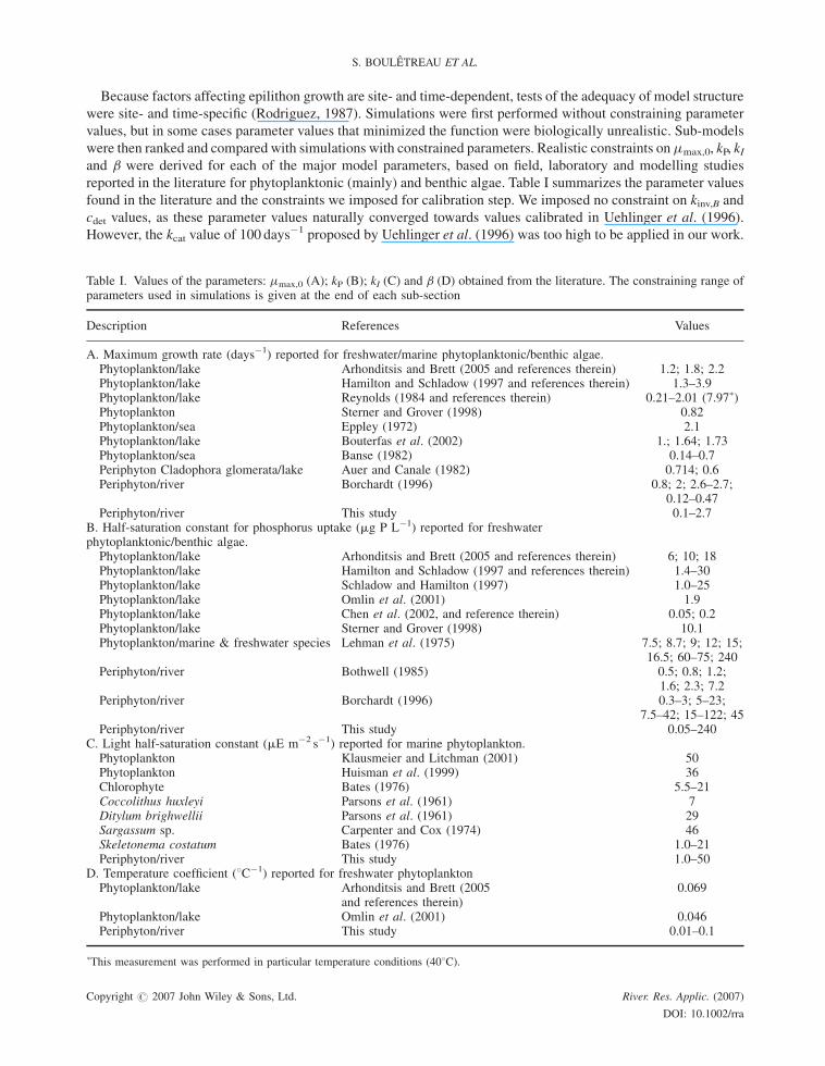
Because factors affecting epilithon growth are site- and time-dependent, tests of the adequacy of model structure

were site- and time-specific (Rodriguez, 1987). Simulations were first performed without constraining parameter

values, but in some cases parameter values that minimized the function were biologically unrealistic. Sub-models

were then ranked and compared with simulations with constrained parameters. Realistic constraints on mmax,0, kP, kI

and b were derived for each of the major model parameters, based on field, laboratory and modelling studies

reported in the literature for phytoplanktonic (mainly) and benthic algae. Table I summarizes the parameter values

found in the literature and the constraints we imposed for calibration step. We imposed no constraint on kinv,B and

cdet values, as these parameter values naturally converged towards values calibrated in Uehlinger et al. (1996).

However, the kcat value of 100 days�1 proposed by Uehlinger et al. (1996) was too high to be applied in our work.

Table I. Values of the parameters: mmax,0 (A); kP (B); kI (C) and b (D) obtained from the literature. The constraining range ofparameters used in simulations is given at the end of each sub-section

Description References Values

A. Maximum growth rate (days�1) reported for freshwater/marine phytoplanktonic/benthic algae.Phytoplankton/lake Arhonditsis and Brett (2005 and references therein) 1.2; 1.8; 2.2Phytoplankton/lake Hamilton and Schladow (1997 and references therein) 1.3–3.9Phytoplankton/lake Reynolds (1984 and references therein) 0.21–2.01 (7.97�)Phytoplankton Sterner and Grover (1998) 0.82Phytoplankton/sea Eppley (1972) 2.1Phytoplankton/lake Bouterfas et al. (2002) 1.; 1.64; 1.73Phytoplankton/sea Banse (1982) 0.14–0.7Periphyton Cladophora glomerata/lake Auer and Canale (1982) 0.714; 0.6Periphyton/river Borchardt (1996) 0.8; 2; 2.6–2.7;

0.12–0.47Periphyton/river This study 0.1–2.7

B. Half-saturation constant for phosphorus uptake (mg P L�1) reported for freshwaterphytoplanktonic/benthic algae.

Phytoplankton/lake Arhonditsis and Brett (2005 and references therein) 6; 10; 18Phytoplankton/lake Hamilton and Schladow (1997 and references therein) 1.4–30Phytoplankton/lake Schladow and Hamilton (1997) 1.0–25Phytoplankton/lake Omlin et al. (2001) 1.9Phytoplankton/lake Chen et al. (2002, and reference therein) 0.05; 0.2Phytoplankton/lake Sterner and Grover (1998) 10.1Phytoplankton/marine & freshwater species Lehman et al. (1975) 7.5; 8.7; 9; 12; 15;

16.5; 60–75; 240Periphyton/river Bothwell (1985) 0.5; 0.8; 1.2;

1.6; 2.3; 7.2Periphyton/river Borchardt (1996) 0.3–3; 5–23;

7.5–42; 15–122; 45Periphyton/river This study 0.05–240

C. Light half-saturation constant (mE m�2 s�1) reported for marine phytoplankton.Phytoplankton Klausmeier and Litchman (2001) 50Phytoplankton Huisman et al. (1999) 36Chlorophyte Bates (1976) 5.5–21Coccolithus huxleyi Parsons et al. (1961) 7Ditylum brighwellii Parsons et al. (1961) 29Sargassum sp. Carpenter and Cox (1974) 46Skeletonema costatum Bates (1976) 1.0–21Periphyton/river This study 1.0–50

D. Temperature coefficient (8C�1) reported for freshwater phytoplanktonPhytoplankton/lake Arhonditsis and Brett (2005

and references therein)0.069

Phytoplankton/lake Omlin et al. (2001) 0.046Periphyton/river This study 0.01–0.1

�This measurement was performed in particular temperature conditions (408C).

Copyright # 2007 John Wiley & Sons, Ltd. River. Res. Applic. (2007)

DOI: 10.1002/rra

A MINIMAL ADEQUATE MODEL FOR RIVER EPILITHON BIOMASS

Model interpretation

To explain model behaviour and to reduce the freedom as much as possible, we interpreted parameter values of

the best sub-model selected in the first modelling step and used step-wise regression analysis (Statview software) to

explore the influence of environmental factors on these. Only variables with p< 0.05 were kept in the equation. The

explicative factors were mean velocity, percentage of sand, conductivity, total nitrogen, total phosphorus, silicate

and canopy cover.

Experimental data set

We used data on epilithon biomass (g AFDM m�2) in the Aguera stream (Northern Spain) published by Elosegi

and Pozo (1998) and Izagirre and Elosegi (2005). The Aguera is a flood-prone, steep, 30-km long stream draining a

145 km2 basin with humid maritime climate. The number of floods, and the duration of flood-free periods in

particular, can change markedly from year to year (Elosegi et al., 2002; Elosegi et al., 2006). Physico-chemical

characteristics of the water are quite contrasting, reflecting the geology and land-use of different parts of the basin

(Table II). At the headwaters (site 2) conductivity and nutrient contents are low, but they increase sharply when the

stream runs through the villages of Villaverde (site 4) and Trucıos (site 5), decrease again further downstream (site

7) and increase below the town of Guriezo (site 9). Izagirre and Elosegi (2005) showed that at open sites flow is the

main temporal controller, whereas at closed sites the effects of light availability prevail, thus giving more similar

seasonal patterns from year to year.

Epilithon sampling was performed monthly during three 12-month periods (January 1990–January 1991;

October 1992–November 1993; October 2001–November 2002) at five sites (2, 4, 5, 7 and 9). Study cases were

named according to measurement period and site (e.g. case 90–2 was collected in 1990 from site 2). Ten stones were

collected at random in a 100 m2-area in a given riffle at each study site. Study sites are between 2–7 km apart, so we

can therefore reasonably assume that differences in stream bottom facies and biomass levels observed from site to

site ensure the relevance of considering them as distinct study cases. In contrast, in the river Necker studies, the

measured biomasses used for comparison with simulated biomasses were sampled in a reach of 2 km length to

ensure good predictability of the succession sequences of epilithon at a local scale, as epilithon distribution is very

patchy and underdeterministic (Uehlinger et al., 1996).

Additional data used for modelling included daily discharge and solar radiation and periodic data on water

chemistry. Discharge was measured daily by the Spanish Northern Hydrological Confederation at site 9 and

recalculated for the other sites from empirical regressions. Following Elosegi and Pozo (1998), we considered a

discharge of 30 m3 s�1 at site 9 as the critical threshold for flood-induced epilithic sloughing. Solar radiation

(J cm�2) was measured by the Spanish Meteorological Institute at San Sebastian, and in some periods of missing

data it was calculated from duration of sunshine in Bilbao, by means of the Angstrom formula, which relates solar

radiation to extraterrestrial radiation and relative sunshine duration (Food and Agricultural Organization of United

States: http://www.fao.org/). Every (measured or calculated) daily radiation value was first converted to PAR

(J cm�2) according to Steemann-Nielsen (1975) and then converted to photon flux density expressed as E m�2. To

calculate the radiation effectively reaching the stream, we corrected the above data for canopy cover. Canopy cover

was measured using 10 vertical photographs taken at each sampling site with a wide-angle lens in winter and

summer foliage. Photographs were scanned, their contrast increased to produce black (covered) and white

(uncovered sky) images, and analysed with NIH 1.55 software (Izagirre and Elosegi, 2005). Water chemistry was

measured approximately every 15 days during 1990–91 and 2001–02, but not during 1992–93. Phosphate was

measured by the stannous chloride method (APHA, 1992) on a Shimadzu UV-1603 spectrophotometer.

RESULTS

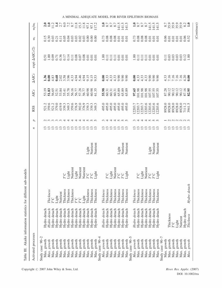
Results of AIC statistics for each sub-model at every study site are listed in Table III. The set of candidate

sub-models (R) varied between years: in 2001 R was 7; in 1990 R was 6 because discharge was always lower than

critical and subsequently kcat was never activated; and in 1992 R was 5, as phosphate and temperature data were not

available and thus kP and b were not activated. One single sub-model was clearly the best of all: in 7 of 11 study

Copyright # 2007 John Wiley & Sons, Ltd. River. Res. Applic. (2007)

DOI: 10.1002/rra

Tab

leII

.G

eogra

phic

al,physi

cal

and

chem

ical

char

acte

rist

ics

of

the

study

site

s(m

ean�

SD

).W

hen

dif

fere

nt

figure

sap

pea

rse

par

ated

by

a/

sign,th

efi

rst

corr

esponds

toth

eper

iod

1990–91,

the

seco

nd

to2001–02

Sit

eS

ite

2S

ite

4S

ite

5S

ite

7S

ite

9

Ord

er2

33

33

Wat

erte

mper

ature

(8C

)11.1

(�4.1

)/12.5

(�4.6

)11.3

(�4.7

)/13.4

(�4.3

)12.7

(�4.0

)/13.8

(�4.3

)13.3

(�3.9

)/14.2

(�3.5

)13.3

(�3.7

)/15.0

(�4.3

)pH

7.7

(�0.4

)/7.4

(�0.2

)7.9

(�0.5

)/7.5

(�0.3

)8.4

(�0.7

)/7.8

(�0.3

)8.6

(�0.5

)/7.8

(�0.2

)7.8

(�0.4

)/7.5

(�0.2

)C

onduct

ivit

y(m

Scm

�1)

172(�

48)/

148(�

42)

243(�

86)/

203(�

74)

308(�

69)/

248(�

59)

262(�

31)/

234(�

34)

234(�

50)/

216(�

37)

Tota

lN

(mg

NL�

1)

646(�

314)/

493(�

284)

940(�

374)/

747(�

361)

950(�

207)/

1161(�

323)

722(�

322)/

914(�

282)

783(�

302)/

839(�

306)

Tota

lP

(mg

PL�

1)

6(�

10)/

8.5

(�11)

128(�

134)/

69(�

64)

111(�

62)/

105(�

99)

20(�

12)/

20(�

23)

103(�

85)/

38(�

31)

Sil

icat

e(m

gS

iL�

1)

2504(�

898)/

3590(�

477)

2021(�

858)/

2749(�

615)

1793(�

734)/

2572(�

691)

963(�

773)/

2006(�

623)

1275(�

623)/

2036(�

582)

Nit

rate

(mg

NL�

1)

590(�

302)/

443(�

281)

806(�

312)/

618(�

365)

830(�

231)/

1013(�

312)

696(�

327)/

848(�

282)

708(�

259)/

774(�

310)

Nit

rite

(mg

NL�

1)

2(�

1.5

)/17(�

12)

31(�

26)/

24(�

14)

32(�

26)/

34(�

18)

5(�

2)/

26(�

14)

35(�

25)/

20(�

9)

Am

oniu

m(m

gN

L�

1)

54(�

80)/

33(�

16)

104(�

112)/

105(�

77)

88(�

56)/

114(�

89)

21(�

17)/

39(�

9)

90(�

82)/

46(�

9)

Vel

oci

ty(m

s�1)

0.7

7(�

0.1

9)/

0.7

5(�

0.3

1)

0.2

1(�

0.2

6)/

0.5

9(�

0.3

0)

0.9

4(�

0.2

1)/

0.9

7(�

0.4

0)

0.8

2(�

0.1

9)/

0.8

1(�

0.3

3)

0.8

3(�

0.3

3)/

0.8

1(�

0.3

9)

San

d(%

)5.0

/25

23/0

2.0

/14

4.7

/05.8

/0C

anopy

cover

(%)

87/6

53.0

/72

8.0

/37

31/3

277/7

3

Copyright # 2007 John Wiley & Sons, Ltd. River. Res. Applic. (2007)

DOI: 10.1002/rra

S. BOULETREAU ET AL.

Tab

leII

I.A

kai

ke

info

rmat

ion

stat

isti

csfo

rdif

fere

nt

sub-m

odel

s

Act

ivat

edpro

cess

esn

pR

SS

AIC

cD

AIC

cex

p(-D

AIC

c/2)

vi

vj/v

i

Stu

dy

case

:90–2

Max

.gro

wth

Hydro

det

ach

13

2521.2

53.1

91.36

0.5

10.1

52.0

Max.

gro

wth

Hyd

rodet

ach

Thic

knes

s13

3359.6

51.83

0.00

1.0

00.3

01.0

Max

.gro

wth

Hydro

det

ach

T8C

13

3521.2

56.6

54.8

30.0

90.0

311.2

Max

.gro

wth

Hydro

det

ach

Lig

ht

13

3379.0

52.5

10.68

0.7

10.2

11.4

Max

.gro

wth

Hydro

det

ach

Nutr

ient

13

3419.9

53.8

42.0

20.3

60.1

12.7

Max

.gro

wth

Hydro

det

ach

Thic

knes

sT8C

13

4339.3

55.4

13.5

80.1

70.0

56.0

Max

.gro

wth

Hydro

det

ach

Thic

knes

sL

ight

13

4349.3

55.7

83.9

60.1

40.0

47.2

Max

.gro

wth

Hydro

det

ach

Thic

knes

sN

utr

ient

13

4359.6

56.1

64.3

30.1

10.0

38.7

Max

.gro

wth

Hydro

det

ach

T8C

Lig

ht

13

4376.9

56.7

74.9

40.0

80.0

311.8

Max

.gro

wth

Hydro

det

ach

T8C

Nutr

ient

13

4392.0

57.2

85.4

60.0

70.0

215.3

Max

.gro

wth

Hydro

det

ach

Lig

ht

Nutr

ient

13

4376.9

56.7

74.9

40.0

80.0

311.8

Max

.gro

wth

Hydro

det

ach

Thic

knes

sT8C

Lig

ht

13

5339.3

60.9

89.1

50.0

10.0

097.1

Max

.gro

wth

Hydro

det

ach

Thic

knes

sT8C

Nutr

ient

13

5339.3

60.9

89.1

50.0

10.0

097.1

Max

.gro

wth

Hydro

det

ach

Thic

knes

sL

ight

Nutr

ient

13

5349.3

61.3

59.5

30.0

10.0

0117.2

Stu

dy

case

:90–4

Max.

gro

wth

Hyd

rodet

ach

Thic

knes

s13

3495.0

55.98

0.00

1.0

00.7

31.0

Max

.gro

wth

Hydro

det

ach

Thic

knes

sT8C

13

4495.0

60.3

14.3

30.1

10.0

88.7

Max

.gro

wth

Hydro

det

ach

Thic

knes

sL

ight

13

4495.0

60.3

14.3

30.1

10.0

88.7

Max

.gro

wth

Hydro

det

ach

Thic

knes

sN

utr

ient

13

4495.0

60.3

14.3

30.1

10.0

88.7

Max

.gro

wth

Hydro

det

ach

Thic

knes

sT8C

Lig

ht

13

5495.0

65.8

99.9

00.0

10.0

1141.5

Max

.gro

wth

Hydro

det

ach

Thic

knes

sT8C

Nutr

ient

13

5495.0

65.8

99.9

00.0

10.0

1141.5

Max

.gro

wth

Hydro

det

ach

Thic

knes

sL

ight

Nutr

ient

13

5495.0

65.8

99.9

00.0

10.0

1141.5

Stu

dy

case

:90–5

Max.

gro

wth

Hyd

rodet

ach

Thic

knes

s13

312203.7

97.65

0.00

1.0

00.7

31.0

Max

.gro

wth

Hydro

det

ach

Thic

knes

sT8C

13

412203.7

101.9

84.3

30.1

10.0

88.7

Max

.gro

wth

Hydro

det

ach

Thic

knes

sL

ight

13

412203.7

101.9

84.3

30.1

10.0

88.7

Max

.gro

wth

Hydro

det

ach

Thic

knes

sN

utr

ient

13

412203.6

101.9

84.3

30.1

10.0

88.7

Max

.gro

wth

Hydro

det

ach

Thic

knes

sT8C

Lig

ht

13

512203.6

107.5

59.9

00.0

10.0

1141.5

Max

.gro

wth

Hydro

det

ach

Thic

knes

sT8C

Nutr

ient

13

512203.6

107.5

59.9

00.0

10.0

1141.5

Max

.gro

wth

Hydro

det

ach

Thic

knes

sL

ight

Nutr

ient

13

512203.6

107.5

59.9

00.0

10.0

1141.5

Stu

dy

case

:90–7

Max

.gro

wth

13

18928.0

87.2

84.3

30.1

10.0

68.7

Max

.gro

wth

Thic

knes

s13

28928.0

90.1

27.1

60.0

30.0

135.9

Max

.gro

wth

T8C

13

28928.0

90.1

27.1

60.0

30.0

135.9

Max

.gro

wth

Lig

ht

13

28928.0

90.1

27.1

60.0

30.0

135.9

Max

.gro

wth

Nutr

ient

13

28928.0

90.1

27.1

60.0

30.0

135.9

Max

.gro

wth

Hydro

det

ach

13

27111.2

87.1

64.2

00.1

20.0

68.2

Max.

gro

wth

Thic

knes

sH

ydro

det

ach

13

33941.5

82.95

0.00

1.0

00.5

21.0

Copyright # 2007 John Wiley & Sons, Ltd. River. Res. Applic. (2007

DOI: 10.1002/rra

A MINIMAL ADEQUATE MODEL FOR RIVER EPILITHON BIOMASS

(Conti

nues

)

)

Tab

leII

I.(C

onti

nued

)

Act

ivat

edpro

cess

esn

pR

SS

AIC

cD

AIC

cex

p(-D

AIC

c/2)

vi

vj/v

i

Max

.gro

wth

T8C

Hydro

det

ach

13

37111.2

90.6

27.6

70.0

20.0

146.3

Max

.gro

wth

Lig

ht

Hydro

det

ach

13

35695.5

87.7

44.7

90.0

90.0

510.9

Max

.gro

wth

Nutr

ient

Hydro

det

ach

13

36176.7

88.7

95.8

40.0

50.0

318.5

Max

.gro

wth

Thic

knes

sT8C

Hydro

det

ach

13

43941.5

87.2

94.3

30.1

10.0

68.7

Max

.gro

wth

Thic

knes

sL

ight

Hydro

det

ach

13

43941.5

87.2

94.3

30.1

10.0

68.7

Max

.gro

wth

Thic

knes

sN

utr

ient

Hydro

det

ach

13

43941.5

87.2

94.3

30.1

10.0

68.7

Max

.gro

wth

T8C

Lig

ht

Hydro

det

ach

13

45961.3

92.6

79.7

10.0

10.0

0128.5

Max

.gro

wth

T8C

Nutr

ient

Hydro

det

ach

13

45537.2

91.7

18.7

50.0

10.0

179.5

Max

.gro

wth

Lig

ht

Nutr

ient

Hydro

det

ach

13

45156.7

90.7

87.8

30.0

20.0

150.1

Max

.gro

wth

Thic

knes

sT8C

Lig

ht

Hydro

det

ach

13

53941.5

92.8

69.9

00.0

10.0

0141.5

Max

.gro

wth

Thic

knes

sT8C

Nutr

ient

Hydro

det

ach

13

53941.5

92.8

69.9

00.0

10.0

0141.5

Max

.gro

wth

Thic

knes

sL

ight

Nutr

ient

Hydro

det

ach

13

53941.5

92.8

69.9

00.0

10.0

0141.5

Stu

dy

case

:92–5

Max

.gro

wth

Thic

knes

s13

22303.1

72.5

05.8

70.0

50.0

318.8

Max

.gro

wth

Lig

ht

13

22444.5

73.2

86.6

50.0

40.0

227.8

Max.

gro

wth

Thic

knes

sH

ydro

det

ach

13

31122.9

66.63

0.00

1.0

00.6

41.0

Max

.gro

wth

Thic

knes

sL

ight

13

32303.1

75.9

79.3

40.0

10.0

1106.6

Max

.gro

wth

Thic

knes

sC

ata

det

ach

13

32303.1

75.9

79.3

40.0

10.0

1106.6

Max

.gro

wth

Thic

knes

sL

ight

Hydro

det

ach

13

41122.9

70.9

64.3

30.1

10.0

78.7

Max

.gro

wth

Thic

knes

sC

ata

det

ach

Hydro

det

ach

13

4973.8

69.1

12.4

80.2

90.1

83.5

Max

.gro

wth

Thic

knes

sL

ight

Cat

adet

ach

13

41304.2

72.9

16.2

80.0

40.0

323.1

Max

.gro

wth

Thic

knes

sL

ight

Hydro

det

ach

13

5973.8

74.6

88.0

50.0

20.0

156.1

Stu

dy

case

:92–9

Max

.gro

wth

13

12649.3

71.4

99.6

30.0

10.0

0123.6

Max

.gro

wth

Thic

knes

s13

21188.2

63.9

02.0

50.3

60.2

02.8

Max

.gro

wth

Lig

ht

13

21515.2

67.0

65.2

10.0

70.0

413.5

Max.

gro

wth

Thic

knes

sH

ydro

det

ach

13

3777.6

61.85

0.00

1.0

00.5

51.0

Max

.gro

wth

Thic

knes

sL

ight

13

31188.2

67.3

65.5

10.0

60.0

315.7

Max

.gro

wth

Thic

knes

sC

ata

det

ach

13

31188.2

67.3

65.5

10.0

60.0

315.7

Max

.gro

wth

Lig

ht

Hydro

det

ach

13

31515.2

70.5

28.6

70.0

10.0

176.4

Max

.gro

wth

Lig

ht

Cat

adet

ach

13

31515.2

70.5

28.6

70.0

10.0

176.4

Max

.gro

wth

Thic

knes

sL

ight

Hydro

det

ach

13

4777.6

66.1

94.3

30.1

10.0

68.7

Max

.gro

wth

Thic

knes

sC

ata

det

ach

Hydro

det

ach

13

4800.3

66.5

64.7

10.0

90.0

510.5

Max

.gro

wth

Thic

knes

sL

ight

Cat

adet

ach

13

41188.2

71.7

09.8

50.0

10.0

0137.4

Max

.gro

wth

Thic

knes

sL

ight

Cat

adet

ach

Hydro

det

ach

13

5777.6

71.7

69.9

00.0

10.0

0141.5

Stu

dy

case

:01–2

Max.

gro

wth

Hyd

rodet

ach

13

2209.1

41.31

0.00

1.0

00.2

51.0

Max

.gro

wth

Cat

adet

ach

13

2323.4

46.9

85.6

70.0

60.0

117.0

Max

.gro

wth

Thic

knes

sH

ydro

det

ach

13

3160.5

41.3

40.03

0.9

90.2

41.0

(Conti

nues

)

Copyright # 2007 John Wiley & Sons, Ltd. River. Res. Applic. (2007

DOI: 10.1002/rra

S. BOULETREAU ET AL.

)

Tab

leII

I.(C

onti

nued

)

Act

ivat

edpro

cess

esn

pR

SS

AIC

cD

AIC

cex

p(-D

AIC

c/2)

vi

vj/v

i

Max

.gro

wth

Thic

knes

sC

ata

det

ach

13

3323.4

50.4

59.1

30.0

10.0

096.3

Max

.gro

wth

T8C

Hydro

det

ach

13

3208.5

44.7

43.4

30.1

80.0

45.5

Max

.gro

wth

T8C

Cat

adet

ach

13

3323.4

50.4

59.1

30.0

10.0

096.3

Max

.gro

wth

Lig

ht

Hydro

det

ach

13

3199.4

44.1

62.8

50.2

40.0

64.2

Max

.gro

wth

Lig

ht

Cat

adet

ach

13

3323.4

50.4

59.1

30.0

10.0

096.3

Max

.gro

wth

Nutr

ient

Hydro

det

ach

13

3209.1

44.7

83.4

70.1

80.0

45.7

Max

.gro

wth

Nutr

ient

Cat

adet

ach

13

3323.4

50.4

59.1

30.0

10.0

096.3

Max

.gro

wth

Cat

adet

ach

Hydro

det

ach

13

3209.1

44.7

83.4

70.1

80.0

45.7

Max

.gro

wth

Thic

knes

sT8C

Hydro

det

ach

13

4160.5

45.6

74.3

60.1

10.0

38.9

Max

.gro

wth

Thic

knes

sL

ight

Hydro

det

ach

13

4158.9

45.5

54.2

30.1

20.0

38.3

Max

.gro

wth

Thic

knes

sN

utr

ient

Hydro

det

ach

13

4160.5

45.6

74.3

60.1

10.0

38.9

Max

.gro

wth

Thic

knes

sC

ata

det

ach

Hydro

det

ach

13

4127.6

42.6

91.3

80.5

00.1

22.0

Max

.gro

wth

T8C

Lig

ht

Hydro

det

ach

13

4209.1

49.1

17.8

00.0

20.0

149.4

Max

.gro

wth

T8C

Nutr

ient

Hydro

det

ach

13

4209.1

49.1

17.8

00.0

20.0

149.4

Max

.gro

wth

T8C

Hydro

det

ach

Cat

adet

ach

13

4209.1

49.1

17.8

00.0

20.0

149.4

Max

.gro

wth

Lig

ht

Nutr

ient

Hydro

det

ach

13

4209.1

49.1

17.8

00.0

20.0

149.4

Max

.gro

wth

Lig

ht

Hydro

det

ach

Cat

adet

ach

13

4209.1

49.1

17.8

00.0

20.0

149.4

Max

.gro

wth

Thic

knes

sH

ydro

det

ach

Cat

adet

ach

13

4209.1

49.1

17.8

00.0

20.0

149.4

Max

.gro

wth

Thic

knes

sC

ata

det

ach

T8C

13

5127.6

48.2

66.9

50.0

30.0

132.3

Max

.gro

wth

Thic

knes

sC

ata

det

ach

Lig

ht

13

5127.6

48.2

66.9

50.0

30.0

132.3

Max

.gro

wth

Thic

knes

sC

ata

det

ach

Nutr

ient

13

5127.6

48.2

66.9

50.0

30.0

132.3

Max

.gro

wth

Thic

knes

sT8C

Lig

ht

13

5127.6

48.2

66.9

50.0

30.0

132.3

Max

.gro

wth

Thic

knes

sT8c

Nutr

ient

13

5127.6

48.2

66.9

50.0

30.0

132.3

Max

.gro

wth

Thic

knes

sL

ight

Nutr

ient

13

5127.6

48.2

66.9

50.0

30.0

132.3

Max

.gro

wth

T8C

Lig

ht

Nutr

ient

13

5127.6

48.2

66.9

50.0

30.0

132.3

Stu

dy

case

:01–4

Max.

gro

wth

13

1874.9

57.08

0.00

1.0

00.1

41.0

Max

.gro

wth

Thic

knes

s13

2858.2

59.6

72.5

90.2

70.0

43.6

Max

.gro

wth

T8C

13

2874.9

59.9

22.8

40.2

40.0

34.1

Max

.gro

wth

Lig

ht

13

2874.9

59.9

22.8

40.2

40.0

34.1

Max

.gro

wth

Nutr

ient

13

2857.4

59.6

62.5

70.2

80.0

43.6

Max

.gro

wth

Hydro

det

ach

13

2732.7

57.6

10.5

30.7

70.1

11.3

Max

.gro

wth

Cat

adet

ach

13

2866.7

59.8

02.7

10.2

60.0

43.9

Max

.gro

wth

Thic

knes

sH

ydro

det

ach

13

3732.8

61.0

84.0

00.1

40.0

27.4

Max

.gro

wth

Thic

knes

sC

ata

det

ach

13

3614.4

58.7

91.7

10.4

30.0

62.3

Max

.gro

wth

Thic

knes

sT8C

13

3874.9

63.3

96.3

00.0

40.0

123.4

Max

.gro

wth

Thic

knes

sL

ight

13

3874.9

63.3

96.3

00.0

40.0

123.4

Max

.gro

wth

Thic

knes

sN

utr

ient

13

3857.4

63.1

26.0

40.0

50.0

120.5

Max

.gro

wth

T8C

Hydro

det

ach

13

3732.7

61.0

84.0

00.1

40.0

27.4

(Conti

nues

)

Tab

leII

I.(C

onti

nued

)

Copyright # 2007 John Wiley & Sons, Ltd. River. Res. Applic. (2007)

DOI: 10.1002/rra

A MINIMAL ADEQUATE MODEL FOR RIVER EPILITHON BIOMASS

Tab

leII

I.(C

onti

nued

)

Act

ivat

edpro

cess

esn

pR

SS

AIC

cD

AIC

cex

p(-D

AIC

c/2)

vi

vj/v

i

Max

.gro

wth

T8C

Lig

ht

13

3874.9

63.3

96.3

00.0

40.0

123.4

Max

.gro

wth

T8C

Nutr

ient

13

3857.4

63.1

26.0

40.0

50.0

120.5

Max

.gro

wth

T8C

Cat

adet

ach

13

3642.8

59.3

82.2

90.3

20.0

43.1

Max

.gro

wth

Lig

ht

Hydro

det

ach

13

3732.7

61.0

84.0

00.1

40.0

27.4

Max

.gro

wth

Lig

ht

Nutr

ient

13

3857.4

63.1

26.0

40.0

50.0

120.5

Max

.gro

wth

Lig

ht

Cat

adet

ach

13

3668.9

59.9

02.8

10.2

40.0

34.1

Max

.gro

wth

Nutr

ient

Hydro

det

ach

13

3732.7

61.0

84.0

00.1

40.0

27.4

Max

.gro

wth

Nutr

ient

Cat

adet

ach

13

3644.7

59.4

22.3

30.3

10.0

43.2

Max

.gro

wth

Cat

adet

ach

Hydro

det

ach

13

3638.8

59.3

02.2

10.3

30.0

53.0

Max

.gro

wth

Thic

knes

sT8C

Cat

adet

ach

13

4607.8

58.6

51.5

70.4

60.0

62.2

Max

.gro

wth

Thic

knes

sL

ight

Hydro

det

ach

13

4732.7

65.4

18.3

30.0

20.0

064.4

Max

.gro

wth

Thic

knes

sL

ight

Cat

adet

ach

13

4607.8

58.6

51.5

70.4

60.0

62.2

Max

.gro

wth

Thic

knes

sN

utr

ient

Hydro

det

ach

13

4732.7

65.4

18.3

30.0

20.0

064.4

Max

.gro

wth

Thic

knes

sN

utr

ient

Cat

adet

ach

13

4607.8

58.6

51.5

70.4

60.0

62.2

Max

.gro

wth

Thic

knes

sC

ata

det

ach

Hydro

det

ach

13

4614.4

63.1

26.0

40.0

50.0

120.5

Max

.gro

wth

T8C

Lig

ht

Hydro

det

ach

13

4732.7

65.4

18.3

30.0

20.0

064.4

Max

.gro

wth

T8C

Lig

ht

Cat

adet

ach

13

4642.8

63.7

16.6

30.0

40.0

127.5

Max

.gro

wth

T8C

Nutr

ient

Hydro

det

ach

13

4732.7

65.4

18.3

30.0

20.0

064.4

Max

.gro

wth

T8C

Nutr

ient

Cat

adet

ach

13

4642.8

63.7

16.6

30.0

40.0

127.5

Max

.gro

wth

T8C

Hydro

det

ach

Cat

adet

ach

13

4638.8

63.6

36.5

50.0

40.0

126.4

Max

.gro

wth

Lig

ht

Nutr

ient

Hydro

det

ach

13

4732.7

65.4

18.3

30.0

20.0

064.4

Max

.gro

wth

Lig

ht

Nutr

ient

Cat

adet

ach

13

4642.8

63.7

16.6

30.0

40.0

127.5

Max

.gro

wth

Lig

ht

Hydro

det

ach

Cat

adet

ach

13

4638.8

63.6

36.5

50.0

40.0

126.4

Max

.gro

wth

Nutr

ient

Hydro

det

ach

Cat

adet

ach

13

4638.8

63.6

36.5

50.0

40.0

126.4

Stu

dy

case

:01-5

Max.

gro

wth

13

12762.0

72.03

0.00

1.0

00.2

91.0

Max

.gro

wth

Thic

knes

s13

22762.0

74.8

62.8

40.2

40.0

74.1

Max

.gro

wth

T8C

13

22762.0

74.8

62.8

40.2

40.0

74.1

Max

.gro

wth

Lig

ht

13

22762.0

74.8

62.8

40.2

40.0

74.1

Max

.gro

wth

Nutr

ient

13

22762.0

74.8

62.8

40.2

40.0

74.1

Max

.gro

wth

Hydro

det

ach

13

22762.0

74.8

62.8

40.2

40.0

74.1

Max

.gro

wth

Cat

adet

ach

13

22762.0

74.8

62.8

40.2

40.0

74.1

Max

.gro

wth

Thic

knes

sH

ydro

det

ach

13

32279.5

75.8

33.8

10.1

50.0

46.7

Max

.gro

wth

Thic

knes

sC

ata

det

ach

13

32762.0

78.3

36.3

00.0

40.0

123.4

Max

.gro

wth

Thic

knes

sT8C

13

32762.0

78.3

36.3

00.0

40.0

123.4

Max

.gro

wth

Thic

knes

sL

ight

13

32762.0

78.3

36.3

00.0

40.0

123.4

Max

.gro

wth

Thic

knes

sN

utr

ient

13

32762.0

78.3

36.3

00.0

40.0

123.4

Max

.gro

wth

T8C

Hydro

det

ach

13

32762.0

78.3

36.3

00.0

40.0

123.4

Max

.gro

wth

T8C

Lig

ht

13

32762.0

78.3

36.3

00.0

40.0

123.4

(Conti

nues

)

Copyright # 2007 John Wiley & Sons, Ltd. River. Res. Applic. (2007)

DOI: 10.1002/rra

S. BOULETREAU ET AL.

Tab

leII

I.(C

onti

nued

)

Act

ivat

edpro

cess

esn

pR

SS

AIC

cD

AIC

cex

p(-D

AIC

c/2)

vi

vj/v

i

Max

.gro

wth

T8C

Nutr

ient

13

32762.0

78.3

36.3

00.0

40.0

123.4

Max

.gro

wth

T8C

Cat

adet

ach

13

32762.0

78.3

36.3

00.0

40.0

123.4

Max

.gro

wth

Lig

ht

Hydro

det

ach

13

32491.7

76.9

94.9

60.0

80.0

212.0

Max

.gro

wth

Lig

ht

Nutr

ient

13

32762.0

78.3

36.3

00.0

40.0

123.4

Max

.gro

wth

Lig

ht

Cat

adet

ach

13

32762.0

78.3

36.3

00.0

40.0

123.4

Max

.gro

wth

Nutr

ient

Hydro

det

ach

13

32762.0

78.3

36.3

00.0

40.0

123.4

Max

.gro

wth

Nutr

ient

Cat

adet

ach

13

32762.0

78.3

36.3

00.0

40.0

123.4

Max

.gro

wth

Cat

adet

ach

Hydro

det

ach

13

32279.1

75.8

33.8

00.1

50.0

46.7

Max

.gro

wth

Thic

knes

sL

ight

Hydro

det

ach

13

42215.3

79.8

07.7

70.0

20.0

148.6

Max

.gro

wth

Thic

knes

sN

utr

ient

Hydro

det

ach

13

42279.1

80.1

78.1

40.0

20.0

158.6

Max

.gro

wth

Thic

knes

sC

ata

det

ach

Hydro

det

ach

13

42279.1

80.1

78.1

40.0

20.0

158.5

Stu

dy

case

:01-7

Max

.gro

wth

Hydro

det

ach

13

22249.6

72.2

07.4

80.0

20.0

242.0

Max

.gro

wth

Cat

adet

ach

13

22255.5

72.2

37.5

10.0

20.0

142.7

Max.

gro

wth

Thic

knes

sH

ydro

det

ach

13

3969.5

64.72

0.00

1.0

00.6

31.0

Max

.gro

wth

Lig

ht

Hydro

det

ach

13

31746.2

72.3

77.6

50.0

20.0

145.8

Max

.gro

wth

Nutr

ient

Hydro

det

ach

13

32056.0

74.4

99.7

70.0

10.0

0132.4

Max

.gro

wth

Thic

knes

sL

ight

Hydro

det

ach

13

4931.7

68.5

43.8

20.1

50.0

96.7

Max

.gro

wth

Thic

knes

sN

utr

ient

Hydro

det

ach

13

4969.5

69.0

54.3

30.1

10.0

78.7

Max

.gro

wth

Thic

knes

sC

ata

det

ach

Hydro

det

ach

13

4916.2

68.3

23.6

00.1

70.1

06.0

Max

.gro

wth

Thic

knes

sC

ata

det

ach

T-C

Hydro

det

ach

13

5916.2

73.8

99.1

70.0

10.0

198.0

Max

.gro

wth

Thic

knes

sC

ata

det

ach

Lig

ht

Hydro

det

ach

13

5885.9

73.4

58.7

30.0

10.0

178.7

Max

.gro

wth

Thic

knes

sC

ata

det

ach

Nutr

ient

Hydro

det

ach

13

5916.2

73.8

99.1

70.0

10.0

198.0

Max

.gro

wth

Thic

knes

sT-C

Lig

ht

Hydro

det

ach

13

5885.9

73.4

58.7

30.0

10.0

178.7

Max

.gro

wth

Thic

knes

sT-C

Nutr

ient

Hydro

det

ach

13

5885.9

73.4

58.7

30.0

10.0

178.7

Max

.gro

wth

Thic

knes

sL

ight

Nutr

ient

Hydro

det

ach

13

5885.9

73.4

58.7

30.0

10.0

178.7

Stu

dy

case

:01-9

Max

.gro

wth

13

11587.5

64.8

32.9

80.2

30.0

74.4

Max

.gro

wth

Thic

knes

s13

21509.0

67.0

05.1

50.0

80.0

213.1

Max

.gro

wth

T-C

13

21587.5

67.6

65.8

10.0

50.0

218.3

Max

.gro

wth

Lig

ht

13

21587.5

67.6

65.8

10.0

50.0

218.3

Max

.gro

wth

Nutr

ient

13

21537.1

67.2

55.3

90.0

70.0

214.8

Max

.gro

wth

Hydro

det

ach

13

21303.6

65.1

03.2

50.2

00.0

65.1

Max.

gro

wth

Cata

det

ach

13

21015.2

61.85

0.00

1.0

00.3

21.0

Max

.gro

wth

Thic

knes

sH

ydro

det

ach

13

31303.6

68.5

76.7

20.0

30.0

128.7

Max

.gro

wth

Thic

knes

sC

ata

det

ach

13

3910.7

63.9

12.0

50.3

60.1

12.8

Max

.gro

wth

Thic

knes

sT8C

13

31509.0

70.4

78.6

20.0

10.0

074.4

Max

.gro

wth

Thic

knes

sL

ight

13

31509.0

70.4

78.6

20.0

10.0

074.4

Max

.gro

wth

Thic

knes

sN

utr

ient

13

31509.0

70.4

78.6

20.0

10.0

074.4

(Conti

nues

)

Tab

leII

I.(C

onti

nued

)

Copyright # 2007 John Wiley & Sons, Ltd. River. Res. Applic. (2007)

DOI: 10.1002/rra

A MINIMAL ADEQUATE MODEL FOR RIVER EPILITHON BIOMASS

Tab

leII

I.(C

onti

nued

)

Act

ivat

edpro

cess

esn

pR

SS

AIC

cD

AIC

cex

p(-D

AIC

c/2)

vi

vj/v

i

Max

.gro

wth

T8C

Cat

adet

ach

13

31015.2

65.3

23.4

70.1

80.0

65.7

Max

.gro

wth

Lig

ht

Hydro

det

ach

13

31303.6

68.5

76.7

20.0

30.0

128.7

Max

.gro

wth

Lig

ht

Cat

adet

ach

13

31015.2

65.3

23.4

70.1

80.0

65.7

Max

.gro

wth

Nutr

ient

Hydro

det

ach

13

31303.6

68.5

76.7

20.0

30.0

128.7

Max

.gro

wth

Nutr

ient

Cat

adet

ach

13

31015.2

65.3

23.4

70.1

80.0

65.7

Max

.gro

wth

Cat

adet

ach

Hydro

det

ach

13

31015.2

65.3

23.4

70.1

80.0

65.7

Max

.gro

wth

Thic

knes

sT8C

Cat

adet

ach

13

4910.7

68.2

46.3

90.0

40.0

124.4

Max

.gro

wth

Thic

knes

sL

ight

Cat

adet

ach

13

4910.7

68.2

46.3

90.0

40.0

124.4

Max

.gro

wth

Thic

knes

sN

utr

ient

Cat

adet

ach

13

4910.7

68.2

46.3

90.0

40.0

124.4

Max

.gro

wth

Thic

knes

sC

ata

det

ach

Hydro

det

ach

13

4910.7

68.2

46.3

90.0

40.0

124.4

Max

.gro

wth

T8C

Lig

ht

Cat

adet

ach

13

41015.2

69.6

57.8

00.0

20.0

149.4

Max

.gro

wth

T8C

Nutr

ient

Cat

adet

ach

13

41015.2

69.6

57.8

00.0

20.0

149.4

Max

.gro

wth

T8C

Hydro

det

ach

Cat

adet

ach

13

41015.2

69.6

57.8

00.0

20.0

149.4

Max

.gro

wth

Lig

ht

Nutr

ient

Cat

adet

ach

13

41015.2

69.6

57.8

00.0

20.0

149.4

Max

.gro

wth

Lig

ht

Hydro

det

ach

Cat

adet

ach

13

41015.2

69.6

57.8

00.0

20.0

149.4

Max

.gro

wth

Nutr

ient

Hydro

det

ach

Cat

adet

ach

13

41015.2

69.6

57.8

00.0

20.0

149.4

The

firs

tco

lum

nin

dic

ates

acti

vat

edpro

cess

es(a

nd

thus

acti

vat

edpar

amet

ers)

:m

ax.gro

wth

form

max,0

acti

vat

ion;

Hydro

det

ach

for

c detac

tivat

ion;

Cat

adet

ach

for

k catac

tivat

ion;

Thic

knes

sfo

rk i

nv,B

acti

vat

ion;

Lig

ht

for

k Iac

tivat

ion;

tem

per

ature

forb

acti

vat

ion

and

Nutr

ient

for

k Pac

tivat

ion.

nis

the

num

ber

of

obse

rved

dat

a.p

isth

enum

ber

of

par

amet

erof

each

-sub-m

odel

.R

SS

corr

esponds

toth

ere

sidual

sum

of

squar

esbet

wee

nobse

rved

and

sim

ula

ted

dat

aof

each

sub-m

odel

.AIC

cis

the

Akai

ke

info

rmat

ion

crit

erio

nad

just

edfo

rsm

allsa

mple

size

s.D

AIC

cin

dic

ates

the

amountof

support

for

the

sub-m

odel

rela

tive

toth

eto

p-r

ankin

gone.

Akai

ke

wei

ght(v

i)is

anoth

erin

dex

of

the

stre

ngth

of

evid

ence

for

each

sub-m

odel

.Itis

the

rati

obet

wee

nD

AIC

cof

the

targ

etsu

b-m

odel

rela

tive

toal

lth

eoth

ersu

b-m

odel

san

dca

nbe

inte

rpre

ted

asth

epro

bab

ilit

yof

the

sub-m

odel

bei

ng

corr

ect

giv

enth

edat

a.v

j/v

iis

the

evid

ence

rati

osh

ow

ing

the

exte

nt

tow

hic

hth

e‘b

est’

sub-m

odel

isbet

ter

than

the

model

inques

tion.A

Di<

2(o

ran

evid

ence

rati

o<

2.7

)su

gges

tssu

bst

anti

alev

iden

cefo

rth

esu

b-m

odel

.E

ver

yca

sew

her

eD

i>

10,i

ndic

atin

gth

atth

em

odel

isver

yunli

kel

y,w

asdel

eted

from

this

table

.V

alues

corr

espondin

gto

the

min

imal

AIC

,to

aD

i<

2an

dto

anev

iden

cera

tio<

2.7

are

inbold

.T

he

sele

cted

‘bes

t’su

b-m

odel

isit

alic

ized

.

Copyright # 2007 John Wiley & Sons, Ltd. River. Res. Applic. (2007)

DOI: 10.1002/rra

S. BOULETREAU ET AL.

Figure 1. Biomass of epilithon at different sites along the Aguera stream. Lines correspond to values simulated with the best model (minimalAIC), dots to observed biomass (� SE). Models selected for sites 5 and 7, period 2001–02 not shown as too simple (exponential increase) to be

relevant

A MINIMAL ADEQUATE MODEL FOR RIVER EPILITHON BIOMASS

cases, the ‘best’ sub-model (with the smallest AICc value) was the 3-parameter model (mmax,0, kinv,B and cdet). The

‘best’ sub-model in case 01–9 included mmax,0 and kcat. In case 01–2, the Akaike weight and the evidence

ratio indicated that three sub-models (2 and 3 parameters) performed similarly. These included mmax,0, cdet

and also kinv,B. In cases 01–4 and 01–5, the simplest sub-model (mmax,0) had the minimal AICc. Thus, 9 of

11 selected sub-models described epilithon biomass dynamics as the equilibrium between growth and

discharge-dependent loss terms. However, including parameters such as b, kI or kP did not result in significant

improvements on AICc values in any of the cases studied. Nevertheless, RSS decreased by inclusion of b in 90–2;

by inclusion of kinv,B and kcat in 01–4; by inclusion of kinv,B and kcat and kI in 01–5; by inclusion of kI and kcat in 01–7

and by inclusion of kinv,B in 01–9. The fits produced with the best and most convenient sub-model are illustrated in

Figure 1. Simulations combining the net growth term limited by biomass thickness and discharge correctly

reproduced the global pattern described by epilithon dynamics in 1990 and 1992. On the other hand, this model

fitted worse in 2001.

Step-wise regressions were performed on log-transformed data from six situations (90–2, 90–4, 90–5, 90–7,

01–2 and 01–7) corresponding to the best sub-model (mmax,0, kinv,B and cdet). The cases 92–5 and 92–9 were

excluded from the analyses because no physico-chemical data were available in 1992. Results showed that mmax,0

was negatively correlated with the percentage of canopy cover, while the other variables, particularly nutrients,

were excluded from the regression (Table IV), suggesting that epilithon maximal growth rate is controlled by

canopy cover (R2¼ 0.86, p¼ 0.007). No significant correlation was found between kinv,B or cdet and the

environmental variables tested.

DISCUSSION

The dataset presented in Elosegi and Pozo (1998) and Izagirre and Elosegi (2005) was a good candidate to check the

biological realism of the model developed by Uehlinger et al. (1996) under contrasting conditions. The monthly

Copyright # 2007 John Wiley & Sons, Ltd. River. Res. Applic. (2007)

DOI: 10.1002/rra

Table IV. Results of step-wise multiple regression analysis between environmental factors (mean velocity, sand %, watertemperature, conductivity, total nitrogen, total phosphorus, silicate and canopy cover %) and parameters of the best sub-models(mmax,0, kinv,B and cdet) of study cases 90–2, 90–4, 90–5, 90–7, 01–2 and 01–7

Dependent variable Independent variable Coefficient Standard error t-value Significativity level

mmax,0 Constant 0.69 0.09 7.54 0.001Canopy cover �0.31 0.062 �5.02 0.007

kinv,B Constant 0.27 0.09 2.89 0.03cdet Constant 0.08 0.02 3.44 0.02

S. BOULETREAU ET AL.

sampling frequency is compatible with the application of models with few parameters allowing only major trends to

be observed and thus emphasizing the role of major environmental factors. The dataset included three 12-month

data series of epilithon biomass sampled at five sites along the channel of the Aguera stream, selected for the

broadest range of environmental conditions. As flood frequency and intensity are known to radically change from

year to year, contrasting hydrological contexts were observed. The sampling year 1990 was characterized by low

discharge (lower than 30 m3 s�1) and a 6-month flood-free period lasting from May to October, which allowed for

an important development of epilithon biomass that peaked at 300 g AFDM m�2. In sampling periods 1992–93 and

2001–02 more frequent floods and higher discharge were recorded, especially in 1992, and peak biomass reached

only 50 g AFDM m�2. Analysis of this dataset concluded hydrology to be the major controlling factor, except at

canopy covered sites where light availability overrides the effect of floods (Izagirre and Elosegi, 2005).

Ecological modelling strives to identify models that capture the essence of a system, explaining observations and

perhaps ultimately permitting prediction. Simple models contain fewer nuisance variables and have greater

generality (Ginzburg and Jensen, 2004). For that reason our aim was to identify a simple model that was in general

agreement with observed data. We used model fitting to investigate the most appropriate and simplest model form

to describe epilithon dynamics. Models with simplicity, parsimony and minimum adequacy based on Occam’s

Razor have recently been promoted in theoretical and applied ecology (Burnham and Anderson, 2001; Johnson and

Omland, 2004). With this objective, model selection was performed by applying a global optimization algorithm to

fit mechanistic non-linear models to time-series data, and AIC to check agreement between modelled and observed

data. AIC and related criteria (e.g. the Bayesian information criterion) provide an alternative to traditional analyses

for evaluating variable or parameter combinations, especially in studies with few hypotheses and a small sample

size. AIC and its related measures were first applied almost exclusively in the context of model selection in

capture-recapture analyses (Lebreton et al., 1992; Anderson et al., 1994) but in the past decade have been

recognized as a valuable tool in more general situations (Johnson and Omland, 2004). AIC is a likelihood-based

measure of model fit that accounts for the number of parameters estimated in a model (Akaike, 1973). It has two

components: negative log-likelihood, which measures lack of model fit to the observed data, and a bias correction

error, which increases as a function of the number of model parameters. Models with a large number of parameters

are penalized more heavily than those with a small number of parameters. Therefore, the model with the lowest AIC

has the best relative fit. If only poor models are considered, the AIC will select the best of the poor models,

highlighting the importance of determining the set of suitable candidate models with respect to the current

knowledge of the modelled processes.

According to AIC results, 7 simulations of 11 in the present study showed that modelling proved to give a correct

fit by means of three parameters (mmax,0, kinv,B and cdet). Epilithon biomass dynamics in the Aguera stream (this

dataset) can be simply simulated by accounting for the same processes as in the river Necker (Uehlinger et al.

dataset). Epilithon biomass dynamics can roughly be considered to be the result of equilibrium between

phototrophic growth and discharge-dependent loss.

The implementation of the density-limited growth parameter (kinv,B) into biomass growth appeared to be

significant in describing epilithon biomass accrual. Light (corrected by accounting for the canopy cover at each

site), temperature and phosphorus limitation processes did not significantly improve the goodness-of-fit and were

much less important than the above-mentioned processes. Although variations in both nutrient conditions and solar

radiation (due to differences in canopy cover) have been used to explain spatial biomass dynamics in the Aguera

Copyright # 2007 John Wiley & Sons, Ltd. River. Res. Applic. (2007)

DOI: 10.1002/rra

A MINIMAL ADEQUATE MODEL FOR RIVER EPILITHON BIOMASS

stream (Izagirre and Elosegi, 2005), their contribution to epilithon development was not underlined by our models:

whatever the conditions (site and year), light availability was not a predominant factor explaining temporal biomass

dynamics. In streams with unpredictable flow patterns, light has been reported not to be a significant predictor of

biomass (Fisher and Grimm, 1988; Biggs and Close, 1989). Nevertheless, results of step-wise regression in the

present investigation suggested a linear dependence of maximum biomass growth rate on canopy cover, in

accordance with conclusions from Izagirre and Elosegi (2005). These paradoxical results raise the question of

representation of the growth light limitation term in the equation. Light was assumed to be an ‘interactive-essential’

resource with the limiting nutrient, following Tilman (1982) and Huisman et al. (1999). It means that both nutrient

availability and light limitation affect the primary producers to some extent. Despite its simplicity, the light

limitation term integrating daily irradiance changes was ultimately not adapted to represent spatial light variability

from one site to another. Canopy cover can be considered to be a more adapted variable than the global daily

radiation to represent light limitation of epilithon in the Aguera stream.

Our study confirmed that the dynamics of epilithon biomass in the Aguera stream are mainly driven by

hydrodynamics, as previously stated in reports on streams and rivers (Biggs and Close, 1989; Biggs and Thomsen,

1995; Bouletreau et al., 2006). Biomass detachment mainly requires a sufficient critical shear stress (linked to

discharge) to dislodge material from the epilithon mat (Biggs and Close, 1989). Regarding the value of the

detachment parameter, we did not observe a correlation between cdet (a descriptor of substrate sensitivity to floods)

and the percentage of sand on the river bottom. Assemblages colonizing fine substrata would probably be scoured

more easily by flooding (Cattaneo et al., 1997). Moreover, under low current conditions biofilms tend to grow as

loose assemblages, which are easily scoured by changes in river flow regime (Peterson, 1996). Hence, this result

suggests that cdet cannot simply be seen as an estimate of the biofilm resistance to shear stress. In 1990, several

floods strong enough to slough epilithon off the substrate were recorded and inter-flood periods were sufficiently

long and stable to allow for large biomass accumulation, mainly due to filamentous algae. In 2001–02, the simple

model including biomass-dependent growth rate detachment losses directly proportional to discharge and biomass

was the minimal adequate model, but in some cases its fit was not particularly good. Poor fit between observed and

modelled data can arise from both process and observational errors. Regarding observational errors, the time-series

was small (13 points) and showed rather large measurement errors with coefficients of variation up to 50%,

reflecting a very patchy distribution of epilithon. Regarding process errors, the temporal pattern described by

epilithon in 2001 was much less conspicuous than the clear cycles of biomass accumulation and loss in 1990.

Unpredictable hydrodynamic changes were not the only substantial factor in biomass loss in 2001, suggesting that

the model could be partly insufficient for explaining parameters and predicting biomass dynamics. For example, the

long low-water period that the Garonne River experienced in 2001 required inclusion of an additional autogenic

biomass loss factor in the model (Bouletreau et al., 2006). A similar 6-month flood-free period was observed in the

Aguera stream in 1990, but epilithon biofilm development persisted, attaining very high biomasses without

autogenic sloughing. The latter finding could be attributed to the mat structure being dominated by cyanobacteria,

as many species of these bacteria can grow heterotrophically, fix atmospheric nitrogen and engage in anoxic

photosynthesis. It can thus be hypothesized that cyanobacteria-dominated epilithon displays a higher resistance to

scouring, forming cohesive mats as observed in the Llobregat River (Sabater et al., 2003).

Temporal dynamics of epilithon can be quite contrasting. Biomass can be well described by alternating accrual

(one simple growth function) and one flow-related loss, especially when large floods combine with short and stable

inter-flood periods. If the inter-flood period is sufficiently stable and long, one or several factors such as seasonal

changes in communities, autogenic sloughing, grazing or internal nutrient loading can interact and produce

complex trajectories of epilithic biomass. On the other hand, when floods are too frequent, epilithic patchiness can

mask temporal differences and no clear pattern can be discerned. Nevertheless our results suggest that the model

formulation developed by Uehlinger et al. (1996) would be a satisfactory minimal adequate model to describe the

biomass dynamics of river epilithon in contrasting conditions.

To improve model performance one should increase model transferability, i.e. its ability to be applied in different

conditions at the relevant spatial and temporal scales without requiring changes in model structure or

parameterizations (Snowling and Kramer, 2001). In the present study the model was indeed transferred both

spatially and temporally, as we used the model formulation developed by Uehlinger et al. (1996) in the river Necker

to estimate the epilithic biomass dynamics in the Aguera stream. The model thus transferred worked pretty well,

Copyright # 2007 John Wiley & Sons, Ltd. River. Res. Applic. (2007)

DOI: 10.1002/rra

S. BOULETREAU ET AL.

especially in hydrological conditions that combine contrasting short low with high water periods, but a

re-calibration of parameters was unavoidable to retain accuracy. Transferability is known to be challenging in

ecological models (Leftwich et al., 1997; Guay et al., 2003). Transferability could perhaps improve making the

model more complex, taking into account additional processes to increase flexibility and more sensitivity.

Designing a model that would be transferable is likely to be an open question for modelling the biomass dynamics

of river epilithon. Nevertheless, this would require an adapted dataset with high number and frequency of observed

data.

ACKNOWLEDGEMENTS

Stephanie Bouletreau was supported by FEDER (Fonds Europeens de Developpement Regional) and a grant for

foreign exchange (ATUPS) from the University Paul Sabatier. Oihana Izagirre did part of this work thanks to a

pre-doctoral grant by the Basque Government. This work was supported by the research projects PIGV 8924

(Basque Government), 9/UPV00118.310-14476/2002 (University of the Basque Country), DGICYT PB459/92,

MCYT BOS2003-04466 (Spanish Government) and by the GIS-ECOBAG (Groupement d’Interet Scientifi-

que-Ecologie et Economie du Bassin Adour Garonne). Discharge data were kindly provided by the Spanish

Northern Hydrographical Confederation and solar radiation data by the Spanish Meteorological Institute.

REFERENCES

Akaike H. 1969. Fitting autoregressive models for prediction. Annals of the Institute of Statistical Mathematics 21: 243–247.

Akaike H. 1973. Information theory and an extension of the maximum likelihood principle. In 2nd International Symposium on Information

Theory, Petrov BN, Csaki F (eds). Akademia Kiado: Budapest; 267–281.

Anderson DR, Burnham KP, White GC. 1994. AIC model selection in overdispersed capture-recapture data. Ecology 75: 1780–1793.

American Public Health Association (APHA). 1992. Standard methods for the Examination of Water and Wastewater, 18th edn. APHA:

Washington, DC.

Arhonditsis GB, Brett MT. 2005. Eutrophication model for Lake Washington (USA) Part I. Model description and sensitivity analysis.

Ecological Modelling 187: 140–178.

Asaeda T, Hong Son D. 2000. Spatial structure and populations of a periphyton community: a model and verification. Ecological Modelling 133:

195–207.

Asaeda T, Hong Son D. 2001. A model of the development of a periphyton community resource and flow dynamics. Ecological Modelling 137:

61–75.

Auer MT, Canale RP. 1982. Ecological studies and mathematical modelling of Cladophora in Lake Huron: 3. The dependence of growth rates

on internal phosphorus pool size. Journal of Great Lakes Research 8: 93–99.

Banse K. 1982. Cell volumes maximal growth rates of unicellular algae and ciliates, and the role of ciliates in the marine pelagial. Limnology and

Oceanography 27: 1059–1071.

Bates SS. 1976. Effects of light and ammonium on nitrate uptake by two species of estuarine phytoplankton. Limnology and Oceanography

21(2): 212–218.

Biggs BJF, Close ME. 1989. Periphyton biomass dynamics in gravel bed rivers: the relative effects of flows and nutrients. Freshwater Biology

22: 209–231.

Biggs BJF, Thomsen HA. 1995. Disturbance in stream periphyton by perturbations in shear stress: time to structural failure and difference in

community resistance. Journal of Phycology 31: 233–241.

Borchardt MA. 1996. Nutrients. In Algal Ecology: Freshwater Benthic Ecosystems, Stevenson RJ, Bothwell ML, Lowe RL (eds). Academic

Press: San Diego; 183–227.

Bothwell ML. 1985. Phosphorus limitation of lotic periphyton growth rates: an intersite comparison using continuous-flow troughs (Thompson

River system, British Columbia). Limnology and Oceanography 30: 527–542.

Bouletreau S, Garabetian F, Sauvage S, Sanchez-Perez JM. 2006. Assessing the importance of a self-generated detachment process in river

biofilm models. Freshwater Biology 51: 901–912.

Bouterfas R, Mouhssine B, Dauta A. 2002. Light and temperature effects on the growth rate of three freshwater algae isolated from a eutrophic

lake. Hydrobiologia 489: 207–217.

Brown LC, Barnwell TO. 1987. The enhanced stream water quality models QUAL2E and QUAL2E-UNCAS: Documentation and user manual.

Report EPA/600/3-87/007, U.S. EPA, Athens, GA.

Burnham KP, Anderson DR. 2001. Kullback–Leibler information as a basis for strong inference in ecological studies. Wildlife Research 28:

111–119.

Copyright # 2007 John Wiley & Sons, Ltd. River. Res. Applic. (2007)

DOI: 10.1002/rra

A MINIMAL ADEQUATE MODEL FOR RIVER EPILITHON BIOMASS

Burnham KP, Anderson DR. 2002. Model Selection and Multimodal Inference: A Practical Information Theoretic Approach. Springer-Verlag:

New York.

Carpenter EJ, Cox JL. 1974. Production of pelagic Sargassum and a blue-green epiphyte in the western Sargasso Sea. Limnology and

Oceanography 19: 429–436.

Cattaneo A, Kerimian T, Roberge M, Marty J. 1997. Periphyton distribution and abundance on substrata of different size along a gradient of

stream trophy. Hydrobiologia 354: 101–110.

Chen C, Ji R, Schwab DJ, Beletsky D, Fahnenstiel GL, Jiang M, Johengen TH, Vanderploeg H, Eadie B, Budds JW, Bundy MH, Gardner W,

Cotner J, Lavrentyev PJ. 2002. A model study of the coupled biological and physical dynamics in Lake Michigan. Ecological Modelling 152:

145–168.

Dodds WK, Jones JR, Welch EB. 1998. Suggested classification of stream trophic state: distributions of temperate stream types by chlorophyll,

total nitrogen. Water Research 32: 1455–1462.

Elosegi A, Pozo J. 1998. Epilithic biomass and metabolism in a north Iberian stream. Aquatic Sciences 60: 1–16.

Elosegi A, Basaguren A, Pozo J. 2002. Ecology of the Aguera: a review of fourteen years of research on a Basque stream. Munibe 53: 15–38.

Elosegi A, Basaguren A, Pozo J. 2006. A functional approach of the ecology of Atlantic Basque streams. Limnetica 25(1–2): 123–134.

Eppley RW. 1972. Temperature and phytoplankton growth in the sea. Fishery Bulletin 70: 1063–1085.

Even S, Poulin M, Garnier J, Billen G, Servais P, Chesterikoff A, Coste M. 1998. River ecosystem modelling: application of the PROSE model

to the Seine river (France). Hydrobiologia 373–374: 27–45.

Fisher SG, Grimm NB. 1988. Disturbance as a determinant of structure in a Sonoran Desert stream ecosystem. Verhanlungen der Internationale

Vereinigung fur Theoretische und Angewandt Limnologie 23: 1183–1189.

Flipo N, Even S, Poulin M, Tusseau-Vuillemin M-H, Ameziane T, Dauta A. 2004. Biogeochemical modelling at the river scale: plankton and

periphyton dynamics. Grand Morin case study, France. Ecological Modelling 176: 333–347.

Ginzburg LR, Jensen CXJ. 2004. Rules of thumb for judging ecological theories. Trends in Ecology and Evolution 29: 121–126.

Guay JC, Boisclair D, Leclerc M, Lapointe M. 2003. Assessment of the transferability of biological habitat models for Atlantic Salmon Parr

(Salmo salar). Canadian Journal of Fisheries and Aquatic Sciences 60(11): 1398–1408.

Hamilton DP, Schladow SG. 1997. Prediction of water quality in lakes and reservoirs. Part I – Model. Ecological Modelling 96: 91–110.

Horner RR, Welch EB, Veenstra RB. 1983. Development of nuisance periphytic algae in laboratory streams in relation to enrichment and

velocity. In Periphyton of Freshwater Ecosystems, Wetzel RG (ed.). Dr. W Junk Publishers: The Hague; 121–134.

Huisman J, Jonker RR, Zonneveld C, Weissing FJ. 1999. Competition for light between phytoplankton species: experimental tests of

mechanistic theory. Ecology 80: 211–222.

Izagirre O, Elosegi A. 2005. Environmental control of seasonal and inter-annual variations of periphytic biomass in a North Iberian stream.

Annales de Limnologie - International Journal of Limnology 41: 35–46.

Johnson JB, Omland KS. 2004. Model selection in ecology and evolution. Trends in Ecology and Evolution 19: 101–108.

Klausmeier CA, Litchman E. 2001. Algal games: the vertical distribution of phytoplankton in poorly mixed water columns. Limnology and

Oceanography 45(8): 1998–2007.

Lebreton J-D, Burnham KP, Clobert J, Anderson DR. 1992. Modeling survival and testing biological hypothesis using marked animals: a

unified approach with case studies. Ecological Monographs 62: 67–118.

Leftwich KN, Angermeier PL, Dolloff CA. 1997. Factors influencing behaviour and transferability of habitat models for a benthic stream fish.

Transactions of the American Fisheries Society 126: 725–734.

Lehman JT, Botkin DB, Likens GE. 1975. The assumptions and rationales of a computer model of phytoplankton population dynamics.

Limnology and Oceanography 20(3): 343–364.

Matthews RA, Buikema AL, Cairns J, Rodgers JH. 1982. Biological monitoring Part IIA–Receiving system functional methods, relationships

and indices. Water Research 16: 129–139.

McIntire CD. 1973. Periphyton dynamics in laboratory streams: a simulation model and its implications. Ecological Monographs 34: 399–420.

Momo FR. 1995. A new model for periphyton growth in running waters. Hydrobiologia 299: 215–218.

Omlin M, Brun R, Reichert P. 2001. Biogeochemical model of Lake Zurich: sensitivity, identifiability and uncertainty analysis. Ecological

Modelling 141: 105–123.

Parsons T, Stephens K, Strickland JDH. 1961. On the chemical composition of eleven species of marine phytoplankters. Journal of the Fisheries

Research Board of Canada 18: 1001–1016.

Paul BJ, Duthie HC, Taylor WD. 1991. Nutrient cycling by biofilms in running waters of different nutrient status. Journal of the North American

Benthological Society 10: 31–41.

Peterson CG. 1996. Response of benthic algal communities to natural physical disturbance. In Algal Ecology: Freshwater Benthic Ecosystems,

Stevenson RJ, Bothwell ML, Lowe RL (eds). Academic Press: San Diego; 375–403.

Power ME, Stout RJ, Cushing CE, Harper PP, Hauer FR, Matthews WJ, Moyle PB, Statzner B, Wais De Bagden IR. 1988. Biotic and abiotic

controls in river and stream communities. Journal of the North American Benthological Society 7: 456–479.

Press W, Flannery B, Teukolsky S, Vetterling W. 1988. Numerical Recipes. Cambridge University Press: Cambridge.

Rawlings JO, Pantula SG, Dickey DA. 1998. Applied Regression Analysis. A Research Tool. Springer: New York.

Reichert P. 2001. River Water Quality Model no. 1 (RWQM1): case study II. Oxygen and nitrogen conversion processes in the River Glatt

(Switzerland). Water Science and Technology 43: 51–60.

Reichert P, Borchardt D, Henze M, Rauch M, Shanahan P, Somlyody L, Vanrolleghem P. 2001. River Water Quality Model no. 1 (RWQM1):

II. Biochemical process equations. Water Science and Technology 43: 11–30.

Reynolds CS. 1984. The Ecology of Freshwater Phytoplankton. Cambridge University Press: Cambridge.

Copyright # 2007 John Wiley & Sons, Ltd. River. Res. Applic. (2007)

DOI: 10.1002/rra

S. BOULETREAU ET AL.

Rodriguez MA. 1987. Estimating periphyton growth parameters using simple models. Limnology and Oceanography 32: 458–464.

Rolland T, Fayolle S, Cazaubon A, Pagnetti S. 1997. Methodological approach to distribution of epilithic and drifting algae communities in a

French subalpine river: inferences on water quality assessment. Aquatic Sciences 59: 57–73.

Sabater S, Vilalta E, Gaudes A, Guasch H, Munoz I, Romani AM. 2003. Ecological implications of mass growth of benthic cyanobacteria in

rivers. Aquatic Microbial Ecology 32: 175–184.

Saravia LA, Momo F, Boffi Lissin LD. 1998. Modelling periphyton dynamics in running water. Ecological Modelling 114: 35–47.

Schladow SG, Hamilton DP. 1997. Prediction of water quality in lakes and reservoirs: part II–model calibration, sensitivity analysis and

application. Ecological Modelling 96: 111–123.

Snowling SD, Kramer JR. 2001. Evaluating modelling uncertainty for model selection. Ecological Modelling 138: 17–30.

Steemann-Nielsen E. 1975. Marine Photosynthesis with Special Emphasis on Ecological Aspects. Elsevier Scientific Publishing: Amsterdam.

Sterner RW, Grover JM. 1998. Algal growth in warm temperate reservoirs: kinetic examination of nitrogen, temperature, light, and other

nutrients. Water Research 32(12): 3359–3548.

Streeter HW, Phelps EB. 1925. Study of the pollution and natural purification of the Ohio River. Bulletin N0. 146, US Public Health Service:

Washington, DC.

Tilman D. 1982. Resource Competition and Community Structure. Princeton University Press: Princeton.

Uehlinger U, Burher H, Reichert P. 1996. Periphyton dynamics in a flood-prone pre-alpine river: evaluation of significant processes by

modelling. Freshwater Biology 36: 249–263.

Copyright # 2007 John Wiley & Sons, Ltd. River. Res. Applic. (2007)

DOI: 10.1002/rra