Channel Impulse Response and Bit Error Rate Correlation at ...
Upload
independentCategory
view
1download
0
CIRCUITS SYSTEMS SIGNAL PROCESS VOL. 13, No. 6, 1994, PP. 759-782
IDENTIFICATION OF A CLASS OF MULTIVARIABLE SYSTEMS FROM IMPULSE RESPONSE DATA: THEORY AND COMPUTATIONAL ALGORITHM*
Arnab K. Shaw,1 Pradeep Misra, l and Ramdas Kumaresan 2
Abstract. A theoretical and algorithmic framework is proposed for the identification of rational transfer function matrices of a class of discrete-time multivariable systems. The proposed technique obtains an optimal approximation from the given (possibly noisy) measured impulse response data. It is assumed that the measured impulse response data corresponds to a system with a strictly proper transfer function matrix. The impulse response fitting error criterion is theoretically decoupled into a purely linear problem for estimating the optimal numerators and a nonlinear problem for the optimal denominators. Based on the proposed theoretical basis, an efficient computational algorithm is developed and illustrated with several examples.
I. Introduction
Mathematical models of linear systems can be broadly classified as nonparametric and parametric models. Nonparametric models include impulse responses, covari- ance functions, and spectral density descriptions, etc. These models tend to be infinite dimensional in nature. Parametrization leads to finite dimensional models. Some examples of parametric models are differential equations, difference equa- tions, transfer functions, and state space descriptions. In parametric modeling, once a model structure has been assigned to the system, the problem is to find the best set of parameters to characterize the quantitative and qualitative behavior of the system.
The problem of model identification of single-input, single-output (SISO) con- tinuous as well as discrete-time systems has been very well studied [1]-[10]. Various recursive and nonrecursive algorithms that minimize prediction or output errors have been developed for identification using input-output (IO) data [1]-[4],
* Received March 30, 1992; revised August 13, 1992; accepted February 8, 1993. Research supported by AFOSR-89-0291 and by WRDC/WPAFB grant F33615-88-C-3605.
1 Department of Electrical Engineering, Wright State University, Dayton, OH 45435. 2 Department of Electrical Engineering, University of Rhode Island, Kingston, RI 02881.
760 SHAW, MISRA, AND KUMARESAN
[6]-[8], [10], [27], [28]. The impulse response matching problem is usually seen as a relatively difficult nonlinear optimization problem, and several linearized and nonlinear optimization algorithms have been proposed [5], [27]-[31], [35], [39]. However, despite the importance of the problem of identification of multi-input, multi-output (MIMO) systems, only a relatively small proportion of the existing literature addresses it. This may be due in part to the following reasons:
1) nonuniqueness in the parametrization of multivariable systems, 2) difficulty in determining a cost function that reflects appropriately the im-
portance of various input-output pairs, and 3) limited success in extending the well-established results from SISO system
theory to identification of multivariable systems.
Only in recent years have researchers started investigating the problem of parametrization (for the purpose of identification) and identification of MIMO sys- tems. Many existing MIMO representations and identification methods are based on state-space formulation. Luenberger had demonstrated that unlike the SISO case the canonical forms of multivariable systems are, in general, not unique [11]. Parametrization of linear MIMO systems and identifiability of various canonical forms have been addressed in [12], [14], [15], [18], where it has been shown that if the order of the system is known, a minimal set of parameters that uniquely define the system can be identified. Researchers in various fields have approached the problem of identification of MIMO or multichannel systems from different di- rections. Among others, Moonen and Vandewalle [21] developed a quotient SVD framework for identifying state-space models from the input-output error covari- ance matrix. Helmicki, Jacobson, and Nett [22] and Gu and Khargonekar [23] have developed robustly convergent identification techniques in the H ~ frame- work. Makila [24] uses a Laguerre series for identification in the H ~ framework, and Rao [25] uses Walsh functions for identification of multivariable systems. In the wide-sense stationary random process framework, Caines and Rissanen [ 13] present a maximum-likelihood method, and Friedlander and Porat [20] present a modified Yule-Walker method for estimating the multichannel ARMA parame- ters. The relationships between canonical forms in state-space representations and ARMA models for stochastic processes have also been addressed in [15], [16]. Generalizations of some SISO results on AR spectrum estimation for MIMO sys- tem identification have been addressed in [17], [19]. More recently, Premaratne et al. developed canonical forms for 2-D MIMO system identification [26]. Other references on MIMO system identification may be found in the publications cited.
In this paper, we study the problem of determining a parametric model (a discrete-time transfer function matrix) from the given impulse response (IR) data. To the best of the authors' knowledge, identification of multivariable systems by impulse response matching has not been reported in the literature. This could be due, in part, to the models used for multivariable system identification. Typically, MIMO systems are described by their matrix fraction description N(z)D -~ (z), where N(z) and D -l (z) are polynomial matrices. Because of the nature of the

THEORY AND COMPUTATIONAL ALGORITHM 761
model, the denominator polynomials of individual elements of the transfer func- tion matrix and their associated modes do not appear explicitly in the model. Consequently, it is not possible to identify the models by matching the impulse response of individual elements. An alternative model, in which the individual de- nominators are manifested explicitly, has been proposed recently by Friedlander and Porat [20]. Following their model definition, it will be assumed that the system to be identified can he represented by a (p x m) rational function matrix
I-all(z) al2(Z) "'" aim(Z)-] 1 la21(z) a22(z) a2m(Z) / A(Z)
G ( z ) = " " " =
[-apl(Z) ap2(Z) avi(Z)A (1.1)
where b(z) is the least common multiple of the denominators of the elements in H(z ) with deg(b(z)) = n, and A(z) is a (p x m) polynomial matrix such that deg(aij(z)) = n - 1, i ( j ) = 1, 2 . . . . . p(m) . Further, it is assumed that the first N terms of the measured (possibly noisy) unit pulse response data of the system,
N - I
n(z) = E H(i)z-i (1.2) i=0
are available, where H(i) represents the matrix of impulse responses at the ith instant.
It is well known that even for a SISO system, when the unknown system contains both poles and zeros, identification of the numerator and denominator polynomial coefficients is a highly nonlinear optimization problem. Two well-known IO data- based algorithms due to Kalman [27] and Steiglitz-McBride (SM) [28] have also been modified for identification from IR data. A decoupled approach using IR data was given by Shanks [29], where an equation error had been minimized to estimate the denominator. It appears that these algorithms could also be generalized for identifying the MIMO model parameters in (1.2). But the algorithms in [27], [29] minimize modified equation errors, whereas the SM method minimizes a linearized and modified fitting error. Furthermore, in [27] and [28], the numerators and denominators are estimated simultaneously. In contrast to these methods, the Evans-Fischl (EF) approach [30] minimizes the modelfitting error norm between the measured and the desired impulse response data. In this respect, provided the degree of the numerator polynomial is one less than the degree of the denominator polynomial, the Evans-Fischl approach can be considered to be "optimal" It may also be noted that complex versions of the decoupled EF method (with conjugate symmetry constraints on the denominator coefficient) have been found to be highly effective for maximum-likelihood estimation of multiple sinusoids [38]-[40] as well as for frequency-wavenumber estimation from array data [41], [42]. In the literature, these methods are collectively referred to as the KiSS/IQML algorithms [311.
The primary purpose of this paper is to generalize the EF method to the case when the number of inputs and outputs is greater than one. We propose a general-

762 SHAW, MISRA, AND KUMARESAN
ized error norm measure by giving equal weight to an individual impulse response corresponding to each input/output pair. One of the attractive features of the pro- posed generalized EF method is that the multidimensional nonlinear optimization problem is theoretically decoupled into a purely linear problem for determining the coefficients in A(z) and a nonlinear problem for b(z). Theoretical results in nu- merical analysis ensure that the global optimum points of the original criterion are identical to the decoupled estimators [37]. It appears that this type of decoupling has not been utilized for MIMO system identification. In the proposed algorithm, after the optimal denominator is found iteratively, estimation of the numerators is a single-step linear problem. This will lead to substantial computational savings when compared to the SM method, where both the denominator as well as the numerators must be iterated simultaneously. It can be shown that the proposed algorithm will produce maximum-likelihood estimates if the disturbances have a Gaussian distribution; otherwise, least squares (LS) estimates will be obtained.
The layout of this paper is as follows. In order to motivate the MIMO formu- lation, the SISO algorithm due to Evans-Fischl is briefly reviewed in Section 2. In Section 3, the error criteria for multivariable systems are defined and the error minimization technique is extended to multi-input, multi-output systems. In Sec- tion 4, we present nontrivial examples to illustrate the performance of the proposed technique. The model identification algorithm is applied to noiseless as well as noisy impulse response data. The results clearly indicate the effectiveness of the proposed computational algorithm.
2. Scalar systems
Assume that the given SISO plant is described by a strictly proper, stable, z-domain transfer function:
a(0) + a(1)z - l + . - . + a(n - 1)z -(n-l) n ( z ) = (2.1)
1 + b(1)z -1 + . . . + b(n - 1)z -(n-l) + b(n)z -n '
where the coefficient of the z ~ term in the denominator has been assumed to be unity without any loss of generality. Using long division, the above transfer function can be rewritten as the following infinite series:
H(z) = h(0) + h(1)z -1 + . . . + h(n)z -n + h(n + 1)z -(n+l) + . . - . (2.2)
Define vectors f, h 6 R N, where
f = [ f ( 0 ) f (1 ) . .- f ( N - 1 ) ] r and (2.3)
h = [h(0) h(1) . . - h ( N - 1)] r,
denote, respectively, the N samples of the measured and the actual impulse re- sponse data. Then the identification of parameters a(i) and b(i) can be stated as
THEORY AND COMPUTATIONAL ALGORITHM 763
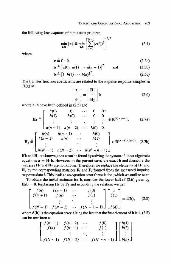
the following least squares minimization problem:
I~-'~N--I 1 1/2 mina,b Ilel{ & mina,b L/--"~ (e(i))2 (2.4)
where
e & f- h (2.5a)
a & [a(0) a(1) -.- a(n - 1)] r and (2.5b)
b & [1 b(1) -.- b(n)] r. (2.5c)
The transfer function coefficients are related to the impulse response samples in H(Z) as
�9 ~ ~ b (2.6)
where a, b have been defined in (2.5) and
h(1) h(0) . . . 0 H 1 ~ . . .. . ~ R (n)• (2.7a)
l h ( n - - 1 ) h ( n - 2 ) . . . h(0)
h(n) h(n- 1) . . . h(0) h(n --I- 1) h(n) ... h(1)
H 2 ~ E R(N-n)x(n+l). (2.7b)
h(N-1) h (N-2) . .- h ( N - n - 1 ) If b and H l are known, then a can be found by solving the system of linear algebraic equations a = I-Ilb. However, in the present case, the exact h and therefore the matrices H1 and H2 are not known. Therefore, we replace the elements of H1 and H2 by the corresponding matrices F1 and F2 formed from the measured impulse response data f. This leads to an equation error formulation, which we outline next.
To obtain the initial estimate for b, consider the lower half of (2.6) given by H2b ---- 0. Replacing H2 by F2 and expanding the relation, we get
f(n + 1) f(n) ... f(1) b 1) =d (b ) , (2.8) . . . . �9 .
f ( N - 1 ) f ( N - 2 ) . . , f ( N - n - 1 ) I_b(n)_l
where d(b) is the equation error. Using the fact that the first element ofb is 1, (2.8) can be rewritten as
f ( n - 1 ) f(n--2) ... f(O) ] I b ( 1 ) l f(n) f ( n - 1) --. f (1) b(2)
. . . . . �9 .
f ( N - 1 ) f ( N - - 2 ) . . , f ( N - - n - 1 ) Lbin)_l
764 SHAW, MISRA, AND KUMARESAN
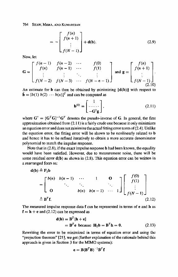
Now, let
Ir f(n) 1 =_ f(n? I) l
_ f(N'-- I) I
+ d(b). (2.9)
l:n n) 1) - �9 f(n + 1) G = f(n 1) -. f (1 ) and g = . �9 �9 "
Lf(N'-2) f ( N - 3 ) . . . f(N -1) f(N'-l)_l (2.10)
An estimate for b can then be obtained by minimizing IId(b)ll with respect to = [b(1) b(2) . .- b(n)] r and can be computed as
b (~ ---- , (2.11)
where G ~ = [GTG]-IG r denotes the pseudo-inverse of G. In general, the first approximation obtained from (2.11) is a fairly crude one because it only minimizes an equation error and does not minimize the actual fitting error norm of (2 �9149 Unlike the equation error, the fitting error will be shown to be nonlinearly related to b and hence it has to be refined iteratively to obtain a more accurate denominator polynomial to match the impulse response�9
Note that in (2.8), if the exact impulse response h had been known, the equality would have been satisfied. However, due to measurement noise, there will be some residual error d(b) as shown in (2�9149 This equation error can be written in a rearranged form as:
d(b) ~ F2b
bm) b(n-1) . . . = . . �9
b(n)
Brf.
b(n - 1)
f (0 ) ]
oo l] q" "'" k f (N ' - 1)
(2.12)
The measured impulse response data f can be represented in terms of e and h as f = h + e and (2.12) can be expressed as
d(b) = Br[h -I- e]
= Bre because H2b = Brh ---- 0. (2.13)
Rewriting the error to be minimized in terms of equation error and using the "projection theorem" [21], we get (further explanation of the rationale behind this approach is given in Section 3 for the MIMO systems):
e = B ( B T B ) - l B r f
THEORY AND COMPUTATIONAL ALGORITHM 765
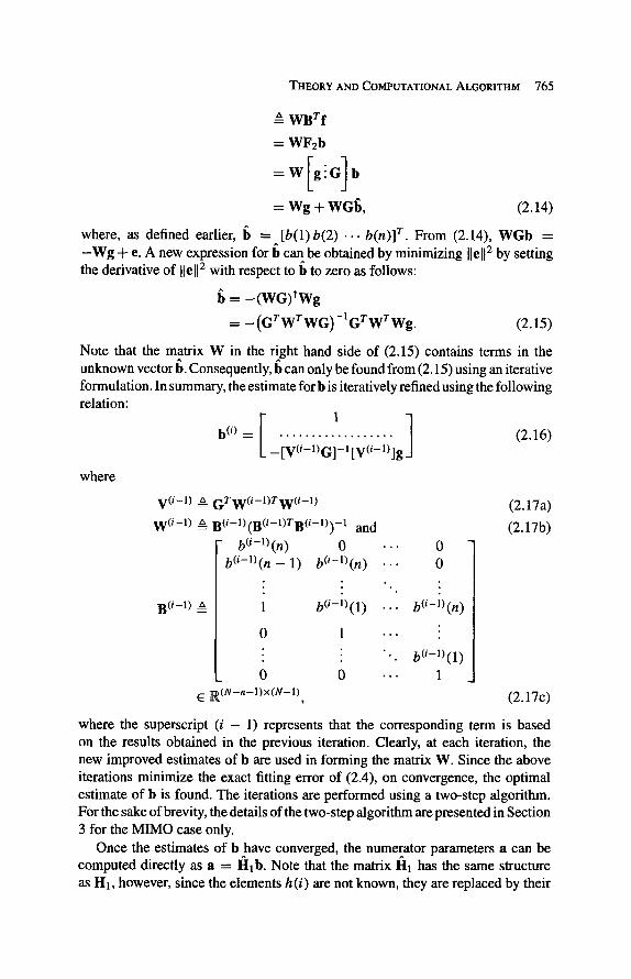
& W B T f
= W F 2 b
= W [ g ! G ] b
= Wg + WGb, (2.14)
where, as defined earlier, f~ = [b(1)b(2) .-. b(n)] r. From (2.14), WGb = - W g + e. A new expression for fJ can be obtained by minimizing Ilell 2 by setting the derivative of Ilell 2 with respect to b to zero as follows:
fa = - ( W G ) t W g
= --(GTWTWG)-IGTWTWg. (2.15)
Note that the matrix W in the fight hand side of (2�9 contains terms in the unknown vector I~. Consequently, b can only be found from (2.15) using an iterative formulation. In summary, the estimate for b is iteratively refined using the following relation:
[ 1 ] b (0 . . . . . . . . . . . . . . . . . . . (2.16)
-[V(i-I)G]-I [v(i-1)lg
where
v(i-l) ,, (~Tw( i -1 ) rw( i -1 )
W (i-1) --~ B( i - I ) (B( i - I )TB( i - I ) ) - I and
B(i_I) t,
b(i-l)(n) b( i - l ) (n -- 1)
1
0
0 E ]~(N-n-l)x(N-l) ,
~ " � 9 0
b( i - l ) (n) . . . 0 �9 ~ �9
b(i-1)(1) . . . b(i-l)(n)
. . � 9
�9 . . . b ( i - l ) ( 1 )
0 . . . 1
(2.17a)
(2.17b)
(2.17c)
where the superscript (i - 1) represents that the corresponding term is based on the results obtained in the previous iteration�9 Clearly, at each iteration, the new improved estimates of b are used in forming the matrix W. Since the above iterations minimize the exact fitting error of (2.4), on convergence, the optimal estimate of b is found�9 The iterations are performed using a two-step algorithm. For the sake of brevity, the details of the two-step algorithm are presented in Section 3 for the MIMO case only.
Once the estimates of b have converged, the numerator parameters a can be computed directly as a = I~Ilb. Note that the matrix I~I1 has the same structure as HI, however, since the elements h(i) are not known, they are replaced by their
766 SHAW, MISRA, AND KUMARESAN
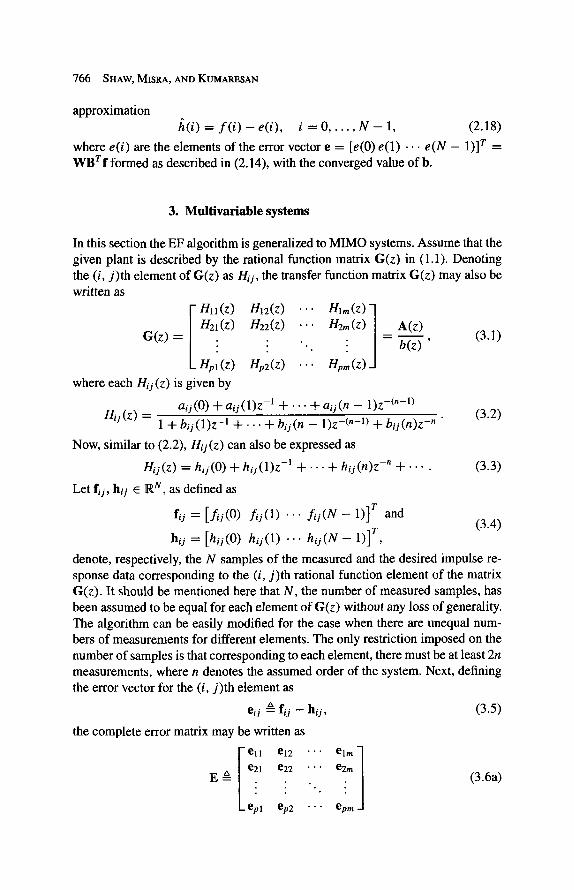
approximation h ( i ) = f ( i ) - e ( i ) , i = 0 . . . . . N - l , (2.18)
where e( i ) are the elements of the error vector e = [e(0) e(1) - . . e ( N - 1)] r = W B r f formed as described in (2.14), with the converged value of b.
3. Multivariable systems
In this section the EF algorithm is generalized to MIMO systems. Assume that the given plant is described by the rational function matrix G(z) in (1.1). Denoting the (i, j ) th element of G(z) as Hi j , the transfer function matrix G(z) may also be written as
I Hl l (Z) H12(Z) " ' " Him(Z) ] H21(Z) H22(Z) H2m(Z) A(Z)
G ( z ) = . . - 9
H,~(z) H,2(z) H , ~ ( z ) J
(3.1)
the error vector for the (i, j ) th element as
eii g fij - hi j,
the complete error matrix may be written as
ell el2 �9 . . e21 e22 �9 �9 �9
E ~ : : "..
epl ep2 �9 �9 �9
earn "]
/ epm _1
(3.5)
(3.6a)
where each Hij (z) is given by
aij(O) + aiy(1)z -1 + . . . + a i j (n - 1)z -Cn-I) Hi j ( z ) = 1 + b i j (1)z -1 + . . . + bi j (n - 1)z -~n-l) + b i j ( n ) z - " " (3.2)
Now, similar to (2.2), Hij (z) can also be expressed as
Hij (Z) = hij(O) "l- h i j ( 1 ) z -1 + " " "-I- h i j ( n ) z -n + ' " �9 (3.3)
Let f i j , hij E R N, as defined as
fij = [ f / j ( 0 ) f i j ( 1 ) ' ' ' f i j ( N - 1)] r and (3.4)
hi j = [hij(O) h i j ( 1 ) "'" h i j ( N - 1)] T,
denote, respectively, the N samples of the measured and the desired impulse re- sponse data corresponding to the (i, j ) th rational function element of the matrix G(z). It should be mentioned here that N, the number of measured samples, has been assumed to be equal for each element of G(z) without any loss of generality. The algorithm can be easily modified for the case when there are unequal num- bers of measurements for different elements. The only restriction imposed on the number of samples is that corresponding to each element, there must be at least 2n measurements, where n denotes the assumed order of the system. Next, defining
THEORY AND COMPUTATIONAL ALGORITHM 767
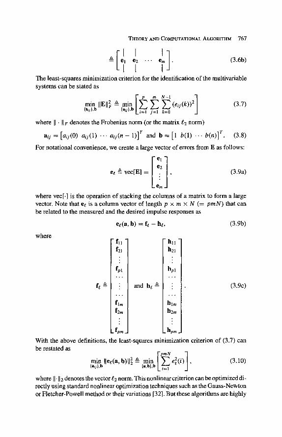
El I1 = 1 e2 - . - e . (3.6b)
I The least-squares minimization criterion for the identification of the multivariable systems can be stated as
min IIEII2e g min (eij(k)) 2 (3.7) {aij},b {aij},b i-----I j = l k=0
where [[ �9 [[ F denotes the Frobenius norm (or the matrix e2 norm)
ai j -~. [a i j (O ) a i j ( 1 ) ' ' ' a i j ( n -- 1)] T and b = [1 b(1) . . . b(n)] r. (3.8)
For notational convenience, we create a large vector of errors from E as follows:
[ e i l ee g vec[El = e2 , (3.9a)
e
where vec[.] is the operation of stacking the columns of a matrix to form a large vector. Note that ee is a column vector of length p x m x N (= pmN) that can be related to the measured and the desired impulse responses as
ee(a, b) = fe - he, (3.9b)
where " h l l
h21
h,l
fe ~ and he ~ : | (3.9c) " I
i
hlm I
. h l m
= f l l -
f21
fpl
flm
f2m
_ fpm _
With the above definitions, the least-squares minimization criterion of (3.7) can be restated as
rain Ilee(a, b)ll~ A min I ~ e ~ 2 ( i ) ] , (3.10) {aq},b {a,b},b L i :1
where I[" 112 denotes the vector e2 norm. This nonlinear criterion can be optimized di- rectly using standard nonlinear optimization techniques such as the Gauss-Newton or Fletcher-Powell method or their variations [32]. But these algorithms are highly
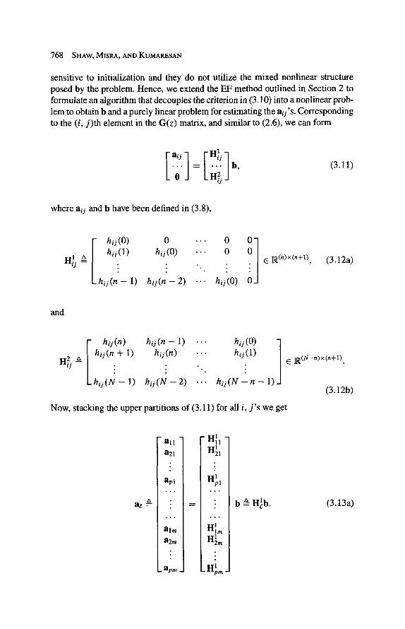
768 SHAW, M1SRA, AND KUMARESAN
sensitive to initialization and they do not utilize the mixed nonlinear structure posed by the problem. Hence, we extend the EF method outlined in Section 2 to formulate an algorithm that decouples the criterion in (3. it)) into a nonlinear prob- lem to obtain b and a purely linear problem for estimating the aij 's. Corresponding to the (i, j) th element in the G(z) matrix, and similar to (2.6), we can form
= [ H ~ ! l b ' (3.11)
where aij and b have been defined in (3.8),
r hij(O) 0 ... 0 0"] I hij(1)n hij(O)" -.... . 0. i J E ]I~ (n)x(n+l) ,
Lhiy( -1) hij(n- 2) ... hi i(0)
(3.12a)
and
[- hiy(n) hiy(n- 1) .-. hij(O) "] HL A | hi j (n + 1) hi j (n) . " h i j (1)
tj I
�9 �9 . . . "
Lhij(N-1) hij(N-2) . . . h iy (N-n -1 )
E ~(N-n)•
(3.12b)
Now, stacking the upper partitions of (3.11) for all i, j ' s we get
] 811 a21
apl I
"" " I ae g " = b ~ H ~ b .
. ~
a i m
a2m �9 I
_ apm _J
- H I 1 -
. . .
rIl~
_ H p , ~ .
(3.13a)
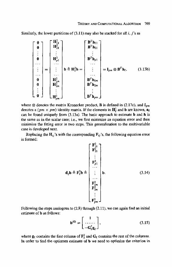
THEORY AND COMPUTATIONAL ALGORITHM 769
Similarly, the lower partitions of (3.11) may also be stacked for all i, j ' s as
- 0 - - H~I r Brhl l 0 H21 BTh21
0 H21 Brhvl
= " b ~ H2b = i = Ipm @ BThe, (3.13b)
0 H2m Brhl,, 0 H22m Brh2.
i " !
_ 0 "2 _BThpm _] - _ Hpm ]
where | denotes the matrix Kronecker product, B is defined in (2.17c), and Ipm denotes a (pm • pm) identity matrix. If the elements in H~ and b are known, ae can be found uniquely from (3.13a). The basic approach to estimate b and h is the same as in the scalar case; i.e., we first minimize an equation error and then minimize the fitting error in two steps. This generalization to the multivariable case is developed next�9
Replacing the Hij's with the corresponding Fij 's, the following equation error is formed:
- F~l "]
~ 1 7 6
d~b ~ F~2b ___a i b. (3.14)
ii2 I Fk
Following the steps analogous to (2.8) through (2.11), we can again find an initial estimate of b as follows:
b ( ~ . . . . i '" ' (3.15/
- G e g e
where ge contains the first column of Fe 2 and Ge contains the rest of the columns�9 In order to find the optimum estimate of b we need to optimize the criterion in
770 SHAW, MISRA, AND KUMARESAN
(3.10). To achieve that, the equation error in (3.14) is rewritten as
[- BTfll -]
de(b)
[_ BT'fpm .J
= (Ipm | Br)fe. (3.16)
Replacing fe by ee(a, b) + he and using (3.13b) we get
de(b) = (Ipm | Br)ee(a, b). (3.17)
In order to minimize the fitting error norm of (3.10), we need an inverse relation- ship between ee(a, b) and de(b). According to the orthogonality principle [31], [36], the error ee(a, b) for a given b and the corresponding optimum ae must be orthogonal to the desired response vector he. Otherwise there would remain some information contained in the nonzero projection of ee (a, b) onto he. The complete basis space orthogonal to this error can be found from equation (3.13b), which clearly demonstrates that the p m ( N - n) columns of (Ipm | B) are orthogonal to he. Hence the error ee (a~', b) corresponding to optimal ae may be formed as a linear combination of all its orthogonal basis vectors as follows:
ee(a ~, b) A (Ipm @ B)c, (3.18)
where c, a vector of unknown constants, needs to be determined. By substituting (3.18) in (3.17) we obtain
de(b) = (Ipm ~ BT)(Ipm | B)C (3.19a)
= (Ipm @ BTB)c. (3.19b)
Hence,
C = (Ipm ~ (BrB)-l)de(b)
= (Ipm ~ (BTB)-IBT)fl; [using (3.16)]. (3.20)
On substituting this back in (3.18) and following the steps in (2.14),
ee(a ~, b) = (Ipm | B(BrB)-|BT)fe (3.21a)
= (Ipm | B(BrB)-l)(Ipm | Br)fe (3.21b)
We(Ipm | Br)fe = WeF~b; [using (3.14)] (3.21c)
A We[ge " Ge]b = Wege + WeGel~. (3.21d)
For an optimum a, this is the fitting error that we need to minimize; i.e., the criterion in (3.10) is equivalent to
min Ilee (a ~, b)II 2. (3.22) b
On achieving the minimum this will produce ee(a~, b*). Note again that in the expression of ee(a~, b), the matrix W does have dependence on the vector b that

THEORY AND COMPUTATIONAL ALGORITHM 771
contains the elements with respect to which the criterion needs to be minimized. The minimization of (3.22) is performed in two phases of iterations. In the first phase, the matrix W is constructed from the estimate of b found at the previous iteration. The new update of b is then obtained from
I)(i-1-1) _ /w( i )G ~tw(i)g : ~, e s e e
[ I '2TIAIT( i ) 'w~( i )~_ " ~ - l l p _ T , l ~ T ( i ) ' u I ( i ) _ = - t ' - ' e "'e " e "-'el "-'e " e " e ge. (3.23)
In summary, the estimate of b is iteratively refined using the following relation:
b (i+l) = , (3.24)
-- iVi/') G ; i - ; (vii; igs where
V~ i) =~ v~c-rwr(i)w(i).,e "~ (3.25)
= Gr [Iem | (Br(i)B(i))-l]. (3.26)
It should be mentioned here that, at iteration (i + 1), the new estimates of b (i) are used in forming the matrix W Ci). Note that the initial estimate b (~ comes from the equation error minimization step of (3.15).
The first phase of optimization alone may not converge to the optimum b that minimizes ee (a~, b) completely, although our experience with many examples does indicate that it comes "fairly" close to the optimum. In some cases, especially when the deviations of the measured responses from the desired ones are relatively large, a second phase of optimization needs to be invoked. In the second phase of iterations, the variation of W w.r.t, b is also taken into account. For the sake of clarity of presentation, the details of the second phase of optimization are included in the Appendix.
On convergence of the second phase, the optimum value b* is found. Substi- tuting b* in (3.21) the optimal error vector ee(a~, b*) is computed. The optimal
impulse response lae is then found from (3.9b) as
fae = fe - ee(a~, b*). (3.27)
Finally, the optimal ae is computed from (3.13a) as
a~ = I2I~b *, (3.28)
where I?t~ has the same form as H~ except that the elements hij (k) are replaced by
the corresponding hij (k) found in (3.26). We should mention here that the decoupled optimization of a and b, as presented
in this paper, falls within a special class of nonlinear optimization problems that have been studied extensively by numerical analysts [37]. Theorem 2.1 in [37] demonstrates that if some of the unknown variables of a nonlinear criterion are linearly related to the error and the other variables are nonlinearly related, and if the variables appear separately, then the original criterion can be decoupled into a
772 SHAW, MISRA, AND KUMARESAN
purely linear problem and a nonlinear problem of reduced dimensionality. Using these results, it can be shown that if the denominator is estimated by optimizing the decoupled criterion in (3.22) and if that estimate is used in (3.26) and (3.27) to compute the numerators, then these estimates correspond to the global optimum of the original criterion in (3.10) [33], [34].
4. Simulation results
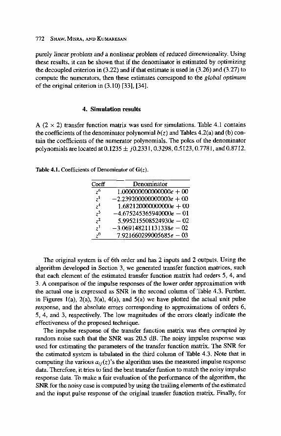
A (2 x 2) transfer function matrix was used for simulations. Table 4.1 contains the coefficients of the denominator polynomial b(z) and Tables 4.2(a) and (b) con- tain the coefficients of the numerator polynomials. The poles of the denominator polynomials are located at 0.1235 4- j0.2331, 0.3298, 0.5123, 0.7781, and 0.8712.
Table 4.1. Coefficients of Denominator of G(z).
Coeff Denominator z 6 1.000000000000000e + 00 z 5 -2.239200000000000e + 00 z 4 1.682120000000000e + 00 z 3 -4.675245365940000e - 01 z 2 5.995215508524930e - 02 z 1 -3.069148211131338e - 02 z ~ 7.921660299005685e - 03
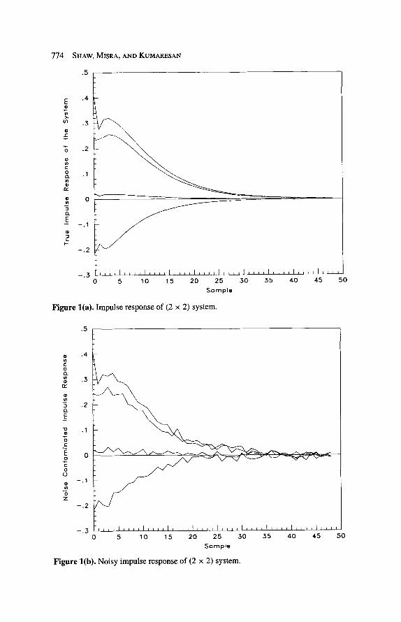
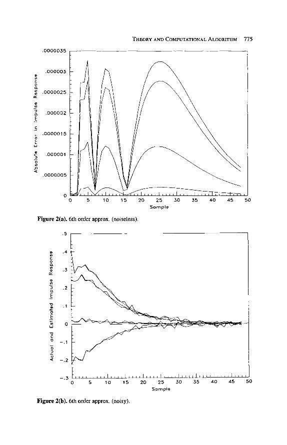
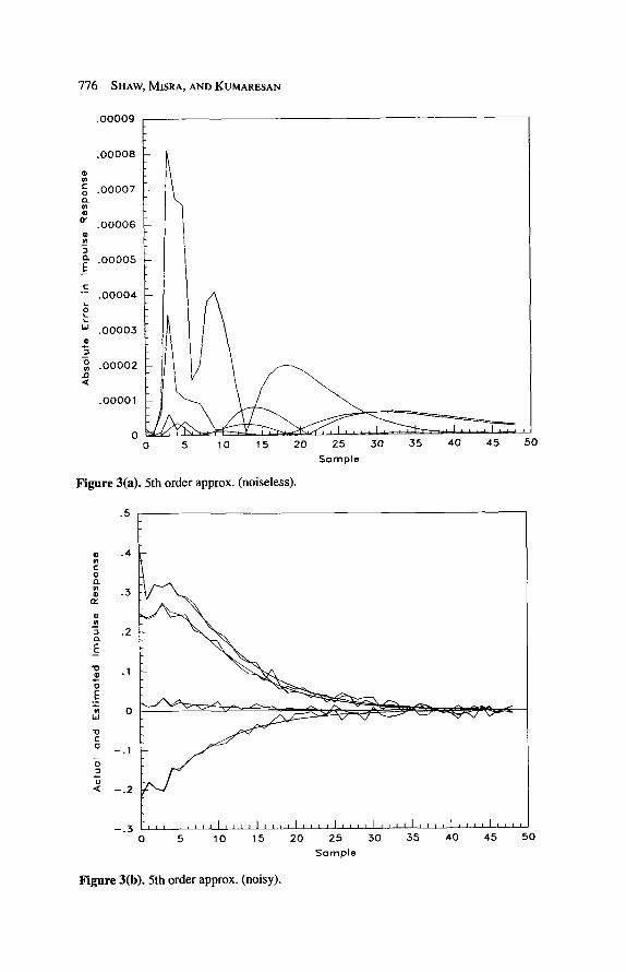
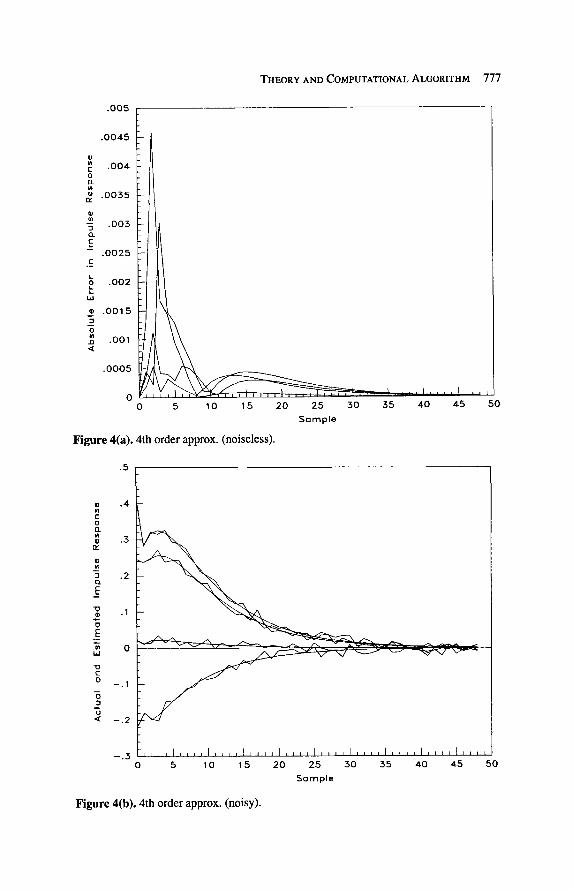
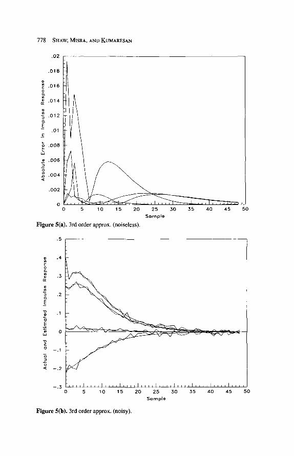
The original system is of 6th order and has 2 inputs and 2 outputs. Using the algorithm developed in Section 3, we generated transfer function matrices, such that each element of the estimated transfer function matrix had orders 5, 4, and 3. A comparison of the impulse responses of the lower order approximation with the actual one is expressed as SNR in the second column of Table 4.3. Further, in Figures l(a), 2(a), 3(a), 4(a), and 5(a) we have plotted the actual unit pulse response, and the absolute errors corresponding to approximations of orders 6, 5, 4, and 3, respectively. The low magnitudes of the errors clearly indicate the effectiveness of the proposed technique.
The impulse response of the transfer function matrix was then corrupted by random noise such that the SNR was 20.5 dB. The noisy impulse response was used for estimating the parameters of the transfer function matrix. The SNR for the estimated system is tabulated in the third column of Table 4.3. Note that in computing the various aij (z)'s the algorithm uses the measured impulse response data. Therefore, it tries to find the best transfer funtion to match the noisy impulse response data. To make a fair evaluation of the performance of the algorithm, the SNR for the noisy case is computed by using the trailing elements of the estimated and the input pulse response of the original transfer function matrix. Finally, for
THEORY AND COMPUTATIONAL ALGORITHM 773
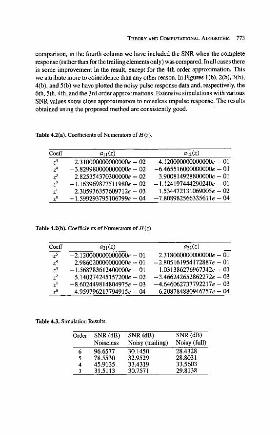
comparison, in the fourth column we have included the SNR when the complete response (rather than for the trailing elements only) was compared. In all cases there is some improvement in the result, except for the 4th order approximation. This we attribute more to coincidence than any other reason. In Figures l(b), 2(b), 3(b), 4(b), and 5(b) we have plotted the noisy pulse response data and, respectively, the 6th, 5th, 4th, and the 3rd order approximations. Extensive simulations with various SNR values show close approximation to noiseless impulse response. The results obtained using the proposed method are consistently good.
Table 4.2(a). Coefficients of Numerators of H (z).
Coeff a l l (Z) al2(Z) Z 5
Z 4
Z 3
Z 2
Z l
Z 0
2.310000000000000e -- 02 --3.829980000000000e -- 02
2.825354370300000e -- 02 --1.163969877511980e -- 02
2.305936357609712e -- 03 --1.599293795106799e - - 0 4
4.120000000000000e -- 01 --6.465516000000000e -- 01
3.900814928800000e -- 01 --1.124197444290240e -- 01
1.534472131069005e -- 02 --7.808982566335611e -- 04
Table 4.2(b). Coefficients of Numerators of H (z).
Coeff a21 (z) a22(z) Z 5
Z 4
Z 3
Z 2
Z 1
Z 0
--2.120000000000000e -- 01 2.986020000000(K~e -- 01
--1.568783612400000e -- 01 5.140274245157200e -- 02
--8.602449814804975e -- 03 4.959796217794915e - - 0 4
2.318000000000000e -- 01 --2.805161954172887e -- 01
1.031386276967342e -- 01 --3.466242652862272e -- 03 --4.646062737792217e -- 03
6.208784880946757e -- 04
Table 4.3. Simulation Results.
Order SNR (dB) SNR (dB) SNR (dB) Noiseless Noisy (trailing) Noisy (full)
6 96.6577 30.1450 28.4328 5 78.5530 32.9529 28.8031 4 45.9135 33.4319 33.5603 3 31.5113 30.7571 29.8138
774 SHAW, MISRA, AND KUMARESAN
.5
E
r t~
.4
.3
.2
.1
o -I o .
E
x. F-
- - . 2
0 5 10 15 20 25 30 35 40 45 50
S o m p l e
Figure l(a). Impulse response of (2 x 2) system.
.5
�9 . 4
t- O Q_
~ .2 E
"o . 1
c o_
E o 0
c 0
- . 1
Z
- . 2
- . 3 t j , i . . . . ] . . . . [ , , , , ] , = , , I , , t , I = , , = I , , , , I J , , , i . . . . 0 5 10 15 20 25 30 35 40 45 50
Sample
Figure l (b) . Noisy impulse response of (2 x 2) system.
. 0 0 0 0 0 3 5
THEORY AND COMPUTATIONAL ALGORITHM 775
~ o c .000005 i
.0000025
. 0 0 0 0 0 2 E
.0000015
. o o o o o l
.0000005
0 2 5
Somple
Figure 2(a). 6th order approx. (noiseless).
.5
50 35 40 45 50
.4
t'l t~
::a .2 o. s
"O .1 0 E
~
'~ o L~ "10 C 0 --.1 -6 D 0 < --.2
- . 5 0 5 10 15 20 25 30 35 40 45 50
Sompie
Figure 2(b). 6th order approx. (noisy).
776 SHAW, MISRA, AND KUMARESAN
. O 0 0 0 g ,
.00008
. 0 0 0 0 7
. 0 0 0 0 6
. 0 0 0 0 5 E
"- .00004
w . 0 0 0 0 3
. 0 0 0 0 2
.00001
i
5 10 15 20 25 30 35 40 45 50
Sample
Figure 3(a). 5th order approx. (noiseless).
. 5
�9 .4 c o O.
.3 o~
E
"0 .1
0 E
, _
o LO
"0 C 0 --.1
-6
- . 3 0
,~- ~ ' ~ . - - <
, t t , l ~ , , J [ . . . . I . . . . I . . . . I . . . . I , , l l l , , i , I , , , , I . . . .
5 10 15 20 25 30 35 40 45 50
Sample
Figure 3(b). 5th order approx. (noisy).
.005
THEORY AND COMPUTATIONAL ALGORITHM 777
.0045
. 0 0 4 o
. 0 0 3 5
-- . 0 0 3
E -- . 0 0 2 5 E
. 0 0 2
. 0 0 1 5
.001
. 0 0 0 5
0 5 10 15 2 0 25 30 35 40 45 50
S a m p l e
Figure 4(a). 4th order approx. (noiseless).
. 5
E o o.
n4
E
"o
E
7 o
*d <
.3
.2
.1
o - --- . . . . . ~ - ~ ~ - - ~
, , , I . . . . I . . . . I , , , , I , , , , I . . . . I . . . . I , , , , I . . . . I . . . .
5 10 15 2 0 2 5 30 35 40 45 50
S o m p l e
- . 1
- . 2
- . 3
Figure 4(b). 4th order approx. (noisy).
778 StrAW, MISRA, AND KUMARESAN
.02 r--
. 0 1 8
.01 6 o
. 0 1 4
-- , 012
E - .Ol
; .008 w
$ . o o 8
5 ~ . 0 0 4
. 0 0 2
0 0 5 10 15 2 0 25 30 55 4 0 4 5 50
S o m p l e
F i g u r e 5 ( a ) . 3 r d o r d e r a p p r o x . ( n o i s e l e s s ) .
.5
�9 . 4
t~
~. .2
E
"0 .1
"6 E
~ o IM
0 --.1
6
o "~ - - .2
- . 5 , , , I . . . . I , , , , I , , , , I . . . . I , , , , I . . . . I . . . . I . . . . I , , , , 0 5 10 15 2 0 25 30 35 40 45 5 0
S a m p l e
F i g u r e 5(b) . 3rd order approx. (noisy).
THEORY AND COMPUTATIONAL ALGORITHM 779
5. Concluding remarks
In this paper we addressed the problem of identification of discrete time transfer function matrices from noisy unit pulse response data. The proposed method is a generalization of an existing technique that estimates the parameters of a discrete time scalar transfer function. The simulation results presented here and exten- sive experience with the proposed scheme clearly indicate that it can be reliably used for estimating the parameters of discrete time transfer functions from their impulse response data. The global optimality properties can be established by re- lating the proposed decoupled criteria to certain theoretical results in numerical analysis [37]. The decoupled estimators have reduced computational complexity when compared to existing methods that estimate the numerator and denomina- tor coefficients simultaneously. The proposed algorithmic framework utilizes the weighted-matrix structure of the decoupled criterion for its minimization using an iterative scheme. The convergence properties of this iterative algorithm need to be analyzed [35].
The major computational load in the proposed algorithmic framework is in performing the iterative refinement, where one needs to invert an (N - p) • (N - p) weight-matrix at each iteration step. But the weight-matrix is symmetric-banded- Toeplitz, and many efficient algorithms are available for inverting these matrices [39], [43], [44]. Specifically, in [43] it has been shown that inversion of such banded Toeplitz matrices only requires O[(N - p) log(N - p)] + O[p 2] operations.
It may be noted here that the limitations of the EF method due to the strictly proper assumption has been removed in a recent work [33], [34], where a decoupled algorithm has been developed for identifying systems with arbitrary numerator and denominator orders. An extension of that work to the MIMO case is currently under progress.
6. Appendix. Computat ional algorithm, Phase II
In this appendix the second phase of the iterative algorithm is described in detail. In this phase, the derivative of the matrix We w.r.t, b is taken into account. The complete error expression is rewritten below,
Ilee(a~, b)ll~ r �9 �9 = e e (a~, b)ee(ae, b). (A.1)
By setting the derivative of this squared norm to zero, we obtain the updated f~(i+l) at the (i + 1)th iteration as,
fl(i+l ) [u( i )G ] - l i -u( i ) ]g , (A.2) ------L e eJ L e J
where (suppressing the superscript (i)),
U e & LerWe + GeW~'We, (A3.a)
780 SHAW, MISRA, AND KUMARESAN
l , OWe A Ipm | , (A.3c)
Ob(k)
o w _-- o.0B,(B B)_I Ob(k) Ob(k) otT(/c)
0B r 0B
0B has the same form as the B matrix defined in (2.17) but filled with Further, ~ all zeros except at the locations where b(k) appears. For example,
1 0 . . . 0 0 1 . . . 0
0B ~ - = 0 0 . - . 1 Ob(n) 0 0 . . . 0
: : "'. 0 - 0 0 . . . 0
Once fi(i+l) is known, b (i+l) can be found from
[ 1 1 [ 1 ] b ( i + I ) = = . (A.4)
This minimization phase continues until b ~i+1) --~ b (i) is reached and this optimum b* vector corresponds to a minimum of the error surface of Ilee (a~, b) 112,
References
[1] R. Isermann, ed., Automatica, Special issue on system identification, vol. 17, 1971. [2] A. E Sage and J. L. Melsa, System Identification, Academic Press, New York, 1971. [3] K.J. Astr~m and E Eykhoff, System identification: A survey, Automatica, vol. 7, pp. 123-1647,
1971. [4] R. K. Mehra and D. G. Lainiotis, System Identification-Advances and Case Studies, Academic
Press, New York, 1976. [5] L. B. Jackson, Digital Filters and Signal Processing, Kluwer, Boston, 1986. [6] J. E Norton, An Introduction to Identification, Academic Press, New York, 1986. [7] L. Ljung, System Identification: Theory for the Users, Prentice-Hall, Englewood Cliffs, NJ, 1987. [8] T. S6derstrSm and E Stoica, System Identification, Prentice-Hall, Englewood Cliffs, NJ, 1987. [9] S. M. Kay, Modern Spectral Estimation: Theory and Applications, Prentice-Hall, Englewood
Cliffs, NJ, 1988. [10] K. J. Astr6m and B. Wittenmark, Computer Controlled Systems: Theory and Design, Prentice-
Hall, Englewood Cliffs, NJ, 1990. [11] D.G. Luenberger, Canonical forms for linear multivariable systems, IEEE Trans. Automat. Contr.,
vol. AC-12, pp. 290-293, 1967.

THEORY AND COMPUTATIONAL ALGORITHM 781
[12] D. Q. Mayne, A canonical model for identification of multivariable linear systems, IEEE Trans. Automat. Contr., vol. AC-17, pp. 728-729, 1972.
[13] E E. Calnes and J. Rissanen, Maximum likelihood estimation of parameters in multivariate Gaussian stochastic processes, IEEE Trans. Information Theory, vol. IT-20, pp. 102-104, Jan. 1974.
[14] K. Glover and J. C. Willems, Parametrizations of linear dynamical systems: Canonical forms and identifiability, IEEE Trans. Automat. Contr., vol. AC-19, pp. 640-646, Dec. 1974.
[15] M. J. Denham, Canonical forms for identification of multivariable linear systems, IEEE Trans. Automat. Contr., vol. AC-19, pp. 646-656, Dec. 1974.
[16] R. L. Kashyap and R. E. Nasburg, Parameter estimation in multivariable stochastic differential equations, IEEE Trans. Automat. Contr., vol. AC-19, pp. 784-797, Dec. 1974.
[17] O. N. Strand, Multichannel complex maximum entropy (autoregressive) spectral analysis, IEEE Trans. Automat. Contr., vol. AC-22, pp. 634-4a40, Aug. 1977.
[18] M. Gevers and V. Wertz, Uniquely identifiable state-space and ARMA parametrizations for mul- tivariable linear systems, Automatica, vol. 20, pp. 333-347, 1984.
[19] T. Ning and C. L. Nikias, Multichannel AR spectrum estimation: The optimum approach in the reflection coefficient domain, IEEE Trans. Acoust. Speech Signal Process., vol. ASSP-34, pp. 1139-1152, Oct. 1986.
[20] B. Friedlander and B. Porat, Multichannel ARMA spectral estimation by the modified Yule- Walker method, Signal Processing, vol. 10, pp. 49-59, 1986.
[21] M. Moonen and J. Vanderwalle, QSVD approach to on- and off-line state-space identification, Int. J. Contr., vol. 51, pp. 1133-1146, 1990.
[22] A. J. Helmicki, C. A. Jacobson, and C. N. Nett, Identification in H~176 A robust convergent nonlinear algorithm, Proc. 1990Amer. Contr. Conf., pp. 386-391, Pittsburgh, PA.
[23] G. Gu and P. Khargonekar, Linear and non-linear algorithms for identification in H ~176 preprints. [24] P. M. Makila, Approximation and identification of continuous-time systems, to appear in Int. J.
Contr.
[25] G. P. Rao, Piecewise Constant Orthogonal Functions and their Applications to Systems and Control, Springer-Verlag, New York, 1983.
[26] K. Premaratne, E. I. Jury, and M. Mansour, Multivariable canonical forms for model reduction of 2-D discrete-time systems, 1EEE Trans. Circuits and Systems, vol. CAS-37, pp. 488-1058, April 1990.
[27] R. E. Kalman, Design of a self optimizing control system, Trans. ASME, vol. 80, pp. 468-478, 1958.
[28] K. Steiglitz and L. E. McBride, A technique for identification of linear systems, IEEE Trans. Automat. Contr., vol. AC-10, pp. 461-464, 1965.
[29] J. L. Shanks, Recursion filters for digital processing, Geophysics, vol, 32, pp. 33-51, 1967. [30] A. G. Evans and R. Fischl, Optimal least squares time-domain synthesis of recursive digital filters,
IEEE Trans. Audio and Electro-Acoustics, vol. AU-21, pp. 61-65, 1973. [31] L. L. Scharf, Statistical Signal Processing - Detection, Estimation and Time Series Analysis,
Addison-Wesley, Reading, MA, 1990. [32] R. F•etcher and M. J. D. P•we••• A rapid•y c•nvergent descent meth•d f•r minimizati•n• C•mputer
Journal, vol. 6, pp. 163-168, 1963. [33] A.K. Shaw, Optimal identification of discrete-time systems from impulse response data, IEEE
Trans. Signal Process., vol. 42, no. 1, pp. 113-120, Jan. 1994. [34] A.K. Shaw, An optimal method for identification of pole-zero transfer functions, International
Symposium on Circuits and Systems, San Diego, pp. 2409-2412, May 1992. [35] P. Stoica and T. S6derstrtim, The Steiglitz-McBride identification algorithm revisited - Conver-
gence analysis and accuracy aspects, IEEE Trans. Automat. Contr., vol. AC-26, no. 3, pp. 712-717, June 1981.
[36] D. G. Luenberger, Optimization by Vector Space Method, Wiley, New York, 1969.

782 SHAW, MISRA, AND KUMARESAN
[37] G. H. Golub and V. Pereyra, The differentiation and pseudoinverses and nonlinear problems whose variables separate, SIAM J. Numer. AnaL, vol. 10, no. 2, pp. 413-432, Apr. 1973.
[38] R. Kumaresan and A. K. Shaw, High resolution bearing estimation without eigendecomposi- tion, Proceedings of lEEE International Conference on Acoustics Speech and Signal Processing, Florida, April 1985.
[39] R. Kumaresan, L. L. Scharf, and A. K. Shaw, An algorithm for pole-zero modeling and spectral estimation, IEEE Trans. Acoust. Speech Signal Process., vol. ASSP-34, pp. 637-640, June 1986.
[40] Y. Bressler and A. Macovski, Exact maximum likelihood parameter estimation of superimposed exponential signals in noise, IEEE Trans. Acoust. Speech Signal Process., vol. ASSP-34, no. 10, pp. 1081-1089, Oct. 1986.
[411 A.K. Shaw and R. Kumaresan, Frequency-wavenumber estimation by structured matrix approx- imation, Third IEEE-ASSP Workshop on Spectrum Estimation and Modeling, pp. 81-84, Boston, Nov. 1986.
[42] A. K. Shaw and R. Kumaresan, Some structured matrix approximation problems, Proc. of the IEEE International Conference on Acoustics, Speech and Signal Processing, New York, NY, pp. 2324-2327, April 1988.
[43] A. K. Jain, Fast inversion of banded Toeplitz matrices by circular decompositions, IEEE Trans- actions on Acoustics, Speech and Signal Processing, vol. ASSP-26, no. 2, pp. 121-126, April 1978.
[44] S. Zohar, Toeplitz matrix inversion: The algorithm ofW. F. Trench, J. Assoc. Comput. Mach., vol. 16, pp. 592-601, Oct. 1969.
Copyright © 2022 FDOKUMEN