sensors

Article

Identification and Localization of Track Circuit FalseOccupancy Failures Based on FrequencyDomain Reflectometry

Tiago A. Alvarenga 1 , Augusto S. Cerqueira 1 , Luciano M. A. Filho 1 , Rafael A. Nobrega 1 ,Leonardo M. Honorio 1,* and Henrique Veloso 2

1 Electrical Engineering Department, Federal University of Juiz de Fora, Juiz de Fora 36036-900, MG, Brazil;tiago.araujo@engenharia.ufjf.br (T.A.A.); augusto.santiago@ufjf.edu.br (A.S.C.);luciano.ma.filho@gmail.com (L.M.A.F.); rafael.nobrega@ufjf.edu.br (R.A.N.)

2 MRS Logística, Juiz de Fora 36060-010, MG, Brazil; henrique.Veloso@mrs.com.br* Correspondence: leonardo.honorio@ufjf.edu.br

Received: 15 October 2020; Accepted: 9 December 2020; Published: 18 December 2020

Abstract: Railway track circuit failures can cause significant train delays and economic losses.A crucial point of the railway operation system is the corrective maintenance process. During thisoperation, the railway lines have the circulation of trains interrupted in the respective sector,where traffic restoration occurs only after completing the maintenance process. Depending onthe cause and length of the track circuit, identifying and solving the problem may take a long time.A tool that assists in track circuit fault detection during an inspection adds agility and efficiency inits restoration and cost reduction. This paper presents a new method, based on frequency domainreflectometry, to diagnose and locate false occupancy failures of track circuits. Initially, simulations areperformed considering simplified track circuit approximations to demonstrate the operation of theproposed method, where the fault position is estimated by identifying the null points and throughnon-linear regression on signal amplitude response. A field test is then carried out in a trackcircuit approximately 1500 m long to validate the proposed method. The results show that theproposed method can identify and estimate the fault location due to a short circuit between rails withhigh accuracy.

Keywords: track circuit failures; frequency domain reflectometry; non-linear regression

1. Introduction

The economic demand and the growing necessity to transport goods and people have raisedrailways’ availability and safety demands. One way to optimize the track’s operationality is to providefast and assertive inspections in its components. The most critical component is the signaling andcontrol system, named Track Circuit (TC) [1]. The TC is a series of circuits installed over the railwaythat measures the shortages between tracks continuity between circuits. Therefore it is a device of vastimportance, which can be employed to locate trains in a stretch and find track breaks.

Occurrences in the TC are related to the railway or to the circuit itself. The most common causesare false occupancy, poor track bed, shortage to the ground or between tracks and broken circuit ortrack, among others [2]. Therefore, any nonconformity in the TC is a critical operational issue and mustbe investigated and corrected before that specific railway section became functional again. Delays infinding and fixing the problem may disrupt the railway’s services and must be quickly corrected.

Two common and critical issues in almost every railway are broken and shorted track circuits.Such occurrences cause discontinuities on the TC that do not indicate or indicates false railway

Sensors 2020, 20, 7259; doi:10.3390/s20247259 www.mdpi.com/journal/sensors

Sensors 2020, 20, 7259 2 of 17

occupancy, respectively. Although simple circuit analyzers can quickly detect both scenarios [3],this equipment fails to identify false negative occurrences and does not provide the exact location ofthe failure. Considering that each TC section may have hundreds of meters, the search for the faultlocation consumes resources and time, generating economic losses.

Considering TC inspections and nonconformity detection, paper [4] compares the differencebetween traditional approaches and new methodologies such as ultrasonic inspections and riskmanagement. It concludes that the main drawback of these new approaches is that they are not able toprovide the location of a broken rail and their inspection time tends to be long since it depends on aninspection vehicle to run through the tracks [5], generating an extra railway occupancy for maintenance.

Paper [6] uses a neuro-fuzzy system for fault detection and diagnosis in TC. Although it haspresented good simulated results, the approach does not indicate the fault location. Paper [7] uses aDempster–Shafer classifier fusion and, although it provides adequate results, they were completelybased on simulation, and the approach is specific for just one type of Alternating Current (AC) TC.Paper [8] has used the track current along with a neural network classifier to diagnose faults, but theapproach does not indicate the fault location.

Methods regarding track circuits are based on collected measurements by trains [7,9] or byspreading sensors [10] through the railway. These two approaches face practical problems such as theTC block for train circulation in faults and the high cost related to the spread sensors throughout therailway line.

In [11], a study was presented analyzing the feasibility of applying the Time Domain Reflectometry(TDR) technique, to identify broken rail on railway lines. The proposed system would be embeddedin the locomotive and from the TDR techniques, would act in the identification of the rail break asit went along the line. To be viable, the system would need to ensure a detection range greater thanthe distance a train in normal cruising conditions expended to brake the composition and thus avoidpossible accidents. It would act in conjunction with Communications-Based Train Control (CBTC)based lines [12], which can perform rail traffic control without the existence of TC, but the CBTCsystem alone cannot perform the detection of broken rails. Through the simulations, the author pointsout to be viable the identification of broken rail at a distance of 1 to 2 miles, depending on the climaticconditions of the track.

The article sought to determine whether the demonstrated concept was technically feasible andwhether further research might be necessary. In order to carry out field tests, it would be necessary todevelop a complex system of coupling between the device and the locomotive. It would be necessaryto evaluate the mechanical design and safety issues of the locomotive, which makes it very difficult toimplement the proposal. Another attenuating factor is the limitation of the energy to be applied to thepulse in order to avoid structural damage due to interactions with the electrical components on thetrack, which could reduce the range of the system.

This paper, in a certain way, served as inspiration for the application of reflectometry to treatproblems in the railway lines. However, it shows great distinction with the methods proposed in work.

There are applications, such as [13], which seeks to detect broken rail by monitoring TC voltageand transmitting information to the train through a radio frequency system. This proposed toolrequires an amount of equipment to be installed by TC, as well as communication systems withtrains. The main purpose is to avoid derailment due to the disruption of tracks. Besides needing alarge number of equipment to be implemented, this proposal differs from the methods proposed inthis work.

In [14] a method of detecting broken rails using acoustic transducers mounted beside the rail wasproposed. Here also consists of a tool to prevent derailment due to the breaking of rails. This proposaldemand for numerous equipment to be installed next to the railway increases the costs of installationand maintenance.

The most common approach in reflectometry is to inject an electromagnetic signal into the tracksand analyze its reflection. By processing information about the injected and reflected signals, it is

Sensors 2020, 20, 7259 3 of 17

possible to retrieve several valuable information regarding the problem, including its exact location.Reflectometry consists of a qualitative analysis of the reflected wave component of an electromagneticsignal propagating through the System Under Test (SUT) [15]. The reflected wave transcribes someinformation of the medium that one wants to characterize. The reflectometry is widespread inseveral sectors in a wide range of applications [16–18]. Nevertheless, the use of Frequency DomainReflectometry (FDR) for TC fault location is not explored in the literature.

Therefore, this paper presents a new method based on FDR to diagnose and locate track circuits’false occupancy failures caused by a short circuit between rails or a due to a discontinuity problem(e.g., broken rail or rail joint discontinuity problem). The proposed method uses the equipmentconnected to the faulty circuit and identifies both problem and location using FDR.

The rest of this paper is organized as follows. In Section 2, the track circuit basic concepts arepresented. In Section 3, the wave propagation in the track circuit is discussed. Section 4 presentsthe proposed method for track circuit fault identification and location. The implemented system andthe field test performed to validate the proposed method are presented in Section 5. In Section 6,a discussion about the field test result is presented. The conclusions of this paper are given in Section 7.

2. Railway Track Circuit

The railway signaling system was started based on controlling the track sections where alocomotive’s presence was detected. Thus the control of local traffic was carried out according to theflow of trains. The primary system used to identify the train for this task was the TC system [19–21].TC is an electrical circuit created through the rails with the primary target of detecting trains’ presencein the corresponding stretch in which it is being applied [19,20]. It can also detect rails’ breaking dueto its working principle, where it acts when circuit interruption occurs [22].

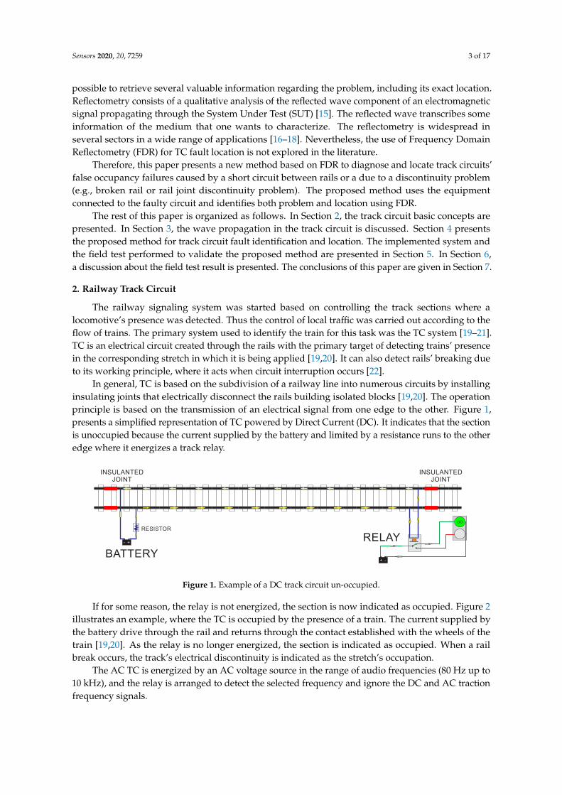
In general, TC is based on the subdivision of a railway line into numerous circuits by installinginsulating joints that electrically disconnect the rails building isolated blocks [19,20]. The operationprinciple is based on the transmission of an electrical signal from one edge to the other. Figure 1,presents a simplified representation of TC powered by Direct Current (DC). It indicates that the sectionis unoccupied because the current supplied by the battery and limited by a resistance runs to the otheredge where it energizes a track relay.

GO

INSULANTEDJOINT

INSULANTEDJOINT

BATTERY

RELAYRESISTOR

+ -

+ -

Figure 1. Example of a DC track circuit un-occupied.

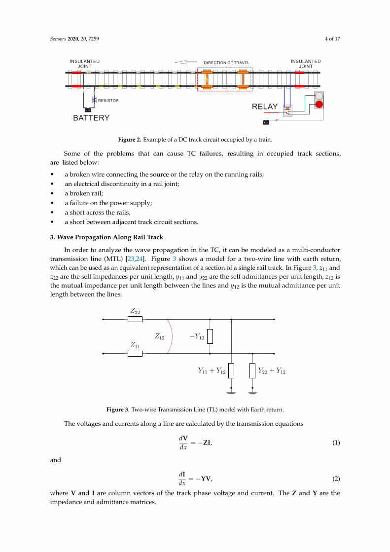
If for some reason, the relay is not energized, the section is now indicated as occupied. Figure 2illustrates an example, where the TC is occupied by the presence of a train. The current supplied bythe battery drive through the rail and returns through the contact established with the wheels of thetrain [19,20]. As the relay is no longer energized, the section is indicated as occupied. When a railbreak occurs, the track’s electrical discontinuity is indicated as the stretch’s occupation.

The AC TC is energized by an AC voltage source in the range of audio frequencies (80 Hz up to10 kHz), and the relay is arranged to detect the selected frequency and ignore the DC and AC tractionfrequency signals.

Sensors 2020, 20, 7259 4 of 17

STOP

INSULANTEDJOINT

INSULANTEDJOINT

BATTERY

RELAY

DIRECTION OF TRAVEL

+ -

+ -

RESISTOR

Figure 2. Example of a DC track circuit occupied by a train.

Some of the problems that can cause TC failures, resulting in occupied track sections,are listed below:

• a broken wire connecting the source or the relay on the running rails;• an electrical discontinuity in a rail joint;• a broken rail;• a failure on the power supply;• a short across the rails;• a short between adjacent track circuit sections.

3. Wave Propagation Along Rail Track

In order to analyze the wave propagation in the TC, it can be modeled as a multi-conductortransmission line (MTL) [23,24]. Figure 3 shows a model for a two-wire line with earth return,which can be used as an equivalent representation of a section of a single rail track. In Figure 3, z11 andz22 are the self impedances per unit length, y11 and y22 are the self admittances per unit length, z12 isthe mutual impedance per unit length between the lines and y12 is the mutual admittance per unitlength between the lines.

Z11

Z22

−Y12

Y11 + Y12 Y22 + Y12

Z12

Figure 3. Two-wire Transmission Line (TL) model with Earth return.

The voltages and currents along a line are calculated by the transmission equations

dVdx

= −ZI, (1)

and

dIdx

= −YV, (2)

where V and I are column vectors of the track phase voltage and current. The Z and Y are theimpedance and admittance matrices.

Sensors 2020, 20, 7259 5 of 17

After deriving both sides and combining (1) and (2) the distance-dependent voltages and currentsare related by the impedance and admittance matrices such that:

d2Vdx2 = ZYV = PV (3)

andd2Idx2 = YZI = PtI, (4)

where

V =

[V1

V2

], I =

[I1

I2

], Z =

[z11 z12

z12 z22

], Y =

[y11 y12

y12 y22

]

and

P =

[z11y11 + z12y12 z11y12 + z12y22

z12y11 + z22y12 z12y12 + z22y22

].

The propagation constant γd and characteristic impedance Z0 are calculated by:

γd =√

ZY (5)

and

Z0 =

√ZY

, (6)

where are variable in the frequency function. The problem can be simplified if spacial symmetryis assumed in the conductor positions such that z11 = z22 and y11 = y22. In such a case,Equations (3) and (4) become

d2

dx2

[V1

V2

]=

[P1 P2

P2 P1

] [V1

V2

](7)

and

d2

dx2

[I1

I2

]=

[P1 P2

P2 P1

] [I1

I2

], (8)

whereP1 = y11z11 + y12z12

P2 = y11z12 + y12z11.(9)

If a differential excitation is considered I1 = −I2 and Equation (8) becomes

d2 I1

dx2 = (P1 − P2)I1, (10)

with a propagation constant

γd =√(z11 − z12)(y11 − y12) (11)

and characteristic impedance

Z0 =√(z11 − z12)/(y11 − y12). (12)

Sensors 2020, 20, 7259 6 of 17

4. Proposed Method for Identification and Location of Track Circuit Failures

In the TC, the rails can be seen as wires of a cable transmitting the information from the transmitter(battery) up to the receiver (relay). Therefore, the track can be modelled as a TL (see Section 3), and adiscontinuity problem such as a broken rail or a short across the rails could be identified and locatedusing the signal reflection properties [21].

The reflection coefficient of a TL can be written as

Γ =Signalre f lected

Signalincident=

ZL − Z0

Z0 + ZL, (13)

where Z0 is the characteristic impedance of the TL and ZL is the impedance of the discontinuity.For instance, the reflection coefficient for an open circuit (ZL = ∞) is 1 and the reflection coefficient fora short circuit (ZL = 0) is −1. The time or phase delay between the incident and reflected signals isrelated to the distance to the fault, and the observed magnitude of the reflection coefficient is related tothe impedance of the discontinuity.

Due to the TC behavior as a TL, that was not designed for communication purposes imposinghigh losses for frequencies above the kHz range, techniques based on FDR are more suitable than theones based on the time domain [25].

FDR sends a set of stepped-frequency sine waves down to the TL [26]. One of the simplest formsof FDR implementation is through Standing Waves Ratio (SWR). SWR systems measure the magnitudeof the standing wave created by the superposition of the incident and reflected signals on the TL [27].The sum of these two sine waves will have a series of peaks that are caused by their constructiveinterference and nulls caused by destructive interference [27]. As the frequency is swept, these nullscan be identified, or the behavior of the resulted curve (frequency × amplitude) can be used in orderto identify and locate the discontinuity.

In SWR, the frequency of the sinusoidal signal is swept within a given bandwidth ( f1 through f2)with step size ∆ f . It reflects back and is superimposed on the incident wave. The combination of theincident and reflected waves (standing wave) can be modeled as

s(t) = A[sin(ωt) + Γe−(α+jβ)xsin(ωt)

], (14)

where s(t) is the observed signal in the injection side, A and ω are the amplitude and angular frequency(which is a scalar measure of rotation rate calculated by ω = 2π f ) of the injected signal, respectively,α is the attenuation constant per unit length of the TL, β is the phase constant per unit length of the TL,Γ is the reflection coefficient (see (13)) and x is two times the location of the impedance discontinuity.

The phase and attenuation constants of a MTL, considering the model in Figure 3, are defined bythe propagation constant γd in Equation (11), where

γd = α + jβ =√(z11 − z12)(y11 − y12). (15)

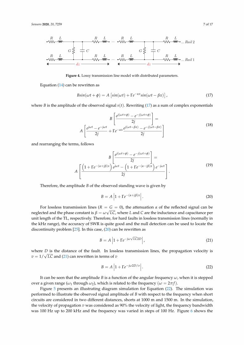
For the specific case of a two-wire lossy transmission line with differential injection, the model inFigure 4 can be used, where R is the line resistance per unit length, L is the line inductance per unitlength, C is the capacitance per unit length between the two conductors and G is the line conductanceper unit length between the two conductors. In this case, the propagation constant results in

γd = α + jβ =√(R + jωL)(G + jωC). (16)

Sensors 2020, 20, 7259 7 of 17

R L

R L

G C

R L

R L

R L

R L

G C

R L

R L

...

...

... Rail 1

... Rail 2

dz dz

Figure 4. Lossy transmission line model with distributed parameters.

Equation (14) can be rewritten as

Bsin(ωt + φ) = A[sin(ωt) + Γe−αxsin(ωt− βx)

], (17)

where B is the amplitude of the observed signal s(t). Rewriting (17) as a sum of complex exponentials

B

[ej(ωt+φ) − e−j(ωt+φ)

2j

]=

A

[ejωt − e−jωt

2j+ Γe−αx ej(ωt−βx) − e−j(ωt−βx)

2j

] (18)

and rearranging the terms, follows

B

[ej(ωt+φ) − e−j(ωt+φ)

2j

]=

A

(

1 + Γe−(α+jβ)x)

ejωt −(

1 + Γe−(α−jβ)x)

e−jωt

2j

.

(19)

Therefore, the amplitude B of the observed standing wave is given by

B = A∣∣∣1 + Γe−(α+jβ)x

∣∣∣ . (20)

For lossless transmission lines (R = G = 0), the attenuation α of the reflected signal can beneglected and the phase constant is β = ω

√LC, where L and C are the inductance and capacitance per

unit length of the TL, respectively. Therefore, for hard faults in lossless transmission lines (normally inthe kHz range), the accuracy of SWR is quite good and the null detection can be used to locate thediscontinuity problem [25]. In this case, (20) can be rewritten as

B = A∣∣∣1 + Γe−jω

√LC2D

∣∣∣ , (21)

where D is the distance of the fault. In lossless transmission lines, the propagation velocity isv = 1/

√LC and (21) can rewritten in terms of v

B = A∣∣∣1 + Γe−jω2D/v

∣∣∣ . (22)

It can be seen that the amplitude B is a function of the angular frequency ω, when it is steppedover a given range (ω1 through ω2), which is related to the frequency (ω = 2π f ).

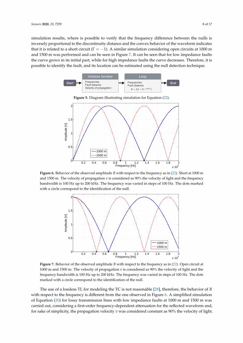
Figure 5 presents an illustrating diagram simulation for Equation (22). The simulation wasperformed to illustrate the observed signal amplitude of B with respect to the frequency when shortcircuits are considered in two different distances, shorts at 1000 m and 1500 m. In the simulation,the velocity of propagation v was considered as 90% the velocity of light, the frequency bandwidthwas 100 Hz up to 200 kHz and the frequency was varied in steps of 100 Hz. Figure 6 shows the

Sensors 2020, 20, 7259 8 of 17

simulation results, where is possible to verify that the frequency difference between the nulls isinversely proportional to the discontinuity distance and the convex behavior of the waveform indicatesthat it is related to a short circuit (Γ = −1). A similar simulation considering open circuits at 1000 mand 1500 m was performed and can be seen in Figure 7. It can be seen that for low impedance faultsthe curve grows in its initial part, while for high impedance faults the curve decreases. Therefore, it ispossible to identify the fault, and its location can be estimated using the null detection technique.

Start FrequenciesFault distanceVelocity of propagation

Initialize Variable

FrequenciesFault distance

Loop

End

Figure 5. Diagram illustrating simulation for Equation (22).

0.2 0.4 0.6 0.8 1 1.2 1.4 1.6 1.8 2x 10

5

0

0.5

1

1.5

2

Frequency [Hz]

Am

plitu

de [V

]

1000 m1500 m

Figure 6. Behavior of the observed amplitude B with respect to the frequency as in (22). Short at 1000 mand 1500 m. The velocity of propagation v is considered as 90% the velocity of light and the frequencybandwidth is 100 Hz up to 200 kHz. The frequency was varied in steps of 100 Hz. The dots markedwith a circle correspond to the identification of the null.

0.2 0.4 0.6 0.8 1 1.2 1.4 1.6 1.8 2x 10

5

0

0.5

1

1.5

2

Frequency [Hz]

Am

plitu

de [V

]

1000 m1500 m

Figure 7. Behavior of the observed amplitude B with respect to the frequency as in (22). Open circuit at1000 m and 1500 m. The velocity of propagation v is considered as 90% the velocity of light and thefrequency bandwidth is 100 Hz up to 200 kHz. The frequency was varied in steps of 100 Hz. The dotsmarked with a circle correspond to the identification of the null.

The use of a lossless TL for modeling the TC is not reasonable [28], therefore, the behavior of Bwith respect to the frequency is different from the one observed in Figure 6. A simplified simulationof Equation (20) for lossy transmission lines with low impedance faults at 1000 m and 1500 m wascarried out, considering a first-order frequency-dependent attenuation for the reflected waveform and,for sake of simplicity, the propagation velocity v was considered constant as 90% the velocity of light.

Sensors 2020, 20, 7259 9 of 17

The result can be seen in Figure 8, where it is possible to verify the attenuation effect on the curvebehavior in contrast to the behavior seen in Figure 6.

0.2 0.4 0.6 0.8 1 1.2 1.4 1.6 1.8 2

x 10

5

0

0.2

0.4

0.6

0.8

1

1.2

Frequency [Hz]

Am

plitu

de

[V

]

1000 m

1500 m

0.2 0.4 0.6 0.8 1 1.2 1.4 1.6 1.8 2

x 10

5

0.96

0.98

1

1.02

1.04

1.06

Frequency [Hz]

Am

plitu

de

[V

]

Zoom

Figure 8. Behavior of the observed amplitude B with respect to the frequency for a lossy transmissionline, as in (20). Short circuit at 1000 m and 1500 m. The velocity of propagation v is constant andconsidered as 90% the velocity of light and the frequency bandwidth is 100 Hz up to 200 kHz.The frequency was varied in steps of 100 Hz. The dots marked with a circle correspond to theidentification of the null.

Figures 6 and 8 were generated by simulation from Equation (22). They were considered a circuitcontaining a short circuit (Γ = −1), and the distances of 1000 m and 1500 m for fault. In Figure 6,the attenuation effects are ignored. The waveforms present successive peaks and nulls produced by thesuperposition of incident and reflected waves, which cause constructive and destructive interferences,respectively. Figure 8, the attenuation was considered, which reduced the amplitude of the peaksand valleys. In the zoom region shown by the figure, it is still possible to observe them. However,the contained attenuation quickly reduces the waveform oscillation and makes it difficult to apply nulldetection techniques.

Figure 9 shows the relationship between the fault position and the frequency of the first null of theamplitude waveform obtained with Equation (22) simulation. In the figure, other fault positions weregenerated, and null detection was applied. It can be observed in Figure 6 the identification of the nullpoint is marked with a circle. These marks are at 89,900 and 134,900 Hz frequencies, which correspondwith null point detection in a short fault with a distance of 1500 m and 1000 m, respectively. The sameanalysis can be observed for Figures 7 and 8. In them were also identified as the null points markedwith a circle.

The demonstration presented in Figure 9, allows estimating the fault position by detecting nullfor the simulated equations. In this situation, with the obtained Fitting, it would be sufficient tocorrelate the frequency of the null point identified to estimate the failure’s position. In the simulation,the velocity of propagation v was considered as 90% the velocity of light, and the frequency bandwidthwas 100 Hz up to 300 kHz.

Sensors 2020, 20, 7259 10 of 17

0 0.5 1 1.5 2 2.5 35

0

500

1000

1500

2000

2500

3000

3500

Frequency [Hz]

Dis

tanc

e [m

]

Short circuit (lossy TL)Open circuit (lossy TL)Short circuitOpen circuit

x 10

Figure 9. Distance from the failure obtained at the frequency of the first null of the amplitude waveform.

Accurate measurements of lossy TL parameters of a TC is not a simple task [23,24,28] and couldintroduce large errors in the fault location estimation. Due to this reason, it is proposed for TCfault identification and location the application of the SWR technique based on the received signalamplitude × frequency curve, using the following procedure:

1. disconnect the track circuit power supply;2. inject in one edge of the track circuit a sinusoidal signal with constant amplitude stepped over a

certain frequency bandwidth;3. for each injected sinusoidal, measure the amplitude of the waveform at the same point that the

signal was injected;4. build the signal amplitude × frequency curve;5. the fault type can be identified through the curve behavior. If the amplitude starts growing,

the fault is related to a low impedance between rails, otherwise, the fault is caused by adiscontinuity problem in a rail joint or due to a broken rail;

6. the location can be estimated through a non-linear regression technique using as inputs theacquired amplitudes for a given frequency scan, avoiding the direct measurement of the trackcircuit parameters.

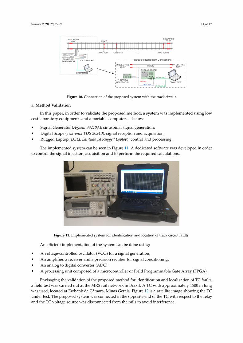
The connection scheme of the proposed system on the TC can be seen in Figure 10. The systemis basically composed of a sinusoidal source generation, a digital signal acquisition system and aprocessing and control device. The figure also shows the details of the connections between theequipment and the rails. The signal generator and oscilloscope are connected to the computer via aUSB cable. The signal tip of the oscilloscope and the signal generator are connected on one side ofthe rails and the other the ground cables of both types of equipment. The software developed allowsthe adjustment of some parameters in the signal generator such as frequency and amplitude and thedata storage process in the oscilloscope. It automates the actuation of the equipment and performs thefrequency variation of the injected signal during the analysis.

Sensors 2020, 20, 7259 11 of 17

COMPUTER

TRACK

USB CABLEGROUND

SIGNAL

POSITION1 POSITION 2 ... POSITION N

FUNCTION GENERATION

100 Hz

OSCILLOSCOPE Details of Equipment Connections

OSCILLOSCOPE

INSULANTEDJOINT

INSULANTEDJOINT

100 kHz

SHUNT

COMPUTERFUNCTION

GENERATION

1 2 3 4 GNDSG

INSULANTEDJOINT

INSULANTEDJOINT

USB CABLE

Figure 10. Connection of the proposed system with the track circuit.

5. Method Validation

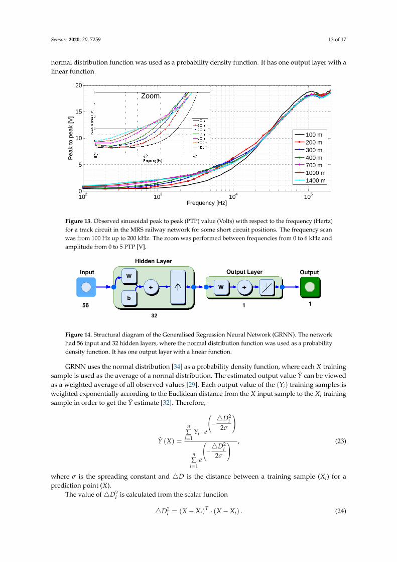
In this paper, in order to validate the proposed method, a system was implemented using lowcost laboratory equipments and a portable computer, as below:

• Signal Generator (Agilent 33210A): sinusoidal signal generation;• Digital Scope (Tektronix TDS 2024B): signal reception and acquisition;• Rugged Laptop (DELL Latitude 14 Rugged Laptop): control and processing.

The implemented system can be seen in Figure 11. A dedicated software was developed in orderto control the signal injection, acquisition and to perform the required calculations.

Figure 11. Implemented system for identification and location of track circuit faults.

An efficient implementation of the system can be done using:

• A voltage-controlled oscillator (VCO) for a signal generation;• An amplifier, a receiver and a precision rectifier for signal conditioning;• An analog to digital converter (ADC);• A processing unit composed of a microcontroller or Field Programmable Gate Array (FPGA).

Envisaging the validation of the proposed method for identification and localization of TC faults,a field test was carried out at the MRS rail network in Brazil. A TC with approximately 1500 m longwas used, located at Ewbank da Câmara, Minas Gerais. Figure 12 is a satellite image showing the TCunder test. The proposed system was connected in the opposite end of the TC with respect to the relayand the TC voltage source was disconnected from the rails to avoid interference.

Sensors 2020, 20, 7259 12 of 17

CDV under test

Figure 12. Satellite image of the track circuit under test from the MRS railway network, located atEwbank da Câmara, MG, Brazil.

Low impedance faults were applied in different locations (150, 200, 300, 400, 500, 600, 700, 800,1000, 1100, 1200, 1300, 1400 and 1500 m) of the TC using a shunt device (a low resistance cable withtwo connectors at the ends that can be fixed on both rails of the TC, acting as a low impedance pathbetween the rails) and for each location, the frequency scan was performed and the peak to peak (PTP)value of the waveform was acquired and stored. Due to practical limitations, it was not possible tobrake a rail or to simulated a discontinuity problem in order to test the system for high impedancefaults. The injected sinusoidal PTP voltage (the Agilent 33210A output resistance is 50 Ω) was 20 V,the frequency scan was performed from 100 Hz up to 200 kHz and for each frequency three acquisitionsof the PTP value of the waveform were stored. The frequency was stepped according to:

• 100 to 1000 Hz in steps of 100 Hz;• 1000 to 10,000 Hz in steps of 500 Hz;• 10,000 to 100,000 Hz in steps of 5000 Hz;• 100,000 to 200,000 Hz in steps of 10,000 Hz.

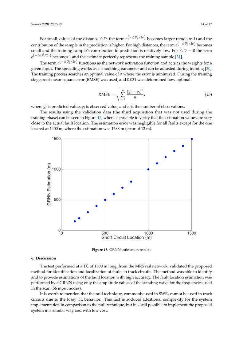
Figure 13 shows the observed PTP value of the acquired waveform with respect to the frequencyfor some faults. As expected, both curves are initially growing indicating that the problem is causedby a low impedance fault. Additionally, the figure shows a zoom region between 0 and 20 kHz onthe abscissa axis and from 0 to 5 volts PTP for the ordinate axis. This region allows observing moreeasily the separation between the waveforms relative to the different distances of the faults, which canbe used for fault location. Now in the region between the frequencies of 25 kHz up to 60 kHz andamplitude of 10 to 15 volts PTP the waveforms are very close to each other. This region containing thewaveforms for different overlapping faults, but does not hinder the proposed method of nonlinearregression of performing the estimation of the position of the faults when analyzing a waveform.

It is worth to mention that the models and simulations presented in Section 4 did not take intoaccount nonlinearities introduced by the system connection with TC such as power limitation of thesinusoidal signal generator, which is one of the main difficulties related to the accurate measurementof the TC parameters [28]. Therefore, as already mentioned in Section 4, in order to provide thefault location a non-linear regression technique can be applied using the amplitude values of thefrequency scan as inputs. In this paper, a Generalised Regression Neural Network (GRNN) [29,30]is used to provide the fault location estimation. GRNN belongs to the category of probabilisticneural network that needs only a fraction of the training samples compared to the algorithms ofa Backpropagation-based neural network [29,31]. It is widely applied in the parameter estimationprocess as can be seen in [32,33] works The network was trained using two acquisitions of the PTPvalue for each scan, leaving the third acquisition for validation. The GRNN input layer is composedby the PTP values of the frequency scan. Figure 14 represents the structure of GRNN applied in theprocess of estimating fault positions. The network had 56 input and 32 hidden layers, where the

Sensors 2020, 20, 7259 13 of 17

normal distribution function was used as a probability density function. It has one output layer with alinear function.

102

103

104

1050

5

10

15

20

Frequency [Hz]

Pea

k to

pea

k [V

]

100 m200 m300 m400 m700 m1000 m1400 m

Zoom

Figure 13. Observed sinusoidal peak to peak (PTP) value (Volts) with respect to the frequency (Hertz)for a track circuit in the MRS railway network for some short circuit positions. The frequency scanwas from 100 Hz up to 200 kHz. The zoom was performed between frequencies from 0 to 6 kHz andamplitude from 0 to 5 PTP [V].

+ +W

W

b

Hidden Layer

Output Layer OutputInput

56 1 1

32

Figure 14. Structural diagram of the Generalised Regression Neural Network (GRNN). The networkhad 56 input and 32 hidden layers, where the normal distribution function was used as a probabilitydensity function. It has one output layer with a linear function.

GRNN uses the normal distribution [34] as a probability density function, where each X trainingsample is used as the average of a normal distribution. The estimated output value Y can be viewedas a weighted average of all observed values [29]. Each output value of the (Yi) training samples isweighted exponentially according to the Euclidean distance from the X input sample to the Xi trainingsample in order to get the Y estimate [32]. Therefore,

Y (X) =

n∑

i=1Yi · e

−4D2i

2σ

n∑

i=1e

−4D2i

2σ

, (23)

where σ is the spreading constant and 4D is the distance between a training sample (Xi) for aprediction point (X).

The value of4D2i is calculated from the scalar function

4D2i = (X− Xi)

T · (X− Xi) . (24)

Sensors 2020, 20, 7259 14 of 17

For small values of the distance 4D, the term e(−4D2i /2σ) becomes larger (tends to 1) and the

contribution of the sample in the prediction is higher. For high distances, the term e(−4D2i /2σ) becomes

small and the training sample’s contribution to prediction is relatively low. For 4D = 0 the terme(−4D2

i /2σ) becomes 1 and the estimate perfectly represents the training sample [31].

The term e(−4D2i /2σ) functions as the network activation function and acts as the weights for a

given input. The spreading works as a smoothing parameter and can be adjusted during training [30].The training process searches an optimal value of σ where the error is minimized. During the trainingstage, root-mean-square error (RMSE) was used, and 0.031 was determined how optimal.

RMSE =

√√√√ n

∑i=1

(yi − yi)2

n, (25)

where yi is predicted value, yi is observed value, and n is the number of observations.The results using the validation data (the third acquisition that was not used during the

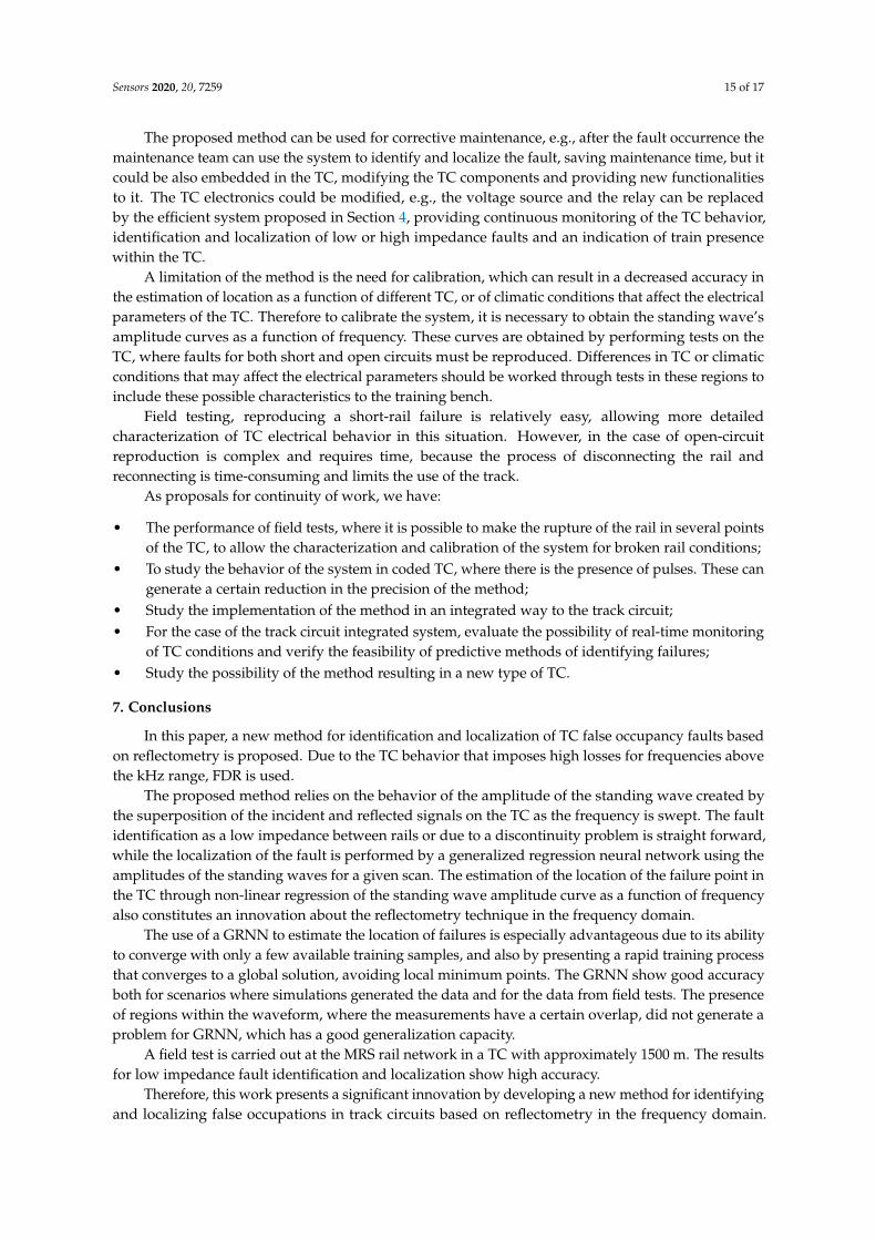
training phase) can be seen in Figure 15, where is possible to verify that the estimation values are veryclose to the actual fault location. The estimation error was negligible for all faults except for the onelocated at 1400 m, where the estimation was 1388 m (error of 12 m).

Figure 15. GRNN estimation results.

6. Discussion

The test performed at a TC of 1500 m long, from the MRS rail network, validated the proposedmethod for identification and localization of faults in track circuits. The method was able to identifyand to provide estimations of the fault location with high accuracy. The fault location estimation wasperformed by a GRNN using only the amplitude values of the standing wave for the frequencies usedin the scan (56 input nodes).

It is worth to mention that the null technique, commonly used in SWR, cannot be used in trackcircuits due to the lossy TL behavior. This fact introduces additional complexity for the systemimplementation in comparison to the null technique, but it is still possible to implement the proposedsystem in a similar way and with low cost.

Sensors 2020, 20, 7259 15 of 17

The proposed method can be used for corrective maintenance, e.g., after the fault occurrence themaintenance team can use the system to identify and localize the fault, saving maintenance time, but itcould be also embedded in the TC, modifying the TC components and providing new functionalitiesto it. The TC electronics could be modified, e.g., the voltage source and the relay can be replacedby the efficient system proposed in Section 4, providing continuous monitoring of the TC behavior,identification and localization of low or high impedance faults and an indication of train presencewithin the TC.

A limitation of the method is the need for calibration, which can result in a decreased accuracy inthe estimation of location as a function of different TC, or of climatic conditions that affect the electricalparameters of the TC. Therefore to calibrate the system, it is necessary to obtain the standing wave’samplitude curves as a function of frequency. These curves are obtained by performing tests on theTC, where faults for both short and open circuits must be reproduced. Differences in TC or climaticconditions that may affect the electrical parameters should be worked through tests in these regions toinclude these possible characteristics to the training bench.

Field testing, reproducing a short-rail failure is relatively easy, allowing more detailedcharacterization of TC electrical behavior in this situation. However, in the case of open-circuitreproduction is complex and requires time, because the process of disconnecting the rail andreconnecting is time-consuming and limits the use of the track.

As proposals for continuity of work, we have:

• The performance of field tests, where it is possible to make the rupture of the rail in several pointsof the TC, to allow the characterization and calibration of the system for broken rail conditions;

• To study the behavior of the system in coded TC, where there is the presence of pulses. These cangenerate a certain reduction in the precision of the method;

• Study the implementation of the method in an integrated way to the track circuit;• For the case of the track circuit integrated system, evaluate the possibility of real-time monitoring

of TC conditions and verify the feasibility of predictive methods of identifying failures;• Study the possibility of the method resulting in a new type of TC.

7. Conclusions

In this paper, a new method for identification and localization of TC false occupancy faults basedon reflectometry is proposed. Due to the TC behavior that imposes high losses for frequencies abovethe kHz range, FDR is used.

The proposed method relies on the behavior of the amplitude of the standing wave created bythe superposition of the incident and reflected signals on the TC as the frequency is swept. The faultidentification as a low impedance between rails or due to a discontinuity problem is straight forward,while the localization of the fault is performed by a generalized regression neural network using theamplitudes of the standing waves for a given scan. The estimation of the location of the failure point inthe TC through non-linear regression of the standing wave amplitude curve as a function of frequencyalso constitutes an innovation about the reflectometry technique in the frequency domain.

The use of a GRNN to estimate the location of failures is especially advantageous due to its abilityto converge with only a few available training samples, and also by presenting a rapid training processthat converges to a global solution, avoiding local minimum points. The GRNN show good accuracyboth for scenarios where simulations generated the data and for the data from field tests. The presenceof regions within the waveform, where the measurements have a certain overlap, did not generate aproblem for GRNN, which has a good generalization capacity.

A field test is carried out at the MRS rail network in a TC with approximately 1500 m. The resultsfor low impedance fault identification and localization show high accuracy.

Therefore, this work presents a significant innovation by developing a new method for identifyingand localizing false occupations in track circuits based on reflectometry in the frequency domain.

Sensors 2020, 20, 7259 16 of 17

The estimation of the failure point at TC through non-linear regression of the steady wave amplitudecurve as a function of frequency is also an innovation in the technique of reflectometry in the frequencydomain. The failures of the track circuits can cause significant economic losses to the railway system.Therefore, the contributions present to the area of electronic instrumentation and rail transport areincredibly relevant. A measurement system has been implemented to validate the proposed method,and field tests have been carried out. The achieved results showed that the method works with goodaccuracy and can be used to speed up and reduce railway companies’ maintenance costs.

Finally, the proposed method can be used for corrective maintenance, or it can be embedded inthe TC, to provide it new functionalities.

Author Contributions: Conceptualization, A.S.C., L.M.A.F., R.A.N., L.M.H., T.A.A. and H.V.; methodology,A.S.C., L.M.A.F., R.A.N. and T.A.A.; software, T.A.A. and L.M.H.; validation, T.A.A., A.S.C., L.M.A.F. and R.A.N.;formal analysis, T.A.A., A.S.C., R.A.N. and L.M.A.F.; resources, A.S.C., L.M.H. and H.V.; writing—originaldraft preparation, A.S.C., L.M.A.F., R.A.N., L.M.H. and T.A.A.; writing—review and editing, T.A.A. and L.M.H.All authors have read and agreed to the published version of the manuscript.

Funding: This work was supported in part by the MRS Logística and Federal University of Juiz de Fora.

Acknowledgments: The authors would like to thank MRS Logística, Federal University of Juiz de Fora,INCT—INERGE, CNPq, CAPES, FAPEMIG and TBE (Transmissoras Brasileiras de Energia) for project number(PD-04380-0002/2015) regulated by ANEEL.

Conflicts of Interest: The authors declare no conflict of interest.

References

1. Patra, A.P.; Kumar, U. Availability analysis of railway track circuits. Proc. Inst. Mech. Eng. Part F J. RailRapid Transit 2010, 224, 169–177. [CrossRef]

2. Diemunsch, K. Track Circuit Failures: Their Impact on Conventional Signaling in CBTC Projects.IEEE Veh. Technol. Mag. 2013, 8, 63–72. [CrossRef]

3. Bowden, R.P. Broken rail detection in non-signaled territory. In Proceedings of the AREMA AnnualConference, Orlando, FL, USA, 29 August–1 September 2010; pp. 8–18.

4. Thurston, D.F. Broken Rail Detection: Practical Application of New Technology or Risk Mitigation Approaches.IEEE Veh. Technol. Mag. 2014, 9, 80–85. [CrossRef]

5. Zarembski, A.M.; Palese, J.W. Managing risk on the railway infrastructure. In Proceedings of the 7th WorldCongress on Railway Research, Montreal, QC, Canada, 4–8 June 2006; pp. 3–5.

6. Chen, J.; Roberts, C.; Weston, P. Fault detection and diagnosis for railway track circuits using neuro-fuzzysystems. Control Eng. Pract. 2008, 16, 585–596. [CrossRef]

7. Oukhellou, L.; Debiolles, A.; Denœux, T.; Aknin, P. Fault diagnosis in railway track circuits usingDempster–Shafer classifier fusion. Eng. Appl. Artif. Intell. 2010, 23, 117–128. [CrossRef]

8. de Bruin, T.; Verbert, K.; Babuška, R. Railway Track Circuit Fault Diagnosis Using Recurrent NeuralNetworks. IEEE Trans. Neural Netw. Learn. Syst. 2017, 28, 523–533. [CrossRef] [PubMed]

9. Sun, S.; Zhao, H. Fault Diagnosis in Railway Track Circuits Using Support Vector Machines. In Proceedingsof the 2013 12th International Conference on Machine Learning and Applications, Miami, FL, USA,4–7 December 2013; Volume 2, pp. 345–350. [CrossRef]

10. Hopkins, B.M.; There, S. Broken Rail Prediction and Detection Using Wavelets and Artificial NeuralNetworks. In Proceedings of the 2011 Joint Rail Conference, Pueblo, CO, USA, 16–18 March 2011; Volume 2,pp. 77–84. [CrossRef]

11. Turner, S. Feasibility of Locomotive-Mounted Broken Rail Detection; Final Report for High-Speed Rail IDEAProject: Guernsey, WY, USA, 2004; Volume 38.

12. Rumsey, A.F.; Achakji, G.; Bois, S.; Braban, C.; Childs, F.; Crispo, M.; Estivals, N.; Gillen, H.; Glickenstein, H.;Graponne, V.; et al. IEEE Standard for Communications-Based Train Control (CBTC) Performance andFunctional Requirements. In IEEE Std 1474.1-2004 (Revision of IEEE Std 1474.1-1999); IEEE: New York, NY,USA, 2004; pp. 1–45. [CrossRef]

13. Sireesha, R.; Ajay Kumar, B.; Mallikarjunaiah, G.; Bharath Kumar, B. Broken Rail Detection System using RFTechnology. SSRG Int. J. Electron. Commun. Eng. (SSRG-IJECE) 2015. [CrossRef]

Sensors 2020, 20, 7259 17 of 17

14. Schwartz, K.; District, B.A.R.T. Development of an Acoustic Broken Rail Detection System; Final Report forHigh-Speed Rail IDEA Project: Washington, DC, USA, 2004; Volume 42.

15. Cataldo, A.; Benedetto, E.D. Broadband Reflectometry for Diagnostics and Monitoring Applications.IEEE Sens. J. 2011, 11, 451–459. [CrossRef]

16. Tsai, P.; Lo, C.; Chung, Y.C.; Furse, C. Mixed-signal reflectometer for location of faults on aging wiring.IEEE Sens. J. 2005, 5, 1479–1482. [CrossRef]

17. Cataldo, A.; Benedetto, E.D.; Cannazza, G.; Huebner, C.; Trebbels, D.; Giaquinto, N.; D’Aucelli, G.M.Controlling the irrigation process in agriculture through elongated TDR-sensing cables. In Proceedingsof the 2017 IEEE International Instrumentation and Measurement Technology Conference (I2MTC), Turin,Italy, 22–25 May 2017; pp. 1–6. [CrossRef]

18. Xudong, S.; Jianzhong, Z.; Tao, J.; Liwen, W. Design of aircraft cable intelligent fault diagnosis and locationsystem based on time domain reflection. In Proceedings of the 2010 8th World Congress on IntelligentControl and Automation, Jinan, China, 7–9 July 2010; pp. 5856–5860. [CrossRef]

19. Scales, J. How Track Circuits Detect and Protect Trains. Railwaysignalling 2014, 1–7.20. Teague, O.E.; Case, C.; Daddario, E.; De Simone, D.; Krambles, G. Automatic Train Control in Rail Rapid Transit;

Office of Technology Assessment: Washington, DC, USA, 1976.21. Alvarenga, T.A. Identificação e Localização de Falhas em Circuitos de Via de Ferrovias Baseada em

Reflectometria no Domínio da Frequência. Ph.D. Thesis, Federal University of Juiz de Fora, Juiz de Fora,MG, Brazil, 2018.

22. Serra, A.M.; Ramos, D.; Dellacqua, F.; Andrade, J.L.G.; Gueiral, M.; Lima, P.H.; Rubiale, P. Sistemas deSinalização: Trilha Técnica; VALER-Educação VALE: Rio de Janeiro, RJ, Brazil, 2010.

23. Hill, R.I.; Carpenter, D.C. In situ determination of rail track electrical impedance and admittancematrix elements. IEEE Trans. Instrum. Meas. 1992, 41, 666–673. [CrossRef]

24. Hill, R.J.; Carpenter, D.C. Rail track distributed transmission line impedance and admittance: Theoreticalmodeling and experimental results. IEEE Trans. Veh. Technol. 1993, 42, 225–241. [CrossRef]

25. Furse, C.; Chung, Y.C.; Lo, C.; Pendayala, P. A Critical Comparison of Reflectometry Methods for Locationof Wiring Faults. Smart Struct. Syst. 2006, 2, 25–46. [CrossRef]

26. Doo, S.H.; Ra, W.S.; Yoon, T.S.; Park, J.B. Fast time-frequency domain reflectometry based on the ARcoefficient estimation of a chirp signal. In Proceedings of the 2009 American Control Conference, St. Louis,MO, USA, 10–12 June 2009; pp. 3423–3428. [CrossRef]

27. Furse, C. Reflectometry for structural health monitoring. In New Developments in Sensing Technology forStructural Health Monitoring; Springer: Berlin/Heidelberg, Germany, 2011; pp. 159–185. [CrossRef]

28. Szelag, A. Rail track as a lossy transmission line Part I: Parameters and new measurement methods.Arch. Electr. Eng. 2000, XLIX, 407–423.

29. Specht, D.F. A general regression neural network. IEEE Trans. Neural Netw. 1991, 2, 568–576. [CrossRef]30. Rutkowski, L. Generalized regression neural networks in time-varying environment. IEEE Trans. Neural Netw.

2004, 15, 576–596. [CrossRef]31. Bauer, M.M. General Regression Neural Network, GRNN-A Neural Network for Technical Use.

Master’s Thesis, University of Wisconsin-Madison, Madison, WI, USA, 1995.32. Meng, X.; Fu, Y.; Yuan, J. Estimating solubilities of ternary water-salt systems using simulated annealing

algorithm based generalized regression neural network. Fluid Phase Equilibria 2020, 505, 112357. [CrossRef]33. Kim, B.; Lee, D.W.; Park, K.Y.; Choi, S.R.; Choi, S. Prediction of plasma etching using a randomized

generalized regression neural network. Vacuum 2004, 76, 37–43. [CrossRef]34. Peebles, P.Z.J. Probability, Random Variables, and Random Signal Principles, 4th ed.; McGraw-Hill: New York,

NY, USA, 2001.

Publisher’s Note: MDPI stays neutral with regard to jurisdictional claims in published maps and institutionalaffiliations.

© 2020 by the authors. Licensee MDPI, Basel, Switzerland. This article is an open accessarticle distributed under the terms and conditions of the Creative Commons Attribution(CC BY) license (http://creativecommons.org/licenses/by/4.0/).