Ice volume and basal topography estimation using geostatisticalmethods and GPR measurements: Application to the Tsanfleuronand Scex Rouge Glacier, Swiss AlpsAlexis Neven1,*, Valentin Dall’Alba1,*, Przemysław Juda1, Julien Straubhaar1, and Philippe Renard1,2

1Centre of Hydrogeology and Geothermics, University of Neuchâtel, Switzerland2Department of Geosciences, University of Oslo, Oslo, Norway*These authors contributed equally to this work.

Correspondence: Alexis Neven (alexis.neven@unine.ch)

Abstract. Ground Penetrating Radar (GPR) is widely used for determining mountain glacier thickness. However, this method

provides thickness data only along the acquisition lines and therefore interpolation has to be made between them. Depending

on the interpolation strategy, calculated ice volumes can differ and can lack an accurate error estimation. Furthermore, glacial

basal topography is often characterized by complex geomorphological features, which can be hard to reproduce using classical

interpolation methods, especially when the field data are sparse or when the morphological features are too complex. This5

study investigates the applicability of multiple-point statistics (MPS) simulations to interpolate glacier bedrock topography

using GPR measurements. In 2018, a dense GPR data set was acquired on the Tsanfleuron Glacier (Switzerland). These data

were used as the source for a bedrock interpolation. The results obtained with the direct sampling MPS method are compared

against those obtained with kriging and sequential Gaussian simulations (SGS) on both a synthetic data set – with known

reference volume and bedrock topography – and the real data underlying the Tsanfleuron Glacier. Using the MPS modelled10

bedrock, the ice volume for the Scex Rouge and Tsanfleuron Glacier is estimated to be 113.9 ± 1.6 Miom3. The direct

sampling approach, unlike the SGS and kriging, allowed not only an accurate volume estimation but also the generation of

a set of realistic bedrock simulations. The complex karstic geomorphological features are reproduced, and can be used to

significantly improve for example the precision of subglacial flow estimation.

Copyright statement.15

1 Introduction

It is widely accepted that global climatic changes are impacting future precipitation rates and temperatures. In Switzerland,

these changes will inevitably induce new stresses on alpine environments and on glaciers’ mass balance (e.g. Haeberli et al.,

2007; Beniston, 2012; Huss and Fischer, 2016). In this context, the monitoring of glacier’s thickness and volume is crucial

1

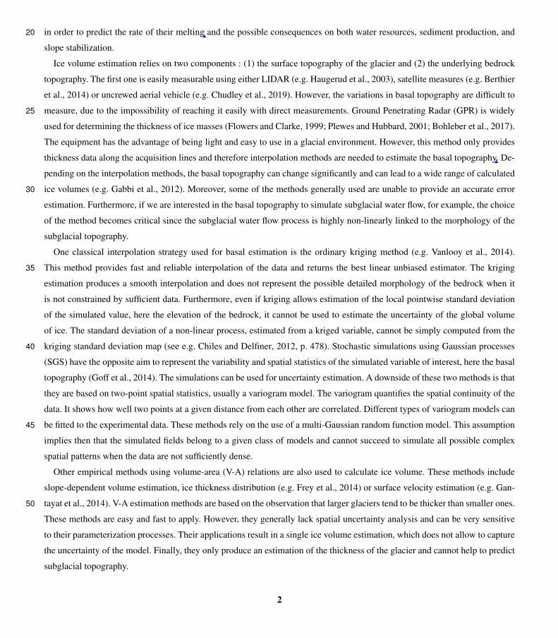
in order to predict the rate of their melting and the possible consequences on both water resources, sediment production, and20

slope stabilization.

Ice volume estimation relies on two components : (1) the surface topography of the glacier and (2) the underlying bedrock

topography. The first one is easily measurable using either LIDAR (e.g. Haugerud et al., 2003), satellite measures (e.g. Berthier

et al., 2014) or uncrewed aerial vehicle (e.g. Chudley et al., 2019). However, the variations in basal topography are difficult to

measure, due to the impossibility of reaching it easily with direct measurements. Ground Penetrating Radar (GPR) is widely25

used for determining the thickness of ice masses (Flowers and Clarke, 1999; Plewes and Hubbard, 2001; Bohleber et al., 2017).

The equipment has the advantage of being light and easy to use in a glacial environment. However, this method only provides

thickness data along the acquisition lines and therefore interpolation methods are needed to estimate the basal topography. De-

pending on the interpolation methods, the basal topography can change significantly and can lead to a wide range of calculated

ice volumes (e.g. Gabbi et al., 2012). Moreover, some of the methods generally used are unable to provide an accurate error30

estimation. Furthermore, if we are interested in the basal topography to simulate subglacial water flow, for example, the choice

of the method becomes critical since the subglacial water flow process is highly non-linearly linked to the morphology of the

subglacial topography.

One classical interpolation strategy used for basal estimation is the ordinary kriging method (e.g. Vanlooy et al., 2014).

This method provides fast and reliable interpolation of the data and returns the best linear unbiased estimator. The kriging35

estimation produces a smooth interpolation and does not represent the possible detailed morphology of the bedrock when it

is not constrained by sufficient data. Furthermore, even if kriging allows estimation of the local pointwise standard deviation

of the simulated value, here the elevation of the bedrock, it cannot be used to estimate the uncertainty of the global volume

of ice. The standard deviation of a non-linear process, estimated from a kriged variable, cannot be simply computed from the

kriging standard deviation map (see e.g. Chiles and Delfiner, 2012, p. 478). Stochastic simulations using Gaussian processes40

(SGS) have the opposite aim to represent the variability and spatial statistics of the simulated variable of interest, here the basal

topography (Goff et al., 2014). The simulations can be used for uncertainty estimation. A downside of these two methods is that

they are based on two-point spatial statistics, usually a variogram model. The variogram quantifies the spatial continuity of the

data. It shows how well two points at a given distance from each other are correlated. Different types of variogram models can

be fitted to the experimental data. These methods rely on the use of a multi-Gaussian random function model. This assumption45

implies then that the simulated fields belong to a given class of models and cannot succeed to simulate all possible complex

spatial patterns when the data are not sufficiently dense.

Other empirical methods using volume-area (V-A) relations are also used to calculate ice volume. These methods include

slope-dependent volume estimation, ice thickness distribution (e.g. Frey et al., 2014) or surface velocity estimation (e.g. Gan-

tayat et al., 2014). V-A estimation methods are based on the observation that larger glaciers tend to be thicker than smaller ones.50

These methods are easy and fast to apply. However, they generally lack spatial uncertainty analysis and can be very sensitive

to their parameterization processes. Their applications result in a single ice volume estimation, which does not allow to capture

the uncertainty of the model. Finally, they only produce an estimation of the thickness of the glacier and cannot help to predict

subglacial topography.

2

Figure 1. Aerial image and Digital Elevation Model captured from Drone images of the Tsanfleuron Glacier, Switzerland.

In the last decades, new geostatistical methods have arisen with the aim to improve the realism of the simulation using another55

form of information that the one expressed by two points statistics and variogram interpretation. Multiple-point statistics

(MPS) simulation algorithms use a training image (TI) to infer the spatial statistics of the model and generate random fields

reproducing these spatial statistics. The TI represents a conceptual knowledge of the variable that is aimed to be simulated,

it can be created by experts or can be extracted from analog data sets. Unlike other geostatistical approaches, MPS does not

require the definition of an analytical two-point statistics model to represent the spatial variability but instead infers it implicitly60

from the TI provided by the user (Journel and Zhang, 2006). MPS simulations benefit from this additional knowledge and can

also be constrained by the acquired data (the conditioning data). These methods allow the creation more realistic spatial patterns

than classical two-points geostatistical methods and can be used to represent the uncertainty by simulating a set of realizations.

Some examples of application can be found in Oriani et al. (2014); de Carvalho et al. (2016); Dall’Alba et al. (2020). In recent

studies, MPS has successfully been applied to estimate subglacial topography from synthetic data (MacKie and Schroeder,65

2020) and to evaluate the probability of subglacial lakes (MacKie et al., 2020a).

The aims of this paper are both methodological and applied. Regarding the methodological aspect, this work aims to demon-

strate the use of the MPS method to combine information provided by GPR data points and Digital Elevation Model (DEM)

to simulate a realistic glacial basal topography. The benefits of using a MPS approach are highlighted by comparing its results

with those obtained with more classical geostatistical methods. Using synthetic test cases, the different methods are compared70

by calculating for each one an ice volume and a roughness estimation, which are then compared against the true synthetic

values. A set of scores are computed to compare the methods. Through this comparison process different parameter sets are

also tested for each methods. This methodological aspect helps to select the most suitable parameter sets and illustrate on a

synthetic case where the target topography is known. This highlights the advantages of the multiple-point simulation approach

for estimating glacier volume and its associated basal’s geomorphology. On the applied side, the objectives are to present new75

3

field data and new estimations of the volume of the Tsanfleuron Glacier, roughly 10 years after the last detailed published

estimation (Gremaud and Goldscheider, 2010).

The Tsanfleuron Glacier and the Scex Rouge Glacier (Fig. 1) are both located in the Diablerets Massif (Schoeneich and Rey-

nard, 2021) in Switzerland. They are connected to each other at the Tsanfleuron pass, but are located on two different faces : the

main slope of the Scex Rouge Glacier is toward the north north-east, while the Tsanfleuron slope is toward the east. Tsanfleuron80

volume was estimated to be 100 Miom3 of ice in 2009 using radio-magneto-telluric data and kriging of the ice thickness, with

an uncertainty of±10% and a maximum measured depth of 138 m (Gremaud and Goldscheider, 2010). According to the mea-

surements, the glacier is currently losing about 1.5 m of thickness per year (Gremaud and Goldscheider, 2010). A more recent

publication, applied to all Swiss glaciers, proposed a volume for Tsanfleuron and Scex Rouge of respectively 200.02 and 8.12

Miom3 in 2016 (Grab et al., 2021). However, the uncertainty on the GPR picking used in the particular case of Tsanfleuron is85

important, especially with thicknesses bigger than 60 m according to a personal communication with one of the author. Both

glaciers lie on carbonate formations that are heavily karstified. The glacier is one of the main feeders of the underlying karstic

system. Tracers tests showed that this network is a significant source of drinking water supply for the community of Conthey

(Gremaud, 2008). Obtaining a better model of the basal topography is therefore a step toward improving the understanding of

the remaining ice volume, the glacial retreat behavior, and its impact on the regional groundwater system.90

The core MPS technique used in this study is the direct sampling algorithm (Mariethoz et al., 2010) implemented in the

DeeSse code (Straubhaar, 2019). This implementation includes several improvements as compared to the original algorithm.

In particular DeeSse can account for multi-resolution structures in the data set (Straubhaar et al., 2020) and inequality data

(Straubhaar and Renard, 2021).

In this paper, the exposed basal surface of the melted glacier zones is employed as a training image for the simulation of the95

covered glacier basal topography. The justification for this modeling decision is that the lithology and general topographical

slope below the glacier and in the exposed area are similar, and therefor the geomorphological features should also be similar.

This idea is validated by the analysis of the area where the glacier retreated in the last dozen years, which exposed geomor-

phological structures similar to the older part. The GPR inferred depths are then used as conditioning points as well as the

topographical data around the glacier.100

Since the exact topography below the glacier is unknown, to analyze and benchmark the performances of different inter-

polation methods, a numerical experiment was designed in which references can be compared to the simulation outputs. For

that purpose, the exposed part of the bedrock is also used (besides being used as TI) to compare the performances of the MPS,

kriging, and sequential Gaussian simulation (SGS) approaches. 20 zones are extracted from the exposed DEM and sampled

to create fake GPR data sets. Using only the sampled data set, the topography in the test zones are interpolated using MPS,105

SGS, and kriging and compared to the reference topography. The true volumes of the synthetic tests are defined as being the

space between the simulated topography and a flat surface representing the top of the ice sheet. The altitude of this ice sheet

is defined as being four meters above the maximum altitude of the simulation. The absolute volumes of the simulations are

then compared to this true volume, using the same ice sheet altitude. Moreover, an estimation of possible flow accumulation

is calculated on the simulated bedrocks and on the reference. The flow accumulation map outline the link between structures110

4

of the topography and the connectivity of the cells. In addition, different parameters sets are tested for each method through

this experiment. Finally, different scores are used to compare the methods. This numerical experiment helps to understand and

visualize the impact of each method on the simulated bedrock shape and volume estimation distribution.

Lastly, the Tsanfleuron and Scex Rouge bedrock’s topography is interpolated using the previously tested methods and pa-

rameters sets. The simulated bedrocks are also compared to recently uncovered bedrock, using a simple estimation of flow115

accumulation. A brief overview of the glacier volume distributions and their evolution through the past time is finally carried

out using the calculated bedrock surfaces and different DEM.

2 Methods

2.1 GPR and DEM acquisition

In summer 2018, a dense GPR acquisition on the Tsanfleuron Glacier was performed (Fig. 2) using a single Radarteam Cobra120

GPR antenna of 80 Mhz centre-frequency, mounted on a backpack with a RTK differential GPS. Total listening time was set

to 1600 ns with a sample rate of 320 MHz. The GPR data were processed using a standard workflow. A time-zeroing was

performed, setting the origin of the time vector when the first arrival is recorded. Our system being a single antenna system,

this time corresponds in fact to the recording of the pulse itself. We then apply a time dependant gain, being the time vector

risen to a power 1.2. A de-wow filter was also added, using the residual median filter method described in Gerlitz et al. (1993).125

We then removed the mean trace to avoid displaying the pulse and the airwave present in all the traces. Finally, a 120 MHz

low pass filter was applied to remove the signals outside of the GPR band. The data were binned in a 2 m grid. The time to

depth conversion was done using a uniform wave propagation speed of 0.168 m/ns (Eisen et al., 2002; Moorman and Michel,

2000). The basal reflector identification and the picking was then performed multiple times, with a random display of the

lines, by four different operators. The random selection of the line was done in order to avoid bias and over interpretation of130

the GPR data reflections. The processing was identical for all operators, however they had the possibility to adapt the display

(colormap and percentile clipping). All of the picked points which showed differences of more than five meters between the

different operators were considered as unsure and therefore rejected. This resulted in a good basal depth estimation in 87 %

of the lines. As expected, the deepest zones (more than 70 - 80 m) are the most difficult to identify precisely, with a smaller

signal-to-noise ratio. An example line is display on Fig.2. The data were then converted to a point set, representing the position135

of the measurement and the altitude of the basal reflector, to be used with the MPS algorithm.

In addition, during the summer in 2019 several UAV flights were realized above the Tsanfleuron Glacier. We conducted five

flights with a Sense Fly EBEE UAV equipped with a 20 megapixel RGB camera. The objective was to have a resolution of

at least 10 cm/pixel everywhere on the glacier, and an overlap of 60 % between the images. The resulting flight altitude was

between 300 m to 600 m above ground. A DEM and an ortho-mosaic (Fig. 1) were generated using a stereoscopic method, and140

the whole domain was geolocated using Ground Control Points. The image processing was done using the commercial Pix4D

software.

5

0 500 m

´

0

200

400

600

800

1000

1200

TWTT [ns]

0 50 100 150 200 250Distance [m]

Line 1036

Line 1036

Normalized Amplitude10-1

Basal reflector

NWSE

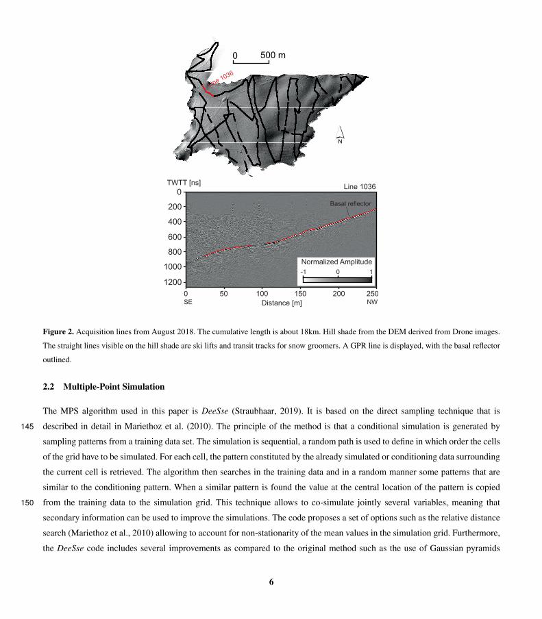
Figure 2. Acquisition lines from August 2018. The cumulative length is about 18km. Hill shade from the DEM derived from Drone images.

The straight lines visible on the hill shade are ski lifts and transit tracks for snow groomers. A GPR line is displayed, with the basal reflector

outlined.

2.2 Multiple-Point Simulation

The MPS algorithm used in this paper is DeeSse (Straubhaar, 2019). It is based on the direct sampling technique that is

described in detail in Mariethoz et al. (2010). The principle of the method is that a conditional simulation is generated by145

sampling patterns from a training data set. The simulation is sequential, a random path is used to define in which order the cells

of the grid have to be simulated. For each cell, the pattern constituted by the already simulated or conditioning data surrounding

the current cell is retrieved. The algorithm then searches in the training data and in a random manner some patterns that are

similar to the conditioning pattern. When a similar pattern is found the value at the central location of the pattern is copied

from the training data to the simulation grid. This technique allows to co-simulate jointly several variables, meaning that150

secondary information can be used to improve the simulations. The code proposes a set of options such as the relative distance

search (Mariethoz et al., 2010) allowing to account for non-stationarity of the mean values in the simulation grid. Furthermore,

the DeeSse code includes several improvements as compared to the original method such as the use of Gaussian pyramids

6

(Straubhaar et al., 2020). This feature simulate patterns at different scale, to ensure that both large and small scale patterns are

well reproduce in the simulation.155

The three main parameters of the method are the maximum number of neighbors (n), the distance threshold (t) and the scan

fraction (f ). n controls how many nodes are used for the pattern comparison between the TI and the simulation grid. t sets

the maximum acceptable dissimilarity when comparing a pattern in the simulation grid and in the TI. Finally, f controls the

maximal fraction of the TI that can be scanned when searching for a pattern. The optimal values of these parameters depend

on the complexity of the pattern that are displayed in the training data set and on the acceptable computing time to obtain a set160

of simulations. Some recommendations on how to select those parameters are presented in Meerschman et al. (2013).

In the case of the Tsanfleuron Glacier, the acquired DEM of the exposed bedrock is used as TI. The hard data are the GPR

lines and the altitude of the bedrock (from the DEM) surrounding the glacier. To obtain the best parameters for this data set,

a series of experiments with different parameter sets was conducted. The methodology to conduct these tests is described in

detail in section 2.4.165

For all the simulations, the multi-scale mode using Gaussian pyramids and relative distance options are activated to get

the best reproduction of the patterns. The first feature improves the simulation of patterns at different scales and produces

more consistent simulation outputs (Straubhaar et al., 2020). The second feature is a way to deal with non-stationary data sets.

Indeed, we are interested here in the relative changes of the topography along altitude. Two patterns that show the same relative

changes even at different absolute altitudes should be considered similar. This option as the advantage of being able to deal170

with non-stationary TI, without any prior de-trending needed. Finally, a secondary variable is used. This variable is not the

main variable of interest, but is simulated jointly to improve the quality of the simulation. Once some points are simulated, the

secondary variable guides the simulation of the neighboring points, reducing the uncertainty and improving the realism. In our

case, the topography gradient is added as a secondary variable in the TI. This variable is not defined in the hard data set.

2.3 Kriging and SGS175

Kriging and sequential Gaussian simulations (SGS) are standard geostatistical techniques that are well described in many

textbooks (e.g. Chiles and Delfiner, 2012). Therefore, we will not describe here the underlying theory of these methods but

rather focus on the specific aspects of their application in our case.

At the scale of the study site, the exposed bedrock topography presents a general slope toward the east and is therefore

non-stationary. To account for this general slope, we decided to remove first the trend present in the DEM and in the hard180

(GPR) data before conducting the variogram analysis. To do so, a polynomial surface is fitted and removed from the data.

By removing the polynomial surface from the data, only the deviation from this surface, which corresponds to the deviation

from the general slope of the glacier, is simulated. At the end of the process, the trend is then added to the interpolated values

to obtain the final basal topography. It is important to note that since the Scex Rouge and the Tsanfleuron Glaciers have two

different orientations, two different trends were interpolated: one was used for the Tsanfleuron Glacier and the other one for185

the Scex rouge glacier. The transition being set at the Tsanfleuron pass. The polynomial interpolated trends being in the form

7

of :

f(x,y) = a+ bx+ cy+ dx2 + exy+ fy2 (1)

= 0− 0.281x− 0.143y− 6.09 ∗ 10−6x2 +7.98 ∗ 10−5xy− 1.28 ∗ 10−5y2 (Tsanfleuron) (2)

= 0+1.78x− 3.37y+4.63 ∗ 10−3x2− 3.26 ∗ 10−3xy+1.505 ∗ 10−3y2 (ScexRouge) (3)190

with a,b,c,d,e,f being the coefficient and x and y the coordinate in the plane. The variogram model used for the SGS and

kriging approaches is shown in Fig. 3. The data set used for calculating the experimental variogram is shown in Fig. 3a on a

map view. It is composed of 7 500 points, 2 500 coming from the acquired GPR data and the other 5 000 points randomly

sampled from the TI. This data set presents a distribution centered around −4.08 m with a standard deviation value of 21.2

m (Fig. 3b) that is close to Gaussian. We therefore did not apply any variable transform to ensure Gaussianity. The variogram195

map (Fig. 3c) does not show a strong and significant anisotropy. Therefore, an omni-directional variogram model is selected

and adjusted to the experimental variogram data. The model is composed of two components: a spherical structure with a sill

value of 344 m2, a range value of 862 m, and a second exponential structure defined by a sill value of 134 m2 and a range value

of 396 m (Fig. 3d). The sequential Gaussian simulations and kriging are performed using the SGeMS open-source software

(Remy et al., 2009).200

2.4 Systematic comparison of the methods

In order to benchmark the different geostatistical algorithms and parameter sets, a systematic testing approach is applied

(Fig. 4). First, the available DEM (the exposed part of the bedrock) is sampled to create 20 synthetic test cases. These are

800×800 m2 wide zones that are randomly selected in the DEM (Fig. 4). Once the zones are selected, two synthetic GPR

acquisition lines are randomly extracted from the topography of each zone. The bed elevation is sampled along the line, and a205

random noise is added to the data. The purpose of this step is to simulate the uncertainty associated with the picking and the

processing. The points are then used as conditioning data. The rest of the data is removed. The three interpolation methods are

then tested to infer the basal topography. For each zone and for each parameter set: 40 MPS simulations, 40 SGS simulations

and one ordinary kriging estimate are performed.

For the MPS approach, nine sets of parameters are considered. They are given in Table 1. The two parameters being tuned210

are the number of neighbors n, and the distance threshold t. The scan fraction is kept low f = 0.0005 because of the size of

the training image. Note that if the distance does not reach the threshold during the scan, the best candidate is chosen and the

cell is flagged. At the end of the simulation, all the flagged points are re-simulated once.

SGS and ordinary kriging are applied using the same variogram model presented in section 2.3, and the data follow the same

de-trending process. The simulations and the kriging estimate are conditioned using the synthetic GPR lines. Two SGS sets215

are generated: the set SGS 1 uses 24 neighbors while the the set SGS 2, uses 40 neighbors. The kriging estimation is realized

using 24 neighbors.

Once the simulations are performed, quality indicators are computed from the predicted and actual topography.

8

sem

ivar

ianc

e

sem

ivar

ianc

e

a)

b) c) d)

Diff

eren

ce fr

om th

e tre

nd [m

]

Figure 3. Variogram analysis. a) the data set is composed of 7 500 points and is assumed representative of the spatial variability of the basal

topography. b) the data set has an approximate Gaussian distribution centered around −4.08 m, no transformation is applied to it. From the

2D experimental variogram map (c) a 2D omni-directional isotropic model is adjusted against the experimental one (d).

Table 1. Parameters sets used for the synthetic tests

Set N° 0 1 2 3 4

n 48 48 48 24 24

t 0.01 0.1 0.05 0.01 0.1

Set N° 5 6 7 8

n 24 12 12 12

t 0.05 0.01 0.1 0.05

9

Present Extent of the glacier

Past Extent of the glacierused as TI

True Bedrock MPS Realisations SGS Realisations

Flow accumulation maps

Kriging

Synthetic GPR Aquisition

2600

2400

Elev

atio

n [m

]

1000

1

10

100

Num

ber o

fco

nnec

ted

cells

1 km

N

True Bedrock Flow

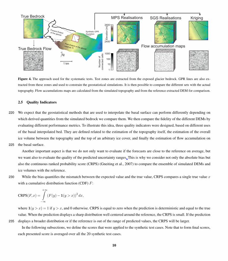
Figure 4. The approach used for the systematic tests. Test zones are extracted from the exposed glacier bedrock. GPR lines are also ex-

tracted from these zones and used to constrain the geostatistical simulations. It is then possible to compare the different sets with the actual

topography. Flow accumulations maps are calculated from the simulated topography and from the reference extracted DEM for comparison.

2.5 Quality Indicators

We expect that the geostatistical methods that are used to interpolate the basal surface can perform differently depending on220

which derived quantities from the simulated bedrock we compare them. We then compare the fidelity of the different DEMs by

evaluating different performance metrics. To illustrate this idea, three quality indicators were designed, based on different uses

of the basal interpolated bed. They are defined related to the estimation of the topography itself, the estimation of the overall

ice volume between the topography and the top of an arbitrary ice cover, and finally the estimation of flow accumulation on

the basal surface.225

Another important aspect is that we do not only want to evaluate if the forecasts are close to the reference on average, but

we want also to evaluate the quality of the predicted uncertainty ranges. This is why we consider not only the absolute bias but

also the continuous ranked probability score (CRPS) (Gneiting et al., 2007) to compare the ensemble of simulated DEMs and

ice volumes with the reference.

While the bias quantifies the mismatch between the expected value and the true value, CRPS compares a single true value x230

with a cumulative distribution function (CDF) F :

CRPS(F,x) =

+∞∫−∞

(F (y)−1(y > x))2dx,

where 1(y > x) = 1 if y > x, and 0 otherwise. CRPS is equal to zero when the prediction is deterministic and equal to the true

value. When the prediction displays a sharp distribution well centered around the reference, the CRPS is small. If the prediction

displays a broader distribution or if the reference is out of the range of predicted values, the CRPS will be larger.235

In the following subsections, we define the scores that were applied to the synthetic test cases. Note that to form final scores,

each presented score is averaged over all the 20 synthetic test cases.

10

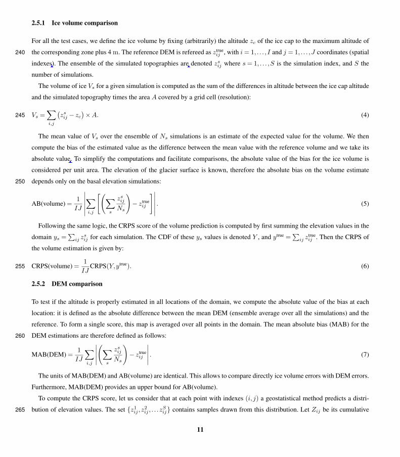
2.5.1 Ice volume comparison

For all the test cases, we define the ice volume by fixing (arbitrarily) the altitude zc of the ice cap to the maximum altitude of

the corresponding zone plus 4 m. The reference DEM is refereed as ztrueij , with i= 1, . . . , I and j = 1, . . . ,J coordinates (spatial240

indexes). The ensemble of the simulated topographies are denoted zsij where s= 1, . . . ,S is the simulation index, and S the

number of simulations.

The volume of ice Vs for a given simulation is computed as the sum of the differences in altitude between the ice cap altitude

and the simulated topography times the area A covered by a grid cell (resolution):

Vs =∑i,j

(zsij − zc

)×A. (4)245

The mean value of Vs over the ensemble of Ns simulations is an estimate of the expected value for the volume. We then

compute the bias of the estimated value as the difference between the mean value with the reference volume and we take its

absolute value. To simplify the computations and facilitate comparisons, the absolute value of the bias for the ice volume is

considered per unit area. The elevation of the glacier surface is known, therefore the absolute bias on the volume estimate

depends only on the basal elevation simulations:250

AB(volume) =1

IJ

∣∣∣∣∣∣∑i,j

[(∑s

zsijNs

)− ztrue

ij

]∣∣∣∣∣∣ . (5)

Following the same logic, the CRPS score of the volume prediction is computed by first summing the elevation values in the

domain ys =∑

ij zsij for each simulation. The CDF of these ys values is denoted Y , and ytrue =

∑ij z

trueij . Then the CRPS of

the volume estimation is given by:

CRPS(volume) =1

IJCRPS(Y,ytrue). (6)255

2.5.2 DEM comparison

To test if the altitude is properly estimated in all locations of the domain, we compute the absolute value of the bias at each

location: it is defined as the absolute difference between the mean DEM (ensemble average over all the simulations) and the

reference. To form a single score, this map is averaged over all points in the domain. The mean absolute bias (MAB) for the

DEM estimations are therefore defined as follows:260

MAB(DEM) =1

IJ

∑i,j

∣∣∣∣∣(∑

s

zsijNs

)− ztrue

ij

∣∣∣∣∣ . (7)

The units of MAB(DEM) and AB(volume) are identical. This allows to compare directly ice volume errors with DEM errors.

Furthermore, MAB(DEM) provides an upper bound for AB(volume).

To compute the CRPS score, let us consider that at each point with indexes (i, j) a geostatistical method predicts a distri-

bution of elevation values. The set {z1ij ,z2ij , . . .zSij} contains samples drawn from this distribution. Let Zij be its cumulative265

11

distribution function (CDF). It can be approximated by these samples. The mean CRPS of DEM (averaged over all locations)

is given by:

CRPS(DEM) =1

IJ

∑i,j

CRPS(Zij ,ztrueij ). (8)

2.5.3 Flow accumulation comparison

Flow accumulation is considered here because often DEM are used to make predictions that are highly affected by its geomor-270

phological structures or its roughness. Reliably predicting the geomorphological patterns of a DEM is critical for example, to

estimate the velocity at which the glacier may move or to simulate how melt water can be channelized at the base of the glacier.

Flow accumulation maps are thus used in this study because they can be computed rapidly and easily. More importantly they

illustrate well the concept of complex geomorphological/roughness description. A flow accumulation map represents in each

cell the number of cells that are located upstream and are used to estimate flow direction and catchment delineation (e.g. Tar-275

boton et al., 1991; MacKie et al., 2020b). They are computed by first estimating the flow direction from the local gradients of

altitude and integrating the number of cells along the flow path. A very bumpy topography, with many local minima, will lead

to small values of accumulation. A smooth topography will lead to more continuous paths and higher accumulation values.

The accumulation is calculated using the Pysheds open source code1 for watershed delineation. This method is used not to

represent precisely the possible flow at the base of the glacier but to compare easily and rapidly the results of the application280

of a highly non-linear process to different bedrock simulations. The ice pressure or the ice coverage is not taken into account,

and only the basal topography is used to estimate the cells connectivity and the possible flow path.

To quantify these differences, the probability density function (PDF) of the flow accumulations for each individual simulation

is compared with the PDF of the reference. A standard indicator to compare two PDFs P and Q is the Jensen-Shannon

divergence (JSD). It is defined as follows:285

JSD(P ||Q) = KLD(P ||M)/2+KLD(Q||M)/2, (9)

with M = (P +Q)/2 and KLD representing the Kullback-Leibler divergence (e.g. MacKay, 2007).

Supposing that the flow accumulation map is given by f trueij for the reference and by fsij for the simulation s. The probability

distributions are created from the flow maps in the following way. First, the set of K = 14 bins are defined: {B1, . . . ,BK}:B1 = (0,1] and Bk = (2k−2,2k−1] for k ∈ {2, . . . ,K}. Each bin is an interval. We then define Fk, the counts of elements fij290

which fall into the interval Bk, that is:

Fk =∑ij

1(Fij ∈Bk) (10)

with 1(Fij ∈Bk) = 1 if Fij ∈Bk, and 0 otherwise. The counts Fk are normalized so that F̃k satisfies:∑

k F̃k|Bk|= 1, where

|Bk| is the length of interval Bk. The function F :R→R defined by: F (x) = F̃k if x ∈Bk, and 0 otherwise, is a probability

distribution function.2951https://github.com/mdbartos/pysheds

12

Let us call F true such a PDF constructed from the reference flow accumulation map and {F s, s= 1, . . . ,S} the family of

PDFs constructed from the simulated DEMs. Then, the mean JSD of flow accumulation is given by:

MJSD =∑s

JSD(F s,F true). (11)

2.6 Tsanfleuron and Scex Rouge’s basal topography estimation

The last step consists of applying the MPS and SGS simulations methods as well as kriging to the actual data set below the300

Tsanfleuron and Scex Rouge Glaciers. The conditioning data are identical for the three methods: the GPR data below the

glacier and the DEM around the glacier to ensure the continuity between the border of the simulated area and the exposed

altitude of the glacier.

For the MPS simulations, we use the parameters and setup described in detail in section 2.2. We activate the multi-resolution

option (Gaussian pyramids), the relative patterns search, and use the topography gradient as a secondary variable. This time,305

only three sets of parameters are used: the ones producing the best scores during the systematic comparison.

The training data set is the complete exposed part of the glacier’s bedrock as a primary variable and its computed gradient

as secondary variable. The DEM is also used directly as hard conditioning data. In total, 120 MPS simulations (40 simulations

per parameters set) are generated.

For the sequential Gaussian simulations and the kriging estimate, the variogram that is employed is the one introduced earlier310

in section 2.3. Both methods use a search ellipsoid of 1500 m and 24 neighbors for the conditioning. 40 SGS simulations are

generated.

The ice volumes are then computed between all the simulated basal surfaces and the ice topography measured in august (end

of summer) 2011 and 2019. For 2011, we use the Alti3D DEM from the Swiss federal office of topography, and our DEM for

2019.315

For 2019, we use the DEM that was acquired in this work (see section 2.1). The statistics of the volumes are then computed

for each method. The standard deviation of the simulated values is used to provide the uncertainty range (2σ) of the volume.

This uncertainty range takes into account only the uncertainty resulting from the spatial variability of the bedrock and its

interpolation using an incomplete data set. These estimations do not encompass the other possible sources of error/uncertainty

that can arise from the GPR data acquisition (picking, time to depth conversion) or for the DEM acquisition. Finally, the flow320

accumulations are computed for all the simulations.

3 Results of the systematic comparison

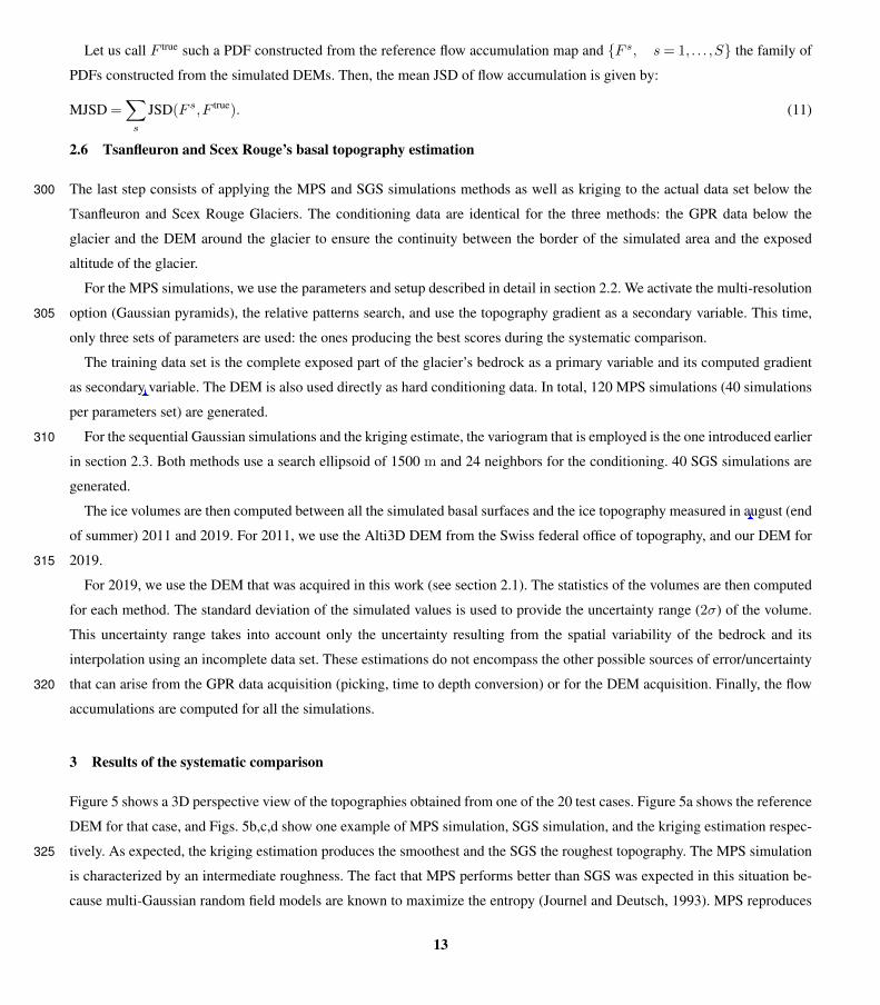
Figure 5 shows a 3D perspective view of the topographies obtained from one of the 20 test cases. Figure 5a shows the reference

DEM for that case, and Figs. 5b,c,d show one example of MPS simulation, SGS simulation, and the kriging estimation respec-

tively. As expected, the kriging estimation produces the smoothest and the SGS the roughest topography. The MPS simulation325

is characterized by an intermediate roughness. The fact that MPS performs better than SGS was expected in this situation be-

cause multi-Gaussian random field models are known to maximize the entropy (Journel and Deutsch, 1993). MPS reproduces

13

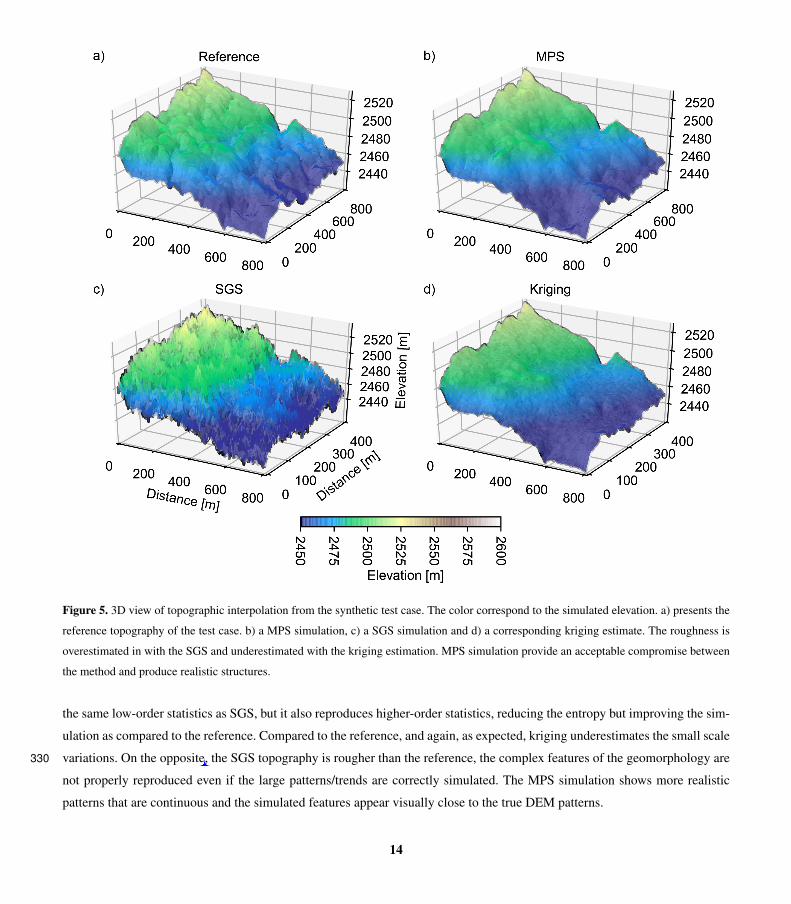
Figure 5. 3D view of topographic interpolation from the synthetic test case. The color correspond to the simulated elevation. a) presents the

reference topography of the test case. b) a MPS simulation, c) a SGS simulation and d) a corresponding kriging estimate. The roughness is

overestimated in with the SGS and underestimated with the kriging estimation. MPS simulation provide an acceptable compromise between

the method and produce realistic structures.

the same low-order statistics as SGS, but it also reproduces higher-order statistics, reducing the entropy but improving the sim-

ulation as compared to the reference. Compared to the reference, and again, as expected, kriging underestimates the small scale

variations. On the opposite, the SGS topography is rougher than the reference, the complex features of the geomorphology are330

not properly reproduced even if the large patterns/trends are correctly simulated. The MPS simulation shows more realistic

patterns that are continuous and the simulated features appear visually close to the true DEM patterns.

14

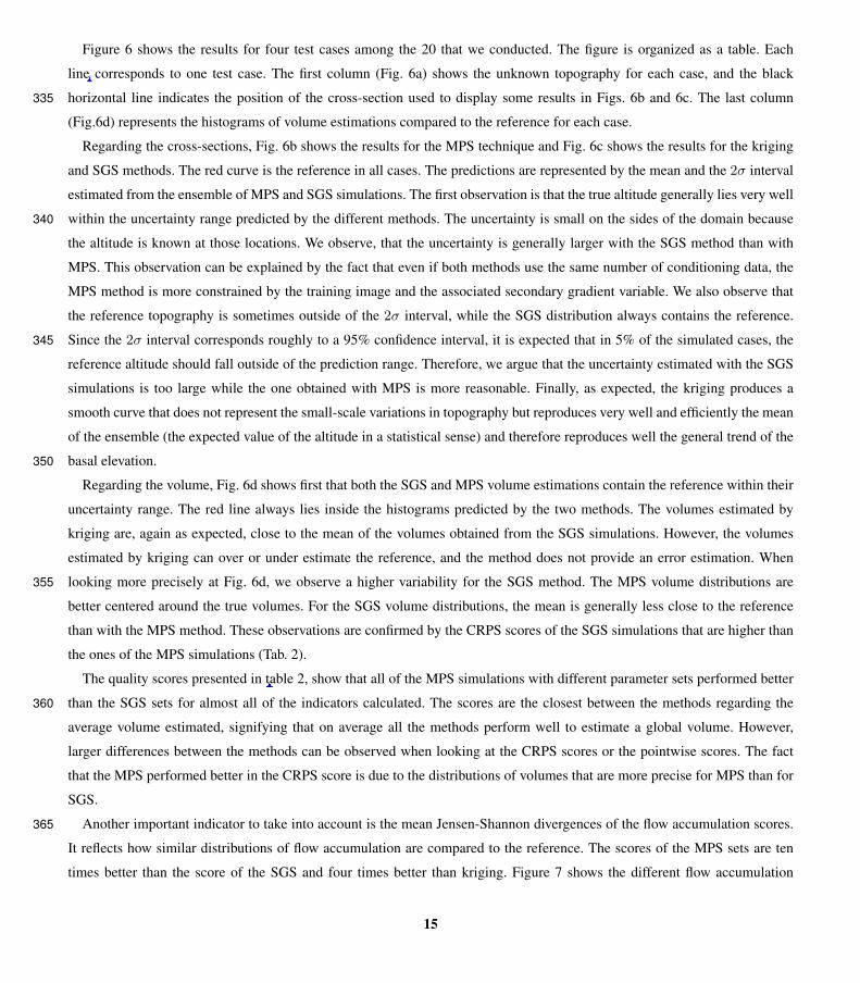
Figure 6 shows the results for four test cases among the 20 that we conducted. The figure is organized as a table. Each

line corresponds to one test case. The first column (Fig. 6a) shows the unknown topography for each case, and the black

horizontal line indicates the position of the cross-section used to display some results in Figs. 6b and 6c. The last column335

(Fig.6d) represents the histograms of volume estimations compared to the reference for each case.

Regarding the cross-sections, Fig. 6b shows the results for the MPS technique and Fig. 6c shows the results for the kriging

and SGS methods. The red curve is the reference in all cases. The predictions are represented by the mean and the 2σ interval

estimated from the ensemble of MPS and SGS simulations. The first observation is that the true altitude generally lies very well

within the uncertainty range predicted by the different methods. The uncertainty is small on the sides of the domain because340

the altitude is known at those locations. We observe, that the uncertainty is generally larger with the SGS method than with

MPS. This observation can be explained by the fact that even if both methods use the same number of conditioning data, the

MPS method is more constrained by the training image and the associated secondary gradient variable. We also observe that

the reference topography is sometimes outside of the 2σ interval, while the SGS distribution always contains the reference.

Since the 2σ interval corresponds roughly to a 95% confidence interval, it is expected that in 5% of the simulated cases, the345

reference altitude should fall outside of the prediction range. Therefore, we argue that the uncertainty estimated with the SGS

simulations is too large while the one obtained with MPS is more reasonable. Finally, as expected, the kriging produces a

smooth curve that does not represent the small-scale variations in topography but reproduces very well and efficiently the mean

of the ensemble (the expected value of the altitude in a statistical sense) and therefore reproduces well the general trend of the

basal elevation.350

Regarding the volume, Fig. 6d shows first that both the SGS and MPS volume estimations contain the reference within their

uncertainty range. The red line always lies inside the histograms predicted by the two methods. The volumes estimated by

kriging are, again as expected, close to the mean of the volumes obtained from the SGS simulations. However, the volumes

estimated by kriging can over or under estimate the reference, and the method does not provide an error estimation. When

looking more precisely at Fig. 6d, we observe a higher variability for the SGS method. The MPS volume distributions are355

better centered around the true volumes. For the SGS volume distributions, the mean is generally less close to the reference

than with the MPS method. These observations are confirmed by the CRPS scores of the SGS simulations that are higher than

the ones of the MPS simulations (Tab. 2).

The quality scores presented in table 2, show that all of the MPS simulations with different parameter sets performed better

than the SGS sets for almost all of the indicators calculated. The scores are the closest between the methods regarding the360

average volume estimated, signifying that on average all the methods perform well to estimate a global volume. However,

larger differences between the methods can be observed when looking at the CRPS scores or the pointwise scores. The fact

that the MPS performed better in the CRPS score is due to the distributions of volumes that are more precise for MPS than for

SGS.

Another important indicator to take into account is the mean Jensen-Shannon divergences of the flow accumulation scores.365

It reflects how similar distributions of flow accumulation are compared to the reference. The scores of the MPS sets are ten

times better than the score of the SGS and four times better than kriging. Figure 7 shows the different flow accumulation

15

a) b) c) d)

Figure 6. Synthetic test results. a) displays the reference DEM on a plan view, the black line showing the location of the cross-sections.

b) presents the distribution of the cross-section simulated with the MPS method (parameter set 3). c) presents the distribution of the cross-

section simulated with the SGS methods (parameter set 1). d) presents the different volume distribution of the methods against the reference

one in red.

probability density distributions for one test case and for the different methods. SGS performs poorly to reproduce the true

probability density distribution, it misses the large flow accumulation values. The high entropy of the simulation creates many

local minima and cannot reproduce the reference statistical distribution. Kriging, provides surprisingly a better distribution in370

these examples. In general, kriging is known to be smoother and therefore it tends to over represent the large flow accumulation

values. For this specific example, the performance of kriging is better than the one of SGS. But, we expect that the kriging

performance will depend very much on the spatial density of the data, when SGS will not. The MPS probability density curve

is the closest to the true DEM one and implies a good performance in pattern reproduction.

Finally, the systematic tests showed that the best parameter sets were the number 6, 3 and 8 for MPS, and the 24 neighbors375

parameter set for SGS. These parameters were then used for the practical application of the Tsanfleuron Glacier.

16

Table 2. Quality indicators averaged over all realizations for different simulation methods (MPS, SGS, kriging) and for different parameter

sets. The rows are sorted by best (lowest) CRPS score of ice volume estimation. CRPS score of ice volume estimation, mean absolute error

of the ice volume, CRPS score of DEM averaged over all points, mean absolute error of DEM averaged over all points, and Jensen-Shannon

divergence of flow accumulation distributions averaged over all simulations.

Method Set CRPS(volume) AB(volume) CRPS(DEM) MAB(DEM) MJSD

MPS 6 1.41 2.01 3.59 4.96 0.014

3 1.42 1.91 3.66 4.92 0.013

8 1.47 2.04 3.64 5.01 0.015

7 1.53 2.11 3.68 5.07 0.015

5 1.60 2.14 3.79 5.06 0.014

4 1.61 2.11 3.79 5.06 0.014

0 1.62 2.06 3.88 4.98 0.018

2 1.70 2.11 3.95 5.05 0.019

1 1.70 2.11 3.95 5.05 0.019

SGS 0 1.97 2.86 4.17 5.54 0.109

1 1.99 2.96 4.18 5.61 0.111

Kriging 0 2.91 2.91 5.45 5.45 0.047

ReferenceMPSSGSKriging

Prob

abilit

y D

ensi

ty

Test case 11

Flow Accumulation Value

10-1

100 101 102 103

10-3

10-5

10-7

Figure 7. Probability distributions of flow accumulation values for example realisation #11. The probability distribution of flow accumula-

tion for the true DEM is compared to an example MPS simulation, kriging map and SGS simulation. The corresponding Jensen-Shannon

divergences with respect to the true distribution are: 0.015 (MPS), 0.228 (kriging), and 0.107 (SGS).

4 Tsanfleuron Glacier’s results

Figure 8 shows the comparison between the basal topography interpolated using SGS, kriging and MPS on a map view and

along two cross-sections through the glacier. The mean global shape produced by the three methods are similar. The SGS

17

Table 3. Volumes of ice computed with the 2019 and 2011 DEM for the Tsanfleuron and Scex Rouge Glaciers.

Tsanfleuron Scex-Rouge Total

Method 2019 [Mio m3] 2011 [Mio m3] 2019 [Mio m3] 2011 [Mio m3] 2019 [Mio m3] 2011 [Mio m3]

MPS 109.8 ± 1.5 143.2 ± 1.5 4.1 ± 0.3 6.6 ± 0.4 113.9 ± 1.6 149.8 ± 1.6

SGS 109.7 ± 1.7 143.3 ± 1.8 4.2 ± 0.2 7.05 ± 0.2 113.9 ± 1.8 150.4 ± 1.8

Kriging 109.0 143.0 4.1 6.8 113.1 149.9

simulations tends to be a little bit noisier, but in terms of expected value (mean value), the figure does not show any significant380

difference between the methods.

Table 3 provides the estimated ice volume and uncertainties. The results from the three methods are very close: between 113

and 114 million cubic meters for 2019. With kriging, it is not possible to estimate the uncertainty range on the volume. But

with the SGS and MPS simulations, we obtain similar uncertainty ranges in the order of 1% for the volume. For comparison,

and to evaluate the ice loss between 2011 and 2019, we also compute the volumes in 2011. The 2011 and 2019 surface DEM385

were both acquired in August. According to the simulations, the Tsanfleuron and Scex Rouge Glacier lost about 25% of their

total ice volume in nine years.

So far, the results obtained by the three methods are very close, because the differences in the spatial distribution of the

basal elevation values are compensated when we integrating them over the whole glacier area to compute the volume or mean

altitude.390

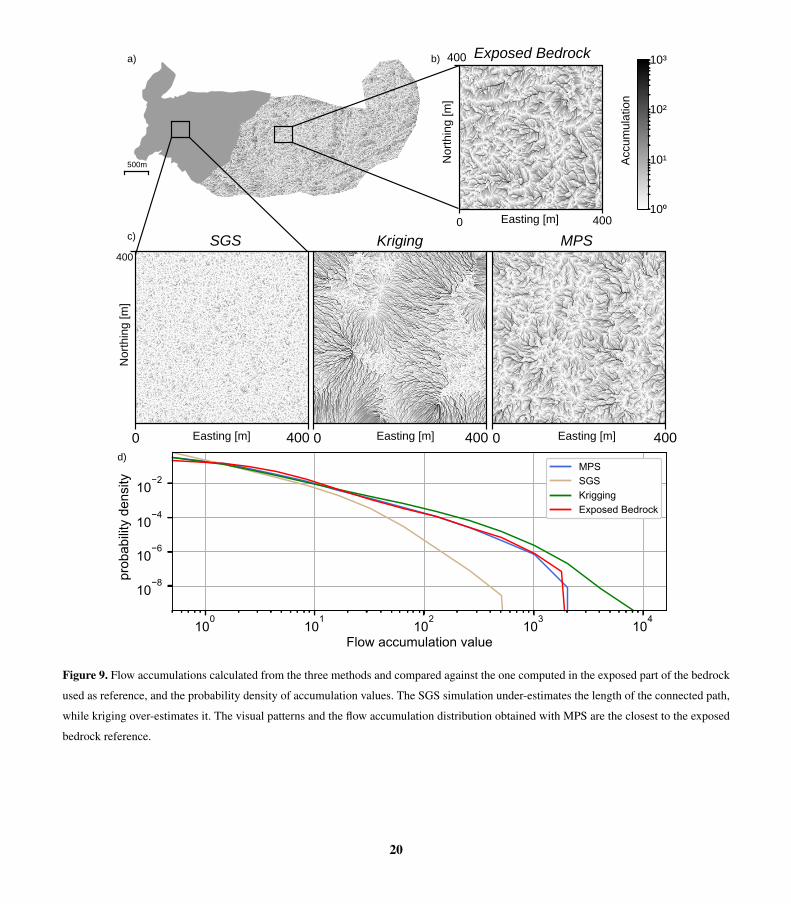
However, the flow accumulation results (Fig. 9) are very different and highly affected by the detailed geomorphological

structures in the interpolated surfaces. The SGS simulations lack realism in this case and cannot predict the high flow accu-

mulations. They are limited to short paths, with many local minima due to an overestimation of the roughness of the simulated

topographies. On the other hand, kriging provides an interpolated topography that is smoother than the reality and overesti-

mates the flow accumulations. Finally, MPS is able to generate more realistic basal topographies. The predicted topographies395

display geomorphological features and roughness that are similar to the structures visible in the uncovered bedrock area.

5 Discussion

5.1 MPS parameterization

When comparing the interpolated basal topographies with the three methods, our results show that the MPS approach provides

the simulations that display geomorphological features that are the closest with the data set. But to obtain those results, the400

DeeSse algorithm needs to be properly parameterized and adequate secondary variables have to be used. During this project,

we have tested various options. Using the topography gradient as a secondary variable proved to be a simple and efficient

solution. But further improvements could certainly be made. One possibility that we considered but did not implement would

be to use as secondary variables two hillshades projection 45 degrees apart from each other. Adding these two variables would

18

0 1000Distance [m]

2000 3000

290027002500

2000

1500

1000

500

0 1000Distance [m]

2000 3000

MPS SGS

Bedrock Elevation [m]

A A

A’ A’B’

B

B’

B

A A’

B B’

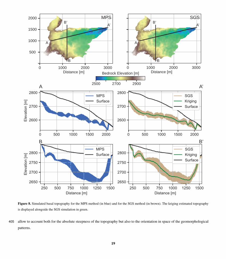
Figure 8. Simulated basal topography for the MPS method (in blue) and for the SGS method (in brown). The kriging estimated topography

is displayed alongside the SGS simulation in green.

allow to account both for the absolute steepness of the topography but also to the orientation in space of the geomorphological405

patterns.

19

500m

0 400

400

Nor

thin

g [m

]

Accu

mul

atio

n

Easting [m]

Nor

thin

g [m

]

Easting [m] Easting [m] Easting [m]0 400

400

0 400 0 400

SGS Kriging MPS

Exposed Bedrocka)

c)

b) 10³

10²

10¹

10⁰

d)

Figure 9. Flow accumulations calculated from the three methods and compared against the one computed in the exposed part of the bedrock

used as reference, and the probability density of accumulation values. The SGS simulation under-estimates the length of the connected path,

while kriging over-estimates it. The visual patterns and the flow accumulation distribution obtained with MPS are the closest to the exposed

bedrock reference.

20

5.2 Ice volume of the Tsanfleuron Glacier

The results from the previous section show that the three geostatistical methods are able to provide consistent and comparable

estimates of the mean basal topography and the overall ice volume. This similarity is expected for the SGS and kriging because

the volume calculation is a linear function of the basal topography, and in this situation kriging and SGS simulations will410

provide the same mean value (see e.g. Chiles and Delfiner, 2012). It was not obvious that MPS would also provide the same

volume because the underlying spatial variability model is different. Kriging and SGS are based on the same variogram model,

but MPS is based on the complete topographic data set and is accounting for higher order statistics. The fact that the three

techniques provide a consistent result is therefore an interesting finding. At the glacier scale, the spatial distributions of the

thicknesses (fig. 10) according to the three methods is consistent. The thickest area is in the northern part of the Tsanfleuron415

area, and presents a roughly E-W orientation.

Only the SGS and MPS methods are able to estimate the uncertainties on the total volume. As explained before, even if

kriging can provide at any point the variance of the altitude, it cannot be used directly to infer uncertainties on the volume.

Covariances between any pair of points would need to be considered and integrated over the whole domain. The volume

uncertainties estimated with the SGS and multi-Gaussian model are in general reliable (see e.g. Chiles and Delfiner, 2012).420

Here, we show that the uncertainties obtained with the MPS are consistent with those obtained with SGS.

For the Scex Rouge and Tsanfleuron Glacier these three methods allow to obtain an estimation 149.8 ± 1.6 Miom3 of ice

for 2011. This result is larger than the 100 Miom3 estimated by Gremaud and Goldscheider (2010) for 2008. We explain this

difference by considering that Gremaud and Goldscheider (2010) employed a different geophysical technique and had fewer

data points over the glacier to interpolate the ice thickness (using kriging). More precisely, they used a radio magneto-telluric425

geophysical method; they also inverted the geophysical signal using two layers assumptions, one representing the glacier and

the other the underlying limestone. The authors indicate that they may have underestimated the actual thickness of the glacier. It

could be due to an erroneous estimation of the electrical resistivity of the glacier possibly affected by the presence of meltwater.

Another geophysical campaign was conducted by Nath Sovik and Huss (2010). They report much deeper ice thickness reaching

up to 180 m in the central part of the glacier. Personal communication with these authors indicate that they are uncertain about430

the very deep data, they obtain a volume in the order of 200 Miom3 for the Tsanfleuron Glacier only in 2009.

Another indirect comparison with existing data was made using year-to-year mass balance (GLAMOS-Glacier Monitoring

Switzerland, 2019). An ice density value of 850±60 kg/m3 was used as recommended in Huss (2013) to perform the conver-

sion between water equivalent (w.e.) and ice volume. With this method, the loss of volume is estimated to be around 34 ± 2.5

Miom3 of ice between September 2011 and 2019. This value is similar to the one we derived with our approach (35.9 ± 3.2435

Miom3 for the MPS).

To finalize that part of the discussion, we would like to recall that several operators did the picking of the depth of the

reflectors independently on our GPR data and that the order in which the data were presented to the operator was randomized.

We also compared the result of the picking from the different operators and removed the part of the data that were not consistent.

21

MPS

SGS

Kriging

depth [m]

Figure 10. Ice thickness calculated from the three methods using the 2019 surface DEM. The SGS and the MPS basal models used are the

averaged model over all the realisations.

22

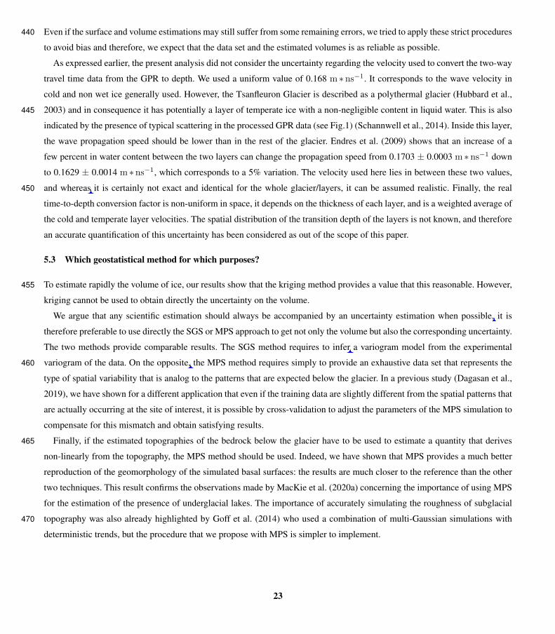
Even if the surface and volume estimations may still suffer from some remaining errors, we tried to apply these strict procedures440

to avoid bias and therefore, we expect that the data set and the estimated volumes is as reliable as possible.

As expressed earlier, the present analysis did not consider the uncertainty regarding the velocity used to convert the two-way

travel time data from the GPR to depth. We used a uniform value of 0.168 m ∗ ns−1. It corresponds to the wave velocity in

cold and non wet ice generally used. However, the Tsanfleuron Glacier is described as a polythermal glacier (Hubbard et al.,

2003) and in consequence it has potentially a layer of temperate ice with a non-negligible content in liquid water. This is also445

indicated by the presence of typical scattering in the processed GPR data (see Fig.1) (Schannwell et al., 2014). Inside this layer,

the wave propagation speed should be lower than in the rest of the glacier. Endres et al. (2009) shows that an increase of a

few percent in water content between the two layers can change the propagation speed from 0.1703 ± 0.0003 m ∗ ns−1 down

to 0.1629 ± 0.0014 m ∗ ns−1, which corresponds to a 5% variation. The velocity used here lies in between these two values,

and whereas it is certainly not exact and identical for the whole glacier/layers, it can be assumed realistic. Finally, the real450

time-to-depth conversion factor is non-uniform in space, it depends on the thickness of each layer, and is a weighted average of

the cold and temperate layer velocities. The spatial distribution of the transition depth of the layers is not known, and therefore

an accurate quantification of this uncertainty has been considered as out of the scope of this paper.

5.3 Which geostatistical method for which purposes?

To estimate rapidly the volume of ice, our results show that the kriging method provides a value that this reasonable. However,455

kriging cannot be used to obtain directly the uncertainty on the volume.

We argue that any scientific estimation should always be accompanied by an uncertainty estimation when possible, it is

therefore preferable to use directly the SGS or MPS approach to get not only the volume but also the corresponding uncertainty.

The two methods provide comparable results. The SGS method requires to infer a variogram model from the experimental

variogram of the data. On the opposite, the MPS method requires simply to provide an exhaustive data set that represents the460

type of spatial variability that is analog to the patterns that are expected below the glacier. In a previous study (Dagasan et al.,

2019), we have shown for a different application that even if the training data are slightly different from the spatial patterns that

are actually occurring at the site of interest, it is possible by cross-validation to adjust the parameters of the MPS simulation to

compensate for this mismatch and obtain satisfying results.

Finally, if the estimated topographies of the bedrock below the glacier have to be used to estimate a quantity that derives465

non-linearly from the topography, the MPS method should be used. Indeed, we have shown that MPS provides a much better

reproduction of the geomorphology of the simulated basal surfaces: the results are much closer to the reference than the other

two techniques. This result confirms the observations made by MacKie et al. (2020a) concerning the importance of using MPS

for the estimation of the presence of underglacial lakes. The importance of accurately simulating the roughness of subglacial

topography was also already highlighted by Goff et al. (2014) who used a combination of multi-Gaussian simulations with470

deterministic trends, but the procedure that we propose with MPS is simpler to implement.

23

6 Conclusions

This study proposes an example of the benefits of using advanced geostatistical methods for basal topography interpolation

and compares three methods: kriging, Sequential Gaussian Simulations, and Multiple Point Statistics.

The three methods are able to provide consistent and similar volume estimations. Kriging and SGS require to analyse the475

statistics of the data, adjust a spatial trend and identify a variogram model. Once this is done, these two methods provide local

estimation of uncertainty. But to get the uncertainty on the volume, one needs to use the SGS method.

The MPS technique is the most versatile: it provides a proper estimation of the volume, as well as local uncertainties

comparable with the other methods. But in addition, it is able to produce realistic basal structures, even in areas where the

data are scarce or the structure complex. Compared to MPS, SGS and kriging tend to produce interpolated surfaces that are480

respectively too smooth or too noisy. Therefore, they can lead to biased predictions when they are used to derive quantities that

depends strongly on the detailed geomorphological structures of the basal topography as illustrated with the flow accumulation

calculations done in this paper. The same type of errors are expected if these topographies are used to simulate the glacier

movement or the basal flow of melted water and the channelling of this flux. In these situations, the detailed structures may be

even more important than the global trend and the MPS approach is recommended. The main limitation of the MPS approach is485

that it requires a Training Image that is representative of the glacier basal structures. Finding the proper analog data is therefore

an important part of the approach and may be difficult for large glaciers with little information about the underlying geology.

In these situations, a possibility could be to test various training images using k-fold cross-validation techniques as shown in

Juda et al. (2020). The case of steep valleys where sediments cover the bedrock can also make the TI selection complex.

Based on the results obtained in this paper and those published by MacKie et al. (2020b), we think that the MPS approach490

could help enhance the accuracy of glacier evolution models. The MPS simulations can be used to better define the initial

conditions as well as to provide a more realistic basal geometry (boundary condition). In addition, because the method is able

to generate a set of simulated topographies, it could be used as the base for a Monte-Carlo analysis. Each simulation can be used

as input for one run of a glacier evolution model. By analyzing the ensemble of results, one can quantifying the uncertainty on

glacier evolution related to an imperfect identification of the basal geometry of the glacier. Looking even further, and making495

an analogy with how the MPS approach is used for groundwater applications (e.g. Jäggli et al., 2018), we can imagine to couple

the MPS approach and glacier evolution model in an inverse Bayesian modeling framework to infer a plausible basal geometry

when little glacier depth data is available and one has to rely on indirect surface observations.

Finally, the ice volumes calculated for the Scex Rouge and Tsanfleuron Glacier with the three methods are in accordance with

the mass balance calculation and are linked with robust error estimation. Our results indicate that there has been a significant500

mass loss at this glacier and that these methods enable higher accuracy ice loss estimates and could enable improvements in

glacier retreat projections. Such improvements could be important for global awareness, political decisions, and preparing the

mountains’ infrastructure for its future evolution.

24

Data availability. A simulation obtained with each method, the mean simulations of SGS and MPS, as well as the DEM and the conditioning

point sets are available on https://github.com/randlab/tsanfleuron_glacier_data.505

Author contributions. A.N. coordinated and conducted a part of the field work. A.N. processed the GPR and drone data. A.N., V.D., J.S.

and P.R. designed and tested the different geostatistical procedures. A.N. and V.D. prepared the data. P.J. participated in the data acquisition,

designed and implemented the quality indicators. A.N., V.D. and P.J. wrote the paper. P.R. initiated and supervised the work, conducted the

field acquisition, and was involved in the writing, and editing of the paper.

Competing interests. The authors declare no conflicts of interests.510

Acknowledgements. The authors would like to thank Marie Vallat and Cyprien Louis, two students who participated in the GPR data col-

lection and initial geostatistical analysis. They are also thankful to Dr. James Irving at the University of Lausanne who provided the GPR

equipment and support. They would like to thanks the Prarochet Hut and the "Glacier 3000" company for the logistic support. Finally, they

want to thank Clemens Schannwell, Emma MacKie and an anonymous reviewer for their numerous comments that helped improving the

quality of the manuscript.515

25

References

Beniston, M.: Impacts of climatic change on water and associated economic activities in the Swiss Alps, Journal of Hydrology, 412-413,

291–296, https://doi.org/https://doi.org/10.1016/j.jhydrol.2010.06.046, hydrology Conference 2010, 2012.

Berthier, E., Vincent, C., Magnússon, E., Gunnlaugsson, A. T., Pitte, P., Le Meur, E., Masiokas, M., Ruiz, L., Pálsson, F., Belart, J. M. C., and

Wagnon, P.: Glacier topography and elevation changes derived from Pléiades sub-meter stereo images, The Cryosphere, 8, 2275–2291,520

https://doi.org/10.5194/tc-8-2275-2014, 2014.

Bohleber, P., Sold, L., Hardy, D. R., Schwikowski, M., Klenk, P., Fischer, A., Sirguey, P., Cullen, N. J., Potocki, M., Hoffmann, H., and

Mayewski, P.: Ground-penetrating radar reveals ice thickness and undisturbed englacial layers at Kilimanjaro's Northern Ice Field, The

Cryosphere, 11, 469–482, https://doi.org/10.5194/tc-11-469-2017, 2017.

Chiles, J.-P. and Delfiner, P.: Geostatistics: Modeling Spatial Uncertainty, Second Edition, vol. 497 of Wiley Series in Probability and Statis-525

tics, John Wiley & Sons, Hoboken, New Jersey, USA, 2012.

Chudley, T. R., Christoffersen, P., Doyle, S. H., Abellan, A., and Snooke, N.: High-accuracy UAV photogrammetry of ice sheet dynamics

with no ground control, The Cryosphere, 13, 955–968, https://doi.org/10.5194/tc-13-955-2019, 2019.

Dagasan, Y., Erten, O., Renard, P., Straubhaar, J., and Topal, E.: Multiple-point statistical simulation of the ore boundaries for a lateritic

bauxite deposit, Stochastic Environmental Research and Risk Assessment, 33, 865–878, 2019.530

Dall’Alba, V., Renard, P., Straubhaar, J., Issautier, B., Duvail, C., and Caballero, Y.: 3D multiple-point statistics simulations of the Roussillon

Continental Pliocene aquifer using DeeSse, Hydrology and Earth System Sciences, 24, 4997–5013, 2020.

de Carvalho, P. R. M., da Costa, J. F. C. L., Rasera, L. G., and Varella, L. E. S.: Geostatistical facies simulation with geometric patterns of a

petroleum reservoir, Stochastic Environmental Research and Risk Assessment, 31, 1805–1822, https://doi.org/10.1007/s00477-016-1243-

5, 2016.535

Eisen, O., Nixdorf, U., Wilhelms, F., and Miller, H.: Electromagnetic wave speed in polar ice: validation of the common-

midpoint technique with high-resolution dielectric-profiling and γ-density measurements, Annals of Glaciology, 34, 150–156,

https://doi.org/10.3189/172756402781817509, 2002.

Endres, A. L., Murray, T., Booth, A. D., and West, L. J.: A new framework for estimating englacial water content and pore geometry using

combined radar and seismic wave velocities, Geophysical Research Letters, 36, https://doi.org/10.1029/2008gl036876, 2009.540

Flowers, G. E. and Clarke, G. K. C.: Surface and bed topography of Trapridge Glacier, Yukon Territory, Canada: digital elevation models

and derived hydraulic geometry, Journal of Glaciology, 45, 165–174, https://doi.org/10.3189/s0022143000003142, 1999.

Frey, H., Machguth, H., Huss, M., Huggel, C., Bajracharya, S., Bolch, T., Kulkarni, A., Linsbauer, A., Salzmann, N., and Stoffel,

M.: Estimating the volume of glaciers in the Himalayan-Karakoram region using different methods, The Cryosphere, 8, 2313–2333,

https://doi.org/10.5194/tc-8-2313-2014, 2014.545

Gabbi, J., Farinotti, D., Bauder, A., and Maurer, H.: Ice volume distribution and implications on runoff projections in a glacierized catchment,

Hydrology and Earth System Sciences, 16, 4543–4556, https://doi.org/10.5194/hess-16-4543-2012, 2012.

Gantayat, P., Kulkarni, A. V., and Srinivasan, J.: Estimation of ice thickness using surface velocities and slope: case study at Gangotri Glacier,

India, Journal of Glaciology, 60, 277–282, https://doi.org/10.3189/2014jog13j078, 2014.

Gerlitz, K., Knoll, M. D., Cross, G. M., Luzitano, R. D., and Knight, R.: Processing Ground Penetrating Radar Data to Improve Resolution of550

Near-Surface Targets, in: Symposium on the Application of Geophysics to Engineering and Environmental Problems 1993, Environment

and Engineering Geophysical Society, https://doi.org/10.4133/1.2922036, 1993.

26

GLAMOS-Glacier Monitoring Switzerland: Swiss Glacier Mass Balance (release 2019), https://doi.org/10.18750/MASSBALANCE.2019.R2019,

2019.

Gneiting, T., Balabdaoui, F., and Raftery, A. E.: Probabilistic forecasts, calibration and sharpness, Journal of the Royal Statistical Society:555

Series B (Statistical Methodology), 69, 243–268, 2007.

Goff, J. A., Powell, E. M., Young, D. A., and Blankenship, D. D.: Conditional simulation of Thwaites Glacier (Antarctica) bed topography

for flow models: Incorporating inhomogeneous statistics and channelized morphology, Journal of Glaciology, 60, 635–646, 2014.

Grab, M., Mattea, E., Bauder, A., Huss, M., Rabenstein, L., Hodel, E., Linsbauer, A., Langhammer, L., Schmid, L., Church, G., Hellmann,

S., Délèze, K., Schaer, P., Lathion, P., Farinotti, D., and Maurer, H.: Ice thickness distribution of all Swiss glaciers based on extended560

ground-penetrating radar data and glaciological modeling, Journal of Glaciology, pp. 1–19, https://doi.org/10.1017/jog.2021.55, 2021.

Gremaud, V.: Géologie du karst de Tsanfleuron, Collection EDYTEM. Cahiers de géographie, 7, 127–134,

https://doi.org/10.3406/edyte.2008.1062, 2008.

Gremaud, V. and Goldscheider, N.: Geometry and drainage of a retreating glacier overlying and recharging a karst aquifer, Tsanfleuron-

Sanetsch, Swiss Alps, Acta carsologica, 39, 2010.565

Haeberli, W., Hoelzle, M., Paul, F., and Zemp, M.: Integrated monitoring of mountain glaciers as key indicators of global climate change:

the European Alps, Annals of Glaciology, 46, 150–160, https://doi.org/10.3189/172756407782871512, 2007.

Haugerud, R. A., Harding, D. J., Johnson, S. Y., Harless, J. L., Weaver, C. S., and Sherrod, B. L.: High-Resolution Lidar To-

pography of the Puget Lowland, Washington —A Bonanza for Earth Science, GSA Today, 13, 4, https://doi.org/10.1130/1052-

5173(2003)13<0004:hltotp>2.0.co;2, 2003.570

Hubbard, B. P., Hubbard, A., Mader, H. M., Tison, J.-L., Grust, K., and Nienow, P. W.: Spatial variability in the water content and rheology

of temperate glaciers: Glacier de Tsanfleuron, Switzerland, Annals of Glaciology, 37, 1–6, https://doi.org/10.3189/172756403781815474,

2003.

Huss, M.: Density assumptions for converting geodetic glacier volume change to mass change, The Cryosphere, 7, 877–887,

https://doi.org/10.5194/tc-7-877-2013, 2013.575

Huss, M. and Fischer, M.: Sensitivity of Very Small Glaciers in the Swiss Alps to Future Climate Change, Frontiers in Earth Science, 4,

https://doi.org/10.3389/feart.2016.00034, 2016.

Jäggli, C., Straubhaar, J., and Renard, P.: Parallelized adaptive importance sampling for solving inverse problems, Frontiers in Earth Science,

6, 203, 2018.

Journel, A. and Zhang, T.: The necessity of a multiple-point prior model, Mathematical geology, 38, 591–610, 2006.580

Journel, A. G. and Deutsch, C. V.: Entropy and spatial disorder, Mathematical Geology, 25, 329–355, https://doi.org/10.1007/bf00901422,

1993.

Juda, P., Renard, P., and Straubhaar, J.: A framework for the cross-validation of categorical geostatistical simulations, Earth and Space

Science, 7, e2020EA001 152, 2020.

MacKay, D. J. C.: Information theory, inference, and learning algorithms, Cambridge University Press, Cambridge, 6th printing edn., 2007.585

MacKie, E. J. and Schroeder, D. M.: Geostatistically Simulating Subglacial Topography with Synthetic Training Data, in: IGARSS 2020 -

2020 IEEE International Geoscience and Remote Sensing Symposium, IEEE, https://doi.org/10.1109/igarss39084.2020.9324563, 2020.

MacKie, E. J., Schroeder, D. M., Caers, J., Siegfried, M. R., and Scheidt, C.: Antarctic Topographic Realizations and Geostatistical Modeling

Used to Map Subglacial Lakes, Journal of Geophysical Research: Earth Surface, 125, https://doi.org/10.1029/2019jf005420, 2020a.

27

MacKie, E. J., Schroeder, D. M., Zuo, C., Yin, Z., and Caers, J.: Stochastic modeling of subglacial topography exposes uncertainty in water590

routing at Jakobshavn Glacier, Journal of Glaciology, 67, 75–83, https://doi.org/10.1017/jog.2020.84, 2020b.

Mariethoz, G., Renard, P., and Straubhaar, J.: The Direct Sampling method to perform multiple-point geostatistical simulations, Water

Resources Research, 46, https://doi.org/10.1029/2008wr007621, 2010.

Meerschman, E., Pirot, G., Mariethoz, G., Straubhaar, J., Van Meirvenne, M., and Renard, P.: A practical guide to performing multiple-point

statistical simulations with the Direct Sampling algorithm, Computers & Geosciences, 52, 307–324, 2013.595

Moorman, B. J. and Michel, F. A.: Glacial hydrological system characterization using ground-penetrating radar, Hydrological Processes, 14,

2645–2667, https://doi.org/10.1002/1099-1085(20001030)14:15<2645::aid-hyp84>3.0.co;2-2, 2000.

Nath Sovik, K. and Huss, M.: Glaciological investigations on three glaciers at Les Diablerets, Alpes Vaudoises, in: Abstract Volume. 8th Swiss

Geoscience Meeting. Symposium 10. Open Cryosphere Session, pp. 243–244, Platform Geosciences, Swiss Academy Swiss Geoscience

Meeting 2010 of Science, SCNAT, University of Fribourg, Switzerland, 2010.600

Oriani, F., Straubhaar, J., Renard, P., and Mariethoz, G.: Simulation of rainfall time series from different climatic regions using the direct

sampling technique, Hydrology and Earth System Sciences, 18, 3015–3031, 2014.

Plewes, L. A. and Hubbard, B.: A review of the use of radio-echo sounding in glaciology, Progress in Physical Geography: Earth and

Environment, 25, 203–236, https://doi.org/10.1177/030913330102500203, 2001.

Remy, N., Boucher, A., and Wu, J.: Applied geostatistics with SGeMS: a user’s guide, Cambridge University Press, Cambridge, UK ; New605

York, oCLC: ocn231580897, 2009.

Schannwell, C., Murray, T., Kulessa, B., Gusmeroli, A., Saintenoy, A., and Jansson, P.: An automatic approach to delineate

the cold–temperate transition surface with ground-penetrating radar on polythermal glaciers, Annals of Glaciology, 55, 89–96,

https://doi.org/10.3189/2014aog67a102, 2014.

Schoeneich, P. and Reynard, E.: Structural Landscapes and Relative Landforms of the Diablerets Massif, in: Landscapes and Landforms610

of Switzerland, edited by Reynard, E., World Geomorphological Landscapes, pp. 123–141, Springer, https://doi.org/10.1007/978-3-030-

43203-4_9, 2021.

Straubhaar, J.: DeeSse user’s guide, Tech. rep., The Centre for Hydrogeology and Geothermics (CHYN), University of Neuchâtel: Neuchâtel,

Switzerland, 2019.

Straubhaar, J. and Renard, P.: Conditioning Multiple-Point Statistics Simulation to Inequality Data, Earth and Space Science, p.615

e2020EA001515, https://doi.org/10.1029/2020EA001515, 2021.

Straubhaar, J., Renard, P., and Chugunova, T.: Multiple-point statistics using multi-resolution images, Stochastic Environmental Research

and Risk Assessment, 34, 251–273, https://doi.org/10.1007/s00477-020-01770-8, 2020.

Tarboton, D. G., Bras, R. L., and Rodriguez-Iturbe, I.: On the extraction of channel networks from digital elevation data, Hydrological

processes, 5, 81–100, 1991.620

Vanlooy, J. A., Miège, C., Vandeberg, G. S., and Forster, R. R.: Ice volume estimation inferred from ice thickness and surface measurements

for Continental Glacier, Wind River Range, Wyoming, USA, Journal of Glaciology, 60, 478–488, https://doi.org/10.3189/2014jog13j162,

2014.

28