IBM Watson Campaign Automation SMS, formerly IBM Silverpop ...
Upload
khangminh22Category
view
4download
0
IBM iDoctor for IBM i
IBM iDoctor for IBM i
7.2 Documentation (Also covers latest changes to 6.1 and 7.1 after March 2015)
IBM iDoctor for IBM i Development Team
24 Apr 2015
Licensed Materials - Property of IBM
Copyright International Business Machines Corporation 2015. All rights reserved.
Abstract
Discover what’s new with IBM iDoctor for IBM i at 7.2. Provides in-depth coverage of all major GUI functions for all components. Also covers the server-side portion of the iDoctor tools such as the various commands used for collecting and analyzing performance data.
Changes
31 Mar 2015 – Initial Creation. Chapters 1-3 and 12 have been updated. Updates for 4-11 are still in progress.
24 Apr 2015 – Chapter 4 (iDoctor GUI, done)
Chapter 5 (General Functions) and 6 (Data Viewer which was previously in chapter 4) are new

IBM iDoctor for IBM i
Table of Contents
1 Introduction ........................................................................................ 15
1.1 Product Overview .............................................................................................. 15
1.1.1 What's New ........................................................................................................................... 15
1.1.2 iDoctor YouTube Channel ..................................................................................................... 15
1.1.3 iDoctor Community ................................................................................................................ 16
1.2 iDoctor Base Support/QIDRGUI Library ............................................................ 16
1.3 IBM iDoctor for IBM i Job Watcher .................................................................... 16
1.3.1 iDoctor Job Watcher vs PT1 (PDI) Job Watcher ................................................................... 17
1.4 IBM iDoctor for IBM i -Collection Services Investigator ..................................... 18
1.4.1 Collection Services Investigator vs PDI Collection Services ................................................. 18
1.5 IBM iDoctor for IBM i Disk Watcher ................................................................... 19
1.6 IBM iDoctor for IBM i Plan Cache Analyzer ....................................................... 19
1.7 IBM iDoctor for IBM i PEX Analyzer .................................................................. 19
1.8 IBM iDoctor for IBM i FTP GUI .......................................................................... 20
1.9 IBM iDoctor for IBM i VIOS Investigator (6.1 or higher) ..................................... 20
1.10 IBM iDoctor for IBM i Must Gather Tools ........................................................ 21
1.11 IBM iDoctor for IBM i Heap Analyzer (5.4/6.1) ................................................ 21
1.11.1 Java heap growth analysis (7.1+) ......................................................................................... 21
2 Installation .......................................................................................... 23
2.1 IBM i Requirements ........................................................................................... 23
2.2 PC Requirements .............................................................................................. 23
2.2.1 Ports needed for GUI access ................................................................................................ 24
2.3 Installation ......................................................................................................... 26
2.3.1 Install options......................................................................................................................... 27
2.3.2 Installation example ............................................................................................................... 28
2.4 Manual install steps ........................................................................................... 33
2.4.1 Windows command prompt FTP method .............................................................................. 33
2.5 Uninstall ............................................................................................................ 36
2.5.1 Server Uninstall ..................................................................................................................... 36
2.5.2 GUI Uninstall ......................................................................................................................... 37
2.6 Applying access codes ...................................................................................... 37
2.7 Viewing access codes ....................................................................................... 37
2.8 PTF Installation ................................................................................................. 38
3 iDoctor for Performance Analysis .................................................... 39
3.1 Components of Performance ............................................................................. 39

IBM iDoctor for IBM i
3.2 Job Watcher ...................................................................................................... 41
3.3 Collection Services Investigator ........................................................................ 43
3.4 Disk Watcher ..................................................................................................... 43
3.5 PEX Analyzer .................................................................................................... 44
3.6 Must Gather Tools ............................................................................................. 44
3.7 Performance Analysis Using the iDoctor GUI .................................................... 44
4 The iDoctor GUI ................................................................................. 47
4.1 Starting iDoctor .................................................................................................. 47
4.2 iDoctor and Internet connectivity ....................................................................... 49
4.2.1 Automatic client updates ....................................................................................................... 49
4.2.2 Automatic server PTF checking ............................................................................................ 49
4.3 Sessions ............................................................................................................ 50
4.3.1 The current session ............................................................................................................... 50
4.3.2 Opening ................................................................................................................................. 50
4.3.3 Saving .................................................................................................................................... 50
4.3.4 Restore Previous iDoctor Session......................................................................................... 51
4.4 MDI Tabbed Styles ............................................................................................ 51
4.4.1 None ...................................................................................................................................... 51
4.4.2 Standard ................................................................................................................................ 52
4.4.3 Grouped ................................................................................................................................. 53
4.5 The Main Window .............................................................................................. 54
4.5.1 Toolbar .................................................................................................................................. 56
4.5.2 Menu Options ........................................................................................................................ 57
4.5.3 Update History ....................................................................................................................... 59
4.5.4 Find Window .......................................................................................................................... 59
4.5.5 Set Font ................................................................................................................................. 60
4.5.6 Preferences ........................................................................................................................... 60
4.5.7 Wait Bucket Preferences ....................................................................................................... 80
4.5.8 Remote Command Status View ............................................................................................ 82
4.5.9 Remote SQL Statement Status View .................................................................................... 84
4.5.10 Graph Comparison Mode ...................................................................................................... 85
4.5.11 IBM i Connections View ........................................................................................................ 87
4.5.12 Power Connections View ...................................................................................................... 94
4.5.13 Discover Connections ......................................................................................................... 103
4.6 Component Views ........................................................................................... 104
4.6.1 Menu Options ...................................................................................................................... 105
4.6.2 Filter libraries ....................................................................................................................... 106
4.6.3 Set local database ............................................................................................................... 107
4.6.4 Properties ............................................................................................................................ 107

IBM iDoctor for IBM i
4.6.5 Field Selection Window ....................................................................................................... 111
4.7 Libraries .......................................................................................................... 112
4.7.1 Menu Options ...................................................................................................................... 112
4.7.2 Run analysis (menu) ........................................................................................................... 113
4.7.3 Copy URL ............................................................................................................................ 113
4.7.4 Copy… ................................................................................................................................. 113
4.7.5 Save… ................................................................................................................................. 114
4.7.6 Transfer Library ................................................................................................................... 115
4.7.7 Clear .................................................................................................................................... 116
4.7.8 Delete .................................................................................................................................. 116
4.7.9 Rename ............................................................................................................................... 116
4.7.10 Properties ............................................................................................................................ 117
4.8 Collections ....................................................................................................... 125
4.8.1 Menu Options ...................................................................................................................... 126
4.8.2 Analyses -> Analyze Collection(s) menu ............................................................................. 127
4.8.3 Analyses -> Run analysis menu .......................................................................................... 129
4.8.4 Generate Reports ................................................................................................................ 129
4.8.5 Copy URL ............................................................................................................................ 130
4.8.6 Copy .................................................................................................................................... 130
4.8.7 Delete .................................................................................................................................. 131
4.8.8 Save .................................................................................................................................... 132
4.8.9 Transfer Collections… ......................................................................................................... 133
4.8.10 Server-side output files ........................................................................................................ 137
4.8.11 User-defined queries ........................................................................................................... 138
4.8.12 User-defined graphs ............................................................................................................ 140
4.9 SQL Tables ..................................................................................................... 141
4.9.1 Analysis output menu .......................................................................................................... 142
4.9.2 Tables .................................................................................................................................. 142
4.9.3 SQL Tables Comparison Wizard ......................................................................................... 144
4.10 Monitors........................................................................................................ 152
4.10.1 Start iDoctor Monitor Wizard ............................................................................................... 154
4.11 PEX+ ............................................................................................................ 160
4.11.1 Menu Options ...................................................................................................................... 161
4.11.2 Contents of a PEX+ collection ............................................................................................. 162
4.12 Choose Database Members ......................................................................... 163
4.13 Analyses ....................................................................................................... 163
5 General Functions ........................................................................... 165
5.1 iDoctor FTP GUI .............................................................................................. 165
5.2 Power .............................................................................................................. 165

IBM iDoctor for IBM i
5.3 SQL catalog functions ..................................................................................... 166
5.3.1 Automatically move tables (or members) to SSDs (7.1+) ................................................... 166
5.3.2 Start Table (or member) Statistics Collection (7.1+) ........................................................... 168
5.3.3 Tables (7.1+) ....................................................................................................................... 169
5.3.4 IBM i Services...................................................................................................................... 179
5.4 Browse Collections .......................................................................................... 184
5.4.1 Menu Options ...................................................................................................................... 185
5.4.2 Filter collections ................................................................................................................... 185
5.4.3 Examples ............................................................................................................................. 186
5.5 Saved collections ............................................................................................ 187
5.5.1 Menu Options ...................................................................................................................... 188
5.6 Work Management .......................................................................................... 189
5.6.1 Scheduled Jobs ................................................................................................................... 190
5.6.2 Active jobs ........................................................................................................................... 190
5.6.3 Subsystems ......................................................................................................................... 196
5.7 ASPs ............................................................................................................... 198
5.8 Disk units ......................................................................................................... 200
5.9 Objects owned by user .................................................................................... 203
5.9.1 Menu options ....................................................................................................................... 203
5.9.2 Object listings ...................................................................................................................... 204
6 The Data Viewer ............................................................................... 205
6.1 Toolbar ............................................................................................................ 205
6.2 Menu Options .................................................................................................. 208
6.3 SQL Editor ....................................................................................................... 212
6.4 Open File Window ........................................................................................... 215
6.5 SQL Message Log View .................................................................................. 216
6.6 Table Views ..................................................................................................... 217
6.6.1 Row Menu Options .............................................................................................................. 218
6.6.2 Column Menu Options ......................................................................................................... 219
6.6.3 Making Row Selections ....................................................................................................... 219
6.6.4 Making Cell Selections ........................................................................................................ 220
6.6.5 Filter ..................................................................................................................................... 220
6.6.6 The Find Window................................................................................................................. 223
6.6.7 Properties ............................................................................................................................ 223
6.6.8 Query Definitions ................................................................................................................. 225
6.7 Graph Views .................................................................................................... 233
6.7.1 Graph Menu ......................................................................................................................... 234
6.7.2 Legend ................................................................................................................................. 236
6.7.3 Filter ..................................................................................................................................... 237

IBM iDoctor for IBM i
6.7.4 iDoctor-supplied graphs ...................................................................................................... 240
6.7.5 User-defined graphs ............................................................................................................ 240
6.7.6 Properties ............................................................................................................................ 240
6.7.7 Graph Definitions ................................................................................................................. 241
6.8 Spool File Views .............................................................................................. 249
7 Power ................................................................................................ 250
7.1 VIOS Advisor ................................................................................................... 250
7.1.1 Analyzing ............................................................................................................................. 250
7.2 nmon ............................................................................................................... 252
7.2.1 Import .................................................................................................................................. 253
7.2.2 Analyze ................................................................................................................................ 253
7.2.3 Collections ........................................................................................................................... 254
7.2.4 Reports ................................................................................................................................ 256
7.3 NPIV collection options ................................................................................... 286
7.3.1 Menu Options ...................................................................................................................... 286
7.3.2 Graph Menu options ............................................................................................................ 287
7.3.3 NPIV Configuration .............................................................................................................. 287
7.3.4 NPIV overview graphs ......................................................................................................... 287
7.3.5 Ranking graphs ................................................................................................................... 292
7.3.6 Selected Item(s) over time graphs ...................................................................................... 293
7.3.7 NPIV Advanced Graphs ...................................................................................................... 294
7.4 Server-side output files .................................................................................... 303
7.4.1 NPIV .................................................................................................................................... 304
7.4.2 VIOS disk mappings ............................................................................................................ 304
7.4.3 HMC configurations ............................................................................................................. 304
8 Job Watcher ..................................................................................... 305
8.1 Starting Job Watcher ....................................................................................... 305
8.2 Job Watcher Component View ........................................................................ 305
8.2.1 Menu Options ...................................................................................................................... 306
8.3 Libraries .......................................................................................................... 306
8.3.1 Menu Options ...................................................................................................................... 307
8.4 Monitors........................................................................................................... 307
8.5 SQL Tables ..................................................................................................... 307
8.6 Super Collections ............................................................................................ 308
8.7 Definitions........................................................................................................ 308
8.7.1 Properties ............................................................................................................................ 308
8.8 Add Job Watcher Definition Wizard ................................................................. 309
8.8.1 Welcome .............................................................................................................................. 309

IBM iDoctor for IBM i
8.8.2 Basic Options ...................................................................................................................... 309
8.8.3 Data Collection Options ....................................................................................................... 310
8.8.4 Advanced Options ............................................................................................................... 317
8.8.5 Job Options ......................................................................................................................... 318
8.8.6 Job/task selection ................................................................................................................ 319
8.8.7 Finish ................................................................................................................................... 323
8.9 Start Job Watcher Collection Wizard (6.1+) .................................................... 324
8.9.1 Welcome .............................................................................................................................. 324
8.9.2 Basic Options ...................................................................................................................... 325
8.9.3 Scheduling Options ............................................................................................................. 325
8.9.4 Termination .......................................................................................................................... 326
8.9.5 Summary ............................................................................................................................. 327
8.10 Collections .................................................................................................... 328
8.10.1 Collection Fields .................................................................................................................. 328
8.10.2 Menu Options ...................................................................................................................... 329
8.10.3 Search ................................................................................................................................. 331
8.10.4 Split ...................................................................................................................................... 333
8.10.5 Stop ..................................................................................................................................... 334
8.10.6 Properties ............................................................................................................................ 334
8.11 Analyses ....................................................................................................... 339
8.11.1 Analyze Collection Window ................................................................................................. 339
8.11.2 Collection Summary ............................................................................................................ 343
8.11.3 Situational Analysis ............................................................................................................. 345
8.11.4 Call Stack Summary ............................................................................................................ 347
8.11.5 Long Transactions ............................................................................................................... 348
8.11.6 Create Job Summary .......................................................................................................... 348
8.12 Collection-wide Graphs ................................................................................ 353
8.12.1 Graph Menu options ............................................................................................................ 354
8.12.2 CPU Utilization .................................................................................................................... 354
8.12.3 Wait Graphs ......................................................................................................................... 355
8.12.4 Wait Graphs -> By Thread................................................................................................... 363
8.12.5 Wait Graphs -> Collection totals .......................................................................................... 363
8.12.6 CPU Graphs ........................................................................................................................ 364
8.12.7 Job counts graphs ............................................................................................................... 367
8.12.8 I/O and memory page graphs .............................................................................................. 370
8.12.9 I/O Graphs -> By Thread ..................................................................................................... 377
8.12.10 I/O Graphs -> Collection totals ........................................................................................ 379
8.12.11 IFS Graphs ....................................................................................................................... 379
8.12.12 Classic JVM Graphs (6.1 or earlier)................................................................................. 380
8.12.13 J9 JVM Graphs (6.1+) ...................................................................................................... 383

IBM iDoctor for IBM i
8.12.14 Top consumers ................................................................................................................ 383
8.12.15 Other Graphs ................................................................................................................... 385
8.12.16 Interval Summary Property Pages ................................................................................... 387
8.12.17 Drilling down into Rankings graphs ................................................................................. 395
8.12.18 Drilling down into Detail reports ....................................................................................... 396
8.12.19 Collection overview menu ................................................................................................ 397
8.12.20 Create Job Summary option ............................................................................................ 397
8.12.21 Split Collection option ...................................................................................................... 397
8.12.22 Run Collection Summary ................................................................................................. 397
8.12.23 SSDs Improvement Estimator ......................................................................................... 397
8.13 Rankings Graphs (via the Collection-Wide graphs) ...................................... 398
8.13.1 Drilling down into rankings graphs ...................................................................................... 399
8.13.2 Ranking graph groupings .................................................................................................... 399
8.13.3 Drilling down to Selected Thread/Job/etc graphs ................................................................ 400
8.13.4 Analyzing multiple threads/jobs/etc ..................................................................................... 400
8.13.5 Display call stack menu ....................................................................................................... 401
8.13.6 Call stacks menu ................................................................................................................. 401
8.13.7 Drilling down into Detail reports ........................................................................................... 402
8.13.8 Collection overview menu ................................................................................................... 402
8.14 Interval Details Property Pages .................................................................... 403
8.14.1 General Section ................................................................................................................... 403
8.14.2 Call Stack ............................................................................................................................ 404
8.14.3 Object Waited on ................................................................................................................. 406
8.14.4 Wait Buckets ........................................................................................................................ 407
8.14.5 SQL ..................................................................................................................................... 408
8.15 Selected Thread Graphs .............................................................................. 409
8.15.1 Drilling up ............................................................................................................................. 410
8.16 Job Watcher Analysis Demos ....................................................................... 410
9 Collection Services Investigator ..................................................... 411
9.1 Starting Collection Services Investigator ......................................................... 411
9.2 Collection Services Investigator Component View .......................................... 411
9.2.1 Configure Collection Services ............................................................................................. 412
9.3 Libraries .......................................................................................................... 413
9.3.1 Menu Options ...................................................................................................................... 414
9.4 Historical Summaries (6.1+) ............................................................................ 414
9.4.1 Start Collection Services Monitor ........................................................................................ 415
9.4.2 Historical Summaries analysis options ................................................................................ 415
9.5 SQL Tables ..................................................................................................... 419
9.6 Collections ....................................................................................................... 419

IBM iDoctor for IBM i
9.6.1 Collection Fields .................................................................................................................. 420
9.6.2 Menu Options ...................................................................................................................... 420
9.6.3 Search ................................................................................................................................. 422
9.6.4 Launch Workload Estimator ................................................................................................ 425
9.6.5 Properties ............................................................................................................................ 426
9.7 Analyses .......................................................................................................... 430
9.7.1 Analyze Collection Window ................................................................................................. 430
9.7.2 Collection Summary ............................................................................................................ 435
9.7.3 System Configuration .......................................................................................................... 437
9.7.4 Situational Analysis ............................................................................................................. 438
9.7.5 External Storage Cache Statistics (6.1.1+) ......................................................................... 439
9.7.6 External Storage Links and Ranks Statistics (7.1+) ............................................................ 440
9.7.7 IASP Bandwidth................................................................................................................... 441
9.7.8 Create Job Summary .......................................................................................................... 443
9.8 Collection-wide Graphs ................................................................................... 448
9.8.1 Graph Menu options ............................................................................................................ 449
9.8.2 CPU Utilization .................................................................................................................... 449
9.8.3 CPU power-savings rate (scaled CPU : nominal CPU) ...................................................... 450
9.8.4 Workload capping delays as a percentage of CPUQ .......................................................... 450
9.8.5 Wait graphs ......................................................................................................................... 450
9.8.6 Wait graphs -> Counts ......................................................................................................... 456
9.8.7 Wait graphs -> Dispatched CPU rankings ........................................................................... 459
9.8.8 Wait graphs -> Disk page fault rankings ............................................................................. 463
9.8.9 Wait graphs -> Disk time rankings (6.1+) ............................................................................ 464
9.8.10 Wait graphs -> Workload capping delay rankings ............................................................... 464
9.8.11 Wait graphs -> Seizes and locks (6.1+) .............................................................................. 466
9.8.12 CPU graphs ......................................................................................................................... 469
9.8.13 CPU graphs -> CPU consumed rankings ............................................................................ 473
9.8.14 CPU graphs -> CPU utilization rankings ............................................................................. 474
9.8.15 System graphs (HMC) (6.1+) .............................................................................................. 475
9.8.16 System graphs (HMC) -> Rankings .................................................................................... 479
9.8.17 System graphs (HMC) -> Shared memory graphs .............................................................. 483
9.8.18 Memory pool graphs ............................................................................................................ 484
9.8.19 Memory pool graphs -> Flattened type ............................................................................... 486
9.8.20 Memory pool graphs (for pool sizes > 1 TB) ....................................................................... 490
9.8.21 Job counts graph ................................................................................................................. 490
9.8.22 Job counts graphs -> Job counts rankings.......................................................................... 493
9.8.23 Job counts graphs -> Net jobs breakdown rankings ........................................................... 494
9.8.24 Job counts graphs -> Short-lived counts rankings .............................................................. 494
9.8.25 I/O and memory page graphs .............................................................................................. 494
9.8.26 I/O and memory page graphs -> Rankings ......................................................................... 498

IBM iDoctor for IBM i
9.8.27 Disk configuration ................................................................................................................ 499
9.8.28 SSD candidate screening (7.1+) ......................................................................................... 503
9.8.29 SSD candidate screening -> job details .............................................................................. 505
9.8.30 Disk graphs .......................................................................................................................... 506
9.8.31 Disk graphs -> by disk path ................................................................................................. 515
9.8.32 Disk graphs -> by disk unit .................................................................................................. 516
9.8.33 Disk graphs -> by I/O processor .......................................................................................... 516
9.8.34 Disk graphs -> by ASP ........................................................................................................ 517
9.8.35 Disk graphs -> by disk type ................................................................................................. 517
9.8.36 Disk graphs -> by I/O adapter (6.1+) ................................................................................... 518
9.8.37 Disk graphs -> Advanced (7.1+) .......................................................................................... 519
9.8.38 Disk graphs -> advanced -> by disk path ............................................................................ 525
9.8.39 Disk graphs -> advanced -> by disk unit ............................................................................. 526
9.8.40 Disk graphs -> advanced -> by I/O processor ..................................................................... 526
9.8.41 Disk graphs -> advanced -> by ASP ................................................................................... 527
9.8.42 Disk graphs -> advanced -> by disk type ............................................................................ 528
9.8.43 Disk graphs -> advanced -> by I/O adapter ........................................................................ 528
9.8.44 IFS graphs ........................................................................................................................... 529
9.8.45 IFS ranking graphs .............................................................................................................. 531
9.9 Analyzing Collection Services Data ................................................................. 532
10 Disk Watcher ................................................................................. 533
10.1 Starting Disk Watcher ................................................................................... 533
10.2 Disk Watcher Component View .................................................................... 533
10.2.1 Menu Options ...................................................................................................................... 534
10.3 Libraries ....................................................................................................... 534
10.3.1 Menu Options ...................................................................................................................... 535
10.4 Monitors........................................................................................................ 535
10.5 Super Collections ......................................................................................... 536
10.6 Definitions..................................................................................................... 536
10.6.1 Properties ............................................................................................................................ 536
10.7 Collections .................................................................................................... 537
10.7.1 Collection Fields .................................................................................................................. 538
10.7.2 Menu Options ...................................................................................................................... 539
10.7.3 Generate Reports ................................................................................................................ 540
10.7.4 Copy .................................................................................................................................... 540
10.7.5 Delete .................................................................................................................................. 540
10.7.6 Save .................................................................................................................................... 540
10.7.7 Transfer to… ........................................................................................................................ 540
10.7.8 Stop ..................................................................................................................................... 540

IBM iDoctor for IBM i
10.7.9 Properties ............................................................................................................................ 541
10.8 Analyzing Disk Watcher Data ....................................................................... 544
11 PEX Analyzer ................................................................................. 545
11.1 Starting PEX Analyzer .................................................................................. 545
11.2 PEX Analyzer Component View ................................................................... 545
11.2.1 Menu Options ...................................................................................................................... 546
11.3 Libraries ....................................................................................................... 546
11.3.1 Menu Options ...................................................................................................................... 547
11.4 Monitors........................................................................................................ 547
11.5 SQL Tables .................................................................................................. 548
11.6 Active Collections ......................................................................................... 548
11.6.1 End PEX Collection ............................................................................................................. 549
11.7 PEX objects .................................................................................................. 549
11.7.1 Create PEX database files .................................................................................................. 550
11.8 Super Collections ......................................................................................... 550
11.9 Definitions..................................................................................................... 550
11.9.1 Properties ............................................................................................................................ 551
11.9.2 PEX Definition Wizard ......................................................................................................... 552
11.10 Filters......................................................................................................... 567
11.10.1 Properties ......................................................................................................................... 568
11.10.2 PEX Filter Wizard ............................................................................................................ 569
11.11 Classic vs SQL based analyses ................................................................ 569
11.12 Collections ................................................................................................. 570
11.12.1 Collection Fields............................................................................................................... 570
11.12.2 Menu Options................................................................................................................... 571
11.12.3 PEX Collection Wizard ..................................................................................................... 573
11.12.4 Copy ................................................................................................................................. 585
11.12.5 Delete ............................................................................................................................... 585
11.12.6 Save ................................................................................................................................. 585
11.12.7 Transfer to… .................................................................................................................... 585
11.12.8 Properties ......................................................................................................................... 585
11.12.9 Collection Folders ............................................................................................................ 601
11.13 Classic Analyses (6.1 and earlier) ............................................................. 601
11.13.1 Classic Analysis Wizard ................................................................................................... 602
11.13.2 Classic Analyses Folder .................................................................................................. 610
11.14 (SQL-Based) Analyses .............................................................................. 615
11.14.1 Analyze Collection Window ............................................................................................. 615
11.14.2 Events .............................................................................................................................. 616

IBM iDoctor for IBM i
11.14.3 CPU Profile by job ........................................................................................................... 621
11.14.4 TPROF ............................................................................................................................. 623
12 Plan Cache Analyzer ..................................................................... 625
12.1 Starting Plan Cache Analyzer ....................................................................... 625
12.2 Plan Cache Analyzer Component View ........................................................ 625
12.2.1 Menu Options ...................................................................................................................... 626
12.3 Plan Cache Snapshots ................................................................................. 628
12.3.1 Snapshot Fields ................................................................................................................... 628
12.3.2 Menu Options ...................................................................................................................... 628
12.4 Super Collections ......................................................................................... 629
12.5 Work management ....................................................................................... 629
12.6 ASPs ............................................................................................................ 629
12.7 Disk units ...................................................................................................... 629
12.8 Analyses ....................................................................................................... 629
12.9 Snapshot Graphs ......................................................................................... 629
12.9.1 Graph Menu options ............................................................................................................ 630
12.9.2 Statement Graphs ............................................................................................................... 630
12.9.3 Plan Graphs ......................................................................................................................... 637
12.9.4 Statement graphs -> Selected plan hash drill down ............................................................ 644
12.9.5 Extract function .................................................................................................................... 646
12.10 Server-side output files .............................................................................. 646
13 VIOS Investigator .......................................................................... 648
13.1 Overview ...................................................................................................... 648
13.1.1 IBM i mode .......................................................................................................................... 649
13.1.2 VIOS mode .......................................................................................................................... 649
13.2 NMON .......................................................................................................... 650
13.3 NPIV ............................................................................................................. 650
13.4 Disk Mappings .............................................................................................. 651
13.5 IBM i mode ................................................................................................... 651
13.5.1 Starting VIOS Investigator ................................................................................................... 651
13.5.2 VIOS Investigator Component View .................................................................................... 652
13.5.3 Import Collection(s) from PC ............................................................................................... 654
13.6 VIOS mode ................................................................................................... 655
13.6.1 Starting VIOS Investigator ................................................................................................... 655
13.6.2 VIOS Investigator Component View .................................................................................... 657
13.6.3 Configuration Summary ....................................................................................................... 658
13.6.4 Data Collection .................................................................................................................... 664
13.7 Create Disk Mapping Window ...................................................................... 668

IBM iDoctor for IBM i
13.8 Power Collection Wizard .............................................................................. 670
13.8.1 Welcome .............................................................................................................................. 670
13.8.2 Connections ......................................................................................................................... 671
13.8.3 Basic Options ...................................................................................................................... 672
13.8.4 NPIV Advanced Options ...................................................................................................... 673
13.8.5 NMON Advanced Options ................................................................................................... 674
13.8.6 NMON Additional Advanced Options .................................................................................. 676
13.8.7 Finish ................................................................................................................................... 676
13.9 Libraries ....................................................................................................... 677
13.9.1 Menu Options ...................................................................................................................... 678
13.10 Disk Mappings ........................................................................................... 678
13.10.1 Menu Options................................................................................................................... 678
14 FTP GUI .......................................................................................... 679
14.1 Menu Options ............................................................................................... 681
14.1.1 Root Folder Menu Options .................................................................................................. 681
14.1.2 Folder Menu Options ........................................................................................................... 681
14.1.3 File Menu Options ............................................................................................................... 681
14.2 FTP Preferences .......................................................................................... 682
14.3 Quick View ................................................................................................... 682
14.4 Upload File(s) from PC ................................................................................. 683
14.5 Download File(s) to PC ................................................................................ 684
14.6 Create Directory ........................................................................................... 684
14.7 Delete ........................................................................................................... 685
14.8 Rename (File) ............................................................................................... 685
15 Server-side components............................................................... 686
15.1 Base iDoctor support (Library QIDRGUI) ..................................................... 686
15.1.1 Commands .......................................................................................................................... 686
15.1.2 Programs ............................................................................................................................. 690
15.1.3 Files ..................................................................................................................................... 691
15.2 Job Watcher (Library QIDRWCH and QSYS) ............................................... 691
15.2.1 IBM i Job Watcher Commands ............................................................................................ 691
15.2.2 iDoctor Job Watcher Commands ........................................................................................ 692
15.2.3 IBM i Job Watcher Files ...................................................................................................... 694
15.3 Collection Services (Library QIDRWCH and QSYS) .................................... 724
15.3.1 IBM i Collection Services Commands ................................................................................. 724
15.3.2 Collection Services Investigator Commands ....................................................................... 725
15.3.3 IBM i Collection Services Files ............................................................................................ 725
15.4 Disk Watcher (Library QIDRWCH and QSYS) ............................................. 725

IBM iDoctor for IBM i
15.4.1 IBM i Disk Watcher Commands .......................................................................................... 726
15.4.2 iDoctor Disk Watcher Commands ....................................................................................... 727
15.4.3 IBM i Disk Watcher Files ..................................................................................................... 728
15.5 Plan Cache Analyzer (Library QPLANCACHE) ............................................ 728
15.5.1 OS Support for the SQL Plan Cache .................................................................................. 728
15.5.2 Plan Cache Analyzer Commands ....................................................................................... 729
15.6 Must Gather Tools (QMGTOOLS library) ..................................................... 729
15.7 PEX and PEX Analyzer (libraries QSYS and QIDRPA) ................................ 729
15.7.1 IBM i PEX Commands ......................................................................................................... 729
15.7.2 QIDRWCH library PEX Analyzer Commands ..................................................................... 731
15.7.3 QIDRPA library PEX Analyzer commands .......................................................................... 732
15.7.4 IBM i PEX Files.................................................................................................................... 733

IBM iDoctor for IBM i
1 Introduction
1.1 Product Overview IBM iDoctor for IBM i is a suite of performance tools used by IBM and customers to collect and analyze performance data in order to quickly solve performance problems on IBM i. The tools may be used to monitor overall system health at a high level or for analyzing performance details within job(s), disk unit(s) and/or programs collected. iDoctor includes many drill-down options to assist you with the most logical next step listed first.
IBM iDoctor for IBM i has been used for many years by several groups within IBM: the IBM Rochester Support Center, the IBM i Benchmark Center, as well as IBM Lab Services (and others) for performance consultancy work. Through the use of the tools by these groups and customer experiences, iDoctor has grown to become one of the top tools relied on for solving difficult performance issues on IBM i.
At 7.2 IBM iDoctor for IBM i includes the following components:
IBM iDoctor for IBM i Job Watcher IBM iDoctor for IBM i Job Watcher-Collection Services Investigator (or Collection Services Investigator)
IBM iDoctor for IBM i Job Watcher-Disk Watcher (or Disk Watcher)
IBM iDoctor for IBM i Job Watcher-Plan Cache Analyzer (or Plan Cache Analyzer) IBM iDoctor for IBM i PEX Analyzer IBM iDoctor for IBM i FTP GUI IBM iDoctor for IBM i VIOS Investigator IBM iDoctor for IBM i Must Gather Tools
Please note: The Collection Services Investigator, Plan Cache Analyzer and Disk Watcher subcomponents of iDoctor are included with an (iDoctor) Job Watcher license. The iDoctor license for Job Watcher is a different offering than the Job Watcher feature included with the Performance Tools LPP (licensed program product, PT1). PT1 is not required in order to run iDoctor. At 6.1 and earlier releases iDoctor also included Heap Analyzer. This component only works with the classic Java JVM which is no longer used at 7.1 and 7.2. All components require IBM i 7.2 (or 7.1/6.1) with the required PTFs for each installed. The required PTFs are listed on the iDoctor website for each release. iDoctor for the V5R4 release is no longer supported and any V5R4 specific functions have been removed from this documentation.
1.1.1 What's New "What's new" PowerPoint presentations are available on the iDoctor website that describe recent features added to iDoctor. Direct links to these presentations are provided below: https://www-912.ibm.com/i_dir/idoctor.nsf/ http://public.dhe.ibm.com/services/us/igsc/idoctor/iDoctorMar2015.pdf http://public.dhe.ibm.com/services/us/igsc/idoctor/iDoctorOct2013.pdf http://public.dhe.ibm.com/services/us/igsc/idoctor/iDoctorJul2012.pdf
These updates will also be described in more detail in the rest of the documentation where applicable.
1.1.2 iDoctor YouTube Channel The iDoctor channel on YouTube is a place where you can find usage tip videos on the iDoctor tools suite.

IBM iDoctor for IBM i
Note: If you do not have access to YouTube, you can also find the videos on the iDoctor website under the Video Library link.
iDoctor YouTube Channel
1.1.3 iDoctor Community The iDoctor Community on the developerWorks website allows you to post, view and search messages about the iDoctor tools. You can also discuss usage tips with other users and ready about the latest updates.
1.2 iDoctor Base Support/QIDRGUI Library iDoctor has server and client components. QIDRGUI library contains functions/programs/commands needed in order for the GUI to function properly. Library QIDRGUI must be installed in order to use any of the iDoctor components with the GUI. In some cases the library is also necessary when running iDoctor commands in other libraries (like QIDRPA/STRPACOL) because it contains several common objects.
1.3 IBM iDoctor for IBM i Job Watcher Job Watcher returns real-time information about all jobs, threads and/or LIC tasks running on a system (or on a selected set of jobs/threads or tasks). The data is collected by a server job, stored in database files, and displayed on a client via the iDoctor GUI. Job Watcher is similar in sampling function to the system commands WRKACTJOB and WRKSYSACT in that each "refresh" computes delta information for the ending snapshot interval. Refreshes can be set to occur automatically, as frequently as every 100 milliseconds. The data harvested from the jobs/threads/tasks being watched is done so in a non-intrusive manner (similar to WRKSYSACT).

IBM iDoctor for IBM i
This data is summarized to show high-level overviews of system performance over time. From these overview charts a user can select a time period of interest and drill down. The drill down graphs from the overview charts into rankings graphs to show the job/thread experiencing the highest amount of work for the desired statistic. From the rankings graphs, users can select one or more job/threads to show how they performed over time.
The biggest advantage to Job Watcher for performance analysis over other tools is its extensive use of wait buckets. These buckets consist of waits that are generally considered good or bad, and seeing the bad ones on a graph like seize contention makes it easy to identify problem areas for further investigation.
The information harvested by Job Watcher includes:
Standard WRKSYSACT type info: CPU, DASD I/O breakdown, DASD space consumption, etc.
Some data previously only seen in Collection Services: "real" user name, seize time, breakdown of what types of waits (all waits) that occurred.
Some data not available anywhere else in real time: details on the current wait (duration, wait object, conflicting job info, specific LIC block point id), 1000 level deep invocation stack including LIC stack frames.
SQL statements, host variables, communications data, activation group statistics
Classic JVM statistics (6.1 and earlier releases only)
J9 JVM statistics
Job Watcher is available for trial evaluation or purchase via this website. A license for Job Watcher includes:
Job Watcher software (licensed by system serial number via an access code)
Collection Services Investigator software
Disk Watcher software
Electronic defect support for the software for the term of the contract
No charge updates to the software for the term of the contract The IBM Redbook for Job Watcher provides many examples for the use of Job Watcher. This Redbook is available through the following link: http://www.redbooks.ibm.com/abstracts/sg246474.html Note: This Redbook was written in the V5R3 timeframe. This document includes many changes to the iDoctor GUI since then.
1.3.1 iDoctor Job Watcher vs PT1 (PDI) Job Watcher At 6.1 and higher the PT1 LPP offers a Job Watcher GUI in the System Director Navigator web interface called Performance Data Investigator. For the most part besides the obvious presentation differences all the functionality provided in the web interface is included with iDoctor. For simplicity, here is a list of key functions provided in iDoctor Job Watcher not included with the web version:
- Time range graphs (ability to adjust the time interval size used for graphing) - Monitors (24 x 7 collection of data) - Collection scheduling - PTF checking - Collection Summary analysis and improved graphing functions as a result - Create Job Summary analysis to add up totals for the desired jobs across collection(s) - Call Stack Summary analysis - Long Transactions analysis - Situational Analysis - Dynamic legend (drag/drop, add/remove fields) - Much faster tables/graphs and better flexibility.

IBM iDoctor for IBM i
- Alternate views (quick toggles to other graph types) - Collection search - Call stack reports - Report Generator – loads graphs and captures screenshots in batch - Send data to IBM support - Feature rich SQL editor - Synchronized tables beneath the graphs - SQL tables comparison wizard
Additional differences are described here: http://public.dhe.ibm.com/services/us/igsc/idoctor/JWComparison.jpg
1.4 IBM iDoctor for IBM i -Collection Services Investigator Collection Services Investigator provides the user with the ability to analyze the performance database files produced by Collection Services. Collection Services is similar to Job Watcher in the statistics collected, but the primary difference is the interval size in Collection Services is usually much longer (5-15 minutes vs 5-15 seconds in Job Watcher). Collection Services Investigator can be used to analyze wait statistics, CPU, and I/O activity. Some types of communications reports are also provided. Collection Services Investigator also includes a function that analyses multiple collections at once for the desired jobs for the purpose of comparing total I/Os, CPU, waits, etc for the collections being analyzed. This is useful when comparing the performance impact of batch runs from one day to the next. At IBM i 6.1 CSI includes support to analyze external storage DS6K/DS8K boxes. At release 7.1 there is also support to analyze external storage link and rank statistics from these devices. This component is available for a trial evaluation or purchase from this website. It is included with Job Watcher.
1.4.1 Collection Services Investigator vs PDI Collection Services At 5.4 and higher a Collection Services GUI is included with IBM i in the System Director Navigator web interface called Performance Data Investigator. Besides the obvious presentation differences most of the functionality provided in the web interface is included with iDoctor. There are a couple of options that are part of both GUIs:
- iDoctor has a “Launch Workload Estimator” option which on the web is called “Size next upgrade”. Both provide a function to take the current collection’s data and send it to WLE for analysis.
- Situational Analysis in iDoctor CSI is similar to the new Health Indicators option in PDI. Here is a list of job functions provided in iDoctor Collection Services Investigator not included with the web version:
- Time range graphs (ability to adjust the time interval size used for graphing) - Disk configuration views - Graphs to analyze external storage cache statistics (6.1+) - Graphs to analyze external storage link and rank statistics (7.1+) - Collection Summary analysis and improved graphing functions as a result - Create Job Summary analysis to add up totals for the desired jobs across collection(s) - IASP Bandwidth analysis - Dynamic legend (drag/drop, add/remove fields) - Much faster tables/graphs and better flexibility. - Alternate views (quick toggles to other graph types)

IBM iDoctor for IBM i
- Collection search - Report Generator – loads graphs and captures screenshots in batch - Send data to IBM support - Feature rich SQL editor - Synchronized tables beneath the graphs - SQL tables comparison wizard
1.5 IBM iDoctor for IBM i Disk Watcher Disk Watcher provides the user with the ability to collect either a statistical summary of disk performance data or a trace of all disk I/O events that occur on a system. The trace mode is recommended as it provides more options for analyzing the data and determining potential disk problems. The Disk Watcher GUI provides many graphs with drill downs for each mode of collection (statistical or trace). Using Disk Watcher the user can take a trace and summarize the trace data into an interval size desired for the purpose of easily graphing the statistics at either or broad or detailed level. The Disk Watcher GUI is available at releases V5R4 and higher. At V5R4, the required Disk Watcher PTFs must be installed to add the Disk Watcher commands to IBM i. At V6R1 the Disk Watcher commands are included in IBM i. This component is available for a trial evaluation or purchase from this website. This component is included with Job Watcher. Note: The lab direction has been to reduce investment in Disk Watcher and to focus our efforts at analyzing disk statistics in the Collection Services and PEX components instead. For this reason there will be very few if any enhancements going into iDoctor Disk Watcher GUI in the years to come.
Collection Services Investigator provides many graphing options under the Disk Graphs folder. The PDIO analysis in PEX provides very detailed trace analysis capabilities that can be graphed at a higher level and drilled into for more detail as needed.
1.6 IBM iDoctor for IBM i Plan Cache Analyzer Plan Cache Analyzer provides the ability to collect and analyze snapshots of the system's SQL Plan Cache. It is designed to complement the features already available in IBM i Navigator for analyzing the Plan Cache by providing several graphs and drill-down options not available there.
The plan cache is a repository that contains the access plans for queries that were optimized by SQE.
For more information that describes the plan cache see this documentation in the IBM i Info Center.
1.7 IBM iDoctor for IBM i PEX Analyzer The PEX Analyzer component is specifically geared towards pinpointing issues affecting system and application performance. The detailed analysis it provides picks up where the PM/400 and Performance Tools products leave off and supplies a drill down capability offering a low-level summary of disk operations, CPU utilization, file opens, MI programs, wait states, DASD space consumption and much more. The client component allows a user to condense and graph PEX trace, statistical and profile data.
PEX Analyzer is available for trial evaluation or purchase via this website. A license for PEX Analyzer includes:
PEX Analyzer software (licensed by system serial number via an access code)
Electronic defect support for PEX Analyzer software for the term of the contract

IBM iDoctor for IBM i
Installation assistance for PEX Analyzer software
No charge updates to PEX Analyzer software for the term of the contract Additional useful information about PEX is available in the iSeries Performance Explorer Tips and Techniques manual, SG24-4781-00. Refer to the following link for more information: http://publib-b.boulder.ibm.com/Redbooks.nsf/9445fa5b416f6e32852569ae006bb65f/90c51da6045d11638525659d002a5807?OpenDocument&Highlight=0,sg244781
1.8 IBM iDoctor for IBM i FTP GUI The FTP GUI is a general purpose tool for viewing data on a system via the FTP protocol. Files can be transferred to/from a system using this tool. When connected to an IBM i system it allows the user to work with either the IFS or the libraries on the system. If working with libraries and objects, many additional options are available to show object properties or view data within tables or construct SQL queries over the data they contain. This interface originally was called Object Explorer but is now just part of the FTP GUI. When connected to a non-IBM i system (VIOS/AIX/etc) the interface functions much more like a standard FTP client. This is a free component offered “as-is”.
1.9 IBM iDoctor for IBM i VIOS Investigator (6.1 or higher) VIOS Investigator combines NMON data and a VIOS to IBM i disk mapping process to help analyze the performance of your VIOS with the power of the DB2 database on an IBM i. VIOS Investigator allows the user to import one or more NMON files into the tool. The NMON CSV files are converted and expanded into DB2 SQL tables which are used to produce graphs with several drill down options. This component provides the following graph types:
Disk graphs (% busy, counts, sizes, rates, block sizes, service times, response times)
Disk configuration (information about the layout and configuration of disks on the system)
Overview graphs (CPUs, memory, kernel, paging statistics, processes)
CPU graphs (CPU utilizations)
TOP graphs (CPU utilization, paging size, character IO, mem usage and faults for the top processes)
If a valid disk mapping has been created then the disk graphs will also provide the ability to rank the data by disk name, disk unit, disk path, ASP or disk type. Without disk mapping, only rankings by disk name can be performed.
VIOS Investigator is a free tool offered “as-is”.
Note: VIOS Investigator can also be used to analyze AIX and Linux systems using nmon data, however, the primary focus is on VIOS analysis with an emphasis on usage by IBM i customers.

IBM iDoctor for IBM i
1.10 IBM iDoctor for IBM i Must Gather Tools Must Gather Tools (QMGTOOLS library) is a set of tools to assist individual IBM support teams collect data for issues concerning their products. For example, the PowerHA menu contains a set of programs that will collect specific items (job logs, SST macro output, VLOGs, and so on) to assist the technical representative in debugging a problem. A user will install this tool and use the menu shown below to collect data for the specific problem:
Must Gather Tools main menu
1.11 IBM iDoctor for IBM i Heap Analyzer (5.4/6.1) Heap Analyzer is used to perform Java application heap analysis and object create profiling (size and identification) over time. Heap Analyzer includes information about:
JVM heap growth/size
The objects being created (type of object, count and object size, object heap size)
The application "Heap Footprint" for memory sizing and performance considerations
Includes a call stack for every snapshot when running in profile mode so objects created can be correlated to functions in the application.
Includes the ability to search the JVM for a particular object to determine where it was created.
Heap Analyzer is a free tool offered “as-is”.
Heap Analyzer processes “Classic JVM” data only. Due to this limitation, it will no longer be updated after release 6.1.
1.11.1 Java heap growth analysis (7.1+) Heap analyzer does not support J9 and will not work at 7.1. There is some support to analyze JVM sizes in Job Watcher for J9 (and classic). However if you wish to analyze in more detail you will need to use other tools.

IBM iDoctor for IBM i
Try using the IBM Support Assistant (http://www-01.ibm.com/software/support/isa/index.html?rcss=rtlrre) to find the recommended toolset(s) for J9 analysis. Specifically MDD4J is available for debugging memory leak scenarios. Garbage Collection and Memory Visualizer is a tool to run over verbose GC that is very good for determining memory size and usage for a particular application, as well as showing all the GC statistics. Also look at command WRKJVMJOB. This command provides access to memory usage information, as well as a command line interface to data collection for the tools mentioned above: MDD4J and GCMV.

IBM iDoctor for IBM i
2 Installation
This chapter includes information about the following:
IBM i installation requirements
PC installation requirements
Ports needed for GUI use
Installing and uninstalling IBM iDoctor for IBM i Note: For PTF requirements visit the iDoctor website http://www-912.ibm.com/I_dir/idoctor.nsf
2.1 IBM i Requirements
IBM i 6.1 or higher
The required PTFs listed at http://www-912.ibm.com/I_dir/idoctor.nsf/ for the applicable download page must be loaded and applied.
The user profile performing the installation must have *SECOFR user class and special authorities *ALLOBJ and *SECADM.
The following host servers (identified by the SERVER parameter values on the STRHOSTSVR command) need to be running on the server: *DATABASE, *RMTCMD, *SIGNON, *SRVMAP
System value QALWOBJRST must be *ALL or (*ALWSYSSTT and *ALWPGMADP)
Note: If English is not installed as the primary language, the user profiles used to connect to the server with should set their CCSID parameter value to 37 for best results.
VIOS Investigator requires OpenSSH option 1 (5733SC1) for the disk mapping function.
2.2 PC Requirements
Windows 7 or higher
IBM i Access for Windows or IBM i Access Client Solutions with the Windows add-on.
4 GB of RAM
Pentium 4 or higher
Microsoft Visual Studio 2012 Update 4 (or higher) redistributable package (the x86 version) must be installed. Links are provided on our download pages.
.NET framework 2.0 or higher (required for VIOS Investigator only)
Java 1.5 or higher (required for VIOS Investigator only) Note: For Windows 7 and using IBM i Access for Windows then version 6.1 SP5 or higher is required. IBM i Access for Windows 7.1 GA or SI36916 or SI37895 can't be used due to bugs with the ODBC driver packaged with those SP levels. Warning: The following IBM i Access for Windows service pack levels do not work properly with iDoctor and if installed, iDoctor usage will be disabled: 1) V5R3 or earlier versions 2) V5R4 GA or SI20465 3) 7.1 GA or SI36916 or SI37895

IBM iDoctor for IBM i
2.2.1 Ports needed for GUI access This section lists the various ports needed for GUI connections on the server. This information was taken from APAR knowledge base document II12227. http://www-912.ibm.com/n_dir/nas4apar.NSF/c79815e083182fec862564c00079d117/fcc664db54c4c549862568720047b5fd
NOTE: The port number in parentheses is the one used to connect to the server via SSL (encrypted session). See more notes after the following list of servers.
The iDoctor GUI utilizes the following server functions listed below: Sign-on 8476 (9476), Central 8470 (9470), Remote Command 8475 (9475), Database 8471 (9471), Data Queue 8472 (9472)
-------------------------------------------------------------- SERVER: Port Mapper DEFAULT PORT: 449 DESCRIPTION: Port mapper returns the port number for the requested server ---------------------------------- SERVER: Sign-on DEFAULT PORT: 8476 (9476) DESCRIPTION: Sign-on server is used for every Client Access connection to authenticate users and to change passwords ---------------------------------- SERVER: Central DEFAULT PORT: 8470 (9470) DESCRIPTION: Central server is used when a Client Access license is required, and also for downloading translation tables. ---------------------------------- SERVER: Data Queue DEFAULT PORT: 8472 (9472) DESCRIPTION: Data Queue server allows access to the AS/400 data queues, used for passing data between applications. ---------------------------------- SERVER: Database DEFAULT PORT: 8471 (9471) DESCRIPTION: Database server is used for accessing the AS/400 database. ---------------------------------- SERVER: Remote Command DEFAULT PORT: 8475 (9475) DESCRIPTION: Remote command server is used to send commands from a PC to an AS/400 and for program calls ---------------------------------- SERVER: File DEFAULT PORT: 8473 (9473) DESCRIPTION: File Server is used for accessing any part of the AS/400 file system ---------------------------------- SERVER: Print DEFAULT PORT: 8474 (9474) DESCRIPTION: Printer Server is used to access printers known to the AS/400

IBM iDoctor for IBM i
---------------------------------- SERVER: Web Admin DEFAULT PORT: 2001 (2010) DESCRIPTION: Used to access web applications served by the AS/400 ---------------------------------- SERVER: DDM DEFAULT PORT: 446 (448) DESCRIPTION: DDM server is used to access data via DRDA and for record level access ---------------------------------- SERVER: Telnet DEFAULT PORT: 23 (992) DESCRIPTION: Telnet server is used to access 5250 emulation ---------------------------------- SERVER: NetServer DEFAULT PORT: 137, 138, 139, 8474 DESCRIPTION: AS/400 NetServer allows access to AS/400 integrated file system from Windows PCs ---------------------------------- SERVER: USF DEFAULT PORT: 8480 DESCRIPTION: Ultimedia services are used for multimedia data ---------------------------------- SERVER: LDAP DEFAULT PORT: 389 (636) DESCRIPTION: Provides a network directory service ---------------------------------- SERVER: Mgmt Central DEFAULT PORT: 5555 (5566) 5544 5577 DESCRIPTION: Management Central server is used to manage multiple AS/400s in a network (See Note 5) -------------------------------------------------------------- Note 1: Ports 449, 8xxx, and 9xxx can be started with the STRHOSTSVR *ALL command. The others need to be started individually, or can be set to autostart when TCP/IP is started (as can 449, 8xxx, and 9xxx). Note 2: Although 8474 is listed next to NetServer, it is only used internally so does not have to be set in your firewall IP filtering. However, that server (print server) must be started for NetServer to work properly. Note 3: If any applications are registered under Application Administration, then the remote command server will be required in addition to what is listed below. Note 4: Port 5544 is required only on V5R1 and later systems and is used for both non-SSL and SSL traffic. Port 5577 is only required for SSL connections between the "central" system and "endpoint" systems. The following is a list of IBM i Access for Windows functions and which servers are used by those functions: -------------------------------------------------------------- FUNCTION: PC5250 display and printer emulation SERVERS USED: Sign-on, Central, Telnet ------------------------------------------ FUNCTION: Data Transfer SERVERS USED: Sign-on, Central, Database

IBM iDoctor for IBM i
------------------------------------------ FUNCTION: Base Operations Navigator Support SERVERS USED: Sign-on, Remote Command ------------------------------------------ FUNCTION: All Operations Navigator function SERVERS USED: Sign-on, Remote Command, File, Print, Database, Web Admin, Mgmt Central, USF, NetServer, LDAP, Data Queue ------------------------------------------ FUNCTION: ODBC SERVERS USED: Sign-on, Database ------------------------------------------ FUNCTION: OLE DB SERVERS USED: Sign-on, Database, DDM, Remote Command, Data Queue ------------------------------------------ FUNCTION: AFP Viewer SERVERS USED: Sign-on, Print ------------------------------------------ FUNCTION: Client Access Install SERVERS USED: NetServer __________________________________________ FUNCTION: Incoming Remote Command SERVERS USED: Uses no specific server, and AS/400 port will vary. PC-side port is 512 ------------------------------------------ FUNCTION: Fax support SERVERS USED: Sign-on, Print ------------------------------------------ FUNCTION: Management Central SERVERS USED: Required: Mgmt Central, Signon, Remote Command Optional: Data Queue, File
2.3 Installation Note: You can install the tools before installing the PTFs if desired. However it is recommended to install the PTFs before collecting performance data. Use the Fix Central website if you need help installing PTFs. After installation you will have the following new libraries on your server depending on the components installed: QIDRGUI - GUI (Base) support QIDRWCH - Job Watcher QIDRPA - PEX Analyzer QMGTOOLS – Must Gather Tools (6.1+) QIDRHAJ - Heap Analyzer (6.1 only) QPLANCACHE - Plan Cache Analyzer Also you will find that directory /QIBM/ProdData/iDoctor will exist in the IFS after installation.

IBM iDoctor for IBM i
2.3.1 Install options
On the iDoctor website you will find several download options for installing iDoctor on the 1st page near the top:
1. “Download the latest automatic client update” – This option can be used if you only want to install the GUI and do not need to install the server-side piece of iDoctor.
2. “Download the installer for Windows and IBM I” – This option is used if you have sufficient network access to download save files (SAVFs) from our FTP site; ftp://public.dhe.ibm.com/services/us/igsc/idoctor/web The installation will download the required SAVFs automatically during installation.
3. “Download the installer with the 6.1 and higher SAVFs included” – This option can be used if you are unable to download the SAVFs with the install program or need to do the installation manually.
4. You can also install server builds using the iDoctor GUI. First connect to an IBM i and on the iDoctor components window press the Check for new server builds button. This option does require you to have full admin-level authority to your PC however.
5. Another option for installing iDoctor on the server-side is to use command QIDRGUI/IDRINSTALL. This option will only work if iDoctor has already been installed at a build level where the command exists (May 2014 or higher.) The next section will present an example of installing iDoctor using option 2 above.

IBM iDoctor for IBM i
2.3.2 Installation example This section will show an example of using the “Download the installer for Windows and IBM i download option”. This is the recommend install method for new users. Step 1 Click the link below from our website to download the latest install image: https://www-912.ibm.com/i_dir/idoctor.nsf/
Step 2 Depending on the web browser installed there will be different prompts/warnings before being able to open the installer. You could also save the file to your PC and open it there instead.
Also note that on Windows 8, the Windows Smart Screen filter may block this program from being able to be opened. If you need to change this setting follow these steps:
1. To temporarily turn the SmartScreen feature off on Windows 8 do the following:
2. Go to the desktop.
3. Press Windows key+C or move your mouse cursor to the upper or lower right corner of the screen
4. Select Settings > Control Panel from the menu.
5. Select System and Security and on the next page Action Center.
6. Click on the Change Windows SmartScreen settings link on the left sidebar.
Note: Be sure to turn this back on if desired. Step 3: This screen identifies the version of iDoctor installed on the PC (if found) and indicates where the server image save files will be installed from. The following options are shown:
iDoctor FTP site: Most users should use this to download the SAVFs from our website.
Download image: Use this option if you picked the install image where the SAVFs are bundled.
User-defined dir: Advanced users can use this option if you need to install using SAVFs in a directory on your PC (or network drive.)
Click the iDoctor FTP site option and click 'Next'.

IBM iDoctor for IBM i
Step 4 On the next screen, click the ‘Accept All’ button then the 'Next' button to indicate acceptance of the license agreements. Use the View button next to each component name to view the desired license agreement. These agreements apply to both the iDoctor client and server code installed. Even if you are only using a trial version, the agreements apply to all users. Step 5 Select the type of installation to perform. This screen allows you to choose whether to install the server side of iDoctor, the client side of iDoctor or both.

IBM iDoctor for IBM i
Step 6 If you are installing the server side of iDoctor you will see a screen asking for the connection information to use to access the server(s). The user profile must have the user class authority of *SECOFR and *ALLOBJ, *SECADM special authorities. If installing on multiple systems the user profile and password must be the same on all systems specified in the system list. If desired you may use the Save and Load buttons to save a system list to a text file or load one into this interface that was previously saved. This file is a simple list of system names or IP addresses with each entry on a separate line.
When clicking ‘Next’, system validation will occur, which means that each system will be checked to make sure they are all ready for iDoctor to be installed. If any errors occur a screen such as the following will be shown that allows you to view the problems and take corrective action.

IBM iDoctor for IBM i
Step 7 The Component Selection screen lists the components to be installed. Note that using Disk Watcher or Collection Services Investigator requires that both the Job Watcher and Basic support options are installed. Note: Base support is required in order to use any of the components. Click 'Next' again on the Component Selection screen, using the default options.

IBM iDoctor for IBM i
Step 8 The next page gives you the option to specify which type of FTP connection should be used when performing the install. Only in unusual circumstances should anything other than the defaults be used on this page. However, if installing over a VPN connection and "Passive" FTP does not work, try using "Active" FTP instead. Also if you have SSL FTP you can check the box to attempt to use that method instead. Clicking 'Next' on this screen will verify that the FTP connection is working between the PC and the server specified (or the 1st server specified if installing on multiple systems). Uncheck the option “Perform FTP connection check” to skip FTP verification. Step 9 This screen allows you to specify the directory the iDoctor client should be installed to. Note: Installing multiple instances of the iDoctor client into different directories on the same PC is not supported or recommended.
Step 10 A summary of your selections appears on the final screen.

IBM iDoctor for IBM i
Step 11 Clicking the 'Finish' button will copy all of the files and run the commands necessary to install the server and/or client portion for the selected components. The server portion of the installation may take a few minutes. After the install completes the setup log file (for each component installed) will be viewable if needed through the install program. To do this, first select the desired component from the progress window to view the setup log for, and then click the Display setup log button. If any errors occur that you are unable to resolve on your own, send the log file to [email protected] for assistance. The log file directory is listed at the bottom of the last panel of the Wizard.
2.4 Manual install steps This section describes the steps to install iDoctor on a system running IBM i 6.1 or higher. Using the GUI install wizard is preferred in most instances but if this is not possible, these steps are the only other way to get iDoctor on the desired system. Requirements The user profile performing the installation must have *SECADM, *ALLOBJ special authorities. Otherwise all objects may not be restored properly. The system value QALWOBJRST must be set to *ALL or certain objects will not be installed properly. Temporarily change this system value if necessary in order to perform this install. Remember to change it back to what it was when you started after the manual install has completed.
2.4.1 Windows command prompt FTP method Step 1 Download the SAVFs that you intend to install from either
http://public.dhe.ibm.com/services/us/igsc/idoctor/iDocInstallFull.exe (all of them) or
http://public.dhe.ibm.com/services/us/igsc/idoctor/web/ (pick and choose desired ones.)

IBM iDoctor for IBM i
Step 2 Examine the directory where you created/saved the SAVFs to ensure that you have the required save files. Each set of .savf files are used to install a particular iDoctor directory as follows: BA*.savf = Library QIDRGUI (GUI support library and VIOS Investigator) HA*.savf = Library QIDRHAJ (Heap Analyzer) JW*.savf = Library QIDRWCH (Job Watcher and all subcomponents) PA*.savf = Library QIDRPA (PEX Analyzer) MG*.savf = Library QMGTOOLS (Must Gather Tools) Note: From this point on some steps or commands issued will indicate which component they apply to. BA, JW, HA, MG or PA. The GUI steps are required to install any of the components. Step 3 Upload the files (matching the system’s VRM) to the server. This can be done manually or by using the uploadSAVFsToIBM.bat file. You can modify this batch file to best suite your needs.
Uploading the SAVFs using the batch file “UploadSAVFstoIBMi.bat”
If using the batch file, you will pick the library to send the save files to and they will be created in save files named BAVxRy, JWVxRy, PAVxRy, HAVxRy and MGVxRy.
Uploading the SAVFs manually
If you don’t use the batch file, then the following commands are needed to send the data to the IBM i. In this example it is assumed that library IDOCINST is used to store the save files. Note: Please replace VxRy with V6R1, V7R1, etc. Run these commands from a green screen session to the IBM i:
DLTLIB IDOCINST CRTLIB IDOCINST CRTSAVF FILE(IDOCINST/BAVxRy)
(JW) CRTSAVF FILE(IDOCINST/JWVxRy) (PA) CRTSAVF FILE(IDOCINST/PAVxRy) (HA) CRTSAVF FILE(IDOCINST/HAVxRy) (MG) CRTSAVF FILE(IDOCINST/MGVxRy)
Now open a Windows Command prompt and issue the following commands in order to send the required save files to the server. Note: Please replace values like <SystemName> with the system you need to FTP the save files to and VxRy with V6R1, V7R1, etc depending on the OS release you are installing. Heap Analyzer is NOT INCLUDED for V7R1. THESE STEPS DO NOT APPLY TO V5R4 and earlier releases since the install process has changed at 6.1 and higher.
CD C:\iDoctor\iDoctorInstall FTP <SystemName> BIN Cd IDOCINST

IBM iDoctor for IBM i
Put BAVxRy.SAVF (JW) Put JWVxRy.SAVF (PA) Put PAVxRy.SAVF (HA) Put HAVxRy.SAVF (MG) Put MGVxRy.SAVF
Step 4 From a green screen window, run the following commands:
CHGSYSVAL QALWOBJRST *ALL - you may want to note the existing value first
(BA/GUI) DLTLIB IDOCSBA DLTLIB QIDRGUI RSTLIB IDOCSBA *SAVF SAVF(IDOCINST/BAVxRy) MBROPT(*ALL) ALWOBJDIF(*ALL) IDOCSBA/INSTIDOCBA
- verify that the message "CPF9898 - SUCCESSFUL iDoctor server Base install." is returned
IDOCSBA/INSTSBSD JOBQ(QGPL/QIDRJW) CRTJOBQ(*YES) SBSD(QSYS/QIDRJW) CRTSBSD(*YES) POOLID(1) (JW) DLTLIB IDOCSJW DLTLIB QIDRWCH RSTLIB IDOCSJW *SAVF SAVF(IDOCINST/JWVxRy) MBROPT(*ALL) ALWOBJDIF(*ALL) IDOCSJW/INSTIDOCJW
- verify that the message "CPF9898 - SUCCESSFUL iDoctor server Job Watcher install." is returned by the command.
(PA) DLTLIB IDOCSPA DLTLIB QIDRPA RSTLIB IDOCSPA *SAVF SAVF(IDOCINST/PAVxRy) MBROPT(*ALL) ALWOBJDIF(*ALL) IDOCSPA/INSTIDOCPA
- verify that the message "CPF9898 - SUCCESSFUL iDoctor server PEX Analyzer install." is returned by the command.
(HA) – only for 6.1 DLTLIB IDOCSHA DLTLIB QIDRHAJ RSTLIB IDOCSHA *SAVF SAVF(IDOCINST/HAVxRy) MBROPT(*ALL) ALWOBJDIF(*ALL) IDOCSHA/INSTIDOCHA
verify that the message "CPF9898 - SUCCESSFUL iDoctor server Heap Analyzer install." is returned by the command. (MG) DLTLIB QMGTOOLS RSTLIB QMGTOOLS *SAVF SAVF(IDOCINST/MGVxRy) MBROPT(*ALL) ALWOBJDIF(*ALL)
Step 5 From a green screen window, run the following commands:
DLTLIB IDOCINST DLTLIB IDOCSBA

IBM iDoctor for IBM i
DLTLIB IDOCSJW DLTLIB IDOCSPA DLTLIB IDOCSHA
Note: The required PTFs listed on the website must also be loaded and applied for the applicable component and OS release before collecting performance data. If you are unable to complete the manual installation successfully contact [email protected] for assistance.
2.5 Uninstall
2.5.1 Server Uninstall To remove iDoctor from an IBM i, several objects and libraries created during the installation must be removed.
From the GUI, within the Connections View, you may right-click the desired system to remove iDoctor from and then pick the “Uninstall iDoctor” menu option.

IBM iDoctor for IBM i
You will be asked to confirm this before continuing:
A CL program called QIDRUNINST is called which performs the actual uninstall of the iDoctor server-side objects and the status of that program and job log is available in the GUI from the view shown at the bottom of the screen (just right-click the view and use the appropriate menu to display the job log).
2.5.2 GUI Uninstall To remove the iDoctor GUI uninstall it just like any other GUI application on Windows. On Windows 7 or higher, use the Control Panel -> Programs and Features option, then look for the IBM iDoctor for IBM i program entry in order to remove it. If you need to run the iDoctor GUI uninstall program in a batch process, then call the iDoctorUninstall.exe with -silent command line parameter like this: iDoctorUninstall -silent This will hide all message boxes and prompting. The uninstall program is installed in the same directory where iDoctor was installed (specified at install time).
2.6 Applying access codes There are two ways to authorize use of iDoctor on the server. Option 1 Provide the access code after launching a component from the GUI. You will be prompted for the access code if a valid access code could not be found on your system. Option 2 By using the green screen command QIDRGUI/ADDPRDACS. Follow these steps: a) Open an interactive session to the server: b) Type QIDRGUI/ADDPRDACS and press F4 c) Type in (or copy/paste) the access code that you were given by IBM Support. d) Press enter. You are now authorized to use IBM iDoctor for IBM i. If you are using the tool with an evaluation code, your access will expire 45 days from the date it was created. Note: if you already had a trial code previously and request a 2nd one, the duration of the code you receive may be less than 45 days at the discretion of IBM.
2.7 Viewing access codes To view existing access codes that have already been applied to an IBM i:

IBM iDoctor for IBM i
1) Open either Job Watcher or PEX Analyzer to open the Component view (tree/list view.)
2) Right-click the Job Watcher or PEX Analyzer icon at the top of the tree and use the Properties menu.
3) The applied keys are listed at the bottom.
2.8 PTF Installation Visit the Fix Central website if you need assistance with installing PTFs.

IBM iDoctor for IBM i
3 iDoctor for Performance Analysis
This chapter covers the components of performance and how they can be analyzed using the iDoctor tools.
3.1 Components of Performance Note: Some images and wording in this chapter have been taken from Chapter 1 of the Job Watcher Redbook. You can find the original/complete text at http://www.redbooks.ibm.com/redbooks/pdfs/sg246474.pdf Several different components may affect performance on the server. These components consist of:
CPU
Disk I/O
Other (seizes, locks, gates) A further breakdown of CPU components might look like Figure 3-1.
Figure 3-1 CPU components Note: LIC assist tasks are defined as tasks running in the background doing work on behalf of a requesting job. Examples are DBL3xxx tasks that handle asynchronous disk I/Os on behalf of jobs, load/dump tasks (LD component) on behalf of save/restore tasks, and on behalf of other LIC tasks. MI in these figures and elsewhere to refer to Machine Instruction–level instructions (below the operating system level), which is referred to in more current documentation as the Technology Independent Machine Interface (TIMI). A further breakdown of Disk I/O components might look like the following figure:

IBM iDoctor for IBM i
Figure 3-2 Disk components Pending (page) Fault/Write wait applies when the system has determined to write some main storage data/program code to disk and there is a wait to actually perform that write to disk. A fault is the result of needing to bring new data or instructions into main storage when there is not enough available space, so least-used data or instructions have to be written to disk first. Note that asynchronous I/O can also become momentarily synchronous (Async I/O Waits) because, for example, the target disk is already busy performing previously issued I/O operations. A further breakdown of the Other components of performance might look like this:
Figure 3-3 Other components

IBM iDoctor for IBM i
Locks include database record locks and object locks. These locks occur above the MI in the operating system. Object lock contention is the conflict between threads involving objects. The OS will frequently obtain locks to perform many common operations like: opening a file, creating/deleting options, moving objects to another library, and changing object ownership. Seizes and gates (a low-level synchronization function) are LIC-level lock/unlock or seize/release mechanisms. Job Watcher and PEX Analyzer provide more details, including the job/thread waiting on an object, the job/thread holding the object, and the object name and type. Job Watcher measures and categorizes gates (wait and related information). Note: Seizes and gates occur below the MI (TIMI) and do not time out. Locks occur above the MI and will eventually time out. Job Watcher can show very long seizes and gates well in the iDoctor GUI. In rare situations, if a system has a large numbers of jobs in seize contention it is not uncommon for these seizes to last for minutes without any CPU use occurring.
Figure 3-4 Summarization of Performance Components Figure 3-4 represents a moderately detailed summarization of the content in the preceding three figures on CPU, Disk I/O, and Other. One or several of these components can be a bottleneck and a problem for some transactions. While the thought of replacing the entire system with a newer, faster model may be an alternative, it might not be the most effective or efficient use of time and resources. With the help of the proper tools, performance can be improved by diagnosing these bottlenecks. By properly balancing system resources, all jobs can run at their optimal level with minimal resource conflicts. Job Watcher , Disk Watcher and PEX Analyzer measure and present all of these components. The strengths of each iDoctor component and how they may be used to help you balance your system resources is covered in the next sections.
3.2 Job Watcher Job Watcher provides information about all 3 components of performance: CPU, Disk I/O and Other (waits/seizes/gates/locks). It is a tool best used for wait analysis but it can also produce useful graphs for CPU and Disk I/O analysis as well. Job Watcher consists of:

IBM iDoctor for IBM i
Tools for collecting data
Tools for analyzing and viewing the collected data Job Watcher returns near-real-time information about a selected set of jobs, threads, or licensed internal code (LIC) tasks. It is similar in sampling function to the system commands WRKACTJOB and WRKSYSACT in which each refresh computes delta information for the ending snapshot interval. In the Job Watcher, these refreshes can be set to occur automatically, even as frequently as every 5 seconds. Better yet, Job Watcher harvests the data from the jobs/threads/tasks being watched in a manner that does not affect other jobs on the system while it is collecting. Job Watcher collected data includes the following:
Standard WRKSYSACT type information CPU DASD I/O breakdown DASD space consumption Current user profile And more
Expanded details about types of waits and object lock/seize conditions
Last run SQL statements syntax
Program/procedure call stack, 1000 levels deep
Job Watcher also includes some data not available anywhere else in real time: Seize time (this includes objects being locked at the operating system level and objects being seized at the microcode level)
Holder and waiter job and thread
Specific LIC block point ID (also referred to as ENUM)
A breakdown of all other waits that occurred
Details about the current wait:
Duration of the wait
Object being waited for
Conflicting job/thread/task information
Specific LIC block point ID
Call stacks
SQL statements, host variables, prepared statement arrays, open cursors
Communications data
Activation group statistics
JVM statistics The data created by the tool is summarized in many different types of reports and graphs via the iDoctor GUI. The client provides a quick picture of what is happening either system wide or on a per-thread basis when multiple different threads are being analyzed. The GUI provides the flexibility to select one or more jobs or a time range and drill down for the details while the collection is in progress or after it has ended. A typical situation for deciding to use Job Watcher is for a job that is taking a long time to run but is using hardly any CPU resource and disk I/Os are not particularly excessive. Job Watcher is an excellent tool to help you determine job waits, seizes, and other types of contention. Identifying why a job or multiple jobs or threads are not doing anything when they should be, is a primary situation to demonstrate a key set of Job Watcher capabilities. Tip: Run Job Watcher when your system is running normally and you are not having performance problems. This gives you a health check of your system so that when it does have performance problems, you have a baseline to make comparisons to. You might want to run Job Watcher over your system for a

IBM iDoctor for IBM i
period in the morning, afternoon, and possibly during the evening when you might have more batch-type jobs running. You could also run Job Watcher over specific key jobs on your system when they are running well for baseline-comparison purposes.
3.3 Collection Services Investigator Collection Services Investigator provides information about all 3 components of performance: CPU, Disk I/O and Other (waits/seizes/gates/locks). It is a tool best used for wait analysis (ideally in conjunction with Job Watcher) but it can also produce useful graphs for CPU and Disk I/O analysis as well. Collection Services Investigator provides the user with the ability to analyze the performance database files produced by Collection Services. Collection Services is similar to Job Watcher in the statistics collected, but the primary difference is the interval size in Collection Services is usually much longer (5-15 minutes vs 5 seconds in Job Watcher). Collection Services is a no-charge part of IBM i that continually collects sets of performance categories on the system. The data is collected into management collection objects that must be converted into database files before analysis with Collection Services Investigator can be performed. Either use the CRTPFRDTA command or the Collection Services functions within IBM Systems Director Navigator or System i Navigator to create these database files. Collection Services does not provide the following metrics that Job Watcher collects:
Call stacks
SQL statements
Activation groups
JVM statistics
Object waited on
Holding thread Despite this Collection Services is useful for a big picture look at how a system has been performing over longer periods of time than what is typically collected by Job Watcher (days/weeks instead of minutes/hours). Collection Services Investigator (CSI) provides exclusive views with many drill downs over the wait bucket statistics at V5R3 and V5R4. At V6R1and higher CSI and Performance Data Investigator within the web-based IBM Systems Director Navigator offers similar views of wait statistics.
3.4 Disk Watcher Disk Watcher provides the user with the ability to collect either a statistical summary of disk performance data or a trace of all disk I/O events that occur on a system. The trace mode is recommended as it provides more options for analyzing the data and determining potential disk problems. The Disk Watcher GUI provides many graphs with drill downs for each mode of collection (statistical or trace). Using Disk Watcher the user can take a trace, then summarize the trace data into an interval size desired for the purpose of easily graphing the statistics at either or broad or detailed level. Disk Watcher is available at releases V5R4 and higher.

IBM iDoctor for IBM i
3.5 PEX Analyzer PEX Analyzer assists the user with the analysis of PEX (Performance Explorer) data. PEX is a component of IBM i. The server-side of PEX Analyzer includes a command STRPACOL that simplifies the process of creating a collection by wrapping the IBM i commands ADDPEXDFN, STRPEX and ENDPEX into one step. The client side of PEX Analyzer includes many graphing and query capabilities that allow a user to quickly identify performance bottlenecks. This component is available for a trial evaluation or purchase via this website.
3.6 Must Gather Tools Must Gather Tools is designed to assist IBM support personnel quickly and easily capture data needed to solve problems of a variety of types. This is a green screen menu driven tool with an optional GUI interface (currently in development.)
After restoring the QMGTOOLS library, add the library to your library list and use the GO MG command to start using this interface.
3.7 Performance Analysis Using the iDoctor GUI All iDoctor components provide a similar GUI experience when analyzing performance data. Performance data resides within a collection. Each component in iDoctor shows the libraries and collections that exist on the current system that contain data of the desired type (Job Watcher displays Job Watcher collections). The collections contain the graphs and tables available categorized based on the different types of statistics available in the data. The hierarchy of these elements looks like this: System/Component Libraries Collections Report folders Reports (graphs and tables) Graphs in iDoctor generally consist of one of three distinct types: Collection-wide by time interval These graphs show some set of statistics across the entire collection over time. The time interval size (collection interval size, 30 secs, 1 min, etc) is configurable by clicking on the clock icon on the toolbar. This gives the effect of zooming in or out by showing more or less detail.

IBM iDoctor for IBM i
Collection-wide by time interval graph example Rankings graphs (such as thread, job, disk unit or pool) These graphs rank objects by statistics for the desired time period. The time period could be the entire collection or the selected time interval that was drilled into from the previous graph type.
Rankings graph example Selected object(s) by time interval These graphs are usually a drill down from the previous graph after selecting one or more objects. They are very similar to the collection-wide by time interval graphs with the key difference that they only show data for the objects selected. This graph often provides the ability to drill up to the previous graph for the selected time period. This gives the user the ability to make comparisons with other objects (threads or disk units for example).

IBM iDoctor for IBM i
Selected object(s) by time interval graph example

IBM iDoctor for IBM i
4 The iDoctor GUI
This chapter covers the iDoctor client and major functions provided in all components. Some common functionality is also covered separately in additional chapters (i.e. Power, Data Viewer.)
4.1 Starting iDoctor iDoctor may be launched in one of several ways:
1. via the IBM iDoctor for IBM i desktop icon 2. On Windows 7; Start -> Programs -> IBM iDoctor for IBM i -> IBM iDoctor for IBM i) or 3. On Windows 8: Start -> IBM iDoctor for IBM i 4. By double-clicking an iDoctor created .idr (session) file. 5. By passing an idoctor:// URL string to a web browser. This is currently only supported in IE or
Firefox. To generate this string, look for a “Copy URL” button or menu where this option is available.
The iDoctor Main Window will be initially shown which will show a list of recent changes made to the tools suite in the iDoctor Update History window.
Pressing Close on this screen will return you to the main window where you can define a connection or pick an existing connection on the IBM i Connections View in order to begin looking at data. Right click in the IBM i Connections View and use the Add Connection menu to add a connection or double-click on a system name shown to connect. Next you will be prompted for your username and password and then shown the iDoctor components window that displays the components available:

IBM iDoctor for IBM i
If the status indicates the component is not available due to a missing access code you can enter the access code at the bottom of this window. If the status message indicates the access code is invalid, these are the possible reasons:
1. Serial number provided to IBM was incorrect. 2. The wrong OS level of the iDoctor server code is installed. This can happen (for example) if
you have iDoctor 5.4 installed and then upgrade the system to 6.1 without also updating the iDoctor server code.
3. The access code entered was for the wrong component (you asked for PEX but really wanted Job Watcher)
4. Access code generation error (on IBM’s side). This could be due to an administrative error, website problem, etc.
Note: If the iDoctor components window does not list the component as “Available”, but lists a message about the client and server build levels not being up to date. You can still continue to launch the component anyway, though some functionality may not work correctly. In that case it’s typically recommended to download the latest version and install it on both client and server. Assuming the desired component is listed as “Available”, double-clicking on it will open the component view for it. Component views display all reporting options available for the desired system and component. Each view can be resized, tiled or manipulated at runtime. Multiple component views may be in use within the same Main Window as desired. To launch a second component view you would either need to revisit the Connections View and double-click the desired system a second time or simply uncheck the option “close window after clicking Launch” on the iDoctor components window.

IBM iDoctor for IBM i
Job Watcher component view example
4.2 iDoctor and Internet connectivity This section describes the functions performed behind the scenes at startup that require an Internet connection in order to be successful. If one is not available or blocked by a firewall on the PC, then these functions will NOT be performed!.
4.2.1 Automatic client updates
When the iDoctor client starts, it will attempt to download a small file from the iDoctor website that is used to determine if a newer client build is available. If one is available you will asked if it should be downloaded and installed.
By picking yes, the latest client will be downloaded, the current client will end, and the default web browser will be started to download the latest client update. After installation completes, the iDoctor GUI will be launched again.
4.2.2 Automatic server PTF checking
When the iDoctor client starts, it will attempt to download a series of small files from the iDoctor website that contains the latest required PTFs for the components of iDoctor. These are used when attempting to start a collection to verify that the required PTFs have been installed on the server before continuing. If the required PTFs are not available you will be shown a list of the missing ones.
You can override this checking and continue with collection anyway but it is generally not advised to do so without consulting first with IBM or at least checking that the PTFs missing are not associated with a system failure/crash.
Tip: You can also check PTF levels for 1 or more systems by selecting them from the IBM i Connections View, right-clicking and using the Check PTFs menu.

IBM iDoctor for IBM i
4.3 Sessions Each time the GUI starts it will keep track of all the windows and reports that are currently opened and save them to a session file. These files are named *.idr and use the current PC date/time when the iDoctor session was started as part of the filename.
Session files are saved to the iDoctor history folder. The easiest way to see this location is to use the File -> Open iDoctor Session… menu option. Here is an example on Windows 7: C:\Users\IBM_ADMIN\AppData\Roaming\IBM\iDoctor\History
4.3.1 The current session
The current session file will be located in the iDoctor history folder and is the most recently created file. Sort by the modified date column in Windows in order to find it.
iDoctor history folder
4.3.2 Opening
Opening a previously saved session will destroy all views and Data Viewers you currently have opened and replace them with views and reports that were saved in the iDoctor session file. To perform this action use the File -> Open iDoctor Session… menu.
Keep in mind that the session file does not store the actual performance data. If data has been deleted where it previously existed, then those reports will not be available and the session should be resaved to a new file.
4.3.3 Saving
Saving an iDoctor session to a file of your choice can be accomplished using the File -> Save iDoctor Session as… menu option. The current session is also saved automatically each time you open/close a view or Data Viewer.
Note: If you wish to avoid having Data Viewer reports removed from the current session file when you need to shut down iDoctor, then close the Main Window while the Data Viewer windows are still open.

IBM iDoctor for IBM i
4.3.4 Restore Previous iDoctor Session
This action can be performed by using the File -> Restore Previous iDoctor Session menu. Using this option will open the 2nd most recent iDoctor session from the history folder. The most recent iDoctor session is the current one.
4.4 MDI Tabbed Styles The MDI Tabbed style interface was a new change to iDoctor’s GUI design as of January 2015.
3 options for controlling the style used are available:
1) None – this is a classic Windows MDI without tabs 2) Standard – Provides tabs and allows users to tile and cascade but you cannot create groups of MDI
tabs to compare with other tabs.
3) Grouped – Tabs cannot be tiled or cascaded but you can create groups of MDI tabs in order to make comparisons.
4.4.1 None
This style is the classic Windows MDI style where the frame window contains one or more child windows that can be individually moved/resized, cascaded or tiled horizontally or vertically. This setting is most like what was previously used in iDoctor before 2015.
If “None” is used, then some newer features are not available:
1) The View -> Full Screen option.
2) You will not be able to group several views/tabs together in order to make comparison with another set of views/tabs.
However, when using “None” you will be able to use the Windows -> Cascade, or Windows -> Tile menus to rearrange the views shown.

IBM iDoctor for IBM i
An example of the “None” MDI Tabbed Style in use is:
Main Window with the MDI Tabbed Style set to None
4.4.2 Standard
The Standard MDI style combines the benefits of using tabs with the classic MDI features of cascading and tiling. However this style does not allow tabs to be grouped together, so it will be more difficult to make comparisons with another set of tabs when using this setting. You can also right-click anywhere on a tab to get additional options such as closing the tab or moving to another tab.
An example of the “Standard” MDI Tabbed Style in use is:

IBM iDoctor for IBM i
Main Window with the MDI Tabbed Style set to Standard
4.4.3 Grouped
The Grouped MDI style allows users to drag and drop tabs/views order in order to create 1 or more groups of tabs. This makes it relatively easy to make comparisons of 1 or more view(s) vs another set of views.
To drag and drop a tab simply left click on a tab and hold the mouse down and move the mouse pointer to the desired part of the window to create a new tabbed group in (top, bottom, left or right.) Once in the correct location Windows will display a shaded rectangle around the area where the new tab will appear. At this point release the left mouse button and the tab will be moved to this location.
Grouped mode does not allow users to Tile or Cascade the views shown within.
Note: Within IBM, this mode is not available for users running IBM supplied Linux (RedHat) laptops running a Windows 7 KVM and also may not work/be available in other similar environments.
An example of the “Grouped” MDI Tabbed Style in use is:

IBM iDoctor for IBM i
Main Window with the MDI Tabbed Style set to Grouped
4.5 The Main Window The Main Window displays the various component views as well as some additional views such as the IBM i Connections View. Each of these views within the Main Window will be discussed in greater detail in the next sections. This section will discuss the general use of the Main Window within IBM iDoctor for IBM i. The heart of the IBM iDoctor for IBM i application is the interface shown below. All components are displayed within this GUI each within a separate "tree/list" view. Each view can be resized, tiled or manipulated at runtime. You can have as many component (a.k.a "tree/list") views up at one time as you wish.

IBM iDoctor for IBM i
Main Window Example

IBM iDoctor for IBM i
4.5.1 Toolbar
Add a connection to the IBM i Connections View.
Shows or hides the Power Connections View.
Shows or hides the IBM i Connections View.
Deletes the selected objects (connections, libraries, collections, etc)
Displays the property pages for the selected object (library, collection, etc)
Copy the selected rows or cells from a list view to the clipboard in text format. This allows you to quickly copy data shown in iDoctor list views into Notepad or other applications that work with text. Note: You can also press Ctrl+C from a list view to copy text from it.
Allows you to set the font used in iDoctor tree and list views.
Displays the iDoctor Preferences interface.
This button will display the Window Manager which lets you work with a list of all tabs/views that are opened. This lets you find and activate the desired one or close one or more views quickly. Note: The Save option is not supported. Use the iDoctor sessions support instead.
Refresh the selected list view or selected branch in a tree. Note: This is not the same as refreshing everything on the screen. In some cases you may need to click on the folder above the current one to refresh the desired objects.
Opens an empty Data Viewer for the system you are currently working with.
Toggles the default time range graph interval size. The iDoctor default value for this is 1-minute intervals. This setting is changeable in the Data Viewer after the graph is opened using the clock icon there. The larger the interval size, the less number of bars produced in the graph and the more time that can be shown on a single graph page. This applies to all components that show data over time. Note: If the data was collected at an interval size greater than the current default time range interval size specified, (such as 15 minute intervals in Collection Services) the data will be shown at the collected interval size since it cannot be broken down further.
This button turns on (when pressed) or off the Graph Comparison Mode. By pressing this button all graphs opened will produce a window with 2 views for comparison purposes. .
This button enables or disables the Situational Analysis background colors across all graphs/components. If graphs are currently open you may need to click on the desired graph after toggling this button on/off in order to see the change take effect on the graph.
This option enables full screen mode. This will temporarily remove all iDoctor menus and toolbar options and maximize the Main Window. To return back to your previous state, simply click the Close Full Screen button or press Esc on the keyboard.
This option displays the properties for iDoctor. This button performs the same action as the Help -> About menu.
This button is used to customize the toolbar. This lets you add or remove buttons, reset the toolbar to its original state and more. Changes are saved to the Windows registry and apply only to the current Windows user.

IBM iDoctor for IBM i
4.5.2 Menu Options
The tables below outline the different types of menu operations that may be performed within the Main Window of the iDoctor GUI.
File Menu Description
Open iDoctor Session…
This option allows a user to open a previously saved iDoctor session file (*.idr.) When choosing this option you will be prompted for the file name to open and if continued all views in the Main Window and Data Viewers will be closed and then the previous session’s state will be restored.
Save iDoctor Session As
Use this option to save the current state of all open views, tables and graphs to a session file.
Restore Previous iDoctor Session
This option can be used to open the last previously used iDoctor session.
Add Connection This option will display the Add Connection window in order to add a new IBM i or Power connection depending on which view (IBM i connections or Power Connections) is currently active. If neither is active then this menu option will be disabled.
Open New Data Viewer
Opens an empty Data Viewer.
Close This will close the active view within the Main Window.
Exit Exits the application. All open windows including Data Viewers will be closed down.
Edit Menu Description
Copy Copies the current selection from the active view to the clipboard. This is only enabled when the active view is a list view or text in a textbox.
Find This option displays the Find Window which can be used to find the next or previous text in a list view.
Find Next Use this option (or press F3) to look for and select the next occurrence of the text last entered on the Find Window.
Find Previous Use this option (or press Shift+F3) to look for and select the previous occurrence of the text last entered on the Find Window.
Set Font Displays a window allowing you to change the font used for the list views in the IBM iDoctor for IBM i application.
Preferences Displays the preferences window letting you work with user preferences. These settings are stored in the PC’s registry.
Wait Bucket Preferences
Displays a window letting you work with preferred colors, patterns and wait buckets to show in iDoctor wait bucket graphs.
Clear iDoctor cache Mainly intended for IBM use, this option clears everything loaded in the GUI’s cache (like menus, graph definitions, query definitions, stored procedure versions installed, etc)
Select all If the current view is a list view or text box, this option will select the entire contents.

IBM iDoctor for IBM i
View Menu Description
Customize This option is used to customize the menu and toolbar options shown. You can control how they appear, remove/add options or reset them to their iDoctor-shipped defaults as desired.
Full Screen This menu will display the Main Window maximized without a menu bar or toolbar in order to use all available space. You can press ESC or use the Close Window button to get out of this mode. Note: This option will be disabled if the MDI tabbed style is None.
MDI Tabbed Style Use this option to change the current MDI tabbed style being used. There are 3 styles of MDI tabs available in iDoctor: 1) None – this is a classic Windows MDI without tabs 2) Standard – allows users to tile and cascade but you cannot create groups of MDI
tabs to compare with other tabs. 3) Grouped – Tabs cannot be tiled or cascaded but you can create groups of MDI
tabs in order to make comparisons.
Application Look Use this option to change the current application look setting used by iDoctor. The available options are various types of color schemes and Windows OS releases.
IBM i Connections View
This menu will either show or hide the IBM i Connections view. If the view is already open there will be a checkmark next to the menu.
Power Connections View
Shows or hides the Power Connections View. If the view is already open there will be a checkmark next to the menu.
Remote Command Status View
This menu will either show or hide the Remote Command Status view. If the view is already open there will be a checkmark next to the menu. This view displays the status of long running remote commands such as copying a collection or sending a collection to another system.
Remote SQL Statement Status View
This menu will either show or hide the Remote SQL Statement Status view. If the view is already open there will be a checkmark next to the menu. This view executes SQL statements used to run stored procedures or user-defined SQL statements from the SQL Editor using the Execute in batch option.
Status Bar This menu will either show or hide the status bar. If the status bar is already visible there will be a checkmark next to the menu.
Refresh Selected This menu will refresh the currently selected portion of a tree/list view. If a tree item is selected and this menu is clicked, everything underneath the tree item, including the tree item will have its data refreshed. If the list has focus and this menu is clicked, the entire list will be refreshed.
Window Menu Description
Cascade Use this menu to rearrange all views in the Main Window in an overlapping sequence starting in the upper left corner of the window. Note: This option is not shown when the MDI tabbed style is set to Grouped.
Tile Horizontally Use this menu to rearrange all views in the Main Window such that each view will have an equal distribution of the available height in the Main Window. The views will not overlap each other. Note: This option is not shown when the MDI tabbed style is set to Grouped.
Tile Vertically Use this menu to rearrange all views in the Main Window such that each view will have an equal distribution of the available width in the Main Window. The views will not overlap each other. Note: This option is not shown when the MDI tabbed style is set to Grouped.
Close All This option can be used to close all open tabs/views.

IBM iDoctor for IBM i
Note: The Window menu also contains a list of all open Data Viewers and views within the Main Window for easy access to them.
Help Menu Description
Update History Shows the Update History window.
iDoctor YouTube Channel
Launches your web browser and takes you to iDoctor channel on YouTube. Note: If you do not have access to YouTube, you can also find the videos on the iDoctor website under the Video Library link.
IBM iDoctor for IBM i documentation
Launches your web browser and takes you to the documentation.
IBM iDoctor for IBM i website
Launches your web browser and takes you to the iDoctor website.
IBM iDoctor for IBM i downloads
Launches your web browser and takes you to the iDoctor download page.
About IBM iDoctor for IBM i
This displays version information for the IBM iDoctor for IBM i client.
4.5.3 Update History
This window is displayed when iDoctor is started by default to show all the recent changes.
iDoctor Update History
The window provides a find textbox that lets you search for the iDoctor function of interest. You may also click the do not show this again checkbox. If you click that checkbox and then want to see the Update History window again, just use the Help -> Update History menu.
Note: For more details on iDoctor updates also visit the iDoctor community.
4.5.4 Find Window
This window is shown whenever a user does a Find operation on an active list view.
Use the Edit -> Find menu (or Ctrl+F) to show this option.

IBM iDoctor for IBM i
Find Window
After providing a search term to look for you can close the window and use the Edit -> Find Next (F3) or Edit -> Find Previous (Shift+F3) menu to look for the next/previous occurrences without needing to have this window visible.
4.5.5 Set Font Another feature of iDoctor is the ability to customize the font used. The Set Font dialog provides the user with this flexibility. To change the font, use the Edit->Set Font menu from the Main Window or Data Viewer (or right-click on an active Table View and use the Set Font... menu). In addition to table views this font is used in all tree/list views and list views elsewhere in the application.
Font window
4.5.6 Preferences The Preferences window allows a user to work with the customizable options in the IBM iDoctor for IBM i client. Several different categories of options are available and each category is presented on a different page.

IBM iDoctor for IBM i
The Preferences window is accessible via the Edit -> Preferences menu in the Data Viewer or from the iDoctor Main Window. See the next sections for information on each page in the Preferences window.
4.5.6.1 Display
The Display page on the Preferences window lets the user work with options that effect the visible presentation of table or graph views in the IBM iDoctor for IBM i client. An example of this interface is shown below:
Preferences - Display
The options available on this page are:

IBM iDoctor for IBM i
Windows title format: Use this option to identify how the titles of iDoctor reports should be named. The dropdown list contains several different possible name formats. Other possible titles are available by modifying the value in the list and including any of the tabs listed below in <>. <system> - The current system the data resides on <collection system> - The name of the system the collection was created on (if known). <library> - Library name for the collection <collection> - Collection name <collection start> - time the collection started (if known) <collection end> - time the collection ended (if known) <report name> - The report description.
Table Views Options
Description
Column headers
This drop down lets the user determine if long field descriptions or short field names (or both) should be displayed in the column headings for of all table views. Note: Short field names will be displayed if the long descriptions are not available within the file being viewed.
Display thousands separators
This option will display thousands separators (as commas) for numeric fields in the table views. (i.e. 1000 will be displayed as 1,000)
Right-click headers displays filter, sort options
If checked, right-clicking columns headers in tables shows a menu with options instead of sorting the table in descending sequence.

IBM iDoctor for IBM i
Graph View Options
Description
Default time range size
This option allows the user to control the default time range grouping for all time interval graphs in iDoctor. This option can be used to summarize many thousands of intervals in the data into a smaller set of bars in order to graph all of the data onto a single screen. For example if you have 1000 1 second intervals in the data, and you pick 1 minute intervals as the time range size, you will end up with a graph of 17 bars summarized together instead of 1000 (the collected interval size).
Bars per page - vertical
Indicates how many bars should be displayed per page in a vertical bar, or stacked vertical bar graph. Up to 300 bars per page are allowed.
Bars per page - horizontal
Indicates how many bars should be displayed per page in a horizontal bar, or stacked horizontal bar graph. Up to 300 bars per page are allowed.
Enable automatic scaling
Indicates if the graph should automatically resize the scale on the Y-axis each time the current position in the graph changes. If this option is turned off the scale will be fixed based on the maximum and minimum values of the first page of the graph when it is opened.
Display patterns When checked, graph patterns or hatchings will be displayed to fill bars instead of solid colors. The graph patterns are configurable using the Primary Y-axis panel of the graph definition interface.
Display situations This preference indicates if situation background colors will be displayed on the
graph. You can also control this option by using the button on the Main Window toolbar.
Always show the legend
Indicates if the graph legend should always be shown when the graph is first opened. If checked this will override the option in some IBM-supplied graph definitions that indicates the graph legend should not be shown.
Legend width percent
Indicates what percentage of the graph window the legend should consume by default. For example if this value were 50, graphs would be displayed with the graph on the left and the graph legend on the right with equal size.
Highlight legend selections in black
When checked, and multiple selections are made in graphs, they will all be shown using a black color. If this option is unchecked, then the 1st selection will be highlighted in black and the 2nd, 3rd, etc selections will use different colors.
Automatically resize fonts and adjust labels
This option controls whether or not the fonts and labels should be automatically resized and adjusted (recommended on).
Enforce legend width percent on resize
Check this option if you want to have width percentage of the graph legend shown be automatically adjusted each time the graph view window is resized. Note: If this option is checked then adjusting the percentage of the legend that is shown manually is not possible.
Show X-Axis values Indicates if labels for the X-Axis values should be displayed.
Show Y2-Axis (if available)
Indicates if the Y2-Axis (the secondary Y-Axis) should be displayed. This axis is not used on all graphs.
X-axis font size Indicates the font size to use for values on the X-Axis. The higher the number the larger the font will appear.
Y1/Y2 axis font size Indicates the font size to use for values on the Y-Axis. The higher the number the larger the font will appear.
X-axis label length limit
Indicates the maximum number of characters to include in X-axis labels.
Minimum bars needed to perform zoom
This option can be used to change how many bars are needed in order to perform a zoom operation. If this value is set to a small number then it will be more likely that the user will accidentally perform a zoom.
Mouse wheel scroll percentage of total bars
This option is used to change how much of the graph to scroll when the mouse wheel is used.

IBM iDoctor for IBM i
Use normalize graphing option
Indicates if the graph normalization option should be used when the graph is first opened. This option divides each time value by the interval’s duration to provide a flattening effect to bar heights in the graph. This option is only available for the vertical bar time range graphs.
Use variable-width bar graphing option
Indicates if the graph variable-width bar option should be used when the graph is first opened. This option draws longer duration intervals with wider bars. This option is only available for the vertical bar time range graphs.
4.5.6.2 Clipboard
The Clipboard page on the Preferences window lets the user work with the 'Copy to Clipboard' options available for table views in iDoctor. An example of this interface is shown below:
Preferences - Clipboard
The options available on this page are summarized in the tables below:
Table Views Option
Description
Text format Select the desired text format when copying records or cell selections to the clipboard. The possible choices are: comma separated, tab separated and rich text format.
Include field headings in copied data
Check this option to indicate that field headings should be included as the first record of data when copying data to the clipboard. If this option is checked you can choose to use short field names or long descriptions for the copied output.
4.5.6.3 File
The File page on the Preferences window lets the user work with options related to creating output files from a table view's data. An example of this interface is shown below:

IBM iDoctor for IBM i
Preferences - File
The options available on this page are:
Table Views Option
Description
Include field headings in output file
Check this option to indicate that field headings should be included as the first record of data when generating the output file. If this option is checked the user may choose to use short field names or long descriptions in the output file. To generate an output file use the File -> Save -> View As... menu for an active Table View in the Data Viewer.
4.5.6.4 PEX
The PEX Analyzer (PEX) page on the Preferences window lets the user work with options related to the PEX Analyzer component of IBM iDoctor for IBM i. An example of this interface is shown below:
Preferences - PEX The options available on this page are:

IBM iDoctor for IBM i
Option Description
Hide Classic analysis options at 5.4 and 6.1
This option indicates if the Classic PEX Analysis creation and display options should be hidden from view. The SQL-based analyses are the currently maintained and preferred method for analyzing PEX data. Note: The Classic Analyses are not maintained and offered only "as-is". The Classic Analyses no longer exist at 7.1.
Sort PDIO times ranking graphs
This option controls the default ORDER by clause of the PDIO times rankings graphs. When checked the sort will be by I/O reads time only instead of I/O reads and writes times (added together).
For stats hier indent call level field with
This option affects the Call Level field for a Statistical hierarchical report. The call level will be indented with the character selected in the drop-down list. The default is a single space for each call level (i.e. 5 spaces are used for 5 call levels)
Displays EVENTDESC field as
Indicates how to display the PEX event descriptions (field EVENTDESC) shown in several reports in the taskswitch analysis. An event such as 3, 8 could be described as either 3-8 or *PMCO or Base events – Performance Measurement Counter Overflow.
4.5.6.5 JW
The Job Watcher (JW) page on the Preferences window lets the user work with options only related to the Job Watcher component of IBM iDoctor for IBM i. An example of this interface is shown below:
Preferences – JW The options available on this page are:
Options Description
Include segments when viewing objects
This option will change the output given on the object waited on graphs and reports to include LIC segments waited on. Many more records may be given in the reports if this option is used.
4.5.6.6 Scheduling
The scheduling page allows you to define the default start time when scheduling collections in iDoctor. The default is 1 week from the current date and time.
An example of this screen is the following:

IBM iDoctor for IBM i
Preferences – Scheduling
These options apply to several data collection Wizards in iDoctor when clicking the Schedule button on the Options screen.
The options available on this page are:
Options Description
Default scheduled date
Indicates the number of days ahead (relative to the current time of the system you are connecting to) to set the default scheduled date/time.
Default scheduled time
Indicates the number of hours ahead (relative to the current time of the system you are connecting to) to set the default scheduled date/time.
4.5.6.7 Confirm
This page contains a set of preferences to control whether you are prompted for confirmation before performing various actions in the GUI.
Preferences - Confirm
The options available on this page are:

IBM iDoctor for IBM i
Options Description
Confirm when closing Data Viewers
Indicates if the user should be warned before closing a Data Viewer. If unchecked and a Data Viewer is closed all views within it are shut down without confirmation.
Confirm when ending iDoctor GUI
Indicates if the user should be warned before closing the iDoctor application. If unchecked and the application is ended (close main window or Use File ->Exit menu) then all Data Viewers and views within them are shut down without confirmation.
Confirm when stopping report generator function
Indicates if the user should be warned before stopping the reporting generator function while it is in progress. Closing the Data Viewer the reports are being loaded into is the method for stopping this function.
Confirm system name when opening new SQL editor
When opening a new SQL Editor, the default action is to prompt the user for the desired system to open the SQL Editor for. By unchecking this option the system will default to whichever system the user is currently working with.
Confirm ASP selection
If checked and opening disk graphs in CSI, DW or PEX that contain data from multiple ASPs, you will be prompted for the desired ASP to view the data for. From this window you will be able to select either a specific ASP or all of them if you desire. Typically for time interval and disk unit ranking graphs performance experts prefer to segregate the data ASP rather than averaging data together across the various ASPs.
Confirm when closing tables or graphs that have dependent property sheets
This option indicates if you should be prompted when closing a graph or table that has child windows opened associated with it that also must be closed at the same time.
Confirm usage of query definition if SQL contains comments
This option will prompt you if the current SQL statement contains comments and you wish to use the Query Definition interface instead of the SQL editor to modify the query. The comments and formatting are lost when using the Query Definition interface.
Prompt for time filtering options when running most PEX Analyzer analyses
If checked, the user will be presented with a screen to allow them to filter the time range to include in the PEX Analyzer analysis output.
Prompt for filtering options when running Collection Summary…
If checked the user will see a screen providing filtering options when running the Collection Summary analysis. This can be useful if you only want to focus the graph output of the initial “Collection Overview” graphs to certain jobs.
4.5.6.8 SQL
This page contains a set of preferences related to SQL statement processing.

IBM iDoctor for IBM i
Preferences - SQL
The options available on this page are:

IBM iDoctor for IBM i
Options Description
Log SQL statements executed Indicates if SQL statements and any errors should be logged to the log file shown. Other debug information is also included. This option is turned off by default but you may be directed to turn it on by IBM support. Note: You should not leave this option on unless necessary as it may cause crashing if you open multiple graphs/tables at once.
Include SQL from local DB queries
Indicates if SQL statements from the iDoctor component databases should be included in the log. Usually this is not desired or needed.
Log file The location of the SQL statements log file created by iDoctor. This file is cleared every time the GUI restarts if the logging option is turned on.
Data Viewer maximum connections
In order to provide the user with a more pleasant experience, the views in iDoctor are multithread but only up to a certain point. This value indicates how many QZDASOINIT jobs are used by iDoctor. For each connection there can be 1 view (table or graph) associated with it. When running time consuming SQL statements the GUI should not appear to hang as long as less than the indicated number of views are actively running SQL statements.
Display Create Stored Procedure SQL script progress
Indicates if the user should be able to view the progress of stored procedures being created when connecting to a system.
Use SQL catalog tables to improve performance
This option controls whether or not newer/faster methods that utilize the SQL catalog tables will be used to display information about the libraries and collections that exist on the system. Although this is generally faster, in some cases "invalid cursor state" or SQL system errors may be shown when listing collections or libraries if the system environment is not setup properly (some versions of the IBM i Access ODBC driver has bugs, or if on the IBM i side the SQL catalog tables are not setup properly or are in a bad state).
Use SQL_FETCH_RELATIVE This is for IBM debug use only. It is used to improve performance when scrolling through large data sets, but may not work on older versions of IBM i Access for Windows.
Override client code page setting with
Check the box only in rare cases when the iDoctor GUI is unable to translate API calls or data sent/received using IBM i Access for Windows or IBM i Access Client Solutions. Work with support for assistance with this setting.
Change query attributes options These options control additional advanced preferences for how the query should be ran. *JOBCTL special authority is required in order to use them.
4.5.6.9 Data Viewer
The Data Viewer tab in the Preferences window lets the user work with options only related to the Data Viewer window within iDoctor. An example of this interface is shown below:

IBM iDoctor for IBM i
Preferences - Data Viewer The options available on this page are:

IBM iDoctor for IBM i
Options Description
Always open new reports into an existing Data Viewer
If checked and opening iDoctor tables/graphs, an existing Data Viewer will be used if one is available.
Maximize reports opened into Data Viewers
When checked every view opened into a Data Viewer is maximized.
Auto refresh reports for active collections every N seconds
This option lets the user specify how often to auto refresh reports in the Data Viewer that are over currently active collections. Note: only the report with the current focus will get refreshed every N seconds.
Always display (scroll to) new data after refresh
This option indicates that after an auto refresh occurs the scrollbar should be adjusted to scroll to the end of the table or graph. This can be useful if new data is consistently being added to the end of the report.
Always show dates on time range graph X-axis
When viewing time range graphs, this option indicates if the date (along with the time) should always be shown on X-axis. By default this option is not checked and the date is not always shown on some graphs depending on the time interval size selection. This option does not apply if the variable-width bar mode option is turned on.
Override to collected interval size time grouping
Normally the overtime graphs will honor the default time range size preference. However if this option is checked, when opening a graph showing a single job/thread over time, the time range will always be set to the collected interval size. Note: This option is checked by default.
Cache popup menus in memory
This option is checked by default with the latest builds. It is used to improve performance when building drill down menus in the Data Viewer.
Name length for generic name grouping graphs
This option can be used to indicate how many characters of the name to use for the generic name graphs shown in iDoctor (PEX, CSI and JW) and also the start position within the name to use. This option can apply to job names, disk resource names, etc.
Tree table indentation pixels per level
This option indicates how much indentation is used in the tree tables per level. The value provided is in pixels.
4.5.6.10 Misc.
This page contains a set of preferences to control some miscellaneous features.

IBM iDoctor for IBM i
Preferences - Miscellaneous The options available on this page are:

IBM iDoctor for IBM i
Options Description
Exclude system names from window titles
This option is used to remove system names from the window titles shown in iDoctor.
Show non-modal property pages in a view
Indicates if property pages should be shown in a view. (Recommended) If this is not used property pages for interfaces such as call stacks will appear outside of the bounds of the Data Viewer window and drill down options from the call stack will appear behind the call stack (or inside of the Data Viewer).
Cache server-side object existence checks
This option allows you to keep track of all CHKOBJs performed by the GUI and not to perform them again until the cache is cleared in order to improve performance. Some interfaces will clear the cache for you in order to avoid misleading results but you may still experience misleading behavior if objects were created/deleted since the cache was cleared. It’s recommended to not use this option unless the connection to the server is poor.
Check for new builds Indicates if a connection should be made to the iDoctor website to determine if new builds are available. If a new build is found, an option will be given to automatically download and install it.
Display update history Indicates if the iDoctor update history screen should be shown when starting the iDoctor client. This panel lists the most recent changes made to iDoctor.
Display splash screen Indicates if the iDoctor splash screen with copyright notice is shown when iDoctor is started.
Disable caching in component views
If checked (the default), data retrieved from the server is not kept and reshown when displaying a folder in the tree again. If this option is unchecked an explicit refresh is required to retrieve data already received from the server. If you are dealing with a slow connection this may be useful but otherwise it is best to leave this option checked to avoid confusion regarding object existence.
Add column table names to the Record Quick View window (if available)
This option will add the table names to the Record Quick View window to make it easier to tell from which table the column is derived from.
Always run analyses in a batch job
This option will cause the Analyses -> Run Analysis XYZ menu options to always run the analysis in a batch job instead of the Remote SQL Statement Status View. If you are working with large collections this may be preferred.
Keep connections alive
This option can be used if connections are regularly dropped on your network to keep your iDoctor connections alive by sending small requests over all iDoctor connections at the specified time interval (in minutes.)
Include debug messages in job log when creating a disk mapping
This option if checked will trigger the “verbose” setting for the create disk mapping program in VIOS Investigator. This causes additional data to generate in the log files and is useful for debugging any issues that may occur.
Maximum number of collections to display
This option is used to control how many collections are returned when displaying a list of collections in a library or other type of containing folder. This is most useful in cases where you have performance delays building lists of collections and only need to see the top N collections.
4.5.6.11 Send to IBM
This page contains a set of preferences to control how data will be sent to IBM. These settings currently only apply to the High-availability data capture function in the Must Gather Tools GUI. IBMSDDUU is used to send the data in that type of transfer to IBM.

IBM iDoctor for IBM i
Preferences – Send to IBM
4.5.6.12 IBM i Access
This page contains a set of preferences related to IBM i Access (either the original Windows version or the newer IBM i Access Client Solutions.) Note: For the remainder of this document when referring to IBM i Access this will apply to either IBM i Access for Windows or IBM i Access Client Solutions with the Windows add-on.
Preferences – IBM I Access
The options available on this page are:

IBM iDoctor for IBM i
Options Description
Install directory This is the directory where IBM i Access is installed.
Version This entry displays the version and service pack information for IBM i Access.
PCOMM directory This value is the directory where IBM Personal Communications is installed. Note: This setting is used by the IBM i Connections View when opening PCOMM sessions from desired LPARs.
Sessions directory This entry is the directory where *.ws are stored on the PC. Note: This setting is used by the IBM i Connections View when opening PCOMM sessions from desired LPARs.
4.5.6.13 Power
The Power page on the Preferences window lets the user work with options that only apply to non IBM i systems (HMC, VIOS, AIX.) An example of this interface is shown below:
Preferences - Power The options available on this page are:

IBM iDoctor for IBM i
Power Connections View
Description
Open at startup If checked, then the Power Connections View will be created when the iDoctor GUI starts.
Display at startup If checked, then the Power Connections View will be initially shown at startup rather than displaying the IBM i Connections View when the iDoctor GUI starts.
Reports Description
Provide ASP filtering options
When disk graphs are opened, indicates if the ASP filtering options will be shown to the user. This means a window will be shown allowing the user to select the desired ASP(s) to graph before the graph is opened. Note: NMON data collected on a VIOS will sometimes contain disks that are not used and not included by the LPAR the disk mapping was created at. Therefore using this option will either exclude these disks or (if disabled) include them.
Disk name filtering This option allows the user to select whether all disks will be shown on the disk graphs or only EMC/Powerpath will be shown or EMC/Powerpath will be excluded.
File Transfers Description
Method When sending files from the PC to a server using iDoctor this option controls which type of transfer method to use. The choices are: 1) FTP via Wininet APIs (this is an unsecure method but typically works) 2) FTP via .NET (this supports SSL transfers) 3) SSH via Putty’s PSCP command (requires Putty to be installed and SSH keys
configured properly)
Binary mode This option controls whether or not the file(s) are transferred using binary or ascii mode by default. This setting will predetermine the default binary mode option on the various interfaces used in iDoctor for transferring files.
Run the dos2unix command after editing remote text files
This option applies to AIX and Linux servers and will cause iDoctor to issue the dos2unix command on any files uploaded as a result of making modifications to them via the iDoctor GUI.
Option Description
Display hidden files and directories
When listing directories on AIX, VIOS, Linux, etc, this option controls whether or not hidden files and directories are displayed.
Use the stat command instead of ls –l to retrieve files
Use this option to control whether or not the stat command will be used when listing directories and files.
Use Putty if available This setting tells iDoctor if Putty is installed and should be used when performing certain functions in HMC Walker and VIOS Investigator. Below is the website where you can download Putty: http://www.chiark.greenend.org.uk/~sgtatham/putty/download.html Checking this option and using Putty for these functions is recommended.
Putty install directory This path should indicate the directory where Putty has been installed.
Remote script directory
This directory indicates where any iDoctor scripts should be installed to. This applies to VIOS, AIX and Linux servers.
Remote data directory This directory indicates the default location where iDoctor created data should be stored.
4.5.6.14 Tips
The Tips page on the Preferences window lets the user work with preferences related to tooltips that appear in dialogs, wizards and property pages.

IBM iDoctor for IBM i
Note: Tables and lists use tracking tooltips by design that are shown immediately when needed and these settings do not apply to them. An example of this interface is shown below:
Preferences – Tips
The options available on this page are:
Tip delay times Description
Initial delay time The amount of time (in milliseconds) the mouse pointer must remain stationary before showing a tooltip/flyover in a window for the first time.
Visible time The amount of time (in milliseconds) the tooltip window will remain visible if the mouse pointer remains stationary.
Reshow time The amount of delay time (in milliseconds) before showing subsequent tooltips.
4.5.6.15 MDI Tabs
The MDI Tabs page on the Preferences window lets the user work with preferences related to the MDI Tabs style interface. An example of this interface is shown below:

IBM iDoctor for IBM i
Preferences – MDI Tabs
The options available on this page are:
MDI Tabbed Style Use this option to change the current MDI tabbed style being used. There are 3 styles of MDI tabs available in iDoctor: 4) None – this is a classic Windows MDI without tabs 5) Standard – allows users to tile and cascade but you cannot create groups of
MDI tabs to compare with other tabs. 6) Grouped – Tabs cannot be tiled or cascaded but you can create groups of MDI
tabs in order to make comparisons.
Note: The rest of these options do not apply if the MDI Tabbed Style is set to None.
Option Description
Show close button on label of the active tab
If checked, then the close button will be visible on the active tab. If unchecked then the close button will be placed at the far right-side of the tabbed group.
Use colors on the MDI tabs
If checked, then automatically assign a color to each tab opened.
Each tabbed group provides a popup menu
If checked, then a popup menu to show all opened views in the tabbed group will be available on the right-side of each tabbed group. If unchecked, then a left and right arrow buttons can be used to navigate through the open views.
Allow tab swapping via drag and drop
If checked, then allow tabs to be reorganized within a tabbed group via drag and drop.
Display icons on MDI tabs
If checked, then icons will be displayed on each tab.
Display tab labels at the bottom
If checked, then the tabs will be displayed at the bottom of each tabbed group rather than at the top.

IBM iDoctor for IBM i
4.5.7 Wait Bucket Preferences The Wait Bucket Preferences window allows a user to work with desired colors and patterns to use when graphing the wait buckets in iDoctor. The Wait Bucket Preferences are accessible via the Edit -> Wait Bucket Preferences menu from the iDoctor Main Window. Note: Any changes made to this interface will not immediately take effect on already open graphs. You must first refresh the list of collections within the desired collection library and then open the desired graph in order to see any changes made to the Wait Bucket Preferences. See the next sections for information on each page in this interface.
4.5.7.1 Colors
The Colors page allows the user to change the default colors for any desired wait bucket. In some cases the wait bucket description only applies to a specific OS VRM and this VRM is listed in the 1st column. This panel also allows a user to specify the pattern to use if the Display patterns preference is enabled. An example of this interface is shown below:
The options available on this page are summarized below:

IBM iDoctor for IBM i
Options Description
Color… button Allows you to modify the color for the selected wait bucket.
Pattern… button
Allows you to modify the pattern for the selected wait bucket.
Restore button This button will discard any changes made to the wait bucket colors, patterns and waits of interest. The IBM-supplied defaults will be used.
List of buckets List of wait buckets and the VRM, color and pattern that currently applies to it.
4.5.7.2 Waits of Interest
The Waits of Interest page lets you pick which wait buckets to display on the wait bucket graphs in iDoctor. It’s important to only add wait buckets that will be helpful in solving performance problems. Therefore it is unwise to add wait buckets to the list where jobs are frequently spending most of their time idle. An example of this interface is shown below:
The options available on this page are summarized below:

IBM iDoctor for IBM i
Options Description
Wait bucket drop down list
List of possible wait buckets to add to the list below.
Add button Adds the selected wait bucket from the drop down list to the list (if not already in the list)
Remove button Removes the selected buckets from the list.
Waits of Interest list
List of Waits of Interest. These are the default wait buckets to display on iDoctor graphs. Note: Keep in mind that not all of these waits will be displayed in the graph’s legend, because the graph legend (in the Y axis) only contains buckets that experienced values greater than zero.
4.5.8 Remote Command Status View The Remote Command Status view shows you the status of certain remote commands being executed on a system. This allows you to perform lengthy operations like copy objects, or delete files or data collections without tying up the GUI. Depending on the function being used you will see one or more commands in the remote command status view. As each command completes you will immediately see its result or error message in the view. You can also close this window and reopen it later while commands are being executed to periodically check the status of the commands issued. Use the View -> Remote Command Status View menu on the Main Window to reopen it.

IBM iDoctor for IBM i
Remote Command Status View (within the Main Window) displaying the status of collections being copied to another library in Job Watcher. The following actions may be taken in the Remote Command Status View by selecting one or more entries and then right-clicking:

IBM iDoctor for IBM i
Popup Menu Description
Show Job Log Shows the job log for the selected system. Each system uses a different QZRCSRVS job to process the commands executed.
Copy Selected Commands to Clipboard
Copies all command strings listed in the entries selected to the Windows Clipboard.
Add Command Displays a window where you can provide your own CL command(s) to run on this system (and/or other systems.)
Remove/Cancel Selected
Use this menu to remove all selected remote command entries from the view. If actively running commands are selected the QZRCSRVS job will end (and be recreated if needed) in order to cancel the command.
Remove/Cancel All Use this menu to remove all remote command entries from the view. If actively running commands are selected the QZRCSRVS job will end (and be recreated if needed) in order to cancel the command.
4.5.9 Remote SQL Statement Status View The Remote SQL Statement Status view shows you the status of SQL statements (usually stored procedure calls) that are running on the system. Depending on the function being used you will see one or more statements in this view. As each statement completes you will immediately see its result or error message in the view. You can also close this window and reopen it later while commands are being executed to periodically check the status of the statements issued. Use the View -> Remote SQL Statement Status View menu on the Main Window to reopen it.

IBM iDoctor for IBM i
Remote SQL Statement Status View (within the Main Window) displaying the status of collections being deleted in Job Watcher. The following actions may be taken in the Remote SQL Statement Status View by selecting one or more entries and then right-clicking:
Popup Menu Description
Show Job Log Shows the job log for the selected system. Each system uses a different QZDASOINIT job to process the statements executed.
Copy Selected SQL Statements to Clipboard
Copies all SQL Statements for the entries selected to the Windows Clipboard.
Add SQL Statement Displays a window where you can provide your own SQL Statements(s) to run on this system (and/or other systems.) Multiple statements may be provided at once. Use a semicolon at the end of each statement.
Remove/Cancel Selected
Use this menu to remove all selected SQL Statements from the view. If actively running SQL statements are selected the SQLCancel API will be issued to cancel the request.
Remove/Cancel All Use this menu to remove all SQL Statements from the view. If actively running SQL statements are selected the SQLCancel API will be issued to cancel the request.
4.5.10 Graph Comparison Mode Note: This option is now somewhat obsolete and may be removed in the future because the MDI Tabbed Groups feature allows you to make comparisons easily via drag/drop.

IBM iDoctor for IBM i
This function is enabled by clicking the button on the toolbar to cause it to be in a “pressed-in” state. Whenever any graph is opened, the user will be prompted to specify the graph they wish to compare it with. The following window is displayed:
Graph Comparison Mode Window In the graph 1 section on the window above, it describes the list of collection(s) that will be graphed. Note: You can select multiple collections and right-click to open a graph against all of them in some cases. In the graph 2 section on the window above, a single collection and graph may be picked to compare against graph 1. Press the OK button to open a window that will compare the 2 graphs.

IBM iDoctor for IBM i
Example of comparing 2 graphs using Graph Comparison Mode
4.5.11 IBM i Connections View The IBM i Connections view allows you to work with all the connections defined to IBM i systems created via IBM i Navigator or iDoctor. You can easily add or remove connections to other systems through this view. The primary purpose of this view is to provide a quick and easy way to launch the iDoctor components for any system desired. The list of connections shown is for the currently active environment (as defined in IBM i Navigator). You can change the currently active connection environment by right-clicking on the list and choosing the Change Environment... menu. Note: You cannot create new IBM i connection environments with iDoctor. You must use IBM i Navigator to do that.
Main Window displaying the IBM i Connections View

IBM iDoctor for IBM i
The list contains several columns. All of these values supplied are based on the last known connection made to the system and may not reflect current system settings.
Column Description
System System/partition name or IP address.
VRM The version/release of the IBM i.
PEX Analyzer access expires
Last day when PEX Analyzer will be available (unless a new access code is supplied by IBM.)
Job Watcher access expires
Last day when Job Watcher and its subcomponents will be available (unless a new access code is supplied by IBM.)
Description An optional description given to the connection within iDoctor.
ASP group The name of the IASP group to use when making the connection. This is a required field if you wish to work with libraries created on IASPs. The value given should match the value supplied after running the command: WRKDEVD DEVD(*ASP)
Relational database name
The name of the relational database to use when making the connection to the system. This is primarily used when connecting to a system with an IASP (in the ODBC connection for the QZDASOINIT job). The value may or may not be same as the ASP group value depending on how the system is configured. The relational database name is listed in the Database component of IBM i Navigator.
FTP This column indicates if the system supports normal (unsecure) FTP. You can uncheck this option in the connecting settings to avoid having iDoctor make unsuccessful connection attempts to a system that requires secure FTP.
SSL This setting indicates if SSL connections should be made for ODBC and IBM i Access remote command / program calls. This value does not yet apply to FTP. iDoctor does not provide secure FTP yet in all of its interfaces.
PEX PTFs missing The list of required PEX PTFs not yet installed. This value is updated only when the PTFs are checked by the GUI.
Job Watcher PTFs missing
The list of required Job Watcher PTFs not yet installed. This value is updated only when the PTFs are checked by the GUI.
Disk Watcher PTFs missing
The list of required Disk Watcher PTFs not yet installed. This value is updated only when the PTFs are checked by the GUI.
The following menu options are available in the IBM i Connections View:

IBM iDoctor for IBM i
Popup Menu Description
Connect Connects to the selected system and displays the iDoctor components window with the status of each component installed on the system. You will be prompted to signon if a connection has not yet been established to the system.
Terminal Sessions – Launch PCOMM
If IBM Personal Communications (PCOMM) is installed and the preferences on the IBM i Access page are configured correctly, then this option will launch a PCOMM session for the selected system. The following are required in order for this function to work correctly.
1) IBM Personal Communications must be installed. 2) In the IBM i Access Preferences, the PCOMM directory must point to where
IBM Personal Communications is installed, the sessions directory must point to where your (*.ws) session files for each system are located.
3) The system name listed in iDoctor must match the system name used for the .ws file name.
Note: This option will not work with IBM Personal Communications 6.0.11 (6.0 MR11) and presumably earlier releases. The green screen session would appear to hang due to a bug with IBM Personal Communications when it is being launched from another program. To resolve this there are 2 options either:
1) Use the Help -> Detect and Repair... menu within a PCOMM session and then reboot the PC. (recommended)
2) Within the PC's BIOS under CPU disable Intel Hyper Threading Technology. (not recommended)
Terminal Sessions – Launch Putty (SSH)
If Putty is installed and preferences on the Power page are configured correctly to allow iDoctor to know its location, then this option will attempt to launch Putty using an SSH connection to the selected system. Note: You may need to run this command on the IBM I before being able to use this option by starting the SSHD server. QSYS/STRTCPSVR SERVER(*SSHD)
Terminal Sessions – Launch Putty (Telnet)
If Putty is installed and preferences on the Power page are configured correctly to allow iDoctor to know its location, then this option will attempt to launch Putty using a telnet connection to the selected system. Note: You may need to run this command on the IBM I before being able to use this option by starting the Telnet server. QSYS/STRTCPSVR SERVER(*TELNET)
Terminal Sessions – Start SSH Server
This option will run command QSYS/STRTCPSVR SERVER(*SSHD) on the desired system to start the SSHD server.
Terminal Sessions – End SSH Server
This option will run command QSYS/ENDTCPSVR SERVER(*SSHD) on the desired system to end the SSHD server.
Terminal Sessions – End all PCOMM sessions
This option will kill all open instances of IBM Personal Communications regardless of whether they were started by iDoctor or not.
Terminal Sessions – End all Putty sessions
This option will kill all open instances of Putty regardless of whether they were started by iDoctor or not.
Check - expiration dates
This option checks the access code expiration dates of all systems selected and updates the applicable columns in the list of connections.
Check PTFs This option checks the required PTF levels for all iDoctor components on the desired system(s). The Performance Group PTF level will be checked as well as the required PTFs for Job Watcher, PEX, Collection Services, Disk Watcher and Must Gather Tools. Upon selecting this option a window is shown that describes any PTFs missing for

IBM iDoctor for IBM i
each system by component:
Check – Cache Battery Status
This option will check the cache battery status for all applicable resources on all selected systems. The results of this check will look something like this:
If you wish to perform this check manually then run the following command: CALL PGM(QSYS/QSMBTTCC)
Check – Cache Battery Status (verbose)
This option is the same as the previous one but more details are provided in the output.
Set Default Signon This option will set the default user name and password for making all types of iDoctor connections. This user name and password will be used on any connections where the “set specific user ID” option has not been set yet.
Add Connection Use this menu to add an IBM i connection to the IBM i Connections View.
Delete This will delete the selected connection(s) from the IBM i Connections View.
Edit This option allows you to modify the selected connection’s settings.
Change Password…
Use this option to change the password on the selected system.
Clear password cache
iDoctor will store encrypted passwords on the PC if the save password checkbox is left checked when signing on to any system. This option will clear this cache for either all systems or all selected systems depending on the submenu selected.
Load iDoctor Stored Procedures
This option loads all iDoctor stored procedures onto the selected system into library QIDRGUI. Note for systems at release V5R4 only: This option is required if you wish to run the QIDRGUI/STRIDRSUM or QIDRGUI/RSTIDRDTA commands since the stored procedures do not get preloaded at install time at that release.
Remove iDoctor Stored Procedures
This option removes all iDoctor created stored procedures on the system from library QIDRGUI. Occasionally registration problems can occur with these procedures and

IBM iDoctor for IBM i
often the easiest remedy is to remove them so the iDoctor GUI can recreate them as they are needed. You may need to restart your client after performing this option.
Delete obsolete analysis files
This option removes any obsolete analysis files from the system.
Export connections Use this option to create a Windows registry file that contains a list of all your IBM I connections. This file can be used to restore all your connections at a later time or to another system.
Uninstall iDoctor This option removes all iDoctor server libraries and objects. After running this option you can view the results (job log) from the Remote Command Status View. If you wish to run this process outside of the GUI then execute the following commands:
CRTDUPOBJ OBJ(QIDRUNINST) FROMLIB(QIDRGUI) OBJTYPE(*PGM) TOLIB(QTEMP) CALL PGM(QTEMP/QIDRUNINST)
Note: No performance data created by iDoctor is deleted using this option. If this is desired, clear the desired performance data from the system first before uninstalling iDoctor.
Select all Selects all connections in the list.
Change Environment...
This menu lets you change the currently active environment as desired. Each environment represents a list of connections. The environments are created using IBM i Navigator.
4.5.11.1 Add/Edit IBM i Connection
This window allows a user to add (or edit) a connection to the list. Simply provide the system name or IP address, the default user mode an optional description and click OK to register the system on your PC and add it to the list. The auxiliary storage pool group should normally be left blank but if you have IASPs and want to look at data stored in libraries created using an IASP, then you can specify the ASP group name and Relational database name to see them. An example of this interface is:

IBM iDoctor for IBM i
The options available on this screen are described in the following table:
Option Description
System System/partition name or IP address.
Default user mode Indicates how the value for the user name to use when making connections to this system will be determined.
Description An optional description given to the connection.
ASP group The name of the IASP group to use when making the connection. This is a required field if you wish to work with libraries created on IASPs. The value given should match the value supplied after running the command: WRKDEVD DEVD(*ASP)
Relational database name
The name of the relational database to use when making the connection to the system. This is primarily used when connecting to a system with an IASP (in the ODBC connection for the QZDASOINIT job). The value may or may not be same as the ASP group value depending on how the system is configured. The relational database name is listed in the Database component of IBM i Navigator.
Use FTP This value should tell iDoctor if the system supports normal (unsecure) FTP. You can uncheck this option to avoid having iDoctor make unsuccessful connection attempts to a system that requires secure FTP.
Use SSL This setting indicates if SSL connections should be made for ODBC and IBM i Access remote command / program calls. This value does not yet apply to FTP. iDoctor does not provide secure FTP yet in all of its interfaces.
4.5.11.2 iDoctor IBM i Components Window
The components window provides the status of the iDoctor components installed on the system selected from the IBM i Connections View.

IBM iDoctor for IBM i
iDoctor IBM i Components Window This window allows a user to launch a component, change the user signed on to the system or apply an access code. After applying an access code the component list will refresh to indicate any changes in status (i.e. Not Authorized -> Available) Note on apply accessing codes: The serial number listed here is for your convenience and verification. If the system serial number has changed, use the “Refresh” button to update the value shown. This button will also refresh the processor group value shown from its last retrieved value. PTF checking for each component does not take place through this interface. PTFs are checked when creating a collection or via the Check PTFs menu from the IBM i Connections View. Use the Check for new server builds button in order to download and install the latest server builds. You can use this option instead of using the iDoctor install program. The options available on this screen are described in the following table:

IBM iDoctor for IBM i
Option Description
Change user This button can be used to change the current user profile used to connect to this system, without needing to go back to the IBM i Connections View.
Component list This contains the list of all components that either are available or could be installed on the desired system. The list provides the component name, build date, access code expiration and status for each component.
In some cases if the server builds are older than the client you may see a message regarding this and the functions that may be broken if the server builds are not updated. Using the tool in this state is up to you but we cannot be supported.
Note: IBMers need to use the iDoctor internal components enabler file in order to be able to see internal components in this list.
Check for new server builds
This button allows a user to install the latest server builds automatically without needing to revisit the iDoctor website and download and install them. Note: You can only use this option if you have admin level authority to your PC.
Close window after clicking Launch
Uncheck this option if you wish to launch/open a component in the background and then perform other options on this screen before continuing.
Launch This button will launch the selected component(s) from the list.
Access code The access code can be entered into this box and then press the Apply button to have it take effect. You should immediately see the status and expiration date change for the component(s) the access code applies to.
System serial number
This value provides the last known system serial number value retrieved for the current system. Press the Refresh button to ensure the value shown is still valid.
Processor group This value provides the last known processor group value retrieved for the current system. Press the Refresh button to ensure the value shown is still valid.
4.5.12 Power Connections View The Power Connections view allows you to work with all the connections defined to non IBM i systems (HMC, VIOS, AIX, Linux, etc) created in iDoctor. You can easily add or remove connections to these types of systems through this view. The primary purpose of this view is to provide a quick and easy way to launch iDoctor functionality for any system desired.

IBM iDoctor for IBM i
Main Window displaying the Power Connections View The top level of the tree/list contains several columns that represent settings for each connection. All of these values supplied are based on the last known connection made to the system and may not reflect current system settings. Note: When iDoctor connects to these systems it will primarily use SSH to make the connection but in some cases FTP will also be used.
Column Description
System System/partition name or IP address.
Type The type of system the connection applies to. The possible values are: 1) HMC 2) AIX 3) VIOS 4) V7000 5) Linux 6) Other
Version The version of the operating system for each connection (if known.)
Description An optional description given to the connection within iDoctor.
FTP This column indicates if the system supports normal (unsecure) FTP. You can uncheck this option in the connecting settings to avoid having iDoctor make unsuccessful connection attempts to a system that requires secure FTP.
HMC This value identifies the managing HMC (if applicable) for the partition. Typically this value is filled by iDoctor after connecting to the HMC and using the Discover Connections interface to find new connections.
HMC Managed System
This value identifies the HMC managed system for the partition.
LPAR ID This column lists the LPAR ID as defined in the HMC for the partition.
SSH Putty Key File An SSH key file can be used on a connection to help ensure a secure connection to this system. Typically these have a passphrase that must be entered when making

IBM iDoctor for IBM i
the connection.
You must use the Putty tool to generate this: http://www.chiark.greenend.org.uk/~sgtatham/putty/download.html
Since this interface is a tree and a list, there are different options available at each level of the tree. The top level of the tree contains a list of all your Power connections. Each type of connection can be expanded either into a new window using the Launch option or you can expand directly in the Power Connections interface. When right-clicking the Power Connections (root) folder, the following options are shown:
Power Connections Menu
Description
Add Connection Use this menu to add a non-IBM i connection to the Power Connections View.
Set Analysis Database
This option allows you to configure which analysis database iDoctor should be using when analyzing non IBM i (Power) performance data.
Export connections Use this option to create a Windows registry file that contains a list of all your non-IBM i connections. This file can be used to restore all your connections at a later time or to another system.
Each type of connection and the options they provide will be discussed in the next sections.
4.5.12.1 HMC Connections
HMC type connections in the Power Connections View, provide access to the HMC, including the ability to drill down and view the managed systems and LPARs within each managed system. You can also utilize the Discover Connections function to look for and add the desired types of connections found on the HMC to iDoctor more easily. When right-clicking on an HMC the following options will be shown:

IBM iDoctor for IBM i
HMC Menu Description
Launch HMC Walker
This option will launch the HMC Walker component for the selected HMC. This provides additional options for capturing configuration data from the HMC or capturing and analyzing performance data using the lslparutil command.
Terminal Sessions – Launch Putty (SSH)
If Putty is installed and preferences on the Power page are configured correctly to allow iDoctor to know its location, then this option will attempt to launch Putty using an SSH connection to the selected system.
Terminal Sessions – Launch Putty (Telnet)
If Putty is installed and preferences on the Power page are configured correctly to allow iDoctor to know its location, then this option will attempt to launch Putty using a telnet connection to the selected system.
Terminal Sessions – End all Putty sessions
This option will kill all open instances of Putty regardless of whether they were started by iDoctor or not.
Discover Connections
This option displays the Discover Connections function to look for and add the desired types of connections found on the HMC to iDoctor.
Add Connection Use this menu to add a Power connection to the Power Connections View.
Delete This will delete the selected connection(s) from the Power Connections View.
Edit This option allows you to modify the selected connection’s settings.
Set Analysis Database
This option allows you to configure which analysis database iDoctor should be using when analyzing non IBM i (Power) performance data.
Export connections Use this option to create a Windows registry file that contains a list of all your Power connections. This file can be used to restore all your connections at a later time or to another system.
Select all Selects all connections in the list.
4.5.12.1.1 Managed systems
Expanding an HMC will reveal the managed systems it contains and also provides the ability to change the lslparutil data collection settings for any of the managed systems. For the purposes of analyzing data it is recommended to keep the sample rate the same for all managed systems that you wish to analyze within HMC Walker.

IBM iDoctor for IBM i
Power Connections View showing managed systems within an HMC Right-clicking on a managed system provides the following options:
Managed System Menu
Description
Set lslparutil sample rate
This option provides the ability to set the lslparutil data collection sample rate for the selected managed systems. The possible values are: 1 minute, 5 minutes, 30 minutes, 1 hour or disable.
4.5.12.1.2 LPARs
Expanding a managed system will display basic information about the LPARs defined within it. If desired, you can also drill down further into a desired LPAR in order to view iDoctor functions available within for each type (IBM i, Linux, AIX, VIOS.)

IBM iDoctor for IBM i
Power Connections View displaying LPARs within an HMC’s managed system Right-clicking on an LPAR provides the following options:
LPAR Menu Description
Launch iDoctor components…
This action will either display the iDoctor components window if the LPAR is an IBM i or it will launch the applicable component for the type of LPAR selected into a new window.
Enable performance collection
This option will set the allow performance collection flag to true for the selected LPARs.
Disable performance collection
This option will set the allow performance collection flag to false for the selected LPARs.
4.5.12.2 VIOS Connections
After the HMC’s in the Power Connections view you will find the VIOS connections (if any exist.) A VIOS connection can be used to drill down into the VIOS Investigator component directly within the Power Connections View or you can right-click and use the Launch option to open VIOS Investigator for the selected system into a new window. When right-clicking on a VIOS the following options will be shown:

IBM iDoctor for IBM i
VIOS Menu Description
Launch VIOS Investigator
This option will launch the VIOS Investigator component for the selected VIOS. This provides options for collecting or analyzing performance data on the VIOS.
Terminal Sessions – Launch Putty (SSH)
If Putty is installed and preferences on the Power page are configured correctly to allow iDoctor to know its location, then this option will attempt to launch Putty using an SSH connection to the selected system.
Terminal Sessions – Launch Putty (Telnet)
If Putty is installed and preferences on the Power page are configured correctly to allow iDoctor to know its location, then this option will attempt to launch Putty using a telnet connection to the selected system.
Terminal Sessions – End all Putty sessions
This option will kill all open instances of Putty regardless of whether they were started by iDoctor or not.
Add Connection Use this menu to add a Power connection to the Power Connections View.
Delete This will delete the selected connection(s) from the Power Connections View.
Edit This option allows you to modify the selected connection’s settings.
Set Analysis Database
This option allows you to configure which analysis database iDoctor should be using when analyzing non IBM i (Power) performance data.
Export connections Use this option to create a Windows registry file that contains a list of all your Power connections. This file can be used to restore all your connections at a later time or to another system.
Create Disk Mapping (VIOS to IBM i)
This option displays the Create Disk Mapping window which allows a user to add an IBM i to VIOS disk mapping to their system. Note: The IBM i used for this function is the same as the analysis database (which must be set to an IBM i, if using this option.)
Reset Disk Mapping Signon
This option removes the SysMgrs file from the IFS under the current user's home directory (if it exists.) This will reset the Create Disk Mapping process so the user can pick a different HMC or HMC user to create the next disk mapping with.
Start Data Collection
This menu provides several options for collecting performance data on the VIOS. You can either open the Power Collection Wizard where the user can define and start a collection of NPIV and/or NMON data on the desired system, or use the options available to collect the specified data without using the Wizard.
Analyze Data (nmon, npiv)
This option allows you to upload nmon or npiv data from your PC to the specified analysis database (IBM i) for graphing purposes.
Install PerfPMR This option can be used to download and install PerfPMR on the selected VIOS.
Open New Data Viewer
Opens a new Data Viewer window. This window is used to display tables and graphs on the system. You can open iDoctor-defined reports into this window or you can also open any database file or SQL table and display the results in graph or table form.
User-defined reports -> Set local database
This option allow the user to view/modify the currently used user-defined reports database. This database is an MS Access file that stores the user defined query and graph definitions.
User-defined reports -> Clear local database column descriptions/colors
This option removes any column descriptions and colors that have been defined by the user from the currently used local database.
User-defined reports -> Clear local database
This option removes everything from the currently used local database
Clear iDoctor cache Mainly intended for IBM use, this option clears everything loaded in the GUI’s cache (like menus, graph definitions, query definitions, stored procedure versions installed, etc)

IBM iDoctor for IBM i
4.5.12.3 Add/Edit Power Connection
This window allows a user to add (or edit) a connection to the list. Simply provide the system name or IP address, the type of connection, default user mode and an optional description and click OK to register the system on your PC and add it to the list. An example of this interface is:
Add Power Connection Window The options available on this screen are described in the following table:

IBM iDoctor for IBM i
Option Description
System System/partition name or IP address.
Connection type This drop down list provides the possible types of connections you can create. The possible values are: AIX VIOS V7000 HMC Linux Other
Default user mode Indicates how the value for the user name to use when making connections to this system will be determined.
Description An optional description given to the connection.
SSH Putty Private key file
An SSH key file can be used on a connection to help ensure a secure connection to this system. Typically these have a passphrase that must be entered when making the connection. You can use the Putty tool to generate this: http://www.chiark.greenend.org.uk/~sgtatham/putty/download.html
Use FTP This value should tell iDoctor if the system supports normal (unsecure) FTP. You can uncheck this option to avoid having iDoctor make unsuccessful connection attempts to a system that requires secure FTP.
HMC The name of the HMC this system is associated with. Note: This is an optional parameter and is prefilled by the Discover Connections interface.
Managed system This name of the HMC managed system that this connection is associated with. Note: This is an optional parameter and is prefilled by the Discover Connections interface.
LPAR ID This value is the LPAR ID as specified on the HMC this connection is associated with. Note: This is an optional parameter and is prefilled by the Discover Connections interface.
4.5.12.4 Set Analysis Database
This window allows a user to configure which type of database to use when working with Power (non IBM i) performance data such as nmon, or lslparutil data from an HMC.
Note: You could also analyze this type of data on an IBM i system under Job Watcher, PEX Analyzer or the other IBM i components by using the General functions -> Power folder.
An example of this interface is:

IBM iDoctor for IBM i
Set analysis database Window
Currently the only supported options are DB2 on IBM i and Oracle on the PC. Support to use other types of databases is being considered but not yet implemented. Also the Oracle on the PC option only applies to HMC Walker and not the VIOS Investigator functions.
4.5.13 Discover Connections
The Discover Connections interface allows HMC users the ability to browse or search for LPARs by name or type. The user will be presented with a list of LPARs matching the search criteria and if desired these connections can be added to the Power Connections View by pressing the Add Connections button.

IBM iDoctor for IBM i
Discover Connections
The options available on this screen are described in the following table:
Option Description
Include These all you to include/exclude LPARs based on the type (IBM i, AIX or VIOS.)
Name filter This option provides the ability to search for an LPAR based on name.
Include only running LPARs
This options gives the ability to only return LPARs that report a Running state from the HMC.
Discover button Press this button to perform a search based on the criteria given.
Remove button This button will remove all selected LPARs from the search results window.
Add Connections This button will add the selected LPARs to the Power Connections View.
4.6 Component Views Component views are the primary means of working with any of the IBM iDoctor for IBM i components. You can have as many component views open within a Main Window as desired.

IBM iDoctor for IBM i
Job Watcher Component View Component views look and feel consistently across the various components. The tree represents the hierarchy of options available within the component you are using. Under the libraries folder, you will find all libraries on the system that contain data for the component you are working with. Under libraries you can find collections, and the reporting options available within. Your current selection in the tree is always displayed in the list portion of the tree/list. Tip: Because of the tendency to deal with large amounts of data and a desire to have the client perform optimally (reduce network traffic, etc.), refresh has been implemented in a way unlike most other
applications. The refresh toolbar button or menu will refresh only the contents of the selected tree branch. For example if a library is selected in the tree, only the contents of the library will be refreshed, not the list of libraries in the tree. Refreshing the list of libraries would require selecting the folder above the list of libraries (the component icon).
4.6.1 Menu Options All component folders (root folder such as Job Watcher, Collection Services Investigator) in iDoctor provide the following menu options:
Menu Description
Explore Displays the contents of the root folder in the right pane of component view.
Filter libraries… This option allows you to filter the libraries shown in the Libraries and SQL tables folder(s) by a generic library name or library owner. This is useful for speeding up the display of the list if the system contains many libraries containing collections (and/or SQL tables).
Open New Data Viewer
Opens a new Data Viewer window. This window is used to display tables and graphs on the system. You can open iDoctor-defined reports into this window or you can also open any database file or SQL table and display the results in graph or table form.

IBM iDoctor for IBM i
User-defined reports -> Set local database
This option allow the user to view/modify the currently used user-defined reports database. This database is an MS Access file that stores the user defined query and graph definitions.
User-defined reports -> Clear local database column descriptions/colors
This option removes any column descriptions and colors that have been defined by the user from the currently used local database.
User-defined reports -> Clear local database
This option removes everything from the currently used local database
Clear iDoctor cache Mainly intended for IBM use, this option clears everything loaded in the GUI’s cache (like menus, graph definitions, query definitions, stored procedure versions installed, etc)
Properties Use this menu to display version information for the current component installed on the current system. The build level of the GUI is also displayed here.
Additional options will be shown depending on the component.
4.6.2 Filter libraries All component views in iDoctor offer an option to filter the list of libraries shown within the “Libraries” folder based on a generic name. Using the Filter libraries… menu from the “Libraries” folder will display the following interface:
GUI element Description
Generic library name
This value must either contain a generic library name such as RON* or All libraries. You may select All libraries using the arrow after changing the filter to a generic name. Previous values entered into this box can be viewed within the drop down list.
Library owner The user profile of the library's owner. Leave blank to include all values.
Remove Removes the current entry from the generic library list of values.
Note: The library filter applies to all components.

IBM iDoctor for IBM i
4.6.3 Set local database
Use this menu option to set the current local reports database. This effects the user-defined queries and graphs that are displayed under collections in iDoctor. After using this menu option, if desired enter a new file name (keeping the extension as .mdb) and the new database will be created.
Tip: You can send your local reports database to other users after you create your own user-defined tables and graphs. After sending the database to them, this option lets other users see your user-defined reports on their PCs.
4.6.4 Properties Each component view has a property page available by right clicking on the component icon and choosing the Properties... menu. The component icon is either the 'PEX Analyzer', 'Job Watcher', 'Heap Analyzer' etc depending on the particular component view you are working with. These properties pages offer high-level configuration settings such as: the build levels, configuring iDoctor job run priorities or listing any missing PTFs.
Job Watcher component menu options
4.6.4.1 General
An example of the General property page for Job Watcher is shown below:

IBM iDoctor for IBM i
Job Watcher component properties – General page The following information is supplied within the General page of this window:
Client Version Information
Description
Client Cnnnnn The client build number installed is listed near the top of this window. Note: Unlike the server build numbers, the client build numbers don’t restart at 1 when new versions of IBM i are released.
Build timestamp The date/time the build was produced.
IBM i access The VRM and service pack level of IBM i Access installed.
iDoctor exe location The directory and filename for the iDoctor GUI application.
iDoctor temp directory
The directory where temp files and some log files created by iDoctor are stored.
iDoctor application data directory
Files needed by iDoctor are stored in this directory. Also the Sessions are stored by default to the History sub directory.
User-defined reports DB
This value displays the location of the user-defined reports database.
Copy Info This option will copy the data on this window to the clipboard as text.
System Info This option will display the Windows System Information utility.

IBM iDoctor for IBM i
Server Version Information
Description
LPAR name The system that the current component view is connected to.
IBM i The version and release of IBM i on the system.
Type-model The type and model of the system.
Processor Group The processor group of the system.
Build Build number of this component installed on the server side. Note: We now prefer to reference server builds by date instead of build number when contacting support.
Build timestamp The date/time the server build was produced. This value is shown in yyyy-mm-dd-hh.mm.ss format.
PEX access code The last PEX Analyzer access code applied on this system.
JW access code The last Job Watcher access code applied on this system.
4.6.4.2 iDoctor Client Jobs
The following is an example of the iDoctor Client Jobs page:
Job Watcher component properties – iDoctor client jobs page This page lets you set the run priority and CPU time slice of all iDoctor client jobs. You can increase the run priority of the jobs that execute SQL statements that perform real-time analysis using the iDoctor GUI. This should only be set by advanced users and does require that the user profile you are connecting to the system with has *JOBCTL special authority. You must shut down the client and restart in order for any changes made on this screen to take effect.

IBM iDoctor for IBM i
Client job settings Description
Run priority Effects the run priority of all QZDASOINIT and QZRCSRVS jobs created by the iDoctor GUI. After the connections are started, the client will attempt to issue a CHGJOB command to adjust its run priority.
CPU time slice Specifies the maximum amount of processor time (in milliseconds) given to each thread in the job before other jobs on the system are given an opportunity to run.
CCSID The CCSID the job(s) should run under. For some analyses in PEX Analyzer CCSID 65535 must be used in order for them to run correctly (this can cause problems on DBCS system however).
Log CL commands Indicates if CL commands should be logged to the job log or not (when possible.)
Remove libraries above QSYS in the library list
Use this option if you have other libraries above QSYS that have unexpected implementation of IBM i commands causing the GUI functions to fail. This option requires *ALLOBJ authority.
4.6.4.3 Server configuration
The following is an example of the Server configuration page.
Job Watcher component properties – Server configuration page The subsystem and job queue used for batch jobs created by iDoctor is shown on this page. If any of the required PTFs are not installed they will be listed on this screen. It’s not recommended to run collections until these PTFs are installed. The default run priorities used when running collections and analyzing collections are shown and may be modified if desired from this page.

IBM iDoctor for IBM i
Note: The analyzing collections value only applies when running the analyses in batch instead of a QZDASOINIT client job. Use the iDoctor client jobs tab to affect the priority of the analysis process at those releases.
4.6.5 Field Selection Window The Field Selection Window is a generic way to work with the fields shown in the list portion of a tree/list view. This window is available via the 'Select fields...' menu from any objects that has field selection enabled. Not all folders in the tree have field selection enabled; only those that have a large number of available fields to display.
Using the Field Selection Window for the list of collections in a Job Watcher library
Field Selection Window

IBM iDoctor for IBM i
Interface Description
First field Lists the first field in the list. It cannot be changed.
Default button Discards all changes and reorders the list of fields to the IBM-shipped defaults.
Toggle Selected button
Hides or shows the selected fields in the list by toggling the checkbox.
Additional fields list List of available fields to include. You can press the space bar or click the Toggle Selected button to check/uncheck the box for the selected fields. Use drag and drop to reorder the fields in the list.
Any changes you make are saved to your PC's registry and reused the next time you open the view you are working with. To restore to the iDoctor-ship default ordering click the "Default" button. The "Toggle Selected" button is a fast way to toggle the show checkbox for several selected fields in the list at once. To select multiples hold down the ctrl or shift key while clicking your mouse on entries in the list.
4.7 Libraries Most components in iDoctor contain the Libraries folder. This folder displays all libraries on the system that contain applicable data for the component you are working with. The list of libraries can be filtered using the Filter libraries… menu found by right-clicking the Libraries folder.
Job Watcher Libraries Folder All libraries have detailed properties and a set of menu options available. This section will discuss each of the library property pages in IBM iDoctor for IBM i as well as all the menu options for a library.
4.7.1 Menu Options A library folder in iDoctor has the following menu options available by right-clicking on the library:

IBM iDoctor for IBM i
Menu Description
Explore Show the collections within the library.
Select fields...
Displays the Field Selection Window. This allows you to configure and reorder the fields that are displayed when showing the list of collections within a library.
Analyses -> Run analysis
Provides a list of available analyses you can run against all collections in all selected libraries. Tip: If you wish these to run in batch job rather than a QZDASOINIT job use the Preference -> Misc. -> Always run analysis in a batch job.
Copy URL Creates a web browser link to the component and library that can be accessed later, or sent to another user.
Copy... Allows you to copy the library's contents into a new library or into an existing one.
Save... This option lets you save the library's contents into a save file on the server.
Transfer to... Allows a user to create a save file of a library and transfer it to another system.
Clear This option clears a library (deletes all objects in the library).
Delete Deletes the library.
Rename Renames the library.
Properties Displays the property pages for the library.
Depending on the component, a library folder may have a menu option available to start a collection in the desired library.
4.7.2 Run analysis (menu)
This option when used on a library, will kick off the desired analysis on every collection found in the selected library.
4.7.3 Copy URL
Use this option to copy and paste a URL into an email or instant messaging program to allow another user to access the same interface currently being viewed. Using this option from a library, will bring up the iDoctor GUI on the PC and open the component and library that was being viewed when this option was taken.
The URL generated by this option starts with idoctor:// and tells your web browser to launch iDoctor and perform the desired action.
4.7.4 Copy… A library may have its contents copied into a new library or into an existing library by using the Copy... menu available by right-clicking on a library within IBM iDoctor for IBM i. This option is an interface over the CPYLIB command. The progress of the library being copied may be viewed using the Remote Command Status View.

IBM iDoctor for IBM i
Copy Library Window
Option Description
From library Displays the name of the library to be copied.
To library The name of the library that will receive the contents of the from library. By clicking the down arrow you can choose from a list of all libraries on the system.
4.7.5 Save… A library's contents can be saved using the Save... menu available by right-clicking on a library within IBM iDoctor for IBM i. This option is an interface over the SAVLIB command. This interface is restricted to saving the library to a save file and is missing some of the advanced options on the command. The progress of the library being saved may be viewed using the Remote Command Status View.
Save Library Window Note: This interface will automatically specify high compression on the SAVLIB command.
Option Description
Library to save The name of the library to be saved.
Save file/library The name of the save file and library to save the contents of the library into. If the save file doesn't exist it is created. If the save file does exist, you will be asked for confirmation before continuing.
Target release Specifies the release of the operating system on which you intend to restore and use the object.

IBM iDoctor for IBM i
4.7.6 Transfer Library This option allows a user to create a save file of the current library and transfer it to another system. After sending the data to the remote system the library is restored to the library name specified.
Transfer Library Window

IBM iDoctor for IBM i
Option Description
Library The name of the library to transfer
Library size Displays the library size and number of objects in the library if the calculate button is processed. Depending on the number of objects and physical file members this option could take several minutes to complete.
Target system The name of the system to send the library to. Either select a system from the list of type the name or IP address in.
Port Port number to use on the FTP connection. This value is used on the STRTCPFTP command parameter PORT.
Secure connection Indicates if the FTP connection used will be secure or not. This value is used on the STRTCPFTP command parameter SECCNN.
Restore to library This is the name of the library the saved library should be restored to on the remote system.
ASP number or device
This is the ASP number or IASP device name of the library to restore the data to. You can use this option along with the Select ASP button to store the data on an IASP.
Clear existing data Check the box if the data on the target system in the restore to library should be deleted.
Save remote job log
If this box is checked, then after the transfer is done, you will be able to right-click the FTPFILE command line in the remote command status view and use the “Open remote ftp job log” menu to view the remote job log.
Target release The OS VRM of the system you intend to restore this save file on.
Data compression The type of compression to use when performing the save.
4.7.7 Clear A library's contents may be cleared using the Clear... menu available by right-clicking on a library within IBM iDoctor for IBM i. This option will initiate (after confirmation) a CLRLIB command over the specified library. The progress of the library being cleared may be viewed using the Remote Command Status View.
4.7.8 Delete A library and all of its data may be deleted using the Delete... menu available by right-clicking on a library within IBM iDoctor for IBM i. This option is an interface over the DLTLIB command. The progress of the library being deleted may be viewed using the Remote Command Status View.
4.7.9 Rename A library may be renamed using the Rename... menu available by right-clicking on a library within IBM iDoctor for IBM i. This option is an interface over the RNMOBJ command.

IBM iDoctor for IBM i
Rename Library Window
Option Description
Current library name
The name of the library to be renamed.
New library name The name to replace the current library name.
4.7.10 Properties The library property pages are accessible by right-clicking on a library and choosing the Properties menu. The next section discusses all of the library properties pages.
4.7.10.1 Library Properties – Overview
The overview property page for libraries displays basic information about the library, including the total size of all objects in the library.

IBM iDoctor for IBM i
The following information is listed on this page:

IBM iDoctor for IBM i
Option Description
Library Name Name of the library.
Type Indicates the libraries type. PROD The library is a production library. Database files in production libraries cannot be opened for updating if a user is in debug mode and requested that production libraries be protected. TEST The library is a test library. All objects in a test library can be updated during test. See the STRDBG command for more details.
Owner The name of the user profile which owns the library.
Create Authority The default public authority used when an object is created into a library. This authority is given to the following users: - Users who do not have specific authority to the object. - Users who are not on the authorization list. - Users whose user group has no specific authority to the object.
The valid values are:
*ALL The user can perform all authorized operations on an object created in this library.
*CHANGE The user can read the object description and has read, add, update, and delete authority to an object created in this library.
*EXCLUDE The user is prevented from accessing an object created in this library.
*SYSVAL The default authority for an object created in this library is determined by the value specified by the QCRTAUT system value.
*USE The user can read the object and its description but cannot change them for an object created in this library.
Authorization list name The name of the authorization list that secures an object created in this library. The default public authority is taken from the authorization list, and the public authority for the object is specified as *AUTL.
Create Object Auditing
The auditing value for objects created in this library. The valid values are:
*ALL All change or read access to the object is logged.
*CHANGE All change access to the object by all users is logged.
*NONE Use or change access to the object is not logged (no audit entry is sent to the security journal).
*SYSVAL

IBM iDoctor for IBM i
The value specified in the system value QCRTOBJAUD is used.
*USRPRF The user profile of the user who accesses the object is used to determine if an audit record is sent for this access. The OBJAUD parameter of the Change User Auditing (CHGUSRAUD) command is used to turn auditing on for a specific user.
Description Library description. You can change this value if you wish.
Created On The date and time the library was created.
Created By The name of the user who created the library and the system it was created on.
Object Domain The domain that contains the object. The possible values are user domain or system domain.
Changed On The date and time the library was changed.
Total Size Total size of all objects in the library including the library itself. Click the calculate button to compute this value. Note: This calculation can take a long time (minutes) depending on the number of objects and members in the library.
Object Count Total number of objects in the library.
ASP Auxillary Storage Pool: A number indicating the identifier of the auxiliary storage pool from which storage space for the library was allocated.
Overflowed Indicates if the object has overflowed the auxiliary storage pool it resides in.
Freed Indicates the storage status of the object (Yes/No). If the storage status is freed, then the object is suspended, otherwise the object is not suspended.
Object Compression
Indicates the compression status of the object.
4.7.10.2 Library Properties – Save/Restore
The save/restore property page displays information about how and when the library was last saved or restored.

IBM iDoctor for IBM i
The following information is listed on this page:

IBM iDoctor for IBM i
Option Description
Saved On The date and time the library was last saved.
Restored On The date and time the library was last restored.
Device Type The type of the device to which the library was last saved. Valid values are: Blank The library was not saved. Diskette The library was saved to diskette. Optical The library was saved to optical. Save file The library was saved to a save file. Tape The library was saved to tape.
Save Command The command used to save the object.
Label The file label used when the object was saved. This value is not shown if the library was not saved to tape, diskette, or optical. The value of this field corresponds to the value specified for the LABEL or OPTFILE parameter on the command used to save the object.
Save File Displays the library and name of the save file.
Volume ID The tape, diskette, or optical volumes that are used for saving the library.
Save Size Displays the size of the save file.
Save Sequence Number
The tape sequence number assigned when the library was saved on tape. If the library was not saved to tape, this value is not displayed.
4.7.10.3 Library Properties – Locks
The locks property page for libraries provides an interface similar to the Work Object Lock (WRKOBJLCK) command. This page will tell you which jobs (if any) have a lock on the library. The following information is shown for each job in the list.

IBM iDoctor for IBM i
Option Description
Job The simple job name of the job that issued the lock request.
User The user name of the job that issued the lock request.
Number The number of the job that issued the lock request.
Lock The lock condition for the request. The possible values are: *SHRRD Lock shared for read. *SHRUPD Lock shared for update. *SHRNUP Lock shared no update. *EXCLRD Lock exclusive allow read. *EXCL Lock exclusive no read. *NONE Lock entry has a null value and is used to select display of lower-level locks.
Status The status of the lock. The possible values are: HELD The lock is currently held by the job. WAIT The job is waiting for the lock. REQ The job has a lock request outstanding for the object.
Scope Specifies whether the lock is scoped to the job or scoped to the thread.
Thread ID Specifies the thread that is associated with the lock. If a held lock is job scoped, the field is blank. If a held lock is thread scoped, the field contains the identifier for the thread holding the lock. If the lock is requested, but not yet available, this field contains the identifier of the thread requesting the lock.
4.7.10.4 Library Properties – Authorities
The Authorities property page shows a list of users that have authority to the library and the users' authorities. This interface is similar to the DSPOBJAUT command.

IBM iDoctor for IBM i
The following information is shown on this page:
Option Description
Object The name of the object for which information is being displayed.
Authorization List The name of the authorization list that is used to secure the named object. The value, *NONE, indicates that no authorization list is used in determining authority to the object.
Owner The name of the user profile which owns the library.
Primary Group The name of the user profile that is the primary group for the library. The primary group can be changed using the Change Object Primary Group (CHGOBJPGP) command.
User List Displays each user authorized to the library and their detailed authorities to it.
The following information is shown for each user in the list.

IBM iDoctor for IBM i
Field Field Description
User The names of users who are authorized to use the object. The value *PUBLIC is used to indicate the authorities of users who are not specifically named and are not in the object's authorization list.
Group A group from which the user receives authority.
Obj Authority The user's authority to the object. This field contains one of the following values:
*ALL The user has all object (operational, management, existence, alter, and reference) and data (read, add, update, delete, and execute) authorities to the object.
*CHANGE The user has object operational and all data authorities to the object.
*USE The user has object operational and data read and execute authorities to the object.
*EXCLUDE The user has none of the object or data authorities to the object, or authorization list management authority to the authorization list.
*AUTL The public authority for the object comes from the public authority on the authorization list securing the object. This value can only be returned if there is an authorization list securing the object and the authorized user is *PUBLIC.
USER DEF The user has some combination of object and data authorities that do not relate to a special value. The individual authorities for the user should be checked to determine what authority the user has to the object.
Obj Opr Object operational authority provides authority to look at the object's attributes and to use the object as specified by the data authorities that the user has to the object.
Obj Mgmt Object management authority provides authority to specify security, to move or rename the object, and to add members if the object is a database file.
Obj Exist Object existence authority provides authority to control the object's existence and ownership.
Obj Alter Object alter authority provides authority to change the attributes of an object, such as adding or removing triggers for a database file.
Obj Ref Object reference authority provides authority to specify the object as the first level in a referential constraint.
Data Read Read authority provides authority to access the contents of the object.
Data Add Add authority provides authority to add entries to the object.
Data Update Update authority provides authority to change the content of existing entries in the object.
Data Delete Delete authority provides authority to remove entries from the object.
Data Execute Execute authority provides authority to run a program or search a library or directory.
4.8 Collections This section describes interface options for collections which are available for any of the components.
Collections exist under a Monitor, Library or within the Browse Collections interface in iDoctor.
Below is an example of a list of collections in a library within Job Watcher:

IBM iDoctor for IBM i
4 collections in library in the Job Watcher component
4.8.1 Menu Options A collection in iDoctor has the following menu options available (right-click):

IBM iDoctor for IBM i
Menu Description
Explore Show the contents of the collection.
Record Quick View
Lists the information about the selected collection(s) vertically in a new window.
Analyses -> Run analysis
Provides a list of available analyses you can run against the selected collection(s.) Tip: If you wish these to run in batch job rather than a QZDASOINIT job use the Preference -> Miscellaneous -> Always run analysis in a batch job.
Report menu options
Most collections will provide menu options that allow a user to open graphs or tables by simply right-clicking the desired collection(s) and picking a report.
Search Some collections will allow a search capability. This typically will give you different types of
data to look and a list of results that match the search. From the search results you will be able to drill down to retrieve more detail.
Generate Reports…
This option can be used to build a report of the desired set of graphs or reports. The report consists of a screenshot of each graph along with its title and collection information. The reports are built into a HTML page and displayed in a web browser when completed.
Copy URL Creates a link to the component, library and collection that can be accessed later, or sent to another user.
Copy... Allows you to copy the collection(s) to another location.
Delete Deletes the selected collection(s).
Save... This option lets you save the collection(s) into a save file on the server.
Transfer to... Allows a user to create a save file of the selected collection(s) and transfer it to another system.
Properties Displays the property pages for the collection.
4.8.2 Analyses -> Analyze Collection(s) menu
Use this option to be presented with a list of possible analyses to run against the selected collections. You can select one or more analyses to run by checking the checkbox next to each. In some components like Job Watcher and Collection Services Investigator, a Situations button will exist that allows you to configure Situational Analysis options.
If you want the analyses to run in a batch job instead of a QZDASOINIT job, then check the checkbox called “Submit this request to a batch job…”. Doing so is usually desired if the collections have large amounts of data or if the analyses are expected to take a long time to run.

IBM iDoctor for IBM i
Analyze Collections Window
After pressing OK, the Remote SQL Statement Status view window will show calls to several stored procedures that are used to create the analysis tables. These tables will appear under the SQL tables folder under the library and collection.
After the analyses are complete it’s important to refresh (F5) the library to ensure that all new data is recognized by the GUI and it used in the reports shown. If a Collection Summary analysis was ran the “Using iDoctor collection summary” flag may also change from “No” to “Yes.” This will typically cause additional reports to shown as well.

IBM iDoctor for IBM i
Using iDoctor collection summary flag changed to Yes after analyses complete
4.8.3 Analyses -> Run analysis menu
This option (by default) when used on a collection, will kick off the desired analysis in the remote SQL statement status view. If the submit to batch preference is used instead, then you must wait until the batch job created finishes.
When complete additional reports will become available (after refreshing the component view).
4.8.4 Generate Reports This interface allows a user to generate an HTML report for the desired graphs or tables. The user can select the reports of interest, and the GUI will automatically open each report, capture a screenshot and then build an HTML page showing all the reports in a single window for review. This feature is intended to allow a user to easily save a series of graphs for comparison with other collections or for a consultant to present their findings to a client. In most components this feature is accessible by right-clicking a collection and choosing the Generate Reports… menu option. An example of this interface is:
iDoctor Report Generator To use this interface, select the desired reports from the list of available reports and press the “Add Selected” button to add them to the included reports list. In order to save the list of included reports for future use, enter a name in the drop down box next to the Save list button and press the Save list button. The “Pages to capture” option indicates how many screenshots are taken for each report (one per page).

IBM iDoctor for IBM i
After pressing Generate Report, each table or graph will be opened into the Data Viewer capturing a screenshot for each one. If you wish to cancel this process, close the Data Viewer while the Report Generator is running. After all reports are loaded an HTML file is built to show all the screenshots captured into a web page. This page will be opened with the default web browser installed on the PC. The following table describes the GUI elements on the iDoctor Report Generator window:
GUI Element Description
Report directory This is the location where the screenshots and HTML file should be stored.
Pages to capture The number of pages of data to capture screenshots for per report. The effectiveness of this option varies based on the preferences used for the number of bars per page for vertical and horizontal bar graphs.
Available reports This is the list of all available reports in the current collection. This is the same list of reports you would find in the GUI if you expand the collection and look at the report folders. Use the drop down list above the list to filter by the category or type of graph.
Select all Use this button to select all reports.
Deselect all Use this option to unselect all reports.
Toggle selected The checked/selected status for the selected reports in the list will be checked/unchecked.
Included (checked) reports
This is the list of reports to be opened by the Report Generator.
Saved reports drop down list
This is a list of saved lists of reports that are available. Selecting a name from the list will update the list of reports selected to the ones indicated in the list. You can define a new list by typing a name into the drop down box and pressing the Save list button. Note: Saved report lists you created are also visible under the Favorites folder (under a collection) in Job Watcher and Collection Services Investigator.
Save list Saves the current selection of reports to the list name given in the drop down list.
Delete list Press this button to remove the saved list of reports shown in the drop down list.
Remove all Removes all reports from the included reports list.
Remove Removes the selected reports from the Included reports list.
4.8.5 Copy URL
Use this option to copy and paste a URL into an email or instant messaging program to allow another user to access the same interface currently being viewed. Using this option from a collection, will bring up the iDoctor GUI on the PC and open the component, library and collection that was being viewed when this option was taken.
The URL generated by this option starts with idoctor:// and tells your web browser to launch iDoctor and perform the desired action.
4.8.6 Copy A collection can be copied by using the Copy... menu found by right clicking on a collection within the component view. This option will execute the appropriate iDoctor collection copy command depending on the type of collection selected. Copying a collection that is still running is not allowed. Multiple collections can be copied at the same time if desired.

IBM iDoctor for IBM i
Confirm Copy Collection Request Window
GUI Element Description
Copy to library The library to copy the collections to. Either type in the library name or click the arrow to display a list of all libraries on the system.
New collection name
This option allows you to copy a collection to a new name within the current library. It will only be visible if a single collection has been selected. Tip: Some iDoctor analyses do not work correctly if the collection name contains an underline (_). So this option will allow you to rename a collection to avoid this design flaw.
Collections to copy The list of collections to be copied to the library specified.
4.8.7 Delete A collection can be deleted by using the Delete... menu found by right clicking on a collection within the component view. This option will execute the appropriate iDoctor delete collection command depending on the type of collection selected. This option is not allowed if the collection is running.

IBM iDoctor for IBM i
Confirm Delete Window
4.8.8 Save One or more collections can be saved by using the Save... menu found by right-clicking collection(s) in the Job Watcher component view. This option will copy the desired collection(s) to a temporary library. Then the collections are saved using the SAVLIB command. After performing the save you will be able to work with this save file using the Saved Collections folder in the GUI.
Save Collection(s) Window

IBM iDoctor for IBM i
GUI Element Description
Save file library The library name the save file will reside in.
Save file name The save file name.
Target release The OS VRM of the system you intend to restore this save file on.
Data compression The type of compression to use when performing the save.
Collections to save list
The list of collections or monitors to save to the specified save file.
4.8.9 Transfer Collections… A collection can be transferred to another system by using the Transfer to... menu found by right clicking on a collection within the component view. This option is only available for collections that are no longer running. The interface varies depending on the value used on the Action drop down list.
Action Indicates the type of action to perform. Collections can be sent to another system and restored (if iDoctor is installed on the remote system), or just sent to an FTP server as a save file and not restored.
If Action is “Send and Restore to an IBM i library”

IBM iDoctor for IBM i
Option Description
Target system The name of the remote system (with iDoctor installed) to send the save file to and have it restored.
Target library The library name on the remote system to restore the collection(s) to.
ASP number or device
The ASP number or independent ASP device name of the remote library. Note: The value given will only be used if the library is recreated. The clear remote library option must be checked.
Disable extended passive mode
By checking this box a SENDEPSV 0 command will be sent at the beginning of the FTP session in order to disable extended passive mode. On some systems such as when connecting to the TESTCASE or ECUREP server this may be required.
Username The user name to use when connecting to the remote system.
Password The password to use when connecting to the remote system.
Port Specifies the port number to be used for connecting to the FTP server. Normally the "well-known" port value of 21 is used to connect to the FTP server. Under some circumstances, the FTP server may be contacted at a port other than port 21. In those situations, the port parameter may be used to specify the server port to connect to. Note: The FTP client subcommands OPEN and SECOPEN each have an optional 'port' parameter which may be used to specify a port other than port 21. Default The value 00021 is used. Secure The value 00990 is used. Port 990 is reserved for secure FTP servers which immediately use Transport Layer Security (TLS) or Secure Sockets Layer (SSL) protocols to encrypt data. 1-65535 The requested port value is used. This value is validated to ensure it is in the proper range. Note: If 990 is specified, the FTP client will perform the same functions as if *SECURE were specified.
Secure connection Specifies the type of security mechanism to be used for protecting information transferred on the FTP control connection (which includes the password used to authenticate the session with the FTP server). Transport Layer Security (TLS) and Secure Sockets Layer (SSL) are compatible protocols which use encryption to protect data from being viewed during transmission and verify that data loss or corruption does not occur. Note: The FTP client subcommand SECOPEN can be used to open a protected FTP connection during an FTP client session. Default If the PORT parameter specifies *SECURE or 990, *IMPLICIT is used; otherwise, *NONE is used. Implicit The FTP client immediately attempts to use TLS/SSL when connecting to the specified FTP server (without sending an AUTH subcommand to the server). If the server does not support implicit TLS/SSL on the specified port, or the TLS/SSL negotiation fails for any reason, the connection is closed.

IBM iDoctor for IBM i
SSL After connecting to the specified FTP server, the FTP client sends an AUTH (authorization) subcommand requesting a TLS/SSL protected session. If the server supports TLS/SSL, a TLS/SSL negotiation performed. If the server does not support TLS/SSL or the TLS/SSL negotiation fails, the connection is closed. None The FTP client does not use encryption when connecting to the specified FTP server.
Target release The IBM i release of the system the collection will be restored to.
Data compression Whether or not the save file should use data compression. For large collections this is recommended to reduce FTP transfer times.
If Action is NOT “Send and Restore to an IBM i library”

IBM iDoctor for IBM i
Option Description
Target system
The name of the FTP server to send the save file to.
Target path The directory and file to send the save file to. The directory must already exist.
Disable extended passive mode
By checking this box a SENDEPSV 0 command will be sent at the beginning of the FTP session in order to disable extended passive mode. On some systems such as when connecting to the TESTCASE or ECUREP server this may be required.
Username The user name to connect to the remote system with.
Password The password to connect to the remote system with. If using anonymous FTP, you can supply your email address as a password if desired.
Port Specifies the port number to be used for connecting to the FTP server. Normally the "well-known" port value of 21 is used to connect to the FTP server. Under some circumstances, the FTP server may be contacted at a port other than port 21. In those situations, the port parameter may be used to specify the server port to connect to. Note: The FTP client subcommands OPEN and SECOPEN each have an optional 'port' parameter which may be used to specify a port other than port 21. Default The value 00021 is used. Secure The value 00990 is used. Port 990 is reserved for secure FTP servers which immediately use Transport Layer Security (TLS) or Secure Sockets Layer (SSL) protocols to encrypt data. 1-65535 The requested port value is used. This value is validated to ensure it is in the proper range. Note: If 990 is specified, the FTP client will perform the same functions as if *SECURE were specified.
Secure connection
Specifies the type of security mechanism to be used for protecting information transferred on the FTP control connection (which includes the password used to authenticate the session with the FTP server). Transport Layer Security (TLS) and Secure Sockets Layer (SSL) are compatible protocols which use encryption to protect data from being viewed during transmission and verify that data loss or corruption does not occur. Note: The FTP client subcommand SECOPEN can be used to open a protected FTP connection during an FTP client session. Default If the PORT parameter specifies *SECURE or 990, *IMPLICIT is used; otherwise, *NONE is used. Implicit The FTP client immediately attempts to use TLS/SSL when connecting to the specified FTP server (without sending an AUTH subcommand to the server). If the server does not support implicit TLS/SSL on the specified port, or the TLS/SSL negotiation fails for any reason, the connection is closed. SSL After connecting to the specified FTP server, the FTP client sends an AUTH (authorization) subcommand requesting a TLS/SSL

IBM iDoctor for IBM i
protected session. If the server supports TLS/SSL, a TLS/SSL negotiation performed. If the server does not support TLS/SSL or the TLS/SSL negotiation fails, the connection is closed. None The FTP client does not use encryption when connecting to the specified FTP server.
Target release
The IBM i release of the system the collection will be restored to.
Data compression
Whether or not the save file should use data compression. For large collections this is recommended to reduce FTP transfer times.
After pressing the Transfer button, a validation step takes place to help detect any problems before continuing. Any errors that occur will be shown to the user. Afterwards commands will be issued on the local and remote servers to copy, save, send and optionally restore the data. These commands will be shown in the Remote Command Status View. If an error occurs during the FTP part (FTPFILE) you can right-click the failing part and use either the Open Remote FTP job log or Open local FTP job log menu. Another option for debugging is to open up an SQL Editor (either in iDoctor or STRSQL) and issue the following query: SELECT * FROM QIDRGUI/FTPLOG
4.8.10 Server-side output files Most collections provide a folder called Server-side output files. This provides access to a list of tables applicable to the current collection. This list contains both iDoctor created files and files created by IBM i performance data collection mechanisms. Each IBM i physical file name and (long) SQL table name is provided in this view. You can right-click this folder and use the Select fields… menu to configure the list of fields shown in this list. Tip: The number of records found in each table is also shown, which if 0 can help indicate a problem.

IBM iDoctor for IBM i
Server-side output files example in Job Watcher
4.8.11 User-defined queries After a query definition has been created it will be displayed in the user-defined queries folder under a collection in any of the iDoctor components. Tip: You can also access the list of user-defined queries in most components by right-clicking the collection under the user-defined queries menu. This folder lists the query definitions available for the current collection. Only queries that were saved over the same type of files as the current selection will be visible. For example, PEX Analyzer queries are not visible when using Job Watcher within the user-defined queries folder. An example of the user-defined queries folder is:

IBM iDoctor for IBM i
User-defined queries folder under a Job Watcher collection The fields shown in the user-defined queries folder are: Report description - name of the report when it was last saved. Last changed – Date and time when the report was last modified. The menu options available for a user-defined query definition are:

IBM iDoctor for IBM i
Menu Description
Open Table Opens the selected query definition as a table view in a new or existing data viewer.
Edit Opens the selected query definition into the SQL Editor. The SQL statement will not be ran until requested by the user. This is most useful if the queries are long running and you wish to modify them before execution.
Delete... Removes the selected query definition(s) from the local user-defined reports database.
Properties Displays the SQL statement behind the selected query definition.
4.8.12 User-defined graphs After a user-defined graph definition has been created it will be displayed in the user-defined graphs folder under a collection in one of the iDoctor components. Tip: You can also access the list of user-defined graphs in most components by right-clicking the collection under the user-defined graphs menu. This folder lists the graph definitions available for the current collection. Only graphs that were saved over the same type of files as the current selection will be visible. For example, PEX Analyzer graphs are not visible when using Job Watcher within the user-defined graphs folder. An example of the user-defined graphs folder is:

IBM iDoctor for IBM i
User-defined graphs folder under a collection in Job Watcher The fields shown in the user-defined graphs folder are: Report description - name of the report when it was last saved. Last changed – Date and time when the report was last modified. The menu options available for a graph definition are:
Menu Description
Open Graph Opens the selected graph definition as a graph view in a new or existing data viewer.
Edit Opens the selected graph definition into a graph view with the SQL Editor initially opened. The SQL statement will not be ran until requested by the user. You can also modify the graph definition before attempting to run the query. This is most useful if the queries are long running and you wish to modify them before execution.
Delete... Removes the selected graph definition(s) from the system.
Properties Displays the SQL statement behind the selected graph definition. Information about the graph settings are not available. Open the graph instead and use the graph definition interface after opening the graph.
4.9 SQL Tables The SQL tables folder in iDoctor is used to manage and work with the SQL tables generated by iDoctor analyses. This view organizes each type of SQL table into its own folder called "Analysis Output". This allows the user to more easily merge, graph and compare results from these tables by selecting the ones of the same type across different libraries and collections.

IBM iDoctor for IBM i
SQL tables folder within the Job Watcher component
Some analyses generate more than 1 type of report. In those cases you may see an Analysis Output folder for each report type for the same analysis.
The SQL tables interface is also available under each library shown under the Libraries folder and also under each collection. This filters down the SQL tables to only include those in the current library (and/or collection.)
4.9.1 Analysis output menu
The SQL tables can be cleaned up (deleted) if desired by right-clicking the selected analysis output folders and using the Delete... menu. You can also select multiple folders when doing this action if desired.
Example of deleting all tables for a specific type
4.9.2 Tables
Within each analysis output folder will be a list of SQL tables found on the system that match the output folder you are working with.

IBM iDoctor for IBM i
List of SQL tables within the Collection Summary Folder
The list of SQL tables contains the following columns:
Column Description
Description Description for the SQL table
Library The library (schema) the table resides in.
Collection(s) The collection the data in the table applies to. In some cases multiple collections will be listed.
VRM The OS VRM of the system the collection was created on.
Comments This is a user defined comment attached to the SQL table. This can be changed by right-clicking the table and using the Edit comment menu.
Job The job filtering used when creating the SQL table (if applicable).
Current user The current user profile filtering used when creating the SQL table (if applicable).
Subsystem The subsystem filtering used when creating the SQL table (if applicable).
Start The start time filtering used when the analysis was created.
End The end time filtering used when the analysis was created.
SQL table name The full SQL table name.
Change date The date the table was last changed.
Physical file The system-generated physical file object name (10 characters max) for the SQL table.
4.9.2.1 Menu options
Right-clicking one or more SQL tables shows the following menu options:

IBM iDoctor for IBM i
Menu Description
Open Table(s) Opens the desired SQL tables in the Data Viewer.
Record Quick View Lists the information about the selected SQL tables vertically in a new window.
Various graph/reporting options
In some cases options may be shown to produce graphs or tables over the current SQL table's data.
Comparisons -> Launch Compare Wizard
This menu launches the SQL tables comparison wizard interface. This wizard allows the user to build reports over the SQL tables to do summarizations and comparisons.
Comparisons -> Run XYZ
Any IBM-supplied definitions that exist and are applicable to the current table are shown under the Launch Compare Wizard menu.
Open merged table This option will be a report that combines all the selected table's data into 1 report. The data is simply UNIONed together and is not summarized.
Create merged table…
This option allows you to build a new table from the contents of all selected tables. You will be prompted for the name and library for the new table.
Edit comment This option allows the user to modify the comment for the given SQL table.
Delete This option lets the user delete the selected SQL table(s).
Properties Displays property information for the SQL table.
4.9.3 SQL Tables Comparison Wizard
This wizard is launched by selecting 1 or more SQL tables right-clicking and using the Comparisons -> Launch Compare Wizard... menu. The wizard is designed to allow the user to build their own summarizations and comparisons for the desired tables. Several different types of reports can be generated. Note: In order to use the Detailed report type (which compares 2 tables), only 2 tables can be selected.
4.9.3.1 Definitions
The Wizard allows the user to save their changes into a Comparison definition. These definitions are only visible on the definition selection panel of the wizard and can be removed there. User-defined definition are stored in the file UserComparisons.mdb in the iDoctor install directory on the PC. If desired this file can be moved to another PC in order to utilize any comparison definitions. Currently there is no built in import/export function to do this.
IBM-supplied definitions are also available for several analyses such as PEX stats, or CSI system configuration.
4.9.3.2 Welcome
The Welcome screen confirms the tables to compare. Note: Note in this example Library = schema and ID is automatically assigned and is used to simplify filtering on the Filter panel (shown later).

IBM iDoctor for IBM i
4.9.3.3 Definition Selection
This panel allows the user to indicate if an existing definition should be used or if a new one should be created. The final panel of the Wizard also allows you to modify the definition name

IBM iDoctor for IBM i
The list of definitions shows the definition name, whether the definition is IBM defined or user-defined and the report types generated by each.
4.9.3.4 (Report) Type Selection
This panel allows the user to indicate which types of reports to generate.
The report type options are described below:
Option Description
Summarized: 1 row per table
Builds a report that summarizes the data in each SQL table into 1 row. If this option is used the output, sort and filter panels will be shown.
Summarized: grouped by desired columns
Builds a report that summarizes the data in each SQL table by grouping on the desired columns. If this option is used the output, group by, sort and filter panels will be shown.
Differences Builds a report that highlights differences between a set of tables. Typically this option is only used if dealing with data where the values in the tables are mostly the same and you only want to identify what has changed. It works well if you are comparing system configurations across many collections/runs and want to ensure that the environment is the same If this option is used the output, sort and filter panels will be shown.
Detailed Builds a report that joins to tables together on the desired columns in order to make a detailed comparison between data in 1 table with data in the 2nd table. Delta values are given between the (numeric) output columns specified between the 2 tables. If this option is used the output, join criteria, sort and filter panels will be shown.
Detailed: Compare 1st to 2nd only
This option builds a detailed report where the delta values are only specified for table A - table B.
Detailed: Compare both ways, UNION results together
This option builds a detailed report where the delta values are shown for both directions (table A - table B and table B - table A). The results are unioned together into the same report.
Detailed: Compare both ways, separate reports
This option builds a detailed report where the delta values are shown for both directions (table A - table B and table B - table A). The results are shown in 2 different reports.
Detailed: Add delta percentages
This option will add an additional column after each delta column generated showing the percentage of the delta value within the absolute value of all deltas for the column. Because this option uses a WITH statement that calls the same subquery many times this option could be very slow.
4.9.3.5 Output
The Output panel allows the user to determine the columns to show from the SQL tables in the reports generated. If one of the summarized type of reports is generated then the list shown in this window will contain a FUNCTION column that specifies how that column should be aggregated when generating the summary report. Multiple functions can be applied if desired (each function generates an additional column in the output.). Select the desired columns to modify and press the Edit button to do this.
Note: Any group by or join columns are automatically added to the report and do not need to be selected on this screen.

IBM iDoctor for IBM i
4.9.3.6 Group By
This panel provides the user with the capability to indicate which columns the data should be grouped on when doing the summary report. This means that the report will contain 1 record for each unique combination of the group by columns indicated.

IBM iDoctor for IBM i
4.9.3.7 Join Criteria
The Join criteria page lets the user specify how the 2 tables should be joined for the Detailed report. Typically these fields should represent the column that give uniqueness to each table's data.
The panel also gives the user the ability to custom to the type of join performed which controls things like whether data found in one table but not the other is included in the detailed report.

IBM iDoctor for IBM i
4.9.3.8 Sort
The sort panel lets the user control the order by for any of the report types generated. To change sort direction, simply select the desired columns and press the appropriate button at the top of the page.

IBM iDoctor for IBM i
4.9.3.9 Filter
The filter panel of the Wizard gives the user the power to do subsetting of the data before the summarization or comparison is performed. Data can be filtered from one table or all tables.
Filters are optional and are currently the only piece of information NOT stored in the definition. They are not stored in the definition because filters typically change often based on the problem at hand.
To add a filter, select the desired column(s) to filter on and press the Add Filter button.
This will generate a report in a new window showing all possible combinations of the selected columns to filter on. From this window you can select the desired values and press the 2nd update button. To control which tables are included in the report, you can deselect one or more tables and press the 1st update button to rebuild the report.
After pressing the 2nd update button, the SQL to use to perform the actual filtering is shown. This can be modified to suit individual needs (such as using LIKE or IN syntax, etc).

IBM iDoctor for IBM i
If a filter being defined should only apply to some of the tables this can be controlled by unselecting tables at the top of the window and rebuilding the list of values to filter.
Pressing the Add Filter button will close the popup window and return to the Wizard, adding the new filter information to the top of the window.
4.9.3.10 Finish
The last panel of the Wizard shows the SQL statements that have been generated by the Wizard for each report type and also gives the user the option to modify the name of the definition to save changes to.

IBM iDoctor for IBM i
4.9.3.11 Reports
After Finish is pressed in the wizard the reports generated by the Wizard are shown in the Data Viewer.
4.10 Monitors Currently the Job Watcher, Disk Watcher and PEX Analyzer components provide an option to start and work with monitors. Monitors allow the user to continuously collect Job Watcher, Disk Watcher and/or PEX data. Monitors run continuously storing only the most recent number of collections desired. Monitors will run until ended manually by the user or when ended via a scheduled job. Monitors can be held and released if the user wishes to stop collecting data, and then continue collection again later. Monitors can also be scheduled to start and end at the desired times. Once a monitor has been started and ended, it must be restarted using the Restart Monitor option. You cannot use the Start New Monitor option to restart an existing monitor.

IBM iDoctor for IBM i
The Monitors Folder is provided in iDoctor to allow the user to work with the monitors that exist on the current system.
Monitors Folder The fields shown in this view are as follows:

IBM iDoctor for IBM i
Field Description
Monitor name The name of the monitor. Monitor names cannot be greater than 7 characters. The collections within the monitor use the monitor name concatenated with 001 through 999.
Monitor library The library name the monitor’s collections reside in.
Collection type Either Job Watcher, Disk Watcher or PEX Analyzer.
Status Indicates if the monitor is currently running or if it has ended.
Last active collection
Provides the collection name in the monitor for either the last active collection or the collection currently running.
Partitions count If the monitor is collecting data simultaneously over multiple partitions this field indicates the number of partitions data is being collected for.
Start time The date and time when the monitor was started.
Collection duration (minutes)
The duration of each collection in minutes. It’s generally not recommended to create a single collection greater than an hour since the larger the collection, the more time consuming it will be to run the queries to analyze the data. On some systems with large numbers of jobs, you may want to set the collection duration to 30 minutes or less.
Maximum collection size (megabytes)
This option indicates the maximum collection size for each collection created within the monitor. This value only applies to Disk Watcher and Job Watcher.
Maximum historical collections
This parameter indicates how many collections the monitor should contain at 1 time. As time progresses, the oldest collections are replaced as new collections are added.
Definition The name of the definition used when the monitor was started.
Description A description given to the monitor when it was started or restarted.
Monitor job The job name that started and ended the collections in the monitor.
The following options are available when right clicking on one or more monitors in the list:
Popup Menu Description
Explore This option allows you to view the collections that are contained within the selected monitor.
Start New Monitor Opens the Start iDoctor Monitor Wizard in order to create a new monitor.
Restart Monitor Opens the Start iDoctor Monitor Wizard to restart the selected monitor. This option is only enabled if 1 monitor is selected.
Hold/Release This option allows the selected monitor to be held. If held the active collection will be ended immediately and no more collections will be started until the monitor is released.
End immediately This option will end the monitor and all active collections defined within immediately.
End after current collection
This option will end the monitor once the current collection running completes.
Delete This option will remove the monitor and all collections contained within them from the system.
Save Use this option to save all collections within the monitor to a save file.
Transfer to Use this option to save and then transfer all collections within the monitor to another system.
Display job log Displays the job log for the selected monitor. This option is only enabled if 1 monitor is selected and the job log exists.
4.10.1 Start iDoctor Monitor Wizard This section describes the interface used when starting (or restarting) an iDoctor monitor. Monitors for Job Watcher, Disk Watcher and PEX can be started at the same time using this interface if desired. When restarting a monitor, the parameters that were used to last start the monitor are preloaded into this interface.

IBM iDoctor for IBM i
4.10.1.1 Welcome
The Welcome page introduces the user to the Monitor. Depending on the client/server build level installed, you may have the option to start the monitor over multiple partitions. Selecting Yes on this screen will allow you to pick the partitions to collect data on. Tip: In order to make it easier to analyze the data, the system clocks on the partitions used should be in sync.
Start iDoctor Monitor Wizard - Welcome
Option Description
Collect over multiple partitions
Select Yes if you want to collect the monitor across multiple partitions.
Pressing Next on the Welcome page shows the Partition Selection screen. The Partition Selection screen shows the user the list of partitions that should be used to collect the monitor on.

IBM iDoctor for IBM i
Start iDoctor Monitor Wizard – Partition Selection
Option Description
Add Adds the partition name or IP address in the text box to the list.
Remove Removes the selected partitions from the list
Load Loads a list of partition names from a text file. The file should have a partition name or IP address with nothing else in it on each line.
Save Saves the current list of partitions to a text file that can be used later via the Load option.
Partition list The list of partitions that the monitor(s) will collect data on.
4.10.1.2 Basic Options
This page allows the user to enter the parameters like the monitor name, library, and the type(s) of monitors to create.

IBM iDoctor for IBM i
Start iDoctor Monitor Wizard – Basic Options The following section lists the parameters available on this interface:
Option Description
Monitor name The name of the monitor. Monitor names cannot be greater than 7 characters. The collections within the monitor use the monitor name plus 001 through 999.
Library The library name the monitor’s collections should reside in.
ASP limit This value indicates the maximum allowed ASP percentage used. If while the monitor is running this value is exceeded the monitor will end. The ASP checked is the same as the ASP that the library resides in.
Maximum collection duration
Indicates how long each collection should run for (in minutes). Tip: Ensure that the definitions specified would allow the collection to run for at least this long to avoid having gaps in the monitor data where no data is being collected.
Maximum collection size
This parameter indicates the maximum size to allow for each collection in the monitor. If the size is exceeded then the collection will stop and there will be a gap in the collection data until the monitor starts the next collection in the sequence. Note: This parameter only applies to JW Monitors 6.1 and higher and DW monitors.
Maximum historical collections
This parameter indicates how many collections the monitor should contain at 1 time. As time progresses, the oldest collections are replaced as new collections are added.
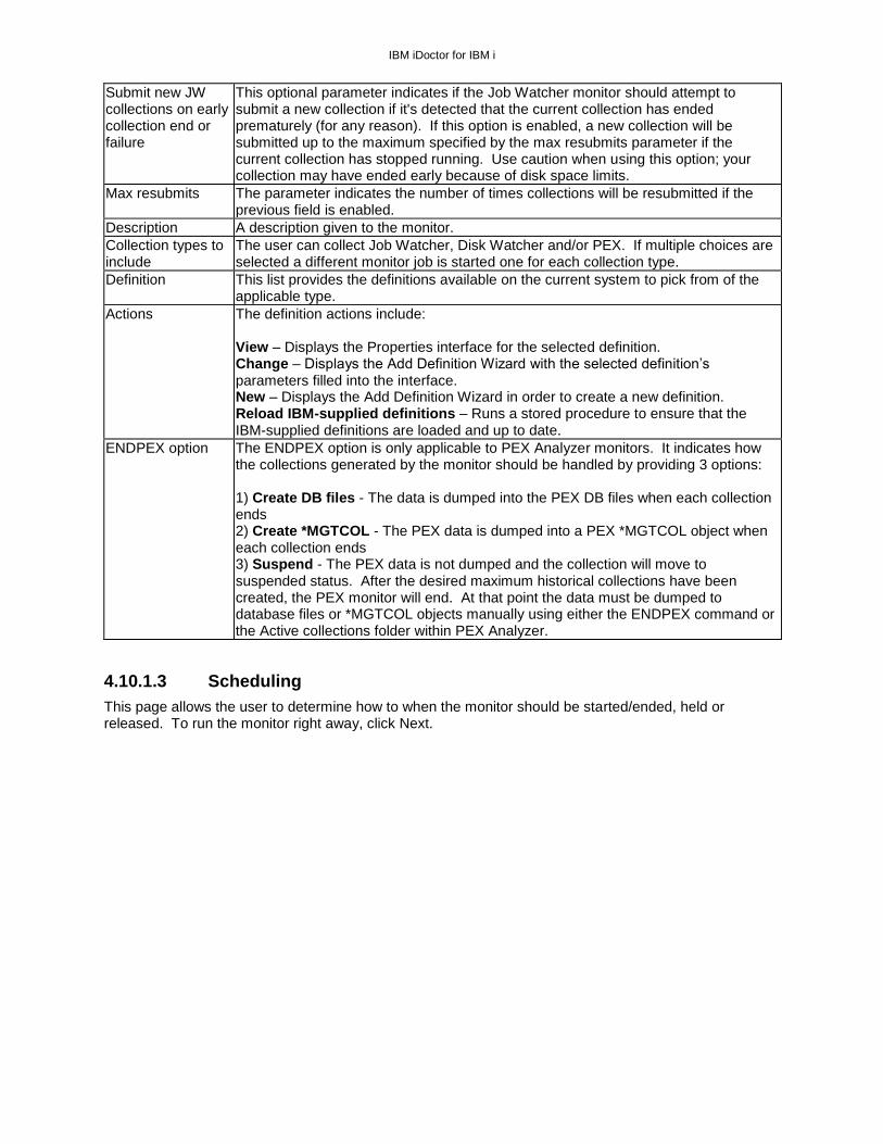
IBM iDoctor for IBM i
Submit new JW collections on early collection end or failure
This optional parameter indicates if the Job Watcher monitor should attempt to submit a new collection if it's detected that the current collection has ended prematurely (for any reason). If this option is enabled, a new collection will be submitted up to the maximum specified by the max resubmits parameter if the current collection has stopped running. Use caution when using this option; your collection may have ended early because of disk space limits.
Max resubmits The parameter indicates the number of times collections will be resubmitted if the previous field is enabled.
Description A description given to the monitor.
Collection types to include
The user can collect Job Watcher, Disk Watcher and/or PEX. If multiple choices are selected a different monitor job is started one for each collection type.
Definition This list provides the definitions available on the current system to pick from of the applicable type.
Actions The definition actions include: View – Displays the Properties interface for the selected definition. Change – Displays the Add Definition Wizard with the selected definition’s parameters filled into the interface. New – Displays the Add Definition Wizard in order to create a new definition. Reload IBM-supplied definitions – Runs a stored procedure to ensure that the IBM-supplied definitions are loaded and up to date.
ENDPEX option The ENDPEX option is only applicable to PEX Analyzer monitors. It indicates how the collections generated by the monitor should be handled by providing 3 options: 1) Create DB files - The data is dumped into the PEX DB files when each collection ends 2) Create *MGTCOL - The PEX data is dumped into a PEX *MGTCOL object when each collection ends 3) Suspend - The PEX data is not dumped and the collection will move to suspended status. After the desired maximum historical collections have been created, the PEX monitor will end. At that point the data must be dumped to database files or *MGTCOL objects manually using either the ENDPEX command or the Active collections folder within PEX Analyzer.
4.10.1.3 Scheduling
This page allows the user to determine how to when the monitor should be started/ended, held or released. To run the monitor right away, click Next.

IBM iDoctor for IBM i
Start iDoctor Monitor Wizard – Scheduling The following section lists the parameters available on this interface:
Option Description
Scheduled start time
Use this option to schedule the monitor to start at a later time.
Scheduled end time Use this option to schedule the monitor to end at a desired date and time.
Scheduled hold time
Use this option to hold the monitor at the desired date and time.
Scheduled release time
Use this option to release the monitor (assuming it’s in a held state) at the desired date and time.
4.10.1.4 Finish
This screen provides a summary of the monitor that will be started/restart on the current system.
For your convenience the remote commands that will be executed in order to start the monitor(s) are listed at the bottom of this page.

IBM iDoctor for IBM i
Start iDoctor Monitor Wizard – Finish
The following section lists the parameters available on this interface:
Option Description
Submit job options This button allows you to change parameters on the SMBJOB commands used to start the monitors.
4.11 PEX+ PEX+ collections are a new type of “super collection” produced by the QMGTOOLS/STRPEX_ command.

IBM iDoctor for IBM i
This option allows a user to collect multiple types of performance data simultaneously and tie them together within one collection. The available types of data that may be included in a PEX+ collection are: Collection Services, PEX, Job Watcher, DBMON, trace connections and XSM SST macro dumps. The PEX+ folder contains the super collections that exist on the current system. Within each super collection a folder exists per type of data that was included in the collection.
PEX+ Folder The fields shown in this view are as follows:
Field Description
Collection library The library name the super collection resides in. There can only be PEX+ collection per library.
Status Indicates if the super collection is currently running or if it has ended.
Collection types included
Lists the collection types that are included by their 2 character identifiers: PA – PEX Analyzer JW – Job Watcher CS – Collection Services
Collection job The name of the job that is collecting the data (if active.)
Command The command string used to start the PEX+ collection.
4.11.1 Menu Options The PEX+ folder provides the following menus:

IBM iDoctor for IBM i
Menu Description
Explore Displays the contents of the PEX+ folder in the list.
Start Collection… This will launch the Start PEX Collection Wizard. In order to kick off a PEX+ collection be sure to check the box on the Options screen called “Start a PEX+ super collection”.
Open New Data Viewer
Opens a new Data Viewer window. This window is used to display tables and graphs on the system. You can open iDoctor-defined reports into this window or you can also open any database file or SQL table and display the results in graph or table form.
4.11.2 Contents of a PEX+ collection Expanding a PEX+ collection provides access to the various types of data that it has collected.
Collections within a PEX+ super collection From here a user can drill down into any of these types of collections and perform the same analysis options they would normally have in the applicable component that the data applies to (i.e. PEX Analyzer, Collection Services Investigator, Job Watcher, etc.)

IBM iDoctor for IBM i
4.12 Choose Database Members This window allows the user to pick which database file members the current report should be displayed over. The window may be displayed during iDoctor use, if a query unexpectedly finds that a file/member needed for a report does not exist. The window is also displayed by using the Choose Database Members menu option from the SQL Editor. An example of this interface is:
Choose Database Members Window For the selected table in the list the Member drop down box will contain a list of all available members. Simply select the desired member and hit the update or update all buttons. The update selected button will only update the member for the selected table. The update all button will update the member for all tables shown in the list. Tip: Press ESC on the keyboard will close this window if you wish to cancel the operation.
4.13 Analyses Analyses in iDoctor are used to process performance data to either summarize the data in some manner or dig deeper and look for specific information to a given performance problem.
Analyses can be found in the main iDoctor components: Job Watcher, PEX Analyzer, Disk Watcher and CSI (Collection Services Investigator).
Analyses are initiated by right-clicking collection(s) (or library(ies)) and using the Analyses menu and picking either the Analyze Collection... menu (which shows a window to pick and choose from any available analyses) or pick one of the available "fast path" analysis options such as "Run Collection Summary", "Run Situational Analysis", etc.

IBM iDoctor for IBM i
A list of available analyses for a collection in Job Watcher.
The Analyses menu is also available if you select multiple collections and right-click. This will run the desired analyses on all the selected collections.
Analyses in iDoctor are SQL stored procedures. When an analysis runs it runs in the Remote SQL Statement Status View at the bottom of the main window. This window shows the progress of the analysis and from there completion or error messages will be shown. If an error is shown, you should right-click the error and use the Display job log menu to view the job log and try to determine the error. Of course if you are unable to determine the reason for the error, send the job log and related information about the component, collection you are trying to analyze to [email protected].
After an Analysis is complete, the tables it creates can be accessed under the SQL Tables folder found in iDoctor under the component icon or under each library within the Libraries folder. Reports are often available from the SQL tables generated by the analysis. In many cases additional reporting options are also available under the collection, by right-clicking the collection an accessing a new menu option applicable to the new analysis.

IBM iDoctor for IBM i
5 General Functions
This section documents the functions available within the General Functions folder in the IBM i components: Job Watcher, Collection Services Investigator, Disk Watcher or PEX Analyzer.
General functions folder in Job Watcher
5.1 iDoctor FTP GUI This folder within the General functions folder provides access to the iDoctor FTP GUI component. This provides functions to access both the IFS and objects within libraries on the IBM i you are connected to.
5.2 Power The Power folder provides access to analysis functions for non IBM i data such as nmon, npiv, VIOS advisor and more. It is provided here as a way for users to analyze already collected data when they may not have authority to connect to the VIOS, HMC, etc. directly.
A different subfolder is provided for each type of data supported.
General functions -> Power folder in Job Watcher
For more information on the Power-based (non-IBM i) functions, please visit the chapter on Power.

IBM iDoctor for IBM i
5.3 SQL catalog functions This folder provides functions related to the SQL catalog tables found on DB2 for IBM i.
SQL catalog functions folder
At 7.1 and higher a collection utility is available that can help you determine which tables and/or members would be good candidates to move to SSDs. This utility can also be used to capture general performance statistics for tables and members over a period of time.
A subfolder called IBM i Services is also available that provides reports made available with recent technology refreshes made to IBM i and DB2 for i in the SQL catalog tables. These reports are opened in the Data Viewer.
Right-clicking the SQL catalog functions folder provides the following options:
Menu Description
Automatically fill SSDs
Note: This function is available at 7.1+ only. This provides the ability to capture performance metrics over time for the desired libraries and tables. This information is used to determine which tables/members would be the best candidates to move to SSDs. Once complete a report will be generated indicating which tables had their media preference changed to *SSD. Note: This function will NOT be available if no SSDs were found on the current system.
Start Collection… Note: This function is available at 7.1+ only. This option is used to capture statistics about the tables or members on the system over time. WARNING: Capturing these statistics can be extremely time consuming and the appropriate filters, number of intervals and interval durations should be used based on the number of tables on your system that you are analyzing.
Filter Libraries… This option can be used to filter the libraries shown under Tables -> Libraries subfolder.
5.3.1 Automatically move tables (or members) to SSDs (7.1+)
This window is used to kick off a process that will determine the best candidates to move to SSDs and automatically change the media preference to *SSD on the tables found based on the filters provided.
An example of this interface is:

IBM iDoctor for IBM i
Automatically move tables to SSDs
The options available on this screen are:
Option Description
Collection library The library where the report will be generated.
Collection The collection or name of the report to generate.
Maximum SSD % used
This setting is used to avoid overfilling the SSDs by keeping the percentage of SSD % space used less than the value provided. If the SSD % used exceeds this value then the media preference setting will not be changed by this process.
Current SSD % used
This will list the current SSD % of disk space used for this system.
Submit to a batch job
This option will submit this process to a batch job rather than running it interactively in the Remote SQL Statement Status View within the iDoctor GUI.
Filters Description
Library filter This can be either the library name or generic library name of the tables to search or blank to look at tables in all libraries. Note: If you have a system with thousands/millions of tables, then using appropriate filters is highly recommended or this process could take hours or even days.
Table filter This is an optional generic table name filter.
Days used This filter allows you to exclude tables that have not been used at least N days since the last IPL.

IBM iDoctor for IBM i
5.3.2 Start Table (or member) Statistics Collection (7.1+) Note: This function is available at 7.1+ only. This option is used to capture statistics about the tables or members on the system over time.
WARNING: Capturing these statistics can be extremely time consuming and the appropriate filters, number of intervals and interval durations must be used based on the number of tables on your system that you are analyzing.
Start Table Statistics Collection
The options available on this screen are:
Option Description
Collection library The library where the collection will be generated.
Collection The collection name to generate.
Interval duration This value indicates how often a fresh snapshot of the statistics will be captured. Keep in mind that if you are analyzing several thousands of tables, the time it takes to capture this data could easily exceed the interval duration. It is typically best to keep this value fairly large such as 60 minutes or greater.
Maximum intervals This value is the number of intervals to collect.
Collect member (or table) statistics
Check this box if you also want to collect statistics at the member (or table) level depending on if you selected the Start Table Statistics Collection or the Start Member Statistics Collection option.
Submit to a batch job
This option will submit this process to a batch job rather than running it interactively in the Remote SQL Statement Status View within the iDoctor GUI.

IBM iDoctor for IBM i
Filters Description
Library filter This can be either the library name or generic library name of the tables to search or blank to look at tables in all libraries. Note: If you have a system with thousands/millions of tables, then using appropriate filters is highly recommended or this process could take hours or even days.
Table filter This is an optional generic table name filter.
Days used This filter allows you to exclude tables that have not been used at least N days since the last IPL.
Exclude tables with 0 random reads
When checked, statistics for tables that had 0 random reads are not captured.
Exclude tables with more sequential reads than random reads
When checked, statistics for tables that had more sequential reads than random reads are excluded.
5.3.3 Tables (7.1+)
The SQL catalog functions -> Tables subfolder provides users the ability to view statistics for all tables on the system in real time or view collected performance metrics on the tables and members on the system.
General functions -> SQL catalog functions -> Tables folder
5.3.3.1 Libraries (metrics since the last IPL)
This folder contains each library on the system or a filtered list of libraries if the Filter Libraries menu option has been used. Within each of these libraries you will the tables they contain and the performance metrics available since the last IPL.
5.3.3.1.1 Tables
By selecting a library you will be presented with a list of all tables found in the library and their statistics. The data is sorted by random reads in descending sequence by default.
If desired you may expand a table to view the members (partitions) within each.

IBM iDoctor for IBM i
Real-time table metrics for the tables within library mccargar
The data provided in this window includes the following:

IBM iDoctor for IBM i
Column Description
% assigned to SSDs
This value represents the current data allocation percentage to SSDs for the table.
Number of members
Number of partitions or members of the table.
Number of rows Number of valid rows in all partitions or members of the table.
Number of pages Number of 64K pages in all partitions or members of the table.
Overflow The estimated number of rows that have overflowed to variable length segments. If the table does not contain variable length or LOB columns, contains 0.
Random reads Number of random read operations of all partitions or members of the table since the last IPL.
Logical reads Number of logical read operations of all partitions or members of the table since the last IPL.
Physical reads Number of physical read operations of all partitions or members of the table since the last IPL.
Sequential reads Number of sequential read operations of all partitions or members of the table since the last IPL.
Data size (megabytes)
Total size of the data spaces in all partitions or members of the table.
Opens Number of full opens of all partitions or members of the table since the last IPL.
Closes Number of full closes of all partitions or members of the table since the last IPL.
Inserts Number of insert operations of all partitions or members of the table since the last IPL.
Updates Number of update operations of all partitions or members of the table since the last IPL.
Deletes Number of delete operations of all partitions or members of the table since the last IPL.
Clears Number of clear operations (CLRPFM operations) of all partitions or members of the table since the last IPL.
Copies Number of data space copy operations (certain CPYxxx operations) of all partitions or members of the table since the last IPL.
Reorganize Number of data space reorganize operations (non-interruptible RGZPFM operations) of all partitions or members of the table since the last IPL.
Index build Number of creates or rebuilds of indexes that reference any partition or member of the table since the last IPL. This does not include maintained temporary indexes.
Change time Maximum timestamp of the last change that occurred to any partition or member of the table.
Last used time Maximum timestamp of the last time any partition or member was used directly by an application for native record I/O or SQL operations. If no partition or member has ever been used, contains null.
Non-SSD space used (bytes)
Space used by all partitions or members for this file allocated to disks other than SSDs (in bytes.)
SSD space used (bytes)
Space used by all partitions or members for this file allocated to SSDs (in bytes.)
5.3.3.1.2 Members
Expanding a table in the tree/list interface will display the list of members and the real-time metrics for each member since the last IPL. The statistics shown are the same as covered for tables in the previous section.
You can also double-click a table to open it in the Data Viewer.

IBM iDoctor for IBM i
5.3.3.2 Table Statistics
This folder provides access to graphs and reports over already captured table statistics data produced by iDoctor. All of the collections found on the system of this type will be displayed.
List of table statistics collections found on a system within Job Watcher
5.3.3.2.1 Collections
Expanding a Table Statistics collection provides the following options:

IBM iDoctor for IBM i
Contents of a Table Statistics collection
Graphs are available under the table statistics and table statistics since last IPL folder.
Note: The table statistics folder will only be shown if more than 1 snapshot has been collected.
5.3.3.2.2 Table Statistics Reports
The graphs available under the Table statistics folder are:
Table statistics folder graphs
These graphs are available for either all tables collected over time, or ranked by the desired metric(s). You may drill down from the over time graphs to the rankings graphs for the selected time period.
Note: All graphs are based on the tables specified to be included in the data collection over the number of intervals and interval durations provided.
5.3.3.2.2.1 Reads
This graph shows the logical and physical reads over time with random reads on the second Y-axis.
Reads

IBM iDoctor for IBM i
5.3.3.2.2.2 Random reads
This graph displays the random reads by itself over time.
5.3.3.2.2.3 Table operations
This graph displays several types of miscellaneous table functions: Opens, closes, inserts, updates, deletes, clear, copy and reorganize.
Table operations
5.3.3.2.2.4 Net rows created
This graph displays the net rows (rows created – rows destroyed) created over time.
5.3.3.2.2.5 Rows overflowed
This graph shows the estimated number of rows overflowed to variable length segments over time.
5.3.3.2.2.6 Net size changes
This graph shows the net data space size changes (in megabytes) over time.
5.3.3.2.2.7 Rankings
The same set of graphs covered previously are also provided as rankings charts by table name. These graphs can either be produced for the entire collection duration or based on the selected time period in one of the over-time charts.
An example is provided below:

IBM iDoctor for IBM i
Random reads by table graph
5.3.3.2.3 Table Statistics since last IPL Reports
The graphs available under the Table statistics since last IPL folder are:
Table statistics since last IPL folder
These graphs are available for either all tables collected over time, or ranked by the desired metric(s). You may drill down from the over time graphs to the rankings graphs for the selected time period.
Graphs named “Cumulative” imply that delta statistics are not provided; the values on these graphs will always stay the same or increase over time.
Note: All graphs are based on the tables specified to be included in the data collection over the number of intervals and interval durations provided.
5.3.3.2.3.1 Cumulative reads since last IPL
This graph shows the cumulative logical, physical ans sequential reads over time with random reads on the second Y-axis.

IBM iDoctor for IBM i
Cumulative reads since last IPL
5.3.3.2.3.2 Cumulative random reads since last IPL
This graph displays the cumulative random reads by itself over time.
5.3.3.2.3.3 Cumulative table operations since last IPL
This graph displays cumulative values for several types of miscellaneous table functions: Opens, closes, inserts, updates, deletes, clear, copy and reorganize.
Table operations

IBM iDoctor for IBM i
5.3.3.2.3.4 Cumulative number of rows since last IPL
This graph displays the cumulative total number of rows for all tables collected and the total number of 64K pages over time.
5.3.3.2.3.5 Cumulative rows overflowed since last IPL
This graph shows the cumulative estimated number of rows overflowed to variable length segments over time.
5.3.3.2.3.6 Sizes
This graph shows the various types of table sizes (in megabytes) over time. Unlike the other graphs these values are not cumulative.
Sizes graph
5.3.3.2.3.7 Rankings
The same set of graphs covered previously are also provided as rankings charts by table name. These graphs can either be produced for the entire collection duration or based on the selected time period in one of the over-time charts.
An example is provided below:

IBM iDoctor for IBM i
Sizes by table for a time period
5.3.3.2.4 Server-side output files
This folder under a Table Statistics collection provides a list of tables that were created as part of the collection. If only 1 snapshot was collected then only table QAIDRDBTBSNAP_<<COLNAME>> will exist in this folder. If more than 1 snapshot was captured then a table of delta statistics for each interval will be calculated and provided in QAIDRDBTB_<<COLNAME>>.
Server-side output files for a Table Statistics collection

IBM iDoctor for IBM i
5.3.3.3 Member Statistics
This folder provides access to graphs and reports over already captured member statistics data produced by iDoctor. All of the collections found on the system of this type will be displayed.
List of member statistics collections found on a system within Job Watcher
An example of a Member statistics since last IPL graph is:
Cumulative reads since last IPL by member
Note: All the the member statistics collections and reports are identical to the ones for Table statistics except instead of providing table rankings graphs they are member ranking graphs. For this reason they are not documented, refer to the previous sections for information about the graphing options for member statistics if desired.
5.3.4 IBM i Services
The General functions -> SQL catalog functions -> IBM i Services folder provides the following reporting options from the data provided with DB2’s SQL catalog tables:

IBM iDoctor for IBM i
General functions -> SQL catalog functions -> IBM i Services folder in Job Watcher
For more information on the data behind these reports visit this web page:
https://www.ibm.com/developerworks/community/wikis/home?lang=en#!/wiki/IBM%20i%20Technology%20Updates/page/DB2%20for%20i%20-%20Technology%20Updates
5.3.4.1 System values
These reports show information about the current IBM i system values. The reports available are:
1) All system values
2) System values related by maximums
5.3.4.2 PTFs
These reports show PTF information for the current system.
5.3.4.2.1 PTFs by product
This report provides a count of the total PTFs for each product ID, option and release level.

IBM iDoctor for IBM i
PTFs by product
5.3.4.2.2 List all PTFs
This report lists all the data available for all PTFs found on the system.
5.3.4.2.3 List PTFs impacted by the next IPL
This report informs you of any PTFs that will be effected by the next IPL.
5.3.4.2.4 List PTFs loaded but not applied
This report provides a list of PTFs loaded but not yet applied.
PTFs loaded but not applied

IBM iDoctor for IBM i
5.3.4.3 Group PTFs
These reports are provide information about the group PTFs found on the system.
5.3.4.3.1 Group PTF list
This report lists all group PTFs found on the system and the PTF group level installed.
Group PTF List
5.3.4.3.2 DB PTF Group Level
This report simply lists the DB PTF Group level.
5.3.4.3.3 Check group PTF currency
This option will check each group PTF and look for any updates available. It will inform you of the level installed and the level that is available.
An example of this report is:
Check group PTF currentcy
Note: In order for this report to work, the iDoctor client QZDASOINIT jobs’ CCSID must not be 65535. You can check or change this by right-clicking the component icon (i.e. Job Watcher, PEX Analyzer, etc.)

IBM iDoctor for IBM i
in the component view and using Properties -> iDoctor Client Jobs then change the CCSID to 37 if necessary.
Component properties -> iDoctor Client Jobs -> CCSID setting
5.3.4.4 Users and groups
5.3.4.4.1 List all group profiles
This report lists all the group profile names and the user profiles that belong to each.
5.3.4.4.2 List all user profiles
This report provides detailed information about all user profiles installed on a system.

IBM iDoctor for IBM i
List all user profiles
5.3.4.4.3 List users having trouble signing on
This report will list all user profiles that have invalid signon attempts to the system.
List users having trouble signing on
5.4 Browse Collections The Browse Collections function displays lists of collections on your system in various ways. All current IBM i collection types used by iDoctor are included in the collections shown. Note: This interface is only accessible if the system has a license to both PEX Analyzer and Job Watcher.

IBM iDoctor for IBM i
This option works by first building a database of the available collections and then grouping and displaying the results in various folders. An example of the ways to browse collections are:
Browse Collections options Within any of these folders are additional folders that appropriately group the data (partition name, library name, etc.) and within those are the lists of collections. In most cases all of the normal graphing/reporting options found in the applicable iDoctor component are also available when right-clicking collections.
5.4.1 Menu Options When right-clicking the Browse Collections folder the following options are available:
Menu Description
Filter collections This menu brings up a window that lets you filter the collections shown by collection owner.
Refresh collections database
This option will refresh the collections database. The database tables are not recreated, but any changes to collections on the system will be checked for and updated in the database.
Full rebuild collections database
This option will completely replace the collections database which may take several minutes. This option may be required if changes have been made to iDoctor (such as additional fields added to the database.)
5.4.2 Filter collections Use this interface to filter the list of collections displayed in the Browse Collections interface by collection owner.

IBM iDoctor for IBM i
5.4.3 Examples
This folder displays each library with the total number of collections and the estimated total size (in megabytes)
Browse Collections -> Library folder
The next example shows the list of Job Watcher collections in a library:

IBM iDoctor for IBM i
Browse Collections -> Library MCCARGAR
Browse Collections -> VRM
5.5 Saved collections Most components allow you to save iDoctor collections to a save file. The Saved Collections folder within a component allows you to work with any saved collections found on the system. Note: This interface will only show collections that were saved using the iDoctor GUI.

IBM iDoctor for IBM i
The interface looks like the following:
iDoctor Saved Collections Folder The folder contains a row for every save file found that contains an iDoctor collection saved using the iDoctor GUI. The following table describes the data shown in this folder:
Field Description
Save file name The name of the save file.
Save file library Library name of the save file.
Saved library The library that was saved.
Command string The command string that was used to save the collection.
5.5.1 Menu Options By right clicking on a save file there are a number of options available:

IBM iDoctor for IBM i
Popup Menu Description
Display Displays the contents of the save file into a new window.
Delete Removes the selected save files from the system.
Restore This option allows you to restore the saved collection to the desired library on the current system. Change the Restore to library parameter if you desire to the restore the collection to a different library than it was originally created in.
Transfer to This option allows you to send the desired save files to another system or to IBM.
Properties Displays object information for the save file.
5.6 Work Management This folder contains functions for working with the scheduled jobs, active jobs and subsystems on the current system.

IBM iDoctor for IBM i
Work Management folder
5.6.1 Scheduled Jobs Most components allow you to schedule collections to run at a later time. The Scheduled Jobs folder allows you to work with the iDoctor created scheduled jobs on the system. The folder contains a row for every iDoctor scheduled job defined on the system. The following table describes the data shown in this folder:
Field Description
Job The name of the job that will be created when the scheduled job is submitted.
Type The type of iDoctor job that will run.
Submitted by The user profile on the system that created the iDoctor scheduled job.
Status The status of the scheduled job. This will either be Scheduled or Held. If the status is Held the scheduled job must be released before it will run.
Scheduled date/time
The date and time when the scheduled job will run. This may list either a specific date and time, a specific day and time to run on a weekly basis, or Daily if this job should run every day.
Next submit date The date when this job is next scheduled to run.
Job entry number The entry number of the scheduled job as defined on the system.
Description A description that has been assigned to the scheduled job entry.
Command The command string that will be executed when the scheduled job runs.
By right clicking on a scheduled job entry there are a number of options available:
Popup Menu Description
Submit immediately Submits the scheduled job immediately. The scheduled job will still run again at the next scheduled date and time.
Hold/Release Hold or release the selected scheduled job entry. If held the scheduled job will not run.
Delete Removes the selected scheduled job entries from the system.
5.6.2 Active jobs This folder allows you to work with the active jobs found on the current system. This folder can also be used to kick off collections or define definitions based on the desired jobs.

IBM iDoctor for IBM i
In addition you can expand a job within the tree to look at the threads it contains. Expanding a thread allows you to easily see its current call stack. Performance data shown in this list like CPU and IOs are based on the time between the initial refresh of this view and the most recent one. You can also reset these statistics by right-clicking the Active jobs folder and using the Reset statistics menu. The list of jobs can also be filtered by right-clicking the Active jobs folder and using the Filter… option. This interface looks like the following:
Work Management -> Active Jobs Folder The folder contains a row for every active job found on the system. The following table describes the data shown in this folder: Tip: Right-click the Active jobs folder and pick the Select fields menu to rearrange or add/remove fields from this list.

IBM iDoctor for IBM i
Field Description
Job name/user/number
The job name/user/number.
Threads The current number of threads found within the job.
Status The status of the initial thread of the job. For more information on the possible values, see the help text for the WRKACTJOB command.
Current user The current user profile identifies the profile under which the initial thread is running at this time.
Type This field shows the type of active job.
Function The last high-level function initiated by the initial thread. This field is blank when a logged function has not been performed. The field is not cleared when a function is completed.
CPU % The percent of processing unit time attributed to this job over the elapsed time compared to the measurement time interval. For an uncapped partition using shared processors, this percentage can be greater than 100 percent.
CPU time (ms) The CPU time used by the job during the elapsed time.
Run priority The current run priority for the job.
Disk IO The number of disk I/Os that occurred for the job during the elapsed time.
Async IO The number of asynchronous disk I/Os for the job during the elapsed time.
Sync IO The number of synchronous disk I/Os for the job during the elapsed time.
Page faults The number of page faults for the job during the elapsed time.
Subsystem The name of the subsystem the job is running in.
Date/time job entered system
The date/time the job entered the system.
CPU time total (ms) Total CPU time consumed by the job (in milliseconds).
Disk IO total The total disk I/Os for the job.
Server type The type of server represented by the job.
Job type code 1 character code that identifies the type of job.
Job subtype code 1 character code that identifies the subtype of the job.
Subsystem library The name of the library the subsystem description resides in.
Function type 1 character code identifying the type of function last performed by the job. See the Work Management API Attribute Descriptions for more information.
DB CPU time total (ms)
Total DB CPU time consumed by the job (in milliseconds).
DB CPU % The percent of processing unit type attributed to DB operations over the elapsed time compared to the measurement time interval.
DB CPU time (ms) The DB CPU time used by the job during the elapsed time (in millseconds).
Interactive transaction response time
The average interactive transaction response time (in milliseconds) for the life of the job.
Transaction total The total number of interactive transactions during the life of the job.
Memory pool The memory pool that the job is running in.
Job user identity The user profile name by which the job is known to other jobs on the system. The job user identity is used for authorization checks when other jobs on the system attempt to operate against the job.
By right clicking on a job there are a number of options available:

IBM iDoctor for IBM i
Popup Menu Description
Explore Displays the list of threads found within the job.
Record Quick View Displays a vertical list of fields for the selected job in a new window. This option is only available from the list side of the view.
Select fields… This option allows you to select the fields to display for the list of threads within the
job. You can only set this option by right-clicking a job name from the tree side of the view.
Start Job Watcher Launches the Start Job Watcher Collection interface. At 5.4 and earlier releases this will also preselect the selected jobs in the interface so that only the selected jobs will be included in the collection. At 6.1 and higher you should use the Add Job Watcher Definition option instead and then start the collection after.
Add Job Watcher Definition
Defines a new Job Watcher definition that collects data only for the selected jobs.
Start PEX Collection
Launches the Start PEX Collection Wizard and preselects the selected jobs in the interface so that the collection only contains data for these jobs.
Add PEX Definition Defines a PEX definition that will collect data over the selected jobs.
Display job log Displays the job log for the selected job. The job log viewer that comes with IBM i Navigator is used.
Delete/End This option will end the selected jobs using the OPTION(*CNTRLD) DELAY(30) parameters.
Reset Statistics (Threads)
This option resets the collected thread level statistics for the selected job.
5.6.2.1 Threads
Expanding a job within the Active jobs folder displays the list of threads the job contains along with performance data from the 1st snapshot and the last snapshot (refresh) of the current view. Performance data shown in this list like CPU and IOs are based on the time between the initial refresh of this view and the most recent one. You can also reset these statistics by right-clicking the job folder and using the Reset statistics menu. Expanding a thread allows you to easily see its current call stack. This interface looks like the following:

IBM iDoctor for IBM i
iDoctor Active Jobs Folder – Threads for a Job
The folder contains a row for every thread found within the selected job from the tree. The following table describes the data shown in this folder: Tip: Right-click the job and pick the Select fields menu to rearrange or add/remove fields from this list.
Field Description
Thread ID Unique identifier for the job’s thread.
Thread status The current status of the thread. The status of a thread may be one of the following values:
Blank The status of the thread is unknown.
CMTW The thread is waiting for the completion of save-while-active checkpoint processing in another job. This wait is necessary to prevent a partial commitment control transaction from being saved to the media.
CNDW The thread is waiting for a condition.
DEQA The thread is waiting for completion of a dequeue operation in the pool activity level.
DEQW The thread is waiting for completion of a dequeue operation. For example, a server may wait for work by waiting for a dequeue operation
EVTW The thread is waiting for an event.
HLD The thread is in a job that is being held.
HLDT The thread is being held.
INEL The thread is ineligible and not currently in the pool activity level.
JVAA The thread is waiting for completion of a Java program operation in the pool activity level.

IBM iDoctor for IBM i
JVAW The thread is waiting for completion of a Java program operation.
LCKW The thread is waiting for a lock.
LSPA The thread is waiting for a lock space to be attached while in a pool activity level.
LSPW The thread is waiting for a lock space to be attached.
MTXW The thread is in a mutex wait. A mutex is a synchronization function that is used to allow multiple threads to serialize their access to shared data.
RUN The thread is currently running in the activity level.
SELW The thread is in a select wait. More information on the select() function is in the Sockets APIs chapter in the System API Reference, SC41-5801.
SEMW The thread is waiting for a semaphore. A semaphore is a synchronization function that is used to allow multiple jobs or threads to serialize their access to shared data.
SIGS The thread has been held by a signal.
SIGW The thread is waiting for a signal.
THDW The thread is waiting for another thread to complete an operation.
TIMA The thread is waiting, in the activity level, for a time interval to end.
TIMW The thread is waiting for a time interval to end.
Thread type The thread type indicates how the thread was created. If this field is requested for a job, the value for the initial thread of the job will be returned. The type of a thread may be one of the following values:
User - The thread was created either as the initial thread of the job or explicitly by the application.
System - The thread was created by an operating system function.
Run priority The current run priority for the job.
Current user The user profile that the thread for which information is being retrieved is currently running under. This name may differ from the user portion of the job name.
CPU % The percent of processing unit time attributed to this thread over the elapsed time compared to the measurement time interval. For an uncapped partition using shared
processors, this percentage can be greater than 100 percent.
CPU time (ms) The CPU time used by the thread during the elapsed time.
Disk IO The number of disk I/Os that occurred for the job during the elapsed time.

IBM iDoctor for IBM i
Async IO The number of asynchronous disk I/Os for the job during the elapsed time.
Sync IO The number of synchronous disk I/Os for the job during the elapsed time.
Page faults The number of page faults for the job during the elapsed time.
CPU time total (ms) Total CPU time consumed by the job (in milliseconds).
Disk IO total The total disk I/Os for the job.
DB CPU time total (ms)
Total DB CPU time consumed by the job (in milliseconds).
DB CPU % The percent of processing unit type attributed to DB operations over the elapsed time compared to the measurement time interval.
DB CPU time (ms) The DB CPU time used by the job during the elapsed time (in millseconds).
By right clicking on a job there are a number of options available:
Popup Menu Description
Call Stack Displays the current call stack for the selected thread.
Record Quick View Displays a vertical list of fields for the selected thread in a new window. This option is only available from the list side of the view.
Select fields… This option allows you to select the fields to display for the call stacks within the thread. You can only set this option by right-clicking a thread ID from the tree side of the view.
5.6.2.2 Call Stacks
Expanding a thread within a job within the Active jobs folder displays the current call stack for the thread. The call stack shows both LIC and above the MI programs/procedures/modules.
Active Jobs Folder – Call Stack for a Thread
5.6.3 Subsystems
The subsystems folder provides the following 2 options for working with subsystems on the current system:

IBM iDoctor for IBM i
Work Management -> Subsystems folder
5.6.3.1 iDoctor subsystems
The iDoctor subsystems shown are based on those specified at install time. With the latest builds this will just show a single subsystem (default QSYS/QIDRJW.)
5.6.3.2 All subsystems
This option displays a list of all subsystems found on the system and allows you to work with the jobs running within each subsystem.
Displaying the active jobs within a subsystem

IBM iDoctor for IBM i
5.7 ASPs The ASPs folder displays disk information for the current system on a per ASP basis. You can also expand the ASPs to see information about the disk units within the selected ASP. This information is similar to WRKDSKSTS but includes extra fields not found there. This interface looks like the following:
iDoctor ASPs Folder The folder contains a row for every ASP found on the system. The following table describes the data shown in this folder: Tip: Right-click the ASPs folder and pick the Select fields menu to rearrange or add/remove fields from this list.

IBM iDoctor for IBM i
Field Description
ASP The ASP identifier.
Disk units Total number of disk units in the ASP.
Total size (GB) The total size of all disk units in the ASP (in gigabytes).
% used The percent of available disk space used.
% warning threshold
The SLIC warning threshold of available disk space used for the ASP.
% protected The percent of ASP disk space that is protected by mirroring or device parity
Type The type of ASP. The possible values are: System ASP User ASP (no libraries) User ASP (with libraries)
ASP system storage (MB)
The amount of storage in megabytes currently allocated in the ASP for system use.
Overflow storage (MB)
The number of megabytes of storage that has overflowed from the user ASP into the system ASP.
Error log size (MB) The number of megabytes of auxiliary storage allocated to the error log.
Machine log size (MB)
The number of megabytes of auxiliary storage allocated to the machine log.
Machine trace size (MB)
The number of megabytes of auxiliary storage allocated to the machine trace.
Main storage dump size (MB)
The number of megabytes of auxiliary storage allocated to the main storage dump space.
Microcode size (MB)
The number of megabytes of auxiliary storage allocated to the microcode and space used by the microcode.
End immediately if system ASP full
This field has meaning in the system ASP (ASP 1) only.
No If a request for space in the system ASP cannot be satisfied because there is not enough
storage, the system will be allowed to continue running.
Yes If a request for space in the system ASP cannot be satisfied because there is not enough
storage, the system will be ended immediately.
Compressed units Whether there are compressed disk units in the ASP. The following are the possible values:
None No compressed disk units in this ASP.
Some Compressed and uncompressed disk units in this ASP.
All All disk units in this ASP are compressed.
Balance status The current status of the balance function for this ASP. The following special values are returned:
No activity No balance activity has occurred for this ASP.
Running The ASP balance function is currently running for this ASP.
Ending The ASP balance function is currently in the process of ending. Either the
time limit has run out or the End ASP Balance (ENDASPBAL) command

IBM iDoctor for IBM i
was issued for this ASP.
Ended before balance complete
The ASP balance function has run, but was ended before the ASP was completely balanced. The Start ASP Balance (STRASPBAL) command
can be used to restart the balance function.
Completed The ASP balance function has completed running. The ASP is completely balanced.
Balance type The type of balance activity that is currently running or was done last.
Mirroring role The current role of a physical IASP.
Not configured Remote IASP mirroring is not configured.
No physical IASP
copy
System does not own a physical IASP copy.
Unknown Remote mirror role is unknown.
Has detached
mirror copy
System owns a detached mirror copy.
Has mirror copy System owns the mirror copy.
Has production
copy
System owns the production copy
By right clicking on an ASP within the list the following options are available:
Popup Menu Description
Reset Statistics This option resets the disk unit level statistics for the selected ASP.
Add Disk Watcher Definition
Defines a new Disk Watcher definition on the system. The interface will preselect the definition to only include the ASPs selected.
Add PEX Filter Defines a new PEX filter using the selected ASP.
Expanding the ASP will show the disk units within. See the next section for more information. The functionality available for units within an ASP is identical to that available in the Disk Units folder.
5.8 Disk units The Disk Units folder displays disk information for the current system. This information is similar to WRKDSKSTS but includes extra fields not found there. This interface looks like the following: Tip: Right-click the Disk units folder and pick the Select fields menu to rearrange or add/remove fields from this list.

IBM iDoctor for IBM i
iDoctor Disk units Folder The folder contains a row for every disk unit found on the system. The following table describes the data shown in this folder:

IBM iDoctor for IBM i
Field Description
Disk unit The disk unit identifier
Disk type The disk unit type
ASP The ASP the disk unit belongs to.
Size (GB) The total capacity of the disk unit (in gigabytes).
% used The percent of available disk space used.
% busy The percent of time the disk unit was busy during the sample period.
I/Os per second The rate of I/Os occurring per second during the sample period.
Avg I/O size (KB) The average size of each I/O occurring during the sample period.
Avg reads per second
The average number of reads per second during the sample period.
Avg writes per second
The average number of writes per second during the sample period.
Avg read size (KB) The average size of each read during the sample period.
Avg write size (KB) The average size of each write during the sample period.
Total I/Os The total number of I/Os during the sample period.
Total I/O size (KB) The total size of all I/Os added together during the sample period.
Total reads The total number of reads during the sample period.
Total writes The total number of writes during the sample period.
Total read size (KB) The total size of all reads added together during the sample period.
Total write size (KB)
The total size of all writes added together during the sample period.
Compression status The current status of compression for this disk unit. The possible values are: Active, Not active
Disk protection type The type of protection that has been assigned to this disk unit. The following values are
returned:
None No storage protection has been set up for this disk unit.
Mirrored This disk unit has been set up with mirrored protection.
Parity This disk unit is part of a parity protection array.
Mirrored status The mirrored status of the unit.
Blank Not mirrored
1 This mirrored unit of a mirrored pair is active (that is, online with current
data).
2 This mirrored unit is being synchronized.
3 This mirrored unit is suspended.
Mirrored reported This mirrored unit reported present. Information concerning this unit may or may not be
current.
0 The mirrored unit is missing. Information concerning the unit may not be current.
1 The mirrored unit reported at the time this information was gathered. The information is
current to that point in time.

IBM iDoctor for IBM i
Mirrored protected The mirrored status of the mirrored pair of which this unit is a member.
0 One mirrored unit of a mirrored pair is not active.
1 Both mirrored units of a mirrored pair are active.
Disk model The model of the disk unit. Disk serial number The serial number of the disk unit.
Resource name The unique system-assigned name of the disk unit.
By right clicking on a disk unit within the list the following options are available:
Popup Menu Description
Add Disk Watcher Definition
Defines a new Disk Watcher definition on the system. The interface will preselect the definition to only include the units selected.
Add PEX Filter Defines a new PEX filter using the selected disk units.
5.9 Objects owned by user This folder provides options for viewing the disk space consumption of objects or files on the system by the current user. Options are available to view the disk space usage for all objects or only objects created by iDoctor.
Objects owned by <User> folder options
5.9.1 Menu options
This folder provides the following menu options:

IBM iDoctor for IBM i
Popup Menu Description
Filter objects by owner
Displays the Filter Objects by Owner window which lets you configure the user profile to view disk consumption for and whether all the object sizes should be loaded before loading the list. Depending on the number of objects involved, the checkbox to load all object sizes could be extremely slow.
Clear object sizes cache
Deletes the cache of object sizes previously loaded from the current GUI session. This will cause them to be retrieved again and is only useful if the sizes have changed recently.
5.9.2 Object listings
Each of the folders provided in this interface display lists of objects on the system. They can be sorted by size and then deleted via the GUI if desired. Use the “load all object sizes” checkbox described above for best results.

IBM iDoctor for IBM i
6 The Data Viewer
The Data Viewer is a frame window within IBM iDoctor for IBM i used for displaying tables and graphs over data on the system. You can have as many Data Viewer windows open at one time as you want. The data behind the views within a Data Viewer may come from any number of systems desired which allows for easier comparisons. These views are manipulated in the same way as within the Main Window (they can be tiled, cascaded, etc). Tables and graphs are typically opened from the component views in the Main Window. There are also drill down options to open tables and graphs directly from the Data Viewer window instead of going back to the Main Window. The data behind a table or graph in the Data Viewer is produced using an SQL query. These SQL statements usually are IBM-defined but the capability to define and open user-defined graphs and queries in the Data Viewer is also supported. The SQL statement behind tables and graphs can either be manipulated in the query definition interface or using the SQL editor found above every table or graph by clicking the SQL button on the toolbar of the Data Viewer. In addition to running SQL statements to produce table and graph views the Data Viewer also has support for viewing spool files containing job logs. An example of a Data Viewer, showing a graph from Job Watcher is shown below:
Data Viewer Example
6.1 Toolbar
The Data Viewer Toolbar The following outlines the different toolbar icons available in the Data Viewer and purpose:

IBM iDoctor for IBM i
Icon Description
Opens a new instance of an SQL Query View. The SQL Query View is used to create a query using Structured Query Language (SQL). The top portion of the view is an area where you can enter an SQL statement (also known as the SQL Editor) and the bottom portion is the result or output from the statement above. You can either edit the statement directly or use the query definition interface to change it. Note: The query definition interface will only work correctly on relatively simple SQL statements.
This option allows you to open any library/file/member on the system using the Open File Window. This window lets you browse for the physical or logical file you wish to open. If you do not specify the member, you will be prompted to select the member from a list.
This option allows you to save the contents of a table view to a file or if viewing a graph to a .jpg image. When using this option on a table the entire contents of the table are saved. You can choose between rich text, comma separated and tab separated text formats. If you wish to include/exclude the header in the saved file, see the Preferences -> File tab.
Use this option to view the available properties for the active graph or table view.
Copies the current selection from the current table, graph, or selection made within the SQL editor to the clipboard. If a table view or SQL editor has current focus, this is only enabled when something has been selected. For graph views this will copy an image of the current graph (without the legend) to the clipboard. If you wish to include the legend in your image, then use Alt-Print Screen to copy the Data Viewer and everything in it to the clipboard. You may want to maximize the current graph view within the Data Viewer before doing this.
This icon displays a window allowing you to set the font used for the table views and the legend used in graph views in the application.
Displays the iDoctor Preferences interface.
This icon allows you to position to the first record in a table view, matching the desired criteria. The Find Dialog will be displayed and you can use it search through a column for a specific value.
Note: The query definition icon was removed from the latest builds because using that interface is not recommended due to its limitations. If you still wish to use this option then right-click the table and use the query definition menu. If you are using a graph, then right-click a field in the legend and use the Add Filter menu to filter data, or the sort option to sort the graph on the desired field.
Refresh the currently active table or graph view.
This button will display the Window Manager which lets you work with a list of all tabs/views that are opened. This lets you find and activate the desired one or close one or more views quickly. Note: The Save option is not supported. Use the iDoctor sessions support instead.
Shows or hides the SQL editor containing the SQL statement behind the current graph or table view.
Shows or hides the graph's legend. This button will display the legend when it is pressed in and not show it otherwise.
Shows or hides the synchronized table view beneath every graph. This table view is synchronized with the graph in all scrolling and selections made.
Displays a list of available alternate graph views available for the current graph. Alternate views (in most cases) allow you to quickly redisplay the graph in another way using the data already retrieved. In a cases the query may need to be reran in order to produce the view.
Modifies the time interval size used for the current time range graph. The SQL statement behind the graph will be reran using a different time range grouping, based on the selection made.
This option lets the user filter the graph by day of week and/or the time of day. This can be useful if you want to exclude weekends or certain hours of the day.

IBM iDoctor for IBM i
It is only enabled on some types of graphs (CSI Historical Summaries).
Normalizes the bars in a time range graph. This option can be useful if there are wide variations in the time taken to produce intervals shown on the graph. For example if Job Watcher was slow to initialize and the 1st 2 intervals took 10 times longer than the rest of the intervals, the rest of the intervals may be barely visible unless this option is turned on. When normalizing a graph, each value on the primary Y axis, is divided by the interval’s duration applicable to each Y axis value. This can create a “flattening” effect to bar heights by drawing time values based on relative contributions.
Toggles the use of variable width bar mode. Intervals that took longer to collect are drawn with wider bars than intervals taking less time. This allows you to see if the collection did not collect intervals at a consistent rate. Typically this can happen if the system is overburdened and the collection itself cannot be performed optimally.
Shows (or hides) the idle waits in wait bucket graphs in CSI and JW. This toggle will show all wait buckets including ones that are typically not of interest or revert back to the original set.
This is the button to enable/disable Side-by-Side Comparison Mode. This option is only enabled if 2 or more graphs or tables exist in the current Data Viewer.
Use this option to synchronize the scrolling of data while in Side-by-Side Comparison Mode. This means when both graphs will scroll together when one of them is scrolled.
Use this option to synchronize the Primary Y axis scaling while in Side-by-Side Comparison Mode. This means when both graphs will use the same min/max values on the primary Y-axis.
Use this button while in Side-by-Side Comparison Mode to create a new comparison graph using data from the 2 graphs being compared. When pressed the default action is to add the data from both graphs together.
Allows the user to jump to the desired record in a table or bar number in a graph. The input field next to this button will keep in sync with the current scroll position with the active graph or table. To jump to a different position, type the desired value into the input field then press the Go button.
Use this option to perform math functions over the selected rows in the current table or table beneath a graph. Clicking this button provides a menu where you can pick which math function to perform (or none). After selecting an option placing the mouse over cells in the selected rows will show the results. The possible math functions are None – No math function is performed, this is the default. Sum – Adds up all values for the current column’s selected rows. Average – Average of all values for the current column’s selected rows. Min and Max – Displays the min and maximum values from the current column’s selected rows. Percent of – Displays the percentage of the current cell’s value of the total from the current column’s selected rows. Delta – Displays the difference between the rows indicated. The following is an example of using the math function to add up the values in a column for the selected rows. The total is shown in the flyover.
This option enables full screen mode. This will temporarily remove all iDoctor menus and toolbar options and maximize the Main Window. To return back to your previous state, simply click the

IBM iDoctor for IBM i
Close Full Screen button or press Esc on the keyboard.
This option displays the properties for iDoctor. This button performs the same action as the Help -> About menu.
6.2 Menu Options This section discusses the menu options available within the IBM iDoctor for IBM i Data Viewer. This only covers the menus available at the top of the Data Viewer window and does not cover the popup menus available within views displayed inside the Data Viewer.
The Data Viewer Menus The table below outlines the different types of menu operations that may be performed within the Data Viewer.

IBM iDoctor for IBM i
File Menu Description
Open iDoctor Session…
This option allows a user to open a previously saved iDoctor session file (*.idr.) When choosing this option you will be prompted for the file name to open and if continued all views in the Main Window and Data Viewers will be closed and then the previous session’s state will be restored.
Save iDoctor Session As
Use this option to save the current state of all open views, tables and graphs to a session file.
Restore Previous iDoctor Session
This option can be used to open the last previously used iDoctor session.
New SQL Query Opens a new instance of an SQL Query View. The SQL Query View is used to create a query using Structured Query Language (SQL). The top portion of the view is an area where you can enter an SQL statement and the bottom portion is the result or output from the statement above. You can either edit the statement directly or use the query definition interface to change it. Any changes you make via query definition will be immediately visible in the top portion of this view.
Open File/Member This option allows you to open any library/file/member on the system using the Open File Window. This window lets you browse for the physical or logical file you wish to open. If you do not specify the member, you will be prompted to select the member from a list if the file is a multiple member file.
Save | View As... This option allows you to save the contents of a table view to a file. When using this option the entire contents of the table are saved. You can choose between rich text, comma separated and tab separated text formats.
Save | Selection As...
The option allows you to save the selected contents of a table to a file. When using this option only the selected records or block of cells are written to the file. When using this option you can choose between rich text, comma separated and tab separated text formats. This option is not available for graph views.
Save | Query Definition...
This option allows you to save the current table's query definition to the local user-defined reports database on the PC. Query definitions are saved into the user-defined queries folder under collections and can be reused. A window will be displayed asking for a description of the query and which component it applies to (if this is not already known).
Save | Graph Definition...
Allows the graph definition behind the current graph view to be saved to the local user-defined reports database on the PC. Graph definitions are saved into the user-defined graphs folder under collections and can be reused. A window will be displayed asking for a description of the graph and which component it applies to (if this is not already known).
Close This menu will close the active view in the Data Viewer.
Print This menu allows you to print the active graph view or contents of the SQL editor. Before using this option, set focus into the desired SQL editor or graph view by clicking inside the view.
Close Data Viewer Use the menu to immediately close the current data viewer and all open views and child windows within it. If queries are currently executing when performing this action, you may have to request this option a 2nd time since the queries will be canceled on the 1st attempt to close the Data Viewer.

IBM iDoctor for IBM i
Edit Menu Description
Undo Undo changes made in the SQL editor with current focus.
Cut Cut the current selection from the SQL editor to the clipboard.
Copy Copies the current selection from the current table, graph, or selection made within the SQL editor to the clipboard. If a table view or SQL editor has current focus, this is only enabled when something has been selected. For graph views this will copy an image of the current graph (without the legend) to the clipboard. If you wish to include the legend in your image, then use Alt-Print Screen to copy the Data Viewer and everything in it to the clipboard. You may want to maximize the current graph view within the Data Viewer before doing this.
Paste Paste the current text selection on the clipboard into the SQL editor.
Find... This option opens the find window for the SQL editor or table view with current focus. When used in an SQL editor it allows you to quickly search for the next occurrence of a value in the SQL statement. This option allows you to reposition the current record position in a table view, based on some input you supply. The Find Dialog will be displayed and you can use it search through a column for a specific value.
Find Next Find the next occurrence of a value within the SQL editor or table view. This option doesn’t apply to graph views.
Find Previous Find the previous occurrence of a value within the SQL editor or table view.
Replace Displays a window allowing you to perform text replacement in the SQL editor.
Set Font This menu displays a window allowing you to set the font used for the table views in the IBM iDoctor for IBM i application. This option does not apply to the graph views. The font sizes used in the graph views are controlled in the Preferences window.
Preferences... This menu displays a window allowing you to set user preferences for the application.
Select All Selects the entire contents of the SQL editor or all rows in a table.

IBM iDoctor for IBM i
View Menu Description
Customize This option is used to customize the menu and toolbar options shown. You can control how they appear, remove/add options or reset them to their iDoctor-shipped defaults as desired.
Full Screen This menu will display the Data Viewer maximized without a menu bar or toolbar in order to use all available space. You can press ESC or use the Close Window button to get out of this mode. Note: This option will be disabled if the MDI tabbed style is None.
MDI Tabbed Style Use this option to change the current MDI tabbed style being used. There are 3 styles of MDI tabs available in iDoctor: 1) None – this is a classic Windows MDI without tabs 2) Standard – allows users to tile and cascade but you cannot create groups of
MDI tabs to compare with other tabs. 3) Grouped – Tabs cannot be tiled or cascaded but you can create groups of MDI
tabs in order to make comparisons.
Application Look Use this option to change the current application look setting used by iDoctor. The available options are various types of color schemes and Windows OS releases.
Record Quick View This menu will vertically display the currently selected record(s) in the active table view if one is available. This can be very useful to see all the details for a specific record of data without having to scroll as much or if you wish to more easily compare to records in a table.
Status Bar This menu will either show or hide the status bar. If the status bar is already visible then there will be a checkmark next to the menu.
SQL Message Log Displays a view containing all SQL statements executed by the iDoctor client and the result (time to execute, or error message). The log is cleared every time the GUI is restarted. The file name for this log specified by the Preferences -> SQL -> Logfile value.
Field Descriptions Use this menu to toggle the display of fields in table views from short names to long descriptions. If a checkbox is next to this menu then long field descriptions are displayed, otherwise short field names are displayed. Changing this setting will affect all future table views opened in the GUI.
Refresh Refresh the current view.
Window Menu Description
Cascade Use this menu to rearrange all views in the Data Viewer in an overlapping sequence starting in the upper left corner of the window. Note: This option is not shown when the MDI tabbed style is set to Grouped.
Tile Horizontally Use this menu to rearrange all views in the Data Viewer such that each view will have an equal distribution of the available height in the Data Viewer. The views will not overlap each other. Note: This option is not shown when the MDI tabbed style is set to Grouped.
Tile Vertically Use this menu to rearrange all views in the Data Viewer such that each view will have an equal distribution of the available width in the Data Viewer. The views will not overlap each other. Note: This option is not shown when the MDI tabbed style is set to Grouped.
Close All This option can be used to close all open tabs/views.

IBM iDoctor for IBM i
Help Menu Description
IBM iDoctor for IBM i website
Launches your web browser and takes you to the iDoctor website.
IBM iDoctor for IBM i downloads
Launches your web browser and takes you to the iDoctor downloads page.
IBM iDoctor for IBM i documentation
Launches your web browser and takes you to the iDoctor documentation page.
About This will display version information for the IBM iDoctor for IBM i client.
6.3 SQL Editor The SQL editor lets you dynamically execute and display the results of an SQL statement. The top portion of the view is an area where you can enter an SQL statement and the bottom portion is the result from the statement above (in either graph or table form).
SQL Editor with attached graph The queries you create with this view may be saved and restored for later use and their definitions can be viewed and manipulated using the query definition interface.

IBM iDoctor for IBM i
Note: The query definition interface may not work properly if the SQL Editor contains complex SQL statements or embedded comments. In order to execute your SQL statement, right-click on the SQL Editor and choose the Execute menu or press the F4 key. This will cause the SQL statement(s) to be reexecuted and the table or graph will be redisplayed. The SQL Editor is used to execute one or more SQL statements in the order that they appear. Each SQL statement must end with a semicolon. Also if you want the results to be viewable under the editor, the last statement must be an SQL WITH or SQL SELECT statement. Typically statements before the SELECT or WITH could be calls to SQL stored procedures or commands to create aliases or drop tables, etc. You can also add any comments to the SQL Editor using two dashes like in this example:
SQL Editor showing comments in 1st line All table and graph views provide an SQL Editor in a hidden view above them. You can show or hide the SQL Editor using the SQL button on the toolbar. You can also open a new SQL Editor with an attached table view called the SQL Query View, using the 1st icon on the toolbar of the Data Viewer. Note: The SQL Editor can be used to run any SQL statements desired within the current QZDASOINIT job. This allows advanced users to define their own stored procedures, drop tables, and create tables or indexes using the SQL editor in iDoctor. For a history of the SQL statements issued and results, use the SQL message log (View -> SQL Message Log menu.) The following options are available in the SQL Editor’s popup menu:

IBM iDoctor for IBM i
Popup Menu Description
Execute Execute the SQL statement within the SQL Editor (excluding any comments).
Execute in batch Executes the SQL statement in the Remote SQL Statement Status View. The result of this request will be shown in that view. Note: If you use this option when an SQL SELECT statement is defined in the SQL Editor, you will be given the option to create a table using the SELECT statement since SQL SELECT statements cannot be executed in batch.
Choose database members
This option resets the members used for the current table or graph. If the tables in the SQL statement do not contain multiple members then the query or graph will simply refresh. If however, multiple members exist in the tables in the query then you will be prompted to select the desired member the query should be over. For more information visit the Choose Database members section.
Display job log Displays the job log for the QZDASOINIT job that is responsible for running the SQL statements shown in the current table or graph.
Convert SQL naming to system naming
This option can be used to modify the SQL statement so that all tables using system naming convention (library/table) instead of SQL naming convention (library.table).
Launch SQL in Run SQL Scripts
This option will copy the contents of the SQL Editor into a temporary file and open it using IBM i Navigator’s Run SQL Scripts window. From this window you can use the Visual Explain interface for performance tuning purposes.
Cut Cut the current selection from the SQL Editor to the clipboard.
Copy Copies the current selection from the selection made within the SQL Editor to the clipboard.
Paste Paste the current text selection on the clipboard into the SQL Editor at the current position.
Find This option opens the find window for the SQL Editor allowing you to quickly search for the next occurrence of a value in the SQL statement.
Find Next Find the next occurrence of a value within the SQL Editor.
Replace Displays a window allowing you to perform text replacement in the SQL Editor.
Select All Selects the entire contents of the SQL Editor.
If executing the SQL statement within the SQL Editor results in an error, the SQL Editor will show the error instead of the expected graph or table view results. Correct the error and rerun the statement in order to display the graph or table attached to the SQL Editor.

IBM iDoctor for IBM i
Example of an error shown in the SQL Editor
6.4 Open File Window This option allows the user to open any library/file/member on the system. A window is displayed where the user can browse for the physical or logical file to open. When the file selection changes, the list of members shown is also updated based on the selection.

IBM iDoctor for IBM i
Open File Window The following table describes the interface elements within this window.
GUI Element Description
Library name Type the name of the library to look for files in. Generic library names are not supported for this field. *ALL may also be used for the library name parameter. However if *ALL is used a generic file name should be used otherwise it could take several minutes in order for the list of files to be built.
File name Type the specific name or generic name of the file to open.
Member name Type the specific name or generic name of the member you are looking for.
Browse button This button updates the lists based on the library/file/member information specified.
Files matching file information list
The list of files matching the file library/file specified.
Members for selected file list
The list of members for the selected file in the file list and that match the member name filter.
Open button Opens the selected library/file/member in the Data Viewer.
6.5 SQL Message Log View This view displays a history of all SQL statements executed by iDoctor in the current session. After each statement listed in the log is either a confirmation that it was successful including the time it took for the system to execute the query or the SQL error resulting from the attempt. This logging must be turned on via the SQL tab in the Preferences interface. From Preferences you can configure the name of the file that will contain the log. If SQL logging is turned on, the log file is cleared

IBM iDoctor for IBM i
every time the GUI is restarted. If multiple instances of iDoctor are running on the PC at the same time, this option won’t work properly. You can open the SQL Message Log by using the View -> SQL Message Log menu in the Data Viewer.
Example of an the SQL Message Log View in the Data Viewer Note: As mentioned in the Preferences -> SQL interface, turning on SQL message logging is primarily for IBM service use only and it should be not be left on in most cases. By doing so there is a higher likelihood you will crash the GUI especially if multiple queries are running simultaneously, so avoid using this option unless you need it in order to help debug a problem.
6.6 Table Views A table view shows data from database files via SQL statements executed on the system. The user can display millions of records in a table view and use the scroll bar to quickly move to the records desired. For performance reasons, only records actually needed to be displayed are loaded into the client via blocking methods allowing quick relative scrolling. The SQL behind the table view can be modified at any time using the SQL Editor. The Query Definition interface is also available for SQL statements that are not overly complex. Filters may also be added by right-clicking the column headers and using the Add Filter menu. The data may also be sorted by clicking the desired column to sort by. Left click will sort a column in ascending sequence. Right click will sort a column in descending sequence. If you hold the down the shift key the next column clicked will be added to the existing sort sequence. You can also change the sort order by modifying the ORDER BY clause of the SELECT statement in the SQL Editor. Another option to modify the sort is using the Sort By tab of the Query Definition interface. Data in a table view may be selected for copy and paste to a file or to the clipboard. A set of records -or- a block of cells may be selected at any one time. Click the left mouse button and drag across the cells

IBM iDoctor for IBM i
desired in order to make a block selection. Once a selection is made, use the Edit | Copy to copy the current selection to the clipboard. Use the File | Save Selection As... menu to write the selection to a file. The record indicator in the status bar will show which records are currently being viewed out of the total possible in the active view. An example of a table view is the following:
Table View Example
6.6.1 Row Menu Options A popup menu is available by right-clicking on any row within the table. The following options are available:
Menu Description
Record Quick View This option will display a vertical view of the current row(s) selected. If multiples are selected this option can be used to show a comparison between two rows in a side-by-side view.
Copy Copies the current text selection to the clipboard. This may consist of rows or block of cells. Make a block selection by holding down the left mouse button and draw a box.
Find... This menu allows the user to reposition the current record in a table view, based on input supplied if matching information is found.
Save Allows the table view, a selection of it or the query definition behind it to be saved.

IBM iDoctor for IBM i
Set Font This menu displays a window allowing customization of the font used for all table views.
Preferences... This menu displays a window allowing the user to set customized settings for the IBM iDoctor for IBM i application.
Graph Definition This menu contains an option to create a new user-defined graph from the current report.
Query Definition This menu contains a set of options each letting the user work with a portion of the query behind the active table view. Tip: This interface doesn’t work with many types of SQL statements. This interface is considered obsolete. You should use the column filtering options instead or learn SQL and use the SQL editor.
Duplicate as table view
This option creates a copy of the current report as a new table view in the Data Viewer.
Properties Displays the properties for the current report. The information shown in the property pages varies based on the type of report being viewed.
Search Google for ‘X’
This option will open the default web browser and do a search on the contents of the table cell you right-clicked on.
Depending on the type of report shown in a table view, other menus applicable to that report type will be shown. These are mentioned in the documentation for each of the components.
6.6.2 Column Menu Options Right-clicking columns provide additional options for filtering, sorting or hiding the column from view. Using these options to filter/sort tables are recommend instead of using the Query Definition Interface. The following options are available:
Menu Description
Sort descending Changes the sort order of the SQL statement, removing existing fields in the sort and adding the current field in descending order to the sort sequence.
Sort ascending Changes the sort order of the SQL statement, removing existing fields in the sort and adding the current field in ascending order to the sort sequence.
Edit… This option lets you change the column description shown for the selected column.
Add filter... Displays the Filter interface for tables and provides options for defining filtering based on the current selection (column, row) in the table.
Remove selected filter
This option removes the filter defined for the current column. When filters are defined, the column header text is shown in a red color.
Remove all filters This option removes all filters defined in the SQL statement that were added by the Table Filtering Interface.
Hide Removes the selected column from view.
Unhide all columns Redisplays all columns that were previously removed using the Hide menu option.
6.6.3 Making Row Selections Row selections are made by selecting the desired row. If you desire to select a continuous range of rows, then hold down the shift key and click again on another row. All rows between the 1st and last selection will be selected. After the selection is made you can copy it to the clipboard by pressing the Ctrl+C keys or using the Copy
button on the toolbar. You can also export the desired rows to an Excel (CSV format) file using the File -> Save Selection As menu.

IBM iDoctor for IBM i
6.6.4 Making Cell Selections Cells in table views are selected in iDoctor by performing the following action: 1) Left-click and hold the button down on the desired (cell). The point clicked on should be the upper left position of the set of cell(s) desired to be selected. 2) With the button held down , move the mouse down and to the right. During this process a box is drawn.
3) Release the mouse button at the desired point, all cells within the box drawn will be selected.
After the selection is made you can copy it to the clipboard by pressing the Ctrl+C keys or using the Copy
button on the toolbar.
6.6.5 Filter The Filter interface is accessed by right-clicking a column and using the Add Filter menu. Filters can be defined on one or more columns and each filter will modify the SQL statement (within the where clause) to perform the desired filtering. The column header text of columns that have filters applied are drawn with a red color. The following shows an example of a table with the Filter window open (but the filter is not yet applied):

IBM iDoctor for IBM i
Table with Filter window, Apply button not yet pressed Pressing the Apply button reruns the query using the desired filter and updates the results.
Table with Filter window, Apply button has been pressed The following options are available:

IBM iDoctor for IBM i
Element Description
Field Lets you select the field to filter on. By default this is the same field that was right-clicked.
Operator The type of operation to use for this filter. The possible values are:
Note: the = (equal) operator may not work for fields derived from the double function.
Value This is the value to apply to the filter. Generally the filter is something like FIELD OP VALUE where OP is the operator, FIELD is the field to filter on and VALUE is a constant numeric or text string.
Add/Update Filter This button will add or update the desired filter in the table. The change does not take effect until the Apply button is pressed or the table is refreshed.
Apply This button will rerun the query behind the table and apply any changes made to filters defined.
Advanced checkbox
This checkbox will hide/display the additional options on this window. Generally they are not needed unless you wish to define more advanced options. See the section of the Record Selection tab of the Query Definition interface for more information (these options behave the same as in that interface)
Filter Window with Advanced options displayed
6.6.5.1 SQL Statement Changes
When filters are used, the SQL statement is modified so that the existing SQL statement becomes a subselect of a new statement. For example the SQL behind the table shown in the previous section is: SELECT * FROM (SELECT * FROM CRAVENS1/QAPYJWINTI ORDER BY INTERVAL) GUI_FILTER
WHERE SYSTDECNT = 1072 ORDER BY INTERVAL

IBM iDoctor for IBM i
The identifier "GUI_FILTER" is used by the iDoctor GUI to indicate that this special type of filtering has been defined. Removing or changing this value will cause he filters to be no longer usable via the GUI.
6.6.6 The Find Window The Find Window allows a user to perform a search over a Table View. Use the Edit -> Find... menu or right-click on a Table View and choose the Find... menu to use the Find Window. Find allows the user to search for a text string within a specific column. An example of the find window is shown below:
Find Window for a Table View The following describes the elements on the Find window.
GUI Element Field Description
Find what Enter the string you would like to search for.
Match case Check this to perform a case-sensitive search.
Match entire cell contents
Check this to indicate that records should only match if the value in the find what text box matches an entire column within the row exactly.
Find All Click this button to find and select all matching occurrences of the Find what value in the table.
Find Next Clicking this button will perform a search over the active Table View for the next occurrence (depending on direction up or down) of the string in the Find what textbox in the specified column. Note: You can also close this window and press F3 to do this action. Shift+F3 will find the previous occurrence.
6.6.7 Properties
This section describes the properties available for all table views in iDoctor. Additional tabs are available in some components for some types of reports.
6.6.7.1 Record Quick View
This window is part of the property pages for a table view. The Record Quick View page shows all of the data for the selected record from the table in a vertical list. This can make it easier to see all the data for a single record if many fields exist in the table. Access this window by double-clicking on any record in a table view or by using the Properties menu. An example of this window for a Job Watcher table view is the following:

IBM iDoctor for IBM i
Record Quick View
6.6.7.2 Query
The Query page of the Properties window displays the SQL statement used to produce the current table view. This window also displays the title of the table view and the overrides (or SQL tables) used to produce the current table view. Because SQL does not support multiple member tables, overrides (see the OVRDBF command) are issued before the query is executed to select which file(s)/member(s) should be used when running the SQL statements. Note: In some cases aliases are used instead of database file overrides, such as when querying multiple collections simultaneously in Job Watcher. An example of this page is the following:

IBM iDoctor for IBM i
Properties - Query Tab
The interface elements within this window are described in more detail in the table below:
Interface Element Description
Description The text description identifying the report. This is shown on the title bar of the view and can be changed. Update the view’s title using the Apply button.
SQL Statement The complete SQL statement for the query definition.
Database file overrides and SQL tables
This list identifies all of the members used for each physical file/member or SQL table in the SQL statement. When a physical file and member is listed an override is used to point to a specific member when executing the query. Note: If the SQL statement contains aliases, then the library and alias name will be listed and the member field will be blank.
6.6.8 Query Definitions NOTE: This interface options are provided "as-is" and will not work properly for several types of SQL Statements. Using the Filter interface, or the SQL Editor is highly recommended instead. Tables and graphs are created via an underlying query definition or SQL Statement. The query definition defines exactly how data is to be retrieved and from what files(s), SQL tables, views or aliases. The Query Definition Interface is an interface over (the outermost portion of) an SQL statement. Most table and graph views in iDoctor provide a query definition menu that lets the user work with the SQL Statement behind the report.

IBM iDoctor for IBM i
The Query Definition Interface allows a user to customize the query for the active table or graph within the Data Viewer. Right-click on the view and use the Query Definition menu to open the Query Definition Interface for the desired tab. The tabs within the interface are: Field selection - indicates the order of the fields and the ones to display or hide Record selection - used to filter out or only include records that meet certain characteristics Sort by - indicates which field(s) the data should be sorted by Group by - allows for the definition of the group by and having clause of the SQL statement In order to use the more advanced features of the Query Definition Interface like the "group by" page, the user needs to have an understanding of basic SQL statement syntax. However, most features like field selection, record selection and sort by have been designed to be understandable by anyone.
6.6.8.1 Limitations
The Query Definition interface is built by parsing the contents of an SQL statement. This parsing works well for many queries but it does not acknowledge all types of SQL syntax. It will parse most SQL select statements containing "joins" but there are some very complex statements that are not parseable. Although a query can be parsed that contains joins the types of joins, and the files being joined are not changeable through the interface. The query definition can be used to adjust the where clause, order by and group by clauses of the outermost part of the SQL statement. Any order by clauses, where clauses, or group by clauses for subqueries within the SQL statement are not configurable through this interface.
6.6.8.2 Field Selection
The field selection panel allows you to hide or reorder the fields in the associated table view. You may also use this panel to create your own fields by using the buttons at the top of the window to add or edit fields. The following types of operations can be performed on the field selection page: • Changing field visibility • Reordering fields • Creating/editing fields
Instructions for performing each of these types of operations follows: Working with field visibility Visible fields are indicated by a checkmark in the Show? column within the Field List. If a field is not checked, then it will not be shown. You may use the Toggle Selected button to check/uncheck the checkbox for the selected fields. This can be very handy when you want to hide or show a large number of fields at once. Reordering fields The order that the fields are displayed in the Field List, directly affects the order that the fields are displayed in the table view. To reorder fields: 1. Select the fields you wish to reorder using the mouse and ctrl/shift keys. 2. Press the left mouse button over one of the selected fields and hold it down.

IBM iDoctor for IBM i
3. Drag the selection to your desired position in the list. You can scroll through to the bottom of the list if desired. 4. Release the left mouse button. Creating new fields To create a new field: 1. Click the New Field button. After doing this a new field will be added to the list below the current selection. 2. Double click on the new field added to the list or select it and press the Edit Field button. 3. Modify the field description, field name and SQL expression through the Edit Field window. The field description will be shown as the column header. The field name is the short name identifier and the expression must be a valid SQL expression for the field list for this query.
Edit Field Window If desired the Edit field window can remain open to change multiple fields at once by clicking other fields from the field list. The values for the selected field will be shown in the Edit Field window as the selection changes. An example of the field selection page is the following:
Field Selection Tab

IBM iDoctor for IBM i
6.6.8.3 Record Selection
The Record Selection Tab allows a user to limit the number of records returned in the active table or graph view. An example of the Record Selection Page is shown below:
Record Selection Tab To Add a Filter: 1. First select the field or type in its short name into the field drop down list. 2. Depending on the type of the field selected, various operators available will be displayed in the operator list. 3. Select the desired operator from the operator list. 4. Type in the value that the operator should test for. For example, to specify only records where CPUTIME field is greater than 10 the operator selected would be > (greater than) and the value would be 10. 5. Press the Add Filter button to add the filter to the list. 6. Press the OK button to close this interface and run the query using the new filter. By selecting more than one concurrent records in the list and pressing the 'Parens ( )' button the user can add or remove a set of parentheses. To remove parentheses around multiple filters, select the range of records that contain the starting and ending parentheses and click the 'Parens ( )' button. Parentheses are necessary in order to make complex evaluations in the where clause of an SQL statement such as: CPUTIME >10 OR (IO > 1000 AND CPUTIME >= 1) As the selection changes in the list, the interface objects above the list will change based on the current selection. This allows the user to quickly change values in the filter list by selecting any item in the list, changing any values from the fields above the list, and clicking the 'Update' button. The 'Update' button will update the selected row in the filter list. A description of all the GUI elements on this panel follows:

IBM iDoctor for IBM i
GUI element name Description
Field drop-down list This is a list of every field in the current report. Select a field to filter by before clicking the 'Add Filter' or 'Update' buttons. The short name of a field may also be entered.
Operator list This is a list of every operator available for the currently selected field. A text field has a different set of available operators than does a numeric field. The set of operators is also different for a timestamp field. The operators 'Field contains', 'Field starts with', 'Field ends with', 'Field xxx', etc are not valid for numeric and timestamp fields. The following operators are supported on this page: Equal Less than Less than or equal to Greater than Greater than or equal to Not equal Is null Is Not null Range List Not List Field contains Field starts with Field ends with Field does not contain Field does not start with Field does not end with
Value text box Use this textbox to enter the value to apply to the current field using the selected operator. The value should match the format presented by the 'Example' label directly beneath the text box. Text fields should have their values enclosed in 'single quotes' and if the operator is 'Range', 'List' or 'Not list' then more than one values each separated by a space is expected. Whenever entering a value, follow the example provided.
Add Filter button This button creates a new filter and adds the filter to the Record Selection Filter List.
Value/Expression button
This button allows the user to enter a valid SQL expression instead of a single value. This provides greater flexibility but requires that you know SQL syntax. Any errors in the SQL statement will prevent the query from running and will cause an SQL error message.
AND/OR options Use this to indicate whether two filters should be ANDed together or OR'd together.
Parens ( ) button The 'Parens ( )' button allows grouping of multiple filters in the Record Selection Filter List into a single logical expression by placing parentheses around the set of filters. If parentheses already exist for the starting and ending record in the selected range, the parenthese will be removed by pressing this button.
Remove All This button will clear the list of filters.
Update button This provides the ability to change the selected filter from the Record Selection Filter List.
Remove button This button allows the user to remove one or more records from the Record Selection Filter List.
Record Selection Filter List
This is a list of all of the active filters to be applied to the report. Use the 'Add Filter' button to add a filter to the list. Press the OK button on the bottom of the Query Definition dialog to close the dialog and display the report using the filters from the list.

IBM iDoctor for IBM i
6.6.8.4 Sort by
The Sort By Page allows a user to change the order in which records are sorted in a table or graph view. This screen displays a list of fields to sort by and the sort direction for each field. The field at the top of the list has highest precedence in the sort sequence. To add a field to the sort sequence list: 1. Select the field to add to the list using the Field drop-down list. 2. Select the sort order: ascending or descending. 3. Press the Add Field button. The new field will be added to the Sort Sequence list.
Sort By Tab The GUI elements on this page are described in the table below:

IBM iDoctor for IBM i
GUI element name Description
Field drop-down list This is a list of every field available to sort by in the active view. Choose the field to add to the 'Field Sort Sequence' list before clicking the 'Add Field' or 'Update'
Add Field button This button adds a field to the sort sequence list, using the sort order currently specified.
Sort order options Each field may be sorted in ascending (A-Z) or descending (Z-A) order. Choose the desired sort order before clicking 'Add Field' or 'Update'.
Default button The default button changes the active sort order to whatever the default sort sequence is for the active report. In most cases, this will clear the sort sequence to nothing. In this case the sort order will be based on an ascending sort by relative record number of the raw data in the file.
Update button The update button will change the sort sequence definition for the currently selected item in the list.
Remove button This button allows the removal of one or more sort definitions from the list.
Field sort sequence list
This list represents the current sort order to apply to the active table or graph. The field at the top of the list has highest precedence in the sort sequence. Selecting any item in the list allows the option to change the value for the selected item using the 'Update' button.
6.6.8.5 Group by
The Group By Tab allows a user to define the fields that should be used as part of a Group by query. The field at the top of the list has highest precedence in the SQL GROUP BY clause. Group by queries are only valid when the fields on the field selection page comply with the rules SQL has with running group by SQL statements. Any fields that are not part of the group by clause must be summarized in order to exist in the field selection or the query will not run. To add a field to the group by list: 1. Select the field to add to the list using the Field drop-down list. 2. Press the Add Field button. The new field will be added to the Group By Field List.
Group By Tab

IBM iDoctor for IBM i
The GUI elements on this page are described in the table below:
GUI element name Description
Field drop-down list This is a list of every field in the active view. Choose the field to add to the 'Group By Field' list before clicking the 'Add Field' or 'Update' button
Add Field button This button adds a field to the group by list.
Clear button Removes all fields from the list.
Update button Use the update button to change the selected field in the list to match the selected field in the drop-down list.
Remove button The remove button will delete all selected fields from the Group By Field List.
Group By Field List This list represents the GROUP BY clause in the Group By query. Selecting any item in the list allows the option to change the value for the selected item using the 'Update' button.
Having clause This is the exact syntax to use for the Having clause for the group by query. Specifying a Having clause is not required.
6.6.8.6 Reset
The reset submenu under the query definition popup menu may be used to reset a query back to its original state. Whenever a table or graph view is loaded the initial SQL statement is saved. If at some point it is desired to discard the changes made to the report, use the Reset menu.
6.6.8.7 Save Query Definition (Save As...)
Query Definitions are saved using the Query Definition -> Save As... menu for an active table view. The query definition behind a graph view is saved using the Graph Definition -> Save As... menu for a graph view. All Query Definitions are saved into the current local database on the client. This is configurable using the User-defined reports menu found by right-clicking on the component icon in the tree/list views. An example of the Save Query Definition interface is shown below:
The interface elements within this window are described in more detail below:

IBM iDoctor for IBM i
GUI element Description
Component The name of the component this query should be visible to.
Version The collection OS version the query definition should be visible to. If this is set as V5R3, then this user defined query will not be visible under a collections of a different OS release. You must save the query multiple times, once for each desired release to accomplish this.
Scope Use this option to set the scope of the query. This determines at which level (all systems, current system, current library, or current collection) the query should be visible.
Replace existing query definition option
Check this box to replace the saved query definition with the one currently being used. This checkbox is only visible if the table view was created from a user-defined query definition.
Description The user-defined description for the definition. This description can be up to 250 characters long.
6.7 Graph Views The graph views in iDoctor display line, bar, area and pie charts built using SQL statements executed against data on the system. There are several different types of graphs supported: vertical stacked bar, vertical bar (side-by-side), horizontal stacked bar, horizontal bar (side-by-side), pie chart, step, area, vertical overlapping bar and horizontal overlapping bar. In most cases, each color in the graph represents a different field from the query and each stacked bar represents a single row in the query results returned. In a few cases in iDoctor, a new 'flattening' technique is used where a single stacked bar may be built from many rows and different values of a single field make up the various colors. (See 12x loop advanced graphs in CSI) The graphs provide an optional attached legend identifying the fields in the SQL statement by color and
where used within the graph. This button on the toolbar may be used to hide or show the legend.

IBM iDoctor for IBM i
Job Watcher graph built from multiple collections Use the scroll bars to navigate through the data shown in the graphs. Due to the potential to view vast amounts of data at one time, the graph data is shown a page at a time. The number of bars shown per page is configurable through the Preferences interface. When scrolling through the data the scale of the axes can be set to adjust automatically. This is another option on the Preferences interface. If automatic scaling is disabled then the graph scale will be set to the maximum/minimum values of the first page shown in the graph. Additional information about each piece of data in the graph is available by moving the mouse over the bar of interest. A flyover help window will appear in yellow providing this information. Some of this information is also displayed in the status bar as the mouse moves from bar to bar. The user can also click on any bar to get a complete look at all the information for that particular piece of the graph and any other applicable data that goes with it (interval, job, etc).. The position indicator in the status bar indicates exactly which bars are being viewed out of the total possible.
Graph position in status bar highlighted in red
6.7.1 Graph Menu iDoctor graphs offer the following features via the right-mouse click popup menu:

IBM iDoctor for IBM i
Popup Menu Description
Preferences Displays the preferences window. With this interface the user can change the number of bars shown per page and customize font and other graph settings.
Change SQL Parameters
Displays the Change SQL Parameters interface allowing you to modify settings in the SQL statement behind the graph. In several graphs in iDoctor parameters are provided to allow users to filter the data more easily (for those that do not know SQL.)
Graph Definition -> Show legend
Displays the legend if it is not already visible.
Graph Definition -> Set bars per page
Allows the user to quickly set the bars shown per page, or to reset this value back to the default.
Graph Definition -> Adjust primary scale
Allows the user to quickly adjust the primary axis maximum value based on a percentage of the current maximum scale value shown. Use the Reset option to set the scale based on the largest value in the graph.
Graph Definition -> Adjust secondary scale
Allows the user to quickly adjust the secondary axis maximum value based on a percentage of the current maximum scale value shown. Use the Reset option to set the scale based on the largest value in the graph
Graph Definition -> General
Displays the graph definition interface’s General tab.
Graph Definition -> X-axis
Displays the graph definition interface’s X-axis tab.
Graph Definition -> Primary Y-axis
Displays the graph definition interface’s Primary Y-axis tab.
Graph Definition -> Secondary Y-axis
Displays the graph definition interface’s Secondary Y-axis tab.
Graph Definition -> Flyover
Displays the graph definition interface’s Flyover tab.
Save As Saves the graph definition.
Query Definition -> Field Selection
Allows the user to modify the fields included in the SQL statement. Note: This feature is provided "as-is" and it will not work properly for all types of SQL statements provided. Use of the SQL Editor to add/remove fields from the SQL statement is highly recommended.
Query Definition -> Record Selection
Allows the user to modify the filters (where clause) defined in the outermost portion of SQL statement. Note: This feature is provided "as-is" and it will not work properly for all types of SQL statements. Use of the SQL Editor or the Filter option from within the graph legend to define filters is highly recommended.
Query Definition -> Sort
Allows the user to modify the sort sequence (order by clause) defined in the outermost portion of SQL statement. Note: This feature is provided "as-is" and it will not work properly for all types of SQL statements provided. Use of the SQL Editor to change the sort sequence is highly recommended.
Query Definition -> Group
Allows the user to modify the grouping (group by clause) included in the SQL statement. Note: This feature is provided "as-is" and it will not work properly for all types of SQL statements provided. Use of the SQL Editor to modify the SQL statement is highly recommended. In some cases the clock icon on the toolbar can be used to change the grouping of "over time" graphs.
Query Definition -> Reset
Updates the sort order for the query behind the graph to the original value when the graph was first opened.
Duplicate -> using a temporary SQL view
This option creates an SQL view in QTEMP over the current SQL statement and reopens a new graph instance using this new view. The view will vastly simplify the SQL statement behind the graph so that it becomes something like "SELECT *

IBM iDoctor for IBM i
FROM QTEMP/VIEWNAME" Note: This option will only work if the SQL Statement contains SQL tables and not mult-member physical files.
Duplicate as Table Produces a new table view based on the SQL Statement used to produce the graph.
Duplicate as Graph Produces a duplicate copy of the graph into a new view.
Properties Displays the properties for the currently selected point on the graph as well as other information such as the SQL statement behind the graph view.
Other popup menu items are shown depending on the type of data/analysis being viewed. These additional options are covered under the documentation for the appropriate analysis type.
6.7.2 Legend All graphs provide an optional legend. The legend view shows all the fields displayed on the graph and also the fields defined in the SQL Statement that are available to be shown on the graph. The Legend View is broken up into the following sections, each representing a portion of the graph:
Interface Element Description
X-Axis (Labels) Contains the fields shown that make up the labels along the X-axis. Up to 3 fields may be used to construct the X-axis labels.
Primary Y-Axis (Bars)
Identifies the list of fields and colors (and patterns) that make up the stacked bar colors in the graph. You can drag and drop fields in this section to rearrange their order shown on the graph. Up to 32 fields may be included in this section.
Secondary Y-Axis (Lines)
Displays the list of fields and colors used for the secondary Y axis lines shown on the graph. These fields are only displayable for vertical bar graphs. Up to 10 fields may be included.
Flyover Fields Displays the list of fields to be displayed as optional flyovers when placing the mouse over an area on the graph. Up to 10 flyover fields may be defined.
Available Fields This section lists all of the fields that are not defined in any of the previous sections in the legend.
Use drag and drop to add, remove or rearrange data shown on the graph. You can also manipulate the legend and graph using the Legend View’s popup menu:
Popup Menu Description
Alternate Views If available, allows the user to quickly switch the graph to another IBM-supplied graph built from the current SQL statement.
Set color Allows the user to change the selected bar or line’s color.
Set pattern Allows the user to change the pattern for the selected bar. These patterns are only visible if the Display Patterns option in the Preferences interface is enabled.
Hide/show borders This option allows you to remove or redisplay the thin border around every bar in the graph. Removing the border around a field in the bar graph can cause it to become more noticeable.
Add to X-axis label Adds the selected field to the X-axis
Add to primary Y-axis
Adds the selected field to the Primary Y-axis
Add to secondary Y-axis
Adds the selected field to the Secondary Y-axis
Add to flyover Adds the selected field to the Flyover.
Remove from graph Removes the selected field from the graph and adds it to the list of Available fields.
Hide legend Hides the legend.
Tip: You can quickly go to the desired page within the graph definition interface by double-clicking the legend view within the section of interest.

IBM iDoctor for IBM i
6.7.3 Filter The Filter interface is accessed by right-clicking a field in the legend and using the Add Filter menu. Filters can be defined on one or more columns and each filter will modify the SQL statement (within the where clause) to perform the desired filtering. The text for fields that have filters applied are drawn with a red color. The following shows an example of a graph with the Filter window open (but the filter is not yet applied):
Graph with Filter window, Apply button not yet pressed Pressing the Apply button reruns the query using the desired filter and updates the results.

IBM iDoctor for IBM i
Graph with Filter window, Apply button has been pressed The following options are available:

IBM iDoctor for IBM i
Element Description
Field Lets you select the field to filter on. By default this is the same field that was right-clicked.
Operator The type of operation to use for this filter. The possible values are:
Note: the = (equal) operator may not work for fields derived from the double function.
Value This is the value to apply to the filter. Generally the filter is something like FIELD OP VALUE where OP is the operator, FIELD is the field to filter on and VALUE is a constant numeric or text string.
Add/Update Filter This button will add or update the desired filter in the graph. The change does not take effect until the Apply button is pressed or the graph is refreshed.
Apply This button will rerun the query behind the graph and apply any changes made to filters defined.
Advanced checkbox
This checkbox will hide/display the additional options on this window. Generally they are not needed unless you wish to define more advanced options. See the section of the Record Selection tab of the Query Definition interface for more information (these options behave the same as in that interface)
Filter Window with Advanced options displayed
6.7.3.1 SQL Statement Changes
When filters are used, the SQL statement is modified so that the existing SQL statement becomes a subselect of a new statement. For example the SQL behind the table shown in the previous section is: SELECT * FROM (SELECT * FROM CRAVENS1/QAPYJWINTI ORDER BY INTERVAL) GUI_FILTER
WHERE SYSTDECNT = 1072 ORDER BY INTERVAL

IBM iDoctor for IBM i
The identifier "GUI_FILTER" is used by the iDoctor GUI to indicate that this special type of filtering has been defined. Removing or changing this value will cause he filters to be no longer usable via the GUI.
6.7.4 iDoctor-supplied graphs iDoctor-supplied graphs are graphs shipped by IBM within iDoctor. Typically iDoctor-supplied graphs will have additional drill-down options to other graphs that are not accessible from the user-defined graphs.
6.7.5 User-defined graphs User-defined graphs are created by the user and saved into a graph definition within the iDoctor local reports database. A user-defined graph can be initially created either from a table view or by modifying and saving an iDoctor-supplied graph. Creating a graph from a table view is done using the Graph Definition | Define New... popup menu of a table view.
6.7.6 Properties
This section describes the Properties interface for iDoctor graphs. Additional tabs are available in some components for some types of reports.
6.7.6.1 Quick View
The Quick View page contains all of the information about a particular bar in the graph from the data retrieved by the SQL Statement. Access this screen by double-clicking on any bar in a graph view.
Graph Properties – Quick View Example
6.7.6.2 Query
The Query page of the Graph Properties window is identical to the Query page for table views.

IBM iDoctor for IBM i
6.7.7 Graph Definitions In IBM iDoctor for IBM i, users can define graphs over data generated by any SQL statement desired. Graphs are defined using a graph definition in iDoctor. Graph definitions supply the unique information that builds a user-defined or iDoctor-supplied graph. Like query definitions, graph definitions are stored on the PC in the local reports database. A graph definition defines everything needed to display the graph including the query definition (SQL statement.) Whenever a graph definition is saved, the query definition is also saved. The menu to create a new graph is the Graph Definition -> Define New... option within a table view. This action will display the graph definition interface. You can also open the graph definition interface for a graph using the graph definition menu or by double-clicking the legend in a graph. There are several panels in the interface that make up the graph definition. These pages are discussed in greater detail in the next sections. A summary of the pages that make up a graph definition is shown below:
Page Name Description
General Defines the general features of the graph, like the type of graph and the graph’s title.
X-axis Defines the field(s) to show on the X-axis as well as the text to separate them if desired.
Primary Y-axis This page defines the fields, colors, patterns and descriptions to use for the bars in the graph. Up to 32 different fields/colors may be defined in the graph definition.
Secondary Y-axis This page identifies the secondary Y-axis. This axis consists of multiple lines of the desired color and width. This axis can only be shown on vertical bar graphs.
Flyover Lists the additional fields to show when the mouse is placed over a bar in the graph.
6.7.7.1 General
The general page lets the user define the graph description, the type of graph to display as well as the number of bars to show on the graph if this should differ from the value shown on the preferences interface. An example of the General Page is shown below:

IBM iDoctor for IBM i
Graph Definition General Tab The GUI elements on this panel are described in detail within the table below:
Element name Description
Graph Description A description of the graph that is displayed as the graph's title. (50 characters max)
Graph type Indicates the layout of the graph. Vertical stacked bar
Vertical bar (side-by-side)
Horizontal stacked bar
Horizontal bar (produces side-by-side bars instead of stacked bars)
’ Pie
Bars per page override
This value can be used to optionally specify the number of bars to show per page on this graph. If a value is not specified on this page then the applicable bars per page value on the Preferences window will be used instead.

IBM iDoctor for IBM i
6.7.7.2 X-axis
The X-axis page lets you define the fields to display as the X-axis label. Up to 3 fields may be used to make up the label and the text to separate each field may be specified here as well. An example of this panel is shown below:
Graph Definition X-axis The GUI elements on this panel are described in detail within the table below:
X-Axis Description The description to display under the X-Axis on the graph. In a user-defined graph, this value defaults to the description of the 1st X-axis field, but it can be changed to something else if desired.
(X-Axis) Field 1 The field to use as the 1st X-axis field on the graph.
(X-Axis) Field 2 The optional field to use as the 2nd X-axis field on the graph.
(X-Axis) Field 3 The optional field to use as the 3rd X-axis field on the graph.
Field separator The text to separate the fields in the X-axis label if multiple fields are used. By default this is a single space.
6.7.7.3 Primary Y-axis
Use the Primary Y-axis page to define the fields that should be displayed on the graph. Each field represents a bar on the graph and can have a different color and customized description. To Add a Field. 1. Select the field you wish to use for the new field from the Field drop-down list. 2. If desired, modify the description of the field from the default field description. 3. If desired, define a color and pattern for this Y-Axis field. If this is not done, a color will be automatically assigned. 4. Click the Add Field button to add the field to the list of fields.

IBM iDoctor for IBM i
Graph Definition Primary Y-axis The elements on this page are described in detail within the table below:

IBM iDoctor for IBM i
Element name
Description
Primary Y-axis Description
A description of the primary Y-axis. (50 characters max)
Scaling - Sync with Y2
This value indicates if the scaling (min/max values) of the primary Y-axis will be in sync with the secondary Y-axis or not.
Scaling - Maximum
This value (if not blank) will be the maximum value shown on the axis.
Scaling - Minimum
This value (if not blank) will be the minimum value shown on the axis.
Flattened Y-axis
If checked, the graph becomes a "flattened" graph. Flattened graphs are built such that each stacked bar is defined from multiple rows in the data. Note: Special SQL syntax is required in order for this to work properly. For an example see the 12x loop graphs in CSI.
Flatten on This value indicates the field the flattened graph is using to define the colors/values shown.
Display patterns
This option allows you to turn patterns on or off in the current graph. It overrides the same setting in Preferences.
Field Allows selection of a field to add to (or modify in) in the field list. Changing the field will update the description to match the field description for the selected field.
Description The 50-character description that identifies the data in the graph for the current field. This description will be displayed in the graph's legend.
Fill Color The fill color to use for the field selected. If no color is selected a color will be randomly assigned.
Pattern Identifies the type of pattern to use for the current field. These patterns will only be shown if the Display Patterns checkbox is checked or the Display Patterns option within the Preferences interface is checked. An example of the interface used to change the pattern is:
To use this interface simply select the pattern desired and press the OK button.
Border color The color to give the border. By the default this color is black but it could be set to another color to make the bar stand out more on the graph than others.
Border width The width of the border around every bar (in number of pixels).
Toggle selected patterns
This option will toggle the selected fields' pattern setting to solid fill or back to a pattern. Use this button in order to more easily construct a graph where only 1 or 2 fields use a pattern and the rest show a solid fill pattern.
Update The update button is used to modify the selected field in the field list. For example this could be used to change the color of an existing field in the field list.

IBM iDoctor for IBM i
Remove This option will remove the selected fields from the list.
Field list Displays the field names, descriptions and colors to use for the bars in the bar graph.
6.7.7.4 Secondary Y-axis
This page allows the user to define a secondary Y-axis on a bar graph. This axis may contain up to 10 fields which are represented as solid lines of the desired color and width. This axis is only visible for horizontal graphs.
Graph Definition Secondary Y-axis
The GUI elements on this page are described in detail within the table below:

IBM iDoctor for IBM i
GUI element Description
Secondary Y-axis description
The title to give the secondary Y-axis.
Scaling - Maximum This value (if not blank) will be the maximum value shown on the axis.
Scaling - Minimum This value (if not blank) will be the minimum value shown on the axis.
Flattened Y-axis If checked, the graph becomes a "flattened" graph. Flattened graphs are built such that each stacked bar is defined from multiple rows in the data. This field is read only on this tab and must be edited on the Primary Y-axis. Note: Special SQL syntax is required in order for this to work properly. For an example see the 12x loop graphs in CSI.
Flatten on This value indicates the field the flattened graph is using to define the colors/values shown. This field is read only on this tab and must be edited on the Primary Y-axis.
Field The list of fields available to add to the secondary Y-axis.
Description The description for the field to show on the legend to add to the secondary Y-axis. (50 characters max)
Color The color to use for the current field.
Line width The number of pixels wide to draw the current line of the secondary Y-axis.
Update The update button is used to modify the selected field in the field list. For example this could be used to change the color of an existing field in the field list.
Remove This option will remove the selected fields from the list.
Field list Displays the field names, descriptions and colors to use for the lines in the graph.
6.7.7.5 Flyover
This page allows the user to define up to 10 additional fields to show on the flyover window for the current graph. Flyovers are shown when the mouse is placed over a point of interest on the graph (like a bar or line).
Graph Definition - Flyover The GUI elements on this page are described in detail within the table below:

IBM iDoctor for IBM i
GUI element Description
Field The list of fields available to add to the flyover.
Description The description for the flyover field to include. (50 characters max)
Update The update button is used to modify the selected field in the field list.
Remove This option will remove the selected fields from the list.
Field list Displays the field names and descriptions for the flyovers on the graph.
6.7.7.6 Save Graph Definition (Save As...)
Graph Definitions are saved using the Graph Definition -> Save As... menu for the active graph view. All Graph Definitions are saved into the current local database on the client. This is configurable using the User-defined reports menu found by right clicking on the component icon in the tree/list views. An example of the Save Graph Definition interface is shown below:
The interface elements within this window are described in more detail below:
GUI element Description
Component The name of the component this graph should be visible in.
Version The collection OS version the graph definition should be visible to. If this is set as V5R3, then this user-defined graph will not be visible under collections of a different OS release. You must save the graph multiple times, once for each desired release to accomplish this.
Scope Use this option to set the scope of the query. This determines at which level (all systems, current system, current library, or current collection) the query should be visible.
Replace existing graph definition option
Check this box to replace the saved graph definition with the one currently being used. This checkbox is only visible if the graph view was created from a user-defined graph definition.
Description The description for the Graph Definition. This description can be up to 250 characters long.

IBM iDoctor for IBM i
6.8 Spool File Views The Data Viewer can be used to display the contents of spool files on the server. Whenever a job log for a collection is viewed that has already ended the job log is displayed in this view. The spool file viewer will read in the entire contents of the spool file into the viewer. Although this will cause delays when reading large files this allows the user to more quickly perform a text search using the Find feature on the toolbar after the data is loaded into the client. Other types of spool files besides job logs are displayable. However, they can only be opened using the Object Explorer component. An example of a Spool File View is shown below:
Spool File View showing a Job Log.

IBM iDoctor for IBM i
7 Power
This chapter covers the functions available that are not specific to IBM i. This includes any type of performance data analysis functions on HMC, VIOS, AIX etc.
You can access these functions in multiple ways:
1) From an IBM i component, visit the General functions -> Power folder. In this case the data is located in the IFS if importing it, or in DB2 in libraries on the current IBM i when analyzing (graphing.)
2) From the Power Connections View, under a VIOS, AIX or Linux type connection -> Power folder. In this case the raw performance data will reside on the remote server, but when analyzing the data it will be stored in the analysis database.
7.1 VIOS Advisor The VIOS Advisor folder provides a listing of VIOS Advisor data that has been found on the remote server (typically either a VIOS or when connected to an IBM, in the IFS.) From this view a user can download the data to the PC in order to unzip and analyze it.
Visit this website for more details on VIOS Advisor:
http://www-01.ibm.com/support/knowledgecenter/POWER7/p7hb1/iphb1_vios_perf_adv.htm
An example of the contents of this folder is:
General functions -> Power -> VIOS Advisor folder in Job Watcher
The following menu options are available when right-clicking the VIOS Advisor folder:
Menu Description
Explore Displays the contents of the folder in the list.
Upload… This option displays the Upload files from PC window which is used to transfer any previously collected VIOS Advisor .tar files from the PC to the server in the desired directory.
Find VIOS Advisor data
This option will scan the specified directories on the server looking for VIOS Advisor data. Afterwards, refreshes of the VIOS Advisor folder will reveal the data found.
Start VIOS Advisor This option provides several choices for how VIOS Advisor data shall be collected.
7.1.1 Analyzing
VIOS Advisor data is stored in a .tar file which will need to be transferred to a system that has a web browser and a .tar file extractor installed. After extracting the data you will need open the vios_advisor_report.xml file in a web browser in order to view the report.
In order to analyze this data on your PC with the iDoctor GUI you will need to have something like 7Zip or WinZip installed and configured to be the default program used when opening .tar files. Here is an example of what the process looks like to analyze this data.

IBM iDoctor for IBM i
1) Right-click the desired .tar file and use the Open menu.
2) Unzip the data to the directory of your choice by pressing the Unzip button.
3) Open the vios_advisor_report.xml into either FireFox or Internet Explorer. This report does not work correctly with Google Chrome.

IBM iDoctor for IBM i
VIOS Performance Advisor Report
7.2 nmon The next folder under Power is nmon which provides the ability to either import or analyze nmon data found on the IBM i.
General functions -> Power -> nmon folder
The following menu options are available when right-clicking the nmon folder:

IBM iDoctor for IBM i
Menu Description
Explore Displays the contents of the folder in the list.
Upload… This option displays the Upload files from PC window which is used to transfer any previously collected nmon files from the PC to the IFS in the desired directory.
Find nmon data This option will scan the specified directories in the IFS looking for nmon data. Afterwards, refreshes of the nmon -> import folder will reveal the data found.
Start nmon This option provides several choices for collecting nmon data.
Analyze Data (nmon, npiv)
This option allows you to upload nmon data from your PC to the current IBM i for graphing purposes. After this process completes the data will be available under the Analyze folder.
7.2.1 Import
This folder displays the available nmon data found on the IFS.
Note: In order to find new data that has been sent to the IFS, you must use the Find nmon data menu option.
General functions -> Power -> nmon -> Import folder
When right-clicking on an .nmon file in this folder, the following menu options are available:
Menu Description
Open (local copy) This option will cause the .nmon file to be downloaded to the PC and then opened using the default program specified by Windows for .nmon files.
Edit This option will open an iDoctor editor which allows you to make changes to the file.
Analyze Data This menu will cause the selected .nmon files to be processed by the iDoctor stored procedure that analyzes nmon data. Once complete the graphable nmon data can be found under the nmon -> Analyze folder.
Upload… This option displays the Upload files from PC window which is used to transfer any previously collected nmon files from the PC to the IFS in the desired directory.
Transfer to This menu provides several choices for sending the .nmon files to another server or the PC.
Delete Removes the selected files from the system.
Rename Renames the selected file.
7.2.2 Analyze
This folder provides a list of all libraries on the current IBM i that contain nmon data.
An example is:

IBM iDoctor for IBM i
General functions -> Power -> nmon -> Analyze folder
7.2.3 Collections Each library contains a list of nmon collections that have been imported into the current system. Each collection consists of a set of iDoctor created SQL tables that were derived from the nmon data and in some cases a VIOS Investigator disk mapping (optional). Each collection contains a detailed set of reporting options (graphs or tables) within it.
List of collections in library mccargar
7.2.3.1 Collection Fields
The list of collections contains several columns which are described below:

IBM iDoctor for IBM i
Field Description
Collection Name of the collection. This is a short unique name (10 characters or less) given to the collection at import time based on the collection name prefix value.
Status Indicates if all necessary VIOS Investigator tables have been created successfully.
Mapping? Indicates if a disk mapping was used when creating this collection. Not having a disk mapping will mean fewer analysis options will be available.
Import File This column displays the original file name that was used when the import occurred.
Description A description given to the collection when the import occurred.
Interval duration The duration of each interval within the nmon data.
Total intervals The total number of intervals (snapshots) taken.
Collector version Depending on the release of nmon, this is either a version number or TOPAS-NMON.
Import time The date and time the import occurred.
Start time The date and time when nmon was started.
Host name The name of the host on the system the nmon data was collected on.
Node name The node name for the system the nmon data was collected on.
User name The user name that started the nmon collection.
Build The nmon build number used.
Command The command used to create the nmon data.
AIX The version of AIX installed when the collection was created.
System serial number
The system serial number of the system where the nmon data was created.
7.2.3.2 Menus
The following menu options are available by right clicking on an nmon collection.

IBM iDoctor for IBM i
Menu Description
nmon Analyzer These graphs are designed to look like the nmon Analyzer Excel spreadsheets as much as possible. The rest of the nmon graphs provided below are designed to look more like the IBM i Collection Services Investigator component so some of the terminology used on those graphs is different. Note: Not all graphs are provided, this is a work in progress.
System graphs These are high-level overview graphs covering a variety of areas on the system (kernel, paging, memory, etc)
System configuration
The system configuration folder shows various reports regarding the hardware and logical configuration of the system.
CPU graphs The CPU graphs show CPU utilizations with or without CPU idle percentages included.
Disk graphs The disk graphs display the various disk statistics provided by nmon. Within the first folder are additional ranking graphs that allow the user to rank by disk name. If a valid disk mapping has been provided then the following additional ranking graphs are available: By disk unit, by disk path, by ASP and by disk type Note: It is highly recommend to include disk response times in your nmon data. See the section on the Start NMON Collection Wizard for more information on how to include these.
TOP graphs These graphs show statistics for the Top processes collected by nmon. The top processes are optionally collected using a CPU filtering parameter within the Start NMON Collection Wizard.
Generate Reports Launches the report generator function that lets you create multiple reports at once.
Copy This function will copy the desired collection to a different name in the same library or copy one or more selected collections to another library.
Delete Removes the selected collections from the system.
Additional menu options that are common to all library folders in iDoctor are discussed here.
7.2.4 Reports
This section describes the reporting options available for nmon collections.
Many graphs are found within several folders under the collection. You can also access this same set of graphs by right-clicking the collection and picking the appropriate menu.
Nmon collection reporting options under Job Watcher -> General Functions -> Power -> Analyze

IBM iDoctor for IBM i
Each folder contains a series of graphs or reports. You can open one by expanding the folder and double-clicking on the desired graph name. You can also open graphs by right-clicking them and choosing the desired menu option to either open the graph in a new Data Viewer or into an existing one.
Some graphs in a folder will have several alternate views available. This allows you to quickly toggle between one graph and a different one. You can also use the Graph Compare icon on the toolbar of the Main Window in order to perform comparisons between graphs.
Tip: Use the graph compare function by clicking the Graph Compare icon on the toolbar of the main window. This will allow you to view two graphs at once with synchronized scrolling. The graph compare function is either on (if pressed in the toolbar on Main Window) or off. Any graph opened while the compare mode is on will produce a split view two areas used to analyze graphs. Either an alternate view graph can be used as the comparison graph or the clock icon can be pressed to compare graphs of different interval sizes. Tip #2: Some graph types (such as the disk graphs) support graphing multiple collections at once. To do this, select all desired collections from the list, then right-click and pick the desired graph from the menu.
7.2.4.1 Menus
Right-clicking a graph gives a menu with the following options:
Menu Field Description
Open graph(s) Opens the selected graphs into a new Data Viewer or an existing one depending on the submenu available that shows the list of Data Viewers (if any are open).
Edit This option will open the graph without running the SQL statement. The SQL Editor will be opened allowing the user to modify the query before running the SQL.
7.2.4.2 nmon Analyzer
These graphs are designed to look like the graphs/sheets found in the nmon Analyzer Excel spreadsheet. It is a recent work in progress and is not yet a complete set of graphs.
For more information on this or to download it, visit this website:
https://www.ibm.com/developerworks/community/wikis/home/wiki/Power%20Systems/page/nmon_analyser
nmon Analyzer folder
7.2.4.2.1 SYS_SUMM – System summary – physical CPUs vs disk I/Os
This graph provides a comparison of the # of physical CPUs used vs total disk I/Os over time.
Note: This graph requires “LPAR” data records to be returned in the nmon output in order for the number of physical CPUs to be listed correctly at a value > 0.

IBM iDoctor for IBM i
SYS_SUMM – System summary – physical CPUs vs disk I/Os
7.2.4.2.2 SYS_SUMM - System summary - CPU % vs disk I/Os
This graph compares CPU utilization with total disk I/Os over time.
SYS_SUMM - System summary - CPU % vs disk I/Os
7.2.4.2.3 DISK_SUMM - Disk total KB/sec overview

IBM iDoctor for IBM i
This graph compares disk read and write sizes over time with I/Os per second.
DISK_SUMM - Disk total KB/sec overview
7.2.4.2.4 CPU_SUMM - CPU Total
This graph provides a breakdown of CPU utilization components over time.
CPU_SUMM - CPU Total
7.2.4.2.5 CPU_SUMM - Logical CPUs

IBM iDoctor for IBM i
CPU_SUMM - Logical CPUs
7.2.4.2.6 CPU_SUMM - CPU by Thread
CPU_SUMM - CPU by Thread
7.2.4.2.7 DISKAVGRIO - Disk IO Average reads per second

IBM iDoctor for IBM i
DISKAVGRIO - Disk IO Average reads per second
7.2.4.3 System Graphs
These graphs display several different types of statistics for the AIX/VIOS or Linux system.
Systems graphs folder
7.2.4.3.1 Collection overview time signature

IBM iDoctor for IBM i
Collection overview time signature
This graphs shows CPU utilization and CPU wait percentage along with disk I/Os per second as the secondary Y-axis (Y2).
7.2.4.3.2 CPUs varied on overview
CPUs varied on overview
This graphs shows CPU utilization and CPU wait percentage along with the number of CPUs varied on over time on the secondary Y-axis (Y2).
7.2.4.3.3 Kernel read/write characters transferred system calls

IBM iDoctor for IBM i
Kernel read/write characters transferred system calls
7.2.4.3.4 Kernel file system functions
Kernel file system functions
This graph displays the number of function calls per second over time for the iget, namei and dirblk functions.

IBM iDoctor for IBM i
7.2.4.3.5 Memory free
Memory free
This graph shows the real memory free in megabytes and also as a percentage on the second Y-axis along with virtual memory free.
7.2.4.3.6 Memory totals
Memory totals
This graph displays total real memory along with the real memory free on the secondary Y-axis.

IBM iDoctor for IBM i
7.2.4.3.7 Memory allocations by category
Memory allocations by category
This graph gives the user an indication of the possible high-level categories that memory is being allocated to.
7.2.4.3.8 VMTUNE parameters
VMTUNE parameters

IBM iDoctor for IBM i
7.2.4.3.9 Paging rates to/from paging space
Paging rates to/from paging space
7.2.4.3.10 Paging rates to/from file system space
Paging rates to/from file system space
7.2.4.3.11 Page scan:free ratio

IBM iDoctor for IBM i
Page scan:free ratio
7.2.4.3.12 Processes: run queue length and swap-ins
Processes: run queue length and swap-ins
7.2.4.3.13 Processes: pswitch and syscall

IBM iDoctor for IBM i
Processes: pswitch and syscall
7.2.4.3.14 Processes: fork and exec
Processes: fork and exec

IBM iDoctor for IBM i
7.2.4.3.15 Processes: read and write
Processes: read and write
7.2.4.3.16 Processes: sem and msg
Processes: sem and msg
7.2.4.4 System configuration
These reports display information about the hardware configuration of the system as reported by nmon.
In some cases if nmon tags like BBBP are shown, then the data is directly from nmon without any modification by iDoctor (besides importing it into the database.)

IBM iDoctor for IBM i
System configuration folder
Note: These views do not display the disk mapping (VIOS to IBM i). For that open the QAIDRNMCOR_<<COLNAME>> table under Server-side output files folder.
7.2.4.4.1 Disk configuration
Disk configuration
7.2.4.4.2 Logical volumes

IBM iDoctor for IBM i
Logical volumes
7.2.4.4.3 I/O adapters (BBBC records)
I/O adapters (BBBC)

IBM iDoctor for IBM i
7.2.4.4.4 Network adapters (BBBN)
Network adapters (BBBN)
7.2.4.4.5 Command output (BBBP)

IBM iDoctor for IBM i
Command output (BBBP)
This report displays command output from running several AIX commands at the time the NMON collection was taken. The commands include the following:
uptime, lsconf, lsps, lparstat, emstat, vmo, lssrad, mpstat, schedo, vmstat, wlm*, oslevel, ifconfig, netstat and more!
7.2.4.4.6 Volume groups (BBBV)
Volume groups (BBBV)
7.2.4.5 CPU graphs
The CPU graphs display CPU utilization over time and also provides an option to rank the CPU utilizations by CPU name under the Rankings folder.
CPU graphs folder
7.2.4.5.1 CPU Utilization

IBM iDoctor for IBM i
CPU Utilization
This graphs shows CPU utilization and CPU wait percentage along with the total varied on CPUs as the secondary Y-axis (Y2).
7.2.4.5.2 CPU Utilization with CPU idle
CPU Utilization with CPU idle
This is the same graph as the previous one except it also includes the CPU idle (%.)

IBM iDoctor for IBM i
7.2.4.6 CPU graphs -> Rankings
The rankings subfolder contains the same graphs as described previously but ranked by CPU name.
7.2.4.6.1 CPU Utilization
CPU Utilization
This graphs shows CPU utilization and CPU wait percentage with the CPU name having the highest utilization shown first.
7.2.4.6.2 CPU Utilization with CPU idle
CPU Utilization with CPU idle
This is the same graph as the previous one except it also includes the CPU idle (%.)

IBM iDoctor for IBM i
7.2.4.7 Disk graphs
The disk graphs display the various disk statistics provided by nmon. Within the first folder are additional ranking graphs that allow the user to rank by disk name. If a valid disk mapping has been provided then the following additional ranking graphs are available: By disk unit, by disk path, by ASP and by disk type Older versions of nmon do not collect all statistics shown in these graphs. In those cases, the graphs or portions of the graph may be all 0s (or show up blank.) Tip: In the Preferences interface on the Power tab, options are available to filter these graphs by ASP or disk name. The disk name filtering option allows you to only show EMC/PowerPath disks or exclude them. After graphs have been opened, use the Change SQL Parameters menu from the graph to modify the parameters/filtering used.
Note: It is highly recommend to include disk response times in your nmon data. See the section on the Start NMON Collection Wizard for more information on how to include these
Disk graphs in VIOS Investigator (the selected subfolders are only shown if a valid disk mapping is included during the import)
7.2.4.7.1 NMON Disk fields
Here is a list of the disk fields collected by NMON that VIOS Investigator utilizes:

IBM iDoctor for IBM i
Field Description
DISKBUSY Disk percent busy
DISKREAD Disk Read KB/s
DISKWRITE Disk Write KB/s
DISKXFER Disk transfers per second
DISKRXFER Transfers from disk (reads) per second
DISKBSIZE Disk Block Size
DISKRIO Disk IO Reads per second
DISKWIO Disk IO Writes per second
DISKREADSERV Disk Read Service Time msec/xfer
DISKWRITESERV Disk Write Service Time msec/xfer
DISKWAIT Disk Wait Queue Time msec/xfer
Note: If new fields are added to NMON and you wish to see iDoctor updated to utilize them, then contact us via email at [email protected].
7.2.4.7.2 Disk percent busy
Disk percent busy
This graphs disk percent busy (calculated as a weighted average that exclude 0 values) along with the average response time and average services times on the secondary Y-axis (Y2).
7.2.4.7.3 I/O counts totals

IBM iDoctor for IBM i
I/O counts totals
This graphs shows the total number of reads and writes along with the average response time and average services times on the secondary Y-axis (Y2).
7.2.4.7.4 I/O size totals
I/O size totals
This graphs shows the total I/O size (in megabytes) for both reads and writes along with the average response time and average services times on the secondary Y-axis (Y2).
7.2.4.7.5 I/O size rates

IBM iDoctor for IBM i
I/O size rates
This graphs shows the I/O size rates for reads and writes (in megabytes per second) along with the average response time and average services times on the secondary Y-axis (Y2).
7.2.4.7.6 I/O rates totals
I/O rates totals
This graphs shows the I/O rates per second for reads and writes along with the average response time and average services times on the secondary Y-axis (Y2).
7.2.4.7.7 Block sizes

IBM iDoctor for IBM i
Block sizes
This graphs shows the average block size (in KBs) along with the average response time and average services times on the secondary Y-axis (Y2).
Note: It is somewhat common for the data behind this graph (field DISKBSIZE) to not be collected by NMON for unknown reasons.
7.2.4.7.8 Service times
Service times
This graphs shows the average read and write service times along with the average response time and average services time on the secondary Y-axis (Y2).
7.2.4.7.9 By disk name
These graphs rank the NMON disk statistics by disk name.

IBM iDoctor for IBM i
There are two possible ways to access these graphs:
1) As a drill down from the overview graphs in the previous section (in this case time filtering is used.)
2) -or- From the by disk name folder (time filtering is not used, entire collection shown.)
The graphs shown are identical to the ones described in the previously with the exception that the graph is grouped by disk name instead of time interval.
The following is an example of this type of graph.
Disk graphs ->By disk name -> Service times example
7.2.4.7.10 By disk unit
These graphs rank the NMON disk statistics by disk unit. This type of graph requires a valid disk mapping to be associated with the collection.
As described previously these graphs can be accessed either as a drill down or under the by disk unit folder. The graphs shown are identical to the ones described previously with the exception that the graph is grouped by disk unit instead of time interval.
The following is an example of this type of graph.

IBM iDoctor for IBM i
Disk graphs ->By disk unit -> I/O size totals example
7.2.4.7.11 By disk path
These graphs rank the NMON disk statistics by disk path (defined in Collection Services Investigator or VIOS Investigator as disk unit and device resource name). This type of graph requires a valid disk mapping to be associated with the collection.
As described previously these graphs can be accessed either as a drill down or under the by disk path folder. The graphs shown are identical to the ones described previously with the exception that the graph is grouped by disk path instead of time interval.
The following is an example of this type of graph.
Disk graphs ->By disk path -> I/O counts totals example
7.2.4.7.12 By ASP

IBM iDoctor for IBM i
These graphs rank the NMON disk statistics by ASP. This type of graph requires a valid disk mapping to be associated with the collection.
As described previously these graphs can be accessed either as a drill down or under the by ASP folder. The graphs shown are identical to the ones described previously with the exception that the graph is grouped by ASP instead of time interval.
The following is an example of this type of graph.
Disk graphs ->By ASP -> I/O rates totals example
7.2.4.7.13 By disk type
These graphs rank the NMON disk statistics by disk type. This type of graph requires a valid disk mapping to be associated with the collection.
As described previously these graphs can be accessed either as a drill down or under the by ASP folder. The graphs shown are identical to the ones described previously with the exception that the graph is grouped by ASP instead of time interval.
The following is an example of this type of graph.

IBM iDoctor for IBM i
Disk graphs ->By disk type -> I/O size rates example
7.2.4.7.14 Disk graphs -> Single disk name, unit, path, etc over time drill down
From any of the ranking graphs described above a user can right-click the desired disk, unit, path, ASP or disk type and perform a drill down to show a graph for just the desired selection over time.
For example to drill into the previous graph shown over time, a user would right-click the bar
An example of initiating this type of drill down is shown below:
Drilling down using the Selected "Disk type" menu. Disk type could have also been disk name, disk unit, disk path or ASP depending on the type of graph.
And then an example of this type of graph is:

IBM iDoctor for IBM i
I/O counts totals for Disk Type 6B22
7.2.4.8 TOP graphs
The top graphs show data only from the Top collected processes by NMON. These processes are the ones that satisfy the top processes CPU filtering parameter when creating the collection.
These graphs display CPU utilization, paging size, character IO, memory usage over time.
Additional graphs are also shown which show the same metrics but ranked by command or PID (process ID)
An example of this type of graph is:
Paging size

IBM iDoctor for IBM i
7.3 NPIV collection options This section describes the options available for NPIV-type collections.
Many graphs are found within several folders under the collection. You can also access this same set of graphs by right-clicking the collection and picking the appropriate menu.
NPIV analysis options in VIOS Investigator
Each folder contains a series of graphs. You can open one by expanding the folder and double-clicking on the desired graph name. You can also open graphs by right-clicking them and choosing the desired menu option to either open the graph in a new Data Viewer or into an existing one.
Some graphs in a folder will have several alternate views available. This allows you to quickly toggle between one graph and a different one. You can also use the Graph Compare icon on the toolbar of the Main Window in order to perform comparisons between graphs.
The options available under a NPIV-type collection include:
NPIV configuration
Overview graphs – Virtual or physical devices summarized
These are standard iDoctor overview graphs, that include drill-downs that rank the devices for time periods of interest, then graph the selected one(s) over time.
Advanced graphs – Displays ALL devices over time.
Some users just want to see all the “gory” details at once without any drill downs.
7.3.1 Menu Options The following VIOS Investigator specific menu options are available by right clicking on an NMON collection in the component view.

IBM iDoctor for IBM i
Menu Item Description
NPIV overview graphs
These are standard iDoctor overview graphs, that include drill-downs that rank the devices for time periods of interest, then graph the selected one(s) over time.
NPIV advanced graphs
These graphs display each individual virtual or physical device over time. In some environments they may not be easily usable if too many devices are shown. In those cases you may need to use SQL to filter the results to a more reasonable set over modify the SQL behind the NPIV overview graphs instead.
NPIV configuration Displays a tree structure showing the NPIV configuration.
Generate Reports Launches the report generator function that lets you create multiple reports at once.
Copy This function will copy the desired collection to a different name in the same library or copy one or more selected collections to another library.
Delete Removes the selected VIOS Investigator collections from the system.
Additional menu options that are common to all library folders in iDoctor are discussed here.
7.3.2 Graph Menu options
Right-clicking a graph gives a menu with the following options:
Menu Field Description
Open graph(s) Opens the selected graphs into a new Data Viewer or an existing one depending on the submenu available that shows the list of Data Viewers (if any are open).
Edit This option will open the graph without running the SQL statement. The SQL Editor will be opened allowing the user to modify the query before running the SQL.
7.3.3 NPIV Configuration
This folder contains a report (tree) that shows the NPIV configuration along with the IBM i disk mapping details (if provided.)
7.3.4 NPIV overview graphs
Overview graphs summarize (add up) data from all virtual (or physical) devices together over time.
Ranking graphs show which devices had the highest metrics.
They show metrics from the FCSTAT command using –n parameter.
Abbreviations used:
• VFC = Virtual Fiber Channel, PFC = Physical Fiber Channel,
• FC/IP = Fiber channel over IP (or IP over FC)

IBM iDoctor for IBM i
NPIV overview graphs folder
The overview graphs folder also includes ranking graphs listed at the bottom that rank the fiber channels in several ways. You can also drill down into these ranking graphs from any of the graphs over time for a desired time period.
7.3.4.1 I/O counts totals [VFC]
Reads/write and control requests summarized for all virtual fiber channels.
7.3.4.2 I/O counts totals [PFC]
Reads/write and control requests summarized for all physical fiber channels.

IBM iDoctor for IBM i
7.3.4.3 I/O size totals [VFC]
Total read and write sizes (in megabytes) over time for the virtual fiber channels.
7.3.4.4 I/O size totals [PFC]
Total read and write sizes (in megabytes) over time for the physical fiber channels.

IBM iDoctor for IBM i
7.3.4.5 FC errors [VFC or PFC]
This graphs shows any error counts that occurred on any of the Fiber channels. A user can select a time period and drill down in order to find out which ones the errors occurred on.
7.3.4.6 FC/IP I/O counts totals [VFC or PFC]
These graphs show the Fiber Channel over IP specific reads/writes and control requests over time.

IBM iDoctor for IBM i
7.3.4.7 FC/IP I/O size totals [VFC or PFC]
These graphs show the Fiber Channel over IP specific reads/writes total sizes (in megabytes.)
7.3.4.8 FC/IP errors [VFC or PFC]
These graphs show any errors specific to FC/IP.

IBM iDoctor for IBM i
7.3.5 Ranking graphs The NPIV ranking graphs provide several options for viewing which Fiber channels had the highest metrics. Each folder provided contains the same set of graphs described in the previous section but instead of showing data over time, the data is grouped by VIOS and LPAR or other ways. Currently these are the possible groupings provided:
By VIOS/LPAR
By VIOS/PFC
By VIOS/PFC/VFC Keep in mind these graphs act as possible drill-down options from the Overview graphs. And you can also drill down again FROM rankings graphs to the selected item(s) over time graphs.
7.3.5.1 Ranking graphs by VIOS/LPAR example
Shows total writes/read and control requests grouped by VIOS and LPAR together.

IBM iDoctor for IBM i
7.3.5.2 Ranking graphs by VIOS/PFC/VFC example
This example groups the data by VIOS, physical fiber channel and virtual fiber channel.
7.3.6 Selected Item(s) over time graphs These graphs show the selected grouping from the Ranking graphs but over time. One or more selections may be used when initiating this drill-down request. An example of this type of graph is shown below:

IBM iDoctor for IBM i
7.3.7 NPIV Advanced Graphs Advanced graphs work great on medium/small configuration, but will be slow on configurations with large numbers of devices. Increase the interval size (clock icon) to improve performance. Abbreviations used:
• VFC = Virtual Fiber Channel • PFC = Physical Fiber Channel • FC/IP = Fiber channel over IP (or IP over FC)
7.3.7.1 Total reads [VFC]
This graph shows the total reads over time for each virtual fiber channel adapter.

IBM iDoctor for IBM i
7.3.7.2 Total reads [PFC]
This graph shows the total reads over time for each physical fiber channel adapter.
7.3.7.3 Total writes [VFC]
This graph shows the total writes over time for each virtual fiber channel adapter.

IBM iDoctor for IBM i
7.3.7.4 Total writes [PFC]
This graph shows the total writes over time for each physical fiber channel adapter.

IBM iDoctor for IBM i
7.3.7.5 Control requests [VFC]
7.3.7.6 Control requests [PFC]
7.3.7.7 Total read sizes [VFC]
This graph shows the total read size over time for each virtual fiber channel adapter.

IBM iDoctor for IBM i
7.3.7.8 Total read sizes [PFC]
This graph shows the total read size over time for each physical fiber channel adapter.
7.3.7.9 Total write sizes [VFC]
This graph shows the total write size over time for each virtual fiber channel adapter.

IBM iDoctor for IBM i
7.3.7.10 Total write sizes [PFC]
This graph shows the total write size over time for each physical fiber channel adapter.
7.3.7.11 No DMA resource errors
These graphs show any DMA resource errors found in the collection.

IBM iDoctor for IBM i
7.3.7.12 No adapter elements errors
These graphs show any adapter elements errors found in the collection.
7.3.7.13 No command resource errors
These graphs show any command resource errors found in the collection.

IBM iDoctor for IBM i
7.3.7.14 FC/IP total reads

IBM iDoctor for IBM i
7.3.7.15 FC/IP total writes
7.3.7.16 FC/IP total control requests

IBM iDoctor for IBM i
7.3.7.17 FC/IP no DMA resource errors
7.3.7.18 FC/IP no adapter elements errors
7.4 Server-side output files This folder contains a list of tables associated with the current collection. This is the set of the tables created during the import/analysis process and they will all begin with QAIDRNM*.

IBM iDoctor for IBM i
Server-side output files folder
7.4.1 NPIV
7.4.2 VIOS disk mappings
7.4.3 HMC configurations
HMC

IBM iDoctor for IBM i
8 Job Watcher
This chapter provides an overview of the interfaces within iDoctor’s Job Watcher component.
8.1 Starting Job Watcher Job Watcher is a component of the iDoctor suite of tools. iDoctor can be started using the Start menu: Start->Programs->IBM iDoctor for IBM i. Once the IBM iDoctor for IBM i application appears, the Job Watcher component is started from the Connection List View by double-clicking on the desired system. A list of available components will appear on the next window. Double-click on the Job Watcher component or select Job Watcher and click the Launch button in order to continue
iDoctor Components Window Note: Collection Services Investigator, Plan Cache Analyzer and Disk Watcher will only be available if Job Watcher is installed correctly and a valid access code for Job Watcher has been applied. These components are included with the Job Watcher license.
8.2 Job Watcher Component View The Job Watcher view is the interface used to add definitions, start new collections or monitors, or work with existing data.

IBM iDoctor for IBM i
Job Watcher Component View The 'Job Watcher' folder contains a list of folders, each providing different features available. Collections can be displayed in various ways, either under the Libraries folder on a per library basis, or under the Monitors or Super Collections folders for Job Watcher collections that exist within a monitor or Super Collection.
8.2.1 Menu Options The following Job Watcher specific menu options are available by right clicking on the 'Job Watcher' icon in the component view above:
Menu Item Description
Add Definition This option displays the Add Job Watcher Definition Wizard. The definition defines characteristics about the collection such as which data options to collect. At 6.1 or higher a definition is required when starting a collection.
Start Collection This menu will open the collection wizard for Job Watcher where the user can define and run a collection. At 6.1 or higher, a definition must be defined first before creating a collection unless you wish to use an IBM-supplied definition.
Start Monitor This menu will open the Start Monitor Wizard for iDoctor where the user can start a Job Watcher, PEX Analyzer or Disk Watcher monitor. Monitors are designed to provide 24x7 collection of performance data.
Start Super Collection
This menu will open the Start Super Collection Wizard for iDoctor where the user can create a collection consisting of data from multiple collection types.
Descriptions for additional menu options that are common to all components can be found here.
8.3 Libraries This folder contains the libraries on the system that contain Job Watcher data (specifically the libraries containing file QAPYJWRUNI). The list displays each library's name and description. By clicking on a library in the tree you will see its contents (the collection(s) that exist in the library)

IBM iDoctor for IBM i
Libraries in the Job Watcher Component View
Note: The method in which the list of libraries is built can be controlled by using the "Preferences -> SQL -> Use SQL catalog tables to improve performance" option. If checked the SQL catalog tables are used to build the list, otherwise the older/slower, but sometimes more reliable method of using IBM i APIs is used. If you get an error "Invalid cursor state" or "SQL system error" when building the list of libraries then try unchecking this preference.
8.3.1 Menu Options The following Job Watcher specific menu options are available by right clicking on a library in the component view.
Menu Item Description
Start Collection... This menu will open the collection wizard for Job Watcher where the user can define and run a collection. At V6R1, a definition must be defined first before creating a collection unless you wish to use an IBM-supplied definition.
Additional menu options that are common to all library folders in iDoctor are discussed here.
8.4 Monitors Job Watcher monitors allow for 24x7 collection of Job Watcher data on a system. They run continuously storing only the most recent collections desired. Job Watcher monitors will run until ended manually by the user. For more information about Job Watcher monitors, see the section on Monitors in chapter 4.
8.5 SQL Tables This folder contains all the SQL tables that exist on the system generated by Job Watcher analyses.
See the SQL Tables section in chapter 4.

IBM iDoctor for IBM i
8.6 Super Collections See the Super Collections section in chapter 4.
8.7 Definitions A Definitions folder is provided in Job Watcher to allow the user to work with the Job Watcher definitions that exist on the current system. An example of this interface is:
Job Watcher Definitions Folder The fields shown in this view are as follows:
Field Description
Definition Name of the definition. IBM-supplied definitions begin with Q.
Description An optional description given to the Job Watcher definition
Command The command string used to create the definition.
The following options are available when right clicking on one or more definitions in the list:
Field Description
Change Definition Opens the Add Job Watcher Definition Wizard and loads the selected definition into it so it can be changed.
Add Definition Opens the Add Job Watcher Definition Wizard in order to create a new definition.
Start Collection Opens the Start Job Watcher Collection Wizard using the selected definition.
Start Monitor Opens the Start iDoctor Monitor Wizard using the selected definition.
Delete Removes the selected definitions from the system.
Properties Displays the properties for the selected Job Watcher definition.
8.7.1 Properties Double-clicking on a definition or using the Properties menu from the Job Watcher Definitions View displays all of the parameters that were used when creating the definition. An example of this interface is:

IBM iDoctor for IBM i
Job Watcher Definition Properties Advanced users can change the command string that defines the definition if desired. If changes have been made to the command string, pressing the OK button will remove the existing definition from the system and replace it using the command string specified. Note: IBM-supplied definitions cannot be changed.
8.8 Add Job Watcher Definition Wizard At release V6R1, Job Watcher was changed so that creating a collection requires a definition. These definitions include all the parameters that define which types of data to include in the collection. A user can use either the IBM-supplied definitions, or create their own by adding a definition to the system using this interface. Note: This is an interface over the IBM i command ADDJWDFN.
8.8.1 Welcome The Welcome page in the Add Job Watcher Definition Wizard introduces the user to the wizard and explains what the wizard will do.
8.8.2 Basic Options The basic options page in the Wizard allows you to enter the definition’s name, description and interval duration. It also provides information about the data collection options selected with a button to configure them.

IBM iDoctor for IBM i
If you wish you can change a definition using this interface by selecting a different definition on the system from the drop down list. This action will discard all changes made into this interface and load the parameters for the definition selected into the Wizard. An example of the Basic Options panel is shown below:
GUI element Description
Definition name This field allows you to either provide the definition name of the definition to add to the system, or select from the existing definitions on the system in order to make updates the definition.
View The view button will display the properties for the definition listed in the definition name field.
Delete The delete button will remove the current definition from the system.
Save The save button will add or update the current definition on the system.
Description The 50-character text description that describes the definition.
Interval duration The size of each sample of data in seconds. Check the collect as fast as possible button to collect the next snapshot immediately after the previous one finishes (no delay).
Data collection options
This section lists the data collection options that are currently defined for the current definition and a button to enter the Data Collection Options window in order to configure them.
Show advanced options
When checked the Advanced options page of the Wizard will be shown when the Next button is pressed. This screen contains options that are normally only set by IBM support personnel.
8.8.3 Data Collection Options The Data Collection Options interface allows you to specify which types of data Job Watcher should collect. The types of data that may be collected are broken up into several different panels.

IBM iDoctor for IBM i
8.8.3.1 Call Stack
The call stack tab allows you to specify whether or not call stacks should be collected and how often. Job Watcher normally only collects call stacks for jobs that used CPU during the interval collected. You may also indicate if call stacks should be collected for jobs that are experiencing performance issues even though no CPU was used. The call stack file is QAPYJWSTK. This file contains a number of trace back table address entries for each call stack, which could be up to 1000 levels deep. The applicable library, program, procedure for each address are listed in the procedure information file QAPYJWPROC. An example of this interface is the following:
GUI Element Description
Collection frequency - Every interval
The call stack will be harvested every interval for every job in the collection that used CPU during each interval.
Collection frequency - Never
The call stack will never be harvested during the collection for any jobs that used CPU.
Collection frequency - Only every Nth interval
The call stack will only be harvested for jobs using CPU every Nth interval. Selecting this option will display a field where the value for N can be entered. If the value for N is 5 then only jobs that used CPU every 5th interval of the collection will include call stacks.
Collect call stacks for jobs in conflict
This option indicates if call stacks should be collected for jobs that are in conflict with other jobs. The value N defines how long the job needs to have been in conflict in order for the call stack to be collected. N is specified in microseconds.
Collect call stacks for jobs in bad waits
This option indicates if call stacks should be collected for jobs that are in bad waits. The value N defines how long the job needs to have been in a bad wait in order for the call stack to be collected. N is specified in microseconds.

IBM iDoctor for IBM i
8.8.3.2 SQL
This page allows the user to define the options for collecting SQL statements for jobs included in the collection. SQL statements are created into file QAPYJWSQL. Host variables for SQL statements are created in QAPYJWSQLH. QAPYJWSQLO and QAPYJWSQLP contain open cursor lists and prepared statement areas if the most detailed choice is selected.
Option Description
None No SQL statements collected. This is the default.
Active SQL statements and host variables
SQL statements will be collected for any jobs that are currently running SQL statements (at the moment each interval is harvested) within the collection. If this option is used it's quite possible not to get any SQL information if the statements that are running complete
Active or Last executed SQL statements and host variables
This option will collect the last executed SQL statement and host variable for every job in the collection, for every interval the job is active. Tip: For most users, this is the recommended choice if you wish to collect SQL statements.
Last executed SQL statements, host variables, prepared statement areas
This option will collect the last executed SQL statement and host variable for every job in the collection, for every interval the job is active. In addition this option will collect information about the prepared statement areas and open cursors for the job running the SQL statement.
SQL collection frequency
If one of the above SQL collection options is selected, this option allows the user to determine how often the SQL data should be collected.
8.8.3.3 IBM Technology for Java
This page allows for the collection of IBM Technology for Java Virtual Machine statistics and thread data. IBM Technology for Java is also known as J9 and is the new 32-bit JVM.

IBM iDoctor for IBM i
JVM statistics for J9 are written to file QAPYJWIJVM. JVM thread data is written to file QAPYJWIJVT. If J9 call stacks are collected they are written to file QAPYJWIJVS. Call stacks for J9 jobs are not collected in the regular call stack file QAPYJWSTK.
Option Description
None No J9 JVM information will be collected. This is the default.
JVM statistics and thread information
J9 JVM statistics and thread information will be collected.
JVM statistics, thread information and call stacks
J9 JVM statistics, thread information and J9 call stacks will be collected.
Collection frequency
If one of the above J9 collection options is selected, this option allows the user to determine how often the J9 data should be collected.
Tip: If you wish to collect this data using the STRJW command, you must specify the “allow multiple threads” parameter on the SBMJOB command using *YES.
8.8.3.4 Activation Groups
This page allows the user to define the options for collecting activation group information for jobs included in the collection.

IBM iDoctor for IBM i
The following table describes the parameters available on this page of the Wizard.
Option Description
None No activation group data collected
Activation group counters in file QAPYJWPRC
If this option is selected, the counters in file QAPYJWPRC (the job/process information file) will be filled. The fields that will be filled are: CURNUMACTG (current number of activation groups) and CURNUMACT (current number of activations)
Activation group counters and complete details
This option will collect the activation group counters in the QAPYJWPRC file as well as additional files containing complete information about the activation groups for all jobs included in the collection. The files filled by this option are: QAPYJWAIGP - general activation group information QAPYJWAIHP - activation group heap sizes and counts QAPYJWAIPA - list of programs in each activation group collection
Collection frequency
If one of the above activation group collection options is selected, this option allows the user to determine how often the activation group data should be collected.
8.8.3.5 Sockets/Communications
This page allows the user to capture communications and socket information for jobs running in the collection. Socket data is collected into files QAPYJWSKTC and QAPYJWSKJB. An example of this window is shown below:

IBM iDoctor for IBM i
Option Description
None No activation group data collected
Every interval Socket information will be collected every interval
Only every Nth interval
Socket information will be collected every Nth interval
8.8.3.6 Rule (applies to JW 5.4 and 5.3 only)
This page is used to define a rule definition for the collection. A rule definition is used to collect data based on certain criteria over the data encountered during collection. Rule definitions are saved into file QAIDRJWRD. An example of creating a rule definition via the green screen is available in file QAIDRJWRD in library QIDRWCH.

IBM iDoctor for IBM i
Field Description
Library List of the libraries found on the system containing existing rule definitions. The value is editable. To save the rule definition into a new library, type the library name into this field before pressing the Save button.
Definition Within the current library selected, the definition (member) names that were found. The value is editable. To save a new rule definition, provide the name into this field before pressing the Save button.
Description Description of the rule definition.
Save, Load, Delete Buttons to save, load or delete a rule definition into the library and definition name specified. Rule definitions are saved into file QAIDRJWRD. When a collection is created that uses a rule definition, a copy of the definition is saved into file QAIDRJWRDB with a member name matching the collection name.
Mode Displays and configures the type of rule definition.
Rule conditions Displays and allows configuration of the conditions against the collection data that should be used when evaluation the rule.
8.8.3.7 Mode Selection
There are two possible modes for rule definitions: per interval and lurk. Per interval mode is used to allow the collection to only contain data for intervals where the conditions defined are met. In addition a program call can be made each interval the conditions are met. Lurk mode allows the collection to investigate the collected data without actually storing it until the rule conditions defined are met. Once the conditions are met, a program can be called, data can begin collection or both. In addition historical data can be dumped to the files for a period of time before the conditions were met.

IBM iDoctor for IBM i
8.8.3.8 Rule Conditions
Rule conditions are defined within the window below over many of the fields in the Job Watcher data files.
8.8.4 Advanced Options The Advanced Options page in the Add Job Watcher Definition Wizard allows the user to configure options that are normally only needed in rare circumstances.

IBM iDoctor for IBM i
An example of this screen is the following:
Add Job Watcher Definition Wizard – Advanced Options
GUI Element Description
Data availability Indicates how soon the collection data will be ready for use. Job Watcher has the capability to collect data for several intervals before actually writing any data to the database files. There are some slight performance gains possible in the collection by specifying “At end of collection”, but the downside to doing this is the data may only exist in the database files until after the collection has ended.
Collection file disk pool threshold
Specifies the percentage of the auxiliary storage pool (ASP) that contains the Job Watcher database files that can be used before the collection is forced to end. Use the Change Storage Threshold function of the Start System Service Tools (STRSST) command in order to change the system threshold for an ASP.
System disk pool threshold
Specifies the percentage of the system auxiliary storage pool (ASP) which can be used before the collection is forced to end. Use the Change Storage Threshold function of the Start System Service Tools (STRSST) command in order to change the system threshold for the system ASP.
8.8.5 Job Options This page allows the user to determine whether all jobs/tasks should be collected, or if specific jobs and tasks should be collected. If the option "Select specific jobs and tasks" is selected then the job/task selection page will be shown next in order for the user to define which jobs and/or tasks should be collected. An example of this window is shown below:

IBM iDoctor for IBM i
Add Job Watcher Definition Wizard – Job Options The following table describes the parameters available on this page of the Wizard. Note: Active jobs/tasks are defined as those jobs or tasks that used the CPU for each interval collected.
Option Description
Include all jobs and tasks
All "active" jobs and tasks running on the system will be collected.
Include all jobs All "active" jobs running on the system will be collected
Include all tasks All "active" tasks running on the system will be collected.
Select specific jobs and tasks
Selecting this option will display the Job/task selection page when the 'Next' button on the Wizard is pressed. This window provides many ways to select or filter which jobs/tasks to collect among the jobs/tasks running on the system.
Collect idle jobs/tasks on 1st interval
This option will collect an interval of data for every job/task found within the collection regardless if the job/thread/task used CPU or not. Normally data is not collected for jobs and tasks that did not use CPU during an interval. If a job never uses CPU throughout the entire collection the job name and thread ID will not be displayable in the reports unless this option is used.
8.8.6 Job/task selection This window provides the user with the ability to select the jobs and tasks to include in the collection. There are six different ways to select the jobs/tasks to use in the collection: Job name, task name, current user profile, subsystem, pool ID, and taskcount. These options are listed within the select by drop down list. After making the selection in the list, pressing the Add... button will display the appropriate interface in order to make the selection and add it to the list of job/task selection criteria. An example of this page of the Wizard is:

IBM iDoctor for IBM i
Add Job Watcher Definition Wizard – Job/Task Selection
8.8.6.1 Job name selection
Pressing the Add... button while "Job name" is selected in the Select by drop down list will display the following window:
Add Job Watcher Definition Wizard – Add Jobs Window This window displays the list of jobs on the system and allows the user to add generic or specific job names to the job/task selection criteria list on the job/task selection page of the Wizard. The following table describes the fields on this window:

IBM iDoctor for IBM i
Option Description
Job Filter information: Job Name
This field is used to specify a generic job name. This job name may be used to either display a list of active jobs running on the system that match the generic name (by pressing the Refresh button), or add a job/task selection criteria using a generic name (by pressing the Add button).
Job Filter information: Job User
This field is used to specify a generic job user name. This job user name along with the job name filter may be used to either display a list of active jobs running on the system that match the generic job user name (by pressing the Refresh button), or add a job/task selection criteria using a generic job user name (by pressing the Add button).
Job Filter information: Job Number
This field is used to specify the job number to use when either filtering the list of active jobs or adding a job selection criteria to the job/task selection page of the Wizard.
Job Filter information: Current user
Indicates the current user profile to use when displaying the list of active jobs. This option only applies to the "Refresh" button for updating the active list of jobs to select from and does not apply to the Add... button (can't select jobs by current user profile using the Add button). To select all jobs for a specific user profile use the "current user profile" selection type on the Job/Task selection page of the Wizard.
Add This button will add the currently specified job information filter (job name, job user and job number) to the list of job/task selection criteria on the Job/Task selection page of the Wizard. This option does not apply to the current user field.
Refresh This button will update the list of "jobs matching the job filter information".
Jobs list This is the list of jobs matching the job name, job user, job number and current user profile specified. This list may be used to select individual jobs to collect in the job watch.
8.8.6.2 Task name selection
Pressing the Add... button while "Task name" is selected in the Select by drop down list will display the following window.
Add Job Watcher Definition Wizard – Add Tasks Window This window displays a field to specify a generic task name to include in the job/task selection criteria list on the job/task selection page of the Wizard. The following table describes the fields on this window:
Option Description
Task name This field is the generic task name. Pressing the Add button will add the generic task name to the list on the Job/task selection page of the Wizard. This field could also contain a specific task name if it is keyed in correctly, but there is not an option to view the list of active tasks from this window.
8.8.6.3 Current user profile selection
Pressing the Add... button while "Current user profile" is selected in the Select by drop down list will display the following window.

IBM iDoctor for IBM i
Add Job Watcher Definition Wizard – Add Current User Profile Window This window displays a field to specify a current user profile name to include in the job/task selection criteria list on the job/task selection page of the Wizard. The following table describes the fields on this window:
Option Description
Current user profile name
This field is for entering the current user profile to collect job information for. Generic names are not allowed for this field.
8.8.6.4 Task count selection
Pressing the Add... button while "Task count" is selected in the Select by drop down list will display the following window:
Add Job Watcher Definition Wizard – Add Task Count Window This window displays a field to specify the task count to include in the job/task selection criteria list on the job/task selection page of the Wizard. The following table describes the fields on this window:
Option Description
Task count This field is the task count which uniquely identifies a job/thread or task on a system. The task count must be entered in 16 character HEX format.
8.8.6.5 Subsystem name selection
Pressing the Add... button while "Subsystem" is selected in the Select by drop down list will display the following window:
Add Job Watcher Definition Wizard – Add Subsystem Window

IBM iDoctor for IBM i
This window displays a list of subsystems that are running on the system to select from. By selecting a subsystem this indicates that all jobs that running in that subsystem will be included in the collection (if not filtered out by other parameters which may also be used). The following table describes the fields on this window:
Option Description
Subsystem Contains a list of active subsystems. Clicking the Add button will add the selected subsystem to the list on the Job/task selection page.
8.8.6.6 Pool ID selection
Pressing the Add... button while "Pool ID" is selected in the Select by drop down list will display the following window:
Add Job Watcher Definition Wizard – Add Pool Window This window allows the user to select the jobs/tasks to include in the job watch by the pool the jobs/tasks are running in. The following table describes the fields on this window:
Option Description
Pool ID This field contains the desired pool ID to collect job/task/threads from. Clicking the Add button will add the selected pool information to the list on the Job/task selection page of the Wizard.
8.8.7 Finish The Finish page provides complete details about all selections made in the wizard. If anything listed doesn't look right, use the Back button to go back and make any changes necessary. After clicking 'Finish' the command (ADDJWDFN) to add the definition to the system will be issued. The command string is listed at the bottom this page, and can be copied to a green screen session and modified if necessary. An example of this interface is:

IBM iDoctor for IBM i
Add Job Watcher Definition Wizard – Finish Note: Click the “Start a collection using this definition” option in order to launch the Start Job Watcher Collection Wizard right after the definition is added to the system.
8.9 Start Job Watcher Collection Wizard (6.1+) Job Watcher provides the capability to collect detailed information about all jobs and tasks on the system. This section covers the creation of a collection using the Start Job Watcher Collection Wizard. The Wizard is accessible via the Start Collection menu on the Job Watcher or library folder icons. This Wizard guides the user step by step through the process of creating a collection. Each page is covered in detailed within the next sections. Note: This documentation covers the 6.1 and higher version of the wizard. At 5.4 many elements of the Add Job Watcher Definition Wizard are included in the Start Job Watcher Collection Wizard. Tip: If Job Watcher data already exists in the library it must match the currently installed OS release of IBM i or you will be unable to collect more data in that library. You cannot combine data of different releases in the same library.
8.9.1 Welcome The Welcome page in the Start Job Watcher Wizard introduces the user to the wizard and offers information about what it will do. Tip: Starting a collection requires a definition. Use the Add Job Watcher Definition Wizard first if you do not wish to use the IBM-supplied definitions.

IBM iDoctor for IBM i
8.9.2 Basic Options The Basic Options Page allows the user to specify the collection name, definition name, library, interval duration, and description as well as scheduling options. The following is an example of this interface:
Start Job Watcher Collection Wizard – Basic Options The following table provides details about each of the parameters on this page:
Field Description
Definition name The name of the definition to create the collection with. A Job Watcher definition contains most of the data collection options that define the types of information to include in the collection. IBM-supplied definitions begin with Q. You can also use the View button to see the properties for the definition selected in the drop down list.
Collection name The name of the collection to create. This name matches the member name used when creating the Job Watcher QAPYJW* database files on the server. If you want the system to generate a collection name for you, use the “Generate using Julian date format” option.
Library The name of the library to create the collection in. If the library does not exist, the GUI will ask if it should be created.
Description A description to give the collection.
Interval duration The size of each sample of data in seconds. Check the “collect as fast as possible” checkbox to collect the next snapshot immediately after the previous one finishes (no delay).
Scheduled start time
This option allows you to schedule when the collection should start.
8.9.3 Scheduling Options This page allows the user to determine a specific date and time for the collection to begin collecting data. By clicking the checkbox the user can optionally include a date/time to schedule the collection. This option will create a scheduled job on the system.

IBM iDoctor for IBM i
Use the iDoctor Scheduled Jobs window to check the status of scheduled iDoctor jobs on the system. Access that window by right clicking the Job Watcher icon in the Job Watcher component view. Tip: To configure the default scheduled time (number of days, hours in advance) preference, see the Preferences -> Scheduling interface. An example of this page of the Wizard is:
Start Job Watcher Collection Wizard – Schedule Collection Start Time
8.9.4 Termination The Termination Page allows the user to specify what conditions should cause the collection to end. Whichever option is satisfied first, will cause the collection to end immediately.
Start Job Watcher Collection Wizard – Termination

IBM iDoctor for IBM i
Field Description
Maximum disk space to consume
If checked, the collection will end if the amount of disk space consumed by the collection reaches the amount specified.
Maximum intervals to collect
If checked, the collection will end once the specified number of intervals has been collected.
Maximum time to collect
If checked, the collection will end once the specified amount of time has elapsed. The time value may be entered in seconds, minutes or hours.
8.9.5 Summary The Summary page provides complete details about all selections made in the wizard. If anything listed doesn't look right, use the Back button to go back and make any changes necessary. After clicking 'Finish' a STRJW command will be issued to start the collection. This command is listed at the bottom this page, and can be copied to a green screen session and modified if necessary. After the collection is started will take several seconds before anything appears in the GUI while the collection is initialized. Use F5 to refresh the list of collection in the collection library in order to work with the new collection.
Start Job Watcher Collection Wizard – Finish The following section lists the parameters available on this interface:

IBM iDoctor for IBM i
GUI Element Description
Submit job options This button allows you to change parameters on the SMBJOB command.
8.10 Collections Moving down the tree within each Library folder are one or more collections that have been created (or are currently being created) within the current library. The green icons indicate active collections and red icons indicate collections that have completed. The status field is used to indicate if any errors occurred during collection or the current status of an active collection.
Job Watcher Collections in a Library Each collection has a status field indicating whether or not it is currently running. You can also tell the status by the color of the icon: Green = active, Red = not active.
8.10.1 Collection Fields The list of collections displays the collection name, description, status as well as several additional fields. Each collection in the list has a set of fields available which can be optionally reordered and displayed. To change the current field selections for the collection list, use the Select fields... menu from the library folder. A listing of the available fields and a short description is provided in the table below:

IBM iDoctor for IBM i
Field Description
Collection Name of the collection. This name matches the member name used in the database files named QAPYJW* that exist in the current library.
Status The status field indicates the status of the job on the system running the collection (if active) or if not active the status indicates whether or not the collection is ready for use.
Ending reason This field indicates what caused the collection to end. There are several possible reasons a collection may end as described below: Size limit – The collection exceeded the maximum disk space allowed as described in the definition. Interval limit – The collection stopped when the maximum intervals to collect was met. Time limit – The collection stopped when the maximum time limit to collect was met. ASP limit – The system ASP limit as defined in SLIC service tools has been exceeded causing the collection to end. Ended by user – Job Watcher detected that the user ended the collection manually. Rule time limit – A rule was defined was not met within the specified time limit. Rule interval limit – A rule was defined that was not met within the specified interval limit. Rule trigger program error – A rule was defined where the conditions were met but when Job Watcher attempted to call the program associated with the rule, the program did not correctly.
Using iDoctor collection summary
Indicates if the collection has been summarized or not. If this is No, then many of the graphs will take longer to run and fewer analysis options will be presented. If certain summary files are missing they will be listed here. Use the Analyses -> Run Collection Summary menu for a collection to create the summary tables.
Collection size (MB)
Displays the approximate size of the collection in megabytes. This size does not include the size of the summary files.
Partition collected on VRM
The version of IBM i that was used to create this collection. It is possible to view and analyze collections from a previous (or even later) release using the GUI. Versions V5R3 through V6R1 are currently supported.
Partition collected on
Indicates the name of the system the data was originally collected on.
Last interval collected
This value shows the last interval collected. If the collection is not running, this value indicates the total number of intervals that were collected.
Active threads/tasks
The total number of active jobs/threads (meaning used CPU in the last interval) detected in this collection. A value is only shown when the collection is actively running.
Description A description for the collection specified at creation time.
Start time The date/time the collection started.
End time The date/time the collection ended (if not active)
Job creating collection
The fully qualified job that created (or is currently creating) the collection.
8.10.2 Menu Options The table below outlines the different types of operations that may be performed by right clicking on a collection within the Job Watcher component view.

IBM iDoctor for IBM i
Menu Item Description
Explore Displays the contents of the collection folder in the right pane of the Job Watcher component view.
Record Quick View Displays the fields for a collection in the list view vertically for easier viewing. Not available from the tree side.
Analyses -> Analyze Collection
Displays the Analyze Collection window showing the available analyses that can be ran against the desired collection(s). Data generated by these analyses are stored in SQL tables which are accessible under the SQL tables folder.
Analyses -> Run ALL default analyses
Creates all analyses with default options.
Analyses -> Run Collection Summary
This analysis summaries the data in the collection in order to improve graphing performance and provide more options to group and manipulate the data. Job and wait bucket statistics are added up on a per interval basis and metrics from file QAPYJWSTS are expanded into an iDoctor SQL table (QAIDRJWGAP_<<COLNAME>>) for easier processing. Note: When running this option you may be prompted (depending on a preference) for any desired filtering you wish to perform against the data. Filtered data can be analyzed under the SQL tables interface. Do not filter the data if you want to analyze it here.
Analyses -> Run XYZ
The rest of the list of Job Watcher analyses is described in the Job Watcher Analyses section.
Wait graphs Contains collection-wide wait summary graphs either by time interval or by thread. If unsure of where to investigate first, the Collection overview time signature under the by time interval subfolder is the best place to start.
CPU graphs Contains collection-wide CPU graphs showing CPU utilization along with Dispatched CPU and CPU queuing.
I/O graphs This option provides collection-wide summary graphs showing IO operations and disk activity by time interval.
IFS graphs This option provides collection-wide summary graphs showing IFS activity by time interval.
Classic JVM graphs These graphs summarize the JVM statistics for all classic JVMs found in the collection.
J9 JVM graphs These graphs summarize the JVM statistics for all J9 JVMs (IBM Technology for Java) found in the collection. This menu is only available at 6.1+.
Top consumers graphs
These graphs show the job, generic jobs or users that used the most CPU or spent the most time in any of the wait buckets.
Other graphs This option provides collection-wide summary graphs showing other types of information such as state transitions and transactions by time interval.

IBM iDoctor for IBM i
Search... Performs a search over the entire collection looking for a specific piece of data specified by the user.
Generate Reports…
This option can be used to build a report of the desired set of Job Watcher tables and graphs. The report consists of a screenshot of each graph along with its title and collection information. The reports are built into a HTML page and displayed in the web browser when completed.
Copy URL Creates a link to the component, library and collection that can be accessed later, or sent to another user.
Copy... Copies one or more collections to another library. Selecting multiples is only available from the list side of the Job Watcher component view.
Delete... Deletes a collection. Select multiple collections in order to delete more than one at a time. Selecting multiples is only available from the list side of the Job Watcher component view.
Save Saves the selected collections to a save file on the system. The save file will be added to the list under the Saved collections folder under the Job Watcher icon.
Split Divides a collection into multiple pieces based on an interval range or a time range. This can be used to focus on a particular set of data or to improve performance of the graphs if the collection is very large.
Transfer to... FTP one or more collections to another system. Selecting multiples is only available from the list side of the Job Watcher component view.
Stop Ends an active collection by issuing the ENDJW command. Once a collection is stopped it cannot be restarted again.
Properties Use this menu to display the property pages for the collection. The property pages provide quick access to additional summary information about the collection.
8.10.3 Search The Search function in Job Watcher allows the user to look for a known job name, program name, subsystem, pool, user profile, or even part of an SQL statement in order to build a report for the detailed data found in the collection that matches the search criteria. The window offers a browse function so the unique values found in the collection for each type can be selected from if desired. You can search over a single collection in the library or multiple collections in the same library if you select multiples before right-clicking them and then use the Search menu. An example of this interface is:

IBM iDoctor for IBM i
Collection Search Window The following table describes the fields in the Collection information frame:
GUI Element Description
Collection Name of the collection(s) to search.
Library Library name of the collection.
Start time The date and time the earliest collection started.
End time The date and time the oldest collection ended.
Total intervals Total number of intervals found in the collection(s).
Starting interval The smallest interval number found in the collection(s).
Ending interval The highest interval found in the collection(s).
Search type The search type allows you to pick which kind of data you want to search for. Changing the selection will change the fields shown in the Search criteria area of the window as appropriate.
Search criteria The content of this section varies depending on the search type selected. Generally you can use the Browse option to find the possible values in the collection(s) for the desired search type. The search drop down lists contain search values used from previous searches. By selecting one and pressing the Remove button you can remove the entry from the list.
Include system tasks
This option is used to include or exclude system tasks from the search results when searching by Job name, subsystem or pool. The default value is to include system tasks in the search results.
Use a case-sensitive search
If you need to search on a mixed case system task name, then check this box.
Time range The time range fields allow you to narrow you search based on the desired time range. The default time values shown match the start time and end times shown at the top of the window.
Search destination This drop down list allows you to pick which Data Viewer to send the search results to if multiple Data Viewers are active.
The Search criteria section allows you to enter the values appropriate for the search type selected. The fields available to search on change based on search type picked.

IBM iDoctor for IBM i
The Time range section allows you to narrow the search to only a specific time period. You may use this for example if a user reports a system slow down within a certain time for example. For example performing a search using search type “Job or task name” with the value QZDA would give a report similar to this:
Job or task name search results From this report there are drill down options available to view graphs for any job and interval selected. For this example, right click and choose an option under the “Selected thread” menu. The other search types such as call stack provide different outputs and drill down options as applicable.
8.10.4 Split
Job Watcher provides a function that allows a user to split a large collection into one or more smaller collections. This is sometimes useful if the time range of interest within a collection is known and you wish to isolate the data for only that time period.
An example of this interface is:
Split Collection Window – Single Split Mode
When performing only a single split, some of the options on the screen are different than when performing multiple splits. The following tables describe the elements shown on this interface:

IBM iDoctor for IBM i
From Frame Element
Description
Collection Name of the collection to search.
Library Library name of the collection.
Total intervals Total number of intervals found in the collection.
Starting interval The 1st interval found in the collection.
Ending interval The last interval found in the collection.
Start time The date and time the collection started.
End time The date and time the collection ended.
Selection Frame Element
Description
Single split/Multi split
Toggles the split type between single and multiple splits
Starting interval The 1st interval to include in the generated collection.
Ending interval The last interval to include in the generated collection.
Starting time The starting time to include in the generated collection.
Ending time The ending time to include in the generated collection.
Select time range/ Select interval range
This is a toggle button that switches from selecting by interval numbers or by timestamp.
Intervals per collection
If multi split mode is enabled this field allows you to enter how many intervals each generated collection should contain.
Minutes per collection
If multi split mode is enabled this field allows you to enter how many minutes each generated collection should contain.
To Frame Element
Description
Collection Name of the collection to generate. When generating multiple collections the name must be less than 8 characters.
Library Library name to place the generated collections into
Note: At 5.4 and higher, the split function does not split data in the summary files. The summary files must be reran after the collection has been split. This option is only available when splitting a 5.3 collection.
8.10.5 Stop An active collection can be stopped by using the Stop menu found by right clicking on a collection within the Job Watcher component view. This option will issue an ENDJOB command for the job running the collection.
8.10.6 Properties This section covers the property pages for a collection. Access the property pages by right clicking on a collection and choosing the Properties menu.
8.10.6.1 General
The General property page provides basic information about the collection such as when it was created.

IBM iDoctor for IBM i
Collection Properties - General The following information is displayed on the General property page:
GUI Element Field Description
Collection Name of the collection. This matches the member name used in the QAPYJW* files on the server in the library specified.
Description Description of the collection.
Library Library the collection resides in.
Status The status of the collection. This could indicate if the job running the collection failed or that the collection is ready for analysis.
Job running collection
Displays the name of the job that created or is currently creating the collection. If the job log is available a button will be shown to display it.
Total time Displays the total run time of the collection in timestamp format.
Total initialization time
Displays the estimated initialization time for the collection in timestamp format. This is an estimate of the amount of time it took between the collection being started and the 1st interval of data being collected
Start time The time the collection was started.
End time The time the collection ended (if it has ended).
Collection size The total size of the collection. This number does not include any summary files generated.
Starting interval The 1st interval number detected in the collection.
Ending interval The last interval number detected in the collection.
Total interval The total number of intervals found in the collection.
8.10.6.2 Creation Settings
The Creation settings property page provides details about the parameters that were used when creating the collection.

IBM iDoctor for IBM i
Collection Properties – Creation Settings The information shown on this window matches the summary page of the Start Job Watch Wizard when the collection was created.
8.10.6.3 Definition
The definition page displays the parameters that were defined in the definition used to create the collection at the time the collection was created.
Collection Properties – Definition
8.10.6.4 Wait Buckets
At V6R1, the wait buckets defined in the system in IBM i changed so that both Collection Services and Job Watcher utilize the same 32 wait buckets. A new bucket was also added for PASE to keep track of time spent in J9.

IBM iDoctor for IBM i
The wait bucket page displays the wait bucket and enums that were used during creation of the collection. These are the building blocks for the wait graphs shown in Job Watcher and Collection Services Investigator. Each specific type of wait is identified by an enum (a wait point on the system) and each enum is given a wait bucket. In Job Watcher we can tell how much time was spent in each wait bucket for each thread during each interval. We can also tell what enum (wait) each thread was in at the end of interval and how long the thread was in that wait (the current wait).
Collection Properties – Wait Buckets Tip: Check the box “Display wait buckets only” if you just want to see a list of all the wait buckets with the ENUM mapping.
8.10.6.5 Situations
The Situations panel shows the Job Watcher Situational Analysis situations that have been defined by iDoctor. From here you can see the ID # of each situation, its name, as well as the problem and resolution descriptions. This page also shows the number of times each situation occurred during the collection via the Total column, however if the collection has not been summarized yet the 0 values may not be accurate (i.e. situations may have in fact occurred)

IBM iDoctor for IBM i
Collection Properties – Situations
8.10.6.6 System
The system property page displays details about the system the collection was created on. This information includes the type, model, operating system VRM and the number of processors.
Collection Properties – System
8.10.6.7 LPAR CPU
The LPAR CPU property page provides details about the CPU utilization on the current partition during collection as well as the current processor capacity (CPC) value.

IBM iDoctor for IBM i
Collection Properties – LPAR CPU
8.11 Analyses The available Analyses in Job Watcher and what they provide is described in this section.
All analyses are written as SQL stored procedures and are initiated from the Analyses menu after selecting one or more collections and right-clicking. Each analysis has a 'fast path' option that allows it to be ran without visiting the Analyze Collection window.
8.11.1 Analyze Collection Window
The Analyze Collection window presents the user with a list of available analyses that can be ran over the currently selected collection(s). It is opened using the Analyze -> Analyze Collection... menu.
Each available analysis is presented to the user on this screen. Special options for Situational Analysis such as creating your own situations or modifying the parameters used by the IBM defined situations are accessible by clicking the Situations button.

IBM iDoctor for IBM i
The controls on this interface and what they do is described in more detail in the following table:
Control Description
Situations... button Opens the Job Watcher Situations window which allows the user to modify the parameters used by the IBM-defined situations or create new ones.
Clear button This button clears all selections.
Toggle selected button
This button changes the checked state of all selected analyses in the list.
Analyses available list
This is the list of the Job Watcher analyses currently available. The analyses available can vary from collection to collection depending on the OS VRM of the system the data was collected on and the data found in the collection. Checking an analysis name indicates that it will be ran when the OK button is pressed.
Submit this request to a batch job
If this option is used an SQL script will be created on the server and ran on the server in a new submitted job. The default behavior is to run the analyses from the Remote SQL Statement Status View which uses a QZDASOINIT job created by the GUI. Though this gives better status of the progress of the analysis processes, it is not ideal if the analysis is expected to take a very long time as closing the GUI would end the analysis processing as well.
Analyses run analyses in a batch job
This option is a preference linked with Preferences -> Miscellaneous tab -> “Always run analyses in a batch job”. If checked the analysis will run in a batch job instead of a remote SQL statement status view.
8.11.1.1 Job Watcher Situations Window
The Job Watcher Situations Window allows the user to control parameters used by the IBM defined situations or to create brand new user-defined situations against the Job Watcher data. Using this interface you can also control which situations should be ran.
An example of this interface is:
The controls on the interface above is described in the table below:

IBM iDoctor for IBM i
Control Description
Selected situation quick edit options
This area contains controls that allow you to modify some of the attributes for the selected situation such as name, filter value and color.
Situation text box This field allows the user to modify the name of the situation.
Update button This button will save any changes made within the Selected situation quick edit options frame to the selected situation in the list.
Filter value text box The filter value text box lets you modify the filter's value to use. The filter value replaces the <<FITLER>> parameter marker within the SQL statement.
Color change button
Changes the situations color shown as the background color when graphed. If multiple situations occur in a time period then the color is always red.
Situations available list
This list contains all the IBM-defined and user-defined situations. The show checkbox/column can be used to avoid running certain situations if desired. The ID number is used to uniquely identify each situation. The filter and filter description (if they exist) are used as a parameter to control whether or not a situation is triggered when the SQL query behind the situation is executed. Color column identifies the color of the situation. SQL column shows the complete SQL statement for each situation. It may be modified by pressing the Edit button.
New button The new button displays the Job Watcher Situations Editor window which allows you to create your own situation.
Edit button The edit button displays the Job Watcher Situations Editor window and fills in the information for the current situation.
Delete button This button lets you delete the currently selected user-defined situations. IBM-defined situations cannot be removed.
Default button This button removes all changes made to the IBM-defined situations and restores them to their original (shipped) state.
Toggle selected button
This button changes the checked state of all selected items in the list.
8.11.1.2 Job Watcher Situations Editor
The Job Watcher Situations Editor window is used to create a new situation or modify an existing one. It allows the user to modify a situation to suit their individual needs. Situations are built from a special SQL that meets certain characteristics:
It must contain the following 4 fields (in this order):
1. ID = situation ID
2. INTERVAL = interval number when the situation occurred
3. TASKCOUNT = unique identifier for the job/task. Use value of 0 if the situation applies to the entire collection.
4. TOTAL = The number of jobs/threads that experienced this situation if the situation applies to the entire collection. Otherwise a value of 1 must be used.
For testing purposes, use the Test SQL button and the “Include job name in results checkbox” to see the jobs in your test collection that match your situation before using. In this way you can modify the SQL Statement to control verbosity to best suit your needs.
An example of this window looks like this:

IBM iDoctor for IBM i
Job Watcher Situations Editor
GUI Element Description
Situation ID The situation ID must be unique and needs to be between 50-99 for user-defined situations.
Color change button
Changes the situations color shown as the background color when graphed. If multiple situations occur in a time period then the color is always red.
Description text box This field allows the user to modify the name of the situation.
Filter value text box The filter value text box lets you modify the filter's value to use. The filter value replaces the <<FITLER>> parameter marker within the SQL statement.
Filter description The filter description describes the filter that has been included in the SQL statement.
SQL Statement examples
The SQL statement examples drop down box contains a list of all IBM-defined situations. Selecting one of these situations replaces the current SQL statement shown. These examples contain comments and should help you get a better idea on how to create your own situation to suit your needs.

IBM iDoctor for IBM i
SQL Statement The SQL statement that performs the testing to see if the situation has been satisfied in the data. Job Watcher tables should be referred to using <<LIBNAME>>/QAPYJWTDE syntax where <<LIBNAME>> is a parameter marker replaced at runtime with the current library and QAPYJWTDE is the desired Job Watcher file. Note: Aliases will be automatically created for you to point to the current collection member and do not need to be referred to here.
The SQL Statement must contain the following 4 fields (in this order):
1. ID = situation ID
2. INTERVAL = interval number when the situation occurred
3. TASKCOUNT = unique identifier for the job/task. Use value of 0 if the situation applies to the entire collection.
4. TOTAL = The number of jobs/threads that experienced this situation if the situation applies to the entire collection. Otherwise a value of 1 must be used.
Include job name in results
This option will modify the SQL statement slightly under the covers in order to display the Job name and thread ID associated with each taskcount found. Because Job name and thread ID are not returned in the situation analysis table they are only shown here for test purposes.
Test SQL This button executes the current SQL statement shown above against the current collection. IF any hits are found they will be shown in the SQL Statement results list.
SQL Statement results
This list contains the result set returned by running the SQL Statement shown above.
Accept button Accepts all changes made and closes the window, returning to the Job Watcher Situations Window.
8.11.2 Collection Summary
The Collection Summary analysis (formerly known as the Summarize option) summarizes the job and wait bucket data in order to improve performance of graphs shown in Job Watcher and to offer more graphing options.
8.11.2.1 Run Collection Summary Window
New in fall 2010, is the ability to create a filtered Collection Summary, or one that reduces the data by job, subsystem, time period, etc. Analyzing filtered Collection Summary is possible through the SQL tables interface. Several graphs are available there by right-clicking the interval summary SQL table generated by this analysis. If you do not wish to filter the data and just run the summary, then just press the OK button when prompted. An example of the Run Collection Summary window follows:

IBM iDoctor for IBM i
This window contains the list of collections to run the analysis over, and several optional filters. You can also attach a comment to all SQL tables generated by the analysis by filling in the comments field. This comment is visible within the SQL tables interface and could be used to help better manage large number of tables.
Control Description
Collection list This is the list of all collections to be analyzed.
Job name filter If a value is provided the data will be filtered by the given portion of the job name. Use the drop down list to control whether the job name should "contain" the value anywhere within the job name or if the job name should only "start with" the value given.
Job user name filter This value allows the user to filter by job user name. Unlike the job name filter this must be an exact match.
Job number filter Filter the data by job number.
Job current user profile filter
Allows the user to filter the data by current user profile.
Subsystem name contains
This value allows the user to filter on subsystem name.
Start time/end time These fields allow the user to filter the start and end time of the resulting tables.
Comments This field contains the comment to apply to all SQL tables generated by the analysis.
Do not show this again
Check this box if you do not wish to see this interface again. Reenable it later via the Preferences -> Confirm -> “Prompt for filtering options when running the Collection Summary Analysis…”
8.11.2.2 Features Offered
After running the analysis the following features become available in Job Watcher:

IBM iDoctor for IBM i
1) Graphing multiple collections (select them and right-click to pick the graph) 2) Search over multiple collections (select them and right-click and pick Search) 3) Collection overview graph shows additional CPU lines on secondary Y axis. 4) Over time graphs provide many more rankings graph drill down options (by job, job user, current user, subsystem, generic job , etc) 5) SQL tables -> collection summary -> right-click selected table(s) to access most of the same graphs accessible under the collection but from here the data will be filtered as specified when running the analysis.
8.11.2.3 SQL Tables Generated
The list of SQL tables generated by the analysis is shown below:
SQL Table folder Table description SQL table
Collection summary Collection summary (Interval summary)
QAIDRJWSUM_<<MBRNAME>> -or- if any parameters are defined then the name becomes: QAIDRJWSUM_<<MBRNAME>>_<<JOBINFO>>_<<CURRENTUSER>>_<<SBS>>_<<STARTTIME>>_<<ENDTIME>>
Wait bucket actives + idles Active and idle wait bucket times
QAIDRJWGAP_<<MBRNAME>>
Threads/tasks list List of identified taskcounts
QAIDRJWTL_<<MBRNAME>>
The Collection Summary analysis SQL tables output folders (selected) as they appear in Job Watcher
8.11.3 Situational Analysis
Situational Analysis is a function in iDoctor that looks for performance problems in a collection as an optional analysis. When ran and if situations (problems) are found in the data, they will be highlighted on the collection’s high level (over time) graphs. Each situation identifies the job(s) associated with the situation and offers drill down options to view those jobs. Users can control the Situations executed when running this analysis by using the Situations... button on the Analyze Collection window.
8.11.3.1 Situations Window
See the Job Watcher Situations Window section for more information.
8.11.3.2 Features Offered
After running the analysis the following features become available in Job Watcher: 1) Over time graphs in Job Watcher will display any situations that occurred as background colors.

IBM iDoctor for IBM i
2) Interval summary -> Situations tab displays the situations that were found in the interval.

IBM iDoctor for IBM i
3) If the option under Preferences -> Job Watcher -> display advanced reporting options is checked then a drill down option under the Details reports menu from the over time graphs will appear called Detail reports -> Situations -> Situation details. This report gives a similar list to the one shown above under the Interval summary interface.
8.11.3.3 SQL Tables Generated
The list of SQL tables generated by the analysis is shown below:
SQL Table folder Table description SQL table
Situational Analysis Situational Analysis Detail file
QAIDRJWANL_DTL_<<MBRNAME>>
8.11.4 Call Stack Summary
This analysis is used to analyze the call stack data captured in Job Watcher to look for stacks that are common or associated with certain performance characteristics.
2 versions of this analysis are available:
1. Call Stack Summary (16 levels)
2. Call Stack Summary (50 levels)
8.11.4.1 Features Offered
After running the analysis the following features become available in Job Watcher:
1) Call stack summary folder appears under the collection containing a report into the list of top call stacks with statistics associated with each.
2) Rankings graph folder is provided which lets you associate CPU or wait bucket times with the call stacks captured during the same interval.
8.11.4.2 SQL Tables Generated
Note: Only 1 file is created for both versions of this analysis (16 levels and 50 levels.) Running the other version will overwrite the previous data created.

IBM iDoctor for IBM i
SQL Table folder Table description SQL table
Call Stack summary Call stack summary file QAIDRJWSTKSUM_<<MBRNAME>>
8.11.5 Long Transactions
The long transactions analysis is perhaps poorly named. This analysis does not look for long running 5250 transactions but instead looks for time periods in the job data where no normally 'idle' waits occurred. It identifies time where jobs spent exclusively doing real work without pause. It also identifies long running SQL statements (assuming those SQL statements also did not experience any 'idle' waits during their execution).
From the SQL table generated by this analysis a user to view the longest periods of activity in the collection and the jobs that caused them.
8.11.5.1 Features Offered
After running the analysis the following features become available in Job Watcher:
1) Right-click collection -> Long transaction folder -> Long transactions for DB server jobs report
2) Right-click collection -> Long transaction folder -> Long transactions for all jobs report Note: These options will only appear if the long transactions analysis table exists AND contains at least 1 record.
8.11.5.2 SQL Tables Generated
The list of SQL tables generated by the analysis is shown below:
SQL Table folder Table description SQL table
Long transactions Job Watcher long transactions
QAIDRJWTXNSUM_<<MBRNAME>>
8.11.6 Create Job Summary The Create Job Summary analysis allows a user to build tables that add up job statistics across 1 or more collections. These summaries are stored in the SQL tables folder in iDoctor. Note: If the collections specified have not already been summarized (i.e. the Collection Summary analysis has not yet been ran), it will be ran automatically by running this analysis. An example of this interface is:

IBM iDoctor for IBM i
Create Job Summary Analysis Window The following table describes the various components of this window.
GUI Element Description
Library The name of the library to select available collections from.
Collection(s) list Displays the list of collections available in the current library to select from.
Add >> Adds the selected collections in the Collection(s) available list to the Collections to summarize list.
Job (10 max) This field indicates which jobs to include in the reports by specifying a portion of the job name. If you leave this field blank all jobs will be included in the report. Up to 10 job name values may be entered. Separate multiple values with a comma. The drop down list allows you to specify if each value used should be a “contains” comparison or a “starts with” comparison.
Current user profile (10 max)
This is the list of up to 10 current user profiles to filter the analysis output on.
Subsystem name (10 max)
This is the list of up to 10 subsystem names to filter the analysis output on.
Start and end time Use these fields to filter the data by time.
Minimum run time (hours)
If you wish to filter the job data by a minimum time the job ran, then enter a value in hours.
Minimum CPU (secs)
If you wish to filter the job data by a minimum CPU time used, then enter a value in seconds.

IBM iDoctor for IBM i
Comments The comments field is used to apply a comment to all SQL tables generated by this analysis.
Collections to summarize
The list of collections to include in the analysis.
Remove / Remove All buttons
Removes collections from the Collections to Summarize list.
Creation options: library
This field allows the user to specify a different library than the current one for the SQL tables generated.
Job totals option If checked a report will be generated that summarizes the data across all collections by job .
Threads totals option
If checked a report will be generated that summarizes the data across all collections by thread/taskcount.
Pressing the Submit button will run the analysis over the desired collections and place the results in the SQL tables repository. One folder is created for each of the SQL table creation options checked. When running the analysis the progress is shown in the Remote SQL Statement Status View.
8.11.6.1.1 Features Offered
After running the analysis the following features become available in Job Watcher under the SQL tables folder by right-clicking the SQL tables.
Thread totals SQL tables graphing options

IBM iDoctor for IBM i
Job totals SQL tables graphing options
Opening a Create Job Summary SQL table and right-clicking individual records provides these additional options:
1. Selected thread (or job) over time 2. Rankings (for either selected jobs, all jobs, or jobs matching a generic job name filter) 3. Filter by menu (to configure how the rankings graphs should be filtered)
8.11.6.2 Statistics provided
The data included in this analysis is generated from job statistics from files QAPMJOBMI, QAPMJOBOS, QAPMJOBWT and QAPMJOBWTG (at 6.1+ only). The columns included in this analysis are: Collection name (except in the job totals for all collections reports)

IBM iDoctor for IBM i
OSVRM Duration of job in hours - (job may have ran longer outside the collected data) Elapsed seconds Start of job included 1-Yes, 0-No - (whether the job started during the collection) End of job included 1-Yes, 0-No - (whether the job ended during the collection) Start timestamp End timestamp Fully qualified job name or task name Thread ID Current user profile (max value, there could be multiples) Job pool Job subsystem Thread CPU microseconds Job CPU microseconds Synchronous database reads Synchronous non database reads Synchronous database writes Synchronous non database writes Asynchronous database reads Asynchronous non database reads Asynchronous database writes Asynchronous non database writes Active to wait transitions Wait to ineligible transitions Active to ineligible transitions I/O pending page faults Waits for asynchronous writes Page faults Allocated DASD pages Deallocated DASD pages Binary overflows Decimal overflows Floating point overflows Stream file reads Stream file writes New mainstore frames stolen Successful removes Max prepared statement areas used Intervals SQL statements running Total threads active since job start Total threads created since job start Communication file writes Communication file reads Logical database writes Logical database reads Logical database others Application input queueing Application input queueing transactions Resource usage time in microsecs Resource usage transactions Display I/O response time in microsecs Display I/O transactions IFS symbolic link reads IFS directory reads IFS lookup cache hits IFS lookup cache misses IFS opens IFS directory creates

IBM iDoctor for IBM i
IFS non directory creates IFS directory deletes IFS non directory deletes Socket reads Socket writes Socket bytes read Socket bytes written Fully opened SQL cursors Pseudo closed SQL cursors Maximum activation groups Task count - (unique identifier for the job/thread/task. In the CS database files this is called TDE) Initial thread task count - (unique identifier for the primary job/thread.) Wait bucket times Wait bucket counts - (these are how many unique occurrences there were within each bucket)
8.11.6.2.1 SQL Tables Generated
This function generates 1 table for each type of report indicated to be created (where <<X>> is a unique number):
SQL Table folder Table description SQL table
Job totals Job totals QAIDRJW4SUM_<<X>>
Thread totals Thread totals QAIDRJW3SUM_<<X>>
Job totals by collection Job totals by collection QAIDRJW2SUM_<<X>>
Thread totals by collection Thread totals by collection QAIDRJW1SUM_<<X>>
8.12 Collection-wide Graphs This section discusses the graphs directly underneath a Job Watcher collection and how to use them.
The collection-wide graphs in Job Watcher are contained within several folders under the collection. You can also access this same set of graphs by right-clicking the collection and picking the corresponding menus.

IBM iDoctor for IBM i
Collection-wide Graphs in Job Watcher
Each folder contains a series of graphs. You can open one by expanding the folder and double-clicking on the desired graph name. You can also open graphs by right-clicking them and choosing the desired menu option to either open the graph in a new Data Viewer or into an existing one.
Often most of these graphs in a folder will have several alternate views available. This allows you to quickly toggle between one graph and a different one. You can also use the Graph Compare icon on the toolbar of the Main Window in order to perform comparisons between graphs.
Tip: Select multiple collections in a library then right-click and choose a graph of interest from the menu to produce a single graph from the selected collections. Tip: Use the graph compare function by clicking the Graph Compare icon on the toolbar of the main window. This will allow you to view two graphs at once with synchronized scrolling. The graph compare function is either on (if pressed in the toolbar on Main Window) or off. Any graph opened while the compare mode is on will produce a split view two areas used to analyze graphs. Either an alternate view graph can be used as the comparison graph or the clock icon can be pressed to compare graphs of different interval sizes. Tip: Use the clock icon on the toolbar to change the default time interval size. This is useful if you have many thousands of intervals and wish to group those intervals into fewer bars than would be shown if you graphed at the Collected interval size.
8.12.1 Graph Menu options
Right-clicking a graph gives a menu with the following options:
Menu Field Description
Open graph(s) Opens the selected graphs into a new Data Viewer or an existing one depending on the submenu available that shows the list of Data Viewers (if any are open).
Edit This option will open the graph without running the SQL statement. The SQL Editor will be opened allowing the user to modify the query before running the SQL.
8.12.2 CPU Utilization
Many of the Collection-wide graphs show different types of CPU utilization.
CPU utilization (green line) – This is the average CPU utilization for each interval as collected by the partition.
Maximum partition CPU utilization (black line) – Because each bar in the graph could contain data from several intervals, this is the highest partition CPU utilization that occurred.
Average collection CPU utilization (blue line) – CPU utilization as taken from the Job Watcher jobs captured by the Job Watcher engine.
A JW collection may not contain all jobs on the system because Job Watcher will 'miss' job cpu contributions if they live and die within a single Job Watcher interval. These contributions don't get recorded in the main JW file QAPYJWTDE. To account for this Job Watcher also collects CPU statistics for the entire system while the collection is running. We call that "partition CPU". At V5R3/V5R4 the file is QAIDRJWCPU, at V6R1 the file is QAPYJWSYS. Given the reasons above, sometimes collection CPU utilization will be less than the partition CPU utilization which can be interesting. (Possibly lots of short lived threads/tasks started up and were within the "collection CPU" statistic).

IBM iDoctor for IBM i
Avg vs maximum is used because the time interval can be configured to something greater than the collected interval size (1 min, 10 min, etc).
If you are looking at the collected interval size however, they will be the same and the green and black lines merge together.
Note: Only the 1st CPU utilization field is shown on the graphs if the collection has NOT been summarized.
8.12.3 Wait Graphs
These graphs show running and waiting time across all jobs in the collection over time. These graphs are wait bucket graphs which divides up the wait times into various buckets. These buckets contains enums which are the individual wait types grouped into each bucket. The wait buckets and enums are visible from the Wait Buckets tab of the Collection’s Properties.
Typically the graph most users start with is the Collection Overview Time Signature graph.
8.12.3.1 Collection Overview Time Signature
Collection Overview Time Signature
This graph shows CPU time and the “most interesting” wait bucket times added together across all jobs on the system. In the example above, a user could right-click intervals where the purple seize time is showing and drill down in order to view the jobs which experienced the highest amount of seize time for the selected time period.
Tip #1: You can make a selection by clicking the 1st bar, hold down the shift key and clicking the last bar of the desired time range and right-click a bar and color in that time period to drill down into the jobs experiencing the most amount of time in that wait bucket you clicked on.
Tip #2: If you wish to group threads in the ranking graphs with groupings (job name, generic job name, subsystem, etc) you must run the Collection Summary analysis first.
Tip #3: If you want to access the “Detail reports” drill down options from these graphs you must enable the Preference -> Data Viewer -> Display advanced reporting options (when available)

IBM iDoctor for IBM i
Tip #4: If you want to estimate how performance might improve if SSDs are installed, right-click the graph and use the SSDs Improvement Estimator menu.
8.12.3.2 Situational analysis overview time signature
Situational Analysis Overview Time Signature
This graph shows the number of times each type of situation occurred in the collection over time. In order to see this graph included in the list of available graphs, the collection summary analysis must been ran. In order to see this graph with any data in it, the situational analysis must also be ran.

IBM iDoctor for IBM i
8.12.3.3 Collection Overview with dispatched CPU Time Signature
Collection Overview with dispatched CPU Time Signature
This graph is identical to the previous one except the CPU time is divided into 2 different buckets:
Dispatched CPU active (red) – This is time spent actually burning CPU.
Dispatched CPU waiting (light yellow) – This is a type of wait time we can measure where we are dispatched to the processor but NOT actually burning CPU.
8.12.3.4 Collection Overview with faulting breakdown Time Signature
Collection Overview with faulting breakdown Time Signature

IBM iDoctor for IBM i
This graph is identical to the Collection Overview Time Signature except the disk page faults time is divided into 2 different buckets in order to distinguish between page fault waits vs IO pending page faults.
8.12.3.5 Collection overview time signature with max waits in-progress
Collection overview time signature with max waits in-progress
This graph is the same as the Collection Overview Time Signature except the longest waits that occurred in any job are shown on the 2nd Y-axis for any of the “interesting” types of waits. These longest waits are captured from the current wait duration field (CURRWTDUR) in the QAPYJWTDE file.
8.12.3.6 Current wait duration time signature with max waits in-progress
Current wait duration time signature
This graph is unlike the others in this folder since it only shows the total wait times for the “current wait”.

IBM iDoctor for IBM i
The “current wait” is the wait time that occurs at the end of every snapshot interval for every job. By adding these waits together and only showing the “interesting wait buckets” across all jobs we may begin to see patterns or situations of interest that would not be otherwise readily apparent.
The 2nd Y-axis on this graph shows the longest single job current wait duration instead.
8.12.3.7 Disk time signature with max disk waits in-progress
This graph is like the Collection overview time signature with max waits in-progress except it only shows fields related to disk times and journal times.
8.12.3.8 Current wait duration time signature
Current wait duration time signature

IBM iDoctor for IBM i
This graph is unlike most others in this folder since it primarily shows the total wait times for the “current wait”.
The “current wait” is the wait time that occurs at the end of every snapshot interval for every job. By adding these waits together and only showing the “interesting wait buckets” across all jobs we may begin to see patterns or situations of interest that would not be otherwise readily apparent.
The 2nd Y-axis on this graph shows the CPU utilization.
8.12.3.9 Seizes and locks time signature
Seizes and locks time signature
This graph just shows seizes, record locks and object lock times.

IBM iDoctor for IBM i
8.12.3.10 Contention time signature
Contention time signature
This graph only shows wait buckets that are usually (but not always) associated with some type of contention on the system. Occasionally there are system tasks that use enums in these buckets as their normal “idle” wait when they shouldn’t.
8.12.3.11 Disk time signature
Disk time signature

IBM iDoctor for IBM i
8.12.3.12 Classic JVM time signature
Classic JVM time signature
This graph show wait time contributions due to classic JVM activity. J9 JVM wait times are shown under the PASE bucket at 6.1 and higher.
8.12.3.13 Communications time signature
Communications time signature

IBM iDoctor for IBM i
These waits are idle waits and indicate time waiting to actually receive or send data or other types of socket waits. An example of a socket receive is what a QZRCSRVS job (iDoctor remote command job servicing the GUI) will do when it is idle waiting for requests from the PC. Once the job receives data over the comm line other types of non-idle waits (CPU, disk IO) will be shown.
8.12.4 Wait Graphs -> By Thread
Under the Wait graphs folder is the By Thread subfolder which contains a set of wait bucket ranking graphs by thread over the entire collection. One graph is listed for each type of wait.
The wait type indicated is used to filter the data (any jobs that did not experience that wait are removed from the ranking chart) and sort the data.
Here’s an example of the rankings sorted by Dispatched CPU.
Collection-wide Wait graphs By Thread Example (ranked by Dispatched CPU)
These are the same set of graphs offered as a drill down from the Wait Graphs (by time interval), with the exception that the time period the graph is over will be for the selected one from the prior graph.
From these ranking graphs you can right-click the desired job and graph its wait buckets over time.
8.12.5 Wait Graphs -> Collection totals
Under the Wait graphs folder is the Collection totals subfolder which contains a set of pie charts showing the same set of graphs from the Wait graphs folder except the times are added together across the entire collection instead of on a per interval basis.

IBM iDoctor for IBM i
Collection overview time signature (collection summary)
It’s important to realize that these percentages shown are only based on the waits given in the legend and NOT for all possible wait types. The wait types that are typically NOT of interest like idle communications or JVM waits are excluded. You can modify the legend to add or remove fields by right-clicking the desired bucket or use drag and drop.
Tip: You can drill down from these graphs in the same way that you drill down from the Collection overview time signature graph, but keep in mind that all drill downs will be against the entire collection.
8.12.6 CPU Graphs
These graphs show CPU utilization and CPU times for the collection in various ways.

IBM iDoctor for IBM i
8.12.6.1 Dispatched CPU breakdown and CPUQ
Dispatched CPU breakdown and CPUQ
This graph shows CPU utilization, CPU queuing and CPU dispatched time divided into 2 different buckets:
Dispatched CPU active (red) – This is time spent actually burning CPU.
Dispatched CPU waiting (light yellow) – This is a type of wait time we can measure where we are dispatched to the processor but NOT actually burning CPU. This is time spent sharing the CPU.
8.12.6.2 Dispatched CPU/CPUq usage by high/low priority

IBM iDoctor for IBM i
Dispatched CPU/CPUq usage by high/low priority
This graph shows CPU and CPU queuing times grouped by high or low priority jobs. For the purpose of the graph, high priority is considered 29 or less. Low priority jobs are considered priority 30 or higher.
The graph also shows the average number of threads/tasks and the average number of low priority threads/tasks each interval.
8.12.6.3 Dispatched CPU/CPUq usage by high/low priority with CPU utilization
Dispatched CPU/CPUq usage by high/low priority with CPU utilization
This graph shows the same graph as the previous one but with CPU utilization on the secondary Y-axis.
8.12.6.4 CPU Graphs -> by Thread
This folder contains the Dispatched CPU and CPU queuing graphs from the Wait Graphs -> by Thread folder
CPU graphs -> By thread folder contents

IBM iDoctor for IBM i
8.12.7 Job counts graphs
These graphs show counts of threads, jobs and system tasks in various ways. Keep in mind however that Job Watcher is a snapshot taker and frequently misses short-lived jobs/tasks/threads. The numbers shown are always an estimate and are not actual results.
You can also drill down from these graphs to get counts by job name, generic job name, etc.
Note: These graphs are only available if the collection summary analysis has been ran.
8.12.7.1 Job counts
This graph shows the total number of active tasks, processes (primary threads) and secondary threads over time. CPU utilization is shown on the 2nd Y-axis.
Tip: Select a time period and right-click and drill down into Job counts by generic job (or other desired groupings) like this:

IBM iDoctor for IBM i
Example of drilling down into job counts by generic job
Job counts by generic job example

IBM iDoctor for IBM i
8.12.7.2 Net jobs created
This graph shows the Net jobs/threads/tasks created over time. Negative values indicate the number of jobs destroyed exceeded the number of jobs created.
8.12.7.3 Short lived job counts
This graph shows the minimum number of jobs that were created and destroyed and only lived for 1 interval. The totals given excludes jobs that lived and died before a single interval could be collected by Job Watcher.

IBM iDoctor for IBM i
Tip: You can drill down into a list of jobs/threads/tasks that contributed to these counts by the desired job grouping.
8.12.7.4 Jobs created/destroyed
This graph shows the number of jobs created and destroyed over time using side-by-side bars.
8.12.8 I/O and memory page graphs
These graphs show physical and logical I/Os, pages allocated and page faults as either totals or rates per second over time. Memory page demand and net page frames requested are also included in this folder.
Tip: You can right-click a time interval or interest and pick the top drilldown menu option to graph the same data as a (job/thread/generic job/etc) rankings graph.

IBM iDoctor for IBM i
8.12.8.1 Memory page demand (6.1+)
This graph displays the memory pages requested and released which gives a sense of how much memory is being utilized by the jobs captured by Job Watcher.
The bars display the total of the page frames requested and released. The 2nd Y-axis displays the 2 values as separate lines instead.
Below is an example of how to drill down into the generic jobs behind the memory page demand shown above:
1.
2.

IBM iDoctor for IBM i
8.12.8.2 Net page frames requested (6.1+)
This graph is like the memory page demand graph except it just shows the Net memory pages requested. A negative value indicates that more pages were released than requested in that time interval.
Below is an example of how to drill down and investigate the threads behind the negative value shown above:
1.

IBM iDoctor for IBM i
2.
3. Now scroll to the bottom to see the negative values

IBM iDoctor for IBM i
8.12.8.3 Disk pages allocated/deallocated (rates/totals)
Disk pages allocated/deallocated
These graphs show disk page allocations and deallocations as well as the net difference (allocations – deallocations) across all jobs in the collection per time interval.
8.12.8.4 Disk reads and writes (rates/totals)
Disk reads and writes
These graphs simply show reads and writes across all jobs in the collection per time interval. The 2nd Y-axis displays the faults per second.

IBM iDoctor for IBM i
8.12.8.5 Physical I/O activity (rates/totals)
Physical I/O activity
These graphs show I/O rates or counts for all physical I/O job counters for all jobs added together per time interval.
These counters include synchronous or asynchronous, database or non-database reads and writes.
The following example shows how to see the same graph grouped by thread:
1.
2.

IBM iDoctor for IBM i
8.12.8.6 Page faults
Page faults
This graph shows total page faults, total I/O pending page faults as well as the rates for each on the secondary Y-axis.
8.12.8.7 Synchronous response
Synchronous response
This graph shows the total number of synchronous reads and writes as well as the avg and maximum read and write response time (in milliseconds) for each interval.
Note: The average and maximum times will only differ if the time range is set to something larger than the collected interval size.

IBM iDoctor for IBM i
8.12.8.8 Logical I/O activity (rates/totals)
Logical I/O activity
These graphs show logical DB I/O rates or counts. Three types of logical I/Os are available: reads, writes and (updates/deletes).
The following example shows how to drill down into Logical I/O activity rates by current user:
1.
2.
8.12.9 I/O Graphs -> By Thread
The I/O graphs By Thread subfolder contains the same series of graphs from the I/O graphs folder but instead of provided graphs over time, these graphs are thread ranking graphs showing only rates.
Tip: If you drilldown from the I/O graphs for the desired time period, you will the option to graph either rates or times under the Thread rankings -> I/O graphs submenu.

IBM iDoctor for IBM i
I/O graphs By thread folder
Here is an example of one of the I/O graphs -> By Thread:
Physical I/O activity rates (Thread ranking graph)
From the above graph a user can right-click the desired thread or task and graph its I/Os over time by picking the default (top) drill down option.
Drilldown example

IBM iDoctor for IBM i
8.12.10 I/O Graphs -> Collection totals
Under the I/O graphs folder is the Collection totals subfolder which contains a set of pie charts showing a subset of graphs from the I/O graphs folder except the I/Os are added together across the entire collection instead of on a per interval basis.
Physical I/O activity (collection summary)
8.12.11 IFS Graphs
These graphs show IFS statistics for all jobs as either rates or totals over time. These statistics include IFS lookup cache hits/misses, opens, reads (symbolic link reads and directory reads), and creates/deletes.

IBM iDoctor for IBM i
IFS Graphs Folder
Tip: You can right-click a time interval or interest and pick the top drilldown menu option to graph the same data as a thread rankings graph.
The following is an example of one of the IFS graphs:
IFS creates/deletes rates
8.12.12 Classic JVM Graphs (6.1 or earlier)
The classic JVM graphs show information about all classic JVMs found in the collection summarized together over time. These statistics show JVM information as of the last garbage collection cycle.
Classic JVM Graphs Folder
Tip: You can rank these graphs by JVM for the desired time interval by right-clicking the interval of interest and choosing the 1st menu option.

IBM iDoctor for IBM i
8.12.12.1 Classic JVM heap consumption
Classic JVM heap consumption
This graph shows the total Classic JVM heap size and total cycle duration (in milliseconds) for all JVMs in the collection over time.
The graph flyover fields include:

IBM iDoctor for IBM i
8.12.12.2 Classic JVM object collection
Classic JVM object collection
This graph shows the total number of objects collected by the garbage collectors in all JVMs found in the collection. Active objects are objects that are still reachable in memory. Dead objects are not reachable in memory and the space was reclaimed by the garbage collectors.
8.12.12.3 Classic JVM net references

IBM iDoctor for IBM i
Classic JVM net references
This graph shows the various types of net references processed – cleared for all classic JVMs found in the collection over time.
The remaining two graphs shows the number of references processed or cleared rather than the net difference as in this graph.
8.12.13 J9 JVM Graphs (6.1+)
The J9 JVM graphs show information about all J9 JVMs (IBM Technology for Java) found in the collection summarized together over time. These statistics show JVM information as of the last garbage collection cycle.
J9 JVM Graphs Folder
Tip: You can rank these graphs by JVM for the desired time interval by right-clicking the interval of interest and choosing the 1st menu option.
Note: The data to build these graphs is NOT collected by default. You must define a definition that includes the IBM Technology for Java data in order for the required files to get created which will then allow these graphs to work.
8.12.14 Top consumers
This folder contains a unique set of graphs that job the top current user profiles, generic job names or threads that used CPU, or any of the most interesting types of wait buckets over time.
These graphs are a special kind of graph called “flattened” graphs in iDoctor. Flattened graphs have special rules in order for them to work correctly they must:
1. Contain a ROWNUM (row number) field in the SQL statement which also must be the field the data is sorted by.
2. The Graph Definition -> Primary Y-axis tab, flatten on value must be the field to “flatten” the multiple records per interval on. This is something like a job name, current user profile, etc where each color on the graph varies based on these values.

IBM iDoctor for IBM i
Top consumers graph folder
An example of this type of graph is shown below:
Current user profiles consuming the most Dispatched CPU time over time

IBM iDoctor for IBM i
Top generic jobs experiencing disk page faults
8.12.15 Other Graphs
This folder contains some additional graphs covering other statistics not found in the previous graphs.
These statistics include: State transitions, transactions and job initiations/terminations.
Other Graphs Folder

IBM iDoctor for IBM i
8.12.15.1 State transitions
State transitions
This graph shows the rate of various types of transitions. The more rare/interesting type of transition is when a job goes from an active (or wait state) to an ineligible to run state. These ineligible to run states are not shown in the graph above but would consist of bars on the graph. The secondary Y-axis is less interesting but shows the rate of active to wait transitions per second.
8.12.15.2 Transaction (rates/totals)
Transaction (rates/totals)
These graphs show the rates or counts for 5250 display transactions along with the average response times.

IBM iDoctor for IBM i
8.12.15.3 Jobs created/destroyed
Jobs created/destroyed
This graph shows the number of jobs/threads created and destroyed over time for the collection. It also shows the CPU utilization fields on the secondary Y-axis.
8.12.16 Interval Summary Property Pages
The interval summary property pages are a series of panels that provide more detailed information about the desired interval from a Collection-wide graph.
To access this interface simply double-click the desired interval from any collection-wide (over time) graph.
A large number of tabs are shown each covering a specific set of metrics or purpose.
8.12.16.1 Quick View
The Quick View tab displays the data from the desired bar/row in a vertical list for easier readability. This shows a complete list of all field descriptions and values from the SQL statement used to build the graph. These fields are grouped together and shown on the other tabs of this interface for easier usability.
8.12.16.2 Wait buckets
The Wait buckets tab shows all jobs in the interval that experienced wait time for the desired wait bucket (specified using the Sort and Filter by drop down list).
In the example below only jobs that had some CPU time are included. The data is also sorted by Dispatched CPU time in descending sequence.

IBM iDoctor for IBM i
Interval Summary - Wait buckets
The General section at the top of this interface is the same on all other pages (except Query.) Therefore the General section fields will be described in the following table but apples to the other tabs too:
GUI Element Description
Threads using CPU this interval
This is the total number of threads/tasks in the interval where CPU usage was > 0.
Threads idle this interval
The total number of threads/tasks where CPU usage was 0.
Threads waiting on objects
The total number of threads/tasks that were waiting on an object. Note: If the collection summary analysis has not been ran, this value may be lower than it really is.
Threads with holder identified
The total number of threads/tasks that had a holder (another thread/task preventing work being done.) Note: If the collection summary analysis has not been ran, this value may be lower than it really is.
Interval The current interval number being analyzed.
CPU utilization The average partition CPU utilization for the interval.
CPU time The total CPU time used by all jobs in the interval.
Interval duration The delta time between the end of this interval and the end of the previous interval.
Interval end The timestamp that marked the end of the current interval.

IBM iDoctor for IBM i
Exclude jobs not in current wait
If this option is unchecked, then all jobs that contain data in the selected wait bucket are shown for the interval. If this option is checked, then only jobs that were in the selected wait bucket during the current wait (the wait that occurred at the end of the interval when the JW snapshot was taken) will be shown.
8.12.16.3 Object Waited on
The Object Waited on tab displays information about the wait objects that were detected by Job Watcher for the jobs/threads running on the system in a single interval. A wait object is the object that the current job wants to use but can’t. Sometimes the current job may be waiting for another job to release its lock on the object.
An example of this interface is:
Object waited on
Tip: If you want to include segments waited on in the output, then check the “Include segments waited on” checkbox.
On the Object waited on page, the list contains all waiting jobs with a wait object identified where the type of wait occurring matches the one shown in the drop down list.
Note: If the drop down list is set to Dispatched CPU or CPU queuing then all jobs that had a wait object are shown.
The list of jobs waiting on objects contains the following fields:

IBM iDoctor for IBM i
Column Description
Waiting job or task information
This is the complete job name/user/number: thread ID or task name that is waiting on the object.
Current wait time This value is the current wait duration (in microseconds). This is how long the job has been waiting on the object to become available. The type of wait is shown in the next column
Current wait (enum/eye catcher) description
This shows the wait enum (number identifying a specific type of wait), and eye catcher (a SLIC code used to identify different types of waits) and a description of the enum.
Wait object The name of the wait object. If the wait object is a file this will contain the library and filename.
Object type and description
This field contains the wait object type and description.
Segment type and description
This is the segment type code and description.
Record number if DB record lock conflict
If the wait type happens to be a record lock, then this field shows the record number where the record lock occurred.
Holding job or task information
This is the job name/user/number (without thread ID) of the holder job. This is the job that is holding/locking the object the current job is waiting on. A holder job will not always be present.
8.12.16.3.1 Drilldown for a particular job waiting on an object
To perform a drill down on a specific job, simply right-click the row for the waiting job and pick one of the “Selected thread” menu options. If the job had a holder on the wait object, you can use the “Holder” menu to drill down into the holder job instead. Often the holder job (or its call stack) shows the cause of the problem whereas the waiter job is usually just one of the “victims” of the holder.
Drilldown example
In the example above you may also notice the special “Holder chase” option. Sometimes holder jobs can be held up by other holders. This report traverses the holder “chain” until no more holders are found.

IBM iDoctor for IBM i
Holder chase example (The waiter job is at level 1 and the holder job is at level 2 with no other holders)
8.12.16.4 Holders
The Holders page is very similar to the Objects waited on page except it only shows jobs in the list that had a holder job. The drilldown options are similar to the ones described previously under the Objects waited on section above.
8.12.16.5 Bad Current Waits
The Bad Current waits tab shows the jobs that were experiencing a known “bad” type of wait at the end of the interval. For 6.1 (and 7.1) this list includes wait bucket numbers 5, 7, 11, 13, 14, 15, 16, 17, 19 and 32.

IBM iDoctor for IBM i
Interval Summary - Bad Current Waits
From the list the user can right-click the desired job and pick one of the “Selected Thread” drill down graphs in order to graph the job’s data over time.
8.12.16.6 Situations
The Situations tab displays jobs that were detected by the Summary process as having experienced one or more situations defined in the Job Watcher Situational Analysis feature.

IBM iDoctor for IBM i
Interval Summary - Situations
Tip: You can put your mouse over the situation ID column to get a description of the situation.
From the list the user can right-click the desired job and pick one of the “Selected Thread” drill down graphs in order to graph the job’s data over time.
8.12.16.7 Physical I/Os
This panel displays physical I/O metrics for the desired interval.
Tip: Right-click the record and use the Record Quick View menu to see all the fields at once more easily.

IBM iDoctor for IBM i
Interval Summary – Physical I/Os
8.12.16.8 Logical I/Os
This panel displays logical I/O metrics for the desired interval.
Interval Summary – Logical I/Os
8.12.16.9 IFS
This panel displays IFS metrics for the desired interval.
8.12.16.10 Transactions
The transactions panel displays information about green screen transactions that occurred in the specified interval.
8.12.16.11 Wait bucket totals
The wait bucket totals panel displays the total amount of time all the jobs in the interval spent time in. Wait buckets that no jobs spent any time in are excluded from the list.

IBM iDoctor for IBM i
Interval Summary – Wait bucket totals
8.12.16.12 Other statistics
The other statistics panel displays numeric overflows, stream file statistics and job state transitions.
8.12.17 Drilling down into Rankings graphs
When drilling down into ranking graphs (from Collection-wide graphs) you can select the desired time period of interest by holding down the shift key and clicking the 1st and last bars of the desired time period. Then right-click on one of the bars in the time period and pick the desired drill down graph.
This action will look something like this:
Drilling down from Collection-Wide graph’s time period into ranking graphs

IBM iDoctor for IBM i
The default action at the top is Thread signatures ranked by disk page faults. This is because the bucket right-clicked on is the disk page faults time bucket. If it had been CPU time then it would give a default drilldown of Thread signatures ranked by Dispatched CPU instead.
However in the event that you don’t want to drill down into wait buckets or the bucket you care about isn’t on the graph you are looking at, you can use one of the XYZ rankings menus and pick from there the desired graph you want.
Here is an example of the options available if you right-click and choose the Thread rankings menu:
Thread rankings drilldown options
All of these graphs categories are the same as those in the Collection-wide graphs
Thread rankings -> wait graphs -> showing the possible wait buckets to rank by
Under wait graphs we see the complete list of wait buckets with the most likely choices listed first and the rest listed under “Advanced”.
See the section on Rankings graphs for more information.
8.12.18 Drilling down into Detail reports
Another drilldown option from the Collection-wide graphs is found under a menu called “Detail reports”. This menu offers a series of table views that provide quick access to many of the raw data found in the collection.
An example of this menu and list of report categories it contains is:

IBM iDoctor for IBM i
All of these reports are based on either the single interval or time range selected.
PLEASE NOTE: This drill down option is only visible if the preference on the Data Viewer tab called "Display advanced reporting options" is enabled.
8.12.19 Collection overview menu
The Collection overview menu from a Collection-wide graph provides the user with the ability to easily open a different Collection-wide graph from the current one. The complete list of graphs (the same list as shown underneath a Job Watcher collection) is provided.
8.12.20 Create Job Summary option
The Create Job Summary menu option allows the user to create a Job Summary for only the time period selected.
PLEASE NOTE: This option is only show if a time range (> 1 interval) has been selected.
8.12.21 Split Collection option
The Split Collection option allows the user to create a new collection from the selected time period in the current one.
PLEASE NOTE: This option is only show if a time range (> 1 interval) has been selected.
8.12.22 Run Collection Summary
This option allows the user to run a filtered Collection Summary analysis for the currently selected interval or time period.
See the section on the Run Collection Summary interface for more information.
8.12.23 SSDs Improvement Estimator
The SSDs improvement estimator is intended to show the user how a wait bucket (over time) graph might look if SSDs were added to the current system. It alters wait bucket graphs in CSI/JW to show possible disk time reductions if SSDs were installed based on % of SSDs, avg SSD I/O response time and estimated improvements to other types of waits besides disk.
Here are a few tips when using this option:

IBM iDoctor for IBM i
1) This function primary modifies disk wait times (buckets Disk page faults and disk non fault reads) If these times are not present on the graph then don't bother.
2) Use the clock icon to summarize the data so that all the data you wish to estimate improvements for is on the current page of the graph. As soon as you scroll the graph the changes are lost.
An example of the interface follows:
The estimations given are truly that and may vary significantly from the data captured after SSDs are installed.
8.13 Rankings Graphs (via the Collection-Wide graphs) This section covers the ranking graphs in Job Watcher that are available as drilldowns from any of the Collection-wide graphs.
Ranking graphs show a list of objects (jobs, threads, units, etc) ranked by the desired metric.

IBM iDoctor for IBM i
Threads ranked by disk page faults
Note: If the collection has NOT been summarized then the only ranking graphs available are the Thread ranking graphs.
8.13.1 Drilling down into rankings graphs
See the related section in the Collection-wide graphs documentation for more information.
8.13.2 Ranking graph groupings
Summarized Job Watcher collections provide several different ranking graphs grouping job data in various ways.
These groupings are described in the following table:
Graph groupings Description
Thread rankings One bar is shown per thread. The data is grouped by taskcount which uniquely identifies every job/thread/task on the system.
Job rankings One bar is shown for each job (all threads added together). The data is grouped by initial taskcount (ITASKCOUNT field).
Job user rankings One bar is shown for each job user name. All jobs having the same user name are grouped together. The data is grouped by the jobname portion of the TDEJOBNAME field.
Generic job rankings
One bar is shown for each generic job name of the default number of characters. You can control this number on Preferences -> Miscellaneous tab.
Current user profile rankings
One bar is shown for each current user profile found in the Job Watcher data. All intervals where jobs had the same current user profile are grouped together.
Pool rankings One bar is shown for each memory pool.
Priority rankings One bar is shown for each job priority.
If the collection has not been summarized, then the only ranking graphs available are the thread ranking graphs.

IBM iDoctor for IBM i
8.13.3 Drilling down to Selected Thread/Job/etc graphs
When drilling down from rankings graphs the default (top) menu is to show the current thread/job/job user/generic job, etc in a time interval graph. By default the time interval size is set to the collected interval size even if this is not your default preference. This was done deliberately since most users prefer to work with the collected interval size when dealing with this type of graph.
However, you can easily change this if desired by clicking the clock icon on the Data Viewer’s toolbar.
Drilldown from a thread rankings graph to show a single job over time
To drill down simply right-click a job/thread/etc and choose the desired option. Typically the top menu is what you want, but you could also use the Selected Thread menu (name varies depending on the graph grouping) if you need to select a different graph than the one you are currently working with.
Thread wait time signature for a specific thread
In the example above the graph is showing the wait bucket times for a single thread over time. Also the graph is automatically scrolled to the start of the time interval displayed in the previous rankings graph.
8.13.4 Analyzing multiple threads/jobs/etc
From a rankings graph you can hold down the Ctrl key and click multiple jobs/threads (depending on the graph grouping) and then when right-clicking you will have the option to combine the data from multiple jobs/threads/etc into a single graph. Just choose the menu option called Selected Thread (combine).
A result of this action looks like this:

IBM iDoctor for IBM i
Selected Threads (combine) menu
The resulting wait graph over time for these threads will combine the wait times from all selections into a single graph.
Graph combining data from multiple threads
The flyover will include the selections that make up the graph.
Also if you wish to select multiple jobs and have a different graph created for each one, (in one step), use the Selected Thread (Separate) menu.
8.13.5 Display call stack menu
The Display Call Stack menu from a rankings graph allows the user to quickly go to the call stack for the 1st interval in the time period indicated at the top of the rankings graph for the selected thread/task.
8.13.6 Call stacks menu
The Call Stacks menu is a special option that allows the user to display all the call stacks for all threads in the selected job from a rankings graph in various ways. This option was initially designed for use when analyzing JVM (Java), but could be used for any type of job if you pick the appropriate menu option from the list.

IBM iDoctor for IBM i
Menu Description
Call stacks for selected job, interval X
This report shows all threads call stacks for the current job for the first interval of the time range selected (in the rankings graph)
Call stacks for selected job, interval X to Y
This report shows all threads call stacks for the current job for the entire time period selected in the rankings graph. Be careful not to pick too large of a time period for this one as the report could take a long time to generate.
Classic JVM call stacks for selected job, interval X
This report shows all threads call stacks for the current job for the first interval of the time range selected (in the rankings graph). This report contains extra fields specific to the classic JVM data. If the job selected is not a classic JVM job then this option won’t provide data.
8.13.7 Drilling down into Detail reports
Another drilldown option from the Rankings graphs is found under a menu called “Detail reports”. This menu offers a series of table views that provide quick access to many of the raw data found in the collection.
An example of this menu and list of report categories it contains is:
All of these reports are filtered on the time period selected by the rankings graph as well as the current selections (jobs/threads) from the graph.
PLEASE NOTE: This drill down option is only visible if the preference on the Job Watcher tab called "Display advanced reporting options" is enabled.
8.13.8 Collection overview menu
This is identical to the menu described previously.

IBM iDoctor for IBM i
8.14 Interval Details Property Pages These pages show information about a thread or task during an interval. The information provided includes the call stack, wait object, holder job, wait buckets, physical disk I/Os, IFS statistics, SQL statements, logical I/Os, display transactions and more.
8.14.1 General Section
The interval details property pages contains a section at the top that is consistent for all (except Quick View and Query). This section allows the user to consistently see required data about the thread or task when viewing any of the property pages.
An example of this section is:

IBM iDoctor for IBM i
GUI Element Description
Primary thread, secondary thread or system task
This label of this first field varies depending on the type of thread or task. This field simply shows the job name/user/number and thread ID or the system task name and taskcount. You can also click this field in order to drill down into one of the Selected Thread graphs.
Interval These buttons allow you to navigate through the intervals for the current job.
Refresh the data for the interval given in the text box.
or Move to the previous or next interval where a TDE record exists. Since Job Watcher only collects these records when CPU was used, gaps may exist in the data and these buttons allow you to quickly jump over these gaps. If on the Call stack tab these buttons will take you to the previous or next valid call stack. If on the SQL tab these buttons will take you to the prior or next collected SQL statement.
These buttons increase or decrease the interval number to the next or prior one.
Job subsystem The subsystem the job is running in.
Thread status The thread status indicates what the thread was doing at the moment the call stack was taken. The possible field values are the same as those for the Status field in WRKACTJOB’s help text.
Job function The function the primary thread of the job was in when the call stack was taken (if any).
Pool The pool number the job is running in.
Current user profile The current user profile identifies the profile under which the initial thread is running at this time. For jobs that swap user profiles, this user profile name and the user portion of the job name can be different.
Current state Indicates the running or waiting state for the thread. The possible values are: RUN, CPUQ or WAIT
Priority This field displays the XPF and LIC priorities.
Original LIC This is the original LIC priority when the job or task started.
Current or last wait Contains the ENUM and eye catcher as well as the enum description. The enum uniquely identifies the type of wait.
Wait duration The duration of the current wait.
Object waited on The name of the object waited on. Several drill down reports are available based on the wait object by clicking this field. These reports indicate how many times the wait object was detected and by which jobs.
Interval duration The elapsed duration of the current interval.
Holding job or task If provided, this field contains the holder job or job that is most likely preventing the current job from using CPU. A holder job could have another job holding it. You can click this field to drill down into the holder job via the Selected Thread menu options.
Interval end The timestamp marking the end of the interval. This is the time (or very close to) when the call stack was taken.
8.14.2 Call Stack
The Call Stack panel helps tell you what the job/application was doing at a particular point in time. The stack can be up to 1000 levels deep and provides complete information about the program/module /procedure for each level. Call stacks are also provided for J9 (Pase) jobs. These have a different look to them as the data must be retrieved from a separate file for J9 call stacks.

IBM iDoctor for IBM i
Above the call stack you may notice a label that indicates how many holder call stacks were collected. This is an unintended feature of Job Watcher where call stacks are collected for holder jobs. If a holder job is holding up many waiter jobs a call stack can be collected of the holder job for every waiter. These are of the holder job for the same interval but at different very slightly different instances in time (perhaps less than a microsecond apart). Most of these stacks are going to be identical and there is currently no way to view these (you just see the 1st one). But the fact that this many holder stacks were collected gives you a strong indicator of how many jobs this particular job was ‘holding up”.
An example of this interface is:
Interval Details – Call Stack
Tip If there is a particularly long procedure name in the stack (they can be hundreds of characters long) and you need to see the entire thing you can right-click the row where the procedure is found and choose the Display Full Procedure Name menu.
If you wish to know how frequently a program/procedure in the stack was found in other call stacks in the collection, you can right-click (1 or more) selected rows from the call stack and a menu option is displayed giving you several ways to look for that same stack information in the other jobs in the collection.

IBM iDoctor for IBM i
Call Stack Reports Menu from Interval Details – Call Stack
An example of one of these reports is:
Jobs with this occurrence (call stack selection): all intervals
Note: the call stack reports do not currently work over the J9 call stack data.
8.14.3 Object Waited on
This page provides extra details about the object waited on not shown in the general section.
This information includes the Object (and segment) type descriptions, type identifiers and LIC wait object handle.

IBM iDoctor for IBM i
Interval Details – Object Waited on
8.14.4 Wait Buckets
The wait buckets tab displays a breakdown of all the wait types that occurred during the thread’s interval. The number of occurrences for each wait bucket and the avg duration is also provided.

IBM iDoctor for IBM i
Interval Details – Wait buckets
The last column in the example above shows the current wait duration in the socket receives bucket. The value of 3.5 seconds means it has been that long since the job used CPU (which you can also see in the interval with 1 occurrence). The wait time before that was (idle) socket receives time.
8.14.5 SQL
The SQL tab displays information about any SQL statements that were running in the job at the end of the interval.

IBM iDoctor for IBM i
Interval Details – SQL
The SQL statement(s) if any are found are shown within the textbox in the bottom left side of the window.
Host variables will often (but not always) be collected separately in the SQL data and iDoctor will attempt to parse them back into the SQL statement where they belong. However this is not always possible and sometimes these host variable values are not even given or in a format that is readable. Check or uncheck the include host variables option to enable or disable this option.
Also information about the SQL package is also provided on this panel if it is available.
The Launch Run SQL Scripts button can be used to open the Run SQL Scripts interface from IBM i Navigator. From there you could use Visual Explain to analyze the performance of the query. Of course if the host variables have not been parsed into the SQL statement, some tweaking of the SQL would be required.
8.15 Selected Thread Graphs This graph type shows the currently selected thread (or job, generic job, user, etc) over time. The size of time interval is configurable (greater than the collected size only) by using the clock icon on the toolbar.
By default when opening this type of Job Watcher graph the data will be shown at the collected interval size for the best level of granularity. However if this requires too much scrolling to the see a big picture view of this particular job, use the clock icon to effectively “zoom out”.

IBM iDoctor for IBM i
Selected Thread graph for a QZDASOINIT job
If viewing a Thread this type of graph contains a visual indicator that the thread had a holder for a particular interval. This is a ^ symbol on the X axis. There are 3 shown in the example above.
From any of these intervals you can double-click to go to the Interval details and view the call stack and holder information. Or you can also right-click the desired interval and a “Holder” menu will appear allow you to view the Holder’s call stack, perform a Holder chase or to graph the holder job over time.
8.15.1 Drilling up
From the Selected thread graphs you can select a time period of interest and right-click to have the same Rankings graphs options available to you but over the new time period. This allows you to navigate through your job over time, find something of interest and then compare that time period with the rest of the jobs on the system.
8.16 Job Watcher Analysis Demos Analyzing Job Watcher data effectively consists of the use of many graphs and reports available within the collections. Some information on how to analyze and use the Job Watcher graphs is provided in demos on the website and additional ones will be added. Visit the following page to access the current iDoctor demos: http://www-912.ibm.com/I_dir/idoctor.nsf/downloadsDemos.html or the iDoctor YouTube channel here: http://www.youtube.com/user/IBMiDoctorForIBMi

IBM iDoctor for IBM i
9 Collection Services Investigator
This chapter provides an overview of the interfaces within the IBM iDoctor for IBM i - Collection Services Investigator component. The Collection Services Investigator component provides a number of interfaces designed to help the user analyze performance problems on IBM i using data collected by Collection Services. Collection Services is shipped with IBM i and is typically run 24x7. This component analyses the database files produced by Collection Services for releases V5R3 and higher.
9.1 Starting Collection Services Investigator Collection Services Investigator is a component of the iDoctor suite of tools. iDoctor can be started using the Start menu: Start->Programs->IBM iDoctor for IBM i. Once the IBM iDoctor for IBM i application appears, the Collection Services Investigator component is started from the Connection List View by double-clicking on the desired system. A list of available components will appear on the next window. Double-click on the Collection Services Investigator component or select Collection Services Investigator and click the Launch button in order to continue
iDoctor Components View
9.2 Collection Services Investigator Component View The 'Collection Services Investigator' folder contains a list of folders, each providing different features available.

IBM iDoctor for IBM i
Collections can be displayed in various ways, either under the Libraries folder on a per library basis, or under the Super Collections folders for Collection Services collections that exist within a Super Collection. A special type of summarized analysis over Collection Services data is provided within the Historical Summaries folder. This provides the ability to graph data over weeks/months. Collection Services data that is stored in *MGTCOL objects is also available under the CS objects folder.
Collection Services Investigator Component View
The Collection Services Investigator Icon (when right-clicked) provides following menu options:
Menu Description
Explore Displays the contents of the root folder in the right pane of component view.
Configure Collection Services
Displays the Configure Collection Services window.
Cycle Collection Services
This option will end the current Collection Services collection and start another one.
Start Collection Services
This option will start a new Collection Services collection if it is not already running.
End Collection Services
This option will end the currently active Collection Services collection.
Additional menu options that are provided with all components are also included.
9.2.1 Configure Collection Services This interface allows the user to change the system default settings for Collection Services data capture. Some of the settings cannot change while Collection Services is running. It must be stopped and restarted in order for the changes to take effect and be visible on this window. An example of this window is:

IBM iDoctor for IBM i
Configure Collection Services
GUI Element Description
Status Displays if Collection Services is active or not and when it was last started.
Library The library where Collection Services data is currently being collected in (if active). This setting cannot be changed by the user.
Default library The library where Collection Services data will reside when it is next restarted.
Data to collect These are data collection categories for Collection Services. The default setting will be pre-selected.
Time interval The time interval indicates how often new data is captured.
Create standard data (DB files) during collection
If checked, the Collection Services DB files (named QAPM*) will be created along with the *MGTCOL object.
Create summary data when collection is cycled
If checked, the Collection Services summary data files will be created.
Cycle every day at Indicates the time of day when a new collection will start each day.
Cycle hours The number of hours between cycles (a new collection starts.)
Keep collection objects permanently
Check this box if you don’t want the system to delete your Collection Services *MGTCOL objects. You can also specify how many hours they should be retained.
Keep standard data (DB files) permanently
Check the box if you don’t want the system to automatically delete your Collection Services DB files. You may also specify how many days the data should be retained.
9.3 Libraries This folder contains the libraries on the system that contain Collection Services DB files (specifically the libraries containing file QAPMCONF). The list displays each library's name and description. By clicking on a library in the tree you will see the collection(s) that exist in the library.

IBM iDoctor for IBM i
Libraries in the Collection Services Investigator Component View
9.3.1 Menu Options
Menu options that are common to all library folders in iDoctor are discussed here.
9.4 Historical Summaries (6.1+) The Historical Summaries folder displays Collection Services data that has been summarized into time periods larger than a single day (weeks/months.)
Data can be created in two possible ways:
1. Right-click the Historical summaries folder and click the Start Collection Services Monitor menu option and submit the job. The data will be summarized every day at the specified time until the job ends. Note: If you wish for this to continue after an IPL you will need to configure your system to resubmit the command.
2. Right-click a library and use the Analyses -> Run Historical Summary menu. This will summarize all Collection Services data within the specified library. This provides the user with a much easier way to graph data from multiple days in a single graph.
After data has been created the Historical Summaries folder will contain an entry for each library on the current system that contains this type of data. Expanding the library will lead to graphing options very similar to those available when analyzing a single Collection Services collection.
Historical Summaries folder in Collection Services Investigator

IBM iDoctor for IBM i
9.4.1 Start Collection Services Monitor
Use this interface to start a batch job that will summarize and consolidate Collection Services data. The data will be created each day at the specified time.
Tip: If the iDoctor Historical Summary database files have changed (see the update history notes), then it will be necessary to use the clear existing historical summary data option. Otherwise the Historical Summary analysis will fail to add new data for all files.
GUI Element Description
Monitor library The library where Historical Summary data will be stored. It is recommended to use the *SAME value where *SAME is the default Collection Services data library.
Summary interval This value indicates the lowest level of detail to provide after the data is summarized. The possible values are 15 minutes, hourly, every 4 hours, every 8 hours, every 12 hours or daily.
Summarize time This is the time of when the data will be summarized. It must be entered in HHMM format. (example: 1300 for 1 pm.)
Clear existing data If checked any existing Historical Summary data will be removed.
Command The command string shown is what the GUI will use to start the Collection Services Monitor. You can copy and paste this to a green screen to best suite your needs.
9.4.2 Historical Summaries analysis options
A large set of graphs are available which are very similar the ones provided in Collection Services Investigator.
Additional graphs are also provided showing what an average day or average week looks like. Those are most useful if the historical summaries contains data from many weeks or months.
An example of the list of graphs available is shown below:

IBM iDoctor for IBM i
Historical Summaries average day and week folders selected
The next section will list some example graphs:
9.4.2.1 Collection overview time signature
This overview graph shows the “interesting” wait bucket times and CPU utilization for all collections included in the analysis.
Each dashed line indicates the start of a new collection (this is usually also the start of a new day.)
Historical summaries – Collection overview time signature
9.4.2.2 Job counts
This graph shows number of tasks, primary threads and secondary threads over several days.

IBM iDoctor for IBM i
Historical summaries – Job counts
9.4.2.3 Physical disk I/O totals
Historical summaries – Physical disk I/O totals

IBM iDoctor for IBM i
9.4.2.4 Memory pool consumption
Historical summaries – Memory pool consumption
9.4.2.5 I/O rates totals with cache statistics
Historical summaries – I/O rates with cache statistics
9.4.2.6 [Average day] Collection overview time signature
The average day graphs take the average hour for of all collections and graphs the results as a single day. In this example shown, it is the average day based on the “interesting” wait buckets.

IBM iDoctor for IBM i
Historical summaries – [Average day] Collection overview time signature
9.5 SQL Tables This folder contains all the SQL tables that exist on the system generated by Collection Services Investigator analyses.
For more information, see the SQL Tables section in chapter 4.
9.6 Collections Moving down the tree within each Library folder are one or more collections that have been created within the current library. Creating collections must be done using the CRTPFRDTA command (from a Collection Services management collection object) or your system needs to be setup to do this for you automatically. See the IBM i Performance Tools documentation for more information. Collection Services collections can also be created from *MGTCOL objects viewed from the CS objects folder.

IBM iDoctor for IBM i
Collection Services Investigator Collections in a Library
9.6.1 Collection Fields The list of collections displays the collection name, description, status as well as several additional fields. Each collection in the list has a set of fields available which can be optionally reordered and displayed. To change the current field selections for the collection list, use the Select fields... menu from the library folder. A listing of the available fields and a short description is provided in the table below:
Field Description
Collection Name of the collection. This name matches the member name used in the database files named QAPM* that exist in the current library.
Status This column indicates if all required collection services DB files exist. If some required files are missing, then some graphing options or analyses may not be available or may not work.
Using iDoctor collection summary
Indicates if the collection is using data generated by the iDoctor collection summary analysis.
DB files VRM The version of the DB files. If this doesn’t match the partition collected on VRM it means the files have been converted to a different release which sometimes causes analysis issues. Tip: Don’t convert Collection Services files from one release to another especially if you want to analyze wait buckets.
Partition collected on VRM
The version of IBM i that was used to create this collection.
Interval duration The size of each interval produced in the database files (in minutes).
Total collection time The total duration of the collection data in timestamp format. Example: 00-10.42.28.000000 is 10 hours 42 minutes, 28 seconds.
Start time The date/time the collection started..
End time The date/time the collection ended.
Partition collected on
The name of the partition the collection was created on.
9.6.2 Menu Options The table below outlines the different types of operations that may be performed by right clicking on a collection within the component view.

IBM iDoctor for IBM i
Menu Item Description
Explore Displays the contents of the collection folder in the right pane of the component view.
Record Quick View Displays the fields for a collection in the list view vertically for easier viewing. Not available from the tree side, only the list side.
Analyses -> Analyze Collection
Displays the Analyze Collection window showing the available analyses that can be ran against the desired collection(s). Data generated by these analyses are stored in SQL tables which are accessible under the SQL tables folder.
Analyses -> Run Collection Summary
This analysis summaries the data in the collection in order to improve graphing performance and provide more options to group and manipulate the data. Job and wait bucket statistics are added up on a per interval basis and metrics from file QAPMJOBWTG are expanded into an iDoctor SQL table (QAIDRCSGAP_<<COLNAME>>) for easier processing. Note: When running this option you will be prompted for any desired filtering (time, job, subsystem, etc) you wish to perform against the data. Filtered data can be analyzed under the SQL tables interface.
Analyses -> Run XYZ
The rest of the list of analyses is described in the Collection Services Investigator Analyses section.
Wait graphs Contains collection-wide wait summary graphs either by time interval or by thread. If unsure of where to investigate first, the Collection overview time signature under the by time interval subfolder is the best place to start. This folder also provides reports on workload capping and seizes and locks (if the appropriate data has been collected.)
CPU graphs Contains collection-wide CPU graphs showing CPU utilization along with Dispatched CPU and CPU queuing.
Memory pool graphs
These graphs show memory pool consumption in various ways by time interval.
Job counts graphs These graphs provides counts of jobs/tasks/threads in several ways.
I/O and memory page graphs
This option provides collection-wide summary graphs showing IO operations and disk activity by time interval.
Disk configuration The disk configuration reports show the layout of disk configuration by ASP -> IOP -> IOA -> Unit.

IBM iDoctor for IBM i
SSD candidate screening
These reports are designed to help a user determine if the current system is likely to benefit from having SSDs installed.
Disk graphs The disk graphs show many views over the disk statistics with rankings by unit, path, IOA, IOP, ASP and disk type.
IFS graphs This option provides collection-wide summary graphs showing IFS activity by time interval.
Communications graphs
The communication graphs includes IOP utilization graphs, socket statistics graphs and SSL handshaking statistics graphs.
Other graphs This option provides collection-wide summary graphs showing other types of information such as state transitions and transactions by time interval.
Virtual I/O graphs This graphs displays virtual I/O statistics.
JVM graphs These graphs display J9 JVM statistics.
SQL graphs These graphs display SQL statistics but only if the appropriate data has been collected. Tip: For more information about enabling this data: https://www.ibm.com/developerworks/community/wikis/home?lang=en#!/wiki/IBM+i+Technology+Updates/page/Job+Level+SQL+Metrics
Search... Performs a search over the entire collection looking for a specific piece of data specified by the user. If you select multiple collections before right-clicking it will search all of them.
Generate Reports…
This option can be used to build a report of the desired set of tables and graphs. The report consists of a screenshot of each graph along with its title and collection information. The reports are built into a HTML page and displayed in the web browser when completed.
Launch Workload Estimator
This option performs a summary of the CPU and disk data found in the current collection and then sends it to WLE (Workload Estimator) for further analysis.
Copy URL Creates a link to the component and library that can be accessed later, or sent to another user.
Copy... Copies one or more collections to another library. Selecting multiples is only available from the list side of the component view.
Delete... Deletes a collection. Select multiple collections in order to delete more than one at a time. Selecting multiples is only available from the list side of the component view.
Save Saves the selected collections to a save file on the system. The save file will be added to the list under the Saved collections folder.
Transfer to... FTP one or more collections to another system. Selecting multiples is only available from the list side of the component view.
Properties Use this menu to display the property pages for the collection. The property pages provide quick access to additional summary information about the collection.
9.6.3 Search The Search function in Collection Services Investigator allows the user to look for a known job name, subsystem, pool, user profile, etc in order to build a report for the detailed data found in the desired collection(s). The Search window offers a browse function so the unique values found in the collection for each type can be selected from if desired. You can search over a single collection in the library or multiple collections in the same library if you select multiples before right-clicking them and then use the Search menu. An example of this interface is:

IBM iDoctor for IBM i
Collection Search Window
The following table describes the fields in the Collection information frame:

IBM iDoctor for IBM i
GUI Element Description
Collection(s) Name of the collection(s) to search.
Library Library name the collections reside in.
Start time The date and time the earliest collection started.
End time The date and time the oldest collection ended.
Total intervals Total number of intervals found in the collection(s).
Starting interval The smallest interval number found in the collection(s).
Ending interval The highest interval found in the collection(s).
Search type The search type allows you to pick which kind of data you want to search for. Changing the selection will change the fields shown in the Search criteria area of the window as appropriate.
Search criteria The content of this section varies depending on the search type selected. Generally you can use the Browse option to find the possible values in the collection(s) for the desired search type. The search drop down lists contain search values used from previous searches. By selecting one and pressing the Remove button you can remove the entry from the list.
Include system tasks
This option is used to include or exclude system tasks from the search results when searching by Job name, subsystem or pool. The default value is to include system tasks in the search results.
Use a case-sensitive search
If you need to search on a mixed case system task name, then check this box.
Time range The time range fields allow you to narrow you search based on the desired time range. The default time values shown match the start time and end times shown at the top of the window.
Search destination This drop down list allows you to pick which Data Viewer to send the search results to if multiple Data Viewers are active.
The Search criteria section allows you to enter the values appropriate for the search type selected. The fields available to search on change based on search type picked. The Time range section allows you to narrow the search to only a specific time period. You may use this for example if a user reports a system slow down within a certain time for example. For example performing a search using search type “Job or task name” with the value QZDA would give a report similar to this:
From this report there are drill down options available to view graphs for any job and interval selected. For this example, right click and choose an option under the “Selected thread” menu.

IBM iDoctor for IBM i
9.6.4 Launch Workload Estimator
This option summarizes the CPU and disk data in the selected collection and then opens a web browser that will send the data to WLE (Workload Estimator) for further analysis.
An example of this option in action is shown below:

IBM iDoctor for IBM i
Launch Workload Estimator Example
9.6.5 Properties This section covers the property pages for a collection. Access the property pages by right clicking on a collection and choosing the Properties menu.
9.6.5.1 General
The General property page provides basic information about the collection such as when it was created and what system.

IBM iDoctor for IBM i
Collection Properties - General
The following information is displayed on the General property page:
GUI Element Field Description
Collection Name of the collection. This matches the member name used in the QAPM* files on the server in the library specified.
Library Library the collection resides in.
System collected on
Name of the system that collection was created on.
System collected on VRM
VRM of the system the collection was created on.
File level Version of the Collection Services files used to create the collection.
Total collection time The total duration of the collection data in timestamp format. Example: 00-10.42.28.000000 is 10 hours 42 minutes, 28 seconds.
Start time The date/time the collection started..
End time The date/time the collection ended.
Interval duration The size of each interval produced in the database files (in minutes).
9.6.5.2 System
The System page provides details about the system at the time the collection was started (as described in file QAPMCONF).

IBM iDoctor for IBM i
Collection Properties – System
Information in this window can also be created into a field-described SQL table using the Analyses -> Run System configuration menu for a collection.
9.6.5.3 Pools
The pools page displays a report of the memory pools that exist on the system. Similar information can also be displayed using the Memory pools graphs under the collection.

IBM iDoctor for IBM i
Collection Properties – Pools
9.6.5.4 Disk units
The Disk units page displays a report over the disk units captured in the collection. The disk graphs under the collection can also be used to produce similar statistics.
Collection Properties – Disk units
9.6.5.5 Wait Buckets
At V6R1, the wait buckets defined in the system in IBM i changed so that both Collection Services and Job Watcher utilize the same 32 wait buckets. A new bucket was also added for PASE to keep track of time spent in J9. The wait bucket page displays the wait bucket and enums that were used during creation of the collection. These are the building blocks for the wait graphs shown in Job Watcher and Collection Services Investigator.

IBM iDoctor for IBM i
Collection Properties – Wait Buckets
Each specific type of wait is identified by an enum (a wait point on the system) and each enum is given a wait bucket. We can tell how much time was spent in each wait bucket for each thread during each interval. We can also tell what enum (wait) each thread was in at the end of interval and how long the thread was in that wait (the current wait). For more information about Wait Buckets, see the Job Watcher white paper:
http://public.dhe.ibm.com/services/us/igsc/idoctor/Job_Waits_White_Paper_61_71.pdf
9.7 Analyses The available Analyses in Collection Services Investigator and what they provide is described in this section.
All analyses are written as SQL stored procedures and are initiated from the Analyses menu after selecting one or more collections and right-clicking. Each analysis has a 'fast path' option that allows it to be ran without visiting the Analyze Collection window.
9.7.1 Analyze Collection Window
The Analyze Collection window presents the user with a list of available analyses that can be ran over the currently selected collection(s). It is opened using the Analyze -> Analyze Collection... menu.

IBM iDoctor for IBM i
Analyze Collection(s) Window
Each available analysis is presented to the user on this screen. Special options for Situational Analysis such as creating your own situations or modifying the parameters used by the IBM defined situations are accessible by clicking the Situations button.
The controls on this interface and what they do is described in more detail in the following table:
Control Description
Situations... button Opens the Situations Window which allows the user to modify the parameters used by the IBM-defined situations or create new ones.
Clear button This button unchecks all analyses that have been selected.
Toggle selected button
This button changes the checked state of all selected analyses in the list.
Analyses available list
This is the list of analyses currently available. The analyses available can vary from collection to collection depending on the OS VRM of the system the data was collected on and the data found in the collection. Checking an analysis name indicates that it will be ran when the OK button is pressed.
Submit this request to a batch job
If this option is used an SQL script will be created on the server and ran on the server in a new submitted job. The default behavior is to run the analyses from the Remote SQL Statement Status View which uses a QZDASOINIT job created by the GUI. Though this gives better status of the progress of the analysis processes, it is not ideal if the analysis is expected to take a very long time as closing the GUI would end the analysis processing as well.
Analyses run analyses in a batch job
This option is a preference linked with Preferences -> Miscellaneous tab -> “Always run analyses in a batch job”. If checked the analysis will run in a batch job instead of a remote SQL statement status view.

IBM iDoctor for IBM i
9.7.1.1 Situations Window
The Collection Services Investigator Situations Window allows the user to control parameters used by the IBM defined situations or to create brand new user-defined situations against the Collection Services data. Using this interface you can also control which situations should be ran.
An example of this interface is:
Collection Services Investigator Situations
The controls on the interface above is described in the table below:

IBM iDoctor for IBM i
Control Description
Selected situation quick edit options
This area contains controls that allow you to modify some of the attributes for the selected situation such as name, filter value and color.
Situation text box This field allows the user to modify the name of the situation.
Update button This button will save any changes made within the Selected situation quick edit options frame to the selected situation in the list.
Filter value text box The filter value text box lets you modify the filter's value to use. The filter value replaces the <<FITLER>> parameter marker within the SQL statement.
Color change button
Changes the situations color shown as the background color when graphed. If multiple situations occur in a time period then the color is always red.
Situations available list
This list contains all the IBM-defined and user-defined situations. The show checkbox/column can be used to avoid running certain situations if desired. The ID number is used to uniquely identify each situation. The filter and filter description (if they exist) are used as a parameter to control whether or not a situation is triggered when the SQL query behind the situation is executed. Color column identifies the color of the situation. SQL column shows the complete SQL statement for each situation. It may be modified by pressing the Edit button.
New button The new button displays the Situations Editor window which allows you to create your own situation.
Edit button The edit button displays the Situations Editor window and fills in the information for the current situation.
Delete button This button lets you delete the currently selected user-defined situations. IBM-defined situations cannot be removed.
Default button This button removes all changes made to the IBM-defined situations and restores them to their original (shipped) state.
Toggle selected button
This button changes the checked state of all selected items in the list.
9.7.1.2 Situations Editor
The Situations Editor window is used to create a new situation or modify an existing one. It allows the user to modify a situation to suit their individual needs. Situations are built from a special SQL that meets certain characteristics:
It must contain the following 6 fields (in this order):
1. ID = situation ID
2. INTERVAL = interval number when the situation occurred
3. OBJID = unique identifier for the job/task, disk arm, disk resource, memory pool etc. Use value of 0 if the situation applies to the entire collection.
4. OBJIDTYPE = type of value in the OBJID field
5. VALUE = the actual value of the metric that exceeded the situations filter (if applicable)
6. TOTAL = The number of jobs/threads that experienced this situation if the situation applies to the entire collection. Otherwise a value of 1 must be used.
For testing purposes, use the Test SQL button to preview results of your SQL statement before saving.
An example of this window looks like this

IBM iDoctor for IBM i
Collection Services Investigator Situations Editor

IBM iDoctor for IBM i
Control Description
Situation ID The situation ID must be unique and needs to be between 50-99 for user-defined situations.
Color change button
Changes the situations color shown as the background color when graphed. If multiple situations occur in a time period then the color is always red.
Description text box This field allows the user to modify the name of the situation.
Filter value text box The filter value text box lets you modify the filter's value to use. The filter value replaces the <<FITLER>> parameter marker within the SQL statement.
Filter description The filter description describes the filter that has been included in the SQL statement.
SQL Statement examples
The SQL statement examples drop down box contains a list of all IBM-defined situations. Selecting one of these situations replaces the current SQL statement shown. These examples contain comments and should help you get a better idea on how to create your own situation to suit your needs.
SQL Statement The SQL statement that performs the testing to see if the situation has been satisfied in the data. Collection Services tables should be referred to using <<LIBNAME>>/QAPMJOBMI syntax where <<LIBNAME>> is a parameter marker replaced at runtime with the current library and QAPMJOBMI is the desired Collection Services file. Note: Aliases will be automatically created for you to point to the current collection member and do not need to be referred to here.
The SQL Statement must contain the following 6 fields (in this order):
1. ID = situation ID
2. INTERVAL = interval number when the situation occurred
3. OBJID = unique identifier for the job/task, disk arm, disk resource, memory pool etc. Use value of 0 if the situation applies to the entire collection.
4. OBJIDTYPE = type of value in the OBJID field
5. VALUE = the actual value of the metric that exceeded the situations filter (if applicable)
6. TOTAL = The number of jobs/threads that experienced this situation if the situation applies to the entire collection. Otherwise a value of 1 must be used.
Test SQL This button executes the current SQL statement shown above against the current collection. IF any hits are found they will be shown in the SQL Statement results list.
SQL Statement results
This list contains the result set returned by running the SQL Statement shown above.
Accept button Accepts all changes made and closes the window, returning to the previous window.
9.7.2 Collection Summary
The Collection Summary analysis (formerly known as the Summarize option) summarizes the job and wait bucket data in order to improve performance of graphs shown in Collection Services Investigator and to offer more graphing options.
9.7.2.1 Run Collection Summary Window
New in fall 2010, is the ability to create a filtered Collection Summary, or one that reduces the data by job, subsystem, time period, etc. Analyzing filtered Collection Summary is possible through the SQL tables interface. Several graphs are available there by right-clicking the interval summary SQL table generated by this analysis.

IBM iDoctor for IBM i
An example of the Run Collection Summary window is shown below:
Run Collection Summary Window
This window contains the list of collections to run the analysis over, and several optional filters. You can also attach a comment to all SQL tables generated by the analysis by filling in the comments field. This comment is visible within the SQL tables interface and could be used to help better manage large number of tables.
Control Description
Collection list This is the list of all collections to be analyzed.
Job name filter If a value is provided the data will be filtered by the given portion of the job name. Use the drop down list to control whether the job name should "contain" the value anywhere within the job name or if the job name should only "start with" the value given.
Job user name filter This value allows the user to filter by job user name. Unlike the job name filter this must be an exact match.
Job number filter Filter the data by job number.
Job current user profile filter
Allows the user to filter the data by current user profile.
Subsystem name contains
This value allows the user to filter on subsystem name.
Start time/end time These fields allow the user to filter the start and end time of the resulting tables.
Comments This field contains the comment to apply to all SQL tables generated by the analysis.
Do not show this again
Check this box if you do not wish to see this interface again. Reenable it later via the Preferences -> Confirm -> “Prompt for filtering options when running the Collection Summary Analysis…”

IBM iDoctor for IBM i
9.7.2.2 Features Offered
After running the analysis the following features become available in CSI:
1. Graphing multiple collections (select them and right-click to pick the graph) 2. At 6.1+, if QAPMISUM file is not available, the wait graphs will become usable. 3. SQL tables -> Collection Summary -> right-click selected table(s) to access the Wait graphs
accessible under the collection but from here the data will be filtered as specified when running the analysis.
4. SQL tables -> Collection Summary Totals -> select 2 tables to perform a wait bucket comparison. 5. SQL tables -> Collection Summary Totals -> Wait graphs (various graphs showing wait buckets) 6. SQL tables -> Collection Summary Totals -> I/O graphs (graphs showing physical disk IO and
logical disk IO statistics)
9.7.2.3 SQL Tables Generated
The list of SQL tables generated by the analysis is shown below:
SQL Table folder Table description SQL table
Collection summary Interval summary QAIDRCSISUM_<<MBRNAME>> -or-
if any parameters are defined then the name becomes: QAIDRCSISUM_<<MBRNAME>>_<<JOBINFO>>_<<CURRENTUSER>>_<<SBS>>_<<STARTTIME>>_<<ENDTIME>>
Collection summary totals Aggregated interval summary
QAIDRCSISUMTOTALS_<<MBRNAME>> -or- if any parameters are defined then the name becomes: QAIDRCSISUMTOTALS_<<MBRNAME>>_<<JOBINFO>>_<<CURRENTUSER>>_<<SBS>>_<<STARTTIME>>_<<ENDTIME>>
Wait bucket actives + idles Wait bucket gap file
QAIDRCSGAP_<<MBRNAME>>
Threads/tasks list Threads/tasks list QAIDRCSTL_<<MBRNAME>>
The Collection Summary analysis SQL tables output folders (selected) as they appear in CSI
9.7.3 System Configuration The system configuration analysis produces a field-described QAPMCONF. QAPMCONF is a file that is very difficult to query by a novice SQL writer. After running the analysis, multiple configurations can be compared in order to find differences under the SQL tables -> System configuration folder.

IBM iDoctor for IBM i
9.7.3.1 Features Offered
After running the analysis the following features become available in CSI:
1) SQL tables -> System configuration -> Select 2 tables and right-click 2 -> compare configurations reports
9.7.3.2 SQL Tables Generated
The list of SQL tables generated by the analysis is shown below:
SQL Tables folder Table description SQL table
Situational Analysis Configuration information QAIDRCS_CONFIG_<<MBRNAME>>
9.7.4 Situational Analysis
Situational Analysis is a function in iDoctor that looks for performance problems in a collection as an optional analysis. When ran and if situations (problems) are found in the data, they will be highlighted on the collection’s high level (over time) graphs. Each situation identifies the job(s) associated with the situation and offers drill down options to view those jobs. Users can control the Situations executed when running this analysis by using the Situations... button on the Analyze Collection window.
9.7.4.1 Situations Window
See the Collection Services Investigator Situations Window section for more information.
9.7.4.2 Features Offered
After running the analysis the following features become available in CSI: 1) Over time graphs in CSI will display any situations that occurred as background colors.

IBM iDoctor for IBM i
2) Interval summary -> Situations tab displays the situations that were found in the interval.
9.7.4.3 SQL Tables Generated
The list of SQL tables generated by the analysis is shown below:
SQL Table folder Table description SQL table
Situational Analysis Situational Analysis file QAIDRCSANL_<<MBRNAME>>
9.7.5 External Storage Cache Statistics (6.1.1+) This analysis is used to process DS6K/DS8K statistics related to cache. It can be useful to determine latency delays between the IBM i box and the external storage subsystem. This data is only available at 6.1.1. or higher if PTF SI36359 is installed . This analyses parses data out from file QAPMXSTGV. If the file does not exist then this analysis won't be available. For additional analysis tips see section 8.2.5 in the following RedBook. http://www.redbooks.ibm.com/redbooks/pdfs/sg247858.pdf
9.7.5.1 Features Offered
After running the analysis the following features become available in CSI: 1) Under the collection, a new folder External Storage cache statistics appears.
These graphs provide over time, by disk unit and ASP over the external storage data. Table views are also provided to access the SQL tables.

IBM iDoctor for IBM i
The by time interval, by disk unit options will prompt you for desired ASP or give comparison option to compare 1 ASP with another.
2) SQL Tables -> External Storage Cache Statistics -> Select the desired table , right-click External Storage Cache Statistics menu appears offering the same graphs as shown under #1 above.
9.7.5.2 SQL Tables Generated
The list of SQL tables generated by the analysis is shown below:
SQL Table folder Table description SQL table
External storage cache statistics
External storage X32 by unit QAIDRCSEXT_UNITS_<<MBRNAME>>
External storage cache deltas
External storage X32 deltas QAIDRCSEXT_<<MBRNAME>>
External storage cache cumulative totals
External storage X32 totals (these are raw totals returned from the DS6K/DS8K box and thus keep increasing over time)
QAIDRCSEXT_TOT_<<MBRNAME>>
9.7.6 External Storage Links and Ranks Statistics (7.1+) This analysis is used to process DS6K/DS8K statistics for links and ranks. This analyses parses data out from file QAPMXSTGD. If the file does not exist then this analysis won't be available. For additional analysis tips see section 8.2.5 in the following RedBook. http://www.redbooks.ibm.com/redbooks/pdfs/sg247858.pdf
9.7.6.1 Features Offered
After running the analysis the following features become available in CSI: 1) Under the collection, a new folder External Storage link and rank statistics appears.
These graphs provide over time graphs for links or ranks, and link rankings and rank rankings. Table views are also provided to access the SQL tables.
2) SQL Tables -> External Storage Links and Ranks -> Select the desired table , right-click External Storage link and rank Statistics menu appears offering the same graphs as shown under #1 above.
9.7.6.2 SQL Tables Generated
The list of SQL tables generated by the analysis is shown below:
SQL Table folder Table description SQL table
External storage links Link deltas QAIDRCSEXT_LINKD_<<MBRNAME>>
External storage ranks Rank deltas QAIDRCSEXT_RANKD_<<MBRNAME>>

IBM iDoctor for IBM i
9.7.7 IASP Bandwidth The IASP Bandwidth analysis was created from an Excel spreadsheet created by David Frost (IBM Lab Services). Its purpose is to analyze the Collection Services data with the intent to determine if the system is a good candidate for migrating to Independent ASPs. When running the analysis you will be prompted for several parameters:
IASP Bandwidth Analysis Options
Parameter Description
Compression rate The estimated network (comm line) compression rate (between the system and the IASP). A value of 1 means no compression. 1.5 (the default) means 50% compression. Values less than 1 should not be used.
Full system bandwidth
Estimated bandwidth required by system without IASPs (in megabits per second). Note: depending on the system/data you may want to adjust this value much higher.
IASP bandwidth Estimated bandwidth required by system with IASPs implementation (in megabits per second) Note: depending on the system/data you may want to adjust this value much higher.
ASP filtering This option allows you to select which ASPs to include when running the analysis.
9.7.7.1 Features Offered
After running the analysis a new folder IASP bandwidth estimations will be available containing the table generated and a subfolder with graphs.

IBM iDoctor for IBM i
IASP bandwidth estimations folder
9.7.7.1.1 IASP bandwidth estimate table
This table represents the statistics generated by the analysis. The statistics generated includes the number of blocks, writes, database write percentage and various bandwidth estimates (all in megabits per second)
IASP bandwidth estimate table
9.7.7.1.2 IASP bandwidth overview graph
This graph displays the database writes for IASPs as well as the full system writes. The estimated bandwidth numbers provided when running the analysis are also given (not visible here because they were way too small.)

IBM iDoctor for IBM i
IASP bandwidth estimate graph
9.7.7.1.3 IASP bandwidth overview graph with lag
This graph is like the previous graph except it includes how much bandwidth lag there would be based on the parameter estimation values given when the analysis was created.
IASP bandwidth estimate graph with lag
9.7.8 Create Job Summary The Create Job Summary analysis allows a user to build tables that add up job statistics across 1 or more collections. These summaries are stored in the SQL tables folder in iDoctor. Note: If the collections specified have not already been summarized (i.e. the Collection Summary analysis has not yet been ran), it will be ran automatically by running this analysis.

IBM iDoctor for IBM i
Advanced Usage Note: At 5.4, the wait bucket times do NOT include wait bucket idle time in intervals where the job used zero CPU. In some types of threads/tasks this may be significant. At 6.1 (with latest builds), these times are included and are derived from file QAPMJOBWTG. An example of this interface is:
Create Job Summary Analysis Window
The following table describes the various components of this window.
GUI Element Description
Library The name of the library to select available collections from.
Collection(s) list Displays the list of collections available in the current library to select from.
Add >> Adds the selected collections in the Collection(s) available list to the Collections to summarize list.
Job (10 max) This field indicates which jobs to include in the reports by specifying a portion of the job name. If you leave this field blank all jobs will be included in the report. Up to 10 job name values may be entered. Separate multiple values with a comma. The drop down list allows you to specify if each value used should be a “contains” comparison or a “starts with” comparison.
Current user profile (10 max)
This is the list of up to 10 current user profiles to filter the analysis output on.
Subsystem name (10 max)
This is the list of up to 10 subsystem names to filter the analysis output on.
Start and end time Use these fields to filter the data by time.
Minimum run time (hours)
If you wish to filter the job data by a minimum time the job ran, then enter a value in hours.
Minimum CPU (secs)
If you wish to filter the job data by a minimum CPU time used, then enter a value in seconds.

IBM iDoctor for IBM i
Comments The comments field is used to apply a comment to all SQL tables generated by this analysis.
Collections to summarize
The list of collections to include in the analysis.
Remove / Remove All buttons
Removes collections from the Collections to Summarize list.
Creation options: library
This field allows the user to specify a different library than the current one for the SQL tables generated.
Job totals option If checked a report will be generated that summarizes the data across all collections by job .
Threads totals option
If checked a report will be generated that summarizes the data across all collections by thread/taskcount.
Pressing the Submit button will run the analysis over the desired collections and place the results in the SQL tables repository. One folder is created for each of the SQL table creation options checked. When running the analysis the progress is shown in the Remote SQL Statement Status View.
9.7.8.1.1 Features Offered
After running the analysis the following features become available in under the SQL tables folder by right-clicking the SQL tables.
Thread totals SQL tables graphing options

IBM iDoctor for IBM i
Job totals SQL tables graphing options
Opening a Create Job Summary SQL table and right-clicking individual records provides these additional options:
4. Selected thread (or job) over time 5. Rankings (for either selected jobs, all jobs, or jobs matching a generic job name filter) 6. Filter by menu (to configure how the rankings graphs should be filtered)
9.7.8.2 Statistics provided
The data included in this analysis is generated from job statistics from files QAPMJOBMI, QAPMJOBOS, QAPMJOBWT and QAPMJOBWTG (at 6.1+ only). The columns included in this analysis are:

IBM iDoctor for IBM i
Collection name (except in the job totals for all collections reports) OSVRM Duration of job in hours - (job may have ran longer outside the collected data) Elapsed seconds Start of job included 1-Yes, 0-No - (whether the job started during the collection) End of job included 1-Yes, 0-No - (whether the job ended during the collection) Start timestamp End timestamp Fully qualified job name or task name Thread ID Current user profile (max value, there could be multiples) Job pool Job subsystem Thread CPU microseconds Job CPU microseconds Synchronous database reads Synchronous non database reads Synchronous database writes Synchronous non database writes Asynchronous database reads Asynchronous non database reads Asynchronous database writes Asynchronous non database writes Active to wait transitions Wait to ineligible transitions Active to ineligible transitions I/O pending page faults Waits for asynchronous writes Page faults Allocated DASD pages Deallocated DASD pages Binary overflows Decimal overflows Floating point overflows Stream file reads Stream file writes New mainstore frames stolen Successful removes Max prepared statement areas used Intervals SQL statements running Total threads active since job start Total threads created since job start Communication file writes Communication file reads Logical database writes Logical database reads Logical database others Application input queueing Application input queueing transactions Resource usage time in microsecs Resource usage transactions Display I/O response time in microsecs Display I/O transactions IFS symbolic link reads IFS directory reads IFS lookup cache hits IFS lookup cache misses IFS opens

IBM iDoctor for IBM i
IFS directory creates IFS non directory creates IFS directory deletes IFS non directory deletes Socket reads Socket writes Socket bytes read Socket bytes written Fully opened SQL cursors Pseudo closed SQL cursors Maximum activation groups Task count - (unique identifier for the job/thread/task. In the CS database files this is called TDE) Initial thread task count - (unique identifier for the primary job/thread.) Wait bucket times Wait bucket counts - (these are how many unique occurrences there were within each bucket)
9.7.8.2.1 SQL Tables Generated
This function generates 1 table for each type of report indicated to be created (where <<X>> is a unique number):
SQL Table folder Table description SQL table
Job totals Job totals QAIDRCS4SUM_<<X>>
Thread totals Thread totals QAIDRCS3SUM_<<X>>
Job totals by collection Job totals by collection QAIDRCS2SUM_<<X>>
Thread totals by collection Thread totals by collection QAIDRCS1SUM_<<X>>
9.8 Collection-wide Graphs This section discusses the graphs directly underneath a collection and how to use them.
The collection-wide graphs in CSI are contained within several folders under the collection. You can also access this same set of graphs by right-clicking the collection and picking the corresponding menus.

IBM iDoctor for IBM i
Collection-wide Graphs in Collection Services Investigator
Each folder contains a series of graphs or reports. You can open one by expanding the folder and double-clicking on the desired graph or report name. You can also open graphs by right-clicking them and choosing the desired menu option to either open the graph in a new Data Viewer or into an existing one.
Often most of these graphs in a folder will have several alternate views available. This allows you to quickly toggle between one graph and a different one. You can also use the Graph Compare icon on the toolbar of the Main Window in order to perform comparisons between graphs.
Tip: Select multiple collections in a library then right-click and choose a graph of interest from the menu to produce a single graph from the selected collections. Tip: Use the graph compare function by clicking the Graph Compare icon on the toolbar of the main window. This will allow you to view two graphs at once with synchronized scrolling. The graph compare function is either on (if pressed in the toolbar on Main Window) or off. Any graph opened while the compare mode is on will produce a split view two areas used to analyze graphs. Either an alternate view graph can be used as the comparison graph or the clock icon can be pressed to compare graphs of different interval sizes. Tip: Use the clock icon on the toolbar to change the default time interval size. This is useful if you have many thousands of intervals and wish to group those intervals into fewer bars than would be shown if you graphed at the collected interval size.
9.8.1 Graph Menu options
Right-clicking a graph gives a menu with the following options:
Menu Field Description
Open graph(s) Opens the selected graphs into a new Data Viewer or an existing one depending on the submenu available that shows the list of Data Viewers (if any are open).
Edit This option will open the graph without running the SQL statement. The SQL Editor will be opened allowing the user to modify the query before running the SQL.
9.8.2 CPU Utilization
Many of the Collection-wide graphs show several different types of CPU utilization. Some of these ma
Avg partition CPU utilization (green line) – This is the average CPU utilization for each interval as collected by the partition.
Maximum partition CPU utilization (black line) – Because each bar in the graph could contain data from several intervals, this is the highest partition CPU utilization that occurred. Avg vs maximum is used because the time interval can be configured to something greater than the collected interval size (15 min, 30 min, 1 hr, etc).
If you are looking at the collected interval size however, they will be the same and the green and black lines merge together.
Average interactive feature utilization just includes 5250 (green-screen) workstation jobs performing I/O operations.
Average batch CPU utilization just includes jobs performing batch work.

IBM iDoctor for IBM i
9.8.3 CPU power-savings rate (scaled CPU : nominal CPU)
This field shows how much CPU was increased or reduced based on power (energy) savings features. iDoctor shows this value as a percentage so that it can exist on the same graph as CPU utilization (100% value in iDoctor equals 1.0 value shown in PDI.)
For more information:
http://ibmsystemsmag.blogs.com/i_can/2010/03/i-can-understand-scaled-cpu-time.html
9.8.4 Workload capping delays as a percentage of CPUQ
This field shows what percentage of CPU queuing (green bar color) on the graph was from workload capping delays. It is only available at 7.1 and only shown if workload capping data is present. A special graph called Collection overview with workload capping time signature will be shown in the data is available.
Collection overview with workload capping time signature
9.8.5 Wait graphs
These graphs show running and waiting time across all jobs in the collection over time. These graphs are wait bucket graphs which divides up the wait times into various buckets. These buckets contains enums which are the individual wait types grouped into each bucket. The wait buckets and enums are visible from the Wait Buckets tab of the Collection’s Properties.
Typically the graph most users start with is the Collection Overview Time Signature graph.

IBM iDoctor for IBM i
9.8.5.1 Collection Overview Time Signature
Collection Overview Time Signature
This graph shows CPU time and the “most interesting” wait bucket times added together across all jobs on the system. In the example above, a user could right-click an interval(s) on the desired wait bucket to drill down and show the jobs that experienced the highest amount of time in the desired wait bucket.
9.8.5.2 Collection Overview with dispatched CPU Time Signature
Collection Overview with dispatched CPU Time Signature
This graph is identical to the previous one except the CPU time is divided into 2 different buckets:
Dispatched CPU active (red) – This is time spent actually burning CPU.
Dispatched CPU waiting (light yellow) – This is a type of wait time we can measure where we are dispatched to the processor but NOT actually burning CPU.

IBM iDoctor for IBM i
9.8.5.3 Collection overview with workload capping time signature (7.1+)
Collection overview with workload capping time signature
This graph is just like the Collection overview graph except it also includes a pink line showing workload capping delays.
9.8.5.4 Seizes and locks time signature
Seizes and locks time signature
This graph just shows seizes, record locks and object lock times.

IBM iDoctor for IBM i
9.8.5.5 Contention time signature
Contention time signature
This graph only shows wait buckets that are usually (but not always) associated with some type of contention on the system. Occasionally there are system tasks that use enums in these buckets as their normal “idle” wait when they shouldn’t.
9.8.5.6 Disk time signature
Disk time signature
This graph just shows wait bucket times related to disk I/O or disk contention.

IBM iDoctor for IBM i
9.8.5.7 Classic JVM time signature
Classic JVM time signature
This graph shows time related to jobs running the classic JVM (Java).
9.8.5.8 DB record lock time signature
This graph only shows DB record lock time.
9.8.5.9 Communications time signature
Communications time signature
These waits are idle waits and indicate time waiting to actually receive or send data or other types of socket waits. An example of a socket receive is what a QZRCSRVS job (iDoctor remote command job servicing the GUI) will do when it is idle waiting for requests from the PC. Once the job receives data over the comm line other types of non-idle waits (CPU, disk IO) will be shown.

IBM iDoctor for IBM i
9.8.5.10 Workload capping delay (7.1+)
Workload capping delay
This graph shows the various workload capping groups defined on the system during the collection and how much times jobs did not run in those groups due to the effects of workload capping. The 2nd Y-axis also shows how much jobs/tasks/threads were added or removed (negative values) to each group.
9.8.5.11 Workload capping processors assigned (7.1+)
Workload capping processors assigned
This graph shows the various workload capping groups defined on the system during the collection and how many processors were assigned to each group. The 2nd Y-axis also shows the amount of workload capping delay time experienced by each group.

IBM iDoctor for IBM i
9.8.6 Wait graphs -> Counts This series of graphs shows the number of individual waits that occurred per seconds within each wait bucket over time. This metric is referred to as Counts per second (i.e. Disk write counts per second).
9.8.6.1 Collection Overview Counts Signature
Collection Overview Counts Signature
This graph shows CPU and the “most interesting” wait bucket counts per second added together across all jobs on the system.
9.8.6.2 Seizes and locks counts signature
Seizes and locks counts signature

IBM iDoctor for IBM i
This graph just shows seizes, record locks and object lock counts per second.
9.8.6.3 Contention counts signature
Contention counts signature
This graph only shows wait buckets that are usually (but not always) associated with some type of contention on the system. Occasionally there are system tasks that use enums in these buckets as their normal “idle” wait when they shouldn’t.
9.8.6.4 Disk counts signature
Disk counts signature
This graph just shows wait buckets related to disk I/O or disk contention.

IBM iDoctor for IBM i
9.8.6.5 Classic JVM counts signature
Classic JVM counts signature
This graph shows wait buckets related to jobs running the classic JVM (Java).
9.8.6.6 DB record lock counts signature
DB record lock counts signature
This graph only shows DB record lock counts per second.
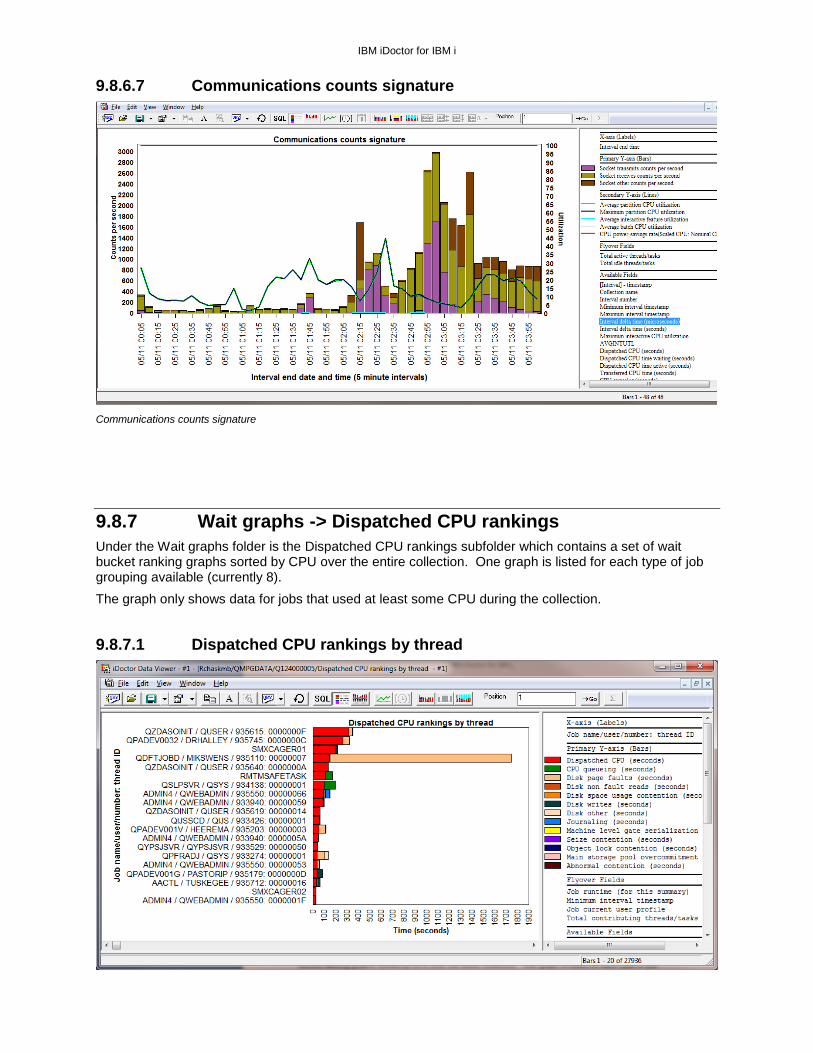
IBM iDoctor for IBM i
9.8.6.7 Communications counts signature
Communications counts signature
9.8.7 Wait graphs -> Dispatched CPU rankings
Under the Wait graphs folder is the Dispatched CPU rankings subfolder which contains a set of wait bucket ranking graphs sorted by CPU over the entire collection. One graph is listed for each type of job grouping available (currently 8).
The graph only shows data for jobs that used at least some CPU during the collection.
9.8.7.1 Dispatched CPU rankings by thread

IBM iDoctor for IBM i
Dispatched CPU rankings by thread
This graph shows the job/threads or system tasks that used the most CPU during the collection. Right-click to show options to graph it over time.
9.8.7.2 Dispatched CPU rankings by job
Dispatched CPU rankings by job
This graph shows the jobs (all threads added together) that used the most CPU during the collection.
9.8.7.3 Dispatched CPU rankings by job user
Dispatched CPU rankings by job user
This graph shows the job user name (all jobs having the same user name added together) that used the most CPU during the collection.

IBM iDoctor for IBM i
9.8.7.4 Dispatched CPU rankings by generic job
Dispatched CPU rankings by generic job
This graph shows the generic job name (all jobs starting with the same N set of characters) that used the most CPU during the collection. You can control the number of characters used in the generic job name grouping by using the option on the Data Viewer tab of Preferences.
9.8.7.5 Dispatched CPU rankings by current user
Dispatched CPU rankings by current user
This graph shows the current user profile (all job time periods that had having the same current user profile added together) that used the most CPU during the collection.

IBM iDoctor for IBM i
9.8.7.6 Dispatched CPU rankings by pool
Dispatched CPU rankings by pool
This graph shows the pool ID (all jobs in each pool added together) that used the most CPU during the collection.
9.8.7.7 Dispatched CPU rankings by priority
Dispatched CPU rankings by priority
This graph shows the job priority (all job time periods that had the same priority added together) that used the most CPU during the collection.

IBM iDoctor for IBM i
9.8.7.8 Dispatched CPU rankings by subsystem
Dispatched CPU rankings by subsystem
This graph shows the subsystems that used the most CPU during the collection.
9.8.8 Wait graphs -> Disk page fault rankings
Under the Wait graphs folder is the Disk page fault rankings subfolder which contains a set of wait bucket ranking graphs sorted by disk page faults time over the entire collection. One graph is listed for each type of job grouping available (currently 8).
The graph only shows data for jobs that had at least some disk page fault time during the collection.
These graphs are the same as the Dispatched CPU rankings graphs with the only difference being these graphs rank disk page faults instead of Dispatched CPU time.
Disk page faults rankings by thread

IBM iDoctor for IBM i
9.8.9 Wait graphs -> Disk time rankings (6.1+)
Under the Wait graphs folder is the Disk time rankings subfolder which contains a set of wait bucket ranking graphs sorted by total disk times (all disk wait buckets 5 through 10 added together) over the entire collection. One graph is listed for each type of job grouping available (currently 8).
The graph only shows data for jobs that had at least some disk time during the collection.
These graphs are the same as the Dispatched CPU rankings graphs with the only difference being these graphs rank disk times (all disk wait buckets 5 through 10 added together) instead of Dispatched CPU time.
Disk time rankings by generic job
9.8.10 Wait graphs -> Workload capping delay rankings
This set of graphs show the effects of workload capping for the desired workload capping group ID. You will be prompted to enter this value before opening any of these graphs.
Workload capping delay rankings graphs
To determine the group IDs for the workload capping group names on your system, view file QAPMSYSWLC from the server-side output files folder.

IBM iDoctor for IBM i
Server-side output files -> File QAPMSYSWLC
Change SQL Parameters -> Prompting for the workload capping group ID
9.8.10.1 Workload capping delay by thread
Workload capping delay by thread

IBM iDoctor for IBM i
This graph shows the effects of workload capping for the desired group ID, by thread.
9.8.11 Wait graphs -> Seizes and locks (6.1+)
These graphs show counts and the jobs experiencing record locks, object locks and seizes.
Wait graphs -> Seizes and locks
9.8.11.1 Record locks
Record locks
This graph is like the collection overview time signature but contains the number of process scoped record locks and thread scoped record locks on the 2nd Y-axis.

IBM iDoctor for IBM i
9.8.11.2 Object locks
Object locks
This graph is like the collection overview time signature but contains the number of process scoped object locks and thread scoped object locks on the 2nd Y-axis.
9.8.11.3 Seize counts
Seize counts
This graph is like the collection overview time signature but contains the total number of seizes on the 2nd Y-axis.
9.8.11.4 Record lock rankings
The seizes and locks record lock rankings graphs allow the user to group the record lock counts by any of the 8 types of job groupings.

IBM iDoctor for IBM i
Record locks by generic job
9.8.11.5 Object lock rankings
The seizes and locks object lock rankings graphs allow the user to group the object locks by any of the 8 types of job groupings.
Object locks by current user
9.8.11.6 Seize counts rankings
The seizes and locks seize counts rankings graphs allow the user to group the seize counts by any of the 8 types of job groupings.

IBM iDoctor for IBM i
Seize counts by job
9.8.11.7 Selected job grouping over time graphs
Any of the 3 types of rankings charts above can be drilled down from by right-clicking a job / current user / etc and picking the 1st option. The result graph will contain the wait buckets times for the desired item and the seizes or lock counts on the 2nd Y-axis. It will look something like this:
Seize counts for a job over time
9.8.12 CPU graphs
These graphs display the various types of CPU and CPU queuing in many different ways. Some graphs are only available at 6.1 or higher.
Note: Some graphs refer to jobs as “high priority” jobs. This is defined the SQL statements as priority 1 to 29. Low priority jobs have a priority of 30 to 99.

IBM iDoctor for IBM i
9.8.12.1 CPU utilization
CPU utilization
This graph breaks down the types of jobs and tasks that are using the CPU into 4 different categories:
1. System jobs
2. System tasks
3. Low priority jobs (excludes the system/IBM i jobs)
4. High priority jobs (excludes the system/IBM i jobs)
9.8.12.2 CPU utilization per job type
CPU utilization per job type
This graph is similar to the previous graph except it breaks down the categories of jobs into 8 types for more granularity.

IBM iDoctor for IBM i
9.8.12.3 Dispatched CPU breakdown and CPUQ
Dispatched CPU breakdown and CPUQ
This graph displays a breakdown of Dispatched CPU showing both the active and waiting (sharing) components along with CPU queuing. The typical CPU utilization fields are shown on the 2nd Y-axis.
9.8.12.4 Dispatched CPU/CPUQ usage by high/low priority
Dispatched CPU/CPUQ usage by high/low priority
This graph shows the Dispatched CPU and CPU queuing for both high and low priority jobs. The 2nd Y-axis displays a count of the number of high and low priority threads or tasks.

IBM iDoctor for IBM i
9.8.12.5 Dispatched CPU/CPUQ usage by high/low priority with CPU util
Dispatched CPU/CPUQ usage by high/low priority with CPU utilization
This graph is the same as the previous graph except the 2nd Y-axis contains the CPU utilization fields.
9.8.12.6 Scaled CPU ratio (6.1+)
Scaled CPU ratio
This graph shows the effects on the CPU because of energy saving features. If the value is 1 then there is no impact on the CPU.
9.8.12.7 Shared pool CPU utilization (6.1+)

IBM iDoctor for IBM i
Shared pool CPU utilization
This graph shows the amount of shared pool CPU utilization (Primary Y-axis) in relation to the normal CPU utilization fields (2nd Y-axis.)
9.8.12.8 Active processors
Active processors
This graph shows the current number of active processors over time along with the CPU utilization fields.
9.8.13 CPU graphs -> CPU consumed rankings
These graphs display the amount of “job” CPU (not the same thing as Dispatched CPU) grouped by one of the 8 job groupings:
1. CPU consumed by thread
2. CPU consumed by job
3. CPU consumed by job user

IBM iDoctor for IBM i
4. CPU consumed by generic job
5. CPU consumed by current user
6. CPU consumed by pool
7. CPU consumed by priority
8. CPU consumed by subsystem
CPU consumed by job
9.8.14 CPU graphs -> CPU utilization rankings
These graphs display the amount of CPU utilization grouped by one of the 8 job groupings:
1. CPU utilization by thread
2. CPU utilization by job
3. CPU utilization by job user
4. CPU utilization by generic job
5. CPU utilization by current user
6. CPU utilization by pool
7. CPU utilization by priority
8. CPU utilization by subystem

IBM iDoctor for IBM i
CPU utilization by generic job
9.8.15 System graphs (HMC) (6.1+)
These graphs show some key statistics (CPU, memory) about the entire system for all partitions.
The CPU data is captured through the HMC and stored in Collection Services file QAPMLPARH. You must be running POWER6 hardware and using firmware level xx340_061 or higher in order to collect this data.
For more information on collecting the CPU statistics for all partitions see this blog post:
http://ibmsystemsmag.blogs.com/i_can/2009/10/i-can-display-cpu-utilization-for-all-partitions.html
The following graphs are derived from the QAPMLPARH data:
System CPU utilization
System memory
System donated CPU time
Physical processor utilization
Shared memory pool data is also captured through the HMC and stored in file QAPMSHRMP. Data is
generated only when a partition is defined to use a shared memory pool. Data is reported
for both the partition's use of the pool as well as pool metrics that are the sum of activity
caused by all partitions using the pool. A POWER6® system with firmware level xx340_075 or later is required for this data to be available
The following graphs are derived from the QAPMSHRMP data:
Shared memory overview
Shared memory pool page faults
Memory for I/Os overview

IBM iDoctor for IBM i
9.8.15.1 LPAR CPU time
This graph shows the total CPU time used by each partition (on a physical system) along with the average CPU utilization over time.
Tip: If you have a large number of bars/colors, you can click the desired system/field in the legend to highlight a particular value.
9.8.15.2 LPAR cycles per instruction and CPU time
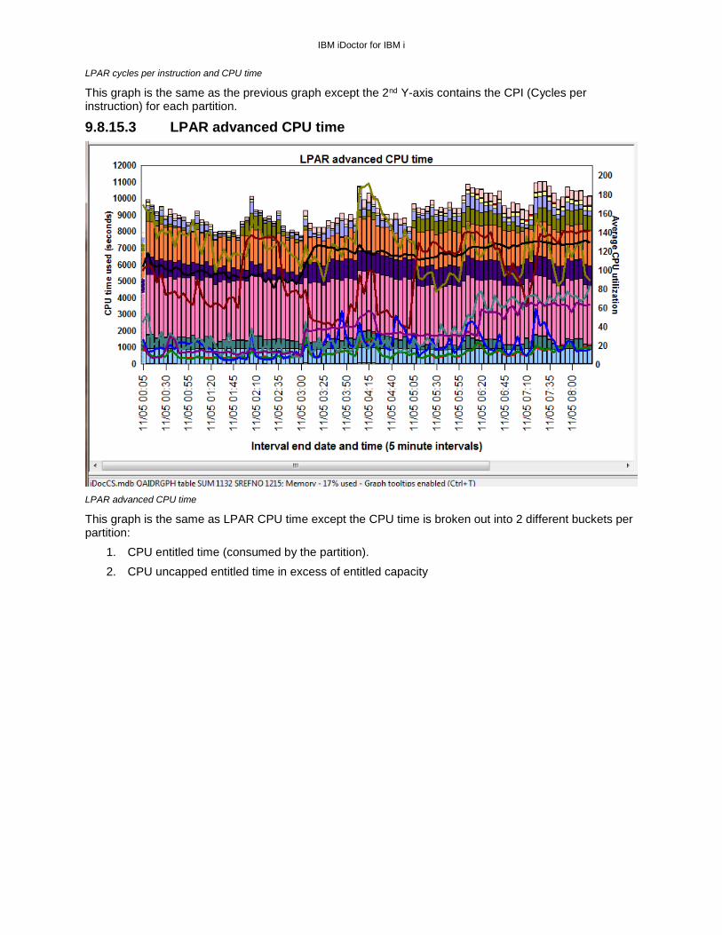
IBM iDoctor for IBM i
LPAR cycles per instruction and CPU time
This graph is the same as the previous graph except the 2nd Y-axis contains the CPI (Cycles per instruction) for each partition.
9.8.15.3 LPAR advanced CPU time
LPAR advanced CPU time
This graph is the same as LPAR CPU time except the CPU time is broken out into 2 different buckets per partition:
1. CPU entitled time (consumed by the partition).
2. CPU uncapped entitled time in excess of entitled capacity

IBM iDoctor for IBM i
9.8.15.4 LPAR memory allocated
LPAR memory allocated
This graph shows the amount of memory allocated per partition (in GBs.)
9.8.15.5 Virtual shared processor pool utilization (per virtual shared pool)
Virtual shared processor pool utilization (per virtual shared pool)
This graph shows each virtual shared pool processor pool (with each virtual shared processor pool ID having a different color) and the total CPU time consumed by all LPARs within each shared processor pool. The 2nd Y-axis shows the available CPU time.

IBM iDoctor for IBM i
9.8.15.6 Physical processor utilization graphs
These six graph shows the CPU utilization for different types of physical processors depending on the filter type shown in brackets next to the graph name.
Some examples follow:
Physical processor utilization overview
Physical processor utilization overview [borrowed state only]
9.8.16 System graphs (HMC) -> Rankings
These graphs are similar to the graphs in the previous section but instead of showing data over time, the partitions or processors are ranked.
Tip #1: Right-click the desired partition to drill into a graph showing just the selected partition over time.
Tip #2: Select 2 partitions and right-click and pick the 1st option to show a comparison graph of both.

IBM iDoctor for IBM i
9.8.16.1 LPAR CPU time (rankings)
LPAR CPU time (rankings)
This graph shows each partition’s total CPU time and average (and max) CPU utilization during the collection.
9.8.16.2 LPAR cycles per instruction and CPU time (rankings)
LPAR cycles per instruction and CPU time (rankings)
This graph is like the previous graph except the average partition’s cycles per instruction is shown on the 2nd Y-axis.

IBM iDoctor for IBM i
9.8.16.3 LPAR advanced CPU time (rankings)
LPAR advanced CPU time (rankings)
This graph shows the CPU entitled time and the CPU uncapped time that exceed the entitled capacity for each partition. The 2nd Y-Axis shows the average CPU utilization.
9.8.16.4 LPAR memory allocated (rankings)
LPAR memory allocated (rankings)
This graph displays each partition’s memory limits and memory allocated. The next graph was created by selecting the 1st two partitions in the graph above, right-clicking and picking the 1st option.

IBM iDoctor for IBM i
LPAR memory allocated graph comparison for two partitions
9.8.16.5 LPAR donated processor time (ranking)
This graph shows the amount of Donated CPU time for each partition.

IBM iDoctor for IBM i
9.8.16.6 Physical processor utilization
Physical processor utilization
This graph ranks each processor by the average physical CPU utilization. The processor ID is shown for each. The 2nd Y-axis displays the maximum processor utilization.
9.8.17 System graphs (HMC) -> Shared memory graphs
These graphs report information about shared memory pool usage. Data is reported for both the partition's use of the pool as well as pool metrics that are the sum of activity caused by all partitions using the pool. The data behind these graphs is created in file QAPMSHRMP.
Note: This data requires POWER6 system with firmware level xx340_075 (or higher.)
9.8.17.1 Shared memory overview
Shared memory overview
This graph shows the rate of I/O memory mapping delays, real memory page faults and shared pool page faults.

IBM iDoctor for IBM i
9.8.17.2 Shared memory pool page faults
Shared memory pool page faults
9.8.17.3 Memory for I/Os overview
This graph shows entitled, optional, actual and maximum memory entitled to perform I/Os.
9.8.18 Memory pool graphs
These graph displays memory pool statistics over time. There are three types of graphs provided:
1. Default type (where a limited number of pools can be shown)
2. Flattened type (where any number of pools can be shown)
3. Large pool sizes ( where pool sizes > 1 TB)

IBM iDoctor for IBM i
9.8.18.1 Memory pool consumption [by percentage]
Memory pool consumption [by percentage]
This default type graph displays up to 24 pools on the primary Y-axis showing the memory consumed and up to 6 pools on the 2nd Y-axis showing faults per second. The memory consumed is shown as a percentage of the total memory available.
9.8.18.2 Memory pool sizes [by percentage]
Memory pool sizes [by percentage]
This default type graph is similar to the previous one except memory pool sizes are shown instead of memory pool consumption.

IBM iDoctor for IBM i
9.8.18.3 Machine pool sizes and rates
Machine pool sizes and rates
This graph just shows the pool size and faulting rates for the machine (base) pool. A machine pool faulting guideline is also displayed as a green line (with a constant value of 10 faults per second.)
9.8.18.4 64K versus 4K page faults for pool <<JBPOOL>>
The graph is intended for IBM service use.
64K versus 4K page faults for pool 1
9.8.19 Memory pool graphs -> Flattened type
These graphs are similar the previous set except there are no limits to the number of memory pools they can show. Also some of the graphs in this folder are not available in the previous folder.
Tip: From these graphs you can right-click a pool to be able to graph any of the job statistics just for the desired pool. Use the “Selected Pool” menu for an over-time graph, and the “Rankings filtered by selected pool” to show a rankings graph filtered by the desired pool.

IBM iDoctor for IBM i
9.8.19.1 Memory pool sizes
Memory pool sizes
This graph displays the memory pool sizes for each pool over time with the faults per second on the 2nd Y-axis.
9.8.19.2 Page fault rates
Page fault rates
This graph is the same as the previous one except the pool sizes and page faults are flipped on opposite Y-axes.

IBM iDoctor for IBM i
9.8.19.3 Memory pool activity levels
Memory pool activity levels
This graph show the average pool activity level for all pools on the primary Y-axis and the pool sizes on the 2nd Y-axis.
9.8.19.4 Transitions to ineligible rates
This graph displays the rates of state transitions to ineligible per second.
9.8.19.5 State transition rates
State transition rates
This graph shows 3 types of state transitions for each memory pool over time.
1. Active to wait transitions per second

IBM iDoctor for IBM i
2. Wait to ineligible transitions per second
3. Active to ineligible transitions per second
9.8.19.6 DB vs non-DB faulting rates
DB vs non-DB faulting rates
This graph shows for every pool:
1. Database faults per second
2. Non-database faults per second
3. Pool size (in megabytes) on the 2nd Y-axis.

IBM iDoctor for IBM i
9.8.19.7 DB vs non-DB paging [pages read/written] rates
DB vs non-DB paging [pages read/written] rates
This graph shows for every pool:
1. Database paging (pages read/written) per second
2. Non-database paging (pages read/written) per second
3. Pool size (in megabytes) on the 2nd Y-axis
9.8.20 Memory pool graphs (for pool sizes > 1 TB)
These graphs are only necessary if you have very large pool sizes that exceed the sizes for the pool fields in file QAPMPOOLB.
All of the graphs described in the previous two sections are provided within this set of graphs except for the 64K versus 4K page faults graph.
Note: These graphs won’t work, if the newer version of file QAPMPOOLB containing an additional set of pool size fields that can handle the larger sizes does not exist in your data library. You will receive an SQL error when trying to open them.
9.8.21 Job counts graph
These graphs display the number of jobs/tasks/threads that exist on the system in several different ways. You can generate list of job counts by a job grouping (by job, by job user, generic job, etc.)
Tip: You can select a time period and right-click to drill down to view the names of the tasks/jobs/threads behind these counts shown.

IBM iDoctor for IBM i
9.8.21.1 Job counts
Job counts
This graph simply shows the number of tasks, processes (primary threads) and secondary threads over time. The 2nd Y-axis displays the CPU utilization fields.
9.8.21.2 Short-lived job counts
Short-lived job counts

IBM iDoctor for IBM i
This graph displays all of the jobs/tasks/threads that only survived for 1 collection services data collection interval or less. This varies but is often set to 5 minutes or 15 minutes.
9.8.21.3 Net jobs created
Net jobs created
This graph displays the net number of jobs/tasks/threads created over time.
9.8.21.4 Net jobs breakdown
Net jobs breakdown
This graph is the same as the previous graph except the net created values for each of tasks, jobs and secondary threads are shown.

IBM iDoctor for IBM i
9.8.21.5 Jobs created/destroyed
Jobs created/destroyed
This graph displays the number of jobs created and destroyed each interval with side-by-side bars.
9.8.22 Job counts graphs -> Job counts rankings
These graphs show the total job counts for any of the job groupings (except thread.) An example is shown below:
Job counts by generic job
Tip: These graphs show data for the entire collection, but you can also drill down into these from the previous graphs in the Job counts folder.

IBM iDoctor for IBM i
9.8.23 Job counts graphs -> Net jobs breakdown rankings
These graph display the net number of jobs/tasks/threads created as a rankings chart for any of the job groupings (except thread.) An example is shown below:
Net jobs breakdown by pool
9.8.24 Job counts graphs -> Short-lived counts rankings
These graph display counts of the short-lived jobs/tasks/threads as a rankings chart for any of the job groupings (except thread.) The short-lived counts refers to jobs/threads/tasks that only lived for a single Collection Services data collection interval or less. An example is shown below:
Short-lived job counts by subsystem
9.8.25 I/O and memory page graphs
These graphs show physical and logical I/Os, pages allocated and page faults as either totals or rates per second over time. Memory page demand and net page frames requested are also included in this folder.
Tip: You can right-click a time interval or interest and pick the top drilldown menu option to graph the same data as a (job/thread/generic job/etc) rankings graph.

IBM iDoctor for IBM i
9.8.25.1 Memory page demand (6.1+)
This graph displays the memory pages requested and released which gives a sense of how much memory is being utilized by the jobs captured by Collection Services.
The bars display the total of the page frames requested and released. The 2nd Y-axis displays the 2 values as separate lines instead.
Below is an example of how to drill down into the generic jobs behind the memory page demand shown above:

IBM iDoctor for IBM i
9.8.25.2 Net page frames requested (6.1+)
This graph is like the memory page demand graph except it just shows the Net memory pages requested. A negative value indicates that more pages were released than requested in that time interval.
9.8.25.3 Pages allocated/deallocated (overlapping bars)
Pages allocated/deallocated (overlapping bars)
This graph displays the total size of pages allocated and deallocated (in megabytes) shown with overlapping bars. The larger value will be on top for each bar. The net pages allocated is shown on the 2nd Y-axis.

IBM iDoctor for IBM i
9.8.25.4 Reads and writes
Reads and writes totals
This section covers the following graphs:
1. Reads and writes totals
2. Reads and writes rates
These graphs displays the reads and writes over time (either as a total or as a rate per second) that were found in the job statistics data (file QAPMJOBMI.) The 2nd Y-Axis displays the faults per second along with the I/O pending page faults.
9.8.25.5 Physical disk I/Os
Physical disk I/O rates
This section covers the following graphs:
1. Physical disk I/O totals
2. Physical disk I/O rates

IBM iDoctor for IBM i
These graphs displays the 8 physical disk I/O counters for sync and async, DB and non-DB reads and writes over time (either as a total or as a rate per second) that were found in the job statistics data (file QAPMJOBMI.) The 2nd Y-Axis displays the faults per second along with the I/O pending page faults.
A red color is used for the 4 types of reads and a green color is used for the 4 types of writes.
9.8.25.6 Logical database I/Os
Logical database I/O totals
This section covers the following graphs:
1. Logical database I/O totals
2. Logical database I/O rates
These graphs shows the logical I/Os over time. This includes reads, writes and others (updates + deletes.)
9.8.26 I/O and memory page graphs -> Rankings
Several different ranking graphs are provided within the I/O and memory page graphs folder. Each of these graph folder provides all 8 job grouping options (thread, job, job user, generic job, current user, pool, priority and subsystem.) The available ranking graph folders (88 individual graphs) are:
1. Memory page demand rankings
2. Net page frames rankings
3. Pages allocated rankings
4. Reads and writes totals rankings
5. Reads and writes rates rankings
6. Physical disk I/O totals rankings
7. Physical disk I/O rates rankings
8. Page fault totals rankings
9. Page fault rates rankings
10. Logical database I/O totals rankings

IBM iDoctor for IBM i
11. Logical database I/O rates rankings
Some examples are shown below:
Page fault totals by generic job
Reads and writes totals by current user
Tip: You can drill down from any of these ranking graphs by selecting the desired job entries and right-clicking and choosing the 1st menu option. This will graph your selection over time using the same graph metrics.
9.8.27 Disk configuration
These reports display information about the system’s disk configuration including the ASPs, IOPs and IOAs.
9.8.27.1 Capacity (in GBs) by ASP with paths
Capacity (in GBs) by ASP with paths

IBM iDoctor for IBM i
This report displays each ASP and type of disk with the total disk units and total paths for each provided along with additional information.
9.8.27.2 Capacity (in GBs) by ASP/IOP with paths
Capacity (in GBs) by ASP/IOP with paths
This report is similar to the previous report except it also includes the data for each IOP.
9.8.27.3 Capacity (in GBs) by ASP/IOP/IOA with paths
Capacity (in GBs) by ASP/IOP with paths
This report is similar to the first report except it also includes the data for each IOP and IOA.

IBM iDoctor for IBM i
9.8.27.4 Disk configuration
Disk configuration
This report lists the complete disk configuration of a partition.
9.8.27.5 Disk configuration (non-operational disks only)
This report is the same as the previous one, except it only lists disks that are detected as not operational when the collection was taken.

IBM iDoctor for IBM i
9.8.27.6 Disk configuration (tree) by ASP/IOP/IOA/Unit
Disk configuration (tree) without disk units shown
This report lets you expand/collapse individual sections of the disk configuration as desired.
Disk configuration (tree) with disk units shown

IBM iDoctor for IBM i
9.8.28 SSD candidate screening (7.1+)
These reporting options are designed to help a user determine if the system would be a good candidate for installing SSDs. The graphing options are filtered by the desired ASP, which lets you focus on a single ASP at a time.
SSD candidate screening options
9.8.28.1 SSD screening summary for ASP <<DSASP>>
When opening this report you may be prompted for the ASP desired to analyze if more than 1 is detected.
It simply indicates an overview of how likely it is that SSDs would improve performance. This is tested by looking at the average read response time for each Collection Services interval and categorizing the intervals into 3 groups:
1. Read response time > 3.5 ms = “likely to improve performance”
2. Read response time between 1.5 and 3.5 ms = “may improve performance”
3. Read response time < 1.5 ms = “unlikely to improve performance”

IBM iDoctor for IBM i
SSD screening summary for ASP 1
9.8.28.2 SSD screening details for ASP <<DSASP>>
SSD screening details for ASP 1
This graph is similar to the previous graph except it shows the data over time for each interval and also displays the average response time and average read and write response times on the 2nd Y-axis for more granularity.

IBM iDoctor for IBM i
9.8.28.3 I/O totals for ASP <<DSASP>>
I/O totals for ASP 1
This graph shows the total reads and writes along with the response times on the 2nd Y-axis.
9.8.29 SSD candidate screening -> job details
This folder contains a single report that looks at the total reads and average read response time on a per job basis.
9.8.29.1 SSD screening details by job
SSD screening details by job
This report lists the jobs in the collection and sorts the data by total disk read wait time (in seconds.) It helps to isolate which jobs are performing disk reads and might be helped by installing SSDs in order to improve disk read response time.

IBM iDoctor for IBM i
9.8.30 Disk graphs
A large number of disk reporting options are available within this folder. This data is based primarily on data found within Collection Services file QAPMDISK. Several different groupings are available as well, which behave similarly in design to the job groupings. Each of these grouping (rankings) folders contain the same set as graphs from the “over-time” set. You can drill down from the over-time graphs into these rankings graphs. These groupings are:
1. By disk path
2. By disk unit
3. By I/O processor
4. By ASP
5. By disk type
6. By I/O adapter (6.1+)
One limitation of file QAPMDISK however is it does not separate out read response times from write response times. At 7.1 however file QAPMDISKRB was added to the system in order to accomplish this and to also provide response time buckets for both reads and writes. These options are included under the Disk graphs -> Advanced folder.
Note: At 5.4, the latest version of file QAPMDISK should be used, otherwise a much smaller set of graphs will be shown. In most cases this will not be a problem however because the PTFs for this update were released many years ago.
For more information about the metrics in these graphs visit the following page:
http://pic.dhe.ibm.com/infocenter/iseries/v7r1m0/topic/rzahx/rzahxqapmdisk.htm?resultof=%22%51%41%50%4d%44%49%53%4b%22%20%22%71%61%70%6d%64%69%73%6b%22%20
9.8.30.1 Disk percent busy for ASP <<DSASP>>
Disk percent busy for ASP 1
This graph displays the (average) disk percent busy for the desired ASP(s), along with the average response times on the 2nd Y-axis. Both the average response time and average service time are provided.

IBM iDoctor for IBM i
9.8.30.2 Buffer overruns/underruns for ASP <<DSASP>>
Buffer overruns/underruns for ASP 1
Buffer overruns are the number of times that data was available to be read into the disk controller buffer from the disk, but the disk controller buffer still contained valid data that was not retrieved by the storage device controller. Consequently, the disk had to take an additional revolution until the buffer was available to accept data.
Buffer underruns are the number of times that the disk controller was ready to transfer data to the disk on a write, but the disk controller buffer was empty. The data was not transferred in time by the disk IOP to the disk controller buffer. The disk was forced to take an extra revolution awaiting the data.
This graph also displays the average response times on the 2nd Y-axis.
9.8.30.3 I/O counts totals for ASP <<DSASP>>
I/O counts totals for ASP 1
This graph displays the total number of reads and writes along with the average response times on the 2nd Y-axis.

IBM iDoctor for IBM i
9.8.30.4 I/O counts categorized totals for ASP <<DSASP>>
I/O counts categorized totals for ASP 1
This graph displays the number of I/Os that occurred based on their response times. Six response time buckets are used each with a different color. The overall average response times are shown on the 2nd Y-axis.
9.8.30.5 I/O size totals for ASP <<DSASP>>
I/O size totals for ASP 1
This graph displays the total I/O size (in megabytes) for both reads and writes that occurred over time. The 2nd Y-axis displays the overall average disk percent full (from each disk unit) for the ASPs selected.
9.8.30.6 I/O size averages for ASP <<DSASP>>

IBM iDoctor for IBM i
I/O size averages for ASP <<DSASP>>
This graph shows the average I/O size (in kilobytes) for both reads and writes. The 2nd Y-axis displays the overall average disk percent full (from each disk unit) for the ASPs selected.
9.8.30.7 I/O size rates with cache statistics for ASP <<DSASP>>
I/O size rates with cache statistics for ASP 1
This report displays the size of all disk reads and disk writes as megabytes per second.
The cache statistics shown on the 2nd Y-axis includes write cache overruns, write cache efficiency and read cache hits.

IBM iDoctor for IBM i
9.8.30.8 I/O size and Ethernet rates
I/O size and Ethernet rates
This graph combines I/O size rates (in megabytes per second) with Ethernet transmission rates. The 2nd Y-axis shows Ethernet MAC errors and frame retries.
9.8.30.9 I/O size and Ethernet rates with total MB/sec
I/O size and ethernet rates with total MB/sec
This graph is the same as the previous one except the total I/Os per second for both the disk and Ethernet portion are added up on the 2nd Y-axis.

IBM iDoctor for IBM i
9.8.30.10 I/O rates totals for ASP <<DSASP>>
I/O rates totals for ASP 1
This graph shows the reads per second and writes per second over time. The 2nd Y-axis displays the average response times.
9.8.30.11 I/O rates totals with cache statistics for ASP <<DSASP>>
I/O rates totals with cache statistics for ASP 1
This graph is the same as previous graph except it shows the cache statistics on the 2nd Y-axis.

IBM iDoctor for IBM i
9.8.30.12 I/O rates categorized totals for ASP <<DSASP>>
I/O rates categorized totals for ASP 1
This graph displays the I/Os per second that occurred based on their response times. Six response time buckets are used each with a different color. The overall average response times are shown on the 2nd Y-axis.
9.8.30.13 I/O rates categorized totals with cache statistics for ASP <<DSASP>>
I/O rates categorized totals with cache statistics for ASP 1
This graph is the same as the previous one except it shows the cache statistics on the 2nd Y-axis.

IBM iDoctor for IBM i
9.8.30.14 I/O total response time categorized totals for ASP <<DSASP>>
I/O total response time categorized totals for ASP 1
This graph adds up the total response times for all I/Os and shows them with different colors based on the six response time buckets. The 2nd Y-axis displays the overall average response times.
9.8.30.15 I/O total service time categorized totals for ASP <<DSASP>>
I/O total service time categorized totals for ASP 1
This graph adds up the total service (hardware) times for all I/Os and shows them with different colors based on the six response time buckets. The 2nd Y-axis displays the overall average response times.

IBM iDoctor for IBM i
9.8.30.16 I/O average response time categorized totals for ASP <<DSASP>>
I/O average response time categorized totals for ASP 1
This graph displays the average response time on a per response time bucket basis. For that reason the smaller 3 buckets will rarely be visible on the graph.
9.8.30.17 I/O avg service and wait time categorized totals for ASP <<DSASP>>
I/O avg service and wait time categorized totals for ASP 1
This graph displays the average response times and average service times on a per response time bucket basis. For that reason the smaller 3 buckets for both the service and response times will rarely be visible on the graph.

IBM iDoctor for IBM i
9.8.30.18 Average device operations rate for ASP <<DSASP>>
Average device operations rate for ASP 1
This graph shows the average device operations rate for all disk units within the specified ASPs.
9.8.30.19 Total queue elements and avg length for ASP <<DSASP>>
Total queue elements and avg length for ASP 1
This graph shows the total queue elements and average queue length for all the disk units within the selected ASPs.
9.8.31 Disk graphs -> by disk path
These graphs are the same as the ones within the disk graphs folder over time, except these are ranking graphs grouped by the disk path (or disk unit and device resource name.)
Tip: You can drill down into any of these ranking graphs from the disk overview graphs by selecting the desired time period and right-clicking and choosing the 1st menu.
An example of this type of graph is shown below:

IBM iDoctor for IBM i
(By disk path) – I/O rates totals
9.8.32 Disk graphs -> by disk unit
These graphs are the same as the ones within the disk graphs folder over time, except these are ranking graphs grouped by the disk unit.
Tip: You can drill down into any of these ranking graphs from the disk overview graphs by selecting the desired time period and right-clicking then Rankings -> Disk graphs -> by disk unit.
An example of this type of graph is shown below:
(By disk unit) – I/O rates categorized totals for ASP 1
9.8.33 Disk graphs -> by I/O processor
These graphs are the same as the ones within the disk graphs folder over time, except these are ranking graphs grouped by I/O processor.
Tip: You can drill down into any of these ranking graphs from the disk overview graphs by selecting the desired time period and right-clicking then Rankings -> Disk graphs -> by I/O processor.

IBM iDoctor for IBM i
An example of this type of graph is shown below:
(By I/O processor) – I/O size averages
9.8.34 Disk graphs -> by ASP
These graphs are the same as the ones within the disk graphs folder over time, except these are ranking graphs grouped by ASP.
Tip: You can drill down into any of these ranking graphs from the disk overview graphs by selecting the desired time period and right-clicking then Rankings -> Disk graphs -> by ASP.
An example of this type of graph is shown below:
(By ASP) – I/O rates totals
9.8.35 Disk graphs -> by disk type
These graphs are the same as the ones within the disk graphs folder over time, except these are ranking graphs grouped by disk type.

IBM iDoctor for IBM i
Tip: You can drill down into any of these ranking graphs from the disk overview graphs by selecting the desired time period and right-clicking then Rankings -> Disk graphs -> by disk type.
An example of this type of graph is shown below:
(By disk type) – I/O counts categorized totals
9.8.36 Disk graphs -> by I/O adapter (6.1+)
These graphs are the same as the ones within the disk graphs folder over time, except these are ranking graphs grouped by I/O adapter (IOA.)
Tip: You can drill down into any of these ranking graphs from the disk overview graphs by selecting the desired time period and right-clicking then Rankings -> Disk graphs -> by I/O adapter
An example of this type of graph is shown below:
(By I/O adapter) – Disk percent busy

IBM iDoctor for IBM i
9.8.37 Disk graphs -> Advanced (7.1+)
These graphs are only available if the 7.1 Collection Services file QAPMDISKRB has been captured. The focus on these graphs is to show response times for both reads and writes. Some of the graphs (those that start with the word “advanced” display 11 response time buckets for reads and/or writes.
9.8.37.1 Reads and writes for ASP <<DSASP>>
Reads and writes for ASP 1
This graph displays the reads per second, writes per second along with read and write response times on the 2nd Y-axis. The average of both is also shown as the orange line.
9.8.37.2 I/O size rates for ASP <<DSASP>>

IBM iDoctor for IBM i
I/O size rates for ASP 1
This graph shows the writes per second and reads per second (in megabytes) along with the response times on the 2nd Y-axis.
9.8.37.3 Advanced I/O totals for ASP <<DSASP>>
Advanced I/O totals for ASP 1
This graph displays total I/O counts by grouping the counts into 11 response time buckets for both reads and writes. The 2nd Y-axis displays the following 5 response time values:
1. Average response time (overall)
2. Average read response time
3. Average read service response time
4. Average write response time
5. Average write service response time
Tip: The legend will most likely not show all 11 buckets for both reads and writes. By design the graph legend on the primary Y-axis only shows fields with non-zero values.

IBM iDoctor for IBM i
9.8.37.4 Advanced write totals for ASP <<DSASP>>
Advanced write totals for ASP 1
This graph is the same as the previous one except it only shows the write buckets on the Primary Y-axis.
9.8.37.5 Advanced read totals for ASP <<DSASP>>
Advanced I/O reads for ASP <<DSASP>>
This graph is the same as the Advanced I/O totals graph except it only shows the read buckets.

IBM iDoctor for IBM i
9.8.37.6 Advanced I/O rates totals for ASP <<DSASP>>
Advanced I/O rates totals for ASP 1
This graph displays the I/Os per second for both reads and writes using 11 response time buckets.
9.8.37.7 Advanced write rates for ASP <<DSASP>>
Advanced write rates for ASP <<DSASP>>
This graph is the same as the previous one except it only shows the write response time buckets.

IBM iDoctor for IBM i
9.8.37.8 Advanced read rates for ASP <<DSASP>>
Advanced read rates for ASP
This graph is the same as the Advanced I/O rates totals graph except it only shows the read buckets.
9.8.37.9 Advanced total response times for ASP <<DSASP>>
Advanced total response times for ASP 1
This graph adds up the total response time for all 11 buckets for both reads and writes.
9.8.37.10 Advanced write response times for ASP <<DSASP>>
This graph is the same as the previous graph except only shows the write response times.

IBM iDoctor for IBM i
9.8.37.11 Advanced read response times for ASP <<DSASP>>
This graph is the same as the previous graph except only shows the read response times.
9.8.37.12 Advanced total service times for ASP <<DSASP>>
Advanced total service times for ASP 1
This graph displays the total service time all 11 response time buckets for both reads and writes.
9.8.37.13 Advanced write service times for ASP <<DSASP>>
This graph is the same as the previous graph except only shows the write service times.
9.8.37.14 Advanced read service times for ASP <<DSASP>>
This graph is the same as the previous graph except only shows the read service times.

IBM iDoctor for IBM i
9.8.37.15 Advanced average response time for ASP <<DSASP>>
Advanced average response time for ASP 1
This graph displays the average response times within each of the 22 response time buckets. 11 buckets for reads and 11 for writes.
9.8.38 Disk graphs -> advanced -> by disk path
These graphs are the same as the set of graphs within the Disk graphs -> advanced folder except they are grouped by disk path (or disk unit and device resource name.)
Tip: You can drill down into any of these ranking graphs from any of the disk graphs -> advanced folder’s graphs by selecting the desired time period and right-clicking and choosing the 1st menu.
An example of this type of graph is shown below:
(By disk path) – Advanced write rates

IBM iDoctor for IBM i
9.8.39 Disk graphs -> advanced -> by disk unit
These graphs are the same as the set of graphs within the Disk graphs -> advanced folder except they are grouped by disk unit.
Tip: You can drill down into any of these ranking graphs from any of the disk graphs -> advanced folder’s graphs by selecting the desired time period and right-clicking and choosing the Rankings -> disk graphs -> advanced -> by disk unit menu.
An example of this type of graph is shown below:
(By disk unit) – Advanced write rates
9.8.40 Disk graphs -> advanced -> by I/O processor
These graphs are the same as the set of graphs within the Disk graphs -> advanced folder except they are grouped by I/O processor (IOP.)
Tip: You can drill down into any of these ranking graphs from any of the disk graphs -> advanced folder’s graphs by selecting the desired time period and right-clicking and choosing the Rankings -> disk graphs -> advanced -> by I/O processor menu.
An example of this type of graph is shown below:

IBM iDoctor for IBM i
(By I/O processor) – Reads and writes
9.8.41 Disk graphs -> advanced -> by ASP
These graphs are the same as the set of graphs within the Disk graphs -> advanced folder except they are grouped by ASP.
Tip: You can drill down into any of these ranking graphs from any of the disk graphs -> advanced folder’s graphs by selecting the desired time period and right-clicking and choosing the Rankings -> disk graphs -> advanced -> by ASP menu.
An example of this type of graph is shown below:
(By ASP) – Advanced total service times

IBM iDoctor for IBM i
9.8.42 Disk graphs -> advanced -> by disk type
These graphs are the same as the set of graphs within the Disk graphs -> advanced folder except they are grouped by disk type.
Tip: You can drill down into any of these ranking graphs from any of the disk graphs -> advanced folder’s graphs by selecting the desired time period and right-clicking and choosing the Rankings -> disk graphs -> advanced -> by disk type menu.
An example of this type of graph is shown below:
(By disk type) – Advanced read rates
9.8.43 Disk graphs -> advanced -> by I/O adapter
These graphs are the same as the set of graphs within the Disk graphs -> advanced folder except they are grouped by I/O adapter (IOA.)
Tip: You can drill down into any of these ranking graphs from any of the disk graphs -> advanced folder’s graphs by selecting the desired time period and right-clicking and choosing the Rankings -> disk graphs -> advanced -> by I/O adapter menu.
An example of this type of graph is shown below:

IBM iDoctor for IBM i
(By I/O adapter) – Advanced read totals
9.8.44 IFS graphs
The IFS graphs are essentially the same as the set of IFS graphs available in Job Watcher. The provide IFS-related statistics for reads, lookup cache hits/misses, opens and directory creates/deletes.
9.8.44.1 IFS read totals
IFS read totals
This graph displays the total IFS symbolic link reads and directory reads on the primary Y-axis and the CPU utilization fields on the 2nd Y-axis.

IBM iDoctor for IBM i
9.8.44.2 IFS read rates
IFS read rates
This graph is the same as the previous one except the values are shown as a rate per second.
9.8.44.3 IFS lookup cache totals
IFS lookup cache totals
This graph displays the total IFS lookup cache hits and misses over time. The 2nd Y-axis displays CPU utilization.

IBM iDoctor for IBM i
9.8.44.4 IFS lookup cache rates
IFS lookup cache rates
This graph is the same as the previous one except the values on the Primary Y-axis are shown as a rate per second.
9.8.45 IFS ranking graphs
A set of IFS rankings graphs are provided within 8 subfolders of the IFS graphs folder. Each folder contains the 8 possible job groupings to choose from. The following ranking graph folders are available:
IFS read totals rankings
IFS read rates rankings
IFS lookup cache totals rankings
IFS lookup cache rates rankings
IFS open totals rankings
IFS open rates rankings
IFS create/delete totals rankings
IFS create/delete rates rankings
An example is shown below:
IFS lookup cache totals by generic job

IBM iDoctor for IBM i
9.9 Analyzing Collection Services Data Analyzing Collection Services data effectively consists of the use of many graphs and reports available within the collections. Some information on how to analyze and use the iDoctor (Job Watcher) graphs is provided in demos on the website and additional ones will be added. The Job Watcher graphs are very similar to the CSI graphs. Visit the following page to access the current iDoctor demos: https://www-912.ibm.com/i_dir/idoctor.nsf/videos.html Tip: Use the graph compare function by clicking the graph compare icon on the toolbar of the main window. This will allow you to view two graphs at once with synchronized scrolling. The graph compare function is either on (if pressed in the toolbar on Main Window) or off. Any graph opened while the compare mode is on will produce a split view two areas used to analyze graphs. Either an alternate view graph can be used as the comparison graph or the clock icon can be pressed to compare graphs of different interval sizes.

IBM iDoctor for IBM i
10 Disk Watcher
This chapter provides an overviw of the interfaces within the IBM iDoctor for IBM i - Disk Watcher component. The Disk Watcher component provides a number of interfaces designed to help the user analyze disk performance problems on IBM i.
10.1 Starting Disk Watcher Disk Watcher is a component of the iDoctor suite of tools. iDoctor can be started using the Start menu: Start->Programs->IBM iDoctor for IBM i. Once the IBM iDoctor for IBM i application appears, the Disk Watcher component is started from the Connection List View by double-clicking on the desired system. A list of available components will appear on the next window. Double-click on the Disk Watcher component or select Disk Watcher and click the Launch button in order to continue
iDoctor Components View
10.2 Disk Watcher Component View

IBM iDoctor for IBM i
Disk Watcher Component View The 'Disk Watcher' folder contains a list of folders, each providing different features available. Collections can be displayed in various ways, either under the Libraries folder on a per library basis, or under the Monitors or Super Collections folders for Disk Watcher collections that exist within a monitor or Super Collection.
10.2.1 Menu Options The following Disk Watcher specific menu options are available by right clicking on the 'Disk Watcher' icon in the component view above:
Menu Item Description
Add Definition This option displays the Add Disk Watcher Definition Wizard.. The definition defines characteristics about the collection such as which data options to collect. At 6.1 or higher a definition is required when starting a collection.
Start Collection This menu will open the Start Disk Watcher Wizard where the user can define and run a collection. At 6.1 or higher a definition must be defined first before creating a collection unless you wish to use an IBM-supplied definition.
Start Monitor This menu will open the Start Monitor Wizard for iDoctor where the user can start a Job Watcher, PEX Analyzer or Disk Watcher monitor. Monitors are designed to provide 24x7 collection of performance data.
Descriptions for additional menu options that are common to all components can be found here.
10.3 Libraries This folder contains the libraries on the system that contain Job Watcher data (specifically the libraries containing file QAPDJWRUNI). The list displays each library's name and description. By clicking on a library in the tree you will see its contents (the collection(s) that exist in the library)

IBM iDoctor for IBM i
Libraries in the Disk Watcher Component View
Note: The method in which the list of libraries is built can be controlled by using the "Preferences -> SQL -> Use SQL catalog tables to improve performance" option. If checked the SQL catalog tables are used to build the list, otherwise the older/slower, but sometimes more reliable method of using IBM i APIs is used. If you get an error "Invalid cursor state" or "SQL system error" when building the list of libraries then try unchecking this option.
10.3.1 Menu Options The following menu options are available by right clicking on a library in the component view.
Menu Item Description
Start Collection... This menu will open the collection wizard for Disk Watcher where the user can define and run a collection. At 6.1+, a definition must be defined first before creating a collection unless you wish to use an IBM-supplied definition.
Additional menu options that are common to all library folders in iDoctor are discussed here.
10.4 Monitors Disk Watcher monitors allow for 24x7 collection of Disk Watcher data on a system. They run continuously storing only the most recent collections desired. Disk Watcher monitors will run until ended manually by the user. Monitors can be held and released if the user wishes to stop collecting data for now and then continue collection again later. Monitors can also be scheduled to start and end at the desired times. Once a monitor has been started and ended, it must be restarted using the Restart Monitor option. You cannot use the Start New Monitor option to restart an existing monitor. A Monitors folder is provided in Disk Watcher to allow the user to work with the monitors that exist on the current system. For more information about monitors, see the section on Monitors in chapter 4.

IBM iDoctor for IBM i
10.5 Super Collections For more information, see the Super Collections section in chapter 4.
10.6 Definitions A Definitions folder is provided in Disk Watcher to allow the user to work with the Disk Watcher definitions that exist on the current system. An example of this interface is:
Disk Watcher Definitions Folder The fields shown in this view are as follows:
Field Description
Definition Name of the definition. IBM-supplied definitions begin with Q.
Description An optional description given to the Disk Watcher definition
Command The command string used to create the definition.
The following options are available when right clicking on one or more definitions in the list:
Field Description
Change Definition Opens the Add Disk Watcher Definition Wizard and loads the selected definition into it so it can be changed.
Add Definition Opens the Add Disk Watcher Definition Wizard in order to create a new definition.
Start Collection Opens the Start Disk Watcher Collection Wizard using the selected definition.
Start Monitor Opens the Start iDoctor Monitor Wizard using the selected definition.
Delete Removes the selected definitions from the system.
Properties Displays the properties for the selected Disk Watcher definition.
10.6.1 Properties Double-clicking on a definition or using the Properties menu from the Disk Watcher Definitions View displays all of the parameters that were used when creating the definition. An example of this interface is:

IBM iDoctor for IBM i
Disk Watcher Definition Properties
Advanced users can change the command string that defines the definition if desired. If changes have been made to the command string, pressing the OK button will remove the existing definition from the system and replace it using the command string specified. Note: IBM-supplied definitions cannot be changed.
10.7 Collections Moving down the tree within each Library folder are one or more collections that have been created or are currently being created within the current library.

IBM iDoctor for IBM i
Disk Watcher Collections in a Library Tip: Collections that contain Trace data can be summarized at V5R3 and higher to produce several Trace only graphs and reports. If a collection has been summarized the Collection summary available/status field will display ‘Yes’.
10.7.1 Collection Fields The list of collections displays the collection name, description, status as well as several additional fields. Each collection in the list has a set of fields available which can be optionally reordered and displayed. To change the current field selections for the collection list, use the Select fields... menu from the library folder. A listing of the available fields and a short description is provided in the table below:

IBM iDoctor for IBM i
Field Description
Collection Name of the collection. This name matches the member name used in the database files named QAPYDW* that exist in the current library.
Status The status field indicates the status of the job on the system running the collection (if active) or if not active the status indicates whether or not the collection is ready for use.
Ending reason This field indicates what caused the collection to end. There are several possible reasons a collection may end as described below: Size limit – The collection exceeded the maximum disk space allowed as described in the definition. Interval limit – The collection stopped when the maximum intervals to collect was met. Time limit – The collection stopped when the maximum time limit to collect was met. ASP limit – The system ASP limit as defined in SLIC service tools has been exceeded causing the collection to end. Ended by user – Disk Watcher detected that the user ended the collection manually.
Type The type of collection created. The valid types are: Full – includes both Trace and Statistical data Statistical – does not include information about all I/Os, only higher-level summary data. Trace – includes information about each I/O that occurred and optionally the causing program, object or memory pool.
Collection summary available/status
Indicates if the collection has been summarized or not. If this is No, then the trace graphs folder is not available under the collection. Use the summarize menu for a Trace or Full type collection to create the required summary files.
Collection size (MB)
Displays the approximate size of the collection in megabytes. This size does not include the size of the summary files.
System collected on VRM
The version of IBM i that was used to create this collection. It is possible to view and analyze collections from a previous (or even later) release using the GUI. Versions V5R3 through V6R1 are currently supported.
Last interval collected
This value shows the last interval collected. If the collection is not running, this value indicates the total number of intervals that were collected.
Description A description for the collection specified at creation time.
Definition The name of the definition used to create the collection
Start time The date/time the collection started.
End time The date/time the collection ended.
Job creating collection
The fully qualified job that created (or is currently creating) the collection.
10.7.2 Menu Options The table below outlines the different types of operations that may be performed by right clicking on a collection within the Disk Watcher component view.

IBM iDoctor for IBM i
Menu Item Description
Explore Displays the contents of the collection folder in the right pane of the Collection Services Investigator component view.
Statistical graphs Provides several graphs over the statistical data generated by Disk Watcher
Trace graphs Provides several graphs over the trace data generated by Disk Watcher. This option is only available if trace data has been collected and the collection has been summarized.
Collection files Displays a table view for the desired file included in the collection.
Generate Reports…
This option can be used to build a report of the desired set of Disk Watcher tables and graphs. The report consists of a screenshot of each graph along with its title and collection information. The reports are built into a HTML page and displayed in the web browser when completed.
Summarize Runs the summary for the collection. Running the summary is recommended before analyzing data. This action will make available the Trace graphs if trace data has been captured.
Copy... Copies one or more collections to another library. Selecting multiples is only available from the list side of the component view.
Delete... Deletes a collection. Select multiple collections in order to delete more than one at a time. Selecting multiples is only available from the list side of the component view.
Save Saves the selected collections to a save file on the system. The save file will be added to the list under the Saved collections folder.
Transfer to... FTP one or more collections to another system. Selecting multiples is only available from the list side of the component view.
Stop Stops an active collection.
Properties Use this menu to display the property pages for the collection. The property pages provide quick access to additional summary information about the collection.
10.7.3 Generate Reports See the Generate Reports section in chapter 4.
10.7.4 Copy See the Copy collection section in chapter 4.
10.7.5 Delete
See the Delete collection section in chapter 4.
10.7.6 Save See the Save collection section in Chapter 4.
10.7.7 Transfer to… See the Transfer to section in chapter 4.
10.7.8 Stop An active collection can be stopped by using the Stop menu found by right clicking on a collection within the Disk Watcher component view.

IBM iDoctor for IBM i
At 5.4 and 5.3, this option will issue an ENDJOB command for the job running the collection. At 6.1 and higher this will issue an ENDDW command.
10.7.9 Properties This section covers the property pages for a collection. Access the property pages by right clicking on a collection and choosing the Properties menu.
10.7.9.1 General
The General property page provides basic information about the collection such as when it was created.
Collection Properties - General The following information is displayed on the General property page:

IBM iDoctor for IBM i
GUI Element Field Description
Collection Name of the collection. This matches the member name used in the QAPYDW* files on the server in the library specified.
Library Library the collection resides in.
Description Description of the collection.
Type The type of collection indicating the type(s) of data captured: Statistical, Trace or Full (which is both Statistical and Trace)
Status The status of the collection. This could indicate if the job running the collection failed or that the collection is ready for analysis.
Job running collection
Displays the name of the job that created or is currently creating the collection. If the job log is available a button will be shown to display it.
GUI Element Field Description
Total time Displays the total run time of the collection in timestamp format.
Total initialization time
Displays the estimated initialization time for the collection in timestamp format. This is an estimate of the amount of time it took between the collection being started and the 1st interval of data being collected
Start time The time the collection was started.
End time The time the collection ended (if it has ended).
Collection size The total size of the collection. This number does not include any summary files generated.
Starting interval The 1st interval number detected in the collection.
Ending interval The last interval number detected in the collection.
Total interval The total number of intervals found in the collection.
10.7.9.2 Creation Settings
The Creation settings property page provides details about the parameters that were used when creating the collection.

IBM iDoctor for IBM i
Collection Properties – Creation Settings The information shown on this window matches the summary page of the Start Disk Watcher Wizard when the collection was created.
10.7.9.3 System
The system property page displays details about the system the collection was created on. This information includes the type, model, operating system VRM and the number of processors.

IBM iDoctor for IBM i
Collection Properties – System
10.8 Analyzing Disk Watcher Data Analyzing Disk Watcher data effectively consists of the use of many graphs and reports available within the collections. Some information on how to analyze and use iDoctor graphs is provided in demos on the website and additional ones will be added in the future. Visit the following page to access the current iDoctor demos: http://www-912.ibm.com/I_dir/idoctor.nsf/downloadsDemos.html Tip: Use the graph compare function by clicking the graph compare icon on the toolbar of the main window. This will allow you to view two graphs at once with synchronized scrolling. The graph compare function is either on (if pressed in the toolbar on Main Window) or off. Any graph opened while the compare mode is on will produce a split view two areas used to analyze graphs. Either an alternate view graph can be used as the comparison graph or the clock icon can be pressed to compare graphs of different interval sizes.

IBM iDoctor for IBM i
11 PEX Analyzer
This chapter provides an overview of the interfaces within the IBM iDoctor for IBM i - PEX Analyzer component. The PEX Analyzer component provides a number of interfaces designed to help the user analyze detailed performance problems on IBM i.
11.1 Starting PEX Analyzer PEX Analyzer is a component of the iDoctor suite of tools. iDoctor can be started using the Start menu: Start->Programs->IBM iDoctor for IBM i. Once the IBM iDoctor for IBM i application appears, the PEX Analyzer component is started from the Connection List View by double-clicking on the desired system. A list of available components will appear on the next window. Double-click on the PEX Analyzer component or select PEX Analyzer and click the Launch button in order to continue
iDoctor Components View
11.2 PEX Analyzer Component View After launching PEX Analyzer from the iDoctor Components view, the PEX Analyzer component view will be shown. This view is the interface used to create new collections or work with existing ones.

IBM iDoctor for IBM i
PEX Analyzer Component View The 'PEX Analyzer' folder contains a list of folders, each providing different features available. Collections can be displayed in various ways, either under the Libraries folder on a per library basis, or under the Monitors or Super Collections folders for PEX collections that exist within a monitor or Super Collection.
11.2.1 Menu Options The following menu options are available by right clicking on the 'PEX Analyzer' icon in the component view above.
Menu Item Description
Add Definition This option displays the PEX Definition Wizard. The definition defines characteristics about the collection such as which events to collect and the type of PEX collection to run. This is an interface over the ADDPEXDFN command.
Add Filter... Displays the PEX Filter Wizard that lets you add a PEX filter on your system in order to limit the amount of data included in the collection. This is an interface over the ADDPEXFTR command.
Start Collection Displays the PEX Collection Wizard that lets you start a new PEX collection on the system. This is an interface over the PEX Analyzer QIDRPA/STRPACOL command, which is a wrapper for the OS commands ADDPEXDFN, STRPEX and ENDPEX.
Descriptions for additional menu options that are common to all components can be found here.
11.3 Libraries The Libraries folder contains a list of libraries, each containing PEX collections or PEX collections that are in the progress of being created to the library. The list displays each library's name and description. By clicking on a library in the tree you will see its contents (the collection(s) that exist in the library)

IBM iDoctor for IBM i
Libraries in the PEX Analyzer Component View
Note: The method in which the list of libraries is built can be controlled by using the "Preferences -> SQL -> Use SQL catalog tables to improve performance" option. If checked the SQL catalog tables are used to build the list, otherwise the older/slower, but sometimes more reliable method of using IBM i APIs is used. If you get an error "Invalid cursor state" or "SQL system error" when building the list of libraries then try unchecking this option.
11.3.1 Menu Options The following menu options are available by right clicking on a library in the component view.
Menu Item Description
Create PEX Collection...
This menu will open the collection wizard for PEX Analyzer where the user can define and run a collection.
Delete all PEX Analyses
This option allows you to remove all PEX Analyses that have been created in the current library.
Delete all PEX Collections and Analyses
This option allows you to remove all PEX Collections and Analyses that have been created in the current library.
Additional menu options that are common to all library folders in iDoctor are discussed here.
11.4 Monitors PEX monitors allow for 24x7 collection of PEX data on a system. They run continuously storing only the most recent collections desired. PEX monitors will run until ended manually by the user. Monitors can be held and released if the user wishes to stop collecting data for now and then continue collection again later. Monitors can also be scheduled to start and end at the desired times. Once a monitor has been started and ended, it must be restarted using the Restart Monitor option. You cannot use the Start New Monitor option to restart an existing monitor. A Monitors folder is provided in PEX Analyzer to allow the user to work with the monitors that exist on the current system. For more information about monitors, see the section on Monitors in chapter 4.

IBM iDoctor for IBM i
11.5 SQL Tables This folder contains all the SQL tables that exist on the system generated by PEX Analyzer (SQL-based) analyses.
For more information, see the SQL Tables section in chapter 4.
11.6 Active Collections A folder is provided in PEX Analyzer that allows a user to view the active PEX collections on the system. This view is very similar to what you see in the green screen by running the ENDPEX command on the system with no parameters.
Active Collections Folder The list of collections displays information such as the total size of the data collected so far and the number of events collected. From this view a user can right-click the desired collection and end the collection, delete it, or view the job log for the job that is creating the collection. The following menu options are available when right-clicking a PEX collection that is still running:
Menu Description
End Collection -> Create DB Files
Displays the End PEX collection window, with the default option set to create the PEX database files.
End Collection -> Create single object
Displays the End PEX collection window, with the default option set to create the PEX management collection object. Once created the data will be accessible from the PEX objects folder.
End Collection -> Delete
Stops collecting immediately and destroys the data that has been collected so far.
End Collection -> Stop
Stops collecting data immediately. The collection files will not be created until initiated by the user using the Create DB Files option.
Restart Destroys the data that has been collected so far and then restarts the collection using the same settings. This option does not work if the collection was started with the STRPEX command instead of the iDoctor STRPACOL command.
Properties Displays the basic collection properties like the name and type. From collection properties you can view the job log of the job running the PEX collection.

IBM iDoctor for IBM i
11.6.1 End PEX Collection The END PEX Collection window will be displayed if you are ending a collection that was started with the STRPEX command instead of the PEX Collection Wizard or the QIDRPA/STRPACOL command.
END PEX Collection The following table describes the elements of this interface:
Field Description
Data format This drop down list controls whether the PEX data is created into database files or a single management collection object.
Library name Library name the collection data will be created in.
Collection name The member name of the PEX files if database files will be created or the name of the PEX management collection object to create.
Description An optional description to give the PEX collection.
11.7 PEX objects The PEX objects folder provides the user with a list of all PEX management collection objects (*MGTCOL) on the system. From this view the user can view the size and location of each object, and use an option to build the database files from any of them.
PEX Objects Folder

IBM iDoctor for IBM i
The following options are available when right clicking on one or more objects in the list:
Menu Description
Create Collection Displays the Create PEX database files window that allows you to build the PEX database files from the selected management collection object.
Delete Removes the selected objects from the system.
Save… Saves the selected management collections object(s) to the desired save file. Collections saved using this option will appear in the Saved Collections folder.
Transfer to… Displays the Transfer Collection(s) window which allows you to save and then transfer the desired collections to another system.
Properties Displays information about the selected PEX object in a window.
11.7.1 Create PEX database files
This window is used to build the PEX database files from a PEX management collection object.
Create PEX database files window
11.8 Super Collections For more information, see the Super Collections section in chapter 4.
11.9 Definitions A Definitions folder is provided in PEX Analyzer to allow the user to work with the PEX Analyzer definitions on the current system. An example of this interface is:

IBM iDoctor for IBM i
PEX Analyzer Definitions Folder The fields shown in this view are as follows:
Field Description
Definition Name of the definition.
Description An optional description given to the PEX Analyzer definition
Created on The date and time when the definition was created.
The following options are available when right clicking on one or more definitions in the list:
Menu Description
Change Definition... Displays the PEX Definition Wizard that lets you change the selected PEX definition.
Add Definition... Displays the PEX Definition Wizard that lets you add a PEX definition to your system.
Start Collection... Displays the PEX Collection Wizard that lets you create a PEX collection on the system using the selected PEX definition.
Delete Removes the selected definitions from the system.
Properties Displays the properties for the selected definition. This option is only enabled if 1 definition is selected.
11.9.1 Properties Double-clicking on a definition or using the Properties menu from the PEX Analyzer Definitions View displays all of the parameters that were used when creating the definition. An example of this interface is:

IBM iDoctor for IBM i
PEX Analyzer Definition Properties
Tip: At the bottom of this view, is the command string that was used to create the definition. This allows you to copy and paste to the green screen on another system to create the same definition there.
11.9.2 PEX Definition Wizard A PEX definition is a member in a specific system database file (QUSRSYS/QAPEXDFN), and it controls most of the aspects of making a PEX collection except the following: • When to begin making the collection • When to end the collection • The library where collection data is stored A PEX definition controls: • Which subset of the hundreds of event types are to be activated • Granularity of CPU sampling • Maximum amount of data to be collected • Subset of jobs or system tasks (or all jobs and all tasks) that are to be traced The PEX Definition Wizard is a full-featured interface over the ADDPEXDFN IBM i command. Use the PEX Definition Wizard to create or modify a PEX definition.

IBM iDoctor for IBM i
11.9.2.1 Welcome
The Welcome page in the PEX Definition Wizard introduces the user to the wizard and offers information about what the wizard will do. When changing an existing PEX definition all of the current values will be prefilled into the appropriate places within the PEX Definition Wizard.
PEX Definition Wizard – Welcome
11.9.2.2 Type Selection
The Type Selection page in the PEX Definition Wizard lets a user decide the most important characteristic about the definition; its type. The value picked adjusts the options shown on the following pages. For example, several options that are only available for trace collections will only be shown if Trace is selected.
PEX Definition Wizard – Type Selection

IBM iDoctor for IBM i
11.9.2.3 Statistical Options
The Statistical Options page in the PEX Definition Wizard lets the user decide the most basic parameters for the Stats definition. This page is only displayed if Statistical was selected as the type of definition to create on the Type Selection page. An example of the Statistical Options Page is shown below:
PEX Definition Wizard – Statistical Options This table defines the parameters available on this page:

IBM iDoctor for IBM i
GUI Element Description
Definition Name of the PEX definition. This value matches the member name of the definition stored in the QUSRSYS/QAPEXDFN file.
Description Specifies the text description that describes the PEX definition.
Data Organization Specifies how the stats data is organized. The possible values are: Flat - The statistics are collected without call levels. Hierarchical - The statistics are collected with call levels.
Add threads/tasks option
This value indicates which jobs and tasks should be included in the collection. The jobs and tasks included for all of these will be reduced if the job and task selection screen are also used. The possible values are: *ALL – All jobs and tasks will be included. *NEW – Only collect jobs and tasks created after the collection begins. *CURRENT – Only collect jobs and tasks that existed when the collect starts.
List all threads/tasks
Specifies whether summary data should be listed for all jobs and tasks in the system, or only those jobs and task specified on the job and task selection screens.
Select specific events for counting
Statistical definitions allow you to define event counters that indicate the total number of events that occurred within each counter bucket. If checked a screen to select the events to count will be shown later in the Wizard.
11.9.2.4 (Statistical Mode) Program Bracketing Events Selection
When creating a PEX Stats definition, this page lets you decide which program call flow events to include. Check the box next to each type of program call flow events to include them in the definition.
PEX Definition Wizard - Program Bracketing Events Selection The following table summarizes the possible program bracketing event groups:

IBM iDoctor for IBM i
Event Group Description
*MISTREND Statistics are to be collected on all machine instructions.
*JVA Statistics are to be collected on Java methods. This includes interpreted Java and Java programs running in JIT mode where the property 'os400.enbpfrcol=1' has been set. This is only for classic JVM, not J9.
*MIENTRYEXIT Statistics are to be collected on programs and procedures. This includes any program that has been compiled at optimization level 30 or below. Optimization level 40 programs are also enabled, but only for procedures that stack a frame on the invocation stack when called (non-leaf procedures).
*PRC At V6R1 this parameter behaves exactly the same as *MIENTRYEXIT.
Use the Set Default button to update the selections on this screen to the default values.
11.9.2.5 (Statistical Mode) Event Selection
This page lets you decide which events to include in the stats counters during collection. There are several counters available (4 at 5.4/6.1 and 8 at 7.1) when working with a stats definition and multiple events can be assigned to the same counter bucket if desired. The purpose of the counter buckets is to provide the total occurrences of all the events specified in each bucket.
PEX Definition Wizard – (Statistical Mode) Event Selection

IBM iDoctor for IBM i
GUI Element Description
Category This drop down lists contains the possible categories of events. Change the value and the list of events will be update to show the events within the selected category.
Counter This drop down lists contains counter buckets to select from. The selected counter is used when adding the selected category events to the Events to collect list.
Category Events list
Displays the list of events to select from within the selected category.
Add Events button Adds the selected events from the category events list to the events to collect list.
Events to collect list Displays the current events to count for this PEX definition. This list shows each specific category and event name to be included in the stats counters.
Remove All button Clears the Events to collect list.
Remove Selected button
Removes the selected events from the Events to collect list.
11.9.2.6 Profile Options
The Profile Options page in the PEX Definition Wizard lets the user decide the main parameters for the Profile mode definition. This page is only displayed if Profile was selected as the type of definition to create on the Type Selection page. An example of the Profile Options Page is shown below:
PEX Definition Wizard – Profile Options This table defines the parameters available on this page:

IBM iDoctor for IBM i
GUI Element Description
Definition Name of the PEX definition. This value matches the member name of the definition stored in the QUSRSYS/QAPEXDFN file.
Description Specifies the text description that describes the PEX definition.
Add threads/tasks option
This value indicates which jobs and tasks should be included in the collection. The jobs and tasks included for all of these will be reduced if the job and task selection screen are also used. The possible values are: *ALL – All jobs and tasks will be included. *NEW – Only collect jobs and tasks created after the collection begins. *CURRENT – Only collect jobs and tasks that existed when the collect starts.
List all threads/tasks
Specifies whether summary data should be listed for all jobs and tasks in the system, or only those jobs and task specified on the job and task selection screens.
CPU Interval Sample
Specifies the size of the interval for the CPU samples taken during collection. A low interval will cause a high number of samples to be taken, and will also cause higher overhead. A low interval will also provide relatively more data.
11.9.2.7 (Profile Mode) Program Selection
The program selection page allows the user to select up to 16 program/module/procedure entries when creating a PEX Profile definition. This page displays a list of selected program information to be captured in the PEX definition. There are also two buttons on this page used to add or remove programs from the list.
PEX Definition Wizard - Program Selection
GUI Element Description
Programs list A list of program information that will be included in the PEX Profile definition.
Remove button This button removes the selected programs from the list.
Add Programs button Use this button to open the Add Programs Window (discussed in the next section). This window is used to browse and add programs to the list.

IBM iDoctor for IBM i
11.9.2.8 (Profile Mode) Add Programs Window
The add programs window allows a user to browse any programs/service programs on the system using generic program and library names for the purpose of adding them to a PEX Profile definition. After finding the programs you want to add to the collection click the Add Selected button to add the selected program/module/procedure to the list. If a program is an ILE program you will see the modules contained within the program in the modules list. If desired select on these modules to see procedure entries found in the module. By selecting a specific program/module/procedure combination you can collect information only about the procedure(s) you are interested in.
PEX Definition Wizard - Add Programs Window The table below summarizes the different elements on this page:
Field Description
Library A text field for entering a library name. Use the arrow to select from all libraries on the system.
Program A text field for entering a program name, or *ALL to include all programs in the library. You can also select a program from the list if the library selected contains programs.
Program type This drop down lists contains the values *PGM and *SRVPGM. This offers the user the choice of viewing programs or service program objects.
Module A text field for entering a module name or *ALL to include all modules. You can also select a module from the list based on the current library and program selected.
Pane size The pane size is the number of consecutive program instruction addresses assigned to each counter. The smaller the pane size, the more fine-grained the program profile information will be.
Procedure A text field for entering a procedure name or *ALL to include all procedures. You can also select a procedure from the list based on the current library, program and module selected.
Add button Add the current program information to the list. This window remains open so you can additional programs before closing.
Close button Close the Add Programs window.
11.9.2.9 Trace Options
The Trace Options page in the PEX Definition Wizard lets the user decide the main parameters for the Trace mode definition. This page is only displayed if Trace was selected as the type of definition to create on the Type Selection page. An example of the Trace Options Page is shown below:

IBM iDoctor for IBM i
PEX Definition Wizard – Trace Options This table defines the parameters available on this page:

IBM iDoctor for IBM i
GUI Element Description
Definition Name of the PEX definition. This value matches the member name of the definition stored in the QUSRSYS/QAPEXDFN file.
Description Specifies the text description that describes the PEX definition.
Maximum data to collect
The maximum amount of disk space the collection should consume in kilobytes. The default value is 500,000.
Trace full action The action to take if the maximum data to collect value is reached. The choices are to either suspend/stop the collection or wrap the data. If the data is wrapped the oldest trace records will be overwritten with the newest ones.
Add threads/tasks option
This value indicates which jobs and tasks should be included in the collection. The jobs and tasks included for all of these will be reduced if the job and task selection screen are also used. The possible values are: *ALL – All jobs and tasks will be included. *NEW – Only collect jobs and tasks created after the collection begins. *CURRENT – Only collect jobs and tasks that existed when the collect starts.
List all threads/tasks
Specifies whether summary data should be listed for all jobs and tasks in the system, or only those jobs and task specified on the job and task selection screens.
CPU Interval Sample
Specifies the size of the interval for the CPU samples taken during collection. A low interval will cause a high number of samples to be taken, and will also cause higher overhead. A low interval will also provide relatively more data.
11.9.2.10 (Trace Mode) Machine Instruction Options
This screen is shown when creating a PEX trace definition in order to decide if MI instructions should be included in the collection.
PEX Definition Wizard – Machine Instruction Options The choices are simply All, none or Select from list. If the “Select from list” option is used, another screen is shown next to allow you to pick individual MI instructions.

IBM iDoctor for IBM i
11.9.2.11 (Trace Mode) Event Selection
This page lets you decide which events to include in the trace collection. Some trace events have different formats that can be collected. This is specified using the Format field in the interface. For example the PMCO event format 2 would include a 16 level deep call stack.
PEX Definition Wizard – (Trace Mode) Event Selection
GUI Element Description
Category This drop down lists contains the possible categories of events. Change the value and the list of events will be update to show the events within the selected category.
Format This drop down lists contains the format types to select from. Not all format types are implemented for every event.
Category Events list
Displays the list of events to select from within the selected category.
Add Events button Adds the selected events from the category events list to the events to collect list.
Events to collect list Displays the current events to count for this PEX definition. This list shows each specific category and event name to be included in the collection.
Remove All button Clears the Events to collect list.
Remove Selected button
Removes the selected events from the Events to collect list.
11.9.2.12 Job/Task Options
On this page you may decide which jobs and tasks should be included in the PEX collection. Selecting specific jobs and tasks is optional, but is often recommended depending on the events selected to reduce the overall size of the collection.

IBM iDoctor for IBM i
PEX Definition Wizard - Job/Task Options
If Selected Jobs or Selected Tasks are picked on this window, then the Job Selection and/or Task Selection pages will be shown next.
11.9.2.13 Job Selection
The job selection page displays a list of selected job information to use in the PEX definition. There are also two buttons on this page used to add or remove jobs from the list.
PEX Definition Wizard - Job Selection

IBM iDoctor for IBM i
The table below summarizes the different elements on this page:
Field Description
Jobs list A list of jobs to collect information about in the PEX definition.
Remove button This button removes the selected jobs from the list.
Add Jobs button Use this button to open the Add Jobs Window (discussed in the next section). This window is used to select and add additional jobs to the list.
11.9.2.13.1 Add Jobs Window
The add jobs window allows a user to add jobs to the Job Selection page in the wizard. Job information can be of two types: generic job name/generic job user/generic job number -or- job name/job user/job number. The "Job Information" portion of the window includes text fields used to define a generic job to add to the Job Selection Page or to use as a filter when refreshing the list of jobs shown in the window. The Add button will add the current generic job to the Job Selection page and the Add Selected button will add the selected jobs from the active jobs list to the Job Selection page.
PEX Definition Wizard - Add Jobs Window The table below summarizes the different elements on this page:

IBM iDoctor for IBM i
Field Description
Name A text field for entering a generic or specific job name. When specifying a generic name use a * at the end of the job name.
User A text field for entering a generic or specific job user. When specifying a generic name use a * at the end of the job user name.
Number A text field for entering a specific job number or *ALL.
Current user A text field that allows you to filter the list of jobs shown (on this screen, not in the definition) based on the current user profile of the jobs.
Add button This button will add the current job name/user/number values in the text fields to the Job Selection page. This can be used to add a generic job name/user/number value such as QZ*/MCCARGAR/*ALL This value indicates all job names starting with QZ, for job user MCCARGAR.
Refresh button This button is used to refresh the active jobs list based on the current values specified in the name, user and number text fields.
Add Selected button
Use this button to add the selected active jobs to the Job Selection Page.
Active jobs matching job information list
This list shows all active jobs on the system matching the current Job information specified.
11.9.2.14 Task Selection
The task selection page displays a list of selected tasks to include in the PEX definition. There are also two buttons on this page used to add or remove tasks from the list.
PEX Definition Wizard - Task Selection The table below summarizes the different elements on this page:

IBM iDoctor for IBM i
Field Description
Tasks list A list of tasks to include in the PEX definition.
Remove button
This button removes the selected tasks from the list.
Add Tasks button
Use this button to open the Add Tasks Window (discussed in the next section). This window is used to add task information to the task list.
11.9.2.14.1 Add Tasks Window
The add tasks window allows a user to add tasks to the Task Selection page in the wizard. The task name can either be *ALL, *NONE, a generic task name like Q*, or a specific task name. Change the task name field and click the add button for each task that you would like to include in your PEX definition
PEX Definition Wizard - Add Tasks Window The table below summarizes the different elements on this page:
Field Description
Name A text field for entering a generic or specific task name. This value can also be *ALL or *NONE. When specifying a generic name use a * at the end of the task name.
Add button
This button will add the current task information to the Task Selection page.
Close button
Closes this window
11.9.2.15 Summary
The summary page of the PEX Definition Wizard presents a summarization of all of the input provided in the wizard. It lists all of the details about the type of PEX definition to create or change, as well as the selected jobs or tasks, and the events to include To create the PEX definition as defined click on the Finish button. After creating your definition you can use the PEX Collection Wizard to create a PEX collection using the new PEX definition.

IBM iDoctor for IBM i
PEX Definition Wizard - Summary
11.10 Filters A folder is provided in PEX Analyzer to allow the user to work with the PEX filters that exist on the current system. This folder is called Filters and is accessible using the PEX Analyzer icon. An example of this interface is:

IBM iDoctor for IBM i
PEX Filters Folder The fields shown in this view are as follows:
Field Description
Filter Name of the PEX Filter
Description An optional description given to the PEX Filter
Created on The date and time when the filter was created.
The following options are available when right clicking on one or more filters in the list:
Field Description
Create PEX Filter... Displays the PEX Filter Wizard that lets you add a new PEX filter to your system.
Change PEX Filter...
Displays the PEX Filter Wizard that lets you change the selected PEX filter. This option is only enabled if 1 filter is selected.
Delete Removes the selected filters from the system.
Properties Displays the properties for the selected filter. This option is only enabled if 1 filter is selected.
11.10.1 Properties Double-clicking on a definition or using the Properties menu from the PEX Filters View displays all of the parameters that were used when creating the filter. An example of this interface is:

IBM iDoctor for IBM i
PEX Filter Properties Tip: At the bottom of this view, is the command string that was used to create the PEX filter. This allows you to copy and paste to the green screen on another system to create the same filter there.
11.10.2 PEX Filter Wizard This interface is based very closely off of the ADDPEXFTR IBM i command. See the help text for this command for more information.
11.11 Classic vs SQL based analyses In the remaining sections of this chapter, there will be content that describes Classic Analyses and the SQL-based analyses. The Classic Analyses are the original set of PEX Analyzer analysis programs that have been in the process of being replaced since mid 2008. With builds after that time the PEX Analyzer component has began to offer users at 5.4 and 6.1 two paths for analysis (Classic and SQL-based). This means two sets of menu options are available for starting analysis and two sets of folders are used to display the contents of these analyses.
By the next release of IBM i OS, 7.1 in 2010 the classic analyses will have been completely replaced with the exception of portions of the Taskswitch analysis (a portion will still be used by the rewritten SQL-based Taskswitch analysis). When connected to an IBM i running 7.1 the classic analysis options will no longer be available. This will remove the 2 analysis paths to take and simplify the user experience.

IBM iDoctor for IBM i
SQL-based analyses have many advantages over the classic analyses such as:
Faster
Easier for the iDoctor team to maintain and enhance
Take advantage of the latest changes to PEX
Provide many more graphing and drill down options
11.12 Collections Moving down the tree within each Library folder are one or more collections that have been created (or are currently being created) within the current library. The status field is used to indicate if any errors occurred during collection or the current status of an active collection. The collection is still running if the status “In Progress” is shown.
PEX Analyzer Collections in a Library
11.12.1 Collection Fields The list of collections displays the collection name, description, status as well as several additional fields. Each collection in the list has a set of fields available which can be optionally reordered and displayed. To change the current field selections for the collection list, use the Select fields... menu from the library folder. A listing of the available fields and a short description is provided in the table below:

IBM iDoctor for IBM i
Field Description
Collection Name of the collection. This name matches the member name used in the database files named QAYPE* that exist in the current library.
Status The status field indicates the status of the job on the system running the collection (if active) or if not active the status indicates whether or not the collection is ready for use.
Type The type field lists either the PEX collection type (Trace, Statistical or Profile) if PEX Analyzer was not used to create the collection, or the PEX Analyzer-supplied definition type if PEX Analyzer was used to create the collection.
System collected on VRM
The version of IBM i that was used to create this collection.
Start time The date/time the collection started..
End time The date/time the collection ended (if not active)
Description A description given to the collection when it was created.
Classic analyses This field lists the total classic analyses that have been generated for the collection and the number that are currently in progress. It does not apply to the SQL-based analyses.
Events The total number of events collected.
Jobs The total number of jobs included in the collection.
Job creating collection
The fully qualified job that created (or is currently creating) the collection.
System collected on
The name of the system where the collection was originally created.
11.12.2 Menu Options The table below outlines the different types of operations that may be performed by right clicking on a collection within the PEX Analyzer component view.
PEX Collections have a different set of menu options depending on if the collection is in progress or if it has finished collecting and is ready for analysis. Collections that are complete and ready for analysis have the following menu options:

IBM iDoctor for IBM i
Menu Item Description
Explore Displays the contents of the collection folder in the right pane of the PEX Analyzer component view.
Classic Analyses This menu contains options to run one of the classic analyses. The 1st menu option is used to create a new classic analysis that does not use the default options. All other menu options called “Run default XYZ” are used to run the desired classic analysis using the default parameters. The analysis options shown in the menu will vary depending upon the events found in the collection.
SQL-based Analyses
This menu contains options to run one of the SQL-based analyses. The 1st menu option is used to create a new SQL-based analysis that does not use the default options. All other menu options called “Run XYZ” are used to run the desired analysis using the default parameters. The analysis options shown in the menu will vary depending upon the events found in the collection.
Record Quick View Displays the fields for a collection in the list view vertically for easier viewing. Not available from the tree side, only the list side.
SQL-based analysis menu options
A series of menu options will be available depending on the SQL-based analyses that have been created. As more SQL-based analyses are created, additional menu options will appear for the collection. These options are used to quickly open the desired report.
PEX collection files This menu option is used to open the desired PEX collection file.
Generate Reports Opens the iDoctor Report Generator in order to capture images for the desires series of SQL-based reports.
Copy... Copies one or more collections to another library.
Delete... Deletes one or more collections and the analyses it contains.
Save… Saves one or more collections to the desired save file. These collections are accessible from the Saved Collections folder.
Transfer to... Save and transfers one or more collections to another system.
Properties Use this menu to display the property pages for the collection. The property pages provide quick access to additional summary information about the collection.
Collections that are in progress have the following set of menu options:
Menu Description
End Collection -> Create DB Files
Stop the collection prematurely and immediately begins dumping the collected data into the PEX collection’s database files.
End Collection -> Create single object
Stop the collection prematurely and immediately begins dumping the collected data into a PEX management collection object.
End Collection -> Delete
Stops collecting immediately and destroys the data that has been collected so far.
End Collection -> Stop
Stops collecting data immediately. The collection files will not be created until initiated by the user using the Create DB Files option.
Restart Destroys the data that has been collected so far and then restarts the collection using the same settings.
Properties Displays the basic collection properties like the name and type. From collection properties you can view the job log of the job running the PEX collection.

IBM iDoctor for IBM i
11.12.3 PEX Collection Wizard Using PEX Analyzer there are two ways to create a new PEX collection. You can either use the PEX Collection Wizard in the GUI or you can use the QIDRPA/STRPACOL green screen command. This section covers the PEX Collection Wizard in the GUI. Note: A 3rd way to create a PEX collection without using iDoctor is via the ADDPEXDFN, STRPEX and ENDPEX commands. PEX Collections are created using a PEX definition. Definitions can be created using the green screen ADDPEXDFN command or via the PEX Definition Wizard, also available in the GUI. PEX Analyzer ships several commonly used PEX definitions called 'PEX Analyzer-supplied' PEX definitions. There are several different PEX Analyzer-supplied definitions that cover the most basic problem types. PEX definitions are used to define the specific types of events to capture on the system. You can access the PEX Collection Wizard using the Create PEX Collection popup menu when right-clicking on either the PEX Analyzer icon or a library icon. PEX Collections are created from a batch job on the server (job name QIDRPACOL). Depending on the type of data collected, the number of events collected, and the size of the system, the collection could take anywhere from 30 seconds to many hours to collect and dump the data into the collection’s database files. For this reason it is important to keep the total time of collection (the Duration parameter) as small as possible.
11.12.3.1 Welcome
The Welcome page in the PEX Collection Wizard introduces the user to the wizard and offers information about what the wizard will do. From here a user can decide which mode to run the wizard in: basic or advanced. Basic mode will follow with a series of questions designed to help a user determine what type of PEX Analyzer-supplied definition best fits the type of performance problem they are having. Advanced mode skips the questions and goes right into the Collection Options page.
PEX Collection Wizard - Welcome

IBM iDoctor for IBM i
11.12.3.2 (Basic Mode) Problem Type Selection
The Problem Type Question Pages present a series of questions designed to help a user more easily determine the type of PEX Analyzer-supplied definition to use. These question pages are only shown when running the Wizard in Basic mode. An expert would typically use Advanced mode and skip these questions. Each set of responses on these pages leads to a single PEX Analyzer-supplied definition. This definition will be automatically selected on the Collection Options Page once definition is determined. The questions will follow a flow from general categories of problems like the page shown below down to very specific questions that when answered will determine exactly which PEX Analyzer-supplied definition best fits the situation.
PEX Collection Wizard - Problem Type Selection
11.12.3.3 Options
The Options Page allows the user to specify the most basic pieces of information about a collection like the PEX definition to use when creating the collection, the name of the collection, library to store the collection in, and more.

IBM iDoctor for IBM i
PEX Collection Wizard - Options The following table provides more information about each of the criteria available on this page:
Field Description
Definition Type This indicates if the PEX definition will be PEX Analyzer-supplied or user-defined. You can define your own PEX definition using the PEX Definition Wizard or via the ADDPEXDFN command. If you select the user-defined option you can click the Details.. button to quickly see all the details for the PEX definition. When using a user-defined PEX definition the rest of the selection pages in the Wizard like Job selection and Task selection are skipped. This is because any Job or Task criteria will come from the PEX definition.
Definition The name of the PEX Analyzer-supplied or user-defined PEX definition. You must select a value from the list. In Basic mode this field will be selected based on the answers to the problem type questions.
Details button Displays the properties for the selected user-defined definition.
Start in standby mode option
Check this box to create the collection but to have it be initially in suspended mode. This option is useful if you need to start the collection at a more exact time (right after a test program is called perhaps) because resuming a suspended collection is much faster than starting a new one
Collection name The name of the PEX collection. The collection name matches the member name created in each of the PEX files stored in the library.
Library name The name of the library to create the PEX collection in.
Description A description to give the PEX collection.

IBM iDoctor for IBM i
Duration (minutes) The total amount of time to spend collecting data. This value is listed in minutes and must have a value from 1 to 1440. Certain definition types like task switch can generate many million events in a relatively short amount of time. Make sure this value is not too large to avoid ending up with much more data than desired.
Maximum data to collect
The maximum amount of disk space this collection should use in kilobytes. The default value is 500,000. This parameter only applies to PEX Analyzer-supplied Trace mode definitions. When using a user-defined PEX trace definitions this parameter is ignored because it is provided within the PEX trace definition.
CPU interval sample
Specifies the size of the interval which CPU samples are taken of the program. A low interval will cause a high number of samples to be taken, and will also cause higher overhead. A low interval will also provide relatively more data. This parameter will be grayed out if it does not apply to the selected PEX Analyzer-supplied definition.
Advanced options This option allows you to configure advanced options that are typically only used by IBM support personnel.
Scheduled start time
This option allows you to schedule when the collection should start.
11.12.3.3.1 Advanced Options
This page allows you to configured advanced options when creating the PEX collection. An example of this interface is shown below:
PEX Collection Wizard – Advanced Options

IBM iDoctor for IBM i
Field Description
Output format Indicates if the collection should be created into the typical PEX database files or into a management collection object. Tip: Create the collection as a management collection object if you wish to send the collection to another system. Use the convert option to generate the database files for a PEX management collection object (*MGTCOL).
Job queue name The job queue that the collection job will be submitted to.
Job queue library The library of the job queue that the collection job will be submitted to.
ENDPEX job priority
This value controls the run priority of the job/threads created for use by the ENDPEX processing of the collected data. The default value is 51, change as you feel is appropriate.
Number of threads for ENDPEX
With the default value of '*CALC', ENDPEX will determine an appropriate number of threads to use when the data is being dumped into the collection files. You can supply a value of between 1 and 256 depending on the impact that you wish on the system when the data is being dumped.
PEX filter The filter (if desired) to use with the PEX collection in order to limit the number of events collected. The drop down list contains all the filters that currently exist on the system. Press the Details button to see the Properties for the selected PEX Filter.
Collect system information
With the default value of 'Yes', WRKSYSSTS and WRKDSKSTS information is collected and saved into two files, SMTRSTS and SMTRDTS in the collection library. The member names in each file will be the same as the collection name. This information can give you insight into what the system was doing during the collection of the PEX data.
Continuous collection (wrap if max size reached)
By default the collection will end if the maximum size to collect is reached. Selecting ‘Yes’ will cause the collection to wrap should this occur such that the oldest events are discarded for the newest ones. Note: Collections that wrap can cause difficulty in performing analysis with PEX Analyzer.
11.12.3.3.2 Scheduling Options
This page allows the user to determine a specific date and time for the collection to begin. By clicking the checkbox the user can optionally include a date/time to schedule the collection. This option will create a scheduled job on the system. Use the iDoctor Scheduled Jobs window to check the status of scheduled iDoctor jobs on the system. Access that window by right clicking the PEX Analyzer icon in the PEX Analyzer component view. An example of this page of the Wizard is:

IBM iDoctor for IBM i
PEX Collection Wizard – Schedule Collection Start Time
11.12.3.4 (Trace Mode) Trace Additional Events
This page is only shown when the PEX Analyzer-supplied definition is one that generates a PEX Trace collection. You will not see this page when creating a collection using a user-defined PEX definition. The list contains additional event groups that can be added to the collection. The more event types you select the more data that will get generated and the longer it will take for your collection to finish processing the data into output files.

IBM iDoctor for IBM i
PEX Collection Wizard - Trace Additional Events
11.12.3.5 Job/Task Options
On this page you may decide if you would like to select specific jobs or tasks to include in the PEX collection. Selecting specific jobs and tasks is optional, but is necessary when you only want to collect data for the job(s) or task(s) you are interested in.
PEX Collection Wizard - Job/Task Options

IBM iDoctor for IBM i
If Selected Jobs or Selected Tasks are picked on this window, then the Job Selection and/or Task Selection pages will be shown next.
11.12.3.6 Job Selection
The job selection page displays a list of selected job information to use in the PEX collection. There are also two buttons on this page used to add or remove jobs from the list.
PEX Collection Wizard - Job Selection The table below summarizes the different elements on this page:
Field Description
Jobs list A list of jobs to collect information about in the PEX collection.
Remove button This button removes the selected jobs from the list.
Add Jobs button Use this button to open the Add Jobs Window (discussed in the next section). This window is used to select and add additional jobs to the list.
11.12.3.6.1 Add Jobs Window
The add jobs window allows a user to add jobs to the Job Selection page in the wizard. Job information can be of two types: generic job name/generic job user/generic job number -or- job name/job user/job number. The "Job Information" portion of the window includes text fields used to define a generic job to add to the Job Selection Page or to use as a filter when refreshing the list of jobs shown in the window. The Add button will add the current generic job to the Job Selection page and the Add Selected button will add the selected jobs from the active jobs list to the Job Selection page.

IBM iDoctor for IBM i
PEX Collection Wizard - Add Jobs Window The table below summarizes the different elements on this page:
Field Description
Name A text field for entering a generic or specific job name. When specifying a generic name use a * at the end of the job name.
User A text field for entering a generic or specific job user. When specifying a generic name use a * at the end of the job user name.
Number A text field for entering a specific job number or *ALL.
Current user A text field that allows you to filter the list of jobs shown (on this screen, not in the collection) based on the current user profile of the jobs.
Add button This button will add the current job name/user/number values in the text fields to the Job Selection page. This can be used to add a generic job name/user/number value such as QZ*/MCCARGAR/*ALL This value indicates all job names starting with QZ, for job user MCCARGAR.
Refresh button This button is used to refresh the active jobs list based on the current values specified in the name, user and number text fields.
Add Selected button
Use this button to add the selected active jobs to the Job Selection Page.
Active jobs matching job information list
This list shows all active jobs on the system matching the current Job information specified.
11.12.3.7 Task Selection
The task selection page displays a list of selected tasks to include in the PEX collection. There are also two buttons on this page used to add or remove tasks from the list.

IBM iDoctor for IBM i
PEX Collection Wizard - Task Selection The table below summarizes the different elements on this page:
Field Description
Tasks list A list of tasks to include in the PEX collection.
Remove button This button removes the selected tasks from the list.
Add Tasks button Use this button to open the Add Tasks Window (discussed in the next section). This window is used to add task information to the task list.
11.12.3.7.1 Add Tasks Window
The add tasks window allows a user to add tasks to the Task Selection page in the wizard. The task name can either be *ALL, *NONE, a generic task name like Q*, or a specific task name. Change the task name field and click the add button for each task that you would like to include in your PEX collection
PEX Collection Wizard - Add Tasks Window The table below summarizes the different elements on this page:

IBM iDoctor for IBM i
Field Description
Name A text field for entering a generic or specific task name. This value can also be *ALL or *NONE. When specifying a generic name use a * at the end of the task name.
Add button This button will add the current task information to the Task Selection page.
Close button Closes this window
11.12.3.8 (Profile Mode) Program Selection
The program selection page allows the user to select up to 16 program/module/procedure entries when creating a PEX Profile collection. This page displays a list of selected program information to be captured in the PEX collection. There are also two buttons on this page used to add or remove programs from the list.
PEX Collection Wizard - Program Selection
GUI Element Description
Programs list A list of program information that will be included in the PEX Profile collection.
Remove button This button removes the selected programs from the list.
Add Programs button Use this button to open the Add Programs Window (discussed in the next section). This window is used to browse and add programs to the list.
11.12.3.8.1 (Profile Mode) Add Programs Window
The add programs window allows a user to browse any programs/service programs on the system using generic program and library names for the purpose of adding them to a PEX Profile collection. After finding the programs you want to add to the collection click the Add Selected button to add the selected program/module/procedure to the list. If a program is an ILE program you will see the modules contained within the program in the modules list. If desired select on these modules to see procedure entries found in the module. By selecting a specific program/module/procedure combination you can collect information only about the procedure(s) you are interested in.

IBM iDoctor for IBM i
PEX Collection Wizard - Add Programs Window The table below summarizes the different elements on this page:
Field Description
Library A text field for entering a library name. Use the arrow to select from all libraries on the system.
Program A text field for entering a program name, or *ALL to include all programs in the library. You can also select a program from the list if the library selected contains programs.
Program type This drop down lists contains the values *PGM and *SRVPGM. This offers the user the choice of viewing programs or service program objects.
Module A text field for entering a module name or *ALL to include all modules. You can also select a module from the list based on the current library and program selected.
Pane size The pane size is the number of consecutive program instruction addresses assigned to each counter. The smaller the pane size, the more fine-grained the program profile information will be.
Procedure A text field for entering a procedure name or *ALL to include all procedures. You can also select a procedure from the list based on the current library, program and module selected.
Add button Add the current program information to the list. This window remains open so you can additional programs before closing.
Close button Close the Add Programs window.
11.12.3.9 Summary
The summary page of the PEX Collection Wizard presents a summarization of all of the selections made in the wizard. It lists all of the details about the selected jobs/tasks/programs as well as information from the Options page like collection name and duration. To submit the job to create the PEX Collection click on the Finish button. After submitting your collection go to the library that the collection is to be created in to see the status of the PEX collection in progress.

IBM iDoctor for IBM i
PEX Collection Wizard - Summary
11.12.4 Copy See the Copy collection section in chapter 4.
11.12.5 Delete
See the Delete collection section in chapter 4.
11.12.6 Save
See the Save collection section in chapter 4.
11.12.7 Transfer to…
See the Transfer to section in chapter 4.
11.12.8 Properties This section covers the property pages for a collection. Access the property pages by right clicking on a collection and choosing the Properties menu. There are three primary types of collections: Trace, Profile and Statistical. The property pages available to the user varies slightly based on the type of collection used and the status of the collection. If the collection is still running then only the General and Creation Settings pages are shown with reduced information available.
11.12.8.1 General
The General property page provides basic information about the collection such as when it was created.

IBM iDoctor for IBM i
Collection Properties – General The following information is displayed on the General property page:
Field Name Field Description
Collection name PEX collection name. The collection name is a unique database file member name in the specified library.
Description Collection description. A user-defined description given to the collection when it is created.
Library Library containing the collection.
System The current system the collection resides on.
Definition The PEX definition used when creating the collection.
Type Trace, statistical, and profile are the three primary types of PEX data. There are two subtypes of statistical - hierarchical and flat.
Status Indicates whether or not the collection is useable or indicates the status of the job creating the collection if the collection is currently in the process of being created.
Show Job Log button
This button is used to display the job log of the job used for creating the PEX collection. If the job log is not found on the system the button will not be visible.

IBM iDoctor for IBM i
Total time The difference between the start and end times for the collection listed in timestamp format.
Start time Date and time the collection started.
End time Date and time the collection ended.
Suspended time (us)
Total number of microseconds the collection was suspended during data gathering. If this field is 0 the collection was not suspended.
Suspend start time Date and time the collection was suspended. If this field is blank the collection was not suspended.
Suspend end time Date and time the collection was resumed. If this field is blank the collection was never suspended.
Jobs These fields indicate the total number of jobs included in the collection and the number of jobs detected on the system but not included.
Threads These fields indicate the total number of threads included in the collection and the number of threads detected on the system but not included.
Tasks These fields indicate the total number of tasks included in the collection and the number of tasks detected on the system but not included.
Events Total number of events included in the collection, and the number of events filtered or missed.
First valid QRECN Indicates the first QRECN found in the collection which is helpful to know if analyzing the data by looking at the raw PEX database files.
Wrap count Indicates if the collection data was wrapped.
11.12.8.2 Creation Settings
The Creation settings property page provides details about the parameters that were used on the STRPACOL command when creating the collection. This panel is only shown for collections created by PEX Analyzer and is not shown for collections created using STRPEX/ENDPEX.

IBM iDoctor for IBM i
Collection Properties – Creation Settings
11.12.8.3 Definition
The definition page displays the parameters that were included in the definition used to create the collection at the time the collection was created.

IBM iDoctor for IBM i
Collection Properties – Definition
11.12.8.4 Events
The Events property page provides information about the events that were captured within the collection.

IBM iDoctor for IBM i
Collection Properties – Events The following information is displayed on the Events property page:
Field Name Field Description
Total events The total number of events collected.
Events missed The total number of events not captured within the collection.
CPU Interval for PMCO Events
A value used to determine the frequency of Performance Measurement Counter Overflow (PMCO) events. A low value generates more PMCO events than a high value.
Events specified in the PEX definition list
A list of events included in the collection. An event is an event type/subtype combination found in the PEX definition. The possible event types are listed within the ADDPEXDFN command.
11.12.8.5 Collection Jobs
The Collection Jobs property page lists every job and thread that was captured in the PEX collection.

IBM iDoctor for IBM i
Collection Properties – Collection Jobs The following information is displayed on the Collection Jobs property page:
Field Name Field Description
Total jobs The total number of jobs in the collection.
Total threads The total number of threads in the collection.
Threads in collection list
A list of all threads included in the collection. Due to the potential for huge amounts of data, a menu is available by right clicking on the list providing additional features. The popup menu offers copy and paste to the clipboard, customizable font, and search capabilities.
11.12.8.6 Not in Collection Jobs
The Not in Collection Jobs property page lists every job and thread that was detected on the system, but NOT captured in the PEX collection. This page also lists the total number of jobs and threads NOT captured.

IBM iDoctor for IBM i
Collection Properties – Not in Collection Jobs The following information is displayed on the Not in Collection Jobs property page:
Field Name Field Description
Jobs not in collection The total number of jobs found on the system but NOT included in the collection.
Threads not in collection
The total number of threads found on the system but NOT included in the collection.
Jobs on system during collection but not in collection list
A list of all jobs and threads NOT included in the collection. Due to the potential for huge amounts of data, a menu is available by right clicking on the list providing additional features. The popup menu offers copy and paste to the clipboard, customizable font, and search capabilities.
11.12.8.7 Collection Tasks
The Collection Tasks property page lists every task that was captured in the PEX collection. This page also lists the total number of system tasks captured (excluding the CFINT tasks).

IBM iDoctor for IBM i
Collection Properties – Collection Tasks The following information is displayed on the Collection Tasks property page:
Field Name Field Description
Total system tasks The total number of system tasks included in the collection. Tasks named CFINT01...CFINTnn where nn equals the number of processors on the system are not included in this total.
Tasks in collection list
A list of all tasks included in the collection. Due to the potential for huge amounts of data, a menu is available by right clicking on the list providing additional features. The popup menu offers copy and paste to the clipboard, customizable font, and search capabilities.
11.12.8.8 Not in Collection Tasks
The Not in Collection Tasks property page lists every task that was detected on the system, but NOT captured in the PEX collection. This page also lists the total number of system tasks NOT captured.

IBM iDoctor for IBM i
Collection Properties – Not in Collection Tasks The following information is displayed on the Not in Collection Tasks property page:
Field Name Field Description
Tasks not in collection The total number of system tasks found on the system but NOT included in the collection.
Tasks on system during collection but not in collection list
A list of all tasks NOT included in the collection. Due to the potential for huge amounts of data, a menu is available by right clicking on the list providing additional features. The popup menu offers copy and paste to the clipboard, customizable font, and search capabilities.
11.12.8.9 System
The System property page provides basic information about the system the collection was created on.

IBM iDoctor for IBM i
Collection Properties – System The following information is displayed on the System property page:
Field Name Field Description
System collected on The name of the system the collection was created on.
IBM i version Version/Release/Mod Level of IBM i.
Type System type
Model System model
Serial Number Unique system serial number
Memory Total system memory
Configured logical DASD
Total number of operational DASD.
LPAR identifier Logical Partition identifier. A value of 0 indicates that this is not an LPAR system.
Maximum processors during collection
Total processors found on the system during collection
Active processors at collection start
The number of processors available to the LPAR when the collection started.
Active processors at collection end
The number of processors available to the LPAR when the collection ended.
Processor mode Either dedicated or shared
Processor multi tasking Either On or Off.
Processor feature Processor feature code
Processor order feature Processor order feature code

IBM iDoctor for IBM i
11.12.8.10 (Trace) CPU Totals
The CPU Totals property page for Trace collections provides information about CPU usage within the collection.
Collection Properties – (Trace) CPU Totals The following information is displayed on the Trace CPU Totals property page:
Field Name Field Description
Jobs including collection overhead (us)
Total number of CPU microseconds including pex collection overhead for all jobs in the collection.
Jobs including collection overhead (% of total)
Percentage of Total CPU used by jobs in the collection.
Tasks including collection overhead (us)
Total number of CPU microseconds including pex collection overhead for all tasks in the collection.
Tasks including collection overhead (% of total)
Percentage of Total CPU used by tasks in the collection.
Total including collection overhead
The total CPU microseconds for the collection including collection overhead.
11.12.8.11 (Profile) CPU Totals
The CPU Totals property page for Profile type collections provides information about CPU usage within the collection.

IBM iDoctor for IBM i
Collection Properties – (Profile) CPU Totals The following information is displayed on the Profile CPU Totals property page:
Field Name Field Description
Jobs including collection overhead (us)
Total number of CPU microseconds including pex collection overhead for all jobs in the collection.
Jobs including collection overhead (% of total)
Percentage of Total CPU used by jobs in the collection.
Tasks including collection overhead (us)
Total number of CPU microseconds including pex collection overhead for all tasks in the collection.
Tasks including collection overhead (% of total)
Percentage of Total CPU used by tasks in the collection.
Total including collection overhead
The total CPU microseconds for the collection including collection overhead.
Total samples Total sample count.
Hits Hit count from the total samples.
Hits (% of total samples) Percentage of hit CPU microseconds used over the total samples in the collection.
11.12.8.12 (Statistical) CPU Totals
The CPU Totals property page for Statistical collections provides information about CPU usage within the collection.

IBM iDoctor for IBM i
Collection Properties – (Statistical) CPU Totals The following information is displayed on the Stats CPU Totals property page:
Field Name Field Description
Total including collection overhead (us)
The total CPU microseconds for the collection including collection overhead.
Collection overhead removed (us)
The total removed collection overhead in CPU microseconds.
Total excluding collection overhead (us)
The total CPU microseconds for the collection excluding collection overhead.
Jobs excluding collection overhead (us)
Total number of CPU microseconds excluding PEX collection overhead for all jobs in the collection.
Jobs excluding collection overhead (% of total)
Percentage of Total CPU excluding collection overhead used by jobs in the collection.
Tasks excluding collection overhead (us)
Total number of CPU microseconds excluding PEX collection overhead for all tasks in the collection.
Tasks excluding collection overhead (% of total)
Percentage of Total CPU excluding collection overhead used by tasks in the collection.
Program/Module (us) Total number of CPU microseconds used by programs and modules.
Program/Module (% of total) Percentage of CPU microseconds devoted to program/module activity of the total CPU.
Unknown (us) Total number of CPU microseconds which cannot be attributed to specific programs or modules.
Unknown (% of total) Percentage of CPU microseconds devoted to unknown activity of the total CPU.

IBM iDoctor for IBM i
11.12.8.13 (Statistical) Library Information
The Library Information property page provides information about the libraries in the PEX collection. This page is only shown for Statistical collections.
Collection Properties – (Statistical) Library Information The following information is displayed on the Library Information property page:
Field Name Field Description
Library information list
List of libraries for programs called within the statistical collection offering several summarized statistics.
11.12.8.14 Collection Size
The Collection Size screen allows you to quickly see the total disk space consumed by the PEX collection at the top of the window as well as the total size of all analysis files generated.
A breakdown of the disk space consumed by each file is also listed.

IBM iDoctor for IBM i
PEX Analyzer – Collection Size
11.12.8.15 Collection Files
The collection files screen displays the PEX files that contain data within the current collection and those that were not used or don’t contain any data.

IBM iDoctor for IBM i
PEX Analyzer – Collection Files
11.12.9 Collection Folders
A collection in PEX Analyzer contains a set of folders each providing a different purpose for analyzing the collection.
The following table describes the folders available and their purpose:
Folder Description
Classic Analyses Contains the list of Classic Analyses available (or currently being generated) for the current collection.
SQL-based Analyses
Contains the list of SQL-based analyses available for the current collection.
Server side output files
This folder provides access to the complete list of PEX files associated with this collection as well as some of the files associated with the Classic mode of PEX Analyzer such as SMTRMOD.
User-defined queries
This folder contains the list of user-defined reports (tables) available for the current collection.
User-defined graphs
This folder contains the list of user-defined graphs available for the current collection.
11.13 Classic Analyses (6.1 and earlier) This section covers the PEX Analyzer interfaces and features related to the classic analyses which are only found when working with data on 6.1 or earlier systems. Classic Analyses were the original ones present in PEX Analyzer it was first released and are based on server programs that manipulate the PEX data written in RPG, CL and PLMI.

IBM iDoctor for IBM i
In recent years a push has been made to convert these programs to SQL stored procedures. The new direction is to create the analyses using SQL stored procedures and the Classic Analyses are no longer behind enhanced.
11.13.1 Classic Analysis Wizard The Analysis Wizard offers users an interface for selecting the classic analysis reports to generate based on the events found in the PEX collection. Selecting the Classic Analyses -> Start Analysis Wizard menu for a collection (with a status of “Ready for analysis”) starts the Analysis Wizard. The Analysis Wizard gathers information such as what type of analysis to create and how the collection data should be filtered and grouped. This information is used to start a program which will create the analysis for the desired collection. Depending on the events in the collection, the analysis options available will vary. The next sections will discuss the interfaces within the wizard.
11.13.1.1 Welcome
The Welcome Page simply informs the user that the wizard allows them to perform analyses over their collection. The content of this page will differ slightly depending on the type of the PEX collection being analyzed.
Analysis Wizard - Welcome
11.13.1.2 Select Analysis To Run
The Select Analysis To Run page is used to select the desired analysis to run against the collection. The available analysis types are determined when the PEX collection was created on the system based on the PEX events included. To help make your selection a detailed description of the currently selected analysis is displayed underneath the list of available analysis types.

IBM iDoctor for IBM i
Analysis Wizard – Select Analysis To Run
11.13.1.3 (Trace) Subset Options
The Trace Subset Options Page presents the possible ways the PEX Trace collection may be filtered. Note: The determination for which options should be enabled is dependent upon the analysis selected. Selecting one or more subset options on this page will cause their corresponding screens to be displayed next.

IBM iDoctor for IBM i
Trace Analysis Wizard – Subset Options
11.13.1.4 (Profile) Presentation Options
The Profile Presentation Options Page allows the user to group and sort the PEX Profile collection data to suit their preferences. The filter percentage field is used to remove any hit count activity below the given percentage.
Profile Analysis Wizard – Presentation Options

IBM iDoctor for IBM i
11.13.1.5 (Trace) Subset Time
The Subset Time Page allows the user to filter the data by a specific time period in the collection. When this page first loads the collection start time and collection end time are shown. The Reset button may be used to discard any changes made on this screen. This type of filtering is only available for PEX Trace collections.
Analysis Wizard – Subset Time
11.13.1.6 Subset Job or Task
The Subset Job or Task Page allows the user to filter a PEX collection by a specific job or task. Task filtering is only available on PEX Trace collections.
Analysis Wizard – Subset Job or Task

IBM iDoctor for IBM i
GUI Element Description
Subset type Allows you to determine if job or task filtering should be used. Changing this to tasks allows you to select 1 or more tasks to generate analyses for.
Job/Task Name Displays the selected job or task name or “Multiples selected” if multiple jobs or tasks have been selected. To view the actual jobs or tasks selected, you will need to revisit the Browse window.
User Job user name if a single job is currently selected.
Number Job number if a single job is currently selected.
Thread ID The thread ID for a job if a single job is currently selected. This value is only used in the filtering if Thread Type is set to Specific Thread.
Thread Type Indicates if all threads should be included in the analysis or just the selected thread.
Browse Displays either the Browse Jobs or Browse Tasks window depending on the subset type selected.
Clear Removes the current selection.
Note: Selecting multiple jobs or tasks on this screen will generate one analysis per job or task selected.
11.13.1.6.1 Browse Jobs Window
The Browse Jobs Dialog allows a user to select the job/thread they would like to filter to the collection by. This window is displayed when the user has chosen to subset a collection by job and they click the Browse... button from the Subset Job or Task page in the Analysis Wizard. Note: Selecting multiple jobs/threads is possible on this screen. This will create a separate analysis for each selection however.
Analysis Wizard – Browse Jobs
11.13.1.6.2 (Trace) Browse Tasks Window
The Browse Tasks Window allows a user to select the task they would like to filter the collection by. This window is displayed when the user has chosen to subset a collection by task and they click the Browse... button from the Subset Job or Task page in the Analysis Wizard. Note: Selecting multiple tasks is possible on this screen. This will create a separate analysis for each selection however.

IBM iDoctor for IBM i
Analysis Wizard – Browse Tasks
11.13.1.7 (Trace) Subset Storage Pool
The Subset Storage Pool Page allows a user to subset by main storage pool. If an invalid storage pool is entered no data will be available in the resulting analysis. This type of filtering is only available for some analyses offered for PEX Trace collections.
Analysis Wizard – Subset Storage Pool
11.13.1.8 (Trace) Subset Disk Unit
The Subset Disk Unit Page allows the collection data to be filtered by a specific disk unit. If an invalid disk unit is entered no data will be available in the resulting analysis. This type of filtering is only available for some analyses offered for PEX Trace collections.

IBM iDoctor for IBM i
Analysis Wizard – Subset Disk Unit
11.13.1.9 (Trace) Subset Program Name
The Subset Program Name Page allows a user to filter by a specific application program name. Choosing All or leaving the field blank will include all programs in the resulting analysis. This type of filtering is only available for some analyses offered for PEX Trace collections.
Analysis Wizard – Subset Program Name
11.13.1.10 (Trace) Subset Object Name
The Subset Object Name Page allows a user to subset on a specific filename. If an invalid library, file, member combination is entered no data will be available in the resulting analysis. This type of filtering is only available for some analyses offered for PEX Trace collections.

IBM iDoctor for IBM i
Analysis Wizard – Subset Object Name
11.13.1.11 Summary
The Summary Page lists all of the user’s selection criteria identifying how the analysis will be created. Clicking Finish will submit the analysis request to the system. If the current collection is a PEX Trace collection an Advanced button is available for setting the optional value for the number of intervals the data will be grouped into.
Analysis Wizard - Summary
11.13.1.11.1 Time Interval Options Window
The Time Interval Options Dialog allows a user to indicate how the resulting time periods within the analysis should be divided. Intervals may be divided into a certain number of seconds or by setting a

IBM iDoctor for IBM i
fixed number of intervals to divide the entire analysis. Selecting a small interval size will consume more disk space but provide additional details in the analysis reports.
11.13.2 Classic Analyses Folder The Classic Analyses folder within a collection displays the Classic Analyses that are currently being generated or are ready for use. The list of analyses displays to the user the analysis type, status, start time, and any filter criteria that was applied to the collection’s data when the analysis was created. Classic Analyses can only be created on collections that are no longer running and they are only creatable on systems where the OS VRM matches the OS VRM of the collection.
PEX Analyzer Analyses within the Classic Analyses Folder
11.13.2.1 Analysis Fields
Each analysis in the list has a set of fields available which can be optionally reordered and displayed. To change the current field selections for the analysis list, use the Select fields... menu from the Classic Analyses folder. A list of the fields and a short description is provided in the table below:

IBM iDoctor for IBM i
Field Description
Analysis Name Indicates the type of analysis in the current library.
Status Indicates if the analysis completed successfully, is current running, waiting to run or if an error occurred. Note: Analyses can only be processed one at a time on the system. You may find analyses with a status of “Waiting on job queue”.
Start time The date/time the analysis started.
Subset information This field lists all the filter criteria or grouping options used during the creation of the analysis.
Job running analysis
The fully qualified job that created (or is currently creating) the analysis.
Analysis command The command string that was used for the creation of the analysis. Tip: Every analysis has a corresponding command (starting with G) in library QIDRPA that may be used if you wish to run PEX Analyzer analyses from the green screen.
Analysis member The member name given to the analysis. Note: Since multiple analyses (each with different parameters) can be created for the same collection member, a different member name is used in the analysis output files generated.
11.13.2.2 Menu Options
The table below outlines the different types of operations that may be performed by right clicking on an analysis within the PEX Analyzer component view.
Analyses have a different set of menu options depending on if the analysis is in progress or complete. Analyses that are complete have the following menu options:
Menu Item Description
Explore Displays the contents of the analysis folder in the right pane of the PEX Analyzer component view.
Record Quick View Displays the fields for an analysis in the list view vertically for easier viewing. Not available from the tree side, only the list side.
Select fields... Displays an interface that lets you modify which fields are shown for analyses. You can optionally include fields such as the analysis command string or analysis member name. This option is only available from the tree side of the PEX Analyzer component view.
Delete... Deletes an analysis. Select multiple analyses in order to delete more than one at a time. Selecting multiples is only available from the list side of the PEX Analyzer component view.
Properties Use this menu to display the property pages for the analysis. The property pages provide quick access to additional summary information about the collection.
Analyses that are in progress have the following set of menu options:
Menu Item Description
Record Quick View Displays the fields for an analysis in the list view vertically for easier viewing. Not available from the tree side, only the list side.
Properties Use this menu to display the property pages for the analysis. The property pages provide quick access to additional summary information about the collection.

IBM iDoctor for IBM i
11.13.2.3 Delete
A collection can be deleted by using the Delete... menu found by right clicking on a collection within the PEX Analyzer component view. This option will execute the DLTPACOL green screen command. This option is not allowed if the collection is running. You must end the collection using the End Collection -> Delete option instead.
Confirm Delete Window
11.13.2.4 Properties
An analysis is a subset of performance data within a collection. There are several property pages for analyses that are defined in this section. A user may invoke the property pages by right clicking on the desired analysis and choosing Properties.
11.13.2.4.1 General
The General property page provides a summary of the most basic information about an analysis.

IBM iDoctor for IBM i
Analysis Properties – General The following information is displayed on the General property page:
Field Name Field Description
Analysis The name of the PEX analysis. An analysis is a consolidation of data in a more useable format to help identify a specific problem type. An analysis can contain from 1 to n different reports. Only some of these reports are graphable but all of the reports are viewable as tables.
Collection name
PEX collection name.
Library The library containing the collection and this analysis.
System The system that the collection was initially created on. This can very likely be a different system than what you are currently connected to.
Status Indicates whether or not the analysis is useable by iDoctor for iSeries. If the status is not 'Complete' then the analysis cannot be viewed in the data viewer.
Analysis Started
Date/time the analysis was started.
Output Database/File Member Name
This is the member name assigned to all reports for this analysis. Each analysis creates one or more G_* files in the collection library.
Show Job Log Button
If the analysis job is currently active, this button will be enabled. Click this button to display the active job log of the analysis creation job being executed on the server.
Job running analysis
The job name/user/number identifying the job currently processing (or that has finished processing) the analysis. If an error occurs in the analysis creation remote program call, you may look at the job log using the job information listed for error reporting purposes.
11.13.2.4.2 Intervals
The Intervals property page provides information about the total size of an interval in an analysis, the start and ending time of the analysis and information about the time the collection was suspended. If the collection was suspended the resulting analysis will have a gap in the data where information was not collected. The total suspended time is also provided on this page.

IBM iDoctor for IBM i
Analysis Properties – Intervals The following fields are available on this page:
Field Name Field Description
Number of intervals The total number of time intervals the analysis data has been broken up into.
Interval size The size of each time interval.
Start time The start time for the data in the current analysis. This is either the subsetted start time or the collection start time.
End time The end time for the data in the current analysis. This is either the subsetted end time or the collection end time.
Suspended time size
The total number of seconds or microseconds where the collecting of data did not occur.
Suspend start time The time that the collection stopped collecting data.
11.13.2.4.3 Subset Information
The Subset Information property page provides detailed information about how an analysis was defined.

IBM iDoctor for IBM i
Analysis Properties – Subset information The following information is displayed on the Subset Information property page:
Field Name Field Description
List of selection criteria
This is a list of all selection criteria that took place for the analysis. It represents how the data in the collection was broken down to produce the analysis.
11.14 (SQL-Based) Analyses The available Analyses in PEX Analyzer and what they provide is described in this section.
All analyses are written as SQL stored procedures and are initiated from the Analyses menu after selecting one or more collections and right-clicking. Each analysis has a 'fast path' option that allows it to be ran without visiting the Analyze Collection window.
11.14.1 Analyze Collection Window
The Analyze Collection window presents the user with a list of available analyses that can be ran over the currently selected collection(s). It is opened using the Analyze -> Analyze Collection... menu.

IBM iDoctor for IBM i
Each available analysis is presented to the user on this screen.
The controls on this interface and what they do is described in more detail in the following table:
Control Description
Toggle selected button
This button changes the checked state of all selected analyses in the list.
Analyses available list
This is the list of the analyses currently available. The analyses available can vary from collection to collection depending on the OS VRM of the system the data was collected on and the PEX events used to create the collection. Checking an analysis name indicates that it will be ran when the OK button is pressed.
Submit this request to a batch job
If this option is used an SQL script will be created on the server and ran on the server in a new submitted job. The default behavior is to run the analyses from the Remote SQL Statement Status View which uses a QZDASOINIT job created by the GUI. Though this gives better status of the progress of the analysis processes, it is not ideal if the analysis is expected to take a very long time as closing the GUI would end the analysis processing as well.
11.14.2 Events
The events analysis shows a visual breakdown of all event categories and individual event types captured in the collection over time. This analysis includes several over time graphs (1 for each PEX event category). The analysis works by dividing up the PEX data into 1 second intervals and then counting the number of events that occurred of each type within each interval.

IBM iDoctor for IBM i
The analysis is accessed under the Collection -> SQL-based analyses -> Events.
Events analysis folder
11.14.2.1 SQL Tables Generated
The list of SQL tables generated by the analysis is shown below:
SQL Table folder Table description SQL table
Events Events 1 second interval summary for <<MBRNAME>>
QAIDRPAINTI_<<MBRNAME>>
11.14.2.2 Features Offered
After running the analysis the following features become available in PEX Analyzer:
11.14.2.2.1 Collection events summary report
This shows a breakdown of the number of events that occurred of each individual type and the format of each event collected (usually 1 or 2). This is very similar to the Events property page for a PEX collection.

IBM iDoctor for IBM i
11.14.2.2.2 Collection event details by thread report
This report is like the 1st report except the data is also grouped by job/thread.
11.14.2.2.3 By time interval graphs
The graphs shown in this folder varies by the PEX events collected. The first graph, Collections events overview provides counts for all events by category.
All other graphs show the individual event types that occurred within each event category over time.
All of these graphs offer many drill down options to determine the jobs that caused the events and more.

IBM iDoctor for IBM i
Drill down example from Collections events overview
11.14.2.2.4 Events totals graphs
The events totals graphs simply give the total number of events that occurred for the various types of job groupings offered in PEX Analyzer (thread, job, job user name, generic job name, pool ID and subsystem).

IBM iDoctor for IBM i
Events analysis -> Event totals graphs
Event totals by thread graph example
From this graph also there are many drill downs available:

IBM iDoctor for IBM i
11.14.3 CPU Profile by job
This analysis shows (estimated) CPU consumption over the entire collection and by job/thread.
The analysis is accessed under the Collection -> SQL-based analyses -> CPU profile by job.
CPU profile by job analysis folder
11.14.3.1 SQL Tables Generated
The list of SQL tables generated by the analysis is shown below:

IBM iDoctor for IBM i
SQL Table folder Table description SQL table
CPU profile by job CPU profile by job for <<MBRNAME>>
G_CPU_<<MBRNAME>>
11.14.3.2 Features Offered
After running the analysis the following features become available in PEX Analyzer:
11.14.3.2.1 CPU profile event details report
This report calculates the estimated CPU consumed between each event by using the data found in the QAYPETIDX file.
11.14.3.2.2 By time interval graph -> Approximate CPU consumption
This graph estimates the CPU consumption by all jobs over time.
Approximate CPU consumption example graph
Select a time period and right-click to drill down, showing the threads that contributed to the CPU time.

IBM iDoctor for IBM i
11.14.3.2.3 by thread -> Approximate CPU consumption by thread
This graph summarizes the CPU consumed across the collection by each thread and ranks them.
11.14.4 TPROF
This analysis shows CPU consumption by jobs, programs, modules, procedures, and MI instructions. It also identifies which components in the OS are consuming the most CPU.
The analysis is constructed using the PEX PMCO (Performance Measurement Counter Overflow) event. If type 2 of this event is collected, then call stack (with 16 call levels of data) are also captured. The call stack data is also utilized by this analysis (if available) and shows what the call stack looked like in the majority of the cases for any desired program/procedure/mi instruction.
The analysis is accessed under the Collection -> SQL-based analyses -> TPROF

IBM iDoctor for IBM i
TPROF analysis folder

IBM iDoctor for IBM i
12 Plan Cache Analyzer
This chapter provides an overview of the interfaces within the Plan Cache Analyzer component.
12.1 Starting Plan Cache Analyzer Plan Cache Analyzer is a component of the iDoctor suite of tools. iDoctor can be started using the Start menu: Start->Programs->IBM iDoctor for IBM i. Once the IBM iDoctor for IBM i application appears, the Plan Cache Analyzer component is started from the Connection List View by double-clicking on the desired system. A list of available components will appear on the next window. Double-click on the Plan Cache Analyzer component or select Plan Cache Analyzer and click the Launch button in order to continue
iDoctor Components Window Note: Plan Cache Analyzer is a subcomponent of Job Watcher and will only be available if Job Watcher is installed correctly and a valid access code for Job Watcher has been applied. This component is included with the Job Watcher license.
12.2 Plan Cache Analyzer Component View The Plan Cache Analyzer view is the interface used to create SQL plan cache snapshots or work with and analyze existing data.

IBM iDoctor for IBM i
Plan Cache Analyzer Component View The 'Plan Cache Analyzer' folder contains a list of folders, each providing different features available. The snapshots are displayed under the Plan cache snapshots folder.
12.2.1 Menu Options The following Plan Cache Analyzer specific menu options are available by right clicking on the 'Plan Cache Analyzer' icon in the component view above:

IBM iDoctor for IBM i
Menu Item Description
Create Plan Cache Snapshot
This option displays a window where the user can specify the library and table to create the new plan cache snapshot into.
After it has been created the Plan cache snapshots folder can be refreshed to display the new snapshot.
View Plan Cache Properties
This option runs a stored procedure (qsys2/dump_plan_cache_properties) that
displays information about the system's plan cache.
Note: If you wish to run this report multiple times in the same window, open up the SQL editor and read the comments about the option to clear the previous data.
Descriptions for additional menu options that are common to all components can be found here.

IBM iDoctor for IBM i
12.3 Plan Cache Snapshots This folder contains the list of Plan Cache Snapshots found on the system. This list can also be found in the IBM i Navigator GUI. Both lists are built from the same repository.
Each snapshot contains a detailed set of reporting options (graphs or tables).
Note: You can also use the IBM i Navigator to create snapshots (their GUI provides additional options for creating snapshots not found in the iDoctor GUI).
Plan cache snapshots folder in the Plan Cache Analyzer Component View
12.3.1 Snapshot Fields The list of snaphots contains several columns which are described in this section. A listing of the available fields and a short description is provided in the table below:
Field Description
Snapshot Name of the snapshot. In most cases this will contain the full library, table and member name information for the snapshot.
Library The name of the library the snapshot was created in.
Table The table name that contains the snapshot data.
Created by The IBM i user profile that created the snapshot.
Date created Date and time when the snapshot was created.
12.3.2 Menu Options The following Plan Cache Analyzer specific menu options are available by right clicking on a snapshot in the component view.

IBM iDoctor for IBM i
Menu Item Description
Statement graphs Provides a set of graphing options that rank the data in various ways by statement (technically the Plan Hash ID)
Plan graphs Provides a set of graphing options that rank the data in various ways by plan ID.
Generate Reports Launches the report generator function that lets you create multiple reports at once.
Delete Removes the selected plan cache snapshots from the system.
Additional menu options that are common to all library folders in iDoctor are discussed here.
12.4 Super Collections For more information, see the Super Collections section in chapter 4.
12.5 Work management See the Work management section in chapter 4.
12.6 ASPs See the ASPs section in chapter 4.
12.7 Disk units See the Disk units section in chapter 4.
12.8 Analyses Currently Plan Cache Analyzer does not provide any iDoctor analyses that produce additional SQL tables. Instead, graphs are immediately available from the snapshot data.
12.9 Snapshot Graphs This section discusses the graphs directly underneath a snapshot and how to use them.
These graphs are contained within 2 folders under the collection. You can also access this same set of graphs by right-clicking the collection and picking the appropriate menu.

IBM iDoctor for IBM i
Graphing options in Plan Cache Analyzer
Each folder contains a series of graphs. You can open one by expanding the folder and double-clicking on the desired graph name. You can also open graphs by right-clicking them and choosing the desired menu option to either open the graph in a new Data Viewer or into an existing one.
Often most of these graphs in a folder will have several alternate views available. This allows you to quickly toggle between one graph and a different one. You can also use the Graph Compare icon on the toolbar of the Main Window in order to perform comparisons between graphs.
Tip: Use the graph compare function by clicking the Graph Compare icon on the toolbar of the main window. This will allow you to view two graphs at once with synchronized scrolling. The graph compare function is either on (if pressed in the toolbar on Main Window) or off. Any graph opened while the compare mode is on will produce a split view two areas used to analyze graphs. Either an alternate view graph can be used as the comparison graph or the clock icon can be pressed to compare graphs of different interval sizes. Note: Unlike the other components, Plan Cache Analyzer does not contain time intervals. Note: Graphing multiple snapshots at once is not currently supported
12.9.1 Graph Menu options
Right-clicking a graph gives a menu with the following options:
Menu Field Description
Open graph(s) Opens the selected graphs into a new Data Viewer or an existing one depending on the submenu available that shows the list of Data Viewers (if any are open).
Edit This option will open the graph without running the SQL statement. The SQL Editor will be opened allowing the user to modify the query before running the SQL.
12.9.2 Statement Graphs
These graphs rank the data in the plan cache snapshot by statement (technically the Plan Hash ID) in various ways to get an idea of the relative performance contributions in terms of CPU, run time, I/Os and more.

IBM iDoctor for IBM i
12.9.2.1 Overview ranked by Total run time
Overview ranked by Total run time
The statements are ranked by Total run time (yellow bar) in this graph. Faults, I/Os, opens, run count, CPU and run times are shown.
12.9.2.2 Overview ranked by Worst run time
Overview ranked by Worst run time
The statements are ranked by the worst run time (grey bar) in this graph. Faults, I/Os, opens, run count, CPU and run times are shown.

IBM iDoctor for IBM i
12.9.2.3 Overview ranked by Total run count
Overview ranked by Total run count
The statements are ranked by the one that ran the most times. Faults, I/Os, opens, run count, CPU and run times are shown.
12.9.2.4 Overview ranked by Total full opens
Overview ranked by Total full opens
The statements are ranked by total full opens (black line). Faults, I/Os, opens, run count, CPU and run times are shown.

IBM iDoctor for IBM i
12.9.2.5 Overview ranked by Total I/Os
Overview ranked by Total I/Os
The statements are ranked by total I/Os (blue line). Faults, I/Os, opens, run count, CPU and run times are shown.
12.9.2.6 Overview ranked by Total faults
Overview ranked by Total faults
The statements are ranked by total faults (orange line). Faults, I/Os, opens, run count, CPU and run times are shown.

IBM iDoctor for IBM i
12.9.2.7 Overview ranked by Total CPU time
Overview ranked by Total CPU time
The statements are ranked by total CPU time (red bar). Faults, I/Os, opens, run count, CPU and run times are shown.
12.9.2.8 Overview ranked by Average run time
Overview ranked by Average run time
The statements are ranked by average run time (not shown but in available fields within the graph legend if desired)
Faults, I/Os, opens, run count, CPU and run times are shown.

IBM iDoctor for IBM i
12.9.2.9 Total I/Os rankings
The statements are ranked by the total reads and faults added together.
Async DB reads, Sync DB reads total faults and CPU time are shown on this graph. Additional fields are available within the graph legend and can be added/removed as desired.
12.9.2.10 Full opens rankings
The statements are ranked by the total number of full opens.
Total full opens and CPU time are shown on this graph. Additional fields are available within the graph legend and can be added/removed as desired.

IBM iDoctor for IBM i
12.9.2.11 Temp storage rankings
The statements are ranked by the total temporary storage used (in megabytes.)
Temporary storage and CPU time are shown on this graph. Additional fields are available within the graph legend and can be added/removed as desired.
12.9.2.12 Total rows fetched rankings
The statements are ranked by the total number of rows fetched.
Total rows fetched and CPU time are shown on this graph. Additional fields are available within the graph legend and can be added/removed as desired.

IBM iDoctor for IBM i
12.9.2.13 Average rows fetched rankings
The statements are ranked by the average number of rows fetched.
Average rows fetched and CPU time are shown on this graph. Additional fields are available within the graph legend and can be added/removed as desired.
12.9.3 Plan Graphs
These graphs rank the data in the plan cache snapshot by Plan ID in various ways to get an idea of the relative performance contributions in terms of CPU, run time, I/Os and more.

IBM iDoctor for IBM i
12.9.3.1 Overview ranked by Total run time
Overview ranked by Total run time
The plans are ranked by Total run time (yellow bar) in this graph. Faults, I/Os, opens, run count, CPU and run times are shown.
12.9.3.2 Overview ranked by Worst run time
Overview ranked by Worst run time
The plans are ranked by the worst run time (grey bar) in this graph. Faults, I/Os, opens, run count, CPU and run times are shown.

IBM iDoctor for IBM i
12.9.3.3 Overview ranked by Total run count
Overview ranked by Total run count
The plans are ranked by the one that ran the most times. Faults, I/Os, opens, run count, CPU and run times are shown.
12.9.3.4 Overview ranked by Total full opens
Overview ranked by Total full opens
The plans are ranked by total full opens (black line). Faults, I/Os, opens, run count, CPU and run times are shown.

IBM iDoctor for IBM i
12.9.3.5 Overview ranked by Total I/Os
Overview ranked by Total I/Os
The plans are ranked by total I/Os (blue line). Faults, I/Os, opens, run count, CPU and run times are shown.
12.9.3.6 Overview ranked by Total faults
Overview ranked by Total faults
The plans are ranked by total faults (orange line). Faults, I/Os, opens, run count, CPU and run times are shown.

IBM iDoctor for IBM i
12.9.3.7 Overview ranked by Total CPU time
Overview ranked by Total CPU time
The plans are ranked by total CPU time (red bar). Faults, I/Os, opens, run count, CPU and run times are shown.
12.9.3.8 Overview ranked by Average run time
Overview ranked by Average run time
The plans are ranked by average run time (not shown but in available fields within the graph legend if desired)
Faults, I/Os, opens, run count, CPU and run times are shown.

IBM iDoctor for IBM i
12.9.3.9 Total I/Os rankings
The plans are ranked by the total reads and faults added together.
Async DB reads, Sync DB reads total faults and CPU time are shown on this graph. Additional fields are available within the graph legend and can be added/removed as desired.
12.9.3.10 Full opens rankings
The plans are ranked by the total number of full opens.
Total full opens and CPU time are shown on this graph. Additional fields are available within the graph legend and can be added/removed as desired.

IBM iDoctor for IBM i
12.9.3.11 Temp storage rankings
The plans are ranked by the total temporary storage used (in megabytes.)
Temporary storage and CPU time are shown on this graph. Additional fields are available within the graph legend and can be added/removed as desired.
12.9.3.12 Total rows fetched rankings
The plans are ranked by the total number of rows fetched.
Total rows fetched and CPU time are shown on this graph. Additional fields are available within the graph legend and can be added/removed as desired.

IBM iDoctor for IBM i
12.9.3.13 Average rows fetched rankings
The plans are ranked by the average number of rows fetched.
Average rows fetched and CPU time are shown on this graph. Additional fields are available within the graph legend and can be added/removed as desired.
12.9.4 Statement graphs -> Selected plan hash drill down
From any of the statement graphs you can right-click the desired plan has and perform a drill down option to see the Plans associated with the plan hash.

IBM iDoctor for IBM i
Selected plan hash drill down options
Opening one of these drill down options will open one of the Plan graphs but only for the selected plan hash ID.
Selected plan hash drill down example graph

IBM iDoctor for IBM i
12.9.5 Extract function
From any of the statement or plan graphs you can select a desired plan hash or plan ID and right-click and use the Extract menu option to extract just the data for that selection into a new snapshot.
This new snapshot can be used within IBM i Navigator's Visual Explain for performance tuning and optimization of the query.
An example of the Extract window is as follows:
Extract to table window
Field Value
Library name The name of the library to store the snapshot data
Table name The table name that will contain the new snapshot data.
Remove existing table If checked and the table specified already exists, any existing data will be deleted without any prompting.
Import into Plan Cache Snapshot Repository
This option indicates if the plan cache snapshot data should be added to the repository. Note: Not selecting this option would mean the snapshot would not be visible within the Plan cache snapshots folder.
Snapshot name This is the snapshot name or description for the new snapshot to be created.
12.10 Server-side output files This folder contains a list of tables associated with the current snapshot.
Currently this list will always just contain 1 table (the table specified at creation time) that contains the plan cache snapshot data.

IBM iDoctor for IBM i
Server-side output files folder

IBM iDoctor for IBM i
13 VIOS Investigator
This chapter provides an overview of the interfaces within the IBM iDoctor for IBM i - VIOS Investigator component.
13.1 Overview VIOS Investigator provides a VIOS to IBM i disk mapping process to help analyze the performance of one or more VIOS systems used by IBM i servers. Currently the following types of data can be collected with VIOS Investigator:
1. PerfPMR – For a default 10-minute collection only. 2. NMON - For the desired duration and number of snapshots 3. NPIV - For the desired duration and number of snapshots. This data comes from fcstat –n
There are two modes for working with VIOS Investigator in the iDoctor GUI:
1. IBM i mode: Connected to IBM i under the VIOS Investigator component. Performance data must be added to the IBM i using the “import” options.
IBM i mode
2. VIOS mode: Connected directly to a VIOS. Performance data can be collected through this
interface. Use the “Analyze” menu on files created under the Data Collection folder to send the data to an IBM i system for analysis. The libraries folder within the same interface lets you work with the data on the specified analysis system (an IBM i).
VIOS mode
VIOS Investigator allows the user to import one or more NMON or NPIV files into the tool. These CSV files are converted and expanded into DB2 SQL tables which are used to produce graphs with several drill down options. If the data type is NPIV, then overview (a summarization of all statistics) and advanced graphs are provided. If the type of data is NMON, then the following graph types are available:
Disk graphs (% busy, counts, sizes, rates, block sizes, service times, response times)
System configuration (information about the layout and configuration of disks and other hardware on the system)

IBM iDoctor for IBM i
System graphs (CPUs, memory, kernel, paging statistics, processes)
CPU graphs (CPU utilizations)
TOP graphs (CPU utilization, paging size, character IO, mem usage and faults for the top processes)
If a valid disk mapping has been created then the disk graphs will also provide the ability to rank the data by disk name, disk unit, disk path, ASP or disk type. Without the disk mapping then only rankings by disk name can be performed.
VIOS Investigator is a free tool offered “as-is”. However NPIV analysis functions are only available for users with a Job Watcher license.
Note: VIOS Investigator can also be used to analyze AIX and Linux systems using NMON data but we focus primarily on VIOS analysis with an emphasis on usage by IBM i customers.
13.1.1 IBM i mode
IBM i mode refers to the options in the iDoctor GUI for working with VIOS Investigator when connected to the IBM i. The IBM i must be added to the list of connections and VIOS Investigator is launched from there.
This mode provides options specific to the IBM i, but lacks collection and browsing options that are only available in VIOS mode.
13.1.2 VIOS mode
VIOS mode refers to the options in the iDoctor GUI for working with VIOS Investigator when connected to a VIOS. The VIOS name must be added to the list of connections and then the connect option is used to launch this feature. This mode allows a user to view files/directories using FTP as well as install PerfPMR and collect data. Options to collect NMON and NPIV data are also provided.
When VIOS mode is first used, the user will be asked which VIOS system(s) data will be collected on. You can collect/view data across multiple VIOS at once. The user will also be asked which IBM i system should be used to analyze the data. In the VIOS mode the Libraries folder lets you work with the analysis data that has been sent to the IBM i.
When VIOS Investigator is used in VIOS mode an iDoctor directory is created on the VIOS and several iDoctor scripts are moved to it (the directory is /tmp/idoctor). By default NMON data is collected into directory /tmp/nmon. NPIV data by default is collected into /tmp/npiv.
Note: When the iDoctor GUI runs in VIOS mode, a telnet session is started in the background in order to issue commands. Occasionally if errors occur the telnet session should be ended (this is process iDoctorTelnet.exe), especially if multiple sessions are erroneously created or unusual errors occur that cannot be resolved. If in doubt view the session and include the contents of text found in that window when reporting errors to iDoctor development.

IBM iDoctor for IBM i
Example of VIOS Investigator background telnet session (iDoctorTelnet.exe)
If you do not wish to permit the iDoctor tool to use remote telnet sessions to your VIOS or install scripts to collect data then you should use IBM i mode only. However NPIV and PerfPMR data collection options will not be available.
13.2 NMON The VIOS Investigator data is created by the NMON or Topas_NMON command found in AIX.
On AIX 6.1 TL02 and Virtual I/O Server (VIOS) 2.1 (or higher) NMON is installed by default with AIX and the topas_nmon command should be used for collecting data for use with VIOS Investigator.
NMON is the primary/preferred collection tool of AIX performance statistics. NMON is similar in nature to Collection Services on IBM i.. Both utilize time intervals and collect high level statistics for CPU, disk, memory and much more.
NMON data however is collected into CSV (comma-separated values) files whereas Collection Services uses DB2 tables. CSV files are difficult to analyze especially if you wanted to analyze a large numbers of them. VIOS Investigator helps simplify this issue by allowing users to import and then analyze multiple NMON files at once.
There are several websites and forums that describe NMON in much more detail than will be done here. Here are some:
http://www.ibm.com/developerworks/wikis/display/WikiPtype/nmon (developerWorks Wiki)
http://publib.boulder.ibm.com/infocenter/aix/v7r1/index.jsp?topic=%2Fcom.ibm.aix.cmds%2Fdoc%2Faixcmds4%2Fnmon.htm (Command parameters)
http://en.wikipedia.org/wiki/Nmon (Wikipedia)
Note: When collecting NMON data for use in VIOS Investigator it is important to use the command option to include disk response times. (-d option)
13.3 NPIV VIOS Investigator includes options to collect NPIV data on 1 or more VIOS systems for analysis.
N_Port ID Virtualization or NPIV is a Fiber Channel facility that allows multiple N_Port IDs to share a single physical N_Port. http://en.wikipedia.org/wiki/NPIV

IBM iDoctor for IBM i
iDoctor includes a data collection script that runs on the VIOS to collect this data. The data is collected for the desired number of intervals and snapshots. The file generated by the script is mostly CSV format however the 1st line contains data about the collection in a fixed format for use by the GUI.
13.4 Disk Mappings Disk mappings (also known as "correlations") refer to the VIOS to IBM i correlations between hdisks and IBM i disk unit numbers and disk path names assigned to them.
For comparison purposes with the Collection Services Investigator whenever possible the disk graphs in VIOS Investigator use the same colors, labels and field names as the disk graphs in Collection Services Investigator. Keep in mind however that the number of disk metrics provided by NMON are far fewer than those found in Collection Services (see the QAPMDISK file.)
In most cases, especially if there have been any known hardware/system changes it is recommended to collect the disk mapping before or immediately after collecting performance data on your VIOS. This will provide additional graphing options (rankings by unit, path, asp or disk type for example) that will otherwise not be available.
Disk mappings are collected using a program written on the IBM i that interrogates the HMC to determine additional disk information useful when performing the analysis that would otherwise not be available with just the NMON data.
Note: If sending data to IBM, please be sure to also include the disk mapping table(s) for your environment.
13.5 IBM i mode This section describes the interfaces that are applicable only to VIOS Investigator using the IBM i connection mode. Interfaces that apply to both modes of VIOS Investigator are covered in the rest of this chapter.
13.5.1 Starting VIOS Investigator VIOS Investigator is a component of the iDoctor suite of tools. iDoctor can be started using the Start menu: Start->Programs->IBM iDoctor for IBM i. Once the IBM iDoctor for IBM i application appears, the VIOS Investigator component is started from the Connection List View by double-clicking on the desired (IBM i) system. A list of available components will appear on the next window. Double-click on the VIOS Investigator component or select VIOS Investigator and click the Launch button in order to continue

IBM iDoctor for IBM i
iDoctor Components Window
13.5.2 VIOS Investigator Component View The VIOS Investigator view is the interface used to work with collections (NMON or NPIV data), create or work with disk mappings and more.
VIOS Investigator Component View The 'VIOS Investigator' folder contains a list of folders, each providing different features available. Collections are available under the Libraries folder. Disk mappings found on the system are under the Disk mappings folder. The SQL tables folder provides access to the raw SQL tables generated by VIOS Investigator during the import process.
13.5.2.1 Menu Options
The following VIOS Investigator specific menu options are available by right clicking on the 'VIOS Investigator' icon in the component view above:

IBM iDoctor for IBM i
Menu Item Description
Create Disk Mapping
This option displays the Create Disk Mapping window which allows a user to add a disk mapping to their system.
Reset Disk Mapping Signon
This option removes the SysMgrs file from the IFS under the current user's home directory (if it exists.) This will reset the Create Disk Mapping process so the user can pick a different HMC or HMC user to create the next disk mapping with.
Start Collection This menu will open the Start VIOS Collection Wizard where the user can define and start a collection of NPIV and/or NMON data on the desired AIX or VIOS system.
Import Collection(s) from PC
This option displays a window that lets a user import NMON and/or NPIV CSV file(s) from their PC into VIOS Investigator.
Start VIOS-mode session
This option will first prompt you for the desired system, then open VIOS-mode VIOS Investigator. This could be used to work with the files on the remote system created by the Start Collection option and then transfer them to the PC or back to the IBM i using the Analyze menu option under the Data Collection folder found in VIOS-mode.
Descriptions for additional menu options that are common to all components can be found here.
13.5.2.2 SQL Tables
This folder contains all the SQL tables that exist on the system generated by the VIOS Investigator import analysis.
SQL Tables Folder in VIOS Investigator
For more information, see the SQL Tables section in chapter 4.
13.5.2.3 Super Collections
See the Super Collections section in chapter 4.
13.5.2.4 Work management
See the Work management section in chapter 4.
13.5.2.5 ASPs
See the ASPs section in chapter 4.
13.5.2.6 Disk units
See the Disk units section in chapter 4.

IBM iDoctor for IBM i
13.5.3 Import Collection(s) from PC
The Import Collection(s) from PC window is used to transfer one or more .nmon or .npiv files on the PC to the IBM i and then convert the data into DB2 SQL tables for analysis with iDoctor.
The NMON data files are CSV (comma-separated value) files and must have been previously transferred from the VIOS (or other AIX partition) using ASCII format. Otherwise the data will not be useable by iDoctor. An optional disk mapping file may also be used to improve the analysis options.
Note: The disk mapping is optional unless the VIOS Investigator tab preference to prompt for ASP filtering options has been selected.
An example of this interface is shown below:
Import Collection(s) from PC window

IBM iDoctor for IBM i
GUI Element Description
Upload file list This is the list of .nmon or .npiv files that will be sent to the IBM i for import into the specified library on the IBM i for analysis.
Add button Opens a window that allows the user to select the files to add to the list.
Remove button Removes the selected files from the Upload file list.
Target library The library name where the collections will be sent to for analysis.
Collection name prefix
This value indicates what each generated collection name will begin with. The actual file name used will still be retained (shown in the list of collections within the target library) but the collection name is a shorter name used to help identify each collection.
Description The description to give each collection being added.
Disk mappings A list of available disk mappings to include in the new collection(s). If desired you may select multiple disk mappings. Only the unique records from all disk mappings table will be included in the final analysis.
13.6 VIOS mode This section describes the interfaces that are applicable only to VIOS Investigator using the VIOS connection mode. Interfaces that apply to both modes of VIOS Investigator are covered in the rest of this chapter.
13.6.1 Starting VIOS Investigator VIOS Investigator is a component of the iDoctor suite of tools. iDoctor can be started using the Start menu: Start->Programs->IBM iDoctor for IBM i. Once the IBM iDoctor for IBM i application appears, the VIOS Investigator component can be started by adding a VIOS type connection to your Connection List. Afterwards double-click it to launch VIOS Investigator on the desired VIOS. The 1st time connecting to a VIOS you will be asked which VIOS system(s) you wish to collect data on. You can select multiple systems if desired. Note: If you want to add systems not shown in the list, then add them to the Connection list first.

IBM iDoctor for IBM i
System Selection for Data Collection Next you will be asked which system to use for analyzing the data collected.
System Selection for Data Analysis The IBM i system selected will be used under the Libraries folder in the VIOS Investigator component view. You can also use the Cancel button and not perform any analysis within this interface if desired.

IBM iDoctor for IBM i
13.6.2 VIOS Investigator Component View The VIOS Investigator view is the interface used to create and work with collected data, disk mappings and more.
VIOS Investigator Component View The 'VIOS Investigator' folder contains a list of folders, each providing different features available: FTP site lets you work with the VIOS from the default directory. You can change this directory by right-clicking this folder. Configuration summary provides several system configuration views or disk, memory, CPUs and NPIV. Data collection folder shows the available performance data. This can be from 1 or multiple VIOS and includes data from NMON/NPIV or PerfPMR. This folder also provides views so you can check the amount of disk space available. Disk mappings folder is a link to the disk mappings that have been created on the IBM i analysis system. Libraries folder is a link to the data available for analysis on the IBM i analysis system associated with this VIOS. /tmp/iDoctor lets you work with the iDoctor build directory. This contains the scripts that allow VIOS Investigator work.
13.6.2.1 Menu Options
The following VIOS Investigator specific menu options are available by right clicking on the 'VIOS Investigator' icon in the component view above:

IBM iDoctor for IBM i
Menu Item Description
Set Analysis System
Pick the IBM i to analyze the NMON/NPIV data on.
Install PerfPMR Runs a script to install PerfPMR on the current VIOS system.
Start PerfPMR This option will run a default 10-minute PerfPMR collection on the current system. Each PerfPMR collection resides in its own directory. You should use a new directory for each PerfPMR collection created. Note: Currently PerfPMR data does not include options for analyzing the data on the IBM i.
Start NMON This menu will open the Start VIOS Collection Wizard where the user can define and kick off an NMON collection on the desired VIOS system(s).
Collect NPIV statistics
This menu will open the Start VIOS Collection Wizard where the user can define and kick off an NPIV collection on the desired VIOS system(s).
Descriptions for additional menu options that are common to all components can be found here.
13.6.3 Configuration Summary
This folder contains several views of the system configuration for the VIOS.
View are provided that show LPAR configuration, memory, CPU information, NPIV and the physical volumes on the VIOS.
13.6.3.1 LPAR configuration
This summary information comes from an NMON.
Note: The data within is cached on the PC. Use the refresh configuration menu if needed.

IBM iDoctor for IBM i
13.6.3.2 NPIV
Provides views over the NPIV configuration showing the physical fiber channel adapters and the virtual fiber channel adapters within each along with the LPAR each VFC is associated with.
Note: The data within is cached on the PC. Use the refresh configuration menu if needed.

IBM iDoctor for IBM i
13.6.3.3 Physical volumes
These view displays information about the Physical volumes defined on the VIOS.
Several drill down options are available that display more details about a specific physical volume and examples are shown below.
Note: The information shown in this folder is NOT cached and does not need to be manually refreshed.

IBM iDoctor for IBM i

IBM iDoctor for IBM i

IBM iDoctor for IBM i

IBM iDoctor for IBM i
13.6.4 Data Collection
The Data Collection folder in IBM i-mode provides options for creating and working with collected data on one or more VIOS.
The following types of data are included: PerfPMR/NMON and NPIV.
These folders work by defining symbolic links to data on the system (where ever it may reside.) If this is the 1st time using this option and you know that data already exists on the system or has been sent over from another system right-click and use the Find menu option to locate the data on the system so it will be included in these views.
The disk free space folder is available for checking the disk space on each VIOS.
13.6.4.1 Menu Options
The following menu options are available by right clicking on the 'Data Collection' folder:
Menu Item Description
Set Data Collection System(s)
Pick one or more VIOS to collect or manage collected data on.
Install PerfPMR Runs a script to install PerfPMR on the current VIOS system.
Start PerfPMR This option will run a default 10-minute PerfPMR collection on the current system. Each PerfPMR collection resides in its own directory. You should use a new directory for each PerfPMR collection created. Note: Currently PerfPMR data does not include options for analyzing the data on the IBM i.
Start NMON This menu will open the Start VIOS Collection Wizard where the user can define and kick off an NMON collection on the desired VIOS system(s).
Collect NPIV statistics
This menu will open the Start VIOS Collection Wizard where the user can define and kick off an NPIV collection on the desired VIOS system(s).

IBM iDoctor for IBM i
13.6.4.2 Disk free space
An example of the disk free space folder is shown below. Expanding any of the file systems will take you to a view to work with the files/folders within the "Mounted on" directory.
13.6.4.3 PerfPMR
This folder lets you view/delete/expand any of the PerfPMR data directories found.
Use the Find menu option to locate existing/new data not shown.
You may also edit the PROBLEM.INFO or view other files within the PerfPMR data as desired before sending the data to IBM.
A transfer (to IBM) function is provided by right-clicking the PerfPMR directory

IBM iDoctor for IBM i
13.6.4.4 NMON
The NMON folder allows a user to work with the .NMON files found on the VIOS.
Use the Find menu to locate any new/existing data not shown.
Use the Analyze menu option to look at the data graphically with iDoctor.

IBM iDoctor for IBM i
13.6.4.5 NPIV
This view allows the user to work with the .NPIV files found on the VIOS.
All these files have a special format created by iDoctor script fc_npiv.sh
Use the Find menu option to locate existing/new data not shown.
Use the Analyze option to look at the data graphically with iDoctor.
13.6.4.6 Analyze Window
The NMON and NPIV data provide an analysis option found using the Analyze menu. This will send the desired files to the specified IBM i analysis system so the data can be graphed.
An example of this interface is:

IBM iDoctor for IBM i
GUI Element Description
Data to analyze This is the list of .nmon or .npiv files that will be sent to the IBM i for import into the specified library on the IBM i for analysis.
Target library The library name where the collections will be sent to for analysis.
Collection name prefix
This value indicates what each generated collection name will begin with. The actual file name used will still be retained (shown in the list of collections within the target library) but the collection name is a shorter name used to help identify each collection.
Description The description to give each collection being added.
Disk mappings A list of available disk mappings to include in the new collection(s). If desired you may select multiple disk mappings. Only the unique records from all disk mappings tables will be included in the final analysis.
13.7 Create Disk Mapping Window This window allows a user to add a new disk mapping to their system by using data from the HMC and the current LPAR.

IBM iDoctor for IBM i
Create Disk Mapping Window Step 1 (Specify table and library name)
First, this window prompts for the SQL table name and library name to create the new disk mapping table into. After clicking OK, the user will need to select the desired HMC (if more than one was detected) and sign on to the desired HMC to gather the disk information from.
Create Disk Mapping Window Step 2 (Select the HMC and signon)
After signing on to the HMC successfully, information about the virtual disks are gathered. A batch job on the IBM i is started and will gather the necessary information and fill the SQL table.
Note: Successful signing on to the HMC using this interface will automatically create a text file called SysMgrs in the IFS under the directory /home/"your_user_profile"/QIBM/iDoctor. This file keeps track of the system managers available and the user ID to connect with. The creation of this file will cause step 2 to be skipped next time, but if you wish to switch to use a different HMC (or if you have problems with the process) deleting this text file would reset the process. A menu option called "Remove Disk Mapping SysMgrs file from IFS" has been provided to do this.
To view the progress of this batch job, expand the Disk mappings folder under VIOS Investigator.

IBM iDoctor for IBM i
Disk Mapping Folder (shows a disk mapping being created)
13.8 Power Collection Wizard The Start VIOS Collection Wizard allows a user to remotely initiate an NMON or NPIV collection against their desired VIOS system(s).
13.8.1 Welcome
Welcome panel
This screen gives the user the option to collect NMON and/or NPIV data.
Note: The NMON option by default will include virtual SCSI statistics.

IBM iDoctor for IBM i
13.8.2 Connections
Connections panel
The Connections panel asks the user to specify the VIOS system(s) to collect the data on.
Note: SSH 2.0 or higher must be installed on the VIOS.
GUI Element Description
System list The list by default contains a list of all VIOS type connections from the My Connections View. It is recommended to add your VIOS systems to the My Connections View so they appear in this list.

IBM iDoctor for IBM i
13.8.3 Basic Options
Basic Options panel
The Basic Options panel asks the user for key information about the NMON and/or NPIV collection such as the directory to create data in, interval duration and the number of intervals to collect.
You may also check the box to show additional advanced options if desired.
GUI Element Description
Data directory This is the directory on each VIOS where data will be created.
Intervals This value indicates how many samples/intervals to collect.
Interval duration This value specifies how much of a delay there is between intervals (in seconds).
Description A description to associate with the collection(s) created.
Note: Not checking the Show advanced options checkbox will take the user directly to the Finish panel.

IBM iDoctor for IBM i
13.8.4 NPIV Advanced Options
NPIV Advanced Options panel
This screen allows the user to specify how the list of virtual fiber channel adapters will be generated by the NPIV data collection process. Because this could take a long time it is important to use the option appropriate for your environment (if it’s frequently changing or not). The following options are provided:
1. Collect once: use this option in most cases 2. Collect every interval: only use this option if your environment is changing very regularly 3. Use specified file: use this option only if your environment rarely changes and the file specified
has the correct data

IBM iDoctor for IBM i
13.8.5 NMON Advanced Options
NMON Advanced Options

IBM iDoctor for IBM i
GUI Element Description
Collection name This if the file name to use for the NMON collection. Using the "generate using default format" is recommended. That format will contain the system name and timestamp automatically within the name. If specifying your own collection name, the name must end with .nmon.
Command to use By default 'topas_nmon' should be used. But if you are on an older version of AIX where NMON is not automatically installed (via the topas_nmon command) and you'll installed NMON yourself on the AIX IBM it is possible to change this value to 'nmon' and it probably will work.
Top processes options: Include
These options indicate whether or not TOP processes will be included by NMON and which option to use. The options available are: None (-t) Includes top processes (-T) Includes top processes and saves command line arguments in the UARG section. (-Y) Includes top processes and adds together all commands with the same name.
Top processes options: CPU filter
Specifies the percentage of process threshold at which the command ignores the TOP processes statistics. The default percentage is .1%. The command does not save the TOP processes statistics if the process is using less processor than the given percentage.
Disk options: (-d) Include disk service times
If checked includes disk service times. Depending on the version of NMON used you may get read service time (DISKREADSERV) and write service time (DISKWRITESERV) separately or you may get them added together into 1 value (DISKSERV). iDoctor will attempt to utilize either appropriately. If you do NOT include this option in your collection then the graphs will not show response times and service times.
Disk options: (-V) Include disk volume group section
If checked includes the disk volume group section.
Disk options: (-k) Limit disk reported to
This value if used will filter the disk data to only include those disk names that match the comma separated list provided. For example you could specify: hdisk1, hdisk2 in the text box next to this value to only include hdisk1 and hdisk2 in the disk graphs provided.
Disk options: (-g) Use disk groups defined in (remote) file
Specifies the file (on the remote system) that contains the user-defined disk groups, using the filename parameter. Each line in the file begins with a group name. The list of disks follows the group name and is separated with spaces. The file can contain a maximum of 64 disk groups. A disk can belong to various disk groups.

IBM iDoctor for IBM i
13.8.6 NMON Additional Advanced Options
Advanced Options panel
The Advanced Options panel lets the user specify additional parameters when creating the NMON collection.
For more information on all of the parameters available (in recording mode) visit this page:
http://publib.boulder.ibm.com/infocenter/aix/v7r1/index.jsp?topic=%2Fcom.ibm.aix.cmds%2Fdoc%2Faixcmds4%2Fnmon.htm
13.8.7 Finish
Finish panel

IBM iDoctor for IBM i
This panel summarizes your selections and includes the remote command string(s) that will be issued on the remote system(s).
13.9 Libraries This folder contains the libraries on the system that contain VIOS Investigator collections. A VIOS Investigator collection is data that has been previously imported onto the system for analysis using the iDoctor GUI. The Libraries folder displays each library's name and description. By clicking on a library in the tree you will see its contents (the collection(s) that exist in the library)
VIOS Investigator Libraries folder (IBM i mode)
VIOS Investigator Libraries folder (VIOS mode)

IBM iDoctor for IBM i
13.9.1 Menu Options The following VIOS Investigator specific menu options are available by right clicking on a library in the component view.
Menu Item Description
Create Disk Mapping
This option displays the Create Disk Mapping window which allows a user to add a disk mapping to their system.
Start Collection This menu will open the Start VIOS Collection Wizard where the user can define and kick off a NMON and/or NPIV collection on the desired VIOS system(s).
Import Collection(s) from PC
This option displays a window that lets a user import NMON CSV file(s) from their PC into VIOS Investigator.
Additional menu options that are common to all library folders in iDoctor are discussed here.
13.10 Disk Mappings The Disk Mappings folder in the VIOS Investigator displays a list of available disk mappings found on the current system. The list also displays any disk mapping that is currently being created and shows its progress. The list of disk mappings is built from two sources: 1) Any disk mappings described in a control file called QAIDRESRI in QUSRSYS. 2) Any SQL table with a long table name beginning with QAIDRCORR* The disk mapping control file is updated whenever a disk mapping is created or removed from the current system. These disk mappings are necessary if you wish to display disk units and device resource names in the disk graphs.
13.10.1 Menu Options The following VIOS Investigator specific menu options are available by right clicking a disk mapping.
Menu Item Description
Display The display option will open the disk mapping SQL table in the Data Viewer and show the results.
Set as default Disk Mapping
This option sets the current disk mapping as the default one to use on the Import interfaces shown in iDoctor (VIOS Investigator and FTP GUI components.)
Create Disk Mapping
This option displays the Create Disk Mapping window which allows a user to add a disk mapping to their system.
Delete Removes the selected disk mappings from the system.
Stop Ends the job that is creating the selected disk mapping. This option only applies to disk mappings that are currently being created.

IBM iDoctor for IBM i
14 FTP GUI
A free GUI exists that provides FTP access to an IBM i or other types of FTP servers. This GUI was created primarily for use with VIOS Investigator to ease the sending/receiving of performance data (such as NMON) to and from AIX (or VIOS) systems. It has only been tested with connections to IBM i, AIX or VIOS systems. Note: The FTP connections are provided via the Windows WININET APIs which currently do NOT support any options for FTP using SSL or other secure ftp modes. This GUI is similar to any other iDoctor component and is accessed via the My Connections view. From the My Connections view you can access this option by right-clicking a “Default” connection type (Default means "IBM i") and choosing the Start FTP session menu.
Starting an FTP session to an IBM i Or you can add a new connection and select the connection type of “FTP”. Once this connection has been added to the list, you can double-click it or right-click it and choose the Connect menu option.
Starting an FTP session to a VIOS
Once opened the FTP GUI window looks like this:

IBM iDoctor for IBM i
FTP Window connected to an IBM i system Note: If connecting to an IBM i system, you will see subfolders to work with either the IFS or the Libraries on the system. These options are not present for other types of connections. There are several options available to the user when right-clicking file(s) or a folder from the FTP GUI as shown in the screenshot below:
FTP menu options for the selected file(s)

IBM iDoctor for IBM i
14.1 Menu Options There are different menu options available in this interface depending on the folder or file clicked on as described in the next sections.
14.1.1 Root Folder Menu Options
There are some unique menu options found when right-clicking the 1st icon in the tree. By default this will be the system default directory for the current user.
Option Description
Set FTP Preferences Use this option to change the current root directory (and the default for next time.) This allows you to specify a subdirectory further down than normal if that makes it faster/easier for you to access the needed files. This option also provides a file and folder name filter option.
Start NMON Collection
Use this option to start a new NMON collection on the desired system. The FTP server must be an AIX (or VIOS) system.
14.1.2 Folder Menu Options The menu options in the FTP GUI found when right-clicking a folder (directory/library) are:
Option Description
Upload Use this option to upload files from the PC to the system within the desired folder (directory or library.)
Create Directory This option will prompt the user for the desired subdirectory to create within the directory represented by the selected folder.
Delete Removes the selected directory or library from the system. It must not contain any subdirectories or files within it.
14.1.3 File Menu Options The menu options in the FTP GUI found when right-clicking a file are:
Option Description
Quick View Displays a window containing the initial portion of the selected file. Only works for text files.
Upload Use this option to upload files from the PC to the system within the desired folder (directory or library.)
Download to PC This option can be used to download the selected file(s) to the PC.
Transfer to another system
Use this option to send files from the current system to an IBM i system in the desired library. This option is often used for sending NMON data from an AIX system to an IBM i system for analysis with VIOS Investigator. If this is the case, set the analysis type option at the bottom of the window to NMON Import and the data will automatically be imported into the database on the IBM i system for analysis.
Create Directory This option will prompt the user for the desired subdirectory to create within the directory represented by the selected folder.
Delete Removes the selected files from the system.
Rename Use this option to rename the selected file on the server (if authorized).

IBM iDoctor for IBM i
14.2 FTP Preferences The FTP Preferences window allows a user to modify the current (default) root directory shown in the FTP GUI. There is also a name filter available will lets you filter the data using a wildcard file/folder name value.
\
FTP Preferences Window
GUI Element Description
Current root directory
Use this option to change the current root directory (and the default for next time.) This allows you to specify a subdirectory further down than normal if that makes it faster/easier for you to access the needed files without needing to renavigate the tree next time.
Name filter The name filter is a wild card string. By default the value is *.* (all files/folders with any extension). Use *.nmon for example to show only NMON files in the current root directory.
14.3 Quick View The quick view window downloads the initial portion of a text file from the FTP server and then displays its contents in a window. You can also now edit text files using this interface.
An example of what this window looks like is:

IBM iDoctor for IBM i
Quick View Window in the FTP GUI
14.4 Upload File(s) from PC The Upload file(s) window allows the user to transfer 1 or more files from the PC to the desired directory (or IBM i library.) It's important to specify the correct transfer type (ASCII) when dealing with NMON files or other types of text files
Upload File(s) from PC Window

IBM iDoctor for IBM i
GUI Element Description
Target directory (or library)
This value contains the desired location to send the file(s) on the PC to.
Transfer type Ascii or Binary Note: Be sure to use Ascii mode when dealing with text files and binary mode for save files and other file types.
Upload file list This is the list of files on the PC that will be transferred to the remote server.
Add button Use this button to add files from the PC to the list.
Remove button This button removes the selected files from the list.
14.5 Download File(s) to PC This option can be used to download the selected file(s) to the PC. The following window will be shown which allows you to specify the location on the PC the files will go and whether the data should be sent in Ascii or Binary format. Only use Ascii mode for text files.
Download File(s) to PC Window
GUI Element Description
Target directory (or library)
This value contains the desired directory on the PC to send the file(s) on the server to.
Transfer type Ascii or Binary Note: Be sure to use Ascii mode when dealing with text files and binary mode for save files and other file types.
Open target directory in Windows Explorer
If checked, then after the download completes, Windows Explorer will be automatically opened to show the files downloaded on the PC.
14.6 Create Directory This option is used to create a directory on the FTP server. By default the window will show the path for the current directory and you will need to modify this path appropriately.

IBM iDoctor for IBM i
Create Directory Window
14.7 Delete The Delete option will remove the file(s) or directories /libraries from the FTP server. If attempting to remove directories or libraries, then their contents must be deleted first. (This is not done automatically by iDoctor.)
14.8 Rename (File) The Rename menu option allows you to change a specific file and give it a new name. This option is not available for directories or libraries.
The interface looks like this:
Rename (File) Window

IBM iDoctor for IBM i
15 Server-side components
This chapter describes the libraries and important commands, programs and files that are either included with iDoctor or come with IBM i. Unless otherwise noted, this information applies to IBM i 7.2, 7.1 and 6.1 only.
15.1 Base iDoctor support (Library QIDRGUI) QIDRGUI library contains functions/programs/commands needed in order for the GUI to function properly. Library QIDRGUI must be installed in order to use any of the iDoctor components with the GUI. In some cases the library is also necessary when running iDoctor commands in other libraries (like QIDRPA/STRPACOL) because it contains several common objects.
15.1.1 Commands The following commands are included in library QIDRGUI:
15.1.1.1 ADDIDRUSR
Use this command to grant the desired user profile the authority to do most tasks required by iDoctor. This command will add the specified user to the QIBM_SERVICE_TRACE, QIBM_SERVICE_JOB_WATCHER and QIBM_SERVICE_DISK_WATCHER function groups. The collection commands (STRJW, STRDW, STRPACOL) perform checks against these function groups to grant a user without *SERVICE authority the ability to run a collection. This command will also grant authority to the following objects: o *ALL to file QAPEXDFN in library QUSRSYS. o *ALL to file QAPYJWDFN in library QUSRSYS. o *ALL to file QAPYDWDFN in library QUSRSYS. o *USE to commands ADDPEXDFN/RMVPEXDFN in library QSYS.
o *USE to commands ADDPEXFTR/RMVPEXFTR in library QSYS.
o *USE to commands ADDJWDFN/RMVJWDFN/STRJW in library QSYS.
o *USE to commands ADDDWDFN/RMVDWDFN/STRDW in library QSYS.
o *USE to commands SAVPFRCOL/STRPFRCOL/DLTPFRDTA in library QSYS.
o *USE to CS API QYPSRSCA in library QSYS.
These authorities are necessary in order for some interfaces in the iDoctor GUI to function properly.
15.1.1.2 ADDPRDACS
Add iDoctor access codes to the system.

IBM iDoctor for IBM i
15.1.1.3 CHKPTFS
This command can be used to check if the given list of MF (SLIC) and SI (IBM i) PTFs exist on a system. An example of calling this command on a 6.1 system is: QIDRGUI/CHKPTFS PTFDATA('002006MF53206 MF51454 SI44916 SI42955 SI41500 SIA2726 SI3AA78 SI28986') FOUND RELEASE LEVEL V6R1M0 FOR PRODUCT 5761999 FOUND RELEASE LEVEL V6R1M0 FOR PRODUCT 5761SS1 PTF *ONLY-SIA2726 V6R1M0 not found. PTF SIA2726 is not loaded and applied. PTF *ONLY-SI3AA78 V6R1M0 not found. PTF SI3AA78 is not loaded and applied. The first 3 characters are the number of MF PTFs. The next 3 characters are the number of SI PTFs. After that each 10 characters should be a PTF name (MF list first, then the SI list of PTFs.)
15.1.1.4 CRTTCPRPT
This command is used by PEX Analyzer to optionally process and analyze PEX data that contains communication events.
15.1.1.5 DLTOLDSUM
This command removes all obsolete iDoctor summaries and analyses files from a system. The types of data that can be deleted with this command are: *ALL: All collection types. *JW: Job Watcher (CRTWCHSUM command output) *PA: PEX Analyzer (All classic analyses except Taskswitch) *CS: Collection Services (CRTCSSUM command output)
15.1.1.6 ENDJOBLCK
This command will end all jobs that have a lock on a library. This is used by the IDRINSTALL command.
15.1.1.7 FTPFILE
This command can be used to send a file from one system to another. This is used by the IDRINSTALL command and when the GUI transfers save files.
15.1.1.8 GETJOBINFO
Returns the current job name/user/number.

IBM iDoctor for IBM i
15.1.1.9 IDRINSTALL
This command allows you to download and install the latest iDoctor server builds from ftp://public.dhe.ibm.com/services/us/igsc/idoctor/web/ If your system does not have access to the Internet then you may copy the SAVFs from this server to your own FTP server in order to install the server builds on partitions within your network.
15.1.1.10 RMVIDRUSR
Revokes authorities granted by ADDIDRUSR.

IBM iDoctor for IBM i
15.1.1.11 RSTIDRDTA
This command restores the iDoctor data found in the given save file to the desired library and afterwards will optionally run the STRIDRSUM command. You can also delete the SAVF after the restore if you have an automated process using this command.
15.1.1.12 RTVSTKDTA
This command calls an RPG program to retrieve call stack data into a user space. This is used by the GUI for showing call stacks.
15.1.1.13 RUNMYSQL
Executes the supplied SQL statement in the current job. This command is now obsolete since IBM i now provides QSYS/RUNSQL that does the same thing at 6.1 and higher.

IBM iDoctor for IBM i
15.1.1.14 STRIDRSUM
This command will start iDoctor summary and analysis processes for the desired collection (or all of them) in the specified library.
All summarizations and analyses will be ran for each component with the normal defaults during iDoctor GUI use specified. If management collection objects (with attribute *PEX or *PFR) are found they will be expanded in the library if this has not been done yet.
Note: This command requires that the stored procedures created by the GUI on the system exist in QIDRGUI. The installation should normally create all of these however at 6.1 and higher.
15.1.2 Programs
Library QIDRGUI contains a number of important programs needed by iDoctor.
15.1.2.1 iDoctor Stored Procedures
All iDoctor SQL stored procedures and SQL functions are created in library QIDRGUI. Many of these are created by the installation at install time. At startup of the GUI, when connecting to a system the GUI will check if the stored procedures are at the required version and update it from SQL source saved with the client if necessary.
Note: The version is identified by the last 3 characters of the description on the *PGM or *SRVPGM object.
15.1.2.2 CHKEXPDATE
This program can be used to determine the current access code expiration dates from the green screen. This information is given in the GUI on the iDoctor components screen when connected to a specific IBM i.
If you call this program like this:

IBM iDoctor for IBM i
CALL PGM(QIDRGUI/CHKEXPDATE)
The PEX Analyzer expiration date will be found in QIDRGUI/CHKCODE20 data area.
The Job Watcher expiration date will be found in QIDRGUI/CHKCODE21 data area.
15.1.3 Files
Some of the physical files provided by iDoctor in library QIDRGUI are described in this section.
15.1.3.1 QAIDRCCINS
This file contains hardware resource information that is grouped by CCIN ID. iDoctor uses the information in this file to better describe some of the hardware configuration reports shown in Collection Services Investigator.
15.1.3.2 QAIDROT
This file provides a list of IBM i object types and descriptions.
15.1.3.3 QAIDRST
This file provides a list of IBM I segment types and descriptions.
15.2 Job Watcher (Library QIDRWCH and QSYS) This section describes green screen commands and functionality related to Job Watcher.
15.2.1 IBM i Job Watcher Commands At 6.1 the Job Watcher support that was only in iDoctor was added to IBM i. The following commands are part of the Job Watcher support included with IBM i in the QSYS library:
15.2.1.1 ADDJWDFN
Adds a Job Watcher definition to the system. http://www-01.ibm.com/support/knowledgecenter/ssw_ibm_i_72/cl/addjwdfn.htm
15.2.1.2 STRJW
Starts a Job Watcher collection. http://www-01.ibm.com/support/knowledgecenter/ssw_ibm_i_72/cl/strjw.htm
15.2.1.3 RMVJWDFN
Deletes a Job Watcher definition. http://www-01.ibm.com/support/knowledgecenter/ssw_ibm_i_72/cl/rmvjwdfn.htm
15.2.1.4 ENDJW
Ends a Job Watcher collection. http://www-01.ibm.com/support/knowledgecenter/ssw_ibm_i_72/cl/endjw.htm

IBM iDoctor for IBM i
15.2.1.5 CPYPFRCOL
Copy a collection to another location. http://www-01.ibm.com/support/knowledgecenter/ssw_ibm_i_72/cl/cpypfrcol.htm
15.2.1.6 CVTPFRCOL
This command will convert a collection created at a previous release to the current release. At 6.1 this command only supports Collection Services collections. At 7.1 and higher it also supports Disk Watcher, Job Watcher and PEX. Note: Using this command is not recommended for use with iDoctor. iDoctor will handle your data regardless of the release it was created on (5.4 and up.) http://www-01.ibm.com/support/knowledgecenter/ssw_ibm_i_72/cl/cvtpfrcol.htm
15.2.1.7 DLTPFRCOL
Deletes one or more collections (either PEX, CS, DW, JW, etc) http://www-01.ibm.com/support/knowledgecenter/ssw_ibm_i_72/cl/dltpfrcol.htm Note: This command will NOT remove iDoctor created analysis files (SQL Tables.).
15.2.1.8 SAVPFRCOL
Saves one or more collections to a SAVF (either PEX, CS, DW, JW, etc) http://www-01.ibm.com/support/knowledgecenter/ssw_ibm_i_72/cl/savpfrcol.htm
15.2.1.9 RSTPFRCOL
Restore one or more collections from a SAVF (either PEX, CS, DW, JW, etc) http://www-01.ibm.com/support/knowledgecenter/ssw_ibm_i_72/cl/rstpfrcol.htm
15.2.2 iDoctor Job Watcher Commands The following commands are included with Job Watcher in library QIDRWCH:
15.2.2.1 CPYJWCOL
This command is used to copy a Job Watcher collection. This action will copy every member matching the collection name from the "from" library to the "to" library. If desired the collection can be renamed by setting the TOCOL parameter with a new name. Note: CPYPFRCOL can also perform this action, but this command is still provided to avoid possible problems where CPYPFRCOL will not allow a collection to be copied based on VRM differences of the database files. This command does NOT also copy iDoctor created SQL tables.
15.2.2.2 DLTJWCOL
This command is used to delete a Job Watcher collection from a user's library on a system. This action will remove the member matching the collection name from every QAPYJW* file found in the library specified. This command also removes all iDoctor created SQL tables.

IBM iDoctor for IBM i
15.2.2.3 DLTJWMON
This command is used to delete a job watcher monitor and all collections it contains on the current system. If the monitor is still running, the monitor will first be ended using the ENDJWMON command. The record in file QGPL/QAIDRJWM1 that identifies the existence of this monitor will also be removed by this command.
15.2.2.4 DMPLONGSQL
Looks for long running SQL in an active collection and dumps plan cache
15.2.2.5 ENDJWMON
This command is used to end the job running a Job Watcher monitor and any jobs currently running collections within the monitor.
15.2.2.6 HLDJWMON
This command is used to hold a job watcher monitor. A held monitor will not delete any old collections or create any new collections until it is released using the RLSJWMON command.
15.2.2.7 RLSJWMON
This command is used to release a monitor that is currently in a held state. Once released the monitor will continue to create new collections and delete old collections normally.
15.2.2.8 RUNPXSTATS
Runs PEX stats flat for the top N CPU jobs in a JW collection
15.2.2.9 STRJWMON
This command is used to start or restart a Job Watcher monitor. Use DLTJWMON to delete an existing monitor.

IBM iDoctor for IBM i
Note: This command should be submitted to batch using the SBMJOB command and not be ran interactively. A monitor is a set of collections that continuously collect data over a system overwriting the oldest collection when it creates a new collection. Monitors are built from a Job Watcher definition which are stored in file QUSRSYS/QAPYJWDFN. A definition indicates the parameters the monitor should use in its collections. Definitions can be created using the iDoctor client or by using the ADDJWDFN command. The maximum historical collections parameter (COLNS) determines how many collections should be saved at one time. A record in file QUSRSYS/QAIDRJWM2 that identifies the existence and status of the monitor is created and updated by this command. See the command’s help text for more information on this command.
15.2.3 IBM i Job Watcher Files
This section describes the Job Watcher database files that come with IBM i and is applicable to release 7.2 only. Fields that are new in release 7.2 will have >>> <<< identifiers around them.
These files are not currently documented by IBM in the IBM Knowledge Center so are provided here for your convenience.
15.2.3.1 Terminology
A few comments about terminology in this section:
Term Description
TDE The TDE (task dispatching element) uniquely identifies a
job/task/thread running on a system. Also known as task count.
In Job Watcher this is reported as a long (8 byte) integer.
In Collection Services and PEX this is reported in HEX and must be converted to decimal in order to compare values with Job Watcher.
Task count The task count uniquely identifies a job/task/thread running on a
system. Also known as TDE.
In Job Watcher this is reported as a long (8 byte) integer.
In Collection Services and PEX this is reported in HEX and must be converted to decimal in order to compare values with Job Watcher.
Interval An interval of data in Job Watcher is produced by producing 2
snapshots and comparing the changes that occurred in terms of metrics between the 2 snapshots.
Many statistics on the system are stored in cumulative counters that go
up over time, so delta calculations are done by Job Watcher and these values are placed in the DB files for each interval.
Also some data produced by Job Watcher is produced by looking only at
the end of the interval (or the 2nd snapshot). This includes call stacks, wait objects and holders.

IBM iDoctor for IBM i
When snapshots occur each task count is examined one at a time by
Job Watcher. Because of this there will be very slight timing differences
involved in the data depending on how many jobs/tasks/threads are running and how well the system is running.
If the system and Job Watcher is not running well then Job Watcher
itself can slow down and be unable to complete the requested
snapshots in the desired time frame. In those cases this can be
visualized in the graphs by using the variable-width bar graphing option in the Data Viewer.
Initial thread task count This refers to the task count for the primary thread for a job.
15.2.3.2 QAPYJWAIGP
This file provides activation group information applicable for each job/task and time interval. This data will only be collected if the ADDJWDFN, ADDDTACGY parameter includes value *ACTGRPDTL.
Field Name Description Attribute Buffer Position
Buffer Length
INTERVAL Interval number: the nth sample database
interval based on the start time of the collection.
B (8, 0) 1 4
ACTGRPKEY Activation group key B (8, 0) 5 4
TASKCOUNT Initial thread task count
This value uniquely identifies the primary thread
of the job that created this activation group. Also known as TDE.
B (18, 0) 9 8
AGRESERVE Reserved B (8, 0) 17 4
ACTGRP Activation group name C (30) 21 30
AGROOTNAME Activation group root program name C (30) 51 30
AGROOTTYPE Activation group root program type H (2) 81 2
AGROOTLIB Activation group root program library name C (10) 83 10
AGTYPE Activation group type H (2) 93 2
AGSTATE Activation group state B (4, 0) 95 2
AGSTGMODL Activation group storage model B (4, 0) 97 2
AGSHARED Activation group shared flag B (4, 0) 99 2
AGMARK Activation group mark B (18, 0) 101 8
AGDFTHSIZ Activation group default heap size B (18, 0) 109 8
AGDFTHBLKS Activation group default heap blocks B (8, 0) 117 4
AGOTHERHS Activation group other heaps B (8, 0) 121 4

IBM iDoctor for IBM i
15.2.3.3 QAPYJWAIHP
This file provides activation group heap information applicable for each job/task and time interval. This data will only be collected if the ADDJWDFN, ADDDTACGY parameter includes value *ACTGRPDTL.
Field Name Description Attribute Buffer Position
Buffer Length
INTERVAL Interval number: the nth sample database interval
based on the start time of the collection.
B (8, 0) 1 4
ACTGRPKEY Activation group key B (8, 0) 5 4
TASKCOUNT Initial thread task count
This value uniquely identifies the primary thread of
the job that created this activation group. Also known as TDE.
B (18, 0) 9 8
AGOTSIZE Activation group other heaps heap size B (18, 0) 17 8
AGOTID Activation group other heaps heap ID B (18, 0) 25 8
AGOTBLKS Activation group other heaps heap block count B (8, 0) 33 4
AGHRESERVE Reserved C (4) 37 4
15.2.3.4 QAPYJWAIPA
This file provides activation group program information applicable for each job/task and time interval. This data will only be collected if the ADDJWDFN, ADDDTACGY parameter includes value *ACTGRPDTL.
Field Name Description Attribute Buffer Position
Buffer Length
INTERVAL Interval number: the nth sample database interval based on the start time of the collection.
B (8, 0) 1 4
ACTGRPKEY Activation group key B (8, 0) 5 4
TASKCOUNT Initial thread task count
This value uniquely identifies the primary thread of
the job that created this activation group. Also
known as TDE.
B (18, 0) 9 8
PACTNAME Program activation program name C (30) 17 30
PACTPGMTYP Program activation program type H (2) 47 2
PACTLIB Program activation program library name C (10) 49 10
PACTRSVD Reserved C (20) 59 20

IBM iDoctor for IBM i
PACTLICTYP Program activation LIC activation type H (2) 79 2
PACTRES Reserved H (2) 81 2
PACTFRAMES Program activation static frame count B (8,0) 83 4
PACTFRAMSZ Program activation total static frame size B (18,0) 87 8
15.2.3.5 QAPYJWBKT
This file lists the wait bucket mapping of bucket numbers and enums at the time of data collection. Only on rare occasions would this mapping/file ever change (via PTFs) within the same IBM i release.
The wait bucket mapping applies to Collection Services, Job Watcher and also PEX Taskswitch events.
Field Name Description Attribute Buffer Position
Buffer Length
BUCKETNUM Bucket number
IBM i maps each type of wait (as well as CPU and CPU queuing) into a specific wait bucket. At 6.1 and higher 32 wait buckets exist on the system.
B (8, 0) 1 4
BUCKETDESC Bucket description C (50) 5 50
BKRESERVED Reserved C (2) 55 2
ENUM Specific type of wait ID number within the IBM i OS.
This is also known as the ENUM.
B (8, 0) 57 4
EYE Eye catcher.
This is special 3 character code also assigned to specific types of waits in order to more easily identify them. This code will be seen in some types of PEX events such as Taskswitch.
C (3) 61 3
15.2.3.6 QAPYJWDFN
This file is used to store the Job Watcher definitions on the system. After the ADDJWDFN command is ran for the first time a copy of this file will exist in QUSRSYS to store each definition created by user. A list of IBM-defined definitions (named Q*) will also be created after ADDJWDFN is first used.
Note: Unlike the other files in this section, this file/member will not be created along with each Job Watcher collection created.
Field Name Description Attribute Buffer Position
Buffer Length
JWDFNNAME Definition name C (10) 1 10
JWDFNDESCR Definition description C (50) 11 50
JWDFNVERS Definition version B (4, 0) 61 2

IBM iDoctor for IBM i
JWDFN Definition
This field stores a binary version of the definition.
C (2800) 63 2800
JWDFNCMD Definition command string
This value contains all the parameters used on the ADDJWDFN command string when this definition was created.
C (5002) 2863 5002
15.2.3.7 QAPYJWIJVM
This file captures IBM Technology for Java (J9) JVM statistics for each job/task running a JVM in each time interval. This data can be used to monitor JVM heap growth over time.
This data will only be collected if the ADDJWDFN, ADDDTACGY parameter includes value *JAVA.
Field Name Description Attribute Buffer Position
Buffer Length
INTERVAL Interval number: the nth sample database interval
based on the start time of the collection.
B (9, 0) 1 4
JMPID Process identifier B (9, 0) 5 4
TASKCOUNT Task count
This number uniquely identifies the job/task/thread running on the system. Also known as TDE.
B (18, 0) 9 8
JMVRSN JVM version G (20) 17 20
JMTYPE JVM type C (1) 37 1
JMPOLICY Garbage collection policy G (30) 38 30
JMRESERVE2 Reserved C (3) 68 3
JMSTRTIM JVM start time Z 71 26
JMINITSZ Initial heap size (KB) B (18, 0) 97 8
JMMAXSZ Maximum heap size (KB) B (18, 0) 105 8
JMHEAPC Current heap allocated (KB) B (18, 0) 113 8
JMHEAPU Heap in use (KB) B (18, 0) 121 8
JMMLCMEM Malloc memory size (KB) B (18, 0) 129 8
JMINTMEM Internal memory size (KB) B (18, 0) 137 8
JMJITMEM JIT memory size (KB) B (18, 0) 145 8
JMSCLMEM Shared class size (KB) B (18, 0) 153 8
JMGCLNBR GC cycle number B (9, 0) 161 4
JMGCREASON GC reason B (9, 0) 165 4

IBM iDoctor for IBM i
JMGCAREA GC area B (9, 0) 169 4
JMGCCMPRSN GC compaction reason B (9, 0) 173 4
JMTGCTTME Total GC time (ms) B (18, 0) 177 8
JMGCLTME GC time last cycle (ms) B (18, 0) 185 8
JMGCMRKDUR GC mark duration (ms) B (18, 0) 193 8
JMGCSWPDUR GC sweep duration (ms) B (18, 0) 201 8
JMGCCMPDUR GC compaction duration (ms) B (18, 0) 209 8
JMGCALCH GC allocated heap space start (bytes) B (18, 0) 217 8
JMGCALCHP GC allocated heap space end (bytes) B (18, 0) 225 8
JMGCHPSTR GC total heap space start (bytes) B (18, 0) 233 8
JMGCHPEND GC total heap space end (bytes) B (18, 0) 241 8
JMGCHPFSTR GC free heap space start (bytes) B (18, 0) 249 8
JMGCHPFEND GC free heap space end (bytes) B (18, 0) 257 8
JMGCSFRCLR GC soft references cleared B (9, 0) 265 4
JMGCWKRCLR GC weak references cleared B (9, 0) 269 4
JMGCFNRCLR GC finalizer refs cleared B (9, 0) 273 4
JMGCPHRCLR GC phantom refs cleared B (9, 0) 277 4
15.2.3.8 QAPYJWIJVS
This file captures IBM Technology for Java (J9) call stacks for each job/task running a JVM in each time interval. Multiple records will be created in this file per job per interval with each record representing 1 level/frame of the call stack within the PASE portion of the call stack for the job.
This data will only be collected if the ADDJWDFN, ADDDTACGY parameter includes value *JAVASTACK.
Field Name Description Attribute Buffer Position
Buffer Length
INTERVAL Interval number: the nth sample database interval
based on the start time of the collection.
B (9, 0) 1 4
JSFRAMENBR Frame number B (9, 0) 5 4
TASKCOUNT Task count
This number uniquely identifies the job/task/thread running on the system. Also known as TDE.
B (18, 0) 9 8
JSMMIF MMI interpreted Java method C (1) 17 1

IBM iDoctor for IBM i
JSJITF JIT compiled Java method C (1) 18 1
JSITRF Interpreted Java method C (1) 19 1
JSDIREXF Direct execution Java method C (1) 20 1
JSJVMETHOD Java method name G (8002) 21 8002
15.2.3.9 QAPYJWIJVT
This file captures IBM Technology for Java (J9) thread information for each job/task running a JVM in each time interval.
This data will only be collected if the ADDJWDFN, ADDDTACGY parameter includes value *JAVA.
Field Name Description Attribute Buffer Position
Buffer Length
INTERVAL Interval number: the nth sample database interval
based on the start time of the collection.
B (9, 0) 1 4
JTOBJHCNT Java objects held count B (9, 0) 5 4
TASKCOUNT Task count
This number uniquely identifies the job/task/thread running on the system. Also known as TDE.
B (18, 0) 9 8
JTHKTID Holder kernel thread ID B (18, 0) 17 8
JTSTATE Java thread state B (9,0) 25 4
JTTHDNAME Java thread name G (12002) 29 12002
JTOBJWT Java object currently waited on name G (12002) 12031 12002
15.2.3.10 QAPYJWINTI
This file is used to identify each interval of data captured by Job Watcher in the collection.
Field Name Description Attribute Buffer Position
Buffer Length
INTERVAL Interval number: the nth sample database interval
based on the start time of the collection.
B (8, 0) 1 4
ISTARTTOD Ending snapshot start time of day Z 5 26
IENDTOD Ending snapshot end time of day Z 31 26
SYSTDECNT System TDE count
Reflects the total number of jobs/tasks/threads that were running on the system at the time the sample was taken.
B (8, 0) 57 4
SELTDECNT Selected TDE count B (8, 0) 61 4

IBM iDoctor for IBM i
The number of jobs/tasks/threads that matched the thread selection criteria on the ADDJWDFN and/or STRJW command.
ASELTDECNT Active selected TDE count
The number of jobs/tasks/threads that matched the thread selection criteria and consumed CPU during the interval. These TDEs will be reported in the QAPYJWTDE file.
B (8, 0) 65 4
EXMTDECNT Maximum system task count B (8, 0) 69 4
ICRITSTAT Conditional criteria status
1 = condition met
0 = condition not met
This field indicates if the conditions defined in the definition on the CONDCTLF parameter (Condition control file) were met during this interval.
C (1) 73 1
IRESERVED Reserved C (7) 74 7
INTUSECS Elapsed interval time in microseconds
This value is the actual duration of the interval. Even if collecting data at a specified duration (such as 5 seconds), the value shown here only rarely will be exactly that value.
B (18, 0) 81 8
15.2.3.11 QAPYJWJVM
This file contained classic JVM data at releases 6.1 and earlier. It is no longer used at releases 7.1 and higher.
15.2.3.12 QAPYJWJVTH
This file contained classic JVM thread data at releases 6.1 and earlier. It is no longer used at releases 7.1 and higher.
15.2.3.13 QAPYJWPRC
This file contains 1 record for each primary (initial) thread of each job in every interval of the collection.
Certain statistics here are only present in this file and apply to all threads of the job unlike the statistics found in the QAPYJWTDE file.
Field Name Description Type Buffer Position
Buffer Length
INTERVAL Interval number: the nth sample database
interval based on the start time of the collection.
B (8,0) 1 4
PRESERVE1 Reserved C (4) 5 4
TASKCOUNT Initial thread task count
This number uniquely identifies the primary job running on the system. Also known as TDE.
B (18, 0) 9 8
JOBSBS Job subsystem C (10) 17 10

IBM iDoctor for IBM i
JOBTYPE Job type C (1) 27 1
JOBFNCTN Job function C (14) 28 14
JOBSTATUS Job status C (4) 42 4
PRESERVE2 Reserved C (3) 46 3
DELTAPRCPU Job CPU in microseconds B (8, 0) 49 8
ACTTHREADD Threads active B (8, 0) 57 4
ACTTHREADC Total threads active since job start B (8, 0) 61 4
CRTTHREADD Threads created B (8, 0) 65 4
CRTTHREADC Total threads created since job start B (8, 0) 69 4
LDIOWRT LDIO writes B (8, 0) 73 4
LDIORD LDIO reads B (8, 0) 77 4
LDIOOTHR LDIO other non reads/writes B (8, 0) 81 4
LDIOUPD LDIO updates
Note: This field is believed to not be implemented and will always be zero.
B (8, 0) 85 4
LDIODEL LDIO deletes
Note: This field is believed to not be implemented and will always be zero.
B (8, 0) 89 4
LDIOFEOD LDIO FEODs B (8, 0) 93 4
LDIOCOMIT LDIO commits B (8, 0) 97 4
LDIOROLLB LDIO rollbacks B (8, 0) 101 4
LDIOOPEN LDIO opens
Note: As of this writing it is unknown if this value refers to native or SQL opens. Will update this once this becomes known.
B (8, 0) 105 4
LDIOCLOSE LDIO closes
Note: This field is believed to not be implemented and will always be zero.
B (8, 0) 109 4
LDIOIXBLD LDIO index builds B (8, 0) 113 4
LDIOSORT LDIO sorts B (8, 0) 117 4
CMNWRT Communication file writes
Note: This field is believed to not be implemented and will always be zero.
B (8, 0) 121 4
CMNRD Communication file reads
Note: This field is believed to not be implemented and
B (8, 0) 125 4

IBM iDoctor for IBM i
will always be zero.
LDTAQSND Data queue sends
Note: This field is believed to not be implemented and will always be zero.
B (8, 0) 129 4
LDTAQRCV Data queue receive
Note: This field is believed to not be implemented and will always be zero. s
B (8, 0) 133 4
LDTAAOP Data area operations
Note: This field is believed to not be implemented and will always be zero.
B (8, 0) 137 4
LUSRSPCIOP User space/index operations B (8, 0) 141 4
TXAPPIQT Application input queueing time in microseconds. B (18, 0) 145 8
TXRSCUT Resource usage time in microseconds. B (18, 0) 153 8
TXDSPLRT Display I/O response time in microseconds. B (18, 0) 161 8
TXINQTRAN Application input queueing transactions B (8, 0) 169 4
TXRSCUTRAN Resource usage transactions B (8, 0) 173 4
TXDSPLTRAN Display I/O transactions B (8, 0) 177 4
IFSSYMLRD IFS symbolic link reads B (8, 0) 181 4
IFSDIRRD IFS directory reads B (8, 0) 185 4
IFSLUCHIT IFS lookup cache hits B (8, 0) 189 4
IFSLUCMIS IFS lookup cache misses B (8, 0) 193 4
IFSOPENS IFS opens B (8, 0) 197 4
IFSDIRCRT IFS directory creates B (8, 0) 201 4
IFSNDIRCRT IFS non directory creates B (8, 0) 205 4
IFSDIRDLT IFS directory deletes B (8, 0) 209 4
IFSNDIRDLT IFS non directory deletes B (8, 0) 213 4
SOCKRD Socket reads B (8, 0) 217 4
SOCKWRT Socket writes B (8, 0) 221 4
SOCKBRD Socket bytes read B (18, 0) 225 8
SOCKBWRT Socket bytes written B (18, 0) 233 8
OPENCURSOR Fully opened SQL cursors B (8, 0) 241 4
PSUCLOCURS Pseudo closed SQL cursors B (8, 0) 245 4
CURNUMACTG Current activation groups B (8, 0) 249 4

IBM iDoctor for IBM i
Note: This value will only be provided if on the ADDJWDFN command parameter ADDDTACGY includes value *ACTGRPSUM. Otherwise the value will be zero.
CURNUMACT Current activations
Note: This value will only be provided if on the ADDJWDFN command parameter ADDDTACGY includes value *ACTGRPSUM. Otherwise the value will be zero.
B (8, 0) 253 4
PRJVMF JVM started C (1) 257 1
PRJVMT JVM type C (1) 258 1
PRCAS Reserved C (255) 259 255
PRCAN Reserved C (255) 514 255
PRCPI Reserved C (255) 769 255
PRCUI Reserved C (255) 1024 255
PRCWN Reserved C (255) 1279 255
PRITFN Reserved C (127) 1534 127
PRITFT Reserved C (63) 1661 63
PRITFL Reserved C (63) 1724 63
PRIPSJT Reserved C (1) 1787 1
PRIPSJ Reserved C (45) 1788 45
PRLPNS Reserved B (8, 0) 1833 4
PRSSSTR Reserved Z 1837 26
PRESERVE3 Reserved C (10) 1863 10
PRESERVE4 Reserved B (18, 0) 1873 8
PRESERVE5 Reserved B (18, 0) 1881 8
CLIENTJOBN Client job name C (28) 1889 28
CLIENTTHD Client thread task count B (18, 0) 1917 8
>>> PRESERVE6 Reserved B (9, 0) 1925 4 <<<
>>> JBSPLFC Spooled files created B (18, 0) 1929 8 <<<
>>> JBSBMJOBS Jobs submitted B (18, 0) 1937 8 <<<
>>> JBSQLSTMT SQL statements B (18, 0) 1945 8 <<<
>>> JBPASCMP SQL PAS compressions B (18, 0) 1953 8 <<<
>>> JBPKGCMP *SQLPKG compressions B (18, 0) 1961 8 <<<

IBM iDoctor for IBM i
>>> JBLRDSQL Logical SQL related reads B (18, 0) 1969 8 <<<
>>> JBLWTSQL Logical SQL related writes B (18, 0) 1977 8 <<<
>>> JBDBUSQL Miscellaneous SQL related operations B (18, 0) 1985 8 <<<
>>> CURTMPSTG Current temporary storage allocated B (18, 0) 1993 8 <<<
>>> PEAKTMPSTG Peak temporary storage allocated B (18, 0) 2001 8 <<<
>>> MAXTMPSTG Maximum temporary storage allowed B (18, 0) 2009 8 <<<
>>> JOBINSCNT Job instructions charged
Note: This field might not be implemented. It appears to always be zero.
B (18, 0) 2017 8 <<<
>>> PRESERVE7 Reserved B (9, 0) 2025 4 <<<
>>> PRESERVE8 Reserved B (9, 0) 2029 4 <<<
15.2.3.14 QAPYJWPROC
This file identifies each program, module and procedure found in the call stacks of jobs captured by Job Watcher. Each call level of a call stack is identified by a trace back table address identifier. These identifiers are found throughout each call stack returned in the QAPYJWSTK file (1 per call level.)
In order to piece together a call stack in Job Watcher, a join from each call stack level returned in the QAPYJWSTK file (STACK field) must be made to this file by resolving the program, procedure associated with each trace back table address.
Up to a max of 1000 levels of the call stack can be returned.
Field Name Description Attribute Buffer Position
Buffer Length
TBTADDR TBT address H (8) 1 8
PGMLIB Program library C (10) 9 10
PGMNAME Program name C (10) 19 10
MODNAME Module name C (10) 29 10
PROCTYPE Procedure type
0 = SLIC
1 = NMI (i.e. “New MI”)
2 = OMI (i.e. “Original Machine Interface”)
http://www.mcpressonline.com/rpg/a-more-complete-view-of-the-machine-interface-of-ibm-i.html
B (4, 0) 39 2
PROCSTRADR Procedure start address H (8) 41 8
PROCENDADR Procedure end address H (8) 49 8
PROCNAME Procedure name C (5002) 57 5002

IBM iDoctor for IBM i
15.2.3.15 QAPYJWRUNI
This file contains 1 record per collection and identifies high level information about the system and collection and the time the data collection was performed.
Field Name Description Attribute Buffer Position
Buffer Length
INTERVAL Interval number
This is the most recent interval of data captured (or the last interval if the collection has ended.)
B (8, 0) 1 4
STARTTOD Start time of day Z 5 26
ENDTOD End time of day Z 31 26
COLLSIZE Data written to file size in KB B (8, 0) 57 4
TDERCDCNT Previous interval TDE count
This is the total number of CPU using jobs/tasks/threads captured to file QAPYJWTDE in the last interval captured (see INTERVAL field.).
B (8, 0) 61 4
CYCUSEC Cycles per microsecond
This is number of system clock cycles per microsecond.
B (8, 0) 65 4
FILELEVEL File level
0 = V5R3
< 3 = V5R4
3 = 6.1
6 = 7.1
8 = 7.2
B (4, 0) 69 2
COLLSTAT Collector status C (1) 71 1
CRITSTAT Conditional criteria status C (1) 72 1
SYSTNAME System name C (8) 73 8
SYSTSERIAL System serial number C (8) 81 8
SYSTTYPE System type C (4) 89 4
SYSTMODEL System model C (4) 93 4
NUMPROC Number of processors B (8, 0) 97 4
OSVRM Operating system VRM C (6) 101 6
CALLJOB Calling job name C (28) 107 28
ENDRSN Collection end reason C (1) 135 1
COLLNAME Collection name C (10) 136 10

IBM iDoctor for IBM i
COLLDESC Collection description C (50) 146 50
STRCMD STRJW Command string C (1002) 196 1002
DFNCMD ADDJWDFN Command string C (5002) 1198 5002
15.2.3.16 QAPYJWSKJB
This file identifies the jobs associated with sockets in file QAPYJWSKTC over time.
It will only be produced if the ADDJWDFN, ADDDTACGY parameter includes value *SOCKETJOBS.
Field Name Description Attribute Buffer Position
Buffer Length
INTERVAL Interval number: the nth sample database interval
based on the start time of the collection.
B (8,0) 1 4
SKJBKEY Key into QAPYJWSKTC file B (8,0) 5 4
SKJOBNAME Job or task using socket C (28) 9 28
15.2.3.17 QAPYJWSKTC
This file provides socket and TCP endpoint information for each job on the system using socket related APIs over time during the collection.
It will only be produced if the ADDJWDFN, ADDDTACGY parameter includes value *SOCKETJOBS or *SOCKETTCP.
Field Name Description Attribute Buffer Position
Buffer Length
INTERVAL Interval number: the nth sample database interval
based on the start time of the collection.
B (8,0) 1 4
SKJBKEY Key into QAPYJWSKJB file B (8,0) 5 4
TASKCOUNT Initial thread task count
This number uniquely identifies the primary job/thread running on the system. Also known as TDE.
B (18,0) 9 8
SOCRESRVAD Reserved C (8) 17 8
SOCRESRVDR Reserved B (4,0) 25 2
SOCKOBJT Socket object type B (4,0) 27 2
SOCRESRV1 Reserved B (8,0) 29 4
SOCRESRVVL Reserved B (4,0) 33 2
SOCRESRVJC Job count B (4,0) 35 2
SOCKFAM Socket family B (8,0) 37 4

IBM iDoctor for IBM i
SOCKTYPE Socket type B (8,0) 41 4
SOCKSTATE Socket state B (8,0) 45 4
SOCKTPIST Socket TPI state B (8,0) 49 4
SOCKERR Socket error B (8,0) 53 4
SOCKRBUF Socket receive buffer size in bytes B (8,0) 57 4
SOCKRLWAT Socket receive lowat size in bytes B (8,0) 61 4
SOCKSBUF Socket send buffer size in bytes B (8,0) 65 4
SOCKRCBQ Socket receive bytes queued B (8,0) 69 4
SOCKLING Socket linger time in seconds B (8,0) 73 4
SOCKLINGO Socket linger on/off C (1) 77 1
SOCKRFC Socket receive flow controlled C (1) 78 1
SOCKEOF Socket end of file C (1) 79 1
SOCKSFC Socket send flow controlled C (1) 80 1
SOCKSECUR Socket secure C (1) 81 1
SOCKNONBLK Socket non blocking C (1) 82 1
SOCKKA Socket keep alive C (1) 83 1
SOCKDBG Socket debug C (1) 84 1
SOCKURCV Socket receive timeout in microsecs B (18,0) 85 8
SOCKUSND Socket send timeout in microsecs B (18,0) 93 8
TCPSTATE TCP state ID B (4,0) 101 2
TCPTPIST TCP TPI state ID B (4,0) 103 2
TCPUPROF TCP user profile C (10) 105 10
TCPRESRV1 Reserved C (2) 115 2
TCPSRCADR TCP source address B (8,0) 117 4
TCPDSTADR TCP destination address B (8,0) 121 4
TCPSRBUF TCP socket receive buffer size in bytes B (8,0) 125 4
TCPRBUF TCP receive buffer size in bytes B (8,0) 129 4
TCPSSBUF TCP socket send buffer size in bytes B (8,0) 133 4
TCPSBUF TCP send buffer size in bytes B (8,0) 137 4
TCPFLAGS TCP flags H (16) 141 16

IBM iDoctor for IBM i
TCPCWND TCP congestion window in bytes B (8,0) 157 4
TCPSQLEN TCP send queue length in bytes B (8,0) 161 4
TCPSUNA TCP suna in bytes B (8,0) 165 4
TCPSNEXT TCP bytes sent B (8,0) 169 4
TCPUSNEXT Application bytes sent to TCP B (8,0) 173 4
TCPSENDWIN TCP send window in bytes B (8,0) 177 4
TCPSENDMAX TCP send maximum in bytes B (8,0) 181 4
TCPRQLEN TCP receive queue length in bytes B (8,0) 185 4
TCPRECVWIN TCP receive window in bytes B (8,0) 189 4
TCPCURRXMT TCP current re-transmits B (8,0) 193 4
TCPRXMTCNT TCP re-transmits B (4,0) 197 2
TCPRXMTTOT TCP re-transmit total B (4,0) 199 2
TCPRXMTFST TCP fast re-transmits B (4,0) 201 2
TCPRESRV2 Reserved C (2) 203 2
TCPMAXBLOG TCP maximum backlog B (8,0) 205 4
TCPCURBLOG TCP current backlog B (8,0) 209 4
TCPLASTACK TCP last ACK B (8,0) 213 4
TCPSRCPT TCP source port B (4,0) 217 2
TCPDSTPT TCP destination port B (4,0) 219 2
TCPSEQNUM TCP sequence number B (8,0) 221 4
TCPACKNUM TCP ACK number B (8,0) 225 4
TCP6SRCADR TCP IP6 source address C (16) 229 16
TCP6DSTADR TCP IP6 destination address C (16) 245 16
SKTCUSECS Elapsed interval time in microsecs B (18,0) 261 8
SOCKFAMC Socket family C (13) 269 13
SOCKTYPEC Socket type C (9) 282 9
SOCKSTATEC Socket state C (13) 291 13
SOCKTPISTC Socket TPI state C (24) 304 24
SOCKERRC Socket error C (15) 328 15
SOCKDESCR Socket descriptor B (8,0) 343 4

IBM iDoctor for IBM i
SOCKHAND Socket handle H (8) 347 8
SOCKLCLPOR Socket local port B (8,0) 355 4
SOCKRMTPOR Socket remote port B (8,0) 359 4
SOCKLCLADR Socket local address C (258) 363 258
SOCKRMTADR Socket remote address C (258) 621 258
TCPSTATEC TCP state C (11) 879 11
TCPTPISTC TCP TPI state C (25) 890 25
TCPSRCADRC TCP source address C (48) 915 48
TCPDSTADRC TCP destination address C (48) 963 48
TCPAPPSBYD Delta application bytes sent to TCP B (8,0) 1011 4
TCPDBS Delta TCP bytes sent B (8,0) 1015 4
TCPDBR Delta TCP bytes received B (8,0) 1019 4
TCPDBA Delta TCP bytes ACKed B (8,0) 1023 4
TCPDSQL Delta TCP send queue length B (18,0) 1027 8
TCPRQLEND Delta TCP receive queue length B (18,0) 1035 8
TCPCURBLOD Delta TCP current backlog B (18,0) 1043 8
TCPDBSPS TCP bytes sent per second B (8,0) 1051 4
TCPDBRPS TCP bytes received per second B (8,0) 1055 4
TCPCWNDCSQ TCP congestion window delta B (8,0) 1059 4
TCPCWNDA TCP congestion alert C (1) 1063 1
TCPDSQLA TCP delta send queue length alert C (1) 1064 1
TCPAPPSBYA TCP retransmits alert C (1) 1065 1
TCPRMTRWIA TCP remote receive window alert C (1) 1066 1
TCPLCLRWID TCP local receive window alert C (1) 1067 1
15.2.3.18 QAPYJWSQL
This file contains the SQL statements detected by Job Watcher. The SQL statements found in this file will either be the currently running SQL statement or the last ran SQL statement depending on the options used in the ADDJWDFN.
Host variables parameter markers will sometimes be found within the SQL statement field. The values for the host variables are stored in a different file, QAPYJWSQLH.
WARNING: These SQL host variable can sometimes contain sensitive customer information, so use appropriate procedures to avoid compromising the sensitivity of this data. If necessary, you can use

IBM iDoctor for IBM i
iDoctor analysis the analysis called Destroy all host variable data in QAPYJWSQLH to permanently delete the host variable data.
This file will only be produced if the ADDJWDFN, ADDDTACGY parameter includes value *SQLSTMT, *SQLCURSTMT or *SQLDETAIL.
Field Name Description Attribute Buffer Position
Buffer Length
INTERVAL Interval number: the nth sample database interval
based on the start time of the collection.
B (8,0) 1 4
SQRESERVE1 Reserved C (4) 5 4
TASKCOUNT Task count
This number uniquely identifies the job/task/thread running on the system. Also known as TDE.
B (18,0) 9 8
SRCLIB SQL package source library C (10) 17 10
SRCFILE SQL package source file C (10) 27 10
SRCMBR SQL package source member C (10) 37 10
SRCDATE SQL package source date C (13) 47 13
PKGLIB SQL package library/container C (18) 60 18
PKGNAME SQL package name C (18) 78 18
RDBSNAME Remote DBS name C (18) 96 18
MORE Another STMT also associated (1 = yes) C (1) 114 1
SQRESERVE2 Reserved C (3) 115 3
HOSTREAL Actual number of host variables B (4,0) 118 2
HOSTLOGGED Number of host variables in QAPYJWSQLH B (4,0) 120 2
STMTCSID SQL statement CCSID B (4,0) 122 2
SQRESERVE3 Reserved B (4,0) 124 2
SQLSTMTLEN SQL statement full length B (8,0) 126 4
SQLSTMT SQL statement C (32002) 130 32002
15.2.3.19 QAPYJWSQLH
This file contains the host variable data for SQL statements detected by Job Watcher.
WARNING: These SQL host variable can sometimes contain sensitive customer information, so use appropriate procedures to avoid compromising the sensitivity of this data. If necessary, you can use iDoctor analysis the analysis called Destroy all host variable data in QAPYJWSQLH to permanently delete the host variable data.
This file will only be produced if the ADDJWDFN, ADDDTACGY parameter includes value *SQLSTMT, *SQLCURSTMT or *SQLDETAIL.

IBM iDoctor for IBM i
Field Name Description Attribute Buffer Position
Buffer Length
INTERVAL Interval number: the nth sample database interval
based on the start time of the collection.
B (8, 0) 1 4
HVARNUM Number of SQL host variables returned B (8, 0) 5 4
TASKCOUNT Task count
This number uniquely identifies the job/task/thread running on the system. Also known as TDE.
B (18, 0) 9 8
HDATANUM Host variable number B (4, 0) 17 2
HVARTYPE Host variable type B (4, 0) 19 2
HDATALEN Host variable full length B (4, 0) 21 2
HDECIMAL Number of decimals B (4, 0) 23 2
HDATA Host variable data C (5002) 25 5002
15.2.3.20 QAPYJWSQLO
This file contains the SQL open cursor lists associated with the jobs running SQL statements in Job Watcher over time during the collection.
This file will only be produced if the ADDJWDFN, ADDDTACGY parameter includes value *SQLDETAIL.
Field Name Description Attribute Buffer Position
Buffer Length
INTERVAL Interval number: the nth sample database interval
based on the start time of the collection.
B (8,0) 1 4
SHRESERVE1 Reserved C (4) 5 4
TASKCOUNT Initial thread task count
This number uniquely identifies the primary job/thread running on the system. Also known as TDE.
B (18,0) 9 8
OSQCCACT Activation group for cursor B (8,0) 17 4
OSQCINDX Statement array index B (4,0) 21 2
OSQCFILE File name C (10) 23 10
OSQCOAID AuthId or library name C (10) 33 10
OSQCCUSR Current user at open time C (10) 43 10
OSQCCMTLVL Cursor commit level C (1) 53 1
OSQCCCTXID Context ID at open time C (8) 54 8

IBM iDoctor for IBM i
OSQCPCLS Psuedo close flag C (1) 62 1
OSQCXTD Extended dynamic flag C (1) 63 1
OSQCTEMP Space-constrained destroy at close flag C (1) 64 1
OSQCHOLD Cursor hold attribute flag C (1) 65 1
OSQCRR Repeatable read cursor flag C (1) 66 1
OSQCCPRCED Opened by QSQPRCED API flag C (1) 67 1
OSQCLOBLOC LOBs associated flag C (1) 68 1
OSQCCMTLVE Commit level escalated flag C (1) 69 1
OSQCUDF Uses UDFs flag C (1) 70 1
OSQCMGLCKS Managing locks flag C (1) 71 1
WSQCHDRCLS Always hard close flag C (1) 72 1
WSQCSEQ SQE processing flag C (1) 73 1
WSQCCNTS NTS use flag C (1) 74 1
OSQCCSRL Cursor name length B (4,0) 75 2
OSQCCSR Cursor name C (130) 77 130
OSQCSTMTL Prepared statement name length B (4,0) 207 2
OSQCSTMT Prepared statement name C (130) 209 130
OCLSTCSID SQL statement CCSID B (5,0) 339 4
OCLSTMTLEN SQL statement full length B (8,0) 343 4
OCLSTMTTXT SQL statement C (32002) 347 32002
15.2.3.21 QAPYJWSQLP
This file contains the SQL prepared statement areas associated with the jobs running SQL statements in Job Watcher over time during the collection.
This file will only be produced if the ADDJWDFN, ADDDTACGY parameter includes value *SQLDETAIL.
Field Name Description Attribute Buffer Position
Buffer Length
INTERVAL Interval number: the nth sample database interval
based on the start time of the collection.
B (8,0) 1 4
SPRESERVE1 Reserved C (4) 5 4
TASKCOUNT Task count
This number uniquely identifies the job/task/thread running on the system. Also known as TDE.
B (18,0) 9 8

IBM iDoctor for IBM i
PSQPSALC Number of allocated entries B (8,0) 17 4
PSQPSNUM Number of in-use entries B (8,0) 21 4
PSQPPSASZ Size of prepared statement area B (8,0) 25 4
PSQPSUBP *ENDSQL option flag C (1) 29 1
PSQPENDJ *ENDJOB option flag C (1) 30 1
PSQPNOCC No CCSID for any host variables flag C (1) 31 1
PSQPENDACT *ENDACTGRP specified flag C (1) 32 1
PSQPCMPTHR Compression threshold B (8,0) 33 4
PSQPDUMCNT Dummy statement count B (8,0) 37 4
PSQPRTNTYP Routine type B (4,0) 41 2
PSQPCMPCNT Number of compresses B (4,0) 43 2
PSQPLSTIDX Last index in area B (8,0) 45 4
SPRESERVE2 Reserved C (1) 49 1
PSQP_SWC In system-wide cache flag C (1) 50 1
PSQPNUMV Host variable count B (4,0) 51 2
PSQPSQTL QDT and access plan length B (8,0) 53 4
PSQPSQL2 Second QDT and access plan length B (8,0) 57 4
PSQPSUSES Usage or Open count B (8,0) 61 4
PSQPCMTUSE Compresses since last used B (4,0) 65 2
PSASTCSID SQL statement CCSID B (5,0) 67 4
PSQPSTML Statement name length B (4,0) 71 2
PSQPSNAM Statement name C (130) 73 130
PSASTMTLEN SQL statement full length B (8,0) 203 4
PSASTMTTXT SQL statement C (32002) 207 32002
15.2.3.22 QAPYJWSTK
This file contains the call stacks associated with each job/task/thread collected by Job Watcher over time.
The call stacks are sampled at the end of each Job Watcher interval and is done in a non-intrusive manner to not affect the jobs that are running. Because of this at times the data found in the call stacks could be in a state of flux and not always accurate.
This file does not actually contain program names, module names or procedure names. This file contains trace back table address entries for each level of the call stack. The TBT address at each call level can be mapped to file QAPYJWPROC in order to resolve the correct program, module and procedure names associated with each one.

IBM iDoctor for IBM i
In cases where a job is running a J9 JVM under Pase, then additional Java specific call stack entries may be available in file QAPYJWIJVS if the data has been collected. For examples of how the data in QAPYJWSTK can be merged with the data in QAPYJWIJVS to form a complete call stack, it is best to view the data in the GUI within a J9 job’s interval details -> call stack panel in Job Watcher.
Field Name Description Attribute Buffer Position
Buffer Length
INTERVAL Interval number: the nth sample database interval
based on the start time of the collection.
B (8,0) 1 4
TASKCOUNT Task count
This number uniquely identifies the job/task/thread running on the system. Also known as TDE.
B (18,0) 5 8
NUMFRAMES Number of stack frames B (8,0) 13 4
REASON Stack collection reason C (1) 17 1
STKERROR Error indicator C (1) 18 1
STACK Call stack C (32002) 19 32002
15.2.3.23 QAPYJWSTS
This file is used to identify the type of wait each active job/task/thread is in throughout the collection.
Because file QAPYJWTDE only produces wait bucket statistics for jobs/tasks/threads that use CPU in each interval, this additional file is necessary to fill the gaps where jobs are still running but did not use any CPU in a Job Watcher interval.
Note: In some cases Job Watcher will detect jobs that are idle and not using CPU but they never produce a QAPYJWTDE record during the collection. The QAPYJWTDE record identifies the job name and thread ID associated with each task count. In instances where task counts are listed in this file as idle but do not exist in QAPYJWTDE you should be able to utilize Collection Services data collected at the same time and perform a check against file QAPMJOBMI. Field JBTDE (when converted from hex to an integer) will match the task count fields provided in Job Watcher for the same job/task/thread.
Field Name Description Attribute Buffer Position
Buffer Length
INTERVAL Interval number: the nth sample database interval
based on the start time of the collection.
B (8,0) 1 4
TDESTATUS TDE status
This field identifies the state of the job/task/thread during the end of this interval. The possible values are:
‘A’ – The job is active and using CPU. This taskcount will also have a record in the QAPYJWTDE file.
‘I’ – The job is active but did not use any CPU. This taskcount will NOT normally have a record in the QAPYJWTDE file unless the “force 1st interval” has been turned on where interval 1 collects all jobs/tasks in the QAPYJWTDE file regardless of CPU usage.
C (1) 5 1

IBM iDoctor for IBM i
‘T’ – The job is running but is in the process of being terminated.
STRESERVE Reserved C (3) 6 3
TASKCOUNT Task count
This number uniquely identifies the job/task/thread running on the system. Also known as TDE.
B (18,0) 9 8
CURWAITD Current wait duration total in microseconds
This value identifies how long the job/task/thread has been in the current wait identified by the CURWAIT (enum) field.
This could range from a few microseconds to days.
B (18,0) 17 8
INTWAITD Current wait duration in this interval in microseconds B (18,0) 25 8
CURWAIT Current or last wait
This is the specific type of wait or enum that occurred.
B (4,0) 33 2
CURWAITBKT Current or last wait bucket number.
See file QAPYJWBKT for wait bucket descriptions.
B (4,0) 35 2
15.2.3.24 QAPYJWSYS
This file provides system-wide high-level CPU statistics over time that are independent of the normal Job Watcher collection mechanism. The normal way Job Watcher works can cause some CPU using jobs to be missed from the collection if they were very short lived and did not live at least 1 Job Watcher interval.
The CPU numbers available in this file can be compared to the total CPU numbers for all jobs detected by Job Watcher to get a feel for the amount of short-lived activity on a system that is not being captured. In those instances you may need to decrease the interval size to a smaller number in order to catch more of these short-lived jobs.
Field Name Description Attribute Buffer Position
Buffer Length
INTERVAL Interval number: the nth sample database interval
based on the start time of the collection.
B (8,0) 1 4
JSTIME Time of day Z 5 26
JSRESERVE1 Reserved B (4,0) 31 2
JSTOTAL Total CPU time used in milliseconds B (18,0) 33 8
JSCFGAV Configured CPU time available in milliseconds B (18,0) 41 8
JSUNCAV Uncapped CPU time available in milliseconds B (18,0) 49 8
JSSECWRKL Secondary workload CPU time used in milliseconds B (18,0) 57 8
JSINTACT Interactive CPU time used in milliseconds B (18,0) 65 8
JSINTACTAV Interactive CPU time available in milliseconds B (18,0) 73 8

IBM iDoctor for IBM i
JSINTTHLD Interactive CPU threshold B (4,0) 81 2
JSINTLMT Interactive CPU limit B (4,0) 83 2
JSCPC Current processing capacity B (8,0) 85 4
JSPCNT Current processor count B (4,0) 89 2
JSRESERVE2 Reserved B (4,0) 91 2
JSRESERVE3 Reserved B (8,0) 93 4
JSRESERVE4 Reserved B (18,0) 97 8
JSRESERVE5 Reserved B (18,0) 105 8
SYPTWAIT CPU thread event wait time in milliseconds B (18,0) 113 8
SYPTREADY CPU thread ready wait time in milliseconds B (18,0) 121 8
SYPTLATEN CPU thread latency time in milliseconds B (18,0) 129 8
SYPTACT CPU thread active time in milliseconds B (18,0) 137 8
SYPTIDLE CPU thread idle time in milliseconds B (18,0) 145 8
SYPTINTR CPU thread interrupt time in milliseconds B (18,0) 153 8
15.2.3.25 QAPYJWTDE
This file contains job statistics including wait buckets for all jobs/tasks/threads on the system that used some CPU during each Job Watcher interval. In intervals where jobs did not use CPU, then a record will be added to file QAPYJWSTS instead to keep track of the type of wait each job is in.
Note: Because of the design of Job Watcher (i.e. the non-intrusive snapshot approach) it is possible it will never collect the job/task/thread name for jobs that never use CPU during the collection. However these can be collected if you wish to force a snapshot for all jobs/tasks/thread on the system by using the INCALLFST(*YES) parameter on the ADDJWDFN command when creating your Job Watcher definition.
For descriptions of the 32 wait buckets, see either file QAPYJWBKT or the collection properties of a Job Watcher collection (Wait Buckets tab.)
Field Name Description Attribute Buffer Position
Buffer Length
INTERVAL Interval number: the nth sample
database interval based on the start time of the collection.
B (8,0) 1 4
STARTOD Time of day at ending snapshot start Z 5 26
TRESERVE1 Reserved C (2) 31 2
TASKCOUNT Task count
This number uniquely identifies the job/task/thread running on the system. Also
B (18,0) 33 8

IBM iDoctor for IBM i
known as TDE.
TDEUSECS Elapsed interval time in microseconds B (18,0) 41 8
STARTUSECS Microsecs since IPL at ending snapshot start
B (18,0) 49 8
ENDUSECS Microsecs since IPL at ending snapshot end
B (18,0) 57 8
THREADID Thread ID in hex H (8) 65 8
ITASKCOUNT Process initial thread task count B (18,0) 73 8
TDEJOBNAME Job/task name C (32) 81 32
THRDSTATUS Thread status C (4) 113 4
CURRUP Current user profile C (10) 117 10
BIRTHDAY Job/task birth time of day Z 127 26
DELTACPU Thread unscaled CPU charged time (microseconds)
B (18,0) 153 8
EXTENDER Job name extender C (2) 161 2
TDETYPE Job or task flag C (1) 163 1
TRESERVE2 Reserved C (1) 164 1
ORIGPRI Original priority B (4,0) 165 2
PRIORITY Current LIC priority B (4,0) 167 2
THREADPRI Current XPF priority B (4,0) 169 2
PRICHG Priority changed flag C (1) 171 1
POOLCHG Pool changed flag C (1) 172 1
POOL Pool ID B (4,0) 173 2
TRESERVE3 Reserved C (2) 175 2
TOTWRT Total DASD writes B (8,0) 177 4
SYNDBRD Synchronous database reads B (8,0) 181 4
SYNNDBRD Synchronous non database reads B (8,0) 185 4
SYNDBWRT Synchronous database writes B (8,0) 189 4
SYNNDBWRT Synchronous non database writes B (8,0) 193 4
ASYDBRD Asynchronous database reads B (8,0) 197 4
ASYNDBRD Asynchronous non database reads B (8,0) 201 4
ASYDBWRT Asynchronous database writes B (8,0) 205 4

IBM iDoctor for IBM i
ASYNDBWRT Asynchronous non database writes B (8,0) 209 4
IOPENDING I/O pending page faults B (8,0) 213 4
SMSYNCIO Waits for asynchronous writes B (8,0) 217 4
FLTS Page faults resulting in DASD reads B (8,0) 221 4
ALLOCATED Allocated DASD pages B (18,0) 225 8
DEALLOCED Deallocated DASD pages B (18,0) 233 8
ALLOCATEDT Total allocated DASD pgs since thread/task start
B (18,0) 241 8
DEALLOCEDT Total deallocated DASD pgs since thrd/task start
B (18,0) 249 8
SEIZE Reserved B (8,0) 257 4
BINOVER Binary overflows B (8,0) 261 4
DECOVER Decimal overflows B (8,0) 265 4
FLOATOVER Float overflows B (8,0) 269 4
STMFRD Stream file reads B (8,0) 273 4
STMFWRT Stream file writes B (8,0) 277 4
MUTEX Mutex time in microseconds B (18,0) 281 8
ACTWAIT Active to wait transitions B (8,0) 289 4
WAITINEL Wait to ineligible transitions B (8,0) 293 4
ACTINEL Active to ineligible transitions B (8,0) 297 4
TRESERVE4 Reserved C (4) 301 4
QCOUNT01 Wait bucket 01 count B (8,0) 305 4
QCOUNT02 Wait bucket 02 count B (8,0) 309 4
QCOUNT03 Wait bucket 03 count B (8,0) 313 4
QCOUNT04 Wait bucket 04 count B (8,0) 317 4
QCOUNT05 Wait bucket 05 count B (8,0) 321 4
QCOUNT06 Wait bucket 06 count B (8,0) 325 4
QCOUNT07 Wait bucket 07 count B (8,0) 329 4
QCOUNT08 Wait bucket 08 count B (8,0) 333 4
QCOUNT09 Wait bucket 09 count B (8,0) 337 4
QCOUNT10 Wait bucket 10 count B (8,0) 341 4

IBM iDoctor for IBM i
QCOUNT11 Wait bucket 11 count B (8,0) 345 4
QCOUNT12 Wait bucket 12 count B (8,0) 349 4
QCOUNT13 Wait bucket 13 count B (8,0) 353 4
QCOUNT14 Wait bucket 14 count B (8,0) 357 4
QCOUNT15 Wait bucket 15 count B (8,0) 361 4
QCOUNT16 Wait bucket 16 count B (8,0) 365 4
QCOUNT17 Wait bucket 17 count B (8,0) 369 4
QCOUNT18 Wait bucket 18 count B (8,0) 373 4
QCOUNT19 Wait bucket 19 count B (8,0) 377 4
QCOUNT20 Wait bucket 20 count B (8,0) 381 4
QCOUNT21 Wait bucket 21 count B (8,0) 385 4
QCOUNT22 Wait bucket 22 count B (8,0) 389 4
QCOUNT23 Wait bucket 23 count B (8,0) 393 4
QCOUNT24 Wait bucket 24 count B (8,0) 397 4
QCOUNT25 Wait bucket 25 count B (8,0) 401 4
QCOUNT26 Wait bucket 26 count B (8,0) 405 4
QCOUNT27 Wait bucket 27 count B (8,0) 409 4
QCOUNT28 Wait bucket 28 count B (8,0) 413 4
QCOUNT29 Wait bucket 29 count B (8,0) 417 4
QCOUNT30 Wait bucket 30 count B (8,0) 421 4
QCOUNT31 Wait bucket 31 count B (8,0) 425 4
QCOUNT32 Wait bucket 32 count B (8,0) 429 4
QTIME01 Wait bucket 01 time in microseconds B (18,0) 433 8
QTIME02 Wait bucket 02 time in microseconds B (18,0) 441 8
QTIME03 Wait bucket 03 time in microseconds B (18,0) 449 8
QTIME04 Wait bucket 04 time in microseconds B (18,0) 457 8
QTIME05 Wait bucket 05 time in microseconds B (18,0) 465 8
QTIME06 Wait bucket 06 time in microseconds B (18,0) 473 8
QTIME07 Wait bucket 07 time in microseconds B (18,0) 481 8
QTIME08 Wait bucket 08 time in microseconds B (18,0) 489 8

IBM iDoctor for IBM i
QTIME09 Wait bucket 09 time in microseconds B (18,0) 497 8
QTIME10 Wait bucket 10 time in microseconds B (18,0) 505 8
QTIME11 Wait bucket 11 time in microseconds B (18,0) 513 8
QTIME12 Wait bucket 12 time in microseconds B (18,0) 521 8
QTIME13 Wait bucket 13 time in microseconds B (18,0) 529 8
QTIME14 Wait bucket 14 time in microseconds B (18,0) 537 8
QTIME15 Wait bucket 15 time in microseconds B (18,0) 545 8
QTIME16 Wait bucket 16 time in microseconds B (18,0) 553 8
QTIME17 Wait bucket 17 time in microseconds B (18,0) 561 8
QTIME18 Wait bucket 18 time in microseconds B (18,0) 569 8
QTIME19 Wait bucket 19 time in microseconds B (18,0) 577 8
QTIME20 Wait bucket 20 time in microseconds B (18,0) 585 8
QTIME21 Wait bucket 21 time in microseconds B (18,0) 593 8
QTIME22 Wait bucket 22 time in microseconds B (18,0) 601 8
QTIME23 Wait bucket 23 time in microseconds B (18,0) 609 8
QTIME24 Wait bucket 24 time in microseconds B (18,0) 617 8
QTIME25 Wait bucket 25 time in microseconds B (18,0) 625 8
QTIME26 Wait bucket 26 time in microseconds B (18,0) 633 8
QTIME27 Wait bucket 27 time in microseconds B (18,0) 641 8
QTIME28 Wait bucket 28 time in microseconds B (18,0) 649 8
QTIME29 Wait bucket 29 time in microseconds B (18,0) 657 8
QTIME30 Wait bucket 30 time in microseconds B (18,0) 665 8
QTIME31 Wait bucket 31 time in microseconds B (18,0) 673 8
QTIME32 Wait bucket 32 time in microseconds B (18,0) 681 8
TRESERVE5 Reserved C (6) 689 6
CURRSTATE Current or last state C (4) 695 4
BLOCKBCKT Current or last blocking bucket B (4,0) 699 2
LICWO Current or last LIC wait object C (4) 701 4
LICWOHNDL Current or last LIC wait object handle H (8) 705 8
WOBASSEG Wait object base segment address in hex H (8) 713 8

IBM iDoctor for IBM i
WOSEGTYP Wait object segment type in hex H (4) 721 4
WOOBJTYP Wait object object type in hex H (4) 725 4
WOOBJNAM Wait object name C (30) 729 30
WOOBJTYPD Wait object obj type description C (35) 759 35
WOSEGTYPD Wait object segment type description C (35) 794 35
TRESERVE6 Reserved C (3) 829 3
HTYPE Holding thread/task type C (1) 832 1
HTASKCNT Holding thread/task task count B (18,0) 833 8
HTASKNAME Holding thread/task name C (32) 841 32
CURRWTDUR Total time in current wait in microsecs B (18,0) 873 8
BLOCKENUM Current or last blocking enum B (4,0) 881 2
TRESERVE7 Reserved C (2) 883 2
RECCNFLCT Ordinal record number if db record lock conflict
B (8,0) 885 4
DFTSOCKD Default socket descriptor B (8,0) 889 4
DFTSOCKTOD Default socket time of day Z 893 26
DFTSOCKCLV Default socket cache level B (4,0) 919 2
DFTSOCKH Default socket handle H (8) 921 8
LISSOCKD Listen socket descriptor B (8,0) 929 4
LISSOCKTOD Listen socket time of day Z 933 26
LISSOCKCLV Listen socket cache level B (4,0) 959 2
LISSOCKH Listen socket handle H (8) 961 8
FRMESTOL New mainstore frames stolen B (8,0) 969 4
SREMOVE Successful removes B (8,0) 973 4
PSAINUSE PSA entries inuse B (8,0) 977 4
SQLINTHRD SQL statement in progress C (1) 981 1
TDPASE PASE run time C (1) 982 1
TDJTHDT JVM thread type BINCHAR 1
983 1
TRESERVE8 Reserved C (1) 984 1
TDKTID Kernel thread ID B (18,0) 985 8

IBM iDoctor for IBM i
TRESERVE9 Reserved B (8,0) 993 4
TRESERVE10 Workload group ID B (8,0) 997 4
TRESERVE11 Workload group latency in microseconds B (18,0) 1001 8
TINDCPU Thread unscaled CPU used in microseconds
B (18,0) 1009 8
TSINDCPU Thread scaled CPU used in microseconds B (18,0) 1017 8
TCPUWC Processor elapsed time in microseconds B (18,0) 1025 8
TVPDLY Virtual CPU delay in microseconds B (18,0) 1033 8
>>> TPGEZSTL Pages marked easy to steal B (9,0) 1041 4 <<<
>>> TRESERVE12 Reserved B (9,0) 1045 4 <<<
>>> SQLCLKTM SQL clock time in microseconds B (18,0) 1049 8 <<<
>>> SQLCPU Thread unscaled SQL CPU used in microseconds
B (18,0) 1057 8 <<<
>>> SQLSCPU Thread scaled SQL CPU used in microseconds
B (18,0) 1065 8 <<<
>>> SQLSDBRD SQL synchronous database reads B (18,0) 1073 8 <<<
>>> SQLSNDBRD SQL synchronous non database reads B (18,0) 1081 8 <<<
>>> SQLSDBWRT SQL synchronous database writes B (18,0) 1089 8 <<<
>>> SQLSNDBWRT SQL synchronous non database writes B (18,0) 1097 8 <<<
>>> SQLADBRD SQL asynchronous database reads B (18,0) 1105 8 <<<
>>> SQLANDBRD SQL asynchronous non database reads B (18,0) 1113 8 <<<
>>> SQLADBWRT SQL asynchronous database writes B (18,0) 1121 8 <<<
>>> SQLANDBWRT SQL asynchronous non database writes B (18,0) 1129 8 <<<
>>> TMPALLOC Total allocated DASD pages since task/thd start
B (18,0) 1137 8 <<<
>>> TMPDEALLOC Total deallocated DASD pages since task/thd start
B (18,0) 1145 8 <<<
>>> SQLHLSTMT High level SQL statements B (18,0) 1153 8 <<<
>>> THDINSCHRG Thread instructions charged B (18,0) 1161 8 <<<
>>> THDINSUSED Thread instructions used B (18,0) 1169 8 <<<
>>> THDTIMBASE Thread time base used (ms) B (18,0) 1177 8 <<<
>>> WOOBJLIB Wait object library C (10) 1185 10 <<<
>>> TRESERVE13 Reserved B (18,0) 1195 8 <<<

IBM iDoctor for IBM i
>>> TRESERVE14 Reserved B (18,0) 1203 8 <<<
>>> TRESERVE15 Reserved B (18,0) 1211 8 <<<
>>> TRESERVE16 Reserved B (18,0) 1219 8 <<<
15.3 Collection Services (Library QIDRWCH and QSYS) This section describes green screen commands and functionality related to Collection Services and iDoctor’s Collection Services Investigator.
15.3.1 IBM i Collection Services Commands The following commands are included with Collection Services in library QSYS:
15.3.1.1 CFGPFRCOL
Configure the parameters used for capturing Collection Services data.
15.3.1.2 CRTPFRDTA
Creates a set of QAPM* database files from a Collection Services *MGTCOL object.
15.3.1.3 CPYPFRCOL
Copy a collection to another location. http://www-01.ibm.com/support/knowledgecenter/ssw_ibm_i_72/cl/cpypfrcol.htm
15.3.1.4 CVTPFRCOL
This command will convert a collection created at a previous release to the current release. At 6.1 this command only supports Collection Services collections. At 7.1 and higher it also supports Disk Watcher, Job Watcher and PEX. Note: Using this command is not recommended for use with iDoctor. iDoctor will handle your data regardless of the release it was created on (5.4 and up.) http://www-01.ibm.com/support/knowledgecenter/ssw_ibm_i_72/cl/cvtpfrcol.htm
15.3.1.5 DLTPFRCOL
Deletes one or more collections (either PEX, CS, DW, JW, etc) http://www-01.ibm.com/support/knowledgecenter/ssw_ibm_i_72/cl/dltpfrcol.htm
15.3.1.6 SAVPFRCOL
Saves one or more collections to a SAVF (either PEX, CS, DW, JW, etc) http://www-01.ibm.com/support/knowledgecenter/ssw_ibm_i_72/cl/savpfrcol.htm
15.3.1.7 RSTPFRCOL
Restore one or more collections from a SAVF (either PEX, CS, DW, JW, etc) http://www-01.ibm.com/support/knowledgecenter/ssw_ibm_i_72/cl/rstpfrcol.htm

IBM iDoctor for IBM i
15.3.2 Collection Services Investigator Commands The following commands are included with Collection Services Investigator in library QIDRWCH:
15.3.2.1 ENDCSMON
This command is used to end the job running the Collection Services Monitor on the system (if it is currently active). A Collection Services Monitor summarizes historical data for the purpose of graphing that data with iDoctor's Collection Services Investigator.
15.3.2.2 STRCSMON
This command is used to start or restart a Collection Services monitor in order to summarize and consolidate Collection Services data for historical analysis purposes. Only 1 Collection Services monitor can be running on a system at a time. Note: This command should be submitted to batch using the SBMJOB command and not be ran interactively.
15.3.3 IBM i Collection Services Files
For more information on this topic please visit the IBM Knowledge Center link below:
http://www-01.ibm.com/support/knowledgecenter/ssw_ibm_i_72/rzahx/rzahxperfdatafiles1.htm
.
15.4 Disk Watcher (Library QIDRWCH and QSYS) This section describes green screen commands and functionality related to Disk Watcher.

IBM iDoctor for IBM i
15.4.1 IBM i Disk Watcher Commands At 6.1 and higher the Disk Watcher commands were added to IBM i. The following commands are part of the Disk Watcher support included in library QSYS:
15.4.1.1 ADDDWDFN
Adds a Disk Watcher definition to the system. http://www-01.ibm.com/support/knowledgecenter/ssw_ibm_i_72/cl/adddwdfn.htm
15.4.1.2 STRDW
Starts a Disk Watcher collection http://www-01.ibm.com/support/knowledgecenter/ssw_ibm_i_72/cl/strdw.htm
15.4.1.3 RMVDWDFN
Deletes a Disk Watcher definition. http://www-01.ibm.com/support/knowledgecenter/ssw_ibm_i_72/cl/rmvdwdfn.htm
15.4.1.4 ENDDW
Ends a Disk Watcher collection. http://www-01.ibm.com/support/knowledgecenter/ssw_ibm_i_72/cl/enddw.htm
15.4.1.5 CPYPFRCOL
Copy a collection to another location. http://www-01.ibm.com/support/knowledgecenter/ssw_ibm_i_72/cl/cpypfrcol.htm
15.4.1.6 CVTPFRCOL
This command will convert a collection created at a previous release to the current release. At 6.1 this command only supports Collection Services collections. At 7.1 and higher it also supports Disk Watcher, Job Watcher and PEX. Note: Using this command is not recommended for use with iDoctor. iDoctor will handle your data regardless of the release it was created on (5.4 and up.) http://www-01.ibm.com/support/knowledgecenter/ssw_ibm_i_72/cl/cvtpfrcol.htm
15.4.1.7 DLTPFRCOL
Deletes one or more collections (either PEX, CS, DW, JW, etc) http://www-01.ibm.com/support/knowledgecenter/ssw_ibm_i_72/cl/dltpfrcol.htm
15.4.1.8 SAVPFRCOL
Saves one or more collections to a SAVF (either PEX, CS, DW, JW, etc) http://www-01.ibm.com/support/knowledgecenter/ssw_ibm_i_72/cl/savpfrcol.htm
15.4.1.9 RSTPFRCOL
Restore one or more collections from a SAVF (either PEX, CS, DW, JW, etc) http://www-01.ibm.com/support/knowledgecenter/ssw_ibm_i_72/cl/rstpfrcol.htm

IBM iDoctor for IBM i
15.4.2 iDoctor Disk Watcher Commands The following commands are included with Disk Watcher in library QIDRWCH:
15.4.2.1 CPYDWCOL
This command is used to copy a Disk Watcher collection. This action will copy every member matching the collection name from the "from" library to the "to" library. If desired the collection can be renamed by setting the TOCOL parameter with a new name. Note: CPYPFRCOL can also perform this action, but this command is still provided to avoid possible problems where CPYPFRCOL will not allow a collection to be copied based on VRM differences of the database files. This command will NOT copy the iDoctor created SQL tables produced by iDoctor analyses.
15.4.2.2 DLTDWCOL
This command is used to delete a Disk Watcher collection from a user's library on a system. This action will remove the member matching the collection name from every QAPYDW* file found in the library specified. This command also removes all iDoctor created SQL tables.
15.4.2.3 DLTDWMON
This command is used to delete a Disk Watcher monitor and all collections it contains on the current system. If the monitor is still running, the monitor will first be ended using the ENDDWMON command. The record in file QUSRSYS/QAIDRDWM1 that identifies the existence of this monitor will also be removed by this command.
15.4.2.4 ENDDWMON
This command is used to end the job running a Disk Watcher monitor and any jobs currently running collections within the monitor.
15.4.2.5 HLDDWMON
This command is used to hold a Disk Watcher monitor. A held monitor will not delete any old collections or create any new collections until it is released using the RLSDWMON command.
15.4.2.6 RLSDWMON
This command is used to release a monitor that is currently in a held state. Once released the monitor will continue to create new collections and delete old collections normally.

IBM iDoctor for IBM i
15.4.2.7 STRDWMON
This command is used to start or restart a Disk Watcher monitor. Use DLTDWMON to delete an existing monitor.
Note: This command should be submitted to batch using the SBMJOB command and not be ran interactively.
A monitor is a set of collections that continuously collect data over a system overwriting the oldest collection when it creates a new collection.
Monitors are built from a Disk Watcher definition which are stored in file QUSRSYS/QAPYDWDFN. A definition is a ADDDWDFN command string that indicates the parameters the monitor should use in its collections. Definitions can be created using the iDoctor client or by using the ADDDWDFN command.
The maximum historical collections parameter (COLNS) determines how many collections should be saved at one time.
A record in file QUSRSYS/QAIDRDWM2 that identifies the existence and status of the monitor is created and updated by this command.
15.4.3 IBM i Disk Watcher Files
For more information on this topic please visit the IBM Knowledge Center link below:
http://www-01.ibm.com/support/knowledgecenter/ssw_ibm_i_72/rzahx/rzahxdwdatafiles.htm
15.5 Plan Cache Analyzer (Library QPLANCACHE) Plan Cache Analyzer contains several programs and commands which are used to analyze the system’s Plan Cache. When library QIDRGUI is installed, iDoctor also restores library QPLANCACHE from a save file included with the install image.
15.5.1 OS Support for the SQL Plan Cache Stored procedures are available to create SQL Plan Cache Snapshots or work with the output. Some of these are used under the covers by Plan Cache Analyzer.

IBM iDoctor for IBM i
For more information on using these yourself, visit the section called Accessing the SQL plan cache with SQL stored procedures in the IBM i 7.1 Information Center.
15.5.2 Plan Cache Analyzer Commands The library QPLANCACHE contains commands that are currently intended for IBM service use only.
15.6 Must Gather Tools (QMGTOOLS library) Must Gather Tools (QMGTOOLS library) is a set of tools to assist individual IBM support teams collect data for issues concerning their products. For example, the PowerHA menu contains a set of programs that will collect specific items (job logs, SST macro output, VLOGs, and so on) to assist the technical representative in debugging a problem. A user will install this tool and use the menu shown below to collect data for the specific problem:
Must Gather Tools main menu For more information on using Must Gather Tools please visit: http://www-01.ibm.com/support/docview.wss?uid=nas8N1010441
15.7 PEX and PEX Analyzer (libraries QSYS and QIDRPA) This section covers the server side for Performance Explorer (PEX) and the iDoctor component that analyses PEX data, PEX Analyzer.
15.7.1 IBM i PEX Commands Here is a list of the PEX commands that are included in library QSYS:
15.7.1.1 ADDPEXDFN
Adds a PEX Definition to the system. http://www-01.ibm.com/support/knowledgecenter/ssw_ibm_i_72/cl/addpexdfn.htm

IBM iDoctor for IBM i
15.7.1.2 ADDPEXFTR
Adds a PEX Filter to the system which are used to reduce the amount of data collected. http://www-01.ibm.com/support/knowledgecenter/ssw_ibm_i_72/cl/addpexftr.htm
15.7.1.3 STRPEX
Starts a PEX session using a definition. http://www-01.ibm.com/support/knowledgecenter/ssw_ibm_i_72/cl/strpex.htm
15.7.1.4 RMVPEXDFN
Deletes a PEX definition http://www-01.ibm.com/support/knowledgecenter/ssw_ibm_i_72/cl/rmvpexdfn.htm
15.7.1.5 RMVPEXFTR
Deletes a PEX filter from the system. http://www-01.ibm.com/support/knowledgecenter/ssw_ibm_i_72/cl/rmvpexftr.htm
15.7.1.6 ENDPEX
Ends a PEX session (or view active ones) http://www-01.ibm.com/support/knowledgecenter/ssw_ibm_i_72/cl/endpex.htm
15.7.1.7 CRTPEXDTA
Creates a PEX collection from a PEX *MGTCOL object.
http://www-01.ibm.com/support/knowledgecenter/ssw_ibm_i_72/cl/crtpexdta.htm
15.7.1.8 PRTPEXRPT
The Print PEX Report (PRTPEXRPT) command prints a formatted listing of the data that was
collected by PEX and saved across a set of physical files in a particular library. http://www-01.ibm.com/support/knowledgecenter/ssw_ibm_i_72/cl/prtpexrpt.htm
15.7.1.9 CPYPFRCOL
Copy a collection to another location. http://www-01.ibm.com/support/knowledgecenter/ssw_ibm_i_72/cl/cpypfrcol.htm
15.7.1.10 CVTPFRCOL
This command will convert a collection created at a previous release to the current release. At 6.1 this command only supports Collection Services collections. At 7.1 and higher it also supports Disk Watcher, Job Watcher and PEX. Note: Using this command is not recommended for use with iDoctor. iDoctor will handle your data regardless of the release it was created on (5.4 and up.) http://www-01.ibm.com/support/knowledgecenter/ssw_ibm_i_72/cl/cvtpfrcol.htm
15.7.1.11 DLTPFRCOL
Deletes one or more collections (either PEX, CS, DW, JW, etc) http://www-01.ibm.com/support/knowledgecenter/ssw_ibm_i_72/cl/dltpfrcol.htm

IBM iDoctor for IBM i
15.7.1.12 SAVPFRCOL
Saves one or more collections to a SAVF (either PEX, CS, DW, JW, etc) http://www-01.ibm.com/support/knowledgecenter/ssw_ibm_i_72/cl/savpfrcol.htm
15.7.1.13 RSTPFRCOL
Restore one or more collections from a SAVF (either PEX, CS, DW, JW, etc) http://www-01.ibm.com/support/knowledgecenter/ssw_ibm_i_72/cl/rstpfrcol.htm
15.7.2 QIDRWCH library PEX Analyzer Commands The following commands are included with PEX Analyzer in library QIDRWCH:
15.7.2.1 DLTPAMON
This command is used to delete a PEX Analyzer monitor and all collections it contains on the current system. If the monitor is still running, the monitor will first be ended using the ENDPAMON command. The record in file QUSRSYS/QAIDRPAM1 that identifies the existence of this monitor will also be removed by this command.
15.7.2.2 ENDPAMON
This command is used to end the job running a PEX Analyzer monitor and any jobs currently running collections within the monitor.
15.7.2.3 HLDPAMON
This command is used to hold a PEX Analyzer monitor. A held monitor will not delete any old collections or create any new collections until it is released using the RLSPAMON command.
15.7.2.4 RLSPAMON
This command is used to release a monitor that is currently in a held state. Once released the monitor will continue to create new collections and delete old collections normally.
15.7.2.5 STRPAMON
This command is used to start or restart a PEX monitor. Use DLTPAMON to delete an existing monitor. Note: This command should be submitted to batch using the SBMJOB command and not be ran interactively. A monitor is a set of collections that continuously collect data over a system overwriting the oldest collection when it creates a new collection. Monitors are built from a PEX definition which are stored in file QUSRSYS/QAPEXDFN. A definition is a ADDPEXDFN command string that indicates the parameters the monitor should use in its collections. Definitions can be created using the iDoctor client or by using the ADDPEXDFN command. The maximum historical collections parameter (COLNS) determines how many collections should be saved at one time. A record in file QUSRSYS/QAIDRPAM2 that identifies the existence and status of the monitor is created and updated by this command.

IBM iDoctor for IBM i
15.7.3 QIDRPA library PEX Analyzer commands The following commands are included with PEX Analyzer in library QIDRPA:
15.7.3.1 CPYPACOL
This command is used to copy a PEX collection. This action will copy every member matching the collection name from the "from" library to the "to" library. If desired the collection can be renamed by setting the TOCOL parameter with a new name. Note: CPYPFRCOL can also perform this action, but this command is still provided to avoid possible problems where CPYPFRCOL will not allow a collection to be copied based on VRM differences of the database files. This command will NOT copy the iDoctor created SQL tables produced by iDoctor analyses.
15.7.3.2 DLTPACOL
This command is used to delete a PEX collection from a user's library on a system. This action will remove the member matching the collection name from every QAYPE* file found in the library specified. This command also removes all iDoctor created SQL tables.
15.7.3.3 ENDPACOL
This command is used to end a PEX collection that was started with the STRPACOL command, prior to the expiration of the initially provided time value. This command has no effect once the time value provided on the STRPACOL has expired. This command can also be used to override the option on the STRPACOL command for how the data is stored.
15.7.3.4 RSMPACOL
This command is used to resume a PEX collection started using STRPACOL with a STNDBY parameter value of ‘Y’.
15.7.3.5 STRPACOL
This command is designed to simplify the collection of PEX data and primarily performs the functions of ADDPEXDFN, STRPEX and ENDPEX commands.
The command can be run in either interactive mode or in batch.
Execution of this command causes a job, QIDRPACOL, to be submitted to the jobq and library specified on this command. This job will be present for the entire life of the collection and any time required for the dumping of the collected data. Ending this job before it's normal completion will most likely invalidate any data that has been collected.
In addition to the functions listed above, the QIDRPACOL job also collects WRKSYSSTS and WRKDSKSTS information at predetermined intervals. This data is then copied into the following files in the collection library:
SMTRSTS, (WRKSYSSTS output),
SMTRDTS, (WRKDSKSTS output).
There will be a member placed in each file having the same name as the data collection.

IBM iDoctor for IBM i
15.7.4 IBM i PEX Files
This section describes the PEX (Performance Explorer) database files that come with IBM i and is applicable to release 7.2 only. Fields that are new in release 7.2 will have >>> <<< identifiers around them.
These files are not currently documented by IBM in the IBM Knowledge Center so are provided here for your convenience.
15.7.4.1 Terminology
A few comments about terminology in this section:
Term Description
TDE The TDE (task dispatching element) uniquely identifies a
job/task/thread running on a system. Also known as task count.
In Job Watcher this is reported as a long (8 byte) integer.
In Collection Services and PEX this is reported in HEX and must be converted to decimal in order to compare values with Job Watcher.
Task count The task count uniquely identifies a job/task/thread running on a
system. Also known as TDE.
In Job Watcher this is reported as a long (8 byte) integer.
In Collection Services and PEX this is reported in HEX and must be converted to decimal in order to compare values with Job Watcher.
15.7.4.2 >>> QAYPEACT <<<
This file produces additional information about PEX program activations. This is a new file at 7.2 and is only produced if the base event *ACTDTA is included on the PEX definition.
Field Name Description Attribute Buffer Position
Buffer Length
QRECN Record number (UNIQUE) B (18,0) 1 8
QPGMADDR Program address
Address of the program being activated
H (8) 9 8
QRECTYPE Record type B (4,0) 17 2
QINVOKER Activation invoker B (4,0) 19 2
QINVTYPE Invocation type B (4,0) 21 2
QFLAGS Program object flags B (4,0) 23 2
QACTMODE Activation mode B (4,0) 25 2

IBM iDoctor for IBM i
QRQACTMODE Required activation mode B (4,0) 27 2
QPGMTYPE Program type B (4,0) 29 2
QAGSTGMDL Group storage model B (4,0) 31 2
QAGTYPE Group type B (4,0) 33 2
QWTSINITS S-inits in cycle (deadlk) B (9,0) 35 4
QGENCODE Generation code B (9,0) 39 4
QACTMARK Activation mark H (8) 43 8
QACTMARK2 Activation mark 2 H (8) 51 8
QGRPMARK Activation group mark H (8) 59 8
QTHREADID Thread ID for s-init wait H (8) 67 8
QNAME Activation group name C (12) 75 12
QRESERVED1 Reserved B (4,0) 87 2
QRESERVED2 Reserved B (4,0) 89 2
QRESERVED3 Reserved B (4,0) 91 2
QRESERVED4 Reserved B (4,0) 93 2
QRESERVED5 Reserved B (9,0) 95 4
QRESERVED6 Reserved B (9,0) 99 4
QRESERVED7 Reserved B (18,0) 103 8
QRESERVED8 Reserved B (18,0) 111 8
15.7.4.3 QAYPEAFN
This file contains resource affinity trace data. It will only be created if one or more resources affinity events (RSCAFNEVT) are included on the ADDPEXDFN command.
Field Name Description Attribute Buffer Position
Buffer Length
QRECN Record number (UNIQUE) B (18, 0) 1 8
QPERIOD Period B (9,0) 9 4
QITVL Interval B (9,0) 13 4
QGRPID Group identifier B (9,0) 17 4
QTGTWTN Target weight modification number B (9,0) 21 4
QNEWRSC New resource B (4,0) 25 2

IBM iDoctor for IBM i
QOLDRSC Old resource B (4,0) 27 2
QGRPRSC Group preferred resource B (4,0) 29 2
QNEWSTT New state B (4,0) 31 2
QOLDSTT Old state B (4,0) 33 2
QNEWWT New weight B (4,0) 35 2
QOLDWT Old weight B (4,0) 37 2
QCURWT Current weight B (4,0) 39 2
QINITWT Initiation weight B (4,0) 41 2
QTRANWT Transition weight B (4,0) 43 2
QWTDFTH Weight differential threshold B (4,0) 45 2
QLODIDX Load index B (4,0) 47 2
QNEWPRC New processors B (4,0) 49 2
QOLDPRC Old processors B (4,0) 51 2
QNEWMEM New memory pages B (9,0) 53 4
QOLDMEM Old memory pages B (9,0) 57 4
QNBRTSK Number of tasks B (9,0) 61 4
QTASKCT Task count H (8) 65 8
QCYCMOV Cycles moved B (18, 0) 73 8
QCYCRCD Cycles recorded B (18, 0) 81 8
QCYCBY Cumulative cycles run by this resource B (18, 0) 89 8
QCYCFOR Cumulative cycles run for this resource B (18, 0) 97 8
QCYCBYFOR Cumulative cycles run for/by this resource B (18, 0) 105 8
QTGTCYC Target cycles B (18, 0) 113 8
QTHLDCYC Threshold cycles B (18, 0) 121 8
QPGSON Cumulative pages allocated on this resource B (18, 0) 129 8
QPGSFOR Cumulative pages allocated for this resource B (18, 0) 137 8
QPGSBYFOR Cumulative pages allocated for/on this resource B (18, 0) 145 8
QFLAGS Controller flags H (8) 153 8

IBM iDoctor for IBM i
15.7.4.4 QAYPEASM
This file contains auxiliary storage management trace event data. It will only be produced if one or more storage events (STGEVT parameter) are included on the ADDPEXDFN command.
Field Name
Description Attribute Buffer Position
Buffer Length
QRECN Record number (UNIQUE) B (18,0) 1 8
QAMSPA MI suspend point address H (8) 9 8
QAMSPK Key for MI suspend point H (8) 17 8
QAMNIA Next instruction address H (8) 25 8
QAMNIK Key for next instruction address H (8) 33 8
QAMSAD Starting address of segment H (8) 41 8
QAMSOF Segment start address offset B (9,0) 49 4
QAMPGS Pages in the segment B (18,0) 53 8
QAMSTS ASM status B (4,0) 61 2
QAMNAC ASM pages outside access group B (4,0) 63 2
QAMASP ASP number B (9,0) 65 4
QAMSTYP Segment type B (4,0) 69 2
QOBJKEY Object key H (8) 71 8
15.7.4.5 QAYPEASPI
This file provides the ASP resource name for any independent ASPs found in the collection related to disk events in file QAYPEDASD.
Field Name
Description Attribute Buffer Position
Buffer Length
QASPNO Independent ASP number B (9,0) 1 4
QASPNM ASP resource name C (10) 5 10
15.7.4.6 QAYPEBASE
This file is included in the collection whenever base events are captured in the PEX trace collection. The possible base events included PMCO, task switch, activation groups, CPU switch and more. See the BASEVT parameter of ADDPEXDFN for a complete list.
Note: Not all base events will add records to this file such as the taskswitch events. Taskswitch event data will appear in the QAYPETSKSW file.

IBM iDoctor for IBM i
Field Name Description Attribute Buffer Position
Buffer Length
QRECN Record number (UNIQUE) B (18,0) 1 8
QBSIAD Instruction address H (8) 9 8
QBSTBT Traceback table address H (8) 17 8
QBSTAD Task address H (8) 25 8
QBSMIN Minor system reference code B (4,0) 33 2
QBSIPL IPL phase text C (24) 35 24
QBSR03 General purpose register 3 H (8) 59 8
QBSR04 General purpose register 4 H (8) 67 8
QBSR05 General purpose register 5 H (8) 75 8
QBSR06 General purpose register 6 H (8) 83 8
QBSR07 General purpose register 7 H (8) 91 8
QBSR08 General purpose register 8 H (8) 99 8
QBSR09 General purpose register 9 H (8) 107 8
QBSR10 General purpose register 10 H (8) 115 8
QBSR11 General purpose register 11 H (8) 123 8
QBSR12 General purpose register 12 H (8) 131 8
QBSEXI Exception Id or act group type B (9,0) 139 4
QBSIXI IMPI exception ID or act group stg model B (9,0) 143 4
QBSETY Exception type or act group state B (4,0) 147 2
QBSFAD Faulting address H (8) 149 8
QBSEPA Excepting program address H (8) 157 8
QBSPIO Offset of pgm instruction B (9,0) 165 4
QBSIIN Interrupt information H (8) 169 8
QBSPAD Program address H (8) 177 8
QBSAGM Activation group mark H (8) 185 8
QBSTHI Thread identifier or act grp creator pgm H (8) 193 8
QBSITF Initial thread flag Y/N C (1) 201 1
QBSLNK Link register or callers address H (8) 202 8
QBSLTB Link register traceback table H (8) 210 8

IBM iDoctor for IBM i
QBSDAR Sampled data address register H (8) 218 8
QBSPLN Statement number or PASE line number B (9,0) 226 4
QBSPCL PASE caller line number B (9,0) 230 4
QBSPTI Procedure type: 0 = ILE 1 = PASE C (1) 234 1
QBSH01 PMC 1: snapshot of task PMC 1 (default is cycles) B (18,0) 235 8
QBSH02 PMC 2: snapshot of task PMC 2 B (18,0) 243 8
QBSH03 PMC 3: snapshot of task PMC 3 B (18,0) 251 8
QBSH04 PMC 4: snapshot of PMC 4 (default = instructions) B (18,0) 259 8
QBSH05 PMC 5: snapshot of PMC 5 (default = instructions) B (18,0) 267 8
QBSH06 PMC 6: snapshot of PMC 6 (default = instructions) B (18,0) 275 8
QBSH07 PMC 7: snapshot of PMC 7 (default = instructions) B (18,0) 283 8
QBSH08 PMC 8: snapshot of PMC 8 (default = instructions) B (18,0) 291 8
QBSCORR SDAR/SIAR Correlated (Y/N) C (1) 299 1
QBSHYPA Hypervisor active flag (Y/N) C (1) 300 1
QBSPRBST Problem state flag (Y/N) C (1) 301 1
QBSSLOT Sampled slot number B (4,0) 302 2
QBSTAGSA Tags active flag (Y/N) C (1) 304 1
QBSSDARRA SDAR Real Address H (8) 305 8
QBSPRFADR Current user profile address H (8) 313 8
QBSMISC Miscellaneous H (8) 321 8
QBSEVVEC Event vector B (18,0) 329 8
QOBJKEY Object key H (8) 337 8
QBSPSMMAT Processor save mode or mobility action type B (4,0) 345 2
QBSPPILSN LPAR physical processor index or LPAR suspend number B (4,0) 347 2
QBSHPIMRC Dynamic HW processor id or LPAR migrate rtn code B (9,0) 349 4
15.7.4.7 QAYPECFGI
This file provides basic configuration information about the definition used on the PEX collection.
Field Name
Description Attribute Buffer Position
Buffer Length

IBM iDoctor for IBM i
QCFNM Definition name C (10) 1 10
QCFDSC Definition description C (72) 11 72
QCFMOD Definition mode C (10) 83 10
QCFUSR User id of definition creator C (8) 93 8
QCFSYS System the definition was created C (8) 101 8
QCFFNM Filter name C (10) 109 10
QCFFDS Filter description C (72) 119 72
QCFFUS User id of filter creator C (8) 191 8
QCFFSY System the filter was created on C (8) 199 8
QCFFTR File containing detailed filter information C (10) 207 10
QCFJOB Jobs to collect on: *, *ALL, *NONE or list file C (10) 217 10
QCFTNM Tasks to collect on: *ALL, *NONE or list file C (227) 10 227
QCFTNB Tasks numbers to collect on: *NONE or list file C (10) 237 10
QCFMI MI programs collected on: *NONE or list file C (10) 247 10
QCFLIC LIC modules collected on: *NONE or list file C (10) 257 10
QCFCPX Machine instructions collected on: *NONE or file C (10) 267 10
QCFMET Metrics collected on: *NONE or list file C (10) 277 10
QCFORG Stats data organization: *FLAT or *HIER C (10) 287 10
QCFCMB Merge stats data from all jobs into one - Y or N C (1) 297 1
QCFLBK Enable LIC bracketing - Y or N C (1) 298 1
QCFSZ Maximum size for trace mode data (in KB) B (9,0) 299 4
QCFWRP Wrap trace mode data - Y or N C (1) 303 1
QCFOPT HW mode option: *HDWEVT or *INSTCNT C (15) 304 15
QCFTSO HW mode time slice: *NON/TIMESLICED C (15) 319 15
QCFFET HW mode first hardware event table entry B (4,0) 334 2
QCFLET HW mode last hardware event table entry B (4,0) 336 2
QCFFIT HW mode first instruction count table entry B (4,0) 338 2
QCFLIT HW mode last instruction count table entry B (4,0) 340 2
QCFITS HW mode interval time slice in milliseconds B(9,0) 342 4
QCFRND Random mode B (2,0) 346 2

IBM iDoctor for IBM i
QCFLAJ List All Jobs/Tasks B (2,0) 348 2
QCFGLB Reserved B (2,0) 350 2
QCFSMP Reserved B (2,0) 352 2
QCFFRC Reserved B (2,0) 354 2
QCFADD Add Threads/Tasks B (2,0) 356 2
QCFTYP Collection type C (10) 358 10
QCFPRF Profile type C (10) 368 10
15.7.4.8 QAYPECMN
This file contains raw communication events trace data. Much of this data follows a specific format based on each type of packet used. Some of these packets are externally documented on Wikipedia.
Field Name
Description Attribute Buffer Position
Buffer Length
QRECN Record number (UNIQUE) B (18,0) 1 8
QCMTYP Type: 1=Stream 2=Dgram 3=Raw 5=SeqPkt B (4,0) 9 2
QCMAID API identifier B (9,0) 11 4
QCMDEN Socket descriptor number B (18,0) 15 8
QCMNRC Return code B (18,0) 23 8
QCMERR Error number B (18,0) 31 8
QCMLAD Local address, key to IP in QAYPERINF if INET/6 H (16) 39 16
QCMLAF Local address flag 4 = IPV4, 6 = IPV6 C (1) 55 1
QCMRAD Remote address, key to IP in QAYPERINF if INET/6 H (16) 56 16
QCMRAF Remote address flag 4 = IPV4, 6 = IPV6 C (1) 72 1
QCMLPO Local port B (9,0) 73 4
QCMRPO Remote port B (9,0) 77 4
QCMADF Family:1=Ux 2=Inet 24=Inet6 6=NetS 99=Tel 200=NetB B (4,0) 81 2
QCMRAW Raw data bytes C (502) 83 502
15.7.4.9 QAYPEDASD
This file provides disk event trace statistics.

IBM iDoctor for IBM i
Field Name Description Attribute Buffer Position
Buffer Length
QRECN Record number (UNIQUE) B (18,0) 1 8
QDDVAD Virtual seg/obj address B (8,0) 9 8
QDDPGS Page count B (18,0) 17 8
QDDUNB Dasd unit number B (4,0) 25 2
QDDASP ASP Number B (9,0) 27 4
QDDMSU Mirror sub unit B (4,0) 31 2
QDDADR Dasd address B (8,0) 33 8
QDDARE Dasd area B (9,0) 41 4
QDDSKP Skip operation - Y or N C (1) 45 1
QDDLRC Dasd logical return code B (4,0) 46 2
QDDBLK Block size in bytes B (4,0) 48 2
QDDPID MS pool id B (4,0) 50 2
QDDATC Asynch IO indicator 0 = False 1 = True B (4,0) 52 2
QDDECT Disk I/O event count B (9,0) 54 4
QDDEIO Exchange I/O flag Y/N, also 2 thru 8, * C (1) 58 1
QDDSPN Span length in pages B (18,0) 59 8
QDDCSM Compressed skip mask H (4) 67 4
QDDPATHF Path flag - S=Single path M=Multipath C (1) 71 1
QDDBUSA Bus address B (4,0) 72 2
QDDBRDA Board address B (4,0) 74 2
QDDCRDA Card address B (4,0) 76 2
QDDIOA IO adapter address B (4,0) 78 2
QDDIOABA IO bus address B (4,0) 80 2
QDDCTLA Controller address B (4,0) 82 2
QDDDEVA Device address B (4,0) 84 2
QDDSMTOTT Total I/O time B (18,0) 86 8
QDDIODFRT Defer queue time B (18,0) 94 8
QDDSMHDWT Hardware time B (18,0) 102 8
QDDDFRQUE Number of ops on Defer queue B (9,0) 110 4

IBM iDoctor for IBM i
QOBJKEY Object key B (8,0) 114 8
QDDDESC Operation description C (4) 122 4
QDDHINT Cache hint B (4,0) 126 2
QDDPRTY Reserved B (4,0) 128 2
>>> QDDPGSZ Page size B (4,0) 130 2 <<<
>>> QDDLINKAGE Linkage indicator B (18,0) 132 8 <<<
>>> QDDRSVD01 Reserved B (4,0) 140 2 <<<
>>> QDDRSVD02 Reserved B (9,0) 142 4 <<<
15.7.4.10 >>> QAYPEDBDMT <<<
This file is new at 7.2 and is produced when ADDPEXDFN DBEVT parameter includes *DASDMETER.
Field Name Description Attribute Buffer Position
Buffer Length
QRECN Record number (Unique) B (18,0) 1 8
QKEY Key B (18,0) 9 8
QREADRESP Average read response time (microseconds) B (18,0) 17 8
QREADCOUNT Read count B (9,0) 25 4
QAVGTOTCYC Average total cycles B (18,0) 29 8
QAVGRUNCYC Average run cycles B (18,0) 37 8
QAVGRATIO Average total to run ratio B (18,0) 45 8
QMAXTOTCYC Maximum total cycles B (18,0) 53 8
QMAXRUNCYC Maximum run cycles B (18,0) 61 8
QMAXRATIO Maximum total to run ratio B (18,0) 69 8
QDASDCOUNT Number of DASD units in this ASP B (9,0) 77 4
QEVENTTYPE Event type B (4,0) 81 2
QSTATE Current state B (4,0) 83 2
QACTION Recommended action B (4,0) 85 2
QASPNBR ASP Number B (4,0) 87 2
QRESERVED1 Reserved B (4,0) 89 2
QRESERVED2 Reserved B (4,0) 91 2

IBM iDoctor for IBM i
QRESERVED3 Reserved B (4,0) 93 2
QRESERVED4 Reserved B (4,0) 95 2
QRESERVED5 Reserved B (9,0) 97 4
QRESERVED6 Reserved B (9,0) 101 4
QRESERVED7 Reserved B (18,0) 105 8
QRESERVED8 Reserved B (18,0) 113 8
15.7.4.11 >>> QAYPEDBIO <<<
This file is new at 7.2 and is only produced when the ADDPEXDFN DBEVT parameter includes *IO.
Field Name Description Attribute Buffer Position
Buffer Length
QRECN Record number (UNIQUE) B (18,0) 1 8
QKEY Key B (18,0) 9 8
QOBJPTR Object pointer H (8) 17 8
QJBSSHRRES Jobs share space to reserve B (18,0) 25 8
QJBSSHR Current jobs share B (18,0) 33 8
QBYTESUSED Bytes used B (18,0) 41 8
QRRN Relative record number B (18,0) 49 8
QJBSHRPCT Job share percent P (5,2) 57 3
QREADSIZE Read size B (9,0) 60 4
QBUFFSIZE Read buffer size B (9,0) 64 4
QBLOCKING Expert cache recommended blocking factor B (9,0) 68 4
QDELTA Buffer delta (bytes or elements) B (9,0) 72 4
QPOOLINDEX Storage pool index B (4,0) 76 2
QTYPE Requested I/O type B (4,0) 78 2
QASP ASP number B (4,0) 80 2
QCLASS Expert cache recommended class B (4,0) 82 2
QREADACTN Read action C (1) 84 1
QRESERVED1 Reserved B (4,0) 85 2
QRESERVED2 Reserved B (4,0) 87 2

IBM iDoctor for IBM i
QRESERVED3 Reserved B (4,0) 89 2
QRESERVED4 Reserved B (4,0) 91 2
QRESERVED5 Reserved B (9,0) 93 4
QRESERVED6 Reserved B (9,0) 97 4
QRESERVED7 Reserved B (18,0) 101 8
QRESERVED8 Reserved B (18,0) 109 8
15.7.4.12 >>> QAYPEDBOPT <<<
This file is new at 7.2 and is only produced when the ADDPEXDFN DBEVT parameter includes *OPTIMIZER.
Field Name Description Attribute Buffer Position
Buffer Length
QRECN Record number (UNIQUE) B (18,0) 1 8
QPLANID Plan ID (Unique) B (18,0) 9 8
QOPID Operation ID B (18,0) 17 8
QSUBOPID Sub-operation ID B (18,0) 25 8
QKEY Key B (9,0) 33 4
QTYPE Type (0=general 1=strategy 2=statistics) B (4,0) 37 2
QOBJNAME Object name C (30) 39 30
QACTION Action ID (1=start 2=end) B (4,0) 69 2
QRESERVED1 Reserved B (4,0) 71 2
QRESERVED2 Reserved B (4,0) 73 2
QRESERVED3 Reserved B (9,0) 75 4
QRESERVED4 Reserved B (18,0) 79 8
15.7.4.13 >>> QAYPEDBOP2 <<<
This file is new at 7.2 and is only produced when the ADDPEXDFN DBEVT parameter includes *OPTIMIZER2.
Field Name Description Attribute Buffer Position
Buffer Length
QRECN Record number (UNIQUE) B (18,0) 1 8

IBM iDoctor for IBM i
QPLANID Plan ID (Unique) B (18,0) 9 8
QKEY Key B (9,0) 17 4
QDATA Data C (116) 21 116
QRESERVED1 Reserved B (4,0) 137 2
QRESERVED2 Reserved B (4,0) 139 2
QRESERVED3 Reserved B (9,0) 141 4
QRESERVED4 Reserved B (18,0) 145 8
15.7.4.14 >>> QAYPEDBRT <<<
This file is new at 7.2 and is only produced when the ADDPEXDFN DBEVT parameter includes *RUNTIME.
Field Name Description Attribute Buffer Position
Buffer Length
QRECN Record number (UNIQUE) B (18,0) 1 8
15.7.4.15 >>> QAYPEDBSGC <<<
This file is new at 7.2 and is only produced when the ADDPEXDFN DBEVT parameter includes *SEGMENTCACHE.
Field Name Description Attribute Buffer Position
Buffer Length
QRECN Record number (Unique) B (18,0) 1 8
QSEGADDR Segment address H (8) 9 8
QLINKREG Link register of caller H (8) 17 8
QKEY Key of caller H (8) 25 8
QSTMTNBR Statement number of caller B (9,0) 33 4
QSIZE Requested segment size B (18,0) 37 8
QMAXSIZE Maximum requested seg size B (18,0) 45 8
QBYTES Bytes allocated/deallocated B (18,0) 53 8
QBLKXFERSZ Block transfer size B (9,0) 61 4
QPAGINGPL ID of paging pool B (4,0) 65 2
QSEGTYPE Segment type H (2) 67 2

IBM iDoctor for IBM i
QCACHESLOT Cache slot B (4,0) 69 2
QCACHEBKT Cache bucket B (4,0) 71 2
QCLEAR Clear segment requested B (4,0) 73 2
QCLEARED Segment cleared B (4,0) 75 2
QTYPE Requested operation type B (4,0) 77 2
QRESERVED1 Reserved B (4,0) 79 2
QRESERVED2 Reserved B (4,0) 81 2
QRESERVED3 Reserved B (4,0) 83 2
QRESERVED4 Reserved B (4,0) 85 2
QRESERVED5 Reserved B (9,0) 87 4
QRESERVED6 Reserved B (9,0) 91 4
QRESERVED7 Reserved B (18,0) 95 8
QRESERVED8 Reserved B (18,0) 103 8
15.7.4.16 >>> QAYPEDBSL <<<
This file is new at 7.2 and is only produced when the ADDPEXDFN DBEVT parameter includes *SEIZELOCK.
Field Name Description Attribute Buffer Position
Buffer Length
QRECN Record number (UNIQUE) B (18,0) 1 8
15.7.4.17 QAYPEDFN
This file exists only in QSYS, and is used to build the QAPEXDFN file in QUSRSYS when a user runs the ADDPEXDFN command for the 1st time.
Field Name Description Attribute Buffer Position
Buffer Length
QAYPEDFN This contains a binary structure used for saving information about the PEX definition.
The iDoctor GUI knows how to interpret most of this which allows you to use the Add/Change PEX Definition Wizard in the GUI to make changes to definitions. Some newer functionality on the ADDPEXDFN command is not yet supported.
C (80) 1 80

IBM iDoctor for IBM i
15.7.4.18 QAYPEDSRV
This file produces disk server event data and is only produced if ADDPEXDFN includes events from the Disk Server Events category (DSKSVREVT parameter.)
Field Name
Description Attribute Buffer Position
Buffer Length
QRECN Record number (UNIQUE) B (18,0) 1 8
QDSPRM DS Parameters C (96) 9 96
QDSEXT DS External Info C (24) 105 24
QDSMSG Work Message Address H (8) 129 8
QDSOBJ Server Object Address H (8) 137 8
QDSTSK DS Task Id C (2) 145 2
QDSCDE DS Termination Code B (4,0) 147 2
15.7.4.19 QAYPEEVENT
This file captures information about the event types that were collected during the PEX collection. It also lists every event available at the current release and how many occurred for each one.
Field Name
Description Attribute Buffer Position
Buffer Length
QEVTY Event type B (4,0) 1 2
QEVSTY Event subtype B (4,0) 3 2
QEVSN Event type description (short) C (20) 5 20
QEVSSN Event subtype description (short) C (20) 25 20
QEVLN Event type description C (50) 45 50
QEVSLN Event subtype description C (50) 95 50
QEVCT Number of occurrences of this event B (18,0) 145 8
15.7.4.20 QAYPEFILSV
This file provides file server event details. It is only included in the collection if the definition includes file server events. This is specified using the ADDPEXDFN command FILSVREVT parameter.
Field Name
Description Attribute Buffer Position
Buffer Length
QRECN Record number (UNIQUE) B (18,0) 1 8

IBM iDoctor for IBM i
QFSRRF Operation indicator C (6) 9 6
QFSSKY iSeries NetServer session key H (16) 15 16
QFSRQF Requested function B (18,0) 31 8
QFSERN ERRNO from the function B (18,0) 39 8
QFSPRT Protocol type B (9,0) 47 4
QFSWDH Working directory handle B (9,0) 51 4
QFSFIH File handle B (9,0) 55 4
QFSFFF FFDC footprint B (9,0) 59 4
QFSNFV NFS version B (4,0) 63 2
QFSNFR NFS: RPC function number B (4,0) 65 2
QFSNFU NFS: UID B (9,0) 67 4
QFSNFE NFS: RPC Errno B (9,0) 71 4
QFSIPF IP address flag 4 = IPV4 6 = IPV6 C (1) 75 1
QFSIPA IP address H (16) 76 16
QFSFNM File name (in unicode) G (642) 92 642
QFSSMB SMB data or NFS dependent data C (130) 734 130
15.7.4.21 QAYPEFQCFG
This file provides hardware configuration frequency information.
Field Name
Description Attribute Buffer Position
Buffer Length
QFQTE Hardware table entry B (9,0) 1 4
QFQCNT Hardware counter B (4,0) 5 2
QFQFR2 Interval in usecs if tbl entry 1, counter 1 B (9,0) 7 4
15.7.4.22 QAYPEFTRI
This file provides information about the PEX filter used when the collection was created.
Field Name Description Attribute Buffer Position
Buffer Length
QFTFTRVER Filter version B (4,0) 1 2
QFTUSERID Created by C (10) 3 10

IBM iDoctor for IBM i
QFTFTRTYP Filter: BAS ASP DSK IFS IP JVA MEM OBJ PGM or USR C (3) 13 3
QFTTRGTYP Trigger: PGMENTEXIT PGMENT or JVAENTEXIT C (10) 16 10
QFTCMF Compare flag: *EQ *NE *GT or *LT C (3) 26 3
QFTFVL Filter length (in bytes) B (9,0) 29 4
QFTILI IP: Local IP address C (63) 33 63
QFTIRI IP: Remote IP address C (63) 96 63
QFTILP IP: Local port B (9,0) 159 4
QFTIRP IP: Remote port B (9,0) 163 4
QFTIAF Addr family: 2=INET 24=INET6 99=UNIX B (4,0) 167 2
QFTICT Type: 1=STREAM 2=DGRAM 3=RAW 5=SEQPACKET B (4,0) 169 2
QFTPLB PGM: Program library C (10) 171 10
QFTPPG Program or filter name C (10) 181 10
QFTPMO Module name System name C (10) 191 10
QFTPTY PGM: Program type *PGM or *SRVPGM C (10) 201 10
QFTCF1 Procedure/method or generic or filter text C (256) 211 256
QFTHF1 Generic hex bytes filter value 1 H (15) 467 15
QFTJVP JVA: Package name C (64) 482 64
QFTJVC JVA:Class name C (64) 546 64
QFTUFT USR: Event type this filter for: 1 to 31 B (4,0) 610 2
QFTUFS USR: Event subtype this filter for: 1 to 31 B (4,0) 612 2
QFTUFO USR: Filter offset in the record B (4,0) 614 2
QFTUFF USR: Type: CHAR HEX INT1/2/4/8 UINT1/2/4/8 C (10) 616 10
QFTUFC USR: Number of compare values specified B (4,0) 626 2
QFTCF2 USR: Character filter value 2 C (30) 628 30
QFTCF3 USR: Character filter value 3 C (30) 658 30
QFTCF4 USR: Character filter value 4 C (30) 688 30
QFTCF5 USR: Character filter value 5 C (30) 718 30
QFTHF2 USR: Hex bytes filter value 2 H (15) 748 15
QFTHF3 USR: Hex bytes filter value 3 H (15) 763 15
QFTHF4 USR: Hex bytes filter value 4 H (15) 778 15

IBM iDoctor for IBM i
QFTHF5 USR: Hex bytes filter value 5 H (15) 793 15
15.7.4.23 QAYPEHEAP
This file is produced when the PEX trace collection includes heap events. This is specified using the ADDPEXDFN command STGEVT parameter with values that contain “HEAP”.
Field Name
Description Attribute Buffer Position
Buffer Length
QRECN Record number (UNIQUE) B (18,0) 1 8
QHPNAM Heap name C (16) 9 16
QHPHCS Heap control segment address H (8) 25 8
QHPASA Allocation start address H (8) 33 8
QHPASZ Allocation size in bytes B (9,0) 41 4
QHPOPR Op type: 0=new 1=delete 32,33=create,destroy heap B (4,0) 45 2
QHPRET Return code: 0 = ok B (4,0) 47 2
QHPCA1 Caller instruction address 1 H (8) 49 8
QHPCK1 Key for caller instruction address 1 H (8) 57 8
QHPCA2 Caller instruction address 2 H (8) 65 8
QHPCK2 Key for caller instruction address 2 H (8) 73 8
QHPCA3 Caller instruction address 3 H (8) 81 8
QHPCK3 Key for caller instruction address 3 H (8) 89 8
QHPCA4 Caller instruction address 4 H (8) 97 8
QHPCK4 Key for caller instruction address 4 H (8) 105 8
QHPCA5 Caller instruction address 5 H (8) 113 8
QHPCK5 Key for caller instruction address 5 H (8) 121 8
QHPMSC Miscellaneous text data C (16) 129 16
15.7.4.24 QAYPEHMON
This file provides hardware data information.
Field Name Description Attribute Buffer Position
Buffer Length

IBM iDoctor for IBM i
QRECN Record Number (UNIQUE) B (18,0) 1 8
QHMPRC Processor B (4,0) 9 2
QHMNM Event/Instruction Name C (256) 11 256
QHMCNT PMC count B (18,0) 267 8
QHMMCR MMCR0 register H (8) 275 8
QHMMCR1 MMCR1 register H (8) 283 8
QHMIMR IMR register H (8) 291 8
QHMTE Table entry number B (9,0) 299 4
QHMPMC PMCS number B (4,0) 303 2
QHMMCRA MMCRA register H (8) 305 8
QHMSHNM Event/instruction short name C (32) 313 32
QHMSHGRP Group short name C (32) 345 32
QHMGRPNM Group Name C (256) 377 256
15.7.4.25 QAYPEHTOT
This file includes hardware instruction totals on a per processor basis.
Field Name
Description Attribute Buffer Position
Buffer Length
QHTPRC Processor B (4,0) 1 2
QHTINS Total number of instructions B (18,0) 3 8
QHTCYC Total number of cycles B (18,0) 11 8
QHTRNC Total number of run cycles B (18,0) 19 8
15.7.4.26 QAYPEIAD
This file produces instruction addresses, keys and statement numbers for call stacks produced by several format 2 events in PEX. Additionally the format 1 STGEVT parameter *HEAP* events will produce call stack addresses in this file.
To convert an instruction address to the readable program, procedure name use the QAYPEPROCI file.
Note: PEX call stacks using this file support a maximum of 16 call levels.
Field Name Description Attribute Buffer Position
Buffer Length

IBM iDoctor for IBM i
QRECN Record number (UNIQUE) B (18,0) 1 8
QIAIAD1 Instruction address 1 H (8) 9 8
QIAIAD2 Instruction address 2 H (8) 17 8
QIAIAD3 Instruction address 3 H (8) 25 8
QIAIAD4 Instruction address 4 H (8) 33 8
QIAIAD5 Instruction address 5 H (8) 41 8
QIAIAD6 Instruction address 6 H (8) 49 8
QIAIAD7 Instruction address 7 H (8) 57 8
QIAIAD8 Instruction address 8 H (8) 65 8
QIAIAD9 Instruction address 9 H (8) 73 8
QIAIAD10 Instruction address 10 H (8) 81 8
QIAIAD11 Instruction address 11 H (8) 89 8
QIAIAD12 Instruction address 12 H (8) 97 8
QIAIAD13 Instruction address 13 H (8) 105 8
QIAIAD14 Instruction address 14 H (8) 113 8
QIAIAD15 Instruction address 15 H (8) 121 8
QIAIAD16 Instruction address 16 H (8) 129 8
QIAKEY1 Address key 1 H (8) 137 8
QIAKEY2 Address key 2 H (8) 145 8
QIAKEY3 Address key 3 H (8) 153 8
QIAKEY4 Address key 4 H (8) 161 8
QIAKEY5 Address key 5 H (8) 169 8
QIAKEY6 Address key 6 H (8) 177 8
QIAKEY7 Address key 7 H (8) 185 8
QIAKEY8 Address key 8 H (8) 193 8
QIAKEY9 Address key 9 H (8) 201 8
QIAKEY10 Address key 10 H (8) 209 8
QIAKEY11 Address key 11 H (8) 217 8
QIAKEY12 Address key 12 H (8) 225 8
QIAKEY13 Address key 13 H (8) 233 8

IBM iDoctor for IBM i
QIAKEY14 Address key 14 H (8) 241 8
QIAKEY15 Address key 15 H (8) 249 8
QIAKEY16 Address key 16 H (8) 257 8
QIASTMT1 Statement 1 B (9,0) 265 4
QIASTMT2 Statement 2 B (9,0) 269 4
QIASTMT3 Statement 3 B (9,0) 273 4
QIASTMT4 Statement 4 B (9,0) 277 4
QIASTMT5 Statement 5 B (9,0) 281 4
QIASTMT6 Statement 6 B (9,0) 285 4
QIASTMT7 Statement 7 B (9,0) 289 4
QIASTMT8 Statement 8 B (9,0) 293 4
QIASTMT9 Statement 9 B (9,0) 297 4
QIASTMT10 Statement 10 B (9,0) 301 4
QIASTMT11 Statement 11 B (9,0) 305 4
QIASTMT12 Statement 12 B (9,0) 309 4
QIASTMT13 Statement 13 B (9,0) 313 4
QIASTMT14 Statement 14 B (9,0) 317 4
QIASTMT15 Statement 15 B (9,0) 321 4
QIASTMT16 Statement 16 B (9,0) 325 4
15.7.4.27 QAYPEJVA, QAYPEJVCI, QAYPEJVMI, QAYPEJVNI
These files are now obsolete at 7.1+ since they applied to classic Java only.
15.7.4.28 QAYPELBRKT
This file includes LIC bracket event data.
Field Name
Description Attribute Buffer Position
Buffer Length
QRECN Record number (UNIQUE) B (18,0) 1 8
QLBTBT Traceback table address for the procedure H (8) 9 8
QLBIAD Instruction address H (8) 17 8
QLBR01 General purpose register 1(stack pointer) H (8) 25 8

IBM iDoctor for IBM i
QLBCIA Caller instruction address H (8) 33 8
QLBCTB Caller traceback table address for the procedure H (8) 41 8
15.7.4.29 QAYPELCPLX
This file includes a list of MI complex instructions that were specified to be collected on the PEX definition used for this collection.
Field Name
Description Attribute Buffer Position
Buffer Length
QRECN Record number (UNIQUE) B (18,0) 1 8
QLBTBT Traceback table address for the procedure H (8) 9 8
QLBIAD Instruction address H (8) 17 8
QLBR01 General purpose register 1(stack pointer) H (8) 25 8
QLBCIA Caller instruction address H (8) 33 8
QLBCTB Caller traceback table address for the procedure H (8) 41 8
15.7.4.30 QAYPELJOB
This file includes the job details that were specified to be collected on the PEX definition used for this collection.
Field Name
Description Attribute Buffer Position
Buffer Length
QLJNM Job name C (10) 1 10
QLJUSR Job user C (10) 11 10
QLJNB Job number C (6) 21 6
QLJTHD1 Thread 1 C (8) 27 8
QLJTHD2 Thread 2 C (8) 35 8
QLJTHD3 Thread 3 C (8) 43 8
QLJTHD4 Thread 4 C (8) 51 8
QLJTHD5 Thread 5 C (8) 59 8
QLJTHD6 Thread 6 C (8) 67 8
QLJTHD7 Thread 7 C (8) 75 8
QLJTHD8 Thread 8 C (8) 83 8
QLJTHD9 Thread 9 C (8) 91 8
QLJTHD10 Thread 10 C (8) 99 8

IBM iDoctor for IBM i
QLJTHD11 Thread 11 C (8) 107 8
QLJTHD12 Thread 12 C (8) 115 8
QLJTHD13 Thread 13 C (8) 123 8
QLJTHD14 Thread 14 C (8) 131 8
QLJTHD15 Thread 15 C (8) 139 8
QLJTHD16 Thread 16 C (8) 147 8
QLJTHD17 Thread 17 C (8) 155 8
QLJTHD18 Thread 18 C (8) 163 8
QLJTHD19 Thread 19 C (8) 171 8
QLJTHD20 Thread 20 C (8) 179 8
QLSBSNM Subsystem name C (10) 187 10
15.7.4.31 QAYPELLIC
This file includes the LIC procedure list that were specified to be collected on the PEX definition used for this collection.
Field Name
Description Attribute Buffer Position
Buffer Length
QLLSEL Selection method B (9,0) 1 4
QLLMID SLIC module Id C (8) 5 8
QLLSAD Start address of range C (16) 13 16
QLLEAD End address of range C (16) 29 16
QLLPSZ Pane size B (9,0) 45 4
15.7.4.32 QAYPELMET
This file provides a list of event definitions that were specified on the definition to be collected.
Field Name
Description Attribute Buffer Position
Buffer Length
QLMCTR Counter B (4,0) 1 2
QLMCAT Metric category C (20) 3 20
QLMTYP Metric type C (20) 23 20
QLMFMT Metric format B (4,0) 43 2

IBM iDoctor for IBM i
15.7.4.33 QAYPELMI
This file provides a list of MI programs that were specified on PEX Profile type definition to be captured.
Field Name
Description Attribute Buffer Position
Buffer Length
QLMTYP MI program type C (10) 1 10
QLMNM MI program name C (10) 11 10
QLMLIB MI program library name C (10) 21 10
QLMMNM MI module name C (10) 31 10
QLMPNM MI procedure name C (258) 41 258
QLMPSZ Pane size B (9,0) 299 4
15.7.4.34 QAYPELNAMT
This file includes a list of task names that were specified to be included on the PEX definition.
Field Name
Description Attribute Buffer Position
Buffer Length
QLTTNM Task name C (16) 1 16
15.7.4.35 QAYPELNUMT
This file includes a list of task numbers that were specified to be included on the PEX definition.
Field Name
Description Attribute Buffer Position
Buffer Length
QLTTNB Task number H (16) 1 16
15.7.4.36 QAYPELTASK
Field Name
Description Attribute Buffer Position
Buffer Length
QLTFLG Task flag: 0= Task Name 1= Task Number C (1) 1 1
QLTTNB Task value C (16) 2 16
15.7.4.37 QAYPEMBRKT
Field Name
Description Attribute Buffer Position
Buffer Length
QRECN Record number (UNIQUE) B (18,0) 1 8
QMBTBT Procedure traceback table address H (8) 9 8

IBM iDoctor for IBM i
QMBIAD Instruction address H (8) 17 8
QMBIDX Instruction index B (4,0) 25 2
QMBHLL HLL statement number B (9,0) 27 4
QMBCIA Caller instruction address H (8) 31 8
QMBCTB Caller traceback table address H (8) 39 8
QMBJIM Interpreted Java method table entry address H (8) 47 8
QMBJII Interpreted Java instruction offset B (9,0) 55 4
QMBJCA Interpreted Java class address H (8) 59 8
15.7.4.38 QAYPEMICPX
This file provides a complete list of the IBM i MI complex instructions.
Field Name
Description Attribute Buffer Position
Buffer Length
QCPIDX Complex MI index B (4,0) 1 2
QCPSNM Short complex MI description C (20) 3 20
QCPLNM Long complex MI description C (50) 23 50
15.7.4.39 QAYPEMIPTR
Field Name
Description Attribute Buffer Position
Buffer Length
QRECN Record number (UNIQUE) B (18,0) 1 8
QMIPTR MI pointer address H (8) 9 8
15.7.4.40 QAYPEMIUSR
This file is produced when either the APIs are used to start and end user-defined PEX transactions or when the operating system events (OSEVT parameter) are included on the PEX definition.
Field Name Description Attribute Buffer Position
Buffer Length
QRECN Record number (UNIQUE) B (18,0) 1 8
QMUCDE User defined code B (9,0) 9 4
QMUPTR Number of MI pointers at start of QMUDTA B (4,0) 13 2
QMUDTA User defined data
For format information see the next section.
C (4018) 15 4018

IBM iDoctor for IBM i
QMUSDBR Synchronous DB Reads B (18,0) 4033 8
QMUSNDBR Synchronous NDB Reads B (18,0) 4041 8
QMUADBR Asynchronous DB Reads B (18,0) 4049 8
QMUANDBR Asynchronous NDB Reads B (18,0) 4057 8
QMUSDBW Synchronous DB Writes B (18,0) 4065 8
QMUSNDBW Synchronous NDB Writes B (18,0) 4073 8
QMUADBW Asynchronous DB Writes B (18,0) 4081 8
QMUANDBW Asynchronous NDB Writes B (18,0) 4089 8
QMUAIOW Waits on Asynchronous IO B (18,0) 4097 8
QMUSPFW Waits on Synchronous IO Pend Faults B (18,0) 4105 8
QMUDBLK DB Locks B (18,0) 4113 8
QMUNDBLK NDB Locks B (18,0) 4121 8
QMUSZ Seizes B (18,0) 4129 8
QMUDBLKTM DB Locks Microseconds B (18,0) 4137 8
QMUNDBLKTM NDB Locks Microseconds B (18,0) 4145 8
QMUSZTM Seizes Microseconds B (18,0) 4153 8
15.7.4.40.1 QMUDTA format information
15.7.4.40.1.1 OSEVT (*DBIO, *DBOPEN)
Byte 1-3: event flag
'CLF'=close
'CLS'=sclose
'DEL'=delete
'GTD'=get direct
'GTK'=get keyed
'GTM'=get multiple
'GTS'=get sequential
'OPF'=open
'OPS'=sopen
'PTM'=put multiple
'PUT'=put
'PTD'=put direct
'RLS'=release
'UPD'=update

IBM iDoctor for IBM i
Byte 4: key flag
Byte 5-14: file name
Byte 15-24: library name
Byte 25-34: member name
Byte 35-38: option list
Byte low order bit in 38 = Data/no data flag bit
Byte 39-48: requested format name
Byte 49-50: # key fields or key length
Byte 51-54: # records retrieved
Byte 55-58: relative record #
Byte 59-60: member #
Byte 61-67: exception signaled / return code
15.7.4.40.1.2 OSEVT(*DTAARA)
Byte 1-3: event flag
'CDA'(CHGDTAARA)
'RDA'(RTVDTAARA)
Byte 4: Local/DDM flag = 'L' or 'D'
Byte 5-14: data area name
Byte 15-24 data area library
Byte 25 data type (i.e. char='C')
Byte 26-27: start
Byte 28-29: value length
Byte 30-49: value
15.7.4.40.1.3 OSEVT(*DTAQ and 1st 3 bytes = ‘DQR’)
Byte 1-3 event flag = 'DQR'
Byte 4 Local/DDM flag = 'L' or 'D'
Byte 5 msg found? 'Y' or 'N'
Byte 6-15 queue name
Byte 16-25 queue library
Byte 26-28 wait time
Byte 29-31 length
Byte 32-51 the msg
Byte 52-53 key length or 0 if non keyed (also end of non-keyed record)
Byte 54-73 key
Byte 74-75 key order
15.7.4.40.1.4 OSEVT(*DTAQ and 1st 3 bytes = ‘DQS’)
Byte 1- 3 event flag = 'DQS'
Byte 4- 4 Local/DDM flag = 'L' or 'D'

IBM iDoctor for IBM i
Byte 5-14 queue name
Byte 15-24 queue library
Byte 25-27 length
Byte 28-47 the msg
Byte 48-49 key len or 0 if non keyed (also end of non-keyed record)
Byte 50-69 key value
15.7.4.40.1.5 OSEVT (*IFSOPEN, *IFSIO)
For AddPexDfn OSEVT(*IFSOPEN and *IFSIO): Note: Opens, creates and closes are recorded if *ifsopen All others are recorded if *ifsio QAYPEMIUSR's QMUCDE field will contain a file descriptor number for successful opens and creates - and all subsequent i/o operations. This file descriptor can be used to group events for a given file, or to find the file name for a particular event, assuming the open/create was recorded (meaning addpexdfn osevt(*ifsopen *ifsio) specified and strpex was done prior to the file being opened or created).
The layout of the data in QMUDTA is: Offset Dec Hex Field Name Data Type and Length --- --- ------------------- ----------------------------------------------- 0 00 IFS eyecatcher char(4) - always set to "IFS" 4 04 API identifier char(20) - API name as defined in the api_names array (currently in Qp0lUti2.C,
CCSID 37) 24 18 errno signed 4-byte - zero if function returned successfully 28 1C API-specific info char(164) - See definitions below 192 C0 --- End ---
Layout of the data starting at offset Hex 1C: open(), open64(), Qp0lOpen() Offset Dec Hex Field Name Data Type and Length --- --- ------------------- ----------------------------------------------- 0 00 oflag signed 4-byte 4 04 mode signed 4-byte (zero if not specified) 8 08 conversion ID signed 4-byte (zero if not specified) 12 0C path CCSID signed 4-byte - used to interpret the path - may be job CCSID 16 10 language char(3) 19 13 region or country char(2) 16 10 path char(143) - If path is longer than 143 bytes, the LAST 143 bytes will be stored here. The field
will be blank padded. 164 A4 --- End ---
creat(), creat64() Offset Dec Hex Field Name Data Type and Length --- --- ------------------- ----------------------------------------------- 0 00 mode signed 4-byte (zero if not specified) 4 04 path CCSID signed 4-byte - used to interpret the path - may be jobCCSID 8 08 language char(3) 11 0B region or country char(2) 13 0D path char(151) - If path is longer than 151 bytes, the LAST 151 bytes will be stored here. The field

IBM iDoctor for IBM i
will be blank-padded. 164 A4 --- End ---
read() Offset Dec Hex Field Name Data Type and Length --- --- ------------------- ----------------------------------------------- 0 00 nbyte signed 4-byte 4 04 bytes returned signed 4-byte 8 08 Reserved char(156), zeroes 164 A4 --- End ---
readv() Offset Dec Hex Field Name Data Type and Length --- --- ------------------- ----------------------------------------------- 0 00 Number of vectors signed 4-byte 4 04 bytes returned signed 4-byte 8 08 vector lengths array of 39 4-byte, containing all the vector lengths 164 A4 --- End ---
write() Offset Dec Hex Field Name Data Type and Length --- --- ------------------- ----------------------------------------------- 0 00 nbyte signed 4-byte 4 04 bytes written signed 4-byte 8 08 Reserved char(156), zeroes 164 A4 --- End ---
writev() Offset Dec Hex Field Name Data Type and Length --- --- ------------------- ----------------------------------------------- 0 00 Number of vectors signed 4-byte 4 04 bytes written signed 4-byte 8 08 vector lengths array of 39 4-byte, containing all the vector lengths 164 A4 --- End ---
close() Offset Dec Hex Field Name Data Type and Length --- --- ------------------- ----------------------------------------------- 0 00 Reserved char(164) - zeroes 164 A4 --- End ---
dup() Offset Dec Hex Field Name Data Type and Length --- --- ------------------- ----------------------------------------------- 0 00 new file descriptor signed 4-byte 4 04 Reserved char(160) - zeroes 164 A4 --- End ---
dup2() Offset Dec Hex Field Name Data Type and Length

IBM iDoctor for IBM i
--- --- ------------------- ----------------------------------------------- 0 00 new file descriptor signed 4-byte 4 04 requested file descriptor signed 4-byte 8 08 Reserved char(156) - zeroes 164 A4 --- End ---
lseek() Offset Dec Hex Field Name Data Type and Length --- --- ------------------- ----------------------------------------------- 0 00 input offset signed 4-byte 4 04 output offset signed 4-byte 8 08 whence signed 4-byte 12 0C Reserved char(152) - zeroes 164 A4 --- End ---
lseek64() Offset Dec Hex Field Name Data Type and Length --- --- ------------------- ----------------------------------------------- 0 00 input offset signed 8-byte 8 08 output offset signed 8-byte 16 10 whence signed 4-byte 20 14 Reserved char(144) - zeroes 164 A4 --- End ---
ftruncate() Offset Dec Hex Field Name Data Type and Length --- --- ------------------- ----------------------------------------------- 0 00 length signed 4-byte 4 04 Reserved char(160) - zeroes 164 A4 --- End ---
ftruncate64() Offset Dec Hex Field Name Data Type and Length --- --- ------------------- ----------------------------------------------- 0 00 length signed 8-byte 8 08 Reserved char(156) - zeroes 164 A4 --- End ---
fsync() Offset Dec Hex Field Name Data Type and Length --- --- ------------------- ----------------------------------------------- 0 00 Reserved char(164) - zeroes 164 A4 --- End ---
fcntl() Offset Dec Hex Field Name Data Type and Length --- --- ------------------- ----------------------------------------------- 0 00 command signed 4-byte 4 04 return value signed 4-byte - This will have different meanings based on the command

IBM iDoctor for IBM i
8 08 third parameter length signed 4-byte - This will be the length of the following field. 12 0C third parameter variable - This will be the exact data specified as the third parameter on the API. It will normally be a 4-byte integer, an 8-byte integer, a flock structure, or an flock64 structure n n Reserved
char(x) - Everything after the third parameter field will be zeroes.
15.7.4.40.1.6 DBSVRCNN and DBSVRREQ
For AddPexDfn OSEVT(*DBSVRCNN and *DBSVRREQ): the layout of the data in QMUDTA is: Layout for QMUDTA:
CONNECT (SVC) WSQ_CLI_PEX_ID CHAR(4), /* eye catcher */ WSQ_CLI_PEX_THRD BIN(32), /* thread (or CLI handle) */ WSQ_CLI_PEX_J# CHAR(6), /* job number of the QSQSRVR job */ WSQ_CLI_PEX_JN CHAR(26), /* job name */ WSQ_CLI_PEX_USER CHAR(10); /* user */
DISCONNECT (SVD) WSQ_CLI_PEX_ID CHAR(4), /* eye catcher */ WSQ_CLI_PEX_THRD BIN(32), /* thread (or CLI handle) */
CLI FUNCTION (CLI) WSQ_CLI_PEX_ID CHAR(4), /* eye catcher */ WSQ_CLI_PEX_HNDL BIN(32), /* statement handle */ WSQ_CLI_PEX_J# CHAR(6), /* job number of the QSQSRVR job */ WSQ_CLI_PEX_JN CHAR(26), /* job name */ WSQ_CLI_PEX_STMT CHAR(3000); /* SQL statement text */
QSQSRVR (entry/exit) /* New for V5R3 */ WSQ_CLI_PEX_ID CHAR(14), /* eye catcher */ WSQ_CLI_PEX_JN CHAR(10), /* job name of the calling job */ WSQ_CLI_PEX_USER CHAR(10), /* user of the calling job */ WSQ_CLI_PEX_J# CHAR(8), /* job number of the calling job */ WSQ_CLI_PEX_CUSER CHAR(10); /* profile used on the connect */
function subtype eyecatcher user code SQLConnect 5 SVC 3 SQLDisconnect 5 SVD 4 QSQSRVR job 5 QSQSRVR ENTRY 5 /* V5R3 */ QSQSRVR job 5 QSQSRVR EXIT 6 /* V5R3 */
user code (entry,exit) SQLPrepare 11 CLI 1,2 SQLExecute 11 CLI 3,4 SQLExecDirect 11 CLI 5,6 SQLFetch 11 CLI 7,8 SQLFetchScroll 11 CLI 9,10 SQLExtFetch 11 CLI 11,12

IBM iDoctor for IBM i
15.7.4.40.1.7 OSEVT(*USRTNS)
For AddPexDfn OSEVT(*USRTNS): the layout of the data in QMUDTA is:
Start offset End offset Data type Description
001 004 Char(4) "API " eye catcher
005 024 Char(20) Application identifier
025 025 Char(1)
Type of data:
'0' - Generic trace point
'1' - Start of transaction
'2' - End of transaction
'3' - Log transaction
026 035 Char(10) Transaction identifier
036 036 Char(1) Filler for alignment
Start of peformance counters
037 044 Unsigned binary(8) Number of synchronous database reads
045 052 Unsigned binary(8) Number of synchronous non-database reads
053 060 Unsigned binary(8) Number of asynchronous database reads
061 068 Unsigned binary(8) Number of asynchronous non-database reads
069 076 Unsigned binary(8) Number of synchronous database writes
077 084 Unsigned binary(8) Number of synchronous non-database writes
085 092 Unsigned binary(8) Number of asynchronous database writes
093 100 Unsigned binary(8) Number of asynchronous non-database writes
101 108 Unsigned binary(8) Number of waits for asynchronous I/O
109 116 Unsigned binary(8) Number of I/O pending faults
117 124 Unsigned binary(8) CPU time (milliseconds)
125 132 Unsigned binary(8) Number of database locks
133 140 Unsigned binary(8) Number of non-database locks
141 148 Unsigned binary(8) Number of seizes
149 156 Unsigned binary(8) Database lock time (milliseconds)
157 164 Unsigned binary(8) Non-database lock time (milliseconds)
165 172 Unsigned binary(8) Seize time (milliseconds)
End of peformance counters
173 176 Unsigned binary(4) Length of user data
177 * Char(*) User data
15.7.4.41 QAYPEPASE
This file includes PASE event data. It is captured by specifying a value other than *NONE on the ADDPEXDFN command’s PASEEVT parameter.

IBM iDoctor for IBM i
Field Name
Description Attribute Buffer Position
Buffer Length
QRECN Record number (UNIQUE) B (18,0) 1 8
QPAPID Process ID H (8) 9 8
QPATID PASE thread ID H (8) 17 8
QPAPGN PASE program path name C (32) 25 32
QPASCV *SIGPRCSND, *SIGTHDSND
Signal number
*SIGRCV
Byte 1: Signal action TiaSignalAuditAction
Bytes 2-4: Reserved
Byte 5-8: Signal number
*SYSCALLSTR
System call vector number
H (8) 57 8
QPAS1P *FORKEND
Parent process ID
*SIGPRCSND, *SIGTHDSND
Target process ID
*SYSCALLSTR
Parameter 1
H (8) 65 8
QPAS2T *THDINITSTR
New thread ID
*SIGTHDSND
Target thread ID
*SYSCALLSTR
Parameter 2
H (8) 73 8
QPAS3T *SYSCALLSTR
Parameter 3
*TRCHOOK
Trace channel
H (8) 81 8
QPAS4H *SYSCALLSTR
Parameter 4
*TRCHOOK
Hook ID
H (8) 89 8
QPAS5W *SYSCALLSTR
Parameter 5
H (8) 97 8

IBM iDoctor for IBM i
*TRCHOOK
Data from hook word
QPAS6W *SYSCALLSTR
Parameter 6
*TRCHOOK
Data Word 1
H (8) 105 8
QPASC7 *SYSCALLSTR
Parameter 7
H (8) 113 8
QPASC8 *SYSCALLSTR
Parameter 8
H (8) 121 8
QPAERN *SYSCALLEND
Error number
H (8) 129 8
QPASCR *SYSCALLEND
Return code
*EXIT
Exit return code/status
H (8) 137 8
QPACMN *SYSCALLSTR/END, *LOADSTR
System call name
C (32) 145 32
QPATDT *TRCHOOK
Remaining data up to max of 1024
C (1026) 177 1026
15.7.4.42 QAYPEPERD
This file contains PEX periodic mode event data. It is suspected that this file is no longer generated/used by PEX at current releases.
Field Name
Description Attribute Buffer Position
Buffer Length
QRECNB Record number (UNIQUE) B (9,0) 1 4
QPRTY Periodic mode type P (3,0) 5 2
QPRSTY Periodic mode subtype P (3,0) 7 2
QPRITV Periodic mode interval P (9,0) 9 5
QPRVRS Periodic mode version P (3,0) 14 2
QPRDTA Periodic mode data C (4034) 16 4034
15.7.4.43 QAYPEPGFLT
This file includes page fault event data. It is captured by specifying a value other than *NONE on the ADDPEXDFN command’s FAULTEVT parameter.

IBM iDoctor for IBM i
Field Name Description Attribute Buffer Position
Buffer Length
QRECN Record number (UNIQUE) B (18,0) 1 8
QPGNIA Next instruction address H (8) 9 8
QPGNIK Key for next instruction address H (8) 17 8
QPGVAD Faulting virtual address H (8) 25 8
QPGTYP Page fault type B (4,0) 33 2
QPGEXC Exception id B (4,0) 35 2
QPGMSP MI suspend point address H (8) 37 8
QPGSPK Key for MI suspend point H (8) 45 8
QPGFTC Processing task count H (8) 53 8
QPGRET Related event B (18,0) 61 8
QOBJKEY Object key H (8) 69 8
QPGPGSZ Page size B (4,0) 77 2
QPGRSVD01 Reserved B (4,0) 79 2
QPGRSVD02 Reserved B (9,0) 81 4
15.7.4.44 QAYPEPPANE
This file provide PEX profile pane data and is only included when running a PEX Profile type collection.
Field Name
Description Attribute Buffer Position
Buffer Length
QPNPID Partition id B (4,0) 1 2
QPNWID Window id B (9,0) 3 4
QPNID Pane id B (9,0) 7 4
QPNTBT Procedure traceback table address H (8) 11 8
QPNSAD First instruction in the pane H (8) 19 8
QPNCNT Number of sample hits in the pane B (18,0) 27 8
QPNSTM MI statement number of instruction B (9,0) 35 4
QPNSTF Mapping state for a pane B (9,0) 39 4

IBM iDoctor for IBM i
15.7.4.45 QAYPEPROCI
This file is used for resolving program/procedure names from procedure trace back table addresses. It is a required file for producing call stacks in PEX from format 2 events. Also see file QAYPEIAD.
Field Name
Description Attribute Buffer Position
Buffer Length
QPRKEY Procedure trace back table H (8) 1 8
QPRPGN MI program name C (30) 9 30
QPRPQL MI program library name C (10) 39 10
QPRTY MI object type B (4,0) 49 2
QPRSTY MI object subtype B (4,0) 51 2
QPRPMD Model: 0=PASE/LIC 1=ILE 2=srvpgm 3=OPM 4=Java B (4,0) 53 2
QPRMNM Module name C (258) 55 258
QPRMQL MI module name qualifier (library) C (10) 313 10
QPRMTM Module time stamp C (16) 323 16
QPRRUN LIC module RU name C (8) 339 8
QPRMSA LIC module start address H (8) 347 8
QPRPNM Procedure name C (258) 355 258
QPRSAD Procedure code start address H (8) 613 8
QPREAD Procedure code end address KEY Field H (8) 621 8
QPRCSZ Procedure code size in bytes B (18,0) 629 8
QPRLNG Procedure language H (8) 637 8
QPRPSP PASE load module path C (258) 645 258
QPRPTI PASE proc type 0 = ILE 1 = PASE C (1) 903 1
QPRPFT PASE fcn type: 1=User 2=Kernel 3=shared object C (1) 904 1
QPRPAT PASE address type: 1 = 32 bit 2 = 64 bit C (1) 905 1
QPRPTC PASE procedure initial thread task count H (8) 906 8
QPRHDR Header C (2) 914 2
15.7.4.46 QAYPEREF
This file is no longer used by PEX.

IBM iDoctor for IBM i
15.7.4.47 QAYPERINF
This file provides miscellaneous resolution information.
Field Name
Description Attribute Buffer Position
Buffer Length
QRKEY Key to resolution data H (16) 1 16
QRTYP Type: 1 = IP addr B (4,0) 17 2
QRDTA Type 1 resolution data C (64) 19 64
15.7.4.48 QAYPERLS
This file provides information about the version of PEX database files.
Field Name
Description Attribute Buffer Position
Buffer Length
QRLVRM Database VRM C (6) 1 6
QRLLVL PEX level indicator P (5,0) 7 3
15.7.4.49 QAYPERMPM
This file includes resource management process management event data. It is captured by specifying a value other than *NONE on the ADDPEXDFN command’s JOBEVT parameter.
Field Name
Description Attribute Buffer Position
Buffer Length
QRECN Record number (UNIQUE) B (18,0) 1 8
QRPMSP Main storage pool id B (4,0) 9 2
QRPSP Storage pool id B (4,0) 11 2
QRPCCI Cost curve index B (9,0) 13 4
QRPLWR *LWSTR
Long wait reason
B (9,0) 17 4
QRPITY *INTERRUPT
Interrupt type
B (4,0) 21 2
QRPOPL *MPLPOOLCHG, *TOBCHMPLPOOL
Old main storage pool id
B (4,0) 23 2
QRPCPU *TSLEND
CPU time used
B (18,0) 25 8

IBM iDoctor for IBM i
QRPTIO *TSLEND
Total I/O count
B (18,0) 33 8
QRPMTS *TSLEND
MI time slice expired
C (1) 41 1
15.7.4.50 QAYPERMSL
This file provides resource management seize lock event data. The file is only captured when the command ADDPEXDFN includes values other than *NONE for the LCKEVT parameter.
Note: TCS refers to Transaction Control Structure.
Field Name Description Attribute Buffer Position
Buffer Length
QRECN Record number (UNIQUE) B (18,0) 1 8
QSLETM Time elapsed in microseconds B (18,0) 9 8
QSLSEG Last object address segment H (8) 17 8
QSLOFF Last object address offset B (9,0) 25 4
QSLNSZ Number of seizes B (18,0) 29 8
QSLRET Number of retries B (18,0) 37 8
QSLHLD Integer hold type B (4,0) 45 2
QSLCFL Last conflicting hold type B (4,0) 47 2
QSLLCKSTS Lock status
xferReq = 1
lockCheck = 2
lockSat = 3
unLockSat = 4
xferSat = 5
scopeChgSat = 6
lockConflict = 7
unlockFailed = 8
xferFailed = 9
lockTimeOut = 10
scopeChgFailed = 11
xferConflict = 12
B (4,0) 49 2
QSLHLDT Hold type
DBWK - Lock Record Weak DBRD - Lock Record Read
C (4) 51 4

IBM iDoctor for IBM i
DBUP - Lock Record Update LSRD - Lock shared read LSRO - Lock read only LSUP - Lock allow update LEAR - Lock Exclusive Allow Read LENR - Lock Exclusive NVAL -
QSLHLDST Hold subtype (I=implicit E=Explicit) C (1) 55 1
QSLSCOPE Scope(0 = Job, 1 = thread, 2 = TCS) B (4,0) 56 2
QSLRRN Record number B (18,0) 58 8
QSLTSCOPE Transfer scope B (4,0) 66 2
QSLHLDTDE Holder TDE number H (8) 68 8
QSLCONTDE Conflictor TDE number H (8) 76 8
QSLTFRTDE Transferee TDE number H (8) 84 8
QSLTRQDE Requestor TDE number H (8) 92 8
QSLHLDTCS Holder TCS
Address of TCS which holds the lock
H (8) 100 8
QSLCONTCS Conflictor TCS
Address of the TCS which is conflicting with the Requesting job/thread/TCS
H (8) 108 8
QSLTFRTCS Transferee TCS
Address of the TCS to which the lock is to be transferred
H (8) 116 8
QSLRQTCS Requestor TCS
Address of the TCS which is requesting the lock operation in question
H (8) 124 8
QSLTCS Associated thread TCS
Address of the Transaction Control Structure associated with the thread.
H (8) 132 8
QSLOBJ Object address H (8) 140 8
QSLOBJKEY Object key H (8) 148 8
QSLEVTSIG Event signaled flag B (4,0) 156 2
QSLTIME Conflict time (in nanoseconds)
Time base delta from when lock was requested and when lock was granted
B (18,0) 158 8
QSLMILNK MI link register H (8) 166 8
QSLLICLNK LIC link register H (8) 174 8

IBM iDoctor for IBM i
15.7.4.51 QAYPERUNI
This file provides 1 record about the general collection start and end times, system information and the definition used.
Field Name Description Attribute Buffer Position
Buffer Length
QRNID Collection Id B (9,0) 1 4
QRNNM Collection name C (10) 5 10
QRNDSC Collection description C (72) 15 72
QRNVER Collector version B (4,0) 87 2
QRNMOD Collection mode from DST B (4,0) 89 2
QRNTCR Collection created time Z 91 26
QRNTSR Collection start time Z 117 26
QRNSTT Collection start time in time base format B (18,0) 143 8
QRNTSD Collection start complete Z 151 26
QRNTEN Collection stop time Z 177 26
QRNTED Collection stop complete Z 203 26
QRNTSS Time suspended Z 229 26
QRNTRZ Time resumed Z 255 26
QRNTTS Total suspended time in microseconds B (18,0) 281 8
QRNTRS Reset time Z 289 26
QRNEVT Total events B (9,0) 315 4
QRNWRP Records overwritten due to wrap B (9,0) 319 4
QRNDSZ Total data size B (18,0) 323 8
QRNPCR Process creating collection C (30) 331 30
QRNHTC Task count creating collection H (8) 361 8
QRNTNM Task name creating collection C (16) 369 16
QRNUSR User who started collection C (8) 385 8
QRNTSY Target system name C (8) 393 8
QRNSER System serial # C (8) 401 8
QRNTYP System type C (4) 409 4
QRNMDL System model C (4) 413 4

IBM iDoctor for IBM i
QRNSSY System started from: remote or local C (8) 417 8
QRNCN2 Conversion factor 2 P (10,6) 425 6
QRNTTC Conversion factor for time base to TOD B (18,0) 431 8
QRNDTC Delta from time of day to wall clock time B (18,0) 439 8
QRNPGS Total pages of memory B (18,0) 447 8
QRNLIC LIC code level C (3) 455 3
QRNXPF XPF code level C (3) 458 3
QRNSVR System version/release/modification level C (6) 461 6
QRNDIP IPLs to DST B (9,0) 467 4
QRNXIP IPLs to XPF B (9,0) 471 4
QRNASP Configured ASPs B (9,0) 475 4
QRNLDS Configured logical DASD B (9,0) 479 4
QRNDAR Number of data areas B (9,0) 483 4
QRNTEX Number of tasks/processes examined by collector B (9,0) 487 4
QRNTNO # tasks/processes not added because already active B (9,0) 491 4
QRNNOI Collection id of task/processes not added B (9,0) 495 4
QRNTAD # of tasks/processes added at collection start B (9,0) 499 4
QRNPAD Number of processes added at collection start B (9,0) 503 4
QRNTCT Number of tasks/processes in the collection B (9,0) 507 4
QRNPCT Number of processes in the collection B (9,0) 511 4
QRNTHC Number of threads in collection B (9,0) 515 4
QRNLIT Number of LIC tasks in the collection B (9,0) 519 4
QRNPFC Processor feature code B (9,0) 523 4
QRNMEC Missed events B (18,0) 527 8
QRNRES Reserved B (18,0) 535 8
QRNTCS Total collector size B (18,0) 543 8
QRNNOP Maximum number of processors B (4,0) 551 2
QRNAPS Active processors at collection start B (4,0) 553 2
QRNAPE Active processors at collection end B (4,0) 555 2
QRNLPI Partition ID (deprecated) C (2) 557 2

IBM iDoctor for IBM i
QRNPOF Processor order feature B (9,0) 559 4
QRNIOF Interactive order feature B (9,0) 563 4
QRNDBC Total system database CPU microseconds B (18,0) 567 8
QRNCPS Total CPU microseconds for secondary workloads B (18,0) 575 8
QRNFTR Number of filtered events B (9,0) 583 4
QRNOVF Overflow counter B (2,0) 587 2
QRNCR0 MMCR0 Register B (18,0) 589 8
QRNCR1 MMCR1 Register B (18,0) 597 8
QRNCRA MMCRA Register B (18,0) 605 8
QRNIMR IMR or IMC register B (18,0) 613 8
QRNTE Table Entry Number B (9,0) 621 4
QRNPRC Processor mode B (4,0) 625 2
QRNTHD Processor multithreading B (4,0) 627 2
QRNCAL Calibration state B (4,0) 629 2
QRNAFNSTT Affinity balancer state 1=CHK 2=VFY 3=ANZ 4=CHGTSK B (4,0) 631 2
QRNPMULVL Performance Monitor Unit Level B (4,0) 633 2
QRNEVT2 Event count 2 B (18,0) 635 8
QRNFTR2 Number of filtered events 2 B (18,0) 643 8
QRNDBSIZE Database file member size B (18,0) 651 8
QRNVRM Database VRM C (6) 659 6
QRNLVLF File level B (4,0) 665 2
QRNLVLD Data level B (4,0) 667 2
QRNFLAGS1 Flags 1 B (9,0) 669 4
QRNFLAGS2 Flags 2 B (9,0) 673 4
QRNRSVD01 Reserved B (18,0) 677 8
QRNRSVD02 Reserved B (18,0) 685 8
QRNRSVD03 Reserved B (9,0) 693 4
QRNRSVD04 Reserved B (9,0) 697 4
QRNRSVD05 Reserved B (9,0) 701 4
QRNRSVD06 Reserved B (9,0) 705 4

IBM iDoctor for IBM i
QRNRSVD07 Reserved C (10) 709 10
QRNRSVD08 Reserved C (10) 719 10
QRNRSVD09 Reserved C (10) 729 10
QRNRSVD10 Reserved C (10) 739 10
QRNEPV Effective processor version B (9,0) 749 4
QRNEPC Effective processor compatibility B (4,0) 753 2
QRNCURPAR Current partition index B (4,0) 755 2
QRNACTPAR Partitions active B (4,0) 757 2
QRNMOB Mobility action B (4,0) 759 2
QRNFLD Processor folding action B (18,0) 761 8
QRNPSTR Processors at start B (4,0) 769 2
QRNPEND Processors at end B (4,0) 771 2
QRNPFSTR Proc fold status at start B (4,0) 773 2
QRNPFEND Proc fold status at end B (4,0) 775 2
QRNPFSSTR Proc fold switch at start B (4,0) 777 2
QRNPFSEND Proc fold switch at end B (4,0) 779 2
QRNPSVSTR Power save mode at start C (4) 781 4
QRNPSVEND Power save mode at end C (4) 785 4
QRNPDLSTR Power draw limit at start C (8) 789 8
QRNPDLEND Power draw limit at end C (8) 797 8
>>> QRNCR2 MMCR2 register B (18,0) 805 8 <<<
15.7.4.52 QAYPESAR
This file provides segment address register event details and is only included when the ADDPEXDFN command includes values on the SAREVT parameter.
Field Name
Description Attribute Buffer Position
Buffer Length
QRECN Record number (UNIQUE) B (18,0) 1 8
QSRSPT MI suspend point address H (8) 9 8
QSRSPK Key for MI suspend point H (8) 17 8
QSRNIA Next instruction address H (8) 25 8

IBM iDoctor for IBM i
QSRNIK Key for next instruction address H (8) 33 8
QSRSAD Range starting address H (8) 41 8
QSRSOF Range starting addr offset B (9,0) 49 4
QSRPGS Pages in the range B (18,0) 53 8
QSRBYT Bytes in the range B (18,0) 61 8
QSRMPL Main storage pool id B (4,0) 69 2
QSRERS Exchange range start address H (8) 71 8
QSRERO Exchange range start address offset B (9,0) 79 4
QSREBY Bytes in exchange B (18,0) 83 8
QSRBSZ Block size in bytes B (9,0) 91 4
QSRPLR Main storage buffer page list requested - Y or N C (1) 95 1
QSRPNA Pin action B (9,0) 96 4
QSRSTL Steal status B (9,0) 100 4
QSRDEN Changed data density B (9,0) 104 4
QSRVAD Virtual addr of page in which error was detected H (8) 108 8
QSRIOC I/O count for operation B (18,0) 116 8
QSRREQ Request type B (4,0) 124 2
QSRERR Error action type B (4,0) 126 2
QSREXI Detected exception id B (4,0) 128 2
QSROPT Operation type B (4,0) 130 2
QSRRET Related event entry count B (9,0) 132 4
QSRFTC Async I/O task count H (8) 136 8
QOBJKEY Object key H (8) 144 8
15.7.4.53 QAYPESEGI
This file provide additional details about the objects and segments that were detected by various types of PEX trace events.
Field Name
Description Attribute Buffer Position
Buffer Length
QSGSAD Segment start address H (8) 1 8
QSGEAD Segment end address H (8) 9 8

IBM iDoctor for IBM i
QSGTYP Segment type B (9,0) 17 4
QSGSZ Seg size in 512 (64k if qsgbl = U or V) byte units B (9,0) 21 4
QSGNFL Segment new flags H (1) 25 1
QSGFLG Segment flag H (1) 26 1
QSGASP Segment ASP number B (4,0) 27 2
QSGXSZ Segment block transfer size B (4,0) 29 2
QSGBL Size attr: B=16MB L=64KB X=Teraspace U=256MB V=4GB C (1) 31 1
QSGPT Permanent or temporary: P or T C (1) 32 1
QSGHLY Holey segment: Y or N C (1) 33 1
QSGRES Resident segment: Y or N C (1) 34 1
QSGIRG In resident address range: Y or N C (1) 35 1
QSGPRE Preassigned segment: Y or N C (1) 36 1
QSGAG Access group segment: Y or N C (1) 37 1
QSGMSD Main store dump seg: Y or N C (1) 38 1
QSGDIR Directory segment: Y or N C (1) 39 1
QSGCRI Critical segment: Y or N C (1) 40 1
QSGMAP SID map segment: Y or N C (1) 41 1
QSGIPL Created in this IPL: Y or N C (1) 42 1
QSGOVR Segment overflowed: Y or N C (1) 43 1
QSGREL Segment is real: Y or N C (1) 44 1
QSGDES Segment destroyed: Y or N C (1) 45 1
QSGDB Database segment: Y or N C (1) 46 1
QSGBSA Segment base start address H (8) 47 8
QSGBSZ Base segment size (pages) B (9,0) 55 4
QSGTY Segment object type B (9,0) 59 4
QSGSTY Segment object subtype B (9,0) 63 4
QSGONM Object name C (30) 67 30
QSGOCX Object context (location) C (30) 97 30
QSGOSZ Obj size in 512 (64k if qsgbl = U or V) byte units B (18,0) 127 8
QSGIFS IFS data: Y or N C (1) 135 1

IBM iDoctor for IBM i
QSPANM IFS path name G (514) 136 514
QOBJKEY Object key H (8) 650 8
15.7.4.54 QAYPESTATS
This file will only be included if the definition specified to collect PEX Stats data.
Field Name Description Attribute Buffer Position
Buffer Length
QSTTCT Task count (UNIQUE) H (8) 1 8
QSTTBT Traceback table address for the procedure H (8) 9 8
QSTCMI Complex MI index B (4,0) 17 2
QSTNDE Parent or child entry id
STATS Flat Merge No - order of first call to procedure
within task STATS Hier = defines call tree order in task
B (9,0) 19 4
QSTPAR Parents id number (hierarchical mode) B (9,0) 23 4
QSTCLV Call level (hierarchical mode) B (9,0) 27 4
QSTPTY Procedure type: MI or LIC C (1) 31 1
QSTINV Procedure invocation count
Number of times procedure called
B (18,0) 32 8
QSTCCT Number of procedures called
Number of procedure calls made by this procedure
B (18,0) 40 8
QSTXCT MI complex instruction count
Number of MI complex instruction calls made within this
procedure
B (18,0) 48 8
QSTSTY Event id: 2=MI proc, 6=MI, 10=java, 14=ntv method) B (4,0) 56 2
QSTICPN Inline CPU time in nanoseconds
Inline procedure execution time (procedure only Pdc over head removed) (timebase format)
B (18,0) 58 8
QSTIETN Inline elapsed time in nanoseconds B (18,0) 66 8
QSWI01 Inline software counter #1 B (18,0) 74 8
QSWI02 Inline software counter #2 B (18,0) 82 8
QSWI03 Inline software counter #3 B (18,0) 90 8
QSWI04 Inline software counter #4 B (18,0) 98 8

IBM iDoctor for IBM i
QIISDR Inline synchronous DB reads B (9,0) 106 4
QIISNR Inline synchronous non-DB reads B (9,0) 110 4
QIISDW Inline synch DB writes B (9,0) 114 4
QIISNW Inline synchronous non-DB writes B (9,0) 118 4
QIIADR Inline asynchronous DB reads B (9,0) 122 4
QIIANR Inline asynchronous non-DB reads B (9,0) 126 4
QIIADW Inline asynchronous DB writes B (9,0) 130 4
QIIANW Inline asynchronous non-DB writes B (9,0) 134 4
QIIPWA Inline I/O pending waits
Inline total waits due to I/O operations
B (9,0) 138 4
QIISWA Inline synchronous I/O waits
Inline count of waits due to synchronous I/O operations
B (9,0) 142 4
QSTCCPN Cumulative CPU time in nanoseconds
Cumulative procedure execution time (procedure plus
everything called by this procedure Pdc overhead removed) (timebase format)
B (18,0) 146 8
QSTCETN Cumulative elapsed time in nanoseconds B (18,0) 154 8
QSWC01 Cumulative software counter #1 B (18,0) 162 8
QSWC02 Cumulative software counter #2 B (18,0) 170 8
QSWC03 Cumulative software counter #3 B (18,0) 178 8
QSWC04 Cumulative software counter #4 B (18,0) 186 8
QCISDR Cumulative synchronous DB reads B (9,0) 194 4
QCISNR Cumulative synchronous non-DB reads B (9,0) 198 4
QCISDW Cumulative synchronous DB writes B (9,0) 202 4
QCISNW Cumulative synchronous non-DB writes B (9,0) 206 4
QCIADR Cumulative asynchronous DB reads B (9,0) 210 4
QCIANR Cumulative asynchronous non-DB reads B (9,0) 214 4
QCIADW Cumulative asynchronous DB writes B (9,0) 218 4
QCIANW Cumulative asynchronous non-DB writes B (9,0) 222 4
QCIPWA Cumulative I/O pending waits
Cumulative total waits due to I/O operations
B (9,0) 226 4
QCISWA Cumulative synchronous I/O waits B (9,0) 230 4

IBM iDoctor for IBM i
QSTSTS Partial Count Status
bit 0 - merge no indicator (used by PDC)
bits 1 to 14 - reserved
bit 15 - Partial count indicator:
0 - complete: procedure entered stack after collection
started and left stack before collection ended
1 - partial: procedure entered stack before collection
started or left stack after collected ended
C (1) 234 1
QSWI05 Inline software counter #5 B (18,0) 235 8
QSWI06 Inline software counter #6 B (18,0) 243 8
QSWI07 Inline software counter #7 B (18,0) 251 8
QSWI08 Inline software counter #8 B (18,0) 259 8
QSWC05 Cumulative software counter #5 B (18,0) 267 8
QSWC06 Cumulative software counter #6 B (18,0) 275 8
QSWC07 Cumulative software counter #7 B (18,0) 283 8
QSWC08 Cumulative software counter #8 B (18,0) 291 8
>>> QSIIC Inline procedure hardware instructions B (18,0) 299 8 <<<
>>> QSCIC Cumulative procedure hardware instructions B (18,0) 307 8 <<<
>>> QSIVTBC Inline procedure execution cycles B (18,0) 315 8 <<<
>>> QSCVTBC Cumulative procedure execution cycles B (18,0) 323 8 <<<
15.7.4.55 QAYPESYNC
This file is produced if the PEX trace collection includes synchronization event data which can be captured using the ADDPEXDFN command SYNCEVT parameter.
Field Name Description Attribute Buffer Position
Buffer Length
QRECN Record number (UNIQUE) B (18,0) 1 8
QSYETM Wait time (in microseconds)
TOD format: Bit 48 = 8 microsecond resolution
B (18,0) 9 8
QSYRTC Return code B (9,0) 17 4
QSYMI1 MI suspend point code address 1 H (8) 21 8
QSYMK1 Key for MI suspend point address 1 H (8) 29 8
QSYMI2 MI suspend point code address 2 H (8) 37 8
QSYMK2 Key for MI suspend point address 3 H (8) 45 8

IBM iDoctor for IBM i
QSYMI3 MI suspend point code address 3 H (8) 53 8
QSYMK3 Key for MI suspend point address 3 H (8) 61 8
QSYMI4 MI suspend point code address 4 H (8) 69 8
QSYMK4 Key for MI suspend point address 4 H (8) 77 8
QSYLSO LIC mutex, condition, semaphore or token
*PTRMTXLOCK, *PTRMTXUNLOCK, *HDLMTXWAIT, *HDLMTXRLS, *MTXCLEANUP
SLIC mutex address
*CONDWAIT, *CONDSET
SLIC condition address
*PTRSEMWAIT, *PTRSEMPOST, *NAMSEMWAIT, *NAMSEMPOST
SLIC semaphore address
*TXNLOCK, *TCNUNLOCK
SLIC token address
H (8) 85 8
QSYUSO User mutex, semaphore or token address
*PTRMTXLOCK, *PTRMTXUNLOCK, *MTXCLEANUP
User mutex address
*PTRSEMWAIT, *PTRSEMPOST, *NAMSEMWAIT, *NAMSEMPOST
User semaphore address
*TXNLOCK, *TCNUNLOCK
User token address
H (8) 93 8
QSYMXT *PTRMTXLOCK, *HDLMTXWAIT
TDE address of mutex holder
*CONDWAIT
TDE address of last condition setter
*PTRSEMWAIT, *NAMSEMWAIT
TDE address of last semaphore poster
*TXNLOCK
TDE address of token holder
*MTXCLEANUP
TDE address of mutex creator
H (8) 101 8
QSYSPI Indicator: 0 = set 1 = pulse C (1) 109 1
QSYMTXNM Mutex name C (16) 110 16
15.7.4.56 QAYPETASKI
This file provides details about the jobs/tasks/threads collected by PEX. Depending on the value provided on the ADDPEXDFN command LSTALLJOB parameter the data will either include only the

IBM iDoctor for IBM i
jobs/tasks specified on the JOB or TASK parameter or will include all jobs/tasks on the system during the collection regardless on if they were captured elsewhere in the collection or not.
Field Name Description Attribute Buffer Position
Buffer Length
QTSTCT Task count (UNIQUE) H (8) 1 8
QTSADR Task address H (8) 9 8
QTSNM Task name C (16) 17 16
QTSFTC Initial thread task count H (8) 33 8
QTSID Task id in hex H (4) 41 4
QTSPL Task pool id B (4,0) 45 2
QTSRES Task resident flag: Y or N C (1) 47 1
QTSMI MI task flag: Y or N C (1) 48 1
QTSPRI Initial task priority B (4,0) 49 2
QTSTSL Task time slice B (18,0) 51 8
QTSAST Task active (clock) microseconds at last start B (18,0) 59 8
QTSASP Task active (clock) microseconds at last stop B (18,0) 67 8
QTSRST Task running (CPU) microseconds at last start B (18,0) 75 8
QTSRSP Task running (CPU) microseconds at last stop B (18,0) 83 8
QTSXST Task existed at start: Y or N C (1) 91 1
QTSXSP Task existed at stop: Y or N C (1) 92 1
QTSJNM Process job name C (10) 93 10
QTSJUS Job user C (10) 103 10
QTSJNB Job number C (6) 113 6
QTSPID Partition id B (4,0) 119 2
QTSITF Initial thread flag Y/N C (1) 121 1
QTSTHI Thread identifier H (8) 122 8
QTSAP1 Accumulated Run Cycles B (18,0) 130 8
QTSAP3 Accumulated Run Instructions B (18,0) 138 8
QTSWRT Task writes B (18,0) 146 8
QTSPWR Task permanent writes B (18,0) 154 8
QTSSDR Task synchronous DB reads B (18,0) 162 8

IBM iDoctor for IBM i
QTSSNR Task synchronous non-DB reads B (18,0) 170 8
QTSSDW Task synchronous DB writes B (18,0) 178 8
QTSSNW Task synchronous non-DB writes B (18,0) 186 8
QTSADB Task asynchronous DB reads B (18,0) 194 8
QTSANR Task asynchronous non-DB reads B (18,0) 202 8
QTSADW Task asynchronous DB writes B (18,0) 210 8
QTSANW Task asynchronous non-DB writes B (18,0) 218 8
QTSPWA Task I/O pending waits B (18,0) 226 8
QTSSWA Task synchronous I/O waits B (18,0) 234 8
QTSDBC Reserved B (18,0) 242 8
QTSSTA Storage pages allocated B (18,0) 250 8
QTSSTD Storage pages deallocated B (18,0) 258 8
QTSPGF Database and non-db page faults B (18,0) 266 8
QTSOHD Collection overhead in CPU microseconds B (18,0) 274 8
QTSACT Task active (clock) time B (18,0) 282 8
QTSRUN Task running (CPU) time B (18,0) 290 8
QTSADDS Times added to collection B (9,0) 298 4
QTSJVTHD Java Thread Name G (514) 302 514
QTSINCOL Task in collection: Y or N C (1) 816 1
QTSHNODE Home node B (4,0) 817 2
QTSAFLVL Affinity level B (4,0) 819 2
QTSAFID Affinity identifier B (9,0) 821 4
QTSPRAFID Preferred affinity resource identifier B (4,0) 825 2
QTSSRST Scaled running (CPU) microseconds at last start B (18,0) 827 8
QTSSRSP Scaled running (CPU) microseconds at last stop B (18,0) 835 8
QTSSRUN Scaled running (CPU) time B (18,0) 843 8
QTSSBS Subsystem name C (10) 851 10
QTSPMC1A Accumulated PMC 1 B (18,0) 861 8
QTSPMC2A Accumulated PMC 2 B (18,0) 869 8
QTSPMC3A Accumulated PMC 3 B (18,0) 877 8

IBM iDoctor for IBM i
QTSPMC4A Accumulated PMC 4 B (18,0) 885 8
QTSPMC5A Accumulated PMC 5 B (18,0) 893 8
QTSPMC6A Accumulated PMC 6 B (18,0) 901 8
QTSTHDNM Thread name C (16) 909 16
QTSWLCGRPS Workload group ID at start B (9,0) 925 4
QTSWLCGRPE Workload group ID at end B (9,0) 929 4
>>> QTSPROCRES Processor resources priority B (4,0) 933 2 <<<
>>> QTSIC Instruction count B (18,0) 935 8 <<<
>>> QTSICOVR Instruction count overhead B (18,0) 943 8 <<<
>>> QTSVTBC Virtual time base cycles B (18,0) 951 8 <<<
>>> QTSVTBCOVR Virtual time base cycles overhead B (18,0) 959 8 <<<
QTSRSVD01 Reserved B (18,0) 967 8
QTSRSVD02 Reserved B (18,0) 975 8
QTSRSVD03 Reserved B (9,0) 983 4
QTSRSVD04 Reserved B (9,0) 987 4
QTSRSVD05 Reserved B (9,0) 991 4
QTSRSVD06 Reserved B (9,0) 995 4
QTSRSVD07 Reserved C (10) 999 10
QTSRSVD08 Reserved C (10) 1009 10
15.7.4.57 QAYPETBRKT
This file provides trace job style bracketing event data. It is only included in the collection when the ADDPEXDFN command PGMEVT parameter includes *PRCEXIT or *PRCENTRY. These events provide similar functionality to what is used/provided by the TRCJOB command.
Field Name
Description Attribute Buffer Position
Buffer Length
QRECN Record number (UNIQUE) B (18,0) 1 8
QTBIAD Instruction address H (8) 9 8
QTBTBT Procedure traceback table address H (8) 17 8
QTBHLL HLL statement number B (9,0) 25 4
QTBCIA Caller instruction address H (8) 29 8

IBM iDoctor for IBM i
QTBCTB Caller traceback table address H (8) 37 8
QTBCHL Caller HLL statement B (9,0) 45 4
QTBFCN Function ID B (4,0) 49 2
QTBEVM Thread event mask 0=events allowed 1=not allowed C (1) 51 1
QTBCLL Invocation call level B (9,0) 52 4
QTBSDR Synchronous DB reads B (18,0) 56 8
QTBSNR Synchronous non-DB reads B (18,0) 64 8
QTBSDW Synchronous DB writes B (18,0) 72 8
QTBSNW Synchronous non-DB writes B (18,0) 80 8
QTBADR Asynchronous DB reads B (18,0) 88 8
QTBANR Asynchronous non-DB reads B (18,0) 96 8
QTBADW Asynchronous DB writes B (18,0) 104 8
QTBANW Asynchronous non-DB writes B (18,0) 112 8
QTBPWA I/O pending waits B (18,0) 120 8
QTBSWA Synchronous I/O waits B (18,0) 128 8
15.7.4.58 QAYPETIDX
This file is used to identify the information needed for every type of PEX trace event captured such as the type of event, when it occurred and the job/task/thread responsible for causing it. One record will always be generated for each trace event.
Field Name Description Attribute Buffer Position
Buffer Length
QRECN Record number (UNIQUE) B (18,0) 1 8
QTITY Event type
Join to QEVTY in QAYPEEVENT for event descriptions.
B (4,0) 9 2
QTISTY Event subtype
Join to QEVSTY in QAYPEEVENT for event descriptions.
B (4,0) 11 2
QTITSP Time of day timestamp Z 13 26
QTITIMN Nanoseconds since the collection started B (18,0) 39 8
QTIECY Task execution cycles B (18,0) 47 8
QTIFTC Task count H (8) 55 8

IBM iDoctor for IBM i
QTIPRN Processor id of the currently active processor B (4,0) 63 2
QTIFLAGS Flags B (4,0) 65 2
QTITIMB Hypervisor timebase B (18,0) 67 8
>>> QMISSEDEVT Missed event count
Events missed prior to this one
B (4,0) 75 2 <<<
>>> QHVLPRCIDX Hypervisor logical processor index B (4,0) 77 2 <<<
>>> QINSTCNT Accumulated instruction count in this task B (18,0) 79 8 <<<
>>> QVTBC Virtual timebase cycles
Accumulated virtual timebase cycles in this task
B (18,0) 87 8 <<<
15.7.4.59 QAYPETSKSW
This file contains task switch event data. It is collected by using one or more *TASKSWT* or *CPUSWT values on the ADDPEXDFN command BASEVT parameter on the PEX definition.
Field Name Description Attribute Buffer Position
Buffer Length
QRECN Record number (UNIQUE) B (18,0) 1 8
QTWIAD Instruction address
*TASKSWTIN
Address of a task
*TASKWTOUT, *TASKSWTOUTINT
Instruction address that caused the switch out
*TASKSWTOUTQ, *TASKAVAIL
Caller address
*CPUSWT
Address corresponding to the yield
H (8) 9 8
QTWIAK Key for instruction address H (8) 17 8
QTWWOA *TASKSWTOUTQ, *TASKAVAIL
Wait object address
*CPUSWT
Faulting phyp AMS address
H (8) 25 8
QTWWDN Wait object description - numeric portion B (4,0) 33 2
QTWWDC Wait object description - character portion C (3) 35 3
QTWWOR Wait object reason
*TASKSWTOUTQ, *TASKAVAIL
This is the specific type of wait that occurred (i.e. enum.)
B (9,0) 38 4

IBM iDoctor for IBM i
QTWPTY Apparent task priority B (9,0) 42 4
QTWTAD *TASKSWTIN, *TASKSWTOUTQ, *TASKSWTOUTINT, *TASKAVAIL
Task address
*CPUSWT
Converted virtual page address of phyp AMS faulting
address
H (8) 46 8
QTWTWC *TASKSWTIN
Task wait cycles
*CPUSWT
Time base cycles between Waiting and enqueued to
dispatcher.
B (18,0) 54 8
QTWTSC *TASKAVAIL
Task sleep cycles
*CPUSWT
Time base cycles between enqueued to dispatcher and
executing
B (18,0) 62 8
QTWCTC *TASKSWTIN (with 7.1 MF50194 or higher)
Task workload capping latency cycles
*TASKAVAIL
Task count causing AFD
H (8) 70 8
QTWHPI Hypervisor processor ID B (9,0) 78 4
QTWUNP Reserved B (9,0) 82 4
QTWIM Reserved B (9,0) 86 4
QTWYT *CPUSWT
Trace log buffer index
B (4,0) 90 2
QTWSIP Reserved B (9,0) 92 4
QTWHRC *CPUSWT
Hypervisor CPU switch in reason code
0: The virtual processor was dispatched at the external
interrupt vector location to handle an IOA interrupt, Virtual
interrupt, or interprocessor interrupt.
1: The virtual processor was dispatched to handle firmware
internal events.
2: The virtual processor was dispatched at the next
sequential instruction due to an H_PROD call by another
partition processor.
3: The virtual processor was dispatched at the DECR
interrupt vector due to a decrementer interrupt. 4: The processor was dispatched at location specified in
load module (boot) or at the system reset interrupt vector.
(virtual yellow button).
B (4,0) 96 2

IBM iDoctor for IBM i
5: The virtual processor was dispatched to handle firmware
internal events
6: The virtual processor was dispatched at the next
sequential instruction to use cycles conferred from another
partition processor
7: The virtual processor was dispatched at the next
sequential instruction for its entitled time slice.
8: The virtual processor was dispatched at the faulting instruction following a virtual partition memory page fault
QTWHNODE Home physical processor node ID B (4,0) 98 2
QTWMSR *CPUSWT
Copy of MSR bits 0:32, 37:41, and 48:63 at time of
preemption
H (8) 100 8
QTWTRCB *CPUSWT
Hypervisor preempt reason code
0: Not used (for compatibility with earlier versions of the
facility)
1: Firmware internal event
2: Virtual processor called H_CEDE
3: Virtual processor called H_CONFER
4: Virtual processor reached the end of its timeslice (HDEC)
5: Partition migration/hibernation page fault 6: Virtual/real memory page fault
B (9,0) 108 4
QTWBLXCOD *TASKSWTOUTQ
Task block exit code (added in v5r4m0)
0=TDNoBlockExit
1=TDIpcfBlockExit
2=TDIocmBlockExit
3=TDVioBlockExit
*TASKAVAIL
wait-object reason (QuBlockRC)
0x00 = QuUnblocked
0x01 = QuInterrupt
0x02 = QuMiInterrupt
0x03 = QuPartialMatch or QuRetry
0x04 = QuDestroyed
0x05 = QuIncoherent
0x06 = QuAtomicRetry
0x07 = QuAborted
0xFE = QuNotDispatched
0xFF = QuAvailable
B (4,0) 112 2

IBM iDoctor for IBM i
QOBJKEY Object key H (8) 114 8
Notes on *CPUSWT event:
1. QTWTWC = xDeltaToEnqueued + xDeltaToReadyToRun
2. QTIFTC = the TDE field in this event does NOT correspond to the task that was running
with the logical processor was preempted. This is the TDE that happened to be active
when the hypervisor trace buffers were unloaded and the corresponding PDC events were
generated.
3. QTITSP = the timestamp on this event IS the time when the preemption/block of the
partition logical processor occurred. This is NOT the time that hypervisor trace buffers
were unload and the PDC events written.
The CPU Dispatch event records information when the hypervisor goes through the process of
removing/redispatching a virtual processor on a physical processor. The CPU Dispatch event is
recorded when the processor is dispatched (switched in) to the partition. The reason the
processor was preempted (switched out) of the partition is presented in the event as the
preempt reason code. The reason the processor was dispatched (switched in) is presented in the
event as the dispatch reason code.
Explanation of hypervisor preempt reason codes:
0: Not used
1: Firmware internal event - example would be firmware detected a processor failure.
2: Processor called H_CEDE - normal flow when the partition gives up a processor when nothing
to dispatch.
3: Processor called H_CONFER - the partition gives up the processor time for this virtual
processor and confers those cycles to another virtual processor in the same partition. An
example would be when one VP to wake up or give cycles to another processor.
4: Processor reached the end of its time slice (H_DEC) - end of entitlement.
5: Partition migration/hibernation page fault - page fault during mobility action
6: Advance memory sharing page fault - page fault that occurs on a pure virtual partition that
belong to a shared memory pool.
Explanation of hypervisor dispatch reason codes:
0: Processor dispatched to handle a virtual IO or real external interrupt.
1: Processor dispatched to handle partition to partition communication.
2: Processor dispatched to handle H_PROD call by another processor - back end of H_CONFER
preempt reason.
3: Processor dispatched due to a decrementer interrupt.
4: Processor dispatched for IPL.
5: Processor dispatched to handle firmware internal events - like machine check.
6: Processor dispatched to use cycles conferred from another processor.
7: Processor dispatched for its entitled time slice - start of entitlement.
8: Processor dispatched when a partition page fault is complete.

IBM iDoctor for IBM i
Example:
Sequence VP #
xHvProcIndex
Proc Preempt Reason
xPreemptReason
Proc Dispatch
Reason
xDispReason
1
2 VP1 dispatched because VP0 did an H_CONFER
0 3 6 VP0 yielded waiting for lock held by VP1.
1 4 7 VP1
Definition of dispatch reasons:
Preempt - virtual processor is being dispatched after returning from a preempt
condition. It is now allowed to consume more processing units
Timeout - virtual processor is being dispatched to handle the expiration of a timer
External interrupt - virtual processor is being dispatched to handle an external
interrupt condition
LpProd - virtual processor is being dispatched due to a request from the logical partition
to force it to run
LpEvent - virtual processor is being dispatched due to another Logical partition signaling
an event to the virtual processor in this partition
Fault - virtual processor is being dispatched due to the completion of a page fault
IPL - virtual processor is being dispatched to perform an initial program load within the
partition
Terminate - virtual processor is being dispatched to handle the termination of the
partition
Unblocked - virtual processor is being dispatched due to the releasing of a block
condition
15.7.4.60 QAYPEUSRDF
This file is typically used by IBM service only. The *SERVICE events in each category will write data to this file (where implemented.)
Field Name
Description Attribute Buffer Position
Buffer Length
QRECN Record number (UNIQUE) B (18,0) 1 8
QUSDTA Data field
Typically this will contain the following:
C (502) 9 502

IBM iDoctor for IBM i
Bytes 1 - 8: B (18,0): Format ID
Bytes 9 – 16: : B (18,0): Resolution info
Bytes 17+: C(*) Client data
15.7.4.61 QAYPEVIO
This file is produced when virtual I/O events (ADDPEXDFN command parameter VRTIOEVT) are included in the PEX definition used for the collection.
Note: The contents of some fields will vary depending on the specific event type collected.
Field Name Description Attribute Buffer Position
Buffer Length
QRECN Record number (UNIQUE) B (18,0) 1 8
QVILUN Logical unit number H (8) 9 8
QVITAG Command tag H (8) 17 8
QVIMTAG Managed tag
*SCSITSKMGMT
Tag of managed command
H (8) 25 8
QVIBUS Adapter bus number B (4,0) 33 2
QVIBOARD Adapter board number B (4,0) 35 2
QVICARD Adapter card number B (4,0) 37 2
QVIUNIT Adapter unit address B (9,0) 39 4
QVIEVTQ Event qualifier
*SCSISERVER
1 = SRP Request
2 = SRP Response
3 = MAD Request
4 = MAD Response 5 = Initialization or Transport Event
*SCSICLIENT
1 = Outgoing SRP Request
2 = Incoming SRP Response
3 = SRP Request queued, CRQ full
4 = SRP Request queued, Server busy
5 = SRP Request queued, Previous cmd pending
6 = SRP Request aborted
7 = Incoming event, no IU
8 = Outgoing event, no IU 9 = SRP Request queued, Insufficient resources
*SCSICMD
1 = CmdRouted
2 = CmdStarted
B (4,0) 43 2

IBM iDoctor for IBM i
3 = CmdComplete
*SCSITSKMGMT
1 = Request Received (iSCSI only)
2 = Cmd Started
3 = Cmd Complete
*ISCSI
1 = Request Received
2 = Response Sent
*DISKSTR
1 = Asynchronous Read
2 = Asynchronous Write
3 = Asynchronous Read For Write
4 = Synchronous Read
5 = Synchronous Clear
6 = Synchronous Write
*OPTSTR
0x0001 = Read
0x0002 = Write
0x0003 = Request Key
0x0004 = Release Key
0x0005 = Import Media
0x0006 = Export Media
0xFExx = SCSI Data Request Op xx
0xFFxx = SCSI Pipe Op xx
*TAPSTR
0x0001 = Read
0x0002 = Write
0x0003 = Read Block Limits
0x0004 = Rewind
0x0005 = Clear Tape
0x0006 = Space Block Forward
0x0007 = Space Block Backward
0x0008 = Space File Forward
0x0009 = Space File Backward
0x000A = Space End of Data
0x000B = Write Tape Mark
0x000C = Write Buffer
0x000D = Retrieve Header
0x000E = Read Position
0x000F = Set Position
0xFExx = SCSI Pipe Op xx (cached)
0xFFxx = SCSI Pipe Op xx (passthru)
*ETHADPT
1 = Transmit outbound frame
2 = Receive inbound frame
3 = Transmit to internal switch
4 = Receive from internal switch
5 = Dropped frame
6 = Link status
QVIFUN Function
*SCSITSKMGMT
B (4,0) 45 2

IBM iDoctor for IBM i
Task management function 0x01 = Abort Task
0x02 = Abort Task Set
0x03 = Clear ACA
0x04 = Clear Task Set
0x05 = Logical Unit Reset
0xFF = Invalid Request
QVISTS Status
*SCSICMD, *ISCSI
0x00 = Good
0x02 = CheckCondition
0x04 = ConditionGood
0x08 = Busy
0x10 = Intermediate
0x18 = ReservationConflict
0x28 = TaskSetFull
0x30 = AcaActive
0x40 = TaskAborted
*SCSITSKMGMT
0x00 = Success
0x01 = Failure
0x02 = Not Supported
B (4,0) 47 2
QVIATTR Task attribute
*SCSICMD, *ISCSI
0x00 = HeadOfQueue
0x01 = Ordered
0x02 = Simple
B (4,0) 49 2
QVISARSTS SAR status H (8) 51 8
QVILBA Logical block address H (8) 59 8
QVIBLOCKS Number of blocks B (18,0) 67 8
QVILENGTH Length
*TAPSTR
Command-specific transfer length
B (18,0) 75 8
QVISARADR0 SAR 0 address H (8) 83 8
QVISARADR1 SAR 1 address H (8) 91 8
QVISARADR2 SAR 2 address H (8) 99 8
QVISARLEN0 SAR 0 length H (8) 107 8
QVISARLEN1 SAR 1 length H (8) 115 8
QVISARLEN2 SAR 2 length H (8) 123 8
QVIDATA Miscellaneous data
*SCSISERVER
256 bytes - SCSI SRP Information Unit (SRP/MAD)
-OR-
C (258) 131 258

IBM iDoctor for IBM i
16 bytes - CRQ Entry (Init/Transport Event)
*SCSICLIENT
256 bytes - SCSI SRP Information Unit (SRP)
-OR- 16 bytes - CRQ Entry (No IU)
*SCSICMD
Command Descriptor Block (CDB)
*ISCSI
16 bytes - Command Descriptor Block (CDB) (requests)
-OR- 16 bytes - SCSI Sense Data (responses)
*ETHADPT
First 128 bytes of frame
QVIDTALEN Data length
*ETHADPT
Total frame length
B (9,0) 389 4
QVIRESCNT Residual count B (18,0) 393 8
QVIOPEN Open indicator
*TAPSTR
0x00 = Closed
0x01 = Open
0xFF = Unknown
B (4,0) 401 2
QVITOKEN Media token
*OPTSTR
Optical volume token
H (8) 403 8
QVIKEY Key
*OPTSTR
Optical volume key
H (8) 411 8
QVIRC Return code
*ETHADPT
Frame or link status
Special values for Dropped frames:
0xC0DE4110xxxxxxxx = Reason code xxxxxxxx
0xBADDEED000000001 = No Client
0xBADDEED000000002 = No Filter
0xBADDEED000000003 = No Transmit Port
0xBADDEED000000004 = Bad Frame Routing
0xBADDEED000000005 = No Connection
0xBADDEED000000006 = Bad MAC Address
0xBADDEED000000007 = Bad Port State
0xBADDEED000000008 = Bad Checksum
0xBADDEED000000009 = Frame Too Big
B (18,0) 419 8

IBM iDoctor for IBM i
0xBADDEED000000006 = No Space Available
0xBADDEED000000006 = Could Not Map Frame Data
Special values for Link Status:
0xC8C40001 = Link Up
0xC8C40002 = Link Down
0xC8C40006 = Shutdown
QVISIOARC SIOA return code H (8) 427 8
Copyright © 2022 FDOKUMEN