ibaAnalyzer - iba-ag.com

ibaAnalyzerExpression Builder

Manual Part 3 Issue 7.0

Measurement Systems for Industry and Energy

2

Manufacturer

iba AG

Koenigswarterstr. 44

90762 Fuerth

Germany

Contacts

Main office +49 911 97282-0

Fax +49 911 97282-33

Support +49 911 97282-14

Engineering +49 911 97282-13

E-mail [email protected]

Web www.iba-ag.com

Unless explicitly stated to the contrary, it is not permitted to pass on or copy this document, nor to make use of its contents or disclose its contents. Infringements are liable for compensation.

© iba AG 2019, All rights reserved.

The content of this publication has been checked for compliance with the described hardware and software. Nevertheless, discrepancies cannot be ruled out, and we do not provide guaran-tee for complete conformity. However, the information furnished in this publication is updated regularly. Required corrections are contained in the following regulations or can be downloaded on the Internet.

The current version is available for download on our web site www.iba-ag.com.

Version Date Revision - Chapter / Page Author Version SW

7.0 08/2019 Revision TS 7.1.0

Windows® is a brand and registered trademark of Microsoft Corporation. Other product and company names mentioned in this manual can be labels or registered trademarks of the corre-sponding owners.

3 Issue 7.0 3

ibaAnalyzer Content

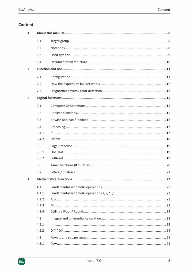
Content

1 About this manual .............................................................................................................8

1.1 Target group.............................................................................................................. 8

1.2 Notations .................................................................................................................. 8

1.3 Used symbols ............................................................................................................ 9

1.4 Documentation structure ....................................................................................... 10

2 Functionanduse .............................................................................................................11

2.1 Configuration ..........................................................................................................11

2.2 How the expression builder works ......................................................................... 12

2.3 Diagnostics / syntax error detection ....................................................................... 13

3 Logicalfunctions .............................................................................................................15

3.1 Comparative operations ......................................................................................... 15

3.2 Boolean functions ...................................................................................................15

3.3 Bitwise Boolean functions ...................................................................................... 16

3.4 Branching ................................................................................................................ 17

3.4.1 If .............................................................................................................................. 17

3.4.2 Switch ..................................................................................................................... 18

3.5 Edge Detection .......................................................................................................19

3.5.1 OneShot .................................................................................................................. 19

3.5.2 SetReset .................................................................................................................. 19

3.6 Timer functions (IEC 61131-3) ................................................................................ 20

3.7 IsData / Coalesce ....................................................................................................21

4 Mathematicalfunctions ..................................................................................................22

4.1 Fundamental arithmetic operations ....................................................................... 22

4.1.1 Fundamental arithmetic operations +, -, *, / .......................................................... 22

4.1.2 Abs .......................................................................................................................... 22

4.1.3 Mod ........................................................................................................................ 22

4.1.4 Ceiling / Floor / Round ............................................................................................ 23

4.2 Integral and differential calculation ........................................................................ 23

4.2.1 Int ........................................................................................................................... 23

4.2.2 Diff / Dif .................................................................................................................. 24

4.3 Powers and square roots ........................................................................................ 24

4.3.1 Pow ......................................................................................................................... 24

4 Issue 7.0

Content ibaAnalyzer

4.3.2 Sqrt ......................................................................................................................... 24

4.4 e functions and logarithms ..................................................................................... 25

4.4.1 Exp .......................................................................................................................... 25

4.4.2 Log .......................................................................................................................... 25

4.4.3 Log10 ...................................................................................................................... 25

4.5 PI ............................................................................................................................. 26

4.6 Sum ......................................................................................................................... 26

4.7 Trigonometric functions ......................................................................................... 27

5 Statisticalfunctions .........................................................................................................28

5.1 Average (Avg) ..........................................................................................................28

5.2 Maxima (Max) .........................................................................................................30

5.3 Minima (Min) ..........................................................................................................32

5.4 Standard deviation (StdDev) ................................................................................... 34

5.5 Percentile ................................................................................................................ 35

5.6 Correlation and covariance (Correl, CoVar) ............................................................ 37

5.7 Kurtosis ................................................................................................................... 38

5.8 Skewness ................................................................................................................ 40

6 Countingandsorting .......................................................................................................42

6.1 Count ...................................................................................................................... 42

6.2 CountSamples .........................................................................................................44

6.3 Sort ......................................................................................................................... 44

7 Time/lengthfunctions ...................................................................................................45

7.1 Convert and resample ............................................................................................ 45

7.1.1 ConvertBase ............................................................................................................45

7.1.2 Resample ................................................................................................................ 45

7.1.3 SampleAndHold ......................................................................................................46

7.1.4 SampleOnce ............................................................................................................46

7.2 Time ........................................................................................................................ 47

7.2.1 Time ........................................................................................................................ 47

7.2.2 AbsoluteTime ..........................................................................................................48

7.3 Conversion from time to length reference ............................................................. 48

8 X-axisoperations .............................................................................................................50

8.1 Shift along the X axis ...............................................................................................50

Issue 7.0 5

ibaAnalyzer Content

8.2 XCutRange / XCutValid ............................................................................................ 51

8.3 XMarkRange / XMarkValid ...................................................................................... 52

8.4 XMirror / XStretch / XStretchScale ......................................................................... 53

8.5 XFirst / XLast / XNow ..............................................................................................56

8.6 XSize / XSumValid ...................................................................................................56

8.7 XValues / YValues ....................................................................................................57

8.8 VarDelay .................................................................................................................. 58

8.9 XY ............................................................................................................................ 58

8.10 XMarker1 / XMarker2 .............................................................................................59

8.11 XBase / XOffset .......................................................................................................59

8.12 FillGaps ................................................................................................................... 59

8.13 XAlignFft ................................................................................................................. 60

9 Vectoroperations ............................................................................................................61

9.1 GetFirstIndex / GetLastIndex .................................................................................. 61

9.2 GetRows .................................................................................................................. 61

9.3 GetZoneCenters ......................................................................................................62

9.4 GetZoneOffset ........................................................................................................62

9.5 GetZoneWidths .......................................................................................................62

9.6 MakeVector ............................................................................................................ 62

9.7 SetZoneWidths .......................................................................................................63

9.8 VectorAvg................................................................................................................ 63

9.9 VectorKurtosis.........................................................................................................63

9.10 VectorMarkRange ...................................................................................................64

9.11 VectorMin / VectorMax .......................................................................................... 64

9.12 VectorPercentile .....................................................................................................64

9.13 VectorSkewness ......................................................................................................65

9.14 VectorStdDev ..........................................................................................................65

9.15 VectorSum .............................................................................................................. 65

9.16 VectorToSignal / SignalToVector ............................................................................. 65

9.17 Traverse / TraverseW ..............................................................................................66

9.18 VectorPolynomial / VectorLSQPolyCoef.................................................................. 67

10 Textfunctions ..................................................................................................................69

6 Issue 7.0

Content ibaAnalyzer

10.1 InfofieldText / ChannelInfoFieldText / ModuleInfoFieldText ...................................69

10.2 TextCompare / CompareText .................................................................................. 70

10.3 ToText / FromText ...................................................................................................72

10.4 TrimText .................................................................................................................. 74

10.5 ConcatText .............................................................................................................. 74

11 Miscellaneousfunctions ..................................................................................................75

11.1 Debounce ............................................................................................................... 75

11.2 Envelope ................................................................................................................. 76

11.3 False / True ............................................................................................................. 76

11.4 GetBit / GetBitMask................................................................................................76

11.5 HighPrecision ..........................................................................................................78

11.6 InfoField / ChannelInfoField / ModuleInfoField ...................................................... 78

11.7 LimitAlarm .............................................................................................................. 80

11.8 ManY....................................................................................................................... 80

11.9 Rand ........................................................................................................................ 81

11.10 Sign ......................................................................................................................... 81

11.11 Technostring ...........................................................................................................82

11.12 WindowAlarm .........................................................................................................82

11.13 YatX / SetYatX ..........................................................................................................83

11.14 PulseFreq ................................................................................................................ 84

12 Filterfunctions ................................................................................................................85

12.1 LP ............................................................................................................................ 85

12.2 PreWhiten ............................................................................................................... 85

13 Technologicalfunctions ...................................................................................................86

13.1 ChebyCoef .............................................................................................................. 86

13.2 CubicSpline ............................................................................................................. 86

13.3 LSQPolyCoef ............................................................................................................88

13.4 Polynomial .............................................................................................................. 89

14 Spectrumanalysis(FToperations) ...................................................................................90

14.1 FftInTimeAmpl / FftInTimePower ........................................................................... 90

14.2 FftOrderAnalysisAmpl / FftOrderAnalysisPower ..................................................... 91

Issue 7.0 7

ibaAnalyzer Content

14.3 FftPeaksInTimeAmpl / FftPeaksInTimePower ......................................................... 93

14.4 FftAmpl / FftPower .................................................................................................94

14.5 FftComplex ..............................................................................................................95

14.6 FftReal / FftRealInverse ........................................................................................... 96

14.7 AWeighting / DbScale .............................................................................................96

14.8 IntSpectrum ............................................................................................................ 97

15 Electricalfunctions ..........................................................................................................98

15.1 Eff ............................................................................................................................ 98

15.2 Delta functions .......................................................................................................99

15.3 Star functions ........................................................................................................102

15.4 Harmonic functions ..............................................................................................105

15.4.1 TIF ......................................................................................................................... 107

16 Supportandcontact ...................................................................................................... 108

88 Issue 7.0

About this manual ibaAnalyzer

1 About this manualThis documentation describes the function and application of the software

ibaAnalyzer.

1.1 Target groupThis manual addresses in particular the qualified professionals who are familiar with handling electrical and electronic modules as well as communication and measurement technology. A person is regarded as professional if he/she is capable of assessing safety and recognizing possi-ble consequences and risks on the basis of his/her specialist training, knowledge and experience and knowledge of the standard regulations.

This documentation addresses in particular professionals who are in charge of analyzing mea-sured data and process data. Because the data is supplied by other iba products the following knowledge is required or at least helpful when working with ibaAnalyzer:

■ Operating system Windows

■ ibaPDA (creation and structure of the measuring data files)

1.2 NotationsIn this manual, the following notations are used:

Action NotationMenu command Menu Logic diagramCalling the menu command Step 1 – Step 2 – Step 3 – Step x

Example: Select the menu Logic diagram - Add - New function block.

Keys <Key name>

Example: <Alt>; <F1>Press the keys simultaneously <Key name> + <Key name>

Example: <Alt> + <Ctrl>Buttons <Key name>

Example: <OK>; <Cancel>File names, paths "Filename", "Path"

Example: "Test.doc"

Issue 7.0 9

ibaAnalyzer About this manual

1.3 UsedsymbolsIf safety instructions or other notes are used in this manual, they mean:

Danger!

Thenon-observanceofthissafetyinformationmayresultinanimminentriskofdeathorsevereinjury:

■ Observe the specified measures.

Warning!

Thenon-observanceofthissafetyinformationmayresultinapotentialriskofdeathorsevereinjury!

■ Observe the specified measures.

Caution!

Thenon-observanceofthissafetyinformationmayresultinapotentialriskofinjuryormaterialdamage!

■ Observe the specified measures

Note

A note specifies special requirements or actions to be observed.

Tip

Tip or example as a helpful note or insider tip to make the work a little bit easier.

Otherdocumentation

Reference to additional documentation or further reading.

10 Issue 7.0

About this manual ibaAnalyzer

1.4 DocumentationstructureThis documentation describes the functionality of the ibaAnalyzer software in detail. It is creat-ed as a guide for familiarization as well as a reference document.

In addition to this documentation, you can also draw on the version history in the main menu Version history (file versions.htm) for the latest information about the installed program version. In addition to the list of corrected program errors, this file also refers to extensions and im-provements to the software by keyword.

In addition, each software update, which includes the main new features, also includes special documentation “NewFeatures...”, offering an extensive description of the new features.

The state of the software to which the respective part of this documentation refers is listed in the revision table on page 2. The documentation of ibaAnalyzer (PDF and printed edition) is divided into four separate parts. Each part has its own chapter and page numbering, beginning with 1, and is updated independently.

Part Title ContentPart 1 Introduction and installation General notes, licenses and add-ons

Installation and program start

User interfacePart 2 Working with ibaAnalyzer Working with data file and analysis, representation

features, macro configuration, filter design, prefer-ences, printing, export, interfaces to ibaHD-Server, ibaCapture and report generator

Part 3 Expression builder Directory of all calculation functions in the expres-sion builder, including explanation

Part 4 Application examples Application examples from the areas of expression editor, report generator and adjustment of the pro-gram interface as well as tips about the classifica-tion for signal names

rama

InPreparation

11 Issue 7.0 11

ibaAnalyzer Function and use

2 FunctionanduseThe expression builder is a tool for entering (mathematical) formulae or expressions which are described in detail in the following sections. It is also possible in principle to manually enter these expressions in the lines of the signal table on the Signal definitions tab.

In order to facilitate these inputs and also to provide a detailed list of possible operations and their syntax, there is the expression builder, which is available in every line in which a signal can be entered.

Fig. 1: Symbol for starting the expression builder.

Note

The button in the toolbar does not open the expression builder, but rather opens the dialog for the logical signal definitions. See Logical signal definitions in part 2 of the manual.

2.1 Configuration

Fig. 2: The Expression Builder

The expression builder consists of three areas.

12 Issue 7.0

Function and use ibaAnalyzer

The part on the left shows a signal tree which is very similar to the one in the signal tree win-dow. However, in contrast to the signal tree window, this window here contains not just the original signals, but also all the expressions which were already created using the expression builder. From this signal tree, you can now select the desired signals or expressions to be used in the calculations.

The right part of the dialog window contains a function tree view with a collection of the avail-able mathematical operations and other functions sorted by subject.

The command input in which you enter the desired expression in several lines is located below these two panes. Above this in the gray area is a short note about the syntax of an operation, if it is marked in the function tree, or a tooltip if the function is marked in the command input.

The <Reset expression> button removes all entries from the command line.

You can enable the "Reference signals by name" check box if you want to use the signal names in the expressions instead of the usual signal designations consisting of [module number:signal number].

Note

When using the signal names as signal reference, it must be guaranteed that the signal names are unambiguous.

2.2 HowtheexpressionbuilderworksThe expression builder makes it possible to apply both the operations as well as the operands, i.e. the signals and expressions, by double clicking or dragging and dropping into the command line. This process is recommended for avoiding write errors and being able to work faster.

The general rule is: The operation or operand that you double-click in the function tree or signal tree is inserted at the position of the cursor in the input line.

So as not to lose the overview of complex expressions, the keyboard shortcut <Ctrl>+<B> can be used to jump back and forth between associated pairs of parentheses.

Note

The function of applying signals and expressions in the command line is only available in the expression builder and cannot be used in the normal signal tree in the signal tree window.

Experienced users can use the input help Intellisense both in the signal table as well as in the command line of the expression builder. For manual inputs, a window automatically opens with possible completions of your input. This includes functions and their parameters as well as sig-nals or virtual expressions which are available in the measuring data file.

Issue 7.0 13

ibaAnalyzer Function and use

By means of cursor control buttons you can select an appropriate entry in the Intellisense win-dow and take it over by pressing <Return>. If you go on typing the range of suggestions will be adjusted accordingly until the expression is finished. If this function is used in the expression builder, all necessary parentheses are also automatically inserted.

2.3 Diagnostics/syntaxerrordetectionIf you have closed the expression builder by clicking the <OK> button, the expression just creat-ed is displayed in the corresponding row of the signal definitions.

Fig. 3: Expression builder diagnosis

Although the expression itself is automatically entered as the signal name, you can simply over-strike it by manually entering a plain text. In the case of more complex, cascaded expressions, we urgently recommend using names which should be as brief as possible and unambiguous in order to ensure that the expression is readily understandable.

In the case of a faulty input with the expression builder, an alert will appear that makes it pos-sible to correct the expression. If <Yes> is clicked, the cursor automatically jumps to the point where the error is presumably located.

Fig. 4: Expression builder diagnosis, error identification

Tip

The function to search for possible errors can also be started manually by press-ing the keyboard shortcut <Ctrl>+<E> in the expression builder.

If the error message is ignored or the error is made during input in the signal definition line, ibaAnalyzer indicates this with a red color.

Fig. 5: Expression builder diagnosis, error identification

In this way, formal or syntax errors can be detected here that would make a calculation impos-sible. In order to obtain more detailed information about the cause of the error, the diagnostics

14 Issue 7.0

Function and use ibaAnalyzer

can be opened with a mouse click on the yellow question mark symbol in the respective signal definition line.

Fig. 6: Expression builder diagnosis, diagnosis window, error

15 Issue 7.0 15

ibaAnalyzer Logical functions

3 Logicalfunctions

3.1 Comparativeoperationse.g. ('Expression1') < ('Expression2')

> Greater>= Greater or equal < Smaller<= Smaller or equal<> Unequal= Equal

Table 1: Comparative operations

DescriptionThe comparative operations >, >=, <, <=, <> and = can be used to compare the values of two ex-pressions (operands) with each other. The result of such an operation is the Boolean value TRUE or FALSE. Original signals, calculated expressions or constant values can be entered as operands. The result can be presented and evaluated as a new expression, such as a signal. This way, bina-ry signals can easily be generated and can then be used as conditions for other functions.

Note

If the crossing point of two curves is located between two measuring points, the result of the comparative operation of the last two measured values is retained until the next measuring point. This means that any change from TRUE to FALSE (or vice versa) is always located at a measuring point. The line which connects two measuring points in the presentation of analog values is just an approxima-tion.

3.2 Booleanfunctionse.g. ('Expression1') AND ('Expression2')

AND Logical ANDOR Logical ORXOR Logical exclusive ORNOT Logical NOT, negation

Table 2: Boolean functions

16 Issue 7.0

Logical functions ibaAnalyzer

DescriptionBinary expressions, such as digital signals, can be linked with each other using the Boolean func-tions AND, OR, NOT and XOR. According to the rules of Boolean logic, the functions return the value TRUE or FALSE. Digital signals, calculated (binary) expressions or the numerical values 0 or 1 can be entered as parameters.

The result can be presented and evaluated as a new expression, such as a signal. This way, bina-ry signals can easily be generated and can then be used as conditions for other functions.

A B A AND B A OR B A XOR B NOT A0 0 0 0 0 11 0 0 1 1 00 1 0 1 11 1 1 1 0

Table 3: Logical functions, truth table

3.3 BitwiseBooleanfunctionse.g. ('Expression1') bw_NOT ('Expression2')

bw_AND Bitwise ANDbw_OR Bitwise ORbw_XOR Bitwise exclusive ORbw_NOT Bitwise NOT

Table 4: Boolean functions (bitwise)

DescriptionThese functions are used for the bitwise linking of two analog values based on Boolean algebra. The functions return a 32Bit integer. 32Bit integers are expected as arguments.

If the arguments are not integers, the decimal part will be dropped before the operation is ex-ecuted. If the arguments are too big so that their absolute value does not fit in a 32Bit integer, the operation is executed only on the 32 low-order bits.

When linking two analog values with a bw function, the individual bits of both values are logi-cally linked. The result then is an analog value of the same type with a bit pattern in accordance with the logical link.

Issue 7.0 17


ExampleFor 2 analog values V1 = 15 and V2 = 2, the results are as follows:

Dec. value Bits Hex Result valueOutput value V1 15 ...1111 0x0000000FOutput value V2 2 ...0010 0x00000002V1 bw_AND V2 ...0010 0x00000002 2V1 bw_OR V2 ...1111 0x0000000F 15V1 bw_XOR V2 ...1101 0x0000000D 13bw_NOT (V1) ...0000 0xFFFFFFF0 -16

Table 5: Truth table for bitwise linking

3.4 Branching

3.4.1 IfIf('Condition’,'IF-True’,'IF-False')

Arguments

'Condition' Condition as an operation with the Boolean results TRUE or FALSE'IF-True' Operation is performed if 'Condition' is TRUE'IF-False' Operation is performed if 'Condition' is FALSE

DescriptionThe If function can be used for a conditioned execution of further calculations. Depending on the Boolean result of a 'condition’, which can itself be an operation, the operation ‘IF-True’ will be executed if the result is TRUE and the operation ‘IF-False’ if the result is FALSE.

Hence, different calculations can be executed in a process-controlled manner. Of course, you can use this function in a nested matter and thus realize further branches.

Tip

If an analog signal is entered for 'Condition', as a condition it will be checked whether the value is greater than (TRUE) or less than (FALSE) 0.5.

18 Issue 7.0


3.4.2 Switch

Switch ('Selector_Expression,' 'Case_1_Expression’,'Value_1_Expression,'

'Case_2_Expression’,'Value_2_Expression,'

...

'Case_n_Expression’,'Value_n_Expression,'

'Default_Value_Expr')

Arguments

'Selector_Expression' Expression that is checked for different conditions'Case_n_Expression' Expression that is compared with ‘Selector_Expression’'Value_n_Expression' Result if ‘Select_Expression’ and ‘Case_n_Expression’ match'Default_Value _Expr' Result if none of the ‘Case_n_Expressions’ match with

‘Selector_Expression’

DescriptionThese instructions compare an incoming ‘Selector_Expression’ with any number of ‘Case_n_Ex-pressions’ resembling the SQL statement CASE. At least 3 arguments are needed. With an even number of arguments, the last argument is automatically interpreted as ‘Default_Value_Expr,’ which is used if none of the ‘Case_n_Expressions’ matches with the ‘Selector_Expression’.

If ‘Selector_Expression’ and ‘Case_n_Expression’ match, the corresponding ‘Value_n_Expres-sion’ is returned. If several ‘Case_n_Expressions’ match the input signal, the first is automatical-ly selected.

The following signals are allowed as ‘Selector_Expressions’:

� A numeric constant

� A text constant

� An equidistant and not equidistant sampled channel

� A text channel

In general, the types of comparison values must match, otherwise the corresponding case is not selected.

Issue 7.0 19


3.5 EdgeDetection

3.5.1 OneShotOneShot('Expression')

DescriptionThis function returns the result TRUE, if the current measured value of 'Expression' is not equal to the previous one. It returns the result FALSE, if the current measured value does equal the previous one.

Tip

The function also works with non-equidistant measuring values.

3.5.2 SetResetSetReset('Set’,'Reset’,'SetDominant=1')

Arguments

'Set' Positive edge sets function to TRUE'Reset' Positive edge sets function to FALSE'SetDominant' Optional parameter (default = 1), which controls which input argument is

dominant if both arguments simultaneously receive a positive edge.'SetDominant' = 1 Set takes precedence over Reset'SetDominant' = 0 Reset takes precedence over Set

DescriptionThis function can be used to control a digital result (TRUE/FALSE) with the help of positive edges (transition from 0 to 1) of the arguments ‘Set’ and ‘Reset’.

A rising edge of the ‘Set’ operand returns a static TRUE. A rising edge of the ‘Reset’ operand re-sets the result to FALSE. The argument 'SetDominant' is optional and determines the dominance of ‘Set’ or ‘Reset.’

Tip

For an analog signal, exceeding the value 0.5 corresponds to a positive edge.

20 Issue 7.0


3.6 Timerfunctions(IEC61131-3)

TOFTOF('in','pt')

DescriptionOff Delay Timer. The output is switched off 'pt' seconds after switching off the 'in' input.

TONTON('in','pt')

DescriptionOn Delay Timer. The output is switched on 'pt' seconds after switching on the 'in' input.

TPTP('in','pt')

DescriptionPulse Timer. The output is switched on for 'pt' seconds after rising edge at the 'in' input.

Tip

A further rising edge during the output pulse does not extend the output pulse and does not restart the pulse.

Issue 7.0 21


3.7 IsData / Coalesce

IsDataIsData('Expression’,'End')

Arguments

'Expression' input signal'End' Length of the output signal

DescriptionThe result of this operation is TRUE if measured values are available for 'Expression.' The result is FALSE if measured values are missing or signals are empty. This function, for example, can be used as condition for other calculations.

Optionally, the 'End' parameter can be entered. With this parameter, you can reduce or extent the resulting signal of the function so that it complies with other signals and can be used for fur-ther links. If you do not specify the 'End' parameter, the length of the result signal complies with that of the input signal (incl. invalid samples).

CoalesceCoalesce ('Candidate1', ‘Candidate2',...)

DescriptionInspired by the corresponding SQL query, the function Coalesce returns the first of its argu-ments, which contains data.

This may, for example, be used to create a safeguard against missing signals in a data file.

2222 Issue 7.0

Mathematical functions ibaAnalyzer

4 Mathematicalfunctions

4.1 Fundamentalarithmeticoperations

4.1.1 Fundamentalarithmeticoperations+,-,*,/e.g. ('Expression1') + ('Expression2')

DescriptionAll signals and expressions can be processed by fundamental arithmetic operations (addition, subtraction, multiplication and division). If digital signals or expressions are used as operands in fundamental arithmetic operations, ibaAnalyzer translates the TRUE values as 1.0 and FALSE as 0.0. The result of a fundamental arithmetic operation is always an analog expression.

4.1.2 AbsAbs('Expression')

DescriptionThe absolute function returns the absolute value (= |value|) of 'Expression.'

Tip

Interpolated values in the case of a sign change between two samples may differ in value.

4.1.3 ModMod('Divident’,'Divisor')

DescriptionThis function returns the modulo of 'Divident' and 'Divisor'. Internally, the function uses the fmod C-function, which permits the use of floating point values for 'Divident' and 'Divisor'.

Modulo r is the remainder of the division divident / divisor so that the following relationship applies in reverse:

Divident = Divisor * x + r, whereby x is an integer number (integer).

Modulo r always has the same sign as 'Divident' and the absolute value of r is always smaller than the absolute value of 'Divisor'.

If 'Divident' < 'Divisor', then the function returns the value of 'Divident'. Mathematically speak-ing, the remainder can also be described as "Divident modulo Divisor.”

Issue 7.0 23

ibaAnalyzer Mathematical functions

4.1.4 Ceiling/Floor/Round

CeilingCeiling('Expression')

DescriptionThis function returns the smallest integer value that is greater than or equal to 'Expression’.

FloorFloor('Expression')

DescriptionThis function returns the largest integer value that is less than or equal to 'Expression’.

RoundRound('Expression')

DescriptionThis function rounds ‘Expression’ up or down to the nearest integer.

4.2 Integralanddifferentialcalculation

4.2.1 IntInt('Expression’,'Reset')

Arguments

'Expression' Measured value'Reset' Optional digital parameter, which can be used to reset the integral or suppress

the integration process. ‘Reset’ can be an expression as well.'Reset' > 0 Integral is reset.'Reset'= 0 Integration released (default)

DescriptionThis function returns the integral of 'Expression'. The ‘Reset’ parameter can be used for reset-ting the integral to zero or suppressing the integration process, e.g. to integrate the same signal for periodical occurrences or reversing processes a number of times. ‘Reset’ can be an expres-sion as well.

24 Issue 7.0


4.2.2 Diff/DifDiff('Expression’,'dy'=0)

DescriptionThis function returns the derivative (or the differential) of 'Expression'. If you set the optional parameter ‘dy’ to True(), only the difference between the measured values is calculated instead of the differential.

ExampleIf 'Expression' is a length measuring signal, the Diff function can be used to determine a speed curve.

4.3 Powersandsquareroots

4.3.1 PowPow('Expression1’,'Expression2')

Arguments

'Expression1' Basis'Expression2' Exponent

DescriptionThis function takes 'Expression1' (basis) to the power of 'Expression2' (exponent).

ExampleCalculating some important powers

(2)^0 = Pow(2, 0) = 1

(2)^-2 = Pow(2, -2) = 0.25

(-2)^2 = Pow(-2, 2) = 4

(10)^(lg 2) = Pow(10, lg 2) = 2

(0)^-1 = Pow(0, -1) = +∞ (infinity)

Tip

The increase of 0 to the power of -1 does not yield an error message, but also no result.

4.3.2 SqrtSqrt('Expression')

DescriptionThis function returns the square root of 'Expression'.

Issue 7.0 25


Note

Although negative values for 'Expression' do not produce an error message, they do not produce a result either.

4.4 efunctionsandlogarithms

4.4.1 ExpExp('Expression')

DescriptionThis function calculates the expression (e) 'Expression'

4.4.2 LogLog('Expression')

DescriptionThis function returns the natural logarithm of 'Expression'.

Note


4.4.3 Log10Log10('Expression')

DescriptionThis function returns the decadic logarithm of 'Expression'.

Note


26 Issue 7.0


4.5 PIPi()

DescriptionThe number Pi () is stored as a constant ( = 3.1415927...) in the system for various kinds of calculations. Use this function to insert the number into your calculation.

4.6 SumSum('Expression’,'Reset'=0)

DescriptionThis operation summarizes all signal values of a function point by point. If the summation is in-terrupted by a reset value, then the summation starts again.

ExampleThe summation starts with the signal value 10 + 9 + 8 + …6. Here, 'reset' = TRUE causes an inter-ruption and the function is reset to zero. After that, the summation starts again.

Fig. 7: Mathematical functions: Sum

Issue 7.0 27


4.7 Trigonometricfunctionse.g. Sin ('Expression')

Sin('Expression') This function returns the sine of 'Expression' in rad.Cos('Expression') This function returns the cosine of 'Expression' in rad.Tan('Expression') This function returns the tangent of 'Expression' in rad.Asin('Expression') This function returns the arcsine of 'Expression' in rad.Acos('Expression') This function returns the arccosine of 'Expression' in rad.Atan('Expression') This function returns the arctangent of 'Expression' in rad.Atan2 ('X,' 'Y') This function returns the arctangent of ‘Y/X’.

Table 6: Trigonometric functions

DescriptionThe standard functions and the related inverse functions are available for various calculations in which trigonometric functions are needed, for example, the calculation of power in three-phase AC systems.

ExampleVisualization of trigonometric functions:

Fig. 8: Visualization of miscellaneous trigonometric functions

2828 Issue 7.0

Statistical functions ibaAnalyzer

5 StatisticalfunctionsibaAnalyzer supports the calculation of miscellaneous statistical functions. Four different ver-sions are available for each function in a normal case:

■ The standard function always calculates the corresponding size across the entire signal

■ The suffix InTime indicates that the corresponding size is formed over intervals of a specified length

■ The suffix Valid is used to calculate the corresponding size over intervals, which are marked with a binary signal

■ The prefix M indicates that the corresponding size is formed over moving intervals of a speci-fied length

5.1 Average(Avg)

Fig. 9: Statistical functions - average

AvgAvg('Expression')

DescriptionThis function returns the average of 'Expression'. It is displayed as a constant value (horizontal line) in the signal strip.

Issue 7.0 29

ibaAnalyzer Statistical functions

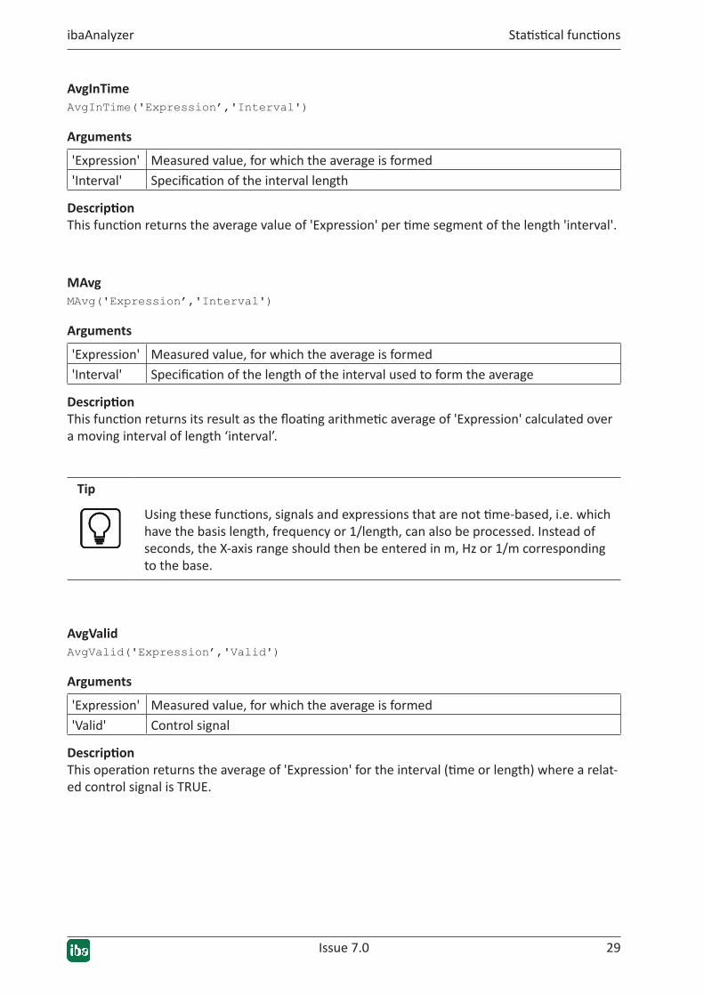
AvgInTimeAvgInTime('Expression’,'Interval')

Arguments

'Expression' Measured value, for which the average is formed'Interval' Specification of the interval length

DescriptionThis function returns the average value of 'Expression' per time segment of the length 'interval'.

MAvgMAvg('Expression’,'Interval')

Arguments

'Expression' Measured value, for which the average is formed'Interval' Specification of the length of the interval used to form the average

DescriptionThis function returns its result as the floating arithmetic average of 'Expression' calculated over a moving interval of length ‘interval’.

Tip

Using these functions, signals and expressions that are not time-based, i.e. which have the basis length, frequency or 1/length, can also be processed. Instead of seconds, the X-axis range should then be entered in m, Hz or 1/m corresponding to the base.

AvgValidAvgValid('Expression’,'Valid')

Arguments

'Expression' Measured value, for which the average is formed'Valid' Control signal

DescriptionThis operation returns the average of 'Expression' for the interval (time or length) where a relat-ed control signal is TRUE.

30 Issue 7.0


5.2 Maxima(Max)

Fig. 10: Statistical functions - Maximum

MaxMax('Expression')

DescriptionThis function returns the maximum value of 'Expression'. It is displayed as a constant value (hor-izontal line) in the signal strip.

Max2Max2('Expression1',‘Expression2')

DescriptionThis function returns the maximum of two signals, 'Expression1' and 'Expression2'. The two sig-nals are compared measured value by measured value, with the larger value in each case being presented as the result.

Issue 7.0 31


MaxInTimeMaxInTime('Expression’,'Interval')

Arguments

'Expression' Measured value, for which the maximum is formed'Interval' Length of the interval over which the maximum should be calculated.

DescriptionThis function returns the maximum value of 'Expression' within each interval of the length 'in-terval'. Signals and expressions being time-based ("interval" in seconds) or length-based ("inter-val" in meters) can be processed.

MaxValidMaxValid('Expression’,'Valid')

Arguments

'Expression' Measured value, for which the maximum is formed'Valid' Control signal

DescriptionThis operation returns the maximum of 'Expression' for the interval (time or length) where a related control signal is TRUE.

MMaxMMax ('Expression’,'Interval')

Arguments

'Expression' Measured value, for which the maximum is formed'Interval' Length of the interval over which the maximum should be calculated

DescriptionThis function returns the maximum of ‘Expression’ within a floating X-axis interval of the length ‘interval’, advancing by one measuring point in each case.

32 Issue 7.0


5.3 Minima(Min)

Fig. 11: Statistical functions - Minimum

MinMin('Expression')

DescriptionThis function returns the minimum value of the 'Expression' signal. It is displayed as a constant value (horizontal line) in the signal strip.

Min2Min2('Expression1',‘Expression2')

DescriptionThis function returns the minimum of two signals, 'Expression1' and 'Expression2'. The two signals are compared measured value by measured value, with the smaller value in each case being presented as the result.

Issue 7.0 33


MinInTimeMinInTime('Expression’,'Interval')

Arguments

'Expression' Measured value, for which the minimum is formed'Interval' Length of the interval over which the minimum should be calculated.

DescriptionThis function returns the minimum value of 'Expression' within each interval of the length 'inter-val'. Signals and expressions being time-based ("interval" in seconds) or length-based ("interval" in meters) can be processed.

MinValidMinValid('Expression’,'Valid')

Arguments

'Expression' Measured value, for which the minimum is formed'Valid' Control signal

DescriptionThis operation returns the minimum of 'Expression' for the interval (time or length) where a re-lated control signal is TRUE.

MMinMMin('Expression’,'Interval')

Arguments

'Expression' Measured value, for which the minimum is formed'Interval' Length of the interval over which the minimum should be calculated

DescriptionThis function returns the minimum of ‘Expression’ within a floating X-axis interval of the length ‘interval’, advancing by one measuring point in each case.

34 Issue 7.0


5.4 Standarddeviation(StdDev)

Fig. 12: Statistic functions Standard deviation StdDev, MstdDev

StdDevStdDev('Expression')

DescriptionThis function returns the standard deviation of 'Expression' .

The standard deviation is calculated by the following formula:

MStdDevMStdDev('Expression’,'Interval')

Arguments

'Expression' Measured value, for which the standard deviation is formed'Interval' Length of the interval over which the standard deviation should be calculated.

DescriptionThis function returns the moving standard deviation of 'Expression' over each time interval of the length 'Interval'. Signals and expressions being time-based ("interval" in seconds) or length-based ("interval" in meters) can be processed.

Issue 7.0 35


StdDevInTimeStdDevInTime('Expression’,'Interval')

Arguments

'Expression' Measured value, for which the standard deviation is formed'Interval' Length of the interval over which the standard deviation should be calculated.

DescriptionThis function returns the standard deviation of 'Expression' over each time interval of the length 'Interval'.

Note

The result of the StdDevInTime function is always specified for the previous in-terval.

StdDevValidStdDevValid('Expression’,'Valid')

Arguments

'Expression' Measured value, for which the standard deviation is formed'Valid' Control signal

DescriptionThis function returns the standard deviation of 'Expression' for the interval (time or length) where a related control signal is TRUE.

5.5 Percentile

PercentilesPercentile('Expression','p'=0.5)

Arguments

'Expression' Measured value for which the percentile is formed'p' The percentile

DescriptionThis function returns the ‘p’-th percentile of ‘expression’.

The ‘p’th percentile is the smallest value of a set of measured values which is greater than p% of the number of values measured. A typical percentile is the 50% percentile, the so-called me-dian. The median divides the set of values measured into two equal halves: 50% of all values measured are smaller than the median value, the remaining 50% are greater than or equal to it. Further typical percentiles are 25% and 75% which, together with the median, enable the divi-

36 Issue 7.0


sion of a set of values measured into four groups, the so-called quartiles. (< 25%, <50%, <75%, ≥75%).

The "Percentile" function determines the percentile value of the total number of measuring points of a signal. The percentile 'p' must be entered as a decimal value, i.e.:

� 50 % --> p = 0.5 (default value)

� 75 % --> p = 0.75

� 95.9 % --> p = 0,959

This function is, for example, particularly useful when it comes to assessing the quality of a product where a particular property must comply with a defined classification.

PercentileValidPercentileValid('Expression’,'Valid’,'p'=0.5)

Arguments

'Expression' Measured value for which the percentile is formed'Valid' Specification of the interval used to form the percentile'p' The percentile

DescriptionThis function returns the percentile of 'Expression' for every interval (time or length) for which a related control signal 'Valid' is TRUE.

PercentileInTimePercentileInTime('Expression’,'Interval’,'p'=0.5)

Arguments

'Expression' Measured value for which the percentile is formed'Interval' Specification of the interval size used to form the percentile'p' The percentile

DescriptionThis function returns the percentile of 'Expression' over each time interval of the length 'Inter-val'.

MPercentileMPercentile('Expression’,'Interval’,'p'=0.5)

Arguments

'Expression' Measured value for which the percentile is formed'Interval' Specification of the moving interval used to form the percentile'p' The percentile

Issue 7.0 37


DescriptionThis function returns the moving percentile of 'Expression' over each interval of the length 'In-terval'. Signals and expressions being time-based ("interval" in seconds) or length-based ("inter-val" in meters) can be processed.

5.6 Correlationandcovariance(Correl,CoVar)

CorrelCorrel('Expression1’,'Expression2')

Arguments

'Expression1/2' Measured values that are calculated for the correlation coefficient

DescriptionThis function calculates the correlation coefficient between ‘Expression1’ and ‘Expression2.’ The entire recording length is taken into account. The function returns a constant value.

McorrelMcorrel('Expression1',‘Expression2’,'Interval')

Arguments

'Expression1/2' Measured values that are calculated for the correlation coefficient'Interval' Specification of the interval used to form the correlation coefficient

DescriptionThis function calculates the correlation coefficient between ‘Expression1’ and ‘Expression2’ over floating intervals of the length 'interval' measured in s, m, Hz or 1/m.

CoVarCoVar('Expression1',‘Expression2')

Arguments

'Expression1/2' Measured values that are calculated for the covariance

DescriptionThis function calculates the covariance between ‘Expression1’ and ‘Expression2.’ The entire re-cording length is taken into account. The function returns a constant value.

MCoVarMCoVar('Expression1’,'Expression2’,'Interval')

Arguments

'Expression1/2' Measured values that are calculated for the covariance'Interval' Specification of the interval used to form the covariance

38 Issue 7.0


DescriptionThis function calculates the covariance between ‘Expression1’ and ‘Expression2’ over floating intervals of the length 'interval' measured in s, m, Hz or 1/m.

5.7 KurtosisThe calculation of the kurtosis is used e. g. for the evaluation and analysis of vibrations. It serves to determine the number of outliers within an vibration signal.

In mathematical terms, the kurtosis is a measure for the relative "flatness" of a distribution (compared to the normal distribution which has a kurtosis of zero). A positive kurtosis indicates a tapering distribution (a leptokurtic distribution), whereas a negative kurtosis indicates a flat distribution (platykurtic distribution).

Fig. 13: Miscellaneous kurtosis functions

This statistical method is particularly suitable for analyzing random or stochastic signals, e. g. in terms of condition-based maintenance (condition monitoring) when analyzing vibrations.

For characterizing the signal curve, methods of probability density or frequency are used. It is assumed that a noise signal with a Gaussian amplitude distribution can be measured in ma-chines in good order after filtering out, e. g., rotational frequency vibration components. In the event of damage, individual pulse signals interfere with this signal, altering the distribution function. By choosing suitable characteristic values such as the crest factor or the kurtosis factor, the machine condition can be evaluated.

If regularly measured, these methods offer an overview of the machine status. However, the disadvantage is that after they increase the characteristic values decrease again. The reason for this is that the number of pulse signals increases with progressive damage. This in turn influenc-es the effective value but barely effects the peak value.

Issue 7.0 39


Modifications of the time signal caused by shock pulses induce a change in the resulting distri-bution function. Thus, damages with a distinctly discrete nature can cause the kurtosis factor to increase sharply. Its absolute value thus allows statements on a damage.

The calculation of the kurtosis is similar to the calculation of the standard deviation 'StdDev'.

KurtosisKurtosis('Expression')

Arguments

'Expression' Measured value, for which the kurtosis is formed

DescriptionThis operation returns the kurtosis of the selected time signal.

KurtosisInTimeKurtosisInTime('Expression’,'Interval')

Arguments

'Expression' Measured value, for which the kurtosis is formed'Interval' Length of the interval over which the kurtosis should be calculated.

DescriptionWith this operation, the selected expression is divided into equal-duration intervals of the length 'Interval’. For these intervals, the kurtosis is subsequently calculated.

MKurtosisMKurtosis('Expression’,'Interval')

Arguments

'Expression' Measured value, for which the kurtosis is formed'Interval' Specification in seconds of the length of the interval over which the kurtosis

is formed

DescriptionThis operation calculates the kurtosis of 'expression' over a floating X axis interval of fixed length 'interval'.

40 Issue 7.0


KurtosisValidKurtosisValid('Expression’,'Valid')

Arguments

'Expression' Measured value, for which the kurtosis is formed'Valid' Control signal

DescriptionThis operation describes the kurtosis for those intervals in which a related control signal is TRUE.

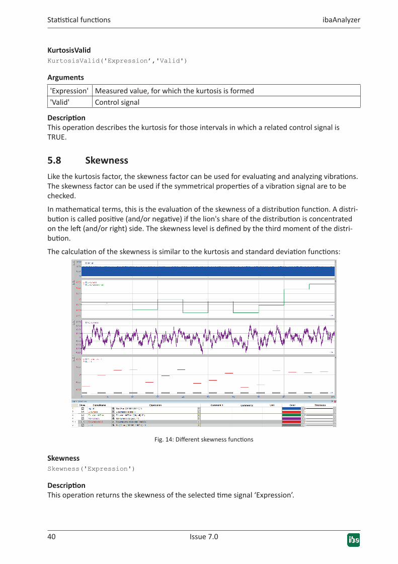
5.8 SkewnessLike the kurtosis factor, the skewness factor can be used for evaluating and analyzing vibrations. The skewness factor can be used if the symmetrical properties of a vibration signal are to be checked.

In mathematical terms, this is the evaluation of the skewness of a distribution function. A distri-bution is called positive (and/or negative) if the lion's share of the distribution is concentrated on the left (and/or right) side. The skewness level is defined by the third moment of the distri-bution.

The calculation of the skewness is similar to the kurtosis and standard deviation functions:

Fig. 14: Different skewness functions

SkewnessSkewness('Expression')

DescriptionThis operation returns the skewness of the selected time signal ‘Expression’.

Issue 7.0 41


SkewnessInTimeSkewnessInTime('Expression’,'Interval')

Arguments

'Expression' Measured value, for which the skewness is formed'Interval' Length of the interval over which the skewness should be calculated.

DescriptionWith this operation, the selected expression is divided into equal-duration intervals of the length 'Interval’. For these intervals, the skewness is subsequently calculated.

MSkewnessMSkewness('Expression’,'Interval')

Arguments

'Expression' Measured value, for which the skewness is formed'Interval' Length of the moving interval over which the skewness should be calculated.

DescriptionThis operation calculates the skewness of 'Expression' over a floating X axis interval of length 'interval'.

SkewnessValidSkewnessValid('Expression’,'Valid')

Arguments

'Expression' Measured value, for which the skewness is formed'Valid' Control signal

DescriptionThis operation computes the skewness over those intervals in which a related control signal is TRUE.

4242 Issue 7.0

Counting and sorting ibaAnalyzer

6 Countingandsorting

6.1 CountCount('Expression’,'Level'=0.5, 'Hysteresis'=0, 'EdgeType'=1, 'Reset'=0)

Arguments

'Expression' Measured value'Level' Specification of the level value'Hysteresis' Specification of a hysteresis band'EdgeType' Indication of whether rising, falling or rising and falling edges should be counted

'EdgeType' <0 only falling edges (leaving out hysteresis band in the nega-tive direction)

'EdgeType' >0 only rising edges (leaving out hysteresis band in the posi-tive direction)

'EdgeType' = 0 falling and rising edges'Reset' Optional digital parameter that can be used to reset the counter. ‘Reset’ can be

an expression as well.'Reset' > 0 Counter is reset.'Reset' = 0 Counter value is retained / continues to count (default)

Note

The 'Reset' condition must not be related to the count function itself.

DescriptionThe function counts the crossings of 'Expression' through 'Level'.

The 'Hysteresis' parameter can be used to define a tolerance band which is above and below 'Level' by equal amounts. Only complete crossings through the tolerance band are counted.

The 'EdgeType' parameter determines which kind of edges are counted. The 'Reset' parameter is used to reset the counter value to 0. 'Reset' can also be formulated as an expression.

ExampleIf you choose 2.5 for 'Level' and 2.0 for 'Hysteresis,' level crossings in the ascending direction are not counted until 'Expression' is > 3.5 and in the descending direction until 'Expression' is < 1.5.

Issue 7.0 43

ibaAnalyzer Counting and sorting

Fig. 15: Miscellaneous count functions

Tip

The count function can also be used for binary signals. For this purpose, choose 0.5 for ‘Level’ and, for example, 0.1 for ‘Hysteresis’. This then means that all changes from FALSE to TRUE and vice versa will be detected and counted.

44 Issue 7.0

Counting and sorting ibaAnalyzer

6.2 CountSamplesCountSamples('Expression’,'Reset'=0)

Arguments

'Expression' Measured value for which the number of signal points is determined'Reset' Optional digital parameter, which can be used to reset or suppress the counting

process. ‘Reset’ can be an expression as well.

'Reset' > 0 counting process is reset.

'Reset' = 0 counting process released (preference)

DescriptionWith this function, the number of the individual signal points can be determined regardless of whether the signal points are equidistant or not. Invalid samples are not counted. If the input signal is invalid, the constant value 0 is supplied as the result.

Tip

This function can also be used in combination with XMarkValid (see XMark func-tions ì XMarkRange / XMarkValid, page 52 ) for example.

6.3 SortSort('Expression’,'Descending'=0)

Arguments

'Expression' Measured value for which the samples are sorted'Descending' Optional digital parameter for reversing the sorting sequence

DescriptionThis function sorts all samples of a curve ('expression') by their values in ascending order from left to right.

Preference: Sorting in ascending order (‘descending’=FALSE). If the samples are to be sorted in descending order from left to right, TRUE has to be set as the second operand.

45 Issue 7.0 45

ibaAnalyzer Time / length functions

7 Time/lengthfunctions

7.1 Convertandresample

7.1.1 ConvertBaseConvertBase('Expression’,'From,’To')

Arguments

'Expression' Measured value for which the base should be modified'From'/‘To' Setup of the base that is to be switched from or to.

0 = time

1 = length

2 = frequency

3 = inverse length

DescriptionThis operation converts an expression from one base into another base. No physical conversion or scaling is carried out.

This function can be used to change the reference value of a signal. This can be advantageous if length-based reference values are used for additional calculations. The existing signal, however, is only time-based.

7.1.2 ResampleResample('Expression’,'Basis’,'interpolate'=1)

Arguments

'Expression' Measured value that is to be resampled'Base‘ New sampling rate of the result'interpolate' Optional parameter to prevent the automatic interpolation for the new mea-

sured values

DescriptionThis operation returns the signal trend of 'Expression' on a new time basis. The momentary val-ues are transferred from the original curve temporally correct in line with the new time basis, so that the length of the new curve is practically the same. The function can also be used for length-based signals. In this case, the value of a distance must be entered in m rather than a time span.

46 Issue 7.0

Time / length functions ibaAnalyzer

Tip

A curve can be graphically smoothed if a larger time basis is used in the resample function because fewer points are connected to each other. The values are not averaged.

7.1.3 SampleAndHoldSampleAndHold('Expression’,'Sample’,'Initial'=0)

Arguments

'Expression' Measured value'Sample' Parameter that determines whether the function follows the measured value (1)

or holds the last measured value (0). 'Sample' can be a condition itself or be de-termined by a different function.

'Initial' Optional parameter (default = 0), which determines the initial value of the func-tion when 'Sample' is inactive at the start of the measurement.

DescriptionThis function is a sample-hold function. The output follows 'Expression' when 'Sample' = TRUE. It remains unchanged when ‘Sample’ = FALSE. With the optional 'Initial' parameter, the initial value of the output can be specified if the function is on "Hold" when called.

7.1.4 SampleOnceSampleOnce('Expression','Sample')

Arguments

'Expression' Measured value'Sample' Digital signal whose rising edges determine the sampling points

DescriptionThis function resamples an 'Expression' input signal at individual points determined by the rising edges of the 'Sample' digital signal. The result has one measuring point per rising edge and is invalid in the ranges in between.

ExampleThis function can be used to display a phase sensor (keyphasor) signal in the time domain. Whenever the phase sensor jumps to 'TRUE', the original signal is sampled. By overlaying both representations, the times of the phase sensor are suitably represented. In the example below, a 180° phase shift can be detected when passing a resonance.

Issue 7.0 47


Fig. 16: The SampleOnce function applied to a vibration signal

7.2 Time

7.2.1 TimeTime('Count’,'Basis')

Arguments

'Count' Number of measuring points to be created'Base‘ Sampling rate of the result

This function returns a linear, time-proportional signal with a number of ‘Count’ values at a dis-tance of 'base.’ The timebasis is stated in seconds. The time values are entered both on the X axis and on the Y axis.

Note

It is not necessary to load a data file as a precondition for using the time func-tion.

48 Issue 7.0

Time / length functions ibaAnalyzer

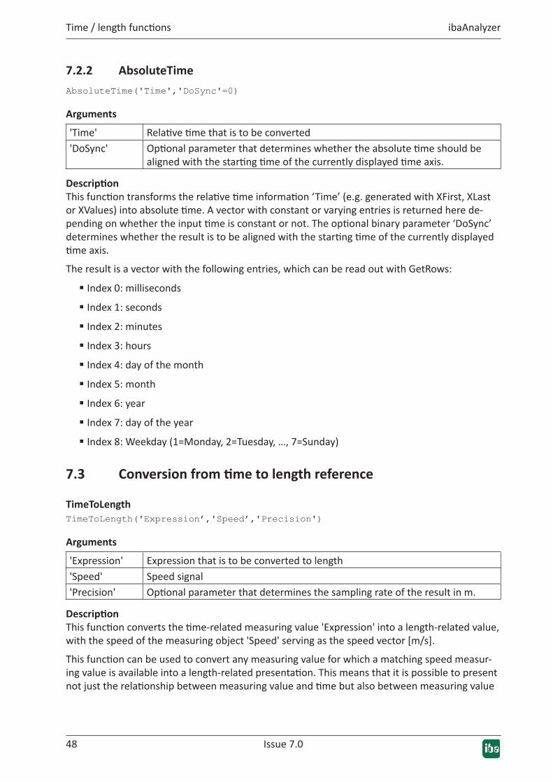
7.2.2 AbsoluteTimeAbsoluteTime('Time','DoSync'=0)

Arguments

'Time' Relative time that is to be converted'DoSync' Optional parameter that determines whether the absolute time should be

aligned with the starting time of the currently displayed time axis.

DescriptionThis function transforms the relative time information ‘Time’ (e.g. generated with XFirst, XLast or XValues) into absolute time. A vector with constant or varying entries is returned here de-pending on whether the input time is constant or not. The optional binary parameter ‘DoSync’ determines whether the result is to be aligned with the starting time of the currently displayed time axis.

The result is a vector with the following entries, which can be read out with GetRows:

� Index 0: milliseconds

� Index 1: seconds

� Index 2: minutes

� Index 3: hours

� Index 4: day of the month

� Index 5: month

� Index 6: year

� Index 7: day of the year

� Index 8: Weekday (1=Monday, 2=Tuesday, …, 7=Sunday)

7.3 Conversionfromtimetolengthreference

TimeToLengthTimeToLength('Expression’,'Speed’,'Precision')

Arguments

'Expression' Expression that is to be converted to length'Speed' Speed signal'Precision' Optional parameter that determines the sampling rate of the result in m.

DescriptionThis function converts the time-related measuring value 'Expression' into a length-related value, with the speed of the measuring object 'Speed' serving as the speed vector [m/s].

This function can be used to convert any measuring value for which a matching speed measur-ing value is available into a length-related presentation. This means that it is possible to present not just the relationship between measuring value and time but also between measuring value

Issue 7.0 49


and distance traveled. Taking the example of a steel strip in a rolling mill, this function is used to determine the distribution of measured values over the strip length. On condition that the pro-cess was designed in such a manner that the beginning and end of measurement are in exact conformity with the head and tail ends of the strip, this function can then also be used to calcu-late the total length of the strip. The largest length value determined is entered as the scale end value of the X axis (autoscale).

'Precision' is an optional parameter in [m]. If no precision value is defined, the points for the length-related curve are calculated and entered in the signal strip on the basis of the number of measuring points of the original signal. If a precision value is defined, for example, 0.1, a new length-related value is calculated and entered as a point of the curve every 0.1 m.

Fig. 17: Time / length functions: TimeToLength

TimeToLengthLTimeToLengthL('Expression’,'Length’,'Precision')

Arguments

'Expression' Expression that is to be converted to length'Length' Length signal'Precision' Optional parameter that determines the sampling rate of the result in m.

DescriptionThis function converts the time-related measuring value 'Expression' into a length-related value, with a length measuring value 'Length' as the position [m].

The explanations given under TimeToLength apply analogously, however, with the only differ-ence that a suitable length or position measuring value is used instead of the speed.

5050 Issue 7.0

X-axis operations ibaAnalyzer

8 X-axisoperations

8.1 ShiftalongtheXaxis

Fig. 18: Time / length functions: shift left / right

ShlShl('Expression’,'Distance')

Arguments

'Expression' Expression that should be moved'Distance' Distance in seconds or meters for length-related signals

This operation returns a signal curve which is shifted by 'Distance' to the left on the X axis com-pared to the original signal. Otherwise, the values measured remain unchanged. The function can be used for time-based signals ('Distance' in seconds) as well as for length-based signals ('Distance' in meters).

ShrShr('Expression’,'Distance')

Arguments

'Expression' Expression that should be moved'Distance' Distance in seconds or meters for length-related signals

This operation returns a signal curve which is shifted by 'Distance' to the right on the X-axis compared to the original signal. Otherwise, the values measured remain unchanged. The func-tion can be used for time-based signals ('Distance' in seconds) as well as for length-based signals ('Distance' in meters).

Issue 7.0 51

ibaAnalyzer X-axis operations

8.2 XCutRange/XCutValid

Fig. 19: X axis operations: XCutRange and XCutValid

XCutRangeXCutRange('Expression’,'Start’,'End')

Arguments

'Expression' Expression from which a part is to be cut out'Start' Start of the selected range in seconds or meters'End' End of the selected range in seconds or meters

DescriptionThis function can be used to cut out a part of a curve. The function can be applied both to time-related and to length-related signal strips. The 'Start' and 'End' parameters, entered in [s] or [m], define the beginning and end of the segment to be cut out.

The cut out part is moved to the beginning of a separate trend view. However, since the X axis (time or length) remains unchanged, the correct time or length reference of the values mea-sured is no longer given.

XCutValidXCutValid('Expression’,'Valid')

Arguments

'Expression' Expression from which a part is to be cut out'Valid' Binary signal that describes the selected range

DescriptionThis function cuts out all the measuring points of a signal trend 'Expression' depending on a 'Valid' condition if this condition supplies the value TRUE. The function can be applied to both time-related and length-related signals. The 'Valid' parameter is a Boolean expression. This can be a digital input signal, the result of a comparative operation, or any other binary expression. Measuring points for which the condition is FALSE are not taken over.

The parts cut out are placed, one after another, at the beginning of a new signal strip.

52 Issue 7.0


8.3 XMarkRange/XMarkValid

Fig. 20: X axis operations: XMarkRange and XMarkValid

XMarkRangeXMarkRange('Expression’,'Start’,'End')

Arguments

'Expression' Expression from which a part is to be selected'Start' Start of the selected range in seconds or meters'End' End of the selected range in seconds or meters

DescriptionThis function can be used to cut out part of a curve in a manner similar to the XCutRange func-tion. The function can be applied both to time-related and to length-related signal strips. The 'Start' and 'End' parameters, entered in [s] or [m], define the beginning and end of the segment to be cut out. The part cut out is displayed in a separate signal strip, however, it also continues to be displayed in the original position on the time or position axis, whilst the measuring points outside the specified range are discarded.

XMarkValidXMarkValid('Expression’,'Valid')

Arguments

'Expression' Expression from which a part is to be selected'Valid' Binary signal that describes the selected range

DescriptionThis function cuts out – in a manner similar to the XCutValid function - all the measuring points of a signal trend 'Expression' depending on a 'Valid' condition if this condition supplies the value TRUE. The function can be applied both to time-related and to length-related signal strips. The 'Valid' parameter is a Boolean expression. This can be a digital input signal, the result of a com-parative operation, or any other binary expression. Measuring points for which the condition is

Issue 7.0 53


FALSE are discarded. The parts cut out are displayed in a new signal strip, retaining their X posi-tions.

Tip

The XMarkValid function is particularly suitable, for example, to highlight limit value violations by using different colors in a signal trend by showing the result signal in the same strip and on the same Y-axis as the original signal. By choosing different colors, the limit-value violation ranges can be clearly identified.

Example: Values within the tolerance range = blue; values out of tolerance = red.

8.4 XMirror / XStretch / XStretchScale

XMirrorXMirror('Expression')

DescriptionThis function can be used to mirror a complete graph (exchanging the beginning and end). The graph is mirrored around the vertical central axis of the entire signal graph. The function can be applied both to time-related and to length-related signal strips.

In this way, measuring graphs of reversing processes (direction reversal) can be compared more easily. In rolling mills, for example, the head and tail end of the strip can be exchanged during (even) reversing passes in order to graphically neutralize the direction reversal. However, in or-der to compare several passes to each other, the corresponding measured values must first be cut out of the original signal using the XCutValid function, so that these values can be individual-ly mirrored and subsequently placed on top of each other.

54 Issue 7.0


Fig. 21: X axis operations: XMirror

The above picture shows the different results of the mirroring operation, depending on whether the segment to be mirrored was previously cut out using XMarkValid (red) or XCutValid (green).

XStretchXStretch('Expression’,'ReferenceExpression')

DescriptionThis function can be used to graphically stretch the curve of a signal to the same (final) length of another signal. The function can be applied both to time-related and to length-related signal strips.

In this way, it is, for example, possible to correlate measured values of a rolled strip from the roughing mill to those from the finishing mill or to compare the individual passes of a reversing mill to each other.

Issue 7.0 55


Fig. 22: X axis operations: XStretch

In the above picture, the rolling force curve of the first pass (blue curve) is stretched to the final length corresponding to the ninth pass.

XStretchScaleXStretchScale('Expression’,'Scale')

DescriptionWith this function, the curve of a signal can be stretched by a specified factor. The scaling factor is also used if the curve is already provided with an offset.

Fig. 23: Stretching a curve by factor

56 Issue 7.0


8.5 XFirst / XLast / XNow

XFirstXFirst('Expression’,'Skip=0’,'SkipInitialEdge=FALSE')

Arguments

'Expression' (Boolean) input signal'Skip' Optional for skipping the first rising edges'SkipInitialEdge' Decides whether the first sample is counted as a rising edge if it is TRUE

DescriptionThis function returns a value on the X-axis (time [s] or position [m]) for which the "Expression' is TRUE for the first time. This means that ‘expression' must be a Boolean quantity. This can be a digital input signal, the result of a comparative operation, or any other binary expression.

XLastXLast ('Expression’,'Skip’=0,'SkipFinalEdge=FALSE')

Arguments

'Expression' (Boolean) input signal'Skip' Optional for skipping the last falling edges'SkipFinalEdge' Decides whether the last sample is counted as a falling edge if it is TRUE

DescriptionThis function returns a value on the X-axis (time [s] or position [m]) for which the "Expression' is TRUE for the last time. This means that ‘expression' must be a Boolean quantity. This can be a digital input signal, the result of a comparative operation, or any other binary expression.

XNowXNow()

DescriptionThis function returns the relative time since the last start of ibaAnalyzer.

8.6 XSize/XSumValid

XSizeXSize ('Expression')

DescriptionThis function returns the total length of ‘expression' in units of the X-axis (time in [s] or position in [m]). The result is at a constant value of 0 if the input signal is invalid.

Issue 7.0 57


XSumValidXSumValid ('Expression')

DescriptionThis function can be used to determine the duration or length for which the condition ‘Expres-sion' is TRUE. Any measuring points for which the condition is not true (FALSE) are disregarded in the calculation. This means that ‘expression' must be a Boolean quantity. This can be a digital input signal, the result of a comparative operation, or any other binary expression.

The result is at a constant value of 0 if the input signal is invalid.

8.7 XValues / YValues

XValuesXValues('Expression')

DescriptionThis function returns the X values for every sample of an expression . What makes this function special is that it will also work on signals or expressions which are not time-based, i.e. length-based (m), frequency-based (Hz) or inverse length-based (1/m).

With a usual time- or length continuous signal, it will return a rising straight line, writing the time or length values along the Y-axis in base units (s, m). The function also works with not equi-distant measured values.

YValuesYValues('Expression’,'TimeBase'=1)

Arguments

'Expression' Input signal'TimeBase' Time base of the output signal

DescriptionThis function returns the Y-values for all measured values of an expression. Regardless of whether the input signal is sampled equidistant or not, the result is an equidistant signal with the time base ‘TimeBase.’

The specification of the time base is optional and ‘TimeBase’=1 is used as the default value.

58 Issue 7.0


8.8 VarDelayVarDelay('Expression’,'Delay')

Arguments

'Expression' input signal'Delay' Time delay in seconds

DescriptionThis operation returns the 'Expression' delayed by a time constant ‘Delay’.

8.9 XYXY('Expression1’,'Expression2’,'Precision')

Arguments

'Expression1' Input signal containing the X-values of the new signal'Expression2' Input signal containing the Y-values of the new signal'Precision' Optional parameter for specifying the sampling rate of the output signal

DescriptionThis function is used if the result from the X-Y visualization is to be used for additional opera-tions. After the selection, the signals of the X and Y axis are assigned to the function.

Please note that in the resulting function, the distances between the signal points are not the same as the distances of the original signals. Also the distance between the signal points is different. With the 'Precision' parameter, a fixed distance between the signal points can be de-termined. If no parameter is entered, the shortest distance of the signal points is used as fixed value for all subsequent operations.

Fig. 24: X-axis operation XY

Issue 7.0 59


8.10 XMarker1/XMarker2XMarker1 () and/or XMarker2 ()

DescriptionThis function returns the position of the marker X1 and/or X2 on the X axis.

8.11 XBase/XOffset

XBaseXBase('Expression')

DescriptionThis function is used to determine the recording time base and length and frequency-based dis-tances between the samples, respectively. In case of an equidistantly sampled signal, the func-tion provides the distance between two samples in X axis units.

If the samples of a signal do not have the same distance, the distance will be displayed in X axis units which would be determined when re-sampling on equidistant samples. By default, this is the smallest distance between two samples of the signal.

XOffsetXOffset('Expression')

DescriptionThis function provides the interval of the first sample of a signal from the beginning of the data file in seconds. The result is negative if the signal starts earlier and positive if it starts later.

If several data files are opened at the same time and the "Synchronize files on recording time" option is enabled, the offset is necessarily not determined with reference to the start of the data file of the selected signal, but to the start of the data file having the earliest starting time.

8.12 FillGapsFillGaps('Expression')

DescriptionThe function FillGaps can be used to fill gaps in a signal 'expression’ through linearly interpolat-ed entries.

This function is especially useful when gaps are created by NULL entries during trend queries from a database.

60 Issue 7.0


8.13 XAlignFftXAlignFft('Expression_fixed','Expression_shift’,'Start’,'End’,'MinScale’,'Max-Scale’,'scale’,'type')

Arguments

'Expression_fixed' Expression that serves as a reference'Expression_shift' Expression that is adjusted to the reference'Start''End''MinScale' The smallest x scaling factor to be checked'MaxScale' The biggest x scaling factor to be checked'scale''type'

DescriptionWith this function, length-based signals with the same physical significance which were mea-sured in different places in the process can be aligned to each other.

Some parameters are described in more detail below.

■ 'Expression_fixed'

A thickness measurement being considered "fixed" in the course of an algorithm, i.e. not scal-able or shiftable. This should be the thickness measurement containing the profile of the other measurement. (In the hot strip-cold strip comparison, this would be the hot strip)

■ 'Expression_shift'

The result of the alignment later refers to this thickness measurement. Thus, this measurement has to be scaled and shifted with the result values.

■ 'Start'

The interval from Start to End indicates the X-intercept where the measurement 'Expres-sion_fixed' can be moved. The zero here is the zero of the expression. Also negative values are permitted. If, compared to "Expression_fixed,' the measurement 'Expression_shift' is allowed to protrude 10 axis units on the left-hand side in the ibaAnalyzer, then the following must apply: Start = -10 .

■ 'End'

Specifies the end of the interval just described. It is recommended to select this end dependent on the length of 'Expression_fixed.' So, for example, End = XSize([Expression_fixed]) or End = 1.2 * Xsize([Expression_fixed]) if an surplus of 20 percent is allowed.

■ 'scale'

By means of this parameter, the ratio between precision and speed can be controlled. The smaller the value, the slower and more reliable the algorithm works. The higher the value, the more the algorithm is accelerated by a heuristic. In case of too high values for 'scale,’ this can lead to a wrong result. For an optimal result, it is recommended to transfer the resolution of the measuring data. If, the samples have a distance of 10 cm, for example, scale = 0.1. If the calcula-tion of results takes too long, the value can be revised upwards.

61 Issue 7.0 61

ibaAnalyzer Vector operations

9 VectoroperationsVector operations extend the analysis options for two-dimensional signals.

Vectors, in previous descriptions often referred to as arrays, can be created in different ways:

� By grouping several signals in ibaPDA and marking the group as "vector"

� By arranging several signals in the logical signal definitions in ibaAnalyzer

� As result of various calculation functions, e. g. FFT functions

In ibaAnalyzer, vectors can be displayed in 2D top view and 3D view. The vector operations in the expression builder serve the use of vector data for further calculations.

Otherdocumentation

You will find extensive notes on these visualizations and their settings in the ibaAnalyzer manual, part 2, types of visualization.

9.1 GetFirstIndex/GetLastIndexGetFirstIndex('Condition') and/or GetLastIndex('Condition')

DescriptionThese functions return the index of the first or last channel in the vector for which the condition ‘Condition’ is true. The vector itself should be an operand of ‘Condition.’ If ‘Condition’ is false for all channels of the vector, the function returns -1.

9.2 GetRowsGetRows('Vector’,'StartIndex’,‘Counter’,'Step')

Arguments

'Vector' Vector from which the individual entries are to be read out‘StartIndex’ First index from which the entries are to be read out'Counter' Number of entries'Step' Step size

DescriptionThis function extracts rows of values from an array. A total number ‘Counter’ of entries is read out based on a ‘StartIndex’ (the smallest possible index is 0) in steps of the size ‘Step.’

62 Issue 7.0

Vector operations ibaAnalyzer

9.3 GetZoneCentersGetZoneCenters('Vector')

DescriptionThis function determines the position of the center of the zone on the Y axis for each zone of the vector. The only argument of the function is the vector. The result is a vector with a number of values in accordance with the number of zones.

ExampleThe GetZoneCenters function is particularly helpful if it is applied to the result of an FftInTime function. The FftInTime function returns a vector with n "zones" as its result which comply with the frequency bands (bins). With the GetZoneCenters function, the center frequencies of the individual bands of the spectrum and thus the frequency vector can be determined. This allows you to differentiate or integrate in the frequency domain by multiplying or dividing the results of the FftInTime and GetZoneCenters function accordingly.

9.4 GetZoneOffsetGetZoneOffset(‘Vector‘)

DescriptionThis function determines the offset of the first zone, i. e. the position of the center of the first zone, based on the zero line of the Y-axis. The only argument of the function is the vector. The result is a constant value.

9.5 GetZoneWidthsGetZoneWidths('Vector')

DescriptionThis function determines the width of each zone of the vector in units of the Y-axis. The only argument of the function is the vector. The result is a vector with a number of values in accor-dance with the number of zones.

9.6 MakeVectorMakeVector(r_0,r_1,...,r_n)

DescriptionThis function creates a vector with the value series r_0 to r_n. The arguments can be constant values or signals and expressions, respectively. This is comparable with the creation of a vector in the Logical signal definitions dialog.

ExampleThe MakeVector function mainly serves to enable macros to return multi-dimensional signals as their results. In the macro editor, the partial results of different calculations can be declared as interim values within the macro. As final macro result, a vector can be defined whose argu-ments are the interim values. The vector is basically used as container for macro results to sim-plify the macro interface.

Issue 7.0 63


9.7 SetZoneWidthsSetZoneWidths('Vector',‘Widths’,'Offset')

Arguments

'Vector' Vector with the (measured) values of the result vector'Widths' Vector containing zone widths as values'Offset' Distance of the zone center of the first zone from the zero line

DescriptionThis function creates a vector with specified zone widths. In doing so, the values of the result vector are taken from a vector 'vector' and the zone widths from a vector ‘widths.’ Since the vector with the zone widths can use expressions as arguments, this function can be used to generate vectors with different zone widths depending on the loaded data. The expressions for defining the zone widths should be constant over time and not change for data loaded once. If this is not the case, the width values will be averaged over the overall period.

ExampleThe function SetZoneWidths (MakeVector(1,2,3,2,1),MakeVector(2,4,10,4,2), -10) creates the same vector as the one that was created with the logical signal definitions. See ibaAnalyzer manual, part 2, chapter Logical signal definitions).

9.8 VectorAvgVectorAvg('Vector')

DescriptionThis function calculates the average of the cross profile for each sample, i. e. the average of all vector tracks per point in time or per X axis position, respectively. The function returns a one-di-mensional signal showing the curve of the cross profile average value over the time/length of the vector signal with the same number of samples.

9.9 VectorKurtosisVectorKurtosis('Vector')

DescriptionThis function calculates the kurtosis of the cross profile for each sample. The function returns a one-dimensional signal showing the curve of the cross profile kurtosis over the time/length of the vector signal with the same number of samples.

Note

Please note that at least 4 signal points must be available, i.e. the vector must have at least 4 entries.

64 Issue 7.0


9.10 VectorMarkRangeVectorMarkRange('Vector’,'Start’,'End')

Arguments

'Vector' Vector with the input signals'Start' Start of the range to be selected'End' End of the range to be selected

DescriptionThis function returns a partial vector of a ‘vector’ with a zone width from 'Start' (lower edge) to 'End' (upper edge).

The positions must be indicated in units of the Y axis. The positions can be both fixed values and signals or expressions and thus be dependent on the data loaded.

The expressions for defining the positions should be constant over time and not change for data loaded once. If this is not the case, the position values will be averaged over the overall period.

9.11 VectorMin / VectorMax

VectorMaxVectorMax('Vector')

DescriptionThis function calculates the maximum of the cross profile for each sample, i. e. the maximum value of all vector tracks per point in time or per X-axis position, respectively. The function re-turns a one-dimensional signal showing the curve of the cross profile maximum over the time/length of the vector signal with the same number of samples.

VectorMinVectorMin('Vector')

DescriptionThis function calculates the minimum of the cross profile for each sample, i. e. the minimum val-ue of all vector tracks per point in time or per X-axis position, respectively. The function returns a one-dimensional signal showing the curve of the cross profile minimum over the time/length of the vector signal with the same number of samples.

9.12 VectorPercentileVectorPercentile('Vector’,'Percentile'=0.5)

Arguments

'Vector' Vector with the input signals'Percentile' The percentile between 0 and 1

DescriptionThis function calculates the percentile of the cross profile for each sample.

Issue 7.0 65


The second argument in addition to the ‘vector’ is the specification of the ‘percentile’ to be cal-culated. Default value is 0.5 (median). The function returns a one-dimensional signal showing the curve of the cross profile percentile over the time/length of the vector signal with the same number of samples.

9.13 VectorSkewnessVectorSkewness('Vector')

DescriptionThis function calculates the skewness of the cross profile for each sample. The function returns a one-dimensional signal showing the curve of the cross-sectional skewness over the time/length of the vector signal with the same number of samples. Please note that at least 4 signal points must be available for this calculation.

9.14 VectorStdDevVectorStdDev('Vector')

DescriptionThis function calculates the standard deviation of the cross profile for each sample. The function returns a one-dimensional signal showing the curve of the cross profile standard deviation over the time/length of the vector signal with the same number of samples.

9.15 VectorSumVectorSum('Vector')

DescriptionThis function calculates the sum of all values of the cross profile for each sample. The function returns a one-dimensional signal showing the curve of the value sum in the cross profile over the time/length of the vector signal with the same number of signals.

ExampleIf you divide the VectorSum expression by the number of vector tracks, the result is the same as with the VectorAvg function.

9.16 VectorToSignal / SignalToVector

VectorToSignalVectorToSignal('Vector’,'XBase')

Arguments

'Vector' Vector with the (constant) input signals‘XBase’ Sampling rate of the output signal

66 Issue 7.0


DescriptionThis function generates a one-dimensional signal from the elements of a vector along the cross profile. Every sample of the resulting signal corresponds to an element of the vector. The result complies with the cross profile.

The ‘XBase’ parameter is optional. If ‘XBase’ is not indicated, the zone widths and the offset of the vector are used. The resulting signal can also receive non-equidistant samples.

ExampleIn connection with the YatX functions and the marker position, the VectorToSignal function can be used to display the cross profile at any position in the vector:

VectorToSignal (YatX([Vector],XMarker1()))

SignalToVectorSignalToVector ('Signal')

DescriptionUnlike the VectorToSignal function, the function SignalToVector creates a vector with constant entries from the signal ‘Signal.’ The zone width and offset are determined by the sampling rate of the input signal. Note that, unlike VectorToSignal, this function has no optional argument for determining the zone widths. The SetZoneWidth can be used for this purpose.

Note

The input signal should have fewer than 1000 samples, as otherwise the signal will not be evaluated and will be marked as too complex.

9.17 Traverse / TraverseW

TraverseTraverse('Signal’,'Position’,'N'=40,‘Min’,‘Max’,'Avg'=1)

Arguments

'Signal' The signal measured by a traversing measuring device'Position' The position of the traversing measuring device along the traverse profile'N' Number of zones of the resulting vector'Min' Optional threshold for the minimum of the range to be mapped'Max' Optional threshold for the maximum of the range to be mapped'Avg' Optional binary parameter for averaging several samples within a zone pass; The

average is formed by default

Issue 7.0 67


DescriptionThis function converts signals originating from a traversing measuring device into a vector for two-dimensional visualization.

TraverseWTraverseW('Signal’,'Position’,'Widths’,'Offset'=0,'Avg'=1)

Arguments

'Signal' The signal measured by a traversing measuring device'Position' The position of the traversing measuring device along the traverse profile'Widths' The width of the resulting zones'Offset' Optional offset of the first zone'Avg' Optional binary parameter for averaging several samples within a zone pass; The

average is formed by default

DescriptionThis function works similarly to Traverse, with the difference being that the dimensions of the resulting vector are set directly via the zone widths ‘Widths’ and an optional offset parameter.

9.18 VectorPolynomial / VectorLSQPolyCoef

VectorPolynomialVectorPolynomial('Coefs’,'Vector')

Arguments

'Coefs' Coefficient of the interpolation polynomial; calculated with VectorLSQPolyCoef'Vector' Sampling points for the analysis of the interpolation polynomial

DescriptionThis function can be used to show the interpolation polynomial that is described by the coeffi-cient ‘Coefs’ as a result of the function VectorLSQPolyCoef.

The sampling points for analyzing the polynomial are determined by the sampling points of the vector ‘Vector.’ If zones ‘offset’ and/or ‘zone width’ are specified, these are also used, otherwise the indices are used as Y-values.

Note

Note that the entries of ‘Vector’ do not play a role here.

68 Issue 7.0


VectorLSQPolyCoefVectorLSQPolyCoef('Vector’,'Degree')

Arguments

'Vector' Vector for which entries the least squares approximation polynominals are cal-culated

'Degree' Degree of the interpolation polynomial

DescriptionThis function is the extension of the function LSQPolyCoef to vectors. The coefficients of an interpolation polynomial of degree ‘Degree’ are calculated using the least squares method for each cross section. The indices of the vector are used as a basis for this, unless a zone offset and/or the zone width were set when the vector was created. In this case, the corresponding values are used as the basis.

69 Issue 7.0 69

ibaAnalyzer Text functions

10 Textfunctions

10.1 InfofieldText/ChannelInfoFieldText/ModuleInfoFieldTextThese functions allow to make information from an info field of a data file, a channel or a mod-ule available as a text channel.

Arguments

'Index' Index of the file and/or the channel or module'InfoField' The info field that is to be read out;

Must be set in quotation marks!'Start' First character of the field content to be read out (optional)

If no value is defined, the complete content is read out'End' Last character of the field content to be read out (optional)

If no value is defined, it will be read from the start to the last character

Note

Two indices must be specified for the function ModuleInfoFieldText. The index of the data file as the first argument and the index of the module as the second. All other arguments remain the same.

InfoFieldTextInfofieldText('FileIndex’,'InfoField',‘Start’,'End')

DescriptionThis function issues the content of an info field as a text channel.

Tip

If you double-click on the desired info field, ibaAnalyzer automatically inserts the corresponding function as new signal into the signal table. If required, you then only have to customize the signal name and beginning/end.

If you want to read out the content of an info field as numerical value, use the Infofield function.

70 Issue 7.0

Text functions ibaAnalyzer

ChannelInfoFieldTextChannelInfofieldText('ChannelIndex',‘InfoField’,'Start’,'End')

DescriptionThis function issues the content of an info field of a channel as text.

ModuleInfoFieldTextModuleInfoFieldText('FileIndex',‘ModuleIndex',‘InfoField’,'Start’,'End')

Arguments

'FileIndex' Index of the file to which the module belongs'ModuleIndex' The index of the module'InfoField' The info field that is to be read out of the module'Start' Start index of the info string'End' End index of the info string

DescriptionThis function works as the InfoFieldText and ChannelInfoFieldText functions, however, it refers to the info fields of a module and not the data file or signal. The function returns a text channel with the content of the specified info field.

10.2 TextCompare / CompareTextTextCompare('Text1’,'Text2’,'CaseSensitive=True')

Arguments

'Text1/2' Both strings that are to be compared'CaseSensitive' Optional parameter which can be used to specify whether case sensitivity is

taken into consideration for the comparison.

DescriptionThis function allows you to compare the text information lexicographically. The function works with contents of text channels as well as with plain text which – used with quotation marks – is directly entered in the signal definition.

Comparison and results:

� The result is -1 if the information of the first text is to be arranged lexicographically before that of the second text.

� The result is 0 if both texts contain the same information.

� The result is +1 if the information of the first text is to be arranged lexicographically after that of the second text.

Issue 7.0 71


ExampleThe following table shows the impact of the ‘CaseSensitive’ parameter:

Text1 Text2 Result CommentTextCompare ("Text1,” "Text2,” 0)

TextCompare ("Text1," “Text2,” 1)

1234 abcd 1234 abcd 0 0 1 = 21234 abcd 1234 bcde -1 -1 1 < 2

"a" comes before "b"

1234 Abcd 1234 abcd 0 1 1 = 2 (not case sensitive)

1 > 2 (case sensitive)

“A” comes after “a”12340 abcd 1234 abcd 1 1 1 > 2

"0" comes after " "1234 0abcd 1234 abcd -1 -1 1 < 2

"0" comes before "a"

12034 abcd 1234 abcd -1 -1 1 < 2 "0" comes before "3"

1234 abcd 1y34 abcd -1 -1 1 < 2 "2" comes before "y"

1z34 abcd 1Y34 abcd 1 1 1 > 1 "z" comes after "Y"

Table 7: Results of the TextCompare function (examples)

72 Issue 7.0


10.3 ToText / FromText

ToTextToText( 'Expression’,'Format'="%g”,'datatype'=0)

Arguments

'Expression' Expression whose content is to be converted into a text channel'Format' Optional parameter for a format string'datatype' Optional parameter that determines the floating-point format

- 'datatype'=0 Default value

- 'datatype'=1 Output is formatted as signed 16-bit integer

- 'datatype'=2 Output is formatted as unsigned 16-bit integer

- 'datatype'=3 Output is formatted as signed 32-bit integer

- 'datatype'=4 Output is formatted as unsigned 16-bit integer

DescriptionThis function converts a numerical signal value into a text channel. In case of equidistant sam-ples of the ‘Expression’ input signal and a constant Y-value, only the value of the first signal point is entered and displayed as sample in the text channel. If the Y value changes, a sample is entered and displayed in the text channel for every new Y value.

If the ‘expression’ input signal does not contain equidistant samples, a sample is entered and displayed in the text channel for each input sample.

The optional parameter ‘format’ is to be entered according to C printf syntax. You can only indi-cate a parameter (%) complying with an IEEE 32 bit floating point value. Default value is %g. This value is also used if you do not indicate the optional parameter.

Examples: %g = conversion of the floating point value into a text %. 4f = text/number with 4 decimal places, etc.

ExampleThe ToText function can be helpful e. g. if trends are visualized containing vast amounts of data. Without constantly changing between the marker and signal view, the numerical values can be easily displayed.

Issue 7.0 73


Fig. 25: Using the ToText function

FromTextFromText('TextChannel’,'Start’,'End')

Arguments

'TextChannel' Text channel to be converted'Start' First character of the field content to be read out (optional)



DescriptionThis function converts the content of the text channel ‘TextChannel’ into a numerical value. The ‘Start’ and ‘End’ parameters can optionally be used as indices in order to not convert the entire string. By default, ‘Start’=0 and ‘End’=length of the string is used.

74 Issue 7.0


10.4 TrimTextTrimText('Text',’RemoveOption=0')

Arguments

'Text' Text channel or expression from which spaces are to be removed.'RemoveOption' Parameter for setting the operating mode:

0 (default): Deleting spaces before and after the text 1: Deleting spaces before the text only 2: Removing spaces after the text only 3: Removing all spaces, also in the text

DescriptionWith this function, you can delete the spaces from texts. This function can be used both in case of text channels already contained in data files and in case of results of the InfofieldText and To-Text functions.

10.5 ConcatTextConcatText('Text1’,'Text2',...)

DescriptionThis function can be used to merge several text channels. Numerical signals are also permissible here. These are automatically converted into text.

If the X-positions of the individual channels do not match, a new entry is created for each exist-ing X-position and the missing entry is replaced by the left neighbor, if present.

ExampleThe file ID is available as a technostring channel for signals in series. There is a product counter for the end products. Both pieces of information should be brought together as a result.

75 Issue 7.0 75

ibaAnalyzer Miscellaneous functions

11 Miscellaneousfunctions

11.1 DebounceDebounce ('Expression’,'Interval')

Arguments

'Expression' Input signal that is to be debounced'Interval' Dead time (reaction time)

DescriptionThis function delivers a debounced signal trend of 'Expression’ with ‘interval’ as dead time in [s]. ‘Interval’ is interpreted as position in [m] for length-based signals.

The function works in a manner similar to an OFF-delay time relay, however, with the difference that the signal change from TRUE to FALSE (falling edge) is presented in realtime, i.e. without delay, unless another change from FALSE to TRUE (rising edge) occurs during the time set.

In this way, it is possible to smooth unsteady signals, for example, from photocells or limit switches. This is particularly important if these signals are used as conditions in certain opera-tions, such as XMarkValid or XCutValid, because every discontinuity would interrupt the calcu-lation of the operation, so that result values would be lost. The difference can be clearly seen in the following picture.

Fig. 26: Miscellaneous debounce functions

76 Issue 7.0

Miscellaneous functions ibaAnalyzer

11.2 EnvelopeEnvelope('Expression’,'Interval')

Arguments

'Expression' Expression around which the envelope curve is to be formed'Interval' X-axis interval

DescriptionThis function calculates the upper envelope of a signal or expression. The envelope is con-structed by linking the high peaks of the signal curve. The quality of the envelope curve can be adjusted by parameter ‘interval.’ Without this parameter, only the maximum peak will be taken into account over the entire recording length of the signal. The parameter ‘interval’ specifies the length of an interval in base units of X-axis (s, m, Hz, 1/m). By using this parameter the peaks inside the interval will be taken into account too and the envelope nestles against the signal curve.

Tip

In order to get an envelope along the lower side of the signal curve, you can en-ter the same function in the form-Envelope (-'Expression’,'Interval')

In this case the low peaks (minimum values) will be linked.

11.3 False / TrueFalse() and/or True()

DescriptionThese operands have the constant value 0 or 1.

In Boolean operations (AND, OR etc.) the value is taken for logical 0 (FALSE), resp. logical 1 (TRUE). In arithmetic operations and in combination with analog values, the value is taken for 0.0, resp. 1.0 ("fixed zero" or "fixed one").

11.4 GetBit/GetBitMask

GetBitGetBit('Expression’,'Bitnumber')

DescriptionThis function returns the Boolean value of the 'Bitnumber' bit of 'Expression' after rounding to the nearest integer value. The rounding limit is in each case the next 0.5 increment. (2.48 --> 2; 2.50 -->3). Valid bit number sequence: 0 (LSB) to 15 (MSB).

Issue 7.0 77


Note

The function does not apply to integers with 64 bits because these data types are not supported by ibaPDA and thus cannot be included in a data file.

ExampleIn the table below, the least significant byte of an integer value with the bits 0...7 is shown as an example. In order to represent the values 0...8, the individual bits are highlighted as with “X.” (X = TRUE)

Bit no. 7 6 5 4 3 2 1 001 X2 X3 X X4 X5 X X6 X X7 X X X8 X

Table 8: Example for bit values

X = TRUE

Tip

If one or more 8-, 16- or 32-bit integers should be reduced to single bits you can ease your work. Just make a right mouse click on the desired signal in the signal tree and select “Show bits” in the context menu. All bits are immediately shown as individual digital signals, without programming the GetBit function. The inter-nal method of this function is the same like for GetBit.

GetBitMaskGetBitMask('Expression’,'Bitnumber')

DescriptionThis function interprets 'Expression' as a bit mask of a float value and returns the value of the bit 'bitnumber'. Valid range: 0 (LSB) to 31 (MSB)

This function was specifically developed for work with data from SimadynD in one particular case where up to 32 digital values are recorded in packed format as a float variable. The GetBit-Mask function only evaluates the valence of the specified bit 'bitnumber' irrespective of wheth-

78 Issue 7.0


er it is part of the mantissa or of the exponent. In contrast to the GetBit function, there is no rounding to the next integer.

Tip

If one or more 32 bit floating values should be reduced to single bits you can ease your work. Just make a right mouse click on the desired signal in the signal tree and select “Show bits” in the context menu. All 32 bits of the signal will be displayed immediately as separate digital signals in new signal strip. The internal method of this function is the same like for GetBitMask.

11.5 HighPrecisionHighPrecision('Expression')

DescriptionWith this function, 'expression' is marked as quantity with double precision. Calculations which are then performed with 'expression' are implemented with double precision, even if the origi-nal expression only has single precision.

Double precision, on the one hand, has the advantage that calculations can be performed more precisely, on the other hand, however, it also has the disadvantage that it requires twice as much memory. Therefore, ibaAnalyzer automatically decides based on the input arguments which precision to be used for a calculation.

11.6 InfoField/ChannelInfoField/ModuleInfoFieldThese functions make it possible to read out information from an info field of a data file, a chan-nel or a module.

Note

The functions InfoField, ChannelInfoField and ModuleInfoField expect a numeri-cal value. If text is to be read out, the functions InfoFieldText, ChannelInfoField-Text and ModuleInfoFieldText must be used. See ì InfofieldText / ChannelInfoF-ieldText / ModuleInfoFieldText, page 69.

Arguments

'Index' Index of the file and/or the channel or module'InfoField' The info field that is to be read out;

Must be set in quotation marks!'Start' First character of the field content to be read out (optional)



Issue 7.0 79


Note

Two indices must be specified for the function ModuleInfoField. The index of the data file as the first argument and the index of the module as the second. All other arguments remain the same.

InfoFieldInfofield('FileIndex’,'InfoField’,'Start’,'End')

Tip

If you double-click on the desired info field, ibaAnalyzer automatically inserts the corresponding function as new signal into the signal table. If required, you then only have to customize the signal name and beginning/end. This method also works in the input box of the expression builder. The function will then be insert-ed at the cursor position.

If you want to read out the content of an info field as text channel, use the ChannelInfofieldText function.

ChannelInfoFieldChannelInfofield('ChannelIndex’,‘InfoField’,‘Start’,'End')

ModuleInfoFieldModuleInfoField('FileIndex’,'ModuleIndex’,‘InfoField’,‘Start','End')

Note

Two indices must be specified for this function. The index of the data file as the first argument and the index of the module as the second.

80 Issue 7.0


11.7 LimitAlarmLimitAlarm('Expression',‘Limit’,'DeadBand’,'Time')

Arguments

'Expression' Measured value'Limit' Limit from which the function returns TRUE'DeadBand' Specification of a dead zone below the limit value, within which the function

does not reset to FALSE'Time' Specification of the time, for which the measured value must be above the limit

until the function returns TRUE

DescriptionThis function monitors the measured value ('Expression') and sets the result to TRUE if the mea-sured value is above the ('Limit') limit value longer than the specified time ('Time'). The result of the function becomes FALSE again if the measured value falls below the limit value by the value specified under the ('DeadBand') deadzone.

Tip

The LimitAlarm function can also be used for a lower limit. For this purpose, only the measured value and the limit value must be flipped, i.e. multiplied by (-1).

For example: LimitAlarm([0:1] *(-1), 9 *(-1), 0.5, 0.4)

11.8 ManYManY('Xbase’,'y0’,'y1',....)

Arguments

‘XBase’ Sampling rate of the output signal'y0’, 'y1',… Y-values of the output signal

DescriptionThis function can be used in order to manually create a signal trend with the "measured values" of 'y0'....'y99', each at a time or position distance of 'Xbase' apart. The 'Xbase' value is ex-pressed in [s] for time-related values and in [m] for length-related values. The number of points is limited to 100.

In this way, it is, for example, possible to enter reference curves to which the signals measured in the field are then compared. Furthermore, it is also possible to add data which is not avail-able as a measuring value to an analysis. Using this function, text channels can also be manually generated entering different values.

Issue 7.0 81


Tip

If you put the parameters y0 to y99 (max.) in brackets, the entered characters are not taken over as numerical values but as ASCII characters.

11.9 RandRand('Count’,'XBase')

DescriptionThis function generates a signal consisting of random numbers within the range of 0 to 32767 for the 'Count' of points in the 'XBase' [s] (time-based) or [m] (length-based). The next picture shows three signals which are all 100 seconds long, but which consist of different numbers of points. The time basis 'XBase' is 1 s, 100 ms and 10 ms.

Fig. 27: Miscellaneous Rand functions

11.10 SignSign('Expression')

DescriptionThis function returns the sign of 'Expression'.

'Expression' > 0 --> +1

'Expression' = 0 --> 0

'Expression' < 0 --> -1

82 Issue 7.0


11.11 TechnostringTechnostring('Index’,'Begin’,End')

Arguments

'Index' Data file index'Begin' Start of the range to be read out'End' End of the range to be read out

DescriptionThis function extracts the string from the data file index ‘Index’ between ‘Begin’ and ‘End.’ The standard start index is 0. This means that it is possible to interpret information from the techno-string as signals (numerical characters only).

The technostring information displayed in the "Info" branch in the signal tree window is evalu-ated. This is, however, subject to the condition that the technostring information was saved by ibaPDA in the data file.

'Begin' and 'End' correspond to the position of the characters in the technostring which limit the range of interest which is to be evaluated as a signal. Only numerical characters can be evaluat-ed. Leading zeros are ignored.

The 'Index' only has to be entered if several data files are open at the same time. The file in the topmost position in the signal tree window has the index 0. All the other files, from top to bot-tom, then have the index 1, 2, and so forth. The index must always be 0 if only one file is open.

11.12 WindowAlarmWindowAlarm('Expression’,'Limit1’,'DeadBand1’,'Limit2’,'DeadBand2’,'Time')

Arguments

'Expression' Measured value'Limit1' Upper limit value, from which the function returns TRUE'DeadBand1' Specification of the dead zone below the upper limit value ('Limit1'), within

which the function does not reset to FALSE'Limit2' Lower limit value, from which the function returns TRUE'DeadBand2' Specification of the dead zone above the lower limit value ('Limit2'), within

which the function does not reset to FALSE'Time' Specification of the time, for which the measured value must be greater than

the upper limit or smaller than the lower limit until the function returns TRUE

DescriptionThis function monitors the measured value ('Expression') and sets the result to TRUE if the mea-sured value is longer than the specified time ('Time') outside the range between the upper limit value ('Limit1') and the lower limit value ('Limit2'). The result of the function becomes FALSE again if the measured value falls below the upper limit by the value specified under 'Dead-Band1', or exceeds the lower limit by the value specified under 'DeadBand2'.

Issue 7.0 83


11.13 YatX / SetYatX

YatXYatX('Expression’,'X’,'Continuous'=0)

Arguments

'Expression' input signal'X' Position at which the value is to be read out'Continuous' Optional parameter for permitting variable values of ‘X’

DescriptionThis function returns as its result the Y value of ‘expression' at position 'X' on the X-axis. The function can be applied to both time-related and length-related signals.

In standard mode, i.e. if the ‘continuous' parameter is not set (or FALSE or 0), the function ex-pects a constant X value and returns a constant Y value.

The 'X' parameter can also be variable, i.e. it can be a function itself. In this case, the continuous mode needs to be activated by setting the ‘continuous' parameter to TRUE or 1. The function then determines the suitable Y value for every value of 'X' .

SetYatXSetYatX('Expression',‘Value’,'XPos')

Arguments

'Expression' Expression that should be changed'Value' The value to be inserted at the position ‘XPos’'XPos’ The X-position where the value ‘Value’ is to be inserted

DescriptionThe function SetYatX makes it possible to create a copy of a signal in which a value has been changed. As a result, it provides a copy of the signal ‘Expression’ where the value ‘Value’ was inserted at the position ‘XPos.’

The function behaves differently depending on whether an equidistantly sampled signal exists or not. In the case of equidistant signals, a distinction is made between the following cases:

■ If ‘XPos’ is smaller than the offset of the signal, the signal is returned unchanged.

■ If ‘XPos’ corresponds to the size of the signal (see XSize) plus the sampling size, the signal is extended to include a sample with the value ‘Value’.

■ In all other cases, the new value is inserted at the position ‘XPos’ or at the next smaller sam-ple position.

For not equidistantly sampled signals, the function replaces the value at the position ‘XPos’, if present, or inserts a new sample.

84 Issue 7.0


Note

The function can also be used to insert text.

11.14 PulseFreqPulseFreq('Expression’,'Omega'=0, 'EdgeType'=2, 'MinFreq'=0.05)

Arguments

'Expression' Pulse counter signal'Omega' Filter frequency'EdgeType' Edge type to be counted

'EdgeType' = -1 Falling edges only'EdgeType' = 0 Rising and falling edges'EdgeType' = 1 Rising edges only'EdgeType' = 2 'Expression' is a pulse counter

'MinFreq' Smallest frequency that is shown

DescriptionThis function computes the frequency of a pulse counter 'Expression'. The unit of the result is pulses/sec or Hz.

A low-pass filter with filter frequency 'Omega' is applied to the result. If 'Omega' is 0 then the low-pass filter is deactivated. 'EdgeType' determines which edges of pulses should be counted. Zero is returned as the calculated frequency if no pulse occurs in 1000 samples.

This function was especially created for using the WAGO incremental encoder 750-631. You may use the function to calculate the speed based on the pulse counter signal from the encoder. The pulse counter value is differentiated taking into consideration possible counter overflows. As the result of the differentiation may include interfering frequencies or noise, a low-pass filter can then be used. The filter frequency to be set should be slightly above the maximum pulse fre-quency.

85 Issue 7.0 85

ibaAnalyzer Filter functions

12 Filterfunctions

12.1 LPLp('Expression’,'Omega')

Arguments

'Expression' Measured value'Omega' Limit frequency for the lowpass filter

DescriptionThis function is a first-order digital lowpass filter with the limit frequency 'omega'. When ap-plied to a signal ‘expression,' it returns a signal which only contains the alternating components with frequencies smaller than 'omega.'

Note

Digital filters which were generated using the filter editor can be saved in the system and are then also available as filter functions in the expression builder.

12.2 PreWhitenPreWhiten('Expression’,'Order')

Arguments

'Expression' Measured value to be filtered'Order' Order of the FIR filter

DescriptionThis function applies an FIR filter with coefficients that are determined using the Yule-Walker equation. It is a high-pass filter that only leaves white noise and the pulse components of the signal.

8686 Issue 7.0

Technological functions ibaAnalyzer

13 Technologicalfunctions

13.1 ChebyCoefChebyCoef('Vector’,'begin_seg’,'end_seg’,'Order’,'CoverFactor'=1)

Arguments

'Vector' Measured values that are to be approximated'begin_seg' Vector segment to be applied first'end_seg' Vector segment to be applied last'Order' Order of the Chebyshev polynomial'CoverFac-tor'

Optional argument for determining the coverfactor

DescriptionThe ChebyCoef function calculates the coefficient of the Chebyshev polynomial of the order ‘Order’ across the cross profile of a vector ‘Vector.’ In the process, only the entries of the vector between the segments ‘begin_seg’ and ‘end_seg’ are taken into consideration. An optional cov-erfactor ‘CoverFactor’ determines the behavior at the edges.

ExampleThe Chebyshev polynomial, named after the Russian mathematician Tschebyschow, turned out to be a suitable mean for describing the profile of a roll gap in a mathematical way. Regarding the roll gap approximation, the orders 0 to 6 of the polynomial are relevant. The function pro-vides the corresponding coefficients for this.

In real life, the coefficients can be derived from the measured values of a flatness measuring roll. The measured values of every zone are collected in a multidimensional signal ‘Vector’ vec-tor. Each array field corresponds to a segment in terms of the cross profile of the gap.

13.2 CubicSplineCubicSpline('Expression’,'X’,'Y')

Arguments

'Expression' Auxiliary signal to determine the sampling rate of the result'X' X-coordinates (sampling points) that define the spline'Y' Y-coordinates that define the spline

DescriptionAs a result, this function delivers a cubic spline that is aligned with the sampling points ‘X’ with the associated values ‘Y.’ The sampling rate and the weighting points of the result are deter-mined by ‘Expression.’

The X coordinates do not have to be unambiguous and sorted. If there are several value pairs with the same X coordinate, only the last value pair will be used for calculating the spline. The remaining value pairs are automatically sorted by X coordinates.

Issue 7.0 87

ibaAnalyzer Technological functions

ExampleFor a series of points, the function delivers a smoothed signal along the calculated spline as a result. The function can be used for interpolating a compensation curve for a signal with few samples:

A curve has only 17 samples over a time of 5000 s (Y values, red curve). The corresponding X coordinates – also only 17 values – are depicted as blue curve. The compensation curve as smoothed signal is to receive a significantly higher resolution (more samples). Therefore, the CubicSplinefunction is transferred a linear function with 5000 samples at an interval of 1 s as 'expression' parameter.

Fig. 28: Using the CubicSpline function

With a high zoom level, the calculated samples of the compensation curve can be seen (green). The original X/Y coordinates form the knots of the splines (purple).

Fig. 29: Spline knot and result curve

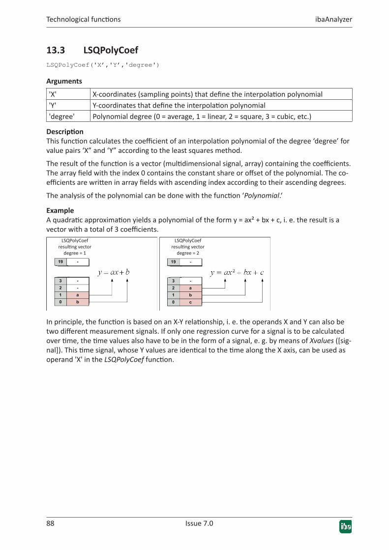
88 Issue 7.0

Technological functions ibaAnalyzer

13.3 LSQPolyCoefLSQPolyCoef('X’,'Y’,'degree')

Arguments

'X' X-coordinates (sampling points) that define the interpolation polynomial'Y' Y-coordinates that define the interpolation polynomial'degree' Polynomial degree (0 = average, 1 = linear, 2 = square, 3 = cubic, etc.)

DescriptionThis function calculates the coefficient of an interpolation polynomial of the degree ‘degree’ for value pairs ‘X” and ‘Y” according to the least squares method.

The result of the function is a vector (multidimensional signal, array) containing the coefficients. The array field with the index 0 contains the constant share or offset of the polynomial. The co-efficients are written in array fields with ascending index according to their ascending degrees.

The analysis of the polynomial can be done with the function ‘Polynomial.‘

ExampleA quadratic approximation yields a polynomial of the form y = ax² + bx + c, i. e. the result is a vector with a total of 3 coefficients.

In principle, the function is based on an X-Y relationship, i. e. the operands X and Y can also be two different measurement signals. If only one regression curve for a signal is to be calculated over time, the time values also have to be in the form of a signal, e. g. by means of Xvalues ([sig-nal]). This time signal, whose Y values are identical to the time along the X axis, can be used as operand 'X' in the LSQPolyCoef function.

LSQPolyCoefresulting vector

degree = 1

LSQPolyCoefresulting vector

degree = 2

Issue 7.0 89

ibaAnalyzer Technological functions

13.4 PolynomialPolynomial('Coefs’,'X')

Arguments

'Coefs' Vector with coefficients, e.g. as result of LSQPolyCoef'X' X-coordinates (sampling points) at which the polynomial is to be evaluated

DescriptionThis function calculates the polynomial value for every sample of ‘X‘ on the basis of a coefficient vector 'Coefs‘. It is required for the representation of regression lines or compensation curves whose coefficients were calculated with the LSQPolyCoef function prior to this.

9090 Issue 7.0

Spectrum analysis (FT operations) ibaAnalyzer

14 Spectrumanalysis(FToperations)ibaAnalyzer can carry out the spectral analysis in the form of the Fast Fourier Transformation (FFT). With the FFT operations available, a time or length based signal can not only be displayed in FFT mode, but also made available as a calculated expression and used for further analyses.

For most of the functions described here, it is possible to either display an amplitude or a power trend. This is indicated by the suffix ‘Ampl’ or ‘Power’ in the function names.

14.1 FftInTimeAmpl/FftInTimePowere.g. FftInTimeAmpl('Expression’,'Samples’,'#Freq’,'min_Freq'=0, 'max_Freq’,'Window'=0, 'Overlap'=0, 'DC-Suppression'=0)

Arguments

'Expression' Expression for which the FFT should be calculated'Time' Determination of the time or length intervals used. This rounds to an inter-

val containing 2^N samples.'#Freq' Number of frequencies displayed'min_Freq' Minimum frequency‘max_Freq' Maximum frequency'Window' Window type:

0 = Square

1 = Bartlett

2 = Blackman

3 = Hamming

4 = Hanning

5 = Blackman-Harris

6 = Flat top‘Overlap' Overlap factor'DC-Suppression' DC suppression

DescriptionThese functions calculate amplitude or power of the Fourier transformation of ‘Expression’ for sections with 2^N samples each. N is determined by rounding the product 'Time' x sampling fre-quency to a power of two.

The result is a vector that contains '#Freq' equally divided frequencies between 'min_Freq' and 'max_Freq' per section. The window type that is used for the calculation can be controlled via the ‘Window’ parameter.

The overlap factor determines the overlapping of the time segments and can be between 0 (no overlapping) and 1 (full overlapping). It is optionally possible to enable the DC suppression with the parameter ‘DC Suppression.’

Issue 7.0 91

ibaAnalyzer Spectrum analysis (FT operations)

ExampleThe FftInTime function can be used to display fluctuating frequencies over time. The resulting vector can be displayed in a 2D view for this purpose.

14.2 FftOrderAnalysisAmpl/FftOrderAnalysisPowere.g. FftOrderAnalysisAmpl('Expression’,'Samples’,'Freq’,'min_Order'=0, 'max_Order’,'Order_division’,'Window'=0,'Overlap'=0,’DC-Suppression'=0)

Arguments

'Expression' Expression for which the order analysis should be carried out'Time' Determination of the time or length intervals used'Freq' Basic frequency for the order analysis (rotational frequency)'min_Order' Minimum displayed order'max_Order' Maximum displayed order'Order_division' Grid width between the integer orders'Window' Window type

0 = Square

1 = Bartlett

2 = Blackman

3 = Hamming

4 = Hanning

5 = Blackman-Harris

6 = Flat top‘Overlap' Overlap factor'DC-Suppression' DC suppression

DescriptionThis function calculates the orders (i.e. multiples of a basic frequency ‘Freq’) for a signal and returns a vector with the orders between ‘min_Order’ and ‘max_Order.’ The number of data points per order is determined by the parameter ‘Order_division.’

The window type that is used for the calculation can be controlled via the ‘Window’ parameter. The overlap factor determines the overlapping of the time segments and can be between 0 (no overlapping) and 1 (full overlapping). It is optionally possible to enable the DC suppression with the parameter ‘DC Suppression.’

Contrary to the FftInTime function, the time/frequency is no longer displayed on the Y axis, but the rotational frequency and its multiple, i.e. the orders. The frequency axis is distorted in ac-cordance with the current revolutions per minute so that the orders are no longer displayed as a curve, but as straight lines. Depending on the function, either an amplitude trend (FftOrder-AnalysisAmpl) or a power trend (FftOrderAnalysisPower) is calculated.

92 Issue 7.0


Note

The function does not yield results if the number of signal points per revolution is more than twice as high as the selected parameter ‘Time.’

ExampleWith the FftOrderAnalysis function, you can calculate an order analysis. Frequencies corre-sponding to the motor speed or its multiple are called orders. The first order complies with the frequency of the motor speed, the second order complies with the frequency of the first order multiplied by the factor 2, etc. The order analysis calculates the level or the level curve of this order.

Fig. 30: Application of FftInTime and FftOrderAnalysis on a vibration signal

An interpolation is carried out between the individual signal points to calculate the FftOrder-Analysis.

Issue 7.0 93


14.3 FftPeaksInTimeAmpl/FftPeaksInTimePowere.g. FftPeaksInTimeAmpl('Expression’,'Samples’,'#Peaks,’ 'min_Freq'=0,'max_Freq’,'Window'=0,'Overlap'=0,'DC-Suppression'=0,'Zero-Padding'=0)

Arguments

'Expression' Expression for which the frequency spectra should be evaluated'Time' Determination of the time or length intervals used. This rounds to an inter-

val containing 2^N samples'#Peaks' Number of peaks displayed'min_Freq' Optional parameter for the minimally considered frequency, i.e. peaks at

lower frequency are not shown‘max_Freq' Optional parameter for the maximum considered frequency, i.e. peaks at

higher frequency are not shown'Window' Window type:

0 = Square

1 = Bartlett

2 = Blackman

3 = Hamming

4 = Hanning

5 = Blackman-Harris

6 = Flat top‘Overlap' Overlap factor'DC-Suppression' DC suppression'Zero-Padding' Adding zeros

DescriptionThis function is used to calculate frequency peaks across smoothed time intervals, which are determined by the parameter ‘Time.’ The ‘#Peaks,’ the highest points between the frequencies ‘min_Freq’ and ‘max_Freq,’ are calculated here. The time line of the frequency and the pairs of peak values are returned as a vector.

The entries are sorted according to the following pattern:

■ Index 0: Frequency with the highest peak

■ Index 1: Amplitude/power of the highest peak

■ Index 2: Frequency with the second highest peak

■ Index 3: Amplitude/power of the second highest peak

■ Etc.

94 Issue 7.0


Tip

To read out the requested values from the result array, you can use the 'Get-Rows' function.

The window type that is used for the calculation can be controlled via the ‘Window’ parameter. The overlap factor determines the overlapping of the time segments and can be between 0 (no overlapping) and 1 (full overlapping). It is optionally possible to enable the DC suppression with the parameter ‘DC Suppression.’ If the parameter ‘Zero_Padding’ is set to 1 or True(), the last window is filled with zeros before calculating the FFT.

14.4 FftAmpl/FftPowere.g. FftAmpl('Expression’,‘Samples’,'Window'=0,‘DC-Suppression'=0,'Zero-Pad-ding'=0)

Arguments

'Expression' Expression for which the Fourier transformation should be calculated'Samples' Number of measured values to be taken into consideration and implied

determination of the used time or length interval, depending on the sam-pling rate.

'Window' Window type:

0 = Square

1 = Bartlett

2 = Blackman

3 = Hamming

4 = Hanning

5 = Blackman-Harris

6 = Flat top'DC-Suppression' DC suppression'Zero-Padding' Adding zeros

DescriptionThese functions calculate the amplitude or power of the Fourier transformation of the signal. The used time section is determined by rounding the measuring points ‘samples’ to a power of two.

Note

The parameter ‘Samples’ is rounded up. At least 128 measuring points must be used.

Issue 7.0 95


The window type that is used for the calculation can be controlled via the ‘Window’ parameter. It is optionally possible to enable the DC suppression with the parameter ‘DC Suppression.’ If the parameter ‘Zero_Padding’ is set to 1 or True(), the window is filled with zeros to calculate the FFT.

14.5 FftComplexFftComplex('Expression’,'inv’,'normalize'=0)

Arguments

'Expression' Expression for which the Fourier transformation should be calculated'inv' Optional parameter for enabling an inverse Fourier transformation'normalize' Optional parameter for selecting a normalization

DescriptionThis function performs a Fourier transformation for a complex signal across the entire expres-sion and returns a vector with a real and imaginary component of the Fourier transformation. The input signal may consist both of an individual signal or a vector consisting of a real and imaginary component. A square window is used for the computation here.

If the parameter ‘inv’ is set to True() or 1, then an inverse Fourier transformation is computed. In this case, the function expects an input signal being either frequency-based or 1/length-based. The result of the operation then is a time-based or length-based signal accordingly.

The following values are permissible for the ‘normalize’ parameter:

� 0: No normalization is carried out.

� 1: The result is divided by the number of samples. For an inverse transformation, the result is not changed.

� 2: The result is divided by the square root of the number of samples. This applies both to a normal and an inverse transformation

� Other values: Function as with value 1.

The number of frequency samples is determined by the number of samples of the input signal. If N is even, N/2+1 frequency points are calculated; the first (DC component) and last point are purely real. If N is odd, (N+1)/2 frequency points are calculated; for those, the DC component is purely real.

96 Issue 7.0


14.6 FftReal/FftRealInversee.g. FftReal('Expression’,'normalize'=0)

Arguments

'Expression' Expression for which the Fourier transformation should be calculated'normalize' Optional parameter for enabling the normalization

DescriptionofFftRealThis function performs a Fourier transformation for a real signal across the entire expression and, as a result, delivers a vector with a real and imaginary component of the Fourier transfor-mation. A square window is used here.

If the parameter ‘normalize’ is set to True() 1, a normalization is performed. If the number of samples (N) of the signal is odd, all frequency values except for the DC component are divided by N/2. If N is even, all frequency values except for the DC component and the last value are divided by N/2.

The number of frequency samples is determined by the number of samples of the input signal. If N is even, N/2+1 frequency points are calculated; the first (DC component) and last point are purely real. If N is odd, (N+1)/2 frequency points are calculated; for those, the DC component is purely real.

DescriptionofFftRealInverseThis function calculates the inverse Fourier transformation, as created with FftReal. The result is real here and the input signal must accordingly be a vector consisting of a real and imaginary component. Otherwise the function works just like FftReal.

14.7 AWeighting/DbScale

AWeightingAweighting('Spectrum’,'Type')

Arguments

'Spectrum' Spectrum'Type' Specification of the type

DescriptionThis function weights a spectrum according to the so-called A-weighting. This is a weighting fil-ter that corresponds to human hearing.

ExampleAfter applying this function, a spectrum can be assessed with respect to the perceptible noise emission.

Issue 7.0 97


DbScaleDbScale('Spectrum’,'Reference')

Arguments

'Spectrum' Spectrum that should be logarithmically scaled'Reference' Optional

DescriptionThis function provides a logarithmic scaling in dB for a signal spectrum. A meaningful result can only be expected if the amplitude of a spectrum exists as an input.

Tip

Functions that calculate such an amplitude are: FftAmpl, FftInTimeAmpl, FftOrderAnalysisAmpl

14.8 IntSpectrumIntSpectrum ('Spectrum')

DescriptionThis function integrates a given spectrum. In this way, the vibration speed can be calculated from the frequency of an acceleration sensor.

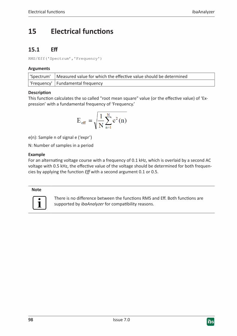
9898 Issue 7.0

Electrical functions ibaAnalyzer

15 Electricalfunctions

15.1 EffRMS/Eff('Spectrum’,'Frequency')

Arguments

'Spectrum' Measured value for which the effective value should be determined'Frequency' Fundamental frequency

DescriptionThis function calculates the so called "root mean square" value (or the effective value) of ‘Ex-pression’ with a fundamental frequency of ‘Frequency.’

e(n): Sample n of signal e (‘expr’)

N: Number of samples in a period

ExampleFor an alternating voltage course with a frequency of 0.1 kHz, which is overlaid by a second AC voltage with 0.5 kHz, the effective value of the voltage should be determined for both frequen-cies by applying the function Eff with a second argument 0.1 or 0.5.

Note

There is no difference between the functions RMS and Eff. Both functions are supported by ibaAnalyzer for compatibility reasons.

Issue 7.0 99

ibaAnalyzer Electrical functions

15.2 Deltafunctions

Fig. 31: Electrical functions, delta grid

The delta functions use the line voltages and line currents in a delta grid to calculate the differ-ent power values.

Arguments

'u12','u13','u23' Connection voltage (same as the phase voltages)'i1','i2','i3' Connection currents'freq' Fundamental frequency

Note

These functions are typically applied to a delta grid, but they can be applied to any grid in which the line voltages and currents are measurable.

DeltaCollectiveUeffDeltaCollectiveUeff('u12’,'u13’,'u23’,'freq')

Calculates the collective effective voltage in a delta grid:

Uxy,eff : the effective value of the line voltage Uxy

100 Issue 7.0


DeltaCollectiveIeffDeltaCollectiveIeff('i1’,'i2’,'i3’,'freq')

Calculates the collective effective current in a delta grid:

Ix,eff : the effective value of the line current ix

DeltaActivePDeltaActiveP('u13',‘u23',‘i1’,'i2’,'freq')

Calculates the active power in a delta grid:

N : the number of samples in a period

uxy : the voltage between the connection x and y (u13 = -u31)

ix : the current in line x

DeltaApparentPDeltaApparentP('u12’,'u13’,'u23’,'i1’,'i2’,'i3’,'freq')

Calculates the apparent power in a delta grid:

Ueff : the collective effective voltage

Ieff : the collective effective current

DeltaReactivePDeltaReactiveP('u12’,'u13’,'u23’,'i1’,'i2’,'i3’,'freq')

Calculates the reactive power in a delta grid:

S : apparent power

P : active power

Issue 7.0 101


DeltaReactivePSDeltaReactivePS('u12','u13','u23','i1','i2','i3','freq')

Calculates the signed reactive power QS in the delta grid:

DeltaActivePFactorDeltaActivePFactor('u12','u13','u23','i1','i2','i3','freq')

Calculates the active power factor in a delta grid:

S : apparent power

P : active power

DeltaReactivePFactorDeltaReactivePFactor('u12','u13','u23','i1','i2','i3','freq')

Calculates the reactive power factor in a delta grid:

Q : reactive power

P : active power

DeltaReactivePFactorSDeltaReactivePFactorS('u12','u13','u23','i1','i2','i3','freq')

Calculates the signed reactive power factor in a delta grid:

QS : signed reactive power

P : active power

102 Issue 7.0


15.3 Starfunctions

Fig. 32: Electrical functions, star grid

The star functions use the phase voltages and phase currents to calculate the different power values.

Arguments

'u1','u2','u3' Phase voltages'i1','i2','i3' Phase currents'i4' Neutral line'freq' Fundamental frequency

Note

These functions are typically applied to a star grid but they can be applied to any grid in which the phase voltages and currents are measurable.

StarCollectiveUeffStarCollectiveUeff('u1','u2','u3','freq')

Calculates the collective effective voltage in a star grid:

Ux_eff : the effective value of phase voltage ux

u4 = u1 + u2 + u3

Issue 7.0 103


StarCollectiveIeffStarCollectiveIeff('i1','i2','i3','i4','freq')

Calculates the collective effective current in a star grid:

Ix,eff : the effective value of the line current ix

StarActivePStarActiveP('u1','u2','u3','i1','i2','i3','freq')

Calculates the active power in a star grid:

N : Number of samples in a period

ux : Voltage of phase x

ix : Current of phase x

StarApparentPStarApparentP('u1','u2','u3','i1','i2','i3','i4','freq')

Calculates the apparent power in a star grid:

Ueff : the collective effective voltage

Ieff : the collective effective current

StarReactivePStarReactiveP('u1’,'u2’,'u3’,'i1’,'i2’,'i3’,'i4’,'freq')

Calculates the reactive power in a star grid:

S : apparent power

P : active power

104 Issue 7.0


StarReactivePSStarReactivePS('u1','u2','u3','i1','i2','i3','i4','freq')

Calculates the signed reactive power QS in the star grid:

StarActivePFactorStarActivePFactor('u1','u2','u3','i1','i2','i3','i4','freq')

Calculates the active power factor in a star grid:

S : apparent power

P : active power

StarReactivePFactorStarReactivePFactor('u1','u2','u3','i1','i2','i3','i4','freq')

Calculates the reactive power factor in a star grid:

Q : reactive power

P : active power

StarReactivePFactorSStarReactivePFactorS('u1','u2','u3','i1','i2','i3','i4','freq')

Calculates the signed reactive power factor in a star grid:

QS : signed reactive power

P : active power

Issue 7.0 105


15.4 Harmonicfunctions

HarmEffHarmEff ('u','Nharm','freq')

Calculates the effective value of 'NHarm' harmonic component of signal 'u.'

u(n) : Sample n of signal u

uReal,k : the real part of the kth harmonic component of u

uImag,k : the imaginary part of the kth harmonic component of u

Uk : the effective value of the kth harmonic component of u

HarmPhaseHarmPhase ('u','Nharm','freq')

Calculates the phase of 'NHarm' harmonic component of signal ‘u:

uReal,k : the real part of the kth harmonic component of u

uImag,k : the imaginary part of the kth harmonic component of u

φk : the phase offset of the kth harmonic component of u

StarHarmUGeffStarHarmUGeff ('u1','u2','u3','freq')

Calculates the effective negative sequence voltage UGeff.:

ux,1 : Fundamental harmonic component (complex) of phase voltage ux

106 Issue 7.0


StarHarmUMeffStarHarmUMeff ('u1', 'u2', 'u3', 'freq')

Calculates the positive sequence system voltage UMeff:

ux,1 : Fundamental harmonic component (complex) of phase voltage ux

StarHarmUnSymStarHarmUnSym ('u1', 'u2', 'u3', 'freq')

Calculates the voltage unbalance in a star grid:

The result is expressed in %.

WeightedDistortionFactorWeightedDistortionFactor ('u’,'Nharm'=50,'freq')

Calculates the weighted distortion factor of 'u' (all phases) using 'Nharm' harmonics:

Un : Effective value of the nth harmonic component of signal u

UnweightedDistortionFactorUnweightedDistortionFactor ('u’,'Nharm'=50,'freq')

Calculates the unweighted distortion factor of 'u' (all phases) using 'Nharm' harmonics:

Un : Effective value of the nth harmonic component of signal u

Issue 7.0 107


15.4.1 TIFTIF ('u’,'Nharm'=50,'freq')

Calculates the Telephone Interference Factor of 'u,' considering the first 'nHarm' harmonics.

Kn = 5*n*freq

Pn = BTS coefficient (British Telephone System)

Un : Effective value of the voltage the nth harmonic component of signal u

U1 : Examples

108108 Issue 7.0

Support and contact ibaAnalyzer

16 SupportandcontactSupport

Phone: +49 911 97282-14

Fax: +49 911 97282-33

Email: [email protected]

Note

If you require support, indicate the serial number (iba-S/N) of the product and the license number.

Contact

Headoffice

iba AG Koenigswarterstrasse 44 90762 Fuerth Germany

Phone: +49 911 97282-0

Fax: +49 911 97282-33

Email: [email protected]

Contact: Harald Opel

Deliveryaddress

iba AG Gebhardtstrasse 10 90762 Fuerth Germany

RegionalandWorldwide

For contact data of your regional iba office or representative please refer to our web site

www.iba-ag.com.

ibaAnalyzer - iba-ag.com

Documents

Transcript of ibaAnalyzer - iba-ag.com