I I I I I I I I I I - ARLIS.org

I I I I I I I I I I I I I I ~

c D 0 0

HD 242.5 .A4 U5 no.68

-

TECHNICAL REPORT NUMBER 68

Alaska OCS Socioeconomic Studies Program

Sponsor: Bureau of Land Management Alaska Outer Continental ~helf Office ;·"

~~~~

··~~

•ORTH ALEUTIAN SHELF STATEWIDE :\ND REGIONAL DEMOGRAPHIC AND CONOMIC SYSTEMS IMPACTS ANALYSIS

NPS

1111111111111111111111111~ 1111111111111111111111111111111111111 32436000011955

The United States Department of the Interior was designated by the Outer Continental Shelf (OCS) Lands Act of 1953 to carry out the majority of the Act's provisions for administering the mineral leasing and development of offshore areas of the United States under federal jurisdiction. Within the Department, the Bureau of Land Management (BLM) has the responsibility to meet requirements of the National Environmental Policy Act of 1969 (NEPA) as well as other legislation and regulations dealing with the effects of offshore development. In Alaska, unique cultural differences and climatic conditions create a need for developing additional socioeconomic and environmental information to improve ocs decision making at all governmental levels. In fulfillment of its federal responsibilities and with an awareness of these additional information needs, the BLM has initiated several investigative programs, one of which is the Alaska OCS Socioeconomic Studies Program (SESP).

The Alaska OCS Socioeconomic Studies Program is a multi-year research effort which attempts to predict and evaluate the effects of Alaska OCS Petroleum Development upon the physical, social, and economic environments within the state. The overall methodology is divided into three broad research components. The first component identifies an alternative set of assumptions regarding the location, the nature, and the timing of future petroleum events and related activities. In this component, the program takes into account the particular needs of the petroleum industry and projects the human, technological, economic, and environmental offshore and onshore development requirements of the regional petroleum industry.

The second component focuses on data gathering that identifies those quantifiable and qualifiable facts by which OCS-induced changes can be assessed. The critical community and regional components are identified and evaluated. Current endogenous and exogenous sources of change and functional organization among different sectors of community and regional life are analyzed. Susceptible community relationships, values, activities, and processes also are included.

The third research component focuses on an evaluation of the changes that could occur due to the potential oil and gas development. Impact eval,uation concentrates on an analysis of the impacts at the statewide, regional, and local level.

In general, program products are sequentially arranged in accordance with BLM' s proposed OCS lease sale schedule, so that information is timely to decisionmaking. Reports are available through the National Technical Information Service, and the BLM has a limited number of copies available through the Alaska OCS Office. Inquiries for information should be directed to: Program Coordinator (COAR), Socioeconomic Studies Program, Alaska OCS Office, P. 0. Box 1159, Anchorage, Alaska 99510.

II

ARLIS Alaska Resources

Library & Information & Anchorage AJm:t,

I I I I I I I I I I I I I I I I I I .I

[J

[

[

[

[

[

E [

c [

c c [

[

[

[

TECHNICAL REPORT NO. 68 Contract No. AA851-CTI-30

Alaska OCS Socioeconomic Studies Program

NORTH ALEUTIAN SHELF STATEWIDE AND REGIONAL DEMOGRAPHIC AND ECONOMIC SYSTEMS

IMPACT ANALYSIS

Prepared for

Bureau of Land Management Alaska Outer Continental Shelf Office

June 1982

THIS DOCUMENT IS AVAILABLE TO THE PUBLIC THROUGH THE NATIONAL

TECHNICAL INFORMATION SERVICE 5285 PORT ROYAL ROAD

SPRINGFIELD, VIRGINIA 22161

US fv\" :-;;:~.~,LS }.A;\N.J:..GfJ,·,:::<! s;:RVi CE

/·J\_--..~-~·.-,,-: ' --:.:1 / _' .. /~.~~·:p\

- =- -- = "-- ·-£------ --- --- -- ---- --- - - .... - - - -~;~- -- --- -- - ...

L r-~

L

Alaska Resources Library & Information Services

Anchorage Alaska

NOTICE

This document is disseminated under the sponsorship of the U.S. Department of the Interior, Bureau of Land Management, Alaska Outer Continental Shelf Office in the interest of information exchange. The United States Government assumes no liability for its content or use thereof.

Alaska OCS Socioeconomic Studies Program North Aleutian Shelf Statewide and Regional Demographic

and Economic Systems Impact Analysis

Prepared by Gunnar Knapp, P.J. Hill, and Ed Porter Institute of Social and Economic Research

ii

-.

'

1

-,

'

~

'"' L

[

[

[

[

[

[

[

[

b [

L

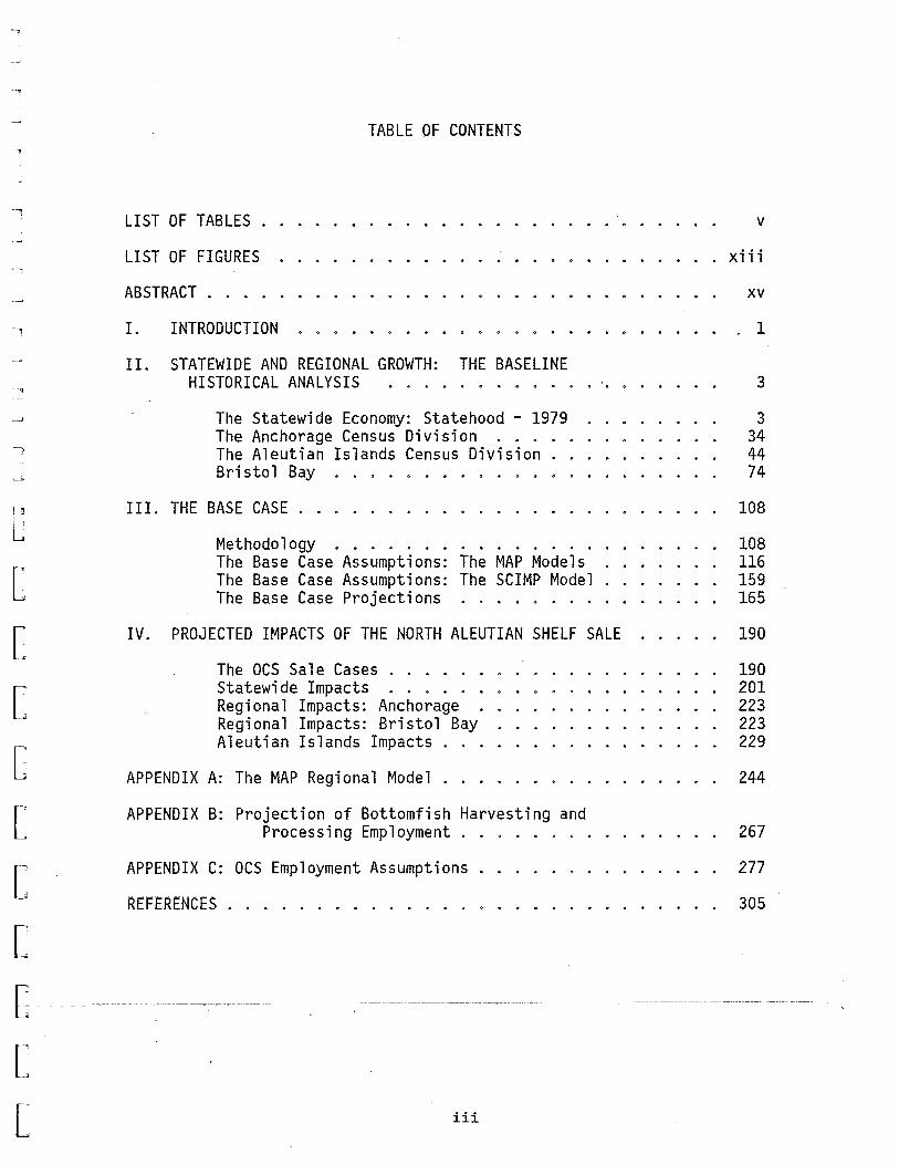
TABLE OF CONTENTS

LIST OF TABLES .

LIST OF FIGURES

ABSTRACT ....

I.

II.

INTRODUCTION

STATEWIDE AND REGIONAL GROWTH: THE BASELINE HISTORICAL ANALYSIS ....

The Statewide Economy: Statehood - 1979 The Anchorage Census Division ... The Aleutian Islands Census Division Bristol Bay

III. THE BASE CASE ..

Methodology ...... . The Base Case Assumptions: The Base Case Assumptions: The Base Case Projections

The MAP Models The SCIMP Model

IV. PROJECTED IMPACTS OF THE NORTH ALEUTIAN SHELF SALE

The OCS Sale Cases ..... . Statewide Impacts ..... . Regional Impacts: Anchorage .. . Regional Impacts: Bristol Bay Aleutian Islands Impacts

APPENDIX A: The MAP Regional Model ...

APPENDIX B: Projection of Bottomfish Harvesting and Processing Employment .

APPENDIX C: OCS Employment Assumptions

REFERENCES . . . . . . . . . . . . . .

iii

v

xiii

XV

1

3

3 34 44 74

108

108 116 159 165

190

190 201 223 223 229

244

267

277

305

J Ab

l J

-·--

J J J J J J J J J J ]

J J J ]·

J

[

[

[

[

[

[

[

[

[

[

[

[

[

[

[

[

C

[

[

1.

2.

3.

4.

5.

6.

7.

8.

9.

LIST OF TABLES

Value of Production for Selected Industries, Various Years, 1960-1979 ....... 0 •••••••

Civilian Employment, Unemployment and Labor Force 1960, 1965, 1970-1978, by Broad Industry Classification 0 •••••••••••• o •

Index of Seasonal Variation in Nonagricultural Employment: Selected Years 1960-1978 ..

Personal Income by Major Component: Alaska, Selected Years, 1960-1978 .. o •••••••••••••••••

Alaska Resident Adjusted Personal Income in Current and Constant 1979 Dollars, 1960, 1965, and 1970-1978 . . . . . . . . . . . . . . . . . .

Distribution of Relative Wage Rates, by Industry, for Alaska, Selected Years, 1965-1978 ....

Change in Real Average Monthly Wage, 1973-1976, Alaska

Rates of Change for the Anchorage and U.S. Consumer Price Index, Selected Years, 1960~1981 .....

Alaska Population and Components of Change: 1965-1978

10. Alaska Population by Age, 1980 ... 0 •

11.

12.

13.

14.

15.

Anchorage Nonagricultural Wage and Salary Employment, Selected Years ................ .

Anchorage Labor Force, Employment, and Unemployment, 1970-1978 . . . . . . . . . .

Anchorage Personal Income 1965-1978 .

Anchorage Population 1965-1980 . 0

Catch and Value to Fishermen, Aleutian Islands Census Division 1970 to 1976, Selected Years .....

16. Shellfish Harvest, Aleutian Islands Census Division, 1962, 1965-1976 ................ .

___ _17. Shellfish Harv_es:t ,by Ar~(l, _ Se 1 ~ct.ed Years 1992-197(5

v

7

13

15

19

22

24

26

28

32

33

36

38

39

41

45

46

47

18.

19.

20.

21.

22.

23.

24.

Residence of Boats and Gear License Holders Fishing the Aleutians ................ .

Military and Related Federal-Civilian Employment and Wages, Aleutian Islands Census Division, 1978 .

Average Civilian Monthly Employment Aleutian Is.lands Census Division, 1965-1978 ......... .

Aleutian Islands Census Division Estimated Resident and Nonresident Employment, 1978 ...... .

Aleutian Islands Census Division: Civilian Resident Labor Force, Total Employment, and Unemployment 1970-1975 . . . . . . . . • . . . . . . . . . . .

Report of Labor Force 1978 Compiled by Bureau of Indian Affairs, Anchorage Agency ........... .

Personal Income by Place of Residence: Aleutian Islands Census Division, 1965-1978 ....

25. Aleutian Islands Personal Income, 1978, by Sector, Components, and Geographic Disposition ....

26. Family Income: Number and Percent of Native and White Families by Income Levels, Aleut Corporation Area

27. Aleutian Islands Civilian and Total Resident Population: 1960, 1970-1978 .............. .

28. Aleutian Islands: Components of Population Change, 1970-1978 . . . . . . . . . . • . . . .

29. Aleut Region Population by Community, 1977

30. Catch and Value to Fishermen, Bristol Bay, 1969 to 1981 ..

31. Bristol Bay Permanent Entry Salmon Permits Gear Type and Residence, 1979 ............. .

32. Average Gross Earnings from Salmon Fishing by Gear Type and Residence, 1979 . . . . . . . . . . .

33. Military and Related Federal Civilian Employment and Wages, Bristol Bay Borough and Bristol Bay Census Division, 1978 .............. .

34. Average Civilian Monthly ~mployment, Bristol Bay Labor Area .. · . . . . . . · . . . . .. . . . . .

vi

49

54

56

59

61

63

65

66

70

72

72

73

76

79

79

86

87

[

[

[

[

[

[

[

[

[

[

c [ r L

[

r "='

[

E l [

[

[

[

[

[

[

[

[

C [

[

[

[

[

[

[

35. Average Civilian Monthly Employment, Bristol Bay Census Division ............. .

36. Average Civilian Monthly Employment, Bristol Bay Borough Division .............. .

37. Bristol Bay Monthly Nonagricultural Employment by Sector, 1979 ............... .

38. Bristol Bay Summary of Employment by Residency of Employees, Large Processors ..... .

39. Bristol Bay Average Annual Estimated Resident and Nonresident Employment, 1979 . . . . . . _ .

40. Summary Employment Statistics, Bristol Bay Labor Area

41. Monthly Labor Force and Employment, Bristol Bay, 1979

42.

43.

44.

45.

46.

47.

48.

Personal Income, Bristol Bay Division

Personal Income, Bristol Bay Borough

Income of Families by Percent in Income Class, Bristol Bay, 1970 ....... .

Population Growth, Bristol Bay, 1960~1980 .....

Components of Population Change, Bristol Bay Borough, 1960-1980 . . . . . . . . . . . . . . . .

. Dillingham Census Area Population by Community, 1980

Summary of Base Case Assumptions: MAP Models

49. Trans-Alaska Pipeline Employment Assumptions

50. Alaska Natural Gas Transportation System Employment Assumptions . . . . . . . . . . . . . . . . .

51. Prudhoe Bay Petroleum Production Employment Assumptions

52. Upper Cook Inlet Petroleum Production Employment Assumptions .............. .

53. National Petroleum Reserve in Alaska Employment Assumptions ........... .

88

89

91

93

95

97

97

100

101

103

105

105

106

118-119

122

123

125

128

130

r 54. Assumed OCS Oil and Gas Discoveries, Base Case . . . . . . . 131 . -=-t:-'-' =- -=- ....=.- ....=.-- --'-'---' =-- ----'- =- .=..-- "-'- -"'----=--~=--== --=--"'-"'· -c-=-=-·'-'--·~"--=-=~-.=-··''·-=-·o==-=-·-=-----·-'-: . ..=-.,-~,- -=---=----..=..- • .o..=·-·o=·=--··'·='·-=--=-· ... ,co=.~~---"-'-'--,'-·-o=-''·~- -'---- . .,-.o- "'--=-=··-" ·-=- .,-.. -.co.---= -.=.....-=--=---~-...=.- --'-- -=---=- ~- -'- c-=. .. ·o==--= --=--~·'' "'--'"-- =- . ..=- '-~--::"'-- -"""- --.~ -"--

[

[ vii

55. OCS Sale BF (Beaufort Sea) Employment Assumptions ...... 133

56. OCS Sale 55 (Gulf of Alaska) Employment Assumptions ..... 134

57. OCS Sale 60 (Lower Cook Inlet) Employment Assumptions .... 135

58. OCS Sale 71 (Beaufort Sea) Employment Assumptions ...... 136

59. OCS Sale 57 (Bering Norton) Employment Assumptions . . . . . 137

60. OCS Sale 70 (St. George) Employment Assumptions ....... 138

61. Beluga Chuitna Coal Production Employment Assumptions ... 139

141-142

144

62.

63.

64.

65.

66.

67.

68.

69.

70.

71.

72.

73.

74.

75.

76.

11 0ther Mining11 Employment Assumptions .

Agricultural Employment Assumptions ..

Logging and Sawmill Employment Assumptions

Nonbottomfish Commercial Fishing and Prncessing Employment Assumptions ......... .

Bottomfish Fishing and Processing Employment Assumptions

Federal Civilian Employment Assumptions

Federal Military Employment Assumptions .

State Revenue Assumptions ...... .

Calculation of Population Data for SCIMP Run, Aleutian Island Census Divison ........ .

SCIMP Model Exogenous Employment Assumptions

Projected Population and Components of Change: Alaska, 1980 to 2000 . . . . . . . . . . . . . . . . . . .

Projected Age Structure of Alaska Population, 1980-2000 .

Projected Employment: Alaska, 1980-2000 ..

Projected Personal Income and Personal Income Per Capita: Alaska, 1980-2000 ........ .

Projected Wages and Salaries by Sector: Alaska, 1980-2000

77. ProjectedReal Wage Rates: A 1 asl<a, 1981-2QOO .

viii

145

146-147

150

152-153

154-155

157

160

163

166

168

169

171

173

175

[

[

[

[

[

[

[

[

c [

c [

[

[

[

[

E [

[

[

[

[

[

[

[

[

[

c [

[

[

[

[

[

[

78.

79.

80.

Projected Alaska and U.S. Inflation Rates, 1980-2000

Projected State Government Revenues: Alaska, 1980-2000 . . . . . . . . . . . . .

Projected State Government Expenditures: 1980-2000 . . . . . . . . . . . . .

Alaska,-

81. Projected Alaska Permanent Fund Balance and Permanent Fund Balance Per Capita: 1980 to 2000 .....

82. Base Case Projected Population and Employment, Anchorage Census Division, 1980-2000 . . . . . . . . . . . . ~

83. Base Case Projected Population and Employment, Bristol Bay Region, 1980-2000 ............. .

84. SCIMP Mode 1 : Basic Sector Employment Projections, Base Case ..

85. SCIMP Mode 1: Government Employment Projections, Base Case . .

86. SCIMP Mode 1: Employment Projections, Base Case

87. SCIMP Model: Population Projections~ Base Case

88. North Aleutian Shelf OCS Resident Alaskan Employment Assumptions for MAP Model Projections .....

89. OCS Employment Inputs for SCIMP Model Runs, Mean Case

90. OCS Employment Inputs for SCIMP Model Runs, Low Case

91. OCS Employment Inputs for SCIMP Model Runs, High Case ..

92. OCS Employment Inputs for SCIMP Model Runs, Alternative Four Case . . . . . . . . . . .

93. OCS Employment Inputs for SCIMP Model Runs, Mean Offshore Loading Case .....

94. OCS Employment Inputs for SCIMP Model Runs, Alternative

95.

Four Offshore Loading Case ......... .

North Aleutian Shelf Sale Oil and Gas Property Tax Assumptions Used for MAP Model Projections ..

r 96. Projected Impact of North Aleutian Shelf Sale Statewide

176

177

179

181

182

183

185

186

187

189

192

193

194

195

196

197

198

200

t: -- c ~- ~-~ ~- ~~~-~ -~-c -c~- -populat-nrrr:--:---.. --.--:---:--:-.- .-~-- : --=--~----:---.---=---=---.- ~-~- -=--=--: - -zaz ·

[

[ ix

97. Projected Impact of North Aleutian Shelf Sale Statewide Total Employment . . . . . . . . . . . . . . . . . . . .

98. Projected Impact of North Aleutian Shelf Sale Statewide Basic Sector Employment . . . . . . . . . . . . . . . .

99. Projected Impact of North Aleutian Shelf Sale Statewide Services Employment • • 0 • • 0 • • • • • • • • • • • •

100. Projected Impact of North Aleutian Shelf Sale Statewide Government Employment .................

101. Projected Impact of North Aleutian Shelf Sale Statewide Real Personal Income ............... . . .

102. Projected Impact of North Aleutian Shelf Sale Statewide Real Per Capita Personal Income 0 • • • • • • • • • • •

103. Projected Impact of North Aleuti~n Shelf Sale Statewide Total Real Wages and Salaries 0 • • • • • • • • • • • •

104. Projected Impact of North Aleutian Shelf Sale Statewide Real Wage Rate in Basic Sector .............

105. Projected Impact of North Aleutian Shelf Sale Statewide Real Wage Rate in Services Sector • • • • 0 0 • • • • •

106. Projected Impact of North Aleutian Shelf Sale Statewide Real Wage Rate in Government Sector . . . . . . . . . .

107. Projected Impact of North Aleutian Shelf Sale, Alaska Rate of Inflation 0 • 0 .. • 0 • • • • • • • 0 • • • • •

108. Projected Impact of North Aleutian Shelf Sale, Total State General Fund Revenues ..............

109. Projected Impact of North Aleutian Shelf Sale, State Government Interest Earnings ..............

110. Projected Impact of North Aleutian Shelf Sale, Total State Government Expenditures . . . . . . . . . . . . .

111. Projected Impact of North Aleutian Shelf Sale, Per Capita State Expenditures . . . . . . . •

112. Projected Impact of North Aleutian Shelf Sale, Accumulated Permanent Fund Balance ....

_______ _]J}. Projected Impact of North Aleutian Shelf Sale, Per -- ----- -Cap-lta-.Ac~t,~mul a ted Pe~ma-ne_n_t_Funa--B~ifance--:---:--:--:

X

204

205

206

207

208

209

211

212

213

214

215

217

218

219

220

221

[

[

[

[

[

[

[

[

[

[

[

[

[

[

[

[

ZZ2 -- - --- -b [

[

[

[

[

[

[

[

[

[

[

[

[

[

[

[

[

[

b······

[ r.

L

114. Projected Impact of North Aleutian Shelf Sale, Anchorage Population .......... .

115. Projected Impact of North Aleutian Shelf Sale, Anchorage Total Employment ....... .

116. Projected Impact of North Aleutian Shelf Sale, Bristol Bay Population ................. .

117. Projected Impact of North Aleutian Shelf Sale, Bristol Bay Tota 1 Emp 1 oyment . . . . . . . . . . . . . . .

118. Projected Absolute Impact of North Aleutian Shelf Sale, Aleutian Islands Basic Sector Nonresident Employment

119. Projected Percentage Impact of North Aleutian Shelf Sale, Aleutian Islands Basic Sector Nonresident Employment

120. Projected Absolute Impact of North Aleutian Shelf Sale, Aleutian Islands Basic Sector Resident Employment

121. Projected Percentage Impact of North Aleutian Shelf Sale, Aleutian Islands Basic Sector Resident Employment

122. Projected Absolute Impact of North Aleutian Shelf Sale, Aleutian Islands Civilian Government Employment •.

123. Projected Percentage Impact of North Aleutian Shelf Sale, Aleutian Islands Civilian Government Employment .

124. Projected Absolute Impact of North Aleutian Shelf Sale, Aleutian Islands Support Sector Employment .....

125. Projected Percentage Impact of North Aleutian Shelf Sale, Aleutian Islands Support Sector Employment .....

126. Projected Absolute Impact of North Aleutian Shelf Sale, Aleutian Islands Civilian Resident Population

127. Projected Percentage Impact of North Aleutian Shelf Sale, Aleutian Islands Civilian Resident Population

128. Projected Absolute Impact of North Aleutian Shelf Sale, Aleutian Islands Total Population (Including Military, Military Dependents, Enclave Residents, and Fishermen) .. ; ............... .

129. Projected Percentage Impact of North Aleutian Shelf Sale, Aleutian Islands Total Population (Including

-Mi-l-itary--Mi-l-itary-Dependents--Enc-lave-Residents ----' . ' , and Fishermen) .................. .

xi

224

225

226

227

230

231

232

233

235

236

237

238

239

240

241

242

130. Employment Composition, 1979 .......... .

131. Assumed Costs of Interregional Service Provision

132. Employment Interaction Matrix, 1979

133. Population/Employment Ratios, 1979

134. Allocation of Harvest Assumptions .

135. Bottomfish Employment Residency Assumptions

136. SCIMP Model Aleutian Islands Bottomfish Employment Assumptions . . . . . . . . . . . . . . . . .

137. Location and Residence Assumptions for OCS Employment, Sale 75 (North Aleutian Shelf) .

138. OCS Employment, Mean Base Case

139. OCS Employment, Low Find (95% Probability) Case .

140. OCS Employment, High Find (5% Probability) Case .

141. OCS Employment, Alternative 4 Case 0 0 0 .. • • •

142. OCS Employment, Mean Base Case with Offshore Loading

251

253

. . . . 264

265

271

273

274

278-279

281-284

285-288

289-292

293-296

143. Alternative 4 Case with Offshore Loading 0 • • • • • •

297-300

301-304

xii

[

[

[

[

[

[

[

[

[

[

[

[

[

[

[

[

---- c [

[

-.,

---;

"'

r.., i L~

[ ~.,

[

[

[

[

[

[

[

[

[

[

c [ r·

L

LIST OF FIGURES

1. Distribution of Wage and Salary Income, Alaska, 1965 and 1978 . .

2. The MAP Statewide Model ....

3. The MAP Statewide Economic Model

4.

5.

Schematic Representation of Regional Model CDMOD

Alaska Census Divisions ..

xiii

29

110

113

245

246

J J . ]

--------- ----------- =----------------

]

J J n J J J J J J J J J J J J

. . . -----------------------·-----------

-.

___ J

" L----"

[

[

[

[

[

[

C [

[

[

[

[

[

[

ABSTRACT

NORTH ALEUTIAN SHELF STATEWIDE AND REGIONAL

DEMOGRAPHIC AND ECONOMIC SYSTEMS IMPACTS ANALYSES

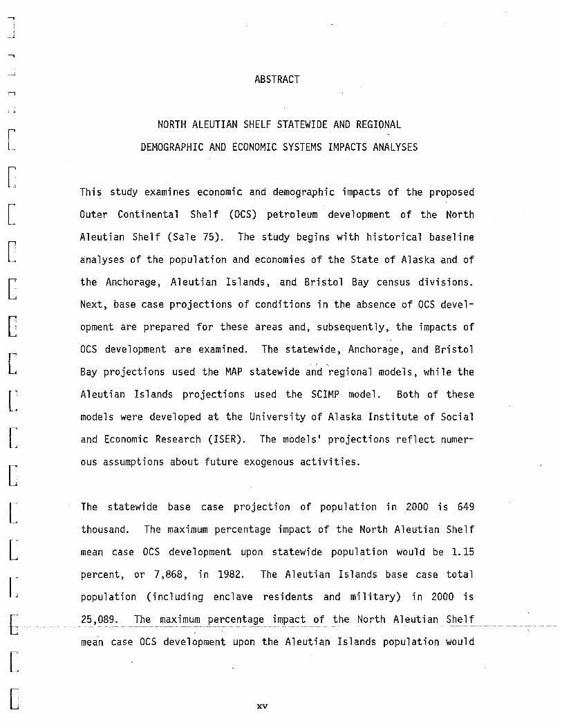
Thi~ study examines economic and demographic impacts of the proposed

Outer Continental Shelf (OCS) petroleum development of the North

Aleutian Shelf (Sale 75). The study begins with historical baseline

analyses of the population and economies of the State of Alaska and of

the Anchorage, Aleutian Islands, and Bristol Bay census divisions.

Next, base case projections of conditions in the absence of OCS devel-

opment are prepared for these areas and, subsequently, the impacts of

OCS development are examined. The statewide, Anchorage, and Bristol

Bay projections used the MAP statewide and regional models, while the

Aleutian Islands projections used the SCIMP model. Both of these

models were developed at the University of Alaska Institute of Social

and Economic Research (ISER). The models' projections reflect numer-

ous assumptions about future exogenous activities.

The statewide base case projection of population in 2000 is 649

thousand. The maximum percentage impact of the North Aleutian Shelf

mean case OCS development upon statewide population would be 1.15

percent, or 7,868, in 1982. The Aleutian Islands base case total

population (including enclave residents and military) in 2000 is

b- ________ _?~ !_0_8~ ~ _ __ T~e __ (TI~){_if11_U~- _p~~ce~~a~e imp~~~ -~f __ tbe_ ~()_l"th Ale_u~~a_n __ S_he~! _

mean case OCS development upon the Aleutian Islands population would

[

[ XV

be 2. 5 percent (822) in 1990. The maximum percentage impacts upon

Aleutian Islands resident employment would be 16.6 percent (145) in

1990. The maximum projected impact upon Aleutian Islands nonresident

or enclave employment (excluding military) would be 27.6 percent (733)

in 1989.

xvi

[

[

[

[

[

[

[

c [

[

c c c [

c [

-& [

L

-,

:

L"

[

[ I' l_

[

[

[

[

[

[

[

[

[

[

b [

[

I. INTRODUCTION

This study is concerned primarily with measuring the economic effects

of the proposed Outer Continental Shelf (OCS) petroleum development in

the North Aleutian Shelf (Sale 75). This study includes a statewide

and regional historical baseline analysis and base case projections

against which the direct and indirect economic effects of North

Aleutian Shelf OCS petroleum development are measured. The analysis

and projections are carried out on a statewide level and for three

regions within the state: the Aleutian Islands, Bristol Bay, and

Anchorage.

Part II of the study contains the historical baseline analysis for

each of the economic areas in question and generally focuses on

specific economic and demographic concerns relevant to an under-

standing of the historic growth of the economies. The base 1 i ne

analysis also assists in laying the foundation for the base case

assumptions regarding future growth of the areas.

Part III contains three important elements. First, the underlying

projection methodology is explained and reviewed in terms of the

economic mode 1 s used and the accuracy and 1 i mi tat ions of the pro-

jection methodology. Second, the assumptions used to 11 drive 11 the

models are presented. Finally, the base case projections for the

respective areas are presented, i.e. , the economic and demographic

projections in th~ ab~ence of OCS development.

[

Part IV of the study presents a description and analysis of the pro-[

jected impacts associated with the proposed North Aleutian Shelf lease [ sale. Results for the different OCS scenarios are discussed, both at

the statewide and regional levels. Supporting materials are contained [ in the appendices. [

[

[

[

c [

[

L [

[

[

[

. - -b

l 2

I

L

[

[

[

[

[

[

[

[

c [

[

[

[

[

[

[

II. STATEWIDE AND REGIONAL GROWTH:

THE BASELINE HISTORICAL ANALYSIS

This chapter provides historic baseline studies for Alaska and for

Anchorage, the Aleutian Islands, and Bristol Bay. These studies are

provided for three reasons. First, they should provide the unini

tiated reader with a general sense of the structure of the economy and

how and why it has changed over time. Second, they provide some indi-

cation of how individuals within the system have benefited from the

functioning of the system; i.e., an assessment of economic well-being ..

Third, they provide guidance in developing assumptions regarding

future development of the economy.

Potential impacts of OCS development will not be felt uniformly

throughout the state. Specific regions within Alaska can be expected

to experience both the brunt of the impacts and to capture dispropor-

tionate shares of the benefits. Therefore, we address not only the

statewide economy, but specific regional economies as well.

The Statewide Economy: Statehood - 1979

At the risk of oversimplification, the economic history of Alaska can

be summarized as one of resources~ defense, disaster, more resources,

b- _____ ~ _ --~~<! _g_o~~Y'_nfl1~1l_~·--~Y'_i~o:r _ t~ _W_o~~ ~-~~r_!!,_ _i~!_~r~~!--~_n_ :t:~~--~~(it_~_f~C:~~9 _ _ _ ___ _ _ ___ _

L [ 3

largely on natural resource exploitation, primarily based on furs,

fish, and hard rock minerals. World War II and the cold war aftermath

lead to a sizable military-government involvement in the state, both

in terms of population and economic activity.

The advent of statehood found an economy reflecting a narrowly based

private sector, largely dependent upon limited natural resource activ

ity, and a large federal civili.an and military presence. In 1960, for

example, federal civilian wages and salaries accounted for 25 percent

of the total civilian wage bill, while state government (5.9 percent)

and local government (5. 1 percent) made up an additional 11 percent of

total wage and salary payments. When military payrolls are included,

42.5 percent of wage and salary income was accounted for by government.

Discovery of the Swanson River oil field in 1957 had done much to

raise expectations about future economic prospects, but it was not

until major discoveries in Cook Inlet during 1965 that the oil and gas

industry became firmly established and significant levels of produc-

tion were assured. The emergence of petroleum resources as a signifi

cant factor in the Alaska economy considerably improved the potential

for private sector development and, more importantly, helped to shore

up the extremely shaky fiscal base of state government.

For the mid- and latter part of the decade of the 1960s, it was to be

natura 1 disaster that provided much of the impetus for economic

4

[

[

[

[

[

[

E [

[

[

[

c c [

c [

t [

[

[

[

[

[

[

[

[

[

[

[

[

[

[

[

[

L

growth. The Good Friday earthquake of 1964 resulted in a major recon-

struction effort which supported levels of economic activity that

probably waul d not have been achieved otherwise. A second disaster,

of lesser statewide magnitude but of great consequence for the Fair-

banks region, was the flood of 1967. Disaster relief and reconstruc-

tion funds, followed later by flood control projects, provided a need-

ed boost for the region's economy.

Discovery of oi 1 at Prudhoe Bay in 1968 marks the beginning of the

1 a test phase of A 1 as ka economic hi story. Deve 1 opment of the super-

giant field, construction of the oil pipeline, and the related flows

of revenue to state government are providing the impetus for sustained

economic growth and diversification that should carry the state well

into the 21st century.

Against this backdrop, we can now look more specifically at several

important dimensions of growth and change in the Alaska economy. As

suggested earlier, there are certain key measures of economic activity

that are central to the analysis. Personal income and employment data

provide insight into the overall growth of the economy and changes in

the composition of economic activity. In addition, these data can be

used as genera 1 indicators of changes in economic we 11-bei ng over

time. An important corollary variable is population growth. It is

also instructive to. review aggregate measures of production for the

r~ ' economy. t- --------- ~-------- ----- ---------------'- --------~--- ----- ---- ----------- ----------- ------- --- ·---------- ----- --------·----- ---------

L [ 5

In addition to these general measures of economic activity, there are

several specific attributes of the economy that need to be considered.

These include such topics as secular and seasona 1 unemp 1 oyment, the

structure of costs and prices, and the role of state government with

respect to determining overall economic activity. Finally, we must

consider issues related to potential future economic activity. We now

turn to specific measures of the economy.

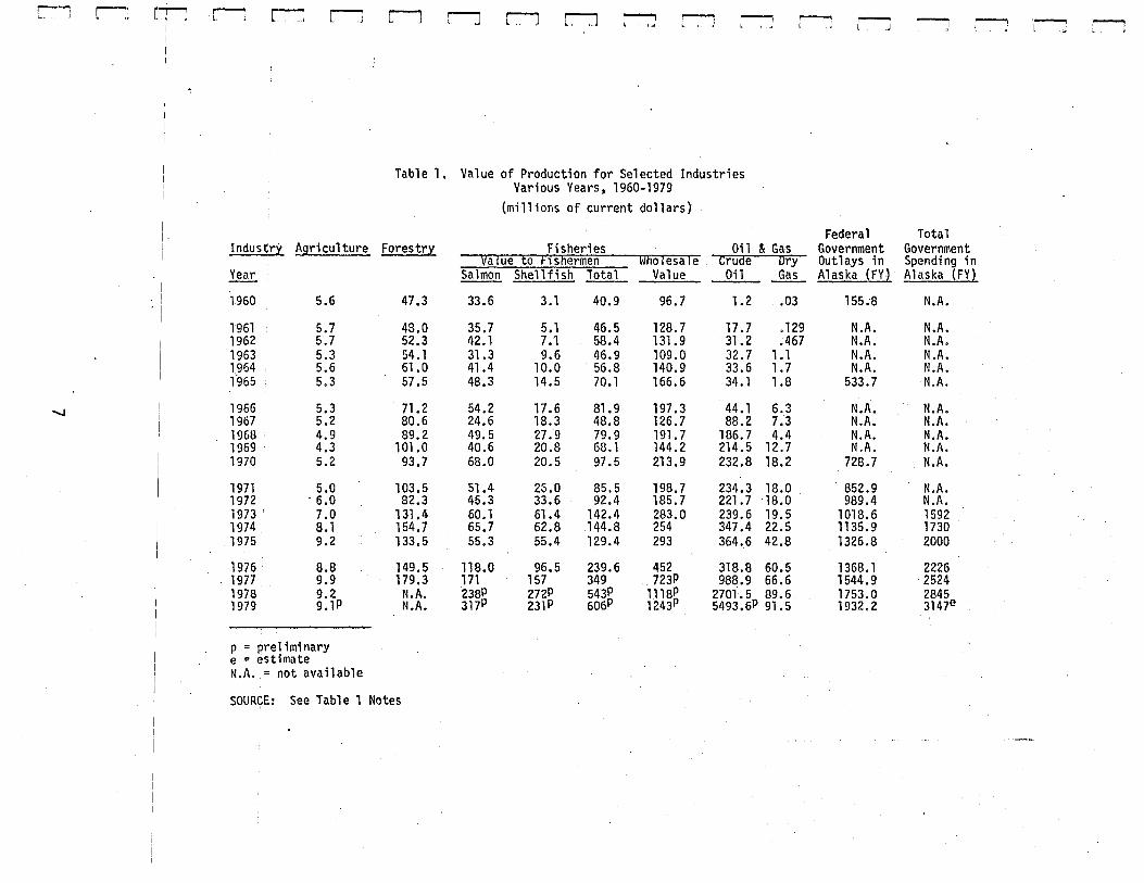
PRODUCTION

Data measuring the gross value of production by industrial classifica-

tion are not available for recent years. However, various measures of

the value of output for selected industries have been compiled and are

presented in Table 1. Except for agriculture, the industries reflect

the primary "export base 11 components of the private sector economy.

Data on federal and total government expenditures have also been in-

eluded for comparative purposes. Furthermore, a large portion of fed-

era 1 government out 1 ays indirectly reflects an export o{ goods and

services by the private sector economy of Alaska.

Fisheries and petroleum have clearly dominated growth in the value of

production in the private sector. Value of catch to fishermen has

grown at an average annual rate of 15 percent over the period, and

wholesale value has grown almost as rapidly (14.4 percent), reflecting

both the substantial growth of shellfishing and rising product prices.

n [

[

[

[

[

[

[

[

[

[

[

[

[

[

[ When deflated by the consumer price index (which is appropriate if we r

------------------------------------------ ~- ----- ---------·--·----------------------------------------·---------------------------·-t-- -

are interested in implicit purchasing power), the value of catch grew

l 6 [

~~~~~~~~~~~~~~~~~~~

Table 1. Value of Production for Selected Industries Various Years, 1960-1979

(millions of current dollars)

Federal Total Industry Agrjculture Forestry Fisheries Oil & Gas Government Government

Value to F1snermen wnolesale Crude Ory Outlays in Spending in Year Salmon Shellfish Total Value Oil ~ Alaska (FY~ Alaska (FY)

1960 5.6 47.3 33.6 3.1 40.9 96.7 1.2 • 03 155.8 N.A •

1961 5.7 48.0 35.7 5.1 46.5 128.7 17.7 .129 N.A. N.A. 1962 5.7 52.3 42.1 7.1 58.4 131.9 31.2 .467 N.A. N.A. 1963 5.3 54.1 31.3 9.6 46.9 109.0 32.7 1 • 1 N.A. N.A. 1964 5.6 61.0 41.4 10.0 56.8 140.9 33.6 1.7 N.A. N.A. 1"965 5.3 57.5 48.3 14.5 70.1 166.6 34.1 1.8 533.7 N.A.

...... 1966 5.3 71.2 54.2 17.6 81.9 197.3 44.1 6.3 N.A. N.A. 1967 5.2 80.6 24.6 18.3 48.8 126.7 88.2 7.3 N.A. N.A. 1968 . 4.9 89.2 49.5 27.9 79.9 191.7 186.7 4.4 N.A. N.A. 1969 4.3 101.0 40.6 20.8 68.1 144.2 214.5 12.7 N.A. N.A. 1970 5.2 93,7 68.0 20.5 97.5 213.9 232.8 18.2 728.7 N.A.

1971 5.0 103.5 51.4 25.0 85.5 198.7 234.3 18.0 852.9 N.A. 1972 . 6.0 82.3 45.3 33.6 92.4 185.7 221.7 18.0 989.4 N.A. 1973 7.0 131.4 60.1 61.4 142.4 283.0 239.6 19.5 1018.6 1592 1974 8.1 154.7 65.7 62.8 144.8 254 347.4 22.5 1135.9 1730 1975 9.2 133.5 55.3 55.4 129.4 293 364.6 42.8 1326.8 2000

1976 8.8 149,5 118.0 96.5 239.6 452 318.8 60.5 1368.1 2226 1977 9.9 179,3 171 157 349 723P 988.9 66.6 1544.9 2524 1978 9.2 N.A .• 238P 272P 543P lll8g 2701'. 5 89.6 1753.0 2845 1979 9.1 p N.A. 317P 231P 606P 1243 5493.6P 91.5 1932.2 3147e

p =preliminary e = estimate N.A. = not available

SOURCE: See Table 1 Notes

Table 1 Notes

The data are primarily obtained from selected tables in The Alaksa Economy: Year-End Performance Report 1978 (Alaska Department of Cornmerce and Economic Development, Division of Economic Enterprise; Juneau, Alaska) and Alaska Statistical Review (Alaska Department of Commerce and EconGmic Development, Divislon·of Economic Enterprise; Juneau, Alaksa, 1980). The. latter source is a preliminary report. Specific sources for each column of the table follow.

Agriculture: page B-13 Alaska Statistical Review (ASR). Value of sales is approximately 74 percent of value of production, with the balance being used on farm.

Forestry: Data from 1960-1971 are from Alaska Statistical Review (1972), p. 90, and reflect total end product value. For 1972-1977, the data are from the 1978 Year End Performance Report and reflect.only forest product exports. Here the series are not comparable, but individually reflect growth in the periods in question. Comparable series are not available over the full period.

Fisheries: Data for 1972-1975 are from the 1978 Year End Performance ~' p. 58. 1976 data are from Alaska Catch and Production: 1976 (Alaska Department of Fish and Game). 1977-1979 data are from ASR (1980). 1960-1971 data are from ASR (1972) p. 74. Data for 1960-71, 1976-79 are comparable. Data for 1972-75 represent approximately 92 percent of total wholesale value.

Oil and Gas: ASR (1980) p. B-3. It should be noted that these data do not include value added in transportation and here reflect approximate wellhead value.

Federal Government Outlays in Alaska: 1960-1977 data are from 1978 Year End Report, p. 105. 1978-1979 data are from ASR (1980), p. E-2. Data are for fiscal year ending in given calendar year. ·

Total Government Spending in Alaska: Data from ·AsR (1980) p. E-1. The total is net of intergovernmental transfers.

[

[

[

[

[

[

[

[

c [

[

[

[

[

[

[

------------------------------------ -----------~------------------------~----------------C--

8

[

[

[

[

[

[

[

[

[

[

[

[

[

[

[

[

[

[

at almost 10.3 percent and the wholesale value by 9.5 percent. Crude

oil and natural gas percentage growth rates are relatively meaningless

since the base in 1960 is negligible, but their significance is obvi

ous. It is also worth noting that in 1978 (the last year for which

data are available) production of minerals other than oil and gas and

sand and gravel amounted to 18.4 million dollars, or about 0.6 percent

of the total value of mineral production. Neither has there been any

significant change in the value of this dimension of mining over the

past two decades. In deflated dollars, federal government expendi-

tures have grown at about 9.3 percent.

Government expenditures are not directly comparable to the value of ..

production in other industries since they reflect not only government

production (wages and salaries) but purchases of goods and services

and transfer payments to individuals. However, in another sense these

expenditures do reflect a measure of demand for production of goods

and services throughout the economy as a whole and underscore the con-

tinuing importance of government spending in the economy.

Of particular significance in overall government spending is the role

of state government spending. The state fiscal history can roughly be

divided into three periods: early post-statehood, Prudhoe Bay sale to

pipeline completion, and Prudhoe Bay production.

r~ ,. During the first period, federa 1 governm~nt_jl_r~~!_~oth ~tate hood L- ~-~- -- ---- --------------------------------- ---- -

l [

transition grants and others, were an important component of state

9

government revenues. The relative decline in federal grants were more

than offset by revenues linked to general economic growth and the de

velopment of Cook Inlet petroleum resources, but expenditures were

constrained by available revenues.

The $900 million Prudhoe Bay lease sale in the fall of 1969 ushered in

the second period and led to an immediate doubling of state government

expenditures. Growth in expenditures continued rapidly, although

still constrained by available revenues and the rapidly diminishing

balance of the lease sale. The third period is marked by the com

mencement of production from Prudhoe Bay; and, for the first time, the

state has significant potential surplus revenues.

The rapid expansion of revenues since 1969 has resulted in a closely

correlated growth of state government expenditures. This is reflected

not only in expanding state government employment and wages but also

by total government expenditures for purchases of goods and services

and transfers to local government. The net result has been that state

government spending (both directly and through local government) has

assumed a significant role in the overall determination of economic

activity in Alaska. This is a pattern which will prevail for some

time into the future.

In summary, the role of natural resources in the growth of the Alaska

economy has been dominated by fisheries and petroleum. Forest ------- ------

products have remained regionally important, primarily for Southeast

10

[

[

[

[

[

[

[

[

l 0 [

[

[

[

[

[

-b[

[

[

[

r [

[

[

[

[

[

[

[

[

[

[ r~ '---'

Alaska, but have not demonstrated significant growth. Agriculture has

remained stagnant, and, in real terms, the value of production has de-

clined. Government has remained a major force in the economy, with

state and local government increasing in relative proportion to total

government.

EMPLOYMENT, UNEMPLOYMENT, AND WORK FORCE

Analysis of employment, unemployment, and work force data is important

for several reasons. First, since labor is one of the key factors of

production, employment data provide a general indicator of the growth

and composition of production over time. The main deficiency with

these data for such purposes is that they ignore changes in factor

proportions over time and differences in factor proportions between

industries. This omission is particularly important in industries

that are highly capital-intensive, such as the petroleum industry.

Also, since these data are based on job counts, they do not reflect

actual man hours of production and, hence, provide only an approximate

measure of labor input.

Second, work force data, in conjunction with total employment data,

determine unemployment. It is instructive to observe the patterns of

unemployment over time and in response to changes in total economic

activity. Third, the data are useful in measuring seasonal patterns

[ of economic activity and how this may have changed over time.

,.

b-- ~ ------- -~- ---- ~ __ ____:__~-~-.

[ r--

L 11

Tables 2 and 3 provide summary data on employment, labor force, and

unemployment for selected years over the 1960-1978 period. Total em-

ployment over this period grew at an annual average rate of 4.9 per-

cent. However, substantial variation in the growth rate is evident.

From 1960-1973, the rate was 3 percent; while for 1974-1978 (reflect-

i ng the pipe 1 i ne boom) the rate was 8. 6 percent. The growth of the

civilian labor force shows a similar pattern, although increasing at a

slightly higher rate. The result of this is that total unemployment

has grown at about 7 percent per year over the period and the unem-

ployment rate has also increased.

It is also worth noting that during the pre-pipeline period the unem-

ployment rate was relatively stable and that the somewhat higher rates

of 1977 and 1978 reflect in large part a readjustment to a more normal

post-pipeline period. These data clearly illustrate the openness of

the Alaska labor market. Large variations in the demand for labor are

primarily met by significant in- and out-migration and by changes in

labor force participation rates. As a consequence, the long-run rate

of unemployment is quite stable and the simple expansion of economic

activity has little effect in terms of reducing unemployment. The

second block of data in Table 2 provides annual average employment

data by broad industry classification. In addition to illustrating

the sustained growth of employment and production in all industry cat-

egories, these data also indicate relative changes in the significance

of specific industries. ------·----------~-----

12

[

[

[

[

[

[

[

[

[

[

[

[

[

[

[

[

b[ r .,

L

r--; ~1 ~ rJ r-l r-l r-l l1 rJ l1 r:J r-:J r---1 l l1 r-J l1 ~ :--J :--J

__, w

I i

Total Civili~n Labor Force I

Total Unemployment . I

% of Total Labor Force . I

Total Emplti'l"nt

Nonagricultutal Wage and Salary Empioyment

Mining I

Contract Construction

r~anufacturi ng

Fobd Processing I

1960

73.6

5.9

8.0%

67.7

TABLE 2. CIVILIAN EMPLOYMENT, UNEMPLOYMENT AND LABOR FORCE 1960, 1965, 1970-1978, BY BROAD INDUST~f CLASSIFICATION

(IN THOUSANDS)

1965

89.8

7.7

8.6%

82.1

1970

91.6

6.5

7.1%

85.1

1971

97.7

8.0

8.2%

89.6

1972

103.6

8.6

8.3%

95.0

1973

109.1

9.3

8.5%

99.9

1974

125.6

9.9

7.9%

115.7

1975

156.0

10.8

6.9%

145.3

1976

168.0

14.0

8.3%

154.0

1977

174.0

16.0

9.2%.

158.0

1978

181.0

20.0

11.0%

161.0

f!!!!?.!._%_ ~-%- Emp. _%_ f!!!!?.!._%_ ~_L ~-%- ~-%- ~-%- ~-%- ~-%- Emp. _%

56.9 100.0 70.5 100.0 92.5 100.0 97.6 100.0 105.4 100.0 111.2 100.0 129.7 100.0 163.7 100.0 173.5 100.0 166.0 100.0 163.2 100.

1.1 1.9

5.9 10.4

5.8 10.1

2.8

1.1

6.5

6.2

3.0

1.6

9.2

8.8

4.3

2.4 1.8 3.0 2.3 3.8 2.3 4.0 2.3 5.0 3.0 5.6 3.

7.0 14.1 10.9 25.9 15.8 30.2 17.4 19.5 11.7 12.2 7.

5.9 10.3 5.9 10.9 6.6 11.5. 7.

Lo~ging, lumber, Pulp 2.2 I

4.9

3.9 2.3. 3.3

3.0

6.9

7.8

3.7

2.8

3.2

7.5

8.4

4.0

3.0

7.4

7.8

3.6

2.8

2.5

7.6

8.0

3.7

2.9

2.1

7.9

8.1

3.7

2.8

2.0

7.5

7.7

3.5

2.7

2.0

7.8

9.4

4.6

3.2

8.5

4.1

2.9

9.6

4.3.

3.6

7.4

3.3

2.8

9.6

4.3

3.4

2.6

2.1

5.1

3.2

2.9

1.8

5.5

3.5

3.3

2.1

6.3

1.8

3.

1 •

Transpo~tation, Communications Publif Utilities 6.8

Trade ]

Financel Insurance, Real Estate

• I Serv1ces I Government I

I Federal I

St~te I

Local

I

12.0 7.3 10.4 9.1 9.8 9.8 10.0 .10.0 9.5 10.4 9.4 12.4 9.6 16.5 10.1 15.8 9.1 15.6 9.4 16.4 10.

7.7 13.5 10.0 14.2 15.4 16.6• 16.1 16.5 17.1 16.2 18.3 16.5 21.1 16.3 26.2 16.0 27.6 15.9 28.5 17.2 28.8 17.

1.4

5.6

2.5

9.8

2.2 3.1 3.1 3.4 3.2 3.3 3.7 3.5 4.2 3.8 4.9 3.8 6.0 3.7 7.1 4.1 7.8 4.7 8.2 5.

7. 5 16.6 11.4 12.3 12. 5 12.8 14.0 13.3 15.2 13.7 18.3 14. 1 25. 1 15.3 27. 7 16.0 27.4 16. 5 27. 6 16.

22.7 39.9 29.7 42.1 35.5 38.5 38.0 38.9 41.~ 39.6. 42.8 38.5 45.3 34.9 49.5 30.2 49.7 28.6 50.7 30.5 52.2 32.

15.6 27.4 17.4 24.7 17.1 18.5 17.3 17.7 17.2 16.3 17.2 15.5 18.0 13.9 18.3 11.2 17.9 10.3 17.7 10.7 18.1 11.

3.9 6.9 7.0 9,9 10.4 11.2 11.7 12.0 13.3 12.6 13.8 12.4 14.2 10.9 15.5 9.5 14.1 8.1 13.9 8.4 14.3 8.

3.2 5.6 5.3 7.5 8.1 8.8 9.0 9.2 11.2 10.6 11.9 10.7 13.1 10.1 15.8 9.7 17.6 10.1 19.1 11.5 19.8 12.

Table 2 Notes

Sources of data: 1960, 1965 ASR (1972) p. 16. It should be noted that the 11 labor force 11 data are actually work force data for these two years and are not directly comparable with the data for 1970-1978. The basic difference between the two series is that work force estimates are based on job counts and, hence, a worker may be counted-more than once if holding two or more jobs. Labor force estimates are supposed to eliminate this double counting. Thus, the work force data for 1960 and 1965 somewhat overstate the actual number of emplo~ed.

In 1970-1978, labor force and total employment estimates are obtained from Alaska Labor Force Estimates by Area (Alaska Department of Labor), various years.

Non-agricultural wage and salary_data are obtained from the Statistical Quarterly (Alaska Department of Labor) for the various years.

14

[

[

[

[

[

[·-,

_,

[

[

[

[

[

[

[

[

[

[

~ [

[

[

[

[

[

[

[

[

[

[

[

[

[

[

[

[

[

TABLE 3. INDEX OF SEASONAL VARIATION IN NONAGRICULTURAL EMPLOYMENT: SELECTED YEARS 1960~1978

1960 1965 1970 1972 1974 1976

Total Nonagricultural Employment 39.4 30.6 22.7 24.6 32.0 23. 1

Contract Construction 156.2 91.7 69.5 77.6 108.2 64.7

Manufacturing 136.3 116.3 107.9 105.2 70.8 78.2

Food Processing 211.5 195.2 196.3 175.3 100.6 112.0

Trade 20.8 20.0 15.6 14.8 25. 1 13.5

Services 28.4 17.2 10.7 16.2 26.8 13.3

Unemployment Rate, All Industries 117.5 74A 59.2 65.1 82.3 45.8

Labor Force 28.2 26.5 21.8 21.0 27.1 21.2

1978

14.0

4i.2

86.5

125.0

12.0

17.8

30.0

12.0

r .. 'SOURCE:. Compiled from Statistical Quarterly (A.!_aska_p~~artm~nt_()__f_Labor)~-' ~--~~ t----- --p-----~---selected years. Seasonal variation is measured as the high month

minus the l·ow.inonth divided by average annual figure, stated as

l a percent. Unemployment data are_from Labor Force Estimates (Alaska Department of Labor), var1ous years.

[ 15

Emp 1 oyment in mining is the one basic sector industry that has in

creased its share of total employment. The federal government share

has declined substantially over the period, while both state and local

government have grown, with much of the growth in state government em

ployment occurring during the 1960s and the early 1970s. Local gov

ernment growth lagged state government in the early years, but by 1975

local government employ~ent exceeded state government employment. Of

particular interest is the growth of support sector activity, includ

ing trade, finance, insurance and real estate, and services. This

growth reflects a s·teady diversification of support sector activity

and the process of import substitution in response to increasing mar

ket size, growth of incomes, and opportunities for specialization. In

short, the data reflect a general maturation of the economy.

It is also of interest to consider changes in seasonal patterns of

economic activity. Table 3 summarizes seasonal activity in selected

industries, as well as for total nonagricultural wage and salary em

ployment, labor force, and unemployment. Seasonal variation is mea

sured as the high month minus the low month divided by the average an

nual figure for the respective variable. Because of secular growth in

the variables, the index tends to overstate seasonality for any given

year, but for comparative purposesJ over time, the index is satisfac

tory.

The data reflect two important dimensions of the Alaska economy.

First, seasonality varies drastically from industry to industry, with

16

[

[

[

[

[

[

[

[

[

c [

[

[

[

[

[

b[

[

[

[

[

[

[

[

[

[

[

[

[

[

[

[

[

[

construction and manufacturing (especially food processing) showing

the greatest seasonal swings. Second, while significant seasonality

remains in all industry, there has been a major reduction over time.

In summary, the data on labor force, employment, and unemployment il-

lustrate several important features of the Alaska economy. First,

while growth has been uneven, aggregate economic activity has in-

creased substantially since statehood. Contract construction, mining,

and support sector industries grew rapidly during pipeline construe-

tion. With the exception of contract construction, levels of employ-

ment achieved at the peak of pipeline construction have generally been

sustained or have increased.

Second, ~tructural change that reflects a general maturing of the eco-

nomy has occurred, as evidenced by the increased share of tota 1 em-

ployment accounted for by support sector activity, including trade,

finance, insurance and rea 1 estate, and services. Coup 1 ed with the

greatly reduced dependence of the state on federal government activity

and the growth of petroleum and fisheries, the data indicate a general

broadening and diversification of economic activity.

Third, in addition to sustained secular growth, there has been a mark-

ed decrease in seasonal swings in economic activity. In part, this

reflects the relative growth of industries with smaller seasonal vari-

-[}-~~--·~·~~---a~-;~~s~~!n addi~ion.' construction and fish processing seasonalit_y~

have also reduced substantially.

L [ 17

Finally, the relative stability of unemployment rates over time clear

ly indicates the openness of the Alaska labor market. The generally

higher than national average unemployment rates have not responded to

aggregate economic expansion historically and probably will not in the

future.

PERSONAL INCOME

Personal income measures that part of the total value of production

that accrues to individuals and includes: wage and salary income;

other labor income; proprietor•s income; income from dividends, inter

est, and rent; and personal transfer payments. While deficient in

many respects as a measure of economic well-being, it is nevertheless

a useful indicator of the degree to which individuals share in the to

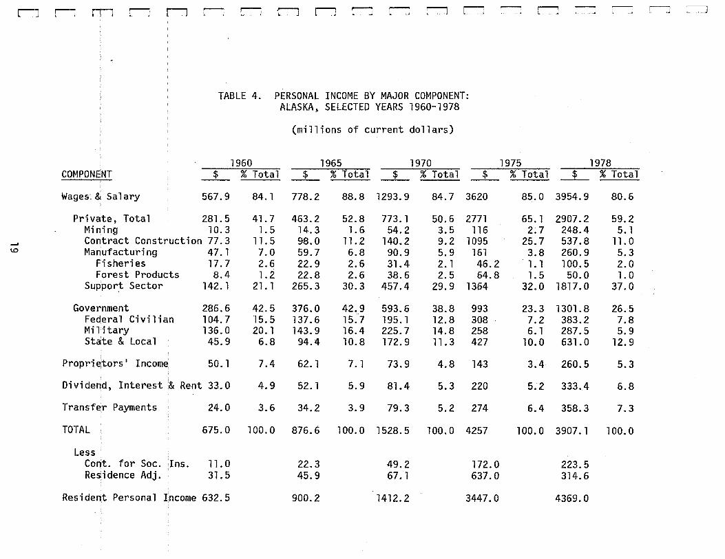
tal benefits of production. Table 4 presents estimates of personal

income for Alaska, by major source, for selected years covering the

period from 1960 through 1978.

Personal income has grown steadily over the entire period, at an aver

age annual rate of 11.3 percent, while for the pipeline period the

growth was about 17 percent per year. Wage and salary income account

ed for the majority of persona 1 income throughout the period, aver

aging 80 percent. In contrast, about 68 percent of U.S. personal in

come is accounted for by wages and salaries. Proprietor income as a

share of total personal income has declined somewhat; while that of

dividends, interest, and rent has increased modestly. The share ac

counted for by transfer payments has increased substantially but still

18

c [

[

[

[

[

[

c [

c c c c [

[

[

b [

[

r-l r-: rTJ rJ rl ____..., l. J r-l Ll r-l r-J r-:J r:-1 r:l

TABLE 4. PERSONAL INCOME BY MAJOR COMPONENT: ALASKA, SELECTED YEARS 1960-1978

(millions of current dollars)

1960 1965 1970 COMPONENT $ % Total $ % Total ___1 % Total $

Wages~& Salary 567.9 84.1 778.2 88.8 1293.9 84.7 3620

Private, Total 281.5 41.7 463.2 52.8 773.1 50.6 2771 Mining 10.3 1.5 14.3 1.6 54.2 3.5 116

__, Contract Const~uction 77.3 11.5 98.0 11.2 140.2 9.2 1095 1.0 Manufacturing 47.1 7.0 59.7 6.8 90.9 5.9 161

Fisheries 17.7 2.6 22.9 2.6 31.4 2. 1 46.2 Forest Produdts 8.4 1.2 22.8 2.6 38.6 2.5 64.8

Suppor:t Sector 142. 1 21. l 265.3 30.3 457.4 29.9 1364

Government 286.6 42.5 376.0 42.9 593.6 38.8 993 Federal Civilian 104.7 '15. 5 137.6 15.7 195. l 12.8 308 Military 136.0 20. l 143.9 16.4 225.7 14.8 258 State & Local 45.9 6.8 94.4 10.8 172.9 11.3 427

Proprietors' Income 50. l 7.4 62. 1 7. l 73.9 4.8 143

Dividend, Interest~ Rent 33.0 4.9 52. l 5.9 81.4 5.3 220

Transfer Payments 24.0 3.6 34.2 3.9 79.3 5.2 274

TOTAL 675.0 100.0 876.6 100.0 1528.5 100.0 4257

Less Cont. for Soc. Ins. 11.0 22.3 49.2 172.0 Residence Adj. 31.5 45.9 67.1 637.0

Resident Personal Income 632.5 900.2 1412.2 3447.0

r-J r-J l"""J :-J L-:J LJ

1975 1978 % Total $ % Total

85.0 3954.9 80.6

65.1 2907.2 59.2 2.7 248.4 5. 1

25.7 537.8 11.0 3.8 260.9 5.3 1.1 100.5 2.0 1.5 50.0 1.0

32.0 1817.0 37.0

23.3 1301.8 26.5 7.2 383.2 7.8 6. 1 287.5 5.9

10.0 631.0 12.9

3.4 260.5 5.3

5.2 333.4 6.8

6.4 358.3 7.3

100.0 3907. l 100.0

223.5 314.6

4369.0

Table 4 Notes

SOURCE: Major components of the table are obtained from U. S. Department of Commerce, Bureau of Economic Analysis reports of personal income by state. Wages and salary figures (row 1) include wage and salary plus other labor income components of personal income. Except for 1960, the private, total row and subcomponents thereunder, contain wage and salary income, other labor income, and proprietors' income. Total income is the sum of the wages and salary row plus proprietors• income; dividends, interest and rents; and transfer payments. Resident personal income is equal to total income less contribution for

. social insurance and the residence adjustment.

20

[

[

[

[

[

[

[

[

c c [

[

[

[

[

[

-&-[

[

[

[

[

[

[

[

[

[

[

c [

[

[

[

[_

[

remains well below the national figure of 12.6 percent. The data also

generally confirm the relative changes in the composition of industry

activity that were observed in the employment data.

The growth of aggregate personal income in Table 4 reflects not only

aggregate growth of production but a 1 so the influence of i nfl at ion.

Table 5 presents aggregate personal income in both current and

constant dollars. Growth of constant dollar personal income has been

significant and has averaged 7.8 percent per year. During the 1974-

1977 period, the growth was even more dramatic at 11.8 percent in real

terms. The combined effects of inflation and the plateauing of eco-

nomic activity following completion of pipeline construction have re-

sulted in a slight decline in real personal income in 1978.

There are two other dimensions of personal income that are particular-

ly important in assessing individual economic well-being: per capita

income and the distribution of income. Table 5 includes data on the

growth of per capita personal income in real and current doTlars.

Real per capita income from 1960-1973 grew at an average annual rate

of 4 percent. The 1973-1978 period, encompassing pipeline construe-

tion and the post-boom readjustment, shows rapid expansion until 1976

and then a substantial drop during 1977 and 1978. The net growth over

the period is only 2 percent per year. Two points are worth noting in

·b-------·--~------~hi~ res~ect. ~ir~t, the rapid expansion of activity occurred during

~ a period of high national inflation and was of sufficient magnitude to

[

[ 21

1960 1965 1970

1971 1972 1973

1974 1975 1976

1977 1978

••

TABLE 5. ALASKA RESIDENT ADJUSTED PERSONAL INCOME IN CURRENT AND CONSTANT 1979 DOLLARS

1960, 1965, and 1970-1978

Millions of Dollars of Personal Income, Total Per Capita Personal Income

Current $ Constant 1979 $ Current $ Constant 1979 $

632.5 1 ,470. 6 2,797 6,503 858.4 1,982.8 3,168 7,318

1,411.9 2,700.3 4,644 8,882

1,557.2 2,954.8 4,939 9,372 1,698.5 3,036.4 5,234 9,631 2,001.5 3,570.0 6,046 10,784

2,436.7 3,822.9 7' 138 11 , 199 3,527.7 4,493.5 9,673 12,321 4,194.8 5 ,421. 4 10,274 13,278

4,313.4 5,346.5 10,455 12,959 4,369.0 4,875.2 10,849 12,106

Average Annual Percent Growth

11.3 7.8 6.9 3.5

--~soi:JR€E-~. -e-urrent-cto~l+ar-p~-rsona-1-and-per-capTta-i-ncome-trom-t:r.-S--:---IJepartme-nt

of Commerce~ Bureau of Economic Analysis. Deflated by Anchorage Consumer Price Index, U.S. Department of Labor.

22

[

[

[

[

[

[

[

[

[

c c [

[

[

[

[

t l [

[

[ 1 ead to addi tiona 1 t'egi ona 1 i nfl at ion in the A 1 aska economy. Thus,

[ the real value of per capita income growth was greatly diminished.

[ Second, the rapid expansion of total economic activity had only a min-

imal effect in raising per capita income, again reflecting the ease of

[ entry into the Alaska labor market.

[ Data on the distribution of personal income are not available for re-

[ cent years, but it is instructive to look at the pattern of wages over

time. Table 6 presents data on relative wages, by industry, for se-

[ lected years over the 1965-1978 period.

[ The numbers reflect the ratio of the average monthly wage for the re-

[ spective industry divided by the average monthly wage for all nonagri-

cultural wage and salary employment. The data must be interpreted

[ with caution since several factors are at work that may account for

year-to-year variability. First, the average monthly wage data re-

[ fleet both straight time and overtime earnings and are thus sensitive

[ to variation in the ratio of straight time to overtime work.

[ Second, the average monthly wage is computed by dividing total wages

by average monthly employment; and average monthly employment, in

[ turn, reflects both full- and part-time work. Thus, the employment

[ data are only an approximation of man hours worked. We are also

looking at fairly aggregate data. Some of the variation within indus-

E------ tries may be accounted for by changes in composition of activity with-~~~~---~------·---------

. . . in the broad industry classifications.

[ r-

L 23

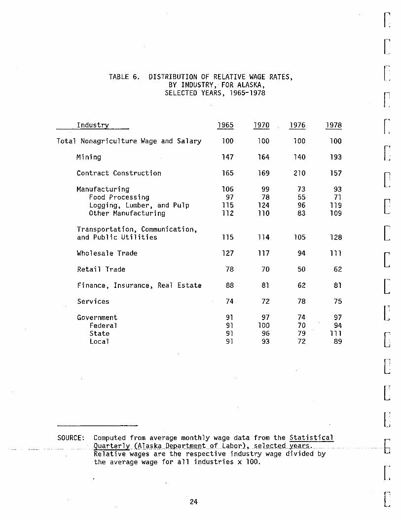
TABLE 6. DISTRIBUTION OF RELATIVE WAGE RATES, BY INDUSTRY, FOR ALASKA,

SELECTED YEARS, 1965-1978

Industr,y 1965 1970 1976

Total Nonagriculture Wage and Salary 100 100 100

Mining 147 164 140

Contract Construction 165 169 210

Manufacturing 106 99 73 Food Processing 97 78 55 Logging, Lumber, and Pulp 115 124 96 Other Manufacturing 112 110 83

Transportation, Communication, and Public Utilities 115 114 105

Wholesale Trade 127 117 94

Retail Trade 78 70 50

Finance, Insurance, Real Estate 88 81 62

Services 74 72 78

Government 91 97 74 Federal 91 100 70 State 91 96 79 Local 91 93 72

1978

100

193

157

93 71

119 109

128

111

62

81

75

97 94

111 89

SOURCE: Computed from average monthly wage data from the Statistical QuarterlY .. (81a?k9~ D~p~rto.teJlt .. Qflab.Q.r), u~ele.c:ted y:ear~ ... Relative wages are the respective industry wage divided by the average wage for all industries x 100.

24

[

[

[

[

[

[

[

[

[

[

[

[

[

[

[

[

b [

[

[

[

[

[

[

[

[

[

c [

[

[

C [

[

[

c--[ r ~

L

The data first indicate the growing disparity of average wage rates,

which would suggest a trend toward a less equal distribution of in-

come. More significant are the changes that occurred at the peak of

pipeline construction in 1976. Major distortions in the structure of

wages are present, and this suggests that the distribution of benefits

during a boom is not uniform, but rather that a small segment of the

economy appears to reap a large proportion of the gains. This feature

of boom economics is further demonstrated by an analysis of changes in

real wages over the 1973-1976 period.

Table 7 shows average monthly wages, by broad industry classification,

deflated by the Anchorage consumer price index (CPI). Use of the

Anchorage CPI is dictated because there is no statewide index. Hence,

the deflation is subject to some error since price changes are not

uniform throughout Alaska. As an approximation, however, the data are

adequate.

It is clear that drastic differences exist among industries and that

the economic benefits of rapid economic expansion tend to be concen-

trated in a select few industries. A major portion of income implied

in the growth of construction wages was also earned by nonresidents or

temporary resident employees. With the exception of business ser-

vices, all components of the support sector and government badly lag-

ged the average growth of wages and, implicitly, relative income.

Federal government and finance, insurance, and real estate real wages - - - - - ~ -~ -- - ~ ---- -- ----- -- - ----~--~-~~----~~-~---~=~:~-~-~-~--:~--~-~-

actually declined_

25

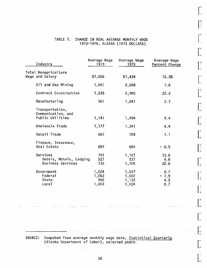
TABLE 7. CHANGE IN REAL AVERAGE MONTHLY WAGE 1973-1976, ALASKA (1973 DOLLARS)

Average Wage Ayerage Wage Industry 1973 1976

Total Nonagriculture Wage and Salary $1,006 $1 ,424

Oil and Gas Mining 1,661 2,068

Contract Construction l ,635 2,985

Manufacturing 961 1,041

Transportation, Communication~ and Public Utilities 1,141 1,494

Wholesale Trade 1,177 1,341

Retail Trade 687 709

Finance, Insurance, Real Estate 897 884

Services 751 1,107 Hotels, Motels, Lodging 527 537 Business Services 732 1 '706

Government 1,024 1,047 Federal 1,062 1, 002 State 992 1,132 Local 1,003 1,024

Average Wage Percent Change

12.3%

7.6

22.2

2.7

9.4

4.4

1.1

- 0.5

13.8 0.6

32.6

0.7 - 1. 9

4.5 0.7

SOURCE: Computed from· average monthly wage data, Statistical Quarterly (Alaska Department of Labor), selected years.

26

[

[

[

[

[

[

[

[

[

[

[

[

[

[

[

[

-f-[

[

[

[

[

[

[

[

[

[

C [

[

[

[

[

[

While much of the inflation that occurred during the period is attri-

butable to national inflation, significant regional inflation result

ing from pipeline construction activity also occurred. Prior to pipe

line construction, the Anchorage CPI had been growing at a less rapid

rate than the U.S. CPl. However, during pipeline construction, this

relationship was reversed, and the Anchorage CPI grew more rapidly.

After the pipeline, however, the inflation rate in Anchorage again

fell below that of the United States. Except for periods of relative

boom in Alaska, consumer prices have tended to rise noticeably slower

in Anchorage than outside Alaska. Over the long run, this will tend

to narrow price differentials between Alaska and the lower 48 states.

Table 8 presents relative rates of growth in the Anchorage and United

States CPis for selected years, and clearly illustrates this pattern.

As one final indication of income distribution patterns, a distribu-

tion relating percentage of total wage and salary income to percentage

of employment has been constructed for 1965 and 1978 (see Figure 1).

The distribution was constructed by ranking industries according to

average monthly wage. The percentage of total employment and total

wage income accounted for by the respective industry was then comput

ed. The cumulative employment and income percentages were then plot

ted, yielding the typical Lorenz-type distribution figure.

[ A comparison of the two distributions reveals a clear shift toward a

l _ .... ______ ~es_s_ uniform distribution of income. This shift is probably accounted

for by two factors. First, as indicated earlier, there has been a

[

[ 27

Anchorage

United States

Anchorage

United States

TABLE 8. RATES OF CHANGE FOR THE ANCHORAGE AND U.S. CONSUMER PRICE INDEX,

SELECTED YEARS, 1960-1981

1960-1970 1970-73 1973-74 1974-75 1975-76 1976-77

1.8

2.8

1977-78

6.3

7.7

4. 1

5.6

13.3

12.0

12.3

7.6

1978-79 1979-80 1980-81

9.4 8.9 7.5

11.5 13.0 10.7

6.5 5.8

5.3 6.5

SOURCE: Derived from tne Bureau of Labor Statistics reports on Anchorage and United States CPis.

28

[

[

[

[

[ [,

[

[

[

c [

[

[

[

[

[

-b [ r .

L

[

[

[

[

[

[

[

c C [

[

[

[

[

[_

[

b--[

[

FIGURE 1. DISTRIBUTION OF HAGE -AND SALARY INCOME ALASKA, 1965 and 1978

100.....,..

90----------·-··•··-- --·· .. ·-----------···--·• •· •• •••• ···--- ··- ·-··• II •

so-··

70-. -··· -------~- .

1978

60-- - . . .. . ... . -· ··- .. -----···· ...

Percent of Hage & Sa 1 ary 50-

Income ·-----.. ------------~·--- ... I

i f ! i

. ---------·-------------------- -·I

! 4o-~-

I i

3o-···:··- ·---------·-··- ,.,,.,_ .... • .. ------------------- i r

-·r- •. ·-·-:- - • l

20=·-···-----~ ··:-:-c--, -.--.!.:~-=~---- - .. i I I

i

0

I .. -- . -: - . - _· :. . . . . . . . .. . .,

--------------------- ··----------------------·--------~--- ~ ·_: :~ .. i -- .. --~- •.. -··-···-· -

.. : -· -. ---·-·-·· --.------ - . . . ... .. .. ... .. i

. _a_· ___ :~~~~----==··-~ .l.. . . -l ..... L-~ ;~-- L ... -~ J . .J. . -..• -- . -· i - - - .

10 20 30 40 50 -~ 60 . 70 80 90 100

Percent of Employment

---· =~-------SOURCE: See text.

29

sizable increase in the share of total activity accounted for by sup-

port sector industries, and these industries generally have lower than

average wage rates. Second, there has been a substantial growth in

the range of relative wages between industries over time.

In summary, real personal income has shown sustained growth over the

entire 1960-1978 period, both in aggregate and per capita terms. The

growth has not been uniformly distributed, however, and the wage com

ponent has become less uniform over time. This was particularly evi

dent during pipeline construction and supports the hypothesis that the

benefits of pipeline construction were largely concentrated in a few

sectors.

POPULATION

The remaining dimension of growth to be considered is population.

Changes in population are divided into two components, natural in

crease (or decrease) and in/out-migration. Natural population growth

results from an excess Of births over deaths and is, hence, determined

by birth and death rates.

Alaska exhibits both the highest birth rate and the lowest death rate

in the United States; and as a result, the rate of natural population

increase is the highest in the United States. This phenomenon is

largely accounted for by the relative youthfulness of the population,

with over~34 percen! of !h_e. popul at i_on~ be!weell_the ~!l~~~-~-f J~- (ll)_d_}Q_~

This age group has· both the highest fertility rate and the lowest

death rat-e.

30

c [

[

[

[

[

[

[

c [

[

[

[

[

[

[

6 [ r

L

[

[

[

[

[

[

[

[

[

[

[

[

[

[

[ -

[ r b

[

[

Net migration (in-migration minus out~migration) is the second factor

contributing to population change. Many factors influence the migra

tion decision; but f9r the Alaska case, it appears that (with the

exception of military-related migration) migration occurs largely in

response to economic opportunity. In the aggregate, relative rates of

unemployment and relative wage differentials in Alaska and elsewhere

should be important in determining the migration decision. At the

individual level, the economic component of the decision is related to

the expected gain resulting from the move. Basically, this is the ex

pected wage differential times the probability of getting a job, less

the cost of making the change. Thus, either a change in relative wage

rates or relative employment opportunities can influence the decision.

That migration is sensitive to economic opportunity is clearly demon

strated b~ patterns of migration that occur during and after pipeline

construction. Data summarizing population and changes in population

for Alaska for the years 1965 through 1978 are presented in Table 9.

Both the relative stability of natural increase and the volatility of

net migration are clear. Natural increase has averaged about 1.5 per-

cent per year; while large variations, even in pre-pipeline years, are

evident in the ·net migration component.

Table 10 presents the age distribution of Alaska in juxtaposition to

the overall U.S. age distribution. As would be expected, the middle

age groups are significantly larger in Alaska than for the United -- ----·------ ----------------~-----~ ---------------- ---- ------ -·---------~-~

States as a whol-e; almost 34 percent of the Alaska population is

31

Year

1965 1966 1967

1968 1969 1970

1971 1972 1973

1974 1975 1976

1977 1978 1979 1980

TABLE 9. ALASKA POPULATION AND COMPONENTS OF CHANGE: 1965-1978

(thousands)

Total Natural Increase Total Chan~

265.2 5.7 10.2 271.5 5.3 6.3 277.9 5.0 6.4

284.9 5. 1 7.0 294.6 5.6 9.7 302.4 6.1 7.8

312.9 5.9 10.6 324.3 5.5 11.4 330.4 5.1 6. 1

351.2 5.6 20.8 404.6 5.9 53.4 413.3 6.3 8.7

411.2 6.8 - 2.1 407.0 6.7 - 4.3 406.2 7.4 - .8 400.5* - 5.7

Net Migration

4.5 1.0 1.4

1.9 4.1 1.7

4.7 5.9 0.9

15.2 47.5 2.4

- 8.9 -11.0 - 8.2

[

[

[

[

[

[

[

[

c [

[

[

*U.S. Census figure for 1980, so comparability is more difficult.

[

[

[

[ SOURCE: Alaska Department of Labor

~~~~~,~~ ~<- -,~-- ~- -- ~-~~~~ '~ ~ ~ b ~- ~

[

32 r'

L

[

r [

[

[

[

[

[

c c c [

[

[

c [

TABLE 10 ALASKA POPULATION BY AGE, 1980

Alaska Age U.S. Age Distribution Distribution

Age Cohort Total (%_Qf_lo_ta U (%of Total)

0 - 4 38,777 9.68 7.21

5 - 9 84,917 8.72 7.37

10 - 14 34,166 8.53 8.05

15 - 19 36,980 9.23 9.34

20 - 24 45,058 11.25 9.40

25 - 29 48,452 12.10 7.29

30 - 34 41,916 10.46 7.75

35 - 39 31,182 7.79 6.16

40 - 44 22,570 5.63 5.15

45 - 49 18,355 4.58 4.89

50 - 54 15,801 3.95 5.16

55 - 59 12,592 3.14 5.13

60 - 64 8,095 2.02 4.45

65 + 11,530 2.88 11.28

SOURCE: U.S. Department of Commerce, 1980 Census of Population: Age, Sex, Race, and Spanish Origin by Regions, Divisions and States: 1980, PC 80-S1-1, p. 4-5.

-b------~- ~---~---~---~~- ~

[ r-

L 33

between ages 20 and 35, where the comparab 1 e figure for the United

States is less than 25 percent. This age group is extremely mobile,

and accounts for a good deal of the migration that occurred during the

pipeline boom.

In summary, Alaska 1 s natural population growth is substantially above

that of the nation as a whole. Furthermore, the response of migration

to economic opportunity is clearly evident. Once again, this empha-

sizes the openness of the Alaska labor market.

The Anchorage Census Division

Anchorage has occupied a central role in Alaska•s growth since state

hood. It has emerged as a key transportation and distribution center,

as well as assuming a dominant role in the growth of other support

sector activity. The area has also become the state center for petro-

leum industry administrative facilities. Its importance as a seat of

Federal government activity in Alaska has been supplemented by rapid

growth of state and 1 oca l government. Because of the size of the

Anchorage economy, it tends to reflect total state activity as well as

to impact upon total economic activity in Alaska. It is because of

its central place in the Alaskan economy that economic activity remote

from Anchorage is often significantly tied to Anchorage.

EMPLOYMENT, LABOR FORCE, AND UNEMPLOYMENT

Direct me~~u~es of_ p~od~«:t i~>n for _ the-. ~n~h()_rag~ __ ~c~n_Ofil,Y are ll_ot:

available. Neither is Anchorage a commodity producer in which resource

based activity is directly important to total economic activity. This

34

[

[

[

[

[

[

[

c c c [

c [

[

[

[

b [ r

L

[

[

[

[

[

[

[

c [

[

[

[

[

[

r [

makes it particularly important to consider the structure and growth

of employment for Anchorage. While such data are only partially re-

flective of total production, they do provide meaningful insights into

changes that have occurred.

Summary data on Anchorage employment, by broad industry classifica-

tion, for 1965 through 1978, are presented in Table 11. Overall

employment has grown at about 7.3 percent per year, and the rate of

growth exceeded the statewide rate of 6~7 percent. While growth has

generally been consistently upward, it accelerated substantially dur-

ing pipeline construction. Since then, growth of employment has mod-

erated; but the level of employment still exceeds that achieved during

the period of pipeline construction. It is also worth noting that, in

contrast to other parts of the state where pipeline construction play-

ed a significant role in the expansion of activity, Anchorage growth

during this period occurred more uniformly throughout most sectors,

reflecting the region's role as a support center.

Several industries expanded more rapidly than the growth of total em-

ployment, including: mining (13.3 percent); transportation, communica-

tions, and public utilities (8.9 percent); wholesale-retail trade (9.4

percent); finance, insurance, and real estate (11.0) percent; services

(11.5 percent); and state and local government (10.5 percent). Con-

struction, manufacturing, and federal government growth rates were all

6 below the regional average for the period. - --- -- --- -- --~--- ---- ----·-- -·---·- -----~-·~~-----~-~-~--~-~-·-~--------------------------------------------------

.

[ r--

L 35

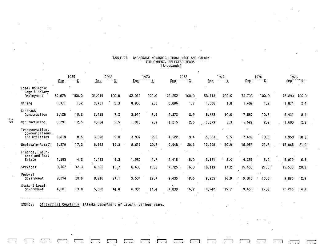
TABLE 1'1. ANCHORAGE NONAGRICULTURAL WAGE AND SALARY El•tPLOYMENT, SELECTED YEARS

(thousands)

1965 1968 1970 1972 1974 1976 1978 @!1?. ! ~ ! ~ ! ~ ! ~ ! ~ ! ~

61

Total NonAgr~c !!.

Wage & Sal,ry 30.678 100.0 34.019 100.0 42.019 100.0 48.252 100.0 58.713 100.0 73.733 100.0 76.893 100.0 Employment!

I

Mining I

0.371 1.2 o. 781 2.3 0.958 2.3 0.806 1.7 1.036 1.8 1.409 1.9 1.874 2.4 I Contract 1

3.126 10.2 2.438 7.2 3.514 8.4 4.272 8.9 5.882 10.0 7.587 10.3 6.431 8.4 Cons tructi em w

2.2 0"'1

"'""'"''"''"! 0. 791 2.6 0.834 2.5 1.018 2.4 1. 215 2.5 1.379 2.3 1.629 1.683 2.2

Transportati n, Communi cations,

5.583 9.5 7.409 10.0 7.950 10.3 and Utilities 2.618 8.5 3.046 9.0 3.907 9.3 4.522 9.4

Who1esale-Re1ail 5.279 17.2 6.552 19.3 8.617 20.5 9.948 . 20.6 12.298 20.9 15.958 21.6. 16.865 21.9 I

Finance, I nsor-ance and Real Estate j 1.295 4.2 1.452 4.3 1.980 4.7 2.415 5.0 3.151 5.4 4.257 5.8 5.019 6.5

ServiC!;lS I

3.767 12.3 4.652 13.7 6.403 15.2 7.725 16.0 10.119 17.2 15.450 21.0 15.538 20.2

Federal I Government j 9.394 30.6 9.216 27.1 9.534 22.7 9.435 19.6 9.925 16.9 9.813 13.3 9.896 12.9

I State & Loca~

Government] 4.001 13.0 5.022 14.8 6.036 14.4 7.839 16.2 9.242 15.7 9.465 12.8 11.266 14.7

SOURCE: st1tistical guarterll (Alaska Department of Labor), various years.

I I

I

I I I

r"J r-:; rr r-J r-J r-J c---1 rJ L"'J r""J c-:J r:J rl r-J r-J L'J r-J r-:J r-J

[

c [

[

[

[

[

[

c c [

c [

[

The growth of the support sector i 11 ustrates the maturing of the

Anchorage economy as was a 1 so observed at the statewide 1 eve 1. A

comparison of statewide and Anchorage support sector employment as a

percent of total employment also indicates the role of Anchorage as a

trade, distribution, service, and financial center for the state as a

whole. Employment as a percentage of total Anchorage employment con-

siderably exceeds comparable figures at a statewide level in trade,

finance, and services. For Anchorage, these industries accounted for

48.6 percent of total employment in 1978; whereas for the state as a

whole the figure is only 39.5 percent. The share of total employment

accounted for by the federal government in Anchorage is also above the

state proportion, and over 50 percent of total federal government em-

ployment in Alaska is based in Anchorage.

The data on labor force and unemployment also illustrates the openness

of the Anchorage economy (see Table 12). Over the period from 1970

through 1979, unemp 1 oyment averaged 7. 4 percent. Whi 1 e temporarily

dropping during pipeline construction, the unemployment rate has risen

again to historic levels in the years since completion of the pipe

line, averaging 7.7 percent for 1978 and 1979. Hence, while rapid

expansion of employment opportunities may temporarily reduce unemploy-

[ .. ______ me_nt, the effects are clearly short-run.

[

b [

[

PERSONAL INCOME

Total and per capita personal income for Anchorage are shown in Table ----- ------------ -- ------- ---~-~- --- --------------- --- ----- ---- -----~---~---~- ------- ----~------ ------- ----- ---------- ----- ---------------- -- --

13, both in current and constant (1978) dollars. In current dollars,

37

TABLE 12. ANCHORAGE LABOR FORCE, EMPLOYMENT, AND UNEMPLOYMENT, 1970-1978

Year Employment Labor Force Unemployment Unemployment Rate

1970 45,757 49,024 3,267 6.7% 1971 49,484 53,902 4,418 8.2 1972 52,395 57,535 5,140 8.9

1973 54,299 60,117 5,818 9.7 1974 54,691 58,661 3,970 6.8 1975 64,721 68,481 3,760 5.5

1976 68,420 73,436 5,016 6.8 1977 79,023 84,513 5,490 6.5 1978 74,819 81,551 6,732 8.3

1979 75,424 81,120 5,696 7.0

SOURCE: Alaska Department of Labor, Labor Force Estimates by Area, selected years.

both total and per capita personal income have grown every year (at

average annual rate of 14.4 percent and 10.0 percent, respectively)

with considerable increases in the rate occurring during pipeline con-

struction. Much of the growth has been negated by inflation, however.

In rea 1 terms, tota 1 incomes grew at 8. 2 percent over the period;

while per capita income grew at 4.1 percent. However, both real

total and per capita personal income have declined slightly since

peaks reached during pipeline construction. It is also worth noting

that the growth rates of Anchorage personal income exceeded those of

[

[

[

[

[

[

r~

[

[

c c [

[

[

[

[

---------- __ ' ____ the-~~~~~--~o:_::mp~~-~b:_:_~::i~ds~------------- _______________________________________ --h-

[ r·,

38 L

[

[

[

[

[

[

[

c [

[

[

[

[

[

[

[

[

[ f~

L

1965 1966 1967

1968 1969 1970

1971 1972 1973

1974 1975 1976

1977 1978

TABLE 13. ANCHORAGE PERSONAL INCOME 1965-1978

Current Dollars Constant.(1978) Dollars

Total Total (mil]_ions) Pe_r_u_Capi ta (mi 11 ions) Per Capita

371 3,412 767 7,056 398 3,595 722 7' 153 462 4,061 900 7,911

502 4,228 953 8,027 570 4,622 1,035 8,391 635 4,997 1,109 8,730

733 5,469 1 ,248 9,313 800 5,631 1,333 9,383 880 6,031 1 ,385 9,490

1,114 7,402 1,550 10,299 1 ,625 . 10,070 2,011 12,463 1,903 10,579 2,212 12,296

2,109 11,592 2,317 12,736 2,128 11 ,839 2,128 11 ,839

Average Annual Percent Growth

14.4% 10.0% 8.2% 4.1%

SOURCE: Bureau of E':=onomjc Analysis, U.$. Department of Commerce.

39

POPULATION

Population for Anchorage grew from 102.3 thousand in 1965 to 185.5

thousand in 1978, at an average annual growth rate of 4.7 percent (see

Table 14). This was substantially in excess of the statewide growth

rate of 3.4 percent. As a result, the Anchorage share of total state

population rose from 38.6 percent in 1965 to 45.6 percent in 1978.

From 1965 to 1969, the Anchorage and statewide populations grew at

about the same rate; while for 1969 through the start of pipeline

construction, the population of Anchorage grew at about 6 percent.

During this period, the state as a whole grew at about 3.6 percent.

Both the state and Anchorage populations grew rapidly during the 1974

through 1976 period (17.7 percent and 20. l percent, respectively), but

the Anchorage population did not peak until 1977; whereas the state-

wide population reached a peak in 1976. However, the decline in

Anchorage population has been proportion ate ly greater than that for

the state as a ~hole. In 1978, statewide population was 6.3 thousand

below the pipeline peak; while the Anchorage population was 10.3 thou-

sand below its peak.

In summary, the Anchorage economy has shown substantial growth over

the entire period reviewed. Steady diversification of the economy is

evident, and the role of Anchorage as an economic center for the state

is clear. Furthermore, economic activity remote from Anchorage is

nevertheless often s i gni fi cant for the Anchorage economy because of

Anchorage's central role.

40

[

l [

[

[

[

[

[

C [

[

[

[

[

[

[

-- -'---- ~_r-, ~=:---

[ r ,

L

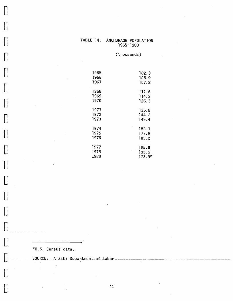
c c c [

[

[

c c D

c c [

c [

[

[

c [ r_,

L

*U.S. Census data.

TABLE 14. ANCHORAGE POPULATION 1965-1980

(thousands)

1965 102.3 1966 105.9 1967 107.8

1968 111.6 1969 114.2 1970 126.3

1971 135.8 1972 144.2 1973 149.4

1974 153.1 1975 177.8 1976 185.2

1977 195.8 1978 - 185.5 1980 173.9*

SOURCE: A1 as ka-Depa~tment -of- -Labor-.--

41

The Aleutian Islands Census Division

The Aleutian Islands Census Division encompasses all of the Aleutian

Islands, the Pribilof Islands, and the Alaska Peninsula from Port

Heiden west. This is the definition used by the 1970 Census and the

Alaska Department of Labor Statistical Quarterly (the 1980 Census used

a slightly different definition).

The economy of the Aleutian Islands Census Division in no sense

reflects a cohesive, functional economic area. This economic area is

composed of several relatively isolated communities and Federal gov

ernment military installations. Private sector activity is almost

totally dependent upon utilization of the abundant fish resources and

includes both harvesting and processing. Harvesting of fur seals on

St. Paul Island is also an important local activity. Minor amounts of

sheep ranching also occur in the region. Military installations at

Shemya and Adak, as well as elsewhere in the region, swell the popu

lation, employment, and income figures for the census division but

have no perceptible links with other economic units within the census

division.

PRODUCTION

Basic sector private production is mostly composed of fisheries

related activity. Both commercial fishing and processing are widely

dispersed throughout the region, although processing is more highly

___ ~~()_n~~ntl"_(3._t~~-~11-~~~-e-~~!-~_1'1_e()rt i_()n_o_f _ _!_t:le census division. Tab 1 es 15

through 17 provide summary data on commercial fishing. In Table 15

the salmon, shellfish, total catch, and value of catch to fishermen

44

[

[

[

[

[

[

[

c l c [

[

c [

[

[

------b-[

[

[

c [

c [

[

[

[

[

c c [

[

[

[

[

Year

1976

1973

1970

TABLE 15. CATCH AND VALUE TO FISHERMEN, ALEUTIAN ISLANDS CENSUS DIVISION

1970 TO 1976, SELECTED YEARS

(catch in million pounds; value in million dollars)

Salmon Shell fish Total 1

Pounds Value Pounds Value Pounds Value -- --

20.910 7.155 154. 262 61.032 175. 921 69. 029

6.993 1.815 60.966 25.135 71. 261 29.243

28.695 5. 102 44.082 9.108 74.540 14.793

1 Totals include minor amounts of other fish. There is also an unreconciled discrepancy for the weight of shellfish in Table 14 and Table 15 for 1973.

SGURCE: Alaska Catch and Production (Alaska Department of Fish and Game, Division of Commercial Fisheries), selected years. Data prior to 1970 not available on a comparable basis.

-C------ ------ ------~- -- -----~---.---~-----~---------------~--------~~ --~ -~ ---~--~ ------~-----~--[

[ 45

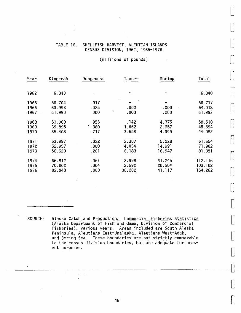
Year

1962

1965 1966 1967

1968 1969 1970

1971 1972 1973

TABLE 16. SHELLFISH HARVEST, ALEUTIAN ISLANDS CENSUS DIVISION, 1962, 1965-1976

(millions of pounds)

King_crab Dungeness Tanner Shrimp

6.840

50.704 . 017 63.993 . 025 .000 .000 61.990 .000 .003 . 000

53.060 . 953 . 142 4.375 39.895 1. 380 1.662 2.657 35.408 .717 3.558 4.399

53.997 .022 2.307 5.228 52.957 . 000 4.054 14.891 56.620 . 201 6.183 18.947

Total

6.840

50.717 64.018 61.993

58.530 45.594 44.082

61.554 71.902 81.951

1974 66.812 . 061 1975 70.002 .004 1976 82.943 .000

13.998 12.592 30.202

31.245 20.504 41.117

112.116 103.102 154.262

SOURCE: Alaska Catch and Production: Commercial Fisheries Statistics (Alaska Department of Fish and Game, Division of Commercial Fisheri~s), various years. Areas included are South Alaska Peninsula, Aleutians East-Unalaska, Aleutians West-Adak, and Bering Sea. These boundaries are not strictly comparable to the census division boundaries, but are adequate for present purposes.

[

[

[

C [

[

[

c c c [

c [

[

[

[

-----~-~---------- ------~~- -------~--------- ---------------------~--------------~-- -----------------b--[

46 [

[

[

[

[

[

[

[

[

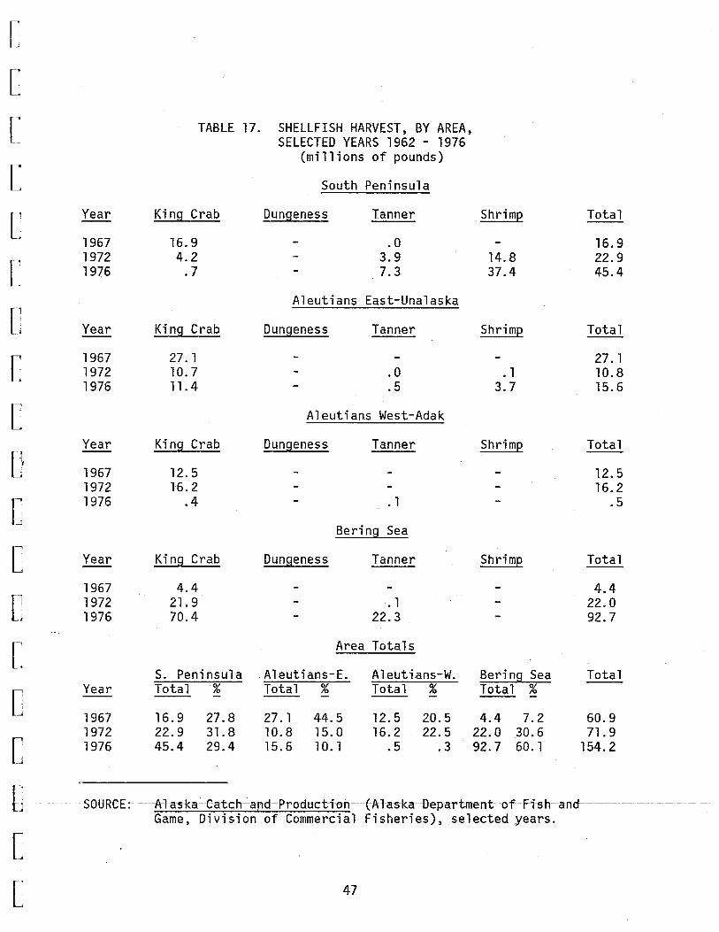
c c~

[

[

[

[

[

[

[

[

[

TABLE 17. SHELLFISH HARVEST, BY AREA, SELECTED YEARS 1962 - 1976

(millions of pounds)

South Peninsula

Year King Crab Dungeness Tanner Shrimp Total

1967 16.9 - .0 - 16.9 1972 4.2 - 3.9 14.8 22.9 1976 . 7 - 7.3 37.4 45.4

Aleutians East-Unalaska


1967 27.1 - - - 27. 1 1972 10.7 - .0 . 1 10.8 1976 11.4 - .5 3.7 15.6

Aleutians West-Adak


1967 12.5 - - - 12.5 1972 16.2 - - - 16.2 1976 .4 - . 1 - . 5

Bering_ Sea


1967 4.4 - - - 4.4 1972 21.9 - . 1 - 22.0 1976 70.4 - 22.3 - 92.7

Area Totals

S. Peninsula Aleutians-E. Aleutians-W. Bering Sea Total Year Total % Total % Total % Total % --

. 1967 16.9 27.8 27.1 44.5 12.5 20.5 4.4 7.2 60.9 1972 22.9 31.8 10.8 15.0 16.2 22.5 22.0 30.6 71.9 1976 45.4 29.4 15.6 10. 1 .5 . 3 92.7 60. 1 154.2

SOURCE: - - Alaska -Catch~ a·nd-Production---(Alas-ka Department of~ fish- and-~-- - - - -- -Game, Division of Commercial Fisheries), selected years.

47

are indicated for recent years. The data clearly show the rapid

increase in both the va 1 ue and vo 1 ume of she 11 fish harvested in the

region.

A longer-run view of shellfish harvest is shown in Table 16 and

highlights the growth in the diversity of shellfish caught. In par-

ticular, both tanner crab and shrimp have provided much of the growth

in the shellfish harvest, helping to offset significant declines in

king crab catches that occurred during the late 1960s and early 1970s.

Finally, Table 17 provides data on the disparities of catch within

areas of the region and how these have changed over recent years.

Significant declines in king crab harvests in all areas are noted,

with the exception of the Bering Sea which has more than offset the

declines in other areas. Tanner crab and shrimp have been increas

ingly important for the South Peninsula and Aleutian-East areas.

In short, major changes in the pattern of harvests, both regionally

and by species, have occurred. The South Peninsula and Bering Sea

areas show overall gains and the Aleutian-East and Aleutian West areas

show net declines. These patterns are also indicated by the percen

tage shares of total shellfish harvest shown in Table 17.

A second, important dimension of understanding commercial fishing in

the Aleutian economy is an analysis of who does the fishing. Data on

-~t!ti~JlQ_j nt_j § _ frS!gmE! rrt~ry_~mL i ~~Rr_g~~Qted i Q_T_gb 1 ELJJ~-~-----Ihe k i_ng __ cral:>~--~----

48

[

C [

[

[

[

[

[

c [

[

[

[

[

[

[

___ c_ c

[

[

[ r Lj

~

[

[

[

[

[

D [

[

[

[

[

[

[

b [ r

L

TABLE 18. RESIDENCE OF BOATS AND GEAR LICENSE HOLDERS FISHING THE ALEUTIANS

Proportion of King Crab Catch Value by Boat Residence

Proportion of Salmon Catch by Residence of Gear License Holder

Place -- Percentage Place Percentage

Kodiak 26.8 Kodiak 41.5

Alaska Peninsula 4.0 Aleutians 20.0

Dutch Harbor 4.3 South Central Alaska 3.2

Out of State 64.9 Anchorage 2.6

SOURCE:

Other Alaska 7. 1

Non-resident 19.2

Unknown 6.5

King Crab: Western Alaska King Crab: Draft Fishery Management Plan (North Pacific Fishery Management Council, Anchorage; Council Review Draft, May 1980). Derived from data on page 30.

Salmon: Derived from Table 9-8, Measuring The Socioeconomic Impacts of Alaska's Fisheries, by George W. Rogers, et al, (Institute of Social and Economic Research; April 1980).

and shellfish industry tends to be dominated by nonresident boats and

crews, and the area of concentration for these vessels is the Bering

Sea. Much of the remainder of the catch is accounted for by Kodiak-

based boats.

49

The information on the salmon harvest is even less precise since the

region covered is southwest Alaska (the Aleutian Census Division plus

Kodiak). It is assumed, with some uncertainty, that the regional pro

portions apply to the Aleutians.

The overall picture that emerges is one in which the bulk of the

commercial fishing in the Aleutians is carried out by fishermen and

vessels which are not resident to the Aleutians. More precise infor

mation would be desirable but is simply not available.

A final dimension of commercial fishing to be considered is that of

employment. No systematic, periodic estimates of commercial fishing

employment are made for the Aleutians (nor for the rest of the State).

Estimates for the 1969 through 1976 period, however, have been com-

piled for the State and regions (Rogers, 1980) and in turn have been

used to estimate employment in the Aleutians for 1978. This has

resulted in an estimate of 756 for average annual employment in com

mercial fishing. Of these, 251 are estimated to be residents of the

Aleutian Islands Census Division.

[

c [

[

[

[

[

[

c [

[

[

[

[ The procedure used to develop these estimates was to compute the ratio

of the 1978 to 1976 catch, by species (salmon, shellfish). and apply -- - [ this ratio to the Rogers• estimates of employment for 1976. Since his [

employment estimate was for the southwest region, it was then neces-

------ _____ §_C!!'.Y_'tQ__C!]J9fa_t_~_'tQ_1h~ Al_~ll_t_ lCiD?_1h_~ t.Qt.E.L~IllPJQ.YillE:!D't._ thlj_§_~_s_t_img_t_e_d_. __________ b _ This was accomplished by apportioning total employment on the basis of

[ r~

50 L

[

[

[

[

[

[

[

[

[

[

[

[

[

[

[

[

L---

l r-~

L

Aleutian to total southwest region ca~ch and implies uniform produc

tivity throughout the southwest region. The result of these manipu-

lations is an estimate of total Aleutian Islands commercial fishing

employment. The estimate of resident employment was developed using

ratios presented in Table 18. It goes without saying that these

estimates of employment are very approximate and subject to consid-

erab 1 e error.

The second major component of the fishing industry in the Aleutians is

processing. The present structure of the processing industry reflects

a mix of shore-based and floating processors engaged in canning and

freezing. The trend is toward freezing an increasing proportion of

the catch.

A tally of processor permits for 1980 compiled from Alaska Department

of Fish and Game records indicates seven shore-based faci 1 iti es at

Dutch Harbor; two at Sand Point; and one each at King Cove, False

Pass, Squaw Harbor, and Port Moller. Some of these permits may cover

firms that are only buying fish for transshipment.

Several floating processor permits are held as well: Dutch Harbor (4),

Sand Point (1), and False Pass (1). In addition, some 31 permits are

held that allow for floating processors to operate throughout the

region. Not all permit holders necessarily utilize their permits, and

several may actually be nothing more than buyers. It is clear, how--------.-,-

ever, that procesiin~ is geographically well dispersed throughout the

Al~utians.

51

Employment data for processing is available for the Aleutians Census

Division from the Statistical Quarterly (Alaska Department of Labor).

For 1978, 1, 621 was the average annua 1 emp 1 oyment in manufacturing,

which for the Aleutians is largely synonymous with fish processing.

As is the case with commercial fishing, it is important to determine

what proportion of the employment was held by residents of the region.

Data regarding this question are fragmentary. In conversations with

industry and local government people, it was estimated that somewhere

between 5 and 15 percent of the employment was held by residents. A

second source of information is The Recommended Community Development

Plan: City of Unalaska, Alaska (Trick, Nyman, and Hayes: November

1977). Accardi ng to this study, 72 out of 875 basic sector jobs

(1976) were held by residents, and these jobs were primarily in fish

processing.

jobs were

This would indicate that about 8.2 percent of processing

held by residents. Community profiles prepared by the

Arctic Environmental Information and Data Center for King Cove, False

Pass, and Akutan also contain data that tend to support the above

sources regarding resident to nonresident ratios.

Using what appears to be a reasonable estimate of the resident share

of processing jobs, 10 percent, then 162 of 1,621 jobs were held by

residents. The remainder (1,459) were held by nonresidents. Of

these, almost all were from outside of Alaska.

52

[

[

[

[

[

[

[

[

[

[

[

[

[

[

[

[

C[

[

[

[

[

[

[

[

[

[

[

[

[

[

[

[

[

[

Significant seasonal variation exists in processing employment,

a 1 though to a much 1 esser degree than is generally the case in the

salmon industry. For 1978, average employment for the four quarters

was, respectively: 1,255 (January-March), 1,782 (April-June), 1,649

(July-September), and 1,798 (October-December). The low first quar-

ter, followed by substantial gains in the second through fourth

quarters, is typical of recent years. Available data do not indicate

how seasona 1 patterns may vary between residents and nonr.es i dents.

The second e 1 ement of basic sector production in the A 1 eut i ans is

Federal government and national defense-related activity. Major

installations are located at Adak, Shemya, and Cold Bay. The largest

of these is the naval station at Adak. According to data supplied by

the Office of Information, Alaska Air Command, there are 1,781 active

duty military and civilian defense-related personnel at Adak, as well

as 1,400 dependents. These figures do not include additional civilian

personnel associated with nondefense activity such as officers• clubs,

post-exchanges, etc. Shemya and Cold Bay do not have resident depen-

dents, and military and civilian defense-related personnel number

approximately 490. Table 19 summarizes military and related federal

civilian employment data for the census division as a whole for 1978.

While the military presence is numerically large, its economic impact

on the economy of the Aleutians is negligible. The units are largely

t---~--~~-~-_ __ _1!_§_}_f_:-suQ_g_orting___MLc;l_~Qnly identifiable ties with the Aleutian or.___ __ _

Alaska economy are transportation services provided by Reeve Aleutian

[

[ 53

TABLE 19. MILITARY AND RELATED FEDERAL-CIVILIAN EMPLOYMENT AND WAGES, ALEUTIAN ISLANDS

CENSUS DIVISION, 1978

Employment Wages (thousands)

Military and Related Civilian Employment

Military Personnel (Active Duty)

Military-Related Federal Civilian Employment

PX and NAF (Largely Part-time) 1

Other Military Related Federal Employment

3,939

3,453

486

330

156

45,952

38,950

7,072

1 ,875

5,127

1 Post exchange and nonappropriate fund activities, including officers• clubs, etc.

SOURCE: Numbers: Basic Economic Statistics of Alaska Census Divisions (Alaska Department of Commerce and Economic Development, Division of Economic Enterprise: November 1979).

Airways (RAA) and some contract construction. One benefit that does

result from the military contracts with RAA is the feasibility of

providing more frequent air service to other communities in the

Aleutians. Contract construction work at the military installations

is generally carried out by non-Aleutian based firms, either from

Alaska or out-of-state.

In summary, basic sector production in the Aleutians is almost en-

[

[

[

[

[

[

[

[

[

[

[

[

[

[

c [

______ t_ir·J~J.Y-~eJ_atad-ta_f_i_sbed_as~aso~cas-or-Eede~a-1-go_v_e~nment-m-iJ-i-tal"-y- [

related activity. Fisheries activity has shown substantial growth but

[

54 [

[

[

[

[

[

[

[

[

C [

[

[

[

[

[

[

is still largely dominated by non-Aleutian resident participants. The

military presence, while substantial, has no significant relationships

with the rest of the census division.

EMPLOYMENT, UNEMPLOYMENT, AND LABOR FORCE

Analysis of employment in the Aleutians is important for the same

reasons that it was important at the statewide level. Table 20 sum-

marizes average monthly employment for the Aleutian Census Division

for the years 1965-1978. Over the period, total employment has grown

substantially at an average annual rate of 5.9 percent. This growth

has been largely dependent upon growth of the fisheries industry and

State and local government. Employment in fish processing grew at an

average annual rate of 14. l percent, while State and local government

grew at a rate of 8.5 percent. Federal government employment, pri-

marily related to national defense, fluctuated considerably over the

period but has shown no appreciable growth. The same is true for

contract construction and transportation, communications, and public

utilities. The support sector components of wholesale-retail trade;

finance, insurance, and real estate; and services have a 1 so expanded

as would be expected. Finance, insurance, and real estate grew at an

average annual rate of 18. 9 percent, a 1 though much of this growth

occurred after 1973. Services grew at 22.7 percent over the period,

but this growth rate must be interpreted with caution. The data for

early years were not reported in the Statistical Quarterly (the source

f~ ' document) because of disclosure rules and, hence, were estimated. The

t------------~-----1-~-~-;e-~~~~~~~on in th;s serie-~ also raises the-;u;stion of incon;is- -

[ tency in the data, possibly due to classification difficulties.

l 55

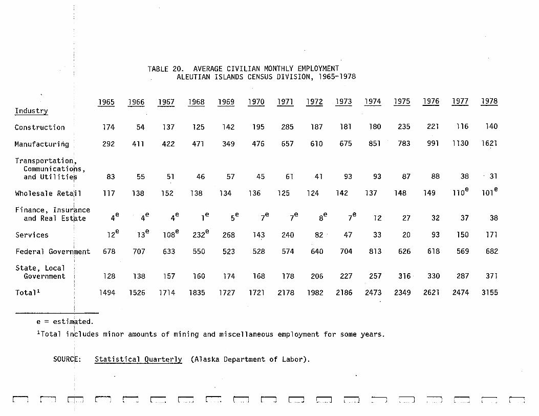
TABLE 20. AVERAGE CIVILIAN MONTHLY EMPLOYMENT ALEUTIAN ISLANDS CENSUS DIVISION, 1965-1978

1965 1966 1967 1968 1969 1970 1971 1972 1973 1974 1975 1976 1977 1978 Industr~

Construction 174 54 137 125 142 195 285 187 181 180 235 221 116 140

Manufacturi fig : 292 411 422 471 349 476 657 610 675 851 783 991 1130 1621

Transportation::, Communicatiof1s, and Utilities 83 55 51 46 57 45 61 41 93 93 87 88 38 31

Wholesale Retajl 117 138 152 138 134 136 125 124 142 137 148 149 llOe 10le

Finance, Insur~nce 4e 4e 4e le 5e 7e 7e Be 7e and Real Estate 12 27 32 37 38

Services 12e l3e l08e 232e 268 143 240 82. 47 33 20 93 150 171

Federal Government 678 707 633 550 523 528 574 640 704 813 626 618 569 682

State, Local Government 128 138 157 160 174 168 178 206 227 257 316 330 287 371

Total 1 1494 1526 1714 1835 1727 1721 2178 1982 2186 2473 2349 2621 2474 3155

e = estimated. I

1Total in1cludes minor amounts of mining and miscellaneous employment for some years.

SOURCE: Statistical Quarterly (Alaska Department of Labor).

~~~~~~~~~~~~~~~~~~~

[

[

[

[

[

[

[

[

[

[

[

[

[

[

r "='

Independent series on wholesale and retail trade are not available for

the entire period. For those years in which retail trade data were

available, there is steady growth indicated. Wholesale trade appears

to be a much higher proportion of total wholesale-retail trade than is

the case statewide, and this is apparently linked to· wholesale trade

activity associated with fisheries. There may also be problems with

the industrial classification of wholesale trade.

Firms may engage in both buying or processing of fish and a 1 so who 1 e-

saling of fish or fish products. The firm's industrial classification

would depend on which activity was of greater proportional signifi-

cance, and this may change from year-to-year. The result is that the

wholesale-retail sector reflects a strong mix of basic and support

sector activity. In conjunction with possible industrial classifi-

cation problems, this would account for the apparent lack of growth in

this sector.

There is one significant omission in the employment data; this is

employment in commercial fishing. Such employment is not included in

the Statistical Quarterly data, and as indicated above, a consistent

series is not available elsewhere. Estimated commercial fishing em-

ployment for 1978, however, was 756. If we include this figure with

total reported employment of 3,155, the commercial fishing employment [

accounted for about 19 percent of total employment for 1978. Commer

E----------~£J~l fishing plus processing employment amounts to 61 percent of total

employment.

[

[ 57

A second issue of concern relates to the residency of job holders.

Table 21 presents estimates of resident and nonresident employment for

1978. The resident/nonresident breakdown for commercial fishing and

processing has already been explained. Allocation of the remainder of

employment has been accomplished as follows: State and local govern

ment is assumed to be resident employment, as is also the case for

transportation, communications, and public utilities; finance, insur

ance, and real estate; and services. Federal government civilian

employment was divided between defense-related and other Federal

government activity. Defense-related employment was assigned to the

nonresident category (in the sense that incomes earned had no impact

on the Aleutian economy) , wh i 1 e other Federal government emp 1 oyment

was treated as resident employment.

Retail trade was assumed to reflect resident employment. Wholesale

trade includes both resident and nonresident employment, and one-half

of the employment in wholesale was treated as resident. This division

was based on discussions of wholesale trade activity in the Aleutians

with the Alaska Department of Labor.

The final industry of concern is contract construction. In conver

sations with several labor unions and contractors who operate in the

Aleutians, it was clear that the vast majority of construction workers

in the Aleutians are not residents of the area. Based on a synthesis

of t.hes~ C::Qf1Y~~t§cttions, it __ \1/_as_ e~tima~t.ect th?t ~ Rgrc:ent _gf ~9ntr9,~:;:t,

58

[

[

[

[

[

[

[

[

[

[

[

[

c [

[

[

E [

[

-,

I L~

[ ,_,

[

[

[

[

[

[

[

[

[

[

TABLE 21. ALEUTIAN ISLANDS CENSUS DIVISION ESTIMATED RESIDENT AND NON-RESIDENT

EMPLOYMENT, 1978

Industry

Commercial Fishing

Manufacturing

Construction

Transportation, Communication, and Utilities

Wholesale/Retail

Finance, Insurance,

Resident

251

162

7

31

89

and Real Estate 38

Services 171

Federal Government Civilian, Military-Related -0-

Other Federal Government 198

State Government 88

Local Government 283

Total 1318

e = estimated.

SOURCE:

Non-Resident

505

1459

133

-o-

12

-o--o-

484

-o-

-o-

-o-

2593

Total

756

1621

140

31

101e

38

171

484

198

88

283

3911

E-- --- -~- -~

[

Commercial fishing; see text on production. Manufacturing total from Statistical Quarterly; see text on production

- - -f'or~ -allocation.-- F"edepa~ go¥ernment -civ-i -1-ian- mil-itary~rela-ted; Table 18 .. All.other data on tables from Statistical Quarterly (Alaska Department of Labor). For division of allocation to resident and nonresident, see text.

L 59

construction employment in the Aleutians was accounted for by resi

dents. The remainder was divided as follows: Anchorage (65 percent),

southcentral Alaska (15 percent), the rest of the State (10 percent),

and non-Alaska (10 percent). While this breakdown is necessarily an

approximation, it does reflect the collective judgment of a wide

variety of participants in contract construction in the Aleutians.

Using the above de 1 i neat ion of emp 1 oyment between resident and non

resident, it appears that just under 34 percent of the civil ian

emp 1 oyment in the A 1 eut i ans is he 1 d by residents. The remaining 66

percent is held by nonresidents. Available data do not permit us to

estimate comparable breakdowns of employment for other years, and it

is not possible to speculate on how the ratio of resident-to-nonresi

dent employment may have changed over time.

Summary data on labor force, unemployment, and employment for 1970-78

are presented in Table 22. It should be noted that the employment

data in this table are not consistent with the data of the previous

tables. First, the present table does not include estimates of com

mercial fishing employment. Second, the data reflect the number of

job holders, whereas the previous tables reflect numbers of jobs. The

data are also supposed to be resident adjusted, although the resident

employment estimate is substantially above that obtained in the

previous table.

~- -~ ~---~~ -- -~-- -~ - ~~--- -~--- -

60

[

c [

[

[

[

c [

C [

c [

[

[

[

[

E [

[

---:!

~

[

,.., r-L~

[

[

[

[

[

[

[

[

[

E [

[

- -

Of particular interest are the data on unemployment and the unemploy-

ment rate. Given the seasonal variation in total activity, the rates

are suprisingly low. This would suggest that several factors are at

work. First, a high degree of seasonal migration is present. Second,

A 1 eut ian residents may tend to drop out of the 1 abor force when

employment opportunities are not present. Third, the data include a

large proportion of government employment which tends to be seasonally

stable.

TABLE 22. ALEUTIAN ISLANDS CENSUS DIVISION: CIVILIAN RESIDENT LABOR FORCE,

TOTAL EMPLOYMENT, AND UNEMPLOYMENT 1970-1975

Unemployment Year Labor Force Employment Unemployment Rate (%)

1970 1688 1575 113 6.7

1971 2041 1930 111 5.4

1972 1880 1763 117 6.2

1973 2109 1945 164 7.8

1974 1968 1830 138 7.0

1975 2371 2207 164 6.9

1976 2302 2147 155 6.7

1977 -2102 1964 138 6.6

1978 2343 2196 147 6.3

souRCE:- -ATaska.·-ra.oor-~Forc-e--Est fmates o.Y-Are-~ctA 1 aska -·oepar'tnferft~or Labor) various years.

61

,. A 1978 survey of potential labor force and employment of the Aleut

population in the Aleutian region indicates that published data on

unemployment may considerably understate the actual situation. Table

23 presents a summary of the survey results. Of the potential labor

of 575, only 278 were employed; only 222 earned $5,000 or more for

that year; and 297 were not employed.

This imp 1 i es an unemp 1 oyment rate of 51.7 percent. This. probably

overstates the "true" rate since only those of the potential labor

force actually employed or seeking employment should be included in

the labor force figures used to determine emgloyment rates. There is

no way to tell what proportion of the potential labor force would

actually seek employment if employment opportunities were available,

but it appears that substanial real unemployment exists that is not

reflected in published statistics.

In summary, considerable growth in employment in the Aleutians has

been evident. This has occurred mainly in response to growth of

fisheries-related activity. This growth has also led to growth of

employment in the support sector. While historical data are not

available to indicate trends, nonresident employment accounts for a

dominant proportion of tota 1 emp 1 oyment. It also appears that the

Native Aleut population has not participated fully in the employment

opportunities reflected by overall growth in total employment.

---~--~·· __ ._Whetbe.r~this_i_s_b,)Lctw_ice_o_Ldue-to __ o.the.L~easons--1-s-not-known.~

62

[

[

[

[

[

[

[

[

C

c [

[

c [

[

[

-{-

L [

[

[

[

[

[

[

[

[

[

[

[

[

[

[

[

[

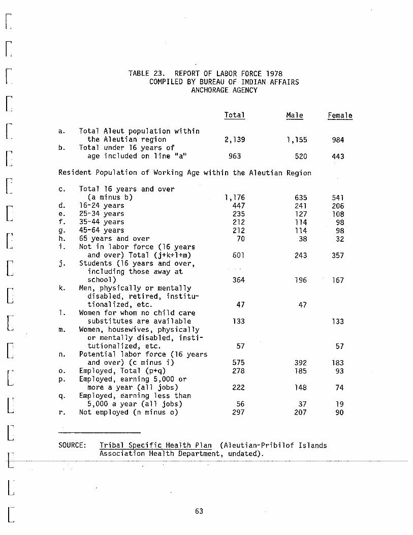
-E---[

[

TABLE 23. REPORT OF LABOR FORCE 1978 COMPILED BY BUREAU OF INDIAN AFFAIRS

ANCHORAGE AGENCY

a.

b.

Total Aleut population within the Aleutian region

Total under 16 years of age included on line 11 a11

Total

2,139

963

Male

1,155

520

Resident Population of Working Age within the Aleutian Region

c. Total 16 years and over (a minus b)

d. 16-24 years e. 25-34 years f. 35-44 years g. 45-64 years h. 65 years and over i. Not in labor force (16 years

and over) Total (j+k+l+m) j. Students (16 years and over,

including those away at school)

k. Men, physically or mentally disabled, retired, institutionalized, etc.

1. Women for whom no child care substitutes are available

m. Women, housewives, physically or mentally disabled, institutionalized, etc.

n. Potential labor force (16 years and over) (c minus i)

o. Employed, Total (p+q) p. Employed, earning 5,000 or

more a year (all jobs) q. Employed, earning less than

5,000 a year (all jobs) - r~ Not employed (n minus o)

1,176 447 235 212 212

70

601

364

47

133

57

575 278

222

56 297

635 241 127 114 114 38

243

196

47

392 185

148

37 207

SOURCE: Tribal Specific Health Plan (Aleutian-Pribilof Islands Association Health Department, undated).

63

Female

984

443

541 206 108 98 98 32

357

167

133

57

183 93

74

19 90

PERSONAL INCOME

Personal income data for the Aleutian Census Division have been com

piled for the years 1965-1978 and are presented in Table 24. Growth

in current do 11 ar tota 1 persona 1 income has been at a rate of about

7.4 percent per year, while per capita income has grown at about 7.2

percent per year. When measured in constant do 11 ars, however, the

growth has been substantially less. Real per capita income grew at

1.4 percent, while real total personal income grew at 1.6 percent over

the period.

Severa 1 aspects of the data suggest that the numbers be interpreted

with caution. First, the Anchorage Consumer Price Index was used to

deflate the personal income series since no more specific index is

available. Hence, the adjustment is only approximate. Second, a

large proportion of the income is related to military and federal

civilian employment directly linked to military activity. Since this

income does not enter the A 1 euti an economy in any meaningful sense,

its inclusion is misleading in terms of considering overall economic

activity.

Third, while the Bureau of Economic Analysis (BEA) which compiles the

data makes a resident adjustment, there is some -question as to the

validity of the adjustment. In particular, it is not clear to what

extent the adjustment captures the effects of commerical fishing and

----p~oce$sJng -i-ncomes- f-1 owJng~ out-o-f-the ~~eg-i-on. - i=-:i nall-y-, -an---analysi s~of-- ·-

64

[

r [

[

[

[

[

[

[

c [

[

[

[

[

[

t [

[

~

~

[

[

[

[

[

[

[

[

[

[

[

[

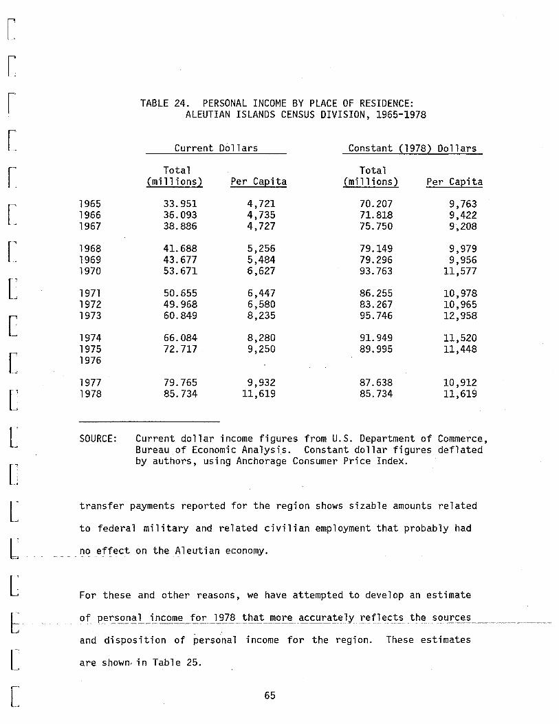
L [

1965 1966 1967

1968 1969 1970

1971 1972 1973

1974 1975 1976

1977 1978

SOURCE:

TABLE 24. PERSONAL INCOME BY PLACE OF RESIDENCE: ALEUTIAN ISLANDS CENSUS DIVISION, 1965-1978

Current Dollars Constant (1978) Dollars

Total Total (millions) Per Capita (millions) Per Capita

33.951 4,721 70.207 9,763 36.093 4,735 71.818 9,422 38.886 4,727 75.750 9,208

41.688 5,256 79.149 9,979 43.677 5,484 79.296 9,956 53.671 6,627 93.763 11,577

50.655 6,447 86.255 10,978 49.968 6,580 83.267 10,965 60.849 8,235 95.746 12,958

66.084 8,280 91.949 11,520 72.717 9,250 89.995 11,448

79.765 9,932 87.638 10,912 85.734 11,619 85.734 11,619

Current dollar income figures from U.S. Department of Commerce, Bureau of Economic Analysis. Constant dollar figures deflated by authors, using Anchorage Consumer Price Index.

transfer payments reported for the region shows sizable amounts related

to federal military and related civilian employment that probably had

no effect on the Aleutian economy.

For these and other reasons, we have attempted to develop an estimate

r~ . C ___ .. _____ of_ p~rs_o!l~ L_,_n~~e __ f_or _lJ]§ _ ~f:l.?J:._!'f'Slt"~-.C!~cur::.a!-~ h'.J'.e_f]_~.f:t_s_t_!J~_ ~.9_U!'~~!5- ___ _ _ _____ _

and disposition of persona 1 income for the region. These estimates

L are shown. in Table 25.

[ 65

TA3LE 25. ALEUTI/l.N" 'isLANDS. PERSONAL INCO!"E, 1978

BY SECTOR, COMPONENTS, AN.D GEOGRAPH~~ DISPOSITION

'.

I :.cc::,e ..

~-Support Contract Col'ir.lerci al · Fish Fed. Gov. Fed. Gov. State & Sector Construction fishing Processing Civilian Military local Govt.

. El\l)OS~!;C:JS HOUSE~OL DS: TOi.:.L ft.LLOC/;."iED BY 11\DUSTRY

~!ases l. Salaries. 3;715 0.381 0 2.353 3.022·.' 0 5.206 Oth.:r Labor lr:t:o;;,e· 0.6g5 0.071 0 0.440 0 0 0 Prc~rietors' lncoio~ 0.951 0.098 12.250 .0 0 ' 0 0 ... -·· u;;;,LLQCt;TED COX?OI\ElnS:

Divi~e~cis, Interest, and Rents

Transfer Pc)7.-ents

C~.IT C·F R:: GI 0!\:

~aoes t Salaries ;:.;. t: he: rc. ~e 0 4.709 0 0 0 0 0 Scu~hcer.\.ra1 0 1.087 . 0 0 0 0 0 F.es: cf State 0 0.725 0 0 0 0 0 F.est cf h'or1d 0.275 0.725 0 21 .173 5.867 40.584 0

(.ther lc.t>or lnco:i•E: ft.~.chor;:ge 0 0.881 . 0 0 0 0 0 Southcentral 0 0.203 0 0 0 0 0

i\est of s:at€ 0 0.136 0 0 0 . 0 0 F:ut cf h'or1d 0.051 0.136 0 3.958 o:· 0 0

Fro;;rii?tors' Jr,c.o:;Je 0.780 0 0 0 0 A;-.chorcge 0 0

Sc:;thc.entral 0 0 33.600 0 0 0 0 F-est of Stcte 0 0 2.130 0 0 0 0 ~est of \-.'orid 0 0 55.870 0 0 0 0

U!\;;Uo~p::D, OUT OF REGiON:

Divi6en~s. lr:terest, and Rf:nts

::e~t of 't!cr1d 7rc.:-1SfE.rS

;:;est ·cf ~·orld . ioi;.L 5.687 9.152 105.630 27.924 8.889 -~0.584 5.206

SOURCE: S~e text on personal income.

e:.c:.

Total -14.677-1.205

13.259

0.3)7 . 3.501

4.709 1.087 0.725

68.E24

O.t.81 0.203

.. 0.135 :. 4.145

0.780 33.600

2.130 56.870

1.623

~ .813•

213.326

[

[

[

.[

[

[

[

[

[

[

[

c [

[

[

[

E [

[

As shown in the tab 1 e, we have indicated persona 1 income sources by

type, accruing from the broad industrial classifications designated at

the top of the table. The left hand column of the table indicates the

estimated breakdown of income to resident and nonresident recipients.

Inclusion of the military and related civilian federal income as non-

resident is a judgmental decision based on the fact that these incomes

do not appear to enter the general income stream of the Aleutian

economy, but rather reflect enclave activity.

While much of the basis for allocating income has already been estab-

lished in preceding sections of this study dealing with the Aleutians,

there are several points that need to be expanded. In general, data

on wages and salary income were obtained from the Statistical Quarterly

for appropriate years. The Bureau of Economic Analysis data on "other

labor income" were apportioned to specific private sector industries

on a proportional basis and then assigned to either resident or non-

resident categories in proportion to resident/nonresident wage and

salary incomes. Dividends, interest, and rent were allocated to

residents and nonresidents on the basis of total wage and salary

income .. Total transfer payments were adjusted to assign military

transfers (except for veterans• pensions) to the nonresident category.

In addition, 10 percent of federal civilian retirement payments were

assigned to residents, with the remainder assigned to nonresidents.

With the exceotion of these adjustments, the remainder of transfer

67

Proprietor•s income is the income of self-employed and unincorporated

enterprises. A large portion of this component for the Aleutians

should reflect commercial fishing income, and it was felt that BEA

figures did not adequately reflect this income. An estimate of non

commercial fishing proprietor•s income was made by assuming that the

proportion of proprietor•s income to wage and salary plus other labor

income was the same for the State as for the Aleutians. This led to

an estimate of noncommercial fishing proprietor•s income of 4.1

million dollars.

Proprietor•s income from commercial fishing was based on the value of

catch. No reliable data exist on net profits from commercial fishing.

It has been estimated, however, that about 35 to 40 percent of the

value of catch is reflected in labor income (Scott, Prospects for a

Bottomfishing Industry in Alaska); hence, 35 percent of the value of

catch has been used to estimate proprietor•s income. This figure has

been used in conjunction with the estimated 1978 southwest region

value of catch to estimate proprietor•s income, as shown in the table,

and was allocated by factors established in Table 18.

In general, the data for 1978 show total personal income of 213.3

million. Of this total, residents who are part of the nonenclave

economy of the region accrued 33 million dollars. Of the 180 million

dollars accruing to nonresidents, about 46.5 million dollars represent

~ .. wa~te~ __ aod __ salanr __ paym~_nts ___ to __ mjJjtary~pe_rs_o.nneJ_and .. related_feder-.a] ____ _

civilian employees, ·with the remainder (133.9 million dollars) going

to other nonresidents.

68

[

[

[

[

[

[

[

[

c [

[

c [

[

[

[

E~

[

[

[

[

[

[

1--, ~·-J

[

[

[

[

[

[

[

[

[

[

[

b ~--

I w

In terms of the regional allocation of the 180 million dollars, about

6.4 million dollars flowed to the Anchorage region; while 34.9 million

dollars went to the southcentral region (primarily Kodiak), with an

additional 3.0 million dollars going to the rest of the State. About

136.1 million dollars primarily from commercial fishing and defense-

related activities appeared to flow outside the State. Thus, while

total personal income was substantial, over 84 percent of the income

created by production in the Aleutians flowed out of the Aleutian

region. These are indeed very high leakages and present a different

picture of the A 1 eut ian economy than that indicated by the BEA per-

sonal income data.

In addition to the analysis of total and per capita income, it is

again appropriate to consider the distribution of income. Recent data

on income distribution are not available, but the Bureau of Indian

Affairs prepared an estimate of the 1974 distribution of income which

is presented in Table 26. The distribution is shown for both Native

and white families. Median income for the two groups is similar, and

both are well below the statewide figure of 12,443 dollars for the

same year. The greatest disparity between Native and white families

appears in the under-5,000 dollar groups, with 26 percent of the

Native families and 13.8 percent of white families with incomes below

5,000 dollars. It should be noted that the non-Native families

include military personnel, whose incomes tend to flatten the distri-

bution somewhat; whereas for the Native distribution, the under-5,000 ------ ---~--- ---~- ------ -- ~------ ---~--- -- -- -- ------------------

dollar and over-1-5,000 dollar income categories are proportionately

more important.

69

TABLE 26. FAMILY INCOME: NUMBER AND PERCENT OF NATIVE AND WHITE FAMILIES BY INCOME LEVELS

ALEUT CORPORATION AREA

Native White

No. of Families Percent No. of Families

Under 1,000 7 2. 1 0 1 , 000-1 , 999 16 4.9 6 2,000-2,999 13 4.0 7

3,000-3,999 30 9.2 31 4,000-4,999 19 5.8 45 5,000-5,999 20 6. 1 55

6,000-6,999 26 8.0 65 7,000-7,999 25 7.7 63 8,000-8,999 21 6.4 72

9,000-9,999 18 5.5 37 10' 000-11 , 999 40 12.2 88 12,000-14,999 31 9.5 102

15,000-24,999 56 17. l 43 25,000-49,999 5 1.5 17 50,000 0 - 0

Median Income $8,357 $8,604

Percent

0 1.0 1.1

4.9 7. 1 8.7

10.3 10.0 11.4

5.9 13.9 16.2

6.8 2.7 0

[

[

[

[

[

[

[

[

[

[

[

[

[

[

[

[ SOURCE: Tribal Specific Health Plan (Aleutian-Pribilof Islands Association ~~.

Health Department, undated). ---~~-- -~~---- .. ,.

[ ['

70 L

[

[

~

[

[

[

[

[

[

[

[

[

[

[

[

[

POPULATION

Aggregate population data for 1960 and the years 1970-78 are presented

in Table 27; it includes total resident and civilian population and

military population. Considerable variation in the military popula-

tion is evident; although for most of the period, it averaged a little

over 3,000. For recent years, it has been somewhat lower, dropping to

1,655 in 1978. Total civilian population has shown a steady increase,

attributable to both natural increase and net in-migration. Table 28

shows the component of change in both civilian and military population

over the 1970-78 period. Civilian population has grown at about 4.8

percent, with natural increase accounting for 47 percent of the total

increase. The remainder is accounted for by net in-migration.

Table 29 provides data on population by community and by Native and

non-Native components. The data totals are not in strict agreement

with the other population data presented but do provide a generally

accurate picture of the population distribution in the census divi-

sian, with major nongovernment-based communities at King Cove, Sand

Point, St. Paul, and Unalaska. I't is no coincidence that (with the

exception of St. Paul) these are the major centers of commercial

fishing activity in the Aleutians.

E ~ ~ ~ ~ ~ -~'~ -~- ~ -~ -~- ------------~----------~- ---~-~------~--- ---~-~-~----------~-------------- ------

[

[ 71

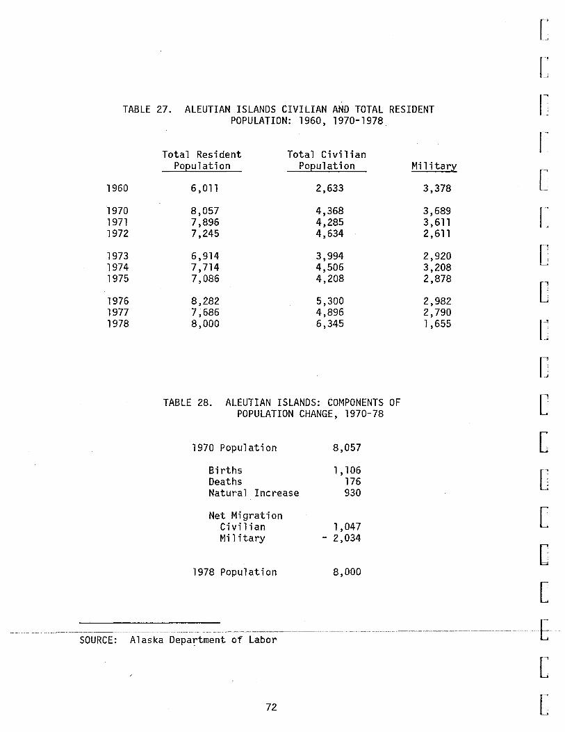
TABLE 27. ALEUTIAN ISLANDS CIVILIAN AND TOTAL RESIDENT

1960

1970 1971 1972

1973 1974 1975

1976 1977 1978

SOURCE:

POPULATION: 1960, 1970-1978

Total Resident Total Civilian Population Population

6,011 2,633

8,057 4,368 7,896 4,285 7,245 4,634

6,914 3,994 7,714 4,506 7,086 4,208

8,282 5,300 7,686 4,896 8,000 6,345

TABLE 28. ALEUTIAN ISLANDS: COMPONENTS OF POPULATION CHANGE, 1970-78

1970 Population

Births Deaths

8,057

Natural Increase

1 , 106 176 930

Net Migration Civilian Military

1978 Population

Alaska Depaftment of Labor

72

1 ,047 - 2,034

8,000

Military

3,378

3,689 3,611 2,611

2,920 3,208 2,878

2,982 2,790 1 ,655

[

[

[

[

[

[

[

[

[

[

[

[

c [

[

[

~ -E~

[

[

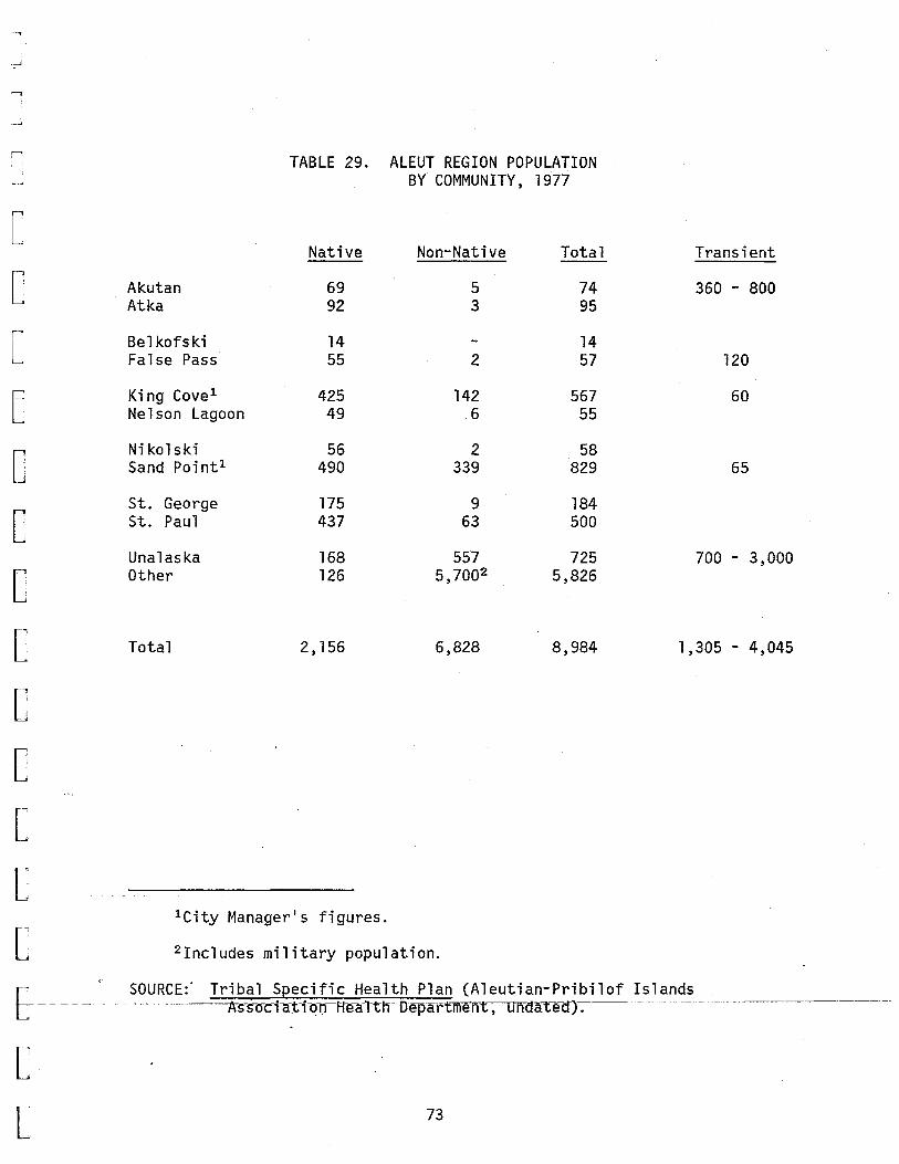
__ j

-.

r

L.-

[

[

[

[

[

[

[

[

[

[

[

[

[

Akutan Atka

Bel kofski False Pass

King Cove 1

Nelson Lagoon

Nikolski Sand Point1

St. George St. Paul

Unalaska Other

Total

TABLE 29. ALEUT REGION POPULATION BY COMMUNITY, 1977

Native Non-Native Total

69 5 74 92 3 95

14 - 14 55 2 57

425 142 567 49 6 55

56 2 58 490 339 829

175 9 184 437 63 500

168 557 725 126 5,7002 5,826

2' 156 6,828 8,984

lCity Manager's figures.

2 Includes military population.

Transient

360 - 800

120

60

65

700 - 3,000

1,305- 4,045

E-' SOURCE:· Tribal ~pecific Health Plan (Aleu~~-an_-!!.ibilof Islands

------------~ -Assoc1 ation l'leal ttl Department- ur'faatea). ~~-. . . ,

[

[ 73

Bristol Bay

Bristol Bay is located in the southwest portion of Alaska on the upper

part of the Alaska Peninsula. As a region, it covers approximately

55,000 square miles, which makes it roughly the size of Iowa or

Illinois. There are a total of 29 villages in Bristol Bay, and a

total population of approximately 5,000 persons. Bristol Bay is, for

statistical purposes, actually two separate areas: the Bristol Bay

Borough (containing the villages Naknek, South Naknek, and King

Salmon) and the Bristol Bay Division (which contains the remainder of

the villages, including Dillingham).

The economy of Bri sto 1 Bay has one pri nci pa 1 component that over

shadows all other activity: the commercial salmon fishery. Although

affected in varying degrees, all villages of the region are impacted

by the sa 1 mon industry. The sa 1 mon resource serves as an economic

base for subsistence living, as well as the commercial economic

activity. In recent years a substantial herring roe fishery has

developed. In addition to the fishing, King Salmon Air Force Station

in King Salmon also accounts for a significant amount of economic

activity, yet its linkages with the other economic units within the

region are minimal.

PRODUCTION

Basic sector production is composed of fishery related activity. Both

[

[

[

[

[

[

[

C

c [

c [

c [

[

[ · 1 t· h. d · · · t· · r~ -~comme~cJ_a ___ ,s_Jng·_an --PJ'ocess~l-ng_assume--ma,Jox·_ econom"JC--p~opor- "Ions -ln---~--~--- ~~C-~

[

74 [

[

[

[

[

[

[

[

[

[

[

[

[

[

[

[

[

the economy of the region. This has. been especially true over the

last three years, as Bristol Bay has had three of the biggest fishing

years ever.

fishing.

Table 30 summarizes information (data) on commercial

The data clearly show tremendous growth in the immediate past. The

history of the fishery is one of boom and bust cycles. Commercial

fishing began in the 1 ate 1800s, and though cyclic in terms of annua 1

harvest, the long run harvest cycle peaked in the mid-30s, followed by

a downward trend until the 1960s. The catch, despite cyclical fluctu-

ations, remained relatively constant (averaging nine million fish)

until the late 1970s. Over the past three years, however, the harvest

has been very high. The average harvest over 1979-81 has been 25 mil

lion fish, with 1980 and 1981 (28.2 and 27.7 million fish) being the

highest and second highest catch in the history of the fishery.

Table 30 also provides the summary data on the newly developing

herring roe fishery. As can be seen, prior to 1977 this fishery was

of little economic consequence. Growth in this fishery has been in

large part a result of low or depleted stocks of herring elsewhere.

Virtually all herring is caught for roe which goes for export. Prices

have varied substantially. Exvessel prices in Bristol Bay were $110/

metric ton in 1976, $155/metric ton in 1977, $330/metric ton in 1978,

and a record high of $650/metri c ton in 1979, and fe 11 to $200 and

E _____ -~ _ ·- !~5_0_2~ _ ~9~~---~~d ]_981 ~ _Y'__~-=~~c~2~e 1!_: _______ · -----·------------------. _____ ----. _____ _

[

[ 75

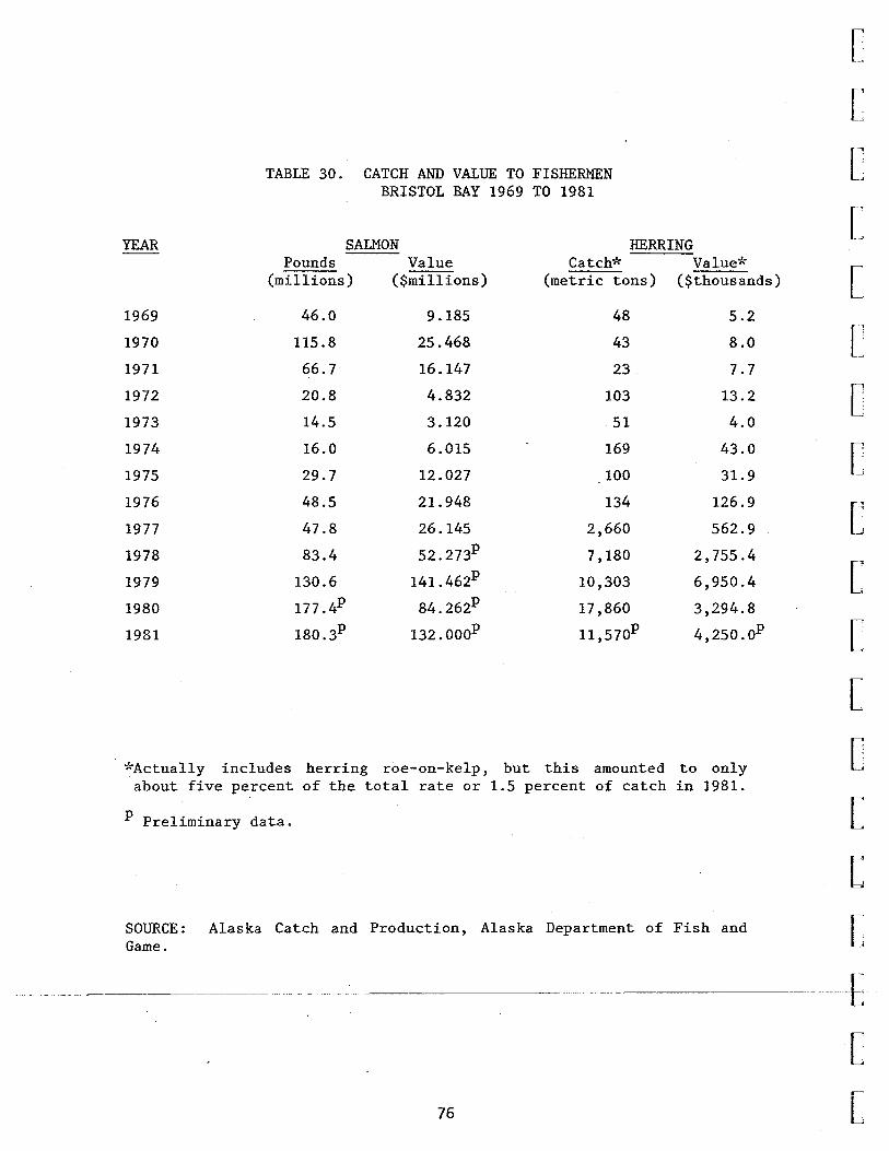
TABLE 30. CATCH AND VALUE TO FISHERMEN BRISTOL BAY 1969 TO 1981

YEAR SALMON HERRING

1969

1970

1971

1972

1973

1974

1975

1976

1977

1978

1979

1980

1981

Pounds (millions)

46.0

115.8

66.7

20.8

14.5

16.0

29.7

48.5

47.8

83.4

130.6

177 .4P

180.3p

Value ($millions)

9.185

25.468

16.147

4.832

3.120

6.015

12.027

21.948

26.145

52.273p

141. 462p

84.262p

132.000p

Catch* Value* (metric tons) ($thousands)

48 5.2

43 8.0

23 7.7

103 13.2

51 4.0

169 43.0

100 31.9

134 126.9

2,660 562.9

7,180 2,755.4

10,303 6,950.4

17,860 3,294.8

11,570p 4,2so.oP

*Actually includes herring roe-on-kelp, but this amounted to only about five percent of the total rate or 1.5 percent of catch in 1981.

p Preliminary data.

SOURCE: Alaska Catch and Production, Alaska Department of Fish and Game.

76

[

[

[

[

[

[

[

[

[

[

[

[

[

[

[

[

E---

[

[

[

[

[

[

[

[

[

[

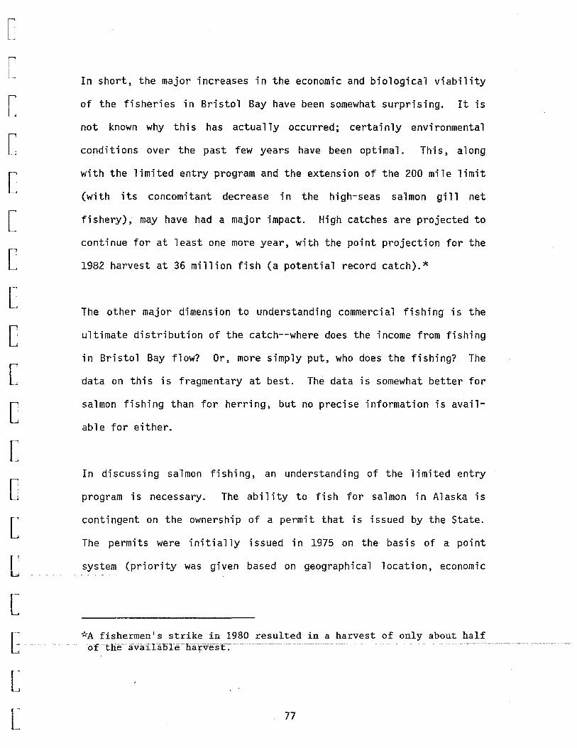
c [

[

[

[

[

[

[

t [

L

In short, the major increases in the economic and biological viability

of the fisheries in Bristol Bay have been somewhat surprising. It is

not known why this has actually occurred; certainly environmental

conditions over the past few years have been optimal. This, along

with the limited entry program and the extension of the 200 mile limit

(with its concomitant decrease in the high-seas salmon gill net

fishery), may have had a major impact. High catches are projected to

continue for at least one more year, with the point projection for the

1982 harvest at 36 million fish (a potential record catch).*

The other major dimension to understanding commercial fishing is the

ultimate distribution of the catch--where does the income from fishing

in Bristol Bay flow? Or, more simply put, who does the fishing? The

data on this is fragmentary at best. The data is somewhat better for

salmon fishing than for herring, but no precise information is avail

able for either.

In discussing salmon fishing, an understanding of the limited entry

program is necessary. The ability to fish for salmon in Alaska is

contingent on the ownership of a permit that is issued by the State.

The permits were initially issued in 1975 on the basis of a point

system (priority was given based on geographi ca 1 1 ocat ion, economic

*A fishermen 1 s strike in 1980 resulted in a harvest of only about half of the avaiL:ioTe ha:rvest-: - -~ - - - --- ---- - - -

77

dependence, and years in the fishery). The permits are transferable;

a fairly substantial market for trading permits has arisen. Each

fishery has a given number of permits that are gear type specific.

Table 31 provides data on the geographical distribution of the owner-

ship of permits. As can be seen, there are 2,600 permits in Bristol

Bay, of which roughly 47 percent a:re held by 11 residents 11 of Bristol

Bay. This is 1979 data; while additional permit transfers have taken

place since then, it is doubtful that these figures would change

appreciably.

However, there is a s i gni fi cant difference in income flows from the

fishery than might be inferred from permit ownership. First, only

38.55 percent of the drift gill net permits and 62.17 percent of the

set gill net permits are in the hands of local residents. The earn-

ings of each of these two gear types are significantly different.

From estimates based on survey analysis of the 1979 harvest, the

average gross income of the drift gill net fleet was $72,000, as

opposed to $16,000 for the set gill net operations (Larson, 1980).

Moreover, there appears to be a significant difference in the earnings

of Bristol Bay residents as compared with nonlocal residents. The

average gross income from fishing (see Table 32) of Bristol Bay drift

gi 11 net operators was $52,000, as opposed to $73,000 for other

Alaskan fishermen and $81,000 for 11 out of state11 residents. The same ,--~-~ ~-~ ~----------- -~-~-•~------ ---~-------- --------------------------- c--~---~--~-~~~-----~- ~--~-·-~---~,-~------~-~~-~-~ ------~----- --~-~--·---- -~~-~~--

type of pattern, -though not to the same degree, exists for set gi 11

net operators.

78

[

[

[

[

[

[

[

[

[

[

[

[

[

[

[

[

E [

[

1

--,

~

I

! ~

[

[

[

[

[

[

[

[

[

[

[

[

[

L L [

TABLE 31. BRISTOL BAY PERMANENT ENTRY SALMON PERMITS GEAR TYPE AND RESIDENCE, 1979

Bristol Bay Non-Bristol Bay Nonresident Resident Alaska Resident Total

Drift gill net 728 662 337 1,727 Set gill net 149 567 196 912 --

Total 877 1,229 533 2,639

PERCENT

Drift gill net 27.7 25.2 12.4 65.3 Set gill net 5.7 21.6 7.4 34.7

Total 33.4 46.8 19.8 100.0

SOURCE: Steve Langdon, Transfer Patterns in Alaskan Limited Entry Fisheries, report to Limited Entry Study Group, Alaska State Legislature, Jan 17, 1980.

Gear T1£e

TABLE 32. AVERAGE GROSS EARNINGS FROM SALMON FISHING BY GEAR TYPE AND RESIDENCE, 1979

All Bris. Bay Other AK Out-of-State Fishermen Residents Residents Residents

Drift gill net $71,696 $52,147 $72,643 $81,002

Set gill net $16,493 $14,724 $17,010 $19,484

SOURCE: Salmon 1980.

Doug Larson, 11 1979 Fishermen Income Survey: Herring and Fisheries," Alaska Sea Grant Program report 80-5, November

79

This difference in productivity is a result of several factors.

Bristol Bay residents tend to have smaller and older boats whereas the

limit boats (32 feet limit) are more likely to be operated by a non

Bristol Bay resident. Langdon found that among Bristol Bay native

fishermen, 40 percent used smaller (less than 32 feet) boats, while

Koslow (1979) reported that more than 90 percent of non-Bristol Bay

residents fished limit boats. The boats of the natives (local resi

dents) tend to be older and at a lower level of technology. This may

also reflect the local residents' access to financial markets and

abi 1 i ty to finance the 1 atest techno 1 ogy. Koslow and Langdon both

note that the income of local residents is almost exclusively depen

dent on salmon fishing, whereas out of area residents are not entirely

dependent on the Bristol Bay run. Koslow (1979, p. 8) found that more

than ha 1 f of the 1 oca 1 captains are dependent on Bri sto 1 Bay income

for more than two-thirds of their income, as opposed to 20 percent for

non-Alaskan captains. Langdon (1981, p. 63) reported that Bristol Bay

native fishermen indicated that 83 percent of their annual incomes

come from salmon fishing and 50 percent indicated that salmon fishing

was their ~ source of income. This would seem to have a substan

tial impact on access to financial markets, which impacts income and

productivity.

Based on relative gear productivity and the tenure of limited entry

permits, it would seem as though a substantial portion of the income

flows to other than local residents. Based on the data presented in

80

[

[

[

[

[

[

[

C

C [

[

[

[

[

[

[

c~

[

[

[

[

[

[

[

[

[

[

[

[

[

[

[

[

[

[

G [

[

Tables 30 and 31, although Bristol Bay residents own 48.8 percent of

the limited entry permits, only 32.3 percent of the income generated

from the harvest flows into Bristol Bay.

Other Alaskan residents receive 21.0 percent of the value of the

harvest (own 19.8 percent of the permits), while 46.7 percent of the

value of the harvest accrues to non-Alaskan residents (who own 33.4

percent of the permits).

The harvest of herring has strikingly different economic character

; st i cs from the sa 1 mon fishery. A 1 though the experience for the

herring fishery is somewhat limited, it appears that little income

flow finds its way into the local economy. From conversation with the

area biologists from the Alaska Department of Fish and Game, only a

small portion of the exvessel value goes to local fishermen. In 1981,

for example, about ten percent of the purse seiners and 80 percent of

the gi 11 netters were 1 oca 1 Bri sto 1 Bay boats. However, the produc

tivity of the gill net fishermen is substantially lower. In 1980,

gill netters harvested a 43,000 pound average per boat, while the same

figure was 247,000 pounds for purse seiners.

The proportion of the catch in terms of income that goes to 1 oca 1

residents is also affected by the predicted harvest. A high harvest

quota attracts more boats from outside the region, dropping the pro

portion of income from the fishery that stays in the local economy. -- ---- --------- --- ~ -----

All this has led to ·requests that the fishery be limited in terms of

81

entry, or that a large portion be allocated to gill netters. (Many of

the local salmon fishermen can convert easily to the herring fishery-

the capital requirements to entering the herring fishery are minimal.)

However, thus far, the herring fishery has not been managed with the

specific intent of affecting the distribution of income (although the

defacto distributional outcome is affected by the particular manage

ment scheme currently used). It remains to be seen if distributional

considerations will become an integral part of the management plan.

From 1981 data and information from Alaska Department of Fish and

Game, of the $4,250,000 exvessel value of the herring harvest, only

$600,000 (or 14 percent) accrued to Bristol Bay residents. As a

percent of ·the tota 1 harvest, this is an increase over the previous

year as a result of a lower predicted harvest quota.

The final dimension of commercial fishery to be considered is employ

ment. No systematic periodic estimates of commercial fishing in

Bristol Bay (or the rest of the state) are made by the Department of

Labor, as fishermen are self-employed and crew members generally work

on a 11 Share" basis, and as such, are not salaried employees. Esti

mates for 1969 ·through 1976 have, however, been compiled for the state

and various regions (Rogers, 1980, p. 13), and wi 11 be used here to

estimate employment for 1979. It is assumed that crew members come

from the same area as the residence of the permit holders. (There may

: ___ be __ l)_QOI"e_sj_d~nt_s __ who ___ h tr_e_ resJrient_s, _ but __ gene_raJ Jy_~b_i_s _ _i_s ___ Jlo_t __ the __

82

[

[

r [

[

[

[

[

[

[

[

[

[

[

[

[

------t-[

L

[

[

[

[

[

[

[

[

c [

[

[

[

[

[

[

case.) Rogers used a crew factor of 2.0 (including the captain) for

drift gill net fishermen and 2.5 for set gill net operations. Based

on those estimates, employment in Bristol Bay is 3,454 for driftnets

and 2,280 for setnets, with 2,741 being local residents.

Rogers estimates are probably low, though. Drift net fishermen

generally employ a 11 first crewman11 for the whole season, but usually

employ a second crewman when the harvest is at the peak. Again, this

is difficult to estimate--Langdon (1980) reported an average crew size

of 1.44 for all Bristol Bay native fishermen, which is more likely.

A 1 so, in a sma 11 portion of the cases (estimated by Langdon as 10

percent), the crewmen of non-Bristol Bay fishermen may be residents of

Bristol Bay. Utilizing this data, total employment is 6,493, with

3,201 being Bristol Bay residents.

The other component of the fishing industry in Bristol Bay is pro-

cessing. The present structure of the processing industry reflects a

mixture of shore-based and floating processors engaged in canning and

freezing. In recent years, the trend has been toward an increase in

the proportion of the harvest that is fresh frozen. In 1976 more than

90 percent of the salmon was canned, as compared to 1980 when approxi-

mately 21 percent of the harvest went to the fresh/frozen market.

Additionally, there is a significant portion of the harvest that is

airlifted into fresh markets and to other processing centers (Kenai

r and Kodiak). c- -- -- --~- -- -~ -- ---::- -- .. -~--~-~~~~~-~----~-~0.--~ -- - --~------ ---- - -- --- - -------- --- -- -

[

L 83

In 1980, more than 180 processors and buyers operated in Bristol Bay.

Of these, about one third were on-shore processors, another third were

floating processors and catcher/processors, and another third were

brokers and buying stations.

Employment data for processing is available for Bristol Bay (both

statistical areas) from the Statistical Quarterly (Alaska Department

of Labor). For 1979, 889 was the average annual employment in manu

facturing; which for Bri sto 1 Bay is 1 arge ly synonymous with fish

processing. As is the case with commercial fishing, it is important

to determine what proportion of the employment is held by residents of

the region.

Data on this question are fragmentary at best. First, it must be

understood that total employment in Bristol Bay is highly seasonal and

is very dependent on salmon fishing. For 1979, average employment in

manufacturing (for both statistical areas combined) for the four

quarters was, respectively: 15 (Jan.-March), 101 (April-June), 1,708

(July-Sept.), and 193 (Oct.-Dec.). The lowest is the first quarter,

with very little activity. Substantial gains are recorded in the

second quarter, especially the latter part. Employment peaks in July

(the salmon run peaks around July 10), and then falls off through

December to the winter low. Available data does not indicate how the

seasonal pattern varies between residents and nonresidents.

84

[

[

[

[

[

[

[

[

c [

[

[

[

[

[

[

-·· - --[.

[ I.

L

__ _,j

--,

~

[

[

[

[

[

[

[

[

[

[

[

[

[

[

[

L

No other employment category exhibits such extreme seasonal varia

tions. The processing firms are reluctant to divulge to what extent

they import labor, but it is probably substantial. Part of the in

crease in processing employment goes to resident workers, but it is

difficult to know how much.

The last element of the basic sector of Bristol Bay is the military.

King Salmon Air Force Station is located in the Bristol Bay Borough

and, as of 1978, had 432 active duty and civilian defense related

personnel (see Table 33). The military preserve is not as numerically

significant as it is in the Aleutians, and the overall regional

economic impact is relatively small. Remote bases tend to be self

contained and self supporting, and have little effect on the local

economy.

In summary, basic sector production in Bristol Bay is almost exclu

sively related to salmon fishing, with its relative importance having

increased as of late. In terms of providing employment in manufac

turing, though, growth has not been substantial because a great deal

of the manufacturing labor is imported. However, the harvests over

the past three seasons have been very large and the near term projec

tions are for continued high harvests (1982 could exceed all previous

harvests). This is likely to have substantial income effects in the

region.

85

TABLE 33. MILITARY AND RELATED FEDERAL CIVILIAN EMPLOYMENT AND WAGES BRISTOL BAY BOROUGH AND BRISTOL BAY CENSUS DIVISION, 1978

Bristol Bay Borough Bristol Bay Census Division EmEloyment Wages EmEloyment Wages

(000) (000)

Military and Related Civilian Employment 9 151 432 4,980

Military Personnel 5 56 420 4,924

Military Related Federal Civilian Employment 4 95 12 58

PX and NAF (largely part-time) 1 0 0 12

Other 4 95 0

1 PX and NAF (Post Exchange and Nonappropriated Fund activities, including officer's clubs and enlisted men's clubs)

SOURCE: Numbers: Basic Economic Statistics of Alaska Census Divisions, Alaska Department of Commerce and Economic Development, Division of Economic Enterprise, November 1979, p. 32-37.

EMPLOYMENT, UNEMPLOYMENT AND LABOR FORCE

The analysis of employment of the Bristol Bay region is important for

understanding the sources of major income flows. These income flows

provide insight into the sources of growth of the 1 oca 1 economy.

Tables 34, 35, and 36 summarize average monthly employment of the

Bristol Bay Region for the years 1965-1980. Table 34 provides data

for the entire region, while Tables 35 and 36 provide breakdowns for

the Brisfol~B-aiCe.nsu~ -Division and-the-BriStol -Bay Borough.

86

58

0

[

[

[

[

[

[

[

[

c c [

[

D

[

[

[

b [

[

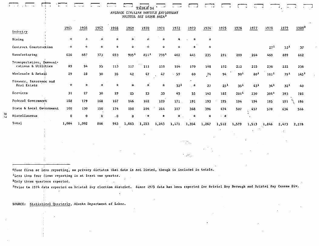
:0 ......

r-1 Ll rT1 ·r-J [~ r-J ~ c:--J T in:r.:~ 34 r:-J r:l r-:J r:J

AVERI1GI~ CJV J l,IAN tlONTJIT,Y ENl'f,OYr:I~N'J' 1\iUS'fOL MY I.!\D,OR hHEI\3

19ti~i .!J<ili .!2G7 1968 19611 ill~ 197~ 1972 1973 1974' L~~~~·:; tD'.

llinin~ , ... ;'c , ... , ... * .,-: * ,.,

* * I

ConLr;11.:t. Con:;truction >'< '~ ,.,

* * .,·: it ,~ oft .....

u.,nufacltlring 626 687 373 693 9os 1 851 1 798 1 402 4lt5 235

Tr.,nspoilation, Domnmni-cations & Util~tics 89 9ft 95 113 117 .111 110 10l, 170 148

Wholesale & Retail 29 28 30 35 42 47 47 59 60 74 . Fi.nance, Insura!lce and

* J21 Real Estate * , .. * * * * * 27

Sc rviccs 31 27 38 29 25 23 33 45 55 142

Federal Government 188 179 168 167 146 162 120 171 191 193

State & Local Go~ernment 100 130 150 174 190 204 264 317 368 396

Niscellaneous 0 0 0 .o 0 '* * * * >'r

Total 1,084 1,002 866 943 1,063 1,253 1,243 1,171 1,354 1,267

*Four firms or less reporting, so privacy dictates that data is not listed, though is included in totals. 1Less lhan four tirms reporting in at least one quarter. 2only three quarters reported.

r-l rJ r-J r-J :--J ~

1975 1976 l.22I. 1978 1979 ~2

27 1 SJ' 37

291 289 264 469 889 662

192 212 215 236 222 236

94 90 1 oo' 101 1 79 1 145 1

25 1 35 1 43 1 341 32 1 1,0

182 201 1 230 304 1 393 786 '

195 194 194 195 191 \·,

186 \

474 507 437 570 636 566 '

. * 1,512 1,579 1,513 ·. 1,846 2,473 2,278

3Prior to 1974 d~ta reported on Uristol Day election district. Since 1975 data has been reported for Brisiol Bay Dorough and Bristol Day Census Div.

SOURCE: Statistical Quartcrl:r::, Alaska Department or Labor.

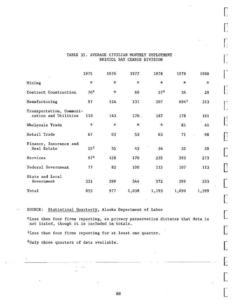
TABLE 35. AVERAGE CIVILIAN MONTHLY EMPLOYMENT BRISTOL BAY CENSUS DIVISION

1975 1976 1977 1978 1979 1980

Mining * * * * * *

Contract Construction 70 1 * 66 27 1 34 29

Manufacturing 97 124 131 207 694 1 313

Transportation, Communi-cation and Utilities 110 143 170 187 178 191

Wholesale Trade * ·/( * •/( 81 41

Retail Trade 67 63 53 63 71 98

Finance, Insurance and Real Estate 25 1 35 43 34 32 29

Services 97 1 128 170 235 393 273

Federal Government 77 82 100 115 107 113

State and Local Government 331 399 344 372 399 333

Total 855 977 1,038 1,193 1,690 1,399

SOURCE: Statistical Quarterly, Alaska Department of Labor

*Less than four firms reporting, so privacy preservation dictates that data is not listed, though it is included in totals.

1 Less than four firms reporting for at least one quarter.

20nly three quarters of data available.

88

[

[

[

[

[

[

[

[

[

[

c [

[

[

[

[

E--[

[

[

[

[

[

[

[

[

[

[

[

[

[

[

[

[

[

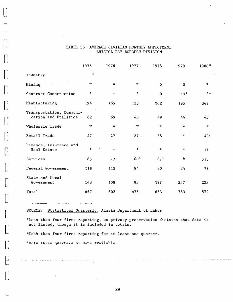
E [

[

TABLE 36. AVERAGE CIVILIAN MONTHLY EMPLOYMENT BRISTOL BAY BOROUGH DIVISION

1975 1976 1977 1978 1979 19802

Industry 1

Mining -~~ * * 0 0 *

Contract Construction * * * 0 191 81

Manufacturing 194 165 133 262 195 349

Transportation, Communi-cation and Utilities 82 69 45 49 44 45

Wholesale Trade * ~" * * * ~'(

Retail Trade 27 27 27 38 * 43 1

Finance, Insurance and Real Estate * * * * ~" 11

Services 85 73 60 1 69 1 i( 513

Federal Government 118 112 94 80 84 73

State and Local Government 143 108 93 198 237 233

Total 657 602 475 653 783 879

SOURCE: Statistical Quarterly, Alaska Department of Labor

*Less than four firms reporting, so privacy preservation dictates that data is not listed, though it is included in totals.

1 Less than four firms reporting for at least one quarter.

20nly three quarters of data available.

89

Over the period, total employment grew substantially at an average

annual rate of 5.1 percent. While the basic industry of fish pro

cessing registered very little growth, other sectors grew at sub

stantial rates.

Manufacturing (synonymous with fish processing) is to a large degree

imported (from outside the region), and is very dependent on the size

of the fish harvest. As with harvest data (see Table 30), with the

exception of the past three years, no consistent pattern exists.

State and 1 oca 1 government grew at a 12. 25 percent rate, whereas

wholesale and retail trade grew at a 11.3 percent rate, and transpor

tation grew at a 6. 7 percent rate. Services grew at a 24.1 percent

rate, yet this rate of growth is based upon a statistical anomaly, and

is probably significantly lower. (Based on the 1965-1979 period, it

still registered a 19 percent rated growth.)

In examining monthly employment .data presented in Table 37, there

appears to be a great de a 1 of vo 1 at i 1 i ty in emp 1 oyment in the manu

facturing, service, and state and local government sectors. It

appears that the increases in emp 1 oyment in the manufacturing and

commercial fishing sector are matched by reductions in each of the

other two sectors. Apparently, most of the variation in employment in

the government takes place in local government employment, where

_positions are _funded _w_ith _the _ int.P.nt.ion of -permitting commercial

fishing during the season.

90

[

[

[

[

[

[

[

c c [

[

[

c [

[

[

E [

[

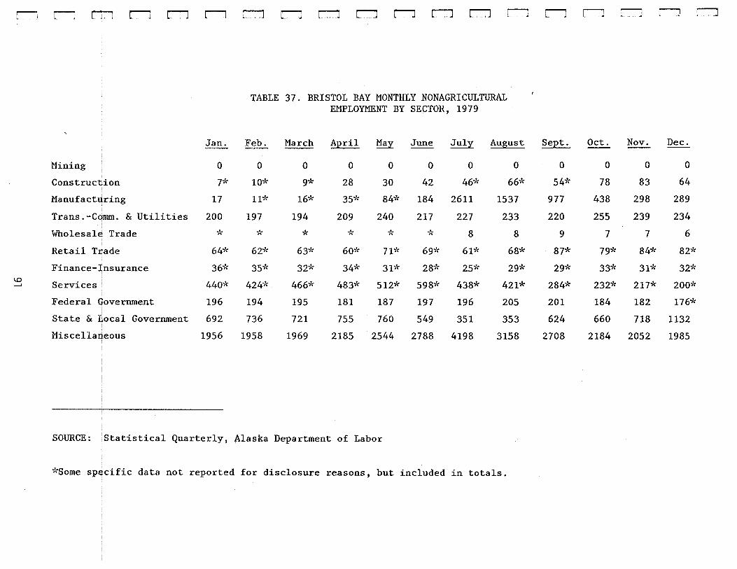
r-Jr-Jri'lr-J~r-J~r-Jr.--Jr-JL'Jr-lr-Jr-lr-Jr--Jr--Jr-lr-J

TABLE 37. BRISTOL BAY MONTHLY NONAGRICULTURAL EMPLOYMENT BY SECTOR, 1979

Jan. Feb. March April May June July August Sept. Oct. Nov. Dec.

Mining 0 0 0 0 0 0 0 0 0 0 0 0

Construcbion ]"'J'( 107\- g-;': 28 30 42 46•k 66* 547"" 78 83 64 !

Manufact.qring 17 11* 167\- 357'> 84-l• 184 2611 1537 977 438 298 289

Trans.-Cdmm. & Utilities 200 197 194 209 240 217 227 233 220 255 239 234 . ,,

Wholesale Trade ";~ 'i'~ * "';'( .,( ... 8 8 9 7 7 6 " 1

I

Retail Trade 64"'• 62;'; 63"'• 60;'; 71''> 69•'> 61* 68-l• 87* 79;'; 84* 82"'•

Finance-~nsurance 36-1• 35•'> 32* 34* 31•'> 28-l• 25"'' 29* 29* 33* 31* 327\-\.0

Services ' 440•\- 424"'• 466•'> 483-l• 512•\- 598* 438* 421* 284•\- 232* 217* 200* __,

Federal Qovernment 196 194 195 181 187 197 196 205 201 184 182 176-l• i

State & Local Government 692 736 721 755 760 549 351 353 624 660 718 1132

Miscellaneous 1956 1958 I

1969 2185 2544 2788 4198 3158 2708 2184 2052 1985

SOURCE: :statistical Quarterly, Alaska Department of Labor

*Some specific data not reported for disclosure reasons, but included in totals.

One significant omission from the employment data is commercial

fishing. Fishing, as previously discussed, is not traditional sal

aried employment. Fishermen work for crew shares (e.g., 15 percent of

the gross to each crewman); and for tax purposes, crewmen and fisher

men are considered to be self-employed. Utilizing previous estimates,

it would appear that fishermen (and crew) accounted for 6,493 jobs,

and that local residents account for 3,201 jobs in fishing employment

(though this is highly seasonal). If we include these figures with

total reported employment, then fishing accounted for 72 percent of

total employment. Commercial fishing and processing account for

80 percent of total employment. Again, it must be reiterated that a

great deal of this employment occurs in a relatively short period of

time (the three months of the salmon harvest).

A second issue in employment, as explained earlier, relates to the

residency of job holders. As indicated above, a significant portion

of employment in commercial fishing is non-resident employment. As

reported previously, the bulk of employment by processors is also

non-resident.

A few of the processing firms have indicated the extent to which they

import labor (Table 38), although there is probably not enough infor~

mation or consistency to be able to make estimates as to the propor

tion of the payroll from processing that goes to non-resident labor.

_____ Emm_i_n"tel"-vj_ews_wj_tb_the---p-cocesso-cs-,-i-t-wou-ld-appear-that-dur-i-ng-the

92

[

[

[

[

[

[

[

c [

[

[

[

[

[

[

[

-E[

L

~~~~~~~~~~~~~~~~~~~

TABLE 38. BRISTOL BAY SUMMARY OF EMPLOYMENT BY RESIDENCY OF EMPLOYEES, LARGE PROCESSORS

Seasonal Peak Local Other Alaska Outside Alaska --1980 1981 1980 1981 1980 1981 1980 1981

Dillingham/Nushagak

Queens"Fisheries 260 300 0 0 86~\- 100~\- 174"k 200~'<-

Peter Pan 210 225 120 120 20 20 70 85

Naknek/Kwichak

Nelbro 280 225 6 6 134 110 140 109 U)

Red Salmon w 197 197 20 20 10 10 167 167

Whitney 120 120 10 10 20 20 90 90

Egegik

Kodiak King 80 85 0 0 19~\- 20~'<- 61* 65*

Diamond·E. 263 263 0 0 66~\- 66* 197* 197*

Columbia Ward 275 300 0 0 150 175 125 125

TOTAL 1,685 1,715 156 156 505 521 1,024 1,038

% of Total 100% 100% 9.2 9.1 30 30 60 61

*Based on a percentage estimate of season peak.

SOURCE: D~ta provided by representatives of respective processors.

processing peak, a substantial portion of the income flow to labor

accrues to non-resident labor. Perhaps 60 percent of this income

flows outside Alaska and 30 percent to non-Bristol Bay Alaskans. It

must be remembered, though, that this is only during salmon season,

which is basically June, July, and August. This is when employment is

at its peak. However, during the other months, there is little migra-

tory labor--the processors bring in the outside labor only for the

fishing season.

This finding is reinforced by data on labor force and employment.

During the peak of the 1979 salmon harvest, data on employment suggest

that there are 4,200 jobs being fi 11 ed, yet the 1 abor force at that

time was only 2,036; it is doubtful that the difference in the two

figures is accounted for by moonlighting.

On average, it appears that 90 percent of processing employment during

the peak period is non-resident employment. (For purposes here, it is

assumed that peak period is July, August and September, and that all

other jobs go to the residents. ) Based on 1979 monthly data of the

6,497 month jobs, 1,885 (29 percent) were held by residents, and 4,612

(71 percent) were held by non-residents. Of the non-residents, one

third of those non-resident jobs (1,537 jobs or .24 percent of the

total) were held by Alaskan residents (outside Bristol Bay). On an

annual basis, employment in processing would be allocated as follows:

[

c [

[

[

[

[

[

c [

[

[

c [

r L..>

[

______ a_d_s_t_oJ_B-aY-.~es_idents_,_l5}_j_obs_;_non~Alaskan_~es_idents_,_384_jobs_; E--other Alaskan residents, 128 jobs.

[

94 [

[

[

[

[

[

[

[

[

c [

c [

[

[

r "'='

[

The allocation of the remainder of employment has been accomplished as

follows: state and local government is assumed to be local residents,

as is a 1 so the case for the remainder of the emp 1 oyment categories.

With the exception of federal government military employment, most of

the other categories are small (construction is the most notable), and

though a portion of employment might be allocated to non-residents,

for purposes here, employees are assumed to be residents.

Using these assumptions, from the data presented in Table 39, it would

appear that 52.3 percent of total employment was held by Bristol Bay

residents. The remaining 47.7 percent is held by non-residents.

Again, it must be emphasized that this is an estimate, but it does

provide a benchmark. Data are not available to make this determina-

tion for other years. Also, it is not possible to speculate how

resident employment shares will change over time.

TABLE 39. BRISTOL BAY AVERAGE ANNUAL ESTIMATED RESIDENT AND NON-RESIDENT EMPLOYMENT, 1979

Industry Resident Non-Resident Total

Commercial Fishing Manufacturing Construction Transportation Communications and Utilities Wholesale and Retail Trade Finance Services Federal Gov't (military) 1978 data

3,201 157 34

178

152 32

393

3,292 6,493 512 669

0 34 0 178

0 152 0 32 0 393

432 432

··~~~--~~;~!~-::_~~-~-a-~0~~~:::n...----------107 0 107 399 0 399 --

[ Total 4,653 4,236 8,889

52.3% 47.65%

[ 95

Summary data on the labor force, employment, and unemployment for

1970-1981 are presented in Tab.les 40 and 41. It should be noted here

that the employment data in this table is fundamentally and defini

tionally different from the employment data in previous tables.

First, as in the previous data, no official data is available on

commercial fishing. Secondly, the data here reflects job holder

status, and is based solely on residents (i.e., resident adjusted).

Thirdly, and perhaps the most important difference, the data reflect

the number of job holders, whereas the previously presented data

reflected the number of jobs. The difficulty here is that it is

possible to hold more than one job, and thus, it is difficult to

adjust income flows on the basis of jobs.

Of particular interest are the 1 eve l s of unemployment and the unem

ployment rate. These are surprisingly low, given the cyclic variation

in employment (number of jobs). However, given the definition of

labor force participation used and the nature of the economy in

Bristol Bay, they less surprising. The data suggests that a substan

tia 1 amount of movement in and out of the labor force is present.

Most observers feel that employment and unemplo¥ment figures are

tenuous when examining "Bush" economies. People tend to enter the

labor force during the summer months when employment opportunities are

present. During the remaining part of the year, although they could

potentially be employed, they are not in the ] abo~ force. This is

96

[

[ ~

[

[

[

[

[

[

[

[

[

[

[

[

[

[

b [

[

[

[

[

[

[

[

[

[

[

[

[

[

[

[

[

[-"

--'

L [

[

TABLE 40. SUMMARY EMPLOYMENT STATISTICS, BRISTOL BAY LABOR AREA

Labor Unemployment Year Force Employment Unemployment Rate (%)

1970 1,384 1,228 156 11.3 1971 1,483 1,280 203 13.7 1972 1,468 1,291 177 12.1 1973 1,547 1,399 148 9.6

1974 1,601 1,494 107 6.7 1975 2,005 1,897 108 5.4 1976 2,096 1,943 153 7.3 1977 1,928 1,778 150 7.8

1978 1,661 1,497 164 9.9 1979 1,838 1,679 159 8.7 1980 1,824 1,573 151 8.3 1981* 1,860 1,723 137 7.4

*Based on the first three quarters only.

SOURCE: Historical Report on Labor Force and Employment, Bureau of Labor Statistics, U.S. Department of Labor.

TABLE 41. MONTHLY LABOR FORCE AND EMPLOYMENT, BRISTOL BAY, 1979

Civilian Labor Force Employment Unemployment Rate

January 1,609 1,433 176 10.9 February 1,686 1,508 199 11.8 March 1,828 1,578 250 13.7 Apri 1 1,811 1,633 178 9.8

May 1,960 1,764 196 10.0 June 1,922 1,768 154 8.0 July 2,036 1,933 103 5.1 August 1,911 1,800 111 5.8

September 1,879 1,775 111 5.9 October 1,939 1,800 139 7.2

- November - - . -1,805- - - --- 1~656 -- --139 -- -- - -- T.T December 1,679 1,527 152 9.1

SOURCE: Statistical Quarterly, Alaska Department of Labor, 1980.

97

primarily because of the way in which labor force participation is

measured. Those persons who have not actively sought work, even

though they may have wanted to work, are considered out of the labor

force; therefore, they don't appear within official estimates of

unemployment. This effect is similar to what is referred to as the

"discouraged worker" effect in national employment data, except in the

Alaskan bush the basic economic structure is somewhat different.

Nonetheless, it is felt by many that the narrow definition of unem

ployment accounts for much of the perceived difference between

published rates of unemployment and the proportion of people who are

not gainfully employed (i.e., unemployed). This shows up somewhat in

labor force participation rates--in 1980, the labor force participa

tion rate for Bristol Bay was 24.5 percent, whereas for Alaska and the

United States as a whole, it was 47.7 and 46.9, respectively. Many

people enter the labor force during the summer when fishing season is

in full swing, and then are out of the 1 abor force unti 1 the next

year.

In a study done by the state in the lower Yukon-Kuskokwim Region, it

was estimated that actual unemployment was 24.7 percent, as opposed to

official estimates of 13.2 percent. The study used a broader (less

restrictive) definition of unemployment that was intended to measure

the available worker pool. The question asked was, "Does

a regular job now, either full- or part-time?"

... want

[

[

[

[

[

[

[

[

[

[

[

[

[

[

[

[

-------------------------~

[

98 [

[

r [

[

[

[

[

[

[

[

[

[

r-, ....

[

[

[

t [

[

This is reinforced further by Langdon's study among resident Bristol

Bay fishermen. While fishing represents the single most important

employment opportunity in Bristol Bay, it is only important for that

middle three-month period. Langdon reported that Bristol Bay native

fishermen received 83 percent of their annual income from fishing, and

that among 58 percent of the fishermen, fishing was their sole source

of income. It is· recognized that salmon fishing is seasonal, yet the

fisherman who is unemployed for the other nine months of the year is

an under-utilized resource.

PERSONAL INCOME

Persona 1 income data for the Bri sto 1 Bay region for the years 1959-

1979 (both statistical areas) have been compiled and are presented in

Table 42 and Table 43. the growth rate of current dollar total per-

sonal income for the Bristol Bay Division and the Bristol Bay Borough

was 11.92 percent and 7. 96 percent respectively. Per capita income

growth for each was 10.49 percent and 6.92 percent respectively.

However, when measured in constant dollars, the growth appears to have

been substantially less. In real terms, per capita income has grown

at a rate of only 5.68 percent in the Bristol Bay Division and 2.1

percent in the Bristol Bay Borough.

A couple of aspects of the above data suggest that the numbers need to

be taken with a fair amount of caution. First, the Anchorage Consumer

Price Index was used to adjust the time series to constant dollar

99

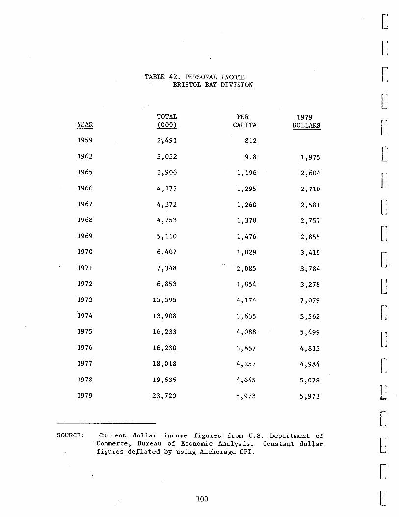
YEAR

1959

1962

1965

1966

1967

1968

1969

1970

1971

1972

1973

1974

1975

1976

1977

1978

1979

SOURCE:

TABLE 42. PERSONAL INCOME BRISTOL BAY DIVISION

TOTAL PER (000) CAPITA

2,491 812

3,052 918

3,906 1,196

4,175 1,295

4,372 1,260

4,753 1,378

5,110 1,476

6,407 1,829

7,348 2,085

6,853 1,854

15,595 4,174

13,908 3,635

16,233 4,088

16,230 3,857

18,018 4,257

19,636 4,645

23' 720 5,973

1979 DOLLARS

1,975

2,604

2, 710

2,581

2,757

2,855

3,419

3,784

3,278

7,079

5,562

5,499

4,815

4,984

5,078

5,973

[

[

[

[

[

[

E c [

[

[

C [

[

[

[ Current dollar income figures from U.S. Department of -~

Commerce, Bureau of Economic Analy-sis_. __ C_Qns_t_ant._d_o_lJar r~ figures de~lated by using Anchorage CPI. r;--

[

100 l-~

[

[

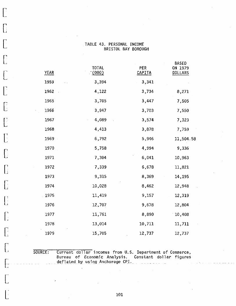
[ TABLE 43. PERSONAL INCOME BRISTOL BAY BOROUGH

[ BASED

TOTAL PER ON 1979

[ YEAR ".(000) CAPITA DOLLARS

1959 3,394 3,341

[ 1962 4,122 3,734 8,271

[ 1965 3,705 3,447 7,505

1966 3,947 3,703 7,550

[ 1967 4,089 3,574 7,323

1968 4,413 3,878 7,759

C 1969 6,792 5,946 11,504.58

[ 1970 5,758 4,994 9,336

1971 7,304 6,041 10,963

[ 1972 7,339 6,678 11,821

1973 9,315 8,369 14,195

[ 1974 10,028 8,462 12,948

[ 1975 11,419 9,157 12,319

1976 12,707 9,678 12,804

[ 1977 11,761 8,890 10,408

1978 13,014 10,711 11,711

[ 1979 15,705 12,737 12,737

[ SOURCE: Current dollar incomes from U.S. Department of Commerce,

Bureau of Economic Analysis. Constant do 11 ar figures

E deflated by using Anchorage CPI.

[

[ 101

amounts, since no more specific index is available. There is a con

siderable difference in prices between Bristol Bay and Anchorage, yet

aside from some tenuous estimates of the gross difference, no consis

tent time series is available. Secondly, the CPI has come under a

significant amount of criticism as of late, in that many feel that it

has consistently overstated inflation, and thus, the rate of real

income growth would actually have been higher over the period.

Thirdly, the data in no way provides any information about the subsis

tence economy. If the poverty level of income were adjusted to

Bristol Bay, it would suggest that the bulk of the population is below

the poverty level. What is missing in the personal income data is the

value of subsistent income and how this has changed over time. Addi

tionally, in examining the data for the two different statistical

areas, it is evident that the income in the Bri sto 1 Bay Borough is

more than twice that in the Bristol Bay Division. This has to be

explained in large part by the fact that Bristol Bay Borough is one of

the centers of commerce, and the portion of individual 1 s existence

that is tied up in subsistence activity is less than in the more rural

areas. The Bristol Bay Division, on the other hand, includes all the

outlying bush communities, in addition to the commercial center of

Di 11 i ngham.

Data on the distribution of income for Bristol Bay is presented in

Table 44. It is recognized that this data is fairly dated, yet it is

important a.s a. p_oi nt of reference_. The _di stri but ion and levels of

income have certainly changed since 1970, but no attempt is made here

to speculate what these changes have been.

102

[

[

[

[

[

[

[

[

[

[

[

[

[

[

[

[

I= c

[

[

[

[

[

[

[

[

[

[

[

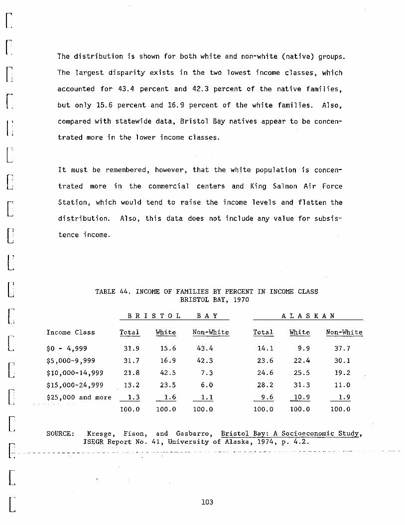
C [

[

[

[

The distribution is shown for both white and non-white (native) groups.

The largest disparity exists in the two lowest income classes, which

accounted for 43.4 percent and 42.3 percent of the native families,

but only 15.6 percent and 16.9 percent of the white families. Also,

compared with statewide data, Bristol Bay natives appear to be concen-

trated more in the lower income classes.

It must be remembered, however, that the white population is concen-

trated more in the commercial centers and King Salmon Air Force

Station, which would tend to raise the income levels and flatten the

distribution. Also, this data does not include any value for subsis-

tence income.

TABLE 44. INCOME OF FAMILIES BY PERCENT IN INCOME CLASS BRISTOL BAY, 1970

B R I S T 0 L BAY ALASKAN

Income Class Total White Non-White Total White Non-White --

$0 - 4,999 31.9 15.6 43.4 14.1 9.9 37.7

$5,000-9,999 31.7 16.9 42.3 23.6 22.4 30.1

$10,000-14,999 21.8 42.5 7.3 24.6 25.5 19.2

$15,000-24,999 13.2 23.5 6.0 28.2 31.3 11.0

$25,000 and more 1.3 1.6 1.1 9.6 10.9 1.9 -- --100.0 100.0 100.0 100.0 100.0 100.0

[

[ SOURCE: Kresge, Fison, and Gasbarro, Bristol Bay: A Socioeconomic Study,

[-------------~~~~R"~~~ort No. 41, University of Alaska, 1974, p. 4.2.

[ r-~

L 103

POPULATION

Aggregate population data for Bristol Bay for 1960, 1970, and 1980 are

presented in Table 45; included is the data on population by racial

group (native and non-native components). Table 46 provides data on

the components of the changes in population between 1960, 1970, and

1980. Overall population grew at a 1.74 percent rate over the two

decades, with the native component growing at a somewhat higher rate.

Virtually all of the population growth in Bristol Bay has been ac

counted for by natural increase. From 1960 to 1970, there was a

substantial increase in natural increase, coupled with negative

changes in military population and net migration.

Between 1970 and 1980, there was a further reduction in military

population, with positive implied net migration and positive natural

increase. However, over the two decades, the changes in mi 1 i tary

population and net migration appear to have been negative. The totals

are not in strict agreement, but the data do provide a generally

consistent picture with respect to the major causes of population

change.

[

[

[

[

[

[

[

[

l [

[

[

[

[

Table 47 provides data on population by community, by native, and [

non-native components. The highest concentration of Caucasians is in [

the Dillingham and Naknek areas (the primary centers of the region).

____________ T_h_o_ugh Caucasians make up 30 percent of the total gogulation,_]£_ger- ~

cent of the Caucasian population resides in these two areas, where

combined they account for 50 percent of the population. [

104 [

[

[

[

[

[

[

[

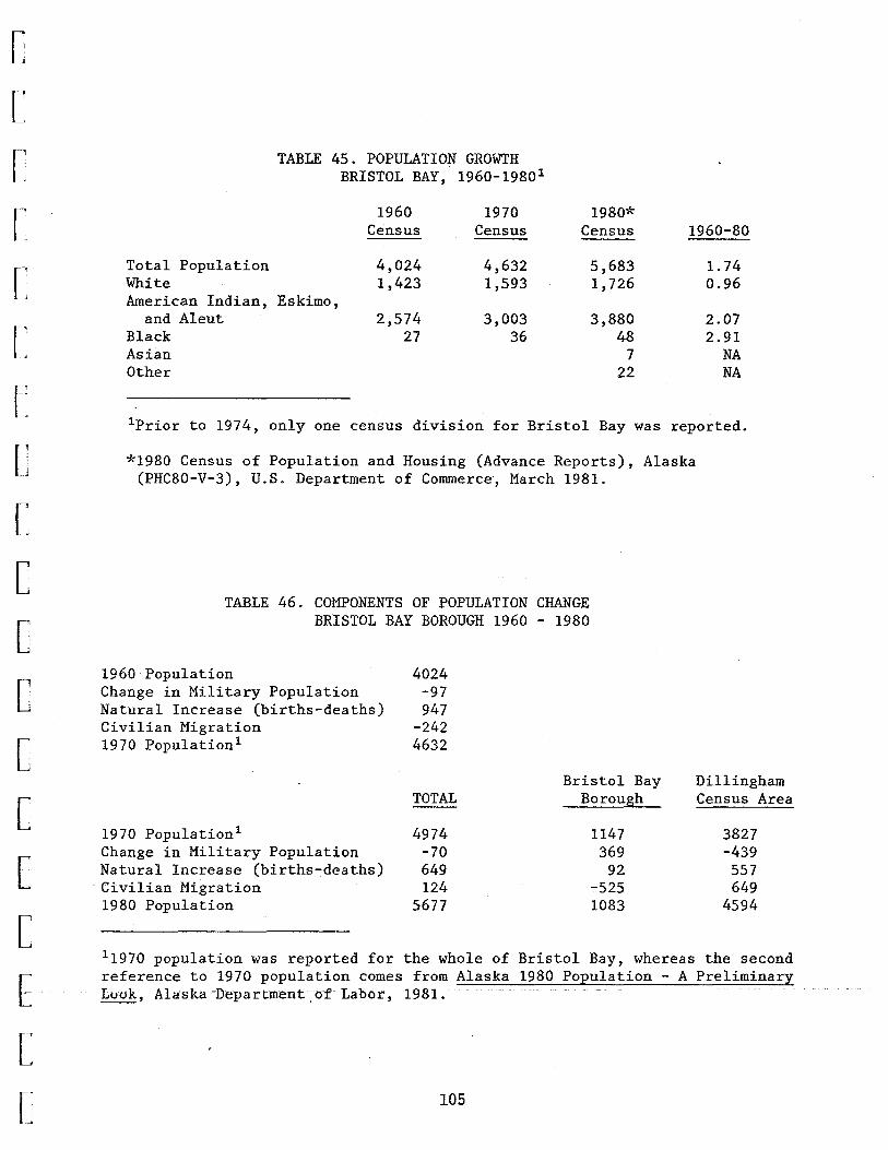
c [

[

[

[

[

[

[

[

E L [

Total Population White

TABLE 45. POPULATION GROWTH BRISTOL BAY, 1960-1980 1

1960 Census

4,024 1,423

1970 Census

4,632 1,593

American Indian, Eskimo, and Aleut

Black Asian Other

2,574 27

3,003 36

1980* Census

5,683 1, 726

3,880 48

7 22

1960-80

1. 74 0.96

2.07 2.91

NA NA

1Prior to 1974, only one census division for Bristol Bay was reported.

*1980 Census of Population and Housing (Advance Reports), Alaska (PHC80-V-3), U.S. Department of Commerce, March 1981.

TABLE 46. COMPONENTS OF POPULATION CHANGE BRISTOL BAY BOROUGH 1960 - 1980

1960 Population Change in Military Population Natural Increase (births-deaths) Civilian Migration 1970 Population1

1970 Population 1

Change in Military Population Natural Increase (births-deaths) Civilian Migration 1980 Population

4024 -97 947

-242 4632

TOTAL --

4974 -70 649 124

5677

Bristol Bay Borough

1147 369

92 -525 1083

Dillingham Census Area

3827 -439 557 649

4594

1 1970 population was reported for the whole of Bristol Bay, whereas the second reference to 1970 population comes from Alaska 1980 Population - A Preliminary Look, Alaska~nepartment.of Labor, 1981.

105

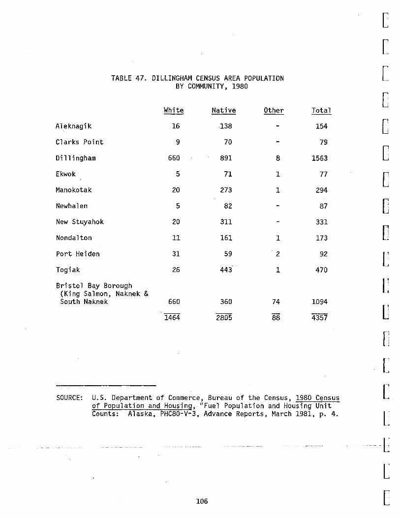
TABLE 47. DILLINGHAM CENSUS AREA POPULATION BY COMMUNITY, 1980

White Native Other Total --Aleknagik 16 -138 - 154

Clarks Point 9 70 - 79

Dillingham 660 891 8 1563

Ekwok 5 71 1 77

Manokotak 20 273 1 294

Newhalen 5 82 - 87

New Stuyahok 20 311 - 331

Nondalton 11 161 1 173

Port Heiden 31 59 2 92

Togiak 26 443 1 470

Bristol Bay Borough (King Salmon, Naknek & South Naknek 660 360 74 1094

1464 2805 88 4357

SOURCE: U.S. Department of Commerce, Bureau of the Census, 1980 Census of Population and Housing, 11 Fuel Population and Housing Unit Counts: Alaska, PHC80-V-3, Advance Reports, March 1981, p. 4.

106

[

[

[

[

[

[

[

[

[

c c [

[

[

[

[

-[

[

[

[

[

[

[

[

[

[

[

[

[

[

[

[

[

[

[

E l [

III. THE BASE CASE

In this part of the report we deal with three critical elements of the

base case. The first of these is the underlying .methodo 1 ogy used to

develop the base case. The second element concerns the assumption re

garding the future economic activity used to develop the projections.

The third is the set of projections themselves.

Methodology

Impact analysis, as carried out in the present study, is based upon a

comparison of sets of economic and demographic projections, where one

set is the standard or base case set. The base case serves as a frame

of reference against which the economic and demographic changes re

sulting from the proposed OCS lease sale can be measured and evaluated.

There are two components of this process that are of particular con

cern. First is the question of the accuracy and consistency of the

projections. Generally speaking, this is dependent upon the validity

of the assumptions utilized regarding future economic growth of the

exogenous variables and the projection methodology employed. More

will be said on both of these points below.

The second concern relates to the degree of information contained in

the projections. Specifically, do the projections contain the infor

mation t~at~. is necessary to adequately jnterpret and evaluate the

impacts?

108

While aggregate data on economic and demographic variables generated

using the projections methodology employed in this study will answer

many questions, it must be recognized that there will be omissions as

well.

At the root of impact analysis is the issue of how economic well

being, both individually and collectively, will be affected by the

proposed action. Two major problems are associated with this process.

First it is not possible to measure all impacts that will result from

the lease sale. In part this is due to the volume of information that

would be required and the inadequacy of the existing methodology to

capture all effects at an acceptable level of cost.

The more serious problem is that many of the effects are not measur

able. While reallocation of resources within the context of the

functioning of the market, in response to economic change, is

desirable from the perspective of efficiency, change on the order of

magnitude imp 1 i ed by OCS activity may a 1 so 1 ead to situations of

market failure and the presence of externalities. These are often

difficult to identify and are certainly difficult to measure.

[

[

[

[

[

[

[

[

c [

[

[

[

[

Even if these effects could be isolated they are usually inseparable L from a further problem, that of income redistribution. Changes in [

income distribution and the relative economic position of individuals

-----~res u 1 t i ng from O_C_S_a_c_tj v i_zy_o_e_c_e_s_s_a_r_iJy_i_mpJ_i_e_s_tb~t_t_b_eLe_wjJJ_I;te E-lossers and gainers and associated changes in economic welfare. These

L 109 [

[

[

[

[

[

[

[

[

[

[

[

[

[

[

[

[

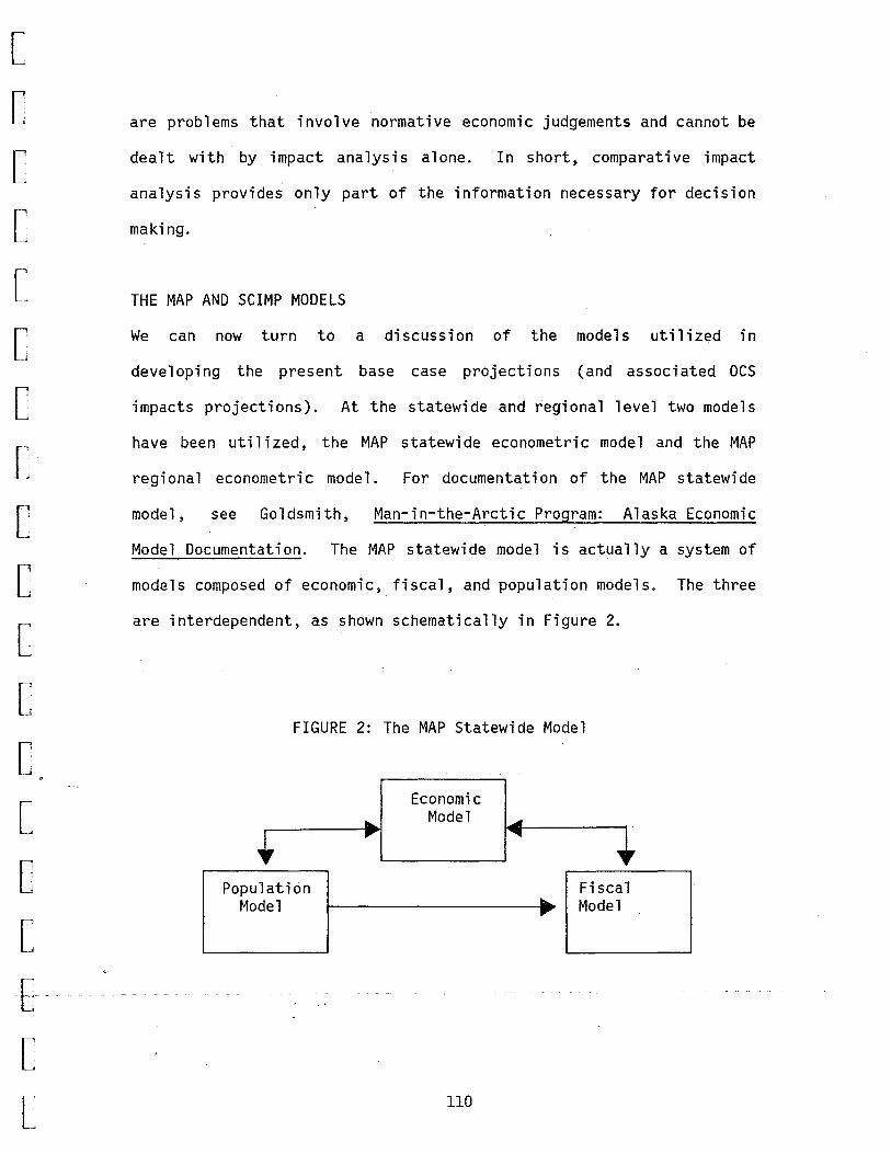
are problems that involve normative economic judgements and cannot be

dealt with by impact analysis alone. In short, comparative impact

analysis provides only part of the information necessary for decision

making.

THE MAP AND SCIMP MODELS

We can now turn to a discussion of the models utilized in

developing the present base case projections (and associated OCS

impacts projections). At the statewide and regional level two models

have been utilized, the MAP statewide econometric model and the MAP

regional econometric model. For documentation of the MAP statewide

model, see Goldsmith, Man-in-the-Arctic Program: Alaska Economic

Model Documentation. The MAP statewide model is actually a system of

models composed of economic, fiscal, and population models. The three

are interdependent, as shown schematically in Figure 2.

FIGURE 2: The MAP Statewide Model

~I Economic

I~ Model

t + Population

I I Fiscal Model ~ Model

5- ---------

[

[ 110

In essence, this states that the economic model receives input from

the fiscal and population models, the fiscal model receives input from

the economic and population models, and the population model utilizes

input from the economic mode 1 s, but not directly from the fi sea 1

mode 1. Thus, when we ta 1 k about the economic mode 1 we are really

describing the. interaction of three models. To simplify things some

what we can describe the important linkages between submodels and then

consider the economic model in more detail.

The population-economic model link is the source of population esti

mates that are of direct interest, and reflect both natural population

change and migration induced by changes in economic conditions. The

population estimates are also used by the economic model for purposes

of computing various per capita values for economic variables.

The significant link with the fiscal model relates to ~he role of

State government expenditures as a source of major economic stimulus

to the aggregate level of economic activity. In turn, State govern

ment (and local government) expenditures are dependent upon two key

factors, the overall level of economic activity and the level of

activity in the petroleum industry. The system allows for a variety

of po 1 icy choices regarding state government spending and is one of

the key points to consider in assessing economic forecasts.

111

[

[

[

[

[

[

[

[

[

[

[

[

[

[

[

[

[

[

[

[

[

[

[

[

[

[

[

[

[

[

[

[

[

[

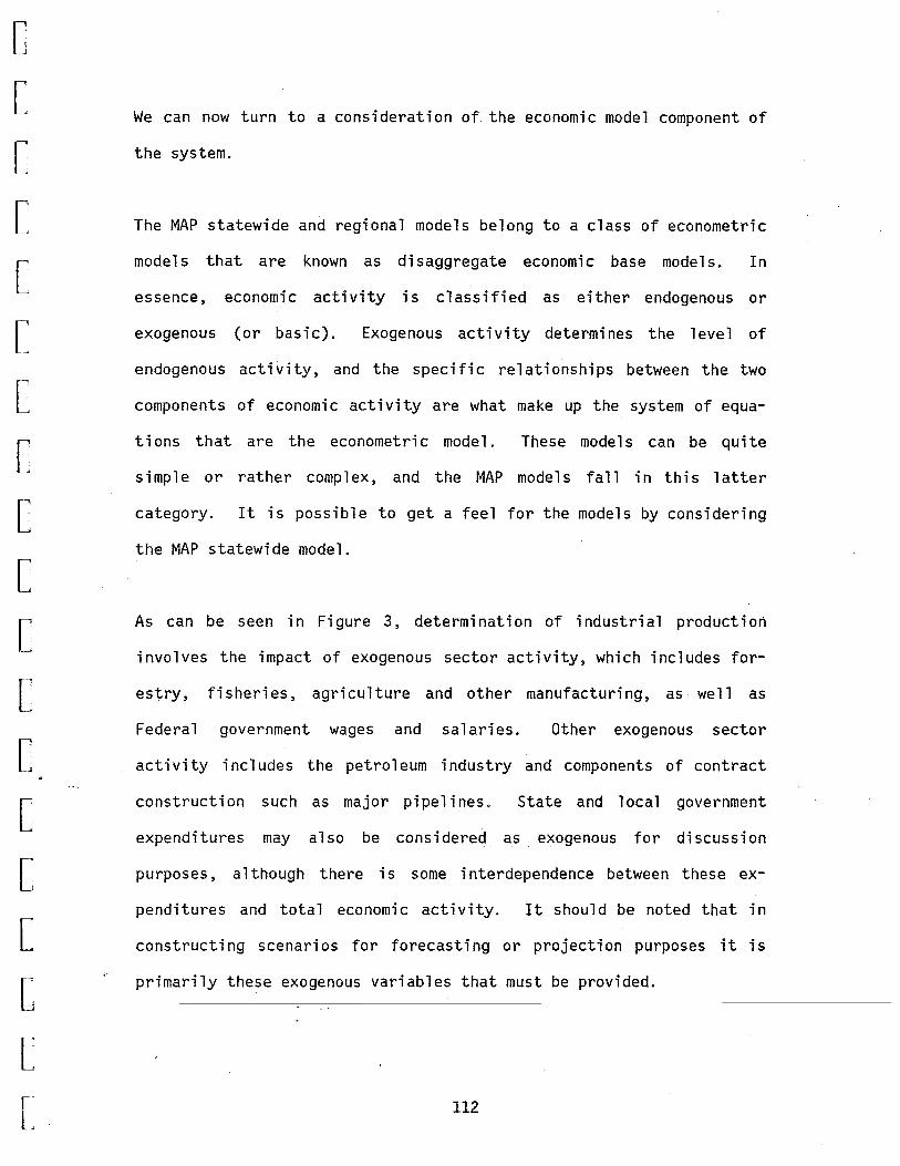
We can now turn to a consideration of the economic model component of

the system.

The MAP statewide and regional models belong to a class of econometric

models that are known as disaggregate economic base models. In

essence, economic activity is classified as either endogenous or

exogenous (or basic). Exogenous activity determines the level of

endogenous activity, and the specific relationships between the two

components of economic activity are what make up the system of equa

tions that are the econometric model. These models can be quite

simp 1 e or rather comp 1 ex, and the MAP mode 1 s fa 11 in this 1 atter

category. It is possible to get a feel for the models by considering

the MAP statewide model.

As can be seen in Figure 3, determination of industrial production

involves the impact of exogenous sector activity, which includes for-

[ -

estry, fisheries, agriculture and other manufacturing, as we 11 as

Federal government wages and salaries. Other exogenous sector

activity includes the petroleum industry and components of contract

construction such as major pipelines. State and local government

expenditures may also be considered as exogenous for discussion

purposes, a 1 though there is some interdependence between these ex

penditures and total economic activity. It should be noted that in

constructina scenarios for forecasting or projection purposes it is

-b ,. primarily these exogenous variables that must be provided.

[ r-L

112

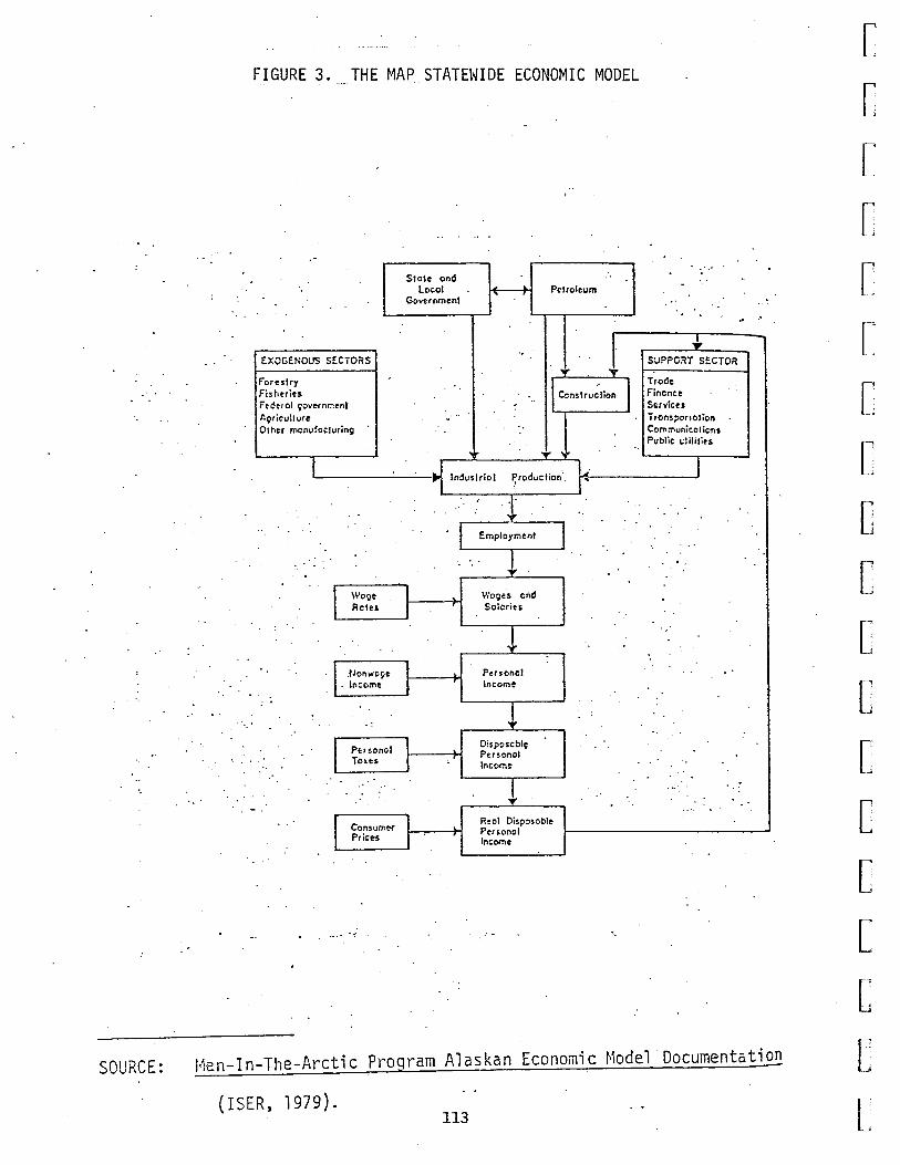
SOURCE:

FIGURE 3. _THE MA~_STATEWIDE ECONOMIC MODEL

EXOGENOUS SECTORS

F"ores!r'y Fisheries. Fe-deral ~vvtrn~tnf .tQrit\JIIure O!her monu!ocluring

... . . (

S!ole ond loco I

Governmenl

'

Pelroleum

Employmenl

-! Wo9ts ond Soiorits

l Per.onol Income

! Oisposcbl~ Personal Inc om~

l

I ,..,

Reel Oisposob!e Penonol lnco,ne

.

• ..

-.... SUPPORT SECTOR

Trode Fine nee Servicu Tronsponolion Communications Public ~:I ililie~

~ .•

l':·c.n-In-The-Arctic Program Alaskan Economic f•1odel· Documentatio.Jl

(ISER, 1979). 113

[

[

[

[

[

[

[

[

[

[

[

c [

[

[

[

[

[ '

r· L

[

[

[

[

[

[

C [

[

[

[

[

[

[

[

[

E L [

These exogenous variables combine with demand from the support sector

and endogenous construction to generate total industrial production.

Industrial production, through a series of steps, determines employ-

ment and income, and finally real disposable personal income, which in

turn is a determinant of support sector and endogenous construction

economic activity. This means that aggregate production depends on

both exogenously determined and endogenously determined economic

activity, where endogenous activity. depends on total activity. As

such, the system is a simultaneous equation structure.

It should also be noted that certain other variables enter the model

as well. In particular, wage rates are used in determining total wage

and salary payments, where the wage rates are in part dependent upon

U.S. wage rates, which are determined exogenously. It should also be

observed that the model is particularly sensitive to the wage rates

used.

The MAP regional model dissagregates the MAP statewide model estimates

for population and for employment in the basic, support, and govern-

ment sectors among 20 regions. Most of these regions correspond to

Alaska census divisions. In order to use the regional model, sce

narios (or future values for exogenous variables) must be specified on

a region a 1 basis. The MAP region a 1 mode 1 is described in Appendix A.

For the Aleutian Islands Census Division projections have been devel-- -- ------ ----- ~------- -------~--~------~----------------- ------~ ----~---~--------~----------------------------- ------ --- --- ----------------------

oped using the small community population impact model (SCIMP). For

114

documentation see Lee Huskey and Jim Kerr, 11 Small Community Population

Impact Model 11• Whereas the MAP models are classified as econometric

models, SCIMP is technically an accounting model. A system of equa-

tions describes the economic and demographic structure of the economic

system. In turn parameters of the equations and a set of exogenous

variable inputs provide the numerical basis for utilizing the model

for projection purposes. It is the determination of parameters for

the model that distinguishes SCIMP from econometric models.

In an econometric model, parameters are typically determined by the

application of econometric methods to historical time series or cross

section data and the parameter estimates are an integral component of

the model. In the case of SCIMP the parameters are determined exog-

enously by a variety of means, including point estimates, assumptions

based on other research, and in some instances by econometric esti

mation techniques. In other words, in SCIMP both the parameters and

exogenous variable data are inputs, while in an econometric model the

parameter estimates are an integral part of the model.

[

[

[

[

L ['

[~

['

[

[

[

[

[

There are both advantages and shortcomings to this approach. On the l~

positive side, SCIMP is generally applicable to small regional

economies, rather than being region specific, as would be the case [

with an e~onometric mode:. This results in substant~ally more limit~d l~

data requ1rements than 1s the case for a fully est1mated econometr1c -

_ ____ ______ ______ mo_d_el._ _Ihe __ "s bo _r_tc viiLtog __ j_s _a]_s_o __ jn dic_at_e_d __ by __ t.bP.~le.~s_.5.t..r·tngent. __ d_ata___ __ _ _________ E __

L 115 [

r [

[

[ f-,

r.,

-·~

[

[

[

[

[

[

[

[

L [

requirements. Specifically, the quality of the parameter estimates

may not be as great as that obtained by econometric techniques.

However, the costs are substantially less.

We can now turn to a discussion of the assumptions utilized in

developing the base case projections. Since distinct sets of assump-

tions are necessary for each of the models, these will be considered

in turn.

The Base Case Assumptions: The MAP Models

The impact of OCS development on the economy will be measured as the

change in the development scenario from the base case scenario. The

base case scenario is that which is projected to occur without the OCS

lease sale of interest. This section describes the base case scenario

which will be used in this study.

A set of assumptions about the future 1 eve 1 s of various exogenous

economic activities defines a development scenario. There are five

types of assumptions required for the MAP model development scenarios.

These are assumptions about the future level of national variables

which directly.or indirectly affect Alaska economic activity; assump-

tions about employment requirements of special projects, such as the

gas pipeline; assumptions about the employment requirements for

exogenous industry and government sectors of the Alaska economy; an

-~- _____ ' __ ji~§_~P!-i e>_n __ ~~ _tQ_t_h_g_lll!m.b~_r _ _gf__ t_Q!J_r_ist_s ___ \\'119 wU_l_yj_§it_l\J§~kq_;_ QJld _____ _ L-o

assumptions about State government revenues and expenditures.

[

[ 116

Our use of assumptions in developing the base case scenarios does not

mean that we are predicting that all or any of these events wi 11

occur, since there is considerable uncertainty with respect to the

levels and timing of the events in these scenarios. What it does mean

is that with a certain degree of probability, we expect the general

level of economic activity to follow this scenario. We assume that

there is a medium probability that the level of activity will be at

least as great as that described by this scenario.

Primarily as a result of the uncertainty attached to the occurrence,

magnitude, and timing of any particular event, agreement about partie-

ular scenarios is hard to achieve even among those most knowledgeable

about the Alaska economy. Emphasizing our concern mainly with general

levels of activity, the probabilistic nature of the specific scenario

should reduce the disagreement.

Our base case assumptions are summarized in Table 48. They include

national variable assumptions, project assumptions, industry and

government assumptions, tourism assumptions, and government policy

assumptions. Below we present a detailed description of these assump-

tions.

[

[

[

[

[

[

[

[

[

[

[

[

[

[ '

-·

[

[

---------------------------------------------------------------------------------------------------------- -----------------------------------------------------L---

[

117 L

[

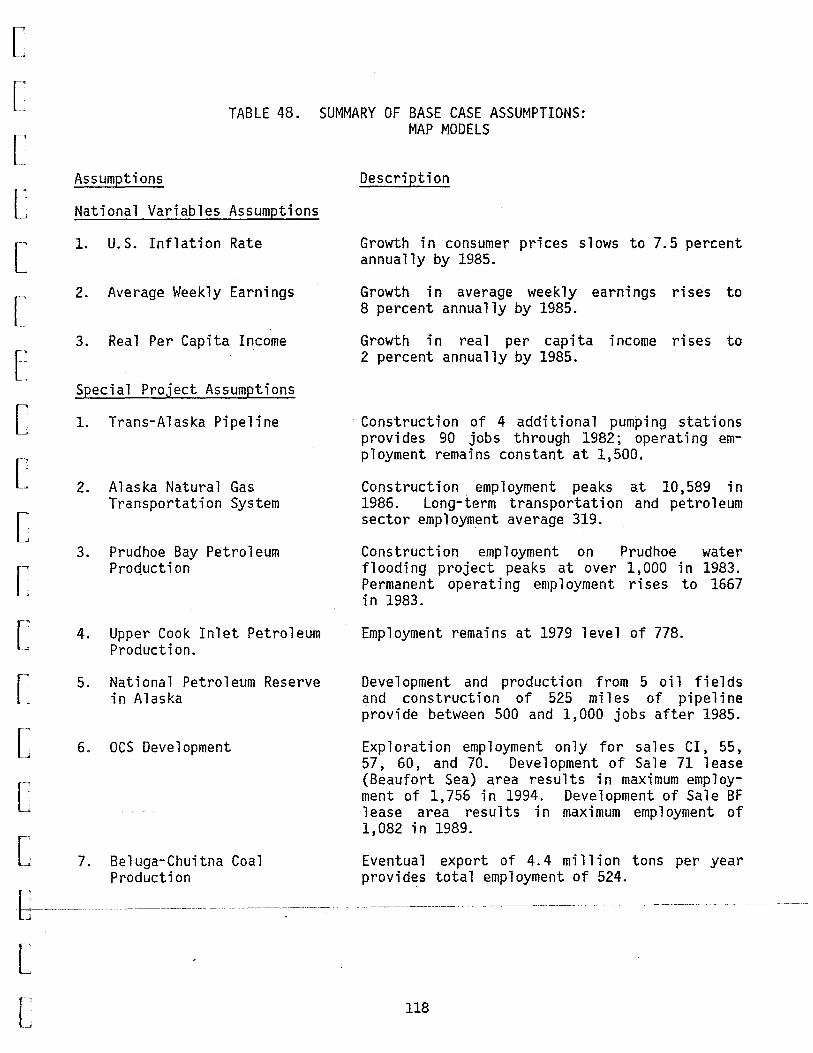
[ TABLE 48. SUMMARY OF BASE CASE ASSUMPTIONS:

[

[

[

[

[

[

[

[

[

[

[

[

r: [

Assumptions

National Variables Assumptions

1. U.S. Inflation Rate

2. Average Weekly Earnings

3. Real Per Capita Income

Special Project Assumptions

1. Trans-Alaska Pipeline

2. Alaska Natural Gas Transportation System

3. Prudhoe Bay Petroleum Prod.uct ion

4. Upper Cook Inlet Petroleum Production.

5. National Petroleum Reserve in Alaska

6. OCS Development

7. Be 1 uga-Chui tna Co a 1 Production

-6------------------------------------·-··

[

l

MAP MODELS

Description

Growth in consumer prices slows to 7.5 percent annually by 1985.

Growth in average weekly earnings rises to 8 percent annually by 1985.

Growth in real per capita income rises to 2 percent annually by 1985.

Construction of 4 additional pumping stations provides 90 jobs through 1982; operating employment remains constant at 1,500.

Construction employment peaks at 10,589 in 1986. Long-term transportation and petroleum sector employment average 319.

Construction employment on Prudhoe water flooding project peaks at over 1,000 in 1983. Permanent operating employment rises to 1667 in 1983.

Employment remains at 1979 level of 778.

Development and production from 5 oil fields and construction of 525 miles of pipeline provide between 500 and 1,000 jobs after 1985.

Exploration employment only for sales CI, 55, 57, 60, and 70. Development of Sale 71 lease (Beaufort Sea) area results in maximum employment of 1,756 in 1994. Development of Sale BF 1 ease area results in maximum emp 1 oyment of 1,082 in 1989.

Eventua 1 export of 4. 4 mi 11 ion tons per year provides total employment of 524.

118

Assumptions Description

Industry and Government Assumptions

1. Other Mining Activity

2. Agriculture

3. Logging and Sawmi 11 Employment

4. Commercial Fishing: Non-Bottomfish

5. Bottomfish Harvesting and_Processing

6. Federal Civilian Employment

7. Federal Military

Tourism Assumptions

Policy Assumptions

Employment increases from a 1979 level of 3,140 at 1 percent annually.

Expansion results in employment of over 1,000 by 2000.

Employment increases from 2,204 · in 1980 to 4,103 in 2000.

Employment levels in fishing and fish processing remain constant at 6,323 and 7 1 123, respectively.

Resident employment rises from 284 in 1981 to 5,518 in 2000.

Rises at 0.5 percent annual rate from 17,915 in 1979 to 19,893 in 2000.

Employment remains constant at 23,333.

Number of tourists visiting Alaska rises at 4 percent annual rate from 505,400 in 1979 to over 1.1 million by 2000.

Exogenous revenues from petroleum production taxes, roy a 1 ty payments, property taxes, and special corporate taxes peak at about $10 billion annually by 1989. Real per capita expenditures grow in proportion to the growth in real per capita income.

119

[

[

[

[

[

[

[

[

[

[

[

[

[

[

[

[

b L r ,

L

[

[

~

[

[

[

[

[

[

[

[

[

[

[

[

[

NATIONAL VARIABLES ASSUMPTIONS

Inasmuch as Alaska is an open economy, it is affected by changes in

the national economy. Consequently, several assumptions about the

future growth of the U.S. economy are required. First, a forecast of

average weekly earnings in the United States is required as an input

into the estimation of Alaskan wage rates. Second, the Alaskan price

level is tied in part to the national price level so that a forecast

of the U.S. consumer price index is needed. Finally, inasmuch as a

major determinant of migration to Alaska is the income differential

between Alaska and the lower 48, a forecast is required of real per

capita disposable income in the United States.

In 1979, consumer prices in the United States rose 11.5 percent,

average weekly earnings grew 7.5 percent, and real per capita dis

posable income grew by 0.5 percent. In the base case, it is assumed

that the growth in U.S. consumer prices slows to a long run rate of

7.5 percent by 1985, that the growth in average weekly earnings rises

to a 1 ong run rate of 8 percent by 1985, and that rea 1 per capita

personal income growth rises 2 percent annually by the mid-80s.

SPECIAL PROJECTS ASSUMPTIONS

Wi_dely differing special projects with major implications for future

Alaskan development have been proposed by a variety of federal and

state agencies and private developers. Each project generates direct

[ _________ ~mp] ()~m~!1~ ~ r1 one _or more _of the sector~ _ ~f _ the A 1 as k~Hl econo111y

I.

L

[ 120

treated as exogenous by the MAP forecasting mode 1. The sectors are

manufacturing, mining, and parts of the construction and transpor

tation sectors. This section presents our assumptions as to the

direct employment generated by each of th·e major projects either

currently in operation or proposed.

1. Trans-Alaska Pipeline (Alyeska

Trans-Alaska Pipeline assumptions are given in Table 49. Trans-Alaska

Pipeline Service (TAPS) employment through 1977 included only the

exogenous construction employment engaged in the initial construction

of the pipeline. Employment since completion in 1977 and future

employment is of two types. These are additional construction of four

pump stations (see Oil and Gas Journal, 2/25/80, p. 72), and exogenous

transportation sector employment associated with operation of the

line.

2. Alaska Natural Gas Transportation System

In December 1980, the Northwest Alaska Pipeline Company received

rights of way for the Alaskan portion of a 4,800 mile pipeline to

transport natural gas from Prudhoe Bay to the United States West Coast

and Midwest (see Oil and Gas Journal, 12/8/80, p. 50). Employment

projections for this project are shown in Table 50. Construction of

the 741-mile Alaskan portion of the line and an accompanying gas

conditioning plant on the North Slope was assumed to get underway in

--1981-and.---to-~be- ope-~ational---bY- 1981-.-- -Constt"-uction-employment.--was -

expected to peak ·at 10,589 in 1986, falling to a long-term total of

319 persons in transportation and petroleum sector employment.

121

[

[

r [

[

[

[

[

[

[

[

[

[

[

[

[

E [

[

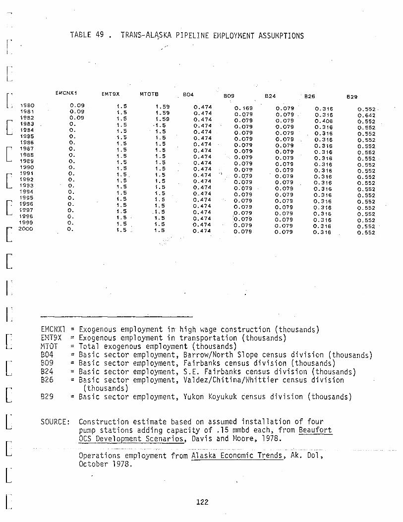
I' I

L •

[

r 1980 1981 1982

[ 1983 1984 1985 1986

[ 1987 1988 1989 1990

L 1991 1992 19'33 ~994

1995

[ 1996 ~997

1998 1999

[ 2000

[

[

[

[

[

[

[

E L [

TABLE 49 . TRANS-ALA_SKA PIPELINE Ef;1PLOYMENT ASSUMPTIONS

EMCNX1 EMT9X MTOTB 804 809 824 826

0.09 1. 5 1. 59 0.474 0.169 0.079 0.316 0.09 1.5 1. 59 0.474 0.079 0.079 0.316 0.09 1.5 1. 59 0.474 0.079 0.079 0.406 0. 1.5 ·1. 5 0.474 0.079 0.079 0.316 0. 1.5 1.5 0.474 0.079 0.079 0.316 0. 1.5 1.5 0.474 0.079 0.079 0.316 o. 1.5 1.5 0.474 0.079 0.079 0.316 0. 1.5 1.5 0.474 0.079 0.079 0.316 o. 1.5 1.5 0.474 0.079 0.079 0.316 0. 1.5 1.5 0.474 0.079 0.079 0.316 0. 1.5 1.5 0.474 0.079 0.079 0.316 0. 1. 5. 1. 5 0.474 .,

0.079 0.079 0.316 0. 1.5 1.5 0.474 0:079 0.079 0.316 0. 1.5 1.5 0.474 0.079 0.079 0.316 0. 1. 5 1.5 0.474 0.079 0.079 0.316 o. 1. 5 1.5 0.474 0.079 0.079 0.316 o. 1. 5 1.5 0.474 0.079 0.079 0.316 0. 1.5 . 1. 5 0.474 .0.079 0.079 0.316 0. 1.5 1. 5 0.474 0.079 0.079 0.316 0. 1.5 1. 5 0.474 0.079 0.079 0.316 0. 1.5 1. 5 0.474 0.079 0.079 0.316

EI1CNX1 = HlT9X =

Exogenous employment in· high wage construction (thousands) Exogenous employment in transportation (thousands)

MTOT = Total exogenous employment (thousands)

829

0.552. 0.642 0.552 0.552 0.552 0.552 0.552 0.552 0.552 0.552 0.552 0.552 0.552 0.552 0.552 0.552 0.552 0.552 0.552 0.552 0.552

B04 809

= =

Basic sector employment, Barrow/North Slope census division (thousands) Basic sector employment, Fairbanks census division (thousands)

B24 = B26 =

B29 =

SOURCE:

Basic sector employment, S.E. Fairbanks census division (thousands) Basic sector employment, Valdez/Chitina/Whittier census division

(thousands) Basic sector employment, Yukon Koyukuk census division (thousands)

Construction estimate based on assumed installation of four pump stations adding capacity of .15 mmbd each, from Beaufort OCS Development Scenarios, Davis and Moore, 1978.

Operations employment from Alaska Economic Trends, Ak. Dol, October 1978.

122

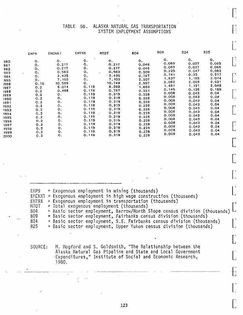
980 981 982 983 ,984 1985 1986 1987 1988 1989 1990 \991 1992 1993 1994 1995 1996 1997 19'38 1999 2000

EMP9

o. o. o. 0. 0. o. o. 16 0.2 0.2 0.2 0.2 0.2 0.2 0.2 0.2 0.2 0.2 0.2 0.2 0.2 0.2

n:P9 HiCNXl El-iT9X HTOT B04 B09 B24 B25

TABLE 50. ALASKA NATURAL GAS TRANSPORTATION SYSTEM EMPLOYMENT ASSUMPTIONS

EMCNX1 EMT9X MTOT 804 809

o. 0. 0. 0. o. 0.217 o. 0.217 0.046 0.069 0.217 o. 0.217 0.046 0.069 0.563 0. 0.563 0.209 0.225

2.435 o. . 2.435 0. 787 0.741

7. 103 0. 7.103 2.207 1. 637

10.589 0. 10.749 2.997 2.062

6.074 o. 119 6.393 1. 663 1. 491

0.468 0. 119 0.787· o. 331 0. 145

o. 0.119 0.319 0.228 0.008

0. o. 119 0.319 0.228 0.008

o. 0. 119 0.319 0.228 0.008

o. o. 119 0.319 0.228 0.008

0. 0. 119 0.319 0.228 0.008

o. 0. 119 0.319 0.228 0.008

0. 0. 119 0.319 0.228 0.008

0. 0. 119 0.319 0.228 0.008

0. o. 119 0.319 0.228 0.008

o. 0.119 0.319 0.228 0.008

o. 0. 119 0.319 0.228 0.008

0. o. 119 0.319 0.228 0.008

= Exogenous employment in mining (thousands)

824

o. 0.037 0.037 0.047 0.33 1. 185 2.069 1. 191 o. 126 0.043 0.043 0.043 0.043 0.043 0.043 0.043 0.043 0.043 0.043 0.043 0.043

= Exogenous employment in high wage construction (thousands)

B25

0. 0.065 0.065 0.082 0.577 2.074 3.621 2.048 0.185 0.04 0.04 0.04 0.04 0.04 0.04 0.04 0.04 0.04 0.04 0.04 0.04

[

[

[

[

[

[

[

[

[

[

[

[ = Exogenous employment in transportation (thousands) ·~ = Total exogenous employment (thousands) [ = Basic sector employment, Barrow/North Slope census division (thousands) · = Basic sector employment, Fairbanks census division (thousands) = Basic sector employment, S.E. Fairbanks census division (thousands) = Basic sector employment, Upper Yukon census division (thousands) [

[ SOURCE: M. Mogford and S. Goldsmith, ''The Relationship between the

Alaska Natural Gas Pipeline and State and Local Government Expenditures,'' Institute of Social and Economic Research, 1980.

[

··------·- - ------ -------- E········

[

123 [

[

[

[

[

[

[

[

[

[

[

[

[

[

[

c [

Although construction did not begin in 1981, total Northwest Alaskan

Pipeline Company employment for the year actually averaged 347 (North

west Alaskan Pipeline Company), somewhat higher than the figure of 217

assumed for 1981. The employment assumptions used also reflect the

delays in construction expected to result from factors such as the

current lawsuit against the pipeline financing waivers recently passed

by Congress.

3. Prudhoe Bay Petroleum Production

Prudhoe Bay petroleum production assumptions are shown in Table 51.

This employment includes that associated with primary recovery opera

tions from the Sadlerochit formation, secondary recovery (using water

flooding) of that formation, new developments of the Kuparuk formation

west of Prudhoe Bay, and the permanent work force of At 1 antic Rich

field Company (ARCO) and British Petroleum (BP) at the main Prudhoe

base headquarters. The key assumptions serving as the basis for the

employment forecasts are the following:

• Seven rigs (4 Sohio, 3 ARCO) continue development drilling at a

rate of 14 wells per year per rig through 1983 (based on esti

mated activity in Oil and Gas Journal, 2/25/80, p. 88).

• The proposed Prudhoe water flooding project begins in 1981 and is

completed by 1985, adding approximately 1 billion barrels of

E-------------!ecoverable reserves to Prudhoe. Construction employment peaks

[

[ 124

1980 1981 19S2 1983 1984 1985 1986 1987 1988 1989 1990 1991 1992 1993 1994 1995 1996 1997 1998 1999 2COO

TABLE 51. PRUDHOE BAY PETROLEUM PRODUCTION .EMPLOYMENT ASSUMPTIONS

~

[

[ EMP9 EMCNX2 MTOT 804

[

[

2.369 0. 2.907 0.035 3.018 0. 491 3. 1~9 1.065 2.202 0.484 2.502 0.05 2.502 o. 2.502 0. 2.502 o. 2.502 0. 2.502 0. 2.502 o. 2.502 0. 2.502 o. 2.502 o.·, 2.502 o. 2.502 o. 2.502 o. 2.502 o. 2.502 0. 2.502 0.

E!I:P9 =

2.369 2.369 2.942 2.942 3.509 3.509 4. 194 4. 194 2.686 2.686 2.552 2.552 2.502 2.502 2.502 2.502 2.502 2.502 2.502 2.502 2.502 2.502 2.502 2.502 2.502 2.502 2.502 2.502 2.502 2.502 2.502 2.502 2.502 2.502 2.502 2.502 2.502 2 .. 502 2.502 2.502 2.502 2.502

[

[

[

[

[

[

Et·IJCNX2 = Exogenous employment in mining (thousands) [ Exogenous employment in average wage construction (thousands) ;

HTOT = B04 =

SOURCE:

Total exogenous employment (thousands) -· Basic sector employment, Barrow/North Slope census division (thousands) [

Construction employment is that associated with Prudhoe v:aterflood project, from U.S. Army Corps of Engineers, Final EIS, Prudhoe Bay Oilfield Waterflood Project, pp. 2-60. For mining employment sources, see text.

125

[

[

L -- t-

[

[

[

[

[

[

[

[

[

[

[

[

[

[

[

[

[

[

E [

l

at over 1,000 in 1983, and operations employment adds 300 to the

permanent Prudhoe work force (Corps of Engineers, 1980).

• The Kuparuk formation west of Prudhoe is developed. Production

at a rate of 50,000 bbls. per day begins in December 1981, rising

to 80,000 bbls. per day in 1982 and rising to 250,000 bbls. per

day by 1986 (Oil and Gas Journal, 12/21/81, p. 32).

• Permanent ARCO and BP emp 1 oyment on the North S 1 ope rises from

1, 000 in 1977 to 1, 667 in 1983, remaining constant thereafter

(based on Prudhoe Bay Case Study, OCS Program Techni ca 1 Report

No. 4).

• Ten additional rigs are active in exploration and development

outside of the Sadlerochit reservoir.

4. Upper Cook Inlet Petroleum Production

Petroleum sector employment in the Kenai-Cook Inlet Census Division

was 778 in 1979 (four quarter average employment, taken from Alaska

Department of Labor, Statistical Quarterly, 1979 issues), consisting

of exploration, development, and production associated with the Kenai

oil and gas fields. Currently, the 120,000 barrels per day output of

oil is expected to dec 1 i ne drastically over the forecast period,

possibly as fast as 15-20 percent per year. The decline may be

partially slow~d, however, by_ a p()ssible re~rilling progran1 bejng __

considered by the operators (see Oil and Gas Journal, 2/4/80, p. 36);

126

and in any case, the prospects for gas development are brighter than

those for oil. Gas production is likely to expand from its current

5,000 MMCF per day once the LNG facility proposed by Pacific Lighting

and Pacific Gas and Electric (see below) are constructed even without

any substantial new discoveries. It is assumed that these increases,

coupled with continued exploration activity and possible enhanced

recovery of oil, will be adequate to maintain Upper Cook Inlet petro

leum employment at its 1978 level throughout the forecast period, as

shown in Table 52.

5. Development of the National Petroleum Reserve in Alaska (NPR-A)

The National Petroleum Reserve in Alaska (previously NPR-4) has been

the target of publicly sponsored exploration for oil and gas since

World War II, first by the Navy and later by the Interior Department.

The first exploration program began in 1944 and ended in 1953, after

discovery of nine oil and gas fields, all but one being noncommercial

(the largest gas field, the Barrow gas field, currently produces for

local consumption). In 1974 Congress directed the Navy to resume

exploration, eventually transferring the program to the Department of

Interior in 1977. To date, this most recent exploration program has

produced 22 dry ho 1 es and severa 1 test we 11 s p 1 anned or in progress

(Oil and Gas Journal, 12/8/80, p. 36).

Nonetheless, USGS estimates that NPR-A can be expected to contain 5.96

bilUon barrels _of _QU ln __ place and_l1..3 tri lli_Qn__c_ub_ic feet_QLgas, __ _ . . .

about 26 perc.ent-of which is likely to be recoverable. A study of

127

[

[

[

[

[

[

[

[

[

[

[

[

[

[

[

[

E [

[

[

[

[

[

[

[

[

[

[

[

[

[

[

[

[

[ r~

t:

[

[

Et~P9 tnOT 812

SOURCE:

1980 1981 1982 1983 1984 1985 1986 1987 1988 198£ 1990 1991 1992 1992 1'3S4 1995 1996 1997 1998 1999 2000

TABLE 52. UPFER COOK INLET PETROLEUM PRODUCTION · ~MPLOYMENT ASSUMPTIONS

.. ~ ;.-

EMP9 MTOT 612

0.778 0.778 0.778 0.778 0.778 0.778 0. 778 0. 778 o. 778 0.778 0.778 0.778 0. 778 0.778 0.778 0.778 0.778 0.778 0.778 0.778 0.778 0. 778 0.778 0.778 0.778 0.778 o. 778 0. 778 o. 778 0.778 0.778 0.778 o. 778 0.778 0.778 0.778 0.778 0.778 0.778 0.778 0.778 0. 778 0.778 0.778 0. 778 0.778 0.778 0.778 0. 778 0. 778 0.778 0. 778 0. 778 o:778 0. 778 o. 778 o:118 0. 778 0.778 0.778 0. 778 0.778 0.778

= Exogenous employment in mining (thousands) =.Total exogenous employment (thousands) = Basic sector employment, Kenai/Cook Inlet census division (thousands)

See text.

128

alternative methods for development of the reserve was completed in

1979 by Interior (see Final Report of the 105(b) Economic and Policy

Analysis, 12/15/79). In late 1980, Congress passed legislation

requiring that the reserve be opened to private leasing by 1982 (Oil

and Gas Journal, 12/8/80). Interior held the first sale on January

27, 1982.

It is assumed that five commercia 1 fie 1 ds are discovered and deve 1-

oped, representing 1.85 billion barrels of oil and 3.73 trillion cubic

feet of gas, as described in the mean scenario of the Interior 105(b)

study. Construction associated with the development includes 525

miles of pipeline. Construction employment peaks at about 600 fol-

lowing each of the several discoveries. Petroleum sector employment

averages about 250/year, and pipeline operation adds 69 to the

transportation sector work force, as shown in Table 53.

6. OCS Development

Prior to the scheduled date of OCS Sale 75, eight other OCS sales will

have occurred, as follows:

Sale

46

CI

BF

55

60 71

57

70

Location

Gulf of Alaska

Lower Cook Inlet

Beaufort Sea

Gulf of Alaska

Lower Cook Inlet

Beaufort Sea

Bering-Norton

St. George

129

Date

1976

1977

1979

1980

1981

1982

1982

1983

[

[

[

[

[

[

[

[

C [

[

[

[

[

[

[

--- --E

[

[

[

[

[

[

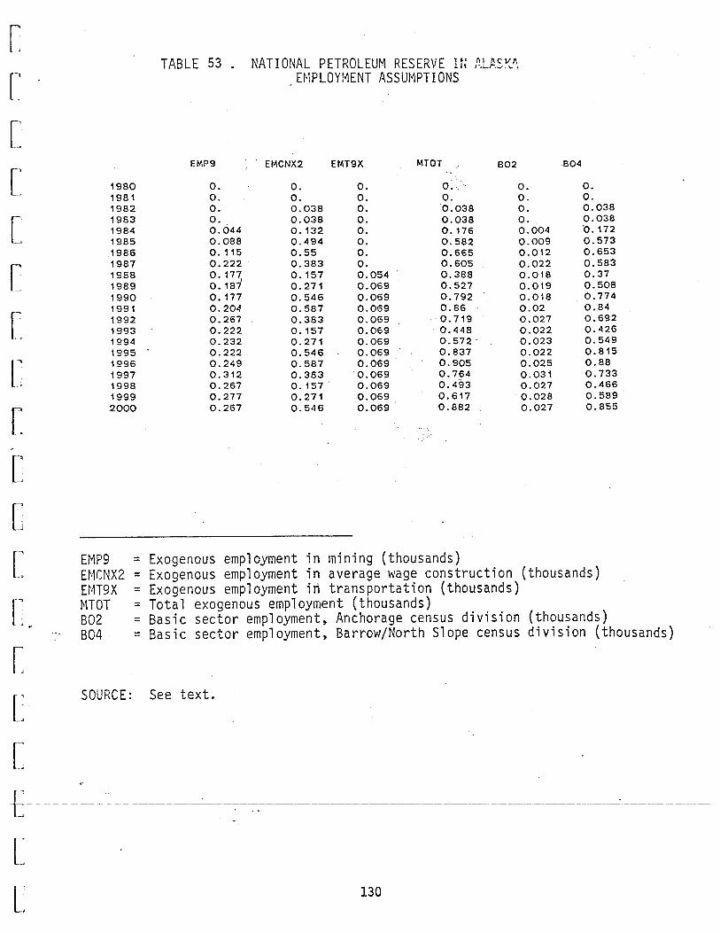
[ r, [

[

[

[

[

[

[~

~ .

[

[

[

TABLE 53 .

EMP9

1980 0. 1981 0. 1982 0. 1983 0. 1984 0.044 1985 0.088 1986 0. 115 1987 0.222. 1958 0.177

I

1989 o. 187 1990 0. 177 1991 0.204 1992 0.267 1993 0.222 1994 0.232 1995 0.222 1996 0.249 1997 0.312 1998 0.267 1999 0.277 2000 0.267

Ei'tP9

NATIONAL PETROLEUM RESERVE I~ EMPLOYMENT ASSUMPTIONS

EMCNX2 EMT9X MTOT

0. 0. 0 .. 0. 0. 0. 0.038 o. 0.038 0.038 o. 0.038 0.132 o. 0. 176 0.494 0. 0.582 0.55 o. 0.665 0.383 o. 0.605 0.157 0.054 0.388 0.271 0.069 0.527 0.546 0.069 0. 792 0.587 0.069 0.86 0.383 0.069 0.719 0. 157 0.069 . 0.448

II I II C" V /'. ~~ . ._r.-·."" •

802

o. 0. 0. o. 0.004 0.009 0.012 0.022 0.018 0.019 0.018 0.02 0.027 0.022

0.271 0.069 0.572- 0.023 0.546 0.069 0.837 0.022 0.587 0.069 0.905 0.025 0.383 0.069 0.764 0.031 o. 157 0.069 0.493 0.027 0.271 0.069 0.617 0.028 0.546 0.069 0.882 0.027

804

0. o. 0.038 0.038 ·o. 172 0.573 0.653 0.583 o. 37 0.508 0. 774. 0.84 0.692 0.426 0.549 0.815 0.88 0.733 0.466 0.589 0.855

= Exogenous employment in mining (thousands) EMCNX2 = Exogenous employment in average wage construction (thousands) EMT9X = Exogenous employment irt transportation (thousands) !'HOT = Total exogenous employment (thousands) 802 = Basic sector employment, Anchorage census division (thousands) 804 = Basic sector employment, Barrow/North Slope census division (thousands)

SOURCE: See text.

E ----------

~

l~

L 130

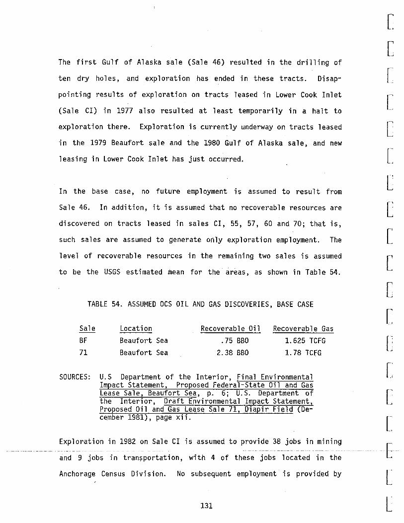
The first Gulf of Alaska sale (Sale 46) resulted in the drilling of

ten dry ho 1 es, and exp 1 oration has ended in these tracts. Di sap

pointing results of exploration on tracts leased in Lower Cook Inlet

(Sale CI) in 1977 also resulted at least temporarily in a halt to

exploration there. Exploration is currently underway on tracts leased

in the 1979 Beaufort sale and the 1980 Gulf of Alaska sale, and new

leasing in Lower Cook Inlet has just occurred.

In the base case, no future employment is assumed to result from

Sale 46. In addition, it is assumed that no recoverable resources are

discovered on tracts leased in sales CI, 55, 57, 60 and 70; that is,

such sales are assumed to generate only exploration employment. The

level of recoverable resources in the remaining two sales is assumed

to be the USGS estimated mean for the areas, as shown in Table 54.

TABLE 54. ASSUMED OCS OIL AND GAS DISCOVERIES, BASE CASE

Sale

BF 71

Location Beaufort Sea Beaufort Sea

Recoverable Oil .75 BBO

2.38 BBO

Recoverable Gas

1. 625 TCFG 1. 78 TCfG

SOURCES: U.S Department of the Interior, Final Environmental Impact Statement, Proposed Federal-State Oil and Gas Lease Sale, Beaufort Sea, p. 6; U.S. Department of the Interior, Draft Environmental Impact Statement, Proposed Oil and Gas Lease Sale 71, Diapir Field (December 1981), page xii.

Exploration in 1982 on Sale CI is assumed to provide 38 jobs in mining

and 9 jobs in tran?portation, with 4 of these jobs located in the

Anchorage Census Division. No subsequent employment is provided by

131

[

[

[

[

[

[-'

--"

[

[

[

[

[

[-,

--

[

[

[

[---,

-~

E-[

L

[

[

[

[

[

[

['

[

[

[

[

[

[

[

L l E [

[

Sale CI. The levels of employment assumed for the rP!"'.:~ning six OCS

sales are shown in Tables 55-60.

6. Beluga-Chuitna Coal Production

USGS has 1 ong recognized the potentia 1 economic s i gni fi cance of a

large number of beds of subbituminous coal on the west side of Cook

Inlet near Tyonek (see USGS, Coal Resources of Alaska, 1967). Re

cently, several alternative proposals for developing the Beluga

Chuitna fields for export to Japan or other Pacific rim locations have

been considered (see Pacific Northwest Laboratory, Beluga Coal Field

Development: Social Effects and Management Alternatives, 1979, and

Bechtel, Preliminary Feasibility Study: Coal Export Program, Chuitna

River Field, Alaska, 1980).

The base case scenario assumes that a co a 1 export program is imp 1 e

mented beginning in 1985. Production begins in 1989 and eventually

reaches 4.4 tons per year. Construction begins in 1985, with peak

employment of 400 in 1987. Operations employment is 524 distributed

80 percent in mining and 20 percent in transportation, as shown in

Table 61.

INDUSTRY AND GOVERNMENT ASSUMPTIONS

In addition to the project-specific assumptions described above, other

portions of the exogenous sectors are affected by trends and events

which must be anticipated, al tholjgh they a_re not. as di rE!ctly_traceable

132

1980 1981 1982 1983 1984 1985 1986 1987 1988 1989 1990 1991 1992 1993 1994 1995 1996 1997 1998 1999 2000

PiP9 = E:·iCNXl = MTOT = B02 = 804 =

SOURCE:

TABLE 55. OCS- SALE BF (BEAUFORT SEA) EMPLOYMENT ASSUMPTIONS

EMP9 EMCNX1 802 804

o. o. 0. 0. 0.066 0.062 0.008 0. 12 0.197 0. 188 0.024 0.361 0. 197 0. 135 0.024 0.308 0.23 0. 211 0.028 0.413 0.066 o. 15 0.01 0.206 0. 112 0.305 0.01 0.407 0.276 0.383 0.01 0.649 0.479 0.466 0.021 0.924 0.616 0.466 ~ 0.036 1.046 0.595 o. 155 0.042 o. ios 0.524 0. 155 0.038 0.641 0.503 0.077 0.037 0.543 0.432 0.155 0.033 0.554 0.435 0. 155 0.033 0.557 0.438 0.077 0.033 0.482 0.44 0.022 0.033 0.429 0.417 0. 0.032 0.385 0.393 0. 0.032 0.361 0.393 0. 0.032 0.361 0.394 o. 0.032 0.362

Exogenous employment in mining (thousands)

MTOT

o. 0. 128 0.385 0.332 0.441 0.216 0.417 0.659 0.945 1.082 o. 75 0.679 0.58 0.587 0.59 0.515 0.462 0.417 0.393 0.393 0.394

Exogenous employment in high wage construction (thousands) Total exogenous employment (thousands) Basic sector employment, Anchorage census division (thousands) Basic sector employment, Barrow/North Slope census division (thousands)

U.S. Department of the Interior, Final Environmental Impact ~tatement, Proposed Federal-State Oil and Gas Lease Sale, Beaufort S~~.

133

[

[

r [

[

[

[

[

[

[

[

[

[

[

[

l - [~-

-"

L L

[

[

[

[

[

L [

[

l [

[

[

[

[

[

[

1980 1981 1982 1983 1984 1985 1986 1987 1988 1989 1990 1991 1992 1993 1994 1995 1996 1997

•1998 1999 2000

EHP9 HlT9X fHOT B02 Bll

SOURCE:

G- -----_,- -----

L l

= = = = =

TABLE ~6 "'~~ r-11o.- ':".- '':'"r nc [llfot;;;Y~' ~ • l.iv.::> ~ .. Lt. ..J..J \. \.iUI-t .;, . -· . .., . ...r.}

·t~PLOYMENT ASSUMPTIONS

EMP9 EMT9X MTOT B 11

0. 0. 0. 0. 0.03 0.013 0.043 0.014 0.03 0.028 0.058 0.024 0.03 0.028 0.058 0.024 0.03 0.02 . 0.05 0.019 0. 0.007 0.007 0.005 . 0. 0. 0. 0. 0. 0. 0. 0. 0. 0. 0. 0. 0. .. 0. 0. 0 . 0. 0. o. 0~ 0. 0. 0. 0. 0. 0. 0. 0. 0. .., 0. 0. o . 0. 0. 0. 0. 0. 0. 0. 0. 0. 0. 0. 0. 0. 0. 0. 0. 0. 0. o. 0. 0. 0. 0. 0. 0. 0. 0. 0.

Exogenous employment in mining (thousands) Exogenous employment in transportation (thousands) Total exogenous employment (thousands)

802

o. 0.03 0.034 0.034 0.032 0.002 o. o. o. 0. o. 0. o. o. 0. 0. o. o. o. o. 0.

Basic sector employment, Anchorage census division (thousands) Basic sector employment, Southeast Alaska (thousands)

U.S. Department of the Interior, Final Environmental Impact Statement, Proposed Federal-State Oil and Gas Lease Sale, Northern Gulf of Alaska.

134

1980 1'38~

1982 1983 1984 1985 1986 1987 1988 1989 i9~0

1991 1992 1993 ~994

1995 1996 1997 1998 ~999

2000

EMP9 EMCNXl EMT9X MTOT 802 Bl2

SOURCE:

TABLE 57 . OCS SALE 60 (LOWER COOK INLET) EMPLOYMENT ASSUMPTIONS

EMP9 EMCNX1 EMT9X MTOT 802

o. o. o. 0. o. 0. 0. o. 0. 0. 0.038 0.028 0.009 0.075 0.004 0.083 o. 0.026 o. 109 0.008 0.09 o. 0.033. 0. 123 0.009 0.075 0. 0.017 0.092 0.008 0.038 o. 0.009 0.047 0.004 0. o. o. ; o. o. 0. o. o. 0. o. o. o. o. 0. o. o. o. o. 0. o. 0. 0. o. 0. o. o. 0. o. 0. o. 0. 0. o. o. 0. o. o. o. o. o. o. o. o. 0. o. 0. 0. o. 0. o. o. 0. o. 0. o. o. o. o. 0. o. o. 0. o. 0. o. o. 0. 0. o. 0.

= Exogenous employment in mining (thousands)

812 '

·o. 0. 0.071 o. 101 0. 114 0.084 0.043 0. 0. 0. o. o. 0. 0. 0. 0. o. 0. o. 0. 0.

= Exogenous employment in high wage construction (thousands) = Exogenous employment in transportation (thousands) =·Total exogenous employment (thousands) = Basic sector employment, Anchorage census division (thousands) = Basic sector employment, Kenai/Cook Inlet census division (thousands)

U.S. Department of the Interior, Final Environmental Impact Statement, Proposed Federal-State Oil and Gas Lease Sale, Lower Cook Inlet. ·

135

[

[

[ r~.

[

[

[

[

[

[

[

[

[

[

[

[

-C-[ I.

L

[

r [

[

[

[

[

[

c [

[

[

[

[

[

[

TABLE 58. OCS SALE 71 ( BE..::.JFORT SEA) EMPLOYMENT ASSUI'Ir tlONS

__ ,... - ... ~ ~ ~ - ... -· -- .. - _..:::.,:_~-.:.,.,::..

EMT9X MTOT .. EMP9 EMCNX2 802 804 -~ .... ..:· .. . .

1980 0. 0. o. 0. < ' 0. 0. 1981 0. 0. 0. 0. 0. 0. 1982 0. o. o. o. 0. 0. 1983 0. 0. o. o. 0. 0. 1984 o. 0.037 o. 0.037 o. 0.037 1985 0.032 o. 0.007 0.04 0.003 0.036 1986 0.052 o. 0.017 0.069 0.005 0.063 1987 0.053 o. 0.018 0.072 0.005 0.066 1988 0.052 o. 0.017. 0.069. 0.005 0.063 1989 0. o. o. o. 0. 0. 1990 o. 0.076 0. 0.076. o. 0.076 1991 1.205 0.077 o. 1. 282 0. 121 1. 162 1992 1.354 0.035 0.09 1.478 .. 0.135 1. 343 1993 1.394 ' 0. 0.247 1.64 o. 139 1. 501 1994 1.394 o. 0.363 1.756 0.139 1.617 1995 1:408 o. 0.363 1. 771 0. 141 1.63 1996 1. 178 0. 0.363 1.541 0. 118 1.423 1927 0.97 0. 0.363 ,1. 333 0.097 1. 236 1998 0.97 0. 0.363' 1. 333 . 0.097 1.236 1999 0.985 o. 0.363 :1.348.

0.099 1. 249 2000 0.996 o. 0.363 1. 358 0. 1 1. 259 ,.. " .. -. ·.,- "·i

-- .:...~~;. ·.

, ____ ,... .. __ ~--<- ·-----

'

E~'ltP9 = Exogenous employment in mining (thousands) H1CNX2 = Exogenous employment in average wage construction (thousands) EMT9X = Exogenous employment in transportation (thousands) fHOT = Total exogenous employment (thousands) B02 = Basic sector employment, Anchorage census division (thousands) 804 = Basic sector employment, Barrow/North Slope census division (thousands)

SOURCE:

E- ... --------Alaska OCS Office, Statewide and Re ional Economic and Demographic Systems, Beaufort Sea 71 Impact Analysis Technical Report #62, Alaska OCS Office Social and Eco-nomic Studies Program.

l [ 136

1980 1981 19[:2 1983 1984 1985 1986 1987 1988 1989 1990 1991 1992 1993 1994 1995 1996 1997 1998 1999 2000

El1P9 = HiCNXl = E!-H9X = !-'!TOT = B02 = Bl8 -

SOURCE:

EMP9

0. o. 0. 0.026 0.056 0.03 0. 0. o. o. o. 0. 0. 0. o. o. o. o. 0. 0. 0.

TABLE 59 . OCS SALE 57 (BERING NORTON) · tMPLOYMENT ASSUMPTIONS

EMCNX1 :·""

EMT9X MTOT. 802

\ o. - \ o. 0. o. 0. o. 0. o. 0. o. 0.015 0.041 0.005 0.031 0.092 0.005 0.016 0.051 o. 0. o. o. 0. o. o. 0. 0. o. 0. 0. o. 0. o. 0. o. o. 0. o. ' 0. o. o. 0. 0. 0. o. o. 0. o. o. 0. o. o. 0. 0 .. o. o. 0. o. o. o. 0. 0. 0.

Exogenous employment in mining (thousands)

818

0. o. o. 0. o. 0. 0.003 0.038 0.006· 0.086 0.003 0.048 o. 0. o. 0. 0. 0. 0. o. 0. 0 .• o. 0. 0. 0. 0. 0. o. o. o. 0. o. 0. 0. 0. o. 0. o. 0. o. 0.

Exogenous employment in average wage construction (thousands) Exogenous employment in transportation (thousands) Total exogenous employment (thousands) Basic sector employment, Anchorage census division (thousands) Basic sector employment, Nome census division (thousands)

.. Alaska OCS Office, Bering-Norton Petroleum Development Scenarios, Economic and Demographic Analysis, Technical

·[

[

[

[

[

[

[

[

[

[

[

[

[

[

[

[ Report #50, Alaska OCS Office Social and Economic Studies ~-.•

--------Program. L

137

l [

[

[

[

[

[

[

[

[

[

[

[

[

[

[

[

[

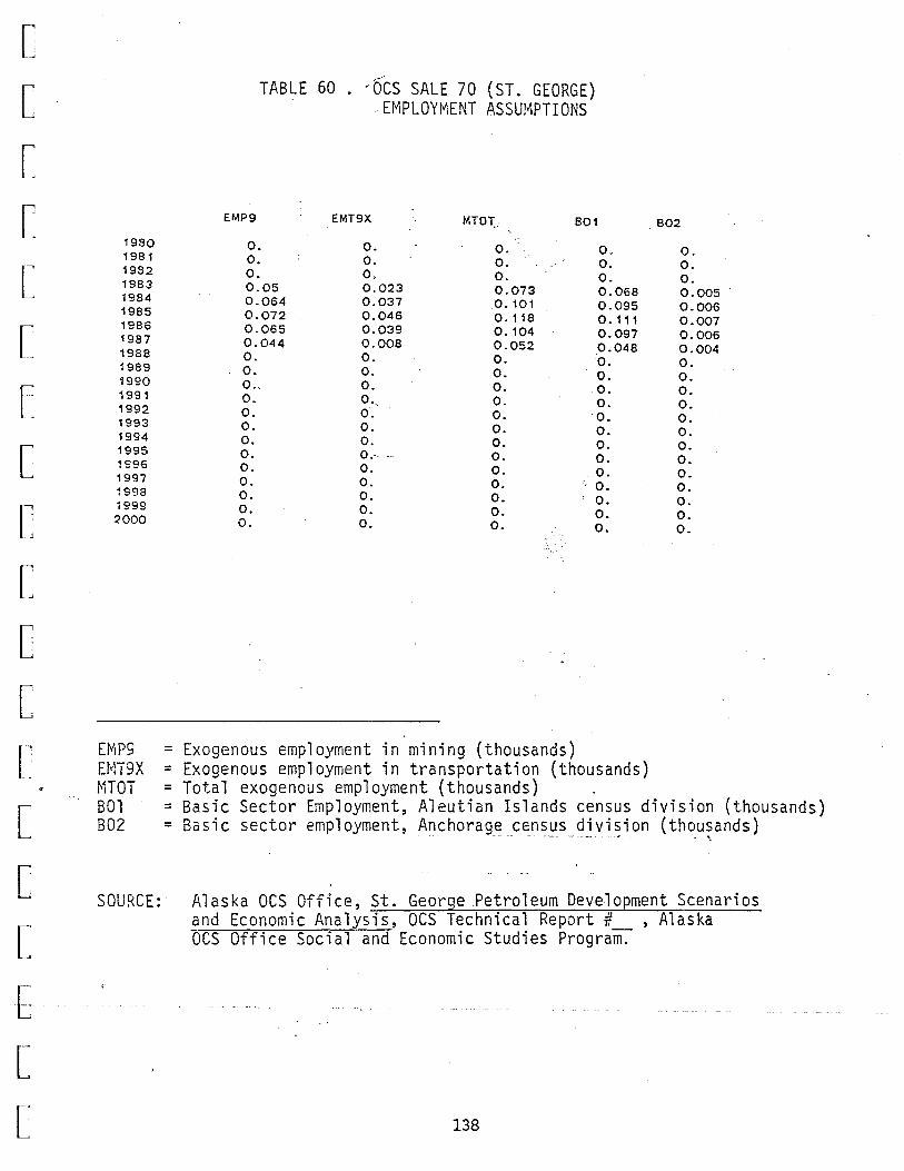
L [

[

1980 1981 1982 1983 1984 1985 1986 1987 1988 ~989

1990 1991 1992 1993 1994 1995 1996 1997 ~998

1999 2000

EI~PS = EHT9X = t-HOT = 801 = B02 =

SOURCE:

TABLE 60 . ·6~S SALE 70 (ST. GEORGE) EMPLOYMENT ASSUMPTIONS

EMP9 EMT9X MTO"I:. 801

0. o. o. 0. 0. o. 0. o. 0. 0. 0. 0. 0.05 0.023 0.073 0.068 0.064 0.037 o. 101 0.095 0.072 0.046 o. 118 0. 111 0.065 0.039 0.104 0.097 0.044 0.008 0.052 0.048 0. 0. 0. 0. o. 0. 0. 0. 0 .. 0. 0. o. 0. 0._ 0. o. 0. 0. 0. o. 0. 0. o. o. o. 0. 0. o. 0. 0.···. o. 0. 0. 0. o. o. 0. 0. 0. 0. o. 0. 0. 0. 0. 0. o. 0. 0. 0. 0. 0.

Exogenous employment in mining (thousands) Exogenous employment in transportation (thousands) Total exogenous employment (thousands)

802

0. 0. 0. 0.005 0.006 0.007 0.006 0.004 0. 0. 0. 0. 0. o. 0. 0. 0. 0. o. 0. 0.

Basic Sector Employment, Aleutian Islands census division (thousands) Basic sector employment, Anchorag_~_ce:_ns~s-~jvi~ion (thousands)

Alaska OCS Office, St. George Petroleum Development Scenarios and Economic Analysis, OCS Technical Report # , Alaska OCS Office Social and Economic Studies Progra~

138

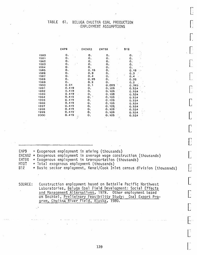
EMP9

1980 1981 1982 1983 1984 1985 1986 1987 1988 1989 1990 1991 1992 1993 1994 1995 1996 1997 1998 1999 2000

TABLE 61. BELUGA CHUITNA COAL PRODUCTION -~MPLOYMENT ASSUMPTIONS

EMP9 EMCNX2 EMT9X 812

o. 0. o. 0. o. 0. o. 0. o. 0. o. 0. o. 0. o. 0. o. 0. o. 0. o. 0.15 o. 0. 15 o. 0.3 o. 0.3 o. 0.4 0. 0.4 o. 0.35 o. 0.35 o. 0.2 o. 0.2 0.21 0.1 0.053 0,36~ 0.419 0. 0.105 0.524 0.419 0. o. 105 0.524 0.419 o. 0.105 0.524 0.419 0. 0.105 0.524 0.419 0. 0.·105 0.524 0.419 o. 0.105 0.524 0.419 0. 0. 10~ 0.524 0.419 o. 0.105 0.524 0.419" 0. 0.105 0.524 0.419 o. 0.105 0.5:Z4

= Exogenous employment in mining (thousands) EMCNX2 = Exogenous employment in average wage construction (thousands) EMT9X MTOT Bl2

SOURCE:

= Exogenous employment in transportation (thousands) = Total exogenous employment (thousands) = Basic sector employment, Kenai/Cook Inlet census division (thousands)

Construction employment based on Battelle Pacific Northwest Laboratories, Beluga Coal Field Development: Social Effects and Management Alternatives, 1979. Other employment based on Bechtel, Preliminary Feasibility Study: Coal Export Program, Chuitna River Field, Alaska, 1980.

139

[

[

[

[

[

[

[

[

[

[

[

[

[

[

[

[

[

[

[

[

[

[

[

[

[

[

[

[

[

[

[

[

[

[

[ ,.

E---------[

L

to specific deve 1 opment projects. These sectors inc 1 ude the fo 1-

1 owing: the portion of mining sector emp 1 oyment not accounted for by

the above projects, which wi 11 be ca 11 ed 11 other mini ng 11; agri cul tura 1

employment; logging and sawmill employment; fish harvesting and pro-

cessing employment; and federal government employment. We turn now to

a discussion of the assumptions used to project employment in these

sectors.

1. Other Mining Activity

In 1979, total mining sector employment in Alaska was 5,773, of which

5,354 was in oil and gas. Of this, 2,633 was accounted for by proj-

ects discussed above. The residual, or 3,140, is classified as 11 other

mining. 11 It consists of administrative personne 1 in Anchorage asso

ciated with minerals industries, a variety of petroleum exploration

activities on the North Slope and elsewhere not broken down by project

(i.e., the Husky operation in NPR-A, various drilling contractors on

state and native lands, seismic work being conducted offshore prior to

OCS lease sales, etc.), and hardrock mining activities.

In the base case, it is assumed that such employment increases from

its current level at a rate of one percent annually, as shown in

Table 62.

2. Agriculture

Currently, agriculture represents a very small sector of the Alaskan

economy, consisting of less than 200 persons, primarily in the

Matanuska-Susitna and Fairbanks census divisions.

140

[ ,.

TABLE 62. 11 0THER MINING 11 E1•1PLOYI~ENT ASSUMPTIONS ,- [

[ -·

EMP9 801 802 804 805 BOB 809 811 ·~

1!?50 3. 171 0.015 1. 995 0.805 0.004 0.053 0.032 0.039

[ 1981 3.203 0.015 2.015 0.813 0.004 0.053 0.033 0.04

.. 1982 3.235 0.016 2.035 0.821 0.004 0.054 0.033 0.04 1983 3.267 0.016 2.056 0.829 0.004 0.054 0.033 0.041 1984 3.3 0.016 2.07€ 0. 838 • 0.004 0.055 0.034 0.041 1955 3.333 0.016 2.097 0.846 0.004 0.055 0.034 0.041 1986 3.367 0.016 2. 119 0.855 0.004 0.056 0.034 0.042 1987 3.4 0.016 2. 139 0.863 0.004 0.056 0.035 0.042 1988 3.434 0.016 2. 161 0.872 0.004 0.057 0.035 0.043

[·

[ 1989 3.469 0.017 2. 183 0.88 0.005 0.058 0.035 0.043 1990 3.503 0.017 2.204 0.889 0.005 0.058 0.036 0.043 1991 3.538 0.017 2.226 0.898 0.005 0.059 0.036 0.044 1992 3. 574. 0.017 2.249 0.907 0.005 0.059 0.036 0.044 1393 3.609 0.017 2.271 0.916 0.005 0.06 0.037 0.045

[ 1994 3.645 0.017 2.293 0.925 0.005 0.061 0.037 0.045 1S'35 3.632 0.018 2.317 0.934 0.005 0.061 0.038 0.046 1996 3.719 0.018 2.34 0.944 0.005 0.062 0.038 0.046 1997 3.756 0.018 2.363 0.953 0.005 0.062 0.038 0.047 1998 3.793 0.018 2.387 0.963 0.005 0.063 0.039 0.047 ~399 3.831 0.018 2. 41 0.972 0.005 0.064 0.039 0.048 2000 3.869 0.019 2.434 0.982 0.005 0.064 0.039 0.048

••• •• i .--·· -~

[

[ ---

[ - --- :·--·· ------.--

·'" . ~:-~- 814 816 817 818 821 825 826 827 829 .c . 0.017 ,198(1. 0.002 0.004 0.003 0.098 0.01 0.004 0. 0.089

1981 0.002 0.004 0.003 0.099 0.017 0.01 0.004 0. 0.09 1982 0.002 0.004 0·.003 0. 1 0.017 0.01 0.004 0. 0.091 1983 0.002 0.004 0.003 0. 101 0.018. 0.01 0.004 0. 0.091 1984 0.002 0.004 .. - 0.003 .0.102 0.018 0.011 0.004 0. 0.092 ~985 0.002 0.004 ··o:oo·3 o. 103 0.01)1 • 0.011 0.004 0. 0.093 1986 0.002· 0.004 0.003 0.104 0.0: 0.011 0.004 0. 0.094

1987 0.002 0.004 0.003 o. 105 0.01~ 0.011 0.004 0. 0.095

1S88 0.002 0.004 0.003 0.106 0.019 0.011 0.004 0. 0.096

1989 0.002 0.005 0.003 0. 107 0.019. 0.011 0.005 0. 0.097

1990 0.002 0.005 0.004 0. 108 0.019 0.011 0.005 0. 0.098

1991 0.002 0.005 0.004 0.109 0.019 0.011 0.005 o. 0.099

1992 0.002 0.005 0.004 o. 11 0.019 0.011 0.005 o. 0. 1

1993 0.002 0.005 0.004 0. 112 0.019 0.012 0.005 0. 0. 101 1994 0.002 0.005 0.004 o. 113 0.02 0.012 0.005 o. 0.102

1995 0.002 0.005 0.004 0. 114 0.02 0.012 0.005 0. 0.103 1996 0.002 0.005 0.004 0. 115 0.02 0.012 0.005 o. 0.104

1997 0.002 0.005 0.004 o. 116 0.02 0.012 0.005 0. 0.105

1398 0.002 0.005 0.004· 0. 117 0.02 0.012 0.005 0. 0.106

1999 0.002 0.005 0.004 0. 118 0.021 0.012 0.005 0. 0.107

2000 0.002 0.005 0.004 0. 12 0.021 0.012 0.005 o. 0.108

[

[

[

[

[ .. ·' ---·-'"'":,"".·· ... ' --- --:- ~

.-"'.-

-E-[

141 [

[

[

[

[

[

[

[~

[

[

[

[

[

[

[

[

[

HiP9 BOl B02 B04 B05 808 E09 Bll B14 Bl6 817

~ Bl8 'B21

B25 826 829

SOURCE:

=Exogenous employment·i~ mining (thous~nds) = Basic sector employment, Aleutian Islands census division (thousands) = Basic sector employment, Anchorage census division (thousands) = Basic sector employment, Barrow/North Slope census division (thousands) = Basic sector employment, Bethel census division (thousands) = Basic sector employment, Cordovall"cCarthy census division (thousands) = Basic sector employment, Fairbanks census division (thousands) = Basic sector employment, Southeast Alaska (thousands) = Basic sector employment, Kobuk census division (thousands) = Basic sector employment, Kuskokwim census division (thousands) = Basic sector employment, Matanuska/Susitna census division (thousands) = Basic sector employment, Nome census division (thousand~) = Basic sector employment, Seward census division (thousands) = Basic sector employment, Upper Yukon census division (thousands) = Basic sector employment, Valdez/Chitina/Whittier census division (thousands) = Basic sector employment, Yukon Koyukuk ~ensus division (thousands)

1979 values from Alaska Department of Labor, Statistical Quarterly, thereafter assumed to gro~ at ohe percent annually.

G ------, __ -------- ------ -- -[

[ 142

'

In the base case, it is assumed that after 1982, state support of an

agricultural industry results in expansion of the existing industry to

over 1,000 persons by the year 2000, as shown in Table 63.

These assumptions are based on scenarios for agricultural development

presented by Michael Scott in Southcentral Alaska's Economy and Popu

lation, 1965-2025: A Base Study and Projections, 1979.

3. Logging and Sawmill Employment

Employment in logging and sawmills is classified by the MAP model as

exogenous manufacturing employment, while employment in pulpmills is

calculated endogenously. In 1979, the Alaskan timber industry har

vested approximately 500 million board feet of lumber.

In the base case, timber output is assumed to rise to 960 million

board feet by the year 2000, implying a rise in manufacturing employ

ment from 2,204 in 1980 to 4,103 in 2000, as shown in Table 64. The

rate of growth in output in this case is approximately equal to the

historical growth in the industry.

4. Commercial Fishing: Non-Bottomfish

Statewide emp l oym~nt in non-bottomfi sh commercia 1 fishing and fish

processing is assumed to remain constant at current levels of about

6,323 and 7,123, respectively. These figures and their regional

breakdowns, shown in Tab 1 e 65, are based on projections to 1980 of

estimates presented in George Rogers, Measuring the Socioeconomic

Impacts of Alaska's Fisheries, ISER (April, 1980).

143

[

[

[

[

[

[

[

[

[

c [

[

[

[

[

[

[

[

[

[

[

[

[

[

[

[

[

[

c [

[

[

[

[

[

[

[

[

~

'

H~AGRI BOl 809 Bl2 Bl7

SOURCE:

--. TABLE 63. AGRICULTURAL H1PLOYHENT ASSUMPTIONS

EMAGRI 801 809 812 817

1980 0. 178 0.013 0.044. 0.008 0. 113 1981 o. 178 0.013 0.044 0.008 0. 113 1982 0.166 0.013 0.04 0.008 0.105 1983 0.204 0.013 0.051 0.008 0.132 1984 0.228 . 0.013 0.058 0.008 0.149 -1985 0.252 0.013 0.064 0.008 0. 167 1986 0.276 0.013 0.071 0.008 o. 184 1987 0.3 0.013 0.078 0.008 .. 0.201 1988 0.357 0.013 0.093 0.008 0.243 1989 0.413 0.013 0.109 0.008 0.283 1990 0.47 0.013 ·6. 125 0.008 0.324 1991 0.527 0.013 0. 141 0.008 0.365 1992 0.583 0.013 0.156 0.008 . 0.406. 1993 0.64 0.013 • 0. 172 0.008 0.447 1994 0.697 0.013 0. 188 0.008· 0.488 1995 0. 753 0.013 0.204 0.008 0.528 1996 0.81 0.013 o. 219 . 0.008 0.57 1997 0.867 0.013 0.235 0.008 ·. 0. 611 1998 0.923 0.013 0. 251 . 0.008 0.651 1999 0.98 0.013 0.267 .. 0.008 0.692 2000 1.037 0.013 0.283 0.008 0.733

: ... /_

. '~.::::

= Exogenous employment in agriculture (thousands) = Basic sector employment, Aleutian Islands census division (thousands) = Basic sector employment, Fairbanks census division (thousands) = Basic sector employment, Kenai/Cook Inlet census division (thousands) = Basic sector employment, Matanuska/Susitna_ census division (thousands)

Scott, M., Southcentral Alaska's Economy and Population, 1965-2025: A Base Study and Projections, 1979.

144

[

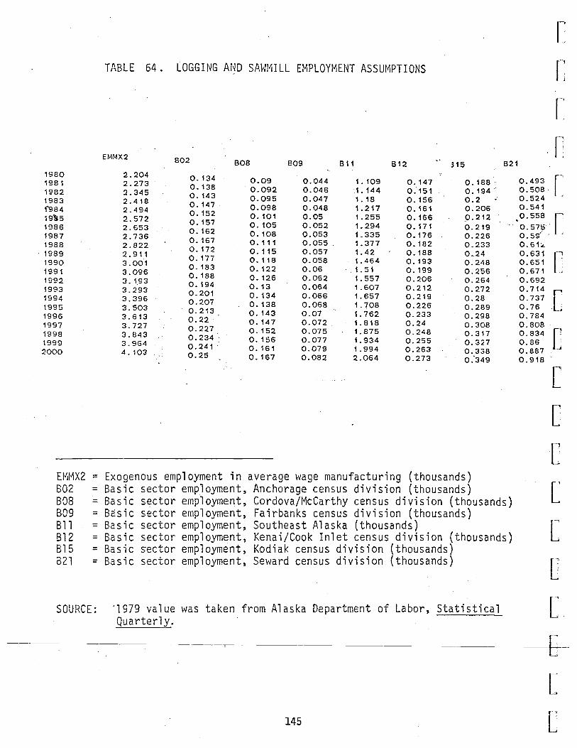
TABLE 64. LOGGING AND SAWMILL EMPLOYMENT ASSUMPTIONS [

[

EMMX2 .[

802 BOB 809 811 812 315 821 1980 2.204 0. 134 0.09 198~ 2.273 0. 138 0.092 1982 2.345 0. 143 0.095 1983 2.418 0. 147 0.098 1'984 2.494 0. 152 o. 101 19'95 2.572 o. 157 o. 105 1986 2.653 0. 162 0.108 1987 2.736 0. 167 0. 111 1988 2.822 0.172 0. 115 1989 2. 911 0. 17i 0.118 1990 3.001 o. 183 0.122 1991 3.096 0. 188 0.126 1992 3. 1_93 0. 194 0.13 1993 3.293 0.201 0. 134 1994 3.396 0.207 0.138 1995 3.503 0.213 o. 143 1996 3.613 0.22. 0.147 1997 3.727 0.227 o. 152 1998 3.843 0.234: 0. 156 1999 3.964 0. 241 . 0. 161 2000 4.103 0.25 0.167

0.044 0.046 0.047 0.048 0.05 0.052 0.053 0.055 0.057 0.058 0.06 0.062 0.064 0.066 0.068 0.07 0.072. 0.075 0.077 0.079 0.082

1. 109 1. 144 1. 18 1. 217 1. 255 1. 294 1. 335 1. 377 1.42 1.464

. 1. 51 1. 557 1.607 1. 657 1. 708 1. 762 1. 818 1.875 1. 934 1. 994 2.064

0. 147 o. 151 0.156 0. 161 o. 166 0. 171 o. 176 0.182 0. 188 0. 193 0. 199 0.206 0.212 0.219 0.226 0.233 0.24 0.248 0.255 0.263 0.273

0. 188 0. 194 0.2 0.206 p.212 0.219 0.226 0.233 0 .. 24 0.248 0.256 0.264 0.272 0.28 0.289 0.298 0.308 0.317 0.327 0.338 0."349

E~~X2 = Exogenous employment in average wage manufacturing (thousands) 802 = Basic sector employment, Anchorage census division (thousands) 808 = Basic sector employment, Cordova/McCarthy census division (thousands) B09 = Basic sector employment, Fairbanks census division (thousands) Bll = Basic sector employment, Southeast Alaska (thousands) 812 = Basic sector employment, Kenai/Cook Inlet census division (thousands) Bl5 = Basic sector employment, Kodiak census division (thousands) 321 = Basic sector employment, Seward census division (thousands)

SOURCE: ·1979 value was taken from Alaska Department of Labor, Statistical Quarterly.

145

0.493 [ 0.508. 0.524 0.541

.0.558. [ 0.57\;i 0.59 .... 0.61:.. 0.631 [ 0.651 0.671 0.692 0.714 0. 737 [ 0. 76 . 0. 784 0.808 0.834 0.86 0.887 0.918

c [

[

[

L [

[

[

b--

[

[

-,

' __ ,

,...._,

,__,

c 21 82

0 BG ~

3 l..-8 30

D 2 a

94 ~5 c I

~ S9

c [ 1980

081 's2 .~83 1984

or 6 7

1988

089 90 91

1992 1993

094 95 ggs

l';j97

cr s - 0

[

c [ f'

L

HW.X2

7. 123 7. 123 7. 123 7. 123. 7. 123 7. 123 7. 123

~ 7. 123

' 7. 123 7. 123 7. 123' 7. 123 7. 123 7. 123 7. 123 7. 123 7. 123 7. 123 7. 123 7. 123 7. 123

812

1.253 1. 253 1. 253 1. 253 1.253 1. 253 1. 253 1.253 1.253 1. 253 1.253 1.253 1.253

·-· 1. 253 1. 253 1. 253 1.253 1.253 1. 253 1. 253 1.253

TABLE 65. NONBOTTOMFISHCOMMERCIAL FISHING AND PROCESSING EMPLOYMENT ASSUMPTIONS

EMF ISH MTOT 801 802 805

6.333 13.485 2. 174 0.479 0.271 6.363 13.485 2. 174 0.479 0.271 6.363 13.485 2. 174 0.479 0.271 6.363 13.485 2. 174 0.479 0. 271 6.363 13.485 2.174 0.479 0. 271

'6.363 13.485 2.174 0.479 0.271 6.363 . 13.485 2. 174 0.479 0. 271 6.363 13.485 2.174 0.479 0.271 6.363 13.485 2. 174 0.479 0.271 6.363 13.485 2. 174 0.479 0.271 6.363 13.485 2. 174 0.479 0. 271 6.363 13.485 2. 174 0.479 0.271 6.363 13.485 2. 174 0.479 0.271 6.363 1.3.485 2. 174 0.479 0.271 6.363 13.485 2. 174 0.479 0.271 6.363 13.485 2.174 0.479 0.271 6.363 13.485 2. 174 0.479 0.271 6.363 13.485 2. 174 0.47S. 0.271 6.363 13.485 2. 174 0.479 0. 271

606 808

1. 63 0.723 1.63 0. 723 1. 63 0.723 1. 63 0. 723 1. 63 0.723 1.63 0.723 1.63 0.723 1.63 0.723 1.63 0.723 1.63 0.723 1.63 0.723 1. 63 0.723 1. 53 0.723 1. 63 0.723 1. 63 0. 723 1. 63 0. 723 1. 63 0.723 1. 63 0.723 1. 63 0. 723

6.363 13.485 2. 174 0.479 0.271 1. 63 .: . 0.723 6.363 13.485 2. 174 0.47$ 0.271 1.63 0.723

.... . .,· .- -- /:.• .. ·- ..... -

814 815 816 817 818 821 826

0.043 2.907 0.004 o. 0.054 0.059 0.053 0.043 2.907 0.004 o. 0.054 0.059 0.053 0.043 2.907 0.004 o. 0.054 0.059 0.053 0.043 2.907 0.004 o. 0.054 0.059 0.053 0.043 2.907 0.004 o. 0.054 0.059 0.053 0.043 - -2.907 0.004 0. 0.054'- '0-:o~r-; 0.053 0.043 2.907 0.004 o. Q.054 0.0~ 0.053 0.043 2.907 0.004 0. 0.054 0.05\:o 0.053 0.043 2.907 0.004 o. 0.054 0.059 0.053 0.043 • 2.907 0.004 o. 0.054 0.059 0.053 0.043 2.907 0.004 o. 0.054 0.059' 0.053 0.043 2.907 0.004 o. 0.054 0.059 0.053 0.043 2.907 0.004 o. 0.054 0.059 0.053 0.043 2.907 0.004 0. 0.054 0.059 0.053 0.043 2. 90_7 0.004 0. 0.054 0.059 0.053 0.043 2.907 0.004 o. 0.054 0.059 0.053 0.043 2.907 0.004 0. 0.054 0.059 0.053 0.043 2.907 0.004 o. 0.054 0.059 0.053 0.043 2.907 0.004 o. 0.054 0.059 0.053 0.043 2.,907 0.004 p. 0.054 0.059 0.053 0.043 2.907 0.004 o. 0.054 0.059 0.053

146

8 11

3.615 3.615 3.615 3.615 3.615 3.615 3.615 3.615 3.615 3.615 3.615 3.615 3.615 3.615 3.615 3.615 3.615 3.615 3.615 3.615 3.615

827

0.22 0.22 .0. 2:! 0.22 0.22 0.22 0.22 0.22 0.22 0.22 0.22 0.22 0.22 0.22 0.~;.2

0.22 0.22 0.22 0.22 0.22 0.22

Hii'JX2 = H'iFISH = l·iTOT = 801 = 802 = 805 = 806 =

~. BOS = 'Bll = Bl2 = Bl4 = 815 = Bl6 = Bl8 = B21 = 826 = B27 =

SOLiRCE:

Exogenous employment in average wage manufacturing (thousands) Exogenous employment in fish harvesting (thousands) Total exogenous employment (thousands) Basic sector employment, Aleutian Islands census division (thousands) Basic sector employment, Anchorage census division (thousands) · Basic sector employment, Bethel census division (thousands) Basic sector employment, Bristol Bay Regton (thousands) Basic sector employment, Cordova/McCarthy census division (thousands) Basic sector employment, Southeast Alaska (thousands) Basic sector employment, Kenai/Cook Inlet census division (thousands) Basic sector employment, Kobuk census division (thousands) · Basic sector employment, Kodiak census d.ivision (thousands) Basic sector employment, Kuskokwim census division (thousands) Basic sector employment, Nome census division (thousands)

[

c [

c D

D

B Basic sector employment, Seward census division (thousands) · o Basic sector employment, Valdez/Chitina/Whi~tier census division (thousands · Basic sector employment, Wad~ Hampton ~ensus division (thousands) .

George Rogers; Measuring the Socioeconomic Impacts of Alaska's Fisheries, Institute of Social and Economic Research, April 1980.

147

0 c D

D

c c [

[

b [ r~

L

[

[

[

[

[

[ '

[

[

[

[

[

[

[

[

[

[

5. Bottomfish Harvesting and Processing

The 1981 American domestic catch of bottomfish in the Bering Sea and

the Gulf of Alaska totaled 107,540 metric tons (North Pacific Fish-

eries Management Council, 1981). This is less than 6 percent of the

optimum yield of 1.9 million metric tons calculated for these areas by

the North Pacific Fisheries Management Council.

Most people agree that the American catch of bottomfish in Alaskan

waters will substantially increase over the next twenty years,

replacing foreign harvests. However, there is considerable uncer-

tainty as to the extent to which employment in Alaska in bottomfish

harvesting and processing may be expected to rise. Past projections

have varied widely, primarily as a result of differences in assump-

tions about total harvests, the location of bottomfish processing

(onshore or offshore), and residency patterns of employees.

A number of factors suggest that the U.S. fishing fleet, and in

particular onshore Alaska processors, are at an economic disadvantage

compared to foreign operations. These are high U.S. labor costs (in

particular in Alaska), high transportation costs from Alaska (due

partly to the Jones Act), lack of a well-developed transportation and

services infrastructure, lack of a highly skilled, stable work force

for an onshore processing industry, lack of U.S. marketing channels

for Alaska groundfish, high American interest rates, subsidization of

r-, ' foreign fisheri~s, high quality standards in foreign markets, and b ~ - - -- -- - ~ - -- ~-~- - -- ~- - -- -------- -~~---~:--~----~-~·~-~--------: ____ ---~-~--=--- --~---~-------- ---------~~----- ~-~- ------------------~------ ~---- -·~-~---~--~ -----------------

[

[

import barriers for foreign markets. These factors are discussed in

148

\

Scott (1980) and Natural Resources Consultants (1980). Working in

favor of the future development of the U.S. bottomfi sh industry are

the commitment of the State of Alaska to this goal and the carrot and

stick provided by U.S. allocations of Alaska groundfish resources to

foreign operators.

The bottomfish harvesting and processing employment assumptions used

in the MAP model runs were based on a number of assumptions, of which

the most important are:

• Domestic harvests grow at a constant rate from their 1981 levels

to optimum yield levels in 2000.

• In 2000, 60 percent of the catch i 5 accounted for by catcher

processors, 20 percent by joint ventures with foreign processors,

and 20 percent by onshore Alaska processors. The allocation of

the domestic catch changes in a linear fashion over time from the

1981 levels of approximately 89 percent for joint ventures and

11 percent for onshore processing.

• 30 percent of catcher processor employees, 80 percent of trawler

employees, and 100 percent of onshore processing plant employees

are Alaska residents.

[

[

[

[

[

[

[

[

[

[

[

[

[

[

[

[

These and other assumptions used in projecting bottomfish employment b-are reviewed in Appendix B. The bottomfish employment projections are

presented in Table 66.

149

[ r-L

~

L~

[

[

[

[

[

[

[

C [

c [

[

[

[

[

[

[ r~

L

~

TABLE 66 BOTTOMFlSH FISHING AND PROCESSING EI~PLOn1ENT ASSUMPTIONS

__ .-_ ....... ..,_·

EMCNX2 ..,

801 EMMX2 EMF ISH 802 B15 MTOT

1980 i981 l982 19S3

'1984 1985 1986 1987 1988 1~89

1990 1991 ~992

1993 1994 1995 1996

.1.997 1998 1999.

2000

Et·1CI~X2 = Et'J~~X2 ::

H1FISH = B01 = B02 = 315 = MTOT =

o. o. 0. 0. o. 0. 0. 0. 0.088 o. 196 0.162 0. 0.122 0.284 0.002 o. 107 0.225 0. 193 0.003 0. 139 0.335 0.003• o. 13 0.259 0.229 0.005 0. 158 0.392 0.003 o. 157 0.297 0.271 0.007·. o. 18 0.458 0.004 o. 19 0.342 0.321 0.01 0. 205 0.535 o.oos 0.229 0.392 0.379 0.014 0.232 0.626 0.006 0.276 0.45 0.449 0.02 0.263 o. 732 0.007 0.332 0.517 0.531 0.026 0.298 0.856 0.008 0.399 ' 0.628 0.338 1. . 0.593. 0.034 0.01 o. 48 . 0.68 0.743 0.044 0.382 1. 169 0.012 0.576 0.78 0.878 0.056 0. 433 1. 367 0.014 0.69 0.895 1.038 0.072 0.489 1. 598 0.016 0.827 1.026 1. 226 0.09 0.552 1. 869 0.019· 0.989 1. 176 1 .449 o. 113 .. 0.622 2. 184 0.023 1. 183 1. 347 1 . 7.11 ':o. 141 0. 701 2.553 0.028 1. 414 1. 543. 2.02 . 0. 176 o. 789 2.985 0.033 1. 689 . 1.768 2.385 0.217 0.887 3.489 0.039 2.016 2.024 2. 81.5 0.268 0.996 4.079 0.046 2.404 2.317 3.322 0.329 1,. 116 4.768 o. 2.866. 2.652 3.9 0.372 1. 245 5.518

.. ,:.~ ·-· .· _,-.'., ...

:·::_"·" ..

Exogenous employment in average wage construction (thousands) Exogenous employment in average wage manufacturing (thousands) Exogenous employment in fish harvesting (thousands) Basic sector employment, Aleutian Islands census division ·(thousands) Basic sector employment 2 Anchorage census division (thousands) Basic sector employment, Kodiak census division (thousands) Total exogenous employment (thousands)

SOURCE: See text.

150

'

6. Federal Civilian Employment

Historically, federal civilian employment has grown at an ~verage

annua 1 rate of about 0. 5 percent. By 1979, such emp 1 oyment had

reached a lev~l of 17,915 persons.

In the base case, it is assumed that the historical growth pattern

continues in the future, raising federal civilian employment to 19,893

by the year 2000, as shown in Table 67.

7. Federal Military Employment

In 1979, active duty military personnel in Alaska numbered 23,323

persons. In the base case, it is assumed that this level is main-

tained throughout the forecast period, as shown in Table 68.

TOURISM ASSUMPTIONS

Recent changes in the specification of the MAP model have been made to

net out those portions of transportation, trade, and service sector

employment generated by tourist activity in the state. Such estimates

are now generated in forecasts as a function of an exogenously fore-

cast estimate of total tourists visiting Alaska during the forecast

period. In 1979, the Alaska Division of Tourism estimated that

505,400 persons visited the state.

In the base case, it is assumed that the number of visitors continues

[

[

[

[

[

[

[

[

c [

[

[

[

[

[

[ to grow at a constant annual rate of 4 percent' reaching over 1.1 r

-------------------=----------~--.--c------. ~-----------------------. ------------------~---------------b---

million persons annually by the year 2000.

[

151 r L

[

[

[

[

[

[

[

[

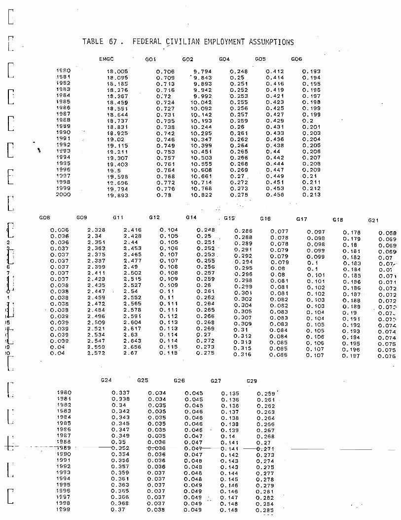
[ 2

t 6 7

£ i1

~·u· I ' I

!5

i[-~ .. I .

l

19 )t [

[

'

GOB

1S80 .1981 1982 1983 1984 1985 1986 1987 1988 1989 1990 1991 ~992

1993 1994 1995 1996 ~997

1998 1999 2000

0.036 0.036 0.036 0.037 0.037 0.037. 0.037 0.037 0.037 0.038 0.038 0.038 0.038 0.038 0.039 0.039 0.039 0.039 0.039 0.04 0.04

1980 1981 1982 1S83 1984 1985 19E6 1987

~6---~-~-~~~~~

L r_,

L

. 1990 1991 1992 1993 1994 1995 1996 1997 1998 1999

TABLE 67 . FEDERAL CIVILIAN EMPLOYMENT ASSUMPTIONS ..-

E!-IGC G01 G02 G04 GOS GOG

18.005 o. 706 9.794 0.248 0.412 0.193 18.095 o. 709 . 9. 843 0.25 0.414 0. 194 18. 185 0.713 9.893 0. 251 0.416 0. 195 18.276 0.716 9.942 0.252 0.419 0.196 18.367 0.'72 9.992 '0.253 0.421 0. 197 18.459 0.724 10.042 0.255 0.423 o. 198 18.551 0. 727 10.092 0.256 0.425 0.199 18.644 0.731 10. 142 0.257 0.427 0.199 18.737 0.735 10. 193 0.259 0.429 0.2 18.831 o. 738 10.244 0.26 0.431 0.201 18.925 0.742 10.295 0.261 0.433 0. 203 19.02 0. 746 10.347 0.262 0.436 0.204 19.115 0.749 10.399 0.264 0.438 0.205 19.211 0.753 10.451 0.265 0.44 0.206 19.307 0.757 10.503 0.266 0.442 0.207 19.403 0. 761 10.555 0.268 0.444 0.208 19.5 0.764 10.608 0.269 0 .. 447 0.209 19.598 o. 768 10.661 0.27 .. 0.449 0.21 19.696 0.772 10.714 0.272 0. 451 0. 211 19.794 0.776 10.768 0.273 0.453 0.212 19.893 0.78 10.822 0.275 0.456 0.213

G09 G 11 G12 G14 G15 G16 G17 G18 G21

2.328 2.416 0.104 0.248 0.286 0.077 0.097 0.178 0.068 2.34 2.428 0.105 o. 25 0.288 0.078 0.098 0. 179 0.069 2.351 2.44 o. 105 0.251 0.289 0.078 0.098 0. 18 0.069 2.363 2.453 0.106 0.252 0.291 0.079 0.099 0. 181 0.069 2.375 2.465 0. 107 0.253 0.292 0.079 0.099 0. 182 0.07 2.387 2.477 0.107 0.255 0.294 0.079 0. 1 0. 183 0.07.~ 2.399 2.49 0. 108 0.256 0.295 0.08 o. 1 0. 184 O.Oi 2.411 2.502 0.108 0.257 0.296 0.08 0. 101 0.185 0.071 2.423 2.515 o. 109 0.259 0.298 0.081 0. 101 o. 186 0.071 2.435 2.527 0.109 0.26 0.299 0.081 0.102 0. 186 0.072 2. 447 2.54 0. 11 0.261 0.301 0.081 0. 102 0. 187 0. 072. 2.459 2.552 0. 11 0.262 0.302 0.082 0.103 0.188 0.072 2.472 2.565 0. 111 0.264 0.304 0.082 0.103 0.189 0.07~ 2.484 2.578 0. 111 0.265 0.305 0.083 0. 104 0.19 0.07. 2.496 2.591 0. 112 0.266 0.307 0.083 0. 104 o. 191 0.07':; 2.509 2.604 0. 113 0.268 0.309 0.083 0. 105 0. 192 0.07.( 2.521 2.617 0. 113 0.269 0.31 0.084 0.105 0. 193 0.074 2.534 2.63 0. 114 ().27 0.312 0.084 0.106 0. 194 0.074 2.547 2.643 0. 114 0.272 0.313 0.085 0. 106 0. 195 0.075 2.559 2.656 0. 115 0.273 0.315 0.085 0. 107 0. 196 0.075 2.572 2.67 0.115 0.275 0.316 0.086 0. 107 0. 197 0.076

G24 G25 G26 G27 G29

0.337 0.034 0.045 0.135 0.259 0.338 0.034 0.045 0.136 0.261 0.34 0.035 0.045 0.136 0.262 0.342 0.035 0.046 0.137 0.263 0.343 0.035 0.046 0.138 0.264 0.345 0.035 0.046 0.138 0.266 0.347 0.035 0.046 0.139 0.267 0.349 0.035 0.047 0.14 0.268 0.35 0.036 0.047 0.141 0.27

-----o-:-Js-2---o-;-03G---o-;-04-7---0-;-1-4-1---0-;-2"7-1i-----------------0.354 0.036 0.047 0.142 0.273 0.356 0.036 0.048 0.143 0.274 0.357 0.036 0.048 0.143 0.275 0.359 0.037 0.048 0.144 0.277 0. 361 0.037 0.048 0. 145 0. 278 0.363 0.037 0.049 0.146 0.279 0.365 0.037 0.049 0.146 0.281 0.366 0.037 0.049 ·- 0.147 0.282 0.368 0.037 0.049 0.148 0.284 0.37 0.038 0.049 0.148 0.285

HiGC = GOl = G02 = G04 = G05 =

'\G06 = G08 = G09 = Gll = Gl2 -Gl4 = Gl5 = Gl6 = Gl7 = Gl8 = G21 = G24 = G25 = G26 = G27 = G29 =

Federal government civilian employment Government Employment, Aleutian Islands census division (thousands) Government Employment, Anchorage census division (thousands) Government Employment, Barrow/North Slope census division (thousands) Government Employment, Bethel census division (thousands) Government Employment, Bristol Bay Region (thousands) Government Employment, Cordova/McCarthy census division (thousands) Government Employment, Fairbanks census divisio~ (thousands) Government Employment, Southeast Alaska-{thousands) Government Employment, Kenai/Cook Inlet censtis division (thousands) Government Employment, Kobuk census division (thousands) Government Employment, Kodiak census division. (thousands)

[

[

[

[

[

[

[

c Government Employment, Kuskokwim cens~$ di~ision (thousands) Government Employment, Matanuska/Susi~a ce~sus division (thousands) Government Employment, Nome census division (thousands) o· Government Employment, Seward census division (thousands) I Government Employment, S.E. Fairbanks census division (thousands) Government Employment, Upper Yukon census division (thousands) Government Employment, Valdez/Chitina/Whittier census division (thousands) 0 Government Employment, Wade Hampton census division (thousands) Government Employment, Yukon Koyukuk census division (thousands)

D

SOURCE: Alaska Department'of Labor, Statistical Quarterly, various issues, for 1979 value. Projections from 1979 as described in text.

D

D [

[

[

----~--~-------------~

L 153 [

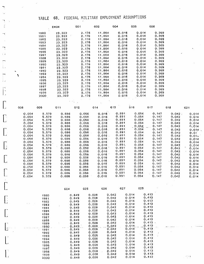
1

~~

TABLE 68. FEDERAL MILITARY EMPLOYMENT ASSUMPTIONS --,

EMGM G01 G02 G04 G05 GOG

1980 23.323 2. 176 11 . 864 0.016 0.014 0.369 1981 23.323 2. 176 11 . 864 0.016 0.014 0.369 1982 23.323 2.176 11.864 0.016 0.014 0.369 1983 23.323 2. 176 11 . 864 0.016 0.014 0.369 1984 23.323 2.176 11 . 864 0.016 0.014 0.369

' 1985 23.323 2.176 11.864 0.016 0.014 0.369 1986 23.323 2. 176 11.864 0.016 0.014 0.369 1987 23.323 2. 176 11.864 0.016 0.014 0.369 1988 23.323 2. 176 11.864 0.016 0.014 0.369

[ 1989 23.323 2.176 11.864 0.016 0.014 0.369 1990 23.323 2. 176 11.864 0.016 0.014 0.369 1991 23.323 2. 176 11.864 0.016 0.014 0.369 1992 23.323 2. 176 11.864 0.016 0.014 0.369

h \ 1993 23.323 2.176 11.864 0.016 0.014 0.369

L 1994 23.323 2. 176 11.864 0.016 0.014 0.369 1995 23.323 2. 176 11.864 0.016 0.014 0.369 1996 23.323 2. 176 11.864 0.016 0.014 0.369 1997 23.323 2. 176 11.864 0.0.16 0.014 0.369

L 1998 23.323 2.176 11.864 0.016 0.014 0.369 1999 23.323 2.176 11.864 0.016 0.014 0. 369 ~

2000 23.323 2.176 11.864 0.016 0.014 0.369

[ GOB G09 G 11 G12 G14 G15 G16 G17 G18 G21

[ 0.0!:4 5.579 0.686 0.056 0.016 0.891 0.054 o. 147 0.042. 0.014 0.054 5.579 0.686 0.056 0.016 0.891 0.0!:4 o. 147 0.042 0.014 0.054 5.579 0.686 0.056 0.016. 0.891 0.054 0.147 0.042 0.014 0.054 5.579 0.686 0.056 0.016 0.891 0.054 0. 147 0.042 0.014 0.054 5.579 0.686 0.056 0.016 0.891 - _o_ ·~.Q5~ o. 147 0.042 0.014

[ 0.054 5.579 0.686 0.056 0.016 0.891 0.054 0. 147 0.042 0.014. 0.054 5.579 0.686 0.056 0.016 0.891 0.054 o. 147 0.042 0.01 0.054 5.579 0.686 0.056 0.016 0.891 0.054 0. 147 6.042 0.01 .. 0.054 5.579 0.686 0.056 0.016 0.891 0.054 o. 147 0.042 0.014

[ 0.054 5.579 0.686 0.056 0.016 0.891 0.054 o. 147 0.042 0.014 0.054 5.579 0.686 0.056 0.016 0. 891. 0.054 o. 147 0.042 0.014 0.054 5.579 0.686 0.056 0.016 0.891 0.054 o. 147 0.042 0.014 0.054 5.579 0.686 0.056 0.016 0.891 0.054 o. 147 0.042 0.014 0.054 5.579 0.686 0.056 0.016 0.891 0.054 o. 147 0.042 0.014

[ 0.054 5.579 0.686 0.056 0.016 0.891 0.054 o. 147 0.042 0.014 0.054 5.579 0.686 0.056 0.016 0.891 0.054 o. 147 0.042 0.014 0.054 5.579 0.686 0.056 0.015 0.891 0.054 o. 147 0.042 0.014 0.054 5.579 0.686 0.056 0.016 0.891 0.054 o. 147 0.042 0.014

[ 0.054 5.579 0.686 0.056 0.016 0.891 0.054 o. 147 0.042 0.014 0.054 5.579 0.686 0.056 0.016 0.891 0.054 o. 147 0.042 0.014 0.054 5.579 0.686 0.056 0.016 0."891 0.054 0. 147 0.042 0.014

[ G24 G25 G26 G27 G29

1980 0.849 0.028 0.042 0.014 0.413

[ 1981 0.849 0.028 0.042 0.014 0.413

1982 0.849 0.028 0.042 0.014 0.413

1983 0.849 0.028 0.042 0.014 0.413

1984 0.849 0.028 0.042 0.014 0.413

[ 1985 0.849 0.028 0.042 0.014 0. 413

1986 0.849 0.028 0.042 0.014 0.413

1987 0.849 0.028 0.042 0.014 0.413

1988 0.849 0.028 0.042 0.014 0.413

c 1989 0.849 0.028 0.042 0.014 0.413

1~_90 (),849 0.()~8- - Q.042 Q,Q14 -~ 0.413~~

1991 0.849 0.028 0.042 0.014 0.413

1992 0.849 0.028 0.042 0.014 0.413

1993 0.849 0.028 0.042 0.014 0.413

[ 1994 0.849 0.028 0.042 0.014 0.413

1995 0.849 0.028 0.042 0.014 0.413

1996 0.849 0.028 0.042 0.014 0.413

1997 0.849 0.028 0.042 0.014 0.413 r~ 1998 0.849 0.028 0.042 0.014 0.413

L ~939 0.849 0.028 0.042 0.014 0. 413·

2000 0.849 0.028 0.042 0.014 0.413 .. i

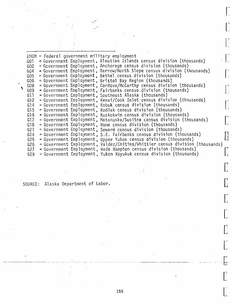
E!·iGt•1 GOl G02 G04 G05 G06

, G08 G09 Gll Gl2 Gl4 Gl5 Gi6 Gl7 Gl8 G21 G24 G25 G26 G27 G29

,-

=Federal government military employment =Government Employment, Aleutian Islands census division (thousands) =Government Employment, Anchorage census division (thousands) =Government Employment, Barrow/North Slope census division (thousands) =Government Employment, Bethel census division (thousands) =Government Employment, Bristol Bay Region (thousands) =Government Employment, Cordova/McCarthy census division (thousands) =Government Employment, Fairbanks census division (thousands) =Government Employment, Southeast Alaska (thousands)

[

[

[

[

[

[

[

[

=Government Employment, Kenai/Cook Inlet census division (thousands) =Government Employment, Kobuk census division (thousands) =Government Employment, Kodiak census division (thousands) =Government Employment, Kuskokwim census division (thousands) =Government Employment, Matanuska/Susitna c~nsus division (thousands) =Government Em~loyment, Nome census di~ision· (thousands) =Government Employment, Seward c~nsus division (thousands) =Government Employment, S.E. Fairbanks census division (thousands) 0· =Government Employment, Upper Yukon census division (thousands) =Government Employment, Valdez/Chitina/Whittier census division (thousands) =Government Employment, Wade Hampton census division (thousands) 0 =Government Employment, Yukon Koyukuk census division (thousands) 1

SOURCE: Alaska Department of Labor.

0 c

155

c [

[

[

- --- ---- ------ b -[

L

..,

~

_ ...

'

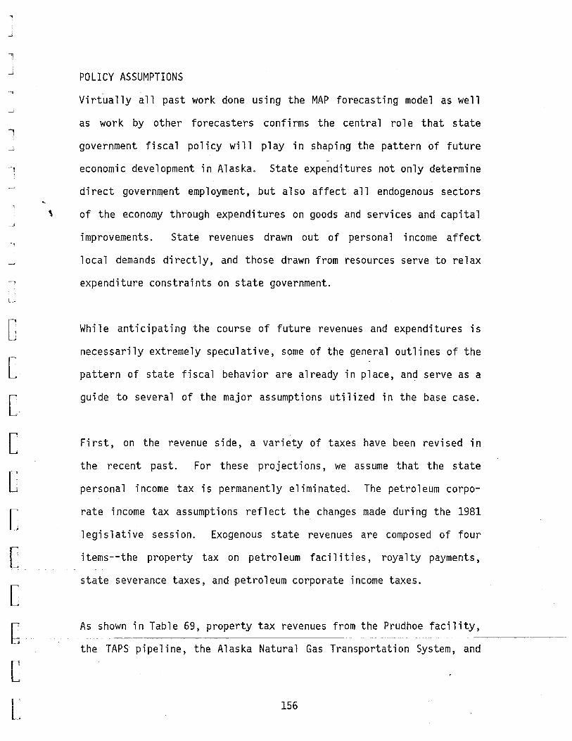
' _j

]

__j

-,

__;

--,

-,

C-..J

[

[

[

[

[

[

[

[

POLICY ASSUMPTIONS

Virtually all past work done using the MAP forecasting model as well

as work by other forecasters confirms the central role that state

government fiscal policy will play in shaping the pattern of future -

economic development in Alaska. State expenditures not only determine

direct government employment, but also affect all endogenous sectors

\ of the economy through expenditures on goods and services and capital

improvements. State revenues drawn out of persona 1 income affect

local demands directly, and those drawn from resources serve to relax

expenditure constraints on state government.

While anticipating the course of future revenues and expenditures is

necessarily extremely speculative, some of the general outlines of the

pattern of state fiscal behavior are already in place, and serve as a

guide to several of the major assumptions utilized in the base case.

First, on the revenue side, a variety of taxes have been revised in

the recent past. For these projections, we assume that the state

personal income tax is permanently eliminated. The petroleum corpo

rate income tax assumptions reflect the changes made during the 1981

1 egis 1 at i ve session. Exogenous state revenues are composed of four

items--the property tax on petroleum facilities, royalty payments,

state severance taxes, and petroleum corporate income taxes.

h-------:----~=- shown in Table 69, property tax revenues from the Prudhoe facility,

the TAPS pipeline, the Alaska Natural Gas Transportation System, and

[ r" L 156

'

1980 1981 i 5'82 17'~33

1984 1985 1 5'86 1987

, 1988 1989 19'7'0 1991 1992 1993 1994 1995 19'i'6 1997 195'8 1999" 2 (1 ()()

TABLE 69 . siATE REVENUE ASSUMPTIONS (Millions of Current Dollars)

~:F'TS F:F· F' S RF'RY FnCSF'X ~

469.9 350. 881.3 135.12 1156. 321.333 1389·. 860. "1678; 358.801 1.~66. 820. 2102. 369 •. 348 2087. 495. 2480. 379.617 2463.- 593"+16 2896. 387 •· 264 2894. 694.8 3497. 397.263 3473 •. 836.4 3978. 543.154 ·'39·~·2 •

..

"$'52+8 3675. 564 .. 186 4404. 969.48 41A9. 58.: .•. 663 4928. 1089.24 4002. 601.828 4830; 1059.84 ~-.t:"..,

.,!t / . ._1..:.. • 614.356 4.641. 1007.16 3656+ 622.681 4631. 994.44 3775. ·"628 •. 037 . 481"4"·;· ... · ... · io-3·o-~6-8 : · 3661 ;· 634.014 4718. 1005.48 3417. 634.542 4481 .. · .... · .. 947.76 3256. 630.545 . ·! 4380. ::.~:_. > _>,. 916-~32 3420. 621.568 4659.

' 969.48 3420. 607.445 .. 4659 • ,_969.48 .. 3420 .. .589.322 4659 ·• . ·'· 969"~'48-342(i ... .. 566.396 , .. ·. 4659. .···. 96.9. 48

RPTS = Oil and gas production taxes (millions of current dollars) RPRY = Oil and gas royalties (millions of current dollars) RPPS = Oil and gas property taxes (millions of current dollars) RTCSPX = Special oil and gas corporate taxes (millions of current dollars)

SOURCES: Alaska Department of Revenue, Petroleum Production Revenue Forecast, third quarter 1981. RPPS also includes property tax estimates for the Northwest Alaska Gas Pipeline, the Trans-Alaska Pipeline, and Federal-State OCS development in the Beaufort Sea, as discussed in Alaska OCS Office, Bering Norton Petroleum Development Scenarios: Economic and Demographic Analys1s,-rechn1ca1 Paper No. 50, Social and Economic-Studies Program, p. 101.

157

[

[

[

[

[

[

[

[

c [

[

[

[

[

[

[

b [

[

1

1

' __j

-,

-,

~

~,;

[

[

[

[

[

c [

[

[

6 [ r~

L

'

OCS development reach over 500 mi 11 ion do 11 ars by the end of the

forecast period. Oil and gas royalty, production tax, and special

corporate tax revenues peak at about $10 bi 11 ion annually by 1989,

based on recent petroleum production revenue forecasts by the Alaska

Department of Revenue.

On the expenditure side, it is assumed that real per capita expendi-

tures will grow over the forecast period in proportion to the growth

in real per capita income.

While this assumed behavior is somewhat more conservative than has

been observed in the last several years, it is impossible to use the

expenditure path of the recent past as a long term trend, inasmuch as

it is simply not sustainable in the long run. The implicitly assumed

unitary income elasticity of expenditures does represent a sustainable

policy over the forecast period.

158

'

The Base Case Assumptions: The SCIMP Model

Utilization of the SCIMP model requires initial period population

figures, projected exogenous employment, and a variety of control

parameters including employment multipliers, demographic parameters,

and labor force participation rates. These assumptions are discussed

in this section.

The assumption was made throughout that th~re is no interaction

between the military populations stationed on Adak and Shemya and the

rest of the economy of the Aleutian Islands. These populations were

assumed to remain constant over the entire peri ad. They were sub

tracted from total population of the region before running the SCIMP

model, and added back into the final population figures. In addition,

OCS offshore emp 1 oyment was assumed to have no interaction with the

rest of the local economy.

POPULATION

Starting population data for 1980 were taken from 1980 census print

outs. Calculation of the input data by age, race, and sex for

civilian population is presented in Table 70. This population was

adjusted upward slightly to allow for consistency with the 1970

definition of the Aleutian Islands census division, which is the basis

for other input data reported for the region by the State of Alaska.

The adjusted 1980 civilian population was 4,328. Adding in the

military popula~ion of 3,915 results in a total 1980 population of -- ----- ---~ --- - -- -- --- -- ---- - - - -- ---- - --

8,243.

159

[

[

[

[

[

[

L c c C

c [

[

[

C [

b [

[

r-i • J

f-1 O'l 0

lJ r:l r-:J ~ c-l c-J r-J r-J r-=J ~ C J L , J j L J J

.... TABLE 70: CALCULATION OF POPULATION DATA FOR SCIMP RUN,

ALEUTIAN ISLAND CENSUS DIVISION

Civilian Population Adjusted Civilian Populationb

i Total Popula-tion (Includ- Military Civilian

Age i ing Milital'y) Population Population Native a Non-Native Native Non-Native Native Cohort Male Female Adak & Shemya) Male __ Eemale Shares Male Female Male Female Male Female Male Female

0-14 857 773 444 377 413 396 . 605 163 156 250 240 183 175 281 270

15-19 576 278 361 111 215 167 .605 85 66 130 101 95 74 146 113

20-24 1,017 523 643 269 374 254 .438 210 143 164 111 236 1.61 184 125

25-29 759 438 424 225 335 213 .438 188 120 147 93 211 135 165 104

30-44 1,204 587 620 297 584 290 .438 328 163 256 127 368 183 288 143

45-64 410 239 44 47 316 192 .438 178 108 138 84 200 121 155 94

64 + 55 52 2 1 53 51 .885 6 6 47 45 I 7 7 53 51

TOTAL 4,878 2,890 2,588 1,327 2,290 1,563 1,158 762 1,132 801 1,300 856 1,272 900

aCalculated from 1980 census data on native population by age group. These data were not sex-specific.

bThe 1980 census definition of the Aleutian Islands excluded four communities: Chigni·k, Chignik Lagoon, Chignik Lake, and Perryville, the population of which totals 475. Civilian population figures were adjusted upwards proportionately by a factor of .12328 to make population figures consistent with statistics issued by the State of Alaska.

SOURCE: ; 1980 census printouts.

_j .J

'

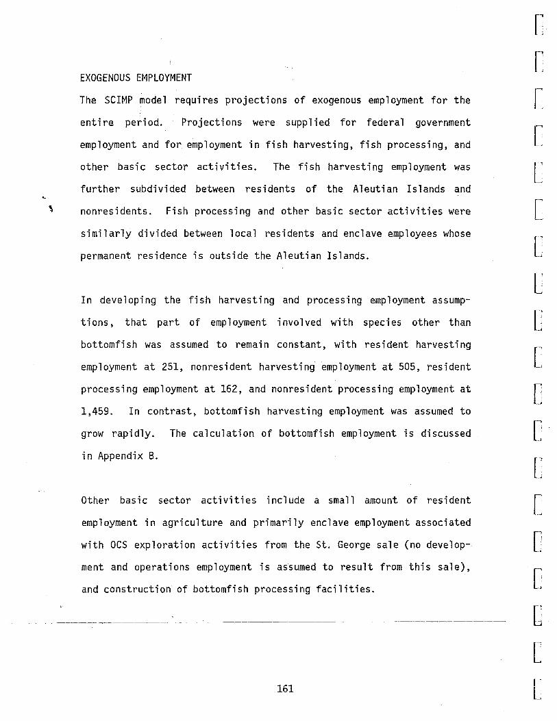
EXOGENOUS EMPLOYMENT

The SCIMP model requires projections of exogenous employment for the

entire period. Projections were supplied for federal government

employment and for employment in fish harvesting, fish processing, and

other basic sector activities. The fish harvesting employment was

further subdivided between residents of the Aleutian Islands and

nonresidents. Fish processing and other basic sector activities were

similarly divided between local residents and enclave employees whose

permanent residence is outside the Aleutian Islands.

In developing the fish harvesting and processing employment assump-

tions, that part of employment involved with species other than

bottomfish was assumed to remain constant, with resident harvesting

employment at 251, nonresident harvesting employment at 505, resident

processing employment at 162, and nonresident processing employment at

1,459. In contrast, bottomfish harvesting employment was assumed to

grow rapidly. The calculation of bottomfish employment is discussed

in Appendix B.

Other basic sector activities include a small amount of resident

employment in agriculture and primarily enclave employment associated

with OCS exploration activities from the St. George sale (no develop-

ment and operations employment is assumed to result from this sale),

and constructio~ of bottomfish processing facilities.

[

[

[

[

[

[

[

[

c [

[

[

[

[

[

[

~--~---~-----'------~ -~-------------~----------------------------------6--[

161 r, L

[

[

[

[

[

[

[

c [.

[

[

[

[

[

[

[

L [ r, L

'

Federal government civilian employment was assumed to rise at a rate

of 0.5 percent annually from a 1980 level of 706.

The exogenous employment assumptions are summarized in Table 71.

EMPLOYMENT MULTIPLIERS

The SCIMP model calculates support sector employment by multiplying

exogenous employment by employment multipliers. A multiplier of .2332

was assumed for all resident employment, based on calculations done

for an earlier study (Tuck and Huskey, St. George Basin Petroleum

Development Scenarios, Economic and Demographic Analysis, 1981, page

101). A much lower multiplier of .0466 was assumed for exogenous

enclave employment, based on the same source. Finally, a figure of

.0233 (half the enclave multiplier) was assumed for nonresident fish

harvesting employment, on the assumption that these workers would have

an even smaller interaction with the local economy. These multiplier

assumptions are shown in Table 71.

State and local government employment was calculated by multiplying

resident civilian population in the previous year by a factor of

. 0948. This reflects an assumption that this ratio remains constant

over time. The figure was based on the ratio of the 1979 average

state and local government employment (reported in the Alaska Depart

ment of Labor•s Statistical Quarterly) to the 1978 civilian population

(calculated by .reducing the 1978 population figure reported in the

162

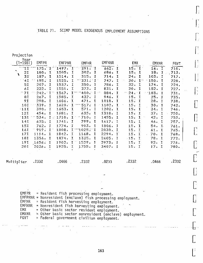
TABLE 71. SCIMP MODEL EXOGENOUS EMPLOYMENT ASSUMPTIONS

Projection Year

_(1=1~.!) EMFPR EMFPNR EMFHR EMFHNR EMX EMXNR -- .......... -·-:~.·x·--··175.- I"""1497. r···· 291c···r 662. I 15 • ·I . 16. 1

' 2I 180. J. 1.505. I 302. I 686 • I 15. I 18. I 31 187. 1 1514. r 315. r 714. 1 24. I :1.03. I

"4I ... 195> :r: "1525. I ·--- 3 31. ; · I ·· 747. I · 30+ r·- ·:t5o.- I 51 207. I 1537. I 350. I 786. I 32. I 61 222. I 1551.. I 373. I 831. I 30. I

... 7I 242.·r···· 1567+ r-- -Aoo •. · r. ···· 884. · I 24. ·r BI 267. I 1585. I 432. I 946. I l 5. I 9J. 298. I :1..~06 > J. 47:1.. I :1.0:1.8. I :1.5 .; I

10I "339. I :1. 6 2 8 • I · ---· 51 7 .- I . 1102. I 15 • I ·11! 390. I :1.653. I 57'l.. I :1.202. I 1. 5-> I 12I 454. I :t.C>81. 1 635. I 1318. I :1.5. I

-1 3 I ·· -- 5 3 4 • · I . ·. 1 7 1 0 • r·-·710. I 1455. I 15. I 141 635. I :1.741.~ I 799. I :1.6 1. 7. I :1.5. I :1.5I 762. I 1774. I 903. I 1806. I l.5. I 16I 91.9. I · :1.808, I --1025; I 2030. I l5) I 171 l11 4. I :1.842. I 1168. I 2294. I :1.5. I 'l.8I 1.356. I 187-4 t I :1.335., I 2605, I t5. J. 19I 1656; I 1902. I .. 1529. I 2973. J. 1. 5. I -201 202C>. I l.925. 1 :1.755. I 3407. X 15. I

M111ti pl i er . 2332 .0466 .2332 .0233 .2332

EMFPR = Resident fish processing employment. EMFPRNR = Nonresident (enclave) fish processing employment. EMFHR = Resident fish harvesting employment. EMFHNR = Nonresident fish harvesting employment. EMX = Other basic sector resident employment. EMXNR = Other basic sector nonresident (enclave) employment. FGVT = Federal government civilian employment.

163

174. I 152. I

· ·103 • I 25. I 28. I 30. I 34. I 37. I 42. I 46. I 54. I· 6:1.) I 70. I 78, I 9;?.. I l 7. I

.0466

FGVT 710.

.713. 717. 720. 724. 727. 731. t

735c-738. 742. 746. 750. 753. 757. 761. 765, 768. 772, 776. 780.

.2332

[

[

[

[

[

[

[

[

c [

[

[

[

[

c [

c [ r L

r L~

[

[

[

[

[

[

[

[

[

[

[

c [

[

[

b L r , L

'

Alaska Department of Labor's Alaska Population Overview [December 1979]

by military and dependent population).

OTHER PARAMETERS

Birth rate and survival rate parameters were based on 1970 census data

and more recent data obtained from the U.S. Department of Health,

Education and Welfare. No noneconomic induced migration was assumed.

Labor force participation rates for white males were assumed to be the

same as those published in the Survey of Income and Education (1976,

Spring). The published labor force participation rates for white

females, native males and native females were adjusted upwards by a

factor of 1.144. This was done so that the 1980 1 abor force (pre

dicted by multiplying the labor force participation rates by the 1980

population figures) would equal the total labor force calculated by

adding 1980 unemployment figures to the total employment figure

projected by the model for 1980.

This completes the description of the base case assumptions. We now

turn to the base case projections.

164

\

The Base Case Projections

The historical baseline analysis and the base case assumptions have

laid the groundwork for the base projections. Before reviewing these

projections, it again needs to be emphasized that the projections are

not forecasts of what actually will occur. These base projections are

projections of economic and demographic variables, given the assump

tion that the specific projects, growth rates, etc., occur. As

discussed above, however, there is a reasonable probability that the

assumptions utilized will generate a growth path that actually will be

obtained or exceeded. With these comments in mind, we can now turn to

the projections.

THE MAP STATEWIDE BASE CASE PROJECTIONS

Population

Projections of population, civilian non-Native natural increase, and

net migration are shown in Table 72. Population growth over the

period 1980-2000 averages 2.4 percent. However, growth is more rapid

during the 1980s (3.1 percent) than during the 1990s (1. 7 percent).

The most rapid population growth {4.7 percent) occurs during the

period 1982-1986. This growth is primarily a reflection of the gas

pipeline construction and the waterflood project at Prudhoe Bay.

During the 1990s fisheries expansion is the main driving force, and

the growth of population is more even.

[

[

[

[

[

[

[

[

c [

[

c [

[

[

[

-~--~~~~------~~-~------------------------ --b~--

[

165 f' L

,.....,

[

[

[

[

[

[

[

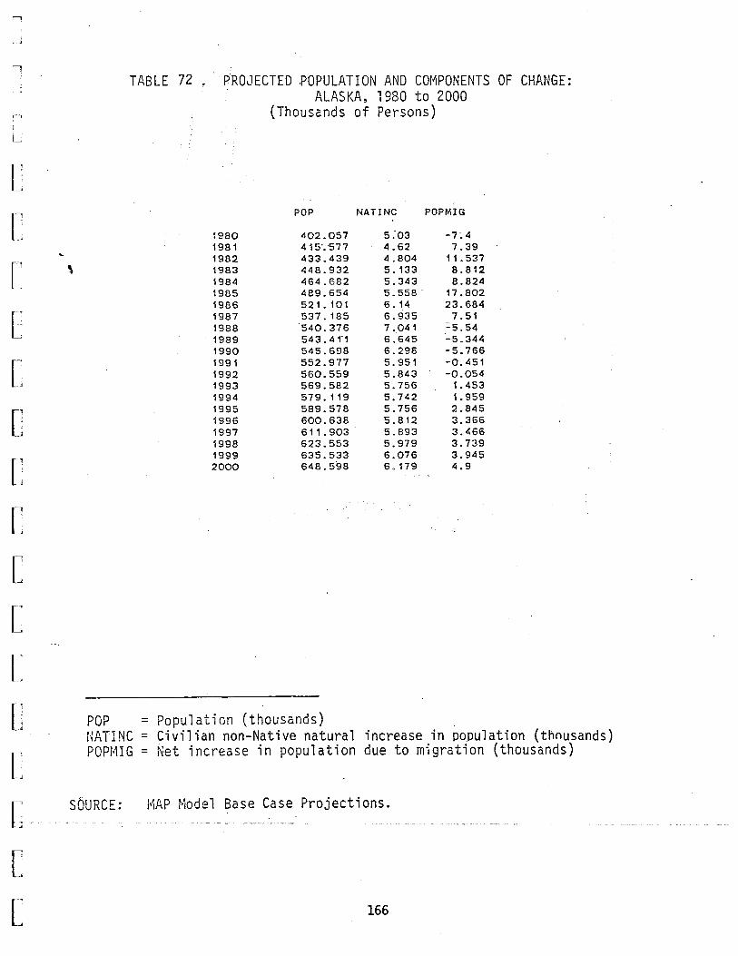
[J

c [

[

[

[

[

c L [ r, L

'

TABLE 72 . ~ROJECTED POPULATION AND COMPONENTS OF CHANGE:

~980

1981 1982 1983 1984 1985 1986 1987 1988 1989 1990 1991 1992 1993 1994 1995 1996 1997 1998 1999 2000

ALASKA, 1980 to 2000 (Thousands of Persons)

POP NATINC POP MIG

402.057 5:o3 -7~4

415".·577 4.62 7.39 433.439 4.804 11 . 537 448.932 5. 133 8.812 464.682 5.343 8.824 489.654 5.558. 17.802 521.101 6. 14 23.684 537. 185 6.935 7.51 "540. 376 7.041 ::.5.54 543.41"1 6.645 -5.344 545.698 6.298 -5.766 552.977 5.951 -0.451 560.559 5.843 -0.054 569.582 5.756 1. 453 579.119 5.742 1. 959 589.578 5.756 2.845 600.638 5.812 3.366 611.903 5.893 3.466 623.553 5.979 3.739 635.533 6.076 3.945 648.598 6.179 4.9

POP = Population (thousands) NATINC = Civilian non-Native natural increase in population (thousands) POPMIG = Net increase in population due to migration (thousands)

SbURCE: MAP Model Base Case Projections.

166

\

Civilian non-Native natural population increases are fairly steady

over the entire period. In contrast net migration shows strong swings

in response to fluctuation in labor demand associated with large

construction projects.

The net result is a population of 649 thousand in 2000, an increase of

61 percent over the 1980 population of 402 thousand. Of this increase

111 thousand is accounted for by civilian non-Native natural increase,

while the balance is attributed to native increase and net migration.

Age Structure

Projections of age structure of the Alaska population are shown in

Table 73. The share of adults stays almost the same throughout the

period, while the shares of children and aged decline and rise by

about two percent, respectively.

Employment

Projections of total employment (EM99), wage and salary employment

(EM991), and employment in the basic sector (EMNS), the support sector

(EMSP), and government (EMG9) are presented in Table 74. Total

emp 1 oyment grows from 204.4 thousand in 1980 to 341.8 thousand in

2000, a growth rate of 2.6 percent. Growth of basic sector employment

(at 2.7 percent) occurs in response to construction, expanding petro

leum-related activity, and growth of bottomfishing. Expansion is

somewhat more rapid in the first decade (3.4 percent) than in the

1990s (2.0 percent).

167

r [

[

[

[

[

[

[

c [

[

[

[

[

[

[

L [

l

[

[

[

[

[

[

[

[

[

[

[

[

[

[

[

[

L [

[

'

TABLE 73 . PROJECTED AGE STRUCTURE OF ALASKA POPULATION, 1980 - 2000

POP.KID POP.AD POP.GER

(Proportion of Total Population)

POP.KID POP.AD POP.GER

1980 0.291 0.669 0.04 1981 0.29 0.668 0.042 1982 0.29 0.668 0.042 1983 ·p.289 0.668 0.043 1984 0.289 0.667 0.044 1985 0.288 0.669 0.044. 1986 0. 287 0.67 0.043 1987 0.287 0.669 0.,043 1988 0.288 0.667 0.045 1989 0.289 0.665 0.047 1990 0.289 0.663 0.048 1991 0.288 0.662 0.05 1992 0.287 0.662; 0.051 1993 0.286 0.662. 0.052 1994 0.284 0.662 0.053 1995 0.283 0.663 0.054 1996 0.281 0.663 0.055 1997 0.28 0.664 0.056 1998 0.278 0.664 0.058 1999 0.277 0.664 0.059 2000 0.276 0.664 0.06

= Share of children (under age 15) in total population = Share of adults (between ages 15 and 65) in total population = Share of aged (over age 65) in total population

SOURCE: MAP Model Base Case Projections.

168

'

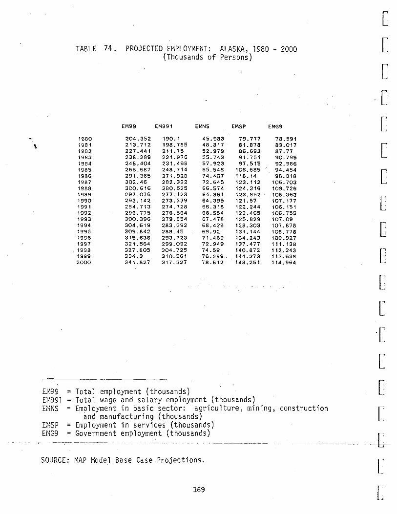
EM99 = EM991 = EMNS =

EMSP = EMG9 =

TABLE 74. PROJECTED H1PLOYMENT: ALASKA, 1980 - 2000 (Thousands of Persons)

EM99 EM991 EMNS EMSP EMG9

1980 204.352 190. 1 45.983 79.777 78.591 1981 213.712 198.785 48.817 81.878 83.017 1982 227.441 211.75 52.979 86.692 87.77 1983 238.289 221.976 55.743 91.751 90.795 1984 248.404 231.498 57.923 97.515 92.966 1985 266.687 248.714 65.548 106.685 94.454 1986 291. 365 271.928 74.407 118.14 98.818 1987 302.46 282.322 72.645 123.112 106.703 1988 300.616 280.525 66.574 124.316 109.726 1989 297.076 277.123 64.861 123.852 108.363 1990 293.142. 273.339 64.395 121. 57 107. 177 1991 294.713 274.728 66.318 122.244 106. 15 1 1992 296.775 276.564 66.554 123.465 106.755 1993 300.396 279.854 67.478 125.829 107.09 1994 304.619 283.692 68.439 128.303 107.878 1995 309.842 288.45 69.92 131.144 108.778 1996 315.638 293.723 71.469 134.243 109.927 1997 321.564 299.092 72.949 137.477 111.138 1998 327.805 304.725 74.59 140.872 112.343 1999 334.3 310.561 76.289 144.373 113.638 2000 341. 827 317.327 78.612 148.251 114.964

Total employment (thousands) Total wage and salary employment (thousands) Employment in basic sector: agriculture, mining, construction

and manufacturing (thousands) Employment in services (thousands) Government employment (thousands)

SOURCE: MAP Model Base Case.Projections.

169

[

[

[

[

[

[

[

[

c [

[

[ r~

L_~

[

[

[

--- ---- L [

[

~

C""""!!

L~

[

[

[

[

[

[

c c c [

[

[

[

[

'

However, growth is most rapid (8.4 percent) over the period 1980 to

1986, reflecting primarily gas pipeline construction. Between 1986

and 1990, fo 11 owing the peak of the pipe 1 i ne construction, basic

sector employment falls. Government growth (1.9 percent) is largely

accounted for by growth of state and local government.

Support sector growth reflects the growth of the basic sector. For

the entire period, growth averages 3. 1 percent. Growth is somewhat

more rapid (at 4.3 percent) during the 1980s than during the 1990s

(2.0 percent).

Support sector employment as a percent of total employment grows from

39.0 percent in 1980 to 43.4 percent in 2000. The share of basic

sector employment also rises slightly, from 22.5 to 23.0 percent,

while the share of government employment falls from 38.5 to 33.6

percent.

In summary, there is considerable growth in employment over the 20-

year period. However, the first 10 years tend to be more volatile and

reflect the concentration of several major projects in the 1982-1986

period. The 1990s growth in employment is somewhat more evenly paced,

responding largely to growth in fisheries.

Personal Income, Wages and Prices

.r ' Personal income projections (measured in 1981 dollars), both total and . 6 --- ~--- --------- -- ---:---~---- --------------------~-----~-----------~---------~r-------------------~------~-,--------------------------

per capita, are shown in Table 75. Total personal income grows from

[

[ 170

\

TABLE 75. PROJECTED.PERSONAL INCOME AND PERSONAL INCOME PER CAPITA: ALASKA, 1980 - 2000

(Millions of 1981 Dollars, respectively)

PI. 81 PIPC.81

PI. 81 PIPC.81

1980 5750.38 14302.4 1981 6060. 18 14582.6 1982 6531.98 15070. 1 1983 6939.5 15457.8 1984 7456.85 16047.2 1985 8594.86 17552.9 1986 9978.68 19149.2 1987 9968.82 18557.5 1988 9344. 13 17291.9 1989 9130.03 16801.3 1990 8983.99 16463.3 1991 9141.17 16530.8 1992 9260.97 1652L 1993 9455.89 16601.4 1994 9662.39 16684.7 1995 9905.07 16800.3 1996 10164.2 16922.4 1997 10428.7 17043. 1998 10711.9 17178.8 1999 11003.9 17314.4 2000 11341.2 17485:7

= Real personal income (millions of 1981 dollars) = Real per capita personal income (1981 dollars)


[

[

[

[

[

[

[

c c c [

[

[

[

[

[

---~-_:____-------~6-[

171 I' L

[

[

[

[

[

[ \

[

[

[

[

[

[

[

[

[

[

_r' .. -- ,. 6--- ---

[

L

5,750 million dollars in 1980 to 11,.341 million dollars in 2000, an

average annual rate of growth of 3. 5 percent. As was the case with

other variables considered, the rate of growth is highest for the

first six years (9.6 percent), turns negative between 1986 and 1990

(-2.6 percent), and rises at 7.2 percent between 1990 and 2000. This

reflects both changes in the rate of growth of employment as well as

changes in the composition of economic activity.

This is more clearly seen in the data on per capita income. Between

1980 and 1986, per capita income grows at an annual rate of 5.0 per

cent, between 1986 and 1990 it declines by 3.7 percent per year, and

for the 1990-2000 period rises by only 0.6 percent per year. The

dec 1 i ne for the period 1986 to 1990 and the subsequent s 1 ow rate of

growth are attributable to two factors. First, an increasing share of

total employment is accounted for by support sector activity, with

relatively lower real wages than the economy as a whole. Second, much

of the growth of basic sector employment during the 1990s is in fish

eries, also an industry with relatively low wage rates.

Projection of total wages and salaries by sector are shown in Table

76. The wage bills in the basic and support sectors mirror the pattern

of growth seen in personal income. Wages in the two sectors peak in

1986 and 1987, respectively, decline steadily until 1990, and then

begin growing again. Support sector wages do not regain peak 1987

1 eve 1 s until 19~5, and basic sector wages do not reach 1986 1 eve 1 s

again during the period.

172

'

TABLE 76. PROJECTED WAGES AND SALARIES BY SECTOR:

1980 1981 1982 1983 1984 1985 1986 1987 1988 1989 1990 1991 1992 1993 1994 1995 1996 1997 1998 1999 2000

ALASKA, 1980 - 2000 (Millions of 1981 Dollars)

WS99.81 WSNS.81 WSSP.81 WSG9.81

4494.67 1150.75 1662.47 1699.02 4705.05 1230.27 11598.34 1810.42 5138.68 1393.41 1770.94 1977.18 54.78. 66 1506. 18 1882.99 2092. 19 5923. 1670.9 2059.9 2194.77 6904.72 2223.38 2391.78 2292.01 8090.04 2847.89 2776.15 2468.32 8045.7 2549.8 2784.6 2713.51 7476.12 1975.08 2689.63 2813.51 7289.87 1838.73 2638.72 2814.44 7169.77 1795.2 2555.89 2820.61 7303.63 1895.67 2577.65 2832.16 7404. 19 1905.61 2608.24 2892. 12 7567.48 1949.57 2673.99 2945.63 7739.2 1988.6 2738.29 3013.94 7939.73 2045.74 2808.96 3086.6 8153.31 2100.89 2885.19 3168.74 8371. 23 2152.27 2965.75 3254.65 8604.6 2212.41 3051.34 3342.23 8844.93 2271.79 3140.04 3434.43 9122.31 2356.55 3237.59 3529.44

WS99.8l =Total real wages and salaries (millions of 1981 dollars) WSNS.8l = Total real wages and salaries in basic sector (millions

of 1981 dollars) WSSP.81 =Total real wages and salaries in service,s (millions of

1981 dollars) WSG9.8l =Total real wages and salaries in government (millions of

[

[

[

[

[

['

[

c c [

[

[

[

[

c [

1981 dollars) --~----------------------~

SOURCE: MAP Model Base Case Projections. [

173 [

[

[

[

[

[

[

E [

[

[

[

[

[

[

[

[

'

Total government wages grow throughout the period at an overall rate

of 3.7 percent with the growth rate for the first 10 years (5.2 per

cent) considerably above that for the second period (2. 3 percent).

Projections of real wage rates are shown in Table 77. These include

the real wage rates for the basic sector (WRNS.81), the support sector

(WRSP. 81), and government (WRG9. 81). Basic sector real wage rates

increase rapidly from 1980 to 1986 (7.3 percent per year), decline at

a rate of 7.6 percent per year until 1990, and then increase at only

0. 7 percent per year until 2000. Over a 11, the growth rate is 0. 9

percent. Support sector rea 1 wage rates grow at an average annua 1

rate of 2.0 percent over the period 1980-1986, decline at a rate of

2.7 percent over the period 1986-1990, and rise at a rate of only 0.4

percent over the period 1990-2000. Overall the growth rate is only

0.2 percent for the entire period. Government wages show the greatest

rate of growth of 1.8 percent over the entire period.

Our discussion of income and wages has been in real terms. Over this

period inflation has been substantial. As shown in Table 78, for most

of the period both the A 1 aska and the United States i nfl at ion rates

are projected to be 7.0 percent or greater.

Government Revenues and Expenditures

State government revenue projections by source are shown in Table 79.

_f~ ______ · ___ ~~e- _v_a_ria~l--e~ _ i.nc_l_ud~: __ ~o~al _ s~~~-e- ---~overnment reve~~es (RSGF._~1) , ___ _ ~ '

petro 1 eum revenues (RP9S. 81), revenues from the Federa 1 government

[

[ 174

'

TABLE 77. PROJECTED R.EAL 1-JAGE RATES: ALASKA, 1981 - 2000 (1981 Dollars)

WRNS.8f WRSP.81 WRG9.81

1930 25025.4 20838.9 21618.4 1981 25201.5 20742.3 21807.8 1982 26301.3 20427.8 22526.8 1983 27019.9 20522.8 23043.1 1984 28846,.6 21123.9 23608.4 1985 33920.1 22419. 24265.8 1986 38274.7 23498·. 9 24978.3 1987 35099.4 22618.5 25430.4 1988 29667.6 21635.4 25641.3 1989 28348.9 21305.4 25972.3 1990 27877.7 21024.1 26317.2 1991 28584.4 21086.1 26680.4 1992 28632.3 21125.2 27091.2 1993 28892. 21251. 27506.1 1994 29056.7 21342.4 27938.4 1995 29258.4 21418.8 :<:8375. 1 1996 29396. 21492.4 28825.8 1997 29503.5 21572.6 29284.9 1998 29660.8 21660.3 29750.3 1999 29778 .·7 21749.5 30222.6 2000 29976.9 21838.6 30700.4

WRNS.81 = Real wage rate in basic sector (1981 dollars) NRSP.Sl = Real wage rate in services sector (1981 dollars) \.o,1RG9 .81 = Real \~age· rate in government ( 1981 dollars)

SOURCE: KAP Model Base Case Projections.

175

[

[

[

[

[

[

[

[

[

[

[

[

[

[

[

[

L [ r L

[

[

[

[

[

[ ' [

[

[

[

[

[

[

[

[

[

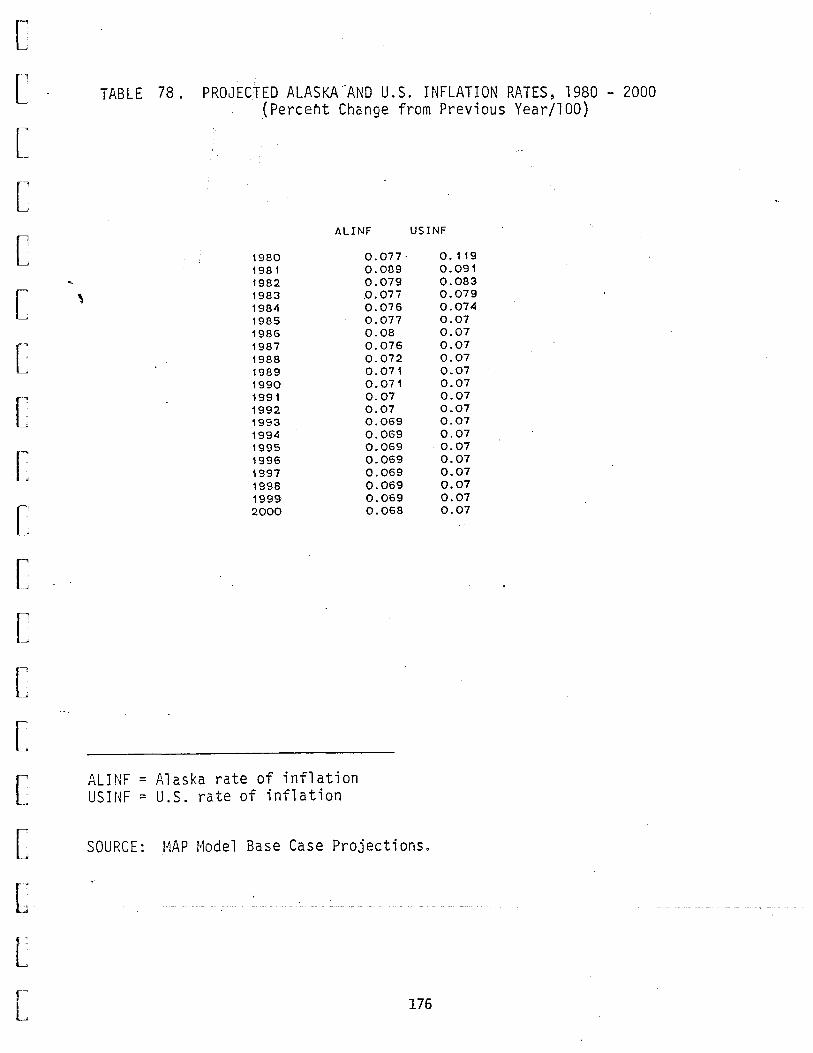
b [ r~

L

TABLE 78. PROJECTED ALASKA.-AND U.S. INFLATION RATES, 1980 - 2000 (Perceht Change from Previous Year/100)

ALINF

1980 1981 1982 1983 1984 1985 1986 1987 1988 1989 1990 1991 1992 1993 1994 1995 1996 1997 1998 1999 2000

ALINF = Alaska rate of inflation USINF = U.S. rate of inflation

0.077· 0.089 0.079 .0.077 0.076 0.077 0.08 0.076 0.072 0.071 0.071 0.07 0.07 0.069 0.069 0.069 0.069 0.069 0.069 0.069 0.068

USINF

0. 119 0.091 0.083 0.079 0.074 0.07 0.07 0.07 0.07 0.07 0.07 0.07 0.07 0.07 0.07 0.07 0.07 0.07 0.07 0.07 0.07


176

TABLE 79 PROJECTED STATE GOVERNMENT REVENUES: ALASKA, 1980 - 2000

(Millions of Dollars)

-

RSGF.81 RP9S.81 RSFD.81 RSIN.81 RSNP.81

1980 2692.22 2014.95 345.618 123.388 553.878 1981 4 192. 1 3726.33 363.311 208.062 257.706

' 1982 5054.43 4164.37 306.687 281.427 608.626 1983 5367.86 4297.47 406.963 427.582 642.812 19!34 5879.05 4649.52 427.574 555.758 673.77 1985 6673.3 5269.06 460.254 676.658 727.584 1986 7426.45 5752.89 501.409 855.013 818.545 1987 8020. 16 6092. 522.459 1051. 22 876.948 19!38. 7911.4 5776.34 526.634 1248.37 886.692 1989 8459.53 6165.5 530.606 1411.77 882.267 1990 8109.96 5630. 15 533.6 1604.5 875.308 1991 7798.32 5154.3 543.126 1763.06 880.963 1992 7541.41 4758. 18 553.048 1889,_14 894.096 1993 7673.88 4773.89 564.856f 1989.98 910.004 1994 7392.73 4377.32 577.337' 2087.26 928.153 1995 7008.22 3907.81 591 .025 2150.64 949.773 1996 6689.39 3541.56 605.499 2174.19 973.645 1997 6602.4 3439.79 620.242 2163.84 998.781 1998 6355.28 3192.31 635.488 2138.02 1024.95 1999 6077.07 2938.51 651.166 2086.07 1052.49 2000 5788.25 2698.28 668.265 2007.42 108.2. 56

RSGF.8l = Total state government revenues (millions of 1981 dollars) R?95.81 = Petroleum revenu~s (millions of 1981 dollars) RSFD.8l = Federal grants (millions of 1981 dollars) RSIN.8l = Interest earnings (millions of 1981 dollars) RSNP.8l =Non-petroleum revenues (millions of 1981 dollars)

SOURCE: MAP Model B~se Case Projections.

177

[

[

[

[

[

[

[-: "

[

c [

[

[

[

[

[

[

6 [ r-· L

r.>

I_~

[

[

[

[

[

[

[

c [

[

[

[

[

[

[

'

(RSFD.81), interest earnings (RSIN.81), and non-petroleum revenues

(RSNP.81). Non-petroleum revenues include federal grants; thus, total

state revenues are the sum of petro 1 eum revenues, interest earnings,

and non-petroleum revenues. Total revenue grows steadily from 2. 7

billion dollars in 1980 to a peak of 8.5 billion dollars in 1990, and

declines steadily thereafter to 5.8 billion dollars in 2000. The bulk

of these revenues are accounted for by petroleum revenues. These peak

in 1989 at 6.2 billion dollars, and decline through the year 2000 to a

level of 2.7 billion dollars.

Receipts from the Federal government increase throughout the period,

from .3 billion dollars in 1980 to • 7 billion dollars in 2000. In-

terest earnings rise from .1 billion dollars in 1980 to nearly 2.2

bi 11 ion do 11 ars in 1996, and then begin to dec 1 i ne. Other revenues

(RSNP.81 -RSFD.81) increase from .2 to .4 billion dollars over the

period.

Expenditure data are presented in Table 80 and include total State

government real expenditures (E99S.81) and real per capita expendi-

tures (ESPC.81). Total expenditures grow at 6.3 percent over the

entire period and at 10.4 percent for the first 10 years. During the

1990s the rate is considerably lower at 2.3 percent.

Growth of real per capita expenditures is very rapid at 70 percent per

r ' year over the period 1980-1983. Thereafter expenditures fluctuate -6-~------~--~------~---~----~--~-~~-----~

[

[

between 7900 and 9600 dollars per capita.

178

\

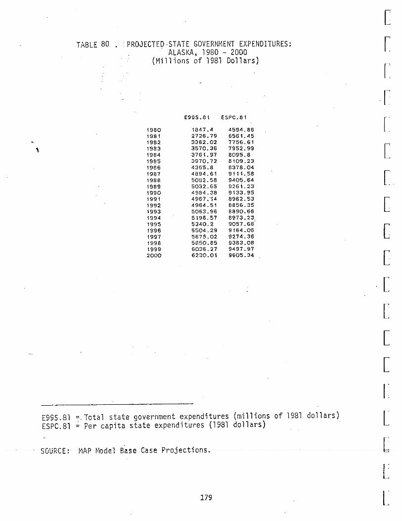
TABLE 80 ~ ·PROJECTED STATE GOVERNMENT EXPENDITURES: ALASKA, 1980 - 2000

(Millions of 1981 Dollars)

E99S.81 ESPC.81

1980 1847.4 459.4. 86 1981 2726.79 6561.45 1982 3362.02 7756.61 1983 3570.36 7952.99 1984 3761.97 8095.8 1985 3970.72 8109.23 1986 4365.8 8378.04 1987 4894.61 9111..58 1988 5082.58 9405.64 1989 5032.65 9261;23 1990 4984.38 9133.95 1991 4967. "14 8982.53 1992 4964.51 8856.35 1993 5063.96 8890.66 1994 5196.57 8973.23 1995 5340.2 9057.66 1996 5504.29 9164.06 1997 5675.02 9274.36 1998 5850.85 9383.08 1999 6036.27 9497.97 2000 6230.01 9605.34

E99S.81 =.Total state government expenditures (millions of 1981 dollars) ESPC.8l = Per capita state expenditures (1981 dollars)

[

[

[

.r [

[

[

[

[

[

[

[

[

[

[

[

--~ --- --- · -5{Jtl·R.-er:----r•'rAP~t,'ro-d-el--B-a-se---c-a-s-e-_:Pr-o-j ee-t-i-on s--.------~-~----- -------- --------· ----- ----- --------------- ~-[ ----

179

l rL

[

[

[

[

[

[

[

[

[

[

[

[

[

[

[

[

'

As shown in Table 81, the permanent fund balance peaks in 1995 and

declines thereafter. This downturn occurs when the decline in the

value of the fund, due to inflation, begins to exceed the increase in

value due to additions to the fund and reinvested interest earnings.

THE MAP REGIONAL BASE CASE PROJECTIONS: ANCHORAGE

The MAP regional model base case projections for Anchorage are shown

in Table 82. The Anchorage population is projected to rise from

179 thousand in 1980 to 286 thousand in 2000, resulting in an overall

growth rate of 2.4 percent. The growth rate is higher during the

first decade (3.0 percent per year) than the second decade (1.8 per

cent per year). Total employment rises slightly faster than popu-

lation (2.6 percent per year). However, employment declines slightly

from 1988 to 1990. Support sector employment rises from 49.3 percent

to 53. 4 percent of tota 1 emp 1 oyment, basic sector emp 1 oyment rises

from 14.4 percent to 16.7 percent of total employment, while govern-

ment employment falls from 36.4 to 29.8 percent of total employment.

THE MAP REGIONAL BASE CASE PROJECTIONS: BRISTOL BAY

MAP regional model projections for Bristol Bay are shown in Table 83.

Population is projected to increase from 5,185 in 1980 to 6,378 in

2000, or at a rate of only 1. 0 percent. Total employment grows only

slightly faster, at a rate of 1.3 percent. The share of basic sector

employment in total employment is projected to fall from 46.6 percent

[_ ____ ~·~ to 39.2 percent;. the · ~ -ffie-nt~Tsprojected~-to

share of government employment in total employ-

rise from 31.6 percent to 37.1 percent; and the

L I' L

180

\

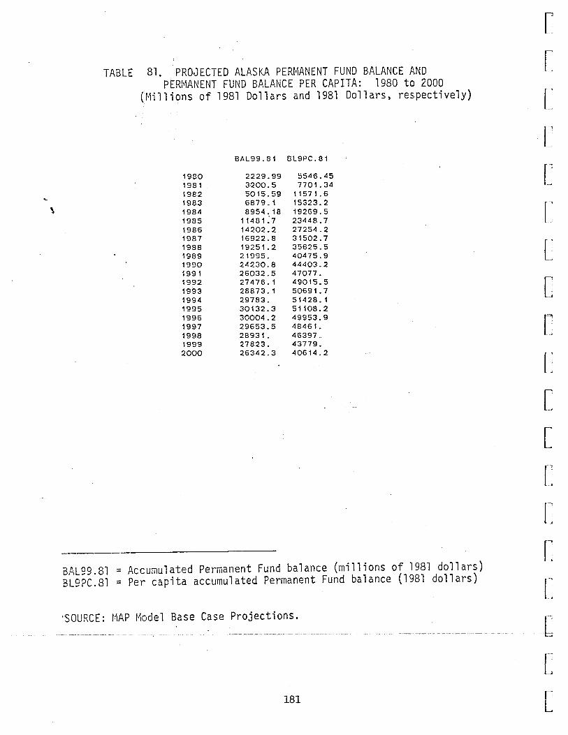
TABLE 81. PROJECTED ALASKA PERHANENT FUND BALANCE AND PERMANENT FUND BALANCE PER CAPITA: 1980 to 2000

(Millions of 1981 Dollars and 1981 Dollars, respectively)

BAL99.81 BL9PC.81

1980 2229.99 5546.45 1981 3200.5 7701.34 1982 5015.59 11571.6 1983 6879. 1 15323.2 1984 8954. 18 19269.5 1985 11481 ~7 23448.7 1986 14202.2 27254.2 1987 16922.8 31502.7 1988 19251.2 35625.5 1989 21995. 40475.9 1990 24230.8 44403.2 1991 26032.5 47077. 1992 27476.1 49015.5 1993 28873.1 50691.7 1994 29783. 51428.1 1995 30132.3 51108.2 1996 30004.2 49953.9 1997 29653.5 48461. 1998 28931. 46397. 1999 27823. 43779. 2000 26342.3 40614.2

BAL99.8l = Accumulated Permanent Fund balance (millions of 1981 dollars) BL9PC.8l = Per capita accumulated Permanent Fund balance (1981 dollars)

~OURCE: MAP Model Base Case Projections.

181

[

[

[

[

[

[

[

[

[

[

[

[

[

[

r-~

-.

[

[

[ rL

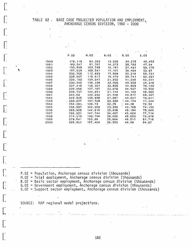
c [

[

[

[

[

[

[

[

[

[

[

[

[

[

[

[

[ r" L

'

P.02 = !~. 02 = 8.02 = G.02 = 5.02 =

TABLE 82 . BASE CASE PROJECTED POPULATION AND EMPLOYMENT, ANCHORAGE CENSUS DIVISION, 1980 - 2000

P.02 M.02 6,02 G.02 5.02

1980 179.118 94.262 13.532 34.276 46.453 19 !3 1 183.547 97.707 14.373 35.793 47.54 1982 190.959 103.788 16.191 37.421 50. 176 1983 197.529 108.541 17. 107 38.464 52.97 1984 202.70!3 112.868 17.929 39.218 55.721 1985 209.807 119.617 19.479 . 39.741 60.397 1986 220. 193 129.547 21.852 41.238 66.457 1987 230.3115 136.328 23.056 43 .. 926 \)9.3116 1900 237.418 138.367 22.665 44.969 70.733 1989 239.566 137.107 22.078 44.527 70.502 1990 239.737 134.851 21.744 44. 145 68.962 1991 243.02 135.232 21.94 8 43.817 69.467 1992 245.945 135.938 21.887 44.041 70.011 1993 250.077 137.706 22.289 'i 44.174 71. 244 1994 254.281. 139.73 22.75 44.46 72.52 1995 258.997 142.202 23.286 44.785 7 4. 132 1996 263.903 144.916 23.838 4 5. 194 75.885 1997 268.921 147.744 24.407 45.624 77.714 1998 274.213 150.756 25.028 46.052 79.676

"1999 279.641 153.89 25.664 46.511 81.716 2000 285.621 157.404 26.353 46.98 84.07

Population, Anchorage census division (thousands) Total employment, Anchorage census division (thousands) Basic sector employment, Anchorage census division (thousands) Government employment, Anchorage census division (thousands) Suppo1~t sector employment, Anchorage census division (thousands)

SOURCE: MAP regional model projections.

182

'

\

TABLE 83. BASE CASE PROJECTED POPULATION AND EMPLOYMENT, BRISTOL BAY REGION, 1980 - 2000

P.OG M.OG 8.06 G.06 5.06

19130 5. 1!35 3.832 1. 784 1. 21 0.!339 19131 5. 248 3.923 1. 795 1. 286 0.843 19!32 5.301 4.046 1.815 1 .368 0.863 1983 5.359 4. 136 1. 827 1. 42 0.889 1984 5.39:2 4.216 1.837 1. 4 57. 0.922 1905 5.366 4.296 1.857 1. 483 0.957 1986 5.384 4.448 1.887 1. 558 1.003 1987 5.59 4.646 1. 902 .. 1. 694 1.05 1988 5. 776 4.727 1. 897 1. 746 1.084 1989 5. 841 4.695 1.889 1. 722 . 1.084 1990 5.886 4.65 1. 884 1. 701 1.065 1991 5.917 4.624 1. 884 1.682 1. 058 1992 5.974 4.637 1. 883 ·, 1. 692 1 .062 1993 6.02 4.656 1.887 1.697 1.071 1994 6.07 4.684 1.892 1. 71 1. 081 1995 6. 11 a 4.717 1.898 1.725 1. 094 1996 6. 169 4.757 1. 905 1. 745 1. 108 1997 6.221 4.8 1. 912 1.765 1. 123 1998 6.272 4.843 1. 919 1. 785 1. 139 1999 6.325 4.889 1. 926 1.807 1. 155 2000 6.378 4.936 1. 935 1. 83 1. 172

P.06 = Population, Bristol Bay Region {thousands) M.06 = Total employment, Bristol Bay Region (thousands) B.06 = Basic sector employment, Bristol Bay Region (thousands) G.06 = Government employment, Bristol Bay Region (thousands) S.06 = Support sector employment, Bristol Bay Region (thousands)

SOURCE: MAP regional model projections.

183

[

[

[

[

[

·[

[

[

c [

[

[

[

[

[

[

[

[ rL

[

[

[

[

[

[

[

[

c [

[

[

[

[

L [

share of support sector employment in total employment is projected to

rise from 21.9 percent to 23.7 percent.

THE SCIMP MODEL BASE CASE PROJECTIONS: THE ALEUTIAN ISLANDS

This section discusses the SCIMP base case projections of employment

and population in the Aleutian Islands. In the tables, years 1-20

' represent the years 1981 to 2000.

Basic sector employment projections from 1981 to 2000 are summarized

in Table 84. Total exogenous employment rises from 2,656 to 9,145, a

growth rate of 6. 7 percent. All of this growth is the result of

expansion in the bottomfish industry. The share of enclave employment

in total employment falls from 81.9 percent to 58.5 percent, reflect-

ing the assumption built into the bottomfish employment projections of

a rising resident share.

Projected government employment is shown in Table 85. Total govern-

ment emp 1 oyment rises from 3, 294 to 4, 284. Most of the increase

results from an increase in state and local government employment from

410 to 1,329. This increase is proportional to the increase in resi

dent population.

Table 86 summarizes total employment. Support sector employment-

equal to basic sector and government employment multiplied by employ-

[ ' ment multipliers, rises from 459 to 1,547, at a rate of 6.6 percent

-- -- - - - - -- - -- -- ---- --- --------- -- -- --·-------

[ f' L

per year. Total employment rises from 6,410 to 14,975, at a rate of

184

\

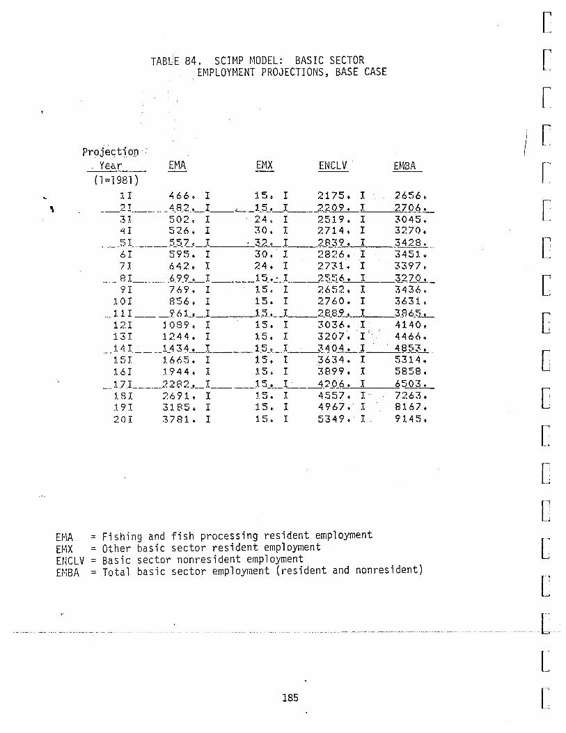
TABLE 84. SCIMP MODEL: BASIC SECTOR EMPLOYMENT PROJECTIONS, BASE CASE

Projecti~m -. YEa. r H1A EMX ENCLV . EMBA

Eiv1A H1X ENCLV HiBA

(1=1981)

1! 466. I 15, I 2175. I 2656. __ 2 I_ __ -· _ 4_8_2 .• _.I __ ,_ __ 1 __ ;;_,_J. ____ 2_? 0 9 • I 2 ~g_q__. _

31 502. I · 24. I 2519. I 3045. 4I 5'26. I 30. J. 2714. I 3270.

. ___ 5 I .. _____ !:!..5_Z._c_J · ~~-t._J __ _.?~-~9. I 34 28. 6 I 595 • I 30 •. I 2826. I 3451. +

7I 642~ I 24. I 2731. I 3397. -·-- 8 L ___ ..... 6 9_9_c:_l _____ 15_._:_l_. ___ 2~_!:!.6_t___]: __ ~270.....!._

9! 769. I 1.5. I 2652. I 3436. 10! 856. I 15. I 2760. I 3631.

___ 11 I ___ 96 l.__. _ _r ___ l_5 __ • __ I ___ 2JL8..9_, _ _! 3.B6.~

12I l089. I 15. I 3036. I 4140. 13I 1244. I 15. I 3207~ r·· 4466. 14 I _____ 1_4 3 4_t-_J_ ______ 1_5_. __ ) ____ ~4. 0_1_. .J. 4 a.~.::.~-L . 15I 1665. I 15. I 3634. I 5314. 16J 1944. I 15. I 3899. I 5858.

__ 17_1_ ______ .2282_._l _____ _l5_. ____ I ___ ___1_2_0_6. I 65_Q~_!_

18I 2691. I 15. I 4557. I' 7263. 191 3185. I 15. I 4967. I 8167. 20I 3781. I 15. I 5349.· I. 9145.

= Fishing and fish processing resident employment = Other basic sector resident employment = Basic sector nonresident employment = Total basic sector employment (resident and nonresident)

185

[

[

[

I L '

[

[

[

[

c [

[ '

[

[ f'

L

[

[

[

[ ,~

L

' ' --'

n I

L TABLE 85. SCIMP MODEL: GOVERNMENT EMPLOYMENT PROJECTIONS, BASE CASE

r l~

[

[

[ '

[

[

[

[

[

[

[

[ _.

[

[

[

[ r~

L

'

Projection Year

( 1 =1961) EHL FGVT EMIL EMGT ~

__ 1 L -·· _ A:i.O • ___ I _____ .7_1_Q_._~_J _____ 2_1Z;u-~_1 ___ 1?94...L 2I · 429. I 713. I 2175. I 3317. 31 443. I 717. I 2175. I 3334. ~I 460. I 720. I 2175. I 3356.

-· ·- - -··--. 47·8-~·- I--·--···-i:?.-1·.---~------21"75·.-I-. ·-i3-7"7:-5I C. I -r I.

81 9I

~-OJ: 1.11

496. I 727. I 21Z5. I 3399. 515. I 731. I 2175. I 3421. 535. I 735. I 2175. I 3444. 556. I 738. I 21.75. I 3470. 58:1.• __ _I ______ ]4.~_. ___ I ____ ~.tz_~_. _ _j ____ ;3l!_Q.~_. 6 'J. 6. I 746. I 2175. I 3537.

121 654. I 750. I 2175. I 3578. 131 _____ .. 697. __ ~ ..... 75?.! __ I ______ _!~ __ 1_?~_.L_I __ lo?.?_~_!_ 14I 748. I 757. I 21.75. I · 3680. 15:i:. 808. I 761. I 2l75. I 3744. :i 6I . . ... 880 __ • __ J ______ .. 7 65. _ _I·-·_ -~_1]_5 • __ __l-___ ~.§2_9 __ ~ l7I 965. I 768. I 2175. I. 3908. 18I 1065. I 772. I 2175. I 4~13.

~- 'l'I U 85 •. I __ 776. I _____ 21?:5!..._~-------~1.}.?.!.. _ _ :;: 0 I 'J. 3 2 9 • I 7 8 0 • I 2 1 7 5 • J. 4 2 8 4 • ---+----------+----------+-----~----+----------

EML = State and local government employment (all resident) FGVT =Federal govel~nment civilian employment (all resident) EMIL= F,ederal government military employment (all resident) ElltGT = Tot a 1 g_o\l_e~~m~'rl_t_ ~m_p_lgyrn_~nt_j(i ll re_sjd_ent)_ ____ _ __

186

'

TABLE 86. SCIMP MODEL: EMPLOYMENT PROJECTIONS, BASE CASE

projection Year

(1=1981) u: 2I 3I 4J: 5I 6I 7J. 8J: 9I

J.OI U. I L;-~r

~- 3 I 14I 15I l.6I 17I l8J: :1.9I 20I

H1BA 2t'>56. I 2706. I 3045. I 3270. :r: 3-428~ :r: 34 51 •. I :3397. I 327 0. I 3436. I 3t?31. I 3865 ~ :r: 4140. I 4466. I 4853 ., I 53:1.4. I 5858) :r: 6503. I 7263. I 8167. I 914~j. :r:

Ef~GT EMS ·---~-- ·----- EMT_T

3294. I 459. I 6410. 3317. I 469. I 6492. 3334. I 485. I 6864. 3356 ~-··I--·---· -:Soo-:--I----7126-: 3377. I 516. I 7321. 3399. I 530. I 7380. 3 4 2 :1. • I -·------·54 ·C ·--I- - -~·-7-3 6.2 ;-3444. I 560. I 7274. 3470. I 585. J. 7490.

. -- -·-· -- -·-. ··--·····--· --- --------3501. I 615. I 7747. 3537. I 652. J. 8054. 3578. I 695. I 8414. 3625 ~-· I---··-· --7 47·:---f----rf839; ·-3680. I 810. J. 9343. 3744. r ; 885. r 9943.

... -----· ------------- ··---3820. I 975. I 10652. 3908. I 1082. I 11494. 4013. I 1211. I 12487. 41 37. I 1 ~c-6 -~-·-·r-·-· -·- i 36"6 9 ;-4284. I 1547. I 14975.

EMBA = Total basic sector employment (resident and nonresident) EMGT = Total government employment (all resident) EMS = Total support sector employment (all resident) EMTT = Total employment (resident and nonresident)

187

[

[

[

[

[

[

[

[

c [

[

[

[

[

[

[

[ __

[ rL

[

[

[

[

[

[

[

[

[

[

[

r~

[

[

[

[

[ ________ -

L r-L

4.6 percent per year. Resident civilian employment (not shown in the

table) rises from 2,060 to 7,452, at a rate of 7.0 percent per year.

Different measures of population are shown in Table 87. The civilian

resident population rises from 4,530 in 1981 to 15,825 in 2000 as a

result of increased resident bottomfish employment. This represents a

rate of population increase of 6.8 percent per year. Enclave popu-

lation (which includes nonresident fishermen) rises from 2,175 to

5,349, at a rate of 4.9 percent per year. The total population of the

region, including military and military dependents as well as enclave

workers, rises from 10,620 to 25,089, a growth rate of 4.6 percent per

year.

188

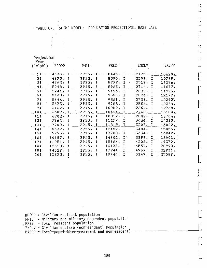
·TABLE 87. SCIMP MODEL: POPULATION PROJECTIONS, BASE CASE

Projection Year

( 1 =1981) BPOPP

----1 I.- __ 4530 •. I 21 4675. I 3I 4862. I

_ 4 L _____ 50 4 8 • I 5J. 5243.. I 6I 5438. I 7I 5646. I 81 5873. I 9I ld. 6 7 ~ I

10I 6509. I .. -·-- -- ..

U. I 6902. T. 12I 7362 •. I

- - :t.3I . -- 7900. J :1.4! 8537. r 15I 9293. I

__ :1.6 L _ 10:1.87+ I 17I 1~.251.. I 18T. 125:1.8. I 19:1 .... 14029. J 20! 1.5825~ I

PMIL PRES. ENCLV BASPP

___ 3915 •.. .J: ____ 9445_._1 _____ . 2175 .___r ____ t 0620 ._ 39:1.5. I 8590. I 2209. I 10799. 3915. I 8T77 •. I ~ 2519c I 11296. 39 t 5 ._. L ____ 8963 ._ __ 1.. _____ 2714 •.. L __ 116 77 •.. 39:1.5. I 9:1.56. I 2839. I :1.1995. 3915. I 9353. I 2826. I 12179. 3915. I 956:1.. I 2731. I 12292~ 391.5. I 9788. I 2556. I 12344. 3915. J. 10082. I 2652. I 12734. 39 _15 .___:r, ___ 1_Q~_2_4_._I ____ 2Z60_• _ _I ____ 13184 .__ 3915. I 1.0817~ I 2889. I 13706. 3915. I 11277. I 3036. I 14313. 3915 ·---~--ttl;!lfiJ __ J ___ 3?J>7_. __ :t_ ___ 15022 ._ 3915. I :1.2452. I 3404. T. 15856. 3915. I 13208. J - 3634. I 16842. 391.5. _ r_ __ J. .11. q_z_. .r_· ____ 3899 • __ .r.. ______ .l8oo :t_. __ 3915. I 15166. I 4206. I 19372. 39:1.5. I 16433. I 4557. I 20990. 3 91. ~ • __ I ________ _12.9._4_4_. ___ ! ______ 49 6 7__. __ I ___ 22 ~ 11_. _ 3915. I 19740. I 5349. I 25089.

BPOPP =Civilian resident population PMIL =Military and military dependent population

rPRES =Total resident population ENCLV = Civilian enclave (nonresident) population

----------- --B-~S-PP- =-"Fo ta-1-po p u-}at+o n-~+re s+dent--and-n o nres-id ent-)

189

[

[

[

[

[ [~

[

[

[

[

[

[

[

[

[

[

[ __

l rL

[

[

l~

[

[

[

[

['

[

[

[

[

[

[

L [

[

l [

IV. PROJECTED IMPACTS OF THE NORTH ALEUTIAN SHELF SALE

In this portion of the report, we describe the six North Aleutian

Shelf OCS sale cases and their projected impacts. Projections of sale

impacts are developed by adjusting the non-OCS base case assumptions

to include direct OCS impacts (primarily employment) and rerunning the

models. The differences between the new projections and the base case

projections represent the combined direct and indirect impacts of OCS

development. We present tables of both absolute impacts (i.e.,

increases in employment) and percentage impacts (i.e., percentage

changes in employment).

The OCS Sale Cases

We analyze the impacts of six different OCS cases, which we refer to

as the low, mean, high, alternative four, mean offshore loading, and

alternative four offshore loading cases, respectively. All of these

cases assume that some oil and gas resources are discovered and

developed. Given this assumption, the low case assumes a level of

resources that will occur with 95 percent probability, the mean case

assumes a level of resources that will occur with 50 percent proba-

bility, and the high case assumes a level of resources that will occur

with only 5 percent probability.

For all of the cases, the Alaska OCS office provided estimates of

employment in different activities for the exploration, construction,

and operations phases of OCS development. This information is repro-

duced in Appendix C. In order to use these employment figures in the

190

MAP and SCIMP models, it was necessary to make assumptions about the

share of employees who would be Alaska residents, and the share who

would be residents of the Aleutian Islands. These assumptions are

discussed in Appendix C. Table 88 presents resident Alaskan OCS

emp 1 oyment for each case. These figures were uti 1 i zed for the MAP

model projections. In the mean case, resident Alaskan employment

rises from 103 in 1984 to 2,072 in 1989, and then declines to a level

of 1, 597 in 1994, remaining at this 1 eve 1 for the rest of the pro-

jection period. In the low case, maximum employment of 597 is reached

in 1987, declining to a constant level of 492 after 1992. In the high

case, maximum employment is 3,436 in 1990, declining to a constant

level of 2,635 after 1996. In the alternative four case and the mean

offshore loading cases, employment levels are approximately 80 percent

of the mean case levels. In the alternative four offshore loading

case, employment levels are approximately 60 percent of the mean case

levels.

Tables 89-94 present Aleutian Islands onshore resident and enclave OCS

employment associated with each case. These figures were utilized for

the SCIMP model projections. In the mean case, local resident employ

ment rises to 161 by 1991, and thereafter remains constant throughout

the projection period. Maximum local resident employment is 53 for

the 1 ow case, 305 for the high case, 127 for the alternative four

case, 119 for the mean offshore loading case, and 95 for the alterna-

[

[

[

[

[

[

t [

[

[

[

[

[

[

[

[

--------~---- . t i v: _fo~--~-~f=ho~y-_e_~~a~ i ~~-case_. -. -. ___________ -. -. ------·----------·----------·-----··--- ____ [ __ _

191

[ rL

L_"

"

i"

[

[

[

[

[ear 1980

[

1981 1982 ~983

1984

[~~:~ 1987 1988 1989

[

'1990 1991

j1992 1993

[

1994 1995 ~996

1997 1998

[1999 2000 ~

[

[

[

L-----, L r " L

t~ean Case

0. 0. 0. o. 0.103 0. 134 0.687 1. 041 1. 781 2.072 1. 738 1. 613 1. 584 1.592 1. 597 1.597 1. 597 1. 597 1. 597 1. 597 1. 597

TABLE 88. NORTH ALEUTIAN SHELF OCS RESIDENT ALASKAN EMPLOYMENT ASSUMPTIONS FOR MAP MODEL PROJECTIONS

(Thousands) ·

~1ean Case Low High Alternative Offshore Alternative IV Case Case Case IV Case Loading Offshore Loadino --. -· - 0. 0. o. 0. o.

0. 0. 0. 0. 0. 0. 0. 0. 0. 0. 0. 0. 0. 0. o.

0.061 0. 158 0.087 0. 103 0.087

0.067 0.205 0.106 0. 134 0. 106

0.38 0. 19 0.395 0.687 0.395

0.597 0.664 0.829 1 .041 0.829

0.488 1. 619 1. 579 1.588 1. 444

0. 429 2.715 1. 54 1 1.767 1. 347

0.453 3.348 1.3 1. 441 1. 101

0.461 3.436 1.237 1.215 0.958

0.492 3. 132 1. 248 1. 224 0.968

0.492 2.611 1. 257 1. 232 0.977

0.492 2.623 1. 26 1. 237 0.98

0.492 2.63 1. 26 1.237 0.98

0. 492 2.635 1. 26 1.237 0.98

0.492 2.635 1. 26 1. 237 0.98

0.492 2.635 1. 26 1. 237 0.98

0.492 2.635 1. 26 1. 237 0.98"

0.492 2.635 1. 26 1. 237 0.98

SOURCE: Alaska OCS Office; residency assumptions presented in Appendix C.

192

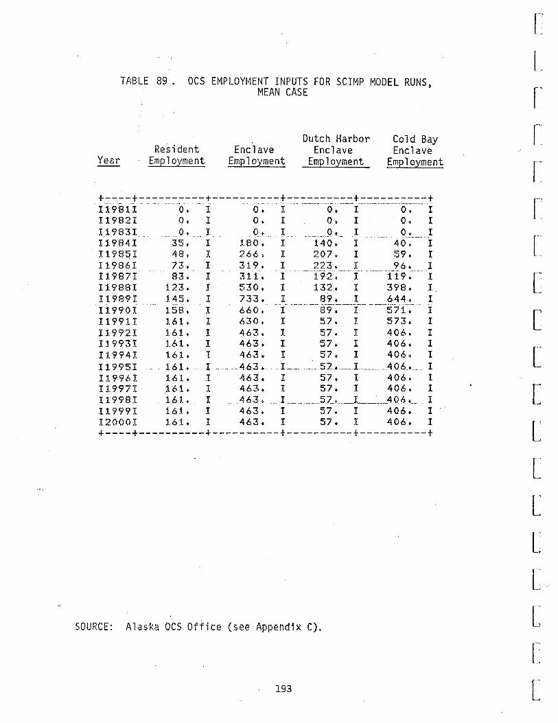
Year

TABLE 89 . OCS EMPLOYMENT INPUTS FOR SCIMP MODEL RUNS, MEAN CASE

Resident Employment

Enclave Employment

Dutch Harbor Enclave

Employment

Cold Bay Enclave

Employment

+----+----------+----------+----------+----------+ ··-· ··- ~~--- ··- .. ······- --- ~- - ---- - --------- . - ------ ------------------------I1981I O. I O. I O. I o. I I1982I o~ I O. I 0~ I O. I I 1983 I.. 0 •.... J Q •. I.. ______ , _ _(_)_. ___ L_ ____ Q_!___ I I1984I 35. I 180. I 140. I 40. I I1985I 48. I 266. I 207. I 59. I I1986I 73. I 319. I 223. I 96. I ····--------------. ----------- ------ ---- ._. .. ___ . I1987I 83. I 311. I 192. I 119. I I1988I 123. J 530. I 132. I 398. I I1989I 145. I 733. I 89. I 644. I

---- ---- --- ----·------ --------------- ---------.---- - -.

I1990I 158. I 660. I 89. I 571. I 119911 161. I 630. I 57. I 573. I I1992I 161. I 463. I 57. I 406. I I1993I 161. I 463. I 57. I 406. I I1994I 161. I 463. I 57. I 406. I I1995I - .. 161. I - .. 463. ! ___ --52 .•. _ _! ______ __4_0_6_.__ I I1996I 161. I 463. I 57. t 406. I I1997I 161. I 463. I 57. I 406. I I1998I 163.. .. I 463. _I _______ 5_7_. ___ I_ _____ _40..St.._ I I1999I 161. I 463. I 57. I 406. I I2000I 161. I 463. I 57. I 406. I +----+----------+----------+----------+----------+

[

[

[

[

[

[

[

[

[

[

[

[

[

[

[

r· ,. ---s-otJRCc-:-A-n-s"l(a-ocs-orfi_c_e_(_s_e_e_A_p_pe-rrcnx-c). [_

193

[ rL

~

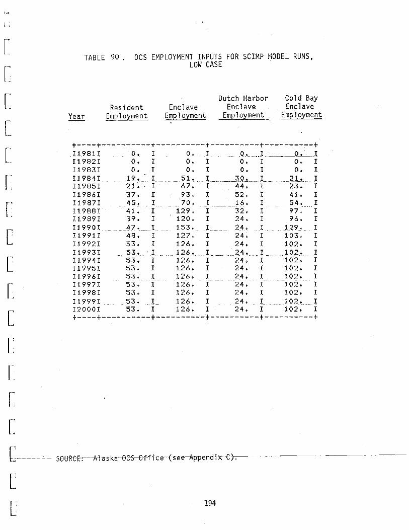
I"

l~

[

[

[

[

[

[

[

[

[

[

[

[

[

[

TABLE 90 . OCS EMPLOYMENT INPUTS FOR SCIMP MODEL RUNS, LOW CASE

Year Resident

Employment Enclave

Employment


Employment

Cold Bay Enclave

Employment

~----~----------T----------~----------+----------+ I :1. ~ 81 I . ___ ·- _ 0 • I 0 • . _ I _ ---·· ____ O_t. __ _I ____ Q_!_ __ _I I1982I 0. I O. I O. I 0. I I:l983I O. T O. I O. I 0. I I 1 9 8 4 I 1 9 • __ I _ _ 5 1 • __ ~------· __ 3 __ Q _ _t ____ I.____ . ___ 2J_._ _ _ I Il.985I 21.- I 67. I 44. I 23. I I1986I 37• I 93. I 52. I 41. I I l. 987 I . __ 4_5 ~ _ I _ . ____ 70. · __ ,I ________ t 6.!. I _____ 54~--- I I:l988I 41. I 129. I 32. I 97. I I1989I 39. I 120. I 24. I 96. I Il990I _______ .:l?• ______ I ___ 1.53. I ______ 24. I _ _1_2,9_._ I I1991I 48. I 127. I 24. I 103. I Il992I 53. I 126. I 24. I 102. I I 1 9 9 3 I .. . _ _ 5 3.. I _ . 1 2 6 • I _ ___ _ _ . 24 ~ .. J ________ 1 0 :2..!. _ I I1994I 53. I 126. I 24. I 102. I I1995I 53. I 1.26. I 24. I 102. I I1996I 53. I 126. I 24. I 102. I

<- ••• --~-- - -------- -- ·-······ ··- -- ··-·· ••••

119971 53. I 126. I 24. I 102. I I1998I 53. I 126. I 24. I 102. I I1999I. . .. 53 •... L 126. I 24. I ________ 102. ___ I 12000I 53. I 126. I 24. I 102. I +----+----------+----------+----------+----------+

-L------'- --&Ol:JReE:---A-1-a-s-k-a-GeS-Gf-f-i-ce-fs-ee-Appendi-x-e-) ~ ~~~~-----

L r- 194 L

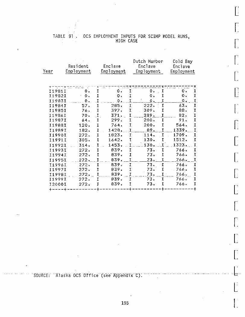
Year

TABLE 91 . OCS EMPLOYMENT INPUTS FOR SCIMP MODEL RUNS, HIGH CASE

Resident Employment

Enclave Employment


Employment

Cold Bay Enclave

Employment

T---- T. --: .. ::_=_:--=-. .::: :~ -:·.-- T ··:.-::-:---- -::_- :-:." "".::.T -:".=-==--=-=-=-=-=--=-.J. . .::.::.:-..=_-.::_:-___-:::.':- T

I1981I O. I O. I O. I O. I I1982I O. I O. I O. I O. I I 1 9 8 3 I ___ .... 0. I ... ___ 0 • ___ I _____ ~:_ _____ O •---~'(_ ________ j). _ I I1984I 57. I 285. I 222. I 63. I I1985I 76. I 397. I 309. I 88. I I1986I 70. I 371. .. I _____ 28Cf_._ ___ L ______ ~?.•_ I I1987I 64. I 299. I 208. I 91. I I1988I 120. I 764. I 200. I 564. I I1989I :1.82 •. I :1.428. ___ _I ______ B_~!.._J,_ ___ l_:}~_<[. ____ I __ I1990I 272. I 1823. I 114. I 1709. I I199:1.I _305. I 1642. I 130. I 1512. I I 19921 ___ 314. _ L __ . 1453 •- __ 1 ____ 1.30 .• __ :( ___ 1323_. _____ I I1993I 272. I 839. I 73. I 766. I I1994I 272. I 839. I 73. I 766. I I 1995! . 272 • __ I. 839. ___ I. ____ Z3. ___ ! _____ ]6/:o. ___ I I1996I 272. I 839. I 73. I 766. I I1997I 272. I 839. I 73. I 766. I I1998I 272. I ..... 839. _l _______ l.:.1+ _____ L ________ ]6g_.__ I I1999I 272. I 839. I 73. I 766. I I2000I 272. J 839. I 73. I 766. I +----+----------+----------+----------+----------+

[

[

~

r~

[

['

[

[

[

[

[

[

[

[

[

[

________ ·· __ SUORCF:--ATas-ka ~CS-OTfTce--(see.Appe-n-dTxCJ:---.-. -.-.. _-.. -. --------.------.-.. -~--------b-[

195 r-L

•

~~

L~

[

[

[

[

[

[

L l [

L r, L

TABLE 92 . OCS EMPLOYMENT INPUTS FOR SCIMP MODEL RUNS, ALTERNATIVE FOUR CASE

Year Resident

Employment Enclave

Employment


Employment

Cold Bay Enclave

Employment

+----+----------t----------T----------t----------T I1981J: o. :r. o. r o. e:r. o. I I1982I ___ - .. o. I e _ _ __ 0 •---- L _______ : _ _o_~-- L ______ e __ O_. ___ I I1983l o. :r. o. I o. I o. J I1984l 29. :r. 138. I 107. I 31. I Il985I 36. :r. :1.89 ·-- -• I__ e•--e••JAZ •. I 42. .. I :ti. 986 I 53, I 248. I 181. I 67. I I1987I 63. I 240. I '·50 ·• I 90. I I:1.988I ... 104. I. ____ 393 • __ !_ ____ 124 • :r. 269. I Il. 989 I Ul. I 493. I 73. I 420. I I1990I 122. I 462. I 73. I 389. I Il991I :1.24. I 44:1 .• I 48. I 393. I I:t.992:t: 127 <· I 368. I 48. I 320. I I1993:t: 127. I 368. I 48. I 320. J I1994I :1.27-. :r. 368. I 48. :r. 320. I __ ,_ ··-··· -··-

I1995I 127. I 368. I 48. :r. 320. I I1996I 127. I 368. I 48. I 120. I I1997I 127. :r. 368. :r. ___ 48 + I 32_0_. I I 1. 998I 127. I 368. I 48. I 120 ·• I I1999I 127. :t: 368. I 48. I 320. I I2000I 127. I 368. I 48. I 320. I +----~----------+----------+----------+----------+

SOURCE: Alaska OCS Office (see-Appenalx C).--

196

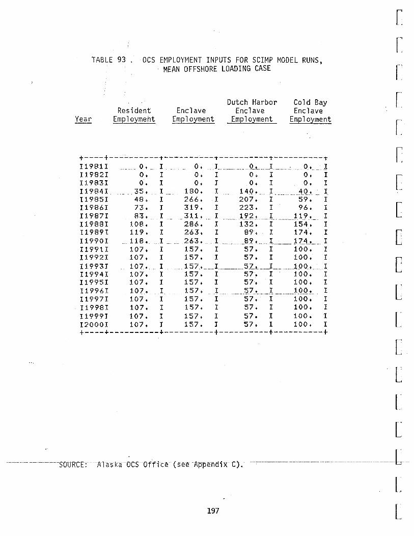
TABLE 93 . OCS EMPLOYMENT INPUTS FOR SCIMP MODEL RUNS, MEAN OFFSHORE LOADING CASE

Year Resident

Employment Enclave

Employment


Employment

Cold Bay Enclave

Employment

t----t----------T----------T----------T---~------T I1981I ····- .. o. I o. J __________ o_. _____ J __ _:_ _____ o_ .. __ ~

u. 982I o. I o. I o. I o. I I:I.983I o. I o. J o. I o. I I1984I --- . 35. ... I ---- 180. I ··-- _14_Q•----~------· _4_Q. -- I t1985I 48~ I 266. I 207. I 59. I I1986I 73. J 319. I 223. I 96. I I:I.987I 83. I .. 3:1.1. I _____ L?..? .. ~ __ t ______ __:l.1_'t• __ I I1988I :1.08. I 286. I 132. I 154. I I1989I U.9. I 263. I 89. I 174. I I1990I 118 •.. I ...... 263. ____ .I ______ a£.L ___ x __ t74_._ ___ I I1991I :1.07 + I 1.57. I 57. I 100. I I1992I 107. I 157. I 57. I 1.00. I Il993J 107. I . . :1. 57_. ____ L ______ 5Z.._. ___ I ________ 100.L _ _I I1994I :1.07. I :1.57. I 57. I :1.00. I I1995I 107. I 157. I 57. I 100. I I:I.996I 1.07. I :1.57 • ... I-- --- --~?-·----~ -- __ _:I.Q_Q! .. I I1997I 1.07. I l.57. I 57. I 100. I I:I.998I :1.07. I 157. I 57. I 100. I U. 999 J 107. I 157. I 57. I 100. I I2000I 107. J 157. J '57. I 100. I +----+----------+----------+----------+----------+

--------- - souRcE·:··-- 7rnrsRa ·ocs- Offfce-cs-ee·--,crp·p-enalx-c)~------------- ------- - -

197

[

[

[

[

[

[

[

[

[

[

[

[

[

[

[

[

_______ [ __

[ rL

'

L_~

[

[

[

[

[

[

[

[

[

[

[

[

[

[

[

[ f' L

TABLE 94. OCS EMPLOYMENT INPUTS FOR SCIMP MODEL RUNS, ALTERNATIVE FOUR OFFSHORE LOADING CASE

Year Resident

Employment Enclave

Employment


Employment

Cold Bay Enclave

Employment

+----+--~-------+----------+---------~+----------+ U981I '0. I o. I o. I o. I l1982I - · ·· 0.--- I------- --- 0. - I- - --------0 +---I --o. -----·I Il983I o. I o. I o. I o. I I1984I 29. I 138. I 107. I 31. I I1985I- ~~6 + -- I - · 1. 89. -- I---- --- -j.4 7+ · I ------ 42+ I I1986I 53. I 248. I 181. I 67. I I:I.987I 63. I 240. I l.50. I 90. I I1988J. ------- 95.--r ---- 260. --I------t24. I -- 136 + I I1989I 94. I 21.0. I 73. r. 137. I I1990I 94. I 210. I 73. I 137. I J.:I.991I - .... 85. I 1.30.: I 48. I 82. I Il992I 85. I 130. I 48. I 82. I I1993I 85. I 130. I 48. I 82. I J. :1.994 I---- - 85.--- I------ 130. - I------ -- · 48. I --- 82 • ·· I I1995I 85. I 130. I 48. I 82. I I1.996I 85. I 130. I 48. I 82. I I1.997I 85. - - I -- 130. I - -- 48.- I - -- 82 + I I:I.998I 85. I :1.30 + I 48. I 82. I r 1999 r 85. I 130. I 48. I 82. J. I2000I - 85. I 130. I 48. I 82 •. I +----+----------+----------+----------+----------+

SOURCE<-- /:1. las-ka- QCS -0-ffic::e--(-see Appendi-x- Gh- - - - -

198

In the mean case, enclave employment peaks at 733 in 1989, and falls

to a constant level of 463 by 1992. In the low case, peak enclave

employment of 153 occurs in 1990, falling to a constant level of 126

by 1992. In the high case, peak enclave employment is 1,823, falling

to a constant level of 839 by 1993. For the alternative four, mean

offshore loading, and alternative four offshore loading cases, re

spectively, peak enclave employment is 493, 319, and 260, falling

subsequently to constant levels of 368, 157, and 130.

In addition to generating employment, OCS development also results in

addi tiona 1 state revenues from property taxes on petroleum industry

facilities. Oil and gas property tax assumptions used- in the MAP

model projections are presented in Table 95. These assumptions are

based on estimates of taxable value of OCS facilities provided by the

Alaska OCS office.

[

[

[

[

[

[

[

[

[

[

[

[

r [

[

[

- -- -~ ~-- ~ --------- -~- _[ --

199

[ rL

...,

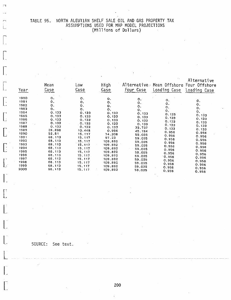
" L_,

[

[

[

[ Year

[ 1980 1981 1982 1983

[ 1984 1985 1986 1987 1988

[ 1989 1990 1991 1992

[ 1993 1994 1995 1996

[ 1997 1998 1999 2000

[

[

['

[

[

[

L r~

L

TABLE 95. NORTH ALEUTIAN SHELF SALE OIL AND GAS PROPERTY TAX ASSUMPTIONS USED FOR MAP MODEL PROJECTIONS

(Millions of Dollars)

Alternative Mean Low High Alternative.· Mean Offshore Four Offshore Case Case Case Four Case Loading Case Loading Case

0. 0. 0. 0. 0. 0. 0. 0. o. 0. 0. 0. 0. 0. o. 0. 0. 0. 0. o. 0. 0. 0. 0. 0. 133 0.133 0. 133 o. 133 o. 133 o. 133 0. 133 0. 133 0. 133 0.133 0. 133 0. 133 0. 133 0. 133 0. 133 o. 133 0. 133 0.133 0.133 0. 133 0. 133 0. 133 0. 133 0. 133 0. 133 0. 133 0. 133 33.737 0. 133 0.133 38.898 10.448 0.956 45.784 0.956 0.956 52.81 15. 117 74.208 59.035 0.956 0.956 68. 113 15.117 97.23 59.035 0.956 0.956 68. 113 15.117 109.892 59.035 0.956 0.956 68. 113 15.117 109.892 59.035 0.956 0.956 68. 113 15. 117 109.892 59.035 0.956 0.956 68. 113 15.117 109.892 59.035 0.956 0.956 68. 113 15.117 109.892 59.035 0.956 0.956 68. 113 15. 117 109.892 59.035 0.956 0.956 68. 113 15.117 109.892 59.035 0.956 0.956 68. 113 15.117 109.892 59.035 0.956 0.956 68. 113 15. 117 109.892 59.035 0.956 0.956

SOURCE: See text.

200

Statewide Impacts

This section discusses statewide impacts of the North Aleutian Shelf

OCS cases, as projected by the MAP statewide model. The accompanying

tables present both absolute (numerical) impacts associated with the

six OCS cases as well as percentage impacts (the size of the impact as

a percentage of the base case projected value of the variables). The

impacts result primarily from the employment associated with the OCS

sales. Where OCS employment levels are similar between cases, the

projected impacts are also similar. Thus, impacts are generally

highest for the high case and 1 owest for the 1 ow case. Impacts for

the alternative four and mean offshore loading cases are slightly less

than for the mean case, and slightly lower still for the alternative

four offshore loading case. Our discussion of the impacts will focus

on the mean case and the high case. However, the tables permit quick

comparison with impacts for the other cases.

POPULATION

As shown in Table 96, the mean case results in a population impact of

9,085 in the year 2000, or a 1.4 percent increase over the base case

population. The maximum percentage impact over the base case popu-

lation is 1.15 percent, in 1989.

The high case population impact is 14,168 in the year 2000, with the

maximum percentage impact of 2.5 percent occurring in 1991.

201

[

[

r [

[

['

l'

[

[

[

[

[

[

L [

[

- --- [-

[ r-L

-,

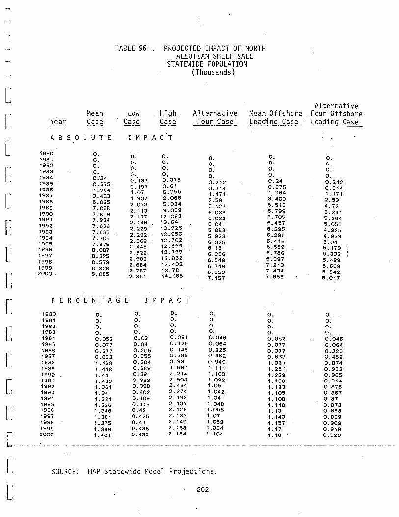
TABLE 96 . PROJECTED IMPACT OF NORTH

ALEUTIAN SHELF SALE STATEWIDE POPULATION

(Thousands)

[ Alternative

[ f~ean Low High Alternative Mean Offshore Four Offshore

Year Case Case Case Four Case Loading Case Loading Case -- --A B S 0 L U T E I M P A C T

L 1980 0. 0. 0. 0. 0. 1981 0. 0. 1982 0. o. 0. 0. 0.

[ 0. 0. o. 0. 0. 1983 0. 0.

o, 0. 0. 0. 0. 1984 0.'24 0.137 o:378 o:24 1985 0.375 0.212 0.212 0. 197 0.61 0.314 0.375 0.314 1986 1.964

[ 1987 1.07 0.755 1.171 1. 964 1. 171 3.403 1988 1. 907 2.066 2.59 3.403 2.59 6.095 2.073 5.024 5.516 1989 7.868 5. 127 4.72 1990 2. 113 9.059 6.039 6.799 5.341 7.859 1991

2. 127 12.082 6.022 6.705 5.264

[ 7.924 2.146 13.84. 6 .. 457 1992 7.626 6.04 5.055

1993 2.229 13.926 5.888 6.295 4.923 7.635 2.292 12.953 6.296 4.939 1994 7.705 5.933 2.369 12.702 6.025 6.416 5.04 1995 7.875

[ 1996 2.445 12.599 6. 18 6.589 5. 179 8.087 2.522 12.769 6.786 5.333 1997 8.325 6.356 1998 2.603 13.052 6.549 6.!:)97 5.499 8.573 2.684 13.402 7.213 5.669 1999 8.828 6.749

2.767 13.78 6.953 7.434 5.842

[ 2000 9.085 2.851 14.168 7.656 7. 157 6.017

-'

[ P E R C E N T A G E I M P A C T

1980 o. 0. 0. 0. 0. 0. 1981 0. 0. 0. 0. o. o.

[ 1982 0. 0. 0. 0. 0. 0. 1983 o. 0. 0. 0. 0. 0. 1984 0.052 0.03 0.081 o'.046 0.052 0.'046 1985 0.077 0.04 0. 125 0.064 0.077 0.064 1986 0.377 0.205 0. 145 0.225 0.377 0.225

[ 1987 0.633 0.355 0.385 0.482 0.633 0.482 1988 1.128 0.384 0.93 0.949 1 .021 0.874 1989 1. 448 0.389 1. 667 1. 111 1. 251 0.983 1990 1 .44 0.39 2.214 1. 103 1.229 0.965

[ 1991 1. 433 0.388 2.503 1.092 1. 168 0.914 1992 1. 361 0.398 2.484 1.05 1. 123 0.878 1993 1. 34 0.402 2.274 1.042 1. 105 0.867 1994 1. 331 0.409 2. 193 1.04 1.108 0.87 1995 1.336 0.415 2. 137 1.048 1 . 118 0.878

[ 1996 1. 346 0.42 2. 126 1.058 1. 13 0.888 1997 1. 361 0.425 2. 133 1.07 1.143 0.899 1998 1.375 0.43 2. 149 1.082 1. 157 0.909 1999 1.389 0.435 2.168 1.094 1. 17 0.919

[ 2000 1. 401 0.439 2.184 1. 104 1. 18 0.928

-- ---- -- -- - -- ---- - --- - - -- - ------- - -

[ SOURCE: MAP Statewide Model Projections.

[ 202

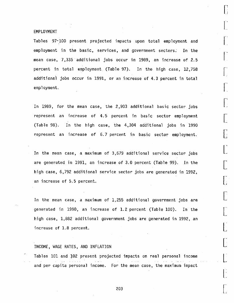
EMPLOYMENT

Tables 97-100 present projected impacts upon total employment and

emp 1 oyment in the basic, services, and government sectors: In the

mean case, 7,335 additional jobs occur in 1989, an increase of 2.5

percent in total employment (Table 97). In the high case, 12,758

additional jobs occur in 1991, or an increase of 4.3 percent in total

employment.

In 1989, for the mean case, the 2, 903 additional basic sector jobs

represent an increase of 4.5 percent in basic sector employment

(Table 98). In the high case, the 4,304 additional jobs in 1990

represent an increase of 6.7 percent in basic sector employment.

In the mean case, a maximum of 3,679 additional service sector jobs

are generated in 1991, an increase of 3.0 percent (Table 99). In the

high case, 6,792 additional service sector jobs are generated in 1992,

an increase of 5.5 percent.

In the mean case, a maximum of 1,255 additional government jobs are

generated in 1990, an increase of 1.2 percent (Table 100). In the

high case, 1,882 additional government jobs are generated in 1992, an

increase of 1.8 percent.

INCOME, WAGE RATES, AND INFLATION

Tables 101 and +02 present projected impacts on real personal income

and per capita personal income. For the mean case, the maximum impact

203

[

[

[

[

[

L ['

[

[

[

[

[

[

[

L [

L [ rL

[

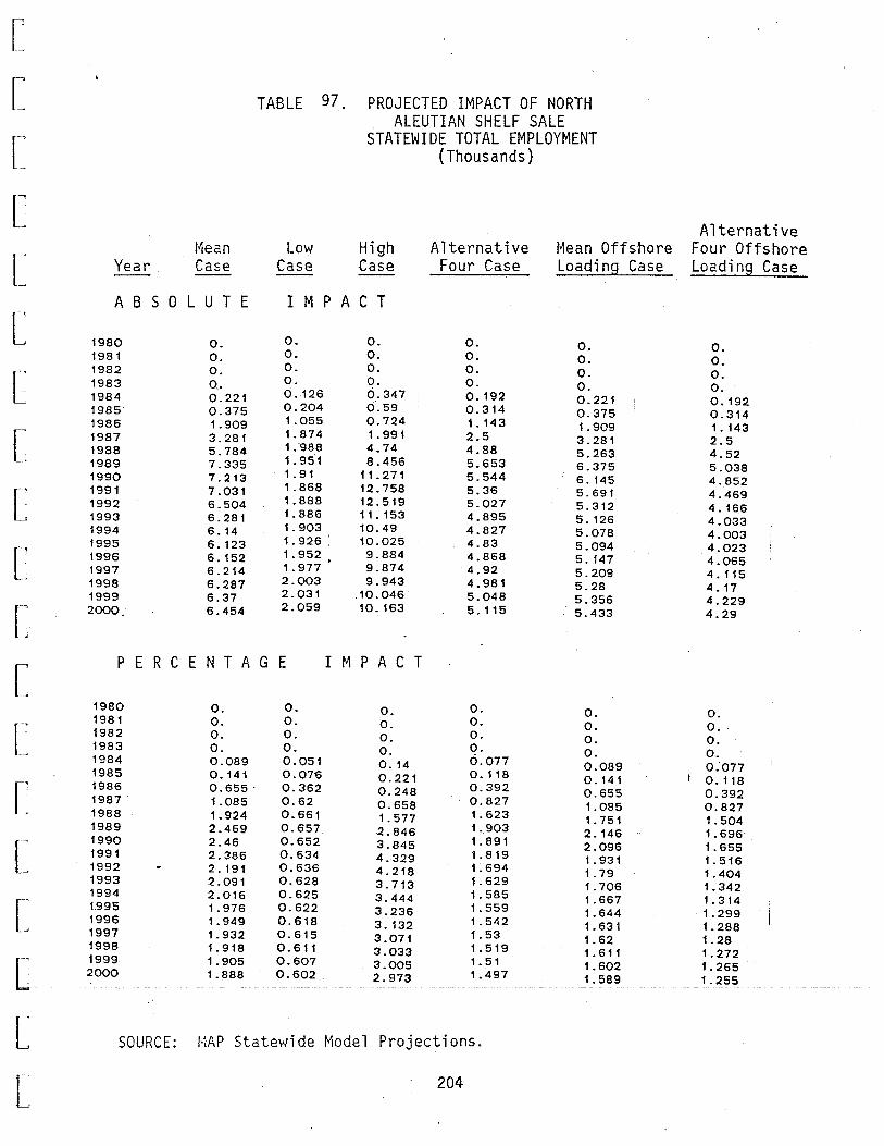
[ TABLE 97 . PROJECTED IMPACT OF NORTH ALEUTIAN SHELF SALE

[ STATEWIDE TOTAL EMPLOYMENT (Thousands)

[ Alternative

t~ean Low High Alternative l~ean Offshore Four Offshore [ Year Case Case .Case Four Case Loading Case Loading Case

A B S 0 L U T E I M P A C T

[ 1980 0. 0. 0. o. 0. o. 1981 0. 0. 0. 0. 0. 0. 1982 0. 0. o. o. 0. o. L 1983 0.. 0. 0. 0. o. 0. 1984 0.221 0. 126 0.347 I 0. 192 0.221 0. 192 1985 0.375 0.204 0.59 0.314 0.375 0.314 1986 1.909 1.055 0.724 1. 143 1. 909 1. 143

[ 1987 3.281 1. 874 1. 991 2.5 3.281 2.5 1988 5.784 1. 988 4.74 4.88 5.263 4.52 1989 7.335 1.951 8.456 5.653 6.375 5.038 1990 7.213 1.91 11.271 5.544 6. 145 4.852

[ 1991 7.031 1.868 12.758 5.36 5.691 4.469 1992 6.504 1. 888 12.519 5.027 5.312 4. 166 1993 6.281 1. 886 11. 153 4.895 5. 126 4.033 1994 6. 14 1. 903 10.49 4.827 5.078 4.003 1995 6. 123 1. 926 . 10.025 4.83 5.094 4.023

L 1996 6. 152 1. 952 9.884 4.868 5. 147 4.065 . 1997 6.214 1. 977 9.874 4.92 5.209 4. 115 1998 6.287 2.003 9.943 4.981 5.28 4. 17 1999 6.37 2.031 10.046 5.048 5.356 4.229

[ 2000 6.454 2.059 10. 163 5. 115 5.433 4.29

[ P E R C E N T A G E I M P A C T

1980 0. 0. 0. o. 0. 0. 1981 0. 0. 0. 0. o. 0 .. [ 1982 0. 0. 0. 0. 0. 0. 1983 0. 0. 0. o. 0. 0. 1984 0.089 0.051 0. 14 0.077 0.089 0.'077 1985 0. 141 0.076 0.221 0. 118 0. 141 I 0. 118

[ 1986 0.655- 0.362 0.248 0.392 0.655 0.392 1987 1.085 0.62 0.658 0.827 1.085 0.827 1988 1.924 0.661 1. 577 1. 623 1. 751 1.504 1989 2.469 0.657 2.846 1.903 2. 146 1.696

[ 1990 2.46 0.652 3.845 1. 891 2.096 1.655 1991 2.386 0.634 4.329 1. 819 1. 931 1. 516 1992 - 2. 191 0.636 4.218 1. 694 1. 79 1.404 1993 2.091 0.628 3.713 1. 629 1.706 1. 342 1994 2.016 0.625 3.444 1.585 1.667 1. 314

[ 1.995 1. 976 0.622 3.236 1. 559 1.644 1. 299 1996 1.949 0.618 3. 132 1. 542 1.631 1.288 1997 1.932 0.615 3.071 1. 53 1. 62 1.28 1998 1.918 0. 611 3.033 1. 519 1. 611 1. 272

[ 1999 1.905 0.607 3.005 1. 51 1.602 1. 265 2000 1.888 0.602. 2.973 1.497 1.589 1.255

--

l SOURCE: MAP Statewide Model Projections.

r· 204 L

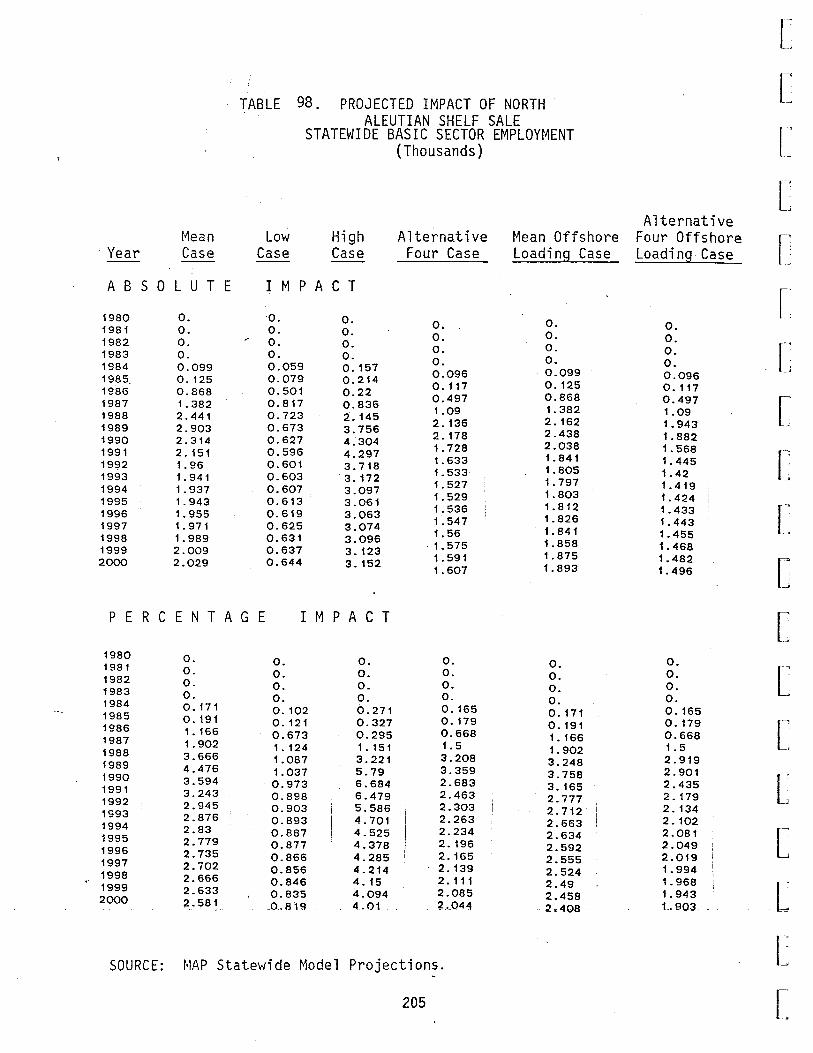
·Year l~ean

Case

A B S 0 L U T E

1980 1981 1982 1983 1984 1985 1986 1987 1988 1989 1990 1991 1992 1993 1994 1995 1996 1997 1998 1999 2000

0. 0. 0. 0. 0.099 0.125 0.868 1. 382 2.441 2.903 2.314 2. 151 1. 96 1. 941 1. 937 1. 943 1. 955 1. 971 1. 989 2.009 2.029

TABLE 98. PROJECTED IMPACT OF NORTH ALEUTIAN SHELF SALE

STATEWIDE BASIC SECTOR EMPLOYMENT

Low Case

High Case

II~ PACT

0. o. 0. 0. 0.059 0.079 0.501 0.817 0.723 0.673 0.627 0.596 0.601 0.603 0.607 0.613 0.619 0.625 0.631 0.637 0.644

o. o. o. o. o. 157 0.214 0.22 0.836 2. 145 3.756 4.304 4.297 3.718 3.172 3.097 3.061 3.063 3.074 3.096 3.123 3. 152

(Thousands)

Alternative Four Case

0. o. o. 0. 0.096 0. 117 0.497 1.09 2. 136 2. 178 1. 728 1.633 1.533 1. 527 1. 529 1. 536 1. 547 1. 56

. 1.575 1. 591 1.607

Mean Offshore Loading Case

0. 0. 0. o. 0.099 0. 125 0.868 1.382 2. 162 2.438 2.038 1. 841 1.805 1. 797 1.803 1. 812 1.826 1.841 1.858 1.875 1. 893

P E R C E N T A G E II~ PAC!

1980 1981 1982 1983 1984 1985 1986 1987 1988 1989 1990 1991 1992 1993 1994 1995 1996 1997 1998 1999 2000

0. 0. 0. 0. 0. 171 0. 191 1. 166 1.902 3.666 4.476 3.594 3.243 2.945 2.876 2.83 2.779 2.735 2.702 2.666 2.633 2.5~!

0. 0. 0. 0. o. 102 o. 121 0.673 1.124 1.087 1.037 0.973 0.898 0.903 0.893 0.887 0.877 0.866 0.856 0.846 0.835 0~8'1.9

0. 0. 0. 0. 0.271 0.327 0.295 1 . 151 3.221 5.79 6.684 6.479 5.586 4.701 4.525 4.378 4.285 4.214 4. 15 4.094 4-.01

0. o. 0. 0. 0. 165 0. 179 0.668 1.5 3.208 3.359 2.683 2.463 2.303 2.263 2.234 2. 196 2.165 2.139 2. 111 2.085 -~·-044-

SOURCE: MAP Statewide Model Projections.

205

0. 0. 0. 0. 0. 171 0. 191 1. 166 1. 902 3.248 3.758 3. 165 2.777 2.712 2.663 2.634 2.592 2.555 2.524 2.49 2.458

- 2.408

A lte rnat i ve Four Offshore Loading Case

0. 0. o. 0. 0.096 0. 117 0.497 1.09 1. 943 1.882 1. 568 1. 445 1. 42 1. 419 1.424 1.433 1. 443 1.455 1.468 1.482 1. 496

0. 0. o. o. 0.165 0.179 0.668 1.5 2.919 2.901 2.435 2. 179 2. 134 2. 102 2.081 2.049 2.019 1. 994 1. 968 1. 943

.1 .• 903

[

[

~

[

[

L [

[

[

[

[

[ [~

[

[

[

L --

[ rL

r [

TABLE 99 . PROJECTED IMPACT OF NORTH

[ ALEUTIAN SHELF SALE

STATEWIDE SERVICES EMPLOYMENT (Thousands)

[ Alternative

[ He an Low High Alternative l~ean Offshore Four Offshore Year Case Case Case Four Case Loading Case Loading Case --

[ A B S 0 L U T E I M P A C T

1980 0. o. 0. o. 0. o.

[ 1981 0. o. 0. 0. 0. o. 1982 0. 0. 0. 0. 0. 0. 1983 0. 0. o. 0. 0. 0.

1984 0. 113 0.059 0. 182 0.09 0. 113 0.09

1985 0.208 0. 1 0.316 0. 162 0.208 o. 162

[ 1986 0.916 0.48 0.407 0.559 0.916 0.559

1987 1. 496 0.823 0.981 1. 149 1. 496 1. 149

"1988• 2.682 0.922 2. 182 2.221 2.436 2.051

1989 3.419 0.942 3.847 2.63 2.987 2.356

[ 1990 3.643 0.951 5.512 2.843 3.009 2.416

1991 3.679 0.946 6.622 2.801 2.794 2. 196

1992 3.432 0.971 6.792 2.643 2.586 2.027

1993 3.313 0.965 6. 106 2.566 2.458 1. 933

1994 3. 198 0.974 5.722 2.507 2.417 1. 905

[ 1995 3. 182 0.985 5.384 2.504 2.419 1. 912

1996 3. 192 1. 5.285 2.521 2.445 1. 933

1997 3.222 1.012 5.261 2.547 - 2.477 1. 959

1998 3.26 1.026 5.293 2.579 2.514 1. 988

[ 1999 3.304 1.041 5.345 2.614 2.555 2.019

2000 3.349 1.056 5.407 2.65 2.596 2.052

[ P E R C E N T A G E II~ PACT

1980 0. 0. 0. 0. o. 0.

1981 0. 0. 0. 0. 0. 0.

[ 1982 0. o. 0. 0. 0. o. 1983 0. 0. 0. 0. o. o. 1984 o. 116 0.06 0. 186 0.092 o. 116 0.092

1985 0. 195 0.094 0.296 0. 152 0. 195 o. 152

[ 1986 0.775 0.406 0.345 0.473 0.775 0.473

1987 1.215 0.669 0.796 0.933 1. 215 0.933

1988 2. 157 0.742 1. 786 1. 96 1.65 1. 755 1.902

1989 2.76 0. 76 3. 106 2. 124 2.412

[ 1990 2.997 0.783 4.534 2.339 2.475 1. 987

1991 3.009 0. 774 5.417 2.292 2.286 1. 796

1992 2.78 0.787 5.501 2. 141 2.094 1. 642

1993 2.633 0.767 4.852 2.04 1. 953 1. 536 1.485

[ 1994 2.493 0.759 4.46 1. 954 1. 883

1. 458 1995 2.427 0.751 4.106 1. 909 1. 844 1996 2.377 0. 745 1.878 1. 821 1.44

3.937 1.425 1997 2.344 0.736 3.827 1. 852 1. 801

1. 411 1998 2.314 0.729 3.757 1. 831 1. 785

[ 1999 2.288 0.721 1. 811 1. 77 1. 399 3.702

2000 2.259 0.712 3.647 1. 788 1.751 1. 384 - --- - - -------

L SOURCE: MAP Statewide Model Projections.

,-206 L

Year ~1ean

Case


STATEWIDE GOVERNMENT EMPLOYMENT (Thousands)

Low Case

High Case


~1ean Offshore Loading Case


1980 1981 1982 1983 1984 1985 1986 1987 1988 1989 1990 1991 1992 1993 1994 1995 1996 1997 1998 1999

.2000

0. 0. 0. 0. 0.009 0.043 0.126 0.404 0.662 1.013 1.255 1.201 1 . 112 1.027 1.005 0.997 1.006 1.021 1.038 1.057 1.076

P E R C E N T A G E

1980 1981 1982 1983 1984 1985 1986 1987 1988 1989 1990 1991 1992 1993 1994 1995 1996 1997 1998 1999 2000

0. o. o. 0. 0.009 0.045 o. 127 0.378 0.603 0.935 1 . 171 1 . 131 1 .041 0.959 0.932 0.916 0.915 0.918 0.924 0.93 _Q.'33_6

0. 0. 0. 0. 0.008 0.025 0.075 0.234 0.342 0.337 0.332 0.326 0.316 0.319 0.322 0.327 0.334 0.34 0.346 0.353 0.359

0. 0. 0. o. 0.009 0.059 0.097 0.174 0.414 0.853 1.456 1. 839 2.009 1 .. 875 1.671 1. 58 1. 537 1. 539 1. 554 1. 578 1.603

II~PACT

0. 0. 0. 0. 0.008 0.026 0.076 0.219 0.312 0. 311 0.31 0.308 0.296 0.298 0.298 0.301 0.303 0.306 0.308 0. 31 0.312

o. 0. 0. 0. 0.009 0.063 0.098 0. 163 0.377 0. 787 1. 358 1. 733 1.882 1.751 1.549 1.452 1. 398 1. 385 1. 383 1.389 1. 394

SOURCE: . t·1AP Statewide ~1ode 1 Projections.

207

o. o. 0. o. 0.006 0.035' 0.086 0.262 0.523 0.844 0.973 0.925 0.852 0.801 0.791 0.791 0.8 0.813 0.827 0.843 0.858

o. 0. 0. o. 0.007 0.037 0.087 0.245 0.477 0.779 0.908 0.871 0. 798' o. 748. 0. 733' o. 727: o. 728' 0. 732: 0.736 0.742 0.747

0. 0. 0. 0. 0.009 0.043 0. 126 0.404 0.665 0.95 1.098 1.055 0.921 0.871 0.859 0.864 0.876 0.891 0.908 0.926. 0.943

0. 0. 0. o. 0.009 0.045 o. 127 0.378 0.606 0.876 1.024 0.994 0.863 0.813 0.796 0.794 0.797 0.802 0.808 0.815 0.82

Alternative Four Offshore Loading Case

0. 0. 0. 0. 0.006 0.035 0.086 0.262 0.526 0.8 0.868 0.828 0.718 0.681 0.674 0.679 0.689 0.701 0.714 0.728 0. 741

0. 0. 0. o. 0.007 0.037 0.087 0.245 0.479 0. 739 0.81 0. 78 0.673 0.636 0.625 0.624 0.627 0.631 i

0.635 0.64 0.645

[

[

[

[

[

[

[

[

c [

[

[.,

.

[

[

[

[

[

l r . L

[

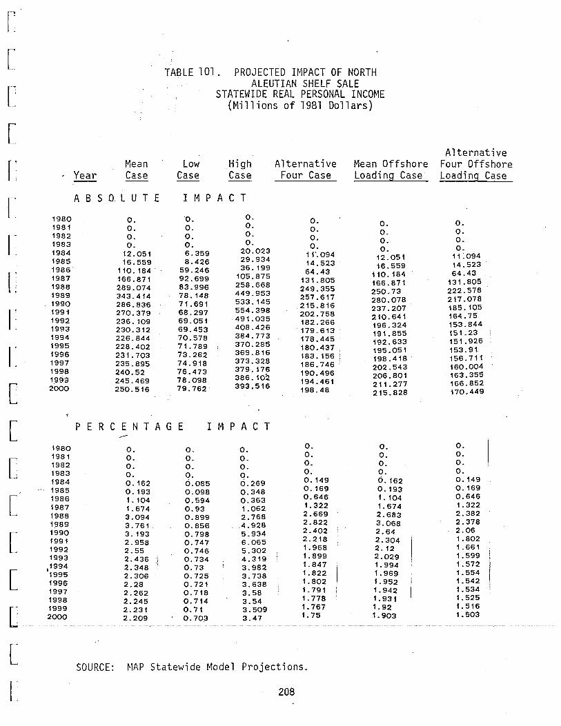
l ~ [

[

[

[

[

[

[

[

[

[

[

[

L [

[

l rL


STATEWIDE REAL PERSONAL INCOME (Millions of 1981 Dollars)

, Year Mean Case

Low Case

High Case



1980 1981 1982 1983 1984 1985 1986 1987 1988 1989 1990 1991 1992 1993 1994 1995 1996 1997 1998 1_999 2000

1980 1981 1982 1983 1984 1985 1986 1987 1988 1989 1990 1991 1992 1993

,1994 1995 1996 1997 1998 1999 2000

A B S 0 L.U T E

0. 0. o. o.

12.051 16.559

110. 184 166.871 289.074 343.414 286.836 270.379 236. 109 230.312 226.844 228.402 231.703 235.895 240.52 245.469 250.516

I H P A C T

0. o. 0. 0. 6.359 8.426

59.246 92.699 83.996 78. 148 71.691 68.297 69.051 69.453 70.578 71. 789 73.262 74.918 76.473 78.098 79.762

0. 0. 0. 0.

20.023 29.934 36. 199

105.875 258.668 449.953 533.145 554.398 491.035 408.426 384.773 370.285 369.816 373.328 379. 176 386. 102 393,516

P E R C E N T A G E I M P A C T ---

0. 0. 0. 0. 0. 162 0. 193 1. 104 1. 674 3.094 3.761 3. 193 2.958 2.55 2.436 2.348 2.306 2.28 2.262 2.245 2.231 2.209

0. 0. 0. 0. c>.o85 0.098 0.594 0.93 0.899 0.856 0.798 0.747 0.746 0.734 0. 73 0.725 0.721 0.718 0.714 0.71 0. 70.3

o. 0. o. 0. 0.269 0.348 0.363 1.062 2.768 4.928 5.934 6.065 5.302 4.319 3.982 3.738 3.638 3.58 3.54 3.509 3.47

0. o. 0. o.

11'. 094 14.523 64.43

131.805 249.355 257.617 215.816 202.758 182.266 179.613 178.445 180.437 183.156 186.746. 190.496 194.461 198.48

0. o. 0. 0. 0. 149 0. 169 0.646 1.322 2.669 2.822 2.402 2.218 1.968 1.899 1.847 1.822 1.802 1. 791 1. 778 1. 767 1. 75

SOURCE: MAP Statewide Model Projections.

208

o. 0. o. o.

12.051 16.559

110.184 166.871 250.73 280.078 237.207 210.641 196.324 191.855 192.633 195.051 198.418 202.543 206.801 211.277 215.828

0. 0. 0. 0. 6. 162 0. 193 1. 104 1.674 2.683 3.068 2.64 2.304 2. 12 2.029 1. 994 1. 969 1. 952 1. 942 1. 931 1. 92 1.903


o. o. o. 0.

11 :o94 14.523 64.43

131.805 222.578 217.078 185. 105 164.75 153.844 151.23 151.926 153.91 156.711 160.004 163.355 166.852 170.449

0. 0. 0. 0. 0. 149 0.169 0.646 1.322 2.382 2.378 2.06 1.802 1.661 1. 599 1.572 1. 554 1. 542 1. 534 1. 525 1. 516 1.503

Year l·iean Case

A B S 0 L U T E

1980 1981 1982 1983 1984 1985 1986 1987 1988 1989 1990 1991 1992 1993 1994 1995 1996 1997 1998 1999 2000

0. 0. 0. 0.

17.645 20.367

138.738 191.871 336 0 117 353 0 16 284.434 248.52 193.801 179.414 167.484 160.848 155.812 151.566 147.512 143.727 139.371


STATEWIDE REAL PER CAPITA PERSONAL INCOME (1981 Dollars)

Low Case

High Case

I 1•1 P A C T

0. 0. 0. 0. 8.937

10. 148 74.238

106.301 88.773 78.176 66.945 59 0 117 57.254 54.906 53.395 51.875 50.699 49.738 48.5 47.285 45.926

0. 0. 0. 0.

30.023 39.211 41.66

125.227 314.973 538.949 599.223 574 .·453 454.273 331. 965 292.043 263.398 250.637 241 0 43 233.836 227.176 219.957


o. o. 0. o.

16.555 18.375 80.426

155.145 294.602 284.207 211.484 184.105 150.043 140.957 133 0 172 128.602 124.547 121.488 118.293 115.297 111 . 82

Hean Offshot~e Loading Case

o. 0. 0. o.

17 0 645 . 20.367 '

138.738 191.871 284.582 301.437 229.594 185.738 162.883 151.648 146.172 141.484 137.605 134.59 131.414 128.398 124.887

P E R C E N T A G E I1,1PACT

1980 1981 1982 1983 1984 1985 1986 1981 1988 1989 1990 1931 ~992

19S3 1994 1995 1996 1997 1998 ~999

2ovo

0. 0. 0. 0. 0 0 11 0. 116 0.725 1 0 034 1 0 944 2.281 1 0 728 1 0 503 1.173 1.081 1.004 0.957 0.921 0.889 0.859 0.83 0:797

0. 0. 0. 0. 0.056 0.058 0.388 0.573 0.513 0.465 0.407 0.358 0.347 0.331 0.32 0. 309 0. 3 0.292 0.282 0.273 0::2~3

0. 0. 0. 0. 0. 187 0. 223 0.218 0.675 1. 822 3.208 3.64 3.475 2.75 2. 1. 75 1. 568 1 0 481 1. 417 1 0 361 1. 3_12 1. 258

o. o. 0. 0. 0. 103 0. 105 0.42 0.836 1. 704 1.692 1. 285 1. 114 0.908 0.849 0.798 0.765 0.736 0.713 0.689 Q.666 0.639

SC:URC~: !·~AP Stal.e\·ii de 1-'1ode 1 Projections.

209

0. 0. 0. 0. 0. 11 0. 116 0.·725 1.034 1. 646 1 0 794 1 0 395 1 0 124 0.986 0.913 0.876 0.8'42 0.813 0.79 0.765

... 0.742 __ 0.714

Alternative Four Offshore~~ Loading Case

0. 0. 0. 0.

16.555 18.375 so. 426

155 0 145 258.582 232.074 178.684 145.488 128.234 120.504 116 0 117 112.477 109.668 107.375 104.852 102.437 99.656

0. 0. 0. 0. 0.103 0.105 0.42 0.836 1.495 1 0 381 1.085 0.88 0.776 0.726 0.696 0.669 0.648 0.63 0.61 0.592 0.57

[

[

r [

[

[

[

[

[

[

[

[

[

[

L [

[

l rL

--,

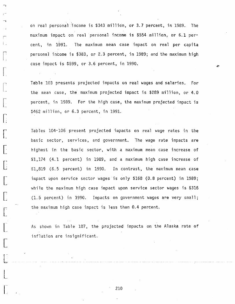
I'

l _ _.

[

[

[

[

[

[

[

[

[

[

[

[

[

[

[ ,L

on real personal income is $343 million, or 3.7 percent, in 1989. The

maximum impact on real personal income is $554 million, or 6.1 per

cent, in 1991. The maximum mean case impact on real per capita

personal income is $383, or 2.3 percent, in 1989; and the maximum high

case impact is $599, or 3.6 percent, in 1990.

Table 103 presents projected impacts on real wages and salaries. For

the mean case, the- maximum projected impact is $289 million, or 4.0

percent, in 1989. For the high case, the maximum projected impact is

$462 million, or 6.3 percent, in 1991.

Tables 104-106 present projected impacts on real wage rates in the

basic sector, services, and government. The wage rate impacts are

highest in the basic sector, with a maximum mean case increase of

$1,174 (4.1 percent) in 1989, and a maximum high case increase of

$1,819 (6.5 percent) in 1990. In contrast, the maximum mean case

impact upon service sector wages is only $168 (0.8 percent) in 1989;

while the maximum high case impact upon service sector wages is $316

(1.5 percent) in 1990. Impacts on government wages are very small;

the maximum high case impact is less than 0.4 percent.

As shown in Table 107, the projected impacts on the Alaska rate of

inflation are insignificant.

210

.;to

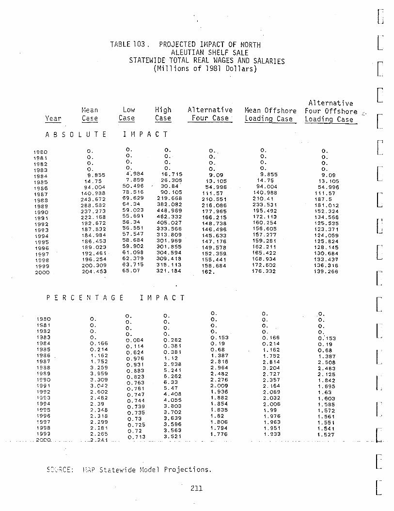
t·~ean

Year Case

A 8 S 0 L U T E

1980 o. 1981 0. 1982 o. 1983 0. 1984 9.855 1985 14.75 1986 94.004 1987 140.938 1988 :1.43.672 1989 288.582 1990 237.273 1991 222. 168 1992 192.672 1993 187.832 1994 184.984 1995 186.453 1996 189.023 1997 192.461 1998 196.254 1999 200.309 2000 204.453


STATEWIDE TOTAL REAL WAGES AND SALARIES (Millions of 1981 Dollars)

Low High Alternative 1•1ean Offshore Case Case Four Case Loading Case --

I 1•1 P A C T

0. 0. 0. 0. 0. 0. 0. 0. 0. o. 0. 0. 0. 0. 0. 0. 4.984 16.715 9.09 9.855 7.859 26.305 13. 105 14.75

50.496 30.84 54.996 94.004 78.516 90. 105 111.57 140.988 69.629 219.668 210.551 210.41 64.34 382.082 216.086 233.531 59.023 448.969 177.965 195.492 55.691 462.332 166.215 172.113 56.34 405.027 148.738 160.254 56.551 333.566 146.496 156.605 57.547 313.809 145.633 157.277 58.684 301.969 147.176 159.281 59.902 301.855 149.578 162.211 61.098 304.594 152.359 165.422 62.379 309.418 155.441 168.934 63.715 315.113 158.684 172.602 65.07 321. 184 162. 176.332

PERCL. r: t~ T A G E I!•1PACT

0. 0. o. 0.

0. 0.

o. 0.

0. 0.

0. 0. 0. o.

0. 166

1980 0. 0.

0. 0. 153

0.214

1981 0. o.

0.282 0.19

1.162

1982 0. 0.084

0.381 0.68

1. 752

1983 0. 166 0. 114

0.381 1.387

2.814

1984 0.214

0.624 1.12

2.816 3.204

1985 1. 162

0.976 2.938

2.964 2.727

1986 1. 752

0.931 5.241

2.482 2.357

1987 3.259

0.883 6.262

2.276 2. 164

1988 3.959

0.823 6.33

2.009 2.069

~989

3.309 0. 763

5.47 1. 936

2.032

1990 3.042 0.761

4.408 1.882

2.006

~991

2.602 0.747 4.055

1. 854 1. 99

1992 2.482 0.744

3.803 1. 835

1. 976

1'393 2.39 0.739

3.702 1.82

1. 963

1994 2.348 0. 735

3.639 1.806

1. 951

1995 2.318

0. 73 3.596

1.794 1. 933

~996

2.299 0.725 3.563

1. 776

~997

2.281 o. 72 3.521

1998 2.265 0.713

1993 -2-.-2-·U 2noo ----

s:·~·~CE: i·:r~.P Stc.tewi de l·iode 1 Projections.

211

Alternative Four Offshore ~:--Loading Case

0. 0. 0. 0. 9.09

13.105 54.996

111.57 187.5 181.012 152.324 134.566 125.535 123.371 124.059 125.824 128.145 130.684 133. 43·7 136.316 139.266

o. 0. 0. 0. 0.'153 0. 19 0.68 1. 387 2.508 2. 483 2. 125 1. 842 1. 695 1. 63 1. 603 1. 585 1. 572 1. 561 1. 551 1. 541 1.527

[

[

r [

[

[

[

[

[

[

[

[

[

[

[

L [_

[ r -L

'

[

[

[

[·

[

[

c [

[

[

L r -L


STATEWIDE REAL WAGE RATE IN BASIC SECTOR (1981 Dollars)

Alternative ~ean Low· High Alternative Mean Offshore Four Offshore

Y~a~ Case Case Case Four Case Loading Case Loadina Case


1930 o. o. 0. 0. 0 · 0 1981 0. 0. 0. o. 0. o: 1~32 0. 0. 0. 0. o. 0. 1~83 o. 0. 0. 0. o. 0. 1934 50.5/8 23.035 91.59 51.02 50.57 8 51.02 1'?85 45.414 25.371 101.531 47.113 45.414 47.113 1936 322.191 170.555 84.863 184.078 322.191 18-1.078 1937 475.9E9 260.285 317.078 394.84 475.969 394.84 1988 1013.35 225.672 1021.39 911.223 822- 6 09 777.781 1939 1173.7 199.66 1802.45 854.82 864.066 655.262 1~90 "704.297 161.195 1819.28 496.422 561.6 4 8 419.711 19'.31 546.926 125.852 1499.51 393.422 406.5 12 316.6i18 1992 399.422 125.391 1001.81 311.777 393.98 310.895 1~a~ 392.039 124.941 642.059 310.977 395.398 314.93 1994 392.352 126.812 603.422 313.18 403.91 4 321.359 1995 394.613 127.059 591.496 314.391 404.98 322.098 1995 337.625 127.871 600.395 316.715 407. 4 2 2 32-1.016 1S97 401.941 129.086 608.176 320.082 4 1 1· 25 327. 1S9S 404.418 129.812 612.43 321.91 413. 238 328.488 1999 407.449 130.73 617.453 324.281 415.9 18 330.645 2000 405.488 130.133 614.687 322.695 413.73 328.793

p E R c c ~~ T .L. G E I 1·1 P A C T ;._

1980 0. o. 0. o. o. 0.

198 1 0. 0. o. 0. o. 0.

1982 0. 0. 0. o. o. 0.

1ao- 0. o. 0. o. o. 0. -~-'

19E4 o. 175 0.08 0.318 0.177 o. 175 0.177

1985 0. ~ 34 0.075 0.299 0. 139 o. 134 o. 139

1S86 O.St.2 0. 446 0.222 0.481 0.842 0.481

1:?87 1.356 0.742 0.903 1.125 1. 356 1.125

~ sc. 8 3.416 0.761 3.443 3.071 2.773 2.622

1000 4. 14 o. 704 6.358 3.015 3.048 2. 3 11

•9S·J 2.526 0.578 ::.526 1.781 2.015 I. 506

~99~ 1. 913 0.44 ::0.246 1. 376 1.422 1. 108

.. ,?~2 1. 395 0. 438 .. ~99 1.089 1. 376 1.086

1CC'l 1.357 0.432 2.222 1.076 1. 369 1.09

1?94 1 :::.:4 0.436 2.077 1.078 1. 39 1. 106

i9?S ~ . ::;.~g o. 434 2.022 1.075 1. 384 1. 101

~ -?~S 1.353 0.435 2.042 1.077 1. 386 1. 102

~;;:· 1.362 0.438 2.061 1 .085 1.394 1. 108

':·~8 1.353 0.438 2.065 1.085 1.393 1. 107

" 1. 368 0.439 2.073 1.089 1. 397 :.4~3

1. 11

oco 1.353 0.434 2.051 1.076 1. 38 1.097

- ----- -

~:,;::;:~: •·:_p St.::~e.-:ide t.';odel Projections.

212

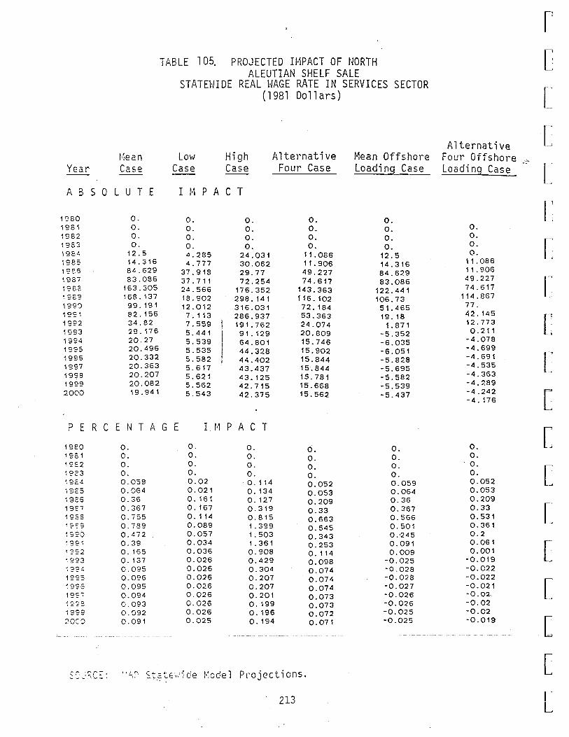
l·~ean Yeal~ c~se

A B S 0 L U T E

1980 o. 1981 0. 1 ~82 0. 4QC": ,_~,.~ ..... 0. 1 92-.! 12.5 ~985 14.316 19E'.S 84.629 1987 83.086 ~?S2. 163.305 'l92~ ~68.137

199') 99.191 .tOC<~ '-- I

82. 156 1992 34.82 ~993 29.176 1994 20.27 1995 20.496 19~5 20.332 1997 20.363 1998 20.207 1999 20.082 2000 19.941

TABLE 10~ PROJECTED IMPACT OF NORTH ALEUTIAN SHELF SALE

STATEWIDE REAL WAGE RATE IN SERVICES SECTOR (1981 Dollars)

Low High Case Case

I 1·'1 P A C T

0. 0. 0. 0. 0. 0. 0. 0. 4.285 24.031 4.777 30.062

37.918 29.77 37.711 72.254 24.566 176.352 18.902 298. 141 12.012 316.031 7. 113 286.937 7.559

I 191.762

5.441 91. 129 5.539 64.801 5.535 I 44.328 5.582 44.402 5.617 43.437 5.621 43. 125 5.562 42.715 5.543 42.375


0. 0. 0. 0.

11 . 086 11.906 49.227 74.617

143.363 116. 102 72.184 53.363 24.074 20.809 15.746 15.902 15.844 15.844 15.781 15.668 15.562

l~ean Offshot~e

Loading Case

0. 0. o. 0.

12.5 14.316 84.629 83.086

122.441 106.73 51.465 19. 18

1. 871 -5.352 -6.035 -6.051 -5.828 -5.695 -5.582 -5.539 -5.437

..... t:" R c E t~ T A G E I f·1 P A C T r' '-

1980 0. 0. o. 0. 1981 c. 0. 0. o. 19E2 0. 0. 0. o.

0. 0. 0.

1983 0. 0. 0. 0. 0. ~9E4 0.059 0.02 0. 114 0.052 0.059 .. ,925 0.064 0.021 0. 134 0.053 ~92-6 0.36 0. 161 0. 127 0.209

0.064 0.36

19:07 0.367 0. 167 0.319 0.33 ~958 0.755 0. 114 0.815 0.663

0.367 0.566

~?E?. 0. 739 0.089 1. 399 0.545 ~ 9:':·.) 0 . .!72 0.057 1. 503 0.343

0.501 0.·245

~99~ 0.39 0.034 1. 361 0.253 0.091 1?S:2 0. 165 0.036 0.908 o. 114 0.009 ~9'23 o. 137 0.026 0. 429 0.098 -0.025 ~'?S:j 0.095 0.026 0.304 0.074 -0.028 1'395 0.096 0.026 0.207 0.074 -0.028 ~9'25 0.095 0.026 0. 207 0.074 -0.027 19':1 0.094 0.026 0.201 0.073 -0.026 ~~=s 0.093 0.026 0. 199 0.073 -0.026 19'?9 0.092 0.026 0. 196 0.072 -0.025 20':') 0.091 0.025 0.194 0.071 -0.025

SC:_:;c~: ":.,? St2~E·,·oide t,1odel Projections.

213

Alternative Four Offshot~e .':-Loading Case

0. 0. 0. 0.

11.086 11.906 49.227 74.617

114.867 77. 42. 145 12.773 0. 211

-4.078 -4.699 -4.691 -4.535 -4.363 -4.289 -4.242 -4. 176

0. o. o. 0. 0.052 0.053 0.209 0.33 0.531 0.361 0.2 0.061 0.001

-0.019 -0.022 -0.022 -0.021 -0.02 -0.02 -0.02 -0.019

[

[

[

[

[

[

[

[

c [

[

[

[

[

[

[

_[

[ r~

L

.....,

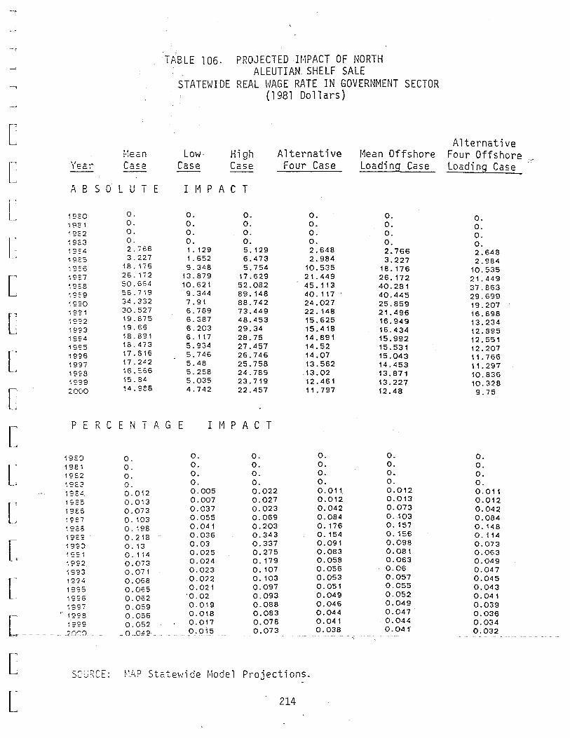
TABLE 106. PROJECTED IMPACT OF NORTH

ALEUTIAN SHELF SALE

! STATEWIDE REAL WAGE RATE IN GOVERNMENT SECTOR

( 1981 Dollars) I L_ -~

[ !·~ean Low· High Alternative l•1ean Offshore

[ ·'{ea':"" C-5se Case Case Four Case Loading Case -- --

A B S 0 L U T E I 1•1 P A C T

[ 1920 0. 0. o. 0. 0. 1921 0. 0. 0. 0. 0. ~9E2 0. 0. 0. 0. 0.

[ ~9C3 0. 0. 0. 0. 0. ~9S4 2.766 1. 129 5. 129 2.648 2.766 ··925 3.227 1. 652 6.473 2.984 3.227 !9=6 iS. 176 9.348 5.754 10.535 18.176

[ ~927 26.172 13.879 17.629 21.449 26. 172 ~SES 50.664 10.621 52.082 45. 113 40.281 ~9::9 56.719 9.344 89. 148 40.117 40.445 "9?0 34.332 7.91 88.742 24.027 25.859 1991 30.527 6.789 73.449 22. 148 21.496

[ ~992 19.875 6.387 48.453 15.625 16.949 1993 19.66 6.203 29.34 15.418 16.434 1994 18.891 6. 117 28.75 14.891 15.992 19=5 13.473 5.934 27.457 14.52 15.531

[ 1996 17.816 5.746 26.746 14.07 15.043 1997 17. 2"2 5.48 25.758 13.562 14.453 1998 16.566 5.258 24.789 .13.02 13.871 ~999 15.84 5.035 23.719 12.461 13.227

[ 20DO 14.988 4.742 22.457 11.797 12.48

[ P E R C E N T A G E I !~ P A C T

19SS) 0. 0. o. o. 0.

[ 1981 0. 0. 0. 0. 0.

1952 0. 0. 0. o. 0.

~S£2 0. 0. 0. 0. 0. ~ ssj_ 0.012 0.005 0.022 0.011. 0.012

1SS5 0.013 0.007 0.027 0.012 0.013

[ 19E6 0.073 0.037 0.023 0.042 0.073

~PE7 0. 103 0.055 0.069 0.084 0 .. 103

19.:.5 0. 198 0.041 0.203 0.176 0. 157

19E9 0.218 0.036 0.343 0. 154 0.156

[ ~9SJ 0. 13 0.03 0.337 0.091 0.098 "C.C,. o. 1 i4 0.025 0.275 0.083 0.081 '-- I 0.058 0.063 ~9'?2 0.073 0.024 0. 179 ~993 0.071 0.023 0. 107 0.056 0.06

[ 1 9'?4 0.068 0.022 o. 103 0.053 0.057

1995 0.065 0.021 0.097 0.051 0.055

1996 0.062 ·o.o2 0.093 0.049 0.052

1997 0.059 0.019 0.088 0.046 0.049

[ ,. ~~~~ 0.056 0.018 0.083 0.044 0.047

0.052 0.017 0.078 0.041 0.044

- - - - - - -~ C:~ ()_ .. - 0 .. 0.~9· 0.015 0.073 0.038 0.041

[ r· L

SCG?CE: t·:.t.P Stc.te\·iide t·iodel Projections.

214

Alternative

Four Offshore

Loading Case

0. 0. o. 0. 2.648 2.984

10.535 21.449 37.863 29.699 19.207 16.898 13.234 12.895 12.551 12.207 11.766 11.297 10.836 10.328 9. 75

0. o. 0. 0. 0. 011 0.012 0.042 0.084 0.148 0. 1 14 0.073 0.063 0.049 0.047 0.045 0.043 0.041 0.039 0.036 0.034 0.032

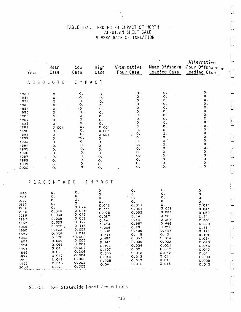
Year !•'lean Case

A B S 0 L U T E

1980 0. 1981 0. 1982 0. 1983 0. 1984 0. i985 0. 1926 0. 1987 0. 1928 0. "000 l_.u ..... 0.001 1990 0. 1991 0. 1992 0. 1993 0. 1994 0. 1995 0. 1996 0. 1997 0. 1998 0. 1999 0. 2000 0.

TABLE l 07 . PROJECTED If.1PACT OF NORTH ALEUTIAN SHELF SALE

ALASKA RATE OF INFLATION

Low Case

High Case


l~ean Offshore Loading Case

II~ PACT

-0. 0. o. 0. 0. 0. 0. 0. 0. 0. 0. 0. o. 0. 0. 0.

-0. 0. 0. 0. 0. 0. 0. 0. 0. 0. 0. 0. o. 0. 0. 0. o. 0. 0. 0. 0. 0.001 0. 0. 0. 0.001 0. 0. o. 0.001 0. 0.

-0. o. 0. 0. 0. 0. 0. 0. 0. 0. 0. 0. o. 0. 0. 0. o. 0. 0. 0. o. 0. 0. 0. o. 0. 0. 0. 0. 0. 0. 0. o. 0. 0. 0.

p E R C E N T A G E I I~ PACT

1980 0. 0. o. 0. 0.

1981 0. 0. 0. 0. 0.

1982 0. 0. 0. 0. 0.

1983 0. 0. o. 0. 0.

1984 0. -0.024 0.043 0. 011 0.

1985 0.028 0.015 o. 111 0.041 0.028

1986 0.083 0.013 0.075 0.053 0.083

1957 0.209 0.068 0.087 0.14 0.209

1c<:P 0.503 0. 127 0.64 0.44 0.304 ~~-

1989 0.873 0. 116 1. 414 0.667 0.446

1990 0. 432 0.057 1. 366 0.23 0.256

1991 0. 306 0.014 1 . 118 0.196 0.147

1992 0. 178 -0.003 0. 717 0. 115 0. 13

1993 0.089 0.005 0.454 0.057 0.074

1994 0.066 0.001 0.241 0.039 0.032

1995 0.04 0.004 o. 198 0.024 0.021

199€ 0.029 0.006 0.107 0.02 0.017

~997 0.019 0.004 0.065 0.013 0.012

1998 0.018 0.005 0.044 0.013 0. 011

".9S9 0.016 0.003 0.035 0.012 0.01

2000 0.02 0.005 0.04 0.016 0.015

S:J::CE: I·'),P Stc.te\·tide l·'iodel Projections.

215

Alternative Four Offshore ~ Loading Case

o. 0. 0.

0. 0. 0. 0. 0. 0. 0. 0. 0. 0. 0. o. 0. 0. 0. 0. 0. 0. 0. 0. 0.

o. 0."011 0.041 0.053 o. 14 0.301 0.389 o. 151 0.124 0.104 0.054 0.023 0.016 0.013 0.01 0.009 0.009 0.012

[

[

r [

[

[

[

[

[

[

[

[

[

[

[

[

[

[ r , L

[

[

[

[

l' [

[

[

[

[

[

[

[

[

[ I , ~-------

[ rL

GOVERNMENT REVENUES, EXPENDITURES, AND THE

PERMANENT FUND BALANCE

As shown in Table 108, the OCS cases have relatively little impact

upon state revenues. The maximum mean case impact is $34 million (0.4

percent); the maximum high case impact is $49 million (0.6 percent);

both occur in 1991. As shown in Table 109, year 2000 state government

interest earnings decline by $22 mi 11 ion (1. 0 percent) in the mean

case and by $35 mi 11 ion (1. 8 percent) in the high case. These de-

clines reflect the impacts of increased government expenditures upon

the permanent fund balance. As shown in Table 110, total state

government expenditures in the year 2000 increase by $74 million (1.2

percent) in the mean case and $106 million (1.7 percent) in the high

case, as a result of the higher state population. However, as shown

in Table 111, state government per capita expenditures decline

slightly, with the maximum high case decline of $44 (0.5 percent) in

2000.

As shown in Table 112, the decrease in the year 2000 permanent fund

ba 1 ance is $340 mi 11 ion (1. 3 percent) for the mean case, and $555

million (1.3 percent) for the high case. On a per capita basis, the

declines are more significant. As shown in Table 113, the year 2000

decrease is $1,079 per person (2. 7 percent) for the mean case and

$1,704 per person (4.2 percent) for the high case.

216

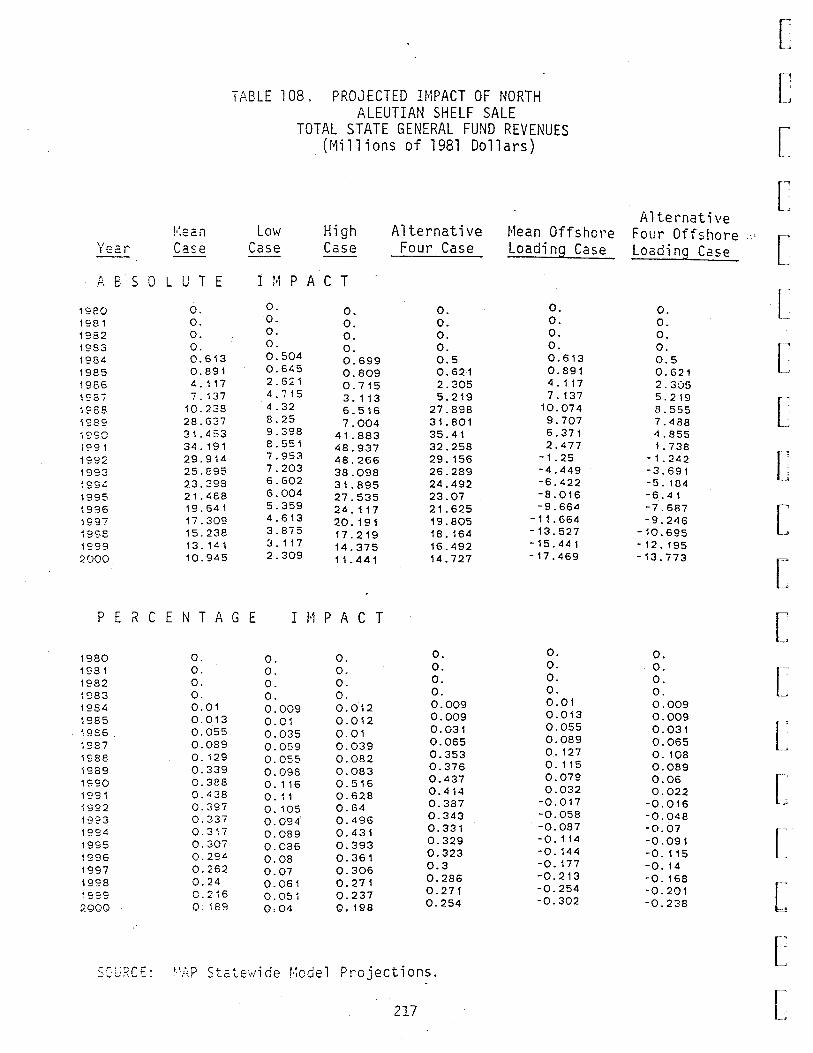
Yec.r

P. 8 s 0

1980 1981 1952 1983 1984 1985 1986 1987 1988 1SS9 ,~or-n , .... :;v

1991 1992 1993 199L~

1995 1936 1997 19S8 1999 2000

p E R C

1980 1981 1932 1~;83

1984 1985 1986 1987 1988 1989 1990 1991 j992 E?·?3 1994 1995 1996 1997

!<ean Case

L U T E

c. 0. 0. 0. 0.613 0.891 4. 117 7. 137

10.238 28.637 31. 4 53 34. 191 29.914 25.895 23.395 21.488 19. 64 1 17.309 15.238 13.141 10.945


TOTAL STATE GENERAL FUND REVENUES (Millions of 1981 Dollars)

Low Case

High Case

I 1·1 P A C T

0. 0. 0. 0. 0. 0. 0. 0. 0.504 0.699 0.6~5 0.809 2.621 0.715 4.715 3. 113 4.32 6.516 8.25 7.004 9.398 41.883 8.551 48.937 7.953 48.266 7.203 38.098 6.602 31. 895 6.004 27.535 5.359 24. 117 4.613 20. 191 3.875 17.219 3. 117 14.375 2.309 11.441


0. o. 0. 0. 0.5 0.621 2.305 5.219

27.898 31. 801 35.41 32.258 29.156 26.289 24.492 23.07 21. 625 19.805 18. 164 16.492 14.727

l~ean Offshore Loading Case

0. 0. 0. 0. 0.613 0.891 4. 117 7. 137

10.074 9.707 6.371 2.477

-1.25 -4.449 -6.422 -8.016 -9.664

- 11 . 664 -13.527 -15.441 -17.469

E N T A G E I 1~1 P A C T

0. 0. 0. 0. 0.

0. 0. 0. 0. 0.

0. 0. o. 0. 0.

0. 0. 0. 0. 0.

0.01 0.009 0.012 0.009 0.01

0.013 0.01 0.012 0.009 0.013

0.055 0.035 0.01 0.031 0.055

0.089 0.059 0.039 0.065 O.Q89

0. 129 0.055 0.082 0.353 0. 127

0.339 0.098 0.083 0.376 0. 115

0.388 0. 116 0.516 0.437 0.079

0. 438 0. 11 0.628 0.414 0.032

0.397 0. 105 0.64 0.387 -0.017

0.337 0.094. 0. 496 0.343 -0.058

0.317 0.089 0. 431 0.331 -0.087

0. 307 0.036 0.393 0.329 -0. 114

0.294 0.08 0.361 0.323 -0. 144

0. 262 0.07 0.306 0.3 -0. 177 0.286 -0.213

Alternative Four Offshore ,, Loading Case

0. 0. o. 0. 0.5 0.621 2.305 5.219 8.555 7.488 4.855 1. 738

- 1. 24 2 -3.691 -5. 104 -6.41 -7.687 -9.246

-10.695 -12.195 -13.773

0. 0. 0. 0. 0.009 0.009 0.031 0.065 0. 108 0.089 0.06 0.022

-0.016 -0.048 -0.07 -0.091 -0. 115 -0. 14

r [

'-[

[

r· [

[

[

[

[

[

[

[

[

[ 1998 0.24 0.061 0.271 -o. 168

~999 0.2~6 0.051 0.237 0.271 -0.254 -0.201

2GGG O~iB9 -0-.-04 G-.-1-SS 0. 254 -0.302 -1"1 """"' ~~--~-·--~-_L

SCLiRCE: ~·~-'\P State\·iide !·~odel Projections.

217

[ rL

[

[

r [

[

[

[

L [

[

[

[

[

[

L [

l·~ean Year Case

A 8 s 0 L U T E

0. 1930 0. 1981 0. 1982 0. 1983 0. 1934 -0.077 1985 -0.242 1986 - 1. 027 1987 -2.617 1988 -5.731 1<.?89 -7.6€5 1990 -9. 129 1991 -10.231 1992 - 11 . 109 19'93 -12. 129 1994 -13.276 1995 -14.573 1996 -16.034 joe---I - n. 719 1998 -19.596 1999 -21.68 2000


Low· Case

STATE GOVERNMENT INTEREST EARNINGS (Millions of 1981 Dollars)

High Alternative l~ean Offshol~e Case Four Case Loadin9_1.?.?e_

I I" P A C T 0. o.

o. 0. 0. 0. o.- 0. 0. 0.

0. 0. 0. 0. o. 0. -0.005 0.

-0.02 0. 011 -0.083 -0.077 -0.026 -0.19 -0.242 -o. 211 -0.084 -0.431 -1.027 -0.695 -0.463 -0.746 -2.427 -1.98 -1. 192 -2.091 -4.837 -3. 199 - 1. 993 -5.488 -7.494 -3.951 -2.407 -10.57 -10.083 -4.425 -2.671 -13.956 -12.729 -4.99 -2.96 -16.773 -15.04 -5.415 -3.306 -19. 103 -17.357

-21.118 -6.012 -3.708 -6.737 -19.722 -4. 182 -23.242 -22.147 -7.605 -4.723 -25.333 -24.652 -8.624 -5.323 -27.567 -27.269

-30.074 -9.83 -5.99 -29.985 -11.202 -6.719 -32.827 -32.822 -12.749 -7.517 -35.851

P E R C E N T A G E I H P A C T

1950 0.

~931 0.

1982 0.

1983 0.

1984 0.

i985 -0.011

1936 -0.028

1987 -0.098

1'?3E -0.21

198~ -0.406

19?.0 -0.478

1SS1 -0.521 -<oc .... I-·- L

-0.544

~993 -0.558

199~ -0.581 jCO-- ~:;,

-o.6n o4CQ;:; I-_.-.....

-0.67 1997 -0.741

1999 -0.939

0. o. 0. 0. 0.002

-0.004 -0.01 -0.044 -0.095 -0. 141 -0. 15 -0. 152 -0. 157 -0. 166 -0.178 -0. 194 -0.217 -0.246 -0.28 -.o. 322

0. o. 0. 0. o. 0. 0. 0. 0. 0. 0. 0.

-0.004 -0.001 0. -0.028 -0.012 -0.011 -0.05 -0.025 -0.028 -0.071 -0.066 -0 . .098 -0. 168 -0. 159 -o. 194 -0.389 -0.227 -0.343 -0.659 -0.246 -0.467 -0.792 -0.251 -0.572 -0.888 -0.264 -0.674 -0.96 -0.272 -0.756 -1.012 -0.288 -0.832 -1.081 -0.313 -0.917 -1.165 -0.35 -1 .019 -1.274 -0.399 -1.139 -1.407 -0.46 -1.275 -1.574 -0.537 -1.437 -1.786 -0.635 -1.635

Alternative Four Offshore :~

Loadinq Case

0. o. o. o.

-0.005 -0.083 -0.211 -0.695 -1.847 -3.938 -5.949 -8.002

-10.08 -11.879 -13.688 -15.543 -17.446 -19.408 -21.458 -23.586 -25.806

0. 0. 0. 0.

-0.001 -0.012 -0.025 -0.066 -0. 1<18 -0.279 -0.371 -0.454 -0.534 -0.597 -0.656 -o. 723 -0.802 -0.897 -1.004 -1.131 -1.286 [

- ·~sss -0.829

- -•- - - - - - "200o- - - - - -- -1 , .. QB-·-· --~-o_. :n~- ••• MO ""' •• ••• ••••••• •• - - __ , ~-~ -~-- -~ -· --· - -- ·- _, ~- -· --~- ·- ~ -·· ···- - ·- ·-- - --- --- - ·-- --· ·- ·- ~ .

L SC~C(Cf: ::..:.;) Stc:t::···:~de :/cdel Projections.

[ 218

Year

A 8 s 0

1980 1981 1982 1983 ~92.4

1985 1986 ~S3?

1988 ~coo t _.._,-

1:?30 199~

1992 1~~?

1994 1995 1996 19.97 1998 4':)0""1 I ~~ _. :::>

20CO

p E R C

1980 1981 1982

'

1983 1984

-- 1985 1956 1987 ~938 <~c.cn ,_.__ 4Qt:'jl) I -·cV

... 0 ..... "' I-:::: l

1992 ~993

'i9?G 19~5

i9?S 1997 "'0~"" ... I--~-~

19?9 20~:00

l·~ean Case

L U T E

0. 0. 0. 0. 1. 726 2. 848

15.23 28. 148 51.535 63.536 63.824 63.836 57.587 57.703 58.559 60.434 62.766 65.484 68.301 71.293 74.242

~A~LE 110. PROJECTED IMPACT OF NORTH ALEUTIAN. SHELF SALE

TOTAL STATE GOVERNMENT EXPENDITURES (Millions of 1981 Dollars)

Low High Alternative l·1ean Offsho1·e Case Case Four Case Loading Case

I !·1 P A C T

0. 0. 0. 0. 0. 0. 0. 0. 0. 0. 0. 0. 0. 0. 0. 0. 1. 029 2.642 1:491 1. 726 1. 607 4 . .275 2.331 2.848 8.535 5.367 9.02 15.23

16.254 16.758 21.391 28.148 17.801 41.449 43.336 47.035 17.703 71 . 691 48.609 56.203 17.738 92.656 49. 102 55.824 17. 801 102.625 48.898 55.09 ~ 8. 168 102.277 44.949 49.512 18.762 92.691 45.324 49.496 19.605 90.422 46.395 50.859 20.496 89.484 48.027 52.75 21. 406 91.434 50.07 55.062 22.316 94.484 52.23 57.461 23.301 98.262 54.52 60.004 24.332 102.426 56.934 62.668 25.348 106.613 59.309 65.309

E ~~ T A G E It·1PACT

0. 0. 0. 0.

0. 0. 0. 0. 0.

o. 0. 0. 0. 0.

o. 0. 0. 0. 0.

0.046 0.027 0. 0.04 0.046

0.072 0.04 o:o7 0.059 0.072

0.349 0. 196 0. 108 0.207 0.349

0.575 0.332 0. 123 0.437 0.575

1 . 0 ~ 4 0.35 0.342 0.853 0.9.25

1. 263 0.352 0.816 0.966 1. 117

1 . 28 0.356 1. 425 0.985 1 . 1 .2

1. 285 0. 358 1. 859 0.984 1.109

1. "62 0.366 .2.066 0.905 0.997

1 . 133 0.37 2.06 0.895 0.977

1. 127 0. 377 1. 83. 0.893 0.979

1.132 0.384 1. 74 0.899 0.988

1. 14 0.389 1. 676 0.91 1 .

1. 154 0.393 1. 661 0.92 1.013

1. 157 0. 398 1. 665 0.932 1.026

1 . 181 0.403 1. 679 0.943 1. 038

1. 192 0.407 1. 697 0.952 1.048 1. 711

SOL!RC::: ~·'.:i.? St<:tei·.'ide t·iodel Projections.

219

c· [

r Alternative

[ Four Offshore Loading Case L~

0. 0.

[ 0. 0. 1.491 2.331 [ 9.02

21.391 40.246 43.887 [ 43.836 43.074 38.512 38.625 39.777

[ 4 1. 328 43.109 44.973 46.961 [ 49.039 51. 109

[

o. [

o. o. o. 0.04 [ 0.059 0.207 0.437 0. 792 0.872

[ 0.879 o. 867 0.776 0.763

[ 0.765 0.774 0.783 0.792 [ 0.803 0.812 0.82 [

l L

TA3LE lll. PROJECTED HiPACT OF NORTH ALEUTIAN SHELF SALE

PER CAPITA STATE EXPENDITURES (1981 Dollars)

L .. -

l__.

~-~

i -L~

l [

[ I

I ~

L=

[

l·:ean Low High Alternative Year Case Case Case Four Case

.~SSOLUT!: I f•1 P A C T

1980 0. 0. 0. 0.

1981 0. 0. 0. 0.

~922 0. 0. 0. 0.

1983 0. 0. 0. 0.

1984 -0.465 -0. 184 -0.898 -0.48

1985 -0.387 0.023 - 1. 371 -0.449

1SE:5 -2.344 -0.816 -1.84 -1.516

1'3E7 -5.285 -2.086 -3.84 -4.086

1923 -~O.G05 -3. 129 -10.652 -8.953

1983 -~6.832 -3.422 -22.094 -13.32

1990 -14.383 -3.082 -31.734 -10.695

1991 -13.082 -2.664 -38.273 -9.574

~992 -17.344 -2.801 -36.645 -12.703

1993 -17.633 -2.828 -38.574 -12.891

1994 -18.035 -2.844 -39.809 -13.102

1995 -18.238 -2.789 -40.914 -13.34

~996 -18.645 -2.832 -41.699 -13.469 o(oo- -18.91 -2.961 -42.504 -13.754 I._,_ I

1SSS -19.207 -3. -43.16 -13.969

~9E9 -19.492 -3.059 -43.828 -14.172

2000 -19.793 -3.121 -44.473 -14.398

? E R C E N T A G E I 1·1 P A C T

1980 1981 1982 1'?83 198~

1985 1986 .rcc.~ ,_._;:

1988 "C,..,_ I- C-=

·~en 1--v

·j 991 1992

0. 0. 0. 0. 0. 0. 0. 0. 0. 0. 0. 0. 0. 0. 0. 0.

-0.006 -0.002 -0.011 -0.006 -0.005 0. -0.017 -0.006 -0.028 -0.01 -0.022 -0.018 -0.058 -0.023 -0.042 -0.045 -0.113 -0.033 -0.113 -0.095 -0.182 -0.037 -0.239 -0.144 -o. 157 -0.034 -o. 347 -0.111 -o. 146 -o.o3 -o. 426 -o.1o7 -o. 1ss -0.032 -o. 414 -o. 143 -0.198 -0.032 -0.434 -0.145

[

0~4 -0.201 -0.032 -0.444 -0.146 1,..~ -0.201 -0.031 -0.452 -0.147 1995 -o. 203 -0.031 _0 455 -o. 147

. 1996 -0.204 -0.032 -0-458 -0.148

~993

• 1ss7

-o. 205 -0.032 -o: 46 -o. 149

Alternative t·1ean Offshore Foul~ Offshore . ..._ Loading Case Loading Case

0. 0. 0. 0. 0. 0. 0. 0.

-0.465 -0.48 -0.387 -0.449 -2.344 -1.516 -5.285 -4.086 -8.879 -7.621

-12.289 -10.156 -9.805 -7.703 -5. 195 -4. 18

-11. -8.996 -11.254 -9.203 -11.461 -9.332 -11.633 -9.391 -11.727 -9.516 -12.004 -9.754 -12.168 -9.898 -12.355 -10.055 -12.539 -10.215

0. 0. 0. 0. 0. 0. 0. 0.

-0.006 -0.006 -0.005 -0.006 -0.028 -0.018 -o·.o58 -0.045 -0.094 -0.081 -o. 133 -o. 11 -0.107 -0.084 -0.058 -0.047 -o. 124 -o. 102 -o. 127 -o. 104 -o. 128 -o. 104 -o. 128 -o. 104 -0.128 -0.104 -o. 129 -o. 105 -o. 13 -o. 105

l 19ss -c.2os ... -0.032 -o 461 -o_ .149 of0CO •

______ ----~..;;; ~~-- -~-=-~-~2~!?_. _ -~-0.032 ___ _.,_o_,_.~L63 ___ -=..O_._t5•~---o. 13 -o. 106 .:_0_._13_j ______ - 0---106---~ ---~--~-~

l rL

..._ r,...-- •_. .. -: ._:.: •• . .:..? Stc.t.t:.·:ide i·~odel Projections .

220

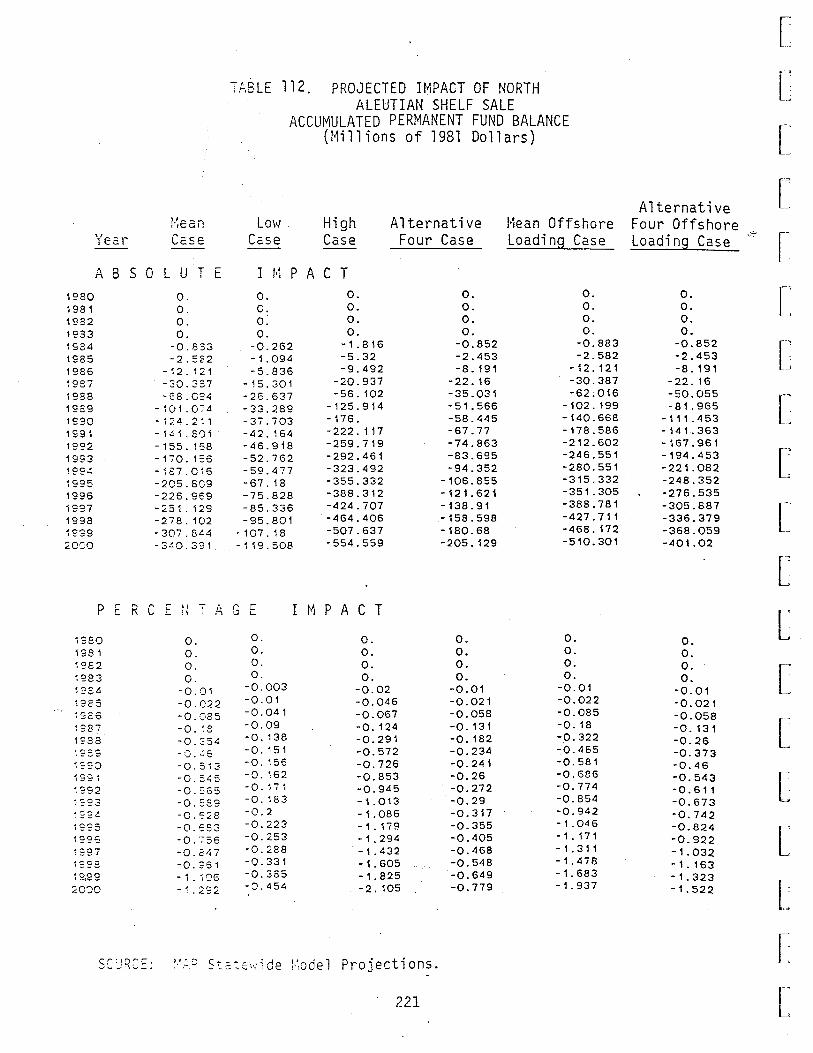
Y ec.l~

A 8 S 0 1980 1981 1982 1933 1984 1985 1986 1987 1988 1989 1990 1991 1992 19S3 1CC" . __ ... ~995

1996 1997 1998 1'999 2000

D t: R c I

1980 198 1 ~?82 "'00? i -"-'"""

i?E-1 1925 I :iCO

~387

1933 ·.-;es 1990 ig·; i ~'::92

i';93 19'::4 1995 ~~9S

~~97

~=:'?5 .. occ 1 -~'- ....

20')0

r-~ean

Cc.se

L U T E 0. 0. 0. 0.

-0.233 -2.::22

- ~ 2. 121 -30.337 -68.0?4

-W1.074 -124.2~1

-1~1.801

-155. 1'.:·8 -170.1::6 -~87.016

-2C5.8C9 -226.9E9 -251.129 -278. 102 -307.8L.4 -3<~0.391

TABLE 112 PROJECTED IMPACT OF NORTH ALEUTIAN SHELF SALE

ACCUMULATED PERMANENT FUND BALANCE (Millions of 1981 Dollars)

Low. High Alternative l'tean Offshore Cc.se Co.se Four Case Loading Case

I 1•1 P A C T 0. 0. 0. o. 0. 0. 0. 0. o: 0. 0. 0. 0. 0. 0. 0.

-0.262 -1.816 -0.852 -0.883 - 1. 094 -5.32 -2.453 -2.582

-5.836 -9.492 -8.191 -12.121

-15.301 -20.937 -22.16 -30.387

-26.637 -56. 102 -35.031 -62.016 -33.289 -125.914 -51 . 566 -102.199 -37.703 -176. -58.445 -140.668 -42.164 -222.117 -67.77 -178.586 -46.918 -259.719 -74.863 -212.602 -52.762 -292.461 -83.695 -246.551 -59.477 -323.492 -94.352 -280.551

-67.18 -355.332 -106.855 -315.332

-75.828 -388.312 -121.621 -351.305

-85.336 -424.707 -138.91 -388.781

-95.801 -464.406 -158.598 -427.711

-107. 18 -507.637 -180.68 -468. 172

-119.508 -554.559 -2.05.129 -510.301

E If ' .A. G C' I 1·1 P A C T ~ ., i L.

0. 0. 0. 0. 0. 0. 0. 0. 0. o. 0. 0. o. 0. 0. 0. 0. 0. o. 0.

-0.01 -0.003 -0.02 -0.01 -0.01

-O.C22 -0.01 -0.046 -0.021 -0.022

-0.085 -0.041 -0.067 -0.058 -0.085

-0. ~ s -0.09 -0.124 -0. 131 -0. 18

-0.354 -o. 138 -0.291 -0. 182 -0.322

-o . .!E -0. 151 -0.572 -0.234 -0.465

-0. )3 -0. 156 -0.726 -0.241 -0.581

-0. 45 -0. ~62 -0.853 -0.26 -0.686

-0. 65 -0. 171 -0.945 -0.272 -0.774

-0. 89 -0. 183 -1 .013 -0.29 -0.854

-o. 28 -0.2 -1.086 -0.317 -0.942

-0. 33 -0.223 -1. 179 -0.355 - 1. 046

-0. 56 -0.253 -1.294 -0.405 -1.171

-0. 47 -0.288 -1.432 -0.468 - 1 . 311

-0. 51 -0.331 -1.605 -0.548 -1.478

- 1 . 06 -0.385 - 1. 825 -0.649 -1.683

- ' a~ -L

-8.454 -2. 105 -0.779 -1.937

SC"...!RC~: ~·· . .:..:: St~~e._.,.;de ~·~odel Projections.

221


0. 0. 0. o.

-0.852 -2.453 -8.191

-22. 16 -50.055 -81.965

-111.453 - 14 1 . 363 -167.961 -194.453 -221.082 -248.352 -276.535 -305.887 -336.379 -368.059 -401.02

0. 0. o. 0.

-0.01 -0.021 -0.058 -0. 131 -0.26 -0.373 -0.46 -0.543 -0.611 -0.673 -0.742 -0.824 -0.922 -1.032 -1. 163 -1.323 -1.522

·:7'-

[ r L

[

[

[

["

[~~

~"

[

[

l [

[

[

[

[

[

[

[ r, L

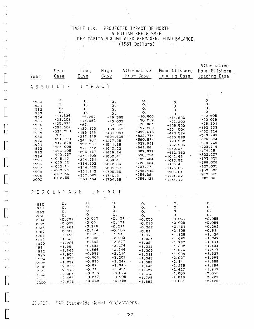
! l ~

[

[

[

E [

[

[

[

[

[

[

[

[

[

[ rL

TA~LE 113. PROJECTED IMPACT OF NORTH ALEUTIAN SHELF SALE

PER CAPITA ACCUMULATEb PERMANENT FUND BALANCE (1981 Dollars)

Alternative Mean Low. High Alternative Mean Offshore Four Offshore

Year Case Case Case Four Case Loading Case Loading Case


1980 °· 0. 0. 0. 0 0. 1981 °· o. o. o. 0 . o. ~'982 o. o. o. o. o. o. 1983 o. ~ 0. 0. 0. o: 0. 1984 -11.~..:>6 -6.262 -19.555 -10.605 -11.836 -10.605 1SS5 -~3-~03 -11.652 -40.035 -20.059 -23.203 -~0.059 1S26 - 1"' 5 · 023 -67. -57.625 -76.801 -125.523 -' 6 · 801

~937 -254.~~4 -139.855 -159.555 -192.203 -254.504 -192.203 ~SS8 -~21.-o9 -185.238 -431 .. 047 -399.016 -473.574 -400.324 1989 -t61. -217.816 -891.605 -538.711 -685 808 -543.293 1990 -s 5 ~· 793 -241.207 -1277.35 -590.574 -793:582 - 6 ~ 6 · 504 1991 -9;1.828 -257.957 -1541.35 -629.828 -862.535 -~19.766 1992 -:..:>1.008 -277.512 -1640.22 -641.66 -919.34 -,~ 3 · 719 1993 -~65.3~5 -295.457 -1629.24 -667.977 -982.363 -714.25 1994 -_93.9o7 -311.809 -1650.41 -690.754 -1042.63 -822.207 1995 -1018.13 -324.531 -1659.41 -709.484 -1093.82 -862.625 1995 -1036.52 -334.602 -1672.86 -723.434 -1136.4 -896.008 1997 =10~5· 4 ~ -344.125 -1691.67 -737.77 -1176.05 -92:.035 1998 10"':· 2 ' -351.812 -1705.35 -748.418 -1208.64 - 95 ·'- 598

1999 - 1071 · 5 ~ -357.699 -1710.9 -754.98 -1234.32 - 972 · 609

2000 - 1078 · 5 ~ -361.164 -1704.95 -756.121 -1251.42 - 985 · 93

? _ R C E N T A G E I M P A C T

1980 0. 0. o. 0. o. 0. 1931 0. 0. 0. 0. 0. 0. 1982 0. o. o. 0. 0. 0. 1983 0. 0. 0. 0. 0. 0. 1Q34 -0.051 -0.032 -0.101 -0.055 -0.061 -0.055

1985 -0.099 -o.os -0.171 -0.086 -0.099 -0.086 ~936 -0.~61 -0.246 -0.211 -0.282 -0.461 -0.282 1987 -0.808 -0.444 -0.506 -0.61 -0.808 -0.61 ~?EB -1.t:55 -0.52 -1.21 -1.12 -1.329 -1.124 ~989 -1.88 -0.538 -2.203 -1.331 -1.695 -1.342 ~·;;:so -1.£25 -0.543 -2.877 - 1 . 33 -1.787 -1.411

1991 -1.S5 -0.548 -3.274 -1.338 -1.832 -1.444 1992 -1.893 -0.566 -3.346 -1.309 -1.876 -1.477 ~9?3 -1.904 -0.583 -3.214 -1.318 -1.938 -1.527 1994 -1.933 -0.606 -3.209 -1.343 -2.027 -1.599 ~995 -1.992 -0.635 -3.247 -1.388 -2.14 -1.688 ~996 -2.075 -0.67 -3.349 -1.448 -2.275 -1.794 •-::0..,. -2.173 -0.71 -3.491 -1.522 -2.427 -1.913 ~ 9 s~ -2.304 -0.758 -3.676 -1.613 -2.605 -2.053 •ceo -2.46' -0.817 -3.908 -1.725 -2.819 -2.222 ;;(;(,(, -2.E56 -0.889 -4.198 -1.862_ -3.081 -2.428

. -,... - --..... • - - 0

...... - ·-· --. '·',:,;:> St.=.:e\·.'1 de !·iode 1 Pl~oject ions .

222

Regional Impacts: Anchorage

Table 114 presents projected impacts on Anchorage population. The

year 2000 population increases by 4,358 (1.5 percent) in the mean case

and by 6,847 (2.4 percent) in the high case.

Table 115 presents projected impacts on the Anchorage employment. In

the mean case, the maximum increase in employment is 3,167 (2.3 per-

cent) in 1990; in the high case, the maximum increase in employment is

5,594 (4.1 percent) in 1991.

Regional Impacts: Bristol Bay

Projected impacts of the North Aleutian Shelf OCS sales in Bristol

Bay, shown in Tables 116 and 117, are very small. The maximum popu-

lation increases projected for the mean and high cases, respectively,

are 26 and 38 (0. 4 percent and 0. 6 percent) in the year 2000. The

maximum employment increases projected for these two cases are 41 (0.9

percent) and 68 (1.5 percent), in 1990 and 1992, respectively. These

population and employment impacts are results of increased levels of

activity in the statewide economy, rather than direct results of OCS

activity.

223

[

[

[

[

[

[

[

[

[

[

[

[

[

[

[

[

[

[ rL

'

[

[

[

[

[

[

[

[

f~iecn

Ytal"' Cc.se

3 s 0 L U T E

1980 0. 4 00 .. l ... u I 0. 1?32 0. ~933 0. 1<.?2.-4 0.116 ~ ·~ 35 0. 181 i~ 36 1.009 ~ ~ 37 1 0 659 1~38 3.009 ~~39 3083 19?0 3.741 l~9~ 3.816 .I"":)"" ·~-.L 3.65A j9?3 3.678 ~=?4 3. 71)2 1==5 3.732 ~fSS 3.878 1997 3.993 <IQ~~ ,.,_u 4. 1 ~ 3 ~:::;g 4.23~

2GOO 4.358

T.L.BLE 114. PROJECTED H'IPACT OF NORTH ALEUTIAN SHELF SALE

ANCHORAGE POPULATION (Thousands)

Low High Alternative 1·1ean Offshore Case Case Four Case Loading Case

I 1,1 P .A. C T

0. 0. o. 0. 0. 0. 0. 0. 0. 0. o. 0. 0. 0. o .. 0. 0.064 0. 187 0.104 0. 116 0.096 0.3 0. 154 0. 181 0.547 0.377 0.6 1.009 0.93 1. 042 1. 281 1. 659 0.986 2.516 2.532 2.693 1. 02 4.523 2.915 3.275 1.016 5.903 2.873 3. 184 1.025 6.75 2.904 3.082 1.069 6.742 2.828 3.032 1. 094 6.278 2.866 3.036 1. 132 6. 174 2.905 3.095 1. 168 6.098 2.978 3. 175 1. 204 6. 181 3.061 3.267 1.2~3 6.309 3. 153 3.368 1. 283 6.478 3.25 3.473 1. 322 6.658 3.347 3.578 1. 362 6.847 3.445 3.685

Alternative Four Offshore Locding Case

0. 0. 0. 0. 0.104 o. 154 0.6 1. 281 2.312 2.556 2.512 2.416 2.38 2.396 2.446 2.51 2.583 2.662 2.745 2.827 2. 911

? E R C E ~ T A G E I 1·1 P A C T 0. 0.

o. 0. 0. 0. 0. 0. 0. 0. o. 0. 0. o. 0. 0. 0. 0. 0. 0. o. 0. o. 0. 0.057 0.051 0.057 0.032 0.092 0.051 0.086 0.073 0.086 0.0~6 0. 1~3 0.073 0.458 0.272 0.458 0.248 0.171 0.272 0.72 0.556 0.72 0.404 0.~52 0.556 1.134 0.974

1~·30

1~8 1 i"?32 ~ '~ ~.2 ~ ,. - , '.:-::. ... . ~"5 1::2.6 1?E"7

1.267 0.415 1.06 1.066 1.367 1.067 .~ ~ 1o59S 0.426 1.888 1.217 1.328 1.048 ~= 0~ 1.56 0.~24 2.~62 1.198 1.268 0.994

·::2~

~.? 1.57 0.422 2.778 1.195 1.233 0.968 -~: 1 425 0.435 2.741 1.15 1.214 0.958

·::~: 1:471 0.438 2.511 1.146 1.217 0.962 -=~: 1.456 0.445 2.~28 1.143 1.226 0.969

[ ;:~~ 1.46 0.451 2.354 1.15 1.238 0.979 ~:;;; 1.47 0.456 2.342 1.16 1.252 0.99 ~~;.:; 10485 0.462 2.346 1.173 1.266 1.001 :::::-:: 1.5 0.468 2.362 1.185 1.28 1.011

t ; ~.~ ~ ~ . 5 1 .1 __ _o .__ 4!3 __ .. __ 2._ 381 1_._ 197 _______ 1 . 2 9__ -----~ ·-----_--,_-;.r;---------1.57n--' 0.4'7_"7 .. ·2.397 1.206

..::.. - .... ·,.,1

[ - 0

......... - --. ··.:.':. :::~:.;o:'ial l·~cdel Projections.

L 224

!·lecn


ANCHORAGE TOTAL EMPLOYMENT (Thousands)

Low. y~·=r C2se Case

High Case


t·1ean Offshore Loading Case

Ll.~SOLUTE I t·1 P A C T

~~30 o. ·o. 0.

1fS1 0. 0. o.

1~32 0. 0. o.

1983 0. 0. 0.

~~-34 0.035 0.047 o. 137

1£=85 0.153 0.085 0.246

~=s6 o. 8'·2 0.446 o. 32

~£'G7 1. 359 0.792 0.854

~~=:2 2.4?9 0.869 2.027

~ ?=.9 3. 191 0.876 3.655

1~'?0 3. 157 0.844 4.865

~?91 3.136 0.823 5.594

~992 2.815 0.828 5.531

1993 2.778 0.826 4.992

1924 2.707 0.836 4.677

~995 2.701 0.848 4.438

~9?6 2. 717 0.862 4.375

i937 2.752 0.875 4.372

~sss 2.792 0.89 4.413

~9S9 2.837 0.905 4.47

2000 2.884 0.92 4.536

,.., - r - -r. G E I f'1 p A C T r' [. !\ \... - i '

1980 0. 0. 0. ~931 0. 0. 0. 19E2 0. 0. 0. ~923 0. 0. 0. ·, 9E4 0.075 0.041 0.122 ~'?25 0. 128 0.071 0.206 ·s:s 0.627 0. 344 0.247 ·s~7 1.019 0.581 0.626 "?EE 1. EOG 0.628 1. 465 ·:=:3 2.327 0.639 2.666 .. ;:o 2.3.!!8 0.626 3.607 • =- = 1 2.319 0.608 4. 137 ~?~2 2. 115 0.609 4.069 ~=~3 2.017 0.6 3.625 ~??4 1-937 0.598 3.347 '??5 1. 399 0.596 3. 121 "'2=6 1. 875 0.595 3.019 ~997 1. 862 0.593 2.959 ~;sc 1. 852 0.59 2.927 -·-·~-=-? __ _1 • _n_~A- . - _Q._58_8 2.905 : :y:.-: 1. 23.2 0.585 2.882

,. - - ,., -.... -. -. -- - ' ..... -. -~ ~egional Model Projections.

225

0. 0.

o. 0.

o. o. 0. o. 0.075 0.085

0. 131 o. 153

0.488 0.812

1.06 1. 389

2.089 2.265

2.46 2.763

2.446 2. 705

2.387 2.548

2.221 2.375

2. 167 2.288

2. 134 2.268

2. 137 2.278

2. 158 2.306

2. 187 2.34

2.221 2.379

2.257 2.294

2.42 2. 462

0. 0. 0. 0. 0. 0. 0. 0. 0.067 0.075 0. 11 0.128 0.377 0.627 0.777 1. 019 1. 51 1. 637 1. 794 2.015 1. 814 2.006 1.765 1. 884 1. 634 1.747 1.574 1. 662 1. 527 1. 623 1.503 1.602 1. 489 1. 591 1. 48 1. 584 1. 473 1. 578 1. 466 1. 573 1;450 L56-4

Alternative Four Offshore Loadinq Case

0. 0. 0. 0. 0.075 0. 131 0.488 1.06

. 1. 928 2. 187 2. 15 2.002 1. 867 1. 807 1. 796 1. 807 1. 83 1. 857 1. 887 1. 919 1. 952

0. 0. 0. 0. 0.067 0. 11 0.377 0.777 1. 394 1. 595 1. 594 1. 481 1. 373 1. 313 1. 285 1.271 1. 262 1. 257 1. 252 1. 247 1.24

[

[

~

[

[

r [

[

[

[

[

[

[

[

[

[

[

[

L

[

[

[

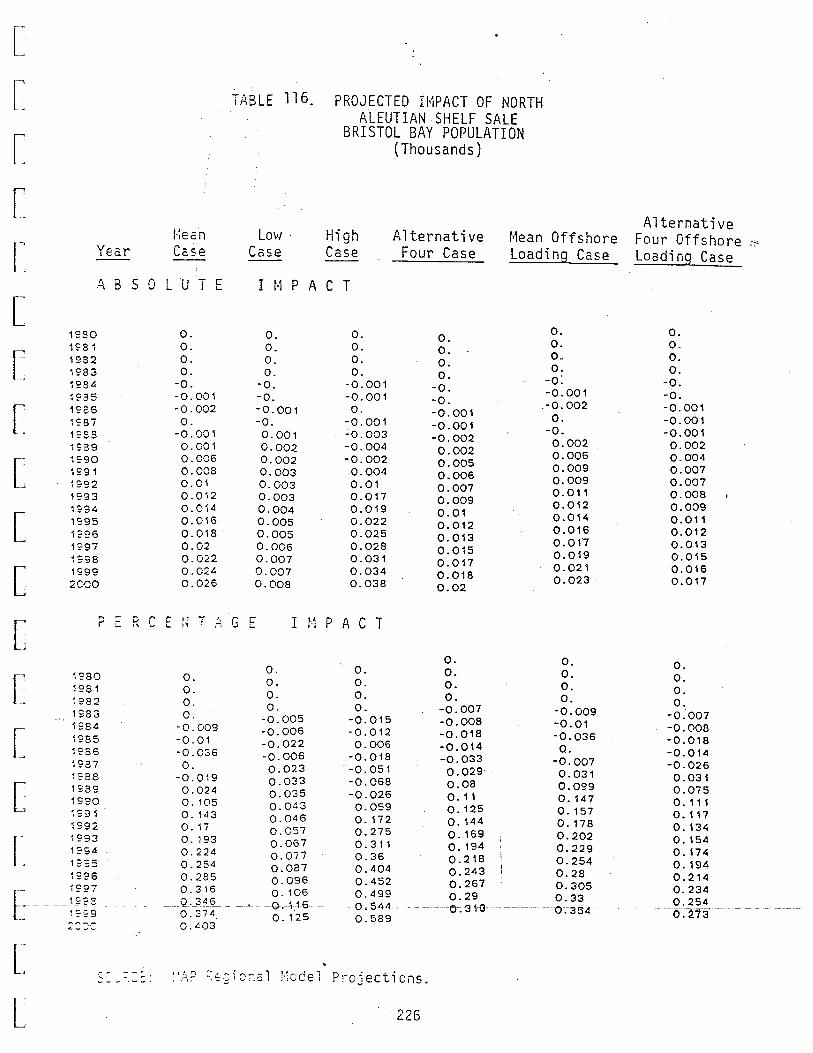
[ l·:ean

[ Year Cc.se --A 8 S 0 L U T E

[ 1S90 0.

[ 1~31 0. 1932 0. 1983 0. 1934 -o. "C~~ I -......, _. -0.001

[ 1S36 -0.002 ~SS7 0. 12SS -0.001 1S39 0.001

[ 1990 0.006 1 S9 1 0.008 1"'0~ 0.01

__ , 1993 0.012

[ 1'?94 0.014 1?95 0.016 1?96 0.018 1?97 0.02 ~SSB 0.022

[ 1999 0.024 2000 0.026


BRISTOL BAY POPULATION (Thousands)

Low High Alternative 1•1ean Offshore Case Case Four Case Loading Case --

I 1·1 P A C T

o. 0. 0. 0. o. 0. 0. 0. 0. 0. 0. o. o. 0. 0. 0. -o: -o. -0.001 -0. -0.001 -o. -0.001 -o. .-0.002 -0.001 0. -0.001 0. -o. -0.001 -0.001 -0. 0.001 -0.003 -0.002 0.002 0.002 -0.004 0.002 0.006 0.002 -0.002 0.005 0.009 0.003 0.004 0.006 0.009 0.003 0.01 0.007 0.011 0.003 0.017 0.009 0.012 0.004 0.019 0.01 0.014 0.005 0.022 0.012 0.016 0.005 0.025 0.013 o.on 0.006 0.028 0.015 0.019 0.007 0.031 0.017 0.021 0.007 0.034 0.018 0.023 0.008 0.038 0.02

[ ? E R C E f~ T ~-- G [:" I 1··1 P A C T '-

[

[

r L>

L

1'230 1S81 ~'282

1983 1?8~

1985 1986 1937 1S88 1 39 1 90 1 91 1992 1S93 1?94 1::.:::::;

1~96

'-- I

0. 0. 0. 0.

-0.009 -0.01 -0.036 0.

-0.019 0.024 0.105 0. 143 0.17 0. 193 0.224 0.254 0. 285 0.316

0. o. o. 0.

-0.005 -0.006 -0.022 -0.006 0.023 0.033 0.035 0.0~3

0.046 0.057 0.067 0.077 0.087 0.096 o. 106

o. 0. 0. o. 0. 0. o. 0. 0. o. 0. 0. -0.007 -0.009

-0.015 -0.008 -0.01 -0.012 -0.018 -0.036 0.006 -0.014 0.

-0.018 -0.033 -0.007 -0.051 0.029 0.031 -0.068 0.08 0.099 -0.026 0. 11 0. 147 0.059 o. 125 0. 157 0. 172 0. 144 0. 178 0.275 0.169 0.202 0. 311 o. 194 0.229 0.36 0.218 0.254 0.404 0.243 0.28 0. 452 0.267 0.305 0. 499 0.29

[

•co-

--~-~~-1~?E 1~·?9--

Q ._3<)§_ -0. 374.

0.33 ~ _ -0.~:16----- e,-~..,.., - --- - - -o~ 31-3- · ~- --- - o~-354- - ---

0.125 2 :·:·C.· 0. 403

0.589

l -- ---:. "'.!) :-.:.-iro".-1 '-~"'-ce' p,-o:ections :::---. ...., ~. ,-.; ,._::::: ...., .. o I • IV I • J I ..

l 226

Alternative Four Offshore .. Loading Case

0. 0. o. 0.

-0. -0. -0.001 -0.001 -0.001 0.002 0.004 0.007 0.007 0.008 0.009 0.011 0.012 0.013 0.015 0.-016 0.017

0. 0. 0. 0.

-0.007 -0.008 -0.018 -0.014 -0.026 0.031 0.075 0. 111 0. 117 o. 134 0. 154 0. 174 0. 194 0.214 0.234 0.254

---6.273--

Yeo.r --P. B S 0

1980 1981 1982 19E3 1984 1985 1986 1987 1938 1989 1990 1991 1992 1993 1994 1995 1996 1997 ~9S8

~S'29

2000

p E R C

1980 1981 ~932

1983 1984 19S5 1986 1937 192.8 1989 1990 1991 1992 1993 1994 1995 1996 1997 1998 <~QCO ·--.J----- 2coo _____

t-'1ec.n Cc.se --

L U T E

0. 0. 0. 0. 0. 0.001 0.006 0.014 0.024 0.035 0.041 0. 041 0.037 0.034 0.033 0.032 0.033 0.033 O.C·34 0.034 0.035

Ti'.BLE 117. PROJECTED HiPACT OF NORTH ALEUTIAN SHELF SALE

BRISTOL BAY TOTAL EMPLOYMENT (Thousands)

Low - High Alternative 1•1ean Offshore Case Case Four Case Loading Case --

I 1·1 P A C T

0. 0. 0. 0. 0. 0. 0. 0.

0. 0. 0. 0. 0. 0. 0. 0.

0. 0.001 0. 0. 0.001 0.002 0.001 0.001 0.003 0.004 0.004 0.006

0.007 0.014 0.008 0.01 0.017 0.023 0.011 0.019 0.033 0.031 0.012 0.028 0.051 0.036 0. 011 0.032 0.064 0.035 0.011 0.031 0.068 0.031 0.01 0.028 0.064 0.029 0.01 0.026

0.01 0.057 0.026 0.028 0.052 0.028 0.01 0.026

0. 011 0.051 0.026 0.029 0. 011 0.051 0.026 0.029 0.011 0.051 0.027 0.03 0. 011 0.052 0.027 0.03

0.053 0.031 0. 011 0.028

E 1~ T A G E I 1·1 P A C T

0. 0. 0. 0. 0.

0. 0. o. 0. 0.

0. 0. 0. 0. 0.

0. 0. 0. 0. 0.

0.009 0.005 0.014 0.008 0.009

0.032 0.02 0.05 0.028 0.032

0. 132 0.074 0.081 0.086 0. 132

0.297 0. 17 0. 155 0.206 0.297

0.513 0. 235 0.35 0.405 0;49

0. 741 0.245 0.695 0.6 0.671

0.881 0.23G . 1.091 0.689 0. 768

0.882 0.228 1. 383 0.673 0. 756

0. 791 0.22 1. 466 0.604 0.666

0.733 0.219 1. 365 0.567 0.621

0. 7 0.22 1. 211 0.549 0.604

0.688 0. 222 1. 112 0.544 0.601

0.686 0.224 1. 068 0.545 0.604

0.689 0. 226 1.054 0.548 0.608

0.694 0.228 1.053 0.552 0.614

c. 7 0.231 1. 058 0.557 0.62

-ec ~7-06~~-------'-- -0---2-33- -~- - -- ~L065--~--~-~-o_._s_G_:L.----~ ___ Q_. (;~§ ____

5C"_;scr:: "::,::J Rtc;;io:!al !·:oce·l P:'ojections.

227

[

r [

Alternative [

Four Offshore Loading Case [

o. [ 0. 0. 0. o. 0.001

[ 0.004 0.01 0.018 0.026

[ .0.029 0.027 0.024 0.023 [ 0.022 0.022 0.023 0.023 0.023

[ 0.024 0.024 [

0. [

0. 0. 0. 0.008

[ 0.028 0.086 0.206 0.39 [ 0.554 0.617 0.594 0.519 0. 486

[ 0.474 0.473 0.476 0.479 L 0.483 0.488 0. 493 L---

l L

8ZZ

J -]

]

]

]

]

]

J J J ]

~

J ]

J J

] ~--------------------------

]

J J J ]

J J ]

]

J ]

J J J J J

L ~ -

[

[ r· L~

[

[

[

[ [-,

[ r~ <=

[ r~

t:

L

L

Aleutian Islands Impacts

This section discusses impacts of the OCS cases upon the Aleutian

Islands, as projected by the SCIMP model. Pairs of tables present

absolute and procentage impacts.

EMPLOYMENT

Nonresident or enclave basic sector employment impacts are shown in

Tables 118 and 119. These represent OCS enclave employment; thus, the

figures in Table 118 reproduce the enclave employment figures of

Tables 89-94. As shown in Table 119, the maximum percentage impact

upon enclave employment is 27.6 percent for the mean case (in 1989)

and 66.1 percent for the high case (in 1990).

Tables 120 and 121 present impacts upon basic sector resident employ

ment. The absolute impact projections presented in Table 120 are

slightly lower than the resident OCS employment shown in Tables 89-94.

This is because the SCIMP model does not treat permanent migrants as

residents in the year of migration. The maximum increases in resident

basic sector employment are 161 after 1991 for the mean case, and 314

in 1992 for the high case; or 16.6 percent in 1990 for the mean case

and 31.3 percent in 1991 for the high case.

229

'-

Year

l ~·::=:: l 1'7'8~~ "i. •7:33 1984 1"7'~7;5

17'8t. 1 '7'87 .:r t;• .-: C1 l .L , ·:-:· , .. I 1'7'8!7'1 1 990i 1.-'91\

7 .. I •r·9·i .L 7' • ''·J 1993 1'?~'4 J

1 ~·95: 1 S:"? 6 i C•C•7 - i J I

197'f.! 1 ·=· r-. q - i 7 I

2000

TABLE 118.

Mean Low Case Case·

PROJECTED ABSOLUTE IMPACT OF NORTH ALEUTIAN SHELF SALE

ALEUTIAN ISLANDS BASIC SECTOR NONRESIDENT EMPLOYMENT

Alternative High Alternative Mean Offshore Four Offshore Case Four Case Loading Case Loading Case

0. -0 + . 0) o. o. (). 0. - 0. o. 0 <· o. o. 0 > o. o. () . () > 0.

180. 5 ~-. 2f:5. :t. :!.8. 180. 138. '266 ~ 67. 397, 189. ?..~6. l89. 3:1.9 < 93. 371 •· 248. 319. 248 •. 31. 1. > 70. 299. ?.40. 3U .• 240.-530. 1 ::-~9. 7t.4. 393, 286, 260 •. 733. 120. 1428. 493. : 263. 210. 660. :l. ~j3. :1.823. ~6?.. - 263. 2l. 0. 630 + 127. 1f..4;;-~. 44:1.. : 157. 1.30. 4!,3 .. 126. :1. ·453. 3 ,!J 8.

; 1.30. :1.57 •

463. 126. 839. 368. 157. 130. -163. l26. 839. 368. :1.57. l. 30. 463. 126. 839, 368. 157. 130,

' :t. 26. 839. ::S68 .. 1.30. 463 > 1.57• 463. 126. 839. 3.~.8 ( 157. 130. 463. 126. 839. 368. 157 <· l30. 463. 126. 839. :;68. 1.57. 130, 463. 126. 839. 368 •· 157. 130.;

:·

- -SOURCE: SChiP -!·'lode 1- Pr-o] ecti ons.

--230

[

c [

[

[

[

[

[

[

[

[

[

[

[

[

[

[---

[

L

! I"

l~ . ·-

~

[

[

[

[ [~

[

[

[

[ [~

[

[

r~ L_;

[ I

L

Year

'· 7'81. lS'B'2 l '7'83 1'7'84 1 s·t: 5 1 ·:n=:t. j_ '7' f; 7 ·1 UC•O J. l \,• "·'

1 '7' F.:·:;:· 1.990 199 ~-1 0•::0')

I I '•• ·

1 ~"7'3: ) C• C• 1..

, I ,• 1

197'5 l '7'.9 .~ i 'i' '7' 7 :1. c;·s:s ). 9 ·? '? 20Cd)

TABLE 119. PROJECTED PERCENTAGE IMPACT OF NORTH ALEUTIAN SHELF SALE

t•1ean Case

o. 0. o. 6.6 9.4

l.1.3 :1.L4 20.7 27.6 2,~. 9 21.8 :1.5 '3 j 4. 4

~.3 '6 12.7 :1.:1..9 l1.() 10.:?. 9.3 8.7

Low Case

o. o. o. 1..9 2,4 3(3 2,6 5.0 4.5 c:' c:' .J ' .J

4.4 4.2 3.9 3.7 3.5 3)2 3.0 .., 0 .:. + \J

'"j <=' ,:. ) .... J

2.4

ALEUTIAN ISLANDS BASIC SECTOR NONRESIDENT EMPLOYMENT

High Case

o. o. 0.

10.5 :1.4,0 j_ 3 .:l :!.0.9 29.9 53d~ 6(-,. 1. 56.8 47.9 26.2 24.6 23. :1.

2:1..5 19.9 18.4 :1.6 > 9 15.7


o. o. 0. 5.1 6.7 8.8 8.8

l.5.4 18 •. 6 l \~. 7 15.3 :1. ?. + :1. 11.5 10.8 1. 0 ( 1 9.4 8.7 8.1 7,4 6.9

t•1ean Offshore Loading Case

o. o. 0. 6.6 9.4

11.3 :1.1. 4 11..2 9.9 9.5 5.4 <=' • .., ~J + .. :.

4.9 4.6 4.3 4 ·> 0 3.7 3.4 3.2 2.9

SOURCE: SCII>lP l·iodel Pro}ed:.1ons.

231


o. o. o. 5.1 6.7 8.8 8.8 10~2 7.9 7 ·) 6 4.5 4.3 4. l 3.8 3.6 3.3 3.1 2.9 2.6 2.4

Year

1'7'81 l q C•·l . · '··' ~~

1s-'f:3 1 c- C• ..1 - ... '-·' . :!. =7' s 5 ; c· c1 l. ..!. ... '-·' ·-= J. •7:87 i S'E:B 1'7·89 1'7" ·7"0 17"?1 1 ~-92 1 '7; 9::. .1 ·;:· ·;· 4 J. s-· 9 ~I "': 1=· C•!.. ~ i •.. _,

i '7"7= 7 .1. ·;:·~·s

1 s:· s.: ~· ;:(J()Cj

TABLE 120. PROJECTED ABSOLUTE IMPACT OF NORTH ALEUTIA~ SHELF SALE

ALEUTIAN ISLANDS BASIC SECTOR RESIDENT EMPLOYMENT

t·1ean Case

() . -0. () . 0 +

() .,. • -, c:" ..: ...... 1 \

50~-

94. 118. 145. 148. '- 61 • 161. t .5 ,_ • 161 .• J..~, 1 .• 1 6 1 t

16:!.. ,_ ·~·'- . 1 61 •

Low Case·

o. 0. o. 0. 0.

1 ' .. 0 •

31. 38 <· -t:' . .:;. ,J <·

44. 48. 53~

53. 53t 53. t:'-..J -!..· +

53 (• 53. 53 ·• 53+

High Case

() . 0. () ,

57. 76. 70. 64.

120. 182. 272. 305. 31.4. 272. '272. 272. 27;~ ~

272 ~·

27::.:: +

272~

27 ~~ +


o. o. o.

29. 36+ 53c 63.

10<1. 1l:!. <

1.22. 124. 1.27. 127. 1.27. '-27 <

'-.2 7. 127. 127. 1.27. 127.

t~ean Offshore Loading Case

o~

o • o.

35. 48. 73 • 83.

108. 119. 1.1.8. 107. 1.07. 107. 1.07. 107. 1.07. 107. 107. 1 () 7 <·

107.


0. o. o.

29. 36 • 53. 63. 95. 94. 94~

85. 85. coca \..1-.J+

Qt:' \J""" +

85. 1"'-1&:"'

•:1 ""'"' •

85 • 85. 8!5. 85.

[

[

[

~

L [

L [

[

[

[

[

[

[

[

[

S_O_O_R_CE_: --srnrP-Fio del-Projections . ------G-[

232 [

[

[

[

[

L ['

[

[

[

[

[

[

[

[

[

L

Year

1. s· r:: l 1. ~· E: ~~ 1 ;7• :?, ~:

:L '7' f~ 4 j_ ·;.·::::5 1 ·;·~:-~. .: '7'::=::7 - '7' f; ~~~ 1. ·;-· ::=:, '?'

1'7''7·•) \

1?'7' t 1'7'9:~· j C·07 .. ~ ~ ·'

j_ -;:· ·::· ~

1 7 s:· 5 "i. ·;:··~· .~.

1"7'•7'7 ::. ·;;··~·F;

i -:;· '7' j' ?(;()()


!•iean Case

0. 0. () ·i

0 t

o, 4.0 7 -:· 5

• 7 'i l. \.J + ~~

:1 5 t ~.

1. '~, .~ 15. ;~ 14.6 12.8

l '· , l 9.6 St2. 7.0 <=" 0 ~· + I

5.0 4.2

Low Case

() . . 0. o. 0. o. 2.6 4.7 ,. .. "-'. \.~ ~ c

, .. ._1

5. 3. 4.9 4.8 4.2 3.7 3.2 2.7 'i -;;: .&!.. f' .,_.

2.0 l. 7 1.4

ALEUTIAN ISLANDS BASIC SECTOR RESIDENT EMPLOYMENT

High Case

o. o. o\

10.3 l2.9 1l.2

9 <· 6 l6.8 23 + ;! 3lv2 31.3 28.4 21.6 :1.8.8 j 6. 2 13,9 11.8 10 + ~.

8~5

7.2


().

o. o. 5 .. 2 6. 1 8t5 9t5

14.6 :1.4 ( ~J :1.4.0 12 <· 7 U .• 5 10. 1 8.8 7.6 6t5 5.5 4.7 4.0 3.3

!·'iean Offshore Loading Case

o. 0. o. 6.3

8. '· 11.7 12.5 l. 5 + 1 15.2 l3.5 1l. 0

9.7 8.5 7.4 t,. 4 c c ...J ~ .• J

4.7 4.0 3 ·} 3 2 •· 8

-L -------SOURCE:.- stu·,p- !~odel Proje.ctions ..

r~

[ 233

Altern.ative Four Offshore Loading Case

o. o. o. 5.2 6' 3. 8.5 0 <=" " t -.J

13.3 12.0 10.8 8.7 7.7 6.8 5~9

5. 3. 4.3 3.7 3 •· 1 2.7 ~, 'i .,..:, f .:.

Tables 122 and 123 present impacts on civilian government employ-

ment. All of these impacts are upon state and local government, as a

result of higher population. For the mean case, government employment

rises by a maximum of 16, or 1.1 percent, in 1993. For the high case,

government emp 1 oyment rises by a maxi mum of 49, or 3. 4 percent, in

1993.

Tab 1 es 124 and 125 present impacts upon support sector emp 1 oyment.

For the mean case, support sector employment rises by a maximum of 46,

or 7.5 percent, in 1991. For the high case, support sector employment

rises by a maximum of 92, or 13.2 percent, in 1991.

POPULATION

Impacts upon civilian resident population are shown in Tables 126 and

127. For the mean case, population rises by a maximum of 173, or 2.3

percent, in 1992. For the high case, population rises by a maximum of

513, or 7.0 percent, in 1992.

Finally, Tables 128 and 129 present impacts upon total population.

This figure includes military personnel and dependents, enclave resi

dents, and fishermen; i.e., all people physically present in the

Aleutian Islands except for offshore OCS workers. For the mean case,

total population increases by a maximum of 843, or 6.2 percent, in

1989. For the high case, total population rises by a maximum of

2,163, or 14.1 p~rcent, in 1990.

234

[

[

[

[

I'

[ r~,

[

[

[

[

[

[

[

[

l ------~-

L r -

L

[

r [ ..

[

[

[

[

[

[

[

[

[

L [ r~ L..

[

[

L r -

L

Year

19f::t 1'7'E:2 i ~'E3 1 '7·t:4 1'7'E5 1 ~'86 1 ,, C=-.L 7 t...J /

19F.:8 1'7"89 1 '7'90 1 S:":=' 1 15·92 1 '7·9~ .17:'7'4. 1 q c;. ~~

,· " ..... .1

j_ '7'9.~.

1 711?7· l S:' =;:: s 19~'9

2000

TABLE 122. PROJECTED ABSOLUTE IMPACT OF NORTH ALEUTIAN SHELF SALE

!•lean Case

o. o. 0 • 0 +

1 • 1 • ·j . .;. " '1 .~.· .. 1:-,) .

:1.0. 1 1:-•. '-·' t

15. 16. 1 C' • . ·-' +

13. 12. 11 • :1. () •

9. 8.

ALEUTIAN ISLANDS CIVILIAN GOVERNMENT EMPLOYMENT

Low Case

0. ·0. ..

1.,_1 +

0 • o. o. l • 1 • 1. • '- . •j ,:. -}

2 f

2. 2 .. 2 +

2t 2 +

2 ~· 2 +

2~

High Case

o. 0+ 0. o. l. ~ ~,

..:.. . 2v ] . 4.

12. 32., 43. 49. 42. 40. 70 •J •.J ..

36. 33~ ·iO .;. I f-

•}t::' • .; ••• ,.1 •

Alternative . Mean Offshore Four Case Loading Case

o. o. 0.

0. o.

'-

o. o. :l .•

0.

1 ( 1. •

'· . 1 •

2 .. 2 t

3 ·> 2 t

t:"

c:- d. .Jt

8. 9.

7 <· 9.

8. 7.

7. 7. '~ .

7. ,fi >

6. c:-d.

6. c:-,J •

f:. ' c:-\,.' t

6. c:-,J •

6, t::' d.

SOURCE: - SCil-'IP l·'iodel- Projections.

235


o. o. 0. 0 +

:1. •

1 • 1 • '1 ...· ... 7 ,_. )

4. 4. 3. 7 ..., . 3. 3. 3 c-

~"' +

3. 3 t

3 •

,.

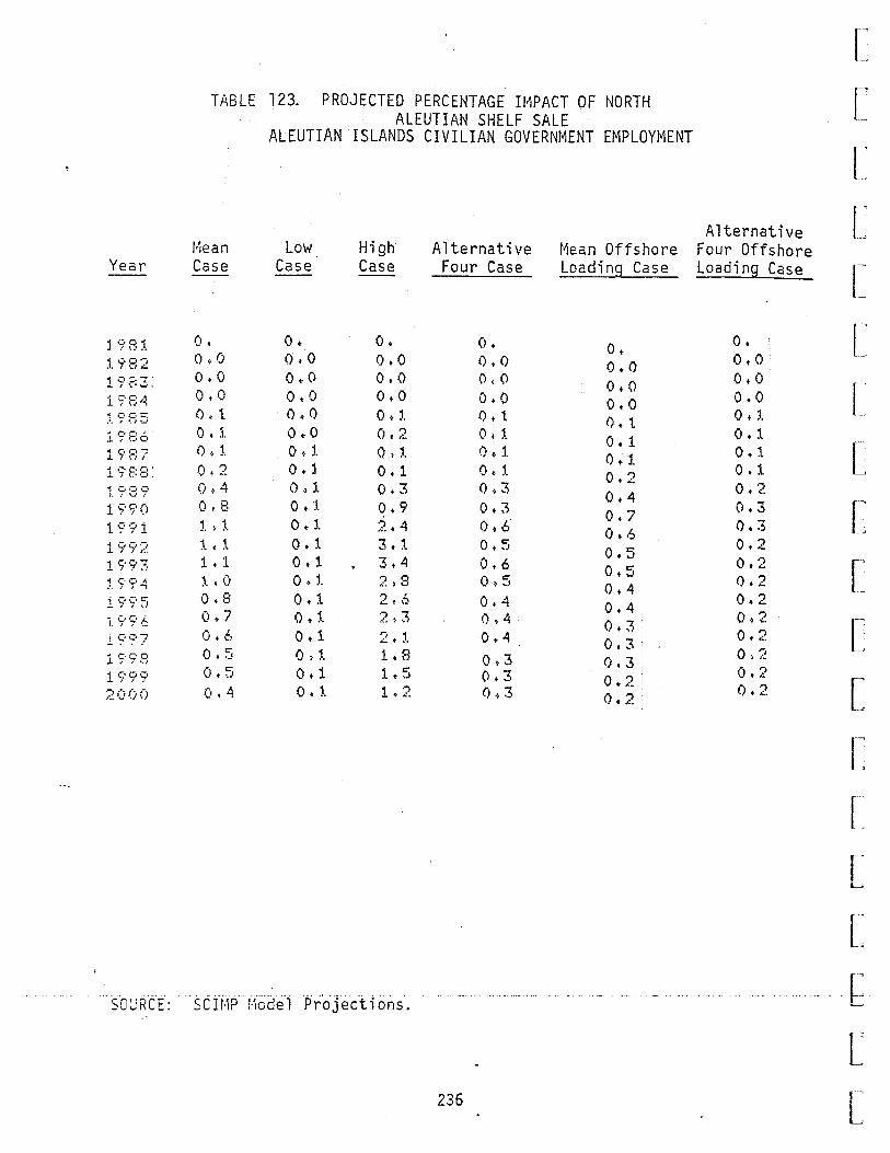
Year

l '7'8 :t. l -;:·:?, 2 1'7~E:3:

1 '7't:4 "' -;· :::; 5 l ·;·::::c. "' r, ,-~: l. 7 •':'.• i

1'7'f.~:=:·

t ·~:. B '7' 1 '7'<7'0 1 '7"? 1 -( 00 .-J .l i i ,,_

1 '7":f::, 1 C•C• 1-: .•. J J ~

:!. '7' .,.. 5 I. S:' ·:;:· .~ l '7''7-'7 19;7'8 1S'9~' ;.:: (:r (j ()

TABLE 12~ PROJECTED PERCENTAGE IMPACT OF NORTH ALEUTIAN SHELF SALE

l·lean Case

0. o.o o.o o.o ().1.

0. l () '• l Ot2 0.4 0.8 l • 1 1 + 1 1 • 1 1.0 0.8 0.7 0 + !:, 0.5 0.5 0.4

ALEUTIAN ISLANDS CIVILIAN GOVERNMENT EMPLOYMENT

Low Case

0. o·. o 0 ,. () o.o o.o o.o o.:t. 0. j 0 ·> l. o.t o.l. 0.1 0.1 o.t 0.1 0. j_

o.1 0. '· 0.1 o.l

High Case

0. o.o o.o o.o O.l 0.2 o,:t. 0.1 0.3 0.9 2.4 3.1 3.4 2~8 •") ' ..:..+W ·") "l .·:.) • .. J

2 t j,

1.8 1.5 1.2


o. o.o (),()

o.o 0. 1 0 •· 1 O.l. 0. :1.

0.3 0.3 0.6 0.5 0.6 0.5 0.4 0.4 0.4 0.3 (),3 0.3

1•1ean Offshore Loading Case

0. o.o o.o o.o 0. 1 0.1 O.l. 0.2 0.4 0.7 0.6 0.5 0.5 0.4 0.4 0.3 0.3, 0.3, 0.2· 0.2


0. o.o o.o o.o 0. l 0.1 0.1 0. 1 0.2 (),3

0.3 0.2 0.2 0.2 0.2 0 ·> 2 0.2 0)2 0 ... , . ..:. 0.2

[

[

[

[

[

r··

[:

[

[

[

[

[

[

l., ~

L [

-- ---- -souR-cT:---sc ITfP-T',oder-rrojecffons~--- -----~-----~------------------------------------ -----L -

[ 236 r·

L

~

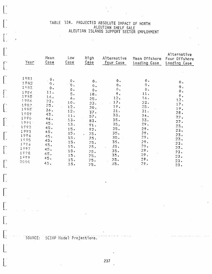
r~

~

[

~

[

[

L [

[

[

['

[

[

[

[

L' -

L r L

Year

1 .,. f.: :t.

1'?:7;2 1 ·~· E: 2. i'?B~ .1. 7';~5 ~ 7'E:f.. 1_ ~· :=:: 7 l ~'E::; "'t C·C;•=• 1. .! \-' ...

19'7'0 i. '?·:;:· 1. iS:S:·~: i y \:;•-;: - ~ # \a1

1 ·;· 94 J.~?5 J. ·~· 'i' .:, 1 ·;t~·; 1•7• ·;· :3 1 ·;· 9 <;· -~(:;f)(';

TABLE 124. PROJECTED ABSOLUTE IMPACT OF NORTH ALEUTIAN SHELF SALE

ALEUTIAN ISLANDS SUPPORT SECTOR EMPLOYMENT

l·1ean Case

o. 0) o.

1 l • 1. 6. ,..,7 ,:.. -· t .-,.c:-.-:. ,.J +

36. 1-..... ,,')<Co

46. 45) 45. 45. 45. 45. -454-45. -45. 45~

43+

Low Case

o. () )

0. 5. 6 +

10. ), 2)

1"' . ~ ~

'· :!. • 13. :1.3, l 5. l. 5 <·

:1.5' 15~

:1.5. 15. :1.5. 15. :1. :.1 +

.

High Case

0 •· 0. o.

j 8 < ·} C' ~--.} .,. 'i-: .. ·.-· c 2(), 37 • 57. 83. s> :l. , 9"' £. +

75. 75, ~~

I...!+

75, 75. 75. 75. -·t:' I ·.J •


o. (). (l.

9. 1.2+ l. 7.

'· 9. 31c ~~3 + _.,. ~'"'· "']t:" .... ·.I. -.,. .... "> ._, +

-.,. .:• ~I t .. .,. .. ") .. J t

-.,. ~ ..... 1. • , a=--.~ -.J o)

35+ -,.,. ..")·.I • -I:' ....~..J + ···c:-

.• "1-.) ·)

!·lean Offshore Loading Case

(). () ·>

(l •

1 1. • t6. 23~ .-.~ .. :· .... ,) 31. 3 it • --.._4,.~ ~

?.9, 29. 29t 29 • 29. 29 • ;~ 9 ~ ;;~ 9 ) 'iQ ..:... , . :?9.

SOURCE: StHiP l·iodel. Projections.

237


o. () >

o. 9 •

,_;~,

17 .. ). 9. 28. ?.7. 27. .,-''· .;') . 23. 23 • 23. 23. 23 .. 'i-,; .:, . '17 ...:..... .... 1 +

23 • '23 +

..

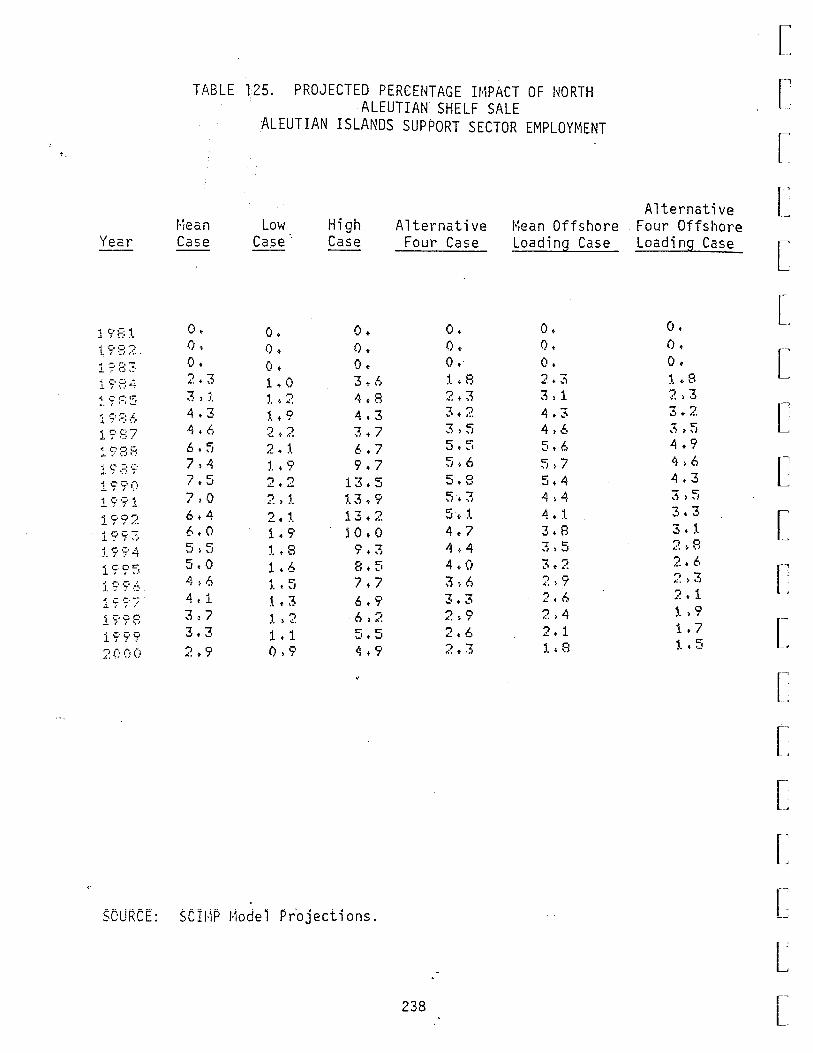
Year

1 <7'81 1.9E!:~.

1 '?E:3 1 '?' E;<~-; ~- s:· :?; 5 1 q;~:.~= 1 ?' ::::7 ~ c:o •:i c. -- .· ···''··'

1 ;;·a·~· 19~'0

:1. '7"? 1 199? 19~·~

J.9'7'4 ~ .-. C•t:" .L-; i'"' ·: C·•=• ,;_ ..!. ,: ... ·.-· .

~ C· .:.-; . .1. .... ,.

1 s··7·f; 1999 :?000


l·iean Case

o. o. 0. 2.3

3) '· 4.3 -4.6 6.5 7,4 ~ "'" /t.J

7.0 6.4 c..o 5)5 5.0 4,6 4. :1.

:-L 7 7 7 \.J t -·

2.9

ALEUTIAN ISLANDS SUPPORT SECTOR EMPLOYMENT

Low Case·.

0. () . 0. 1.0 , .-, .. ~ .,:,

L9 '2 ~ 2 2. ~.

~ .• '7' 2 .. 2 2 l ~.

2. ~.

1.9 L8 1. 6 , "'" .. + \.,}

1. 3 1 ') .. ·) "-•

1 t 1 0.9

High Case

o. () . o. 3.6 4.8 4.3 3 ... 7 6.7 9.7

13.5 t3.9 13t2 l 0. 0 9.~

8.5 7.7 6.9 6,2 5.5 4.9


o. o. 0. ~. <· 8 2.~

3 .. 2 3.5 1:" "'" ._1 + "-'

5,6 5.8 1:" 7 • .. } (- -..J

5c- :1.

4.7 4.4 4.0 3,6 3.3 2.9 2.6 ,., ... ,;. t ·~

l·'iean Offshore Loading Case

o. 0 +

0 t ., ~

.:... .. "-..,

3,:1. 4.3 4) t.:. 5.6 5.7 5.4 4,4 4. :1.

2· + 8 7 "'" -.1) ._I

7 '") '"' t .: .

2,9 2.6 2,4 2 t 1 :1.. 8


o. () . 0. :1.. 8 ~~:, 3 3.2 ~ 1:" .. ~ ) ... J

4.9 4,6 4.3 ~ "'" .. '> 'd

3.3 3. ~ 2:,8 2.6 ,., 7 ,;, ) \.J

2.1 ,_ l 9 1. 7 1..5

[

[~

[

[

[

['

r~

[

[

[

[

[

[

[

[

[

S-OURC-E: $CH1P r-iode1 Projections. C-L

238 r,

L

F'

L~

[

[

[

[

[

[

[

[

[

L [

[

L r ,

L

Year

1S"'8'. 1S:'S2 1 ·;•[:3 17'B4 i '7't:5 1 '7'8t. J. ;: ;::: 7 19BE: .t·:::·s·;:· 1 ii' s-· t) 1'7: 9 ). 1'7'92 1 71171 3 1994 1 s-· 9 ~ l"? '? ,~. 1 s·_'71 ? 1 ·;:••7 :3 1 ·:;· C:· !;•

' ' ' :~coo

TABLE 12~ PROJECTED ABSOLUTE IMPACT OF NORTH ALEUTIAN SHELF SALE

ALEUTIAN ISLANDS CIVILIAN RESIDENT POPULATION

l·'iean Case

0. o. o. 8.

).!') •

20. '?3 +

57. J.j_(l,

162. 1 . . !; 0 • 173. :1.:. 9 • l40. l24. !. U. • 10:?..

<;·5 ~

90 <·

86.

Low Case

0 <·

() . 0 • 3 t

(} . 10 ,. • 7 ,1, .... ~

1 t., J. 5; 18. :1.8. 20 <·

20. :;::l.. 2 1 • :n., 2 j • ")·-· ...: .. ·:.. )

")'j ..:....:-+

:?. 2 •

High Case

o. 0. o.

15 .. 20. j 8. l5. 37.

:t 25) 340. -158. 513. 446. 4'27. 405. 378. 346. 307. ;~6 7 +

2:~5 t


0 ' o. 0. 8. 9.

14. UL 7' ..,o ,. 48. 84. 79~

se.. 79. 73. 68. .s5. 63. ,_s 1 • 60. 59.


0. () . o. 8.

J. () • 20. :?.3 ) 51+ '7'9. 91. 17. 69. t-3 • ~9. 56. C.'7 ... J \..} +

51. 50 • 49 • <'19.

- SOURG:E> SCJHP- l·'iGde 1- Pr-oj ec-U ORS-.

239


0. () . 0. 8. 9.

l 4 +

:1.8. -") ~4!..+

4l.. 40. 35. -I:' ,..."t~ +

-I:' .;.;.

:~ 4. -.:1 ~ I +

~~5 • -I:' "~ ... r +

:~5' 36c :36~

'·

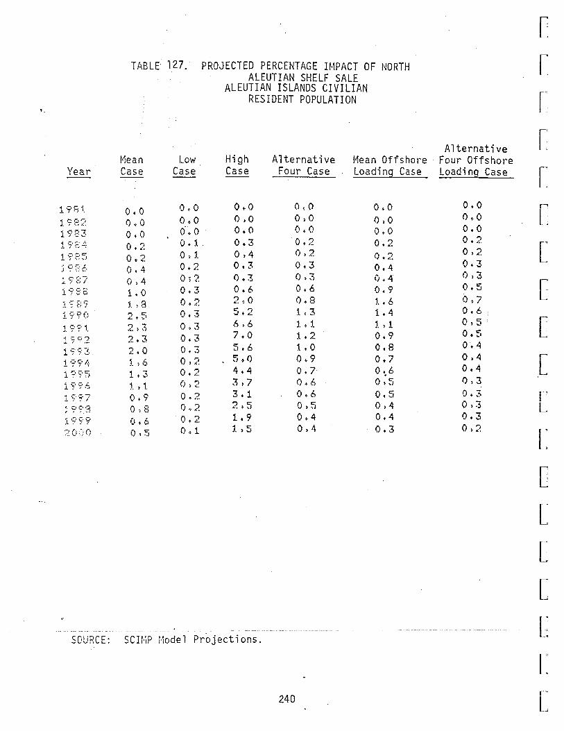
Year

j_ ·;· ~~ i.

j_ ·~ ~~ :? "'I (')C•7 .l. / l_, .. _.

of .-. ,-. l: .L 7 f:. -;

1 '7' F: 5 :i S:: F~ f..,

: ·?:E:7 i'?'~=~c: ... - .-, .-. .l :: •":.• 7

J. ·:;:· ~· t) l'"i-' s:· 1. "".:. o·-:· •·· . .:.. is··;·~:.

i ·~· '1' 1.~ 1 ·:: .. ;· 5 i ·~··;·.L;,

J.•:-·7'7 ~- s=· ·;· ~:i

1'7' ~- '7' ·~: 0:.·; 0

TABLf 127. PROJECTED PERCENTAGE IMPACT OF NORTH ALEUTIAN SHELF SALE

f•'lean Low Case Case

o.o o.o 0 ,. 0 o.o o.o 6.0 0.2 0. 1.

0.2 0. :1.

0.4 0.2 0.4 0>?.

1.0 0.3 l. , 8 0 + ;~ "') t:' ~ + ~·

0.3 "') -,~. > .... 0.,3 2 + :~ 0.3 2.0 0.3 :1. ,-s o.?. 1. 3 0.2 l. > 1. (),?.

0.9 0.2 o.s () . ;~ 0.6 0.2 (), ~ 0.1

ALEUTIAN ISLANDS CIVILIAN RESIDENT POPULATION

High Alternative 1•1ean Offshore Case Four Case Loading Case

o.o o.o o.o o.o o.o 0.0 o.o o.o o.o 0.3 Ot2 0.2 0,4 () ';;-~ ().2 0.3 0.3 0.4 0.3 0.3 0.4 0.6 0.6 0.9 2 ., 0 0.8 l.6 r: "') ~·~ 1.3 1.4 6 .• 6 1. • :1. 1. ' 3. 7.0 1 • 2. 0.9 5.6 1. 0 0.8

. 5 > 0 0 ,, 9 0.7 4.4 0.7 0 ._{:, 3,7 ().6 0.5 3.1 0.6 0.5 .., t:' ~. ·) ... J 0.5 0.4 1.9 0.4 0.4 :1. '5 0.4 0.3

SOURCE: SCIMP Model Projections.

240


o.o o.o o.o 0.2 0.2 0.3 (),3 0.5 () ., 7 0.6 0) 5 ~

0.5 0.4 0.4 0.4 (),3 0.3 0.3 0.3 0.2

[

[

[

[

[

[

[

[

[

[

[

[

[

[

[

[

l [ r"

L

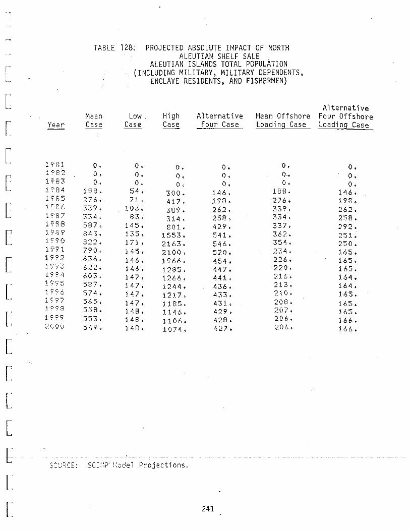
i l ___ _

[

[

[

[

[

[

[

[

[

[

[

L [

l l r .

L

Year

1'7'f:::l. j_ ·~: :3 '2 1 :7•83 1 .-. ,-, " - '; :::·...., o': ,-.• - =-~- 7 •:-: ._1

1 '7·:::.::. 1·:·::;; 1~:?B8

1 ?:;'7' 1 '7 '7' () 1 ~"? 1 1 '7"7' :? 17''1'3 :L S· ~;· 4 1'7' :7• 5 ~- ·;· ';· .~.

1 S" 9/•" .: -~·9:3

1 ·:;··:::·s· ::?00()

TABLE 128; PROJECTED ABSOLUTE IMPACT OF NORTH ALEUTIAN SHELF SALE _

ALEUTIAN ISLANDS TOTAL POPULATION (INCLUDING MILITARY, MILITARY DEPENDENTS,

ENCLAVE RESIDENTS, AND FISHERMEN)

t•1ean Case

0. 01' 0 t

188. ~: 7 c.. t

339. 334. .:-o~ ...J·~ I <·

843. 1:• .-J ~I 1-•L....:.. t

790. 636. 622. 603. 5S7. 574. .:-•.::-,_I C' .... 1 f.

1:"1:."0 • ... 1 ._1 \.) .;.

553. 549~

Low . Case

0. 0. 0.

54. 7 ,_ •

1.03. 83 -~

145. 1"';~ ~·· -..• ... J +

171 • 145. 146. :1 A6. 147. J 4 7. l47. 147.

'· ·~ 8 • 1-48. 14:3.

High Case

o. (). 0 •

3004-417. 389. 3:!.4. 80:1..

:!.553. 2:1.63. 2lOO. j '7'66. 1 '1 ,., c.·

.:... C•..J +

1 ;~66 +

:1.244. 12:1.7 ·>

:11.:35 • , '- 4 6. j 10 6. :t074.


0. o. 0.

146. 1'78 ~ 262. 'it:"O .,:, ... J ._, )

429 •· 54:!.. 54 6 (· 520. 454. 447. 44:l.. 436. 433~

431.. 429. 428. 427.

t•1ean Offshore Loading Case

0. o .• 0 •·

188. 276. -~o ~,_j I + 7-iJ. .. ! ... ~ I fo

337. 362+ 354. 234. 226. 220. 2t6~

213. 210. 20B. 207. 206. ~:(Jt..+

r"'·-~"'.- sr~"::>· l'-,o'el Pl'O~e~tions ,::: .... ·:._;~Lt.: ""'..;.!'L :';\...· J \... .

241


o. o. o.

146. l$'8. 262. 258. ;

1 92 t

;~ 5 '· 4

250. l .~5. 165 .. 165. :1.64. 164. '-·~5 +

1 t.5. 1.65. j 66. 1.66.

TABLE 129. PROJECTED PERCENTAGE IMPACT OF NORTH ALEUTIAN SnELF SALE

ALEUTIAN ISLANDS TOTAL POPULATION (INCLUDING MILITARY, MILITARY DEPENDENTS,

ENCLAVE RESIDENTS, AND FISHERMEN)

l·ie2n Low High Alternative !•1ean Offshot·e Year Cc.se Case Ca.se Four Case Loading Case

:1 S'f.: ~- o.o o.o o.o o.o o.o 1 '?82 o.o o,o o.o o.o 0.() 1983 o.o o.o o.o o.o o.o j C• •=• .~ • .i ... ;.., 1 + t, 0.5 '") t:" 1 • 2. 1.6 .:.a t \,J

"! qc.c:-.L ,· •.; •• J 2.3 0.6 3,4 '· .. :; 2.3 lS'S6 2.7 o.s 3.1 2.l 2.7 t '7'87

·"") L . .:. ~ '-J 0.7 '") t:"

··- 1- ._ ... 2, l. 2 + \':>

~t ~·Bf..:: 4.5 1.2 6 • l 3.4 2.7 j_ '? !3 '1' 6.2 l..O :!.0 ., 9

4 ''· 2(- 8

1 s:· s:· () 5.9 1.3 j 4 • l. 4.0 2.6 1.'7''?l

C' t:" l.O :1.3,3 :3.7 1.7 ,J + d

1 ~·s·;;· · 4.3 l • 0 1.2.1 3.l L6 ~- '7'93 4.0 1 + 0 7.9 2.9 1.4 t-?94 3.7 0.9 7.4 2.7 1. 3 1 oc•r.:: .. · ........ 3.4 0 •. 9 6.9 ~, t:" 1 '") .. · .. i ..... t .:.

'· '7' '7' .-:. 3.l 0 ., 8 6.3 :!.v~ 1 t 2

1 C·C•7 • -~ •• ,1

2.8 o.s 5.8 '") '") .:... + .:.. 1.1

:L '? -;· B '") , .·: .. ·~ 0,7 t:" '1

.J + .o\. 2t0 '· . () 1 C••::••:;:·

~ .· . 2.4 o.t. 4.6 '· • 8 0.9 ;~ (:r (} Ct 2 ., :t 0.6 4. :1. l.7 0 • :=j

SC:;RCE: scn;p l·iodel Projections.

242


o.o o.o o.o 1.2 :1..6 2. ~ 2.:1. '") -.:.. ......... 1.,9 1.9 3..2 1 • j 1.1. 1.0 :1. + 0 0.9 0.8 0.8 o·., + I

0.7

[

[

[

[

[

[

[

[

[

[

[

[

[

[

L [

l [ ('

L

[

[

r [

[

[

[

[

[

[

[

[

[

[

L [

APPENDIX A: THE MAP REGIONAL MODEL

Introduction

This appendix presents in general outline form the structure of the

new MAP regional model utilized in this report. This model replaces a

more cumbersome model used in earlier OCS studies.

In developing this model, several major objectives were addressed.

These objectives are the following:

• that the structure be simple and generalizable

• that the parameters be specified in terms with clear, intuitive meaning

• that the regions be disaggregated to census division levels

• that the model be sufficiently flexible to be tied easily to the MAP statewide model.

This appendix is organized as follows: Part II examines in detail the

structure of the model. Part III presents estimates of the model

parameters.

Structure of the Model

OVERVIEW

The model consists of two components as shown in Figure 4. Given an

exogenous estimate of statewide employment, by sector (provided from a

[ _____ '_ -· _ ~~~r_e;;p~ndi.ng state model run), and vectors of basic and government

emp 1 oyment in each of the twenty regions shown in Figure 5, the

[ I -

L 244

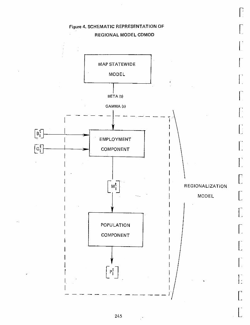
~ [G

l J

l J

I

I I I

I I I

Figure 4. SCHEMATIC REPRESENTATION OF

REGIONAL MODEL CDMOD

MAP STATEWIDE

MODEL

J BETA (t)

GAMMA (t)

[

[

[

[

[

[

------ ----· - --- --··· f [

... - EMPLOYMENT

COMPONENT

c~u- ·

' POPULATION

COMPONENT

w

I I I I I I

[

[

[ REG I 0 N ALl ZA T I 0 N

I [ I MODEL '

: I c I [ I ,

I r· I ---'

I [ I

[Pf] :_; b------------1 I

___________ l/ [

r .

245 L

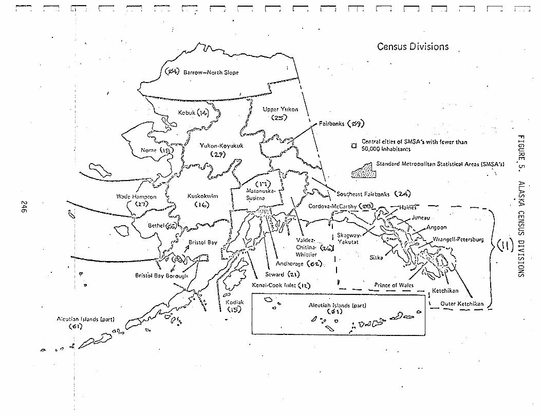
r; r--:

1'\.)

.f:::> O'l

C'l: r--: r-1 r---: ,----, k "' r-J r-1

Barrow-North Slope

rJ r-:1 r-1 rn

r-- , 1

1 "'- I ,.j \ ;>< . ~ ~$

~ Kcbuk (14)' / Upper Yukon . _J (7.:S) '

~ r.rP''~~.;f 1./ ~ ,:\Fcirbanks (¢9) ((: . 'l tqo."""'" '.1 ~

""' ·• •.• .,.. u on· oyu u y

r-l r-l :--.1 :--] ~

Census Divisions

~ ..... "l-- .ri y k K k k c).:s-~ ~\1' ·,. O Cer.t~al citi~s of SMSA's with fewer than

Nom;]! (\ .. ) ~ ,.,..../') 50,000 inhabitan:s -.../"" , ( 2.?) -,.-:-1' '

C:::"'-. " ~u->J 1 11'7 ;.-,.,, '~ ~\ ~ Stond"d Mmoooliun Stot;'""' A'"' ISM~~'>) ~ _ .......... , .;F..J &/ \ ~~ \? a :.\. .._,,.......... . . r:. ,.,...,) . (1 .... , \ ~-~ . Vl ~ 'I ? ~ r Matilnusk<J· \'~ ~·¥ f\ · . r,., .i'\

WJdc H,1 mp:on ~ Kuskokwim '- Susitn\1 ~ /'" ~\ Southeast F;mbanks '-41'-'11

-..,..__ ( <n) ;,) ( 1~) ~ · r:'":"'!._..J \ Cordov;:·McCJrthy (q;e)_ .-... -Haines -(\.. -~ _\_, ~~·--- !... r.~·-.,..:::-.-::.:j:';) r.r 11-:,.:;:r-'-;:- _ , 0 / "-.J. ~_ . ..,../ 4 "'r'''l\ 1i?._ ~)c.,.;;;-. Juneau

--

~

.,

....... Ci) c ;;:c rr1

(]1 . )::> r )::> (/)

·~ n rr1 :z: (/)

c (/)

<\"1 (- 13cl.hel~)\~~ ~ ~ \~j\ U'~ "-.) ~~' _.._Angoon · ~ \_ .A C'J ; }\i\ ~ :I <:: S'-ka'"'S"W'"a•yx. '-\

• t,J 7 ~~ .. J

r.~] Bristol Bay /' \ f~ Va~d.cz· . Yakutat • '\· t, ~·.·

~ .1 4 ,..r;· ..... , . Ch1t1na· r,./"\J .rr;~ -.,,-..,. (} ,. ~- ~ 1'\.\,1 \,40."0,.1 \· f.Y

........__ _....!!cf'(f>-"'r\. ~ l.··i'/ ''\ . Whittier I . ~~ i)~('\ ~ (HJ ~

'i\ )".::h(J )>') .{/) Anciwoge (o-z.") ,7:.;'J,;v-- "·• •• !.~.] ' . r / I I ..., l · , ;,

fi' BristolDayOorouur:"/~.tJ Seward (1..\) . ~~\f.\ co '>/_ \ Kenai-Cook lnlr.: {11..) » Prince of Wales

· -1 - - ...__ - - - Ketchikan · • 'f vo . I

° Kodiak 0 ·• .~ \".. :\ ~ Aleutian (5lands (part) I \ Outer Kctch1r:an \ (IS; I c.... (~$'\) (') 0 -- --

" - ~ .ct::J .c::::so , .(1 0 ' )),0{;:::>,.. ~ ..

I'

r.>

1\:r'Jti.ln (6a)sland~ (part)

~o(l...,

or'J ~ pd-/'

....... (/) ....... 0 :z: (/)

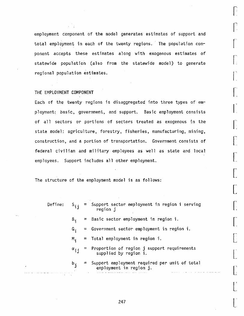
employment component of the model generates estimates of support and

total employment in each of the twenty regions. The population com-

ponent accepts these estimates along with exogenous estimates of

statewide population (also from the statewide model) to generate

regional population estimates.

THE EMPLOYMENT COMPONENT

Each of the twenty regions is di saggregated into three types of em-

ployment: basic, government, and support. Basic employment consists

of a 11 sectors or portions of sectors treated as exogenous in the

state mode 1: agriculture, forestry, fisheries, manufacturing, mining,

construction, and a portion of transportation. Government consists of

federal civilian and military employees as well as state and local

employees. Support includes all other employment.

The structure of the employment model is as follows:

Define: s .. lJ

B. 1

= Support sector employment in region i serving region j

= Basic sector employment in region i.

Gi = Government sector employment in region i.

M. 1

a .. lJ

b . J

= Total employment in region i.

= Proportion of region j support requirements supplied by region i.

= Support employment required per unit of total employment in region j.

247

r [

r [

[

[

[

[

[

[

[

[

[ [ -

[

L [

L r -

L

[

[

[

['

[

[

[

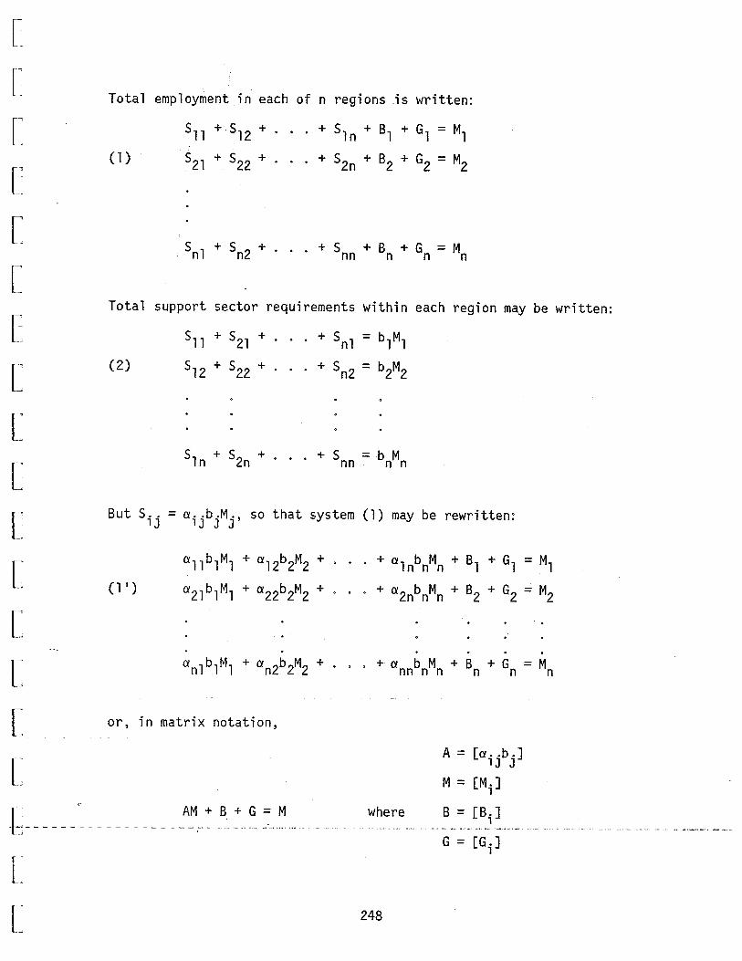
L f' [

[

[

[

r [

l

Total employment in each of n regions is written:

(1)

511 + 512 +

521 + 522 + .

+ 51n + Bl + Gl = M1

+ 52n + B2 + G2 = M2

5 l + 5 2 + . . . + 5 + B + G = M n n nn n n n

Total support sector requirements within each region may be written:

(2)

s, + 521 +

512 + 522 +

51n + 52n +

+ 5nl = blMl

+ 5n2 = b2M2

+ 5 = b M nn n n

But 5 .. =a .. b.M., so that system (l) may be rewritten: lJ lJ J J

(l')

a1lb1Ml + a12b2M2 +

a2lblMl + a22b2M2 +

+ a1nbnMn + B1 + G1 = Ml

· + a2nbnMn + B2 + G2 = M2

.

a 1b1M1 + a 2b2M2 + ... + a b M + B + G = M n n nn n n n n n

or, in matrix notation,

A= [a .. b.] 1J J

M = [M.] 1

L ' AM+B+G=M - - - - - - ·- - - - - - - -- - - - - -- -- .--- ·- -· .. . .... -· -·· ... . -·· ·- ·-· -- -· ·-· ..

where B = [B.] 1

L [ 248

G = [G.] 1

If the A matrix were known, then total employment is calculated as a

linear function of basic and government employment, or

(3) M = [I - A] -l [B + G]

Of course, we do not know A. By incorporating known region a 1 data

with a single simplifying assumption and a behavioral hypothesis

describing the allocation of interregional support demands, however,

it is possible to estimate A for a point in time, say 1979.

Known Regional Data. Regional employment for 1979 was available from

the Alaska· Department of Labor publications, specifically Statis-

tical Quarterly and Alaska Economic Trends. The breakdown of such

employment by basic, government, and support sectors is shown in

Table 130 for 1979.

A Simplifying Assumption. Since the major concern of the regional

mode 1 is to capture the effect of support sector demands which are

supp 1 i ed in regions other than the one giving rise to such demands,

rather than to examine the effects of differential support demands

across regions, it seems plausible, or at least not overly restric

tive, to impose the condition that

(4) b = b = 1 2 = bn = b = ( 1 _ B ~ G )

249

[

[

[

r [

L E

[

[

[

[

[

[

[

[

[

[

l r-L

[

[

[

[

['

[

[

[

[

[

[

[

[

r~

[

[

L L f"

L

That is, a unit of total employment, wherever it occurs in the state,

is assumed to give rise to the same support sector requirements. The

difference between regions, then, is so 1 ely the difference in the

locations from which these demands will be supplied.

This assumption has the obvious disadvantage that it neglects real

interregional differences in demand for support sector services.

However, it also has several advantages which may more than compensate

for this shortcoming. Most obviously, it reduces our estimation

problem by n-1 parameters. More importantly, it is extremely valuable

as a tool for maintaining consistency with the statewide MAP model,

both in a static and a dynamic sense. Currently, a unit of basic

sector employment in the state model has the same· static employment

impact regardless of its location in the state. Regionally varying

bj • s would produce differing total statewide static impacts by loca

tion, thus being inconsistent with the state model. Furthermore, the

introduction of b exogenously provides a valuable tool for maintaining

dynamic consistency between the models. By letting b vary with time

so as to reflect the corresponding state run, we both force the A

matrix to vary over time to reflect the same degree of structural

change represented by the state model and force the employment totals

to replicate the statewide results.

A Behavioral Hypothesis. The major reason that not all support sector

requirements ar~ supplied internally from that region is that it would

be more costly to do so than to secure those services from a different

250

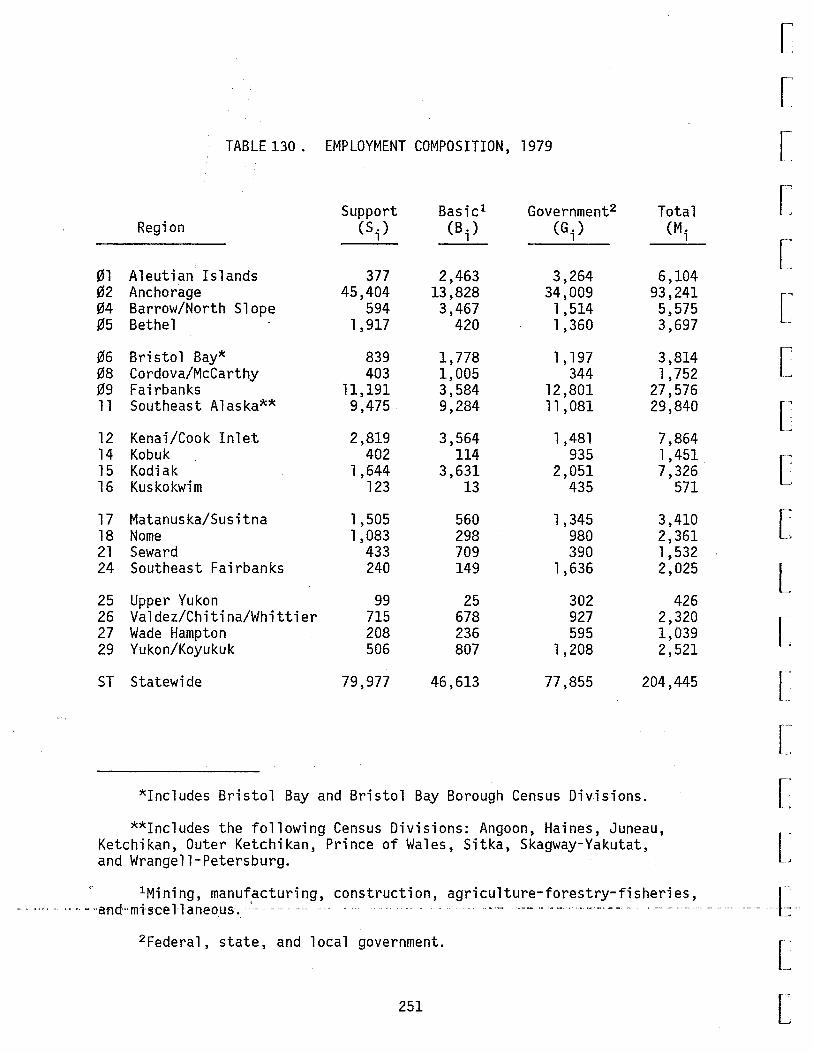
TABLE 130 . EMPLOYMENT COMPOSITION, 1979

Support Basic1 Government2 Total Region (S.)

1 (B.)

1 (G.)

1 (M.

1

01 Aleutian Islands 377 2,463 3,264 6,104 02 Anchorage 45,404 13,828 34,009 93,241 04 Barrow/North Slope 594 3,467 1,514 5,575 05 Bethel 1,917 420 1,360 3,697

06 Bristol Bay* 839 1,778 1,197 3,814 08 Cordova/McCarthy 403 1,005 344 1,752 09 Fairbanks 11,191 3,584 12,801 27,576 11 Southeast Alaska** 9,475 9,284 11 ,081 29,840

12 Kenai/Cook Inlet 2,819 3,564 1 ,481 7,864 14 Kobuk 402 114 935 1 ,451 15 Kodiak 1 ,644 3,631 2,051 7,326 16 Kuskokwim 123 13 435 571

17 Matanuska/Susitna 1 ,505 560 1 ,345 3,410 18 Nome 1,083 298 980 2,361 21 Seward 433 709 390 1 ,532 24 Southeast Fairbanks 240 149 1,636 2,025

25 Upper Yukon 99 25 302 426 26 Valdez/Chitina/Whittier 715 678 927 2,320 27 Wade Hampton 208 236 595 1,039 29 Yukon/Koyukuk 506 807 1 ,208 2,521

ST Statewide 79,977 46,613 77,855 204,445

*Includes Bristol Bay and Bristol Bay Borough Census Divisions.

**Includes the following Census Divisions: Angoon, Haines, Juneau, Ketchikan, Outer Ketchikan, Prince of Wales, Sitka, Skagway-Yakutat, and Wrangell-Petersburg.

1Mining, manufacturing, construction, agriculture-forestry-fisheries, '",and ,mi see Haneo.us. · - · · · ·

2 Federal, state, and local government.

251

[

[

r r [

[

L [

[

[

[

[

[

r-

L L c L f-

L

[

[

r~

L [

[

L [

[

[

[

[

[

[

L [

r~

L L

region. It is only natural, then, that the cost of supply should be

the major determining factor ·in deciding on which other regions to

supply the requirements. Such costs as transportation, communication,

etc. are generally expected to increase with distance and to decrease

with the size of the support sector source of the region. Speci f-

ically, we will assume that such costs are:

(5) c .. 1J

R •• - k ...2J. where - M.

1

c .. 1J

R •• 1J

M. 1

= cost of supplying a unit of support service to region j from region i

= distance* between regions i and j

= total employment of region i

k = an arbitrary constant

and are as presented in Table 131 for k = 1000.

The total costs of interregional service provision are then:

(6) n n

C = I I j=l i=l

c .. s .. 1J 1J

We hypothesize that the S;j's actually chosen in any given time period

are chosen in such a way as to minimize the costs of providing the

required services observed in region j from each of the sources of

such supply i.

*Air fares were used as a proxy for distance since straight line distances fail to capture the structure of statewide transportation and communications networks.

252

TABLE 131.

Demand Region

Supply Region "' I

~1 ~2 ~4 ~5 ~6

1 ~+·Aleutian Islands 0 33 52 45 23 ~f Anchorage 2 0 1 1 1 ~'r Barrow/North Slope 57 20 0 33 30 ~5 Bethel 75 20 50 0 35

I

~~ Bristol Bay 37 15 45 34 0 ~8 Cordova/McCarthy 199 18 83 61 50 ~$ Fairbanks 9 2 3 4 4 H Southeast Alaska 10 . 3 7 5 5

I Kenai/Cook Inlet .16 12 28 2 12 9

I

lf' Kobuk 203 63 112 92 101 N 15 Kodiak 34 7 22 17 7 U'l 16 Kuskokwim 433 77 215 207 175 w

I

~~ Hatanuska/Susitna 65 6 39 28 22. 1·8 Nome 125 39 69 39 62

I Seward 147 14 89 63 2~ 51

2,i S.E. Fairbanks 144 43 69 80 71

25 Upper Yukon 674 197 268 319 329 26 Valdez/Chitina/

I Whittier 106 19 68 51 43 2:17 Wade II amp ton 273 78 204 27 132 2·9 Yukon Koyukuk 107 . 27 52 56 49

I -1-*· Indicates C .. < 0.5.

1J

r~ r-:; fl r-:: . r--; r-l ;---" c ,J r-J

ASSUMED COSTS OF INTERREGIONAL SERVICE PROVISION

~8 ~9 11 12 14 15 16 17 18

57 42 47 36 48 41 40 37 48 * 1 1 * 1 1 * * 1

26 15 36 22 29 29 22 24 29 29 28 43 25 36 3~ 32 25 25

23 28 37 19 39 13 26 20 . 39 0 47 38 29 70 46 43 30 70 3 0 4 3 3 3 2 3 3 2 3 0 3 6 4 4 4 6

6 9 13 0 14 8 8 5 14 85 57 122 75 0 96 76 76 28 11 11 18 9 19 0 13 9 19

133 74 228 109 194 161 0 112 123

15 21 31 11 33 20 19 0 33 52 35 75 46 17 59 30 47 0 35 48 70 26 74 46 43 27 74 59 29 79 52 70 67 50 53 70

272 77 315 239 270 310 176 244 270

10 41 38 27 58 40 38 28 58 109 126 161 95 101 144 141 97 62 40 20 61 34 20 '46 11 35 20

r-J r-J r-l r-l ~ ~

21 24 25

37 48 47 >'r 1 1

24 25 20 26 44 37

20 38 37 31 68 66

3 2 1 4 5 4

5 13 13 78 97 79 10 19 18

116 177 131

12 32 30 48 60 49 .

0 72 69 54 . 0 45

249 216 0

28 57 55 99 163 158 -36 44 33

~ ~

26

40 ·* 28 32

26 13 3 3

8 93 13

154

19 57 43 65

300

0 120' 44

27

47 1

38 8

36 64 5 6

13 72 20

256

30 27 67 83

385

54 0

45

,..------, J

29

44 1

24 38

33 57

2 5

11 34 16 49

26 21 59 54

197

48 110

0

~ ~

[

[ ~-,

[

[

[

[

[

[

[

[

[

[

[

[

L

Estimating the Interregional Interaction Matrix. The hypothesis of

(c) and the condition of (b) imply that our observed 1979 data repre-

sented the solution to a constrained minimization problem of the form:

(7)

n n Min .L .L

j=l i=l c .. s .. lJ lJ

sr s 11 -+ s 12 + + S = M79 _ 879 79 2n 1 1 - G1

$21 + $22 + ... + $2 = M79 - 879 - G79 n 2 2 2

Snl + Sn2 + ... + S = M79 - 879 - G79 nn n n n

Sll + $21 + ... + S 1 = b79M79 n 1

s,2 + s22 + ... + s = b79M79 n2 2

5ln + 52n +

s .. > 0 lJ -

v i,j

+ S = b79M79 nn n

[ ______________ _

[ r· L 254

Note that s .. = a . . b79M~9 , so that problem (7) may be reformulated in 1 J 1 J J

terms of decision variables with a far more intuitive meaning than the

Sij•s, namely the aij•s. The reformulated problem is then:

(71)

where

Min b79 n L

j=l

n L C. a M79

i=l 1j ij j

ST ~ll + ~ M79IM79 12 2 1 +

79 79 ~21 Ml IM2 + a22 +

79 ~ M79IM79 = N1 I b79

ln n 1 79 Ml

79 ~ M79IM79 = N2 I b79

2n n 2 79 M2

79 ~ M79IM79 +a M79IM79 +

nl 1 n n2 2 n ~ - N 79 nn - _!! I b

M79 n

~,, + ~21 + · · · + anl = 1

~12 + a22 + · · · + an2 = 1

~, + ~2 + . . . + a n n nn = 1

~ .. > 0 1J - "'i,j

7S 79 · 79 79 ·· N. = M. · · - B. - G. . 1 1 1 1

255

[

[

[

[

[

[

E [

[

[

[

[

L [

[

[

c [ rL

[

[

~

[

[

[

[

[

[

[

[

[

[

[

[

[

which, assuming that a feasible solution exists, can be solved using a

standard linear programming routine.

The solution, a set of nxn aij•s, comprises a matrix which we will

call the regional interaction matrix. Each entry, aij' represents the

share of support requirements in region j supplied from region i.

Each of the columns, therefore, must sum to unity. Thus, a quick

glance down each column provides a subjective test of the plausibility

of the matrix. ~ priori, one would expect nonzero entries in all of

the di agona 1 elements and a 1 ong the rows of the regi ona 1 support

centers (Bethel, Fairbanks, Nome,) and probably along the entire row

corresponding to Anchorage, which is a statewide support center.

Summary. Once the regional interaction matrix has been determined for

a single year, say 1979, then this together with b79 determines fully

the A matrix which existed in 1979. For projections to a future

period t, we will assume that the interregional interaction matrix

remains stable, but that b changes in the regional model as it does in

a corresponding run of the statewide model. Therefore, employment is

estimated in year t as

(8) M(t) = [I - A(t)]-l [B(t) + G(t)]

where A(t) = b(t) [a~~]

The Population Component

[_ _____ - ,-- -Cur~en-t-ly,- tf:le population ,model is. specifi-ed .. as , independent of the

L employment model. We can define:

r -L

256

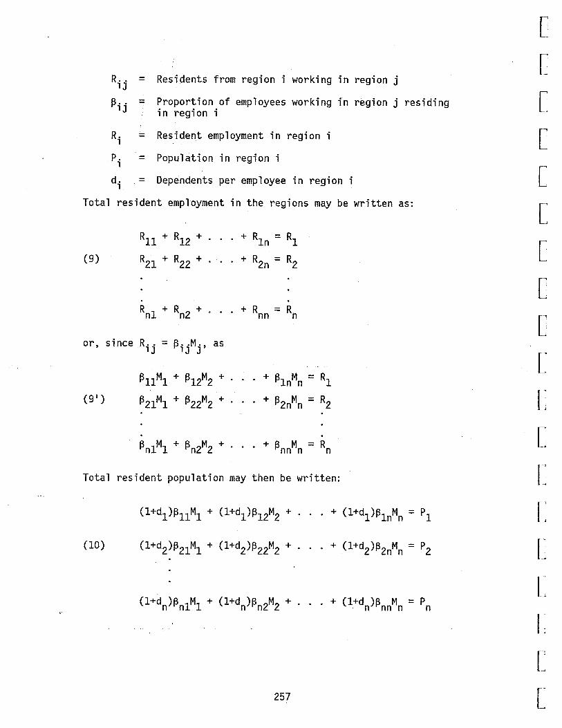
R .. 1J

= Residents from region i working in region j

~ .. = Proportion of employees working in region j residing 1J in region i

R. 1

= Resident employment in region i

p. 1

= Population in region i

d. 1

= Dependents per employee in region i

Total resident employment in the regions may be written as:

(9)

Rll + R12 + .

R21 + R22 +

+ Rln = Rl

+ R2n = R2

Rnl + Rn2 + · · · + Rnn = Rn

or, since R .. = ~- .M., as 1J 1J J

~llMl + ~12M2 + · + ~lnMn = Rl

(91) ~21Ml + ~22M2 + . . . + ~2nMn = R2

~nlMl + ~n2M2 + + ~ M = R nn n n

Total resident population may then be written:

(l+dl)~llMl + (l+d1)~12M2 + ... + (l+dl)~lnMn = pl

(10) (l+d2)~21Ml + (l+d2)~22M2 + ... + (l+d2)~2nMn = p2

(l+dn)~nlMl + (l+dn)~n2M2 + · · · + (l+dn)~nnMn = pn

[

[

~

[

[

[

[

[

[

[

[

[

[

[

[

L --------~---------------~

L 257 [

..,

[

[

[

[

[

[

[

[ ~

[

[

L L r·

L

[

or in matrix notation

(11) QM = p where Q = [ ( 1 +d . ) ~ .. ] 1 lJ

M = [Mi]

p = [Pi]

Now, the interregional structure of nonresident employment is captured

in the Q matrix, called the location matrix, which is unknown and must

be estimated.

Generally, there are three properties which this matrix should ideally

satisfy. First, it would be desirable that such a structure reflect

differential dependency rates across regions (d; :f. dj). Second, it

should reflect independence of extra-regional employment changes.

That is, if employment does not change in region i, population should

not change in region i. Third, it should be consistent with the state

model. Unfortunately, it is impossible to satisfy all three prop-

erties simultaneously.

The first and second property may be satisfied by assuming that

employees reside in the region of their employment. If such is the

case, then the interregional location matrix, composed of the ~ij's,

is the identity matrix, and system (9) implies that

(12) d. =pi - 1 1 -M.

1

(i = 1, ... , n)

258

so that Q is a diagonal matrix which can be estimated using 1979 data.

Unfortunately, this procedure cannot be made consistent with the

statewide model since total population impacts of changes in the

scenarios will be dependent on the location of employment as well as

its magnitude, while it is currently independent of location in the

statewide mode 1.

By adjusting the di•s over time, so that

(13) (1 + d~) 1

t I Mi ]

79) * [ 79 Mt = ( 1 + di I (1 +d1 ) 1 * a (t)

where a(t) = statewide population-to-employment ratio, we can force

consistency with the state model, but at a cost of giving up the

independence of extra-regional employment change property. Now, a

change in employment in region j # i will change the adjustment factor

in (13), thus changing total population in region i even if employment

does not change in region i.

Consistency with the state mode 1 and independence of extraregi on a 1

employment changes may be achieved by requiring that all di • s are

equal to the statewide average, but this fails to satisfy the first

property and is inconsistent with an identity location matrix. If we

are willing to abandon the first property, the problem may be solved

in much the same way as was the problem posed in estimating the param-

eters of the emp 1 oyment component, by so 1 vi ng the fo 11 owing 1 i near

programming problem:

259

[

[

[

[

[

[

[

[

[

[

[

[

[

[

[

[

[

l r-L

-,

I L_

l=

[

[

[

[

[

[

[

[

l"

L [ ~-

L

Min

ST

(14)

n n I I C .. R ..

j=l i=l lJ lJ

Rll + Rl2 + ... + Rln = Rrg

R21 + R22 + . . · + Rnn = R~g

R + R + + R = R79 nl n2 · · · nn n

Rll + R21 + ... + Rnl = (l+d79) Mig

Rl2 + R22 + ... + Rn2 = (l+d79) M~g

Rln + R2n + + R = (l+d79) M79 nn n

260

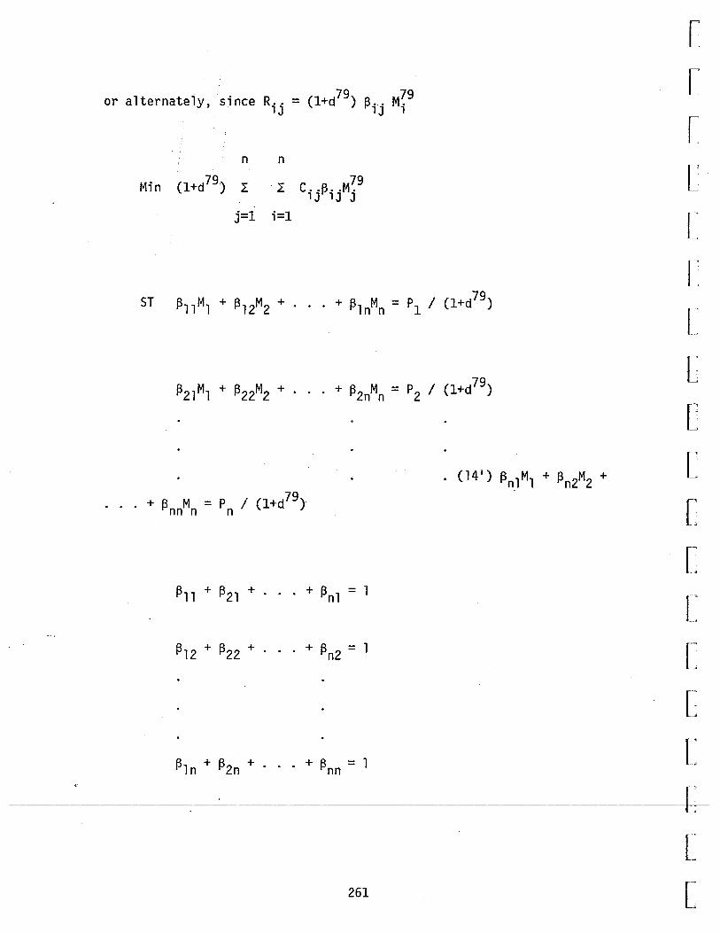
J l

~J

J J ]

']

J J J J J ]

]

J J J J J

T9Z

uu L = 9 + + uzg + Ulg

+ ZZg + Zlg

L = LUg+ .•• + Llg + Llg

I=~ T=f f fL fL ·w-·s··:> r 6L

u u

I' i ~

[

[ r, L"

[

[=

[

[

[

[

[

[

[

[

[

The current version of the model adopts the second of these three

alternate procedures, using an identity location matrix and adjusting

the di's over time as described by equation (13).

While such a procedure has the obvious advantage of simplicity, it has

several serious drawbacks. First, as mentioned earlier, such a speci-

fication necessarily will produce population impacts in regions where

no employment changes have occurred, as a consequence of the adjust-

ment factor in equation (13). The operation of this factor gives the

model the property that growing regions will attract population from

(relatively) stagnant regions. However, within the constraints of the

limited scope of this project, it was felt that such a drawback was

less serious than those associated with the available alternatives.

Furthermore, there are several reasons to believe that this effect is

likely to not be a serious shortcoming of the model. First, the

population drawn from stagnant regions is quite small and is generally

offset by induced increases in government employment which are always

more widely dispersed than initial changes in basic employment. More

importantly, however, the direction of the effect will always be the

same as a rea 1 effect-- i nterregi on a 1 migration, which has been ne-

glected entirely. Thus, the drain may actually offset, at least in a

small way, a known estimation error. Nonetheless, the population

estimation procedure must be regarded as generally much weaker than

the employment component described earlier, and it needs to be

[' ' improved with further research. -t::~ ~------ ~-- ~ ~ --=~- -~ -~ ~ ~ ~-:- ~-~-~-=--- -~--~---- ------- --~------ -· ------- ---- ~ ---- --·-·--- --·----- -·-------- ~--·-·- -- ·-------

[

[ 262

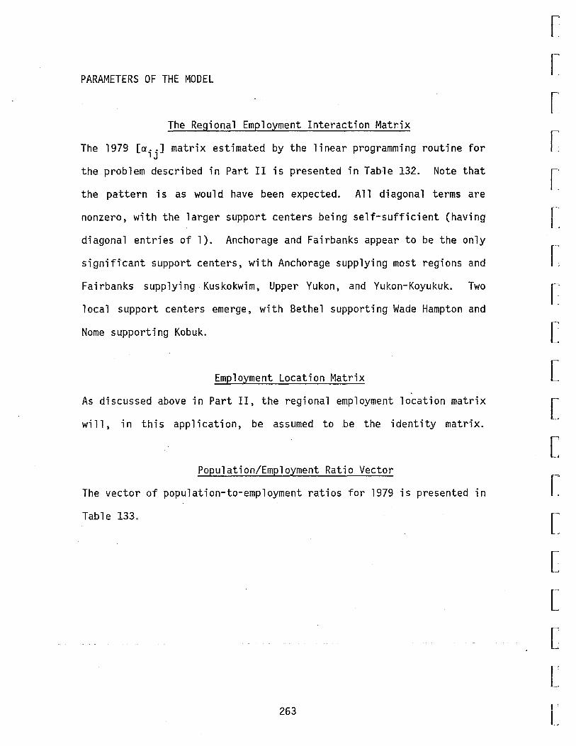
PARAMETERS OF THE MODEL

The Regional Employment Interaction Matrix

The 1979 [a .. ] matrix estimated by the linear programming routine for lJ

the problem described in Part II is presented in Table 132. Note that

the pattern is as would have been expected. All diagonal terms are

nonzero, with the larger support centers being self-sufficient (having

diagonal entries of 1). Anchorage and Fairbanks appear to be the only

significant support centers, with Anchorage supplying most regions and

Fairbanks supplying Kuskokwim, Upper Yukon, and Yukon-Koyukuk. Two

local support centers emerge, with Bethel supporting Wade Hampton and

Nome supporting Kobuk.

Employment Location Matrix

As discussed above in Part II, the regional employment location matrix

will, in this application, be assumed to be the identity matrix.

Population/Employment Ratio Vector

The vector of population-to-employment ratios for 1979 is presented in

Table 133.

263

[

[

r [

[

[

[

[

[

[

[

[

[

[

[

[

c l f -

L

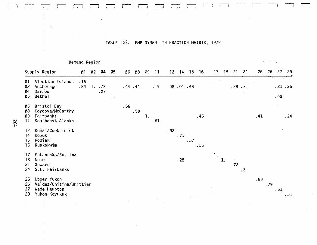
r-: ~ ~ ll ~ :---l

Demand Region

ll ~ J r-J r-l r-J ~ l J ~ ;--, l I _J l _1

TABLE 132. EMPLOYMENT INTERACTION MATRIX, 1979

Supply Region 01 02 04 05 06 08 09 11 12 14 15 16 17 18 --01 Aleutian Islands . 16 02 Anchorage .84 1 .. 73 .44 .41 . 19 .08 .01 .43 04 Barr.ow .27 05 Bethel 1.

06 Bris;tol Bay .56 08 Cordova/McCarthy .59 09 Fairbanks 1. .45

1'\) 11 Southeast Alaska .81 0'1 .f:>

12 Kenai/Cook Inlet .92 14 Kobuk .71 15 Kodiak .57 16 Kuskokwim .55

17 Matanuska/Susitna 1. 18 Nome .28 1. 21 Seward 24 S.E. Fairbanks

25 Upper Yukon 26 Valdez/Chitina/Whittier 27 Wade Hampton 29 Yukon Koyukuk

r-----1 l '

21 24

. 28 . 7 .

.72 .3

r----"1

"'

25

.41

.59

:--J rJ ll

26 27 29

.21 .25

. 49

.24

.79 .51

.51

TABLE 133. POPULATION/EMPLOYMENT RATIOS, 1979

Region Population Employment

~1 Aleutian Islands 7,030 6,104 ~2 Anchorage 177,981 93,241 ~4 Barrow/North Slope 4, 771 5,575 05 Bethel 9,739 3,697

06 Bristol Bay 5,204 3,814 08 Cordova/McCarthy 2,475 1,752 09 Fairbanks 54,000 27,576 11 Southeast Alaska 51,319 29,840

12 Kenai/Cook Inlet 23,244 7,864 14 Kobuk 4,695 1,451 15 Kodiak 9,956 7,326 16 Kuskokwim 2,941 571

17 Matanuska/Susitna 18,910 3,410 18 Nome 6,755 2,361 21 Seward 3,152 1,532 24 S.E. Fairbanks 5,507 2,025

25 Upper Yukon 1,482 426 26 Valdez/Chitina/Whittier 7,013 2,320 27 Wade Hampton 4,853 1,039 29 Yukon Koyukuk 5,325 2,521

ST Statewide 406,352 204,445

265

Population/ Employment

1.15 1.91 0.86 2.63

1.36 1.41 1.96 1.72

2.96 3.24 1.36 5.15

5.55 2.06 2.06 2.72

3.48 3.02 4.67 2.11

1.99

[

[

[

[

r· [

[

L [

[

[

[

L [

[

[

[

L L

" I

l.~

[

[

[

[

l~

[

[

[

[

[ [~

[

[

[

b------~

L L

APPENDIX B: PROJECTION OF BOTTOMFISH HARVESTING

AND PROCESSING EMPLOYMENT

The MAP and SCIMP models require as inputs projections of resident and

nonresident employment in fish harvesting and fish processing. One

source of emp 1 oyment in these areas which has not been important in

the past, but which may expand greatly in the future, is bottomfi sh

harvesting and processing. The 1981 bottomfish harvest in the Bering

Sea and the Gulf of Alaska totaled 1,614 thousand metric tons. Of

this, the U.S. harvest accounted for only 108 thousand metric tons, or

6. 7 percent of the total, while foreign fishing fleets (primarily

Japan, the U.S.S.R., Korea, and Taiwan) accounted for the rest (Alaska

Department of Fish and Game; National Marine Fisheries Service).

While most observers expect that U.S. bottomfish harvests will rise

greatly over the next 20 years, the total extent of this increase and

its effects on employment are highly uncertain. A number of factors

suggest that the U.S. fishing fleet, and in particular onshore Alaska

processors, are at an economic disadvantage compared to foreign opera

tions. These are high U.S. labor costs (in particular in Alaska),

high transportation costs from Alaska (due partly to the Jones Act),

1 ack of a we 11-deve 1 oped transportation and services infrastructure,

lack of a highly skilled, stable labor force for an onshore processing

industry, lack of U.S. marketing channels for Alaska groundfish, high

American intere?t rates; subsidization of foreign fisheries, high - - - ·- -

quality standards in foreign markets, and import barriers for foreign

267

markets. These factors are discussed in Scott (1980) and Natural

Resources Consultants (1980). · Working in favor of the future devel-

opment of the U.S. bottomfish industry are the commitment of the State

of Alaska to growth of the industry and the carrot and stick provided

by U.S. allocations of Alaska groundfish resources to foreign operators.

Widely varying estimates of employment impacts of bottomfish industry

expansion have been produced by earlier studies such as those by Sea

Grant (Terry, 1980), and Earl R. Combs, Inc. (1981). The difference

in these estimates can be attributed to differences in assumptions

about total U.S. harvest levels, the allocation of the harvest between

different harvesting and processing methods, employment requirements

per metric ton harvested and processed, and the residency patterns of

harvesting and processing employees. In order to project employment

for this study, assumptions were made with respect to each of these

variables, based on past studies and other available evidence.

The assumptions used to project Aleutian Islands employment for the

SCIMP model varied slightly from those used to project statewide and

census division employment for the MAP model, due to the availability

of more recent harvest data and a revision of residency assumptions.

The assumptions are presented below.

1. Total Domestic Bottomfish Harvest, by Region. The North Pacific

Fisheries Management Council divides A 1 aska bottomfi sh resources by

two regions, the Gulf of Alaska and the Bering Sea/Aleutian Island

268

[

[

[

[

['

['

[

[

[

[

[

[

[

L [

[

l ,. L

[

l. [

[

L [

[

[

[

[

[

[

[

[

area. We used this same regional division. A similar division was

used by the Sea Grant study (Terry, 1980), except that only the

Chirikov/Shumagin (western) part of the Gulf of Alaska was studied.

Earlier studies by Sea Grant (Terry, 1980) and Earl R. Coombs (1981)

assumed that U.S. domestic bottomfish harvests will rise from present

levels to a maximum sustained yield level in the year 2000. The Sea

Grant study assumed a constant growth rate, with most of the growth

occurring towards the end of the period, while the Combs study assumed

a normal growth path, with much more rapid growth during the early

part of this period.

The assumptions in these studies are to a large extent arbitrary. The

rate and form of U.S. takeover of the Alaska bottomfishery will depend

upon uncertain economic trends and political and management decisions.

Our own best guess is that the growth of the U.S. bottomfish industry

will proceed relatively gradually at first, due to the unfavorable

economic factors listed above, but will eventually be substantial, as

a result of improving markets and political and management support of

a U.S. industry. Therefore, we assumed that in each region the

domestic catch would grow at a constant rate of growth from 1981

~~ harvest levels to the optimum yield level. This assumption is similar

[ to the Sea Grant assumption, except that we choose the optimum yield

rather than maximum sustained yield as the harvest level when total

L------·----~~~lacement is achieved. This is the harvest level which the North

L r-L 269

Pacific Fisheries Management Council attempts to achieve, and varies

slightly from the maximum yield for biological and economic reasons.

The North Pacific Fisheries Management Counci 1 fisheries management

plans give optimum yields for the Bering Sea and Gulf of Alaska as

1,559,226 metric tons and 361,550 metric tons, respectively (Bering

Sea Management Plan, Table 62, page 6-1a, and Gulf of Alaska Manage

ment Plan, page III-1).

The MAP model employment projections assumed a 1981 harvest level of

87,381 metric tons for the Bering Sea, and 20,159 metric tons for the

Gulf of Alaska, based on preliminary Alaska Department of Fish and

Game figures. The SCIMP model used a 1981 Bering Sea harvest level of

87,512 metric tons.

Resulting total harvest projections are shown in Table 134.

2. Allocation of Catch. All domestic bottomfish harvesting and

processing was assumed to be by three methods: harvest by U.S.

trawlers working in joint ventures with foreign processing ships,

harvest by U.S. catcher-processors for offshore processing, or harvest

by U.S. trawlers for onshore processing plants located in the Aleutian

Islands (for Bering Sea harvests) or on Kodiak Island (for Gulf of

Alaska harvests). The proportion of harvest allocated to each method

was assumed to change in a linear fashion over time from starting to

ending values, presented below:

270

[

[

[

[

L [

[

[

[

[

[

[

[

[

[

[

[

L r ,

L

~

[

[

[

[

['

L [

[

[

[~

.

['

[

[

L L [

[

L

TABLE 134: ALLOCATION OF HARVEST ASSUMPTIONS

Joint Trawlers Venture Catcher Fishing for Trawlers Processors Onshore Processing

Starting Values (MAP Models) .89 0 .11

Starting Values (SCIMP Mode 1) .897 .026 . 077

Ending Values (Both Models) .20 .60 .20

The high ending share for catcher processors reflects an assumption

that this form of harvesting and processing will eventually prove most

economical for development of the U.S. domestic bottomfish industry.

3. Employment per Metric Ton Harvested and Processed. The fo 11 owing

figures are assumed for employment coefficients:

Offshore Processing .00323 Employees/metric ton Trawlers Fishing for

Onshore Plants .00222 Employees/metric ton Onshore Processing Plants .00746 Employees/metric ton Joint Venture Trawlers .00222 Employees/metric ton

The first three figures are based on emp 1 oyment assumptions in

the Sea Grant study (Terry, 1980, pp. 46, 47). The offshore proc-

essing figure is an average for all bottomfish species (Terry, 1980,

Table 4.110, p. 525). We assumed the same employment coefficient for

joint venture trawlers as for trawlers fishing for onshore plants.

271

4. Residency. For the MAP models, residency patterns were assumed

to remain constant throughout the projection period. For the SCIMP

model employment projections, residency shares were assumed to in

crease in a linear fashion over time from 1981 until 2000, as a result

of growth in local communities and establishment of a year-round

harvesting and processing industry. These assumptions are shown in

Table 135.

The MAP model residency assumptions were used for the census division

breakdown of employment for the regional model. Thus, employees

fishing in the Bering Sea, but residing in Kodiak, were considered to

be located in Kodiak for the regional model base case assumptions.

This was in contrast with the treatment of 11 enclave 11 employment in the

MAP region a 1 mode 1 assumptions, where, for instance, emp 1 oyment at

Prudhoe Bay is considered to be 1 ocated in the Barrow/North S 1 ope

region, even though very few of these employees reside in the region.

5. Onshore Processing Plant Construction Employment. A ratio of

.0015 man-years of construction employment per metric ton increase in

onshore processing plant capacity is assumed. This construction

employment is assumed to occur in the year prior to the increase in

onshore processing capacity. For the SCIMP model runs, all of this

employment was assumed to be nonresident.

272

[

[

[

[

[

r~

[

[

[

[

[

[

[

[

[

[

L ~

L L

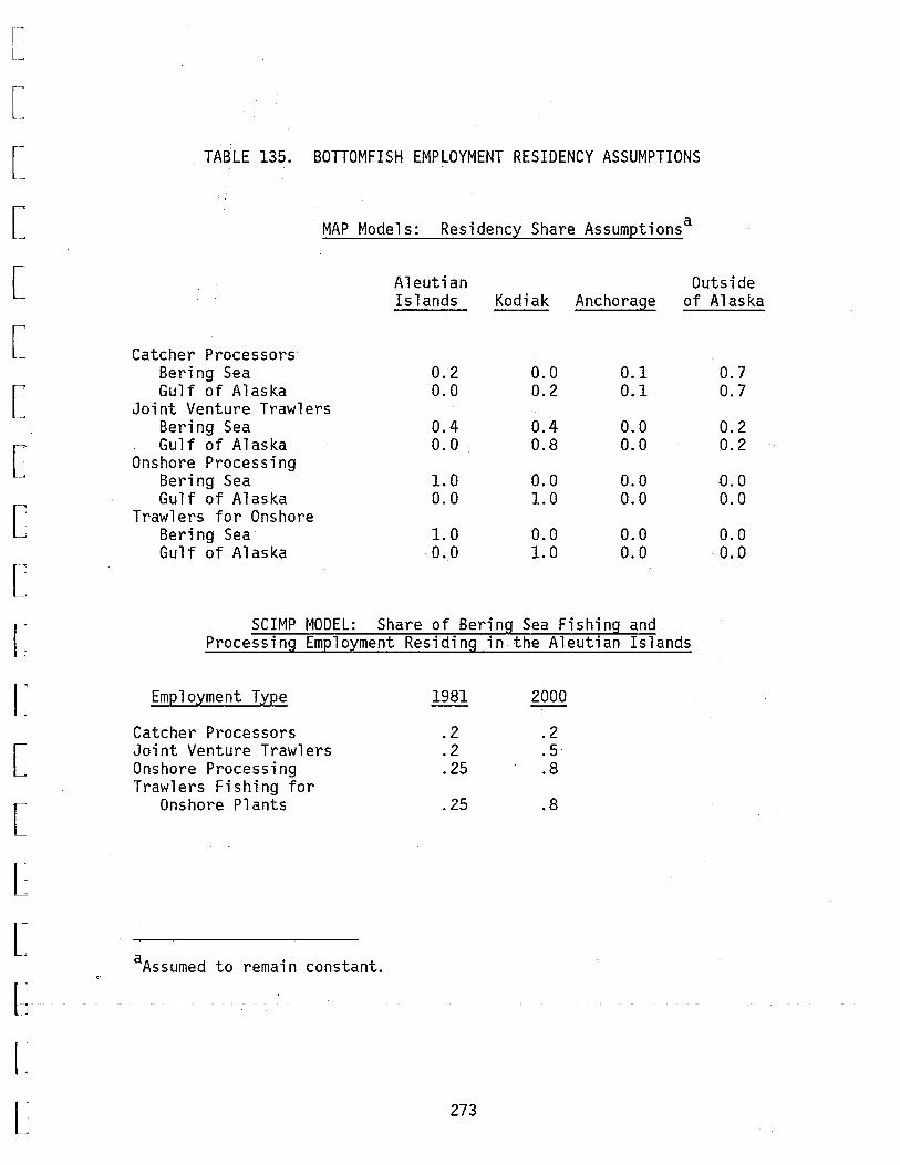
I l -

[

[

[

[

[

[

[

[

[

[

[

[

[

L [

[

L l

TABLE 135. BOTTOMFISH EMPLOYMENT RESIDENCY ASSUMPTIONS

MAP Models: Residency Share Assumptionsa

Aleutian Outside Islands Kodiak Anchorage of Alaska

Catcher Processors· Bering Sea 0.2 0.0 0.1 Gulf of Alaska 0.0 0.2 0.1

Joint Venture Trawlers Bering Sea 0.4 0.4 0.0 Gulf of Alaska 0.0 0.8 0.0

Onshore Processing Bering Sea 1.0 0.0 0.0 Gulf of Alaska 0.0 1.0 0.0

Trawlers for Onshore Bering Sea 1.0 0.0 0.0 Gulf of Alaska 0.0 1.0 0.0

SCIMP MODEL: Share of Bering Sea Fishing and Processing Employment Residing in the Aleutian Islands

Employment Type 1981 2000

Catcher Processors .2 .2 Joint Venture Trawlers .2 .5 Onshore Processing .25 .8 Trawlers Fishing for

Onshore Plants .25 .8

aAssumed to remain constant.

273

0.7 0.7

0.2 0.2

0.0 0.0

0.0 0.0

Employment Projections

The bottomfish employment projections based on these assumptions are

presented in Table 66 (Chapter III, page 150) for the MAP models, and

in Table 136 for the SCIMP model.

TABLE 136. SCIMP MODEL ALEUTIAN ISLANDS BOTTOMFISH EMPLOYMENT ASSUMPTIONS

1981 1985 1990 1995 2000

Total Harvest 87,512 160,500 342,400 7,307,000 1,559,000

Em.P.]_Qyment

Joint Venture Trawlers

Resident 35 70 147 262 346 Nonresident 139 197 283 360 346

Catcher Processors

Resident 1 15 66 212 604 Nonresident 6 61 264 848 2,417

Trawlers Fishing for Onshore Plants

Resident 4 13 52 178 554 Nonresident 11 23 50 94 138

Processing Plants

Resident 13 45 177 600 1,864 Nonresident 38 78 169 315 466

SOURCE: See text.

274

[

[

L [

[

[

[

[

[

[

[

[

[

[

[

[

l [ r--

L

[

[

[

[

[

[

[

[

[

[

[

[

[

[

[ [ r ~

Appendix B Sources

Alaska Department oj Fish and Game, Groundfish Catch Statistics, included in North Pacific Fisheries Management Council briefing paper (November 24, 1981).

Earl R. Combs, Inc. 1981. St. George Basin and North Aleutian Shelf Commercial Fishing Analysis. BLM Alaskan Outer Continental Shelf Office Technical Report No. 60 (BLM, Anchorage, October).

North Pacific Fishery Management Council. 11 Fishery Management Plan for the Gulf of A 1 as ka Groundfi sh Fi shery 11 (Anchorage, North Pacific Fishery Management Council, June 1981).

North Pacific Fishery Management Council. 11 Fishery Management Plan for Groundfish in the Bering Sea/Aleutian Island Area11 (Anchorage, North Pacific Fishery Management Council, November 19, 1979).

Terry, Joseph M., Roger G. Scoles, and Douglas Larson. (Alaska Sea Grant Program, University of Alaska). 1980. Western Alaska and Bering Norton Petroleum Development Scenarios: Commercial Fishing Industry Analysis, OCS Technical Report No. 51 (Anchorage, Alaska OCS Office, August).

~ - - - - - - - - - - - - - -

[ r ,

L 275

l 9LZ c J

J ]

J l ]

]

J J J J J ]

J -J --~

J J J J

l ~

[

[

[~

[

[

[

[

[

[

[

[

APPENDIX C: OCS EMPLOYMENT ASSUMPTIONS

OCS annual employment figures were provided by the Alaska OCS office.

These figures were broken down according to the phases and activities

shown in column (1) of Table 137. These figures are reproduced as

Tables 138-143, corresponding to the different OCS cases studied.

In order to use these emp 1 oyment figures in the MAP mode 1 s, it was

necessary to make assumptions regarding the shares of OCS workers who

would be Alaska residents. These assumptions are shown in column (4)

of Table 137. For use in the SCIMP model projections for the Aleutian

Islands, it was necessary to make assumptions regarding the shares of

OCS workers who would be residents of the Aleutian Islands. These

assumptions are shown in column (5) of Table 137. Both the state

residency and local residency assumptions are based on a paper by Will

Nebesky and Lee Huskey, entitled 11 Patterns of Resident Employment in

Alaska 1 s Outer Continental Shelf Industry11 (November, 1981).

[- - - - - - - - - -

L L 277

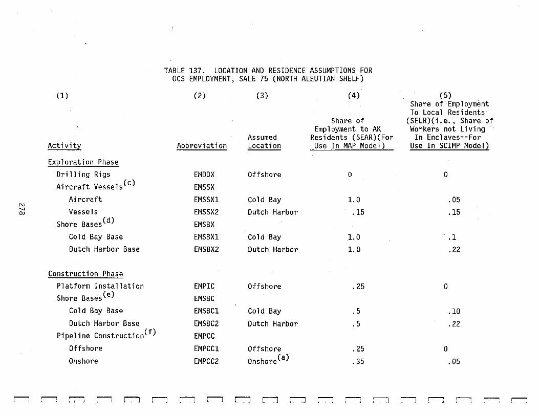
TABLE 137. LOCATION AND RESIDENCE ASSUMPTIONS FOR OCS EMPLOYMENT, SALE 75 (NORTH ALEUTIAN SHELF)

(1) (2) (3) (4) (5) Share of Employment To Local Residents

Share of (SELR)(i.e., Share of Employment to AK Workers not Living

Assumed Residents (SEAR)(For In Enclaves--For Activity Abbreviation Location Use In MAP Model) Use In SCIMP Model)

Exeloration Phase Dri 11 i ng Rigs EMDDX Offshore 0 0 Aircraft Vessels(c) EMSSX

Aircraft EMSSX1 Cold Bay 1.0 .05 N ....... Vessels EMSSX2 Dutch Harbor .15 .15 (X)

Shore Base/d) EMSBX Cold Bay Base EMSBX1 Cold Bay 1.0 .1 Dutch Harbor Base EMSBX2 Dutch Harbor 1.0 .22

Construction Phase Platform Installation EMPIC Offshore .25 0 Shore Base/e) EMSBC

Cold Bay Base EMSBC1 Cold Bay . 5 .10 Dutch Harbor Base EMSBC2 Dutch Harbor . 5 .22

Pipeline Construction(f) EMPCC Offshore EMPCC1 Offshore .25 0 Onshore EMPCC2 Onshore(a) .35 .05

L'lr-Jr:--:r-lr:-J~r-l:-Jr-lr-Jr-J~rt-:~r-lr--Jl~:---Jr-:-J

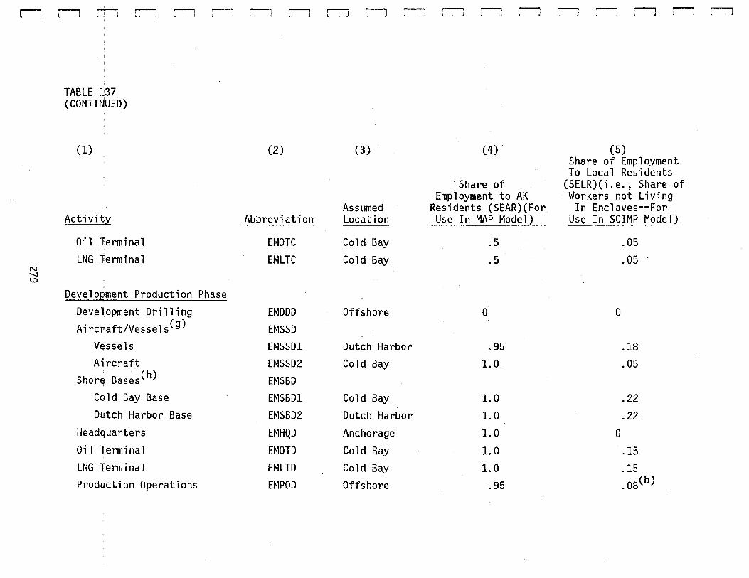
r-l r-l rT--1 r--;

N -......! 1.0

TABLE 1:37 (CONTINUED)

(1)

Activity

Oil Terminal LNG Termi na 1

r-1 r-l :--l r-l

(2)

Abbreviation

EMOTC EMLTC

Develo~ment Production Phase Development Drilling EMDDD Aircraft/Vessels(g) EMSSD

Vessels EMSSD1 Aircraft EMSSD2

Shore Bases(h) EMSBD Cold Bay Base EMSBD1 Dutch Harbor Base EMSBD2

Headquarters EMHQD Oil Terminal EMOTD LNG Terminal EMLTD Production Operations EM POD

r--l r--1 r--1

(3)

Assumed Location

Cold Bay

Cold Bay

Offshore

Dutch Harbor Cold Bay

Cold Bay Dutch Harbor Anchorage

Cold Bay Cold Bay Offshore

r-l ,..._.._..,

r--1 ~ r-1 :-l :-l :--J

(4) (5) Share of Employment To Local Residents

Share of (SELR)(i.e., Share of Employment to AK Workers not Living

Residents (SEAR)(For In Enclaves--For Use In MAP Model) Use In SCIMP Model)

.5 .05

. 5 .05

0 0

.95 .18 1.0 .05

1.0 .22 1.0 .22 1.0 0

1.0 .15 1.0 .15

.95 .08(b)

TABLE NOTES

(a)Onshore pipeline construction local resident employees were assumed to live at Cold Bay.

(b)No assumption was made as to the location of residence of those workers who work offshore but live locally, i.e., in the Aleutians. Presumably, they would live either in Cold Bay or Dutch Harbor.

(c)Assumed to be 20 percent aircraft and 80 percent vessels, based on a ratio of one helicopter to two vessels during exploration (Alaska OCS Office).

(d)Assumed to be 20 percent Cold Bay Base and 80 percent Dutch Harbor Base, based on aircraft and vessel breakdown.

(e)Same as (d).

(f)Assumed to be 85 percent offshore and 15 percent onshore.

(g)Assumed to be 34 percent aircraft and 66 percent vessels, based on a ratio of one helicopter to one vessel during development and production (Alaska OCS Office).

(h)Assumed to be 34 percent Cold Bay Base and 66 percent Dutch Harbor.

280

[

[

[

[

[

['

t'

[

[

[

[

r~

·~;;

[

L r [

L [

[

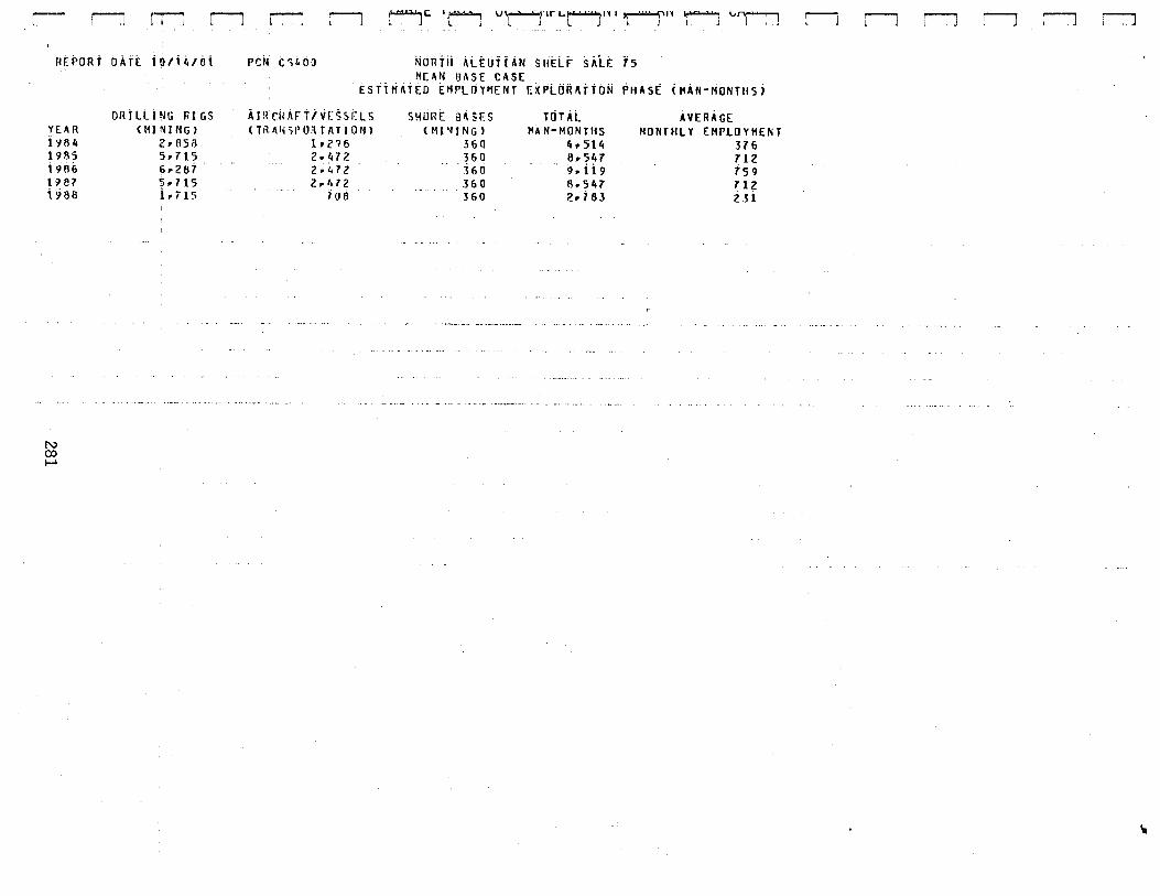
~~ r-:1 r~ r-l

HtPORt ti~tt igfj~l~t

YUR 1\18 4 19!15 i9il& 1H7 t9ea

N (X) 1-J

DHiLli% RIGS OHNING)

Z, 1\Sil 5r715 Gr26l . 5 .. 115 iril5

r--:

PCN t;L.oo

r----'1 L J

~[;, I~ V~'lr L.~11 I ,~11 1.~ vni'"'""""'' L J L J , J l J l , J l. J I. ' .i

N~Rt~ ALtUii4N SHtLt silt ts H[AN aASE CASE

ESii~AfED tH~LdYMENT E~PltiAAiib~ ~HASt t"AN-~bNTHS)

4rRcHArtlvr:s5as (TRAW;ro:tTATION)

lr2?6 z~ 472 2~472 2rlol2

7oe

SHOI~E t!A SF.S U1PII NG)

360 3&0

-:i&o 3&0 l60

TOTAL I!A N-HONTI15

4 .. 514 a .. 547 9rii9 8r547 z .. 7aJ

AVERAGE MONTHLY EMPlOYMENT

H& 712 759 712 2H

c-l r-l c--J :--:1 :--J r-:-1

\i

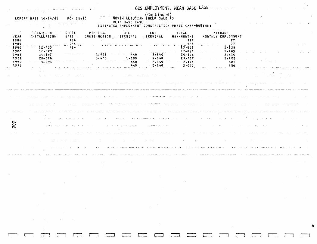
REPORT DATE ioi14t6i PC~ cs~oio

PLArrcir.M SHrHt

OCS EMPLOYMENT, MEAN BASE CASE -· ... __ . _ ... (Con.tinued) NORTH ALEUTIAN SHELF SALE 75 MEAN ~liSE CASE

t5Tii'IATED EMPLOYMENT coNsfihicTiiiN PHASE UAN-HONTHSJ

PIPELiNE ·aiL LNG TOTAL AVERAGE YEAR INSTALLATION 8 A 5~ Cf1NSTilUCTION TERMII\AL TERMINAL HAN-HONTHS HONTHLY EHPlOYHENT 1984 1985 i 9136 .. 1987 i968 1989 i990 19 'Jl

I'.> (X) I'.>

r--: r-:i

12;7:35 ......... 11·829 24;i97 20·376 s ... 094

r-:---; r---'1 l. I

n4 9~ 4 92 i, ····-

2.92i 5• 4 T 3

r--: ~ ,, j L~J

924 77 924 - . !7

ijo659 lol38 17,829 1•485

· i.4o 2;646 30 .. 198 £·516 lolOO 4o840 29.789 2o4f2 ··

4'• 0 2o640 6ol74 681 1,40 2o640 3·080 256

c:1 c::::J c-:J [ __ ~ c:J ,....._.., L .. , j :---"] ....---,

'

~

:-:---1 :---l :--:1 :--:1

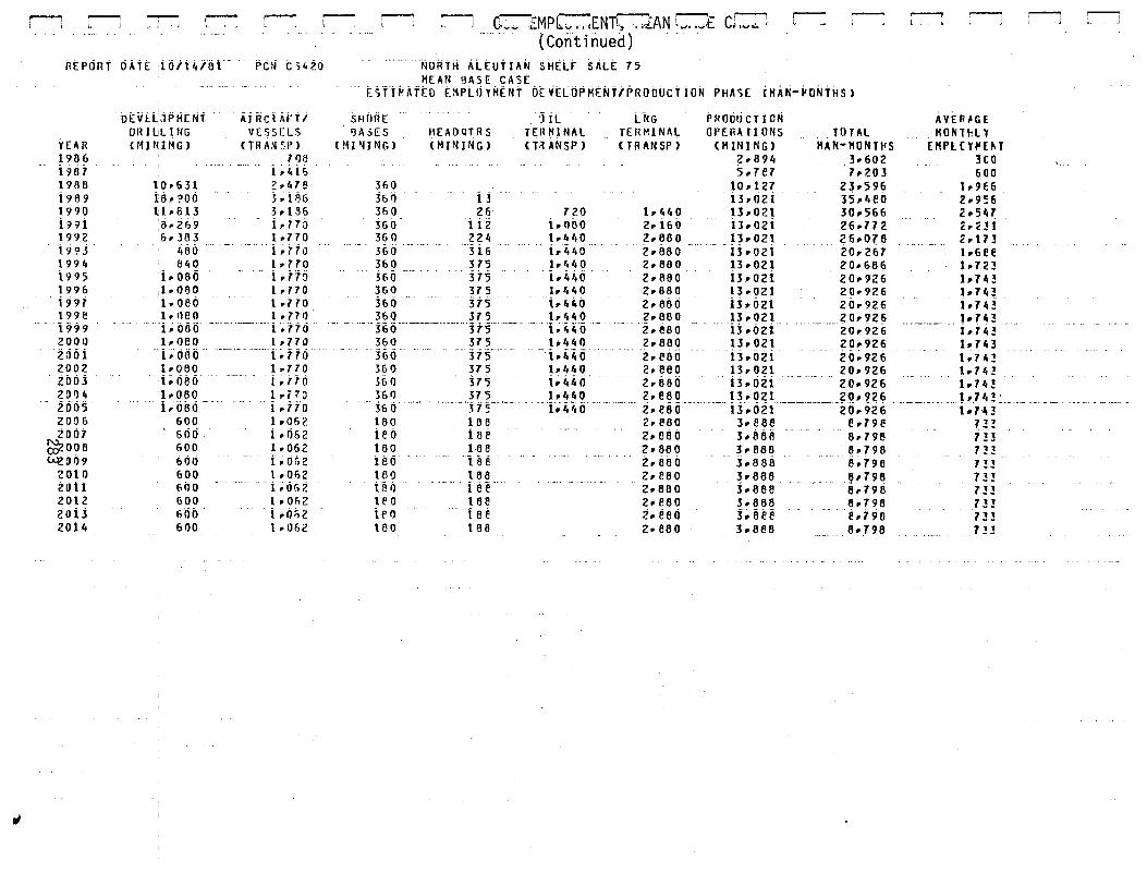
rJ

,--..., \

:---l ,j r ,. r-- r--1 .-'

----, '

r----" '· J 0---;-MP':---lENT---;:AN r----'1- cr--,.....,, L...,...;., i: !!....., • , ·~ L, ·• 1·1!. ~ ...... ,...:..."'t. j-,....,..:.. •

(Con-tinued)

r---: ~ ,....---, ' :-l ~ :--l

REPORt ti.\tt :it}ii4/ot· rc:.i cs426 ]6~t~ ALttittA~ s~E:LF" ~'Lt 7s MEAN 9ASE CASE

YEAR 1986 i91i7 1988 l989 1990 i9gi 1992 l99j' \994 i.99S 1996 i99i 199(! i999 2000 zooi 2002 2003 201)4 2665' 2006 20!l1

~008 wzoo9

2010 ZOi1 2012 20i3 2014

• • ••• • I . •• • . ~

DEVI:.LJPHENT DRll!LING <11lNHiGJ

AiRel AFT/ . vqsEL s ORA.'l~Pl

71)8 ' i;~i~

l0r631 2r478 ii8 .. ?00 5 .. ii3& t1 .. 813 3 .. 136 "8,.2&9 - i .. rta 5.303 lr770

48i> -- .. - . i .'rio 640 1•770

i .. o86 i.rto ,lr080 1r770 i.o6o i .776 1rll8() lr77!) i~oao -----------i-~776

1.oeo 1·770 -i~·ooo·· ----·- ······· r;Tto lr080 1r770 t.oso i~7r6 1·080 1 .. 770 ··· · i.oao-···· ---·-·i.7fo

600 1 •062 600 ir0&2 600 lr062 6Qo i~o52 600 lr062 600 600 600 6f)0

· i. o&z 1 • 0&2 i .o&2 lr062

t~il~ifto tMPLdY~tkt bt~tLh~~t~ti~ROOUCt~O~ ~HASE iHi~-~O~t~Sl

$~tORE 131\SES

<Ml"HNG>

360

HEJIOQTRS <MINING)

3&0 ij

5iL TERHlNfll (HANSP)

360 26 720 j&o ii2 i.oao 360 22~ 1·4'·0 360 .... .... ... 3i6 t .. ~40 3&0 375 1•440 360 ······ . 375 . i .. ~40. 3&0 375 1r4ft0 JGO .... 375 . - \,.i,i,(J 3&0 375 1 .. 440 ····· ···· ---36o··---------------·Hs· ---- -- -i~~;.-o -360 375 1 .. 440 3 6 0 . . . .. ... -- '37 5" . --. i .. ;; ;; 0 3&0 375 lr440 3&0 375 i~i,i,(j 3&1) 315 lr4lt0

· -··3r; o· ------ ------- .. 3 1 5-··-- · ---T~;; -;, o· 160 166 ieo tile 160 188 ieo He 180 168 iao ····· iee· ll'O 168 tro - iae \80 188

LNG TERMINAL <TRANSP)

1r440 2• i&o z,.eao 2. 66 0 2·880 lr660 2r860 z,. 6ilo z,.eeo 2.e6o 2 .. e8o z.8eii z,.eeo z .. ileo z.aao 2·880 2r880 2rllBO 2. 880 z.a8o 2· 660

.. 2 .. 880 2·880 2 .. eao 2r880

PROO~CTiO~ AVER~GE OPERAflONS TOTAL . HONT~LY

CHINING> HAN-HONT~S EKPLCY~E~T 2·894 31'602 3CO 5 .. 7er ·7 .. 203 Goo

10•127 23r596 t.9e6 iJ .. o2i Js.r.eo 2·9~6 13·021 30 .. 566 2·547 i3 .. ozi 26.772 2·2~i 1Jr02\ 26•078 2•173 ii .. o2i zo,.267 ··- t.6ee 13r02l 20•686 1r72~ i3r02i 20•926 ir74~ 13r02l 20r926 1r743 ii.~21 20•926 l·74i 13r021 20•926 1r7ft~ .. u,. 0 2 i ....... 2 0,. 9 2 i; ... - ·-- .. i,. 7 ~ 3

13r021 20r926 lr7ftJ "ii.ii2i zii;926 1r74! 1J,.Q21 20r926 lr7ft!

· ii .. o2i ·-·-··· 20•926 1·74~

. -- q.q~l ____________ ?9•9.26. -----···- .... ~ .. J4!~.-- ·•· -·--- ... -------tJ.o21 20 .. 926 t.7~~ Jr888 8•798 3r861i 8•798 3r866 8•798 3 .. e61i ······ · 8 .. 798

3•868 8•798 j,.8iJ8. ....... .... iir798

3·668 8•798 j,.eee eri98 3r888 8•798

73! 7~~ 73! 7! ~ 73~ n~ 733 1:n 73:!

~

HlPORT OA'~ 11/l~/Fl

HAl< 1'}/!4 l'J i3 ~ Hil6 l'}r)l

1 'i I) 6 19 ~) 1 fil)

19 '11 1'11<:: 19 '7 3 1:174 tn~ 19 9(,

1':197 l99b lJ?\1 2000 2001 2002 200 3 2 0 1)1.

2005 N21J•l& 0020 I) l .P.2oo t3

2009 2U10 2011 2012 zdu 2014

_.., L J ~

1-tl NI 'Hi 3. c t 1: Gr075 •I r Slo 1

tlr C.&< ~ 3· p 5 s.:.z?'• ~5·220 2lr7u2 1 ·1, 'JiH

.11 .. 177 14r~:Pb

l!ol-'3& llo f! 36 14•836 l4r~3!j

14r836 (1.,63fJ l4oll3b 1 lo o/l 3 (i 1'trll3& tt •• e3& 14·836

t.,f5(, 4r8)6 H856 4rC5& ... as& 4rl.l5& 4·1''>6 t.,f!Sf, 4rl.l56

r--: r:-:

f'CN c•:t, lol

SI'~:..ThUCilON } :~t. 'J2 '•

1 3, 6 5? 17ro29 30r1HJ 2<Jr799

1Jrli4 3.0~0

r-1 ~ ' J :--l

OCS EMPLOYMENT, MEAN BASE CASE {Continued)

NORT~ ~lEUTIA~ "HfLF ~Al[ 75 ~ L fl N ,J A S E C ,\ '.i E ~UIH1~liY !1F flTIIF.Cl EMPLOl'MF.NT <MAN-MONTHS)

TRANSPORTfiTlO~~ TOTAL 1. 29 (, 5r438 z, 47;; 'iri.Tl 3, te-o 26·380 3rl!3!! 33r579 3rl8 (, 56r 577 3 rl3 6 65r269 5, 346 38·7~0 5r010 29.852 6r0?0 26r078 u. 09 0 20r267 6r090 20r61lG r;, 09 0 20r926 £.·090 20• 926 6. 09 0 20r926 6r090 20•926 Gr090 20• 926 £,. 09 0 20r926 &.G~O 20~926

&.090 20· 926 6·090. 20•926 &rO?O zo, 926 &rO?O 20, 9 26 J, 94 2 er19e J, 94 2 8.?96 3.~Jit2 l!r79P. 3·942 e. 196 3~942 8, 7 96 3. 94 2 e.79B 3r'i42 6r798 3r 94 2 8r798 3.942 8~798

r-1 rJ li r-1 rJ r:

TCTIIL MO~THLY EMPLOYMENT

~53

r----

769 2, 19 e 2~798

~ .714 s. ~39 3~228

z~~o7

2 ~ 17 3 1r686 1~723 1r743 1r743 t. 7 4 3" 1· 7 4 J 1·743 1·743 1r743 1r743 1· 7 4 J 1·743 1·743

733 733 733 7 3.3 733 7.33 733 733 733

:----: r----"11 ' ~ ~ lJ ~

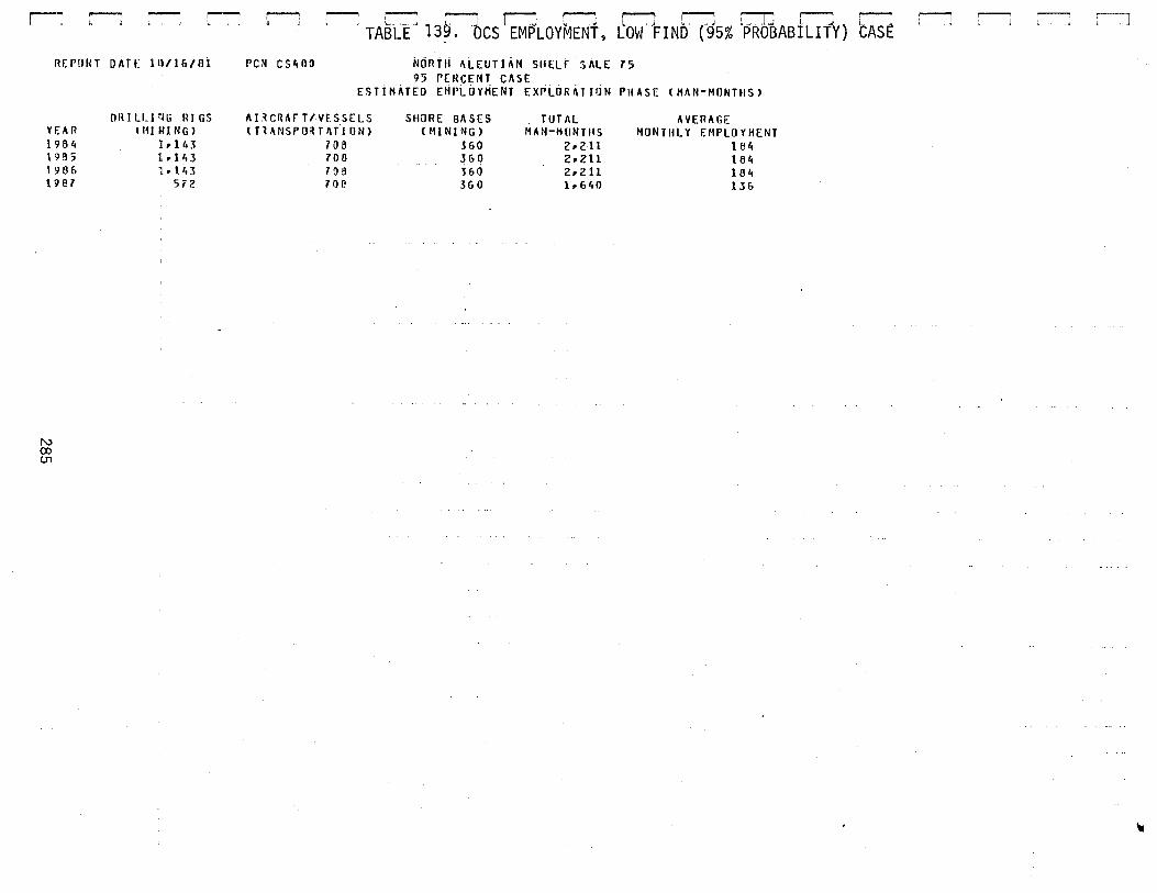
r-~ r-: r-1 L.l

REPORT DATE ln/l&t8i

YEAR 1964 1'1!15 196& 19e7

N co U'1

OIHLLPiG RIGS UH lll NG)

1~14J t .tt, 3 1·1'.3

512

C---'1 r-l TABLE J 13f.Jocs tEM~LOY~ENt, Lcow +rNb (Js% lr>RM~ABILifY) CASE

PC)I CSitOD ~6RT~ ~LEUTIAN s~tLt SALt 75 95 PERCENT CASE

ESTIMATED EHPLtiY~ENT EXPL~R.TitiN PHASE CMAN-HONTHSi

AI-~ CRAFT/VESSELS SHORE SA SES TOTAL AVERAGE <TlANSPO~TATION> <MINING) NAN-HliNTilS MONTilLY EMPLOYMENT

708 5&0 2~ 211 184 706 3&0 2r2ll 16ft 7!>9 .HIJ 2· 211 16ft roe 3&0 lrGftO 13&

;----1 ' J

["""J :--J :--l

~

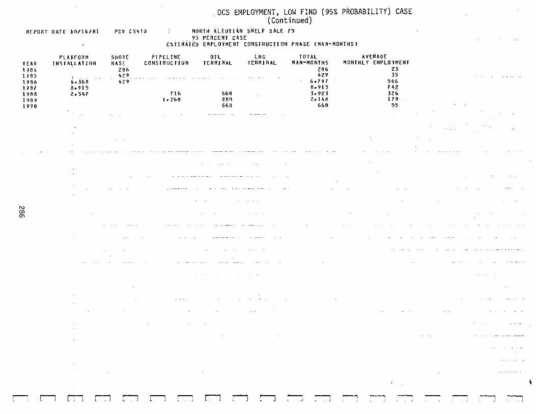
REPORT DATE 10/16/6l

YEA I! \964 U65 1966 1:167 1986 1969 1990

N co O'l

f'LATFORH JN'5TALLATIIJN

6.3&6 e.!H5 2.547

l~ Ll r-:-J r----'1 L . '

OCS EMPLOYMENT, LOW FIND (95% PROBABILITY) CASE (Continued)

PC~ C 54 i () NoRt~ ALttiTI~N ~kELt sALt t~

SUOiiE BAS::

266 4~9

lo2 9

r-1

95 PERCENT CASE ESTIHATtD t~PLOYHENT CONSTRUCTIO~ PHASE (HAN-MONTHS>

PTf'ELINE CONSTRUCTION

71& l• 2&8

r-J r--'1 • j

OIL TERHI NAL

r-1

660 eell 660

LNG TERMINAL

TOTAL HAN-HONTHS

28& 429

6·797 6.915 J. 923 2·148

660

AVERAGE HONTHLY EHPLOYHENT

23 35

566 742 326 179

55

r-1 r-J lJ r-1 liJ ...-----, L J ~

~

~ :-l ~ ~

r~ r; r;---1

HEPOHT OATE l•'ll ()/ 131

YEAR 1;181)

l g fl1 1988 1989 1~?0

1991 1 7 92 11?3 19?4 1995 09& \:19 7 199& t 99 9 2Q(}I) 2 001 20:>2 2:)[)3

N (X) '.J

OEVI.Lll~HENT OHILL~Nr,

PUNUHil

2~126 2~12& 2rl26 Ull91l

!120 240

,_21, o '240 :2r.o : 2'• 0

.; 2 ltl) 2'·0 240 21o0

240 2i,o

r---'1 r-; l.

I'C~ C'>lo2!l

AJHCUFT/ VESSELS

(TRfi~Sn

354 1 08 7 08 351o 354 JH 354 55 4 J; t, 354 351o 354 351, 354 JH 35'· 354

35 '·

rJ !""'"'"i l J r-Jcs L,.,,.lov~h~•,), Lb;JIND· \ :~~% ~1'\uo"ABIL.~. • .1) Qn..J...J iJ IJ' ~ ~-J

(Continued) NORTII ALEUTIAN SIIELF SALE 7 5 95 I'EBCENT C'-SE

ESTIMATED EMI'LUYHENT OEVELOI'HENT/PHOUUCTION I'HA5l (HAN-MONTHS)

511 URE Oll LNG PHOOtJCTION AVERAGE BASES HEAOQTilS TEflHINfll TEll HI NAL OI'[RA T IONS TOTAL HONHL Y

(MINING) (HJNINGJ CTRANSPl (fflfiNSPl (HJNING) HAN-MONTHS f.HPLCYHENT 1r919 2r 27 3 U9 3·839 4r54l 378

360 3r839 7r033 586 J& I) i3 3r839 6rn92 557 3&0 26· 7 20 3r839 7r425 618 361) 92 lr!li!O 3 r 6 39 7r615 634 360 \12 lr440 3r839 6r225 518 36<) i i 2 i r t, 40 3 • B 39 &r 345 '3(8 360 112 lr4loQ 3.839 G. Jt,s 521! 360 112 lr440 3r 839 6r345 5<:e 3&0 112 1·'·40 3· 839 6r ]loS 528 360 112 lr440 3r839 Gr345 5 26 3&0 112 1 r 4 fo 0 3 r 8 39 Gr 345 528 3&6 \i2 lrio40 3r839 6r345 528 361'1 1 12 lr440 3 r 839 Gr ]loS 528 3&0 il2 lr4t,o 3r639 Gr Jlo5 526 3&1) 1 12 1 r folof') 3r839 6 r ]to 5 52e 360 t 12 t r 4 t, 0 3rll39 Gr ]loS 528

~

KEP~RT DATE 10116/81

YEIIR 1 g flit lilll5 1\1 e & 1967 t'i'ne 1909 19qO 1991 1H2 1'1?3 \ g 91t 1!195 U9& 19H i996 19~9

2000 20J1 2 \)0 2 20D3

N co co

r-~ . ' ~

HI NI N (j t. 503 \r503 3r422 4-7 71 &r 37.5 &r 33 0 &dH 6rl61 4r 4 J1 It. 551 ltr551 '•. 551 It. 551 ltr55l ;t.55i 4•551 ~.sst 4•551 ;t. 55 i 4r55l

r-1"-1~ 1 J r-:

PC~ csr, 31)

CUN5TfWCTION 20& 429

&.791 6r9\5 5r923 2 • \It 8

&61)

r--1 r-1

OCS EMPLOYMENT, LOW FIND (95% PROBABILITY) CASE (Continued)

NORTII AlEUTIAN S11Elf SALE 75 95 PERCENT CIISE SUH~II~Y br OIRECf EHPLOY~ENT (MAN-MONTHS)

..---, ' ,I

Tfli\NSPORTATION 7 0 (l

. 706 1 r 0& 2 h41&

70!! 35 4

lr011o lr434 1rl9i. lr791o lr794 1· 794 1•794 1r19 4 i.79i, •• 7 9 4 i.r9i, lr794 i. 79 4 lr 7 9 4

r1 rJ r-1

TOTAL 2rlo97 2r&40

llr28l 15rl02 l0r95&

II• o rto 8rOe5 7. & 15 (j,. 225 &.345 6· 3 45 &r Jlo 5 &r 3 45 &r 31o5 &. 31t5 6r345 &. 31t5 6.345 &. 3~5 6.345

r:l rJ

TOTAL MONTHLY EMPLOYMENT

208 220 9lt 0

l•251J 913 736 673 &31t 518 528 526 520 528 528 528 528 520 528 528 528

.r--1 ' ~ ll r---i

J ["j ~ _j ll ~

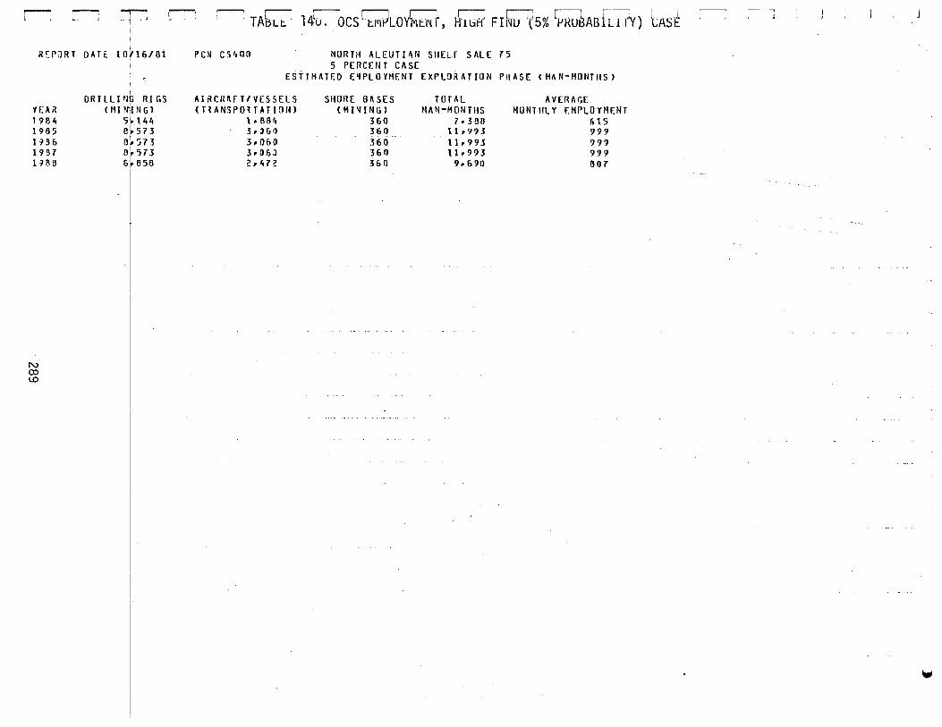
r-: r--: rr: ' RF.PJRT DATE IOfl&/Oi

YEAR , 981, 1965 1:1!1& 19 !H 1:188

N (X) 1.0

I

ORI LLI 'lG Rl GS (HI Nil N G l

5 1~\41, e 1~ 573

I Bt 57 3 B,,r 57 3 £>!~ B 58

,..----,

rJ TAbLt i 14'u. ocslt,VtAov~u:.t'li", HlbHJ Fif'lu ·(s% LPI<U~ABfL~I]Y) 1cAs£

PC:-1 C5'•00 NORTH ALEUti~N SHELF SALE ts 5 PERCENT CASE

ESTrHATED E"PLOYHENT EXI'UJRATION PftASE CHAN-HONTIISJ

AIRCR~FTIVESSELS (l~ANSPOtTATIOHJ

l ~ 88 r, l~:J&I)

3~0&0 3~0&J

2~'·72

SliOilE BI\SES (Hl'ONGJ

3&0 3&11 3&0 3&0 3&0

TOTAL HAN-HONTilS

7 .JB!J 11~993

\1~993 11~993 9~&90

AVERAGE MONTHLY EMPLOYMENT

&'l5 999 999 999 807

,.---1 i -

--, l

w

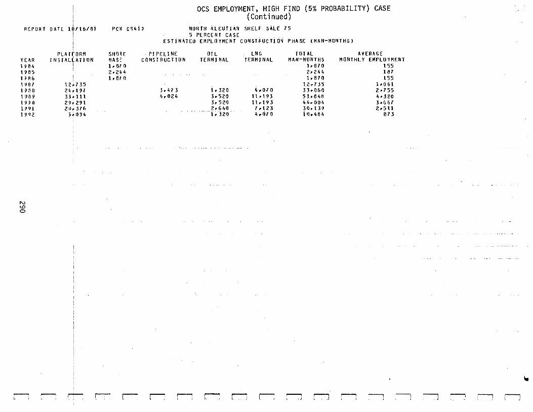
REPORT DATE. 1~116/fli PC~ C54ij

PLA TrORM SHO~E

OCS EMPLOYMENT, HIGH FIND (5% PROBABILITY) CASE (Continued)

NUR Til ALEUT I AN SHELF SALE 75 5 PERCENT CASE

ESTiMATED EIII'LOYMENT CONSTfiUCTIO"i PllASE <MAN-MONTHS>

PI PEL! NE OTL LNG TOTAL AVEIUGE Y EfiR I IHTALLATI ON BAS~ CONStRUCTION TERMINAL TERMINAL HAN-MONTHS MONTHLY EMPLOYMENT

1 9 !l '• \9fl5 1 Hl6 \9!37 \;188 1'18 9 19 :11)

11? 1 lgQ2

N lD 0

r-~ ~

12~735 2~ 197 33 111 29 291 21J 376

; 1)?4

,_ i ~

1r 67 0 2·2~4 1• Bl 0

r--l !

r---" L, J

3. 473 '•. 021,

rJ r-l

lr870 155 2•21,4 167 lr870 155

12·735 1r0 61 i. 320 r .. oro 33 .. 061) 2•755 3r520 llr\93 5 1r 61,6 4d20 3 .. 52!) 11 .. 193 41t,.00'• 3r6G7 2•640 7r123 30.139 2•5\1 i ~ 32t> ". !)1 0 i 1),. I, 8ft ail

r-1 r-1 r-J l"J rl r--J r-J [""""! ,....---, I

,....--, ' J :--l

~

r---J

r-: r-:: CiJ ~ r--1

REPORT OATE l0/t6/8i rcN csi,z:>

H. fiR 19B7 1 980 1:18 9 \:190 19 'Jl 19 92 1 '19 5 1 i19'• 1995 U9& 1197 1990 1999

·2ooo 2001 211!)2 2003 200'• 2005 200& 2007

.... ~ 0:16 t.ei)09 1-t":> 1 () 2J 11 2J\ 2 21)13 20\4 2015 2llt6 2!117 21i11l 2H9 2ll20

DEVELOPMENT DRILLING <MINING)

2U~2&3

21·263 2~~350 2\~2&3

1~~415 ~.633 t.oeo ~;440 ·~680 -~&80 ~~680 i~~~6 -~680 •• 6BO tr680 ~.6811 •• 680 ij.6~0 ~.680 lr660 ~.660 io680 t~&ao (.~~0 (.&oo ~.~~~· Lr&BO t.&do ~~~eo

840 840 840

AIRClAFTI VESSELS

<TRfi~';P) 7 ()!}

l. 77 J 3~1£1&

~·240 ~ • 95;; ,, • 95& 2. ,, 7 !l z,i,7s ~ •'•7' ~ ·476 2·47!1 ~. i,ra ~·-+7!1 z .. idii -~·478 2ofo78 z,t,76 ~.;,;~ z~HB

~. 4 73 ~r47B

~ •'• 7 3 2·'•78 ~·47!1 ~~478

~.478 ~ ~476

~~473 ~·47!1 z~4ta ~.,,n

lrHB 1rlo15 t.4t6

~ r-l .---.. r--r r-l r---J ( ,- Ln r ~11 $ E ,-------, • j O.~ _ .;:.~·1PIL .... c. NT~ . __ GH l. _ .... D -. .. . JRQB, ·-_.::.IT,., _:'"\ l J

(Continued) NORTH ALEUTifiN SHELF SALE 75 5 PERCENT CASE

ESTJHATED EHPLOY~ENT DEVELOPMENT/PRODUCTION PHASE (MAN-MONTHS>

SHORE BASES

<HHIING) HEAOQTRS <HPONG>

360 13

OIL TERMINAL <TRANSP)

360 26 2•040 360 125· 3.060 360 256 loo080 36o '•I'• 4~ooo 3&6 ····· 552 i,.oeo 360 636 4rOEO 360 697 ,,.oao 361) 697 4 rOEQ 360 697 4.rOBO 360 697 4~0EO

LNG TERMINAL (JRANSP)

2~400

3r600 4~8oo ,,. 600 ,,.8oo 4oll01l '•• 600 4~81)0

4.eoo 3 6 0 ·- . ---· 6 ij i ---· ... - " • 0 8 6 ..... -- .. "· 800

i,. 800 3&0 697 4·060 36h . 69t ~.686 360 697 t.~oao 3&1) ···- - · 697" ;;.oaii 360 &97 4.oao 3&6 ........ ··-- ·6-97 -· - .... i..oeo 3&0 &?r 4•080 361) 697 4oOEQ 360 697 4~oeo

360 G 97 4r0f0 360 697 4o080 i i; o --- --- - ----- 6 9 7- - - - ... 4; 6 8 o 3&0 697 4.080 ji;(j -· .. - -·-··-- & 97·-·--····-· 4~666 360 697 4·080 3&o ··· - -··-&?i ···-- - ··-· ~~oilo -361) 697 ltrOEO t li o --- · -- -- -n ~ · --181) 181)

31o 9 149

4·600 1,. BOO 4o800 t,. BOO 4r800 4o600 4o800 4o800 ,,. 800 4o800 4·600

·4.8oo ~o~eoo

4o800 '•• 800 iuiloo 4.600 ;,~aoo 4.euo '• ~eo o

PRODUCTION OPERA fi ONS

<MINING> 2•69/o 7·234

13·021 17•3&1 20~255

20•255 20•255 20•255 20·255 20r255 20·255 20r255 20· 255 20·255 20. 2 55 20·255 20•255 20·255 20~255

20• 255 20·255 20r 255 20.255 2!lo255 20•255 20r25S 20·255 20 ~ 2 55 20~255

20•255 20r255 &~804 6.804 &~6o4

TOTAL HAN-MONTHS

3~&02 9r l)l)t,

37·843 47o698 60.706 s•;. 970 '•6·602 41.158 33r69l 31tol10 34.350 34o350 34.350 3i..356 3lo.o350 3' .. 350 34•350 31,.350 34o350 34·350 34r350 31,. 350 34.350 34.350 34.350 34.350 34·350

· 34.350 Jlu350 34 .. 350 34r350 ii .. 389 14r389 ii .. 389

-, '

AVER~GE

MONTHLY EHPLCYI'ENT

300 750

3olS3 3o974 5.o5e 4.o664 3.r900 3r 4 29 2.r807 z~e~oz Zr eEl 2oBE2 2r!!62 2.e6i 2ri!E2 2rB62 2rB62 2rB62 2r862 ZrB62 z~e62

z~eE2 z.eez z~BEZ

2o66? .. z.eez 2·862 z~li62 2·862 z;e6z 2·862

- i r i9 9- ·· 1·199 lr199

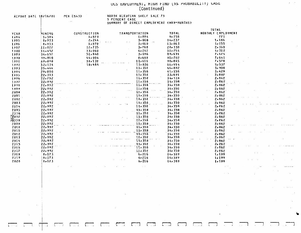
Rt:P!JRT DATt.

YEAR 1Y84 1!185 UB& U37 1 ~ 86 191.\9 1910 19!11 \992 1993 1994 1995 1:19& 1 ~H 1~'11!

1999 2()01) 2001 201)2 2003 2004 2()05 2JJ6 ~307 ""J)6 2()09 20\1) 2()11 2012 2()13 2() 1 '• 2Jl5 2ll t. 2>17 2)18 2J\ 9 20211

r-~ r-

I

I

I . . 1r/\&181

i '

IHINING ! 5, 51) 4 I a, 933 18·933 u.ou 114·4'52 ,~4· 6'57 ~9·010 ft9rl,l'JO ~2·13'• ~5.4'•4

~~:~~~ 22.752 Z2r9n F-2,992 22· 992 ~2·9?2 22.992 I •

~2· 992 22· 992 ]·

22· 992 22.992 ¢2·992 f-2· 992 22• 992 zz, 992 r-2. 9n 22r992 ?2,992 22r992 ~2.992 22· 992 22.992 2z, 992 ]8.i73 6.173 tlri73

rr-: i

rJ

PCN CS4 3)

CONSTHUCTION lr671) 2, 2ft '• 1r370

12, 7 35 33· 060 51·8'•8 i,t,.004 J:J .139 \(),i,!ii,

r:--; r-J

U~~ tM~LUYMtNI, HlbH tlNU \0~ ~KU~A~!L!IYJ ~A~t

(Continued) NORTH AlEUTIAN SHELF SALE 75 5 PERCENT CASE SU~Hi~~ tit DIRECT E~PLtiYHENT <MAN-HONTHSI

TRANSPORTATION TOTAL 1·884 9r253 3· 060 l'tr237 j, •1611 13· 66 3 3· 766 26· 330 4r242 51r754 3r186 69r691 8·668 9lr 702

1lr616 90. 8lt5 ij~ 83& 66•454 1 1, 35 f 46•81)2 1 i, 35 6 t,\.158 11, 35 e 33r691 i 1 rJ5e 31.,1io 11.358 3ftr351)

.... -···-··--- iid58 .. - -· 3i,, 35o 11· 35 6 Hd50 ilrJSiJ H• j5o 1 t r35 6 3ftd50 ii .. J5e Jt,,j5o ~ 1 .35~ .. .... 3ft·350 1 1, 35 e 31 .. 350 1 1, 35 8 3ftr350 1 i. 35 e 3ft, 350 11.356 34·350 li, 35 6 H•350 11,35 8 3ftr350 ·-····· i 1 ~ 35 8 34.350 llr358 341' 350

···ti.Ha· 34•350 t1, 35 e 3ft,.350 ti. .35 il 3~.350 11• 35 E 3it•351) ·· n. j5ii 31,, j5ri 11, 35 e 31,350 6~21& iftr369 6,. 216 14•369 &• 2i & 1ltr369

[""! L"l rJ r-l r:) r-J

TOTAL MONTHLY EMPLOYMENT

771 lr\86 lrl55 2r360 4· 312 7rlt74 7. 6 '• 1 7·570 5• 537 3· 900 3rft29 2·8117 z,oft2 2.e62 2·862 2•862 2·862 2• 862 2·862 2• 862 2· e&2 2r862 2r862 2r662 z, 862 2·862 21'662 2r862 z,. 862 2r862 Zr662 2· 862 2, 8 62 2r862 t.t99 1 .. 199 iri99

L:'l r-1 lJ -

~ -' ,.-----, ' ) c--J ~

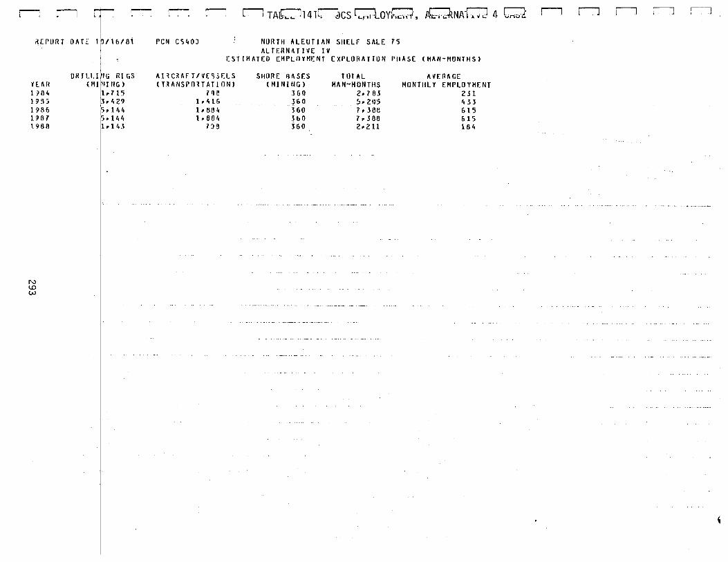
r-: ll I r--1

I . ~EPORT OATE lr/16/61

YlAH U04 1:1 g:; 1906 BB7 \966

N 1.0 w

I

I OHILLIING RIGS

(HININGI 1r715 3r lo2? 1';,. lltlt 5 r 1 for, lrl4.~

1:--:---: ll

PCN C540J

ll TA~'"''"' ll41r:-lJcs l L..pi~lon.'"''/' A(~ rJ~NAtd J 4 Ln-.~t

NORHt ALEUTIAN SltELF SALE 75 ALTERNATIVE IV

ESTIMATED EHPLIIYHENT EXPLORATION PltASE (HAN-HONTIISJ

Al~C~AFT/VE)5F.LS

(TlANSPOlTATIONI 7H

lrlol& 1 r 80 4 1 r 80 '•

7:1!}

SIHJRE BASES (HINHIG)

]60 ~6 () 360 360 360

TOTAL MAN-HONTflS

2· 7 83 s. 205 7. 388 7. 3 88 2· 211

AVERAGE HtJNTitL Y EMPLO YHENT

231 ,, 3 3

615 615 161,

ll r:l iJ lJ :~j

'

REP~RT DATE 10/16/0i I'C~ C54ll

PLATFOHM SUO~E

OCS EMPLOYMENT, ALTERNATIVE 4 CASE (Continued)

NORTH ALEUTIAN SHELF SALE 75 ALTERN~TIVE IV

E~TIMATtO EMPLOYMENT tUNSt~UCTlON PHASE (MAN-~ONtHSl

Pii'ELINE OIL LNG 1\VERI\GE YEAil INSTALlATION BAS~ CONSTRUCTION TERMINAL TERMINAL

TOTAL MAN-MONTHS

924 _ 921o 7P292

15•202 20.79& 2 Qp 50 5

MONT IlLY EMPLO YHENT 77 1984

1905 BB& 19fl7 l!IBil \ 9119 1990 1991

N 1..0 ..p.

r-: r-:J

9Uo 9Z t, . ---

& .. 3&6 924 \5:r2fl2 z 4 !ol97 l ,,,. 009 z .. 51· 7

rTJ rn r--1

. ~---·--·- .. ·•· .. ····· ··-·

2P 92i ;.;,o 2• 92\ t. too

41o0 440 ···-··· ···-····· ... ·- .. ·-·

rJ rl L1

. ·-··· ········-·· ..

i,z.Js 2.475 i.23B

... 1._238

rJ r-:J rJ

/IP225 t.& 70

r"'l rJ

77 &07

1•273 2·399 1•700

ll

352 139

ll

~

r--1 ll ~ ~

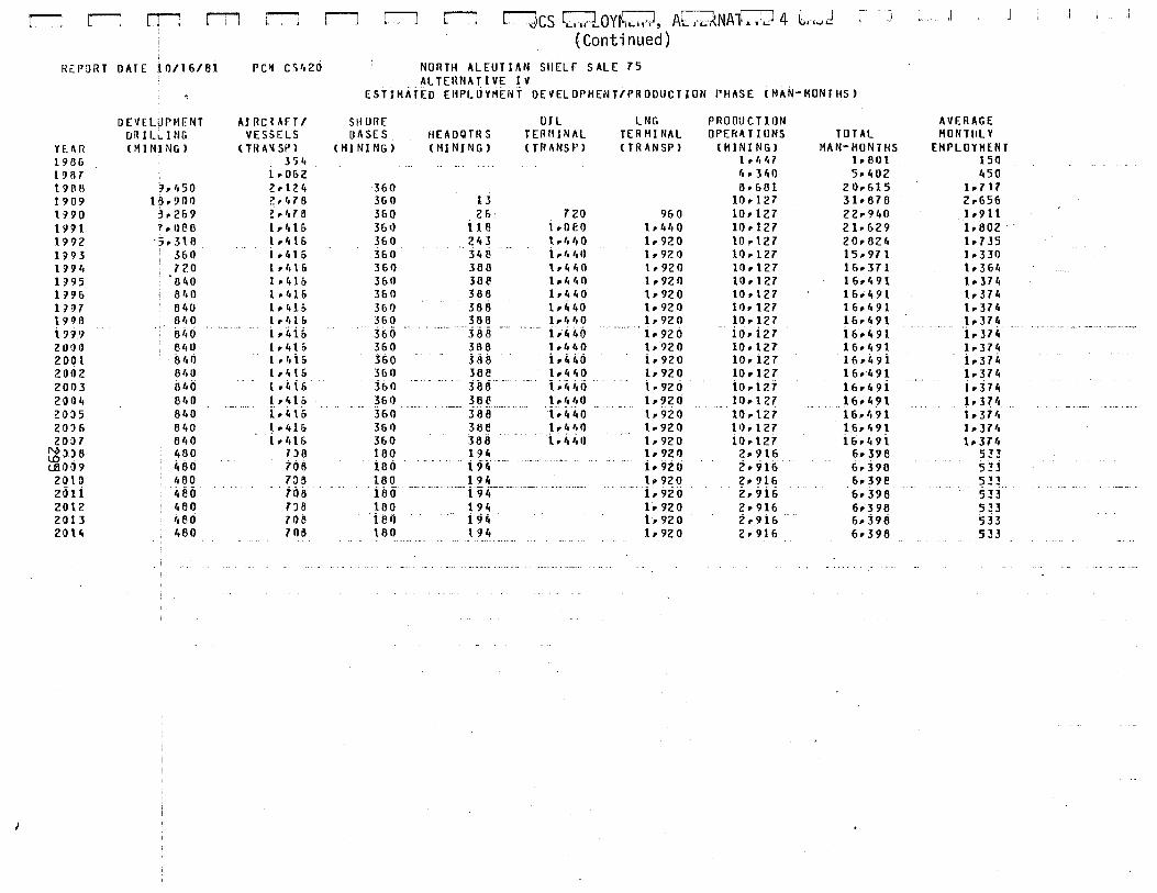
r-: r-: rrJ rT1 - rJ r.-l r-l ncs D ... ov~ ..... J, r---"1 ,---,--, ' j lJ t j A''- ,._,{NAl ... · ... • 4 6 ...... .:. (Continued)

HEPGRT DATE 10/1&/Bi rc~ cst,zti NO~TH ALEUTIAN SHELF SALE 75 ALTERNATIVE IV

EStJM~i~D EHPLtiYH~Nf OEVELDPMENT/PRODUCTION PHASE lM~~-MONTHS)

DEVELllPHfNT AJRCli\FT/ Sfl URE UIL LNG PRODUCT I llN AVERAGE DR 1 L~ I NG VES5EL5 HASES HEI\DQTRS TER11INAL TERMINAL OPERHIUNS TOTAL HONT~LY

y f.tl R <HINP.IG) ( TR A .. SP l <HJNINGJ <lUNING) <TRANSf') <TR ANSP) <MINING) MAN-MONTHS EMPLOYMENT 196& 354 1·'•'•7 lr801 150 1 :1!17 lr0&2 '·. 3 '• () 5rlt02 It 50 1988 ~.,,so z ·124 3&0 6r&61 20r&l5 lr 7 17 1909 1Br91ll) ~.r.ra 3& 0 13 10r127 3lr670 2r&5& \:190 3.2&9 ~·lt76 3&0 2& 720 9&0 10rl27 22• 91t0 lr911 1991 1rOB8 t .. lft& 3&0 ll8 1r0f0 1r t,t, 0 10rl27 21·&29 lr002 1992 "5.318 ~·'·1& 360 21f3 t." ,, 0 t, 920 10. t 27 20r821t lr735 1993 361) lrltl& 3&0 jt, ~ i ·"Itt) t, 920 10r127 15.971 lr330 199ft 720 l ',, t & 360 388 t." t,l) t, 920 10r127 16r371 lr36lo 1:195 8lo0 lrltlo 361) 38 e lrlo ItO 1, 92 0 10rl27 16r491 lr 37lo 1'19& 8'· 0 1. 41& 360 388 1, '•" 0 1r 92 0 10.127 16r 4 91 lrHlo UH 81t0 lrltl& 3&0 388 1r440 lr 920 10r127 16rft91 lr 311, 19911 8'•0 lr41& 3&0 388 lrlo loO 1, 920 10. 12 7 16rlt91 1 r 311, ;_ 99.9 o4o

··-· .. ir4i& :56o -- -- ·····- "3 8 8 -- -- - i.;, 46 ............

i. 92 6 ··· io. iu i6r49i ir314 ......... ·-··· --------·-·---

21)1)1) 8ft0 lrlol& 3&0 368 l ,, 4 0 lr920 10. 12 7 16•'•91 lr374 2001 840 t.4i& 360 jail i,i,i,(l i. 92 0 lOr i27 16r49i irH~ 2002 840 l • t, t & 3&1) 388 lr If 40 lr920 10. 12 7 16r491 lr371o 2003 840 l ~ i,t i; :i&o

- ... - .. ·-

386 ;_;;,;,i) i. 920 io.i2r l6r49i lr37lo 21)04 840 ··-····-··

lrlflf> .. ._. 3GI) 36~ t~foltO .. . -··· 1 r920 10r127 16~491 ~~ 37'•

~O:J5 840 i.4t6 :560 ··· ··· · ---- ja ii ·--- T.~i,o 1 ~ 92 0 10rl27 16~'•91 t, 374

2 () :>6 840 ~~416 3&1) 3ae t, It '•0 lr920 l1)r127 16r491 1 ~ 374 2 () 07 61t0 ,, '•l & 3&0 3a6 i~44o 1, 92 0 10rl27 iGr49l h374 ~JJ8 480 7J6 180 191, lr921J 2~ 91 & 6 .. 398 533 UIOD9 480 706 iBO - .. - 194 -- ... -···· . --- i, 9~ 0 Zr9t6 6rJ96 5 33

2010 480 7!)!J 160 194 1 .. 920 2, 916 6~ 39e 533 2jjti 4eo .. 766 . i 8 0 --- ..... ---- i9 ;.---- -- -- ... --- .. . .. -- i. 92 ri z,9i& 6r396 s:!f-2012 loBO 7:JB 180 l 9, lr 920 2•916 6r396 533 ZDi3 480 708 · i e il . ··-· .. -. i 9 4--- . ---- ·······- ir 926 2, 9 i& . 61' 398 533 2011, 1,60 7 0!1 160 t 9ft 1· 92 0 2·916 6r396 533 .........

-·· ·····"''•• ..

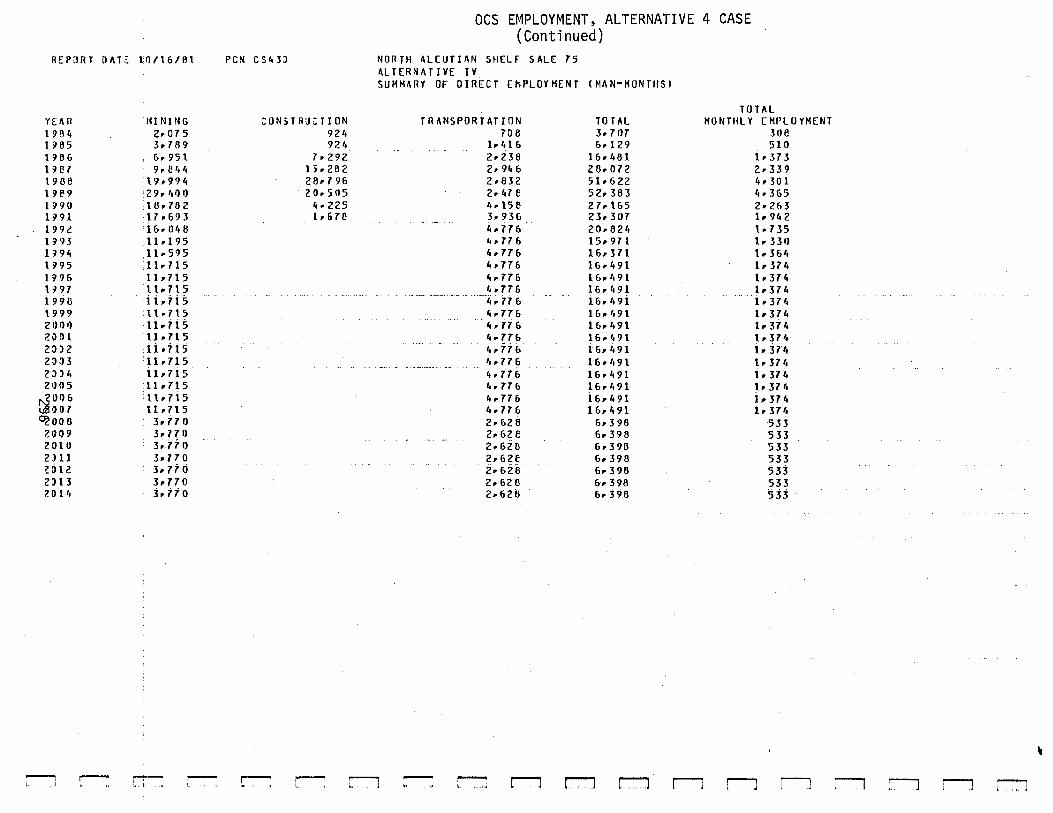
REPJRT OATE ~0116/Bl

YEAR 1984 1985 1966 1H7 1988 l9f\9 U90 1Hl 19 92 BH 119ft 1:195 1H& l:/97 i998 1999 2 t)l)t) 2()!)1 20)2 2303 2J)4 21)05

~01)6 ()07

q0()6 2()1)9 2010 2) 11 2612 2J 13 20i4

r----1 r-::

1111 N IN G 2• 07 5 3r769 6r 951 9. e '• 4

l9r994 29· 40 I} liJ.762 17.69 3 1&.048 llr195 llr5?5 11r715 11,715 t\r715 ii.7i5 1tr715 1lr715 llr715 lir715 llr715 11•715 llr715 l1r715 tlr715 3d7 0 3r771) 3.770 3r170 3. 7 t (j 3r770 3. tt 0

rrl I

l,"l

PCN C54JJ

;:;ONHRU:;TION 924 924

7•292 1)r262 26·79& 2()r505

'•, 225 1r &78

............

OCS EMPLOYMENT, ALTERNATIVE 4 CASE (Continued)

NORTH ALEUTIAN SHELF SALE 75 ALTERN.\TIVE IV SUMMARY OF DIRECT EMPLOYMENT (MAN-MONTHS>

TRANSPORTATION TOTAL 70 6 3r 707

lr 416 6. 129 2·238 16r481 2· 9ft 6 28r072 2·832 5lr622 2• 47 E 52.363 4, 15 E 2 7,\65 3r936 23r307 ·-- .. 4· 77& 20· 821t 4. 77 6 15r 971 t., 77& 16.371 4r776 1&r491 4· 77 & 1&.491 4r776 16r491 -·- ---· --- --- ;;. 77 f, i 6. 4 9 i 4·77& 16· '•91 ". 77 & 16r491 4r77b 1Gr491 4. 77 b i 6. 491 ,., 77& 16·'·91 .... . ..... -··-~· ... -· 4r776 16r491 ". 77 & 16· '•91 4r776 l6r491 4r776 16. 4 91 2• 62 8 6. 3 96 2· 62€ 6r 398 ... -· 2•6Z8 &r396 2r62€ 6. 398 Zr626 &r 396 2r 62 6 6r 398 2r&26 &r 398

TOTH MONTHLY EMPLOYMENT

308 510

1· 37 3 2· 339 4. 30 1 4.365 2•263 1· 94 2 1r735 1· 331) i. 3&1, lr 37 4 1· 37 4 1· 374 ir371t 1.374 i .. 31" 1r37'• i. :37'• 1. 37" i. 31 i, lr 37 '• 1, 37 4 lr 37 4

533 533 533 533 533 533 533

[""'"') r---; :--1 r-l r-i r-1 r:J r-l r-J r-l r-J

~

:--:l :---1 :-J :-:--J

r-: r-:-: r:-1 r'"l

REPORT IJATL: 1'U0f./Bl

YUR 1964 1;185 1911& 1Y87 1968

N 1..0 .....,

DiU Lll1 NG RIGS <IIJ·: i'U N G J

:z. P-513 s. 715 &r287 '5. 7 15 1 lr715

'·

r-l :--l rJ TABLE 142.

r-J~L'Jr:-:Jr-Jr-7]r-lr-J OCS EMPLOYMENT, MEAN BASE CASE WITH OFFSHORE LOADING

PCtl c;t,OO NO~T~ ALEUTI~N ~HELF SALE 7~ t'UII \1\.H •:\•;<:- DrF3110'H:': LIJ~DING

ESTI~ATEJ EMPLOYMENT fYPLDR~rra~ PHASE Ct'AN·t'C~THSJ

AIIi Ch ~F T/ VE3SI:LS SHORE 8\~ES TliTAL AVEnAGE nr. AN~P Uii H T 1 U~ J (l'H•li"IG) MAflt-Hl:NHI;) ~O~T~LY ~HPLOYMENT

.l. z 9£, 360 4rSllt 376 z,tt72 · 3611 1:.54i 7 12 2r47(' H:O 9·11.9 759 2r47Z. ~(j() f:. 541 712

708 3&C 2·193 231

:--:J ~ r-l :----1

FIEPORT OATl 2/01'/et

I PU~FORr.

YEAR IHSTALLATION 1 9i.l4 I

1\185 1

19~6 12P735 1~87 lf,829 19B6 2~·197 1989 20·376 199U 5.616 1191

N U) ())

r-J r-; rrJ I I

rJ

PCii C51tl0

OCS EMPLOYMENT, MEAN BASE CASE WITH OFFSHORE LOADING (Continued)

~ORTH ALEUTIAN SHELF SALE 75 l'f.IIN tl:\SE CASE - UFI'SHORE LOADING

ESTIHATED EMPLOYMENT CONSTkUCTION PHASE lMA~-I'CNTHSl

SHORE 8 A St:

924 924 924

r-1

PIPELINE CONSTRUCT ION

87 8

r--. ' Ll

OIL TER!1If1Al

LNG TEHMINI\L

rJ r--1 r--1

TOTAL HAN-MOIITI'S

9£4 924

13P659 17.829 24.197 21,254 5P6H

r-:1 ~ ' J

AVEiiAH I'UNTHLY EHFLO~~ENT

77

i."l

77 1,138 1, 4 E5 2P016 1,171

4E8

,.----., ' J r-1 :---1 :--J :-J r-l

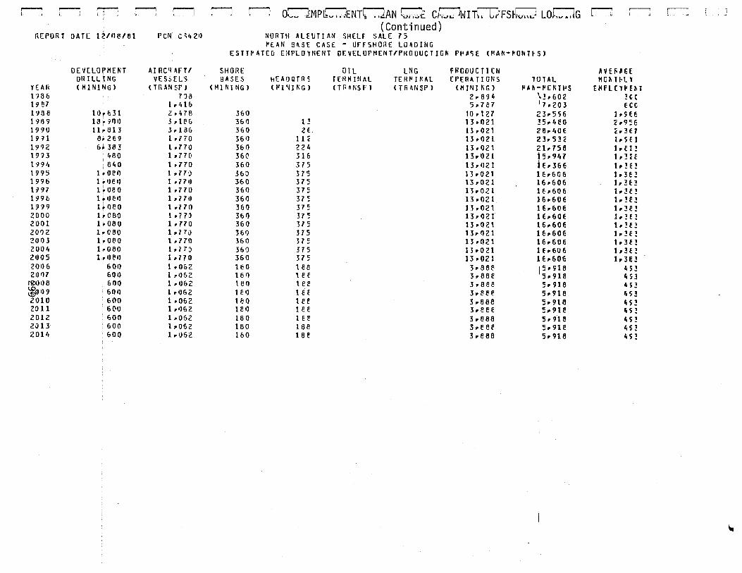
r---; r-. rr-1 rn r-l :--J r-:· Q._,~ lt1P!k•v, .iENTQAN C,·,·.:.f C~\•/IT(, L.J:FShvi\I_J LQJ.. ..... ,JG l"l ~ ~ c-:1

REPORT DATE l~/08/61 (Continued)

I'CN C ~'• 2•1 NORTH ALEUT! AN SHELF SALE 75 I'EAN 8~SE CAS£ - OFFSHORE l040ING

ESTI~ATED EMPLOlHENT OEYELOPMENT/PKODUCT!G~ P~~~E OIAN-I<OtiHSJ

DEVELOfMENT AI RC'l 1\FTI SHORE OIL LNG FRGOUCTlCN AYHHE DHILLING VES5EL'5 i:lASES 11EAOQTR~ rEilHINAL TE IH1 I l'iAl CPER.\T I ON S lOlAL MGI'Ili·U

YEAR (M!NltlG) (TRANSP> <MINING) <f"' 'H l'i G l CTI'ANSf) <Tii4NSPJ <HPIJt\G) P'H-I'Ill'illlS EHFLCHEI\1 198& 7')i:l 2r89~ \:!r602 !(( 19 87 lr4l& 5 r7e7 1 7r203 ECC 191Hl to• 631 2rlt78 360 10·127 23r5S6 1 r SEE 19139 13. :101) 3 r18& 36() n 13 r021 !SrltEO £r9~E 1990 ll.r813 3r1B& 360 2€ 13 r021 28r40E c • H 7 l9H a. 2 6 9 t.no 361} 11<: 13·021 2 3r 5::! ( lrH 1 1992 6~ 38 3 l.r770 361'1 22~ 13. 1)21 2lr758 1. en 19?3 480 1 r77D 3&C 316 13rQ21 i5r941 1 r ~ H 1994 840 1, 770 360 375 13r021 ier36E 1 r ~ E ~ 199S 1.oeo l • 7 7 ') 360 375 13•021 1Er606 1, 3€ ~ 1996 1 o 1)€ I) 1 • 771) 360 375 13·021 16r606 lr:!E! U97 1 ~ 08 0 1 r7 70 360 375 l3r021 1Er606 1r!E~ 199b t•oeo 1. 7711 360 37~ 13.021 16r60E 1r~E:! 1:199 loOilO l r17 0 360 375 n .o2t 1Er60E lr3E! 2000 1~c8o 1. 7 71) 361) 37~ 13r021 1Er60E 1 r ~ E :! 2001 1• 08 0 1. 770 360 37~ 13 ·021 l6r606 lr~f! 2002 Ho8o 1 • 7 7 [) 360 375 13rll21 lErGOE lr ~ E:! 2003 l~Ol\0 1.770 360 375 13r021 1Er60E t.H! 2004 1 ·.oeo 1·77~ 3&0 375 13 •021 1E. 606 lr3E! 21)1)5 lrllllll 1 ·11 0 360 375 13.021 H~6oe 1 r3E! 21)1)6 600 1 • 0&2 11:0 1!!8 3r 881l l~d18 ~S! 21)1)7 601) 1 r0&2 lt!f) lE f 3·888 5·911! 4 s 3

('g)!) I) 8 . 600 L, 062 l!JO tee 3·888 Sr916 4S! :i}J I) 9 601'1 1.1)62 tel) 1 E E 3r8el' 5r918 453 2010 600 l. 062 180 tee 3r66e Sr9l8 45! 2011 GOO 1 ·•1&2 teo 1E € 3r88f Sr91E 4 s:! 2012 600 lr062 18 0 1 E l! 3.888 Sr9l!! 4S! 2013 600 1r062 180 188 3 .. eee Sr91E 4 s:! 2014 &00 1r052 180 tBe 3·886 s. 918 4S~

~

HCPORT OATl 12/0P/~1 rc:i cs'dO

YE..41< M 1 N 1 'I(; Cl· ~i.S THIC T l r:P1 19!!4 3· 21.e 9 ('t,

1\il:lS b. 1)7 5 ') 24 19tH, ·~. 54 1 l.h&'J? 19 8i 11.•!!62 p r-32:> 198ii ?3d93 ~'··197 }')~ 9 32rL?tt 21,254 1 HI) z:;,2:>.o 5rlllc 1991 21r762 1 ~ 'J2 1~r9eE

1913 Ur!.77 1:1 '?4 1·4·596 1'1'1~ 14rl:l3& lH& 1~·836 1997 1'•• a 3 f: 19?ii l4•B3& 19:19 14riiH> 20110 14r83o 20•) 1 1'••e3& zon \ltrl\36 20rl J 14.f36 201}1, \4r:l3& 200 5 14.836 200 (j ,., 856 tQ~) 1 4r656 ~OOo ltr(i56 20J') 4r856 2«)1 0 4rt3(, 20tl 4rB56 21112 '"f. 56 2013 4re'i& 2:J1U. 4r 85 &

r-: rJ rr r-l r-J r-l r-l

U~~ ~M~LUTMtNI, MtAN ~A~t ~A~t W!IH Utt~HUKt LUAU!Nb (Continued)

~URTH ~LEUTJAN ~~ELF SALE 75 l't.&N ~,,E C1\~t;. - rrr 51fiJ.If: lo.Jf\UINr; 5UII:-I.\EY Cf Lilr'!:'CT El FLOYHUH ti'AI\-HHH~J

TC1Al T H ~ t-. ') P ') :<1 1\ T ! 0 J, TOTAL HC~l~LY E~FL(YHE~T

1 r<:'H:. s, 4 3 e i 453 ?rlt7i.' 9rltil 71:9 5r\1'() 2€.31'0 2r198 .l. f -~ t 33.579 !r79€ :l.t ~ t ~1). 576 4r214 3,186 56,734 4,728 :; • 1 :;1 t. 3'•·022 2~e3s t. n e 2 3r 5 J 2 1. s 6 1 1, f7 0 21..750 1 • E 1 3 1 ·17 0 1'5.547 1.:32 e 1 .7711 16.3&6 1r :!6 3 1· 77 () 1F.rE06 1. ~ e 3 1.7711 16rErJ6 t. :?I: 3 1· 7 70 H·liOG t.3e3 lrii'l· 16• Gllf.i t. ~ e 3 1. 77 0 lf:r6tl6 1!~1!3 t.nc l6r6CG t :?e3 lrl7U 16.606 1~383 \, 7H l6r6C6 lr383 1, 77 C) lErECG 1· 3B 3 1.770 tE.fi06 t. 38 3 lri711 lE. 606 t .. :? e 3 1 • 06 (: s.~Ia ~93 1, f)f, 2 s. 9 te 493 lr062 s. ~ Ie 493 1r!)fi(: s. s 18 ~<;3

1, Of> 2 5rHE 493 lrrJ&(: s.s1e 1 ~ 9 3 I, t)f> 2 5.9 tE 493 1. 06(. s. 918 ~93 1, 1)62 s. 91e 493

r-J r:--J r-J r--:1 r:J rn ll r-l

loo

r-l :-:J ~ r-:-J

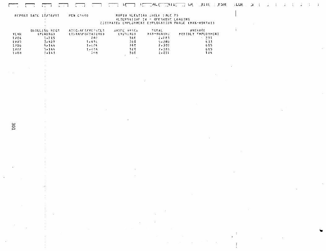
[""'] r-:: r:J rl

FEPnRT ~A~l 1~/~0/Rt

Yl ~H 1H4 1 \1 ,] 'S 1?3& 1\1 .~ i' \1/l:J

w 0 ......

0:1 ILL I •; G li I G S (~il\11-iG>

: • 7 1 '5 1. t, 2? ~.144 '5. lit 4 1 • 1 4 ~

r--1 ll

f'Cf~ C <- 4'l0

Lj 1/c--J I r-J f\L 1.~-JU. I 1 L-:J l,/-1~

NURTH ALE~T!A~ ~HELF ~ALE 75 •1LH.!l'lU J'IF iV - OFF'iiiQ:;c: lliAL'ING

jH I tl I Jr-::>Hl

[3TPl~HU I::!H'l.,JYMCI\T [~PI_I]f;ATJDN PH•':.i[ CMAI\-M'JI'\Tif3l

ATi:c"u itV£ '~~:u ;i H:H~ E •l ~ s t!: H•l"AL AVEHAG( ( T: I " N 'il' i) il T A f-11) rl ) ( NPI L·l G) Hl\-rH.N TH5 t'I.!~THLY ~ MPLO HEN T

i' ,, i· HO £ • ; e 3 ~H \ • 4 , l; .160 ';.:,. .~ 05 t, 3 3 1 r t \'4 Hr. 7. Jel.: 6 1 '5 1 p r.; ~. r, HC ; •. He GIS

;1\ll 3&0 ~.:~11 1 f.'•

JLUP, Jj j

~

HL ll:l<l'lH I 1 V t. '1- l./-\.)1: l'l.l 11"1 UrI" .)J1UI<l: LUHU Hlll

·(Continued)

REPORT DATL 12/0e/61 PCN C~4lll NORTH ~LEUT 1.\N SHELF S ~LE i5 ~lT[ilNAT!'I[ IV- UFFSIIO.l[ l\lAll!NG

YE .\ ii HJ4 1:1 '.i '5 198& l9P7 l9~f.i 19119 19 '}() HH

w 0 N

r~

PL~TFORM

I~SlALl~TION

Ll

&,5&6 t;.2f2 ?4·197 14.GQ9 5.069

r:J

;flDrtC BA ;f.

92.:. '}2 4 '12 c.

r; (""I

E;TJPATED EHPLQYMENT COK~T~UCTION PHASE l~A~-~CNTHSl

fJPELJNE L~~SiRUCTJG~

r:u

Ll ["""]

J!L TEh'U 1\Al

C-::J

I.'JG i r:F ~~; ~1.\L

C"J c:::J

f[TAL ~~N-MOTI'S

9;:4

924

c:-:J

7·2~2 1':5·2~2 24.117 11 .. eE1

J,(Jf.9

r-l

A v Eli AHI PCI\THLY EMFL~'PENT

•71

rn

71 6'H

1·273 '.b 16 1·21,0

2'::5

rJ LJ

II.

~ :--l ~ .-----, ' .J

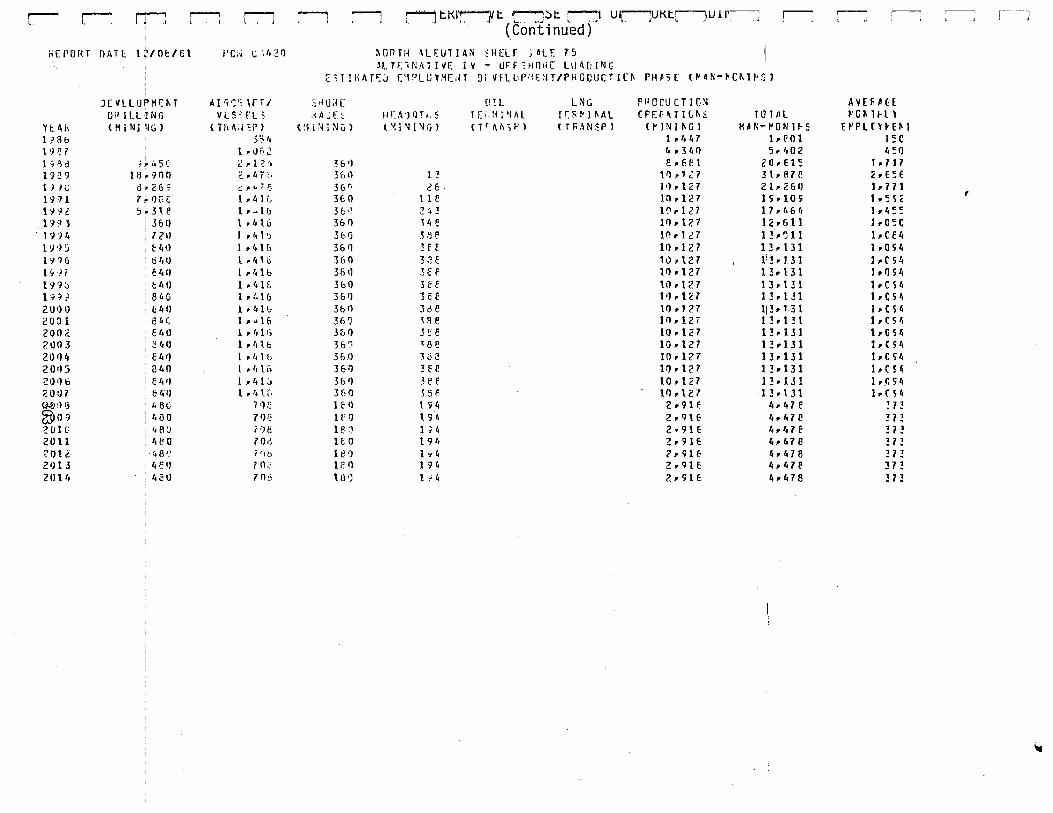
~ t ~ ~ ~ rr

k[I'OUT OAT(. lUOl::/5\ i'C:. C ;t, :!0

JEVlLUPMr:IIT A l :< ·: '': \F i I Uil ILL! NG Vi:.S:f:L)

Yt. llh (MPH%> c Th~:l.~P> 1?3b .)'; '• l '} ~ 7 l • () f•;: liono 1~ie5C 2 ~ 1 ? :~ 1 fi) 9 l!JdOO z. 4 7 '· H lv d•269 ~ .r I.., i r:. 1'}'71 7 • •JG [ 1·41<, 1 '} ':li :, d1.e 1, ~ 1 b 1 '}'/ J 3611 l.ol.l G 1 ':1 ') t, ' l (l) 1 , r, 1 •) l<J9S ' 1: 4•1 1 • 4 l!) 1 \1 '16 '640 l ,I,, 0 1<, H . t ~I) 1 •'• 1& 199:.> t: l.t) lrlolS t'fn 840 1ri..l6 2000 t:4() lr41•o 2001 e&c: 1, y 16 21)112 6411 l • t, 16 2003 ' 54() 1 • 41. b 201) 4 ct.•l I , t,\ b 201)5 . 040 t.t,,,, 21)1)& t 1,1) .l.rltL• 2 0 1)1 E t,IJ 1 r ·~ \ [,

(N}!ll.\ ' .:. 80 ; <) i; ~09 t,()Q 7/}i)

2 (J lL' 480 Fie 2011 ' t,{• 0 70d 21>12 48{' ;ri

21)13 t, fll 70 21114 ' 4.':0 70

r-l ..._ rJt.KI'rJVt. r--J.:::>t. r:-]1 UlrJUKt.~Uli'IJ

(Continued) r--1

l\OnTH ·\L F.UT l AN : H ELF i Al [ 7 S ALTC<N,\ilv[ IV - UFF~HO~E LU,D!NG

C: '1 !I'; II T 10 iJ E '1 f' L U ~ !iF: ; IT nL Hll:PI~t:H/PRGI]UCT 10 PH ,SE OHi-HI\11'!:: l

.1u:n: O!L L:-JG PflCCU CT JC:-.1 A~E~ II r: .\ •) (JT '· ~ 1 r: :1: '·I IlL rr:r.~HAL (f'f:Fr\TIOS 101/\l

Cl N i N li l ('lJ'nNGl CJ!I\~)Pl CHAN~Pl 0' IN I JIG l ~~~N-I'ONHS 1 , t, 4 7 l•f01 4 • 3 41) '5·402

H>'l e.Ht 21J,E15 3611 l ~ 1{),127 3t.ue 36r, .,?f.. 1 <) , 1 2 7 21.2611 360 1 lf. Hl.127 lS•lOS H•' ;> .. ~ - ~- 10·127 17•464 36 0 3 1, e 1 C). 1?. 7 12·611 3(>0 H!~ ll'rl27 l~·'Jll 36 ,, ~ff 11),127 13·131 361) 3~c 10.127 ti ~, 1.3 1 3!i I) Hf lll•l27 1~·131 3b0 He 10·127 13·131 361) HE l•Jr127 ~~.1~1

3b0 3de tCJ.127 11~·131

3& ~· ~ !l e 11'lrl2i l~rl3l 3fJ I) 3~e 10·127 1~·131 3&'! (a.c; 10 rl27 1~rl31 3f,.O :~ ~3 ~ 10rl?7 13r131 361) He 11)·127 1~·131 3b 1) 3ef 10.127 Url31 3 (,!) HP 10.127 13·\31 1 f I) l 9 4 2 r91E t.. 41 e 11'1) 1. 9·~ 2.r9\E l,rt.7f! 1 e. ~1 114 2. 91€ t,,t,7f HO 194 2r91E t,, 47 8 lt<O 1 ~ 4 <'•'<IE 4. 4 7 8 U~ll 1 9 4 2. 91E t.,t,7e l 0 ') 1 ~ 4 2 • 'HE 4r478

~ u ·~

1

AVEF~H ~'GIITH'

HPLCHHT ISC ~~!)

I, 111 ;:,E~E

1, 771 1 , 5 s c t.~~~ J,C5C: 1, C€ ~ 1 , 0 s I, 1 .rs ~ 1riJSl, 1, cs 4 1rCS4 1. c s ~ 1, ( s 4 t.os~ 1•CS4 lrOSt. 1, cs 4 1 •. r. s 4 1. (S 4 ~n

!71 ~1? ~ 7 1 ! 11 371 ~73

:----l J

~

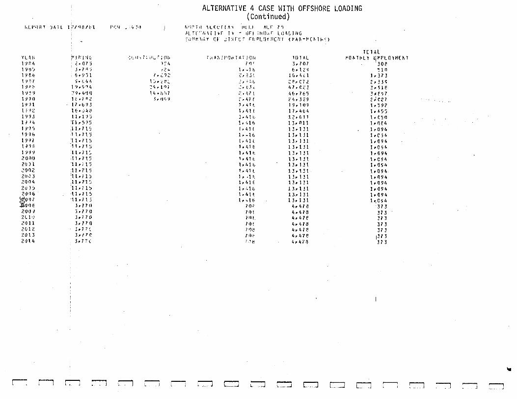
ld:I'1Jil1 ')fill 17/'111/t-\ p r: ~~ ~ ·, :, ,?-tJ

Ylo\ii :~ J ~:I :'J t· ·.:t .. /1'; :.,1;,; ~; (11'~

1 •J I' 4 2·07) 171,

1 ') lj J j. 7"' ·; •2 .. 19 6b or9)1 ., ,. t: '7::: 1.')'\i' ) ,. t t,J, 1. ~,. 't~ '-1 9 p ~· '1. 'J • 9'"~ r, :: '•, l ('} i ' ') :' ') :? 9. t, '·' ,, 1,1, • i:l ,, 7 1 :I'Hl 1 c. • i ~ 2 ~ .. •1 rJ r.; l'J'}l :11rb'J3 l : ·J ., •. <. 1 t. ·.i!, tl 1 'J '} J 1 1 • 1 '} :i 1 j 14 Tlr5'?5 1 9 ']) ,11171) 199b .1, ' • 7 t 'j 19H '1 1 • 7 1 5 t 9'H 1 1. 7l ::; 1 ')'} '} 11r71:. 21Jilt} 11r715 20 )1 llri'15 2002 11·715 zo.J 3 11·; 1::, .?1}04 llr715 ZuJ:J 1lril~ 21)'1 & ·llr715 ~01)7 tlrl1.5 ~o,>c 5r77tl 201) ·~ 3. 77ll 2tl•J 3·i70 2•>11 3r 710 ZvU 3 # 7 7 (

·~o 13 3 r 7 7 ()

2tH4 3r i7 (

r~ r-1 r:-J r-J r-1 r--i

ALTERNATIVE 4 CASE WITH OFFSHORE LOADING (Continued)

N '1 :' T i I \ L E L: l l .\ ~ I I I. U AI_ r 7 •; "L.Ti.'~-~~\[ l~F I~ - t)FI ihf.l.,r l.1l~ulNG

·~<J.'I~\,\V GF ,;J:if'~;T FI:Pl~JY~·![/1! (t'AI\-11 0il<>

T It A :0, ; I' I],; T A i ) 11 It lll 1 A l 7 I) ~ 3r707

1. ··1 b & • 1 z q :~, !: J ·~ 1 !j. ~ c: 1 .: , .: ~ t. ;:l'rCU ;: , t: ~ <. r, 7, r.;: ~ ;.-.: , .'t 7 l 4&r 765 ;·, lo 7 I ('I,. 3 29 , , 4, (; 1 9. 1 1)9 t, r,u l7r464 I , t, t b J.Z.t::11 lr •<1 I? l3r011 lr ~ l! 13.tJ1 1. u 16 13r131 [,loU 13rl3l 1. t, 1E 13r131 t. 41 t; 13rl31 , • 41 (. 13• 1.H 1r41b l.h131 1. • r, 1 l I. 3 r 1 3 1 I r •I t l3r131 t. c, 1( 13rl31 1. ;.1 6 l3r13l t.41l 13rl31 1 •. ,u; l3r131

701.' ~,, 41 e 7 •1! 4•H8 7llt 4· "7e 71)! "• Ha 7 1lc 4r4ill 71)1' 4r47e ;.lt,; 4. 4 i'l)

c--J r:-J CJ r-:J c:::::J c::::J ro

TCl.U rO~l"Ll ~~PLOlHE~T

:30 fl ~ 1 II

1 r3 7 3 2 • ~.H ~.SH

~-f<;7 2~f.27 1·592 lr£55 ,.r,so 1 rll € 4 t.094 lrC;4 1. 0 9 ~ lrO o;t. 1r094 lrC94 lr '] S 4 t.094 lr094 t.OS4 lr()94 lr094 1 ., c s t,

313

CJ

373 !73 373 373 1~73 373

r----'1 L

,----., l ;J :---:-l

,....._.._, .. J

~

:--:-l

[

[~

r [

[

[

[

[

[

[

[

[

[

[

[_

[

[

[

[

REFERENCES

Alaska Consultants, Inc. 1970. City of Sand Point Comprehensive Plan. Alaska State Housing Authority, Anchorage.

Alaska Department of Commerce and Economic Development. 1979. Numbers: Basic Economic Statistics of Alaskan Census Divisions. Juneau.

Alaska Department of Fish and Game. Alaska Catch and Production: Commercial Fisheries Statistics. Various years.

Alaska Department of Fish and Game. 1981. Statistics, (included in North Pacific Briefing Paper). Juneau.

Groundfish Catch Fishery Management

A 1 ask a Department of Labor. A 1 ask a Labor Force Estimates. . Various years.

Alaska Department of Labor. Alaska Economic Trends. Various years.

Alaska Department of Labor. 1979. Occupational Employment Statistics.

A 1 ask a Department of Labor. 1979. Alaska Population Overview. Juneau.

A 1 ask a Department of Labor. 1981. Alaska 1980 Population: A Preliminary Look. Juneau.

Alaska Department of Labor. 1981. Lower Yukon-Kuskokwim Region Labor Market Analysis. Juneau.

Alaska Department of Labor. 1964-1980. Statistical Quarterly. Juneau.

Arctic Environmental Information and Data Center. 1978. Village Profiles for False Pass, St. Paul, St. George, Belkofski, Nelson Lagoon, Nikolski, Atka, Akutan, and King Cove. Prepared for the Alaska Department of Community and Regional Affairs.

Arthur D. Little, Inc. 1978. The Development of a Bottomfish Industry: Strategies for the State of Alaska. Technical Appendix, Vol. 2. A Report to the Office of the Governor.

Earl R. Comos, Inc. 1981. St. George Basin and North Aleutian Shelf Commercial Fishing Analysis. Bureau of Land Management,

-- · Anchon;.ge. OCS Technicu.l 1~eport No. 60.

305

Goldsmith, S. and E. Porter. 1981. Alaska Economic Projections for Estimating Electricity Requirement for the Railbelt. Institute of Social and Economic Research, University of Alaska, Anchorage.

Jones, D.iVI. 1973. Patterns of Village Growth and Decline in the Aleutians. Institute of Social, Economic, and Government Research, University of Alaska, Fairbanks.

Koslow, J.A. 1979. Limited Entry Policy and the Bristol Bay, Alaska Salmon Fishermen. A report prepared for the Alaska State Legislature.

Kresge, D.T., S.R. Fison, and A.F. Gasbarro. 1974. Bristol Bay: A Socioeconomic Study. Institute of Social, Economic, and Government Research, University of Alaska, Fairbanks.

Lanydon, S. 1980. Transfer Patterns in Alaskan Limited Entry Fisheries. Report for Limited Entry study group of the Alaska State Legislature.

Langdon. S. 1981. The 1980 Salmon Season and Bristol Bay Native Fishermen: Performance and Prospects. Bristol Bay Native Association, Dillingham, Alaska.

Larson, D. 1980. 1979 Fishermen's Income Survey: Herring and Salmon Fisheries. Alaska Sea Grant Program Report 80-5.

North Pacific Fishery ivlanagement Counci 1. 1979. Fishery Management Plan for Groundfish in the Bering Sea/Aleutian Island Area. Anchorage.

North Pacific Fishery i"lanagement Council. 1981. Fishery Management Plan for the Gulf of Alaska Groundfish Fishery. Anchorage.

Rogers, G., R.F. Listowski, and D. Mayer. 1980. Measuring the Socioeconomic Impact of Alaska's Fisheries. Institute of Social and Economic Research, University of Alaska, Anchorage.

Terry, J.l"l., R.G. Scoles, and D.M. Larson. 1980. Western Alaska and Bering Norton Petroleum Development Scenarios: Commercial Fishing Industry Analysis. Alaska Sea Grant Program, University of Alaska. OCS Technical Report No. 51.

Tremont, J.D. 1981. Resources, Developmental Timeframes, Infrastructure Assumptions and Block Deletion Alternatives for Proposed Federal Lease Sales in the Bering Sea and Norton Sound. Bureau of Land Management, Anchorage. OCS Technical Paper No. 1.

306

[

r~

r [

[

[

[

[

[

[

[

[

[

L L r~ L

[

L l

r [

[

[

L [

F [

[

[

[

[

[

[

[

[

L L r -L

Tryck, Nyman, and Hayes. 1979. Recommended Community Development Plan: City of Unalaska, Alaska. Prepared for the City of Unalaska.

Tuck, B.H. and L. Huskey. 1981. St. George Basin Petroleum Development Scenario: Economic and Demographic Analysis. Bureau of Land Management, Anchorage. OCS Technical Report No. 57.

U.S. Department of Commerce, Bureau of the Census. 1981. Alaska Final Population and Housing Unit Counts. PH C 80-V-3. U.S. Government Printing Office, Washington, D.C.

307

]

1 J J J J J J J J J ]

]

J J J J D

80£

I I I I I I I I I I - ARLIS.org

Documents

Transcript of I I I I I I I I I I - ARLIS.org