Hypergraph matrix models and generating functions - arXiv

arX

iv:2

204.

1136

1v1

[m

ath.

CO

] 2

4 A

pr 2

022

HYPERGRAPH MATRIX MODELS AND GENERATING FUNCTIONS

MARIO DEFRANCO AND PAUL E. GUNNELLS

Abstract. Recently we introduced the hypergraph matrix model (HMM), a Hermitianmatrix model generalizing the classical Gaussian Unitary Ensemble (GUE). In this modelthe Gaussians of the GUE, whose moments count partitions of finite sets into pairs, arereplaced by formal measures whose moments count set partitions into parts of a fixedeven size 2m ≥ 2. Just as the expectations of the trace polynomials TrX2r in the GUEproduce polynomials counting unicellular orientable maps of different genera, in the HHMthese expectations give polynomials counting certain unicelled edge-ramified CW com-plexes with extra data that we call (orientable CW) maps with instructions. In this paperwe describe generating functions for maps with instructions of fixed genus and with thenumber of vertices arbitrary. Our results are motivated by work of Wright. In particularWright computed generating functions of connected graphs of fixed first Betti number asrational functions in the rooted tree function T (x), given as the solution to the functional

relation x = T e−T .

1. Introduction

1.1. We begin by recalling the Gaussian Unitary Ensemble (GUE) matrix model and itsconnection to counting orientable maps. For more information, we refer to Harer–Zagier[15], Etingof [10, §4], Lando–Zvonkin [17], and Eynard [11].

Let V be the N2-dimensional real vector space of N × N complex Hermitian matricesequipped with Lebesgue measure. For any polynomial function f : V → R, define

(1)⟨f⟩

=

∫V f(X) exp(−TrX2/2) dX∫

V exp(−TrX2/2) dX,

where Tr(X) =∑

iXii is the sum of the diagonal entries. Let k ≥ 0 be an integer, andconsider (1) evaluated on the function on V given by taking the trace of the kth power:

(2)⟨TrXk

⟩.

We denote by Pk(N) the quantity (2) as a function of N . For k odd (2) clearly vanishes.On the other hand, it turns out that if k = 2r is even, then P2r(N) is an integral polynomialin N of degree r + 1 with the following combinatorial interpretation.

Let Π be a polygon with 2r sides. We define a pairing π of the sides of Π to be a partitionof the edges into disjoint pairs. We say that π is an oriented pairing if the edges have been

Date: April 22, 2022.2010 Mathematics Subject Classification. 81T18, 81T32, 05C65, 05C30.Key words and phrases. Matrix models, hypergraphs, hyperbaggraphs, generating functions.The second author was partially supported by NSF grant 1501832. We also thank Alejandro Morales

and Eric Fusy for helpful comments.

1

http://arxiv.org/abs/2204.11361v1

2 MARIO DEFRANCO AND PAUL E. GUNNELLS

oriented such that as one moves clockwise around the polygon, paired edges appear withopposite orientations. Any oriented pairing π of the sides of Π determines a rooted orientedunicellular map Mπ. By definition this means Mπ is a closed orientable topological surfacewith an embedded graph—namely the images of the edges and vertices of Π—such thatthe complement of the graph is a 2-cell, and the graph has a distinguished vertex and adistinguished edge containing that vertex.(1) Let v(π) be the number of vertices in thisgraph. Then we have

(3) P2r(N) =∑

π

Nv(π),

where the sum is taken over all oriented pairings of the edges of Π. For example, we have

(4) P4(N) = 2N3 + N, P6(N) = 5N4 + 10N2, P8(N) = 14N5 + 70N3 + 21N.

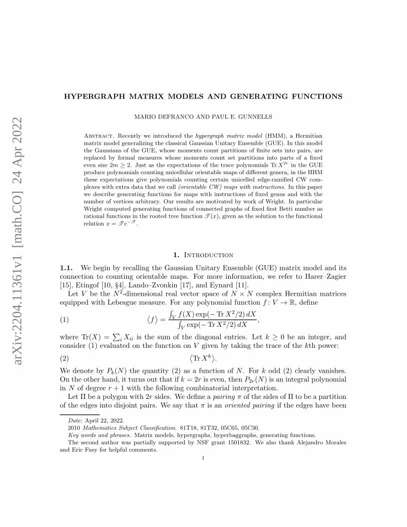
The three oriented pairings of a square giving P4(N) are shown in Figure 1.

PSfrag replacements

N3N3N1

Figure 1. Computing P4(N) = 2N3 + N . The leftmost surface is a toruswith embedded graph having one vertex. The next two are the 2-spherewith embedded graph having three vertices.

1.2. In [6] we defined a generalization of the GUE that we call the hypergraph matrixmodel (HMM). The HMM depends on an integer m ≥ 1; when m = 1 the HMM coincideswith the GUE. The connection with hypergraphs is that just as the 1-dimensional GUEcan be used to construct generating functions of graphs, the 1-dimensional HMM can beused to construct generating functions of certain hypergraphs. For more details about thisconnection, we refer to [10, §3] and [6, Section 2].

To explain the HMM, we first recall the combinatorial interpretation of the Gaussianmoments. Let x be a real variable. Suppose we normalize the measure dx on R such that∫∞−∞ e−x2/2 dx = 1. Consider the moment

(5)⟨xk⟩

:=

∫ ∞

−∞xke−x2/2 dx.

If k is odd, we have⟨xk⟩

= 0. If k is even, then it is well known that⟨xk⟩

is the Wicknumber

W2(k) =k!

2k/2(k/2)!,

1Throughout, we allow graphs to have loops and multiple edges.

HYPERGRAPH MATRIX MODELS AND GENERATING FUNCTIONS 3

which counts the pairings of the finite set [[k]] := {1, . . . , k}. The Gaussians appear in theGUE when one writes the variable matrix X in terms of the underlying N2 real coordi-nates. Indeed the measure exp(−TrX2) dX is then just a product of Gaussians, althoughwith different normalizations for the diagonal and off-diagonal coordinates. This is theunderlying reason why the expectations of the traces (1) are related to pairings.

In the HMM we replace the product of Gaussians exp(−TrX2/2) dX in (1) with a formalmeasure dXm that is a product of certain one-variable measures dxm. The moment

(6)⟨xk⟩m

:=

∫xk dxm

is defined to be 0 if m does not divide k, and otherwise is given by the generalized Wicknumber

(7) W2m(k) =k!

m!k/m(k/m)!,

which counts the number partitions of [[k]] into disjoint subsets of order 2m. Again using thereal coordinates to define the product measure dXm, one can then define the expectations

(8)⟨TrXk

⟩m

:=

∫

VTrXk dXm.

We let P(m)k (N) denote (8) as a function of N .

The main results of [6] show that (8) vanishes unless k = 2mr, and otherwise P(m)2mr(N)

is an integral polynomial of degree r + 1. For instance, when m = 2 we have

P(2)8 (N) = 6N3 + 21N2 + 8N, P

(2)12 (N) = 57N4 + 715N3 + 2991N2 + 2012N,

P(2)16 (N) = 678N5 + 19405N4 + 228190N3 + 1151300N2 + 1228052N.

In [6] several combinatorial interpretations are given for the polynomial P(m)2mr(N), including

(i) counting walks on digraphs, (ii) counting points on subspace arrangements over finitefields and (iii) enumerating unicellular CW maps with instructions, a generalization of mapsthat have ramified edges and extra gluing data.

1.3. The goal of the current paper is to give generating functions for the coefficients of

P(m)2mr(N). The case m = 1 (GUE), which corresponds to counting unicellular maps, has

been considered by a variety of authors. For a (rather incomplete) list, one can refer toHarer–Zagier [15], Eynard [11], Lass [18], Chapuy [2, 3], Chapuy–Feray–Fusy [4], Bernardi[1], and Goulden–Nica [13].

More precisely, we consider the rational polynomials

(9) P(m)2mr :=

1

2mrP

(m)2mr(N) ∈ Q[N ],

whose coefficients count weighted unicellular CW maps with instructions: the contibutionof each map has been multiplied by the inverse of the order of its automorphism group.


For our purposes it is more convenient to work with the coefficients in the falling factorialbasis. Thus let (N)k = N(N − 1) · · · (N − k + 1), and write

P(m)2mr(N) =

r+1∑

l=0

α(m)l,r (N)r+1−l,

For g ≥ 0, we put

(10) G(m)g (x) =

∑

v≥1

α(m)g,g−1+vx

v ∈ Q[[x]].

Thus G(m)0 is the generating function of the leading coefficients of the P(m) in the falling

factorial basis, the series G(m)1 is that of the subleading coefficients, and so on. For example,

when m = 1 we have

G(1)0 = x2/2 + x3/2 + 5x4/6 + 7x5/4 + 21x6/5 + · · · ,

G(1)1 = x/2 + 3x2/2 + 5x3 + 35x4/2 + 63x5 + 231x6 + · · · ,

G(1)2 = 3x/4 + 15x2/2 + 105x3/2 + 315x4 + 3465x5/2 + · · · ,

and when m = 2,

G(2)0 = x2/4 + 3x3/4 + 19x4/4 + 339x5/8 + 927x6/2 + · · · ,

G(2)1 = x/4 + 39x2/8 + 1057x3/12 + 26185x4/16 + 157754x5/5 + · · · ,

G(2)2 = 35x/8 + 1845x2/4 + 180785x3/8 + 862005x4 + · · · .

We call g the genus, since when m = 1 it agrees with the genus of the surface underlying

the map. The series G(m)g are our basic objects of study. More examples can be found in

Appendix A.

We remark that the series G(m)0 were already essentially computed in [14]. Indeed, we

have

G(m)0 (x) =

∑

v≥1

C(m)v

2mvxv+1,

where C(m)v is a hypergraph Catalan number [14, Definition 2.5].

1.4. We are almost ready to state our results, but before we do we must recall work ofWright [22], whose results inspired ours. Let V (G) (respectively, E(G)) be the vertices(resp., edges) of G, and let v(G) = |V (G)| (resp., e(G) = |E(G)|). The excess of G isdefined to be e(G)−v(G). Wright studied generating functions of connected graphs of fixedexcess. This work was revisited by Janson–Knuth– Luczak–Pittel [16], at least for excesses≤ 1; other expositions appear in Flajolet–Sedgewick [12, II.5] and Dubrovnin–Yang–Zagier[8, §3.1].(2)

2The authors of [8] do not explicitly refer to Wright’s work, but they do prove the relevant results weneed.


For g ≥ 0 let Γ(g) be the set of connected graphs G with first Betti number g. Thequantity g is called the loop number in the physics literature; it exceeds the excess by1: g = e(G) − v(G) + 1. Let AutG be the full automorphism group of G generated bypermuting vertices and parallel edges, as well as flipping and permuting loops. We considerthe generating function

(11) Wg(x) =∑

v≥1

∑

G∈Γ(g)

xv(G)

|AutG| ,

which we regard as enumerating weighted graphs: the coefficient [xv]Wg is not the numberof connected graphs with first Betti number g, but rather the sum of them weighted by theinverses of the orders of their automorphism groups. For example, we have

W0 = x + x2/2 + x3/3 + 2x4/3 + 25x5/24 + 9x6/5 + 2401x7/720 + · · · ,W1 = x/2 + 3x2/4 + 17x3/12 + 71x4/24 + 523x5/80 + 899x6/60 + · · · ,W2 = x/8 + 7x2/12 + 101x3/48 + 83x4/12 + 12487x5/576 + 3961x6/60 + · · · .

Wright showed that for g ≥ 1 the series (11) can be computed in terms of what is essentiallythe series for the g = 0 case. Let T be the inverse series of xe−x:

(12) T (x) = x + x2 + 3x3/2 + 8x4/3 + · · · .

The series T is the generating function of weighted rooted trees.(3) Let Γ≥3(g) ⊂ Γ(g) bethe finite subset of graphs with all vertices having degree at least 3. Then if g ≥ 2, we have

(13) Wg(x) =∑

G∈Γ≥3(g)

1

|AutG|T v(G)

(1 − T )e(G), g ≥ 2.

One can also give expressions for g = 0, 1 in terms of T , but these are exceptional (§3).

1.5. Our main results, Theorems 4.2, 5.2, and 10.1, give expressions for the series G(m)g

respectively for g = 0, g = 1, and g ≥ 2. Like Wright’s theorem, the expression for g ≥ 2is a sum over the finite set Γ≥3(g) and is given in terms of certain tree functions, butthere are other ingredients involved. One must also sum over balanced digraph structureson “thickenings” of graphs in Γ≥3(g), and over sets of oriented spanning trees of directedgraphs.

We remark that although our results were inspired by those of [22], our results do not

generalize Wright’s: the series G(m)g is not a generalization of Wg, and in particular G

(1)g 6=

Wg.

3The series T is sometimes called the Lambert series because it is essentially the power series for Lam-bert’s W -function [7, §4.13]. Apparently the series T was first considered by Eisenstein [9], although he didnot interpret the coefficients in terms of trees.


1.6. Here is a guide to the paper. In §2 we recall results from [6] that explain how to

compute the polynomials P(m)2mr(N) in terms of walks on graphs. In §3 we present Wright’s

computation of his generating functions. Section 4 gives the computation of the series G(m)0

(Theorem 4.2) and the additional tree functions needed to compute G(m)g for g ≥ 1; these

series might be of independent interest. In §5 we compute G(m)1 (Theorem 5.2). The next

three sections §§7–9 give the ingredients we need to compute G(m)g for g ≥ 2. In §10 we

state and prove our main theorem. We conclude with some examples. Section 11 discusses

some examples and complements, and in Appendix A we give examples of G(m)g for small

m and g.

2. Coefficients of P(m)2mr(N) and walks on graphs

2.1. In this section we recall results from [6]. The main result is that P(m)2mr can be

computed in the falling factorial basis as a finite sum over certain graphs G involving threequantities:

(i) A walks contribution, which counts Eulerian tours on digraphs built from G.(ii) A moment contribution, which incorporates the moments of the measure dXm.(iii) A contribution from the automorphism group of G.

We treat each of these in turn, beginning with the walks contribution.

2.2. Let Γ[r] be the set of connected graphs with r edges and any number of vertices.

Any G ∈ Γ[r] has a canonical thickening to a graph G with 2mr edges: we simply replace

each edge e in G with 2m edges running between the endpoints of e. Note that G dependson the parameter m, although we omit it from the notation.

2.3. Let D(G) be the set of balanced digraph structures on the thickening G. Thus an

element of D(G) is an assignment of orientations to the edges of G such that at each vertexv the total indegree In(v) equals the total outdegree Out(v). The set D(G) is clearly finite,

and since the degree of each vertex of G is even, the set D(G) is nonempty.

2.4. The set D(G) is naturally in bijection with the set of lattice points in a polytope.To see this, first we define a partition of the edges E(G). Define an equivalence relationon edges by e ∼ e′ if (i) e and e′ are loops at a common vertex or (ii) e and e′ are paralleledges running between the same two distinct vertices. Let S(G) be the set of equivalenceclasses. We call the classes of type (i) the loop classes and those of type (ii) the nonloopclasses. We write

S(G) = Ss(G) ⊔ Sp(G) ⊔ Sl(G).

where

• Ss(G) is the nonloop classes represented by singletons,• Sp(G) is the nonloop classes not represented by singletons, and• Sl(G) is the loop classes,


Thus for example S ∈ Sp(G) is the equivalence class of a full set of > 1 parallel edgesbetween two distinct vertices in G. We also have the corresponding partition of the edges

E(G) = Es(G) ⊔ Ep(G) ⊔El(G).

For e ∈ Es ∪ Ep, let #»e be e with a fixed arbitrary orientation. We fix these orientationsso that parallel edges are oriented in the same direction. For each S ∈ Ss ∪ Sp, choose tworeal variables aS , bS . We take aS (respectively bS) to count the edges in a digraph structure

on G running parallel to e ∈ S and in the same (resp., opposite) direction of #»e . For thedigraph to be balanced, the aS , bS must satisfy

aS , bS ≥ 0, aS + bS = 2m|S| for all S ∈ Ss ∪ Sp,(14)∑

S

ε(S, v)(aS − bS) = 0 for all v ∈ V (G).(15)

In (15) the sum is taken over all classes S containing an edge e meeting v, and ε(S, v) = 1if v is the tail of #»e and equals −1 otherwise.

The real solutions to (14)–(15) define a lattice polytope(4) Xm(G), and it is clear thatD(G) is in bijection with the lattice points in Xm(G). Given an integral solution, we callthe integers {

aS, bS∣∣ S ∈ Ss ∪ Sp

}

the digraph parameters. Note that the solution aS = bS = m|S| for all S gives a balanced

digraph for any G; we call this the canonical digraph structure.It is clear that any γ ∈ D(G) has an Eulerian tour. Following Lass [18], we call two

Eulerian tours essentially different if one cannot be obtained from the other by permutingloops or parallel edges. We often abbreviate essentially different Eulerian tour by EDET.

2.5. Definition. Let G be a graph and let γ ∈ D(G) be a balanced digraph structure on

the thickening G. We define the walks contribution W (γ) to be the number of essentiallydifferent Eulerian tours on γ.

2.6. Next we consider the moment contribution M(γ). Let x, y be real variables and letz = x + y

√−1 be a complex variable. We use the generalized Wick numbers (7) to define

moments on powers of x, y and by linearity on powers of z, z. For our purposes we willneed two different normalizations for these moments:

• Loop normalization: We put⟨xk⟩m

=⟨yk⟩m

= Wm(k) if m | k, and 0 otherwise.

• Nonloop normalization: We put⟨xk⟩m

=⟨yk⟩m

= Wm(k)/2k if m | k, and 0otherwise.

2.7. Now let γ ∈ D(G) be an balanced digraph structure on G with parameters {aS , bS}.We define M(γ) by taking a product over the edges of certain Wick numbers.

• Loop subsets: Let S ∈ Sl(G) be a loop subset. We define

M(S) =⟨x2m|S|

⟩m,

where the moment is computed using the loop normalization.

4This polytope is a variant of the flow polytope.


• Nonloop subsets: Let S ∈ Ss(G)∪Sp(G) be a nonloop subset. Let aS , bS be thecorresponding digraph parameters. We put

M(S) =⟨zaS zbS

⟩m,

where the moment is computed using the nonloop normalization.

2.8. Definition. We define the moment contribution M(γ) to be the product∏

S∈S(G)

M(S).

2.9. Finally we define the contribution from the automorphism group of G. Let AutGbe the full group of automorphisms of G generated by permuting vertices and edges. SinceG has loops and parallel edges, AutG also includes automorphisms that fix the vertices,namely permuting parallel edges, permuting loops at a vertex, and interchanging the half-edges of a loop at a vertex. Let Autv G ⊂ AutG be the subgroup that acts trivially on thevertices.

2.10. Definition. We define Autv G to be the quotient AutG/Autv G.

2.11. We can now state the result from [6] that gives an explicit expression for the

coefficients of the polynomials P(m)2mr(N). Recall that (N)k denotes the falling factorial

N(N − 1) · · · (N − k + 1).

2.12. Theorem. [6, Proof of Theorem 3.6] Let Γ[r] be the set of connected graphs with redges and with any number of vertices. Let D(G) be the set of balanced digraph structures

on the thickening G. Let W (γ), M(γ), and Autv G be defined as in Definitions 2.5, 2.8,and 2.10. Then we have

P(m)2mr(N) =

∑

G∈Γ[r]

(N)v(G)

|Autv G|∑

γ∈D(G)

W (γ)M(γ).

For an example of computing P(m)2mr(N) using this result, we refer to [6, Example 3.7].

2.13. Corollary. For g ≥ 1 we have

(16) G(m)g (x) =

1

2m

∑

G∈Γ(g)

xv(G)

(v(G) + g − 1)|Autv G|∑

γ∈D(G)

W (γ)M(γ).

If g = 0, the series G(m)0 is given by the same expression (16), except that the sum is taken

over graphs with at least 2 vertices.

2.14. Remark. The contribution M(γ) can vanish for certain γ ∈ D(G). Indeed, accordingto [6, Lemma 3.4], the moment

⟨zazb

⟩m

is nonzero only if the exponents satisfy 4 | a − b.Thus there will typically be many lattice points in Xm(G) that give balanced digraphs butwill not contribute to (16). If one wishes to keep only the nonzero terms in (16), one canreplace the canonical lattice in the space defining Xm(G) with a sublattice.


2.15. We conclude this section by recalling the BEST theorem for counting Eulerian tourson balanced digraphs. For more information we refer to [20, 5.6].

Let γ be a balanced digraph with vertex set V (γ). For any vertex v ∈ V (γ), an orientedspanning tree T rooted at v is a spanning tree of the undirected graph underlying γ suchthat the edges in γ point towards v. Let σ(γ, v) be the number of oriented spanning treesof γ with root v.

2.16. Theorem. [20, BEST Theorem 5.6.2] Let γ be a balanced digraph. Let e be an edgeof γ, and let v be the initial vertex of e. Then the number of Eulerian tours of γ with initialdirected edge e is given by

(17) σ(γ, v)∏

u∈V (γ)

(Out(u) − 1)!.

3. Wright’s generating functions of graphs

3.1. The goal of this section is to recall the proof of (13) and the related expressions forg = 0, 1 in terms of the tree function T (x). The original ideas go back to Wright [22];our reference is [8, §3.1]. While these results are not explicitly needed in the sequel, the

computation of G(m)g is analogous, and thus they serve as a warmup for later results.

3.2. First we consider g = 0. Writing

W0(x) =∑

v≥1

W0,vxv,

we see that W0,v counts the weighted trees with v vertices. This is almost the same asT (12); the only difference between [xv]W0 and [xv]T is that the latter counts weightedrooted trees with v vertices. There are v ways to choose a root in a tree contributing toW0,v. This implies [xv]T = vW0,v, and thus

T (x) = xd

dxW0(x).

From this we have

(18) W0(x) =

∫x−1

T (x) dx,

which gives an expression for W0 in terms of the tree function T .

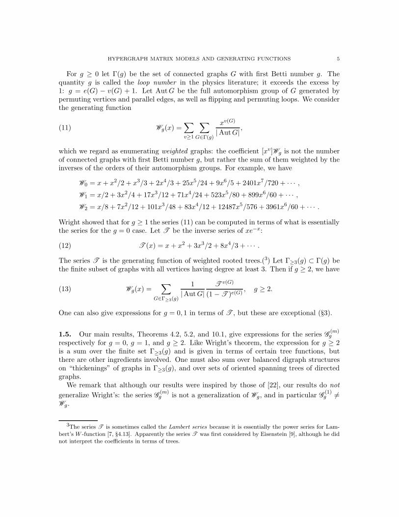
3.3. Next we consider g = 1. A connected graph G with g = 1 consists of a unique k-cycleCk with no backtracking and with rooted trees attached to its vertices (Figure 2). We sayG is built from Ck by grafting rooted trees at the vertices. The contribution to W1 of allsuch graftings onto Ck is T (x)k/2k. The T k comes from enumerating the possible choicesof k ordered weighted rooted trees, and the 2k is the order of the automorphism group ofCk. Thus

(19) W1(x) =1

2

∑

k≥1

T k

k=

1

2log( 1

1 − T

).


Figure 2. Grafting rooted trees onto a cycle.

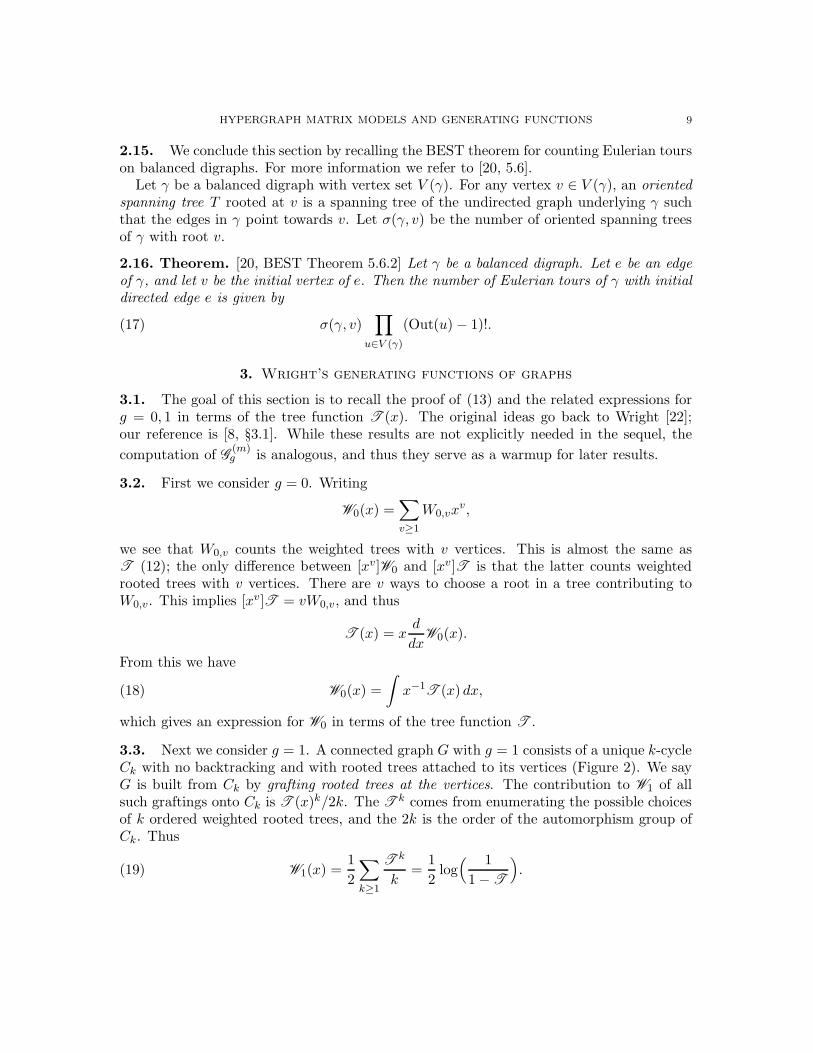
3.4. Finally we consider g ≥ 2. Let H ∈ Γ(g). Then there is a unique graph G ∈ Γ≥3(g)that can be constructed from H. We first erase any degree 1 vertices and their attachededges. We continue doing this until there are no more vertices of degree 1 to obtain a graphG′. Next if there are any degree 2 vertices, we erase them and join the corresponding edgesinto a single edge. After eliminating all degree 2 vertices, the result is the graph G. Wecall G the reduction of H (Figure 3).

PSfrag replacements

−→

H G′ G

Figure 3. Reducing a graph H ∈ Γ(2) to G ∈ Γ≥3(2).

It is clear that the reduction map Γ(g) → Γ≥3(g) is surjective. Conversely, any graphin Γ(g) can be built by starting with a graph in Γ≥3(g), subdividing edges by adding somedegree 2 vertices, then grafting rooted trees onto the original vertices and those of degree2. The contribution of G ∈ Γ≥3(g) to Wg is thus

1

|AutG|Tv(G)(1 + T + T

2 + · · · )e(G) =1

|AutG|T v(G)

(1 − T )e(G).

Summing over all G ∈ Γ≥3(g) we obtain (13):

(20) Wg(x) =∑

G∈Γ≥3(g)

1

|AutG|T v(G)

(1 − T )e(G), g ≥ 2.

3.5. To finish the discussion, we show that the indexing set Γ≥3(g) in (20) is finite. Indeed,if G ∈ Γ≥3(g) has dk vertices of degree k, then

v(G) =∑

k≥3

dk, e(G) =1

2

∑

k≥3

kdk,


which implies

(21) 2g − 2 =∑

k≥3

(k − 2)dk.

This means the degree sequence (d3, d4, d5, . . . ) corresponds uniquely to a partition of 2g−2,and so there are only finitely many such sequences for each g. Moreover each degreesequence leads to only finitely many possibilities for a graph, so the sum (20) is finite. Tosummarize,

• all the Wg, g ≥ 2, are rational functions in T ;• the series W1 is the log of a rational function in T ; and• the series W0 is the integral of x−1T .

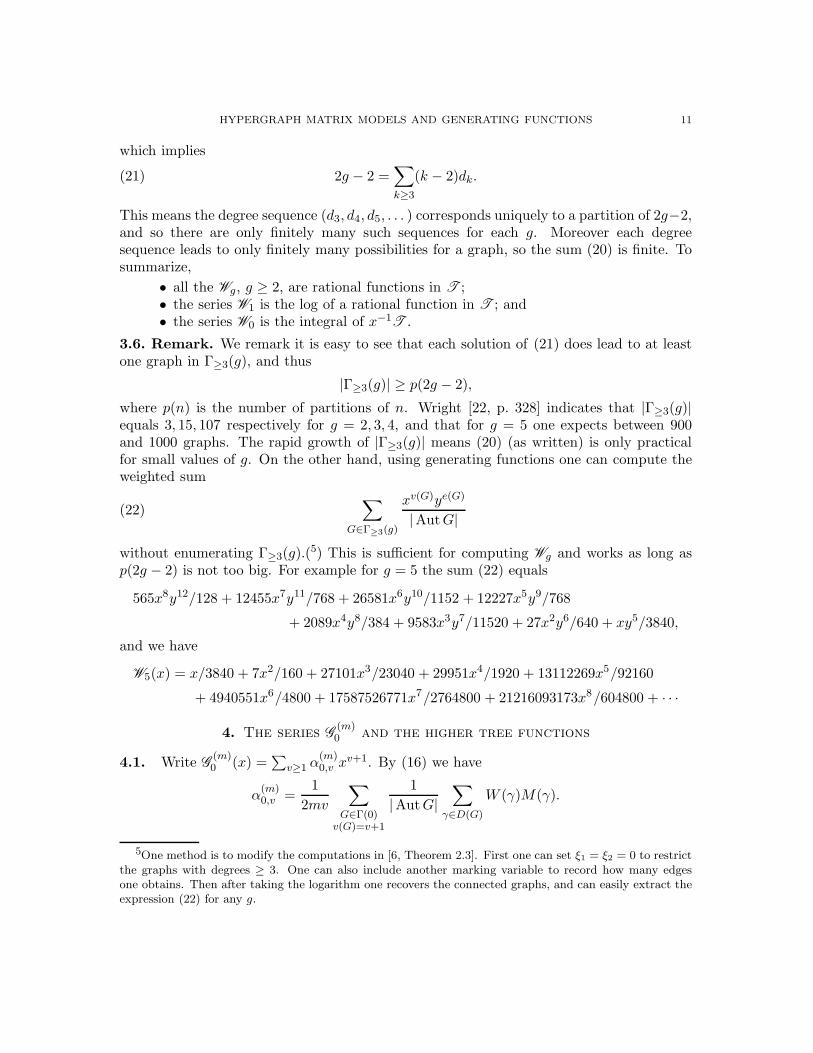
3.6. Remark. We remark it is easy to see that each solution of (21) does lead to at leastone graph in Γ≥3(g), and thus

|Γ≥3(g)| ≥ p(2g − 2),

where p(n) is the number of partitions of n. Wright [22, p. 328] indicates that |Γ≥3(g)|equals 3, 15, 107 respectively for g = 2, 3, 4, and that for g = 5 one expects between 900and 1000 graphs. The rapid growth of |Γ≥3(g)| means (20) (as written) is only practicalfor small values of g. On the other hand, using generating functions one can compute theweighted sum

(22)∑

G∈Γ≥3(g)

xv(G)ye(G)

|AutG|

without enumerating Γ≥3(g).(5) This is sufficient for computing Wg and works as long asp(2g − 2) is not too big. For example for g = 5 the sum (22) equals

565x8y12/128 + 12455x7y11/768 + 26581x6y10/1152 + 12227x5y9/768

+ 2089x4y8/384 + 9583x3y7/11520 + 27x2y6/640 + xy5/3840,

and we have

W5(x) = x/3840 + 7x2/160 + 27101x3/23040 + 29951x4/1920 + 13112269x5/92160

+ 4940551x6/4800 + 17587526771x7/2764800 + 21216093173x8/604800 + · · ·

4. The series G(m)0 and the higher tree functions

4.1. Write G(m)0 (x) =

∑v≥1 α

(m)0,v xv+1. By (16) we have

α(m)0,v =

1

2mv

∑

G∈Γ(0)v(G)=v+1

1

|AutG|∑

γ∈D(G)

W (γ)M(γ).

5One method is to modify the computations in [6, Theorem 2.3]. First one can set ξ1 = ξ2 = 0 to restrictthe graphs with degrees ≥ 3. One can also include another marking variable to record how many edgesone obtains. Then after taking the logarithm one recovers the connected graphs, and can easily extract theexpression (22) for any g.


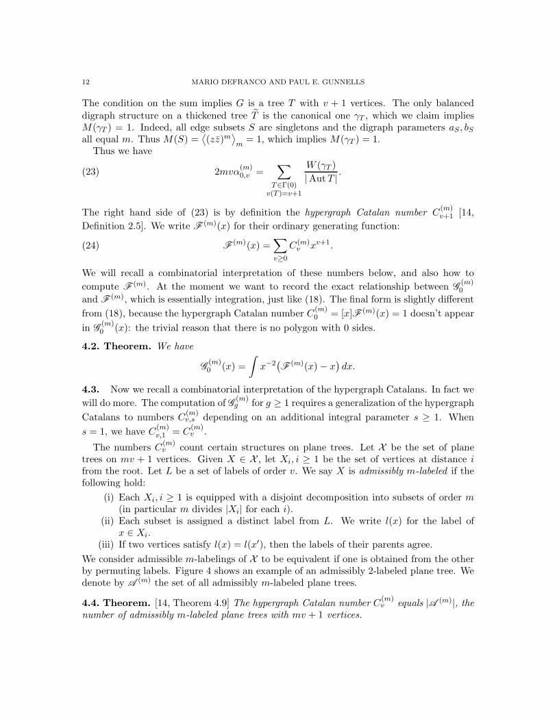
The condition on the sum implies G is a tree T with v + 1 vertices. The only balanced

digraph structure on a thickened tree T is the canonical one γT , which we claim impliesM(γT ) = 1. Indeed, all edge subsets S are singletons and the digraph parameters aS , bSall equal m. Thus M(S) =

⟨(zz)m

⟩m

= 1, which implies M(γT ) = 1.Thus we have

(23) 2mvα(m)0,v =

∑

T∈Γ(0)v(T )=v+1

W (γT )

|AutT | .

The right hand side of (23) is by definition the hypergraph Catalan number C(m)v+1 [14,

Definition 2.5]. We write F (m)(x) for their ordinary generating function:

(24) F(m)(x) =

∑

v≥0

C(m)v xv+1.

We will recall a combinatorial interpretation of these numbers below, and also how to

compute F (m). At the moment we want to record the exact relationship between G(m)0

and F (m), which is essentially integration, just like (18). The final form is slightly different

from (18), because the hypergraph Catalan number C(m)0 = [x]F (m)(x) = 1 doesn’t appear

in G(m)0 (x): the trivial reason that there is no polygon with 0 sides.

4.2. Theorem. We have

G(m)0 (x) =

∫x−2

(F

(m)(x) − x)dx.

4.3. Now we recall a combinatorial interpretation of the hypergraph Catalans. In fact we

will do more. The computation of G(m)g for g ≥ 1 requires a generalization of the hypergraph

Catalans to numbers C(m)v,s depending on an additional integral parameter s ≥ 1. When

s = 1, we have C(m)v,1 = C

(m)v .

The numbers C(m)v count certain structures on plane trees. Let X be the set of plane

trees on mv + 1 vertices. Given X ∈ X , let Xi, i ≥ 1 be the set of vertices at distance ifrom the root. Let L be a set of labels of order v. We say X is admissibly m-labeled if thefollowing hold:

(i) Each Xi, i ≥ 1 is equipped with a disjoint decomposition into subsets of order m(in particular m divides |Xi| for each i).

(ii) Each subset is assigned a distinct label from L. We write l(x) for the label ofx ∈ Xi.

(iii) If two vertices satisfy l(x) = l(x′), then the labels of their parents agree.

We consider admissible m-labelings of X to be equivalent if one is obtained from the otherby permuting labels. Figure 4 shows an example of an admissibly 2-labeled plane tree. Wedenote by A (m) the set of all admissibly m-labeled plane trees.

4.4. Theorem. [14, Theorem 4.9] The hypergraph Catalan number C(m)v equals |A (m)|, the

number of admissibly m-labeled plane trees with mv + 1 vertices.

HYPERGRAPH MATRIX MODELS AND GENERATING FUNCTIONS 13PSfrag replacements

aa bb

cc dd

ee ff

Figure 4. An admissible 2-labeling of a plane tree.

4.5. Now we define the numbers C(m)v,s by modifying this interpretation. Let s ≥ 1 be an

integer. Given a plane tree X, let x1, . . . , xd be the children of the root, written in order.We say X has d subtrees. Let ξ be a composition of d into s parts. Then ξ determinesan ordered decomposition of {x1, . . . , xd} into s contiguous subsets, some of which mightbe empty. We say the pair (X, ξ) is a plane tree with its subtrees placed into s regions.A example is shown in Figure 5. The plane tree X has 4 subtrees and s = 6. (We haveomitted the vertex labels to keep the figure cleaner.) In this example ξ = (0, 0, 2, 1, 1, 0),and thus the 4 subtrees of X are being placed into 4 regions. We have drawn boundingsegments in the plane to indicate the 6 regions R1, . . . , R6.

PSfrag replacementsR1

R2

R3

R4

R5

R6

Figure 5. The composition ξ = (0, 0, 2, 1, 1, 0) determines a placement ofthe 4 subtrees into 6 regions.

4.6. Definition. Let A(m)s be the set of pairs (X, ξ), where X is an admissibly m-labeled

plane tree with mv + 1 vertices and d subtrees, and ξ is a composition of d into s parts.

We define C(m)v,s = |A (m)

s | and put

F(m)s (x) =

∑

v≥0

C(m)v,s xv+1.


Clearly F(m)1 (x) = F (m)(x), the generating function of the hypergraph Catalans. Here

are some examples for m = 2:

F(2)1 (x) = x + x2 + 6x3 + 57x4 + 678x5 + 9270x6 + 139968x7 + · · · ,

F(2)2 (x) = x + 3x2 + 24x3 + 267x4 + 3546x5 + 52938x6 + 862974x7 + · · · ,

F(2)3 (x) = x + 6x2 + 63x3 + 834x4 + 12672x5 + 212436x6 + 3854223x7 + · · · ,

F(2)4 (x) = x + 10x2 + 135x3 + 2130x4 + 37320x5 + 709560x6 + 14472855x7 + · · · .

4.7. We now explain how to compute the generating functions F(m)s . We recall a basic

result from counting plane trees with extra structure, which follows easily from assemblingfacts in Flajolet–Sedgewick [12]; full details can be found in [14].

4.8. Proposition. [14, Proposition 5.3]

(i) Let A(x) =∑

k≥0 akxk ∈ Z[[x]] be an integral formal power series with ak ≥ 0. Let

PA be the set of all colored plane trees such that any vertex with k children canbe painted one of ak colors. Let PA ∈ Z[[x]] be the ordinary generating function ofPA, so that the coefficient [xn]PA(x) of xn counts the trees in PA with n vertices.Then PA satisfies the functional relation

(25) PA = xA(PA).

(ii) Let B(x) =∑

k≥0 bkxk ∈ Z[[x]] be another integral formal power series with bk ≥ 0.

Let PA,B be the set of all colored plane trees such that (a) any non-root vertexwith k children can be painted one of ak colors, and (b) if the root vertex has degreek then it can be painted any one of bk colors. Let PA,B ∈ Z[[x]] be the ordinarygenerating function of PA,B. Then PA,B satisfies the functional relation

(26) PA,B = xB(PA),

where PA satisfies (25).

For any pair t ≥ 0, r ≥ 1, let λ(r, t) be the dimension of the space of degree t homogeneouspolynomials in r variables. We have

λ(r, t) =

(r − 1 + t

r − 1

).

4.9. Theorem. Put

ℓ(x) =∑

d≥0

Wm(dm)λ(m,dm)xd

and

hs(x) =∑

d≥0

Wm(dm)λ(m, sm)xd.

Then the set Pℓ,hsof (ℓ, hs)-colored plane trees is in bijection with the set of all admissibly

m-labeled plane trees A(m)s whose subtrees have been placed into s regions.


Proof. The proof is a simple modification of the proof of [14, Theorem 5.6]. There we showedthat there is a bijection between admissibly m-labeled plane trees A (m) and (ℓ, h1)-coloredplane trees P(ℓ,h1). To extend [14, Theorem 5.6] to the current setting, we need only observe

this bijection takes pairs (X, ξ) ∈ A(m)s exactly to (ℓ, hs)-colored plane trees. Indeed, the

only new feature is that in [14] if a the root of a plane tree had degree d, we colored it by aset partition of [[dm]] into subsets of order m, which gives Wm(dm) colors and agrees withh1. Now, however, we also color the root by a choice of composition ξ of d into s parts.This is exactly accomplished by the coloring series hs(x). �

4.10. To conclude this section, we explain why the tree series F(m)s (x) are needed to

compute G(m)g for larger g. The key is the following proposition, which shows how the

series appear when counting EDETs after grafting trees onto a fixed graph.

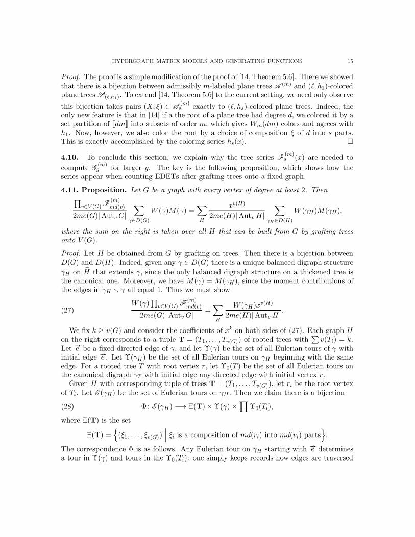
4.11. Proposition. Let G be a graph with every vertex of degree at least 2. Then∏

v∈V (G) F(m)md(v)

2me(G)|Autv G|∑

γ∈D(G)

W (γ)M(γ) =∑

H

xv(H)

2me(H)|Autv H|∑

γH∈D(H)

W (γH)M(γH),

where the sum on the right is taken over all H that can be built from G by grafting treesonto V (G).

Proof. Let H be obtained from G by grafting on trees. Then there is a bijection betweenD(G) and D(H). Indeed, given any γ ∈ D(G) there is a unique balanced digraph structure

γH on H that extends γ, since the only balanced digraph structure on a thickened tree isthe canonical one. Moreover, we have M(γ) = M(γH), since the moment contributions ofthe edges in γH r γ all equal 1. Thus we must show

(27)W (γ)

∏v∈V (G) F

(m)md(v)

2me(G)|Autv G| =∑

H

W (γH)xv(H)

2me(H)|Autv H| .

We fix k ≥ v(G) and consider the coefficients of xk on both sides of (27). Each graph Hon the right corresponds to a tuple T = (T1, . . . , Tv(G)) of rooted trees with

∑v(Ti) = k.

Let #»e be a fixed directed edge of γ, and let Υ(γ) be the set of all Eulerian tours of γ withinitial edge #»e . Let Υ(γH) be the set of all Eulerian tours on γH beginning with the sameedge. For a rooted tree T with root vertex r, let Υ0(T ) be the set of all Eulerian tours onthe canonical digraph γT with initial edge any directed edge with initial vertex r.

Given H with corresponding tuple of trees T = (T1, . . . , Tv(G)), let ri be the root vertexof Ti. Let E (γH) be the set of Eulerian tours on γH . Then we claim there is a bijection

(28) Φ: E (γH) −→ Ξ(T) × Υ(γ) ×∏

Υ0(Ti),

where Ξ(T) is the set

Ξ(T) ={

(ξ1, . . . , ξv(G))∣∣∣ ξi is a composition of md(ri) into md(vi) parts

}.

The correspondence Φ is as follows. Any Eulerian tour on γH starting with #»e determinesa tour in Υ(γ) and tours in the Υ0(Ti): one simply keeps records how edges are traversed


in γ and in the γTi. This gives a map

(29) π : Υ(γH) −→ Υ(γ) ×∏

Υ0(Ti)

that is clearly surjective. Furthermore, given a tour w ∈ Υ(γ) and tours wi ∈ Υ0(Ti), toassemble them into a tour in Υ(γH) one needs to choose how much of wi to execute eachtime the vertex vi is entered in w. This is given by a composition ξi of md(ri) into md(vi)parts. Indeed, the outdegree of ri in γTi

is md(ri), and the indegree of vi in γ is md(vi).Thus vi is visited md(vi) times during γ, and the total number of times we can exit ri toexecute part of γTi

is md(ri). Thus in (29) the preimages under π correspond to the setΞ(T), and (28) is a bijection.

Now we pass to EDETs. The total number of Eulerian tours on γ is 2me(G)|Υ(γ)|.Therefore

(30) W (γ) = 2me(G)|Υ(γ)|ω(γ)

,

where

(31) ω(γ) :=∏

S∈Ss∪Sp

aS!bS ! ·∏

S∈Sl

(2m|S|)!;

in (31) the aS , bS are the digraph parameters of γ, and Ss, Sp, Sl are the edge classesof G. If H corresponds to the tuple of trees T, then to compute W (γH) we must divide2me(H)|Υ(γH )| by (31) as well as by

J(T) :=

v(G)∏

i=1

(2me(Ti))!.

Thus by (28) we have

(32) W (γH) = 2me(H)|Ξ(T)| · |Υ(γ)|J(T) · ω(γ)

v(G)∏

i=1

|Υ0(Ti)|.

Now we consider all H contributing to the coefficient xk, and we incorporate automor-phisms. Since every vertex of G has degree at least 2, we have |AutH| = |AutG|

∏|AutTi|.

Since trees have no loops or parallel edges, we have |Autv H| = |Autv G|∏ |AutTi|. Thus(30) and (32) imply

(33)∑

H,v(H)=k

W (γH)

2me(H)|Autv H| =W (γ)

2me(G)|Autv G|∑

T=(T1,...,Tv(G))∑v(Ti)=k

|Ξ(T)|J(T)

v(G)∏

i=1

|Υ0(Ti)||AutTi|

.

To complete the proof, it remains to observe that the quantity

∑

T=(T1,...,Tv(G))∑v(Ti)=k

|Ξ(T)|J(T)

v(G)∏

i=1

|Υ0(Ti)||AutTi|


in (33) is exactly the coefficient of xk in∏

v∈V (G) F(m)md(v). �

4.12. Remark. When m = 1, the series F(1)1 is the ordinary generating function of the

Catalan numbers. When s > 1 the series are related to self-describing sequences due to

Sunik [21], and to counting certain standard tableaux.

5. The series G1

5.1. The goal of this section is to prove the following theorem, which is the computationof the series G1(x) in terms of the generalized tree functions. Let log≥n(x) be the powerseries for log(1/(1 − x)) with the terms of degree < n omitted:

log≥n(x) = log( 1

1 − x

)−

n−1∑

k=1

xk

k

=xn

n+

xn+1

n + 1+

xn+2

n + 2+ · · · .

5.2. Theorem. Let F = F(m)2m (x). Let P be the set of pairs

P ={

(a, b) ∈ Z2∣∣ a, b ≥ 0, a + b = 2m,a− b ≡ 0 mod 4

}.

Let

β(a) =a

2m

(2m

a

).

Then we have

G(m)1 (x) =

F

2m+

⟨(zz)2m)

⟩m

F 2

4m

+1

2m

(β(m)F )3

(1 − β(m)F )+

∑

(a,b)∈Pa6=b

1

2(a− b)log≥3

( 1 − β(b)F

1 − β(a)F

),

where the moment⟨(zz)2m)

⟩m

is computed using the nonloop normalization.

5.3. The proof of Theorem 5.2 occupies the rest of this section. By §3.3, any graph Hwith g = 1 is a k-cycle Ck with rooted trees grafted onto its vertices, which we denote T1,. . . , Tk. We consider each of the quantities that appear in the formula (16). We shall seethat the description is mostly uniform in k, although k = 1, 2 are exceptional.

5.4. First we consider the group Autv Ck. The group AutCk has order 2k for all k, butonly for k ≥ 3 does |Autv Ck| = 2k. If k = 1 we have |Autv(C1)| = 1 since the onlynontrivial automorphism of C1 fixes the vertex. If k = 2 we have |Autv C2| = 2, sincepermuting the two edges does not affect vertices. To summarize,

|Autv Ck| =

1 if k = 1,

2 if k = 2,

2k if k ≥ 3.


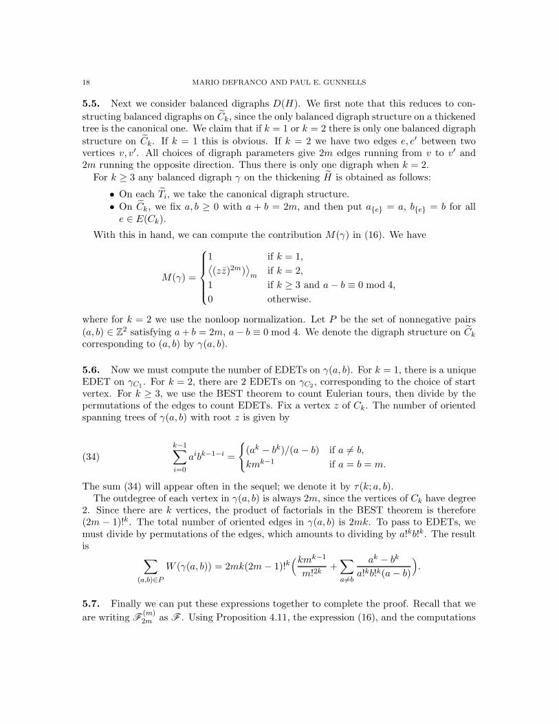
5.5. Next we consider balanced digraphs D(H). We first note that this reduces to con-

structing balanced digraphs on Ck, since the only balanced digraph structure on a thickenedtree is the canonical one. We claim that if k = 1 or k = 2 there is only one balanced digraph

structure on Ck. If k = 1 this is obvious. If k = 2 we have two edges e, e′ between twovertices v, v′. All choices of digraph parameters give 2m edges running from v to v′ and2m running the opposite direction. Thus there is only one digraph when k = 2.

For k ≥ 3 any balanced digraph γ on the thickening H is obtained as follows:

• On each Ti, we take the canonical digraph structure.

• On Ck, we fix a, b ≥ 0 with a + b = 2m, and then put a{e} = a, b{e} = b for alle ∈ E(Ck).

With this in hand, we can compute the contribution M(γ) in (16). We have

M(γ) =

1 if k = 1,⟨(zz)2m)

⟩m

if k = 2,

1 if k ≥ 3 and a− b ≡ 0 mod 4,

0 otherwise.

where for k = 2 we use the nonloop normalization. Let P be the set of nonnegative pairs

(a, b) ∈ Z2 satisfying a + b = 2m, a− b ≡ 0 mod 4. We denote the digraph structure on Ck

corresponding to (a, b) by γ(a, b).

5.6. Now we must compute the number of EDETs on γ(a, b). For k = 1, there is a uniqueEDET on γC1 . For k = 2, there are 2 EDETs on γC2 , corresponding to the choice of startvertex. For k ≥ 3, we use the BEST theorem to count Eulerian tours, then divide by thepermutations of the edges to count EDETs. Fix a vertex z of Ck. The number of orientedspanning trees of γ(a, b) with root z is given by

(34)

k−1∑

i=0

aibk−1−i =

{(ak − bk)/(a − b) if a 6= b,

kmk−1 if a = b = m.

The sum (34) will appear often in the sequel; we denote it by τ(k; a, b).The outdegree of each vertex in γ(a, b) is always 2m, since the vertices of Ck have degree

2. Since there are k vertices, the product of factorials in the BEST theorem is therefore(2m − 1)!k. The total number of oriented edges in γ(a, b) is 2mk. To pass to EDETs, wemust divide by permutations of the edges, which amounts to dividing by a!kb!k. The resultis

∑

(a,b)∈P

W (γ(a, b)) = 2mk(2m− 1)!k(kmk−1

m!2k+∑

a6=b

ak − bk

a!kb!k(a− b)

).

5.7. Finally we can put these expressions together to complete the proof. Recall that we

are writing F(m)2m as F . Using Proposition 4.11, the expression (16), and the computations


above, we have

G(m)1 (x) =

F

2m+

⟨(zz)2m)

⟩m

4mF

2

+∑

k≥3

F k

2mk

2mk(2m− 1)!k

2k

∑

(a,b)∈P

(kmk−1

m!2k+∑

a6=b

ak − bk

a!kb!k(a− b)

).

The sum over k can be simplified as follows. Writing

(35) β(a) =a

2m

(2m

a

),

we have1

2

∑

k≥3

1

k

( k

m(β(m)F )k +

∑

(a,b)∈Pa6=b

(β(a)F )k − (β(b)F )k

a− b

).

Interchanging the sum over k with the sum over (a, b) and using the definition of log≥n

completes the proof of Theorem 5.2.

6. The series Gg for g ≥ 2: preliminaries

6.1. Now we pass to general g ≥ 2. Given G ∈ Γ≥3(g), let D(G) be the set of balanced

digraph structures on the thickening G. Let Σ(G) be the set of spanning trees of G. Weput an equivalence relation on Σ(G) by T ∼ T ′ if (i) T and T ′ have edges in Sp(G) and (ii)T is obtained from T ′ by permuting edges in a given parallel class S ∈ Sp(G). We fix onceand for all a set Σ0(G) ⊂ Σ(G) of representatives for the tree classes.

For each γ ∈ D(G) and T ∈ Σ0(G), we will define a power series R(γ, T ) ∈ Q[[x]] using

rational functions in the tree series F(m)s (x). Like the walks and moment contributions in

§2, R(γ, T ) will be built as a product over the edge classes S(G). Our final formula for

G(m)g (x) will take the shape

(36) G(m)g (x) =

∑

G∈Γ≥3(g)

∑

γ∈D(G)

∑

T∈Σ0(G)

R(γ, T ).

Each sum in (36) is taken over a finite set, which thus yields a finite expression for ourgenerating function in terms of rational functions in tree functions.

6.2. Our strategy will be the same as in §5. Let G′ be a graph obtained from G ∈ Γ≥3(g)by subdividing edges with new vertices of degree 2. We encode G′ by subdivision parameters

{ke ∈ Z ≥ 0 | e ∈ E(g)},where ke is the number of new vertices added to e (thus e has been subdivided into ke + 1new edges in G′). Each S ∈ S(G) will have one or more subdivision parameters attachedto it. We will compute how the quantities W,M depend on the subdivision parameters,as well as any adjustments to |AutG| necessary to compute |Autv G|. At the very endwe apply Proposition 4.11 and insert tree functions for the vertices, to account for graftingtrees onto G′, and sum over the subdivision parameters to obtain rational functions.


For the convenience of the reader, we summarize the notation/terminology we will usewhen constructing R(γ, T ):

• G ∈ Γ≥3(g).• z is a fixed vertex on G.• γ is a balanced digraph on G.• {aS , bS | S ∈ Ss ∪ Sp} is the set of digraph parameters for γ with respect to

some fixed orientations #»e of the edges; all edges in a parallel edge class have thesame orientation. The parameter aS counts the edges in S that point in the samedirection as #»e , and bS counts the edges that point in the opposite direction.

• T ∈ Σ0(G) is a spanning tree of G. By abuse of notation we will also consider Tto be an oriented spanning tree, by orienting each edge such that z is the root. Ifwe need to distinguish between T and T equipped with this orientation, we write#»

T for the latter.• Suppose e appears in T and e ∈ S. Then either #»e or − #»e (the same edge with

opposite orientation) appears in#»

T . We denote by cS the digraph parameter dis-

tinguished by the orientation of e in#»

T . More precisely,

cS =

{aS if #»e ∈ #»

T ,

bS if − #»e ∈ #»

T .

• R(γ, T ) will be given as product of factors R•(S, γ, T ), where • ∈ {s,p, l}. Thesethree cases are covered in §§7–9. We will give their ingredients in the followingorder:(A) contributions to correct automorphism counts (adjusting |AutG| to |Autv(G)|);(M) contributions to M(γ);(O) contributions to the outdegree product in the BEST theorem;(E) factors needed to pass from Eulerian tours to EDETs;(F) tree function factors arising from subdividing; and(T) contributions to the spanning tree counts in G′.

We conclude this section by stating a lemma relating spanning trees in G to those in asubdivision G′. We omit the simple proof.

6.3. Lemma. Let G be a graph and let e ∈ E(G). Let G′ be obtained from G by subdividinge into two edges e1, e2 by adding a degree 2 vertex. Let i : G− e → G′ be the inclusion. LetT be a spanning tree of G.

(i) If e ∈ T , then i(T − e) ∪ {e1, e2} is a spanning tree of G′.(ii) If e 6∈ T , then i(T ) ∪ {e1} and i(T ) ∪ {e2} are distinct spanning trees of G′.

Moreover, all spanning trees of G′ arise in this way, starting with a spanning tree of G.�

7. The series Gg for g ≥ 2: single edges

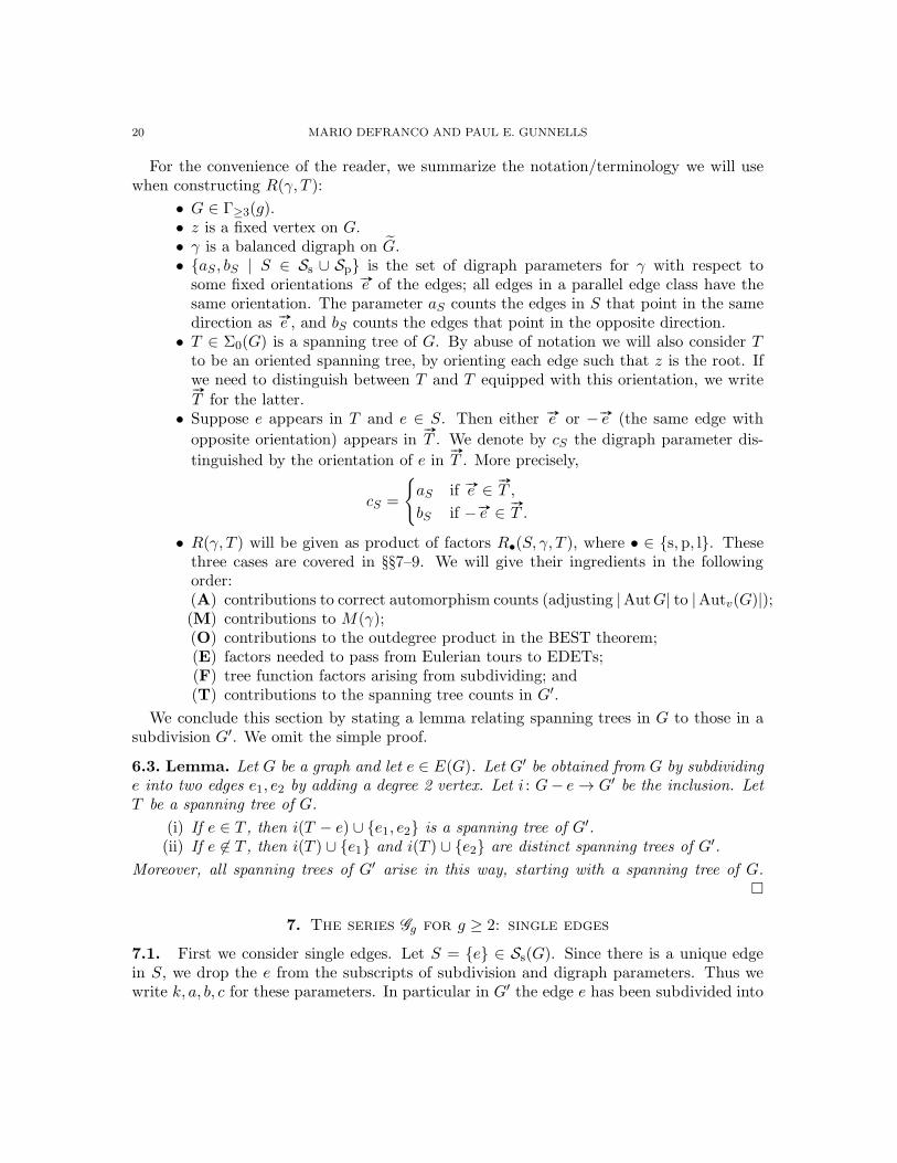
7.1. First we consider single edges. Let S = {e} ∈ Ss(G). Since there is a unique edgein S, we drop the e from the subscripts of subdivision and digraph parameters. Thus wewrite k, a, b, c for these parameters. In particular in G′ the edge e has been subdivided into


a set E of k + 1 new edges. Note that in the digraph γG′ each edge in E becomes a edgesdirected one way, and b edges directed the other. Figure 6 shows e and E ⊂ E(G′), as wellas the corresponding part of γ(G′) when m = 4.

PSfrag replacements

e E

Figure 6. m = 4, a = 6, b = 2.

(A) There is no correction to the automorphism counts, since any automorphism thatacts nontrivially on e will act nontrivially on the new vertices in G′.

(M) After subdivision, we have k + 1 groups of a edges running in one direction and bedges running in the other, with a + b = 2m. Thus in the computation of M(γ), each ofthese groups contributes

⟨zazb

⟩m

, which equals 1 if a−b is divisible by 4, and is 0 otherwise.(O) Now we consider the outdegree contribution. We have divided e into k + 1 edges

with all new vertices having degree 2. Thus in γG′ each new vertex will have outdegree 2m.This means we need a factor of (2m− 1)!k for the BEST theorem.

(E) Next we have the correction term to pass from Eulerian tours to EDETs. In γG′ wehave k + 1 groups of a edges running in one direction and b edges in the other. These canbe permuted among themselves, which gives a factor of 1/(a!b!)k+1.

(F) Next we have the tree functions for the new vertices in G′; this gives (F(m)2m )k.

(T) Finally we consider counting spanning trees. If e ∈ T , then by Lemma 6.3 we mustselect one edge from each group to build a tree in G′. Thus there are ck+1 choices.

If e 6∈ T , then to build a spanning tree of γG′ we must first pick an edge of E to delete,and then make choices from the directed edges to point back at the endpoints of e. Thetotal contribution to the number of spanning trees is therefore

ak + ak−1b + · · · + abk−1 + bk = τ(k + 1; a, b).

7.2. Combining these contributions together, we obtain

∑

k≥0

A(k)(2m − 1)!k

a!k+1b!k+1(F

(m)2m )k,

where A(k) = ck+1 or τ(k + 1; a, b) depending on whether e ∈ T or e 6∈ T . If we sum overk ≥ 0, we obtain the contribution Rs(S, γ, T ). To give the final result, and to simplify laterformulas, we introduce some notation. Assume a + b = 2m, and let K ≥ 0. Then let

(37) µ≥K(c) =c(β(c)F

(m)2m )K

a!b!(1 − β(c)F(m)2m )

;


if 4 | (a−b); otherwise put µ≥K(c) = 0. Here c ∈ {a, b}, and will be unambiguously selectedby the context in which µ appears. Also let

(38) ϕ≥K(a, b) =

1

a!b!(a− b)

(a(β(a)F

(m)2m )K

1 − β(a)F(m)2m

− b(β(b)F(m)2m )K

1 − β(b)F(m)2m

)if a 6= b,

1

m!2(1 − β(m)F

(m)2m

)2 − 1

m!2

K∑

i=1

i(β(m)F(m)2m )i−1 if a = b = m,

if 4 | (a− b); otherwise put ϕ≥K(a, b) = 0.

7.3. Definition. Let S = {e} ∈ Ss(G) be a edge class consisting of a single edge. Letγ ∈ D(G), and T ∈ Σ0(G). We define

(39) Rs(S, γ, T ) =

{µ≥0(c) if e ∈ T ,

ϕ≥0(a, b) otherwise,

where a = aS, b = bS are the digraph parameters for S.

7.4. Example. Using Definition 7.3 we can compute the contribution of any G ∈ Γ≥3(g)with no loops and no parallel edges. Looking ahead to Theorem 10.1, we see that Gcontributes

K(m)4 (x) :=

∏v∈V (G)(md(v) − 1)!F

(m)md(v)

|AutG|∑

γ∈D(G)

∑

T∈Σ(G)

∏

e∈E(G)

Rs({e}, γ, T )

in the sum over Γ≥3(g).We illustrate with the complete graph G = K4, which has g = 3. Each vertex has degree

3, and |AutG| = 24. The digraph structures that give nonzero expectations for m ≥ 1 arecounted by

1, 15, 15, 65, 65, 175, 175, 369, . . . .

The distinct numbers in this list are called the rhombic dodecahedral numbers, and equaln4 − (n− 1)4, n ≥ 1 [19, Series A005917].

We consider m = 2. The thickening G has 4 parallel edges for each edge in G. Up tosymmetry, the 15 digraphs are the following:

• There are 8 obtained by choosing a vertex v, orienting the edges incident to vas in the canonical digraph (two inedges, two outedges), and then orienting theremaining edges opposite v in one of two different cycles (all edges pointing in thesame direction).

• There are 6 obtained by choosing a pair of opposite edges e, e′ in G. The edges in Gcorresponding to e, e′ are oriented as in the canonical digraph, and the remainingedges are oriented into one of two different cycles.

• Finally we have the canonical digraph.

There are of course 16 = 42 spanning trees in G by Cayley’s theorem. If we fix a vertexz, then each T becomes an oriented spanning tree

#»

T rooted at z. A given#»

T may not becompatible with a given digraph structure γ, since γ may not have any edges oriented in


the same direction as a given edge of T (the corresponding cS vanishes). Note that for the

canonical digraph, any#»

T is compatible and has cS 6= 0 for all S.Computing the various Rs(S, γ, T ) is somewhat tedious by hand, but is easily done on a

computer. One finds for the final series

K(2)4 (x) = 566875x4/2 + 31318750x5 + 4134735625x6/2 + 106250840000x7 + · · · .

8. The series Gg for g ≥ 2: parallel edges

8.1. Next we consider S a set {e1, . . . , en} of n parallel edges. The digraph γ determinesparameters aS , bS with aS + bS = 2m|S|.

Suppose that in passing to G′ we insert subdivision points in the first r edges e1, . . . , er(Figure 7). Let k1, . . . , kr be the corresponding subdivision parameters. After subdividing,

we must consider the possible digraph structures on the thickening G′. We have r + 1 newdigraph parameter pairs a1, b1, . . . , ar+1, br+1. The pairs ai, bi, i = 1, . . . , r correspond tothe subdivided edges e1, . . . , er, and the final pair ar+1, br+1 corresponds to the remainingn − r unsubdivided edges. These parameters record how the flow through the set S isdistributed among the first r edges and the remaining n− r. The new parameters must benonnegative and must satisfy the system

ai + bi = 2m for i = 1, . . . , r,(40)

ar+1 + br+1 = 2m(n − r),(41)∑

ai = aS ,∑

bi = bS .(42)

Note that if r = n, we have an+1 = bn+1 = 0.

PSfrag replacementsv v′

Figure 7. Subdividing a group of parallel edges. Here n = 7, r = 3, andthe subdivision parameters are 3, 3, 2.

Let D(γ, r) be the finite set of integral solutions to this system. We call this set the localdigraph parameters of S. Our final contribution will include a sum over D(γ, r). Now weconsider the various contributions.

(A) The automorphism correction is (n − r)!, since the edges er+1, . . . , en have no sub-division points, and thus any permutation of them does not move any vertices.

(M) The total contribution to the moments is

r+1∏

i=1

⟨zai zbi

⟩m.

This product vanishes unless ai − bi is divisible by 4 for all i. If this holds, then in fact⟨zai zbi

⟩m

= 1 for i = 1, . . . , r.


(O) Each new vertex has degree 2 in G′. Thus the outdegree contribution to the BESTtheorem is

r∏

i=1

(2m− 1)!ki .

(E) The ambiguity factor in passing from Eulerian tours to EDETs comes from permut-ing the last n− r edges and the new edges obtained after subdivision. Thus it equals

ar+1!br+1!r∏

i=1

(ai!bi!)ki+1.

(F) We have a tree function F(m)2m for each new vertex in G′. Thus we obtain

r∏

i=1

(F(m)2m )ki .

(T) Finally we consider the spanning trees in G′. There are two cases: (i) some ei wasin the spanning tree T for G, and (ii) no ei was in T .

For (i), let the original endpoints of the ei be v, v′. By Lemma 6.3 we must use some ei,or its new edges after subdivision, to make a spanning tree in G′. Suppose we use ei with

i ≤ r. Then there are cki+1i possible choices for edges to connect v, v′ after subdividing ei,

and τ(kj + 1; aj , bj) choices for the other subdivided edges ej, j 6= i. If we instead use anedge from the unsubdivided ones ei, i ≥ r + 1, then we have cr+1 choices to connect v, v′

and τ(ki + 1; ai, bi) choices for i = 1, . . . , r. The total number is therefore

(43) cr+1

r∏

i=1

τ(ki + 1; ai, bi) +

r∑

i=1

cki+1i

∏

j≤rj 6=i

τ(kj + 1; aj , bj).

Note that if r = n, then cn+1 = 0 since it is either an+1 or bn+1, and the first term in (43)vanishes.

For (ii), we don’t connect v, v′ in this case. The total number of trees is thus

(44)r∏

i=1

τ(ki + 1; ai, bi).

8.2. Now we combine all these contributions together by summing over the subdivisionparameters ki and using that we have

(nr

)choices for the subset of r edges to be subdivided.

To not overcount, we must sum over ki ≥ 1. This leads to the following.

8.3. Definition. Let S = {e1, . . . , en} ∈ Sp(G). Let γ ∈ D(G) and T ∈ Σ0(G). Given0 ≤ r ≤ n, let D(γ, r) be the digraph structures given by the parameters (40)–(42) .

(i) Suppose no ei is in the spanning tree T ∈ Σ0(G). Then we put

Rp(S, γ, T ) =

n∑

r=0

∑

D(γ,r)

n!

r!·⟨zar+1 zbr+1

⟩m

ar+1!br+1!

r∏

i=1

ϕ≥1(ai, bi).


(ii) Suppose some (and therefore exactly one) ei ∈ T . Then we put

Rp(S, γ, T ) =

n∑

r=0

∑

D(γ,r)

n!

r!·⟨zar+1 zbr+1

⟩m

ar+1!br+1!

·(cr+1

∏

i≤r

ϕ≥1(ai, bi) +

r∑

i=1

µ≥1(ci)∏

j≤rj 6=i

ϕ≥1(aj, bj)

).

9. The series Gg for g ≥ 2: loops at a vertex

9.1. Finally we consider the edge classes S ∈ Sl(G). Suppose S consists of n loopse1, . . . , en at a vertex v. Let (r, s, t) be a composition of n. Suppose the subdivisionparameters k1, . . . , kn satisfy (i) ki ≥ 2 for 1 ≤ i ≤ r, (ii) ki = 1 for r + 1 ≤ i ≤ r + s, and(iii) ki = 0 for i > r + s (Figure 8).

As with the parallel edges, we have a set of local digraph parameters after subdivision.Fix an arbitrary orientation of the ei. The first r edges have parameters ai, bi ≥ 0, i =1, . . . , r, with ai + bi = 2m. The next s edges have a unique digraph structure: ai = m, bi =

m for i = r + 1, . . . , r + s. The last t edges each become m loops in G′. We let D(γ, r, s)be this set of local digraph parameters {ai, bi | i = 1, . . . , r + s}.

Figure 8. Subdividing a set of loops. Here n = 6, r = 2, s = 1, t = 3, andthe subdivision parameters are 7, 5, 1.

(A) Any permutation or flip of the first r loops moves the new vertices. Permutations ofthe next s loops move vertices, but flipping them does not. Neither permutations nor flipsof the last t loops affect any vertices. Thus the automorphism correction factor is 2s+tt!.

(M) The total contribution to the moments is

(45)⟨x2mt

⟩m·

r∏

i=1

⟨zai zbi

⟩m·

r+s∏

i=r+1

⟨(zz)2m

⟩m.

The first moment uses the loop normalization; all others use the nonloop normalization.The product (45) vanishes unless ai− bi is divisible by 4 for i = 1, . . . , r. If this holds, thenin fact

⟨zai zbi

⟩m

= 1 for i = 1, . . . , r.

(O) Each new vertex has degree 2 in G′. Thus the outdegree contribution to the BESTtheorem is

r+s∏

i=1

(2m− 1)!ki .


(E) The ambiguity factor in passing from Eulerian tours to EDETs comes from permut-ing the new edges in the first r loops, the two groups of 2m edges for the next s loops, andthe last 2mt loops. Thus it equals

(2mt)! · (2m)!2s ·r∏

i=1

(ai!bi!)ki+1.

(F) We have a tree function F(m)2m for each new vertex in G′. Thus we obtain

(F(m)2m )s

r∏

i=1

(F(m)2m )ki .

(T) No ei ∈ S can appear in any T ∈ Σ0(G), but there will be nontrivial contributionsto spanning trees after subdividing, since the new vertices need to be reached. The first rloops give τ(ki+1; ai, bi) for i = 1, . . . , r. The next s loops each give 2m, since the spanningtrees must point back to the vertex z, which is a fixed vertex in G. Finally the last t loopsdo not appear in any spanning tree.

9.2. Now we combine all these contributions together by summing over the subdivisionparameters ki, and use that we have

( nr s t

)choices for the r, s, and t loops, to obtain the

following:

9.3. Definition.

Rl(S, γ, T ) =∑

(r,s,t)r,s,t≥0

r+s+t=n

2s+tt!

(n

r s t

)⟨x2mt

⟩m

(2mt)!

⟨(zz)2m

⟩sm

(2m)!s(F

(m)2m )s

∑

D(γ,r,s)

r∏

i=1

ϕ≥2(ai, bi)

10. The main theorem

Finally we put all this together to prove our main result.

10.1. Theorem. Let G ∈ Γ≥3(g) with g ≥ 2. Let d(v) be the degree of v ∈ V (G). LetΣ0(G) be the set of representatives of spanning trees of G. Let D(G) be the balanced digraph

structures on the thickening G. For each γ ∈ D(G) and T ∈ Σ0(G), put

R(γ, T ) =1

|AutG|∏

v∈V (G)

F(m)md(v)(md(v) − 1)!

×∏

S∈Ss

Rs(S, γ, T )∏

S∈Sp

Rp(S, γ, T )∏

S∈Sl

Rl(S, γ, T ),

where the functions Rs, Rp, Rl are respectively given in Definitions 7.3, 8.3, 9.3. Then

(46) G(m)g (x) =

∑

G∈Γ≥3(g)

∑

γ∈D(G)

∑

T∈Σ0(G)

R(γ, T ).


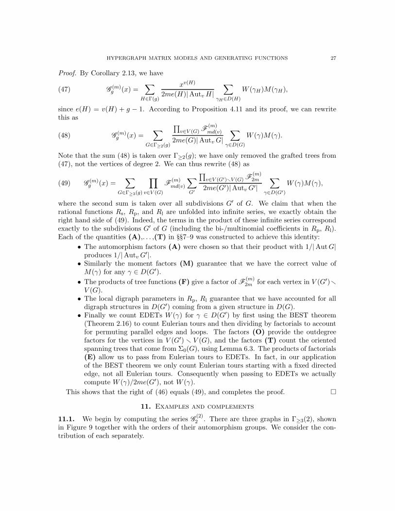
Proof. By Corollary 2.13, we have

(47) G(m)g (x) =

∑

H∈Γ(g)

xv(H)

2me(H)|Autv H|∑

γH∈D(H)

W (γH)M(γH),

since e(H) = v(H) + g − 1. According to Proposition 4.11 and its proof, we can rewritethis as

(48) G(m)g (x) =

∑

G∈Γ≥2(g)

∏v∈V (G) F

(m)md(v)

2me(G)|Autv G|∑

γ∈D(G)

W (γ)M(γ).

Note that the sum (48) is taken over Γ≥2(g); we have only removed the grafted trees from(47), not the vertices of degree 2. We can thus rewrite (48) as

(49) G(m)g (x) =

∑

G∈Γ≥3(g)

∏

v∈V (G)

F(m)md(v)

∑

G′

∏v∈V (G′)rV (G) F

(m)2m

2me(G′)|Autv G′|∑

γ∈D(G′)

W (γ)M(γ),

where the second sum is taken over all subdivisions G′ of G. We claim that when therational functions Rs, Rp, and Rl are unfolded into infinite series, we exactly obtain theright hand side of (49). Indeed, the terms in the product of these infinite series correspondexactly to the subdivisions G′ of G (including the bi-/multinomial coefficients in Rp, Rl).Each of the quantities (A),. . . ,(T) in §§7–9 was constructed to achieve this identity:

• The automorphism factors (A) were chosen so that their product with 1/|AutG|produces 1/|Autv G

′|.• Similarly the moment factors (M) guarantee that we have the correct value ofM(γ) for any γ ∈ D(G′).

• The products of tree functions (F) give a factor of F(m)2m for each vertex in V (G′)r

V (G).• The local digraph parameters in Rp, Rl guarantee that we have accounted for all

digraph structures in D(G′) coming from a given structure in D(G).• Finally we count EDETs W (γ) for γ ∈ D(G′) by first using the BEST theorem

(Theorem 2.16) to count Eulerian tours and then dividing by factorials to accountfor permuting parallel edges and loops. The factors (O) provide the outdegreefactors for the vertices in V (G′) r V (G), and the factors (T) count the orientedspanning trees that come from Σ0(G), using Lemma 6.3. The products of factorials(E) allow us to pass from Eulerian tours to EDETs. In fact, in our applicationof the BEST theorem we only count Eulerian tours starting with a fixed directededge, not all Eulerian tours. Consequently when passing to EDETs we actuallycompute W (γ)/2me(G′), not W (γ).

This shows that the right of (46) equals (49), and completes the proof. �

11. Examples and complements

11.1. We begin by computing the series G(2)2 . There are three graphs in Γ≥3(2), shown

in Figure 9 together with the orders of their automorphism groups. We consider the con-tribution of each separately.


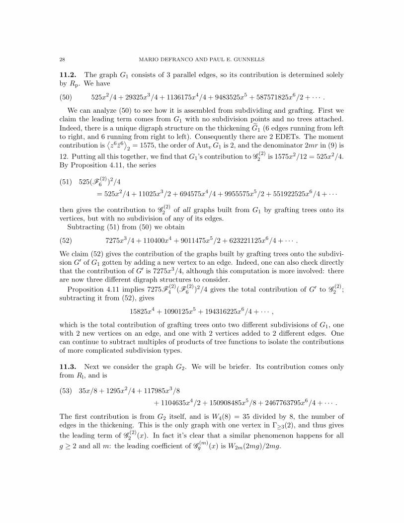
11.2. The graph G1 consists of 3 parallel edges, so its contribution is determined solelyby Rp. We have

(50) 525x2/4 + 29325x3/4 + 1136175x4/4 + 9483525x5 + 587571825x6/2 + · · · .We can analyze (50) to see how it is assembled from subdividing and grafting. First we

claim the leading term comes from G1 with no subdivision points and no trees attached.

Indeed, there is a unique digraph structure on the thickening G1 (6 edges running from leftto right, and 6 running from right to left). Consequently there are 2 EDETs. The momentcontribution is

⟨z6z6

⟩2

= 1575, the order of Autv G1 is 2, and the denominator 2mr in (9) is

12. Putting all this together, we find that G1’s contribution to G(2)2 is 1575x2/12 = 525x2/4.

By Proposition 4.11, the series

(51) 525(F(2)6 )2/4

= 525x2/4 + 11025x3/2 + 694575x4/4 + 9955575x5/2 + 551922525x6/4 + · · ·

then gives the contribution to G(2)2 of all graphs built from G1 by grafting trees onto its

vertices, but with no subdivision of any of its edges.Subtracting (51) from (50) we obtain

(52) 7275x3/4 + 110400x4 + 9011475x5/2 + 623221125x6/4 + · · · .We claim (52) gives the contribution of the graphs built by grafting trees onto the subdivi-sion G′ of G1 gotten by adding a new vertex to an edge. Indeed, one can also check directlythat the contribution of G′ is 7275x3/4, although this computation is more involved: thereare now three different digraph structures to consider.

Proposition 4.11 implies 7275F(2)4 (F

(2)6 )2/4 gives the total contribution of G′ to G

(2)2 ;

subtracting it from (52), gives

15825x4 + 1090125x5 + 194316225x6/4 + · · · ,which is the total contribution of grafting trees onto two different subdivisions of G1, onewith 2 new vertices on an edge, and one with 2 vertices added to 2 different edges. Onecan continue to subtract multiples of products of tree functions to isolate the contributionsof more complicated subdivision types.

11.3. Next we consider the graph G2. We will be briefer. Its contribution comes onlyfrom Rl, and is

(53) 35x/8 + 1295x2/4 + 117985x3/8

+ 1104635x4/2 + 150908485x5/8 + 2467763795x6/4 + · · · .

The first contribution is from G2 itself, and is W4(8) = 35 divided by 8, the number ofedges in the thickening. This is the only graph with one vertex in Γ≥3(2), and thus gives

the leading term of G(2)2 (x). In fact it’s clear that a similar phenomenon happens for all

g ≥ 2 and all m: the leading coefficient of G(m)g (x) is W2m(2mg)/2mg.


11.4. Finally we have the graph G3. Its contribution comes from factors of type Rs andRl, and is

(54) 25x2/4 + 2075x3/4 + 102575x4/4 + 2010125x5/2 + 138990425x6/4 + · · · .

Adding together (50), (53), and (54) we find

(55) G(2)2 (x) = 35x/8 + 1845x2/4

+ 180785x3/8 + 862005x4 + 234817185x5/8 + 1890948935x6/2 + · · · .

We remark that we do not know an analogue of the technique in Remark 3.6 to compute

G(m)g for large g without enumerating all of Γ≥3(g).

v

PSfrag replacements

|AutG1| = 12 |AutG2| = 8

|AutG3| = 8

Figure 9. The three graphs in Γ≥3(2).

11.5. Next we consider the classical case of the GUE (m = 1) in more detail. The

polynomials P(1)2r (N) can be easily computed using a generating function due to Harer–

Zagier (cf. [17, §3.1]); The first few are (cf. (4))

P(1)2 (N) = N2/2, P

(1)4 (N) = N3/2 + N/4,

P(1)6 (N) = 5N4/6 + 5N2/3, P

(1)8 (N) = 7N5/4 + 35N3/4 + 21N/8.

The generating functions G(1)g (x), g ≤ 3 are

G(1)0 = x2/2 + x3/2 + 5x4/6 + 7x5/4 + 21x6/5 + 11x7 + · · · ,

G(1)1 = x/2 + 3x2/2 + 5x3 + 35x4/2 + 63x5 + 231x6 + 858x7 + · · · ,

G(1)2 = 3x/4 + 15x2/2 + 105x3/2 + 315x4 + 3465x5/2 + 9009x6 + 45045x7 + · · · ,

G(1)3 = 5x/2 + 105x2/2 + 630x3 + 5787x4 + 45297x5 + 318447x6 + 2072040x7 + · · · .


One can check that these do reproduce the polynomials P(1), after passing from the fallingfactorial basis to the usual monomial basis:

(N)2/2 + (N)1/2 = N2/2,

(N)3/2 + 3(N)2/2 + 3(N)1/4 = N3/2 + N/4,

5(N)4/6 + 5(N)3 + 15(N)2/2 + 5(N)1/2 = 5N4/6 + 5N2/3,

7(N)5/4 + 35(N)4/2 + 105(N)3/2 + 105(N)2/2 + 105(N)1/8 = 7N5/4 + 35N3/4 + 21N/8.

The computation of the last polynomial used the first coefficient of G(1)4 , which we know

(§3.4) equals W2(8)/8.

11.6. We remark that, even though the polynomials P(1) are defined in terms of counting

weighted orientable unicellular maps, the series G(1)g include contributions from graphs that

can only appear in nonorientable unicellular maps, such as 2 vertices connected by twoparallel edges.

On the other hand, it is possible to give Wright-like expressions enumerating orientableunicellular maps of fixed genus h. Instead of the sets Γ≥3(g), we take the finite set of genush orientable unicellular maps M (h) that are the reductions of all the orientable unicellularmaps of genus h. In particular their 1-skeleta will be a subset of Γ≥3(g) where g = 2h. In theliterature this is known as the method of schemes, and is due to Chapuy–Marcus–Schaeffer[5].

For example, let M (1) = {M1, M2} be the genus 1 orientable unicellular maps in Figure10. The orders of their automorphism groups are 4 and 6 respectively. Their 1-skeleta arerespectively the graphs G1, G2 ∈ Γ≥3(2). These maps are the reductions of all genus 1orientable unicellular maps, in the sense that any of the latter can be built from M1,M2 bysubdividing edges and grafting trees. Just like with the series Gg, the trees are placed intovarious regions. However this time we are actually physically placing trees on an orientablesurface, which means the correct tree function to use is F = F (1), the ordinary generatingfunction of the Catalans:

F = x + x2 + 2x3 + 5x4 + 14x5 + 42x6 + · · · .After thinking about how the subdivision and placement works, the pleasure of which weleave to the reader, one sees that the Wright-like expression is

x/(1 − F )4

4(1 − x/(1 − F )2

)2 +x2/(1 − F )6

6(1 − x/(1 − F )2

)3

= x/4 + 5x2/3 + 35x3/4 + 42x4 + 385x5/2 + 858x6 + · · · .

The coefficient of xk is the weighted count of genus 1 orientable unicellular maps with k

vertices. In particular it equals the subleading coefficient of P(1)2r (N), where r = k + 1.

References

[1] O. Bernardi, An analogue of the Harer-Zagier formula for unicellular maps on general surfaces, Adv.in Appl. Math. 48 (2012), no. 1, 164–180.


PSfrag replacements

M1 M2

Figure 10. The reduced genus 1 maps

[2] G. Chapuy, The structure of unicellular maps, and a connection between maps of positive genus andplanar labelled trees, Probab. Theory Related Fields 147 (2010), no. 3-4, 415–447.

[3] G. Chapuy, A new combinatorial identity for unicellular maps, via a direct bijective approach, Adv. inAppl. Math. 47 (2011), no. 4, 874–893.

[4] G. Chapuy, V. Feray, and E. Fusy, A simple model of trees for unicellular maps, J. Combin. TheorySer. A 120 (2013), no. 8, 2064–2092.

[5] G. Chapuy, M. Marcus, and G. Schaeffer, A bijection for rooted maps on orientable surfaces, SIAM J.Discrete Math. 23 (2009), no. 3, 1587–1611.

[6] M. Defranco and P. E. Gunnells, Hypergraph matrix models, Mosc. Math. J. 21 (2021), no. 4, 737–766.[7] NIST Digital Library of Mathematical Functions, http://dlmf.nist.gov/, Release 1.1.4 of 2022-01-15,

F. W. J. Olver, A. B. Olde Daalhuis, D. W. Lozier, B. I. Schneider, R. F. Boisvert, C. W. Clark, B. R.Miller, B. V. Saunders, H. S. Cohl, and M. A. McClain, eds.

[8] B. Dubrovin, D. Yang, and D. Zagier, Classical Hurwitz numbers and related combinatorics, Mosc.Math. J. 17 (2017), no. 4, 601–633.

[9] G. Eisenstein, Entwicklung von ααα

. ..

, J. Reine Angew. Math. 28 (1844), 49–52.[10] P. Etingof, Mathematical ideas and notions of quantum field theory, available from

www-math.mit.edu/∼etingof/, 2002.[11] B. Eynard, Counting surfaces, Progress in Mathematical Physics, vol. 70, Birkhauser/Springer, [Cham],

2016, CRM Aisenstadt chair lectures.[12] P. Flajolet and R. Sedgewick, Analytic combinatorics, Cambridge University Press, Cambridge, 2009.[13] I. P. Goulden and A. Nica, A direct bijection for the Harer-Zagier formula, J. Combin. Theory Ser. A

111 (2005), no. 2, 224–238.[14] P. E. Gunnells, Generalized Catalan numbers from hypergraphs, Electron. J. Combin. 28 (2021), no. 1,

Paper No. 1.52, 29.[15] J. Harer and D. Zagier, The Euler characteristic of the moduli space of curves, Invent. Math. 85 (1986),

no. 3, 457–485.[16] S. Janson, D. E. Knuth, T. Luczak, and B. Pittel, The birth of the giant component, Random Structures

Algorithms 4 (1993), no. 3, 231–358, With an introduction by the editors.[17] S. K. Lando and A. K. Zvonkin, Graphs on surfaces and their applications, Encyclopaedia of Mathe-

matical Sciences, vol. 141, Springer-Verlag, Berlin, 2004, With an appendix by Don B. Zagier, Low-Dimensional Topology, II.

[18] B. Lass, Demonstration combinatoire de la formule de Harer-Zagier, C. R. Acad. Sci. Paris Ser. I Math.333 (2001), no. 3, 155–160.

[19] N. J. A. Sloane, Online Encyclopedia of Integer Sequences, available at oeis.org.


[20] R. P. Stanley, Enumerative combinatorics. Vol. 2, Cambridge Studies in Advanced Mathematics, vol. 62,Cambridge University Press, Cambridge, 1999, With a foreword by Gian-Carlo Rota and appendix 1by Sergey Fomin.

[21] Z. Sunik, Self-describing sequences and the Catalan family tree, Electron. J. Combin. 10 (2003), Note5, 9.

[22] E. M. Wright, The number of connected sparsely edged graphs, J. Graph Theory 1 (1977), no. 4, 317–330.

HYPERGRAPH

MATRIX

MODELS

AND

GENERATIN

GFUNCTIO

NS

33

Appendix A. Examples of Gg

m G(m)0 (x)

1 x2/2 + x3/2 + 5x4/6 + 7x5/4 + 21x6/5 + 11x7 + 429x8/14 + 715x9/8 + 2431x10/9 + O(x11)2 x2/4 + 3x3/4 + 19x4/4 + 339x5/8 + 927x6/2 + 5832x7 + 326439x8/4 + 19935963x9/16 + 41062743x10/2 + O(x11)3 x2/6+5x3/3+430x4/9+7150x5/3+178160x6+56884400x7/3+2813812000x8 +1712301278000x9/3+4156291931860000x10/27+O(x11)4 x2/8 + 35x3/8 + 5075x4/8 + 3521875x5/16 + 632774975x6/4 + 216912857000x7 + 4147718813494375x8/8 + 63445001652155046875x9/32

+ 45358226806367283484375x10/4 + O(x11)5 x2/10 + 63x3/5 + 9996x4 + 139108158x5/5 + 5563080718146x6/25 + 21304570653435636x7/5 + 834024715253210846736x8/5

+ 11914956019396567890508896x9 + 7159118148880765211316108608784x10/5 + O(x11)6 x2/12 + 77x3/2 + 529837x4/3 + 4236584737x5 + 389093885143656x6 + 103951883534149644840x7 + 66464625342098684554314384x8

+ 89031583111338263998369110425544x9 + 226882507639908104856032696370170600496x10 + O(x11)7 x2/14 + 858x3/7 + 23643048x4/7 + 719818214544x5 + 761736881828317824x6 + 19890091205586992696537088x7/7

+ 1462480414853122505621647925600256x8/49 + 5296882526955042374928855101040107624448x9/7+ 289378206931080342008004282036570702635383799808x10/7 + O(x11)

8 x2/16 + 6435x3/16 + 1093132755x4/16 + 4189518834318675x5/32 + 12789261471380923418175x6/8+ 83653285789705777304380006500x7 + 232714435447974068218421872500830070375x8/16+ 450580766581918742133057691058873988427995046875x9/64+ 66577050254084689335011968052311347098762983586132124375x10/8 + O(x11)

9 x2/18 + 12155x3/9 + 38865369400x4/27 + 224396619941386750x5/9 + 10568964372411801962927750x6/3+ 23406053777968695174488548034562500x7/9 + 22608292449374493728456232435833623726000000x8/3+ 631377425706842492186064055388314507534328247515000000x9/9+ 146415040193166445578321910204976829328192757969036532154956250000x10/81 + O(x11)

10 x2/20 + 46189x3/10 + 156327779036x4/5 + 24550017450057210683x5/5 + 40288257357688473370014249901x6/5+ 421795713069639073592252496895953739582x7/5 + 20488501368379858937904964722489355369283655924016x8/5+ 3689644411278439406922287219109006620041431766233435541621568x9/5+ 2084651796127409275171394859267740680422750018266628726230222158866466184x10/5 + O(x11)

11 x2/22 + 176358x3/11 + 7647037369608x4/11 + 10915046033893459789968x5/11 + 208825449554970891825780671394048x6/11+ 2831839254360209065821483392498206940318208x7 + 2316892466620063091353698696530631770384310687210928128x8

+ 8110630946423855711520713287693292112294656381212102639305749526528x9

+ 100972721844729199137629840094010555618643839225533556449970936697396719873548288x10 + O(x11)

Table 1. The series G(m)0 for various m.

34

MARIO

DEFRANCO

AND

PAUL

E.GUNNELLS

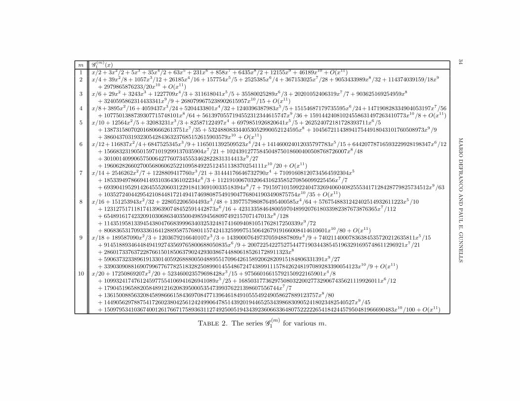
m G(m)1 (x)

1 x/2 + 3x2/2 + 5x3 + 35x4/2 + 63x5 + 231x6 + 858x7 + 6435x8/2 + 12155x9 + 46189x10 + O(x11)2 x/4 + 39x2/8 + 1057x3/12 + 26185x4/16 + 157754x5/5 + 2525385x6/4 + 367153025x7/28 + 9053433989x8/32 + 114374039159/18x9

+ 2979865876233/20x10 + O(x11)3 x/6 + 29x2 + 3243x3 + 1227709x4/3 + 311618041x5/5 + 35580025289x6/3 + 20201052406319x7/7 + 903625169254959x8

+ 3240595862314433341x9/9 + 2680799675238902615957x10/15 + O(x11)4 x/8 + 3895x2/16 + 4059437x3/24 + 5204433801x4/32 + 1240396387983x5/5 + 15154687179735595x6/24 + 147190828334904053197x7/56

+ 1077501388739307715748101x8/64 + 5613970557194552312344615747x9/36 + 15914424081024558631497263410773x10/8 + O(x11)5 x/10 + 12564x2/5 + 32083231x3/3 + 82587122497x4 + 6979851926820641x5/5 + 262524072181728393711x6/5

+ 138731580702016806662613751x7/35 + 532488083344053052990052124595x8 + 1045672114389417544918043101760508973x9/9+ 38604370319323054284363237685152615903579x10 + O(x11)

6 x/12 + 116837x2/4 + 6847525345x3/9 + 1165011392509523x4/24 + 141460024012035797783x5/15 + 64420778716593229928198347x6/12+ 156683231905015971019299137035904x7/21 + 1024391277584504875018600400508768726007x8/48+ 3010014099065750064277607345553462822831314413x9/27+ 19606282660270056806062522109584922512451138370254111x10/20 + O(x11)

7 x/14 + 2546262x2/7 + 1228809417760x3/21 + 31444176646732790x4 + 71091608120734564592304x5

+ 1853394978669414931036436102234x6/3 + 112191006703206431623585270856099225456x7/7+ 6939041952914264555206031229184136910033518394x8/7 + 7915971015992240473269406040825553417128428779825734512x9/63+ 1035272404429542108448172149417469808754919047768041903490875754x10/35 + O(x11)

8 x/16 + 151253943x2/32 + 228052206504493x3/48 + 1397757980876495400585x4/64 + 5767548831242402514932611223x5/10+ 1231275171181741396390748452591442873x6/16 + 4231335846480059704899207618033982387673876365x7/112+ 6548916174232091030686340350049859456809749215707147013x8/128+ 11435195813394543804766839996340325324817416094081051762817250339x9/72+ 80683653170933361641288958757680115742413259997515064267919166008414610601x10/80 + O(x11)

9 x/18 + 189587090x2/3 + 1203679216640107x3/3 + 143900076497370594887809x4/9 + 74021140007836384535720212635811x5/15+ 91451889346448494192743569765800688050835x6/9 + 2007225422752754477190344385451963291695748611296921x7/21+ 2860173376372287661501850637902429303867448806185261728911323x8

+ 5906373233896191330140592688800504889551709642615892062820915184806331391x9/27+ 339030908816907996776778251832825089901455486724743899111578426248197089283390054123x10/9 + O(x11)

10 x/20 + 17250869207x2/20 + 523460023579698428x3/15 + 97566016615792150922165901x4/8+ 1099324174761245977554106941626941089x5/25 + 16850317736297508032200277329067435621119926011x6/12+ 1790451965882058489121620839500053547399376221398607556744x7/7+ 13615008856320845898666158436970847713964618491055549249058627889123757x8/80+ 14490562978875417260238042561242499064785143920194465253439868309052418023482540527x9/45+ 150979534103674001261766717589363112749250051943439236066336480752222265418424457950481966690483x10/100 + O(x11)


HYPERGRAPH

MATRIX

MODELS

AND

GENERATIN

GFUNCTIO

NS

35

m G(m)2 (x)

1 3x/4 + 15x2/2 + 105x3/2 + 315x4 + 3465x5/2 + 9009x6 + 45045x7 + 218790x8 + 2078505x9/2 + 4849845x10 + O(x11)2 35x/8 + 1845x2/4 + 180785x3/8 + 862005x4 + 234817185x5/8 + 1890948935x6/2 + 237793731875x7/8

+ 930399023100x8 + 117663720672365x9/4 + 1900266044070095x10/2 + O(x11)3 77x/2 + 72562x2 + 30009350x3 + 10280579400x4 + 3658261039160x5 + 1491680067031588x6 + 729844653641699526x7

+ 433489372122070371240x8 + 309745940001212295052780x9 + 261891076428894172851532340x10 + O(x11)4 6435x/16 + 165046365x2/8 + 1112593168665x3/16 + 236663849715480x4 + 17600341065798248505x5/16

+ 31078789546809537473985x6/4 + 1319481703145262519322964955x7/16 + 2476799604846061873047750387285x8/2+ 199090249189138121971283755029243765x9/8 + 2574962587392198618100308020091493760655x10/4 + O(x11)

5 46189x/10 + 16671436353x2/2 + 223860132037399x3 + 7648026953950977594x4 + 485230365078411716232612x5

+ 319493821749765037584889653974x6/5 + 15657595846461128720675122036809094x7

+ 6176229944803737214210334186152831066722x8 + 3579777621181045714314704486350520500645242404x9

+ 2893488391090598220413674334197875035971303358739346x10 + O(x11)6 676039x/12 + 4020649596600x2 + 2648282038452752611x3/3 + 305073077224518147820457x4 + 263445965041708572528771592590x5

+ 1987690460788987576093939555431724381x6/3 + 11575564605880212320228689951412973889953823x7/3+ 40796928744360103714744030383601651967209396789201x8

+ 2076809590266914583719656282023706333521336331576677089768x9/3+ 53131191274484186284816220649209868804416052294470109218750485069x10/3 + O(x11)

7 5014575x/7 + 14853865945093200x2/7 + 3944396285733144972000x3 + 14080257416242165101623191200x4

+ 164136655070860919228052973306996800x5 + 7963567689382365008448110010645698384079600x6

+ 1123699102842309195689283902392972144152904236100800x7

+ 2256110625863372547880902839761751171507560102609828206168000x8/7+ 1129961539059001970451043695947559095072311179494408722337211966984000x9/7+ 131695805305487185246452181778558041000191649379126019772533309318461244982800x10 + O(x11)

8 300540195x/32 + 18878669392183676829x2/16 + 610241819764163714517332121x3/32 + 722364922604422998315893355104460x4

+ 3623863437352070918534948180462182007331897x5/32 + 850390376622185287573118983757464079688347889380961x6/8+ 11783054048078221264040880277065942943188562080960725818533339x7/32+ 11533639759284784434770233447749832483540533472461690938388807315293493x8/4+ 685170839905386560975202160107133286451901755827294134999606804325599793221394613x9/16+ 8960619686783079974829603212713949975870289157392370136878832982656658838355556246845031759x10/8 + O(x11)

9 756261275x/6+4076281886503589420075x2/6+291491340669707075823290582525x3/3+40071867596945571422276932811026392750x4

+ 253857304535751141356364561021090304858539561500x5/3+ 4604105999972157532616141037507813252196108750629194217850x6/3+ 131666983676987844755762656268864651107767021468074027572815728288750x7

+ 28243534384710028911252564511951832660850228392373269469253220235604502274505050x8

+ 37438622728343342360386241936370078370994606975743901557826986346905373626733949158174965300x9/3 + O(x10)



Department of Mathematics and Statistics, University of Massachusetts, Amherst, MA

01003-9305

Email address: [email protected]

Department of Mathematics and Statistics, University of Massachusetts, Amherst, MA

01003-9305

Email address: [email protected]

Hypergraph matrix models and generating functions - arXiv

Documents

Transcript of Hypergraph matrix models and generating functions - arXiv